^ из \SOURCE

STATEMENTS.

SPACE AWO T)WE

, SCALES ^

Л y.VARtABLE

Lectures presented at an

tnternationa) Seminar CourseCOMPUTING

AS A LANGUAGE OF PHYStCS

Trieste, 2-20 August 1971 organized by the

¡nternationa) Centre for Theoretica)

Physics, Trieste

¡NTERNATtONAL ATOMiC ENERGY AGENCY, VtENNA, 1972

COMPUTING AS A LANGUAGE OF PHYSICS

INTERNATIONAL CENTRE FOR THEORETICAL PHYSICS, TRIESTE

COMPUTING AS A LANGUAGE OF PHYSICS

LECTURES PRESENTED AT AN INTERNATIONAL SEMINAR COURSE

AT TRIESTE FROM 2 TO 20 AUGUST 1971 ORGANIZED BY THE

INTERNATIONAL CENTRE FOR THEORETICAL PHYSICS, TRIESTE

INTERNATIONAL ATOMIC ENERGY AGENCY VIENNA, 1972

THE INTERNATIONAL CENTRE FOR THEORETICAL PHYSICS (ICTP) in T rieste was established by the International A tom ic E nergy A gency (IAEA) in 1964 under an agreem ent with the Italian Governm ent, and with the assistance o f the City and U niversity of T rieste .

The IAEA and the United Nations Education, Scientific and Cultural Organization (UNESCO) subsequently agreed to operate the Centre jointly from 1 January 1970.

M em ber States o f both organizations participate in the work of the Centre, the m ain purpose of which is to foster , through training and research , the advancement of theoretica l ph ysics, with specia l regard to the needs of developing countries.

COMPUTING AS A LANGUAGE OF PHYSICS IAEA, VIENNA, 1972

STI/PU B /306

Printed by the IAEA in Austria December 1972

FOREWORD

The International Centre for T heoretica l P hysics has maintained an in terd iscip linary character in its research and training program as far as d ifferent branches of theoretica l physics are concerned. In pursuance of this aim the Centre has organized extended resea rch cou rses with a com prehensive and synoptic coverage in varying d iscip lin es. The firs t of these — on plasm a physics — was held in 1964; the second, in 1965, was concerned with the physics o f particles; the third, in 1966, covered nuclear theory; the fourth, in 1967, and the sixth, in 1970, dealt with condensed m atter and im perfect crysta lline solids; the fifth, in 1969, and the seventh, in 1971, w ere cou rses on nuclear structure. The proceedings o f a ll these cou rses w ere published by the International A tom ic E nergy A gency. The present volum e re co rd s the proceedings o f the eighth cou rse , held from 2 to 20 August 1971, which dealt with computing as a language of physics. Grants from the United Nations Developm ent P rogram m e, the Organization o f A m erican States, the International Bureau for Inform atics-International Computation Centre and the DigitalEquipm ent C orporation made it possible for the Centre to in crease the participation o f scien tists from developing cou n tries .

The program o f lectures was organized by P ro fe sso rs L . B ertocch i (T rieste , Italy), L . Kowarski (CERN), S .J . Lindenbaum (Brookhaven and New Y ork, U S A ) a n d K . V . R oberts (Culham, UK).

Abdus Salam

Д Ж Т О Я М Ь N O TÆ

Tbe papers and d iscu ssions incorporated in tbe proceeding's published by tbe Jnternationai Л tom ic E nergy A gency are edited by tbe A gen cy 's e d i- toria i sta ff to tbe extent considered n ecessa ry fo r tbe re a d e r 's assistance. Tbe views expressed and tbe générai styie adopied rem ain, how ever, tbe respon sib iiity o f tbe named authors o r participants.

P o r tbe saJre o f speed o f pubiication tbe present Proceeding's bave been printed by com position typing and pboto-o ffset iitbograpby. WitAtin tA elim i­tations im posed by this method, every effort bas been m ade to maintain a high ed itoria l standard,* in particular, tbe units and sym bois em pioyed are to tbe fu iiest practicab ie extent tbose standardized o r recom m ended by tbe com petent internationai sc ien tific bodies.

Tbe a ffilia tion s o f authors a re tbose given at tbe tim e o f nom ination.Tbe use in tbese P roceed in gs o fp a rticu ia r designations o f countries o r

terr itor ies does not im piy any judgement by tbe ^ g en cy a s to tbeiegai status o f sucb countries o r te rr ito r ie s , o f tbeir authorities and institutions o r o f tbe delim itation o f tbeir boundaries.

Tbe mention o f sp ec ific com panies o r o f tbeir products o r brand-names does not impJy any endorsem ent o r recom m endation on tbe part o f tbe fnternationai a to m ic E nergy Agency.

CONTENTS

Part I: General Introduction

Com puters and physics (IA E A -SM R -9/26) .................................................. 3K . V . R o b e r t s

The im pact of com puters on nuclear science (IA E A -S M R -9 /7 ) ......... 27L . K o w a r s k i

Part II: C lassica l com putational physics

O ccu rren ce of partial differentia l equations in physics and them athem atical nature o f the equations (IA E A -S M R -9 /1 4 a ).................. 41D .E . P o t t e r

D ifferen ce schem es and num erical algorithm s (IA E A -S M R -9 /1 4 b ).. 57D . E . P o t t e r

P lasm a physics, space physics and astrophysics(IA E A -S M R -9 /14c) .............................................................................................. 79D. E . P o t t e r

P lasm a, gravitational and vortex sim ulation (IA E A -S M R -9 /1 3 )......... 95R . W. H o c k n e y

P a rtic le -fie ld interactions: num erical techniques and problem s(IA E A -SM R -9/13b) .............................................................................................. 109R . W. H o c k n e y

The solution o f P o isson 's equation (IA E A -S M R -9 /l3 c) ......................... 119R . W . H o c k n e y

D ifferen ce m ethods in fluid dynam ics, with applications(IA E A -S M R -9 /17) .................................................................................................. 129J. K i l l e e n

A pplication o f com puters to problem s o f controlled therm onuclearrea cto rs (IA E A -S M R -9 /10) ............................................................................. 157M .N . R o s e n b l u t h

Monte Carlo techniques in statistical m echanics (IA E A -S M R -9 /ll) . 165M .N . R o s e n b l u t h

A fluid transport algorithm that works (IA E A -S M R -9 /1 8 )...................... 171J. P . B o r i s

P art III: Quantum Computational P hysics

Statistical m ethods for bubble cham ber analysis (IA E A -SM R -9/28) . 193E. L o h r m a n n

Data p rocessin g for e lectron ic techniques in h igh-frequencyexperim ents (IA E A -SM R -9 /25) ....................................................................... 209S. J . L i n d e n b a u m

M ulti-particle h igh -energy reactions (IA E A -S M R -9 /26) ......................... 235S. P . R a t t i

O ptica l-m odel and coupled-channel calculations in nuclearphysics (IA E A -S M R -9 /8 ) ................................................................................ 281J. R a y n a 1

Computer sim ulation in so lid -sta te physics (IA E A -SM R -9/15) ............ 323R. B u l l o u g h

The quantum computational physics o f atom s and m olecu les(IA E A -SM R -9 /20) ................................................................................................ 337R . K . N e s b e t

A ccurate calculation of c ro ss -s e c t io n s for non-reactive m olecu larco llis ion s (IA E A -SM R -9/19) ............................................................................ 375W. A . L e s t e r , Jr.

P art IV: Sym bolic analysis

Com parative survey o f program m ing languages (IA E A -SM R -9/21) . . . 391J. A . C a m p b e l l

Translation of Sym bolic ALGOL I to Sym bolic ALGOL II(IA E A -SM R -9 /22) ............................................................. .................................... 485G. K u o - P e t r a v i c , M. P e t r a v i c a n d K. V. R o b e r t s

A utom atic Optim ization o f Sym bolic ALGOL program s:I. G eneral princip les (IA E A -SM R -9/24) ............................ ...................... 491M. P e t r a v i c , G. K u o - P e t r a v i c a n d K. V. R o b e r t s

The DELPHI-SPEAKEASY system (IA E A -SM R -9/16) .............................. 521S. C o h e n

Introduction to LISP (IA E A -S M R -9 /9 ) .............................................................. 529D. L u r i é

Generation o f Feynman diagram s by the use of FORTRAN(IA E A -SM R -9 /12) ................................................................................................ .. 555M. P e r r o t t e t

Computer solution of sym bolic problem s in theoretical physics(IA E A -S M R -9 /27) ......................... ........................................................................ 567A . C. H e a r n

Faculty and Participants 597

PART I: GENERAL INTRODUCTION

IA E A -SM R -9/26

COMPUTERS AND PHYSICSK .V . ROBERTS UKAEA Research Group,Culham Laboratory,Abingdon, Berks,United Kingdom

Abstract

COMPUTERS AND PHYSICS.This introductory paper begins by discussing from a fairly fundamental point o f view what computers

really do and why they should be important to physics. For example, how significant has their impact been in the quarter of a century which has elapsed since the electronic digital computer was invented, and what may be expected of them in the future? How can we ensure that they realize their true scientific potential and that massive programming effort is used to maximum effect! Does computational physics have something to contribute to computer science and software engineering! A brief look is then taken at one particular field o f computational physics, namely the numerical solution of sets o f coupled partial differential equations which describe the time evolution o f classical systems.

1. INTRODUCTION

I shall begin this introductory paper by d iscussing from a fa ir ly funda­m ental point o f view what com puters rea lly do and why they should be im ­portant to physics. How significant has their im pact been in the quarter of a century which has elapsed since the e lectron ic digital com puter was invented, and what m ay be expected o f them in the future? How can we ensure that they rea lize their true scien tific potential and that m assive program m ing effort is used to m aximum effect? Does computational physics have som ething to contribute to com puter scien ce and software engineering?I shall then take a b r ie f look at one particu lar fie ld of computational ph ysics, nam ely the num erical solution o f sets o f coupled partia l differential equations which d escribe the time evolution o f c la ss ica l system s.

An excellent review o f the subject is given in the book Com puters and their R ole in the P hysica l S ciences, edited by Fernbach and Taub (1970).This d escr ib es the origin o f the e lectron ic digital com puter (in which com pu­tational physics played a considerable part) and gives many re fe ren ces . M ore specia lized papers can be found in the Journal o f Computational P hysics (A cadem ic P re ss ), Computer P hysics Communications (North-Holland) and the annual review ser ie s Methods in Computational P hysics (A cadem ic P ress ). The International P hysics P rogram L ibrary , operated by Q ueen's U niversity, B elfast, in association with Computer P hysics Com m unications, has recently been established to publish the program s them selves in digital form .

Figure 1 indicates the main branches o f computational ph ysics, together with certain fields which might m ore prop erly be regarded as part o f com ­puter science (languages and translators) o r software engineering (operating system s). The relation between these fields and com putational physics may be com pared to the relation between m athem atics and theoretica l physics, or between engineering and experim ental physics (F ig. 2). Good languages and good operating system s are vital to the proper growth o f computational

3

4 ROBERTS

FIG. 1. Some of the areas in which computing has an impact on physics.

physics and th erefore ph ysicists can be expected to play a part in their developm ent just as they have always done in many branches o f m athem atics and engineering.

F igure 3 represents the interplay between the three main ways of approaching a physica l prob lem : experim ental, theoretica l and com puta­tional. Each has its ch aracteristic m ethods of approach, its advantages and lim itations, som e o f which w ill be mentioned below .

1. 1. T heoretica l physics

T heoretica l physics m akes considerable use o f analogies, many of which are geom etrica l in character; for exam ple, the calculus was o r i ­ginally based on the idea of gradients and areas. F am iliar concepts in

IA E A -SM R -9/26 5

FIG. 2. In the past, mathematics and theoretical physics have been closely associated with one another and similarly for experimental physics and engineering. Computational physics requires advanced techniques in computer science and software engineering and in turn may be expected to contribute to these disciplines.

FIC.3. Interplay between the three main ways of approaching a physical problem.

6 ROBERTS

three dim ensions are generalized to n or to an infinite number o f dim ensions. T heoretica l physics re lie s heavily on the use o f sym bolism , enabling many actual cases to be d escribed by a single a lgebraic form ula; it is p o s it io n -fre e , since it can survey any portion o f space-tim e with equal ease, fo r exam ple, the inside o f a neutron star at som e distant epoch; and it is s ca le -fre e , ranging at w ill from the scale o f a quark to that o f the whole un iverse, and from 10*23 seconds to 10^° years. It is universal, in the sense that one p iece of theory, such as C oulom b's law or L ap lace 's equation, can be applied to innumerable actual situations.

T heory m akes extensive use of linearization . There is alm ost a m otto, "When in doubt, lin ea rize ". Any linear p ro ce ss is re latively easy to solve by analytic techniques, and weakly non-linear p ro ce sse s by perturbation theory. Strongly non-linear p ro ce sse s are much m ore difficult. Sym m etry and conservation laws are related to one another and play an essentia l ro le , not only in basic theory but also in the solution of p ra ctica l p rob lem s, as by the method o f separation o f variables. Com plex function theory has a s im ilar dual ro le ; it appears to be fundamental to h igh-energy physics and to the theory o f ord inary differential equations and at the same tim e is o f great p ractica l use in the solution o f tw o-dim ensional prob lem s because o f its relation to L a p la ce 's equation. Many of the m athem atical methods used in theoretica l physics have been sum m arized by M orse and Feshbach (1953).

Approxim ation techniques are essential. Som etim es this means separat­ing out a few o f the many degrees of freedom o f a large system , or d is ­tinguishing between widely different t im e -sca le s as in the method of adia­batic invariants. In other cases such as statistical m echanics the number o f degrees o f freedom is treated as infinite since this m akes the form ulae much sim pler.

These are som e o f the m athem atical too ls ; p ractica l tools include pencil and paper, chalk and blackboard, books, journals and m eetings. Theoretica l physics is cheap but it requ ires high IQ. Another im portant feature is that theory is self-enhancing; by practicing it, one becom es a better theoretician. This is not n ecessa r ily true o f experim ental physics (which requ ires the organization of staff and finance, the building of apparatus and the m anage­ment of con tracts), nor of computational physics (which involves struggling with awkward and unreliable computing system s, much handling o f cards and paper, and a continual search for e r r o r s in the program s). A m ajor task w ill be to build this feature of 'self-enhancem ent' into computational physics by im proving the techniques.

1. 2. Experim ental physics

E xperim ental physics provides the ultimate test and source o f in form a­tion fo r theory, just as theory provides the equations to be solved by com pu­tation. With great ingenuity the scope of experim ents and observations has gradually extended both ways from human sca le o f the range 10 cm to 10^° light years in length, and 10*23 seconds to 10^° years in tim e. But experim ental physics is neither p osition -free nor s ca le - fr e e , and the cost of an experim ent depends very much on the sca le o f the phenomenon which is under investigation. W here the expense is high, it m ay be preferable to use theory o r computation, although experim ental m odelling is often also o f great use.

IA E A -SM R -9/26 7

No experim ent is exact and the potential sou rces of e r ro r must always be carefu lly examined.

1. 3. Computational physics

Computational physics com bines som e o f the features o f both theory and experim ent. Like th eoretica l physics it is p os it ion -free and s ca le - fr e e , and it can survey phenomena in ph ase-space just as easily as rea l space.It is sym bolic in the sense that a p rogram , like an a lgebraic form ula, can handle any number o f actual calcu lations, but each individual calculation is m ore n early analogous to a single experim ent or observation and provides only num erical o r graphical resu lts .

To som e extent it is possib le to solve the equations on a com puter without understanding them, just as one can ca rry out an exploratory experim ent. With m ore com plicated phenomena involving a considerable range of length and tim e sca les it is , how ever, essentia l to make analytic approxim ations before putting the problem on to the com puter, otherw ise im possib ly large amounts o f m achine tim e or storage space m ay be needed. Not m ore than about 10 d egrees o f freedom can be handled on present-day com puters, or 10 if they a ll interact with one another. Thus computational physics can fill in the range between few -particle dynam ics and statistical m echanics.

D iagnostic m easurem ents are re la tive ly easy com pared to their counter­parts in experim ents. This enables one to obtain m any-particle corre la tion s, fo r exam ple, which can be checked against theory. On the other hand, there must be a constant search for 'com putational e r r o r s ' introduced by finite m esh s izes , finite time steps, etc. , and it is preferab le to think of a la rg e - scale calculation as a num erical experim ent, with the program as the apparatus, and to em ploy a ll the m ethodology which has prev iou sly been established for rea l experim ents (notebooks, control experim ents, e r ro r estim ates and so on).

Computational physics is particu larly suitable fo r n on -lin ea r, non- sym m etrica l phenomena where the usual theoretica l m ethods do not apply (such as in weather calcu lations), but often the program s are easier to w rite and the calculations go much faster in sim ple situations such as rectangular Cartesian geom etry with r ig id ,p erfectly conducting walls.

It is often possib le to take situations that norm ally are only handled a lgebra ica lly and to display them in p ictoria l form . Thus computing can put life into somewhat abstract subjects and might be of great help, for exam ple, in the teaching o f com plex variable theory.

F inally, there is great danger if computational ph ysicists becom e too preoccup ied with mundane details o f computing at the expense o f the physics itse lf, but the only solution here seem s to be to get the details right once fo r a ll, just as at one stage it was n ecessa ry to introduce r igorou s lim iting p ro ce sse s into m athem atics.

1 .4 . Exam ples

Som etim es one method of approach w ill be m ore appropriate and som e­tim es another; frequently they w ill work in pa irs and at tim es a ll three m ethods m ust be used together. An exam ple where computational techniques

8 ROBERTS

are particu larly appropriate is in the solution o f equations which describe the internal structure and evolution of stars (Iben, 1970). The equations are com plicated and non-linear but they are w ell-defined , and provided that spherica l sym m etry can be assum ed, they are w ell within the range that com puters are able to handle. On the other hand, analytic m ethods have difficu lty because of the non-linearity , while it is clea rly awkward to do experim ents o r even to make observations (except with neutrinos) in the in terior o f a star.

The book by Betcher and Crim ínale (1967) on Stability o f P ara lle l Flow s gives a good account of the way in which analytic and computational techniques can support one another in one branch of fluid dynam ics.Harlow (1970) has provided a general bibliography of papers dealing with num erical techniques fo r solving two- and three-d im ensional tim e-dependent prob lem s in fluid flow.

1 .5 . P hysics and inform ation

The purpose o f a com puter is to p rocess inform ation. P hysicists do spend a great deal of time handling inform ation of one kind or another and any im pact that com puters have on physics must eventually result from this fact. Many of the techniques used for handling scien tific in form a­tion have reached a high degree o f sophistication, particu larly in theoretical ph ysics , and here it is likely to take a long tim e before com puters can com pete on equal term s; for exam ple, the developm ents in the physical scien ces which occu rred within 5 years due to the d iscovery of S chrödinger's equation can hardly be paralle led by those which have occu rred within 25 years due to the invention o f the e lectron ic digital com puter. But in cases where conditions have been m ore suitable for the introduction of com ­puters, such as the p rocess in g o f large amounts of digital data from m easu r­ing devices and the automatic control o f experim ental equipment, their im ­pact has been m ore obvious.

2. HARDWARE

Let us therefore go right back to the beginning and try to see what com puters can in princip le do. B asica lly , an e lectron ic com puter is a device fo r handling binary inform ation o r data contained in a fast m em ory o r store . The data is conventionally represented as an ordered set of 0 's and l ' s (bits), grouped into bytes and w ords. In p rocess in g this data the com puter obeys a sequence o f instructions which are them selves r e ­presented by binary inform ation and are drawn from the same store (Fig. 4). The sequence o f instructions is called a p rogram .

It is preferab le to think o f the program as fixed inform ation, while the data w ill in general vary during the cou rse o f the computation. There is in fact an interesting analogy between a data p ro ce sso r and a dynam ical system , in which the program corresponds to the Hamiltonian H( q , p ) while the data values correspond to the com plete set of canonical co -ord inates and m om enta {q , p } which between them define the current state of the system . A s the computation proceed s, the p rog ress iv e m odification of the data by the program corresponds to the tim e evolution o f the dynam ical system .

¡A E A -S M R -9 /26 9

INSTRUCTIONS

The data values can be made to control:

(a) The action of the current instruction.(b) The location of the next instruction to be obeyed.

This fa cility enables the program to make decisions which depend on the current data values and is nowadays usually im plem ented by firs t tran s­ferrin g the n ecessa ry con trol inform ation from the main store into subsidiary fast storage devices ca lled re g is te rs , one o r m ore o f which can be consulted while an instruction is being interpreted.

2. 1. Dynamic program m odification

B ecause the program instructions can also be regarded as data it is p ossib le , in prin cip le , for a com puter to p ro ce ss its own instructions during the course o f a run. This is quite a fundamental idea because it m eans that the program itse lf can evolve dynam ically, as w ell as the data values. At one tim e this property was regarded as essentia l (Goldstine and Von Neumann, 1963; Elgot and Robinson, 1964; Goldstine, 1970), but it seem s that the essentia l tasks ha.ve now been taken over by the use of re g is te rs , and se lf-m od ify in g program s are currently regarded as bad p ractice because they are so difficult to understand. F or exam ple, no lega l FORTRAN or ALGOL program can m odify itself.

In m athem atics, one som etim es finds that a generalization is rem arkably productive and leads to a host o f new resu lts (real com plex num bers); at other tim es, it almost, seem s to kill p rog ress altogether (tim e-dependent Hamiltonians H( q , p , t ) o r non-Ham iltonian system s; groups -> sem i-grou ps). We do not know on which side of the fence these dynam ically, se lf-evo lv in g program s are likely to lie . I shall not d iscu ss them further here but it m ay be that this is an area where substantial advances in computational physics w ill be made one day.

10 ROBERTS

2.2. U niversality of hardware

There is a sense in which a ll com puters are the same (Pasta, 1970):

"A s an exam ple of the kind of thing we are talking about, consider the Turing m achine, a m odel invented in the 1930's by the m athe­m atician A . M. Turing. This abstract m odel is very sim ple. In one form it is a device with a finite num ber of internal states and a tape of arb itrary length m arked into squares. At any mom ent it can read a sym bol on the tape. Based on that sym bol and on the internal state, the m achine can initiate actions to change the sym bol and to m ove the tape one square left o r right.

One would expect such a machine to be lim ited in the kinds of things it could do and yet Turing showed that any effective computation perform ed on any com puter can be perform ed on a Turing m achine.The universality of this m achine allow s us to establish truths about it which w ill apply to a ll other m achines and consideration of this and other equivalent m odels has increased our understanding of com puters, p rogram s and com putations, a ll o f which can be fitted into this sim ple m odel. "

T urin g 's theorem suggests that any fundamental advances in computational physics are m uch m ore likely to com e from better theoretica l techniques, from im proved algorithm s and languages or from software engineering than from im proved hardware. During the past 25 years there have been steady quantitative im provem ents in the architecture o f com puters and in their speed, storage s ize , re liab ility , versatility and convenience, together with a p ara lle l decrease in the cost per unit o f computation, but there have been no rad ica l changes of princip le.

2. 3. Some p ractica l im provem ents

There a re , how ever, a number of potential im provem ents of a p ractica l kind whose com bined effect might be so dram atic as to appear fundamental. These include:

(a) Networks o f com puters linked together via the com m unications system

(b) M assive d ire c t -a c ce s s storage devices(c) U ltra -h igh -speed character and vector displays(d) An extended character set, including the Greek alphabet and

m athem atical sym bols(e) Im proved ergonom ics o f m an-m achine interaction(f) Further d ecrea ses in cost, and im provem ents in re liab ility of

on -lin e system s

These developm ents might make it practicab le for a 'p ow er-a ss isted ' algebra fa cility to be introduced, by which a th eoretica l physicist working at a console could autom atically and alm ost instantaneously manipulate analytic expression s appearing on the screen by issuing com m ands to the system to perform standard transform ations and in tegrals. This has already been partly im plem ented at Stanford U niversity in an experim ent

tA E A -SM R -9/26 11

on the teaching o f elem entary algebra in sch oo ls , but in ord er to com pete with pen cil and paper it is im portant to get the p ra ctica l details right.

V ery fast, pow erful and selective in form ation -retrieva l fa cilit ies might a lso becom e p ossib le , enabling a scientist working in one fie ld to fam iliarize h im self rapidly with the state o f the art in another. -In this connection, a fundamental technique that has been developed in com puter science might w ell be applied to reduce the bulk o f the regu lar scien tific literature, nam ely that o f the subroutine o r m a cro . Theorem s, diagram s, form ulae, definitions, conventions, e t c . , which are constantly being reproduced in fu ll, could be stored in one p lace and autom atically called into use when requ ired , sim ply by naming them. At the same tim e, the notation could be autom atically changed to fit that o f the paper in which they w ere called.

Another poss ib ility is to have a dynamic style of publication, containing not only a lgebraic form ulae but p rogram s for evaluating them num erically o r displaying them graphically on a screen as a function o f param eters selected by the 'rea d er '.

3. DATA TRANSFORMATIONS

So far, we have only considered binary strings o f 0 's and l 's . These are not in them selves very interesting and their im portance lie s in the ease with which they can be tran sferred to and from other types of data form at (F ig. 5). B inary o r 'd ig ita l' data is free ly interchangeable between e le c t r i­ca l signals, m agnetic record in g m edia and holes in punched cards or paper tape, although at different speeds. E le ctr ica l inform ation can read ily be converted from analogue to digital form and v ice versa , although with som e lo s s o f content. Apart from this, it should be em phasized that output by the com puter is usually much faster, cheaper and m ore convenient than input as illustrated by the dashed lines in F ig. 5. It is re la tive ly easy for a com puter to display a table, draw a graph or make a m ovie film o r even to talk, but much harder to get this inform ation back into digital form . T h ere fore , so far as com puters are concerned, digital inform ation ought to be regarded as the p rim ary form , while printed output, graphs, speech, etc. are tem porary form s intended only fo r com m unication with people.

3.1. Digital inform ation

D igital inform ation has a number o f im portant advantages. It can be transm itted alm ost instantaneously from point to point, updated, duplicated, stored and retrieved , autom atically manipulated in different ways and displayed to people in a variety o f fo rm s. We can in fact regard a set of data as an operand D and a display program as an operator , various form s o f display A ¡ being generated as products

A ; = P ; D (1)

If, for exam ple, a calculation leaves its output in a random a cce ss file , then not only can a physicist working at a console cause the resu lts of the

12 ROBERTS

FIG. 5. All forms of digital data are freely convertible into one another (full lines). Printing and display are also straightforward. Analogue-digital conversion can be carried out without difficulty and a computer can be made to talk (long dashes). Those transformations which are represented by short dashes are much more difficult to carry out and should be avoided where possible by storing all data in digital form.

calculation to be displayed in various ways so that he can understand their meaning, but he can also use the same file as input for a further ser ies o f calcu lations. These advantages are lost if the output file is sim ply printed and then destroyed.

D igital inform ation does, however, have a num ber o f grave disadvantages which must be carefu lly taken into account if it is to serve as a medium for scien tific com m unication. It is extrem ely frag ile , and on many com puter system s even m inor damage to an index can cause all the data on a storage device to be lost. Few of the scien tific d iscoveries o f antiquity would have survived if their record in g m edia had suffered from this disability. And digital inform ation does re ly heavily on good indexing; com pare brow sing through a m agnetic d isc file with brow sing through a lib ra ry of scien tific books.

4. ALGORITHMS, PROGRAMS AND SOFTWARE

Com puters can ca rry out any p ro ce ss which we know how to reduce to a lgorithm ic form ; that is any p rocess for which we can p rescr ib e a definite set of ru les no m atter how com plicated. U ltim ately this p rocess must be reduced to the manipulation of a binary bit pattern and the algorithm itse lf must be expressed in a sim ilar form (Fig. 4), but in p ractice we can develop our algorithm s in a m ore convenient language and then use a second algorithm to ca rry out the conversion autom atically (F ig. 6 ). In fact, a prim ary input device such as a teletype usually p erform s a prelim inary conversion to binary form , and this is then subsequently transferred by one or m ore system program s such as com p ilers , link ed itors, etc. until the binary instruction code o f the machine is finally reached.

IA E A -SM R -9/26 13

ALGORITHM' IN SOURCE

.LANGUAGE

CONVERSION ALGORITHM

/Translator program \ \ or compiler /

FIG. 6. An algorithm can be expressed in any ' source language', a second algorithm or sequence o f algorithms being used to convert this automatically into binary machine code.

Three requirem ents are:

A. It must be possib le to find an algorithm to ca rry out the requ ired p ro ce ss .

B. The algorithm must be coded fo r a sp ecific m achine.C. The num ber o f com puter operations requ ired for the p ro ce ss must

not be too large.

Much o f the effort in com putational physics at the present tim e is occupied by requirem ent B, and since this is rather a m echanical task it tends to divert attention from the physics p roper. H ow ever, just because it is a m echanical task it should itse lf be automated. The ultimate solution is one in which the languages which are m ost suitable for people who are in vesti­gating and expressin g the algorithm s are also intelligible to com puters and can be autom atically converted by them into efficient binary code.Some com m ents on how this m ay be achieved w ill be made in Section 8, in connection with Sym bolic ALGOL.

A lgorithm s fo r som e o f the p ro ce sse s used in physics have existed for m any years, fo r exam ple, arithm etic, and the solution o f sets of coupled ord inary d ifferentia l equations by finite d ifference m ethods. Here the com puter was able to make an im m ediate im pact. In h igh -energy physics a great deal of e ffort has been put into algorithm s fo r pattern recogn ition in connection with the p rocess in g o f bubble cham ber data, and with considerable su ccess (Snyder, 1970; K ow arski, 1970). Some su ccess has been achieved with

14 ROBERTS

autom atic theorem proving and with the autom atic solution o f elem entary integrals by analytic m ethods, but neither have influenced physics as yet.In other cases where theoretica l physicists have no algorithm s and must p roceed intuitively, as in the form ulation o f new concepts, com puters have a lso naturally had little influence.

4. 1. A lgorithm ic and program m ing languages

In order to satisfy requirem ents A and В it w ill be n ecessa ry to develop:

D. P ow erfu l, intelligible a lgorithm ic languages.E. A substantial body o f algorithm s expressed in these languages, for the

solution o f physical prob lem s.F. Means for converting these algorithm s into efficient binary machine

code for the various types of com puter system .

A h igh -leve l program m ing language such as FORTRAN or ALGOL enables algorithm s to be expressed in a form which is rela tively convenient for people to use, while at the same tim e allowing them to be translated without too much difficulty into reasonably efficient machine code. A lgorithm s are in m any ways s im ilar to m athem atical theorem s and need to be made in tellig ible and universa l for the same reasons. Unfortunately the existing languages cannot be com pared in scope to m athem atical notations such as non-com m utative a lgebra and the tensor calculus. F urtherm ore, it is nowadays very difficult to introduce a new program m ing language because of the cost o f developing and maintaining the n ecessa ry translators or com p ilers fo r a variety of different com puter system s. The result has been that for ph ysicists the state of the art has rem ained frozen for many years; although many resea rch languages have been developed by individual com puter scien tists during the last two decades, only FORTRAN (introduced in 1957) and ALGOL (introduced in 1960) are of m ajor im portance in physics. These have awkward d e ficien cies which in princip le could be easily put right, but which rem ain uncorrected because of the d ifficu lty of reaching international agreem ent and then m odifying a ll the existing com p ilers . The restriction to s ix -ch a ra cter identifiers in FORTRAN and the om ission o f com plex num bers, COMMON and EQUIVALENCE declarations and standard input-output fa cilit ies from ALGOL are typ ica l exam ples.

It was hard fo r m athem atics to p rog ress until a good notation had been introduced in order to express the operations o f arithm etic and algebra (Ball, 1908); try calculating in Roman num erals' It has a lso been said that the developm ent o f English m athem atics was held up for m ore than a century by re liance on the m ethods and notation o f Newton rather than those of Leibnitz. Computational physics is likely to rem ain equally constrained until it becom es a straightforw ard m atter to introduce pow erful new notations in which algorithm s can be expressed . Even the hardware restriction to upper-case le tters , num erals and a few specia l characters constitutes a severe lim itation, com pared to the great variety o f sym bol types, sizes and positions which are exploited in m athem atics.

The solution appears to be for scien tists them selves to develop and publish m achine-independent or portable com p ilers , program generators and m a c ro -p ro ce s s o rs in addition to the growing literature o f application

tA E A -SM R -9/26 15

program s and packages. If these are written in m odular form and w ell documented it should be re la tively straightforw ard to extend them to m eet new situations in the sam e way that m athem atical theorem s are continually generalized and extended.

5. A SCIENTIFIC SOFTWARE LITERATURE

C learly , theoretica l physics would hardly p rog ress at a ll if every w orker had to build up a ll the m athem atics that he needed right from the beginning, and it w ill not be practicab le to develop the enorm ously com plex algorithm s and program s that w ill be requ ired in computational physics unless each individual is able to stand on the shoulders o f his p re d e ce sso rs .

5. 1. Coding problem

It might be argued that although the algorithm s them selves should be published in the regular scien tific journals, coding them fo r a sp ecific application should be left to the individual w orker. This, how ever, is u nrealistic because o f the very high cost o f coding and because o f the long delays involved.

Some figures have recen tly been published on the costs o f com puter software and the effort needed to w rite it. F or IB M -360 software the cost o f each instruction has been estim ated at $50-60 , with0.2 instructions produced per m an-hour (B em er, 1970). F igure 7 shows the growth in software requirem ents in term s o f lines of code for su ccessive m achines (M cC lure, 1969), while F ig. 8 exp resses it in term s of m illions of m an- hours spent (B em er, 1970). Both in crease exponentially with tim e, by a factor o f about 200 in 10 years, and it seem s that both P ark inson 's law and the P eter P rincip le must surely be in operation (David, 1969). B em er rem arks: "M y nightm ares com e from im agining a new system scheduled for 1972. If the M cC lure chart holds true to give 25 m illion instructions, then the best figures we have say it w ill cost a b illion and a quarter dollars , produced by 15 000 p ro g ra m m e rs ." Y et,accord ing to Barbe (1970),only 2% o f the $36 b illion s ' worth o f software in operation in the United States is transferable from one com puter to another; the rest is doom ed to die with the hardware.

P hysicists m ay be doing a little better, since Snyder (1970) estim ates that a 60 000-w ord bubble-cham ber analysis program written in FORTRAN might requ ire 10 m an -years o f program m ing effort which would represent a coding rate som e 15 tim es faster.

5. 2. Publication, portability and m odularity

Since computational ph ysicists do not generally have this amount of m oney to spend, the operating system s, com pilers and applications program s which they need w ill not get written unless som e better method is found. It does appear, how ever, that three techniques which have worked w ell in scien ce and m athem atics in the past could go a long way tow ards solving the problem .

16 ROBERTS

Y E A R — *-

<к01 Z -Ï S и. о и

50 -

20 -

10 -

5 -

2 -

I -

SOFTWARE PRODUCTIVITY

(TOTAL BUDGET FIGURES)

0S360/

¿ A ' 1107(1964-5)

^ / J> G E 4 0 0

"1 I t г0.025 0.05 0.1 0.2 0.5 I !

MILLIONS OF INSTRUCTIONS

FIG. 8. Effort spent on software construction (Bemer, 1970). Because productivity has not increased with tim e, both the cost and the effort required for software construction are increasing exponentially at a similar rate to that of Fig. 7.

IA E A -SM R -9/26 17

The firs t technique is that of open publication. The new journal Computer P hysics Com m unications (North-Holland) has recently been founded to publish details o f w ell-docum ented, re fereed , tested physics p rogram s. A ssocia ted with this is the International P hysics Program L ib ra ry at Q ueen 's U niversity, B elfast, which publishes the program s - them selves in digital form . I have argued elsew here the advantages of such a schem e (R oberts, 1969). One im portant advantage is that by 'exposing ' the program listings to public cr it ic ism the standards are likely to be fo rced up. A prim ary reason why the standards in software engineering are so low is that there are so few m odels to w ork from , because program s are regarded as com m ercia lly valuable and are not therefore seen by m ore than a few people. The existence o f a high-quality open scien tific program literature should serve as a stimulus to the whole computing industry, just as the regu lar scien tific and m athem atical literature o f books and journals does for technology.

The next technique is that of portability, which is the same as 'uni­versa lity ' in science and m athem atics. Once a new program , subroutine package, com piler or scien tific operating system has been developed and published, it should be possib le to run it at any scien tific laboratory or university throughout the w orld , just as one can read any journal article or textbook. There are two b asic requirem ents for this:

(a) Scientific lib ra r ies must be persuaded to subscribe to the journal tapes, in the same way that they do to the regular scien tific journals, and to make their contents as readily available as are books and papers.

(b) The published program s must be written in universally available languages.

At present, only the universal h igh -level languages FORTRAN and ALGOL are accepted by Computer P h ysics Com m unications. An important further requirem ent is a lo w e r -le v e l universal language in which com pilers can be written and in which they can generate their output (Fig. 9). A s soon as this is available, a single im plem entation of each new language w ill make it available on a ll m achines, thus saving excess ive duplication o f effort and averting the danger of different im plem entations being out of step, as happens with FORTRAN and ALGOL at the present tim e.

This idea was proposed m any years ago, in connection with the so - called U niversal Computer Oriented Language or UNCOL (M ock et a l . ,1958). It enables N languages to be im plem ented on M m achines with a total amount of effort N + M instead of NM. Another possib le way of im plem enting the idea is by m eans o f m a cro -p ro ce s s o rs (Poole and W aite, 1970). It seem s unlikely that new scien tific languages can be universally introduced except in som e such way as this.

F igure 10 illustrates what I believe the structure o f the scien tific software literature E should eventually be; it has been drawn to para lle l F ig . 1 which shows the structure o f computational physics itse lf. Note that it includes the regu lar scien tific literature, since I have assum ed that in due course books and journals (or at least automatic indexes to them) w ill be made available in digital form . There is a significant danger here.In the past, the scien tific literature has always been com pletely 'v is ib le ', even though it has been published, in large part, by com m ercia l firm s.

18 ROBERTS

FIG. 9. It is now difficult to introduce new scientific programming languages because of the need to reach agreement on standardization and the cost o f constructing a new compiler for each type of computer system. A better solution would be to construct just one compiler which would then be published. Both the compiler itself and its target code must be expressed in a suitable universal language so that they can be used on any system.

If it ever gets tran sferred to p rop rietary data banks which can be autom ati­ca lly consulted, fo r a fee , but can never be openly inspected by the scien tific com m unity as a w hole, then there is a great danger that it w ill becom e corrupted. Even the standard FORTRAN lib ra ry functions often contain m istakes.

Once established, E m ay be expected to in crease steadily with time like the regu lar scien tific literature and to be equally permanent; there are already program s that have been in use for m ore than 10 years and which have been run on a whole ser ies of m achines. At any given epoch,E w ill be run on a variety o f different hardware types H^, Hg, Hg . . . .A s E expands, it w ill be le s s and le s s econ om ica lly practicable to recode even m ajor portions o f it fo r each new hardware system Hg, and this is why portability is essential. The m ost that can be done w ill be to recode certain replacem ent m odules R i , Rg, R 3. . . . (F ig. 10) which are executed with very high frequency and so occupy a substantial fraction o f the com puter tim e.

IA E A -SM R -9/26 19

HARDWARE

FIG. 10. Programs and data o f significance to science should be published in digital form to ensure that they are freely available and that their efficiency and reliability can be checked. This 'digital literature' Z should include not only scientific applications programs but also operating systems and compilers. Most o f it should be expressed in universal form so that it can be used on any machine. Replacement modules written in assembly language are used in the interests o f efficiency for those modules which have a high execution frequency.

The third im portant technique is m odularity, which is the same as the 'P rin cip le o f A bstraction ' in m athem atics. T heoretica l physics works by developing a number of separate too ls , e. g. vector algebra, tensor calculus, group theory, G reen 's functions, L ap lace 's equation, and then com bining them together in m any different ways. This m eans that when a new branch o f theoretica l physics has to be mapped out, much of the n ecessa ry m athe­m atics is already available (as with Schrödinger 's equation and quantum m echanics in 1926). It also m eans that theoreticians can often m ove free ly from one fie ld to another because they recogn ize the language.

20 ROBERTS

Suppose that we build a set o f program m odules o f n different types, with m m odules o f each type. Then, by com bining these together in all possib le ways, the number o f com plete program s we can form is o f order m " , while the w ork requ ired is only o f o rd er mn. Even allowing for many non-viable com binations,this is still a considerable advantage. To put it in another way, suppose that a single new module is developed o f one particu lar type; then m""^ new program s can in princip le be constructed from it, an am plification factor o f Nm"*^ .

T ypical exam ples might be the introduction o f a new type o f co-ord inate system (e. g. spherical p o lars), or a new graphical display package. P r o ­vided that the existing program s are p rop erly constructed, many of them can quickly make use o f these with little further effort.

6 . THE POWER AND LIMITATIONS OF COMPUTERS

I have stressed the organizational problem at som e length because this is the single m ost important p ractica l task facing computational physics at the present tim e. There are many algorithm s in the literature which are not being exploited because of the effort needed to code them. There are many good program s that can only be used in one o r two m ajor laboratories (notably the L os A lam os hydrodynam ics codes), and others which have gone out o f use because their originators m oved on to other work. A lso , there are large num bers o f significant research languages which have not m oved very far from the com puter science departments where they w ere developed; m eanwhile, FORTRAN has been frozen since 1964. H ow ever, these are all p rob lem s which can be solved by persuasion and good planning, along the lines I have already indicated. A m ore basic problem is whether or not there are any fundamental lim itations on the use of com puters in physics.

It is som etim es thought that com puters w ill eventually k ill theoretica l physics; a ll that one w ill need to do is to program the equations and p ress the button in order to get a num erical answ er. This is very far from being the case. Consider an assem bly of N partic les , interacting via N ewton's laws o f m otion and gravitation. If N is sm all (say equal to the number of planets together with the sun), then it is indeed possib le to solve the equa­tions rather accurately over long epochs using the com puter, and in this sense one might say that much of the analytic w ork done in the 18th and 19th centuries on the c la ss ica l few -body problem in astronom y was not s tr ictly n ecessa ry . Fortunately, com puters w ere not available then because the m odules developed during the course o f this work (e. g.Lagrangian and Hamiltonian m echanics and perturbation theory) turned out to be of great use in other fie lds such as quantum m echanics and statistical m echanics.

B ecause the num ber o f elem entary interactions between N particles in creases as N^, straightforw ard computational techniques becom e im ­practicable as soon as the num ber o f partic les greatly exceeds 100 o r , at m ost, 1000. Statistical m echanics is difficult to apply because o f the infinite potential energy that can be re leased when two gravitating p articles approach each other, and the two lines of attack, th eoretica l and computational, must support one another.

IA E A-SM R-9/26 21

T heoretica l physics r e lie s to a large extent on finding adequate ap­proxim ations. Often this is a question of separating the various tim e- s ca les in a problem . F or exam ple, the Born-O ppenheim er method used in m olecu lar theory treats the nuclei as fixed when calculating the electron energies and w ave-functions from which one obtains a potential function to be used in solving the m otion o f the nuclei them selves. T im e -sca le s are equally important in computational physics because if a naive approach is adopted, the cost o f the calculation w ill be determ ined by the shortest t im e -sca le tminOf the problem and w ill r ise to astronom ica l values if the ratio o f this to the largest t im e -sca le t^ ^ becom es too great.

In the case of an assem bly of N gravitating stars the shortest tim e- scale is likely to be determ ined by the orbita l periods o f c lose binaries which can decrease without lim it. These must somehow be decoupled from the problem , e. g. by treating the motion analytically until the perturbations due to nearby stars becom e too great. The N^ difficu lty might be rem oved by rep lacing the effect o f the interactions outside a given distance by that o f a mean fie ld , so that the amount of calculation in creases only as N.

R esearch of this type often p roceed s in one o f two ways:

(a) T heoretica l approxim ations are devised to rem ove d ifficu lties en ­countered in the com putation, and then these approxim ations are verified using the com puter.

(b) The num erical calculations turn up unexpected and striking resu lts , which can then be given a sim ple analytic explanation.

Thus the th eoretica l and com putational approaches are com plem entary to one another.

One instance where com puters could have been of great assistance during the 19th century is in the solution o f the N avier-Stokes equations fo r v iscou s flow. If these equations had been solved num erically in two dim ensions at m oderate Reynolds num bers, boundary layers o f finite thickness would have autom atically developed in the neighbourhood o f solid su rfaces, and the interpretation o f this phenomenon should have led to the d iscovery of boundary layer theory and an understanding o f the problem o f flight m uch ea rlie r than actually occu rred . Shocks and Karman vortex streets would have autom atically turned up in a s im ilar way.

It is interesting to notice another com plem entarity between the th eoretica l and computational approaches, since theory finds it easier to deal with thin boundary la yers , while com puters find it easier to deal with thick ones (covering severa l space steps).

6. 1. P artia l d ifferential equations

When we turn to partia l d ifferential equations the lim itations of com ­puters becom e even m ore apparent. Excluding h igh -energy physics for which the equations them selves are not w ell defined but their num ber seem s to be infinite, we find three situations in decreasing order o f com plexity, as indicated below .

22 ROBERTS

N um bers o f dim ensions

Schrödinger

V lasov

Configuration space

C lassica l phase space

R eal space

3N

6

N avier-Stokes 3

V lasov 's equation describ ing the phase space m otion o f particles interacting via long-range fie lds is important in plasm a ph ysics, while the N avier- Stokes equations o f hydrodynam ics are a prototype for many sim ilar sets o f coupled partia l differential equations in m agnetohydrodynam ics, a stro ­ph ysics, geophysics and other fie lds.

A ssum ing that we need at least 100 space points in each d irection to achieve good accu racy ( i . e . 25 F ourier m odes with ë 4 poin ts/m ode), the amount of storage needed is 1003N for Schrödinger 's equation, 100^ for V lasov 's equation, and 100^ for hydrodynam ics.

It is now just becom ing practicable to compute with 10 m esh points using m achines such as the CDC S T A R -100 so that three-d im ensional hydrodynam ics prob lem s should shortly be fa ir ly routine provided that the Reynolds num ber is not too high. To achieve the same accu racy with V lasov 's equation requ ires a further factor o f 10 in storage capacity and speed which is difficult to envisage at the present tim e, although a factor o f 10 can perhaps be anticipated. But this method o f solving Schrödinger 's equation is out o f the question for a ll but the sim plest situations.

One is again led to the need for making adequate approxim ations before putting a problem on to the com puter and this o f course is done in quantum m echanics, for exam ple, by the method of m olecular orb ita ls (Clementi,1970). In general, insight is likely to com e not only from the num erical resu lts them selves but also from studying the accu racy of the various approxim ations and trying to understand why they work as they do.

6. 2. Turbulence problem

It has recen tly been pointed out by Em m ons (1970) that a stra ightfor­ward num erica l attack on the problem of hydrodynam ic turbulence in three dim ensions is doom ed to fa ilure, since to solve the sim plest turbulent pipe flow problem would requ ire 10 ° m esh points and 1 0 ^ operations altogether fo r a R eynolds num ber Rg = 5 X 1 0 ^, occupying perhaps 100 years on existing com puters (or 10^ operations and the full age of the universe at Rg = 10 ).Here again one must look fo r a com bination o f m ore subtle computational techniques com bined with physica l insight and good theoretica l approxim ations.

7. DISPERSION RELATIONS

When a partia l d ifferential equation is solved on a com puter, one effect is to change the d ispersion relations of linearized perturbations o r sm all- amplitude waves. This happens because derivatives are rep laced by d ifferen ces, so that,for example,

, f ( x+Ax) - f(x - Ax) d f / d x - ----------- ^ ------------ (2 )

IA E A -SM R -9/26 23

.2 . , , 2 f ( x + A x ) - 2 f ( x ) + f ( x - A x )d f /d x ----------- * -'(A x)4---------------- ^

The resu lt is that a lgebra ic d ispersion relations are rep laced by m ore com plex trigonom etric ones, since

^ s i n _ k A x (4)Ax

, ' 2 (cos k A x - 1)* (Ax)2

and so on.Depending on the d ifference schem e, on the equations them selves

and on the ratio o f the 'm esh speed ' A x /A t to the various ch aracteristic speeds o f the problem (where At is the tim e-step ), this replacem ent can cause stable waves to becom e unstable or damped, and non -d ispersive waves (e. g. sound-w aves) to becom e d ispersive . A good part of the papers o f these P roceed in gs is concerned with such prob lem s, the situation being quite analogous to the replacem ent o f a continuum by a d iscrete lattice in so lid -sta te physics.

This analogy with so lid -sta te physics might usefu lly be exploited further. In particu lar, since there is a maxim um wave-num ber k^^that can be r e ­presented on a lattice with finite spacing A x, when two waves Sg interact to give a new wave к = k^+ kg with ¡kl > k ^ ^ , this energy must be diverted to som e other m ode ]k' ¡ < k ^ ^ by a type o f umklapp p ro ce ss which is known in computational physics as 'a liasin g '. This leads to e r ro rs in turbulence investigations, and the energy at high wave num bers must be rem oved by som e form o f a rtific ia l damping before it can cause damage.

The sim plest exam ple o f num erical d ispersion is given in the solution o f the one-d im ensional advective equation

where V is a constant. This evidently d escr ib es a wave m oving with uniform v e locity V; thus p reserv in g its shape unchanged, and the dispersion relation is '

(j = kv (7)

Making the replacem ent (4) but keeping At sm all, we find

<s)

This m eans that disturbances o f short wavelength propagate m ore slow ly and that for

kA x = 7Г (9)

24 ROBERTS

there is no propagation at all. A pulse can leave a train of waves behind it which m ay be m isinterpreted as a rea l physical phenomenon, and a function (such as the density or tem perature), which accord ing to the d ifferential equations must rem ain everyw here positive, can take negative values in the num erical calculation.

Equation (6 ) is significant because it is the prototype o f a ll the hydro- dynamic equations, in which the left-hand side o ccu rs as the Eulerian derivative. It is a lso c lose ly associated with V lasov 's equation. A dvective e r r o r s are o f im portance in m eteorology where v represents the speed with which disturbances are ca rried by the wind.

8. SYMBOLIC PROGRAMMING

I d iscussed ea rlie r the possib ility o f finding a generalized language which would be suitable not only for the form ulation and d iscussion of algorithm s, but a lso for program m ing the com puter itse lf. I should like to finish this paper by mentioning how this has been very la rgely achieved for one particu lar field , nam ely the solution of c la ss ica l fie ld equations fo r in itial-value problem s (Roberts and B or is , 1971; R oberts and P eckover, 1971; K u o-P etrav ic, P etravic and R oberts, 1971). The method is known as Sym bolic ALGOL and is described in detail in papers SM R -9/22 and SM R -9/24 in these P roceed ings.

FORTRAN, and m ore particu larly , ALGOL 60, were designed for this dual purpose but have two m ajor w eaknesses; firstly , they do not in­clude much of the notation that theoretical physicists norm ally use, and secondly, they have no power o f extension other than through the use of subroutines or p rocedu res.

We have, how ever, been able to show that by writing ALGOL program s in a particu lar way, they can be brought into very close correspondence with the notation o f vector analysis. F or exam ple, the m agnetic diffusion equation

- ¡ ^ - = C u r l ( V X B ) - C u r l ( n C u r l B ) (10)

can be program m ed in Sym bolic ALGOL I as

A B [C 1,Q ] := B + D T *(C U R L (C R O SS(V ,B ))-C U R L (E TA *C U R L(B ))); (11)

independently o f the co-ord inate system and of the number o f dim ensions. M ost of the notation is obvious but it should be explained that the prefix 'A ' denotes 'a r ra y '. C l stands for the current component (or the first component o f a ten sor), while Q represents the lo ca l m esh point at which В is being evaluated.

M odularity has been achieved because the same statement (11) will w ork just as w ell for sph erica l polars as for a Cartesian system , if one sim ply 'plugs in' o r 'sw itches on' a different definition o f the CURL operator. The definition o f CURL in Cartesian co -ord inates is

IA E A -SM R -9/26 25

rea l p rocedure CURL(A); rea l A;CURL := R P(D E L(R P(A )))-R M (D E L(R M (A ))j; (12)

which gives som e idea o f the con cisen ess o f Sym bolic ALGOL I as w ell as o f its sim ilarity to the notation o f theoretica l physics. Here R P, RM are mutually inverse rotation op era tors , perm uting the vector com ponents (123) in the positive (231) and negative (312) d irections resp ective ly , while DEL is a vector finite d ifference operator.

Sym bolic ALGOL I executes quite slow ly because o f a large num ber of nested procedure ca lls . To get around this prob lem , we have shown that statements such as (1 1 ) can be converted either autom atically o r by hand into an equivalent form called Sym bolic ALGOL II, which when executed w ill autom atically generate an optim ized program in any desired output language. F or this purpose they are plugged in to an ALGOL program called the P etrav ic Generator which is supplied with m odules analogous to (12) in order to define the d ifference schem e, co -ord inate system , target language and so on,which are requ ired for the particu lar job .

The target code is about as fast as w ell-w ritten FORTRAN, and an added advantage is likely to be that code can equally w ell be produced fo r com puters fo r which no com piler is yet available, or even for which FORTRAN is not particu larly suitable, such as the new CDC STAR-100 which is able to p ro ce ss com plete vectors in one operation without using a DO loop.

What we are doing here is to use the com puter itse lf to w rite the p r o ­gram , instead o f writing it by hand. Since much o f the w ork is tedious and m echanical, this is a very natural developm ent, but the interesting point is that the instructions which must be fed to the com puter to make it ca rry out this task are in virtual on e-to -on e correspondence with the orig inal m athem atical statement o f the prob lem . This is a situation which is rem iniscent o f both quantization and second quantization, in which the equations always seem to rem ain the sam e but get interpreted in different ways. If it can be exploited further, we m ay be able to use much o f the form alism o f m athem atical physics itse lf as the a lgorithm ic language for program m ing com puters.

In this sense I believe that one o f our im m ediate aim s should be to weld m athem atical and com putational physics into a coherent whole.

B I B L I O G R A P H Y

BALL, W .W .R.(1908). AShortAccountofthe History of Mathematics, reprinted, Dover Publications,New York (1960).

BARBE, P. (1970), Software Engineering (TOU, J. T . , Ed.), 2 Vois, Academic Press, New York and London, V o l . l , p. 151.

BEMER, R.W. (1970), ib id .. p. 121.

BETCHER, R ., CRIMINALE, W .O . (1967), Stability o f Parallel Flows, Academic Press, New York and London.

CLEMENTI, E. (1970), in Computers and their Role in the Physical Sciences* (FERNBACH, S . , TAUB, A. H ., Eds), Cordon and Breach, New York, p .437.

* Referred to as CRPS.

26 ROBERTS

DAVID, E .E ., Jr. (1969), Software Engineering, Report on a Conference sponsored by the Nato Science Committee, Garmisch, October 1968, p .62,

ELGOT, G ., ROBINSON. A. (1964), J. Ass. comput. Mach. 11, 365.

EMMONS, H. W. (1970), Critique of Numerical Modelling o f Fluid-Mechanics Phenomena, Annual Review o f Fluid Mechanics, V ol.2 (VAN DYKE, M ., VINCENTI, W .G ., WEHAUSEN, L V ., Eds), Annual Reviews I n c ., Palo Alto., C a lif., p. 15.

FERNBACH, S . , TAUB, A .H ., Eds (1970), Computers and their Role in the Physical Sciences, Gordon and Breach, New York.

GOLDSTINE, H.H. (1970), CRPS, p. 51.

GOLDSTINE, H .H. j NEUMANN, J. von (1963), in John von NEUMANN, Collected Works, Vol. 5, Pergamon Press, Oxford.

HARLOW, F.H . (1970), Numerical Methods for Fluid Dynamics, An Annotated Bibliography, Los Alamos Rep. LA-4281.

IBEN, I . , Jr. (1970), CRPS, p. 595.

KOWARSKI, L. (1970), CRPS, p .479.

KUO-PETRAVIC, G . , PETRAVIC, M . , ROBERTS, K .V . (1971), Automatic Optimization of Symbolic Algol Programs, I. General Principles (submitted to J. comput. Phys.).

McCLURE, R.M. (1969), Software Engineering, Report on a Conference sponsored by the Nato Science Committee, Garmisch, October 1968, p .66.

MOCK, O . , OLSZTYN, J ., STEEL, T . , STRONG, J ., TEITTER, A . , WEGSTEIN, J. (1958),Communs Assoc, comput. Mach.

MORSE. P .M ., FESHBACH, H. (1953), Methods of Theoretical Physics, 2 Vols, McGraw Hill, New York.

PASTA, J.R. (1970), CRPS, p.203.

POOLE, P .C ., WAITE, W .M . (1970), Software E ngngl, 167.

ROBERTS, K .V . (1969), Comput. Phys. Communs 1, 1.

ROBERTS, K. V . , BORIS, J.P. (1971), The Solution o f Partial Differential Equations using a Symbolic Style o f A lgol, J. comput. Phys. 8 , 1 .

ROBERTS, K. V . , PECKOVER, R.S. (1971), Symbolic Programming for Plasma Physicists, Culham Laboratory Preprint CLM-P257.

SNYDER, J.N. (1970), CRPS, p .463.

TURING, A .M . (1937), Proc. Lond. math. Soc. (2) 42, 230.

IAE A-SM R-9 /7

THE IMPACT OF COMPUTERS ON NUCLEAR SCIENCEL. KOWARSKI CERN,Geneva, Switzerland

Abstract

THE IMPACT OF COMPUTERS ON NUCLEAR SCIENCE.Nuclear physicists were the first large-scale scientific users of computers. As computer techniques

developed in the 1950s and 1960s, they became indispensable in an ever growing variety o f tasks of pure and applied nuclear science. The following categories of tasks are considered : (1) Theory and mathematical preparation o f experiments; (2) Experimentation at its various stages — before, during and after the collection o f data; (3) Simulation and "computer experiments"; (4) Operation and control o f nuclear machines;(5) Documentation. This survey is given in a historical perspective with some emphasis on initial difficulties and gradual adaptation. Near-future prospects, especially in high-energy physics¡ are discussed, leading to the formulation of a conflict between the threat o f dehumanization and a humanistic hope.

1. DEFINITION OF A COLLISION

Any kind ö f physica l resea rch , whether pure o r applied, is today la rgely a com puter-aided activity, but this is essentia lly a very recent state o f things, hardly half a generation old. P h ysics , o f cou rse , is a much older activity, with its established way o f life and thinking. And established ways do not always com bine very kindly with new ways. That is why the intrusion o f com puters into physics was so much o f a sudden event, best described in term s o f a collision , and that is the meaning of the word "im pact" in the title o f this paper.

Nowhere has the im pact been as dram atic as in nuclear physics and in its spectacular applications, firs t m ilitary and later on industrial.This whole domain o f knowledge should be called nuclear scien ce , because it is not only ph ysics. But there the ph ysicists played a dominant ro le , and a lso they w ere the firs t and the m ost im portant u sers of com puters, so in this paper, there is not much d ifference between talking o f nuclear science or o f nuclear physics.

To d escribe the im pact and its consequences, I shall p roceed in a h istorica l way. I com e before you as a w itness, as one who was active in nuclear scien ce before the com puters cam e and who was w ell situated to watch what happened when they did com e. And as an observer o f this sequence o f events I m ay perhaps allow m yse lf to make a few guesses as to how it is going to develop. A lso , as a w itness, I m ay be forgiven for talking at som e length about things I know a little better and skipping brie fly over those of which I know le ss .

2. DOMAINS OF PENETRATION

2. 1. Introductory survey

Let us start at a definite tim e-point, say 1950. In the public mind this is the "a tom ic a ge", still at the zenith of its glory. We nuclear scientists

27

28 KOWARSKI

are the scien tific w izards, ours is the m ost prom inent scien ce . We have heard that "e le c tron ic ca lcu lators" are being developed som ew here. They m ay be im portant for statistics o r finance, but not fo r us, except perhaps fo r certain unusually intricate things like som e particu larly m essy partial d ifferential equations. Anyhow, radio tubes are clum sy, m em ories are even c lu m sier , it a ll w ill take tim e, it does not concern us at present.

Y et, we w ere drawn in pretty quickly. One sim ple reason : the com puter development took m oney. It started in P rinceton , then it was taken up by Remington Rand (not IBM yet at that time.' ) but "the atom " was the w eal­thiest prospective user and so the firs t u ser-m otivated com puters were built in p la ces like Argonne, and in particu lar in L os A lam os, where Stanislas Ulam and his pupils played a considerable ro le in these early beginnings.

O ccasion s for using com puters gradually spread all over nuclear scien ce . At firs t , they a rose only in the nuclear scien tist 's o ffice , at his blackboard, where theories are made and le isu re ly calculations perform ed before and after the experim ent — not yet at the mom ent when the scientist is in actual contact with the nuclear phenomenon, not actually in the laboratory o r at the nuclear factory . At this stage, the com puters are usefu l fo r what might in arm y use be called staff work, not fo r field work.

Then the com puters began to get c lo se r to experim entation and to the laboratory itse lf. H istorica lly , this happened firs t in connection with handling the data left after the actual contact with the nuclear phenomenon (data analysis); at a later stage, com puters becam e involved d irectly in this contact itse lf, and thus com pleted the invasion o f another domain o f nuclear scien ce — the resea rch laboratory.

A fter the laboratory study of nuclear phenomena com es the application — nuclear m achines and fa ctories . This constitutes the third domain. C om ­puters cam e finally even to the lib rary , "no place to h ide", so to speak.A fter we have gone through this picture of a com plete encirclem ent of nuclear scien tists by com puters, we shall try to see how the nuclear scientist reacted to this increasing involvem ent, what made him happy or unhappy and how this, not always easy, relationship m ay be expected to evolve.

2. 2. At the blackboard: m athem atics and theories

Let us now look again at a scientist in 1950 at his blackboard, away from the nuclear phenomenon. He m ay have been using a desk calcu lator, the cog -w h eel type; if the infant e lectron ic com puters can provide only the same kind o f se rv ice , then they are hardly n ecessa ry and if they can do som ething e lse — but the nuclear scientist sees no need for anything e lse . This is the usual v icious c ir c le which, at firs t , is very effective in keeping the atom and the com puter apart.

Yet gradually it dawns on our scientist that there m ay have been cases in his past when an attempt to solve a problem with a desk calcu lator had to be abandoned because o f the sheer volume o f work. E lectron ic computation, being faster, can go further in this d irection , and so the realization com es that fast arithm etic can help in solving a lgebraic equa­tions, d ifferential equations, partial d ifferential equations (a whole new world opens there), m atrix p rob lem s, com plicated functions, etc., etc.The com puter then becom es the indispensable too l in a spreading d iversity of u ses.

IAE A-SM R-9 /7 29

Through the arithm etic of Cartesian co -ord in a tes , the way is open to the use o f com puters fo r handling geom etry — firs t through the printing p lotters and m ore recen tly on the cath ode-ray displays. A physicist could hardly appreciate this roundabout way as long as he had to stay away from the com puter operation. But once it becam e possib le to put the com puter on -line to the p h y s ic is t 's m ental approaches to the prob lem , com puterized geom etry was recogn ized as a valuable technique, known nowadays under the name o f "in teractive graph ics".

We have just had the firs t glim pse o f the on -lin e concept — a com puter tim ed to operate in step with another operation outside itse lf, in this case a human thinking p ro ce ss . We shall return to this many tim es and in various contexts. The firs t problem here is that of m ism atched speeds: a com puter working as sluggishly as the human mind is a com puter la rge ly wasted, and only when com puters becam e cheaper per unit of operation, this waste becam e econ om ica lly p ossib le ; that is why this particular on-line use is such a recent developm ent.

I mention only fo r the sake o f com pleteness such extensions o f the com puter use as form al log ic , non -num erica l a lgebra, gam es theory, a rtific ia l intelligence, etc. They have so far had rather little relation to anything nuclear, except perhaps the recogn ition o f visual patterns, on which we shall com m ent below , and som e very recent applications o f sym bolic algebra, reported in paper S M R -9 /27 in these P roceed in gs. In particu lar, the sym bolic treatm ent o f Feynman diagram s is relevant to a ll o f high- energy physics.

A ll this can be seen as generalized m athem atics and to a ll this can be applied the rem ark made som e ten years ago by J. T. Schwartz o f the New Y ork university: "M athem atics has always sought to reduce the unlim ited natural com plexity o f facts and ideas to a humanly manageable size ; it is like mining o f diamonds from the surrounding ro ck s . But the in creasingly cheap power o f m achines enables us to manage far greater m asses of irredu cib le com plexity; it is still an extraction p ro ce ss , but it is m ore com parable to the other usefu l form o f carbon — the mining o f coa l" . This analogy illustrates the d ifference between the spirit o f m athem atics and that o f com puter scien ce and helps us to rea lize that being a computational ph ysicist, or a com putational nuclear chem ist, or what not, is not at a ll the same thing as being a m athem atical physicist and so on, so that, in fact, a new way of life in nuclear scien ce has been opened. So much fo r the im pact at the blackboard.

2. 3. Com puters in the laboratory : before the run

Now com es the laboratory , the contact with the nuclear phenomena.I would like to mention here that our forefathers seem to have been m ore carefu l about describ ing our various ways o f dealing with the phenomena. When a physicist m easu res, using a known technique, som e third decim al in the lifetim e of a nucleus or a partic le , which otherw ise is w ell fam iliar and w ell behaved, he hardly should be called an experim enter. And when a junior physicist looks at a bubble film from a cham ber built years ago and from a run record in g the overa ll e ffects of a given beam on a given target, he does not experim ent, he ob serves . Yet, a ll this is now called experim entation, so we shall have to use that w ord a little loose ly .

30 KOWARSKI

In any nuclear "experim ent", the cru cia l mom ent is that when the animal is actually being k illed , I mean when the nucleus o r the photon or whatnot is actually striking the detector. That is the phase of data collection ; before it com es the preparation, the setting-up o f the apparatus, and after it com es the handling o f data and the arriva l at m eaningful scien tific con ­clusions. Com puters are now essentia l to a ll o f these three stages — b e fore , during and a fter, which I have once called C lass 1, 2 and 3 of com ­puter use in experim entation. My next rem arks apply ch iefly to a vast variety o f nuclear experim ents using the e lectron ic kind o f detection which is now current in h igh -energy physics as w ell as in low -en ergy ph ysics, nuclear chem istry , etc . , and — as you w ill see — a c lo se r look at these applications w ill lead us to som e slight changes in the definition o f these three c la sses .

The setting-up o f an experim ent rea lly starts with som e thinking at the blackboard (we have already dealt with that) and, nowadays, increasingly often with prelim in ary computations which try to sim ulate the future ex p eri­m ental situation — we shall return to that below . A fter this m ore or le ss theoretica l pream ble, the experim enter m ay need the com puter for such C lass-1 work as checking the apparatus, testing its perform ance on blank runs and tr ia l runs, adjusting the e lectron ic log ic , etc.

Let me quote here two fa ir ly recent opinions from eminent physicists on the relevance of C la s s -1 com puter u se . An opinion from M. I. T. :"If m ore than 30-40 counters are used in the same experim ent, then a com puter is n ecessa ry in the setting-up stage". Another, from Princeton: "W e try to choose our experim ents so that the apparatus is sim ple enough to be set without using a com puter. If it is not, then there are too many in terfaces, the flex ib ility is lo s t " . The prevailing trend seem s to be away from this happily austere ideal.

A com puter in C lass 1 must be fast enough to follow the fast working o f the apparatus in "re a l tim e". This is another kind of on -line use — on -line to the apparatus. It m ay requ ire a rather large com puter, e. g. a P D P -6 o r -10 , but in m ost cases a sm aller size (such as P D P -9 ) seem s to be adequate; still sm aller com puters, like the P D P -8 , are hardly u se ­ful anym ore in this connection. The same not too big com puter m ay be useful when the experim ent is actually going on, fo r the purpose o f c o lle c ­ting the incom ing data and to put them on a single re co rd such as a m agnetic tape. It is convenient to consider this particular function as belonging still to the C lass 1, although it already takes p lace during the actual k ill.

2. 4. During the run

C lass 2 is the m ost m odern and the hottest prob lem , because it ra ises a ll sorts o f issu es about the requ ired m inim um size of the com puter, its location and the wasteful use o f its available tim e. The k ill, usually called the run, m ay som etim es go on for days or w eeks. The scientist wants to know if his incom ing resu lts are worthwhile; therefore he has to extract the meaning from the data as they a rr ive , if not a ll o f them, at least from sam ples. This extraction very often requ ires the active intervention o f the sc ien tist 's m ental p ro ce sse s , if any; therefore the com puter m ust be available on -line both to the nanoseconds tim esca le o f the apparatus and to the seconds tim esca le o f the thinker. A lso , full p rocess in g up to the

ÍA E A -SM R -9/7 31

physics-m eaningfu l conclusion often requ ires definitely a large com puter — a 6400, a 360/65 or m ore — to be made available to every interested user right on the site where his experim ent is actually taking p lace. C lass 2 is essentia l: accord in g to its resu lts the physicist m ay have to m odify the experim ental run o r even to stop it altogether.

It is amusing to see how m odest were the experim entalist 's C la s s -2 requirem ents only a few years ago. A leading Columbia low -en ergy physicist, Dr. L idofsky, reported in 1964 that the currently used system involved r e ­cording the output o f his multichannel analyser on paper tape, then sending the tape by m essenger to a distant sm all com puter which would produce m agnetic tape, then using another m essenger to bring that tape to a 7090 com puter. The elim ination of the firs t m essenger — that is , putting a P D P -4 on -line to the analyser — was at that tim e in p rog ress . The p oss ib ility o f using a large com puter on -lin e , via data links, was mentioned as a utopian ideal. T o -d ay thé tendency is to build in a not too sm all com puter, such as a P D P -9 (the sam e as in C lass 1), and if this is not enough fo r C lass 2, to have a p ra ctica lly on -line a c ce s s , via data links and tim e-sh arin g , to a rea lly b ig com puter. How n ecessa ry this is going to be w ill be seen from two illustrations: accord ing to P. E gelstaff (Harwell) a typ ical analyser o f 1956 had 100 channels. By I960 he got to a few thousand. Much m ore recen tly , ä report on Dr. G h iorso 's rad iochem ica l investigations in B erkeley m entioned an analysing set-up involving three variables (the chem ical nature o f the sam ple, tim e in tervals, the height o f the pulse) and a total o f severa l hundred thousand channels.

2. 5. A fter the run

And now, the run is over and we are left with the bulk o f the record ed data, already partly p rocessed through the C lass-1 and -2 com puters, a lready sam pled as to their physica l meaning. What com es now is C lass 3. F or a large category o f experim ents, m ostly in h igh -energy physics (all o f bubble cham ber experim ents and severa l kinds o f those with spark cham bers), a ll com puter use is C lass 3, because the resu lts of the d e tec­ting run are at firs t record ed v isually on film without any recou rse to a com puter. But then visual data have to be p rocessed through film -m easu rin g and pattern -recogn izing stages before they are reduced to a set o f computable num erical data. On the w hole, it can be said that the use o f a film -m easu rin g machine re -in trod u ces a ll the headaches which have been avoided during the in itial detection, that is the film -taking stage. Now, to handle the film inform ation, we face again the need for a sm allish com puter on -line to the m easuring m achine, a b igger com puter on -line to a m onitoring physicist, etc. There is also the problem of insertion of human help to overcom e the occasion a l w eaknesses of the inform ation process in g by m achine.

The final domain o f data handling, or the C lass 3 p roper, consists in the reduction o f the raw computable data to their m eaningful scien tific conclusion. Dr. L idofsky (Columbia university) quoted, as a typical exam ple o f the 1964 era , an experim ent on gamma rays from som e excited levels o f a nucleus; there the computable data amounted to over two m illion bits and the final conclusion was expressed in about 100 bits. In 1970,Dr. M acleod (CERN) mentioned in a lecture cases o f n early 10 000 record ed bits per second o f e ffective run. We are p rogressin g , aren 't wej

32 KOWARSKI

The last reduction stage in bubble experim ents is the SUMX program , about which Lohrmann reports in paper S M R -9 /28 in these P roceed ings.The c lo se r you get to the intelligent conclusion , the m ore important is the active participation o f the scientist; a ll the problem s of interactive operation, p rop erly planned tim e-sh arin g , on -line a cce ss to a big com puter and so on, have to be tackled as an increasingly accepted part o f a physi­c is t 's life .

About ten years ago this was not foreseen at all. Data co llection and reduction , recognition o f visual patterns, etc. , w ere thought to be amenable to a com plete automation; the scientist would only com e in to muse over the final print-out.

System s o f bubble film analysis invented around 1960, such as HPD and PE PR , w ere inspired by this "id ea l" but did not succeed in achieving it fu lly. In the much sim pler task o f analysing spark-cham ber film , the elim ination o f human intervention has been pushed farther, but even there not to the very end. Since the m id-1960s the style o f using com puters in nuclear experim ents began to shift tow ards a proper com bination o f the human operator with the m achine, instead of trying to do away with the human altogether; o lder bubble-film p rocess in g devices began to be ex ­ploited in a system atica lly interactive mode, and newer devices (e. g. those known as P o lly and Sweepnik) exp licitly em bodied the princip le of m an- machine sym biosis .

2.6. Simulation

We are now going to take the scientist out o f his laboratory and let him proceed further, but before that we must return him once m ore to the blackboard. Having got used to the com puter in connection with the in­com ing physica l data, he noticed that he can learn a lot about the pheno­menon without taking any data at a ll. Instead o f using experim ental data as input, he can use an inflow o f random num bers — and let the com puter p ro ce ss them accord in g to a ll the ru les he already knows to be valid for that particu lar category of physica l phenomena. This kind of study is known as sim ulation. S trictly speaking, it is not a branch o f experim ental scien ce at a ll, and yet it looks very much like one, and one often hears now­adays of "com puter experim ents". In its purest form com puter sim ulation studies p rob lem s which are fu lly known in their b asic prin cip les but too com plex to allow the derivation o f con crete num erical resu lts from such prin cip les — a situation which often o ccu rs when dealing with m any-body prob lem s, liquids, p lasm as. Then there is the m ixed form which takes in actually observed data and then uses them as input for com puter simulation o f their subsequent evolution; m eteorology and astrophysics, in particu lar, make use o f this method. "C om puter experim ents" are mentioned in the papers by Hockney and by R oberts in these P roceed ings.

Simulation is also useful in C la s s -1 w ork as a m eans o f studying the perform ance of instrum ents from an input of random num bers rather than the physical data. Design and tr ia l o f e lectron ics ; testing of photographic optics and their d istortions in the new, very com plex bubble cham bers; testing o f bubble p rocess in g program s by trying them on sim ulated track co -ord in ates — a ll these are suitable domains for sim ulation by com puter.

2. 7. Com puters in nuclear fa ctories and m achines

A fter this excursion back to the blackboard, we now can turn to the scientist who has p roceeded from the laboratory to the application, where his scien tific work is concerned with actually running a definite device or m achine. In the h istory o f introduction o f com puters into nuclear scien ces and their applications, one o f the firs t domains considered was the con trol of nuclear rea cto rs . R eactors are fa ir ly quiet and steady dev ices , but if not enough attention is given to'the evolution o f radioactivity o r of neutron fluxes within them, they m ay tend to get astray from the equilibrium position chosen fo r their functioning. T h ere fore , the operator in charge o f the rea ctor has at his d isposal various sensor devices which show the neutronic state inside the reactor . A ccord in g to these indications, he takes his decisions and intervenes, if n ecessa ry , to change the working conditions o f the rea cto r , so as to bring the chain reaction to a desired lev e l o f intensity.

A ll this, in p rincip le , could be done by a com puter. The sensors could transm it their readings to the com puter which would digest the data, arrive at a log ica l decision and intervene accord ing to this decision . This could be done with a speed and an a ccu ra cy far greater than those obtainable from a human operator, which would be useful for ensuring a safety feature that m ay yet prove to be very valuable for som e reactor types in som e cr it ica l stages of their functioning.

These prospects have been a ired in many theoretica l d iscussions;I was involved in som e o f them back in 1963. F ive years later, at a con ­feren ce held in Norway, I could see that the d iscussions had rem ained la rge ly theoretica l and not much use was made of them in p ra ctice . Some beginnings in this respect were reported from Canada and Japan; I do not know how much has been done since then.

Another field o f nuclear technology where com puters can make effective decis ions , is the running o f particle a cce lera tors which is of d irect interest to us in h igh -energy physics. In the experim ental equipment around the a cce lera tor there are many m ore tasks for controlling com puters; they are now used extensively for handling the p rim ary and secondary beam s and, increasingly , in the functioning o f very big bubble cham bers or e lectron ic experim ental set-ups (the latter also in low -en ergy nuclear experim ents).A ll these com puters act as a sw itch-board m echanism which becom es n ecessa ry when the log ic o f switching is enorm ously com plex an d /or has often to be changed.

IA E A -SM R -9/7 3 3

2. 8. Com puterized documentation

A s the last domain in which com puters have invaded the nuclear sc ien ­t is t 's life , we have to mention the library , documentation and scien tific inform ation in a la rger sense. The firs t way of using com puters in these activities was the com puterized production o f catalogues. Instead o f in ­scrib ing catalogue entries in tim e-honoured fo lios or card file s , they can be put on com puter-readable tape. The com puter can then perform certain standard operations suitable for arranging the catalogue data in a desired form , and print out the resu lts so that the printed catalogue can be made available in as many cop ies as requ ired and not just one card file in the

34 KOWARSKI

central lib ra ry . If the catalogue entry contains not only the c la ss ica l indications such as the authors' nam es, the title o f the document, the year o f its publication and so on, but a lso a few keywords or other "d e scr ip ­to rs " to give an idea of what the subject m atter is about, then the computer can be used to make searches through large sets of entries and to print out a list o f documents in a given collection which, by their content, c o r ­respond to som e form ulated demand. F or a p rec ise characterization o f a document by keyw ords, help from a human docum entalist has so far been n ecessary . Schem es have been proposed for the com puterized extraction o f keyw ords from a given text by making it optica lly a ccess ib le to the com puter, which would single out the keywords on the basis o f their f r e ­quency in the document or o f their appearance in som e specified context. Many theoretica l studies and experim ents of this sort have been perform ed , but the p ractica l resu lts have, so far, been rather m eagre; as in bubble- cham ber analysis, the "id ea l" of elim inating all human intervention m ay soon be rep laced by the deliberate developm ent o f an optimum combination o f man and m achine.

3. RESPONSE TO THE INVASION

I have said enough about what tasks the nuclear scien tists are now considering as legitim ate fie lds for using com puters, and how the growing im portance o f com puters and o f their on -line interaction with scien tific thinking has induced the nuclear scientist — has forced him — to becom e at least a com puter technician if not always a com puter scientist. In term s of a w ell-w orn p iece of p o litica l wit, those o f the atom ic era have been dragged into the com puter era scream ing and kicking. A fter the com plete a loofness o f 1950 they gradually came to view the com puter as an occa s ion ­a lly useful blackbox, alm ost im possib le to understand and not much worth the effort o f understanding, a ccess ib le only through an e so te r ic language — there was no p ra ctica l FORTRAN in those early years, because computer tim e was too p reciou s to be wasted in such crude ways. Only p rofessiona l applied m athem aticians could approach the blackbox and with these, for the next ten years or so, the nuclear scientist had to co -op era te w illy - n illy , m ost often n illy.

The invasion o f the laboratory was probably started around 1955 by Luis A lvarez and his group, with com puterized m easuring m achines for bubble-cham ber p ictures. A new kind of interface had to be designed, p laced between the film -re co rd e d data and the com puter; soon afterw ards, another such interface appeared in low -en ergy physics between the pulse analyser and the com puter. The nuclear scientist tended to design and build these interm ediate devices all by h im self, helped only by his faithful, m odest e lectron ic technicians. They som etim es would build a whole custom -built specia lized com puter, without even rea liz ing it. It was the tim e o f what I used to ca ll tricky hardware — very ingenious, very rigid . Equivalent trick s by software were already thinkable, but nuclear men were shy o f them.

Not for long. N uclear physicists began to learn FORTRAN. Since physics is defined as what physicists do (it is quite o ffic ia l, not just m y jok e), com puters did duly becom e a part o f physics. It seem s alm ost incred ible today that only eight years ago, on the highest d irecting level

IAE A-SM R-9 /7 35

of CERN, I was told (in fu ll view of an approaching c r is is of CERN computing fa c ilit ies ) that a "c ra sh e ffort" could be approved only in physics but not in com puters. Today such a deliberate opposition would sound rather unnatural.

A s scien tists get used not only to w riting their own program s, but also to sitting on -line to an operating com puter, as the new kind o f nuclear scientist develops — neither a theoretician , nor a data-taker, but a data- p ro ce sso r specia lized in using com puters — they becom e too impatient to sit and wait while their job is being attended to by com puter m anagers and operators. Turn-around time vexations can ultim ately be solved only in two ways: one is to provide each experim ental group-with its own com puter, available for on -line inclusion into its experim ental set-up or fo r its p r o c e s s ­ing operations; and the other is tim e-sharing o f bigger com puters, with r e ­m ote con so les . Both o f these solutions have been adopted in the current p ractice .

4. PROSPECTS AND VALUES

4. 1. L iberation in space

Storage o f raw data for subsequent p rocess in g begins to be noticeable as a m eans o f reso lv in g som e contradictions im posed by geographical separation between the a cce lera tor and its average u ser. A university physicist can then p erform a very significant part o f his experim ental w ork without leaving his own cam pus, esp ecia lly if data transm ission by telephonic links is available to supplement the conveyance o f data by m ail or m essen ger. P erhaps, when links as com prehensive as those used in te lev ision becom e available at long distance, there w ill be even le s s reason for the u ser to spend a lot of his tim e on the site where his physical events are being produced. This m ay even abolish the kind of snobbery which de­crees today that only those m ay be considered as ph ysicists who are bodily present at the k ill, that is at the place and time when the particle is actually com ing out o f the a cce lera tor and hitting the detector.

Today the campus u ser tends to use his own com puter only in C lass 1 and 3 of his activ ities, in term s o f the classifica tion explained above, and to comm ute for the C lass 2 o f his p rocess in g work. A s the rem aining de­pendence on site fa cilit ies dim inishes, this alm ost com plete liberation from the geographical dilem m a can acquire a d irect politica l sign ificance. We can envisage a state o f things when there w ill be only one b iggest m achine in the whole w orld available fo r som e problem s in h igh -energy physics or in high- flux low er-en erg y nuclear re sea rch . It w ill be unthinkable to concentrate all the leading experim entalists o f the world around this m achine: decentra­lization o f experim entation is n ecessa ry in order to keep alive the teaching by prom inent scientists.

4.2 . Liberation in tim e

In addition to this in creasing liberation in space, com puters can already give freedom from severa l kinds o f tim e lim itations. We are no longer obliged to conform ou rse lves to the nanosecond region o f speeds in which the events are actually happening: we can re co rd them in their rea l tim e.

36 KOWARSKI

and then p ro ce ss and study the re co rd s in our own tim esca le . The other form o f tim e liberation is the poss ib ility of rep rocess in g an event in som e new ways long after its orig inal handling. The events can be stored in a rch ives, where we can return and brow se, and now and then, perhaps, extract som e new meaning from an old record .

The third way is the liberation from the tyranny o f the Big M achine's tim e schedule. Because the physicist is no longer com pelled to be present when the physica l event is actually happening, he can organize his work in a better equilibrium with his teaching duties.

4. 3. Dangers and hopes

The vision o f these huge and costly m achines, spitting their p articles into alm ost as huge and no le s s costly assem blies of detecting apparatus, every day of the year and every m illisecon d o f the day — the yield has to justify the investm ent, you know! — is in a way terrify ing. The era of the ingenious scientist, who sets up his apparatus to catch Nature behaving this or that way, seem s to be past. The m achine w ill have to run just "because it is th ere ", and accord ing to its own ru les. And from each run — there w ill be not m uch sense in calling them experim ents any m ore — there w ill be a rich harvest o f record ed data, like a deep -sea dredge com ing up with its load o f pebbles and fishes . A nuclear scientist w ill prepare the run and sift the harvest, follow ing the exam ple o f today's oceanographers, selenolog ists and arch eolog ists .

There w ill be a lot o f attempts to judge such new situations by old value cr iteria . What is a physicist? What is an experim enter? Is sim ula­tion an experim ent? Is the man who accum ulates print-outs o f solved equa­tions a m athem atical ph ysicist? And the ultimate w orry : are we not going to use com puters as a substitute for thinking? There is an interesting recent precedent fo r this in creased re liance on com puters. In the early 1950s hydrogen bom bs w ere developed sim ultaneously in the Soviet Union and in the United States o f A m erica , and a little later in the United Kingdom. They w ere su ccessfu lly brought to the point where they could rea lly work, I mean explode. The French scien tists, attacking the sam e problem in the 1960s, felt that they needed a cce ss to the b iggest scien tific com puters available at that tim e and which certainly w ere not available in the 1950s to their A m erican , Soviet or B ritish colleagues. The United States government em bargoed som e o f the biggest A m erican com puters when it learned that they w ere to be used in a French hydrogen-bom b p ro je ct . The French scien tists protested that this made their w ork as good as im possib le . We are led to believe that with their methods as they had developed by that tim e, this w ork did indeed becom e im possib le in the absence o f very big com puters, and to take this episode as a striking illustration o f the irrev ers ib le evolu­tion o f working habits in nuclear scien ce , due to the advent o f com puters.It is , o f cou rse , only fa ir to assum e that the standards o f desirable accu racy had gone up in the intervening decade so as to ensure m ore com pletely re liab le p red ictions o f perform ance than those which w ere available in the early 1950s.

In h igh -energy physics itse lf it is noticeable that bubble-cham ber tech ­nique has got further tow ards what we might ca ll too much dependence on com puters than its other branches o f experim entation. The contemplation

IA E A -SM R -9/7 37

o f this and other such trends leads us to the form ulation o f a dehumanized utopia in which nuclear scien tists w ill produce very fine m easurem ents and w ill make no d iscov eries . In som e sense we m ay be obliged to say that this situation is already largely prevailing in h igh -energy physics, esp ecia lly in Europe. But, o f cou rse , the full dehumanization is only an extrapolation lim it. M oreover, we must never forget that the com puters are also available for constructing a hum anistic utopia: they o ffe r us the poss ib ility o f brow sing over stored data with a ll intact human ingenuity to give a new sense to the already p rocessed events; the overa ll d irection o f experim entation by a creative human; the fruitful sym biosis between man and m achine. W illiam M iller form ulated in 1964 an ideal: "W e must decide what to do and the machine w ill maybe te ll us how to do it" . I might add: how to do it by operating the m achine. But as long as we decide, and not the m achine, there is hope.

PART II: CLASSICAL COMPUTATIONAL PHYSICS

IA E A -SM R -9/14a

OCCURRENCE OF PARTIAL DIFFERENTIAL EQUATIONS IN PHYSICS AND THE MATHEMATICAL NATURE OF THE EQUATIONSD .E . POTTERDepartment of Plasma Physics,Imperial C ollege,London, United Kingdom

Abstract

OCCURRENCE OF PARTIAL DIFFERENTIAL EQUATIONS IN PHYSICS AND THE MATHEMATICAL NATURE OF THE EQUATIONS.

This paper is introductory in discussing how partial differential equations arise in physics and in reviewing some simple properties which are nevertheless important when considering methods of solution on the computer. The importance o f principles o f conservation in physics, and in particular in classical physics, is stressed and they are used to derive some important examples o f partial differential equations.The use o f Fourier analysis and the derivation o f dispersion relations is reviewed for waves, advection, diffusion and potential problems. The time-scales o f interest in initial-value problems are isolated, as a preamble to the concepts of stability and accuracy in difference solutions. The essential non-linearity o f the few- and many-body problem is discussed. The general initial-value problem is defined and the concepts o f a discrete mesh in space and time are introduced. A comparison is made between a continuous function and a mesh vector by Fourier analysis, illustrating that the essential approximation on a difference mesh is the limitation to long-wavelength modes. Integration of the initial-value problem in time over finite time-steps is introduced.

1. INTRODUCTION

The power o f d ifferential calculus has led to the very wide application of the concepts o f continuous m edia and continuous fie lds. In using such concepts, continuous functions in space and tim e are defined which describe the prop erties of the m edium , and on applying the quantitative princip le of ph ysics, partia l d ifferentia l equations are obtained which couple the p ro p e r ­ties of the medium in space and tim e.

To illustrate the very wide application o f this concept, and consequently the very wide occu rren ce o f partia l d ifferential equations, a few fie lds which re ly on such a concept are listed : in c la ss ica l electrodynam ics, M axw ell's equations are form ulated by defining continuous electrom agnetic fie lds and continuous source functions; solids are frequently treated fo r sim plicity as a continuum, though we know otherw ise; a great variety o f fluids (liquids, gases, p lasm as, the galactic fluid) m ay be treated with m ost ease as a con ­tinuum; other exam ples are phase fluids and "continuous fie lds o f fo r ce " in c la ss ica l and quantum m echanics.

Although it is clear that the partia l d ifferential equations o f physics arise in a great variety of ways, and from very different prob lem s, n ever­theless such equations and system s of equations repeatedly take the same form or s im ilar ones. This is essentia lly because a great deal o f the ph ilo ­sophy o f physics and in particular c la ss ica l physics has been form ulated in

41

42 POTTER

Surface I S

F IG .l. Conservation of energy.The heat conduction (diffusion) equation is obtained by applying the principle of the conservation of energy to an arbitrary volume, V. The energy in the volume V may only alter by a flux o f energy ^across the surface S o f V.

term s o f prin cip les o f conservation. Some sim ple but vital exam ples com e readily to mind: m ass cannot be created or destroyed; momentum is con ­served ; total e le c tr ic charge is an invariant; etc. To stress this point and to develop som e system s o f partial differential equations with which we w ill be concerned, som e particular exam ples m ay be considered [ l ] .

1. 1. C onservation of energy in a solid

C lassica lly , energy is transported in a solid by conduction. Since the solid is a rig id stationary body, the variable energy density (e) in the solid is given by the therm al energy or tem perature. Hence the principle of conservation o f energy is invoked and m ust be satisfied when considering the energy in a finite volum e V o f the solid of surface S (F ig. 1). By the princip le of the conservation o f energy, the rate of change o f energy in V must be equal to the flux o f energy q a cross the surface S o f V:

E nergy in volum e

s

v s

Applying the d ivergence theorem to the second term and for a constant volum e V,

!A E A -S M R -9/14a 43

Ж ж V* q dT = ОV V

The energy density is proportional to the tem perature T , and experim entally it is found that the heat flux q depends on the gradient o f the tem perature. Hence, defining a proportionality constant, the conductivity K,

The essentia l princip le described by the diffusion equation in this case is then the princip le o f the conservation o f energy.

1 .2 . Conservation o f e le c tr ic charge

Another inform ative exam ple, in electrom agnetic theory, is the princip le o f the conservation o f e le c tr ic charge. Again, th erefore , in a volum e V o f surface S, the change rate o f charge in V must be equal to the flux of charge (current J) a cro ss the surface. If p is the charge density p (r ,t) then,

- V - KVT = 0

(1)V s

and applying the divergence theorem ,

(2 ) -

This is of course just one o f M axw ell's equations, since using Gauss law (V * D = p, where D is the e le c tr ic fie ld ),

and on integrating and noting that V- (curl X ) = 0,

— +j*= v x x9D( 3 )

where X = H is the m agnetic field by A m p ere 's law.

1. 3. C onservation o f m agnetic flux

S im ilarly , F araday 's law is an expression o f the conservation o f m agnetic flux: m agnetic flux cannot be created or destroyed, since the change rate o f the total flux through a surface S is related only to the

44 POTTER

FIG. 2. Conservation o f magnetic ñux.Faraday's law is a statement o f the conservation of magnetic flux.

e le ctr ic fie ld around the boundary 4 of S (Fig. 2),

and applying Stoke's theorem ,

ЭВ + V X E = 0 (4)dt

1. 4. Conservation o f m ass and momentum in a fluid

In a fluid, the basic c la ss ica l p rin cip les of the conservation o f m ass, the conservation o f mom entum (Newton's third law) and the conservation o f energy are used to derive equations to describe the dynam ics o f a fluid. Defining a variable p (r ,t ) , the density o f the fluid, we invoke the first princip le to state that the change rate o f m ass in the volume V must equal the m ass flux cross in g the surface S of V (Fig. 3). The m ass flux through any surface elem ent dS is just pv* dS. Hence,

V s

and using the d ivergence theorem , a d ifferential equation for the con serva ­tion of m ass is obtained.

^ p + V - p? = 0 (5)

IA E A -SM R -9/14a 45

The continuityequation in hydrodynamics is obtained by applying the principle of the conservation of mass. The total mass in the volume V may only be altered by the existence of a net mass flux across the surface S o f V.

Sim ilarly , by demanding that momentum be conserved , an equation o f m otion in the fluid is obtained. Consider the conservation o f momentum in the X -d ire ct ion (Fig. 4). The total X -m om entum in the volum e V is

J J J PVx<^V

The X -com ponent of momentum o f the fluid in the volum e V is in creased in tim e, by momentum being convected a cross the surface S,

pv¡¡ V - dSs

and by the sum o f the p ressu res (p) in the X -d irect ion on the surface S,

- F p ^ x - dS

Hence conservation o f X -m om entum yields the equation

46 POTTER

X-momentum

------------------------------------- - Cx

FIG.4. Conservation of momentum.The vector momentum equations in hydrodynamics are obtained by applying the classical principle o f the conservation of momentum. Both the thermal pressure and the centre-of-mass kinetic momentum contribute to the flux across the surface.

By the divergence theorem ,

J J J V- (pv„ V + p e j dTV V

th erefore .

i j y p V x + V - ( pvxv + p e x ) = 0 (6)

Sim ilarly , the equations o f m otion are obtained fo r the y and z d irections. We sum m arize these three equations as

^ j - p v + V - ( p v v + p ? ) = 0 (7)

where ? is the unit tensor. These equations are the hydrodynam ic equa­tions describ ing the m otion o f a com pressib le fluid.

To sum m arize, I have illustrated how partial differential non-linear equations governing a variety of physical system s are obtained from sim ple

!A E A -S M R -9 /14a 47

fundamental prin cip les o f conservation . The d ifferentia l equations are "con serva tive" and they take the general form

where Й is a vector o f the dependent variables and f = f(u).

2. FOURIER ANALYSIS AND THE DISPERSION RELATION

P artia l d ifferential equations couple points in space and time and m any o f the essentia l and sim ple p rop erties of a partial differential equation o r a system of partia l d ifferentia l equations can be described by the behaviour o f a wave in space and tim e. When considering such sim ple o r general properties of an equation it is usefu l to assum e period ic boundary conditions and to apply the techniques of F ourier analysis. If u(x, t ) is p eriod ic over X , then, provided u satisfies sim ple conditions (D irichelet conditions) (Ref. [2] , Vol. 1), u can be expanded as an infinite F ourier ser ies :

u(x , t) = ^ u j t ) e x p ( ^ ^ ) (8 )k = o

where

u^t) = ^ jiu (x ,t )e x p (9)X

It is stressed that for a continuous medium the function u must be described by an infinite set of m odes.

Let us consider four types of p ro ce s s e s which m ay be described by rather sim ple partial d ifferential equations but which in m ore com plex form s keep recu rrin g in interesting physical p rob lem s. In particular, we shall be interested in the tim e -s ca le s т o f these p rocesses .

2 . 1 . W aves and the wave equation

The phenomenon o f waves and wave m otions o ccu rs so frequently that it is not n ecessa ry to enum erate som e exam ples. Consider the particular case o f a wave on a stretched string, where the displacem ent g(x, t) o f the string is described by a wave equation

9 ^9t2 - V,. 3x2 = 0

The param eter V$ is in this case given by the tension T in the string and the m ass per unit length m o f the string, V. = J T / m . If L is a characteristic

48 POTTER

length along the string, then we can define a ch aracteristic tim e т as the tim e fo r a travelling wave to propagate over the length L,

In a m ore sophisticated way, we consider a F ourier m ode on the string

? ( x , t ) = $ e x p ( i ( u t - k x ) ) (1 0 )

Inserting the mode in the wave equation, for a given wave number k, u must satisfy

- t j2 + = 0 (1 1 )

where u is the angular frequency associated with the wave, к is the wave num ber, к = 2я-/Х, and X is the wavelength. Thus a ch aracteristic tim e­scale T m ay be associated with the wave

2jr _ 27Г X^ u " V.

Equation (11) is the d ispersion relation of the partial d ifferential equation. In obtaining d ifference solutions to such equations we w ill be interested in the ch aracteristic tim es which may be associated with the physical p ro ce ss . It is also noteworthy that, if a ve locity v = 9g/9t o f the d isp lace­ment and the angular displacem ent 6 = 9g / 9x are defined, the second- ord er wave equation m ay be written as two coupled fir s t -o rd e r equations

y - v . ë - °

2.2. A dvective equation

The advective equation is related to the wave equation and a r ises when prop erties o f a fluid are advected (or convected) by the fluid. The term has already com e up in the equations o f hydrodynam ics (Eqs 5, 7). The conservation o f fluid m ass m ay be written as

+ v - V p + p V - v = 0

^ R + p v . v = o

]A E A -SM R -9/14a 49

where d /d t = 9 / 9t + v ' V is the total tim e derivative o r Lagrangian derivative. The property o f fluid density is a lo ca l property o f a fluid elem ent, and as the elem ent m oves in the fluid, its density is advected with it. In the in ­com pressib le case but with a variable-density fluid, the con serva tion -o f- m ass equation is

(14)

the advective equation. It is c lear that when obtaining equations for any intensive property of any fluid in the in itial-value problem , the advective term s w ill a rise in the equation describ ing that property.

Again it is im portant to assign a t im e-sca le to the p ro ce ss o f advection: obviously the tim e -sca le of interest in this case is sim ply the time fo r a point in the fluid to m ove over the ch aracteristic distance L,

L

I v

v is now the ce n tre -o f-m a ss ve locity and not a phase ve locity . M ore p r e ­c ise ly , we obtain the d ispersion relation fo r the advective equation fo r a F ourier mode

p = p exp (i(ut - kx))

Consequently,

i (u - к - v) = 0 (15)

T- - RjL - 2 л- X" V * S ] VI

2.3. Diffusion equation

The diffusion equation is very fam iliar and a r ises in a multitude of p rob lem s in ph ysics. In one dim ension and in the sim plest case the equation takes the form

where u (x ,t ) is a dependent variable and К is a diffusion coefficien t. In m ore com plex form s the equation can include inhom ogeneous o r source term s on the right-hand side and it becom es non-linear when the conductivity

50 POTTER

or diffusion coefficien t is a function of the dependent variable К = K(u). The tim e -sca le of interest here is the diffusion time

LS

M ore specifica lly , we can consider again the effect o f the diffusion equation on a F ourier mode

u = u^exp (i(ut - kx))

and consequently, fo r a constant conductivity K,

itj + Kk2 = 0

u = iKk^ (17)

The d ispersion relation for the sim ple diffusion equation is obtained. The angular frequency м is now im aginary and hence the mode decays in tim e. The t im e -sca le fo r this decay is

_ 27Г _ 27Г _ ' u ' Kk2 " 2 т г К ( )

2 .4 . E llip tic equations

Finally, the ellip tic equation, arising from boundary value problem s, might be included as a fourth exam ple. Again, such equations are com m on and fam iliar in ph ysics: L a p la ce 's equation and P o isson 's equation are exam ples,

V-(j< = 0 (19)

= - p (2 0 )

The dependent variable ф might be an e lectrosta tic o r gravitational potential, while the inhom ogeneous term or known "sou rce function", p, might be a charge or m ass density. These equations resu lt from considering static solutions o r a lternatively in cases where it has been assum ed that inform ation is transported instantaneously. If the analogy with the previous three p ro ­cesses o f wave propagation, advection and diffusion is maintained, in the case o f the ellip tic equation the angular frequency o f a F ourier m ode is e ffective ly infinite, and the tim e -sca le for inform ation to propagate over a sca le length L is e ffective ly zero .

U 00

IA E A -SM R -9/14a 51

3. FORMAL CLASSIFICATION OF PARTIAL DIFFERENTIAL EQUATIONS

We have considered four types of com m only occu rrin g partia l d ifferential equations in ph ysics. In their linear form s we see that three o f them are each a specia l case o f the general secon d -ord er tw o-dim ensional equation

a, b, c , d, e, f, g m ay be functions o f the independent variables x, y and o f (non-linear). We c la ss ify form ally secon d -ord er partial d ifferential equations as:

F or a detailed d iscussion o f the prop erties o f partia l differential equations and analytic methods o f solution, see R ef. [2] , Vol. 2.

4. NON-LINEAR PHENOMENA

In Sections 1-3 , the occu rren ce o f partia l d ifferential equations in physics and som e sim ple linear p rop erties o f those equations have been surveyed. These properties are fam iliar since analytic theory is particu ­la r ly su ccessfu l in describ ing linear phenomena. H owever, apart from the sim plest prob lem s, analytic m athem atics breaks down in describ ing non-linear phenomena, while com putational physics re lie s on no such property , and the subject can th erefore give us a considerable understanding o f such p rop erties . P a rticu larly in the few - and m any-body prob lem s the essentia l property with which we must deal is the non-linear coupling between the fo rce fie ld and the p a rtic les . A s an exam ple, though a general one, if we describe a c la ss ica l m any-particle distribution by the distribution in phase space f(p ,q , t), then the distribution o f p articles in phase space might satisfy the tim e-dependent equation

where J is a Jacobian with resp ect to p, q, and H is the Hamiltonian o f the system , which depends on the particu lar fo rce law between the p a rtic les . Since the Hamiltonian w ill in general be a function of the distribution, the problem is non -linear. A s an exam ple o f such a p rob lem , we could describe

(2 1 )

hyperbolic: when b - 4 a c > 0

p arabolic: when b^ - 4 a c = 0

ellip tic : when b^ - 4 a c < 0

52 POTTER

a galaxy o f stars by the distribution o f stars in phase space, f, which sa tis­fies the V lasov equation

ф is the gravitational potential, G the gravitational constant and m the m ass o f a star. In this problem the distribution defines the potential, while the potential between the stars defines the tim e-evolution o f the distribution and the problem is strongly non-linear. It is this essentia l coupling between the Hamiltonian and the distribution which ensures that a ll few - or m any- body prob lem s, in whatever particular assem bly they a r ise , are non-linear: exam ples occu r in V lasov system s in hydrodynam ics, in atom ic and m o le ­cular physics (c. f. H a rtree-F ock approach) [3 ], in m eteorology , in ocean o­graphy, and in the structure o f stars or galaxies.

A s a particu lar exam ple o f a non-linear phenomenon, the case of shocks.in a com pressib le gas m ay be considered.

We frequently analyse sm all-am plitude disturbances or waves on som e equilibrium configuration (for exam ple, sound waves in the atm osphere), and the question a r ise s , "what is the effect when the waves no longer have a sm all amplitude relative to the equilibrium ? " . In this instance, long-w avelength m odes tend to dissipate their energies to shorter wavelengths. We might ask the question then, "what is the final distribution of energies among the m odes? " . Such a problem a r ise s in describ ing shocks or large-am plitude disturbances in com pressib le hydrodynam ics or plasm as, and it would seem that sim ulation on the com puter would provide a valuable approach to the problem .

5. INITIAL-VALUE PROBLEM

Many system s o f partia l d ifferentia l equations o f interest are tim e- dependent, and it is useful, before considering m ethods o f solution on the com puter, to define the general in itial-value problem . This problem occu rs in ev ery branch o f ph ysics , and, involving as it does the idea o f prediction , it is o f prim e interest in computational physics. It is particu larly applicable to solution on the com puter, since we can evolve the solution in the rea l tim e o f the com puter.

Given a system defined by the state vector u, in the space domain R, if u is defined at tim e t = 0 in R , u = u °, and if u is defined on the surfaceS o f R fo r a ll t ид, we wish to determ ine u fo r a ll t in R. Such a specification o f u is obtained as solution to the in itial-value equation

jL + v - V , f - V ^ - ^ f =0

(22)

IAE A-SM R-9/14a 53

where L is an a lgebra ic operator for ordinary d ifferentia l equations or a spatial differentia l operator fo r partia l differential equations; u are the initial conditions and u^ are the boundary conditions.

A s im plied by this form ulation, any h igh -order (in the tim e derivative) partia l differentia l equation (say of order n) m ay be written as n fir s t -o rd e r (in the tim e derivative) partia l d ifferential equation. Such an exam ple is illustrated in the case o f waves on a stretched string (Section 2. 1), where by defining two dependent variables of translational ve locity o f displacem ent and the lo ca l angle to the equilibrium position o f the string, two coupled fir s t -o rd e r equations are obtained from the wave equation. Another sim ple exam ple fo r illustrating the approach is the equation o f m otion o f p articles in, say, a gravitational field . The position o f a star in space m ay be deter­m ined from New ton's second law o f motion

. 2-+^ = - V ^ , t )

where ф is the gravitational potential through which the star m oves. The equation is reduced to two fir s t -o rd e r equations by defining the velocity v(t) o f the particle

dx _ ^dt " ^

^ = - V < j , ( 3 , t )

6. DISCRETE ARITHMETIC ON THE COMPUTER:INTEGRATION OF THE INITIAL-VALUE PROBLEM ON A TIME MESH

The essentia l property of the description o f physical system s on the com puter is that they be d iscrete and finite. This is demanded in the firs t instance because the m em ory bank of a com puter is finite: only a finite number o f variables m ay be stored in the m achine (typically, on large presen t-day m achines, the central m em ory may have variable storage locations o f the order o f 128 000 "w ord s"). H ow ever, there is a further lim itation; since the com puter p erform s arithm etic in a finite amount of tim e, only a finite number of arithm etic operations m ay be perform ed (e. g. on the CDC 6600, o f the ord er o f 10*? operations may be perform ed per second).

Thus we m ay not d escribe a continuum in its entirety. A pproxim ations must be em ployed to d iscretize continuous functions, and the partia l d if­ferentia l equations o f ph ysics. Let us consider the in itial-value problem and attempt to obtain a d iscrete representation o f the solution in tim e. This m ay be achieved m ost read ily by defining a m esh o r lattice in tim e, by dividing the tim e dim ension into a set o f sm all tim e intervals A t" , and by describ ing the evolution of the system in tim e by a representative set o f solutions at each point in tim e between the time intervals

n

t"=m = 0

54 POTTER

Given the state of the system at tim e t" , u ", the solutions m ay be obtained at the next tim e-step t"+ i over the interval At"+i by integrating the tim e- dependent equations (Eq. (22))

n

Con se quently, t"+i

u"+i = u "+ У Lu dtn

The integral on the right-hand side m ay not be evaluated exactly since the state u is not known for a ll tim es t in the intervals t" á t á t " ^ .The essentia l approxim ation is now em ployed. We assum e that if the tim e interval At"*^ is sm all, the integral m ay be approxim ated by som e tim e average between t^and t"*^

u"+i = ( l -e )A t "* \ L u )" + eA t"*''(Lu)"^ (23)

where the param eter e is an interpolation param eter, 0 á e á 1. T herefore ,

( i -e A t " + iL " + i)u "+ i = (1+ ( l - e ) A t " ^ L " ) u "

I is the unit operator and, in a n on -linear problem ,L " = L (u "). In general, a m atrix equation is obtained at each tim e-step relating the solution, u ", at the old t im e ,t " , to the solution at the new tim e-step , u"*^ . Initial conditions define the state u° at t = t° . Hence we m ay p roceed over m any su ccessive tim e-steps obtaining the solutions u " su ccess ive ly . In the case where e = 0, the method is said to be explicit, since the new state u"** is defined exp licitly by the equations; otherw ise, the method is said to be im p lic it. The requirem ents, properties and exam ples o f such difference solutions are dealt with in paper SM R -9/14b in these P roceed ings.

7. ' SPACE MESH

The concept o f a tim e m esh has been introduced to d iscretize the time dim ension. It is c lear that the space dim ensions must be d iscretized as w ell, and a space m esh or lattice is introduced to approxim ate continuous functions. If X is a spatial independent variable, it is divided by a set of lattice points j, 1 á j á J.

Axj¡—---- ¡_____ !____ I_____I_____t_____I____ I____ I_____I1 2 3 j j

X -* X

IAE A-SM R-9 / 14a 55

j - i

Given a continuous function f(x), the function f m ay be represented by a vector {fj} such that

fj = f(Xj)

A continuous function f * (x ), which approxim ates f(x ), m ay be obtained by interpolation.

F or Xj S X í Xj + i

(Xj + 1 - Xj) J ( X j^ - X j )

C learly , for the case where f(x) is a slow ly varying function o f x, f*(x) is a good approxim ation fo r f(x). This idea o f a "good " o r "p o o r" approxi­m ation to the function f(x) m ay be established quantitatively by expanding the function f(x) and the vector {fj} in F ou rier s e r ie s . The application of F ourier se r ie s is d iscussed in Section 2 where it is stressed that, in general, a continuous function, f(x), m ay be expanded over a p eriod ic interval X into an infinite set o f F ourier m odes o f wavelengths X /n -* oo for n = 0. The vector representation { f ¡} is o f finite dim ension J, and {fj}m ay only be expanded by the finite F ou rier se r ie s o f J m odes

where

j = i

Thus, the representation {f¡} includes only the long-w avelength m odes belonging to the function f. The d ifference approxim ation therefore is a long-w avelength approxim ation. When the function f is rapidly varying (the amplitudes of the short-w avelength m odes are large), the e r ro rs in a d ifference approxim ation w ill be very large and v ice versa .

Having defined a space m esh , d ifference approxim ations to continuous derivatives m a y b e form ulated. Consider the firs t derivative d f/dx . C learly , a consistent approxim ation on the m esh to the firs t derivative is the d if­feren ce derivative (Fig. 5)

56 POTTER

f

j-' j j+1X

(a)

f

j-) j j+)X

(b)FIG. 5. (a) The conventionally used difference derivative ((f j+ i * f j - i ) /2 A ) as an approximation to thedifferential derivative d f/dx at the point Xj. The difference method is a "good" approximation if functions are slowly varying (the amplitudes of the long-wavelength modes are large).(b) The difference method is a "poor" approximation if functions are rapidly varying (the amplitudes of the short-wavelength modes are large).

Sim ilarly , the secon d -space derivative is usually approxim ated by the difference derivative

if A = AXj = A x j .^ Again, these approxim ations are "g o o d " , in som e sense, in the case where f is a slow ly varying function. These ideas are quantified in paper SM R -9 / 14b in these P roceed in gs, where the extent of the d ifference approxim ation is evaluated and where particu lar d ifference schem es and algorithm s fo r im portant system s of partia l d ifferential equa­tions are developed.

[1 ] POTTER, O .E ., An Introduction to Computational Physics, to be published, John W iley, London (1972).[2 ] COURANT, R ., HILBERT, D ., Methods of Mathematical Physics, John Wiley (Interscience), New York

(1953), V o l. l , p .69-82; V o l.2.[3 ] DAVYDOV, A. S ., Quantum Mechanics, Pergamon Press, London (1966) 350.

Д22f j + f j - i

R E F E R E N C E S

IA E A -SM R -9/14b

DIFFERENCE SCHEMES AND NUMERICAL ALGORITHMS

D .E . POTTERDepartment of Plasma Physics,Imperial C ollege,London, United Kingdom

Abstract <

DIFFERENCE SCHEMES AND NUMERICAL ALGORITHMS.The methods of numerical analysis as applied to the differential equations and systems of partial differen­

tial equations in physics are introduced. The techniques o f Fourier analysis are used to analyse difference algorithms. The initial-value problem is introduced and the requirements o f a numerical integration scheme are discussed with particular reference to the consistency, stability, accuracy and efficiency o f various methods. By considering time-dependent ordinary differential equations, the Euler, leap&og, two-step, and im plicit methods are introduced and subsequently applied to partial differential equations.The von Neumann stability condition is discussed with the aid o f Fourier analysis and is applied, for various difference methods, to the diffusion and advective equations. The conditions for stability are related to the physical times o f interest discussed in paper SMR-9/14a. Dispersion and diffusion on a difference mesh are illustrated and conservative schemes considered. Finally, methods o f solving systems o f parabolic equations and systems o f hyperbolic equations are summarized.

1. INTRODUCTION

In paper SM R -9/14a in these P roceed ings, the o ccu rren ce , the form and the sim ple properties o f partial d ifferential equations in physics are surveyed and it is shown how equations, continuous in space and tim e, must n ecessa rily be form ulated fo r the com puter by finite representations on d iscrete lattices o r m eshes in space and tim e. It is suggested that the essentia l approxim ation o f such d ifference methods is a long-wavelength approxim ation. In this paper, it is illustrated how the extent o f the d ifference approxim ation may be evaluated quantitatively, and from this knowledge a variety o f im portant num erical schem es and their properties may be enum erated.

F irst, the d ifference calculus is considered; subsequently, by considering ordinary differentia l equations, a number o f important integration schem es fo r the in itial-value problem are listed which are a lso essentia l fo r the solution o f partial differentia l equations. Then, with the aid o f F ourier techniques, an analysis o f d ifference solutions to system s o f partial d ifferen ­tial equations is given.

2. DIFFERENCE CALCULUS AND THE EXTEN T OF THE DIFFERENCEAPPROXIMATION

A continuous function f ( X ) may be represented by a v ector {fj} on a d if­feren ce m esh 1 ä j s J,i and, while fo r p eriod ic boundary conditions f(x) may

* Paper SM R-9/L4a. these Proceedings.

57

58 POTTER

be expanded by an infinite F ou rier se r ie s , the vecto r {fj} may only be r e ­presented by a finite F ou rier ser ies in the long-w avelength m odes. The first d ifference derivative may be com pared with the first differentia l deriva ­tive by considering the effect o f each operator, respectively , on a F ourier mode

The firs t d ifferentia l derivative is

ddx

The first d ifference derivative has the form^

u. - u .1 +1 j - i AiU * ----------------

du= (1 )

Û / " < ( X j + A ) tk (X j-A )'

" 2Ä ^ " ikxj

- á e [ i c ik A i д -ik A A V ' * 2

, ikXj 1 sin kA= u e ^------ 1-------A

(2)

^ № u j ( 3 )

C learly, in the lim it o f long wavelengths where kA is sm all, the d ifference derivative A* is a good approxim ation to the d ifferential derivative d /d x . The right-hand side o f E q .(3 ) may be expanded in sm all kA

A'u = ik j l - + 0 (k ^ )j^ U j

F o r the short wavelengths, where kA approaches one, the d ifference approxi­mation is a poor one and the e rro rs are large.

S im ilarly, we may com pare the second difference derivative with the second d ifferentia l derivative and estim ate the approxim ation

u. - 2u .+ u .Д1 - J + i J+iА ^ и ------------------------- (4)

' Paper SM R -9 /14a , these Proceedings.

IAEA-SM R-9/L4b 59

F or a F ou rier mode u = u e ^ , o f wave number k,

whilei l u f i k ( X j + A) ik (x .-A )1

^ u = ^ - j e 1 - 2e 1+ e j

2'Uj (1 - cos kA) (5)

F o r long wavelengths, where kA is sm all, we may expand the cosine, then,

A^u = - u ^ i l V l - ^ - ^ + ^ ^ + 0 (kA6)

thus.

А " * { ' - т У + ° , " ' A * ) } 3 ? <=)

Again, fo r long wavelengths (sm all k) the approxim ation is a good one. The procedure illustrated here for first and second d ifferences shows the general approach used in determ ining the accu racy o f a d ifference algorithm and it may be applied readily to m ore com plex schem es. P articu larly for boundary value prob lem s, the method may be applied in many dim ensions and the su fficiency o f the m atrix representation o f a d ifferential operator may be determ ined. We shall not be concerned here further with the elliptic equa­tion and boundary value prob lem s, since these are analysed in som e detail in papers SMR-9/13-a, b, с in these P roceed in gs.

3. REQUIREMENTS OF A DIFFERENCE SOLUTION TO THE IN ITIAL-VALUE PROBLEM

The in itial-value problem is form ulated in Section 5 o f paper SM R -9/14a in these P roceed in gs. The state of a system in som e region R may be defined by the set o f dependent variables which, written as a vector , u, satisfy a set o f f ir s t -o rd e r d ifferentia l equations

# = Lu (7)

60 POTTER

where L in general is a spatial differential operator. Representing u on a d ifference m esh, L becom es a m atrix operator and we could integrate this equation over sm all tim e-steps , At, to obtain solutions u "* ia t the new tim e- step n +1

( I - e A t L ) u " + i = ( I + ( l - e ) A t L ) u " (8)

where 0 g e 1. Thus a d ifference schem e may be described by a d ifference operator С

u "^ = (I - e AtL)*' ( I + ( l - e )A tL )u " (9)

u "+ i= C u " ( 10 )

where the operator С is a function o f the tim e-step and sp ace -step , C(At, A ). In choosing the operator С we must question what cr iteria must be satisfied fo r a particu lar d ifference schem e. The im portant properties o f a difference approxim ation with which we shall be concerned may be sum m arized under the headings

consistency accuracy stability e fficiency

C learly , the first requirem ent to be demanded is that in som e manner our d ifference system approxim ates the differential system . Form ally , the requirem ent o f consistency may be specified as

Lt. Lt.At- о A-*o C (A t,A ) - I

At * ^

w here ß is som e finite num ber; if this condition w ere not satisfied , the d ifferen ce schem e would in no manner sim ulate the in itial-value problem o f interest.

Beyond this requirem ent, however, two sou rces o f e r ro r s which affect the accu racy o f the solution exist. The first o f these is term ed the truncation e r r o r which is caused by the approxim ation involved in sim ulating the d ifferen ­tial equations by the d ifference equations. The essence o f this approxim ation has been pointed out previously (Section 2), where we have seen that it a rises from representing a continuous variable by a set o f d iscrete points.We have seen that such e r ro rs are dependent on the mesh intervals in time and space, At, A, and we may readily determ ine the magnitude of the e r ro r . In choosing a d ifference schem e, we are required to m inim ize the truncation e r ro r .

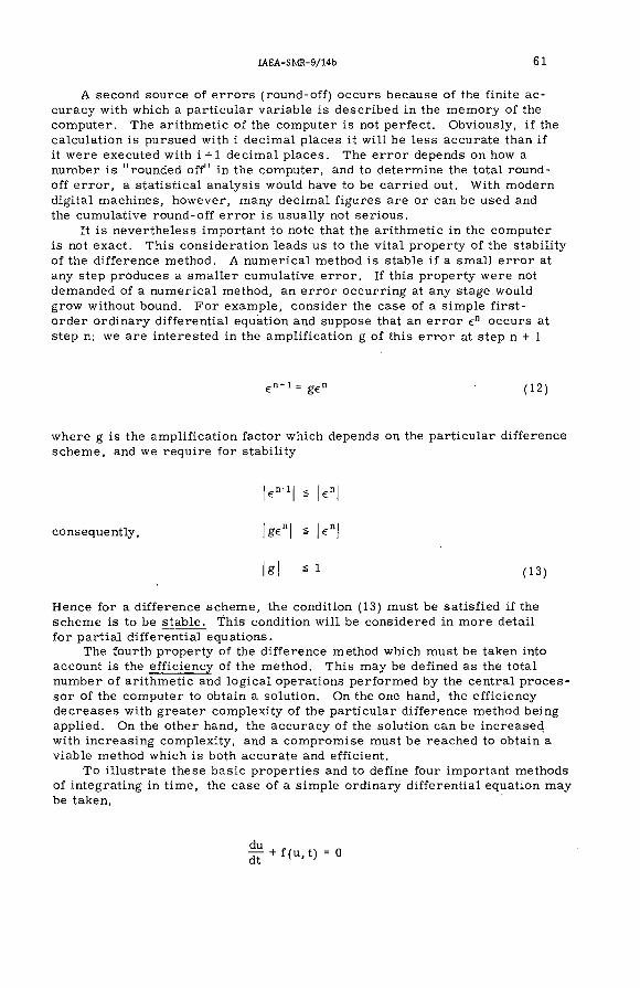
IA E A -SM R -9/14b 61

A second source o f e r ro rs (round-off) o ccu rs because o f the finite a c ­curacy with which a particu lar variable is described in the m em ory o f the com puter. The arithm etic o f the com puter is not perfect. Obviously, if the calculation is pursued with i decim al places it w ill be less accurate than if it w ere executed with i + 1 decim al p laces. The e r r o r depends on how a number is "rounded o ff" in the com puter, and to determ ine the total round­o ff e r ro r , a statistica l analysis would have to be ca rried out. With m odern digital m achines, however, many decim al figures are or can be used and the cumulative rou nd-off e r ro r is usually not seriou s.

It is nevertheless important to note that the arithm etic in the com puter is not exact. This consideration leads us to the vital property o f the stability o f the d ifference method. A num erical method is stable i f a sm all e r r o r at any step produces a sm aller cumulative e r ro r . If this property w ere not demanded o f a num erical method, an e r ro r occu rrin g at any stage would grow without bound. F o r exam ple, con sider the case o f a sim ple firs t- ord er ordinary d ifferentia l equation and suppose that an e r r o r e" occu rs at step n: we are interested in the am plification g o f this e r r o r at step n + 1

еп+i= ggn ( i 2 )

w here g is the am plification factor which depends on the particu lar d ifference schem e, and we require fo r stability

l e ^ l á ]e"l

consequently, - l^"l

k ! - I (13)

Hence for a d ifference schem e, the condition (13) must be satisfied if theschem e is to be stab le . th is condition w ill be considered in m ore detail for partial d ifferentia l equations.

The fourth property o f the d ifference method which must be taken into account is the e ffic ien cy o f the method. This may be defined as the total num ber o f arithm etic and log ica l operations perform ed by the central p r o c e s ­sor o f the com puter to obtain a solution. On the one hand, the e ffic ien cy d ecreases with greater com plexity of the particu lar d ifference method being applied. On the other hand, the accu racy o f the solution can be increased with increasing com plexity, and a com prom ise must be reached to obtain a viable method which is both accurate and efficient.

To illustrate these b asic properties and to define four important methods o f integrating in tim e, the case o f a sim ple ordinary d ifferential equation may be taken,

^ + f ( u , t ) = 0

62 POTTER

As the sim plest interesting example of such an equation, the decay equation may be given,

3 .1 . E uler method

If u is given at step n, namely u"(u° is defined by initial conditions), we wish to determ ine u at step n + 1. The sim plest method is the E uler explicit f ir s t -o r d e r method (F ig . 1)

In the E uler method, the function f is evaluated only at tim e t", and hence the method is explicit and f ir s t-o rd e r accurate in the tim e-step At only. To investigate the stability o f the method, it is assum ed that a sm all e rro r , e " , exists at step n and we question how the e r r o r is am plified to step n + 1. To do so, the d ifference equation (14) is linearized about the sm all e r ro r e"

u"*i = u" - f(u " ,t" )A t (14)

gi+i = gt. _ 9f_

and using the definition for the am plification factor (Eq. (12)),

g (15)

f

FIG. 1. Euler explicit method. Between time-steps tn and tR+1, only the first term in a Taylor expansion about time t** is used to integrate the equations.

IA E A -SM R -9/14b 63

t ь°/ ,

//

neutraНу stobte

\ /\

/\

FIG.2. Example of stability in the Euler explicit solution to the decay equation(decay time 7 = 1 .0 ). The three cases shown iHustrate a stable, an unstable and a neutrally stable solution as the time-step At is varied about the stability condition ( At s 2 .0 ).

C learly, fo r decay type equations, where 8 f /8 u s 0 , the stability condition is satisfied i f the tim e-step is su fficiently sm all such that

F or exam ple, in the decay equation, with decay tim e т, 3 f/8u = l /т , we requ ire fo r stability:

This is illustrated in F ig . 2, where the case o f a stable, neutrally stable, and unstable solution o ccu rs as the tim e-step , At, is varied accord ing to the condition (7).

3 .2 . Leapfrog method

S econ d-order accu racy may be obtained by storing the variable u at two t im e -le v e ls (F ig .3 ) :

At g 2т (17)

u " ' i - f(u ", t")2At

u" - f(u"+i, t"+i)2Atu',n+2 =„n (18)

64 POTTER

FIG.3. Leapfrog scheme. Second-order accuracy is achieved by using a three-level formula at any step. The meshes (X and O) can becom e uncoupled.

The sam e method o f stability analysis is applied as b e fore , but now e r ro rsat three tim e -lev e ls , e are related:

n+1Эи 2 A te" (19)

= 1 - 8f Эи 2 Atg

T herefore ,

+1 where 3fЭи 2 At (2 0 )

There are two roots fo r the am plification factor (corresponding to second- ord er accuracy) and fo r n on -oscilla tory equations, where the param eter is not im aginary; the magnitude o f the am plification factor for one of the roots is always greater than one. This a rises because we have introduced an arb itrary com putational mode, and the variables on the even mesh 2n are not coupled to the variab les on the odd m esh 2n + l . This w ill be considered in m ore detail later, but clearly , if the computational mode can be rem oved, either because the equations are oscilla tory (a is im aginary as in a pair of coupled equations) o r by a filtering technique, the leapfrog schem e is parti­cu larly sim ple and has secon d -ord er accuracy .

3 .3 . T w o-step explicit method

An extrem ely useful method with wide application is to "tim e centre" n+l

the integral, / f dt, by a tw o-step p ro ce ss . The tw o-step method uses the

IAE A-SM R-9/14b 65

E uler explicit method as a first stage in evaluating the dependent variable,u, tem porarily at tim e, t= t^ (a u x i l ia r y calculation):

A uxiliary u"^ = u " - f ( t " , u " ) y ^ (21)

Main u "^ = u " - f ( t " ^ , u"+*)At (22)

The am plification factor g is

At

Again, fo r the case 9f/9u â 0, stability is achieved for a su fficiently sm all tim e-step ,

2.0

ÊÎЭи

(23)

3 .4 . Im plicit secon d -ord er method

In the three methods described above, the solution at each tim e-step is obtained in explicit form and a stability cr iter ion for the tim e-step must always be satisfied . We may form ulate an im plicit se con d -ord er accurate

n+lmethod by evaluating the tim e integral / f dt by a tim e average (F ig. 4):

n

u"+i = u" - ^A t (f(u ", t") + f(u "^ , t " ^ (24)

The am plification factor, g, satisfies

ЭиAt2

9ÍЭи

At2 S

1 - 9fЭи At

1 + Эи At'n+1

(25)

F or the case 9f/9u ё 0, the magnitude of the am plification factor is always sm aller than one, and the method is unconditionally stable, which is c learly a great advantage o f an im plicit method. We have not, however, obtained the new dependent variab le , и"*!, exp licitly in term s o f known quantities, and a possib ly com plex a lgebraic equation must still be solved at each tim e-step . F o r m ore sophisticated methods and a detailed d iscussion o f ordinary d if­ferentia l equations, see Ref. [1] .

66 POTTER

f

f / ' ' J l / / / / Л ! / / / . / /)

tFIG.4 . Implicit second-order scheme. Second-order accuracy is achieved by time-averaging the integration.

4. VON NEUMANN STABILITY CONDITION FORPARTIAL DIFFERENTIAL EQUATIONS

The im portant properties of a d ifference solution to the in itial-value problem have been enum erated and the nature o f the d ifference approxim ation as a long-w avelength approxim ation in describ ing only the long-wavelength m odes o f the dependent variables has been described . F or ordinary d ifferen ­tial equations the im portant property o f stability in the explicit case depends prim arily on the magnitude o f the tim e-step in com parison to the physical tim es o f interest in the problem , and,by evaluating the d ispersion relation o f a system o f partial differentia l equations,we have d iscussed the important t im e -sca le s o f interest which occu r in physical prob lem s. These ideas may now be synthesized in evaluating the properties o f a num erical solution to a system of partial d ifferentia l equations.

F o r a system o f partial differential equations the solutions are obtained at each tim e-step by operating a m atrix C(At, A) on the solution at the p re ­vious tim e-step (see E q .(lO ))

To determ ine the stability o r to obtain the d ispersion relation of the difference schem e, the.problem may be sim plified by separately investigating the modes on the m esh. If С is constant (otherw ise a linear approxim ation is applied) and the space interval is period ic , then fo r a F ou rier mode

(26)

= u (k) e '^ j

the set o f equations (E q .(26 )) may be transform ed

IAEA-SM R-9/14b 67

G (At, к) is the am plification m atrix o f the d ifference schem e, fo r the F ourier mode k. F o r stability, we demand: if the amplitude o f a F ou rier mode isfinite at tim e t = 0. then it must rem ain finite fo r all tim e-steps n. Namely,

where К is a positive finite num ber. Using the definition o f the am plification m atrix,

F o r large n, К"-* 1. In general, G is a m atrix o f order I fo r a system of I f ir s t -o r d e r partial d ifferentia l equations, and the magnitude o f G is given by its determinant,

Von Neumann took into account the possib le occu rren ce of a growing loca l term in the partial d ifferentia l equation and he has shown that a n ecessary and sufficient condition fo r stability is (R ef. [2])

w here g* is the com plex conjugate o f g .. In the partial d ifferential equations o f interest, the m atrix С is in fact not a constant but might vary over the space and tim e lattice. The stability condition then reduces to a " lo ca l" condition, i . e . it must be satisfied everyw here on the m esh. The above d iscussion , generalizing the concept o f stability in application to partial d if­ferentia l equations, is m erely illustrative. F o r a m ore detailed and rigorous d iscussion , see Ref. [2 ].

u"[ < K¡u о (28)

û"(k) = G"û°(k)

G"û°(k)l < Kjû°(k) - (29)

T herefore ,

G"l < Ki

G¡ < К " (30)

i

G¡ = n gLi = l

We therefore make plausible the condition for stability

(31)

g¡¡ S 1 +Q (A t) fo r all i and k. (32)

The eigenvalues g. can be com plex:

I Si I = + J g * g i (33)

68 POTTER

5. EXPLICIT FIRST- ORDER SOLUTION TO THE DIFFUSION EQUATION

As a sim ple exam ple to illustrate this approach to stability, we consider a fir s t -o rd e r accurate (in the tim e-step) d ifference solution to the diffusion equation with constant conductivity, analogous to the E uler method. The diffusion equation

is sim ulated by the d ifference equation

F o r a F ou rier mode in space, u? = u " e ^ j ,

-n+l ikx; u (k )e ^ , K A t / ik(Xj+ A) + eik(Xj- A)

Consequently,

, 4KAt . - kA = 1 - sm 2 — (36)

T h erefore , fo r ]gl á l ,4KAt

AZ g 2

.2At á 0 . 5 ^ (37)

F or stability, a maximum value of the tim e-step is obtained. This time correspon ds to the largest diffusion tim e on the space m esh (A^/K), and the result is hardly surprising . The accu racy of the method is fir s t -o r d e r only in the tim e-step and secon d -ord er in the space-step , with e r ro rs e.

e = О (At) + O(A^)

IA E A -SM R -9/14b 69

6. ADVECTIVE EQUATION: EXPLICIT FIRST-ORDER INTEGRATION

We have seen how important the advective equation is , and we consider a possib le d ifference solution in first order as fo r the diffusion equation. The advective equation

Эи Эи_— + V — = 0at ax

is sim ulated on a d ifference m esh by

n + 1 n v A t / n n A

Considering a F ou rier mode as before ,

. v A t . .1 ---- — i sm kA) u

g = l - - ^ ^ i s i n k A (39)

g is now com plex and its magnitude in the com plex plane is

¡g js = 1 + sin kA) (40)

Thus the von Neumann stability condition in this case cannot be satisfied for any tim e-step At, and the method is unconditionally unstable. This result leads to considerable difficulty in many fluid sim ulations.

We may, however, obtain a fir s t -o rd e r explicit solution, with the loss o f se con d -ord er accuracy in the sp ace -step by replacing the algorithm (Eq. (38)) by

(41)

where the value o f the variable at the old tim e-step has been rep laced by a spatial average. Again, fo r a F ou rier mode of wave number k, the am plification factor now becom es

g = c o s k A - i - r — s in k A (42)

70 POTTER

T herefore ,2

sin^ kA

= 1 - sin^ kA (43)

and therefore the von Neumann stability condition (E q .(32)) is satisfied if

This method has considerable im portance in hyperbolic equations and is known as the Lax method. Again, the maximum perm issib le tim e-step is associated with the fastest speed on the mesh o r the ch aracteristic physical time described by the equations. This condition for the tim e-step fo r hyper­b o lic equations is known as the C ouran t-F riedrich s-L ew y condition [3 ] .

7. DISPERSION AND DIFFUSION ON A DIFFERENCE MESH

The von Neumann stability condition has very wide applicability and perm its us to obtain a stability cr iterion in the sim plest way. It te lls us little , how ever, of the m ore detailed properties of a particular d ifference solution. If m athem atically the problem is not too com plicated, ideally we may obtain the d ispersion relation o f the differentia l system . Let us con ­sider the case of the Lax method applied to the advective equation. In one dim ension, fo r a constant velocity v, as fo r the d ifferential system s, the d ispersion relation fo r a F ou rier mode in space and tim e is

v )A t —i— á 1

(44)v

u + vk = 0 (45)

F or the Lax d ifference schem e (E q.(41)),

{<cos kA - — sin kA

and the d ispersion relation fo r the d ifference method is

(46)

2 Section 2 .2 o f paper SM R -9/14a, these Proceedings.

In general, u is com plex. Let ы = П + iy, and equating the rea l and im aginary parts o f the d ispersion relation (E q .(46)) separately,

tan f2At = —7— tan kA A (47)

2

sin^ kA (48)

In the specia l case where vA t/A = 1 , у = 0, and

HAt = - kA

Я + vk = 0 (49)

which is identically the d ispersion relation o f the d ifferential system (Eq.(45)). In general, however, fo r a variable ve locity v, or a non-linear problem , the param eter vA t/A is sm aller than one, at least on m ost points on the m esh.In this case , the im aginary part o f the angular frequency ex ists, у >0, and

Thus, in general, the Lax method gives r ise to diffusion on the m esh; unlike the differentia l system , F ou rier m odes decay on the m esh. In addition, d n /d k ^ v for all m odes; different m odes travel with different speeds on the m esh: the solution is d isp ers iv e . F o r long wavelengths (kAand HAt sm all),an expansion o f the d ifference d ispersion relation (Eqs (47, 48)) shows agreem ent with ttrb d ifferential d ispersion relation to firs t o rd er. But to second ord er in the Lax method, particularly for short wavelengths, the effects o f d ispersion and diffusion can be very severe . This is a difficult problem in the sim ulation of hyperbolic equations that may only be m inim ized by turning to methods o f se con d -o rd er accuracy .

8 . CONSERVATION ON A DIFFERENCE MESH

When a system o f partial d ifferentia l equations is non-linear, we may define a particular d ifference method, but there still rem ains a variety of ways o f d ifferencing non-linear term s. Since many o f the partial differential equations o f physics are conservative, as shown in paper SMR- 9 / 14a, it would be useful to demand that the corresponding d ifference equations are them selves conservative. M ore specifica lly , we seek d ifference equations which identically con serve the energy, m ass, momentum, and the magnetic flux of the system irresp ective o f the e r ro rs incurred by the finite d ifference lattice.

C onsider, say, a rectangular region R bounded by the boundary B. The region R may be divided by a m esh into a set o f elem entary rectangular ce lls ,

(50)

72 POTTER

FIG.5. A conservative scheme employs integrated variables in each space ce ll, C, N, E, S, W. The fluxes are defined only on the surfaces which divide the cells. Hence, if a differential system is conservative, a difference scheme may be devised which identically conserves the same variables on the mesh.

each o f volum e А т. In two dim ensions, there are IJ rectangular boxes (F ig . 5). The system o f conservative partial d ifferential equations^

9u 3^ + V - f ^ 0 (51)

may be integrated over each space-tim e box o f volum e AyAt between the sp ace -lik e su rfaces t"'*' , t". At ce ll C,

n+1 n+l

t" C t" с

T herefore ,

tn+l

j y u ^ d T - - ^ y u " d T = J " d t j f ? -d S (52)С С Surface

of С

where the left-hand side has been integrated over tim e, and on the right- hand side, the d ivergence theorem has been applied. On the m esh, instead o f defining the intensive variable of, say, density or momentum density, the total m ass o r total momentum, respectively , in each box o r c e ll may be defined. Thus,

3 Section 1 o f paper SM R-9/14a, these Proceedings.

IA E A -SM R -9/14b 73

In addition, the fluxes f -d S are defined on the surfaces of each ce ll. F or the ce ll ij, there are four fluxes (c = E, S, W, N),

3 - ,

T herefore ,

t" "

Although a particular d ifference schem e has not been defined, since we have not here defined the fluxes in tim e, this form ulation has the con sid er­able advantage that i f the d ifferential system con serves the variables udf, the d ifference schem e also identically con serves these variab les . F or , if Eqs (53) are summed over all the boxes ij, in R, the fluxes cancel in pairs, since fo r exam ple,

F = - FE.. w . .u t + i. j

T herefore ,J - J - ^

^ F А т "iji=l j=l 1=1 j=l

Hence the variab les J udT are identically conserved in R except fo r the R

fluxes crossin g the boundary В of R. By defining the fluxes Fgin tim e, a large set o f conservative d ifference schem es may be obtained.

9. SUMMARY OF METHODS FOR PARABOLIC EQUATIONS

With the techniques now available, a number o f important and useful methods fo r solving parabolic d ifference equations are brie fly sum m arized below . As an exam ple, the sim ple diffusion equation in one dim ension is used, but this is not to detract from the wide generality of the m ethods.

9 .1 . E xplicit f ir s t -o r d e r method

иП+1 = цП + KAt / n _ + u \ ) (54)j J A \ J+i j J-V

The am plification fa ctor is

g (At, K) = 1 - (1 - cos kA)

fo r stab ility :

ДЗAt á 0 .5

7 4 POTTER

e = О (At) + O(A^)

9 .2 . C rank-N icholson im plicit method

S econ d-order accu racy in the tim e-step is obtained by using an im plicit method:

n + l n K A t / n n \ K A t / n+1 n+l n - l\

The am plification factor is

i KAt . ?kA '1 - -Â = r s m 2 —

^ , KAt . ? kA

and the schem e is th erefore unconditionally stable with e r ro rs

e = O(At^) + O(A^)

We are still left with the problem o f solving a m atrix equation fo r u"* on the mesh at each tim e-step .

9 .3 . L eapfrog method for the diffusion equation

A seem ingly consistent method, as fo r ordinary differential equations, is the tw o -tim e -lev e l leapfrog method

<ss)

The am plification fa ctor fo r a = ^ 2^ (1 -co s kA) is

-a , <0*2

g can be less than minus one for all and the method is th erefore un­conditionally unstable.

IAE A-SM R-9/14b 75

9 .4 . D ufort-F rankel method

By slightly altering the leapfrog schem e (E q .(56 )), the D ufort-F rankel schem e is obtained:

n+i - n - i . 2KAt / n / n+1 . n - l \ . n t ,+ ^ 2 - W j + i - W j + " j ; + ( 5 7 )

F or a

A

2KAt A2 '

The schem e is explicit, and the am plification fa ctor is

g = icrcos kA ± \/1 - sin kA <

The modulus of the am plification factor g is always less than unity, so that the method is unconditionally stable, with e rro rs

10. SUMMARY OF METHODS FOR HYPERBOLIC EQUATIONS

To define these methods, the set of hyperbolic conservative equations in one dim ension are taken as an example

^ + ^ F = 0 9t Эх

where F = F (u ). It is found that stability cr iter ia (C ou rant-F riedrich s-L ew y condition [3]) are obtained

At g С (58)

where С is a constant o f the ord er o f unity and v is the largest velocity on the m esh. F or the advective equation, the fluxes are defined by F =vu, and v is som e ce n tre -o f-m a ss velocity . A lternatively, in w ave-like equations, v is a phase velocity .

10 .1 . Lax f ir s t -o rd e r schem e

(59)

76 POT,TER

time

FIG. 6. The conservative leapfrog scheme, which may be applied to conservative hyperbolic equations.A three-tim e-level formula is used (n -1 , n, n+ 1 ). The time derivatives are defined between the levels n - 1 and n+1, and the fluxes are defined at the intermediate space-time points.

w here, for the advective equation, the am plification factor g is

, . vAt . , ^g = cos kA - i —— sm kA s A

and, th erefore , for stability,

A* - v

e = O (At) + O(A)

10.2. Leapfrog schem e

Three tim e levels are used to obtain the d ifference equations (F ig .6)

(60)

and the am plification fa ctors g are

= ior ± J - 0-2 + 1

where

IAE A-SM R-9/14b 77

and,for a sufficiently sm all tim e-step , A t s A / j v ] , stability is achieved with the magnitude o f the am plification factor equal to one. Hence no diffusion a r ises , and the e r ro rs are o f the order

e = O(A^) + O(At^)

Decoupling between the m eshes can occu r, however.

10.3. T w o-step (L ax-W endroff) method

A method o f very wide applicability for hyperbolic equations is the two- step method or Lax-W endroff method. Just as for ordinary differential equations (Section 3.3) , we evaluate tem porary or auxiliary variab les at the half tim e-step to t im e-cen tre the equations. The auxiliary step uses the Lax method:

- й

which is used to define the fluxes ^ main step:

Main step:

The condition fo r stability is

A t s

«s2<

e = O(At^) + O(A^)

As with the leapfrog method, diffusion only occu rs to high order in kA, but in this case no extraneous com putational mode is introduced.

R E F E R E N C E S

[1] SMITH, G .D ., Numerical Solution o f Partial Differential Equations, Oxford University Press, Oxford(1968).[2] RICHTMYER R .D ., MORTON, K .W ., Difference Methods for Initial-Value Problems, John Wiley (Inter­

science), N ewYork(1967).[3] COURANT, R., FRIEDRICHS, К .О ., LEWY, H ., Math. Annin 100 (1928) 32.

¡AEA-SM R-9/14C

PLASMA PHYSICS, SPACE PHYSICS AND ASTROPHYSICSD .E . POTTERDepartment of Plasma Physics,Imperial C ollege,London, United Kingdom

Abstract

PLASMA PHYSICS, SPACE PHYSICS AND ASTROPHYSICS.Fluid problems which occur in the structure of stars, in the solar system and in laboratory and fusion

plasmas are surveyed. These topics are described by the hydrodynamic equations with the inclusion of self- consistent long-range forces: in gravitational hydrodynamics, used to study the evolution, structure and behaviour o f stars, the self-consistent gravitational field must be included; in magnetohydrodynamics, the self-consistent electromagnetic fields must be included. Systems of equations for the gravitational and electromagnetic cases are developed, and some simple properties of such equations are analysed. In particular, the important frequencies associated with the gravitational frequency and with Alfvén waves are stressed. The difference solutions o f two particular problems are used to illustrate the general approach. In the gravitational case, a one-dimensional model o f stellar pulsation is discussed and an im plicit solution to the non-linear equations described. The approach is also applicable to one-dimensional problems in magnetohydrodynamics. In the electromagnetic case, explicit models for two-dimensional problems are briefly outlined. Such multidimensional problems are o f importance in thermonuclear fusion physics, in

1. INTRODUCTION: FLUID EQUATIONS AND LONG-RANGE FORCESIN LABORATORY AND ASTROPHYSICAL PLASMAS

The scope o f the title o f this paper is extrem ely broad, covering, as it does, a wide range o f fluid ob jects from laboratory plasm as to stars and galactic fluids. To define the subject o f the paper m ore p rec ise ly , we are interested in describ ing m any-particle (that is nuclear o r star-like) assem blies , interacting by long-range forces (gravitational or e le c tro ­m agnetic), by nuclear fo rces and by radiation tran sfer. We shall be concerned only with fluid descriptions o f such assem blies, sin ce the evolution o f distributions in p h ase-space , as described by, say, the V lasov equation, is d iscussed in papers SM R -9 /13a , b, с in these P roceed in gs .

The hydrodynam ic equations, which d escribe fluids interacting under their therm al p ressu re , as o ccu rs in, say, the earth 's atm osphere, are introduced in papers SM R -9/14a and S M R - 9 / 1 7 i n t h e s e P roceed in gs. We m ay d escrib e m any prob lem s in fusion ph ysics, in stars , and in the so lar system by the inclusion o f other fo rce s and other energy transfer p ro ce sse s . In describ ing the structure and evolution of stars, the se lf-con sisten t gravitational field produced by the stellar m ass m ust be included. In laboratory plasm as or the m agnetosphere, the se lf-con sisten t m agnetic fields must be in corporated and the plasm a is described by m agnetohydro- dynamic(M HD) equations. T h esep rob lem sa re strongly non-linear, since the occu rren ce o f the fluid produces the field , which in turn interacts back as a fo rce on the fluid, and apart from the sim plest p rob lem s, solutions may

79

80 POTTER

only be obtained com putationally. In addition, experim entally, both stellar ob jects and laboratory plasm as are very difficult to study, firs tly because they are both hot and destroy any probes, and secondly because both scale tim es and sca le lengths are either very short (laboratory plasm as) or very long (ste llar and space ob jects). A considerable understanding o f such fluid prob lem s m ay be obtained m ost read ily by sim ulating interesting problem s on the com puter.

To illustrate the range of physics involved and to introduce som e im portant prob lem s, som e exam ple problem s are listed which are described by gravitational hydrodynam ics or m agnetohydrodynam ics.

1 .1 . G ravitational hydrodynam ics

1 . 1 . 1 . Evolution of stars

Once a star is form ed by condensation from the ga lactic hydrogen m atter, it is o f in terest to evolve the h istory o f the star over long tim e- sca le s . A radial equilibrium is described by the expansive therm al p ressu re o f the stellar m atter and the contractive se lf-grav itational field o f the star. Our dominant concern here is the equilibrium o f energy, by production through nuclear reactions in the star in terior on the one hand, and,on the other hand, by lo ss through outward radiation [ 1 ].

1 . 1 . 2 . Stellar atm ospheres

When investigating stars experim entally, it is the outer atm osphere which is observed . The gravitational hydrodynam ic equations are solved in planar geom etry, but to describe fully the stellar atm osphere, com plex radiation phenomena must be studied, including m an y-species partially ion ized phenomena [ 2 ].

1 . 1 . 3 . Pulsation of stars

The full tim e-dependent gravitationalhydrodynam ic equations must be included in the non-linear prob lem when a s ta r 's radial equilibrium is un­stable. Stars m ay pulsate radia lly over t im e -sca les typ ica lly o f 10 seconds in non-linear m odes [ 3 ] .

1 . 1 . 4 . Gravitational collapse of stars

G eneral re la tiv istic hydrodynam ic equations are used to d escribe the rapid collapse, p r ior to supernova explosions o f old stars [ 4 ] .

1.2. M agnetohydrodynam ics

1.2. 1. L aboratory plasm as and pinches

The m a croscop ic behaviour o f dense laboratory plasm as is described by the interaction o f plasm a and m agnetic p ressu re , produced by currents in the plasm a [ 5 ].

IAE A-SM R-9/14C 81

1 . 2 . 2 . Fusion plasm as

Plasm a is trapped in very strong externally produced m agnetic fie lds.The sm all fields produced by the plasm a are nevertheless of great im portance in defining the length o f containment. These problem s are essentially three-d im ensional [ 5 ] .

1 . 2 . 3 . M agnetosphere

The m agnetosphere is a three-d im ensional prob lem in the interaction between the solar wind and the dipole m agnetic fie ld of the earth.

1 . 2 . 4 . Solar flares

A lso o f interest in astrophysics are problem s which involve both the gravitational field and the electrom agnetic field in the hydrodynam ic equations. In particu lar, one might include as exam ples o f such problem s the structure o f pulsars and the m agnetic field o f galaxies.

2. HYDRODYNAMIC EQUATIONS WITH SELF-CONSISTENT FIELDS

2. 1. Introduction to the equations

C la ss ica lly and in three d im ensions, we m ay d escribe a fluid hydro- . dynam ically by a set o f five tim e-dependent equations in the fluid density

(p), momentum density (pv), and internal energy density (pe) [6 , 7 ].

M ass :

^ - + V - ( p v ) = 0 ( 1 )

A cce lera tion :

dvP ^ = - V - P + F (2)

Internal energy:

^ - ( p e ) + P - V v + V - ( p e v + q ) = S ( p , e ) (3)

The p ressu re P is, in general a tensor (with trace 3p - the sca lar pressure) which might include v iscou s e ffects , and q is an energy flux which might include heat conduction or radiation diffusion. The gravitational or e le c tro ­m agnetic interactions m ay be included by defining additional fo rce s F in the acceleration equation ( 2) and supplementing the hydrodynam ic equations with equations for the fie lds . In the gravitational case,

F - pg - - pV<% (4)

82 POTTER

where is a gravitational potential, determ ined se lf-con sisten tly by P o isso n 's equation:

= 4jGp (5)

In studying stars, their evolution and structure, the energy flux q is a radiation diffusion term , and additional source term s, S(p, e), may occu r, for exam ple, through nuclear reactions.

If L is a sca le-length , these equations define in the first p lace the advection o f the fluid (frequency и = l^l/L) and secondly they d escribe sound waves (frequency ( 1 /L ) siyp/ p, where -y is the ratio of sp e c if ic heats) .In addition, gravitational oscilla tions occu r with frequency Ug =V4lrGpJ,and these couple to sound waves and lead, for exam ple, to the phenomenonof pulsating stars . It is these characteristic frequencies we must follow in tim e-integrating the equations 1.

In the m agnetohydrodynam ic case, the fo rce F is the m agnetic fo rce

F = i l x B (6)

where В is the m agnetic field and j the current density, given by A m përe 's law,

. i ^ V X B (7)

Unlike the gravitational case, the m agnetic field , in general, must be d es ­cribed by tim e-dependent equations as defined by F araday 's law,

^ + cV X Ë = 0 (8)

The e le c tr ic field to be used in this equation depends on the properties of the particu lar m agneto-flu id being studied. In the sim plest case , the Lorentz e le c tr ic field (in the fram e o f the m oving fluid) is defined by Ohm's law [ 5 ]

Ë + í v X В = r¡Y (9)

Again, in the magnetohydrodynam ic case , the ch aracteristic frequencies associated with advection and sound waves o ccu r . But, in addition, the m agnetic field acts as a p ressu re on the fluid and consequently A lfvén or m agnetosonic waves o ccu r, with a ch aracteristic frequency L /V ^ , where Уд is the A lfvén speed,

The res is tive e le c tr ic field in Faraday 's law leads to the diffusion o f the m agnetic field , and correspondingly the sou rce term , S, in the energy

* See papers SM R*9/14a and S M R -9/14b, these Proceedings.

[A E A -SM R -9 /14c 83

equation (3), includes Joule heating. These equations are supplemented by an equation o f state relating sp ecific internal energy density to the p ressu re o f the plasm a, ,

e = e ( P , P, Y) (11)

2.2. Simple properties of the equations

Unlike hydrodynam ic p rob lem s, the physical system s described above include gravitational energy (рф) and m agnetic energy ( ( l / 87r)B^) respective ly . Consequently, field energy and therm al energy are interchangeable and great variations in the fluid param eters can o ccu r. This leads to strongly non­linear p rob lem s, and ch aracteristic frequencies (gravitational frequency o r A lfven frequency) can vary v ery considerably over regions o f the problem . F or exam ple, in star structure prob lem s, densities between the inner core and the outer regions o f stars vary by many orders o f magnitude, and^ consequently, the gravitational frequency m ay be very large in the co re of a star but very sm all in the atm osphere of a star. In exp licit calculations such large variations can lead to difficu lties if the tim e-step is not to becom e too sm all.

S im ilarly , in the magnetohydrodynam ic case, plasm a densities may vary by three or m ore ord ers o f magnitude and the A lfven speed becom es very large in tenuous plasm a (since = B/V4rp). Thus the C ourant- F r ied r ich s -L ew y condition^ on an explicit tim e-step ,

A

where A is the m esh space-step , can lead to very sm all t im e-steps . A pproxim ations must be introduced to avoid sm all tim e-steps in such circu m stan ces .

3. ONE-DIMENSIONAL GRAVITATIONAL CASE: STELLAR PULSATION

Some o f the phenomena which arise from the study o f stars and which have been investigated by fluid sim ulation have been outlined in the previous section . These problem s are very d iverse, but the essential approach may be illustrated particu larly by describ ing the method of solution for problem s in stellar pulsation. Up to the present tim e, these prob lem s have been studied in one dim ension and the p ossib ly im portant p ro ce sse s o f convection from the centre o f stars have th erefore not been d escribed .

Stellar pulsation has been observed experim entally in certain stars for som e tim e, particu larly by the use o f Doppler shift m easurem ents from the surface o f such stars . T yp ica l frequencies o f the pulsation are o f the order o f 10^ s, associated with surface ve locities o f 50 km * s 'l . The method of sim ulation o f this prob lem , which is d iscussed here, has been devised and applied by C hristy [ 3 , 8 , 9 ] .

2 See paper S M R -9/14b, these Proceedings.

84 POTTER

In one dim ension the use o f a Lagrangian m esh and the rapid solution of tridiagonal m atrix equations [ 10], which facilitate the use o f im plicit d ifferen ce m ethods, admit a re la tive ly sim ple form ulation o f the prob lem on the com puter. This is equally true for magnetohydrodynam ic problem s in one dim ension where the sam e techniques are applied [11 ].

3 .1 . System o f equations

If r is an independent variable describ ing a radial shell in the star, a Lagrangian mesh m ay be defined,

(12)

where v is the cen tre -o f-m a ss fluid velocity . It is convenient to define as a variable the m ass with the shell o f radius r,

M(r) = J 4?rs^p(s)ds (13)0

F rom the continuity equation (Eq. (1)), in the Lagrangian fram e,

ТГ = °C learly , the m ass contained within each sph erica l Lagrangian shell is a constant. Thus, in this sim ple geom etry, P o isso n 's equation (5) m a y b e integrated im m ediately to define the lo ca l gravitational acceleration ,

g = (15)

and assum ing a sca lar p ressu re , pi = P , the a cce lera tion equation (Eq. (2)) becom es

d v _ GM(.r) ^ Э рdt ' r2 ' p Эг '

It proves useful to use as the independent Lagrangian space variable the contained m ass, M, rather than the radius, r (M is a sca lar single-valued function of r ). The acce lera tion equation takes the form :

É L _G M . 4 ^ 2 Эр (17)dt r2 ЭМ ^

and г = r(M , t). The final equation for the energy or tem perature of the fluid m ay be taken from the equation fo r the internal energy density (Eq. (3)),

IAE A-SM R-9/14C 85

where a sca lar p ressu re has been assum ed, and the energy flux q is dominated by radiation diffusion. A lternatively, this equation m ay be com bined with the equation for the kinetic energy and gravitational energy of the fluid to derive an equation for the conservation o f total energy,

A ( í v 2 - ^ + e ) + - á . ( 47rr2pv+q)=o

The conserved quantity in the tim e derivative includes, respective ly , k inetic energy, gravitational energy, and internal o r therm al energy. Frequently, and as has been d iscussed in papers SM R -9 /14a , SM R -9 /14b (these P roceed in gs), it is p re ferab le to use an equation for the conserved quantity (Eq. (19)) rather than the equation for the unconserved quantity, in this case the sp ec ific internal energy density (Eq. (18)). H ow ever, in this particu lar prob lem , large variations occu r between the gravitational energy and therm al energy in different regions o f the star, and in particu lar, there exist regions of low density on the surface of the star, where the calculation o f the tem perature from the total energy equation would yield large e rro rs from the sm all therm al energy term . Hence in this prob lem the tem perature is determ ined d irectly from the therm al energy equation (Eq. (18)).

The radiation flux term q depends essentia lly on the opacity, к (p, e), o f the lo ca l stellar m ateria l. We apply Stefan's law and obtain an expression for the energy flux,

q = -47rr2 ( 20)3 к р Э г

a is the Stefan-Boltzm ann constant. The inclusion o f this term makes the internal energy equation (17) parabolic and d escrib es the em ission and ab­sorption of radiation energy by the m a croscop ic coefficien t, l /к, which must be determ ined by considering the particu lar m icro sco p ic p ro ce sse s for a given p rob lem : Brem sstrahlung radiation and absorption and indeed atom ic phenom ena. In the in terior o f stars where particles are fu lly ionized, a very good functional approxim ation for the opacity к is к p/T^, but in the ste llar atm osphere, particu larly through the "ionization fron t", к m ay have a m ore com plex form . Finally, we define the sp ec ific internal energy density by an equation of state (for exam ple, in the fully ionized region * p / [ P ( l * ' l ) ]) which m ay be com plex through the ionization front. The

prob lem has now been reduced to three fir s t -o rd e r , one-dim ensional t im e- dependent equations (Eqs (11, 15, 17)) in the three dependent variab les, r(M , t), v(M, t) and e(M , t). The equations are essentia lly hyperbolic, describ ing advection (frequency ш), sound waves (u^) and gravitational oscilla tion s (шс)< but the in clusion o f the radiation term makes the energy equation parabolic with a d iffusion 'frequency '

86 POTTER

3.2. D ifferen ce solution

The Lagrangian independent variable M is d iscretized by spherical shell boundaries i, which define mesh ce lls i-^ ,

The dependent variables of radius and ve locity are defined at the m esh boundaries r " , vP 'i with the velocities defined at the h a lf-tim e-step s t"'$ . A ll other variables (the intensive variables) m ay be defined as ce ll quantities at i-^ and at integer t im e-step s . Thus, given the radius and p ressu re , at integer tim es, the acceleration equation is integrated on a tim e-cen tred , sp ace -cen tred schem e:

and,consequently, the new radial positions,at integer t im es,o f the ce ll boundaries are determ ined,

It rem ains to solve the equation for the energy density. The essential prob lem here is the non-linear diffusion equation, which is m ost readily solved im p licitly by the stable С rank-N icholson method, and a stability cr iter ion related to the diffusion frequency (шд) is th erefore avoided. C onsider the equation for the internal energy density e (Eq. (18)) which may be w ritten as

P i+ i, e ¡ .^ Г ;

: L м.

i - l i - § i i*t- i +1

(22)

(23)

The loca l density of each ce ll is determ ined

,n+l = Mi - M j-i (24)P

(25)

where R is the radiation diffusion coefficient,

2 4a 4T,3(26)

IAE A-SM R-9/14C 87

and we have written the internal energy density, e = e^T. The second termis exp licitly known, but the radiation diffusion coefficien t and the sp ecific internal energy density are functions of the unknown tem perature T . A solution m ay be obtained by iterating (over steps p) around the non-linear term s and using the C rank-N icholson m ethod^to tim e-d iffe ren ce the equation:

The equation is tim e-cen tred and sp ace -cen tred and the term on the righ t- hand side is exp licitly known. The left-hand side is a tridiagonal set of equations in the tem perature T at each tim e-step n + 1 and at each iteration step p + 1. When the tridiagonal equations are sim ply inverted [ 5] , im proved coefficien ts and are determ ined over the m esh, and thelinear tridiagonal equations are solved again to convergence. The tim e- step is then com pleted.

Because the gravitational frequency is an increasing function o f the density and the tim e-step must be chosen sm aller than the tim e of this frequency, the inner boundary is not taken at r = 0, but over a sm all, rigid, radiating sphere at the centre o f the star. E quilibrium initial conditions are im posed. C hristy [3 ] has obtained solutions fo r a wide range of equilibria . N on-linear steady-state oscilla tion s (o f amplitude typ ica lly 10%) are obtained illustrating the fundamental properties obtained experim entally. The detailed results are too extensive to d iscuss here.

The dominant m odes found from the sim ulations are either the fundamental or first overtone (one node), and after severa l periods o f oscilla tion , only one m ode ex ists. P a rticu la rly of interest, how ever, is the result that, given the sam e equilibrium but perturbing the initial state with either a la rg e - amplitude fundamental or a large-am plitude overtone, different steady-state oscilla tion s m ay be obtained in either the fundamental or first overtone.Thus the final state "rem em b ers" the tim e-h istory of the star [ 3 ] .

4. TWO-DIMENSIONAL MAGNETOHYDRODYNAMIC SYSTEM - THE COAXIAL Z-PIN CH

Unlike stellar prob lem s, prob lem s in m agnetohydrodynam ics, both in fusion and in the so la r system , are o f particu lar interest in two or three dim ensions (toroidal fusion p lasm as; the m agnetosphere; so lar ñ a res ). In two dim ensions, even on presen t-day com puters, the prob lem is fa ir ly sev ere : for exam ple, on a 64 X 64 m esh, typ ica lly we must so lve s ix tim e-dependent

2 See paper SM R -9/14b, these Proceedings.

= s " (27)

88 POTTER

approaching 1 MA between coaxial electrodes. A two-dimensional supersonic shock is produced (time t ) which collapses at the end of the centre electrode to form a thermonuclear plasma (time t^). The calculation simulates the experiment in the (r, z) plane to which the magnetic field (B^) is always perpendicular.

coupled equations over probably one thousand tim e-steps, producing then about 3 X l ( f dependent variab les. Again, the variety o f problem s is im m ense, and the basic approach shall be illustrated by using as an example a tw o-d im ensional explicit sim ulation o f a laboratory non-cy lin drica l su per­sonic pinch, which o ccu rs between coaxial e lectrodes and which produces a therm onuclear plasm a (F ig. 1).

We m ay w rite the m agnetohydrodynam ic equations m ost conveniently in conservative form .

M ass:

+ v9t pv = 0 (28)

Momentum:

+ p + B f i _ i 3 n . o (29,

M agnetic flux:

. ^ r + V - ( v B - B v ) = V X r i - ^ V X Ë (30)9t ' ' 4л- ' '

These equations are the sam e as given in Section 2, except that the magnetic fo rce term has been included within the momentum flux tensor (Eq. (29)) to

[AE A-SM R-9/14C 89

obtain conservative equations. In general, in fully ionized plasm as it is n ecessa ry to define separate e lectron and ion internal energy densities, Cg, e¡, the equations for which are non-conservative.

E lectron therm al energy:

P e , , + P e V ' V + V - ( p e ¿ v + q j = n f + p (31)

Ion therm al energy:

l ^ - p e i + P i V - v + V - ( p e i V + q¡) = - V : V v + p ^ L l i (g2)

qe and q¡ are the e lectron and ion heat conduction term s resp ective ly . V is the ion viscous tensor and is the tim e for equipartition between electrons and ions. In general, in three dim ensions, these equations define a set o f nine dependent variables u = (p, pv, B, p&e< pe¡) where equations of state relate = Cg(Pg, p), = ^i(Pn p)- In the absence ofres is tiv ity r), v is cos ity p, and heat conductivities and the equations are h yperbolic and describe advection (м — A / ¡v¡), sound waves (u A/v^ ), and A lfvén waves (u ^ A/vA), and in the explicit case the tim e-step is lim ited by a C ou ra n t-F ried rich s-L ew y condition,

A t sV +, У ( Pe + P i )

4я-р

(33)

Unlike the one-dim ensional case, m atrix equations resulting from tw o- or three-d im ensional p rob lem s are extrem ely difficu lt to solve, particu larly for the non-linear or variable coefficien t case . In the specia l case of P o isso n 's equation, the eigenvectors of a resulting d ifference m atrix are known and a variety o f exact methods o f solution are available. This is not the case for the general e llip tic equation with variable coefficien ts, and tim e-consum ing iterative m ethods, such as the A lternating-D irection - Im plicit or Chebyshev m ethods, would have to be applied at each tim e-step for the im plicit solution of the above equations.

F or m ultidim ensional p rob lem s, explicit m ethods have been m ost su ccessfu l. C ertainly for high-beta supersonic problem s (beta is the plasm a p ressu re com pared to the m agnetic p ressu re ), the diffusion p rocesses are sm all but im portant and may also be included explicitly . To avoid large num erical diffusion, we use a secon d -ord er method in the tim e-step to integrate the equations; the L ax-W endroff method is particu larly appropriate. We m ay w rite the equations as

- s (34)

90 POTTER

FIG. 2. In gravitational and electromagnetic hydrodynamic problems, large interchanges between field energy and thermal energy occur. The diagram illustrates the problem in the case of a magnetohydrodynamic simulation (plasma focus, Fig. 1) where in the vacuum region (large magnetic energy) the Alfvén speed becomes very large and a small time-step must be avoided. The calculation region is divided into a plasma region and a vacuum region: the time-independent electromagnetic equations must be solved in the two-

where the sou rce term s S arise only in the case o f the internal energy equations. Interm ediate values in tim e and space are found by the Lax m ethod. In two dim ensions, at the point (x ¡, y ¡) = С, at tim e t":

A uxiliary step

Main step

where F"*^ = F(u"*^) and the subscripts N, S, E , W re fe r to adjacent com pass points.

The diffusion term s are a lso included exp licitly by the sam e approach, but the sou rce term s in the internal energy equations, o f v iscous heating, joule heating, equipartition and adiabatic com pression , may be included im plicitly .

One o f the m ajor problem s in m agnetohydrodynam ic sim ulations is the occu rren ce of low -den sity regions where m agnetic p ressu re rep laces plasma pressu re and A lfvén speeds becom e very la rge . In the case o f a coaxial shock a "vacuum reg ion " exists behind the shock, and we must avoid a very sm all tim e-step as defined by the C ou ran t-F ried rich s-L ew y condition (E q .(33 )). H ere the m agnetic field is in the azimuthal d irection ; in the vacuum region (F ig. 2) we perm it no currents to flow, so that the vacuum m agnetic field is given by A m pere 's law,

IA E A -SM R -9 /14c 91

V E LO C tTY

Tim e = 0 .1071

z

Tim e

ï ....................- JTim e

м -'

t : \

§ .

T im e = 0 .8 0 2 3

FIG. 3. Two-dimensional simulation o f the plasma focus experiment. The diagrams illustrate, for successive times, the density in a moving shock and the associated flow velocity vectors.

92 POTTER

FIG.4. Dependent variables in the plasma focus shock, drawn above the two-dimensional (^z)-plane. Behind the shock, the large magnetic energy and low density, giving rise to very large Alfvén speeds,

where I is the total current flowing in the c ircu it. When the m agnetic fields exist in the plane o f the calculation, it is n ecessary to so lve L ap lace 's equation for the m agnetic vector potential in the vacuum region with varying boundaries,

V^A = 0 (37)

In laboratory plasm as and in the case o f the coaxial gun, the calculational plasm a domain is coupled with an external circu it which provides the e le c tro ­m agnetic energy,

3? ( L I ) = Q / C

L = В - d Ss

problems and in the magnetosphere, it is essential to describe anisotropic phenomena, associated with a vector magnetic field, on multidimensional ^computational lattices.

tAE

A-SM

R-9/14c

94 POTTER

where I is the current, L the inductance o f the system , С a capacitance and Q the charge on the capacitance (F ig. 1).

A s an exam ple o f such a sim ulation, num erical solutions o f the motion o f a tw o-dim ensional coaxial shock and the consequent collapse to form a therm onuclear plasm a on the axis o f the system are illustrated in F igs 3 and 4. The shock travels with a speed v = 2 X 107 cm * s*i and tem peratures o f 1. 5 keV are obtained in the hot contained pinch.

Another interesting example is the m otion o f a shock para lle l to magnetic field lines, which sw itches on a third component of the m agnetic field (F ig. 5). The rev erse phenomenon (sw itch -o ff shock) is believed to be of im portance in annihilating the m agnetic fie ld in so lar fla res .

In m agnetohydrodynam ics, the anisotropy introduced by the m agnetic field leads to a variety o f wave phenomena (Alfvén and W histler waves) which travel preferen tia lly along the m agnetic field . In addition, the co e f­ficients o f resistiv ity , v iscos ity , and heat conductivities are tensor quantities associated with the m agnetic field [ 1 2 ], and,in future sim ulations in both space physics and fusion physics, these an isotrop ic MHD phenomena must be sim ulated in two and three dim ensions for the full elucidation of the subject [13] .

R E F E R E N C E S

[1 ] KIPPENHAHN, R., WEIGERT. A ., HOFMEISTER, E., in Methods in Computational Physics (ALDER, В., FERNBACH, S ., ROTENBERG, M ., Eds), Academic Press, New York, 1 (1961 )129 .

[2 ] MIHALAS, D ., in Methods in Computational Physics (ALDER, В., FERNBACH, S ., ROTENBERG, M ., Eds), Academic Press, New York, 7 (1967) 1.

[3 ] CHRISTY, R .F ., Astrophys. J. 144 (1966) 108.[4] MAY, M. M ., WHITE, R. H ., in Methods in Computational Physics (ALDER, в., FERNBACH, S .,

ROTENBERG, M ., Eds), Academic Press, New York, 7^(1967) 219.[5 ] ROBERTS, K .V ., POTTER, D .E ., in Methods in Computational Physics (ALDER, В., FERNBACH, S .,

ROTENBERG, M ., Eds), Academic Press, New York, 9^(1970) 339.[6 ] COWLING, T .G ., Magnetohydrodynamics, John Wiley (Interscience), New York (1957).[7 ] KILLEEN, J ., "Difference Methods in Fluid Dynamics, with Applications", paper IAEA-SMR-9/17,

[8 ] CHRISTY, R .F ., Rev. mod. Phys. 36 (1964) 555.[9 ] CHRISTY, R. F ., in Methods in Computational Physics (ALDER, В., FERNBACH. S ., ROTENBERG, M .,

Eds), Academic Press, New York, 7 (1967) 191.

[11 ] HAIN, K ., HAIN, G ., ROBERTS, K .V .. ROBERTS, S .J ., KÖPPENDORFER, W ., Z. Naturf. 15a 12 (1960) 1039.

[12 ] SHKAROFSY, I .P ., BERNSTEIN, I. B ., ROBINSON, B .B ., Physics Fluids 6 (1963) 40.[13 ] POTTER, D .E ., "Multidimensional magnetohydrodynamic calculations", Proc. Second Conf.

Computational Physics, The Institute of Physics and the Physical Society, London (1970).

IA E A -SM R -9/13

PLASMA, GRAVITATIONAL AND VORTEX SIMULATIONR.W. HOCKNEYComputer Science Department,Reading University, Reading,United Kingdom

Abstract

PLASMA. GRAVITATIONAL AND VORTEX SIMULATION.

vortex simulation. Examples are given o f the use o f such models in the study o f electron devices, galactic evolution and fluid flow stability.

In this paper, we shall d iscuss the use of p a r tic le /f ie ld calculations in the sim ulation of p lasm as, galaxies and vortex flow s. We shall d escribe the sim ulation in term s of the plasm a case and show that by suitable sca ling the same m odel can be used fo r the case of galaxies and vortices .

THE QUASI-ELECTROSTATIC PARTICLE MODEL

In a particle m odel, the plasm a is represented by calculating the m otion of a "la rg e num ber" (usually 10 to 10 ) o f representative ions and electrons as they m ove through the fields of all the other particles.The m otion is governed by N ewton's laws and the only fie ld we consider in this m odel is the e lectrosta tic fie ld of the assem bly (except perhaps fo r a fixed external m agnetic fie ld ).

The m odel is term ed "q u a s i-e le ctrosta tic" because, although the pa rtic les m ove dynam ically accord in g to Newton's laws, the fie ld is at a ll tim es the e lectrosta tic fie ld due to the present positions of a ll p articles . That is to say, we con sider only non -re la tiv istic ve locities when the v e locity o f transm ission of the fie ld (i. e. the velocity of light) is very much greater than the v e loc ities of the particles.

In contrast to an M H D -plasm a, the m ain properties of such an e le c t r o ­static plasm a a r ise from charge separation and inertia. These lead to:

(a) P lasm a oscilla tion s at a frequency Up given by = 4!rne2/m and a ch aracteristic tim e of Tp = 27r/tjp. Here n, e and m are the density, charge and m ass of the p article , respective ly .

(b) Charge separation over distances of the ord er of the Debye length, Xp given by = к Т /(47гпе^). The Debye length is a characteristic length of the system . Here к is the Boltzm ann constant, and T the absolute tem perature.

The above behaviour is in sharp contrast to the behaviour of an MHD- plasm a which m ay be m ore fam iliar to many readers. In the MHD- plasm a one is interested in tim e sca les much greater than and distance s ca les much greater thanXp. On this tim e and space sca le , the system

95

96 HOCKNEY

m ay be considered to be neutral and all the effects present in the quasi­e lectrosta tic plasm a are ignored. F urtherm ore, in the M HD-plasm a on e 's interest is focused on the m agnetic fie ld produced by currents flowing in the system and the effect of this fie ld on the m otion of the plasm a. In the e lectrosta tic plasm a, the m agnetic fie ld of a m oving charge is ignored.

The e lectrosta tic particle m odel is useful in the study of(a) sm a ll-s ca le , h igh -frequency m icro -in sta b ilities which give rise

to anomalous diffusion and resis tiv ity effects.(b) V e loc ity -sp a ce instabilities, tw o-stream instability, Landau

damping, Debye shielding.(c) P rob lem s involving many inter-penetrating stream s.

H ow ever,because the m agnetic fie ld of a m oving charge is ignored,the m odel is only applicable to low densities fo r which ß = n k T /(B o /87r) « 1, where Bg is the strength of som e external m agnetic fie ld im posed on the problem , fo r exam ple, the containing fie ld in the case of a problem in controlled nuclear fusion.

A ll com puter m odels of a plasm a are wrong in one way or another.A particle m odel is wrong in the firs t instance because we represent a rea l system of say 10-^ p articles by a m odel with at m ost about 10 . We return to the question of the effect particle number on the properties of the m odel later on. We m ay a lso , as in the e lectrosta tic m odel, ignore many of the fie lds actually present in the physical system .

An M HD-fluid m odel is wrong because the velocity distribution function of the p artic les , f(v), is not allowed to change and the m odel cannot cope with inter-penetrating stream s. If, on the other hand, we go to a solution of V la sov 's equations which m ay be said to sim ulate a system of an infinite number of p a rtic les , to overcom e the problem s of particle num ber, then we swop e r ro rs due to using too few p articles fo r e r ro rs due to having too few spatial and ve locity m esh points on which to solve the V lasov equation.

THE TIM ESTEP LOOP

The sim ulation proceed s in a se r ie s of tim esteps during which the field is assum ed to rem ain constant. We store in the com puter the co -ord inates (x,y)t and (Vx, Vy^'^DTof the p artic les , where t is the time and DT the tim estep, and we find it convenient in the d ifferencing to regard the ve locity as given one half tim estep before the positions. The positions and v e loc ities are advanced stepwise in tim e as follow s:

(a) Find the fie ld on each particle due to the present positions (х;у)* of a ll p articles .

(b) A cce lera te each particle fo r a short tim e, DT accord ing to Newton'slaws;

tAEA-SMR-9/13

to obtain rev ised positions and velocities

97

(x,y)4-DT, ^)t+№*T

DIFFERENCING OF NEWTON'S EQUATIONS

The sim plest d ifferencing schem e is used which is centred in time

------- ' = q^E + --------- -------------- X ^

t+DT_ ç t .X "X _ r t+ DTDT

where x, V , Bg are vectors .This schem e is im plicit in the new ve locity how ever, the

equations are linear in the ve locity and an explicit expression can be obtained fo r the new velocity . We note a lso that if the ve locity is elim inated the resulting d ifference equation is the same as that obtained by d ifferencing Newton's equation in the form

d x . m -^2* = fo rce

with the second derivative represented as

d^x x '* °T -2 x '+ x '+ °Tdt D T '

The integration in tim e is explicit and we m ay expect there to be a stability requirem ent lim iting the size of the tim estep. In fact, one m ay show that fo r stability (jpDT < 2 , where Up is the highest plasm a frequency, which is due to the e lectrons. This is a severe lim itation on the size of the tim e- step and the magnitude of physical tim e that can be studied in this type of sim ulation.

FINDING THE FIELD

Tw o m ethods are available fo r finding the fie ld in step (a), the method of "action at a distance" and the "m esh m ethod".

A ction at a distance

F o r sm all num bers of p artic les , N <1000, it is possib le to find the fie ld on each particle by adding up contributions from all the other (N -l)

98 HOCKNEY

p a rtic les . Since this must be done fo r each particle the number o f arith ­m etic operations and hence the com puter time used w ill be proportional to N (N -l) o r fo r large N.

The fie ld on the i-th particle due to a ll others is

Tifii

j=l ¡¡9

which would take about IO N arithm etic operations to compute. T o find the fie ld on all N pa rtic les therefore takes about 10 operations.

T o see the meaning of this in p ra ctice , let us con sider a com puter which takes about 1 ps fo r an arithm etic operation (e. g. CDC 6600,IBM 360/91). Then the time fo r the fie ld calculation in each tim estep is:

N = 100 tim estep = 0 .1 s= 1000 = 10 s= 10000 = 1 5 mi n= 100000 = l d

Since a^useful com puter experim ent w ill include at least 1000 tim e-steps, it is c lea r that at m ost 1000 particles can be m oved in a sim ulation using the "a ction at a distance" method. Simulations of this type are perform ed in studies of c lu sters of a few hundred stars. F o r plasm a and galactic sim ulations,how ever, one must seek an alternative method which w ill allow one to m ove many thousands of p articles . T o do this a method in which the number of operations is proportional to N, be found.

The m esh method

In the m esh method the region of calculation is divided into a regular a rra y of ce lls as shown in F ig . 1. A t the centre of each ce ll, there is a m esh point at which the values of variables applying to that c e ll are calculated. In the present context, these variab les are the charge density and the e lectrosta tic potential. The fie ld in the region is then determ ined by solving the appropriate differential equation by fin ite -d ifferen ce m ethods operating on the variab les given at the m esh points. T o con serve storage it is usual to solve fo r the potential and then derive the fie ld s by differencing as fo llow s:

(1 ) exam ine (x ,y ) fo r each particle and assign a unit of charge to the appropriate m esh point. This gives a charge distribution p(x, y) on the m esh.

(2) Solve the P oisson equation

= - 4 т р

to give the e lectrosta tic potential. The 5-point d ifference approxim ation m ay be used

^i, j - i + <¡ ! ' i . j+i+<?' i - i , j+^i+i , j*4<¡[ ' i , j = - 4 т р ц Н 2

where H is the m esh interval.

lA E A -SM R -9 /13 99

FIG. 1. The mesh method * showing the division o f space into cells and the mesh points used in the solution o f Poisson's equation. A typical problem showing "stars" on a 48 x 48 mesh, [from HOCKNEY, R. W ., Astrophys. J. 150 (1967) 197, Chicago University Press].

(3) D erive the fie ld in each ce ll by d ifferencing

Ë = -grad ф

The sim plest fin ite -d ifferen ce approxim ation fo r the fie ld in the (i, j) c e ll is

Ex = (^i-i.j - A+i . j ) / 2H

Ey = (^i.j-i * ^ i.j+ i)/2H

In the above schem e let us suppose there are on average p particles p e r m esh ce ll, then there w ill be N /p m esh points. It w ill be shown in another paper by the author in these P roceed ings that, in sim ple geom etries, the number of arithm etic operations requ ired to solve P o isson 's equation [ 1 ] is proportional to the number of m esh points (neglecting a slow ly varying logarithm ic dependence). Hence the num ber of operations fo r stage (2) above is proportional to the num ber of p articles N. Stages (1)

100 HOCKNEY

and (3) a lso requ ire a fixed number of operations fo r each particle and hence the total number of operations requ ired by the m esh method is proportional to N. We find in a typical case that 100 000 p articles can be m oved one tim estep in 5 s on a CDC 6600 or IBM 360/91 which is som e­thing like 100 tim es the number of p articles that can be m oved using action at a distance.

NGP approxim ation [2]

P article m odels d iffer in the manner in which charge is assigned to the m esh in stage (1 ) above and the m anner in which the fie ld is obtained in stage (3). We have described above the sim plest schem e, which is known as the nearest-grid-point approxim ation (NGP) in which all the charge o f a particle is assigned to the nearest m esh point as shown in F ig . 2.In stage (3) the fie ld is taken to be the same fo r all particles in the same ce ll and is given by the sim plest d ifference given above.

The NGP is very sim ple com putationally and can be reduced by appro­priate scaling to a program like:

F o r every particle compute:

E X = P H I(I-1 ,J) - PHI(I+1, J)

E Y = PH I(I,J-1) - PH (I,J+1)

DX = DX + EX

X = X + D X

DY = DY + EY

Y = Y + D Y

N.G.R C. I. C.(NEAREST GRID POINT) (CLOUD IN CELL)

BUNEMAN. HOCKNEY et. al. BIRDSALL, FUSS et. al.

FIG. 2. The relation between cells, mesh (or grid) points and clouds in the NGP and C1C models. The region is divided into cells by straight lines. There is a mesh point shown by a cross at the centre o f each ce ll. In CIC this is the centre o f a square cloud. The shaded areas show the portion o f the cloud in each ce ll, and the arrows the mesh points with which the parts are associated, [from HOCKNEY, R. W ., Meth. Comput. Phys. 9 (1970) 135, Academic Press].

I = X

J = Y

X

X X X

X

IA E A-SM R-9/13 101

FIG. 3. The force F&/H) between two particles with separation x/H for the NGP and CIC models. The dots show the (x /H yi interaction between point charges, [from HOCKNEY, R. W. , Meth. Comput. Phys. 9 (1970) 135,

such a loop has six operations per particle and is probably short enough to use the "loop m od e" o r instruction stack fa c ilit ies of com puters like the CDC 6600 or IBM 360/91. The charge assignm ent loop is particulary sim ple:

I = X

J = Y

Q(I, J) = Q (I,J) + CH

where CH is the unit of change.The disadvantage with the NGP schem e is that the fo rce between two

interacting p articles varies like a staircase with separation, as is shown in F ig . 3. The sharp changes at the steps lead to a high level of noise in the system and a poor conservation of energy (a few per cent conservation over 1000 steps is considered good).

CIC approxim ation [3]

T o overcom e the noise p rob lem s associated with NGP the clound-in - c e ll method (CIC) was devised. In this method, the co-ord inate of a partic le is regarded as the centre of a square cloud of change of uniform density. In assigning the density in stage (1) the charge of the cloud is apportioned to the four neighbouring m esh points accord ing to the proportion of the cloud that lies in each of the four ce lls associated with the m esh points. In stage (3) the NGP fie ld is calculated in each of the four neigh­bouring ce lls . The total fie ld on the cloud is then found as the weighted average of the neighbouring fields, using as weights the areas of the cloud

102 HOCKNEY

in each ce ll. A program fo r the above method using an obvious notation might look like:

I = X

J = Y

Now w ork out the weights

U = X - I

V = Y - J

A = (1 -U )

В = (1 -V )

Now assign charge to the m esh points

Q01 = Q01 + A. V . C H

Q l l = Q l l + U. V. CH

Q00 =Q00 + A . B . C H

Q10 =Q10 + U . B . C H

where 00 re fe rs to the bottom left m esh point in F ig . 2:10 " " " " right " " "01 " " " top left " " ' "11 " " " top right " " "

F o r the fie ld calculation one has the NGP fie ld in a ll ce lls :

E00 = PHI (left) - PHI (right) about 00 ce ll E10 = sim ilarly " 10 "E l l = s im ilar ly " 11 "E01 = s im ilar ly " 01 "

and sim ilar ly fo r the у -fie ld ; then the total fie ld is

Е Т0Т Х = A . V . E 0 1 + U. V. E11 + A . B .E 00 + U. B. E10

and s im ilar ly fo r ET0TY.Since the weights are too num erous to store between stages (1) and

(3) they m ust be recalcu lated and the total number of operations per p artic le fo r CIC is about 34 com pared with 7 fo r NGP. The disadvantage of the CIC method is that it m ay take 4 to 5 tim es longer to com puter per particle than NGP. H ow ever, the CIC m odel is perhaps ten tim es le s s noisy and is the only method that can be used in som e cases.

The area-w eighting technique used in CIC is the same as a b ilinear interpolation and hence we find in F ig . 3 that the resulting fo rce law is like a linear interpolation between the step values of the NGP fo rce law. It is c lea r ly a much m ore accurate and sm oother approxim ation to the exact г** fo rce law between interacting line charges which is given by the dots in F ig . 3.

IA E A-SM R-9/13 1 0 3

GRAVITATIONAL ANALOGY

The e lectrosta tic particle m odel which has just been described can be applied to a gravitational problem by re -sca lin g . We note that the force law between interacting charges is

F = - Ч2r2

and between interacting m asses is

F = +r^

Hence^if we use an e lectrosta tic m odel with a charge-to-m ass ratio q /m equal t o jG , the square root of the gravitational constant, and in addition change the sign som ew here in the loop , then we have a gravitational sim ulation.

T here is , how ever, a m ore difficu lt problem associated with the absence o f gravitational e lectrodes. It is necessary to m odify the boundary cond i­tions of the potential problem to those associated with a gravitational prob lem . T his usually m eans that the gravitational potential should decay away to infinity correctly , without the potential being specified anywhere.In contrast, a typical e lectrosta tic problem has the potential specified on a near boundary. Consequently, considerable rev ision is likely to be n ecessary in the potential solving routine; a method fo r doing this is described in Ref. [4].

If a tw o-dim ensional e lectrosta tic particle sim ulation is converted to a gravitational sim ulation, one has a sim ulation of in fin itely-long rod -lik e stars. Such a tw o-dim ensional m odel m ay be interesting in its own right and have som e rea lism in sim ulating long c ig a r -lik e galaxies such as NGC 2685. H ow ever, the sim ulation of a thin-disk galaxy is much m ore interesting as it is a good m odel fo r the study of the origin and evolution o f sp iral structure. F o r this one needs a m odel of point (in contrast to rod) stars m oving in a plane and the potential calculation m ust reproduce co rre c t ly the r* potential of interacting point m a sses (and not the log(r) interaction of lin e -m a sses ). This cannot be achieved by solving P o is so n 's equation in two dim ensions, but F ou r ie r transform techniques are available and described in Ref. [1].

THE VORTEX ANALOGY

In an e lectrosta tic sim ulation with a high external m agnetic fie ld Bg the m otion of the gyrating p articles can be accounted fo r adequately by the guiding-centre approxim ation, which gives the ve locity d irectly from the e le c tr ic fie ld

V = сВ

104 HOCKNEY

or, in com ponent form ,

ir - -Ç. TT - - 2_^ ' Bz ^ * В , Эх

where ф is given by

V (j) = -4ir p(x, y)

UHLL WRLL

PLñSMR COOROS FLUX

1 1 \ ' * ъ

! f Г ! * **

' V <й

у ^

^ ^ ^ ^

! < < ^ i ) ! ) ^PLPtSMt)

POTENTtñL

FIG. 4. A Simulation o f plasma flow across a strongmagnetic field, showing top left * particle positions, top right - flux arrows, and bottom - electrostatic potential, [from HOCKNEY, R. W ,, Physics Fluids 9 (1966) 1826, A .I .P . ] .

IA E A -SM R -9/13 105

)

0.0 0.2 0.4 0.6 0.8

'

1.0 1.2 Í.4 ¡.6 1.8

r. r '

'Q ... №? #

2.0 2.2 2.4 2.6 2.8

№ № V

З.о 3.5 4.0 4.5 5.0

FtC. 5. The development of an elliptical bar galaxy under differential rotation. Time in units o f rotations oftheouterstars. [from HOCKNEY, R .W ., Publ. Astronom. Soc. Pacific 80(1968) 662].

An analogous situation a r ises in tw o-dim ensional in com pressib le and inviscid flow. In this case the velocity is derived from a stream function ^ by

Эу Эх

The vorticity , g, is then defined as the curl o f the stream function. Hence

^ c u r l V Vy V,

Com paring these fo rm alism s one can see that the stream function and vorticity are analogous to the e lectrosta tic potential and charge distribution. In this analogy the m oving charges m ust be thought of as m oving elem ents o f vorticity .

1 0 6 HOCKNEY

0 10 20 30 40

,у *

50 60 70 80 90

100 200 300 400

FIG. 6. The Kelvin-HeJmholtz instability seen in a thin electron beam in a strong magnetic Held or by analogy in the vortex layer between two fluids passing each other with equal and opposite velocities, [from LEVY. R .H ., HOCKNEY, R .W .. Physics Fluids 11(1968) 766, A .I .Р .] .

APPLICATIONS

A nom alous diffusion

An e lectrosta tic m odel with a fixed external fie ld has been used to study the anom alously high transport of plasm a a cro ss a containing m agnetic fie ld [2]. F igu re 4 shows the output from such a sim ulation. At the top left are the positions of all the sim ulated particles and at the top right are flux arrow s showing the flow of both ions and electrons. At the bottom is an isom etr ic view o f the potential showing the wave that gives r ise to the unexpectedly high transport of p articles from the plasm a at the bottom to the wall at the top.

Gravity

A m odified electrosta tic particle m odel has been used to study the evolution of galaxies. F igure 5 shows still fram es from a com puter-m ade m ovie displaying the evolution of a bar-shaped galaxy under the influence of d ifferentia l rotation, produced by the presen ce of a heavy central nucleus [5]. F am ilia r sp ira l shapes are observed but these are transitory and disappear a fter about five rotations.

IA E A -SM R -9/13 107

V orticity

An e lectrosta tic particle m odel with guiding-centre m otion has been used to study the stability of a thin beam of e lectrons in the in terior of a containing v esse l [6]. If the beam is thinner than about one fifth of the v esse l, it is found to be unstable to the K elvin-H elm holtz slipping stream instability. The nature of the instability is shown in F ig . 6 which contains still fram es from a com puter-generated m ovie. The beam is observed to wind up into v ortices . The linear-grow th region can be obtained by c la ss ica l analysis but the com puter m odel obtains, in addition, the non­linear saturation amplitude.

V iewed by the vortex analogy, the com puter experim ent of F ig . 6 can be regarded as showing the vortex layer between two fluids slipping past each other with different ve locities . The vortic ity is then confined to a thin layer at the junction of the fluids. In the right conditions this layer is unstable and the vortic ity re -d istr ibu tes itse lf as shown in the figure.

R E F E R E N C E S

[1 ] HOCKNEY, R .W ., Meth. Comput. Phys. 9 (1970) 135.[2 ] HOCKNEY, R. W. , Physics Fluids 9 (1966) 1826.[3 ] BtRDSALL, C. K. , FUSS, D ., J. Comput. Phys. 3 (1969) 494.[4 ] HOCKNEY, R. W ., Astrophys.J. 150 (1967) 797.[5 ] HOCKNEY, R. W ., Publ. Astronom. Soc. Pacific 80 (1968) 662.[6 ] LEVY, R .H ., HOCKNEY, R .W ., Physics Fluids 11 (1968) 766.

IAEA-SM R-9 / 13b

PARTICLE-FIELD INTERACTIONS: NUMERICAL TECHNIQUES AND PROBLEMS

R .W . HOCKNEY Computer Science Department, Reading University, Reading, United Kingdom

Abstract

PARTICLE-FIELD INTERACTIONS: NUMERICAL TECHNIQUES AND PROBLEMS.Errors inherent in the use o f a particle model in the simulation o f a physical system are discussed. These

arise from N, the particle number, H, the interval o f the space mesh, and DT, the time-step. Measurements are presented that show that the collision rate o f both the NCP and CIC models are the same and depend mainly on N. Stochastic heating which leads to poor energy conservation depends on N in the same way as the collision rate but also strongly depends on H, DT and the model used. The CIC has substantially less heating than the NGP model. Recommendations are made for the choice o f H and DT.

AIM OF MODEL

In particle fie ld sim ulations using the m esh method the object is usually to sim ulate a co llis ion less system . That is to say, it is desired to have the co llis ion tim e o f the m odel greater than the tim e o f the sim ulated ex­perim ent. Such a sim ulation can be used to sim ulate a physical system with a very long co llis ion tim e such as a 'c o llis io n le ss ' plasm a or a galaxy of stars . A lternatively , co llis ion a l effects may be added to such a sim ula­tion in a controlled and detailed way to obtain a sim ulation, e. g. o f a co llision -dom inated sem i-con ductor o r co llis ion a l plasm a.

SOURCES OF ERROR

The principal sou rces o f e r r o r in a particle m odel a rise from N — the number of particles which is always much le ss than in the physical system ; H — the space m esh in terval, and DT — the tim e-step , both o f which must be finite. The effect o f these e r ro rs is seen p rim arily in the d istortion of the co llis ion tim e and the introduction of stochastic heating.

COLUSION TIME

The co llis ion tim e may be defined as the tim e, on average, fo r a p a r t id e to be deflected 90° from its in itial d irection due to co llis ion s with other p artic les . In a plasm a, we are not dealing with h a rd -b illia rd -b a ll c o l ­lis ion s but with the accum ulation o f many sm all-an gle scatterings which a test particle su ffers as it bounces o ff the Coulom b fie ld of other p articles .F igure 1 shows som e orbits o f a typ ica l particle within a sim ulation, and

109

110 HOCKNEY

ORBITS

FIG. 1. Typical orbits o f simulated electrons and ions in a computer model o f a plasma. There is one dot per time-step in the motion. Electrons and ions can be distinguished by the difference in their velocities. [This and all other figures from J. Comput. Phys. 8 (1971) 19. Academic Press].

if < i(t) is the angular deflection of the i-th particle at tim e t from its initial d irection then the average square deflection is

N

<<^(t)> ^ ( t ) ) / Ni=l

The co llis ion tim e 7# is defined as the tim e fo r the square root of the quantity to reach 90°. F igure 2 shows the results o f such a m easurem ent made in a therm al tw o-dim ensional com puter plasm a.

E FFE C T OF PARTICLE NUMBER

It is som etim es difficu lt to see why the co llis ion tim e in creases as the partic le number in creases because one might think at firs t that, with m ore p articles to co llid e with, this tim e would be decreased . But one must rem em ber that as m ore particles are used to sim ulate the sam e system , le ss charge is associated with each particle and this rapidly de­crea ses the co llis ion c ro s s -s e c t io n of each particle . This effect overweighs that due to the in crea se in the number of co llis ion s and the co llis ion tim e is , in fact, in creased .

!A E A -S M R -9 /13b U l

DEFLECTION TtME

This m ay be seen from an examination o f the R utherford-C oulom b scattering cro ss -s e c t io n :

If q — charge o f partic le , m — m ass o f p article , d — density o f p artic les , v — average particle ve locity , and a — collis ion a l c ro s s -s e c t io n

then co ll is io n s /s are given by dva. The R utherford c r o s s -s e c t io n is p rop or­tional to q^/fm ^v^). Hence the co llis ion rate is

d q*V ос —ч— 9

If in the m odel we have 's ' e lectrons per particle of the m odel then q = se , m = sm e, d = n /s where e, me and n are the e lectron ic charge, m ass and physical plasm a density. Then

(s e)4 s / v^(sm)^ v ^ n ? (1)

Hence the co llis ion rate in the m odel is in creased by a factor s over that oí the rea l plasm a, 's ' is the ratio of number o f e lectrons in the plasm a to the number o f particles in the m odel and is typ ica lly 1 0 .

112 HOCKNEY

In term s of the co llis ion tim e т = and the particle number N, Eq. (1)becom es

_ Tplasma - N 'model g ^ "plasma

which shows the in crease of co llis ion tim e with particle number.The d ifference between a rea l plasm a and a com puter plasm a may be

visualized by considering a sandy beach of 1 0 - grains of sand (corresponding to the rea l plasm a) and a rocky beach, e . g . at Grignano, of 10^ boulders (corresponding to the com puter plasm a). Both beaches contain the same m ass of m ateria l but they have vastly different properties from the bather's point of view . If the bather wishes to reach the sea from his beach hut he may do so in a straight line on the sandy beach, but would be obliged to follow a circu itous route with many large deflections on the rocky beach.In the form er case , one has the long co llis ion tim e associated with the rea l plasm a and in the latter case the short co llis ion tim e and large deflections associated with the com puter plasm a.

MACROSCOPIC PROPERTIES

If a com puter m odel exaggerates the co llis ion a l effects by many orders o f magnitude, one must be concerned with the effect on other properties such as plasm a frequency and Debye length.

The plasm a frequency is given by

Up = 4 т п е ^ /т

Hence

("p)model 4^ (*S ) (sm e) " ("pe)plasma (3)

and the plasm a frequency is unaffected by the particle number used in the sim ulation. Since the Debye length Xp * vth/"pe, it w ill be unaffected provided we make the particle ve locity v the same in the m odel as in the rea l plasm a. This is always done. It may s im ilarly be shown that the amount of subdi­v ision , s, does not affect other m a croscop ic quantities.

EFFECTS OF MESH SIZE

M easurem ents have been made o f the co llis ion tim e in a tw o-dim ensional therm al plasm a for both the NGP and CIC m odels [ 1 ]. These are found to be fitted to 20% by the relation

= d(X , + w 2 )Tp

(4)

IA E A -SM R -9/13b 113

Nc =n(X§ + M ñ

FIG.3. The dependence o f collision time on particle number and width for the NGP, CIC. HNGP and HCIG models.

where d is the particle density and W the particle width. F o r both NGP and CIC it is found n ecessary to associa te a particle width W = H to the m esh spacing. F igure 3 shows the results o f these m easurem ents fo r a wide range o f conditions.

The co llis ion tim e can be said to depend p rim arily on the number of p articles used and, to a sm all extent — via W — on the m esh size . It is not dependent on the tim e-step DT and it is found to be the sam e, within the lim it of experim ental a ccu racy , fo r the NGP and CIC m odels. Some smoothing procedures have the effect of broadening the particle and this can affect the co llis ion tim e via the particle width W.

STOCHASTIC HEATING

E rro rs o f a random or stochastic nature occu r as particles pass c e ll boundaries of the m esh o r as fie ld variations are ignored because of the use o f a finite tim e-step . These e r ro rs may be regarded as being equivalent to the introduction o f a stochastic e rro r fie ld at each tim e-step . This leads to a random walk in ve locity space and consequent stochastic heating of the system . This in itse lf constitutes a lo ss of energy conservation .

The heating tim e is defined as the tim e fo r the in crease in energy due to stochastic heating to equal k T /2 . Since т*ц depends on the particle number in the sam e way as Tcoib we study the ratio Thisis found to be a com plicated function o f the tim e-step DT and space m esh H.

This dependence is shown in F ig . 4 fo r four m odels. These are the NGP and CIC and two others, HNGP and HCIC, obtained from them by smoothing

114 HOCKNEY

HNGP HCIC

FIG.4. Variation o f heating time in the parameter plane (M peDT, H /Xp).

the potential b e fore use. It is desirable to keep the ratio as largeas p oss ib le , and it is evident from F ig . 4 that fo r any value o f H/Xp there is an optimum value fo r MpgDT. This optimum path through the param eter plane is given by

(upeDT)opt = m in i H 1Л-D

(5)

and is shown in F ig . 5 and also by the dotted line in F ig . 4.It is evident that a t im e-step la rger than the optimum w ill result in a rapid in crease in stochastic heating, whilst a tim e-step shorter than the optimum decreases the stochastic heating very little . One has a lso to avoid getting too c lo se to MpgDT = 2 which represents the stability lim it fo r the tim e integration schem e.

A long this optimum path the heating tim e is given by

(6 )

IAE A-SM R-9/13b 115

MpgDT

FIG. 5. Regions o f the parameter plane (h ^ D T , H A o) ^nd the optimum path.

where

IQ = 2 NGP

= 41 CIC

= 6 .4H N G P

= 200 HCIC

The heating tim e is then very strongly dependent on the m odel used as w ell as on the s ize o f the sp a ce - and tim e-steps .

CHOICE OF MODEL

The resu lts obtained in the previous sections enable us to choose rational­ly between the available m odels fo r any particular application. The basis o f the ch oice w ill be the cost in com puter tim e o f sim ulating a co llis ion less plasm a fo r a given num ber of plasm a periods using a given num ber of m esh points. The cost w ill be a ssessed on the basis of the number of arithm etic operations involved, and it w ill be assum ed that a plasm a may be regarded as co llis ion less up to a tim e equal to the co llis ion tim e o f the m odel.

. The number of particles used must be selected on the basis o f the number of co llis ion less plasm a periods P that are requ ired using Eq. (4),

p = (T c o l l /T p e ) = d (A .p + w " ) / K i (7)

116 HOCKNEY

Then the number of particles n ecessary in a region of s ize L cm X L cm is

N = d = K i P L^/(X^,+ W^)

The tim e-step used w ill be chosen from the optimum path on the basis of the value o f H/Xp using Eq. (5)

(upe DT)opt = min (l/2)H /A .o, 1 (8)

The number S of steps requ ired is then given by

g = Ртре ____2 rP ____ , .D T . p t * ( " p e D T ) . p t ' ^

If we let Kg (m odel) be the cost of computing fo r a given m odel per step per partic le then the total cost is

2т K 5K 1 P ^ (L /H )2( U p ^ D T ) . p t (()LD/H)2 + ( W / H ) 2 )

We note that the cost is proportional to the square of the number o f c o ll i ­sion less plasm a periods requ ired and to the number of m esh ce lls . Hence we com pare the cost per square co llis ion less plasm a period per m esh ce ll which is

c/(PL/H)S = 1И^о/Н)' + (^/Н)2)

This function is plotted in relative units fo r the different m odels as a function o f (H/Xp) in F ig . 6 . On the basis of the number o f com puter opera ­tions we have taken Ks(CIC o r HCIC) = 5 K 5 (NGP or HNGP). Because of this fa ctor , the NGP and HNGP m odels are always cheaper if they can be used. H ow ever, the noise in these m odels prevents their being used fo r large values o f (H/Xp). If we assum e that a m odel can be used provided the heating to co llis ion tim e ratio (тн /тссм ) is greater than 10 (and th erefore the total energy conservation better than 2. 5%) then the m odels may only be used on the solid parts of the cu rves. If in addition we only use smoothing when the unsmoothed m odel is too noisy, in order to keep as much spatial

IA E A -SM R -9/13b 117

Ю

CIC

HCIC

NGP HNGP CIC HOC0 .)

0.1 10H/Xo

FIG. 6. The cost per square coHisionless plasma period per mesh ceU in relative units for the NGP. CIC. HNGF and HCIC models.

resolution as p ossib le , then we find that there is a favoured zone o f (H/Xp) where each m odel is cheapest. This is given by the tableau

where the name of the m odel is written between the values o f H /Xp fo r which it is best suited.

If one is le ss conservative and allow s computing up to а (тн /тсо11 ) * equivalent to a total energy conservation of 25%, then the dotted parts of the curves of F ig . 6 may be used and the favoured ranges o f (H/Xp) for the different m odels are

Under these circu m stances, none of the m odels considered here can be used for H/Xp > 14.

Oi-NGP-0. 45<-HNGP-^0. 8<-CIC^2. &-HCIC^4. 5

O^NGP-1. 543N G P-2. 5 -C IC -6 . 5-HClC^14

R E F E R E N C E

[1 ] HOCKNEY. R .W .. J. Comput. P hys.'8 (1971)19.

IA E A -SM R -9 /13c

THE SOLUTION OF POISSON'S EQUATIONR.W . HOCKNEYComputer Science Department,Reading University,Reading, United Kingdom

Abstract

THE SOLUTION OF POISSON'S EQUATION.Iterative methods for the solution o f Poisson's equation are considered first and the convergence rates o f the

SOR, Gauss-Seidel and Chebyshev methods are compared. Direct methods, based on Fourier analysis and cyclic reduction are then discussed, and finally measurements are given o f the execution times for Poisson solvers using a variety o f computers and compilers.

In many areas of com putational physics, particu larly in tim e-dependent sim ulations, a central prob lem is the rapid solution of the fie ld equations.In the past few years a variety of specia l d irect methods have been developed which can be used in sim ple geom etries, and, in this case, are very much superior to the m ore com m only known iterative m ethods. In this paper, we shall confine our attention to the solution of one equation, nam ely that of P oisson :

= - 47гр(х, у) (1)

ITERATIVE METHODS

B efore proceed in g to a d iscussion of the specia l d irect methods, we start by quoting som e convergence results fo r the m ost com m only used iterative methods, in order to dem onstrate how bad the convergence can be.

We con sider the solution of P o isso n 's equation in the square with ze ro values for the potential on the boundary. The five-point d ifference approxi­mation is used

+ ^i+l . j + ^ i . j - i + + i " 4^ i , j = -4?rpi.jH^ = q i j - (2)

We consider three iterative methods:

(a) G auss-Seidel method

Equation (2) is solved fo r ^¡,j and this form ula is used to update mesh values in som e ordered sequence, e .g . line by line. F resh ly computed values im m ediately overw rite old values on the m esh and the hence latest values are always used on the right-hand side

new t i latest values^i,j " ^ "t* ' Qi.j] (3)

120 HOCKNEY

(b) S u ccessive over-re laxation (SOR)

In this method, the new value is calculated as an average of the used by G auss-Seidel and the old value. A constant ш, the relaxation factor, determ ines the weighting:

new i old<hj = + (1 * (4)

1 g u g 2

F or the square a form ula exists for мь, thebestvalue of the fa ctor u.

(c) Chebvshev method

A variant of SOR in which u varies every half iteration has better convergence p roperties than SOR. This is the Chebyshev method in which the iteration is divided into two parts. The firs t half is the adjustment of all odd points (i. e. those fo r which i + j is odd) on the mesh by Eq. (4), the second half iteration is the s im ilar adjustment over the rem aining even points.

The relaxation fa ctor varies at each half iteration accord in g to

= 1

- 2 " ' )

where p = cos 7r/n fo r an n x n mesh. It can be shown that = Иь, so that the Chebyshev method starts with a half iteration of G auss-Seidel (when u = 1 ) and then sm oothly varies u until one is perform ing SOR with и =

CONVERGENCE RATES

If is the exact solution to the P o isson problem then we define the e r ro r v ector at the t-th iteration to be

. (5)i.j i.j 't . j ' '

and the norm of the e r r o r vector to be

(6)

A ll the above iterative p ro ce sse s are linear and the t-th iterate of the e rro r can be related by a m atrix M(t) to the initial e r ro r ,

e(t) = (7)

IAE A-SM R-9/13C 121

its initial value) with the number o f iterations, for SOR, Gauss-Seidel and Chebyshev methods on a 128 x 128 mesh using Odd/Even ordering. [from M eth . Comput. Phys. 9 (1970) 166, Academ ic Press],

Taking norm s and dividing we have

4 ! ¡ g M(t) (8)i (0) i - H ^

Hence Ц м ^ Ц is an upper bound on the factor by which the in itial e rro r is reduced in t iterations. Fortunately, fo r the P o isson problem in the square, ]]м ^ )]] can be calculated by analysis fo r all the above iterative methods, and the results are plotted in F ig. 1 fo r a 128 x 128 mesh.

F rom this figure it can be seen that the convergence of the G auss- Seidel method can be so slow that the method is u se less . The SOR method, whilst it gives a reasonable convergence rate fo r large t, can give unexpectedly bad results fo r sm all num bers o f iterations. In fact, it is possib le fo r the e r ro r to in crease in size by 30 tim es in the fir s t ten iterations. The su periority of the Chebyshev method is seen in that it overcom es this prob lem with SOR and, as may be proved analytically, Ц м ^Ц is a m onotonically decreasing function of t. Even with the Chebyshev method it can be seen that about n iterations are requ ired to guarantee an e rro r reduction by a factor of 1 0 " to 10" .

We should like it to be c lea r what the above theoretical results mean. They do not mean that fo r any particu lar case the e r ro r decay w ill follow the curve of' F ig. 1 but only that no e r r o r decay curve met in practice can r ise above the lines in the figure. The curves are therefore a w ors t-ca se

122 HOCKNEY

resu lt. The e r ro r bound is sharp, however, because of the equality in Eq. (8). This means that there exists an initial e r ro r vector which would give an e r ro r decay curve that w ill touch any chosen point on the curves.

We hope this b r ie f d iscussion of the m ost com m only used iterative m ethods and convergence results w ill motivate the follow ing d iscussion of d irect m ethods. These are methods that so lve the d ifference equations (2) in a known finite number of arithm etic operations that are equivalent in work to about 5 to 10 SOR iterations. It is c lea r that within this tim e one can guarantee no significant reduction o f the e r ro r by any o f the iterative m ethods.

DIRECT METHODS

A d irect method of solution is one in which a single solution is obtained after a fixed finite number of arithm etic operations which is accurate to within, say, 10 tim es the rounding e r ro r . This contrasts with an iterative method in which many approxim ate solutions are found which, if a ll goes w ell, converge gradually towards the solution to the problem .

If we let be the vector of unknown values on the j-th line, then the P o isson prob lem can be expressed in m atrix form as:

+ + + j = l , 2, . . . , n - l

with 0Q =^n = O and

The specia l form of these equations enables the variab les on every other line of the mesh to be elim inated. This p rocess which we ca ll odd /even (or cy c lic ) reduction is fundamental to many d irect m ethods. Let us take threeneighbouring equations fo r the j * 1 , j and j + 1 lines:

^ j-2 + ^

? j - i + A<j)j + + i = qj ( 10)

+ A<Pj + i + ^j + 2 ' 4 j+i

A ll re feren ce to the odd lines j * 1 and j + 1 (considering j to be even) is elim inated if we m ultiply the central equation by the m atrix -A and add.We then obtain

<%j-2 + (21 - A^) + ф] + 2 = q j -1 + q j+1 - Aqj (11)

ÍAE A-SM R-9/13C 123

If now we define new values fo r and appropriate to the firs t leve l o f reduction as

A<H 21 - A^, q(D = q j . i + qj + i ' Aq^ (12)

then the reduced equations are

^ j -2 + <pj + ^j + 2 = qj (13)

j = 2, 4, 6 , . . . , n-2

The reduced equations on the even lines are n /2 in number. They are a lso m ore com plex sin ce A ^ , be in gaprodu ct of two tridiagonal m atrices, is five-d iagonal in form . However, as regards the dependence on j, they are in the same form as the original Eqs (10). Hence the p ro ce ss of reduction can be repeated to obtain equations on every fourth line with A and q defined by

A.( ) = 21 - (A (^)2 is now nine-diagonal

q'3> = q ^ + ^ \ - A ^ - (14)

A whole fam ily of d irect methods can now be envisaged depending on how often the reduction is repeated and how the reduced equations are finally solved.

Solution of reduced equations

The reduced equations are em inently suited to solution by F ourier analysis using the techniques of C ooley, Tukey [1] and others which are now generally re fe rred to as the F F T (Fast F ourier T ransform ). To c la ss ify as such a transform , the number of operations needed to compute all the n harm onic amplitudes from n data values must be proportional to n loggn.This is to be com pared with the n operations requ ired if the harm onics are computed by the defining se r ie s . When n is large (say > 100) the saving in com puter time is dram atic. It is probably fa ir to say that any direct algorithm that uses an n F ou rier analysis calculation is throwing away, quite unnecessarily , m ost of the potential advantage that the method has.

Solution by F ou rier analysis of the reduced equations like (13) is worth­while only because sines and cosin es are the eigenvectors of the rather specia l operator A, and a lso of the derived operators A ^ , A^), etc. It is because of this that the resulting equations fo r the harm onic amplitudes are uncoupled, and the equations fo r each harm onic amplitude may be solved independently.

On F ou rier analysis of the reduced equations (like 13) one obtains equations fo r the harm onic amplitudes ^ and q^:

^ - 2 + ^ ! i + ^ 2 = 4^ (15)

where we can see that the com plicated m atrix A ^ has been reduced by F ou rier analysis to a sca lar quantity X. The indexing in Eq. (15) has been given fo r one leve l of reduction, but the above rem arks apply, with appro­priate indices, to an analysis p erform ed at any level.

124 HOCKNEY

The harm onic equations (15) are a tridiagonal system and can be solved by any convenient m eans. We recom m end the method of cy c lic reduction [2] fo r p eriod ic conditions in y and Gauss elim ination [3] fo r other conditions (and n ecessa r ily if X in a m ore difficu lt prob lem depends on j).

Solution of the tridiagonal system (15) gives the harm onics of the potential on the specified lines. A F ou rier synthesis (of cou rse using an F F T algorithm ) gives the potential values on these lines.

The rem aining lines

Having obtained the solution ф on som e lines, the rem aininglines may be solved for using the appropriate reduced equation. Supposing we had taken two levels of reduction then we would know the potential on every fourth line. The solution on every second line can then be obtained by using the reduced equations of the fir s t level (Eq. (13)), on every even line, in the form

= q ^ - ^ j-2 " <Pj + 2 j even (16)

Since j is even, <Pj_2 and <Pj + 2 are known values from every fourth line. Equations (16) are solved by any suitable method, e. g. G auss-elim ination or cy c lic reduction, and it is im portant to note that a ll the m atrices A^) can be expressed as products of tridiagonal m atrices . F or exam ple,

A(i) = 21 - A = (-J2Ï - A )(j21 + A) (17)

Hence the solution of equations like Eq. (16) can be perform ed by su ccessive application of a routine fo r solving tridiagonal system s. This is clea rly better than multiplying out the A and solving the five-d iagonal system A ^ d irectly . S im ilar considerations apply to any leve l of reduction Ü.

T o return to our exam ple, the solution of Eq. (16) yields the solution on all even lin es. The solution on the odd lines is then obtained sim ilarly from the original equations:

A ^j = qj - q j - i - qj + i (18)

The F A C R (i) method

The method just described may be sum m arized:

(a) reduce equations to level(b) solve equations of leve l ' Í ' by F ourier analysis getting solutions on

every (2 ^)-th line.(c) expand getting solution of interm ediate lines.

This method has been re fe rred to variously as the FACR(jP) [4] method and CORF [5] algorithm . If F F T is used, the number of operations to solve the P o isson equation on an n x n m esh is, fo r a particu lar im plementation,

n^[2 + 4. 5 + (5 loggn - 4)/2^] (19)

This function is plotted in F ig. 2 as a function of JP fo r a 128 x 128 mesh.A clear minimum in the num ber of operations is seen at two levels of

reduction and there is little gain in two levels as com pared to one. The

IAEA-SM R-9/13C 125

FIG.2. The number o f operations per mesh point for the FACR(C), DFA and DCR algorithms on a 128 x 128 mesh. [from M eth . Comput. Phys. 9_(1970) 161, Academ ic Press].

(a) ORIGINAL EQUATIONS (b)AFTER ODD/EVEN REDUCTION

(c)AFTER FOURIER ANALYSIS

(d) AFTER CYCLIC REDUCTION AND FOURIER SYNTHESIS

(e) SOLUTION ON ODD LINES

FIG. 3. The different stages o f the FACR( %) algorithm. The circles show the positions o f the variables related at each stage; even-lines are shown as solid lines and odd-lines are shown as dashed lines, [from Meth. Comput. Phys. 9 (1970) 149].

126 HOCKNEY

TABLE I. MEASURED EXECUTION TIMES (s) FOR 3 POISSON-SOLVING PROGRAMS ON A VARIETY OF COMPUTERS. THE STAR INDICATES THE FASTEST PROGRAM IN EACH CASE. 128 x 128 MESH IS USED E XC E PT WHERE SPECIFIED

ALGORITHM FACR(Í) Modified FACR (logg n - 1)

COMPUTER POT1 XYPOIS ODDEVN COMPILERR. Hockney O. Buneman A . George

IBM 0.50 0.99 0.35* FORTRAN H^360/91 opt = 2

CDC 0.75 - - ASSEMBLY6600 1.93 1.64* 2.79 FTNb

2.78* 3.24 5.79 RUNC

IBM 2.56* 3.47 3.18 FORTH opt = 2^360/75 3.74* 5.66 : 5.84 FORTRAN G^

360/67 3.53* 6.15 - FORTH opt = 2

370/155 4.90 H opt = 2*36.50 - - GC

IBM 0.37^ - - 32 x 327090 ASSEMBLY

ICL 7 .0 5.26 3.48* 32 x 324130 FORTRAN*^

Scaled from measured value o f 0.832 on 48 x 48 mesh, b These compilers claim to optim ize object code, с Compilers with no claim to optimization.

equivalent num ber of SOR iterations is given on the right-hand side based on there being seven operations per point in the SOR calculation. A ll the d irect methods considered get the solution com prise le ss than 10 SOR iterations.

Buzbee et al. [5] have shown that the FACR(4) algorithm rapidly loses accu racy as Ü is in creased . Since the algorithm becom es slow er if > 2 and there is not much speed advantage in Ü = 2 over jP = 1, the accuracy consideration leads one to favour an JÜ = 1 algorithm . Such an algorithm has been in su ccessfu l use fo r many years [2] and a recent version P0T1 is w ell documented [4, 6]. The relation between quantities during the FACR(JÜ) algorithm is shown in F ig . 3.

BUNEMAN ALGORITHM

An attractive feature of the reduction p rocess is that if Í = log^ n - 1 then the prob lem is reduced to the solution of a single equation fo r the central line of the m esh. This may be solved by repeated application of a

IAE A-SM R-9/13C 127

tridiagonal equation so lv er without the need fo r F ou rier analysis. Un­fortunately, as already mentioned, the method is num erically inaccurate and cannot be used. Buneman, however, has rephrased the algorithm slightly and, at the expense of introducing an extra arithm etic operation, made the method accurate. This method is ca lled DCR in F ig. 2 and two im plem entations have been com pared by the author. They are XYPOIS [7] written by Buneman and ODDEVN written by Alan G eorge, both at Stanford U niversity.

COMPARISON OF PROGRAMS

The program s POT 1, XYPOIS, ODDEVN have been run and accurately tim ed (using a CPU tim er) on a variety of com puters using a variety of com p ilers . The resu lts are interesting and are shown in Table I.

We see that the com puter tim e depends strongly on the particu lar com puter and com p iler used, som etim es m ore than on the algorithm itself. We find, fo r exam ple, thatODDEVNis three tim es faster than XYPOIS on the 360/91 but that XYPOIS is a lm ost tw ice as fast as ODDEVN on the 6600. A lso we find that the algorithm with the minimum num ber of arithm etic operations (P O T l)is not always the quickest in execution (see 360/91, 4130 & 6600 under FTN ). The lo ss of e ffic ien cy when using FORTRAN as opposed to A ssem bly code even with an optim izing com piler is quite striking. ^

OTHER GEOMETRIES

The m ethods described above depend heavily fo r their speed on the problem having sim ple enough geom etry fo r sines and cosines to be the eigenfunctions of the operator A. A curved rather than rectangular boundary or the p resen ce of e lectrod es in the in terior destroy this fact. H owever, extensions to the methods have been developed that allow the inclusion of a num ber of in terior and surface e lectrodes and cover som e cases of m ixed boundary conditions [8].

R E F E R E N C E S

[1 ] COOLEY, J .W ., TUKEY, J .W ., Math. Comput. 19 (1965) 291.[2 ] HOCKNEY, R .W ., J. Ass. comput. Mach. 12 (1965) 95.[3 ] VARGA, R. S ., Matrix Iterative Analysis, Prentice Hall, Englewood Cliffs, New Jersey (1962).[4 ] HOCKNEY, R .W ., Meth. comput. Phys. 9 ( 1970) 135.[5 ] BUZBEE, B .L ., GOLUB, G .H ., NIELSON, C .W ., Method o f Odd/Even reduction and factorisation with

application to Poissons equation. Technical reports CS128 (1969) and STAN-CS-70-155 (1970), Stanford University, Stanford, California.

[6 ] CHRISTIANSEN, J., HOCKNEY, R .W ., Comput. Phys. Communs 2^1971) 139.[7 ] BUNEMAN, О ., TechnicalReportSUIPR 294(1969), InstituteforPlasmaResearch, Stanford University,

Stanford, California.[ 8] HOCKNEY, R. W ., P0T4 - a fast Direct Poisson Solver for the rectangle allowing some mixed boundary

conditions and internal electrodes, IBM Research Report RC2870 (May 1970), IBM Research Laboratory, Yorktown Heights, New York.

IAEA-SM R-9/ П

DIFFERENCE METHODS IN FLUID DYNAMICS, WITH APPLICATIONS

J. KILLEENUniversity o f California,Lawrence Livermore Laboratory,Livermore. C alif, andDepartment of Applied Science,Davis, C a l i f . ,United States o f Am erica

Abstract

DIFFERENCE METHODS IN FLUID DYNAMICS. WITH APPLICATIONS.

1. INTRODUCTION

In this paper, com putational m ethods fo r solving the d ifferentia l equa­tions o f fluid dynam ics are d iscu ssed . T im e-dependent, in itial-value prob­lem s in one and two spatial dim ensions a re considered .

A general introduction to this subject is given in Chapters 12-13 of R ef. [1]. A pplications o f these m ethods to im portant p ractica l problem s o f hydrodynam ics are found in R efs [2 ,3 ] , and applications to problem s in plasm a physics are found in R ef. [4]. These last three re feren ces are volum es in the se r ie s of books published annually on Methods in Compu­tational P hysics. In addition, recent work in the fie ld o f computational fluid dynam ics can be found in the Journal o f Computational P hysics published by A cadem ic P ress every two months.

Section 2 presents the Eulerian and Lagrangian form s o f the differential equations to be solved . In Section 3, the main top ic o f this paper is con­s idered — the solution o f the equations by fin ite -d ifferen ce m ethods. The stability o f these d ifference schem es is con sidered , but the m ethods for determ ining stability are not given in detail as they are the subject of papers SM R -9 /14a , S M R -9 /1 4 b a n d S M R -9 /1 4 c in these P roceed ings.

Section 4 deals with the addition o f diffusion term s to the d ifferential equations and d iscu sses d ifference m ethods appropriate fo r such problem s.In this last section , som e applications o f the m ethods to m ore com plicated system s o f equations which a r ise in m eteorology and m agnetohydrodynam ics are a lso studied.

2. EQUATIONS OF FLUID DYNAMICS

In this section , we shall give the d ifferential equations o f fluid dynam ics neglecting d issipative effects such as v iscos ity and therm al conduction.

129

130 KILLEEN

There are two descriptions used in fluid dynam ics — the E ulerian, in which a fixed co -ord inate system is used fo r the spatial variab les, and the Lagrangian, in which a co -ord inate system is em ployed which m oves with the fluid.

2 .1 . Eulerian form

Let r denote the position vector . The fluid is characterized by the density, p (r ,t ) , the p ressu re , p (r ,t ) , the sp ec ific internal energy, e (r ,t ) , and the fluid velocity , u (r , t). The conservation o f m atter is expressed by the follow ing equation

(1)

The equation o f m otion is

(2)

The energy equation is

(3)

In one dim ension the above equations are

(5)

(6 )

where fo r slab sym m etry, r =x, <r= 1, fo r cy lin drica l sym m etry, r = (x 2 + y 2 ) i / 2, 3 = 2 , and fo r sph erica l sym m etry,

r = ( x ^ + y ^ + z ^ , Cf = 3

In tw o-d im ensional C artesian co -ord in ates we have

Pt +UPx +VPy =-p(U x+V y) (7)

(8 )

P(v, + U V x + V V y ) = - Py (9)

' IAE A-SM R-9/17 131

p (e t+ u e x + v e y )= -p (U x + V y ) (1 0)

where u and v are x and y com ponents of the velocity and we have used the subscript notation fo r derivatives. The above form o f the equations is ca lled the advective form . We could a lso w rite the above equations in conservation form , e. g. we can write Eq. (7) as

P t + ( P U ) x + ( P V ) y = 0 (11)

Although Eqs (7) and (11) are equivalent, when we con sider their d ifferenceapproxim ations later we shall see that it is som etim es advantageous to usethe conservation form .

We can a lso consider the energy equation in a different form . From Eq. (1) we have

— l d pV -u = ---- ^p dt

where We can then write E q .(3 ) as

de p dp dt p2 dt

and if we define the sp ecific volum e V = 1 /p , then we have

(1 2 )

If we com pare this with the relation

dt ^ d t dt (14)

we have d s /d t = 0, hence if we are considering fluid flow satisfying Eq. (3) o r (13) then the entropy, s , is constant in tim e.

2 .2 . Equation o f state, sound speed

To solve a fluid dynamic prob lem , we need a fourth equation which is a relation between the p ressu re , energy, and density or sp ec ific volum e.We shall assum e that the therm odynam ic properties of the fluid are described by an equation o f the form

P = P (e ,V ) (15)

which is ca lled the equation o f state.When perform ing a calculation we need to know the sound speed in the

fluid as a function o f space and tim e, i. e.

\ЭУ (16)

We have

where

132 KILLEEN

4P = 4V

ÊE-18 V / , ^ \ 3 e

dV

But since entropy is constant, i. e. ds = 0, we have

с = V Ê P ) . f э в . )ЭеУу \ 8V / ,

A s an illustration , consider the ideal gas law

(У - l)e

then

2 .3 . Lagrangian form

с = (ypV)^ = (yp /p )*

(17)

(18)

We shall derive the Lagrangian form o f the equations in two dim ensions. C onsider a particle at (a ,b ) at t = 0; at a later tim e, its co -ord in ates w ill be

x = x(a, b, t)

у = y (a ,b ,t )

The com ponents o f the velocity o f a particle are

u (a ,b ,t ) = (x t )a ,b constant

v (a ,b ,t ) = (y ^ a ,b constant

We define the Jacobian o f the variab les x and у as functions o f the rea l variab les a, b

' Ха Уа

Xb Уь

By the ru les of im plicit differentiation

ax = bx = -

c L y " * * * J b y * J X д

In the x - d irection the equation o f m otion is

IAE A-SM R-9 /1 7 1 3 3

X , = - ^ P x

1 ,= - ^у(РаУь'РьУа

and in the y -d irection we have

Ун ** " p (Pa^y ^Pb^y

In the continuity equation we have

Now,

and

T h ere fore ,

Ux ^Vy 1- a x ^"^b^x ^V^ay * *V[ by

= У ( Ч а У ь - и ь У а * V ^ X b + V b X j

J = Х,Уь -у^Хь

Jt = ^ У ь +X^Vb -V^Xb-y^Ub

divu * у -It

The continuity equation is then

/i +J

p J

134 KILLEEN

Integrating we get log p J = constant, or

pJ = Po(a-b)

The energy equation is

e + pV = 0

We sum m arize the Lagrangian equations in two dim ensions

Xt = u Yt = v (19)

u, = - -^ - [р ,У ь -Р ь У ,] (20 )

V, = - ^ j [ P b X , - p ^ x J (2 1 )

pJ = Po (22)

€t + p V ; = 0 ( 2 3 )

P = P ( e , V ) ( 2 4 )

These equations take on a particularly sim ple and useful form in one di­m ension. A s with the Eulerian equations, we com bine the form ulas by writing с = 1 ,2 ,3 for slab, cy lindrica l, o r sph erica l sym m etry. With r as the Lagrangian variable we have

ct-l

< " . у - - ( Ю № '33'

№ = " <26>

(27)Po \ r / Эг

IAE A-SM R-9/ П 135

P = P (e ,V ) (29)

where R (r ,t ) is the position o f the fluid elem ent at tim e t, which was at r = 0 a t t = 0 .

3. DIFFERENCE METHODS

3. 1. Lagrangian d ifference equations

A d ifference schem e for the solution o f Eqs (25) - (29) is given in F ig. 1. We subdivide the r , t domain as shown above and denote R (rj , t^) = R ",

etc.,a-l

n+i n-j VoAtД: - U j ( ^ ) ( P ^ - P ° i ) (30)Ar

R ?^ - R =.Atu*j^ (31)

n+i_ (R ? :y -(R ^ y -за-

= (33)

P ^ = P ( ^ , V ^ ) (34)

where V„ = 1 /P g .The above system is an explicit schem e as long as the calculations

are perform ed in the given o rd er. In Eq. (33), the quantity p?+ must be estim ated at firs t and then the last two equations are iterated at least once on each tim e step. This centring gives a schem e that is accurate to second order in At and Ar.

The stability condition for the system o f equations (3 0 )- (34) is given by

1 f o r a l l n j (35)Rj + i ' R ]

In one-d im ensional p rob lem s, the Lagrangian schem e is very sim ple and perhaps the best to use. Another advantage o f the Lagrangian method is in prob lem s where there are different m ateria ls present with differentequations o f state. The Lagrangian variable identifies fluid elem ents so -the co r re c t equation o f state is autom atically used.

In two dim ensions the Lagrangian method has the seriou s disadvantage that the m esh becom es badly d istorted in tim e and re -zon in g is required .

136 KILLEEN

N evertheless, for problem s with severa l m ateria ls it is widely used [2].In on e-flu id prob lem s such as in m eteorology , ocean circu lation , and m agnetohydrodynam ics, the Eulerian form o f the equations is preferable .

When shocks are present in the flow , the Eqs (30) and (33) are m odified to include the von N eum ann-R ichtm yer [1] a rtific ia l v iscos ity .

3 .2 . Eulerian d ifference equations — hyperbolic system s

The d ifferentia l equations (4 ) - (6 ) or (7 ) - (10) form what is ca lled a hyperbolic system . C onsider the system o f equations

9u¡Эх 1 , 2 ,, (36)

H i

H ere the a¡j and b¡ are functions o f x, y, u i , U2, . . . , u^. This system o f equations is non -linear, but the coefficien ts do not depend on Эи^Эх o r SUj/Эу. A system such as this is ca lled a quasi-linear system . Let us transform system (36) as follow s:

E . .8ujЭх

¡ 4 j = i i = l

Now we choose the v ¡ such that

(37)

Then we can w rite Eq. (37) as

Ê V -

k, j = 1 , 2 ,

Эх9ujЭу

0

Note that for this system we have n ch a racteristic d irections given by

к = 1 , 2 , . . . , ndy -— - Л ьdx

The equation fo r the eigenvalues is

det(A - M)

^2 13a 22* X а 2з ,

&1п3 2n

= 0

IAE A-SM R-9/ П 137

If A (A = (a¡j )) has n rea l eigenvalues, not n ecessarily distinct, and has a fu ll set of eigenvectors = (V) , v^g<. . . . ), к = 1, 2, . . . , n, then Eq. (36)is ca lled a hyperbolic system . If A is sym m etric , then Eq. (36) is said to be a sym m etric hyperbolic system . This is o f note because much o f the theory fo r hyperbolic system s has been developed for sym m etric hyperbolic system s. We can w rite Eq. (36) in vector form as

where we have made the notational changes of rep lacing x by t and у by x. Now con sider an exam ple

u, +AUx + В = 0

Pt +UPx +P"x

A ssum e, as an equation o f state, P = kp^. Then

S O

Hence we can write

сU t + U U x + — P x = o

or

" t 1 + [ u c 2 / p l [ * U x l Q

- P t J L P U J L P x J

To find the ch a ra cter is t ics , we set

det(A - XI) = 0or

U- X с 2/p= ( u - x f - c ^ = 0

p u - X

We find

X = u ± с

138 KILLEEN

Hence.the ch a ra cteristics aredxdt

We can w rite Eqs (4) - (6 ),in the form

3 U + A g + B = 0 (38)

w here U and В are three-d im ensional column v ectors and A is a 3x3 m atrix. Since we a re mainly in terested in the advective te rm s, we shall consider the sim p ler system

We con sider a fin ite -d ifferen ce grid with = jA x , tn = nAt, where j and n a re in tegers and U" = U ( X j , t „ ) . The sim plest d ifference approxim ation to Eq. (39) is

which is unstable. (The stability cr iteria given in this d iscussion are derived assum ing that the coefficien ts are constant, so fo r our non-linear equations they m ust be regarded as lo ca l conditions which must be tested num erically . ) A better schem e is the s o -ca lle d "upstream -dow nstream " d ifferen ce equation. F or sca la r u we have

Эи Эи 9t ^ Эх

The d ifferen ce equations are

a" Atn+1Ui = U: - - ^J J AxU j + l - " j

u? -u " -i

if aj < 0

i f a? > 0(40)

The stability condition is ¡aA t/A xI < 1. A schem e with h igh er-ord er accu racy is the " le a p -fro g " equation

цп + 1 ^ п - 1 _ A^Aj-(U?+i - U ? i ) (41)

which has the same stability condition ¡aA t/A x ¡ < 1 fo r a ll eigenvalues a of A , but has the disadvantage o f being a th ree -lev e l equation. Another equa­tion which has se con d -ord er accuracy but uses only two tim e levels is based on the expansion

tAEA-SMR- 9 /И 139

If A is assum ed constant, then we have the d ifference equation

When A is not constant, the above equation can becom e m uch m ore com ­plicated . The condition is ¡aA t/A x ¡ < 1. Again with A assum ed constant we can go to fou rth -ord er accuracy by using five points:

и Г - 12 ( ^ г ) t 3 ( ^ 1 - U ^ ) - ( U j % - U ^ ) ]

' À ( % r ) [ 30 u? - 1 6 (U^^ + u ^ ) + ( u ^ - ^ .^ ) ]

3

+ Ä ( ^ ) ^ ^ ^

Equations (4 0 )- (43) a re a ll exam ples of exp licit d ifference schem es and they a ll have the sam e stability cr iteria .

It is som etim es possib le to w rite the system in conservation form

^ + ^ = 0 9t Эх (44)

where F is an m -dim ensional column v ecto r . The system of equations (4) to (6 ) can be put into this form . We define m =pu and e = p(e+^u^), where p, m , e a re the m a ss , momentum and energy per unit volum e. The equations take the form (44) where U and F(U) are v ecto rs , defined as

p m

u = m F(U) = ( m 2 /p) + p

e _(e + p ) m / p _

The p ressu re is given by the equation p = P (e, V ), where P (e, V) is the equa­tion o f state o f the fluid. F or the Lagrangian form ulation in slab sym m etry, we can elim inate R to give:

ЭУ9t

9uЭх (46)

140 KILLEEN

and define E , the total energy per unit m ass, E = e+ u ^ /2 . Then with

*v * -u

u = u F(U )= V. P.E _ . PU .

where p = P (E -u ^ /2 ,V ) , the equations are in the conservative law form .The L ax-W endroff system o f d ifference equations is given by

+ ^ ( й ) F ? ) -A ] - j (F ? - F ? i) ] (48)

where the m atrix A(U) is the Jacobian o f F(U) with resp ect to U, that is , the m atrix com ponent A¡j is

A , j = 8F ¡ / 8Uj

and the m atrix A ^ denotes A (^ [U ^ +U ?]).W here A is a constant m atrix , F(U) = AU, and the system reduces to

Eq. (42). An equivalent tw o-step L ax-W endroff procedure with second- ord er accu racy was proposed by R ichtm yer:

^ (U ^ + U 4 )j+1 (F" - F ") 2Ax J+i ) ' (49)

U'n+1 U!*- — pn+i)j A x ' h i (50)

The stability condition in the Eulerian form ulation is found by examining the Eulerian equations in the advection form

where

u P 0 P0 u 1 /P U = u

_0 pc^ u -P -

The stability condition fo r the L ax-W endroff d ifference equations is then

IA E A -SM R -9/17 141

where the m atrix A was assum ed to be constant.S im ilarly , fo r the advection form o f the Lagrangian equations, where

*0 -V . 0 " ' V *

A = 0 0 Vo и = u

_0 V o(c/V )S 0 ^ - P -

its eigenvalues are 0 , ±сУ ^ /У , so that the stability condition is

A rtific ia l v iscos ity can appear im plicitly in the d ifference equations and resu lts in an attenuation o f short-w avelength com ponents o f the solution.The L ax-W endroff schem e fo r the advection form

È H + A ^ Oat эх

where U is a v ector and A is a constant m atrix , may be written as

U i^ -U ? , д U?n - U?-i _ At 2 U ^ i - 2 U ? + U ? - i At 2Ax 2 (Ax)S

A solution fo r the d ifference equation, U(x, t), w ill not be an exact solution o f the d ifferentia l equation, but w ill be a solution o f the m odified d ifferential equation

^ + A g = Q U (53)

We can determ ine Q to various o rd ers o f At by demanding that U satisfy the d ifferen ce equation to the specified ord er in At, for exam ple, that the d ifferentia l equation solution U satisfy

+ (Uj+1 - V E T 7 ^ ' 2u¡*+uy.i) = 0[(A t f ]

which, on Taylor se r ie s expanding, y ields fo r Q

QU = - l A [ ( A x ) 3 ] ^ (54)

This Q is d ispersive but not d issipative. Solving to the next o rd er , the next co rrection is

Q 'U = - Í A 2 A t[(A x )2 - ( A A t ) 2 ]-¡L-U (55)

where the correction is now Q + Q ', which is d issipative. E m pirical resu lts show that even with this dissipation , oscilla tion s and non-linear instabilities

142 KILLEEN

can occu r near sonic points o r stagnation points. There an eigenvalue of A (u, U ±c) is ze ro and the corresponding eigenvalue o f the am plification m atrix goes to one. Additional dissipation is then needed to prevent non­linear instabilities. (R eca ll that a ll o f our stability analysis has been done assum ing A is constant. If the solution variab les, hence A , vary fast near a sonic point o r stagnation point, our stability analysis may be invalidated. )

3. 3. Tw o-dim ensional Eulerian d ifference equations

The Eulerian form o f the differential equations in two dim ensions,Eqs (7 ) - (10), can be written as

where U is a four-d im ensional column vecto r and A and В are 4x4 m atrices . The d ifference schem es d iscussed in the previous section can be generalized to two dim ensions. In the case o f the upstream -dow nstream and lea p -frog m ethods the extension to two dim ensions is obvious. With the secon d -ord er schem e, Eq. (42), we must be m ore carefu l [5]. C onsider the sim pler equation

We can represent E q .(42 ) by the equation (I+ A ')U " . A natural ex­tension o f the one-d im ensional schem e fo r a regular m esh X j , y with intervals A x, Ay would be to take

) + ^ ( и ^ д - 2 Uj*,x )

- § ( U ? ,M - U ^ . J + ^ ( U ^ ^ - 2 U ^ + U ^ . J (58)

where

= AAt " Ax

and

Ay

are the d im ensionless interpolation coefficien ts in the two d irections. This expression involves the five values o f U at the m esh point (X j, y^) and the four surrounding points. We represent Eq. (58) by the equation

тП+1U = (1+A ' + B ')U "

= RU"

IA E A -SM R -9/17 143

F rom the point o f view o f a tw o-dim ensional T ay lor se r ie s expansion of U about the point (Xj, y^) the c ro s s -te rm A B (A t)^(8^U /9x3y) is m issin g , and so the suggested schem e is not truly accurate to second ord er.

W orse than this is the fact that this schem e is unstable. F or an eigen­v ector o f the form

e'"*i e ^ k

the associa ted eigenvalue o f the recu rsion m atrix R is

r g = 1 - ia sin k A x - a^(l - cos kAx) - iß sin ^Ay - ß^(l - cos ÍAy) (59)

An exam ple o f an eigenvalue outside the unit c ir c le is given fo r cos kx = cos^ y = l / 2 , thus sinkx = sin iy = 3^ /2 . In ca s e a = j3 then

,2 (60-)¡ Д ! = 1 + <2 + #4 È 1

This is an exam ple o f an instability arisin g out o f the interaction o f two d ifference sch em es, each o f which is stable. Using the m atrix notation, we have an exam ple of the fact that, although the recu rsion m atrix 1+A ' d escrib ing advection in the x -d ire ction has eigenvalues on o r in the unit c ir c le and thus ch aracterizes a stable d ifference schem e, as is a lso the case fo r the recu rsion m atrix 1+B ' describ ing advection in the y -d irection , it cannot be concluded that the com bined recu rsion m atrix 1+A ' +B ' has its eigenvalues on o r in the unit c ir c le .

H ow ever, by a different com position o f the two one-d im ensional opera­tors a stable schem e can be generated. Follow ing the method o f fractional tim e steps the recu rsion m atrix is taken to be the product o f the one­dim ensional m a trices . Thus

R = (I+ A ')(I + B ') (61)

The stability o f the individual fa ctors is maintained in the product. In the sim ple exam ple con sidered here the two m atrices com m ute and so may be taken in either o rd er . This recu rsion m atrix R d iffers from the ea rlie r one by the term A B = BA, which prov idesth e fu ll secon d -ord er a ccu racy m issin g from the ea r lie r schem e, as w ell as stability.

In applying this schem e, the d ifference equation can be written as à sequence of two equations

U jj = U?,h - ^(UP.b+1 - U ^ . J + ^ (U ? h + i-2 U ? h + U ?h-i)

(62)

/ т т П + i * ? Т Т ^ * 2_ ] _ т т П + ^ \j . k J . b 2 ' j + l ' k * * 2 ' j + 1 ' k * * 3 ' k J ' l . k '

The com putational p rocess involved in a single tim e-step is divided into two cy c le s . In the firs t of these, advection in the y -d irection only is evaluated,

144 KILLEEN

whereas in the second, advection in the x -d ire ction only is evaluated starting, o f cou rse , with the resu lts o f the firs t cy c le . The fractional tim e-step no­tation is a convenience, and the results o f the firs t cy cle would seem to have no particular physical significance.

The conservation form o f Eqs (7) - (10) takes the form

8U + 8F + 8G . o9t Эх Эу (63)

wherep m n

m ( m 2 / p ) + p m n/pи = n F = m n/p G = (n2 /p ) + p

e (e + p )m /p (e + p )n /p

a n d m = pu, n = pv, e = p [e+ ^ (u 3+ v2 )].A d irect tw o-dim ensional generalization o f schem es (49) and (50) is

used:= ^(и!*+1 д+ и ? .ц + + Uj\.i)

(F" 2Ax j+ii j Й+1 c-i)

j+li ' j-ic ) '

(64)

(65)

This schem e has been used by Burstein [ 6 ] fo r hypersonic flow . F or the L ax-W endroff schem e, a stability analysis which results from assum ing A and В constant y ields the condition

AtA " <r*\/8

W here Ax = Ay = A , and cr* is the maximum eigenvalue o f A or B. E m pirically , this can be exceeded by a factor o f 2 in the steady state, if non-linear instabi­lities at shocks and stagnation points are not encountered. There a value o f At, one-tenth o f that requ ired by the stability condition, can be unstable. Negative densities w ere found em pirica lly in this case . The problem o f unit values in the am plification m atrix , with no e ffective damping, was r e s ­ponsible. To stabilize the d ifference equations, an a rtific ia l v iscos ity term is introduced of the form

^ [5 x (Q x 6 x U )+ 6 y (Q y 6 y U ) ] (6 6 )

where the 6 's a re centred d ifferen ce operators and and Qy are quadratic polynom ials in A and В resp ective ly ,

Q„ = ^ a „ A " Qy = ^ b n B " n = 0 , 1 , 2

n n

IAEA-SMR- 9 /П 145

By proper choice of the coefficien ts (a^), (b „), the eigenvalues o f Q^ and Qy w ill be proportional to the d ifference of the eigenvalues o f A and В a cro ss a m esh interval. Thus, where U changes slow ly , a and b„ w ill be sm all; a lso the a rtific ia l v iscos ity w ill be sm all. It w ill be significant where U changes rapidly.

To analyse the stability with the a rtific ia l v iscos ity present, A and В are assum ed loca lly constant, and fo r the case

Q x = ^ ^ Qy = Í <3в2

the resulting stability condition is

At i , i 1r = — áAx ' ' JI3

Thus the a rtific ia l v iscosity im proves stability. How ever, em pirica l resu lts must be consulted because we have again linearized the problem by assum ing A and В constant. F or the above condition the cr iterion is r s 0 .408. E m pirica l resu lts are:

r Condition of solution

0. 65 Unstable at 90 cy c le s (negative densities)

0. 55 Negative v e loc ities at 350 cy c le s nearstagnation point

0 .45 Negative v e loc ities at 640 cy c le s nearstagnation point

0. 35 No negative v e loc ities or densities at2500 cy c les

4. APPLICATIONS

In this section , we shall con sider a few applications of the methods d iscu ssed in the previous sections.

4. 1. The m otion o f the earth 's atm osphere

This section is based on the work o f Leith [5]. In this m odel the hydro- dynamic and therm odynam ic evolution o f a m oist atm osphere on the whole globe is com puted, taking into account such external influences as solar heating, evaporation and surface friction . The equations are those describ ing the therm odynam ic relations and conservation o f m ass, m om entum , energy, and w ater vapour.

It is assum ed that the atm osphere is always in hydrostatic equilibrium . This means that the pressu re at a given point is determ ined by the weight per unit area o f the a ir above that point. A differential expression o f this assum ption is the hydrostatic relation

dp = - gp dz (67)

146 KtLLEEN

giving the increm ent in p ressu re dp in term s o f an increm ent in height dz fo r given density p. H ere g is the (assum ed constant) acce leration o f gravity that transform s the m ass elem ent pdz into a weight elem ent gp dz.

The hydrostatic assum ption rules out the possib ility o f dynamic pressu re d ifferen ces leading to vertica l a cceleration s. F or horizontal sca les of motion large com pared to the thickness o f the atm osphere this assum ption is valid.

The hydrostatic assum ption perm its the replacem ent o f z by p as an independent variab le . There must be a replacem ent o f p by z as dependent variab le . The dependent variable that is used is the geopotential y = g z , giving the potential energy per unit m ass and serving as a m easure of the height o f a given pressu re surface.

The earth is considered to be a sphere of radius a = 2/?r x 10 000 = 6366 km. H orizontal position co -ord in ates are latitude 9 and east longitude X.

It is im portant to distinguish two kinds o f tim e derivative. The Eulerian tim e derivative 9 /9 t is based on the rate of change at a fixed point in the space co -ord in ates (8,X , p). The Lagrangian tim e derivative D /D t is based on the rate o f change at a point im bedded in and m oving with the fluid.

The horizontal velocity com ponents are

u = a c o s 9 - ^ (68)

V = a § ^ (69)

positive towards the east and pole respective ly .In the pressu re co -ord in ate system the vertica l velocity component is

positive downward. In term s o f these velocity com ponents the relation between the two kinds o f tim e derivative is

D - Э ^ 1 Э 1 8 ЭDt 9t ^ a c o s 8 9X ^ а Э б "Э р

The kinem atic boundary condition at the earth 's surface p =p gives

s \ D t ./ 9t S a c ó s e \9A./( 'а \ Э е ^ ^

where u$, v^ are surface wind com ponents, and the partial derivatives (9p^/9X)g, (9pg/98)s are taken in the earth 's surface.

At the top o f the atm osphere p = 0 we have

и = 0 (73)

IAEA-SMR- 9 /П 147

Dry a ir is assum ed to be a perfect gas satisfying the gas law

^ = p<y = RT (74)

where R = 2 . 87x10^ cm ^/s^ deg is the gas constant, T is the absolute tem perature in degrees K elvin, and cr = l /p is the sp ec ific volum e.

W ater vapour is a lso assum ed to be a perfect gas, but fo r it the gas constant R ' is greater with R /R ' = cr = 0. 622.

In the pressu re co -ord inate system an elem ent o f volum e is an elem ent o f weight

d p d x d y = - p g d z d x d y = - g d m (75)

where dm is a m ass elem ent. Thus conservation o f m ass requ ires non- divergent three-d im ensional flow , i . e .

D + § T ° (76)

where D is the divergence o f the tw o-dim ensional wind fie ld calculated ina pressu re surface from horizontal com ponents u ,v , i . e .

Эи ^ 9v cos iЭА. эё (77)

Using the boundary condition Eq. (73) at p = 0, Eq. (76) can be integrated to give

P

ы(р) = D (p ')dp 'о

(78)

The a cce lera tion equations in the pressu re co-ord inate system are

. = + ,73,

<s°)

The bracket term s take into account C orio lis and cen trifu ga l-force term s; Я is the angular velocity o f the earth 's rotation. and 1^ are friction a l fo rce com ponents due largely to eddy v iscos ity . The acceleration due to p ressu re d ifferen ces in this system is given by the negative gradient of geopotential.

With no heat sou rces or sinks the motion o f a p a rce l o f a ir in the atm osphere is adiabatic; that.is, if s is entropy per unit m ass,

(S i)

148 KILLEEN

A m ore convenient m easure o f entropy is the potential tem perature 0 defined as the tem perature that a p arce l o f a ir would have if adiabatically com pressed to a standard pressu re p^. F or a ir , with *y=Cp/Cy = 1 .4 ,

where

i = 0 _4 _ 2 _ R * ' y " 1 .4 " 7 Cp

When heating o ccu rs , the potential tem perature equation becom es

ж = в ; ( у ) * 4

where q is the heating rate.In the p ressu re co -ord inate system this equation is

ЭТ , 1 Э Т , 1 ЭТ T Э9 1 . ,Q^ ^ Г ^ ё э х + ^ э ё + ^ э ^ с ^

This is a form ulation o f the law of conservation o f energy which im plicitly takes into account changes in potential energy associated with changes in internal energy in a hydrostatic atm osphere.

The heating rate q includes the heating due to incom ing so lar radiation, the re lea se of latent heat associated with water vapour condensation, and the eddy diffusion o r convection o f heat. It a lso includes the cooling due to outgoing te rrestr ia l radiation.

The m ixing ratio p o f gram s o f water vapour to total gram s in a p arcel o f a ir is changed during its m otion only by precipitation , evaporation, and eddy diffusion. If we denote by r these sou rces and sinks, we have then

D p _ Эр 1 Эр 1 Эр Эр . . .Dt 9t " a cos 6 ЭХ ^ а Эб " Эр ^

The finite d ifference equations are based on two separate, fixed Eulerian space-tim e m eshes which are distinguished as even and odd. Some dependent variab les such as tem perature and water vapour concentration are defined on the even m esh; others suchas horizontal velocity com ponents are defined on the odd m esh.

P ressu re , p, is used as a vertica l co -ord in ate ; even m esh points are at pressu re levels of 100, 200, 400, 600, 850, and 1000 m b. Latitude, 8, and longitude, X, are used as horizontal co -ord in ates. Even m esh points are at even m ultiples o f 5° in latitude and in longitude between the equator and 60° latitude. Polew ard o f 60° a coarsen ing o f the m esh in the longitudinal d irection is introduced. F or 65°, 70°, and 75° latitude the even m esh points are at even m ultiples o f 1 0 ° in longitude, fo r 80°, at even m ultiples o f 20°,

IAEA-SM R-9/ П 149

and fo r 85°, at even m ultiples of 40°. The pole is an even m esh point. The tim e variable t is Greenw ich C ivil T im e. The even m esh tim es are even m ultiples of 10 m inutes starting from midnight.

Equations (79), (80), (84) and (85) form a system o f advection equations o f the type d escribed in the last section. The schem e that is used to solve them is the fractional t im e-step o r "sp litting" method given by Eq. (62), generalized for variable coe fficien ts .

4 .2 . Advection -d iffusion equations, m agnetohydrodynam ics

In many tim e-dependent problem s o f p ractica l interest we have, in addition to the hydrodynam ic equations o f hyperbolic type, coupled diffusion equations, i. e. equations of parabolic type. It is not unusual to have both o f these types o f equations in the sam e system . '

The fin ite -d ifferen ce m ethods fo r diffusion equations are different from those that we have been considering in that it is usually advisable to use im plicit d ifference schem es. We shall illustrate these techniques with the equations o f m agnetohydrodynam ics. The problem s that we have chosen to d iscuss have a ll com e from plasm a physics — the physics o f fully ionized gases. We have taken these problem s from controlled therm onuclear r e ­search because this program has provided the im petus fo r much o f the theo­re tica l developm ent o f the subject and because only num erical m ethods could give the answ ers to sp ec ific questions in the design and analysis o f experi­m ents. S im ilar problem s o ccu r in geophysics.

There are many m athem atical m odels that are used to d escribe a plasm a in a m agnetic field and these vary from the description o f s in g le -p artic le orbits to the kinetic theory o f ion ized gases. The fluid m odel, o r m agneto­hydrodynam ics (MHD), is basic , and any experim ent is firs t analysed to determ ine if MHD equilibria and stability exist. Within the fluid theory various degrees of com plexity are con sidered . The so -ca lle d ideal MHD is an infinite conductivity approxim ation. In som e m odels the pressu re is a sca lar function, but in som e problem s it is n ecessary to consider it as a tensor with different values along and perpendicu lar to the m agnetic fie ld . The m ore rea listic m odels include the transport coe fficien ts , e. g. therm al conductivity and e le c tr ica l res is tiv ity , and these can a lso be sca lars or ten sors . In this section , we have made no attempt at com pleteness in describ ing MHD m odels, but have picked problem s fo r their computational in terest. The num erical m ethods d escribed have a ll been used in the m odel­ling o f actual experim ents.

The application o f com puters to plasm a physics has advanced rapidly in the last few years. Volume 9 o f Methods in Computational P hysics (1970) [4] is devoted to this fie ld . M ost o f it is devoted to a rtic les on the solution o f the V lasov o r co llis ion less Boltzmann equation and these include the m an y-particle sim ulation techniques. There are two chapters on co llis ion a l plasm a m odels — one on the num erical solution o f the F okker-P lanck equa­tion fo r a plasm a and one on magnetohydrodynam ic calcu lations. The artic le by R oberts and Potter [7] gives a good review o f the ro le o f MHD com puta­tions and d iscu sses m ethods fo r the solution o f tim e-dependent problem s.

The use o f num erical calcu lations in the design and analysis o f pinch experim ents has been o f cen tra l im portance. In m ost o f these computations the equations o f m agnetohydrodynam ics are used. The earliest problem s used the infinite conductivity theory in analysing the linear pinch. At

150 KILLEEN

L iv erm ore , in ord er to analyse som e experim ents, we coupled the pinch dynam ical equations with the external c ircu it equations. The resulting set o f d ifferentia l equations was solved num erically.

A s the stability theory o f the pinch advanced and m ore com plex experi­ments evolved , such as the diffuse "sta b ilized " pinch, hardcore pinch and theta pinch, m ore elaborate num erical computations have been made. Fortunately, at this sam e tim e, the speed and capacity o f computing m achines have been increasing at a rapid rate.

Most o f the above experim ents have been analysed with computations on a tim e-dependent, fully ion ized hydrom agnetic m odel. E lectr ica l r e s is t i­vity and therm al conductivity o f the plasm a are included and separate tem pera­tures are assigned to the electrons and ions. The equations that we shall con sider are

9v -*^ + (v .V )v = jx B -V p

(8 6 )

(87)

+ (? .V )e ¡ = - (y - 1)9¡ d ivv + 1 d iv (k ¡ve ¡) (8 8 )

^ + ( v . v ) e ^ = - ( y - i ) e , d i v v + i d i v ( k ^ v e j - - ^ L Ê L + ^ n j ^ ( 8 9 )

+ (v - V)B = - В d ivv + (B ' V)v - cu rl r]j (90)

where p is the plasm a p ressu re , p = p (8¡ + 6^), 6 ¡ and 0, a re the ion and electron tem peratures, 5 is the m agnetic fie ld , and j = c u r l5 . Equations (88 ) - (90) are exam ples o f advection-diffusion equations. Let us consider E q .(90 ) in one-d im ension using the cy lindrica l co -ord inate r as the spatial dim ension. Let B^ = B (r ,t ) , v, = v (r ,t ) , and r)(r,t) is the e le c tr ica l resistiv ity , then Eq. (90) becom es

ЭВ 1 Э , 1 Э ^ Э1Л

It is im portant [1] to use an im plicit d ifference approxim ation fo r the diffusion term in Eq. (91), otherw ise At m ust satisfy r)At/(Ar)^ á 1 /2 , which is a very severe condition. The equation can be treated by the "splitting" technique [1] which is a lso used in m ulti-d im ensional prob lem s. The ca l­culation o f each tim e-step is split into two cy c le s . On the firs t cy c le the advection equation

^ + i ^ - ( r v B ) = 0 ( 9 2 )

is solved by one o f the exp licit d ifference equations described previously .

tA E A -SM R -9/17 151

On the second cy c le the diffusion equation

ЭВ 1 Э / э в \

is solved by an im plicit d ifference schem e (which is stable) using the results o f the firs t cy c le .

We can write an im plicit d ifference approxim ation to Eq. (93). Let rj = jA r , t„ = nAt, B "= B (r j,tn ) , etc. C onsider the follow ing equation

-.П+1 - B? 9Ati (Ar)^r. B ^ ) - г ^ п ^ в Г ' - B ^ ) ]

+ [г. , ( B " , - В") - г. ,Г)" , ( B " - B " i ) ]( A r ) ^ T j J+i j J'i J'i J ^

(94)

where 9 is a weighting constant; fo r stability we must have 1/2 á 6 s l . In the above it is assum ed that the have already been com puted. We must solve an algebraic system of the form

- ^ В ^ + ^ В ^ - у ^ В ? ^ ^ (95)

fo r j = 1 , . . . , J -1 . In order to solve the linear system given by Eq. (95) we use the algorithm given in R ef. [1]. Let

B ^ E ^ B ^ + F " (96)

where Ej and F^ are determ ined by the recu rren ce relations

Fj" = (ß ^ -y ? E ^ i ) " '( 6? + 7 ^ . 1 ) (98)

fo r j = 1 ,. . . , J. To determ ine E¡¡, F^ we use the boundary conditions at r = 0, e. g. if ЭВ/Эг = 0 then Eg = 1 , Fg = 0 o r i f B (0 ,t) = Bg then Eg = 0,Fo = Bo. The computation con sists o f two sw eeps of the r m esh. On the firs t sweep the E? and F " are computed using Eqs (97) and (98), and on the return sweep the В "^ а г е computed from Eq. (96).

To give a better description o f many o f the experim ents in CTR p ro ­gram s a tw o-dim ensional m odel is needed. We con sider a cy lin drica l system with azim uthal sym m etry. The variab les are then functions o f r , z , and t. Because of the su ccess o f the ea rlie r calcu lations in describ ing certain experim ents, we shall again con sider the hydrom agnetic m odel. F or pur­poses of d iscussion we shall consider a tw o-flu id m odel (unequal e lectron and ion tem peratures) with therm al conduction. The velocity has com ponents v, and Vg and the m agnetic field has com ponents B , and B^. This m odel is

152 KtLLEEN

suitable for analysing theta pinches, con ica l plasm a guns, and other cy lindri­ca l m agnetic com pression experim ents. The use o f com puters fo r two- dim ensional magnetohydrodynam ic calculations is w ell established. The current density is = (0, jg , 0) with

ЭВ, ЭВ? (99)

Equations (86 ) and (87) can be written in term s o f cy lindrica l c o ­ordinates r and z as the follow ing hyperbolic system

dt or oz (10 0 )

where

В

p v. P 0

u = Vr A = 0 v . 0

Vz 0 0 v .

Vz 0 p p(vr/r)

0 v . 0 F = - (B z/p )je + ( l /p )3 p /3 r0 0 Vz (Br/p)je + ( l /p ) 8p / 8z

The d ifference schem es discussed in Section 3 fo r one-dim ensional hyperbolic system s can be generalized with som e m odifications to Eq. (100). The sim plest exp licit schem e would be to rearrange the equations so that A and В are diagonal with v and as the diagonal elem ents and then use the "upstream -dow nstream " differencing schem e. Let z¡= iA z,rj = j A r , and t =nAt, then

Un+1 и - -Aj. ¡At

Ar

. At F

Ui.j+i - u" -

U "j - L'i'.,-.

B ijA t ицAz

и "

u ä i.j - u;-.j

if (Vr )i.j < 0

if (V )" j > 0

if ( v j ^ < 0

i f ( v j ^ . > 0

where A ' and B' are diagonal and F' is suitably m odified from F. This schem e is e ffective fo r short tim e calculations such as the im plosive phase o f a theta pinch or the expansion of a plasm a a cro ss a m agnetic field . For longer tim e integrations a h igh er-ord er schem e is advisable, such as the angled-derivative and staggered m esh schem es d iscussed by R oberts and W eiss [8 ]. Another schem e is the fractional tim e-step method given by Eq. (62) or the tw o-step L ax-W endroff method.

In their tw o-d im ensional MHD codes Freem an and Lane [9] and R oberts and Potter [7] use a m odified form o f the L ax-W endroff method fo r the advective equations.

tA E A -SM R -a/17 153

The equations fo r the fie ld com ponents and B in cy lin drica l c o ­ordinates r and z are given by

Эу, Эг; / ЭВг 8Bz r 9 z / 9z 9 z \ 9 z 3r

+ 1 Í J L í Э В г ) Э Br Br r 9 r \ 3 r / 9z2 r 2

ЭВ ЭВ^ ЭВ_з9t Эг ^ 8z

тэ [ Ê ï i + ï i t + я Эя / ЭВг ЭВд^\Эг r / ^ 9 r * 9 r \ 9 z " Эг

1 _Э_Г ЭВ.*\ Э^Вз г Э г \ Э г / 9z ^

We see that these equations are of parabolic type. To avoid a severe tim e­step restriction the m ost suitable method o f solution is the alternating- d irection im plicit d ifference schem e [1]. F or this purpose it is convenient to w rite the above system in the form

ЭВ Э2в . э ^ в ^ . э в ^ Э В ^ , ^ . . . . .= + c - 9 ^ + d 8 F + e 9 r + fB (1 0 1 )

where

In the com putational sequence we calcu late p, v^, v^ at the new tim e-step using Eq.(lOO ). Hence we know v . , v^ and their derivatives at tim e t^^.

154 KILLEEN

In the ADI method we treat r derivatives im plicitly on one tim e-step and the z derivatives im plicitly on the next step. The d ifference equation for n even is

ТЭ . -] T3 П+ Í f) -г-) 1 П+1B i . j - B i j _ ^ n + i B i , j + i - 2 B i , i +

At ''i (Ar)2

+ .P B M .j - 2B?,j + B?-i,j n+i B?j+i - B?,^i(Az)3 2Ar

n Bj*+l,j - B*i-i,j lr.n+l^-,n+l -n ,n i

The d ifference equation fo r the next tim e-step (n odd) is

B*jj - B?. At

B j . j + i - 2 B ? . j + B j . j - i(Ar)

+ сП+1 -Dj+l,J 2B " j + B "'i.( A z ) 2 + d, B",'+i - B j.i-i

2Ar

+ e n+1 R j-i.j2Az + y [ f i j B ^ + f^ B [ , j ]

The above d ifferen ce approxim ations lead to the follow ing a lgebraic system s to be solved , fo r n even

/ \П+1 П+1 . / о \ П+1 П+1 / П+1 TD П+1 / <- \ П

and fo r n odd

+ ^ о ) Г 'В Г ' - B ^ i.j = C c ) L

In the firs t equation we have a tri-d iagon a l m atrix equation to solve for each value o f i, and in the second equation we have a s im ilar problem for j. Hence we can use the algorithm mentioned earlier fo r one-dim ensional diffusion prob lem s, but in this case the unknowns are vectors and the co e f­ficien ts are 2 x 2 m atrices .

The pair o f equations (88) and (89) can be solved in a s im ilar manner.In a version of their code, Freem an and Lane [9] solve the advective equa­tions exp licitly , but solve the diffusion equations by the ADI method as above. In the code o f R oberts and Potter [7] both the advection and diffusion are done explicitly .

We have developed a general method fo r solving num erically tw o- dim ensional, tw o-flu id m agnetohydrodynam ic equations [10]. The method uses secon d -ord er accurate, alternating d irection im plicit finite d ifference equations. The accu racy and im plicitness of the codes which have been

1AEA-SMR- 9 /17 155

developed using this method are features not available in previously reported cod es . The equations which are solved by the codes are given by Eqs (86 ) to (90). The equations are solved in cy lindrica l co -ord inates with axial sym m etry , so that no variation in the azim uthal d irection o ccu rs .

Denoting U as a nine-com ponent vector whose com ponents are de­pendent variables and к as a four-com ponent vector whose com ponents are the transport coe ffic ien ts , each a function o f U, i. e.

and

U = (p, v ,, Vy, v^, 8^, B ,, B „, B J

к = K(U) = (K¡, Kg, 1/T^q, n)

Eqs (86 ) - (90) can be written in cy lin drica l co -ord in ates with axial sym m etry as

3U э и Э^и Э^и Эк Э < Л . ^ Г + т Г - э 7 ' э Г - э ^ ' э ^ - * э ? - э ^ - °

where Т is a n ine-com ponent, non-linear vector function o f the arguments indicated. The alternating d irection im plicit finite d ifference approxim ations to Eq. (102) have one tim e-step o f the form

( A ) ^ . U ^ + ( B ) ? , j U ^ , j - ( C ^ j U ^ . j = V ^ . (103)

and the follow ing tim e-step

( A ' ) ^ U ^ + - ( C ' ) " Y u " j ! i = v ; " ^ (104)

In the above equations. А , А ', В, В ', C, and С ' are 9x9 m a tr ices , V andV ' a re n ine-com ponent v ecto rs , and the su perscrip t n and subscripts i and j re fe r to the sp ace -tim e point (t " , r ¡ , Zj). The d ifference equation is t r i­diagonal in the im plicit quantities and is solved by a generalization to vector equations o f the method given by R ichtm yer and Morton [1] fo r sca lar equations.

Tokamak and L evitron geom etries involve a ll three com ponents o f the fluid velocity and m agnetic fie ld . The com puter codes written to calculate a ll nine dependent variab les are a lso set up to calcu late severa l subsets of the nine variab les . The subsets are

u = (p, v ,, e , , B j

applicable to one-d im ensional theta pinches,

u = (p, v ,, e ¡, e , , By, B j

applicable to one-d im ensional stabilized z-p inch es, and

U = (p, v ,, v , e ¡, B ,, B J

156 KILLEEN

appropriate fo r tw o-dim ensional theta-pinch geom etries and laser-p rod u ced plasm a expansion studies. For one-d im ensional calculation , o f cou rse ,B ' and С' are ze ro and the calculations are perform ed fo r only one valueo f j.

It is difficu lt to a ssess at this tim e the extent o f the advantages of the alternating d irection im plicit MHD calculations over the severa l explicit schem es reported with resp ect to enhanced num erical stability. Our ca lcu la ­tions perform ed to date indicate num erical stability for tim e-steps severa l tim es la rg er than would be allowed with an explicit method. It is expected that the im plicitness and secon d -ord er accuracy o f the method presented above w ill allow calculations covering a longer rea l tim e than is presently feasib le with explicit m ethods. With the advent o f the new generation of com puters it is certain that alternating d irection im plicit calculations in m agnetohydrodynam ics and other areas of com putational physics w ill be perform ed m ore and m ore frequently.

R E F E R E N C E S

[1 ] RICHTMYER, R .D ., MORTON, K .W ., Difference Methods for Initial'Value Problems, J.Wiley, N ewYork(1967).

[2 ] ALDER, B ., FERNBACH, S ., ROTENBERG, M ., Methods in Computational Physics 3, Fundamental

[3 ] ALDER, B. , FERNBACH, S . , ROTENBERG, M. , Methods in Computational Physics 4, Applications inHydrodynamics, Academic Press, New York (1965).

[4 ] ALDER, B .. FERNBACH, S ., ROTENBERG, M ., Methods in Computational Physics 9, Plasma Physics, Academic Press, New York (1970).

[5 ] LEITH, C .E ., in Methods in Computational Physics 4, Academic Press, New York (1965) 1.[6 ] BURSTEIN, S .Z . , J. Comput. Phys. 1 (1966) 198.[7 ] ROBERTS, K .V . , POTTER, D .E ., in Methods in Computational Physics 9, Academic Press, New York

(1970) 340.[8 ] ROBERTS, K .V ., WEISS, N .O ., Math. Comput. 20 (1966) 272.[9 ] FREEMAN, J .R ., LANE, F .O ., inProc. A .P. S. Topical Conf. Numerical Simulation o f Plasma,

Los Alamos, N. Mex. (1968), LA-3990, paper C7.[10 ] LINDEMUTH, I ., KILLEEN, J ., inProc. 4th Conf. Numerical Simulation o f Plasma, Naval Research

Laboratory, Washington, D .C . (1970).

IA E A -SM R -9/10

APPLICATION OF COMPUTERS TO PROBLEMS OF CONTROLLED THERMONUCLEAR REACTORS

M .N . ROSENBLUTH Institute for Advanced Study,Princeton, N. J . ,United States of America

Abstract

APPLICATION OF COMPUTERS TO PROBLEMS OF CONTROLLED THERMONUCLEAR REACTORS.A discussion of the successful applications o f computing, and its failures, to the study o f the problem

o f stably confining a plasma in a so-called magnetic bottle.

In this paper, I shall d iscu ss p rim a rily the su ccessfu l applications of computing, and its fa ilu res, to the study o f the controlled re lease of therm onuclear energy, i. e. the problem o f stably confining a plasm a in a so -ca lle d m agnetic bottle. F or those totally unfam iliar with this problem let m e b r ie fly outline the idea. To produce a fusion energy re lea se it is n ecessa ry to heat the plasm a (consisting o f light elem ents such as deuterium or a deuterium -tritium m ixture) to tem peratures sufficient to overcom e the Coulomb repulsion between nuclei, that is , to tem peratures o f the order o f 10^°K, at which point the therm onuclear reaction rates m ay becom e appreciable. To keep p ressu res at a reasonably low lev e l where they can be held by conventional m ateria l structures, this im plies densities o f the order o f 1 0 6/ cm^, and the reaction rates then indicate the n ecessity o f confinement tim es o f the order o f 0 . 1 s o r m ore .

Note that at tem peratures of 10^°K in deuterium sound speeds are of the ord er o f 1 0 S c m /s and hence natural hydrodynam ic d isassem bly tim es are very short in rea son a b le -s ized structures — much shorter than reaction tim es.

To d igress b rie fly from the main thread o f our argument, it should be noted that one way around this dilem m a would be to relax the requirem ent o f reasonable p ressu res and consequent low densities. An extrem e of this is the hydrogen bom b, which is of course not a very attractive type o f power station. R ecently, considerable interest has been aroused in the poss ib ility of "m in i-b om b s" in which high p ressu res are attained very b rie fly by shining intense la ser light on solid deuterium -tritium pellets, with consequent yields sm all enough to be contained and utilized for pow er. Some m agnetic shock schem es such as im ploding a m agnetized plasm a with a m eta llic liner or the so -ca lle d "p lasm a focu s" are other conceivable m ethods o f obtaining densities high enough to achieve therm onuclear burn on a tim esca le com patible with hydrodynam ic d isassem bly. In a ll these im pulsive concepts m ost o f the ph ysics is w ell described by the standard hydrodynam ic o r m agnetohydrodynam ic equations, and tw o- o r th ree- dim ensional standard computing techniques are both suitable and essentia l fo r their investigation.

157

158 ROSENBLUTH

How ever, in this paper, I wish to confine m y com m ents to what is now generally considered to be the m ost prom ising line of approach — that involving low -p ressu re long-tim e confinement by static m agnetic fie lds — in particu lar the Tokamak concept. Let m e mention the basic idea. The tra jectory of a charged particle in a hom ogeneous m agnetic fie ld is o f course a sp ira l along the fie ld lines with gyroradius a = M V c/eB . With easily rea lizable fie lds these rad ii transverse to the field are o f the order o f a few m illim etres , hence representing satisfactory transverse confinem ent. To prevent lo s s along the field lines it is natural to consider wrapping them into a torus as shown in F ig. 1. Here we depict a con figura­tion sym m etric around the m ajor axis, i. e. 9/Эф = 0, with a p rim ary m agnetic fie ld B ,. Now, however, a problem a rises in that the field is no longer uniform since from A m p ère 's Law we see В ^ l / R with R the m ajor radius. In such an inhomogeneous fie ld there exist m agnetic drifts upwards or downwards caused by the fact that the c ir c le s o f gyration are la rg er tow ards the outside o f the torus. This leads to rapid particle lo ss .

A sim ple expedient for curing this is to provide also a poloidal m agnetic fie ld B@ as shown in c ro ss -s e c t io n in F ig. 2. Now the fie ld is a sp ira l con ­sisting o f the main toroidal field B^ plus the poloidal fie lds Bg. A s the

R

FIG. 1. Toroidal co-ordinate system.

В<р (toroidat fietd)

FIG. 2. Poloidal and toroidal field components.

!A E A -S M R -9/10 159

particle orb its along the sp ira l fie ld its m agnetic drifts cancel so that it rem ains centred on a toroidal m agnetic surface depicted in F ig. 2. An easy way to see this is to note that two constants of the m otion exist, the total, energy e = Y mV2 and the canonical angular momentum p<p = R(mv^, + eA^) where A¡p is the vector potential from which Bg is derived. RA^ is constant along a fie ld line. F rom these constants we see im m ediately that m otions away from the m agnetic surface are lim ited in amplitude to the order o f a gyroradius in the poloidal field .

How can we provide such a poloidal m agnetic fie ld? The sim plest method is to apply a voltage around the torus, hence drawing a plasm a current and creating the desired fie lds. This is the idea o f the Tokamak.Other possib le schem es involve the use of levitated internal rings as in the spherator, or external h elica l windings (inducing m ore com plex fields but with the same basic princip le) as in the stellarator.

Thus with the Tokamak a sim ple, sa tisfactory m agnetic container for single p articles m ay be achieved. This, how ever, is only the beginning o f the problem . There rem ains firs t the problem o f creating and heating the plasm a and drawing the appropriate plasm a currents. Much m ore d iffi­cult, there rem ains the problem of plasm a co llective e ffects and stability.That is , when a plasm a is introduced into the system it is capable o f producing charges and currents which m ay serve as the sou rces o f fie lds which destroy the confinem ent properties of the bottle. M oreover, these co llective effects m ay be unstable, sm all perturbations growing rapidly to destroy confine­ment. W hile analytical linear theory m ay go a long way in d iscussing such questions, only experim ent or p ossib ly com puter sim ulation seem s suitable for deciding the cru cia l nonlinear evolution o f such instabilities.

The equations governing the system are the Boltzmann equation for the e lectron and ion distributions:

with consequent charge and current densities

p = e /fd^v У = e / fvd^v (2 )

plus M axw ell's equations. We observe that Eq. (1) is a six -d im ensional tim e-dependent equation. At firs t sight it might appear that with particle sim ulation techniques it might be bare ly tractable on a com puter. However, this is not so , due to the wide range o f phenomena with different tim esca les which m ay o ccu r. Thus e lectrosta tic plasm a oscilla tion s have frequencies o f ' ' - lO ^ /s , as do e lectron gyrations; A lfven waves and ion sound waves m ay have frequencies o f 10^; hydrodynam ic m otions and instabilities,10^; drift waves and trapped particle m odes in which we are interested,10 (resistive phenomena, 1 0 ^); while we must study confinement tim es o f the order o f 1 0 "I s.

C learly , a brute fo rce approach is hopeless and only a very carefu l delineation o f particular questions o f interest with a consequent ta iloring of the equations to elim inate rapid phenomena o f no interest w ill allow

160 ROSENBLUTH

com puters to be o f help. Let me now indicate som e o f these questions and how the com puter has been utilized.

th e sim plest such question is the m agnetic fie ld structure itself.F or ax isym m etric currents it is easy to show that the fie lds indeed have the desired structure of nested toro ids. H ow ever, co ils are not p erfect and the fie ld structure is quite sensitive to sm all e r r o r s . The com puter m ay be o f great help here. F irs t, the vector potential is calculated from the applied currents, В is determ ined and then a field line is follow ed from the defining equation:

rde _ B@ Rd<p_ B ç ds В ds В ds В ^

In this application, com puters have been invaluable since the size and p recis ion of field co ils are only achieved with great cost, and while analytical mapping theory is capable of understanding the situation quali­tatively, the n ecessa ry num erical fa ctors are only attainable num erically.An interesting exam ple is the stellarator where later com puter runs indi­cated that many of the ea rlie r experim ents w ere ruined because the field lines were unconfined. A typical stellarator fie ld structure is revealed in F ig . 3. Here we see n ice nested toroids near the m agnetic axis, surrounded by an "island structure", outside which the fie ld lines are e ffective ly ergod ic and wander to the w alls, being u se less for confinement.

Nowadays, carefu l field structure computations are an essentia l feature of experim ental design. A sim ilar situation ex ists with respect to single particle orb its in slightly im perfect m agnetic fie lds (for p erfect sym m etry they can be calculated analytically). For exam ple, it is known, and this is the basis for m agnetic m irro r confinem ent, that the m agnetic mom ent ^ = m V ^/2eB o f a particle is an adiabatic invariant o f the m otion. That is , fo r fie lds in which (a ¡/B ) (dB /dx) = e 1, i .e . the field varies only a little in a gyroradius, the m agnetic mom ent changes only like e " ° ^ , with a a constant o f order unity which is difficult to determ ine analytically.To determ ine it accurately num erically fo r various shaped fields by com puter usage m ay mean a factor o f ten savings in equipment cost by indicating n ecessa ry fie ld p roperties . A s im ilar situation ex ists with respect to s te l­larator orb its.

Returning now to the m ore com plex co llective e ffects , we m ay divide the d iscussion into two parts — equilibrium and stability. For equilibrium considerations it is sufficient to consider an axisym m etric situation, and we are interested in the evolution o f plasm a density, tem perature, and currents under the influence o f the applied e le c tr ic fie lds. Here the govern­ing equations are those of the so -ca lle d n eoc la ss ica l theory, which deter­mine resis tiv ity , particle and therm al diffusion, and various therm o­e le c tr ic coe ffic ien ts , together with M axw ell's equations. N um erical inte­gration o f these equations by various authors, particu larly Duchs, Furth, and Rutherford, have succeeded in casting considerable light on the ex ­perim ental Tokamak resu lts . To date, such calculations have been one­dim ensional (radial), adequate for sm all aspect ratio r /R , but could and w ill be extended without too much difficu lty to the tw o-dim ensional (r, 6 ) case . In fact, prelim inary tw o-dim ensional investigations using a hydro- dynamic m odel and non-se lfconsisten t fie lds have already been made.

IA E A -SM R -9/10 161

Here a degree of subtletyin excluding uninteresting fast A lfvén and sound waves along the fie ld lines is required.

The principal result o f com parison with experim ents has been that while there is considerable agreem ent with n eocla ss ica l predictions of plasm a behaviour, nonetheless there certainly exists an anom alously rapid skin effect — penetration o f current into the plasm a — pointing to the existence o f som e sort of instability leading to anomalous dissipation.With somewhat le ss certainty, because the im purity lev e l is unknown, there are strong indications in the steady state o f an anom alously high e lectron therm al transport.

This brings us to the rea lly cru cia l question — plasm a stability. At least to date the com puter has not helped much here. Let us examine the- com plexities o f the situation. I believe the basic problem is that the Tokamak is in fact very stable. In the fam iliar linear pinch, for exam ple, hydrom agnetic instabilities are very strong, com parable in rate to the fastest m agnetohydrodynam ic waves which can exist in the system .Such fast m odes are easily amenable to com puter study, but in the Tokamak the kink m odes are driven extrem ely feeb ly and hence are hard to see by sim ulation — and likely to be m asked by num erical noise.

F or Tokamak plasm as which are large in sca le and only subject to low -frequ en cy oscilla tion s, it is possib le to average out the fast gyration in Eq. (1) and reduce the governing equations to a one-d im ensional V lasov- Boltzmann equation along the field lin es, which is com plicated by the fact that the fie ld geom etry is tim e-vary in g , plus the usual MHD-type fluid equations a cro ss the lines. Only som e very prelim inary num erical work has been attempted on this system . H ow ever, som e phenomena, particu larly the kink mode (see F ig. 4) o r its res is tive variant, the tearing m ode, are probably adequately described by the pure fluid MHD equations.

The linear stability o f an MHD equilibrium against arb itrary perturba­tions is described by an energy prin cip le , the system being se lf-ad join t, in which it is studied whether an arb itrary plasm a displacem ent ^(r) can low er the plasm a energy. In the Tokamak case , this m ay involve carefu l tr ia l functions, a great deal o f integration, and algebraic com plexity even though the theory is in princip le w ell known. An interesting application o f com puter a lgebraic manipulation to the problem o f evaluating the energy integrals has been made by Biskamp and the Garching group.

162 ROSEN BLUTH

PLASMA"KINKED " PLASMA

FIG. 4. Kink instability.

(b )

FIG. 5. Distribution functions for strong and weak instabilities, (a ) Two-stream instability; (b) Tokamak case.

A m ore interesting question is the nonlinear evolution o f these kink m odes which after a ll determ ines their effect on the plasm a. To study this in fu ll would be a three-d im ensional tim e-dependent problem com plicated by the weakness o f the m ode already re fe rred to. P robably considerable inform ation could be obtained by studying a restr icted number o f harm onics o f the b a sic h e lica l perturbation, i . e . a 2^ D calculation. A s yet, these studies have not been attempted.

F inally, there rem ains the question o f the m icro in stab ilities , those fo r which the MHD equations are not adequate but which involve the use o f at least the V lasov equation along field lines as m entioned ea r lie r .

H ere, a great deal of linear analytical theory has been done on so - called drift waves and trapped-particle m odes but the co rre ct treatment o f rad ial eigenfunctions rem ains to be done. N eedless to say, the rea l interest is again in the nonlinear problem .

IAE A-SM R-9/10 163

TABLE I. POSSIBLE COMPUTER APPLICATIONS TO ASPECTS OF THE TOKAMAK PROBLEM

CalculationsPresentstatus

Relativeimportance

Full treatment-time-dependent Fokker-Planck

No

Accurate determination o f vacuum fields

У 1

Single-particle orbits У 1

Evolution and 1 D guiding centre equilibrium

У 1

Evolution and 2 D MHD equilibrium

" Important for large r /R ( l /4 )

Yes, not too hard

Evolution and 2 D guiding centre equilibrium

Important for large r /R ( l /2 )

Yes, difficult

MHD instabilities - linear algebraic 1 Yes

Resistive m o d e — linear 1 Yes

MHD instabilities — nonlinear 2 2 } D or weak instability 3D time dependent

Tearing modes — nonlinear 2 Different timescales

Anomalous transport coefficients - nonlinear drift waves, trapped

5 3D or 2^D weak

To see the com plexities fo r the com puter, let us b r ie fly com pare the situation for the cu rren t-driven drift wave with that o f the much computed tw o-stream instability. In both cases the instability a rises because the distribution function of particle ve locity p ara lle l to В is not single-valued (see F ig . 5) because o f the currents being drawn. In this case an interaction , such as ion sound waves, which con serves total mom entum m ay low er the plasm a energy by "interchanging" high and low ve locity p a rtic les . In the tw o-stream instability (F ig. 5a), where the distribution function is v iolently non-m onotonic, the sheet m odel sim ulations o f K. R oberts and others have shed great light on the nonlinear evolution.A s the distribution approaches m ore that o f F ig . 5b the instabilities becom e m ore and m ore feeb le and the num erical sim ulation o f the e ffects o f interest is p rog ress iv e ly obscu red by n um erica l noise.

164 ROSENBLUTH

Further, for actual Tokamak situations the distribution is com pletely lin early stable against a ll such one-dim ensional m odes, and only the so - called drift wave with (j ^*k^ (a ¡/n ) (dn/dx) Vi and tj ^k^Vd rem ains unstable. A s mentioned b e fore , its rad ia l dependence is also cru cia l. Hence, instead o f studying a very strong one-dim ensional e ffect, we are faced with sim ulat­ing a very weak three-d im ensional one. The techniques of sim ulation clea rly w ill need to be greatly extended to study this case and probably som e com ­p rom ises with the fu ll problem made. N onetheless, it seem s clear that the behaviour o f these drift m odes, and the s im ilar ly com plex trapped particle m odes, holds the key to the Tokamak future.

In Table I, possib le com puter applications are listed to aspects of the Tokamak problem with som e assessm ent of their present status, probable im portance, and com m ents. In the column m arked "present status" a check m ark indicates presently functioning codes; a ^-m ark indicates the beginning of useful operation.

IA E A -SM R -9/11

MONTE CARLO TECHNIQUES IN STATISTICAL MECHANICS

M .N . ROSENBLUTH .Institute for Advanced Study,Princeton, N .J .,United States of America

Abstract

MONTE CARLO TECHNIQUES IN STATISTICAL MECHANICS.A study of the behaviour of systems with several hundred interacting particles, giving information

on the properties o f large assemblages.

One o f the earliest applications o f com puters to physics was in the area o f statistical m echanics. It was obvious that since it was now feasib le to follow system s of severa l hundred interacting p a rtic les , one might be able to learn something about the p rop erties o f large assem blages — equa­tions o f state, transport coe ffic ien ts , and perhaps the nature of phase transitions. In particu lar, the nature of the liqu id -so lid transition has never rea lly been understood — whether, for exam ple, its existence might depend on m any-body attractive potentials or whether it should be exhibited by m olecular system s interacting through only repulsive tw o-body potentials. Does it exist in two dim ensions?

The m ost obvious com puter approach to the problem is sim ply a time integration of the dynam ical tra je c to r ie s of N interacting p articles p laced in a box. Since N ^/2 pair potentials are involved, this can be very tim e consum ing esp ecia lly if long-range fo r ce s , e. g. Van der W aals' attractions, are im portant, and for this reason m ost applications of this so -ca lled "m olecu lar dynam ics" approach have been restricted to the hard sphere problem where only nearby pa irs need be considered. A detailed d iscussion o f this top ic is given by K illeen in paper SM R -9 /17 in these P roceed ings.

One question which im m ediately a r ises is how big is N — how large a system is needed? It helps, and is conventional among all w orkers in the fie ld , to use p eriod ic boundary conditions, so that p articles near the right-hand boundary are also considered as neighbours of those near the left-hand boundary. Thus, the m ateria l is considered to be com posed of a p eriod ic array o f identical sam ples o f N partic les .

One expects, o f cou rse , that a finite assem blage of p articles w ill exhibit large fluctuations and w ill not have p erfect phase transitions but sm eared-out ones. In p ra ctice , one sim ply tr ies different values o f N, hoping that n early asym ptotic resu lts are obtained for com putationally feasib le values. In fact, sam ples o f severa l hundred seem to give good resu lts .

Let me now turn to the Monte Carlo calculations — the alternative to the straightforw ard dynam ical method. We are d iscussing a c la ss ica l problem and the method is based on G ibbs' canonical ensem ble which says that the relative probability of any point in phase space is sim ply exp (-H /k T )

165

166 ROSENBLUTH

with the Hamiltonian H = К + V. Thus, we can calculate any desired ensem ble-averaged physica l quantity by:

A s is w ell known, the velocity integrals m ay always be done explicitly , if we assum e velocity-independent potentials due to the sim ple dependence of the kinetic energy on velocity . Hence, the average reduces to a 3N- dim ensional integral over configuration space:

F or exam ple, to find the equation of state p(Y , T ), the volume Y could be varied by changing the box s ize , the tem perature varied in Eq. (1), and the p ressu re determ ined from the v ir ia l theorem :

where we have assum ed a tw o-body potential dependent only on the distance r¡j between the i-th and j-th m olecule . Our task would then be to use Eq. (1) to make a canonical average o f the last term in Eq. (2) o r equivalently to find the canonical average of the tw o-particle distribution function.

It is clear that a straightforw ard integration technique to evaluate the integrals in Eq. (1) is hardly feasib le since even if we chose a very crude m esh o f 10 points per dim ension we would have 10^ m esh points. On the other hand, it is obvious that if we have to perform a m ultidim ensional in tegral o f a sm oothly varying function we can obtain accu racy of order 1 / -УМ by sim ply summing over M random ly chosen points. This is the idea o f Monte Carlo integration, firs t suggested, I be lieve , by S. Ulam.

F or our problefn , this m ost naive Monte Carlo approach would then consist o f assigning random positions to the N p a rtic les , calculating the values o f A and V, repeating this M tim es, and deducing

(1)

(2 )

A = M

M

While this would be a co rre c t procedure, it is not a p ractica l one for the reason that there is usually a strong repulsive core to in term olecu lar potentials. Hence, when we choose a random point in phase space, it is

IA E A -SM R -9/11 167

highly probable that two m olecu les w ill be c lose together, V w ill be very la rge , the exponential very sm all, and we w ill have chosen a very un­im portant point in phase space.

C learly , what we need is a weighted sam pling procedu re , one which se lects points in phase space not with equal probability , but with weighted probability exp (-V /k T ). To accom plish this, we play the follow ing game beginning from an arb itrary initial configuration:

(1) Make a random m ove. F or exam ple, choose a particle at random , choose a d irection at random . Move the particle a distance R Z , whereZ is an appropriately chosen maximum displacem ent and R is a random num ber between zero and one.

(2) Calculate the change in potential energy A V caused by the m ove.This involves calculation o f the change o f N tw o-body potentials. IfAV < 0, allow the m ove. If AV > 0, take a random num ber R ' between 0 and 1 and allow the m ove if R '< exp (-A V /k T ).

(3) A fter m odifying the configuration or not, accord in g to rule (2), begin again with rule (1 ) fo r the next m ove and iterate the procedure as m any tim es as desired .

If only rule (1) w ere used, then c lea r ly after m any m oves we would have sam pled a ll phase space with equal probability. By applying also rule (2), we sam ple phase space with the proper Gibbs weighting factor.To see that our prescrip tion indeed leads to proper phase space averages, we note that the probability F (x) that the configuration is at point X in phase space obeys the steady-state equation

F(X ) = P (X ' -*X )F (X ')

where P(X'-* X ) -is the probability o f m oving from X ' X . Since the ratio o f P ( X ' - * X ) a n d P ( X - * X ' ) is just the Gibbs weighting factor e x p [V (X ') - V (X )/k T ] it is c lear that a solution fo r F (X ) is e x p [-V (X )/k T ].By a method analogous to that used in dem onstrating B oltzm ann's H -theorem , we m ay indeed show that the canonical distribution is always approached b y F .

A fter a transient determ ined by the arb itrary in itial configuration has died away, we m ay assum e th erefore that the sam pled configurations are in the canonical ratio and calculate the desired statistical averages. How­ever, one w ord o f caution is in o rd er. Since m oves always go to neigh­bouring configurations it is clear that many m oves are needed to cover a ll phase space, i. e. to be e ffective ly ergod ic . In p ra ctice , it has been found that it is about optim al to choose the maximum displacem ent Z so that about half the m oves are allowed. With this ch o ice , a cy cle o f a few N m oves (i. e. each particle m oves a few tim es) seem s adequate fo r sam pling phase space.

The main virtue of.the Monte C arlo technique v is -à -v is the m olecular dynam ics technique is that a m uch m ore rapid m otion through phase space is allowed since to m ove each particle once in the Monte Carlo procedure takes about as much computation as one dynam ical tim e-step . On the other hand, the latter is lim ited to be quite sm all to get accurate tra je cto r ie s , while Z m ay be chosen re la tively large.

168 ROSENBLUTH

The main disadvantage o f the Monte Carlo technique is that it is lim ited to computation o f equilibrium properties while, by follow ing the dynam ics, one m ay study rates of approach to equilibrium , transport coe fficien ts , etc.

Perhaps the m ost interesting resu lt obtained with these m ethods is the unequivocal dem onstration from the p ressu re versus volume curves that in both two and three dim ensions a solid -liqu id phase transition (with about 5% expansion) o ccu rs even for a fluid o f hard spheres. In the Monte Carlo runs, one sees quite clea rly a sudden change from a situation (liquid) where m oves ca rry p articles free ly throughout the box to a situation (solid) where only sm all oscilla tion s around fixed positions occu r with reasonable frequency. N eedless to say, just at the m elting point there is a rather slow relaxation from the lattice to the fluid structure and 5 or 10% fluctua­tions in p ressu re are seen corresponding to surface energies between coexisting solid and liquid phases in our very finite box.

F or future w ork it would seem to m e that with presen t-day com puters one could study by the Monte Carlo method m ore com plex m ateria ls, for exam ple, polyatom ic m olecu les where both relative position and orientation o f neighbours is relevant.

Finally, I would like to close by d iscussing a possib le com puter Monte Carlo study of another fundamental statistical m echanics problem — the zero tem perature equation of state o f a m any-body system o f B ose-E instein p a rtic les such as helium -4. This is o f course equivalent to finding the ground-state of such a system , governed by the Schrödinger equation

h 2E^ = - — (3)

where again the equation is to be interpreted as being in the 3N -dim ensional configuration space and therefore too com plex for straightforw ard integra­tion techniques.

Again we m ay consider a Monte Carlo technique. Here we note the analogy between Eq. (3) and a diffusion equation. F or exam ple, to d escribe neutronics in a rea ctor structure, we m ay use the diffusion approxim ation

^y = DV^n + ^ (? )n (4)

where D is the diffusion coefficient and cr the lo ca l fiss ion cro ss -s e c t io n .F or com plicated rea ctor structures an alternative approach to the solution o f Eq. (4) is sim ply to follow the tra jector ies o f individual neutrons through the structure, allowing them to scatter or fiss ion . This is the Monte Carlo neutronics method widely used by rea ctor designers. We now propose to solve the Schrödinger equation in the same way — representing the wave function ^ by a few random ly chosen system s o f N p a rtic les , just as the neutron density n is represented by a few typical neutrons. (Note that the Monte Carlo neutronics method actually is a solution o f the integral diffusion equation rather than Eq. (4). H owever, by allowing the scattering mean free path to becom e appropriately sm all, the integral problem always becom es equivalent to the diffusion approxim ation. )

[A E A -SM R -9/11 169

The term E^ in Eq. (3) is rep laced by - 9^ /3t (note this is not the usual tim e-dependent Schrödinger equation) and E is then determ ined by the m ultiplication rate of the system . Naturally, in such a sam pling calculation, only the fastest growing eigenm ode w ill be seen. This corresponds to the low est energy eigenvalue, hence we determ ine the ground-state energy. M oreover, as we are not en forcing any particu lar sym m etry on the wave function, the low est wave function w ill autom atically be sym m etric and the method applies to a B ose-E instein fluid.

To go back to the neutronics analogy, we see that since the sample neutrons are in fact N -body system s the calculation is indeed rather am bitious. N onetheless, 18 years ago, using the MANIAC com puter, m y wife and I succeeded in getting a reasonably good fit to the helium -4 p ressu re versu s volum e curve. C uriously enough, the low er m ass of helium -3 seem ed also to account pretty w ell for its higher ground-state energy even though the statistics w ere of course in correct. H ow ever, with the rela tively crude com puter we used, the fluctuations w ere very large and the work rem ains unpublished. P robably the calculation could be done w ell on present com puters.

IA E A -SM R -9/18

A FLUID TRANSPORT ALGORITHM THAT WORKSJ.P . BOMS Naval Research Laboratory, Washington, D . C . , United States o f Am erica

Abstract

A FLUID TRANSPORT ALGORITHM THAT WORKS.This paper describes a class o f explicit, Eulerian finite-difference algorithms for solving the continuity

equation which are built around a technique called "flux correction". These Flux-Corrected Transport Algorithms are o f indeterminate order but yield realistic, accurate results. In addition to the mass-conserving property o f most conventional algorithms, the FCT algorithms strictly maintain the positivity o f actual mass densities, so steep gradients and inviscid shocks are handled particularly well. This paper concentrates on a one-dimensional version called SHASTA.

INTRODUCTION

This paper proposes a new approach fo r num erically solving the con ­tinuity equation which yields physically reasonable resu lts even in c ircu m ­stances where standard algorithm s fa il. This new approach, called F lu x- C orrected Transport (FC T), leads to a c la ss o f algorithm s which strictly en force the non-negative property o f rea listic m ass and energy densities. A s a resu lt, steep gradients and shocks can be handled particu larly w ell.A one-dim ensional explicit E ulerian F C T algorithm is described here, and severa l com putational exam ples and com parisons with m ore conventional m ethods are given. R evised version s o f this paper are in preparation including com plete treatm ents o f the fluid equations on shock and piston problem s.

In m ost conventional approaches using an Eulerian fin ite -d ifferen ce grid [ 1 , 2 ] , the solution of

9t (p v ) (1)

is approxim ated by expanding loca lly up through a given ord er in the two param eters

= i9 p / 8 x-

v<5t = 6x

(2)

In pursuing this approach, the standard fin ite -d ifferen ce expansions can be endowed with certain desirable qualitative features such as stability

171

172 BOMS

and exact conservation . F o r fin ite -d ifferen ce methods of a given ord er, typ ically the firs t or second, the distinguishing qualitative features are determ ined by the e r r o r term s. The cru cia l im portance of the form of the e rro r com es glaringly to light in regions where e a n d /or 6 is o f order unity, i. e. in m ost problem s of physical interest.

In reg ion s where the m ass density p(x) and the flow ve locity v(x) in Eq. (1) are sm ooth, m ost se con d -ord er sch em es, such as L ax-W endroff [ 3 , 4 ] o r leapfrog [1 , 4 -6 ] , treat the continuity equation quite adequately.In shocks and steep gradients, how ever, 6 is o f order unity. In regions o f large ve locity e is o f o rd er unity because one always wants to take as large a tim estep as p oss ib le , 6 is also of o rd er unity near sou rces o f fluid near sinks, and at in terfaces. In all o f these ca ses , the truncation e r ro rs , form ally of asym ptotic order e3 or €¿¡2 , are, in fact, as large as the solution, so num erical garbage is certain to a rise . Using h igh er-ord er num erical m ethods in these regions does not help because the term s at a ll orders are roughly the same size .

The FC T fin ite -d ifferen ce technique described here [7 ] circum vents these steep-gradient problem s by requiring another physical property of the continuity equation, positivity, instead of v igorou sly adhering to an asym ptotic ordering. The technique is a lso stable and m ass-con serva tive and is essentia lly secon d -ord er in regions where the concept o f o rd er is meaningful. The FCT technique is of indeterm inate order near sharp gradients, the physica l behaviour of the continuity equation being folded into the technique d irectly . The FC T technique described here is explicit and E ulerian and th erefore genera lizes easily to tw o-and three-d im ensional p rob lem s.

The FC T class of algorithm s consist of two m ajor stages, a transport or convective stage (stage I) follow ed by an antidiffusive or correctiv e stage (stage II). Both stages are conservative and maintain positivity . Their interaction enables FC T algorithm s to treat strong gradients and shocks without the usual d ispersively -generated ripp les.

We illustrate the FC T princip le by considering in detail a one-dim ensional explicit algorithm ca lled SHASTA. Section I o f this paper d iscu sses the transport stage in SHASTA. It has a sim ple geom etric interpretation which gen era lizes fo r tw o-and three-d im ensional applications. Section 1 also contains a detailed analysis of the transport stage. Section 2 is devoted to the antidiffusion stage of the algorithm (stage II) which co rre c ts num erical e rro rs introduced in stage I (Transport). An analysis of e r ro r in the overa ll algorithm is presented.

Section 3 treats the square-w ave problem in one dim ension using severa l conventional d ifference schem es as w ell as the FCT technique introduced in this paper and im plem ented in SHASTA. The concepts of d ispersion and diffusion used in sections I and II are a lso applied to these conventional sch em es. This analysis allows a m ore com plete understanding of the new technique in light of the problem s encountered in these ea rlie r fin ite -d ifferen ce schem es [ 1 , 4 , 8 ] .

The SHASTA subroutine can be generalized to include equations of the momentum and p ressu re type as w ell as perfect continuity equations fo r the m ass and energy density.

The resu lts of severa l shock and piston calculations w ill be com pared to other num erical m ethods of solving these problem s in a future paper.We wish to em phasize here that the new algorithm em ploys no adjustable

IA E A -SM R -9/18 173

a rtific ia l v is cos ity of the von Neumann type [ 1 , 9] and displays none of the undershoot-overshoot phenomena which plague other fin ite -d ifferen ce methods [ 8] .

In section 4 the workings of the algorithm are described qualitatively and applications for the FCT algorithm s are d iscussed .

1. THE TRANSPORT STAGE (STAGE I)

The transport stage of the FC T algorithm in one-d im ension has a geom etric interpretation with a sim ple extension to m ulti-d im ensional calcu lations. F igure la shows the u n iform ly-spaced E ulerian grid at the beginning of the cy cle (t = 0). The densities { p j°} are known and the v e locities { Vj^} are known at t = <5t / 2, half a tim e-step ahead. We seek the densities { pj^} at the end of the tim e-step when t = <5t. Stage I o f the algorithm proceeds by considering individually each of the flu id -elem ent trapezoids form ed by connecting adjacent density values with straight line segm ents.This p ie ce -w ise linear density p ro file is fully consistent with the definition of the total m ass,

6x (3)

(a) t = 0ion

( X

С X

FIG. 1. The transport stage o f the 1 D FCT algorithm SHASTA (stage I). Linear interpolations are used throughout so that mass is conserved and the density is non-negative as long as I v6t/6x¡ <

174 BORIS

The short arrow s at the grid points' j and j + 1 indicate representative motions the fluid at these grid points might undergo. In the exam ples and analysis of this paper I con sider only ]v ô t /6x[ < у so that no grid point can convect past the ce ll boundaries, indicated by v ertica l dashed lines in F ig . la, in one cy c le . This restr iction is probably not strictly n ecessary but ensures that no two grid points c ro ss in a single cy c le , a n ecessary condition for this algorithm . It a lso sim plifies the program m ing im m ensely.

F ollow ing the m otion o f this fluid elem ent fo r one tim e-step in a Lagran­gian sense, the two boundaries m ove by amounts v¡^ 6t and Vj^ <5t. At the end o f the cy c le , the fluid element has been convected and deform ed as shown in F ig . lb . The height of each side of the trapezoid is varied in inverse proportion to the contraction or dilation in x o f the base o f the trapezoid.Thus

6x + 6Í ( v Í - V j i ) and

j 6x + 5t (V j^ - Vji)

It is c lea r from these form ulae that the area o f the fluid elem ent, and hence the m ass, is fully conserved . It is a lso c lea r that the valves p ^ a n d are always non-negative if a ll the { pjO} are non-negative initially and if

; vôt óx < £ (5)

This ensures that the m ass density, interpolated back onto the original grid , is a lso non-negative.

The v e loc ities used in Eqs (4) are evaluated at the centred tim e but not the centred position with respect to the m otion o f the fluid at the grid points. Thus, the transport is not fully secon d -ord er . This m inor defect is easily rectified by using m odified v e loc ities found by linearly interpolating on the grid . That is , rep lace v^ in Eqs (4) with

- 4V{ 1 - 2

1 -

j+

-3- V*2 Vj-i

(6 )

(Vj* < 0)

where €j = 3t/ôx

Interpolation of the displaced fluid elem ent back onto the original E ulerian grid is accom plished sim ply, as shown in F ig . l c . The area o f the trapezoid lying to the right of the ce ll boundary (midway between the j-th and the j+ l -s t grid points) can be calculated by a sim ple linear interpolation. This amount of fluid is assigned to grid point j+1. The rem ainder of the fluid in the trapezoid (resid ing to the left of the c e ll boundary) is assigned to grid point

IA E A -SM R -9/18 175

j , since it lie s in the j-th ce ll. A ll o f the fluid elem ents are tr.eated in the sam e way and independently. Thus, a portion o f the flu id -elem ent trapezoid which extended from j-1 to j initially a lso gets assigned to grid point j . In a s im ilar way the c e ll j+1 a lso gets som e o f the fluid originating between grid points j +1 and j+ 2 .

The transport p rescrip tion can be expressed a lgebra ica lly as

П+1 — Í ИP j - 2 Q - P j . 1 + Q .( 1 -^ Q .) + Q+ d - ? Q + ; P j " + Í Q ' P ^ (?)

where Qj. = (i + v^ 6t / 6x ) / ^ j+ l* ) 6t / 6x

F o r a uniform velocity fie ld , this reduces to

This is a sim ple tw o-sided differencing of the dilation term plus a strong diffusion. Without the velocity-independent diffusion it is identical to the tw o-step L ax-W endroff algorithm .

The treatm ent at the boundaries depends entirely on the physical problem being sim ulated and w ill not be considered in detail here since the geom etric and num erical interpretation of any particular boundary condition is a straightforw ard generalization o f the above.

This transport stage is conservative and non-negative as prom ised but has a very la rge , z e ro th -o rd er diffusion associated with it as w ell as the usual se con d -ord er d ispersion and velocity-dependent diffusion. This ze ro th -o rd er diffusion a rises principally as shown in F ig . 2 fo r the specia l case of v = 0. C onsider p = 0 at a ll grid points but one as in F ig . 2a. Thefluid in the two shaded regions is withdrawn from ce ll j and added to ce llsj - 1 and j + 1 during stage I. This strongly diffusive effect amounts to operating on the initial density p ro file { Pj°} in the follow ing way:

1 _ 0 , Hin ( 0 о 0 < 0 ) /rt\Pj ' " i + F kPj+1 'З Pj + P j - J

In this sim ple ze ro -v e lo c ity exam ple the diffusion coefficien t "g-" is strictly g = 0 .125 . In the case of n on -zero v e loc ities is roughly 0.125 plus a sm all velocity-dependent term .

C onsider the slightly m ore general problem where e = v6t / 6x is constant, greater than ze ro , but le ss than 0. 5. Let

p.o g e ^ (10)

176 BORIS

(b) i i ! t = 8!\ i ! AFTER

j / \ ! STAGE

1/8-

where the c e ll index j is to be distinguished from i = JIT, к is the wave num ber, and the superscrip t is the tim e-step number. This in itial condition correspon ds to the physical solution

p (x ,t) = e f " e-tbv(t-to) (1 1 )

an infinite wave propagating to the right. The transport p rescrip tion Eq. (8) g ives r is e to an am plification coefficien t

i

P.o1 - + €' 1 - c o s kóx ) - ie sin kóx (1 2 )

The two velocity-dependent term s, proportional to e and e, d escribe the phase propagation o f the wave and include sm all velocity.-and wavenum ber- dependent e rro rs in both phase and amplitude o f the wave. Without the sin kóx term , Eq. (12) looks like a pure three-point diffusion equation. Some o f the e ^/2 term is involved in the wave phase change so the actual diffusion in Eq. (12) has a sm aller coefficien t than (1 /8 + e^/2). F urtherm ore, the velocity-dependent part is also wave-num ber-dependent.

Using Eq. (12) we find the am plification factor:

12

1 - 4 (1 - c o s k ó x )Pj

- — ( l - 2e^) (1 - c o s kóx )2 (13)

IA E A -SM R -9/18 177

which is always less than unity for [e j (the num erical wave always decays in tim e and hence the transport schem e is stable). With a velocity-dependent diffusion o f the form (1 / 8 +<?(к)/2 ), we would have

* 21 - (^ + и) (1 - cos kóx)Ip. /p .° j " j '

The effective velocity-dependent diffusion coefficien t a then follow s from this equation and from Eq. (13).

c(k ) = 1 ; i 2 o_ (1 - eos kóx) ' * _ N . (1 - eos kóx) . 2

The quantity a(k) is always positive , i. e. damping. Thus the effect of the velocity is always to in crease the diffusion. When the wavelengths are sufficiently long or e su fficiently sm all that

is much la rger than ^ e ( l - 2e^),

( l - 2e2)

(1 - cos kóx)

The maximum diffusion coefficien t (kóx=7r) is

(15)

(16)

The analysis o f the transport stage of SHASTA so far has considered only the diffusion e r ro rs . The phase e rro r in stage I is also a function of wavenumber kóx (here identical with the param eter ó defined by Eq. (2)) and ve locity e. Define xp (e ,k ) to be the position where the im aginary part of pji goes to zero , x is zero at t = 0 for the exact solution (1 1 ) and the num erical solution (10). Thus at t = ót the deviation of x (e ,k ) from the analytically exact value eóx m easures the phase e rro r as a function o f e and k. Setting Im (pj ) = 0 in Eq. (12) with Xp= jóx gives

e sin kóx " * 1 - (^ + e^) (1 - cos kóx) (17)

F or long wavelengths this gives the relative phase e rro r

- eóxe ó x

2 2 к ÓX 24

4 4+ О (к óx ) (18)

178 BORIS

Equation (18) shows that the algorithm is se con d -ord er accurate and that the phase e rro rs reduce fo r la rger ve lo c it ie s , becom ing fou rth -order a c ­curate when [e] = Y, the maximum allowable ve locity . Equation (17) also shows that the num erical phase velocity is sm aller than the actual transport ve locity fo r a ll wavelengths. The very shortest wavelength, kóx = 7r, does not propagate at a ll, accord ing to Eq. (17). Section 3 com pares these phase e rro rs with those o f other w idely-used methods fo r solving the continuity equation [4 ] .

2. THE ANTIDIFFUSION STAGE (STAGE II)

A s seen in the previous section, stage I o f the FCT algorithm SHASTA has quite sm all phase e rro rs for long and interm ediate wavelengths but has a large diffusion which is only weakly velocity dependent. In particular, fo r zero ve locity stage I g ives e ffectively the diffusion equation

p. + l / 8 ( p ^ - 2 p . ° +p0_^) (19)

R em oval o f this erroneous diffusion by applying an equal and opposite antidiffusion im m ediately suggests itse lf. Equation (19) can be inverted in one dim ension since it is tridiagonal. Thus we could take the results of stage I { pji} and find a corrected density { pj^} by solving the im plicit equation [ 1 0 ] .

+ 1/8 — iPj+i

1 , — 1 - 2p . + 0 . 1 4 -1 ( 2 0 )

This would e ffectively rem ove the factor of ^ from Eq. (12) in the e = 0 lim it and gives in general

. 1 - ( ? + e^) (1 - c o s kôx) -ie sin k6x_[ 1 - i (cos kóx]

(2 1 )

The squared amplitude is

Pj [ 1 - ^ ( 1 - c o s kóx)]2

The residual diffusive amplitude fa ctor , in this case , has a minimum value [ 1 - 8е З (1 - 2еЗ )].

This im plicit approach has severa l m inor drawbacks:1) It is im plicit and hence difficult to generalize to m ulti-d im ensions.

IA E A -SM R -9/18 179

2) It is not positive in trinsica lly and it would be m ore expensive to apply the flux-lim iting procedure (to be defined shortly) that does make the antidiffusion positive.

3) The result is only slightly better than the follow ing explicit approach which is faster and sim pler,

so we concentrate, in this paper, on the follow ing explicit equation:

p / = p / - 1 / 8 ( p ^ - 2р / + р^_1) (23)

N otice that this antidiffusion step adds only a rea l m ultiplicative factor to Eq. (12) and hence does not disturb the phases:

1 + (1 - cos k<5x)

The amplitude of the m odified p. is

& 1 - 1 /16 (1 - c o s kóx)^

X 1 - ^ (1 - cos k$x)

(24)

( l - 2e^) (1 - c o s kôx)^

(25)

The velocity-dependent term in Eq. (25) is sm aller than in Eq. (22) but a sm all velocity-independent term has been added.

We see that the antidiffusion.as given in Eq. (23), is certainly not positive. The sim ple exam ple of F ig . 3 shows why this is so. The antidiffusion of stage II, which is only intended to rem ove num erical e r ro rs introduced in stage I, in fact introduces additional num erical e r ro rs at grid points j and j+1 in the figure. New maxima and m inim a are form ed where they are physically unreasonable. The new minimum is in fact negative.

FIG.3. Showing the non-positive tendencies o f antidiffusion. At gridpoint j a new maximum will be created by antidiffusion and the new minimum at j+1 will be negative.

The follow ing qualitative lim itation on the antidiffusive m ass fluxes suggests itself.

The antidiffusion stage should generate no new m axim a or minima in the solution, nor should it accentuate already existing extrem a.

This qualitative condition obviously lim its stage II to just those anti­diffusive correction s which are positive. What is not so obvious is how to make this lim iting procedure both quantitative and coservative in a sim ple way. This is done by lim iting the s ize of antidiffusive m ass fluxes without allowing their sign to change, thus the name F lu x -C orrected Transport.

In m ore quantitative term s, the antidiffusion stage can be written the follow ing way:

130 BORIS

P / * * f j 4 ) (26)

where the {i j+ i} are the lim ited antidiffusion fluxes. These are defined to be

sgn ( A j + ^ ) max 0, min ( A j . ^ - sgn ( A j + ^ ) , "1 /8 " ¡ A j + ij ,

A j + ¿ - s g n ( A j + ) (27)

1 1where Aj+^ = pj+i - pj . It is c lear im m ediately from the form o f Eq. (26) that this second stage is a lso fully conservative. The p rescrip tion given by Eq. (27) a lso ensures that the density rem ains positive and develops no new extrem e as a few tria ls w ill convince the reader.

The factor 1 /8 of Eq. (23) has been rep laced by " 1 /8 " . The quotation m arks indicate that m ore exact cancellation of e rro rs can be achieved, if one expends a sm all amount o f computational effort by including at least rough approxim ations to the velocity-and wavenum ber-dependent correction s <?(k) (Eq. (14)). In the next section , we com pare this FCT algorithm with other m o r e -o r - le s s standard schem es. These com parisons, fo r the m ost part are made on the sim plifying basis that "1 /8 " = 0. 125.

3. THE SQUARE-WAVE TEST PROBLEM

This section com pares the one-dim ensional FCT algorithm given in the preceding section with three contem porary, explicit, E ulerian, fin ite- d ifference techniques. They are the "on e -s id ed " f ir s t -o rd e r schem e [1 1 ], the se con d -ord er Lax-W endroff tw o-step schem e, and the secon d -ord er " lea p frog " schem e. Tables I, II and III show the am plification fa ctors , phase behaviour andlong wavelength relative phase e r ro r of each algorithm applied to the F ou rier harm onic with wavenumber к = 27r/X. The co rre c t th eoretica l result is a lso shown fo r com parison.

In this section , we assum e, as ea r lie r , that v is spatially and tem porally constant and define e = v6t/5x. Then the four algorithm s and the exact analytic form ula are linear operations except fo r the flu x -co rrection part of stage II. Each harm onic can be treated independently and should be a

lA E A -SM R -9 /18 181

TABLE I. COMPARING THE AM PLIFICATION FACTOR SQUARED FOR FOUR DIFFERENCE SCHEMES AND THEORY. ONLY THE LEAPFROG METHOD, OF THOSE SHOWN, HAS NO DAMPING

Algorithm Order Square o f the amplificatic

Theory <=C 1

One-sided 1 1 - 2 1 € 1 (1 - [ € ] ) (1-cos kóx) strong damping

Lax-Wendroff 2 1 - (e2 -e 4 ) ( l - c o s k<5x)2 weak damping

Leapfrog 2 1 (exact result) no damping

SHASTA (FCT) "2" [ 1 - 1/16 (1 -cos k5x)2]2

- ^ ( l - 2 e2) ( l - c o s k5x)2 [ 1 + i (1-cos kóx)]2

TABLE II. THE SINGLE-CYCLE PHASE SHIFT FOR FOUR DIFFERENCE SCHEMES AND THEORY. THE EXPRESSIONS ARE VALID FOR A L L WAVELENGTHS WITH FIXED VELOCITY

Algorithm Order Phase shift x in one cycle*

Theory kxp = k€ óx [Хф = vót]

One-sided 1 € sin kóxtan Хф [ i _ i g i ( i -co s kóx)]

Lax-Wendroff 2 tankxp ^ -g z d -c o s k ó x ) :

Leapfrog 2f ' \ /1 - ( 1 - - sin2 kóx)2

tan kx<a = y 2

(1--^- sin? kóx)

SHASTA (FCT) "2" tankxp [ i . ( i + ^ ) ( i_ c o s M x ) ]

X г Ь - " 6 t 1 {here 6 = ^ }

travelling wave of constant amplitude moving with velocity v (independent of k). F in ite -d iffe ren ce a lgorithm s, in general, cause each harm onic to trave l at the wrong velocity and cause the amplitude to vary slow ly in tim e.

C onsider firs t Table I for the harm onic am plitudes. The am plification factor is the relative change in the amplitude of the F ou rier harm onic during one com putational cy cle of the given algorithm . T heoretica lly the amplitude should rem ain constant for a ll tim e. The second order leapfrog method alone achieves this resu lt — not a great su rprise since the leap frog method is rev ers ib le and a lso gives undamped solutions to wave equations. The

182 BOMS

TABLE III. COMPARISON OF LONG- AND INTERMEDIATE- WAVELENGTH RELATIVE PHASE ERRORS. THE FCT-ALGORITHM HAS A FOUR TIMES SMALLER ERROR, FOR SMALL VELOCITIES, THAN THE OTHER METHODS

Algorithm Order Relative phase error'*'

Theoryx--v<5t ,

--------- = 0 (no error)vót

One-sided 1Ici €?= - (1 /6 - ^ + 0(k4óx4)

Lax-Wendroff2 " = - ( 1 / 6 - у ) к ! 6 х 2 + 0 ( к ' '6 Х ' ' )

Leapfrog 2 " = - ( l / 6 - ^ ) k ! 6 x 2 + 0 ( k " ó x ' ) 24

SHASTA (FCT) "2"X<7)'VÓt-2 --------- = . (1 /24 - — ) k2óx2 + 0(k4 6x4)

vót 6

other three algorithm s give damped solutions with the shorter wavelengths decaying quite rapidly. The on e-sided method has particularly strong d if­fusion. The damping is linear in ¡v¡ and only secon d -ord er in кбх. Thus with e = 0 . 2, a m ode of four ce lls wavelength loses 18% o f its amplitude in one cy c le . Half o f the m odes in the system (all those with shorter wavelength) are even m ore strongly damped.

The L ax-W endroff tw o-step method has much low er in trinsic damping, of order and k^6x4. Thus for the sam e m ode with A. = 4 6x the am plification factor is ^ 0. 94. C learly leapfrog is best by this cr iterion . In practical usage, how ever, both the L ax-W endroff and leapfrog algorithm s requ ire an additional diffusive sm oothing term to keep d ispersively generated ripples from pulling the density negative near even m oderate gradients. A typical value, per cy c le , is 5 0 .0 5 . Thus both Lax-W endroff and leapfrog are m ore diffusive in practice than the new algorithm , which nevertheless guarantees non-negative values because o f the flu x -correctin g procedure. When v e lo c ity - and w avenum ber- dependent correction s to Eq. (23) are included, or if the im plicit antidiffusion is used, the num erical diffusion of the new algorithm can be made alm ost non-existent.

Table II shows phase behaviour as a function of e and к for the exact solution and for the four a lgorithm s. Xp is the position of the Im(p) = 0 point at the end o f one cycle , assum ing Im(p) = 0 at x = 0 in itially. The theoretica l resu lt is x^ = vót, independent o f k. F or long wavelength, all expression s have the co rre c t lim it, as is to be expected. When кбх equals 7Г (2 ce lls per wavelength), the phase velocity vanishes for all four algorithm s.

IA E A -SM R -9/18 183

tan kxp = 1,

tan = 1 ,

tan _ 2 ' 3;tan кХф = 15/7 ,tan кХд, = 1.

As an exam ple consider short wavelengths for which kóx = 7r/2 (fou r-ce lled m odes). A lso take e = ^- Then

(theory)

(one-sided)

(Lax-W endroff) (28)

(leapfrog)

(FC T algorithm )

The new algorithm and the on e-sided algorithm give the co r re c t resu lt in this specia l case . F or shorter wavelengths a ll algorithm s give basica lly nonsensical resu lts .

Table III shows the relative phase e rro r for one cycle for the four algorithm s. The relative phase e rro r is defined to be [ x -v 6t ] / v 6t. A ll four algorithm s have phase e rro rs quadratic in kôx. F or m ost problem s o f in terest the e2 term s can be neglected since « 1. At long wavelengths the on e-sided schem e has a term proportional to ¡el which com petes with the 1 /6 term where e approaches This com petition e ffectively reduces the relative phase e rro r .

L ax-W endroff and leapfrog have com parable relative phase e rro rs at long and interm ediate wavelength. The last line o f Table III shows that the relative phase e rro rs o f the FC T algorithm are typically four tim es sm aller than those o f the other m ethods for sm all velocity at long and interm ediate wavelengths. The e r ro r becom es fourth order as the velocity gets large( e - ? ) .

Since the one-sided , fir s t -o rd e r algorithm has fa ir ly good phase p ro ­perties even though strongly diffusive, one can apply a velocity-dependent anti-diffusion stage to co rre c t the diffusion problem . This has been done in tests, with good resu lts . The conservative on e-sided schem e, however, provides no in trinsic guarantee that positive quantities w ill rem ain positive. D ispersively generated ripp les and regions of negative density m ay still get through the anti-diffusion stage to spoil the solution.

In sum m ary, these tables show that the F C T algorithm is a lso superior to the other m ethods in regions o f x where the solutions are sm ooth and the flu x -co rre ction s unnecessary.

Diffusion behaviour in the sim ple form using 0.125 for "1 /8 " is not noticeably better than pure L ax-W endroff but slightly superior to Lax- W endroff and leapfrog in their practica l form where filtering has been applied to keep the solutions positive. The phase behaviour of the FC T algorithm is considerably better than for the other m ethods, however, and the flux-lim iting correction o f stage II gives it excellent additional properties .

To these resu lts should be added the conclusions of M orton who has com pared seven different algorithm s in somewhat greater detail than we have attempted here [ 4]. These seven algorithm s include the basic methods in com m on use today. In addition to the three basic methods d iscu s ­sed above, he includes treatm ents of the C row ley fou rth -order method [12], the Crank-N icholson method [10], the F rom m extension of L ax-W endroff [13] and the R obert-W eiss fou rth -order method [5]. His paper contains two m ajor resu lts :

184 BONS

IN ITIAL p(X)

0 X(ce4 no.)----- 100

INITIAL V(X)

X(ceH no.) - 100

FIG.4. Initial conditions for the square-wave comparison runs. The system is 100 cells long and periodic; the velocity is constant, and vót/óx = 0 .2 . The square wave is 20 cells across.

(1) The leapfrog algorithm is the best of the generally applicable basic m ethods.

(2) Im plicit and sem i-im p lic it algorithm s of the Crank-N icholson type should be restr icted to use in diffusion equations where an explicit tim e differencing would result in a prohibitively sm all tim estep to ensure num erical stability.

Computer calculations confirm the conclusions of the analysis given above. T ests w ere perform ed on square-w aves travelling with constant ve locity . A ll four algorithm s of Tables I, II, and III w ere tested with identi­cal in itial conditions and identical tim estep. The initial condition in seen in F ig . 4 and the com parison o f the four algorithm s at two later tim es is shown in F ig . 5. The square wave is initially 20 ce lls wide with height 2 .0 . The background density is 0. 5 and constant throughout the rest o f the system . The system is 100 ce lls long with period ic boundary conditions. The ve locity was chosen so that vót/óx = 0 .2 for all cases.

The L ax-W endroff test was perform ed with a sm all additional diffusion to keep the solution from becam ing negative. The leapfrog case was run with the sam e leve l o f diffusion and looks appreciably better because under­shoots and overshoots are sm aller. No undershoots are v isib le in the one­sided calculation because o f the m assive diffusion. The SHASTA one­dim ensional F C T calculation shows rem arkably good agreem ent with the exact solution when the к -dependent correction s in the factor " l / 8" are included approxim ately. F igure 6 shows a com parison o f the SHASTA subroutine resu lts for both the " 1 / 8" corrected calculation and the " 1 / 8" = 1/8 calculation. The correction , called a "steepen er", enhances the antidiffusion coefficien t in regions where short wavelengths predom inate. The uncorrected calculation has no overshoots or undershoots but residual fou rth -order d if­fusion rounds the corn ers o f the square wave somewhat. Even this resu lt is obviously qualitatively far superior to the three basic m ethods shown in F ig .5.

tA E A -SM R -9/18 185

t = 20 cycle =100 t = 160 cycle = 800

ONE­SIDED

LAX­WEND.

-2

'ООО X(ce)lno) 100

FIG.5. Square-wave test comparisons at two times during the calculation. The solid line is the analytic solution, the dots are computed values. Computed values at the background level o f 0 .5 are not all plotted.

2

)

° 0 20 40 60 80 100X (cell no.) ------

FIG.6. Comparison o f the 1 D FCT-algorithm SHASTA with and without к and v dependent correctionsto the antidiffusion coefficient. Notice the improvement obtained even by the simple formulation "1 /8 " = 0.125in comparison with the standard schemes o f F ig .5.

* -< "l/8 " = .!25- - - "l/8 " including corrections

t = l 6 0 cycle 8 0 0''

, *

-

186 BORIS

FIG. 7. A test o f SHASTA on a problem where new maxima and minima appear physically. Mode 2 is excited initially using an analytic tim e- and space-dependent velocity and Mode 4 grows with tim e. The weak clipping phenomenon at maxima and minima is a result o f the simple flux-limiting correction o f stage H.

Figure 7 shows a further test o f the 1 D F C T algorithm . The continuity equation is solved analytically for a tim e- and space-dependent density o f the form

p(x, t) = 1 + ? sin

The corresponding velocity fie ld is:

k i (x-vot) 2t+ irr----- sin к^х3t ^ (29)

v (x ,t) = - Vn1 sm ki(x-Vgt) + sin k^ Vgt

(30)

2 ''maxC O S k g X - 1

where VQ, k^, kg, and t max are constant and p(x, t) is given by Eq. (29).This exact ve locity was used in the SHASTA subroutine to solve the

continuity equation num erically for the density. A nalytic and computed solutions for the density are plotted for com parison at three tim es. This

tA E A -SM R -9/18 187

problem has a growing sinusoidal density component and a travelling sinu­soidal com ponent. Their interaction creates a situation in which new m axim a and m inim a are continually form ing and m oving physically . This test would a lso be handled reasonably w ell by the leapfrog and L ax-W endroff algorithm s. It shows that flux-lim iting , as perform ed in stage II o f the algorithm , does not preclude the appearance and disappearance o f extrem a in the solution when they occu r physically.

Great p rogress in treating full sets o f fluid equations on strong shock problem s has been made recently , tw o-dim ensional versions o f F C T a lgo ­rithm s have been devised and tested, and a cy lindrica l M H D -m odel has been program m ed. These algorithm s and calculations w ill be published in a se r ie s o f three a rtic les in the near future.

4. CONCLUSIONS

A new class of algorithm s for solving continuity and continuity-like equations has been presented. It features a secon d -ord er treatm ent of the advective term s, is conservative, and is non-negative. The F C T - algorithm fo r one-dim ension, as em ployed in a program ca lled SHASTA, consists o f two distinct stages. The first, or transport, stage so lves the continuity equation by a (linear interpolation) three-point form ula which has an appealing geom etric interpretation. The second, or antidiffusion stage, co rre c ts the num erical e r ro r s introduced during the firs t stage.

The strong diffusion o f stage I, coupled with the antidiffusion and sim ple flu x -correctin g procedure of stage II m akes the new FCT algorithm s work. The flux correction allow s the overa ll algorithm to rem ain non-negative and stable while reducing spurious num erical diffusion, the usual stabilizing elem ent o f m ost m ethods, to a very low leve l. The condition that no new m axim a or m inim a be generated by the antidiffusion of stage II seem s to be the cru cia l fa ctor . The exact details o f the stage I algorithm seem to be o f only m inor im portance as long as the effective diffusion is su fficiently great to ensure that the transport o f stage I is non-negative. This means qualitatively that the diffusion introduced in stage I m ust be la rger than any d ispersive e r r o r . Then the lo ca l residual diffusion, taken to be the diffusion of stage I minus the lim ited and hence sm aller antidiffusion of stage II, can always be large enough, in princip le, to cancel the d ispersion . That is, the FCT algorithm s leave a large residual diffusion behind loca lly which is equal and opposite to the lo ca l d ispersion e r r o r . Both term s are o f zero order but com bine to give an accurate solution.

Although the particular version o f stage I used in the SHASTA subroutine has excellent phase properties to recom m end it, there are many adequate transport algorithm s with sufficient diffusion. The basic conservative one­sided method m ay not p ossess adequate diffusion on its own to rem ain p os i­tive, but this additional diffusion could be added externally. This approach has a lso been tried with the leap frog method with good resu lts . Hain has pointed out that the L ax-W endroff tw o-step method with an additional d if­fusion is equivalent to the stage I transport algorithm in the specia l case o f constant ve locity .

The orig inal m otivation for developing this new algorithm a rose from considerations o f la rg e -s ca le m ulti-flu id , m ulti-d im ensional calculations on com puters just now becom ing available. It is c lear that the C PU -speeds

188 BORIS

o f the newer m achines are increasing faster than the size of the fast core storage. T herefore , if one does not wish to buffer sections o f the calculation into and out of co re from external storage, im provem ents in accu racy w ill not com e principally from in creases in resolution . The n ecessa ry im p rove­ments w ill com e from achieving a greater accu racy per grid point by ex ­pending m ore C P U -cy cles . By this argument the F C T algorithm s w ill be used to im prove a ccu racy or the newer faster m achines without requiring longer or la rger runs than on the slow er existing m achines.

Thus it is appropriate to c lose this paper with a few tim ing con s id er ­ations. In the sim ple 1 D form s used for the tests o f section 3, the Lax- W endroff method is m arginally slow er than the leapfrog method; the one­sided method, without tests, is 1 .4 tim es slow er than leapfrog, and the SHASTA subroutine is *42.9 tim es slow er. When effective resolution is taken into account, however, the F C T -algorithm s regain this factor easily .In a shock problem , e .g . com parable calculations using one of the basic m ethods with a von-Neumann v iscos ity would requ ire roughly 3-5 tim es m ore ce lls to achieve com parable resolution . This requ ired decrease in 5x im plies a corresponding decrease in 6t. Thus 9-25 tim es m ore grid - p o in t-tim e-steps would have to be perform ed using a standard method than would be requ ired o f the FCT algorithm . This m eans, in practica l ca lcu la ­tions, involving steep gradients that a given e rro r tolerance can be achieved by F C T in 3-8 tim es le ss com puter execution tim e. The savings in m ulti- d im ensions could be even m ore substantial. An even m ore com pelling argument fo r the F C T approach can be derived by considering strong-shock p roblem s. The use of a sufficiently large a rtifica l v iscos ity to suppress ripp les at the shock in conventional algorithm s usually introduces a severe diffusive stability restriction on the tim e-step because the v iscous diffusion dominates the flow . Thus, even on grids with the same áx, the FCT algorithm s m ay consum e le ss com puter tim e by taking longer tim e-steps — and give a much better answer in the bargain.

A C K N O W L E D G E M E N T S

I would like to acknowledge discussions on this method with D .L . Book, K . Hain, C .E . W agner, B .E . McDonald and D .V . A nderson o f the Naval R esearch L aboratory . The substance of this m ore recen t joint resea rch w ill be contained in a se r ie s o f three collaborative papers which expand the applicability o f the SHASTA F C T method to other d ifference schem es, to m ulti-d im ensions, and to com plex physical prob lem s. I would particularly like to thank David Book for his help in preparing this m anuscript and in all phases o f F C T -re se a rch since joining NRL.

R E F E R E N C E S

[1 ] RICHTMYER, R .D ., MORTON, K .W ., Difference Methods for Initial Value Problems, Interscience Publishers, New York (1967).

[2 ] Methods in Computational Physics ^ Fundamental Methods in Hydrodynamics (ALDER, B., FBRNBACH, S ., ROTENBERG, M ., Eds), Academic Press, New York (1964).

[3 ] LAX, P .D ., WENDROFF, B., Systems o f Conservation Laws, Communs pure appl. Math. 13 (1960) 217.

IA E A -SM R -9/18 189

[4 ] MORTON, K .W ., Stability and Convergence in Fluid Flow Problems, Proc. R. Soc. A323 (1971) 237.

[5 ] ROBERTS, K .V . , WEISS, N .O ., Convective Difference Schemes, Maths Comput. 20 (1966) 272.[6 ] HALTINER, G .J ., Numerical Weather Prediction, Naval Weather Research Facility Report NWRF

30-0768-142, July 1968.[7 ] BORIS, J .P ., BOOK, D .L ., Flux-Corrected Transport-1. SHASTA, A Fluid Transport Algorithm

That Works (to be published), this paper contains an expansion o f the present material and an extension to com plete systems o f fluid equations. It is the first o f three articles in a series.

[ 8] EMERY, A .F . , An Evaluation o f Several Differencing Methods for Inviscid Fluid Flow Problems,J. Comput. Phys. 2 (1968) 306.

[9 ] von NEUMANN, J ., RICHTMYER, R .D ., A Method for the Numerical Calculations o f Hydrodynamical Shocks, J. appl. Phys. 21 (1950) 232.

[ 10] CRANK, J . , NICHOLSON, P ., A Practical Method for Numerical Integration o f Solutions o f Partial Differential Equations o f Heat Conduction Type, Proc. Camb. phil. Soc. 43 (1947) 50.

[ 11] One-sided difference schemes o f the type we test here are attributed to R. Le Levier by Richtmyer and Morton (1953).

[12] CROWLEY, W .P ., Mon. Weath. Rev. 96 (1968) 1.[ 13] FROMM, J .E ., A Method for Reducing Dispersion in Convective Difference Schemes, J. Comput. Phys.

3 (1968) 176.

PART III: QUANTUM COMPUTATIONAL PHYSICS

IA E A -SM R -9/28

STATISTICAL METHODS FOR BUBBLE CHAMBER ANALYSISE. LOHRMANNDeutsches Elektronen-Synchrotron DESY,Hamburg, Federal Republic o f Germany

Abstract

STATISTICAL METHODS FOR BUBBLE CHAMBER ANALYSIS.1. Introduction; 2. Display o f data; 3. Estimating parameters from experimental distributions;

4. Maximizers (minimizers).

1. INTRODUCTION

Bubble cham ber p ictures contain a large amount of inform ation.A fter the care taken in m easuring and reconstructing events in the bubble cham ber, one wants to retrieve as much of this inform ation as possib le in term s of quantities of im m ediate physical interest. This is done with the help o f program s which can display and statistica lly analyse large sam ples of bubble cham ber data. These program s consum e m ore than half of the total com puter time devoted to bubble cham ber analysis. So, although m ost of them are, in p rincip le , quite sim ple, they have to be engineered very w ell to be optim ally adapted both to the u se r 's needs and to the com puter installation.

2. DISPLAY OF DATA

A s a firs t step in the statistical analysis one wants to look at one- and tw o-dim ensional frequency distributions of experim ental quantities.We shall describe two program system s which accom plish this. The follow ing difficult points have to be solved by these program s: handling large amounts of input (typically up to *^100 tapes), making optimum use o f available com puting resou rces (storage space, peripherals, software assistance), and making them easy to m odify and to use. The last point is m ost im portant. F o r program s which are meant fo r a large number of u sers , the interface between man and program requ ires carefu l engi­neering and a knowledge of the psychology of the physicist.

2. 1. E xam ples of plotting on e- and tw o-dim ensional distributions

T his is to give a few exam ples of the type of output of plotting program s. C onsider, e. g. a bubble cham ber experim ent, which has yielded a number o f events of the follow ing reaction: yp ^ p 7г+тг*.

One wants to study resonance production in the 7r^7r' system . The program should th erefore take the follow ing steps: Take the experim ental data, which in the sim plest case w ill be just the four-m om enta of a ll the p a rtic les , calculate the 7r+7r" invariant m ass

= (E,+ + Е ,- )2 - (P,+ + f

193

I N S I D E

+ L -------- L ---------L ---------L ---------L ---------L ---------L --------- L ---------L8C T

X X X XXX XX XX X X *

6 0 T XXXX XX X X XX

X X X X X X X X X X X Xxxxx xxxx xxxx xxxxx

xxxxx xxxxxx xxxxxx xxxxxx xxxxxx xxxxxx xxxxxx

2 0 T X X X X X Xxxxxxxx

X X X X X X X X X X X X X X X X X X X X X X X X X X X

X X X X X X X X X X X X X X X X X X X X X X X X X XX X XX

X X X X X X X X X X X X X X X X X X X X X X XX X X X X X X X X X X X X X X X X X X X X X X X X X X X X X X X X X

X X X X X X X X X X X X X X X X X X X X X X X X X X X X X X X X X X X X X X X X X X X X X+ L -------- L ---------L ----------------------------------- L --------------- L ----------------- L ------------------L ----------------- L -L ---------------------------------------------------------------------------------------------------------------------------L ----------L ------------------L ----------------- L ----------------- L ----------------- L ----------------- L ----------------- L ----------------- L ----------------- L ----------------- L - --------------- L ----------------- - L --------------- L ----------------- L -. 0 0 . 4 0 0 0 . 8 0 0 1 . 2 0 0 1 . 6 0 0 2 . 0 0 0 2 . 4 0 0 2 . 8 0 0 3 . 2 0 0 3 . 6 0 0 4 . 0 0 0 4 . 4 0 0

1 1 1 3 4 7 6 4 3 1 1 12 3 1 3 6 0 6 8 5 9 5 7 1 1 0 5 3 9 3 ( 8 5 6 7 1 4 4 3 1 1 8 8 6 4 3 6 1 1 3 2 4 2 2 1 1 .

*

5 0 6 . 0 0 C U T LOW 0 . 0 OUT H IG H 0 . 0 T O T A L 5 0 6 . 0 0 O A T E 1 3 / 0 2 / 7 0 P - C 0 0 6 1 / 0

M A S S E R H O - O E L T A Y - P R O J E C T ÏO N

FÍG.1. Massdistributionofir*ir" from theieactionyp->pir+n" a t4 .5 G e V . D atafrom theA achen - Hamburg-Heideîberg-München Streamer Chamber CoHaboration.

194 LOHRMANN

IA E A-SM R-9/28

- l í e o s 6 s I

195

0.95 s cos 6 i I

<%Hdeg)FIG. 2. Scatter plot o f polar cosine versus azimuth angle o f K^(890) decay, observed in the reaction K*p-?K°pir', shown for three slices in the cosine o f the production angle e (from Ref. [4 ]) .

and plot the distribution of the m asses of the тг+тг* system . F igu re 1 shows this distribution, which dem onstrates the presen ce of the p" resonance.

In a tw o-dim ensional o r scatter plot two quantities are plotted against each other, each event being represented by one point. F igure 2 shows such a plot, displaying the decay distribution (polar versus azimuthal angle) of the K* resonance decay, observed in the reaction K 'p K°p т*. These p lots can be produced conveniently by a CRT display and photographed. H ow ever, fo r large num bers of events, these p ictures becom e m essy and

1 .2 0 0

1.000

0.800

0.600

0.400

0 .2 0 0

THE PLOT M*(P!+P!-

1 1211

12 12 11 2 1 1 1124 1

11 1 2 2 1 ? 1 21?!! 3

1 2 ? 2 1 1111 1112 12

11

1

1 1 l 1 1 1 212 ! 1............ 1 1 1l 11 111

1 1 11 1 1 12 2 !2 1 1 1 1 1 1 2 2 1 1 111 1 1 21 1 1 11 1

11 2 1 1 1 1 ! 1 1 11 1 1 1 1 2 11 1 11 1

1 31 11 1 2 1 11211 11 111H1 1 1 1 1 11 2 1221121 1______ . . . — - 715 I ¿1112 211 2 11 1 1

1 31215121 12 31233312 22111121 2 111 2 2 11 2 32112! ) 1 21142121 31211 11 1 1!1 1113Î32 11 223351 123!1 224234 4Ц 213 22 11

1 3141222 152 42134 221424623263 332 112 111122132214143332 35311 323115623532243412 1 21 112 П 51 541Ц Ц 30 43 445125122*1734374 6 1 22111! U 1 231323243П13 S5311553277425364424H21 23 1 1!121232111?24A246 25442536412352 33113 3 2 1

2 13234421 42 !15?524t2624l2 41 !2 ! 131111! 13 12 121 113123? 2 21233141 1223261 23 521 1 1323111 11225] 12 12 15741212121 1142134441 111 1 121 3111221Î 44 1? 22211112 21214 112211 1 11

1 U221 11 1111 115312211?!? 11 224 U ! ? l

13131 2 152

1 23 3 22 14 422 12 42 111 .21 1Ü211 1

)2 3132 311 22 2

11 1! l i n n 21 11

!

! 121 1 1 1 1 2 2 2

111Э1 1 11 1 1432 ! 1 ? 2

12 32

2 J11 11111 131 2 2 113 2 1 1 3 2 1

12 Ч З П П 2 1 2 323 1 1l 13! 1 21 11 11 1 27 1!1 1 2 1 1

! 112 2 21 1 2 !2111 21 2 1 11 221 ? 11 1 11? ! 1! 1 1 112 2 12 1

--------- 1 2111 1HI

11 212131212 . .1 12111 1 1 1 2 1 1 1 1 111 1 1 2 2 1

1 1 2 2 1 3 11 1 1

1 1 1 1 1

1 12!11 1

11 ! 1 2 1 1112 1

/L /L /L /L /L /L /L /L /L /L /L000 1.200 1.400 1.600 1.900 2 .000 2 .200 2 .400 2 .600 2 .800 3 .000 3.200TAINS laco EVENTS , 0 EVENTS OUTStM PLOT P-COOE 0 / HS. 1*(PP1+) PP!+P!- PtGAMWA! ШТШМ E4

FIG.3. ScarterpIotofthem asses(7r+7r*)versus(p7r+)from theyeactionyp-^pn*7r a t2 G e V , showing the p and A resonance bands. Data from the Aachen-Bonn-Hamburg-Heideiberg-München Bubble Chamber Collaboration.

IA E A -SM R -9/28 197

hard to evaluate num erically. Then it is better to represent the tw o- dim ensional distribution by printing the num ber of events in a tw o-dim ensional grid of points on a lin e-prin ter. F igure 3 shows an exam ple.

We shall now d escribe two program system s which have been designed to plot data. It should be em phasized that these program s are com pletely general. They can be used and have been used outside the bubble cham ber field .

2 .2 . SUMX

SUMX was firs t designed at the UCRL at B erkeley.A m odified , further developed and w ell docum ented version exists

at CERN [1].SUMX reads a data sum m ary tape (DST) (or possib ly other tapes)

event by event into a COMMON area. One event is form ally defined to be just a b lock of w ords. F o r specified w ords in each event SUMX can m ake h istogram s, tw o-dim ensional scatter d iagram s, ideogram s, output lis ts and ordered lists and calculate mean values and variances. SUMX w orks through a num ber of p ro ce sso rs = b locks = subroutines, which are con trolled by a main program and the inform ation supplied by con trol cards. The follow ing are exam ples of a few of these subroutines:

TAPE reads input DST and stores one event in COMMON BOUT (X loc)BLOCK 4 m anipulates, com bines h istogram s made by BLOCK 6 BLOCK 6 m akes h istogram s and ideogram sBLOCK 7 m akes tw o-dim ensional scatter plotsBLOCK 13 m akes a m ini-D STSELECT defines truth-function by m eans of specified tests on the dataCHARM allow s the u ser to include subroutines fo r auxiliary calculations.

Of cou rse SUMX contains many m ore p ro ce sso rs than those described here. Exam ple of a set of con trol cards to handle a problem :* NEW PASS 430 ,0 1)

EXAM PLE PASS* TAPE 20 2)

11 DST E XP 93 3)* SELECT 4)

TEST 3124 BETWEEN 12. 15.

* BLOCK 6 5)'TITLE OF HISTOGRAM

30 1 9.5 6)210 5)220 5)'TITLE OF NEXT HISTOGRAM

50 2.5 -10 3 7)430.

* A L L DONE

Com m ents:1) Only the firs t 430 w ords of each event are of interest.2) Only 20 events are read from DST (for debugging purposes).

198 LOHRMANN

3) L og ica l tape number 11.4) SELECT is invoked. It defines a test number 3 as having the value =

true, if the 124th word is between 12 and 15, i. e. 12 < BOUT (124) < 15. T est 3 has the value = fa lse otherwise.

5) BLOCK 6 is in vo lved top lotth ew ords BOUT(210) and BOUT (220).6 ) The h istogram has to have 30 bins, of width 1, with starting value 9. 5.7) S im ilar to 5) and 6), but here BOUT (430) is only plotted, if test 3 = true. The follow ing fa c ilit ies of SUMX m erit specia l com m ent:1) SELECT:

SUMX o ffe rs a very con cise way to define conditions under which w ords are included in p lots. It is done by defining a truth-value fo r the outcom e of a number of tests, which are identified by a test number NT.The truth-values fo r each event are evaluated fo r all test num bers NT and are stored fo r each event in a test vector. This test vector can be included in the DST.

Exam ple :

TEST 3115 BETWEEN 71.31 73.8525 BETW EEN 10.2 11.0

AND 39 BIGGER 63 19.2

This m eans: TEST 31 = true, if

((71.31 < BOUT (15) < 73. 85). O R . (10.2 <B O U T (25) <11))

AND . (BOUT (39) >(B O U T(63) + 19.2))

TEST 31 = fa lse otherw ise.

2) BLOCK 13:

This routine allow s producing a sm aller DST, containing only those events which are actually used fo r plotting, and only those w ords fo r each event, which are of in terest fo r plotting.

This can greatly reduce costly tape-handling.

3) The follow ing fa cilit ies are , among other things, interesting:

A fa cility to produce a se r ie s o f s im ilar control cards, a diagnosis fa c ility which identifies all form ally in correct con trol cards, a facility to include new inform ation on the DST and a fa cility to define m ultiple tests.

4) Storage space:

SUMX needs about 25K storage space. In addition, it needs a working space to assem ble the one- and tw o-dim ensional plots. This can be a seriou s lim itation since runs requiring m ore than 100 such plots are not unusual. The problem is solved by 1) giving SUMX a maximum of storage space by dynam ical storage allocation and 2) breaking a SUMX pass up into severa l physical passes if necessary . Each pass produces a number

IA E A -SM R -9/28 199

of plots allowed by the available storage space, then the DST is read again, m ore plots are m ade, etc. This is a costly p rocess and encourages a p o licy to include a ll inform ation ever to be plotted on the DST and not to re ly too much on the CHARM routines.

2 .3 . HYBRID

HYBRID was developed by the Hamburg bubble cham ber group, m ainly by H. Butenschön [2].

Its m ain two d ifferen ces to SUMX are the follow ing:1) Rather than having a set of fixed subroutines inside the system , the u ser m ust w rite his own subroutines to read in, test, manipulate and plot data. This m akes the use le ss con cise , but o ffers m ore versatility .2) The storage problem is handled differently, as shown below . HYBRID needs only storage space fo r one one-dim ensional and one tw o-dim ensional plot. This allow s m ore generous use of CH ARM -like subroutines to do auxiliary calculations on the data and encourages the use of a sm aller amount of input data, which m ay be of interest, if tape handling becom esa bottleneck.HYBRID works through the follow ing four steps:1) Read input tape, se lect data to be plotted, w rite new tape.2) Read new tape, calculate plot indices (i. e. bin num bers) and plot

num ber (i. e. number of plot) fo r each event, com bine the numbers in one com puter word. Each word contains inform ation to store one event in one plot. Output on new tape, blocked to 1500 w ords.

3) Use IBM sorting routine SORT to sort these w ords accord ing to plot number.

4) Build up p lots, one plot at a tim e, change of plot number signals output of plot.The saving of time accom plished is shown by the follow ing example:

T o produce 180 tw o-dim ensional plots with 8000 events took 540 minutes on the IBM 7044 fo r a straightforw ard procedu re , and only 40 minutes with the procedure described above.

HYBRID o ffe rs the h igh -energy physics u ser the follow ing fa cilit ies : F o u r -v e c to rs of pa rtic les can be stored in COMMON P (100, 10). The firs t index I of P (I,K ) identifies the particle by its number. The second index К m eans the com ponents of the fou r-vector: К = 1:1^. К = 2:F^,,К = 3:1^, К = 4:E (total energy), К = 5 :M (m ass).The follow ing subroutines are , among others, available:C ALL ADD (N1, N2, N3): Adds the fou r -v e cto rs of particles stored in P(N1, K) and P (N 2, K) and stores the resulting fo u r -v e cto r in P (N 3, K). C A LL ANG (N1, N2, ACOS, PHI): calcu lates the angle PHI, ACOS = cos (PHI) between the three-m om enta of particles N1 and N2.C A LL CROSS (N1, N2, N3): Same fo r the cross -p rod u ct.C A LL DOT (N1, N2, D)D = dot-product between N1 and N2.C A LL LENGTH (N1, S) ca lcu lates length S of three momentum of particle N1. C A LL LOR (N1, N2, N3) m akes L orentz-transform ation of particle N1 into rest system of particle N2, stores the result in N3.C A LL PLOT (A, M l) enters A into histogram number M l.C A LL DPLOT (А, В , M2) enters A and В into tw o-dim ensional scatter plot number M2 .

200 LOHRMANN

Exam ple program s:

1 ) input

SUBROUTINE RBT (ENDE)COMMON A(100)DATA E O F /3 H E O F/, M /0 /I F ( M .E Q .5 0 ) G O T 0 200 READ (10) A C A LL CALCUL M = M + 1

100 RETURN 200 ENDE = EOF

GO TO 100 END

This program w ill read 50 events into the array A. Each event is m odified by CALCUL.One could a lso om it the READ statement and use CALCUL to produce a sim ulated input of M onte-C arlo events.2) Suppose we have a reaction with the particle num bers chosen as follow s:

K+(l) + p (2 ) -> т+(3) p(4) K+(5) ir"(6)

Suppose one wants to look at the scatter plot of M ass (я^р) vs. M ass (К^т*) to study Л -K * production, and one wants the m ass distribution fo r events which have possib ly a lso a A (1236) produced. This is a c ­com plished by the follow ing program :

SUBROUTINE WAHL 1 COMMON P(100, 10)C A LL ADD (3, 4, 7)C ALL ADD (5, 6 , 8)C A L L D P L O T (P (7 ,5 ) , P (8 ,5 ) , 1)IF (P (7 ,5 ) .L T . 1 .45 ) C ALLPLO T (P (8 ,5 ) , 1)RETURNEND

3. ESTIMATING PARAM ETERS FROM EXPERIM ENTAL DISTRIBUTIONS

This is generally ca lled 'curve fitting '. The follow ing is just to rem ind the reader of the m ost im portant statistical form ulas used. Those not fam iliar with the m ethods should consult the literature [3].

3. 1. Maximum likelihood

Let f(x , a) be a distribution density of the (experim ental) quantity x, containing a param eter a, and properly norm alized:

IA E A -SM R -9/28 201

FIG. 4. Definition o f standard deviation o :¡ o f the parameter a^L^i^x * Ца^, аУ), the line is L = const - -(l/2 )( lo g g used for calculating L).

If a number of (independent) observations is m ade, yielding values x^, Xg, . . x„, the joint probability is

P (xp . . . ) = n ^ ^ i - a) = P (a) i=l

The best estim ate of a is given by the condition P (a) = m axim um . In p ra ctice , one p re fe rs to use the likelihood function

nL (a ) = log P(a) log f (x^ a )

i=l

The best estim ate of a is given by L (a ) = max.The variance of a (at its m ost likely value a = a*) is given by

These resu lts can be generalized if L depends on severa l param eters a^ ag, . . . a . Let us introduce the vector of a -v a lu e s^ ^ = (a^ ag, . . . a ) and of x -va lues У = (x^ Xg, . . . x„). T = transposed m atrix. Then we have L (x, *3). The vecto r s? is determ ined by the condition L (a ) = maximum. IfL (a ) can be differentiated everyw here, this amounts to

8L /3a ¡ = 0 , i = 1, 2, . . . or V, L = 0

The e r r o r m atrix is given by

Г 8 2 L 1-l_9a¿ Эа

The m eaning of the e r r o r of ag is exem plified in F ig . 4 fo r the case of two param eters a .

202 LOHRMANN

3. 2. Method of least squares

Suppose that the values y of a m easurem ent are distributed around a curve r) = r)(x, a), where a is a set of param eters and x an independent variable fixed by the conditions o f the experim ent. M ore p rec ise ly , assum e that

< y (x )X = n (x , a)

andк

n ( x , a ) = ^ f ¡ ( x ) - a i

i= o

C all the residuals

€í = y¡ -ч (х ^ а )

Then fo r a wide c la ss of p rob lem s a best estim ate of the param eters a is given by the condition

minimumi = l

If the have a Gaussian distribution, this fo llow s from maximum lik e li­hood (prove this). Introduce the m atrices

and

fo(xi) fl(x i) Í2 (Xi)[A] = fo (X2) f l ^ ) ^ ÍX2)

4(Хз) fi(xs) ^(Хз)

3 ? -A - a

Then

S

F rom V, S = 0 fo llow s

variance of

a = (A?- A)*i - A? - ;

a = ' (A? ' A )"'

where cr^is the variance of e (con sidered constant).

[A E A -SM R -9/28 203

3. 3. Simple exam ple (from W. P. Swanson [3]

C onsider a double scattering experim ent: 7гр-ягр*.The proton spin is analysed through a second scatter on carbon. Let

9, ф be the polar, azimuth angles of the second scatter. The probability o f the second scatter is

where p is the (unknown) polarization of the proton, a (9 ¡) the analysing pow er o f carbon, i. e. known function of 6.

Suppose that we have observed a number of events N. Then the best estim ate of the proton polarization p accord in g to m axim um likelihood is sim ply given by

F o r a fixed experim ental sam ple one has to find that value of p, which m akes L(p) = m ax. This can, in prin cip le , be done by calcu lating L(p) fo r many values of p and looking where the maxim um is. Methods of solving problem s of this kind w ill be d iscu ssed below .

With the method of least squares we would have to group our events into boxes of 9¡, values. C all N ( 6^ ^ ) the number of events observed in a box centred at 6¡, . Then one would m inim ize the expression

This leads to a straightforw ard determ ination of p and its e rro r , w hereas with the m axim um -likelihood method it can be a tedious undertaking to find the m axim um of L. H ow ever, the m axim um -likelihood method is fre e of the a rb itrarin ess in deciding on the boxes to group the data. Since it treats each event individually, it does not have the difficu lty of the lea st- squares method either, where the number of events in each box must exceed a minimum value (usually ten).

3 .4 . Sophisticated exam ple [4]

C onsider the reaction К "р ->К °т"р (4300 events).One wants to study the K* decay distribution (K 'p -*K * 'p ) in the presence

o f other background reactions (like K 'p -* A°(1236) K*\ K 'p -* Y ^(1600) 7r", etc. The probability function is

P; = ( l + p -a (e ¡)c o s 4 ¡;) /2 7 r

i=NL ( p ) = ) lo g (l + p -a (9 ¡ ) cos<&¡)

sum over bins

X [ l + a 3 ^ k ) + b R e ^ (k ) + c R e ^ (k ) ]

204 LOHRMANN

, О.! * О-o.l0.4

- 0.2

О0.8

0.6

! °-4 0.2

О0.6

2.) BeV/c 2 .4 5 BeV/c 2 .6 4 BeV/c

Momentum tronsfer squared ( B e V / c ) ^0.2 0.4 0.6 0.8 1.0 0.2 0 4 0.60.8 t.O 1.2 0.2 0.40.6 0.8 1.0 ¡.2 1.4

оь 0.2

°l.

1 ' , '----r-

! +

-- ]---1---1-- ! " Г -- !

— t---- <

! ! "1" "] 1 ) !

¡i

l'

-

;

-

' ' о ' 1 r t t,^ !! t — )-*--- !.0 0.8 0.6 0.4 0 2 1.0 0.8 0.6 0.4 0.2 1.0 0.8 0.6 0.4 0.2

Cos 9

FIG. 5. Differential cross-section and spin-density-matrix elements as a function o f К production angle in the reaction К p-^K^ p for three incoming momentum values (from Ref. [4 ] ) . The solid curves are predictions from a model calculation.

NiNpBW

= fraction s of the num ber of events com ing from background reactions (A(1236)K°, N11688) K°, 3^(1600) 7Г, 3<*(1765)я"), N11512)K°= total phase space fo r i-th resonance = total three body phase space fo r the event = B r e i t -W igner resonance form of the energy E¡ and width

a ,b , c = linear functions of the K* decayspin density m atrix elem ents p^

к = unit vector in the d irection of the л"Each event is entered into P with its appropriate values of the invariant

m a sses into the BW expressions and the value of k in to th esp h erica lh a rm on ics . The likelihood function is then m axim ized fo r the 9 param eters r ¡ , r x, a,b, c. The resulting values of a ,b , с are used to calculate the spin density m atrix elem ents p¡ of the K* decay. A ctually the procedure was done fo r various intervals of the K''° production angle 9 and the resu lts displayed as a function of 6 . This is shown in F ig . 5. F o r fitting procedu res of this com plexity it is im portant to check that the probability distribution with the fitted values of the param eters actually is a good fit to the data. A com parison between the data and the predicted distribution of the K/'' decay angles, as calcu lated from the fitted values of a ,b , с is shown in F ig . 6 (see a lso F ig . 2).

It indicates that the fit is indeed a good description of the data.

IA E A -SM R -9/28 205

Po!or2 .)B e V /c

Azimutho!2.45BeV/c ^ 2.64BeV/c

Potar Azimutho)-!.O^cos9it.O( 530 events)

A / %

-I.OicosesI.O (542 events)

Л А

-I.OscosesLO (2 !27 events)

А Л0.9scos93l (347 events) 08icos9il.0 (273 events)

л А

0.95icos9il.O, (387 events)

0.7 s coses 03п П

(458 events)

A A

*I.Oscos8sO.{Î (269 events) 0.8755 cos0sO.95

n г^ П n J(453 events)

— LH L* L! и ч

0.2*cos#*0.7 (386 events)

А Д

-1 / \ ) 360* Cos а ф (deg)

0.7 coses 0.875 (577events)

Л А-I.OscosesO.2 (339 events) -!,0^cos9^0.7

r \

(7Ю events)

M

Cos e ¿ ( deg ) Cos а ^(deg)

FIG, 6. Polar cosine and azimuth decay-angle distributions o f K '' (890) at three incoming momentum values and various intervals in production angle. The solid curves are the distributions predicted from the maximum - likelihood solution for the parameters a ,b ,c (from Ref. [4 ]) .

4. MAXIMIZERS (MINIMIZERS)

An im portant step in applying the method of maximum likelihood consists in finding an extrem um fo r the likelihood function L (a), which m ay depend on m any variab les. Owing to the wide range in the possib le behaviour of these functions, there is no single algorithm , giving an optim al solution in all ca ses . Even fo r a given single prob lem , the character of L(a) m ay change as one approaches the maxim um .

4 .1 . MINUIT

An exam ple fo r the use of different strategies depending on the ch aracter of the function is offered by the program MINUIT. It operates in three steps:1) If L(a) is very irregu lar, one just sam ples the a -param eter space at

a number of points in ord er to find an extrem um . T o this effect values of all param eters a are chosen random ly by taking them from a Gaussian distribution centred at the starting value of a, with a width = starting param eter e rro r .

206 LOHRMANN

FIG. 7. MINUIT program strategy.

2) If L(3.) is m ore regu lar, i .e . A^L ex ists, one can use a 'ravine search ' method with R osenbrook 's method to locate the extrem a [5]. The m ethod is explained below fo r two variables and -L (a ), i. e. looking fo r a minimum (F ig. 7).One starts at som e point (1) and varies ai fo r a minimum of F (a^ a2 =

fixed). : point (2). Next one keeps ai fixed and v a ries a fo r a new minimum o f L :point (3). The line (1-3) defines the approxim ate d irection of a ravine, along which the search is continued. A lgorithm to find the minima:1) Go from L(a^) to L(a^+ S).2) If L (a + S) <L (a): : 's u c c e s s ' : replace a by a^+ S, rep lace S by dS, go

to 1 ).3) If L (a+ S )>L (a) : 'fa ilu re ' : rep lace S by ß- S, go to 1). Repeat this

until one gets a sequence su ccess -fa ilu re , then use the last three points to pred ict the minimum of a parabola.

MINUIT uses the param eters a = 2, ß = -0 . 3,3) If V L(a) and the second derivatives exist and are w ell behaved, one

uses the D avidon's [6 ] variable m atrix algorithm . It has the follow ing steps:

1) based on current estim ate of [V] = [3^L/3a¡ 3a¡J* and on V L calculate a new m inim al value of L , evaluate VL there.

2) F orm the vecto r r = [V] - V L , and p = VL^ - r s vertica l distance tom inim um , to check approach to minimum and convergence.

3) New estim ate of [V] from old [V] and new V L, avoids inversion of derivative m atrix [3^L /3a¡ 3a^].

4 .2 . M LFIT

With this program [7] as an example we explain in som e m ore detail how one can look fo r an extrem um if firs t and second derivatives are available. Expand L(a) to second order:

L(3 + Vg) = L(a) + g? - Aa + i - Aa^ - G - Aa

where Aa? = [Aa^ Aag, . . . ]gT = [3 L /3 a i, 3L/3a2, . . . ] G ;, ^ L / S a ^ a ,

IA E A -SM R -9/28 207

Extrem um of L:3L/8a¡ = 0

leads to

g + G ' Aa = 0

Aa = -G *i- g = V - g (1)

Another strategy con sists in just going along the d irection of the gradient:

A g = t - gleading to

L (a + t - g) = t - gT- g + it^ - gT- G -

optim al step length t : 9L / 8t = 0 leads to

g T 'G --§

Aa = - ^ ^ ' g (2 )

The step actually made by M LFIT is a com bination of the two poss ib ilities (1 ) and (2 ):

Aa = -K*I - g,where

К = G + e- (2 - 1) - 'I , I = unit m atrix,g ^ g

A ccord in g to the num erical values of the param eters e and .6, the step is m ore like Eq. (1) o r m ore like Eq. (2). The d ecis ion on e and is made accord in g to a certain strategy, which depends on the resu lt obtained at each step. The p ro ce ss is term inated if the change of the function at the last step is sufficiently sm all and if a certa in lim it fo r the param eter has been reached.

R E F E R E N C E S

[1 ] CERN, T . C . , Program Library SUMX 3 0 .10. 68.[2 ] BUTENSCHÖN, H ., DESY Report 66/29; internal DESY Report R 1 - 69/1.[3 ] See, e .g . HUDSON, D .J ., CERN 64-18; SWANSON, W .P ., DESY Report 6 6 /П (in German).[41 FRIEDMAN, J.H. , ROSS, R. R ., Phys. Rev. Letts 16 (1966) 485. For a more recent complicated

example see ABRAMOVICH. M. e t a ] . , Nucl. Phys. В 23 (1970) 466.[5 ] SHEPPEY, G .C ., CERN 68-5.[6 ] DAVIDON, W .C ., Computer J. 10 (1968) 406.[7 ] BLOBEL, V .. DESY Report 71/18.

IA E A -SM R -9/25

DATA PROCESSING FOR ELECTRONIC TECHNIQUES IN HIGH-FREQUENCY EXPERIMENTS*S.J. LINDENBAUMBrookhaven National Laboratory, Upton, N .Y . andPhysics Department, C ity C ollege of C ity University o f New York,United States o f Am erica

AbstractDATA PROCESSING FOR ELECTRONIC TECHNIQUES IN HIGH-FREQUENCY EXPERIMENTS.

A discussion on the use o f on-line computer techniques with large arrays o f directly digitizable detectors is presented.

I would like to say that I think the title of the Seminar C ourse,"Com puting as a Language of P h y s ics" , is both an appropriate and interesting one. Of cou rse , what constitutes a language and how it is em ployed are subject to wide variations.

Language can be a varied subject ranging from prim itive m an's sign signals to a pow erful m odern language with rich vocabulary, written as w ell as voca l.

Furtherm ore, language com m unications can range from exchange of letters to a rapidly changing dialogue between individuals or public-m eeting type of interactive debate. Thus, although there is no doubt that computing is by now a language of physics fo r all d iscip lines, I believe that in the field of Data P rocess in g fo r E lectron ic Techniques in H igh-E nergy P hysics, computing has reached its m ost advanced and p ro lific level as "a language of p h y s ics" . In particu lar, in the use of the ON-LINE COMPUTER TECH­NIQUE coupled with a m assive a rray of d irectly digitizable detectors; computing can be characterized as an Interactive Language of enorm ous inform ation exchange capability between the physicist and his rather sophisticated detector dev ices . In fact, as a result of this intensive dialogue capability, the physicists are now able to make enorm ous escalations in the com plexity of their apparatus and the scope and accu racy of their m easure­ments. Thus the resultant intensification of the investigation of nature by the e lectron ic detector and com puter techniques has been truly im pressive and fruitful fo r the research physicist.

The sim plest type of m odern (high-energy) detector is the scintillation counter te lescope . These devices tell the physicist each time a particle (which he generally would have se lected by beam transport to have near- m onochrom atic momentum and would have identified by using v e loc ity - m easuring Cherenkov counters) passed through each counter in time co in c i­dence (after allowing fo r travel tim e). Those num bers w ere displayed on sca le rs , which one must rem em ber w ere orig inally developed in what was.

* Work performed under the auspices o f the US Atom ic Energy Commission.

209

210 LINDENBAUM

(a )F IG .l(a ). A total cross-section measurement(conceptual schematic only). The incident beam and the transmitted percentage o f incident beam are determined (as a function o f solid angle subtended by the final counter) when a known amount of liquid hydrogen absorber is placed (target full) or removed (target empty) from the beam. Thus the total nuclear interaction cross-section o f a proton for the incident particle can be obtained via extrapolation to zero solid angle.

(b )FIG .l(b ). The differential elastic-scattering cross-section do/dO can be determined at a particular (mean) scattering angle, by choosing an appropriate combination o f magnetic field and positioning o f the last two counters so that only elastically scattered particles can pass through all counters. An inelastic momentum spectrum o f particles produced at a particular polar angle can also be obtained by varying the magnet currents. By re-positioning the counters downstream o f the hydrogen target, different polar angles can be measured.

IA E A -SM R -9/25 211

- м - и H2

T A R G E T

(e )

FIG. 1(c). The magnetic-analysis method for elastic scattering shown in Fig. 1(b) can, in principle, be used at all angles or momentum transfer squared. An alternate method which depends on selecting the required kinematics between the two particles after the scattering is shown in this figure. It can be used fruitfully when enough momentum transfer has taken place so that the target proton can escape the hydrogen target without excessive multiple scattering. The combination o f magnetic analysis on one or both particles as well as

then, h igh -energy physics (i. e. nuclear p h ysics). These basic sca les of two elem ents made possib le the developm ent of the m odern digital com puter. In the late forties and through the next decade of the fifties, many im portant experim ents were done this way. (See F igs 1(a)-(c) fo r explanations of these techniques. )

In addition to Hg, ph ysicists used other absorber m ateria l targets including a technique called ran ge-cu rve analysis to determ ine the nature o f the incident beam . Their dedicated o ff-lin e com puter was usually a slide rule or a m echanical desk ca lcu lator. Som etim es an o ff-lin e digital com puter was used in M onte-C arlo-type sim ulations or other calculations of c o r r e c ­tions. In particular, detailed phase-sh ift analyses of differential e lastic scattering requ ired the use of an o ff-lin e digital com puter.

In 1962, after severa l years of developm ent, a new approach was taken [ 1 ] which com pletely changed the style of doing digitizable electron ic detector ph ysics . The m otivation fo r this was sim ply how does one obtain a large fraction of the solid angle in e lastic scattering com bined with high resolution in angle and momentum and the high counting rates typical fo r e lectron ic detectors .

In princip le , one could rep lace each counter in the downstream part of the telescope by a large area of m ore counters. However, because of technical difficu lties and the absolutely im possib le task of em ploying a sufficient quantity of conventional e lectron ic log ic and sca lers , and the im possib ility of using the usual techniques of analysis in such a com plex system , a new approach was needed; F igures 2 (a)-(d) show the method developed. The counters in F ig. 1(b) and 1(c) w ere rep laced by a set of counter hodoscopes. A hodoscope is an array of adjoining long, thin, rectangular slab detector elem ents which locate a Cartesian co-ord inate of a p article traversing its plane surface. The actual position of a single p article in space is determ ined by the in tersection of perpendicular elem ents o ftw o cro sse d h o d o sco p e s ( i .e . x and y hodoscope planes). If there is m ore than one particle incident on a hodoscope array, a third crossed plane of elem ents para lle l to som e interm ediate angle (i. e. 45° to the x and y d irections) is added to uniquely identify the co -ord inates of each particle .

F igures 2(a) and 2(b) show the two counter-hodoscope arrangem ents used and F ig. 2(c) shows a typical hodoscope.

2 1 2 LIU DEN BAUM

S C A T T E R E O PA R T iC L E

IA E A -SM R -9/25 213

S tA B T

)NCREMENTRUN MO. SPECTRA

(d )

FIG.2(a). The magnetic spectrometer, counter-hodoscope on-line computer system for detection of (7 -20) BeV/c small-angle elastic scattering (arrangement I) at the Brookhaven 33-BeV altemating-gradient synchrotron. Hodoscopes HI and HII determine the horizontal projection o f the scattered direction o f an incident particle after scattering in the hydrogen target. The vertical elements o f hodoscope HIII determine its reflection in the magnet and hence momentum, while the horizontal elements determine the vertical projection of the direction o f the scattered particle.

FIG.2(b). The counter-hodoscope on-line computer system for selecting larger-angle elastic scattering by determining the space locations of the incident particle (telescope plus hodoscope HO), the forward scattered particle (hodoscope HS), and the recoil particle (hodoscopes HT and HR). Then coplanarity and proper kinematic angles were required to select elastic scattering.

and F ig .2 (b ) .

214 LINDENBAUM

Fig. 2(e) Typical on-line scope display o f momentum spectra showing elastic-scattering peak.

The only p ra ctica l way of handling the debugging and data from such a com plex a rray of elem ents, was to use d ig ital-com puter data handling and analysis techniques. F or this system , the on-line com puter technique [2] was fir s t developed. This was the firs t truly on -line com puter experim ent in physics since the event trigger selection ; the record in g of the basic pulse data from the detectors, the transm ission of data to the com puter, and their evaluation in the desired p rocessed form to give answers to cru cia l th eoretica l questions were all controlled by electron ic devices without human bias or interruption except fo r the p re -s to re d program s, control com m ands, and entering of sum m aries of m onitors, param eters of location of the counters, the beam momentum, etc. The program flow chart is shown in F ig . 2(d). F igure 2(e) shows a typical on -line scope display feedback to the experim entalists a m ile away.

As a result of these on -line com puter experim ents, it was shown that the h igh -energy d iffraction -type e lastic scattering did not shrink universally as pred icted by the then popular dom inance of the vacuum -pole Regge theory. Rather, as shown in F igs 3(a) and 3(b), p + p did shrink, while

+ p did not.The experim ents just described used the M erlin com puter, a general-

purpose com puter which was patterned after the Maniac II and built at Brookhaven with 8, 192 words of 48 bit co re and with an average computing speed of about l /7 th of an IBM7094. It was located about a m ile from the experim ent. A lo ca l digital data handler accepted and separately stored the digital data from the experim ental detectors each beam burst from the 33-B eV Alternating Gradient Syncrotron (AGS) and then between pulses p laced the data on tape and sim ultaneously transm itted it to the M erlin com puter via a tw o-w ay telephone line in a link which fed back desired scope display data.

L ater applications of the on-line com puter technique involved a CERN m issing m ass sp ectrom eter [3] (F ig. 4) which em ployed, in addition to counter hodoscopes, son ic cham bers as part of the digitizable detectors .

A s a resu lt of the rapidly in creasing in terest from the Brookhaven u ser com m unity in these new on -line com puter techniques, the author and som e of his colleagues and the Brookhaven P h ysics Department organized, in 1964, a general u ser fa cility ca lled the O n-Line Data F acility which

IA E A -SM R -9/25 215

(a )FIG .3(a). The quantity (d o /d t ) / { [ o t (P ) ] / [ o t (2 0 GeV/c)]}^ in mb/fGeV/c)'^ for 7 - to 20-G eV /c p-p elastic scattering, which is proportional to (d a /d t)/(d o /d t)op t plotted versus t.

( b )

FIG. 3 (b). The quantity {[с^ (20 G eV /c)]/[o^ .(P )]}^ (do/dt) in m b/(G eV /c)^ for 7 - to И -G eV /c тг - p, which is proportional to d o /d t /(d o /d t)op t plotted versus t. The solid line is a least-squares fit to all the -p data. The dotted line is a least-squares fit to all the previously reported тг - p data.

216 LINDENBAUM

FIG. 4. Simplified schematic o f a sonic spark chamber set up (20 d) for studying missing-mass inelastic reaction я + p-*p + x " . The direction and velocity o f the recoil protons lare measured, and then the mass of the missing particle x" is deduced by using energy and momentum conservation.

C O LU M BtA -H ARV ARD G ROUP

P R tN C ETO NC R O U P

B N LG ROUP

COLUMBtAO ROUP

B N LGROUP

YALEGROUP

(TESTtNG)

DATA HANDLER

TTY

P O P 9

REM O TE U S E R S STATiON

) DEC TA P E )

L P T ITTY 1

DATA HANDLER

DATA HAN D LER

DATA HANDLER

¡Jlílcro- M T

P D P 8

!T r iJM T

BNL GROUP CARN EC tE-TEC H G ROUP

SU N Y G ROUP

D A IA HANDLER

(a)

___ !

CORE CORE16K 16K

I/ o CONT

P D P 6PRO CESSO R

L - . J

TTYSC A N

C ARDREADERPUNCH

M T

CORE CORE16K 16K

CORE16K

!---------

!OtSC ][500K

FIG. 5 (a). The configuration o f the PDP-6 complex o f the Brookhaven On-Line Data Facility.

# 4 7 8ST E tN B E R C E RGROUP

# 3 9 0Y A LE GROUP

# 3 7 5 SU N Y GROUP

& Ю - .Г DATA 1_ }_ HANDLER j

P D P 8

LUïJ------- ¡!------------- tL! P D P 9 0 R 1 5 ! - t________ )

# 4 1 4 E #453 B N L CROUP (KYC)A)

# 4 UM!CH!CAN PRtNCEIOM G RO U P

! DEC TAPE !

LPT [T T Y

REMOTE U SERS STAT!ON

DATAH A N D LE R .

DATAH ANDLER

# 3 7 0B N L C RO U P (U N D EN B A U M )

I TTY

D ATAH A N D LE R

# 4 6 3 LSUNY-NORTHEASTERN C R O U P

# 4 3 0 Y A L E -N A L GROUP

# 4 7 7 C O LU M BIA RO CH ESTER N A L CROU P

f u i !P D P )5 t-

Й П г TDDP516 Г

TTŸ]

ы Д .DEC.TAPES

P D P 6 PROCESSOR

CORE16K2

DtSC 5 0 0 К

D !SC 50 0 К

a:<z<шрuo:Q.

(b )

COREз:к!6y$ CORE 32 К

1.6 ц s CORE 16K

CORE16K

CORE16K-iHL

CORE16K_2RS_

M LD E C 1A P ES

P D P 1 0PROCESSOR

CORE16K-UH-

M T M T MT

FIG.5(b). The configuration o f the combined PDP-6/10 complex o f the Brookhaven On-Line Data Facility.

IAEA

-SMR-9/25

217

218 LINDENBAUM

FIG. 6. The elastic differential тг' + р scattering cross-sections after subtraction o f single CoulDinb scattering. The dashed line represents the best fit with a = ratio (FN)Re/(FN)lm = 0.

FIG. 7. Block diagram o f hardware configuration o f CERN focus system.

IA E A -SM R -9/25 219

FIG. 8. The system o f data processing for track chambers at the JINR and Serpukhov in the USSR.

contained a P D P -6 interactive tim e-sharing com puter which was put into se rv ice early in 1965 [2]. The com puter was located in one, and then eventually two, 40' long by 10' wide road-type truck tra ile rs at the AGS.

F igure 5ashows a typical arrangem ent of this fa cility severa l years la ter when the bulk of the e lectron ic detector experim ents at Brookhaven w ere utilizing it. The tim e sharing of two rea l experim ents firs t occu rred in 1965- 66 and the proliferation of m u lti-u ser use by 1969 is indicated in F ig .5a . Two to three on-line u sers w ere accom m odated sim ultaneously and the rem ainder of users who w ere debugging and preparing for the next phase went in rotation in an o ff-lin e queue v ia the d isc .

The experim ents included a study of sm all-angle scattering [5] of 7r*** + p and p + p in the C ou lom b-interference region, to determ ine the real part of the scattering amplitude in order to test the p ion-nucleon forw ard d ispersion relations.

Other experim ents included: a check of C P-invariance in the K=*= decay via the mode which was consistent with no violation [6 ]; a study of the effective m ass of charged muon pairs which appear to support e lectron ic .scaling; a study of nucleon isobars produced in p - p co llis ion s [7]; a p recis ion study of 7r^ -p a n d p - p , p - p c ro ss -s e c t io n s which, together with the sm all-angle scattering experim ents, dem onstrated that the P om er- anchek theorem would not com e true to som ew here in the range beyond 25 000 GeV to perhaps one m illion GeV [8, 5]; a study of polarization in K^ + p by a Yale group [9] (F ig. 6 ).

Any one of the typical experim ents was supported by the follow ing equipment: a lo ca l digital data handler o r sm all satellite com puter

2 2 0 LINDEN BAUM

(a )

FIG. 9 (a). This figure shows the wire spark-chamber hodoscope winder built in the high-bay area o f the Physics building. It can wind up to 23' by 23' sensitive area with wire spacing adjusted to any desired distance from 0 .0 2 0 " and up. The wire chamber frame rotates about its vertical axis while it is positioned on ground steel beds. The wire feed point is driven by a lead screw along the vertical slide. The tension on the wire is controlled utilizing a long vacuum column to better than 5%.

(often supplied by the experim ental group), an on -lin e link to the P D F - 6 com plex when the experim ent is running with lo ca l teletypes fo r com m unication with the P D P -6 . G enerally, only a sam ple (typically, at least, 10%) of the data is p rocessed on -line and each u ser is provided with individual scope d isp lays. P rin ters and h igh -perform ance tapes are located in the com puter tra ile rs and in som e instances rem ote I /O stations near u sers . A typical u ser on -line program va ries from 2 0 K- 45K of 36 bit words and requ ires from approxim ately 25% to 50% of the p r o c e s s o r time available.

The ever in creasing demand for on-line com puter se rv ice s at B rook - haven National L aboratory led to the addition of a P D P -10 com puter in the sum m er of 1969 and F ig . 5(b) (#3 -1020-70 ) shows the total P D P 6/10 com plex available since the latter part of 1969.

We now have the capability of serving 4 - 6 on -line u sers sim ultaneously, with many o ff-lin e u sers a lso making use of the d isc rotation system to debug their program s and p ro ce ss n ecessa ry data b e fore their scheduled exp eri­m ental runs. The time sharing (or m ulti-program m ing) capability is a very valuable technique fo r a sc ien tific user facility .

At CERN, the application of the O n-L ine Com puter technique has been p r im a rily via sm aller lo ca l com puters at each experim ent. E a r lie r attempts to hook on -lin e to the CDC6600 (6500 com plex) led to excess ive demands

IA E A -SM R -9/25 2 2 1

(b )

FIG. 9 (b ). A photograph o f the sparks in the chamber set, downstream o f the magnet.

222 LINDENBAUM

S.C.[

(d)

FIG. 9 (d ). Arrangement used in Ад experiment.

on the central fa c ility and "b ycycle on -lin e", i. e. shorter turn around o ff ­line fo r tapes delivered to the central fa cility has been utilized. Recently, m ore d irect on -line use of the CDC6600 has been developed via the Focus rem ote a ccess system shown in F ig. 7, in which a CDC-3100 com puter with 32K of 24 bit w ords serves as an interface between the on-line user and the CDC6600/6500 com plex.

F or a num ber of years attempts to use the Brookhaven CDC6600 com plex d irectly from a loca l satellite com puter, have been in p rog ress . It is the author's opinion that both better and m ore econom ica l serv ice can be obtained if the CDC6600 com plex is reserved for o ff-lin e batch with as rapid turn­around tim e as p ossib le . To this end, a low -p r ice link is being provided from the P D P 6/10 com plex to the CDC6600 com plex. The d irect alm ost instant turn-around, on -line support in this system would still be provided by the P D P 6/10 com plex but batch p rocess in g would be entered routinely and autom atically to the CDC6600 com plex and returned autom atically.This system econom izes enorm ously on the m em ory and I/O requ ired by the on -lin e satellites and is far m ore satisfactory in turn-around tim e and general flex ib ility and scope of serv ice provided.

F igure 8 shows a b lock diagram of the USSR computing fa cility [10] fo r track (bubble and spark cham bers) p icture p rocess in g at the JINR and the Serpukhov a cce le ra to rs , and probably can be taken as representative of the com puter fa c ilit ie s available for supporting electron ic detector experi­ments at the various labora tories .

The BESM -4 is a 3 -address com puter with 8K m em ory of 45 bit words and a 600k w ord drum. It operates at about 20 000 instructions p er second. The Minsk-22 is a 2 -a d d ress machine with a co re m em ory of 8K of 37 bit w ords and a m em ory cy c le time of 24 ^s.

The BESM - 6 com puter works at a speed of one m illion one-address instructions per second, has 32K core m em ory of 48 bit words and a 512K w ord drum.

The TPA is a Hungarian com puter with 4K basic m em ory of 12 bit word length and 1. 0 ps cy cle tim e. It can be com pared to a PDP 8.

IA E A -SM R -9/25 223

(a )FIG. 10(a). On-line display o f four views o f a K° decay detected in the forward spectrometer. To the left there are the views before entering the magnet, plan view at the bottom, elevation at top. To the right there are similar views after the magnet. The bright, short horizontal lines represent the spark positions in the chamber gaps; the dotted lines through them are the tracks fitted by the computer. On each track in the bottom righthand view, the short vertical line representing the size o f the trigger counter in hodoscope H4 struck by the pion can be seen. The vertical lines at the left o f each view are rulers for calibration, representing 10 inches (total length) in all views except the lower righthand view, where the ruler is 75 inches long.

In the on -line com puter system s, the counter hodoscopes were soon supplem ented with the (w ire) spark cham ber hodoscopes which are m ore econ om ica l and better suited fo r large solid -angle m ulti-particle detectors with m inim al multiple scattering. However, the time resolution of a spark cham ber hodoscope is two orders of magnitude w orse, and it must be supplemented with a triggering system (to pulse the spark cham bers), which is usually com posed of scintillation counter hodoscopes or the newly developed continuously sensitive proportional cham ber hodoscopes.

A s an exam ple of construction and operation of a very large digitized spark cham ber hodoscope system with the on -line com puter technique, we can use the BNL D ouble-V ee M agnetic Spectrom eter developed by the author and his co -w o rk e rs [ 1 1 ].

F igu re 9(a) shows how large fib erfla ss fram es are spun on an axis and about twenty 5 m il A l-w ire s are wound per inch horizontally upon it. The w ire is fastened to one side and cut from the other side. Two such planar fram es with the p ara lle l w ires facing each other and separated by a spacer (with 2 vacuum sea ls and a partia l vacuum between them) make an x, y or w (45°) spark -cham ber hodoscope. A magnetic w ire runs a cross (but insulated from ) the conducting w ire. When a suitable trigger log ic pulse occu rs , a voltage pulse of about 7 kV is applied between the w ire planes of each hodoscope, and a spark appears w herever a charged particle has

224

500

LINDENBAUM

8.0 G E W C P I - P - * K O Y *

400

30 0

200

too

lí

t o 2.0 ЗЛ

REC . M A S S S Q .O E V S Q

( b )FIG. 10(b). The missing mass-square distribution for the process т* + р^-К° + ММ. Incident momentum is8 .0 GeV/ с . The masses and mass widths shown for the Y*'s are from the table o f Particle Properties.

FIG. 11. The set-up o f Piroue et al. to measure the dependence o f the decay o f on themomentum o f the "odd" pion.

IA E A -SM R -9/25 225

M tSS IN G M A S S (MeV)

FIG.12(a). Ag splitting in the missing-mass spectrum - MM-spectrometer and boson spectrometer, combined data.

FIG.12(b). The K'Kg effective ( i .e . invariant) mass spectrum observed in the reaction тг' + р-+К °+К " + р

Ksfor 20.3 GeV/ с incident 7r' on hydrogen. The solid line is a Breit-Wigner-type fit corresponding to Í = 2. The dashed line is a "dipole fit" which obviously is unacceptable.

226 LINDENBAUM

F IG .12(c). The K'Kg invariant mass (GeV) observed in the reaction tt' + p -* K ' + K° + p for П . 2 GeV/ с tr"A.

incident on hydrogen. The solid line is a Breit-Wigner-type fit corresponding to % = 2. The dashed line is a linear fit to the background.

traversed the plane. The appearance of a tim e-exposed picture of the sparks in a spark -cham ber module com posed of 2x, 2y and one w-cham ber is shown in F ig . 9(b).

Each spark causes a m agnetostrictive pulse to occur on the m agnetistatic read-out line and the tim e of transit of each pulse when detected by a trans­ducer at the end allow s one to determ ine where the spark was. This opera­tion is done autom atically by e lectron ic devices and the spark read-out is done in both d irections by the independent read-out w ires and the results averaged. Standard Neelium gas is used at approxim ately atm ospheric p ressu re with quenching by a lcohol vapour.

A schem atic illustrating how the D ouble-V ee S pectrom eter could be used to detect an event of the type

7Г + p - * + Л

T + 7Г p + 7Г

is shown in F ig . 9(c).F igure 9(d) illustrates the arrangem ent used in the Ag experim ent to be

d escribed la ter.F igure 10(a) shows how the on -line com puter autom atically reconstructs

two view s of a K° going forw ard before and after the forw ard magnet, thus allowing com plete reconstruction in space (using the w -cham bers to uniquely match the tracks in the two view s) and hence m easuring everything including the mom enta.

Downstream Cherenkov counter hodoscopes w ill be available soon and can be used to d irectly identify the and 7 r " .

F igure 10(b) shows a typical m issin g -m ass spectrum accom panying the K" exhibiting the Л, E and various Y* peaks.

The handling of data, the reconstruction of the event and even the com plete analysis are a ll done autom atically by the com puter. T ypically, s 10% of the data is analysed on line by the PDP10 which takes about one second CPU tim e to com pletely p ro ce ss one event. The bulk o f the data is reduced o ff-lin e by the CDC6600 which takes about 1 /4 second of C PU -tim e p er event.

tEV

EN

IS

PER

S№

V)/

tDE

lEC

40

N

EF

FIC

IEN

CY

)

IA E A -SM R -9/25 227

FIG. 12(d). A¡¡ meson not split.

228 LINDEN BA UM

FIG. 13. Plan view o f the experimental area at SLAC, showing the three magnetic spectrometers in end station A . The spectrometers pivot on rails about a common target point. A beam o f electrons or photons strikes the target, and the angle and momentum o f scattered or produced particles (e*, п*, K*, p, etc .)

The w ire spark -cham ber apparatus used fo r looking for asym m etries in the odd-charge pion in K* decay via the т -m ode (i. e. д** + 7f**+ 7r") is shown in F ig. 11. In this case a P D P -9 , a loca l satellite, was used fo r diagnostic and m onitoring purposes but the raw data w ere still sent to the P D P 6 / 10 fo r the c r it ica l on -line and a lso som e o ff-lin e analysis. A study of the invariant ¡и-p a ir m ass produced in proton-uranium co llis ion s was a lso perform ed by a Columbia group (Christenson et al. ) with a data handler on line to the P D P 6 / 10. The result was consistent with the scaling hypothesis fir s t p roposed at SLAC.

An experim ental resu lt which caused a great deal of concern was the apparent split in the Ag m eson d iscovered by a CERN group using the m issing- m ass technique [3] (See F ig. 12(a)). This led to many speculations including the exotic double-pole hypothesis.

IA E A-SM R-9/25 229

300FASTPULSEINPUTS(DIGITAL)

8FASTANALOGPULSEINPUTS

40FASTSCALERINPUTS

200ОСANALOGINPUTS

¿VC

GATE

FIG. 14. Block diagram showing the interface to the SDS9300.

230 LINDENBAUM

* и/, -/i READ-OUT

(а)

FIG. 15(a). The proposed MK 1(b) arrangement with x, and wires being read out through the striated top.

(b)

FIG. 15(b). An end view o f the MK 1(b) readout arrangement. Wi and w (45° inclined) wire planes alternate in the arrangement.

The BNL M .P .S . is a variant o f the above basic design.

IA E A -SM R -9/25 231

FIG. 16. Top view o f target and spark chamber. CERN Omega Project.

F igure 12(b) shows the resu lts obtained. A B erkeley Bubble Chamber group then found that the A+ was not split [12(a)]. The forw ard leg of the BNL D ouble-V ee sp ectrom eter was used to detect the decay products of the Ag produced in the reaction : (20 GeV/с ) т ' + р -* A g + p and dem onstrated that the A gw as not split [12(b)].

A generally s im ila r and sim ultaneous experim ent at CERN which had2 5% w orse resolution and a 25% better statistica l e r r o r a lso concluded the A j m eson was not split [12 (c)].

A m ore d irect repeat of the CERN m issing-m ass exponent by a N ortheastern-SUNY group [12] using the BNL OLDF a lso cam e to the conclusion that the Ag m eson was not split [ 1 2 (d)].

Thus it is c lea r that these techniques have had a sizable im pact on m odern h igh -energy physics research .

232 LINDENBAUM

FIG.П . System layout fot computet system associated with the CERN Omega project. The main computer is a С H 10070 (French Í 7). The smaller on-line computers are EMR 6130.

The SLAC 20-G eV electron a cce lera tor has used a number of magnetic spectrom eters with counters to m easure the angle and momentum of p artic les scattered or produced from a target which is bom barded by high- energy e lectron s or photons [13].

The on -line com puter system con sists of an SDS9300 with 32K of core , an extensive set of peripherals, a d isc m onitor, and a m ultiplexed interface system able to com m unicate with over 300 devices each having up to 24 bits of inform ation. The com puter, however, is dedicated to one experim ent at a tim e. F igure 13 shows a plan view of the spectrom eter. F igure 14 shows the interface to the SDS9300.

The next planned im portant step found in these techniques can be ch aracterized as m u lti-particle magnetic spectrom eters with near 47r -so lid - angle coverage . F igure 15 shows such a system being developed at BNL [14]. It is expected to becom e operational in two to three years. The sam e auto­m atic com puter data analysis w ill be com ployed and the BNL OLDF w ill be u tilized. F igure 16 shows the CERN Omega p ro ject which is a generally s im ilar device but in its firs t stage w ill em ploy optical spark cham bers.A plum bicon video system is being developed to automate the data analysis. F igure 17 shows the on -line com puter system . F igure 18 shows one typical m odule of a m odular m u lti-particle spectrom eter system proposed by the author fo r use at NAL [16].

It is c lea r that these new techniques already have had an enorm ous im pact on the p ro g re ss of physics sin ce they allow fo r m ore than four or five ord ers of magnitude in crease in data rates accom panied by much greater system atic p rec is ion than h eretofore attainable and a lso allow autom atic data p rocess in g and analysis.

With the advent of the m u lti-particle spectrom eter, another dram atic step forw ard w ill be taken. It is clear that only with a su fficiently pow erful and versatile on -line com puter com plex one can possib ly undertake the debugging and su ccessfu l use of these com plex d ev ices . Thus the on-line com puter technique has com e a long way since its inception.

IA E A -SM R -9/25 233

FIG. 18(a). A proposed MK II arrangement.

0 2 4 $FT.

(b )

FIG.18(b). The MK II preceded by a cylindrical magnet ( i .e . field along beam) for analysing wide-angle particles.

234 LINDENBAUM

A C K N O W L E D G E M E N T S

The author w ishes to thank P ro fe sso r Abdus Salam, and P ro fe sso r L . B ertocch i, and the many m em bers of the ICTP staff fo r their co-operation during his stay there.

R E F E R E N C E S

[1 ] (a) LINDENBAUM, S .J ., inlnstr. High Energy Physics (Proc. Conf. CERN, Geneva, 1962) North Holland, Amsterdam (1963) 297; Nucl. Instrum. Meth. 20Д1963) 297,(b) FOLEY, K .J., LINDENBAUM, S .J ., LOVE, W .A ., OZAKI, S ., RUSSELL. J .J ., YEAN, L .C .L .,Phys. Rev. Letts M (1963) 376, 543 and U (1963) 425, 503; Nucl. Instrum. Meth. 30 (1964) 45.

[2 ] For a general review see LINDENBAUM, S.J., Ann. Rev. nucl. Sei, 16 (1966) 619.[3 ] MAGLIC, B .S ., COSTA, G ., BLEIDEN, R ., LEFEBVRES, F .. FREYTAG, D ., ISELIN, F .,

SLOTTENHAUR, H ., in High Energy Physics (Proc. 12th Int. Conf. Dubna, 1964).[4 ] LINDENBAUM, S .J ., in Nucleär Electronics (Int. Symp. Versailles, France, 1968); LINDENBAUM, S .J .,

OZAKI, S ., in Data Handling Systems in High Energy Physics (Int. Conf. Cambridge, March, 1970); published by CERN, Geneva (1970).

[5 ] FOLEY, K .J ., JONES, R .S ., LINDENBAUM, S .J ., LOVE, W .A ., OZAKI, S ., PLATNER, E .D .,QUARLES, C .A ., WILLEN, E .H ., Phys. Rev. 181 (1969) 1775.

[6 ] FORD, W .T ., PIROUE, P .A ., REMMEL, R .S ., SMITH, A .J .S ., SOUDER, P .A ., in Data Handling Systems in High Energy Physics (Int. Conf. Cambridge, March 1970); published by CERN, Geneva (1970).

Í7 ] ANDERSON et a l ., Phys. Rev. Letts 16 (1966) 855.[8 ] LINDENBAUM, S .J ., Symmetry PrinciplesofH ighEnergies(1965). Invited papers(1967) 122; published

by FREEMAN, W .A . and C o .; Contemporary Physics (Proc. Symp. Trieste, 1968) 2, IAEA, Vienna (1968) 123.

[9 ] REBKA, 3 .A ., ROTHBERG, G .A ., ETKIN, A ., GLUDIS,'P., GREENBERG, J., HUGHES, V .W .,KONDO, K ., LEE, D .C ., MORI, S ., THOMPSON, P .A ., Phys. Rev. Letts 24(1970) 160.

[10 ] GOVORAN, N .N ., INKIN, V .D ., KHARZHAVIN, Y u .A . , MOSCHORYAKOV, M .G ., MOROZ, V .l . , POSE, R ., SHIGAEV, V .N ., SKENDENKOV, V .N ., in Data Handling in High Energy Physics (Int. Conf. Cambridge, March 1970); published by CERN, Geneva (1970).

[11 ] Paper presented by LINDENBAUM, S .J ., International Conference in High-Energy Physics, (Int. Conf. Dubna, 1964)(SMORDINSKY, Y .A . , Ed.) Page41P, Atomizdat, Moscow (1966); LINDENBAUM, S .J.. Argonne Conf. (O ct. 1968); Experimental Meson Spectroscopy, Philadelphia (May 1970).

Í12] (a) ALSTON e t a l . , Phys. Letts 33B (1910) 607.(b) FOLEY, K .J ., LOVE, W .A ., OZAKI, S ., PLATNER, E .D ., LINDENBAUM, S .J ., WILLEN, E .H ., Phys. Rev. Letts 26 (1971) 413.(c) GRAYER et a l ., Phys. Letts 34B(1971) 333.(d) Northeastern-SUNY Collaboration, B ow en eta l., Phys. Rev. Letts (in press).

[ 13] BOGORSKI, A . , Sky Top Conf. on Computer Systems in Experimental Nuclear Physics, published by USAEC CONF-690 301 (1969) 139.

[1 4 ] LINDENBAUM, S .J ., "Multiparticle Magnetic Spectrometer Systems with Electronic Digitized Detectors, Sec. Int. Conf. Experimental Meson Spectroscopy, Philadelphia, May 1 - 2 (1970)", (BELTAY, ROSENFELD, Eds). The Brookhaven M. P. S. is essentially a further development o f the MKI(b) described in this reference.

[15] CERN-OMEGA Project, Working group report.[16 ] S e e R e f.[1 4 ].

IA E A -SM R -9/26

MULTI-PAR TI CLE HIGH-ENERGY REACTIONSS .P . RATTI Istituto di Física andSezion elN FN , M ilano,Italy

MULTI-PARTICLE HIGH-ENERGY REACTIONS.1. Introduction; 2 . Number o f variables involved in a collision; 3. The crucial problem o f strong

interactions; 4 . Some examples o f Non-Monte-Carlo methods; 5. Typical computer experiments;6 . Search for sensitive quantities; 7. Longitudinal phase-space(LPS) analysis; 8; An example o f the choice o f 3n-5 variables; 9. Concluding remarks.

1. INTRODUCTION

The nature o f this contribution is fundamentally different from that o f the paper by P ro fe sso r Lindenbaum in these P roceed in gs.

P ro fe sso r Lindenbaum has faced the problem o f the com puter used in perform ing an experim ent in order to co lle ct inform ation as autom atically as possib le .

Our task is d ifferent, if not, in a sense, opposite. Given occasion a lly an experim ent perform ed by using a fully autom atic set-up, the experim ent m ay be finished but the interpretation o f the experim ental resu lts m ay be just at the beginning. Som etim es, the crude experim ental inform ation has a straightforw ard d irect interpretation in term s o f physical quantities; m ore often, the physical inform ation is included in "an unknown function o f a ll the m easured quantities". This is particu larly true in the case o f h igh-energy co llis ion s leading to many particles in the final state.

B efore going into details, it is , at least, worth mentioning why high- energy co llis ion s leading to many particles in the final state are important [1 ]. This is sim ply because at high energies the c ro s s -s e c t io n for inelastic p ro cesses is about 75% o f the total c ro s s -s e c t io n so that the com prehension o f these in elastic final states is relevant for an understanding o f the phenomena taking place in the co llis ion . M oreover, from a theoretica l point o f view, since 1961, the contribution o f inelastic p ro cesses to unitarity has been considered essentia l to understand the asym ptotic behaviour o f "tw o- body co llis io n s" .

2. NUMBER OF VARIABLES INVOLVED IN A COLLISION

Let us firs t face the naive problem o f counting how many independent variab les are involved in a h igh -energy co llis ion between particles a and b, producing n particles Ci (i = 1 , 2, . . . . , n)

Abstract

(1)

i = l

235

236 RATTI

Of each particle we "m easure at best the m om enta" Pi and the energies E i, i . e . the "four-m om en ta" P¡ = (p ¡, E ¡) .

This adds up to 4N quantities

In a given re feren ce fram e O ^ (x, y, z) we have

P i = P X i + P y ¡ + P z ^ P i = ^ P x ¿ + Р у д + P z ¡

If we suppose that the m asses m i o f each final particle are known we get n equations between the 4n variables ( i .e . n constraints) from E¡ = J p? +m .

This leaves (4N - N) = 3N variables

To reaction (1 ) the energy-m om entum conservation laws have to be applied.

F or the sake o f sim plicity , let us assum e, once for a ll, the overa ll ce n tre -o f-m a ss system , as a re feren ce fram e (F ig . l ) , so that

Рд = (P*, 0, 0, J p*2 +m^ ); P = (- p*, 0, 0, Jp*2 + )

In such a re fe ren ce fram e energy-m om entum conservation reads:

^ =: 0 (a)1 = 1

^ E i = E , + E ^ (b)

we then have 4 additional constraints and

This gives (3 N -4 ) independent variables

IA E A -SM R -9/26 237

FIG.2. Rotation around the beam axis.

Finally, in m ost experim ents neither the incom ing particle a nor the target particle b has a definitely oriented spin (unpolarized beam s and targets) so that rotation around the x -a x is o f F ig . 1 (rotation around the beam axis) does not change the physics, at a ll (see F ig . 2).

This assum ption introduces an additional constraint which reduces the num ber of independent variables by one:

This finally gives (3N - 5) independent variables

Thus, the m ajor problem is that o f choosing the m ost convenient (3 N - 5) variab les on the basis of which one can describe the function (of a ll m ea s­ured, independent, variab les) containing the physical inform ation. There is , o f cou rse , no unique choice , and it is often a pure m atter o f taste which angles, mom enta, invariant m asses etc. are chosen.

P ro fe sso r Lohrmann, in his contributon to these P roceed in gs, gives a large variety o f poss ib ilities .

The com m on undiscussed starting point is, however, the set o f 4 N four-m om enta o f the N final particles (plus the four m om enta o f the two collid ing particles which are assum ed here to be known).

At this point, it is c lear that the very elaborate data handling needed requ ires an intensive use o f the com puter as an indispensable too l fo r the analysis o f the physical content hidden in an experim ent.

It is m ore than obvious that the com plexity o f the problem in creases as the number o f final particles in crea ses .

Let us take a "tw o-body co llis ion "

a + b -* c + d (2 )

and the e lastic scattering

a + b -* a + b (2a)

The number of independent variables is

N = 3N - 5 =1

238 RATTI

One variable is enough to d escribe the p rocess ; e .g . the scattering angle 0* in the ce n tre -o f-m a ss system (F ig .3 ). N onetheless, as a matter o f princip le , one can ask two naive questions:

a) which variable (which angle)?b) which re feren ce fram e?F or the sim ple "tw o-body" case the use o f Lorentz-invariant quantities

is very helpful.Given any four-m om entum P= (p, E) the dot products a re L orentz-

invariant

P - P = p 2 - E 2 = - m 2 ( 3 )

In reaction (2), as sketched in F ig . 4, using four-m om enta in the cen tre- o f-m a ss system Рд, Рь, Pg, P¿¡, fo r which the energy-m om entum con serva ­tion reads

P^ +P^ + Pd (4 equations)

one can define three invariant quantities (M andelstam variab les, see F ig .4)

IA E A -SM R -9/26 239

s =(Рд +Рь s (Р^ + P j ) ^ (square of the total energy in the cen tre-o f-m a ss system ) (4)

t = - (Pc - Pa - (Pd - Pb ) '

U = - ( P „ - P, ) 2 = ^ ( P , - P b ) '

It is easy to show that the follow ing equation holds:

s + t+ u = m ^ +m^ +m^ +m^ (5)

Now since we suppose that s is known (experim ent perform ed at a given energy J*s, or at a given momentum, in the ce n tre -o f-m a ss p*), m ost often the L orentz-invariant variable - t is used instead of 6 * (F ig . 3) which is not re la tiv istica lly invariant.

F rom Eqs (4) and for the e lastic scattering (2a) it is straightforw ard to derive the form ula

- t = 2 p*s (1 - cos 9*) (6 )

An enorm ous amount o f experim ents has proved that for "tw o-body co llis io n s " t is very sensitive to the dynam ics o f the p ro ce ss .

The situation is , how ever, not so sim ple for higher m ultip licity of particles in the final state.

F o r reaction (1), we have

n = 3 N = 3 n -5 = 4

n = 4 N = 3 n -5 = 7

n = 5 N = 3 n -5 = 1 0

and, taking the definition o f s from relations (4), we have n different t 's (and, equivalently, n different u 's ) :

t i = - ( P a - P c i ) ' ( ? )

Thus, the choice o f the N independent variables m ost sensitive to the dynam ics o f the p rocess is no longer a naive problem .

3. THE CRUCIAL PROBLEM OF STRONG INTERACTIONS

The bulk of the problem o f understanding h igh -energy co llis ion s (2) is that o f understanding what happens when a large amount o f energy is concen ­trated in a very sm all volum e (o f order 10-I3x 10-13 x 10*13 cm 3, the in ter­action volum e, —volum e o f a nuclear particle) for a very short tim e (of ord er 10*23 s, the interaction tim e, i. e. the tim e needed to cro ss the nuclear dim ensions, 10*13 cm at the speed o f light). Now,A) there does not exist, as yet, a com plete and w ell established theory

o f strong interactions;

240 RATTI

IA E A -SM R -9/26 241

В) the number o f independent variables is such that there is no end to the num ber o f physical quantities (effective m asses, momentum transfers — squared angular momentum and momentum corre la tion s, e tc . ) which can be m easured experim entally and com pared with the theoretical predictions.Under the present circum stances the com puter, through data analysis,

is the only tool useful in searching for those variables which m ost explicitly contain the physical inform ation.

One exam ple [1] m ay be interesting in order to show a typical picture of a set of h igh -energy co llis ion s . Consider the follow ing reactions:

pp -* pn л"*' (8a)

- * p n 7r + X 7r ° 's (x = 1 , 2 , ..............) (8b)

P P 7Г я" (8c)

-* РР7Г+ Я" 7Г° (8d)

-* p n у* т* (8e)

studied at an incident momentum of 4 G e V /с in the laboratory system (s = 9. 2 GeVS).

In all reactions (8 ) there is an abundant production of the nucleon isobar (рд-*) with m ass M = 1236 MeV, width Г =120 MeV, spin J = 3 /2 and isotop ic spin 1 = 3 /2 , known as A (1236).

F igure 5 shows the correla tion s between the production angle 9* of the (pw^) system and its m ass M (pir*) — an old-fashioned way o f presenting the data. One ob serves a striking forw ard-backw ard collim ation of the produced (p%*) system (peripheral co llis ion ) and this is only one o f the very many aspects o f a ll reactions (8 ).

Now, how are the things going?i) Is there essentia lly pionization (F ig. 6a)?

ii) Is there lim iting fragm entation (F ig. 6b)?iii) A re there m ore sophisticated m echanism s (F ig. 6 c)?iv) Which "quanta" of the interacting field are exchanged in any of the

pictures shown in F ig . 6?

242 RATTI

FÎG. 7. Structure o f " fireballs " .

a b

FIG.8. Ideal Row diagrams o f two possible approaches.

IA E A-SM R-9/26 243

The c ir c le s drawn in F igs 6 are called "f ire b a lls " by cosm ic ray physicists [3]. Several am bitious theorists propose a description of the "inner part" of the fireba lls in term s o f exchange o f definite quanta (quasi­p articles , R egge poles, e t c .) as sketched in F ig . 7a, b, by suggesting that the rea l m echanism at w ork is a "m ultiperipheral p ro ce ss " as shown in F ig . 7c.

In this fram ew ork, the com puter m ay be the key to the possib le solution o f the problem . Since the only two true statements which can be made are:A) a set of experim ental inform ations on a given reaction is a data

sum m ary tape (DST) containing the n fou r-v ecto rs (p¡ , E ) o f the n final parti c les,

B) Any true theory (or, m ore rea listica lly , any good m odel) has to d escribe a ll experim ental features,

the com puter might be the key to the possib le solution o f the problem in two ways, in a sense one opposite to the other (F ig . 8).

The firs t possib ility is , at firs t sight, the m ost straightforw ard:A) Take the theory ( i .e . the explicit form of the proper transition m atrix

elem ents), manipulate the b asic theoretica l ideas to obtain m easurable physical quantities. M ost often this leads to com puter experim ents,in which, by means of a M onte-C arlo technique, one generates hypo­thetical e lem entary events ( i .e . a theoretica l set of four-m om enta on a DST) to be com pared, in all details, with the rea l ones (F ig. 8a).

B) take the crude experim ental inform ation, handle the data in order to build up basic m easurable quantities as near as possib le to the basic theoretica l ideas. This leads to an "a -p r io r i" choice o f the (3n - 5) independent variables and to a proper data analysis (F ig . 8b).Only in very particular cases one can avoid — or reduce to a minimum —

M one-C arlo-generated events and perform explicit theoretica l calcu lations.In the follow ing, we shall firs t illustrate the application o f s im p le-

minded m odels to specia l cases and then brie fly d iscuss the two approachesA) and B) mentioned above.

4. SOME EXAM PLES OF NO N-M ONTE-CARLO METHODS

In the early sixties, when high energy meant som e GeV/ с incident momentum in the laboratory system , the typical "inelastic co llis ion " was the production of one or two pions, e .g . som ething like the reactions (8a) and (8c):

pp -* pn 7Г

pp ^ pp 7! 7Г*

If one goes back to the Yukawa theory o f nuclear interactions the "quantum" o f the nuclear field was assum ed to be the pion; thus, for reaction (8a), a good picture could be the one drawn in F ig . 9 with the exchanged quantum equal to a pion (one-p ion exchange m odel (OPE)) [4].

At the vertex A one has essentia lly a yN scattering p rocess , while at the vertex B, one has

- Í25 = (P 5 * Pz (9)

244 RATTI

FIG.9. Pion exchange.

Ф

10bтэ

- íFIG.10. D iffe ientia lcross-sectiondo/dt forreaction(8a) a t4 G e V /c . Dash-dotted line is the OPE prediction.

i . e . i) the exchanged quantum is a "virtual pion" (o ff-th e -m a ss -sh e ll),ii) the scattering p rocess at the vertex В is not a "re a l pion-nucleon sca tterin g".

The O P E -m odel leads to a production amplitude o f the type

(2Jexch * 2) Lab (1 0 )

where m^ch is the m ass of the exchanged quantum, J^ch is its spin,F (t) is an "a -p r io r i" unknown function o f the Lorentz invariant (m easurable) quantity tgg.

F rom relation (10) we obtain at fixed s

d t Fg exp( + Bt) X sm all correction s ( 10 ' )

On the other hand, given S34 (the square o f the effective m ass o f the %N system "3 4") one accounts for the vertex A by using the rea l д-N scattering at different S34 ( i .e . assum ing - t g s ^ m ^ ) . This kind o f calculations is done by using a com puter tim e of the order o f 10 - 100 s .

F igure 10 shows the com parison of the experim ental data with the prediction o f the m odel fo r reaction (8a) at S = 9 .5 GeV^ [5] (Piab =4 G eV /c ) .

IA E A -SM R -9/26 245

FIG. 11. Two possible OPE diagrams contributing to reaction (8c).

d & b)d cos Эту* COS Отт*

5

3

1

0 0.5 1

*** *1tl?

FIG. 12. a) distribution o f cos6^ in reaction (8c) at 4 G eV /c;

b) distribution o f cos9^+ in reaction (8c) at 4 G eV /c;

c) distribution o f cose$ - in reaction (8c) at 4 G eV /c;

Dashed lines are the OPE predictions.

246 RATTI

The same procedure can be used for reaction (8c) where there are two possib le p rocesses (F ig . 11).

In this case, use can be made of the known p rocesses

7]-*"* p --------- * 7Г* p

7Г* P --------- ' !Г 'p

and, with som e m ore sophisticated manipulation,

7Г° P --------- * p

Again with proper o ff-th e -m a ss -sh e ll correction s and with a com puter time o f 100 - 1000 s it is possib le to reproduce the experim ental data reasonably w ell.

F igure 12 shows the com parison of the prediction o f the m odel with the experim ental data at 4 G e V /с [1 ,6 ].

Even the angular correla tion between the two final pions (F ig. 12d) is not badly reproduced.

Now, the m odel m akes sense (is it an accident?), as long as J e x c h * 0< otherw ise, from relation ( 1 0 ), cr-+ oo when S-> ю if Jg^ch ^0 and the "on e -p a rtic le -exch a n g e -m od e l" is a d isaster.

5. , TYPICAL COMPUTER EXPERIMENTS

To avoid this d ifficu lty and to have

a) cr -+ к (or, possib ly , to zero ) when S oo,b) C (t )^ exp(bt) (dumping effect)

severa l theoreticians have suggested the use of the R egge-p o le idea [7], i . e . the exchanged quanta are not only "qu asi-p artic les o ff-th e -m a ss shell" but they are "o ff-th e-an gu lar-m om en tu m -sh ell", as w ell. In the amplitude A (s, t), Jgxch does not enter as an integer but rather as ^ (t)< a rea l function o f t (Regge tra jectory ), which becom es integer only when - t =т^хсЬ (non-physical reg ion ).

In this picture, the production amplitude becom es

A (s ,t )= F ( t ) (S /S o ) " * M (1 1 )'

where x indicates the tra jectory exchanged (say, in a graph o f the type shown in F ig . 9); Sg is a scaling factor (usually put equal to 1) and the d ifferentia l c r o s s -s e c t io n takes the form

g ^ = C ( t ) E ^ ( 2 a x ( t ) - 2 ) (1 2 )

with

TABLE I. CROSS-SECTIONS FOR тг'р INTERACTIONS A T 11 G eV /c

IA E A -SM R -9/26 247

No. Reaction (mb)Number

o f events

(1) р т *tr" 0 .6 6 ±0 .1 0 1002

(2) П7Г*** И * 0 .8 0 ±0 .1 0 1518

(2 ') птг+д", no p " , no f ° (°) 0 .6 0 ± 0 .0 9 1146

(3) ртг+-п"тг' 1 .1 4 ± 0 .1 1 3403

(3 ') pir+TT'w', noA*""**, n o p ° ( ° ) 0 .5 1 ± 0 .0 5 1527

(3a) А + * !Г 'Т '(° ) 0 .3 2 ±0 .0 3 940

(3b) p p " ir '( ° ) 0 .3 5 ± 0 .0 4 1053

(4) ртг + 7г*тг'7г0 1 .2 4 ± 0 .1 1 3922

(5) птг+т+тг-т- 0 .6 8 ± 0 .0 5 1993

(6) 0 .2 9 ± 0 .0 3 286

(7) Р!Г+Т+Т*7Г*ТГ*Т" 0 .7 1 ±0 .0 7 816

(8) n ,+ , r - ^ - 0 .3 0 ± 0 .0 3 235

(°) C u ts:p ": 0 .6 8 < M (n + T T -)< 0 .8 8 G e V ,where тг" with low momentum transfer from the incoming 7r* is taken in the case o f reactions (3*) and (3b).

f ° : 1.17 < М(тг+тГ)< 1.37 GeV.A'*""': 1.12 < M (p tr+ )< 1.34 GeV.

The dumping factor can be preserved and lot o f w ork has been done in recen t years follow ing such an approach.

If one is am bitious enough one can even try to d escribe m ulti-particle p rocesses by m eans o f graphs s im ilar to those sketched in F ig . 7c [ 8] .

H owever, a lot o f com plication a r ise s .Let us give an exp licit exam ple. Am ong others, a large collaboration

between the labora tories o f Genova, Hamburg, Milano and S aclay [ 9] has analysed the reactions shown in Table I (which includes a lso a proper "reaction la b e l" as a guide-line to the follow ing F igs 14 and 15 at 11 G eV /c incom ing momentum o f the negative pions, using a m odel proposed by Chan, L osk iew icz and A llison [10].

The production amplitude for each m ultiperipheral graph is (in a rather hidden way, it includes the princip le m entioned above)

A " = П ( y + í " ) ( S i + l W (14)1=1 *

where n is the m ultip licity of the final particles, s =(P¿ +Pi+i - (n^ +iRi+i)2,

ti *(^A ' and g¿, к are constant and alm ost arb itrary .r = l

248 RATTI

Not enough, the production amplitude A* for the p rocess leading to n final particles has to be obtained by adding all possib le permutations of the final p articles , i . e .

w here j =1, 2, . . . .m , are the permutations o f the final p articles . (To be s p e c ific in the sim plest case, for the reaction ?r* p-* л "7г°р one has three amplitudes A^) , A^) , A^) corresponding to the permutations sketched in F ig . 13 .)

Now what is worth pointing out here is that such a com puter experim ent requests of the order o f som e hundred hours o f IBM 360/75.

In addition, the number o f free param eters (unknown) is increasing rapidly.

Nonetheless, if one considers com parisons o f the experim ental data with the computed expectations (F igs 14-17), som e o f them are satisfactory, the rest is not.

The follow ing com m ents can be m ade:1) S in g le -particle distributions (Figs 14 to 20) are re la tive ly w ell

reproduced;2) The transverse m om enta (Figs 14-17, left-hand distributions) are m ost

insensitive to the various final states;3) The computed expectations have statistical e rro rs (shown explicitly by

the full lines in F ig . 18) which are not negligible in spite o f the enorm ous amount o f com puter tim e used.

4) Some corre la tion s, such as resonant states, are obviously not reproduced if they are not explicitly introduced in the amplitudes (F igs 19-20).With resp ect to this last item , it turns out that the explicit introduction

o f resonant states does im prove the agreem ent between experim ental data and the com puter experim ent, but, on the other hand, does not change

(14')

0

FIG. 13. Double Regge diagrams contributing to reaction (1) o f Table I.

IA E A -SM R -9/26 249

FIG. 14. Transverse momentum q versus longitudinal momentum r¿ in the centre-of-mass system together with the projections on both axes for the nucleon o f the indicated reactions. Predictions o f the multi-Reggemodel ( ----- ), the statistical model ( — ) and the OPE model are given in this and in the followingFigs 15-17 (reaction number indicated in Table 1).

eK

pnf

s/0.

08

GeV

/c

250 RATTI

FIG. 15. q versus r for the "leading" я* o f the indicated reactions. (Reaction number indicated in Table I .)

fMBn

ts/00

8GeW

cIAEA-SMR-9/26

reacf/on versus P* рагйс/?

251

Table I .)

eye

nfs

/0

.08

G

eV/c

252

P г м с ^ о п P v e r s a s P * par//c/e P *

RATTI

GeV/c GeV/c

FIG.17. q versus r for the 7r0 o f the indicated reactions. (Reaction number indicated in Table I .)

IA E A -SM R -9/26 253

FIG.18. Longitudinal momentum for the тг° o f а) 1002 events; b) 7т'р^р 2тг*г^тг" 3922 events.Calculations with P Í — ) and p Í ----- ) exchange. The points with error bars are the results o f the Monte-

the situation dram atically, e .g . F ig . 21 shows the effect of the explicit introduction of the A (1236) isob a rs in the reaction

pp -----------* 7Г 7Г* pp

at 8 G eV /c on the s in g le -p artic le distributions [11].Is this situation satisfactory? Of course not, because

A ) too many param eters m ean too few b asic physical inform ation;B) s in g le -p artic le distributions are not enough "se le c t iv e " to im prove our

knowledge; and finally,

254 RATTI

GeV

FIG. 19. a) M p „-; b) Мр^о and с) М „ -„о forT*p-^ptr*4^ d) М ^ - , e) М ^ + ; and f) Мд.+^- fot

С) the peripheral idea derived from the experim ental observation of lim ited transverse-m om entum distributions gave orig in to the p e r i­pheral m odels. Now ask the question: is there a "non -periphera l p ro ce ss "? The answer may be: yes, the annihilation p rocess !But even the annihilation p rocess [12]

pp ---------- 1 п т (n = 3, 4, 5, 6 , 7) at 5 .7 G eV /c

shows a tran sverse momentum distribution (F ig. 22) o f the type

^ - = k e x p ( - p y o , 1 7 ) (1

which is quite s im ilar to the dozens o f reactions shown in F igs 14 to 17!Thus, the "d irect approach" of the com puter experim ent m ay not be

the best way o f reaching the truth, and an alternative method has to be adopted.

IA E A -SM R -9/26 255

G eV

FIG .20 . а) Мртг*й*! b) M pyf - ; c) M p тг * ' ^ тг ir M 7f тт ^ ; О M - for ?r p —*ртг^тг^тг .The combinations with both negative pions are taken in Fig. 20b. The full lines are the Monte-Carlo pre­dictions o f the m odel.

6 . SEARCH FOR SENSITIVE QUANTITIES

A s was mentioned in the previous section , to study co llis ion s o f e le ­m entary particles leading to high m ultiplicity o f final bodies (particles or resonances),com puter experim ents im plying heavy manipulation o f the basic theoretica l ideas (F ig. 8a) and going down d irectly to the crude experim ental inform ation show two weak points*.

a) They are com puter-tim e-consum ing and relatively inaccurate (statistical e r ro rs shown in F ig. 18);

b) They introduce a number o f a lm ost-free param eters which are not quite kept under con tro l throughout the manipulation.

On the other hand, experim ental results show that som e m easurable quantities are not very sensitive to the theoretica l assum ption (i. e. trans­v erse m om enta), while som e other quantities depend strongly on the m echa­nism s at work.

The observation that the tran sverse momenta (p^) of the final particles are not dram atically a ffected by the dynam ics of the high-energy p rocess is relevant (although not strictly n ecessary ) fo r the follow ing considerations.

We have now the c lea r feeling thata) the param eter s (square of the total ce n tre -o f-m a ss energy) is im portant;

256 RATTI

pp-.ppTT*n"at 8.1 GeV/с

FIG.21. Longitudinal momentum distribution for the final particles o f reaction (8c) studied at 8 G eV /c. Dashed lines: Monte-Carlo prediction using formula (14). Full lines: Monte-Carlo prediction correcting for the presence o f the A++ (1236) and A'*'(1236) resonances.

b) Ip^l is not a good param eter, andc) Рц, the longitudinal component o f the three-m om enta along the beam

ax is , is m ost sensitive to the particu lar ch a ra cteristics o f the co llis ion s . Follow ing the flow -d iagram o f F ig . 8b we have now to try a proper

handling o f the experim ental data in ord er to obtain the experim ental in­form ation as a function o f the m ost proper 3n-5 variab les. To assum e trans­v erse mom enta as som e o f the 3n-5 variab les is o f no prim ary use to under­stand the m echanism s at w ork in h igh-energy co llis ion s . This experim ental fact adds the advantage that the num ber o f cru cia l variab les may be less than 3n-5.

IAEA -S M R -9 /26 257

P, tG eV /c)

FIG.22. Distribution o f the transverse momenta for all charged pions produced in annihilations with four or six charged pions (14916 tracks at 5.7 G eV /c). The dashed line represents the best-fitted curve o f the type (15).

B efore going into the rea l choice o f the 3n-5 variab les, which, as has already been m entioned, is not a unique set, let us consider how far from the crude experim ental inform ation (DST) one can go "experim enta lly".

To do th is, we go back to an undergraduate introductory cou rse on elem entary particles [13].

B asic knowledge of quantum m echanics and a little m athem atics is needed.

A ll the inform ation about a physical system is contained in a state v ector ])//)> [13b]; then fo r a reaction

a +b -* ^ c ¡i = l

let us ca ll ¡i)> the state vector o f the in itial system (a + b ) and [f)> the state v ector o f the final state ( S c ¡ ) .

258 RATTI

F rom S -m atrix theory [13a] the transition m atrix elem ents read

<f ls l i> = óf ; + i (27r)4¿(Qi-Qf)N<flT] i ) (16)

where is the total four-m om entum of in itial system , Qf the total fou r- momentum o f final system , and <5(Q' - Qf ) im poses energy-m om entum con ­servation; N is a norm alization factor.

In the follow ing, we shall define as transition m atrix elem ent (called A in form ulas (10), (12), (14), fo r example) the quantity

It is c lear that M contains a ll the physical inform ation on the p rocess under consideration.

On the basis o f relations (16) and (17), quantum m echanics allow s the calculation o f the c ro ss -s e c t io n a fo r a given p rocess as

where Ф is the flux fa ctor given by l/P ^""V *s and dV^ is an elem ent o f the ph ase-space volum e.

F rom form ula (18) we shall observe the follow ing:A) M contains a ll the physics;B) Ф contains inform ation on the external conditions (beam -m om entum ,

total energy Vs, etc. );C) dV^ contains the kinem atics.

Since we know a p r io r i , when we perform an experim ent, everything about Ф we have to try to get rid o f kinem atics — a fa ctor which may m ask physical inform ation — in order to reach as d irectly as possib le inform ation on ¡M ¡2 .

A fter having done this, we can m easure ¡м }^ as a function of a good set o f 3n-5 variab les.

To get rid o f k inem atics, we have to work out the form of the L orentz- invariant ph ase-space volum e dV explicitly .

F or reaction (1) we have

^ P ¡ = 0 , and =\fs are a ll quantities in the overa ll cen tre -o f-m a ss

(17)

(18) '

i = lsystem .

i ^ l

IA E A -SM R -9/26 259

A s a m atter o f princip le our requirem ents are com pletely fu lfilled if we m easure the fully differentia l c ro s s -s e c t io n

o r , equivalently,

-?гг = ф 1м ^ (2 0 )dVR

This is easily done in an experim ent using an infinite running tim e and an infinite number of experim ental inform ation, to begin with. (That is , having an extrem ely large number o f (3n-5)3 elem entary volum e units dV^ , the density of experim ental points drastically goes to ze ro . )

7. LONGITUDINAL PHASE-SPACE (LPS) ANALYSIS

We shall postpone to the next section the exam ple of an explicit choice o f a full set o f 3n-5 variab les, at least, in the case o f three bodies produced in a co llis ion .

Here we want to point out the possib ility o f a com prom ise , on the basis of which one can make p rogress along the lines of the diagram shown in F ig. 8b.

F or the sake of sim plicity we shall suppose that a ll final particles are de­tected, i. e. a ll final p¡ are known. (Nowadays sucha co llis ion is ca lled an exclusive reaction [14]. )

Let us decom pose the v ectors p¿ into their longitudinal components q¡ and transverse com ponents r¡ (F ig . 23):

Pi = + ? i (2 2 )

q¡ is , o f cou rse , alw ays, by definition, d irected along the beam axis.

260 RATTt

The momentum conservation laws split into two parts:

(23)

where the can be neither a ll positive nor a ll negative. The energy conservation E¡ = Vs now reads

Note that Vis s 2 p^ for large s. ^Let us com m ent on Eq. (24): F irst o f a ll, we can arrange the q ¡ 's :

Secondly, let us keep in mind the experim ental idea that the 's are typically "sm a ll" com pared to the q ¡ 's . A ccord in g to relations (25) this cannot be true fo r "a ll i" ; nonetheless, without losing the generality of the argum ent, we follow the suggestion put forw ard by Van Hove [15] and con sider the lim iting situation r = 0 , m¡ = 0.

Equations (23) and (25) now becom e

where К Vs.Equation (26) defines a geom etrica l polyhedron; the lim iting rep re ­

sentative points lie on a hyperplane H^-i with n- 1 dim ensions (because of the constraint (23)) in a space S„ o f n dim ensions where n is the num ber of final p articles . Now, we have:

A) Since m¡ 0 for m ost o f the p a rtic les , the "tru e" hypersurface K^-i w ill be contained in H ^ ;

B) Since r¡ 0, the physical points w ill not actually lie on the hyper­surface K „ .i , but rather in its vicinity .

Let us explicitly m ention two exam ples fo r n = 3 and 4. If we take n = 3, Eqs (23') and (26) read

(24)

(25)

(23')

(26)

91 + 92 + 43= o (2 3 ")

(26')

Equation (26 ')defines a hexagon (F ig. 24). This is easy to understand from elem entary considerations. If the q^s (i = 1, 2, 3) a re defined to be positive ,

IA E A -SM R -9/26 261

Eq. (26') presents the property o f the triangle (the sum of the distances of any point, inside a triangle, from the boundary lin es, is a constant); since the q ¡ 's are relative num bers (and a ll o f them cannot have the sam e sign), there are s ix possib le perm utations o f the particles 1 ,2 and 3. F rom Eq. (23") im m ediately the hexagon follow s.

A s is shown in F ig. 24, the representation o f the "point" P = (q ^ ,q ^ , q^) is obtained by m easuring the d istances q ¡ from three axes form ing 1 2 0 ° and properly oriented:

a) since m¡ 0 the actual hypersurface Kg is inside the hexagon Hg;b) since r¡ / 0 the rea l points lie inside Kg.Now (at fixed s), one variable is su fficient to identify the longitudinal

configuration o f a three-body co llis ion com pletely .It is worth mentioning that, as a m atter o f princip le , we d isregard the

r ¡ 's only tem porarily . If, in addition, we im pose, e .g . 0< r¡ < e, we se lect a "sh e ll" or a " s l ic e " a ll along Kg.

Let us now take n = 4:Q i+qg + q g + q ^ o (23'")

h i I + k g l + h g l + lq J = к (2 6 ")

Equation (26") defines a cuboctahedron H3 (F ig . 25).

262 RATTI

Triangular faces represent longitudinal configurations with one value o í < 0 (q¡ > 0 ) and the other q ¡'s negative (positive).

Rectangular faces represent longitudinal configurations having two positive q .'s and two negative q j's .a) Since m¡ / 0, the actual hypersurface Kg is inside the cuboctahedron Hgb) Since r / 0, the rea l points lie inside Kg.

In this ca se , two variab les are sufficient to identify the longitudinal configuration o f a four-body co llis ion com pletely.

D E

FIG.25. a) The cuboctahedron; b) the surface K3 inside H3 is indicated.

IA E A -SM R -9/26 263

7 .1 . Further sim plification

It is obvious that in Eq. (26) К is related to J"s. F or exclusive reactions one can introduce [16] "redu ced longitudinal mom enta x ¡" which eliminate the explicit dependence o f the s ize o f the polyhedron on -is .

In fact,

q. I = 2Q (27)

is a known quantity.^ Define

2q, (28)

Using the new reduced variab les , Eqs (23) and (26) read

^ x ¡ = 0 (29)1=1

^ IxJ = 2 (30)1 = 1

The ordering o f the q ¡ 's now becom es

x ¡ < x g < . . . x ^ < 0 < x ^ ^ . . . < x ^ (25 ')

and, from (29) and (30)

ï n

+ 1 (31)i = 1 j = Ü + 1

By making use o f the new variab les , x ¡ 's ,w e c a n , in a rather elegant way, get rid o f kinem atics and explicitly derive Eq. (21) given in section 6 .We sim ply have to transform the variables q to x¡ by making use ofa) the two constraints (31);b) the fact that Q is not an overa ll constant but is known, say, "event by

even t".In Eq. (19) we have to transform

dgP; = d q ¡d 2?; -----> dx¡ dg?;

264 RATTI

F rom relations (27) and (28) follow s

q¡ = Qx¡

and

dq ¡ = Qdx ; + X; dQ

F rom relation (31) follow s

0

n -1

dx„ = -

so that the final transform ation becom es

n -l

(32)i 4

Energy conservation á ( X ) E ¡ ' Vs) now reads

6 + r? + x^ - \fs

and it has to be evaluated at a given Q ', i. e. a new D irac function 6(Q - Q ') has to be introduced.

This leads to a new m ultiplication factor

8(J (m^ + r^) + x^Q?) 3Q

Q Е ё (33)1 = 1

Thus, finally

n-3(34)

i = l i = 2\E,E

i = l

F rom Eqs (21) and (34) im m ediately follow s the expression of the fully differentia l c ro s s -s e c t io n :

der $Q n-3

M (34<)n - l n

П Е . Ц ж .j=2 i=l i = l

Equation (34) still contains the very high dim ensionality o f the problem but really rem oves kinem atics from the physical inform ation.

F or sake of sim plicity we define

(35)

n

dV.L = dg?¡i = l

F rom relation (34) follow s

dxg dxg . . . dx„-i M ^dV^ (36)

If, fo r the m om ent, we give up the am bitious idea o f studying the fully d ifferential c ro s s -s e c t io n we have a good chance o f obtaining physical in form a­tion on the value o f the transition m atrix elem ent averaged over the trans­v e rse m om enta. (This last lim itation is obviously not needed but it is im ­posed by the lim ited num ber o f events available in a h igh-energy experim ent. ) F rom form ula (36) follow s

w here W is a m easurable quantity.This approach provides the possib ility o f obtaining m odel-independent

inform ation on the main properties o f the m atrix elem ents responsib le fo r a given exclusive co llis ion .

7 .2 . Some experim ental results

It is interesting to show som e experim ental resu lts obtained by using the L P S -an alysis . LPS is essentia lly , firs t o f all, a new kind o f "data presentation" which enables us to condense the experim ental inform ation in one single plot.

F igure 26 shows the longitudinal configurations o f the reaction [17]:

studied at 8 G e V /c (F ig . 26a), while F ig . 26b shows the main longitudinal ch aracteristics o f the sub-sam ple

(37)

(38)

7Г+Р -* 7T° A " (1236) (38')

266 RATTI

A T 8 G e V / сЯ*р -> р7г^ ?г0 A T 8 G e V / с

1 . 1 2 < ( p i f ) MASS < 1 . 3 4 GeV

2244 EVENTS

FIG.26. Van-Hove plot for the reaction (3 8 ') and т*р -* тг" A++ at 8 G eV /c .

FIG.27. Hexagon for the "quasi-three-body" reaction (3 8 " ) .

IA E A -SM R -9/26 267

qCK'J = 0 qtTr) = 0

! 1 ev.

FIG.28. Unfolded half cuboctahedron for reaction (39).

The forw ard-backw ard collim ation o f particles is c lea r ly seen as w ell as the a lm ost com plete absence o f forw ard going nucleons.

A final particle can be indeed a "reson an ce" as in the case of the reaction [18]

т г " р - ' ^ и ° ( 7 8 4 ) р ( 3 8 " )

-------* 7Г* 7Г '7Г°

studied at 11 .7 G eV /c (F ig . 27).The sam e kind of "data presentation" can be adopted fo r a four-body

co llis ion . To show an unusual reaction let us take [19]

7 г * р - * К ° К ° т Г р ( 3 9 )

studied at 11 .2 G eV / c.

268 RATTI

F irs t o f a ll, Xp < 0 m ost o f the tim e. By assum ing Xp < 0, one has to take from F ig . 25 half cuboctahedron.

Such a half cuboctahedron can be unfolded in one plane.F igu re 28 shows the longitudinal configurations o f reaction (39). In the

figure, the ce n tre -o f-m a ss d irections o f the final particles are graphically indicated (forw ard -going particles are com ing out from the upper vertex, backw ard-going particles from the low er vertex). Because o f the presence o f two identical particles (K° and K° are experim entally indistinguishable) half o f the figure is empty, i . e . one quarter o f the cuboctahedron fully d escr ib es the longitudinal configuration o f reaction (39). F igure 28 is a three-d im en sion a l representation . In fact, the'neutral particles (K °, K °) can escape detection so that the "detection e ffic ien cy " introduces non­integer weighting fa ctors .

The equivalent number o f events in F ig . 28 is represented by the length o f the vertica l segm ents; the basis o f the segm ent indicates the longitudinal configuration of a ll the four particles representing an event.

So much fo r the data presentation. Let us now turn to the experim ental m easurem ents o f the integrated values of the transition m atrix elem ents a ccord in g to relation (37) in the case o f fou r- and five -b od y co llis ion s .

Let us firs t take the reactions

7Г P ^ 7Г 7Г 7Г p

TT* P -* T**" 7Г+ Я" P

(40)

(41)

R eaction (40) has been com pared at 11 and 16 G eV /c [16].R eactions (40) and (41) have been com pared at both energies [20].To each final particle we assign a proper x¡ ordered accord ing to r e la ­

tion (25). T here are two identical pions (7r ^ , ), a pion of oppositecharge (7Гцпцке ) and the proton.

We can then arrange the x ¡ 's as is shown schem atically in F ig . 29.

Xp Хц Xs Xf

x < 0 <------------- ¡ -------- ' X f > 0P

Half cuboctahedron Half cuboctahedron

'-------------------------- .------------------- 'Quarter of cuboctahedron

FIG.29. Arrangement o f x js .

If we se le ct 'a p r io r i ' Xp < 0, X f> 0, a plot of x versus Xu com pletely identifies the longitudinal configuration o f the co llis ion . F rom relation (31) and from the definition o f the "fa st" pion, for the configuration with two "fo rw a rd "-lik e pions, we have

x j. + x = + 1

and the maxim um value o f Xg is 0 .5 .

IAEA -S M R -9 /26 269

FIG.30. a) Values o f o w given by Eq.(42) obtained by a plotter and comparing quantitatively reactions (40) and (41) at 11 and 16 G eV /c;

b) Qualitative description o f the longitudinal configurations. Upper vertex going forward, lower vertex going backward in the centre-of-mass system.

Figure 30 shows the quantity^:

< 7 w = s / l M l 2 d V ^ = f ( x , . , x J (42)

fo r both reactions (40) and (41).

в The extra factor s is introduced in order to make the comparison o f ) M ¡2 at two different energies easier.

270 RATTI

FIG.31. Slope n o f Eq.(44) in different LPS-regions showing the presence of the two diffraction processes (n as 0 in the triangular regions).

In F ig . 30, one notices im m ediately that the values o f <jw in the two triangles are energy-independent and isospin-independent, while this is not the case for the values in the two rectangles.

L et us consider the triangles. If there is d iffraction d issociation Aw (11 GeV) = Aw (16 GeV) and A ^ (!Гр)= (А м (тг+р)). Now, F ig . 30 strongly supports this idea. M ore quantitatively, we m easure

A w = J c w d X s d * u ( 4 3 )

define

and determ ine

R " " (*s- "u )

for reaction (40). F igure 31 c lea r ly shows the existence o f longitudinal configurations (inside the triangles) having n ^ O , giving a m odel-independent evidence for the diffraction d issociation o f the pion

D J 7ГР - (Зтг)р (45)

and the d iffraction d issocia tion o f the nucleon

Dp) 7Г p -* 7Г (p 7Г+ 7Г* ) (46)

IA E A -SM R -9/26 271

TABLE II. THE RATIOS OF WEIGHTED PARTICLE DENSITIES A w ,FOR POSITIVE AND NEGATIVE INCIDENT PIONS, IN THE RESPECTIVE SUB-SECTORS OF THE LPS-REGIONS SKETCHED IN FIG. 30b

Ratio o f densities

Value

Expectedfrom

factorization

observed

at 11 G eV /c (Ref. [20a])

at 16 G eV /с (Ref.[20b]

A w /A W (Dp) 1 0 .8 9 ± 0 .1 3 1.04

A *^/A ^ (D ) 1 0 .9 0 ± 0 .0 5 1.03

A ÿ f/A w (1) A ^f /A (11) 1 .9 4 ± 0 .5 4 2 .2 ± 0 .4

<3<] [> 1 .6 3 ±0 .1 6 2 .4 ± 0 .3

The com parison o f reactions (40) and (41) at the sam e energy gives other m odel-independent inform ation. Compare the different regions (in brackets the particles going in the sam e cen tre -o f-m a ss d irection ):

P 7Г* p

D „ ) (T^T^TT^fp) (Tr'Tr'TT+Hp)

D p ) ( T ^ f T r + Tr'p) (7Г')(7Г*7Г*Р)

I ) (7Г+Д--*-) (ртг *) (7Г* 7Г* ) (ртт'" )

II ) ( ^ 7Г' ) ( Р Т ' ' ) (Л Я-' ) ( р т * )

We m easure A w accord ing to E q .(43 ) (see Table II).One im m ediately obtains A^ = A ^ ; A ^ = ^bp

= -фИ- within e r ro rs (47)A* A *II i

This experim ental observation is quite im portant because IF M can be factorized , in the two ratios (47) the part o f M describ ing the pion vertex 7r K - * ( 2 T g ) o r 7r 3-* (тгдл-^) cancels out.

Again, in a m odel-independent way, one supports factorization p rop er­ties o f M fo r charge-exchange production p ro ce sse s .

Consider now the five -b od y reactions

7Г P "* 7Г 7Г 7Г* P (48)

!Г* p -* 7Г* 7Г* 7Г* !Г П (49)

Using the sam e labelling as in F ig . 29 or F ig . 30 we can cut into s lice s XQ (or x+) and reduce the analysis to the preceding case (F ig . 32).

272 RATTI

7Г* p - p0

7Г 7Г* TTl 7Г2

X pГ1

" o " l +X X 1 Xs X f

V - 0 * !

1u

и Л -

0 +1 11 r

* n1L

x !+

X g Xs X f

T p - n 4 " l " 2

Cut into s lice s ,__

X f > 0

X f > 0

FIG.32. Cutting into slices.

FIG.33. Possible double diffraction dissociation processes in the reactions (48) and (49).

Now m easure A ^ accord ing to relation (43) for the charge-exchange (Aw) reaction (49) and the non-charge exchange (A^ ) reactions (48), in the particular configurations shown in F ig . 33.

One m ay now ask the question: Is there double d iffraction dissociation [ i . e . я--* (3?r) and N-* (N y)]?

If the answ er is yes the ratio o f the two cro ss -s e c t io n s is that expected for the branching ratio o f an isospin state decaying into a pion-

Р7Гnucleon system decaying, in its turn, intoand I пл^ )> = I i , - ^>1 1 , 1 >-

Thus, from the C lebsch-G ordan coefficien t, we expect

0 >

AW ? aw[(37r)(p7r°)]_A^ ^ [ ( 3 ^ ) ( п т + ) ] ' (50)

F igure 34 which presents the value o f R at 16 G e V /с [21] as a function o f x ° ( x j ), c lea r ly shows the existence o f a particular longitudinal configura­tion (x°, x ^ ^ - 0 . 2 ) which verifies Eq. (50), proving, in a m odel-independent way, the existence o f a double-d iffraction d issociation p rocess [16].

Several other features can be studied by using this technique. What is im portant to point out here is that a proper choice o f the variables (and the

.IA EA -SM R -9/26 273

FIG.34. Param eterRofEq.(50) versus (x ", x^) indicating the existence o f double diffraction dissociation for (x ", x+) æ - 0 .2 .

com puter plays a cru cia l ro le in this) allow s us to extract extrem ely im ­portant physical inform ation, by properly handling the data accum ulated in an experim ent.

8 . AN EXAM PLE OF THE CHOICE OF 3n-5 VARIABLES

In this section we finally give an exam ple for the choice of a com plete set o f 3n-5 variab les. To reduce the techn ica lities, we shall lim it ou r­se lves to a th ree-body case . The method has been suggested by Dao et al. [22]. In R e f .[22], a lso the cases n = 4 and n = 5 are considered explicitly . Of cou rse , the problem is connected with the high dim ensionality o f the space to be considered and, even if the com puter can store p roperly all the inform ation needed, an easy three-d im ensional representation (e .g . in a graphic display) is possib le and particu larly instructive for n = 3.

274 RATTI

FIG. 35. Explicit representation o f a hexagon for reaction (38) indicating the variables defined in Eqs (51) and (52).

FIG.36. Dalitz plot for reaction (38). Shaded areas are the "resonance bands"; hatched areas are the "overlapping regions".

IA E A -SM R -9/26 275

Let us go back to our hexagon and consider reaction (38).A s was mentioned in section 7, one variable, the angle u, is sufficient

to identify the longitudinal configuration of the final state.

The Van-H ove angle и is the firs t variable

The overa ll "transverse configuration" can be taken care o f by using a param eter depending on the distance R o f the representative point from the centre (F ig. 35).

Let us define explicitly the three unit vectors (ûp , û„+ , û„o ) indicat­ing the "forw ard " d irection o f pp, Pr+ and p^" .* A s was m entioned in section 7, their d irections are 120° apart from each other.

I f ) .................. ^ (+120° rotation) (51)

V32< 2 ( - 1 2 0 ° rotation)

Let us define, in the re feren ce fram e (51) shown in F ig . 35, the distance

R = j 2 / 3 (q2 + q ^ + q 2 j (52)

and the Van-H ove angle

u = tan*^ 17з q . (53)

The "ph ase" я-/2 is a m atter o f convention and in F ig . 35 the value M = 0 is indicated.

Now Rmax is defined by the "lim iting conditions" (26) o f Section 7 i . e .

1 Чр) + Ь , Н + 1 ч„° ! = -/з (26")

obtained im posing r ¡ = 0, m¿ = 0 .The "tran sversa lity " o f the interaction is then indicated by the quantity

Z = ^ — (54)max

Z is the second independent variable

In reaction (38) the production o f resonances generates "co rre la tio n s " . In the particular case , one can have

т г ^р - А^( 1 2 3 6 ) т г ° а) ( А ^ - р т г + )

- p p " ( 7 5 0 ) b) ( p + - 7 ^ ; r ° )

A+(1236) л-'*' с) (A**' -* р 7г°)

276 RATTI

R esonances are best studied in a Dalitz plot (Caption 7 o f R ef.[13a ]),i. e.

Т р + Т , / +Тт° =Шр + m ^+m ^ (56)

where T ¡ is the kinetic energy o f particle i. F or any "quasi tw o-body" reaction proper Tj is approxim ately constant.

F o r reaction (55a) T\o as const since Mp„+ ^ const,F or reaction (55b) Tp ^ const since M„+„o ^ const,F or reaction (55c) T„+ ^ const since Mp„o ^ const.F igu re 36 exp licitly shows a Dalitz plot which reprodu ces, because o f

Eq. (56) and § 0, the properties of a triangle.Then,

Two kinetic energies are the additional independent variables

We have reached finally our target.F igure 37 shows that Z s; 1 and again the transversa lity is not essential.

M on te-C arlo-generated events using a statistical phase space (F ig. 37a) have ( Z ) > ^ 0 .5 ; rea l events at 3.92 GeV/ с (F ig. 37b) have 0.9.

If we then neglect the variable Z , an alm ost com plete description of a th ree-body reaction is contained in a prism plot in which the Dalitz plot is analysed as a function o f и (F ig . 38).

TABLE III. VARIABLES

n = 3 3n - 5 = 4 variables

2 kinetic energies

w angle

Z = R/R max

200

оо:<oo

b)

.5R/R<noK.

to

FIG.37. a) Distribution o f the variable Z defined by Eq.(54) obtained by Monte-Carlo events o f reaction (30) using statistical phase space:

b) Distribution o f Z for real events o f reaction (38) at 3 .92 G eV /c .

IA E A -SM R -9/26 277

z

FIG. 38. The prism p lot.

Z

FIG.39. Experimental prism plot for reaction (38) at 3.92 G eV /c obtained with a graphic display.

It is quite im p ressive how the experim ental resu lts look like in such a plot (F ig . 39). They lie on a kind o f sp ira l around the central axis parallel to u and the "q u a si-tw o-bod y" reactions are clea rly separated. The "reson an ces bands" (shaded areas in F ig . 36) are "stretch ed " along the м-a x is and the "overlapping reg ion s" (hatched areas in F ig . 36) a re reduced.

278 RATTI

9. CONCLUDING REMARKS

The use o f the com puter in the analysis of h igh -energy co llis ion s has becom e essentia l in order to obtain significant inform ation from ex p eri­mental data. In m u lti-p article production p rocesses the experim ent is far from being finished with the collection of the crude experim ental data.

Heavy manipulation and intensive use o f the com puter is needed in any case :

a) for "data presentation";b) for elaboration o f theoretical m odels;c) fo r manipulation of experim ental data to m easure significant

quantities.H igh-energy physicists m ust becom e com puter experts not only in

order to rapidly co lle ct experim ental data, but a lso to properly handle them. Any kind of tool (o f hardware or software type) suitable to make easier the com m unication between man and com puter (handy languages, graphic display, on -line conversational dev ices, e t c .) w ill becom e m ore and m ore relevant in the future.

R E F E R E N C E S

[1] RATTI, S ., "Inelastic collisions o f hadrons", Subnuclear Phenomena (X1CH1CHI, A ., Ed.), Academic Press (1970) 541.

[2] BERTOCCHI, L ., FERRARI, E ., "High-energy strong interactions o f elementary particles", High Energy Physics (BURHOP, E .H .S ., Ed.) 2, Academic Press (1967) 72.

[3] KIDD, J .M ., "Interactions at very high energies", ib id ., 266.[4] See, e .g . HEARN, A .C ., DRELL, S ., "Peripheral Processes", High Energy Physics, (BURHOP, E .H .S .,

Ed.) Academic Press (1967) 219.[5] COLETTI, S ., KIDD, J ., MANDELLI, L ., PELOSI, V ., RUSSO, V ., TALLONE, L ., ZAMPIEKt, E.,

CASO, C . , CONTE. F ., GROSSO, C . , TOMASINI, G ., NuovoCim . 49A (1967) 479.[6] BODINI, L ., CASÉ, L .. KIDD, J., MANDELLI,' L ., RATTI, S ., RUSSO, V ., TALLONE, L ., CASO, C.

CONTE, F .. DAMERl, M ., TOMASINI, G ., N uovoCim . 58A (1968) 475.[7] See, e .g . a) COLLINS, P .D .B ., SQUIRES, E .i ., "Regge poles in particle physics", Springer Tracts

in Modern Physics N o.45, Springer (1968).b) OMNES, R ., FROISSART, H ., Mandelstam theory and Regge Poles — Benjamin Press (1965).

[8] See, e .g . RATTI, S ., in High Energy Collisions o f Hadrons (Proc. Top. C on f., 1968, Report CERN 68-7) 1 (1968) 611.

[9] CASO, C . . CONTE. F ., TOMASINI. G .. BASSLER, E ., CORDS, D .. DREWS. G ., VON HANDEL, P ., NAGEL, H ., SCHILLING, P ., CASE, L ., MANDELLI, L ., RATTI, S .. VEGNI, G ., DARONIAN, P ., DAUDIN, A . , GANDOIS, B .. MOSCA, L ., NuovoCim . 66A (1970) 11.

[10] CHAN, H .H ., bOSKIEWICZ, J ., ALLISON, W .W .H ., NuovoCim . 57_A (1968) 93.[11] BARATOV, M ., LEGUYADER, J ., SENÈ, M .. GINESTET, J., MANESSE, D ., TRAN, H .A .,

VIGNAUD, D ., BARTKE, I . , Nucl. Physics B20, (1970) 573.[12] BÖCKMANN, K ., NELLEN. В ., PAUL, E ., WAGINI, В ., BORECKA, I . , DIAZ, J ., HEEREN. U ..

LIEBERMEISTER, U ., LOHRMANN, E ., RAUBOLD, E ., SODING, P ., WOLFF, S ., KIDD, J .M ., MANDELLI, L ., MOSCA, L ., PELOSI, V ., RATTt, S ., TALLONE, L ., N uovoCim . 42 (1966) 954.

[13] See, e .g .a) KÁLLÉN, G . , Elementary Particle Physics, Addison-Wesley (1964), Chapter 1;b) WILLIAMS, W .S .C ., "An Introduction to Elementary Particles", 2nd Ed., Academic Press, (1971)

Chapter 1.[14] FEYNMAN. R .P ., Physical Review 23 (1969) 1415.[15] VAN HOVE, L ., Physics Letts 2 8 В (1968) 429.

VAN HOVE, L ., Nucl. Physics 9B (1969) 331.[16] KITTEL, W ., RATTI, S ., VAN HOVE, L ., Nucl. Physics 3 0 В (1970) 333.[17] BARTSCH, J. et a l ., Nucl. Physics В19 (1970) 381.

IA E A -SM R -9/26 279

[18] Durham-Genova-Hamburg-Milano-Saclay Collaboration - "Observation o f the B-meson in the reaction тг+р-^^Отг^р at 11.7 G e V /c ", presented by RATTI, S ., Int. Conf. Meson Resonances and Related Electromagnetic Phenomena (Proc. Conf. Bologna, April, 1971) (to be published).

[19] TOMASINI, G ., TREVISAN, U ., BORZATTA, P ., PELOSI, V ., RATTI, S ., TALLONE-LOMBARDI, L ., GOUSSU, O ., VINCENT, M .A ., Longitudinal configurations o fth ree -a n d four-body reactions containing strange particles produced in-n'p collisions at 11.2 G e V /c ", University o f Milano preprint IFUM 121/AE (1971) (to be submitted to Nuovo C im .).

[20] a) TOMASINI, G ., BASSLER, E ., SAHINI, M ., SCHILLING, P ., BORZATTA, P ., CECCHET, G .,LIOTTA, L ., RATTI, S ., DAUDIN, A ., FACCINI, M .L ., JABIOL, M .A .. Longitudinal phase space analysis o f the reaction тг+р тг+тг+тг'р and comparison o f the reactions тг±р тг^тг+тг'р at the same energy, University o f Milan preprint IFUM 120/AE 1971 (to appear in Nuovo C im .)

b) The comparison at 16 G eV /c is a personal contribution o f S. Ratti to the Amsterdam Conference on Elementary Particles (1971), using unpublished data privately communicated by G.J. Bossen.

[21] KITTEL, W ., private communication.[22] DAO, F .T . , HODOUS, M .F ., PLESS, I .A . , SINGER, R .A ., Phys. Rev. Letts 27 (1971) 1481.

IA E A -SM R -9/8

OPTICAL-MODEL AND COUPLED-CHANNEL CALCULATIONS IN NUCLEAR PHYSICSJ. RAYNALService de physique théorique,Centre d'études nucléaires de Saclay,9 1-G if-sur-Y vetteFrance

Abstract

OPTICAL-MODEL AND COUPLED-CHANNEL CALCULATIONS IN NUCLEAR PHYSICS.Optical-m odel and coupled-channel calculations basically amount to solving a second-order differential

equation without first derivatives or a system o f such equations, although the most general direct reaction mechanism leads to a set o f coupled integro-differential equations. The main numerical methods used for this problem are presented. They are the Numerov method, the modified Numerov method better adapted to coupled equations than the preceding one, the StOrmer and the De Vogelaere methods. Simple ex­pressions for the errors are derived; these methods are discussed from the point o f view of stability in the asymptotic region when the step size is increased; practical examples o f the effects of the step are given. However, all these coupled-channel calculations are time-consuming. The sequential iteration for coupled equations (ECIS) leads to a drastic reduction in computational time in many cases. This method can be used for sets o f integro-differential equations but has been only applied to sets of second-order differential equations including first derivatives. The first iteration is related to the DWBA, but gives results in problems beyond the scope of DWBA. The ECIS method can be used in an integral form (Green function) or a differential form as in the code ECIS70. The automatic search methods are also presented. The optical-m odel code MAGALl, for spin 0, 1 /2 and 1 particles, is described, and also the attempts to introduce automatic search into a coupled-channel code: ECIS71.

The op tica l-m od el ca lcu lations, and their generalizations, the coupled-channel calculations as w ell as the so -ca lle d d istorted-w ave B orn approxim ation (DWBA), are alm ost the only kind o f computation used by the physicist interested in nuclear reaction c ro ss -s e c t io n s and polarizations.

The optica l m odel fo r e lastic scattering is such a sim ple problem [1] that alm ost any method can give accurate results in a reasonable tim e with the h igh-speed com puters available by now. F or coupled-channel calculations [2 ], the question o f num erical methods is m ore cru cia l because com putational tim e is a lim it to the num ber o f channels which can be coupled. So, we shall firs t present the problem o f coupled-channel scattering and then the m ore useful num erical methods (but, ch iefly , the one which I use, o f which I have w ider experience and which has been applied to very different prob lem s).

The coupled-channel concept, as num erical solution to a set o f coupled d ifferentia l equations, can be cr it ic ized as a waste o f time in many applications. I have developed an iteration procedure [3] som e years ago; it provides the sam e results in le ss tim e. This "sequential iteration method fo r coupled equations", ca lled ECIS (equations couplées en iteration séquentielle), is an approxim ation between DWBA and coupled- channel com putations. The d ifferen ce between its firs t iteration and

281

282 RAYNAL

DWBA is very sm all (only due to the "sequential" use o f the equations).The f ir s t iteration can provide good results fo r m ultistep excitations; it needs m ore tim e than DWBA. The convergence o f the iterations is usually fast. F urtherm ore, the EC1S method can deal with sets o f coupled in tegro-d ifferen tia l equations, although it has only been applied to coupled se con d -o rd er d ifferentia l equations including firs t derivatives [4], for which the usual h igh -speed integration techniques cannot be applied.

The optica l m odel depends upon som e param eters known to, say, 10%. To do a computation with som e param eters, to com pare with experim ental data, to change som e param eters and to com pare again 'is a long and boring w ork. Since a long tim e, there have existed automatic search program s fo r op tica l-m od e l calculations; now a generation o f automatic search program s fo r coupled-channel fits is approaching. The automatic search problem consists o f two parts: management o f inform ation on the fit and computation o f this inform ation. We shall consider the second point in greater detail both in op tica l-m od el and coupled-channel ca lcu la ­tions, because it is c lo se ly related to the problem without automatic search .

If we sum m arize the problem to the solution o f a set o f coupled se con d -ord er d ifferentia l equations, the application o f these m ethods is not lim ited to nuclear reactions involving two particles only. In fact, these methods w ere originated by astronom ers, but the details of their application are quite different because we do not need such an accuracy . They are used in som e approaches to the three-body prob lem , fo r bound- state calculations [5] and fo r scattering [6 ]. I even had the opportunityto give som e hints to a physicist interested by electrom agnetic optics [7],which, I think, w ere very useful to him.

1. THE PHYSICAL PROBLEM

We shall firs t present the optical m odel fo r s p in -1 /2 p a rtic les . Then, we shall con sider the rotational m odel, which is its straightforw ard generalization to som e inelastic scattering prob lem s, as an exam ple of coupled equations.

1.1. The optica l m odel

The elastic scattering o f a particle by a medium o r heavy nucleus o f m ass A and charge Z , fo r an incident energy E la rg er than 10 MeV, is described by a solution o f

( T - E + V o p t ^ O (1 )

where T is the kinetic energy. The usual optica l m odel is

- V i f ( r , ai , Ri ) - i V g f ( r , as, R2 ) - 4iagVg ^ f ( r , ag, R 3)

where f is the Saxon-W oods form factor:

f ( r , a, R) = (1 + e x p ((r -R ') /a ))"^ with R ' = R A ^

IA E A -SM R -9/8 283

F or charged p a rtic les , the optica l potential includes the Coulom b potential which is usually calculated from a uniform ly charged sphere o f radius R'c = R cA ^s :

Vcoul = % ? - ( § - Щ й ) r < R ' c

= Z e 3 - fo r r > R ' cr

When the spin o f the incident particle is not zero , the optica l potential includes also a sp in -orb it potential

h V 1 d 1 d2 M, ^ r dr ^4, R 4) + ÍV 5 * as, Rg)j^ - a)

where is the pion rest m ass.The solution o f E q .(l) m ust be a plane wave plus an outgoing wave.

Its asym ptotic form must be given by

i V 1Фо = exp (ik - r + ir; In (kr - к - r)) ] c)> + у — f^^. (6)

^ e x p (ikr - 14 In (2kr)) ]<?') (2)

where c is the com ponent o f the spin at infinity, к the momentum and 4 the Coulomb p< ^am eter. The angular-m om entum expansion o f this solution is

Ф о = 4 7 г ^ ^ i ^ e x p ( i c T ) i ) f ) ; j ( r ) < . e s n a l j m ) < i s p ' c ' l j m ) '

(3)Y y * ( 6 ) Y ^ ' ( ? ) ¡ a ' >

where is the Coulomb phase-sh ift.Introducing this expansion into E q .( l ) , we obtain fo r r > R'^:

r_d^_ + 1 ) , ,_2 . ^°Pt ^ 2 i i k 1 ^ л - п /A\^ ^ 2 " ^ ' ^ 2 у ^central T ^ s p . or. у ' ^ J ^ (^ )

where ^ is the reduced m ass and у the eigenvalue o f (Í - a). F or r < R'c , the Coulom b potential is different. The solution o f Eq.(4) must vanish at the orig in ; beyond the range o f the nuclear potentials, it can be ex ­pressed by the two standard solutions o f the equation: the regular Coulomb function, Fg(y], kr), and the irregu la r one, G%(n, kr). The linear com bina­tion corresponding to the asym ptotic form o f Eq.(2) is

f^ .(r) = F j,(4 , kr) + C¡¡ ( с Д ч , kr) + i F,, (4 , k r ) ) (5)

Introducing this asym ptotic form into E q.(3) and identifying it to E q.(2), we obtain

f o c ' ( e ) = 0o o ' f c ( 6) + ^ ^ e x p ( 2i ^ ) c j

X^^s<na[jm )<(^s^'c']jm )>Y^ ( й ) У^( г )

w here f;.(6) is the Coulom b amplitude

" " 2k s in i! i g exp (^ -in ln (sin^ ^ 6) + 2 icr(, ) (6 )

F or a sp in -1 /2 p article , there are two different amplitudes:

A (6) = f i i = f = fc(0) + ^ ^ exp (2ia^)$

X j ( 4 + l ) C ^ + j P C ^ j (cos 6)

В (6) = f i . i = f . i i = ^ ^ exp (2ia^)Í

x j c , - c , j - p ^ ( c o s e )

284 RAYNAL

A ( 6) l ' + ¡B ( 6 ) l '

2 Im A* (6) В (6 ) a (6)

1.2. The rotational m odel

The interaction between the particle and the target is som e potential V (r, r ' ), where r ' is the intrinsic axis o f the nucleus. This potential is param etrized by quadrupole and hexadecupole deform ations ßg and ß^, using a radius R(9)

The c ro s s -s e c t io n is given by

a (6 ) =

and the polarization

P ( 8) =

R ( 6 ) = R o ( 1 + ßg Y g ( 6 ) + Y ^ ( 6 ) )

IA E A -SM R -9/8 285

where 6 is the angle between r and r ' . This radius is used instead o f the in the usual expressions o f the optical potential. The potential can be

expanded into m ultipoles

V ( r , ? ' ) = 4 i r ^ V b ( r ) Y [ ( ? ) Y f ( ? ' )

where there are only even values ofF or an initial state o f the target and a final one,

m em bers o f a rotational band starting by a 0 + , the potential between an ingoing wave l^ i¡,M i/ coupled to J, M and an outgoing wave

also coupled to J and M, is

^ ( r ) ( - ) ^ * * (2X + 1 ) J (2 1 ¡ + l ) ( 21f + l ) ( 2j ; + l ) ( 2jf + l)

when the spin o f the incident particle is

F o r a 0^-^ 2+ excitation and fo r an ingoing wave o f given í ¡ , j ¡ , the total spin o f the system is j¡ and its parity 7r = ( * ) ^ . F or a sufficiently large J and a given parity there are five outgoing waves jPf, jf; j f ranges from - 2 to ^ + 2 and ^ is the value j f + ^ o r j f - which has parity д. We obtain a set o f six coupled equations

y'i' + ^ yj = E iX (7)j

where

Vij = ^ V^(r) (8 )

This sum includes the optica l potential fo r X = 0, which is diagonal. The energies E ¡ are the incident energy o r the outgoing energy o f the particle .

The m ultipole expansion of the sp in -orb it potential is not straight­forw ard . Some years ago, B lair and Sherif [8 ] obtained excellent resu lts , starting from

286 RAYNAL

which leads to [4]

r ^ ' V x ( r ) 7 i + ( 7 i ' 7 f ) ^ ^ ^ + H - ( y f - Y i ) ( 7 f - Y i - l ) ) (9)

m ultiplied by the sam e geom etrica l coefficien t as for the central potential. If V (r) is iso trop ic , this interaction gives back the usual optical spin- orb it potential. It introduces firs t derivatives into the coupled equations.

1.3. Number o f coupled equations

The number o f coupled equations is la rger than the number o f channels taken into account. Let us consider n channels. In the i-th channel, the spin o f the particle is s ¡ , the spin o f the target I¡ and the product o f the in trinsic parities o f the particle and the target e ¡ . A count o f the possib le quantum num bers g ives, for a total spin J su fficiently large and a parity 4,

(2 I ¡ + l ) ( 2 S í + l ) + € ¡ ' ( - ) J + 4

w here e 'j = 0 if ^ o r s¡ is h a lf-in teger and e\ = if ^ and s¡are in tegers.

The sum o f the Ni can be large: fo r the scattering o f protons on a 0+ - 2 -4^ - 6+ rotational band, there are 28 equations. F o r the scattering o f c -p a r t ic le s on the sam e lev e ls , there are 16 equations fo r parity 4 = (-)I and only 12 fo r parity 4 = but the sets o f 12 equations havenot to be solved because none o f them apply to the ground state.

The num ber o f coupled equations d ecreases when the total J is sm aller than the largest value o f Ií + s ¡ because som e quantum num bers are forbidden.

1.4. N orm alization o f the solution and c ro s s -s e c t io n

The solution must have the asym ptotic form o f Eq.(2) as long as the in itial channel is concerned and pure outgoing waves fo r all the other channels. The asym ptotic value of the radial solution must be

y¡ = F . + C* (G . + iF , )( 10)

Yf = C ' (G ^ + i F ^ )

By identification we obtain

7Г V . 4 * CfT ¿L exp (lcr,,. + i(y^ )

X ( ^ s ^ a J j i m i X j J j m ^ J j M X ^ s y f d f j j i m f ) (H)

X < j f I f m f ^ l j M > Y ^ ' (R;) Y ^ ( 6 f)

ÏA E A -SM R -9/8 287

w here с and ^ are the p ro jection o f the spins o f the particle and the target, and i and f re fe r to the initial and final states. These amplitudes are s im plified in the helicity form alism [9] in which the spins o f the particles are pro jected on their mom entum . The transform ation is obtained by choosing an axis o f quantification along k¡ for the in itial state and along kf fo r the final state; the helicity o f the target is then the opposite o f the p ro jection o f its spin. A fter sum m ation o f the rotation m atrix elem ents fo r the spins and the sph erica l harm onics o f Eq . ( l l ) we obtain

^hel."f°f

with

m h e l . 1 ü f - t f if = :— ) i exp (i a , + i a . ) С f

X < . e ¡ s O a . ] j . o . ) > < j . I .< y . ¡ J M ¡ ) < . 2 f S 0 a f l j f a f ) (12)

The c ro s s -s e c t io n is given by

d<y(6) _ _______ 1_______ k^dn (2s + l) (21¿ + l ) ki f (6 )

P olarization and asym m etries are sim ple expressions o f the amplitudes.As is shown by E q.(12), there is an interm ediate step between the

computation o f the coefficien ts С and the computation o f the amplitudes: the coefficien ts o f sim ple angular functions.

2. THE INTEGRATION METHODS

The integration m ethods can be separated into two groups: the ones which need only two values at som e points to compute the function at the next point and the other ones which need m ore inform ation on the func­tion at the preceding points. Each group can be divided into two subgroups: they use o r do not use the firs t derivative.

In the firs t group, with firs t derivative, there are the Runge-Kutta m ethods, which are not very appropriate to our prob lem . In the same group, without firs t derivative, there are the Cow ell m ethod, its s im p li­fication , the N um erov m ethod, and what we have called the "m odified N um erov" method. We shall m ainly be concerned with these last m ethods. A ll methods o f this group have been studied quite intensively fo r the optica l m odel [ 1 ].

288 RAYNAL

In the second group, with firs t derivative, there is the De V ogelaere method used at B erkeley fo r coupled channels and, without firs t derivative, the Störm er method used in T a m u ra 's code.

With any integration m ethod, one can con sider that there are three su ccess iv e prob lem s: the starting values, the integration itse lf and the matching [1, 3].

2.1. The starting values

Let us con sider a system o f N se con d -ord er d ifferentia l equations (without firs t derivative). F or a physical prob lem , the diagonal couplings are finite at the orig in , and the coupling between angular mom enta and JÜ j com es from a m ultipole X, at least equal to ]jSi - ¡ and there wouldbe a singular point in the interaction if it does not d ecrease as r \ Around the orig in , the set o f equations can be written as

Out o f the 2N solutions, there are only N vanishing at the orig in . They can be expanded into T aylor se r ie s and chosen as

The differentia l equations provide recu rren ce relations among the b ' s .If the integration method needs the firs t derivative, these T aylor

se r ie s can be used to obtain the starting values at r = h; how ever, the starting values

introduce e r ro rs of the ord er h^. H ere, A is an arbitrary constant, sm all in general because the functions in crease during integration and the su perscrip ts define independent solutions.

If no firs t derivative is needed, the starting values can be

These startm g values can also be used fo r in tegro-d ifferen tia l equations.

2.2. The integration

Let us con sider a single equation

{ d r 2

Ci + 1 ¡?¡ + 3f . (r) = r + b r + ...

fj (r) = bj + ... if

f ¡ ( h ) = A ó ; j f ' j ( h ) = A ( ^ + l ) ó ^

f j ( 0 ) ^ 0 f¡(h ) = A 6 ¡ j

f " (r ) = V(r) f(r)

IA E A -SM R -9/8 289

and give short indications fo r coupled o r inhomogeneous equations.The E uler method is the sim plest; the second d ifference of the

function is identified with its second derivative. The function at point r+h is given by

f (r+h) = 2 f(r) - f (r-h ) + h^f"(r) (13)

when the,truncation e r ro r A = h^f ^ (r ) /12 is neglected . This method, o f which the final e r r o r is o f the ord er o f h^, has been often used to solv coupled equations.

2.2 .1 . C ow ell, Num erov and m odified Num erov methods

The C ow ell [10] method is based on the follow ing relation between a function and its second derivative at three equidistant points

$ (r+h) = f(r+h) - h^ f"(r+h)/12 = 2f ( r ) + 5 h ^ f"(r )/6 - f (r-h )

+ h ^ f" ( r -h )/12(14)

with the truncation e r r o r A = -h^ f ^ ( r ) / 2 4 0 . The function at points r -h and r com pletely defines the solution; the algorithm gives (r+h), from which

f (r+h) = $ (r+h)/ " Y2 V (r+h)]"

The N um erov method [11] uses exactly the sam e relation but does not evaluate the function f at any point and considers only the expression §.The algorithm is

§(r+h) = 2 g(r) - ? (r -h ) + u(r)(15)

u(r) = h ' f " ( r ) = i _ h 4 ( r ) / 12' ^(r)

Many authors [12] see no d ifference between these two methods although the second one is faster.

The m odified N um erov method [1, 3] rep laces the division o f the last algorithm by an expansion

^(r+h) = 2 $(r) - § (r -h ) + u(r)

u(r) = h V(r) (1 + h V(r ) / 12) ? ( r )

The truncation e r r o r is now A = h^V^(r) f(r )/1 4 4 - h ^ f^ ^ (r )/2 4 0 . If V(r) is constant (sinusoidal o r exponential behaviour) the truncation e r ro r is sm a ller than fo r the N um erov method. F o r these two m ethods, if the function f(r ) is needed, it can be obtained by

f(r) = ^(r) + u(r) /12 (17)

290 RAYNAL

o r by

f(r ) = (g (r+h) + 10 ^(r) + g (r -h ))/12 (18)

The application o f the m odified Num erov method to coupled equa­tions is straightforw ard. The m atrix o f the N solutions at the point r+h can be obtained from the m atrix of the solutions at the points r and r -h by

^ ( r + h ) = 2 ^ ( r ) - ^ ( r - h ) +uj*(r)

u h r ) = ^ ^ j ( r ) ^ ( r ) (19)j

% ( r ) = h ' v ¡ j ( r ) + h 4 ^ V ¡ b ( r ) V b j ( r )к

The function is

^ M = ? i ( r ) + u ^ ( r )/12

The computation o f y* is the product o f two NX N m atrices , which can be reduced by a fa ctor two, taking into account the sym m etry o f V. The computation o f u needs also a product o f two NX N m atrices , which cannot be reduced. Each o f these one and half m ultiplications o f m atrices r e ­quires N3 operations and m akes the computation slow .

The Num erov method can also be used. A division o f m atrices is n ecessa ry at each step. The number o f operations is the sam e as fo r the m ultiplication at the lim it o f large N but program m ing is m ore difficult.

F o r an inhom ogeneous equation [13]:

f" (r ) = V(r) f(r) + W(r)

the definition o f §(r) can be changed into

g(r) = ( l - h ^ V ( r ) / 1 2 ) f ( r )

and the algorithm becom es

g(r+h) = 2 g(r) - € (r-h ) + u(r) + {W (r+h) + 10 W (r) + W (r-h)} /1 2 (20)

with

h^V(r)u (r) = -— , 9 - ,' . - ^(r) fo r the Num erov method' l - h ^ V ( r ) / 1 2 ' '

= (h^V(r )+h**V^( r ) / 12) g( r ) fo r the m odified Num erov method.

IA E A -SM R -9/8 291

2.2.2 . Stornier and De V ogelaere methods

The Storm er [14] method uses the follow ing algorithm :

f(r+h) = 2 f(r) - f(r -h ) + h (299 f" ( r ) - 176 f" (r -h ) + 194 f" (r -2 h )(21 )

- 96 f" (r -3 h ) + 19 f"(r -4 h ))/2 4 0

with a truncation e r ro r A = 3h^f (r ) /4 0 . This method is not se lf - starting as the preceding ones; som e steps o f the E uler method with sm a ller s ize are usually used around the orig in . F o r coupled equations, only one m atrix m ultiplication is used at each step. This method is used by T a m u ra 's code Jupitor.

The De V ogelaere [15] method uses the function and its derivative at one point plus an approxim ate value o f the function in the middle o f the last step. The algorithm s are

f (r+ ih ) = f(r) + ^h f ' (r) + h^(4 f" (r ) - f " ( r - ih )) /2 4

f(r+h) = f ( r ) + h f ' ( r ) + h ^ ( 2 f " ( r ) + 4 f " ( r + ))/12 (22 )

f ' (r+h) = f ' ( r )+ h (f"(r ) + 4 f " ( r + §h) + f"(r+ h ))/6

with truncation e r ro rs A = h^ f ^ ( r ) / 120 and A' = -13 h^f ( r ) / 1440 ++ h^V(r) f ^ ^ (r )/1 9 8 . This method is used by G lendenning's code. It needs two m ultiplications o f m atrices at each step and the evaluation of the potentials in the m iddle o f the steps.

2 .3. Matching

The integration is perform ed up to som e point R for which the potentials vanish. T here, the set o f coupled equations is a set of single equations of which the solutions are known: in the general case, they are the Coulom b functions. The matching is usually done with the functions and their first derivatives. H ow ever, if the first derivative is not used in the integration, the matching can be done with the functions at the points R -h and R +h.

Let us consider the N um erov method. T here are subroutines for the Coulom b functions kR), G%(]i, kr) and their first derivatives. From these values, four steps o fN um erovin tegrationw ithhalf stepsize , together with an interpolation form ula for th e firstd eriva tive , give us g^( n; k(R±h) ) and <^(r), k ( R±h) ) , where

^ (4 , kr) = Fg (ч,кг) - h ^F; ' ( n , kr ) / 12

and the sam e holds for

292 RAYNAL

The num erical solution к is a linear com bination with coefficien ts o f the solutions which have ingoing waves only for the equation j :

^ (R + h ) = ^ ^ { ^ ( R + h ) ó ¡ j + C j [g[(R+h) + i^ T (R + h )]j j

^ i ( R- h ) = ^ ^ j ^ ( R - h ) 6ij + C ¡ [ ^ ( R - h ) + i ^ ( R - h ) ] j (23)j

Let us consider the m atrices

Ak - { ? i ( R+h) ^ (R -h ) - ? h R - h ) ^ (R + h )}i {^ (R + h ) ^ (R -h ) - ^ ( R - h ) ^ (R + h )}

gk {? h R + h )^ î (R-h) - gh R -h )^ S (R+h)}' { g ^ ( R + h ) ^ ( R - h ) - ^ ( R - h ) ^ ( R + h ) }

The matching equations becom e

A** = ) a-k{§ + i cj'} Z-j j и i

J

B hj

and then^

B ^ = - ^ ( A ^ + i B j ) C ¡j

The С coefficien ts are obtained by the d ivision o f two N X N m a trices . If this d iv ision is considered as the resolution o f a set o f linear equations o f which the right-hand sides are one colum n o f the m atrix B, the Cj for a fixed i are obtained. If there is only one entrance equation, the CH are needed only for the value of j which corresponds to this equation: the W ronskian relations allow the transposition o f the m atrix C.

With first derivatives, the computation is s im ilar : the m atrices A and В are the W ronskians o f the num erical solutions with the irregu lar and the regu lar Coulom b functions, resp ective ly .

The m atrix (A+iB) can be quasi-singular i f the num erical solutions do not rem ain independent. This difficulty is usually not present, but happened to me once lately . It can be avoided by a Schmidt orthogonalizationprocedure between the num erical solutions, e. g. at each fortieth integration point.

IA E A -SM R -9/8 293

2. 4. W ronskian relations

The solutions o f coupled equations satisfy relations s im ilar to the W ronskian for a single equation. With these W ronskian relations, the sym m etry properties o f the m atrix С can be deduced from the sym m etries o f the potential. Furtherm ore, the e rro rs due to the integration - truncation, rou n d -o ff and m atching e r ro rs - can be evaluated.

Let us consider two o f the m ost general system s o f in tegro-d ifferen tia l equations:

. ^ f,(r) V . (r) f.(r) + ^ / к . ( г , г ' ) f .(r ')j j

* ^ S ¡ ( r ) Vj (r) g.(

(24a)

^ 1 ^ 2 g¡(r) (r) gj(r) + ¿ j K . . ( r , r ' ) S j(r ') + W ,(r) = 0

(24b)

and evaluate the expression

W = ^ { f i (r ) g ; ( r ) - g i ( r ) f'i' ( r ) j drо i ^

R R R

= ^ y ( v i j ( r ) - V j i ( r ) ) f j ( r ) g ^ ( r ) d r d r J d r ' ( K ^ ( r , r ' ) - К д ( г ' , г ) )

i, j 0 i j 0 0 ^R ' R

X f j ( r ' ) g^(r) W^(r) g .(r) dr W ( r ) f^(r) dr (25)i 0

If g(r) and f(r) are regu lar at the origin , the firs t m em ber o f Eq. (25) is

Between the solutions f-' and g** which have an ingoing wave only for the equations j and k, resp ective ly , taking into account the W ronskian relation o f the Coulom b functions, we obtain

W =i^ (26)

294 RAYNAL

When the set o f E q.(24b) is identical to the set (24a), and there are no W¡(r) term s, taking into account the sym m etry properties o f the coupling, W vanishes and we obtain the tim e rev ersa l invariance:

.hi С ' = d m.j J m¡ *

This relation exists even with com plex potentials: it is the re c ip roc ity inva­rian ce . It can be used to sim plify the computation o f the m atrix C.

The relation between the im aginary part o f the potential and the c r o s s - section is obtained with E q .(2 4 b ), the com plex conjugate o f Eq. (24a) (a lso without Wi(r) te rm s). For a solution which has an ingoing wave for equation j, we obtain

W = - 2i tt _kj_. 2m, Im j V kj If il'

j " A 2nij ! i'

(r) - 2 i ^ j y Im K^.(r, r ') f . l r ) f¿(r ') dr dr ' i, к ik

where Im - / iSlRLi IcHl^is the residual c ro s s -s e c t io n .J ¿—,п ь к { ' i J

Looking at the right-hand side, we can say:

1) When all the coupling potentials are rea l, the residual c r o s s -section vanishes. This property is the unitarity o f the S -m atrix . Thereaction c r o s s -s e c t io n o f the initial channel Im СИ - Ic-iPis the sum o f thej ' rc ro ss -s e c t io n s o f the channels taken into account.

2) When only the diagonal loca l potential has an im aginary part o f a definite negative sign, there is a positive residual reaction c ro ss -s e c t io n : the reaction c ro s s -s e c t io n in the elastic channel is greater than the total c r o s s -s e c t io n o f a ll the channels taken into account.

3) With a phenom enological im aginary part in a ll the couplings, as is usual in the m a cro sco p ic m odels, the residual reaction c r o s s -s e c t io n can be negative. In general, the effect o f the im aginary part o f the diagonal potential is so strong that the residual c ro s s -s e c t io n is la rger than the sum o f the c ro s s -s e c t io n s in the channels taken into account.

The sam e method can be used to compute the e rro rs due to truncation, rou n d -o ff or a m atching point too c lose to the orig in . Let us consider the system o f equations

f'i'(r) = - ^ V ; j ( r ) fj(r)j

(27)

IA E A -SM R -9/8 295

If the integration method does not use first derivatives, the num erical solution is given by

^ (r+ h ) = 2 ? ¡(r ) -7 ¡(r -h ) - h 2 [ ? ! ' ( r ) ]

while the true solution is

fi(r+h) = 2 f;(r) - f^ r -h ) - h 2 [ f ! ' ( r ) ] + A^

The bracket [ f " ( r ) ] is the second derivative only to the order h^. So, the num erical function is a solution of

(r) + A i/h '

The W ronskian relation yields

kk r k- 2m^ k ' 2m j ^

Using the sym m etry property (26) o f the m atrix С we obtain

^ C ^ C ^ - C ^ ^ L ^ / f i ( r ) A^dr

which is the expression o f the total truncation e r r o r . H ere, A^ is an ex p re s ­sion o f the derivatives o f the num erical function. The true function can be rep laced by the num erical one to compute the e r r o r .

If the rou n d -o ff e r ro r is due to chopping, the e rro r at each step is N e f(r) where e is the p rec is ion of the machine and N a constant which depends on the program m ing in question. The sam e method as above yields the total e r ro r , which is the sam e as adding a constant term N e/h^ to all the diagonal potentials. Note that, when the lo ca l truncation e rro r is o f the order h , the total e rro r is Ah^ + B/h^ and is minimum for som e value o f h which depends upon the m achine. On an IBM -360, we use single p recis ion for the potentials and double p rec is ion for the integration algorithm in order to avoid rou n d -o ff questions. The rou nd-off is a lso elim inated by a "sum m ed" method, which uses the d ifference o f the function at two neighbouring points and the value at one point instead o f the values at two neighbouring points.

When the integration method uses first derivatives, the total truncation e r ro r is different and there is no rou n d -o ff e r ro r [1 ].

The e rro r com ing from a matching point chosen too c lo se to the origin is given by

A C " dr" i, j R

296 RAYNAL

It is obtained in the sam e way. The order o f magnitude o f this e rro r is given by the integral o f the potential from the matching point to infinity.

A ll these e rro rs have a sim ilar form : the m atrix elem ent o f som e radial operator. When introduced into the amplitudes (11), their sum is the m atrix elem ent o f this radial operator between a coupled-channel solution with an incident wave in the in itial channel along k ¡ and another solution with its incident wave in the final channel along k^. The effect on the amplitudes depends upon the scattering angle but rem ains, roughly speaking, o f the sam e order as for the phase shifts.

2 .5 . Stability and stepsize

There is always a reg ion before the matching point where the poten­tials are v ery sm all, but the num erical integration must be perform ed anyway. This reg ion is reduced as much as possib le but can be large in som e cases as Coulom b excitation fo r which the interaction d ecreases as 1 /r^ . If the centrifugal potential can be neglected, the solution is a sinus (o r an exponential for bound channels). So, it is interesting to study the behaviour o f the integration method from the point o f view o f stability and stepsize when applied to the equation y" = ± y.

Let us consider the n '^ p o in t of the Euler method:

f((n+l)h) = 2f(nh) - f((n -l)h ) ± h2f(nh)

If we rep lace f(nh) by x", we obtain a quadratic equation:

x2 - (2 ± h ) x + 1 =0

where the roots are

x i, Xg = 1 + h ± h J l +h^/ 4

in the exponential case y" = y and

Xi.Xg = 1 - ^h2 ± ihJl -h 2 /4

in the sinusoidal case y" = -y . If, at the first point, the solution is a x i+ b x 2, at the n'th point, it is ax^+bxg. A fter long num erical integration, only the la rgest root shows up, for any starting value, because there is always a sm all adm ixture between the two roots com ing from round-off e r r o r s . F or this reason , in the exponential case (com putation o f bound states) the integration must be perform ed backwards in the ex terior region and the solution must be matched to the result o f a forw ard integration in the in terior reg ion . In the sinusoidal case , the norm o f the com plex roots is unity and their argument is approxim ately ± h: the d ifference between the argument and the step is the e rro r introduced at each integration point.

The corresponding equation is :

for the N um erov (or the Cowell) m ethod:

(1 + h^/12) (1 + x ) - (2 ± 5h^/6)x = 0

IA E A -SM R -9/8 297

for the m odified Num erov method:

(1 + x3) - (2 ± h 2 + h 4 /1 2 )x = 0

for the Störm er m ethod:

x - ( 2 ± 299h^/240)x^ + (1 ± 176h3/240)x3

+ (194h^/240)x^± (96h^/240)x + 1 9 ^ /2 4 0 = 0

for the De V ogelaere method:

x3 - (2± 23h^/24+h^/12)x2 + (l ±h^/12 - h^ /24)x±h2/24 = 0

for the function and its first derivative and another th ird -ord er equation for the function in the m iddle o f the step.

Table I gives the exact values o f the argument and the norm o f the com plex roots o f these five m ethods in the sinusoidal case , for step s izes0 .1 , 0 .5 and 1. E xcept for the E uler method, the Störm er method, which is the best for steps o f 0 .1 , becom es the w orse for la rger steps.

F igures 1 to 5 show the roots o f these equations in the sinusoidal and exponential cases for values o f the step h up to 4.

The Euler method (F ig . 1) breaks down fo r h = 2; beyond, there is a rea l root sm aller than -1 which gives an o sc illa tory instability. The Num erov method (F ig . 2) blow s up at h = \Í6 and yields an oscilla tory behaviour. The m odified Num erov method (F ig . 3) blow s up at h = \Zl*2 and gives an exponential solution. The norm o f the com plex root is unity for a ll these three m ethods.

The Störm er method (F ig . 4) has five roots o f which one is always rea l and two always com plex conjugate. For h o f the order o f 1 .1 , the rea l

TABLE I. ARGUMENT AND NORM OF THE COMPLEX ROOT OF THE RECURRENCE RELATION IN THE INTEGRATION OF sin x

Step 0.1 0.5 1.0

Euler 0.1000417136 0.5053605103 1.047197609

Numerov 0.1000000208 0.5000657862 1.002186027

Modified Numerov 0.0999999861 0.4999549343 0.998377755

Störmer 0.0999999942 0.4996016588 0.970518542

De Vogelaere 0.0999999688 0 . 4999 049 5 05 0.997294979

Norm o f Störmer 1.000000037 1.000405218 1.001849737

.N orm o f De Vogelaere 0.99999999S3 0.9999723707 0.998183180

298 RAYNAL

FIG. 1. Asymptotic behaviour o f the Euler method. The full curve is the real root (from -2 to +3). The mixed curve is the norm o f the complex roots. The long dashed curve is the argument o f the complex roots (starting from 0 at the left-hand side o f the figure). The short dashed curves are the theoretical values.

root becom es sm aller than -1 and gives an osc illa tory instability. This rea l root follow s a curve o f which a part is the increasing exponential; the decreasing exponential disappears for h = 0 .845 .

The De V ogelaere method (F ig . 5) has always a rea l roo t which becom es dangerous for h = 2.8 in the sinusoidal ca se . The argument o f the com plex root is good very far (up to h = 2) but the norm o f this root becom es poor above h = 1. The com plex root disappears at h = 2 .65 .

The e rro r of the roo t related to the increasing exponential with h = 1 is -3 .69% for the E uler, 0. 20% for the Num erov, -0 .1 2 % for the m odified Num erov, - 0. 85% for the Störm er and -0 .1 7 % for the De V ogelaere m ethod.

The e rro rs obtained at R =60 for angular momenta 0, 10, 20 and 40 with different integration methods are shown in Table П. The Störm er method starts with the firs t points o f the De V ogelaere m ethod. This table shows that the Störm er method is best for sm all steps and low angular m omenta but becom es w orse when la rger steps are used. A repu lsive potential reduces the e r ro rs as is already indicated in this table by the

IA E A -SM R -9/8 299

FIG.2. Asymptotic behaviour o f the Numerov method. Same notations as for Fig. 1.

effect o f the centrifugal potential. They are in creased by an attractive potential, w hereas an im aginary part in the potential reduces them drastica lly .

This d iscu ssion o f the stepsize up to so large values is not irrelevant as shown in Figs 6 to 9. The curves o f F igs 6 and 7 are the c ro s s -s e c t io n and the polarization obtained in the rotational m odel with the program ECIS70, which uses an iteration m ethod, for protons o f 24.5 MeV o n ^ N e . The rea l potential is V = 57 MeV, R = 1 .0 5 and a = 0. 75, the im aginary potential is a surface potential with W = 6. 3 M eV, R = 1. 33 and a = 0. 55 ferm i, the sp in -orb it potential is V = 3 .95 , R = 0 .8 8 and a = 0.31 ferm i; the deform ation param eters are ßg = 0 .47 and = 0 .0 5 . The к values o f the channels are , resp ective ly , 1 .035 , 1.007 and 0 .9 59. The full curve is obtained with h = 0. 2 and the dashed one with h = 1. In F ig . 6 there are only d ifferen ces for the e lastic c ro s s -s e c t io n because o f the in terference between C oulom b and nuclear am plitudes. T here are already important d ifferen ces for the polarization (F ig . 7) because the step is very large

FIG.3. Asymptotic behaviour o f the modified Numerov method. Same notations as for Fig. 1.

Fig. 4. Asymptotic behaviour o f the Störmer method. Same notations as for Fig. 1. The norm o f the complex roots is plotted negative in the exponential case to avoid

300 RAYN

AL

IA E A -SM R -9/8 301

FIG. 5. Asymptotic behaviour o f the De Vogelaere method. Same notations as for Fig. 1.

com pared to the width o f the sp in -orb it form factor, even sm eared out by the rotational m odel. The last curve was obtained with h = 1 .2 , which is a too large step even for the c ro s s -s e c t io n s .

F igures 8 and 9 are c ro ss -s e c t io n s obtained with the sam e program for the scattering o f 104 MeV (^-particles by ^N i in the vibrational m odel. The potential is a volum e potential with V = 90 M eV, W = 22 MeV,R = 1. 35 ferm i and a = 0. 55 ferm i. The 2+ state is coupled to the ground state and the 4* to the 2+ by a vibration with j3 = 0 .2 2 . The values o f к are, resp ective ly , 4 .173 , 4 .142 and 4 .119 . The elastic c ro s s -s e c t io n is shown in F ig . 8. The curves are obtained with steps o f 0 .0 5 , 0. 3, 0 .375 and 0 .4 ; d ifferen ces between steps 0. 05 and 0. 3. can be seen only after 60°; the step o f 0. 375 gives m ore d ifferen ces in the sam e region and different values at the m inim a in the forw ard angles; with steps o f 0 .4 , the curve is com pletely changed. Note that the step s ize o f the sinus in the asym ptotic region is about ir/2 for h = 0. 375 and 1. 67 for h = 0. 4, and a lso that these steps are sm aller than the diffuseness o f the form factors o f the potentials. For the

302 RAYNAL

TABLE II. ADMIXTURE OF THE IRREGULAR FUNCTION WHEN INTEGRATING THE RADIAL EQUATION WITHOUT POTENTIAL UP TO kr = 60

Numerov Modified Numerov Störmer De Vogelaere

h = 0 .1

L = 0

L = 10

L = 20

L = 40

-0 .124 (-4 )

-0.699 (-5 )

-0 .340 (-5 )

-0 .351 (-6 )

0.831 (-5 )

0 .458 (-5 )

0 .224 (-5 )

0 .253 (-6 )

0.331 (-5 )

0.308 (-5 )

0.165 (-5)

0.362 (-6 )

0.186 (-4 )

0 .104 (-4 )

0.508 (-5 )

0.549 (-6)

h = 0 .2

L = 0

L = 10

L = 20

L = 40

-0.199 (-3 )

-0 .112 (-3 )

-0 .544 (-4 )

-0 .512 (-5 )

0.133 (-3 )

0.736 (-4 )

0.359 (-4 )

0.406 (-5)

0.208 (-3 )

0.151 (-3 )

0.743 (-4 )

0.126 (-4 )

0.297 (-3 )

0.166 (-3 )

0.808 (-4 )

0.867 (-5 )

h = 0 .5

L = 0

L = 10

L = 20

L = 40

-0 .785 (-2 )

-0 .440 (-2 )

-0 .213 (-2 )

-0 .226 (-3 )

0.538 (-2 )

0.296 (-2 )

0.143 (-2 )

0.161 (-3 )

0.456 (-1 )

0.269 (-1 )

0.121 (-1 )

0.140 (-2 )

0.113 (-1 )

0.629 (-2 )

0.307 (-2 )

0.325 (-3 )

h = 1.0

L = 0

L = 10

L = 20

L = 40

-0 .130 (+0)

-0 .726 (-1 )

-0 .345 (-1 )

-0 .381 (-2 )

0.969 (-1 )

0.521 (-1 )

0.246 (-1 )

0.216 (-2 )

-0 .191 (+2)

0.137 (+1)

0.466 (+0)

0.418 (-1 )

0.167 (+0)

0.895 (-1 )

0.447 (-1 )

0.489 (-2 )

in elastic c ro s s -s e c t io n s (F ig . 9), there are very sm all d ifferences for the 2+ when the step 0. 375 is used and the 4+angular distribution changes only when the step s ize is in creased from 0. 375 up to 0. 4.

F rom these two exam ples, one can conclude that the stepsize cannot be too much la rg er than the diffuseness o f the potential and that a product kh o f the order o f ?r/2 can still y ield interesting resu lts .

3. EC IS AND DWBA

The resolu tion o f system s o f coupled equations, as it had been d es ­cribed above, needs v ery long tim e. The step -by -step integration methods cannot be applied to in tegro -d ifferentia l equations.

The D istorted-W ave Born A pproxim ation can be used when the coupling potentials are sm all. If we consider a m ultiplicative param eter in front o f these potentials, the DWBA is the linear term in the expansion o f the solution as a function o f this param eter; the ECIS method is the computation o f the follow ing term s.

FIG. 6. Cross-sections o f 24. 5 MeV protons on ^Ne in the rotational model. The full curve was obtained with h = 0. 2 fermis, the dashed one with h = 1. 0 and the mixed curve with h = 1. 2.

Ep = 24 .5 MeV

о

-:5

.5

0

-5

.5

0

-.5

FIG.7,

IAEA

-SMR-9/8

303

Е м - 1 0 4 M eV

FIG. 8. Elastic cross-section of 104 MeV a-particles on ^Ni in the vibrational model. The full curve was obtained with h = 0. 05, the dashed one with h = 0. 3, the dotted one with h = 0. 375 and the mixed curve with h = 0.4.

О

FIG.9. Inelastic cross-section for the 2* and the 4*** in the same calculation as for Fig. 8.

RAYNAL

IA E A -SM R -9/8 305

The first step o f these approxim ations is the separation o f the total Hamiltonian into an "unperturbed Ham iltonian" and a "res id u a l interaction" The unperturbed Hamiltonian is diagonal: usually the optical m odel which gives the best fit to the e lastic scattering. We choose

2m,d '

diS -V °*"+V ¡i(r)h f¡(r)

- - Уц(г) fj(r) К ц (г .г ') f j ( r ') d r ' (27)

and we want the solution for X = 1.

3. 1. The Green function

The left-hand sides o f these equations are not coupled. Each o f these uncoupled equations has two lin early independent solutions :

1) the regu lar function f° com pletely defined as vanishing at the origin and by its asym ptotic value

which is the usual op tica l-m odel wave function;

2) the irregu lar solution g° com pletely defined by its asym ptotic value

g°(r) =G g.(4; ,k ^ ) + iF g .(4 ¡ ,k ¡r )

which can be obtained by a backwards integration from the matching radius to the orig in with the asym ptotic form as starting values; near the origin , it in creases as r* ¡.

The W ronskian relation

g°(r) f° '(r ) - f°(r) g° '(r) = ^

holds between these two solutions and allows us to w rite the solution o f the coupled system o f equations in an integral form .

Let us denote by W i(r) the right-hand side o f the i-th equation. The general solution is

f¡(r) = a f°(r) + b g?(r) + j^ ^ i ( r , r ') W ¡( r ' ) d r '

306 RAYNAL

where ^ i(r , r ') is the G reen 's function of the hom ogeneous equation, defined by

JË—2m ;

d ' , .2 * T-2

- dr^ +V¡¡¡* ^ ¡(r , r ') = 6 (r - r ')

The definition o f the G reen 's function is not unique. Two conditions must be chosen to define it. The G reen 's function which is regu lar at the origin and has an outgoing asym ptotic form is

? i(r .r ') f ° ( r j g°(r>)

where r< is the sm aller o f the two lengths r and r ' and r is the la rger one.The solution of the coupled system of equations with an ingoing wave

for the equation к is given by

ij(r ') f j ( r ')0 J

( r " ) d r " } f ^ ( r ') d r ' + f ° ( r ) j f V ij— ' ^(Г-) f^ (r ')j 0

RV г 1

+ K ^ (r ',r " ) f^ (r " )d r 'Y g i ( r ') d r 'j 0

The coefficien t o f the outgoing wave in the asym ptotic part is given by

R Rк _ -0 2пгцХ

j 0 j о 0

f^(r " ) f i ( r ') d r" dr'

This is the integral equation for С which involves the solution o f the coupled system and the optical solutions of the uncoupled equations.

3. 2. The D istorted-W ave Born A pproxim ation

The solution fj*(r) can be expanded in pow ers o f X:

f j<(r) = ^ f ^ r ) X"

IA E A -SM R -9/8 307

This expansion can be introduced into the integral equation. Using the fact that the coefficien t of each pow er of X vanishes, we obtain

for n = 0:

for n = 1 :

f ^ " ( r ) = f°(r ) 6^

g ° (Г) / -{ V¡n (r ') f^ (r ') + / Kik(r', r " ) f^ (r") dr" j f? (r ') d r '} f ? <

^ к

+ f°(r ) / { v ¡ n ( r ' ) f^ (r ') + ( r ' , r " ) f^ (r") d r " } g ° ( r ') d r "

for any other value o f n:

X f ^ \ r " ) d r '^ f ? ( r ' ) d r ' + f° ( r ) V^j(r') dr 'r j

R

/ K ^ (r ',r " ) f j " * ^ ( r " ) d r " } g ° ( r ' ) d r 'j 0

The DWBA is not defined for the wave function but only for the phase sh ifts. It is the firs t order in the expansion

The are the coefficien ts o f g °(r) in fi"^ (r) when r is greater than thematching radius. The DWBA resu lt is

С( l)k _ 2 m jf A , V¡x(r) f° (r ) + / K ^ r . r ') f° (r ') d r 4 f ° ( r ) d r

It involves only the optical wave functions o f the ingoing and the outgoing channel. F or this reason , the DWBA is w idely used, but always to the firs t ord er.

The re c ip ro c ity relation exists for DWBA but unitarity is los t . The value o f the С is proportional to Xand the c ro s s -s e c t io n to X . in many ca ses , X is a param eter o f the m odel obtained by fitting the calcu lation to

308 RAYNAL

the experim ents: the best example is the determ ination o f the deform ations in the vibrational m odel.

The m ain advantage o f the DWBA is the sim p licity o f its u se . Many prob lem s, relevant o f the coupled-channel method, are solved with it because the tim e o f computation is much sm aller and the results are often quite the sam e. A lm ost all the problem s involving coupled in tegro- d ifferentia l equations are solved by DW BA: an exam ple is the m icro sco p ic descrip tion o f nuclear reactions with fin ite-range fo rce s and antisym m etri- zation.

The main defects o f DWBA are:

1) the im p ossib ility o f solving problem s of double excitation. If there is no d irect coupling between the equations i and k, but both o f them are coupled to the equation j, the DWBA result vanishes. The secon d -ord er term is obtained only i f f ^ ( r ) is known everyw here, and the computation of som e unperturbed irregu lar functions g° is n ecessa ry fo r that. An example o f this situation is the 4+ in 3SNi shown in F ig. 9.

2) the lim itation to the firs t order introduces doubts as to the results because it is always interesting to know the h igh er-ord er e ffects .

3 .3 . ECIS

The ECIS method (sequential iteration for coupled equations) is designed in order to solve sets o f coupled in tegro-d ifferentia l equations when the coupling term s are not too strong. It has only been applied to the m a cro s ­cop ic m odels o f inelastic scattering, with non-diagonal potentials including first-d eriva tive term s. There can be som e cases for which this method fa ils : for exam ple [1 6 ] , the inelastic scattering of 100 MeV ar particles on

described in the rotational m odel with a deform ation of 0. 4 (deform ation too large for this nucleus).

The usual method o f solving coupled equations needs too much computing tim e, because we obtain as many solutions as there are equations, although only one is needed. The ECIS method is a search for this solution by iteration . Its advantage in the usual coupled-equation m ethods, from the point o f view o f computational tim e, is proportional to the number o f equations and in versely proportional to the number o f iterations needed.

The ECIS method supposes som e ordering o f the channels: first, the ground state and, a fter, the state which is m ost strongly coupled to the ground state; any channel must be coupled to som e preceding one.

Each iteration is not related to the corresponding pow er of the param eter Xand presents som e prop erties which are :

1) the first gives a better result than the DWBA, because there is a lready an effect in a double-excitation problem ;

2) the second often gives the same resu lts as the coupled channels;3) the last, defined by a convergence test on the phase shifts, must

give the sam e resu lt as coupled equations.

The storage requ ired by this method is la rger than for usual coupled equations. T here is an integral and a d ifferential way o f doing the iterations. The d ifferentia l one has been used firs t but we shall present the integral method first.

IA E A -SM R -9/8 309

The equations are ord ered : 0 for the ground state (we suppose that there is only one equation for this state), 1 , 2 , . . . for the others states. The ze ro th -o rd er approxim ation is

f ^ ' ( r ) = f ° ( r ) f ^ ( r ) = 0

w here i stands for 1 , 2 , . . . . Let us suppose that there is no integral term . F or the firs t iteration, we consider the equation with i = 1 and obtain

R

f ^ ( r ) = - I") V io(r ') f ^ ( r ') d r ' 0

then, the equation with i = 2:

R

f ^ C ) = J ^ 2( r , r ' ) { v 20(r ') f ^ ( r ') +V 2l ( r ') f ^ ( r ' ) } d r '

and, in general,

R i - l

f f ( r ) = - ^ J ^ i ( i - ^ ' ) { Y i o ( i " ) f o ° \ r ' ) + ^ V ^ ( r ' ) f ^ ( r ' ) j d r ' 0 j=l

When these operations have been com pleted on all the equations, the main part o f the firs t iteration is done. A s far as the phase-sh ifts are concerned,

is exactly the DWBA resu lt but С ^ includes already secon d -ord er correction s due to f ^ ( r ) . The second part o f the first iteration is the com putation of

R N

f ^ ( r ) = f° (r ) - ^ ^ ( r , r ' ) ^ . ( r ' ) f ^ ( r ' ) d r '0 0 j=l

The n-th step o f the iteration includes the computation o f

R

* 0i - l N

+ ^ V ¡ j ( r ') fj"' ( r ' ) V^j ( r < ) f ( r ' ) d r '

^i M+i

and a lso

f ^ ( r ) = f°(r ) - ^ i ^ ( r , r ' ) { ^ V o j ( r ' ) fW (r ') h d r ' ° 0 j=l

310 RAYNAL

The resu lt o f each iteration depends on the sp ec ific order chosen for the equations. For each channel, the equations can be ordered with increasing angular momentum, to obtain decreasing couplings, as it was recom m ended for the channels them selves.

If there is m ore than one equation rela ted to the ground state, the whole p ro ce ss must be done again fo r all o f them : the e ffic ien cy o f the ECIS method is proportional to the ratio o f the total number o f equations to the number o f those related to the ground state.

3 .4 . Integral involving a G reen 's function

We have d iscu ssed fast and p re c ise methods for the integration o f d ifferentia l equations. The computation of

f(r) = ^ ^ ( r , r ') g (r ') d r 'о

m ay seem to be triv ia l, but it is worthwhile to indicate how to perform this operation with the sam e p rec is ion . The usual m ethods do not apply because the G reen 's function does not have continuous derivatives.

The integration methods for the d ifferential equation give the function at equidistant points with a p rec is ion on the phase shifts o f the order h^. To obtain a sim ilar p rec is ion on the integral, let us consider the trapeze method, written as fo llow s:

(n+ l)hz"' i 2J f (r )d r = - h [f(nh) + f((n + l)h )] + Y 2*ff'(nh) - f '( (n + l )h ) ]nh

with an e r ro r o f the order h^. Taking into account the expression o f the G reen 's function, we obtain

f(nh) = { g ° ( n h ) ^ g ( A ) f°(ih) + f ° (n h )^ g ( ih ) g ° ( ih ) } - ^ ^ g(nh)i= l i=n+l .

We have taken into account that the function g(r) vanishes at the orig in and at the infinity and that the first derivative o f the integrand vanishes a lso at the two ends o f the in terval. Consequently, in order to obtain a p re c ise value o f the integral, the best is to com pute:

n

F(nh) = ^ r E g ( i h ) f°(ih) i= l

G(nh) = ^ ^ g ( i h ) g°(ih)i=n+l

and, a fter:

f(nh) = g°(nh) F(nh) + f°(nh ) G(nh) - ^ ^ g(nh)

ÍA E A -SM R -9/8 311

With this correctin g term , the trapeze method is as p re c ise as the in te­gration m ethods. Without such a correction term , any method introduces e r ro rs o f the order h^.

Such a procedure was suggested by R . Schaeffer [17] when writing a DWBA program for the m icro sco p ic descrip tion o f inelastic scattering. The m ultipoles o f a Yukawa potential, as used in this program for the tw o-body interaction , behave as a G reen 's function. A previous method, which used G(nh) defined like F(nh) and the d ifference G(Nh)-G(nh) instead o f G(nh) in the expression o f f(nh), gave too im portant rou nd -off e r ro rs when the range o f the Yukawa potential was sm all. The change was introduced when the sp in -orb it was added to this program [ 4 ] . The sp in -orb it interaction is a sum o f term s with geom etrica l coefficien ts such that the co rrection s cancel out. C om parison o f m atrix elem ents between h a rm on ic -osc illa tor wave functions without nodes showed d iscrepan cies with values obtained with M oshinsky brackets o f the order o f 0 .1% when the range is equal to the step h and som e per cents when the range is ha lf o f the step.

3 .5 . The d ifferentia l method

The ECIS method can bë applied to d ifferential equations, giving at each step exactly the sam e resu lt as for the integral method already d escribed . Let us w rite the system

+ V ^ (r)f¡(r ) = - ^ j ( r ) f j ( r )

F irst, the unperturbed regu lar solution f°(r ) must be obtained for each equa­tion. The zeroth order solution vanishes for a ll the equations not related to the ground-state and is fg(r) for the ground state.

For the first iteration, to begin with, there is the equation i = 1 :

f'i(r) + V n (r) fi(r) = - Vio(r) f^ ( r )

o f which we need a solution which is regu lar at the orig in and purely out­going beyond the range o f the potentials. A num erical solution z i(r) is obtained with the starting values

Zi(0) = 0 zi(h) = 0

The solution which we are seeking is o f the form zi(r) + a f°(r) where a is defined by the two conditions :

zi(R -h ) + a f°(R -h ) = c f^ (G ^(R -h ) + i F ^ (R -h )}

Zi(R+h) + a f °(R-Hi) = C ^ ' {G^(R-Hi) + i F^ (R-Hi)}

312 RAYNAL

which also give the value o f the phase-sh ift C ^ . When a is known, the function f ^ ( r ) is form ed by adding af°(r) to the num erical solution z^(r). Then, the i = 2 equation is solved with f^^(r) and f^ ( r ) in the right-hand side and the p ro ce ss is continued to the last equation.

The second part o f the first iteration is to obtain a solution o f the equation

fo(r) +Voo(r) f . (r ) = - ^ V J r ) f ^ ( r )

with an incident wave plus an outgoing wave beyond the range o f the potentials. A num erical solution zo(r) is obtained with the sam e starting values. The solution needed is a lso o f the form zo(r) + a f°(r) but a is defined by the two conditions:

zo(R -h ) + a fg(R-h) = F iJR -h ) + C ^ (G iJ R -h ) + i F ^(R -h)

z„(R+h) + a f°(R+h) = F^(R+h) + C ^ (G ^ (R + h ) + i j^ (R + h ))

which give a lso .F or the follow ing iterations, all the already known functions are used

on the right-hand side.The storage requirem ent is the sam e for the integral and the d ifferen ­

tial approach: we need the values in a ll points o f the iterated solution and o f the functions f¡°(r), plus the values o f the functions g.°(r) in the integral approach or the values o f the diagonal potentials V ¡¡(r) in the differential one. The integral approach has been introduced recently in a new program EC IS 71 and seem s to be quicker than the differential approach; the longest part o f the calcu lation is the computation o f the right-hand sides which is the sam e in the two approaches.

3 .6 . C onvergence and Padé approxim ation

F igures 10 to 13 show resu lts obtained in the vibrational m odel for inelastic scattering o f 16 .5 MeV protons on^°Ni. The optical param eters a re : V = 49 .15 MeV, R = 1. 25 ferm i and a = 0. 65 ferm i for the rea l potential, W = 11. 30 M eV, R = 1. 25 ferm i and a = 0. 47 ferm i for a surface im aginary potential and V = 5. 4 M eV, R = 1 .1 2 ferm i and a = 0. 47 ferm i for the spin - orbit interaction . The energy o f the 2* is 1. 333 M eV. F or the ground state, the curves presented as resu lts o f first, second, . . . order are, in fact, the zeroth , first, . . . o rd er .

With a deform ation 0. 231 which is the norm al value, the second iteration p ra ctica lly gives the sam e resu lts as the coupled-channel method, as is shown in F ig . 10 for the c ro ss -s e c t io n s and in F ig . 11 for the polarizations.If the deform ation is in creased up to 0 .4 , the fourth iteration is n ecessary to give the true resu lt (F ig . 12 and 13). The d ifference between the zeroth - o rder and the fir s t -o rd e r resu lt in the elastic c r o s s -s e c t io n (labelled as first and second order on F ig. 12) is ch aracteristic o f an in crease o f the

б (c m.)

FIG. 10. Results o f the successive iterations for the cross-sections o f 16.5 MeV protons on ^Ni in the vibrational model with a physical deformation.

e(c.m.)

FIG. 11. Analysing powers in the same calculation as for Fig. 10.

IAEA

-SMR-9/8

313

e (c.m.)

FIG. 12. Same calculation as foi Fig. 10, with an increased deformation. FIG. 13. Analysing powers in the same calculation as for Fig. 12.

314 RAYN

AL

IA E A -SM R -9/8 315

depth o f the im aginary part o f the potential. A s the optical param eters w ere chosen by fitting the ze ro th -o rd er resu lt to the elastic experim ental data, this exam ple em phasizes the n ecessity o f decreasing the im aginary part when the coupling is strong.

The method is not used with so sm all a number o f iterations. Only, a maximum number o f iterations is given ( 20 for exam ple). For a given value o f total angular momentum and parity, two iterations are perform ed .If for all the equations the d ifferen ces are sm aller than a givennum ber (0.0001 for exam ple), the system is solved ; i f not, another iteration is done. The p ro ce ss is stopped at the n-th iteration i f the d ifferences between the resu lts o f the n-th and the (n - l ) - th one are le s s than this num ber. Usually, the number o f n ecessary iterations d ecreases for large angular m om enta. When this number is only two, one can assum e that the DWBA is sufficient and one can lim it the resolu tion for higher angular momenta to only one iteration.

This method o f iteration can give divergent resu lts . The convergence can be acce lerated and the possib ility o f d ivergence alm ost elim inated by Padê approximants [1 8 ] . The resu lt o f the n-th iteration can be written:

p i

i . e . the sum o f the n first term s o f the T aylor expansion o f som e function for the value unity o f the variab le . The Padë approximant rep laces this T aylor expansion by the ratio o f two polynom ials with the sam e number o f coe ffic ien ts . An accurate resu lt can be obtained further than the poles o f the function which lim it the c ir c le o f convergence o f the T aylor expansion.

As an exam ple o f the Padë approxim ants, let us consider the following equations :

y " + y + V z = 0 V = A i f r < тwith

z " + z + V y = 0 V = 0 i f r > 7 r

and look for the solution which becom es

y = s in r + C i(A )e x p ( i r )

z = C 2 (A )ex p (ir )

for r la rg er than 7r. Ci (A) is an even function o f A and Cg (A) is an odd one. In fact, this is a square w ell prob lem because Ci (A) ± Cg(A) is the phase shift of a single equation y" + y ± V y = 0. The convergence radius o f the se r ie s is around 0 .6 ; but, for A = 3, the Padé approximant gives the good resu lt to 10* with 9 iterations.

At the fourth iteration, we compute the Padë approxim ants obtained with the three first iterations and with all o f them . If the d ifference is le s s than a given value we keep the Padê resu lt. S im ilarly , the Padé approximant o f the n-th iteration is com pared to that o f the (n - l ) - th iteration .

316 RAYNAL

Up to now, we have only found one case for which this method fa ils : the in elastic scattering o f 100 MeV ^ -p a rtic les o n ^ u . The d ivergence was perhaps a num erical instability because it did not happen for the sam e angular momenta in the integral approach and in the d ifferential one; for som e angular mom enta, the Padê approximants oscilla ted between different values.

3 .7 . The ECIS70 code

The Buck and H ill's code for coupled channels was-the starting point o f the ECIS procedu re : only the integration method and the matching was to change. At the beginning, there was the p ossib ility o f usings usual coupled- channel methods for a part o f the channels and iteration for the others. F igure 14 shows results obtained fo r the elastic scattering o f 18. 5 MeV protons on ^N i in the vibrational m odel and the inelastic scattering on a 2"** state described by a phonon with ß=0. 22 and a 4+ state described by two phonons. The full curve is the coupled-channel resu lt, the dashed curve is the first approxim ation of ECIS, which is already good for the 4+; the dotted curve is the resu lt o f a coupled-channel calculation between the 0+ and the 2+, com ­pleted by a first iteration for the 4+. This p ossib ility was dropped because it was too com plicated and did not seem n ecessary .

The codes w ere alm ost com pletely rew ritten when the B lair and Sherif deform ed spin orbit was introduced. The first derivatives introduced in the non-diagonal potentials by the deform ed spin orbit are obtained by

f'(r ) = jL (i(r+h) . f (r -h )] - ^ [f(r+2h) - f(r -2 h )]

+ 6 5 h [ f ( r + 3 h ) - f ( r - 3 h ) ]

FIG. 14. Inelastic scattering o f 18.5 MeV protons on ^Ni in the vibrational model with a two phonons 4+ state. The full curve is the coupled-channel result. The dashed curve is the first ECIS iteration. The dotted curve is the result o f a 0* -2+ coupled-channel calculation followed by a DWBA calculation for the 4*** state.

IA E A -SM R -9/8 317

in the m iddle o f the range o f integration, set equal to zero for the three last points and computed by sim pler form ulas fo rth e two firs t points. The usual coupled-equation integration method (m odified Numerov) is included in the code but cannot be used for deform ed sp in -orb it potential.

A s it is d ifficu lt to know the storage requirem ents in advance, the MAIN deûnes a large a rray which is cut into parts by the program it s e lf which defines in it all the arrays needed as soon as their dim ensions are known.In this way, there is no lim itation , at all, except for the s ize o f the com puter. T o solve a large p roblem , there is only a MAIN o f five cards to com pile in order to change this array . V ery recen tly , R enardy suggested a procedure which defines this a rray as all the reg ion left free by the p rogram .

T here is no change from the orig inal H ill 's program for the vibrational m odel. In the rotational m odel, the form factors are obtained by Gauss integration. The asym m etric rotational m odel is added: the form factors are calculated by integration on the sphere with 36 points, the weights o f which w ere obtained once for a ll by the inversion o f the m atrix o f rotation m atrix elem ents at these points (this p rocedure means that the potential is supposed to be expanded only with 36 rotation m atrix elem ents, the coefficien ts o f which are obtained by solving a set o f 36 linear equations). The number o f m ultipoles is lim ited to 15 ( i .e . L = 8, whereas 36 is L = 14).

F or the usual coupled equations, theV^ are com puted in as many points at a tim e as is allowed by the storage . F or the iterations, a ll the potentials can be computed be fore or at each step o f the iteration . T here is no d ifferen ce in the vibrational m odel at its first order because there is only one form factor by V^, but for the rotational m odel the tim e can be divided by two i f the Vij are calculated beforehand. This is a storage prob lem . It is u se less to compute the and to store them on a scratch tape from the point o f view o f tim e, at least with our m achine.

The helicity form alism is used for am plitudes. Consequently, rotation m atrix elem ents are used instead o f Legendre polynom ials. They are computed by upwards recu rren ce relations (which are not the best for large va lu es).

The Coulom b functions [19 ] are obtained by subroutines written at the Com puter Departm ent o f Saciay. The geom etry coefficien ts [ 20 ] are also w ritten there; they are even too p re c ise for the p rob lem and take a non- negligible amount o f tim e.

4. AUTOMATIC SEARCH FOR PARAM ETERS

A com parison o f the fits to the experim ental data obtained with d if­ferent sets o f param eters m ay be given quantitatively by introducing the quantity

x2 (<?(^) - < ?* (e ¡))/A a * (e ¡)f

where cr*(8i) is experim entally given at the angle and Acr*(8¡) is the experim ental e r r o r . Separate x^ can be defined for the c r o s s -s e c t io n and the polarization in each channel. The total is their sum , p oss ib ly with som e weight. The x can be co rrected in ord er to take into account the

318 RAYNAL

detector width by using an averaged calculated value and angular e rro r by in creasing the experim ental e r ro r when the slope o f the theoretica l curve is la rge . When the absolute norm alization X*of the experim ental data is not known, the cr iter ion defines a norm alization X as m inim izing:

x^ x ) [(X<7(6¡) -<7*(e¡))/A<y*(e;)f + [(Х-Х*)/АЬ*]2

where X* and AX* are, resp ective ly , an estim ated value and the e rro r reducing the range of variation o f X.

4. 1. Chi square m inim ization

To find the minimum of the x , starting from som e point pg in the p ara ­m eter space, som e inform ation is needed on the behaviour of this function around the point pg. When the number N of param eters under investigation is large, the best inform ation is given by

X^(Po+ ^p) t (<?i(Po) (Po) *^p" i

= A + 2 В ' Л р + А р - C - A p

where A is the x itse lf, and the vector В is half the gradient of the x with resp ect to the param eters:

and the m atrix С is an approxim ation of the second derivatives of the x :

This inform ation is obtained by N + 1 calculations, including a central run and the change of each param eter - one at a tim e — or only a central run including the computation of N derivatives. The com plete computation of the second derivatives would requ ire ( l /2 )(N +1){N + 2) calculations.

This approxim ate quadratic expansion of the x^ is positive-defin ite and there is a m inim um at som e point p . If the distance ¡Po * p I is sm all in a m etric defined by som e unit chosen fo r each param eter, the next run w ill be at the point p . If ¡p o 'p I is too large, the next run w ill be at som e m axi­mum distance frompQ, in the direction of p. A fter this, there are various p oss ib ilities . If the computation of derivatives does not m ultiply the computing time by N + 1, the sam e p ro ce ss is started again. One can do a single calculation without derivatives at the new point and an other one twice further if the x^ decreased or in the middle if the x increased: a parabolic

IA E A -SM R -9/8 319

approxim ation [21] between pg and the two new points gives a new starting point fo r the whole p ro ce ss , if it is not too far. T here are m ore elaborate methods [22] which co r r e c t the m atrix С by com puting only one derivative; they suppose that the x curvature does not change too much from a point to another; at the end, the com plete m atrix of second derivatives is obtained.

The op tica l-m odel codes of Oak Ridge use the parabolic approxim ation. The op tica l-m odel code MAGALI can use the parabolic approxim ation or not, and the coupled-channel code ECIS71 com putes always the derivatives; these two program s obtain the derivatives in about 40% of the time needed fo r a central calculation. In these p rogram s, the maximum distance between two runs is a multiple (tw ice, fo r example) of the distance between the two preceding points; this p rocedure in creases the speed of the search . If the in creases, the change of param eters is divided (by 10, fo r exam ple).If the x does not decrease by, at least, 0. 01% at two su ccess ive points or i f the change of param eters is le s s than a given value, the search is stopped.

The derivative of С with resp ect to the param eter p is

ij

F o r a single equation, f? as w ell as fi" are the optical solutions. F or a coupled system , the derivatives are needed only fo r n related to the ground state. If m is not a lso related to the ground state, the ECIS method gives the functions f? but not the functions f][". Consequently, this form ula can only be used fo r the optical m odel without further assum ptions. -

4 .2 . The MAGALI code [23]

The conclusion of R ef. [1] was that an optica l-m odel code was still to be written. The UCLA code SCAT4 was m odified into SEEK [24] (and MERCY at B erkeley ). The MAGALI code was written in 1966 with the p ossib ilities allow ed at that tim e by the IBM 7094 or CDC 3600 m achines. In fact, there are three program s in one (for spin 0, 1/2 and 1) with com m on arrays in equivalence. It used overlays with two stages (for com patibility with the CDC overlay structure). At the firs t lev e l o f this structure, there is input of data o r computation and output. The second branch includes grid, automatic search , Coulomb functions, computation of potential and the second leve l o f overlays which can be s ix different parts of the program : fo r computationor output, fo r spin 0, 1 /2 o r 1. If I = 2s + 1, the different segm ents can becalled on a CDC machine by:

CALL SEGMENT (2*1- 1) fo r computationCALL SEGMENT (2*1) fo r output.

The num ber of overlays can be reduced on IBM 7094 m achines. This p r e ­vious version can be used on a CDC machine without changes except m ore p re c ise Coulom b functions. The size is around 140 000g and is reduced below 100000g by the overlay structure. A different version was written fo r the IBM -360 with sim ple p recis ion fo r potentials, double p recis ion fo r integration algorithm s, matching and am plitudes. Its s ize is 240K without overlays.

320 RAYNAL

A ll the sixteen op tica l-m odel param eters can be set constant, equal to another, in grid, in automatic search , or all the possib le com binations only by giving a grid step or not, a search unit or the number of a preceding para­m eter to which it must be equal. This mixture of grid and automatic search allow s the best fit as a function o f a param eter to be found. The grid and search procedure is acce lerated by starting from the param eters of the last fit for the second point o f a grid and extrapolating the last two results for the follow ing ones. The grid is follow ed forw ard and backward in ord er to do the next calculation with the sm allest d ifference of param eters as p ossib le . The reaction c ro s s -s e c t io n can also be included into the grid .

The matching radius is determ ined by a given relative decrease of the potentials and can be changed during the search if the potentials are pushed outside. The Coulomb functions are com puted at the beginning, but computed again if the matching point is changed. The number of partia l waves is fixed by the requirem ent that the last С should be le ss than a given value; they can be only 40 values fo r spin 1, and 60 fo r spins 0 and 1 /2 .

The m odified Num erov method is used with the variable kr. There can be only 400 integration steps and the step size is increased if needed. The derivatives o f the phase shifts are computed with only one half of the integra­tion points. The form factors are calculated with the minimum number of exponentials, and a lso their derivatives, when required. A surface form factor must have a diffuseness la rger than the step (а й h /k) and there is no search on the radius or the diffuseness of a form factor the diffuseness of which is less than two steps. There have been no studies about these lim itations, but they are quite natural. At very low energy, the step h must be decreased in order to be sm aller than the w ave-length inside the potential; the lim itations mentioned above stop the computation when m easures o f caution o f this kind are not used.

T im e-requ irem en t m easurem ents w ere made in R ef. [1]. They show that, although the integration tim e is the main one, the computation of c r o s s - section is quite long. The computation of the derivatives of phase shifts requ ires computation of the square of the wave function which is 25 to 30% as much work as an integration step and two and a half m ore than a derivative.As it is done fo r a step out of two and not from the beginning of the integra­tion fo r large angular momenta, there is a 15% increase of time as soon as a derivative is required and 75% fo r ten derivatives. But the derivatives of c ro ss -s e c t io n s or polarizations need m ore than 50% of the time n ecessary fo r the c ro ss -s e c t io n s or the polarizations them selves.

Lately, the im aginary sp in -orb it potential, which is alm ost never used, has been replaced, in a variant of the IBM -360 version , by a tensor potential fo r spin-1 p a rtic les . The form factor is a second derivative of the Saxon- W oods fo rm fa ctor norm alized to a maximum value unity. With this potential, the radial equations fo r j, JÜ = j - 1 and j, JÜ = j + 1 are coupled. The deriva­tives of the phase-sh ifts are calculated by Eq. (28).

4 .3 . The ECIS71 code

The ECIS71 code is, in princip le, the ECIS70 code with automatic search . The integral version of the ECIS method has been added.

There is no c lear indication which is the best way of obtaining derivatives with a sufficient a ccu racy fo r an efficient search . Many of them are available in this code and can be chosen by som e control read in the data. Their

IA E A -SM R -9/8 321

relative e ffic ien cy can change with the case . When applied with test cases s im ilar to 22Ne described by F ig . 6 and 7, all of them are equivalent (at least, the x d ecreases with a ll of them).

A firs t approach is the use of the ECIS method itself. The param eters are slightly changed and the iteration is started with the last solution, with the hope of very fast convergence. However, in the test case, a change of only 1 MeV fo r the depth of the rea l potential needs alm ost as many iterations as the firs t calculation. A firs t choice is to p erform the iterations up to convergence. A second choice is to use only one iteration, the critériu m being not the p rec is ion of the derivatives, but that the minimum of the x is reached in le ss tim e. A third choice is the use of DWBA: in the ECIS method, even with only one iteration, we com pute the function of equation i = 1, then use it fo r equation 2, and so on; in DWBA, we do not include the co rrection of the function of equation 1 in equation 2; except fo r the computation of right-hand sides, which is the same in the two cases, the number of operations is three tim es less in the DWBA approxim ation.

The second approach is the use of Eq. (28). H owever, only the solution with an ingoing wave in the initial channel is known. S trictly speaking,Eq. (2 8) can be used only fo r the variation of the elastic scattering. However, in many cases, the solution with an ingoing wave in the exit channel can be rep laced by the uncoupled optical solution. The derivatives of the potential are obtained by d ifference of the potentials fo r two slightly different sets of param eters. When the param eters are varied one at a tim e, many d eriva ­tives vanish, and the computation is speeded up by skipping them. This method is the fastest.

The geom etrica l coefficien ts are independent of the param eters. They can be calculated only at the fir s t run and stored on a scratch tape. The rotation m atrix elem ents fo r the experim ental angles can be stored on the sam e tape. The advantages of this storage depends upon the com puter.On the IBM 360-91 at Saclay the tim e requirem ents fo r storage are such that the geom etrica l coe ffic ien ts can be calculated in about the sam e tim e.

The wave functions of the last run are read from a scratch tape and the new functions are written on another scratch tape. These tapes are exchanged when the x dim inishes. If the storage p ossib ilities are sufficient, all the derivatives are calculated at the sam e tim e, fo r each set of equations; if not, they are calculated one after the other. When the derivatives are calculated one after the other, a ll the wave functions must be read and the time of computation is in creased by this operation.

So, the ECIS71 code includes computation of derivatives, using methods ranging from alm ost the same calculation as fo r the central run to very fast approxim ations. In the test cases studied up to now, the x d ecreases alm ost as w ell with any of these m ethods, but there is no guarantee that this w ill always happen.

With overlays, this code needs le ss than 100 К (one third of which fo r system subroutines and basic functions as square root or exponential). This figure does not include the main storage fo r which 80 К is sufficient in alm ost all the p roblem s.

5. CONCLUSIONS

The m ost efficien t methods of computation are not the firs t a physicist would think of. Som etim es they differ from the m athem atical presentation

322 RAYNAL

of the problem . Our op tica l-m odel approach is very different from the one of the coupled-channel calculation.

F or the op tica l-m odel calculation, we use a num erical method which does not use the wave function d irectly ; other methods which are two or three tim es s low er give the wave function.

F or the coupled-channel problem , with the ECIS method, we obtain the wave function itself, which is not given d irectly by the usual m ethods. The d ifferen ce of computation tim e is drastic, in the case of many equations. M oreover, each step of the ECIS method can be schem atized by diagram s; this method is c lo se r to the language of physicists who need som e visualization.

The storage requirem ent of the ECIS method is greater than the one of the other m ethods. It is a general feature of quick codes. But the storage is lim ited by the use of large steps of integration which is allowed by the integration method.

R E F E R E N C E S[1 ] MELKANOFF, M .A ., RAYNAL, J ., SAWADA, T . , Methods Comput. Phys. 6, Academic Press,

New York (19 66).[2 ] TAMURA, T . , Rev. mod. Phys. 37 (1965) 679.[3 ] RAYNAL, J ., Equations couplées et DWBA, Aussois (1968) Report LYCEN, 6804.[4 ] RAYNAL, J ., Symposium sur les Mécanismes des Réactions Nucléaires et Phénomènes de Polarisation,

Université Laval Quebec (1969).RAYNAL, J., Spin-orbit interaction in the inelastic nucleon scattering, Nuclear Theory Course, Trieste (1971).

[5 ] BEINER. M ., FABRE de la R1PELLE, M ., Report IPNO/TH 184, May 1970.[6 ] ZAKHARIEV, B .N ., PUSTOVALOV, V .V ., EFROS, V .D ., Sov. Journ. Nucl. Phys. 8(1969) 234.

REVAI, J ., RAYNAL, J ., in a communication to the Symposium on the Three-Body Problem and RelatedTopics, Budapest (July 1971).

[7 ] NEVIERE, M ., CERUTTI-MAORI, G ., CAD1LHAC, M ., Optics Communications 3^(1971) 48.[8 ] SHERIF, H ., BLAIR, J .S ., Phys. Letts 26B (1968) 489.

SHERIF, H ., Spin dependent effects in proton inelastic scattering - Thesis University o f Washington (1968).[9 ] JACOB, M ., WICK, G .C ., Anns o f Physics 7^(1959) 404.

[10] COWELL, P .H ., CROMMELIN, A .C .D ., Appendix to GreenwichObservations for 1909, Edinburg(1910)84. MANNING, M .F ., MILLMAN, J ., Phys. Rev. 53 (1938) 673.

[11 ] NUMEROV, B .V ., M onthlyN oticesRoy. Astr. Soc. 84(1924) 592; Publ. Observ. Astrophys. Central Russie 2 (1923) 188.COLLATZ, L ., The Numerical Treatment o f Differential Equations, Springer-Verlag (Berlin, 1960) 167.

[12] BLATT, J .M ., J. Comp. Phys. 1 (1967) 382 and the majority o f "Numerical Analysis" books.[13] RAYNAL, J., MELKANOFF, M .A ., SAWADA, T . , Nucl. Phys. АЮ1 (1967) 369.[14] STÖRMER, C ., Arch. Sei. Phys. et Nat. (1907) 63; COLLATZ, L ., ibid.125.[15 ] DE VOGELAERE, R ., J. Res. Nat. Bur. Std. B54(1955) 119.[16] SCHEIMER, G .R ., private communication. I am indebted to Dr. Schweimer for a serious check o f ECIS70.[ 17] SCHAEFFER, R ., Un Modèle Microscopique pour la Diffusion Inélastique de Protons à Basse et Moyenne

Energie, Thesis Orsay (1970) Report CEA-R-4000.[18] PADE, H ., Sur la représentation approchée d'une fonction par des fractions rationnelles, Ann. Sei. Ec.

Norm. Sup. Paris 9 (1892) la n d 16 (1899) 395.WALL, H .S ., Continued Fractions, Van Nostrand, New York (1948).

[19] BARDIN,C ., DANDEU, Y ., GAUTIER, L ., GUILLERMIN, J ., LENA, T . , PERNET, J .M ., NoteCEA-N-906 (1968).

[20] LAFON, R ., Report DCE-SaclayNo.326 (1967).[21] MADDISON, R .N ., Рю с. Phys. Soc. (London) 79 (1962) 264.[22 ] POWELL, M .J .D .. The Computer Journal 7 (1964) 303.[23 ] RAYNAL, J ., A Fortran-IV Program for Automatic Searches with the Nuclear Optical Model for Spin 0,

1/2 and 1-Particles, DPhT/69-42 (1969).[24] MELKANOFF, M .A ., RAYNAL, J ,, SAWADA, T ., SEEK, a Fortran Program for Automatic Searches in

Elastic Scattering Analyses with the Nuclear Optical Model - UCLA Report 66-10 (1966).

IA E A -SM R -9/15

COMPUTER SIMULATION IN SOLID-STATE PHYSICS

R. BULLO UGHTheoretical Physics Division,Atom ic Energy Research Establishment,Harwell, Berks,United Kingdom

Abstract

COMPUTER SIMULATION IN SOLID-STATE PHYSICS.Various applications of computer simulation methods applied to the study of defects in crystalline

solids are surveyed. The discussion emphasizes the physical significance of the various applications rather than the computational techniques involved.

It is not possib le here to adequately survey a ll the aspects o f so lid - state physics to which com puter sim ulation methods have been applied.I shall therefore re s tr ic t the discusáion to the defect solid state; this is not a com pletely arb itrary restr iction since I believe that com puter sim ulation methods have proved particu larly valuable in in creasing our understanding o f defect properties .

It is useful to identify five separate defect fie lds in which com puter sim ulation has proved valuable:

1. Fast neutron cascade and ion penetration studies2. Shock waves in crystalline solids3. Therm al motion and atom transport4. Static defects — their atom ic configurations, se lf and interaction

energies5. Computer sim ulation o f e lectron m icroscop e diffraction contrast

defect im ages

Each o f these fie lds involves distinct sim ulation procedu res, and to convey the overa ll scope o f com puter sim ulation to the defect solid state, each field is b r ie fly d iscussed . Those fie lds that have provided particu larly fruitfu l areas for com puter sim ulation are d iscussed in m ore detail.

1. Fast neutron cascade and ion penetration studies

A knowledge o f the num bers and distribution o f point defects produced by either fast neutrons or h igh -energy charged p articles interacting with solids is an im portant aspect o f radiation damage. F or exam ple, such inform ation is requ ired for understanding the technological problem of sw elling o f structural com ponents in the co re o f fast rea ctors [1 ].

When a fast neutron or h igh -energy charged particle interacts with an atom in a solid , the atom can be displaced with a kinetic energy which can exceed 100 keV. This prim ary knock-on atom (PKA) interacts with

323

324 BULLOUGH

its neighbours in the solid and causes a cascade o f displaced atom s to develop until the maximum kinetic energy fa lls below the displacem ent threshold for the solid [2 ]. The energy dissipation in the cascade is achieved by a com bination o f e lastic and inelastic p ro ce sse s , the latter being o f m ajor im portance for h igh-energy co llis ion s . The essential damage function we wish to compute is ¡/(E), which is the number o f atom displacem ents (number of interstitia ls and vacancies) resulting from a PKA o f energy E. P revious analytic theories o f such cascade form ation have been developed for amorphous solids and yield expressions for y(E) o f the form

y(E)= K E / 2 E p

where Ер is the displacem ent threshold energy (typically — 25 eV for copper) and К is re fe rre d to as the displacem ent e ffic ien cy (K= 1 for a hard-sphere m odel with no anelastic energy lo ss [3] ).

Such cascades were first sim ulated by B eeler and B esco [4] in crystalline solids in which both therm al vibrations and anelastic lo sses w ere ignored. M ore recent calculations by T orrens and Robinson [5] are m ore sophisticated and have culminated in a cascade program o f great generality named "M ARLOW E" which is being continuously developed by the theoretica l groups at Oak R idge, Saclay and Harwell. The im petus fo r this work stem s, o f cou rse , from interest in the fast reactor design problem s [1 ].

The sim ulation is achieved by a re la tive ly sim ple tw o-body collision m odel. Such a tw o-body co llis ion m odel is c lea rly appropriate at high energies; how ever, the m odel is also satisfactory even at low energies if a suitable choice o f anisotropy in the displacem ent energy is made.

In F ig. 1, a schem atic representation of the co llis ion cascade is given.The deflection and energy transfer in each binary co llis ion depend on the form o f the repulsive interatom ic potential and the magnitude o f the im pact param eter; in general, the result o f the co llis ion requ ires a re latively sim ple quadrature. In the MARLOWE program the co llis ion event is preceded by a search routine which checks whether sim ultaneous co llis ion s should be included. In such cases the sim ple binary co llision m odel is rep laced by a m ore com plex m ultiple co llis ion m odel [5 ]. At the end o f each collision the e lectron excitation energy is rem oved from the kinetic energy of the p ro je ct ile atom. Since the entire cascade is produced in a total time le s s than a lattice vibration period the e ffects o f tem perature on the function y(E) can be incorporated using a static m odel. In fact, in MARLOWE, the Debye m odel is used and each atom is given a suitable sm all therm al displacem ent from its lattice site and then considered stationary fo r the duration o f the co llis ion . The damage function ¡/(E) is then constructed by sim ulating fo r each PKA energy E a total of ten cascades with the d irection o f the PKA random ly chosen. To give an idea of the magnitude o f the com pu­tations: on an IBM 360 91 m achine, a 10 keV cascade requ ires about 2 s e ­conds machine tim e and a 100 keV cascade requ ires about 70 seconds.

An interesting and im portant resu lt o f the somewhat prelim inary calculations using MARLOWE is that the early K inchin-Pease resu lt [3] is quite good if the PKA energy is sim ply reduced by the total inelastic energy lo s s . This c lea r ly indicates, in com plete contrast to the first sim ulations o f B eeler and B esco [4 ] , that channelling p ro ce sse s (very

IA E A -SM R -9/15 325

FIG. 1. Schematic representation o f the collision cascade.

+ displaced atom; D vacant site.

structure-dependent) are not im portant in the overa ll energy lo s s p ro ce ss . H ow ever, it should be em phasized that much m ore work is required, esp ecia lly concerning the e ffects at low en erg ies, before too much con ­fidence can be put in the resu lts . The annealing ch aracteristics are p a r­ticu larly im portant, since we rea lly wish to know the net num ber of point defects that can contribute to the gross sw elling p ro ce ss and not just the instantaneous number produced in each cascade. Such annealing studies can be made by the sim ulation procedu res [6] used to study actual therm al m otion and atom transport d iscussed below .

The ion penetration or channelling sim ulations have a lso been a c ­com plished using a binary co llis ion m odel. The b asic observation is that a beam o f energetic ions incident upon a crystalline target c lose to one o f its principal crysta llograph ic axes or planes exhibits unusually sm all rates o f energy lo ss and penetrates very deeply into the target.It is worth em phasizing that such channelling phenomena w ere actually firs t observed in a com puter sim ulation experim ent by Robinson and Oen [7] and then subsequently found in many rea l system s. Such tra je cto r ie s can be made highly regular and provide a pow erful technique for studying the fo rce s between the ion and the atom s of the target at separations o f about 1 Â , which is a separation very difficult to examine by other m ethods [8 ].

C oncerning the actual sim ulation, it w ill su ffice to say that because o f the high v e locities o f the channelled ions and the large im pact param eters associated with the individual co llis ion s the conditions for the application of the c la ss ica l im pulse approxim ation are m et. The ions suffer only a slight deflection in each co llis ion and in these circum stances the d iscrete atom ic nature o f the planes bordering the channel can be ignored and an equivalent planar continuum can be used.

2. Shock waves in crysta lline solids

I shall d iscuss this subject only very brie fly ; I have included it because the sim ulation work that has been done, though rather p relim inary in nature, does c lea r ly show that the usual continuum understanding o f shock propaga­tion is inadequate. To the best o f m y knowledge, no tru ly three-d im ensional

326 BULLOUGH

LA TT ICE POSITION

FIG.2. Stress profile for one-dimensionat face-centred cubic lattice [9 ] . Note the oscillations behind the shock front С — such oscillations are not present in the usual continuum model.

studies have yet been m ade. Tsai and Beckett [9] and V erlet [10] have made on e- and tw o-dim ensional studies. The tw o-dim ensional lattice is ' held in equilibrium under a sim ple M orse potential extending to fourth neighbour, and such lattice m odels have been used to study the actual dynam ics o f shock propagation, the lattice energies and the value o f the Gruneisen param eter (a m easure o f the partition o f energy) behind the shock front. The shock was introduced into the stationary sem i-in fin ite lattice by allowing a s im ilar sem i-in fin ite lattice, travelling with a uniform velocity , to impinge on its surface. The subsequent atom m otions were follow ed by an iterative procedure which involved finding the positions of a ll the lattice points at each instant of tim e, so that the equations of motion for a ll the atom s affected by the shock wave w ere satisfied within a p r e s ­cribed tolerance. F rom such atom positions, the density and stress p r o ­file s w ere obtained, and the propagation velocity o f the shock front was then obtained from the positions of the shock front at different instants of tim e. A typical stress p ro file behind the shock front is shown in F ig. 2.F or p rec ise details o f the lattice m odel, with its various constrained de­g rees o f freedom , the paper by T sai and Beckett [9] should be consulted.

3. T herm al m otion and atom transport

One of the m ost interesting sim ulations of a vibrating lattice in which various in trinsic diffusion p ro ce sse s were studied has been made by Tsai, Bullough and P errin [6 ]. These authors used a sm all crystallite of body- centred cubic iron that was maintained in equilibrium at the co rrect lattice spacing with a central fo rce potential. The potential, due to Chang [11], was constructed from a set o f quartic polynom ials so that the response of the lattice was co rre c t to second and third ord er. A tem perature was assigned to the lattice by ensuring a Maxwellian distribution to the velocity com ponents o f the lattice points in random ord er. Subsequent motion o f the lattice points and any defect (vacancies or in terstitia ls) were calculated by solving the c la ss ica l equations of m otion for the atom s.

Such a dynamic sim ulation requ ires a great deal o f repeated relaxation, and the largest b lock o f lattice (with period ic boundary conditions) that could be studied was only 10 X 10 X 10 unit ce lls (about 2000 atom s). About 30 com plete relaxations per period of atom ic vibration were requ ired to ensure

IA E A -SM R -9/15 327

0.015^

0 10 20 30 40 5 0 6 0

FIG. 3. Time development o f the energies in the b . c . c . lattice model (250 atoms and 1 interstitial atom) at a simulated temperature o f T /6 = 4 .08 . EP and EK are respectively the potential and kinetic energies per atom in units of 16.8 eV. EK^. EKy and EKg are the kinetic energies in the x, у and z degrees of freedom. The curves EK and EKy have been displaced downward from the curve EKg in order to show all the curves more clearly. The starting points, marked by circles, show the kinetic energy to be 0.0078 in each degree o f freedom. The averaged values ЕРду " 0.0114 and ЕКду - 0.0119 were obtained over a period from T - 10 to 200. The difference between ЕРду and ЕКду shows the lack o f equipartition o f the potential and kinetic energies due to the anharmonicity o f the interaction potential. (From Ref. [6 ] ) .

sufficient accu racy throughout the oscilla tion . The p rec ise tem perature was defined by assigning to each (perfect) lattice point, in random ord er, ve locity com ponents with a Maxwellian distribution and a mean kinetic energy o f kT in each degree of freedom . Since the kinetic energy is a maxim um and the potential energy a m inim um , this is an allowable though highly im probable configuration. H ow ever, as shown in F ig. 3, as the lattice points are allowed to m ove from their static equilibrium sites, the total kinetic energy 3 kT very quickly becom es equally distributed between kinetic and potential energy; thus in only one period o f atom ic vibration we have approxim ate equipartition o f energy, and at the same tim e the atom ic displacem ents change from the zero in itial displacem ents to an approxim ate Maxwellian distribution. The deviation from p rec ise equipartition, due to the anharm onicity in the potential, is a lso indicated in the figure.

This m odel was used to study the diffusion o f vacancies and interstitia ls and yielded interesting activation energies and entropies. It is clear that this sim ulation procedu re , which enables actual annealing studies to be made on the com puter and also allow s the p rec ise jump frequencies to be observed , is o f great potential value. This is particu larly true when the speed o f arithm etical operations is increased (with present machine speeds such com plete dynamic sim ulations are only just feasib le) and when m ore physica lly reliab le interatom ic potentials are available.

4. Static defects — their atom ic configuration, se lf and interaction

3 2 8 BULLOUGH

energies

The two sim ulation studies that I shall use to b r ie fly illustrate the static calculations are from Bullough, P errin and Englert. Bullough and P errin [12] studied the aggregation o f interstitia ls in a body-centred cubic lattice (iron), and P errin , Englert and Bullough [13] used the sim ulation procedure to make an extensive study o f point and line defects in a fa ce -cen tred cubic lattice (copper).

When certain b. c. c. m etals, including <?-iron, are irradiated with neutrons the displaced in terstitia l atom s are observed to aggregate in the form o f planar circu lar platelets or edge dislocation loops orientated on {111 } planes [14, 15]. To understand why the aggregation o ccu rs with this particular m orphology involves a knowledge of the mode of nucléation o f the aggregate; thus we wish to know: what is the form o f the interstitial aggregate nuclei and at what stage in its growth and by what p ro ce ss does it becom e the observed dislocation loop?

This nucléation problem was investigated by a static sim ulation p r o c e ­dure using an atom ic parallelepiped containing alm ost 6000 atom s. The atom s were held in equilibrium , at the co rre c t body-centred cubic a -iron lattice spacing, under a pair potential constructed by Johnson [16]. To construct the potential V (r), Johnson [16] fitted it to the short-range e lastic m oduli (the long-range electron ic contributions w ere rem oved by the method o f Fuchs using a free e lectron m odel). The potential was represented by three splines such that V(r) was set to zero with zero slope and curvature midway between second and third neighbours and was matched at short range to the radiation damage potential o f E rginsoy, V ineyard and Englert [17 ]. A dynamic relaxation method was used in which the finite d ifference form o f the c la ss ica l equations o f m otion was solved by period ic "quenching" as the total kinetic energy passed through a maximum value [1 2 ,1 8 ]. This relaxation method ensures very rapid convergence to the absolute minimum in total potential energy and has the distinct advantage that m etastable configurations can usually be avoided and the true stable configuration found. To avoid any spurious effects o f possib le boundary constraints on the defect configuration, the equilibrium configuration was first obtained with the surface atom s held rigid in their p erfect crysta l positions and then fo rce s w ere im posed on these atom s to simulate the surrounding infinite crystal. The whole assem bly, including the surface atom s, was then allowed to further relax and the fo rce s on the latter w ere ra ised in d irect proportion to their' subsequent displacem ents.In this way the internal atom ic configuration was not prejudiced .

The procedure was to su ccessive ly insert interstitia ls near the centre o f the assem bly , relaxing com pletely between each addition, and to allow the aggregation to p roceed . We found [1 2 ], in agreem ent with Johnson's orig inal work on the single interstitial [16 ], that the isolated interstitial adopted a split dum b-bell configuration along a [110] axis. When subsequent in terstitia ls w ere put in the vicinity o f this in terstitia l they w ere found to aggregate with a ll their axes para lle l to the same [110] axes. At this stage we w ere able to identify the nucléation plane as the (110) plane and it was apparent that the "tw o sides" of the nucleus w ere beginning to shear over to try to rem ove the high energy stacking fault a cro ss the nucleus. The transition to the observed m orphology actually occu rred when the nucleus

IA E A -SM R -9/15 329

had incorporated sixteen in terstitia ls. At this stage the (110) fault com ­p letely sheared over and the rhom bus-shaped aggregate becam e a g liss ile d islocation with a [111] B urgers vector. This loop then low ered its s e lf ­energy by slipping on its {110 } faced glide p rism into a pure edge orientation such that it lay on the observed (111) plane. A schem atic representation o f the single interstitia l in c - ir o n is shown in F ig. 4 where we recogn ize the split dum b-bell configuration with its-axis along a <(110 )> d irection ; a p r o ­jection o f the actual com puter output is given in F ig. 5 where the dum b-bell form is confirm ed. It is particu larly interesting to note the extensive relaxations along the ^111 ) c lose -p a ck ed d irection associated with this

FIG.4, Split dumb-bell configuration (schematic) o f a single interstitial in the body-centred cubic lattice.

FIG. 5. Projection on to the (110) plane o f the relaxed atomic configuration around the split dumb-bell single interstitial. The extra interstitial atom is marked O.

330 BULLOUGH

point defect. In F ig. 6, the relaxed configuration associated with four such in terstitia ls is given, and the final s ix teen -in terstitia l g liss ile platelet is shown in F ig. 7. The sim ulation study thus prov ides a consistent and detailed explanation o f the orig in o f the interstitia l {111 } d islocation loops observed in irradiated a -iron .

The d irect sim ulation method is particu larly usefu l for the study of d islocations in crystalline solids since the com plex topologica l features o f such defects preclude the use of the somewhat sim pler lattice statics m ethods [19, 20 ,21] that have proved so valuable in the study of point defects in m etals and ion ic solids. To obtain the atom ic configuration associated with a straight dislocation in copper, it is again n ecessa ry to set up a parallelepiped o f d iscrete atom s such that the atom s form a p erfect fa ce -cen tred cubic lattice with the copper lattice spacing, subject to an appropriate interatom ic potential V (r). The potential used by P errin ,Englert and Bullough [13] was orig inally constructed from a set of ten spline functions by Englert and Tompa [22] by fitting to the follow ing physica l data: the elastic constants, the fo rce constant data [19] which provided the best fit to the phonon d ispersion data o f Sinha [23 ], the best value o f vacancy form ation energy (1. 09 eV ), the experim entally observed in trinsic stacking fault energy (70 e r g /c m ), and the B orn-M ayer radiation damage potential determ ined by Gibson et al. [18] for interatom ic distances le s s than the first-neighbour separation. F inally, it was truncated at the third neighbour with zero slope and curvature and together with the volum e- dependent term it was constrained to hold the copper lattice in equilibrium at the co rre c t lattice param eter (3. 608 Â ). A particular feature o f this potential is its o sc illa to ry form between the second and third neighbour.The presen ce o f such an oscilla tion is consistent with the long-range poten­tials deduced by secon d -ord er perturbation theory with a pseudopotential

FIG. 6. Projection on to the (110) plane o f the relaxed atomic configuration around a group o f four interstitials. The axes of the component split interstitials are all parallel to each other but a small shear has occurred across the two sides o f the platelet.

IA E A -SM R -9/15 331

FIG. 7. Sixteen-interstitial platelet. The fault has disappeared and the platelet has becom e a glissile dislocation loop which lowers its energy by gliding into a { 111} orientation B' D ' .

[24] ; it appears in the present em p irica l construction as a d irect result o f the constraint im posed by the fit to the stacking fault energy. The fa ces o f the parallelepiped were appropriate {110}, {111 } and {112 } cry sta llo - graphic planes and the dislocation was arranged to lie through the centre o f the assem bly and orthogonal to the two {112 } fa ces . In the direction o f the d islocation line, sp ec ifica lly the [112] d irection , the assem bly was only six lattice planes thick, and period ic boundary conditions w ere im posed a cro ss these two (112) fa ces ; the d islocation was thus autom atically long and straight. To accom m odate the long-range strain fie ld o f the d islocation , the assem bly was made as extensive as possib le in the two directions orthogonal to the d islocation line. About 900 atom s w ere actually relaxed and the requ ired dislocation configuration was im posed on the in itially p erfect lattice by giving the boundary layer o f atom s the appropriate, an isotrop ic e lastic displacem ents.

Several im portant d islocations and their interactions with point defects have been studied. It w ill su ffice to d escribe b r ie fly som e o f the resu lts for the d issociated pure edge d islocation . This is one o f the com m on g lissile d islocations in an f. c. c. m etal like copper [25] and c lea r ly an understanding of its p rop erties w ill provide useful insight into the ov era ll deform ation prop erties o f copper. It lie s along the [112] d irection with a total B urgers vector b = a /2 [110] and can d issociate into a pair o f Shockley partia l d is ­locations by the reaction [25]

P O S m O N O f LEFT PART!AL CENTRE OF tHSLOCAHON P O S !T !O N OF R!6HT PARHAL

FIG. 8. ( I l l ) рю^есйоп of the atoms above and below the slip plane for the relaxed dissociated edge dislocation and the variation o f relative displacement across this slip plane. The relative displacement curves were obtained by calculating the deviation o f the atoms in the upper (111) slip plane from the centroids o f the corresponding triangles of atoms in the lower (111) slip plane. The precise positions and widths of the two partials are indicated by the a r r o w s .--------upper (111) plane; ------------ lower (111) plane.

IAE A-SM R-9 /1 5 333

з с П Ю ]))N UNITS OF TOTAL BURGERS VECTOR)

FIG. 9. Comparison between the (anisotropic) elastic and fully relaxed relative displacements across the slip plane of the dissociated edge dislocation. In both cases the partials are separated by 9 .2 b. The elastic partials have a width o f about 2 b whereas the relaxed partials have each increased their widths to just over 5 b.

The equilibrium separation of these partia ls a rises from a balance between the e lastic repulsion between the partia ls and the attraction from the stacking fault separating them. In the present atom ic m odel this separation was obtained by a se lf-con sisten t method which involved repeatedly recalcu lating the boundary displacem ents as the partia ls m oved tow ards their equilibrium separation. It is essentia l, because o f the unavoidable restr iction s on the size o f the assem bly, that the boundary setting should be exactly consistent with the configuration near the centre o f the d islocation . With an initial assum ed separation o f 8b the iterative p ro ce ss converged to give the final partia l separation o f 9. 2 b.

A (111) pro jection o f the atom s above and below the slip plane o f the d islocation is shown in F ig . 8. The positions o f the two partia ls are indicated and the stacking fault arrangem ent at the centre o f the dislocation is apparent. The two partia ls are very wide, as indicated in detail in F ig. 9, where we see that the widths have increased from about 2 b to just over 5 b in going from the elastic continuum solution to the relaxed atom ic configuration.This resu lt is in striking agreem ent with the known ductility o f copper; the c r it ica l shear stress to m ove a d islocation is an exponentially decreasing function o f its width [25]. A lso a carefu l study o f the tensile strains in the slip plane o f the dislocation shows that, in contrast to the e lastic m odel, the strains have an o sc illa to ry form ; this resu lt is in beautiful agreem ent with P a rson 's recent h igh -resolution e lectron m icroscop y observations of dislocation co res in such m etals [26].

F inally, the m odel has been used to calculate the interaction energy between in trinsic point defects (vacancies and in terstitia ls) and dislocations. To do this it was n ecessa ry to extend the parallelepiped in the dislocation direction and then drop the period ic boundary conditions. The boundary atom s o f a sm aller three-d im ensional subassem bly w ere held in their p r e ­vious relaxed d islocation positions and the point defect was p laced near the centre of the subassem bly; the internal atom s w ere then relaxed and the interaction energy deduced. The position o f the point defect relative to the dislocation was then varied by sim ply changing the location o f this

334 BULLOUGH

atom ic subassem bly relative to the d islocation itse lf. These calculations have shown that in terstitia ls have a much la rger interaction with dislocations than do vacancies. This is a not unexpected result but nonetheless gratifying since, for exam ple, such a p referentia l interstitia l attraction was a funda­mental hypothesis o f our theoretica l explanation o f void growth in m etals irradiated to a high dose with fast neutrons [1 ]. Of particular interest to d islocation theory was the observation that at very short range the vacancies are bound to the dislocation by the secon d -ord er inhom ogeneity interaction, whereas at distances of only one neighbour separation from the slip plane the fir s t -o rd e r size effect appears to dominate and the vacancies are repelled from the dilated regions and attracted to the com pressed regions [27 ]. F urtherm ore, it was found that the point defects interacted strongly with the entire faulted region and not just with the partials them selves. The interstitia l interaction was dominated com pletely by the size effect in ter­action with strong attraction to the dilated regions.

5. Computer sim ulation o f e lectron m icroscop e diffractioncontrast defect im ages

The resu lts o f theoretica l e lectron m icroscop e im age calculations have usually been presented as p ro files giving the variation o f transm itted or d iffracted intensity along a line in a plane norm al to the e lectron beam whereas the corresponding experim ental resu lts are norm ally in the form of a m icrograph . It therefore follow ed that computed intensities displayed as a sim ulated m icrograph might ultim ately be a m ore useful representation o f the theoretica l resu lt since an easy and im m ediate com parison with the experim ental m icrograph would be p ossib le . The sim ulation o f such m ic r o ­graphs, firs t achieved by Head [28] using a com puter line printer, has now been developed on a S trom berg-C arlson 4060 m icro film re cord er which is inherently m ore versatile and capable of much better definitions [29, 30].The S -C 4060 plotter has the capability of generating a set o f 116 alpha­num eric and specia l characters on a grid of 4096 X 3072 addressable positions. The output is norm ally in the form of a 35 mm positive . Images are form ed by constructing a square m esh of about 30 000 c lose ly spaced

FIG. 10. Image comparison for a perfect dislocation loop in a molybdenum crystal. The diffracting vector is [121 ]. The plane of the micrograph is (012) and the loop radius is 230 Â . E - experimental micrograph; S - computer-simulated micrograph.

IA E A -SM R -9/15 335

sm all dots (typical spacing ^ 0. 1 m m on 35 mm film ) whose intensities and s izes are varied by repeated plotting. Repeated overprinting o f the dots gives a set o f leve ls o f grey which is used to represent the range o f theoretica l intensities that arise in the computation o f the im age of, fo r exam ple, a lattice defect in a crysta l.

By carefu l calibration the optimum density o f points and num ber of overprint can be obtained in ord er to match p re c ise ly the sim ulated and rea l e lectron m icroscop e im ages. The theoretica l intensities are calculated by n um erica lly integrating the wave equation for the transm ission o f e le c ­trons through the defect crysta l [31 ]. To illustrate the resu lts o f this p roced u re , a com parison between an experim ental and sim ulated im age o f an edge d islocation loop in molybdenum is given in F ig. 10. The details are given in the figure caption. It is at once apparent that the sim ulated im age is quite as good as (if not better than) the actual m icrograph. This im age sim ulation technique c lea r ly has very wide applications and should provide a very useful aid to the experim entalist in the interpretation of e lectron m icrographs o f crysta l defects.

R E F E R E N C E S

[1 ] BULLOUGH, R ., PERRIN, R .C ., Proc. Albany Conf. Radiation Induced Voids in Metals(CORBETT, J .W ., Ed.). Albany, N. Y . , June 1971, CONF-710601.

[2 ] THOMPSON, M .W ., Defects and Radiation Damage in Metals, Cambridge University Press, Cambridge (1969) 143.

[3 ] KINCHIN. G .H .. PEASE, R .S .. Rep. Prog. Phys. 18 (1955) 1.[4 ] BEELER. J .R .. BESCO, D .G .. J .a p p l. Phys. 34 (1963) 2873.[5 ] TORRENS, I. M ., ROBINSON, М. T . , Interatomic Potentials and the Simulation o f Lattice Defects

(BEELER, J .R ., GEHLEN, P .C ., Eds), BattelleColloq. , Harrison Hot Springs, B.C. (1971).[6 ] TSAI, D .H ., BULLOUGH, R ., PERRIN, R .C ., J. Phys. C , s o lid s t . Phys. 3 (1970) 2022.[7 ] ROBINSON, M .T ., OEN, O .S . , Appl. Phys. Lett.2 (1963) 30.[8 ] ROBINSON, M. T . , Interatomic Potentials and the Simulation o f Lattice Defects (BEELER, J. R .,

GEHLEN, P .C ., Eds), B attelleC olloq., Harrison Hot Springs, B.C. (1971).[9 ] TSAI, D .H ., BECKETT, C.W., J.geophys. Res. 71 (1966) 2601; Proc. Behaviour o f Dense Media

under High Dynamic Pressure, IUTAM, Paris, Sep. 1967, Gordon and Breach, New York (1967) 99.[10 ] VERLET, L .. Phys. Rev. 159 (1967) 98.[11 ] CHANG, R ., Phil. Mag. 16(1968) 1021; Proc. Conf. Calculation o f the Properties o f Vacancies

and Interstitials, Misc. Publ. 287, National Bureau o f Standards, Washington, D .C . (1966).[12] BULLOUGH, R .. PERRIN. R .C .. Proc.R. Soc. A305 (1968) 541.[13 ] PERRIN, R .C ., ENGLERT, A ., BULLOUGH, R ., Interatomic Potentials and the Simulation of

Lattice Defects (BEELER, J .R ., GEHLEN, P .C ., Eds), B attelleC olloq., Harrison Hot Springs,B.C. (1971).

[14 ] EYRE. B .L .. BARTLETT, A .F ., Phil. Mag. 12 (1965) 261.[15] MASTERS, B .C ., C .E .G .B . Rep. (B). N245(1964).[1 6 ] JOHNSON, R .A .. Phys. Rev. 134(1964) A1329; 145(1966)423.[17 ] ERG1NSOY. C . , VINEYARD, G .H ., ENGLERT. A . . Phys. Rev. 133 (1964) A595.[18] GIBSON. J .B ., GOLAND, A .N ., MILGRAM, M .. VINEYARD. G .H .. Phys. Rev. 120 (1960) 1229.[19] BULLOUGH, R .. HARDY. J .R ., Phil. Mag. 17 (1968) 833.[20] FLOCKEN, J .W ., HARDY, J .R ., Phys. Rev.. 175 (1968) 919.[21 ] KANZAKI, H .. J. Phys. Chem. Solids 2 (1957) 24.[22 ] ENGLERT, A . . TOMPA, H .. Tech. Rep. E .R .A .,R e f .l6 /9 9 , Union Carbide Corp. (1969).[23 ] SINHA, S .K ., Phys. Rev. 143(1966)422.[24 ] HARRISON, W ., Interatomic Potentials and the Simulation o f Lattice Defects (BEELER, J. R .,

GEHLEN. P .C ., Eds), B attelleC olloq., Harrison Hot Springs, B.C. (1971).

336 BULLOUGH

[25] COTTRELL, A. H ., Dislocationsand Piastic Flow in Crystals, Clarendon Press, Oxford (1953).[26 ] PARSON, J. R ., Interatomic Potentials and the Simulation o f Lattice Defects (BEELER, J. R .,

GEHLEN, P .C ., Eds), Battelle C olloq ., Harrison Hot Springs, B.C. (1971).[27 ] BULLOUGH. R ., NEWMAN, R .C ., Rep. Prog. Phys. 33 2 (1970) 101.[28 ] HEAD, A .K ., Aust. J. Phys. 20 (1967) 557.[29 ] MAHER, D .M ., PERRIN, R .C ., BULLOUGH, R ., Phys. Status Solidi (b) 43 (1971) 707.[30 ] BULLOUGH, R ., MAHER, D .M ., PERRIN, R. C ., Phys. Status Solidi (b) 43 (1971) 689.[31] HOWIE. A . , WHELAN. M .J ., P roc .R . Soc. A263 (1961) 217; A267 (1962) 206.

IA E A -SM R -9/20

THE QUANTUM COMPUTATIONAL PHYSICS OF ATOMS AND MOLECULESR.K. NESBETIBM Research Laboratory,San José, C a lif .,United States of America

Abstract

THE QUANTUM COMPUTATIONAL PHYSICS OF ATOMS AND MOLECULES.This paper surveys computational methods currently used in applications o f quantum theory to the

structure and physical properties o f atoms and molecules. Emphasis is placed on applications that require large-scale computation or that involve a major effort of organization or programming. Specific applica­tions and algorithms are discussed for three major computational areas: systems of integro-differential equations, matrix methods, and symmetry algebra. To illustrate the criteria used in development o f new methods for large-scale computation, a case study is given of a computer program for electron-atom scattering calculations.

1. INTRODUCTION

Purpose o f atom ic and m olecu lar calculations

In atom ic and m olecu lar ph ysics , well-know n and understood theory is being applied to com plex system s involving many interacting electrons and nuclei. The validity o f the underlying Schrödinger o r D irac quantum m echanics is not in doubt. H ow ever, the p rec ise experim ental im p lica ­tions o f the theory can be very unclear, requiring a log ica l chain o f ap­proxim ative assum ptions. The ability to do quantitative o r even qualita­tively c o rre c t calculations can be very helpful in such circum stances.In p ra ctice , both qualitative and quantitative calculations are of value. Some general purposes served by this w ork, with an illustrative example in each case , w ill be given here.

a. Qualitative o r m odel calculations

Any proposed new refinem ent o f theory o r o f computational method must be tested on sim ple but rea listic problem s before it can be used with con fidence. F or exam ple, low -en ergy electron scattering by the hydrogen atom is currently being used as a test o f form al m ethods, because results can be com pared with the very accurate variational calculations o f Schwartz and others [1].

T heoretica l calculations can be very helpful in testing the qualitative valid ity o f proposed explanations o f new o r unexpected experim ental observations. R ecently, the experim ental technique and form al analysis o f ion-atom scattering data has advanced to the point that perturbations appearing in the data can be attributed to sp ec ific cross in gs o f adiabatic potential surfaces [2]. A b-in itio calculations o f these potential su rfaces, while not yet o f quantitative accuracy com parable to the experim ental data,

337

338 NESBET

are nevertheless sufficient to verify the proposed qualitative assignment o f perturbations to cross in gs between sp ecific m olecu lar energy states.

B efore definitive experim ents can be ca rried out, o r in som e ca ses , even designed, predictions o f new phenomena can be tested by qualitative ca lcu lations. A recent exam ple is the p roposa l [3] that high-tem perature superconduction might occu r in long-chain m olecules with a sp ecific structure. This hypothesis is being tested by sem i-em p ir ica l calcu lations, which w ill either indicate the unlikelihood o f the proposed phenomenon, o r suggest sp ec ific m olecu lar system s to be synthesized for experim ent [4].

b. Quantitative calculations

E xperim ental data o f in trinsically very high precis ion m ay be subject to m isidentification. This happens particu larly in sp ectroscop y , where many different transitions can occu r with s im ilar intensity in a given frequency range. Unless enough data are available to provide internal c ro s s -c h e c k s , the assignm ent o f a given transition can be ambiguous. In the case o f the very com m on and thoroughly studied m olecule CO, sy ste ­m atic calculations o f valence and Rydberg e lectron ic excited states in­dicated that a particu lar state had been m isidentified [5]. When transitions to this state w ere subsequently observed under higher resolution than had prev iou sly been p oss ib le , the proposed new identification was confirm ed [6].

It is often im possib le , fo r detailed experim ental reason s, to make d irect m easurem ents o f data o f fundamental sc ien tific o r technological in terest. Calculations o f high quantitative accuracy are required to obtain such data fo r atoms and m olecu les. F or exam ple, d irect m easure­ments o f nuclear quadrupole moments are not p ossib le , because labora ­tory fields o f quadrupolar sym m etry are too weak to com pete with the extrem ely strong internal e lectrostatic fields o f atoms and m olecu les. Internal field strengths are o f the order o f volts per angstrom , o r 10 V per centim etre. Only the product o f a nuclear quadrupole mom ent with the e le c tr ic field gradient due to its e lectron ic environment can be m easured d irectly . To make use o f these data, accurate calculations o f e le c tr ic field gradients in atoms and m olecu les are required. Recent developm ents o f theory and computational procedure indicate that ca lcu ­lations o f sufficient accu racy have becom e possib le fo r light atoms [7].

C hem ical and physica l phenomena affecting atoms and m olecules can be so com plex that sim plifying assumptions must be introduced in any attempt to interpret experim ental data. Such assumptions can often be tested by quantitative calculations on sim ple m olecules o r atom s, when a d irect experim ental test is not possib le . A situation o f this kind o ccu rs in the theory o f the condensed phases o f ra re -g a s system s. A param etrized tw o-body potential energy function must be deduced from physical and therm odynam ic properties o f condensed phases and m ixed gases. P e r ­turbation theory can be used to indicate the functional form o f the long- range attractive potential, but the sh ort-ran ge repulsive potential can only be obtained by ab-initio diatom ic m olecule calculations o f adequate a ccu racy to avoid spurious resu lts . The range o f choices fo r param etrized functional form s was greatly reduced when such calculations on m ixed ra re -g a s diatom ic system s showed that the repulsive potential was of nearly pure exponential form over severa l logarithm ic decades o f magnitude [8].

IA E A -SM R -9/20 339

Applications o f quantum theory to e lectron ic properties o f large m olecu les can be made only if approxim ations are introduced. F or this purpose it is n ecessa ry to have system atic and accurate data fo r the sim plest system s, atoms and diatom ic m olecu les . T h e s e data can then be com bined in "s e m i-e m p ir ica l" calculations on large m olecu les . E le c ­tron ic corre la tion en erg ies , defined as energy co rrection s to the H artree- F ock o r independent-electron approxim ation, have been found to be very useful in this context. Since the corre la tion energy is a purely theoretical concept, not subject to experim ental m easurem ent, such system atic data can only be obtained by computation. Data o f this kind w ere obtained by system atic H artree -F ock calculations on atoms and ions o f the firs t third o f the p eriod ic table [9]. M ore recently , d irect calculations o f e lectron p a ir -co rre la tion energies fo r the ground states o f atoms up to argon have been carried out [10].

Com puter usage and requirem ents

Computations in atom ic and m olecu lar physics make use o f the full range o f fa cilit ies o f m odern com puter system s. The sp ec ific req u ire ­ments w ill be d iscussed separately here fo r two aspects o f this work: developm ent o f algorithm s and production calcu lations. An effective hardware and software system must m eet these often com plem entary sets o f requirem ents concurrently , without degrading either usage, so that new m ethods can be developed while production work on sp ec ific applications goes forw ard.

a. Developm ent o f algorithm s

A ccess to a specia lized application program package is essential.The structure o f computational p rocedures is often very com plex, involving severa l different stages o f calculation, each o f a different m athem atical ch aracter. It is important to make as much use as possib le o f an existing package o f m odular program s when testing a new method that affects only one m ajor stage o f an overall.com putation . Otherw ise, the task of r e ­writing an entire set o f p rocedu res, debugging each step, could easily be an insuperable obstacle to any seriou s innovation.

To im plem ent this requirem ent, there must be maintained on -line (at least, as seen by the user) a lib ra ry o f m odular specia lized application program s. A sim ple updating procedure with tem porary update capability is required , so that tested production program s can be used free ly with new o r tem porarily updated program m odules fo r testing changes and innovations.

Rapid turnaround is also essentia l. This requirem ent must be satisfied fo r w ork that makes use o f a specia lized on -lin e program package, as described above, subject o f cou rse to the obvious upper lim its on central p rocessin g unit (CPU) tim e that distinguish test and debugging runs from production w ork. A com puter system is inadequate if it can provide rapid turnaround only fo r triv ia l w ork, but cannot at the sam e tim e provide for updating o f the com plex program packages needed in la rg e -sca le production calcu lations. Why should any test run turnaround tim e (from input to test resu lts available fo r examination) be greater than the sum o f rea l time requirem ents fo r reading input, lib ra ry a cce ss , CPU utilization, and

340 NESBET

writing output? Any great excess over this sum must be attributed to an unbalanced, overloaded , or inadequately designed o r managed hardware and softw are system .

F ailure to achieve efficien t turnaround becom es a pow erful incentive against innovative w ork , since the level o f concentration needed to create o r m odify com plex methods and program s is very high. The practica l effect o f this fa ilure must be to degrade the overa ll e ffic ien cy o f a com puter installation, since without flexible testing and innovation, e rro rs and inefficient p rocedures in production program s can too easily be perpetuated.

b. Production calculations

A very im portant requirem ent for production calculations in atom ic and m olecu lar physics is the ability to handle scratch data lists o f som e­tim es enorm ous s ize . F or exam ple, eigenvalues o f m atrices with severa l m illion independent elem ents are required in p ractica l calcu lations. Such data lists cannot be contained in the h igh-speed m em ory o f any existing o r foreseea b le com puter. As hardware m em ory capacity has in creased , the requirem ents fo r such scratch data storage have increased much m ore rapidly. Hence a fundamental requirem ent is fo r large on -lin e auxiliary m em ory capacity together with adequate data transfer rate (concurrent with CPU processin g) to keep the CPU functioning efficien tly .

A tom ic and m olecu lar computations can make use o f the largest available h igh-speed m em ories . If adequate scratch storage is available, with adequate data transfer rate, it is often possib le to devise com puta­tional algorithm s in which the data flow efficien tly through a buffer system . This can greatly reduce the maximum demand fo r high-speed m em ory capacity, since the latter is used prim arily as a buffer, and not fo r passive storage o f entire data lis ts . Unless such a computation is to becom e hopelessly input/output (I/O ) bound, the softw are system must provide fo r concurrent I/O scheduling by the application program .

L a rg e -sca le computations clea rly benefit from increased CPU speed. Some o f the w ork considered here has only becom e feasib le within the last decade because o f advances in com puter technology. H ow ever, because o f continuing refinem ents o f m ethodology and computing technique, the magnitude o f problem undertaken has tended to grow even faster than the com puter hardware capability.

F o r obvious p ractica l reasons, computational e ffic ien cy is an ex ­trem ely im portant cr iterion fo r methods and program s used for la rge - sca le com putations. Since com piled program s in m odular packages tend to be used over and over again in different production runs, the only im portant cr iterion fo r com p ilers in this context is the e ffic ien cy o f the com piled code. This requirem ent is exactly com plem entary to that for com pilers in test runs, where the im portant cr iterion is turnaround time and not efficien t execution o f the com piled test code.

C riteria fo r e ffective methods

P rog ress toward developing methods capable o f obtaining valid and useful results in atom ic and m olecular computations has required innova­tions in pure theory, in applied m athem atics, and in the organization of com puter p rogram s. The m ost effective methods have been designed with

IA E A -SM R -9/20 341

the help o f all three of these d iscip lin es. To be o f use, computational m ethods must satisfy c r ite r ia of efficien t and accurate pure computation, o f efficien t data handling, and o f ability to produce physically meaningful re su lts .

2. SURVEY OF APPLICATIONS

Despite the wide variety o f computational techniques used fo r different sp e c ific problem s in this fie ld , the fundamental problem in each case is to obtain an approxim ate solution o f the m any-particle Schrödinger equa­tion. F o r stationary states, this is a linear eigenvalue equation o f the form

where H is a d ifferentia l operator depending on space and spin co -ord inates o f all nuclei and e lectrons in a given atom or m olecu le . F or bound states, Фд is norm alizable (quadratically integrable) over an infinite spatial volum e in all co -ord in a tes , but in scattering theory , boundary conditions requ ire a sp ec ific o sc illa to ry asym ptotic functional form , and the wave function is not norm alizable. To con sider the interaction with radiation, the tim e-dependent Schrödinger equation must be used

w here the wave function is expanded as a superposition o f stationary states

The slow ly -vary in g coefficien ts Ca(t) are obtained by standard tim e- dependent perturbation theory, and the principal com putational problem is the evaluation of the eigenfunctions Фа.

The m ost im portant areas o f application w ill be described brie fly h ere , with an indication o f the com putational methods used in each case . Three main c la sses o f com putational problem s can be abstracted from this survey. These are, resp ective ly , system s o f in tegro-d ifferen tia l equations, m atrix equations, and sym m etry algebra. Details o f the m ost e ffective algorithm s used fo r these three c la sses o f problem s w ill be given in follow ing sections .

N uclear co -ord inates

a. Rotation

(1)

(2)

(3)

The rotational wave functions fo r m olecu les can be expressed in term s o f the irredu cib le representation m atrix elem ents o f the three-d im ensional rotation group, given as functions o f the E uler angles that param etrize

342 NESBET

a rotation. E lectron ic and nuclear spin can be taken into account by standard vector-cou p lin g m ethods, which are applications o f the sym m etry a lgebra o f the rotation group. M atrix elem ents required fo r the com puta­tion of rotational energy levels o r o f transition probabilities can be ex ­p ressed in term s o f the n -j sym bols o f angular momentum theory [11].

b. V ibration

A nalysis o f the vibrational wave functions o f m olecules is greatly s im plified by the use o f norm al m odes, which diagonalize the quadratic form o f internuclear potential energy expanded about an equilibrium nuclear conform ation. This analysis can be sim plified in conform ations possessing point-group sym m etry, by use o f group representation theory.In its sim plest fo rm , for a single norm al mode o r fo r a diatom ic m olecule , the vibrational Schrödinger equation is an ordinary d ifferentia l eigenvalue equation. This presents no important com putational problem .

To provide sim ple param etric form ulas fo r vibrational energy lev e ls , sp ecia l functional fo rm s, such as the M orse potential, are often introduced as approxim ations to vibrational potential functions. The se m i-c la s s ic a l approxim ation (WKB method) can be used, because o f the large e ffective nuclear m ass, to derive very accurate potential functions from observed values o f vibrational energy levels [12].

c . Scattering and reactions

The quantum theory o f atom ic or m olecu lar co llis ion s requires continuum solutions o f the effective Schrödinger equation fo r the nuclear co -ord in ates o f the com bined system form ed by co llis ion . Inelastic scattering o ccu rs by rotational o r vibrational excitation o f the colliding sp e c ie s , and chem ica l reactions occu r when structural rearrangem ents are possib le during the co llis ion . An added com plication, o f great ex ­perim ental in terest, o ccu rs when the internuclear potential energy hyper­su rfaces corresponding to different e lectron ic states becom e degenerate fo r som e nuclear conform ation. Then, because o f this cu rv e -cross in g , changes o f e lectron ic state as w ell as vibrational o r rotational excitation can contribute to inelastic scattering and to chem ica l reactions.

F o r scattering on a single potential su rface , the relatively large nuclear m ass makes it possib le to use s e m i-c la s s ica l approxim ations, associating a Lagrangian phase integral with each possib le c la ss ica l tra jectory , and then 'considering the in terference between an ensem ble o f tra jectory wave functions. This approach ju stifies such sim plifications as considering only the dynam ics o f a c la ss ica l reaction path, along which the potential function is stationary with respect to all but one norm al m ode o f nuclear m otion. C u rve -cross in g can be taken into account by the Landau-Zener form ula [13], an application o f the s e m i-c la s s ica l approxim ation.

A full quantum -m echanical treatment o f inelastic o r reactive scattering requ ires a very great com putational e ffort. Even fo r scattering at therm al en erg ies , rotational excitation o f the collid ing species must be taken into account. The problem is inherently a m any-channel problem , requiring the solution o f a system o f coupled d ifferentia l equations [14].

IA E A -SM R -9/20 343

E lectron ic wave functions

a. H a rtree -F ock calculations

The sim plest N -particle function that can have the sam e sym m etry properties as a true e lectron ic stationary state wave function is a Slater determ inant, or 'an tisym m etrized product o f on e -e lectron wave functions.The latter are usually re ferred to as orb ita l wave functions o r sim ply as o rb ita ls . If a stationary state wave function is approxim ated by a single Slater determ inant, the H artree -F ock variational equations for the orb ita ls are a system o f coupled non-linear in tegro-d ifferen tia l equa­tions. F or atom s, because o f sph erica l sym m etry , only a single inde­pendent variable o ccu rs in each equation, and the system o f equations can be integrated by methods to be described below [15]. F or m olecu les , each equation contains two o r m ore independent variab les, and no d irect method o f solution o f such system s o f coupled partial d ifferentia l equations is known. Instead, m olecu lar orbita ls are expanded as linear com binations o f basis functions centred on the various atom s, and a system o f m atrix equations is solved [16]. As the basis orb ita l set is extended to com plete­n ess , the m atrix method becom es form ally equivalent to integration of the corresponding H artree -F ock equations.

V arious generalizations are p ossib le . If the variational tr ia l function is taken to be a linear com bination o f Slater determ inants, the resulting equations fo r the orb ita ls are s im ila r in form to the H a rtree-F ock equations, but o f m ore com plex structure. A sim ilar rem ark holds fo r re la tiv istic equations (H a rtree -F ock -D ira c), which w ill not be considered in detail here.

b. E lectron ic corre la tion

The H artree -F ock equations correspond to a very useful approxim a­tion to a solution of the m an y-electron Schrödinger equation, but the ap­proxim ation is incapable o f describ ing accurately the detailed interaction between e lectron s. In the H artree -F ock approxim ation each electron interacts only with an average "se lf-co n s is te n t" fie ld . The residual e ffect o f the e lectron ic Coulomb repulsion , known as e lectron ic corre la tion , can be very im portant in sp e c ific applications, but requ ires calculations going beyond the lim itations o f the H artree -F ock approxim ation.

The form al m any-body perturbation theory derived from quantum field theory , making use o f Feynm an diagram s and the so -ca lle d "linked- c lu ster" expansion, has been su ccessfu lly adapted to the e lectron ic corre la tion problem fo r atoms [17]. The com putational techniques r e ­quired are s im ila r to those fo r the atom ic H artree -F ock equations, sin ce , in prin cip le , a com plete set o f continuum orbitals must be generated.The specia lized m ethods used to generate and evaluate lin ked -clu ster diagram s have been d escribed by K elly [17].

A m ore straightforw ard approach to the e lectron ic corre la tion problem is the m atrix method known as "superposition o f con figurations". The wave function o f E q .(l) is expanded as a linear com bination o f Slater determ inants, and the coefficien ts in this expansion are obtained as an e igenvector o f the m an y-e lectron Hamiltonian m atrix in the Slater deter­minant basis . A com plete orthonorm al set o f basis orbita ls generates a

344 NESBET

com plete orthonorm al set o f Slater determ inants, so this method is capable, in p rincip le , o f obtaining an arb itrarily accurate stationary- state m an y-e lectron wave function. In p ra ctice , the dim ensionality o f the m an y-electron Hamiltonian m atrix in creases so rapidly with the number o f e lectrons and with the s ize o f the orb ita l basis set actually used (always fin ite), that the method cannot be used except with sim plifying procedures such as m atrix perturbation theory. In this method, m atrix elem ents must be evaluated as definite integrals, but no system s o f d ifferential equa­tions are solved . Hence the method is form ally the sam e fo r atoms and m olecu les , but the task o f evaluating the n ecessa ry integrals is significantly m ore d ifficu lt fo r m olecu les .

A system atic procedure has been developed that makes use o f the m atrix technique o f superposition o f configurations, but shares with p e r ­turbation theory the property o f being a step -b y -step procedure that eventually converges to exact resu lts . This method makes use o f the form al m athem atical structure of a lattice decom position o f the many- e lectron H ilbert space, represented in a basis o f Slater determ inants.The m ethod, which w ill be described in m ore detail in a follow ing section , represents a generalization o f the independent-pair m odel introduced by B rueckner in nuclear m any-body theory [18]. A h ierarch y of variational equations is used, equivalent at the tw o-p article leve l to the Bethe- Goldstone equation of nuclear theory, adapted to take advantage o f the ord inary H artree -F ock approxim ation as the zeroth leve l o f the h ierarch y [19].

c . E lectron scattering

The wave function fo r electron scattering by an N -electron atom or m olecu le has the general form

H ere Op is the N -e lectron wave function fo r a stationary state o f the target atom o r m olecu le ; ¡¿/p is the continuum orb ita l fo r an electron in the open scattering channel defined by Op; js?*is an antisym m etrizing operator; and the functions Ф are norm alizable N + l-e lectron functions that in princip le form a com plete orthonorm al set. F o r low -en ergy scattering, the asym ptotic potential function, except for Coulomb and centrifugal term s, is dominated by a polarization potential due to e lectron corre la tion . Both o f the two types o f term s in Eq.(4) are needed to describe this e ffect. H ence e lectron ic corre la tion must be taken into account from the outset in scattering theory.

In the c lose -cou p lin g method [20], the second expansion in Eq.(4) is truncated to a very sm all num ber o f term s, written in the form o f the firs t expansion, but with norm alizable "c losed -ch a n n el" orb ita ls i//q, antisym m etrized into "pseudostate" polarization functions Oq. The v a ria ­tional equations fo r the functions i q and the open-channel orb ita ls i p are then solved as a system o f coupled in tegro-d ifferen tia l equations. This method is esp ecia lly suitable fo r e lectron-hydrogen scattering, since the

(4)

IA E A -SM R -9/20 345

target eigenfunctions Op are known exp licitly , but the method has also been applied to heavier atoms with appropriate approxim ations.

In an attempt to extend accurate scattering calculations to heavier atom s, and eventually to m olecu les , linear expansion methods have recently been applied to the electron -atom scattering problem . As in bound state calcu lations, system s of m atrix equations must be solved , but the principal com putational step is the evaluation o f m atrix elem ents o f the e lectron ic Hamiltonian opera tor, expressed as definite integrals.The integrands contain continuum orbitals and the integrals are considerably m ore d ifficu lt to compute than in the case o f bound states. A case study o f the developm ent and im plem entation o f this method w ill be given in the section below .

Interaction with perturbing fields

a. Static fields

The interaction o f an atom or m olecu le with external perturbing fields can always be treated by perturbation theory. F ir s t -o r d e r interactions are governed by static m ultipole m om ents, computed as mean values o f the appropriate operators in a statistica l ensem ble o f stationary states, usually dominated by the e lectron ic ground state. Such resu lts are ob ­tained as a byproduct o f calculations o f e lectron ic stationary states.

Secon d-order interactions are governed by generalized p o larizab ilities . Computations requ ire evaluation o f the f ir s t -o r d e r perturbed wave function fo r a given perturbing fie ld , as w ell as o f ground o r low -lying excited e lectron ic stationary states. The specia lized com putational procedures available fo r polarizability calculations are s im ilar to those used fo r stationary states, and w ill not be d escribed in detail here.

The non-C oulom bic interaction with nuclear m agnetic and e le ctr ic quadrupole mom ents is responsible fo r hyperfine structure in atom ic and m olecu lar spectra . Computations are s im ila r to those fo r static m ultipole m om ents.

b. Dynamic fields - radiation

R elatively little accurate work has been done in the field o f radiative transition rates. An accurate representation, including corre la tion e ffe cts , o f both in itial and final state is needed. Calculations require essentia lly the sam e techniques as stationary state calcu lations. Some recent work in this area is given in Ref. [21].

The c r o s s -s e c t io n fo r coherent scattering o f radiation (Rayleigh scattering) is governed by a frequency-dependent dynamic polarizability , which is computed in a manner s im ilar to the static polarizability . The mixed e le c tr ic and m agnetic dipole dynam ic polarizability governs optical activity. A ccurate calculations o f optical activity have not yet been carried out because o f the d ifficu lties o f such calculations fo r m olecu les .

The transition rate o r c ro s s -s e c t io n fo r incoherent scattering o f radiation (Raman scattering) also requ ires computation of a dynamic polarizab ility depending on two different frequ en cies, fo r the incident and scattered radiation. Few ab-in itio calculations o f Raman intensities have been ca rried out, again because o f the d ifficu lty o f m olecu lar calcu lations.

346 NESBET

In the h igh -energy lim it o f scattering, either o f radiation o r o f e le c ­tron s, the Born approxim ation becom es valid , and e lastic scattering c ro s s -s e c t io n s can be expressed in term s o f m atrix elem ents involving only the e lectron ic ground state. Inelastic scattering requ ires a sum o f se con d -ord er m atrix elem ents, analogous to that occu rrin g in polarizability ca lcu lations. If this sum is sim plified by a c losu re approxim ation, the total scattering c ro s s -s e c t io n can be expressed in term s o f corre la tion p rop er­ties o f the e lectron ic ground-state wave function [22]. Few accurate calculations o f X -r a y scattering o r o f h igh -energy e lectron diffraction have been ca rried out, and this w ork w ill not be d iscussed in detail here.

3. SYSTEMS OF INTEGRO-DIFFERENTIAL EQUATIONS

Such system s o f equations arise in variational approxim ations to the solution o f the stationary state equation

(H -E) Ф = 0 (5)

F o r bound states, this equation follow s from requiring the variational functional

I = (^ )H -E l^ ) (6)

to be stationary. Then, since H is H erm itian,

(á ^ lH -E ¡^ )= 0 (7)

which im plies E q.(5) if 6Ф and Ф vanish fo r infinite values o f the particle co -ord in a tes .

The Hamiltonian operator is o f the form

H = H A ( a i . . . ) + H B ( b i . . . ) + H A B ( a i - . . ; b i - . . ) ( 8 )

where the subsets o f co -ord inates are chosen differently fo r different purposes.

a. B orn-O ppenheim er expansion

If the co -ord in ates {b } in E q.(8) are taken to be the nuclear co-ord inates o f a m olecu le , and {a } to be the e lectron ic co -ord in a tes , a stationary- state m olecu lar wave function can be expressed as

*8=^*А<х(Ъ ;а)Ф ва,в(Ь) (9)

where fo r each nuclear conform ation there is a com plete orthonorm al set o f e lectron ic wave functions satisfying equations

{Нд+НАв -Е и (Ь )} ФАи(Ь;а) = О (10)

IA E A -SM R -9/20 347

The param etric dependence o f the e lectron ic wave function fo r energy lev e l a on the nuclear co -ord in ates is indicated. The energy functions Ед(Ь) serve as potential energy hypersurfaces fo r the nuclear m otion.

The nuclear wave functions Фви. в are determ ined by a coupled system o f d ifferentia l equations. These equations follow from the variational p rin cip le , E q.(7), in the form

( 6g Ф ц ¡ H - E g l ^ g ) = О

=Ф (ФАи1Н -Е в 1 -в )= 0 , a l l a (1 1 )

=3. {Нв(Ь)+Х^(Ь)+Еи(Ь)-Ев}Фва.б(Ь) = - ^ Х ^ . ( Ь ) ^ ' , в ( Ь )

where

X c to '(b ) = (Ф А а 1 Н в '^ А а '* ^ 'А и 'Н в )а " (^*Аа1[Тв< ^ А а '] )а (1 2 )

The operator Тв is the nuclear kinetic energy operator, which acts on the param etric nuclear co -ord inates in the e lectron ic wave function as indicated here. Since the ratio o f e lectron ic to nuclear m asses is very sm all, the functions Хца-(Ь) can often be neglected , leading to the widely used adiabatic approxim ation [23]. The sign ificance o f cu rv e -cross in g is c lea r from the structure o f Eqs (11), sin ce the coupling term s Xcta' cannot be neglected when two potential hypersurfaces E^ and E^' in tersect. This can invalidate the adiabatic approxim ation fo r atom -atom or m olecu lar scattering .

Even in the adiabatic approxim ation, when E q .( l l ) reduces to a d if­ferentia l equation in the nuclear co -ord in a tes , a further separation of rotational and vibrational co -ord in ates leads to a system o f coupled d ifferentia l equations. An exam ple o f this is d iscu ssed , in detail, in the paper by L ester in these P roceedings [14] who considered inelastic scattering o f Li* by the H2 m olecu le .

In the e lectron ic and vibrational ground state o f H2 , rotational ex ­citation is p oss ib le , and an expansion in rotational wave functions o f the m olecu le leads to coupled equations in the two rem aining co -ord in ates: r fo r the d isplacem ent o f Li* from the centre o f m ass o f H2, and the angle ^ betw een vector r and the H 2 m olecu lar axis. The energy surface in e lectron ic state a is expanded in sph erica l harm onics

E^(R, r , i¿/) = ^ v„ (R , г) Рд (cos i¿/) (13)

с

where R is the H2 interatom ic distance. The coefficien ts ve (R, r) are rep laced by mean values in the H2 vibrational ground state

v<! (r) = (0 ) v (R, r) ¡0) s v ,, (R e , r) (14)

348 NESBET

and .the wave function fo r nuclear motion is approxim ated by an expansion o f the form

* B K = ^ U y (r )Y y (e ,^ ) (15)

У

H ere 8,< specify the orientation of the H2 axis in a sp ace -fixed fram e of re fe ren ce , and у sym bolizes the angular quantum num bers. With these approxim ations and expansions,

( y ' l E ^ ( b ) - E l y ) ^ ( y ' l . c l y ) u , ( r ) - i k \ . y '(16){

and the variational equations reduce to the form

(T - ik ^ )U y (r ) = (у 'Н т )Ч у . ( г ) (17)

where T is an e ffective kinetic energy operator.

b. C lose-cou p ling equations

Equations (17) are typical o f c lose -cou p lin g equations, in this example a system o f d ifferentia l equations. F or open scattering channels the boundary conditions are

ruy (r) 0, r -> 0

U y(r)*'-aQ ySin(kyr) + <2iyC 0S (kyr), r-*oo (18)

E lastic and inelastic c ro ss -s e c t io n s are determ ined by the asym ptotic coe ffic ien ts Ир, # 1 .

The method used by L ester [14] to integrate the close -cou p lin g equa­tions is that proposed by de V ogelaere [24], which w ill not be discussed in detail h ere . In a recent review o f num erical methods applicable to such system s o f equations, A llison [25] advocates the use o f an iterative m atrix version o f the Num erov m ethod, which w ill be described in m ore detail be low .

A new method o f great prom ise has recently been developed by Gordon [26]. In scattering solutions o f the Schrödinger equation, a r e ­latively sm ooth potential function leads ch aracteristica lly to an o scilla tory wave function. Standard num erical m ethods attempt to construct a sm ooth fit to the wave function, point by point. F o r a rapidly oscilla ting function, many points are requ ired . Gordon proposes to construct a sm ooth fit to the potential by a p iecew ise linear function. Then the wave function is given as an exact solution over each p iecew ise interval, expressed in term s

IA E A -SM R -9/20 349

o f A iry functions. This method can lead to a very great reduction in the num ber of integration points required fo r given accuracy . The method can be applied to coupled equations as w ell as to a single equation. The analysis needed to m atch A iry functions at boundary points has been given by G o rd o n [26].

These methods can all be applied to the bound-state eigenvalue p roblem . A com puter program using the N um erov method and an iterative method to match inward and outward integration and determ ine the eigen ­value has been distributed through SHARE by C ooley [27].

c . The N um erov method

The m ost w idely used method fo r differentia l equations of the Schrödinger form fo r y(x),

У" + ?У = g (19)

with no explicit firs t derivative, is the method o f Num erov [28]. E x­pansion o f the d ifferentia l equation by central d ifferen ces gives the recu rren ce form ula fo r interval A x = h,

" llF ^ (gn+i + 1° ën + gn-i ) + e r ro r term (20)

The e r r o r term is

' 240

In the Num erov m ethod, Eq.(20) is solved fo r уд+i fo r a step -b y -step solution . If Eq.(20) is a m atrix equation, this requ ires inversion o f the m atrix [1 + (h2/12)fn+i ] at each step. The iterative procedure o f A llison [25] is designed to sim plify this inversion . Since Eq.(20) is o f the form o f a recu rren ce relation, it can be extended as a tridiagonal m atrix equation coupling a sequence o f integration points. D irect solution o f the resulting m atrix equations, by m ethods such as Gauss elim ination, is used in p ra ctica l applications to avoid num erical instability when y(x) is an ex ­ponentially decreasing function [29]. The Num erov method requ ires separate p rocedures to start the integration from a boundary point and to change m esh s ize . The de V ogelaere method has a la rger e r ro r term but avoids these specia l p rocedures [24].

When the N um erov method is used in an iterative procedu re , as in eigenvalue problem s o r solution o f H artree -F ock equations, the e rro r

jte rm can be estim ated from the previous iteration and used to in crease the a ccu racy o f the integration [30]. F or this purpose, the e r r o r term is used in the form

(22)

350 NESBET

Since y" is given as g -fy from Eq.(19), this requ ires only the central fou rth -d ifferen ce o f the product of the integrated function and the given function f.

d. H a rtree -F ock equations

In the sim plest case , valid fo r c lo se d -sh e ll ground states, the N -e lectron H a rtree -F ock wave function is a single norm alized Slater determ inant

which im plies a system o f in tegro-d ifferentia l equations with the canonical form

Фо = det <&i ... фы

^ i(l)

(23)

^n(N)

The variational E q.(7) in this case is

(5 $ J H -E l Ф„) = 0 (24)

(25)

F or a m an y-electron Hamiltonian operator o f the form

(26)

the e ffective on e -e lectron Hamiltonian operator isN

(27)i=l

sum m ed over occupied orb ita ls o f Фо, where

(28)

The second equation here defines an exchange potential in term s o f a linear integral operator. Exchange is treated as an inhomogeneous term in integrating the H a rtree -F ock equations.

IA E A -SM R -9/20 351

F o r general e lectron ic configurations, the system o f H artree -F ock equations cannot be reduced to the uncoupled form indicated in E q.(25), since a m atrix o f Lagrange m ultip liers e¡¡ couples the equations fo r d ifferent orb ita ls . F o r an atom , in the nonrelativistic approxim ation, angular integrations can be ca rried out explicitly to give a coupled system o f radial equations o f the form

- ^ - + ^ У ( п Г г ) - е - L í á i í ldr2 ^ у nC, nC p2

(29)n'/n

The function Pn (r) is r tim es the radial fa ctor o f an occupied orbita l.The angular factor is a sph erica l harm onic with angular momentum quantum num bers jP, m%. Index n is the usual principal quantum num ber. E lectron spin is included form ally as a factor in the orb ita l function, with spin quantum num bers s = ^, т $ .

The methods used to integrate Eqs (29) have been review ed in detail by H artree [31] who em phasizes methods used before the introduction o f m odern digital com puters. M ore recent w ork, adapted to com puters, is d escribed by F ro e s e -F is ch e r [29], who has published a description o f a p rogram using the Num erov method [32].

The functions Y and X in Eqs (29) are sums o f potential energy term s derived from Eqs (28) by integrating over angular and spin variab les.The in tere lectron ic Coulom b potential is expanded in the well-know n ser ies

к +k

<з°'к s=-k

where r^, r^ denote, resp ective ly , the greater o r le s s e r o f r^, Г2 - AU contributions to the potential energy term s are o f the form

Y ^ ( n ^ ,n T ;r ) = У r U k ( r , s ) P ^ ( s ) P n ' i ' ( s ) d s (31)о

where

rU]( = (s /r)^ , s < r

= ( r / s ) ^ , s > r

T o evaluate E q.(31), it is convenient to define the function

Z b (n 4 ,n '.C ';r ) = j^ (s /r ) '* P ^ g (s )P ^ .^ (s )d s (34)о

(32)

(33)

352 NESBET

F irs t Z^ is obtained by outward integration o f the d ifferentia l equation

(35)

starting from Z^(0) = 0. Then Y¡¡ is obtained by inward integration of

-F- Y , = k+1 2k+l(36)

starting from

(37)

This tw o-step procedure is m ore stable num erically than d irect integration o f the equivalent equation

РпЧ- (Г) (38)

In a com puter program fo r H artree -F ock equations [29, 32], changes o f the integration step s ize can be avoided by using ,p = ln r as independent variab le . Then an equation o f the form

P = X , 0 < r < ° o (39)

becom es

И р '

2 i( r ' ^ P ) = r ^ x , - 0 0 < p < 00 (40)

The m atrix Num erov method is used to integrate the c lose -cou p lin g equations fo r e lectron -a tom scattering [20, 33], s im ilar in form to the H a rtree -F ock equations, but including continuum orbitals fo r open scattering channels.

4. MATRIX METHODS

If an e lectron ic bound-state wave function is expanded in the form

Ï = ) Ф с

i. e. in a linear com bination o f Slater determinants

% = d e t(^ „ . . . . . . ^ ) (42)

IA E A -SM R -9/20 353

the usual variational princip le leads to m atrix eigenvalue equations fo r the expansion coefficien ts ,

) (H - E ó ) с = 0, all ^ (43)

If the m an y-e lectron Hamiltonian operator, is given by Eq. (26), the m atrix elem ents in Eqs (43) are o f the form

" i - с - ((Р ]к1ч) ; (p q ¡Q ¡r s ) } (44)

w here I .e . denotes "lin ea r com bination".The essential com putational problem is to evaluate the m atrix elem ents

H ^ as linear com binations of definite integrals, and then to obtain eigen­values and e igenvectors of the Hamiltonian m atrix. F or m olecu les , the orb ita ls are expressed as linear com binations o f basis orb ita ls chosen to sim plify the m ulti-d im ensional quadrature problem involved in evaluating the "e le c tros ta tic integrals" (p q lQ ¡r s ) . F o ra to m s , the orb ita ls can be taken to be som e convenient com plete orthonorm al set, o r , alternatively, can be expanded as linear com binations of sim ple basis functions.

a. M atrix H artree -F ock method

Since the H artree -F ock equations fo r a m olecule are partial d ifferential equations, they cannot be integrated by any known num erical m ethod. F or this reason , m olecular H a rtree -F ock orbita ls are expressed as linear com binations of basis orb ita ls r?p,

" У 4 p Cp i ( 4 5 )

P

and the H artree -F ock equations are solved in m atrix form [3 4 ] . The same technique can be used fo r atom s [ 3 5 ] . It is w idely used to provide approxi­mate atom ic H a rtree -F ock orb ita ls fo r use in m olecu lar calcu lations or in calcu lations of atom ic physical properties and e lectron ic corre la tion e ffects.

F or a c lo se d -sh e ll ground state (single-determ inant wave function), the variational equation, Eq. ( 2 4 ) , leads to the m atrix H artree -F ock equations,

У [ ( P l ^ o k ) - ^ (p]q)J % = 0 , all p (46)q

The m atrix elem ents requ ired here are

(P ¡^% lq) = (P ¡K ¡q ) + У (p i¡Q -Q P lq i) (47)i(o cc )

354 NESBET

= ( p ¡ K l q ) + ^ j ) ^ C tiC s i { [ p q ¡r s ] - [p s ¡q r ] } (48)r s i

where the e lectrosta tic integrals over basis orb ita ls are

[p q ¡r s ] = ^ y \ p ( l ) r )J l) r*2 4 f(2 ) M*(2) dT ^dfg (49)

The sam e integrals o ccu r in both Coulomb and exchange term s in the m atrix method. The operator is defined by Eq. (47). Equation (46) is solved by iteration of m atrix eigenvalue calculations.

If Nb linearly independent basis orb ita ls are used in a calculation, the number of e lectrosta tic integrals [pq] r s ] is proportional to N ,. A ll of the possib le sim plifications of Eq. (49), using sym m etry algebra, spin reduction, and specia l co -ord inate system s to sim plify the six -d im ensional spatial integration, serve only to reduce the coefficien t of N in the com ­puting tim e fo r a given application. F or m olecu les , the number o f integrals requ ired fo r a reasonably accurate expansion of H artree -F ock orbitals is such that evaluation of the electrostatic integrals becom es the rate- determ ining step of any computation. It is n ecessary to devise methods of evaluation o f these integrals that lend them selves to m ass production with­out sa cr ific in g num erical accuracy. Several of these m ethods w ill be d iscussed below .

b. Superposition of configurations

A com plete orthonorm al set of orb ita l functions generates a com plete orthonorm al set of N -e lectron Slater determ inants, form ed from all N -fo ld subsets of the basis orb ita ls. Starting from re feren ce Slater determinant Фо, the N -e lectron H ilbert space is m ost easily d escribed in term s of v irtual excitations o f this re feren ce state determinant. Given the basis orb ita l set

{<^ , Фа) , 1 i^ N < a . (50)

w here o r b it a ls ^ are occupied шФд, and orb ita ls are unoccupied, atypica l virtual excitation is described by rep lacing n occupied orbita lsi. j . . . - by unoccupied orb ita ls a, b, . . . . This produces a Slater determinant

a b . . .Ф ц... = det(^ Фь . . . (51)

w here occupied orb ita ls are rep laced subject to

i < j < . . . N < a < b < . . . (52)

The N -e lectron H ilbert space [Y] can be expressed as a d irect sum of d isjoint spaces such as (ij) , obtained by including all possib le virtual ex­citations o f the indicated subset of occupied orb ita ls. This d irect sum is

[T ] = (0) ( i ) (ij) + . . . + (1 N) (53)

IA E A -SM R -9/20 355

In the notation used here, a disjoint space of v irtual excitations o f n sp ec i­fied occupied orb ita ls is denoted by

Г ab...( Ч . . . ) = ( ф ц _ ^ (54)

where i, j , . . . are fixed and a, b, . . . take on all possib le values subject to E q . (52). In m any-body perturbation theory, the virtual excitation

is denoted by a diagram with backw ard-d irected (hole) lines labelledi, j , . . . and forw a rd -d irected (particle) lines labelled a, b, . . . .

If N), independent orb ita ls are used to d escribe an N -e lectron system ,the total dim ension o f all d isjoint virtual excitation spaces of o rd er n(n indices) is the product o f binom ial coefficien ts

N Y N b - N ^ ( ^ . . (55)

Although the effective coefficien t can be decreased by use of sym m etry algebra, this rapid in crease of dim ensionality with n is the fundamental p ra ctica l lim itation of the method o f superposition o f configurations.

Given an orb ita l basis of dim ension N^, the Hamilton-ian m atrix o f Eq. (43) is of linear dim ension proportional to (NN^)^ if all virtual e x c i­tations are included in the variational wave function. Even fo r atom s, if Nb is su fficiently large to give meaningful resu lts , calculations becom e im practica l fo r N greater than four o r so. A system atic way o f avoiding (o r , at least, o f deferring) this rapid growth o f dim ensionality can be based on the general concept o f a decom position o f the H ilbert space [Ÿ ] into nested subspaces.

[ i j . . . ] = (0)icX i jc X

where the summation indices have values restr icted to subsets o f those present in the sym bol X = [ ij . . . ] . In w ords, the variational subspace [ ij . . . ] is the d irect sum o f all disjoint virtual excitation subspaces whose indices form a subset o f the given lis t ij . . . . The variational subspace so defined contains Фд [ denoted by (0)] and all virtual excitations affecting the specified occupied orb ita ls ф;, фц . . . in any com bination.

The variational spaces form ordered sequences o f nested subspaces. The whole subspace structure constitutes a lattice decom position o f the H ilbert space [Ÿ ] as indicated in F ig. 1.

A s indicated in the figure, it is convenient to define

(i) + ; (4 ) + (56)

[0 ] = (0) = {Ф о} (57)

In general, [0 ] is the linear space o f a m ulti-determ inant H a rtree-F ock calculation that defines the zeroth lev e l o f virtual excitation.

Each entry on such a lattice diagram corresponds to an independent variational calculation. Each calcu lation is equivalent to solution of a

356 NESBET

[Ф]

/ / \

FIG. 1. Lattice o f nested sub-spaces o f the Hilbert space [ 4' ] .

generalized n -p artic le Bethe-G oldstone equation, and the lattice o f varia ­tional subspaces corresponds to solution of a h ierarchy of Bethe-G oldstone equations, proceeding through the lattice diagram in order o f increasing ord er n. Calculations of atom ic hyperfine structure and o f e lectron ic corre la tion energies have been ca rried out by this method [ 19 ].

Each variational subspace [ ij . . . ] corresponds to a variational wave function , expanded in Slater determinants as in Eq. (41). F or the ground state, the coe ffic ien ts in this expansion are obtained as the eigen­v ector corresponding to the low est energy eigenvalue o f the Hamiltonian m atrix H ^ defined by the Hilbert space [ ij . . . ] . The g ross increm ent of any physical property, defined as a m ean value o f som e operator F, is defined fo r norm alized by

A F ( i j . . . ) = ('Рц... ) - F ( , o (58)

where index zero r e fe r s to the re feren ce state Фд. Then a net increm ent of this physical property is defined inductively as the d ifference between the d irectly computed g ross increm ent and the sum of all net increm ents that correspon d to proper subspaces of [ ij . . . ] on the lattice diagram.B y this definition, the net increm ent f is

f i j . . . = A F ( i j ( 5 9 )i c X i j c X

where the sum m ations are restricted as in Eg. (56). The net increm ent f¡¡ is included in this definition to allow fo r a correction to FgQ when space [ 0] represents a configuration, containing Slater determinants in addition to Ф о.

tA E A -SM R -9/20 357

These definitions of g ross and net increm ents establish a bookkeeping procedure with the property that, in the lim it o f com pleteness of the orbita l basis set, the exact mean value is given by

This is just the sum of all possib le net increm ents. C learly this resu lt holds fo r any lattice decom position o f the H ilbert space [Ÿ ], giving a h ierarchy of variational calculations that must converge to the exact result fo r any m ean value physical property in a finite number o f steps. In p ractice , calculations of e lectron ic correla tion energies can be truncated after n = 2 and calculations o f hyperfine interactions after n = 3 [1 9 ] . C alculations at the lev e l n = 2 correspon d to the "independent pair m odel" introduced by B rueckner in nuclear m any-body theory [ 18, 36] and ch arac- terized byso lu tion of the tw o-p article equation o f Bethe and Goldstone [ 37].

Eigenvalues and e igenvectors o f the very large m atrices that occu r in this w ork are obtained by a rapidly converging iterative algorithm , in a form adapted to efficient handling of sym m etric m atrices [ 38].

F orm al m any-body perturbation theory, in the form derived by B rueckner and Goldstone [3 9 ], has been applied to the calcu lation o f e lectron ic corre la tion effects by K elly [1 7 ] . The corre la tion energy is expressed as a sum to infinite ord er of "lin k ed -c lu ster" diagram s, each equivalent to a sp ec ific form ula involving effective on e -e le ctron energy param eters and a product of tw o -e lectron m atrix elem ents. The order of the diagram is the number of m atrix elem ents in this product. F or exam ple, the second- ord er diagram , including exchange, w ritten as indicated in F ig. 2, is evaluated as

The param eters e are on e -e le ctron energies, diagonal m atrix elem ents o f an effective on e -e lectron operator as in Eq. (25). If this operator is not the H artree -F ock operator, on e -e lectron potential term s must be included in the num erators of the perturbation diagram form ulas.

The e lectron ic corre la tion energy is given by the sum to infinite order of all lin ked -clu ster energy diagram s. In p ractica l calculations, approxi­mate summation techniques are used to sum certain c la sses of diagram s to infinite ord er, but the general summation is truncated at second or third order [1 7 ] .

P hysica l p rop erties defined as m ean values are given by a s im ilar in­finite sum of diagram s, but each diagram includes a specia l vertex, sym bolizing a m atrix elem ent (p) F[ q) o f the operator whose mean value is requ ired . It can be shown [19 ] that each net increm ent f i j . . . , as defined by Eq. (59) in the form alism based on a lattice decom position of the N- e lectron H ilbert space or h ierarchy of generalized B ethe-Goldstone equa­tions, is a sum to infinite order of all linked F -d iagram s in which hole lines occu r with all o f the indicated indices ij . . . . Thus the generalized

< F > - F .o = f .+ (60)

(ab ]Q -Q P ¡ i j f (61)C a + е ь - Ci - € j

358 NESBET

a b

FIG. 2. Second-order energy diagram.

B eth e -Goldstone method can be considered within the context o f perturbation theory to be sim ply a system atic p rocedure o f computing partial sum m a­tions o f perturbation diagram s.

Although continuum functions have been used fo r the requ ired com plete set o f orb ita ls in perturbation theory [1 7 ] , d iscrete com plete sets could equally w ell be used, as in applications of superposition o f configurations.If this w ere done, evaluation o f m atrix elem ents would involve the same com putational procedu res in perturbation theory as in the generalized B eth e-Goldstone method.

The essentia l convergence problem in expanding an e lectron ic wave function as a linear com bination o f Slater determinants is that a tw o- particle interaction requ ires a wave function expressed in relative c o ­ordinates, not as a sum of products of on e-e lectron orbital functions. A sy s ­tem atic p rocedure fo r including corre la tion fa ctors , explicit functions of relative co -ord in ates, in the m an y-e lectron wave function has recently been proposed by B oys and Handy [4 0 ] . Calculations by this method use techniques s im ilar to those of m atrix m ethods considered here.

c. M olecu lar integrals

A number o f specia lized m ethods have been developed to evaluate the e lectrosta tic integrals given by Eq. (48). B ecause H artree -F ock orbita ls fo r a given atom A can be represented to high accuracy as linear com bina­tions o f exponential orb ita l functions,

these functions are used in m olecu lar calculations w herever p ossib le .The efficient evaluation of th ree- and fou r-cen tre e lectrosta tic integrals is a very d ifficu lt problem . B ecause of this, an expansion o f m olecular orb ita ls in Gaussian basis functions, with quadratic exponential factors exp (-а гд ), is used fo r calcu lations on polyatom ic m olecu les . The general e lectrosta tic integral fo r Gaussian basis orb ita ls can be evaluated in closed form [4 1 ] . An interm ediate method, which takes advantage of the m ore rapid convergence of expansions in exponential functions, but r e ­presents the latter as tran sform s o f Gaussian orb ita ls in order to evaluate

'm u lticentre e lectrosta tic integrals, has been developed by Shavitt [4 2 ] .M ethods fo r evaluation of m ulticentre integrals fo r exponential basis

orb ita ls have been review ed by H arris and M ichels [4 3 ] . In addition to the e lectrosta tic integrals, on e -e lectron integrals o f the follow ing form s are requ ired in variational calculations:

(62)

(a ¡b ), (a ¡T lb ) , (a) Vc ¡b) (63)

IA E A -SM R -9/20 359

These are, resp ective ly , overlap, kinetic energy, and nuclear attraction in tegrals. The overlap, kinetic energy, and tw o-cen tre nuclear attrac­tion integrals can be evaluated in closed form . Special methods fo r th ree -cen tre nuclear attraction integrals are described by H arris and M ichels [4 3 ] .

One approach to m ulticentre e lectrosta tic integrals is based on the expansion of 1 / r ^ given by Eq. (30). This can be expressed in the m ore explicit form

± = У У И - m H pK '(i) p"i(2) (64)1-12 ^

Each product of basis orb ita ls defines a charge density that can be ex ­panded in spherical co -ord in ates about a fixed point,

ab = i , i .im

.ab imo i(65)

Then the general e lectrosta tic integral has the form

[ ab )cd ] =Ц!'

^_4л_\ 2д+1

(Д+ ¡7У rß dr^ ,.ab „cd

P+l „ ( l ) f J 2 ) (66)

On integrating by parts, this can be put into the m ore sym m etrica l form

16д-2 ( [+ 2p+l (< -

1L ./ dx ) : J x2M+2

0

ab и + 2f ( r j r . dr Г 1cd ^+2

* '„ /13) 1-2 dr^ (67)

The transform ation from Eq. (66) to Eq. (67) is o f fundamental p ractica l im portance in facilitating computation o f the very large number o f e le c tro ­static integrals requ ired in a typ ica l m olecular calculation. In Eq. (67), the outer integration is done by m odified Gauss quadrature, requiring evalu­ation of the integrand at a specified set o f points { x J , corresponding to weights in the quadrature form ula. F or a given value o f p , index у has only a lim ited range o f values (often only one, depending on m olecular sym m etry). Then the integral is of the general form , truncated in (py) as the se r ie s converges,

. ab I cd] s W, F ^ ( i ) cdF (i) (68)

W hile the number of integrals is proportional to (w here is the number of basis orb ita ls), only the double sum m ation indicated in Eq. (68) is p e r ­form ed fo r each final integral. The much m ore com plex computations

360 NESBET

requ ired to obtain the term s F ^ ( i ) are weighted only by the number of charge distributions Pat,, hence by N ^ . By use of data-handling methods to store and retr ieve tables o f F j^ (i) , this density weighting can greatly reduce the total computational effort when is even m oderately large (-^30).

T he-one-centre expansion of general m ulticentre integrals leads to an infinite se r ie s in index ¡n. In many ca ses , this se r ie s converges rather slow ly, and specia l m ethods are needed to extrapolate a finite number of se r ie s term s to convergence. Evaluation of the coefficien ts f ^ ( r ) in Eq. (65) is also a source of difficulty in the method.

The e lectrosta tic interaction l / r ^ can also be represented by a two- centre expansion in spheroidal co -ord inates. This leads to a method that has been used extensively fo r calculations on diatom ic m olecu les [4 4 ] .The expansion, due to Neumann, is expressed in term s of regular (P) and irregu lar (Q) associated Legendre functions,

12 Жi=0 m=-C

( - 1 ) ( 2.2 + 1 )(JÜ- m )!(Л+ m ) ! (69)

where the plane spheroidal co -ord inates (e llip tica l co-ord inates) are

+ 1*в) ; (70)

and R is the separation of atom s A and B. The integral [ ab] cd] is p ro ­portional to

t'+i Г I = (-1 ) J dx

l

d_ Qf,(x)dx P j ( X )

(71)

where

,ab ab 2 ¡И /2= f Ю (? - i ) (72)

with f^ th e coefficien t o f a tw o-cen tre expansion of Рдь, s im ilar to Eq. (65). A s shown by Ruedenberg [4 4 ] , the W ronskian o f the associated Legendre d ifferentia l equation can be used to elim inate the irregu lar functions Q by the form ula

(м+ У H(м- У ) ! ( X ^ - 1 ) ( P J ( X ) ) 2

(73)

When this is substituted in Eq. (71), and m odified Gauss quadrature is used fo r the outer integration, the e lectrosta tic integrals reduce to the charge- density weighted form o f Eq. (68).

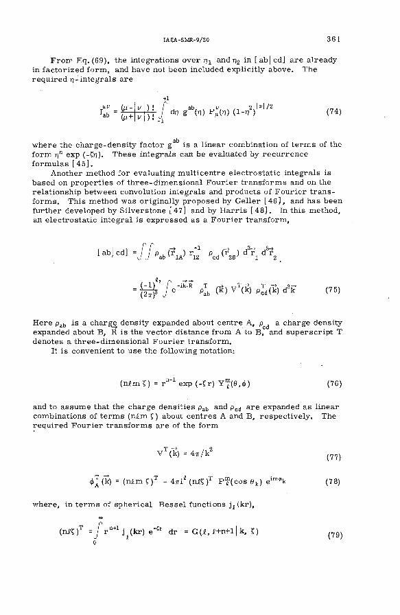
IA E A -SM R -9/20 361

F rom Eq. (69), the integrations over r)i and % in [ ab¡ cd] are already in fa ctorized form , and have not been included explicitly above. The requ ired T]-integrals are

ab(p - ) :(M+ ) :

ab,d)i g (ч) о " / s /1 2 . H /2Рц(1 ) ( i -ч ) (74)

where the charge-density fa ctor g ^ is a linear com bination of term s of the form r]" exp (-&*)). These integrals can be evaluated by recu rren ce form ulas [ 4 5 ].

Another method fo r evaluating m ulticentre e lectrosta tic integrals is based on prop erties of three-d im ensional F ourier tran sform s and on the relationship between convolution integrals and products o f F ourier tran s­form s. This method was orig inally proposed by G eller [4 6 ] , and has been further developed by S ilverstone [47 ] and by H arris [4 8 ] . In this method, an e lectrosta tic integral is expressed as a F ourier transform ,

ab I cd] = / / p . ( r ) r p (r ) d^r d' ' J J 'a b ' lA'* 12 *cd ' 28^ 1

( Й ^ У ^ pfb (Й) V ^ k) p j,(^ ) d 'k (75)

Here Pab is a charge density expanded about centre A , p^ a charge density expanded about B, R is the v ector distance from A to B, and superscript T denotes a three-d im ensional F ou rier transform .

It is convenient to use the follow ing notation:

(njPm^) = r " ^ e x p ( -^ r )Y ^ (e , ,H (76)

and to assum e that the charge densities рдь and p^ are expanded as linearcom binations of term s (n ím Q about centres A and B, respective ly . Therequired F ourier tran sform s are of the form

yT (k ) = 4 ^ /k ' ( 7 7 )

ф][(к) = (n im ^ )T = 47г^(пЯ)Т P T (c o s e ^ ) е ^ "к (78)

w here, in term s o f sph erica l B esse l functions jg (kr),

(п Я ) = J r j (kr) e"^ dr = G (^ ,í+ n + l¡k , Qо

(79)

362 NESBET

E fficient m ethods fo r computation of the integrals over spherica l B esse l functions denoted by G here have been developed fo r w ork in e lectron -atom scattering theory [ 4 9 ].

The final fo rm of the e lectrosta tic integrals is a linear com bination of term s of the form

cL У jJ k R ) (n ^ )T dk (80)0

Lwhere с ( i , Í ' ) is an angular momentum coupling coefficien t. When m odi­fied Gauss quadrature is used fo r the outer integral over k, the general e lectrosta tic integral reduces to a charge-density weighted expansion

[ ab] cd] У W¡ (i) K ^ . (i) (81)L M ' i

A o n e -centre charge distribution constructed from exponential basis o rb i­tals can be expressed as a finite sum o f term s (nim!Q. The sum over (LjC^' ) in Eq. (81) reduces to a finite sum fo r the tw o-cen tre "C oulom b" integral between two on e-cen tre charge densities. E fficient form ulas for evaluation o f such integrals have been derived from recu rren ce relations fo r the integrals of Eq. (80) [4 8 ] .

5. SYMMETRY ALGEBRA

Group representation theory can be used to take full advantage of sym m etry in sim plifying atom ic and m olecu lar calculations. E ffective use of such sym m etry algebra can require very com plex and sophisticated program organization. Computations of sym m etry algebra tend not to be very tim e-consum ing, despite the com plexity of the form alism , but such computations are important when they can reduce the m ost heavily weighted steps of an overa ll computation by a significant factor.

B asic concepts

Given a group ^ of sym m etry operations (G ), and a set of functions {¡//) such that the transform ed functions G< are defined and can be expanded in the linear space spanned by f<^}, sym m etry-adapted functions i /^ a r e defined by

(G), all G e S? (82)

The expansion coe ffic ien ts Г are m atrix elem ents of an irreducib le representation [50] of group characterized by sym m etry species index X and by subspecies indices p ,p '. In general, thefunctions are com plex

ÍA E A -SM R -9/20 363

and the m atrices Г unitary. In w ords, a sym m etry-adapted function ^ transform s as a basis function fo r irredu cib le representation Г^, c o r r e ­sponding to row Ц of the representation. The index a- here is used to distinguish essentia lly different functions that share the same tran s­form ation properties .

In its m ost general sense, the term configuration can be used to denote a linear space closed under operations of a given transform ation group, in the sense that G^ lies in the linear space if i// does. A function that can be expressed as a linear com bination of the functions {<//], and hence lies in the linear space, is said to belong to the configuration. F o r basis functions i/'ct of a configuration, the transform ation law is

G<^ ^ ^ r^ (G ), all G e S? (83)В

If the functions are orthonorm al, a unitary transform ation can be found that puts Eq. (83) into the form of Eq. (82). This transform ation converts the m atrix Tg , into a d irect sum of irreducib le representation m a tr ices , which occu r as d isconnected square m atrix b locks strung along the diagonal of the transform UTU'1 o fr j^ . This operation is called com plete reduction of the m atrix Г ^ , and the original m atrix is said to be reducible if m ore than one b lock can occu r in the d irect sum.

F o r finite groups, m atrices of a given reducible representation can be com bined linearly to give a p ro je ct ion operator which produces an unnorm alized sym m etry-adapted function with the given sym m etry sp ecies indices when applied to an arb itrary basis function of the given representation [50]. When the same irredu cib le representation o ccu rs m ore than once in the reducible representation generated by a given configuration, Schmidt orthonorm alization of the p ro jected functions can be used to produce an orthonorm al set of sym m etry-adapted functions, spanning the configuration.

F o r continuous groups, in particu lar fo r the three-d im ensional rotation group, le s s d irect m ethods must be used, as described below . In any case the construction of orthonorm al sets of sym m etry-adapted functions from a given configuration is an important step in the p ractica l use of sym m etry a lgebra, since such functions are assum ed in sp ecific applications of group representation theory.

A linear operator Q which acts on the functions transform s as GQG'Iunder sym m etry transform ations, if the functions <// transform as G< .C orresponding to the definition of sym m etry-adapted function, an irreducib le tensor operator is defined by the linear transform ation law,

С й дм С *^ У и л м -1^ -м (С ), a l l G e ^ (84)M'

Many im portant applications of sym m etry algebra make use of the W igner-E ckart theorem [11, 50, 51] fo r m atrix elem ents of irredu cib le tensor operators:

(сХ р 1Ядм1е'Х'м') = (хр1ям [х 'р ') (ахЦя^Ц^'Х ') (85)

364 NESBET

The great sim plification achieved by this form ula is due to the fact that the subspecies indices (p,M,¡u') occu r only in the fa ctor (Xp ¡AM¡X'jLí'), à generalized C lebsch -G ordan coefficien t which depends only on transform ation p rop erties . . The reduced m atrix elem ent (cX ЦПдЦа'Х') contains a ll in ­form ation relevant to the sp ecific operator Я and functions ^ . In the specia l case of an invariant operator,

Thus m atrix elem ents o f such an operator vanish unless X=X' and ¡u=p', and are otherw ise independent of the subspecies index p.

It is often requ ired to evaluate m atrix elem ents of tensor operators constructed as sym m etry-adapted linear com binations of products of sim p ler operators. Such m atrix elem ents can be expressed in term s of generalized coupling coefficien ts (n -j sym bols), and of reduced m atrix elem ents of the sim ple operators. F o r exam ple, with re feren ce to the rotation group and angular momentum eigenfunctions and quantum num bers, the m atrix elem ent of a tensoria l sca lar product of two com m uting tensor operators is

The coupling coefficien t indicated here in cu rly brackets is a 6 -j sym bol, equal except fo r a phase fa ctor to a Racah W -coe ffic ien t [11].

T o make use of the W igner-E ckart theorem , it is n ecessa ry to construct sym m etry-adapted wave functions o r basis functions fo r linear expansion and to com pute the n ecessary generalized coupling coe ffic ien ts . A program that com putes general n -j sym bols fo r the rotation group has recently been published [52]. When large numbers of such coefficien ts are required fo r repetitive use, it would be desirable, in p rincip le , to prepare tables fo r a cce ss during a particu lar calculation. The number of indices in typ ical coupling coe ffic ien ts can lead to very large tables, and to a difficult data retrieva l problem on a com puter.

A pplication to the N -e lectron problem

With respect to a sym m etry group % and its irredu cib le representations (X), a configuration can be defined fo r an N -e lectron system as the linear space spanned by Slater determinants whose occupied orbitals have indices represented by

(XplOOIX'iu') = ¿хм 6^- (86)

(88)

fo r all possib le values of the set of subspecies indices {¡n¡}. This definition is com patible with the general definition given above of a configuration as

IA E A -SM R -9/20 365

a linear space c losed under a group of transform ations. Since all ch oices of are im plied, an N -e lectron configuration can be sym bolized by

] " [ ( n X ) j ^ = ( n i ^ i ) (n g X g ) - ( п ь Л ы ) (8 9 )

where d¡ is the occupation number of the subshell with quantum num bers (nX)¡. Index n (principal quantum number) is used to denote different subshells of the same sym m etry species.

Although essentia lly different approaches have been used, it is con ­venient to represent sym m etry-adapted N -e lectron wave functions as linear com binations of the basis Slater determinants of a configuration as defined above. In the n on -re la tiv istic approxim ation fo r atom s (R ussell-Saunders or L -S coupling), spin and orbita l angular momentum representations of the rotation group are uncoupled. The orbital sym m etry indices (X; ^) becom e the quantum num bers (J!, s; mg, m j , with s = The N -e lectron sym m etry indices (Л ;М ) becom e quantum num bers (L , S; M^, Mg). O rbital quantum num bers i = 0, 1 ,2 , . . . are denoted by the conventional sym bols s ,p ,d , . . . , respective ly , and quantum num bers L = 0 ,1 ,2 , . . . are denoted by S, P ,D , . . . . The spin quantum num bers m = +ж are denoted by ß, <?, respective ly . An N -e lectron sym m etry-adapted function is an eigenfunction of operators I ? and 3^, with eigenvalues f^ L (L + l) and ï?S (S + l), respective ly . T hese quantum num bers are condensed into a term sym bol of the form

(90)Ms ML '

A s an exam ple, con sider the ls^2s^2p? ground-state configuration of atom ic carbon. The c losed subshells ls^ and 2s^ can be ignored, since only one choice of (m%, m j values is p ossib le . The basis Slater d e ter­minants fo r this configuration can be grouped accord in g to quantum num bers M^ = ЕШр and Mg = Em and listed in a Slater table as shown in Table I.

TABLE I. SLATER TABLE FOR CONFIGURATION p2

Mg = l 0

ML = 2 . *DВ 6

Pt Pt

1 3p 3p + *D

Po Pi Po Pi ' Po Pi

0 3p 3p + *D + 's

p " Pt* P-tP?. POP?. POP" ...

366 NESBET

Since all configurations with a single np open shell have the same structure, the principal quantum number n can be om itted, and each determinant is denoted by a ¡symbol

H ere m has values -1 , 0, +1 and m has values +-=r denoted by ß,<?, respective ly .

The possib le L , S term s in a given configuration can be ascertained by sim ple inspection of the Slater table. This fo llow s from the fact that the linear space defined by each box of the table must be closed under unitary transform ations of the configuration that p reserve quantum numbers M and Mg. M oreover, any L , S term that occu rs in the configuration accounts fo r exactly one function in the linear space of each box with M = -L , - L + l , . . . , L and Mg = -S, -S + l , . . . , S, because by definition the configuration is closed with respect to sym m etry operations, which m ix up a ll M and Mg values. This property can be expressed m ost d irectly in term s of ladder operators:

L = + iLy(92)

S* = Sx + iSy

constructed from the indicated angular momentum operators [11]. F o r generalized angular momentum j ,m , the ladder operator has the property that

(93)

Since the "lad der" of m values term inates with m = j, it follow s that

= 0 (94)

An im m ediate consequence of this result is that

j+ ^ ,E 0 , M j ^ , ) > 0 (95)

is a n ecessa ry and sufficient condition fo r ^ to be a sym m etry-adapted f u n c t i o n ^ with j = m . A s applied to L, S configurations, the L*, S+ operatorë connect adjacent boxes in the Slater table either vertica lly or horizontally , respective ly . The theorem of Eq. (95) im plies that any box containing m ore determ inant sym bols than both the adjacent boxes fo r M^+ 1 and Mg+ 1 m ust represent a linear space containing a term L = M^,S = Mg. A s indicated in the exam ple o f Table I, the term s can be enum erated by working inwards through the Slater table, starting with the largest values of M and Mg.

In Table I, a unique determinant o ccu rs with M = 1, Mg = 1, with vacant boxes above and to the left. Hence a 3p term (L = 1, S = 1) is present in the configuration, including all nine possib le M^, Mg com binations.

ÍA E A -SM R -9/20 367

Sim ilarly, a unique determinant has M^ = 2, Mg = 0, with vacant boxes above and to the left, indicating a ID term (L = 2, S = 0). T hese two term s account fo r the entire table except fo r the box M^ = 0, Mg = 0, which contains three determ inants, indicating the final term to be S (L = 0, S = 0).

The m ost straightforw ard method of constructing L, S term functions is to apply the theorem of Eq. (95) to those boxes in the Slater table with M^, Mg equal to L , S values fo r expected term s. This gives a set of hom o­geneous equations fo r coe ffic ien ts of the sym m etry-adapted functions, obtained from m atrix elem ents of the ladder operator L* and S*. The L, S eigenfunctions obtained in this way from Table I are , in the notation of Eq. (90),

3p . ct a1*1 Po Pi

^ = p p? (96)

¿So = 3** (p. p - pg pg + p p^)

T hree distinct m ethods fo r constructing sym m etry-adapted N -electron wave functions w ill be considered here.

a. Default

This designation is intended to em phasize the fact that sym m etry- adapted functions represent a convenience and not a necessity in N -electron wave function calcu lations. In m atrix m ethods, if the set of basis functions is chosen to span com plete configurations, an eigenvector of the m atrix of an invariant Hamiltonian n ecessa rily represents a sym m etry-adapted variational wave function except in ca ses of accidental degeneracy. When there are additive sym m etry quantum num bers, such as M^, Mg, and parity fo r atom ic wave functions, only basis functions with given values of these quantum num bers need be included.

T o ensure that a variational calcu lation should produce sym m etry- adapted functions in L -S coupling, any variational H ilbert space that in ­cludes a given determinant should be extended to include a ll determinants of the sam e configuration with the same M^, Mg, and parity. This means that each box in a Slater table should be included o r excluded in its entirety from the variational wave function. If this rule is follow ed, the method of variational calcu lations of wave functions based on lattice decom position of the N -e lectron H ilbert space leads to sym m etry-adapted functions at each stage of calculation [19]. A sim ilar procedure can be follow ed fo r the m ore com plicated variational wave functions requ ired in e lectron scattering theory.

b. P rog ress iv e vector coupling

When the com putational saving due to reduction o f the size of m a trices o r of system s of coupled equations outweighs the consideration of sim plicity o f com putational p rocedure and program m ing, sym m etry-adapted functions can be constructed explicitly . An effective general method has been proposed by Fano [54] and im plem ented in a published com puter program byH ibbert [55].

368 NESBET

This method uses the technique of p rogress ive vector coupling. Sub­shells of equivalent orbita ls (sam e n values) are adjoined in sequence and p rog ress iv e ly coupled to definite L and S values fo r antisym m etric wave functions. The term structure fo r antisym m etric functions fo r each subshell (niyi is obtained by p rogress ive coupling o f one n i-orb ita l to the term s of (n^)^* . This coupling within each subshell is defined by fractional parentage coe ffic ien ts , which can be com puted and tabulated independently fo r each possib le subshell. A program fo r p - and d -subshells has been published [56].

The method of Fano and Hibbert p roceeds through the construction of sym m etry-adapted functions Ï to the evaluation of m atrix elem ents (Ÿ ¡н !^ '). P rog ress iv e vector coupling schem es must be specified fo r Ï and Ï ' . In addition to fractional parentage coe ffic ien ts , general coupling coefficien ts (n -j sym bols) are required fo r the calculation. These are supplied by the program of Burke [52].

c. P ro jection operator tables

P rop erties of p ro jection operators can be used to sim plify m atrix elem ents of an invariant operator [57]. The general form ula is

П1ц

¡ H l ^ ) = (k , /k ^ ^ ^ x * a^j (Ф^Н ^ ) (97)i= i j= i

where the functions Ï are orthonorm alized sym m etry-adapted functions, each with a dual expansion of the form

= k j Ф; (98)j=l 1=1

The function

9j = ^LS§j- Where <9^= <^s (99)

is defined by action of the L, S pro jection operator ^^s °n a Slater deter­minant Ф]. In Eqs (98), if there are n determinants of specified M^, Mg, and parity in a given configuration, index m á n is the number of sym m etry- adapted functions of given L, S in that configuration. The essential sim plification achieved by Eq. (97) is that m , which fo r configurations with severa l open subshells m ay be very much sm aller than n, definesthe range fo r one of the two summation indices. P roperties of reducedm atrix elem ents m ay be used, as in other m ethods, to sim plify computation of the m atrix elem ents (Ф ^Н^ ) between Slater determinants.

The coe ffic ien ts {a ; x} fo r any given configuration can be obtained d irectly by an algorithm that m akes use of the hom ogeneous equations,E qs (95), constructed from m atrix elem ents of the ladder operators L/ and S . The only auxiliary coupling coefficien ts requ ired in using this method are the Gaunt coe ffic ien ts c**(^m; ^ 'm ') tabulated by Condon and Shortley [53]. M atrix elem ents for the two term s in configuration d have been com puted in detail as an exam ple of this method [57].

IA E A -SM R -9/20 369

CASE STUDY: ELECTRO N -ATO M SCATTERING

A s indicated in Eq. (4), the wave function fo r e lectron scattering by an N -e lectron atom is of the form

Index p is used here to denote different partial waves as w ell as energies. In prin cip le , each function 6p is an exact stationary state wave function fo r the target atom , corresponding, fo r open channel p, to target atom energy E p<E , where E is the total energy of the N + 1 -e lectron system .The functions [Ф } constitute a H ilbert space of norm alizable N + 1 -e lectron wave functions, which can be expressed in term s of virtual excitations as in the stationary state problem . Thus the summation over p is infinite, in princip le , and techniques such as the lattice decom position of (Ф^}, in analogy to the structure illustrated in F ig . 1, must be used to make ca lcu ­lations feasib le .

In the c lose -cou p lin g form alism , the summation over {Ф^} is severely truncated, but each such closed -chan n el wave function that is included in the sum is com puted variationally. The closed -chan n el N + 1 -e lectron wave functions are written in the form

where is a quadratically integrable closed -chan n el orbita l, and 6q is a specified "pseudostate" o r polarization function, chosen so that the e le ctr ic dipole polarizability of som e function 8p can be com puted from a fir s t - ord er wave function proportional to 6q . The variational equations fo r the open- and closed -channel orb ita ls (i^ ; ^ ) , fo r Np open and Nq closed channels, form a system of Np + Nq coupled in tegro-d ifferen tia l equations in the radial variab les. Since the number of coupled equations in creases with each addition to the set of functions {Ф^}, it is im practica l to ca rry such calculations to the quantitative lim it o f com pleteness of the Hilbert space {Фр}.

T o take the fu ll H ilbert space {Ф^} into account, it was proposed that m atrix m ethods be used fo r a ll c losed -chan n el functions, and a system atic h ierarchy of variational calcu lations be ca rr ied out based on a lattice decom position of this H ilbert space [58]. The variational equations take the form of a system of coupled in tegro-d ifferentia l equations fo r the open-channel orbita ls <//p, coupled to a system of m atrix equations of large dim ension.

The system of coupled in tegro-d ifferen tia l equations can be elim inated com pletely if the channel orbita ls ^p are them selves expanded as linear com binations of specified basis functions. Then the scattering calculation becom es a pure m atrix calcu lation to determ ine these expansion c o ­efficients. F o r a single scattering channel, the radial fa ctor fp(r) of !//p sa tisfies the usual bound-state boundary condition at r = 0 and has the asym ptotic form , fo r orbital angular momentum ip,

( 10 0 )

( 101 )

(102)

370 NESBET

This can be written in the m ore general fo rm , a lso applicable to m ulti­channel scattering,

Scattering c ro s s -s e c t io n s can be computed from the coefficien ts (c^ jp. obtained by setting each of the coefficien ts o-Qp- in turn equal to unity, with all others zero . E xcept fo r constant fa ctors , the square array of c o ­e fficien ts <?ip obtained in this way is equal to the reactance m atrix R ,' often denoted by К in the literature [59]. B ecause of the form assum ed fo r the wave function, Eq. (100), the functions Sp and Cp can be orthogonalized to a ll of the norm alizable basis orbitals in a given calculation. This w ill be assum ed here. Then the functions serve to expand the inner part of the channel orb ita ls, as w ell as to represent corre la tion and polarization e ffects through virtual excitations.

A serious p ractica l d ifficu lty o ccu rs in attempting to apply standard variational m ethods [60, 61] to evaluate the coefficien ts a in Eq. (103).The com puted reactance m atrix elem ents have spurious poles whose location , as a function of energy, varies with an arb itrary change of the basis set used fo r linear expansion of a variational wave function [62].New analysis o f this prob lem , fo r multichannel as w ell as single-channel scattering [63], showed that these spurious singularities could be avoided by alternative use of the Kohn [60] o r inverse Kohn [61] m ethods, re ferrin g to variational calculation of the elem ents of the reactance m atrix or of its re c ip roca l, respective ly . The choice of form alism depends on an easily computed criterion . B ecause of the com plexity of calculations requ ired , it would be very difficult to design a reliab le general com puter p rogram if unpredictable resu lts could arise from any given calculation.

F o r e lectron -neutra l atom scattering, the regu lar spherical B esse l functions j%(kr) satisfy the boundary conditions requ ired of the functions S in Eq. (103). The actual functions used are obtained by orthogonalizing jt(kr) to a ll norm alizable basis orbitals with the same J?-value. The radial fa ctors of these basis orbita ls are taken to be of the form r""i exp(-^r). Functions С are obtained from a linear com bination of j^ i (k r ) and j ^ k r ) , chosen to agree with the firs t two term s of the asym ptotic expansion of Пд(кг), the irregu la r spherical B esse l function [64].

Despite the fact that a ll integrals involve only one centre, the e le c tro ­static integrals involving m ixed exponential and B esse l functions are non­trivia l. The m ost difficu lt integral required in electron -atom scattering, fo r two or m ore open channels of different energy, is the exchange integral,

fp " з'Ор Sp + <?ip Cp (103)where

(104)

X fX ppqlkik^ß) = У j j k i r i ) i { ^ e * " t ^ ^ ( k g r g ) ^ e"^' di^dri (105)

IA E A -SM R -9/20 371

It was found n ecessary to develop a number of new form ulas and m ethods to evaluate these e lectrosta tic scattering integrals e fficien tly to high accu racy [65]. The even m ore difficu lt problem of evaluating electrostatic integrals over Coulom b wave functions, requ ired fo r variational calculations o f e lectron -ion scattering, has recently rece ived attention [66].

In applying the Kohn o r inverse Kohn variational form alism to the wave function indicated in Eq. (100) it is n ecessary to construct the v a r i­ational functional

(Ÿ ¡H -E lï) ^ ^¡p м у <?jq (106)ij pq

where the coefficien ts a are defined in Eq. (103). The auxiliary m atrix M y is defined by [63]

= M ? ' X I M^ ( M % M^. (107)Ц V

where i = I, j = J with values 0, 1 as in Eq. (103), and p, q are open channelindices. The m atrices com bined in Eq. (107) are the bound-bound m atrix(Hermitian)

M ^ = H ^ - E 6 ^ (108)

where

Н ^ = (Ф , НФ„) (109)

the bound-free m atrix (Hermitian)

мР, =(Ф^, (H -E )e 'P ) (110)

and the fr e e - fr e e m atrix (non-Herm itian)

M ^ = (6-P, (H -E) б*"*) (111)

Here

eip = ^ 8 p ^ p (112)

The m atrix M ^ h a s the dim ension of the N + 1-particle H ilbert space.As indicated by Eq. (55), this dim ensionality grow s very rapidly with N¡,, the num ber of basis orb ita ls, and with the level of virtual excitation taken into account. It is easily p ossib le , in calculations on re latively light atom s, to have a m atrix M ^ with severa l m illion n on -zero elem ents. Standard m ethods of m atrix inversion are extrem ely inefficient fo r such a m atrix , because the elem ents m ust be a ccessed in a non-sequential ord er. When only a sm all fraction of the m atrix can be contained in the random a cce ss fast m em ory of a com puter, non-sequential p rocessin g presents a very difficu lt data handling problem .

372 NESBET

Instead of inverting the m atrix Eq. (107) can be evaluated in ­d irectly by a method that avoids non-sequential data p rocessin g , and in fact bypasses an entire step of m atrix p rocess in g as com pared with use of Gauss elim ination [67]. Since a ll m atrix elem ents considered here are rea l num bers, the bound-bound m atrix can be fa ctorized in the form

Cp Ipp (113)P

defining the low er triangular m atrix T p and a diagonal sign m atrix Cp whose diagonal elem ents are ±1 only. An auxiliary rectangular m atrix В is defined in term s of the bound-free m atrix by

P

The m a trices T and В can both be constructed by sim ple algorithm s r e ­quiring only sequential data p rocess in g [67]. Equation (107) is evaluated in the form

м у = м ^ - ^ в ^ в ^ (115)

p

In im plem enting this m ethod, the problem of constructing com puter program s of general applicability was sim plified by not constructing sym m etry-adapted L, S eigenfunctions. Instead, by including com plete boxes in the relevant Slater tables in constructing the determinant list {Ф ] , and by diagonalizing the com puted reactance m atrix , advantage is taken of the fact that the final eigenchannel wave function is n ecessa rily sym m etry-adapted. T his is an exam ple of the default method of sym m etry a lgebra. At a la ter stage o f developm ent, when the general method and program s have been thoroughly tested, the linear dim ensions of m atrices requ ired in this method can be considerably reduced by explicit construction of L , S eigenfunctions p r io r to the evaluation of m atrix elem ents.

R E F E R E N C E S

[1 ] SCHWARTZ, C ., Phys. Rev. 124 (1961) 1468; ARMSTEAD, R. L ., Phys. Rev. Г71 (1968) 91;GA1L1T1S, М ., in Physics o f Electronic and Atomic Collisions (Proc. 4th Int. Conf. Montreal, 1965) 10.

[2 ] SMITH, F. T. , in Atomic Physics (Proc. 1st Int. Conf. New York, 1969) Plenum Press (1969) 353.[3 ] LITTLE, W .A. , J. Polymer S e i., Pt. C, Polymer Symposium (1967) 3.[4 ] LITTLE, W .A . , J. chem. Phys. 49 (1968) 420; GUTFREUND, H ., LITTLE, W .A ., Phys. Rev. 183

(1969) 68; J. chem. Phys. 50 (1969) 4468, 4478.[5 ] LEFEBVRE-BRION, H ., MOSER, C .M ., NESBET, R .K ., J. m ol. Spectr. 13 (1964) 418.[6 ] T1LFORD, S. G ., VANDERSL1CE, J .T . , WILKINSON, P .G ., Can. 1. Phys. 43 (1965) 450.[7 ] NESBET, R .K ., Phys. Rev. Letts 24 (1970) 1155; Phys. Rev. A2^(1970) 1208.[8 ] MATCHA, R. L ., NESBET, R .K ., Phys. Rev. 160 (1967) 72.[9 ] CLEMENT], E ., 1BMJ. Res. Develop. 9Suppl. (1965) 2; J. chem. Phys. 38 (1963) 2248; 39 (1963) 175.

[10] NESBET, R .K ., Phys. Rev. 175 (1968) 2; A3 (1971) 87.[11] EDMONDS, A .R ., Angular Momentum in Quantum Mechanics, Princeton University Press, Princeton (1957);

ROSE, M. E ., Elementary Theory o f Angular Momentum, John Wiley, New York (1957).

IA E A -SM R -9/20 373

[12] VANDERSLICE, J .T ., MASON, E .A ., MAISCH, W .G ., J. mol. Spectr. 3 (1959) 17.[13] LANDAU, L ., Z. Phys. Sov. Union 2(1932) 46; ZENER, C ., Proc. Roy. Soc. (London) A137(1932) 696.[14] LESTER W .A ., Jr., Methods in Computational Physics 10 (1971) 211: see also these Proceedings.[15] HARTREE, D .R ., The Calculation ofA tom ic Structures, John Wiley, New York (1957).[16] ROOTHAAN, C .C .J ., Rev. mod. Phys. 23 (1951) 69.[17] KELLY. H .p ., Adv. chem. Phys. 14 (1969) 129.[18] BRUECKNER, K .A ., Phys. Rev. 96 (1954) 508; 97 (1955) 1953; ¿00 (1955) 36; TheMany-Body

Problem (DE WITT, B. , Ed.), John Wiley, New York (1959) 47.[19] NESBET, R. K. , Adv. chem. Phys. 14 (1969) 1; Phys. Rev. A2 (1970) 661.[20] BURKE, P. G ., SEATON, M .J., Methods in Computational Physics 10(1971) 1.[21] WEISS, A. W ., Phys. Rev. 162 (1967) 71.[22] TAVARD, C ., J. deC him . Phys. 66 (1969) 1130; TAVARD, C ., BONHAM, R. A . , J. chem. Phys.

50 (1969) 1736.[23] KOLOS, W ., Adv. Quantum Chem. 5 (1970) 99.[24] DEVOGELAERE, R .. J. Res. Natl. Bur. Std. 54 (1955) 119; LESTER, W .A ., Jr., J. comput. Phys. 3

(1968) 322.[25] ALLISON, A .C ., J. comput. Phys. 6 (1970) 378.[26] GORDON, R .G ., J. chem. Phys. 51 (1969) 14.[27] COOLEY. J. W ., Math. Comput. 15 (1961) 363; SHARE Program No. 1072.[28] NUMEROV, B ., Publ. del'O bserv. Astrophys. Central Russie 2 (1933) 188; HAMMING, R. W .,

Numerical Methods for Scientists and Engineers, McGraw-Hill, New York (1965) 215.[29 ] FROESE, C ., Can. J. Phys. 41 (1971) 1895.[30] FROESE-F1SCHER, C . , Comput. Phys. Communs2(1971) 124.[31] HARTREE, D .R ., The Calculation o f Atomic Structures, John Wiley, New York (1957).[32] FROESE-FISCHER, C ., Comput. Phys. Communs 1 (1970) 151.[33] BURKE. P .G ., Adv. Phys. 14 (1965) 521; CONNEELY, L1PSKY, SMITH, BURKE, HENRY,

comput. Phys. Communs 1 (1970) 306.[34] ROOTHAAN, C .C .J ., Rev. mod. Phys. 23 (1951) 69.[35] NESBET, R .K ., Rev. mod. Phys. 33 (1961) 28; 35 (1963) 552; ROOTHAAN, C .C .J..B A G U S, P .S .,

Meth. Comput. Phys. 2 (1963) 47.[36] GOMES, L .C ., WALECKA, J .D ., WEISSKOPF, V .F ., Ann. Phys. (NewYork) 3 (1958) 241.[37] BETHE, H .A ., GOLDSTONE, J ., Proc. Roy. Soc. (London) A238 (1957) 551; SZASZ, L.,

Z. Naturf. 14a (1959) 1014.[38] NESBET, R .K ., J. chem. Phys. 43 (1965) 311; SHAVITT, I ., J. comput. Phys. 6 (1970) 124.[39] GOLDSTONE. J ., Proc. Roy. Soc. (London) A239 (1957) 267.[40] BOYS, S. F ., HANDY, N .C ., Proc. Roy. Soc. (London) A310 (1969) 43, 63.[41] BOYS, S. F ., Proc. Roy. Soc. (London) A200 (1950) 542.[42] SHAVITT, I . , Meth. comput. Phys. 2 (1963) 1.[43] HARRIS, F .E ., MICHELS, H .H .. Adv. chem. Phys. 13 (1967) 205.[44] RUEDENBERG, K .. J. Chem. Phys. 19 (1951) 1459; MERRYMAN, P ., unpublished program (1957);

MERRYMAN, P ., MOSER, C .M ., NESBET, R .K ., J. chem. Phys. 32 (1960) 631; HARRIS, F .E .,J. chem. Phys. 32 (1960) 3.

[45] CORBATO, F.J. , J. chem. Phys. 24 (1956) 452.[46] GELLER, M ., J. chem. Phys. 41 (1964) 4006.[47] SILVERSTONE, J ., J. chem. Phys. 47 (1967) 537; 48 (1968) 4098, 4106.[48] HARRIS, F. E. , J. chem. Phys. 51 (1969) 4770.[49] LYONS, J .D ., NESBET, R .K ., J. comput. Phys. 4 (1969) 499; HARRIS, F .E ., MICHELS, H .H .,

J. comput. Phys. 4 (1969) 579.[50] HAMERMESH, M ., Group Theory, Addison-Wesley, New York (1962); WIGNER, E. P ., Group

(1959).[51] ECKART, C ., Rev. mod. Phys. 2 (1930) 305.[52 ] BURKE, P. G ., comput. Phys. Communs ¿ (1 9 70 ) 241.[53] CONDON, E. U ., SHORTLEY, G .H ., The Theory o f Atomic Spectra, Cambridge University Press,

NewYork(1951).[54] FANO, U ., Phys. Rev. 140 (1965) A67.[55] HIBBERT, A ., comput. Phys. Communs ¿ (1 9 70 ) 359.[56]. ALLISON. D .C . S. , comput. Phys. Communs ¿(1 9 70 ) 15.[57]N ESBET, R .K ., J. math. Phys. 2 (1961) 701.

374 NESBET

[58] NESBET, R .K ., Phys. Rev. 156 (1967) 99.[59] MOTT, N. F ., MASSEY, H .S .W ., The Theory o f Atomic Collisions, Oxford University Press, New York

(1965).[60] KOHN, W ., Phys. Rev. 74 (1948) 1763.[61] HULTHEN, L ., Ark. Mat. astron. Fysik35A 25 (1948); RUB1NOW, S . l . , Phys. Rev. 98 (1955) 183;

WILLIAMS, K .L ., Proc. Phys. Soc. (London) 91 (1967) 807.[62] SCHWARTZ, C ., Ann. Phys. (New York) 16 (1961) 36.[63] NESBET, R .K ., Phys. Rev. 175 (1968) 134; 179 (1969) 60.[64] ARMSTEAD. R. L .. Phys. Rev. 171 (1968) 91.[65] LYONS. J .D ., NESBET. R .K .. J. comput. Phys. 4 (1969) 499; HARRIS, F.E ., MICHELS. H .H .,

). comput. Phys. 4 (1969) 579.[66] BÖTTCHER, C .. I. comput. Phys. 6 (1970) 237; RAMAKER, D .E ., J. math. Phys. 13 (1922) 161.[67] NESBET. R. K ., J. comput. Phys. 8 (1971) 483.

IA E A -SM R -9/19

ACCURATE CALCULATION OF CROSS-SECTIONS FOR NON-REACTIVE MOLECULAR COLLISIONSW .A . LESTER, Jr.IBM Research Laboratory,San José, C a l i f . ,United States o f Am erica

Abstract

ACCURATE CALCULATION OF CROSS-SECTIONS FOR NON-REACTIVE MOLECULAR COLLISIONS.Computational considerations encountered in the accurate calculation o f cross-sections for rotational and

vibrational excitation o f molecules by heavy-particle collision are presented and discussed in the context o f the model problem of scattering by a rigid rotator. The nature o f the problem is delineated: calculation of the

1. INTRODUCTION

Computation is playing an increasingly significant ro le in the elucidation of physica l phenomena on the m icroscop ic sca le . E lsew here in this volum e, Nesbet d iscu sses com putational methods of atom ic and m olecular physics.This is such a broad topic, however, that a useful purpose might be served here by focusing b rie fly on the origin of som e of the m ore im portant com puta­tional prob lem s and methods of solution that have arisen in a branch of m olecu lar physics that has undergone increased activity in recent years: the determ ination of c ro ss -s e c t io n s fo r non -reactive m olecular co llis ion s .In the present paper, attention is lim ited to inelastic encounters; B ern ­stein [1] has given an excellent review of e lastic scattering.

Recent experim ental advances [2] in m olecu lar-beam scattering [3], u ltrason ic d ispersion [4], and optical flu orescen ce [5] have begun to yield c ro ss -s e c t io n s fo r rotational and vibrational energy transfer by heavy- particle co llis ion between se lected initial and final quantum states of target m olecu les. To assist the interpretation of these experim ents, e fforts have been initiated by a number of groups to compute accurately cro ss -s e c t io n s fo r these p ro ce sse s [6]. Extensive d iscussions of computational methods in m olecu lar scattering have very recently appeared [7].

C ro ss -se ct io n s of in terest here are of im portance in a variety of physical p ro ce s s e s . These include cooling of in terstellar space [8], line broadening [9], relaxation phenomena in gases [10], and chem ical reactions [11].

The goal of scattering studies is to understand the laws of interaction between collid ing system s. There are basica lly two approaches to the problem . One is to start with experim ental results and then, based on the interpretation of m easurem ents, in fer the form and magnitude of the interaction. This procedure is naturally lim ited by the validity of the assum ptions made and is intertwined with the unfolding of distributions

375

376 LESTER

n ecessa ry to yield inform ation on individual scattering events. The other approach is to compute c ro ss -s e c t io n s directly from the basic laws of physics. The latter point of view is follow ed here and form s the basis fo r the computa­tional aspects that fo llow . Of course, the test of calculations is agreem ent with p re c ise m easurem ents.

2. NATURE OF THE PROBLEM

A. P otentia l-energy surfaces f!2 l

The ab -in itio calculation of atom ic and m olecular properties requ ires, in general, the solution of the Schrödinger equation which in the tim e- independent form is

НФ = ЕФ (1)

Denoting the m asses, charges, and co -ord inates Of the p articles as follow s (in atom ic units),

P article Mass Charge C o-ordinates

nucleus a z . R<)t(Xa' Yg, Zg)e lectron i 1 -1 fi (Xi, y¡, z¡)

the Hamiltonian (in the absence of external fie lds) may be written

N n

a = l i = l

where

v - У ^ + У ' - ^ + У ^ (3)Z-j r¡g r¿j Rctßi, a i < j a < 6

and the denom inators of the term s of Eq. (3) are interparticle distances.The term s on the right-hand side of Eq. (2) represent the total nuclear and e lectron ic kinetic energies, and the total potential energy, respectively .Those on the right-hand side of Eq. (3) designate the total n u clea r-e lectron ic , e le c tro n ic -e le c tro n ic , and nuclear-n u clear potential energies, respectively .

B ecause of m ass d ifferen ces, nuclear ve lo c it ie s are sm all com pared with e lectron ic v e lo c it ie s . This form s the basis of the clam ped-nuclei approxi­mation o r B orn-O ppenheim er separation of nuclear and e lectron ic motion.In this approxim ation, the Schrödinger equation fo r e lectron ic motion,

(4)

LAEA-SMR-9/19 377

is obtained by deleting the total nuclear kinetic energy term from Eq. (2) so that the e lectron ic Hamiltonian is sim ply

H ^ = - ^ A i + V (5)1 = 1

In Eq. (4), E ^ is a function of the nuclear co -ord inates

E^ = E "'(R i, R2____ _ Ru) = E^(R) (6)

and

Ф*^ = Ф ^ ( Г 1 , Г2 , . . . , Гд , R i , R 2, . . . , R N ) = Ф ^ ( г , R ) (7 )

F or a particu lar system and sp ecified nuclear geom etry, one can, in prin cip le , solve Eq. (4) and determ ine the eigenvalues E* . These solutions, together with solutions fo r other nuclear arrangem ents, define a set of potentia l-energy su rfaces. F o r applications to date, only the ground-state surface (determ ined by the low est eigenvalue fo r each nuclear arrangem ent) o r a few of the low est-ly in g potentia l-energy surfaces have been of im m ediate interest.

The potential energy fo r nuclear motion is defined as the e lectron ic energy E ^(R) (which is not s tr ictly e lectron ic since it contains the in ter- nuclear repulsion term ) so that the nuclear Schr&dinger equation may be written

N

{ ' 2 E " ( R ) j Ф"""(Й) = ЕФ""^(Й) (8)0 = 1

Note that the ze ro of potential energy is the infinitely separated nuclei.In n on -reactive m olecular scattering, the physica lly appropriate zero

o f energy is the constituent m olecu les at infinite separation. T herefore, E ^(R ) in Eq. (8) is rep laced by

V(R) = E ^(R ) - E^(oo) (9)

where E^(oo) designates the e lectron ic energy fo r infinitely separated fragm ents and intram olecu lar distances set equal to those of the isolated fragm ents. In addition, a term describ ing the internal motion of the separated m olecu les must be included. Thus the nuclear Hamiltonian has the form

= (1 .)a = l

where H^t is the total Hamiltonian fo r internal motion of the fragm ents. See Section 2. В fo r the exp licit fo rm of expression (10) fo r rotational excitation o f diatom ic m olecu les by atom im pact.

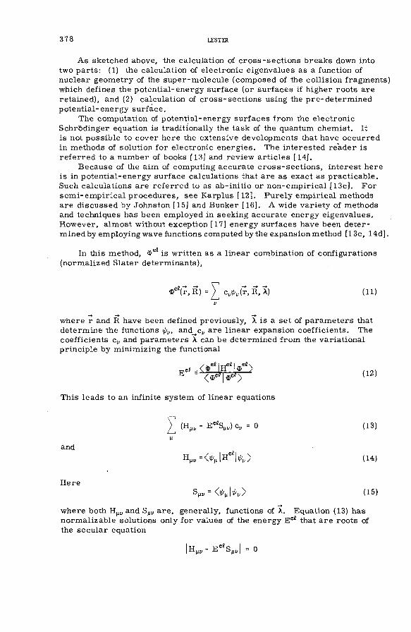
378 LESTER

A s sketched above, the calculation of c ro ss -s e c t io n s breaks down into two parts: (1) the calculation of e lectron ic eigenvalues as a function of nuclear geom etry of the su per-m olecu le (com posed of the co llis ion fragm ents) which defines the potentia l-energy surface (or su rfaces if higher roots are retained), and (2) calculation of cro ss -s e c t io n s using the pre-determ ined potentia l-energy surface.

The computation of potentia l-energy su rfaces from the electron ic Schr&dinger equation is traditionally the task of the quantum chem ist. It is not possib le to cover here the extensive developm ents that have occu rred in m ethods of solution fo r e lectron ic en erg ies. The interested reader is re fe rred to a num ber of books [13] and review artic les [14].

B ecause of the aim of computing accurate c ro ss -s e c t io n s , interest here is in potentia l-energy surface calculations that are as exact as p racticab le . Such calcu lations are re fe rred to as ab-in itio or n on -em pirica l [13c]. F or s e m i-e m p ir ica l p roced u res, s e e K a rp lu s [1 2 ]. P urely em pirica l methods are d iscussed by Johnston [15] and Bunker [16]. A wide variety of methods and techniques has been em ployed in seeking accurate energy eigenvalues. H ow ever, a lm ost without exception [17] energy surfaces have been deter­m ined by em ploying wave functions computed by the expansion method [1 3c, 14d].

In this method, Ф^ is written as a linear com bination of configurations (norm alized Slater determ inants),

ф".(r, R) c ^ ( r , R, X) (11)

where r and R have been defined previously , X is a set of param eters that determ ine the functions and c¡, are linear expansion coe fficien ts . The coefficien ts c^ and param eters A. can be determ ined from the variational princip le by m inim izing the functional

' (Ф ^ )ф ^ )

This leads to an infinite system of linear equations

(H„„ - E '% „ ) c„ = 0 (13)

(14)and

Here= (15)

where both H ^ and Sp„ are , generally, functions of X. Equation (13) has norm alizable solutions only fo r values of the energy E ^ that are roots of the secu lar equation

¡H „„- E < % „¡ = 0

IA E A -SM R -9/19 379

The principal lim itations in obtaining accurate solutions are due to the follow ing com putational d ifficu lties:

(a) Integral evaluation [18]. Significant advances are being made in the calculation of m u lti-cen tre integrals and associated data handling which arise from expansions of the functions ^ in linear com binations of basis functions [13b, c, 14d]. The difficu lties a rise , on the one hand, from the m athem atical com plexity of the integrals that must be computed, e .g . S later-type functions [13b], and, on the other hand, from the large num ber of integrals that m ust be treated fo r sa tisfa ctory accu racy fo r other ch oices of functions, e .g . G aussian-type functions [13b].

(b) Scope of com putations. In co llis ion problem s, knowledge is requ ired of computed potentia l-energy su rfaces from large to sm all in term olecu lar distances as a function of relative orientation. This means, in general, that many energy calculations must be perform ed in order to gain a representation of the in term olecu lar interaction adequate fo r scattering studies. In the non-overlap region one may often take advantage of perturbation theory of in term olecu lar fo rce s [19] to reduce the number of computations ord inarily needed.

(c) A ccu ra cy requ irem ents. At the present tim e, it is not known how e rro rs in potential energy surfaces are quantitatively re flected in the e rro rsof derived cross -se ction s . Of cou rse , qualitative considerations such as the predominant dependence of rotational c ro s s -s e c t io n s on the long- range region and vibrational energy transfer on short-range co llis ion s can be tested on com paratively crude surfaces.

(d) Lack of d irect checks. Since potentia l-energy surfaces are not ob serv ­ables, the determ ination of the validity of com puted surfaces is a m ore difficu lt prob lem than the establishm ent of e rro rs in calculated p r o ­perties of stable system s. This p laces a heavy burden on num erical methods and procedu res em ployed in the evaluation o f m olecu lar in ter­actions to insure accurate resu lts.

At the present tim e, variational calculations o f potential energy surfaces fo r n on -reactive system s can be usefully distinguished by the number of term s retained in Eq. (11). The s in g le -term calculation which reaches its ultimate form in the H a rtree -F ock approxim ation [13, 14], corresponding to the optimum specification of the param eters X, is the one m ost com m only ca rr ied out. Such calculations fo r individual m olecules are now essentia lly routine and a number of com puter program s follow ing this method has been widely dissem inated [20]. . H owever, re latively few calculations of in ter- m olecular su rfaces have been perform ed in this approxim ation [2 1 ].

Except fo r calculations on purely hydrogen-containing system s (Нд, H3, HJ, Щ) [20, 22], few calculations beyond the single-con figuration leve l have appeared. Such computations are not as yet routine, but a num ber of efforts are in p rog ress [23].

B. C ross -se ction s

The use of potential energy su rfaces in the determ ination of m olecular dynam ics may be exem plified by the consideration of rotational excitation of diatom ic m olecu les by atom im pact. The scattering form alism described below p ossesses a number of features com m on to treatm ents o f scattering

380 LESTER

in other areas of physics that are easily recogn izable if the nature of the p articles and origin of angular momentum coupling are appropriately changed. The present developm ent, due to Arthurs and Dalgarno [2 4 ], follow s from a treatm ent of nuclear scattering theory [25].

The theory is applicable to scattering of a structureless particle (e. g. a atom) by a rigid rotator (diatom ic m olecule) of mom ent of inertia I. The incident relative kinetic energy is restricted to be sufficiently low that there is no excitation of vibrational and e lectron ic degrees of freedom . F or sim plicity , consideration is restricted to states.

The nuclear Hamiltonian fo r an atom A and m olecule В С takes the form , see (10),

§ (^ 7 ^ 3d "S'

where H ^ rep laces H ¡^. In cen tre -o f-m a ss co-ord inates, it is convenient to express form ula (16) as follow s:

H " ^ = - ^ A p - H , ° t + V ( p , ? ) (1 7 )

where the f ir s t term is the k in etic-en ergy operator fo r relative motion in which

p = MA(MB+M<-.)/(MA + M ,j+ M c ) (18)

H ere, the potentia l-energy surface V is expressed in term s of p, the position of incident particle A relative to the centre of m ass of m olecule BC, and r, the co -ord inate specifying the relative positions of В with resp ect to C.In addition, it should be noted that

[ H , „ t - j ( j + l)/2 I]Y jn ,. (?) = 0 (19)

where the functions Y j^ a re the fam iliar spherica l harm onics and r sp ecifies the orientation of the interm olecu lar axis.

B asis functions are constructed that are eigenfunctions of and where J is the total angular momentum compounded from the rotational angular momentum j and the orbital angular momentum Í , i. e. J = j with associa ted pro jection s o n th e z -a x is denoted by M, m j , and m^, viz.

3 ^ ( P , ¿ ) = ^ ( j4 m jm J jiJ M )Y ^ . ( ^ ) Y ^ ( p ) (20)

m j.m g

where the coefficien ts are the well-known C lebsch-G ordan coefficien ts.The nuclear wave function is expanded in this set,

Ф (R) = $j(P, r) = ^ P U j-r(P )^ rl'(P . r) Jj-r

(21)

ÍA E A-SM R-9/19 381

Substitution of expression (21) into the nuclear Schrödinger equation with Hamiltonian (17) and carrying out the usual further reductions yields the system of coupled equations

where

2 Л'(Л' + 1)[dp' p2 u ^ . (p) = У (p )u j^ „(p ) (22)

kj. = 2 ^ [E - j ' ( j ' + D/21] (23)

and

(P) = 2 p / / ^ . V ^ . . d p d ^ (24)

Note that E consists of contributions from the rotator initially in state j and the kinetic energy of relative motion. At su fficiently large r such that the in term olecu lar potential is negligible, the functions u ^ . (r) may be written in term s of the defining relation fo r the scattering m atrix:

-i^ k jp - ( k . /k . . ) ^ (j'.C', j4)

x exp it kj.p -(25)

where S is diagonal in J and independent of M.A sym ptotically , before co llision , Ф (р, r) is a plane wave which in the

absence of external fie lds may be chosen incident along the z axis (0 = 0),

J M )i'(2 j! + l) 'p "^J = 0 M = -J

- Л Лx exp - expJM

(p. I') (26)

A fter the scattering event, the long-range behaviour of the wave function is written

- - - V i ^ k, Ÿ iФ (р, r ) - e x p ( i k j . p ) Y j m j ( r ) + ^ — (^1-^) P exp (ik j'r)

j 'm j., jm j (p) Y jm j ( r ) (27)

382 LESTER

where°° J J + j J + j ' <!'

E X E Z .C-4' i 1 ?r

J = 0 M = -J C = ¡J - j ¡ =

x (2Í + 1) (jjCmjO)jjCJM) ( j 'jP 'm j'm /lj '-e 'J M )

x (6j-j<Sc-{-S j.g.jj}) (p) (28)

Total c r o s s -s e c t io n s are obtained from the ratio of the flux of inelasti- ca lly scattered p articles to the incident flux. F or excitation from channel (jm j) to channel (j'm j. ), these c ro ss -s e c t io n s are given by

Averaging expression (29) over m j and summing over m j., yields the total c ro s s -s e c t io n fo r j j ' transitions

C. Scope of the com putational prob lem f 261

Equation (30) provides a useful starting point fo r examining the m agni­tude of the com putational e ffort. It is c lea r that fo r a j j ' transition at energy k , scattering m atrices are required fo r each term of a large sum (in princip le , infinite). In addition, the evalution of the scattering m atrix fo r each J involves the solution of an, in princip le, infinite system of ordinary se con d -ord er coupled d ifferential equations, Eq. (22).

The evaluation of Eq. (30) from known scattering m atrices is trivia l; the p ra ctica l d ifficu lty lie s in solving the coupled equations to yield scattering m atrices fo r the requisite number of J values needed to establish convergence of Eq. (30), and, in addition, to solve system s of equations that are large enough to perm it quantitative assessm ent of e rro rs in S-'.

By fa r the greatest computing tim e is spent in the poin t-by-poin t inte­gration of the system of d ifferential equations. A llison [27] has recently com pared the novel approach of Gordon [6g], De V oge la ere 's method [6c, 7b, 28] and the iterative N um erov procedu re . He concludes that fo r solving large sets o f coupled se con d -ord er ordinary linear differential equations fo r a set of energies or associated param eters using potential functions that are known only to a few p er cent accuracy , fu ll consideration should be given to G ordon 's method. On the other hand, he states that if the potential functions are known m ore accurately and higher p recis ion is required such as fo r the evaluation of d ifferentia l c ro ss -s e c t io n s , or if it is not convenient to repeat the calculation im m ediately fo r different energies, then the established step -b y -step methods are still v ery satisfactory and of com parable speed.

(29)

J + j J + j '

(30)

J = 0 í = ¡J -jl i '^ J - j ' l

IA E A-SM R-9/19 383

3 . P R E L I M I N A R Y R E S U L T S F O R R O T A T I O N A L E X C I T A T I O N O F H gBY Li+

R ecently a number of experim ental groups have reported ion -m olecu le co llis ion experim ents in which the energy lo ss of the scattered ion is observed [3b ]. Such m easurem ents provide for the firs t tim e d irect inform ation on the energy and angular dependence of c r o ss -s e c t io n s for rotational and vibrational energy transfer. To assist the interpretation of experim ents concerned with vibrational excitation of Hg by Li**" co llis ion s, calculations near the H artree-F ock lim it w ere ca rr ied out at approxim ately 210 nuclear arrangem ents to determ ine a potentia l-energy su rface in sufficient detail fo r accurately computing c ro ss -s e c t io n s fo r rotational- v ibrational excitation [21b, с].

P rep ara tory to computations of these c ro ss -s e c t io n s , the region of the potential energy surface fo r fixed Hg bond length [21b] has been used in calculations of integral c ro ss -s e c t io n s fo r pure rotational excitation follow ing the fo rm a lism outlined above. A sum m ary of these results fo llow s.

F igure 1 presents a representative sam pling of com puted interaction energies fo r the equilibrium H2 bond length (chosen as 1. 4 a .u . ). These

F IG .l. Li+ -Hg interaction potential fot Чцн = 1 .4 a .u . fot 0° (collinear), 45°, and 90° approaches.

384 LESTER

FIG.2. Radial components o f the potential-energy function for Li"** - Нд for R^H = 1*4 a .u . See Eq.(31).

E{eV)

FIG.3. Integral cross-sections for the 0 -+ 2 and 2 -+ 0 rotational transitions in employing the full potential- energy function and the leading two terms. SeeEq.(31).

IA E A -SM R -9/19 385

FIG.4. Partial wave contributions to integral cross-sections for the 0 -* 2 rotational excitation o f Hg by Li*** collision at selected centre-of-mass energies (in electron volts).

results together with those not displayed w ere fitted[21b] to the following analytical form to facilitate evaluation of coupling-m atrix elem ents, i. e.(in e lectron volts)

4

V(P, r) = ^ (р)Рд (p -r ) ,

i = о

where

vo(p) = 599. 3367 exp (-2 . 03p) + 84. 8930 exp (-2 . 06p)

+ 6 .6183p"3 - 118.6957p^ (3la)

vg(p) = -153. 946 exp (-2 .03p ) + 366. 0221 exp (-2 . 06p)

+ 1 1 .9 284p ^ - 19.0837p"^ (31b)

and

v^p) = -365. 08443 exp (-2 . 03p) + 408. 99089

x exp (-2 . 06p) - 0. 4614379р*з + 4 . I5251p"^ (31c)

The radial com ponents of the potential function are displayed in F ig. 2. Based on the d issociation energy of Щ and the energy of Li***, the in ter­action potential is presum ed to be approxim ately 0. 01 e*V from the H artree- F ock lim it.

F igure 3 shows integral c ro ss -s e c t io n s fo r the transition j = 0 -* j ' = 2 obtained from solutions of Eqs (22) retaining, at m ost, four channels, and j = 2 j ' = 0 determ ined by detailed balancing considerations. F igure 4

2 â p g 12 a. u. (31) even

386 LESTER

FIG. 5. Comparison o f integral cross-sections for the 0 -> 2 rotational transition in Ид by Li* impact computed by the DW (distorted-wave approximation), EDW (exponential-distorted-wave approximation based on Seaton, R e f.[3 0 ]), and CC (close-coupling method).

reveals the partia l wave contributions to the integral cross -se ction s . Finally, in F ig . 5, the coupled-equations solutions are com pared with various perturbation approaches; the distorted-w ave approxim ation [24, 29] and a method suggested by Seaton [30]. Note the striking poorness of the approxi­mation methods fo r the present ion -m olecu le system which is in distinct contrast to resu lts of previous studies of neutral atom-Hg rotational energy transfer studies [6a, b].

Although the c lo se -cou p led results are a marked im provem ent over the approxim ate methods (due, in part, to the fact that they num erically satisfy certain conservation conditions fo r the S ), the accu racy of these results has not yet been ascertained. Calculations are in p rogress to determ ine this by testing the sensitivity of the cro ss -s e c t io n s to the target state expansion. In addition, the rig id rotator approxim ation has been found to be a rather poor approxim ation fo r the H + H2 system [31]. This point w ill a lso be tested by s im ilar computations em ploying, how ever, the vibrationally averaged ab-in itio surface [21c].

R E F E R E N C E S

[1 ] BERNSTEIN, R .B ., Adv. chem. Phys. 12, Wiley, New York(1966) 75.[2 ] An excellent review o f the capabilities o f various rotational and vibrational relaxation experiments has

been given by GORDON. R .G ., KLEMPERER, W ., STEINFELD, J .I ., A. Rev. phys. Chem. 19 (1968) 215.[3 ] (a) BERNSTEIN, R .B ., in Potential Energy Surfaces Chem. (Proc. Conf. Sanjosb, California, 1971)

RA18, IBM Corp., 27 and references contained therein;(b)TOENNlES, J .P . , i b i d . ,3 4 ;(c) MORAN, T .F . , PETTY, F ., TURNER, G .S ., Chem. Phys. Letts 9 (1971) 379 and references contained

therein.[4 ] PRANGSMA, G .J ., HEEMSKERK, J .P .J ., KNAPP, H .F .P ., BEENAKKER, J .J .M ., Physica 50 (1970) 433

IA E A -SM R -9/19 387

[5 ] MOORE, C .B ., in Potential Energy Surfaces Chem. (Proc. Conf. San José, California, 1971) RA18, IBM C orp., (1 9 4 ) 40 and references contained therein; BERGMANN, K ., DEMTRODER, Z . , Phys. 243 (1971) 1 and references contained therein.

[6 ] (a) ALLISON, A .C . ,DALGARNO, A ., Proc. phys. Soc. (London) 90 (1967) 609;(b) JOHNSON, B .R .. SECREST, D ., J. chem. Phys. 48(1968) 4682;(c) LESTER, W .A ., Jr., BERNSTEIN, R .B ., J. chem. Phys. 48 (1968) 4896;(d) ERLEWEIN, W ., VONSEGGERN, M ., TOENNIES, J .P ., Z . Phys. 211 (1968) 35;(e) KINSEY, J .L ., RIEHL, J .W ., WAUGH, J .S ., J. chem. Phys. 49 (1968) 5269;(f) BURKE, P .G ., SCRUTTON, D ., TAIT, J .H ., TAYLOR, A .J ., J. Phys. B 2 (1969) 1155;(g) GORDON, R .G ., J. chem. Phys. 51 (1969) 14;(h) SAMS, W .N ., KOURI, D .J ., J. chem. Phys. ^1(1969) 4809 and subsequent papers in J. chem. Phys.;(i) FREMEREY, H ., A Computer Program for the Calculation o f Differential Scattering Cross Sections

for Coupled Vibrational and Rotational Excitation o f Diatomic Molecules by Atom Collision,Especially Several Preliminary Calculations for the Vibrational Excitation o f Hg by He Collision,Thesis, Physical Institute o f the University o f Bonn (1970), (in German).

[7 ] (a) GORDON, R .G ., Methods in Computational Physics, 10(1971) 81;(b) LESTER, W .A ., Jr., ib id ., 10(1971) 211;(c) SECREST, D ., ib id ., 10 (1971) 243.

[8 ] FIELD, G .B ., SOMERVILLE. W .B ., DRESSLER, K ., A. Rev. Astron. Astrophys. 3 (1966) 207.[9 ] BIRNBAUM, G ., Adv. chem. Phys. 12 (1967) 487.

[10] HERZFELD, K .F ., LITOVITZ, T .A . , Absorption and Dispersion o f Ultrasonic Waves, Academic Press,New York (1959).

[11] SPICER, L .D ., RABINOVITCH, B .S ., A. Rev. phys. Chem. 21 (1970) 349.

Academic Press, New York (1970) 320.[13 ] (a) EYRING, H ., WALTER. J ., KIMBALL, G ., Quantum Chemistry, Wiley. N ewYork(1944);

(b) SLATER, J .C ., Quantum Theory o f Molecules and Solids 1, Electronic Structure o f Molecules, McGraw-Hill, New York (1963);

(c) MCWEENY, R ., SUTCLIFFE, B .T ., Methods o f Molecular Quantum Mechanics, Academic Press,New York (1969).

[14] (a) KOTANI, M ., OHNO, K ., KAYAMA, K ., Encyclopedia o f Physics 37, part 2, Springer-Verlag,Berlin (19 6 1 )1 ;

(b) DAVIDSON, E ., Physical Chemistry, Academic Press, New York (1969) 113;(c) PAUNZ, R ., Physical Chemistry, Academic Press, New York (1969) 185-247 and references contained

therein;(d) MCLEAN, A .D ., In Potential Energy Surfaces Chem. (Proc. Conf. San José, C a lif., 1971) (1971) 87.

[15] JOHNSTON, H .S ., Gas Phase Reaction Rate Theory, Ronald Press, New York (1966).[16] BUNKER, D .L ., Proc. Int. School o f Physics, Enrico Fermi, Course 44, Academic Press, New York

(1970) 355-371.[17] For an exception, see CONROY, H ., ib id ., 349.[18 ] A review o f the integral problem has been given by HUZINAGA, S ., Prog, theor. Phys. Suppl. 40

(1967) 52.[19] (a) HIRSCHFELDER, J .O ., CURTISS, C .F ., BIRD, R .B ., Molecular Theory o f Gases and Liquids, Wiley

(1964) Ch. 13;(b) BUCKINGHAM, A .D ., Adv. chem. Phys. 12 (1967) 107;(c) MARGENAU, H ., KESTNER, N ., Theory o f intermolecular Forces, Pergamon Press (1969).

[20] For a recent listing, see KRAUSS, M . , in Potential Energy Surfaces Chem. (Proc. Conf. San José, California, 1971) RA 18, IBM C orp., 6.

[21] For a recent survey o f potential-energy surface calculations, see KRAUSS, M . , Ann. Rev. Phys.Chem. 21 (1970) 39. Restricted Hartree-Fock calculations appearing since this review include:(a) GORDON, M .D ., SECREST, D ., J. chem. Phys. 52 (1970) 120 (also includes configuration

interaction computations);(b) LESTER, W .A ., Jr., ibid. 53 (1970) 1511;(c) LESTER, W .A ., Jr., ibid. 54(1971) 3171;(d) LESTER, W .A ., Jr., IBMJ. Res. Develop. 15 (1971) 222.

[22 ] LIU, B ,, Int. J. quant. Chem. (to appear).[23 ] HOHEISEL, K ., STAEMLER, V ., KUTZELNIGG, W ., Private communication, Li^ + H ; BENDER, C .F .,

SCHAEFER, H .F ., Private communication, F + H ; WAHL, A .C ., private communication, Li + Hg.

388 LESTER

[24] ARTHURS, A .M ., DALGARNO, A ., Proc. R. Soc. (London) A256 (1960) 540.[25 ] BLATT, J .M ., BIEDENHARN, L .C ., Rev. mod. Phys. 24(1952) 258.

[27] ALLISON, A .C ., J. Comput. Phys. 6 (1970) 378.[28] DE VOGELAERE, R .. J. Res. Nat.Bur. Stand. 54, 119 (1955); LESTER, W .A ., Jr., J. Comput. Phys. 3

(1968) 322.[29 ] ROBERTS, C .S ., Phys. Rev. 131(1963) 209.[30] SEATON, M .J ., Proc. phys. Soc. (London) 7j7 (1961) 174.[31] WOLKEN, G ., KARPLUS, M ., MILLER, W .H ., to be published.

PART IV: SYMBOLIC ANALYSIS

IA E A -SM R -9/21

COMPARATIVE SURVEY OF PROGRAMMING LANGUAGES*

J.A . CAMPBELLDepartment of Physics, Center for Particle Theory andDepartment o f Computer Sciences,University of Texas,Austin, T ex .,United States o f America

Abstract

COMPARATIVE SURVEY OF PROGRAMMING LANGUAGES.The range o f programming languages available to the physicist is reviewed. Knowledge o f FORTRAN

is assumed. Three major classes o f languages are distinguished: languages for numerical processing, languages for symbolic processing, and string-processing languages. In that order, the ch ief representatives o f the three classes for the purpose o f discussion are FORTRAN, LISP and SNOBOL. Other languages o f each type are outlined to showhowitispossible to make approaches to certain computing operations which are different from the approaches used by the ch ief languages o f each class, and sometimes better. PL/1 is mentioned as a-language which is intended to combine attributes o f all three classes. Two further classes o f less general interest are acknowledged: languages for simulations (e. g. SIMULA 67) and systems for the management o f large data-bases (e .g . RFMS). Operations or structural properties which are common to all or most o f the languages are set out individually and their treatment by different languages is examined on a comparative basis. Several programming problems are given, together with their solutions in different languages, side by side. Including FORTRAN, 13 languages are discussed.

1. INTRODUCTION: TYPES OF LANGUAGES

The only previous survey o f program m ing languages fo r physicists which I know (Ref. [B l] ) begins with FORTRAN and other languages where purely num erical operations are expressed in a fa ir ly natural way and brings in various non-num erical ideas gradually without calling specia l attention to what is going on. In an ideal w orld , this is the ideal way to talk about the subject. In p ra ctice , though, one tends to learn FORTRAN firs t and to believe that FORTRAN = num erical analysis = computing. T herefore , a m ental b a rr ie r grow s up against the idea o f non-num erical applications of com puters. Any progra m m er-p h ysic ist who has firs t acquired such a b a rr ie r and has then jum ped it is aware o f a change o f outlook which is sudden, not gradual. F or that reason , I shall make the distinction between c la sses o f languages in this paper quite sharp.

C lass distinctions m ay be fun, as people who have used them as hooks on which to hang learned a rtic les in so c io log ica l journals occasion a lly tell us, but other m ore solem n people are dedicated to the idea that such things should be abolished. In computing, the person in this latter category (class? ) norm ally sits in the front row o f the audience at lectu res and

* Preparation supported in part by National Science Foundation grant GJ-1069.

391

392 CAMPBELL

responds to any description o f the use of an exotic language for solving a non-num erical problem with the objection , "But you can do that in FORTRAN". To this, there is no rea l answer except the generalization,"You can do anything in any language". The point, how ever, is to use the language best suited to the job . One firs t identifies the type o f computation needed for a particular prob lem , and then chooses the language designed for that type of computation in which the easiest solutions to the problem can be written. The word "ea s ie st" is the starting point for many debates, o f cou rse , but one way to approach the question is to say that the easiest program to w rite, use, and explain to som ebody else is the program which exp resses the algorithm for S as nearly as possib le (in log ica l term s) to the expression o f the algorithm in the usual m ixture o f m athem atical notation and on e 's own native language^.

This paper is organized around the assumption that there are five recogn izably different types o f program m ing language:

(1) Languages fo r num erical computation (e. g. FORTRAN, ALGOL, FRED, A PL )

(2) Languages for sym bolic computation (e .g . LISP, P O P -2 , REDUCE, L6)

(3) S trin g -processin g languages (e .g . SN.OBOL, CONVERT)(5) Languages for sim ulations (e. g. SIMULA 67, GPSS)(6) Languages fo r management of large data bases (e. g. RFMS and

perhaps COBOL).

In an introductory course for physicists, there is a case for concentration on the firs t three types at the expense o f the other two, because of the greater general interest in the problem s which these three can solve. This is not to say that physica l scientists have ignored types 5 and 6: simulation of com plex experim ents in a language such as SIMULA 67 before the ex p eri­ments are built up m ay even save m oney, and W. H. Jefferys (A stronom y Department, Univ. o f Texas) has coded de V aucouleur's R eference Catalogue of 2597 Bright Galaxies in a form in which RFMS can be used to ask scien tific questions like, "How many galaxies in the catalogue are sp iral and have values o f the index U -В between x and y? " .

Observant readers w ill notice that there is no type 4 mentioned above. The divisions among the first three types are open to cr it ic ism , on the ground that a good language o f any one type can also be used to program operations o f the other two types. To choose any one o f these languages as a veh icle for d iscussion o f that point, which is a p erfectly co rre ct point, m ay offend enthusiasts for one or m ore o f the other languages. Hence I define:

(4) Languages designed to com bine features of the fir s t three types and to o ffer a little of everything (e. g. P L /1 ).

* Because o f a combined econom ic and historical accident. I mean 'English' when I write this, although I realize the different rewards that may follow from the description o f algorithms in other especially rewarding natural languages like Czech and Hebrew.

IAE A-SM R-9 /2 1 393

In Section 3, there are subsections for m ost o f the languages which have been m entioned so far. The firs t language belonging to each type T w ill be taken as the language which "defin es" T. Other languages in any T w ill be d iscussed le s s thoroughly, but the specia l or im portant features which distinguish them from the "defin ing" language w ill be em phasized.For each one o f these subsidiary languages, I have tried to se lect the features which have given m e the m ost pleasant su rprises at the tim e that I have firs t studied it. P leasant su rprises seem to com e from two categories :

(a) Features which co rre c t or avoid basic faults in the design o f already known languages (e. g. the requirem ent to declare arrays of fixed size in DIMENSION statements in FORTRAN, which is rem oved by the dynamic a rray -declaration s in P L /1 and sim ilar languages or by the com plete freedom from array declarations in FRED).

(b) Features which extend the u s e r 's im agination about what can be done with a language of a given type. (Exam ples: dynamic lis ts in P O P -2 , re co v e ry from e r r o r s with the help of the function ERRORSET in LISP, the wide variety of m odes o f pattern-m atching in CONVERT. ) O ne's first reaction to a good exam ple is probably, "Now why didn't I think o f that idea b e fo r e ? " . The next reaction , after a few seconds, tends to be, "L e t 'ssee if I can think of som e new uses for this feature which are not described in the program m ing m anual".

To sum up, the principal language o f each type illustrates standard ways o f attacking som e ch aracteristic program m ing prob lem s. The other languages are d iscussed to show that there are interesting alternative ways o f doing the same things.

It has been said that languages which are produced by com m ittees are bland and hom ogenized. The im plied coro lla ry , that languages produced by individuals are individualistic and som etim es startling to the taste, has not been said so often, but it is a statement which is worth consideration. To attract the re a d e r 's attention to Section 3, I claim that I know four languages (at least one o f which is mentioned in that Section) from whose style and structure it is possib le to deduce not only som e important personal ch a ra cteristics o f the authors, but also their orig inal or present nationali­ties. M odest but appropriate p r izes are o ffered to people who can guess any of these languages and who submit convincing short essays to explain their reasoning and back up their conclusions.

What is a program m ing language? The question a r ises by im plication whenever w riters of sym bolic program s gather to d iscuss o r advertise their products. The intending u ser som etim es hears o f a "language" for algebraic manipulation, and som etim es o f a "sy s tem ". The situation is confused by the fact that system s som etim es evolve into languages. The c la ss ic exam ple o f this transform ation is from A. C. H earn 's system REDUCE of 1966 (a set o f program s written in LISP, in itially for ca lcu la ­tions o f specia l interest to particle ph ysicists and with a sm all subset of LISP functions for input/output conversion between LISP data and a m ore readable data-form at-like FORTRAN notation) to the present REDUCE language (see Section 3. 2. 2) which has a com plete syntax and which can be used fo r the construction o f quite com plicated new program s. Un­fortunately, there is no c lea r-cu t method of identifying a language, but one can apply a few tests which m ay be helpful under som e circum stances, e. g.

394 CAMPBELL

(a) Is there a com piler which w ill translate the p rog ra m m er 's state­ments into machine code if asked to do so?

(b) Is it possib le to use BNF notation to describe the syntax o f what­ever the program m er is allowed to w rite?

A n sw erso f "y e s " to both o f these questions im ply that one is looking at a language and not just a system or som ething le ss than that, but the questions do not settle the m atter. H ow ever, one test which can be applied with a subjective probability of about 95% for being right is:

(c) Suppose that A and В are both candida/tes for the honour o f being regarded as languages. If it is possib le to w rite an interpreter for A inВ and an in terpreter for В in A , then A and В are both honourable languages. F or exam ple, the suggestion that LISP and FORTRAN are both languages is reasonable. It is possib le to write a FORTRAN interpreter in LISP (indeed, the firs t version o f FRED cam e out somewhat like this, except that it con ­tained som e im provem ents over FORTRAN design) and it is also possib le to w rite a LISP interpreter in FORTRAN (in Uppsala U niversity, M. N ordstrom , E. Sandewall, and D. B reslaw have done it and they have given the resu lt the name LISP F I). It is not difficu lt to find s im ilar illustrations fo r other pairs o f languages.

A fter a fashion, the question "What is a program m ing language? " has been answ ered, but only at the p rice o f having m ore questions to answer.What is BNF? What is an interpreter for a language L, and what kind o f relation does it bear to a com piler fo r L? These are questions which can be avoided if one sticks to the fam iliar ground of FORTRAN, but whose answ ers m ay alm ost be regarded as n ecessa ry before one em barks on a com parative survey o f program m ing languages of different types. They th erefore lead sm oothly into Section 2, where they are answered and where som e other im portant aids to a description of different types of languages are introduced.

R eferen ces on the subject as a whole are still few enough to be assem bled after only a short search . A ll the entries in part В o f the re feren ces are very useful. The item s in part С are a lso likely to be of interest to physical scien tists who wish to know about past applications o f sym bolic program m ing.

2. DISTINCTIONS AMONG TYPES OF LANGUAGES

In Section 1, the fact that a DIMENSION statement can only declare arrays of fixed s izes was quoted as a defect of FORTRAN. While it is true that there are som e purely num erical computations which demand dynamic declarations if they are to work e fficien tly , these are greatly outnumbered by the num erical computations which are happy to abide by the restriction o f fixed array s izes . Data structures of s izes which are fixed and known before the computation begins are the rule rather than the exception in num erical p rocess in g , but the situation is quite the opposite for m ost sym bolic program m ing exam ples. In other w ords, structures in non-num erical work m ay grow at unpredictable rates and make unpredict­able demands on storage. The FORTRAN array must th erefore be rep laced by an ordered structure which can be expanded in size at any tim e during a

IA E A -SM R -9/21 395

computation. A structure which is easy to expand at a m om ent's notice is the diagram of F ig. 1. A ll the inform ation in F ig. 1, together with its ordering, is represented if we abbreviate it by the list (AB, CD, EF) or (AB CD EF). To add an elem ent GH at the right-hand end o f the diagram is a sim ple step. F irst we find a new box like one o f the three boxes in F ig. 1 and put GH into its left-hand half and an "end" m arker like the d ia­gonal bar at the right-hand extrem ity o f F ig . 1 into its right-hand half.Then we rub out the diagonal bar to the right of EF in F ig. 1 and rep lace it by an arrow which leads to the new box. If only we can find a m eans of accom m odating a structure like F ig. 1 inside the com puter, we have solved the problem of how to represent data which grow in size at unpredictable rates during computation. But this is easy. Let each box be a single w ord inside the com pu ter 's storage. The w ords do not need to be in any specia l positions with resp ect to each other, as long as the arrow s in F ig. 1 point out w ords unam biguously. A word in fast storage can usually be d is ­tinguished unam biguously by its address. T h erefore , the arrow from any one place P to the next box N in the structure need only be represented inside the com puter by the address of N stored in P . T echnically these arrow s o r addresses are called poin ters, and entire structures such as those in F ig. 1 are called lis ts . L ist p rocess in g of som e kind is basic to m ost languages not built purely fo r num erical analysis.

t AB I 4 -------t CD I 4 ------ EF t / 1

Even at this early stage o f d iscussion , it is possib le to make som e amusing techn ical observations about the consequences o f choosing lis t - p rocess in g languages for on e 's w ork. The partitioning o f boxes or w ords in F ig . 1 is fa ir ly obviously (two partitions of equal length) the sim plest assum ption about the form of elem ents in lis ts . This m ay be one o f the reason s fo r the com parative popularity of the language LISP (Section 3. 2) or "L ist P rocess in g Language", which uses it, but one can a lso build a rb itrarily com plicated structures with arb itrary partitionings (see Chapter 2 o f Ref. [B4] ). H ow ever, let us begin by considering the de­ceptively sim ple question o f m axim al use of fast storage for a LISP-like language. If, as is usual, the store con sists of a num ber o f w ords equal to a pow er 2°, then it takes n bits o f storage to represent each address of a w ord in the store uniquely. Thus, from F ig. 1, a pointer requ ires n b its, so that the total length o f a box o r w ord as shown is 2n bits. Hence, if the m anufacturer of a com puter presents you with a store o f 2" w ords, it is im possib le to use a ll o f the store p rop erly fo r a L ISP-like language unless the word length is at least 2n bitsj F or FO R TR A N -like languages, which are the only languages that a m ajority ö f the w orld u ses, there is no restrictin g connection between store size and w ord size , which is why m anufacturers can se ll com puters with 16-bit o r 24-bit w ords and get away with the claim that they are providing "gen era l-pu rp ose" scien tific m achines. The scorn im plied in m y statement is based on the fa ir ly reliab le folk lore that no interesting scien tific calculation in a lis t -p ro ce ss in g system is happy

396 CAMPBELL

inside a store o f le s s than 32K words (IK = 1024), which requ ires the w ord- length to be at least 30 bits for unique addressing.

A second sim ple question: assum ing that one begins the addition o f a new elem ent GH to the list (AB CD E F), as in the d iscussion o f F ig. 1, by putting GH into a new box o r w ord, where does this word com e from ? How do we know that the w ord which we choose out o f storage as a home for GH is not being used already to hold som e needed item o f data? The answer is that a ll w ords which are initially free are strung together on a single lis t , the "fre e -s to ra g e lis t " . When a new w ord is required , it is m ere ly picked up from the head (left-hand end) of the fre e -s to ra g e list.

Yet another question: what happens when the fre e -s to ra g e list is reduced to nothing? If this o ccu rs , the storage is full — not a likely happening in FORTRAN, but lis t -p ro ce ss in g computations are le s s w ell-d iscip lin ed . The only hope for the computation to go on is that som e o f the w ords in storage are occupied by m ateria l which is no longer needed. The p ro ce ss o f identi­fying these w ords and putting them together to make a new free -s to ra g e list, which is called garbage co llection , is d iscussed in Section 5. 6. Garbage co llection has no analogue in FORTRAN. At this point it is only appropriate to note that one or two bits in any word in free -s to ra g e space m ust be reserved , over and above the bits used to represent pointers or data, to help with the book-keeping involved in garbage co llection . Thus a 2 " -w ord store used fo r lis t p rocess in g must actually have a w ord-length strictly greater than 2n bits.

An alternative and slightly longer introduction to m ost o f these points, in connection with an introduction to LISP, is available in Ref. [ C4 ].

The d iscussion o f lis ts serves to distinguish num erical languages (type 1) from languages o f types 2 and 3. How about a distinction between languages for sym bolic p rocess in g (type 2) and str in g -p rocess in g languages (type 3)? With the help of F ig . 1, this is not difficu lt to prov ide. In F ig . 1, and in its condensed form (AB CD EF), the b asic and interesting item s o f data are obviously A B, CD, and E F, which either stand fo r them selves o r are m aybe nam es o f variables (as they .would be if we m et them in a FORTRAN statem ent), accord in g to the context. Nowhere are we particu ­la r ly interested in breaking AB into its component characters A and B. AB is an irredu cib le item o f data, an 'atom ' in LISP. (In fact,the left-hand half o f the firs t word in F ig. 1 in LISP does not even contain a display- code representation o f AB — consider the d ifficu lty o f putting such a thing into half a word o f any reasonable com puter in the case o f a 24-ch aracter atom such as the name of a W elsh railw ay station, which is a lega l atom in LISP — but another kind of pointer, to a com pletely different region o f storage where the unique representation o f the atom AB and its properties begins. ) M oreover, for (AB CD EF) as data fo r a language like LISP, we do not care whether AB and CD are separated by one blank space or ten; the translation of each alternative into F ig. 1 is the sam e. On the

I < I — <------ -t A I — j----------) В I - 4 - ]

---- -¡blank I — )---- -) С I — ]---* — -

FIG. 2. The beginning o f one possible representation o f (A8 CD EF) for a string-processing language.

IA E A -SM R -9/21 397

other hand, there are certain situations (e. g. text-editing) where every blank is significant and where a ll ch aracters (including blanks and brackets) should be treated on the sam e footing. N evertheless, the data as a whole m ay run to unpredictable s izes , so that we still need a list to store our inform ation in the com puter. In this case , F ig. 1 is rep laced by a list which m ay p ossib ly begin like the list in F ig. 2. F or such applications, a s tr in g -p rocess in g language like SNOBOL is the best choice . Operations such as the editing o f texts or p rogram s, or translation between one data- form at (or language) and another, are ideally suited to str in g -p rocessin g .At firs t sight, this application m ay seem to rew ard the physicist le s s than sym b ol-p rocess in g (e .g . in LISP or REDUCE), but there are occasion s when one has second thoughts about the appearance o f the kilogram s of output which som etim es com e out of sym b ol-p rocess in g program s, and one wants to transform it into a m ore readable style by m eans of an analysis which in effect must go through the output character by character. R e ­feren ce [C6] gives an exam ple where exactly this type of transform ation could have been helpful.

We can now return to one o f the questions ra ised in Section 1,the question o f B N F . A ccord in g to whose books you read, this is an abbreviation for either Backus Naur F orm or Backus N orm al F orm . The inventor o f both traditions is John Backus, who was also strongly involved in the orig inal design of FORTRAN. The second name belongs to the same P. Naur whose name appears on the early ALGOL report in Ref. [A 3 ]. BNF is a m eans of defining the b asic item s o f a program m ing language and building up a com plete description of the syntax of a language in term s o f those item s. A s an exam ple o f its use, I shall attempt a description o f LISP syntax here (as­suming for s im plicity that this LISP does not handle octa l num bers). Parts o f the syntax are named between angular brackets )> and ( . A concept is being defined if it o ccu rs to the left o f the relational operator Thev ertica l bar ¡ denotes " o r " . A ll other quantities stand fo r them selves.To save horizontal space, let us assum e that we begun by defining ( a l f ) as any letter of the alphabet, A o r В . . . . or Z . We next go on to the ord inary num bers, num erical atom s in LISP, and follow them with the definition o f non-num erical atom s.

- (d ig it ) 0 l l l 2 ] 3 l 4 ] 5 ¡ 6 ] 7 l 8 l 9

< digits > : : = < digit ) ¡ < digit ) < digits )>

< s ig n > :: = +1-

( float ) : := (d ig it s ) . (d ig it s ( exponent )> E ( sign )< (d ig it s ) I E ( digits )>

(n u m e r ica l atom ) > : : = ( digits )< ¡ ( sign )> ( digits ) [ ( f lo a t )> ¡

( sign )> ( float I ( digits ) ( exponent ) ¡

( sign )>( digits ) ( exponent ) ¡ ( float ) ( exponent )> ¡

( sign )>( float ) ( exponent )>

( character ) : : = ( alf ) I ( sign )> I * ¡ / ¡ ( digit

( ta il ) >: : =( character )> I ( character )> ( ta il ))

(L IS P a to m )> ::= ( num erical atom )> ¡ ( a l f )> ¡ ( a l f )> ( t a i l ) (2. 1)

398 CAMPBELL

This is not the com plete set o f definitions, because nothing m ore com plicated than an atom has been defined above. So far, m ost o f the definitions re p re ­sent acceptable FORTRAN, but there are two exceptions. F irstly , no num erica l atom o f a form - . 5 o r . 5 or 5. is allowed here, because the period is a specia l LISP character with an interpretation which is confused by such form s (-0 . 5 and 0. 5 and 5. 0 are allowed, though). Secondly, non-num erical atom s can have ch aracters +, - , * or / anywhere but in the position o f the firs t ch aracter, because LISP (unlike FORTRAN) does not regard them as ch aracters with a specia l meaning.

What we have seen in (2. 1) is only a foundationfor syntax. The interesting parts of BNF definitions are the parts which build on such foundations and which look rad ica lly different for rad ica lly different pa irs o f languages. M oreover, the length o f the BNF superstructure can te ll us som ething about the theoretica l c la rity behind the language. It is possib le to a ssert that long superstructures and many different syntactic term s indicate that the theo­re tica l justification for a language is murky, to say the least. LISP escapes such abuse from the sidelines. Here is the com plete superstructure which concludes its definition in BNF:

(S -e x p r e s s io n ^ :: = (L IS P atom )> ¡ ((S -ex p ress ion )> .(S -ex p ress ion )> )

(2.2 )Thus the only allowed item in LISP m ore com plicated than an atom is the S -exp ression , defined by (2. 2). (Hence it seem s that the list (AB CD EF) is not acceptable to LISP — see Section 3 . 2 . )

I shall go no further with BNF here, except to make three com m ents. F irs t, among com puter scien tists there is a whole abstract way o f life based on com parative studies o f languages via BNF. To the physicist com paring languages from an earthy point of view , this news is o f no com ­fort, but the inform ation about the existence of an abstract treatment may be o f som e help to people who wish to scan through technical papers and textbooks in the future. Second, one practica l use for BNF is in the description of a language which is intended to be transplanted from one type o f com puter to another. Often, the firs t task in im plem enting a language on a new com puter is to write a com piler for it which is acceptable to that com puter. This is a long ex erc ise if it is done by hand, but there exist program s ("com p iler com pilers") which can produce com pilers for a language L to run on a machine M if they are given details o f the machine code fo r M, plus a BNF definition o f L.

The third com m ent deals with an apparent weakness o f BNF and eventually leads m e into m y next topic. BNF allows no sim ple way of saying, for exam ple, "an atom consists o f no m ore than n ch aracters".If, in Section 1, I try to see if FORTRAN is a language, then apparently FORTRAN fa ils the test, because (say) there is no method o f stating that the m axim um length of a H ollerith (H form at) string is 49 characters. A ctually there is a crude way around the problem : I can define a h ierarchy o f types( H string o f length 1 )> ::= 1H (ch a ra c te r

( H string o f length 2 )>:: = 2 H ( ch a ra cter^ (ch a ra cte r )* , e t c . ,

but after 49 o f them the elegant flavour o f the BNF definition has disappeared;

IA E A -SM R -9/21 399

BNF does not take to this type o f iterative description very w ell, so it must o ffer som e com pensation in ord er to have survived. The com pensation is v isib le in (2. 1) and esp ecia lly in (2. 2): quantities given in term s o f them ­selves can be defined in a very tight and com pact form . The operation o f writing quantities in term s o f them selves is ca lled recu rsion .

R ecursive definitions o f functions or subroutines are not encouraged in FORTRAN, because o f a d ifficu lty in evaluation. Consider the m ost com pact definition of the fa ctoria l function fo r positive integers:

fa ctoria l (n) <-if n = 1 then 1 else n tim es fa ctoria l (n - 1) (2.3)

F or the fa ctoria l o f 4, the firs t run through the function produces the resu lt o f 4 tim es fa ctoria l o f 3. B efore the final answer is obtained, the fa ctoria l o f 3 must be evaluated, but 4 must be stored while 3! is calculated. This is a sim ple exam ple o f the general idea that a recu rs iv e computation needs a specia l area o f storage to set aside partia l resu lts o f the computation which are to be re cov ered and used later. Further, the partia l results are re cov ered and p rocessed in the rev erse ord er from the one in which they were generated; in 4J, the firs t actual m ultiplication to be carried out is 2 X 1, then 3 X 2 = 6, and finally 4 X 6 . We have one new (non- FORTRAN) structure which is ideal to handle such a situation: the list.A list on which a ll deletions and insertions are made at the same end (conveniently at the head o r left-hand end in a LISP list as in F ig. 1) is a lso suggestively called a fir s t-in last-ou t stack o r a push-down lis t .Any system which is designed to p ro ce ss recu rsive functions o r subroutines m aintains a push-down list autom atically to store and retrieve partial r e ­sults o f recu rsion . If you wish to allow recu rsion in FORTRAN, you must exp licitly create and maintain a push-down list in a specia l region o f storage reserv ed for that purpose. The questions o f push-down lis ts ("Has the im plem entation of the language got a push-down list o r , if not, how easy is it to create o n e ? " ) and the ability to handle recu rs ive procedu res are good talking-points in com parisons o f languages. R ecursive p rocedu res,(2. 3) for exam ple, usually have term inating conditions unrelated to the lengths o f their calculations (contrast this with the need to give an upper lim it to an index in a c la ss ica l DO loop in FORTRAN) so that they are very p ractica l fo r non-num erical computation in which the lengths o f their data are unpredictable.

The last unanswered question from Section 1 is the question o f " com pilers versus in terpreters" . F or people who have been brought up on FORTRAN, com pilation seem s to be a com pulsory p ro ce ss . C onservatives m ay insist that com pilation m eans translation into machine code, while lib era ls m ay be prepared to concede that a com pilation has occu rred if there has been a translation into anything not equal to FORTRAN, but both probably agree on its com pulsory nature. Both are wrong. There is the rad ica l alternative that a FORTRAN (or other language) structure which its w riter would call a "p rog ra m " can be treated as "data" by som e other program which is not n ecessa rily in the same language. On the basis o f what it interprets to be the meaning o f the firs t p rogram , this second program can be written to produce the same output as the firs t program would have produced by itse lf if it had been com piled and then run. Suppose that the computation "2 + 3" is specified in a FORTRAN program . On com pilation, 2 and 3 are translated into a binary form and stored in certain locations, and the sign + is translated

400 CAMPBELL

into a p iece o f machine code which specifies the hardware operation o f ad­dition. Later, when this section of the com piled program is run, the result of 5 is calculated and stored. A suitable interpreter com putes and stores 5 at the tim e that it reads as data the string o f sym bols "2 + 3 " , because it contains pre -p rogram m ed ru les for what to do when it sees the sym bol +. B rie fly , that is the d ifference between com pilation and interpretation.

What are the specia l advantages of an in terpreter? One advantage is that any one statement o f a program can be executed as soon as it is read, without the need to wait for the rest of the program . Thus an interpretative system is the best base for so -ca lled "conversational" languages, in which the u ser sits at a teleprinter and expects to get the answer 5 as soon as he types 2 + 3 follow ed by a carriage return. FRED is a language o f this type, which has progressed„through in terpreters in LISP, ALG OL, and FORTRAN. A second advantage o f an interpreter is that it can detect form s o f a state­ment which are wrong and send the user o f a conversational language an im m ediate e rro r m essage which hopefully te lls him what to do in order to type a co rre c t version . A third advantage is that, treating a program as data, an in terpreter can change the structure o f that program . There are prob lem s in artific ia l intelligence (e. g. the m ission aries-and-cann iba ls problem in Ref. [C7] ) in which even the co rre c t answer m ay be o f le ss interest than the structure o f a "learning" or self-op tim izing program at the end of a computation, given that the initial program contains only som e sim ple-m inded algorithm s.

N orm ally an in terpreter is used when there is a need to p reserve the orig inal structure o f a p rogram , e. g. so that the program can be changed while it runs and still be understandable at the end of a run, or to assist debugging, but it is also used when there is no com piler at all. When both com pilers and in terpreters are available, the tim e to ca ll upon a com piler is when a program not designed to make alterations to itse lf is free from obvious bugs and is ready for long or repetitive production runs. The com piler stands a fa ir chance o f decreasing the space requ ired to store a program (good LISP com p ilers produce com piled code which usually occupies 80 to 100% o f the space taken by the corresponding interpreted program ), but com piled program s can be expected to run between tw ice and ten tim es as fast as interpreted program s.

Languages which operate happily under the control o f in terpreters frequently d iffer from FORTRAN -like languages in som e important and c learly -n oticeab le p rop erties of notation. We have already seen an exam ple, in 2 + 3, which helps to explain the reason for the d ifference. A s long as an operator takes a fixed and known number of arguments and o ccu rs a known num ber o f tim es in a given context, it is reasonable to turn an interpreter loose on a structure written in the infix notation o f 2 + 3, in which the operator is sandwiched between its argum ents. H owever, for the expression2 + 3 + 4 + 5 + 6 + 7, repeated scans fo r the context o f + waste tim e and space. The p rocess in g is m ore efficient if repeated operators are rep laced by a single o ccu rren ce o f an operator in a convenient position , e. g.+ 2 3 4 5 6 7. This alternative notation is known as prefix notation. H ere, each operator stands to the left o f a ll its argum ents. The translation o f the sum above into a lis t is (PLUS 2 3 4 5 6 7 ) . In a ll L ISP-like languages, p refix notation, which is the ru le , m akes the construction o f an interpreter rather easy. In p rocess in g the a rb itrarily com plicated list structure in som e function-definition , the interpreter can be assured that, whenever it

IA E A -SM R -9/21 401

finds a substructure which is a list o f atom s, the firs t atom is the name of a function and the rem aining atom s stand for its argum ents. Further, if it finds a list whose firs t m em ber is an atom , there is a good bet that this m em ber is the name o f a function and the rem aining m em bers are substructures which, when analysed by recu rsive application o f the same rule o f thumb, can eventually be evaluated to generate argum ents for the function. The expression (TIMES (PLUS (QUOTIENT 15 5) 8) (MINUS 6)) exem plifies the ru le. Without knowing much about LISP, it is still possib le to look at the "defin ition" o f the LISP in terpreter in Appendix В o f Ref. [ Al l ] and rea lize that it must be much shorter than a FORTRAN interpreter which can take account co rre c t ly of a ll the trick s o f FORTRAN IV. The main reason fo r this shortness is the use o f p refix notation as a convention o f the LISP language.

The language P L /1 is d iscu ssed in Section 3. 4 as an exam ple o f a language which com bines features o f num erical p rocess in g , lis t p rocess in g , and string manipulation. In prin cip le , th erefore , anyone who has a problem requ iring aspects of all three operations can write his p rogram s in P L/1. H ow ever, p rob lem s o f sim ulation o f com plex system s, which have uses for each o f the three operations, have been sufficiently w idespread to ca ll for specia l languages of their own. SIMULA 67 is a language o f this type. Languages for sim ulation do not differ in essentia ls from other languages in the appearance that they present to the u ser , but internally they must be capable o f new tr ick s , e. g. the organization o f each basic task in a com plex sim ulation as a separate "p rog ra m ", the capability o f imitating p ara lle l p rocess in g o f tasks which run in p ara lle l in rea l life , and the detection, as e r r o r s (even at the tim e o f com pilation if poss ib le ), of situations where data is being used under the wrong assum ptions about the previous behaviour o f the sim ulation. If a ll these advanced capabilities are to be available autom atically as a part of a language, it must already be able to ca ll on all the internal aids to operation (e. g. push-down lis ts ), which are ch aracteristic o f (say) FORTRAN plus LISP plus SNOBOL, be fore the u ser ever sees it. This requirem ent sets a very demanding standard which m ay not have been m et fu lly yet in languages fo r sim ulations, but it is one reason why they are usually based on existing languages. A s an exam ple, the foundation for SIMULA 67 is ALGOL 60, and the ALGOL face is the face that SIMULA 67 presents to the external w orld.

The prob lem s of management o f large scien tific data bases are not always w ell-defined . If I wish to store inform ation on, for exam ple,2597 bright galaxies, with the idea of d iscovering a ll kinds of interesting relationships among m em bers o f the sam ple at som e later date, I am som e­what handicapped in m y choice o f internal representation in storage by the fact that I do not always have a c lear im pression o f the kinds o f question which I shall want to ask about the sam ple tom orrow , o r next week, or next year. The best that I can do is to identify all the attributes which are likely to be interesting and arrange lis ts o f a ll the m em bers with given attributes. The structure of storage then becom es very com plicated very quickly, as F ig. 3 illustrates. T here, I am assum ing that m em bers1, 3, 4, 6, 8 . . . p ossess attribute A , m em bers 2, 3, 5, 7, 8 . . . p ossess attribute B, and 1, 2, 6, 7 ,. . . p o sse ss attribute C. The resu lt is a non- planar and m ultiply-linked list structure with each node or elem ent con ­taining pointers o f severa l different types and th erefore being severa l w ords long. A lready we are som e distance away from the s im plicity o f F ig. 1 and

402 CAMPBELL

FIG. 3. Storage of part o f a large scientific data-base by means of the Heath Robinson or Rube Goldberg method.

LISP. Chapter 2 o f R ef. [B4] contains a discussion o f m ultiply-linked structures and how to handle them d irectly , but fortunately the u ser o f a language which in terrogates such a data-base does not have to w orry about internal im plications. His only concern is with how to ask questions in the language. Individual questions are usually quite short and self-con ta ined , so that there is not even likely to be a need fo r a "p rogram " in the usual sense. The syntax is then as c lose as possib le to natural language. Labels for concepts cannot always be descrip tive , so the u ser has to learn them from the gentleman who has written the procedu res for storing the data­base, but otherw ise the conventions are easy to learn . F or exam ple, in the case o f the question mentioned e a r lie r , the num ber o f sp ira l galaxies with x < U - В < y, one m ay type

PRINT COUNT C8 WHERE x < C35 AND C35 < y;

(knowing that C8 is a label re ferr in g to sp ira l galaxies and C35 to the index U - B). Thus, from the standpoint o f the co lle cto r o f languages, the u s e r 's view o f the languages fo r management o f data-bases is neither a com plex nor an exciting one. The benefits of knowing about their existence lie en tirely in the value o f the answ ers to the questions which we m ay use them to pose . T h ere fore , they deserve an honourable mention, for com pleteness, in a course o f lectu res which surveys program m ing languages o f interest to ph ysicists .

3. DESCRIPTION OF SPECIFIC LANGUAGES

3. 1. FORTRAN

A knowledge o f FORTRAN IV is assum ed. T herefore , no com m ent.

IA E A -SM R -9/21 403

FORTRAN is a rela tive ly unstructured language. This is a proposition which becom es c lea rer if we consider the tendency for FORTRAN answ ers to many com plicated program m ing e x e rc ise s to take the form o f a giant main program plus a few short subroutines (or occasion a lly a m icro sco p ic main program plus a few giant subroutines). In a sm all num ber o f highly com plicated ca ses , it m ay be proh ibitively difficult to split up the giant exfoliations because each ten lines o r so o f the program contain transfers to statement num bers in every other ten -line group in the program . (I choose ten only fo r the sake o f an exam ple. ) H ow ever, in m ost cases we can draw horizontal lines a cro ss the program s in severa l p la ces, such that there is either a m inim al amount o f com m unication a cro ss the lines by tran sfers or no com m unication o f this type at a ll, i. e. one c ro sse s a line only by sequential execution of the last statement before a line follow ed by the firs t statement below the line. W here we can make such div isions, there is a reason for having a language which encourages us to think o f the d ivisions d irectly in term s of structured procedu res which re fle ct the actual log ica l organization o f the program in a c lear way and to show exactly where each log ica l bu ilding-block begins and ends. ALGOL is such a language which pays close attention to this type o f organization.(Some people say that its attention is so c lo se as to be neurotic, but that is another story . *) (For this asterisk , see explanation later on. )

Apart from the consideration o f being able to detect an overa ll log ica l structure in a program with the naked eye, there is the question o f the extent to which the listing o f a program should manage to d escribe what the program itse lf is intended to do. Binding statements like A = В in FORTRAN are perhaps clear enough and we can always "explain" what is happening in sections of FORTRAN program s by using a plentiful supply o f com m ent cards, but otherw ise individual statem ents do not look much like individual statements in anybody's natural language, so that their m eanings are obscure at tim es. We can write a fa ctoria l function in FORTRAN which m akes use o f the word " i f " in IF statem ents, but to som e­body who knows no FORTRAN it is unlikely to be as c lear as the definition (2. 3). What is needed is a language in which the representation o f the English (2. 3) is som ething like

PROCEDURE FACTORIAL (N);

IF N = 1 THEN 1 ELSE N X FACTORIAL (N - 1); (3. 70)

This is ALGOL (m ore o r le s s )* — a language in which program s can be self-docum enting. ALGOL was designed partly for that purpose: it is now an accepted feature o f com puting journals that published algorithm s are written in ALGOL fo r ease o f understanding.

A third justification fo r one ch a racteristic o f ALGOL is e ffic ien cy of computation, although by no m eans a ll the ch aracteristics o f ALGOL prom ote e ffic ien cy . LISP is a language which accepts both num erical and sym bolic data, but manuals warn u sers that the purely arithm etical operations in LISP are so slow that they should be avoided as far as p ossib le . Num bers and sym bols are different types of data, so they are stored differently, and the bias o f uses o f LISP is such that the sym bolic type o f data has a

3. 1. 1. ALGOL

404 CAMPBELL

sim ple representation. When a LISP program a cce sse s a num erical atom fo r an arithm etical operation, it has to find the "num ber" attribute o f this atom , convert it to a form suitable for the operation, perform the operation, make the inverse conversion on the resu lt, and store the result in a rather n on-sim ple representation. AU this trouble com es about because there is no opportunity in the language to declare that som e variab les are of num erical TYPE and have only num erical values. When such declarations are possib le in a program , the com piler (or even an in terpreter) can ensure that values o f d iffering types are stored in different regions of the com puter, with efficien t use of each region and efficient a cce ss free from the need for specia l tests o r p relim inary searches. FORTRAN II had one im plicit declaration, in that nam es o f variables beginning with I through N were assum ed to stand for integers whose storage was reserved at the tim e o f com pilation on a different and m ore com pact basis than for other variables. C lassica l ALGOL takes this tendency to the extrem e, in the sense that it is regarded as good program m ing form to declare the types o f a ll variables at the time that they are introduced. F rom the points of view o f docum enta­tion and o f com piling e ffic ien cy , this ch aracteristic o f ALGOL is a Good Thing, although people who are responsible for com m ents like the ones labelled by an asterisk (*) ea rlie r in this section have been heard to com plain that one spends so much time in declaring things in ALGOL that one never gets around to any rea l program m ing. (This is not n ecessa r ily the view o f the a u th or .)

What is the standard version of ALGOL? A side from the issue o f lo ca l d ia lects pecu liar to individual computing cen tres, the published re feren ces to ALGOL som etim es quote ALGOL 60 and som etim es ALGOL 68. A quick answer to the question is that, at the tim e o f writing, I know o f no im p le­mentation which has either the full ALGOL 68 o r an exact subset of it.Several years o f experience with ALGOL 60, which was the orig inal stan­dard, led to the establishm ent o f many new needs that this standard did not m eet. ALGOL 68, which is the second try at a fa ir ly universal a lgorithm ic language, has features for alm ost any algorithm ic requirem ent that a p rogram m er can think o f, as a fast scan o f R ef. [A4] w ill dem onstrate, but its description is now so long that a com plete im plem entation w ill r e ­quire tru ly Herculean labours. At present, the m ost hopeful sign is the existence o f a system ALGOL 68 R, containing a restr icted but useful subset of ALGOL 68 plus som e deviations, at the Telecom m unications R esearch Establishm ent in M alvern, United Kingdom. If at som e time in the future you see tra ile rs fo r M r. J. -L . G odard 's film "A lphaville,M ark 2", in which the villainous central com puter is ca lled a 68 instead of or 60, and speaks F rench with either a W orcestersh ire or a Dutch accent, you can assum e that ALGOL 68 is working som ew here. Until that tim e,I re fe r to ALGOL 60.

H ere are som e prop erties which contrast ALGOL with FORTRAN.

3. 1. 1. 1. Treatm ent o f sym bols

A language fo r a lgorithm ic description which lim its itse lf to upper­case alphabetical sym bols, as on the IBM 026 card punch, is likely to be le s s expensive than one which allows a ll alphabetical sym bols. The ALGOL convention is to allow a ll alphabetical sym bols, including b o ld -fa ce le tters ,

IA E A -SM R -9/21 405

norm ally indicated by underlining in m anuscripts (or on F lexow riters connected to ancient com puters). B old -fa ce type is used only to com posespecia l w ords in ALG OL. The m ost im portant o f these are:

go to com m ent a rra y (3. 71)

if then e lse (3. 72)

do fo r step until while (3. 73)

begin end procedure (3. 74)

rea l integer Boolean switch label value (3. 75)

The m ixture o f type fa ces m akes a lgorithm ic descriptions in ALGOL easy to read, but the language still has to be accom m odated on com puters which can only digest the sym bols on an 026 card punch. In these ca ses , the con ­cession is made that lo w e r -ca se letters translate into u p per-ca se le tters , and the quantities in (3. 71) through (3. 75) are surrounded by quotation m arks, usually either the escape character ' or the character given by ( shift 2 on a teleprinter keyboard.

The uses of the specia l nam es in (3. 71) can be deduced from FORTRAN experience; a rray is the analogue (though not an exact analogue) of DIMENSION in FORTRAN.

3. 1. 1. 2. Conditional statements

Unlike the variety o f IF statem ents in FORTRAN, ALGOL has only one general form . Its two sim plest m anifestations are

if p,iif p then v^

but in m ore com plicated exam ples we find the structure

if p then v e lse if p then v . . . .

. . . e lse if p . then v ^ e lse v- (3 .76)---------------* n - l ----------- n - l --------- " ' '

for any set o f quantities p (where the type o f the value o f p is Boolean) and v which are legal ALGOL expression s (including other expressions o f the form (3. 76)). Binding operations like A = В from FORTRAN can be com bined with conditional expression s if they are written in p lace of a v^ e. g. ii a = 2 then a := b. N otice that ALGOL distinguishes between binding operations and the use o f = to test fo r equality, but FORTRAN does not. There is little chance o f am biguity in the use o f = in FORTRAN because the meaning o f the operator is usually determ ined by its context, but ALGOL leaves nothing to chance in this case.

The advantage o f the form (3. 76), particu larly in documentation, is that it is easy to read and understand. M ost languages copy roughly the structure o f (3. 76) rather than the structure of IF statements in FORTRAN.

406 CAMPBELL

3. 1. 1. 3. Compact descriptions of iteration

The line o f exam ples o f b o ld -fa ce type, (3. 76), contains w ords which have specia l uses in ALGOL to regulate the lo ca l and repeated computations which FORTRAN handles with DO loops. Many DO loops, particu larly those fo r the assignm ent of in itial values in arrays, surround a single binding statement which is to be executed iteratively . ALGOL allow s all the n ecessa ry inform ation to be expressed in one statement, in a readable and natural form . F or exam ple, the FORTRAN code

DO 25 J = 1, 86, 5

25 N( J) = J * * 3

translates into

fo r j := 1 step 5 until 86 do n[j] := j f 3; (3. 77)

in ALGOL.The last word in (3. 73), while, also acts as a m odifier fo r the condi­

tions under which an iteration is perform ed and preced es do. An illustration of its use is that an ALGOL equivalent of

14 Y = X

15 IF(A. LE. В) GO TO 16

A = A - Y

GO TO 15

16 - - -

is

n l4 : for y := x while b > a d o a : = a - y ;

If the iterative loop cov ers m ore than one statement, e. g. Sg, Sg, then these statements can still follow do in sequence, provided that they are surrounded by the m arkers begin and end, as in

do begin S^; end; (3 .78)

The general use o f the m arkers is described below .

3. 1. 1. 4. B lock structure and its delim iters

A ll ALGOL program s are organized into w ell-defined b locks. Each b lock of statements and declarations is m arked at the beginning by begin and at the end by end. This is true for isolated instances like (3. 78) as w ell as fo r fu ll-fledged instances of b locks which would be subroutines in FORTRAN.

B locks can be nested like DO loops in FORTRAN, and tran sfers from statements in an inner b lock to statements in b locks which surround it are

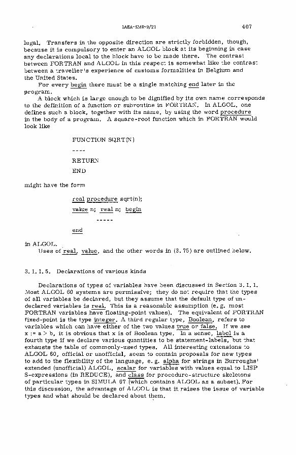
IA E A -SM R -9/21 407

legal. T ran sfers in the opposite d irection are str ictly forbidden, though, because it is com pulsory to enter an ALGOL block at its beginning in case any declarations lo ca l to the b lock have to be made there. The contrast between FORTRAN and ALGOL in this resp ect is somewhat like the contrast between a tra v e lle r 's experience of custom s form alities in Belgium and the United States.

F or every begin there must be a single m atching end later in the program .

A block which is large enough to be dignified by its own name corresponds to the definition o f a function o r subroutine in FORTRAN. In ALG OL, one defines such a block , together with its name, by using the word procedure in the body of a program . A squ are -root function which in FORTRAN would look like

FUNCTION SQRT(N)

RETURN

END

might have the form

rea l procedure sqrt(n);

value n; rea l n; begin

end

in ALGOL.U ses o f rea l, value, and the other w ords in (3. 75) are outlined below .

3. 1. 1. 5. D eclarations o f various kinds

D eclarations of types of variab les have been d iscussed in Section 3. 1. 1. Most ALGOL 60 system s are perm iss ive ; they do not requ ire that the types o f a ll variab les be declared , but they assum e that the default type of un­declared variab les is rea l. This is a reasonable assum ption (e. g. m ost FORTRAN variab les have floating-point values). The equivalent of FORTRAN fixed-point is the type in teger. A third regular type, B oolean, r e fe r s to variab les which can have either o f the two values true o r fa lse . If we see x := a > b, it is obvious that x is o f Boolean type. In a sense, label is a fourth type if we declare various quantities to be statem ent-labels, but that exhausts the table o f com m only-used types. A ll interesting extensions to ALGOL 60, o ffic ia l o r unofficia l, seem to contain proposa ls fo r new types to add to the flex ib ility o f the language, e. g. alpha fo r strings in B urroughs' extended (unofficial) ALG O L, sca lar for variab les with values equal to LISP S -exp ress ion s (in REDUCE), and c la ss for p roced u re-stru ctu re skeletons o f particu lar types in SIMULA 67 (which contains ALGOL as a subset). F or this d iscussion , the advantage o f ALGOL is that it ra ises the issue o f variable types and what should be declared about them.

408 CAMPBELL

Quantities declared by switch are specia l a rrays: arrays of statem ent- labels of type la b e l. These arrays allow neat tran sfers s im ilar to the computed GO TO in FORTRAN. The set o f declarations

label f, g, h;

switch trans := f, g, h ;

makes it possib le for

go to trans [if x < 3 then x else entier (1 + 7 /x )]

to transfer con trol to h if x = 3, g if x = 2 or 4 through 7, o r f otherwise (as long as x is positive).

3. 1. 1. 6. Call by name and ca ll by value

Suppose that we are in a part of a FORTRAN program and find the statement N = 3. A fter that statement has been executed, where in the program is the inform ation available that N now stands fo r 3, and where is this news unknown? If we are in a function o r subroutine from which N is not to be returned, and if N is not a COMMON variable, the in form a­tion is lo ca l to that subprogram . If we are in the main program , the in ­form ation is in accessib le to any functions or subroutines (except those that take this N as an argum ent), unless N is a COMMON variab le . If N is com m on, the news is available in every region which is headed by a COMMON declaration . We tend to take this state o f a ffa irs fo r granted if we have been brought up on FORTRAN. ALGOL treats the question in a slightly different way, so that we have to think carefu lly about it.

If we want a certain variable to be purely lo ca l to a b lock , so that bindings made to it do not affect the state of quantities with the same name anywhere outside the b lock , we must declare it by using value at the head o f the block . A declaration

value a, b, c;

indicates that bindings made to a, b, and с inside the block are to be fo r ­gotten when one gets past the b lock 's end m arker and that these bindings have no effect on u ses o f variables named a, b, and с outside that b lock .Any quantities not so declared have their changes (if any) inside the block a ccess ib le in any other b lock where they are not protected by being named in a value declaration . A quantity which is ca lled in a b lock where it has occu rred as an argument o f value is said to be "ca lled by value". Otherwise it is "ca lled by nam e". This distinction is , under a different label, exactly the same as the distinction between " lo ca l" and "g loba l" quantities which com es up again in Section 4. 3.

If we attach great value to the idea that one should be protected against situations where casual bindings of variables in som e part o f a program produce surprising s id e -e ffe c ts elsew here in the program where the same nam es are used, then FORTRAN is a fa il-sa fe system . Autom atic tran s­m ission o f inform ation does not happen unless we ask for it in a COMMON declaration. Judged by the same standard, ALGOL is unsafe. H owever,

IA E A -SM R -9/21 409

if this leads to m ore thought on the part o f the program m er, the lack of safety m ay not be a bad thing.

3. 1. 2. JOSS or CAL or FRED

A ll three o f these languages share the same essentia ls. The main reason for the d ifferen ces in nam es can probably be traced to lo ca l pride.I apologize for m y own involvem ent in what is , after a ll, -one o f the seven deadly sins, but I shall nevertheless ca ll a ll o f the languages FRED in these notes. Our choice of the name FRED is in honour of J. F red Nurke.

While designed orig inally as a language for num erical p rocessin g , FRED d iffers from FORTRAN and ALGOL in being intended fo r con versa ­tional (rather than ba tch -p rocessin g ) use. This intention dictates some specia l p rop erties o f FRED. One obvious property o f this kind is that every statement has an identifying num ber. The num ber is available for tran sfers o f control, as in FORTRAN, but it is equally important to label each statement uniquely to allow the user to add, m odify or delete lines of h is program by re fe rr in g to the labels. These labels are floating-point num bers. The program m er can break his program into log ica l parts (see Section 3. 1. 2. 2) by giving the sam e integer num ber to each statement in a part. Thus statements 2. 2, 2. 23 and 2. 231 are a ll m em bers of part 2, and their order in the program is fixed by the order o f their decim al fr a c ­tions. The idea behind the fractional notation is that if the u ser decides that he wants to insert a new statement between 2. 23 and 2. 231, he can choose the number 2. 2305 . . . and so on. If one m ere ly types a statement preceded by a number N, it is autom atically inserted into the program in the c o rre c t place suggested by N.

3. 1. 2. 1. Desk calcu lator

The m ost sim ple conversational system that one can wish for is a system which w ill evaluate expression s which are typed in and w ill print out the resu lts . E xam ples of expressions m ay be 2 + 3 or

ABS(ENTIER(SIN(LOG(COS(EXP(SQRT(RANDOM(0 ))))))))(3. 79)

L ists o f expression s m ay also be used to save tim e and space, e. g. 2 + 3,3 + 4, 4 + 5 on entry ca lls for the printing o f 5 7 9. To im itate a program while still doing som ething only worthy o f a desk ca lcu lator, FRED can p ro ce ss

1.0 DEMAND X

1. 1 Z = SQRT(X)

1.2 "SQUARE ROOT O F ", X , "IS ", Z

RUN

410 CAMPBELL

and produce the expected resu lt. DEMAND is the input operation: execution o f statement 1 . 0 causes the output o f

X =

on the teleprin ter. The program then waits for the u ser to enter a number (free form at) before going on.

A ll o f the conventional infix operators and functions (e. g. (3. 79)) are available in the desk -ca lcu lator m ode.

3. 1. 2. 2. Compact descriptions o f iteration

FR E D 's answ ers to the prob lem s o f iteration resem ble those of ALGOL, but there are som e alternatives which are made possib le by the structure o f the language. The equivalent of

_if a = b then fo r j := 1 step 5 until 86 do n[j] := j 3;

in FRED is (with the statement number omitted)

N[J] = J t 3 FOR J = 1 BY 5 TO 86 IF A = В

In other w ords, the ord er o f the operation and the various m od ifiers in FRED is reversed over that o f ALGOL. Such inessential d ifferences are am using because, while they are no obstacle to understanding, they show how much variety can be found in sim ple p ro ce sse s o f thought.

In FRED, the w ords BY and TO rep lace step and until from ALGOL. WHILE and while have the same meaning. H ow ever, FRED adds the alternative m od ifiers UNTIL (not now to be confused with until) and UNLESS to the rep erto ire , fo r use in the same context as WHILE. In a ll ca ses , wesucceed in our intention that iterative FRED statements with m od ifiersshould read like English.

There is no prov ision for m ore than one operation per statement in FRED, so that the " do begin S i; S2 ; S3 end" structure o f ALGOL must be handled in a different way. The statements S¡ form a log ica l part of any program , which means that they can be given separate statement num bers in FRED with the sam e integer value. An equivalent of

i f a = b then do begin S ^ Sg; S3 end;

с := 3;

in FRED is therefore

2. 6 DO PAR T 3 IF A = В

2. 7 TO STEP 4. 0

3 . 0 S i

3 .1 S ,

3 . 2 S 3

4. 0 С = 3 (3. 80)

IA E A -SM R -9/21 411

Beware the temptation to leave statement 2. 7 out o f (3. 80)J This causes part 3 to be executed tw ice. F or som e no doubt p sych olog ica l reason , such e r r o r s — (3. 81) — seem to be o f the m ost com m on type in FRED.

Exam ple (3 .80 )a lso dem onstratesthe distinctionbetw een a STEP and a PART and shows that TO STEP n is the analogue o f GO TO n in FORTRAN. Statements beginning with TO PART or with DO STEP (also a com m on source o f the (3. 81) e r r o r ) are allowed and have the obvious m eanings.

3. 1. 2. 3. A rrays

Section 6. 3 contains an account o f how arrays are maintained in FRED. Out o f that account, I shall mention here only that the FRED interpreter uses a lis t structure for storage of elem ents o f a rrays. If we are dealing with arrays of fixed dim ensionality in which all elem ents from index 1 to a known index n are present, then any use o f pointers is unnecessary and wastes space, but the idea behind the list structure is that we do not always want to be lim ited to FO R TR A N -like arrays.

The firs t benefit o f the hidden list structure is that indices can run from any integer (including negative num bers) to any other in teger, without having to take steps o f + 1. If we only want to define A [-5 ] and A[2] at som e stage, there is no need to reserv e space for the undefined intervening elem ents o f A , because there is a pointer from the p lace where A [-5 ] is stored which points d irectly to A [2 ] . To put in a new elem ent is as sim ple as the alteration o f pointers. T herefore it is unnecessary to use DIMENSION statem ents to declare arrays in FRED. If a quantity is follow ed by sub­scrip ts inside square brackets, that is a sufficient identification fo r an array elem ent.

A second novelty which becom es possib le because of the lis t structure (see Section 6. 3) is that the dim ensionality o f an array need not be fixed: the quantities A (an ord inary variab le), A [ l ] , A [2 ,-7 ] a n d A [0 ,2 ,4 ,6 ] can a ll coex ist in storage without com plications. This is a further stretching o f the range o f p ossib ilities for what can be done with arrays.

3. 1. 2. 4. U ses for specia l characters

A fter setting up the m ost basic operations in FRED and adopting the conventional uses for som e ch aracters (e. g. * fo r m ultiplication and t for exponentiation) on the teleprinter keyboard, we noticed that there were a few ch aracters left unused. Although it is no way to design a language (except if the language is A P L ), we ro se to the challenge o f finding m eaning­ful uses for them. H ere are two resu lts .

F irstly , the p ictor ia l appearance o f the character-L (s h if t l)> suggested a form o f reduction, at the tim e that an early FRED program was required to evaluate many expression s of the form "x modulo y ". The coincidence was too pleasant to be ignored. In FRED, "x modulo y" is now represented b y x j . y .

Secondly, the character (TAB or tabulate) was still unused when there w ere one o r two requests from u sers for a crude curve-p lotting facility .In the FO R TR A N -interpreted version o f FRED, where we have explicit con tro l over the output bu ffers, we chose -* n to mean "tabulate to column

412 CAMPBELL

n from the left m argin o f the page". As repetitions o f the character I in the same column im itate a line o r axis and * is a good way o f m arking points o f a curve, we can, fo r exam ple, produce a good plot o f the sine function, with values o f the independent variable at the left of the page, if we execute the single FRED statement.

X , - 30, " I " , -* 15*SIN(X) + 30. 5, FOR X = 0. 2 BY 0. 2 to 7. 0

Although the use o f the character -* was thought up rather casually, it has since proved to be a valuable feature o f FRED if one can judge by the reactions o f u sers .

This story has no m ora l. It m ere ly shows a sm all p iece o f h istory and suggests that certain adm ired features o f other languages m ay once have been invented in the same unsystem atic way.

3. 1. 2. 5. F a cilities for tracing

If a program runs without e rro r conditions but produces resu lts which are obviously wrong, one method of co llectin g inform ation on the fault is to run the program again, causing the value o f each binding operation and the destination o f each transfer o f control to be printed out. In FRED, the u ser m ay issue the command TRACE to achieve this e ffect. Then, every binding operation like A = 3 in the program is printed out as it is m ade, and any transfer to statement n causes the output of the m essage BRANCH TO STEP n. The comm and UNTRACE turns o ff a ll o f the tracing m essages.

A s w ell as being available as comm ands external to a p rogram , TRACE and UNTRACE m ay be inserted as actual statements in the program to provide tracing o f only a lim ited part of its operation. The usefu lness o f the in ­sertions is in creased because TRACE and UNTRACE, like any other statem ents, m ay be restricted further by m od ifie rs , e .g .

5. 92 TRACE IF A = В UNLESS N > 15

Although these fa c ilit ies m ay often be o f great value to the u ser , they are not yet generally available in the better-know n num erical languages.

3. 1. 2. 6. E rro rs

A firs t princip le o f any good conversational language is that no e rro r should be allowed to end a whole job . The reason , of cou rse , is that the u ser at his teleprinter o r term inal keyboard is in a position to co rre ct the e rro r im m ediately and try his calculation again, provided that he rece iv es an in tellig ible m essage about the nature o f the e r ro r . F or exam ple, the typing o f the statement

3 .4 Z = (X - Y * (X + Y)

should produce the m essage

MISSING )

IA E A -SM R -9/21 413

and a chance to put statement 3. 4 in again. S im ilarly , i f the' comm and DO PART 16 FOR N = 5 BY -4 TO -7 controls

16. 3 A = SQRT (N),

then during the run o f the program it is reasonable to expect inform ation about the p lace as w ell as the type o f the e r r o r , e. g.

ERROR IN STEP 16.3:

ARGUMENT < 0 fo r SQRT.

Both o f the exam ples above w ork as shown in FRED.FRED has about 35 e r ro r m essages to cover m ost o f these eventualities.

No system is p erfect, how ever. Only about 34 o f them can be understood d irectly . The last e r ro r m essage, which appears if none of the firs t 34 m ay be made to fit the cr im e, is :

WHAT WAS THAT?

3. 1 . 3 . A PL

The syntax o f FORTRAN is adequate for m ost num erica l p rogram s, and there is a fa ir range o f specia l characters (e. g. *, +, - , ] ) which are reserv ed to denote com m only-used operations. In ALGOL and FRED we have seen suggestions for extensions in syntax, but the poss ib ility of extensions to the set of ch aracters has been put to one side. A P L looks rather bare when syntax is considered , but it has a wide range o f specia l ch aracters with m athem atical sign ificance, thanks to the requirem ent that it should see the outside w orld through an IBM 2741 term inal with an A P L keyboard. A P L is a conversational language which is p rocessed by an in terpreter that must expand the u s e r 's com pact expression s. Thus A P L does not make an easier internal job o f p rocess in g instructions to do a particu lar m athem atical task than (say), FRED, but it m ay turn out that the u ser has le s s work in typing the n ecessa ry instructions in A PL because som e function o f two argum ents x and y, which is not sim ple to express in natural language, happens to be available in A P L as x ? y, where ? stands fo r one of the specia l ch aracters. This com pactness is only part o f the story; suitable com binations o f the existing operators can express very com plicated but usefu l m athem atical manipulations in short form s which are tru ly rem arkable (e. g. (3. 82)). The extra im portance o f such form s is that they give us a com pletely new picture of what can be done m athem atically with a program m ing language. The point o f the present d iscussion o f A P L is to concentrate on these educational novelties.

3. 1. 3. 1. Dual uses o f operators

To extend the range o f distinct operations by roughly a factor of 2, the prin cipa l sym bolic operators have both unary ( ?x, where ? is the operator) and binary (x ? y) m eanings. F or exam ple, if we assum e that

414 CAMPBELL

A is the argument of unary form s o f operators and A and В are the arguments in the b inary case , we find:

OPERATION UNARY

x sign of A

4- 1 /A' * eA

@ log g A

J A.'

Г A if A is an integer,otherw ise 1 + entier (A)

L entier (A)

О лА

where entier (x) = x if x is a positive integer, o r the largest integersm aller than x if x is positive and has a decim a l-fraction part, and entier (x) = -en tier (-x ) if x < 0. The function TRIG is the sine if A = 1, a rcsin if A = -1 , cos if A = 2, a r c co s if A = -2 ................

3. 1. 3. 2. P recedence

Given an expression like A + В / С * D ** N in FORTRAN, it is possib le to see that it is p ro cessed as (A) + (В /С * (D ** N)) because o f sim ple ru les o f p receden ce which put ** ahead o f * and / , which are in turn ahead o f +. To d iscover which of * and / (which are on the same lev e l of p r e c e ­dence) com es firs t , we have to apply an altogether different rule which says that the scope o f a binary operator does not extend past its right-hand argument and that the scan fo r operators goes str ictly from left to right. Hence B /C * P m eans (В /С ) * P and not B /(C *P ). If that explanation does not seem to be c lea r , then nobody is happy — except the supporter o f A P L .In A P L , there is one sim ple ru le for precedence which rep laces the re la tive ­ly com plicated conventions in other languages: the right-hand argument o f any operator is everything between that operator and either the end o f the line or the firs t unpaired right-hand bracket, w hichever com es firs t . One surprising (unless you have thought o f it b e fore ) consequence o f this sim ple rule is that the expression A - B - C - D - E does not mean A - ( B + C + D + E), as in FORTRAN, but A - (В - (C - (D - E ))). In other w ords, A - B - C - D - E in A P L m eans the sam e thing a s A ' - B + C - D + E i n FORTRAN! This exam ple generates a ll kinds of passions fo r and against A P L and is th ere ­fore a suitable top ic to bring up at parties where m any com puter scientists are present.

BINARY

A t i m e s B

A / BA3

i°§ A B

binom ial coefficient

maxim um o f A and В

maximum o f A and В

TRIG (B)

tA E A -SM R -9/21 415

3. 1. 3. 3. Compact operations

F or exam ples of the kind where re la tive ly com plicated operations can be com pressed into a sm all number of sym bols, A P L re lie s on the rew ards bestow ed by the ru le of precedence mentioned in Section 3. 1. 3. 2 and on the variety of operator interpretations suggested in Section 3. 1. 3. 1. Two exam ples o f operations on sca lars quoted in R ef. [Bl ] are:

(a) E fficient factored form o f a + bz + cz^ + dz^. . without brackets

A + Z X B + Z X C + Z X D . . .

(b) Continued fraction s, e. g.

1a ------------ :—b + 1

ч - T

which in A P L becom es A + + B + -^C + + D (3 .82)

3. 1. 3. 4. True and fa lse

In ALG OL, variables o f Boolean type can take on the values true or fa lse . These values are com pletely distinct from any other value quantities in the system , in particu lar the integer values 1 and 0. There is a s im ilar distinction in LISP. On the other hand, there is nothing to stop the con stru c­tion o f a program in any language in which the Boolean truth-value is denoted by the integer 1, and fa lsity by 0. A P L uses this convention autom atically. Thus the value o f the log ica l test A > В is the integer 1 if A is greater thanB, o r 0 otherw ise. The value can be bound (binding operator is <- in A PL ) to som e variable without further ado, e. g. С *-A > B. N orm ally , one m ay believe that there is no point in doing purely arithm etic computations on num bers which have log ica l orig ins , but one p ra ctica l consequence o f r e ­laxing the rule is that conditional tran sfers (-* is the analogue in A P L for "GO T O ") can be written in a com pact form . F or exam ple, the FORTRAN transfer

IF (A - B) 15, 25, 35

m ay be rendered as

^ 15 + (10 X A = B) + 20 X A > В

Other applications fo r num erical operations on the A P L log ica l "tru e" and "fa lse " values are not hard to find.

3. 1. 3. 5. A rrays and operations on arrays

F or the same reason s as in FRED, arrays in A P L can be created at any tim e by the naming o f elem ents, without the need fo r anything like a

416 CAMPBELL

DIMENSION statement. There are two ch aracteristics o f FRED arrays which could have been reproduced in A P L , but which were not. The first is the freedom to leave gaps in arrays by defining disjoint elem ents like A [-5 ] and A[2j while saying nothing about the others (and the freedom to have indices le ss than 1). The second is the legality of having different num bers o f ind ices for A in storage at the same tim e. The reason for requiring A P L arrays to have conventional behaviour with resp ect to indices is that there are specia l array-operations which make no sense or little sense unless the FRED freedom s are abridged. F or exam ple, there is the "d im ension" operator p whose value in the context pA, where A is an array with n indices running from 1 to Ui, 1 to u g , . . . 1 to u „, is the one-d im ensional a rray with the n components Ui, Ug , . . - Un. The quantity ppA is then also defined quite log ica lly as a one-d im ensional array with one elem ent whose value is n. Since arrays whose elem ents are also arrays are allowed in A P L , it is important for the program m er to be able to make these repeated applications o f the "d im ension" operator to find out what is going on in his book-keeping.

Another justification for the conventional treatm ent of array indices is in the existence of global operations. In FRED, if the sca lar A and e le ­ments o f the array A exist sim ultaneously, A + 3 m eans "add 3 to the sca lar A ". In A P L , where A cannot be both things at once, the value of A + 3, if A is an array (required to be one-dim ensional in this case), is an array of the same size , constructed by adding 3 to each elem ent o f A. Thus the e ffects o f operators (like +) d iffer accord ing to the types of their argum ents.

An array with given values can be set up in one A P L instruction, e. g.

V <- 2 3 5 7

causes V to be a one-d im ensional array with V [l] = 1, . . . . , V[4] = 7.To stretch this a rray to include V[5] = 11, we have only to write

V ^ V, 11 (3. 83)

and the extra elem ent is concatenated by the com m a operation. If both argum ents o f the com m a are named arrays, we produce entire new arrays by concatenation.

The binary use o f the operator p is for in itializing or rebuilding arrays; to make A equal to an arra y o f ten ze roes , we write

A <- 10 pO

At this stage it is easy to see how arrays of arrays a r ise . We achieve a 10 X 10 array o f ze roes with

A *- 10 10 pObut

A *- 10 pO 0

is a one-d im ensional array with ten elem ents, each being an array with two elem ents o f ze ro . (Warning. Apparently this is a m inority convention

IA E A -SM R -9/21 417

for hom e-built A P L system s, and it is not true in the canonical IBM system . T here, the meaning o f xpy is that the array of dim ensionality x is to be created out o f elem ents o f y, repeated from the beginning of y if y is too short to fi ll up the entire new array. )

Certain global operations which are w ell-defined "o v e r " a one­dim ensional a rray are signified by the sym bol / which stands for the quotient operation in other num erical languages. F or exam ple, the sum over the last a rray V, which is 2 + 3 + 5 + 7 + 1 1 = 2 8, is denoted by + /V. The maxim um over V, which is 11, is denoted by ГУ V.

Of n ecessity , this must be only a b r ie f survey of A P L . Other features, particu larly those operations on arrays which give the language much o f its power for expressing long calculations in a line or two of p rogram s, are set out at much greater length in R efs [A5, A 6 ] . H ere, the ob ject is sim ply to show how a new approach to num erical program m ing which concentrates on com pact and w ell-chosen notation can extend our ideas about how to write languages and program s in this fie ld , which has been dominated fo r so long by FORTRAN conventions.

3. 2. LISP

Section 2 contains an introduction to the ideas of sym bol-m anipulation and o f lis t -p ro ce ss in g at the same tim e. In all of the sym bol-m anipulating languages d iscussed below , the list is the basic structure in storage, but that does not im ply that the two ideas are the sam e. In princip le , one can w rite sym bol-m anipulating program s (e. g. in FORTRAN, by heavy use of the A form at) without lis ts , and program s in a lis t -p ro ce ss in g language which operate purely on num bers or lis ts o f num bers. F or m ost cases, how ever, calculations involving sym bol-m anipulation seem to have the property that interm ediate and final resu lts are o f uncertain length, so that the natural medium o f storage becom es the list, with pointers, rather than the FORTRAN array. Thus lis t -p ro ce ss in g and sym bol-m anipulation are intim ately connected, but they are still not the same thing. Having made this d iscla im er, I hope that I can m ove on sa fely to the lis t-p ro ce ss in g aspects o f LISP firs t . I quote LISP as the principa l exam ple o f a sym bol- manipulating language because of the h istorica l im portance of LISP, the considerable num ber o f uses (see R efs [ C4, C5] ) to which physical scien tists have put it already, and the fact that im plem entations of LISP exist for a ll large scien tific com puters.

We left LISP in Section 2 at the stage (2. 2) where the syntax had been com pleted by the definition o f "S -ex p ress ion " . To repeat (2. 2), we have

(S -ex p ress ion )< ::= (L IS P atom ^ ¡ ( (S -e x p r e s s io n )>. (S -e x p re s s io n ^)

The period " . " is thus a specia l sym bol, because it denotes the operation of concatenation o f S -exp ress ion s into m ore com plicated S -expression s. E very building-up operation in pure LISP must therefore make heavy use of p eriods. F or exam ple, som e atom s in LISP are NIL, E F, CD, and AB. These are also S -exp ress ion s , by the firs t alternative in (2 .2 ). By the second alternative, so are (E F . NIL), (CD. (E F . NIL)) and (A B . (CD . (E F . NIL))). In the structure (E F . NIL), we are using the period as an operator to associa te EF and NIL. Given the conventional

418 CAMPBELL

partitioning of a w ord in the com pu ter's free storage for LISP, the sim plest association o f EF and NIL can be arranged if we put a representation o f EF into the left-hand half of a w ord and a representation o f NIL into the right- hand half. In the p rog ra m m er 's form of LISP, (EF . NIL) is the equivalent of this s ing le-w ord structure. (CD . (EF . NIL)) behaves like (CD . x) and requ ires a new word with CD in the left-hand half and a representation of x in the right-hand half. But here x is too large to fit into half a word, so the "representation o f x " is a pointer which points to the word that contains (E F . NIL). If I repeat this argument with (A B . (CD. (E F . N IL))),I get a th ree-w ord structure whose specification is identical to F ig. 1. (Rem em ber that the diagonal bar in the last half-w ord o f F ig. 1 is shorthand fo r NIL. ) In Section 2, though, F ig. 1 is described as the LISP representa­tion of (AB CD E F), which is an easier and m ore natural p iece o f inform ation than the one with many periods and brackets which I have just built up from (2. 2). F or convenience, then, LISP accepts the two form s (AB CD EF) and (AB . (CD . (EF . NIL))) as being equivalent; the two notations are called list notation and dot notation respective ly . To get from one to the other, it is only n ecessa ry to rem em ber the two identities written below . In each identity, dot notation is given on the left and list notation on the right.

(x . NIL) = (x)

(x . (y)) = (x y)

In the identities, x is any S -expression and y is anything.The b asic constructive operation in LISP is the operation o f joining two

S -exp ress ion s (e. g. x and (y)) together to form a compound S -expression (e. g. (x y)). A ll S -exp ress ion s can be built up eventually by repeated uses of the basic operation of construction. In LISP, this operation is the function CONS. CONS applied to arguments x and (y) gives the value (x y); inside the system , CONS takes a new word W off the free -s to ra g e list and puts a pointer to x in the left half o f W and a pointer to (y) in the right half o f W. C onversely , LISP also needs functions to reso lve a compound structure into its " le ft" and "righ t" parts. The function CAR applied to (x y) has the value of x (i. e. it looks into the left half o f W to see what it can find there), an d th efu n ction C D R h asth eva lu e(y )(i.e . the quantity which is "found" in the right half o f W). These three functions are conceptually the m ost basic functions o f LISP and a ll l is t -p ro ce ss in g system s contain them under som e name or other. The nam es CAR and CDR perm it one helpful abbrev i­ation: frequently we need to apply chains of CAR and CDR operations, e. g. "C AR o f CDR" or "CDR of CDR o f CAR ". The abbreviations here, which LISP recog n izes , are CADR and CDDAR respectively . The com plete c lass of lega l abbreviations, which contains a total of 28 functions, has m em bers with nam es CnnR, CnnnR, and CnnnnR, where each n can stand fo r either A or D.

Having disposed of the n ecessa ry background for LISP here and in Section 2, we can now go on to consider individual parts and features of the language.

(a) Boolean log ic and pred icates

A s in ALG OL, there are two specia l LISP atom s whose job it is to represent true and fa lse . These atom s are T and NIL. (The two uses of

IAE A-SM R-9 /2 1 419

NIL which we now know do not con flict with each other. ) P red icate functions, whose purpose is to ask questions (e. g. "Is x NIL? " or "Is x an atom ? ") , are functions whose values are either T or NIL in LISP.

The m ost useful p red icates in the LISP language are given below . W hereI explain the value o f a predicate in term s o f x and y, I mean that the p red i­cate has these two argum ents. If I talk only of x, the predicate has only one argument.

NULL: True (T) if x = NIL, and fa lse (NIL) otherw ise.

ATOM : T if x is an atom , NIL otherw ise.

NUMBERP: T if x is a num erica l atom , NIL otherw ise.

EQ: T if x and y stand for the same atom (for the sake of uni­form ity among a ll LISP system s, we should assum e that EQ gives the right answer only for non-num erica l atom s),NIL if x and y are different atom s, otherw ise the answer depends on whether (T) or not (NIL) x and y start in the same place in storage.

EQUAL: T if x and y are equal S -exp ress ion s , and NIL otherw ise.Thus EQ should be used to test for equality if x and y are known to be non-num erica l atom s, but the slow er function EQUAL should be used in a ll other cases.

ZEROP: T if x = 0, NIL if x is a n on -zero num erical atom , and ane rro r condition otherw ise, e. g. if x = NIL.

LESSP: T if x < y (where x is the firs t argument o f LESSP), NILif the num bers x and y do not satisfy this condition. O ther­w ise, the sam e caution as for ZEROP applies.

MEMBER: T if the S -exp ression x is a m em ber of the list y, and NIL otherw ise.

AND:

OR:

T if all o f its argum ents are S -exp ression s o r evaluate to give S -exp ress ion s which are not equal to NIL, and NIL otherw ise.

T if any one of its argum ents is an S -expression or evaluates to give an S -expression which is not equal to NIL, and NIL otherw ise.

The pred icates AND and OR accept variable num bers of arguments up to 20.

(b) Conditional expression s

The translation into LISP o f the English " i f Pi then v^ else if pg then Vg. . . . e lse if Pn^ then v^.^ e lse v „ " is not sm oothly readable like (3. 76), but it is still unambiguous. It is :

(COND (Piv^) (p^Vg)------ (Pn-iVn-i) (T v „))

which is probably the sim plest form we can get when we apply the boundary conditions that the expression should be an S -exp ression free from visib le

420 CAMPBELL

periods in lis t notation and should distinguish each pairing (p¡, v¡) o f p ro ­position and value c learly . LISP uses the function COND to do what IF does in m any other languages.

F or p we can write any S -expression which represents a proposition .A predicate function, with its argum ents, is the obvious choice , but T and NIL are also valid propositions by them selves. Further, the convention in LISP is that any S -expression whose value is not NIL can be p laced in a position p. , and COND w ill then behave as if this p w ere just T.

COND m ay be used to define functions with a multiple choice o f values or in som e circum stances to produce tran sfers of control (like IF in FORTRAN), provided that som e v¡ is an S -exp ression corresponding to a transfer statement.

(c) Structure o f function-defin itions

We can write our own functions F in term s o f the functions Fp already available in the LISP system to do slightly m ore com plicated things than these functions w ill do. Then perhaps we decide that we want a further lev e l o f com plication, represented by functions Fg which we write in term s of F^ and Fp. A fter going through about four layers o f this p ro ce ss , we a rrive at the m ost com plicated program s which have been used in physics. O ne's "p rogra m " is a union of a ll the functions o f each lev e l F except Fg.In contrast to the situation in num erical languages, where there is usually a main program follow ed by a few subroutines or functions, a LISP program m ay consist of one short function f^ which is written in term s of a few functions in the c lass F ¡^ , where each function in F ^ ca lls perhaps one or two others in I^_^ and severa l in F^.g . . . . and so on. The program then con sists of a collection o f function-defin itions in no particular ord er, follow ed probably on the last card o f the deck by a ca ll to f^, with the ap­propriate argum ents, which sets o ff the entire calculation. T herefore , to w rite a program , it is only n ecessa ry to know how to define a function.

The expression which must be punched on cards or typed at a term inal to specify a function-definition is:

(name (LAMBDA arguments form ))

where "nam e" is the name of the function, and "argum ents" is a list of the nam es o f the dummy arguments to be used inside " fo r m " , which is the body o f the definition. A fter the reassurances in Section 2, we can be sure that it is lega l to define the function recu rs iv e ly , i. e. to use "nam e" again inside " fo rm " if we wish. Hence, we have a ll the inform ation that we need to define the fa ctoria l function, using the LISP conventions that we have seen so far. It is

(FACTORIAL (LAMBDA (N)(COND ((ZERO P N) 1)

(T (TIMES N (FACTORIAL (SUBI N )))) )))

In this definition, SUBI is a function which has a value equal to the value o f its argument minus one. The com plications (? ) o f form and brackets are a ll consequences o f the conventions which we have seen already, in-

IAE A-SM R-9 /21 421

eluding the convention o f p refix notation, in which operators are written to the left o f a ll their argum ents. M oreover, the operator-nam e and all of the argum ents are always made into one list for sim plicity , e. g.(ZEROP N) rather than ZERO P (N) or even (ZERO P (N)). The last two form s are illega l in this context.

R ecursion and the use o f COND go together w ell, as the last example shows. F or people who p re fer the sequential organization of steps, which is possib le in FORTRAN, there is an alternative way of setting out a function-definition like a sm all (FORTRAN) program . The specia l atom PROG is used to notify the LISP interpreter whenever this is about to happen, and the outline of the definition becom es

(name (LAMBDA arguments

(PROG pvariables x XgXg. . . . x^ )))

where "p variab les" is a lis t o f the nam es o f variables (apart from those named in "argum ents") used only inside that sm all program or PROG feature, rather like the argum ents fo r a value declaration in ALGOL. Each x ¡ is either an individual statement or an atom which serves as the label fo r statement x ^ . O ccasionally it is rather ea sier to define a function in term s of the PROG feature than by other m ethods, e. g. in the case of REVERSE, whose value is the rev erse of the list which is fed in. The definition of REVERSE is

(REVERSE (LAMBDA (U) (PROG (X)

G (COND ((NULL U) (RETURN X)))

(SETQ X (CONS (CAR U) X))

(SETQ U (CDR U))

(GO G) )))

This function returns (EF CD A B ), given (AB CD E F), by su ccess ive ly picking off left-hand m em bers of the PROG fea tu re 's copy U o f the structure with CAR and placing them at the left-hand end o f the list X with CONS (all program variables like X are in itially given values o f NIL). U is shortened by one elem ent when CDR is called. F inally, when U has been reduced to NIL, the value built up on X is returned as the answer. The orig inal copy of the input structure is left untouched, however. It is instructive to w ork through this exam ple, using F ig. l a s a re feren ce if diagram s are helpful.

REVERSE displays a ll o f the new ch aracteristics of the PROG feature: statem ent-labels, GO, SETQ, and RETURN. SETQ is the binding operator inside PROG features: the firs t argument o f SETQ stands fo r itse lf, while the second argument is evaluated. S im ilarly , the argument of the transfer comm and GO stands for itse lf. Everything e lse in the individual statements o f the PROG is evaluated by the LISP interpreter.

To get FACTORIAL and REVERSE defined, it is not sufficient m ere ly to put the definitions as shown into a card deck. A lis t o f such definitions must firs t be given as an argument to the LISP function DEFINE. How this is done is shown in an exam ple o f a program (see (e) below ).

422 CAMPBELL

(d) Quote

In any language which allows sym bols and nam es as data, the designers have to contend with the problem of what to do about the ambiguity that a name m ay som etim es be requ ired to stand fo r itse lf and som etim es for another quantity. Suppose that we wish to write a function FN in LISP in which the dummy variable happens to be X and which gives the atom X as a value if the value o f the variable is a number and NIL otherw ise. This is adm ittedly a confusing specification , but it serves to underline the problem of quotation. The answer has the form

(FN (LAMBDA (X) (COND ((NUMBERP X )? ) (T N IL )))

where ? cannot just be X , because then the function applied to any number sim ply gives back that num ber as a value. We need X with som e form of quotation-m arks, possib ly like "X " , but ? must a lso be a lega l p iece of LISP data. LISP 's solution is to rep lace ? by (QUOTE X). W henever a quantity q is to stand fo r itse lf and is being used in a context where the in terpreter does not take this fact fo r granted (i. e. alm ost anywhere inside function-definitions except in the first-argum ent position for SETQ, or as the argument for GO — R efs [A10, A l l ] supply m ore inform ation on this question), it is written as (QUOTE q).

(e) Structure o f LISP program s

The last two cards in a deck which contains a sim ple LISP program are by convention

STOP))))))FIN

where FIN begins in column 8. The STOP card contains severa l right-hand brackets, one to stop reading of the deck and the other to f i l l in for brackets which have been left out of the program by mistake (so that the reading can still stop). B efore that, in the program itse lf, there are 2n S -expression s. An odd-num bered S -expression 2 m -1 (m § n) is either the name o f a function o r a nam eless specification o f a functional operation with the form "(LAM BDA argum ents fo rm )" . The list o f argum ents fo r the function is then given in the position 2m. If the function 2 m -1 has zero argum ents, S -expression 2m is ( ); for one argument, the even-num bered structure is (a^, fo r two argum ents, (a ^ g ) , and so on. The LISP interpreter treats the entire program as data, reading it exactly as it stands (i. e. it m akes no attempt to evaluate the argum ents) and then applying function 1 to argum ent-list 2, function 3 to argum ent-list 4, etc. The non-evaluation o f argum ents som e­tim es confuses the novice p rogram m er who wants to ca rry out som e kind of compound operation, so it is worth dem onstrating with an exam ple. If I punch

NUMBERP ( (TIMES 2 4 6))

expecting the m ultiplication to give the number 48 and the resulting evalua­tion o f the test in NUMBERP to return the value T, I shall be surprised

IA E A -SM R -9/21 423

by the actualva lue NIL. It is actually the unevaluated expression (TIMES 2 4 6) which is inspected for "n u m b er-n ess", and o f course the resu lt is NIL. To get the expected answer T, I need to punch

(LAMBDA (X) (NUMBERP (EVAL X NIL))) ((TIMES 2 4 6))

where I have put in the demand fo r an extra evaluation explicitly . The function EVAL has this purpose o f evaluating its first argument and r e ­turning that value; in m ost sim ple situations the second argument of EVAL is just NIL.

N ext, here is an exam ple o f a LISP "p rogram " . The function LTIMES has the job of giving the product of a ll num bers occu rrin g in any list which is submitted to it, o r NIL if there are no num bers in the list. The function ATOMSOF gives as its value a list o f a ll the atom s which occu r at the top leve l of a lis t which m ay also contain m ore com plicated m em bers. The function XN gives the set-th eoretic in tersection of its two argum ents. F inally, we m ay want to define a function SUPERFN which can ca ll a ll o f these three, e. g. a function o f two argum ents which returns the product of a ll num bers which are com m on to the top leve ls of the argum ents. (Itw ill not be the m ost efficient such function, but it w ill be adequate fo r this dem onstration. ) A card deck which sets up the functions and then tests them is:

DEFINE ((

(LTIMES (LAMBDA (U) (COND ((NULL U) NIL)

((NUMBERP (CAR U)) (LTIMES2 U))

(T (LTIMES (CDR U))) )))

(LTIMES2 (LAMBDA (U) (COND ((NULL U )l)

((NUMBERP (CAR U)) (TIMES (CAR U) (LTIMES2 (CDR U))))

(T (LTIMES2 (CDR U))) )))

(ATOMSOF (LAMBDA (U) (COND ((NULL U) NIL)

((ATOM (CAR U)) (CONS (CAR U) (ATOMSOF (CDR U))))

(T (ATOMSOF (CDR U))) )))

(XN (LAMBDA (X Y) (COND ((NULL X) Y)

((MEMBER (CAR X ) Y) (CONS (CAR X)(XN (CDR X) (DELETE (CAR X ) Y ))))

(T (XN (CDR X) Y)) )))

(DELETE (LAMBDA (X Y) (COND ((NULL Y) NIL)

((EQUAL X (CAR Y)) (CDR Y))

(T (DELETE X (CDR Y))) )))

(SUPERFN (LAMBDA (A B) (LTIMES (ATOMSOF (XN A В ))) ))

))ATOMSOF ( (А (В C) 2 (E 3) FGH))

424 CAMPBELL

LTIMES (((A 2) HOMMES 40 CHEVAUX 8))

XN ( (AB CD EF) (GH CD 9) )

SUPERFN ( (A 2 В 6 С 7) ((W 2) X 7 Y 6))

STOP ))))))

FIN

A s you can see, the deck m ixes what you might norm ally have called program and data. The first odd-num bered S -expression is DEFINE, so that the next S -exp ression (a list of one argument x, where x is a lis t of function-defin itions), which is your "p rog ra m ", can be defined. When this task is finished, any function in the program can be addressed by name and used to p ro ce ss your data, as in the cases shown. In this deck, there are five applications of functions to data. A s a resu lt, the output contains the five answ ers

(LTIMES LTIMES2 ATOMSOF XN DELETE SUPERFN)(A 2 FGH)

320

(CD)

42

in a better-annotated form than I have given them here.This exam ple displays many of the standard ch aracteristics o f LISP

program s and therefore repays carefu l study. The best way o f study is to work through the given tests o f the functions with pen cil and paper, regarding you rself as the LISP interpreter.

There is an introduction to LISP in Ref. [C4] and another exam ple o f a LISP program in Section 6. 2.

(f) Further b asic functions

In the m ost basic LISP system s fo r large com puters, a little over 80 functions are available. We have seen about half o f this collection by name here already. While som e of the rem aining functions are for ad­vanced applications, others belong to useful categories which have not been considered so far. Eight functions which represent som e o f the basic ca tegories are d iscussed below . The lo w e r -ca se letters x, y, and z are used to stand for the values o f their arguments when they are called from inside som e other function-definition , e. g. one which the program m er m ay have written for h im self.

(LENGTH x): The value is the num ber o f elem ents in the list x at the top leve l, e. g. 3 for (А В С) and 2 for ((А В) (C D)). When x = ( ) or NIL, the value is zero .

(APPEND x y): If x and у are lis ts o f arb itrary lis ts , the value is a single lis t form ed by the concatenation of cop ies of x and y, e. g. when x = (А В C) and y = (D E F ), the value is (А В С D E F).

IA E A -SM R -9/21 425

(LIST x y z . . . ): LIST accepts variable num bers o f argum ents, between1 and 20. The value is a single list exhibiting x, y, z . . . as m em bers.F or exam ple, if x = (А В С), у = (D E F ), and z = 6, the value is ((A В C)(D E F ) 6).

(SUBST x y z): The value is a copy o f z which has been changed by the replacem ent of each occu rren ce of y at any lev e l by x, i. e. it is a function fo r substitution o f x for y in z.

(PRINT x): The value is x, although PRINT is interesting for its effect rather than its value. We m ay be satisfied with the answer which a function produces in som e computation and which the interpreter autom atically puts into the output, but on som e occasion s we m ay want to have news (e. g. for debugging) o f interm ediate resu lts like x which are achieved in the m iddle o f the computation. We can cause this inform ation to appear also in the output by changing x to (PRINT x) at the relevant parts of the program .

(MAPLIST x f): Frequently we need to perform operations on a list x which involve repeated applications of som e function f to x, then to CDR of x, then to CDDR of x, etc . This is a global mapping operation in which the effect of f is mapped onto x in a particu lar way. F or flex ib ility it m ay be a good thing to have a standard LISP function which can accept functional argum ents like f, con trol their application to f, and return the value of the mapping. MAPLIST is the sim plest o f these mapping functions. It behaves as if its LISP definition were

(MAPLIST (LAMBDA (X,FN) (COND ((NULL X ) NIL)

(T (C O N S (F N X ) (MAPLIST (C D R X ) FN))) )))

With M APLIST, it becom es possib le to define LISP functions in alternative sty les, so that one can choose the best or m ost efficien t style for a given situation. One exam ple of alternatives is a function DOUBLE which, given a list purely o f num bers, returns a list in which each num ber from the o r i ­ginal lis t is doubled. R ecu rsive ly the definition is

(DOUBLE (LAMBDA (U) (COND ((NULL U) NIL)

(T (CONS (TIMES 2 (CAR U)) (DOUBLE (CDR U)) )) )))

but with the use o f MAPLIST we can also write

(DOUBLE (LAMBDA (U) (MAPLIST U

(FUNCTION (LAMBDA (J) (TIMES 2 (CAR J)) ))) ))

The specia l atom FUNCTION is used to label any functional argument for a mapping function.

(DEFLIST x y): The form of x is a list o f tw o-elem ent sublists, e. g. ((R iVi) (agVg) . . . ). The second quantity y has an atom as its value. The value of DEFLIST is the list ( a ^ g . . . ), but this is unimportant beside the effect of the function, which is to associa te with each a ¡ the property v¡ under the indicator y. If y = EXPR, the operation of DEFLIST does exactly

426 CAMPBELL

the same as (DEFINE x ), i. e. the indicator which the system maintains internally to identify stored function-definitions is EXPR. A quick look back at the program under (e) above shows that the argument for DEFINE has the requ ired form fo r the x given here, so that the stored fünction- definition under the indicator EXPR fo r any function-nam e is always (LAMBDA argum ents form ). DEFLIST, a generalization o f DEFINE, perm its us to decide on as many properties as we like fo r any atom and to associa te them with the atom by using DEFLIST repeatedly. How the association is maintained inside storage in such cases is described in Section 5. 5. In particle physics and the analysis o f Feynman diagram s in LISP (Ref. [C8] ), the atom s which identify partic les are labels P I , P2 . . . for mom enta, but we can ca rry along a ll the other d iscrete inform ation about p a rtic les by using DEFLIST to associate with, e. g. , P I a m ass under the indicator MASS, a spin with SPIN, a polarization with POL, and so on.

(GET x y): Having used DEFLIST to store inform ation, we need an inverse function to re co v e r it. This is GET. If x stands for an atom and y is an indicator, the value o f GET is the property stored under that indicator. If x does not have the property y at a ll, the value o f GET is NIL.

(g) ERRORSET

Som etim es we m ay have a good idea of where e r r o r s m ay occu r in a com plex program but be unable to try out our ideas without running the program to see what happens. In term s o f LISP, the evaluation of som e e rro r -p ro n e expression S should behave as: " if S is e r r o r - f r e e , the answer is S, but otherw ise som e specia l value is returned to denote an e r r o r " . Thus, if we make an e r ro r in S, the computation does not collapse as in m ost languages, but we can re co v e r control and d irect the computation to try som e other alternative. In LISP, this highly valuable state of a ffa irs can be brought about with the use o f the function ERRORSET to control the evaluation o f S. The form of ca lls to ERRORSET is

. . . . (ERRORSET s n i a) . . . .

where s is the expression to be evaluated, n is the maxim um number of CONS operations to be allowed before an e r ro r trap o ccu rs (which is useful in detecting infinite loop s), i is an indicator whose value is T if we wish e rro r m essages to be printed out but NIL otherw ise, and a is a list o f pa irs of arguments from s and their values. F or exam ple, if we have a p iece o f program in which s stands for (FN X Y), and the values o f the variables are resp ective ly (A B) and 5, then the value o f a is ((X A B) (Y . 5)).

If the evaluation of the expression denoted by s is co rre ct and has the value v, then ERRORSET returns the value (v). If there is an e r ro r , the value is NIL. T herefore the u ser or h is program can identify e rro rs im m ediately.

Once the unusual idea o f an e r r o r -r e c o v e r y operation like ERRORSET has been established, intending u sers can easily think o f im provem ents, e. g. a range of atom ic values 1, 2, 3 . . . instead of NIL in the case of e r r o r s , with each value signifying a different type o f e rro r so that the p r o ­gram can react accord ingly . Some of these fa cilit ies are being added to

IA E A -SM R -9/21 427

languages which I have not surveyed here. The im portant contribution of LISP has been to show that a function ERRORSET is p ractica l to build and operate.

(h) U ses o f LISP in physics

M ost of the sym bolic computations with applications to physics have been in LISP (see R efs [C4, C5] ). In turn, m ost o f these computations have used the system s REDUCE-1 and REDUCE-2. For a physicist who does not wish to learn LISP in ord er to use existing program s, the ch ief b a rr ie rs to understandingare brackets andprefixnotation. M ost L ISP -based system s are now either evolving into languages (as REDUCE has done already) or are equipped with specia l functions which accept FO R TR A N -like input in infix notation and translate it se cre tly into LISP be fore p rocess in g it. This m akes the u s e r 's life ea s ie r . M ore details are given in Sections 3. 2. 2, 6. 2 and 6. 6. H ow ever, if you have prob lem s for sym bolic computation which do not seem to be suited to existing program s, there is enough inform ation here to enable you to make your own experim ents with LISP. The rew ards which a study o f LISP has to o ffer are substantial, quite apart from the consideration o f whether or not you have any im m ediate physical p rob lem s to solve.

3 .2 .1 . PO P-2

LISP and P O P -2 grew up in the same kinds of environm ent, in the neighbourhood o f designers and u sers with an interest in the top ic o f a rti­fic ia l intelligence. The m ost noticeable d ifferen ces o f P O P -2 from LISP at firs t inspection are that P O P -2 looks much m ore like ALGOL and does not seem to contain so many bew ildering brackets as LISP. An explanation for the firs t d ifference is that exposure to the influence o f ALGOL is a m ore o r le s s continuous p ro ce ss in the United Kingdom but a rather random one in the United States. There are severa l reasons for the second d if­fe ren ce , but one which m ay be quite convincing is that LISP was firs t im p le­mented in 1959, when large conversational computing system s were not available, but P O P -2 was built as a conversational language. An impatient u ser sitting at a teleprinter is not rendered any m ore patient by the need to count his brackets as carefu lly as a LISP program m er must do.

The absence o f bracket-counting p rob lem s, and the presence o f som e fast arithm etical fa c ilit ies for conversational u sers , m eans that PO P-2 resem b les FRED for som e sim ple applications, e. g.

A = 5 t 2 + 5 /2

В = 2 * A - 1

Вwhich is the sequence of FRED instructions that causes the eventual printing o f 53, is rendered as

VARS A , B;

5 f 2 + 5 / 2 - > A

2 * A - 1 - > В

В = >

428 CAMPBELL

in P O P -2 . (Note the requirem ent that variables are declared , to reserve space for them, and also note the conventions for binding and printing. )When the applications are sym bolic, the notation o f P O P -2 is close to that of either ALGOL or REDUCE, which m akes conversational computing easier than in LISP. In the example of the definition o f the function LENGTH (see Section 3. 2 (f)), contrast the LISP input

DEFINE ((

(LENGTH (LAMBDA (X) (PR O G (N ) (SE TQ N O )

G (CO N D ((N U L L X ) (RETURN N))) (SETQ N (A D D IN ))

(S E T Q X (C D R X )) (G O G ) ))) ))

with the rather sim pler P O P -2 construction

FUNCTION LENGTH X; VARS N;

0 - > N;

G: IF NULL(X) THEN N EXIT;

N + 1 - > N ; T L ( X ) - > X ; GOTO G END; (3 .84)

which a lso displays the P O P -2 conventions for the LISP concepts o f GO, PROG, SETQ and RETURN. The basic lis t -p ro ce ss in g functions CAR and CDR have the m nem onic nam es HD (head) and TL (tail), an old B ritish convention from the days of the language CPL which m akes it im possib le to abbreviate chains of HD and TL functions in the manner o f LISP.

The main difference between P O P -2 and LISP program s, as in (3. 84), is in readability. B asic sym b ol-p rocess in g functions tend to have the same nam es (apart from CAR and CDR, and also CONS, which is the infix operator :: in P O P -2) and basic ideas in the two languages, but the added virtue o f P O P -2 is that it contains extra features that extend on e 's ideas about sym bol-m anipulation. To som ebody brought up on LISP, a reading o f Ref. [A16] causes the same kind of educational m ind-stretch ing that a reading o f an A P L manual produces in som ebody whose sole background is in FORTRAN. The follow ing deals with som e o f the m ore interesting extra features.

3. 2. 1. 1. Dynamic lis ts

The LISP lis ts which we have seen so far are known as "sta tic lis ts " in P O P -2 . Even if we add and subtract elem ents, the lis ts are still "sta tic" in the sense that they are always sitting inside the storage and occupying som e space there. H ow ever, there are occasion s when calculations need to operate on co llection s o f data of uncertain but great length whose natural representations are lis ts . Consider the p ossib ility that we need a list L o f prim e num bers in in creasing ord er, so that we can find and make ca l­culations with the nth prim e. If nothing is known about n in advance except that it m ay be quite la rge , a static lis t of p rim es is not appropriate because it m ay occupy a large amount of storage between uses. There are further chances o f in efficien cy if we have generated and stored statically either le s s than n p rim es or m ore than the largest n which is wanted. The best

IA E A -SM R -9/21 429

solution is to have L associated not with a static lis t but with a rule R which sp ecifies how to generate the n^ elem ent of L , assum ing that the list of n -1 elem ents ex ists. This is possib le in P O P -2 : L is then called a dynamic list.

To define a dynamic list, we firs t define R (usually as a function) and then associa te R with L by m eans o f the function FNTOLIST which is reserv ed fo r this purpose. To take a sim pler exam ple than the list o f p rim es, fo r which R is somewhat com plicated , suppose that we need a dynamic lis t o f harm onic num bers defined as the sum of the re c ip ro ca ls o f j as j runs from 1 to n. The code is

VARS M ,N ; 0 - > N; 0 - > M;

FUNCTION HNEXT; N + 1 - > N ; M + 1 .0 /N - > M ; M END;

FNTOLIST (HNEXT) -> L;

Follow ing this construction, L can be p rocessed as if it w ere an ordinary list, e. g. a function N TH (n,x), which se lects the n^ elem ent o f the list x, w ill give the 15^ harm onic num ber if it is called in the context NTH (15, L).

Other uses for dynamic lis ts , which are obviously very econ om ica l in occupation of storage, are given in R efs [A16, В 1].

3. 2. 1. 2. P ervasive influence o f the push-down list

The LISP program m er u ses the language's internal push-down list im p licitly whenever he ca lls a recu rs ive function and whenever one o f h is functions ^ must have partial resu lts o f its computation stored before it can ca ll som e other function fg . H owever, there are no LISP functions which he can use to operate exp licitly on this push-down list or stack. In P O P -2 , any computed quantity goes onto the top of the stack, and the operator - >, whose first purpose is to achieve bindings, actually has the m ore basic purpose of taking the top elem ent o ff the stack and binding it to the quantity to the right of the > sign. In other w ords, the step 5f2 -> X says "ca lcu late the square of 5, put the resu lt at the top of the stack, and then rem ove the top elem ent o f the stack and bind it to X " .

The consequence of this convention is that the two halves of what is taken fo r granted as a single binding operation in other languages each have a separate interpretation in P O P -2 . The statement

Y

m eans "put the value o f Y on top o f the stack", and this meaning extends to a su ccession of quantities Y, Z , . . . which are added to the stacl$ one after the other. The statement

- > Y

m eans "take the top elem ent o ff the stack and bind it to Y ".The stack conventions make it possib le to give sensible meanings to

functions which return m ore than one value, e. g. the quotient-plus- rem ainder function / / , whose values in a case such as 3 7 / / 13 are 11, 2.

430 CAMPBELL

Since these both go onto the stack, the way to assign the quotient to Q and the rem ainder to R is to write

3 7 //1 3 - > Q - > R

This flex ib ility is extended to lis t -p ro ce ss in g by m eans of functions like DEST, which takes a list x as its argument and puts both HD and T L of x onto the stack as values. If we want to w rite a function FN of x with n values v ^ Vg, . . . v„ , we have only to make a definition with the follow ing ch a racteristics :

FUNCTION FN X; . . . ; v^, Vg , . . . v END;

Finally, the explicit a ccess ib ility o f the stack allow s severa l different m eanings for c lo se ly -re la ted statem ents. F or exam ple, if I use SIN(1. 57), the sine o f 1. 57 is p laced onto the stack. If I choose SIN( ), this is an instruction to calculate the sine of whatever is on top of the stack (the ca ll . SIN has the same e ffect, where the period behaves like the EVAL comm and in LISP). It is a lso possib le to w rite only SIN, in which case the "va lue" o f SIN is loaded onto the stack. This is a risk y business in LISP, but the P O P -2 rule is that the value of the name o f a function is the definition of that function.

3. 2. 1. 3. Definition o f infix operators

Som etim es, for convenience o f notation, a frequently-used prefix operator or function-nam e is easier to w rite as an infix operator. There are two steps to this replacem ent: firstly , the association o f p refix and infix op era tors , and secondly, the assignm ent o f a precedence to the infix operator so that it has an unambiguous meaning in unbracketed expression s, where existing prefix operators like +, * , and / have the im plied precedence which we m eet in languages like FORTRAN. P recedence is described by an integer N, the h igh est-p riority operators having the sm allest N (e. g. N = 2 fo r T, 5 fo r +, and 7 fo r =, the test fo r equality).

The second step is taken care of by a single P O P -2 statement of the form :

VARS OPERATION preceden ce operator;

while the firs t step is sim ply a m atter o f associating a p refix operator or function-definition with "o p e ra to r" . A s an exam ple, consider the definition o f a predicate operator / = (as near as we can get to in POP^-2 in the absence o f that character) fo r "not equal", with the same precedence 7 as =. We make it with

VARS OPERATION 7 /= ;

LAMBDA X Y ; NOT(X = Y) E N D -> NONOP /= ;where NONOP acts here like QUOTE in LISP. Note that - >, which assigns a value, assigns a function-definition to /= . Unlike LISP (which has the use o f DEFLIST and an indicator for every occasion ), then, P O P -2 norm ally allow s an atom to represent either a variable or a function-nam e, but not both at once.

IA E A -SM R -9/21 431

If we write a binding operation like Y = CAR(X) in a FO RTRAN -like notation, it can be understood to mean "se t Y to the firs t elem ent o f X " .The operation CAR(X) = Y, or "se t the firs t elem ent o f X to the value o f Y ", is not defined in m ost languages despite the obvious convenience o f the notation. (In the same notation, the LISP alternative would be sim ply R P L A C A (X ,Y ) — not very revealing. ) P O P-2 allow s certain named functions F to occu r on either side o f the binding operation, which helps to in crease the convenience o f program m ing. Naturally, the system does not make use of exactly the sam e function-definitions in both contexts; which one of two alternatives is actually used is determ ined from the p o s i­tion of F . On the left of - >, F is ca lled a se lector , and on the right of the operator it is an updater. The functions HD and TL behave in this way.

Any function F which we define is autom atically a se le cto r . To give F a lso the meaning of an updater, we invent and define som e new function, say X F , which can actually perform the updating operation which we would like F to ca rry out when it is p laced to the right o f - >. Then, the final step to give F the requ ired property is just

X F - > UPDATER (F);

This sim ple and helpful fa cility is also available in SNOBOL and P L /1 .

3. 2. 1 .5 . R ecords

Although this subsection ca rr ie s an insignificant num erical heading, it ra ises an important new question in lis t -p ro ce ss in g and sym bol-m anipulation. Suppose that we want to make our computations on structures which are too com plex (e. g. with too many subdivisions o f data o r too m any n ecessa ry poin ters) to fit eas ily into the LISP list, which is the only pointer-dependent m ethod o f storage described in detail above. Must we then go to a new language which is built around exactly our structure? Surely not, b e ­cause unless we are very lucky we shall not find a system program m er som ew here who has guessed our needs in advance and has already written a language to m eet them. The answer to our problem is contained in any language in which there are com m ands to create general new data-types and structures which the u ser can ta ilor to his own demands. Although L^, SNOBOL and P L /1 (out of the languages mentioned below ) also have such features, P O P -2 em bodies them in a particu larly convenient form .

An item o f any general data-type is a r e co rd in P O P -2 . If a re cord contains n distinct com ponents o f in form ation, we need at least n + 2 func­tions to manipulate it — n of them to give as values the corresponding com ponents o f the re co rd , one (of n argum ents) to create a re cord and fill it with new inform ation, and one to abolish it. The im provem ent in con ­venience which P O P -2 o ffe rs over the other languages which handle general data-types is the ability to define and name a ll n + 2 functions at the tim e that the structure o f any particu lar type of re co rd is firs t stated. The P O P -2 function RECORDFNS (x ,y ), where x is a general name fo r the c la ss o f r e co rd being defined, creates a pattern for a ll re co rd s o f type x, and p la ces n + 2 function-defin itions on the stack. The top definition is for re co rd -cre a tio n , the one underneath is for re cord -a b o lition , and the

3. 2. 1. 4. S electors and updaters

432 CAMPBELL

rem aining n definitions are for a ccess of com ponents n, n - 1 , . . . , 1. The argument y is a list o f n elem ents e¡ which sp ecifies the s izes and natures o f the n com ponents. The value of e¡ is m if component i is always to be a non-negative integer le s s than 2 "\ COMPND fo r certain compound item s (e .g . non -num erica l data), o r 0 if the component obeys no particular re str iction s . Thus if we want to build a r e co rd o f type FARM whose com ponents are resp ective ly the number of cow s, dogs, cats, chickens and arm adillos on the farm , we should write

RECORDFNS(FARM, [8, 4, 5, 14, 0] ) - > ARMADILLOS - > CHICKENS

- > CATS - > DOGS - > COWS - > ABOLISHF - > CREATEF;

I have guessed at the maxim um populations in the second argument, which is by convention o f PO P -2 delim ited by square brackets. Subsequently I can create a farm MCDONALDS by a statement like

CREATEF (200, 10, 6, 1500, 139) - > MCDONALDS;

and later see what the arm adillo population is by

ARMADILLOS(MCDONALDS) = > ;

which prints 139. The functions which a ssess individual com ponents m ay be used as updaters as w ell as se le cto rs , e. g. I m ay wish to re cord an arm adillo plague on M cDonald's farm by writing

2844 - > ARMADILLOS (MCDONALDS);

F inally, because I m ay forget what data-type MCDONALDS represen ts ,I can use an interrogative function DATAWORD whose value is the type, e.

DATAWORD(MCDONALDS) = >

prints the word FARM.Europeans unfam iliar with the concept o f "a rm ad illo " should consult F ig. 4

FIG. 4. Armadillo, by courtesy of Jim Franklin.

IA E A -SM R -9/21 433

A s a generalization o f the idea behind the ERRORSET function in LISP (Section 3. 2 (g)), which allow s lo ca l re co v e ry of con trol o f a computation in the case o f an e r r o r , it m ay be n ecessa ry in som e computations (e. g. "learn ing" p rogram s in a rtific ia l intelligence, or im itations o f para lle l p rocess in g in sim ulations o f system s) to jump back to som e previous state S o f the entire program , recoverin g a ll o r any specified part o f S on demand. A recen tly added feature of P O P -2 allow s jum ps back to S, given that a function A PPSTA TE is used at the orig inal point of achievem ent o f S to p r e ­serve inform ation about S fo r later re feren ce . If the value o f APPSTATE is bound to som e x, then later ca lls of REINSTATE(x) cause jum ps back to S. Values o f global variab les (see Sections 2 and 4. 3) and record s cannot yet be saved as p a rt 'o f S. Any lo ca l variab les m ay have their values p reserved , and a third function BARRIERAPPLY is used to identify them correctly , amongst other things.

The fa c ilit ies described here com plem ent rather than overlap those o f LISP, because there is no function ERRORSET in P O P -2. H ow ever, it is possib le that the generality o f state-saving in P O P -2 w ill be extended in the future. A LISP system fo r a rtific ia l in telligence, with fa cilit ies for state- saving and backtracking, is under developm ent by E. Sandewall and his colleagues at Uppsala U niversity.

3 .2 .2 . REDUCE or NEW LISP

The previous h istory of REDUCE is w ell documented (Refs [A17, A18, C9, CIO] ). O riginally, as R E D U C E -1, it was a system of LISP program s fo r sym bolic manipulation and specia lized calcu lations (e. g. evaluation of tra ces of products o f D irac m atrices in quantum field theory) in particle ph ysics. A s physicists p re ferred FO R TR A N -like notation, e. g.

U B (L 1 ,P 4 )*G (L 1 ,M U )* (G (L 1,P 6) + P M )* G (L 1 ,N U )* U (L 1 ,P 2 ) (3.85)

for

ü(p^) 7^7-Pg + nip) 7^u(pg)

on ferm ion line 1, rather than an equivalent prefix -notation form in LISP, the LISP program s soon grew functions M ATH PRM T and MATHREAD to com m unicate between expression s like (3. 85) and S -exp ression s fo r input and output. O riginally the input consisted o f a se r ie s o f com m ands, ranging from sim ple subscrip t-declarations such as

INDEX MU, NU;

up to the maxim um com plexity o f SIM PLIFY x, where x was any expression o f the form (3. 85). The syntax was m inim al. The subsequent h istory o f REDUCE-1 and REDUCE-2 has been a h istory of in creasing capabilities in syntax, with the aim o f achieving agreem ent with ALGOL ru les plus extensions for sym bolic manipulation. The A L G O L -like steps have until recen tly still been p rocessed by greatly extended version s of the early functions MATHPRINT and MATHREAD, written in LISP, but now the set

3. 2. 1. 6. State-saving and backtracking

434 CAMPBELL

o f p erm issib le statem ents for input to R ED U CE -2 looks to the user like a language "RED U CE", and the system REDUCE-2 (previously in LISP) is presently being rew ritten in REDUCE. A s an exam ple o f contrasting sty les, a definition o f the function REVERSE (see Section 3. 2(c) for the LISP definition) in REDUCE is

LISP PROCEDURE REVERSE U; BEGIN SCALAR X;

G: IF NULL U THEN RETURN X;

X : = CAR U . X;

U := C D R U ; GO T O G ; END;

It is easy to see how the L ISP-like operations are adapted to the syntax o f ALGOL and a lso what is the justification for the new types lisp (for p rocedu res producing S -exp ression s) and sca lar (an exact analogue o f PROG in LISP). The prefix operation CONS has becom e an infix operator " . " in REDUCE. Lastly, there is no am biguity if functions o f one argument do not have their argum ents surrounded by brackets.

B ecause any LISP function can be rew ritten in this syntax as a "LISP proced u re" whose notation is quite c lose to on e 's natural usage, the syntax is an ideal basis for the teaching o f lis t -p ro ce ss in g . The general feeling at present is that the name REDUCE, which has no obvious LISP con ­notations, should be changed to re fle ct them; suggestions so far have been REDUCE LISP, RLISP, and New LISP (where LISP - Old LISP). A s the last of the three alternatives is m y own suggestion, I shall use it further here, but only h istory can decide what the new name shall be.

I shall not go into a long description o f REDUCE here , because o f the existence of R e f.[A17] and because P ro fe sso r Hearn has described REDUCE in paper SM R -9 /27 in these P roceed in gs, but som e o f the specia l features of the language are potentially v e ry useful and should not be overlooked in a general survey.

3. 2. 2. 1. O rdering

In PO P -2 it is possib le to define any new operator with a given p r e c e ­dence with resp ect to the existing operators , but to do so it is n ecessa ry to know the precedence-num bering of those operators. The requirem ents o f REDUCE are not quite so stringent. If x is an operator to be defined with a p receden ce which the user d esires to be just ahead of or equal to the precedence o f an existing operator y, the declaration

PRECEDENCE x, y;

ach ieves that resu lt.Long and badly organized sym bolic output is one o f the banes o f the

life o f the u ser o f program s for sym bol-m anipulation. REDUCE alone seem s to concede that fact, and to do som ething about it. If it is desirable to have quantities a, b, c, d. . . in that order everyw here in the output (and esp ecia lly inside individual term s), then

ORDER a ,b , c , d . . . ;

IA E A -SM R -9/21 435

is the REDUCE comm and which sets up the co rre ct ordering. F inally, the benefits o f factorization o f com m on su b -expression s in long sym bolic output are obvious. If such su b -expression s are a ,b , с . . . , then

FACTOR a ,b , с . . . ;

causes each one to be factored in the output. A quantity can be a variab le - name X , a p refix function of X , such as COS(X), or a p refix function of anything, e. g. m ere ly COS.

3. 2. 2. 2. Substitution

How to deal with substitution is one of the key ill-fo rm e d problem s o f sym bolic manipulation. The u ser of such program s never gets to see the substantial amount o f work which goes on behind the scenes to make substitution m ore efficien t, but o ccasion a lly the appearance of a spectacular new operation for substitution in a sym bolic language m ay alert him to the fact that p rog ress is being made in this field . REDUCE contains a rem ark ­ably wide range o f fa cilit ies for substitution, which is the product o f a great deal o f h ero ic work. The fact that one can d escribe a certain type o f substitution ea sily in REDUCE or English should not be allow ed to obscure the other fact that no actual im plem entation of substitution is triv ia l.

The m ost popular type o f substitution is one in which a given expression is to be rep laced everyw here by another expression . REDUCE u ses a com m and LET for such ca ses , e. g.

LET Y f 3 = 5*K - 19, Z = COS(X);

M oreover, the substitution m ay extend to a c lass o f expression s, not just to an expression in sp ec ific variab les, e. g. we m ay want to make the approxim ation cos x = 1 - x^ /2 for a ll x, not just X = X. In REDUCE, we can do this by writing

FOR A L L X LET COS(X) = 1 - (X t2 ) /2 ;

In other w ords, LET accepts m od ifie rs , including the usual range IF, UNLESS, etc. which we find in FRED. T herefore , LET can set up condi­tional substitutions. A final use of LE T is to declare ru les which im prove sim plifications, e. g.

FOR A L L X LE T L O G (E ÎX ) = X;

o r extend existing functions, e. g.

FOR A L L Y LET DF(FN (Y), Y) = G(Y);

where DF p erform s sym bolic differentiation.There are cases where casual use o f LE T can give the system an

acute attack o f indigestion, e. g.

LET A = В + C, C = D + A , X = X + 1 ;

436 CAMPBELL

because after each substitution with LET the system checks again to see if renewed substitutions are possib le within the existing set o f ru les. W henever a replacem ent is to be made just once, REDUCE uses SUB, a different operator. An exam ple o f its use is

SU B (X ,X + 1, 2*X - 41);

i. e. not only does it make a single replacem ent, but the u ser is required to say exactly where it is to be made.

3. 2. 2. 3. M atrix operations

A variable-nam e used to denote a m atrix must be so declared via the MATRIX comm and. Then, any such variable can be bound to a m atrix with MAT, whose arguments are lis ts r , where each r gives the elem ents o f a sp ecific row , e. g.

U := M A T ((1 ,0 ,0 ) , (0 ,1 ,0 ) , (0 ,0 , 1));

which sets U equal to the 3 X 3 unit m atrix.The advantage o f the com pressed notation is that global operations

on m a tr ices , e. g. U*V fo r a m atrix product and UT- (-1 ) fo r m atrix in ­v ersion , can be denoted sim ply. Some num erical languages (e. g. PL /1) o ffer the same notation for num erical m a trices (but rem em ber that here the m atrix elem ents can also be arb itrary sym bolic expressions^ ). A s for substitution, the s im plicity o f notation hides a great deal o f work on ingenious algorithm s for sym bolic operations, which are now a part o f REDUCE.

Calculation o f tra ces and determinants of m atrices is rendered easy by the existence of REDUCE functions TRACE and DET.

3 .2 .3 . L^

The explanation o f the pecu liar name is that L^ is B ell Telephone L abora tories ' L ow -L eve l Linked L ist Language. While L^ has been o v e r ­taken in term s o f w idespread use by other languages fo r lis t-p rocess in g , it contains two prop erties which are o f interest in a general d iscussion o f lis t -p ro ce ss in g languages. These are:

(1) A bility to handle a p rog ra m m er 's definitions o f list elem ents with 2 w ords of storage and arb itrary partitioning in each word, insteadof the single word with two equ a l-s ized partitions in LISP. (We have already seen this property in re co rd s in POP-2, but L^ preceded P O P -2, and unlike P O P -2 it allow s the u ser to say exactly where the boundaries between partitions shall be drawn. )

(2) Individual instructions which com e much c lo se r to the appearanceo f m achine code than in m ost languages and which are in 1 : 1 correspondence with m ach ine-code instructions in som e cases.

The advantage o f these two prop erties , for occasion s when it is needed, is that a program m er in L^ is much c lo se r to the m ach ine-code leve l than he is in r iv a l languages. He must therefore give up the convenience o f

IA E A -SM R -9/21 437

having his program s resem ble natural language, but in return he gets the convenience (ch aracteristic o f m achine code, if one has the patience to use it) o f being able to w rite program s which m ay run faster and make m ore e fficien t use o f storage than program s in h igh er-leve l languages.

3. 2. 3. 1. Definition o f elem ents o f storage ("b lock s")

When I want to define a b lock (an exam ple of the entity described in(1) above) in L^, I must reserv e a space fo r it inside storage, define the partitions which I want inside each b lock , and construct som e naming schem e which gives each partition (and the block itse lf) a name which isunique. The naming system in L is unusual but effective . There are26 fixed startin g-p laces in storage, named A through Z , in which pointers to b locks can reside . If I want to re serv e a b lock o f 2" w ords which is identified by a pointer from starting-p lace p, I write the L instruction (p ,G T ,n ), where GT denotes "get b lock " . (Most L^ instructions have this fo rm , with the principal argument firs t , the named operation second, and subsidiary argum ents in the rem aining positions. ) Next, I can define partitions (" fie ld s ") inside the b lock , by means o f a se r ie s o f instructions

(m, Df, firs t , last),

where each fie ld has a s in g le -ch a ra cter name which is substituted for f, m is the num ber o f the word (beginning from 0) in which the fie ld is to lie , and " f ir s t " and "last" are the num bers o f the firs t and last bits o f the field . F or exam ple, if I wish to im itate IBM 7090 LISP structures in L^ (sing le­w ord elem ents, 15-bit fie lds fo r CAR and CDR parts inside a 36-bit word with bits num bered from 0 to 35), I must write a sequence such as

(p, GT, 0) (0, DA, 3 ,15 ) (0,D D , 21 ,35)

fo r som e p. Subsequently, I can find the fie ld equivalent to CAR(p) by w riting pA, and the CDR fie ld by using pD.

To set up lis ts in the LISP sense, I must repeat the sequence of operations given im m ediately above (or write an L^ subroutine for it) fo r each new elem ent o f the list, but with p rep laced by som e q p, then insert into the fie ld pD the pointer found in q. In other w ords, I am doing step by step in great detail what LISP does autom atically with CONS. This is a good exam ple for the contention that L^ fo r ce s the p rogram m er to think carefu lly on a lev e l close to that o f m achine code.

3. 2. 3. 2. Sam ples o f operations

If we are to allow the range o f data which can be accom m odated in LISP, fie lds in L^ must be able to hold poin ters, num bers, or H ollerith strings (in im itation o f n on -num erica l atom s). F or m ost L^ operations on p oin ter-lik e fie ld s , there are separate nam es for operations on fields o f the other two types, e. g. (K, E, L ) tests for equality o f the fie lds К and L , while (К, EO, 56) tests for the presen ce o f the octa l num ber 56g in the fie ld K, and (K, EH, L) tests for the presen ce o f the litera l atom L in K.In LISP, the same tests are , resp ective ly , (EQUAL К L ), (EQUAL K 56Q), and (EQ К (QUOTE L )). W herever appropriate, it can be assum ed that fo r any operator x there are a lso op era tors xO, xD (decim al) and xH.

438 CAMPBELL

A further selection o f available operators is :

A - arithm etical addition

S - arithm etical subtraction

M - arithm etical m ultiplication

V - arithm etical division

DP - copy an entire blockP - make the principal argument (which preced es P ) point to the

same block as the subsidiary argumentО - log ica l "O R "N - log ica l "AND"

IN - the only input operation: (p, IN ,n) reads a card and puts the firs t n colum ns of the card , le ft-sh ifted , into p.

PR - printed output

PU - punched output

B Z - representative o f a conversion o f types for input or output, BZ converts blanks to zeroes .

FC - (S, F C ,x ) saves the current contents o f fie ld x on an auxiliary push-down list which L^ maintains for that purpose. (R ,F C , x) takes the top elem ent off this list and puts it in x.

3. 3. Exam ple o f a program

One short exam ple is sufficient to give the flavour o f L^ program s and to display the distinctive appearance which the syntax dictates. Suppose that we want to write a function whose job it is to see if x is a m em ber of a L ISP-like list y, and to print the answ er, which is either TRUE or FALSE.In New LISP a definition is

LISP PROCEDURE MEMBER* (X, Y);

IF NULL Y THEN PRINT 'FALSE

ELSE IF X = CAR Y THEN PRINT 'TRUE ELSE MEMBER* (X, CDR Y);

In L^, a corresponding description is

THEN (S, F C ,Y )

ROUND I F (X , E, YA) THEN (4, PRH, TRUE) RESET

IF (YD, EQ, 0) THEN (5 ,PR H , FALSE) RESET

THEN (Y, P , YD) ROUND

RESET THEN (R, FC, Y) DONE

where I use the standard convention that 0, as a pointer to w ord 0, acts like the LISP list-term in ator NIL, and the labelling o f A and D fie lds is

IA E A -SM R -9/21 439

by analogy with Section 3. 2. 3. 1. The extra L^ feature which is m issing from the New LISP program is the provision to save a p icture of the com plete y before the calculation (because (Y, P , YD) changes the pointer out o f the base fie ld Y at each step, th erefore losing the orig inal y) and re co v e r it afterw ards with (R ,F C , Y). LISP must of course do the same thing, but it does so autom atically. Once again, th ere fore , L requ ires the program m er to think about the question, and hence to w ork one level c lo se r to m achine code.

F or any L6 statement, the syntax is rather bare. In particu lar, the fact that many lines begin with THEN is a consequence o f the absence o f an ELSE option. Apart from the form s shown above, the options IF ANY, IFA LL and IFNALL (" if not a ll") are available.

An interesting alternative to L which perm its sections of program s that display both o f the specia l p rop erties which I have concentrated on in this section , but which is em bedded in an A LG O L -like syntax, is the language PL360 (Ref. [C l l ] ), not to be confused with P L /1 or APL360 or A P L . I do not d iscu ss PL360 here, because I have not yet had a chance to use it.

3 .3 . SNOBOL

String-m anipulation, the third main c lass o f program m ing, leads to languages which are distinct in appearance from anything else which we have explored in Section 3 up to this point. SNOBOL program s are laid out sequentially, as in FORTRAN or FRED, one statement to a line, and they do contain statements which are purely num erical, e .g . N = N + 1 (with com pulsory blanks on each side o f infix operators such as + and =), but they have also som e statements whose overa ll form is quite unfam iliar. M ost of those re fe r to com parisons o f strings and to pattern-m atching on strings. In SNOBOL, the structure of string-m atching statements is either

ABC DEF = G

which m eans "update the value v o f ABC to the string obtained by replacingthe firs t o ccu rren ce in v o f the string which is the value o f DEF by thestring which is the value o f G ", or

ABC DEF (3 .86)

which "su cce e d s" if the value o f DEF is a string contained in v and " fa ils " otherw ise. F or exam ple, if we have prev iously executed the binding statements

ABC = 'THE TIME IS * 'DEF = '* '

G = 23.59

the value o f ABC after ABC DEF = G is the string 'THE TIME IS 23. 59 '.In SNOBOL the single quotation m arks are used to delim it strings.

440 CAMPBELL

The fact that (3. 86) either succeeds or fa ils suggests that the whole structure m ay take on values true or false which can be used elsew here.This idea is not used in SNOBOL; instead, one distinguishes the two values by having the option o f transferring to one p lace in the program in the case o f su ccess and another p lace after fa ilure. That is the reason fo r the unusual form o f "GO TO" in SNOBOL. Any statement m ay have on its right a colon (:) follow ed by one o f these alternatives:

(x) - go to x

S(x) - go to x if the statement su cceeds, otherw ise p ro ce ss thenext statement

F(x) - go to x if the statement fa ils , otherw ise p ro ce ss thenext statement

S (x )F (y ) - go to x if the statement succeeds, otherw ise go to y.

A statem ent-label x begins in column 1 o f a card and is separated from the rest of a statement by a blank; unlabelled statements begin to the right o f column 1.

If we set out in a language such as REDUCE or New LISP to write (3. 86) with tran sfers to D1 in the case of su ccess or D2 in the case of fa ilu re, the best we can do is

IF M EM BER(D EF,ABC) THEN GO TO D1 ELSE GO TO D2;

while SNOBOL is satisfied with

ABC DEF :S(D1)F(D 2) (3 .87)which is sh orter, as befits the description o f what is the m ost basic matching operation. M oreover, the New LISP exam ple is wrong, because MEMBER operates on S -exp ress ion s and not strings. (R em em ber the contrast b e ­tween F ig . 1 and F ig. 2 in Section 2. ) The concise form o f (3. 87) follow s from the requirem ent that a good str in g -p rocess in g language should ex ­p ress its b asic operations as sim ply as p ossib le .

Inside individual statem ents, SNOBOL allow s som e structures which are not para lleled in other languages. The v ertica l bar " ¡" denotes "O R ", as in BNF. The expression

'A B C ' I 'W XY' I Z - (3 .88)

m eans "the string ABC or the string WXY or the value o f Z " . Patterns such as (3. 88) perm it greater flex ib ility for string-m atching operations which must be expressed in term s of alternatives. F or exam ple, if Z stands fo r '123 ', the match

X XX 'A B C ' I 'W XY' ¡Z

succeeds if the value o f X XX includes any of the strings ABC, W XY or 123.The usefu lness o f m atches can be ca rried one step further with the

binding operator " . " . If the match above su cceeds, I can see which o f the three alternatives has caused the su ccess by binding it to YYY, e. g.

IA E A -SM R -9/21 441

Still another step is the test for multiple parts of a pattern, e. g.

X X X ('A B C ' I 'W XY' I Z ) . YYY ('U ' ¡ 'V ' ) . Z Z Z

which su cceeds if the value o f XXX contains a string from the fi^st pattern follow ed im m ediately by a string from the second pattern. If this value is 'UVW XYU', then the m atch succeeds with YYY = 'W XY' and Z Z Z = 'U '.If the value is 'U V W XY Z', the m atch fa ils and in particu lar nothing is bound to YYY. How ever, if we want the resu lts o f partia l su ccesses like the match to 'W X Y ', we can rep lace the "conditional" binding operator, the period (which works only upon total su ccess of a m atching statement), by the unconditional binding operator

With these descrip tions, it is possib le to understand the broad outline o f SNOBOL program s. In (a) to (f) below , I introduce the SNOBOL answ ers to other demands which can reasonably be made on a general string- p rocess in g language.

(a) Input and output

Any naming o f the atom INPUT causes a card im age to be read from the input m edium , and the value of INPUT is the resulting string (80 ch a ra c­te rs , including blanks, from an IBM card). Thus x = INPUT sets x to the ch a ra cter-str in g from the firs t available card im age in input.

A ca ll o f the form OUTPUT = x prints x o r transm its it to the standard output file , while PUNCH = x punches it on cards.

(b) Concatenation

An analogue o f CONS from lis t -p ro ce ss in g languages is the concatena­tion of strings. In SNOBOL, it is sufficient to write n strings (n > 1) or their nam es, one after the other, separated by blanks, to cause concatena­tion. If X = 'D E F ', then

W = 'A B C ' X 'GHJ'

binds to W the single string 'ABCDEFGHJ'. The three orig inals o f the strings on the right-hand side of the binding operator are unchanged.

Here is the p lace for another im portant com parison between string- p rocess in g and sym bol-m anipulation. Follow ing concatenation o f the sym bols AB and CD into the S -exp ression (AB . CD), CAR and CDR in LISP or HD and TL in P O P -2 can be used to re co v e r the orig inal com ponents. In str in g -p rocess in g , on the other hand, the concatenation gives 'A B C D ', which ca rr ie s within it no m arker to indicate where the join has been made. Thus there is no unique operation in SNOBOL corresponding to CAR or CDR.

(c) Functions to describe specia l patterns

A pattern such as (3. 88) is a static pattern, analogous to a "sta tic lis t " . Frequently, though, we need to make "dynam ic" m atches to patterns whose

X XX ('A B C ' I 'W XY' I Z ) . YYY

442 CAMPBELL

form we can only d escribe by giving a rule., e. g. "any pattern containing only decim al d ig its", o r "a ll ch aracters up to the next Several functions and patterns with standard nam es are available fo r the dynamic construction o f patterns:

NULL

ANY(x)

NOTAN Y(x)

SPAN(x)

BREAK(x)

LEN(n)

POS(n)

BAL

- the null string, a string of length zero

- a pattern m atching any single character in the string x

- the com plem ent o f ANY(x)

- a pattern m atching any string which contains only the ch aracters given in x

- a pattern m atching any string up to, but not including, the firs t occu rren ce o f a character given in x

- a pattern m atching any string o f n characters

- behaves like a predicate function which has the value true if we have currently just finished looking at the n'** character o f a string, and fa lse otherw ise, i. e. it isa pattern which "m atch es" under the true condition, and fa ils otherw ise

- a pattern which m atches any string that contains balanced parentheses — hence useful fo r checking LISP p rogram s'

(d) Conventional functions with values

The la rgest group o f functions with analogues in languages o f other types contains the functions for log ica l com parisons, e .g . EQ(x, y), which tests fo r equality o f two num bers. The other five nam es NE, GE, GT, LE and LT have the same m eanings as in FORTRAN. If x and y are not num bers, but strings, the co rre c t test fo r equality is not with EQ but with ID E N T(x,y). DIFFER(x, y) tests for inequality. Another amusing function which com es into its own for str in g -p rocess in g is LG T(x, y), which is true if x fo llow s y in d ictionary ord er ("x is lex ica lly greater than y "), and false otherw ise. Use of the log ica l test-functions is exem plified by a p iece of SNOBOL code to ensure that two strings named by A and В are concatenated in alphabetical o rd er and bound to C:

C = LG T(A , B ) B A :S(N EXT)

С = A В

N E X T ____

Apart from the log ica l functions, there are three usefu l functions with a ccess ib le values. TRIM(x) has as its value the string le s s any trailing blank ch aracters. SIZE(x) gives the length o f the string x. D U PL(x,n) gives an n -ch a ra cter string made out of n. o ccu rren ces o f the sin g le- character string x.

IA E A -SM R -9/21 443

(e) Definition o f new data-types

SNOBOL has an analogue o f the P O P -2 function RECORDFNS, which m eans that (although it is p rim arily a s tr in g -p rocess in g language) SNOBOL can also indulge in such things as lis t -p ro ce ss in g . The function which d e c la re sn e w types is DATA, in the context

D A T A ('n am e(fie ld l, f ie ld 2 ,. . . . ) ' )

somewhat s im ilar to RECORDFNS, except that there is no need to declare anything about the s izes o f fie lds. I can, fo r exam ple, allow LISP lists inside SNOBOL with the declaration o f DATA('LISPW ORD(CAR, CD R)'), and later construct the equivalent of (A . B ), bound to C, by the statement С = LISPW O RD ('A ', 'B ') . The functions CAR and CDR can then be used as in LISP, as se le cto rs , but a lso like updaters in the sense of P O P -2 , e. g. CAR(C) = 'X ' changes the value o f С to ( 'X ' . 'B ') .

To test fo r types, the function DATATYPE acts like DATAWORD in P O P -2 . Thus the value o f D ATATYPE(C) in SNOBOL is LISPWORD.

(f) Some conclusions

F or any p rocess 'in vo lv in g editing o f text o r data, o r translation from one language to another, a str in g -p rocess in g language which operates d irectly on sequences o f ch aracters is the m ost convenient too l available. When a language like SNOBOL is on its own hom e-ground in such p ro ce sse s , it p rov ides the m eans o f w riting program s which are shorter and usually ea sier to understand than program s in r iv a l languages designed prim arily fo r sym bolic or num erical com putations. Because I cannot illustrate that point here except by contrasting a short SNOBOL program with a non-short program in another language, I p re fe r to leave it until Section 6. 4, which contains a discussion o f a problem which is ideally suited to string- p rocess in g .

On the subject o f translation from one "language" to another, it som e­tim es happens that there is a system o f program s in som e language L which requ ires o f the u ser an ungainly type o f input with which he is not at ease.F or exam ple, we m ay consider the case o f a physicist fo rced to com m uni­cate with the system REDUCE-2 (Ref. [A17] ) in LISP S -exp ress ion s with p re fix notation and many brackets. The designer of the system then usually com es to the rescu e with a specification o f a "language" which the u ser can handle easily , plus an extra set o f operations which translates com m ands autom atically into a form acceptable to L . In RED U CE-2, the functions to translate between REDUCE and LISP are p resently in LISP, although they are equally easily (perhaps m ore easily ) written in SNOBOL. C loser to home ( i .e . Austin, T exas), the system TRIGMAN fo r sym bolic computations in ce lest ia l m echanics (Ref. [ C12] ) now has a h igh -level "language" fo r the u ser and a SNOBOL translator to bring his com m ands into a language which the system can accept. Further work o f this type is going on in Texas.

3. 3. 1. CONVERT

The b a sic version o f the pattern-m atching language CONVERT (Ref. [A7] ) is operated under the con trol o f an in terpreter in LISP, although there is

444 CAMPBELL

no reason why CONVERT should be im possib le to detach from its original foundation and provide with an in terpreter o r com piler in another suitable language, including machine code. F or exam ples o f the exact way in which CONVERT program s are put into the com puter as argum ents o f the LISP function CONVERT, R ef. [A7] is the best sou rce . H ere, I shall confine m y attention to som e o f the constructions which play the same parts in CONVERT as either patterns o r functions in SNOBOL. CONVERT o ffers a w ider range of options than basic SNOBOL.

F irst, som e basic pattern-nam es:

=SAME= - a structure which m atches whatever structure e (notn ecessa rily only a string) is currently under examination

= = - a pattern which m atches any expression

=ATO= - a pattern matching any atom in the LISP sense

=NUM= - a pattern matching any num eral

= = = - the "indefinite fragm ent" which m atches any fragm ent.(This is not the same as ==, as can be seen from (=== ==) which m atches any list containing at least one elem ent. )

(=AND=P1 P 2 . . . P n )

(=OR= P i P 2 . . . P n )all patterns P I . . . Pn must match e

at least one o f P I . . . Pn must m atch e

Next, rather than the sim plistic approach of SNOBOL where there is only one "type" o f m atch, CONVERT w orks, on a LISP base, as if it were under the control o f a LISP function (RESEMBLE p h e), where h is a list o f descrip tions defining how p must "resem b le " e in order for a m atch to be su ccessfu l. The quantity h is a lis t o f 3n elem ents, where the middle elem ent o f each trip le is a name for the mode of resem blance. Exam ples o f trip les which are understandable without further d iscussion o f the internal workings o f CONVERT are:

(x) REP (p n) - x stands fo r a fragm ent in which p is repeated n tim es,e. g. (== 3) for a lis t o f 3 elem ents

(x)CU V p - su ccessfu l if p o ccu rs in e, and also associa tes thenum ber of such occu rren ces with x

(x) UAR p - x m atches in e whatever fragm ent is la rger than p

(x) BU V p - only fragm ents in e m atching p w ill be accepted andassociated with x fo r later re feren ce

Finally, som e functions:

(=PRNT= x) - the same as OUTPUT = x in SNOBOL

(=RAND= x y) - causes a random choice to be made between x and y

(=COMP= x y ) - set-th eoretica l d ifference o f x and y, e. g. if x = (А В C) and у = (В С D), the resu lt is (A)

IA E A -SM R -9/21 445

(=UNON= x) - where x is a list o f two lis ts , =UNON= treats theselike the two arguments o f the LISP function UNION in Section 3. 2(e)

(=ARRY= m n r ) - creates an array o f n elem ents, whose m ^ elem entis given by the rule r , which o f course m ay be a function o f m

(=ENTR= x m a) - sets the array-e lem en t a[m ] to x

(=EXTR= m a ) - has a[m] as its value

F or an indication of how an actual CONVERT program is written, see R ef. [A 7] for sym bolic differentiation. The main purpose o f the d iscussion in this section is to show how one can approach som e basic SNOBOL-like operations in a manner different from SNOBOL, and occa sion a lly extend their scope.

3 .4 . P L /1

In Section 1, I defined as "type 4" the languages which are actually designed to o ffe r equally usable fa c ilit ies fo r a ll o f the principal op era ­tions which we have seen in the firs t three c la sses . The ob ject of the present short section is sim ply to com m ent on what P L /1 p rov ides in fa c ilit ie s fo r num erical p rocess in g , sym bol-m anipulation and lis t - p rocess in g , and string-m anipulation. When it was firs t devised , P L /l was prom oted in c ir c le s not unrelated to IBM as a su ccessor to FORTRAN, with added features to in crease the range o f prob lem s to which it could be applied, but it does not seem to have rep laced FORTRAN as a language fo r use in scien tific computing centres. Perhaps this is because num erical p rogram m ers are p leased with FORTRAN, sym bolic p rogram m ers are p leased with Old or New LISP, and string-m anipulators are p leased with SNOBOL. F or what it is worth, I must add that I have been told that one o f the la rgest European exclusive u sers o f P L /1 is (was? ) the R o lls -R oy ce com pany. A rather interesting recent scien tific application o f P L /1 by Drouffe [C13] is in the autom atic writing o f FORTRAN program s for phenom enological analysis o f data from experim ental h igh -energy physics. Even in that case , though, one w onders why the P L /1 program s w ere not used fo r autom atic w riting o f P L /1 p rogram s instead. In the absence of "pure P L /1 " applications, I shall not fee l the need fo r an exhaustive description o f the language. What I give below is a quick sum m ary of the specia l p rop erties o f P L /1 in each of the three categories that I have defined already.

(a) N um erica l p rocess in g

F or num erical p rocess in g , the binding operations o f FORTRAN are retained, but the structure o f program s and the form o f conditional state­m ents are borrow ed from ALGOL. Each part of the program is a PROCEDURE. By tradition, a program begins with PROCEDURE OPTIONS(MAIN); everything e lse , including definitions of other named procedu res corresponding to functions and subroutines, o ccu rs inside

446 CAMPBELL

the scope o f the main procedu re . The ch aracteristics o f a P L /1 program in its b asic statem ents are w ell shown in the exam ple below , which is a laborious operation, to read in 5 floating-point num bers which are each equal to either an integer o r an integer plus 1/ 2, calculate their fa ctoria ls , and print out the answ ers.

PROCEDURE OPTIONS(MAIN);

DECLARE ANS(5) FLO AT, VALS(5) FLO AT, PARKF FIXED,(PARK, PARK2) FLO AT, SPI FLO AT INITIAL(1. 77245385);

FAC: PROCEDURE(N) RETURNS (FLOAT);

DECLARE (N ,L ) FLO AT, M FLO AT IN ITIAL(l.O );

L = N;

INIT: IF L < = 0. 0 THEN RETURN(M);

M = L*M ; L = L - 1. 0; GO TO INIT;

END FAC;

GET LIST (VARS);

D2: DO J = 1 BY 1 TO 5;

PARK2 = VALS(J); PARKF = PARK2; PARK = PARKF; ANS(J) = FAC(PARK2);

IF P A R K -i= PARK2 THEN ANS(J) = ANS(J)*SPI;

END D2;

PUT LIST (ANS);

END;

A s you can see in the exam ple, the parentage o f each step can be assigned to either FORTRAN or ALG OL, except that the argument o f DO seem s to com e from FRED (a tem poral illusion , I think), and that the P L /1 princip le is to use the DECLARE statement to declare the type o f everything in sight. The range o f attributes which is available as part o f any declaration is very wide, including BINARY, BIT, CHARACTER, R E A L, COM PLEX, FIXED, FLO AT, POINTER, PICTURE, and in itial-value via INITIAL.M ost o f these nam es are self-explanatory , but we shall m eet CHARACTER and POINTER again below . There is a la rger exam ple o f a P L /1 program in Section 6 .4 .

(b) String p rocessin g

The method o f writing a ch aracter-str in g into a P L /1 program is exactly the same as the method in SNOBOL, i. e.

A = 'STRING'

has the same meaning in both languages. In P L /1 , the only extra precaution is that A should be declared as a variable o f the appropriate type. If it is known that A w ill stand fo r a ch aracter-str in g of exactly n ch aracters , the

IA E A -SM R -9/21 447

relevant argument for DECLARE is A CHARACTER(n). O therw ise one guesses at a maxim um length m that the string w ill attain, and d ecla res A CHARACTER (m) VARYING.

The character-handling functions do not have the variety o f SNOBOL, but in princip le one can write p rocedu res around them to define any function o r m atching operation which exists in SNOBOL. The functions are LENGTH(s), whose value is the num ber of ch aracters in $, SU B S T R (s,n ,m ), whose value is the substring o f length n + m - 1 which is found in s, b e ­ginning at the n^ character o f s, and INDEX(s, c ), whose value is n if the firs t o ccu rren ce o f the character с in s is character n o f с o r 0 if с does not occu r in s. In a ll ca ses , an e r r o r w ill occu r if s is not o f CHARACTER type.

Concatenation o f strings in P L /1 requ ires the strings o r their nam es to be associated through a double vertica l bar, e. g. if X has the value 'D E F ', then the value of

'A B C ' l l x l l 'GHJ' is the string 'ABCDEFGHJ'.

(c) Structures, including list structures

A "stru ctu re" in P L /1 is the same type o f thing as a re co rd in PO P-2 o r a b lock in L , although its declaration contains som e useful new features. A structure, for exam ple, can have its attributes organized on as many different h ierarch ica l levels as the program m er wants, with the generic name fo r the structure on leve l 1. One structure in which there are four lev e ls m ay turn up in banks which use P L /1 p rogram s, as

DECLARE 1 CUSTOMER BASED (P),

2 NAME,

3 SURNAME CHARACTER (25) VARYING,

3 FIRSTNAME CHARACTER (20) VARYING,

2 ACCOUNT,

3 CHEQUE,

4 BALANCE FLO AT,

3 SAVINGS,

4 BALANCE FLO AT; (3. 89)

where P now represents a pointer to the structure which can be used for operations like the linking o f structures into lis ts when such a b lock is created later. (3. 89) serves as a tem plate fo r creation o f one such structure every tim e that

ALLOCATE CUSTOMER;

is called , in exact p ara lle l with the m ethods in P O P -2 and SNOBOL. When the structure is available, individual fie lds are addressed in a new but quite log ica l notation, e. g.

448 CAMPBELL

CUSTOMER. ACCOUNT. SAVINGS. BALANCE (3. 90)

fo r the savings-account balance. C onstructions such as (3. 90) can be used both as se le cto rs in the P O P -2 sense, to return values o f com ponents, o r as updaters to attach new values to com ponents.

To create a L ISP-like word for sym bol-m anipulation, we can get away with much le s s than the com plexity o f (3. 89). In fact, a sufficient treat­ment is

DECLARE 1 LISPWORD BASED (P),

2 CAR CHARACTER (25) VARYING,

2 CDR POINTER;

Then, suppose that we have a list structure to which LISTHEAD (another variable o f type POINTER) points, and we wish to join a new elem ent X to the left-hand end as we m ay do with CONS in LISP. The CONS operation can be written 2

CONS: PR O C E D U R E S, LISTHEAD) RETURNS (POINTER);

DECLARE X CHARACTER (25) VARYING, P POINTER;

A LLOCATE LISPWORD;

LISPWORD. CAR = X ; LISPWORD. CDR = LISTHEAD;

LISTHEAD = P; RETURN(P);

END CONS;

To set U and V to CAR and CDR of the structure, we write

U = LISTHEAD - > CAR;

V = LISTHEAD - > CDR;

where the sequence x - > y indicates "the y component o f the structure pointed to by x ".

F rom such m odest beginnings, one can hope to build up a lis t-p ro ce ss in g system in P L /1 . Unfortunately this is very much o f a d o -it -y o u rse lf job , because P L /1 does not maintain such automatic aids to lis t-p rocess in g as a push-down list. Not only must we write such sim ple functions as CONS if we wish to im itate LISP in P L /1 , but we must a lso w rite a com plete LISP interpreter. This m ay be difficult, but it is not im possib le , i. e. the claim that lis t -p ro ce ss in g system s based on P L /1 and of interest to physicists can be written is co rre ct. At least one version o f the somewhat con troversia l a lgebraic system FORMAC (see R efs [B3, C14] ) is supported by a P L /1 foundation.

This is not the most efficient way of writing CONS, but it serves the purpose o f description, and does not require discussion of additional features of PL/1.

IA E A-SM R-9/21 449

"Sim ulation" usually means "n u m erica l sim ulation o f a com plex p ro ce ss which can be described in term s of the interaction o f sim pler p r o ce s s e s " .It is possib le to reduce p rob lem s of this type to FORTRAN program m ing p rob lem s if one p ersev eres for long enough, but there are particular ch aracteristics of sim ulations (e. g. m odelling o f the perform ance o f tasks in para lle l, or interrupts that switch from one p ro ce ss to another and back again) which are im portant enough to be described with specia l term inology. In such ca ses , where a type of computation with many specia lized concepts sits on top of a general foundation, there is a tendency to build specia lized languages to cope with the prob lem s. Simulation is one case of this kind.F or sufficiently esoteric .app lica tion s, a casual u ser can lose sight of the foundations because of the pecu liar appearance o f the language which may be o ffered to him. In order to describe sim ulations con cise ly , and at the same tim e to make available a ll the standard capabilities o f num erical computation (which is the parent of sim ulation), a good language for sim ula­tion should contain a good and c lear num erical language L as a subset and define its own specia l extensions in term s of the syntax o f L. My personal choice o f the m ost p leasing language for sim ulation is SIMULA 67, which contains (m ost of) ALGOL 60 as a subset. One of the additional m inor reason s fo r the ch oice , but one which is worth stating, is that SIMULA 67 has available (for p rogram m ers who wish to construct working m odels of the rea l world) the widest range o f procedu res fo r generating random num bers with different distributions that I have encountered in any language. People with a taste to learn m ore about other languages fo r sim ulation, and about what fa cilit ies they have in com m on, m ay find many answers in R ef. [C 1 5 ].

In contrast to FORTRAN, where a sm all num ber o f functions or sub­routines, each with a distinct form and purpose, interact in a fixed way with a main program and are not ord inarily requ ired to have much com m uni­cation with each other, sim ulations handle c la sses of "subroutines" whose m any m em bers m ay share a given overa ll form and interact frequently with each other or with subroutines in other c la sses . F or exam ple, con­sider a network o f 200 sm all shops, each one belonging to the c lass "sm a ll shop" but having d ifferen ces in details from the other m em bers, interacting with a central agency fo r distribution o f som e product and also interacting with each other fo r inform ation on things like esp ecia lly su ccessfu l sales cam paigns in one store o r news o f the lo ca l effects o f sa les at large d is ­counts. This description im plies two d ifferen ces from standard FORTRAN or ALGOL program m ing. F irstly , we need the labour-saving ability to define the essentia l features of a c la ss , so that we can later ca ll up the definition autom atically to produce a new m em ber of the class . (This is rather like the ability to define a new data-type, as in P O P -2, SNOBOL and P L /1 , along with a function fo r creating exam ples of the data-type, but now we must consider the extension that the new data-types are functions or subroutines instead of being static structures. ) Secondly, because the subroutines interact with each other in a com plex way, e. g. by form ing queues to com pete for som e re so u rce , by suspending their computation at som e tim e and resum ing it at a later tim e, or otherw ise behaving like re a l- life ob jects , sequential storage alone is not enough: the sim ulator must use lis t structures and com plicated system s of pointers to take

3. 5. SIMULA 67

450 CAMPBELL

account of the actual behaviour o f the system . In this resp ect, we have found the key d ifference between languages for simulation and pure n um erica l languages.

SIMULA 67 m eets the firs t of the two conditions by introducing the new concept o f c la ss to its ALGOL base. A c lass is actually an ALGOL block structure preceded by the declaration class . W here actions are specified inside the b lock , it looks like an ALGOL function-definition, but it is a lso possib le m ere ly to define variab les, data-types, and fa c ili­ties (e. g. lists and a lis t -p ro ce ss in g facility , amongst other things, if a declaration begins with SIMSET class . . . ). In both ca ses , there are obvious advantages in the further SIMULA 67 fa cility fo r definition of h ierarch ies o f c la sse s , e. g.

c la ss K1

K l c la ss K2

K2 c la ss КЗ (3. 91)

One property of (3. 91) is unusual. In one sense, КЗ is a subclass o f K2, which is a subclass of K l, but in another sense K1 is a subclass o f K2, which is a subclass of КЗ. The first sense re fe r s to m od ifiers o f the name K l, e. g. if K l = "b o ttle " , K2 = "w hisky b ottle ", and КЗ = "enorm ous whisky bottle". The second sense is that a ll the variables and fa cilit ies defined as part o f K l autom atically becom e part o f K2 after the declaration K l c la ss K2 . . . , and then a ll these properties from both K l and K2 are available to КЗ after K2 c la ss КЗ . . . . I can make a concrete exam ple by supposing (as is possib le in princip le) that SIMULA 67 is used to sim ulate the operation o f FRED. If I write such a sim ulation, then the c la ss K l m ay contain a com plete specification o f the LISP in terpreter and LISP, K2 a specification o f the LISP program which is the in terpreter for FRED, and КЗ a specification o f FRED itse lf. (In fact, there is a legal connection between КЗ and K2 (or K l): FRED ca lls LISP through a command LISP which I have not m entioned previously . )

A further use o f (3. 91) com es naturally to hand if on e 's problem for sim ulation can be defined with only a sm all num ber of concepts in a c lass Kn, where these concepts are too general to connect with existing SIMULA 67 operations in a c lass K l. Then, if the problem is highly structured, one w rites the concepts in term s of slightly le ss general concepts in К class n -1 , connects this c la ss with n -2 . . . and so on, down to a c la ss K2 which is sim ple enough to connect sm oothly with K l.

Once a c la ss К is defined with general arguments labelled in the de­finition by, say, X I , X2 . . . , a new m em ber o f К is created (analogously to A LLOCATE К in P L /1 or K (x i, xg . . . ) in SNOBOL) by a ca ll

new K(X], Xg. . . )

The second condition above is m et, whenever I begin a sim ulation which would m ere ly look like

SIMULATION begin ____

if I happened to be sim ulating a FORTRAN -like p ro ce ss , if I write

IA E A -SM R -9/21 451

SIMSET class SIMULATION b e g i n ____

because SIMSET contains the fa cilit ies fo r handling the lists which simulate various types o f queue in m ore com plex p ro ce sse s . The lis ts in SIMSET are "doubly-linked lis ts " (see Section 6. 3), in which there is a pointer from elem ent x to elem ent y for ev ery pointer from y to x. The reason for this duality is that there are (in addition to the single-ended queue which is m odelled by a LISP list) many situations fo r sim ulation where additions to a lis t are at one end while deletions are at the other (e. g. a w ell- behaved queue at a bus stop), o r where additions and deletions go on at both ends (e. g. the 08. 30 queue in T rieste , P iazza Oberdan, fo r the bus to I. C. T . P. and M iram are; deletions at the ta il o f the queue occu r when­ever the conductor announces a change o f mind about where the bus w ill stop). R eference [B4] d iscu sses queues and their definitions and u ses in detail.

The ch ief autom atic use which SIMULA 67 m akes o f its queues in SIMSET is to im itate para lle l p rocess in g o f b locks. In actual situations which are suitable for sim ulation, quite often we find that severa l p r o ­ce sse s are running at once, while the sim ulation on a com puter can only handle one thing at a tim e. SIMULA 67 u ses the queues fo r the book­keeping which is n ecessa ry to convert para lle l p rocess in g to an equivalent form o f ser ia l p rocess in g , a fter SIMSET has also invented a variable which im itates the behaviour of rea l tim e.

We can expect the insides o f p rocedu res which are m em bers o f any c la ss in SIMULA 67 to look like ALGOL procedu res for the m ost part, as m ost sim ulations are c lo se ly related to num erical p rocess in g , but a lso to contain extra features which re fe r sp ecifica lly to the behaviour o f sim ulations. A selection o f such features, whose meanings in broad outline can be guessed from their nam es, is : activate, after , b e fore , at, in , delay, inspect, is , p r io r , reactiva te , and when.

In this b r ie f sum m ary, it is not possib le to show any convincing exam ples o f program s for sim ulations, because the interesting program s tend to be rather long. I have used SIMULA 67 here in the m anner of a text for a serm on , to com m ent on the specia l properties o f sim ulations.M ore inform ation can be obtained from R efs [A20, C 1 5 ].

3. 6. RFMS

The general ch aracteristics o f system s fo r management o f large data­bases are d iscussed in Section 2 and illustrated somewhat confusingly in F ig. 3. H ow ever, a ll one needs to know about the data-base is a lis t of the types o f questions which one can ask o f it and the types of additions and changes which one can make to the data inside it. RFMS is an example of a system in which it is easy for the scien tific u ser to com m unicate with his data. B esides the use of RFMS to maintain a catalogue o f galaxies which is mentioned in Section 2, it is not hard to think o f many potential applications which m ay treat the RFMS data-base and language as a scien tific inform ation system . At present, such system s requ ire a very large external storage and their use is expensive, but as our experience with data-bases in creases and com puter technology develops, it is reasonable to hope that m ore people working in physics w ill have a cce ss to them.

452 CAMPBELL

I include com m ents about RFMS here for com pleteness of the survey, because RFMS (as a representative o f severa l other system s) presents an appearance to the u ser which is rather different from anything that I have review ed so far.

RFMS con sists of four m odules: DEFINE, LOADER, RETRIEVAL and UPDATE, whose nam es describe their purposes.

DEFINE defines the structure of a data-base and gives it a name.The form of the definition bears an extrem ely close resem blance to the definition o f h iera rch ica l structures with DECLARE in P L /1 (Section 3 .4 (c )). A typ ical declaration m ay be

DEFINE;

NEW DATA BASE PERSON;

1) NAME (NAME WITH 50 PERCENT PADDING)

2) BIRTHDATE (DATE)

3) AGE (INTEGER NUMBER)

4) SEX (NAME)

5) BANK BALANCE (DECIMAL NUMBER)

6) OVERDRAFTS (DECIMAL NUMBER WITH MANY FUTURE ADDITIONS)

7) GENERAL COMMENTS (TEXT)MAP; (3.92)

The set (3. 92) d ecla res the form o f a new data-base and associa tes it with the type PERSON as soon as MAP is called. The layout in (3. 92) is easy to understand and very easy to w rite. I have included a fa ir ly wide range of RFMS d escrip tors along with the com ponents. The only ones which requ ire explanation are the PADDING and ADDITIONS options, which are used to reserv e extra storage space for new m ateria l corresponding to the component which they describe . PADDING and ADDITIONS mean roughly the same thing; MANY translates to 60%.

The LOADER, which is called im m ediately afterw ards, is used to enter data in the form specified within DEFINE, e. g.

LOAD;

ENTRY TERMINATOR IS FAREW ELL;

1) NURKE, J. FRED 2 ) 10/10/1582

3) 388 4) MALE

5) 1531.78 6 )0 .0 0

7) BAD CREDIT RISK - LIKELY TO DIE A T ANY TIME

FAREW ELL

SAVE DATA BASE ON x; (3 .93)

Again, the exam ple is a lm ost com pletely se lf-d escr ip tiv e . The name x is the name o f the file on which the inform ation is to be saved. I have

IA E A -SM R -9/21 453

chosen the e ld erly gentleman in (3. 93) to illustrate something which is a c ­tually an e r ro r as I have written it — RFMS re fu ses to accept dates ea rlie r than 15 O ctober 1582.'

The RETRIEVAL stage allow s us to ask questions about the data­base. The standard com m and is

PRINT x BY LOW y WHERE z; (3. 94)

The BY and WHERE options m ay be om itted if desired . If there is any natural ordering possib le on the component y, the inclusion o f BY LOW y produces that ordering o f the output. The firs t quantity x stands for either a single component o f the data-base or a list of com ponents. Each component of num ber n m ay be re fe rred to by its name or by Cn, e. g.PRINT NAME and PRINT C l have the same e ffects here. A lso in x (and in z), the name or Cn label m ay be preceded by COUNT, SUM, AVERAGE, MAX, MIN or SIGMA (standard deviation) if the component is a num ber, with the obvious resu lts . The WHERE clause m ay include a single condition z o r a sequence of conditions separated by AND or OR or NOT. The action to the left of WHERE is then carried out under the con tro l o f the condition(s) z. In individual conditions, we are perm itted to make tests on any com ponents of the data-base with the six relational op era tors (e. g. EQ, GT) whose nam es are the same as in FORTRAN.Other m od ifiers for use in tests include EXISTS, HAS and A T.

The UPDATE module accepts individual statements of the form (3. 94), but here PRINT can be rep laced by CHANGE, REMOVE, ADD, and ASSIGN or by certain other operators like INSERT under suitable conditions. M odi­fication of the data-base therefore has great generality.

At present, there are not many languages for management o f data­bases which are widely available fo r use outside their home institutions. Hence it is unlikely that you can obtain im m ediate experience of such languages in the same way that you can expect to seek out experience in the languages o f the other types. F or that reason , I have not gone into m ore details. H ow ever, there is not much scope fo r im provisation in data­base languages; I pred ict that the standard com m ands in future w ill continue to resem ble the RFMS com m ands which I have introduced here.

4. POINTS OF COMPARISON WITH ANALOGUES IN FORTRAN

4 .1 . Input

One important distinction to make in a survey is between languages (like FORTRAN) with requirem ents that the program m er use FORMAT statements to give structure o f a highly sp ecific kind to his data, and fr e e - form at languages (e. g. SNOBOL, A P L , FRED) with input comm ands but no form ats at all. In an interm ediate category there are languages where the ru les for writing data are sp ec ific but unchangeable (S -expressions in LISP), but where the free -fo rm a t situation still ex ists. F ree form at is good for convenience, but form at specifica tions are helpful to check data­types and to make som e form s o f output m ore pleasing to the eye.

454 CAMPBELL

P L /1 is in a specia l category, because it allow s'both alternatives. The input statement GET LIST (a ^ a g . . . ) sim ply reads a ^ ag . . . free of form ats, but the data can be structured if the EDIT option is used. This has the form

GET EDIT ( a ^ , a g , . . . ) ( f ^ , f g , . . . )

where f¡ is essentia lly the form at corresponding to a. . Individual form ats resem ble those in FORTRAN quite c lose ly , e. g. the equivalents o f FORTRAN Ex. y, Fx. y, Ix, Ax and yX are resp ective ly E (x ,y ), F (x , y), I (x ), A(x) and X (y). The same alternatives are available for output, when PUT EDIT rep laces PUT LIST.

4 .2 . D eclarations of types

ALGOL is the fashion-setting language for the subject of declarations o f types. The basic num erical and Boolean types are d iscussed in Section 3.1.1; Ref. [A4] (ALGOL 68) gives a picture o f the variety of types which is n e ce s ­sary for a p erfectly general a lgorithm ic language.

When FORTRAN and P L /1 are a lso considered , ALGOL 60 occup ies the m id d le -o f-th e -roa d position on declarations. FORTRAN does not make use o f exotic types, and in m ost num erical calculations it is possib le in any case to identify the default type o f a variable by looking at the firs t character o f its name. A s befits a language for num erical analysis, FORTRAN also o ffe rs the types DOUBLE (double-precision ) and COMPLEX which are not generally available in ALGOL system s. P L /1 , in its eagerness to declare everything, covers the much wider range o f types (including CHARACTER for s tr in g -p rocess in g and POINTER for hardy lis t -p ro ce ss in g p ioneers) which is given in Section 3. 4 (a).

Next in com plexity, there are languages which allow specia l variab le - types in connection with specia l applications, e. g. c la ss fo r a c la s s -o f - p rocedu res in SIMULA 67 and M ATRIX for m atrices in REDUCE.

Finally, and m ost interesting, we have the languages which contain instructions which the program m er m ay use to define new data-types. If we define a new type t, we can later conjure up new storage for one specim en o f t with each ca ll o f ALLOCATE t in P L /1 or t(x^, X g .. . ) in SNOBOL (where t has fie lds x ^ Xg . . . ). P O P -2 additionally requ ires a naming function n to be associated with t, after which re feren ce to n (x i , xg, . . . ) as a se lector p icks up the n ecessa ry storage. M ore detailed d iscussion of these fa cilit ies is available in Section 3, under the headings of the languages concerned.

In e ffect, LS is a lso accepting a new data-type every tim e that a b lock with a new structure is defined, but that is not educational news because no exp licit TYPE declaration is involved.

4. 3. L oca l versu s global variables

Once again, ALGOL is the language-heading (Section 3. 1. 1) under which the question is firs t ra ised . B riefly , ALGOL variables in any b lock are global (a ccess ib le to b locks nested inside that block) unless they are "locked out" o f any b lock by a value declaration there, while FORTRAN variables are lo ca l to their b locks (not that there is much b lock -stru ctu re in FORTRAN)

IA E A -SM R -9/21 455

unless a COMMON declaration gives them p erm ission to roam free ly through different parts o f a program . P L /l adopts the same convention as ALGOL, except that value is rep laced by DECLARE to render a variable lo ca l to a b lock . This leads to the P L /1 princip le that a variable used in a block but not present in the b lo ck 's DECLARE statement is global. Other languages with leanings tow ards ALGOL syntax (P O P -2, REDUCE) follow the conven­tions o f ALGOL. The sam e is true of SNOBOL.

F or languages with a b lock structure, there are o f course varying degrees o f "g lob a lity ", accord ing to how many b locks the p rogram m er allow s to see any variable in its global ro le . In LISP, where there are no type-declarations and many m ore "b lo ck s" (each function is a b lock) than in a typical ALGOL program , the question is posed in black and white: "Is a variable lo ca l to a given function o r is it global to a ll functions? " . P urely lo ca l values are bound to variab les by the function SETQ, which is d iscussed in Section 3. 2, but the different binding function CSETQ is used whenever a variable is to be given a global value. Usually, for safety, one arranges that no variab le - name which w ill be given a global property is ever used as a lo ca l variable (som e LISP in terpreters are so confused by variab les with both types of value that they always override the lo ca l with the global value, which can cause nasty su rprises if one is accustom ed to the opposite convention of ALGOL).

4 .4 . P recedence o f operators

A P L is unique among languages with its one sim ple rule for precedence o f operators : "The argument o f an operator is everything to the right of the operator up to the firs t unpaired right-hand bracket or the end of the line, whichever com es f ir s t" . A s noted in Section 3. 1. 3, this can lead to som e unusual consequences, e. g. that A -B -C -D -E in A P L gives the same value as A -B + C - D + E in FORTRAN and other languages, but to devotees o f A P L the rule also has its virtues.

Other languages follow the lead o f FORTRAN for how to assign precedence o f fam iliar operators in unbracketed expression s. REDUCE and P O P -2 give the program m er the option o f changing the ru les fo r precedence if he so w ishes, and this property is d escribed in Sections 3. 2. 1 and 3. 2. 2. One noteworthy extra feature o f REDUCE is that it allow s any named prefix operator p to be used alternatively as an infix operator with the same name, by m eans o f the declaration

INFIX p;

This helps to make REDUCE program s resem ble natural language m ore c lo se ly , e .g . one m ay think o f a general predicate function IS (x ,y ), which is true if x has the attribute y in som e sense, and write a conditional statement such as

IF IS(X, SM ALL) THEN GO TO BLOAT;

but if IS has been declared as an infix operator, we have the option o f using the excellent se lf-d escr ip tiv e form

IF X IS SMALL THEN GO TO BLOAT;

456 CAMPBELL

I have drawn on this freedom in REDUCE or New LISP exam ples in Sections 6. 2 and 6. 4.

4. 5. =

Here is a pleasant subsection with no deep meaning. Its main purpose is to show how many different answers the human mind can provide to one sim ple question. We have seen in the preceding Sections that = can be used either as a binding operator or as a test for equality. Som etim es p rogra m ­m ing languages use it for both tasks, but m ost languages have a separate convention fo r each operation. Below, I give a lis t of what severa l languages do in each instance. You m ay draw your own conclusions.

LANGUAGE BINDING EQUALITY

FORTRAN = EQ.

ALGOL : =

FRED, P L /1

A P L

LISP SETQ (loca l), CSETQ (global) EQ, EQUAL

PO P -2 - >

REDUCE :=, <- =, EQ, EQUAL

SNOBOL $ EQ, IDENT

4. 6. Conditional expressions

' This is another subsection in the sp irit o f Section 4. 5. I shall first w rite the fo rm s of severa l languages fo r the test X ë Y , and then use the abbreviation p fo r this test, in substitution into each language's version o f the English " i f p is true, go to statement 6, otherw ise go to statement 7".

(1) Test p

FORTRAN: (X. G E .Y )

REDUCE, FRED, A P L : X Y

P L /1 , P O P -2 : X > = Y

LISP: (OR (GREATERP X Y) (EQUAL X Y )), a lso (LESSP Y X)

L 6; (X, G, Y) (X, E, Y ), also (Y, L, X )

SNOBOL: GE(X, Y)

(2) Conditional expression

FORTRAN: IF p GO TO 6

7 ____

IA E A -SM R -9/21 457

REDUCE, P L /1 , ALG OL: IF p THEN GO TO SIX ELSE GO TO SEVEN

P O P -2: IF p THEN GOTO SIX ELSE GOTO SEVEN CLOSE

FRED: TO STEP 6. 0 IF p

TO STEP 7 .0

A PL : -* 7-p

LISP: (COND (p (GO SIX))) (GO SEVEN)

L" : IFANY p THEN SIX

THEN SEVEN

SNOBOL: p :S(SIX)F(SEVEN)

4. 7. Functions and subroutines

The distinction between a function and a subroutine in FORTRAN is that variables whose values are to be returned are m entioned in the argum ent- lis t along with variab les transm itted to the subroutine, while a ca ll to a function f contains only input to the function, whose unique value is bound to the name f before execution o f the RETURN statement in the function- definition. This distinction is not available in the sim plest non-num erical languages (REDUCE, LISP, SNOBOL), where every function returns just one value. When a user w ishes to return m ore than one value, the answer in these languages and in the sim plest view s o f P L /1 and ALGOL is to tran s­m it from f to a surrounding o r external part p of a program as m any extra values as are needed by binding them inside f to global variables which are a ccess ib le inside p.

If we want to return two values fo r a function f in LISP o r REDUCE, there is a sim ple trick available. If these values are x and y , f can be defined to return CONS(x, y). Then, im m ediately after the ca ll to f is com pleted in p, and the value is bound to (say) w, we re co v e r x and y by taking su ccess iv e ly the CAR and CDR o f w. This trick generalizes to n values.

In P O P -2, a function can return n values naturally, because the standard happening is that any or a ll values are p laced on the stack as the last step in evaluation. Then, we can p ick them off the stack and bindthem su ccess ive ly to x , y . . . via -> x - > y ............. There are alreadym ultip le-valued functions in P O P -2, e. g. DEST(x), which gives both CAR(x) and CDR(x) as values, but we are also allowed to define our own n-valued functions if we wish.

4. 8. A rrays

If the FORTRAN array is a standard, its m ost obvious failing is that it does not perm it us to define arrays dynam ically, i. e. to write DIMENSION A(N), where N is either read in or calculated at run-tim e. Fortunately the only other language in our present co llection which shares this failing is c la ss ica l LISP, and very few LISP program m ers fee l a need to use the language's ARRAY feature anyway. Any good language can be handled by a system in which dynam ical declarations o f arrays are allowed (ALGOL, POP-.2, REDUCE, SNOBOL, P L /1 ).

458 CAMPBELL

FRED goes one step further in abolishing a rray -declaration s altogether, fo r reason s which are explained in Sections 3. 1. 2 and 6. 3 and illustrated in Section 6. 2.

FORTRAN, LISP, P O P -2 and P L /1 re fe r to array-e lem en ts inside ord inary brackets ( ), which means in p ractice that any quantity (e. g. SIN) already defined as a function cannot a lso re fe r to an array. In FRED, square brackets [ ] are used around indices o f an array to re lax this r e s t r ic ­tion. ALGOL and A P L a lso use square brackets. SNOBOL is a lone e c ­cen tric in this resp ect: the indices o f an array are surrounded by angular brackets <( )>.

A P L deserves a com plete section to itse lf on the subject of exotic but u sefu l array-handling operations which are not para lle led in any other language. One can only do justice to the subject by reading a suitable re feren ce (e. g. [A5] o r [A6] ). I look forw ard to the day when an equally versatile array-handling language designed p rim a rily fo r conversational non-num erica l w ork w ill be available. Language-designers m ay like to regard this as a challenge.

4. 9. Communication with machine code

Som etim es, for the sake of efficient program m ing o r to make changes in the standard behaviour of a system , one needs the ability to w rite a p iece o f on e 's program in machine code. In FORTRAN, m ost people are probably fam iliar with the freedom to write individual functions or subroutines in this way. F or m ost other languages, sad to say, the manuals either contain no inform ation at a ll on m achine-code insertions o r hint unhelpfully that the u ser has no business to be playing around at that leve l because the languages them selves are adequate fo r the computing which he wants to do.

L^ gives the program m er no m eans of breaking into the m ach ine-code leve l, but (or perhaps "b eca u se") it provides instructions which com e close to being in 1 : 1 correspondence with m ach ine-code instructions. N ever­theless , it seem s that one cannot use L^ instructions to a lter the L^ system . The language PL360 (Ref. [C l l ] ) may o ffer greater flex ib ility in that d ir e c ­tion, in the part which is devoted to the p rocess in g o f m achine code, but it is hard to say until one has actually used PL360.

LISP has an exp licit branch which reaches down into machine code and which allow s m achine code to be exploited at any stage o f a program .The branch is a function L A P , whose first argument consists o f a list of m a ch in e-cod e-lik e instructions and whose second argument consists o f a lis t o f pa irs associating each identifier in the firs t argument with an address in storage. Any m ach ine-code m nem onic fo r an instruction x m ay be used inside LAP if it is firs t associated with the corresponding operation -code

* which one actually finds inside any word o f a stored program where x is the operation to be executed. The function OPDEFINE, which takes a lis t of quantities (x¡ op¡) as its argument, does this job for any x¡ not already known to LAP. Without further com m ent, I define a specim en o f LAP fo r use in IBM 7090 LISP.

OPDEFINE (( (XEC 522Q8) (TRA 2Q9) ))DEFINE ((

(INSET (LAMBDA (U V) (LAP (CONS U (LIST (LIST V))) NIL)))

IA E A -SM R -9/21 459

(GETCEL (LAMBDA (U) (PROG2 (INSET 12321Q (PLUS U 5Q10)) (GETT) )))

))'LAP (( (GETT SUBR 0) (XEC EXEV) (LDQ OCTD) (TRA MKNO))

((O C T D . 54Q1) (E X E V . 12321Q) (M K N O . 13645Q)))

The purpose o f INSET is to insert the value o f V into the w ord in storage whose address is the value o f U. GETCEL p erform s the inverse operation. GETT is a m ach in e-coded function (a SUBR where a function coded in norm al S -exp ress ion s is an EXPR) o f zero argum ents which GETCEL must use. Q indicates an octa l num ber. The definitions are listed here only to give an im pression o f the appearance o f a LAP insertion into LISP. The m ach ine-code operations above are made into acceptable S -exp ression s by being surrounded by brackets.

P resent version s o f FRED and REDUCE have the same abilities as LISP, but only because they can ca ll on LAP inside LISP. H ow ever, it would be n ice to see genuine m ach ine-code extensions in every general- purpose language fo r non-num erica l p rocess in g .

5. POINTS OF COMPARISON WITHOUT OBVIOUS ANALOGUESIN FORTRAN

5. 1. Construction o f compound item s o f inform ation from basic item s

The purpose of this subsection is to com m ent on the handling o f the various non-num erica l languages of the b asic operation whose name in LISP is CONS. N um erical p r o ce s s o rs cannot o ffer exact equivalents of this operation, i f only because the existence o f som ething analogous to CONS or concatenation im plies the existence of pointers fo r a language to manipulate, while FO R TR A N -like languages re ly on sequential structures. F or the sake o f argum ent, though, one can say that the binding o f a value to the a rray -e lem ën t A[n + 1] in FRED, when the previous maxim um value o f the index fo r A in a program has been n, amounts to a crude form of concatenation. A lso , one can put the array-concatenating com m a in A P L under that heading, in the form that it is used in (3. 83).

The various non-num erica l concatenating operators are given below .

LANGUAGE D A TA -TY PE OPERATOR ARGUMENTS

REDUCE

P O P -2

LISP

SNOBOLP L/1

sym bolic

sym bolic

sym bolic

string

string

CONS (prefix)

:: (infix), CONS (prefix)

. (infix), CONS (prefix)

blank > 1

> 1

2

2

2

5. 2. R esolution o f compound item s into their basic components

460 CAMPBELL

In the introductory parts on str in g -p rocess in g in Sections 2 and 3. 3, it is already pointed out that there is no unique inverse of CONS in the analysis of strings. If I am given the string 'ABCD ' and the inform ation that it has just been produced by concatenation o f two sm aller strings, there is no way for me to identify those strings except to insist that each string ca rry around with it a re cord o f its previous h istory. The number of legitim ate pure str in g -p rocess in g prob lem s where such inform ation is needed is so sm all that language-designers have left such com plicated options out o f their system s. H ow ever, I can easily d issect a string-one character at a tim e, e. g. if I wish to rem ove and bind to В the first character o f the non-null string labelled by С, I write

С L E N (l) . В =

in SNOBOL, and

В = SUBSTR(C, 1, 1)

С = SUBSTR(C, 2)

in P L /1 .F or languages based on lis ts , the p ro ce ss o f resolution is central and

sim ple. If I have made the binding equivalent to z = CONS(x, y) in som e such language, I re co v e r x by a ca ll to CAR of z (LISP, REDUCE) or HD of z (P O P -2). The corresponding operations for у are CDR or TL. In L^, if the CAR and CDR parts of a b lock are labelled by A and D, the opera ­tions are resp ective ly (x, P , zA) and (у, P , zD).

5 .3 . Quote

In connection with the introduction to LISP, we have seen the need for a distinction between the case where a name stands for itse lf and the case where it stands fo r som ething e lse (e. g. a value). In ord inary writing, we distinguish the firs t case by putting quotation m arks around the name.The sam e distinction actually exists in FORTRAN a lso , but it tends to lurk below the threshold of con sciou sn ess, e. g. we do not often make mental com parisons between the unquoted form ABC and the "quoted" form s 3HABC or 3LABC. The need for the distinction is c lea r ly strongest in a language where sym bols are used regu larly as p ieces o f data as w ell as nam es. LISP so lves the problem of quoting x by writing (QUOTE x) for any lega l x. The answ ers which are o ffered in other cases to the question of quotation of ABC are given below .

LANGUAGE D A TA -TY PE QUOTED FORM

LISPFORTRAN

FRED

string

string

string

$$$A B C $

3HABC or 3LABC

"A B C "

IA E A-SM R-9/21 461

A P L , SNOBOL, P L /1 string 'A B C '

REDUCE sym bolic 'A B C '

REDUCE string "A B C "

CONVERT sym bolic ("QUO* ABC)

P O P -2 string ^ABC^

P O P -2 sym bolic inside a list bounded by [ and ] [ABC]

P O P -2 other sym bolic "A B C "

REDUCE needs only one quotation m ark for a sym bolic expression , because the in terpreter autom atically p rov ides a m atching quotation m ark as soon as it has read exactly one S -expression .

In m ost sym bolic languages, num bers and the sym bols for truth and fa ls ity stand for them selves, without quotation.

5 .4 . O riginals versus cop ies

W henever a function in a non-num erical language m akes im plicit or explicit use of the language's analogue of CONS, the effect is that its operands them selves are not changed but that pointers are stored in the new word which CONS picks up from the fre e -s to ra g e list and subsequently manipulated. If you wish, you can say that such operations use the originals o f their operands as tem plates on which to m odel cop ies for later manipula­tion. This prevents the orig inals from being m odified so that we can never subsequently ca rry out tem plate-like operations on their in itial form s.Thus the idea of calculating with cop ies is the standard idea in LISP, REDUCE and P O P -2. The drawback o f the idea is that, if we know that we want to make perm anent changes to an original, it w astes space to make the changes on a copy while the orig inal rem ains untouched. F or people who have the courage o f their convictions, th erefore , LISP and REDUCE provide functions R PLACA and RPLACD which make permanent changes to the CAR and CDR partitions o f LISP w ords. In REDUCE or New LISP, an operation to create a copy o f the list y in which the first elem ent o f y is rep laced by x is

CONS(x, CDR y) o r x . CDR y

but the corresponding change fo r the original o f y is

R P L A C A (y ,x )

The operation which creates a copy in P O P -2 is

x :: TL(y)

but HD is used as an updater to alter the orig inal o f y, as in

x - > HD(y)

462 CAMPBELL

In str in g -p rocess in g languages, by contrast, we operate on originals m ore often than on cop ies , p re c ise ly because "past h istory" o f strings is generally unimportant. A SNOBOL statement like

A 'S ' = 'С ' (5 .80)

where A = 'SOW', produces a change in the orig inal o f A to 'COW '. If we want to leave A untouched, we m ust firs t insert a binding A = В and then do the string-m atching operation on B, not A.

P L /1 does not face this question fo r str in g -p rocess in g , because its standard functions (Section 3 .4 (b )) are so few in num ber. A u ser who builds s tr in g -p rocess in g operations as com plex as (5. 80) on the P L /1 base m ust decide for h im self whether he wants the operations with the sim plest appearance to act on orig inals or cop ies . This is the c la ss ica l libertarian approach, which has something to be said for it if one does not com plain about the work involved.

5. 5. P roperty lis ts and ob ject lists

In a system which re lie s on lis t -p ro ce ss in g , the problem s (especia lly those which ph ysicists tend to pose — see R ef. [C8] ) which one so lves often demand that the b asic atom s be given all kinds of distinct properties of varying types and lengths and that any of the prop erties should be available im m ediately if one m akes a suitable re feren ce to the atom. LISP allows an easy solution from the p rogra m m er's point of view , as mentioned in Section 3. 2, by having a function DEFLIST(x, ind) which stores properties that have the associated indicator "in d ", and a function GET(atom , ind) which re co v e rs a requested property o f a given atom. W here are the p ro p e r ­ties stored? The neatest answer is that each atom should p ossess its own private lis t o f p rop erties , o f the rough form in d ip rop i indgpropg . . . ). This is the situation for LISP and REDUCE, where DEFLIST and GET operate d irectly and autom atically on the property lis ts of atom s; we must build such structures at a very early stage if we want to set up a new general l is t -p ro ce ss in g system (e. g. by embedding it in P L /1 , follow ing the start provided in Section 3. 4 (c)). The newest REDUCE o ffe rs functions named PUTPROP and GETPROP to rep lace DEFLIST and GET.

Ho.w do DEFLIST and GET know where to find the entry-point ^ for a given atom ? The system must maintain a form o f storage S in which each n on -num erica l atom is located at a fixed and unique place where its ^ can be found. It is not clear from firs t prin cip les how S should be organized, but the key requirem ent is that a function like GET should be able to find the co rre c t entry-point for its firs t argument with as little searching o f S as p oss ib le . Although S is a sequential array in som e sm all LISP system s, p ra ctica l experience suggests that the best form for the widest range of situations is a lis t o f lis ts of atom s. (The choice ra ises som e extrem ely interesting active questions in com puter sc ien ces , but this is unfortunately not the p lace to go into them. ) T ypically , as in LISP, the list is called the ob ject list. A lso , in LISP, it is the value o f the atom OBLIST, and you can look at it in any LISP system to which you have a cce ss by executing

EVAL(OBLIST NIL)

IA E A-SM R-9/21 463

It is an instructive ex erc ise for n on -sp ecia lists to try to determ ine what the severa l atom s in any sublist o f the main list have in com m on.

5 .6 . Garbage co llection

Repeated ca lls to functions like CONS can eventually exhaust the fr e e - storage lis t . When this happens, a computation cannot continue unless som e o f the space fo rm erly occupied by the free -s to ra g e list is filled with m ateria l (garbage) that can be d isposed o f to re lease som e m ore free storage. A w ord contains garbage if one cannot reach it by follow ing up any chain of pointers beginning from sp ec ific p la ces p (e. g. entry-points ^ on the ob ject list) which are guaranteed to hold live m ateria l. Thus, automatic garbage co llection is a tw o-stage business. In the firs t stage, searches are started from all known p laces p to follow pointers and m ark each w ord which is found in this way by (say) changing a sp ec ia lly -reserv ed bit В in each word from 0 to 1. A fter this stage, a ll w ords with the corresponding bit still equal to 0 contain garbage by definition. The second stage is a sequential search through the region which contains the w ords for use in free storage. F or w ords with В = 1, В is m ere ly reset to 0. The w ords with B = 0 at the tim e o f the scan are strung together, with a pointer from each word to the next, to form a new fre e -s to ra g e list.

An alternative form o f garbage collection is the "re fe ren ce count" m ethod, in which any w ord o r b lock contains a fie ld or partition F that re co rd s the number o f pointers which point to that b lock from elsew here. When a new pointer to the b lock is created , the contents o f F are in creased by 1, and they are decreased by 1 whenever a pointer is broken or changed. When F = 0, the b lock is returned to the free -s to ra g e list.

Garbage co llection is another top ic which is o f great interest in com ­puter sc ien ces . It is treated in detail in Chapter 2 o r R ef. [В 4 ]. H ere, I mention the top ic only in outline to show a little m ore o f the foundation (novel if your background is only in num erical p rocessin g ) on which languages and system s for lis t -p ro ce ss in g and str in g -p rocess in g are built.

I leave you with a paradox. Garbage collection is a functional operation like any other m ach ine-coded functional operation. Indeed, the garbage co lle c to r in LISP is a function: RECLAIM. Functions requ ire free -s to ra g e space in which to manipulate partia l and final resu lts o f their com putations. The garbage co lle c to r is ca lled when other functions have found that this fre e -s to ra g e space is full. T h erefore , how can the garbage co lle cto r com pute? R eferen ce [B4] contains no conclusive answ ers, but at least it keeps the d iscussion going on a suitably n on -triv ia l level.

5. 7. Structures m ore com plicated than arrays

There are two steps in the creation of a rb itrarily com plicated structures. F irstly , there is the definition o f the size and internal partitioning o f the b asic elem ents o f the structures. Whether we make the definitions by using com plicated com binations o f arrays o f arrays in A P L , or RECORDFNS in P O P -2 , o r the b lock -defin ing operations GT and Df in L6, o r =ENTR= in CONVERT, o r DATA in SNOBOL, or DECLARE with h iera rch ica l form s in P L /l , o r DEFINE in RFMS, the consequences are much the sam e. In the second step, we fill a rb itrary partitions o r fie lds in each b lock with pointers o r links to and from other

464 CAMPBELL

block s. A P L and CONVERT are left somewhat behind at this step, but P O P -2 , L^, SNOBOL and P L /1 allow us the freedom to build alm ost any structure that we want. R eference [B 4 ], Chapter 2, gives som e practica l exam ples o f com plicated structures. . The freedom is so great in any one o f the last-m entioned four languages that it is difficult to guard against over-en thusiasm . The point is that we have now com e a very long way from the condition o f being confined to FORTRAN and operations on pure num bers. The lim iting factor in the u ses o f com puters and computational structures fo r partly o r wholly non-num erical physical p rob lem s is not the set of FORTRAN conventions but rather the p rogra m m er's ingenuity in making use o f the other languages that are presently available. (Watch out, how ever, fo r too high a connectivity in m ultiply-linked structures.' The consequences are stated in R ef. [C 1 6 ]. )

6. EXAMPLES

6. 1. The K epler equation

The K epler equation in ce lestia l m echanics is u - L = e sin u, or a lternatively u = v + L , v = e sin (L + v ). F or appropriately sm all e and L, the solution to u can be generated by su ccessive approxim ations, starting with u = L o r v = 0. To contrast a conversational with a non-conversational n um erical language, and a reasonable one with a better one (for this problem anyway), I give program s in FORTRAN and FRED below . I pad out the num ber o f lines to equal values by w riting "No analogy . . . " where a state­ment in one language does not correspond to a statement in the other.

(1) FORTRAN

PROGRAM KEPLER (INPUT, OUTPUT)

R EAL L

1 FORM AT(2F10. 5)

2 FORM AT(lX18H TH E VALUE OF U IS F10. 5)

R E A D 1,E , L

V=E*SIN (L)

VTEM P = 0 .03 IF (A B S(V -V TE M P). GE. 1. 0E-06)GO TO 4

VALUE = V + L

PRINT2, VALUE

GO TO 61No analogy in FORTRAN

4 VTEM P = V

V = E*SIN(L +V )

GO TO 3

IA E A-SM R-9/21 465

61 CALL EXIT

END

(2) FRED

Four lines with no analogy in FRED

1. 0 DEMAND E ,L

1. 1 V = E*SIN(L)

1 .3 V T E M P = 0

1. 4 DO PART 2 UNTIL A B S(V -V TE M P) < 1. OE-06

No analogy in FRED

1. 7 "THE VALUE OF U IS", V + L

No analogy in FRED

1. 8 DONE

2 .0 V T E M P = V

2. 1 V = E*SIN(L +V )

Three lines with no analogy in FRED

The lin e -b y -lin e d ifferen ces speak for them selves.

6. 2. Ram anujan's number\

What is the sm allest number that can be expressed as the sum of two N ^ pow ers of positive integers in two different w ays? R eference [C17] puts the question and gives the answer for N = 3. F or N = 2 it is 65 = 12 + 8 = 42 + 7 2 . Suppose that we have to w rite a program to calculate Ram anujan's number for given N by the m ost obvious and inefficient method (generation o f p oss ib ilities p, such that the firs t p which happens to be generated tw ice is the num ber). It is unsporting to use FORTRAN and put the values o f p into a fixed array, because we do not know in advance how big the array must be. The best medium o f storage is either a list (LISP, REDUCE) or an array which can expand indefinitely (FRED).Below are program s in a ll three languages, which illustrate firs tly the d ifferences in appearance between Old LISP and New LISP code for exactly the same problem , and secondly the added inform ation that a sim ple program in FRED can give because it stores p -va lues and other things in elastic a rrays.

(1) LISP, or Old LISP

DEFINE ((

(RAMANUJAN (LAMBDA (N) (PROG (POWERLIST NEWPOWER NEWINTEGER POWERSUM SUMLIST TEM P)

(SETQ NEWINTEGER 2) (SETQ POWERLIST (QUOTE (1)))

466 CAMPBELL

J (SETQ TEM P POWERLIST) (SETQ NEWPOWER (EXPT NEW POWERN))

H (COND ((NULL TEM P) (GO G)))

(SETQ POWERSUM (PLUS NEWPOWER (CAR TEM P)))

(COND ((MEMBER POWERSUM SUMLIST) (RETURN POWERSUM))

(T (SETQ SUMLIST (CONS POWERSUM SUMLIST))))(SETQ TEM P (CDR TEM P)) (GO H)

G (SETQ POWERLIST (CONS NEWPOWER POWERLIST))

(SETQ NEWINTEGER (ADD1 NEWINTEGER)) (GO J) )))

))RAMANUJAN(3)

The variable SUMLIST is not undefined at its firs t ca ll: all p rogram - variab les autom atically re ce iv e the in itial value NIL. The key to the use o f the function is the test (MEMBER POWERSUM SUMLIST). SUMLIST, a lis t o f indefinite length, is the medium o f storage.

(2) REDUCE, or New LISP

INFIX MEMBER;

LISP PROCEDURE RAMANUJAN N;

BEGIN SCALAR POWERLIST, NEWPOWER, NEWINTEGER,POWERSUM, SUMLIST, TEM P;

NEWINTEGER := 2;

POWERLIST := '(1);

J: TEM P := POWERLIST; NEWPOWER := N EW INTEGERtN;

H: IF NULL TEM P THEN GO TO G;

POWERSUM := NEWPOWER + CAR TEMP;

IF POWERSUM MEMBER SUMLIST THEN RETURN POWERSUM

ELSE SUMLIST : = POWERSUM . SUMLIST;

TEM P := CDR TEM P; GO TO H;

G: POWERLIST := NEWPOWER . POWERLIST;

NEWINTEGER := NEWINTEGER + 1; GO TO J;

END;

RAMANUJAN 3;

In REDUCE, at present the first stage is an automatic translation to LISP. The advantage o f REDUCE over LISP, as this exam ple shows, is its readability.

IA E A -SM R -9/21 467

If we use arrays rather than lists for this p rob lem , we have an in ­expensive m eans o f record in g not only the actual wanted num ber, but a lso the constituents of the sums them selves, i. e. if we find by com parison that POWER[I, J] = POWER [K ,L ] is the num ber, we a lso know the values o f I, J ,K and L at the same instant. The FRED program th erefore provides a ll five item s o f inform ation in the output.

1 .0 NEWINTEGER = 3

1.03 POWER [1] = 1

1. 1 DEMAND N

1.12 POW ER[2] = 2 fN

1.15 POWER [2 ,1 ] = POWER [2] + 1

(3) FRED

1. 2 SIGNAL = 0

2 .0 POWER [NEWINTEGER] = NEWINTEGER tN2. 1 DO PART 3 FOR J = 1 TO NEW INTEGER-1 WHILE SIGNAL = 02. 2 TO STEP 6. 0 IF SIGNAL = 1

2. 3 NEWINTEGER = NEWINTEGER + 1

2. 5 TO STEP 2. 0

3. 0 A = POWER [NEWINTEGER] + POWER [J]

3. 1 DO PART 5 FOR L = K - 1 B Y - 1 T 0 1 FOR К = NEWINTEGER-BY -1 TO 2 WHILE SIGNAL = 0

3. 2 TO STEP 6. 0 IF SIGNAL = 1

3. 3 POWER [NEWINTEGER] =A

5. 0 SIGNAL = 1 IF A = POWER [K, L]5. 1 TO STEP 6. 0 IF SIGNAL = 0

5. 3 J, " t " , N, "+ " , NEWINTEGER, " t " , N, "= " , L , " t " , N, "+ " ,K ,

6. 0 "TH A T'S A L L , FOLKS"RUN

The occu rren ces o f the tran sfers to the dummy step 6. 0 follow from the im portant and usefu l rule of FRED: "If a TO statement tran sfers con trol out o f a PA R T which is being executed by the DO PART statement num bered n, the con trol is always tran sferred to the statement follow ing statement n".

6. 3. Case h istory o f arrays in FRED

The point has a lready been made in Section 3. 1. 2 that the reason for the freedom o f FRED arrays from the need fo r declarations o f size is that the FRED interpreter u ses lis ts to store their elem ents. If we wish to

468 CAMPBELL

add a fifth elem ent to a sim ple array which already has its firs t four e le ­m ents, we m ere ly rem ove the "end" m arker (NIL, in LISP) in the right- hand half o f the word whose left-hand half either contains o r points to elem ent 4 and rep lace it by a pointer to the new elem ent. This general property has been put to good use in the FRED program in Section 6. 2.

In the LISP notation for lis ts , a possib le "va lue" fo r A if A [l] = 10 and A [2] =20 is ((1 10) (2 20)). At the same tim e, we have to accom m odate values for genuine sca la rs som ew here. It wastes effort to have two different indicators fo r these two values, as long as we can use one representation. This is quite p ractica l, because if A = 5 the "va lue" structure of (NIL 5 (1 10) (2 20)) now holds a ll o f the inform ation about A unambiguously. Hence we have a system in which sca lars and one-d im ensional a rra y - elem ents can coexist. M oreover, there is no reason to stop us treating each substructure separately in the same way: for exam ple, if we wish to add A [2 , 6] = 26 to the co llection , we change the part (2 20) to read (2 20 (6 26)). At each stage we can in crease the dim ensionality sm oothly by one unit, but what is the answer if it is requ ired to define A [ l , 3, 5] = 13. 5? The substructure must look like (1 10 (3 ? (5 13 .5 ))), where ? stands where A [ 1 ,3 ] would be if we had a value for it — but this elem ent is not yet defined. F or such a situation, we rep lace ? by NIL, where the meaning o f NIL is taken to be "correspon d in g elem ent not defined". The p re s c r ip ­tion for a m ethod of a rra y -stora ge in which elem ents of different dim en­sionalities live peacefu lly together is now com plete.

The addition o f new elem ents is sim ply a p rocess o f finding the co rre ct positions fo r the new elem ents in the co rre c t leve ls o f the "va lue" structure by com parisons o f in d ices, follow ed by som e straightforw ard internal juggling o f poin ters. Deletion o f elem ents is neither m ore nor le ss difficult.

Although our choice o f representation looks reasonable, it has a built-in defect which becom es evident as soon as one gets away from the program m ing o f toy dem onstration exam ples. Not many u sers want to take advantage o f the freedom to m ix d im ensionalities. M ost o f them p re fer to use one-d im ensional arrays and to make the arrays as large as possib le without causing the system to collapse for want o f space in storage. If you have an array of N elem ents in FORTRAN, the chances are that you want to w rite DO loops around it. Unfortunately, re feren ce to F ig. 5 shows that a loop in FRED such as

A[J] = A [J] + J FOR J = 1 TO N

takes a chain of J -1 CDR operations in LISP to find A [J ] , and a further J -1 o f them to red iscov er the co rre c t p lace to put the updated value of A [J ] . Hence the com plete loop ca lls CDR a total o f N^- N tim es. For

1 - w t -t— -ЧГ

IA E A -SM R -9/21 469

N = 200, as in F ig. 5, this is rather expensive! When an indignant user presented us with evidence o f just this exam ple, we made a sm all but im portant change in the representation. The trouble was caused by the fact that early FRED in terpreters regarded the point o f entry to the array, shown by the broken -line pointer in the top left-hand corn er o f Fig-. 5, as fixed. Our cure was to m ove this pointer to point to the m ^ top -lev e l w ord whenever we entered the a rray to find the elem ent A [m ]. The rew ard was that each a cce ss as part of a loop then requ ired just one ca ll to CDR.

The alert reader w ill have noticed a new disease hidden in the cure (but perhaps not as quickly as we did). A s long as m is increasing, we are doing w ell, but what happens when (a) m is decreasing , or (b) we have finished one loop and wish to start another one at m = 1? In F ig. 5, we can only use LISP functions (CAR and CDR) to follow pointers downwards and to the right — never upwards or to the left. At this stage, if we are confined to standard LISP, we must give up — the d isease is incurable unless we first k ill the patient and rebuild him accord ing to com pletely different ru les. H ow ever, LISP u sers with com puters in the CDC 6000 se r ie s have the ingredients for a rem arkable new cure. In the 60-bit w ord of these m achines there is enough space for three fu ll-s ize d parti­tions where standard LISP (as in F ig. 5) has only two. In fact, if we im plem ent standard LISP on a CDC6400 o r 6600, we must choose to waste on e-th ird o f each w ord in free storage. The earliest bu ilders o f 6600 LISP, being econ om ica l people, chose instead to make this partition available through non-standard functions, CSR for a cce ss (c. f. CAR and CDR) and RPLACS for replacem ent o f contents in any such partition. Our use of this gift was im m ediate: w herever we had a pointer out o f a w ord w to word Wg within the top line o f a standard structure like F ig. 5, we used the CSR partition o f Wg to point back to w^. By this m eans, we have chosen fo r storage o f arrays the "doubly-linked lis t" (see Section 3. 5 and Chapter 2 o f Ref. [B4] ) in which it is equally easy to go backwards as to go forw ards. F igure 6 illustrates the new situation. F or m ulti-d im ensional a rra ys , the schem e is the sam e; the broken-line pointer is then the m eans of entry from leve l N - l to the lev e l containing the index, for every N > 1. The orig inal disease is finally cured.

This section has the dual purposes o f being a short com m entary on an application o f a lis t -p ro ce ss in g language which shows up a lim itation o f the standard version o f that language, and o f giving a look behind the scenes at FRED to indicate som e o f the d ifficu lties involved in the design o f an in terpreter for a conversational language.

^ 1 1 ! i...— П ) l^t! / l A [ u l _ / l L Z j A [ 2 i L / l

FIG. 6. Revised storage o f a FRED array by means o f a doubly-linked list.

470 CAMPBELL

6 .4 . Some automatic rep a irs to FORTRAN program s

Suppose that we are given the ex erc ise o f p rocess in g a FORTRAN card deck to detect som e sim ple pecu liarities for further attention. To make the ex erc ise m ore con crete , consider the follow ing requirem ents:

(a) If a card is found which is not a legal com m ent card ( 'С ' orin column 1, blanks in colum ns 2 -6 ), or which has a statem ent-num ber that is not righ t-ju stified to column 5, or which contains a beginning o f a statement which does not start with an alphabetic character in column 7, o r which is not a lega l continuation card , it is to be printed out together with a number which shows where it o ccu rs in the deck.

(b) Any card which is not a com m ent card and which does not containin colum ns 73-80 either blanks or a label x follow ed by a sequence o f decim al digits is to be given the same treatment as in (a). This acts as a check against accidental punching o f a statement past column 72. It is assum ed that the label x begins in column 1 of a card which p reced es the FORTRAN deck and is therefore read in before p rocess in g o f the main part of the ex e rc ise begins.

(c) Let m and n be in tegers of le s s than 6 digits. If any card is found to have a statement beginning with "R E A D (m ,n )", a card is punched on which the statement is changed to begin with "READn, " .

(d) The same as in (c), except that "W R IT E (m ,n )" is changed into "PRINTn, " .

P rogram s are given below in SNOBOL, REDUCE or New LISP, P L /1 and FORTRAN for this e x e rc ise . It is therefore possib le to get an idea o f the b a sic operations in each language and to com pare them. Not surprisingly, since this is a string -p rocess in g problem , SNOBOL wins on the grounds of com pactness o f its program .

(1) SNOBOL

&ANCHOR = 1

COMMA = ', '

BLANK = ' 'IDENTIFY = 'CARD NUMBER = '

NUMBERS = '0123456789'A L F = 'ABCDEFGHIJKLMNOPQRSTUVWXYZ'

SERIAL = TRIM(INPUT)

* NEXT, PATTERNS FOR STATEMENTS, COMMENTS ANDCONTINUATIONS

STATEMENT 1 = ( SPAN(BLANK) ¡ NULL )SPAN(NUMBERS) BLANK POS(6) ANY(ALF)

STATEMENT = DUPL(BLANK, 6) A N Y(ALF)

CONTINUE = DUPL(BLANK, 5) NOTANY(BLANK)

COMMENT = ( 'C ' I '* ' ) DUPL(BLANK, 5)

IA E A -SM R -9/21 471

LABEL = SERIAL SPAN (NUMBERS)

P73. 80 = TAB(72) ( LABEL ¡ DUPL(BLANK, 8) )

CARD = 0

START TEXT = INPUT

CARD = CARD + 1

TEXT COMMENT

TEXT ( STATEMENT

TEXT P73. 80

OUT OUTPUT = TEXT

STATEMENT 1

:F(END)

:S(START)

CONTINUE ) :F(OUT)

:S(IO)

* NOTE HOW THE NEXT STATEMENT IS CUNNINGLY ARRANGED TO READ LIKE ENGLISH

OUPUT = IDENTIFY CARD ¡(START)

IO TEXT ( ( LEN(6 ) . COL6 ) ( BREAK ('C) . COMMAND ) '( '

( BREAK(COMMA) . DISCARD ) COMMA ( SPAN(NUMBERS). STNO )

F(START)

S(PCH)

F(START)

:F(ERR)

: (START)

') ' ) . BEGINNING

COMMAND 'READ'

COMMAND 'W RITE'

COMMAND = 'PRINT'

PCH TEXT BEGINNING = COL6 COMMAND STNO COMMA

DUPL(BLANK, 2 + SIZE(DISCARD))

PUNCH = TEXT

ERR OUTPUT = 'IMPOSSIBLE ERROR'

END

(2) REDUCE, or New LISP

INFIX MATCHES;

SERIAL := READ( );

LISP PROCEDURE REPAIR;

BEGIN SCALAR CARD, TEXT, ENDTEXT, X , C, BEGINNING;

X := DUPL(BLANK, 5); CARD := 0;

START: TEXT := READCARD( );

IF NULL TEXT THEN GO TO EXIT;

CARD := CARD + 1;

COMMENT NOTICE THE USE OF "M ATCHES" IN INFIX NOTATIONNOW;

IF TEXT MATCHES (STAR . X ) OR TEXT MATCHES ( 'C . X ) THENGO TO START

472 CAMPBELL

ELSE IF STATEMENT TEXT OR STATEMENT1 TEXT ORCONTINUE TEXT THEN GO TO P7380

ELSE GO TO OUT;

P7380: ENDTEXT := T A B (72,TE X T );

IF LABEL ENDTEXT OR DUPL(BLANK, 8) MATCHES ENDTEXT THENGO TO IO;

OUT: PRINTCARD TEXT; PRINT LISTf'C A R D NUMBER CARD);GO TO START

IO: IF TAB(6, TEXT) MATCHES '(R E A D) THEN GO TO READ

ELSE IF TAB(6, TEXT) MATCHES ' ( W R I T E ) THEN GO TO PRINT

ELSE GO TO START;

READ: С := 0; BEGINNING := FIR ST (10,T E X T); GO TO BOTH;

P R IN T:C := 1; BEGINNING := C ON C(FIRST(6,TEXT), ' ( P R I N T ) ) ;BOTH: X := STNO(TAB(10 + C, TEXT), 0, 1);

PUNCHCARD CONC(BEGINNING, CDR X , COMMA . DUPL(BLANK,CAR X ),

T A B (69-C -C A R X-LEN GTH CDR X , TEX T)); GO TO START;

EXIT: PRINT "TH A T'S A L L , FOLKS";

END;

The LISP function CONC used above concatenates its argum ents, lis ts , into one long list. A function READCARD, which has as its value a list o f the 80 ch aracters , including blanks, on an IBM card, is assum ed to exist, although in p ractice one must write it in term s of LISP ch aracter- handling functions. The functions PRINTCARD and PUNCHCARD are also assum ed.

The New LISP program looks rem arkably short, but it does not provide a com plete solution to the problem . This is because we must still define a large number of short subsidiary functions (including one for each o f the tested patterns STATEM ENT, STATEMENT1 and CONTINUE). When this is done, the length of the total program becom es alarm ingly great.We now proceed with that task.

LISP PROCEDURE MATCHES (X, Y);

IF NULL X THEN NIL ELSE IF NULL Y THEN T ELSE IF CAR XEQUAL CAR Y THEN MATCHES(CDR X , CDR Y) ELSE NIL;

LISP PROCEDURE STATEMENT U;

BEGIN SCALAR N; N := 6;

G: IF N = 0 THEN RETURN LITER CAR U

ELSE IF CAR U EQ BLANK THEN N := N - l ELSE RETURN NIL;

U := CDR U; GO TO G;

END;

LISP PROCEDURE TAB (N ,U ); IF N = 0 THEN U ELSE TA B (N -1, CDR U);

LISP PROCEDURE DUPL(CHAR, NUMBER);

IF NUMBER = 0 THEN NIL ELSE CHAR . DUPL(CHAR, NUM BER-1);

LISP PROCEDURE FIRST (N ,U );

IF N = 0 THEN NIL ELSE CAR U . FIRST(N -1, CDR U);

LISP PROCEDURE STATEMENT1 U;

BEGIN SCALAR P ,Q ; P := 0;

G: IF Q := DIGIT CAR U THEN P := P + 1

ELSE IF NULL Q AND CAR U EQ BLANK THEN P := P + 1

ELSE IF CAR U EQ BLANK THEN RETURN (P = 5 AND LITER CADR U)

ELSE IF P > 5 THEN RETURN NIL;

U := C D R U ; GO T O G ;

END;

LISP PROCEDURE CONTINUE U;

BEGIN SCALAR N; N := 5;

G: IF N = 0 THEN RETURN NOT (CAR U EQ BLANK)

ELSE IF CAR U EQ BLANK THEN N := N - l ELSE RETURN NIL;

U := CDR U; GO TO G;

END;

LIST PROCEDURE LABEL U;

BEGIN

IF U MATCHES SERIAL THEN GO TO G ELSE RETURN NIL;

G: U := TAB(LENGTH SERIAL,U );

H: IF NULL U THEN RETURN T ELSE IF NOT DIGIT CAR U THENRETURN NIL;

U := CDR U; GO TO H;END;

LISP PROCEDURE STNO (U ,N , M);

IF NUMBERP M THEN STNO(CDR U, N + 1, IF CAR U EQ COMMATHEN NIL ELSE M)

ELSE IF CAR U EQ " ) " THEN (N - LENGTH M ). REVERSE M

ELSE STNO(CDR U, N+ 1, CAR U . M);

(3) P L /1

REPAIR: PROCEDURE OPTIONS(MAIN);

DECLARE TEXT CHARACTER (80), LSERIAL FIXED,

IA E A -SM R -9/21 473

474 CAMPBELL

BLANK CHARACTER (1) INITIAL (' '),

A L F CHARACTER (26) INITIAL('ABCDEFGHIJKLMNOPQRSTUVW XYZ'),

COMMA CHARACTER (1) INITIAL ( ' , ' ) ,

NUMBERS CHARACTER (10) INITIAL ('0123456789'),

CARD FIXED INITIAL (0),

SERIAL CHARACTER (7) VARYING,

PLACE CHARACTER (24) VARYING,

(А, В, C, EIGHTS) FIXED;

DECLARE PUNCH FILE OUTPUT;

ON ENDFILE (SYSIN) GO TO EXIT;

SPAN: PROCEDURE (TEST, FORM) RETURNS (FIXED);

DECLARE TEST CHARACTER (8) VARYING, FORMCHARACTER (26) VARYING,COUNT FIXED INITIAL (0);

G: IF INDEX(TEST, F O R M )-i= 1 THEN RETURN (COUNT);

COUNT = COUNT + 1;

IF LENGTH(TEST) = 1 THEN RETURN (COUNT);

TEST = SUBSTR(TEST, 2);

GO TO G;

END SPAN;

DUPL: PROCEDURE (CHAR, NUMBER) RETURNS (CHARACTER (80) VARYING);

DECLARE CHAR CHARACTER (1), NUMBER FIXED,RESULT CHARACTER (80) VARYING INITIAL (' ');

H: IF NUMBER = 0 THEN RETURN (RESULT);RESULT = CHAR I I RESULT;

NUMBER = NUMBER - 1;GO TO H; .

END DUPL;

GET LIST (SERIAL);

LSERIAL = LENGTH(SERIAL);

EIGHTS = 8 - LSERIAL;

START: GET LIST (TEXT);

CARD = CARD + 1;

/ * TEST FOR COMMENT, NON-NUMBERED STATEM ENT, ANDCONTINUATION * /

IA E A -SM R -9/21 475

IF (SUBSTR(TEXT, 1, 1) = 'C ' I SUBSTR(TEXT, 1, 1) = '* ')SPAN(SUBSTR(TEXT, 2, 5), BLANK) = 5 THEN GO TO START

ELSE IF ((SPAN(SUBSTR(TEXT, 1 ,6 ), BLANK) = 6) / \

INDEX(SUBSTR(TEXT, 7 ),A L F ) = 1) ]

((SPAN(SUBSTR(TEXT, 1 ,5 ), BLANK) = 5)

SUBSTR(TEXT, 6, l ) - i = BLANK) THEN GO TO P7380;

/ * NOW FOR NUMBERED STATEMENTS - THE NEXT LINE IS TO SAVETIME AND SPACE * /

A = SPAN(SUBSTR(TEXT, 1, 5), BLANK);

IF —i((A + S P A N (S U B S T R (T E X T ,A + l,5 -A ),N U M B E R S ) = 5 ) / \

SUBSTR(TEXT, 6, 1) = BLANK

INDEX(SUBSTR(TEXT, 7), A L F ) = 1) THEN GO TO OUT;

P7380: PLACE = SUBSTR(TEXT, 73);

IF (SPAN(PLACE, BLANK) = 8) ¡

(SUBSTR(PLACE, 1, LSERIAL) = SERIAL

SPAN(SUBSTR(PLACE, LSERIAL + 1, EIGHTS), NUMBERS)= EIGHTS) THEN GO TO IO;

OUT: PUT LIST (TEXT);

PUT LIST ('CARD NUMBER = '.CARD);

GO TO START;

IO: IF SUBSTR(TEXT, 7, 5) = 'READ (' THEN GO TO READ

ELSE IF SUBSTR(TEXT, 7, 6) = 'W RITE(' THEN GO TO PRINT

ELSE GO TO START;READ: С = 0;

PLACE = SUBSTR(TEXT, 1 ,10);

GO TO BOTH;

PRINT: С = 1;PLACE = SUBSTR(TEXT, 1, 6) ¡ I 'PRINT'

BOTH: A = INDEX(SUBSTR(TEXT, 7), COMMA);

В = INDEX(SUBSTR(TEXT, 7), ') ') ;

TEXT = PLACE I I SU BSTR(TEXT,A + 1 , B - A - 1 ) ] ] COMMA ¡ I

D U P L (B L A N K ,A -C -1 0 ) ] ¡SU BSTR(TEXT, В +1);

OPEN FILE (PUNCH) OUTPUT;

PUT FILE (PUNCH) LIST (TEXT);

CLOSE FILE (PUNCH);

GO TO START;

476 CAMPBELL

EXIT: END REPAIR;

The signs—i, I and/\ represent resp ective ly NOT, OR and AND in PL/1.

(4) FORTRAN (Program written by Mr. G eorge A . Sarvey)

PROGRAM RFO RT(IN PUT,OUTPU T)

INTEGER COL(80), P R E X ,R E E D (5 ),Z E R O ,A ,Z ,W R IT (6 ),C O M M A ,S ,RPAR,EN N (3)

1, AST, C, BLK, CARD, PREXP DIMENSION IMAGE(80), IDENT(8)

DATA (REED(I), 1=1, 5), ZERO, A , Z , (WHIT(I), 1=1, 6), COMMA, RPAR, (ENN(I), 11=1,3 )/lR R ,IR E , 1RA,1RD,1R(,1R0,1RA, 1RZ,1RW ,1RR,1RI,1RT, 1RE,1R(,1R,

2, IR ), IRE, 1RN, 1RD/

DATA NINE, AST, BLK, C / 1R9, IR *, 1R , IR C /

CARD = 0

READ 100, (IDENT(I), 1=1,8)100 FO R M AT(8R l)

300 READ 101, (COL(I), 1=1,80)

101 FORM AT(80R1)

CARD = CARD + 1

* COMMENT CARD CHECK

3005 IF (C O L (l). EQ. C. OR. C O L(l). EQ. AST)GO TO 300

" CONTINUATION-CARD CHECKS

IF(COL(6). EQ. BLK)GO TO 302

* CONTINUATION-CARD LABEL CHECK

DO 1 I = 1, 5IF(COL(I). N E.BLK)GO TO 301

1 CONTINUE

GO TO 300

301 ASSIGN 300 TO PREX

GO TO 400

302 DO 2 1= 1, 5

IF (C O L(I).N E .B LK )G O TO 303

2 CONTINUE

GO TO 3035

IA E A-SM R-9/21 477

303 DO 3 J = 1, 5

IF(COL(J). L T . ZERO. OR. COL(J). GT. NINE)GO TO 304

3 CONTINUE

* CHECK ALPHABETIC CHARACTER IN COLUMN 7

3035 IF (C O L (7 ).L T .A .O R . COL(7). GT. Z)GO TO 301

DO 41= 1, 5

* CHECK FOR READ(M ,N )

IF (C O L (I+6). NE.REED(I))GO TO 305

4 CONTINUE

N=1 1

GO TO 306

304 ASSIGN 450 TO PREX

GO TO 400

* CHECK FOR W RITE(M .N )

305 DO 5 1 = 1 ,6

IF(COL(I+6). N E .W R IT (I))G O T 0 500

5 CONTINUE

N=12

* SHIFT M ATERIAL L E FT ON CARD - NOT REQUIRED BUT NICE

306 DO 6 1=1,3

IF(COL(I+N). EQ. COMMA)GO TO 307

6 CONTINUE

GO TO 301

307 S=I+1

L=N+I+1

DO 7 K = L , 21

IF(COL(K). EQ.RPAR)G O TO 3087 CONTINUE

GO TO 301

308 DO 8 K= L , 21

COL(K-S)=COL(K)

IF(COL(K). EQ. RPAR)COL(K-S)=COM M A8 CONTINUE

DO 9 K=22, 72

9 C O L(K -S)=C O L(K )

CAMPBELL

* READ NEXT CARD, AND STORE IN "IM AGE"

3085 READ 102, (IM AGE(I),I=1,80)

102 FORM AT(80R1)

* CONTINUATION-CARD CHECK

IF(IM AGE(6). NE. BLK)GO TO 310

DO 10 K=1,S

10 COL(72-S+K)=BLK

* CALL PUNCH FOR FIRST CARD

ASSIGN 309 TO PREXP

GO TO 401

* SHIFT FROM CONTINUATION CARD TO "C O L "

309 DO 11 K =l, 80

11 COL(K) = IMAGE(K)

CARD=CARD+1

GO TO 3005

310 DO 12 K=1,S

12 COL(72-S+K)=IMAGE(K+6)

ASSIGN 311 TO PREXP

GO TO 401

* MOVE LABEL AND SEQUENCE OF "IM AGE" TO "C O L "

311 DO 13 K =l, 8

COL(K)=IMAGE(K)

13 COL(72+K)=IMAGE(K+72)

* M OVE/SHIFT CENTRE OF "IM AGE" TO "C O L "

M = 72-SDO 14 K=7, M

14 COL(K)=IMAGE(K+S)

C AR D =C AR D +1

GO TO 3085

500 IF(IDENT(1). EQ. BLK)GO TO 304

DO 15 K=73, 80

IF((IDENT(K-72). EQ. BLK. AND. (COL(K). L T . ZERO. OR. COL(K).G T . NINE)). OR.

1(ID EN T(K -72).N E. B LK .A N D .ID E N T(K -72).N E .C O L(K )))G O TO 304

15 CONTINUE

IAE A-SM R-9/21 479

450 DO 16 К = 1, 3

IF(COL(K+6). NE.ENN(K))GO TO 300

16 CONTINUE

GO TO 600

* PRINTING OR PUNCHING OF INTERESTING CARDS

400 PRINT 200, (C O L (I),I= l,8Û ), CARD

200 FO RM ATflH ,80R1,4X , 10HCARD NO. =, 15)

G O T O P R E X

401 PUNCH 201, (COL(I), 1=1, 80)

201 FORM AT(80R1)

GO TO PREXP

600 CONTINUE

CALL EXIT

END

6. 5. Sym bolic differentiation

Sym bolic differentiation is one o f the fam ous problem s o f sym bolic computation. It is generally believed that this subject was the firs t to be treated by a program which was a genuine exam ple o f sym bol-m anipulation, in 1953 (Ref. [C18] ). Simple exam ples are given below , in which it is assum ed that the only form s allowed in input are in S -expression prefix notation, with only the operators PLUS and TIMES, and with each operator having only two argum ents. Of cou rse it is not difficult to extend program s to deal with a ll rea lis tic ca ses , since differentiation (unlike sym bolic inte­gration) is a sim ple prob lem , but the program s here are kept short because the main ob ject is to display the program m ing languages and not the a l­gorithm . A P O P -2 program fo r differentiation is given on page 36 o f R ef. [A 1 6 ], and a CONVERT program on page 613 of R ef. [A 7 ]. The program s below are in REDUCE and SNOBOL. There is an interesting contrast: the REDUCE program treats the S -exp ression input as a list and handles it accord ingly , but the SNOBOL program p ro ce sse s it as it stands, as a string including brackets.

(1) REDUCE, or New LISP

LISP PROCEDURE DIFF (E ,X );

IF ATOM E THEN IF E EQ X THEN 1 ELSE 0

ELSE IF CAR E EQ 'PLUS THEN LIST('PLU S, DIFF(CADR E ,X ),DIFF(CADDR E ,X ))

ELSE IF CAR E EQ 'TIMES THEN

LISTCPLUS, LIST('TIM ES, CADDR E, DIFF(CADR E ,X )),

LIST('TIM ES, CADR E, DIFF(CADDR E ,X )))

480 CAMPBELL

ELSE ERROR L IS T f'lL L E G A L SYNTAX IN DIFF " ,E , " W . R. T. " ,X ) ;

(2) SNOBOL

&ANCHOR = 1

A L F = 'ABCDEFGHIJKLMNOPQRSTUVWXYZ'

NUMBERS = '0123456789'

SIGNS = '+ - '

LISP = A LF NUMBERS SIGNS

LPAR = '( '

RPAR = ') '

BLANK = ' '

NEXT = LPA R BLANK RPAR

LISPATOM = BREAK(BLANK)v ANY(NUMBERS) v ( ( AN Y(ALF)

vANY(SIGNS) ) SPAN(LISP) ) v AN Y(ALF)

LBA L = ( LPAR BREAK(RPAR) RPAR ) v BREAK(NEXT)

LSPACE = SPAN(BLANK) v NULL

LISPNULL = LPAR LSPACE RPAR

DEFINE ('CAR (A )B ') :(ENDCAR)

:F(ERCAR)CAR A ( LSPACE LPAR LSPACE ( LBAL . В ) )

В = TRIM(B)

B LPAR

В LISPATOM . CAR

:S(FIN)

:S(RETURN)F(ERCAR)

¡(RETURN)FIN CAR = В

ERCAR OUTPUT = 'ERROR IN CAR ' A

ENDCARPUTCDR = LSPACE LPA R LSPACE *B LSPACE

DEFINE('CDR(A)B, C, D ') : (ENDCDR)

CDR В = CAR (A)

С = TRIM(A)

С PUTCDR = LPAR

С = TRIM(C)

С LISPNULL

С = NULL

:F(ERCDR)

:F(LAST)

LAST CDR = С : (RETURN)

ERCDR OUTPUT = 'ERROR IN CDR ' A

IA E A-SM R-9/21 481

ENDCDR

D E FIN E ('D IFF(E ,X )C A R E , CDRE') :(ENDIFF)

DIFF E B R E A K ('O ') :S(NOATOM)

DIFF = ID EN T(E,X) ' 1' :S(RETURN)

DIFF = ' O' ¡(RETURN)NOATOM CARE = CAR(E)

CDRE = CDR(E)

DIFF = IDENT(CARE, 'PLU S') LPAR 'PLUS ' D IFF(C AR (C D R E),X )

BLANK D IFF(CAR(CD R(CD RE)),X ) RPAR :S(RETURN)

CARE = ID EN T(C A R E ,'TIM E S') CARE BLANK :F(ERDIF)

DIFF = '(PLUS (' CARE CAR(CDR(CDRE)) D IFF(C AR (C D R E),X ) ') ('

CARE CAR(CDRE) DIFF(C AR (C D R (C D R E)),X ) ') ) ' :(RETURN)

ERDIF OUTPUT = 'ILLEGAL SYNTAX IN DIFF ' E 'W. R. T. 'X

ENDIFF

* NOW WE READ E AND X FROM INPUT

AGAIN E = NULL

START Y = TRIM(INPUT) :F(END)

E = E Y

E BAL ' :F(START)

X = TRIM(INPUT)

* AND NOW, A T LAST, THE DIFFERENTIATION ITSELF

OUTPUT = D IF F (E ,X ) :(AGAIN)

END

The program above shows three exam ples o f function-defin itions in SNOBOL, the quantities follow ing the bracketed argument o f a function being lo ca l variables in that function. The operation *, as in *B in PUTCDR, is the SNOBOL equivalent of the LISP QUOTE for certain variab les. The sign v in this program is an alternative to the "O R " sign [ on the printer (but the two are the same on punch and teleprinter keyboards).

6. 6. Styles in languages

W here do we go from here? Some of the languages which we have seen, such as FORTRAN, are not always understandable to the beginner, because their syntax is not c lear from an attempt to make analogies with natural language. These languages probably owe their uneasy m ixture of English and m athem atical notation to the fact that they w ere designed early in the h istory o f computation, when the u s e rs ' p ressu re fo r m ore congenial languages was not so w ell developed as it is today. One can distinguish two c la sses of u sers : one which scorn s syntax and looks for a com pressed

482 CAMPBELL

m athem atical notation (e. g. A P L ), and one which grow s happier as the languages (e. g. REDUCE) approach c lo se r to everyday linguistic usage.I expect the languages for these two groups to diverge a little in styles, so that there is m ore A P L -lik e notation for the A P L fa n ciers , and m ore R ED U CE-like notation for the natural-language fan ciers . To the physicist interested in non-num erical program m ing, there w ill probably always be a case for a language r ich in syntax, which m ay mean that future develop­m ents o f specia l interest w ill resem ble REDUCE, with extensions. F or sp ec ific u ses , e. g. manipulation o f P oisson se r ie s in m echanics, there m ay be sp ec ific com m ands (e. g. SERIES, which m ay declare variables to stand for entire trigonom etric se r ie s which can be stored in very com pact data-structures if that inform ation is known), but the com m ands w ill probably still be embedded in a language like REDUCE. The alternative to REDUCE is the full ALGOL 68, if and when the full ALGOL 68 becom es available in working form on a large com puter, but the general d irection o f developm ent which adds new specia l w ords to an existing syntax is clea rly defined. Our present w ork in T exas, on ä large number o f specia l operations fo r part of a general "a lgebra m achine", has tended in this d irection alm ost without the design ers ' being aware o f it. Development of a r iva l A P L -lik e set of languages is not im possib le (e. g. fo r operations in group theory), and there is unlikely to be any con flict, because both form s o f language have their advantages on the right occa sion s . Finally, there w ill (probably) always be FORTRAN in the centre as a bridge between the two groups.R eca ll the com m ent early in Section 1: " . . . you can do [anything] in FORTRAN ". It would be nice to regard as prophecy the w ords o f M r. W. Yeats ("Things fa ll apart; the centre cannot hold") in this resp ect, but the prophecy w ill probably take a long tim e to fu lfil.

R E F E R E N C E S

A. Manuals and descrip tions o f sp ecific languages

(The firs t re feren ce listed for each language is the best introductory re feren ce . )

(ALGOL)

[A l ] BAUMANN, R .. FELICIANO, M ., BAUER. F. L ., SAMELSON, K . , Introduction to ALGOL, Prentice-Hall In c ., Englewood Cliffs, N.J. (1964).

[A 2] DUKSTRA, E .W ., Primer o f ALGOL 60 Programming, Academic Press, New York (1962).[A 3] NAUR, P. e t a l . , Communs Ass. comput. Mach. 6 (1963) 1.[A 4] Van WIJNGAARDEN, A . , Final Draft Report on the Algorithmic Language ALGOL 68, Springer-

Verlag, Berlin (1969).

(APL)

[A 5] KATZAN, H ., APL Programming and Computer Techniques, Van Nostrand-Reinhold, New York (1970). [A 6] IVERSON, K . , A Programming Language, John Wiley and Sons, New York (1962).

IA E A -SM R -9/21 483

(CONVERT)

[A 7] GUZMAN. A . , MeINTOSH, H .V ., CommunsAss. comput. Mach. 9 (1966) 604.(Mote articles by H. V. McIntosh on applications are to be found in Acta Mexicana de Ciencia y Tecnología. )

(FRED, also JOSS and CAL)

[A 8] CAMPBELL, J .A ., JEFFERYS, W .H ., FRED, Texas U niv., Computation Center, Austin, Тех. (1970). [А 9] CAL Reference Manual, Com-Share In c ., AnnArbor, M ich. (1969).

(LISP)

[A 10] WEISSMAN, C . , LISP 1 .5 Primer, Dickenson Publishing C o . , Belmont, Calif. (1967).[ A l l ] MCCARTHY, J. et a l . , LISP 1 .5 Programmer's Manual, MIT Press, Cambridge, Mass. (1965).

(L6)

[A 12] KNOWLTON, K .C . . CommunsAss. comput. Mach. 8 (1965) 623; 9 (1966) 616.

(PL /1)

[A 13] BATES, F ., DOUGLAS, M. L ., Programming Language/One, P ren tice-H allln c., Englewood Cliffs. N .J . (1967).

[A 14] FIKE, C .T . , PL/1 for Scientific Programmers, Prentice-Hall In c ., Englewood Cliffs, N.J. (1970). [A 15] POLLACK, S. V . , A Guide to PL/1, Holt Rinehart and Winston In c ., New York (1969).

(P O P -2)

[A 16] BURSTALL, R .M ., COLLINS. J .S ., POPPLESTONE, R .J .. Programming in POP-2, Edinburgh University Press, Edinburgh (1971).

(REDUCE)

[A 17] HEARN, A .C ., REDUCE-2 User's Manual, Stanford Artificial Intelligence Project Memo AIM -133, Stanford University, Calif. (1970).

[A 18] HEARN, A .C . , in Interactive Systems for Experimental Applied Mathematics (KLERER, M . , REINFELDS. J . . Eds), Academic Press. New York (1968) 79.

(RFMS)

[A19] DÄLE, A . , Remote File Management System User's Manual, University Co-Op, Austin, Tex.(1971).

(SIMULA 67)

[A 20] BIRTWISTLE, G .. SIMULA BEGIN, NorskRegnesentral, Oslo, Norway (1970).[A 21] DAHL. O . - J . . MYHRHAUG, B ., NYGAARD, K . . SIMULA 67, Common Base Language,

' Norsk Regnesentral, Oslo, Norway (1970).

(SNOBOL)[A22] GRISWOLD. R .E ., POAGE, J .F ., POLONSKY, I .P . . The SNOBOL4Programming Language.

P ren tice-H allln c., Englewood Cliffs, N.J. (1968).(A 23]F O R T E . A . , SNOBOL3Primer, MIT Press, Cambridge, Mass. (1967).

484 CAMPBELL

B. G eneral re feren ces on program m ing languages and algorithm ic methods

[B l] BARRON, D .W ., Programming Languages, Proc. 1970 CERN Computing and Data Processing School, CERN, Geneva (1971) 1.

[B2] ROSEN, S . , Programming Systems and Languages, McGraw-Hill Inc. , New York (1967).[B3] SAMMET, J. E ., Programming Languages - History and Fundamentals, P ren tice-H allln c.,

Englewood Cliffs, N.J. (1969).[B4] KNUTH, D .E ., The Art of Computer Programming, Vol. 1, Fundamental Algorithms, Addison-

Wesley, Reading, Mass. (1968).[85] KNUTH, D .E ., The Art of Computer Programming, V o l.2, Seminumerical Algorithms, Addison-

Wesley, Reading, Mass. (1970).

C. Further re feren ces on types and applications of non-num erical program m ing

[C l] Proc. Second Symp. Symbolic and Algebraic Manipulation, Association for Computing Machinery, New York (1971).

[C 2] Communs Ass. comput. Mach. 9 (1966), August edition.[C 3] Communs Ass. comput. Mach. 14(1971), August edition.[C 4] CAMPBELL, J .A ., Comput. Phys. Communs 1 (1970) 251.[C 5] BARTON, D . , FITCH, J.P. , Applications o f algebraic manipulative programs in physics, Rep.

Prog. Phys. 35 (1972) 235.[C 6] CLARK, R .B ., MANNY, B .L ., PARSONS, R .G ., Ann. Phys. 69 (1971) 522.

(MICHIE, D . , Ed.), Edinburgh University Press, Edinburgh (1968) 131^[C 8] CAMPBELL, J .A ., HEARN, A .C ., J. comput. Phys. 5(1970) 280.[C 9] HEARN, A .C ., Bull. Am. phys. Soc. 9 (1964) 436.

[CIO] HEARN, A .C ., Communs Ass. comput. Mach. 9 (1966) 573.[ C i l ] WIRTH, N ., J. Ass. comput. Mach. 15 (1968) 37.[C12] TEFFERYS.W.H., CelestialM ech. 2 (1970) 474.[C13] DROUFFE, J .M ., "Automatic generation of programs in high energy phenomenology", Colloquium

on Computational Methods in Theoretical Physics, Centre National de la Recherche Scientifique, Marseille (1970) 11.22.

[C14] SCONZO, P ., LESCHACK, A .R ., TOBEY, R .G ., Astr. 1. 70 (1965) 265.[C15] GORDON, G ., System Simulation, Prentice-Hall In c., Englewood Cliffs, N.J. (1969).[C16] DEUTSCH, A .J ., "A subway named Moebius", Fantasia Mathematica(FADIMAN, C ., Ed.),

Simon and Schuster, New York (1958) 222.[C17] HARDY, G. H ., A Mathematician's Apology, Cambridge University Press, Cambridge (1969) 37. [C18] KAHRIMANIAN, H .G ., Analytical Differentiation by a Digital Computer, M .A . thesis, Temple

University, Philadelphia (1953).

IA E A -SM R -9/22

TRANSLATION OF SYMBOLIC ALGOL I TO SYMBOLIC ALGOL II

G. KUO-PETRAVIC, M. PETRAVIC Department of Engineering,University o f Oxford, Oxford

K .V . ROBERTSCulham Laboratory, Abingdon, Berks,United Kingdom

Abstract

TRANSLATION OF SYMBOLIC ALGOL I TO SYMBOLIC ALGOL II.This paper describes the logic o f the translator program used for the translation of Symbolic ALGOL I

to Symbolic ALGOL II, without referring to any processing language which may be used for this purpose. The syntax analysis which involves a reduction to REVERSE POLISH, and subsequent decoding back to a set of nested procedures in Symbolic ALGOL II, are fully explained.

A s has been noted in a previous paper [ 1 ], Sym bolic ALGOL I has a form which is c lo se ly analogous to that o f m athem atical ph ysics , and it can th erefore serve as a language o f com m unication between computational p h ysic ists . This should lead to a rapid p rogress in the interchange o f ideas and program s, which has so far been ham pered to som e degree by the m achine dependence o f all program s and the lack o f a su fficiently flexible method o f com m unication. Sym bolic ALGOL I, although lega l ALG OL, uses this language in such a way that the actual physics contained in a program can be expressed in a con cise , in tellig ible and general form , in much the sam e way as in m athem atical p h ysics . H owever, by its v ery generality this style o f writing program s has lost a large factor in speed because o f the n ecess ity o f repeated procedure ca lls . T h ere fore , in order for Sym bolic ALGOL I to be a useful language for production calcu lations, som e automatic technique o f optim ization m ust be developed. F urtherm ore, the method should be a rela tive ly sim ple one, so that it is easy to im plem ent on any m achine with its existing com pilers and peripheral softw are. In a ser ies o f papers [ 2, 3] we have set out to show how a gain in speed o f a few orders o f magnitude may be achieved by a tw o-stage p ro ce ss o f optim ization, involving firs t the use o f the STAG E-2 M a cro -P ro ce sso r [4 ] and then ALGOL itse lf. In this paper we shall be concerned only with the firs t stage o f the optim ization, which is the autom atic translation o f Sym bolic ALGOL I into a second style o f A LG OL term ed Sym bolic ALGOL II.

The aim o f the translator program should be to accept, as input, d if fe r ­ential equations in their m athem atical form or in a form which is c lose ly analogous to it, such as Sym bolic ALGOL I. It is obvious that som e text manipulation and syntax analysis is requ ired be fore Sym bolic ALGOL II, which consists o f nested procedu re ca lls , can be produced. The ability to manipulate text is satisfied by a lm ost any h igh -leve l language such as FORTRAN or ALG OL, but another approach is to use a string p ro ce sso r such as STAGE 2 [4 ] . In this paper we shall only d escrib e the log ic o f the

485

486 KUO-PETRAVtC et al.

p ro ce ss leading to the production o f Sym bolic ALGOL II, which could be im plem ented by a wide range o f languages. For com pleteness, how ever, we should mention that the STAG E-2 M a cro -P ro ce s s o r [4 ] , as im plem ented on the Culham KDF9, was in fact used in the translator p rogram . M ore details about the program in STAGE 2 are contained in R ef. [3 ] .

We shall now proceed to illustrate our method by way o f an exam ple, which is the right-hand side o f the m agnetic equation used in the TRINITY program [ 1 ] . In Sym bolic ALGOL I this equation reads:

В = dT * (C url ( C ross (v, B) ) + eta * D elsq (B) );

The firs t step is to rep lace the operator names by sym bols such as a, ß, у, etc . We note that the operators are o f two kinds; the p re fix operator like C url and D elsq which operates on its right-hand side only, and the in fix operator like C ross which acts between two operands. The latter is w ritten in Sym bolic ALGOL I as a p rocedure with two argum ents. It is desirable at this stage to rep lace C ross (v, B) by ((v)ar(B)), where a is any sym bol, to bring it in line with other norm al operators, e .g . * / . For the sake o f illustration , let us take here a m ore com plex exam ple:

- . - . x C ross ( v + C url (B), C url ( C ross (v, B) ) ) + - - - -

— — x C ross ( v + C url (B ), C url ( C ross (v, B) ) ) + -----------------

------- --- * ( (v + C url (B) )<y(Curl (C ross (v, B) ) ) ) + ----------

We set up a counter which counts brackets, taking opening bracket( = +1 and closing bracket ) = -1 . Taking first the second half o f the linewe count to the first unbalanced closing bracket and rep lace it by ) . S im ilarly , the first unbalanced opening bracket counting backwards in the firs t half o f the line is rep laced by The name C ross is coded into a sym bol such as a and the following substitution made:

< ^ ( (

, - ) " (

> - ) )

Returning to the case o f the m agnetic equation, we would then have:

В + dT * ( Curl ( ( ( (v) a (B) ) ) + eta * D elsq (B) )

P re fix operator names like Curl and D elsq are then coded. They are r e c o g ­nized by the fact that they appear before an opening bracket ( and after an operator or another opening bracket (. We then have

В + dT * ( <3 ( ( (v) a (B) ) ) + eta * у (В) )

w here C url has been coded into ß and D elsq into y . In order to take into account the operator preceden ce im plied in this statement by the con ­figuration o f its brackets and the nature o f its operators, this statement is turned into a one-d im ensional REVERSE POLISH string which then has bu ilt-in operator p reced en ce . The ru les for output in REVERSE POLISH

IA E A-SM R-9/22 487

a re : (i) Operands are written into the REVERSE POLISH string in a back ­ward sequence. A dummy operand denoted by Я is written to the string when a p re fix operator appears, (ii) O perators are stacked on an operator stack. If the operator on top o f the stack is of higher or equal p riority to the incom ing operator, then the operator on stack is output, (iii) Brackets are treated as specia l operators . An opening bracket ( goes on stack without com parison , and a closing bracket ) causes the output o f all operators down to the previous opening bracket ( and rem oves this opening bracket ( from stack.

The resultant REVERSE POLISH string reads:

+ x -t- x уВ Я eta j3irB v Я DT В

where a blank space im m ediately follow ing an operand is inserted to act as break character for operands.

A s the operator sym bols can be made to point to the addresses for the operator nam es, it is easy in general to retrieve the operator nam es. How­ever, som e ru les regarding the output o f brackets and com m as have to be form ulated. The operators and operand's in the REVERSE POLISH string are examined sequentially. An operand is recogn ized by the fact that it is follow ed by a blank ch aracter. The output form at is determ ined by the follow ing ru les :

operator preceded by operator

operator preceded by operand

operand preceded by operator

operand preceded by operand

Output

operator (

, operator (

operand , op era n d )

Add to test string

X

YX

Y Z

The configuration o f brackets and com m as built up in this p ro ce ss must be rem em bered in order that co rre c t sets o f opening bracket, com m a, and closing bracket ( , ) should be present when the output is com pleted . This is achieved by adding to a test string the letter X whenever an opening bracket ( is output, Y whenever a com m a , is output, and Z whenever a closing bracket ) is output. In our exam ple we have:

+ * + * yB П eta ß&B v Я dT В

sum (m ult(sum (m ult(Delsq(B, Я), eta), C u rl(C ross(B , v), Я) j , dT), B)

X X X X X Y Z Y Z Y X X Y Z Y Z Z Y Z Y Z A

W henever a Z is added to the test string, a triad o f XYZ is com pleted and can be rem oved from the string. We then tentatively assign another closing

488 KU0-PETRAV1C et al.

bracket, that is to say, add another Z to the rem ainder o f the test string and test i f a sequence o f XYZ exists at its end. If yes, a closing bracket ) can be definitely output at this point and another XYZ deleted from the string. When no m ore sequence o f XYZ can be found at the end o f the test string, the last Z is rem oved . It may be seen from the exam ple that the closing bracket in dotted line has been assigned in this way. If this w ere absent, there would then be an unbalance o f brackets and com m as when the end o f the line is reached . At this point the test string should becom e a null string.

A s a consequenceof the use o f REVERSE POLISH, all operands appear in re v e rse order to that in the original statement. While this presents no d ifficu lty to the arithm etic unit o f a com puter, it is undesirable in Sym bolic ALGOL II as we do not want to define operators like C ross in different order from their conventional definition. We, th erefore , p erform an interchange o f operands within each triad o f opening bracket, com m a and closing bracket ( , ) . A counter which counts opening bracket ( = +1, com m a , = 0, and closing bracket ) = -1 enables us to p ick out the appropriate triad:

counter 1 2 3 4 5 5 4 33 4 5 5 44 322 1 0

sum (m ult(sum (m ult(Delsq(B, П), eta), C url(C ross(B , v), П)), dT), B)

sum /m ult(sum (m ult(D elsq(B , Í2), eta), C url(C ross(B ,v),f2 )), dT) $B\

sum<(B :mult( sum( mult(D elsq( В, Я), eta) ,C url( C r os s ( B, v ), П) ), dT) ^

When the counter reg isters 1 and the character is an opening bracket ( , this is rep laced by / . When the counter again reg is ters 1 and the character is a com m a , , this is rep laced by $ . F inally, when the counter reg isters 0 and the character is a closing bracket ) , this is rep laced b y \ .We then sim ply interchange the operands delim ited by the characters / $ and $ \ resp ective ly . Operands within this triad have then been in ter­changed, and the corresponding brackets are inactivated by replacing the character / by <( , $ b y : , and \by)>. The whole interchange p rocess is repeated again, and this tim e the next lev e l down w ill be interchanged.This continues until we obtain:

sum <(B :m ult(D T:sum (C url(n :C ro ss (v :B ^u lt^eta iD elsq^H :B

Finally, by re p la c in g (-* ( , , and )> ^ ) , and deleting the dummyoperand П, we obtain the desired resu lt:

Equate (B , sum (B, mult(DT, sum (C url(C ross(v , B)), mult(eta, D elsq (B )))))).

The procedure Equate has to be created separately after the recogn ition of the = sign in the input equation.

In F ig . 1(a), the input to the translator program TRANSTAG is listed , as obtained from a Sym bolic ALGOL I v ers ion o f the three-d im ensional MHD code TRINITY [1 ] . In F ig . 1(c), the corresponding output is listed . H ow ever, with a triv ia l m odification, TRANSTAG can be made to handle input as shown in F ig . 1(b) where the equations are written in an entirely m athem atical form . H ere the user has to define (x ^ = C ross , (D ^ = dot, e t c . , although in prin cip le , sym bols such as V x , may be created on the teletype thus making the definitions unnecessary.

IA E A -SM R -9/22 489

M Nrbi.'RHO = HHO -D T *P )H R H O *^ H 'FO U ' Ct-=) ' S T b H ' t ' U N 4 L ' 3 'P O '

M V = ( H H J ' ^ + D T * ( - b h A D t R H O t l b M + D O K B ' B ^ S ^ D t K H H O + T E N f b i ^ - T b N i R i B ) !M tNU'PELSOtRHO + l / ^ / N E b R H O ;

' F O R ' C )= ) ' S T E H ' t ' U N l i L ' 3 'P O 'M B = B + B H * (C U R L< C R O SS tV^ B ) )+ ET A *PELSQ (B ) ) !M TEM=TEM+PT*(-P)V(TEM<^)+AA^PA 'DELSQtTEM)M *(3-GA^4MA)*SA\<(TEM)*DH/(\<) + ( GAMMA-) ) * E T A *D O H C U R L < B ) .C U H L (B ) )К /SAV(RHO)*(GAMMA-) )* i^u*(DOT<CURL(V )FCURH V) ) + Р ) ^ ( ^ ) ' Й ) Я

(a)

M SCALAR EQUATtON t ;M DhHO/PT = -P)^(RHO*V);M VECTOR EQUATtON g;M DU/DT^(Pt К <B<T*P) -RHO*( V<TH/) )-GHADtRH0*TEM+(B<D>P)/2.U)H +NU*PELSQtRHO*V))/RMOjM HECTOR EQUATtON 3!M DB/PT=CURL( \/<Л>В) ^ E T A 'D E L S Q (B ) :M SCALAR EQUATtON /<¡M DT EM ' D T = - P t К 1 EM * V ) + К АИИА* PEL S Q ( T EM )M * ( S-GAMMA)*SA^{TEM )*Pt V)*< GAMMA- t ) *ET A * < C U R H B X P > C U R L (B ) )M /SAV( RHO)+ < GAMMA-) ) *N U * ( (CURL( V X D T C U R U V) ) + p t V ( V ) ' ? ) ) ;

(b)

E Q U A T K NF . k H H O ^ D ! F F ( K H O . M U L T ( D T ^ P i V < K U L T ( h H O ^ ) ) ) ) ) - < U U U 6 U U )' F O R * C ! = 1 ' S T E . H * ï ' U N U L * 3 ' Ï ) 0 ' - ( U U U 7 U U )E Q U A T K ^ # O U O T ( S U M ( K U L T ( R h J # ^ ) # K U L T ( U T # S U K ( D ! P K D Î F F ( B L A N K . C R A D ( S U M ( M U L

(UU )2UU)T ( R H 0 . 7 E M ) . Q U û T ( D 0 T ( B . B ) # h N U M ( 2 ) ) ) ) ) # D i \ / ( P i F F < M U L T ( H h O . T E N ( \ / ^ ) ) ^ T F N ( P #

(UUA3UU)B ) ) ) ) # M U L 1 ( N U ^ O E L S O ( K U L T ( H h O . ^ ) ) ) . ) ) ) . N E ^ R H O ) ) * - ( U U ^ ^ U U )' F O h * C i = l ' S T E P * ï ' U N 1 1 L * 3 ' 0 0 ' * - ( U U 4 5 U U )

E Q U A T K P * S U h ( P ^ M U L T ( D T . S U M < C U R L < C h O S S < \ < # r ) ) # M U L T < b T A . D E L S Q ( B ) ) ) ) ) ) - ( U U 5 Ó U U )

L O U A I t.( T E ^ # S U ^ < T E M . K U L T ( D T # S U H < S U M < S U M ( S U M ( D í F K B L A N K # D Í \ / ( M U L T ( TEi -j. 1/) ) ( ( J U ^ M U U )

) # K U L T ( K A P P A # P E L S Q < Т Е М ) ) ) * M U L T ( M U L T ( D i F F ( F . N U ^ < 2 ) # G A M M A ) # S A ^ ( l E K ) ) # D ! К <UU9 UU)

) ) ) # Q U O T ( M U L I ( K U L K D ! F K b A M M A , H N U M ( 1 ) ) # E T A ) # D O T ( C U R L ( P ) F C U R L ( P ) ) ) # $ A \ / ( R ( U t U U U U )

H O ) ) ) * K U L T < M U L 7 ( D t F K C A M K A # R N U M < 1 ) ) * N U ) * S U M t D O T < C U R L ( \ / ) . C U R L < \/) ) # E X P ( D i Í U t U Í U U )

^ ( ^ ) # 2 ) ) ) ) ) ) ) - C U l U 2 U U )

(c)

FIG. 1. (a) Input to the translator program TRANSTAG as obtained from a Symbolic ALGOL I version ofthe three-dimensional MHD code TRINITY.

(b) Modified input.(c) Corresponding output to input shown in (a).

490 KUO-PETRAVIC et al.

On the KDF9 at Culham L aboratory, TRANSTAG took 18 minutes to p ro ce ss the four equations o f TRINITY. This is not extrem ely fast; how ­ever, such translation need only be perform ed once for a given problem and thus this tim e would be quite tolerable .

A C K N O W L E D G E M E N T S

The authors wish to express their thanks to' M r. W. Holman for assistance in STAG E-2 program m ing, and to D r . P .C . P oole for the im plem entation o f STAGE 2 at Culham and for many helpful d iscu ssion s .

R E F E R E N C E S

[ 1] ROBERTS, K. V . , BORIS, J. P ., The solution of partial differential equations using a Symbolic Style of ALGOL. J. comput. Phys. 8 , 1 (1971) 83.

[2 ] PETRAV1C, M ., ROBERTS, K .V ., KUO-PETRAVIC, G ., The automatic optimization of Symbolic

[3 ] KUO-PETRAVIC, G ., PETRAVIC, M ., ROBERTS, K .V ., The Translation o f Symbolic ALGOL! to Symbolic ALGOL 11 by the STAGE 2 Macro-Processor, A User's Guide, PDN 4/71, Culham Laboratory.

[4 ] WAITE, W .M ., The m obile programming system STAGE 2, Communs Ass. comput. Mach. (1970) 415.

IAE A-SM R-9 /2 4

AUTOMATIC OPTIMIZATION OF SYMBOLIC ALGOL PROGRAMS: I. GENERAL PRINCIPLES*

M . PETRAVIC, G. KUO-PETRAVIC Department o f Engineering Science,Oxford University, Oxford

K . V . ROBERTSCulham Laboratory, Abingdon, Berks,United Kingdom

Abstract

AUTOMATIC OPTIMIZATION OF SYMBOLIC ALGOL PROGRAMS: I. GENERAL PRINCIPLES.The symbolic style o f programming referred to as Symbolic ALGOL I [1] appears to have a number o f

advantages when applied to the solution o f sets o f nonlinear partial differential equations. Programs written in that style are clear, elegant and concise and their modular structure enables large parts o f the programs to be used over and over again for many different problems. Such programs, however, tend to be slow because they involve a large number o f nested procedure calls at execution time.

Finite difference methods in several dimensions require in general that a relatively small number o f equations be solved a large number o f times and much is gained i f these nested procedure calls are executed only once. This is achieved by a generator or translator program, written in ALGOL, which processes input written in a related style named Symbolic ALGOL II. Usually, only finite difference equations in very compact symbolic form are input, while output is com pletely explicit and can be in a number o f computer languages. O f greatest interest are ASSEMBLER code modules automatically produced in this way. They are competitive in speed with fully hand-optimized FORTRAN versions and are produced effortlessly and

1. INTRODUCTION

This paper d escrib es how A LG OL 60 can be used as a pow erful m a cro ­p ro ce sso r which enables the sym bolic expressions o f c la ss ica l vector ana­lys is to generate efficient target code autom atically by the use o f controlled side e ffects . The target languages produced so far have been IBM-360 ASSEMBLER code, FORTRAN, ALGOL and ICL KDF9 USERCODE, but it appears that any language might be generated in a s im ilar way. The target code can be optim ized by physical sym m etry declarations; for example, if Vg =0 (no rotation) and 8 f/9 z =0 fo r a ll functions f (no z-dependence), then appropriate declarations can be used to suppress term s in which such quantities o ccu r as products. The method can be used for generalized orthogonal curvilinear co -ord inates and an exam ple w ill be given. F inally, it would seem that the method might be extended without difficulty to other kinds o f sym bolic form alism .

A previous paper [1] showed how ALGOL could be used for the sym bolic solution o f problem s in computational physics, especia lly those in which

* For Part II, see Ref. [6 ] .

491

492 P E T R A V I C e t a l .

sets of partial d ifferentia l equations are solved by finite d ifference methods using a d iscre te m esh. A vector equation such as

^Y = Cur l ( VX B) + r)V^B (1)

can be program m ed sym bolica lly in the c lose ly s im ilar form

A B [C 1 ,Q ] :=CURL(CROSS(V, B ))+ E T A X D E L S Q (B ); (2)

a style o f program m ing which has been term ed Sym bolic ALGOL I [ 1]. Here the left-hand side o f Eq. (2) is an array elem ent representing the magnetic field В in the C l-d ire ct io n (C l =1, 2 or 3) at the m esh point Q, while m ost of the identifiers on the right-hand side are sym bolic operators or functions which are c lo se ly analogous to their counterparts in Eq. (1) and are r e ­presented by rea l p rocedu res. Details of the choice of co -ord inate system ,the number o f dim ensions, the boundary conditions and the d ifference schem e are excluded from Eq. (2) and are dealt with at a low er level just as in the fam iliar sym bolic notations of m athem atical physics.

Sym bolic ALGOL I (SA/1) enables com plex problem s to be coded in a con cise form which is virtually system -independent and should be readily in tellig ib le to physicists because it is c lo se to the m athem atical language which they norm ally use. By way o f exam ple, Table I shows the partial d ifferentia l equations which are used in the 3D magnetohydrodynam ic TRINITY code [1], while Table II shows the same equations program m ed in SA/1. The d ifferen ces are fa irly m inor and are partly due to the restr icted c lass of sym bols currently available on com puter input devices such as the teletype or card punch.

The advantages o f sym bolic notation are c lear enough. The ALGOL p roced u re-op era tors are neat and con cise and have the same form al p rop er­ties as their m athem atical counterparts, so that the manipulation o f state­ments and the construction of new expressions are quick, intelligible and easy to check fo r e r r o r s . A typical exam ple is the operator CURL, represented in a Cartesian co-ord inate system by the short procedure:

rea l procedure CURL(A); rea l A; CURL: = R P(D E L(R P(A )))-R M (D E L(R M (A )));(3)

H ere RP and RM are rotation operators which rotate the 1, 2, 3 - components o f vectors or tensors in either the positive (RP) or negative (RM) d irections (F ig. 1), while DEL is a finite d ifference operator. These rotation operators a re re c ip ro ca l to one another so that

R P(RM (A)) = RM (RP(A)) = A (4)

while the property

R P(R P (A ))=R M (A ) (5)

is a lso often used in three d im ensions. The use o f vector and tensor op era ­tors ensures that statem ents are independent of the co -ord inate system (covariant), the com ponents being hidden and appearing only at execution Mme.

IA E A -SM R -9/24

TABLE I. 3D MHD EQUATIONS USED IN THE TRINITY CODE

493

Continuity equation 9p = -V .pv

Momentum equationô (p v i) Э , .

at

" ' S " " ' " " ' " * — = VX(v X B) + 7]V!? 9t

.(т7) + ( 2 - y ) TV-"v + KV2T

+ (у -l)T!]'Vp + (y -1) M[(VX*v)! +(V . v)2]

Pressure Píj = pTÓ¿j+pV¿Vj+Y

Current j = VX В

A ll these properties com bined with m odularity and portability of program s [2] make SA/1 a powerful tool fo r the quick and e r r o r - fr e e develop­m ent o f large and com plex physics or engineering program s. However,SA/1 executes quite slow ly because of the great number o f nested procedure ca lls and is therefore not too useful for 2D and 3D production runs, although this depends on how w ell the ALGOL 60 com piler has been written. Its m ain application to date lies in the testing of prototype program s on a coa rse m esh over a few tim e steps. In this way, standard test resu lts are obtained for com parison with future better-optim ized and faster versions of the sam e program , written, for exam ple, in ordinary ALGOL,FORTRAN or ASSEMBLER code [1].

The aim of the present paper is to ca rry the theory of Sym bolic ALGOL one stage further. We shall show that by a further slight transform ation of a vector expression such as Eq. (2) it can be made to generate optim ized code autom atically. In this new style o f program m ing, which is term ed Sym bolic ALGOL II (SA/11), Eq. (2) in fact becom es

E Q U A T E (B , S U M (B , M U L T (D T , S U M (C U R L (C R O S S (V , B )) , M U L T (E T A , D E L S Q (B ) ) ) ) ) ) ; ( 6 )

and the statements o f Table II a re rep laced by those of Table III. The reason for this transform ation is to rep lace the arithm etic operators +, - , X, / , : = , which occupy a priv ileged position in h igh -level languages, by their generalized counterparts SUM, DIFF, MULT, QUOT which are rea l p ro ce ­dures, and EQUATE which is a procedure. Once this has been done, these procedures can ,o f cou rse ,be given any interpretation that we choose, and they can in particular be made to generate optim ized code in any desired program m ing language by m eans of side effects as explained in Section 2.

494 P E T R A V IÍe ta l .

TABLE II. 3D MHD EQUATIONS PROGRAMMED IN SYMBOLIC ALGOL I

procedure INVOKE DIFFERENCE EQUATIONS;

begin

CONTINUITY EQUATION: D T := 2 x DELTA T; C 1: = C 2: = 1;

Q : = 1 + I+1+(J+1)XPI + (K+1)XPIXP);

NEW RHO : = RHO - DT x DIV(RHO X V);

MOMENTUM EQUATION: DT: = 2 x DELTA T /( l + NU/EPS);

for C l : = 1 ,2 ,3 do

AVCCl.Q]: =(RH0XV + DTX (-DIV2ÍP) + NU X DELSQ(RHOx V)))/NEW RHO;

ARHOIQ] : = NEW RHO;

MAGNETIC EQUATION: DT: = 2 x DELTA T / ( l + ETA/EPS);

for C l : = 1 ,2 ,3 do

AB[C1,Q]: = B + DTX (CURL(CROSS(V,B)) + ETA X DELSQ(B));

TEMPERATURE EQUATION: DT:=2xDELTA T /( l +KAPPA/EPS); C l : = l ;

ATEM[Q] : = TEM +DTx(-D IV(TEM x V) + KAPPAx DELSQ(TEM)

+ (2 -GAMMA)X SAV(TEM)X DIV(V) +(GAMMA - l ) x (ETAX

SQM(CURL(B))/SAV(RHO)+NU x (SQM(CURL(V)) + DIV(V) 1 2 )));

end;

real procedure P;

P: = if C1 = C2 then (RHOx(TEM +V X V ) + Q.5XDOT(B,B) -BXB) else (RHOXVXV2 - BXB2);

Note: The differences in the treatment o f p and j between Tables I, II and HI are not essential.

FIG. 1. Positive and negative rotation operators.The operators RP, RM rotate vector components cyclica lly in the positive and negative directions,respectively, and satisfy the symbolic relations R = R3=R^R_ = R _R^=1, from which R . = R. etc. (here R^_= RP, R -R M ).

IA E A -SM R -9/24 495

TABLE III. 3D MHD EQUATIONS PROGRAMMED IN SYMBOLIC ALGOL II

CONTINUITY EQUATION:

EQUATE(NEWRHO, DIFFÍRHO, MULT(DT(1),DIV(MULT(RHÖ, V)))));

MOMENTUM EQUATION:

for C l : = 1 ,2 ,3 do

EQUATE(V,QUOT(SUM(MULT(RHO, V),MULT(DT(2),DIFF(SUM(DIV

(DIFFtTEN(B, B). MULT(RHO(TEN(V, V)))), MULT(NU, DELSQ(MULT(RHO, V)))).

GRA D(SUM(MULT(RHO, ТЕМ), MULT(RNUM(0.5 ), DOT(B, B))))))). NEWRHO));

MAGNETIC EQUATION:

for C l : = 1 ,2 ,3 do

EQUATEfB, SUM(B, MULT(DT(3), SUM(CURL(CROSS(V, B)), MULT(ETA, DELSQ(B))))));

TEMPERATURE EQUATION:

EQUATE(TEM, SUM(TEM, MULT(DT(4), SUM(DIFF(SUM(MULT(MULT(DIFF

(RNUM(2.0), GAMMA), SA V(TEM)),DIV(V)),MULT(KAPPA,DELSQ(TEM))),D1V(MULT

(ТЕМ, V))),SUMÍQUOT(MULT(DIFF(GAMMA , RNUM(l.O)), MULT(ET A, SQUARE

(CURL(B)))),SAV(RHO)),MULT(DIFF(GAMMA,RNUMd.O)),MULT(NU,SUM

(SQUARE(CURL(V)),EXP(DIV(V),INUM(2))))))))));'

Note: Equations Í5) and (6) have been incorporated into the main equations although they can bedefined separately. The four calls o f the procedure DT take into account the Dufort-Frankel factors [1 ].

The languages generated so far have been IBM -360 ASSEMBLER code, optim ized ALGOL and FORTRAN, and ICL KDF9 USER CODE which is s im ilar to REVERSE POLISH and th erefore has a theoretica l as w ell as a practica l in terest. The transform ations from Table I and Table II to Table III obey p rescribed ru les and we have in fact carried them out auto­m atica lly by two separate m ethods. One method uses the STAGE-2 M acro- P r o ce s s o r [3, 4 ] , and the other uses ALGOL 60 as a string p rocessor and syntax analyser [ 5 ] . In practice , these transform ations are not difficult to perform by hand.

An SA/11 generator program looks very much like the corresponding SA/1 calculational program except that som e of the auxiliary statements must a lso be changed from form (2) to form (6), so that, fo r exam ple, CURL becom es

rea l procedure CURL(X); rea l (X); CURL: = D IFF(RP(DEL(RP(X))),RM (DEL(RM (X)))); (7 )

The purpose o f (7) is , how ever, rather different from that o f (3) because instead o f actually calculating num erical values d irectly , the program now w orks out which program m ing instructions are needed to calculate these values and then generates the instructions, either printing them or punching them out on cards or placing them in a file for subsequent execution.C learly, there is a close correspondence between the two p rocesses o f ca l-

496 PETRA VIC et a l.

culation and code generation — for example, in both SA/1 and SA/II the storage locations are evaluated by manipulating sym bolic operators — and so CURL, DEL and other operators appear virtually unaltered. The autom atically-generated m odules can be incorporated into control program s which are written in FORTRAN, ALGOL or any other convenient language, as d iscussed in Section 6.

An SA/11 generator program is not a com piler, and it is shorter, m ore flex ib le and easier to w rite than m ost com p ilers . We shall endeavour to explain the relation in Section 6. Since it is coded in ALGOL and has at least as many nested procedure calls as SA/1, it m ay also not be as fast as som e com p ilers . However, the point is that each statement in Table III is executed only on ce , instead of many m illions o f tim es as in a norm al run. Code generation from Table III actually occupies about 10 seconds on the IBM 360/91, which is com parable with ordinary job overheads and much le ss than the duration of a typical production run which m ay last for severa l minutes o r even hours. The only rea l requirem ent is that the generated ASSEMBLER code should be efficient, and it turns out in practice to be slightly m ore efficien t than the corresponding FORTRAN written by a good program m er and com piled with the IBM FORTRAN H Option 2 C om piler.

The basic idea of SA/11 is quite straightforw ard and w ill be explained in Section 2, nam ely that side effects of typed procedures can be used to generate code. Some com plications a r ise in a p ractica l program because it is desirable to make the generated code as efficient as p ossib le . As we have already mentioned, it should be possib le in a problem in which Vg =0 or 9 f/9 z = 0 to declare these sym m etry conditions to the generator program and to have it autom atically eliminate all term s which are then known to be identically zero . This can be achieved by making use of the fact that the rea l procedures in a statement such as (6) pass num erical values to one another. The sim plest version o f SA/11 outlined in Section 2 treats these values as dum m ies, but they can be em ployed for a variety o f purposes including optim ization. A zero value is assigned to basic term s or products which are known to be identically zero in the physical problem , and this value is used to control the way in which the code is generated. U nnecessary brackets and signs are elim inated in a s im ilar fashion.

Code generation is ca rried out by a rea l procedure TRIPOP (triple operator), an doperatorssu chasS U M , DIFF, MULT, QUOT sim ply ca ll TRIPOP to generate the appropriate output. Although TRIPOP is quite short, its working is fa ir ly com plex, and to avoid burdening the present d iscussion it w ill be described in detail elsew here [6 ]. A b r ie f account is, however, given in Section 3.

Since ALGOL is likely to be useful for other types of sym bolic m anipula­tion, it m ay be appropriate, after som e exam ples have been given, to list those features o f the language that we have found to be im portant, and this is done in Section 8. It w ill, how ever, becom e evident a lm ost from the beginning that re cu rs ion and ca ll by name play a significant part, together with a number o f other facilities which are not available in a language such as FORTRAN. A m ore practica l point is that although ALG OL allows identifiers to have a rb itrary length, som e com pilers (including that o f the IBM 360) distinguish only the firs t six ch aracters . To make this paper c lea rer , we have in som e cases used long E nglish-language identifiers, but in the program itse lf [7] the identifiers are restricted to six characters or less to avoid possib le clashes.

IA E A -SM R -9/24 497

2. CODE GENERATION

The generation of code by an expression such as

SUM(X, MULT(Y, Z )) (8)

is sim ple to explain. We firs t need a procedure PRINT ((s tr in g ^ ) which w ill output an arb itrary string of ch aracters , taking into account any specia l requirem ents to leave gaps at the beginning and end o f the line. In term s o f this we define the a lgebraic sym bols:

procedure PLUS; PRINT ('+ ') ; (9)p rocedure STAR; PRINT ( '* ') -

and the sym bols to be used as identifiers in the generated code:

rea l procedure X; begin PRINT ( 'X ') ;X = 1; end;

rea l procedure Y; begin PRINT ( 'Y ') ; Y = 1; end; (10)rea l procedure Z; begin PRINT ( 'Z ') ;Z = 1 ; end;

Finally, there are two arithm etic operators:

rea l procedure MULT(A, B); rea l(A , B);

begin rea l CALL; CALL : = A; STAR; CALL : =

and

B; MULT : = 1; end;(11)

rea l procedure SUM(A, B); rea l(A , B);

begin rea l CALL; CALL : = A ; PLUS; CALL : = B; SUM: = 1; end;(12)

2 .1 . Explanation

E xactly what happens is illustrated by the tree shown in F ig . 2. When the statement 'C A L L : =A ' is encountered, the rea l procedure X is invoked by name from SUM, causing a sym bol 'X ' to be generated. The loca l variable CALL in SUM is set equal to 1 but this value is d isregarded.A '+ ' sym bol is next produced. F inally, MULT is entered by 'C A L L : =B ' which generates the sym bols 'Y ', 'Z ' in the sam e way, so that we get

X + Y * Z (13)as requ ired .

Several points m ay be noticed:

(a) Typed procedures are used to generate the code.(b) The actual generation takes place by m eans of side e ffects; the

statementC A L L : =A;

498 PETRAVIC et a l.

causes the string o f sym bols associated with the form al param eter A to be constructed, how ever com plex an expression A m ay represent.

(c) A p rec ise o rd er is forced on these side e ffects , independently of the ord er in which the ALGOL com piler w riter m ay choose to evaluate the term s in an arithm etic expression such as P + Q or P X Q .

(d) It is im m ateria l whether rea l or integer procedures are used, but we have chosen rea l procedures for com patibility with SA/1.

(e) At this stage, the values associated with the rea l procedures have no sign ificance; only the side effects are im portant. In Section 3, we shall, how ever, indicate how a su itably-chosen assignm ent of values can be used to rem ove expressions which are known to be identically zero .

2 .2 . Generation o f indices

The variable indices defining a particular component o f a vector variable, and the m esh point at which it is to be evaluated, are specified by global variables whose values a re controlled by the cy c lic rotation operators R P(X ), RM(X) and the displacem ent operators E P(X), EM (X). The action o f these operators re lie s on the ALGOL "ca ll by nam e" facility [8, 9]. In the exam ple

rea l procedure R P(X); rea l X;

begin C1: = C P[C 1]; R P := X ; C 1: = CM [C1]; end;

the procedure X is made to use the value of Cl defined within the procedure RP, because it is evaluated at the tim e the statement RP : =X; is executed and not at the tim e o f the ca ll to RP, as would be the case if the "ca ll by value" alternative w ere used.

2 .3 . Generation of REVERSE POLISH -

The reader might be excused for wondering what exactly has been achieved so far; starting from the a lgebra ic expression (13), we have con ­verted it autom atically or by hand into the SA/11 form (8) and then proved that this is capable o f reproducing the orig inal expression . The rea l advantages are , first, that the generated code can represent a con sid er­able expansion o f the orig inal which m ay be in sym bolic vector or tensor

FIG.2. Generation o f code by the expression SUM (X,M ULT(Y,Z)).

lA E A -SM R -9 /24 499

form , and second, that by making sm all changes in the basic procedures such as PLUS, STAR, X , Y, Z , MULT, SUM we can generate the code in a lo w e r -le v e l and th erefore m ore efficient language.

To illustrate this second point we show how to convert (8) into the REVERSE POLISH form

X ,Y , Z , * , +, (14)

which is in on e-to -on e correspondence with the ASSEMBLER language (or 'USERCODE') o f the ICL KDF9 on which Sym bolic ALGOL was first developed. To do this we sim ply m odify the five procedures (9) and (10) in order to add an extra com m a, e .g .

procedure PLUS; P R IN T ('+ ,'); (15)

and then rev erse the order o f the second and third statements in the arithm etic operators (11) and (12), e .g . :

C A L L := A ; C A L L := B ; STAR; M U L T := 1 ; (16)

which then enables (8) to generate (14).

2 .4 . B rackets

The question of brackets has so far not been taken into account in generating a lgebraic expressions such as (13). Thus at present

X X (Y + Z ) (17)

would be converted by

MULT(X, SUM(Y, Z)) (18)

into

X * Y + Z (19)

which is wrong, although the corresponding REVERSE POLISH string is still co rrect:

X , Y, Z , +, *, (20)

The sim plest way o f correctin g this is to enclose the output from each arithm etic operator in a pair o f brackets by means o f two procedures OPENB, CLOSEB, so that, fo r exam ple, (12) becom esreal procedure SUM(A, B); real(A , B);

begin real CALL; OPENB; C A L L E A ; PLUS; C A L L := B ; SUM :=1; CLOSEB; end; (21)

Then expressions (8) and (18) generate the co rre c t output

(X + (Y *Z )) ( 2 2 )

500 PETRAVIC et a l.

and

(X * (Y+Z)) (23)

resp ective ly .A com plicated expression w ill now produce a large number of

unnecessary pairs of brackets, but although these make the expression d iffi­cult for a human to understand, they should not trouble a FORTRAN or ALGOL com piler; in fact, they might w ell shorten the com pilation time since questions o f operator precedence need no longer be reso lved . How­ever, in order to make the generated code m ore elegant and in tellig ible, we have im plem ented a method for rem oving the unnecessary bracket pairs; this is described in R ef. [6].

Another d ifficu lty which occu rs with the KDF9 is that the nesting store or arithm etic stack has finite depth (in practice about 13), so that a su f­ficiently long string of identifiers unrelieved by operators could cause it to overflow . To m onitor this situation (which has not yet occu rred in the problem s that we have treated), one can introduce a level counter and print out a warning to the u ser when overflow is detected. In m ost cases he can then permute the order in the SA/11 expression to produce a better pattern. F or example,

which requ ires a sm aller stack. Overflow is m ore likely to occu r with the IBM 360 which has only four floating-point re g is te rs , and here we perform autom atic dumping and restorin g of reg is ters when n ecessary , as explained in R ef. [ 6].

3. PROCESSING THE EQUATIONS

The central procedure of the SA/11 generator program is EQUATE, which for ALGOL output is

SUM(MULT(Y, Z ) ,X ) (24)

instead o f (8) leads toY, Z , * ,X , +, (25)

procedure EQUATE(X, Y); rea l X , Y;

begin rea l CALL;NEXTLINE; PRINT : = fa lse ;

if X = 0 then go to EXIT;

PRINT : =true; SIGN : = 0;

C A L L := X ; ASSIGN;

if Y = 0 then T E X T (1 ,'0 ') ;

SEMICOLON;

(26)

EXIT;

end;

IA E A -SM R -9/24 501

A sim ilar version is used for any other target code, but the explanation is sim p ler fo r this particular exam ple and m ay give som e idea o f the power o f the sym bolic m ethod. ASSIGN generates the assignm ent sym bol ' fo r the IBM 360.

Suppose that (26) is called by the statement

EQUATE(B, SUM(B, MULT(DT, CURL(CROSS(V, B ))))); (27)

as in Table III but without the res is tiv e diffusion term . Because this is a vector equation it w ill be called three tim es with Cl = 1, 2, 3 and we shall suppose that Bg has been declared identically zero . The tree of rea l procedure ca lls is indicated in F ig .3 .

The auxiliary ca ll to NEXTLINE does any editing that is required, e .g . ruling a line a cro ss the output page, and printing is then switched off. The left-hand side X o f the expression , in this case B^, By or B^, is next tested to see if it is identically zero , which, as explained m Section 1, w ill be represented by a zero value. If so, there is no point in generating

EQUATEM

В SI/

имMULT*

/ \DT CURL

DIFF*/ \

KP RM

DEL '

¡ *MULT

DIFF* R2DS

/ \EP EM

RP RP

I ^CROSS

t *D)PF

/ \RP RM

I ^MULT*

/ \ v RP

FIG.3. Procedure н ее for the magnetic equation (21).Each arithmetic operator indicated by * calls the TRIPOP operator recursively to control the optimization process. Branches broken o ff with / / are similar to the full branch shown on the diagram. Terminal symbolsV, B, DT, R2DS generate the code, while RP, RM manipulate the global component variable C l, and EP, EM manipulate the mesh location.

502 PETRA VIÓ et a l.

anything, and the right-hand side is skipped (C l =3). Note that since X is a rea l procedu re , the statement if X = 0 t h e n ......... involves further op era ­tions at a low er level

A ssum ing that the component is not identically zero , we switch printing on again, make sure that no + sign w ill be printed, and re feren ce X once m ore , subsequently calling the procedure ASSIGN. This se r ie s o f actions w ill generate som e expanded form such as

B l ( /Q / ) .= (28)

depending on the hardware representation and on the way in which array com ponents are being re feren ced . Note that the num erical value in (28) is that o f the form al param eter V.

The whole of the testing and generation of the right-hand side is now contained in the deceptively sim ple statement

if Y = 0 then TEXT(1, '0 ') ; (29)

Some possib le cases for the right-hand side Y are:

(a) Constant. Since printing is now switched on, the num erical r e p re ­sentation o f the constant is generated.

(b) N on -subscripted variab le . The character string corresponding to this variable is generated.

(c) A rray varia b le . If this variable has been declared to be identically zero , it w ill not be printed and the value 0 w ill be returned, causing the second part of the if statement to print 'O '. If it is not identically zero ,it w ill print its own character representation, including any n ecessary vector or tensor com ponents.

(d) A rithm etic expression . The outerm ost arithm etic operator calls TRIPOP which sw itches o ff the printing and tests the whole of the expression , TRIPOP being called again recu rs iv e ly by each o f the internal arithm etic op era tors , including those in CURL and CROSS. If it is finally determined to be identically zero , then 'O' is printed. Otherwise this outerm ost TRIPOP initiates a second scan which prints a ll those sub-expressions which w ere found to be not identically zero the firs t tim e they w ere tested.

A s an exam ple. Table IV shows ALGOL 60 target code generated for the IBM 360 for M axw ell's two equations

W ^ C u r l ñ ^ L - C u r l É

in orthogonal curvilinear co-ord inates using a m esh o f s ize (14X 10X 42).The sou rce statem ents w ere:

t Since X is real it is perhaps not good practice to test whether or not it is exactly zero but we have found no difficulty on the ICL KDF9 or IBM 360. The procedure values are always set to integers or sums or differences o f small integers and it is hard to see why trouble should arise with any computer. If it does, one can simply test for X < g where 0 < € « 1.

lA E A -SM R -9 /24 503

for Cl = 1, 2, 3 doEQUATE(EFIELD, SUM(EFIELD, M ULT(DCT(8), CURL(HFIELD))));

fo r Cl = 1, 2, 3 doEQUATE(HFIELD, DIFF(HFIELD, M ULT(DCT(7), CURL(EFIELD))));

(30)

In this case no sym m etry conditions w ere im posed. DCT7 and DCT8 are tim e-step fa ctors which w ill usually be the sam e.

TABLE IV. M AXW ELL'S EQUATIONS IN 3D ORTHOGONAL CURVILINEAR CO-ORDINATES GENERATED IN IBM 360 ALGOL

-COMMENT'..........................................................................................;

HFIELDK/Q/) - =HFIELDl(/Q/)-DCT7*((EFIELD3(/Q+ 14/)*H 3(/+2/)-EFlELD3(/Q- 1

4 /)* H 3 (/-2 /))* R2DQ2-(EFIELD2(/Q+ 140/) * H 2(/+3/) -EF1ELD2(/Q - 140/) *

H2(/-3/))*R2DQ3)*RH PH M l;

'COM M ENT'............................................................................... ........ ;

HF1ELD2Í/Q/). =HF[ELD2(/Q/)-DCT7*((EFlELDl(/Q+ 140/)*H l(/+3 /)-E F IE L D l(/Q - 14

Q /) *H 1(/ -3 /)) * R2DQ3-(EFIELD3(/Q+ 1 /) - H 3 (/+ l/) -EF1ELD3(/Q - 1 /) *

H2(/ - 1 /)) * R2DQ1) * RHPHM2;

-COMM ENT'................— ...................................................................;

HFIELD3(/Q/). =H nELD3(/Q/)-DCT7*((EnELD2(/Q+ l/)*H 2(/+ l/)-E F IE L D 2(/Q -

1 /) * H2(/ -1 /)) * R2DQ1 -(EFIELDM/Q+ 14/) * H K /+2/) -EFIELDK/Q- 14/) *

Hl(/-2/))*R2DQ2)*RHPHM 3;

'COM M ENT'............................... - ...................................................... ;

EFIELDK/Q/). =EFIELDl(/Q/)+DCT8*((HFIELD3(/Q+ 14/)*H 3(/+2/)-H FIELD3(/Q - 1

4 /) * H3(/ -2 /)) * R2DQ2 -(HF1ELD2( /Q+ 140/) * H 2(/+3/) -HFIELD2(/Q - 140/) *

H2(/ -3 /)) " R2DQ3) * RHPHM1 ;

-COMMENT'........................................................................................ ;

EFtELD2(/Q/). =EFIELD2(/Q/)+DCT8*((HFIELDl(/Q+ 140/)'''H l(/+3/)-H FIELD l(/Q - 14

. Q /)*H l(/-3 /))*R 2D Q 3-(H n E L D 3(/Q + l/)*H 3(/+ l/)-H F IE L D 3(/Q - 1 /)*

H3(/ - 1/)) * R2DQ1) * RHPHM2;

-COMMENT'.................................................................. - .......... ........ ;

EFIELD3Í/Q/). =EFIELD3(/Q/)+DCT8*((HFIELD2(/Q+ l/)*H 2(/+ l/)-H F IE L D 2(/Q -

1/)*H 2(/-1/))*R2DQ1-(H FIELD1(/Q+ 14/)*H l(/+ 2 /)-H F IE L D l(/Q - 1 4 /)*

H l( / -2 /)) *R2DQ2) * RHPHM3;

Note: In this example, PI= 14 and PJ= 10, hence the displacements in the 1 ,2 ,3 - directions are (1, -1), (14, -14) and (14x 10, -14x 10) respectively.

504 PETRAVIC et a l.

4. PHYSICAL CONSTANTS AND VARIABLES

P rov ision is made for handling non-subscripted variables which may be constants or functions only of the tim e, and sca lar , vector and tensor functions. A typical 'declaration ' specified by the user is, for exam ple,

rea l procedure B; B := V E C T O R ( 5 , l , 'B ',1 ,1 ,0 ) ; (31)

This calls the rea l procedure VECTOR which in the ALGOL 60 output version reads

rea l procedure VECTOR(ORDINAL NUMBER, LENGTH, S, V I, V2, V3);

integer ORDINAL NUMBER, LENGTH, V I, V2, V3; string S;

begin

VECTOR : Cl = 1 then VI else if Cl = 2 then V2 else V3;

if not PRINT then go to EXIT;

SIGN IT; TEXT(LENGTH, S);

COMPONENT; SHIFT;

EXIT:

end; (32)

The param eter ORDINAL NUMBER is not being used here; it controls the actual storage region used by В which is important in som e ASSEMBLER language version s and is retained for consistency . LENGTH gives the length o f the identifier string 'B ' which w ill be used in target statements, instructions and com m ents, in this case 1. The last three param eters V I, V2, V3 define whether o r not the x, y, z components are identically zero .In this case , the u ser has specified V3 = 0 so that B^ is taken to be identically ze ro . B ecause VECTOR returns the value 0 whenever Cl =3, the z-com ponent o f the m agnetic equation w ill be suppressed altogether (Section 8), and a ll term s in which Bz o ccu rs as a product w ill be suppressed on the right-hand side of any other equation. Otherwise, when PRINT = true, the procedure VECTOR w ill proceed as follow s:

SIGN IT Examine the value o f a global variableSIGN and output either a prelim inary '+ ', or no sign.

TEXT(LENGTH, S) Output the string S of length LENGTH, in our exam ple 'B '.

COMPONENT Output the current value o f the co m ­ponent C l, e. g. '2 '.

SHIFT Output ' [ ' or ' ( / ' follow ed by thesighed num erical value of the current displacem ent from the lo ca l m esh origin , and finally a closing bracket, ' ] ' or ' / ) ' .

IA E A -SM R -9/24 505

A typica l output for ALGOL on the IBM 360 is

+B 2(/Q +73/) (33)

and s im ila r ly for FORTRAN except for the absence of the slashes. Several other version s have been developed; fo r exam ple, the displacem ents can be handled sym bolica lly so that the code does not have to be regenerated when the m esh size is changed, or one might generate 'B Y ' instead of 'B 2 ' for clarity .

The operators R P, RM act on the global variable Cl as determ ined by a lgebra ic and analytic operators such as DOT, CROSS, DIV, CURL and th ere fore enable the co rre ct component label to be calculated. S im ilarly, vector translation operators EP, EM, which are called whenever a space derivative o ccu rs , are used to calculate the position on the lattice relative to the central point Q of the lo ca l m esh 'm o le cu le '. In (33) this appears as a num erical displacem ent of 73 w ords within the region o f co re store occupied by the array B2.

A sca lar is handled in a p rec ise ly s im ilar way by the rea l procedure SCALAR which requ ires only a single value 0 or 1 and does not need to ca ll COMPONENT, and correspondingly for constants on the one hand, anä ten sors on the other.

4 .1 . A ddressing of variables

We have already mentioned that the generated code can be in any chosen com puter language. W hatever the language, however, we obviously have to be able to print som e form o f address at which the value of a particular variable defined on a sp ec ific m esh point is stored . The addressing can be com pletely sym bolic, e .g . in ALGOL, via an array

(location 34 of variable b lock 6 m odified by reg ister 15), or it can be partly num erical and partly sym bolic as in IBM -360 ASSEMBLER code

Here the displacem ent in bytes defines both the variable and the position in the xy-plane relative to the centre o f the m olecu le , DISPQ is a general reg ister which contains the current centre, while PLUSDZ is a reg ister which shifts one m esh unit in the z -d ire ction . The com m ents on the right- hand side give the FORTRAN notation. A fu ller exam ple of IBM-360 ASSEMBLER code produced in this way is shown in Table V. Several other ch o ices a re possib le . In any case, the address w ill depend on the variable in question, on the co -ord inate d irection on to which a vector variable is being projected, and on the m esh point at which the expression should be

B [C 1 ,Q + D X -D Y ], (34)

it can be coded num erically as in KDF9 USERCODE

V34P6M15 (35)

(36)

506 PETRAVIC et a l.

TABLE V. IB M -360 ASSEMBLER CODE GENERATED FOR THE SECOND COMPONENT OF THE MAGNETIC EQUATION

Operation Location Variable Levelcode

00 001

LE 0,0308(,DISPQ) B2+0+0 01 002

LE 2.CONSTANT+008 DT 02 003

LE 4,0296(PLUSDZ,DISPQ) V2+0+0 03 004

ME 4,0312(PLUSDZ,DISPQ) B3+0+0 03 005

LE 6,0300(PLUSDZ,DISPQ) V3+0+0 04 006

ME 6,0308(PLUSDZ,DISPQ) B2+0+0 04 007

SER 4,6 03 008

LE 6,0296(MINSDZ,DISPQ) V2+0+0 04 009

ME 6,0312(MINSDZ,DISPQ) B3+0+0 04 010

SER 4 ,6 03 011

LE 6,0300(MINSDZ,DISPQ) V3+0+0 04 012

ME 6,0308(MINSDZ,DISPQ) B 2+0+0 04 013

AER 4,6 03 014

ME 4,CONSTANT+O16 RECDS2 03 015

LE 6,0324(,DISPQ) Vl+1+0 04 016

ME 6,0340(,DISPQ) B2+1+0 04 017

STE 0,STÛRAGE+000 05 018

LE 0,0328 V2+1+0 05 019

ME 0,0336(,DISPQ) B 1+1+0 05 020

SER 6,0 04 021

LE 0,0260(,DISPQ) Vl-1+0 05 022

ME 0,0276(,DISPQ) B2-1+0 05 023

SER 6,0 04 024

LE 0,0264(,DÏSPQ) V2-1+0 05 025

ME 0,0272(,DISPQ) B 1-1+0 05 026

AER 6,0 04 027

ME 6,CONSTANT+O16 RECDS2 04 028

SER 4,6 03 029

LE 6.CONSTANT+004 ETA 04 030

LE 0,0564(,DISPQ) B2+0+1 05 031

AE 0,0052(,D1SPQ) B2+0-1 05 032

AE 0,0308(PLUSDZ.DISPQ) B2+0+0 05 033

AE 0,0308(MINSDZ,DISPQ) B2+0+0 05 034

IAE A-SM R-9 /2 4 507

TABLE V (cont. )

Operationcode

Location Variable Level

AE 0,0340(, DISPQ) B2 + 1+0 05 035

AE 0,027 6(, DISPQ) B2 -1+0 05 036

STE 2.STORAGE+004 06 037

LE 2,=E '+6.0000 '+00' 06 038

ME 2,0308(,DISPQ) B2+0+0 06 039

SER 0,2 05 040

MER 6,0 04 041

ME 6,CONSTANT+O2û REDSSQ 04 042

A ER 4,6 03 043

LE 2.STORAGE+004 02 044

MER 2,4 02 045

LE O.STORAGE+OOO 01 046

AER 0,2 01 047

STE 0,0308(, DISPQ) B2+0+0 01 048

Note: The code is efficient, with no extra address-manipulation instructions. Out o f the48 instructions, four are concerned with stack overflow. Note that comments are also generated automatically.

evaluated. These three quantities are defined in all the Sym bolic ALGOL program s [1] by the variable name and by the global integer variables Cl and Q.

Because the generator program does not evaluate the physical ex ­p ression s itse lf, it always has to leave the central point o f the difference schem e undetermined and re fe r to it as Q, or e lse to point to the reg ister in which the current value of Q w ill be kept during the subsequent execution run. These reg is te rs can be re fe rre d to d irectly (M l5) or sym bolica lly (DISPQ). The variable name, on the other hand, is known at the tim e of the generation run and so the num erical value of Cl (or, if the variable name is coded num erically , som e arithm etic com bination of that code num ber and the value o f C l) can be output. Table V shows an exam ple o f IBM -360 ASSEMBLER code produced in this way.

Although in ALGOL or FORTRAN we could represent a sca lar variable by an array with as many subscripts as there are dim ensions n, and a vector variable by an (n+ l)-d im ensional array, this is often not desirab le . The use o f m ultidim ensional arrays requ ires m ore reg is ters and address calculations and slow s down execution. O ne-dim ensional arrays are th ere ­fore to be pre ferred for the representation of physical variables when the execution count is high.

508 PETRA Vtd et a l.

D ecision s must thus be made about whether to have separate arrays for d ifferent vector com ponents of the sam e variable or , if not, in which order they are to be stored in a single array. Even for sca lar variables it has to be decided in which way a three-d im ensional set o f values is going to be mapped into a one-d im ensional array . These strategic decisions cannot all be made autom atically and the best solution w ill depend on particular circum stances like the type o f the m esh, the sym m etries o f the problem , the ord er in which the m esh is scanned, the total number o f m esh points, the s ize and type o f co re and backing storage available and so on. In p ra c ­tica l term s this m eans that even when the output language has been selected , sm all changes to the generator program w ill be n ecessa ry from problem to prob lem . In m ost cases, how ever, these changes w ill be confined to one procedure (SHIFT), and w ill consist in replacing one sim ple function o f the component C l, the lattice displacem ent vector (K l, K2, КЗ), and the core storage 'd istan ces ' (DELTA1, DELTA2, DELTA3) between elem ents one lattice spacing apart by another sim ple function o f the sam e integer variables. Since any SA/11 program w ill in this way be m esh-dependent, we give a b r ie f description o f the m esh that the TRINITY program assum es [1].

4. 2. F inite d ifference m esh used for TRINITY

The m esh is assum ed to be Cartesian, of up to three dim ensions, and equispaced. The num bers o f m esh points in the x, у and z d irections are denoted by PI, PJ and PK respective ly , so that the total number of m esh points is SIZE = PIX PJX PK. This includes six guard planes introduced to enable the sam e d ifference expressions to be used on the physical boundaries of the volum e as inside it. The m esh points are counted in the x-d irection , starting along the in tersection of the first y - and the first z-p lane num bered by integers I, J and K. The num erical relation is

Q = I + (J - 1 )X P I + ( K -1 ) X P I X P J (37)

F.or output in ALGOL or FORTRAN we choose separate arrays for each vector com ponent in which the values are packed with increasing number Q. A ll the arrays are then of the same s ize equal to PI X PJ X PK and are functions only o f one index Q.

This way o f mapping the three-dim ensional m esh on to one-dim ensional arrays im plies that two m esh points which are adjacent in the y -d irection correspond to array elem ents PI storage locations apart and that, if the points are adjacent in the z -d irection , the corresponding elem ents w ill be PIX PJ locations apart. The single m esh index changes by DELTA3 =P IX P J if the shift is in the z -d ire ction . It is the vector displacem ent operators EP and EM that cause, on a single application, a shift by one m esh point in the d irection determ ined by the current value o f C l . The number of shifts in the x, у and z d irections is denoted in the program by the global integers K l, K2 and КЗ from which, knowing PI and PJ, the corresponding change in Q can be calculated.

It is som etim es desirable to interleave the variable arrays so that the variable values at one m esh point Q are stored sequentially in the m em ory, e .g . in the order

RHO, V I, V2, V3, B l, B2, B3, ТЕМ (38)

IA E A -SM R -9/24 509

follow ed by the sam e sequence for the next m esh point (Q +l) and so on. A djacent values o f the sam e variable are then, say, 32 bytes apart. This enables physical data planes to be transferred readily to and from the backing store as a single b lock and can be done either in ASSEMBLER code or , in FORTRAN, by the use o f EQUIVALENCE statem ents. In all cases the SA/11 program can readily be adapted to calculate the co rrect word or byte position in the store .

A sim ilar situation exists when the core store is too sm all to hold the com plete set o f physical data. The largest size o f m esh on which TRINITY has been run has 60X 80X 48 points and requ ires two IBM-2301 drums to accom m odate the 7 M bytes o f data. A ll the calculation then takes place within three sectors o f a rotating quadrupole buffer, the fourth se cto r being used to transfer data to and from the core store in parallel with the ca lcu la ­tion. The SHIFT procedure has been adapted so that it always re fe rs to the co rre c t areas o f buffer storage.

5. ORTHOGONAL CURVILINEAR CO-ORDINATES

Sym bolic vector algebra and analysis on a Cartesian lattice in SA/1 have been described elsew here [1] and few changes are requ ired for SA/11. It may, how ever, be of interest to dem onstrate how the method has been extended to generalized orthogonal curvilinear co -ord in ates, with spherical polar co -ord inates as a specia l case .

The generalized definitions for divergence and curl can conveniently be written as

У ai / a (h fA i: Y ^ ( 3q +

c u r l A = ^ ^ [ ^ ^ - L g h A Ü (40)

w here (a ^ ag, ag ) are unit v ectors , h = (h i, h 2, Ьз) a re sca le fa ctors , and +, - denote positive and negative cy c lic rotation resp ective ly .

These a re translated into SA/11 as

rea l procedure DIV(A); rea l A; DIV:=M ULT(DOT(D EL(M U LT(A, HPHM)), R2DQ), RH1H2H3);(41)

real procedure CURL(A); real A;

CURL : = MULT(D1FF(RP(M ULT(DBL(RP(MULT(A, H, ))), R2DQ)),

RM (M ULT(DEL(RM (M ULT(A, H))), R2DQ))), RHPHM);(42)

where

rea l procedure DEL(X); rea l X; D E L := D IF F (E P (X ),E M (X )); (43)

510 PETRA VIÓ et a l.

Z

-3

Y

æ

This leaves the rea l procedures to be defined

H -* (h i, hg, hg) (vector function)

RH1H2H3-* l / ( h i h 2hg) (sca la r function)

RHPHM l/(h ^ h *) (vector function)

R2DQ ^ l / ( 2 - D Q ) (vector)

(44)

The m nem onic 'R ' m eans re c ip ro ca l and sign ifies that division is avoided in the in terests o f efficien cy , and for sim ilar reasons h ih 2 h3 and h+h" are defined separately instead o f being constructed from h.

When using the leapfrog schem e [1] we find it useful to store the sca le fa ctors and quantities that are constructed from them on a subsidiary m esh centred on the point Q, which m ay either contain 7 points i f only one d is ­placem ent ^ A q¡ o ccu rs at a tim e (F ig . 4) or 27 if they occu r together. Then, for exam ple, RHPHM becom es a rea l procedure which generates the code

with I in the range (-3 , 3) as in Table IV.The generated target module is therefore still independent o f the c o ­

ordinate system although it does depend on the sym m etry. To run the target program we m ust reload the variables on the subsidiary m esh whenever they a lter. In spherica l polars the sca le factors are

so that we can m inim ize the amount o f recalcu lation by assigning the variab les in ord er o f q i = <p, q 2 " 9 , Чз =r with the innerm ost scan over q^, although this is not n ecessa r ily the best choice on other grounds.

Some further im provem ents can be made if the co -ord inate system is specified at generation tim e; for exam ple, h[ might be autom atically suppressed since it is known to be unity.

6. THE PROBLEM PROGRAM AND THE GENERATOR PROGRAM

The problem program m ay be in any desired com bination o f languages, and by no m eans all o f it need be constructed autom atically. One convenient approach is to use FORTRAN for the m ore straightforw ard control sections

RH PH M 1[I], RH PH M 2[I], RHPHM 3[I] (45)

h, =1, h g = r , h^ = r s in 8 (46)

[A E A -SM R -9/24 511

of the program , and for setting up core storage, and to use autom atically- generated A SSE M BLER -code m odules to handle the solution o f the partial d ifferential equations them selves as w ell as any com plexities due to boundary conditions. Changes to the physics can then be made re liab ly and quickly, sim ply by generating a new module and linking it to the rem ainder of the program . The autom atically-generated m odules operate on variables in the COMMON storage area and com m unicate with the re s t of the program either via COMMON or through argument lis ts . To switch to a new type of com puter system , it is only n ecessa ry to a lter the generator program so that it outputs the appropriate ASSEMBLER code.

An alternative approach is to use a com bination o f ALGOL 60 control program and A SSE M BLER -code m odules. This approach has advantages if the lo ca l ALGOL system is su fficiently powerful, but in m ost cases FORTRAN is at present to be p referred .

One th erefore starts by developing a strategy for the problem which takes into account its m odular structure, the layout o f co re and backing storage, the com m unication between program m odules, the choice of language and program m ing style for each m odule and so on. Those parts o f the program whose execution count is low should be optim ized accord ing to considerations other than those o f CPU efficien cy ; for exam ple, they should be made in tellig ib le or easy to write and to debug. P ortability should a lso be planned right from the start, so that low -lev e l m odules designed for one com puter system can be rapidly rep laced by those written fo r another.

6 .1 . The generator program

An ASSEMBLER code rep lacem ent for an SA/1 m odule o f the prototype program is constructed by incorporating the corresponding SA/11 module into the generator program which is then run (F ig. 5). We v isualize a se r ie s o f related physical p rob lem s, run either on one com puter at a single laboratory or on a range o f different com puters at severa l labora tories .If the generator program has been constructed properly , only a sm all part o f the work has to be repeated for each new situation. This saves tim e and m akes it easier for one person to understand a range o f program s, since they share a fam ily resem blance like m em bers of related b io log ica l sp ec ie s .

The generator program ought to be highly m odular since there are a number o f requirem ents which m ay w ell need to be changed independently. E xam ples a re :

(a) Computer system on which the code is generated(i) ALGOL character representation

(ii) System output procedures(b) Computer system for which the code is generated

(i) Character representation(ii) Language

(iii) System facilities(c) Number o f dim ensions and co-ord inate system(d) Mesh and storage layout(e) Symbols used for variables and constants(f ) N um erical m ethods and d ifference schem es(g) P hysica l equations(h) Boundary conditions( i ) P hysica l coefficien ts (e .g . therm al conductivity)

512 PETRAVIC et a l.

The method o f solution is first tried out by writing a prototype program which is used to produce sets o f test results. Modules o f the prototype are next reconstructed either by hand or with the SA/11 generator program to make them more efficient. Test results from the production program are then compared with those from

Figure 6 shows the relation between the m odules which have been developed so far, while Table VI provides a list. In Section 7 we shall go through this lis t b rie fly , indicating what the various m odules do. A detailed description together with a program listing and test runs w ill be published elsew here [6].

6. 2. R elation to com pilers and m acro -gen era tors

In m athem atics or theoretica l physics it is always possib le fo r an author to devise a new notation o r extension to the accepted 'language' and, having defined it for the read er, to use it throughout a paper or a course o f re sea rch . This flex ib ility has been largely unavailable in computing scien ce ,

IA E A -SM R -9/24 513

FIG. 6. Relation between the modules o f the generator program.An arrow indicates that one module makes use o f procedures belonging to the other. Note that all output is channelled through a single short module BASIC OUTPUT so that only this module has to be changed to run the program on another computer.

514 PETRAVIC et a l.

w here it has been custom ary to use rather standardized and lim ited languages such as FORTRAN, ALG OL or P L /1 which are constructed either by manu­facturers o r by international com m ittees and translated by com pilers which are expensive and tim e-consum ing to w rite and to maintain. The only degree o f freedom left to the individual has been the ability to define sets o f library subroutines or procedures which in effect becom e additions to the standard notation. There is no lim it on the extensions which can be achieved in this way, but program s tend to run slow ly if they make considerable use of procedure ca lls , as in SA/1.

M a cro -p ro ce sso rs such as STAGE 2 [4] enable any string of sym bols to be given a meaning. The user is free to define sets o f m acros which convert any string into any other string and eventually into the code of som e high- or low -lev e l language whose e ffic ien cy depends so le ly on his own ingenuity. Thus the full flex ib ility of m athem atics is achieved provided that the character set is wide enough.

SA/11 appears to lie som ew here in between. The form al structure of the input string is constrained by the syntax o f ALGOL so that there is usually an excess ive number o f brackets, as in Table III, but the m anipula­tions that can be ca rried out are quite general and it is rem arkably easy for the individual u ser to m ake alterations or additions to the 'language' by changing the basic procedures o f the generator program . An SA/11 generator program is also quite short, usually only a few hundred ALGOL statem ents. Thus we have e ffectively at our d isposal an u ltra -h igh -leve l 'language' com piler which is d ifferen ce -sch em e and problem -dependent but is a lso easily changed by any user.

7. STRUCTURE OF THE GENERATOR PROGRAM

The current version divides log ica lly into 6 m ain m odules and 13 sub- m odules as shown in Table VI.

I. BASIC OUTPUT. In transferring the generator program to a new com puter system the firs t task is to rew rite this m odule, which form s a link to the standard ALGOL output procedures o f the com puter on which the generator is being run. (This need not o f course be the sam e as the com puter for which the optim ized code is being produced. ) The ICL KDF9 version occupies about 25 cards and it can usually be rew ritten for another system in a few h ou rs . The m odule defines the output channel and sets up standard form ats, and contains procedures which enable the output to be manipulated in a straightforw ard system -independent way, e .g .

The com plete set is enough to generate code and com m ents in any language.

BLANKS(N)

LINEOutput N blank spaces

Start a new line

OUTNUM(L, F ,X ) Output the value of an arithm eticexpression X in form at F , length L

T E X T(L , S) Output a string S o f length L.2

s The simpler procedure PRINT discussed in Section 2 did not contain the parameter L, which helps the output procedures to organize the layout o f the line.

IAE A-SM R-9 /2 4 515

TABLE VI. LIST OF GENERATOR PROGRAM MODULES AND SUBMODULES

I. BASIC OUTPUT

II. CHARACTERS

III. MATHEMATICS A

111.1. ARITHMETIC

111.2. ALGEBRA

IV. MATHEMATICS В

IV . 1. CA RTESIA N A NA LYSIS LEA PFROG

IV .2. SPACE AND TIME SCALES

V. OUTPUT ORGANIZATION

V. 1. TRANSLATION LOGIC

V .2 . SIGNS, SPACES, NUMBERS AND FUNCTIONS

V .3 . VARIABLE CLASSES

V .4 . COMPONENTS AND DERIVATIVES

V . 5. COMMA NDS A ND REGISTER CHECKS

V .6 . INITIALIZATION

VI. PROBLEM DEFINITION

VI. 1. PHYSICAL CONSTANTS AND VARIABLES

V I .2. CONTROL STATEMENTS

V I.3. SOURCE STATEMENTS

II. CHARACTERS. This a lso contains no subm odules. It is made up o f a dozen or so sim ple statement procedures which enable one to re fe r to sym bols like ( , + ; = etc. by sym bolic nam es: OPENB, COMMA, PLUS, SEMICOLON, EQUALS. Although this somewhat slow s down code genera­tion, it m akes the program much ea sier to read and quicker to w rite, particu larly in view o f the awkward way in which string quotes are often represented in A LG O L. Exam ples are:

p rocedure EQUALS; TEXT(1, ' = ');

procedu re CLOSEB; T E X T ( 1 , ') ') ; '

p rocedure OPENSB; T E X T (1 , '[ ') ;

p rocedure MINUS; TEXT(1, ' - '

The firs t argument gives the length of the string, in this case 1.

III. MATHEMATICS A . The firs t m athem atics module com prises the subm odules

ARITHMETIC

ALGEBRA

516 PETRAVIC et a l.

The firs t submodule contains a set o f procedures

SUM(X, Y)

DIFF(X, Y)

MULT(X, Y)

MULT21(X, Y)

Q U OT(X, Y)

SUM3(X, Y, Z)

which are a ll dealt with by a single fa ir ly com plex procedure TRIPOP (trip le operator) explained elsew here [5], e .g .

rea l procedure SUM3(X, Y, Z ); rea l X , Y, Z ; SUM3 : = TR IP O P(5,X , Y, Z , 1, 1);

The firs t argument o f TRIPOP is an operation code, the second to fourth arguments are the operands, and the last two specify the firs t or second indexes (in the case o f a second-rank tensor). P rocedure SUM3 is con ­venient when handling 3D sca lar products and d ivergences while MULT21 is used for handling tensor contractions. The others deal with the arithm etic operations +, - , x, / .

The ALGEBRA submodule contains the rotation operators RP and RM and the vecto r -a lg eb ra ic operators DOT and CROSS.

IV. MATHEMATICS B. In the sim plest version , the second m athem atics m odule contains the two submodules

A s its name im plies, the first o f these subm odules depends on the m esh geom etry and on the d ifference schem es used (although not on the physical problem or on the com puter system ). The procedures EP, EM, DEL,GRAD, DIV, CURL, SAV, DELSQ are fa ir ly d irect translations of the SA/1 version s already published [1 ]. The other submodule deals with the constants At, 2AS and ( A S ) 2 and can be a lso read ily extended.

V. OUTPUT ORGANIZATION. This module depends on the output language. It m ay contain up to six submodules o f which num ber 5 is omitted in the ALGOL target version .

V. 1. TRANSLATION LOGIC. Contains m ost of the log ic needed to generate the output code and to elim inate expressions which are identically ze ro , as w ell as unnecessary brackets. It th erefore deserves a m ore detailed description which is given in R ef. [6].

V .2 . SIGNS, SPACES, NUMBERS AND FUNCTIONS. A number o f standard utilities are provided here, som e of which depend on the output language or form at. F or exam ple, a line overflow in FORTRAN requ ires that a continuation sym bol should be punched in column 6; overflow in ASSEMBLER language is handled in a different way, while at the end of an ALGOL statement a sem icolon is requ ired . Signs, integer and rea l num bers and elem entary m athem atical functions are a lso provided for .The m ost im portant procedure is EQUATE which is d iscussed in Section 3.

( 4 8 )

1. CARTESIAN ANALYSIS LEAPFROG

2. SPACE AND TIME SCALES

IA E A -SM R -9/24 517

V. 3. VARIABLE CLASSES. Contains procedures which deal with constants, sca la rs , vectors and tensors, o f which (32) is an exam ple.

V .4 . COMPONENTS AND DERIVATIVES. Contains the procedures COMPONENT and SHIFT which generate the code fo r re feren cin g storage locations, including any subsidiary calculations that a re needed.

V .5 . COMMANDS AND REGISTER CHECKS. (IB M -360 ASSEMBLER code only). Contains procedures REGISTER REGISTER, REGISTER STORAGE which issue IB M -360 instruction m nem onics, and STORE IF OVERFLOW which determ ines whether or not the requ ired reg is te r is a lready in use, if so copying it into a reserved location in co re store .

V . 6. INITIALIZATION. Contains a procedure START which in itializes the variable o f the generator program .

VI. PROBLEM DEFINITION. This module is provided by the user and consists o f three subm odules which have been kept as sim ple and as close to the physics as possib le :

1. PHYSICAL CONSTANTS AND VARIABLES

2. CONTROL STATEMENTS

3. SOURCE STATEMENTS

Table III gives the sou rce statem ents for TRINITY while (31) is an example o f a variable declaration . T ypical initialization statem ents are

N D I M := 3 ;P I := P J := P K : = 8; (49)

(use an 8X 8X 8 m esh in three dim ensions).

8. CONCLUDING REMARKS

A sa tisfa ctory solution to the slow ness o f program s written in Sym bolic ALGOL I has been found. Using a style known as Sym bolic ALGOL II, it has been possib le to translate finite d ifference equations autom atically into fully explicit codes in a number o f target languages. The best o f these codes are fully com petitive in speed with hand-optim ized FORTRAN and are fast enough to make the solution o f tim e-dependent m agnetohydrodynam ic equations in three space dim ensions a feasib le proposition . In a recent e x e rc ise , a 3D plasm a code in rotating sph erica l co -ord inates was designed and w ritten in about four days using the SA/11 m ethod. The sam e translator program can be used for other system s of fluid equations and also for prob lem s in two dim ensions. Although the advantages of the method are sm aller when applied to sim p ler problem s, repetition o f effort can still be avoided. M ore im portant, the use of w ell-tested procedures reduces program m ing e r ro rs , in particu lar those of a num erical nature which are often im possib le to detect except experim entally through a com parison with another calculation. Though at firs t sight triv ia l, this m ay prove to be one of the im portant attractions of the method.

The underlying princip le is that instead o f writing a problem program by hand, one constructs a generator problem which w rites it autom atically.

518 PETRA VIC et a l.

B ecause this generator program is built up from prefabricated m odules and is a lso highly sym bolic it can be developed and altered very quickly.

In essen ce we are using ALGOL as a powerful m acro -gen era tor which is capable of substituting one expression into another as w ell as perform ing many subsidiary calcu lations. Because a value is associa ted with each substitution, extra inform ation can be ca rried along which allows som e optim ization to be done. A further extension might be to relate this value to a generalized variable type (e .g . log ica l, integer, rea l, com plex, quaternion, m atrix or whatever), so that any n ecessary conversions can be ca rried out and the basic operators SUM, DIFF, MULT, etc. can be interpreted in the appropriate way in each case . This is c lose to the p ro ce ­dure follow ed in m athem atics, which allow s operators such as +, - , X to be fre e ly generalized to new ob ject c la sses . Other interesting possib ilities are to apply the SA/11 technique to other kinds o f program such as operating system s and com p ilers , and to other types of com puter such as the CD С STAR.

The features of ALGOL 60 that appear to be n ecessa ry or useful for this kind of w ork are [ 8, 9] :

(a) Call by name. Needed for the sym bolic substitution o f one ex ­pression into another.

(b) P aram eterless typed procedu res. Just as in m athem atics, a function need have no explicitly -indicated arguments (FORTRAN does not allow this).

(c) E nglish-language identifiers o f any length, with blanks ignored.Can be used to make program s m ore in tellig ible and to avoid bulky com m ents.

(d) Elim ination o f the unnecessary word 'C A L L '.(e) A bility to have severa l statements on one line. Both (d) and (e)

make program s m ore con cise and attractive.( f ) No overhead on procedure declarations. Often these declarations

are only one card long, and one line in the com piler listing, instead of severa l pages as in FORTRAN.

(g) B lock structure for variable scop es . Global variables can be passed into a procedure im plicitly without the need for a bulky COMMON deck or argument lis ts .

(h) R ecursion . Typed procedures can be substituted into one another without restr iction as requ ired by m athem atical physics.

( i ) Side e ffects . A vailable also in other languages, but mentioned here as being cru cia l to the whole m ethod.

A C K N O W L E D G E M E N T S

The early planning of SA/11 was carried out in collaboration with D r. J .P . B oris . We should like to thank D r. F . Hertweck and his colleagues at the Institut für Plasm aphysik, Garching, F edera l Republic o f Germ any, fo r making available to us the excellent fa cilit ies o f the IB M -3 6 0 /91 Computing Centre at the Institute. We should a lso like to thank M r. R .S . P eck over for many d iscussions on Sym bolic ALG OL, and D r. N. K. W insor fo r providing an im proved com piler.

IA E A -SM R -9/24 519

R E F E R E N C E S

[1] ROBERTS, K. V . , BORIS, J .P ., The solution o f partial differential equations using a symbolic style o f ALGOL, J. comput. Phys. 8 (1971) 83.

[2] ROBERTS, K .V ., PECKOVER, R .S ., "Symbolic programming forplasma physicists", inProc. Fourth Conf. Numerical Simulation o f Plasmas, U .S. Naval Research Laboratory, Washington, D .C ., November 1970, O ffice o f Naval Research, Department o f the Navy (July 1971) 165.

[3] KUO-PETRAVIÓ, G ., PETRAVIC, M ., ROBERTS, K .V ., The Translation o f Symbolic ALGOL I toSymbolic ALGOL П by the STAGE 2 Macro-Processor, Culham Laboratory preprint CLM-P 275.

[4] WAITE, W .M ., The m obile programming system STAGE 2, Communs Ass. comput. Mach. 13 (1970) 415.[5] KUO-PETRAVIÓ, G ., PETRA VIÓ, M ., ROBERTS, K .V ., The translation o f Symbolic ALGOL I to

Symbolic ALGOL II using ALGOL 60, to be submitted for publication in Comput. Phys. Communs.[6] PETRAVIC, M ., KUO-PETRAVIC, G ., ROBERTS, K .V ., "Automatic optimization ofSym bolicALGOL

programs, II. Codegeneration", to be published.[7] PETRAVIC, M ., KUO-PETRAVIC, G ., ROBERTS, K .V ., The Symbolic ALGOL II generator program, to

(1967).[9] BAUMANN, R ., FELICIANO, M ., BAUER, F .L ., SAMUELSON, K ., Introduction to ALGOL, Prentice-Hall

(1964).

IA E A -SM R -9/16

THE DELPHI-SPEAKEASY SYSTEM*S. COHEN

Argonne National Laboratory, Argonne, 111., United States of Am erica

Abstract

THE DELPHI-SPEAKEASY SYSTEM.This paper describes a system of modular computer programs designed to provide investigators in the

physical sciences with more convenient access to the power of a modern computer. Constructed within the framework of a special storage technique, the routines o f the system resemble true mathematical opera­tors. A new problem is programmed by bringing together the needed operators with a simple directive program. To make the construction of this control program even more direct, a new interpretative com ­puter language called SPEAKEASY has been designed. The power of this language to provide quick results has already proved its worth. The growth of this language is greatly enhanced by a recently added facility, used at execution time, by which it can be dynamically linked to user-contributed routines from logically

INTRODUCTION

The growth in capabilities of hardware and softw are system s in m odern com puters has tended to an increased isolation o f the norm al resea rch scientist. To properly use a com puter, the scientist is expected to know ever m ore about the detailed structure o f a too l which should be an aid in his resea rch . This burden of additional knowledge can only be met by sa cr ific in g tim e which might better be spent in his own resea rch discip line.

H istorica lly each new com puter study is ca rried out in much the sam e way. The entire problem is analysed in the context of the available com puter system . Then a large efficien t com puter program is constructed to ca rry out the sp ec ific calculation. E xisting subroutines are used p rim arily to evaluate specia l functions needed during the calculation. This seem ingly straightforw ard approach to com puter studies is com m on p ra c ­tice today and is very little advanced over that used severa l years ago.Each pro ject in effect starts anew and involves the tim e-consum ing and frustrating p ro ce ss o f debugging a m assive and detailed com puter program . Such an approach is hardly able to m eet the needs o f a scien tist who knows little o f the advanced fa c ilit ies available in the com puter and has only a transient interest in the details of program construction . Nor is such an approach likely to evolve into one that can exploit the increased capability o f new m achines.

The DELPHI-SPEAKEASY system [1 ] is a p ro ject aim ed at providing resea rch ers in the physical sc ien ces with a m ore d irect approach to the power o f a m odern com puter. It does so by providing u sers with a highly m odular library of interlinkable routines that can be joined together into an operational program . Built into the structure o f this system is the

521

522 COHEN

concept o f an evolutionary increase in its capability fo r application to new prob lem s. Each new module added to the system enhances the overa ll pow er o f the system . E ase o f use is a prim e consideration in all d ecis ion s made in specifying the system .

A system atic developm ent such as this provides an interface between a growing com puter com plex and a re latively untrained user. M odules o f the system can be designed to exploit the power of the m achine without requ iring the user to acquire a detailed understanding of their operation. The lon g -term growth capability cannot be overem phasized. Each problem su ccessfu lly carried out within the system provides future u sers with new capabilities. It th ere fore becom es easier and easier to carry out new problem s. P rop er design specifications o f m odules also ensure that calculations are carried out efficiently.

NAMED-STORAGE MANIPULATORS

Each module of the DELPHI system has been designed as a "clean" subroutine, i. e. one intended to resem ble a m athem atical operator as c lose ly as p ossib le . A specia l storage technique ca lled NAMED STORAGE [2] was developed to aid in their construction. Sets of data, each with its associated structure-defin ing inform ation, are stored in a specia l dynam ic- storage array and assigned a re feren ce name. The task o f the NAMED- STORAGE subsystem is to retain the inform ation assigned to it and to make the inform ation available to the executing program on demand. .All re feren ce to such data is by its assigned name.

Each set o f data stored in NAMED STORAGE ca rr ie s inform ation about the kind o f data (e. g. floating point, integer, alphabetic o r the like) in addition to the structure o f the defined ob ject (e. g. 10 X 10 m atrix, 300- component array , a sca lar or som e other). It is th erefore possib le to construct general routines to operate on named quantities to produce new named resu lts . Such routines are designed fo r operations on sets of data rather than on individual elem ents. D ata-directed routines com bined with the dynam ic-storage schem e provide pow erful execution-tim e capabilities.

Each routine can be written to ca rry out a c la ss of m athem atical a lgo­rithm s. A s an exam ple, the FORTRAN calling sequence fo r a routine for m ultiplication could be

C ALL M ULT ( 'A ' , 'B ' , 'C ')

where litera l variab les are indicated by enclosing them in apostrophes.The routine M ULT can be designed to include all that is norm ally meant by the operation m ultiply. The statement above means multiply the object called A by the ob ject ca lled В and create a resultant called C. If A is a 2 X 3 rea l m atrix and В is a 3 X 5 rea l m atrix, then this subroutine should define a rea l 2 X 5 m atrix named С with elem ents arrived at by the usual ru les o f m atrix algebra. The operation of the routine MULT is data- d irected in much the way that the m athem atical operation o f m ultiply is dependent on its operands. The operation o f multiply can be fully and com pletely program m ed once and fo r a ll within this single subroutine.

IA E A -SM R -9/16 523

Since com plete inform ation about the structure of the operands is available, extensive checking is feasib le . In the above exam ple, an attempt to m ultiply a 2 X 3 m atrix by a 4 X 5 m atrix resu lts in the calling o f a standard e r ro r routine.

Routines such as the one described above are re fe rred to as NAMED- STORAGE MANIPULATORS. M anipulators, since they are written only once, can be written with extrem e concern about e ffic ien cy and com pleteness.

Since m anipulators are com pletely self-con ta ined , one can w rite new m anipulators that use other m anipulators internally. F or greater e ff i­c ien cy , these com posite m anipulators can later be rep laced by m ore com pactly written routines. The evolutionary p ro ce ss o f system develop ­ment w ill eventually lead to a com plete set o f efficient routines.

A large number o f m anipulators o f the type described above make up the DELPHI system . Each is a m athem atical operator — a program m ed algorithm ic specifica tion fo r a sp e c ific task. The value o f such a set of routines should be apparent. In program m ing a new problem , one is able to draw free ly on a library o f w ell-tested operators . The task o f writing a new program is greatly eased since m ost of the triv ia l parts o f the com putations are ca rr ied out within the standard packages. The u ser can concentrate on the log ic of the calcu lation at a lev e l c lo se r to that of the prob lem o f interest. B ecause of the extensive checking fa c ilit ies built into the m anipulator routines, it is also unlikely that an e r r o r w ill pass undetected.

Each m anipulator is in som e sense triv ia l. It ca rr ie s out a single straightforw ard operation. Often the operation is so sim ple that one questions the need fo r a specia l routine fo r this purpose. It should be understood that the lib rary of m anipulators is o f value only insofar as it is com plete. The m anipulators can be view ed as an extension o f the sim ple bu ilt-in functions of m ost system s. One ra re ly thinks about the operations inside such routines as SIN, ABS, etc. when writing new p ro ­gram s. The intent of the DELPHI system is to provide a much la rger lib ra ry o f operations to be used in a s im ilar way.

SPEAKEASY

The existence of a com plete lib rary of m anipulators m eans that a p ro ­gram applying them con sists entirely of ca lls to m anipulators. A section o f such a program might be

FORTRAN statement Meaning

Call M ULT ( 'A ' , 'A ' , 'D ') D = A * A

C all M ULT ( 'А ' , 'В ' , 'C ' ) C = A * B

C all ADD ( 'C ' , 'D ' , 'E ') E = C + D

Call PRINT ( 'A ' , 'B ' , 'E ') P R IN T (A , В, E)

The meaning o f each statement is shown on the right. A com puter program could be written to accept statem ents such as the righ-hand ones and to generate the ca lls shown on the left. Such a program has been written and has resulted in the creation o f a new com puter language ca lled SPEAKEASY.

524 COHEN

SPEAKEASY : c 1 0 : 3 9 AM 1 0 / 1 2 / 7 1

IN P U T . . .M = M ATR IX (3 ,3 :1 2 ! 4 5 9 .5 10 2)IN P U T . . . P R I NT M

M (A 3 BY 3 MATRIX)1 2 34 5 9.510 2 0

IN P U T . . .M=-M+TRANSP0SE(M)IN P U T . . .T- l/M IN P U T . . . P R I NT M T

M (A 3 BY 3 MATRIX)2 6 136 10 11.513 11.5 0

T (A 3 BY 3 MATRIX).82399 -.93146 .38006

-.93146 1.053 -.34268.38006 -.34268 .099688

IN P U T . . .M*T

M*T (A 3 BY 3 MATRIX)1 0 00 1 00 0 1

IN P U T . . .E IG E N V A L U E S (M )

E IGENVALUES(M ) (A VECTOR WITH 3 COMPONENTS) 24.621 .49696 -13.118

IN P U T . . .E IGENVECTORS(M)

EIGENVECTORS(M) (A 3 BY 3 MATRIX)-.50014 -.65278 -.56898

.64579 -.71891 .25714

.5769 .23884 -.78111

The power of this language is that it provides a quick and con cise m eans of connecting the manipulative routines into a workable program .

SPEAKEASY is operational (in severa l version s) on com puters of the IBM -360 se r ie s . Great effort has been expended in providing u ser-orien ted d ecis ion s throughout the language. The notation itse lf c lose ly resem bles that of usual m athem atics and is th erefore easily and quickly learned.The intent is always to provide the scientist with the answers to his p ro ­b lem s quickly and in a form as easily read as possib le .

The result o f having this pow erful and easily used language available is already apparent. M ajor problem s can and have been solved in a single day. This should not be surprising; a m odern com puter is after all a very fast and sophisticated dev ice . P roperly used, the vast storehouse of in­form ation available to such a machine can be harnessed to the needs of

IA E A-SM R-9/16 525

IN P U T . . .A = A R R A Y (3 ,3 :1 2 3 4 5 9.5 10 2) IN P U T . . . P R I NT A

A ( A 3 BY 3 ARRAY)1 2 34 5 9.510 2 0

IN P U T . . .A=A+TRANSPOSE(A)IN P U T . . .R = l/ A

WARNING —I N S T A T . " R = l / A " D I V I S I O N BY ZERO.

IN P U T . . . P R IN T A R

A ( A 3 BY 3 ARRAY)2 6 136 10 11.513 11.5 0

R ( A 3 BY 3 ARRAY).5 .16667 .076923.16667 .1 .086957.076923 .086957 0

IN P U T . . .A * R

A*R (A 3 BY 3 ARRAY)1 1 11 1 11 1 0

IN P U T . . .SUM ASUM A = 73

INPUT .. .AVERAG E AAVERAGE A - 8.1111

FIG. 2. The part of the SPEAKEASY run in which the array algebra is illustrated. Note the differences between the algebra o f arrays and that of matrices ( Fig. 1).

specia lists such as resea rch scien tists. A fter all, the demands of the scien tist usually are rather clea rly form ulated requests w ell within the capacity o f the m achines. The difficulty encountered in using m ost com ­puter languages is that the scientist is fo rced to spend m ost of h is effort on the mundane parts of the calculation — the triv ia l loops, the input and output form ats, the choice of dim ension statem ents, etc. E rro rs are m ore likely in these m icro sco p ic details of program s because the scientist is probably thinking m ore about the physical problem and not about the a rtifi­c ia l steps he must take to so lve it.

SPEAKEASY is a much m ore d irect com puter language. It bridges the gap between a scientist and the com puter by forcin g the com puter to do much of the detailed w ork and by letting the scien tist concentrate on the rea l sc ien tific problem . The chances for e rro r are greatly reduced in this language because of its con cise and natural form .

F igures 1 to 4 are a sam ple run o f the current production version of SPEAKEASY. Both the input and output are shown here (the input in for­mation is labelled on the left by INPUT . . . ). R ealize that this is the com plete run. A side from standard jo b -co n tro l cards, the dozen or so cards indicated in these figures are all that w ere needed to produce the resu lts .

526 COHEN

IN P U T . . . X - G R ID ( 0 ,1 0 , ( .2 ) ) IN P U T . . . Y - S ) N ( X ) * E X P ( - X ) I N P U T . . .T A B U LA TE (X ,Y )

X Y X Y X Y X Y

0 0 2.6 .038288 5 .2 -.0048736 7.8 4.0914E-4.2 .16266 2.8 .020371 5 .4 -.0034903 8 3.3189E-4.4 .2610! 3 .007026 5 .6 -.0023343 8.2 2.5838E-4.6 .30988 3.2 -.0023795 5 .8 -.0014066 8.4 1.9217E-4.8 .32233 3.4 -.0085282 6 -6.926E-4 8.6 1.3521E-41 .30956 3.6 -.012091 6.2 -1.6862E-4 8.8 8.8166E-51.2 .28072 3.8 -.013688 6.4 1.9365E-4 9 5.0859E-51.4 .24301 4 -.013861 6.6 4.2381E-4 9.2 2.2521E-51.6 .20181 4.2 -.01307 6.8 5.5033E-4 9.4 2.0495E-61.8 .16098 4.4 -.011683 7 5.9909E-4 9.6 -1.1807E-52 .12306 4.6 -.0099884 7.2 5.9254E-4 9.8 -2.0322E-52.2 .089584 4.8 -.0081982 7.4 5.4934E-4 10 -2.4699E-52.4 .061277 5 -.0064612 7.6 4.844E-4

IN P U T . . .TO TAL INTEGRAL(Y :X )TOTAL INTEGRAL(Y :X ) - .4967

IN P U T . . .AVERAGE YAVERAGE Y -= .048696

IN P U T . . .AVERAGE X AVERAGE X - 5

INPUT .. .W HEREVER (A B S ( Y ) LT .001) Y-=0 IN P U T . . .TABULATE (X Y)

X Y X Y X Y X Y

0 0 2.6 .038288 5.2 -.0048736 7.8 0.2 .16266 2.8 .020371 5.4 -.0034903 8 0.4 .26103 3 .007026 5.6 -.0023343 8.2 0.6 .30988 3 .2 -.0023795 5.8 -.0014066 8.4 0.8 .32233 3 .4 -.0085282 6 0 8.6 01 .30956 3.6 -.012091 6.2 0 8.8 01.2 .28072 3 .8 -.013688 6.4 0 9 01.4 .24301 4 -.013861 6.6 0 9.2 01.6 .20181 4.2 -.01307 6.8 0 9.4 01.8 .16098 4.4 -.011683 7 0 9.6 02 .12306 4.6 -.0099884 7.2 0 9.8 02.2 .089584 4.8 -.0081982 7.4 0 10 02.4 .061277 5 -.0064612 7.6 0

LINKULES

The pow er o f a language such as SPEAKEASY resid es in its ability to m eet the needs o f u sers . A s long as m odifications of the p ro ce sso r rem ain totally under the control o f the orig inators, growth is lim ited. A rather recent addition to the p ro ce sso r has provided capabilities that should e lim i­nate such constraints.

During p rocessin g , if SPEAKEASY encounters a w ord that is not de­fined in either the u s e r 's program or in the standard SPEAKEASY p ro ­ce sso r , severa l added lib ra r ie s are searched. These lib ra r ies contain com piled subprogram s and represent additional manipulative routines

IA E A -SM R -9/16 527

IN P U T . . .VOCABULARY* * * STANDARD WORDS * * *A F AM MFAM VFAM RECLASS VECTOR MATRIX SYMMAT ASYMMATARRAY ARRAY2D DtAGMAT GRID INTEGERS ROWMAT COLMAT ** *UNtTMAT VEC MAT SMAT AMAT AID A2D DMATVARtABLE INTS ROWARRAY COLARRAY ** UMAT GOTO IFEXECUTE WHERE WHEREVER LOC LOCS S IG N )F I С SETNULL S E U N F INACCURACY SPACE COH-HDTH DOMAIN MARGINS 0NERR0R AUTOPRIN FREETIME READ WRITE PUNCH EIGENVAL EtGENVEC NORM D IAGELSTRACE DET INVERSE TRANSP TRANS POS S IN COS TANCOT A S IN ACOS ATAN ACOT LOG EXP SQRTABS SIGN SINH COSH GAMMA LOGGAMMA REALPART IMAGPARTINTPART FRACPART CONJUGAT REAL ]MAG WHOLE FRAC CONJRANKED RANKER N0R00TS TOTAL I NT INTEGRAL DERI V ROOTS INTERPORDERED ORDER NOZEROS TOT 1 NT INTEG DERIVAT! ZEROS INTERPOLMtN ROWM t N COLMIN MAX ROWMAX COLMAX NOELS N0R0WSN0C0LS LOCMIN LOCMAX SUM SUMROWS SUMCOLS SUMSO. SUMSQROWSUMSQCOL PROD PR0DR0WS PR0DC0LS LENGTH* * * L IN K U LES***AVERAGE BATFLAP BESSEL CLEBSCH COULOMB CUMPROD CUMSUM EtGENSYSERF ERFC FCPOT FCTRPOT FS3SID ES GEIGEN H0WB0UND LOWERTRIMASSAMU MASSMEV MAXOF MAX0FC0L MAX0FR0W MELD MINOF MIN0FC0LMtNOFROW NEUMANN N IN E J OBJECT GRAPH QLEG RACAH RANDOMREAL8 REIDPOT RHOMBUS RKCOUL SETGAUSS SETJACOB SETLAGUE SETLEGENSIMEQ S I X J SPHBES SPHBESN SSD IFFEQ SSD IFF2 SSGRID THREEJTRIANGLE UPPERTRI VDISTORT XLOC

* * * AVA ILABLE DOCUMENTS <ARGUMENT BESSEL COULOMB CUMPROD CUMSUM EIGENSYS ERF ERFCGEIGEN HENCEFOR H0WB0UND INDEX LOWERTRt MASSAMU MASSMEV MAXOFMELD MINOF NEUMANN NOECHO NOLIST OBJECT QLEG RANDOMSETGAUSS SETJACOB SETLAGUE S I MEO SPHBES SPHBESN UPPERTRI

FIG.4. The current SPEAKEASY vocabulary, which is available on demand from the processor. This figure shows the standard words and linkules available at Argonne. Note the variety of [he words in the vocabulary.

which are not in the basic program . If the re feren ce name o f such a sub­program is identical to the unknown w ord, then that subprogram is loaded and execution control is tran sferred to it. A com pletion control is r e ­turned to the SPEAKEASY p ro ce sso r .

R ealize that the com pilation o f each such subprogram , re fe rred to as a LINKULE, is entirely independent of the SPEAKEASY p ro ce sso r .LINKULES may be added, deleted and rep laced without involving the basic p ro ce s s o r at all. Each u ser or group o f u sers may have a private set o f linkules. New operations can be added to the language by adding them to the com m unal linkule library . Growth in pow er of the SPEAKEASY language now com es mainly from the u ser comm unity and has becom e m ore rapid and varied than it would otherw ise have been.

The concept of dynam ic linking is so pow erful that m ost o f the stand­ard operations o f SPEAKEASY are now being tran sferred to linkule lib ra rie s . In this way the s ize of the b asic SPEAKEASY p ro ce sso r can be decreased to the benefit of all u sers .

AVAILABILITY

The production vers ion s of SPEAKEASY are available fo r use in installa­tions having an IB M -360 system with M o d e l-50 o r la rger m achines.Special interactive vers ion s fo r IBM -2250 display stations are also avail­able. C opies o f these program s and descrip tive manuals fo r the language are available from the author.

528 COHEN

R E F E R E N C E S

[1 ] COHEN, S ., The DELPHI-SPEAKEASY system, Comput. Phys. Communs 2(1971) 1.[2 ] COHEN, S ., Named Storage with Manipulator Routines, Argonne National Laboratory Rep. No. ANL-7021

(1964).

lA E A -S M R -9 /9

INTRODUCTION TO LISP

D. LU K E *CERN, Geneva

Abstract

INTRODUCTION TO LISP.1. Preliminary; 2. The concept o f a list; 3. Machine representation o f lists; 4. S-expressions;

5. Basic LISP functions; 6. USP programming; 7. LISP program structure ** property lists; 8. A short LISP program for symbolic differentiation.

1. P relim in ary

LISP (an acronym for LIST PROCESSOR) is a program m ing language designed fo r the manipulation of a particu lar type of data structure known as a " l is t " o r m ore generally an "S -ex p ress ion " . The language was developed about ten years ago by a group at M. I. T . led by M cCarthy [1].LISP d iffers from FORTRAN or ALGOL in that it is designed fo r sym bol m anipulation but not — or at least not p rim arily — fo r num erical computation. Its key areas of application are those which ca ll fo r large amounts of sym bolic computation. In physics these include quantum fie ld theory and group theory [2 -5 ]. Other domains of application in which LISP has proved its usefu lness are differential and integral ca lcu lus, algebra (including non-com m utative a lgebras), m athem atical log ic , game theory, graph theory, e le c tr ica l c ircu it analysis and a rtific ia l intelligence.

Our aim is to introduce the reader to the b asic concepts and program m ing techniques of LISP. F o r this purpose, the original form of the language — ca lled "LISP 1 .5 " — is no't too convenient. The syntax of LISP 1. 5 d iffers con siderably from that of other h igh er-leve l program m ing languages and the beginner is therefore faced with a double burden — m astering the b asic techniques of lis t program m ing and at the same tim e coping with an unfam iliar syntax. T o avoid this we shall use, instead of LISP 1. 5, a recently developed L ISP-like language whose syntax is very c lo se to that of ALGOL. This language, ca lled REDUCE [6], is the program m ing language fo r a general system fo r a lgebraic problem solving developed by Hearn [7 -9 ]. In the text, we shall re fe r to the language sim ply as LISP or REDUCE!.

The organization of this introduction is as fo llow s. In Sections 2, 3 and 4, we introduce the concept of a list and an S -expression and d iscuss how these structures are represented within the com puter. In Section 5, we present the five basic LISP functions CAR, CDR, CONS, ATOM and EQ. Section 6 is devoted to the techniques of LISP program m ing: severa l sim ple LISP program s are explained and the concept of a "lam bda expression " is introduced. In Section 7, we sum m arize som e general features of LISP

* Permanent address: Department o f Physics, Technion-lsrael Institute o f Technology, Haifa, Israel.

The REDUCE system itself is written in LISP 1. 5 so that REDUCE can be regarded as a third-level language.

529

530 LURIE

program structure and d iscu ss the manipulation o f "p rop erty lis ts " . The final section, Section 8, d escr ib es a sim ple LISP program to ca rry out sym bolic differentiation.

T here is far m ore to LISP than can be covered here. The present introduction w ill have served its purpose if it enables the reader to turn to the m ore technically oriented literature on the subject and begin writing his own LISP program s. The prim ary source of inform ation on LISP 1. 5 is the "LISP 1. 5 P rog ra m m er 's Manual" [1] but R efs [10-12] are also extrem ely useful. F o r further inform ation on REDUCE the reader should consult R efs [6 -9 ].

2. The concept of a list

L ists can be described either at the m achine leve l — in term s of how lis ts are represented inside a com puter — or at the u ser leve l in term s of a convenient paper and pencil notation. At the u ser leve l we m ay define a list as an ordered sequence of elem ents enclosed within a pair of parentheses. An exam ple is the list of three elem ents

(А В С) (1)

E lem ents of a list can be either (a) atom s or (b) lists . A tom s are the irredu cib le building b locks of lis ts ** they are elem ents which cannot be analysed further. In (1), the three elem ents A , B , and С are a ll atom s.An exam ple of a lis t containing both atom s and lists is

((А В) C (D E) F ) (2)

This contains four elem ents: (А В), C , (D E ) and F . L ists can be nested within lis ts down to any level; we might have, fo r exam ple,

( ( ( A B ) ) ( C ( D E ) ) F ) (3)

L ists therefore exhibit a h ierarch ica l structure: we can speak of theleve ls of a list. One way to display this h ierarch ica l structure graphicallyis by m eans of a tree with branches leading down to the various levels.In F ig . 1, fo r exam ple, we display a possib le tree representation fo r the

FIG. 1. A possible tree representation o f the list (((A B)) (C (D E)) F).

IA E A -SM R -9/9 531

lis t (3). A m ore convenient representation is in term s of a binary tree where each vertex has exactly two branches pointing downwards. We shall introduce the binary tree representation in Section 3 when we d iscuss the way lis ts are structured inside the m achine.

A list that contains no elem ents is ca lled the null lis t and is denoted by the sym bol ( ).

In LISP an atom can be either a number — integer, rea l or floating point — in which case we speak of a num eric atom , or it can be a string of capital letters and decim al digits, e .g .

A

SIGMA2

AVERYLONGSTRINGOFCHARACTERSX2Y4Z6

with the restriction that the firs t ch aracter m ust be a letter. A tom s of this type are called litera l atom s. The maximum allowed length of an atom depends on the particu lar LISP im plem entation in use; in the CDC 6000 im plem entation, fo r exam ple, the maxim um allowed length is 30 characters.

T o every atom the LISP system associa tes a property list consisting of a sequence of the a tom 's attributes, each one follow ed by the corresponding value of the attribute. F o r exam ple, an atom PROTON might have a property list of the form

(PNAME PROTON SPIN ONEHALF ISOSPIN ONEHALF)

The attributes (also ca lled "in d ica tors") are here PNAME (an acronym for PRINT NAME), SPIN and ISOSPIN, and are each follow ed by the corresponding values. In this way we can use the property list as a convenient structure on which to "hang" any inform ation about the atom that we might need. We shall d iscu ss property lis ts in m ore detail in Section 7.

3. Machine representation of lists

It is c lea r that if lists consisted only of linear arrays of atom s, say (А В С) fo r exam ple, these could be stored in sequential m em ory locations in much the same way as FORTRAN arrays. It is the h ierarch ica l structure o f lists — the fact that list elem ents can them selves be lis ts — which fo r ce s one to adopt a m ore flex ib le , m ore com plex storage arrangem ent. Without entering into details of com puter hardware, we shall represent a com puter word as a c e ll or rectangle containing a pair of addresses ca lled "p o in ters":

T o each list elem ent — whether it is an atom or a sublist — we now associa te a c e ll in which the firs t pointer designates where in the m ach ine's

532 LURIE

m em ory the corresponding elem ent is to be found, while the second pointer designates where the continuation of the list is located.

A s an exam ple, con sider the m ach in e-level representations of the lis ts (1) and (3). T hese are displayed in F ig s 2 and 3, respective ly . F o r atom ic lis t elem ents, e. g. A , В or C, the firs t pointer in the corresponding rectangle points to the property list of the atom. On the other hand, if the elem ent is a sublist, e. g. (A B), the pointer designates the address of the sublist. The end of a lis t o r a sublist is represented by 0* , a pointer to som e fixed location in the m achine. Since at the end of a list the continuation is sim ply the list containing no elem ents we can identify the sym bol 0 with the null lis t sym bol ( ) introduced previously.

The type of structure exhibited in F igs 2 and 3 is in fact just a binary tree. Each rectangle represents a node o f the tree and each node is connected to two adjacent nodes by a pair of branches represented by the two pointers. The m ach in e-leve l representation of a list is a lso re ferred to as a "linked lis t" : the pointers serve as links between com puter w ords

Р И А ) PL(B) Р Ц С )

FIG. 2. M achine-level representation o f the list (А В С).

PL(A) P U B ) PL(D) PL(E)

FIG. 3. Machine-level representation o f the list (((А В)) (C (D E)) F).

tA E A -SM R -9/9 533

which can be, and generally are , scattered random ly throughout the m em ory as a resu lt of the com plex transform ations to which lis t structures are subjected in the cou rse of a computation.

F o r the sake of convenience, we shall frequently use an abbreviated notation fo r the m ach in e-leve l representation in which (a) we suppress pointers to atom ic property lis ts and sim ply w rite the corresponding atom in the firs t a d d ress -fie ld of the rectan g le , and (b) rep lace -*,<У by the atom ic sym bol NIL. Thus ( A B C ) , fo r exam ple, w ill be sim ply represented as

but it should be borne in mind that this is sim ply an abbreviation. It is not the atom s А , В , C, and NIL but pointers to the corresponding property lis ts that are stored in the ce lls which make up the list structure.

NIL is unique in that it is the only elem ent of a lis t structure which is both a list and an atom at the sam e tim e: we have the identity

NIL = ( )

4. S -expression s

In addition to lis ts , LISP can a lso p ro ce ss a somewhat m ore general type of data structure known as an S -expression ("sym b olic expression ").An S -expression is either

(1) an atom , e. g. A(2) a dotted pair of atom s, e. g. (B .C )(3) a dotted pair of S -exp ress ion s , e .g . (A. (B .C )) or ((A. (B .C )).(D .E ))

S -exp ress ion s are best understood by re ferrin g to the m ach in e-level representation: A dotted pair is represented by a ce ll containing a pair of pointers, the firs t pointing to the firs t elem ent o f the pair and the second pointing to the second elem ent. An exam ple is shown in F ig . 4 where weexhibit the m ach in e-leve l representation of ((А. (В. C)). (D .E )).

FIG. 4. M achine-level representation o f the S-expression ((A. (B. C )).(D . E)). The atom names represent pointers to the corresponding atomic property lists.

534 LURIE

How are S -expression s related to lis ts ? We have seen that in a list structure the second pointer in each ce ll always points to a list, never to an atom except fo r the list term inator NIL. When we rem ove this restriction and allow the second pointer to point to atom s other than NIL we get the m ore general concept of an S -expression . Thus lis ts are particu lar instances of S -expression s and can always be represented as such. F o r exam ple, the list (A) is just the dotted pair (A. NIL); the list (A B) is the dotted pair (A. (B .N IL )). By the sam e token, S -expression s like (A. B) or (А. (В. C)) are not lists since they feature second pointers to atom s other than NIL. The S -expression displayed in F ig . 4 has two such pointers ** to the atom s С and E. If the corresponding pointers w ere to be rep laced by NIL we would get a lis t ((A B)D).

5. B asic LISP functions

The LISP system contains five basic functions from which, in principle, a ll other lis t p rocess in g functions can be built up. The fir s t of these functions is

(I) CAR(X)

where the variable X is any S -expression other than an atom: thus X must be a dotted pair. The value of CAR(X) is defined to be the left part of the dotted pair representing the S -expression . In particu lar, it follow s that if the dotted pair happens to be a list then the value of CAR(X) is the firs t elem ent of the list. Use of CAR(X) when X is an atom is illegal.

T o illustrate the use of this function, say we wish to ca ll CAR(X) fo r the argument (А. (В. C)). We write

C A R ('(A .(B .C ))) ; (4)

and the system returns the value A. A s a further illustration the function ca lls

C A R C (A B C )); (5)

and

C A R ( '( (A B ) C (D E ) F ) ) ; (6)

return the values A and (A B) respective ly since these are the firs t elem ents of the corresponding lists .

Note the single quotation-m ark preceding the argument of the function in (4), (5) and (6). This is used to inform the LISP system that the S- expression which fo llow s the quotation-m ark stands fo r itself. This is an extrem ely im portant concept in LISP and should be clea rly understood. C onsider the case of FORTRAN. In FORTRAN a string of sym bols like A o r SIGMA2 norm ally stands fo r a variable having a num erical value at any given tim e during the computation o r the name of a function or sub­routine which operates on num erical data. If we wish SIGMA2, fo r exam ple, to stand fo r itse lf we must indicate this by writing it as a Hollerith constant, i. e. 6HSIGMA2. The situation in LISP is analogous except fo r the fact

IA E A -SM R -9/9 535

that the data is now prim arily sym bolic rather than num eric. L itera l strings w ill norm ally be interpreted by the LISP system as standing either fo r variables having S -exp ression s as their values o r fo r functions which operate on S -expression s (like CAR in the present exam ple). T o indicate that the string stands fo r itse lf we use the quotation-m ark. The meaning of the quotation-m ark in LISP is essentia lly the same as in ordinary language: London re fe rs to a city but "London" re fe rs to the w ord itself.

T o recapitulate, the LISP system attempts to evaluate eyery non­quoted litera l string that it encounters during execution of a program . So the rule is: Quote any S -exp ression which one w ishes to shield from evaluation, i. e. w rite 'A — not A — if A stands fo r itself. Note, how ­ever, that fo r num eric atom s, quoting is not n ecessary as these are always interpreted as standing fo r them selves.

The second basic LISP function is

(II) CDR(X)

where X is again any S -expression other than an atom. The value of CDR(X) is defined to be the right part of the dotted pair. In particular, if X is a list then the value of CDR(X) is the list derived from X by r e ­m oving its firs t elem ent. Use of CDR(X) is illega l if X is an atom. As an illustration, the function ca lls

C D R ('(A .(B .C ))); (7)

CD R ('(A В С)); (8)

C D R ( '( (A B )C (D E ) F ) ) ; (9)

return the values (В. С), (В C) and (C (D E ) F ) respectively .

The third basic function is the "con stru ctor" function

(III) CONS(X,Y)

a lso denoted [6]

X. Y

This acts as the inverse to CAR and CDR in the sense that it reconstructs a list o r an S -exp ression from the com ponents that have been obtained by application of CAR and CDR. The argum ents X and Y are both S -expression s and the value of CONS(X, Y) is the dotted pair (X. Y). As an exam ple, the function ca ll

C O N S C A ,'(B C )); (10)

returns the value (А. (В C)) or in list notation (A B C ) . A s a further exam ple, the function call

C O N S ('(A .B ),'(C )); (11)

returns ((A .B ).(C )) o r ((A .B ) C).

536 LURIE

The fourth function is a predicate

(IV) ATOM(X)

which tests if the argument X is an atom. If so, then ATOM(X) returns the value T (true), if not, it returns the value NIL (false). The LISP system uses the two specia l atom ic sym bols T and NIL to denote truth and fa ls e ­hood, resp ective ly . E xam ples of the use of ATOM(X) are the calls

A TO M ('A ); (12)

ATOM (NIL);3 (13)

A T O M f(A B C )) ; (14)

which return the values T , T and NIL respectively .

The last basic LISP function is the predicate

(V) EQ(X, Y)

which tests whether X and Y are the same atom. If so, EQ(X, Y) returnsT , if not, it returns NIL. N orm ally, EQ(X, Y) should not be used if either X or Y or both are non-atom ic as it m ay return a wrong result.

The firs t two functions * CAR and CDR ** are called "se le c to r " functions since they can be applied repetitively to se lect any component of a given list. F o r exam ple, if we wish to "p ro je ct out" the atom В from the list ((А В) C (D E)) we sim ply form

CAR(CD R(CAR('((A В) C (D E )))));

giving us the value B. The LISP system provides a convenient abbreviated notation fo r such com binations of CAR and CDR. We sim ply concatenate the sequence of m iddle letters and sandwich it between С and R. Thus CAR(CDR(CAR(X))) can be written as

CADAR(X)

and sim ilar ly CAR(CAR(CDR(CDR(X)))) can be abbreviated to^

CAADDR(X)

The functions CAR and CDR have a sim ple interpretation in term s of the m ach in e-leve l representation. In the list (А В С ), fo r exam ple, the CAR

Note that special atoms like NIL and T need not be quoted when they appear in programs. The reason is that they have themselves as values. This is explained in the LISP 1 .5 Programmer's Manual [1 ] . p .22.

3 Functions like CADR, CDAR, CADAR, etc. are very useful in LISP programming. The possibility of defining these mnemonic abbreviations explains why "CAR" and "CDR" are preferred to the more descriptive terms "head" and "ta il". The terms CAR and CDR were originally coined by McCarthy as abbreviations for "contents o f address part o f register" and "contents o f decrement part o f register",respectively.

IA E A -SM R -9/9 537

is the pointer to the property list PL(A ) while the CDR is the pointer to the continuation, i. e. the list (В C). S im ilarly, fo r the list ((A)) (F ig. 5), the CAR of ((A)) is (A), represented bythe pointer to the low er ce ll in F ig . 5 while the CDR is the null list ( ) represented by the pointer NIL in the upper ce ll. The NIL pointer in the low er c e ll is the CDR of the sublist (A) while the CAR of (A) is the pointer to the property list of the atom A.In general, the CAR and CDR of a list o r sublist are just the pair of pointers contained in the corresponding ce ll:

CAR CDR

We have stated that the con stru ctor function, CONS(X, Y ), acts as the inverse of CAR and CDR. It is im portant, how ever, to understand the action of CONS at the m achine level. Given an S -exp ression (X. Y) stored in som e ce ll, the constructor CONS(X, Y) = (X. Y) is not a pointer to the sam e ce ll. Instead, a new storage ce ll is allocated to represent CONS(X, Y). In this new ce ll , the fir s t pointer is set to point to X and the second to point to Y. This is illustrated in F ig. 6a. A s a further exam ple, suppose we have a list (А В С) stored in the m achine. F igure 6b illustrates the action of

CONSCA, '(B C))-> (А В С)

t о) (b )

FIG. 6. Action o f CONS function at machine level.

538 LURIE

Again, the result is not the original pointer to (А В С) but a pointer to a new ce ll. Each ca ll to CONS during execution of a program resu lts in the allocation of a new word of storage. The latter is obtained from a specia l lis t of a ll available w ords ca lled the " fr e e storage lis t" . When a word is requ ired follow ing a ca ll to CONS, the CAR of the free storage lis t is a llocated and the free storage list is reset to the CDR of what it was previously . C learly som e m eans o f returning w ords to the free storage list is n ecessa ry since the free storage list can be quickly exhausted during program execution. It is one of the advantages of LISP that this task is not the p rogra m m er's responsib ility but is perform ed autom atically by a specia l routine known as the "garbage co lle c to r " . C alled whenever the free storage list runs out of w ords, the garbage co lle c to r m arks all ' w ords that form part of active lis t structures — i. e. which are needed by the computation — and then returns all unneeded w ords to the free storage list from which they can again be a llocated when needed.

6. LISP program m ing

A s was stated at the beginning of the preceding section, once the five basic functions CAR, CDR, CONS, ATOM and EQ are made available to the u ser, precoded in m achine language, all other lis t p rocessin g functions can, in p rincip le , be defined as LISP program s in term s of the five prim itive functions.

C onsider, fo r exam ple, the very important predicate function NULL(X) which tests whether X is the atom NIL — i. e. the null list — and returns the value T if it is and NIL if it is not. A short program fo r NULL(X) in the REDUCE language is

LISP PROCEDURE NULL(X);

IF ATOM (X) THEN EQ(X, NIL) ELSE NIL;

The syntax used here is essentia lly the same as that of ALGOL and the m eaning of the program should be im m ediately apparent. If X is an atom then NULL(X) is true if EQ(X, NIL) is true; otherwise NULL(X) is false (NIL). The program is p refaced by a procedure declaration which defines NULL as a LISP function with a single argument X. X plays the ro le of a "fo rm a l param eter" which must be rep laced by an "actual" o r effective param eter when the function NULL is ca lle d t T o ca ll NULL fo r an actual param eter X = (A B ), fo r exam ple, the u ser w rites

N U L L ('(A B ));

and upon execution the system should return the value NIL since (A B) is not the null list.

A further point con cern s the use of parentheses enclosing arguments o f functions. REDUCE allow s the u ser to suppress these parentheses

The terms "formal parameter" and "actual parameter" are taken from FORTRAN or ALGOL terminology but it should be borne in mind that these "parameters" are in fact list variables.

lA E A -S M R -9 /9 539

in the case of functions of a single argum ent. Thus the program fo r NULL(X) could equally w ell be written in the form

LISP PROCEDURE NULL X ;

IF ATOM X THEN EQ(X, NIL) ELSE NIL;

Use of this fa cility im proves the readability of LISP program s and we shall make use of it throughout the rem ainder of this paper.

We have used the above sim ple program fo r NULL(X) as an illustration of som e elem entary features of LISP program m ing, but in p ractice the NULL predicate is used so often that it would be extrem ely inefficient to code it in LISP. In fact, NULL together with over one hundred other frequently used list p rocess in g functions are precoded — usually in m achine language — and m ade available to the u ser as part of the LISP system F o r the purpose of this introduction, how ever, we shall p roceed as though this w ere not the case and, rather than provide the reader with a form al syntactic description of REDUCE as given in Ref. [6], we shall use REDUCE to code severa l com m only-used LISP functions. This w ill illustrate both the syntax of the language and, m ore im portant, the basic techniques used in handling lists .

Am ong these techniques, the m ost important is that of recu rsion .The FORTRAN language m akes no prov ision fo r this; it re lie s exclusively on iteration fo r the perform ance of repetitive operations. In p ractice , this is largely true a lso of ALGOL, although ALGOL does in fact allow recu rsion to be used. F o r handling lis ts , however, recu rsion is far m ore convenient than iteration and LISP program m ing techniques re ly very heavily on this tool.

C onsider the follow ing exam ple of a recu rsive program to append a lis t Y to a lis t X:

LISP PROCEDURE APPEN D(X, Y);IF NULL X THEN Y ELSE C O N S (C A R X ,A P P E N D (C D R X ,Y ));

Let us ca ll APPEND fo r the actual param eters X = (A B) and Y = (С D).We write

A PPE N D ('(A В ), '(C D));

and upon execution the system should return the value (А В С D). It is worth tracing through the action of the program to see how the recu rsive m echanism w orks. On the firs t ca ll to APPEND, X = (A B) and Y = (C D) and the procedure returns the value (we om it quotes) CONS(A,APPEND((B), (C D))). We have therefore a second ca ll to APPEND fo r X = (B), Y = (C D) and the p rocedure is re -en tered fo r this new set of actual param eters.

L]SP also provides functions for doing arithmetic on numeric atoms. We shall refer briefly to some o f these in Section 8.

540 LURIE

FIG. 7. Result o f APPENDing (A B) to (C D) at machine level.

P roceed in g in this fashion we have the follow ing sequence (we suppress quotation-m arks for the readability)

APPEND((A B), (C D)) CON S(A ,APPEN D ((B),C D)))

CONS(A, CONS(B,APPEND (N IL,(C D))))

CONS(A, CONS(B, (C D)))

CONS(A, (В С D))

(А В С D)

Note that on the final ca ll to APPEND, X is NIL; hence the procedure returns the value Y, i. e. (C D). This accounts fo r the third line above.It is instructive to look at the result of appending (A B) to (C D) at the m achine level. This is shown in F ig. 7. The original lists (A B) and (C D) still exist in the m achine. On the other hand, (C D) has grown a new list of heads to form the lis t (А В С D), as a result of the CONSing operations ca rr ied out during the execution of APPEND.

We see that recu rsion has here its usual m athem atical meaning: a function is defined in term s of itself. The procedure is w ell defined because at each step one w orks down the list X by m eans o f CDR until one eventually reaches the null list at which point the procedure p rescr ib es the value Y. The LISP system of course must keep track of the in ter­m ediate resu lts along the way so that it can work its way back, as in lines 4 and 5 above, but this is not the p rogram m er 's responsibility .

A second exam ple is the function SUPERREVERSE which rev erses all levels of a list, i. e.

SUPERREVERSE('((A В) C (D E) F ))-* (F (E D) С (В A))

A short LISP program to do this uses the APPEND function defined above:

LISP PROCEDURE SUPERREVERSE X;

IF ATOM X THEN X

ELSE APPEND(SUPERREVERSE CDR X , LIST SUPERREVERSE CAR X );

IA E A -SM R -9/9 541

where the function LIST X defined by

LISP PROCEDURE LIST X ;

CONS(X, NIL);

serves to transform X to (X). The log ic of the program fo r SUPERREVERSE is that if X is an atom (including the null list) then SUPERREVERSE(X) is just X itself. Otherw ise it is the result of appending (a) the list obtained by applying SUPERREVERSE to CAR X and making this a list, to (b) the lis t obtained by applying SUPERREVERSE to CDR X. N otice that in this exam ple recu rsion w orks on both the CAR and the CDR of the main list,i. e. on both the m ain lis t and on all its sublists. This is n ecessary in ord er that a ll leve ls of X be reversed . A program which would reverse only the top leve l of a lis t X would be

LISP PROCEDURE REVERSE X ;

IF NULL X THEN NIL

ELSE APPEND(REVERSE CDR X , LIST CAR X );

H ere recu rsion w orks only on the CDR of the main list as we work our way down it. A s an e x erc ise we urge the reader to apply REVERSE and SUPERREVERSE to a few exam ples to get a feeling fo r the operation of the program s.

LISP program s can a lso be written using iteration. A s an exam ple, con sider a program to find the firs t atom of a list:

LISP PROCEDURE FIRST ATOM X ;

BEGIN

G: IF ATOM X THEN RETURN X ;

X := CAR X ;

GO TO G END;

Note the specia l syntax here: A label — in this case , G — can only be used within a "com pound statem ent" — a se r ie s of statements enclosed between a BEGIN and an ENDS. The iteration p roceed s by computing su ccess ive CARs of X by m eans of the assignm ent statement X := CAR(X). When the firs t atom is found, RETURN X transfers con trol out of the loop and sets X as the value of the procedure.

A precise syntactic definition o f a compound statement is given in Ref. [ 6]

(com pound statement^ : : = BEGIN(compound tail^(com pound tail^> : : = (un labelled compound tail^)

I ( label^ : ( compound tail ^(unlabelled compound tail^> : : = (statem ent^ END

! (s ta tem en t^ ; ( compound tail^>

This notation for syntax definition is due to J. W. Backus. For example, the notation ( a )> : : = ( b ^ ¡ ( с ^ : ( d ^ means that the syntax element a is either the syntax element b or the syntax element с followed by a colon followed by the syntax element d. Note the use o f recursion in the above definition.

542 LURIE

FIG. 8. Operation o f SUPERREVERSE on the list (( A B) (C D)).

When should one use recu rsion and when should one use iteration?B y and large , recu rsion is m ore convenient when dealing with lists.Iteration is only convenient when a program proceed s sequentially down a list o r a sublist without backtracking. F o r exam ple, in the above program FIRSTATOM , the iteration proceeds by su ccess ive ly computing CARs until the firs t atom is found. Under these conditions, a recu rsive program , i. e.

LISP PROCEDURE FIRSTATOM X ;

IF ATOM X THEN X ELSE FIRSTATOM CAR X ;

does not represent any rea l gain as far as convenience is concerned. S im ilarly, one could just as easily have written an iterative program fo r the REVERSE function; the reader might do this as an ex erc ise . If, how ever, the same operations are to be ca rried out on the main list and all its sublists, as in SUPERREVERSE fo r exam ple, then recu rsion proves to be far m ore convenient. T o see this, con sider the operation of SUPER­REVERSE on the list ((A B) (C D)) represented in F ig .8 . An iterative program would have to take into account the fact that once the sublist (A B) had been reversed it would be n ecessary to backtrack to the main list p r ior to reversin g (C D). But the pointers are unidirectional — we cannot use CAR or CDR to help us backtrack — so that additional book-keeping variables would be requ ired to enable the program to find its way back to the main list. R ecursion does this fo r us autom atically but an iterative program to do the same job would look extrem ely clum sy. The reader might try to write an iterative program fo r SUPERREVERSE to convince h im self of this.

Iteration and recu rsion can also be used jointly. A good exam ple is the follow ing program fo r SUPERREVERSE which is partly iterative and partly recu rsive :

LISP PROCEDURE SUPERREVERSE X;

BEGIN SCALAR A, B;

L: IF NULL X THEN RETURN A;

B := C A R X ;

IF ATOM В THEN GO TO M;

В := SUPERREVERSE B;

IA E A -SM R -9/9 543

M: A : = CONS(B, A );

X := CDR X;

GO TO L

END;

Note the statement SCALAR A ,B ; Its function is to declare two list variables A and В fo r use by the program . When SUPERREVERSE is ca lled , these variab les are autom atically in itialized to NIL by the system and are then reset by the assignm ent statements during execution. This program provides a nice illustration of the points made above: recu rsion is used on the su ccess ive CARs of the main list * thus allow ing fo r autom atic backtracking once a sublist is reversed — while iteration is used to w ork down the main list and down each sublist by taking su ccessive CDRs.

T here is a particu larly useful c la ss o f LISP functions which take functions as their argum ents. The m ost im portant such function is MAPLIST defined by

LISP PROCEDURE M A PLIST(X ,FN );

IF NULL X THEN NIL

ELSE CONS(FN X , MAPLIST(CDR X , FN)) ;

MAPLIST is a function of two arguments. The first, X , is a list variable while the second argument FN is a function of a single argument. The value of MAPLIST as defined by the above procedure is a new list com posed of the elem ents obtained by applying FN su ccess iv e ly to X , CDR X ,CDDR X , CDDDR X , and so on. A s an illustration of the use of MAPLIST let us suppose that we wish to input a list ((А В) (C D E)) and output a list com posed of the firs t atom s of the two sublists. We write

M A PLIST('((A В) (C D E )), FUNCTION FIRSTATOM );

and the system w ill return the value (A C). O bserve that FIRST ATOM appears here preceded by the w ord FUNCTION; this in form s the LISP system that it is dealing with a functional argument, not an ordinary variable, and ensures that the functional argument w ill be p rocessed correctly ^

Let us take another exam ple: Suppose we wish to CONS an atom V on to every elem ent of a list, say (A B С). We might firs t define a new function CONSV by

LISP PROCEDURE CONSV X ;

CO N S('V ,C AR X );

and then ca ll MAPLIST with the functional argument CONSV :

M A PLIST('(A В С), FUNCTION CONSV);

' A detailed explanation o f how this works is given in Ref. [1 0 ]. p. 64.

544 LURIE

This returns the value ((V. A) (V .B ) (V .C )). But if CONSV is to be used only once in the course of a la rger program we might wish to avoid giving it an explicit name. How, then, are we to re fe r to it in the ca ll to M APLIST? LISP allow s us to do this by m eans of a device ca lled a "lam bda expression " [13,14]. Instead of defining a new function as above we sim ply write

M A PLIST('(A В С), FUNCTION (LAMBDA (X); CO N S('V ,C AR X )));

and the system again returns the value ((V .A ) (V .B ) (V .C )). The key point here is that the LISP interpreter recogn izes the lambda expression

(LAMBDA (X); C O N S('V ,C AR X))

as a function o f a single argument X whose operative part — the so -ca lled "body" of the lambda expression — is C O N S('V ,C AR X). B ecause X is enclosed in parentheses im m ediately follow ing the word LAMBDA, the in terpreter knows that the sym bol X in CONSC V, CAR X)) is the variable which m ust be paired to the actual argument, in this case the list (А В С). T his p ro ce ss of pairing variab les with arguments is ca lled "lam bda binding".

Lambda expressions are treated by the system in exactly the same way as functions defined by LISP PROCEDURE declarations. F o r exam ple, instead of ca lling APPEND fo r the actual arguments (A B) and (C D):

A PPE N D ('(A В), '(C D));

we could equally w ell write

(LAMBDA (X ,Y ); A P P E N D (X ,Y ))('(A B ), '(C D));

In the latter case the lambda expression

(LAMBDA (X, Y); APPEND(X, Y))

is recogn ized as a function o f two variables X and Y and the ca ll is executed by firs t binding X to the first argument (A B ), binding Y to the second argument (C D), and then applying the body of the lambda expression , in this case APPEND(X, Y ), to the effective arguments (A B) and (C D). Lambda expression s with three or m ore argum ents can also be defined. H ow ever, only single-argum ent functions can be used as functional argu ­m ents fo r MAPLIST.

Owing to the specia l syntax of REDUCE, lambda expressions are p rim arily a convenient program m ing device. In LISP 1.5, however, lambda expression s play a cru cia l ro le . Indeed all u ser-defined functions in LISP 1. 5 are program m ed as lambda expressions which are represented in the m achine in the form of lists [1]. What the REDUCE system does is to translate LISP PROCEDURE function definitions into LISP 1.5 lambda expressions.

T o conclude this section, consider the follow ing LISP program which takes as input data a list of n atom s and outputs a list of the n! permutations o f the input list. The program consists of four function definitions — MAPCON, MAPCONS, DELETE and PERMUTE - follow ed by a ca ll to PERMUTE fo r the input lis t (A B С). The value returned is the list ((А В С) (А С В) (В А С) (В С А) (С А В) (С В А)).

IAE A-SM R-9 /9 545

LISP PROCEDURE M APCON (X,FN );

IF NULL X THEN NIL

ELSE APPEND(FN X , MAPCON(CDR X ,F N ));

LISP PROCEDURE M APCONS(V,U);

MAPLISTÍU, FUNCTION (LAMBDA (X); C O N S (V ,C A R X )));

LISP PROCEDURE DELETE,(V,U);

IF NULL U THEN NIL

ELSE IF EQ(CAR U, V) THEN DELETE(V, CDR U)

ELSE CONS(CAR U ,D E L E T E (V ,C D R U));

LISP PROCEDURE PERMUTE X;

IF NULL X THEN LIST NIL

ELSE MAPCON(X, FUNCTION (LAMBDA (J);

MAPCONS(CAR J, PERMUTE D E L E T E (C A R J ,X ))));

PER M U TE('(A В С));

The function MAPCON in the above program is s im ilar to MAPLIST except that the resulting list is obtained by APPENDing rather than by CONSing. s The second function MAPCONS(V,U) CONSes an S -expressionV onto a list U; this is essentia lly the function we considered ea r lie r except that V is now a variable. D E LETE (V,U ) deletes the atom V from a list of atom s U. A ll three functions are called by the function PERMUTE which produces the list of perm utations from the input list. The log ic in the definition of PERMUTE is fa ir ly tricky and we urge the reader to trace it through carefu lly .

7. LISP program structure * property lists

A com plete LISP program norm ally con sists of a number of function definitions prefixed by LISP PROCEDURE declarations and a number of calling statements in which system functions a n d /or user-defined functions are applied to initial data. A sm a ll-sca le exam ple is provided by the perm utations program at the end of the preceding section, which consists of four function definitions and one ca ll to a u ser-defined function, i. e. PERMUTE. Such a function ca ll is re fe rred to as a "top leve l" ca ll — it is on the same leve l of the program as the function definitions for MAPCON, MAPCONS, DELETE and PERMUTE. The ca ll to MAPCON in the definition o f PERMUTE is a secon d -lev e l ca ll and the ca ll to MAPCONS is third level. Large LISP program s m ay involve hundreds of functions that ca ll each other on different levels.

In the definition o f MAPCON given in Ref. [1 ] a concatenation operation is used instead o f APPEND. At the user level the effect is the same as in our definition but there is a difference at the machine level.

546 LURtE

The top level of a program can a lso contain - in addition to function definitions and function ca lls — assignm ent statements which set values to variables that are "g lob a l" to the entire program . V ariables which appear in the variable list of a LISP PROCEDURE definition, i. e. X and Y in

LISP PROCEDURE APPEND(X, Y);

IF NULL X THEN Y

ELSE CONS(CAR X , APPEND(CDR X , Y));

are loca l to the relevant function; they are bound when the function is called but their bindings cannot be retrieved outside the scope of the function ca ll. G lobal variab les are used when it is n ecessary to transm it inform ation between functions at a ll levels of the program . Thus if we wished to re fe r throughout the program to a certain fixed list, say (A B С), we could either re fe r each tim e to ' ( A B С) o r alternatively we could define a global variable G and give it the value (А В С) by m eans o f the top -leve l assignm ent statement

G := '(А В С);

G can then be used in place of (А В С) throughout the program .A s in a ll program m ing languages, the u ser can se lect whatever names

he p leases fo r his LISP functions subject to certain restriction s: it is illega l to use (1) names whose fir s t character is a number, (2) names of functions already present in the LISP system , and (3) "re se rv e d w ords".The latter are w ords which are used by the syntactical constructions of the REDUCE language such as IF, THEN, ELSE, BEGIN, END, RETURN, LAMBDA and FUNCTION or the specia l atom ic sym bol NIL. A further set of reserved w ords [6] is DO, FOR, STEP, UNTIL and WHILE which are used in form in g DO loops^ as in ALGOL.

In Section 2, we re fe rred to the fact that for every atom read into the m achine, the LISP system creates a property list which stores inform ation about the atom. These properties are of two types:

(1) P rop erties represented by single elem ents that convey inform ation just by their presence o r absence. These are ca lled flags.

(2) P rop erties represented by two elem ents. The firs t elem ent is then ca lled an indicator and the second is a pointer to the corresponding value.

A sim ple exam ple should illustrate this concept. In F ig . 9, a possib le property list fo r an atom ic sym bol "PROTON " is displayed. Although details m ay vary from one im plem entation to another the structure exhibited in F ig . 9 is fa ir ly typical. The property list is ch aracterized by having the specia l constant -1 as its firs t elem ent; this is ca lled the "atom .head". This is follow ed in our exam ple by one flag, FERMION, to indicate that the atom ic sym bol represents a ferm ion . There is then a sequence of indicators — NAME, SPIN, ISOSPIN — and after each indicator a pointer

lA E A -S M R -9 /9 547

PL( PROTON)

FIG. 9. A property list for the atomic symbol PROTON.

to the corresponding value. B ear in mind that flags are them selves atom ic sym bols having their own property lis ts . The same applies to indicators . and their values; the exception here is the value of PNAME which is sim ply a string of ch aracters ** "PROTON " * representing the print name of the atom. The com puter word or w ords in which the print name is stored is located in a specia l area of m em ory ca lled the full w ord space.

LISP provides a number of functions fo r a ccess in g inform ation on atom ic property lis ts o r fo r adding new properties to these lists . The function ca ll

FLA G (X , 'FERMION);

p laces the flag FERMION on the property lis t of each atom in the list X.In particu lar, if X is the one elem ent list ('PROTON) the flag FERMION- is p laced on the property list of PROTON. T o test fo r the presen ce of a flag, LISP a lso provides a predicate function F LA G P; the calling statement

FLA G PC A , 'FERM ION);

returns T if the atom A has the flag FERMION on its property list and NIL otherw ise. Note that whereas the firs t argument of FLA G is a lis t , the firs t argument of FLA G P is an atom .

T hree other functions, PUT, DEFLIST and GET are designed to handle indicators. PUT is a function of three argum ents, P U T (A ,I,V ), which p laces the indicator I and its value V on the property lis t of the atom A . Thus in our exam ple, if we ca ll

PUTCPROTON, 'MASS, 'M );

the system w ill add the indicator MASS and its associated value M to the property list. T o put different values o f a given indicator onto different atom s, one uses the function D E FLIST(X ,I) which takes two arguments: the firs t , X , is a list of atom -value pairs and the second, I, is the indicator to be used. Thus the ca ll

DEFLIST('((PROTON ONEHALF) (RHO ONE) (PION ZER O )), 'SPIN);

548 LURIE

p laces the spins 1 and 0 on the property lis ts of PROTON, RHO and PION respectively . F inally , the function G E T (A ,I) allow s one to retrieve the value corresponding to the indicator I on the property list of the atom A. If the indicator is absent, GET returns the value NIL, otherw ise it returns the corresponding value. In our exam ple, the function ca ll

GETCPROTON, 'SPIN);

returns the value ONEHALF.The functions PUT, DEFLIST and GET allow the user to have direct

a cce ss to property lis ts but it should be borne in mind that the u ser is often accessin g these property lists in d irectly as a resu lt of the various m anipulations perform ed by the LISP system . The m ost important use to which property lis ts are put by the system is in associating function names to the corresponding functional definitions. We have noted earlier that in LISP 1. 5 functional definitions are represented by lam bda-expressions which are stored in the form of lis ts inside the m achine. T hese lambda expressions are linked to the corresponding function names through the property lists . When a function is called, the LISP in terpreter searches the property list of the atom ic sym bol representing the function name, retrieves the associated lambda expression and applies it to the arguments o f the function. The system a lso uses property lis ts to store the bindings o f global variables.

8. A short LISP program fo r sym bolic differentiation

In this section , we present a LISP program which takes as its input an a lgebraic expression — suitably represented in the form of a list * and com putes its derivative. T o keep the program fa ir ly short, only the follow ing differentiation ru les are im plemented:

(2) 4 * = 0 fo r y # xdx

. d(u+v) du dv dx dx dx

d(u. v) dv du4 - i ----- ' = u . — + v . —dx dx dx

In a p ractica l differentiation routine, one would of cou rse have to im plement ru les to handle d ifferen ces, quotients, pow ers, sines and cos in es , etc.H ere our purpose is sim ply to illustrate how lis t-p ro ce ss in g techniques can be applied to ca rry out a lgebraic manipulations.

The firs t task is to find a suitable way to represent a lgebraic expressions as lists . The m ost convenient way to do this is to use the so -ca lle d P olish

IA E A -SM R -9/9 549

p refix notation (invented by the P o lish m athem atician Lukasiew icz) in which operators are written to the left of their argum ents. Here are som e exam ples:

The rule is that a lgebraic operators and variab les becom e LISP atom s and that the operators PLUS and TIMES are allowed to have only two operands at a tim e.

A listing of the differentiation routine is given at the end of this section. It accepts as input an algebraic expression represented as a list in Polish p refix form . The output is the differentiated expression , a lso in P olish p refix form . The heart of the program is the function DERIV which p e r ­form s the actual differentiation. The four other functions SIMPLIFY,SPLUS, STIMES and COLLECT are included in order to sim plify the P olish prefix expressions produced by DERIV. The program is essentia lly a REDUCE version of parts of a LISP 1. 5 differentiation algorithm given by W eissm an [11]; the latter includes additional fa c ilit ie s fo r handling d ifferen ces, quotients and pow ers as w ell as functions fo r translating from ordinary m athem atical notation to p refix notation and back again.

Let us con sid er each of the five functions in turn. A s we have indicated, the actual work of differentiating a P olish prefix expression is done by the function D E R IV (E ,X ). H ere E is the a lgebraic expression that is to be differentiated with resp ect to X. The structure of the algorithm fo r DERIV is sim ply a step -b y -step im plem entation of the four differentiation ru les stated above. Line 2 of the program tests if the argument E is an atom ; if so, rules 1 and 2 are resp ective ly applied in lines 3 and 4 of the program . Thus a ca ll to D E R IVf'X , 'X) w ill return the value 1, while a ca ll to D E R IV('Y , 'X ) w ill return 0. If the argument E is not an atom then, in accordance with our input convention, it must be a list o f the form

where "op era tor" stands fo r either PLUS or TIMES and where the two argum ents are either atom s o r are them selves lis ts of this form . The program therefore checks the CAR of E to decide if it is PLUS or TIMES.If it is PLUS then rule 3 is applied in lin e 6; if it is TIMES then rule 4 is applied (lines 8, 9, 10). The program uses the auxiliary function

LIST(A, B , ____N) = CONS(A, C O N S(B ,____ CONS(N, NIL). . . ))

generalizing the LIST function of a single argument introduced in Section 6. A s a sim ple exam ple, con sider the top -lev e l ca ll

A lgebra ic expression

x + y

L ist representation

(PLUS X Y)

(TIMES X Y)

(TIMES X (PLUS Y Z))

(PLUS X (PLUS Y Z))

x . yx . (y + z)

x + y + z

(operator argument i argumentg)

D E R IV ('(T IM E SX X ), 'X );

550 LURIE

Since the CAR of the list is TIMES, lines 8, 9 and 10 yield the partially evaluated expression

LIST('PLUS, LIST('TIM ES, 'X , DERIV('X , 'X )), LIST('TIM ES, 'X , D E R IV fX , 'X )))

with two recu rs ive ca lls to DERIV('X , 'X ). Since D E R IV('X , 'X) is 1 (line 3), the value returned at the top level is

(PLUS (TIMES X 1) (TIMES X 1))

A s a second exam ple, we take the top -lev e l ca ll

DERIV('(PLUS (TIMES 3 (TIMES X X)) (TIMES 2 X )), 'X );

This com putes the derivative of 3x^ + 2x in Polish prefix notation. We leave it to the reader to verify that the value returned in this case is

(PLUS (PLUS (TIMES (TIMES X X) 0)

(TIMES 3 (PLUS (TIMES X 1) (TIMES X 1))))

(PLUS (TIMES X 0) (TIMES 2 1)))

F rom these exam ples it should be c lea r that the Polish prefix expressions returned by DERIV are badly in need of sim plification. The last expression , fo r exam ple, could be sim plified to

(PLUS 2 (TIMES 6 X))

by building a few obvious sim plification ru les into the program . This task is assigned to the second function, SIMPLIFY. SIMPLIFY takes as its input the Polish prefix expression produced by DERIV and outputs the expression in sim plified form . In carrying out the sim plifications, SIMPLIFY ca lls SPLUS and STIMES; these two functions in turn ca ll the function COLLECT.

A glance at the program fo r SIMPLIFY shows that it uses a compound statement with two program variables A and B; these are introduced fo r convenience in writing the program . The algorithm is purely recu rsive and states that if E is an atom then the value of SIM PLIFY(E) is E itself, w hereas if E is a list, i. e. an algebraic expression o f the form

(operator argum ent argumenta)

then, depending on whether the operator is PLUS or TIMES, the value of SIMPLIFY(E) is resp ective ly the value returned by SPLUS when applied to the list

(PLUS SIMPLIFY(argumenti) SIM PLIFY(argument2))

o r the value of STIMES applied to

(TIMES SIMPLIFY(argumenti) SIMPLIFY(argumenta))

tA E A -SM R -9/9 551

The log ic here is that SPLUS and STIMES are ca lled only fo r arguments that are already in their sim plest form owing to the ea r lie r application of SIMPLIFY on the su b -expression s. The im plem entation of the actual sim plification ru les is th erefore assigned by SIMPLIFY to SPLUS and STIMES (and to COLLECT since the latter is ca lled by SPLUS and STIMES).

The two functions SPLUS and STIMES are fa ir ly s im ilar in structure and we shall d iscuss only SPLUS. We firs t observe that the program ca lls upon six as yet undefined functions — NUMBERP, ZERO P, ONEP, AND, EQUAL and EVA L. These are in fact LISP system functions [1,11] . NUMBERP is a predicate function which takes a single argument and tests if it is a num ber (i. e. a num eric atom ). If so , it returns T , if not, it returns NIL. ZEROP and ONEP are single argument pred icates which are true if their argum ents are 0 and 1 respective ly . AND is a predicate function which takes any number of arguments (in our case only two: NUMBERP CADR E and ZEROP CADR E in line 26) and returns T if all the arguments are true, otherw ise NIL. EQUAL is a predicate function of two argum ents X and Y; it returns T if X and Y are identical S -expression s and NIL if they are d ifferent. Thus EQUAL is the generalization to arb itrary S -expression s of the elem entary predicate EQ.

The final function E V A L is one which plays a key ro le in the workings of the LISP in terpreter [1,11] . It is used here fo r convenience only.When applied to a list of the form

(fn a rg i a rg 2 . . . arg„)

where fn is som e system or u ser-defined function of n argum ents, EVAL returns as its value the function fn applied to the values of the n argum ents.If, in particu lar, the n argum ents are quoted then the value returned by E VAL is just

fn(arg-[, argg . . . a r g j

A rm ed with these definitions we now turn to the actual operation of the function SPLUS. The input to SPLUS is always a list of the form

(PLUS a b)

where a and b are either atom s o r lis ts (a lgebraic expression s in Polish form ) that are already assum ed to be in their sim plest form . The function firs t checks to see if both a and b are num eric atom s. If so then (line 23) SPLUS returns as its value the result of applying E VA L to the list (PLUS a b). PLUS is in fact a LISP system function which takes two num eric atom s as its argum ents and returns their sum. Thus E V A L — and hence SPLUS -* w ill return the value a + b in this case. A s an exam ple, if SPLUS is given the argument (PLUS 2 1) it w ill return 3 as the value.

A ssum ing now that b is a number but a is not, the algorithm goes on (line 24) to check if b is zero ; if so, the value returned is a. If b is n on -zero, SPLUS form s the list (PLUS b a) and passes it to COLLECT (line 25) fo r further possib le sim plifications.

If b is not a number then line 26 checks to see if a is zero ; if so, b is returned as the value of SPLUS. If this fa ils , the algorithm proceeds to check if a and b are identical S -exp ression s. If they are , SPLUS form s

552 LURIE

the list (TIMES 2 a) and ca lls COLLECT with this argument (line 27). If a ll these steps fa il the original list is passed on to COLLECT.

The input to COLLECT from SPLUS is th erefore a list o f the form (PLUS a b) in which the firs t argument a is always the num eric atom if there is one; the second argument is either a litera l atom or a list. COLLECT attempts to ca rry out som e further sim plifications by means o f som e elem entary pattern matching. If COLLECT rece iv es a list (PLUS a b) where a is a list but where b is a (non-num eric) atom it ca lls itse lf recu rs iv e ly with the list (PLUS b a) as its argument (line 44). This ensures that the firs t argument is always an atom if there is one. It then ca rr ie s out the follow ing simplifications-.

(1) If a and b are num bers then (lines 47-49)

(PLUS a (PLUS b c)) -> (PLUS a + b c)

(TIMES a (TIMES b c)) -> (TIMES a*b c)(2) If a and с are num bers then (lines 52-54)

(PLUS (PLUS a b) (PLUS c d)) -> (PLUS a+ c (PLUS b d))

(TIMES (TIMES a b) (TIMES с d)) -> (TIMES a*c (TIMES b d))

If none of these sim plifications can be applied, COLLECT returns the list unchanged.

This concludes our d iscussion of the program . The actual listing fo llow s. The final statement in the program illustrates the calling sequence when applying the program to its initial data.

LISP PROCEDURE DERIV (E,X); 1

IF ATOM E THEN 2

I F E Q ( E , X ) T H E N 1 3

E L S E O 4

ELSE IF EQ(CAR E,'PLUS) THEN 5

LIST('PLUS,DERIV(CADR E,X),DBRIV(CAHDR E,x)) 6

ELSE IF EQ(CAR E,'TIMES) THEN 7

LIST('PLUS, 8

LIST('TIMES,CADDR E,DERIV(CADR E,X)),

LIST('TIMES,CADR E,DERIV(CADDR E,X))) 10

9

ELSE NIL;

LISP PROCEDURE SIMPLIFY E;

BEGIN SCALAR A,B;

1213

14IF ATOM E THEN RETURN E}

A := CAR E;

В LIST (A,SIMPLIFY CADR E,SIMPLIFY CADDR E);

RETURN IF EQ(A,'PLUS) THEN SPLUS В

16

17

ELSE IF EQ(A,'TIMES) THEN STIMES В 18

ELSE В 19

20END;

[A E A -S M R -9 /9 553

LISP PROCEDURE SPLUS E; 21

IF NUMBERP CADDR E THEN 22

IF NUMBERP CADR E THEN EVAL E 23

ELSE IF ZEROP CADDR E THEN CADR E 24

ELSE COLLECT LIST(CAR E,CADDR E,CADR E) 25

ELSE IF NUMBERP CADR E AND ZEROP CADR E THEN CADDR E 26

ELSE IF EQUAL(CADR E,CADDR E) THEN COLLECT LIST('TIMES,2,CADR E) 27

ELSE COLLECT E; 28

LISP PROCEDURE STIMES E; 29

IF NUMBERP CADDR E THEN 30

IF NUMBERP CADR E THEN EVAL E 31

ELSE IF ZEROP CADDR E THEN 0 32

ELSE IF ONEP CADDR E THEN CADR E 33

ELSE COLLECT LIST(CAR E,CADDR E,CADR E) 34

ELSE IF NUMBERP CADR E THEN 35

IF ZEROP CADR E THEN 0 36

ELSE IF ONEP CADR E THEN CADDR E 37

ELSE COLLECT E 38

ELSE COLLECT E; 39

LISP PROCEDURE COLLECT E; 40

IF ATOM E THEN E 41

ELSE IF ATOM CADDR E THEN 42

IF ATOM CADR E THEN E 43

ELSE COLLECT LIST(CAR E,CADDR E,CADR E) ' 44

ELSE IF EQ(CAR E,CAADDR B) AND NUMBERP CADR CADDR E THEN 4$

IF NUMBERP CADR E THEN 46

LIST(CAR E, 47

EVAL LIST(CAR B,CADR E,CADR CADDR E), 48

CADDR CADDR E) 49

ELSE IF ATOM CADR E THEN E 5O

ELSE IF EQ(CAR E,CAADR E) AND NUMBERP CADADR E THEN 51

LIST(CAR E, $2

EVAL LIST(CAR E,CADADR E,CADR CADDR E), 53

LIST(CAR E,CADDR CADR E,CADDR CADDR E)) 54

ELSE E * 55

ELSE E{ ^6

SIMPLIFY(DERIV('(TIMESX.X),'X))¡ 57

554 LURIE

R E F E RE N C E S

[1 ] MCCARTHY, J .. ABRAHAMS, P. W ., EDWARDS, D .J ., HART, T .P . , LEVIN, M .I . , LISP 1.5 Programmer's Manual, M .I .T . Press (1965).

[2 ] CAMPBELL, J.A. , HEARN, A .C ., J. comput. Phys. 5 (1970) 280.[3 ] CAMPBELL, I .A . , Comput. Phys. Communs 1^(1970) 251.[4 ] BRODY, T. A . , Symbol Manipulation Techniques for Physics, Gordon and Breach, New York (1968).[5 ] CALMET, I . , PERROTTET, M ., J. comput. Phys. 7(1971) 191.[6 ] HEARN, A .C ., REDUCE 2 Symbolic Mode Primer, Stanford Artificial Intelligence Laboratory Operating

Note 62 (Oct. 1970).[7 ] HEARN, A .C ., REDUCE 2 User's Manual, Stanford Artificial Intelligence Project Memo No.AIM-133

(Oct. 1970).[8 ] HEARN, A. С , REDUCE 2: A System and Language for Algebraic Manipulation, Proc. Second Symp.

Symbolic and Algebraic Manipulation, Los Angeles, C a lif ., March 1971.[9 ] HEARN, A .C ., "REDUCE, a user-oriented interactive system for algebraic simplification", Interactive

Systems for Experimental Applied Mathematics (KLERER, M. , REINFELDS, J . , Eds), Academic Press,New York, London (1968) 79.

[10] BERKELEY, E .C ., BOBROW, D, G . , The Programming Language LISP: Its Operation and Applications, M. ï, T. Press (1964).

[11] WEISSMAN, C ., LISP 1.5 Primer, Dickenson Publ. Co. Inc. Belmont, Calif. (1967).[12] HEARN, A .C . , Standard LISP, Stanford Artificial Intelligence Project Memo No. AI-90 (May 1969).[13] CHURCH, A ., The Calculi o f Lambda Conversion, Princeton University Press, Princeton, N.J. (1941).[14] McCARTHY, J . , Recursive functions o f symbolic expressions and their computation by machine,

Communs Ass. comput. Mach. 3 (1960) 184.

IA E A -SM R -9/12

GENERATION OF FEYNMAN DIAGRAMS BY THE USE OF FORTRANM. PERROTTETCentre de physique théorique,С . N. R. S. , Marseille,France

Abstract

GENERATION OF FEYNMAN DIAGRAMS BY THE USE OF FORTRAN.A FORTRAN program which generates unrenormalized Feynman diagrams is described. This program is

based on combinatorial analysis only and acts in the following way: given either an interaction or a mixture of interactions, a number of vertices, a number of external lines and their types, it constructs all the cor­responding graphs. To achieve this, one introduces a matrix N(i, j), 1 — i - IS, 1 — j — IT, where i is the index of rows, IS is the number of vertices, j is the index of columns, and IT /2 is the number of lines in­volved in the interaction. To each kind of field appearing in the interaction a line of definite type is associated, which is characterized by a positive integer. A line o f type b connected to the vertex К will be labelled by the pair ( К b). All the lines o f the vertex К lie in the К-th row of N, which is simply the juxtapositiono f all the pairs ( К bj), j = 2 ,4 .........IT. An internal line is taken to be the connection of two pairs of thesame type; the construction of diagrams consists o f all possible connections o f such pairs. The external lines are defined to be lines which cannot be connected: they are expressed in N by pairs (0 0). The matrix obtained from N by taking into account the external lines is the main input of the program. In the output a diagram is given by a three-column matrix denoted by 1RES. A row of 1RES is of the form (K b H) and represents an internal line of type b connecting the vertices К to H. Various elimination tests are performed in order to obtain only inequivalent diagrams.

The program which we are going to d escrib e , is called FRENEY; it deals with the problem o f generating all the Feynman diagram s [ 1 ] to a given order fo r a given physical p ro ce ss , i. e. fo r given external lines. T here w ere two reasons fo r carry ing out this work; in fact, at high orders in the perturbation expansion, when w riting the diagram s by hand, we risk , firs t , forgetting a graph and, secondly, writing the sam e diagram tw ice, under different form s. F or exam ple, the graphs shown in F ig. 1 are quite different in QED, but identical in the -theory .

We now present som e definitions. A diagram (or graph) [ 2] is built up from dots (o r vertices) and lines, under conditions which we are now going to make p rec ise . Let us start with the definitions: a line is said to be internal if both ends are attached to dots, and external if only one end is attached to a dot. We have the condition that a line is attached, at least, to one dot and a dot, at least, to one line. The lines can be different; in this case , we shall speak o f different types of lines. F or exam ple, in F ig. 1 we have two types of lines, sym bolized by a dashed line and a solid line. A dot is said to be internal if all lines joined to it are internal; it is said to be external in the opposite case . F or a given interaction, the number and type of lines joined to a dot are fixed. In general, the in terac­tion w ill be the sam e fo r each dot o f a graph; if this is not the case , we shall speak of a m ixture o f interactions. F inally, the order of a graph is the number of its dots, both internal and external.

555

556 PERROTTET

FIG. 1. Graphs different in QED, but identical in Á ф\

Let us give an exam ple. In Fig. 1, the graphs are of order 7. We have m ore p rec ise ly 4 internal dots (labelled by 4, 5. 6 and 7), 3 external dots (labelled by 1, 2 and 3), 9 internal lines and 3 external lines. The interaction for these graphs can be written

2X Фз

the fie ld (o r line) Ф1 corresponding to the dashed line (we could say that this line is of type 1), the fie ld Ф2 corresponding to the solid line (let us say, type 2). The power of ^ е Ф 1 fie ld indicates how often it is connected to a dot. X is som e coupling constant, com pletely irrelevant fo r our purpose.

G enerally, the problem of constructing diagram s can be form ulated in the follow ing way:

Given two integers IS and m , with IS > 0, m й 0, and an interaction

AX 7Г Ф, ( 1 )i=i ^

We have now to find all the graphs with IS dots and m external lines o f fixed type, i. e. o f fixed index i%.

Of cou rse , IS and m must be com patible with the chosen interaction. With regard to this point, we re ca ll the well-know n relation fo r the X Ф theory (here i i = Í2 = . . . = 1д)

A - IS - 2L = m (2)

where L is the number of internal lines o f the diagram . We note that s im ilar relations hold fo r m ore com plicated interactions where we have different types of fie lds. So we have fo r the X Ф1 Ф theory [ 3] :

2 IS - 2 Lg = m 2

IS - 2 L i = m^(3)

IA E A -SM R -9/12 557

where L^ is the number o f internal lines o f the Ф1 fie ld , Lg that o f the Ф2 fie ld , m i the number o f external lines of the Ф fie ld , mg that of the Ф2 field . A possib le way o f solving the problem stated above is to introduce a m atrix

In this m atrix, i labels the lines and j the colum ns. By definition, IT = 2A (see expression (1)), i. e. IT is tw ice the num ber of lines joined to a dot.F or exam ple, in QED we have IT = 6 and in X Ф theory IT = 8. Let us rem ark that the FRENEY program w ill be general enough to allow the construction of graphs with a m ixture of interactions; in this case IT w ill be defined as tw ice the maximum number o f lines joined to a dot. We should now like to em phasize the fact that the IS dots of a graph must always be labelled by the integers 1 , 2 , . . . , IS. This rem ark is essentia l fo r the program to w ork properly . This allows one to associa te each line of the m atrix N(i, j) to a dot and, m ore p rec ise ly , the i-th line to the i-th dot.A s any interaction is allowed, like in expression (1), it must be possib le to have lines of different types: these types w ill be labelled by the integers 1 , 2 , 3 , . . . We can now build up a pair (s b) where s is the label of a dot and b the type of a line joined to this dot. Let us denote by (s bj) j = 2 , 4 , . . . , IT the A pairs corresponding to the set of the lines joined to the dot s.The i-th line o f the N m atrix w ill be the juxtaposition of the pairs (i bj)

The relation between expression (4) and the N m atrix elem ents can im m e­diately be written as

When there is just one kind of interaction, expression (6) holds fo r all i.A slightly m ore com plicated ru le must be used in the case o f a m ixture of interactions [ 4 ] . Let us illustrate the ru les we have just stated with an exam ple in X Ф Ф2 theory and try to build up the m atrix giving the 4-th ord er graphs; there are two types of lines to consider; we must take bg = 1, b^ = bg = 2 in order to satisfy ru le (5) concerning the order between the types. One has IS = 4 and IT = 6 since we have 3 lines per dot. F o llow ­ing rule (6) and taking account of the ord er between the bj we have

N ( i , j ) , i = l , 2 ..........I S , j = 1 , 2 , . . . , IT

j = 2 , 4 , . . . , I T , i .e .

(i b<¡) (i b¿) (i bg) . . . (i brr) (4)

Let us rem ark that, fo r technical reasons, we im pose the order

(5)

N (i,j) = i fo r j odd(6 )

N(i, j) = bj fo r j even

N (i,j) =

1 1 1 2 1 2

2 1 2 2 2 23 1 3 2 3 24 1 4 2 4 2

(7)

558 PERROTTET

To build up the graphs, the problem is then to com bine two by two the pairs o f the N m atrix, in all possib le ways. A ccord in g to our previous defin i­tions, the external lines w ill be lines which cannot be com bined; we shall rep lace in N(i, j) the elem ents o f the pairs corresponding to these lines by ze ros . So the test w ill be easy fo r the com puter: if the second element o f a pair is different from zero , one tr ie s to com bine this pair with another pair o f the sam e type; if it is zero , we go to the follow ing pair, etc. F or our exam ple, if one wants the se lf-en erg ie s (i. e. graphs with two external lines) o f the<î^ fie ld at 4-th ord er , the N m atrix w ill becom e:

N ( i , j ) =

0 0 1 2 1 20 0 2 2 2 23 1 3 2 3 24 1 4 2 4 2

(3)

showing c lea r ly that a type-1 external line (i. e. fie ld Ф ) is attached to the dot 1 and another type 1 external line is attached to the dot 2. The external lines must be absolutely tied to the firs t dots of the N -m atrix . Thus in expression (8) it is not possib le to take 1 and 4 o r 3 and 4 as external dots. H ow ever, their position in a fixed line does not m atter, as long as it correspon ds to the type wanted.

F inally, if one has m^ external lines attached to a dot, m 2 external lines to another, mg to a third, etc. with n^ > mg > m > . . . then one must always attach the m^ external lines to dot 1, the m^ external lines to dot 2, etc.

The main data o f the program w ill be a m atrix such as m atrix (8), taking into account the external lines. Of cou rse , m atrix (7) may be data, but it w ill give 4 -th -o rd e r graphs without external lines, in the X Ф1 Ф2 theory. Let us now adduce som e exam ples with illustrations. F irst, there are som e graphs generated by m atrix (7) (F ig . 2) and by m atrix (8) (F ig . 3).

The se lf-en erg ies o f ^ е Ф 2 field at 6-th ord er are obtained by taking the follow ing N -m atrix :

* 1 1 0 0 1 22 1 0 0 2 23 1 3 2 3 24 1 4 2 4 25 1 5 2 5 26 1 6 2 6 2

(8a)

\ ;

V /!

/ \ \¿_____ 't

FIG. 2. Graphs generated by matrix (7).

FIG. 3. Graphs generated by matrix (8).

IA E A -SM R -9/12 559

/ / ^ —^ ^ * 's. / ***^J i i___* ' \____ ___Л------------ ¿—s---- ь------ ---- í-í------ s—¿—------- ^1 2 1 2 1 2

FIG.4. Graphs generated by matrix (8a).

FIG.5. Graphs generated by first of m atrices(8b).

FIG. 6. Graphs generated by second of matrices (8b).

This m atrix gives r is e to graphs as shown in F ig. 4.

The v ertice s (i. e. graphs with 3 external lines) at 5-th ord er are obtained from

0 0 1 2 1 2* 1 1 1 2 0 02 1 0 0 2 2 2 1 2 2 0 03 1 0 0 3 2 or N (i,j) = 0 0 3 2 3 24 1 4 2 4 2 4 1 4 2 4 2_5 1 5 2 5 2_ 5 1 5 2 5 2

The firs t m atrix (8b) w ill produce graphs as shown in F ig. 5, while the second m atrix (8b) w ill give the graphs shown in F ig. 6.

560 PERROTTET

1 2 !

FIG. 7. Graphs generated by matrix (8 c).

FIG.8. Graphs generated by m atrix(8d).

Of cou rse , these graphs are the same as the previous ones since they d iffer only by the dot numbering.

The scattering graphs (i. e. with 4 external lines) at 6 -th order in the X Ф theory are obtained from the m atrix:

0 0 1 1 1 1 1 10 0 2 1 2 1 2 10 0 3 1 3 1 3 10 0 4 1 4 1 4 15 1 5 1 5 1 5 16 1 6 1 6 1 6 1

which w ill give r is e to the graphs displayed in F ig. 7.

We can a lso con sider the m atrix

(8c)

N (i,j)

1 0 0 0 0 1 0 0 0 0

3 1 3 14 1 4 15 1 5 16 1 6 1

(8d)

which w ill give r ise to the graphs shown in F ig. 8.

Thus we know how to build up the N -m atrix fo r every physical p rocess . We now want to d escribe how the FRENEY program w orks to com bine the pa irs o f the N -m atrix to generate all the diagram s. The b asic rule to be observed is that we can only combine pairs of the same type. We re ca ll here that the type is defined with a positive integer. We shall take the follow ing procedure to build up the diagram s, after having done an N -m atrix copy in the N C p m atrix (this in order to keep the content of the N -m atrix som ew here).

IA E A -SM R -9/12 561

P rocedu re A

One looks fo r the firs t n on -zero pair; fo r this purpose, we begin by i = 1, j = 2 and sweep the line from left to right with only even j; we go to the follow ing line if all types o f the firs t line are zero , etc. Having found a n on -zero pa ir, let us say fo r i = I, j = J, we ca ll the dot number N Spl (it is NCj&(I, J - l ) = I by expression (6)) and the type NTY (it is N C p(I, J))r Then the pair is erased i. e. its type is set to be zero , NC%Ù(I, J) = 0.Then we look in the I + 1 st line, always by sweeping from left to right for a pair with the same type o f NTY. If we do not find it, we go to the follow ing line, etc. It is possib le that we do not find it in any of follow ing lin es. Then we are sure that we must seek in the NS%Ù1 line. When the second pair is picked up, fo r i = I, j = J, we can build up a triplet (NS^)1 NTY I) which constitutes an internal line o f type NTY joining dots N Spl and I. We then erase the last found pair with the statement NC{&(I,J) = 0.

Let us now consider NC^)(i, j) = N(i, j) fo r all i and j. Let us denote by NINT the number o f internal lines fo r the sought diagram s. P r o ­cedure A applied NINT tim es to the NC%& m atrix, this m atrix being m odified at each application of A since one then e ra ses two pa irs, w ill give r is e to NINT internal lines; these lines w ill be m em orized in the 1RES (K, NINT, 3) m atrix with К = 1, К labelling the su ccess ive ly constructed 1RES m atrices. Let us rem ark that NINT, easily determ ined, constitutes data fo r FRENEY. So, fo r m atrix (8), we have NINT = 5; let us apply5 tim es the p rocedure A to the copy NCp of this N m atrix; we obtain su ccessive ly the internal lines

1 2 2

1 2 2

3 1 43 2 43 2 4

This m atrix is the firs t graph built up; it is m em orized in the 1RES (1, Д, m) m atrix. It corresponds to the graph shown in F ig. 9. Now we have N C p(i, j) = 0 for all i and even j. Suppose we have obtained the graph number K. To build up the next graph, we use the follow ing procedure, after having done an N m atrix copy in the NC^) m atrix:

P rocedure В

We look in the N IN T-1-th line of the 1RES (K, NINT, 3) m atrix that we have just obtained to see whether the dot (ca lled NSj&) of the third column can be m odified, i. e. increased by one unit. It cannot be m odified in the two follow ing cases:

FIG.9. Graph corresponding to internal lines 122, 122, 314,324, 324.

562 PERROTTET

1) the dot NSp is the dot number IS;2) the m odified dot NS^) (ca lled NSpP = NSp + 1) with the corresp on d ­ing type constitutes a pair which appears let us say NEPAL tim esin the N m atrix. If this pair appears LIFE tim es in the previous lines o f 1RES it is not possib le to make it appear again if LIFE = NEPAL.

Now if the dot NS^) cannot be m odified we look again in the same line of 1RES whether the dot NS^)P can be m odified. If the dot NSpP cannot be m odified , we look whether the dot NSOP = NS^) + 2 can be m odified, etc. During this search , two cases can o ccu r: either one of the NSOP dots (o r NSO) can be m odified o r at som e point NS^)P (or NS^)) = IS. In this last case we begin again procedure В in the N IN T-2-th line o f 1RES. If in th'is line the dot of the third column cannot be m odified (in the general sense given above), we look in the N IN T-3-th line o f 1RES, etc. If the dot of the third colum n of the first line cannot be m odified, we have built up all the diagram s and the procedure stops. However, suppose we have m odified the dot o f the third colum n of the L -th line. Then we erase from NC^)(i, j) all the pa irs appearing in the 1RES m atrix up to the m odified L -th line.Once this has been done, we copy 1RES (K, L, 3) m odified in IRES(K+1, L, 3) and we begin again procedure A with the last pa irs o f N C p(i, j) . The internal lines so obtained allow us to com plete the 1RES (K +l, NINT, 3) m atrix, which we seek then to m odify follow ing procedure B, etc.

Of cou rse , it has been n ecessary to im prove these two basic p rocedu res. We shall now brie fly describe these im provem ents.

It is easy to see that it is possib le to obtain, by application of p ro ­cedures A and B, two 1RES m atrices which d iffer only by a perm utation of lines and thus correspond to the sam e graph. So we have been led to the definition o f the so -ca lle d standard form of an 1RES m atrix, which p e r ­m its the com parison between the differently constructed graphs. This standard form is defined as fo llow s, fo r any К and fo r all i = 1 , 2 , . . . , NINT-1

P rocedu re С

B ecause of p rocedure A, we always have

IRES(K, i, 1) s IRES(K, i+1,1) (9)

If the equality holds in this relation, we must have with the sam e i:

IRES(K, i, 2) g IRES(K, i+1,2) (10)

If the equality holds in this last relation, we always must have with the sam e i:

IRES(K, i, 3) ä IRES(K, i+1 ,3) (11)

Let us rem ark that if the equality in relation (9) does not hold, thenrelations (10) and (11) are possib ly not satisfied . The procedure С con sti­tutes the firs t elim ination test of graphs.

We now go to the second elim ination test o f graphs. With regard to the internal dots, we rem ark that we are going to obtain, by applying p ro ce ­dures A and B, the two graphs (we take again the N m atrix (8)) shown in

IA E A-SM R-9/12 563

FIG. 10. Graphs produced by m atrix(8).

Fig. 10. These two diagram s d iffer only by the dot num bering. The second elim ination test w ill allow us to elim inate graphs that d iffer from a given graph only by another internal dot numbering. This test w orks as follow s:

P rocedure D

One m akes a perm utation o f the labels of the internal dots on the IRESYM copy of the 1RES m atrix of the graph considered. The resulting m atrix (s t ill called IRESYM) is then put in the standard form and finally com pared to previously constructed 1RES m a trices . P rocedu re D is repeated for all possib le perm utations o f the internal dot labels, until one finds the equality with another graph, or until all perm utations are exhausted.

We now com e to the general schem e of the FRENEY program . Suppose we have constructed the graph number К (with К ё 2); then

P rocedure E

One looks whether it is possib le to m odify the graph num ber К which is not still in the standard form .E l] the_answer_is_yes: Then we denote by L the number o f the 1RES (K, NINT, 3) line which has been m odified. Then we put the graph number K - l in the standard form and we com pare it to the previous ones. Two cases can occu r fo r this firs t elim ination test (C test):

a^) The graph num ber K - l is equal to the one of the previous graphs.We must then elim inate it, which is achieved by rep lacing it by the graph number K. One then applies the end of. procedure В which constructs a new 1RES m atrix, having number K. Then we go to E.

Og) The graph num ber K - l is different from all the previous graphs.One then applies the second elim ination test to it, if n ecessary : i. e. the number IM AX of internal dots is ё 2 (for IM AX = 0 or 1, we use the end of the procedure B, which constructs a new 1RES m atrix having number K+l and we return to E). Two cases can occu r fo r this second elim ination test D -test) :

ßi) F or som e perm utation of the internal dot labels, we find the equality with the one of the previous graphs. The graph number. K - l is elim inated by rep lacing it by the graph number K. One applies then the end o f p ro ­cedure В which constructs a new 1RES m atrix having number К and we return to E).

ßg) A fter exhausting all possib le perm utations, we find that the graph number К d iffers from all the previous ones. One then applies the end o f p rocedure В which constructs a new 1RES m atrix having num ber K+l and we return to E.

564 PERROTTET

TABLE I. SOME RESULTS

1) QED (interaction Фд Ф3)

KMAX NADJA MAX NINT T

4th order, photon self-energy 5 7 2 5 7"

6th order, photon self-energy 34 271 4 8 12"

4th order, electron self-energy 5 7 2 5 6 "

6th order, electron self-energy 34 271 4 8 13"

5th order, vertex 14 19 2 6 5"

7th order, vertex 151 1351 4 9 1 - 12 "

4th order, photon-photon scattering 9 9 0 4 6 "

6th order, photon-photon scattering 117 181 2 7 9"

2) Theory À Ф2

4th order, field self-energy 5 11 2 5 6 "

6th order, Ф1 field self-energy 39 664 4 8 25"

4th order, Ф2 field self-energy 8 11 2 5 6"

6th order, Ф2 field self-energy 58 619 4 8 24"

5th order, vertex 25 58 2 6 7"

7th order, vertex 303 5431 4 9 9 '7 "

3) Theory \Ф**

3th order, self-energy 4 8 1 5 7"

4th order, self-energy 13 69 2 7 9"

5th order, self-energy 60 1334 3 9 25"

E2) The answer is no: Then the program stops, after examination o f the two last constructed m atrices ; different cases occu r accord ing to IMAX ä 2 o r IMAX á 1.

We would now like to add som e com m ents to this rough description o f the FRENEY program :

1) The К index labels the different graphs; an index NADJA labels all the su ccess ive ly constructed graphs.

2) It is possib le to save much m achine tim e by m odifying the stop test as fo llow s: the program w ill stop as the second internal dot appears in 1RES (K, 1,3) . B ecause of the sym m etric character of the internal dots, new graphs w ill not be built up from this point.

IA E A -SM R -9/12 565

Finally, we should like to make p rec ise the input, the output and give som e resu lts . At the beginning of the program there are two PARAM ETER cards which content the num erical values of

IS IT NINT KM

M AX M AXFA

IS, IT and NINT have already be defined. KM is a number greater than the maxim um of К and must be chosen large enough because we do not a p r io r i know the number o f differently constructed m atrices . M AX is the num ber of internal dots and M AXFA = M A X ! . Then the program reads the N m atrix, line by line. We su ccess ive ly find in the output:

1) the m atrix N (i,j) ;2) the m atrix NPERMU, if n ecessary , which contains all the perm u­

tations of internal dot labels;3) the num erical values o f som e quantities, which indicate the manner

in which the program stopped. F or exam ple, if the last two constructed m atrices have been elim inated, or only the last one, etc.

4) the KMAX different constructed m atrices 1RES.The program has been checked by obtaining the w ell-know n diagram s at low order in X Ф1 Фи , X Ф , QED th eories. For QED we have used the interaction X Ф1 Ф Ф3 , fie ld Ф1 corresponding to the photon, Фд а^Фд to the electron . This schem e allows us to do oriented e lectron lines and to avoid the presen ce o f "tadpoles" (i. e. o f e lectron loops with an odd dot num ber). We know, by F u rry 's theorem , that these graphs have a zero contribution. We should also like to em phasize the fact that, by its con s­truction, the program gives exactly the diagram s which appear in the S -m atrix . F or exam ple, the photon-photon scattering graph at 4 -th order appears 6 tim es, while the corresponding graph in X Ф theory appears3 tim es, because in this case lines are not d irected .

In Table I , , we indicate som e resu lts . T is the machine tim e needed on 1108 Univac Computer.

R E F E R E N C E S

[ 1] Any textbook on quantum field- theory.[2 ] For general properties of graphs, see

BERGE, C ., Théorie des graphes et ses applications, D unod(1967), Paris.HARARY, F ., Graph Theory and Theoretical Physics, Academic Press, London and New York(1967).

[3 ] VISCONTI, A ., Théorie quantique des champs, tome II, G authier-V illarsetC ie., Paris(1965).[4 ] More details on the FRENEY Program, and the listing, can be found in PERROTTET, M ., Thèse de

3ème Cycle, Marseille (1970).

IA E A -SM R -9/27

COMPUTER SOLUTION OF SYMBOLIC PROBLEMS IN THEORETICAL PHYSICS *

A .C . HEARNDepartment of Physics, University of Utah,Salt Lake City, Utah,United States of America

Abstract

COMPUTER SOLUTION OF SYMBOLIC PROBLEMS IN THEORETICAL PHYSICS.A survey o f the computing techniques currently available for the solution o f non-numerical problems

in theoretical physics and related areas is presented. The subject is considered in three general sections.In the first section, a comparison is made between the more familiar numerical calculation by computer and the analogous algebraic calculation, and the limitations of the latter are discussed in detail. Several

manipulation, illustrates some o f the programming techniques which are used in this field. Several specific programming examples are presented and some current system implementations are discussed in detail. In the final section, a more general symbolic problem is discussed, namely the computer analysis of physical theories represented in terms o f diagrams. It is also discussed to what extent a com pletely automated computer calculation of an analytic expression for a physical cross-section or related parameter in quantum electro*

INTRODUCTION

It often com es as som ething o f a su rprise to physicists used to thinking o f a com puter as a num erical or control device to learn that it can a lso be used to perform algebraic and m ore general sym bolic calcu lations. In particu lar, much o f the theoretica l p rog ress in our understanding o f quantum electrodynam ics during the last few years has been helped by the use o f com puters to p erform the tedious gamma m atrix algebra involved in these calcu lations. In this paper, I shall survey som e o f the applications o f sym bolic computing techniques which have been made to physical p rob lem s. B ecause the field is extrem ely broad, how ever, I cannot hope to cover every application and so I shall lim it m y se lf to a se lection o f top ics which re fle ct m y own resea rch in terests . These top ics are considered under three general section headings. Section 1 is intended for the casual reader who w ishes to obtain a rough idea o f the extent to which the com puter can be used to ca rry out a lgebraic ca lcu lations. Section 2 is for those who want to know in greater detail how the com puter actually does an a lgebraic calcu lation . This is illustrated by considering in detail a particular aspect o f a lgebraic sim plification , nam ely polynom ial manipulation. Finally, in Section 3, a m ore general sym bolic prob lem is d iscussed , nam ely the com puter analysis o f physical theories represented in term s o f d iagram s.

Work supported in part by the National Science Foundation under Grant No. GJ -32181. Computer time supported by the Advanced Research Projects Agency of the Office of the Department o f Defense under Contract No. F30602-70-C-0 300 at the University o f Utah.

567

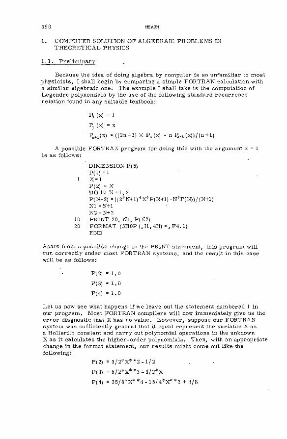
568 HEARN

1. COMPUTER SOLUTION OF ALGEBRAIC PROBLEMS IN THEORETICAL PHYSICS

1. 1 . P relim in ary

Because the idea o f doing algebra by com puter is so unfam iliar to m ost p h ysic ists , I shall begin by com paring a sim ple FORTRAN calculation with a s im ilar a lgebraic one. The example I shall take is the computation o f Legendre polynom ials by the use o f the follow ing standard recu rren ce relation found in any suitable textbook:

(x) = 1Pi (X) = X

^ i ( x ) =( (2n + l ) X P n ( x ) - n H - i ( x ) ) / ( n + l)

A possib le FORTRAN program for doing this with the argument x = 1 is as fo llow s:

DIMENSION P(5)P( l ) =1

1 X=1P(2) = X DO 10 N = 1, 3P(N+2) = ((2*N+1)*X*P(N+1)-N*P(N))/(N+1)N1 = N+1 N2 = N+2

10 PRINT 20, N1, P(N2)20 FORMAT (3H 0P(, 11, 4 H) = , F 4 . 1 )

END

A part from a p oss ib le change in the PRINT statement, this program w ill run co rre c t ly under m ost FORTRAN system s, and the result in this case w ill be as fo llow s:

P(2) = 1 . 0

P(3) = 1 . 0

P(4) = 1 . 0

Let us now see what happens if we leave out the statement numbered 1 in our program . M ost FORTRAN com pilers w ill now im m ediately give us the e rro r diagnostic that X has no value. H ow ever, suppose our FORTRAN system was sufficiently general that it could represent the variable X as a H ollerith constant and ca rry out polynom ial operations in the unknown X as it calcu lates the h igh er-ord er polynom ials. Then, with an appropriate change in the form at statement, our results might com e out like the follow ing:

P(2) = 3 /2 *X **2 - 1 /2

P(3) = 5 /2 *X **3 - 3 / 2 * X

P(4) = 35/8*X* *4 - 15/4*X* *2 + 3/8

IA E A-SM R-9/27 569

This exam ple shows us one o f the basic d ifferen ces between a num erical calcu lation using FORTRAN, for exam ple, and an algebra ic calculation in which indeterm inants such as X which have no p re -ass ign ed value can appear in the calcu lation . H ow ever, there are many other d ifferen ces between system s for doing algebra on the one hand and arithm etic on the other. We d iscu ss these in the next subsection.

1. 2. D ifferen ces between a lgebra ic and num eric calculations

Some o f the m ajor d ifferen ces between a lgebra ic and num eric calculations by com puter are sum m arized in Table I. M ost o f the entries in this table are se lf-exp lan atory , but it is probably worthwhile to d iscuss them in m ore detail. The first point is that m ost num eric system s are now very w ell documented and w idely available. F or exam ple, standards exist on the form o f FORTRAN, and if they are follow ed, the chances are that the program w ill run on a random com puter. On the other hand, a lgebraic system s are experim ental in nature, subject to constant change and, except in a very few cases, available only on sp ec ific com puters. The second m ajor contrast is in the method o f operation o f the system . A FORTRAN or ALGOL system , for exam ple, is usually organized in three stages. In the first stage, the u ser program is com piled into assem bly language. In the second stage, a system loader loads the program into com puter m em ory and, finally, the program is executed in the GO step. This com p ile -loa d -g o mode of operation is particu larly w ell suited to batch operation o f com puters and makes the m ost efficient use o f com puter core , as the com piler is not requ ired , for exam ple, after the first stage. A lgebra ic system s on the other hand are quite often designed to be interactive so that the user

TABLE I. DIFFERENCES BETWEEN NUMERIC AND ALGEBRAIC SYSTEMS

NUMERIC ALGEBRAIC

WELL DOCUMENTED EXPERIMENTAL

WIDELY AVAILABLE LIMITED DISTRIBUTION

SMALL SYSTEMS LARGE SYSTEMS

external libraries internal libraries

C-L-G (compile-load-go) INTERACTIVE/INTERPRETIVE

FIXED SPACE REQUIREMENTS UNKNOWN SPACE REQUIREMENTS

CALCULABLE TIME REQUIREMENTS UNKNOWN TIME REQUIREMENTS

POWER GROWTH RATES EXPONENTIAL GROWTH RATES

FIXED OUTPUT SIZE UNKNOWN OUTPUT SIZE

570 HEARN

com m unicates with the com puter statement by statement rather than in one com plete p rogram . They a lso tend to be interpretative rather than com piled in the sense that the system w ill interpret each statement given by the user and only com pile it i f asked by the u ser . Because a large number o f system subroutines are n ecessa ry for a lgebraic calcu lations, a m ajor part o f an a lgebraic system must be kept in co re or easily a ccess ib le during the whole calculation. It m ay even be n ecessary to keep a com piler resident or avail­able during execution i f it proves n ecessary to com pile som e o f the state­ments in the interactive dialogue. Some o f these subroutines (and a com piler is one) need not be in co re all the tim e, but, as I shall explain later, for reasons o f operating e ffic ien cy it is usually n ecessary to keep a re la tively large number o f these routines in co re during execution. N um erical system s also have a large system subroutine lib ra ry at their d isposal, containing elem entary functions such as sine and cosine, or m ore sophisticated routines such as those for B esse l function evaluation or num erical integration. H ow ever, it is already known at the loading step which routines are needed in a com p ile -loa d -g o system , whereas the system does not know which routines are needed in advance o f the execution steps in an interactive calculation.

The third m ajor d ifference is that, once the num eric program has been com piled , the amount o f m em ory n ecessary for execution can be calculated, and the system can th erefore decide whether there is sufficient space in the computing system to run the job before execution starts. In a lgebraic system s on the other hand, the a lgebraic expressions must often be stored in core during the calculation and one cannot predict in advance how large these w ill be. It is th erefore possib le for an algebraic calculation to term inate during execution because the amount of co re n ecessary for the calculation exceeds that available in the system . The sam e thing can be said about the tim e requirem ents for a calcu lation . For the num eric program , sufficient resea rch in the m athem atical theory o f computation has been perform ed to enable one to gauge rela tive ly accurately how long a calculation w ill take. On the other hand, the techniques for sym bolic calculation are so new that one cannot make such accurate tim e estim ates, and in fact the sam e calculation m ay take orders o f magnitude longer i f an inefficient organization step was introduced during the calculation. Related v ery c lose ly to this point is the fact that m ost num eric calculations follow sim ple pow er growth rate law s. F or exam ple, the calculation o f the inverse o f a m atrix is a p ro ce ss whose tim e requirem ents grow roughly as n3 with the order n o f the m atrix . On the other hand, the tim e requirem ents for a lgebraic calculations such as polynom ial manipulation can grow at exponential rates with the s ize o f the expression . Thus, re la tive ly m inor changes in the organization o f such a calculation can have dram atic effects on the tim e which the calculation takes. For these reasons it is n ecessary to design the algorithm s for sym bolic computation very carefu lly i f one is to com plete calculations in an econom ic tim e.

A final point is that whereas one knows in a num erical calculation how much output one can expect in a norm al calculation, it is im possib le to p red ict in many cases how much output a sym bolic calculation w ill produce. F or exam ple, the determinant o f a sym bolic m atrix o f order n m ay contain n! term s if no cancellations o ccu r . Thus, the calculation o f the determinant o f a m od est-s ized m atrix can astonish the u ser by producing output containing thousands and thousands o f term s covering many pages o f paper.

IAE A-SM R-9 /2 7 5 7 1

TABLE II. SOME ALGEBRAIC SYSTEMS IN CURRENT USE

SYSTEM DATE COMPUTER APPLICATIONS

ALPAK^ -.I960 IBM 7090 /

7090 F O R M A L 1963 IBM 7090 /

7090 SCHOONSCHIpa 1964 IBM 7090 /

MATHLAB 1965 7090/PDP-6/10 X

REDUCE 1^ 1965 PDP-6/10, IBM 360 /

6600 SCHOONSCHIP 1966 CDC 6600 /

PL/1 FORMAC 1966 IBM 360 /

SYMBAL 1967 CDC 6600 ?

SAC 1967 most ?

REDUCE 2 1969 many /

CAMAL 1969 ATLAS 11 (TITAN) /

1AM 1970 PDP-10 ?

M ACSYMAb ? M IT PDP-10 X

SCRATCHPAD b ? IBM 360 X

A LTRAN b ? most X

^ obsolescent

b under development

I have spent som e tim e going through these d ifferen ces sim ply to convince the intended u ser that sym bolic computing techniques m ay not be the panacea for all a lgebra ic p rob lem s. One has to ex e rc ise a certain amount o f restra int in choosing problem s to solve by these m eans. On the other hand, we do see an increasing number o f su ccessfu l applications o f such techniques to rea lis tic prob lem s, and I would p red ict that in the next few years a whole new range o f calculations may open up because o f these m ethods.

I have mentioned that there are system s for perform ing a lgebraic calculations by com puter, and in Table II som e .(but by no means all) exam ples o f algebra system s are listed which have been developed over the last ten years and which offer the user facilities with varying degrees o f sophistication . Several o f these program s are now obsolescent but do have h istor ica l im portance for developm ents in the field . Anyone interested in doing resea rch in this area should certainly investigate the capabilities o f these various system s, and one good sou rce o f inform ation is Ref . [ 1 ] .

572 HEARN

As far as Table II is concerned, I think that one o f the m ost im portant columns from a u s e r 's point o f view is the last, which lis ts whether the system has actually been used for any published applications. In point o f fact, only CAM AL [ 2] , FORMAC [ 3 ] , REDUCE [4 ] andSCHOONSCHIP [5 ] have been used in any significant number o f published calculations so far. Even m ore interesting is the fact that three o f these system s have been developed by p h ysic ists ! (FORMAC was not). T hose system s in Table II which are not re feren ced sp ecifica lly are described in Ref . [1 ].

1 . 3 . G eneral ch aracteristics o f a lgebraic system s

So far, we have been concerned with the d ifferen ces between system s designed for non-num erical a lgebraic calculations and those designed for num erical ca lcu lations. H ow ever, suppose that after all m y warnings you decide that you want to use one o f the program s listed in Table II. What general ch aracteristics can you expect to find in these program s? A d iscu ssion o f this subject falls naturally into four subsections, namely:

(1) The form o f the language by which the u ser com m unicates with the com puter.

(2) The general capabilities such as polynom ial manipulation, pattern matching or substitution, for exam ple, offered to the u ser o f the p rogram .

(3) The sp ecific packages provided by the system or available from other u se rs .

(4) The m an-m achine in terface, in other w ords, the ease or lack of it in actually com m unicating with the com puter.

Since the subject o f language design is covered so well by the paper of Cam pbell [6 ] , I shall m erely outline the main problem s h ere . U sers are usually offered a com plete system for a lgebraic manipulation rather than a set o f subroutines in a program lib ra ry . Such system s usually adopt a program m ing style which is s im ilar in form to one o f the com m only used num erical program m ing languages such as FORTRAN, ALGOL or P L / 1 .Some o f these, such as FORMAC, are im bedded d irectly in the num erical system (in this case P L / 1 ) . Others, such as REDUCE 2, have a top level ALGOL structure but are im bedded in another language (LISP in this case). Finally, there are system s, such as SCHOONSCHIP, which are written m ainly in assem bly language, but which o ffer the u ser an A LG O L - or FO R TR A N -like style (in this case FORTRAN).

A ll system s o ffer u sers com m ands which are unique to a lgebraic manipulation and thus they provide extensions o f the num erical language style adopted. The m ost pow erful system s offer the u ser the ability to extend the language further, or m odify the sou rce language d irectly . F or exam ple, in the case o f REDUCE, the sou rce language in which the program is written is the sam e as that used by the u ser when he w rites p rogram s.The point is that any one system is not a ll things to all people, and so a user who is offered a system incapable o f easy m odification is bound to be frustrated eventually.

1 . 4 . G eneral capabilities available in algebra program s

No m atter how flexib le or beautiful the language offered by a system to the u ser , its ultim ate su ccess in solving problem s rea lly depends on the

IA E A -SM R -9/27 573

general capabilities which the designer built into his program and the e ffic ien cy they p ossess in execution. The system s presently available o ffer such a variety o f capabilities that I would like to d iscuss those of m ost im portance to us in p h ysics . Let me begin by making a few com m ents about my distinction between what I ca ll general capabilities and what I ca ll sp ec ific packages. And again an analogy with the way that, say, FORTRAN operates is probably the easiest to u se . When a FORTRAN program is com piled , the FORTRAN com piler, which is loaded into co re , knows enough about the syntax o f com m on sou rce expressions to generate the requ ired assem bly code . In other w ords, the com piler contains at a very basic lev e l a syntax analyser and possib le optim izer designed to generate efficient code for an expression such as A + В - C . On the other hand, if a u ser requests a ca ll to the function COS, thenm ost com pilers re feren ce this function by leaving instructions for the loader to load this function from secondary storage. If the routine requ ired is not available in this manner then the u ser must supply it h im self. Thus the B esse l function may be known to the FORTRAN com piler but not the Gegenbauer polynom ial. I re fe r to these latter exam ples as sp ec ific packages because they are not always requ ired during the average calculation and th erefore need not always be in co re during the execution p ro ce s s . H ow ever, the syntax analysis which I d iscussed earlier is an exam ple o f what I ca ll a general capability in the sense that it is always needed during com pilation and it th erefore becom es inefficient to segm ent this part o f the program and swap it in and out o f secondary storage. The sam e thing is true to a la rger extent for a lgebraic calcu lations, but in this case , the decision as to what is a general capability and what is a sp ec ific package is not so clear cut. How ever, there are certain p rocedu res which appear to be so fundamental that it becom es im p ossib ly inefficient i f these are not kept in co re or easily a cce ss ib le during a calcu lation . T hese are the general capabilities that I now wish to d iscu ss; a lis t o f them is given in Table III.

The m ost basic o f all these general capabilities as far as an algebra program is concerned is polynom ial manipulation. By this I mean the ability o f a program to expand polynom ials, co lle ct like term s, order the term s, and so on. Because these techniques are so im portant. Section 2 is devoted to an account o f the m ost com m on methods used today. In addition, by m y d iscussing this particu lar prob lem in depth, you w ill be able to appreciate the type o f program m ing techniques which are n ecessary throughout this field .

A surprisingly wide range of a lgebra ic problem s can be solved by a system which contains routines for polynom ial manipulation plus som e capability for elem entary function manipulation, substitution and d iffe r ­entiation. In fact, a system such as FORMAC is o f this type. H ow ever, in m y mind the next log ica l general capability to be considered as part o f a com plete system for algebra is the ability to manipulate rational functions.At first sight, it might seem that all this requ ires is the ability to represent the ratio o f two polynom ials. H ow ever, a new important technique is requ ired in this case , namely, the ability to compute the greatest com m on d iv isor o f two polynom ials. F or exam ple, the expression (A **2+2*A *B +B **2)/(A **2-B **2) is obviously le ss aesthetically pleasing th an (A + B )/(A -B ). What we have rea lly done in going from the first to the second expression is to recogn ize that the polynom ials have a greatest com m on d iv isor o f A+B and divide it out. This is a le ss com plicated p rocess

TABLE III. GENERAL CAPABILITIES OF AN ALGEBRA SYSTEM

5 7 4 HE ARM

POLYNOMIAL MANIPULATION

RATIONAL FUNCTION MANIPULATION

POLYNOMIAL EXTENSIONS

SUBSTITUTION

STRUCTURAL EXTENSIONS

than factoring the polynom ials. T o see that this is true, consider the num erical analogue. The greatest com m on d iv isor (gcd) o f two numbers can be found quite read ily by E u clid 's algorithm , which is w ell known to any m athem atics student. On the other hand, the factorization o f a number into its prim e irredu cib le com ponents requ ires a m ore com plicated sieve p rocess , and from a com putational view is m ore tim e-consum ing. The sam e is true in the a lgebraic case .

It turns out in fact that one can a lso extend E uclid 's algorithm to polynom ials. H ow ever, whereas the num erical Euclidean algorithm w ill find the greatest com m on d iv isor o f two numbers re la tively quickly, the analogous a lgebra ic algorithm can be excruciatingly slow in som e cases [ 7 ]. For exam ple, it might take a day of computation tim e and an extrem ely large co re on a CDC 6600 to find the greatest com m on d iv isor o f two polynom ials o f degree 100, say, by E uclid 's algorithm . Although p o ly ­nom ials o f such a large degree are not norm ally encountered in the d a y -to - day w ork o f a ph ysicist, we do unfortunately tend to use a large number of variab les , and it turns out that the degree o f com plexity o f the calculation is roughly equivalent to the number of variables m ultiplied by the highest pow er o f all variab les . Consequently, the calculation o f the greatest com m on d iv isor o f two polynom ials involving ten variab les, in which the highest degree is 5, turns out to be at least as com plicated as the computation of the greatest com m on d iv isor o ftw op o ly n om ia lso f degree 50 in one variab le .

B ecause o f the extrem e in efficiency o f E uclid 's algorithm for such calcu lations, much effort has been devoted over the last five years to finding a m ore e fficien t a lgorithm . R ecently, it has been found that one can exploit som e nineteenth-century m athem atics to achieve a much faster calcu lation . What one does is to use finite field or m odular arithm etic.In other w ords, one calcu lates the greatest com m on d iv isor o f two single variab le polynom ials in which the integer coefficien ts are considered in a finite fie ld . Thus, i f one was working, say, modulo 7, then the only in tegers one would con sider would be 0 through 6, and 6+2, for exam ple, would be rep laced by 1. The computation o f a greatest com m on d iv isor using m odular arithm etic takes significantly le s s tim e than the analogous calcu lation over the in tegers. The m odular calculation becom es relevant because o f a v e ry sim ple theorem which says that i f two polynom ials are re la tively prim e ( i .e . have a greatest com m on d iv isor o f 1) over a prim e m odular field then they are re latively prim e over the in tegers. Since two

IAE A-SM R-9 /2 7 575

polynom ials m ore often or not are re la tive ly p rim e, one can determ ine this fact v e ry quickly by using finite field arithm etic. If the two polynom ials are not re la tively p rim e, then it is possib le by a straightforw ard construction procedu re to determ ine the gcd from various prim e field resu lts . (If anyone is interested in review ing the h istory o f the interesting search for a m ore efficient gcd algorithm , he is re fe rred to R ef. [ 7 ] . An account o f these techniques can a lso be found in an excellent book by Knuth [ 8 ] . ) The results can be dram atic. F or exam ple, L oos [9 ] has program m ed the latest gcd algorithm in REDUCE and we find that the gcd o f two polynom ials o f degree 100 can be found in a m atter o f seconds now. In term s o f the computing time n ecessary , the new algorithm represents a dram atic im provem ent over the Euclidean algorithm ; the latter has an exponential growth rate, whereas the computing tim e for the new algorithm grows at a rate le ss than n with the degree n o f a univariate polynom ial. This again illustrates that, in sym bolic manipulation, it is v e ry im portant that the algorithm s be designed as e fficien tly as possib le i f rea lis tic calculations are to be p oss ib le . No m atter how large the com puter is , the exponential growth rate o f the Euclidean algorithm lim its drastica lly the class o f prob lem s which one can so lve by using it.

P olynom ial extensions. There are very few calculations in physics which do not requ ire the introduction o f at least the elem entary functions such as sine and cosine in the calcu lation . T h ere fore , m ost system s provide the u ser with certain o f the elem entary functions together with their com m on p rop erties . The better system s a lso allow the u ser to add their own functions and define rules for manipulation. One way o f introducing these functions is to regard those residual form s which resu lt after sim plification ru les have been applied as polynom ial variab les and manipulate them as such in calcu lations. For exam ple, an expression such as cos(x+y) might be best treated by expanding it by the ru le cos(x+y) = cos x cos y - sin x sin y.In other calculations it might best be le ft alone. In the form er case , residual expressions cos x, cos y, sin x and sin y resu lt from such expansions, w hereas in the latter case cos (x+y) rem ains as a residual form . My point now is that these residual form s can be considered as variab les as far as polynom ial and rational function manipulation is concerned. F or this reason , I regard the introduction o f such functions as polynom ial extensions. REDUCE, for exam ple, con siders them in this m anner. This is not the only way to treat elem entary functions, how ever, and som e system s might treat them in an entirely different m anner. This is one p lace where one can see the wide d ifferen ces in the philosophy concerning representations ö f expressions which exist among the m anufacturers o f the various algebra system s m entioned. T here is a trem endously wide range o f view s on this subject; those in terested in learning m ore about this are re fe rred to the review artic le by M oses [ 10] .

Substitution. T here are v ery few sym bolic prob lem s which do not requ ire som e substitution capabilities for their solution. Such substitutions might be a sim ple as

"rep la ce a ll o ccu rren ces o f m by 0"

576 HEARN

or involve com plicated conditions such as

" fo r all values o f x and y, rep lace cos(x )*cos(y ) by (co s (x + y ) + c o s ( x - y ) ) / 2 "

or

"rep la ce cos(x)^ + sin(x)^ by 1 for a ll values o f x"

or again,

" fo r all p, n and y, rep lace p ^ „ by p^"

or

" i f n = 0 then rep lace fac(n) by 1, otherw ise rep lace fac(n) by the value o f n * fa c (n -l)" .

It is obvious that i f a sufficiently rich com puter language existed for ex ­pressin g such rep lacem ents, plus a system which could im plem ent them, then m ost a lgebraic prob lem s for which a known algorithm exists could be solved by such a system . M ost of the a lgebraic system s now available o ffer the u ser facilities for introducing som e ru les o f this type. In addition, a whole c lass o f ru les, such as those which define D irac gamma m atrix a lgebra, for exam ple, may be offered as an integral part by the system bu ilder. In the latter case , the rules are usually com piled into efficient m achine code procedu res which can exploit knowledge o f the explicit internal representation o f expressions and so gain e ffic ien cy in execution. On the other hand, m ost system s which allow u ser-in trodu ced replacem ents o ffer interpretative evaluation of these ru les, in that the parts o f the ex ­p ress ion under consideration are matched, identifier by identifier, against the ru les introduced by the u ser . This technique is obviously le ss efficient than the use o f com piled code, but it o ffe rs greater flex ib ility to those u sers who wish to change ru les during a calculation. H ow ever, experience has shown that at least the basic rules for polynom ial and rational function manipulation must be com piled i f calculations are to be finished in an econom ic tim e. This point was best proved by an experim ental system [11 ] which did in fact perform all a lgebraic manipulations by interpretative matching against ru les introduced by the u ser . This system was so general that even a rule for the co llection o f equal term s as sim ple as x + x = 2x must be specified by the u ser . Such generality led to im possib ly inefficient calcu lations, and th erefore any system designed for p ractica l use must o ffer a nucleus o f com piled procedures in addition to efficien t techniques for interpretativepatternm atching and substitution. The ideal system would o f cou rse allow for the replacem ent o f any given expression f(x, y, . . , z) by another expression g(x, y, . . . , z) where the param eters x, y and z may stand for constant expressions or have various conditions im posed on them. A s can easily be seen, a ll the exam ples which we gave ea rlie r o f possib le general substitutions are o f this type.

This general m atching problem , which I have d iscussed in severa l publications [ 12 , 13 ] , has still not been solved e fficien tly enough for use in la rg e -s ca le calcu lations, and as a result m ost system s com prom ise

ÍA E A-SM R-9/27 577

at som e point in the type o f substitutions allowed. P robably MACSYMA com es c loses t to providing com pletely general substitutions [14] although REDUCE allows a wide range of possib le ru les . Apart from these two system s, how ever, the p oss ib le substitutions allowed by m ost other system s are much m ore lim ited, and this does tend to lim it their e ffe ctiv e ­ness in som e calcu lations.

Structural extensions. The capabilities d iscussed so far, together with, say, a differentiation package which I shall consider in the next section, make up quite a pow erful a lgebraic manipulation system . H ow ever, unless the u ser has re latively straightforw ard prob lem s, he w ill quickly d iscover that he wants to add new facilities to the program or even change the way that som ething as b a s ica sa p o ly n om ia l is treated by the system . Thus the final general capability which I think the good algebra system must provide is the ability to p erform structural extensions, in other w ords, the user should be able to change the algorithm s rather straightforw ardly or to add new ones to suit his own purposes. This problem is m ore one o f language design than o f capabilities per se because i f the program is written in a m odular way and the u ser language is related in a straight­forw ard way to the language used for the im plem entation o f the system , then the inform ed u ser can make such changes. H owever, as this question must be considered when one designs the algorithm s for perform ing the general capabilities d iscu ssed , I have included it in this section for com pleteness.

1.5 . Specific packages

Once a system has been built which includes the general capabilities d iscu ssed in the previous section, it becom es a re la tive ly straightforw ard m atter for the system builder and often for the user to add the routines n ecessary to perform the sp ecific calculations o f in terest to him . A list o f som e such possib le sp ec ific capabilities or packages which might be n ecessary is given in Table IV.

I am sure that there are som e system builders who would consider the first such fa cility in the lis t, nam ely differentiation, as belonging to the previous section . The point is that the ru les for differentiation are so easy to define that the com puter im plem entation is a very straightforw ard m atter. In fact, to m y knowledge, the v ery first com puter program s written for perform ing algebra ic manipulation w ere differentiation program s [ 15 , 16 ] . T hese w ere, o f cou rse , v e ry rudim entary by our present-day standards but represented a trem endous advance in conceptual thinking about com puters twenty years ago. D ifferentiation is now considered so easy to p erform by com puter that it is usually given as an ex erc ise in c la sses on non-num erical program m ing.

It is interesting to observe that the ease with which functions can be differentiated sym bolica lly by com puter contrasts m arkedly with the num erical analogue. N um erical differentiation is a re la tive ly difficult p ro ce ss because it tends to accentuate irregu larities in the function being differentiated, and th ere fore , i f there is any significant statistical e rro r in the input data, the resulting num erical derivative can be quite inaccurate. The opposite is true o f integration. Because it is a sm oothing p ro ce ss , num erical integration has been one o f the great su ccesses o f com puterized num erical analysis, whereas sym bolic integration is an extrem ely difficult

578 HEARN

TABLE IV. SPECIFIC CAPABILITIES OF AN ALGEBRA SYSTEM

DIFFERENTIATION

INTEGRATION

GAMMA M ATRIX ALGEBRA

TENSOR ALGEBRA

GENERAL NON-COMMUTATIVE ALGEBRA

POLYNOMIAL FACTORIZATION

MATRIX MANIPULATION

ASYMPTOTIC OPERATIONS

TRANSFORM TECHNIQUES

and com plicated p ro ce ss to perform by com puter. H ow ever, it represents one o f the m ost interesting resea rch problem s in a lgebraic manipulation at the m om ent.

Apart from two pioneering experim ental program s for analytical inte­gration [ 17 , 18 ] , m ost sym bolic integration by com puter has been done by table look-up or pattern matching. This latter method has o f course been very useful in severa l important quantum electrodynam ics (QED) ca lcu ­lations, but it is im portant to em phasize that in this case we are sim ply using the com puter as a book-keeping device in order to make the substi­tutions for the various integrals which arise in the calcu lations. M ore im portant, one needs to know the integral o f every b asic function encountered in order to ca rry out the integration. If we m eet a function whose integral has not been previously computed, then either we must sit down and do it by hand or leave it in an undeterm ined form . Current work in this area prom ises techniques for the sym bolic integration o f indefinite integrals by essentia lly -algorithm ic m eans. This means that the program , when confronted with a new integrand never seen b e fore , w ill actually find an analytical form for the integral i f it exists in the class o f functions that we are considering. This w ork is based on som e im portant theoretica l resu lts by R isch [19] who showed that a com plete a lgorithm ic decision procedure exists for the evaluation o f integrals for m ost elem entary functions including logarithm ic or exponential extensions, provided that the integral exists as a m em ber o f this c la ss . The algorithm also decides i f the integral does not belong to this c la ss . Thus, to give two sim ple exam ples, this algorithm can determ ine the integral o f cos x, since both integrand and integral are com posed o f exponentials. On the other hand, the algorithm w ill decide that the e rro r function / exp( -x^) dx is not an elem entary function.

R isch has recen tly extended his ideas to cover nearly a ll functions which a physicist is lik e ly to m eet in day-to -day analysis. It should now be poss ib le , for exam ple, to produce a program capable o f integrating all

IAE A-SM R-9/27 579

single variable functions which one m eets in m ost physica l calculations, and severa l groups are attempting to develop such p rogram s. Whether these ideas can be su ccessfu lly extended to m ultidim ensional integrals rem ains to be seen, but one can o f course be optim istic. H ow ever, it is c lear that we now know enough about analytical integration to be able to perform a com plete sym bolic computation o f any fou rth -order p ro ce ss in QED, and severa l groups, including my own, are studying this prob lem in detail. I shall say m ore about this in Section 3. F or those interested , a recent survey paper outlines som e o f the problem s which arise in im plem enting R isch 's work [20] .

It m ay com e somewhat as a su rprise to readers to find that I have listed gamma m atrix algebra and tensor manipulation as sp ec ific packages. F rom a h istorica l point o f view , the need to calculate very com plicated p ro ce sse s in QED m otivated the development o f many program s for solving these sp ec ific p rob lem s severa l years ago. Two such program s, namely V eltm an 's SCHOONSCHIP and m y own REDUCE, which w ere orig inally developed for this purpose, rem ain in wide use today. Although these two program s began as sp ec ific system s for solving problem s in h igh-energy ph ysics, it was quickly recogn ized by Veltm an and m y se lf that the techniques em ployed w ere quite general, and thus the program s evolved into general- purpose a lgebraic manipulation system s. Several other program s for gamma m atrix algebra which appeared at about the sam e tim e have not survived because o f their lack o f generality or poor language design. What we rea lize now, as I have said ea r lie r , is that the key capability in such program s is polynom ial manipulation, and once one has an understanding o f how to represent polynom ials and polynom ial extensions in the com puter, the addition o f routines for solving the sp ec ific prob lem s associated with gamma m atrix algebra and tensor manipulation is straightforw ard. One can build quite respectable routines for this purpose by sim ply program m ing the algorithm s one finds in standard textbooks on quantum electrodynam ics such as that by B jorken and D re ll [21 ]. H ow ever, there are algorithm s m ore suited for com puter evaluation o f traces o f gamma m a trices , and, in particu lar, one by Kahane [22] represents a distinct advantage over those found in textbooks. R ecently , C hisholm and I developed a new algorithm for trace calculation [23] which extends that developed by Kahane and which, although rather com plicated to d escr ib e , should be re la tive ly straight­forw ard to program for the com puter. We believe that this new algorithm w ill lead to further e ffic ien cies in trace calculation and also reduce the amount o f com puter code n ecessary . We may thus reach the point where the amount o f code n ecessary to provide for these facilities is a very sm all part of the whole system . This is rather iron ic when you consider that REDUCE was orig inally regarded as a program for taking traces o f D irac gamma m atrices!

Many other useful fa cilit ies such as polynom ial factorization , general m atrix manipulation, asym ptotic operations and the manipulation o f expressions by transform techniques becom e p ossib le , given the basic fa cilit ies described in the previous section . If the language is pow erful enough, then the u ser can add such facilities h im self in term s o f the prim itives provided to p erform the basic operations. H ow ever, it should be em phasized that there is no system yet in existence which can provide all these techniques, although they w ill surely becom e available in the next yea rs .

580 HEARN

1. 6 . M an-m achine c om m unication

The fourth and last general feature o f a lgebraic sim plification system s which I wish to d iscuss is the question o f m an-m achine com m unication. By this, I mean the way in which the u ser com m unicates with the program both in term s of input o f prob lem s and output o f resu lts . Although the program language itse lf m ay provide sp ecific operations for input and output, this feature rea lly depends much m ore upon the com puter available than the a lgebra program itse lf, although the latter must be organized in a way to take account o f interactive facilities i f these are available.

A d iscu ssion o f the com plete input-output problem could again occupy a whole paper and so I shall lim it m yse lf to a few general observations.F irst, our experience has shown that pain less a lgebraic calculations from the u s e r 's point o f view can only be accom plished in a com puter with a high speed m em ory o f 40 000 words or m ore . Of cou rse , useful calculations have been perform ed in sm aller m em ories , and a c lever program m er can make optimum use o f whatever facilities he has at his disposal. H owever, the average u ser who does not want to involve h im self too heavily in questions o f system design w ill find h im self in a constant fight with the operating system on a sm all com puter in order to get the space he needs for his ca lcu lations. I would th erefore strongly advise anyone against attempting such calculations unless a large enough com puter is available. Secondly, the m ost su ccessfu l calculations have been made using tim e-sharing in ter­active computing system s, such as the system available on the Digital Equipment C orporation P D P -10 with which I am m ost fam iliar. A com plete a lgebraic calculation depends so much on the knowledge gained at each step in the calculation that constant m an-m achine interaction is n ecessary . This can only be done p rop erly if the need for resubm itting a job at each step is elim inated, as is only possib le in an interactive system . Within such an environment a cathode-ray tube display and keyboard backed by som e method for making hard copy is the best term inal available today. In fact, by using displays with line-draw ing capabilities it is possib le to display sym bolic out­put in a tw o-dim ensional textbook form , which is o f course a much m ore readable and inform ative presentation o f results than can be achieved by line prin ters o r teletypes. Although such term inals are quite expensive at present, new m odels are now appearing which should be w ell within the budget o f m ost com puter cen tres. In addition, cheap hard copy o f the display im ages by xerograph ic means is becom ing available.

F inally, we have the problem o f input. Our natural tw o-dim ensional representation o f m athem atical equations must be converted to a linear form for com puter input using presently available hardware. H ow ever, som e prom ising resea rch in p rog ress on the use o f input tablets o r light or sonic pens points to a future tim e when we can input our problem s d irect form our notebooks in standard textbook notation. P rogram s for doing this a lready exist, but they are too slow and cum bersom e for general use at present

2. POLYNOMIAL MANIPULATION

2.1. P relim in ary

Because o f its extrem e im portance as the key capability in a lgebraic sim plification , I would like to spend som e tim e considering techniques

tA E A -SM R -9/27 581

which have been developed for manipulating polynom ials by com puter.I shall consider the problem under three headings, namely, polynom ials

with no variab les, polynom ials o f one variable, and polynom ials o f many variab les . In the context we are d iscussing here, a polynom ial with no variables is o f course a num ber, and one might think at first sight that this is a triv ia l case which need not be d iscu ssed . H ow ever, it is im portant to rea lize that in an a lgebra ic calculation, where one is concerned with exact resu lts , it is m ore suitable to consider numbers as in tegers, o r ratios o f in tegers, rather than as floating point num bers with their inherent in a ccu ra cies . F or exam ple, an a lgebra ic calculation whose result is zero is significant because one thenhas an exact p roo f that the relevant expression is identically z e ro . On the other hand,, i f the resu lt has a floating point value o f 10"38, can one then say that the resu lt is still rea lly zero? In order to ensure uncom prom ising accu racy in calcu lations, then, so that such questions can be resolved , m ost system s provide for u sers to introduce not only integers but rational numbers as the ratio o f two in tegers. A lgebra program s usually also allow floating point numbers by way of com prom ise because engineers typ ically like to introduce numbers in this form i If one is working with irrational num bers it is better to introduce them as sym bols. In other w ords, an a lgebra ic resu lt Зл^-lO is far m ore meaningful than an equivalent floating point expression .

Once one has decided in a given calculation to do all arithm etic exactly, a prob lem a rises if the integers one is working with grow la rger than the word length of the m achine being used. One can o f course resort to double or trip le p rec is ion arithm etic, but this again im poses an ultimate lim it on the s ize of the num bers which can be handled. It is obvious that one needs unlim ited p recis ion arithm etic for com plete a ccu racy . In other w ords, you must use a representation for numbers which does not lim it you to any fixed s ize ; if you do im pose a lim it, then the next calculation is always bound to exceed it. (This must be som e form o f P ark inson 's Law !) In Ref . [ 8 ] , Chapter 4, one finds a very elegant d iscussion o f the problem of doing m ultiple p rec is ion arithm etic by com puter, and I would certainly com m end a study o f this particu lar section to anyone interested . H owever, Knuth depends on the use o f arrays for doing his calculations because he w orks in term s of fix ed -s ized , although large, multiple p rec is ion numbers rather th a n v a ria b le -s ize num bers. F or arb itrary p rec is ion in tegers, a lis t-stru ctu red representation is usually em ployed [24] .

In order to understand how one can do arb itrary p rec is ion arithm etic by com puter, let us re ca ll that integers are written as a sequence of digits with an im plicit radix. Thus the decim al integer 10372 stands fo r the sum2 + 7 X 1 0 + 3 X 1CP + 1 X 10^. The so -ca lle d "new math" teaches h igh -sch ool students these days that the radix need not n ecessa rily be ten, and one can have binary, octal, and so on, representations o f num bers. P rovided one knows the radix then, one could represent an integer with an arb itrary number of digits as a lis t o f those digits, as in (1 0 3 7 2) for the above exam ple. Such a list, o f cou rse , would provide a com puter representation for a number o f any s ize , and Lurié [25] shows how such lists can be represented in the com puter. How ever, it is c lea r ly inefficient to make each number in the list a single decim al digit. A m ore efficient rep resen ­tation resu lts if we make the radix the s ize of a com puter word so that the "d ig its" in our list becom e single p rec is ion in tegers. H ow ever, even though the individual elem ents o f such a list (u ug . . . u j can now be quite

582 HEARN

large in tegers, it is usual to re fer to this as an n -p lace integer, and to each U; as a digit with respect to the radix b we are using. H ow ever, if the radix is taken to be, say, 236, then we requ ire a translation phase to show that the number (12345 7890) has the decim al representation 848341940313810, but this translation is quite straightforw ard. It also turns out to be easier to work with a list in which the last significant digit appears firs t on the list. Thus we represent the number u = ^Ug. . . u„ by the lis t (u„u„_i . . . U]). The number 10372 with radix 10 would therefore be written a s ( 2 7 3 0 1).

We still have to represent the sign o f such an integer, and there are severa l ways o f doing this. One easy way is to associate a sign indicator ( e . g . POSNUM or NEGNUM) with the atom representing the arb itrary p rec is ion integer and make the above list structure the corresponding property . Once a convention such as this is adopted, one need only perform manipulations on the magnitude of the integers .concerned, and I shall th erefore consider only this from now on. There are also m ore efficient ways for representing such numbers internally in the com puter, but I shall not d iscuss these here.

The routines for handling such arb itrary integers with p recis ion are described in som e detail in Ref . [24] and can be obtained from Knuth's m ultiple p rec is ion routines by sim ple transposition . In order to illustrate a typical program which one could w rite, the lis t-p ro ce ss in g equivalent of the array program which Knuth uses for multiplying two such numbers is given here. I shall write this in a form which m irrors Knuth's notation, so that anyone interested can com pare this lis t -p ro ce ss in g program with the a rra y -p rocess in g program of Knuth. In a p ractica l im plem entation of this algorithm , one would probably w rite as much as possib le o f it in assem bly language in order to gain e fficien cy , but the form o f the algorithm would be much as given here.

The algorithm we are considering takes two non-negative arb itrary p rec is ion integers u = U]U2. . - Un and v = - with radix b, written inour list notation as (u„ . . . UgUi) and (v^ . . . v^v^), and form s their product w = WiWg.. . written as (w^^ . . . w^w^ . The usual pencil and paper wayo f form ing such a product is to calculate the partial products U1U2 . . . UnX Vj first for 1 á j ám and then add these together with an appropriate scale factor based on the radix. However, Knuth points out that in a com puter it is best to do the addition concurrently with the m ultiplication as is done in the follow ing procedure LM ULT:

SYMBOLIC PROCEDURE LMULT (U,V) ;BEGIN SCALAR W,U1, W l, W2; INTEGER K, T ;

M l: W : = N Z E R O ( L E N G T H U + L E N G T H V);%we only rea lly need to set firs t N elem ents to 0;W l := W;

M2: IF NULL V THEN RETURN W;W2 := W l;

M 3: U1 := U;К := 0; %this variable stores ca rry in M4 loop;

M4: T := CAR U1*CAR V + CAR W2 +K;K : = T / B ;RPLACA(W 2, T -K *B ) ;

IA E A -SM R -9/27 583

M5: U l := CDR U l;W2 := CDR W2;IF Ul THEN GO TO M4;RPLACA(W 2, K);

М б: V := CDR V;W1 := CDR W l;GO TO M2

END;

SYMBOLIC PROCEDURE NZERO N;%this function creates a list o f N ze ro s ;IF N=0 THEN NIL ELSE 0. NZERO (N- l ) ;

Additional lis t -p ro ce ss in g algorithm s for addition and d ivision o f such numbers may be found in Ref . [24] . It is a lso a useful ex erc ise to ca rry through the m ultiplication operations by hand using the above algorithm .

2.2. Univariate polynom ial manipulation

The d iscussion o f the com puter manipulation of polynom ials in one variable becom es triv ia l once we have considered routines for arb itrary p rec is ion integer arithm etic. It is easily seen that a polynom ial such as x + 3x^ + 7x + 2 is no m ore than a generalized arb itrary p rec is ion integer in which the radix is now the variable x rather than the integer b. Thus, we could represent the above polynom ial by a lis t representation (2 7 3 0 1) with the low est pow er first and the variable name X im plicit (it could be stored in a global variable VAR, for exam ple). T here is , how ever, an im portant d ifference between the integer case and the polynom ial case, namely, that the ca rry in our m ultiplication algorithm is no longer present so that the algorithm is much sim p ler. Thus, a program fo r multiplying polynom ials using the above list representation could be written as fo llow s:

SYMBOLIC PROCEDURE PM ULT (U, V );BEGIN SCALAR W, U l, W l, W2;M l: W := NZERO(LENGTH U + LENGTH V);

Wl := W;M2: IF NULL V THEN RETURN W;

W2 := W l;M 3: U l := U;M4: RPLACA(W 2, CAR U1*CAR V + C A R W2);M5: Ul := CDR Ul ;

W2 := CDR W2;IF Ul THEN GO TO M4;

М б: V := CDR V;Wl := CDR W l;GO TO M2

END;

We thus see that we can consider single variable polynom ial operations as sim ply num erical operations on the coe ffic ien ts . The transform ation of the lis t o f coefficien ts to, say, an A L G O L -like output form is then a sim ple m atter of translation. H ow ever, there are som e disadvantages in the above

584 HEARN

approach. Quite often the polynom ials that we encounter even in one variable are sparse in the sense that not all pow ers of each variable actually appear in the expression encountered. The above representation requ ires an explicit zero to be p laced in the list for any pow er which does not actually appear in the polynom ial under consideration. The polynom ial x^°° + 1 would th erefore have a representation consisting o f a list of two ones enclosing ninety-nine ze ro s , which is clea rly wasteful in space and ultim ately in the tim e taken for manipulation. In order to see how we can get around this problem , we pass on now to m ultivariate polynom ial representations, of which, o f cou rse , single variable polynom ials are a su b -c la ss .

2.3. M ultivariate polynom ial manipulation

In discussing representations o f m ultivariate polynom ials, I shall lim it m yse lf to those which are canonical. By this I mean that if we have two polynom ials which are representations o f the sam e function then they w ill have the sam e canonical form . If one surveys current system s, one finds that there are only two classes of such representations in general u se . The first of these represents the polynom ial p(x^ Xg, . . . , x J in the distributive form

P ( * i , x z ....... x j = / C ¡ , ,¡ x i ' x ¿ . . . x , " (2 . 1 )

w here the С 's are num erical coefficien ts . In the second representation, the polynom ial p is written as a power se r ie s in one variable whose coefficien ts are functions o f the rem aining n-1 variab les. Thus,

Pi(Xs.....xjx^i (2.2)

i=0

The polynom ial coefficien ts p¡(xg, . . . , x j are them selves expanded as a pow er ser ies in xg and this representation continues until only numbers rem ain. F or exam ple, the polynom ial

P = ( x + y ) 3 + 3 x - 2 y ( 2 . 3 )

p ( X i , X2, . . . , Xn)

when w ritten in the first representation has the form

lx^y° + 2xy + 3xy° + lx°y2 - 2x°y (2.4)

whereas in the second representation it has the form

( ly °)x 2 + (2 y +3y") x + ( ly3 - 2y)x° (2. 5)

H ow ever, although there are only two such basic representations in general use, one can find as many ways of im plem enting them as there are sy stem sÍ F or exam ple, the variables can occu r exp licitly in the representation, or be stored separately and occu r im p lic itly . S im ilarly, variables ra ised to a zero pow er can occu r explicitly or be om itted. Numbers can occu r as in tegers, ratios o f integers or rea l num bers. The ch oice o f the leading variable in the second representation can be made in many different ways;

IA E A -SM R -9/27 585

it might be introduced by the u ser, o r it might be decided by som e internal ordering in the system , and so on. H owever, it is im portant to recogn ize that neither representation requ ires every pow er of each variable between highest and low est to o ccu r as did our single variable polynom ial rep resen ­tation d iscussed in the previous section .

E xperim ental analyses by various people have shown that in m ost a lgebraic calculations the second representation is m ore efficient in p rincip le than the first in term s o f tim e and space required to perform a given calculation. H ow ever, the d ifferen ces in many cases can be very sm all, and so both representations have their cham pions.

In order to illu stra tep ra ctica l im plem entations o f these rep resen t­ations, I shall consider one exam ple o f each type, although, as I said ea r lie r , nearly every system in Table II could provide exam ples of one or the other representation.

A s an exam ple o f a system which uses the distributive representation, ALPAK (and its newer vers ion ALTRAN) is probably the best documented [26] . In this system , although lis t structures are used, they are not quite the LISP types which L urié [25] has d iscu ssed . In the A LPA K case , a polynom ial is represented by a basic unit o f m em ory called a block which contains three poin ters. The firs t points to a v ector which contains a list o f the names o f the variab les in the polynom ial, the second points to a vector of coefficien ts , and the third points to an array o f exponents. In the latter array, the colum ns correspond to the variab les and the row s to the coe fficien ts . The row s are ordered num erically. Thus, the polynom ial i n E q . (2.3) has the representation shown in F ig. 1.

In this representation, operations on polynom ials, such as addition and m ultiplication, becom e num erical operations on the coefficien t and exponent a rrays. Addition, for exam ple, is a sim ple m erging o f the exponent arrays with appropriate adjustm ents to the coefficien ts when two exponent row s are equal. Full details on the im plem entation o f these techniques m ay be found in the cited re feren ces .

FIG. 1. ALPAK representation o f the polynomial P = (x + y)2 + 3x - 2y.

586 HEARN

A s an exam ple o f a system which uses the recu rsive representation,I would like to d iscuss the standard form adopted in the REDUCE system . Using the LISP dotted pair notation, the REDUCE standard form is defined by the follow ing Backus-N aur syntax:

(standard form)> ::= () ¡(integer)* ¡((standard term)>.(standard form ^) (2.6)

(standard term)* ((standard power)>.(standard form)>) (2. 7)

(standard pow er^ ::= ((v a r ia b le^ .(n o n -z e ro positive in teger)>) (2.8)

D efinition (2. 6) means that a standard form is either an empty list (representing ze ro ), an integer, or an expression consisting o f a dotted pa ir o f a standard term and a standard form . S im ilarly, a standard term is a dotted pair o f a standard pow er and a standard form , and a standardpow er is a dotted pair of a variable and a n on -zero positive integer. Thusa standard term represents one term in the pow er ser ies Eq. (2 . 2), and a standard pow er represents a variable ra ised to a positive integer pow er. C om parison of Eq. (2.2) with the above equations also shows that the dotted pair represents an im plicit addition in Eq. (2. 6), m ultiplication in Eq. (2. 7) and exponentiation in Eq. (2. 8).

The BNF definition of the standard form is not com plete until details o f the ordering convention are specified . This is based on the machine location in core o f the constituent variables (which are stored uniquely). S im ilarly , the ord er o f standard term s in a standard form is based on the exponent of the leading standard pow er, highest exponent first. With these conventions, equal polynom ials have the sam e standard form .

Using this particu lar representation, the polynom ial in Eq. (2. 3) would be written in the form (assum ing X is ordered ahead o f Y ):

( ( ( X . 2 ) . 1 ) ( ( X . 1 ) ( ( Y . 1 ) . 2 ) . 3 ) ( ( Y . 2 ) . 1 ) ( ( Y . l ) . - 2 ) )

Polynom ial com bination operations on such form s are again relatively easy to program because of the recu rsive nature of the representation. As an exam ple o f the type of program m ing which one finds in this case, a function ADD F which adds two polynom ials represented in this form is given below . This particu lar function uses the auxiliary function ADDN for adding a number to a polynom ial and a system function ORDP to define an ordering among expression s. The definition is quite straightforw ard, provided one is used to recu rsive program m ing, and it is another useful ex erc ise for the reader to take two polynom ials written in standard form and ca rry through the addition by means o f this p rocedu re :

SYMBOLIC PROCEDURE ADDF (U,V) ;IF NULL U THEN V

ELSE IF NULL V THEN U ELSE IF ATOM U THEN ADDN(U, V)ELSE IF ATOM V THEN ADDN(V, U)ELSE IF CAAR U = CAAR V

IAEA-SM R-9/2T 587

THEN BEGIN SCALAR X, Y ;X := ADDF(CDAR U, CDAR V);Y := ADDF(CDR U, CDR V);RETURN IF NULL X THEN Y ELSE (CAAR U . X) . Y

ENDELSE IF ORDP(CAAR U, CAAR V) THEN CAR U . ADDF(CDR U,V) ELSE CAR V . ADDF(U, CDR V );

SYMBOLIC PROCEDURE A D D N (N ,V );;IF NULL V THEN N

ELSE IF ATOM V THEN (LAMBDA M ; IF M=0 THEN NIL ELSE M)(N+V) ELSE CAR V . ADDN(N, CDR V );

2. 4. In fix -prefix translation

Once the system designer has decided upon a particu lar representation (or representations) for polynom ials, such as those outlined here, there still rem ains the problem o f converting a polynom ial w ritten in a FORTRAN or A L G O L -like notation into this internal representation and the translation o f the resu lts back into such an infix form . This particu lar prob lem is m ore one o f syntax translation than algebra ic sim plification per se, but it is still part o f the general subject o f sym bol manipulation with which this paper is concerned. H ow ever, a com plete d iscussion o f this subject would be a paper in itself, so I shall have to lim it m yse lf to a few general com m ents. M ost system s begin by translating the input into an internal p re fix form in ways' s im ilar to those described by K u o-P etravic [ 27] . This p re fix form is converted into whatever polynom ial representation is used, and then translated back to p re fix form and hence printed in infix form by sim ilar techniques. I would, how ever, like to close by mentioning som e interesting ideas which P etrick [ 28] d iscu sses in a recent paper. He suggests the poss ib ility o f using a translator writing system (that is , a program which autom atically w rites translators for you) to develop a translator which goes d irect from the infix input right to the standard form em ployed, thus bypassing the interm ediate p refix step. His paper is eminently readable and uses the W eissm an differentiation program [29] , which Lurié [25] d iscu sses , as an exam ple o f a prob lem where this method could be applied.I com m end a study o f P e tr ick 's paper to anyone at all interested in working in this field .

3. SYMBOLIC ANALYSIS FOR PHYSICAL THEORIES REPRESENTEDBY DIAGRAMS

3.1. P re lim in ary

T here are many p ro ce sse s in physics and related fields which are represented in term s o f diagram s. In quantum electrodynam ics, for exam ple, we c la ss ify parts o f the perturbative expansions from quantum field theory in term s o f diagram s, known as Feynman diagram s, which d escrib e the evolution o f the p ro ce ss with tim e. In e le ctr ica l circu it theory, one represents the circu it by a diagram in which specia l sym bols are used to represent the various components in the circu it, and the lines

588 HEARN

represent the w ires along which the currents flow . In operations analysis, one is concerned with depicting som e p ro ce ss in term s o f a flow chart which could d escrib e , for exam ple, at what tim es m aterials and workm en should a rrive at a building site so that everything is there when needed, but not before (so that cost is m inim ized). Again, in statistical m echanics, one uses diagram s to d escribe term s in a perturbative approxim ation to a physica l p ro ce ss . S im ilar exam ples m ay be found in m any-body theory and the theory o f turbulence, to name a few.

The usual way in which such diagram s are u tilized is to p erform a mapping on the diagram m atic structure so that a sym bolic expression resu lts whose value is a particu lar param eter associated with the diagram .For exam ple, in QED, the m atrix elem ent (in the quantum m echanical sense) which corresponds to any diagram can be derived unam biguously from it by the application o f a w ell-defined set o f ru les, known as Feynman ru les . The m atrix elem ent so derived is now an algebra ic expression which can be related by conventional techniques to a physica lly m easurable quantity such as the c ro s s -s e c t io n o f a p ro ce ss o r the m agnetic mom ent of a p article . In circu it analysis, one applies the standard network form ulas to a given diagram in ord er to calculate, fo r exam ple, the current o f the outputs from the circu it. Such representations o f p ro ce sse s are ideally suited to sym bolic analysis by com puter. H ow ever, the techniques which we use are now m ore general than those which we have d iscussed in the previous sections because our data are no longer sim ply a lgebraic expression s. In particu lar, the analysis o f such p ro ce sse s in these term s requ ires the use o f graph theoretica l ideas in order to represent the diagram s and analyse their topologica l p rop erties .

In point o f fact, a considerable amount o f graphical analysis has a lready been perform ed by com puter. M ost o f this has been in operations resea rch [ 30] , although work on m ore general graph theoretica l problem s has recen tly been published. In particu lar, there is one system called GRASPE written in LISP [ 31 ] which analyses very extensively the topological properties of a graph. This particular system uses a very general rep resen ­tation fo r graphs and can answer quite com plicated questions about graphs re la tively quickly. On the other hand, m ost o f the graphical work in operations resea rch has used program s written in assem bly language for analysing d iagram s. At least one ALGOL system for graph analysis is also in existence [ 32] . H ow ever, what I would like to d iscuss here is how one can use general LISP p rocess in g techniques for the analysis of such prob lem s, and I shall concentrate on describ ing methods used in one particular program developed by Cam pbell and m yse lf [ 33] for analysing Feynman graphs in QED.

Feynm an's method for calculating a c ro s s -s e c t io n from a diagram , as given in any standard textbook on re la tiv istic quantum m echanics such as Ref . [21] , consists o f the follow ing eight steps:

(1) T ra ce through the diagram all ferm ion lines which start from an external line and w rite down the contributions to the m atrix elem ents as given by the Feynman rules as each line and vertex is encountered.

(2) T ra ce the closed internal ferm ion loops in the diagram and write down the Feynman contributions to the m atrix elem ent for each line and vertex .

IA E A -SM R -9/27 589

(3) Add the contributions to the m atrix elem ent from each boson and any rem aining (fe rm ion -free ) vertices in the diagram .

(4) Put in the overa ll factors for the diagram such as a factor of -1 for each closed ferm ion loop.

(5) Sim plify the m atrix elem ent to the extent o f co llectin g all comm uting term s together and p oss ib ly sim plifying som e o f the term s by the use o f the D irac equation.

(6) If internal loops occu r in the diagram , it is now n ecessary to integrate over the unknown loop mom enta.

(7) If there are any such loops, then one should ca rry out any renorm alization o r regularization required, in ord er to extract the physica lly m eaningful part of the diagram .

(8) One now has a m atrix elem ent which can be a lgebra ica lly m ani­pulated further to give the requ ired result in term s o f the m asses and sca lar products o f the momenta o f the particles occu rrin g in the diagram .

During the last few years, severa l people, including m yself, have been concerned with the p ossib ility o f carrying through non-triv ia l calculations of this type com pletely by com puter. Although we are not yet at the point where we do have a com pletely automated calculation, we have com e a long way along the road to su ccess in this area . It can be seen that a lgebra ic calculations o f the type d iscussed in the firs t section are just one aspect o f this whole calculation. Even though the a lgebraic techniques can be em ployed at various steps in this p ro ce ss , it is rea lly only at the last step, when one takes the m atrix elem ent and calculates a physical quantity, that the prob lem is c lea r ly a lgebra ic. In the other steps, one is dealing with m ore general sym bolic data and, in particu lar, with graphs and their representations. Let m e th erefore begin by describ ing our method for representing Feynman graphs in the com puter. This is not the only method which can be em ployed and the GRASPE representation [31] is far m ore general. H ow ever, the representation d iscussed below suits Feynman diagram s particu larly w ell because one conventionally a ssocia tes physical p roperties with the lines in the diagram s rather than the vertices and hence can consider the lines as the basic entities in the diagram .

3. 2. Com puter representation o f Feynman diagram s

In the representation we have chosen, we represent the vectors or m om enta of a diagram by variables (or atom s in LISP). Although the components o f the vectors have physical relevance, it is unimportant, as far as the graphical properties are concerned, to show these explicitly .We give all v ectors in the diagram an explicit orientation. Follow ing standard p ra ctice , ferm ions are oriented in the d irection in which the particle trave ls . We choose the orientation o f bosons to be in the d irection o f in creasing tim e. T o say that a particle enters or leaves a vertex is now explicit, and we can associa te with each vertex a lis t o f incom ing vectors and a lis t o f outgoing v ecto rs . We then define a vertex as a dotted pair of these two lis ts . Thus, in F ig. 2, which shows som e o f the Feynman diagram s which contribute to the w ell-know n p rocess o f e lectron Compton scattering, vertex A in the first diagram has incom ing vectors P I and K l, an outgoing vector P3, and a vertex representation ((PI Kl ) . (P3)) .

590 HEARN

P) А р з p 2 p ] p 4 p 2

FIG.2. Some of the Feynman diagrams which contribute to electron Compton scattering. Electrons are represented by straight lines and photons by wavy lines.

We can now define a diagram as a lis t o f vertices and a p rocess as a lis t o f diagram s. The full representation for the first diagram in F ig. 2 is th erefore ( ( (PI Kl ) . (РЗ)) ((P3) . (P2 K2))) . This particular representation o f a diagram requ ires no definite ordering of the vertice s in the diagram list. Furtherm ore, all graphical properties o f the diagram may be found by sim ple scanning o f the representation. F or example, those vectors internal to a diagram must occu r in both the firs t half o f one vertex and the second half o f another. T h ere fore , if we scan the whole diagram and make a list o f all vectors which enter each vertex, those vectors which appear tw ice in the lis t represent internal v ectors . We can th erefore find them by using the follow ing three functions:

ALLVECTORS DIA := IF NULL DIA THEN NILELSE APPEND(CAAR DIA, APPEND(CDAR DIA,

ALLVECTORS CDR DIA));

REPEATS X := IF NULL X THEN NILELSE IF CAR X MEMBER CDR X

THEN CAR X . REPEATS' CDR X ELSE REPEATS CDR X;

INTVECTORS DIA := REPEATS ALLVECTORS DIA;

Other p rop erties o f the diagram may be found in a s im ilar fashion.The various physica l properties o f the particles in a diagram may

be included by using the property lists o f the relevant atom s as described by L urie [ 25] . F or exam ple, the statement

PUT ( ' PI , 'MASS, 'EM );

assigns the m ass EM to the variable P I . H ow ever, in ord er to make it ea s ier for the u ser o f our program , a m ass assignm ent can be made by the sim pler declaration

MASS P I = EM;

IAEA-SM R-9/2T 591

The comm and MASS has the effect o f making a property lis t assignm ent of the above type. Other properties such as the spin of the p a rtic les , or whether the ob ject is a particle o r antiparticle and so on, may be declared in a s im ilar m anner.

Once we are able to determ ine the general properties of a diagram such as a specification o f the inputs, internal vectors and so on, we are in a position to con sider the various steps in the Feynm an method for calcu lation listed above. I shall th erefore consider these one by one and d iscuss to what extent it is possib le to ca rry them through by com puter.

Rather than build up the m atrix elem ent as we go, we have found it ea sier to tra ce out a ll the ferm ions and bosons in the diagram in a first pass and then apply the Feynman rules to the resulting list of paths in a second p ass. The determ ination of these paths is quite straightforw ard.If we adopt the convention that a ll ferm ions have a flag FMN on their property lis ts , then it is sim ply a m atter o f scanning, say, the outputs of the diagram , finding each ferm ion and follow ing it back through each vertex . We can then subtract those ferm ions encountered in this p rocess from all ferm ions in the diagram . The rem aining ferm ions must be part of closed loops, unless an e rro r has been made in specifying the diagram , and we can th erefore start with one of these and trace a closed path from it. This p rocedu re can then be repeated until a ll rem aining ferm ions are accounted fo r . F erm ion conservation can of cou rse be autom atically checked as we scan the diagram . The rem aining bosons and fe rm ion -free vertices are finally found by a subtraction p ro ce ss .

3.3. Computation o f the m atrix elem ents

Now that we have the physical structure o f the diagram mapped out, it is again rela tive ly easy to determ ine the Feynm an m atrix elem ent. The application of the Feynman rules to calculate the physical m atrix elem ents from a diagram is in fact a good exam ple o f a unique mapping o f one data space onto another. The ru les which determ ine this mapping are easy to specify , and the result o f the mapping depends only on the properties o f the p articles and vertices in a diagram . F rom a system design point of view , there are two problem s which must be con sidered ; first, the s p e c if i­cation and storage o f the rules them selves, and secondly, the application o f the rules to a given diagram .

T o specify a Feynman rule for an arb itrary line requ ires inform ation on the particle type and also whether it is internal or external to the diagram . Except for the am biguity between the photon and neutrino, it is sufficient to identify a particle by its status (external or internal) and m ass to specify a rule uniquely. To include the photon and neutrino in this schem e, they are given the sym bolic m asses WLA and WNU resp ective ly . Adjustm ents are made in the m atrix routines so that these sym bols are replaced by zero when they occu r in exp ress ion s . Other p articles are given m ass attributes which re fle ct their conventional labellings.

A general rule fo r a line also contains inform ation on the momentum, polarization v ectors and indices o f the particle , which are not known at the tim e the rule is sp ecified . T o allow fo r this, the program accepts the atom MOM as a (dummy) representation for the momentum o f the particle , the atom s INI, IN2, e t c . , for ind ices, a n d P O L l , POL2, e t c . , for p o la r iz ­ation v ectors . In specifying ru les fo r lines involving gamma m atrices and

592 HEARN

spinors we also use a dummy line identification sym bol LN as the first argument o f the relevant operator. This sym bol is required in general in ord er to distinguish between different ferm ion lines in a diagram . Having adopted these conventions, a rule for a line in a diagram is specified in the form

L ((m a ss symbol)>, (status)*) = (e x p re ss io n ^ ,

where

(status > EXT ¡INT.

Such ru les are added to the system by the command FRULE as in the follow ing exam ples:

FRULE L(EM , INT) = I*(G(LN, MOM) +EM )*PRO PR(M O M , EM),

L(EM , EXT) = U(LN, MOM);

In these exam ples, the only unfam iliar sym bols are G which is used to represent a D irac gamma m atrix operator (in the sense that G(L, P) ^ y.P fo r a ferm ion line labelled by the line identification sym bol L), and PR OPR, which represents a propagator denom inator ( i . e . , P R O PR (P ,M ) = 1 /(P .P -M ^ )).

The specification of a rule for a vertex is made in a s im ilar manner.Full details on this are given in Ref . [ 33] for anyone interested.

Once the appropriate ru les for lines and vertices have been specified and stored internally on tables, the calculation o f the relevant m atrix elem ents from the physical structure we have mapped out from the diagram becom es a sim ple prob lem in table look-up and pattern matching. In fact, the techniques requ ired to do this are s im ilar to those which are used in im plem enting the substitution m echanism s d iscussed in Section 3. 2. Again, a full account o f these may be found in Ref . [ 33] , and so I shall not go into detail here. Some sim plification of the m atrix elem ents can also be perform ed at this stage by the use o f an appropriate a lgebraic sim plification program .

3.4. Integration over internal loops

If it is p oss ib le to trace out at least one continuous closed path in a Feynman diagram , the m atrix elem ent derived from that diagram w ill contain at least one n on-triv ia l four-d im ensional integral over an internal four-m om entum . A second type o f integral that a rises in calculating m easurable quantities is defined over phase space or momentum space for p articles produced in the p rocess but not detected. This latter type of integral, how ever, is encountered during the sim plification and reduction o f the absolute square o f the m atrix elem ent but not at this log ica l point in the calcu lation o f the Feynman diagram . H ow ever, we m ention it here because the problem s associated with both types o f integrals are essentia lly the sam e and so we can lim it ou rselves to a consideration of the first type o f integral.

B asica lly , the method used to obtain such integrals is to param etrize the integrands in term s of a convenient set o f variables [ 34] and then w rite

IAEA-SM R-9/2T 593

the contribution o f such a term as a m ultidim ensional integral which the com puter can then manipulate either as an undeterm ined form or as a closed analytic expression . Until recently , the analytic calculation of such m ulti­d im ensional integrals by com puter had been a form idable task and only amenable to automatic computation in a few sim ple ca ses . H ow ever, it was recen tly recogn ized th a tm ost integrals occu rrin g in calcu lable orders o f QED m ay be c la ss ified in term s o f a specia l c lass o f functions introduced by N ielsen [35] . Several people are now looking in detail at program s to perform such integration, although the only one published to date is the P eterm an SINAC program [36] . We must s tre ss , how ever, that such techniques are not com pletely algorithm ic (as w ere the R isch methods d iscu ssed in Section 1.5) . It is n ecessary to know in advance a ll possib le basic integrals which can occu r in the input expression in ord er to perform an integration su ccessfu lly . H ow ever, once one has c lass ified these in te­gra ls , it is possib le to take a general expression which a rises in such calculations and reduce it autom atically to a sum o f term s, each o f which is a known integral.

Two possib le types of d ivergences can be met during this integration procedu re . The firs t a rises because individual term s in the answer may be them selves divergent even though the sum is not. C are must therefore be taken in com bining the term s so that these d ivergences disappear. This p ro ce ss is norm ally re fe rre d to as regu larization and creates no rea l problem s in com puter im plem entation. The second type o f d ivergence requ ires the explicit rem oval of infinities in the resu lt by a p rocess known as renorm alization .

As far as developing a com pletely automated system for quantum electrodynam ics is concerned, renorm alization presents one o f the m ost d ifficu lt challenges. Of all the p ro ce sse s d iscussed so far, this is the one in which heuristics play the greatest ro le in deciding how the expressions should be manipulated. H ow ever, recent work suggests that it is possib le to p erform renorm alization com pletely autom atically, and program s for doing this are under developm ent. The conventional textbook approach is b iassed tow ards a diagram m atic analysis [34, 37] , but there are other renorm alization schem es [38, 39] in existence which are m ore a lgebraic. C urrent resea rch in com puter im plem entation tends towards the graphical method o f renorm alization , how ever, because there are too many inspired guesses n ecessa ry in the a lgebra ic approach to make it easily adaptable to com puter im plem entation. An interesting account o f som e w ork in this area m ay be found in R e f. [ 3 7 ].

3. 5. Final determ ination o f physical param eters

Now that we have our integrals expressed either in term s of exact analytic form s o r undeterm ined expressions and all d ivergences rem oved, we are in a position to calculate a physically interesting quantity, such as a c ro s s -s e c t io n o r a m agnetic m om ent. In either case , the extraction of the relevant quantity is again a straightforw ard problem and presents little difficu lty after one has m astered the techniques d iscussed in the earlier section s . This then prov ides us with an algebraic expression which an algebra program such as REDUCE o r SCHOONSCHIP is able to evaluate su ccessfu lly .

594 HEARN

In a typical n on -triv ia l problem , the final step requ ires a num erical calculation, esp ecia lly if we have left integrals in an undeterm ined form . Because a lgebraic program s them selves are usually inefficient for extensive num erical computation, the answer in such cases is usually provided in the form o f a FORTRAN or ALGOL expression which can be inserted in the appropriate num erical program .

By com bining all the program s d escribed in this section , we see that we do indeed have a system capable o f carrying through an appropriate calcu lation com pletely autom atically. We are even able to generate the diagram s them selves from a specifica tion o f the order o f the p rocess considered , i f need be [33] . H ow ever, it is important to recogn ize that we are not rea lly at the point yet where we can perform a non-trivia l calcu lation in fou rth -order QED by these means without human intervention. The trouble is that many com plicated heuristic decisions must be made during the calculation in order to keep the s ize o f the interm ediate ex ­p ression s form ed under control. This is a lesson which a theoretical physicist must quickly learn if he hopes for su ccess in hand calculations in this field . It is equally im portant in a com puter program that such control be exercised . This point must be stressed even m ore in sym bolic than num eric calculations because, as d iscussed ea r lie r , the computation tim e and storage requirem ents tend to grow at exponential rates rather than the pow er rates encountered with num erical analysis.

Future w ork in this field m ust be d irected towards understanding ways in which one can keep the s ize o f these expressions under control. Our own experience suggests that this is not an insoluble problem although it m ay be hard to teach the com puter everything that is n ecessary . We have found, for exam ple, that we can make considerable reduction in the s ize of expressions by exploiting the many sym m etries which occu r in the physical prob lem under consideration. B asic geom etrica l and topologica l sym m etries o f the diagram s under study, fo r exam ple, profoundly lim it the possib le form o f the expressions which can occu r in these calcu lations. So far, we have only been able to exploit such sym m etries by hand intervention at various steps o f the calculation . This is hardly automated ph ysics, but I think that one should look on the bright side and d ecla re this a great su ccess for interactive computing, which o f course it is . H ow ever, I still look forw ard to the day when n on-triv ia l calculations in QED o f the type we are d iscussing can be done com pletely autom atically, but to do this we shall have to understand much better how to recogn ize the deep structure of expressions and exploit that structure autom atically.

CONCLUSION

In the previous three sections, I have given exam ples o f physical prob lem s which are being solved by sym bolic means on a com puter. The utilization o f com puters for such calculations is now a m atter o f re cord .In addition to the exam ples d iscussed , one can find applications of these m ethods to problem s in ce lestia l m echanics, general relativity, plasm a theory, th eoretica l chem istry, chem ical engineering and structural engineering, to name a few.

I have a lso tried to indicate those calculational techniques which are su fficiently w ell developed to be o f p ractica l use right now and those which

IAE A-SM R-9/27 595

should be available in the near future. In two o r three years, fo r exam ple, sym bolic integration by com puter w ill becom e com m onplace, results w ill be displayed in textbook notation on cathode-ray tube displays or other output dev ices , and m aybe we shall even input our prob lem s by sim ply writing the relevant expressions on a com puter tablet. Some problem s which one now con siders tedious and tim e-consum ing, such as those which occu r in quantum electrodynam ics, w ill be com pletely automated. M ore ­over, because we shall have better calculational tools at our d isposal, we shall a lso gain a much better idea o f the range o f p rob lem s which are am enable to exact solution. It is evident that this field , as far as physical application is concerned, has a very prom ising future, and I recom m end it to anyone interested in innovative uses o f the com puter for solving physical prob lem s.

R E F E R E N C E S

[1 ] PETRICK, S. R. (Ed. ), Proc. Second Symposium on Symbolic and Algebraic Manipulation, Association for Computing Machinery, New York (1971).

[2 ] BARTON, D ., BOURNE, S .R ., HORTON, J .R ., Comput. J. 13 (1970) 243.BOURNE, S. R., HORTON, J .R ., The CAMAL System Manual, Computer Laboratory, Cambridge, England (1971).

[3 ] TOBEY, R. G. e t a l . , PL/I-FORMAC Symbolic Mathematics Interpreter, IBM Corporation Contributed Program Library 360 D 03.3004, Hawthorne, New York (1967).

[4 ] HEARN, A .C ., "REDUCE, a user-oriented interactive system for algebraic simplification",Interactive Systems for Experimental Applied Mathematics (KLERER, M ., REINFELDS, J ., Eds), Academic Press, New York, London (1968) 79.HEARN, A .C ., REDUCE 2 User's Manual, Stanford Artificial Intelligence Project Memo No. AIM-133 (1970).

[5 ] VELTMAN, M ., SCHOONSCHIP, A CDC 6600 Programme for Symbolic Evaluation of Feynman Diagrams, CERN, Geneva (1965).

[6 ] CAMPBELL, J .A ., "Comparative survey o f programming languages", paper IAEA-SMR-9/21, these Proceedings.

[7 ] BROWN, W .S ., J. Ass. comput. Mach. 18 (1971) 478,[8 ] KNUTH, D .E ., The Art o f Computer Programming, V o l.2, Seminumerical Algorithms, Addison-

Wesley, Reading, Mass. (1969).[9 ] LOOS, R ., A Set o f REDUCE 2 Functions for the Computation of the Greatest Common Divisor using

Modular Arithmetic, University o f Utah Computational Physics Group Rep. No. UCP-4 (1971).[10 ] MOSES, J ., Communs Ass. comput. Mach. 14 (1971) 527.[11 ] FENICHEL, R., An On-line System for Algebraic Manipulation, Ph. D. thesis, Harvard, Cambridge,

Mass. (1966).[12] HEARN, A .C ., Proc. 1968 Summer Institute on Symbolic Mathematical Computation, IBM

Programming Laboratory Rep. FSC 69-0312 (1969) 3.[13 ] HEARN, A .C ., The Computer Solution o f Algebraic Problems by Pattern Matching, Proc. Second

Colloquiumon Advanced Computing Methods in Theoretical Physics, CNRS, Marseilles (1971).[14] FATEMAN, R ., Proc. Second Symposium on Symbolic and Algebraic Manipulation, Association for

Computing Machinery, New York (1971) 311.[15] KAHRIMANIAN, H .G ., Symp. Automatic Programming for Digital Computers, Office o f Naval

Research, Washington, D. C. (1954) 6.[16 ] NOLAN, J ., Analytical Differentiation on a Digital Computer, M .A . thesis, Massachusetts Inst,

o f T ech ., Cambridge, Mass. (1953).[1 7 ] SLAGLE, J. R ., J. Ass. comput. Mach. 10 (1963) 507.[1 8 ] MOSES, J., Symbolic Integration, Project MAC Rep. No. M AC-TR-33, Ph.D. thesis, Massachusetts

Inst, o f T e ch ., Cambridge, Mass. (1967).[19 ] RISCH, R ., Trans. Am. math. Soc. 139 (1969) 167.[20] MOSES, J ., Communs Ass. comput. Mach. 14 (1971) 548.

596 HEARN

[21 ] BJORKEN, J .D .. DRELL, S .D ., Relativisüc Quantum Mechanics, McGrawHiU, New York (1964).[22 ] KAHANE, J., J. math. Phys. 9 (1968) 1732.[23 ] CHISHOLM, ). S .R ., HEARN, A .C ., to be published.[24 ] COLLINS, G .E ., Communs Ass. comput. Mach. 9 (1966) 578.[25 ] LURIÉ, D ., "Introduction to LISP", paper IAEA-SMR-9/9, these Proceedings.[2 6 ] BROWN, W. S ., HYDE, J .P ., TAGUE, B .A ., The ALPAK System for Nonnumerical Algebra on a

Digital Computer. Bell Syst. tech. J. 42 (1963) 2081¡ 43 (1964) 785; 43 (1964) 1547.HALL, A .D ., Jr., Communs Ass. comput. Mach. 14(1971) 517.

[2 7 ] KUO-PETRAVIC, G ., PETRAVIC. M .. ROBERTS, K .V . , "Translation o f Symbolic ALGOU to Symbolic ALGOL II", paper IAE A -SMR-9/22, these Proceedings.

[2 8 ] PETRICK, S .R., Proc. Second Symposium on Symbolic and Algebraic Manipulation, Association for Computing Machinery, New York (1971) 224.

[29 ] WEISSMAN, C ., LISP 1 .5 Primer, Dickenson, Belmont. Calif. (1967).[30 ] KAHN, A .B ., Communs Ass. comput. Mach. 6Д1963) 473.[3 1 ] PRATT. T .W ., FRIEDMAN, D .P .. Communs Ass. comput. Mach. 14(1971) 460.[3 2 ] CRESPI-REGHIZZI, S ., MORPURGO, R., Communs Ass. comput. Mach. 13 (1970) 319.[33 ] CAMPBELL, J .A ., HEARN, A .C ., J. comput. Phys. 5 (1970) 280.[3 4 ] BJORKEN, J .D ., DRELL. S .D .. Relativistic Quantum Fields, McGrawHill, New York (1965).[3 5 ] NIELSEN, N .. Nova Acta Leopoldina, Halle 90 (1909) 125.

KÖLBIG, K .S ., MIGNACO, J .A ., REMIDDI, E., BIT 10 (1970) 38.[36 ] PETERMAN, A ., Subtracted Generalized Polylogarithms and the SINAC Program, CERN Rep.

No. TH. 1451 (1972).[3 7 ] CALMET, J ., PERROTTET, M ., J. comput. Phys. 7 (1971) 191.[38 ] KUO, P .K ., YENNIE, D .R ., Ann. Phys. 51 (1969) 496.[3 9 ] APPELQUIST, T ., Ann. Phys. 54 (1969) 27.

FACULTY AND PARTICIPANTS

ORGANIZING

Abdus Salam (Chairman)

L. Kowarski

K. V. Roberts

S.J. Lindenbaum

L. Bertocchi (Local co-ordinator)

LECTURERS

J.P. Boris

J. Browne*

R. Bullough

J.A . Campbell

V. Casarosa*

S. Cohen

COMMITTEE

International Centre for Theoretical Physics, Trieste, Italy

D .D . Division,CERN, Switzerland

Culham Laboratory,UKAEA, Abingdon, Berks, UK

Department o f Physics, Brookhaven National Laboratory,Upton, L .I . ,N .Y . ,U S AandDepartment o f Physics, City College o f the City University, New York, N .Y ., USA

Institute o f Theoretical Physics, University o f Trieste, Italy

Plasma Physics Division, USANaval Research Laboratory,Washington, D .C. 20 390, USA

Department o f Computer Sciences, USAThe University of Texas,Austin, Tex. 78712, USA

Theoretical Physics Division, Building 8 .9 , UKAtomic Energy Research Establishment,Harwell, Didcot, Berks., UK

Department o f Physics, AustraliaThe University o f Texas,Austin, Tex. 78712, USA

C .N .U .C .E . ItalyVia S. Maria 36, 56100 Pisa, Italy

PhysicsDivision, USAArgonne National Laboratory,9700 S. Cass Avenue,Argonne, 111. 60439, USA

* The contribution o f this lecturer is not published in these Proceedings!

598 FACULTY AND PARTICIPANTS

A. C. Heam

R.W. Hockney

F. James*

J. Killeen

L. Kowarski

C. Kretschmar*

C. Kuo-Petravic

R. Le Bail *

W .A . Lester

S.J. Lindenbaum

E. Lohrmann

D. Lurié

L. Montanet*

R. K. Nesbet

E. Pagiola *

M. Perrottet

Department o f Physics,The University o f Utah,Salt Lake City, Utah 84112, USA

Computer Unit,University of Reading Whiteknights, Reading, Berks., UK

D .D . Division, CERN,1211 Geneva 23, Switzerland

Lawrence Radiation Laboratory,

Livermore, Calif^ 94550, USA

D .D . Division, CERN,1211 Geneva 23, Switzerland

Digital Equipment Corporation,Maynard, Mass.01754, USA

Department o f Engineering Science, Oxford University,43 Banbury Road, Oxford, UK

S .I. Division, CERN,1211 Geneva 23, Switzerland

IBM Research Division, M onterey& Cottle Roads,San Jose, Calif. 95114, USA

Department of Physics,Brookhaven National Laboratory,Upton, L .I . , N .Y . 11Э73, USA

DESY,Notkestieg 1, 2 Hamburg 52,Federal Republic o f Germany

D .D . Division, CERN,1211 Geneva 23, Switzerland

permanent:Department of Physics,Technion-Israel Institute o f Technology, Haifa, Israel

T .C . Division, CERN,1211 Geneva 23, Switzerland

IBM Research Laboratory K07/028, Monterey and Cottle Roads,San José, Calif. 95114, USA

T. C. Division, CERN,1211 Geneva 23, Switzerland

Centre de Physique Théorique,31, Chemin J. Aiguier,13 Marseille 9^, France

USA

UK

USA

USA

France

USA

Yugoslavia

France

USA

USA

Federal Republic o f Germany

Belgium

France

USA

Italy

FACULTY AND PARTICIPANTS 599

M. Petravic Department o f Engineering Science, Oxford University,43 Banbury Road, Oxford, UK

D.E. Potter Plasma Physics Department,Imperial College of Science and Technology, Prince Consort Road,London SW 7, UK

UK

S. P. Ratti Istituto di Física, Gruppo Alte Energie, Via Celoria 16, 20133 Milano, Italy

Italy

J. Raynal CEN de Saclay,Service de Physique Théorique, В. P. No. 2,91 Gif-sur-Yvette, France

France

K. V. Roberts Culham Laboratory, UKAEA, Abingdon, Berks,,UK

UK

M .N. Rosenbluth School o f Natural Sciences,The Institute for Advanced Study, Princeton, N.J. 08540, USA

USA

Y. Sarrazin* Digital Equipment Corporation, 81 Route de l 'A ire ,1211 Geneva 23, Switzerland

France

EDITOR

Trieste, Italy

LIST OF LECTURERS FOR INTRODUCTORY WEEK ON FORTRAN LANGUAGE

G. Alberic / o ICTP, Miramare, Italy

Italy

B. Carminati Centro di C alcolo, Via A. Diaz 19, Trieste, Italy

Italy

M . H m eljakVia A. Diaz 19, Trieste, Italy

Italy

600 FACULTY AND PARTICIPANTS

PARTICIPANTS

S .Z . Abas

5 .5 . Abdel-Zaher (Mrs. )

M. C. Abramo (Miss)

M. H. Abul-Magd (Mrs. )

J.-C . Adam

K. Afewu

A. Aharony

5 .5 . Ahmad

A .M . Airoldi (Mrs.)

D.E. Ajakaiye (Miss)

M .A . Alam

S. Alcántara Montes

G, Aleix

Department o f Mathematics,University College o f North Wales, Bangor, North Wales, UK

.National Research Centre,Sh. El-Tahrir,Dokki-Cairo,Arab Republic of Egypt

Istituto di Física,Université di Messina,Via dei Verdi, Messina

Physics Department,Cairo University,Giza, Arab Republic o f Egypt

CEN/FAR,B.P. N o .6,92 Fontenay-aux-Roses, France

Leipzigerstrasse 38,6 Frankfurt/M 90,Federal Republic o f Germany

Department o f Physics and Astronomy, Tel-Aviv University,Ramat-Aviv, Tel-Aviv, Israel

Istituto di Fisica,Via Marzolo 8,35100 Padova, Italy

Gruppo Plasmi — CNR,Via Celoria 16, 20133 Milano, Italy

Department o f Physics,Ahmadu Bello University,Zaria, Nigeria

Physics Department,University of Tabriz,Tabriz, Iran

Physique Mathématique,Université Libre de Bruxelles,50, Ave. F.D . Roosevelt,В. 1050 Brussels, Belgium

Institut de Calcul Numérique,118, route de Narbonne,3 1 -Toulouse 04, France

Pakistan

Arab Republic of Egypt

Italy

Arab Republic o f Egypt

France

Ghana

Israel

Pakistan

Italy

Nigeria

Pakistan

M exico

* Means that the participants also gave a seminar.

FACULTY AND PARTICIPANTS 601

S. Ali

F. K. A. Allotey

D. Andrews

C. Aragone

F. Arbab

L.F. Amould

C. Arzola-Sánchez

D. Banks

М. B. Bari

M. Barmawi

S. Barmo

S. C. Bazaj

Institute o f Physics,University o f Islamabad,77-E Satellite Town,Rawalpindi, Pakistan

University o f Science and Technology, University Post O ffice,Kumasi, Ghana

Danish Space Research Institute,Lundtoftevej 7,2800 Lyngby, Denmark

Instituto de Física,J. Herrera y Reissig 565,Montevideo, Uruguay

Departamento de Física,Universidad del Valle,C ali, Colombia

Institut de Physique,Université de Liège,SartTilman (Liège 1),B-4000, Belgium

Departamento Académ ico de Física, Universidad Nacional Mayor de San Marcos, La Victoria, Lima, Peru

Physics Department,University o f Stirling,Stirling, Scotland, UK

Department o f Physics,Faculty of Science,University o f Tabriz,Tabriz, Iran

Institut Teknologi Bandung,Caneca 10, Bandung, Indonesia

Institut fur Theoretische Kernphysik, Kaiserstrasse 12, 75 Karlsruhe,Federal Republic o f Germany

Department o f Computer and Communications Sciences,University of Michigan,Ann Arbor, Mich. 48104, USA

Institute o f Nuclear Research,Department XXI,Swierk, Poland

Pakistan

Ghana

UK

Uruguay

USA

Belgium

Peru

UK

Pakistan

Indonesia

Syria

India

Poland

F. Benassi Laboratorio Fisica Cósmica,Gruppo Spazio,Via Celoria 16, 20133 Milano, Italy

602 FACULTY AND PARTICIPANTS

E. Bittoni

L. Bodini (Mrs.)

E. Boeker

G .C . Bonsignori

F .G . Bottiglioni

M. Bouten

M .-C . Bouten-Denys (Mrs.)

C. Bovet

F .M .O . Brander

D.J. Buchanan

I. Cadez

G .M . Carabelli (Mrs. )

C .A . Caroni (M rs.)

CNEN - Centro di Calcolo,Via Mazzini 2,40126 Bologna, Italy

INFN,Via Celoria 16,20133 Milano, Italy

Natuurkundig Laboratorium der Vrije Universiteit,De Boelelaan 1081,Amsterdam, Buitenveldert, Netherlands

IstitutodiFisica "A. Righi",Via Irnerio 46,40126 Bologna, Italy

Association EUR-CEA,B.P. No. 6,92Fontenay-aux-Roses, France

CEN/SCK,Boeretang 200,B-2400 M ol, Belgium

CEN/SCK,Boeretang 200,B-2400 M ol, Belgium

S. I. Division, CERN,1211 Geneva 23, Switzerland

Institute o f Theoretical Physics - FACK, S-402 20 Goteborg 5, Sweden

Department o f Theoretical Physics, University o f St. Andrews,St. Andrews, Fife,Scotland, UK

Studentski trg 16/IV ,P.O. Box 57,11001 Belgrade, Yugoslavia

IMAF,Laprida 854,Cordoba, Argentina

C .I . T .E .F .A .,Zufrategui y Varela,Prov. de Buenos Aires, Argentina

Italy

Italy

Italy

Belgium

Belgium

Sweden

UK

Yugoslavia

Italy

Argentina

E. Castelli Istituto di Fisica, Via A. Valerio 2, 34127 Trieste, Italy

Italy

FACULTY AND PARTICIPANTS 603

F. Castelli (M rs.)

F. Cavallini

M. Ceschia

S. Chamswasdi (Mrs.)

L .-C . Chen

C -x . Chuan

E. Coffou

A. P. Colleraine

O .D . Corbella

S. Costa

G .D . Craig

J.G. Dardis .

E. F. Da Silveira

Laboratorio Astronomico,Via Tiepolo 11,34100 Trieste, Italy

Istituto di Fisica,Via A. Valerio 2,34127 Trieste, Italy

Istituto di Fisica,Via A. Valerio 2,34100 Trieste, Italy

Applied Scientific Research Corp. o f Thailand,Bangkhen, Bangkok, Thailand

Instituut voor Theoretische Fysica, Katholieke Universiteit,Nijmegen, Netherlands

Département de Physique Atomique,Faculté des Sciences,Université de Saigon,So 227, duong Công-Hoa,Saigon, Viet-Nam

Institute "R. Boskovic",P.O . Box 1016,Zagreb, Yugoslavia

Department o f Physics,Florida State University,Tallahassee, Fla. 32306, USA

IMAF,Laprida 854,Córdoba, Argentina

Istituto di Elettrotecnica e di Elettronica, Centro Gas Ionizzati - CNR,Via Gradenigo 6 /a ,35100 Padova, Italy

Institut fur Theoretische Kernphysik, Schlossgartenstrasse 9,Technische Hochschule Darmstadt,61 Darmstadt, Federal Republic o f Germany

Arlington, Va. 22217, USA

CEN de Saclay,D. Ph. N. B. E ..B.P. N o .2,91 Gif-sur-Yvette, France

Italy

Italy

Italy

Thailand

China

Viet Nam

Yugoslavia

UK

Argentina

Italy

USA

USA

Brazil

L. De Anda (M rs.)

Computer Centre, Essex University, Colchester, UK

Argentina

604 FACULTY AND PARTICIPANTS

O. De Barbieri

N. Deciu

M.J. De Jong

H.R. Depuydt (Miss)

S. De Schrijver*

E. Detyna

E.A . Dogukan (Miss)

A. Drukier

C .J. Elliott

M .K . El-Mously

F. Fabbri (Miss)

D. Falk

P. Fasoli-Stella (Mrs. )

M. Foshina (Miss)

B.M. Furmanska (Miss)

Service ICN, Centre d'Etudes Nucléaires, Cedex 85, 38 Grenoble Gare, France

Institute of Atom ic Physics,P.O . Box 35.Bucharest, Romania

Environmental Laboratory,Box 15, Code 5334,Point Mugu, Calif. 93041, USA

CEN/SCKBoeretang 200, B-2400 M ol, Belgium

CDC,46, Avenue des Arts,1040 Brussels, Belgium

Department of Physics,Royal Holloway C ollege,Englefield Green, Surrey, UK

Physics Department,Middle East Technical University, Ankara, Turkey

Danish Space Research Institute, Lundtoftevej 7,2800 Lyngby, Denmark

Department o f Physics,University o f Alberta,Edmonton 7 (Alberta), Canada

Physics Department, Faculty o f Science, Ain Shams University,Abbassia, Cairo, Arab Republic o f Egypt

CNEN,Via Mazzini 2,40138 Bologna, Italy

Institut fur Theoretische Physik,Freie Universität,Arnimallee 3, 1 Berlin 33,Federal Republic o f Germany

ISPRA, CCR-EURATOM,21021 Varese, Italy

Instituto de Energia Atóm ica,Caixa Postal 11049,Sao Paulo, Brazil

Institute o f Nuclear Research,Lab. o f High Energy Physics,A l. M ickiewicza 30,Krakow, Poland

Italy

Romania

USA

Belgium

Belgium

Poland

Turkey

Poland

Canada

Arab Republic o f Egypt

Italy

Federal Republic o f Germany

Italy

Brazil

Poland

FACULTY AND PARTICIPANTS 605

J.C . Gallardo

M. Gbordzoe

C. Georgalas

L. Georgalas (M rs.)

A .L . Gibson

P. Giupponi

V.E. Godwin

S. P. Goel

L .A . Gomez de Ibarra

G .P. Gopal

J. Gratton

R.C. Grimm

P.S. Grover

M . Guillemot

T .D . Hadnagy

L. Halpern

c / o ICTP,Miramare 586, Trieste, Italy

Weimarstrasse 39,7 Stuttgart 1, Federal Republic o f Germany

N .R .C . "Democritos",Aghia Paraskevi,Attikis, Athens, Greece

N.R+C. "Democritos",Aghia Paraskevi.Attikis, Athens, Greece

Department of Natural Philosophy, University o f Glasgow,Glasgow W2, Scotland, UK

CNEN, Laboratorio Gas Ionizzati,Via E. Fermi,00044 Frascati (Roma), Italy

Fourah Bay College,University o f Sierra Leone,Freetown, Sierra Leone

Physics Department,Kurukshetra University,Kurukshetra (Haryana), India

Istituto di Fisica,Piazza Torricelli 2,56100 Pisa, Italy

Rutherford Laboratory,Chilton, Didcot,Abingdon, Berks., UK

Departamento de Física,Facultad de Ciencias Exactas y Naturales, Perú 222, Buenos Aires, Argentina

Culham Laboratory, UKAEA,Abingdon, Berks., UK

Department o f Physics and Astrophysics, University o f Delhi,Delhi 7, India

S. P. P .,B.P. N o.6 ,92 Fontenay-aux-Roses, France

Department o f Physics, University o f Utah, Salt Lake City, Utah 84112, USA

Physique Mathématique,Université Libre de Bruxelles,50, Ave. F .D . Roosevelt,B-1050 Brussels, Belgium

Argentina

Ghana

Greece

Greece

UK

Italy

Sierra Leone

India

M exico

Kenya

Italy

Australia

India

France

USA

606 FACULTY AND PARTICIPANTS

M .Y .M . Hassan

C. Hegedus

P. Heinrich

J. Hendekovic

A. Houari

M .H . Hughes

F. Insinger

C. Jacoboni

Z . Jaeger

L.E. Janicke

M. lires

J.-L. Joly

T. Kamimura

B.R. Karlsson

A.B. Khalil

Physics Department,Cairo University,Giza, Arabe Republic o f Egypt

Central Research Institute for Physics, P.O . Box 49,Budapest 114, Hungary

Kärntner Ring 11, IAEA,A-1010 Vienna, Austria

Institute "R. Boskovic",P.O . Box 1016,Zagreb, Yugoslavia

Département de Physique,Université Mohammed V,Avenue Moulay Chérif,Rabat, M orocco

Culham Laboratory, UKAEA,Abingdon, Berks,, UK

IBM Nederlands N. V . ,Scientific Relations,Postbus 9999,Amsterdam, Netherlands

Istituto di Fisica,Laboratorio di Elettronica,Via Vivaldi 70,41100 Modena, Italy

Israel Atomic Energy Commission,Soreq Nuclear Research Centre,Yavne, Israel

Institut fur Plasmaphysik,Postfach 365,517 Julich, Federal Republic o f Germany

Institute o f Physics,Na Slovance 2,Prague 8, Czechoslovakia

Institut de Calcul Numérique,118, route de Narbonne,31-TouIouse 04, France

Institute of Plasma Physics,Nagoya University,Nagoya, Japan

Institute or Theoretical Physics - FACK, S-402 20 Göteborg 5, Sweden

Department o f Mathematics,Faculty of science, Cairo University, Giza, Arab Republic of Egypt

Arab Republic of Egypt

Hungary

Austria

Yugoslavia

UK

Netherlands

Italy

Israel

Federal Republic o f Germany

Czechoslovakia

France

Japan

Sweden

Arab Republic Of Egypt

FACULTY AND PARTICIPANTS 607

T. Khan (Mrs. )

J.D. Kilkenny

H. Kobeissé

D. Kodric

A .A . Kobine

K .S. Kolbig

S. R. Komy

A. Lagonegro (Mrs. )

M. Lagonegro

A. Lamont

D .W . Lamotte

A. Laratta

A .C . Le jeune

A. B. Lidiard *

I.A . Lilja

c / o ICTP,Miramare 586, Trieste, Italy

Plasma Physics Group,Imperial College o f Science and Technology, Prince Consort Road,London SW 7. UK

Department of Physics,Lebanese University,P.O . Box 7142,Beirut, Lebanon

home: Via Ghirlandaio 22 /2 ,34100 Trieste, Italy

D .D . Division, CERN,1211 Geneva 23, Switzerland

D .D . Division, CERN,1211 Geneva 23, Switzerland

Faculty of Science, Assyout University, Assyout, Arab Republic o f Egypt

Centro di C alcolo,Via A. Diaz 19,34100 Trieste, Italy

home: Via B. Angelico 2 /1 ,34100 Trieste, Italy

Department o f Natural Philosophy,University o f Glasgow,Glasgow W 2, Scotland, UK

S. I. Division, CERN,1211 Geneva 23, Switzerland

Istituto di Elaborazione della Informazione, Via S. Maria 46,56100 Pisa, Italy

Physique Nucléaire Théorique,Université de Liège,Sart Tilman (Liège 1), Belgium

Theoretical Physics Division,Building 8 .9 ,Atomic Energy Research Establishment, Harwell, Didcot, Berks.,UK

Department o f Physics,University o f Jyvâskylâ,Nisulankatu 78,Jyv3skylS, Finland

Pakistan

UK

Lebanon

Italy

UK

Federal Republic of Germany

Arab Republic o f Egypt

Italy

Italy

UK

Belgium

Italy

Belgium

UK

Finland

608 FACULTY AND PARTICIPANTS

T .J .L. Lindén

P. Lipnik

M .D . Lloyd

S.C . Loh

M .D . de Lonngi (Mrs. )

P .A . Lonngi

V. Lopac (M rs.)

P. Lundborg

C .H . Lutterodt

P.A . Machin (Miss)

D. Mack

F. H. Makary

L. Mango (M rs.)

ESRO-ESOC,Robert-Bosch-Strasse 5,6100 Darmstadt, Federal Republic o f Germany

Centre de Physique Nucléaire,Avenue Cardinal Mercier,Parcd'Arenberg,3030 H évedé-Louvain, Belgium

Unilever Computer Services, Ltd. ,Station House, Harrow R d.,Wembley, Middlesex, UK

Computing Centre,The Chinese University o f Hong Kong,545 Nathan Road, Kowloon, Hong-Kong

Comision Nacional de Energía Nuclear,Av. Insurgentes Sur 1079,Apdo. Postal 27 190,M exico 18, D .F . , M exico

Comissián Nacional de Energía Nuclear,Av. Insurgentes sur 1079,Apdo. Postal 27-190,M exico 18, D.F.

Institute "R. Boskovic",P .O . Box 1016,Zagreb, Yugoslavia

Institute o f Physics,University o f Stockholm,Vanadisvggen9,S-113 46 Stockholm, Sweden

Department o f Mathematical Physics, University o f Birmingham,Edgbaston, Birmingham 15, UK

Atlas Computer Laboratory,Chilton, Didcot, Berks., UK

Institut für Theoretische Physik,Universität Tübingen,KÖstlinstrasse 6,D-7400 Tübingen,Federal Republic o f Germay

National Research Centre,Sh. El-Tahrir,Dokki-Cairo,Arab Republic o f Egypt

CSN Casaccia - CNEN,Via Anguillarese km 1 .6 ,S. M ariadiG aleria ,00060 Roma, Italy

Sweden

Belgium

UK

UK

Mexico

M exico

Yugoslavia

Sweden

Ghana

UK

Federal Republic o f Germany

Arab Republic o f Egypt

Italy

FACULTY AND PARTICIPANTS 609

M. Mazzanti

C.R. McKee

E. Menapace

P. Mengoli

N. Metzler

F. Michel

M. Milgtom

J.R. Morales

K .J.M , Moriarty

F. Moser

H. A. Muñera

Central Research Institute for Physics,P.O . Box 49,Budapest 114, Hungary

INFN,Via Celoria 16,20133 Milano, Italy

New M exico Institute o f Mining and Technology,Socorro, N .M . 87801, USA

Instituto de Estudios Nucleares,Junta de Energía Nuclear,Madrid 3, Spain

CNEN,Via Mazzini 2,40138 Bologna, Italy

CNEN,Via Mazzini 2,40138 Bologna, Italy

Department o f Physics,Tel-Aviv University,Ramat-Aviv, Tel-A viv, Israel

Theoretical Physics Department,Centre Universitaire de l'E tat,7000 Mons, Belgium

Physics Department,The Weizmann Institute o f Science,Rehovoth, Israel

Istituto di Elettrotecnica e di Elettronica, Centro Gas Ionizzati - CNR,Via Gradenigo 6 /a ,35100 Padova, Italy

Universidad de Chile,Facultad de Ciencias,Casilla 653, Santiago, Chile

Theoretical Physics Department,Imperial College o f Science and Technology, Prince Consort Road,London SW 7, UK

Institut für Plasmaforschung,Universität Stuttgart,Pfaffenwaldring 31, 7 Stuttgart 80,Federal Republic o f Germany

Instituto de Asuntos Nucleares,Apartado 8595, .Bogotá, D .E ., Colombia

Hungary

Italy

USA

Italy

Italy

Israel

Belgium

Israel

Italy

Chile

Canada

Federal Republic o f Germany

Colombia

A. Musgrove

P. Mussio

J. Nadrchal

M. Y. Navet

I. Nedelkov

O .A . Novaro

C. Nussbaum

C.E. Okeke

S. E. Okoye

P.P. Ong

A. H. Osman

R. Oteng

P. Palazzi *

L. Panattoni

R. A. Pasmanter

610

A .A .E .C ., Lucas Heights,2232 New South Wales, Australia

Laboratorio Física Cósmica - CNR,Via Celoria 16,20133 Milano, Italy

Institute o f Solid State Physics, Cukrovarnicka 10,Prague 6, Czechoslovakia

Ecole des Mines,Parc de Saurupt,54 Nancy, France

72 Boul. Lenin,Sofia 13, Bulgaria

Instituto de Física UNAM,Z . P. 20,M exico City, M exico

Institut de Physique,Université de Neuchâtel,2000 Neuchâtel

Physics Department,University of Nigeria,Nsukka, East Central State, Nigeria

Department o f Physics,University o f Nigeria,Nsukka, East Central State, Nigeria

Physics Department,University o f Singapore,Bukit Timah Road, Singapore

Physics Department,University o f Khartoum,Khartoum, Sudan

Department o f Physics,Faculty of Science, University College, Cape Coast, Ghana

D .D . Division, CERN,1211 Geneva 23, Switzerland

FACULTY AND PARTICIPANTS

IBM,Lungamo M ediceo 40,56100 Pisa, Italy

Department o f Electronics,The Weizmann Institute o f Science, Rehovoth, Israel

Australia

Italy

Czechoslovakia

France

Bulgaria

Mexico

Switzerland

Nigeria

Nigeria

Singapore

Sudan

Ghana

Switzerland

Italy

Argentina

FACULTY AND PARTICIPANTS 611

A. Patkos

E. Peleg

N. Peleg (Miss)

J.O . Peralta

M .-T . Peralta (M rs.)

F. Petrossi

J.S. Phillips

M. Popescu

R. Pozzoli

M. Profant

L. Questa (Miss)

V. Radojevic

J. Rant

K. Rashid

Department o f Atomic Physics, Eötvös University,Puskin u. 5 -7,Budapest VIH, Hungary

Department o f Nuclear Physics,The Weizmann Institute o f Science, Rehovoth, Israel

State of Israel, Ministry o f Defense, P.O . Box 7063,Tel-A viv, Israel

Facultad de Ciencias,Universidad de Los Andes,Merida, Venezuela

Facultad de Ciencias,Universidad de Los Andes,Merida, Venezuela

Facoltà di Scienze,Université degli Studi,34100 Trieste, Italy

Department o f Physics,University of Toronto,

Bd. Pacii 222,Bucharest 16, Romania

Gruppo Plasmi,Via Celoria 16,20133 Milano, Italy

Postfach 365, 517 Jülich 1,Federal Republic of Germany

Istituto di Fisica,Via Celoria 16,20133 Milano, Italy

Institute "B. Kidric",Zgrada 53. P.O .B. 522,Belgrade, Yugoslavia

Institute "J. Stefan",Jamova 39,Ljubljana, Yugoslavia

Department of Physics,University o f the Punjab,New Campus, Lahore, Pakistan

Hungary

Israel

Israel

Argentina

Italy

UK

Romania

Italy

Czechoslovakia

Italy

Yugoslavia

Yugoslavia

Pakistan

612 FACULTY AND PARTICIPANTS

C.R. Rathbone

J.A . Reynolds

M. Ribaric

A . Rigal

A .M . Romaya

L.P. Rosa

Saifuddin

I.A . Sakr

S. Sala

M .A . Sallam

V. K. Samaranayake*

A. Sandoval

M .C .R . Scherer

J.N. Schmit

Mathematics Department,University o f Malaya,Kuala Lumpur, Malaysia

Istituto di Chimica,Université di Trieste,34100 Trieste, Italy

Culham Laboratory, UKAEA,Abingdon, Berks,. UK

Institute "J. Stefan",Jamova 39, Ljubljana, Yugoslavia

Institut de Calcul Numérique,118, route de Narbonne,31-Toulouse 04, France

Department o f Nuclear Physics,University of Oxford,Keble Road, Oxford 0X1 3RH, UK

COPPE-UFRJ,P.O. Box 1191,ZC-00 Rio de Janeiro, Brazil

Institute of Physics,University of Islamabad,77-E Satellite Town,P.O. Box 226, Rawalpindi, Pakistan

National Research Centre,Sh. El-Tahrir, Dokki-Cairo,

INFN,Via Celoria 16,20133 Milano, Italy

Ministry of Education,Sanba, Yemen

Department o f Mathematics,University o f Sri Lanka,Colom bo 3, Sri Lanka

Max-Planck Institut für Kernphysik, Postfach 1248, 69 Heidelberg 1,Federal Republic o f Germany

Institut d 'Agronomie Spatiale,Avenue C irculaire3,B-1180 Brussels, Belgium

Institut de Physique, Université de Liège, Sart Tilman (Liège 1),B-4000, Belgium

UK

Italy

UK

Yugoslavia

France

Iraq

Brazil

Pakistan -

Arab Republic o f Egypt

Italy

Yemen A. R.

Sri Lanka

M exico

Belgium

Luxembourg

FACULTY AND PARTICIPANTS

P. Schmuck

M. Sessa

V .P . Seth

W.J. Sharp

M .C .A . Silva (Mrs. )

A. Skorupski

M .A . Smiljanic

J. Z . Soln

M. Soop

A. S^renssen*

Y. Soshkovich

T. S. Stanev

A .M . Stemlieb

H.J. Strubbe

Zentrum für Datenverarbeitung, Universität Tübingen,Köllestrasse 1, 7400 Tübingen,Federal Republic o f Germany

Istituto di Fisica,Via A. Valerio 2,34127 Trieste

Physics Department,Allahabad University,Allahabad, India

Department of Natural Philosophy, University o f Glasgow,Glasgow W 2, Scotland, UK

Faculdade de Ciencias,R. Escola Politécnica,Lisbon 1, Portugal

Institute of Nuclear Research, ul. Hoza 69,Warsaw, Poland

Institute of Physics,11000 Belgrade, Yugoslavia

Department of Physics,University o f Illinois,P.O . Box 4348,Chicago, III. 60680, USA

Casella Postale 70, ESRIN,00044 Frascati (Roma), Italy

M .P .S . Division, CERN,1211 Geneva 23, Switzerland

Tel-A viv University,Ramat-Aviv, T el-A viv, Israel

Institute o f Physics,Cosmic Rays Laboratory,72 Boul. Lenin, Sofia 13, Bulgaria

Department o f Physics and Astronomy, T el-A viv University,Ramat-Aviv, T el-A viv, Israel

Institute for Theoretical Physics, University o f Utrecht,Maliesingel 23, Utrecht,Netherlands

Austria

Italy

India

UK

Poland

Yugoslavia

Yugoslavia

Sweden

Norway

Israel

Bulgaria

Israel

Belgium

P. Sverzellati INFN,Via Celoria 16, 20133 Milano, Italy

Italy

614 FACULTY AND PARTICIPANTS

S. Svetina

B .D .C .B . Syme

A. Taroni

C. Tebaldi

Z .D . Thorne Jr.

M. Tomás

M. Tomsië

R.W. Townsend

M. Troppmann

J. K. Trulsen

M. E. Trunk

G.H . Tuttle

C. Uberoi (Mrs.)

E. Valente

R .A. Vails

Institute "J. Stefan",Jamova 39,Ljubljana, Yugoslavia

Kelvin Laboratory, N.E. L .,East Kilbridge,Glasgow, Scotland, UK

CNEN - Centro di C alcolo,Via Mazzini 2,40138 Bologna, Italy

Istituto di Fisica,Via Irnerio 46, 40126 Bologna, Italy

COPPE-UFRJ,Caixa Postal 1191,ZC'OO Rio de Janeiro, Brazil

Division de Física,Junta de Energía Nuclear,Madrid, Spain

Institute "J. Stefan",Jamova 39, Ljubljana, Yugoslavia

Simulation Laboratory,Code 5340,Point Mugu, Calif. 93041, USA

M .P .I. für Plasmaphysik,D-8046 Garching,Federal Republic o f Germany

Department o f Physics,University o f Tromso,P.O. Box 387, Tromso 9001, Norway

Institut für Plasmaforschung, Universität Stuttgart,Pfaffenwaldring 31, 7 Stuttgart 80, Federal Republic of Germany

Culham Laboratory, UKAEA, Abingdon, Berks.,UK

Department o f Applied Mathematics, Indian Institute o f Science,Bangalore 12, India

INFN,Piazzale delle Scienze 5,00185 Roma, Italy

Centro de Investigación Digital (CID), Facultad de Tecnología,Universidad de la Habana,Havana, Cuba

Yugoslavia

UK

Italy

Italy

Brazil

Spain

Yugoslavia

USA

Federal Republic o f Germany

Norway

Federal Republic o f Germany

UK

India

Italy

Cuba

FACULTY AND PARTICIPANTS 615

A. Van der Meulen

A. Van Deursen

R. Van Maercke

G. Verri

T. Vertse

G. Viola

F. Vitalis

K. U. Von Hagenow

S. Vukovic

H. G. K. Walther

M. L. Watkins

H. Weicksel

M. Weissmann (Miss)

P*H. Whiting III

F .О .M. Institute of Atomic and Molecular Physics,Kruislaan407, Amsterdam-0, Netherlands

Department of Mathematics,Delft University of Technology,Julianalaan 132, Delft, Netherlands

Physics Department,University o f Leuven,Celestijnenlaan 200D,Héverlé, Belgium

Laboratori Nazionali di Frascati,Casella Postale 70,00044 Frascati (Roma), Italy

Institute o f Nuclear Research,Bem-ter 18c,Debrecen 1, Pf. 51, Hungary

Olivetti, Ivrea,Direzione Marketing,Servizio Software,Via Jervis 77, Ivrea 10015, Italy

F .O .M . Institute o f Atom ic and Molecular Physics,Kruislaan 407,Amsterdam-0, Netherlands

Institut für Plasmaphysik,D-8046 Garching,Federal Republic o f Germany

Institute o f Physics,P.O . Box 57,11001 Belgrade, Yugoslavia

Kernforschungsanlage,517 Jtilich, Federal Republic o f Germany

Plasma Physics Group,Imperial College of Science and Technology, Prince Consort Road,London SW 7, UK

Institut für Physik,Jacob-Welder-Weg 11,Postfach 3980, 6500 Mainz,Federal Republic o f Germany

Facultad de Ciencias,Universidad de Chile,Casilla 653, Santiago, Chile

Department of Physics,Syracuse University,Syracuse, N .Y . 13210, USA

Netherlands

Netherlands

Belgium

Italy

Hungary

Italy

Netherlands

Federal Republic o f Germany

Yugoslavia

Federal Republic o f Germany

UK

Federal Republic of Germany

Argentina

USA

616 FACULTY AND PARTICIPANTS

V .A . Williams

T,-C. Wong

P .E .S. Wormer

D. Yeboah-Amankwah

P.E. Zadunaisky

J.D .L . Zeiler

A .O . Zohni

Department o f Physics and Electronics, University o f Ife,Ile -Ife , Nigeria

Physics Department,University o f Western Ontario,London (Ontario), Canada

Department o f Theoretical Chemistry, University o f Nijmegen,Toernooiveld Nijmegen, Netherlands

Department o f Physics,University o f Ghana,Legon,Accra, Ghana

Departamento de Física,Universidad de la Plata, C a l l e l l5 y 4 9 ,La Plata, Argentina

Institut für Theoretische Physik,Freie Universität,Arnimallee 3,!B e r lin 3 3 ,Federal Republic o f Germany

c / o ICTP,Miramare 586, Trieste, Italy

Nigeria

UK

Netherlands

Ghana

Argentina

Federal Republic o f Germany

Arab Republic of Egypt

and physicists present at the Centre.

HOW TO ORDER <AEA PUBUCAHONS

Exctusive sates agents for IAEA pubtications, to whom a!) ordersand inquiries shoutd be addressed, have been appointed in the fottowing countries:

U N IT E D K IN G D O M Her M ajesty's Stationery Office, P .O . B ox 569, London S.E.l

U N IT E D STATESO FAM ER IC A U N IP U B , Inc., P.O. B ox 433 , New Y ork , N .Y . 10016

)n the foHowing countries tAEA pubtications may be purchased from the sates agents or booksetters tisted or through your major tocat booksetters. Payment can be made in tocat currency or with UNESCO coupons.

ARGENTINA Comisión Nacional de Energía Atómica, Avenida del Libertador 8230, Buenos Aires

AUSTRALIA Hunter Publications, 38 A Gipps Street, Collingwood, Victoria 3066 BELGIUM Ойсе International de Librairie, 30, avenue Marnix, Brussels 3 CANADA Information Canada, 171 Slater Street, Ottawa, Ont. K1A OS 9

C.S.S.R. S.N.T.L., Spilená 31, Prague 1Alfa, Publishers, Hurbanovo námestie 6, Bratislava

FRANCE Ойсе International de Documentation et Librairie, 48, rue Gay-Lussac, F-75 Paris 3С

HUNGARY Kultura, Hungarian Trading Company for Books and Newspapers,P.O.Box 149, Budapest 62

INDIA Oxford Book and Stationery Comp., 17, Park Street, Calcutta 16 ISRAEL Heiliger and Co., 3, Nathan Strauss Str., Jerusalem ITALY Agenzia Editoriale Commissionaria, A.E.I.O.U., Via Meravigli 16,

1-20123 MilanJAPAN Maruzen Company, Ltd., P.O.Box 3030, 100-31 Tokyo International

NETHERLANDS Martinus Nijhoíf N.V., Lange Voorhout 9— 11, P.O.Box 269, The Hague PAKISTAN Mirza Book Agency, 63, The Mall, P.O.Box 729, Lahore-3

POLAND Ars Polona, Céntrala Handlu Zagranicznego, Krakowskie Przedmiescie 7, Warsaw

ROMANIA Cartimex, 3-3 13 Decembrie Street, P.O.Box 134-133, Bucarest SOUTH AFRICA Van Schaik's Bookstore, P.O.Box 724, Pretoria

Universitas Books (Pty) Ltd., P.O.Box 1337, Pretoria SWEDEN C.E.Fritzes Kungl. Hovbokhandel, Fredsgatan 2, Stockholm 16

U.S.S.R. Mezhdunarodnaya Kniga, Smolenskaya-Sennaya 32-34, Moscow G-200 YUGOSLAVIA Jugoslovenska Knjiga, Terazije 27, Belgrade

Orders from countries where sates agents have not yet been appointed and requests for information shoutd be addressed directty to:Pubtishing Section,

^ tnternationat Atomic Energy Agency,Kärntner Ring 11, P.O.Box 590, A-1011 Vienna, Austria

INTERNATIONAL ATOMtC ENERGY AGENCY V IENNA. 1972

PRICE: US (2 ! .00Austrian Schi)ting$ 488,- )C? 00; f.Fr.)03,.; DM67,.)

SUBJECT GROUP: Ht Physics/Theoretical Phy