Computations of Uniform Recurrence Equations Using MinimalMemory Size�Bruno Gaujaly, Alain Jean-Mariezand Jean Mairessex(gaujal@loria.fr,ajm@sophia.inria.fr,mairesse@liafa.jussieu.fr)January 6, 2000AbstractWe consider a system of uniform recurrence equations (URE) of dimension one. We showhow its computation can be carried out using minimalmemory size with several synchronousprocessors. This result is then applied to register minimization for digital circuits and parallelcomputation of task graphs.Keywords uniform recurrence equation, register minimization, circuit design, taskgraph, (max,+) linear system.

�Partially supported by the European Grant BRA-QMIPS of CEC DG XIII.yLORIA/INRIA Lorraine, 615, rue du jardin botanique, B.P.101, 54602 Villers-les-Nancy Cedex, FrancezINRIA Sophia-Antipolis, B.P. 93, 06902 Sophia Antipolis Cedex, FrancexLIAFA, CNRS-Universit�e Paris 7, Case 7014, 2 place Jussieu, 75251 Paris Cedex 05, France.1

1 IntroductionDe�nition 1.1 (URE). We consider Q-valued variables Xi(n); i 2 V; n 2 K, where Q is anarbitrary set, V a �nite set, and K �Zp for some p 2 N. These variables satisfy the equationsXi(n) = Fi�Xj(n� ); (j; ) 2 �i�; 8n 2 K : (1)The sets �i, called dependence sets, are �nite subsets of V �Zp. The collection of Equations(1) is called a set of Uniform Recurrence Equations.There is no restriction on the generality of the functions Fi except the fact that they are com-putable. The system S de�ned by Equation (1) is said to be uniform because the dependencesets �i do not depend on n. The integers are called the delays. It is possible to have twodelays ; 0 2Zp; 6= 0 such that (j; ) 2 �i and (j; 0) 2 �i.There are various motivations to study URE. They appear in the description of di�erentialequations using �nite di�erence methods or in the study of discrete event systems. The casep > 1 and K = Zp has often been studied in the literature, see [16]. In this case, some of themajor issues are the constructivity [16] and loop parallelization [8]. These problems and othersappearing in this framework will be discussed in x A.In this paper, we consider only the simple case where K = Z(systems of dimension one). Thecomputational model considered is that of parallel processors with a shared memory (CREW-PRAM model: Concurrent Read Exclusive Write-Parallel Random Access Memory ). Moreprecisely, a computation is performed by a processor, using data stored in the memory. Forexample, to compute Xi(n), it is necessary to have at least j�ij memory locations, each locationcontaining one of the data fXj(n � ); (j; ) 2 �ig. In a model of parallel processors withshared memory, there are several processors which can make computations simultaneously andalso access the same memory locations simultaneously.The problem investigated consists in minimizing the \memory size":What is the minimal number of memory locations that is needed to compute allthe variables Xi(n) of Equation (1) using a CREW-PRAM computational model?We solve this problem in the recycled case (see Section 2.2 for the de�nition) by proving that itis equivalent to the search for minimal cuts in the dependence graph associated with the systemof URE. This provides polynomial algorithms to compute the minimal memory requirements.We show that the solution of this problem has many applications. Indeed, URE appear in themodeling of logical circuits, systolic arrays or program loops. Our result can be used practicallyfor the optimization of circuit design. Given a digital circuit, we show how to �nd another circuitwith the same functional behavior and using a minimal number of registers. This applicationwill be discussed in x 7.Our results can also be used in another context, namely, in order to obtain the most e�cientrepresentation of task graph systems for parallel computation purposes. The evolution of atask graph can be represented as a linear system over the (max,+) algebra of the form x(n +1) = A(n)x(n), where x(:) 2 Rkmax and A(n) 2 Rk�kmax. Our results enable us to obtain a2

linear representation of a task graph with a minimal dimension k for the matrices A(n). Thisapplication will be treated in x 8.The paper is organized as follows. In Section x 2, we precise the de�nition of a system ofURE and we present two associated graphs, the dependence graph and the reduced graph. InSection x 3 we describe the problem that we are going to address. In particular, we restrict ourattention to recycled systems of URE. Sections 4 and 5 investigates the relations that can befound between cuts in the dependence graph and the memory size required for an execution ofthe URE; Section x 6 presents the interpretation of the above quantities in the reduced graph.Finally in Sections 7 and 8, two applications are described, for digital circuits and (max,+) linearsystems respectively. In Appendix x A and x B, we consider the related problems of schedulingand sequential executions.2 Basic ModelsFrom now on, we consider URE of dimension 1. More precisely, we consider the set of variablesXi(n); i 2 V; n 2Zand the equationsXi(n) = Fi�Xj(n� ); (j; ) 2 �i�; n 2Z ; (2)where the sets �i are �nite subsets of V �Z.A system of URE is constructive if given the values of the \negative" variables Xi(n); n 6 0(initial data), there exists an ordering of the equations such that, 8i; 8n > 0, all the variablespresent in the right hand side of the equation de�ning Xi(n) can be computed before Xi(n).Equivalently, the constructivity assumption can be written as follows:For each cycle (i1; 1); : : : ; (ip; p); ip+1 = i1 such that (ij+1; j+1) 2 �ij ; j 2 f1; : : : ; pg thenPpj=1 j > 0.Remark 2.1. Under the constructivity assumption, Farkas Lemma states that it is possible tocome back to Equation (1) with all the sets �i included in V � N, using a simple renumberingof the variables (i.e. Xi(n) := Xi(n + ci) for some constants ci 2 Zindependent of n). Thisrenumbering actually amounts to a retiming of the system. This notion will be studied in detailsin Section 6.1.From now on, the system S that we consider is always assumed to be constructive. We presenttwo equivalent ways of describing S: the dependence graph and the reduced graph.Example 2.2. The illustrative examples in this section correspond to the system:8>><>>: X1(n) = F1(X3(n� 1))X2(n) = F2(X1(n� 2))X3(n) = F3(X2(n); X4(n� 2))X4(n) = F4(X3(n� 1); X4(n� 1)): (3)3

2.1 Dependence graphWe introduce the graph D of the dependences between the variables Xi(n).De�nition 2.3 (dependence graph). The dependence graph associated with a system of UREis the graph D with (V �Z) as the set of nodes. There is an arc from the node (i; n) to the node(j;m) if Xj(m) = Fj(Xi(n); : : :) or equivalently if (i;m� n) 2 �j (notation: (i; n)! (j;m)).The n-th column in D is the set of nodes f(i; n); i 2 V g. The i-th line in D is the set of nodesf(i; n); n 2Zg. In the following, we will refer to nodes (i; n); n 6 0; as negative nodes and nodes(i; n); n > 0; as positive nodes.It is immediate from the de�nition of an URE that D is 1-periodic, i.e.(i; n)! (j;m)() (i; n+ 1)! (j;m+ 1) :The constructivity assumption implies that the graph D is acyclic. We have represented inFigure 1 the dependence graph corresponding to the system of Example 2.2.-1 0 1 2 Columns� � �432

Lines1Figure 1: Dependence graph associated with the system S of Equation (3).The dependence graph appears under various forms and names in the literature, for example:developed graph, PERT graph, unfolded process graph or activity network.2.2 Reduced graphSince the dependence graph D is 1-periodic, it can be folded into a reduced graph R.De�nition 2.4 (Reduced graph).The reduced graph is an arc valued graph R = (V;E;�). The set of nodes is V and there is anoriented arc e 2 E from i to j if 9 2Z s.t. (i; ) 2 �j : (4)This arc is valued with the delay �(e) = . If there exist several delays verifying condition(4), E contains several arcs between the nodes i and j, with corresponding values. Furthermore,we consider the functions Fi; i 2 V , to be associated with the nodes of R.4

There is an arc from i to j in E, if and only if there are arcs from the line (i; :) to the line (j; :)in the dependence graph. The system S is constructive if and only if the sum of the delays alongany circuit in R is strictly positive.The reduced graph associated with the system S of Example 2.2 is represented in Figure 2. Thedelays associated with the arcs are depicted in boxes. 1210 12 31 42Figure 2: Reduced graph associated with the system S of Equation (3).Reduced graphs appear in the literature under the following names: computation graph, Syn-chronous Data Flow graphs, process graphs or uniform graphs.It should be clear from the de�nitions that there is a one to one correspondence between thethree models. Indeed, a system can be given by its reduced graph as well as its dependencegraph or system of equations.2.3 Recycled assumptionIn the following (Sections x 4,5,7 and 8), we will only study a special case of URE, where thecomputation of the variable Xi(n) cannot be done before the computation of Xi(n � 1). Thiscase appears naturally in task graphs (see x 8) and in other applications. This constraint can bemodeled by imposing a dependence between Xi(n � 1) and Xi(n), for all i and n. Formally, itresults in having (i; 1) 2 �i; 8i; for the system of URE. Equivalently, it results in having a selfloop with delay one (hence the name recycled) at each node of R, or in having arcs between thenodes (i; n) and (i; n+ 1) in D. Such arcs will be called recycling arcs in the sequel. Figure 3depicts an example of a recycled system.32

11

0

0

11

1

3

2

1Figure 3: Recycled reduced graph and recycled dependence graph.5

2.4 ConnectednessWe say that a system of URE is (strongly) connected if the graph R is (strongly) connected. Inthe remainder of the paper, we will always consider systems of connected (but not necessarilystrongly connected) URE.In fact, we will see that, for a recycled connected URE and for games M1;M2 and M3 (tobe de�ned below), a valid computation with a minimal number of memory locations requiresall its memories at each instant. It implies that the minimal number of memories necessaryto compute a non-connected recycled URE is the sum of the minimal numbers of memoriesnecessary to compute the di�erent connected components independently.3 Synchronous ExecutionsWe want to minimize the memory size required in the synchronous computation of a system S.Among the related problems that have been studied in the �eld of URE, we can mention thebasic scheduling problem and the sequential computations. These questions and their relationwith the one considered in the paper are discussed in the Appendices x A and x B.3.1 Pebble gamesLet us work with an URE and its associated dependence graph D as de�ned in x 2.1. We wantto compute iteratively all the variables Xi(n); n 2 N. At each step, the variables which arenecessary to carry out the computations have to be stored in some memory locations. Ourgeneral objective will be to solve the following problem:What is the minimal number of memory locationsneeded to compute all the variables Xi(n)?We give a description of this problem in terms of a pebble game. A pebble game is played on agraph. At each step, a �nite number of pebbles are located on the nodes of the graph, with atmost one pebble per node. The position of the pebbles evolves by adding or removing pebblesaccording to some rules.Di�erent variants of pebble games have been used in the literature to model memory allocationproblems, see for example [21, 25]. A pebble corresponds to a memory location and puting apebble on a node corresponds to the computation of the variable associated with the node andits storage into the memory. Removing a pebble from a node corresponds to erasing this datafrom the memory.Now, we give a more formal de�nition of the pebble game in our framework. Here, the graphconsidered is the dependence graph D of an URE.De�nition 3.1 (con�guration). A con�guration is a �nite subset of V �Z, the set of nodesof D. A con�guration represents the position of the pebbles at some stage of the game. There isat most one pebble per node.De�nition 3.2 (execution, successful execution, step). An execution of the pebble gameis a sequence of con�gurations e = fA(t); t 2 Ng, such that for all t, the con�guration A(t+ 1)can be obtained from A(t) through the rules of the pebble game. The passage from A(t � 1) to6

A(t) is called the step t of the game. An execution of the game is successful if all positive nodesreceive a pebble during the execution, i.e. for all (i; n) 2 V �N; 9 t 2 N; s.t. (i; n) 2 A(t).In the following, we will always consider successful executions and refer to them simply asexecutions. An execution corresponds to a computation of all the variables fXi(n); i 2 V; n 2 Ng.The number of pebbles used by an execution e = fA(t); t 2 Ng is:P(e) def= supt2N jA(t)j ; (5)where jA(t)j represents the cardinal of A(t). Our general objective is rede�ned below. It will bereferred to as the Problem MinPeb.Problem 1 (MinPeb). Determinemine P(e) and an execution eo such that P(eo) = mine P(e):In the following, we de�ne several sets of rules, each of them de�ning a di�erent pebble game.The di�erent sets of rules, called M1;M2 andM3, correspond to di�erent computation modelsfor the URE and are related to di�erent notions of cuts and delays (see x 4 and x 5). Also, theirrelevance will be justi�ed by the applications given in x 7 and x 8. We use the expressions `setof rules Mi' or `gameMi' indi�erently.M1 : Synchronous Execution. The set of rules M1 is:� (R1) (starting rule) Initially, a �nite number of pebbles are put on negative nodes only,with at least one pebble on column 0: A(0) � V �Z�; A(0)\ (V � f0g) 6= ;;� (R2) (playing rule) one step of the game consists in any number of moves of type (R3),followed by any number of moves of type (R4);� (R3) (adding pebbles) put a pebble on an empty node (i; n). At step t, this is possibleif and only if each in�nite oriented path (see De�nition 4.1) ending in (i; n) intersectsA(t � 1);� (R4) (removing pebbles) remove a pebble from a node.Remark 3.3. Comments of rule (R2).Note that our de�nition of P(e) considers only the number of pebbles at the end of the stepand not in intermediate stages (after (R3) and before (R4) for example). It corresponds to theassumption that all the moves done in one step can be performed simultaneously. This is whythis is called a synchronous execution. This remark also applies to gamesM2 and M3.Remark 3.4. Comments on rule (R3).Rule (R3) may look cumbersome since one may put a pebble on a node which is very far tothe right from the current position of the pebbles. Its intuitive meaning for the calculation ina system of URE is the following one: at the beginning of step t, the variables which are inmemory are the ones corresponding to A(t� 1). A new pebble can be put on a node (i; n) if thecorresponding variable Xi(n) can be computed given the variables in memory. This does not saythat this computation has to be direct. It may be done using the variables in memory and the7

appropriate compositions of the initial functions Fi. Since the initial functions are arbitrary,no notion of the \complexity of a function" is used here. Hence the the function obtained bycomposition of a �nite number of initial functions can be considered just as yet another arbitraryfunction and its computation does not require any additional memory.However, it seems reasonable to consider that function compositions should have a `cost', notin terms of space as mentioned above, but in terms of time. A step of the game may have aduration which depends on the \complexity" of the compositions. The discussion of this aspectof the problem is postponed until the Appendix, see x A.2.We illustrate rule M1 on the example of Figure 4. We have represented a small part ofthe dependence graph of the URE: X1(n) = F1(X1(n � 1); X2(n � 1); X3(n � 1)); Xi(n) =Fi(Xi�1(n); X1(n� 1); X2(n� 1); X3(n� 1)) for i = 2; 3.t+ 1columnsstep t+ 2step t+ 1

tFigure 4: Rule M1. Three pebbles are needed.At step 0, we have three pebbles on nodes (i; 0), i = 1; 2; 3 (rule (R1)). At step 1, it followsfrom rule (R3), that a pebble can be put on any positive node. For instance, let us considernode (2; 1). The associated variable can be computed as follows:X2(1) = F2�F1 (X1(0); X2(0); X3(0)) ; X1(0); X2(0); X3(0)� :By keeping the original pebbles untouched, we can use one additional pebble to mark all thenodes one by one. In this way, we obtain a succesful execution using four pebbles. It is howeverpossible to do better.Consider the following execution, illustrated in Figure 4. After step t�1, assume there are threepebbles on nodes (i; t� 1), i = 1; 2; 3. At step t, we can put simultaneously three pebbles onnodes (i; t) and we remove the initial pebbles (rule (R3) used three times followed by rule (R4)applied three times). At step t+ 1, we put the three pebbles on nodes (i; t+ 1) and so on. Thenumber of pebbles needed by this execution is three.GameM1 can be seen as a model of computation of an URE where several synchronous proces-sors are used in parallel during the computations. These processors can access the same memorylocations at the same time. More precisely, this is a model of a CREW-PRAM (Concurrent ReadExclusive Write-Parallel Random Access Memory, see for instance Reif [22]) computation of theURE. The number of processors needed at one step is equal to the number of moves of type(R3) (i.e. the number of computations realized). For more details, see x A.28

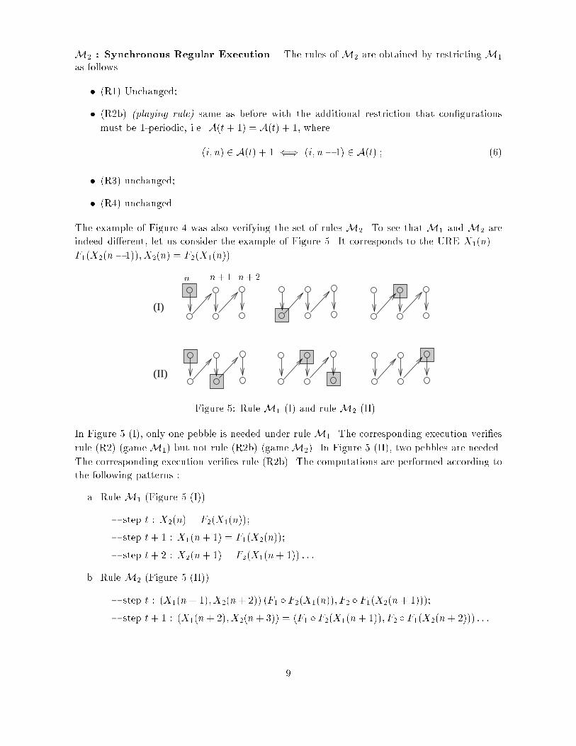
M2 : Synchronous Regular Execution. The rules of M2 are obtained by restricting M1as follows.� (R1) Unchanged;� (R2b) (playing rule) same as before with the additional restriction that con�gurationsmust be 1-periodic, i.e. A(t+ 1) = A(t) + 1, where(i; n) 2 A(t) + 1 () (i; n� 1) 2 A(t) ; (6)� (R3) unchanged;� (R4) unchanged.The example of Figure 4 was also verifying the set of rules M2. To see that M1 and M2 areindeed di�erent, let us consider the example of Figure 5. It corresponds to the URE X1(n) =F1(X2(n� 1)); X2(n) = F2(X1(n)).(I)

(II)

n n+ 1 n+ 2Figure 5: Rule M1 (I) and rule M2 (II).In Figure 5 (I), only one pebble is needed under rule M1. The corresponding execution veri�esrule (R2) (gameM1) but not rule (R2b) (gameM2). In Figure 5 (II), two pebbles are needed.The corresponding execution veri�es rule (R2b). The computations are performed according tothe following patterns :a. Rule M1 (Figure 5 (I)).{ step t : X2(n) = F2(X1(n));{ step t+ 1 : X1(n+ 1) = F1(X2(n));{ step t+ 2 : X2(n+ 1) = F2(X1(n+ 1)) : : :b. Rule M2 (Figure 5 (II)).{ step t : (X1(n+ 1); X2(n+ 2)) (F1 � F2(X1(n)); F2 � F1(X2(n+ 1)));{ step t+ 1 : (X1(n+ 2); X2(n+ 3)) = (F1 � F2(X1(n+ 1)); F2 � F1(X2(n+ 2))) : : :9

Note that in the execution under ruleM2, we have to perform the function compositions F2 �F1and F1 � F2. In x A.2, we discuss the `cost' of function compositions.Game M2 corresponds to the same computational model as game M1, which is the CREW-PRAM model. The di�erence is that in an execution of M2, the variables in A(t) are obtainedfrom the ones in A(t � 1) by always applying the same operator. This is interesting for im-plementation purposes. A non-regular execution of M1 would be practically very intricate toimplement since each step would be essentially di�erent. Another advantage of an executionof M2 is that the number of memory locations needed to carry out the calculations is easy tocompute: it is equal to jA(t)j (independent of t).M3 : Synchronous One-Pass Execution. The rules ofM3 are obtained by restricting theones of M2 as follows.� (R1) Unchanged;� (R2c) (playing rule) same as (R2b) with the following additional restriction. Each node inD must be computed only once during the whole execution.� (R3) unchanged;� (R4) unchanged.In rule (R2c), the important point is the di�erence that exists between computing a node andkeeping the result into the memory.1

2

1

2

(I)(II) step t+ 1step tstep t step t+ 1n n+ 1 n + 2Figure 6: Rule M2 (I) and rule M3 (II).Let us consider the example of Figure 6 (I). Each node on line 1 is computed twice, whereaseach node on line 2 is computed only once. Let us detail this. Node (1; n+ 2) is computed atstep t (it is needed as an auxiliary for the computation of node (2; n+2)) but it is not kept intomemory. Node (1; n+2) is then computed a second time at step t+1. On the other hand, node(2; n+ 2) is computed at step t and is kept into the memory. It does not have to be computeda second time at step t+ 1, as the computed value is just moved from one register to another.10

In Figure 6 (I), we have an example of an execution satisfying rule M2 but not M3. On theother hand, in Figure 6 (II), we have an execution which veri�es rule M3. The correspondingcomputation pattern is :� Rule M3 (Figure 6 (II)).{ step t : (X1(n+ 1); X2(n+ 1)) = (F1(X1(n); X2(n)); F2( F1(X1(n); X2(n)); X2(n) );{ step t+1 : (X1(n+2); X2(n+2)) = (F1(X1(n+1); X2(n+1)); F2(F1(X1(n+1); X2(n+1)); X2(n+ 1) ) : : :The computational model corresponding to game M3 is still the CREW-PRAM model. Rule(R2c) may look cumbersome but it actually corresponds to a natural notion for the applicationsto be detailed later on.Notations In the following, we use the notations :� E : the set of all possible (synchronous) executions under rule M1.� RE : the set of all possible executions under rule M2. Elements of RE will be calledregular executions.� ORE : the set of all possible executions under rule M3. Elements of ORE will be calledone-pass regular executions.Since the rules are increasingly restrictive, we have ORE � RE � E .4 Cuts in the Dependence Graph and their Relation withM1;M2From now on, it is always implicitly assumed that the system under study is recycled, see x 2.3.In this section, we concentrate on games M1 and M2.We introduce the notions of cuts and consecutive cuts in a dependence graph. We show thatcuts (resp. consecutive cuts) are closely related to executions of the pebble game under gameM1 (resp. game M2).We show that there always exists a minimal cut which is consecutive (Lemma 4.7). It will allowus to prove Theorem 4.11, the main result of the section:mine2RE P(e) = mine2E P(e) = minC cut of D jCj ;where the notations are de�ned in x 3.1. As a direct consequence, we show in x 4.3 that ProblemMinPeb can be solved with a polynomial algorithm for gamesM1 and M2.4.1 De�nitionsLet us recall some classical de�nitions of graph theory, all de�ned on the dependence graph D.For further references, see [9, 14] for example.De�nition 4.1 (path). A path is a sequence of nodes and arcs in D of the form � � � !(i0; n0) ! (i1; n1) ! (i2; n2) ! � � � ! (ik; nk) ! � � � . A path is bi-in�nite if it contains anin�nite number of negative nodes and an in�nite number of positive nodes.11

A non consecutive cut A consecutive cutFigure 7: Consecutive and non consecutive cuts.De�nition 4.2 (cut). A cut C is a set of nodes in D such that any bi-in�nite path contains atleast one node of C. A cut with a minimal number of nodes is called a minimal cut.De�nition 4.3 ( ow). A ow is a set of bi-in�nite paths such that any two paths do not shareany node. A ow containing a maximal number of paths is called a maximal ow. A ow F is1-periodic if we have: the arc (i; n)! (j;m) belongs to F if and only if (i; n+ 1)! (j;m+ 1)belongs to F .The most classical notion of cut involves arcs rather than nodes and a ow is a set of pathswhich do not share arcs rather than nodes. However a simple transformation, each node beingreplaced by two nodes connected by an arc, would allow us to go back to the original de�nitions.De�nition 4.4 (section). A section S in D is a set of nodes with exactly one node per line,S = f(i; ni); i 2 V g.Note that since D is recycled, a cut contains at least one node per line. Using this property, onecan de�ne the left and right sections of a cut.De�nition 4.5 (left, right section). The left (resp. right) section Cw, with w for west, (resp.Ce, with e for east) of a �nite cut C is the set of nodes (i; n) in C such that the nodes (i; n�h); h >0 (resp. (i; n+ h); h > 0) do not belong to C.De�nition 4.6 (consecutive cut). A cut C in D is consecutive if on each line of D, C con-tains only consecutive nodes, i.e.:For all i 2 V , (i; n) 2 C and (i; n+ 1) 62 C ) (i; n+ k) 62 C; 8k > 0.Examples of consecutive and non-consecutive cuts are displayed in Figure 7.Lemma 4.7. There exists a minimal cut of D which is a minimal consecutive cut.Proof. Let C be a minimal consecutive cut. We will prove that C is a minimal cut. First, weprove that there are no arcs from Cw to Ce + k; k > 2 (where (i; n) 2 Ce + k i� (i; n� k) 2 Ce).12

C Cr + 1ClFigure 8: Graph G made from the right and left sections of CLet us assume that there exists such an arc, that we denote by (i; n)! (j;m). By 1-periodicity,there is an arc between nodes (i; n� 1) and (j;m� 1). Now consider the bi-in�nite path� � � ! (i; n� 3)! (i; n� 2)! (i; n� 1)! (j;m� 1)! (j;m)! (j;m+ 1)! � � �It does not intersect C which is a contradiction.We consider the sub-graph G of D made of the nodes Cw [ (Ce + 1) and the arcs between Cwand Ce+1 in D, see Figure 8. We recall that a cut in a �nite graph G is a set of nodes such that,when removed from G, there is no arc remaining. The set Cw is a cut in G. Let � be a cut in Gof minimal size. We have j�j 6 jCwj. If j�j < jCwj then (CnCw)[� would be a consecutive cutin D strictly smaller than C, which would contradict the fact that C is a minimal consecutivecut. Therefore, we have j�j = jCwj.An adapted version of a famous \minimax" theorem �rst proved by K�onig (1931) states that wecan �nd j�j node-disjoint arcs in G. Since j�j = jCwj = jCe + 1j, these arcs de�ne a one to onemapping � from Cw to Ce + 1. From �, we construct a ow in C in the following way. Selectall the arcs of the form ((i; n) + k)! (�(i; n) + k) for all (i; n) 2 Cw and all k 2Z. These arcsform a 1-periodic ow F in D of size jCj.Let Cm be a minimal cut in D. Since F is formed by node-disjoint paths, Cm must contain atleast jFj nodes, jCmj > jFj = jCj. We conclude that jCmj = jCj.This lemma is interesting by its own. In particular, it gives a proof of the minimax theorem(which exists in many versions) for an in�nite 1-periodic and recycled graph.Corollary 4.8. The size of the minimal cut is equal to the size of the maximal ow in D.Furthermore, there exists a maximal ow F in D which is 1-periodic.4.2 Cuts and pebblesLemma 4.9. Let C be a �nite consecutive cut. There is a regular execution e 2 RE such thatC is a con�guration of e.Proof. Let C be a consecutive cut in D. We want to prove that it is possible to have A(t) = Cand A(t+1) = C+1 (note that C+1 = (CnCw)[ (Ce+1)). It is enough to prove that for eachnode (i; n) in Ce+1, there is no in�nite path P terminating in (i; n) that does not intersect thecut. But if such a path could be found, then the bi-in�nite path P [ f(i; n+ h); h 2 Ng wouldnot intersect C. It would contradict the fact that C is a cut.13

312 (b)n

(a)n+ 1 n+ 2

Figure 9: Two counter-examples.The converse of Lemma 4.9 is not true: a con�guration of a regular execution need not be aconsecutive cut. This is illustrated on Figure 9-(a). Also note that there are non-consecutivecuts which are not con�gurations of a regular execution, as illustrated in the example of Figure9-(b). In this example, the node (2; n+2) belongs to C + 1 but cannot be computed using onlyvariables in C (as it depends on (3; n) for example). Therefore, the cut C can not belong to aregular execution.Lemma 4.10. A con�guration of any execution e 2 E is a �nite cut in D. Conversely, let Cbe a �nite cut in D. There is an execution e 2 E such that C is a con�guration of e.Proof. Let A(t) be the t-th con�guration of some execution e belonging to E . All the con�gu-rations of e are �nite by de�nition. Therefore the total number of nodes that received a pebbleup to step t is �nite.Now, assume that A(t) is not a cut. By de�nition, there exists a bi-in�nite path P which doesnot have any node in A(t). According to rule (R3) of game M1, no node on P will receive apebble during the execution, after step t. Combining this and the fact that the total number ofnodes that received a pebble up to step t is �nite, only a �nite number of positive nodes on Preceive a pebble during the execution e. This contradicts the fact that e has to put pebbles onall nodes.Let us prove the converse result. Let C be a �nite cut. Let e = fA(t); t 2 Ng be any regularexecution of game M1. Such executions exist (see Lemma 4.9). Let N be the set of positivenodes (i; n) such that there exists an in�nite path ending in (i; n) and which does not intersectC. As C is a cut, N is �nite. Let T = supft j (N [ C)\ A(t) 6= ;g. Note that T is �nite sincefA(t)g is regular and N is �nite. We de�ne ~e = f ~A(t)g as follows:~A(t) = 8><>:Stn=0 A(n) if t 6 T;C if t = T + 1;A(t� 1) if t > T + 1 :Let us show that ~e is an execution of M1. We have C � STn=0A(n), therefore, it is possibleto set ~A(T + 1) = C. By de�nition of T , A(T + 1) does not intersect N , therefore, we can set~A(T + 2) = A(T + 1). Finally, ~e contains all nodes in fA(t); t 2 Ng and therefore all positivenodes. 14

We are now ready to state the main result of this section which states that, within all executionsin E , regular executions are dominant for Problem MinPeb.Theorem 4.11. Let us consider a recycled system of URE. We play the pebble game on itsassociated dependence graph D under rules M1 and M2. We havemine2RE P(e) = mine2E P(e) = minC cut of D jCj :In words, there exists a regular execution which requires a minimal number of pebbles, thisnumber being equal to the size of a minimal cut.Proof. It is a direct consequence of Lemmas 4.10, 4.9 and 4.7. First, note that all con�gurationsare cuts, according to Lemma 4.10. Let C be a consecutive cut of minimal size, which exists byLemma 4.7. By Lemma 4.9, C is a con�guration of a regular execution.Theorem 4.11 has several interesting corollaries. First, it allows one to focus on regular execu-tions since no fancy irregular execution of the URE can be done with fewer pebbles. Then, itprovides a polynomial method to �nd an optimal execution as shown in x 4.3.4.3 Complexity results for M1 and M2Proposition 4.12. Let R = (V;E;�) be the reduced graph associated with a recycled systemof URE with non-negative delays. We set �A = Pe2E �(e). For games M1 and M2, ProblemMinPeb can be solved using an algorithm having a complexity O ��2AjV j2�.If the system of URE has negative delays, it is possible to go back to non-negative delays (seeRemark 2.1) and apply Proposition 4.12 to the new system.In order to prove Proposition 4.12, we are going to compute a maximal ow in D and then applyCorollary 4.8. If we want to use the algorithm of Ford and Fulkerson [9] to compute a maximal ow, we need �rst to restrict ourselves to a �nite graph.We call span of a cut the di�erence between the largest and the smallest of the numberings ofcolumns containing a node of the cut.A slice of D of dimension n is de�ned as the subgraph of D having nodes f(i; k); i 2 V; 0 6k 6 ng [ fT;Bg where T (Top) and B (Bottom) are two special nodes. There is an arcT ! (i; k); 0 6 k 6 n; if 9(j; l); l < 0; such that there is an arc (j; l)! (i; k) in D. There is anarc (i; k)! B; 0 6 k 6 n; if 9(j; l); l > n; such that there is an arc (i; k)! (j; l) in D.If a consecutive minimal cut spans over less than n columns, then D and a slice of dimension nhave the same minimal consecutive cut (the special nodes T and B are not allowed to belongto the cut). So it is important to determine, or at least to bound, the span of a consecutiveminimal cut.Lemma 4.13. If all the delays are non-negative, the span of a minimal consecutive cut issmaller than the total sum of the delays in R, i.e. smaller than �A =Pe2E �(e).Proof. Let C be a minimal consecutive cut and let F be a maximal 1-periodic ow, see Corollary4.8. 15

The associated maximal 1-periodic ow, see Corollary 4.8, F is a set of paths in D. First, thesepaths cover all the nodes in D. Indeed, by the 1-periodicity of F , if a node (i; n) is not in F ,then the whole line (i; :) is not in F , but this means that the bi-in�nite path f(i; n); n 2Zg canbe added to the ow F and this contradicts the maximality of F .Let P1 be any path in F . It follows from the 1-periodicity of F that P1 is periodic. Leti0; i1; � � � ; il1; i0; i1; : : : be the successive lines visited by the path P1. Let (i0; n) and (i0; n+ k1)be the consecutive nodes visited by the path P1 on line (i0; :). Using the 1-periodicity of F , thetotal number of paths intersecting lines i0; i1; � � � ; il1 in F is k1. It implies that the cardinal ofC over the lines i0; i1; � � � ; il1 is exactly k1 (Corollary 4.8). Assume that the span of C on linesi0; i1; � � � ; il1 is strictly greater than k1. Then there exists a column, say n, not intersecting Cand such that on some of the lines fi0; i1; � � � ; il1g, C is on the `right' of column n and on someothers C is on the `left' of column n. Let l be such that C is on the `right' of n at line il andon the `left' at line il+1. There exists an arc of the type (il; n)! (il+1; n+ h); h > 0 (the delaysnilil+1are non-negative) in the ow F . Then the path f(il; n� u); (il+1; n+ h+ v); u; v 2 Ng does notintersect the cut C, see the Figure 4.3. This is a contradiction. We conclude that the span of Cover the lines i0; i1; � � � ; il1 is smaller than k1. By de�nition of R, there exists a circuit L1 in Rcontaining the nodes i0; i1; � � � ; il1 and of total delay k1.The path P1 and all its shifts are in the ow F and contain all the nodes in the lines i0; i1; � � � ; il1.If i0; i1; � � � ; il1 do not cover all the lines, a new path P2 in F not intersecting the lines i0; i1; � � � ; il1ranges over di�erent lines, say il1+1; il1+2; � � � ; � � � ; il2, and de�nes a circuit L2 in R similarly.The span of C on the lines il1+1; � � � ; il2 is smaller than k2, the total delay of circuit L2. We applythe same argument until all lines in D are covered. This de�nes a set H of circuits partitioningthe nodes of R.We build a new multi-graph G starting with R and where each circuit in H is merged into onesingle node. The graph G has jH j nodes and the arcs of G correspond to the arcs of R which donot belong to any circuit in H . Considering two nodes in G, say L1 and L2, the span of C overlines i0; � � � ; il2 can be choosen to be smaller than k1+k2+d, where d is the maximum delay onall arcs between the nodes L1 and L2 in G. Overall, the cut C can be choosen to have a spanwhich is smaller than the sum of the delays on all the circuits in H plus the sum of the delayson all the arcs in G . No delay is counted twice in this upper bound. Therefore, the total spanof C is smaller than the total sum of the delays in R.Proof of Proposition 4.12. A slice of D of size �A has the same minimal consecutive cut as Ditself. The computation of the maximal ow in a �nite slice can be done using the augmentingpath algorithm, see [9, 14]. Starting with a 1-periodic ow (the recycled lines) and maintainingthe 1-periodicity throughout the construction yields a maximal 1-periodic ow. The complexityof this construction of the maximal ow is O(�2AjV j2). By Corollary 4.8, it provides the sizeof a minimal cut in D. Furthermore, a standard procedure provides a minimal consecutive cut16

starting from a maximal ow (with a complexity O(�AjV j)). Using Lemma 4.9, an execution ofgameM2 (orM1) using a minimal number of pebbles, is obtained from the minimal consecutivecut.For the gameM3, the problemMinPeb is solved by working on the reduced graph. A polynomialalgorithm is given in x 6.5.5 Compatible Cuts and their Relation with M3We introduce the notion of compatible cuts. It enables us to show Theorem 5.5, the main resultof the section, which is the analog of Theorem 4.11:mine2ORE P(e) = min fjCj; C compatible cut of Dg :Let us introduce some new de�nitions.De�nition 5.1 (crossings). We say that an arc crosses a section S = f(i; ni); i 2 V g fromleft to right if it is an arc of the form (i; ni � h) ! (j; nj + l) with h > 0 and l > 1. An arc(i; ni + l)! (j; nj � h) crosses S from right to left if l > 1 and h > 0.De�nition 5.2 (compatible section, compatible cut). A section in D is compatible if noarc crosses the section from right to left. A consecutive cut is said to be compatible if its rightsection is compatible.Roughly speaking a compatible cut is a consecutive cut which agrees with the dependencerelations in the system of URE. Compatible cuts are connected to one-pass executions throughthe next two lemmas.Lemma 5.3. Let C be a compatible cut. There is a one-pass regular execution e 2 ORE suchthat C is a con�guration of e.Proof. Let C be a compatible cut. Since C is consecutive by de�nition, Lemma 4.9 tells us thatC is a con�guration of a regular execution which can be written as e = fC + t; t 2 Ng. Supposethat e is not one-pass. This means that there exists a node, say (j;m) which is computed twicein e.Let us assume that node (j;m) receives a pebble at step t0 and that this pebble is removed atstep t1, t1 > t0. By regularity of the execution e, node (j;m) will not be used at step t > t1+1.Indeed, a node in C + t only depends on variables in C + t � 1 or `below'.Now assume that node (j;m) is used at step t < t0 to compute another node, say (i; n). Thepath (j;m) ! (i; n) crosses the right section of C + t from right to left. Therefore it containsan arc that crosses the right section of C + t from right to left. This contradicts the fact that Cis compatible.Lemma 5.4. The con�guration of a one-pass regular execution is a compatible cut.Proof. Let e = fC + t; t 2 Ng be a one-pass regular execution. First, C is a cut by Lemma4.10. Next, C is consecutive. Indeed, if C is not consecutive on line i, then each variable Xi(n)receives a pebble at least twice in e, and a fortiori this means it is computed at least twice.17

It remains to show that C is compatible. Assume that C is not compatible. Then, thereexists a node (i; n) belonging to the right section of C + t, a positive integer k and a node(j;m) 2 (C + t + k)n(C + t) such that the arc (j;m) ! (i; n) belongs to D. But this impliesthat in the execution e, the computation of Xj(m) is performed twice: once as an auxiliarycomputation at step t to compute Xi(n) and once at step t+ k. This contradicts the fact thate is one-pass.Theorem 5.5. Let us consider a recycled system of URE. We play the pebble game on itsassociated dependence graph D under rules M3. We havemine2ORE P(e) = min fjCj; C compatible cut of Dg :Proof. It is an immediate corollary of Lemmas 5.3 and 5.4.Minimal compatible cutMinimal (non-compatible) cutFigure 10: Non compatible and compatible cuts.It can be that no minimal consecutive cut in D is compatible. This is the case in Figure 10where the minimal compatible cut contains 5 nodes while there is a minimal consecutive cut ofsize 4.Therefore, rule M3 requires more memory in general than rule M2.6 Delays in the Reduced GraphIn the previous sections, we have investigated the relations between executions of a system ofURE and cuts in the dependence graph. In this section, we connect these two notions withvalues of the delays in the reduced graph.Let us consider a system of URE S with variables fXi(n); i 2 V; n 2Zg and a regular executione = fA(t); t 2 Ng of the system. We introduce the modi�ed system ~S with variables f ~Xi(n); i 2V; n 2Zg and the execution ~e = f ~A(t); t 2 Ng de�ned as follows:ci = maxfn 2Z� j (i; n) 2 A(0)g~Xi(n) = Xi(n+ ci)~A(t) = f(i; n) s.t. (i; n+ ci) 2 A(t)g18

1 1

1 1

2

1

1

3-1

2

1

1

10

1

2

3

1RrRretiming r = (1;1;0) D

Drisomorphism frSrfr(Sr)

Figure 11: Retimed reduced graph and dependence graph.The above de�nition is such that the right section of ~A(0) is S0 = f(i; 0); i 2 V g. Viewed onthe dependence graphs, the passage from S to ~S corresponds to a shift of the lines. Viewed onthe reduced graphs, it corresponds to a retiming, i.e. a modi�cation of the value of the delays,while preserving the graph topology.We show (Lemma 6.6 and 6.7) that the total number of delays in ~R is closely related to regularexecutions. As a consequence, we obtain a polynomial algorithm to solve ProblemMinPeb underrule M3, see x 6.5.6.1 RetimingDe�nition 6.1 (retiming). Let R be the reduced graph of a system of URE. A retiming of Ris a node function r : V !Zwhich speci�es a new graphe Rr, with the same nodes and arcs asR. The value of the delay on an arc e = (i; j) in Rr is equal to �r(e) = �(e) + r(i)� r(j).The notion of retiming is classical in digital circuits (see [17] and x 7, where we provide a detailleddiscussion of its usefulness in this context ) and in Petri nets, where it corresponds to the �ringof transitions (see x 8).In the example of Figure 11, the new values of the delays correspond to a retiming r such thatr(1) = 1; r(2) = 1 and r(3) = 0.Retiming may create negative delays as in Figure 11.Lemma 6.2. Two retimings r and r0 yield the same value of the delays in a connected graph Rif and only if there exists a constant h 2Zsuch that 8i 2 V; r(i) = r0(i) + h.Proof. First, if r(i) = r0(i)+h for all i 2 V , then on any arc e = (i; j), �r(e) = �(e)+r(i)�r(j) =19

�(e)+r0(i)�r0(j) = �r0(e). Conversely, if �r0(e) = �r(e), then r(i) = r0(i)+h and r(j) = r0(j)+hfor some h 2Z. As R is connected, the constant h is the same for all the nodes in V .The question that arises now is what is the notion corresponding to retiming in the system ofURE S and in the dependence graph D? To answer this question, let us consider the graphDr associated with the retimed reduced graph Rr. This dependence graph can be constructeddirectly from D by shifting the lines as described in Lemma 6.3.Lemma 6.3. A retiming r in R corresponds to a transformation fr between D and Dr de�nedby: fr : D ! Dr(i; n) ! (i; n� r(i))The transformation fr is an isomorphism of graphs, meaning that there is an arc between u andv in D i� there is one between fr(u) and fr(v) in Dr. It will also be called a retiming of D.Proof. By de�nition of D, there is an arc from (i; n) to (j;m) in D if the delay in R on arc (i; j)is = m � n. The delay in Rr on arc (i; j) is r = + r(i)� r(j) = (m � r(j))� (n � r(i)).It implies that there is an arc between (i; n� r(i)) and (j; n� r(j)) in Dr. Therefore, fr is anisomorphism between D and Dr.We recall that the notion of section was introduced in De�nition 4.4. We associate with aretiming r in R, the section Sr = f(i; r(i)); i 2 V g in D.Lemmas 6.2 and 6.3 tell us that two retimings r and r0 are similar (in the sense that they yieldthe same value of the delays) if and only if they are associated with two sections Sr and S 0rwith Sr = Sr0 + h, for some h 2 Z. This relation enables us to de�ne a parallelism relationbetween sections in D as well as between retimings in R. We say that section Sr (resp. retimingr) is equivalent to section Sr0 (resp. retiming r0) if Sr = Sr0 + h, for some h 2 Z. In thefollowing, we will always consider one arbitrary section among the equivalence class and call itthe section associated with the retiming r, for instance S0 corresponds to the equivalence classof f(i; 0); i 2 V g.6.2 Counting the delaysGiven a graph R = (V;E;�), we de�ne the total number of delays of R as follows�A(R) =Xi2V X(j; )2�i : (7)It corresponds to the number of delays appearing in the graphical representation of the reducedgraph R as de�ned in x 2.2. See for example the graph R on Figure 12.Given a graph R = (V;E;�), another quantity of interest is the following one�B(R) =Xj2V maxf j 9i s.t. (j; ) 2 �ig : (8)20

When the delays are positive (8e 2 E;�(e) > 0), �B corresponds to the total number of delays(�A) in a modi�ed reduced graph obtained by performing a forward splitting of the nodes. Inthe context of digital circuits, this is also called register sharing, see x 7.2. Here is, given underthe form of an algorithm, the formal construction of the Forward Splitting algorithm.Algorithm 6.4 (Forward Splitting).Input: Reduced graph R = (V;E;�) with � > 0, functions associated with the nodes: fFi; i 2V g.1. Set V 0 = V and E 0 = ;. Associated functions F 0i = Fi; i 2 V .2. For all node v 2 V , let � be the maximum delay on all the output arcs of v.� Set v0 = v.� If � > 0, create � new nodes in V 0, called v1; � � � ; v�. Set F 0vi = Id, theidentity function, for i = 1; : : : ; �.� For each arc e = (v; u) 2 E with delay �(e) = , create an arc e0 = (v ; u)in E 0 with delay �0(e0) = 0.� Add the arcs (vi; vi+1), 0 6 i 6 � � 1, in E 0, with delay �0 = 1.Output: Split reduced graph R0 = (V 0; E 0;�0) with �0 > 0, functions associated with the nodes:fF 0i ; i 2 V g.It is important to remark that the split graph R0 is not necessarily recycled, as opposed to R.We come back to this point in x 6.4.The following proposition, easy to prove, justi�es the Forward Splitting operation.Proposition 6.5. Let R be a reduced graph with positive delays and R0 the associated splitgraph.(i)- The associated systems of URE S and S 0 have the same behavior. More precisely, borrowingthe notations of the algorithm, we have8v 2 V; n 2Z; X 0v(n) = Xv(n) and 8vi 2 V 0 n V; n 2Z; X 0vi(n) = Xv(n� i) :(ii)- Furthermore, we have �B(R) = �A(R0) = �B(R0) : (9)Note that in order for Equation (9) to make sense, it is necessary to extend the de�nitions of�A and �B to non-recycled graphs.In Figure 12, R0 is the Forward Splitting of R. In the split graph, there are two \dummy"nodes (associated with the identity function), represented by black dots. We have �A(R) = 8and �B(R) = �A(R0) = �B(R0) = 5. 21

2 delays5 delays

011 �A(R0) = �B(R) = 00 0�A(R) =R 1i = a0 a1 a2R0

2i1 1Figure 12: A reduced graph and the associated split graph.6.3 Delays, cuts and pebblesGiven a section S = f(i; ni); i 2 V g in D, we de�ne the cut C(S) in the following way.C(S) def= f(i; n); i2 V; n 6 ni j 9j 2 V;m > nj ; (i; n)! (j;m)g : (10)The cut C(S) is consecutive and its right section is S. Furthermore, if any node is removed fromthe left section of C(S), then it is not a cut anymore.In a cut C, a node (i; n) 2 C is redundant if Cnf(i; n)g is a cut. Any consecutive cut C with noredundant node on its left section is characterized by its right section S only. More precisely, itveri�es C = C(S).We are now ready to state the relations between delays in R and consecutive cuts in D.Lemma 6.6. (i)- The number of delays �B(R) is equal to the cardinal of C(S0). (ii)- Let r bea retiming of R and Sr an associated section in D. Then the number of delays �B(Rr) is equalto the cardinal of the cut C(Sr) in D (resp. C(S0) in Dr).Proof. The isomorphism fr transforms the section Sr in D into the section S0 in Dr. Hence (ii)is implied by (i). Let us work on graph D. We are going to prove that �B(R) = jC(S0)j. Weconsider a node i of R. Let m = maxf j 9j; (i; ) 2 �jg (we have m > 1 as (i; 1) 2 �i) andlet j be such that (i;m) 2 �j . There is an arc in D from (i;�m) to (j; 0) and no arc from anode on the `left' of (i;�m) (and on line i) to a node on the `right' of S0. Hence C(S0) containsthe nodes (i;�m+1); � � � ; (i; 0) on line i. The same argument repeated on each line �nishes theproof.We recall that the arcs crossing a section from right to left and from left to right are de�ned inDe�nition 5.1.Lemma 6.7. (i)- The number of delays �A(R) is equal to the number of arcs crossing S0 fromleft to right minus the number of arcs crossing it from right to left. (ii)- Let r be a retiming ofR and Sr an associated section in D. The number of delays �A(Rr) is equal to the number of22

arcs in D (resp. Dr) crossing section Sr (resp. S0) from left to right minus the number of arcscrossing Sr (resp. S0) from right to left.Proof. For the same reason as in Lemma 6.6, it is enough to prove (i). Let (i; j) be an arc of Rwith delay > 0. In D, this arc induces exactly arcs crossing S0 from left to right, the arcs:(i;� + 1)! (j; 1) � � � (i;�1)! (j; � 1); (i; 0)! (j; ) :Similarly, an arc (i; j) with delay < 0 induces exactly � arcs crossing S0 from right to left:(i; 1)! (j; + 1) � � � (i;� � 1)! (j;�1); (i;� )! (j; 0) :The same argument applied to all the lines �nishes the proof.The notion of compatible cut introduced in De�nition 5.2 has a very natural interpretation interms of delays.Lemma 6.8. Let r be a retiming of R and Sr an associated section in D. The retimed reducedgraph Rr has only non-negative delays if and only if the cut C(Sr) is compatible in D (equiv.the cut C(S0) is compatible in Dr).Proof. If Rr has only non-negative delays, the argument used in the proof of Lemma 6.7 showsthat all the arcs crossing Sr in D, cross it from left to right. It implies that the cut C(Sr) iscompatible. The converse result is proved by contradiction, using again the proof of Lemma6.7.In Figure 13 (this example is the same as the one of Figure 10), we have represented the retimedreduced graphs associated with two sections (cuts) of D. One of them is compatible and theother one is not compatible.6.4 SummaryIn x 4.2, we have established the relations between executions of the pebble game and cuts inthe dependence graph. In x 6.3, we have established the relations between cuts and delays. Asa by-product, we obtain the relations between delays and pebble con�gurations.More precisely, let e = fA(t); t 2 Ng be an execution such that A(t) is a consecutive and non-redundant (see p. 22) cut for all t. Note that we did not assume that e is regular. With thecon�gurations A(t), we associate a retiming r(t) and a reduced graph Rr(t) as follows:r(t)i = maxfni j (i; ni) 2 A(t)g :We have the following situations:� If the execution e belongs to E , the con�gurations A(t) may have di�erent shapes at eachstep. Then, the reduced graphs Rr(t) may have changing values for the delays.� For an execution e belonging to RE , the con�gurations are just shifted between two steps.It implies that the reduced graphs Rr(t) are all identical, with a �xed value of the delays.23

1

3

2

4

1

3

1

4

Minimal compatible cut

2

1

Minimal (non-compatible) cutCorresponding delays

1

2

1

1

01 3

0

1

2

1 13

1

1

2

1

1

1

-1

4

4

1

1

(II)(I)

Figure 13: Compatible and non compatible cuts, non-negative and negative delays.� Finally, an execution e belonging to ORE corresponds to identical reduced graphs Rr(t)with �xed and non-negative values of the delays.In the following table, we provide a summary of the main relations established so far betweenexecutions of a system of URE, cuts in D and delays in R.Games Executions Cuts in D Delays in RM1 execution in E arbitrary cut changing delaysM2 regular execution, RE consecutive cut �xed delaysM3 one-pass reg. exec., ORE compatible cut non-negative �xed delaysA general remark is that the main theoretical results, Theorems 4.11 and 5.5, apply only torecycled graphs. Using them, we have been able to solve Problem MinPeb for an initial graphwhich is recycled. However, the solution proposed involves the construction of an associatedgraph, which is not recycled. It is not a problem as we do not need to apply Theorems 4.11 or5.5 on this associated graph.6.5 Complexity results for M3Proposition 6.9. Let R = (V;E;�) be the reduced graph associated with a recycled systemof URE. Under game M3, Problem MinPeb can be solved using an algorithm of complexityO(jEj2 log jV j+ jV jjEj log2 jV j). 24

Proof. As detailed above, there is a one-to-one correspondence between minimal one-pass regularexecutions and retimed reduced graphs with non-negative delays.In Leiserson and Saxe, x 8 of [17], an algorithm is given to solve the following problem: �nd a re-timed reduced graphRr with only non-negative delays and minimizing �B(Rr). It is a minimum-cost ow algorithm; it provides an explicit solution and its complexity is O(jEj2 log jV j +jV jjEj log2 jV j). Using Lemma 5.3 and 6.6, the cut C(Sr) is compatible and the executionfC(Sr) + t; t 2 Ng is one-pass regular and solves Problem MinPeb under rules M3 according toTheorem 5.5.The algorithm of [17] was developed in the context of digital circuits, see x 7. An e�cientimplementation of this algorithm can be found in Shenoy and Rudell [24].7 Application 1 : Registers in Circuit DesignIn this section we will show how the previous results relate to the problem of register mini-mization in digital circuits. The interest of the relation is two-fold. First, algorithms developedfor digital circuits can be used to get optimal executions of a system of URE, see the previoussection. Second, we will show that the results proved so far enable to prove some new resultsfor recycled digital circuits, see Theorem 7.4 below.7.1 De�nition of a circuitA digital circuit is constituted by functional gates, wires and registers. More precisely , (i)- afunctional element computes an output data from one or several input data. For example, in thecase of a logical circuit, the functional elements will be boolean logical gates (AND, OR,: : : );(ii)- A wire between element i and element j enables to transfer the output data of i whichbecomes an input data for j; (iii)- A register corresponds to a storage facility, or a memory cellof �nite size. If there are p registers between elements i and j, it enables to keep in memory thelast p values computed by the element i.The model of the behavior of the system is the following. There is a global clock for the system.Between two clock ticks, here are the operations taking place.� Functional element : (1)- receive the input data from upstream registers or elements; (2)-compute a new output data; (3)- send the output data to downstream registers or elements.� Register : (1)- transmit the stored data downstream to another register or a functionalelement; (2)- remove the stored data; (3)- receive and store a new data from upstreamfrom another register or a functional element.Between two clock ticks, these operations are performed at all functional elements and registers.Let Xi(n) be the n-th variable computed at element i. Since registers are �nite size memorycells, the variables Xi(n) can only take a �nite number of values. The set of all these possiblevalues is denoted by W .After n clock ticks, for each element i, the variables fXi(m); m 6 ng have been computed. Thenumber of registers on a wire between i and j corresponds to the number of variables Xi(n� k)25

which need to be still in the memory in order to carry on the computation of the variablesXj(n+m); m > 0.It follows from the previous description that a digital circuit can be viewed as the reduced graphR of some system of URE. The functional elements of the circuit correspond to the nodes of R,the wires to the arcs and the registers to the delays. The computation operation correspondingto the functional element i is denoted by Fi to be consistent with previous notations. In theremainder of the section, we will use indi�erently the terminology of digital circuits and the oneof reduced graphs. We consider only constructive circuits, i.e. circuits whose associated URE isconstructive, and recycled circuits, i.e. circuits whose associated reduced graph is recycled.The speci�city of digital circuits (with respect to general reduced graphs) is that only non-negative registers (delays) have a physical meaning.In Figure 14, we have represented the ow of data between clock ticks in a digital circuit. Thegraphical convention is consistent with the one of reduced graphs.jjjiii

After n� 1 ticksAfter n ticksAfter n + 1 ticks Xi(n)Xi(n� 1)Xi(n+ 1) Xi(n� 1)Xi(n� 2) Xj(n� 1)Xj(n+ 1)Xj(n)Xi(n)Figure 14: Digital circuit computing Xj(n) = Fj(Xi(n� 2); : : :).7.2 Minimizing the number of registersWe consider Problem MinReg which is classical in circuit design, see for instance Leiserson andSaxe [17], x 8.Problem 2 (MinReg). Given a recycled circuit, �nd a new circuit preserving the functionalbehavior and having a minimal number of registers.To make this statement precise, we have to de�ne rigorously the functional behavior and thenumber of registers of a circuit.Let fXi(n); i 2 V; n 2 Zg and f ~Xi(n); i 2 ~V ; n 2 Zg be the variables computed by the originaland the new circuits respectively. The preservation of the functional behavior means that wehave: 8i 2 V; 9u 2 ~V ; 9ci 2Zs.t. 8n 2Z; Xi(n) = ~Xu(n + ci) : (11)Registers can be viewed as delays in a reduced graph and the number of registers of a circuitR is the quantity �A(R) de�ned in Section x 6.2. Now, starting from a circuit R, we can26

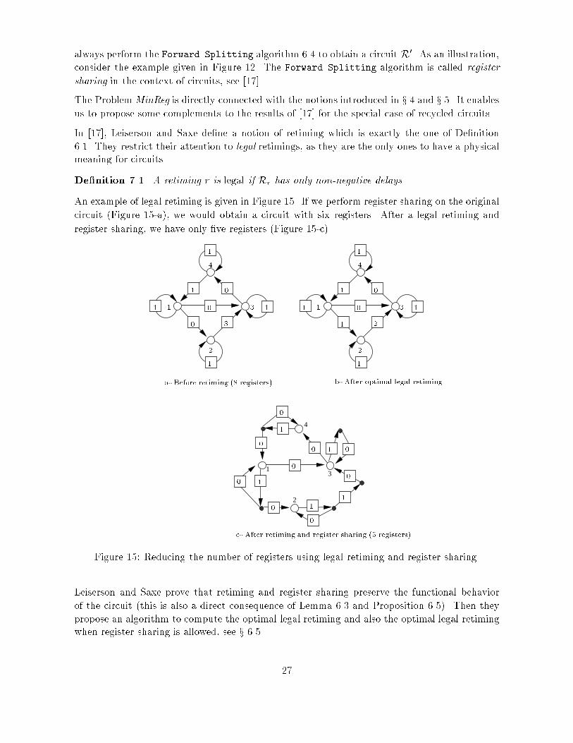
always perform the Forward Splitting algorithm 6.4 to obtain a circuit R0. As an illustration,consider the example given in Figure 12. The Forward Splitting algorithm is called registersharing in the context of circuits, see [17].The ProblemMinReg is directly connected with the notions introduced in x 4 and x 5. It enablesus to propose some complements to the results of [17] for the special case of recycled circuits.In [17], Leiserson and Saxe de�ne a notion of retiming which is exactly the one of De�nition6.1. They restrict their attention to legal retimings, as they are the only ones to have a physicalmeaning for circuits.De�nition 7.1. A retiming r is legal if Rr has only non-negative delays.An example of legal retiming is given in Figure 15. If we perform register sharing on the originalcircuit (Figure 15-a), we would obtain a circuit with six registers. After a legal retiming andregister sharing, we have only �ve registers (Figure 15-c).1

3

4

2

0 11

10

10

2 10 01

1 01 00 04

111 1 30a- Before retiming (8 registers) b- After optimal legal retiming1 021 1023 11 14 3

c- After retiming and register sharing (5 registers)00Figure 15: Reducing the number of registers using legal retiming and register sharing.Leiserson and Saxe prove that retiming and register sharing preserve the functional behaviorof the circuit (this is also a direct consequence of Lemma 6.3 and Proposition 6.5). Then theypropose an algorithm to compute the optimal legal retiming and also the optimal legal retimingwhen register sharing is allowed, see x 6.5. 27

However the question whether other circuit transformations can be used to get a circuit witheven fewer registers remains to be answered.Let us consider the best possible retiming in the original circuit without restricting ourselvesto legal retimings. It corresponds to the choice of a minimal consecutive (but not necessarilycompatible) cut in the associated dependence graph D, see x 6.4. In the corresponding reducedgraph, there may be some negative delays that cannot represent registers. However, it is possibleto perform some appropriate modi�cations to go back to positive delays. It is done by duplicatingsome nodes in the circuit.The Duplicate algorithm takes as input a graph R = (V;E;�) and produces a new graphR0 = (V 0; E 0;�0);�0 > 0. In the description to follow, we use the notion of delays on paths: if Pis an oriented path in R then the delay of P is the sum of all the delays on the arcs of P .Algorithm 7.2 (Duplicate).Input: Reduced graph R = (V;E;�), functions associated with the nodes: fFi; i 2 V g.1. Set V 0 = V and E 0 = ;. Associated functions F 0i = Fi; i 2 V .2. For each node v in V , let k(v) be the minimum delay of all paths in R startingin v.� Set v0 = v.� If k(v) < 0, then create jk(v)j additional nodes in V 0, v1; � � � ; vjk(v)j, withassociated functions, F 0vi = Fv.3. For each arc (u; v) 2 E with delay �(u; v) = , create in E 0 all the arcs oftype (umax(0;j� ); vj) with delay max(0; � j) for all 0 6 j 6 max(0; k(v)).Output: reduced graph R0 = (V 0; E 0;�0), �0 > 0. Associated functions fF 0i ; i 2 V 0g.For each node v 2 V , k(v) is �nite and is reached on a �nite path since the constructivity of Rimplies that all circuits in R have a strictly positive delay.The following proposition justi�es the use of the Duplicate algorithm.Proposition 7.3. Let S and S 0 be the systems of URE associated with R and R0 respectively.(i)- S and S 0 have the same functional behavior. More precisely, borrowing the notations of theDuplicate algorithm, we haveX 0vj(n) = Xv(n+ j); 8vj 2 V 0; 8n 2Z; (12)(ii)- we have �B(R) = �B(R0).Proof. The proof of (i) follows directly from the construction rules of R0. Consider (12), spe-cialized to j = 0, we get X 0v0(n) = Xv(n). The original circuit is embedded in the new circuit.As for (ii), note that all the arcs exiting a duplication node (of type vj ; j > 0) have a zero delay.As for the new arcs from the nodes of type v0, they all have delays smaller than or equal to thedelays of the arcs of the original graph. The original arcs are kept with their original delaysunchanged. We conclude that �B(R) = �B(R0).28

It is important to remark that the reduced graph R0 (hence the associated system of URE)obtained by duplication is not recycled anymore.We illustrate the algorithm Duplicate on an example. The circuit of Figure 16-a is obtainedfrom the one of Figure 15-a by performing a non-legal retiming. By applying the Duplicatealgorithm, we obtain the circuit of Figure 16-b, where node 1 has been duplicated into nodes 10and 11.11

1

1

0

0

0

0

0

0 1

11 0

1

0

0

0

0

2

1 13

1

1

1

1

1

1

4

-1

2

1

1

4

13

1

1

b- after duplication

0

0

0

3

4

2

a- circuit after optimal general retiming

c- after duplication and register sharing (4 registers)

111010 11

Figure 16: Reducing the number of registers using retiming, duplication and register sharing.Now, after performing register sharing, the resulting circuit has only 4 registers (see Figure 16-c). The minimal number of registers we could get with only legal retimings and register sharingwas 5, see Figure 15-c.We now state the general result.Theorem 7.4. Let us consider a recycled digital circuit. When the functions computed at eachnode are general, a circuit with the same functional behavior and a minimal number of registerscan be obtained by performing solely the three following operations (in this order):1. General retiming; 2. Duplicate algorithm; 3. Forward Splitting algorithm (register shar-ing).Proof. Let us consider a recycled graph R = (V;E;�) (associated dependence graph D). Werealize the following operations: 1. Perform the optimal general retiming, to obtain a graph R1.2. Apply the Duplicate algorithm to R1 to obtain the graph R2.3. Transform the graph R2 into R3 by applying the Forward Splitting algorithm.29

Let us detail the �rst operation. We �nd a minimal consecutive cut C of D (Proposition 4.12).Let f(i; r(i)); i 2 V g be the right section of C. We de�ne the retimed graph R1 = Rr. UsingLemma 6.6, �B(R1) is equal to the cardinal of C.The three operations preserve the functional behavior of the circuit, see Lemma 6.3, Propositions6.5 and 7.3. Furthermore, as a consequence of Proposition 7.3 and Equation (9), we have�B(R1) = �B(R2) = �A(R3). We conclude that �A(R3) = jCj. It remains to be proved thatthere exists no other circuit, having the same functional behavior as R, and with fewer registersthan R3.We consider R0 = (V 0; E 0;�0) another circuit which has the same functional behavior as R. LetD0 be the dependence graph associated with R0. The preservation of the functional behaviorimplies that the set of nodes in D is included in the set of nodes in D0. The mapping of thenodes of D onto D0 that preserves the functional behavior is denoted by �. By de�nition,Xi(n) = X 0�(i)(�(n)), if the node (i; n) in D is mapped on the node (�(i); �(n)) = �(i; n) in D0.We consider a minimal cut C of D. In D0, we suppose that there exists a cut C 0 such thatjC0j < jCj. We can assume that in D0, we have �(C) on the `left' of C 0 and �(C + k) on the`right' of C 0, by choosing k large enough.We recall thatW denotes the �nite set of possible values for a variable Xi(n). In the dependencegraph D, there exists a ow (node-disjoint paths) from C to C+k of size jCj (Corollary 4.8). Itimplies that there is a general dependence between the variables attached to C and the variablesattached to C + k, which can be put under the form of a general function F :W jCj !W jCj. Inparticular, the functions Fi in Equation (2) can be chosen such that F is bijective. For example,choose Fi(Xj(n� ); : : :) = Xj(n� ) if the arc (j; n� )! (i; n) belongs to the ow. In thiscase, the function F is merely a permutation of the coordinates.Now let us consider the graph D0, using the existence of the cut C 0, the function F can bedecomposed as F :W jCj !W jC0j ! W jCj. As W is �nite, it contradicts the fact that F can bebijective.The smallest cut C 0 in D0 is at least as large as C. Finally, by using Lemma 6.6, we concludethat �A(R0) > �B(R0) = jC 0j > jCj = �A(R3).As recalled above, in Leiserson and Saxe [17], only legal retimings were considered. In Theorem7.4, by considering all possible retimings, we were able to obtain a circuit with less registers,and even a minimal number of registers. However, in doing so, we obtain a circuit with a pos-sibly larger number of functional elements. Hence, the practical interest of Theorem 7.4 alsoneeds to be discussed in terms of the compared costs of functional elements and registers. Infact, the number of functional elements is increased both by the Duplicate and by the ForwardSplitting algorithms. On the one hand, in the Forward Splitting case, only \dummy func-tions" are added. In the context of circuits, they consist in simple wire connections and do notperform any operation so that they should be very cheap to implement. On the other hand,in the Duplicate case, the added elements are equivalent to some of the original functionalelements. Hence they could be more expensive to implement.30

7.3 Summary and complexityThe transformations done to a circuit in order to obtain an equivalent circuit with the minimalnumber of registers can be summarized by the following scheme.optimal forwardretiming duplicate splittingR �! R1 �! R2 �! R3�(R1) 2ZE1 �(R2) 2 NE2 �(R3) 2 f0; 1gE3�B(R1) minimal �B(R2) = �B(R1) �A(R3) = �B(R2)Corollary 7.5. Let us consider a recycled digital circuit. A new circuit solving Problem MinRegcan be obtained with an algorithm of complexity O(�A(R)2jV j2 + jV j3).Proof. In the proof of Theorem 7.4, the algorithms used to go from R to R1, from R1 to R2and from R2 to R3 are all polynomial, and R3 is a solution to the Problem MinReg.To obtain R1, we apply the algorithm of Proposition 4.12 whose complexity is O(�2AjV j2). Toobtain R2, we apply the Duplicate algorithm 7.2, whose complexity is O(jV j3 + �AjEj). Letus justify this complexity. The �rst step consists in computing the quantities k(u); u 2 V . Itis equivalent to the search of a minimal weight path in a weighted graph. This can be doneusing Floyd algorithm with a complexity O(jV j3), see for instance Gondran and Minoux [14],Chapters 2 and 3. Let M = maxv2V (0;�k(v)). From the constructiveness, it follows that Mhas to be smaller than �A. Now, the second step of the algorithm consists in creating at mostM jV j nodes and M jEj arcs. The complexity of this step is at most O(�AjEj).To obtain R2, we apply the Forward Splitting algorithm 6.4. In this algorithm, we create atmost �B nodes and jEj arcs, which accounts for a complexity O(�B + jEj).Corollary 7.5 is interesting as it is not straightforward to extend the original algorithm of Leis-erson and Saxe (for legal retimings, see x 6.5) to general retimings.8 Application 2 : Task Graphs EvaluationTask graphs are widely used in the modeling and analysis of parallel programs and architectures,see [1]. Yet, the performance evaluation of task graphs is di�cult in general.The term task graphs covers a wide variety of models, with the following common feature:each task depends on a �nite number of tasks, and can be executed only when all the tasks itdepends on are completed. Here, we consider repetitive task graphs which are bi-in�nite taskgraphs generated by the periodic replication of a given �nite task graph (with set of nodes V ),see [3].Let us denote by Xi(n); i 2 V; n 2Z, the epoch when the n-th occurence of task i is completed.Let the sets �i; i 2 V; describe the dependences between tasks. The variables Xi(n) are givenby a recursion of the following form:Xi(n) = max(j; )2�i(Xj(n� ) + �j;i; (n)); i 2 V; n 2Z; �j;i; (n) 2 R : (13)31

We will present the optimization problem which arises in the fast parallel computation of theevolution equations of task graphs, and apply the preceding results to solve it.8.1 Max-Plus recurrencesThe evolution equations (13) can be viewed as both a specialization and a generalization of asystem of URE. On the one hand, the functions have a speci�c form, implying only the operationsmax and +. On the other hand, the functions depend on n. We call a \Max-Plus Recurrence"(MPR), an equation of the form (13). From now on, we assume that the MPR is constructiveand recycled, i.e. that 8i; (i; 1)2 �i. It is a natural assumption for task graphs as it means thatthe n-th occurence of a task can not start before the completion of the (n� 1)-th occurence ofthe same task.The (max,+) formalism is a convenient tool to work with MPR. We brie y introduce it.De�nition 8.1. The (max,+) semiring Rmax is the set R[ f�1g, equipped with the two oper-ations max and +, denoted respectively by � and (a� b = max(a; b) and a b = a+ b). Theelements �1 and 0 are the neutral elements of the laws � and respectively.For matrices of appropriate sizes, we de�ne (A�B)ij = Aij �Bij = max(Aij ; Bij), (AB)ij =LlAil Blj = maxl(Ail + Blj), and for a scalar a, (a A)ij = a Aij = a + Aij . When noconfusion is possible, we abbreviate AB to AB.We can rewrite Equation (13) with the previously de�ned notations. Let X(n) be the columnvectors of coordinates Xi(n) and let A( ; n) be the matrix with coordinates A( ; n)ij = �j;i; (n)if (j; ) 2 �i and A( ; n)ij = �1 otherwise. Now let U = f j 9i; j s.t. (j; ) 2 �ig and = maxU . We have X(n) =M 2U A( ; n)X(n� ) : (14)This is a linear system in the (max;+) semiring.Representation of order one A standard step in the analysis of linear systems is the trans-formation of a recurrence like (14) into an \equivalent" system of order 1, such as (15), where~X(n); ~X(n� 1) 2 R~Vmax and A(n� 1) 2 R~V�~Vmax .~X(n) = A(n� 1) ~X(n� 1) : (15)The system in Equation (15) is \equivalent" to the original one if it preserves the functionalbehavior, meaning that 8i 2 V; 9u 2 ~V ; 9ci 2 Zs.t. 8n 2 Z; Xi(n) = ~Xu(n+ ci). We say thatthe system in (15) is an order one representation of the original one.Assume that all the delays in (14) are greater or equal to 1. Then the transformation can bedone by setting ~XijV j+j(n) = Xj(n� i); i = 0; : : : ; � 1; j 2 V :32

In this case, the dimension of the order 1 representation is j ~V j = jV j . We will see belowthat an order 1 representation can be obtained without any assumption on the delays (exceptconstructivity).We can now de�ne the main problem to be addressed in this section:Problem 3 (MinSize). Given a recycled MPR, �nd an equivalent MPR of order 1 and ofminimal dimension.For strictly positive delays, it follows from the discussion above that the minimal dimension isat most equal to jV j . We will see that in general it is much lower. Problem MinSize is verynatural. A practical motivation for it is provided in next section.Remark 8.2. In Problem MinSize, the optimality of the size of the representation should beunderstood as the best possible that can be obtained without making assumptions on the valueof the numbers �i;j; (n). When these numbers are constant and known, this knowledge may beexploited to obtain a minimal realization in the sense of linear system theory [20, 10], which isnormally smaller than ours. Finding a minimal realization is a di�cult problem, and algorithmsare known only in very speci�c cases. A deeper investigation of the relations between the twoapproaches is an interesting direction for further research.8.2 Parallel evaluation of MPRThe evaluation of a MPR consists in computing all the variables X(n). We assume that we wantto perform this evaluation using a parallel machine. If we have an order 1 representation of thesystem, a possible and e�cient algorithm is the parallel pre�x principle: as the multiplication ofmatrices in (max,+) is associative, it is possible to divide the computation of A(n) � � �A(1)into smaller products A(p) � � � A(q) which may be computed by di�erent processors.The number of operations required to compute the variables up to X(n) on a CREW-PRAMmachine with P processors is O(`3(n=P +log(P ))), where ` is the size of the matrix of the linearsystem. Since n and P are �xed parameters, the complexity is minimized by having an order 1representation of the MPR of minimal dimension.8.3 Reduced graphsAs for any system of URE, we can associate a reduced graph R = (V;E;�) to a given MPR. Toeach node i 2 V , we associate the sequences f�j;i; (n); n 2Zg, (j; ) 2 �i.We will show that the solution to Problem MinSize is a matrix of dimension minr �B(Rr); r 2ZV . This result seems to be new.We transform any reduced graph by the following procedure. For each node in the reducedgraph, we create new (dummy) nodes and new arcs in a tree-like fashion, as in Figure 17, suchthat each arc in the new reduced graph has a delay at most one. The added dummy nodes arerecycled (the recyclings are not shown on the �gure).More formally, the transformation can be done using the algorithm Forward Splitting-IIdescribed below. We use the notation u� to denote the set of successor arcs of u. It is notassumed that the delays are positive. 33

4

3

2

1 1 1 1

1

1

�1u0 = uu �1�3 �2�3�2 u2u1 u3Figure 17: Forward Splitting-II of a reduced graph.Algorithm 8.3 (Forward Splitting-II).Input: Recycled reduced graph R = (V;E;�). Sequences f�j;i; (n); n 2Zg.1. We set V 0 = V;E 0 = ;.2. For all node u 2 V , let �(u) = maxa2u� �(a). As the graph is recycled, wehave �(u) > 1.If �(u) = 1 then u and u� remain unchanged.If �(u) > 1, then� in E 0, set u0 = u and create �(u)�1 recycled nodes u1; � � � ; u�(u)�1. Createthe arcs ai = (ui; ui+1) with delay �0(ai) = 1 for i = 0; : : : ; �(u) � 2. Thesequences associated with nodes ui; i > 0 are: f�0ui;ui+1 ;1(n); n 2Zg= 0.� For each arc (u; v) in E with delay ,{ if 6 1 then create in E 0 the arc (u0; v0) with delay and sequencef�0u0;v0; (n)g = f�u;v; (n)g{ else create in E 0 the arc (u �1; v0) with delay 1 and sequencef�0u0;v �1;1(n)g = f�u;v; (n)gOutput: Recycled reduced graph R0 = (V 0; E 0;�0). Sequences f�0u;v; (n); n 2Zg.The new reduced graph has a maximum delay per arc equal to 1.Proposition 8.4. We use the notations de�ned in the above algorithm.(i)- The reduced graph R0 has the same functional behavior as the original graph R:X 0ui(n) = Xu(n� i); 8u 2 V; 8n 2Z: (16)(ii)- The number of nodes in R0 is jV 0j = �B(R).Proof. Point (i) follows directly from the algorithm. Let us prove point (ii). Using the notationsof Algorithm 8.3, in the new reduced graph, we have �(u) nodes (u0; u1; � � � ; u�(u)�1), for eachnode u in R. The total number of node in R0 is Pu2R �(u) = �B(R).34

Proposition 8.4 is already an improvement over the standard representation as we obtain anorder 1 MPR of dimension �B(R) instead of jV j. Another improvement consists in �nding �rsta retiming r of the graph such that �B(Rr) is minimized.To �x the notations, let R = (V;E;�) be the original reduced graph and R1 = (V;E;�1) be aretimed reduced graph minimizing �B . We perform the Forward Splitting-II algorithm onR1 to get a new graph ~R = (~V ; ~E; ~�) with all delays smaller or equal to one.Some of the delays of ~� might be negative. However, we prove that it is still possible to get anorder 1 representation of dimension j ~V j of the MPR associated with ~R. We denote by a� theending node of an arc a 2 ~E.Lemma 8.5. Let f ~Xi(n); i 2 ~V ; n 2Zg be the variables associated with ~R. We have~X(n) = B(n) ~X(n� 1); (17)with Bij(n) = max�2�j;iPa2�\ ~E �a;~�(a)(n�m(a; �)), where �j;i is the set of all the paths fromj to i in ~R with total delay equal to one and m(a; �) is the total delay on the path � from a� tonode i.Proof. The �rst stage of the proof consists in showing that all paths ending in node i have atotal delay at least 1 provided they are long enough. Let � be a path ending in i. The length(number of nodes) of � is denoted by l(�). Let h be the sum of the negative delays in ~R:h = Pa2 ~Emin(0; ~�(a)): Assume that l(�) > (�h + 2)j ~V j. Therefore, the path � must containat least �h + 2 cycles. By constructivity, each cycle has a total delay which is strictly positive.The set of cycles contained in � is denoted C(�). Then,~�(�) = Xp2� ~�(p)= Xp2C(�) ~�(p) + Xp2�nC(�) ~�(p) > jC(�)j+ h > 2 :All the paths in �j;i have a length smaller than (�h + 2)j ~V j. Since the graph ~R is �nite, then�j;i is a �nite set.Now, the equation on variables ~Xi(n) in ~R can be written as~Xi(n) = max(j; )2~�i( ~Xj(n � ) + ~�j;i; (n))= max(j; )2~�i; =1( ~Xj(n � 1) + ~�j;i;1(n)) _ max(j; )2~�i; 60( ~Xj(n� ) + ~�j;i; (n))In the latest equation, we replace all the variables ~Xj(n� ); 6 0, by their value until gettingonly variables of the type ~Xj(n � ); = 1. By using the distributivity of + with respect tomax, we get Equation (17).Using the results of the previous sections, and in particular Theorems 4.11 and 7.4 and Lemma6.6, we obtain the following theorem. 35

Theorem 8.6. Given a recycled MPR, its associated MPR of order 1 and of minimal size(Problem MinSize), has the same size as the minimal cut in the dependence graph of the MPR.Proof. We provide a sketch of the proof, which is an adaptation of the one of Theorem 7.4. There,we used in a critical way the existence of a �nite set W of possible values for the variables ina digital circuit. In a MPR, the variables take their value in R[ f1g, but on the other end,the function involved are all (max,+)-linear. Hence, we adapt the argument of Theorem 7.4 asfollows.We have to prove that a (max,+) linear function from RjCj to RjCj (jCj being the size of theminimal cut in the dependence graph D) where the coe�cients �ijk(n) are arbitrary may notbe further reduced.Let C = f(i1; n1); � � � ; (ijCj; njCj)g be a minimal cut in D and let fXij(nj); j = 1; � � � ; jCjg bethe corresponding set of variables. Now, choose an integer k large enough such that C and C+kdo not share any node. There exists jCj node-disjoint paths in D from C to C + k. Let FC bethe ow constituted by these paths. On each one of these paths, choose all the � variables tobe equal to 0. On all the arcs between C and C + k which do not belong to those paths, set the� variable to be smaller than �maxj;k jXij(nj) �Xik(nk)j. Let (il; nl + k) be the successor on(C + k) of (ij ; nj) following the ow FC . We have Xil(nl + k) = Xij(nj).The set fXij(nj + k); j = 1; � � � ; jCjg is formed by independent variables for all k and cannotbe reduced. The corresponding matrices B(n) are permutation matrices (i.e. there exists apermutation � such that B�(j);j = 0 and Bij = �1 for i 6= �(j)). The remainder of theargument follows Theorem 7.4.8.4 Summary and complexityA summary of the algorithm to �nd a solution to problem MinSize is given by the followingscheme. reduced optimal forwardgraph retiming splitting II Lemma 8:5MPR �! R �! R1 �! R2 �! MPR'order k �(R1) 2ZE1 �(R2) 6 1 order 1dim. jV j �B(R1) minimal jV2j = �B(R1) dim. jV2jCorollary 8.7. Let us consider a recycled MPR. An order 1 representation solving ProblemMinSize can be obtained with an algorithm of polynomial complexity to obtain graph R2 andpseudo-polynomial complexity to construct matrix B(n).Proof. This is a sketch of the proof. Let R = (V;E;�). The graph R1 is obtained using thealgorithm of Proposition 4.12 whose complexity is O(�A(R)2jV j2). The graph R3 is obtained byapplying the Forward Splitting-II Algorithm. In this algorithm, we create at most �B(R2)nodes and �B(R2) + jEj arcs. Its complexity is at most �B(R2) + jEj. The computation ofan element of matrix B(n) de�ned in Lemma 8.5 is NP-complete (reduction of knapsack withmultiplicities). However, it can be obtained with pseudo-polynomial complexity using dynamicprogramming techniques (similar to knapsack).36

Given an initial reduced graph R, Problem MinReg in x 7 and Problem MinSize in x 8 are solvedusing the same graph ~R, which is the retimed graph of R minimizing �B . However, the exactsolutions of Problems MinReg and MinSize are obtained by performing two di�erent type oftransformations on ~R, yielding two di�erent graphs, say Rreg and Rsize.In general Rreg does not provide a solution to Problem MinSize (it does not have a minimalnumber of nodes) and Rsize does not provide a solution to Problem MinReg (it does not have aminimal number of registers). To check this, consider for instance the graph of Figure 12 andapply the Forward Splitting-II algorithm to it. We conclude that the problems MinReg andMinSize are di�erent, although related.8.5 Event graphsEvent Graphs, a subclass of Petri nets, are commonly used to model Discrete Event Systems,see [2, 19]. The graphical formalism for Event Graphs is close but di�erent from the one ofreduced graphs, see Figure 18.22 10 12 31 4 1 3 412 (b)(a)Figure 18: Transformation of a reduced graph (a) into a Petri net (b).In the case of a Timed Recycled Event Graph, the dynamic can be represented by a Max-PlusRecurrence like in (13) with �i;j; (n) = �i(n) + hi;j ; �i(n) > 0; hi;j > 0. Since the variables�i;j; (n) are not general, the MPR of order one given by Theorem 8.6 may not be minimal. Forexample, the removal of implicit places may reduce the dimension of an order 1 representation.Let us also mention that preliminary results on the Problem MinSize for Event Graphs wereproved in [4, 11, 13], precisely the existence of an order 1 representation of dimension �A(R)(> �B(R)).9 Conclusion and PerspectivesLet us summarize the main results obtained. We restricted our attention to recycled systems ofURE. We proved that the optimal solutions for Problem MinPeb are the same for games M1and M2, Theorem 4.11. On the other hand, an optimal solution for game M3 may be strictlybigger than one for the games M1 and M2, see the example of Figure 10.There exists polynomial algorithms to solve Problem MinPeb for the games M1, M2 and M3,see x 4.3 and x 6.5. These results have been applied to minimize the number of registers in adigital circuit and to minimize the size of a (max,+) recurrence.To complete the picture, it would be nice to extend all the previous results to the non-recycledcase. The key results which would make everything else easy to generalize are of two types.37

Results related to cuts, see x 4.1, and results linking cuts and regular con�gurations, see x 4.2.For example, is it possible to �nd a minimal cut which is consecutive (generalization of Lemma4.7)? Can we �nd a minimal consecutive cut which is a regular con�guration (generalization ofLemma 4.9)? We are currently investigating these di�erent issues.Acknowledgment The authors would like to thank Jean-Claude Bermond, Alain Darte,St�ephane Gaubert, St�ephane Perennes and Mike Robson for numerous discussions and sug-gestions.References[1] V. Adlakha and V. Kulkarni. A classi�ed bibliography of research on stochastic PERTnetworks: 1966-1987. Technical report, Dept. of Op. Res., University of North Carolina,Chapel Hill, 1987.[2] F. Baccelli, G. Cohen, G.J. Olsder, and J.P. Quadrat. Synchronization and Linearity. JohnWiley & Sons, New York, 1992.[3] F. Baccelli, A. Jean-Marie, and Z. Liu. A survey on solution methods for task graph models.In G�otz, Herzog, and Rettelbach editor, Proceedings of the 2nd QMIPS Workshop, Univ.of Erlangen, 1993.[4] H. Braker. Algorithms and Applications in Timed Discrete Event Systems. PhD thesis,Delft Univ. of Technology, 1993.[5] P. Chretienne. Les R�eseaux de Petri Temporis�es. PhD thesis, Universit�e Paris VI, Paris,1983.[6] G. Cohen, D. Dubois, J.P. Quadrat, and M. Viot. A linear system-theoretic view of discrete-event processes and its use for performance evaluation in manufacturing. IEEE Trans.Automatic Control, AC-30:210{220, 1985.[7] A. Darte, L. Khachiyan, and Y. Robert. Linear scheduling is nearly optimal. ParallelProcessing Letters, 1(2):73{81, 1991.[8] A. Darte and F. Vivien. Automatic parallelization based on multi-dimensional scheduling.Technical Report 24, LIP, ENS Lyon, September 1994.[9] L.R. Ford and D.R. Fulkerson. Flows in Networks. Princeton University Press, 1962.[10] S. Gaubert, P. Butkovi�c, and R. Cuninghame-Green. Minimal (max,+) realization of convexsequences. SIAM J. on Control and Opt., 36:137{147, 1998.[11] B. Gaujal. Parall�elisme et simulation de syst�emes �a �ev�enements discrets. PhD thesis,Universit�e de Nice-Sophia Antipolis, 1994.[12] B. Gaujal, A. Jean-Marie, and J. Mairesse. Minimal representation of uniform recurrenceequations. Technical Report RR-2568, INRIA, Sophia-Antipolis, France, 1995.38

[13] B. Gaujal and A. Jean Marie. Computational issues in stochastic recursive systems. InJ. Gunawardena, editor, Idempotency, pages 209{230. Cambridge University Press, 1998.[14] M. Gondran and M. Minoux. Graphes et algorithmes. Eyrolles, Paris, 1979. Engl. transl.Graphs and Algorithms, Wiley, 1986.[15] C. Hanen and A. Munier. A study of the cyclic scheduling problem on parallel processors.Discrete Appl. Math., 57:167{192, 1995.[16] R. Karp, R. Miller, and S. Winograd. The organization of computations for uniform recur-rence equations. J. Ass. Comp. Mach., 14(3):563{590, 1967.[17] C. Leiserson and J. Saxe. Retiming synchronous circuitry. Algorithmica, 6:5{35, 1991.[18] J. Mairesse. Stabilit�e des syst�emes �a �ev�enements discrets stochastiques. Approche alg�ebrique.PhD thesis, Ecole Polytechnique, Paris, 1995. In english.[19] T. Murata. Petri nets: Properties, analysis and applications. Proceedings of the IEEE,77(4):541{580, 1989.[20] G.J. Olsder. On the characteristic equations and minimal realizations for discrete-eventdynamic systems. In Proc. 7-th Int. Conf. on Anal. and Optim. of Systems, volume 83 ofLNCIS, pages 189{201, San Jose, USA, 1986. Springer.[21] N. Pippenger. Advances in pebbling. In Proc. ICALP, number 140 in LNCS, pages 407{417.Springer Verlag, 1982.[22] J.H. Reif, editor. Synthesis of Parallel Algorithms. Morgan Kaufmann Publ., 1993.[23] R. Sethi. Complete register allocation problems. SIAM J. Comp., 4(3):226{248, 1975.[24] N. Shenoy and R. Rudell. E�cient implementation of retiming. Proc. ICCAD 1994, SanJose, USA, 1994.[25] G.X. Viennot. Trees. In M. Lothaire, editor, Mots, pages 265{297, Paris, 1990. Herm�es.39

A Appendix: Scheduling ProblemsThe problem of organizing e�cient computations for URE on parallel computers has been consid-ered by several authors. However, the investigations have often been oriented towards speedingup the execution with no or little consideration for memory requirements. We quickly describethe main results in this area as a way to put our approach in perspective.A.1 De�nition of a scheduleAssume that at time 0, the strictly negative variables Xi(n); n < 0; are known. Assume alsothat each computation of a variable is done in one time unit.De�nition A.1 (schedule). We de�ne a schedule as a set of instants fti(n); i 2 V; n 2 Ngsuch that ti(n) > tj(n� ) + 1 if (j; ) 2 �i (with the convention ti(n) = 0; 8i 2 V; 8n < 0).The instant ti(n) is necessarily larger than the length (number of arcs) of a longest path in Dfrom column -1 to (i; n). A schedule is said to be as soon as possible (`asap') if ti(n) is exactlyequal to the length of the longest path from column -1 to (i; n).A �rst question that has been addressed is:What is the number of processors required to carry outa computation as soon as possible?This number is often called the degree of parallelism of the URE. In general, the solution is givenby the size of the maximal anti-cliques (instead as the minimal cuts of the present paper) in thedependence graph.Once this question is settled and provided a su�cient number of processors is available (i.e.larger than the degree of parallelism of the system), another problem is to characterize the`asap' schedule. This is often called the basic scheduling problem. For the `asap' schedule, it hasbeen proved, see [5, 6, 2], that:9N; 8n > N; ti(n) = �in + di(n) ; (18)where �i 2 R+ and di(n); n > N , is a periodic real function. The real maxi �i is called thecycle time of the system. A schedule satisfying (18) is said to be linear. For systems of higherdimension (i.e. when K =Zp; p > 1; in Equation (1)), there are some partial results on how toapproximate the as soon as possible schedule using linear schedules, see [7, 8].When the number of available processors is �xed and less than the degree of parallelism ofthe URE, �nding an optimal schedule (i.e. a schedule such that limnmaxi ti(n)=n is minimal)becomes NP-hard, see [15].All the results mentioned above are more or less related to the problem of minimizing thenumber of processors used. On the other hand, in this paper, we considered the dual problem:how many memory locations are necessary to carry out the computation of an URE, the numberof processors being unlimited.First, we should say that, in general, a computation `asap' requires a lot of memory. It maynot even be bounded when the reduced graph R is connected but not strongly connected. Thismakes the alternative of using a smaller memory size attractive. Second, the usual time-space40

trade-o� tells us that some interesting results can be expected to arise when minimizing thememory size.We have shown in the previous sections how to obtain executions using a minimal memory size.In general the schedules associated with these minimal-memory executions are not `asap'. Anatural question to ask is whether they are very far from the `asap' execution or not.For minimal-memory executions, the number of processors needed to carry out the computationswill in general be greater than the degree of parallelism. A second natural question is whetherit is very far from the degree of parallelism or not. These two questions are now investigated.A.2 Number of processors and linearity of the scheduleIn gamesM1;M2 andM3, rules (R2), (R2b) or (R2c) do not limit a priori the number of movesof type (R3) which are feasible in one step. It corresponds to a computational model where thenumber of processors available is not limited. However, one can notice a posteriori that the totalnumber of processors needed in the computation is bounded by the maximal number of pebblesP(e) used during the execution e. Hence, the number of processors needed to implement anexecution solving Problem MinPeb is kept under control.In mimimal-memory executions, in a single step, we have to compose several of the functions Fide�ning the URE to compute the new variables, see x 3.1.To take into account the `cost' of function composition, we give to each step a duration. Weassume that step t lasts l(t) units of time, where l(t) is the length of the longest path in D joininga node of A(t � 1) to a node of A(t) and containing no other node in A(t � 1). Note that l(t)is also the length of the longest chain of function compositions performed during step t. This isconsistent with the assumption that each function computation requires one unit of time. Withthis convention, we can now de�ne the schedule associated with a synchronous execution.De�nition A.2. Let e = fA(t); t 2 Ng be an execution of game M1 (or M2 or M3), and letl(t); t 2 N; be the time duration of step t. Then the schedule of e, f�i(n); i 2 V; n 2 Ng is de�nedby �i(n) = TXt=0 l(t); where T = infft j (i; n) 2 A(t)g :One veri�es easily that this is indeed a schedule according to De�nition A.1. Let us justifyDe�nition A.2. Within one step, the computations are done in parallel. The duration of one stepis the one of the longest computation done in the step. After each step, there is a synchronizationbarrier which makes the duration of the execution to be the sum of the durations of the steps.One important point is that �i(n) denotes a time instant and not a step of the game. Indeed,there might be a big di�erence between the time instant and the step at which nodes arecomputed. Here is an illustration for game M1 (see also the discussion following Figure 4 in x3.1). The initial pebbles remain untouched through the whole execution. An additional pebbleis used to mark successively all the positive nodes. In such a case, marking a node on columnn takes one step and (n) units of time. Marking all the nodes up to column n requires (n)steps and (n2) units of time. The schedule associated with this execution is quadratic.41

We proved that minimal-memory executions can always be choosen to be regular, Section x 4.It implies that all steps have a constant duration l(t) = l. Moreover, exactly one new variable iscomputed on each line of D at each step. It implies that the schedule is linear with cycle timel. Therefore, the linear schedules are dominant for our problem. We conclude that the loss intime e�ciency, when compared with `asap' executions, is kept under control.Among regular executions, one-pass regular executions (game M3) are dominant in terms ofexecution time, since they never \lose" time by computing the same variable twice. However,as seen in Section x 6, they may require more memory than general regular executions.To summarize, when compared with `asap' executions, minimal-memory executions may lose abit in terms of numbers of processors needed and execution speed but may gain a lot in termsof memory size. They provide new insights on the trade-o�s between time and space in thecomputation of a system of URE.B Appendix: Sequential ExecutionsIn Section x 3.1, we introduced di�erent variants of pebble games. All these games allow si-multaneous moves of the pebbles. Here is another one, de�ned by rule M4, which is close tothe ones de�ned in [21, 23]. Here, pebbles are put on the nodes one at a time when all directpredecessors already have a pebble.B.1 De�nition of a sequential gameM4 : Sequential Execution Rules� (R1) (initial position) A(0) � V �Z�; A(0) \ (V � f0g) 6= ;;� (R2d) (playing rule) one step of the game consists in using rule (R3b) at most once followedby any number of moves of type (R4);� (R3b) (adding pebbles) a pebble can be put on an empty node if all the direct predecessorsof this node have a pebble;� (R4) (removing pebbles) remove a pebble from a node.Let us consider the example of Figure 19. It corresponds to the same URE as in Figure 4.n n+ 1step t step t+ 1 step t+ 2213 Figure 19: Sequential rule M4. Five pebbles are needed.42

Here is a possible execution. At step 0, there are pebbles on the nodes (1; 0); (2; 0) and (3; 0),so that (R1) is satis�ed. After step t, suppose that there are three pebbles on the nodes(1; n); (2; n) and (3; n) respectively. At step t + 1, we can put a pebble on node (1; n+ 1) sinceall its predecessors (i; n) have a pebble (rule (R3b)). At step t + 2, we put a pebble on node(2; n + 1). At step t + 3, we put a pebble on node (3; n + 1) and we remove the pebbles onnodes (i; n) since they are not needed anymore (rule (R3b) then rule (R4) three times). Then,we reiterate the previous three steps.It is impossible to use fewer pebbles. The minimal number of pebbles required to compute thegraph under rule M4 is �ve, to be compared with the three pebbles needed under rules M1 orM2.As for the computational model of the game, M4 corresponds to performing sequential com-putations. It is relevant if we want to model the computation of the URE using a sequentialcomputer which has a single processor and makes a single computation at each step. The re-moval of pebbles being a \passive" operation, several such manipulations are allowed in a singlestep (the data is not actually removed from the memory, it will just be overwritten the nexttime this memory location is used).In game M4, a single processor is used. Furthermore, any reasonable execution will computeexactly one new node at each step. Hence, the associated schedule is linear with cycle time jV j.Remark B.1. GameM4 can be adapted to be played on a �nite binary tree (for more details,see the proof of Proposition B.2). In this case, the minimal number of pebbles is known as theStrahler's number. This number appears in various �elds ranging from hydrology and combina-torics to molecular biology. For a nice survey paper, the reader is referred to Viennot [25].B.2 Complexity results for M4Under gameM4, the problem of determining the minimal number of pebbles to compute a gen-eral directed acyclic graph (ProblemMinPeb-DAG) was proved to be NP-complete by Sethi [23].We prove a similar result for the Problem MinPeb, by showing that an instance ofMinPeb-DAGcan be embedded into an instance of MinPeb.Proposition B.2. Let D be the dependence graph associated with a system of URE. SolvingProblem MinPeb for game M4 is NP-hard. For the subclass of recycled URE, the same problemis still NP-hard.Proof. First we need to de�ne more precisely what is the pebble game M4 on a DAG. Let Vbe the set of nodes of a DAG G. A con�guration is a subset of V and an execution is a �nitesequence of con�gurations fAG(t); t = 0; : : : ; Lg (where L is the length of the execution). Anexecution is successful if all the nodes V receive a pebble during the execution. Rules (R2d),(R3b) and (R4) remain the same. Rule (R1) is modi�ed as follows: (R1b) (initial and �nalposition) AG(0) = AG(L) = ;.Given a DAG G with set of nodes V , we construct a dependence graph D with set of nodes V �Zin the following way. If there is an arc between nodes i and j in G, then for all k 2Z, we put anarc between nodes (i; k) and (j; k) and an arc between nodes (i; k) and (j; k+ 1). We also addthe recycling arcs in D ((i; k)! (i; k+ 1); 8i 2 V; 8k 2Z). An example is given in Figure 20.43

125 3 4 54231Figure 20: Embedding of an arbitrary DAG in a dependence graph.Starting from an execution of the pebble game on G, fAG(t); t = 0; : : : ; Lg, we construct anexecution of the pebble game on D, fA(t); t 2 Ng, as follows. The initial con�guration isA(0) = f(i; 0); i 2 V g. When a pebble is added on node i in G, we add a pebble on node (i; 1)in D. When a pebble is removed from node i in G, we remove a pebble from node (i; 0) in D. Itfollows that at step L, we have A(L) = f(i; 1); i2 V g. Then, we complete the execution fA(t)gby repeating the same steps periodically, i.e. A(t + kL) = A(t) + k; 8t; k 2 N (see (6)). If theexecution in G uses p pebbles, the execution in D requires p+ jV j pebbles.Conversely, from an execution of the game on D, we construct an execution of the game on Gin the following way. By de�nition, we have A(0) � fV �Z�g. We set AG(0) = ;. When apebble is added on node (i; 1), a pebble is added on node i. When a pebble is removed fromnode (i; 0), a pebble is removed from node i. If the execution in D uses P pebbles, the executionin G requires less than P � jV j pebbles.One can see that the above transformations map optimal executions into optimal executions(optimal in the sense of Problems MinPeb and MinPeb-DAG). Hence, the minimal number ofpebbles needed in D is the minimal number of pebbles needed in G plus the number of nodes ofG. Therefore, the NP-completeness of the problem for DAG, Sethi [23], implies that the problemfor dependence graphs is at least NP-complete, i.e. NP-hard.Proposition B.2 contrasts with the results proved for games M1, M2 and M3, for which aminimal-memory execution was obtained in polynomial time, in the recycled case. See x 4.3(gamesM1 and M2) and x 6.5 (gameM3).Remark B.3. Let us consider the dependence graph of Figure 20. The execution described inthe proof of Proposition B.2 solves Problem MinPeb with a number of pebbles which evolvesas: 5; 7; 6; 7; 6; 5; : : : . The number of pebbles used during an optimal execution is not alwaysconstant. Hence, if we consider a non-connected URE, it is not true that the minimal number ofpebbles needed is equal to the sum of the minimal number of pebbles needed for each connectedcomponent independently. This contrasts with the situation for games M1;M2 and M3, see x2.4. 44