I

I

I

I

I I

I I

I

I I

I

I I I

I

I.

I

I

344

Computational Aspects of the Mobius Transform Robert KENNES and Philippe SMETs•

IRIDIA, Universite Libre de Bruxelles Av. F. D. Roosevelt 50- CP 194/6

B-1050 Brussels - Belgium E-mail: r01505@bbrbfuOl.bitnet

Abstract

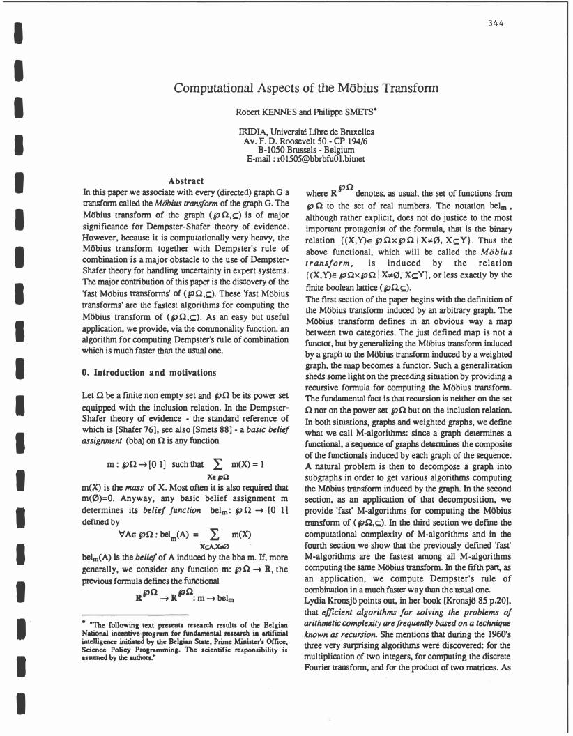
In this paper we associate with every (directed) graph G a transform called the MObius transf orm of the graph G. The Mobius transform of the graph (pO,�) is of major significance for Dempster-Shafer theory of evidence. However, because it is computationally very heavy, the Mobius transform together with Dempster's rule of combination is a major obstacle to the use of Dempster­Shafer theory for handling uncertainty in expert systems. The major contribution of this paper is the discovery of the 'fast Mobius transforms' of (PO.�). These 'fast Mt>bius transforms' are the fastest algorithms for computing the Ml>bius transform of (pO,�). As an easy but useful application, we provide, via the conunonality function, an algorithm for computing Dempster's rule of combination which is much faster than the usual one.

0. Introduction and motivations

Let 0 be a fmite non empty set and p 0 be its power set

equipped with the inclusion relation. In the Dempster­Shafer theory of evidence - the standard reference of which is [Shafer 76], see also [Smets 88] - a basic belief assignment (bba) on 0 is any function

m : p0-+[0 1] such that L m(X) = 1

XepO m(X) is the mass of X. Most often it is also required that m(0)=0. Anyway, any basic belief assignment m determines its belief function belm: p 0 -+ [0 11 defmed by

'VAe po: belm(A) = L m(X) Xs;A,X.c(J

belm(A) is the belief of A induced by the bba m. If, more generally, we consider any function m: pO-+ R, the previous formula defmes the functional

R�'0-+ R110: m-+ belm

• "The following text pmenu research mulu of t!'e B�gi� National incentive-prognm for fundamental research m artific�al intelligence initiated by lhe BeJaian Swe, Prime Minister's Office, Science Policy Proaramming. The scientific responsibility is assumed by lhe authors."

where R p 0 denotes, as usual, the set of functions from

p 0 to the set of real numbers. The notation belm , although rather explicit, does not do justice to the most important protagonist of the formula, that is the binary relation {(X,Y)e pOxpO I X�0. X�Y}. Thus the above functional, which will be called the Mobius t r a ns form, is induced by the relation {(X,Y)e poxpo I X�0. X�Y}, or less exactly by the

finite boolean lattice (pQ,�). The ftrst section of the paper begins with the defmition of the Mobius transform induced by an arbitrary graph. The Mobius transform defines in an obvious way a map between two categories. The just defined map is not a functor, but by generalizing the Ml>bius transform induced by a graph to the M�bius transform induced by a weighted graph, the map becomes a functor. Such a generalization sheds some light on the preceding situation by providing a recursive formula for computing the M()bius transform. The fundamental fact is that recursion is neither on the set 0 nor on the power set pO but on the inclusion relation. In both situations, graphs and weighted graphs, we defme what we call M-algorithms: since a graph determines a functional, a sequence of graphs determines the composite of the functionals induced by each graph of the sequence. A natural problem is then to decompose a graph into subgraphs in order to get various algorithms computing the MObius transform induced by the graph. In the second section, as an application of that decomposition, we provide 'fast' M-algorithms for computing the MObius transform of (pQ,�). In the third section we defme the computational complexity of M-algorithms and in the fourth section we show that the previously defmed 'fast' M-algorithms are the fastest among all M-algorithms computing the same Mobius transform. In the fJ.fth part, as an application, we compute Dempster's rule of combination in a much faster way than the usual one. Lydia Kronsjo points out, in her book [Kronsj() 85 p.20], that efficient algorithms for solving the problems of arithmetic complexity are frequently based on a technique known as recursion. She mentions that during the 1960's three very surprising algorithms were discovered: for the multiplication of two integers, for computing the discrete Fourier transform, and for the product of two matrices. As

a matter of fact all these efficient algorithms are based on recursive formulas. The present paper is in keeping with this observation. Due to lack of space, no proof will be given in this paper. All theorems are proved in [Kennes 90].

1. The Mobius functor

1.1 How graphs operate on functions

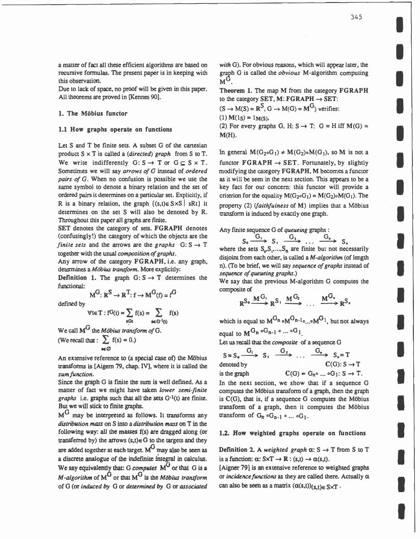
LetS and T be finite sets. A subset G of the cartesian productS x Tis called a (directed) graph from S to T.

We write indifferently G: S � T or G � S x T. Sometimes we will say arrows of G instead of ordere d pairs of G. When no confusion is possible we use the same symbol to denote a binary relation and the set of ordered pairs it determines on a particular set. Explicitly, if R is a binary relation, the graph {(s,t)e SxS I sRt) it determines on the set S will also be denoted by R. Throughout this paper all graphs are finite. SET denotes the category of sets. FGRAPH denotes (confusingly!) the category of which the objects are the finite sets and the arrows are the graphs G: S � T together with the usual composition of graphs. Any arrow of the category FGRAPH, i.e. any graph, determines a MObius transform. More explicitly: Definition 1. The graph G: S � T determines the fwlctional:

defined by

V'te T : fG(t) = I, f(s) = I, f(s) IGt MO-I(t)

We call � the Mobius tr�orm of G.

(We recall that: I, f(s) = 0.) M0

An extensive reference to (a special case of) the M()bius transforms is [Aigern 79, chap. IV], where it is called the sum [unction.

Since the graph G is flnite the sum is well defmed. As a matter of fact we might have taken lower semi-finite graphs i.e. graphs such that all the sets G·l(t) are flnite. But we will stick to fmite graphs.

MG may be interpreted as follows. It tranSforms any distribution mass on S into a distribution mass on T in the following way: all the masses f(s) are dragged along (or transferred by) the arrows (s,t)e 0 to the targets and they

are added together at each target ..tJ may also be seen as a discrete analogue of the indefmite iiue@'lll in calculus. We say equivalently that: G computes � or that G is a

M-algorithm of M0 or that M0 1s the Mobius transform

of G (or induced by G or determined by G or associated

345

with G). For obvious reasons, which will appear later, the g�h G is called ·the obvious M-algorithm computing

M .

Theorem 1. The map M from the category FGRAPH

to the category SET, M: FGRAPH �SET:

(S � M(S) = R5

, G � M(G) = M0) verifies:

(1) M( ls) = lM(S), (2) For every graphs G, H: S � T: G = H iff M(G) = M(H).

In general M(G2oG1) � M(G2)oM(GJ), so M is not a

functor FGRAPH � SET. Fortunately, by slightly modifying the category FG RAPH, M becomes a functor as it will be seen in the next section. 'This appears to be a key fact for our concern: this functor will provide a criterion for the equality M(G2oG1) = M(G:z)oM(Gt). The

propeny (2) (faithfulness of M) implies that a M�bius transform is induced by exactly one graph.

Any fmite sequence G of queUI!ing graphs :

So � St � � S. where the sets S0,S1, ••• ,S0 are finite but not necessarily

disjoint from each other, is called a M -algorithm (of length n). (To be brief, we will say seqUI!nce of graphs instead of sequence of QUI!UI!ing graphs.) We say that the previous M-algorithm G computes the composite of

S M Gt S MG2 R 0-----+ R I -----+

which is equal to M0n oM0n·1o ... oM01, but not always

equal to MOD oGn-1 0 ••• o01. Let us recall that the co1'71p0Site of a sequence G

G, G 2 G. S =So � St � � S. = T

denoted by C(G): S � T is the graph

In the next section, we show that if a sequence G computeS the MObius transform of a graph, then the graph is C(G), that is, if a sequence G computes the MObius transform of a graph, then it computes the Mtsbius transform of On oG0.1 o ... oG1.

l.l. How weighted graphs operate on functions

Definition l. A weighted graph a: S � T from S to T

is a function: a: SxT � R : (s,t) � a(s,t). [Aigner 791 is an extensive reference to weighted graphs

or incidence functions as they are called there. Actually a can also be seen as a matrix (a(s,t))(s,t)e SxT.

I I I

I

I I I I

I

I I I

I I I

I I

I

I

I

I

I

I

I

I

I I

I

I I

I

I

I I

I

I

I

I

The product of weigthed graphs is defmed as follows: Definition 3. If a. : S --+ T and P : T--+ U are two weighted graphs, their product a.•P is defmed by

a.•P (s,u) = L a.(s,t)·P(t,u) teT

This is in fact the product of the matrices a. and p. Each set S defines its identity weighted graph �s. the Kronecker function of S [Aigner 79 p.l40], which is the characteristic function of Is as a subset of SxS. The �s's are the identities of the product. As a consequence, we get the category WGRAPH the objects of which are the finite

sets and the arrows are the weighted graphs a: S --+ T together with the product. In the same way we defined the Mobius transform of a graph we define the M<>bius transform of a weighted graph. Definition 4. The weighted graph a.: S --+ T determines the following functional

� : RS --+ R T : f--+ Ma.(f) = f" defmed by

\>'te T: f<X(t) = L, f(s)·a.(s,t) seS

�will be called the Mobius transform of a. This is the product of the column-vector (f(s))se s by the matrix (a.(s,t))(s,t)e SxT. Ma may be seen as a discrete analogue of the Stieltjes indefinite integral in calculus and admits the same interpretation as M0 where the a(s,t) are scaling factors. Now, M turns out to be a functor. Theorem 2. The map M : WGRAPH --+ SET:

(S--+ M(S) = Rs, a--+ M(a) = M� from the category of weighted graphs to the category of sets is a functor we call the Mobius functor. This functor is faithful.

As in the case of graphs, we say that the following sequence of queueing weighted graphs

a.. CX z � So--'-+ S1 � . .. S. is aM-algorithm of weighted graphs (of length n) which computes the composite functional of

S �· S �z Ma.• S R0�R · � ... � R · In this case theorem 2 shows that the composite functional is also the MObius transform of CXJ* ••• •an: So--+ Sn. The following theorem is then simply another phrasing of the JRCeding theorem: Theorem l'. The following sequence of weighted graphs

346

S = So � s. � � S.=T computes the Mobius transform of (only of) a.t• ... •an .

We now provide a link between the two categories FGRAPH and WGRAPH.

Each graph G !:: SxT determines its weighted graph �G· the zeta-function of G [Aigner 79 p.l40], which is its characteristic function (except for its codomain) as a subset ofSxT:

l;c,: SxT --+ R : (s,t) --+ l;c,(s,t) �0(s,t) = 1 iff (s,t)e G and, �0(s,t) = 0 iff (s,t)E G.

It is trivial to see that: which means:

\>'fe R5 \>'te T : L, f(s).�0(s,t) = L f(s) -I seG (t) ses

Remark: For every fmite set S, the set of weighted graphs S --+ S, equipped with the operation of addition. with the real scalar multiplication and with the product is a R­

algebra. In this R-algebra, the inverse (if it exists) of l;a is called the Mobius function of G, which is not to be confused with the M<>bius transform of G.

Lemma 1. The sequence G G. 02 G.

S=So� s. � � S.= T computes the MObius transform of C(G) iff the sequence of weighted graphs

�01 �Gz �0. S=S0---'--+ s. (<� ••• � S.=T computes the MObius transform of l;c(G) . (and thus: �(G)= l;o.•l;<�z* ... •l;c,.) The following section examines the meaning of the equality �(G)= l;o.•l;oz • ... •l;o. 1.3. Graph decomposition

The need for decomposing graphs (relatively to •) will become clear when we will see that a decomposition of a graph may decrease its computational complexity. In fact, the basic idea to getting a 'fast MObius transform' is to decompose the inclusion relation of pn.

Definition 5. Let G be the following sequence of graphs 01 02 G. S =So---'-+ S 1 � ---'--+ S.= T

a path u of G is a n-tuple (g1, ... ,gJe G1x ... xG. such that 'lie { l, ... ,n-1}: target(&) = source(&.1). The source of u is the source of g1 , the target of u is the target of g0• Note

that contrary to the ordered pairs. the source and target of a path do not detennine a path. The set of paths with source in Xt:S and with wget in Yt:T is denoted by P0(X,Y). For the sake of brevity Po({s},{t}) is replaced by Po(s,t) .

The following map; P0(S,T) � G11o ... oG1: (glt····8n)

--+ gno ... ogl = 81···8n = (source(gt).target(gn)) defmes

the usual composition or product of arrows. The inverse of the preceding map gives for each arrow (s,t) the set of its factorizations of the form g •... g. where g,eG,. Lemma 2. If G is the following sequence of graphs

S=So � s. � . . . � S.=T then (�1•l;o2 • ••• •t;o.)(s,t) = #Po(S,t)

Saying that every arrow g of C (G) has a unique factorization of the form g1 ••• g. where g.e G, is equivalent

to saying that Po(S,T) � C(G): (g ..... ,g.) � g1 ••• g. is a bijection. So, finally we get the fundamental theorem: Theorem 3. Let G be the following sequence of graphs

01 G2 G. S=So � s. � � S .=T G computes the MlR>ius transform of a graph iff G computes the M6bius transform of the graph C(G): S � T

iff Po(S,T) � C(G) : (g ..... ,g.) � g1 ... g. is a bijection.

2. The Mobius transform of ( p O,t;:)

2.1 The fast Mobius transforms

Let us fust recall the notion of the Hasse graph of a partial order relation.

Definition 6. If (P .s) is a partially ordered set, then the reflexive Hasse graph of :Sis H(:S) = {(a,b)e PxP I a:Sb and �xe P: a<x � b�}: P � P. The non-reflexive

Hasse graph of (P,S) isH(<) =((a.b)e PxP I a<b and �xe P: a<x � �}. The transitive closure of H(:S): P � P is :S: P � P, and furthennore it is pan of the folklore that (with respect to the inclusion relation) H(:S) is the smallest subgraph of :S which meetS that property. Thus,

H(:S) is characterized by the two p-operties:

(1) T(H(:S)) =:Sand (2) T(G) = :S � H(:S) _t: G.

We recall that G is a M-algoritbm of M0. In this section we describe other M-algorilhm.s of M0, and we show in section 4 that all these M-algorithms are optimal for a specific complexity measure. The next theorem provides a family of M-algoritbms for computing the M6bius transform of G=((X,Y)e pnxpn I X�Y}. We call

347

these M-algorithms the Hasse M-algorithms of G or the fast Mobius transforms of G. Theorem 4. If 0 = {at,az, ... ,a11}, then the following M-algorithm H of length n:

Ht Hz H pn � pn � � ton

where Hi= ((X,Y)e pnxpnl Y=X or Y=Xu{ai}} computes the Mobius transfonn of G={(X,Y)e pnxpn\ Xt:Y}.

Note the fundamental fact: U(H) = H(t:) = H(G). That is the reason for also calling them the Hasse M-algorithms of G. If we take into account the condition X�. the previous theorem simply becomes: Theorem 4'. If n = {at,az, ... ,a0}, then the following M-algorithm H of length n :

Ht Hz H n pn � pn � . . . � pn

where

Hi= {(X,Y)e p Ox p n I X:;t0 and (Y=X or Y= Xu{ai})} computes the MObius transform of {(X,Y)e pOxpn I x�. Xt;:Y}.

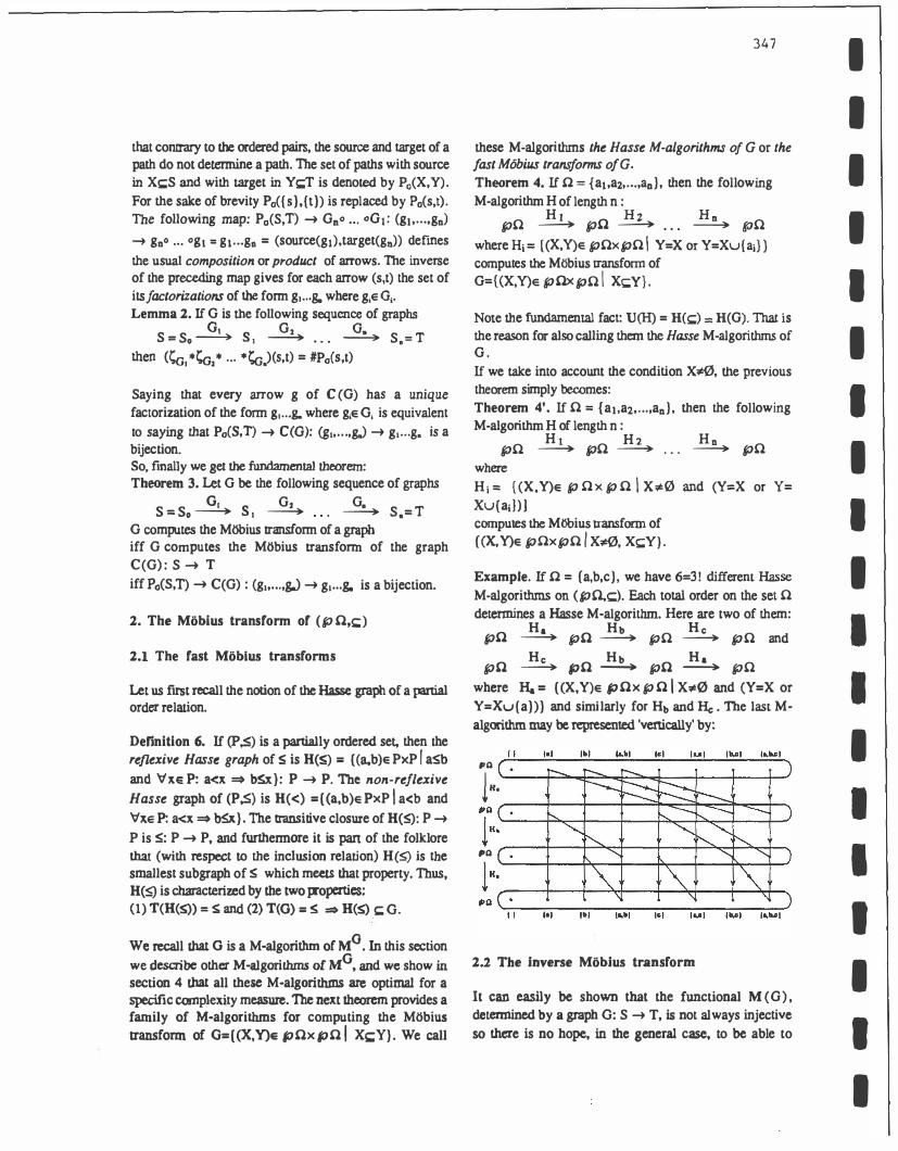
Example. If 0 = {a,b,c}, we have 6=3! different Hasse M-algoritbms on (pO.c). Each total order on the set n determines a Hasse M-algoritbm. Here are two of them:

Ha Hb He pn � pn � pn � pn and He Hb Ha

pn � pn ----+ pn � pn where Ha= {(X,Y)e pnxpniX'If0 and (Y=X or Y=Xu{a})} and similarly for Hb and He. The last M­algorithm may be represented 'vertically' by:

I'Q

l Ho 1'0�.---+---+--�--�������� !H·�---+---+��--�--������ fiQ

lH,�---+---+��--����--�--�

2.2 The inverse Mobius transform

It can easily be shown that the functional M (G), detennined by a graph G: S � T, is not always injective so there is no hope, in the general case, to be able to

I

I I

I

I I

I I I

I I I I

I I

I I

I I

I I I I

I I

I I I

I

I I

I I I I

I I

I

'reverse' (i.e. to get a left inverse of ) M(G). That means that there does not always exist a functional F: T -+ S such that: F o M(G) = 1 (the identity function on R5). The problem of the existence of an inverse has a nice solution in the more general setting of weighted graphs. In fact, if !;a has an inverse (for the product •), then because M is a functor we get: Ca • (!;o)·l = C15 and so we have: (M(I;o)tl o M(G) = 1 (the identity function on R5). The Mlibius inversion theorem gives a sufficient condition on the graph G for the functional M(� to be a bijection.

Mobius inversion theorem [Aigner 79 p.141]. For every partial order relation graph G:S-+ S, there exists a weighted graph J.1.o = <!;or1 such that: �G • llG =�IS= l1a. Co· The weighted graph lla = (!;oY1 is called the Mobius

function of G.lla= SxS-+ R : (s,t)-+ ll(S,t) is described recursively by:

'v'(s,t)e SxS: J.!<J(s,t) =- L Jl<;(s,x) =- L Jl<;(x,t) s�x<t s<x�t

with the following 'halting conditions': 'v's,te S: J.Lo(s,s) = 1, and llo(S.t) • 0 if (s,t)E G. There also exists an iterative formula [Birkhoff 61 p.15] and [Aigner 79 p.146]:

00

'v'(s,t)e SxS: J.l<;(s,t)"' L ( -l)i Ai(s,t) i•O

where M{s,t) = the number of chains of length i from s to t (i.e. totally ordered subsets of i+1 elements with s as minimum and t as maximum) For our concern we simply need to find the inverse (with respect to •) of the graph Hi ={( X,Y)e pOxpO I Y=X or Y=Xu{a 1} } . In this case. it can readily be verified either directly or by using the MObius inversion theorem that the following weighted graph is an inverse (hence the

inverse) of Hi· Ill: pOxp O-+ R , defined by: 'v'Xe p O: lli(X,X) = 1, lli( X,Xu{ail) = -1, else

lli<X. Y) = 0. Thus we get: Theorem 5. If 0 = {at.a2 .... ,2n}, then the following M­algorithm of weighted graphs computes the inverse Mlibius transform of (PO.�):

pn 2:4 pn � � pn where the J.4: pOxpO-+ Rare defmed by: V'Xe p n: lli(X,X) = 1, J.Li(X,Xu{ad) = -1, else

lli(X.Y) = 0.

348

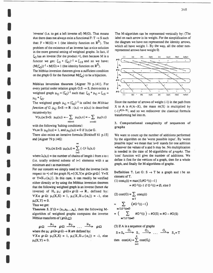
The M-algorithm can be represented vertically by: (The label on each arrow is its weight. For the simplification of the diagram we have not represented the identity arrows, which all have weight 1. By the way, all the other non­represented arrows have weight 0)

tel la.cl lb.cl la.b.cl PO ��������--�--������

1 �. PO r-----------���������--� !�;-----�-�� PO

1�.���-�

Since the number of arrows of weight ( -1) in the path from X to A is #(A-X), the mass m(X) is multiplied by ( -1 )#(A-X), and so we rediscover the classical formula transforming bel into m.

3. Computational complexity of sequences of graphs

We want to count up the number of additions performed by the algorithm on the 'worst possible input'. By 'worst possible input' we mean that 'a+b' stan� for one addition whatever the values of a and b may be. No multiplication is needed in the case of M-algoritbms of graphs. The 'cost' function will give the number of additions. We defme it first for the vertices of a graph. then for a whole graph. and fmally for M-algoritbms of graphs.

Definition 7. Let G: S -+ T be a graph and t be an element of T. (1) costo(t) = max{O,#G·l(t) -1}

= #G·l(t)-1 if G·l(t) ""0, else 0

(2) cost(G) = 2, costa(t) I&T

= 2, (#G·l(t)-1) I& T,G·1(t)ll0

= ( L #G·l(t) ) - #G(S) = #G- #G(S) •T,G"1(t)ol0

(3) If A is a sequence of graphs G, G2 G.

S=So � S, � � S.=T D

then cost(A) = L cost(Gi) j .. l

Examples: 1. Cost of the obvious M-algorithm G of M((X,Y)e pnxpn I x�0. X�Y)

We get: cost(G) = 3° -2°+1 + l, if #.Q = n

2. Cost of the Hasse M-algorithm H of M{(X,Y)e pnxpnl x�0. X�Y}

We get: cost(H) = n 2n-l- n, if #.Q = n

Comparison between the two M-algorithrns:

#.Q #p.Q cost( G) cost (H) 5 32 180 15 8 256 6 050 1 016

10 1 024 57002 5 110 12 4096 523 250 24564 15 32 768 14 283 372 245 745 20 106 3.109 I07

3. Cost of the Hasse M -algorithm of M� We get: cost(H) = n 2n-l , if #0 = n

cost(G)/cost(H) 2.4 5.9

11.1 21.3 58.1

332.3

4. Optimality of the fast Mobius transforms

The following theorem provides a lower bound for the complexity of the M-algorithrns computing the M<Sbius ttarunonnof afuti� l�tire. Theorem 6. Let (L$) be a fmite lattice. If A is aM­algorithm of graphs computing M:S, then cost(A) ;;:: cost(H(S)).

In fact a slightly more general result can be proved: Theorem 7. Let (P,:S) be a finite partially ordered set in which every upper bounded subset has a least upper bound. If A is a M-algorithm of graphs which compu�s Ms. then cost(A) ;;:: cost(H(:S)).

As a corollary of theorem 7 we get that the Hasse M­algorithms of (p n.�) are optimal among all M-

algorithrns computing �. Corollary 1. The fast Mobius transforms of

( p n,�) are optimal.

Let n = {a�oa2, ... .an} and (pO,�) be the corresponding fini� boolean Wtire. If (1) A is aM-algorithm of graphs

which computes M�. and (2) H is a Hasse M-algorithm

of M!;;

pn ...!!4 pn �

349

where Hi= {(X,Y)e pnxpnl Y=X or Y=Xu{ai}}, then cost( A)� cost(H).

We get the same result if we add the condition X* 0. Indeed: Corollary 2. The fast Mobius transforms for D·S theory are optimal.

Let n = {a�oa2, ... ,ao}. If (1) A is aM-algorithm of graphs which computes the Mobius transform M G of G={(X ,Y)e pnxpnl X;t0, X!;;Y}, and (2) H is the following algorithm :

Ht H2 Hn pn � pn � ... � pn where Hi= {(X,Y)e p nxpnlx�0 and (Y=X or Y=Xu{ai})}, then cost( A) � cost(H)

Remark: the condition 'every upper bounded subset has a least upper bound ' cannot be removed otherwise we get counter-examples.

S. Application

5.1 Statement of the problem

An application of the previous techniques to the computation of Demps�r rule of combination is shown in this last section. The framework is the Dempster-Shafer theory of evidence.

Most often, in DS theory, the easiest way to represent pieces of evidenre is by using basic belief assignments, say mt and m2. The mass distributions m1 and m2 are then combined together. Finally, the combined mass distribution m1®m2 is most easily interpreted when transformed back into its corresponding belief function and/or plausibility function. So, we in�d to compute the transformmon (m1,m2) � m1®m2 � Plm10m2: first, by using the usual algorithms, and second by using the fast algorithms developed in the preceding sections. Eventually we compare the cost, both in additions and in multiplications, of the two computing ways. Let us first briefly recall the defmitions of commonality function, plausibility function and Demps�r·s rule of combmmon.

5.2 Commonality functions

We have seen that the MObius transform induced by the relation ((X,Y)e pOxpn I x�0. X�Y) on pn is a functional which, in the D-S theory of evidence, is said to transform a basic belief assignment on pO into a belief

function. There are other interesting MObius transforms ( induced by other relations!), one of which transforms a

I

I I

I

I

I

I I I

I

I

I

I

I I

I

I

I I

I

I

I

I

I

I

I I

I

I

I

I

I

I

I

I

I

I

I

basic belief assignment into the so-called commonality function. Thus any basic belief assignment m determines its commonality function Qm: pn. � [0 1] defined by:

'VAe pD. : �(A)= L m(X) �A

Om(A) is the commonality number of A induced by the bba m. In our general setting this transform is the Mtibius transform induced by the relation {(X,Y)e pn.xpn. I JQY}. All that has been said for the relations [(X,Y)e pn.xgon I X'lf0, X�Y} and (X,Y)e pO.xpn I X�Y} applies as well for the relation

defining the commonality function. So we get (by reversing the arrows) the Theorem 8. If D.= {at,a2, ... ,a0), then the following M-algorithm H of length n :

Ht H2 H ""0. � ""0. � n ,..... If" II" • • • � p ....

where H1= {(X,Y)e pn.xpn. I Y=X or Y=X-{ail) computes the Mtibius transform of H={(X,Y)e pO.xpn. I X::2Y). Moreover, any other M-algorithm G computing M H satisfies cost(G)�cost(H).

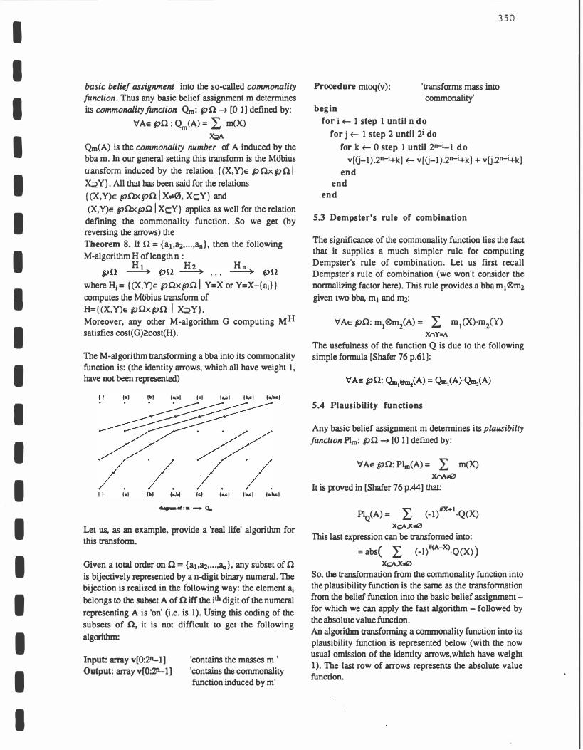
The M-algorithm transforming a bba into its commonality function is: (the identity arrows, which all have weight 1, have not been represented)

1•1

II 1•1

1�1 )a,�) )c)

...... 11:•-Q.

la.cl llo.cl la.lo.c)

, ... , ''"' , ..... ,

Let us, as an example, provide a 'real life' algorithm for this transform.

Given a total order on n = {a1,a2, ... .aa), any subset of n is bijectively represented by a n-digit binary numeral. The bijection is realized in the following way: the element a1 belongs to the subset A of n iff the ilh digit of the numeral representing A is 'on' (i.e. is 1). Using this coding of the subsets of n, it is not difficult to get the following algoothm:

Input: array v[0:2n_ 1] Output: array v[O:zn-1]

'contains the masses m ' 'contains the commonality function induced by m'

350

Procedure mtoq(v): 'transforms mass into commonality'

begin

for i +- 1 step 1 until n do

for j +- 1 step 2 until 2i do

for k +- 0 step 1 until 2n-L1 do

v[G-1).2°-4k] +- v[G-1).2°-4k] + vU.2°-4k] end

end end

5.3 Dempster's rule of combination

The significance of the commonality function lies the fact that it supplies a much simpler rule for computing Dempster's rule of combination. Let us first recall Dempster's rule of combination (we won't consider the normalizing factor here). This rule provides a bba m1®m2 given two bba, mt and m2:

'VAe pD.: m1®m2(A) = L m1(X)·miY) Xr\Y=A

The usefulness of the function Q is due to the following simple formula [Shafer 76 p.61]:

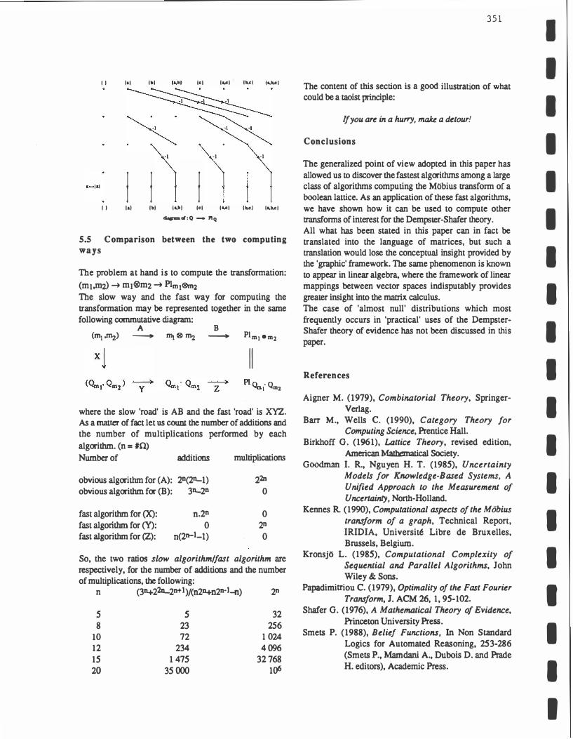
5.4 Plausibility functions

Any basic belief assignment m determines its plausibilty

function Plm: pD.� [0 1] defmed by:

'V Ae pD.: Plm(A) = L m(X) Xr>A,;0

It is proved in [Shafer 76 p.44] that:

Pl (A) "" (-l)#X+I.Q(X) Q = � X�,;0 This last expression can be transformed into:

= abs( L (- l)#(A-X)·Q(X)) X�ol0

So, the transformation from the commonality function into the plausibility function is the same as the transformation from the belief function into the basic belief assignment -for which we can apply the fast algorithm - followed by the absolute value furiction. An algorithm transforming a commonality function into its plausibility function is represented below (with the now usual omission of the identity arrows, which have weight 1). The last row of arrows represents the absolute value function.

II It) (b)

I I I I 1•1 I b)

·I

(c)

I (a,b) (c)

·I

diaFtmoi:Q- PIQ

(a,c) lb.cl (a,b,c)

·I

(a,c) lb.cl (t,b,c)

S.S Comparison between the two computing ways

The problem at hand is to compute the transformation:

(m1,m2) � m1®m2 � Plm1®m2 The slow way and the fast way for computing the transformation may be represented together in the same following commutative diagram:

A B (m,�) - Int®� - Plm,•mz

II Pl n ·Q

...., 1 mz

where the slow 'road' is AB and the fast 'road' is XYZ. As a matter of fact let us count the number of additions and the number of multiplications performed by each algorithm. (n = #0) Number of additions multiplications

obvious algorithm for (A): 2D(21L1) obvious algorithm for (B): 3JL2n

fast algorithm for (X): fast algorithm for (Y): fast algorithm for (Z):

n.2n 0

n(2n-Lt)

22n 0

0 2D 0

So, the two ratios slow algorithm/fast algorithm are respectively, for the number of additions and the number of multiplications. the following:

n (31422JL2n+l)f(n2J4n2D·Ln) 2D

5 8

10 12 15 20

s 23 72

234 1 475

35000

32 256

1 024 4096

32 768 106

351

The content of this section is a good illustration of what could be a taoist principle:

If you are in a hurry, maJce a detour!

Conclusions

The generalized point of view adopted in this paper has allowed us to discover the fastest algorithms among a large class of algorithms computing the MObius transform of a boolean lattice. As an application of these fast algorithms, we have shown how it can be used to compute other transforms of interest for the Dempster-Shafer theory. All what has been stated in this paper can in fact be translated into the language of matrices, but such a translation would lose the conceptual insight provided by the 'graphic' framework. The same phenomenon is known to appear in linear algebra. where the framework of linear mappings between vector spaces indisputably provides greater insight into the matrix calculus. The case of 'almost null' distributions which most frequently occurs in 'practical' uses of the Dempster­Shafer theory of evidence has not been discussed in this paper.

References

Aigner M. (1979), Combinatorial Theory, Springer­Verlag.

Barr M., Wells C. (1990), Category Theory for Computing Science, Prentice Hall.

Birkhoff G. (1961), Lattice Theory, revised edition, American Mathematical Society.

Goodman I. R., Nguyen H. T. (1985), Uncertainty Models for Knowledge-Based Systems, A Unified Approach to the Measurement of Uncertainty, North-Holland.

Kennes R. (1990), Computational aspects of the Mobius transform of a graph, Technical Report, IRIDIA, Universit� Libre de Bruxelles, Brussels, Belgium.

KronsjO L. (1985), Computational Complexity of Sequential and Parallel Algorithms, John Wiley & Sons.

Papadimitriou C. (1979), Optimality of the Fast Fourier Transform, J. ACM 26, 1, 95-102.

Shafer G. (1976), A Mathematical Theory of Evidence, Princeton University Press.

Smets P. (1988), Belief Functions, In Non Standard Logics for Automated Reasoning, 253-286 (Smets P., Mamdani A., Dubois D. and Prade H. editors), Academic Press.

I

I

I

I

I

I

I I

I

I

I

I

I

I I

I

I

I

I