Compression of periodic images for faster phase retrieval

Compression of periodic images forfaster phase retrieval

Amos Talmi1 and Erez N. Ribak2,*1Timi Technologies, Ltd., Ramat Hashofet 19238, Israel

2Department of Physics, Technion–Israel Institute of Technology, Haifa 32000, Israel

*Corresponding author: [email protected]

Received 27 April 2010; revised 9 August 2010; accepted 20 August 2010;posted 27 September 2010 (Doc. ID 127595); published 0 MONTH 0000

In fringe analysis, or in projected grids for shape-from-shade, deviations from periodicity are used forfinding phase changes. In another example, a Hartmann–Shack sensor produces a deformed grid of spotson a camera. The gradients of the original wavefront are calculated from that image by centroiding thespots or by demodulating them. The computation time rises linearly with the number of pixels in theimage. We introduce a method to reduce the size of the image without loss of accuracy prior to the cal-culation to reduce the total processing time. The compressed result is superior to an image measuredwith reduced resolution. Hence, higher accuracy and speed are obtained by oversampling the image andreducing it correctly prior to calculations. Compression or expansion coefficients are calculated throughthe requirement to maintain the integrity of the original phase data. © 2010 Optical Society of AmericaOCIS codes: 150.0150, 220.4840, 100.2650, 100.5070, 010.7350, 010.1080.

1. Analyzing Periodic Images

The image of a small source through a Hartmann–Shack (HS) sensor is a grid of light spots, separatedby dark areas. Distortion of the phase of the incomingwavefront causes those spots to move from their ori-ginal position [Fig. 1(a)]. The phase deviations arecalculated from those movements [1,2]. The observedlight spots are quantized by the pixels of the image.Smaller pixels (or a magnified image) produce moreaccurate positions of the spots (relative to the inter-spot distances). One prefers a very large image, witha large pitch (distance in pixels) between adjacentlight spots. On the other hand, processing time is pro-portional to the total number of pixels in the image.Hence, one would prefer a smaller image with ashorter pitch for quicker processing. We are facedwith the problem of wishing to have many pixelsper period for accuracy and at the same time havingfewer pixels for faster data processing. A similar con-

tradiction occurs in projected grid profilometry andin fringe analysis.

How to resolve this conflict? We propose to recordthe image using a large pitch between the light spots,then to reduce the image in a smart manner, and pro-cess the reduced image. The gain is enormous: usingevery second column in x and every second row in ywould reduce the processing time by a factor of 4. Ifthe original image has a pitch of 18, and we reduce itin each dimension by four, to get an effective pitch of18=4 ¼ 4:5, we reduce the computation time by a fac-tor of 16. Such a compression method should retainthe higher accuracy in the spot positions. Simplebinning of pixels does not conserve this accuracy. In-stead, we suggest a compounded binning, where theintensity of the source pixel is divided among a fewclose destination pixels in the compressed image.The internal division among the destinations ischosen so as to conserve the HS phases. For example,let us assume that we wish to compress the one-dimensional pixel array fI1; I2; I3; I4;…g by a factorof 2, into fI12; I34; I56;…g. An ideal binning formulawould allow one to reconstruct the originalfI1; I2; I3; ;…g from the reduced fI12; I34; I56;…g

0003-6935/10/320001-01$15.00/0© 2010 Optical Society of America

10 November 2010 / Vol. 49, No. 32 / APPLIED OPTICS 1

using an interpolation formula with few errors. Thesimplest binning rule is I12 ¼ I1 þ I2, I34 ¼ I3 þ I4,and a restoration formula of I3 ¼ 1=2I34. This causeslarge restoration errors. A better procedure could beI034 ¼ 1=4I2 þ 3=4I3 þ 3=4I4 þ 1=4I5 and a restora-tion formula of I3 ¼ 3=4I034 þ 1=4I012, which is moreaccurate (provided that the image varies slowly). Inour case, we are interested in accurate positions oflight spots. An ideal binning, for us, would have bothfI1; I2; I3; I4;…g and fI012; I034; I056…g yield identicalcenter-of-mass (or centroid) results.

We assess the quality of the reduction by compar-ing the processed results of the input images versusthe reduced ones. Our aim is to reduce the image insuch a way that the calculated wavefront gradientswill remain true. The wavefront is assumed to besampled densely enough, such that its gradient var-ies smoothly between grid points. We exploit this factto expand the gradient as a two-term Taylor series,with the error given by the third term. The reductioncoefficients are tailored to keep the two terms exact.

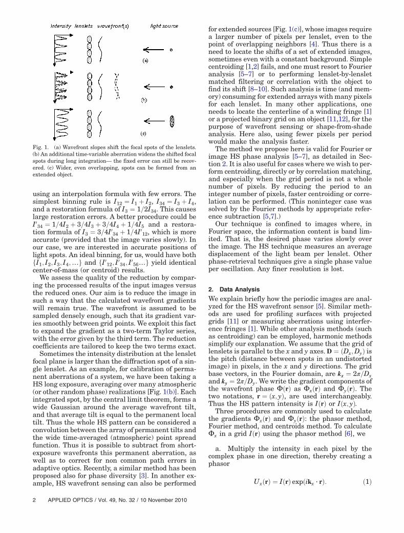
Sometimes the intensity distribution at the lensletfocal plane is larger than the diffraction spot of a sin-gle lenslet. As an example, for calibration of perma-nent aberrations of a system, we have been taking aHS long exposure, averaging over many atmospheric(or other random phase) realizations [Fig. 1(b)]. Eachintegrated spot, by the central limit theorem, forms awide Gaussian around the average wavefront tilt,and that average tilt is equal to the permanent localtilt. Thus the whole HS pattern can be considered aconvolution between the array of permanent tilts andthe wide time-averaged (atmospheric) point spreadfunction. Thus it is possible to subtract from short-exposure wavefronts this permanent aberration, aswell as to correct for non common path errors inadaptive optics. Recently, a similar method has beenproposed also for phase diversity [3]. In another ex-ample, HS wavefront sensing can also be performed

for extended sources [Fig. 1(c)], whose images requirea larger number of pixels per lenslet, even to thepoint of overlapping neighbors [4]. Thus there is aneed to locate the shifts of a set of extended images,sometimes even with a constant background. Simplecentroiding [1,2] fails, and one must resort to Fourieranalysis [5–7] or to performing lenslet-by-lensletmatched filtering or correlation with the object tofind its shift [8–10]. Such analysis is time (and mem-ory) consuming for extended arrays with many pixelsfor each lenslet. In many other applications, oneneeds to locate the centerline of a winding fringe [1]or a projected binary grid on an object [11,12], for thepurpose of wavefront sensing or shape-from-shadeanalysis. Here also, using fewer pixels per periodwould make the analysis faster.

The method we propose here is valid for Fourier orimage HS phase analysis [5–7], as detailed in Sec-tion 2. It is also useful for cases where we wish to per-form centroiding, directly or by correlation matching,and especially when the grid period is not a wholenumber of pixels. By reducing the period to aninteger number of pixels, faster centroiding or corre-lation can be performed. (This noninteger case wassolved by the Fourier methods by appropriate refer-ence subtraction [5,7].)

Our technique is confined to images where, inFourier space, the information content is band lim-ited. That is, the desired phase varies slowly overthe image. The HS technique measures an averagedisplacement of the light beam per lenslet. Otherphase-retrieval techniques give a single phase valueper oscillation. Any finer resolution is lost.

2. Data Analysis

We explain briefly how the periodic images are anal-yzed for the HS wavefront sensor [5]. Similar meth-ods are used for profiling surfaces with projectedgrids [11] or measuring aberrations using interfer-ence fringes [1]. While other analysis methods (suchas centroiding) can be employed, harmonic methodssimplify our explanation. We assume that the grid oflenslets is parallel to the x and y axes. D ¼ ðDx;DyÞ isthe pitch (distance between spots in an undistortedimage) in pixels, in the x and y directions. The gridbase vectors, in the Fourier domain, are kx ¼ 2π=Dxand ky ¼ 2π=Dy. We write the gradient components ofthe wavefront phase ΦðrÞ as ΦxðrÞ and ΦyðrÞ. Thetwo notations, r ¼ ðx; yÞ, are used interchangeably.Thus the HS pattern intensity is IðrÞ or Iðx; yÞ.

Three procedures are commonly used to calculatethe gradients ΦxðrÞ and ΦyðrÞ: the phasor method,Fourier method, and centroids method. To calculateΦx in a grid IðrÞ using the phasor method [6], we

a. Multiply the intensity in each pixel by thecomplex phase in one direction, thereby creating aphasor

UxðrÞ ¼ IðrÞ expðikx · rÞ: ð1Þ

Fig. 1. (a) Wavefront slopes shift the focal spots of the lenslets.(b) An additional time-variable aberration widens the shifted focalspots during long integration— the fixed error can still be recov-ered. (c) Wider, even overlapping, spots can be formed from anextended object.

2 APPLIED OPTICS / Vol. 49, No. 32 / 10 November 2010

b. Smooth by averaging: use a flat sliding-win-dow FSðrÞ, the window being a rectangle of sizeDx ×Dy:

WxðrÞ ¼ FSðrÞ ⊗ UxðrÞ

¼ ðDxDyÞ−1XDx

u¼1

XDy

ν¼1

Ux

�uþ x −

12Dx; νþ y

−12Dy

�: ð2Þ

Repeat this smoothing once or twice more. In gener-al, get a phasorWðrÞ by smoothingUðrÞwith a kernelFðrÞ or WðrÞ ¼ FðrÞ ⊗ UðrÞ.

c. Extract the phase of the phasor, Φx ¼argfWðrÞg. The amplitude jWxðrÞj represents thesmoothed intensity of the spots inside the pupil. Itis assumed for the time being that all spots areequally bright and the amplitude is constant.

d. The gradient of the wavefront is proportionalto that phase Φx, related through the pitch andthe focal length. In other applications the surface re-lief is proportional to Φx.

e. Starting with multiplication with phaseexpðiky · rÞ, repeat steps (a)–(c) to obtain Φy.

The double-pass flat window is equivalent to a tri-angular kernel, and a third pass smooths it evenfurther into a bell shape similar to 1þ cosðxÞ. Otherwindows or convolution kernels were also proposed[9,10], to be used in a single pass.

As an intuitive explanation, assume that theimage is composed of a single spot of light of ampli-tude A at ðx0; y0Þ, plus some constant backgroundC. Multiplying IðrÞ by the phase expðix2π=DÞ givesUxðx; yÞ ¼ C expðix2π=DÞ þ δðx−x0Þδðy − y0ÞA expðix02π=DÞ. Averaging over D,the constant term C oscillates and averages tozero, while the concentrated peak contributesA expðix02π=DÞ. Hence, the phase of the average isexactly x02π=D—proportional to the peak position.If the peak is two or three pixels wide, the resultantphase is the center of mass of the peak. If the image isalmost periodic with period D, the next cell wouldhave a similar peak at position x0 þD and contributeexactly the same phase; hence, one could averageover a few neighboring cells and get the same result.Refer to [2] for a detailed analysis.

Performing the process by the Fourier method isessentially the same, with a slightly differentsmoothing kernel f ðxÞ ¼ sinðπxÞ=ðx − x3Þ [5,7]. Theequivalent steps are a0 and a00 replacing (a) and b0and b00 replacing (b):

a0. Calculate the (fast) Fourier transform of the im-age, ~IðqÞ ¼ FfIðrÞg.

a00. Translate the transform by the reciprocal wavevector, ~IxðqÞ ¼ ~Iðq − kxÞ.

b0. Cut the high-frequency values by some low-passfilter AðqÞ, ~WxðqÞ ¼ AðjqjÞ~IxðqÞ.

b00. Inverse transform the result into the spatialdomain, WxðrÞ ¼ F−1f ~WxðqÞg.

The resultant WxðrÞ is similar to the phasor ofstage (b) above. Both methods are identical if AðqÞ(step b0) is a Fourier transform of the kernel FðrÞ.Note that the direct phasor method is quicker be-cause it skips the transformations into the Fourierspace and back.

The centroid method finds the positions of thespots by calculating their centers of mass. The gradi-ent Φ is proportional to the displacement of the spotfrom the unperturbed position, divided by the focallength. Here the image is divided into cells aroundeach unperturbed spot. The cell number ðμ; νÞ is ofdimensionsDx ×Dy, centered on an unperturbed spotat ðμDx; νDyÞ. The intensity of light in this cell isIμ;νðrÞ where r varies inside the cell. The centroidof each cell is the spot position, �rμ;ν ¼ hrIμ;νðrÞi=Iμ;νðrÞ. Using FðrÞ ¼ 1 for −D=2 < r < D=2, FðrÞ ¼ 0;otherwise, the intensity in each cell may be writtenas Iμ;νðx; yÞ ¼ Iðx; yÞFðμDx − x; νDy − yÞ and the cen-troid is

�rμ;ν ¼ �rðμDx; νDyÞ

¼

Px0;y0

r0FðμDx − x0; νDy − y0ÞIðx0; y0ÞPx0;y0

FðμDx − x0; νDy − y0ÞIðx0; y0Þ ;

xμ;ν ¼ limw→0

1wargfFðrÞ ⊗ IðrÞeiwxg;

yμ;ν ¼ limw→0

1wargfFðrÞ ⊗ IðrÞeiwyg: ð3Þ

Hence, Eq. (3) is a special case of the phasor meth-od where [step (c) above] Φx ¼ argfFðrÞ ⊗ UðrÞg,with a boxcar kernel F, and w replacing jkj ofEq. (1). Note that ðμ; νÞ are integers, as well as thepixels x0 and y0, while the cell boundaries are frac-tional; border pixels contribute partly to one cell,partly to the other. In general, the centroid methodis very sensitive to slow variation in the averagebackground illumination, and some threshold algo-rithm must be used. Also, the spots must lie withinthe unperturbed cells, namely, the displacementsmust be less than D=2.

Some may argue that the optimal smoothing FðrÞshould be rotation invariant, others may choose de-composable Fðx; yÞ ¼ F1ðxÞF2ðyÞ, and some othersmay proclaim that FðrÞ should not be symmetric:Fðx; yÞ ≠ Fðy; xÞ. For Φx it is Fðx; yÞ, and for Φy it isFðy; xÞ. Our reduction scheme applies equally wellto all such cases. We only require that it scaleswith the pitch, FðDx;Dy; x; yÞ ¼ Fðx=Dx; y=DyÞ. Theexamples cited below use Fðx=Dx; y=DyÞ ¼ Fðx=DxÞFðy=DyÞ, because the equations are simpler inthis case.

3. Image Reduction or Expansion

If the pitch, D, is an integer, the calculations are sim-pler. First, operations such as the moving average,


centroiding, or correlations are normally defined forinteger-size windows. Fractional-size windows re-quire interpolations. In practice, the design may aimat D ¼ 16 and end with (measured) D ¼ 15:87 pixels.In addition, it sometimes turns out that Dx ≠ Dy. Forinstance, with resonant acousto-optic lenslets [4,13],the pitch is set by the cell dimensions. If we are goingto change the image dimensions, why not aim atconvenient integer pitch values D ¼ Dx ¼ Dy?

Resizing physical images is a trivial operation: usea different zoom setting of the camera lens. Once theimage is digitized, resizing requires approximate in-terpolation formulas. Two well-known methods arewidely used for reduction by an integer factor, sayby R. The first one is binning, where each group ofR pixels is represented by a single pixel whose valueis the average of the original R values. The other oneis sampling, where that value is one of the R values,usually the central. Those conventional binningmethods treat every group separately. We use a dif-ferent binning process, where the representing valuefor the group is influenced by values of pixels in near-by groups. We introduce a scheme that works withany resizing factor, integer or real, and producesmuch more accurate results for HS images.

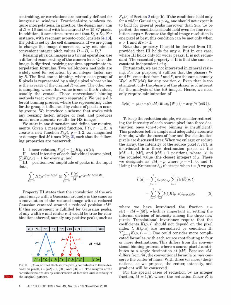
We start in one dimension and define our require-ments. Given a measured function, IðtÞ, t ¼ 1; 2…ncreate a new function I0ðgÞ, g ¼ 1; 2…m, magnifiedor demagnifiedM times (Fig. 2), such that the follow-ing properties are preserved:

I. linear relation, I0ðgÞ ¼ PtKðg; tÞIðtÞ;

II. total intensity of each individual source pixel,PtKðg; tÞ ¼ 1 for every g; andIII. position and amplitude of peaks in the input

data,

X∞t¼−∞

IðtÞe−ðt−cÞ2=2σ2 ≅X∞g¼−∞

I0ðgÞM

e−ðg−cMÞ2=2σ2M2:

Property III states that the convolution of the ori-ginal image with a Gaussian around c is the same asa convolution of the reduced image with a reducedGaussian centered around a reduced position cM00.If this requirement is fulfilled for Gaussian peaks,of any width σ and center c, it would be true for com-binations thereof, namely any positive peaks, such as

FSðrÞ of Section 2 step (b). If the conditions hold onlyfor a wider Gaussian, σ > σ0, one should not expect itto hold for general peaks narrower than 2σ0. To beperfect, the conditions should hold even for fine reso-lution steps σ. Because the digital image resolution isone pixel at best, this condition can be met only whenσ > 1 and Mσ > 1.

Note that property II could be derived from III,provided that III holds for any σ. But in our case,where III holds only for wider peaks, II is not redun-dant. The essential property of II is that the sum is aconstant independent of g.

Fortunately, we are not interested in general resiz-ing. For our purpose, it suffices that the phasors WandW 0, smoothed from I and I0, are the same, namelyWðcÞ ≅ W 0ðcMÞ for any position c. Even that is toostringent: only the phase φ of the phasor is of interestfor the analysis of the HS images. Hence, we needonly require minimization of

δφðcÞ ¼ φðcÞ − φ0ðcMÞ≡ argfWðcÞg − argfW 0ðcMÞg:ð4Þ

To keep the reduction simple, we consider redirect-ing the intensity of each source pixel into three des-tination ones (one-to-two binning is insufficient).This produces both a simple and adequately accurateformula, while the cases of four and five destinationpixels are discussed later. When we enlarge or reducethe array, the intensity of the source pixel t, IðtÞ, isdistributed into three destination pixels at the½tM� − 1, ½tM�, and ½tM� þ 1 positions, where ½x� isthe rounded value (the closest integer) of x. Thesewe designate as ½tM� þ p where p ¼ −1, 0, and 1.Using the Kronecker δi;j (0 except when i ¼ j) we get

I0ðgÞ ¼X1p¼−1

δg;½tM�þp

Xnt¼1

IðtÞKðp; tÞ

¼X1p¼−1

Xnt¼1

IðtÞKðp; sÞδg−p;½tM�; ð5Þ

where we have introduced the fraction s ¼sðtÞ ¼ tM − ½tM�, which is important in setting theinternal division of intensity among the three newpixels. Translational invariance require that thecoefficients Kðp; sÞ should not depend on the pixelindex t. Kðp; sÞ are normalized by condition II:P

1p¼−1 Kðp; sÞ ¼ 1. One could consider more compli-

cated formulas, with each source contributing to fouror more destinations. This differs from the conven-tional binning process, where a source pixel t contri-butes to a single destination at ½tM�. Because ½tM�differs from tM, the conventional formula cannot con-serve the center of mass. With three (or more) desti-nations, as we propose, the center, intensity, andgradient will be conserved.

For the special cases of reduction by an integerfraction, M ¼ 1=R, where the reduction factor R is

Fig. 2. (Color online) Each source pixel j contributes to three des-tination pixels, l ¼ ½jM� − 1, ½jM�, and ½jM� þ 1. The weights of thecontributions are set by conservation of location and intensity ofthe original pattern.4/CO


an integer, the solution is simpler, as there are onlyRpossible values of s. Enumerating them by d, s ¼ d=R,we explicitly insert the Kronecker delta and get

I0ðgÞ ¼XR−1d¼0

X1p¼−1

XN=R

t¼0

IðtRþ dÞKðp;dÞδg;tþ½dM�þp; ð6Þ

andP

pKðp;dÞ ¼ 1. There are exactly 3R coefficientsK . This number of coefficients is much fewer than 3n,required for general reduction (or expansion).

Now we wish to find the values of the coefficientsK , demanding conservation of the phasors: the onecalculated from the original image, WðrÞ ¼FðrÞ ⊗ UðrÞ, should have the same phase as theone calculated from the resized image W 0ðr0Þ ¼F0ðr0Þ ⊗ U 0ðr0Þ [see step (b) in Section 2]. For an arbi-trary point c, those are

WðcÞ ¼X∞t¼−∞

IðtÞeiktF�t − cD

�;

W 0ðcMÞ ¼X∞g¼−∞

I0ðgÞM

eikg=MF

�g − cMDM

�;

where F is the smoothing kernel, and k ¼ 2π=D. Min-or errors near the edges are ignored. Rewriting I0 interms of I [Eq. (5)] we get

WðcÞ ¼X∞t¼−∞


�;

W 0ðcMÞ ¼X∞

t;g¼−∞

X1p¼−1

IðtÞKðp; sÞδg−p;½tM�

× eikg=MF

�g − cMDM

�:

Using the definition of the fractions ¼ sðtÞ ¼ tM − ½tM�, we write ½tM� as tM − s, andthe Kronecker delta differs from zero wheng ¼ tM þ p − s, thus

W 0ðcMÞ ¼X∞t¼−∞

X1p¼−1

IðtÞF�tM þ p − s − cM

DM

�

× Kðp; sÞeikðtMþp−sÞ=M

¼Xt

IðtÞeiktXp

F

�t − cD

þ p − sDM

�Kðp; sÞ

× eþikðp−sÞ=M: ð7Þ

The formula forW 0ðcMÞ is identical to the formula forWðcÞ, except the summation over p. The smoothingkernel is smooth itself and is expanded as a Taylorseries:

F

�t − cD

þ p − sDM

�¼ F

�t − cD

�þ p − s

DMF0�t − cD

�

þ 12

�p − sDM

�2F00

�t − cD

þ α�; ð8Þ

where 0 < α < ðp − sÞ=ðMDÞ. Substituting into Eq. (7)and comparing the terms for each eitk we get from thezeroth derivative


�¼ IðtÞeiktF

�t − cD

�Xp

Kðp; sÞeikðp−sÞ=M:

ð9Þ

And from the first derivative

0 ¼ IðtÞeiktF0�t − cD

�Xp

p − sDM

Kðp; sÞeikðp−sÞ=M:

The conditions are

1 ¼X1p¼−1

Kðp; sÞeik0ðp−sÞ;

0 ¼X1p¼−1

ðp − sÞKðp; sÞeik0ðp−sÞ;

where k0 ¼ k=M. These are two complex conditions,solvable by two complex K coefficients, resulting ina complex reduced image. This valid mathematicaloption—a complex image—introduces physicalcomplications we prefer to avoid. Writing eiρ ¼cos ρþ i sin ρ, ρ ¼ k0ðp − sÞ, we get four real equationsfor each s (fraction) value, which we wish to solvewith only three real variables Kðp; sÞ. Because weare interested in conserving the phase of W, whileamplitudes are of secondary importance [if at all,see Eq. (4)], we choose the three real relations:

1 ¼X1p¼−1

Kðp; sÞ cos½k0ðp − sÞ�; 0

¼X1p¼−1

Kðp; sÞ sin½k0ðp − sÞ�; 0

¼X1p¼−1

ðpþ sÞKðp; sÞ sin½k0ðp − sÞ�:

With the solution


Kðp; sÞ ¼ 3p2 − 2sin½k0ðp − sÞ� ·

12cotanðk0sÞ þ cotan½k0ð1 − sÞ� þ cotan½k0ð−1 − sÞ� : ð10Þ

Thus for each source pixel t in the original array I,we first calculate the fraction s ¼ tM − ½tM�. Next wecalculate the three coefficients Kð−1; sÞ, Kð0; sÞ, andKð1; sÞ using Eq. (10). Then we distribute IðtÞ amongthe three target pixels g ¼ ½tM� − 1, ½tM�, ½tM� þ 1 ofthe resized array I0 as IðtÞKð−1Þ, IðtÞKð0Þ, andIðtÞKð1Þ (Fig. 2). The total I0ðgÞ is the sum of all suchcontributions [Eq. (6)].K depends on k0, the wave vec-tor in the new image k0 ¼ k=M ¼ 2π=ðD;MÞ.

We have chosen to conserve the real part of the in-tensity, rather than the intensity of the peak. Thisminute change, using cos½k0ðp − sÞ� instead of 1, hasa negligible effect. In general, the optimal relationswould have both 1 ¼ P

pKðp; sÞ and 1 ¼ PpKðp; sÞ×

cos½k0ðp − sÞ�.The centroid method [Eq. (3)] has the same two

complex conditions, in the limit of w (or k) tendingto zero [Eq. (3)]. Those complex conditions are fullysatisfied by [in the limit k → 0, expðikxÞ is 1]

Kð−1; sÞ ¼ ðjsj − sÞ=2;Kð0; sÞ ¼ 1 − jsj;Kð1; sÞ ¼ ðjsj þ sÞ=2: ð11Þ

Note that one of the three constants is identicallyzero, and it is a linear interpolation two-termformula.

For five target pixels, we only provide the final va-lues. The corresponding five-term formula is reachedby using the following parameters (notice that the or-der of indices is inverted for clarity later):

a1 ¼ sinðk0sÞ= sin k0;

B2 ¼ 12½s cosðk0sÞ − a1 cos k0�;

B1 ¼ 12a1 − 2B2 cos k0; A2 ¼ 2sB2;

A1 ¼ 12a1 − 4A2 cos k0;

A0 ¼ cosðk0sÞ − 2A1 cos k0 − 2A2 cosð2k0Þ;Kð0; sÞ ¼ A0; Kð�1; sÞ ¼ A1 � B1;

Kð�2; sÞ ¼ A2 � B2: ð12Þ

4. Errors

The error δφ [Eq. (4)] is the difference in the phasebetween the original and final arrays, argfWðcÞg−argfW 0ðcMÞg. It is caused by two different contribu-tions. First, terms with the second derivative of thesmoothing kernel F were ignored [Eq. (8)]. The smal-

ler the second derivative, the smaller is the relativeerror ε:

ε ¼ 12

�pþ sDM

�2F00

�t − cD

þ α�=F

�t − cD

�: ð13Þ

Second, the interpolation formula employs threeterms, rather than five or more, and does not con-serve the total number of photons, losing some accu-racy. Weighted against the smaller error is the factthat interpolation formulas with fewer terms aremore robust and less prone to artifacts (the higherthe order, the more sensitive it is to noise).

This error estimation has two hidden assumptions—that the kernel F has finite second derivatives, andthat F scales exactly with the expansion factor M.When this is not true, as is the case of a single-passmoving average (a boxcar integrator), one should usea more detailed analysis (if possible). Fortunately,this case is not of importance. Boxcar integrationis used by the plain-vanilla centroid method. Modernversions [14] augment this with correlations,matching filters, or other operations. Such compli-cated centroid variations are best analyzed by simu-lations, as in [14].

The second case of interest is double-pass smooth-ing, used in the phasors method (Section 2). The con-volution kernel for the double-pass moving averageis FðxÞ ¼ D − jxj. The second derivative {actuallythe second difference, ½f ðxþ 1Þ þ f ðx − 1Þ − 2f ðxÞ�=2}, is zero except at x ¼ −D, 0, D. Hence the error is

δφðcÞ ¼ argfW 0ðcMÞg − argfWðcÞg

¼ argXp;g;t

IðtÞIðgÞF�t − cD

�F

�g − cþ ðp − sÞ=M

D

�

× Kðp; sÞeikðg−tÞþikðp−sÞ=M

¼ argXp;g;t

IðtÞIðgÞ½D − jt − cj�½D

− jg − c − ðp − sÞ=Mj�Kðp; sÞeikðg−tÞþikðp−sÞ=M:

Again, because Kðp; sÞ conserves linear terms, onlyterms with jg − c − ðp − sÞ=Mj ¼ 0, �D contribute anyimaginary parts. An exact estimate is complicated;instead, we investigated the behavior by actual com-putations, or simulations.

We assume a practical situation: the pitch D is notan exact integer, and one cannot align a chosen spotto fall exactly in the center or edge of a pixel, but atsome fraction of it. This means that the original im-age includes—right from the start—some samplingand quantization errors, in addition to noise-inducederrors. The light distribution is sampled pixel by


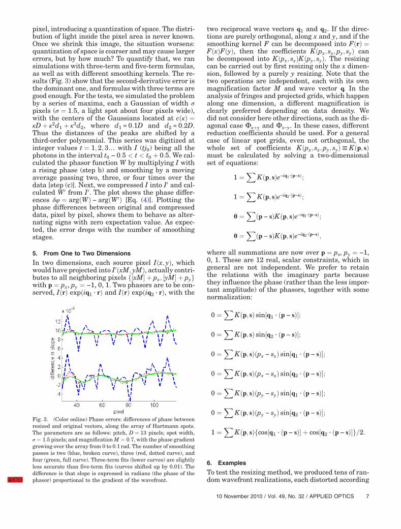
pixel, introducing a quantization of space. The distri-bution of light inside the pixel area is never known.Once we shrink this image, the situation worsens:quantization of space is coarser andmay cause largererrors, but by how much? To quantify that, we ransimulations with three-term and five-term formulas,as well as with different smoothing kernels. The re-sults (Fig. 3) show that the second-derivative error isthe dominant one, and formulas with three terms aregood enough. For the tests, we simulated the problemby a series of maxima, each a Gaussian of width σpixels (σ ¼ 1:5, a light spot about four pixels wide),with the centers of the Gaussians located at cðκÞ ¼κDþ κ2d1 þ κ3d2, where d1 ≈ 0:1D and d2 ≈ 0:2D.Thus the distances of the peaks are shifted by athird-order polynomial. This series was digitized atinteger values t ¼ 1; 2; 3… with I (tj0) being all thephotons in the interval t0 − 0:5 < t < t0 þ 0:5. We cal-culated the phasor function W by multiplying I witha rising phase (step b) and smoothing by a movingaverage passing two, three, or four times over thedata [step (c)]. Next, we compressed I into I0 and cal-culated W 0 from I0. The plot shows the phase differ-ences δφ ¼ argðWÞ − argðW 0Þ [Eq. (4)]. Plotting thephase differences between original and compresseddata, pixel by pixel, shows them to behave as alter-nating signs with zero expectation value. As expec-ted, the error drops with the number of smoothingstages.

5. From One to Two Dimensions

In two dimensions, each source pixel Iðx; yÞ, whichwould have projected into I0ðxM; yMÞ, actually contri-butes to all neighboring pixels f½xM� þ px; ½yM� þ pygwith p ¼ px, py ¼ −1, 0, 1. Two phasors are to be con-served, IðrÞ expðiq1 · rÞ and IðrÞ expðiq2 · rÞ, with the

two reciprocal wave vectors q1 and q2. If the direc-tions are purely orthogonal, along x and y, and if thesmoothing kernel F can be decomposed into FðrÞ ¼FðxÞFðyÞ, then the coefficients Kðpx; sx;py; syÞ canbe decomposed into Kðpx; sxÞKðpy; syÞ. The resizingcan be carried out by first resizing only the x dimen-sion, followed by a purely y resizing. Note that thetwo operations are independent, each with its ownmagnification factor M and wave vector q. In theanalysis of fringes and projected grids, which happenalong one dimension, a different magnification isclearly preferred depending on data density. Wedid not consider here other directions, such as the di-agonal case Φxþy and Φx−y. In these cases, differentreduction coefficients should be used. For a generalcase of linear spot grids, even not orthogonal, thewhole set of coefficients Kðpx; sx;py; syÞ≡ Kðp; sÞmust be calculated by solving a two-dimensionalset of equations:

1 ¼X

Kðp; sÞe−iq1·ðp−sÞ;

1 ¼X

Kðp; sÞe−iq2·ðp−sÞ;

0 ¼X

ðp − sÞKðp; sÞe−iq1·ðp−sÞ;

0 ¼X

ðp − sÞKðp; sÞe−iq2·ðp−sÞ;

where all summations are now over p ¼ px, py ¼ −1,0, 1. These are 12 real, scalar constraints, which ingeneral are not independent. We prefer to retainthe relations with the imaginary parts becausethey influence the phase (rather than the less impor-tant amplitude) of the phasors, together with somenormalization:

0 ¼X

Kðp; sÞ sin½q1 · ðp − sÞ�;

0 ¼X

Kðp; sÞ sin½q2 · ðp − sÞ�;

0 ¼X

Kðp; sÞðpx − sxÞ sin½q1 · ðp − sÞ�;

0 ¼X

Kðp; sÞðpx − sxÞ sin½q2 · ðp − sÞ�;

0 ¼X

Kðp; sÞðpy − syÞ sin½q1 · ðp − sÞ�;

0 ¼X

Kðp; sÞðpy − syÞ sin½q2 · ðp − sÞ�;

1 ¼X

Kðp; sÞfcos½q1 · ðp − sÞ� þ cos½q2 · ðp − sÞ�g=2:

6. Examples

To test the resizing method, we produced tens of ran-dom wavefront realizations, each distorted according

Fig. 3. (Color online) Phase errors: differences of phase betweenresized and original vectors, along the array of Hartmann spots.The parameters are as follows: pitch, D ¼ 13 pixels; spot width,σ ¼ 1:5 pixels; and magnificationM ¼ 0:7, with the phase gradientgrowing over the array from 0 to 0:1 rad. The number of smoothingpasses is two (blue, broken curve), three (red, dotted curve), andfour (green, full curve). Three-term fits (lower curves) are slightlyless accurate than five-term fits (curves shifted up by 0.01). Thedifference is that slope is expressed in radians (the phase of thephasor) proportional to the gradient of the wavefront.4/CO


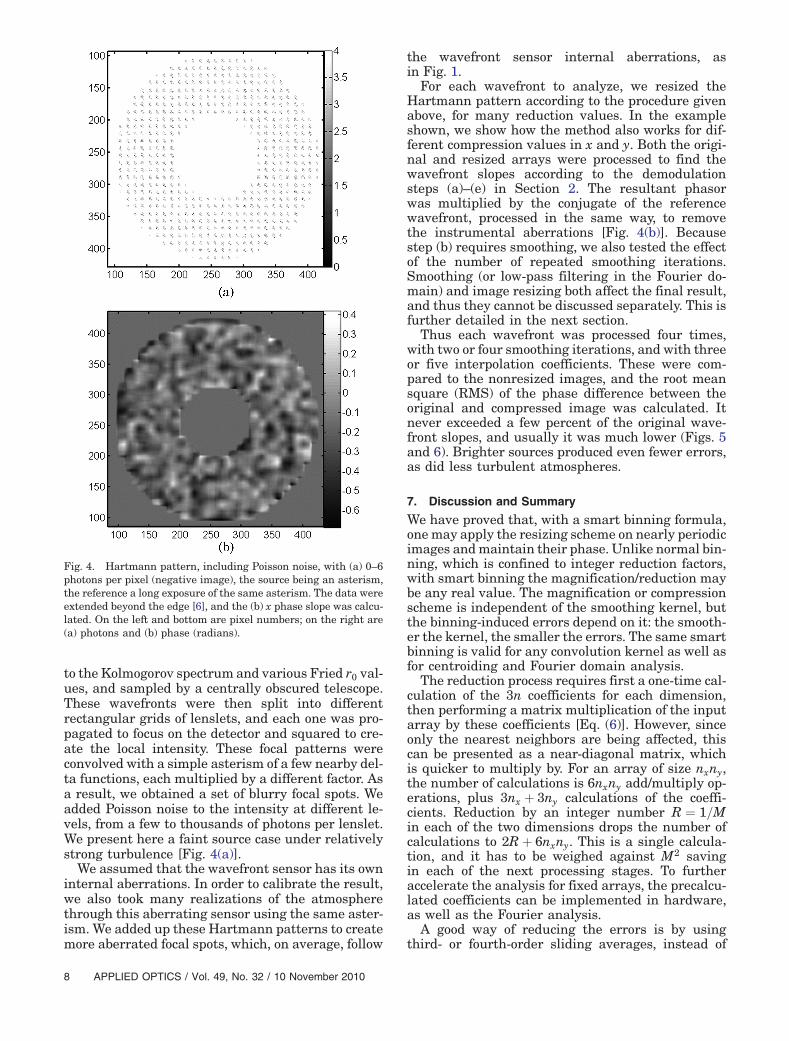
to the Kolmogorov spectrum and various Fried r0 val-ues, and sampled by a centrally obscured telescope.These wavefronts were then split into differentrectangular grids of lenslets, and each one was pro-pagated to focus on the detector and squared to cre-ate the local intensity. These focal patterns wereconvolved with a simple asterism of a few nearby del-ta functions, each multiplied by a different factor. Asa result, we obtained a set of blurry focal spots. Weadded Poisson noise to the intensity at different le-vels, from a few to thousands of photons per lenslet.We present here a faint source case under relativelystrong turbulence [Fig. 4(a)].

We assumed that the wavefront sensor has its owninternal aberrations. In order to calibrate the result,we also took many realizations of the atmospherethrough this aberrating sensor using the same aster-ism. We added up these Hartmann patterns to createmore aberrated focal spots, which, on average, follow

the wavefront sensor internal aberrations, asin Fig. 1.

For each wavefront to analyze, we resized theHartmann pattern according to the procedure givenabove, for many reduction values. In the exampleshown, we show how the method also works for dif-ferent compression values in x and y. Both the origi-nal and resized arrays were processed to find thewavefront slopes according to the demodulationsteps (a)–(e) in Section 2. The resultant phasorwas multiplied by the conjugate of the referencewavefront, processed in the same way, to removethe instrumental aberrations [Fig. 4(b)]. Becausestep (b) requires smoothing, we also tested the effectof the number of repeated smoothing iterations.Smoothing (or low-pass filtering in the Fourier do-main) and image resizing both affect the final result,and thus they cannot be discussed separately. This isfurther detailed in the next section.

Thus each wavefront was processed four times,with two or four smoothing iterations, and with threeor five interpolation coefficients. These were com-pared to the nonresized images, and the root meansquare (RMS) of the phase difference between theoriginal and compressed image was calculated. Itnever exceeded a few percent of the original wave-front slopes, and usually it was much lower (Figs. 5and 6). Brighter sources produced even fewer errors,as did less turbulent atmospheres.

7. Discussion and Summary

We have proved that, with a smart binning formula,one may apply the resizing scheme on nearly periodicimages andmaintain their phase. Unlike normal bin-ning, which is confined to integer reduction factors,with smart binning the magnification/reduction maybe any real value. The magnification or compressionscheme is independent of the smoothing kernel, butthe binning-induced errors depend on it: the smooth-er the kernel, the smaller the errors. The same smartbinning is valid for any convolution kernel as well asfor centroiding and Fourier domain analysis.

The reduction process requires first a one-time cal-culation of the 3n coefficients for each dimension,then performing a matrix multiplication of the inputarray by these coefficients [Eq. (6)]. However, sinceonly the nearest neighbors are being affected, thiscan be presented as a near-diagonal matrix, whichis quicker to multiply by. For an array of size nxny,the number of calculations is 6nxny add/multiply op-erations, plus 3nx þ 3ny calculations of the coeffi-cients. Reduction by an integer number R ¼ 1=Min each of the two dimensions drops the number ofcalculations to 2Rþ 6nxny. This is a single calcula-tion, and it has to be weighed against M2 savingin each of the next processing stages. To furtheraccelerate the analysis for fixed arrays, the precalcu-lated coefficients can be implemented in hardware,as well as the Fourier analysis.

A good way of reducing the errors is by usingthird- or fourth-order sliding averages, instead of

Fig. 4. Hartmann pattern, including Poisson noise, with (a) 0–6photons per pixel (negative image), the source being an asterism,the reference a long exposure of the same asterism. The data wereextended beyond the edge [6], and the (b) x phase slope was calcu-lated. On the left and bottom are pixel numbers; on the right are(a) photons and (b) phase (radians).


the second-order one we have advocated before(Fig. 5). The cost is a small loss of spatial resolutionand of time. The gain is a drop in binning-inducederrors, as well as elimination of phase jumps and vor-tices due to defective lenslets and phasors with neg-ligible intensity. A blocked lenslet transmits no light,causing phasors dominated by random noise; a half-blocked lenslet causes a nonsymmetric light spot anderrors in spot position [15]. A third-order smoothingeffectively replaces a blocked lenslet with a ghost ofits neighbor lenslets. In general, it averages the lens-let intensity with ghosts of its neighbors. Fourth-order smoothing sums farther neighbors, too. In thecorresponding Fourier analysis (steps a0, b0 of Sec-tion 2) a low-pass filter plays a similar role. We usedthe window function cos2ðqxÞcos2ðqyÞ.

There are a few pitfalls to note and avoid:

1. Applying the same smoothing kernel for boththe reduced and the unreduced images, namely, thesame function of the pitch D. This is natural if onesmooths with a Gaussian or any other mathematicalfilter that is defined for real numbers. In the case of

the sliding sum [steps (a), (b) above], or centroiding,where operations are normally defined for an integernumber of pixels, this may require interpolation. Forinstance, if the original image had been reduced by2:27 × 2:46, and if the reduced image is smoothedby summing over 4 × 4 pixels, this is equivalent tosmoothing the original image by 9:04 × 9:84 pixels.In general, simple smoothing over some (integer) P ×Q window in the compressed image corresponds to acomputation-intensive smoothing over MP ×MQwindow in the original image.

2. The position of the average, for instance theaverage of pixels jþ 1 through jþ 14 should be at-tributed to jþ 7:5 {which is then compressed into apixel ½ðjþ 7:5ÞM�}.

3. Edge problems: edges need to be excluded orimages extended before resizing. The same appliesto smoothing operations. If there is no informationnear the edge (the HS pattern is smaller than themeasured array), this is trivial: one extends the imageby adding rows and columns of zeros around, then dis-cards results influenced by those extra pixels. Other-wise, one should expand the HS image smartly,adding extra lines/columns whose values depend onthe known boundary ones [6,7,16]. In general, reduc-tion by a factor RðR > 1Þ requires extra T lines andcolumns on each side, where T ¼ ceilð1:5RÞ for thethree-term formula. Three-pass smoothing adds1:5D to T; four-pass smoothing adds 2D.

4. The case of zero amplitude. Measured HSimages are usually composed of an aperture withspots of light, surrounded by a region with only back-ground noise. Any calculation of spot shifts outsidethe aperture is doomed to failure: there are no lensletsthere. Some of the lenslets may be partiallyoccluded by the aperture andprovide limited informa-tion [15]. Outside the aperture, the amplitude of thephasor W drops to zero and the phase is pure noise.This is in contrast with our assumption that the pha-sor has constant amplitude. We employed a mechan-ism to flag points with phasors smaller (in amplitude)than a fraction of the average amplitude. This wasused in Fig. 4 to set the aperture borders as well.The same caution applies to cases of wavefront vor-tices or simply dirty lenslets, where the amplitudealso drops to zero. The unreliable pixels were givena constant value, equal to the average of all others.In shape-from-shade problems (profiling by projectedgrids), the same problem occurs when changing fa-cets, where the grid lines might seem to run in a dif-ferent direction, helping also to find the facet edges.

5. Low signal cases. In stellar adaptive optics,where the number of photons is extremely limited,the division of photons into many pixels increasesboth shot noise and readout noise, and the benefitsof large-format detectors are limited. This factor isless important now, with the recent introduction ofvery low noise detectors and with the need for posi-tion accuracy brought about by more pixels per spot.All large new telescopes (with diameter > 25m) areplanned to have more than eight pixels per spot.

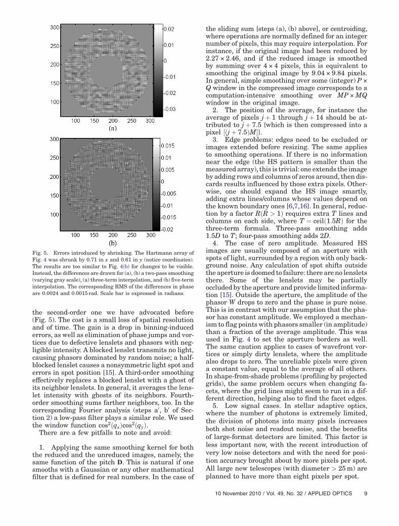
Fig. 5. Errors introduced by shrinking. The Hartmann array ofFig. 4 was shrunk by 0.71 in x and 0.61 in y (notice coordinates).The results are too similar to Fig. 4(b) for changes to be visible.Instead, the differences are drawn for (a), (b) a two-pass smoothing(varying gray scale), (a) three-term interpolation, and (b) five-terminterpolation. The corresponding RMS of the differences in phaseare 0.0024 and 0:0015 rad. Scale bar is expressed in radians.


6. Deviations from periodicity. We choose an op-timal smart binning formula, in the sense that byusing appropriate procedures, both the original im-age and the reduced one produce the same results.If the period is known in advance to be nonconstant,such as in closed fringes or a HS pattern of a largedefocus, then the compression coefficients will notbe global, but they might still be calculated locally.

Our method compresses grossly oversampledimages, and it should be compared to other compres-sions methods applied to images with similar infor-mation content, namely, slowly changing phases. Theoversampling comes about because D ×D pixels(where D is the pitch) are used to record the x–y posi-tion and the intensity of a single peak. That is, asmany as D2 values are used where three should suf-fice. Ng and Ang [17] propose three figures of merit,to quantify compressions:

1. compression ratio, in pixels: (number of com-pressed pixels)/(number of original pixels);

2. compression ratio, in bits or bytes: (length ofcompressed file)/(length of original file); and

3. root mean square error: jQ ðcompressedÞ−Q ðoriginalÞj, where Q is the desired quantity, suchas phase versus position.

Using this terminology, our pixel compression ratiois exactly M2, where M is the magnification ratio. Inbytes, our compression is 1=2M2, because the inten-sity in the new image must use 16, not 8, bits. Therange of possible magnifications is limited by Ny-quist: the pitch in the compressed image must beD0 > 2, and practicallyD0 > 3. Under such limitation,the compression ratio is D2=9.

What about errors? We constructed our compres-sion formula to produce zero errors in the ideal case.We tested our method with noisy data, and found it toproduce results Q (compressed) very close to the ori-ginal Q, with ΔQ much smaller than the expectednoise in Q (Section 3 and Fig. 2). Figure 7 sum-marizes many simulations: the RMS of the difference(peaks in the reduced image minus their location be-fore reduction). The figure demonstrates that veryhigh levels of noise in the input have some influenceover the produced differences. In general, five termsare better than three terms. But spreading the infor-mation over more than a single cell, while the phasevaries largely from cell to cell, is not recommended:that is, using a five-term formula for a case of outputpitch of three pixels (a full cell is 3 × 3 pixels),produces higher errors than a three-term formula.Thus, the five-term formula should only be usedwhen D0 ≥ 4.

Alfalou and Brosseau [18] considered a muchwider scope of compressions, both before and after

Fig. 6. Errors introduced in reduction from Fig. 4 by 0.71 in x and0.61 in y, as in Fig. 5, but with further smoothing and thus lowererrors. The difference between the original and the reduced slopeis shown for (a), (b) a four-pass smoothing (varying gray scale),(a) three-term interpolation, and (b) five-term interpolation. Thecorresponding RMS differences are 0.0014 and 0.0012 radians.

Fig. 7. Root mean square shift in the location of the peaks beforeand after reduction, in differently reduced images and differentnoise levels. An input image (as in Figs. 4–6) with a pitch of 16pixels was reduced to various pitches as marked, both with N ¼3 and N ¼ 5 terms formulas. The indicated peak intensities Iare realizations of 3�p

3, 12�p12 and 36�p

36 photons.Results were calculated using a four-pass smoothing, and areexpressed in pixels of the reduced images.


processing, including schemes of reducing the imagesfor storage and transmission, such as JPEG orJPEG2000 specially modified to the task at hand.In this respect, our work is very limited: after proces-sing, the only relevant information is the position ofthe peak. That is, a compression ratio of D2. We dealtonly with a preprocessing operation, so we did notimprove, nor impair, this D2 ratio. Perhaps a specialversion of wavelet compression, constructed to con-serve both amplitude and position of peaks, coulddo better than our method. The gain, however, couldnot be larger than a factor of 2: at the very least, fourpixels must define a peak in x and y, while our tech-nique allows for nine pixels per peak.

A test version of the program is available at http://physics.technion.ac.il/~eribak/reduce.

This work was supported in part by the France–Israel Research Cooperation fund, the Israel ScienceFoundation (ISF), and by the Ministry of IndustryMagnet program. E. R. wishes to thank C. Daintyand the Walton Fellowship of Science FoundationIreland. The comments of anonymous reviewershelped improve this presentation.

References1. D. Malacara, ed., Optical Shop Testing (Wiley, 1978).2. R. K. Tyson, Principles of Adaptive Optics, 2nd ed.

(Academic, 1998).3. L. M. Mugnier, J.-F. Sauvage, T. Fusco, A. Cornia, and

S. Dandy, “On-line long-exposure phase diversity: a powerfultool for sensing quasi-static aberrations of extreme adaptiveoptics imaging systems,”Opt.Express16, 18406–18416 (2008).

4. E. N. Ribak, “Harnessing caustics for wave-front sensing,”Opt. Lett. 26, 1834–1836 (2001).

5. Y. Carmon and E. N. Ribak, “Phase retrieval by demodulationof a Hartmann–Shack sensor,” Opt. Commun. 215, 285–288(2003).

6. A. Talmi and E. N. Ribak, “Direct demodulation ofHartmann–Shack patterns,” J. Opt. Soc. Am. A 21, 632–639(2004).

7. C. Canovas and E. N. Ribak, “Comparison of Hartmannanalysis methods,” Appl. Opt. 46, 1830–1835 (2007).

8. T. Berkefeld, D. Soltau, and O. von der Luhe, “Multi-conjugateadaptive optics at the Vacuum Tower Telescope, Tenerife,”Proc. SPIE 4839, 66–76 (2002).

9. L. Poyneer, “Scene-based Shack–Hartmann wave-frontsensing: analysis and simulation,” Appl. Opt. 42, 5807–15(2003).

10. S. Özder, Ö. Kocahan, E. Coskun, and H. Göktas, “Opticalphase distribution evaluation by using an S-transform,”Opt. Lett. 32 591–593 (2007).

11. D. M. Meadows, W. O. Johnson, and J. B. Allen, “Generation ofsurface contours by moiré patterns,” Appl. Opt. 9, 942–947(1970).

12. G. S. Spagnolo, G. Guattaria, C. Sapia, D. Ambrosini,D. Paoletti, and G. Accardo, “Contouring of artwork surfaceby fringe projection and FFT analysis,” Opt. Lasers Eng.33, 141–156 (2000).

13. A. Stup, E. M. Cimet, E. N. Ribak, and V. Albanis, “Acousto-optic wave front sensing and reconstruction,” Appl. Opt. 48,A1–A4 (2009).

14. S. Thomas, T. Fusco, A. Tokovinin, M. Nicolle, V. Michau, andG. Rousset, “Comparison of centroid computation algorithmsin Shack–Hartmann sensor,” Mon. Not. R. Astron. Soc. 371,323–336 (2006).

15. Y. Carmon and E. N. Ribak, “Centroid distortion of a wave-front with varying amplitude due to asymmetry in lens dif-fraction,” J. Opt. Soc. Am. A 26, 85–90 (2009).

16. A. Talmi and E. N. Ribak, “Wavefront reconstruction from itsgradients,” J. Opt. Soc. Am. A 23, 288–97 (2006).

17. T. Ng and K. Ang, “Fourier-transform method of data com-pression and temporal pattern analysis,” Appl. Opt. 44,7043–7049 (2005).

18. A. Alfalou and C. Brosseau, “Optical image compression andencryption methods,” Adv. Opt. Photon. 1, 589–636(2009).


http://physics.technion.ac.il/~eribak/reduce





Compression of periodic images for faster phase retrieval

Documents

Transcript of Compression of periodic images for faster phase retrieval