Components of Grizzly Bear Habitat Selection: Density, Habitats, Roads, and Mortality Risk

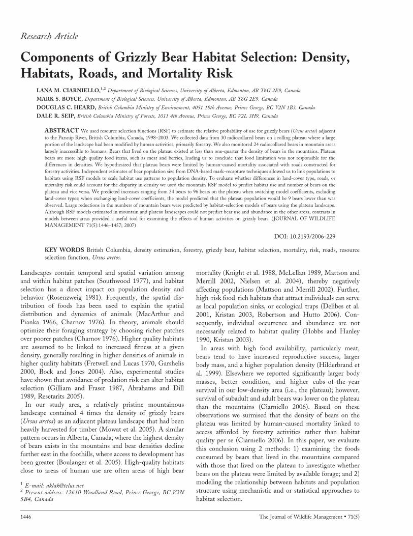
Research Article

Components of Grizzly Bear Habitat Selection: Density,Habitats, Roads, and Mortality Risk

LANA M. CIARNIELLO,1,2 Department of Biological Sciences, University of Alberta, Edmonton, AB T6G 2E9, Canada

MARK S. BOYCE, Department of Biological Sciences, University of Alberta, Edmonton, AB T6G 2E9, Canada

DOUGLAS C. HEARD, British Columbia Ministry of Environment, 4051 18th Avenue, Prince George, BC V2N 1B3, Canada

DALE R. SEIP, British Columbia Ministry of Forests, 1011 4th Avenue, Prince George, BC V2L 3H9, Canada

ABSTRACT We used resource selection functions (RSF) to estimate the relative probability of use for grizzly bears (Ursus arctos) adjacent

to the Parsnip River, British Columbia, Canada, 1998–2003. We collected data from 30 radiocollared bears on a rolling plateau where a large

portion of the landscape had been modified by human activities, primarily forestry. We also monitored 24 radiocollared bears in mountain areas

largely inaccessible to humans. Bears that lived on the plateau existed at less than one-quarter the density of bears in the mountains. Plateau

bears ate more high-quality food items, such as meat and berries, leading us to conclude that food limitation was not responsible for the

differences in densities. We hypothesized that plateau bears were limited by human-caused mortality associated with roads constructed for

forestry activities. Independent estimates of bear population size from DNA-based mark–recapture techniques allowed us to link populations to

habitats using RSF models to scale habitat use patterns to population density. To evaluate whether differences in land-cover type, roads, or

mortality risk could account for the disparity in density we used the mountain RSF model to predict habitat use and number of bears on the

plateau and vice versa. We predicted increases ranging from 34 bears to 96 bears on the plateau when switching model coefficients, excluding

land-cover types; when exchanging land-cover coefficients, the model predicted that the plateau population would be 9 bears lower than was

observed. Large reductions in the numbers of mountain bears were predicted by habitat-selection models of bears using the plateau landscape.

Although RSF models estimated in mountain and plateau landscapes could not predict bear use and abundance in the other areas, contrasts in

models between areas provided a useful tool for examining the effects of human activities on grizzly bears. ( JOURNAL OF WILDLIFE

MANAGEMENT 71(5):1446–1457; 2007)

DOI: 10.2193/2006-229

KEY WORDS British Columbia, density estimation, forestry, grizzly bear, habitat selection, mortality, risk, roads, resourceselection function, Ursus arctos.

Landscapes contain temporal and spatial variation amongand within habitat patches (Southwood 1977), and habitatselection has a direct impact on population density andbehavior (Rosenzweig 1981). Frequently, the spatial dis-tribution of foods has been used to explain the spatialdistribution and dynamics of animals (MacArthur andPianka 1966, Charnov 1976). In theory, animals shouldoptimize their foraging strategy by choosing richer patchesover poorer patches (Charnov 1976). Higher quality habitatsare assumed to be linked to increased fitness at a givendensity, generally resulting in higher densities of animals inhigher quality habitats (Fretwell and Lucas 1970, Garshelis2000, Bock and Jones 2004). Also, experimental studieshave shown that avoidance of predation risk can alter habitatselection (Gilliam and Fraser 1987, Abrahams and Dill1989, Resetarits 2005).

In our study area, a relatively pristine mountainouslandscape contained 4 times the density of grizzly bears(Ursus arctos) as an adjacent plateau landscape that had beenheavily harvested for timber (Mowat et al. 2005). A similarpattern occurs in Alberta, Canada, where the highest densityof bears exists in the mountains and bear densities declinefurther east in the foothills, where access to development hasbeen greater (Boulanger et al. 2005). High-quality habitatsclose to areas of human use are often areas of high bear

mortality (Knight et al. 1988, McLellan 1989, Mattson andMerrill 2002, Nielsen et al. 2004), thereby negativelyaffecting populations (Mattson and Merrill 2002). Further,high-risk food-rich habitats that attract individuals can serveas local population sinks, or ecological traps (Delibes et al.2001, Kristan 2003, Robertson and Hutto 2006). Con-sequently, individual occurrence and abundance are notnecessarily related to habitat quality (Hobbs and Hanley1990, Kristan 2003).

In areas with high food availability, particularly meat,bears tend to have increased reproductive success, largerbody mass, and a higher population density (Hilderbrand etal. 1999). Elsewhere we reported significantly larger bodymasses, better condition, and higher cubs-of-the-yearsurvival in our low-density area (i.e., the plateau); however,

survival of subadult and adult bears was lower on the plateauthan the mountains (Ciarniello 2006). Based on theseobservations we surmised that the density of bears on theplateau was limited by human-caused mortality linked toaccess afforded by forestry activities rather than habitatquality per se (Ciarniello 2006). In this paper, we evaluatethis conclusion using 2 methods: 1) examining the foodsconsumed by bears that lived in the mountains comparedwith those that lived on the plateau to investigate whetherbears on the plateau were limited by available forage; and 2)modeling the relationship between habitats and population

structure using mechanistic and or statistical approaches tohabitat selection.

1 E-mail: [email protected] Present address: 12610 Woodland Road, Prince George, BC V2N5B4, Canada

1446 The Journal of Wildlife Management � 71(5)

Recent habitat-modeling techniques suggest a way to linkhabitat selection and population structure (Rosenweig andAbramsky 1997, Boyce and McDonald 1999, Manly et al.2002, Boyce and Waller 2003), but the efficacy of thatapproach has never been tested. Habitats for animals can bemodeled using resource selection functions (RSF; Manly etal. 2002). Although these models are simply statisticaldescriptions of use of the landscape, RSF models can belinked to populations if reference areas exist where densitiesare known (Boyce and McDonald 1999). By combining theresults of DNA mark–recapture population estimation withhabitat-based density-modeling techniques it is possible todistribute density across the landscape. In particular,habitat-based density modeling can be used to evaluatewhether differences in density is attributable to differencesin habitat, roads, and or the risk of human-caused mortality.We think that such a link between land-cover features andpopulation models may provide useful insights into theconsequences of human activities on wildlife populations.

STUDY AREA

The 18,096-km2 study area was centered along the ParsnipRiver in central-eastern British Columbia, Canada(548390N, 122836 0W; Fig. 1). The ecosection line, asdelineated by the British Columbia Ministry of Water,Land and Air Protection (Victoria, BC, Canada), representsa topographic division between a plateau (10,624 km2) thatcontained rolling hills and flat valleys, and the west and eastslopes of the Hart Ranges of the Rocky Mountains (7,472km2). Elevations ranged from 600 m to 1,650 m in theplateau, and 720 m to 2,550 m in the mountains. Theplateau was warmer and had less precipitation than themountains (x̄¼ 2.68 C, 72 cm rainfall, 300 cm snowfall vs. x̄

¼ 0.38 C, 154 cm rainfall, 700 cm snowfall; DeLong et al.1993, 1994).

The subboreal spruce (SBS) biogeoclimatic zone domi-nated the plateau and some lower-elevation areas in themountains (e.g., along major rivers). Most forests on theplateau were a mix of white spruce (Picea glauca), pine (Pinus

contorta), and subalpine fir (Abies lasiocarpa). Black spruce(Picea mariana) bogs occurred in lower elevation wet areas.Interior Douglas-fir (Pseudotsuga menziesii) occurred insmall portions on the plateau and lower elevation mountainvalley bottoms. Aspen (Populus tremuloides), cottonwood (P.

balsamifera), and paper birch (Betula papyrifera) were presentwithin these forests, especially along riparian areas and inareas disturbed by logging or wildfires.

The Engelmann spruce–subalpine fir zone occurred abovethe SBS and dominated the mountainous portion of thestudy area. Higher elevation mountain habitats consisted ofsubalpine parkland predominantly comprised of subalpine firand Engelmann spruce (P. engelmannii). Subalpine mead-ows supported forbs such as glacier lily (Erythronium

grandiflorum), Indian hellebore (Veratrum viride), andarrow-leaved groundsel (Senecio triangularis). Large burnswithin the mountains had abundant huckleberries (Vacci-

nium membranaceum), blueberries (Vaccinium myrtilloides),

and Canadian buffalo-berry (Shepherdia canadensis). Thealpine-tundra biogeoclimatic zone began at approximately1,400 m and typically consisted of small shrubs orkrummholtz, heath communities. Barren rock or alpinesnow and ice at elevations over 2,400 m were ,1% of thestudy area.

The plateau landscape was harvested heavily for timberand logging was expanding in 4 main river valleys (Missinka,Hominka, Table, and Anzac rivers) leading from the plateauinto mountainous areas. On the plateau, the majority oflogging had occurred since the 1960s, resulting in a mosaicof forest habitats in various successional stages. There were 2resource-based towns, 3 backcountry-logging camps, 2sawmills, and an extensive network of forestry roads. A 2-lane paved highway bisected the plateau portion of the studyarea. In the mountains, the only permanent disturbances tobears were a railway line for coal extraction that extendedonto the plateau and road networks expanding up the low-elevation valleys. Recreational activities occurred in bothlandscapes, including hunting, fishing, snowmobiling, andhiking. The majority of the study area was within the Arcticwatershed where bears do not have access to salmon(Oncorhynchus spp.) runs. There were a few provincial parkswithin the study area, but they were small relative to the sizeof grizzly bear home ranges.

METHODS

Bear CaptureWe captured grizzly bears using aerial darting, leg snares, orculvert traps and fitted them with very high frequency(VHF) collars (Lotek Inc., Aurora, ON, Canada), GlobalPositioning System (GPS) collars (Televilt Ltd., Lindes-berg, Sweden), or ear-tag transmitters between August 1997and spring 2003. We placed effort in trapping throughoutthe study area by varying both trapping methods (i.e., snares,culverts, and aerial darting) and distribution of trap sites.For example, we did not only rely on aerial darting in themountains, but we also set snares in low-elevation forestsand subalpine areas. Similarly, we aerial-darted in thesubboreal forest of the plateau.

We immobilized bears with Telazol (tiletamine HCL andzolazepam HCL) and sometimes we added ketaminehydrochloride. We extracted a first premolar tooth for agedetermination (Matson’s Laboratory, Milltown, MT). TheUniversity of Alberta’s Animal Care Committee, followingthe Canadian Council on Animal Care guidelines andprinciples, approved bear handling procedures (protocol no.307204).

RadiotelemetryWe monitored bears with VHF telemetry. We monitoredbears during May–October at a frequency of twice per weekin 1998–2002, once per week in 2001–2002, and aminimum of once every 2 weeks in 2003, using a single-engine fixed-wing aircraft. We obtained some aerialrelocations from a helicopter. We used only low-levelrelocations in which we were confident of the position of theanimal for analysis. Once we relocated the bear, we took

Ciarniello et al. � Grizzly Bear Density and Habitat Selection 1447

Universal Transverse Mercator (UTM) coordinates with a

hand-held GPS unit. We further mapped relocations and

verified them on 1:50,000 topographic maps. We classified

relocations east of the ecosection line as mountain, whereas

we referred to relocations on the west as plateau.

Although VHF relocations collected during daylight hours

might not be representative during the entire diel period

(Belant and Follmann 2002), we felt justified in assuming

that our data were unbiased by time of day and year (season)

because we monitored the bears extensively during all

seasons. Also, because of the broad cross-section of radio-

collared bears by age, sex, and reproductive status, weassume that the locations were representative of thepopulation as a whole.

We took a Polaroid photograph of each bear location. Weplaced a dot on the photograph marking the location of thebear and we provided a north arrow. We used the photo andUTM to identify the location for subsequent micrositehabitat investigations.

Microsite Habitat InvestigationsWe visited a random sample of bear relocations to gain anunderstanding of the mechanisms of bear use. We

Figure 1. Study area for determining grizzly bear habitat use and density, including mountain and plateau boundary line just east of the Parsnip River, BritishColumbia, Canada, 1998–2003. The shaded box contained within the core of the larger study area represents the DNA-based population census boundaryand encompassed mountain and plateau landscapes.


performed site investigations after the bear was known tohave left the area and they usually occurred, with theexception of active carrion sites or den sites, within 7 days ofthe relocation. We centered a 10 3 10-m (100-m2) plot onwhat we determined to be the primary activity feature. Weused criteria such as visual location, telemetry reliability, ageof the sign, scat, hair, or tracks to identify such features.Because microsite investigations relied on radiotelemetrydata (one point in time) we were limited in our ability todetermine the primary activity (e.g., we were unable towatch bears and devise an activity budget). Therefore, ratherthan using time as a criteria for primary activity, wesubjectively defined the primary activity by the predominanttype of bear sign. We classified bear activities into foraging(i.e., ants, berries, carcass or meat, cambium, digging forroots, digging for rodents, grazing vegetation, nonnaturalattractants, or bees or wasps), traveling, mortality of thebear, resting, rubbing on trees, denning, other, or unknown.We used chi-square tests to make comparisons betweenfoods consumed by bears inhabiting the mountains andplateau (significance level was considered a ,0.05).

Geographic Information System DataWe selected a set of predictor variables from GeographicInformation System (GIS) data that characterized habitatsthat we thought were selected by grizzly bears (Table 1). Ifcorrelations between predictor variables were �0.7 we ranseparate models for correlated variables to avoid collinearity(Sokal and Rohlf 2000).

We used terrain resources inventory maps (TRIM2; BCMinistry of Water, Land, and Air Protection, Victoria, BC,Canada) to build digital elevation maps (DEM) to obtainelevation, slope, aspect, and hillshade data. We used forest-cover maps (FCM; BC Ministry of Forests, Prince George,BC, Canada) to obtain the predominant forest stand orland-cover type, and stand age. We built road networks byamalgamating FCM with layers obtained from the majorforestry operators within the study area: Canadian ForestProducts (Canfor) East, Canfor West, the Pas Lumber, andSlocan Forest Products Ltd., in Prince George, BritishColumbia, Canada. Raster layers (i.e., DEM, slope, aspect,hillshade, and distance to roads) had a resolution of 25 m(i.e., cell size 25 3 25 m). We based the forestry data (e.g.,age, ht, forest type) on vector GIS layers that wererasterized, also with a resolution of 25 m.

Greenness is the second component of the standardtasseled cap transformation for Landsat 5 TM satellite data(White et al. 1997) and we calculated it for 4 satellite imagesusing ERDAStImagine (Leica Geosystems, Atlanta, GA)at a 30-m pixel resolution. Greenness is an index of theamount of green herbaceous phytomass in a pixel (Mace etal. 1999). Pixels with lush green vegetation have highgreenness values, sparse or senesced vegetation reflect lowergreenness values, and nonvegetated areas have very lowvalues (Mace et al. 1999).

We built the mortality risk layer by assessing therelationship between human-caused grizzly bear moralitylocations (1) and nonmortality telemetry relocations (0)

using logistic regression (see Ciarniello 2006). We estimatedseparate mortality models for mountain and plateau land-scapes (Ciarniello 2006). We scaled values 0–1; values closerto 1 represented higher security area (i.e., lower risk ofhuman-caused bear mortality). We then used the fittedmodel in GIS to form a layer reflecting the relativeprobability of human-caused grizzly bear mortality acrossthe study area.

Resource Selection FunctionsWe estimated resource-selection functions reflecting therelative probability of use for the foraging season usinglogistic regression. To capture the primary foraging season,we removed UTM radiotelemetry coordinates when eachbear moved to ,1 km of its den site for autumn and spring.We employed a variation on Design 2 (Manly et al. 2002),third-order selection (Johnson 1980), at the landscape scalebecause the study area extent was occupied by grizzly bears.Following this design, we pooled data from individualanimals and we calculated GIS attributes for each bearrelocation (i.e., used resource units). By pooling data amongyears we assumed that habitat availability was fairly static,which we think is a fair assumption given the short durationof our study. We assumed the following logistic discrim-inant function to characterize the influence of covariates onrelative use, w(x):

wðxÞ ¼ expðb1x1þb2x2þb3x3 . . . bpxpÞ ð1Þ

where bi are selection coefficients for each covariate, xi, for i

¼ 1, 2, . . . p ( Johnson et al. 2006). Bear relocationsrepresented used sites, and we assigned them a value of 1.To characterize availability, we assigned 36,192 randomlyidentified sites a value of zero (1 location/500 m2, 14,944 inmountains and 21,248 in plateau). We generated randompoints using the program HawthsTools (Beyer 2004) forArcGISt 8.3. We estimated models using Stata 7.0 (StataCorporation, College Station, TX).

We considered a set of 5 candidate models that we deemedbiologically relevant to grizzly bear habitat use (Anderson etal. 2000, Burnham and Anderson 2002). We chosecandidate models that allowed us to examine whether thelower density of plateau bears was a function of the differentlandscape attributes between areas. Further, to apply thehabitat-based density technique we needed the samecoefficients in both plateau and mountain models. Forexample, because we did not record any bear use of the smallarea of alpine on the plateau we withheld alpine fromanalysis, even though alpine areas were common in themountains and highly used by mountain bears. We basedmodel selection on Akaike Information Criterion (AIC;Burnham and Anderson 2002); however, to make themodels comparable we did not necessarily choose theindividual model with the lowest AIC score (the mostparsimonious model) but rather the best models in whicheach variable occurred within both landscapes. We usednormalized Akaike weights (AICw) to evaluate whether acandidate model was the best model (Anderson et al. 2000).


We considered coefficients with confidence intervals thatdid not overlap zero to be statistically significant.

We assessed the predictive capability of each model using aSpearman’s rank correlation based on 5-fold cross validation(Boyce et al. 2002). In this procedure, we estimated an RSFmodel using a random draw of 80% of the data and we usedthis model to predict the frequency of occurrence in thewithheld 20% using 10 RSF bins; we repeated the process 5times, replacing the withheld 20% and removing the next20% (Boyce et al. 2002). A model that has strong predictivecapabilities will have a higher number of locations in binswith the highest RSF scores. We used the highest rankedmountain and plateau models to create GIS maps of relativeprobability of grizzly bear use across each landscape.

Habitat-Based Density ModelingBecause the w(x) values were skewed, we performedcalculations using the square-root transformation of w(x)to obtain RSF values that were proportional to probability ofuse (Keating and Cherry 2004, Johnson et al. 2006). First,we calculated an RSF score for each use and randomlandscape location. Using the random locations we thenbinned the landscape into 10% increments providing a

gradation from the poorest to the most-selected habitats.

We scaled binned RSF scores (i.e., 0–1) for each landscape

by dividing by the maximum RSF value. Then we calculated

the relative use:

UðxiÞ ¼wðxiÞAðxiÞX

j

wðxjÞAðxjÞð2Þ

where w(xi) is the bin midpoint RSF value, and A(xi) is area

for the ith habitat variable, xi.

We obtained population densities for the mountains and

the plateau from a DNA-based population estimate from

spring 2000 at 49 bears/km2 (95% CI ¼ 43–59) in the

mountains and 12 bears/km2 (95% CI ¼ 7–28) in the

plateau (Mowat et al. 2005). We estimated the density of

animals, D(x), by the ith habitat type using:

DðxiÞ ¼N �UðxiÞAðxiÞ

ð3Þ

Here the number of bears in the mountains or the plateau,

N, is divided by the area of relative use, A(xi), characterized

Table 1. Description of variables from Geographic Information System layers used to select candidate models for grizzly bears in the mountain and plateaulandscapes of the Parsnip River study area, British Columbia, Canada (1998–2003).

Variable

% landscape

Mountain Plateau Leading land-cover type

Primary land-cover categories used in modeling:

True firs 34 10 Stands dominated by subalpine firPine 7 27 Stands dominated by lodgepole pineSpruce 30 35 Stands dominated by spruce speciesMixed-wood 2 13 Stands dominated by cottonwood, aspen, or common paper birchShrub 3 6 Areas with no or few trees and large expanse of shrubs, most frequently occurred

adjacent to swamps and rivers or subalpine

Withheld land-cover categories:

Alpine 23 0.1 Dynamic, high-elevation, largely forb- and or shrub-dominated parkland orkrummholz subalpine fir

Black spruce 1 2 Stands dominated by black spruceDouglas Fir 0.05 1 Stands dominated by Douglas firMeadow 0.05 2 Large, open forb-dominated areasRock and bare ground 0.2 0.03 Typically high-elevation mountain topsSwamp 0.5 3 Water table above ground surfaceAnthropogenic 0.2 1 Areas of human settlement or regular maintenance, such as along the railway line.

Excludes harvested areas

Variable Type Description

Topographic features:

Crown closure Linear Relative amt of gaps in a forest stand in 10% increments from closed or dense (100%)to open (0%)

Elevation Linear Elevation above sea levelForest ht Linear Ht of the forest (m)Greenness Linear Calibrated greenness valuesHillshade Linear Combination of slope and aspect to measure solar insulation as it varies with

topography (azimuth: 225, sun-angle: 45). Negative coeff. indicate selection forcooler, northeast aspects, whereas positive coeff. reflect selection for warmer southwestaspects.

Risk layer (human-influencedrisk of bear-mortality only)

Scaled 0–1 Evaluates the relative probability of grizzly bear mortality risk by landscape (seeCiarniello 2006)

Road Linear Straight-line distance to the nearest road in metersStand age Categorical Early seral 0–45 yr including shrub, meadow, noncommercial and nonproductive

brush, swamps, and alpine. Young forest 46–99 yr. Old forest 100þ yr.


by the respective habitat model (Boyce and McDonald1999).

We then used the model coefficients for bear habitatselection in the mountains to see how well we could predictnumbers and densities of bears on the plateau. Conversely,we predicted bear numbers and densities expected in themountains based on the RSF model coefficients estimatedfor the plateau. We examined the effects of the followingsets of variables: land-cover types (5 coeff./landscape), riskof human-caused bear mortality (1 coeff.), primary andsecondary or decommissioned logging roads (2 coeff.), andthe entire model (12 coeff.), on the predicted number ofbears in the mountains versus the plateau. To do this weexchanged coefficients for only the variable(s) in questionbetween landscape models while leaving the remainingvariables and coefficients as they occurred in the originalmodel. For example, when exchanging the predominantland-cover types, we exchanged only the model coefficientsfor true firs, spruce, pine, mixed woods, and shrubs (i.e., 5coeff.), preserving all of the remaining 7 coefficients.

RESULTS

We monitored 24 bears that lived in the mountains (17 F:7 M) and 30 bears that lived on the plateau (17 F:13 M),resulting in 1,527 locations in the mountains (1,281 F:246 M) and 972 locations on the plateau (726 F:246 M).

Habitat InvestigationsWe visited 21% of randomly selected bear locations (n ¼534) to conduct microsite habitat investigations (n [moun-tain] ¼ 202, n [plateau] ¼ 332). Bear foraging was theprimary activity identified at 381 of the 534 (71%) sitesvisited. Grazing on grasses and forbs was common to bothmountain and plateau bears (v2¼ 0.069, P¼ 0.8). However,bears that lived on the plateau foraged more on berries thanbears that lived in the mountains (v2 ¼ 7.31, P ¼ 0.006).Furthermore, bears that lived on the plateau scavenged orkilled more large game (v2¼ 11.72, P , 0.005) and fed onmore ants (v2 ¼ 10.15, P , 0.005) than bears that lived inthe mountains. We investigated 27 carrion sites of apparent

prey on the plateau; the majority were moose (Alces alces),although we also recorded black bears (U. americanus),domestic cattle, and beavers (Castor canadensis). Werecorded only one carcass in the mountains, which was agrizzly bear cub-of-the-year thought to have been killed by aradiocollared adult male. On one occasion a mountain bearwas thought to be excavating a caribou (Rangifer tarandus)carcass from an avalanche path in spring. However, we werenot able to access this site due to terrain limitations. Bearsthat lived in the mountains appeared to obtain the majorityof their meat by digging for rodents, an activity we did notrecord for bears living on the plateau. We never detectedbears eating fish, in part because they were primarily in theArtic watershed and did not have access to spawning runs ofsalmon. Mountain bears dug for roots and bulbs of plantsmore than plateau bears (v2 ¼ 43.28, P , 0.001).

Resource-Selection FunctionsOf the 5 candidate models examined, the model we usedranked first in the mountains and second on the plateau(Tables 2, 3). The DAIC value for first and second-rankedplateau models was 0.32, indicating that support for eithermodel was comparable (Burnham and Anderson 2002). Inthe mountains the second-ranked model had a DAIC of3.06; therefore, we chose the first-ranked mountain model.

In the mountains, 10 of the 12 variables measured hadconfidence intervals that did not include zero, suggestingthat those parameters were predictors of mountain bear useof the landscape (Table 2, Fig. 2). The 5-fold cross-validation provided a mean Spearman’s rank correlationbetween predicted and observed of 0.94 (P , 0.002),indicating that this model consistently predicted thedistribution of bears. On the plateau, 7 of 12 variablesmeasured had confidence intervals that did not include zero(Table 3, Fig. 3), yet the plateau model also had excellentpredictive ability with rS ¼ 0.93 (P , 0.002).

Mountain bears used forested land-cover types of true firs,spruce, and mixed woods less than available (Table 2).Confidence intervals for pine and shrub land-cover includedzero, suggesting no selection for these types. On the plateau,

Table 2. Resource-selection function model coefficients,a standard errors, and 95% confidence limitsb for grizzly bear habitat selection in the mountainlandscape of the Parsnip River study area, British Columbia, Canada, 1998–2003.

Variablesc b SE L95%CL U95%CL AIC AICw DAIC

Crown closure �0.018 0.003 �0.023 �0.012 7275.52 0.82 0.00Greenness 0.035 0.002 0.032 0.039Hillshade 0.004 0.001 0.002 0.005True firs �0.341 0.117 �0.570 �0.113Spruce �0.960 0.137 �1.228 �0.691Pine �0.347 0.287 �0.909 0.215Mixed-wood �1.066 0.541 �2.125 �0.006Shrub �0.079 0.176 �0.425 0.267Distance to highway 7.66E�05 3.75E�06 6.92E�05 8.39E�05

Distance to primary logging road �1.48E�04 7.20E�06 �1.62E�04 �1.34E�04

Distance to secondary and decommissioned logging roads 1.56E�04 1.24E�05 1.32E�04 1.80E�04

Risk of human-caused bear mortality �21.108 3.507 �27.983 �14.234

a AIC¼ Akaike’s Information Criterion; AICw¼ normalized Akaike wt; DAIC¼ AIC relative to the most parsimonious model.b L95%CL ¼ lower 95% CL; U95%CL¼ upper 95% CL.c Bold variables had CIs that did not include zero.


we were able to detect selection by bears for spruce andshrub landscapes (Table 3). There was no detectableselection for or against true firs, mixed-wood, or pine-dominated forests by plateau bears.

Common to bears in both areas was selection for opencanopies, higher greenness scores, and southwest-facing

aspects (i.e., hillshade). Bears in the mountains avoidedlandscapes where the risk of human-caused bear mortalitywas highest, whereas there was no detectable selection for oragainst these areas on the plateau.

Coefficients associated with road variables were oppositebetween mountain and plateau models. Bears in the

Table 3. Resource selection function model coefficients,a standard errors, and 95% confidence limitsb for grizzly bear habitat selection in the plateaulandscape of the Parsnip River study area, British Columbia, Canada, 1998–2003.

Variablesc b SE L95%CL U95%CL AIC AICw DAIC

Crown closure �0.008 0.002 �0.011 �0.004 7464.54 0.46 0.32Greenness 0.015 0.004 0.008 0.022Hillshade 0.005 0.002 0.002 0.008True firs 0.074 0.175 �0.269 0.416Spruce 0.617 0.137 0.349 0.885Pine �0.049 0.156 �0.356 0.257Mixed-wood 0.206 0.160 �0.107 0.519Shrub 1.071 0.160 0.758 1.384Distance to highway �8.14E�05 5.23E�06 �9.16E�05 �7.11E�05

Distance to primary logging road 2.08E�05 1.56E�05 9.85E�06 5.15E�05

Distance to secondary and decommissioned log roads �2.84E�05 5.59E�05 �1.38E�04 8.11E�05

Risk of human-caused bear mortality �3.875 2.663 �9.095 1.345

a AIC¼ Akaike’s Information Criterion; AICw ¼ normalized Akaike wt; DAIC¼ AIC relative to the most parsimonious model.b L95%CL¼ lower 95% CL; U95%CL ¼ upper 95% CL.c Bold variables had CIs that did not include zero.

Figure 2. Relative probability of grizzly bear occurrence in the mountain landscape of the Parsnip River study area, British Columbia, Canada, 1998–2003.Lighter areas represent an increased relative probability of use (greater resource selection function values).


mountains were a greater distance than random fromhighways and secondary or decommissioned logging roads(Table 2). However, mountain bears used areas closer toprimary logging roads. On the plateau, more bears werelocated closer to the highway than random (Table 3). Therewas no selection for or against secondary or decommissionedlogging roads on the plateau. The lack of detectableselection may have been a product of the high density ofthese road types in the plateau; the average distance from asecondary road on the plateau was 558 m (x̄ [highway] ¼13.46 km; x̄ [primary] ¼ 3.17 km). Plateau bears avoidedprimary logging roads (Table 3).

Habitat-Based Density ModelingIn both landscapes there were proportionately more bears inbins with large RSF values (Figs. 4, 5). For an RSF to be

truly proportional to the probability of use the frequency ofuse should be approximately linear relative to RSF (Johnsonet al. 2006), so we used a square-root transformation of w(x)values as the RSF. Even though the mountains and plateauwere adjacent, when we recalculated

ffiffiffiffiffiffiffiffiffiffiffiffiffi½wðxÞ�

pvalues using

the mountain model with the plateau data (and vice versa)and then compared those results with the observed


p

values obtained using the mountain data and model (andvice versa), we found poor predictive capability betweenlandscapes (Figs. 6, 7). We attribute these patterns to thefact that the available land-cover types, amount of primaryand secondary or decommissioned roads, and risk of human-caused bear mortality were dissimilar between areas.

To clarify the role that differences in these covariatesplayed between the mountains and plateau, we examinedhow grizzly bear density would be expected to change if weapplied the observed RSF values in the mountains to theplateau RSF model (Table 4). For the plateau, all predicteddensities fell within the confidence interval outlined in

Figure 3. Relative probability of grizzly bear occurrence in the plateaulandscape of the Parsnip River study area, British Columbia, Canada, 1998–2003. Lighter areas represent an increased relative probability of use(greater resource selection function values).

Figure 4. Frequency of the number of grizzly bears in each of the 10resource selection functions (RSF) score landscape bins for the mountainlandscape of the Parsnip River study area, British Columbia, Canada, 1998–2003. We partitioned the mountain landscape into 10 bins of equal area.We applied the frequency of bear use to bins as defined from randomlocations and we calculated the number of bears in each habitat bin.Resource selection functions values are based on the bin mid-points.

Figure 5. Frequency of the number of grizzly bears in each of the 10resource selection functions (RSF) score landscape bins for the plateaulandscape of the Parsnip River study area, British Columbia, Canada, 1998–2003. We partitioned the plateau landscape into 10 bins of equal area. Weapplied the frequency of bear use to bins as defined from random locationsand we calculated the number of bears in each habitat bin. Resourceselection functions values are based on the bin mid-points.


Mowat et al. (2005; Table 4); however, the confidenceinterval represents a large range in density.

We estimated changes in population size obtained byswitching models by comparing our estimated N with theobserved N obtained from the DNA mark–recaptureestimate adjusted for study area size (N ¼ 127). The onlypredictor variables that predicted a reduced number of bearson the plateau were the available land-cover types. Wepredicted a decrease of 9 bears on the plateau (i.e., obs N of127 bears in plateau study area minus predicted land-cover-swap N of 118 bears) when we applied the land-cover datafrom the mountains into the plateau RSF model. Con-versely, the plateau population increased by 34 bears whenwe took the model coefficients associated with primary andsecondary logging roads from the mountain model (i.e., ifplateau bears avoided secondary logging roads similar tomountain bears, we would expect 34 more bears on theplateau landscape). If the risk of human-caused mortalitywas similar to what we observed in the mountains weestimate an increase of 49 bears on the plateau (Table 4).Lastly, we examined the effect of switching the modelcoefficients for all variables. If bears on the plateau hadsimilar patterns of selection to mountain bears, we expectthat the population of bears on the plateau would be 1.75times higher than the observed population (predicted N ¼223).

We also performed the analysis in reverse (i.e., using datafrom the plateau in the mountain RSF model). Wepredicted a lower density of grizzly bears when the plateaumodel was applied on the mountain landscape, which werewell below the confidence intervals outlined in Mowat et al.(2005; Table 4). We obtained a slightly larger effect byswitching the risk of human-caused mortality. We predicteda decrease to 31 bears (4 bears/1,000 km2) if the risk ofhuman-caused mortality was similar to what we observed inthe plateau. Similarly, swapping coefficients for primary andsecondary or decommissioned logging roads, and availableland-cover types provided a predicted N of 34–36 bears (5bears/1,000 km2). Applying the plateau bear model to themountain landscape reduced the model-predicted number of

bears in the mountains from the observed 363 bears to 42bears (Table 4).

DISCUSSION

Our results suggest that the availability of foods does notappear to be limiting the density of bears on the plateau.Our habitat use data supported earlier work using stableisotopes, which revealed that plateau bears ate up to 10times the amount of meat and or ants as mountain bears(Mowat and Heard 2006), whereas body condition indicesshowed they were considerably heavier and in bettercondition (Ciarniello 2006). Because body mass and accessto meat has been correlated with increased density in grizzlybear populations (Hilderbrand et al. 1999), we expected thedensity of bears to be at least as high on the plateau as in themountains. Instead, compared with other DNA-basedpopulation estimates in interior British Columbia, grizzlybear density in the mountains was high (McLellan 1989,Hovey and McLellan 1996), but density on the plateau waslow (Mowat and Strobeck 2000) despite the high-caloriefoods they consumed.

We suggest that the density of bears was affected by bearselection or avoidance of areas close to open roads and therisk of human-caused mortality rather than differences inhabitat. We found no evidence that the 4-fold difference inbear density between the mountains and the plateau couldbe attributed to differences in the respective land-covertypes. Indeed, based on differences in land-cover alone,swapping model coefficients predicted a reduction in thenumber of bears on the plateau. Because we exchangedcoefficients for only the variables in question, this suggeststhe effect of habitat alone cannot account for the differencein the number of grizzly bears between the mountains andthe plateau.

Our model-swapping results point to the importance ofroads and associated risk of human-caused mortality on beardensity between the mountains and the plateau, althoughthe magnitude of response does not account for the entire 4-fold difference. We do not think that the selection by bearsfor areas closer to the highway on the plateau was a true road

Figure 6. Plot of each resource selection function (RSF) point predicted inthe plateau landscape versus the RSF scores predicted using the mountainmodel with the plateau data for the Parsnip River study area, BritishColumbia, Canada, 1998–2003. We define the RSF to be


p(see eq.

3).

Figure 7. Plot of each resource selection function (RSF) point predicted inthe mountain landscape versus the RSF scores predicted using the plateaumodel with the mountain data for the Parsnip River study area, BritishColumbia, Canada, 1998–2003. We define the RSF to be


p(see eq.

3).


effect but rather a product of heavy bear use of a pipelineand power-line corridor that paralleled the highway. Thosecorridors were among the first areas to contain new growthin spring, providing good foraging conditions for bears.

We noted that unlike plateau bears, mountain bearsprimarily foraged in high-elevation open alpine andsubalpine bowls in a landscape far less affected by humans.The attraction by mountain bears to high-elevation sitesprovided a natural separation between bears and humans.Earlier work revealed higher survival and less human-causedmortality of mountain bears (Ciarniello 2006). Fewsecondary logging roads, decreased logging traffic, distancefrom centers of human population, and late melting of snowin spring limited human use of even primary logging roadsin the mountains, providing a degree of isolation. In themountains, timber was mostly transported from the block toprimary logging roads using helicopters, resulting in lesstraffic and a less extensive road network than on the plateau.We suggest that the higher relative probability of use nearprimary logging roads was because mountain bears were at alower risk of human-caused mortality than plateau bearswhen foraging adjacent to these roads (Ciarniello 2006). Onthe plateau, the avoidance of areas near primary loggingroads was presumably due to the high volumes of loggingtruck traffic. Numerous studies have documented avoidanceof roads by bears (Mattson et al. 1987, McLellan andShackleton 1988, Kasworm and Manley 1990, Mace et al.1996).

Mountain bears avoided secondary or decommissioned-logging roads, whereas plateau bears selected areas closer tothose road types. Earlier work showed that human-causedbear mortality was highest closest to secondary or decom-missioned logging roads (Ciarniello 2006). We think thatthe extensive secondary and decommissioned road network(i.e., low-human-use roads) on the plateau, combined withthe high risk of human-caused bear mortality in these areas(Ciarniello 2006), made the backcountry of the plateau anattractive sink (Delibes et al. 2001) or ecological trap(Schlaepfer et al. 2002, Nielsen et al. 2006, Robertson andHutto 2006). We found that bears that lived on the plateaurelied on foods found in early seral stands, particularly forbs,moose, ants, and berries. During the last 50 years since fire

suppression was implemented, logging has created themajority of early seral stands on the plateau. In the RSFanalysis, selection for early seral stands was reflected in partby the selection for higher greenness scores and opencanopies. The regenerating vegetation in cutblocks had highgreenness scores, and bears were attracted to those areas.

Predictable or low levels of human use in spite of adverseconsequences may allow bears to habituate (Herrero 1985,Jope 1985, McLellan and Shackleton 1989, Mace et al.1996). In our study area, human use of the secondary ordecommissioned road network appeared to be low exceptduring the autumn hunting season. During spring, thoseroads were difficult to travel due to snow and surface mud,and during summer most people remained close to primarylogging roads for camping or berry picking. However,during the autumn hunters in search of ungulates often useddifficult-to-access backcountry roads on the plateau. There-fore, although RSF models predicted a high relativeprobability of occurrence in early seral areas, and forestryoperations provided attractive early seral stage habitats forbears, they also have been responsible for an increasednumber of open roads on the landscape, which, in turn, hasled to increased human access, contact with bears, andhuman-caused bear mortality (Ciarniello 2006).

Due to hypothesized opposite effects of roads, applyingmodel coefficients from the plateau RSF to the mountainlandscape predicted a decline in mountain bears. As timber-harvesting activities move further into the mountains,mountain bears will be subjected to more of the risksoperating on the plateau landscape. We predict a decline inthe number of mountain bears if human access is notproperly managed and if mountain bears continue to use thelandscape as modelled (e.g., selecting for closer distances toprimary logging roads). The predicted decline in the numberof mountain bears might in part be attributed to their nothaving learned cues necessary to survive in a high human-caused mortality-risk landscape (Schlaepfer et al. 2002,Nielsen et al. 2006).

Our results suggest that areas that are attractive to bears aspredicted by RSF models could act as attractive sinks. Weagree with Johnson et al. (2004:249) that if such patterns inmortality are not recognized conservation initiatives may be

Table 4. Expected grizzly bear numbers (N) and density in the mountain and plateau landscapes when we applied resource selection function modelcoefficients from the mountains to the plateau landscape and vice versa for the Parsnip River study area, British Columbia, Canada, 1998–2003.

Exp population density

Model covariates (coeff. exchanged) Mountains Plateau

Model-swapping results N Bears/1,000 km2 N Bears/1,000 km2

Land-cover types (true firs, spruce, pine, mixed-wood, and shrubs) 36 5 118 11Roads (primary and secondary and decommissioned) 34 5 161 15Risk of human-caused bear mortality (risk layer) 31 4 176 17Entire model (all model coeff.) 42 6 223 21DNA mark–recapture estimatesa

Obs population size (N) 363 49 127 12CLs 43–59 7–28

a From Mowat et al. (2005).


‘‘harmful’’ to population persistence. For example, if we hadnot previously examined the type and location of mortalities(Ciarniello 2006), we might have improperly interpretedmodel results by suggesting that increasing the number ofroads (e.g., highways on the plateau or primary loggingroads in the mountains) on the landscape would result in anincrease in grizzly bears. However, if caution is appliedduring extrapolations, proper application of the link betweenhabitat and density provides a useful tool for examining andquantifying the effects of human activities on grizzly bears.

We suggest that the decrease in density of mountain grizzlybears predicted by the plateau RSF model was also likely dueto extrapolation to a landscape with a different suite ofavailable resources regardless of similar underlying selectionpatterns by bears (Figs. 4, 5). Our results suggest cautionwhen applying RSF results to different areas even thoughbears in both landscapes had comparable selection forvariables that influence food availability in northern environ-ments (i.e., SW-aspect hillshade values, open canopies, andhigher greenness scores). Unlike Manly et al. (2002:187)where the presence of galaxiid fish were predicted ‘‘very well’’at sites where trout were present, we predicted markedlydifferent RSF models in our adjacent areas (Figs. 6, 7), eventhough both of our models had excellent internal predictivecapability and were proportional to the probability of use.Such extrapolations have been completed for grizzly bears inthe Bitterroot Mountains of Idaho and Montana, USA,where it was thought that bear densities could be predictedbecause the RSF models were from landscapes assumed tocontain similar available resources (Boyce and Waller 2003).From our results, we suggest that extrapolation of RSFmodels into areas with a different suite of available resourcesmay be misleading. For example, we had to omit a highlyused land-cover type (i.e., alpine) by mountain bears whenusing the plateau model to predict the number of grizzlybears in the mountains, which likely underestimatedmountain-bear density. We likely would have predicted ahigher number of bears for the mountain landscape hadgrizzly bears on the plateau used alpine areas and had webeen able to estimate the alpine beta coefficient.

The results of the habitat-based density modeling suggestthat simply providing habitat is not enough to sustaingrizzly bear populations at their current numbers. Wepredict that if our current system of forestry managementcontinues, and logging roads remain accessible to the publicafter the timber has been extracted, the number of bears willdecline. We suggest that for grizzly bears to remain viableoutside of protected areas, we must maintain places securefrom the risk of human-caused bear mortality across eachlandscape.

MANAGEMENT IMPLICATIONS

The opposite road coefficients and their effect on grizzlybear density suggest that emphasis should be placed on boththe level and type of human use on roads rather than roadnetworks. Access management plans should focus onreducing active road density. We suggest using indirect

techniques such as removal of a bridge prohibiting humanaccess past the obstruction to influence the extent andlocation of human impacts. We also suggest placing coresecure areas throughout working forests where regenerationof blocks is encouraged to promote early seral bear foods andhuman access is restricted. For example, we suggest leavingdebris in blocks and on roadways to increase opportunitiesfor bears to forage on ants while restricting human access.Similarly, allowing natural regeneration promotes berry-producing shrubs, whereas planting alder (Alnus spp.) onroadways restricts motorized access.

ACKNOWLEDGMENTS

Forest Renewal British Columbia, and the Forest Invest-ment Accounts, through Canadian Forest Products Ltd.,and the Pas Lumber, provided funding for the ParsnipGrizzly Bear Project. Slocan Forest Product Ltd., BritishColumbia Ministry of Water Land and Air Protection,British Columbia Ministry of Forests, and the McGregorModel Forest Association provided additional projectsupport. L. Ciarniello received graduate support from theNatural Science and Engineering Research Council ofCanada, the Province of Alberta Fellowship, and theUniversity of Alberta. We thank J. Swenson, A. Derocher,C. Cassady St. Clair, and F. Schmiegelow for comments onthe manuscript. The success of this project was possible dueto field assistance provided by J. Paczkowski, E. Jones, G.Watts, I. Ross, C. Mamo, D. A. Bears, and numerousvolunteers. H. Beyer provided GIS expertise. M. Woodsand P. Hengeveld of the Peace-Williston CompensationProgram allowed us to monitor some of their study animals.Comments provided by the Associate Editor and 2anonymous reviewers improved this manuscript.

LITERATURE CITED

Abrahams, M. V., and L. M. Dill. 1989. A determination of the energeticequivalence of the risk of predation. Ecology 70:999–1007.

Anderson, D. R., K. P. Burnham, and W. L. Thompson. 2000. Nullhypothesis testing: problems, prevalence, and an alternative. Journal ofWildlife Management 64:912–923.

Belant, J. L., and E. H. Follmann. 2002. Sampling consideration forAmerican black and brown bear home range and habitat use. Ursus 13:299–315.

Beyer, H. L. 2004. Hawth’s Analysis Tools for ArcGIS, version 2[software]. Available at ,http://www.spatialecology.com.. Accessed 15Oct 2004.

Bock, C. E., and Z. F. Jones. 2004. Avian habitat evaluation: shouldcounting birds count? Frontiers in Ecology and the Environment 8:403–410.

Boulanger, J., G. B. Stenhouse, G. MacHutchon, M. Proctor, S. Himmer,D. Paetkau, and J. Cranston. 2005. Grizzly bear population and densityestimates for the 2005 Alberta (Proposed) Unit 4 Management AreaInventory. Report Prepared for Alberta Sustainable Resource Develop-ment, Fish and Wildlife Division. ,http://www.srd.gov.ab.ca/fw/bear_management/pdf/2005_Population_estimate_4C_FINAL_jan_6_edits.pdf.. Accessed 21 Jan 2006.

Boyce, M. S., and L. L. McDonald. 1999. Relating populations to habitatsusing resource selection functions. Trends in Ecology and Evolution 14:268–272.

Boyce, M. S., P. R. Vernier, S. E. Nielsen, and F. K. A. Schmiegelow.2002. Evaluating resource selection functions. Ecological Modeling 157:281–300.


Boyce, M. S., and J. S. Waller. 2003. Grizzly bears for the Bitterroot:predicting potential abundance and distribution. Wildlife Society Bulletin31:1–14.

Burnham, K. P., and D. R. Anderson. 2002. Model selection and inference:a practical information theoretic approach. Second edition. Springer-Verlag, New York, New York, USA.

Charnov, E. L. 1976. Optimal foraging: the marginal value theorem.Theoretical Population Biology 9:129–1136.

Ciarniello, L. M. 2006. Demography and habitat selection by grizzly bears(Ursus arctos) in central British Columbia. Dissertation Department ofBiological Sciences, University of Alberta, Edmonton, Canada.

Delibes, M., P. Gaona, and P. Ferreras. 2001. Effects of an attractive sinkleading into maladaptive habitat selection. American Naturalist 158:277–285.

DeLong, C., D. Tanner, and J. J. Jull. 1993. A field guide for siteidentification and interpretation for the southwest portion of the PrinceGeorge Forest Region. British Columbia Ministry of Forests Publication24, Victoria, Canada.

DeLong, C., D. Tanner, and J. J. Jull. 1994. A field guide for siteidentification and interpretation for the northern Rockies portion of thePrince George Forest Region. British Columbia Ministry of ForestsPublication 29, Victoria, Canada.

Fretwell, S. D., and H. L. Lucas, Jr. 1970. On territorial behavior and otherfactors influencing habitat distributions in birds. I. Theoretical develop-ment. Acta Biotheoretica 19:16–36.

Garshelis, D. L. 2000. Delusions in habitat evaluation: measuring use,selection, and importance. Pages 111–164 in L. Boitani and T. K. Fuller,editors. Research techniques in animal ecology: controversies andconsequences. Columbia University Press, New York, New York, USA.

Gilliam, J. F., and D. F. Fraser. 1987. Habitat selection under predationhazard: test of a model with foraging minnows. Ecology 68:1856–1862.

Herrero, S. 1985. Bear attacks: their causes and avoidance. WinchesterPress, Piscataway, New Jersey, USA.

Hilderbrand, G. V., C. C. Schwartz, C. T. Robbins, M. E. Jacoby, T. A.Hanley, S. M. Arthur, and C. Servheen. 1999. The importance of meat,particularly salmon, to body size, population productivity, and con-servation of North American brown bears. Canadian Journal of Zoology77:132–138.

Hobbs, N. T., and T. A. Hanley. 1990. Habitat evaluation: do use/availability data reflect carrying capacity? Journal of Wildlife Manage-ment 105:325–329.

Hovey, F. W., and B. N. McLellan. 1996. Estimating population growth ofgrizzly bears from the Flathead River drainage using computersimulations of reproductive and survival rates. Canadian Journal ofZoology 74:1409–1416.

Johnson, C. J., S. E. Nielsen, E. H. Merrill, T. L. McDonald, and M. S.Boyce. 2006. Resource selection functions based on use–availability data:theoretical motivation and evaluation methods. Journal of WildlifeManagement 70:347–357.

Johnson, C. J., D. R. Seip, and M. S. Boyce. 2004. A quantitative approachto conservation planning: using resource selection functions to map thedistribution of mountain caribou at multiple spatial scales. Journal ofApplied Ecology 41:238–251.

Johnson, D. H. 1980. The comparison of usage and availability measure-ments for evaluating resource preference. Ecology 61:65–71.

Jope, K. L. 1985. Implications of grizzly bear habituation to hikers. WildlifeSociety Bulletin 13:32–37.

Kasworm, W. F., and T. L. Manley. 1990. Road and trail influences ongrizzly bears and black bears in Northwest Montana. InternationalConference on Bear Research and Management 8:79–84.

Keating, K. A., and S. Cherry. 2004. Use and interpretation of logisticregression in habitat selection studies. Journal of Wildlife Management68:774–789.

Knight, R. R., B. M. Blanchard, and L. L. Eberhardt. 1988. Mortalitypatterns and population sinks for Yellowstone grizzly bears, 1973–1985.Wildlife Society Bulletin 16:121–125.

Kristan, W. B., III. 2003 The role of habitat selection behavior in

population dynamics: source–sink dynamics and ecological traps. Oikos103:457–468.

MacArthur, R. H., and E. R. Pianka. 1966. On optimal use of a patchyenvironment. American Naturalist 100:603–609.

Mace, R. D., J. S. Waller, T. L. Manley, K. Ake, and W. T. Wittinger.1999. Landscape evaluation of grizzly bear habitat in western Montana.Conservation Biology 13:367–377.

Mace, R. D., J. S. Waller, T. L. Manley, L. J. Lyon, and H. Zuuring. 1996.Relationships among grizzly bears, roads and habitat in the SwanMountains, Montana. Journal of Applied Ecology 33:1295–1404.

Manly, B. F. J., L. L. McDonald, D. L. Thomas, T. L. McDonald, and W.P. Erickson. 2002. Resource selection by animals: statistical analysis anddesign for field studies. Second edition. Kluwer, Dordrecht, TheNetherlands.

Mattson, D. J., R. R. Knight, and B. M. Blanchard. 1987. The effects ofdevelopments and primary roads on grizzly bear habitat use in Yellow-stone National Park, Wyoming. International Conference on BearResearch and Management 8:33–56.

Mattson, D. J., and T. Merrill. 2002. Extirpations of grizzly bears in thecontiguous United States, 1850–2000. Conservation Biology 16:1123–1136.

McLellan, B. N. 1989. Dynamics of a grizzly bear population during aperiod of industrial resource development, I. Density and age–sexcomposition. Canadian Journal of Zoology 67:1856–1860.

McLellan, B. N., and D. M. Shackleton. 1988. Grizzly bears and resourceextraction industries: effects of roads on behaviour, habitat use, anddemography. Journal of Applied Ecology 25:451–460.

McLellan, B. N., and D. M. Shackleton. 1989. Grizzly bears and resourceextraction harvesting and road maintenance. Journal of Applied Ecology26:371–380.

Mowat, G., and D. C. Heard. 2006. Major components of grizzly bear dietsacross North America. Canadian Journal of Zoology 84:473–489.

Mowat, G., D. C. Heard, D. R. Seip, K. G. Pool, G. Stenhouse, and D. W.Paetkau. 2005. Grizzly Ursus arctos and black bear Ursus americanusdensities in the interior mountains of North America. Wildlife Biology11:31–48.

Mowat, G., and C. Strobeck. 2000. Estimating population size of grizzlybears using hair capture, DNA profiling, and mark–recapture analysis.Journal of Wildlife Management 64:183–193.

Nielsen, S. E., M. S. Boyce, and G. Stenhouse. 2006. A habitat-basedframework for grizzly bear conservation in Alberta. Biological Con-servation 130:217–229.

Nielsen, S. E., S. Herrero, M. S. Boyce, R. D. Mace, B. Benn, M. L.Gibeau, and S. Jevons. 2004. Modelling the spatial distribution ofhuman-caused grizzly bear mortalities in the Central Rockies ecosystemof Canada. Biological Conservation 120:101–113.

Resetarits, W., Jr. 2005 Habitat selection behaviour links local and regionalscales in aquatic systems. Ecology Letters 8:480–486.

Robertson, B. A., and R. L. Hutto. 2006. A framework for understandingecological traps and an evaluation of existing evidence. Ecology 87:1075–1085.

Rosenzweig, M. L. 1981. A theory of habitat selection. Ecology 62:327–335.

Rosenzweig, M. L., and Z. Abramsky. 1997. Two gerbils of the Negev: along-term investigation of optimal habitat selection and its consequences.Evolutionary Ecology 11:733–756.

Schlaepfer, M. A., M. C. Runge, and P. W. Sherman. 2002. Ecological andevolutionary traps. Trends in Ecology and Evolution 17:474–480.

Sokal, R. R., and F. J. Rohlf. 2000. Biometry. Third edition. W. H.Freeman, New York, New York, USA.

Southwood, T. R. E. 1977. Habitat, the template for ecological strategies.Journal of Animal Ecology 52:497–512.

White, J. D., S. W. Running, R. Nemani, R. E. Keane, and K. C. Ryan.1997. Measurement and remote sensing of LAI in Rocky Mountainmontane ecosystems. Canadian Journal of Forest Research 27:1714–1727.

Associate Editor: McCorquodale.


Components of Grizzly Bear Habitat Selection: Density, Habitats, Roads, and Mortality Risk

Documents

Transcript of Components of Grizzly Bear Habitat Selection: Density, Habitats, Roads, and Mortality Risk