Complex Function Theory

Complex FunctionTheory

MATH 5030

CHIANG, Yik Man1

November 29, 2017

1Typesetting by CHEUNG, Tsz Yung and Edmund CHIANG

Contents

1 Analytic Functions 11.1 Notations . . . . . . . . . . . . . . . . . . . . . . . . . 11.2 Cauchy-Riemann Equations . . . . . . . . . . . . . . . 21.3 Line Integrals . . . . . . . . . . . . . . . . . . . . . . . 31.4 Local Cauchy Integral Formula . . . . . . . . . . . . . 51.5 Consequences . . . . . . . . . . . . . . . . . . . . . . . 81.6 Liouville’s Theorem . . . . . . . . . . . . . . . . . . . . 111.7 Maximum Modulus Theorem . . . . . . . . . . . . . . . 141.8 Branch of the Logarithm . . . . . . . . . . . . . . . . . 161.9 Cauchy’s Theorem . . . . . . . . . . . . . . . . . . . . 201.10 Homotopy version of Cauchy’s Theorem . . . . . . . . 251.11 Open Mapping Theorem . . . . . . . . . . . . . . . . . 351.12 Isolated Singularities . . . . . . . . . . . . . . . . . . . 401.13 Rouché’s theorem . . . . . . . . . . . . . . . . . . . . . 45

2 Conformal mappings 482.1 Stereographic Projection . . . . . . . . . . . . . . . . . 482.2 Analyticity revisited . . . . . . . . . . . . . . . . . . . 562.3 Angle preserving mappings . . . . . . . . . . . . . . . . 592.4 Möbius transformations . . . . . . . . . . . . . . . . . 632.5 Cross-ratios . . . . . . . . . . . . . . . . . . . . . . . . 682.6 Inversion symmetry . . . . . . . . . . . . . . . . . . . . 722.7 Explicit conformal mappings . . . . . . . . . . . . . . . 762.8 Orthogonal circles . . . . . . . . . . . . . . . . . . . . . 802.9 Extended Maximum Modulus Theorem . . . . . . . . . 85

i

CONTENTS ii

2.10 Phragmén-Lindelöf principle . . . . . . . . . . . . . . . 90

3 Riemann Mapping Theorem 943.1 Metric Space . . . . . . . . . . . . . . . . . . . . . . . 943.2 Arzela-Ascoli Theorem . . . . . . . . . . . . . . . . . . 1043.3 Normal Family of Analytic Functions . . . . . . . . . . 1113.4 Riemann Mapping Theorem . . . . . . . . . . . . . . . 1153.5 Boundary Correspondence of Conformal Mappings . . . 1203.6 Space of Meromorphic Functions . . . . . . . . . . . . 1213.7 Schwarz’s reflection principle . . . . . . . . . . . . . . . 1233.8 Schwarz-Christoffel formulae . . . . . . . . . . . . . . . 129

4 Entire Functions 1444.1 Infinite Products . . . . . . . . . . . . . . . . . . . . . 1444.2 Infinite Product of Functions . . . . . . . . . . . . . . . 1494.3 Weierstrass Factorization Theorem . . . . . . . . . . . 1514.4 Factorization of Sine Function . . . . . . . . . . . . . . 1574.5 Introduction to Gamma Function . . . . . . . . . . . . 1584.6 Jensen’s Formula . . . . . . . . . . . . . . . . . . . . . 1634.7 Hadamard’s Factorization Theorem . . . . . . . . . . . 1684.8 Poisson-Jensen Formula . . . . . . . . . . . . . . . . . 176

5 Periodic functions 1815.1 Simply periodic functions . . . . . . . . . . . . . . . . . 1815.2 Period module . . . . . . . . . . . . . . . . . . . . . . . 1835.3 Unimodular transformations . . . . . . . . . . . . . . . 1845.4 Doubly periodic functions . . . . . . . . . . . . . . . . 1885.5 Weierstrass elliptic functions . . . . . . . . . . . . . . . 1915.6 Weierstrass’s Sigma and Zeta functions . . . . . . . . . 1935.7 The differential equation satisfied by ℘(z) . . . . . . . 1985.8 Elliptic integrals . . . . . . . . . . . . . . . . . . . . . . 202

6 Modular functions 2046.1 The function λ(τ) . . . . . . . . . . . . . . . . . . . . . 2056.2 Growth properties of λ(τ) . . . . . . . . . . . . . . . . 208

CONTENTS iii

6.3 Covering property of λ(τ) . . . . . . . . . . . . . . . . 209

7 Picard’s theorem 2167.1 Monodromy . . . . . . . . . . . . . . . . . . . . . . . . 2167.2 Picard’s theorem . . . . . . . . . . . . . . . . . . . . . 217

Chapter 1

Analytic FunctionsWe shall give a brief review of the basic results in complex functionscentred around Cauchy’s integral formula in its general form and itsimmediate consequences.

1.1 NotationsC = z = x+ iy : |x| <∞, |y| <∞, i2 = −1:= complex plane;C = C ∪ ∞:= extended complex plane or Riemann sphere;B(z0, r) = z : |z − z0| < r:= open disk;B(z0, r) = z : |z − z0| ≤ r:= closed disk;<(z):= real part of z;=(z):= imaginary part of z.

Definition 1.1.1. 1. A set S ∈ C is connected if for any two pointslying in S, there exist a polygonal curve lying entirely in S andconnecting the points.

2. A region G ∈ C is an open connected set.

1

CHAPTER 1. ANALYTIC FUNCTIONS 2

1.2 Cauchy-Riemann EquationsDefinition 1.2.1. Let G be an open set in C and f : G→ C. Then fis differentiable at a ∈ G if the limit

limh→∞

f(a+ h)− f(a)h

exists; the value of the limit is denoted by f ′(a) which is called thederivative of f at a. If f is differentiable at each point of G, then wesay f is differentiable on G.

Definition 1.2.2. A function f : G→ C is analytic if f is continuouslydifferentiable on G i.e., f ′ is continuous at every point of G.

We shall show later (see Remark 1.11) that analyticity of f alone(i.e., without the continuity assumption) implies the continuity of f ′(in a neighbourhood). That is, the function must be continuously dif-ferentiable. This is certainly not the case in real function theory; thereexist many real functions such that their derivatives are not continu-ous. (e.g. |x|)

It is an easy exercise to show (from the definition) that if f(z) =u(x, y) + iv(x, y) is analytic, then u and v satisfy the Cauchy-Riemannequations at z:

∂u

∂x= ∂v

∂y,

∂u

∂y= −∂v

∂x.

Note that the partial derivatives are continuous and the converseis also true.

Theorem 1.2.3. Let u and v be real-valued functions defined on aregion G and suppose that they have continuous derivatives there. Thenf : G → C, f = u + iv is analytic if and only if both u and v satisfythe Cauchy-Riemann equations.

Proof. See Conway p.41-42.


1.3 Line IntegralsDefinition 1.3.1. A path in a region G ⊂ C is a continuous functionγ : [a, b]→ G (a < b). A path is smooth if γ′ exists and also continuouson [a, b]. Let a = t0 < t1 < t2 < · · · < tn = b be a partition on [a, b],then a path γ : [a, b] → G is piecewise smooth if it is smooth on eachsubinterval [ti−1, ti], i = 1, . . . , n.

Remark. We note that if γ′(t) 6= 0 implies that γ has a tangent at t.Some authors will simply assume, in addition to the existence and thecontinuity for the smooth curve γ, to have γ′ 6= 0.

Definition 1.3.2. We define the length of a piecewise smooth curveto be

l(γ) =∫ ba|γ′(t)| dt.

This is clearly a well-defined number. Suppose that f : G → C iscontinuous and γ[a, b] ⊂ G, we define the line integral along γ to bethe number ∫

γf =

∫ baf dγ =

∫ baf(γ(t))γ′(t) dt.

In fact, it can be shown that the integral always exists (see Conwayp.60-62) and it is independent of any particular parametrization (seeConway p.63-64).

Definition 1.3.3. Let f and γ be defined as above. Then we definethe line integration of f along γ with respect to the arc length as

∫γf |dz| =

∫ baf(γ(t))|γ′(t)| dt. (1.1)

The integral clearly exists since f is continuous, and γ is piecewisecontinuous. It is easy to verify that∣∣∣∣∣

∫γf dz

∣∣∣∣∣ ≤∫γ|f | |dz|.


Remark. The (1.1) becomes l(γ) if f(t) ≡ 1.Theorem 1.3.4. Let γ : [a, b] → G be a piecewise smooth path in aregion G with initial and end points α and β. Suppose f : G → C iscontinuous with primitive F : G→ C (i.e. F ′ = f), then∫

γf = F (β)− F (α). (γ(a) = α, γ(b) = β)

Proof. By definition of line integral above,

∫γf =

∫ baf(γ(t))γ′(t) dt

=∫ baF ′(γ(t))γ′(t) dt

=∫ ba

(F γ)′(t) dt= F (γ(b))− F (γ(a))= F (β)− F (α).

by the Fundamental Theorem of Calculus.

Definition 1.3.5. A curve γ : [a, b]→ C is said to be closed if γ(a) =γ(b).

We deduce immediately from the above theorem that∫γf = 0

when γ is a closed piecewise smooth path and with f as in the abovetheorem.Remark. (i) All of the above definitions and results about piecewise

smooth paths can be generalized to rectifiable paths. We shallrestrict ourselves to piecewise smooth paths in the rest of thecourse. See Conway for more details.

(ii) Although the treatment here (and in most books) about line in-tegral is short, complex line integral is considered to be a veryimportant contribution from Cauchy (in a paper dated 1825).


1.4 Local Cauchy Integral FormulaTheorem 1.4.1 (Local Cauchy Integral Formula). Let f : G → C beanalytic and that B(a, r) ⊂ G, γ(t) = a+ reit, t ∈ [0, 2π]. Then

f(z) = 12πi

∫γ

f(w)w − z

dw

for any z ∈ B(a, r).

To prove this theorem, we require

Proposition 1.4.2. Let ϕ : [a, b]×[c, d]→ C be a continuous function.Define g : [c, d]→ C by

g(t) =∫ baϕ(s, t) ds.

Then g is continuous. Moreover, if ∂ϕ∂t

exists and is a continuousfunction on [a, b]× [c, d], then g is continuously differentiable on [c, d]and

g′(t) =∫ ba

∂ϕ

∂t(s, t) ds. (1.2)

Proof. Since ϕ : [a, b] × [c, d] → C is continuous and hence it just beuniformly continuous on its domain. It follows easily that g, as definedabove, must be continuous on [c, d]. In order to prove (1.2), it sufficesto show that

g(t)− g(t0)t− t0

−∫ ba

∂ϕ

∂t(s, t0) ds

can be made arbitrarily small.Since ϕt(s, t) = ∂ϕ

∂t(s, t) is continuous on [a, b] × [c, d], it must be

uniformly continuous there. Thus, given ε > 0, there exists a δ > 0such that

|ϕt(s′, t′)− ϕt(s, t)| < ε


whenever (s′ − s)2 + (t′ − t)2 < δ2. In particular,

|ϕt(s, t)− ϕt(s, t0)| < ε

if a ≤ s ≤ b and |t− t0| < δ. Hence for |t− t0| < δ, we have∣∣∣∣∣∫ tt0ϕt(s, τ)− ϕt(s, t0) dτ

∣∣∣∣∣ < ε|t− t0|.

But the integrand of the last inequality equals, with a fixed s,

(ϕ(s, t)− tϕt(s, t0))− (ϕ(s, t0)− t0ϕt(s, t0))= ϕ(s, t)− ϕ(s, t0)− (t− t0)ϕt(s, t0).

Hence|ϕ(s, t)− ϕ(s, t0)− (t− t0)ϕt(s, t0)| < ε|t− t0|

whenever a ≤ s ≤ b and |t− t0| < δ. But this is precisely∣∣∣∣∣∣g(t)− g(t0)t− t0

−∫ baϕt(s, t0) ds

∣∣∣∣∣∣ < ε|b− a|

after integration with respect to s on both sides. This proves g′(t) =∫ ba ϕt(s, t) ds. But ϕt is continuous and so g′ must also be continuous.

Example 1.4.3. Show that∫ 2π

0

eis

eis − zds = 2π

whenever |z| < 1.

Solution. Since ϕ(s, t) = eis

eis − tz, for 0 ≤ t ≤ 1, 0 ≤ s ≤ 2π, is

continuously differentiable, it follows from Prop 1.4.2 that

g(t) =∫ 2π

0ϕ(s, t) ds =

∫ 2π

0

eis

eis − tzds.


But∫ 2π

0

zeis

(eis − tz)2 ds = −izeis − tz

∣∣∣∣∣2π

0= −ize2πi − tz

− −ize0 − tz

= 0.

for all t ∈ [0, 1]. Hence g(t) = constant, and in particular,

g(0) =∫ 2π

0

eis

eis − 0 ds = 2π.

For t = 1, we have the required equality.

Now, we are sufficiently prepared to prove Theorem 1.4.1.

Proof of Theorem 1.4.1. For any B(a, r) ⊂ G, we are required to show

f(z) = 12πi

∫γ

f(w)w − z

dw

where γ(t) = a+ reit, t ∈ [0, 2π].Without loss of generality, it is clear that we may consider a = 0

and r = 1 only. Since the translation f(a + rz) will take that B(0, 1)to any preassigned B(a, r). Thus we aim to show

f(z) = 12πi

∫γ

f(w)w − z

dw = 12π

∫ 2π

0

f(eis)eiseis − z

ds, z ∈ B(0, 1).

Considerϕ(s, t) = f(z + t(eis − z))eis

eis − z− f(z),

where t ∈ [0, 1], s ∈ [0, 2π], |z| < 1. Clearly ϕ is continuously differen-tiable. Hence

g(t) =∫ 2π

0ϕ(s, t) ds


is also continuously differentiable, and

g′(t) =∫ 2π

0

∂

∂t

f(z + t(eis − z))eiseis − z) − f(z)

ds

=∫ 2π

0

(eis − z)f ′(z + t(eis − z))eiseis − z

ds

=∫ 2π

0f ′(z + t(eis − z))eis ds

= 1itf(z + t(eis − z))

∣∣∣∣∣2π

0= 0

for each t ∈ [0, 1]. Hence g(t) = constant. Then∫ 2π

0

f(z)eiseis − z

− f(z) ds = g(0) = g(1) =

∫ 2π

0

f(eis)eiseis − z

− f(z) ds.

But∫ 2π

0

f(z)eiseis − z

− f(z) ds = f(z)

∫ 2π

0

eis

eis − z− 1

ds = 0

by the Example 1.4.3 above. Hence g(1) = 0. And this is precisely

2πf(z) =∫ 2π

0

f(eis)eiseis − z

ds = 1i

∫γ

f(w)w − z

dw.

The result follows.

1.5 ConsequencesWe now investigate some consequences of the local Cauchy Integralformula.

Theorem 1.5.1. Let f be analytic on B(a,R). Then

f(z) =∞∑n=0

an(z − a)n


for z ∈ B(a,R) where an = f (n)(a)n! and the series has radius of con-

vergence at least R.

Proof. Let r > 0 such that B(a, r) ⊂ B(a, R). Suppose γ(t) = a+reit,t ∈ [0, 2π]. Define M = maxz∈γ[0,2π] |f(z)| since γ[0, 2π] is compact andf is continuous on γ[0, 2π]. By Theorem 1.4.1, we have

f(z) = 12πi

∫γ

f(ζ)ζ − z

dζ, ζ = γ(t) = a+ reit.

We claim that

f(z) = 12πi

∫γ

f(ζ)ζ − a+ a− z

dζ

= 12πi

∫γ

f(ζ)(ζ − a)

(1− z−a

ζ−a

) dζ

= 12πi

∫γ

f(ζ)ζ − a

∞∑k=0

(z − aζ − a

)kdζ

=∞∑k=0

(z − a)k · 12πi

∫γ

f(ζ)(ζ − a)k+1 dζ :=

∞∑k=0

ak(z − a)k.

This is because∣∣∣∣∣z − aζ − a

∣∣∣∣∣ < 1 and∣∣∣∣∣∣ f(ζ)ζ − a

(z − aζ − a

)k∣∣∣∣∣∣ ≤ M

r

|z − a|r

k .

So the series∑ f(ζ)ζ − a

(z − aζ − a

)kconverges uniformly by applying M-

test.Thus we could interchange the integral and summation signs in the

above computation. But the series

f(z) =∞∑k=0

ak(z − a)k


can be differentiated indefinitely within its radius of convergence, andthe derivatives are given by

f (n)(z) =∞∑k=0

n(n− 1) · · · (n− k + 1)ak(z − a)k−n, n = 1, 2, 3, · · ·

so thatf (n)(a) = n!an.

Hence1

2πi∫γ

f(ζ)(ζ − a)n+1 dζ = an = fn(a)

n!for each n ≥ 0. This completes the proof.

We deduce immediately from the above theorem that

Theorem 1.5.2. Suppose f : G → C is analytic and B(a, r) ⊂ G.Then

(i) f is infinitely differentiable; and

(ii)

f (n)(a) = n!2πi

∫γ

f(ζ)(ζ − a)n+1 dζ, γ(t) = a+ reit.

The next theorem is another very important result in complex anal-ysis. It will be derived from Theorem 1.5.1 above. However, someauthors prefer to derive it directly and deduce the Cauchy Integralformula as a consequence.

Theorem 1.5.3. Let f be analytic on B(a,R) and suppose γ is anyclosed piecewise smooth curve in B(a,R). Then f has a primitive and∫

γf = 0.


Proof. Suppose z ∈ B(a,R) and f(z) = ∑∞n=0 an(z − a)n by Theorem

1.5.1. It can be easily verified that the function defined by

F (z) =∞∑n=0

ann+ 1(z − a)n+1

has the same radius of convergence as that of f(z). Clearly F is dif-ferentiable, and F ′(z) = f(z). Hence, F is a primitive of f in B(a, R).

Suppose γ : [a, b]→ C is as in the assumption, then∫γf(z) dz =

∫ baf(γ(t))γ′(t) dt

=∫ baF ′(γ(t)γ′(t) dt

=∫ ba

d

dtF (γ(t)) dt

= F (γ(b))− F (γ(a))= 0

since γ is closed.

1.6 Liouville’s TheoremDefinition 1.6.1. We say a function f that is analytic everywhere inC an entire function.

Clearly, any entire function has the power series representation inB(a, r) for any a ∈ C and any r > 0. So the power series must havean infinite radius of convergence.

Proposition 1.6.2. Let G be an region. If f : G→ C is differentiablewith f ′(z) = 0 for all z ∈ G, then f is a constant on G.

Proof. Let z0 ∈ G and f(z0) = w0. Set

A = z ∈ G : f(z) = w0 ⊂ G.


We aim to show that A = G by proving that A is both open andclosed. Then a standard topological argument gives A = G. Hence, fis constant on G.

Let zn be a sequence in A and zn → z as n → ∞. Then by thecontinuity of f , we have

w0 = limn→∞ f(zn) = f( lim

n→∞ zn) = f(z).

Hence z belongs to A. This proves that A is closed.Let a ∈ A, B(a, ε) ⊂ G and z ∈ B(a, ε). Let

g(t) = f(tz + (1− t)a), 0 ≤ t ≤ 1.

Then

g(t)− g(s)t− s

= f(tz + (1− t)a)− f(sz + (1− s)a)tz + (1− t)a− (sz + (1− s)a)

· tz + (1− t)a− (sz + (1− s)a)t− s

→ f ′(sz + (1− s)a) · (z − a) (Chain rule)= 0 · (z − a) = 0,

as t → s. That is g′(s) = 0. So f(z) = g(1) = g(0) = f(a) = w0.Since z ∈ B(a, ε) is arbitrary, we conclude that B(a, ε) ⊂ A. Hence Ais open. This completes the proof.

Theorem 1.6.3 (Liouville’s Theorem). Any bounded entire functionmust reduce to a constant. That is, there is no non-constant entirefunction.

Proof. Let z ∈ B(z, r) ⊂ C. Then Theorem 1.5.2 implies

f ′(z) = 12πi

∫γ

f(ζ)(ζ − z)2 dζ, γ = z + reit, t ∈ [0, 2π]


So

|f ′(z)| ≤ 12πi

∫γ

|f(z)||ζ − z|2

|ireit| dt

≤ upper bound of |f |r

→ 0 as r →∞.

Hence f ′(z) = 0 for every z ∈ C.

Alternatively,

|an| =∣∣∣∣∣∣ 12πi

∫γ

f(ζ)(ζ − z)n+1 dζ

∣∣∣∣∣∣≤ upper bound of |f |

rn→ 0 as r →∞

for each n ≥ 1. Hence

f(z) =∑an(z − a)n = a0 = constant.

Definition 1.6.4. Let f : G→ C and a ∈ G such that f(a) = 0. Thena is a zero of f with multiplicity m ≥ 1 if there is an analytic functiong such that f(z) = (z − a)mg(z) and g(a) 6= 0.

We deduce the following important theorem from the Louville The-orem.

Theorem 1.6.5 (Fundamental Theorem of Algebra). Every polyno-mial P (z) = anz

n + · · ·+ a0 can be factored as

P (z) = c(z − b1)k1 · · · (z − bm)km,

where c is a constant, b1, . . . , bm are the zeros of P and k1+· · ·+km = n.

Proof. It suffices to show that P has at least one zero if it is non-constant, so that we have P (z) = (z − a)g(z), and then obtain thegeneral form via induction on the degree of P .


So let us suppose that P (z) 6= 0 for all z ∈ C. Then

F (z) := 1P (z)

is an entire function on C. But F (z) → 0 uniformly as z → ∞ alongall possible paths, so we can find an M ′ > 0 and R > 0 such that|F (z)| < M for z ∈ C \B(0, R).

Notice that F is also continuous on B(0, R) since P has no zerosthere. Hence we may find a M ′′ > 0 such that |F | < M ′′ on B(0, R)since the closed disk is a compact set and F is continuous on it.

Let M = max M ′,M ′′, we see that |F | < M for all z ∈ C. SoF , and hence P, must reduce to a constant by Louville’s theorem. Itcontradicts to the assumption that P is an arbitrary polynomial.

1.7 Maximum Modulus TheoremTheorem 1.7.1 (Isolated Zero Theorem). Let G be a region, f : G→C be analytic. If the set Z := z ∈ G : f(z) = 0 has a limit point inG, then f ≡ 0 in G.

Proof. Let a be a limit point of Z := z ∈ G : f(z) = 0. Then wecan find a sequence zn in G, zn → a and f(zn) = 0. Since

0 = limn→∞ f(zn) = f(a),

so f(a) = 0. Theorem 1.5.1 implies that for some R > 0 such thatB(a, R) ⊂ G, we have

f(z) =∞∑k=0

ak(z − ak)k

Suppose that there is an integer N where 0 = a0 = a1 = · · · = aN−1but aN 6= 0. Then we can write

f(z) = (z − a)Ng(z),


in B(a, R) where g is analytic there and g(a) 6= 0. But since g isanalytic and hence continuous in B(a, R), we can find 0 < r < R suchthat g(z) 6= 0 in B(a, r). But since a is a limit point, so there is ab ∈ B(a, r) different from a such that 0 = f(b) = (b− a)Ng(b) 6= 0. Acontradiction. So no such integer N can be found. Thus, the set

A := z ∈ G : f (n)(z) = 0 for all n ≥ 0.

is non-empty.We next show that A is both closed and open. Let z belongs to

the closure of A, and zk ⊂ A converges to z. Since each f (n) iscontinuous, it follows that 0 = limk→∞ f

(n)(zk) = f (n)(z). Hence z ∈ Aand A is closed.

Let a ∈ A and B(a, R) ⊂ G. Then f(z) = ∑ak(z−a)k in B(a, R),

and f (n)(a) = 0 for each n. So f(z) = 0 in B(a, R). Then clearlyB(a, R) ⊂ A. Hence A is open. Since A is non-empty, so A = G.

Corollary 1.7.1.1 (Identity Theorem). If f = g on a sequence ofpoints having a limit point in G, then f ≡ g on G.

Theorem 1.7.2 (Maximum Modulus Theorem). Let G be a regionand f : G → C is analytic. If there exists a point a ∈ G such that|f(z)| ≤ |f(a)| for all z ∈ G, then f is constant.

Proof. Let z0 be an arbitrary point in G such that |f(z0)| = |f(a)|,B(z0, r) ⊂ G, γ(t) = z0 + reit, t ∈ [0, 2π].

By Cauchy’s integral formula,

f(z0) = 12πi

∫γ

f(ζ)ζ − z0

dζ

= 12πi

∫ 2π

0

f(z0 + reit)reit

ireit dt

= 12π

∫ 2π

0f(z0 + reit) dt.


We may suppose that |f | is non-constant on ∂B(z0, r) for somer > 0. Hence, there exists a t0 ∈ [0, 2π] and δ > 0 such that

|f(z0 + reit)| < M = |f(a)| on [t0 − δ, t0 + δ].

Hence

M = |f(z0)| ≤∣∣∣∣∣ 12π

∫t∈[0,2π]\[t0−δ,t0+δ]

f(z0 + reit) dt∣∣∣∣∣

+∣∣∣∣∣ 12π

∫t∈[t0−δ,t0+δ]

f(z0 + reit) dt∣∣∣∣∣

<M

2π (2π − 2δ) + M

2π2δ = M.

A contradiction since M ≮ M. Hence |f | ≡ M in B(z0, r), then fis constant in B(z0, r) (Use f ′ = ux + ivx and Proposition 1.6.2). Now,since B(z0, r) is non-empty open subset of G, then by the IdentityTheorem, f is constant on G.

Theorem 1.7.3 (Minimum Modulus Theorem). Let f : G → C beanalytic and G is a region. If there exists a ∈ G such that |f(z)| ≥|f(a)| for all z ∈ G, then either f is a constant or f(a) = 0 i.e. a iszero of f.

Proof. Exercise.

1.8 Branch of the LogarithmDefinition 1.8.1. Let G be a region and f : G → C is continuous.We call f(z), a branch of the logarithm if ef(z) = z for every z ∈ G.

If ew = z, then we write w = log z = f(z). But ew+2πik = ew = z forevery integer k. Hence for each z, the equation ew = z has an infinitenumber of solution for w = log |z| + i(arg z + 2πk). Let G = C \ x :x ≤ 0 and −π < arg z < π. The function

f(z) = log |z|+ i arg z, z ∈ G


is called the principal branch of the logarithm. The other branches ofthe logarithm are given by

fk(z) = log |z|+ i arg z

for (2k − 3)π < arg z < (2k − 1)π., k ∈ Z \ 1. (Principal branchf = f1, i.e., k = 1)

The principal branch of the logarithm is analytic on C\x : x ≤ 0.

Proposition 1.8.2. Let γ : [0, 1] → C be a closed piecewise smoothcurve and assume that a /∈ γ. Then

12πi

∫γ

dζ

ζ − a∈ Z.

This proposition seems trivial since∫γ

dζ

ζ − a=∫γd(log(ζ − a)) =

∫γd(log |ζ − a|) + i

∫γd(arg(ζ − a)).

When γ has described a complete revolution, γ(t) returns to its initialposition, so the first integral ∫γ d(log |ζ − a|) = 0; and i ∫γ d(arg(ζ − a))gives 2πik, where k is the number of the complete revolutions that γaround a. However, the function arg(ζ − a) is not uniquely determined(multi-valued), so the above argument is not precise.

Proof. One of the easiest proofs available is to consider the function

g(t) =∫ t

0

ζ ′(t)ζ(t)− a dt.

Note thatg(1) =

∫ 1

0

ζ(t)ζ(t)− a dt =

∫γ

dζ

ζ − a.


We aim to show that eg(t)

ζ(t)− a is constant on [0, 1]. Consider

d

dt

eg(t)

ζ(t)− a

= g′(t)egζ(t)− a −

ζ ′(t)eg(ζ(t)− a)2

= eg ζ ′(t)

(ζ(t)− a)2 −ζ ′(t)

(ζ(t)− a)2

= 0

for t ∈ [0, 1]. Thus

eg(0)

ζ(0)− a = eg(1)

ζ(1)− a =⇒ eg(0) = eg(1).

But g(0) = 0, so eg(1) = 1.Hence

g(1) =∫ 1

0

ζ ′(t)ζ(t)− a dt =

∫γ

dζ

ζ − a= 2πik

for some integer k. Then the result follows.

Definition 1.8.3. Let γ : [0, 1]→ C be a closed and piecewise smoothcurve, and a /∈ γ. We define

n(γ; a) = 12πi

∫γ

dζ

ζ − a

to be the index of γ with respect to a or the winding number of γ arounda.

Suppose γ(t) : [0, 1] → C is a curve, we define −γ(t) = γ(1 − t).If σ : [0, 1] → C is another curve such that γ(1) = σ(0), then γ + σmeans

(γ + σ)(t) =γ(2t), 0 ≤ t ≤ 1

2σ(2t− 1), 1

2 < t ≤ 1.It is left as an exercise to verify that


(i) n(−γ; a) = −n(γ; a)

(ii) n(γ + σ; a) = n(γ; a) + n(σ; a).Proposition 1.8.4. Let γ : [0, 1]→ C be a closed and piecewise smoothcurve, and a /∈ γ. Then n(γ; a) is constant for any a belongs to abounded component of C \ γ, and zero for a belongs to the unboundedcomponent.Remark. There is only one unbounded component since γ is a com-pact set.Proof. Let a and b belong to the same component D of C \ γ. Sincen(γ; a) and n(γ; b) both equal to some integers, it suffices to proven(γ; a) is continuous on D. (Then, n(γ;D) is connected, and sincen(γ;D) ⊂ Z, n(γ;D) is a constant integer only.)

Let d = minζ∈γ|ζ − a|, |ζ − b|. Then, by definition,

|n(γ; a)− n(γ; b)| =∣∣∣∣∣ 12πi

∫γ

( 1ζ − a

− 1ζ − b

)dζ

∣∣∣∣∣= 1

2π

∣∣∣∣∣∣∫γ

a− b(ζ − a)(ζ − b) dζ

∣∣∣∣∣∣≤ 1

2π∫γ

|a− b||(ζ − a)(ζ − b)| |dζ|

≤ |a− b|2πd2

∫γ|dζ|

= |a− b|2πd2 l(γ)→ 0,

as |a−b| → 0. Hence n(γ; a) is continuous on any components of C\γ.For a belongs to the unbounded component of C \ γ, let d =

minζ∈γ|ζ − a| By the above argument, we have

|n(γ; a)| = 12π

∣∣∣∣∣∫γ

dζ

ζ − a

∣∣∣∣∣≤ 1

2πdl(γ).


But minζ∈γ|ζ − a| → ∞ as a → ∞. Hence, |n(γ; a)| → 0 asa→∞. Since n(γ; a) is constant and so n(γ; a) = 0 in this unboundedcomponent because n(γ; a) was proved to be continuous.

1.9 Cauchy’s TheoremWe next prove the general Cauchy Integral formula and Cauchy’s the-orem. In particular, we give conditions on n(γ; a) so that the Cauchytheorem holds.Proposition 1.9.1. Let γ be a piecewise smooth curve and ϕ is afunction continuous on γ. For each m ≥ 1, define, for z /∈ γ

Fm(z) =∫γ

ϕ(ζ)(ζ − z)m dζ.

Then, Fm is analytic on C \ γ and F ′m = mFm+1.

Proof. We first show that Fm is continuous on C\γ. Since γ is compactand ϕ is continuous on γ, we may let M = maxz∈γ |ϕ(z)|.

Let a and b belong to the same component (if any) of C \ γ. Then,as in the proof for n(γ; a),

|Fm(a)− Fm(b)| =∣∣∣∣∣∣∫γ

ϕ(ζ)(ζ − a)m −

ϕ(ζ)(ζ − b)m

dζ

∣∣∣∣∣∣≤M

∫γ

∣∣∣∣∣∣ 1(ζ − a)m −

1(ζ − b)m

∣∣∣∣∣∣ · |dζ|.So, it remains to estimate the function inside the integrand: Since

Am −Bm = (A−B)(Am−1 + Am−2B + · · ·+ ABm−2 +Bm−1).

Putting A = 1ζ − a

and B = 1ζ − b

, and let d = minζ∈γ|ζ−a|, |ζ−b|, gives

|Fm(a)− Fm(b)| ≤ mM|a− b|dm+1 l(γ)→ 0 as a→ b.


Hence, Fm is continuous on C \ γ.Let a, b ∈ C \ γ and A, B as defined above. Then

Fm(a)− Fm(b)a− b

= 1a− b

∫γϕ(ζ)(A−B)(Am−1 + Am−2B + · · ·+ ABm−2 +Bm−1) dζ

= 1a− b

∫γϕ(ζ)(a− b)AB(Am−1 + Am−2B + · · ·

+ ABm−2 +Bm−1) dζ=∫γϕ(ζ)(AmB + Am−1B2 + · · ·+ ABm) dζ

−→∫γϕ(ζ)(Bm+1 +Bm+1 + · · ·+Bm+1) dζ

= m∫γϕ(ζ)Bm+1 dζ

= m∫γ

ϕ(ζ)(ζ − b)m+1 dζ

= F ′m(b)

as a→ b.Hence, Fm is analytic with its derivative given at the end of the

above expression.

Theorem 1.9.2 (Cauchy’s Integral Formula - First version). Let Gbe an open subset of C and f : G → C be analytic. If γ is a closedpiecewise smooth curve in G such that n(γ;w) = 0 for all w ∈ C \ G,then for a ∈ G \ γ,

n(γ; a)f(a) = 12πi

∫γ

f(ζ)ζ − a

dζ.

Proof. Define ϕ : G×G→ C by

ϕ(z, w) =

f(z)− f(w)

z − w, if z 6= w

f ′(z), if z = w.

(Exercise: Show ϕ is continuous and z 7→ ϕ(z, w) is analytic.)


Let H = w ∈ C : n(γ;w) = 0. Then H is open since n(γ;w) iscontinuous on C\γ and integer-valued i.e., 0 is open in Z. From thedefinition of G and H, we deduce that C = G ∪ H and G ∩ H 6= ∅.Define g : C→ C by

g(z) =

∫γ ϕ(z, ζ) dζ, if z ∈ G∫γf(ζ)ζ − z

dζ, if z ∈ H.

Next, we verify that g is well-defined on G ∩H.

∫γϕ(z, ζ) dζ =

∫γ

f(z)− f(ζ)z − ζ

dζ

=∫γ

f(ζ)− f(z)ζ − z

dζ

=∫γ

f(ζζ − z

dζ − f(z) · 2πi n(γ; z)

=∫γ

f(ζ)ζ − z

dζ,

since z ∈ G ∩H. Hence, g is a well-defined function on C.It follows from Proposition 1.9.1 that g is an entire function, and

from Proposition 1.8.4, H must contain the unbounded component ofC \ γ (because if n(γ;w) = 0, then w ∈ H). For z belongs to theunbounded component, we have

limz→∞ g(z) = lim

z→∞

∫γ

f(ζ)ζ − z

dζ =∫γf(ζ) lim

z→∞1

ζ − zdζ = 0

since f is bounded on γ and limz→∞1

ζ − z= 0 uniformly.

So, there exists an R > 0 such that |g(z)| ≤ 1 for |z| ≥ R, and sinceg is bounded on the compact set B(0, R), then g is a bounded entirefunction. Hence g is constant by Liouville’s Theorem. Thus, g(z) = 0for all z ∈ C.


That is, for a ∈ G \ γ,

0 = g(a) =∫γ

f(ζ)− f(a)ζ − a

dζ

=∫γ

f(ζ)ζ − a

− f(a) · 2πi n(γ; a).

This completes the proof.

Theorem 1.9.3 (Cauchy’s Integral Formula - Second version). Let Gbe an open subset of C and f : G → C is an analytic function. Ifγ1, . . . , γm are closed piecewise smooth curves in G such that

n(γ1;w) + · · ·+ n(γm;w) = 0

for all w ∈ C \G, then for all a ∈ G \ γ and γ = γ1 ∪ · · · ∪ γm,

f(a)m∑k=1

n(γk; a) =m∑k=1

12πi

∫γk

f(ζ)ζ − a

dζ.

Proof. The proof is similar to that of Theorem 1.9.2 except to definesuitable ϕ, H and g.

Theorem 1.9.4 (Cauchy’s Theorem - First version). Let G be an opensubset of C and f : G → C is an analytic function. If γ1, . . . , γm areclosed piecewise smooth curves in G such that

n(γ1;w) + · · ·+ n(γm;w) = 0

for all w ∈ C \G, thenm∑k=1

∫γkf = 0.

Proof. Put f(z)(z−a) instead of f(z), and then apply Theorem 1.9.3.

Remark. We note that Cauchy’s theorem was published around 1825,while Goursat’s theorem was around 1900.


Theorem 1.9.5 (Morera’s Theorem). Let G be a region and f : G→ Cbe a continuous function such that∫

Tf = 0

for every closed triangular curve T in G, then f is analytic on G.

Remark. A closed triangular curve is a closed three sides polygon.

Proof. It suffices to show that f has a primitive on each open disks inG. In fact, we may assume G = B(a,R) since G is open.

Let z ∈ B(a,R) and define

F (z) =∫[a,z]

f.

Suppose z0 ∈ B(a,R), then

F (z) =(∫

[a,z0]+∫

[z0.z]

)f.

b

b

ba

z

z0

Figure 1.1: B(a,R)

So

F (z)− F (z0)z − z0

= 1z − z0

∫[z0,z]

f

= 1z − z0

∫[z0.z]

(f(ζ)− f(z0)) dζ + f(z0).


Hence∣∣∣∣∣∣F (z)− F (z0)z − z0

− f(z0)∣∣∣∣∣∣ ≤ sup

ζ∈[z,z0]|f(ζ)− f(z0)| ·

∣∣∣∣∣ 1z − z0

∣∣∣∣∣∫[z0,z]|dζ|

= supζ∈[z,z0]

|f(ζ)− f(z0)|

→ 0 as z → z0.

Hence, F ′(z0) = f(z0). But F must be infinitely differentiable, sof is analytic on B(a,R).

1.10 Homotopy version of Cauchy’s The-orem

Definition 1.10.1. Let γ0, γ1 : [0, 1] → G be two closed piecewisesmooth curves in a region G. Then we say that γ0 is homotopic to γ1is there is a continuous function Γ : [0, 1]× [0, 1]→ G such that

Γ(s, 0) = γ0(s), Γ(s, 1) = γ1(s), 0 ≤ s ≤ 1;

Γ(0, t) = Γ(1, t), 0 ≤ t ≤ 1.

γ1

γ0

Figure 1.2: γ0 is homotopic to γ1

Remark. (i) If we write Γ(s, t) = γt(s). Then the above definitiondoes not require γt(s) to be piecewise smooth.

(ii) If γ0 is homotopic to γ1, we write γ0 ∼ γ1. Note that ∼ definesequivalent classes on closed piecewise smooth curves in G:


(a) γ0 ∼ γ0 by the identity map,(b) If γ0 ∼ γ1, then Λ(s, t) = Γ(s, 1− t) would give γ1 ∼ γ0,(c) If γ0 ∼ γ1 and γ1 ∼ γ2 with homotopy Γ and Λ respectively,

then the homotopy Ψ : [0, 1]× [0, 1]→ G given by

Ψ(s, t) =Γ(s, 2t), 0 ≤ t ≤ 1

2Λ(s, 2t− 1), 1

2 < t ≤ 1

shows that γ0 ∼ γ1.

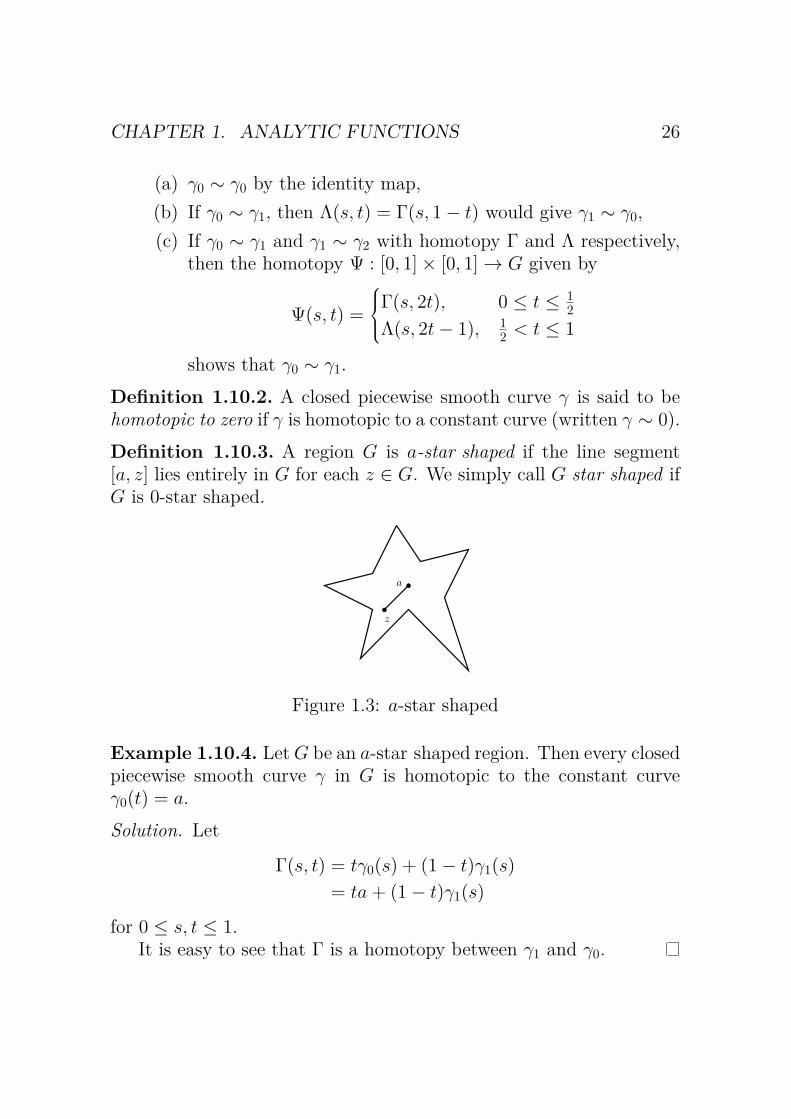
Definition 1.10.2. A closed piecewise smooth curve γ is said to behomotopic to zero if γ is homotopic to a constant curve (written γ ∼ 0).Definition 1.10.3. A region G is a-star shaped if the line segment[a, z] lies entirely in G for each z ∈ G. We simply call G star shaped ifG is 0-star shaped.

a

z

Figure 1.3: a-star shaped

Example 1.10.4. LetG be an a-star shaped region. Then every closedpiecewise smooth curve γ in G is homotopic to the constant curveγ0(t) = a.

Solution. Let

Γ(s, t) = tγ0(s) + (1− t)γ1(s)= ta+ (1− t)γ1(s)

for 0 ≤ s, t ≤ 1.It is easy to see that Γ is a homotopy between γ1 and γ0.


Remark. A convex region is a-star shaped with respect to any a thatbelongs to G.Definition 1.10.5. If γ0, γ1 : [0, 1] → G are two piecewise smoothcurves in a region G such that γ0(0) = a = γ1(1), γ0(1) = b = γ1(1).We say γ0 is (fixed end points) homotopic to γ1 (γ0 ∼ γ1) if there existsa continuous map Γ : [0, 1]2 → G such that

Γ(s, 0) = γ0(s), Γ(s, 1) = γ1(s), 0 ≤ s ≤ 1;

Γ(0, t) = a, Γ(1, t) = b, 0 ≤ t ≤ 1.

γt

γ1

ab

γ0

γ0

γt

γ1

a = b

Figure 1.4: γ0 is (fixed end points) homotopic to γ1

Similarly, it can be verified that ∼ is an equivalence relation on thepiecewise smooth curves satisfying the above definition. (See Conwayp.93)

And note again that, the intermediate path γs(t) = Γ(s, t) for 0 ≤s ≤ 1 and t fixed, need not be piecewise smooth.Theorem 1.10.6 (Cauchy’s Theorem - Second version). Suppose f :G→ C is analytic and γ is a closed piecewise smooth curve in G suchthat γ ∼ 0, then ∫

γf = 0.

Theorem 1.10.7 (Cauchy’s Theorem - Third version). Suppose f :G → C is analytic and γ0, γ1 : [0, 1] → G are two closed piecewisesmooth curves such that γ0 ∼ γ1, then∫

γ0f =

∫γ1f.


Proof. Let γ0 and γ1 be as in the hypothesis, and Γ : I2 → G (I =[0, 1]) be the corresponding continuous function. Since I2 is compact,Γ must be uniformly continuous on I2. Thus Γ(I2) is compact and isa proper subset of G. Hence

d(Γ(I2),C \G) = inf|x− y| : x ∈ Γ(I2), y ∈ C \G = r > 0.

There exists an integer n > 0 such that

|Γ(s′, t′)− Γ(s, t)| < r

whenever |(s′, t′)− (s, t)|2 < 4n2 and (s′, t′), (s, t) ∈ I2.

Set

Jjk = [ jn,j + 1n

]× [kn,k + 1n

] (0 ≤ j, k ≤ n− 1)

(this forms a partition of I × I) and

ζjk = Γ( jn,k

n) (0 ≤ j, k ≤ n).

As the diameter (= diagonal) of Jjk is√ 1n2 + 1

n2 =√

2n

<2n, we

must have Γ(Jjk) ⊂ B(ζjk, r) for 0 ≤ j, k ≤ n− 1. (∪jkB(ζjk, r) formsan open cover of Γ(I2); also it is a proper subset of G by the choice ofr > 0.)

LetQk = [ζ0k, ζ1k, . . . , ζnk]

be the closed polygon (since ζ0k = ζnk) for 0 ≤ k ≤ n.We will first show that ∫

γ0f =

∫Q0f

and ∫Qnf =

∫γ1f,


then ∫Qkf =

∫Qk+1

f (0 ≤ k ≤ n− 1).

Thus ∫γ0f =

∫Q0f = · · · =

∫Qkf = · · · =

∫Qnf =

∫γ1f.

LetPjk = [ζjk, ζj+1,k, ζj+1,k+1, ζj,k+1, ζjk]

be a closed polygon. (See Figure 1.5)

Pjk

ζj,k+1

ζj+1,k+1

ζjkζj+1,k

b

bb

b

Figure 1.5: Pjk

But Γ(Jjk) ⊂ B(ζjk, r), hence Pjk ⊂ B(ζjk, r) in which f is analytic.So ∫

Pjkf = 0 (0 ≤ j, k ≤ n− 1)

by Theorem 1.5.3.We now show ∫

γ0 f = ∫Q0 f , where

Q0 = [ζ00, ζ10, . . . , ζn0].

Let σj(s) = γ0(s) for jn≤ s ≤ j + 1

n, (0 ≤ j ≤ n− 1). (See Figure

1.6)Clearly σj+[ζj+1,0, ζj0] is a closed piecewise smooth curve inB(ζj0, r)

and so ∫σj+[ζj+1,0,ζj0]

f = 0.


σj(s)ζj,0

ζj+1,0

Q0

γ0

Figure 1.6: σj(s)

That is ∫σjf = −

∫[ζj+1,0,ζj0]

f =∫

[ζj0,ζj+1,0]f

So ∫γ0f =

n−1∑j=0

∫σjf =

n−1∑j=0

∫[ζj0,ζj+1,0]

f =∫Q0f.

Similarly, we can prove ∫γ1 f = ∫

Qn f. Finally, we show ∫Qk f =∫

Qk+1 f (0 ≤ k ≤ n− 1). Clearly we have 0 = ∑n−1j=0

∫Pjk f.

Pjk

Pj+1,k

ζj+1,k+1

ζj+2,k+1

ζj+2,k

ζj+1,k

ζjk

ζj,k+1

Figure 1.7: Pjk and Pj+1,k

It follows from the Figure 1.7 that∫[ζj+1,k,ζj+1,k+1]

f


of∫Pjkf cancels the ∫

[ζj+1,k+1,ζj+1,k]f

of∫Pj+1,k

f . Thus

0 =n−1∑j=0

∫Pjkf =

∫Qkf −

∫Qk+1

f.

Theorem 1.10.8. Let γ be a closed piecewise smooth curve in G withγ ∼ 0. Then n(γ; a) = 0 for all a ∈ C \G.

Proof. The proof follows from Theorem 1.10.6. Since 1z − a

is analyticon G if a ∈ C \G,

n(γ; a) = 12πi

∫γ

1ζ − a

dζ = 0.

We note that the converse of Theorem 1.9.8 is not true. That is,there exist a γ such that n(γ; a) = 0 for all a ∈ C \G but it is not truethat γ ∼ 0. (See exercise). Thus Theorem 1.9.2 and 1.9.3 are moregeneral than Theorem 1.10.6 and 1.10.7.

Theorem 1.10.9. If γ0 and γ1 are two piecewise smooth curves joininga to b and γ0 ∼ γ1, then ∫

γ0f =

∫γ1f.

Proof. Since γ0 ∼ γ1, so there exists a continuous map Γ : I2 → Csuch that

Γ(s, 0) = γ0(s), Γ(s, 1) = γ1(s), 0 ≤ s ≤ 1;

Γ(0, t) = a, Γ(1, t) = b, 0 ≤ t ≤ 1.


a b

γ1

γ0

Figure 1.8: γ0 ∼ γ1

Because γ0 − γ1 is a closed piecewise smooth curve, we define

γ(s) =

γ0(3s), 0 ≤ s ≤ 13

b,13 < s ≤ 2

3γ1(3− 3s), 2

3 < s ≤ 1.

Next we show γ ∼ 0 by claiming that Λ : I2 → G is a suitablefunction:

Λ(s, t) =

Γ(3s(1− t), t), 0 ≤ s ≤ 13

Γ(1− t, 3s− 1 + 2t− 3st), 13 < s ≤ 2

3γ1((3− 3s)(1− t)), 2

3 < s ≤ 1.

Note that

Λ(s, t) = γt(s), Λ(s, 0) = γ0 − γ1, Λ(s, 1) = a = b.

It is easy to see that Λ is continuous at s = 13 ; and at s = 2

3 becauseΓ(1− t, 1) = γ1(1− t). So, Λ is continuous on I2.

Hence0 =

∫γf =

∫γ0f −

∫γ1f.

Definition 1.10.10. An open set G is called simply connected if itis connected and every closed curve in G is homotopic to zero (i.e.,γ ∼ 0).


a b

γ1

γ0

γ

t

s

1

10

t

(1− t, 1)

(1− t, t)

1− t

For a fixed t

Figure 1.9: Λ(s, t) and [0, 1− t]× [t, 1]

So we have the following version of Cauchy’s Theorem.

Theorem 1.10.11 (Cauchy’s Theorem - Fourth version). If G is sim-ply connected, then ∫

γ f = 0 for every closed piecewise smooth curveand every analytic f .

The notion of simply connected region lies much deeper than itappears. We shall study this in a more detailed way in a later chapter(pending). Here we chiefly want to prove some immediate consequencesof analytic function defined on simply connected region.

Theorem 1.10.12. Suppose the region G is simply connected, andf : G→ C is analytic. Then f has a primitive on G.

Proof. Let a ∈ G and γ : [0, 1] → G be a piecewise smooth curve (ifclosed, then by Theorem 1.5.3 immediately) in G where γ(0) = a.

b

b

b

G

a

γ0

γ1

z0z

Figure 1.10: γ0 − γ1


Define an expression F (z) =∫γf(ζ) dζ. We first verify that F is

well-defined.Since γ0 − γ1 ∼ 0, Cauchy’s Theorem implies that∫

γ0−γ1f dζ =

∫γ0f dζ −

∫γ1fdζ = 0.

Hence F is independent on the choice of γ. Thus F is a well-definedfunction.

To show F is analytic and F ′ = f , we consider r > 0 so small suchthat B(z0, r) ⊂ G. Replace γ by γ + [z0, z] in F :

F (z) =∫γ+[z0,z]

f.

Then we have

F (z)− F (z0)z − z0

− f(z0) = 1z − z0

∫[z0,z]

(f(ζ)− f(z0)) dζ.

By the similar argument in the proof of Morera’s Theorem, we candeduce that F ′ = f and F is analytic.

The next result lies deeper.

Theorem 1.10.13. Let G be simply connected and f : G → C be ananalytic function such that f(z) 6= 0 for any z ∈ G. Then there isan analytic function g : G → C such that f(z) = eg(z). If z0 ∈ Gand ew0 = f(z0), then we may choose g such that g(z0) = w0. Sosimply connected region implies every non-vanishing analytic functioncan have a logarithm.

Proof. Since f has no zeros, and f ′

fis analytic on G. By Theorem

1.10.12, we let g to be a primitive of f′

f. Consider

d

dz

(f

eg

)= f ′ − g′f

eg= 0.


Thus f = (constant)eg = eg+c, where c is a constant.So, if z0 ∈ G and ew0 = f(z0), we may find a suitable integer k such

that w0 = g(z0) + c + 2πk. Now define g = g + c + 2πk, which is therequired function.

Remark. The converse of the above statement also hold, namely that,G is a simply connected region if every non-vanishing analytic functionf can be represented as f = eg for same analytic function g on G. Werefer to [1] or [3] for the detail.

1.11 Open Mapping TheoremDefinition 1.11.1. If γ is a closed piecewise smooth curve in G suchthat n(γ;w) = 0 for each w ∈ C \ G. We call such curve homologousto zero (γ ≈ 0).

The following contour shows that although γ ∼ 0 implies γ ≈ 0,the converse is not true. One can verify that following figure has γ ≈ 0but γ 6∼ 0 since n(γ; a) = 0 = n(γ; b). The contour was first writtendown independently by C. Jordan (1887) and L. Pochhammer (1890).

Figure 1.11: Pochhammer contour

Remark. The Beta function is defined by the integral

B(x, y) =∫ 1

0tx−1(1− t)y−1 dt, (1.3)


where <(x) and <(y) > 0 so that the integral converges. However, ifwe remove the restriction<(x) and <(y) > 0, then we can still computethe beta function via Pochhammer contour to

B(x, y) =∫ (1+, 0+, 1−, 0−)

(Pochhammer)tx−1(1−t)y−1 dt = −eπi(x+y)4π2

Γ(1− x)Γ(1− y)Γ(x+ y) dt.

(1.4)See [9] for the detail.

By using Cauchy’s Theorem, we shall see below some topologicalresults of different natures.

Theorem 1.11.2. Let G be a region and f : G→ C analytic on G withzeros a1, . . . , am (counted with multiplicity). If γ is a closed piecewisesmooth curve in G such that ak 6∈ γ for each k, and if γ ≈ 0 in G, then

12πi

∫γ

f ′

f(ζ) dζ =

m∑k=1

n(γ; ak).

Proof. According to previous discussion,

f(z) = (z − a1) · · · (z − am)g(z), g(z) 6= 0, z ∈ G.

Then for z 6= a1, . . . , am, we have

f ′

f(z) = 1

z − a1+ · · ·+ 1

z − am+ g′

g.

So1

2πi∫γ

f ′

f(ζ) dζ = 1

2πi∫γ

dζ

ζ − a1+ · · ·+ 1

2πi∫γ

dζ

ζ − am+∫γ

g′

gdζ

= n(γ; a1) + · · ·+ n(γ; am) +∫γ

g′

gdζ.

Since γ ≈ 0 and g′

gis analytic on G, by the Cauchy Theorem - First

version, we have ∫γ g′gdζ = 0. This completes the proof.


Corollary 1.11.2.1. Let f , G and γ be as in the preceding theoremexcept that a1, . . . , am are the roots of f(z) = α (counted according tomultiplicity). Then

12πi

∫γ

f ′(ζ)f(ζ)− α dζ =

m∑k=1

n(γ; ak).

We next prove the important Open Mapping Theorem. But wefirst need the following theorem.

Theorem 1.11.3. Let f : G→ C be analytic where f(a) = α. Supposef − α has a zero of multiplicity m. Then we can find an ε > 0 and aδ > 0 such that for all ξ in 0 < |ζ − a| < δ, the equation f(z) = ξ hasexactly m simple roots in 0 < |z − a| < ε. (A simple root of f(z) = ξis a zero of f − ξ with multiplicity 1.)

×

bcbc

bcb b

bb

bc

ǫ < d2

γ = ∂B(a, ǫ)

a

f×b

ζ

α

δ

σ = f(γ)

Figure 1.12: f : G→ C, f(a) = α

Proof. Letd = inf

w∈C\G|a− w|.

Since the zero a of f − α is isolated, we may choose ε < d

2 suchthat f(z)− α 6= 0 in 0 < |z − a| < ε. Then we have the representation

F (z) = f(z)− α = (z − a)mg(z)


over the disk B(a, ε), where g is analytic and g 6= 0 there.Let γ be the boundary of B(a, ε), and write σ = f(γ). Since C \ σ

is open, we can find a component of C \ σ containing α, and a numberδ > 0 such that B(α, δ) is a proper subset of this component.

Consider

n(σ;α) = 12πi

∫σ

dw

w − α

= 12πi

∫γ

F ′(ζ)F (ζ) dζ

= 12πi

∫γ

m

ζ − adζ + 1

2πi∫γ

g′(ζ)g(ζ) dζ

= m+ 0 = m

since γ is closed and g 6= 0 on B(a, ε). (So g′

ghas a primitive.)

According to Proposition 1.8.4, n(σ; ζ) is a constant on this com-ponent for each ξ ∈ B(α, δ) \ α. Theorem 1.11.2 gives

n(σ; ξ) = 12πi

∫σ

dw

w − ξ

= 12πi

∫γ

f ′(ζ)f(ζ)− ξ dζ

=n∑k=1

n(γ; ak)

where ak for k = 1, . . . , n are the zero of f − ξ in B(a, ε). But γ is acircle, so n(γ; ak) = 1 for 1 ≤ k ≤ n. But then we must have m = n.Theorem 1.11.2 again implies that each of these zeros ak is a simpleroot of f − ξ. This completes the proof.

We deduce immediately the following important result.

Theorem 1.11.4 (Open Mapping Theorem). Let f be a non-constantanalytic function defined on a region G. Then f is an open mapping,i.e. f maps open sets onto open sets.


Proof. Suppose U ⊂ G is open. To show f(U) is open, it suffices tofind a δ > 0 for each ξ ∈ f(U) such that B(ξ, δ) ⊂ f(U). But thisfollows easily from Theorem 1.11.3 that there exist ε, δ > 0 such thatB(a, ε) ⊂ U , B(α, δ) ⊂ f(B(a, ε)). In fact, only part of the conclusionin Theorem 1.11.3 is used.

We now can give a second proof for the maximummodulus theorem.

Theorem 1.11.5 (Maximum Modulus Theorem). Let G be a regionand f : G → C is analytic. If there exists a point a in G such that|f(z)| ≤ |f(a)| for all z ∈ G, then f is constant.

Second proof (Topological argument). Suppose α ∈ f(G) and f(a) =α, a ∈ G. Then we can find a δ > 0 such that B(α, δ) ⊂ f(G) by openmapping theorem. Hence there exist points in B(α, δ) with modulusstrictly longer than |α|. Hence max |f(z)| cannot occur at an interiorof G.

We now consider the definition of an analytic function. Since themain result we use is Morera’s Theorem, we could do this immediatelyafter the proof of Morera’s Theorem.

Recall that f : G → C is analytic on G if f is continuously differ-entiable.

Theorem 1.11.6. Let G be an open set and f : G → C is differen-tiable. Then f must be analytic on G. That is, f is differentiable ifand only if f is continuous differentiable.

Proof. According to the statement of the theorem, it suffices to show f ′

is continuous. But by using Morera’s Theorem, we can show that f isanalytic directly. See, for examples, [1], [3], [4] for a proof of Goursat’sTheorem.

Remark. It follows from Theorem 1.11.6 that we could define analyticfunction simply that f is merely differentiable (without continuity) ateach point of an open set G.


1.12 Isolated SingularitiesWe have proved that every zero of an analytic function must be iso-lated; and as indicated that this property is not shared by real func-tions. The next natural question is about the singularities of analyticfunctions, i.e., the nature of points a such that f(a) undefined, suchas f(a) =∞. The following is a list of examples:

1. √z − 1

has a (square-root) branch point at z = 1.

2.ln(z − 1)

has a logarithmic branch point at z = 1.

3.e1/(z−1)

has an essential singularity at z = 1 (see below).

4.tan[ln(z − 1)]

has a non-isolated essential singularity at z = 1 (see below).

We can deal with a small selection of singularities in this course. Inthe case where f(a) =∞, the standard way to investigate the problemis to consider F (z) = 1

fat a i.e. F (a) = 1

∞= 0. Since any zeros

are isolated, we may assume F has no zeros in 0 < |z − a| < δ forsome δ > 0. So F has only one zero at a i.e. any singularities of fwith f(a) = ∞ must be isolated (just like the zeros). It turns outthat there are only a few types of singularities for analytic functions,and the easiest way to study them is by considering the power seriesexpansions of the functions around the singularities.


Theorem 1.12.1 (Laurent Series, 1843). Let f(z) be analytic functionin an annulus Γ(a;R1, R2) = z : R1 < |z − a| < R2. Then

f(z) =∞∑

n=−∞an(z − a)n

and the series converges uniformly in Γ(a;R1, R2) = z : R1 < |z−a| <R2. The coefficients an are given by the formula

an = 12πi

∫γ

f(ζ)(ζ − a)n+1 dζ

where γ is any circle in Γ(a;R1, R2) centred at a, and for all integersn.

Proof. Let r1 and r2 be two real numbers such that R1 < r1 < r2 < R2,and σ be a straight line segment joining the boundary of Γ(a; r1, r2)and passing through a. Let γ1(t) = a + r1e

it, and γ2(t) = a + r2eit for

t ∈ [0, 2π], then any closed curve inside γ := γ2 +σ− γ1−σ is ∼ 0. ByCauchy’s formula we obtain, for z ∈ Γ(a; r1, r2),

ba

R1

γ1 γ2

R2

σ

Figure 1.13: γ := γ2 + σ − γ1 − σ


f(z) = 12πi

∫γ

f(ζ)ζ − z

dζ

= 12πi

(∫γ2

+∫σ−∫γ1−∫σ

)f(ζ)ζ − z

dζ

= 12πi

∫γ2

f(ζ)ζ − z

dζ − 12πi

∫γ1

f(ζ)ζ − z

dζ

= 12πi

∫γ2

f(ζ)(ζ − a)

(1− z−a

ζ−a

) dζ − 12πi

∫γ1

f(ζ)(z − a)

(1− ζ−a

z−a

) dζ=∞∑n=0

(z − a)n 12πi

∫γ2


+∞∑n=0

(z − a)−n+1 12πi

∫γ1f(ζ)(ζ − a)n dζ

=∞∑n=0

an(z − a)n +−1∑−∞

(z − a)n 12πi

∫γ1f(ζ)(ζ − a)−n−1 dζ

=∞∑n=0

an(z − a)n +−1∑−∞

an(z − a)n (uniform convergence)

wherean = 1

2πi∫γ1

f(ζ)(ζ − a)n+1 dζ for n ≥ 0

andan = 1

2πi∫γ2

f(ζ)(ζ − a)n+1 dζ for n ≤ −1.

Let γ = a + reit for t ∈ [0, 2π] and R1 < r1 < r < r2 < R2. Byconstructing suitable contours involving γ, we may bring the abovetwo line integrals over γ2 and γ1 respectively to the common curve γ.Thus we obtain the formula for an as stated in the theorem.

Remark. We remark that Laurent expansion of an analytic functionin a punctured disk gives a beautiful generalization of Taylor expansionof analytic function.


Looking at the Laurent expansion of the functions in the abovetheorem, there are several possibilities:

(i) ak = 0 for all k ≤ −n for some integer n > 0; the point a is calleda pole of order n;

(ii) there are infinitely many ak 6= 0, k ≤ −1; the point a is called anessential singularity of f at a;

(iii) ak = 0 for all k ≤ −1, then a is called a removable singularity off at a.

• If f has a pole of order n, then

f(z) =n∑k=1

ak(z − a)k +

∞∑k=0

ak(z − a)k

where the sum ∑nk=1 ak/(z − a)k is called the principal part of f

at a, and |f | → ∞ in the manner of O(|z − a|−n) as z → a.

• If f has a removable singularity at a, then f(z) = ∑∞k=0 ak(z−a)k

in 0 < |z − a| < δ (some δ > 0). But we clearly have f → a0 asz → a, thus we may define a new function at a by g(z) = f(z)for 0 < |z− a| < δ and g(z) = a0 at z = a. Then g is an analyticfunction in |z − a| < δ. Thus f is almost analytic at a if it hasa removable singularity at a and so from this point of view, thiscase is less interesting.

We shall discuss the implication of pole later. The behaviour off near an essential singularity is very different. It is not true that|f | → ∞ as z → a.

Example 1.12.2. 1. The sin z/z has a removable singularity at z =0.

2. The Euler-Gamma function Γ(z) has simple poles at each of neg-ative integers (see a later chapter).


3. The Weierstrass function ℘(z) has double poles at the vertices ofits fundamental period parallelograms (see a later chapter).

4. The e1/z, sin(1/z) and cos(1/z) all have an essential singularity

at z = 0.

5. Show the following Laurent expansion

e12 (z−1/z) =

∞∑−∞

akzk,

whereak = 1

2π∫ 2π

0cos(kθ − sin θ) dθ.

Theorem 1.12.3 (Casorita-Sokhotskii-Weierstrass-1864). Suppose fhas an essential singularity at a. Then for every δ > 0, f(Γ(a; 0, δ)) =C.

The statement of this theorem is equivalent to given any ρ, ε > 0and any c ∈ C, there is a point z inside 0 < |z − a| < ρ in which|f(z)− c| < ε. That is to say, given any c, f tends to c as the limit asz tends to a through a suitable sequence of complex numbers.

Proof. We first show that f is unbounded on any punctured disksΓ(a; 0, δ).

Suppose |f(z)| ≤ M for all z ∈ Γ(a; 0, δ). Let γ(t) = a + Reit,t ∈ [0, 2π], then

|an| =∣∣∣∣∣∣ 12πi

∫γ


∣∣∣∣∣∣ for n ≤ −1

= 12π

∣∣∣∣∣∣∫ 2π

0

f(a+Reit)(Reit)n+1 iReit dt

∣∣∣∣∣∣≤MR−n

→ 0 as R→ 0.


Hence an = 0 for all n ≤ −1 and f has a removable singularity atmost. A contradiction.

Let us now assume that δ > 0 is chosen so small that f − c hasno zero in Γ(a; 0, δ). Then the function φ(z) = 1

f − cis analytic in

Γ(a; 0, δ). We claim that φ has an essential singularity at a. For if φhas a pole at a, then f = 1

φ+ c would be analytic at a; while if φ has

a removable singularity, then f either has pole or analytic at a. Thisis a contradiction.

We now apply the result obtained above to φ i.e. φ is unboundedon Γ(a; o, δ), so |f − c| = 0 on Γ(a; 0, δ). That is, given ε > 0, thereexists z ∈ Γ(a; 0, δ) such that

|φ(z)| > 1/ε,

i.e.,|f(z)− c| = |1/φ(z)| < ε.

So we could find a sequence εn = 1/n and δn such that δn → 0 andzn ∈ Γ(a; 0, δn) so that zn → a for and f(zn)→ c. This completes theproof.

1.13 Rouché’s theoremThis is an application of the argument principle discussed earlier.

Theorem 1.13.1 (E. Rouché). Let f(z) and g(z) be analytic in thedomain D containing the closed, piece-wise smooth curve γ. Suppose

|f(z)| > |g(z)|, for all z ∈ γ.

Then f(z) and f(z) + g(z) have the same number of zeros, countingmultiplicity, in the domain enclosed by γ.


Proof. It is evident from the assumption that |f(z)| > |g(z)|, for allz ∈ γ that both f(z) and f(z) + g(z) do not have zeros on γ.The argument principle assets that

∆γ arg(f(z) + g(z)

)= ∆γ arg

[f(z)

(1 + g(z)

f(z))]

= ∆γ arg f(z) + ∆γ arg(1 + g(z)

f(z)).

But since1 >

∣∣∣∣∣∣g(z)f(z)

∣∣∣∣∣∣ =∣∣∣∣∣∣(g(z)f(z) + 1

)− 1

∣∣∣∣∣∣ ,on γ. It follows that 1 + g(z)

f(z) can never circle around w = 0. Hence

∆γ arg(f + g) = ∆γ arg f(z) + 0.

Thus

Nf+g = 12πi

∫γ

(f + g)′(z)f(z) + g(z) dz = 1

2πi∫γ

f ′(z)f(z) dz = Nf

inside γ, as required.

Example 1.13.2. If f(z) has zero of order two at a, and a pole oforder 3 at b, where both a and b are inside γ, then

∆γ arg f(z) = 2π(2− 3) = −2π.

Example 1.13.3. Determine the number of roots of

z7 − 4z3 + z − 1 = 0

in |z| < 1.On |z| = 1, we write

f(z) = −4z3, g(z) = z7 + z − 1.


Then |f(z)| = 4 and |g(z)| ≤ |z|7 + |z| + 1 = 3 Hence |f(z)| > |g(z)|on |z| = 1. Thus Rouché’s theorem asserts that f + g has the samenumber of zeros as that of f = −4z3 in |z| < 1. Thus there are 3 zerosinside |z| < 1.

Exercise 1.13.1. Prove the open mapping theorem for analytic func-tion by applying Rouché’s theorem.

See next chapter for an hint.

Chapter 2

Conformal mappings

2.1 Stereographic ProjectionOne known problem with numbers in the complex plane C = (x, y) :−∞ < x, y < +∞ do not have an ordering like the real numberson the real-axis R. Riemann’s (1826-1866) idea is to add an idealpoint, denoted by ∞, to C to obtain an extended complex plane C =C ∪ ∞. This construction can get around the problem of ordering.The resulting C is compact which can be vasualised by the followingconstruction.

We show that there is an one-to-one correspondence between

S = (x1, x2, x3) ∈ R3 : x21 + x2

2 + x23 = 1

and C = C ∪ ∞. The S is called the Riemann sphere.Let N = (0, 0, 1) and z ∈ C. If we join the straight line between

N and z, the straight line intersects the sphere S at Z = (x1, x2, x3)say. The construction clearly exhibits an one-to-one correspondencebetween S \ N and C. Note that Z → N as |z| → ∞. We mayassociate N with ∞ and obtain the bijection between S and C. Thisis known as the Stereographic projection.

Suppose P (x1, x2, x3) = Z ∈ S associates with z = (x, y) ∈ C.Then we may associate z the notation P with coordinate (x, y, 0).

48

https://en.wikipedia.org/wiki/Riemann_sphere

https://en.wikipedia.org/wiki/Stereographic_projection

CHAPTER 2. CONFORMAL MAPPINGS 49

b

b

b

N

Z

z

S

Figure 2.1: Riemann sphere

Then we have, by considering similar triangles formed by the line seg-ment NP and projecting onto the x−, y− and z−axes respectively,

|NP ||NZ|

= x

x1= y

x2= 1

1− x3, (2.1)

so thatz = x+ iy = x1 + ix2

1− x3.

Then|z|2 = x2

1 + x22

(1− x3)2 = 1 + x3

1− x3,

hencex3 = |z|

2 − 1|z|2 + 1 .

Thenx1 = z + z

1 + |z|2 , x2 = z − zi(1 + |z|2) .

This clearly shows a one-one correspondence between S\(0, 0, 1) andC with the N = (0, 0, 1) corresponds to ∞. We also note that theupper hemisphere where x3 > 0 corresponds to |z| > 1 and the lowerhemisphere of S corresponds to |z| < 1. An advantage with this Rie-mann sphere model is that it puts all complex numbers including ‘∞’in equal footing since any number can be rotated to N and vice-verse.


From a geometrical viewpoint, it is evident that every (infinite)straight line in the z−plane is transformed into a circle on S thatpasses through the North pole N , and conversely. Hence, every circle(straight line included) on the z−plane corresponds to a circle/straightline on S.Theorem 2.1.1. A circle on the Riemann sphere is mapped under theStereographic projection into a circle (including a straight line) of theC, and conversely.

Proof. Show that1. a circle equation that lies on the Riemann sphere is an equation

of the formax1 + bx2 + cx3 = d

subject to 0 ≤ c < 1 and a2 + b2 + c2 = 1 (this is the intersectionof the plane and the unit sphere).

2. the above equation can be rewritten in the form

a(z + z)− ib(z − z) + c(|z|2 − 1) = d(|z|2 + 1)

3. the above equation can be further rewritten into the form

(d− c)(x2 + y2)− 2ax− 2by + d+ c = 0,

which is clearly a circle equation in the C and it becomes a straightline. equation if and only if c = d.

That is, a circle on the Riemann sphere S corresponds to eithera circle or a straight line on C. In the case the circle on S passesthrough the North pole N = (0, 0, 1), then the corresponding straightline (also considered as an unbounded circle passes through) to ∞.

Exercise 2.1.1. Show that if z and w are two points in C so thattheir images lie on two diametrically opposite points on the Riemannsphere, then

wz + 1 = 0.


Theorem 2.1.2. The stereographic projection is isogonal (i.e., themapping preserves angles).

Proof. The statement of the theorem means that the tangents of twocurves in the C intersect at point z0 is equal to the angle made by twotangents at the corresponding intersection point of two image curveson the Riemann sphere. We shall make two assumptions:

1. that the Stereographic projection preserves tangents. We skipthe detail verification of this fact. But this is not difficult to seesince the Stereographic projection is a smooth map,

2. that without loss of generality that the two curves in C are (in-finite) straight lines.

Suppose the two straight line equations are given by

a1x+ a2y + a3 = 0 (x3 = 0);b1x+ b2y + b3 = 0. (x3 = 0) (2.2)

It follows from (2.1) that the two plane equations become respectively,

a1X1 + a2X2 + a3(X3 − 1) = 0;b1X1 + b2X2 + b3(X3 − 1) = 0.

In the limiting case when X3 = 1, we have the two tangent planeequations

a1X1 + a2X2 = 0;b1X1 + b2X2 = 0. (2.3)

at N(0, 0. 1) parallel to the C. Clearly the angle between the twocurves in (2.2) is the same angle between the two lines in (2.3).

Note that any two intersecting circles in general positions on S canbe rotated so that the intersection point passes through the North poleN . This consideration takes care of the preservation of the angle ofintersection of two curves in general position in C under the Stereo-graphic projection.


Theorem 2.1.3. Let z1, z2 be two points in C and Z1, Z2 be theirimages on the Riemann sphere S under the Stereographic projection.We denote a(Z1, Z2) to be arc length between Z1 and Z2. Then

limz2→z1

a(Z1, Z2)|z1 − z2|

= 21 + |z1|2

. (2.4)

That is, the ratio depends on position only. So the Stereographic pro-jection is called a pure magnification.

We easily deduce from the above theorem that

Theorem 2.1.4. Let C = z = z(s) : 0 ≤ s ≤ L be a piecewisesmooth curve in C. Let Γ be the image curve of C on the Riemannsphere under the Stereographic projection. Then the length `(Γ) of Γis given by

`(Γ) =∫ L

0

2|dz(s)|1 + |dz(s)|2 .

Let d(Z1, Z2) denote the chordal distance between Z1 and Z2 on S.We also write

χ(z1, z2) := d(Z1, Z2).where z1, z2 are the corresponding points in C.

Theorem 2.1.5. Let z1, z2 ∈ C. Then

χ(z1, z2) = 2|z1 − z2|√1 + |z1|2

√1 + |z2|2

. (2.5)

Sinceχ(z1, z2) := d(Z1, Z2) ≈ a(Z1, Z2)

as z1 → z2. So the Theorem 2.1.3 follows from the equation (2.5) inthe limit z2 → z1.

Proof. Let z1 = (x1, y1) and z2 = (x2, y2) and none equal to ∞. Weconstruct a plane passing through the following three points:

(0, 0, 1), (x1, y1, 0), (x2, y2, 0).


Figure 2.2: Riemann sphere slide

Then we have the above figure.We deduce from the Riemann sphere S that

d(N, z1) =√

1 + |z1|2, d(N, z2) =√

1 + |z2|2.

One can see from similar triangles consideration on the Riemmansphere S that

x1

x= 1− x3

1 = x2

y.

Hence

1 + |z|2 = 1 + x2 + y2 = 1 + x21

(1− x3)2 + x22

(1− x3)2

= 2(1− x3)(1− x3)2 = 2

1− x3.

andd(N, Z)d(N, z) = 1− x3

1 = 21 + |z|2 .


holds. This gives raise to

d(N, Z1) = 2√1 + |z1|2

, d(N, Z2) = 2√1 + |z2|2

.

We conclude that

d(N, z1)d(N, Z1)= 2 =d(N, z2)d(N, Z2).

Hence the triangles ∆Nz1z2 and ∆NZ1Z2 are similar. Hence

d(Z1, Z2)d(z1, z2)

= d(N, Z2)d(N, z1)

.

It follows from the above consideration that

d(Z1, Z2) = d(z1, z2) ·d(N, Z2)d(N, z1)

= 2|z1 − z2|√1 + |z1|2

√1 + |z2|2

.

as required.

We are ready to prove Theorem 2.1.3.We observe the relation

d(Z1, Z2)a(Z1, Z2)

= sinαα

,

holds, where α is the angle between the line segments NZ1 and NZ2from the above figure. Hence

a(Z1, Z2)|z1 − z2|

= d(Z1, Z2)|z1 − z2|

≈ χ(z1, z2)|z1 − z2|

→ 21 + |z1|2

as z2 → z1.We also note that

χ(z1, ∞) = limz2→∞

χ(z1, z2) = 2√1 + |z1|2

,


which follows from the Riemann sphere (geometric) or the Theorem2.1.5 (algebraic) considerations. Thus we define the chordal distanceto be

χ(z, z′) =

2|z − z′|√1 + |z|2

√1 + |z′|2

, z, z′ ∈ C

2√1 + |z|2

, z′ =∞.

Alternative derivation

of the chordal distance. Suppose (x1, x2, x3) ∈ S associates with z =(x, y) ∈ C and (x′1, x′2, x′3) ∈ S associates with z′ ∈ C.

Then the distance or the length of the chord joining (x1, x2, x3) and(x′1, x′2, x′3) on S is given by√

(x1 − x′1)2 + (x2 − x′2)2 + (x3 − x′3)2.

On the other hand,

(x1 − x′1)2 + (x2 − x′2)2 + (x3 − x′3)2 = 2− 2(x1x′1 + x2x

′2 + x3x

′3).

Exercise 2.1.2. Show thatx1x

′1 + x2x

′2 + x3x

′3

= (z + z)(z′ + z′)− (z − z)(z′ − z′) + (|z|2 − 1)(|z′| − 1)(1 + |z|2)(1 + |z′|2)

= (1 + |z|2)(1 + |z′|2)− 2|z − z′|2(1 + |z|2)(1 + |z′|2)

Exercise 2.1.3. Verify the formaula for chordal distance using theabove formala.Exercise 2.1.4. Verify that χ(z1, z2) = χ(z1, z2) = χ(1/z1, 1/z2).Exercise 2.1.5. Describe a ε−neighbourhood of a pont z0 in thechordal metric.


Metric space

The chordal distance χ(z1, z2) defines a metric on C. This is because

1. χ(z1, z2) ≥ 0 and with equality if and only if z1 = z2;

2. χ(z1, z2) = χ(z2, z1);

3. χ(z1, z3) ≤ χ(z1, z2) + χ(z2, z3),

where the third item follows from

Exercise 2.1.6. Let a, b, c ∈ C. Then

(a− b)(1− cc) = (a− c)(1 + cb) + (c− b)(1 + ca).

Exercise 2.1.7. Show that the above metric space is complete.

2.2 Analyticity revisited

Local properties of one-one analytic functionsWe recall that if f : E → P and there correspond only one pointin E for every point in P under this f , then we say the map f isinjective. This defines a function g on P , denoted by z = g(w), calledthe inverse function or inverse mapping of f . In particular, wesee that g[f(z)] = z.

Let w = f(z) = u(x, y) + iv(x, y). Then one can view f as amapping R2 −→ R2 given byx

y

7−→u(x, y)v(x, y)

.What is a criterion that guarantee the existence of an inverse mappingfor the above mapping?


Standard material from calculus courses asserts that if∣∣∣∣∣∣∣∣∣∣∂u

∂x

∂u

∂y∂v

∂x

∂v

∂y

∣∣∣∣∣∣∣∣∣∣6= 0, at z0 = (x0, y0),

then the Implicit function theorem asserts that an inverse function off exists there. That is, if the Jacobian is non-zero at z0. But then theCauchy-Riemann equations give∣∣∣∣∣∣∣∣∣∣

∂u

∂x

∂u

∂y∂v

∂x

∂v

∂y

∣∣∣∣∣∣∣∣∣∣=∣∣∣∣∣∣ ux −vxvx ux

∣∣∣∣∣∣ = u2x + v2

x = |f ′(z0)|2.

This leads to the following statement.

Theorem 2.2.1. Let f(z) be an analytic function on a domain D suchthat f ′(z0) 6= 0. Then there is an analytic function g(w) defined in aneighbourhood N(w0) of w0 = f(z0) such that g(f(z)) = z throughoutthis neighbourhood.

Proof. Since ∣∣∣∣∣∣∣∣∣∣∂u

∂x

∂u

∂y∂v

∂x

∂v

∂y

∣∣∣∣∣∣∣∣∣∣= |f ′(z0)|2 6= 0,

so the Implicit Function theorem asserts that is a neighbourhoodN(w0)of w0 = f(z0) in which f has a local inverse at w0u

v

7−→x(u, v)y(u, v)

.Moreover, the analytic Implicit Function theorem asserts that thestronger conclusion that since f is analytic at z0 so the g(w) is an-alytic at w0.

http://en.wikipedia.org/wiki/Implicit_function_theorem


We prove that a strong form of converse of the above statementalso holds. Please note we could apply the Theorem 1.11.3 to provethe theorem. But we prefer to apply the Rouché theorem instead.Theorem 2.2.2. Let f(z) be an one-one analytic function on a domainD. Then f ′(z) 6= 0 on D.

Proof. We suppose on the contrary that f ′(z0) = 0 for some z0 and wewrite f(z0) = w0 . We first notice that f ′(z) 6≡ 0. For otherwise, f(z)is identically a constant, contradicting to the assumption that f(z) isone-one on D.Since the zeros of f ′(z) are isolated , so there is a ρ > 0 such thatf ′(z) 6= 0 in z : 0 < |z − z0| < ρ. Because of the assumption that fis one-one, so

f(z) 6= f(z0) on |z − z0| = ρ.

On the other hand, |f(z)| is continuous on the compact set |z−z0| = ρso that we can find a δ > 0 such that

|f(z)− f(z0)| ≥ δ > 0 on |z − z0| = ρ.

Let w′ be an arbitrary point in w : 0 < |w′ − w0| < δ. Then theinequality

|f(z)− w0| ≥ δ > |w′ − w0|holds, so that the Rouché theorem again implies that the functionf(z)− f(z0) = f(z)− w0 and the function

[f(z)− f(z0)] + [f(z0)− w′] = f(z)− w′

have the same number of zeros inside z : |z−z0| < ρ. But f ′(z0) = 0so f(z) − f(z0) has at least two zeros (counting multiplicity). Hencef(z) − w′ also has at least two zeros (counting multiplicity) in z :|z − z0| < ρ. But f ′(z) 6= 0 in z : 0 < |z − z0| < ρ, so there areat least two different zeros z1 and z2 in z : |z − z0| < ρ so thatf(z1) = w′ and f(z2) = w′, thus contradicting to the assumption thatf(z) is one-one.


2.3 Angle preserving mappingsWe consider geometric properties of an analytic function f(z) at z0such that f ′(z0) 6= 0. Let γ = γ(t) : a ≤ t ≤ b a piece-wise smoothpath such that z0 = γ(t0) where a ≤ t0 ≤ b and z′(t0) 6= 0, and

Γ := w = f(z(t)) : a ≤ t ≤ b.

That is, Γ = f(γ).It is clear that the assumption z′(t0) 6= 0 above means that the path γmust have a tangent at t0. Thus,

df [z(t)]dt

∣∣∣∣∣∣∣t=t0

= df(z)dz

∣∣∣∣∣∣∣z=z0

· dzdt

∣∣∣∣∣∣∣t=t0

= f ′(z0) · z′(t0) 6= 0

since f ′(z0) 6= 0 and z′(t0) 6= 0. We deduce

Arg df [z(t)]dt

∣∣∣∣∣∣∣t=t0

= Arg df(z)dz

∣∣∣∣∣∣∣z=z0

+ Arg dzdt

∣∣∣∣∣∣∣t=t0

.

Let θ0 = z′(t0) denote the inclination angle of the tangent to γ at z0 and

positive real axis, and let ϕ0 := Arg df [z(t)]dt

∣∣∣∣∣∣∣t=t0

denote the inclination

angle of the tangent to Γ at w0 = f(z0). Thus

Arg f ′(z0) = ϕ0 − θ0.

Now let γ1(t) : z1(t) : a ≤ t ≤ b and γ2(t) : z2(t) : a ≤ t ≤ b be twopaths such that they intersect at z0. Then

ϕ1 − θ1 = Arg f ′(z0) = ϕ2 − θ2.

That is,ϕ2 − ϕ1 = θ2 − θ1.

This shows that the difference of tangents of Γ2 = f(γ2) and Γ1 = f(γ1)at w0 is equal to difference of tangents of γ2 and γ1 at z0.


f

γ2

γ1

γ′2(t2)

γ′1(t1)

σ2

σ1

σ′1(t1)

σ′2(t2)

Figure 2.3: Conformal map at z0

Definition 2.3.1. An analytic f : D → C is called conformal at z0if f ′(z0) 6= 0. f is called conformal in D if f is conformal at eachpoint of the domain D.

We call |f ′(z0)| the scale factor of f at z0.

Theorem 2.3.2. Let f(z) be analytic at z0 and that f ′(z0) 6= 0. Then

1. f(z) preserves angles (i.e., isogonal) and its sense at z0;

2. f(z) preserves scale factor, i.e., a pure magnification at z0 in thesense that it is independent of directions of approach to z0.

We consider a converse to the above statement.

Theorem 2.3.3. Let w = f(z) = f(x + iy) = u(x, y) + iv(x, y) bedefined in a domain D with continuous ux, uy, vx, vy such that they donot vanish simultaneously. If either

1. f is isogonal (preserve angles) at every point in D,

2. or f is a pure magnification at each point in D,

then either f or f is analytic in D.


Proof. Let z = z(t) be a path passing through the point z0 = z(t0) inD. We write w(t) = f(z(t)). Then

w′(t0) = ∂f

∂xx′(t0) + ∂f

∂yy′(t0),

That is,

w′(t0) = 12

∂f∂x− i∂f

∂y

z′(t0) + 12

∂f∂x

+ i∂f

∂y

z′(t0). (2.6)

That is,w′(t0)z′(t0)

= ∂f

∂z(z0) + ∂f

∂z(z0) ·

z′(t0)z′(t0)

where we have adopted new notation

∂f

∂z:= 1

2

∂f∂x− i∂f

∂y

, ∂f

∂z:= 1

2

∂f∂x

+ i∂f

∂y

.

If f is isogonal, then the arg w′(t0)z′(t0) is independent of arg z′(t0) in the

above expression. This renders the expression (2.6) to be independentof arg z′(t0). Therefore, the only way for this to hold in(2.6) is that

0 = ∂f

∂z:= 1

2

∂f∂x

+ i∂f

∂y

,which represent the validity of the Cauchy-Riemann equations at z0.Thus f is analytic at z0. This establishes the first part.

We note that the right-hand side of (2.6) represents a circle ofradius ∣∣∣∣12

(∂f∂x

+ i∂f

∂y

)∣∣∣∣centered at ∂f/∂z. Suppose now that we assume that f is a puremagnification. Then the (2.6) representation this circle must either


have its radius vanishes which recovers the Cauchy-Riemann equations,or the centre is at the origin, i.e.,

0 = ∂f

∂z= 1

2

∂f∂x− i∂f

∂y

or the equivalently f(z) is analytic at z0 and hence over D.

Remark. If f(z) is analytic at z0, then it means that f preserves thesize of the angle but reverse its sense.

Example 2.3.4. Consider w = f(z) = ez on C. Clearly f ′(z) = ez 6= 0so that the exponential function is conformal throughout C. Observe

w = ez = ex + eiy := Reiφ,

so that the line x = a in the is mapped onto the circle R = ea in thew−plane, while the horizontal line y = b (−∞ < x < ∞) is mappedto the line Reib : 0 < R < +∞. One sees that the lines x = aand y = b are at right-angle to each other. Their images, namely theconcentric circles centred at the origin and infinite ray at angle b fromthe x−axis from the origin are also at right angle at each other. Theinfinite horizontal strip

G = z = x+ iy : |y| < π, −∞ < x <∞

is being mapped onto the slit-plane C\z : z ≤ 0. Moreover, theimage of any vertical shift of G by integral multiple of 2π under fwill cover the slit-plane again. So the f(C) will cover the slit-plane aninfinite number of times.


Figure 2.4: Exponential map

2.4 Möbius transformationsWe study mappings initiated by A. F. Möbius (1790–1868) on the Cthat map C to C or even between C. Möbious considered

The mapping

w = f(z) = az + b

cz + d, ad− bc 6= 0

is called a Möbius transformation, a linear fractional trans-formation, a homographic transformation. In the case whenc = 0, then a Möbious transformation reduces to a linear functionf(z) = az+ b which is a combination of a translation f(z) = z+ b anda rotation/magnification f(z) = az. If ad− bc = 0, then the mappingdegenerates into a constant.

We recall that a function f having a pole of order m at z0 is equiv-alent to 1/f to have a zero of order m at z0 . Similarly, a function havea pole of order m at ∞ means that 1/f(1

z) to have a zero of order mat z = 0.

The mapping w is defined on C except at z = −d/c, where f(x)has a simple pole. On the other hand,

f(1/ζ) = a/ζ + b

c/ζ + d= a+ bζ

c+ dζ= a

c

https://en.wikipedia.org/wiki/August_Ferdinand_M%C3%B6bius


when ζ = 0. That is, f(∞) = a/c. So f(z) is a one-one map betweenC = C ∪ ∞. One can easily check that the inverse f−1 of f is givenby

f−1(w) = −wd− bcw − a

, w 6= a

c.

Thus f−1 : ac7→ ∞, ∞ 7→ −d

c(Since

f−1(1η

)= −d/η − b

c/η − a= −d− bη

c− aη= −d

c

as η = 0. Thus f−1(∞) = −dc. Similarly, since

1f−1(w)

∣∣∣∣a/c

= −cw − adw − b

∣∣∣∣w=a/c

= 0.

Thus f−1(ac

)=∞.

)

Theorem 2.4.1. The above Möbius map is conformal on the Riemannsphere.

Proof. Let c 6= 0. Then

f ′(z) = ad− bc(cz + d)2 6= 0,

whenever z 6= −dc . Hence f(z) is conformal at every point except per-

haps when z = −d/c where f has a simple pole. So we should check if1

f(z) is conformal at z = −d/c. But

( 1f(z)

)′∣∣∣∣z=−d/c

= − f′(z)

f(z)2

∣∣∣∣−d/c

= ad− bc(cz + d)2 ×

(cz + d

az + b

)2

= − ad− bc(az + b)2

∣∣∣∣−d/c

= −(ad− bc)c2

(ad− bc)2 = −c2

ad− bc6= 0.


Hence f is conformal at −d/c, whenever c 6= 0.Similarly, in order to check if f is conformal at ∞, we consider,

when c 6= 0(f(1ζ

))′=(a+ bζ

c+ dζ

)′= bc− ad

(c+ dζ)2 = bc− adc2 6= 0

when ζ = 0 and whenever c 6= 0. Hence f is conformal at ∞ if c 6= 0.If c = 0, then we consider f(z) = az + b

d= αz + β instead. Since

f ′(z) = α 6= 0 for all z ∈ C, so f is conformal everywhere. It remainsto consider

1f(1/ζ

) = 1α/ζ + β

= ζ

α + βζ.

Hence f(∞) =∞. We now consider the conformality at ∞:( 1f(1/ζ)

)′ζ=0

= α

(α + βζ)2

∣∣∣∣ζ=0

= 1α6= 0,

as required.

Exercise 2.4.1. Complete the above proof by considering the casewhen c = 0.

Exercise 2.4.2. Show that

1. the composition of two Möbius transformations is still a Möbiustransformation.

2. For each Möbius transformation f , there is an inverse f−1.

3. If we denote I be the identity map, then show that the set of allMöbius transformations M forms a group under composition.


Theorem 2.4.2. Let w = f(z) = az + b

cz + d. Then f(z) maps any circle

in the z−plane to a circle in the w−plane.

Remark. We regard any straight lines to be circles having infinite radii(+∞).

Proof. We note that any az + b

cz + dcan be written as

w =ac

[z + b/a

z + d/c

]= a

c

[1 + b/a− d/c

z + d/c

]

= a

c

[1 +

(bc/a− d1

) 1cz + d

]

= a

c+(bc− ad

c

)( 1cz + d

),

Showing that w can be decomposed by transformations of the basictypes:

1. w = z + b (translation),

2. w = eiθ0z (rotation),

3. w = kz (k > 0, scaling),

4. w = 1/z (inversion).

In fact, we can write the T (z) as a compositions of four consecutivemappings in the forms

w1 = cz + d, w2 = 1w1, w3 =

(bc− adc

)w2, w4 = a

c+ w3,

From the geometric view point, the translation z + b or rotation w =eiθ0z all presences circles (lines). So it remains to consider scaling


w = kz (k > 0) and inversion w = 1/z.Let us consider the circle equation (centred at z0 = (x0, y0) with radiusR). Then

(x− x0)2 + (y − y0)2 = R2.

That is,x2 + y2 − 2x0x− 2y0y + (x2

0 + y20 −R2) = 0.

Substituting z = x+ iy, z = x− iy

zz + −22 (z0 + z0)

12(z + z)− 2

2i(z0 − z0)12i(z − z) + z0z0 −R2.

This can be rewritten as

zz +Bz +Bz +D = 0,

where B = −z0, D = x20 + y2

0 −R2.Conversely, suppose B = −z0, |B|2 −D = R2 > 0, then the above

equation represents a circle equation centred at −B = z0 with radius

R =√|B|2 −D.

In fact, |z − (−B)| =√|B|2 −D. We consider the scaling : w = kz.

The circle equation becomes

1k2 ww + B

kw + B

kw +D = 0.

Thusww + kBw + kBw + k2D = 0

Clearly, k2D is a real number, and√k2 |B|2 − k2D = k

√|B|2 −D > 0.

Hence the above equation is a circle equation in the w−plane.It remains to consider inversion w = 1/z. Then the equation becomes

1ww

+ B

w+ B

w+D = 0,


orww + B

Dw + B

Dw + 1

D= 0.

clearly 1/D is a real number, and |B/D|2 − 1/D = 1D2 (|B|2 −D) > 0.

So the equation is a circle equation in the w−plane.

2.5 Cross-ratiosLet

T (z) = az + b

cz + d(2.7)

be a Möbius transformation, and let w1, w2, w3, w4 be the respectivelyimages of the points z1, z2, z3, z4. Then it is routine to check that

wj − wk = ad− bc(czj + d)(czk + d)(zj − zk), j, k = 1, 2, 3, 4.

Then

(w1 − w3)(w2 − w4) = (ad− bc)2∏4j=1(czj + d)(z1 − z3)(z2 − z4) (2.8)

Similarly, we have

(w1 − w4)(w2 − w3) = (ad− bc)2∏4j=1(czj + d)(z1 − z4)(z2 − z3). (2.9)

Dividing the (2.8) by (2.9) yields

(w1 − w3)(w2 − w4)(w1 − w4)(w2 − w3)

= (z1 − z3)(z2 − z4)(z1 − z4)(z2 − z3)

. (2.10)

Definition 2.5.1. Let z1, z2, z3, z4 be four distinct numbers in C.Then

(z1, z2, z3, z4) := (z1 − z3)(z2 − z4)(z1 − z4)(z2 − z3)

= z1 − z3

z1 − z4: z2 − z3

z2 − z4(2.11)


is called the cross-ratio of the four points. If, however, when any oneof z1, z2, z3, z4 is ∞, then the cross-ratio becomes

(∞, z2, z3, z4) := z2 − z4

z2 − z3,

(z1, ∞, z3, z4) := z1 − z3

z1 − z4,

(z1, z2, ∞, z4) := z2 − z4

z1 − z4,

(z1, z2, z3, ∞) := z1 − z3

z2 − z3,

respectively.

The equation (2.10) implies that we have already proved the fol-lowing theorem.

Theorem 2.5.2. Let T be any Möbius transformation. Then

(Tz1, T z2, T z3, T z4) = (z1, z2, z3, z4). (2.12)

Remark. The above formula means that the cross-ratio of four pointsis preserved under any Möbius transformation T (z).

Example 2.5.3. We note that the cross-ratio when written as

(z, z2, z3, z4) = (z − z3)(z2 − z4)(z − z4)(z2 − z3)

= z − z3

z − z4: z2 − z3

z2 − z4

is a Möbius transformation of z that maps the points z2, z3, z4 to1, 0, ∞ respectively.

Theorem 2.5.4. Let z1, z2, z3 and w1, w2, w3 be two sets of three arbi-trary complex numbers. Then there is a unique Möbius transformationT (z) that satisfies T (zi) = wj, j = 1, 2, 3.


Proof. The cross-ratio formula

w − w3

w − w4: w2 − w3

w2 − w4= z − z3

z − z4: z2 − z3

z2 − z4

does the trick.

Example 2.5.5. Find a Möbius transformation w that maps −1, i, 1to −1, 0, 1 respectively.It follows that

w − 0w − 1 : −1− 0

−1− 1 = z − iz − 1 : −1− i

−1− 1 .

So2ww − 1 = z − i

z − 1( 1

1 + i

).

Hencew = 1 + iz

i+ z.

Arrangements

The above arrangement of the four points z1, z2, z3, z4 in the construc-tion of our cross-ratio is not special. One can try the remaining twentythree different permutations of z1, z2, z3, z4 in the construction. How-ever, we note that

λ := (z1, z2, z3, z4) = (z2, z1, z4, z3) = (z3, z4, z1, z2) = (z4, z3, z2, z1)

so that the list reduces to six only. They are given by

(z2, z3, z1, z4) = λ− 1λ

, (z3, z1, z2, z4) = 11− λ

(z2, z1, z3, z4) = 1λ, (z3, z2, z1, z4) = λ

λ− 1 , (z1, z3, z2, z4) = 1−λ.


The above list contains all six distinct values for the cross-ratio for dis-tinct z1, z2, z3, z4. If, however, two of the points z1, z2, z3, z4 coincide,then the list of values will reduce further. More precisely, if λ = 0 or1, then the list reduces to three, namely 0, 1, ∞. If λ = −1, −1/2 or2, then the list reduces to three again with values −1, 1/2, 2. There isanother possibility that

λ = 1± i√

32 .

See exercise.Moreover, if we put z2 = 1, z3 = 0, z4 = ∞, then the cross-ratio

becomes(λ, 1, 0, ∞) = λ,

which means that λ is a fixed point of the map.

Theorem 2.5.6. Let z1, z2, z3, z4 be four distinct points in C. Thentheir cross-ratio (z1, z2, z3, z4) is real if and only if the four points lieon a circle (including a straight line).

Proof. Let Tz = (z1, z2, z3, z).We first prove that if z1, z2, z3, z4 lie on a circle/straight-line in C,

then Tz is real. But by the fundamental property that T is the uniqueMöbius map that maps z1, z2, z3 onto 0, 1, ∞. Hence T is real onT−1R. It remains to show that the whole circle/straight-line passingthrough z1, z2, z3 has Tz real.

If Tz is real, then we have Tz = Tz. Hence

aw + b

cw + d= aw + b

cw + d.

Cross multiplying yields

(ac− ca)|w2|+ (ad− cb)w + (bc− da)w + bd− db = 0


which is a straight-line if ac−ca = 0 (and hence ad−cb 6= 0). Moreover,in the case when ac− ca 6= 0, the above equation can be written in theform ∣∣∣∣w + ad− cb

ac− ca

∣∣∣∣ =∣∣∣∣ad− bcac− ca

∣∣∣∣,which is an equation of a circle.

Exercise 2.5.1. Verify that

(λ, 1, 0, ∞) = λ.

Then use this identity to give a different proof of the above theorem:(z1, z2, z3, z4) is real if and only if the four points z1, z2, z3, z4 lie ona circle.

Exercise 2.5.2. Show that if one of z2, z3, z4 is∞, the correspondingcross-ratio still maps the triple onto 1, 0, ∞. Namely the

(z, ∞, z3, z4) := z − z3

z − z4,

(z, z2, ∞, z4) := z2 − z4

z − z4,

(z, z2, z3, ∞) := z − z3

z2 − z3,

2.6 Inversion symmetryWe already know that the point z and its conjugate z are symmetricalwith respect to the real-axis. If we take the real-axis into a circle C bya Möbius transformation T , then we say that the points w = Tz andw∗ = T z are symmetric with respect to C. Since the symmetry is ageometric property, so the w and w∗ are independent of T . For suppose


there is another Möbius transformation that maps the real-axis ontothe C, then the composite map S−1T maps the R onto itself. Thus theimages,

S−1w = S−1Tz, S−1w∗ = S−1T z

are obviously conjugates. Hence we can define

Definition 2.6.1. Two points z and z∗ are said to be symmetrical withrespect to the circle C passing through z1, z2, z3 if and only if

(z∗, z1, z2, z3) = (z, z1, z2, z3).

In order to see what is the relationship between z and z∗, we con-sider the following special case.

Example 2.6.2. When z3 =∞. Then the symmetry yields

z∗ − z2

z − z4= z2 − z4

z1 − z4.

That is,|z∗ − z2| = |z − z2|

first showing that the z and z∗ are equal distances to z2 (which isarbitrary on C). And

=(z∗ − z2

z1 − z2

)= −=

( z − z2

z1 − z2

)

finally showing that the z and z∗ are on different sides of C.

Theorem 2.6.3. Let z and z∗ be symmetrical with respect to a circleC of radius R and centred at a. Then

z∗ = R2

z − a+ a.


Proof. We note that

(zj − a)(zj − a) = R2, j = 1, 2, 3.

Thus we have

(z, z1, z2, z3 = (z − a, z2 − a, z3 − a, z3 − a)

=(z − a, R2

z1 − a,

R2

z2 − a,

R2

z3 − a,)

=( R2

z − a, z1 − a, z2 − a, z3 − a

)

=( R2

z − a+ a, z1, z2, z3,

):= (z∗, z2, z3, z3)

as required.

We deduce immediately that

Theorem 2.6.4. A Möbius transformation carries a circle C1 into acircle C2 also transforms any pair of symmetric points of C1 into apair of symmetric points of C2.

Remark. 1. (z∗ − a)(z − a) = R2,

2. The symmetry point a∗ =∞ for the centre a above.

3. The expression

z∗ − az − a

= R2

(z − a)(z − a) > 0

implying that z and z∗ lie on the same half-line from a.

We briefly mention the issue of orientation. Suppose we have acircle C. Then there is an analytic method to distinguish the in-side/outside of the circle by the cross-ratio. Since the cross-ration


Figure 2.5: Inversion: z and z∗

is invariant with respect to any Möbius transformation, so it is suffi-cient to consider the inside/outside issue of the real-axis R since wecan always map the circle C onto the R. Let us write

(z1, z2, z3, z) = az + b

cz + d

where a, b, c, d are real coefficients (since z1, z2, z3 ∈ R). Then

=(z, z1, z2, z3) = ad− bc|cz + d|2

=z.

Suppose we choose z1 = 1, z2 = 0 and z3 = ∞. Then a previousformulai

(z, 1, 0, ∞) = z

implies that =(z, 1, 0, ∞) = =z, so that =(i, 1, 0, ∞) > 0 and=(−i, 1, 0, ∞) < 0. The ordered triple, namely 1, 0, ∞ clearly indi-cates that the point i is on the right of R (in that order) and the otherpoint −i is on the left of R (in that order). But any circle C can bebrought to the real-axis R while keeping the cross-ratio unchanged. Sowe have

Definition 2.6.5. Let C be a given circle in C. An orientation of Cis determined by the direction of a triple z1, z2, z3 (i.e., z1 7→ z2 7→ z3


) lying on C. Let z 6∈ C. The point z is said to lie on the right of Cif =(z, z1, z2, z3) > 0 of the oriented circle. The point z is said to lieon the left of C if =(z, z1, z2, z3) < 0 of the oriented circle.

Definition 2.6.6. We define an absolute orientation for each finitecircle with respect to∞ in the sense that the∞ is on its right (we callthis outside), otherwise, on its left (we call this inside).

2.7 Explicit conformal mappingsExample 2.7.1. Find a Möbius mapping that maps the upper half-plane H onto itself.Suppose f(z) = az + b

cz + dmaps the upper half-plane onto itself.

Then f(z) must map any three points x1, x2, x3 on the x-axis inthe order x1 < x2 < x3 respectively to three points u1 < u2 < u3 onreal-axis. It follows that is “no turning" on the real-axis, thus implyingthat

arg f ′(x1) = 0 or f ′(x1) > 0.Moreover, one can solve for the coefficients a, b, c and d by solving

ui = axi + b

cxi + d, i = 1, 2, 3.

One notices that a, b, c and d are therefore all real constants. But

f ′(x1) = ad− bc(cx1 + d)2 > 0,

implying that ad − bc > 0. Since f must map C one-one onto C, theupper half-plane onto itself. Thus we deduce that

f(z) = az + b

cz + d, ad− bc > 0.


Conversely, supposew = f(z) = az + b

cz + d,

where a, b, c and d are real and ad− bc > 0. Then for all real x,

f ′(x) = ad− bc(cx+ d)2 > 0, and arg f ′(x) = 0.

That is, there is “no turning" on the real-axis. Therefore w must mapthe real-axis onto the real-axis, and hence Therefore w must map theupper half-plane onto upper half-plane.

Exercise 2.7.1. Prove directly, that is without applying f ′, that it isnecessary sufficient that ad− bc > 0 for

1. f maps H into H;

2. that the above map is “onto".

Example 2.7.2. Construct a Möbius mapping f that maps upperhalf-plane into upper half-plane such that 0 7→ 0 and i 7→ 1 + i.

According to the last example, we must have

f(z) = az + b

cz + d, ad− bc > 0,

where a, b, c and d are real. Since f(0) = 0 implying that b = 0. Onthe other hand,

1 + i = f(i) = ai

ci+ d= i

ei+ f,

say. That is, e− f = 0 and e+ f = 1, or e = f = 12 . Hence

w = 2zz + 1 .


Example 2.7.3. Show that a Möbius mapping f that maps the upperhalf-plane H onto 4 = z : |z| < 1 if and only if

w = f(z) = eiθ0z − αz − α

, =α > 0, θ0 ∈ R.

Suppose f : H → 4. It follows that f must map the x−axis onto

|w| = 1. Let us consider the images of z = 0, 1 and ∞. Since f(z) =az + b

cz + d, ad− bc 6= 0. Thus 1 = |f(0)| =

∣∣∣ bd

∣∣∣, implying |b| = |d| . We alsorequire f(∞) to lie on |w| = 1 which is necessary finite. But we knowfrom a previous discussion that

|f(∞)| =∣∣∣∣∣f(1ζ

)∣∣∣∣∣ζ=0

=∣∣∣∣∣a+ bζ

c+ dζ

∣∣∣∣∣ζ=0

=∣∣∣∣∣ac∣∣∣∣∣ = 1,

implying that |a| = |c| . So

w = az + b

cz + d= a

c× z + b/a

z + d/c= a

c

z − z0

z − z1

where |z0| = |b/a| = |d/c| = |z1| . Since |a/c| = 1, so there exists a realθ0 such that a

c = eiθ0. Thus

w = eiθ0z − z0

z − z1, |z0| = |z1| .

Consider1 = |f(1)| =

∣∣∣∣∣z − z0

z − z1

∣∣∣∣∣implying |z − z0| = |z − z1| or

(1− z1)(1− z1) = (1− z0)(1− z0).

Notice that |z1| = |z0| . Hence

1− z1 − z1 + |z1|2 = 1− z0 − z0 + |z0|2.


Thus2<(z1) = z1 + z1 = z0 + z0 = 2<(z0)

or <(z1) = <(z0). Hence z1 = z0 or z1 = z0. We must have z1 = z0, forif z1 = z0, then f(z) is identically a constant. Thus

f(z) = eiθ0(z − z0

z − z0

).

Since f(z0) = 0 so =(z0) > 0.Conversely, suppose

f(z) = eiθ(z − αz − α

), z ∈ H.

Then |w| < |f | =∣∣∣∣z − αz − α

∣∣∣∣ < 1. If z lies on the lower half-plane, then

|w| < |f | =∣∣∣∣z − αz − α

∣∣∣∣ > 1. If z lies on the real axis, then |w| =∣∣∣∣z − αz − α

∣∣∣∣ =

1. Since f maps C to C in a one-one manner, so f must maps the Honto |w| < 1.

Remark. If =(z0) = =(α) < 0, then f maps the upper half-plane ontothe lower half-plane.

Exercise 2.7.2. Find a Möbius transformation w : H → 4, i 7→ 0.So

w = f(z) = eiθ0(z − iz + i

).

Exercise 2.7.3. Let 4 = z : |z| < 1. Show that a Möbius transfor-mation f that f : 4 → 4 if and only if there exists θ0, |α| < 1 suchthat

w = f(z) = eiθ0z − α1− αz .


2.8 Orthogonal circlesWe follow the ideas of Riemann and Klein to visualise the effects ofconformal mappings. We use the toy models of Möbius transformationsto allow us to have a glimpse.

Consider the map

w = h(z) = kz − az − b

,

where k is some non-zero constant to be chosen later. The map carriesz = a to w = 0 and z = b to w = ∞. This means that any straight-line passing through the origin in the w−plane has its preimage to passthrough the points z = a and z = b, and this preimage must be a circle(may be a generalised circle, i.e., a straight-line) in the z−plane.

On the other hand, the circles centred at the orgin in the w−planeare of the form |w| = ρ for some ρ > 0. That is,

∣∣∣∣z − az − b

∣∣∣∣ = ρ/|k|.

Hence the loci of the h−1|w| = ρ/|k|, which must also be a circle,also lies on the z−plane. The relation

|z − a| = (ρ/|k|) |z − b|

describes the loci of the point z so that the distances of it to a and b arein a constant ratio. Such circles, denoted by C2, are calledApollonius’circles and the points a and b are called the limit points. It is clearthat the family of concentric circles |w| = ρ/|k| are always at rightangles with any straight-line through the origin in the w−plane. Sotheir preimages, denoted by C1 are orthogonal to the Apollonius circlesC2. In general, we denoted by C ′1 and by C ′2 the images of C! andApollonius circles C2, respectively, under a Möbius transformation inthe w−plane. Obviously, the C ′1 and C ′2 are orthogonal to each otherat their intersections.

We have the following theorem.

https://en.wikipedia.org/wiki/Circles_of_Apollonius

https://en.wikipedia.org/wiki/Circles_of_Apollonius


Figure 2.6: Orthogonal circles

Theorem 2.8.1. Let a and b be two given points, C1 and C2 as definedabove. Then

(i) there is exactly one C1 and one C2 through each point in C exceptat the limit point a and b in the z−plane;

(ii) the tangent of each C1 and that of each C2 are orthogonal to eachother at the points of intersections;

(iii) reflection in C1 transforms every C2 into itself and every C1 intoanother C1;

(iv) reflection in a C2 transforms every C1 into itself and every C2into another C2;

(v) the limit points are symmetric with respect to each C2, but notwith respect to any other circle.

Proof. We consider the special case that a = 0 and b = 0 so that thecircles passing through 0 and ∞ become straightlines passing throughthe origin in the z−plane. Then


(i) it is clear since there is only one straightline passing through anynon-zero finite point and the origin, and only one circle intersect-ing with the straightline and orthogonal to it at that point;

(ii) follows since the C2 are concentric circles;

(iii) also follows since it is clearly that any reflection of a concentriccircle C2 with respect to any straight line passing through theorigin remains unchange. Reflection of any C1 (straightline) withrespect to a C1 is obviously another C1;

(iv) follows from Theorem 2.6.3 when considering symmetric pointslying on a straightline is reflected upon each other lying on thesame straightline with respect to a C2. So a C1 is mapped ontoitself with respect to any C2. Let C2 relfect with respect toanother C2. Then parts (i) and (ii) imply that each point ofthe image of C2 upon reflection must be orthogonal to each C1and this implies the image must be a circle. The image circle C2must be different from its preimage except itself because of thesymmetric principle Theorem 2.6.3;

(v) this is obvious because of the choice.

Having established the special case a = 0 and b = 0, the general case(i-v) for arbitrary a and b follow since one can map a C1 by a Möbiustransformation to a straightline C ′1 passing through the origin and theneach corresponding C2 becomes a circle C ′2 centred at the origin so thatC2 must be orthogonal to C1 because any Möbius transformation isconformal on C.

Fixed points

The general Möbius transformation T that carries a to a′ and b to b′can be written as

w − a′

w − b′= k

z − az − b


which is an application of cross-ratios. Suppose we impose the require-ment that a = a′ and b = b′. That is, we assume that

z = T (z) = az + b

cz + d,

which will have two fixed points Ta = a and Tb = b since we havea quadratic equation in z. In the exceptional circumstance, we have adouble root from the quadratic equation so that we are left with onedouble root. The transformation T maps C1 to C ′1, C2 to C ′2 and a, bto a′, b′.

Theorem 2.8.2. Let w = T (z) be a Möbius transformation that sat-isfies,

w − aw − b

= kz − az − b

.

Then

(i) the whole circular net consists of C1 and C2 are mapped ontoitself. That is, the union of C ′1 and C ′2 are the same as the unionof C1 and C2;

(ii) when the images C ′1 and C ′2 are plotted on the same graph as C1and C2, then

(a) the arg k represents the difference of the angle made by thetangents at the point of intersections between the circles C1and C ′1;

(b) the

|k| = |w − a|/|w − b||z − a|/|z − b|

measures the ratio of the above right-hand side concerningthe Apollonius circles C2 and C ′2,

(iii) C1 = C ′1 if k > 0 (with orientation reversed if k < 0), where thepoints on Tz on C1 flow toward b upon increasing the value of k,and we call T hyperbolic;


(iv) C2 = C ′2 if |k| = 1, then as arg k increase, the Tz circulates alongC2, and we call T elliptic.

Proof. Exercise.

Definition 2.8.3. If two fixed points of a Möbius transformation Tcoincide, then we call the transformation parabolic.

Rotations of the Riemann sphere

Let us consider a subgroup R of the set of all Möbius transformationthat represent the rotation of the Riemann sphere S about its centre.Let us assume that the axis of rotation passes through the antipodalpoints Z0 and Z1 whose images on C are z0 and z1. Then we knowthat they are z0 and z1 = −1/z0 since z0z1 + 1 = 0.

Theorem 2.8.4. The Möbius transformation

w − z0

1 + z0w= k

z − z0

1 + z0z, k = cosα + i sinα (2.13)

(i) leaves the points z0 and −1/z0 invariant;

(ii) leaves the points Z0 and Z1 corresponding to z0 and −1/z0 re-spectively, on the Riemann sphere S invariant;

(iii) rotates the plane that intersects the S in a great circle passingthrough Z0 and Z1 by an angle of α.

Proof. The statements (i) and (ii) are clear. It remains to verify the(iii). It is left as an exercise for the reader to check that if Tz = w,

∣∣∣∣ w − z0

1 + z0w

∣∣∣∣ =∣∣∣∣ z − z0

1 + z0z

∣∣∣∣ = ρ > 0


then their chordal distance is

χ(z, z0) = χ(w, z0) = ρ√1 + ρ2 .

Let Z and W be the images of z and w respectively. Then it followsfrom (2.13) that the T is a rotation of the Riemann sphere S throughthe plane containing the great circle passing through the points Z0, Zand Z1 to the plane containing the great circle Z0, W and Z1.

2.9 Extended Maximum Modulus Theo-rem

Let us recall some knowledge about metric spaces. Let (X, d) be ametric space. Then F ⊂ X is closed if X \ F is open. Let A ⊂ X bea subset, the closure A of A is defined by

∩F : F is closed and A ⊃ F.

The boundary ∂A of A is defined by ∂A = A ∩ (X \ A).Let G be a subset of C. We write

∂∞G =∂G if G is bounded;∂G ∪ ∞ if G is unbounded.

to be the extended boundary of G in C. If a =∞, then the B(a, r) isunderstood in terms of chordal metric.

Example 2.9.1. Let G = z : | arg z| < π2. Then

∂G = z = x+ iy : x = 0, ∂∞G = ∂G ∪ ∞.


G

Figure 2.7: G = z : | arg z| < π

2

Definition 2.9.2. Let G ⊂ C and f : G→ R be continuous. Supposea ∈ ∂∞G, then we define

lim supz→a

f(z) = limr→0

(supzf(z) : z ∈ G ∩B(a, r)

)= L

andlim infz→a f(z) = lim

r→0

(infzf(z) : z ∈ G ∩B(a, r)

)= l.

If a 6=∞, the above definition can be written as:Given ε > 0, there exists r > 0 such that

L− ε < supzf(z) : z ∈ G ∩B(a, r) < L+ ε.

In particular, f(z) < L+ ε for all z ∈ G ∩B(a, r).Similarly, given ε > 0, there exists r > 0 such that

l − ε < infzf(z) : z ∈ G ∩B(a, r) < l + ε.

In particular, f(z) > l − ε for all z ∈ G ∩B(a, r).

If a =∞, we understand B(a, r) is with the chordal metric and thelim sup, lim inf have similar interpretations.

Note also that, it follows easily limz→a f(z) exists if and only ifL = l (a ∈ ∂∞G).Theorem 2.9.3 (Maximum Modulus Theorem - Extended version).Let G ⊂ C be a region and f : G→ C is analytic. Suppose

lim supz→a

|f(z)| ≤M


for some M > 0 and all a ∈ ∂∞G. Then |f(z)| ≤M for all z ∈ G.

Proof. LetH = z ∈ G : |f(z)| > M + δ

for a fixed δ > 0. We aim to show that H = ∅. Since then |f | ≤ Mbecause δ > 0 is arbitrary. It follows from the elementary fact inreal analysis that H is open because |f | is continuous. We next showthat H has no intersection with a region near the ∞ and in particularH ∩ ∂∞G = ∅, and hence H is a bounded set.

By the hypothesis lim supz→a |f(z)| ≤ M for all a ∈ ∂∞G, for theabove δ > 0, there exists r > 0 such that

|f(z)| < M + δ

for all z ∈ G ∩ B(a, r). Hence H ⊂ G. This argument works whetherG is bounded or unbounded, and a = ∞. Thus H ∩ ∂∞G = ∅ andhence H is bounded. Therefore H is a compact set.

Note that |f(z)| = M + δ when z ∈ ∂H since H ⊂ z ∈ G :|f(z)| ≥ M + δ. Thus either f is constant on H by Theorem 1.7.2(hence f is constant on G by Identity theorem since H is open andnon-empty) or H = ∅. But if f is constant on G, where |f | = M + δ,then it contradicts the hypothesis that |f | < M + δ near ∂∞G. ThusH = ∅. This completes the proof.

We shall apply the maximum modulus theorem to characterize cer-tain analytic map of unit disk. We first recall

Theorem 2.9.4 (Schwarz’s Lemma). Let ∆ = z : |z| < 1 be theunit disk. Suppose f : ∆→ C is analytic such that |f(z)| ≤ 1 for eachz ∈ ∆, and f(0) = 0. Then |f(z)| ≤ |z| for all z ∈ ∆ and |f ′(0)| ≤ 1.

Moreover, f(z) = eiθz for a fixed θ whenever |f ′(0)| = 1 or |f(z)| =|z| for some z 6= 0.

Proof. Define

F (z) =

f(z)z, z 6= 0;

f ′(0), z = 0.


F is thus analytic on ∆.

Moreover, |F (z) =∣∣∣∣∣∣f(z)z

∣∣∣∣∣∣ ≤ 1|z|→ 1 as |z| → 1. It follows from

Theorem 2.9.3 that |F (z)| ≤ 1.If |F (z)| = 1 for some z ∈ ∆ (i.e. either |f(z)| = |z| for some z 6= 0

or |f ′(0)| = 1), then F is a constant eiθ for some θ ∈ [0, 2π] by themaximum modulus theorem 1.7.2 since |F | ≤ 1 for all z ∈ ∆. And sof(z) = eiθz.

Exercise. Suppose φ(z) is analytic on |z| ≤ R, where |φ(z)| ≤ 1 andφ(0) = 0. Show that |φ(z)| ≤ r

Ron |z| = r, where r < R.

Proposition 2.9.5. Suppose |a| < 1, then

ϕa(z) = z − a1− az

is a conformal map mapping ∆ onto ∆, ∂∆ to ∂∆. Moreover, ϕ−1a =

ϕ−a, ϕ′a(0) = 1− |a|2 and ϕ′a(a) = (1− |a|2)−1.

Proof. Since |a| < 1, ϕa is clearly analytic. In fact, ϕa is conformal(Exercise). We only show

|ϕa(eiθ)| =∣∣∣∣∣∣ e

iθ − a1− aeiθ

∣∣∣∣∣∣=∣∣∣∣∣∣eiθ · e

iθ − ae−iθ − a

∣∣∣∣∣∣= |eiθ − a||e−iθ − a|

= 1.

Hence ϕa(∂∆) = ∂∆. The remaining conclusion is left as an exercise.

Proposition 2.9.6. Suppose f : ∆ → ∆ is analytic and f(a) = α.Then

|f ′(a)| ≤ 1− |α|21− |a|2 . (max. value of |f ′(a)|)

Moreover, equality occurs if and only if f(z) = ϕ−α(cϕa(z)), |c| = 1.


Remark. We may assume |α| < 1. Otherwise f is a constant.

Proof. Define g = ϕαf ϕ−a, Then g(∆) ⊂ ∆, and g(0) = ϕα(f(a)) =ϕα(α) = α− α

1− αα = 0. Clearly g is analytic and thus |g(z)| ≤ |z| and|g′(0)| ≤ 1 by Schwarz’s Lemma. But

g′(0) = 1− |a|21− |α|2f

′(a).

Thus|f ′(a)| ≤ 1− |α|2

1− |a|2 . (2.14)

Equality will occur if and only if there exists a c such that |g′(0)| =|c| = 1 and g = cz.

We can now prove the converse of Proposition 2.9.5.Theorem 2.9.7. Let f : ∆ → ∆ be an one-to-one analytic functiononto ∆. Suppose f(a) = 0. Then there is a c such that |c| = 1 and

f = cϕa = cz − a1− az .

Proof. Since f is bijective, we let g : ∆→ ∆ to be f−1. So g(f(z)) = zfor all z ∈ ∆.We apply (2.14) to both f and g to derive the inequalities:

|f ′(a)| ≤ 11− |a|2 and |g′(0)| ≤ 1− |a|2.

On the other hand, 1 = g′(0)f ′(a). Thus, |f ′(a)| = (1−|a|2)−1 since1

1− |a|2 ≤ |f′(a)| ≤ 1

1− |a|2 .

Then, since ϕ0(z) = z, Proposition 2.9.6 gives f = cϕa for some c with|c| = 1.

Remark. A simple consequence of the maximum modulus of entirefunctions is that the function M(r) = M(r, f) = max|z|=r |f(z)| is anincreasing function of r, i.e. M(r1) ≤M(r2) if r1 ≤ r2.


2.10 Phragmén-Lindelöf principle

Example 2.10.1. Let f(z) = exp(γza), γ > 0, a ≥ 12 , be defined on

C.Note that |f(z)| = exp(raγ cos(aθ)), and cos(aθ) < 0 if

Sn : (2n− 1) π2a < θ < (2n+ 1) π2a

for all odd integers n, cos(aθ) > 0 for θ ∈ Sn and for all even integers;and |f(z)| = 1 if θ = π

2a(2n + 1) for all integers n. Note that each Snhas an opening π

a.

We conclude that |f | → 0 (so bounded) on each sector Sn (n odd);and |f | → ∞ on Sn (n even); and f is bounded on the boundary ofSn.

Clearly, logM(r, f) = γra and it is possible for an entire functionto be bounded on two rays making angle of π

awith each other without

being bounded inside the sectors Sn (n even). Phragmén (1863-1937)observed that this example is the best possible in 1904.

Theorem 2.10.2 (Phragmén). Let G =z : | arg z| < π

2a, a ≥12

and f : G→ C is analytic. If f is bounded on ∂G and

logM(r, f) = o(ra),

then f is bounded on G.

So for each analytic function f on G and bounded on ∂G, either fis bounded on G or

lim supr→∞

logM(r, f)ra

> 0.

We shall prove a more general result than that by Phragmén.


Theorem 2.10.3 (Phragmén-Lindelöf Theorem). Let G be a simplyconnected region and f : G → C be analytic. Suppose there existsa non-vanishing, bounded analytic function w(z) : G → C such that|w(z)| ≤ 1 on G. Moreover, if ∂∞G = A ∪B, then

(i) lim supz→a |f(z)| ≤M, for every a ∈ A;

(ii) lim supz→b |w(z)|ε|f(z)| ≤M, for every b ∈ BR and ε > 0,

then, |f(z)| ≤M for all z ∈ G.

Proof. Set F (z) = w(z)εf(z) for z ∈ G. Since w 6= 0 on G and so wecan find an analytic branch for logw and thus wε = exp(ε logw) is awell-defined analytic function (a branch). It follows from the hypothe-ses (i) and (ii) that

lim supz→z0∈∂G

|F (z)| ≤M.

By the maximum modulus principle (extended version), we deduceimmediately that |F (z)| ≤M must hold for all z ∈ G. Thus

|f(z)| ≤ |w(z)|−εM, for all z ∈ G.

Since ε > 0 is arbitrary, we may let ε→ 0 to obtain

|f(z)| ≤M, z ∈ G

as required.

Theorem 2.10.4 (Phragmén-Lindelöf (1908)). Let a ≥ 1/2 and

G =z : | arg z| < π

2a

.

Suppose f : G → C is analytic and lim supz→a |f(z)| ≤ M for alla ∈ ∂∞G, where M > 0 is a fixed constant. Suppose further that thereexist constants K, b < a such that

|f(z)| ≤ K exp(rb) as z →∞, z ∈ G.

Then |f(z)| ≤M for each z ∈ G.


Proof. We choose a constant c such that b < c < a, and define

F (z) = w(z)εf(z)

in G, where ε > 0, w(z) = exp(−zc). Notice that

|w| = exp(−rc cos cθ) ≤ 1.

Let z = reiθ, θ = ± π

2a. Then |w(z)| = exp(−rc cos cθ) ≤ 1.Hence for a ∈ ∂G,

lim supz→a

|F (z)| = lim supz→a

|w(z)|ε|f(z)|

≤ lim supz→a

|f(z)| ≤M.

For z ∈ G,

|F (z)| = |w(z)|ε|f(z)|≤ K exp[−εrc cos(cθ) + rb]→ 0 < M

when |z| → ∞, since cos cθ > 0, θ ∈(− π

2a ,π2a), c < a.

It follows from Theorem 2.10.3 that, |f(z)| ≤M for all z ∈ G.

We shall consider a generalization of Theorem 2.10.4 below. Itfollows from Example 2.10.1 and the hypothesis of Theorem 2.10.4that we cannot relax the size of the angle in G or the constant b there.But this is exactly what we try to do.

Theorem 2.10.5 (“Generalisation"). Assuming the hypothesis and no-tation in Theorem 2.10.4, but f satisfies, instead, for each δ > 0, thereexists K > 0 such that

|f(z)| ≤ K exp(δra) (K = K(δ))

uniformly in G. Then |f(z)| ≤M for all z ∈ G.


Proof. LetF (z) = exp(−εza)f(z)

in G, where ε > 0 is a fixed constant choosing arbitrarily. We maysuppose 0 < δ < ε since δ > 0 is arbitrary. Suppose z = r ∈ R, then

|F (z)| = | exp(−εza)||f(z)| = exp[−εra cos 0]|f(r)|≤ K exp[(δ − ε)ra]→ 0

as r →∞. Hence |F (z)| ≤ M ′ for all z > 0, where M ′ = sup|F (z)| :z > 0.

We now apply Theorem 2.10.4 to the sector

S1 : θ ∈(0, π2a

)and S2 : θ ∈

(− π

2a, 0).

By the hypothesis |F | ≤ M on the rays θ = π/2a and θ = −π/2a.We conclude that |F | ≤ maxM,M ′ on S1 and S2. We claim thatM ′ ≤ M. For suppose M ′ > M, then we can find a z = x0 ∈ Rsuch that |f(x0)| = M ′. This is a contradiction to maximum modulusprinciple unless F reduces to a constant, and so M ′ ≤M .

We completes the proof by letting ε→ 0 in |f | ≤ exp(εra)M.

Chapter 3

Riemann MappingTheoremLet G be an open set in C. We consider families of analytic functionsfn, fn : G → C and ask for condition on fn so that we couldextract a convergent subsequence fnk which converges uniformly ina certain sense. Such consideration is of fundamental importance incomplex function theory. As an application, we shall prove the cele-brated Riemann mapping theorem at the end of this chapter. We shalldevelop the theory step by step, first to continuous functions and thento analytic and meromorphic functions. On the other hand, we shallconsider functions with values in a general complete metric space Ωalthough Ω = C or Ω = C is our primary considerations.

3.1 Metric SpaceDefinition 3.1.1. Let (Ω, d) to denote a complete metric space withthe metric d on Ω. Suppose G is an open subset of C, then C(G,Ω)denotes the set of all continuous functions from G to Ω.

In order to develop C(G,Ω) to have a meaning of compactness, wehave to clarify several issues, such as how to turn C(G,Ω) into a metricspace, what are the topology on it etc.

94

CHAPTER 3. RIEMANN MAPPING THEOREM 95

Let us first recall some basic facts about point-set topology.

Definition 3.1.2. (i) A metric space S is complete if every Cauchysequence converges;

(ii) A subset X of a metric space S is compact if and only if everyopen covering of X contains a finite subcovering. (Heine-Borelproperty) (See Ahlfors p.60)

Proposition 3.1.3. Let X be a compact subset of a metric space. ThenX is complete and bounded.

Proof. Let xn be a Cauchy sequence and suppose that xn 6→ y forany y ∈ X as n→∞. Then there exists an ε > 0 such that d(xn, y) >2ε for infinitely many n. With the same ε, there exists n0 such thatd(xn, xm) < ε for n,m > n0. We choose a n > n0 such that d(xn, y) >2ε. Then 2ε < d(xn, y) ≤ d(xn, xm) + d(xm, y) < ε + d(xm, y) for allm > n0. So d(xm, y) > ε for all m > n0, i.e. all open balls B(y, ε)contains only finitely many xn.

Let U be the union of open balls which contain only a finite numberof xn. If we suppose xn dose not converge, then U is an open coveringof X all open balls contains only finitely many xn by the precedingparagraph, or considering if any one of the open balls contain an infinitenumber of xn, then xn will converge by the preceding paragraph.

Then, since X is compact, we could find a finite subcovering ofthe original covering. But this implies xn is a finite sequence. Acontradiction. Hence xn must converge.

Fix an x0 ∈ X. Then ∪r>0B(x0, r) is am open covering of X.Thus X ⊂ B(x0, r1)∪ · · · ∪B(x0, rm). Let r = max1≤i≤m ri. So for anyx, y ∈ X, d(x, y) ≤ d(x, x0)+d(x0, y) < 2r and thus X is bounded.

In fact, a compact set is not just bounded, but totally bounded.

Definition 3.1.4. A subset X of a metric space S is totally boundedif for every ε > 0, X can be covered by finitely many balls of radius ε.

Theorem 3.1.5. A metric space is compact if and only if it is completeand totally bounded.


Proof. It remains to prove a compact set is totally bounded in ” =⇒ ”.But this is easy, since ∪x∈XB(x, ε) is an open cover of X. We extracta finite subcover B(x1, ε) ∪ · · · ∪B(xm, ε) of X by compactness.

” ⇐= ” We now assume X to be complete and totally bounded.Suppose X has an open covering U which does not contain any finitesubcovering. Let εn = 1/2n. We know that X can be covered byfinitely many B(x, ε1), hence there must exist a B(x1, ε1) has no finitesubcovering otherwise X must have a finite subcovering. But B(x1, ε1)is itself totally bounded (why?), hence there exists a ball B(x2, ε2)which does not admit a finite subcovering. Continuing the process, weobtain a sequence xn with the property that B(xn, εn) has no finitesubcovering and xn+1 ∈ B(xn, εn). But then

d(xn, xn+p) ≤ d(xn, xn+1) + d(xn+1, xx+2) + · · ·+ d(xn+p−1, xn+p)

< εn + εn+1 + · · ·+ εn+p−1 <1

2n−1 .

Thus xn is a Cauchy sequence and suppose xn → y. This ymust belong to a B(y, δ) which belongs to an open set in the originalcover U . We choose n so large that d(xn, y) < δ/2 and εn < δ/2. Butd(x, y) ≤ d(x, xm)+d(xn, y) < δ/2+δ/2 whenever d(x, xn) < εn < δ/2.That is B(xn, εn) ⊂ B(y, δ) ⊂ an open subset of U. A contradictionsince B(xn, εn) has no finite subcovering by construction.

We state the following results without proofs.

Corollary 3.1.5.1. A subset of R or C is compact is and only if it isclosed and bounded.

Theorem 3.1.6. A metric space is compact if and only if every infinitesequence has a limit point.

Corollary 3.1.6.1. Any infinite sequence in a closed and bounded sub-set of R and C has a convergent subsequence.


Theorem 3.1.6 can be rephrased as a metric space is compact ifand only if every infinite sequence has a convergent subsequence. Wecalled such space to have the Bolzano-Weierstrass property.

We shall return to the question asked at the beginning of this chap-ter namely how to make C(G,Ω) to have the Bolzano-Weierstrss prop-erty. But for C(G,Ω) we have another name.

Definition 3.1.7. A family F ⊂ C(G,Ω) is normal if each infinitesequence in F contains a convergent subsequence converges to a func-tion in C(G,Ω). (Note that the precise definition is not given at thisstage.)

Note that this definition differs to a subset to be sequentially com-pact (i.e. Theorem 3.1.6) in a metric space, because we do not requirethe limit of the infinite sequence to be in the subset.

Our first question is how to turn C(G,Ω) into a metric space. Theproblem being that G is an open set and even continuous functionsmay not behave well on an open set. So compact sets are much moresuitable for our consideration especially for an infinite sequence. Weshall first investigate some fundamental point-set topology result tosee how one can approximate an open set by compact subsets.

Proposition 3.1.8. Suppose that G is an open set, then there existsa sequence Kn of compact subsets of G such that G = ∪∞n=1Kn.Moreover, the sequence can be chosen so that

(i) Kn ⊂ intKn+1

(ii) for each compact subset K of G, we can find an n such thatK ⊂ Kn;

(iii) every component of C \Kn contains a component of C \G.

Proof. Let A ⊂ X and x ∈ X, recall that the distance from x to A isdefined by

d(x,A) = infd(z, a) : a ∈ A, where (X, d) is any metric space.


One way to construct the compact subset Kn is to let Kn consist ofall points in G at distance ≤ n from the origin, and at distance ≥ 1/nfrom the boundary ∂G. That is, we define

Kn = z ∈ G : |z| ≤ n ∩ z ∈ G : d(z,C \G) ≥ 1/n

which is bounded; and being the intersection of two closed sets mustitself be closed. The interior intKn is just z ∈ G : |z| < n ∩ z ∈G : d(z,C \G) > 1/n. Hence intKn+1 ⊃ Kn and (i) is satisfied. It isalso easy to see from the definition of Kn that G = ∪∞1 Kn.

But since also Kn+1 ⊃ intKn+1, we get G = ∪∞1 intKn as well.Suppose now K is a compact subset of G. G = ∪∞1 intKn impliesthat intKn forms an open cover of G and also of K. But K iscompact so we can find a finite subcovering ∪N1 intKn of K. Since∪N1 intKn ⊂ intKN ⊂ KN , there exists an N such that K ⊂ KN .

To prove part (iii), we need to show every component of C \ Kn

contains a component of C \ G. Since Kn ⊂ G for each n, we haveC \ G ⊂ C \ Kn. It follows that the unbounded component of C \ Gmust be a subset of the unbounded component of C\Kn for each n. Italso follows from the definition of Kn that the unbounded componentof C \Kn must contain z : |z| > n as a subset. So for any boundedcomponent D (open) of C \ Kn, it must contain a point z such thatd(z,C \ G) < 1/n. By definition we can therefore find a w ∈ C \ Gsuch that |w−z| < 1/n. But then z ∈ B(w, 1/n) ⊂ C\Kn. Since disksare connected and z is in the component D of C \Kn, B(w, 1/n) ⊂ D.If D1 is the component of C \ G that contains w, then it follows thatD1 ⊂ D.

The sequence of compact sets Kn such that ∪Kn = G, Kn ⊂ Kn+1is called an exhaustion of G by compact sets.

Metric Space C(G,Ω)

Suppose (S, d) is a metric space then it is easy to show that

d′(s, t) = d(s, t)1 + d(s, t) (s, t ∈ S)


is also a metric on S, and hence (S, d′) is another metric space. (Verifythat d′(s, t) ≤ d′(s, q) + d′(q, t) and d′(s, t) = 0 ⇐⇒ s = t.)

It is also not difficult to check that d and d′ induce the same topol-ogy on S i.e. a subset T is open in (S, d) if and only if it is open in(S, d′); a sequence is a Cauchy sequence in (S, d) if and only if it is aCauchy sequence in (S, d′), etc.

Let G be an open set in C and according to Proposition 3.1.8, thereis an exhaustion of G by the compact set Kn, Kn ⊂ intKn+1, G =∪∞1 Kn. Suppose f, g ∈ C(G,Ω), and we recall that C(G,Ω) denotesthe set of all continuous functions f : G→ Ω. We define

ρn(f, g) = supd(f(z), g(z)) : z ∈ Kn.

It is easy to see that ρn is a metric on C(Kn,Ω) for each n since (Ω, d)is a metric space. We further define

ρ(f, g) =∞∑n=1

12n ·

ρn(f, g)1 + ρn(f, g)

≤∞∑n+1

12n = 1

since ρn(f, g)/(1+ρn(f, g)) ≤ 1. By the above discussion ρ satisfies thetriangle inequality, ρ(f, g) = ρ(g, f). Finally suppose ρ(f, g) = 0. Thenρn(f, g) = 0 and f = g on Kn. But G = ∪Kn. So f = g identicallyon G. So ρ is a metric on C(G,Ω) and (C(G,Ω), ρ) is a metric space.(We shall see later that (C(G,Ω), ρ) is in fact a complete metric space.)

If fm → f in C(G,Ω) with sequence to ρ, then fm → f uniformlyon each compact subset Kn of G. (See later if this is unclear to you atthis point.)

Since the construction of the metric space (C(G,Ω), ρ) depends ona particular exhaustion Kn, we naturally ask will Kn affects thetopology on (C(G,Ω), ρ) i.e. if O is open with respect to Kn, wouldO be still open with respect to another exhaustion? To do so, werequire the following characterization of open sets in (C(G,Ω), ρ) interms of the metric d on Ω.


Proposition 3.1.9. Let ρ be the above metric defined on C = C(G,Ω).(i) For every ε > 0, there exist a δ > 0 and a compact set K ⊂ G

such that for f, g ∈ C, supd(f(z), g(z) : z ∈ K < δ impliesρ(f, g) < ε.

(ii) Conversely, if we are given a δ > 0 and a compact set K ⊂ G,there exists an ε > 0 such that for f, g ∈ C, ρ(f, g) < ε impliessupd(f(z), g(z) : z ∈ K < δ.

Proof. (i) Let ε > 0 be given, we choose an integer p so large suchthat ∑∞p+1 1/2n < ε/2. Let δ > 0 be chosen so small such thatfor 0 < t < δ, we have t/(t + 1) < ε/2. Recall that G =∪Kn, now let K = Kp, and consider those f and g such thatsupd(f(z), g(z)); z ∈ K < δ. But ρk(f, g) ≤ ρp(f, g) for 1 ≤k ≤ p. Hence

ρ(f, g) =∞∑1

ρk(f, g)2k(1 + ρk(f, g)) =

p∑1

+∞∑p+1

ρk(f, g)2k(1 + ρk(f, g))

≤p∑1

12k ·

ε

2 +∞∑p+1

12k

<ε

2 + ε

2 = ε

as required.

(ii) Suppose now a δ > 0 and a compact set K ⊂ G is given. Suppose∪Kn = G is an exhaustion of G by compact set. Then there existsan integer p such that K ⊂ Kp. Choose ε > 0 so small such that

2pε1− 2pε < δ.

Suppose ρ(f, g) < ε, thenρp(f, g)

2p(1 + ρp(f, g) < ε,

i.e.ρp(f, g) < 2pε

1− 2pε < δ.


Thus supd(f(z), g(z)) : z ∈ K ≤ ρp(f, g) < δ as required.

What is an open ball in (C, ρ)?Ans: B(f, ε) = g : ρ(g, f) < ε.

What about an open set in (C, ρ)?Ans: Since open set is an union of open balls, or for each f in the openset, there exists an ε > 0 such that B(f, ε) is a proper subset of theopen set.

We immediately obtain:

Proposition 3.1.10. A set U ⊂ (C, ρ) is open if and only if for eachf ∈ U , there exist a compact set K ⊂ G and a δ > 0 such that

U ⊃ g : d(f(z), g(z)) < δ : z ∈ K.

Proposition 3.1.10 clearly indicates that any open set U of (C, ρ) isindependent of the particular exhaustion Kn used to define ρn andhence ρ. This answers the question raised before Proposition 3.1.9.

Here we again answer a claim made before Proposition 3.1.9.

Proposition 3.1.11. Let fn be an infinite sequence in (C(G,Ω), ρ).Then fn → f ∈ (C(G,Ω), ρ) if and only if fn(z) converges to f(z)uniformly on every compact subset of G.

Proof. ” =⇒ ” Let K ⊂ G be an arbitrary compact set. By (ii) ofProposition 3.1.8, there exists a compact set KN in the exhaustion∪Kn = G so that K ⊂ KN ⊂ Kn for all n ≥ N. Thus ρN(fm, f) → 0as m→∞ since

ρN(fm, f)2N(1 + ρN(fm, f)) ≤

∞∑1

ρN(fm, f)2N(1 + ρN(fm, f)) = ρ(fm, f)→ 0

as m→∞. But

supd(fm(z), f(z)) : z ∈ K ≤ supd(fm(z), f(z)) : z ∈ KN → 0


as m → ∞ by Proposition 3.1.9(ii). Hence fm → f on any compactset K ⊂ G.

The converse is left as an exercise.

So far we have not used the assumption at the beginning that Ω isa complete metric space.

Theorem 3.1.12. (C(G,Ω), ρ) is a complete metric space.

Proof. Suppose fn is a Cauchy sequence in (C(G,Ω), ρ). That is ,given ε > 0, there exists a N > 0 such that ρ(fn, fm) < ε whenevern,m > N.

By Proposition 3.1.9(ii), given any compact set K ⊂ G and δ > 0,we have

supd(fn(z), fm(z) : z ∈ K < δ (3.1)whenever n,m > N. That is, fn(z) is a Cauchy sequence in C. Thusfn(z) must converge to a complex number f(z), say. This is true forevery z ∈ K. So we obtain a function by f : K → C, z 7→ f(z).

We need to verify that fn → f with respect to ρ and that f ∈C(G,Ω). Let z be an arbitrary element of K, then there exists anm0 = m0(z) such that d(fm(z), f(z)) < δ for m > m0.

Let n > N and z ∈ K, we have

d(fn(z), f(z)) ≤ d(fn(z), fm(z)) + d(fm(z), f(z)) ≤ δ + δ = 2δ (3.2)

by choosing m > m0 sufficiently large. It follows from (3.1) that (3.2)holds uniformly for all z ∈ K and n > N. That is, fn → f uni-formly on every compact subset K of G. Proposition 3.1.10 impliesthat ρ(fn, f)→ 0 as n→∞. Moreover since fn → f uniformly on K,f must be continuous. Since K is arbitrary, f must be continuous onG by Proposition 3.1.8, i.e. f ∈ C(G,Ω).

Recall that a family F ⊂ C(G,Ω) is normal if every infinite se-quence has a subsequence which converges to a function in C(G,Ω).Note that the limit is not required to be a member of F . This andTheorem 3.1.6 imply that


Proposition 3.1.13. A family F ⊂ C(G,Ω) is normal if and only ifF is compact (or F is relatively compact in C(G,Ω)).

We now relate the concepts of normality and total boundedness.We recall, from Theorem 3.1.5 that, a subset is compact if and only ifit is complete and totally bounded. Hence Proposition 3.1.13 can berephrased as: F ⊂ C(G,Ω) is normal if and only if F is complete andtotally bounded. F being a subset of F is also totally bounded, i.e.given ε > 0, F ⊂ ∪N1 B(fi, ε) for some f1, . . . , fN of F . So for everyε > 0, there exist f1, . . . , fN ∈ F such that for every f ∈ F , there existan i such that ρ(f, fi) < ε.

We now state this in terms of the original metric d.

Exercise.

Let S = x = (x1, x2, . . .) : xi ∈ R, only finitely many xi 6= 0. Then(S, d) is a metric space, where d(x, y) = max|xi − yi|. Is (S, d) com-plete? Show that the δ−neighbourhoods are not totally bounded.

Theorem 3.1.14. A set F ⊂ C(G,Ω) is normal if and only if forevery compact set K ⊂ G and δ > 0, there exist f1, . . . , fn ∈ F suchthat for each f ∈ F , there exists an i among 1, . . . , n with

supd(f(z), fi(z)) : z ∈ K < δ. (3.3)

Proof. Suppose F is normal; hence F is compact and thus totallybounded. So for each ε > 0, there exist f1, . . . , fn among F such thatF ⊂ ∪n1B(fi, ε).

Let K ⊂ G be compact and δ > 0 be given. According to Proposi-tion 3.1.9(ii), we may choose ε > 0 such that for each f ∈ B(fi, ε), wehave

supd(f(z), fi(z)) : z ∈ K < δ.

Conversely, suppose F has the property (3.3), then it is clear thatF also has this property (3.3). By Proposition 3.1.13, it is equivalent


to show that F is a compact subset of (C, ρ) in order to show that Fis normal. But F is compact if and only if it is complete and totallybounded. Since F satisfies (3.3), F is totally bounded by Proposition3.1.9(i). But F is a closed subset of the complete metric space (C, ρ),so it must be complete also. This proves that F is normal.

We have essentially established the theory part of Normal family.However, it is still too general to be applicable. For example, onemain result is by Montel: A family of analytic functions is normalif and only if the family is locally bounded. We shall define the termlocally bounded precisely later. It essentially means each f in the familyis bounded on every ball. To make the connection, we still need toestablish several links, some of them are very important on their own.

3.2 Arzela-Ascoli TheoremDefinition 3.2.1. A set F ⊂ C(G,Ω) is equicontinuous at a pointz0 ∈ G if for every ε > 0, there is a δ > 0 such that for |z − z0| < δ,d(f(z), f(z0)) < ε for every f ∈ F .

Similarly, F is equicontinuous over a set E ⊂ G if for every ε > 0,there exists a δ > 0 such that for |z − z′| < δ, d(f(z), f(z′)) < εwhenever z, z′ ∈ E and for every f ∈ F .

Remark. If F = f, then F is equicontinuous at z0 means just f iscontinous at z0. And F = f is equicontinous over a set E ⊂ G if fis uniformly continuous over E.

Lemma 3.2.2 (Lebesgue’s Covering Lemma). Let (X, d) be a compactmetric space. If G is an open covering of X, then there is an ε > 0such that for each x ∈ X, there is a set G ∈ G with B(x, ε) ⊂ G.

Proof. Since X is compact, Theorem 3.1.6 implies that every infinitesequence has a convergent subsequence. Let G be an open cover ofX, suppose on the contrary that there is no such ε > 0 can be found.In particular, for every integer n there is a point xn ∈ X such thatB(xn, 1/n) is not contained in any member G of G. But xn must


have a subsequence xnk converging to x0 ∈ X, say. There must be aG0 ∈ G such that x0 ∈ G0. Choose ε > 0 such that B(x0, ε) ⊂ G0. LetN > 0 such that d(x0, xnk) < ε/2 for all nk > N . We further choosenk such that nk ≥ maxN, 2/ε, y ∈ B(xnk, 1/nk). Then d(x0, y) ≤d(x0, xnk)+d(xnk, y) < ε/2+ε/2 = ε. That is B(xnk, 1/nk) ⊂ B(x0, ε) ⊂G0 ∈ G. A contradiction.

Remark. The ε > 0 in the above lemma is known as Lebesgue’s num-ber.

Proposition 3.2.3. Suppose F ⊂ C(G,Ω) is equicontinuous at eachpoint of G. Then F is equicontinuous over each compact subset of G.

Proof. Let K ⊂ G be a compact set and fix ε > 0. F is equicontinuousat each point w of K means that there exists a δw > 0 such thatd(f(w), f(w′)) < ε/2, for all f ∈ F and |w − w′| < δw.

The set B(w, δw) : w ∈ K forms an open cover of K. ByLebesgue’s Covering Lemma, there exists a δ > 0 such that for eachz ∈ K, B(z, δ) is contained in one of these B(w, δw). So if z′ ∈ B(z, δ),then d(f(z), f(z′)) ≤ d(f(z), f(w)) + d(f(w), f(z′)) < ε/2 + ε/2 = εfor all f ∈ F whenever z′ ∈ B(z, δ). Hence F is equicontinuous overK.

Theorem 3.2.4 (Arzela-Ascoli Theorem). A set F ⊂ C(G,Ω) is nor-mal if and only if

(i) F is equicontinuous at each point of G;

(ii) for each z ∈ G, f(z) : f ∈ F is compact in Ω.

We shall postpone the proof of Arzela-Ascoli Theorem and give anapplication first. (Full detail will be given later.)

Theorem 3.2.5 (Montel’s Theorem). Let H(G) be a subset of C(G,Ω)of all analytic functions f : G → Ω = C. (Note that H(G) is com-plete.) Then F ⊂ H(G) is normal if and only if F is locally bounded.

In order to prove the Arzela-Ascoli Theorem, we need the followinglemma.


Lemma 3.2.6 (Cantor Diagonalization Process). Let (Xn, dn) be ametric space for each n ∈ N, and let X = ∏∞

1 Xn be their Cartesianproduct. Let ξ = (xn), η = (yn) ∈ X. Then

d(ξ, η) =∞∑n=1

dn(xn, yn)2n(1 + dn(xn, yn))

defines a metric on X ((X, d) is a metric space). Let

ξk = (xkn)∞k=1 = (xk1, xk2, xk3, . . .) ∈ X,

then ξk → ξ = (xn) say, in (X, d) if and only if xkn → xn ∈ Xn foreach n as k →∞.

Moreover (X, d) is compact if (Xn, d) is compact for each n.

Proof. It is left to the reader to verify that (X, d) is a metric space.” =⇒ ” Suppose first that ξk → ξ in (X, d), i.e. d(ξk, ξ) → 0 as

k →∞. Then, for each n ∈ N, dn(xkn, xn)→ 0 as k →∞ since

limk→∞

dn(xkn, xn)1 + dn(xkn, xn)

≤ limk→∞

d(ξk, ξ)2n = 0.

”⇐= ” Suppose now that dn(xkn, xn)→ 0 for each n ∈ N as k →∞.Given ε > 0, we choose l so large that ∑∞

n=l+1 1/2n < ε/2, andchoose a δ > 0 so small that t

1 + t<ε

2 if t < δ. Since dn(xkn, xn) → 0as k →∞, there exists a K > 0 such that dn(xkn, xn) < δ if k > K for1 ≤ n ≤ l. Hence

d(ξk, ξ) = l∑

1+∞∑l+1

dn(xkn, xn)2n(1 + dn(xkn, xn))

<l∑1

12n ·

ε

2 +∞∑l+1

12n < ε

by the choice of l and k above. Hence d(ξk, ξ) → 0 as k → ∞. Thisproves the first part of the lemma.


Suppose now that (Xn, dn) is compact for each n ∈ N. By Theorem3.1.6 it suffices to prove that every infinite sequence contains a conver-gent subsequence. We now come to describe the famous Cantor diag-onalization process. Let ξk = (xkn) = (xk1, xk2, xk3, . . .), k = 1, 2, 3, . . ., bea sequence in (X, d) where each xkn ∈ (Xn, dn)

Since X1 is assumed to be compact, so (xk1)∞1 has a convergentsubsequence converges to a point x1 say, in X1 (by Theorem 3.1.6). Sothere is a subset of N denoted by N1 such that k ∈ N1. Similarly sinceX2 is compact, we can find a subset of N1 denoted by N2 such thatxk2 → x2 ∈ X2 as k → ∞, k ∈ N2. It is to be noted that xk1 → x1 andxk2 → x2 as k → ∞, k ∈ N2. By the same method we may repeat theabove procedure for X3, X4, . . . and obtain N2 ⊃ N3 ⊃ N4 ⊃ N5 ⊃ · · · .

We now let kj be the j−th element in Nj, then

ξkj = (xkj1 , xkj2 , x

kj3 , . . .)

converges to ξ = (xn) = (x1, x2, x3, . . .) as kj →∞ with j. To see this,we note that limkj→∞ x

kjn = xn for each n, since kj ∈ Nj ⊂ Nn when

j ≥ n. This completes the proof.

Now we are ready to prove the Arzela-Ascoli Theorem (Theorem3.2.4).

Proof of Arzela-Ascoli Theorem. ” =⇒ ” Let us first assume that Fis normal. We deal with (ii) first. So fix a z ∈ G and define a mapF : C(G,Ω)→ Ω by f 7→ f(z).We aim to prove that F is a continuousmapping. Proposition 3.1.9(ii) implies that given f, g ∈ C(G,Ω) andε > 0, we can find a δ > 0 such that

d(f(z), g(z)) < ε whenever ρ(f, g) < δ. (K = z)

The statement is equivalent to

d(F (f), F (g)) < ε whenever ρ(f, g) < δ.

That is, F is a continuous mapping from C(G,Ω) to Ω. Since F isnormal, and so F is compact, it follows F (F) is also compact in Ω.


Since this argument works for each z ∈ G, it completes the argument.

We now show that F is equicontinuous at each point z0 of G. Fixz0 ∈ G, and let ε > 0 be given. We choose R > 0 such that B(z0, R) ⊂G. Let K = B(z0, R) which is a compact set. According to Theorem3.1.14, there exist f1, . . . , fn ∈ F such that for each f ∈ F , there existsa k ∈ 1, . . . , n with

supd(f(z), fk(z)) : z ∈ B(z0, R) = K < ε

3 .

We now make use of the fact that fk is continuous at z0. That is,there exists a 0 < δ < R such that |z − z0| < δ implies

d(fk(z), fk(z0)) <ε

3for 1 ≤ k ≤ n. Therefore given ε > 0, f ∈ F , there exists a δ > 0 (witha suitable k) such that |z − z0| < δ implies

d(f(z), f(z0)) ≤ d(f(z), fk(z)) + d(fk(z), fk(z0)) + d(fk(z0), f(z0))<ε

3 + ε

3 + ε

3 = ε.

” ⇐= ” We now prove the converse. So suppose (i) and (ii) of thetheorem hold. Let zn be an rational enumeration of G (i.e. zn hasrational real and imaginary parts, zn ∈ G). We define

Xn = f(zn) : f ∈ F ⊂ Ω

for every n. By (ii) of the hypothesis (Xn, d) is a compact metric space.Hence Lemma 3.2.6 implies X = ∏∞

1 Xn, with the metric as defined inLemma 3.2.6, is again a compact metric space .

For each f ∈ F we define a sequence

f = (f(z1), f(z2), f(z3), . . .) ∈ X.

Suppose fk is an infinite sequence in F , we shall prove fk → f ∈C(G,Ω) by proving that fk is a Cauchy sequence in the C(G,Ω).But C(G,Ω) is complete and hence F must be normal.


As for f , we define

fk = (fk(z1), fk(z2), . . .)

which is an infinite sequence in the compact metric space X. ByTheorem 3.1.6 fk has a convergent subsequence which we still de-note by fk. Suppose limk→∞ fk(zn) = wn, Lemme 3.2.6 implieslimk→∞ fk = ξ = (wn).

So our strategy is to show given ε > 0, K is an arbitrary compactsubset, there exists a J > 0 such that

d(f(k(z), fj(z)) < ε whenver k, j > J

and for z ∈ K. Then by Proposition 3.1.9(i), fk will be a Cauchysequence in C(G,Ω).

Since K is compact, let R = dist(K, ∂G) > 0, and

K1 =z ∈ G : d(z,K) ≤ R

2

.

So K1 is again compact and K ⊂ intK1 ⊂ K1 ⊂ G.We clearly have the values of fk at zn when k is large, fk(zn) ∼ wn

(k sufficiently large). We use the hypothesis that F is equicontinuousover K to gain control of fk(z) when z is close to one of zn. Since F isequicontinuous at each point of G, it is equicontinuous over K1. Thatis, with the ε > 0 given above, we can find a δ > 0 such that δ < R

2and

d(f(z), f(z′)) < ε

3for all f ∈ F whenever |z−z′| < δ and z, z′ ∈ K1. LetD = zn∩K1 =ξi. Then the open sets B(ξi, δ) : ξi ∈ D is an open cover of K.(See Figure 3.1)

ButK is compact, so we can find a subcovering of disks with centresξ1, ξ2, . . . , ξn ∈ D.

Note that limk→∞ fk(ξi) exists for each i, hence there exists a J > 0such that for j, k > J , d(fk(ξi), fj(ξi)) <

ε

3 for each of i = 1, . . . , n.


R

R/2

K

K1

G

b

b

b b b

z

ζi ζi+1 ζi+2

δ×

Figure 3.1: B(ξi, δ) : ξi ∈ D

Now let z be an arbitrary point in K, z ∈ B(ξi, δ) for some i, so

d(fk(z), fj(z)) ≤ d(fk(z), fk(ξi)) + d(fk(ξi), fj(ξi)) + d(fj(ξi), fj(z))<

ε

3︸︷︷︸equicontinuous

+ ε

3︸︷︷︸convergence

+ ε

3︸︷︷︸equicontinuous

= ε

provided j, k > J. This completes the proof.


3.3 Normal Family of Analytic FunctionsLet G be an open subset of C and let H(G) be a subset of C(G,C)consisting of analytic functions f : G → C. Thus almost all basicproperties of C(G,Ω) are carried over to H(G). However, it is notclear that if H(G) is closed (and hence complete).

Theorem 3.3.1. Suppose fn is a sequence in H(G) and f ∈ C(G,Ω)such that fn → f. Then f ∈ H(G), and f (k)

n → f (k) for each k ≥ 1.

Proof. Let T be a triangle contained inside a disk D ⊂ G. Since Tis a compact set, fn converges to f uniformly over T. Hence ∫T f =lim ∫

T fn = 0 by Cauchy’s Theorem. But this is true for every T ,Morera’s Theorem implies that f must be analytic on every disk D ⊂G. That is, f is analytic on G.

To show f (k)n → f (k), this follows from Cauchy’s integral formula.

Let a ∈ G. Then there exists R > r such that B(a, r) ⊂ B(a,R) ⊂ G.Let γ = ∂B(a,R) then Cauchy’s integral formula gives, for z ∈ B(a, r),

f (k)n (z)− f (k)(z) = k!

2πi∫γ

fn(w)− f(w)(w − z)k+1 dw.

Let Mn = max|fn(w)− f(w)| : w ∈ γ. Then Mn → 0 as n→∞since fn → f in C(G,Ω). Thus

|f (k)n (z)− f (k)(z)| ≤ k!

2πMn

∫ 2π

0

1(R− r)k+1Rdθ

= k!MnR

(R− r)k+1 → 0 as n→∞.

Hence f (k)n → f (k) uniformly onB(a, r). SupposeK is an arbitrary com-

pact set of G. Then we can find a1, . . . , am such that K ⊂ ∪m1 B(ai, r).So f (k)

n → f (k) uniformly on K and thus ρ(f (k)n , f (k)) → 0 in H(G) by

Proposition 3.1.11.

Corollary 3.3.1.1. (i) H(G) is a complete metric space;


(ii) If each fn : G→ C is analytic and ∑∞n=1 fn(z) converges uniformlyon compact sets to f , then

f (k)(z) =∞∑n=1

f (k)n (z).

Note that both Theorem 3.3.1 and Corollary 3.3.1.1 have no ana-logues in real variable theory. Can you think of some examples?

Here is again an unusual theorem.

Theorem 3.3.2 (Hurwitz’s Theorem). Let G be a region and fn : G→C are in H(G). Suppose fn → f 6≡ 0, B(a,R) ⊂ G and f(z) 6= 0 on|z − a| = R, then there is an integer N such that for n ≥ N , f and fnhave the same number of zeros in B(a,R).

Proof. Let us recall Rouché’s Theorem: (see Conway p.125) Supposef and g are analytic in a neighborhood of B(a,R) and have no zeroson |z − a| = R. Suppose further that

|f(z) + g(z)| < |f(z) + |g(z)|

for all |z − a| = R, then f and g have the same number of zeros withdue count of multiplicities of multiple zeros.

Since f(z) 6= 0 on |z − a| = R, therefore

δ = inf|f(z)| : |z − a| = R > 0.

The hypothesis fn → f uniformly on |z − a| = R implies there is anN such that fn 6= 0 for all n ≥ N . But

|f(z)− fn(z)| < δ

2 < |f(z)| ≤ |f(z)|+ |fn(z)|

for all n sufficiently large. We conclude the theorem by applyingRouché’s theorem.

Corollary 3.3.2.1. Suppose G is a region and fn ⊂ H(G), fn → fin H(G). Suppose fn(z) 6= 0 for each z ∈ G and n, then either f ≡ 0or f(z) 6= 0 for all z ∈ G.


Definition 3.3.3. A family F ⊂ H(G) is locally bounded if each a ∈ G,there is a M > 0 and an r > 0 such that for all f ∈ F ,

|f(z)| ≤M, for all z ∈ B(a, r).

We immediately deduce

Proposition 3.3.4. A family F ⊂ H(G) is locally bounded if andonly if for each compact set K ⊂ G there is a constant M such that

|f(z)| ≤M, for all f ∈ F and z ∈ K.

Theorem 3.3.5 (Montel’s Theorem). A family F ⊂ H(G) is normalif and only if F is locally bounded.

Proof. ” =⇒ ” Suppose F is normal and not locally bounded. ByProposition 3.3.4, there exists a compact set K ⊂ G and f ∈ F suchthat sup|f(z)| : z ∈ K = ∞. So we can find a sequence fn ⊂ Fsuch that sup|fn(z)| : z ∈ K ≥ n. But F is normal, so there exista subsequence fnk → f uniformly on any compact subsets. That issup|fnk(z)− f(z)| : z ∈ K → 0 as k →∞.

Since f ∈ H(G) and |f | ≤M , z ∈ K for some M > 0. But

nk ≤ sup|fnk(z)| : z ∈ K≤ sup|fnk(z)− f(z)| : z ∈ K+ sup|f(z)| : z ∈ K→ 0 +M as k →∞

A contradiction.” ⇐= ” Suppose now that F is locally bounded. Then the set

f(z) : f ∈ F is clearly compact, and it remains to show F is equicon-tinuous at each point of G. Let a ∈ G and ε > 0 be given. Tt followsfrom the hypothesis that there exists an M > 0 and r > 0 such thatfor all f ∈ F , |f(z)| ≤M for z ∈ B(a, r). Now choose a z in |z−a| < r

2(z ∈ B(a, r/2)). Put γ(t) = a + reit, 0 ≤ t ≤ 2π. Then we have, forw ∈ γ, |w − z| ≥ |w − a| − |a − z| > r

2 . An application of Cauchy’sintegral formula on γ gives


× ×a

zw

R

γ

Figure 3.2: z ∈ B(a, r/2)

|f(z)− f(a)| ≤ 12π

∣∣∣∣∣∣∫γ

f(w)(z − a)(w − a)(w − z) dw

∣∣∣∣∣∣≤ 1

2π2πM |z − a||reit|r2

|ireit| = 2Mr|z − a| < ε (independent of f)

provided we choose δ < minr

2 ,r

2Mε

. Hence given ε > 0, there exists

a δ > 0 such that |f(z)− f(a)| < ε for all f ∈ F and z ∈ B(a, δ).

Corollary 3.3.5.1. F ⊂ H(G) is compact if and only if F is closedand locally bounded.

Example 3.3.6. Let S be the normalized class of one-to-one conformalmapping on the unit disk with Taylor’s expansion

f(z) = z + a2z2 + a3z

3 + · · · .

It is well-known that

|z|(1 + |z|)2 ≤ |f(z)| ≤ |z|

(1− |z|)2 , for all |z| < 1 and f ∈ S.

Montel’s theorem implies that S is a normal family.


Theorem 3.3.7 (Another theorem of Montel). Let G be a region andF ⊂ H(G). Suppose each f ∈ F omits same two fixed values a, b ∈ Cin their range. Then F is normal.

The above theorem is called as Fundamental normality test.

Remark (Bieberbach conjecture). |an| ≤ n, for all n ≥ 2 and f ∈ S.Proved by de Branges in 1984.

3.4 Riemann Mapping TheoremDefinition 3.4.1. Two regions G1 and G2 in C are said to be con-formally equivalent if there exists an one-to-one analytic map f withf(G1) = G2.

We note that Louville’s theorem implies that C is not equivalentto the unit disk ∆.

Theorem 3.4.2 (Riemann Mapping Theorem). Let G ⊂ C be a simplyconnected region where its complement contains at least one point. Leta ∈ G. Then there is a unique one-to-one analytic mapping f : G→ Cthat satisfies f(G) = ∆ = z : |z| < 1 and f(a) = 0, f ′(a) > 0.

Suppose f and g are Riemann mappings for G1 and G2 respectivelywith f(G1) = ∆, g(G2) = ∆. Then g−1 f : G1 → G2 is an one-to-oneanalytic map such that (g−1 f)(G1) = G2.

It is clear to see that conformally equivalent is an equivalence re-lation mapping all simply connected regions where their complementsare non-empty.

Proof of Riemann Mapping Theorem. Let G be a region as assumedin the theorem. We shall divide the proof into five stages. Let a ∈ G,we define the family

F = f ∈ H(G) : f one-to-one, f(G) ⊂ ∆, f(a) = 0, f ′(a) > 0.

The theorem will be proved if we can find a f ∈ F such that f(G) = ∆.


(A) (F is non-empty). Let b ∈ C \G is non-empty by the hypothesis.Since G is simply connected, Theorem 1.10.13 asserts that we canfind an analytic function g with

g(z) =√z − b = exp

(12 log(z − b)

), g(z)2 = z − b.

It is easily observed that g is one-to-one analytic function.Then the open mapping theorem (Theorem 1.11.4) asserts thatthere is a real number r > 0 with B(g(a), r) ⊂ g(G). We nextshow B(−g(a).r) ∩ g(G) = ∅. For suppose there exists a z ∈ Gwith g(z) ∈ B(−g(a), r), then

|g(z)− (−g(a))| < r.

This inequality can be written as

| − g(z)− g(a)| < r.

In other words, −g(z) ∈ B(g(a), r). Hence there exists a w ∈G such that g(w) = −g(z), squaring both sides yields w − b =g(w)2 = g(z)2 = z− b. So w = z, and 2g(z) = 0. A contradiction.Hence B(−g(a), r) ∩ g(G) = ∅.

g(G)T

∆

1

Figure 3.3: T g : G→ ∆


For any three points fixed on ∂B(−g(a), r), we can always finda unique Möbius mapping T (z) = az + b

cz + d(: C → C) such that

T (∂B(−g(a), r)) = ∂∆ and T (C\B(−g(a), r)) = ∆. Hence T g :G → ∆. It remains to make T g a member of F . But this iseasy. Suppose T g(a) = α, then we define ϕα = z − α

1− αz whichis an automorphism with ϕα(α) = 0. Hence (ϕα T g)(G) ⊂ ∆with (ϕα T g)(a) = 0.

Since each of ϕα, T and g is conformal, so is ϕα T g. That is,(ϕα T g)′(z) 6= 0 for all z ∈ G. We finally choose a suitable θ,so that eiθ(ϕα T g) ∈ F . Hence F is non-empty.

(B) (F = F∪0). Note that the zero function 0 is not conformal. Letfn be a sequence in F . Suppose fn → f . We show either f ∈ F(not identically zero) or f ≡ 0. We first deduce that f(a) = 0and f ′(a) ≥ 0 since the convergence is uniform on every compactsubsets of G.Let z1, z2 ∈ G. We choose an r > 0 so small that z1 6∈ B(z2, r).Then fn(z) − fn(z1) 6= 0 on B(z2, r) since fn ∈ F and so one-to-one. According to Corollary 3.3.2.1, we have

fn(z)− fn(z1)→ f(z)− f(z1) = 6= 0, for all z ∈ B(z2, r);≡ 0, for all z ∈ B(z2, r).

If f(z) ≡ f(z1) for all z ∈ B(z2, r), then f(z) ≡ 0 on G sincef(a) = 0. If, however, f(z) 6= f(z1) for all z ∈ B(z2, r), thismeans f(z2) 6= f(z1) whenever z1 6= z2. So f is one-to-one onG. But this implies f ′(z) 6= 0 for each z ∈ G, and in particularf ′(a) > 0. Hence f ∈ F as required.

(C) (Existence of the largest f ′(a) > 0). Note that (C) and (D) beloware related. Consider the mapping H(G)→ C given by f 7→ f ′(a)(a is already fixed in G). By Theorem 3.3.1 the mapping f →


f ′(a) is continuous. But F is locally bounded (since |f | < 1 foreach f ∈ F) and so normal. That is, F is compact by Proposition3.1.13. The image of F under the above continuous mapping mustalso be compact in C. Hence there exists a f ∈ F such thatf ′(a) ≥ g′(a) > 0 for all g ∈ F . But F 6= ∅ by (A) so there existsa non-constant f ∈ F such that f ′(a) ≥ g′(a) > 0 for all g ∈ F .

(D) (The f found in (C) has f(G) = ∆). We suppose that there existsa w ∈ ∆ such that f(z) 6= w for all z ∈ G. Then the function

f − w1− wf 6= 0

for all z ∈ G. We may define an analytic branch h : G→ C by

(h(z))2 = f(z)− w1− wf(z) .

Letk(z) = |h

′(a)|h′(a)

h(z)− h(a)1− h(a)h(z)

.

It is not difficult to observe that h(G) ⊂ ∆ and k(G) ⊂ ∆. Wealso have k(a) = 0 and k′(z) 6= 0. In fact, k ∈ F since

k′(a) = |h′(a)|h′(a) h

′(a) 1− |h(a)|2(1− |h(a)|2)2

= |h′(a)|1− |h(a)|2 > 0.

On the other hand, |h(a)|2 =∣∣∣∣∣∣ f(a)− w1− wf(a)

∣∣∣∣∣∣ =∣∣∣∣∣0− w1− 0

∣∣∣∣∣ = |w|.

Notice that

2h(z)h′(z) = d

dz(h(z))2 = f ′(z)(1− |w|2)

(1− wf(z))2 .

Thus2h(a)h′(a) = f ′(a)(1− |w|2).


Finally,

k′(a) = |h′(a)|1− |h(a)|2 =

f ′(a|(1− |w|2)2|h(a)|

1− |h(a)|2

= f ′(a)1 + |w|

2√|w|

> f ′(a).

A contradiction. This completes the proof of (D).

(E) (Uniqueness of f). Suppose g also satisfies (A)-(D), then f g−1 : ∆ → ∆ is an one-to-one, onto analytic map. Notice thatf g−1(0) = f(a) = 0. So Theorem 2.9.7 shows that there is aconstant c = eiθ and f g−1(z) = cz for all z ∈ ∆. That isf(z) = cg(z) for all z ∈ G which gives 0 < f ′(a) = cg′(a). Butg′(a) > 0, so c = 1 and f(z) = g(z).

Remark. The simply connectedness implies the existence of analyticsquare root function which is all we need to prove the conclusion.

Corollary 3.4.2.1. Among the simply connected regions, there areonly two equivalence classes; one consisting of C alone and the othercontaining proper simply connected regions.


3.5 Boundary Correspondence of Confor-mal Mappings

Suppose f is a conformal mapping from the unit disc ∆ to a simplyconnected domain D. We are concerned with under what circumstancethat we could extend the f to the boundary |z| = 1.

Lemma 3.5.1. Let f : ∆ → C be continuous, f(∆) = D. Supposelimz→ξ f(z) exists for every ξ with |ξ| = 1. Then the function f : ∆→C defined by

f(z) =f(z), |z| < 1,

limz→ξ f(z), |ξ| = 1,

is the unique continuous extension of f to |z| ≤ 1. Moreover, ¯f(∆) =D.

The lemma provides a way to define a possible meaning of a con-tinuous extension of f to |z| = 1. Interested reader can consult Palka’sbook [8, Chap. XI] or Ahlfors’ [1].

Definition 3.5.2. A plane domain/region G is finitely connected alongits boundary if corresponding to each point z of ∂G and each r > 0,there exists an s ∈ (0, r) such that G∩B(z, s) intersects at most finitelymany components of the open set G ∩B(z, r).

Theorem 3.5.3 (Väisälä & Näkki). Let f : ∆→ C be conformal. Thef can be extended to a continuous mapping f of ∆ onto f(∆) if andonly if f(∆) is finitely connected along its boundary.

Definition 3.5.4. A plane domain/region G is locally connected alongits boundary if corresponding to each point z of ∂G and each r > 0,there exists an s ∈ (0, r) such that G ∩ B(z, s) intersects exactly onecomponent of G ∩B(z, r).

Theorem 3.5.5. Let f : ∆→ C be conformal. Then f can be extendedto a homeomorphism f of f(∆) if and only if f(∆) is locally connectedalong its boundary.


etc.etc.

z0 z0

finitely connected at z0 not finitely connected at z0

bb

G G

Figure 3.4: Finitely connectedness along different boundaries

Definition 3.5.6. A set J of points in C is called a Jordan curve if Jis the boundary of some simple closed path. (J is compact and hencebounded.)

Theorem 3.5.7 (Jordan Curve Theorem, Jordan 1887). The comple-ment of a Jordan curve J has exactly two components, each having Jas its boundary. One of these components is a bounded set (the insideof J), while the other is unbounded (the outside of J).

Definition 3.5.8. A domain/region G ⊂ C with the property that ∂Gis a Jordan curve is called a Jordan domain.

Theorem 3.5.9 (Caratheodory-Osgood Theorem). A conformal map-ping f of ∆ onto a domain D can be extended to a homeomorphism of∆ onto D if and only if D is a Jordan domain.

3.6 Space of Meromorphic FunctionsDefinition 3.6.1. LetM(G) ⊂ C(G, C) denote the space of meromor-phic functions on the region G.

Theorem 3.6.2. Let fn ⊂ M(G), fn → f in C(G, C). Then eitherf is meromorphic or f ≡ ∞. If each fn is analytic or f ≡ ∞.


Corollary 3.6.2.1. M(G) ∪ ∞ is a complete metric space. (w.r.t.spherical metric)

Corollary 3.6.2.2. H(G) ∪ ∞ is closed in C(G, C).

Example 3.6.3. fn(z) = n(z2 − n) is analytic on C for each n. Thefn → ∞ uniformly on each compact subset of C. While f ′n(z) =2nz is not a normal family, since f ′n(0) = 0 and f ′n(z) → ∞ forz 6= 0. So F is normal 6=⇒ F′ is normal.

Definition 3.6.4. ρ(f)(z) = 2|f ′(z)|1 + |f(z)|2 is called the spherical deriva-

tive of f . It is defined even at the poles of f .

Recall that the chordal distance under the stereographic projectionis given by

d(f(z1), f(z2) = 2|f(z1)− f(z2)|√(1 + |f(z1)|2)(1 + |f(z2)|2)

∼ 2|f ′(z1)|dz1 + |f(z1)|2

as z2 → z1.

Let γ be the curve in C. The length of f(γ) under the stereographicprojection on the Riemann sphere is given by∫

γρ(f)(z) |dz|.

Theorem 3.6.5. F ⊂ M(G) is normal in C(G, C) if and only ifρ(f)(z) is locally bounded on F .


3.7 Schwarz’s reflection principleLet G ⊂ C be a region, and G = z : z ∈ G. Clearly if a region G issymmetrical with respect to R, then G = G.

Theorem 3.7.1. Suppose G = G. We denote G+ = z ∈ G : =z > 0,G− = z ∈ G : =z < 0 and G0 = G ∩ R. Suppose f : G+ ∪ G0 → Cis continuous, analytic on G+ such that f is real on G0. Then

g(z) :=f(z) z ∈ G+

f(z) z ∈ G0 ∪G−(3.4)

is analytic on G.

Figure 3.5: Schwarz’s relfection along the R

Remark. We note that if f is only defined on G+ and continuous andreal on G0, then we can use the above g to extend f across to G−by reflection. By the identity theorem applied to R, so that such anextension is unique.


Proof. It is clear that g is analytic on G+ and G−. It remains to con-sider if g is analytic on G0. That is, if g is analytic in a neighbourhoodB(x0, , r), where x0 real and for every x0 ∈ G0 and a correspondingr > 0. We could achieve this by proving for each triangle T withinB(x0, r) the integral ∫T g dz = 0. Then g is analytic in B(x0, r) byMorera’s theorem. Thus, if the triangle T lies entirely in G+ with nointersection with G0, then

∫T f = 0 since f is analytic there. Similarly

if T lies entirely in G−. So we assume that T ∩G0 6= ∅.

Figure 3.6: One triangle and one quadrilaterial

In general, either T ∩G0 is a single point or it is a line segment. Theformer consideration obviously gives ∫T f = ∫

T g = 0. The latter meansthat the G0 deivdes the T into two pieces. Without loss of generality,we may assume that G+∪G0 contains the triangle T ′ = [a, b, c, a] partof T and [a, b] lies on G0, leaving the quadrilateral part in G− ∪G0.

Notice that g = f is uniformly continues on T ′ since T ′ is a compactset. That is, given ε > 0, there is a δ > 0 such that if z, z′ ∈ T ′, and|z − z′| < δ, then

|f(z)− f(z′)| < ε.

We construct a sub-triangle T ′′ = [α, β, c, α] of T ′ such that one of


Figure 3.7: Integration along the quadrilaterial

the sides [α, β] is parallel and close to [a, b] and hence to the R. Wemay parametrise the horizontal line segments [a, b] and [β, α] by

(1− t)a+ tb, (1− t)α + tβ, (0 ≤ t ≤ 1).

So now with the given ε > 0, we choose δ > 0 so that

|α− a| < δ, |β − b| < δ (0 ≤ t ≤ 1),

hence

|(1− t)α + tβ − ((1− t)a+ tb)| ≤ (1− t)|α− a|+ t|β − b|≤ δ(1− t+ t)= δ.

This implies

|f [(1− t)α + tβ]− f [(1− t)a+ tb)]| < ε, (0 ≤ t ≤ 1).


Thus∣∣∣∣ ∫[a, b]f−

∫[α, β]

f∣∣∣∣

=∣∣∣∣(b− a)

∫ 1

0f [(1− t)a+ tb)− (β − α)

∫ 1

0f [(1− t)α + tβ] dt

∣∣∣∣≤ |b− a|

∣∣∣∣ ∫ 1

0f [(1− t)a+ tb)−

∫ 1

0f [(1− t)α + tβ] dt

∣∣∣∣+ |(b− a)− (β − α)|

∣∣∣∣ ∫ 1

0f [(1− t)α + tβ] dt

∣∣∣∣≤ |b− a| ε+ |(b− a)− (β − α)|M≤ ε`(T ′) + |(b− a)− (β − α)|M≤ ε`(T ′) + 2δM

where `(T ′) stands for the length of the parameter of T ′, and M =max|f(z)| : z ∈ T ′. The estimates of the remaining integrals areeasy: ∣∣∣∣ ∫[a, α]

f∣∣∣∣ ≤ |α− a|M ≤Mδ,

∣∣∣∣ ∫[b, β]f∣∣∣∣ ≤ |β − b|M ≤Mδ.

We finally deduce∣∣∣∣ ∫T ′f∣∣∣∣ =

∣∣∣∣ ∫T ′′f +

∫[a, b, β, α, a]

f∣∣∣∣

=∣∣∣∣ ∫[a, b, β, α, a]

f∣∣∣∣

=∣∣∣∣ ∫[a, b]

f −∫

[α, β]

∣∣∣∣ + ∣∣∣∣ ∫[a, α]f∣∣∣∣ + ∣∣∣∣ ∫[b, β]

f∣∣∣∣

≤ ε `(T ′) + 4δM≤ ε (`(T ′) + 4M)

since we may choose δ < ε. This shows that ∫T ′ f = 0. We concludethat f is analytic in B(x0, r). Hence g is analytic on G.

The above is called Schwarz’s1 reflection principle. We can map theabove upper half-plane onto a circle and the real-axis R to |z− a| = r.

1 H. A. Schwarz (1843-1921): advisor Karl Weierstrass

https://en.wikipedia.org/wiki/Hermann_Schwarz


Theorem 3.7.2 (Schwarz reflection principle: second version). LetG1 denote a simply-connected domain interior to Ca := z : |z − a| =r with an arc γ on Ca such that every point of int(γ) has a semi-circular neighbourhood in B(a, r) ∩ γ. Let f : G1 → C be analyticand continuous on G1 ∪ γ. Suppose f(γ) = Γ consists of an arc of thecircle Cb := w : |w − b| = R. Then we can extend f to the regionG2, obtained by reflecting G1 with respect to Ca, mapping every z ∈ G1to

z∗ = a+ r2

z − abeing the symmetric (inverse) point of z in G1, and

f(z∗) = b+ R2

f(z)− b,

in G2 so that the new function is analytic in G = G1 ∪ γ ∪G2.

Proof. Let z ∈ G1. Then we recall that the symmetric point z∗ withrespect to the circle Ca is given by

z∗ = a+ r

z − a.

Let MCa be the Möbius transformation that maps the circle onto Rwith the notaton z 7→ Z. We also denote the inverse point of w = f(z)with respect to the circle|w − b| = R to be

w∗ = b+ R

f(z)− b.

We also denote the Möbius transformation that maps the circle


|w − b| = R onto R by MCb with the notaton w 7→ W . Then we have

f(z∗) = f MCa(Z∗)= F (Z∗) = F (Z)= F (Z)= W (= W ∗)= MCb(w∗)= MCb(f(z)∗)

= b+ R2

f(z)− b,

where F = f MCa.

Figure 3.8: Schwarz reflection with respect to circles

One can achieve a more general reflection below.

Theorem 3.7.3. Let G1 and G2 be two simply-connected domains suchthat

1. G1 ∩G2 = ∅;


2. G1 ∩ G2 = γ where γ is a smooth curve such that every interiorpoint int(γ) of γ has a neighbourhood lying entirely inside G :=G1 ∪ int(γ) ∪G2.

Let fj(z) be analytic in Gj, continuous in Gj ∪ γ, j = 1, 2 such thatfor every point ξ ∈ γ

limD13z→ξ

f1(z) = h(ξ) = limD23z→ξ

f2(z)

for some complex-valued function h : γ → C. Then there exists ananalytic function f in G such that f(z) = fj(z) for each z ∈ Gj,j = 1, 2.

3.8 Schwarz-Christoffel formulaeThe Riemann mapping theorem that we discussed is an existence re-sult. It is rather difficult to construct explicit formulae that actuallyrealise the theorem for even reasonable shape simple-connected regions.But a given simply connected can be approximated by polygons, so itbecomes of interest to find explicit formulae for conformal of polygons.Theorem 3.8.1 (Schwarz (1869), Christoffel (1867)). Let f be a one-one conformal mapping that maps the upper half-plane H+ onto theinterior of the a polygon D = [w1, w2, · · ·wn] with the interior angles

0 < αkπ := (1− νk)π < 2π,

at each of the vertices wk, k = 1, · · ·n. Suppose −∞ < a1 < a2 < · · · <an < ∞ are real numbers on R such that f(ak) = wk, k = 1, · · ·n.Then f is given by

f(z) = α∫ z

0

dz

(z − a1)1−α1(z − a2)1−α2 · · · (z − an)1−αn+ β

= α∫ z

0

dz

(z − a1)µ1(z − a2)µ2 · · · (z − an)µn+ β

(3.5)

where α, β are two integration constants, where the νk, k = 1, · · · , nare the corresponding exterior angles.

https://en.wikipedia.org/wiki/Elwin_Bruno_Christoffel


We recall that from elementary geometry that if the above polygonD is convex, that is, 0 < νk < 1, then

n∑k=1

νπk = 2π.

Proof. Since the boundary of the proposed polygon D is certainly aJordan curve, we immediately deduce from Theorem 3.5.9 that there isa conformal mapping f from the upper half-plane H+ onto the D suchthat f can be extended continuously to the real-axis R and f(R) = ∂D.Let us label

f(ak) = wk, k = 1, · · · , nwn+1 = w1 that are the vertices of the polygon D. Let us denotef(ak, ak+1) = Lk, k = 1, · · ·n. Then we can apply Schwarz’s reflectionprinciple (Theorem 3.7.2) to a chosen H+ ∪ (ak, ak+1) for some k ∈1, · · · , n and reflect along (ak, ak+1) to continue f to the lower half-plane H−. But this corresponds to a reflection image D′ obtained fromD after a reflection of D along its side Lk. In fact, the D′ = f(H−).where we have reused the notation for the extension of f onto thedomain H+∪(ak, ak+1)∪H−. But the Riemann mapping theorem againasserts that there is a one-one conformal mapping f that maps H− ontoD′. So we may apply the Schwarz reflection principle (Theorem 3.7.2)again to reflect H− along one of the other intervals (ak+1, ak+2)2 say,to the upper half-plane H+. This again corresponds to the reflectionof D′ along its side Lk+1 to a symmetrical region. The resulting image,which we denote by D′′ is of identical shape as D where we started off,but located in a different position. The Riemann mapping theoremagain implies that there is a f that maps the upper half-plane H+ ontothe D′′. Since we can superimpose theD to D′′ by a translation and arotation, so we have

f(z) = Af(z) +B (3.6)in H+ for some constants A, B3.

2Any other side will do.3In fact, A = eiθk .


Figure 3.9: Even number of reflections

We deducef ′(z) = Af ′(z) 6= 0

throughout the H+ since f is conformal there. Moreover,

g(z) := f ′′(z)f ′(z)

= f ′′(z)f ′(z) (3.7)

in H+. This shows that the function g is analytic in H+. A similarconsideration leads to a similar conclusion that g is analytic in H−,and hence on

H+ ∪nk=1 (ak, ak+1) ∪H−

by the Schwarz reflection principle. Hence g is analytic on C exceptperhaps at ak, k = 1, · · ·n. Let us investigate what happens at theseak. Let us consider the behaviour of f when z changing from the linesegment (ak−1, ak) to (ak, ak+1). We have

f(z) = f(ak) + (z − ak)αkh(z)

where h is analytic in a neighbourhood at z = ak and h(ak) 6= 0(imagine that z lies on a line segment slight above the R. Thus f(z)−


f(ak) changes an angle αkπ from Lk−1 to Lk when z “passes through"ak.

Figure 3.10: “Opening" an angle

Hence

f ′(z) = αk(z − ak)αk−1h(z) + (z − ak)αkh′(z)

= (z − ak)αk−1[αkh(z) + (z − ak)h′(z)

]:= (z − ak)αk−1φ(z),

(3.8)

where φ(z) is analytic at ak and φ(ak) 6= 0. Thus,

f ′′(z)f ′(z) = αk − 1

z − ak+ φ′(z)φ(z) .

This shows that the function g defined above is analytic in C exceptat the ak, k = 1, · · · , n where it has a residue αk − 1 at each simplepole ak. Thus the function

f ′′(z)f ′(z) −

n∑k=1

αk − 1z − ak


is an entire function, and in fact including z =∞. To see this we notethat f and its analytic continuation are bounded at ∞, that is, wehave the Laurent expansion at ∞:

f(z) = f(∞) +O( 1zm

), z →∞

for some integer m ≥ 1. We deduce that g has a simple pole at ∞.This shows that

f ′′(z)f ′(z) −

n∑k=1

αk − 1z − ak

≡ 0

by Liouville’s theorem. The above formula implies that

f ′(z) = αn∏k=1

(z − ak)αk−1.

integrating the above formula from 0 to z yields the desired formula.

Remark. We can continue the above reflection along one (ak, ak+1)from H+ to H− and then from H− to H+ via another interval (aj, aj+1)any number of times for different k and j in the above construction.The upshoot is that evey time we complete a cycle we end up witha different function valued at the same point in the upper half-planeand similarly in the lower half-plane. This suggests that we shouldconsider that these different values from different "reflected values" tobe different branches of an analytic function w = F (z) defined onC\ ∪nk=1 (ak, ak+1). The above proof shows that the g = f ′′/f ′(z) soconstructed is independent of the branches chosen. In fact, we haveshown that it is globally defined in C.

Remark. The reader may have noticed that we did not discuss theactual locations of the real numbers −∞ < a1 < a2 < · · · < an < ∞and the constants α, β in the Schwarz-Christoffel formula above. Thisturns out to be a difficult unsolved problems. However, we can still pre-scribe a1, a2, an to w1, w2, wn say after a suitably chosen Möbius trans-formation. However, given a polygon with more than three vertices, it


becomes a non-trivial problem to determine the other points a4, · · · , anon the real axis. This is partly due to the fact that the Schwarz-Christoffel formula only precribes the angles αk, but not the lengthof (ak, ak+1) (recall that conformal map does not preserve lenghts ingeneral). The remaining unknowns are a4, · · · , an real numbers andtwo complex numbers α and β. We deduce from the formula (3.5) thatwhen z = x > an, then

arg f ′(x) = argα,

and the line segment (an, a1) (via C) corresponds to the side Ln =[wn, w1] of the polygon D. But arg f ′(x) = argα corresponds to theangle that Ln makes with the real-axis R. This shows that argα isknown. On the other hand, putting z = a1 in (3.5) yields f(a1) = β.This implies β = w1 is therefore also known. We are left with n − 2real unknown constants

a4, · · · , an, |α|

to be determined. On the other hand, we have a further n−2 equations

`([wk, wk+1]) = |α|∫ ak+1

ak

∣∣∣∣ n∏k=1

(z − ak)αk−1∣∣∣∣ |dz|

k = 4, · · · , n (with an+1 = an) that can be used to compute thea4, · · · , an, |α|. But the determination is generally difficult if not im-possible.Example 3.8.2. Find a conformal mapping from the upper half-planeonto an equilateral triangle of side lenght `.

That is the three angles of the triangle are all equal to αkπ =π/3, k = 1, 2, 3. According to the last remark, the Schwarz-Christoffelformula completely determine the aj, wj = f(aj), k = 1, 2, 3. So letus choose

a1 = −1, a2 = 0, a3 = 1.Then the SC-formula (3.5) yields

w = f(z) = α∫ z

0

dt

(t− (−1))1−1/3t1−1/3(t− 1)1−1/3 + β,


Without loss of generality, we may choose f(a2) = f(0) = 0. Henceβ = 0. Moreover, we have

` =∣∣∣∣α ∫ 1

0

dt3√t2(t2 − 1)2

∣∣∣∣,implying that

α = `∫ 1

0

dt3√t2(1− t2)2

.

Hence

f(z) = `

∫ z0

dt3√t2(t2 − 1)2∫ 1

0

dt3√t2(1− t2)2

is the desired mapping.

Figure 3.11: Schwarz equaliterial triangle

Exercise 3.8.1. Replace the above equilateral triangle with an isosce-les right trangle with α2 = 1

2 , α1 = α3 = 14 , with the length of the

hypotenuse `.


Example 3.8.3. Construct a one-one conformal map from the upperhalf-plane H+ to a rectangle with coordinates [−K, K, K+iK ′, −K+iK ′] for some K > 0.

Figure 3.12: Elliptic function of the 1st kind

We recall that a slight variation of Riemann mapping theorem al-lows us to assert tht there is a one-one conformal mapping from thefirst quadrant of the z−plane to the rectangle with vertices [0, K, K+iK ′, iK ′] such that the points 0, 1 and ∞ in the z−plane are mappedonto the points 0, K, iK respectively. So we have the following corre-spondences:

[0, 1] 7→ [0, K], [1, ∞) 7→ [K, K + iK ′] ∪ [K + iK ′, iK ′].

So there is a 0 < k < 1 so that the point z = 1/k > 1 is mapped ontothe point K + iK ′. This also implies that the positive imaginary axisz = iy : y > 0 is being mapped onto the line segment [0, iK ′].

So we obtain the desired mapping H+ → [−K, K, K + iK ′, −K +iK ′] after reflecting the Riemann mapping obtained above with re-spect to the imaginary axis, so that the real-axis R is mapped onto[−K, K, K + iK ′, −K + iK ′], and the points −1/k,−1, 1, 1/k aremapped onto the points −K+ iK ′, −K, K, K+ iK ′ respectively. The


explicit formula is therefore given by

f(z) = α∫ z

0

(z + 1

k

) 12−1

(z − 1) 12−1(z + 1) 1

2−1(z − 1

k

) 12−1

+ β

= α′∫ z

0

dz√(1− z2)(1− k2z2)

+ β

Let z = 0 in the variable above. Then clearly β = 0. We choose thebranch of square root above in accord to positive value when z lies in(0, 1). But f(1) = K. So

K = α′∫ 1

0

dz√(1− z2)(1− k2z2)

.

This allows us to determine the constant α′ > 0 provided we know thevalue of k. Moreover, since f(1

k) = K + iK ′, so

K + iK ′ = α′∫ 1/k

0

dz√(1− z2)(1− k2z2)

= α′∫ 1

0

dz√(1− z2)(1− k2z2)

+ α′i∫ 1/k

1

dz√(z2 − 1)(1− k2z2)

since there is a change of arg(1 − z), amongst all the factors of (1 −z2)(1− k2z2), by −π. It follows that

K ′ = α′∫ 1/k

1

dz√(z2 − 1)(1− k2z2)

.

Letz = 1√

1− k′2t2

in the above integration, where k′2 = 1 − k2 and 0 < k′ < 1. It isroutine to check that the above substitution yields

K ′ = α′∫ 1

0

dt√(1− t2)(1− k′2t2)

.


We therefore deduce the relationship:

K ′

2K =

∫ 1

0

dz√(1− z2)(1− k′2z2)

2∫ 1

0

dz√(1− z2)(1− k2z2)

. (3.9)

We see that both the numerator and denominator have similar inte-grands. As k increases from 0 to 1, the integral

∫ 1

0

dz√(1− z2)(1− k2z2)

increases from∫ 1

0

dz√1− z2 = π

2 to∫ 1

0

dz

1− z2 = +∞.

That is the interval (0, 1) is being mapped onto [π2 , +∞). While kincreases from 0 to 1, its complementary value k′ decreases from 1 to0. So the numerator

2∫ 1

0

dz√(1− z2)(1− k′2z2)

behaves in a similar behaviour but in the opposite direction, namely,it decreases monotonically from +∞ to π. We deduce that the ratioK ′/2K, decreases monotonically, as a function of k, from +∞ to 0. Sothere is a unique 0 < k < 1 such that (3.9) holds for a given K andK ′. This allows us to compute an approximate (and hopefully to knowexactly) value of k, and hence α′.

Definition 3.8.4. The above integral where α′ = 1,

K(k) =∫ z0

dz√(1− z2)(1− k2z2)

is called the (Legendre form) of complete elliptic integral of thefirst kind.


Figure 3.13: Modulus of an elliptic integral: Byrd and Friedman, p.17

Theorem 3.8.5 (Schwarz-Christoffel: second version). Let f be a one-one conformal mapping that maps the upper half-plane H+ onto theinterior of the a polygon D = [w1, w2, · · ·wn] with the interior angles

0 < αkπ := (1− νk)π < 2π,

at each of the given vertex wk, k = 1, · · ·n. Suppose the correspondingpoints −∞ < a1 < a2 < · · · < an−1 < ∞ are real numbers on R suchthat f(ak) = wk, k = 1, · · ·n− 1, and an =∞, f(∞) = wn. Then f isgiven by

f(z) = α∫ z

0

dz

(z − a1)1−α1(z − a2)1−α2 · · · (z − an−1)1−αn−1+ β (3.10)

where α, β are two integration constants.

Proof. The transformation

z = a− 1ζ

(i.e., ζ = −1/(z − a)), a < a1

transforms the upper half-plane H+ onto itself such that the a1 < · · · <an−1 are mapped onto b1 < · · · < bn−1 and an = ∞ to bn = 0. Hence


we may apply (3.5) to

F (ζ) = f(a− 1

ζ

)

and this yields

F (ζ) = α′∫ ζ

0

dζ

(ζ − b1)1−α1 · · · (ζ − bn−1)1−αn−1ζαn−1 + β′

= α′∫ ζ

0

n−1∏k=1

(ζ − bk)αk−1ζαn−1 dζ + β′.

Hence

f(z) = F (ζ) = α′∫ zz0

n−1∏k=1

( −1z − a

+ 1ak − a

)αk−1( −1z − a

)αn−1ζ2 dz + β′

= α′∫ zz0

n−1∏k=1

( ak − z(z − a)(ak − a)

)αk−1( −1z − a

)αn−1 dz

(z − a)2 + β′

= α′′∫ zz0

n−1∏k=1

(z − ak)αk−1 1(z − a)

∑αk−n+2 dz + β′

= α′′∫ z

0

n−1∏k=1

(z − ak)αk−1 dz + β′′

since ∑nk=1 αk = n− 2.

Example 3.8.6. Let us apply the above formula to obtain an equilat-eral triangle of side length `. That is, we may assume the three pointson the real axis to be

a1 = 0, a2 = 1, a3 =∞.

Then αk = π/3, k = 1, 2, 3. The formula (3.10) yields

f(z) = α∫ z

0

dz

(z − 1) 23 z

23

+ β.


The side length ` can be expressed as integration of arc-lenght:

` = |α|∫ 1

0|f ′(z)| |dz|

= |α|∫ 1

0|z

13−1(z − 1) 1

3−1||dz|

= |α|∫ 1

0t

13−1(t− 1) 1

3−1 dt

= |α|Γ(13)Γ(1

3)Γ(1

3 + 13) = |α|Γ(1

3)2

Γ(23) ,

where Γ(z) denotes the Euler-Gamma function (see later) and it isknown that

B(α, β) =∫ 1

0tα−1(1− t)β−1 dt = Γ(α)Γ(β)

Γ(α + β) ,

provided that <α > −1 and <β > −1.

Example 3.8.7. In general, if we consider the image of 0, 1, ∞ tobe the general triangle ABC with angles απ, βπ, γπ with side lengthsa, b, c respectively, then we have the Schwarz-Christoffel map to be

f(z) =∫ z

0zα−1(1− z)β−1 dz

where we have chosen C1 = 1 and C2 so that f(0) = 0. Then we cancompute the side length of, say,

c =∫ 1

0|f ′(z)| |dz| = Γ(α)Γ(β)

Γ(α + β) .

But since Γ(x)Γ(1− x) = π

sin πx , so

c = Γ(α)Γ(β)Γ(1− γ) = 1

πsin(γπ) Γ(α) Γ(β) Γ(γ)

since α + β + γ = 1. Similarly, the side lengths of the other two sidesare given by

a = 1π

sin(απ) Γ(α) Γ(β) Γ(γ)


andb = 1

πsin(βπ) Γ(α) Γ(β) Γ(γ).

Example 3.8.8. Apply a SC-formula to show that the conformal map-ping f that maps H+ onto the half vertical strip:

−π2 < <(w = f(z)) < π

2 ; =(w) > 0.

such that −1 7→ −π2 , 1 7→ π

2 , ∞ 7→ ∞ is given by

f(z) =∫ z

0

dz√1− z2 = sin−1 z.

Exercise 3.8.2. Show that the formula

f(z) =∫ z

0

dz√z(1− z2)

maps the upper half-plane H+ onto the interior of a square of sidelength

12√

2πΓ(1

4)2.

Exercise 3.8.3. Given a polygon D with vertices w1, · · · , wn and in-terior angles αk k = 1, · · · , n, has one of its angles, α2 = 0, say. Seethe figure below. Derive a Schwarz-Christoffel formula mapping theupper half-plane to this polygon. (Hint: Consider the polygon withn + 1 sides constructed from that of the original polygon with a linesegment drawn from new vertices w21 and w22 each on the parallelsides of D with α2 = 0 and perpendicular to the parallel sides. Use theSchwarz-Christoffel formula of this polygon to approximate the desiredmapping).


Figure 3.14: The second angle is 0

Chapter 4

Entire Functions

4.1 Infinite ProductsDefinition 4.1.1. Let zn be a sequence of complex numbers, and wewrite pn = ∏n

1 zi to denote the nth-partial product of zn. If pn → pas n→∞. We say the infinite product exists and denote the limit byp = lim pn = ∏∞

1 zi. If pn does not tend to a finite number or pn → 0,then we say ∏∞

1 zi diverges.

Example 4.1.2. Determine the convergence of (1+1)(1−12)(1+1

3) · · · .

Solution. Define

pn =(1 + 1)(1− 1

2) (1 + 13) · · · (1− 1

n), n even;(1 + 1)(1− 1

2) (1 + 13) · · · (1 + 1

n), n odd.

=

(1 + 1)1

243

34 · · ·

n

n− 1n− 1n

= 1, n even;

(1 + 1)12

43

34 , · · ·

n− 1n− 2

n− 2n− 1

n+ 1n

= 1 + 1n, n odd.

Hence pn → 1 as n→∞, and we conclude that

(1 + 1)(1− 12)(1 + 1

3) · · · = 1.

144

CHAPTER 4. ENTIRE FUNCTIONS 145

Note that we also have

(1 + 1)(1− 12)(1 + 1

3) · · · =∞∏n=1

1− (−1)nn

.

From Example 4.1.2, we see that the last number 1− (−1)nn

in thepartial product pn tends to one as n → ∞. This is true in general.

For suppose pn → p, then zN =∏N

1 zi∏N−11 zi

→ p

p= 1 as N → ∞. In

view of this observation, it will be more convenient for us to considerinfinite product of the form ∏∞

1 (1 + an) where an → 0 as n→∞ if theinfinite product converges. We now prove a fundamental convergencecriterion.

Theorem 4.1.3. The infinite product ∏∞1 (1 + an) is convergent if andonly if given ε > 0, there exists an N > 0 such that

|(1 + an+1) · · · (1 + am)− 1| < ε

for all m > n ≥ N.

Proof. Suppose ∏∞1 (1 + ai) = p. Let pn be the nth-partial product of∏∞1 (1 +ai), then pn is a Cauchy sequence in C. That is, given ε > 0,

there exists an N such that |pn| >|p|2 and

|pn − pm| < ε|p|2

for all m > n ≥ N. Thus

|(1 + an+1) · · · (1 + am)− 1| = |pn|∣∣∣∣∣pmpn − 1

∣∣∣∣∣ 1|pn|

= |pm − pn|1|pn|

< ε|p|2

2|p|

= ε


for all m > n ≥ N , as required.Conversely, suppose given 1 > ε > 0, there exists an N such that

for m > n ≥ N we have ∣∣∣∣∣pmpn − 1∣∣∣∣∣ < ε.

Let p′k = pkpN

for all k ≥ N and N fixed, then

1− ε < |p′k| < 1 + ε < 2.

Notice that the assumption is equivalent to∣∣∣∣∣∣p′m

p′n− 1

∣∣∣∣∣∣ < ε.

That is|p′m − p′n| < ε|p′n| < 2ε

for all m > n ≥ N. Hence p′m is a Cauchy sequence. So pn is alsoa Cauchy sequence and thus converges in C.

If all the an are positive. Then we have

Proposition 4.1.4. Suppose all the an > 0. Then ∏(1+an) convergesif and only if ∑ an converges.

Proof. Suppose ∏(1 + an) converges. By

a1 + · · ·+ an ≤ (1 + a1) · · · (1 + an)

we conclude immediately that ∑ an <∞.Conversely, since 1+a < ea for all a > 0, hence (1+a1) · · · (1+an) <

ea1+···+an. Thus ∏(1 + ai) converges.

Definition 4.1.5. The infinite product ∏(1+an) is said to be absolutelyconvergent if the product ∏(1 + |an|) converges.


We recall from Example 4.1.2 that the infinite product

(1 + 1)(1− 12)(1 + 1

3) · · ·

is not absolutely convergent. The converse, however, is definitely true.

Theorem 4.1.6. If ∏(1 + |an|) converges, then ∏(1 + an) converges.

Proof. Method I: The result follows immediately from the observationthat

|(1 + an+1) · · · (1 + am)− 1| ≤ (1 + |an+1|) · · · (1 + |am|)− 1,

and by Theorem 4.1.3.

Method II: Let pn = ∏n1(1 + ai) and Pn = ∏n

1(1 + |ai|). Then

pn − pn−1 = (1 + a1) · · · (1 + an−1)an,Pn − Pn−1 = (1 + |a1|) · · · (1 + |an−1|)|an|,

and|pn − pn−1| ≤ Pn − Pn−1.

Since Pn →∏∞

1 (1 + |ai|), we have ∑n2(Pi − Pi−1) = Pn − P1 converges.

But then ∑∞2 (pi − pi−1) converges absolutely by the above inequality.

Hence the limit ∏(1 + an) exists.

Theorem 4.1.7. A product ∏(1 + an) is absolutely convergent if andonly if ∑ an converges absolutely.

Proof. If ∏∞1 (1 + |an|) converges then∑ |an| must converges by Propo-

sition 4.1.4. The converse also follows from Proposition 4.1.4.

We deduce immediately that

Proposition 4.1.8. ∏∞1 (1 + an) converges if ∑∞1 an converges abso-lutely.


We next turn to the study whether the statement "if ∏(1+an) = p,then ∑ log(1+an) = log p" holds? Here log p is the principal logarithm.

Proposition 4.1.9. If ∑ log(1 + an) converges, then ∏(1 + an) con-verges. If ∏(1+an) converges, then

∑ log(1+an) converges to a branchof log(∏ (1 + an)) .

Proof. Let sn = ∑n1 log(1 + ai) then the hypothesis implies that sn →∑∞

1 log(1 + ai) = s, say, as n→∞. That is,n∏1

(1 + ai) = esn → es, n→∞

i.e. ∞∏1

(1 + ai) = es.

Suppose now p = ∏∞1 (1 + ai) converges. Let pn = ∏n

1(1 + ai).Then we must have log pn

p→ 0 as n → ∞. We decompose it as

log pnp

= Sn − log p+ hn(2πi). Then

log pn+1

p− log pn

p= log(1 + an+1) + (hn+1 − hn)2πi.

But the left side tends to zero as n → ∞. Also log(1 + an+1) → 0 asn → ∞. Thus hn+1 − hn = 0 for all n sufficiently large. Let it be h.Then

sn − log p+ h(2πi) = log pnp→ 0.

That is sn → S = log p− h(2πi) answering the question raised beforethe proposition.

Finally, we give a criterion for the absolutely convergent product∏(1 + ai) in terms of ∑ log(1 + ai).

Theorem 4.1.10. ∏∞1 (1+ai) converges absolutely if and only if∑∞

1 log(1+ai) converges absolutely.


Proof. The result follows immediately from Theorem 4.1.7 and thelimit

limz→0

log(1 + z)z

= 1.

It suffices to show ∑ | log(1 + ai)| and∑ |ai| converges and diverges

together. The details is left to the reader.

Example 4.1.11. 1.∞∏1

(1 + 1

nα

)converges whenever α > 1.

2.∞∏1

1− 2n(n+ 1)

= 13 .

3.∞∏1

(1 + x

n

)=+∞, x > 0

0, x < 0.

4.∏

(1 + zn) is absolutely convergent for every |z| < 1.

5. If ∑ an converges absolutely, then ∏(1+anz) converges absolutelyfor every z. For example ∏(1 + z

n2

)converges absolutely.

6. If ∑ an and ∑ |an|2 are convergent, then ∏(1 + an) is convergent(Hint: log(1 + an) = an +O(|an|2)).

7. Suppose a2n−1 = −1√n+ 1

, a2n = 1√n+ 1

+ 1n+ 1+ 1

(n+ 1)√n+ 1

.

Then ∏(1 + an) converges, but ∑ an and ∑a2n both diverge.

8. If an is real and ∑an is convergent, then the product ∏(1 +

an) converges or diverges to zero according to ∑a2n converges or

diverges respectively.

4.2 Infinite Product of FunctionsIt is not difficult to see that the main results from the previous sectioncan be generalized to infinite product of functions.


Let G be a region in C, and fn be a sequence of analytic functionsdefined on G.

Theorem 4.2.1. Let fn ⊂ H(G) and ∑∞1 |fn| converges uniformly

on every compact subsets of G. Then the infinite product ∏(1 + fn(z))converges uniformly to an analytic function f on G , i.e. ∏∞1 (1+fn) =f ∈ H(G).

Moreover, f has a zero at those, and only those points of G at whichat least one of the factors is equal to zero. The order of such a zerois finite and is equal to the sum of the orders to which those factorsvanish there.

Proof. Let K be any compact subset of G. Since ∑ |fn| convergesuniformly on K, there exists a M > 0 such that ∑∞1 |fn(z)| < M forall z ∈ K. Thus, for any n ∈ N, we have

(1 + |f1(z)|) · · · (1 + |fn(z)|) ≤ e|f1(z)|+···+|fn(z)| < eM

for all z ∈ K. Set Pn(z) = ∏n1(1 + |fi(z)|). Then

Pn(z)− Pn−1(z) = (1 + |f1(z)|) · · · (1 + |fn−1(z)|)|fn(z)|< eM |fn(z)|

for all n ≥ 2 and all z ∈ K. Hence∣∣∣∣∣∣n∏1

(1 + fi(z))− (1 + f1(z))∣∣∣∣∣∣ ≤

n∑i=2

(Pi(z)− Pi−1(z))

< eMn∑i=2|fi(z)| < e2M

for all z ∈ K. So we deduce that ∏∞1 (1 + fi(z))− (1 + f1(z)) convergesuniformly on K. But H(G) is complete, so ∏∞1 (1+fi(z))−(1+f1(z)) isanalytic and hence ∏∞1 (1 + fi(z)) is analytic on K. But K is arbitrary,so ∏∞

1 (1 + fi(z)) is analytic on G.Since ∑ |fn(z)| < ∞ for each z ∈ K, there exists an N ∈ N such

that ∑∞n |fi(z)| < 1

2 for all n > N. Suppose now that z ∈ K and


f(z) = 0. It follows that ∏∞N+1(1 + fi(z)) 6= 0 on K and hence the

order of the zero is equal to the sum of orders of those factors (i.e.∏N1 (1 + fi(z)) vanishes there).

Remark. It is clear from the proof of Theorem 4.1.10 that ∑ |fi(z)| and∑ | log(1 + fi(z))| converge and diverge together. So we could rephraseTheorem 4.2.1 such that the hypothesis ∑ |fi| < ∞ is replaced by∑ | log(1 + fi)| < ∞. It turns out that both conditions are useful inapplications.

4.3 Weierstrass Factorization TheoremSuppose f is entire and non-vanishing. Then we can write f as egwhere g is an entire function (see Theorem 1.10.13). If f has onlya finite number of zeros (can be repeated) z1, z2, . . . , zn, say, then

f

(z − z1) · · · (z − zn)is entire and non-vanishing. Thus we have f(z) =∏n

i=1(z − zi)eg. A natural question is for an representation for f asabove when f has an infinite number of zeros. We can also view theabove question as an interpolation problem: Given z1, z2, . . . , zn, . . .and w1, w2, . . . , wn, . . ., find an entire function f such that f(zi) = wifor i = 1, 2, 3, . . .. If wi = 0 for i = 1, 2, . . ., then our question becomea special case of the interpolation problem.

Thus a natural guess of an answer of the interpolation is the func-tion

f(z) = zmeg(z)∞∏1

(1− z

zi

).

But it is unclear of whether such a function exists since the infiniteproduct may diverge. According to Proposition 4.1.8,

∞∏1

(1− z

zi

)con-

verges if∑∣∣∣∣ z

zi

∣∣∣∣ = |z|∑∣∣∣∣ 1

zi

∣∣∣∣ is convergent for every z. Thus if zn = n2,

then∑∣∣∣∣ 1

zn

∣∣∣∣ =∑ 1n2 <∞ and so f has the above factorized form.


Weierstrass was able to construct a convergent-producing factorcalled primary factor so that a factorization of f always exist regardlessof the given sequence zn.

Definition 4.3.1. Let p ≥ 0 be an integer. We define the Weierstrassprimary factor by

Ep(z) = E(z, p) =

(1− z) exp

z + z2

2 + z3

3 + · · ·+ zp

p

, p ≥ 1;

1− z, p = 0.

Theorem 4.3.2 (Weierstrass Factorization Theorem). Let an be asequence of complex numbers with lim an = ∞. Then there exists anentire function f with f(an) = 0 for all n and f has a zero at z = 0 oforder m ≥ 0. In fact, f is given by

f(z) = zmeg(z)∞∏n=1

Epn

( zan

)

= zmeg(z)∞∏n=1

(1− z

an

)exp

[ zan

+ · · ·+ 1pn

(z

an

)pn ],

where g(z) is an entire function and pn is any non-negative integersequence for which

∞∑1

( r

|an|

)pn+1<∞

for each r > 0.

Remark. (i) pn = n − 1 always satisfy the hypothesis. The idea isto choose pn as simple as possible.

(ii) The above factorization has already taken care of the multiplicityof an.

Lemma 4.3.3. Let p be a non-negative integer. Then

(i) |Ep(z)− 1| ≤ |z|p+1 if |z| ≤ 1;


(ii) | logEp(z)| < k

k − 1|z|p+1 if |z| < 1

kand k > 1;

(iii) |Ep(z)− 1| < 6|z|p+1, if |z| < 12.

Proof. (i) We expand Ep into a power series:

Ep(z) = 1 +∞∑1akz

k

where all the ak are real. Differentiating both sides yields

E ′p(z) =∞∑1kakz

k−1. (4.1)

But the left side is equal to

E ′p(z) = [(1− z)(1 + z + z2 + · · ·+ zp−1 − 1] expz + z2

2 + · · ·+ zp

p

= [(1− zp)− 1] exp

z + z2

2 + · · ·+ zp

p

. (4.2)

By comparing the coefficients of (4.1) and (4.2), we deduce a1 =· · · = ap = 0 and ak ≤ 0 for the rest of k. Thus for |z| ≤ 1,

|Ep(z)− 1| =∣∣∣∣∣∣∞∑p+1

akzk

∣∣∣∣∣∣ = |zp+1|∣∣∣∣∣∣∞∑0ap+k+1z

k

∣∣∣∣∣∣≤ |z|p+1

∞∑0|ap+k+1| = −|z|p+1

∞∑0ap+k+1 = |z|p+1

since 0 = Ep(1) = 1 + ∑∞p+1 ak and so ∑ |ak| = −∑

ak = 1.


(ii) Since

| logEp(z)| =∣∣∣∣∣∣log(1− z) + z + z2

2 + · · ·+ zp

p

∣∣∣∣∣∣=∣∣∣∣∣∣−z − z2

2 − · · · + z + z2

2 + · · ·+ zp

p

∣∣∣∣∣∣=∣∣∣∣∣− 1p+ 1z

p+1 − 1p+ 2z

p+2 − · · ·∣∣∣∣∣

≤ |z|p+1( 1p+ 1 + 1

p+ 2 |z|+1

p+ 3 |z|2 + · · ·

)

≤ |z|p+1(1 + |z|+ |z|2 + · · · )

< |z|p+1(

1 + 1k

+ 1k2 + · · ·

)= k

k − 1|z|p+1.

(iii) By the definition of Ep(z),

|Ep(z)− 1| =∣∣∣∣∣∣(1− z) exp

z + z2

2 + · · ·+ zp

p

− 1∣∣∣∣∣∣

≤ exp |z|p+1

p+ 1 + |u|p+2

p+ 2 + · · ·− 1

by 1− z = exp−z − z2

2 − · · ·

≤ exp[|z|p+1(1 + |z|+ |z|2 + · · · )]− 1

= exp|z|p+1 1

1− |z|

− 1

< exp(2|z|p+1)− 1≤ 2|z|p+1 exp(2|z|p+1) ∵ ex − 1 ≤ xex for x ≥ 0< 2|z|p+1e1 < 6|z|p+1.

Now we can prove Theorem 4.3.2.


Proof of Theorem 4.3.2. Let an be the given sequence of complexnumbers such that an → ∞ as n → +∞. Thus given any |z| = r, wecan find an N > 0 such that |an| > 2r, or

∣∣∣∣∣ zan∣∣∣∣∣ < 1

2 for |z| < r. ThusLemma 4.3.3(iii) gives

∣∣∣∣∣Epn

(z

an

)− 1

∣∣∣∣∣ < 6∣∣∣∣∣ zan

∣∣∣∣∣pn+1

<

r

|an|

pn+1

for n > N and |z| < r. It follows from the hypothesis that the sum∑(Epn(z/an)− 1) converges uniformly and absolutely on any compactsubset of B(0, r). Theorem 4.2.1 implies that the infinite product∏∞

1 Epn(z/an) converges to an analytic functions in B(0, r). But ris arbitrary, so it is actually an entire function.

Suppose f is an entire function with zeros given by an, thenf/

∏∞1 Epn(z/an) is zero-free. Hence we can find an entire function g

such thatf(z) = zmeg(z)

∞∏1Epn

(z

an

)

where m ≥ 0 is an integer.It is easy to see that we can always find the sequence pn by choos-

ing pn = n − 1. Since ∑ ∣∣∣∣∣ ran∣∣∣∣∣pn+1

<∑(1

2

)n< +∞ for each r. This

completes the proof of the theorem.

Alternatively, we can prove the theorem by applying Lemma 4.3.3(ii).We choose k > 1 and N so large that |an| > kr for n > N and |z| < r.Thus ∣∣∣∣∣logEpn

(z

an

)∣∣∣∣∣ < k

k − 1

∣∣∣∣∣ zan∣∣∣∣∣pn+1

<k

k − 1

(1k

)pn+1.

Choose pn = n − 1 again implies ∑ | logEpn(z/an)| converges uni-formly. The discussion in the remark after Theorem 4.2.1 shows that∏∞

1 Epn(z/an) converges to an entire function. You may fill in the de-tails as an exercise.


Remark. Note that some authors will phrase Theorem 4.3.2 as: Letan be a sequence of complex numbers with lim an = ∞, then thereexists pn such that the following f is an entire function

f(z) = zmeg(z)∞∏1Epn

(z

an

)

where g is an entire function.This is because we can always obtain the estimate, as in the proof,

∣∣∣∣∣Epn

(z

an

)− 1

∣∣∣∣∣ < 6(1

2

)pn+1.

Hence any increasing non-negative integer sequence pn will make∑ |Epn(z/an)− 1| converges uniformly.

Proposition 4.3.4. Suppose G is an open set and fn ⊂ H(G) suchthat f = ∏

fn converges in H(G). Then

(a) f ′ =∞∑k=1

f ′k ∏n 6=k

fn

(b) f ′

f=∞∑k=1

f ′kfk

on any compact subset K ⊂ G provided f 6= 0 on K. (See Conwayp.174)

Proof. (Sketch) For (a), Consider F ′k = ∑ki=1 (f ′i

∏n 6=i fn) =

(∏k1 fi

)′.By Theorem 3.3.1, since we have Fk → f , then

∣∣∣f ′ − ∑ki=1 (f ′i

∏n 6=i fn)

∣∣∣converges in H(G) and f ′ = ∑∞

i=1 (f ′i∏n 6=i fn) as required.

For (b), let K be an arbitrary compact set. Hence |f | > a > 0 forall z ∈ K. Then∣∣∣∣∣∣f

′

f− F ′kFk

∣∣∣∣∣∣ =∣∣∣∣∣∣f′Fk − fF ′kfFk

∣∣∣∣∣∣→ 0 as k →∞

since F ′k → f ′ and Fk → f in H(G).


4.4 Factorization of Sine FunctionWe define

sin z = z − z3

3! + z5

5! − · · ·+ (−1)n z2n−1

(2n− 1)! + · · · .

Since this series is convergent uniformly and absolutely on anyclosed disk centred at the origin, we could rearrange the terns so that

sin z = 12i(e

iz − e−iz).

It follows that each zero of sin(πz) is simple. In fact, the zeros arereal and equal to 0,±1,±2, . . . ,±n, . . .. Let ak be the non-zero zeros.Then

∞∑k=1

r

|ak|

2

=∞∑−∞

(n 6=0)

(r

n

)2= r2

∞∑−∞

(n 6=0)

1n2

always converge for each r > 0 by choosing pn = 1. It follows fromthe Weierstrass factorization theorem (Theorem 4.3.2) that

sin πz = zeg(z)∞∏−∞

(1− z

n

)ez/n

= zeg(z)∞∏1

1− z2

n2

for some entire function g(z). We deduce from Proposition 4.3.4 that

π cotπz = πcos πzsin πz = 1

z+ g′(z) +

∞∑1

2zz2 − n2

converges uniformly on compact subsets of C \ Z.We now need a standard contour integration result which can be

found p.122 in Conway :

π cotπz = 1z

+∞∑1

2zz2 − n2 for z ∈ Z.


Hence g is identically a constant. In fact g(z) = log π because sin πzπz

→1 as z → 0. We finally obtain

sin πz = πz∞∏1

1− z2

n2

.

4.5 Introduction to Gamma FunctionWe shall only introduce the definition of Gamma function and leaveits more difficult asymptotic expansion to a later chapter when timeallows. To begin with, let us consider the following entire functiondefined by

G(z) =∞∏1

(1 + z

n

)e−z/n.

The infinite product G converges to an entire function in H(C) withonly negative zeros −1,−2,−1, . . . . Similarly the function G(−z) hassimilar properties except the zeros are 1, 2, 3, . . .. It is readily seen thatπzG(z)G(−z) = sin πz.

Consider now G(z − 1) which has the same zeros as G(z) plus anew zero at the origin. Hence there exists an entire function γ(z) suchthat

G(z − 1) = zeγ(z)G(z).We shall determine γ(z). To do so, we take the logarithmic deriva-

tive on both sides:∞∑1

( 1z − 1 + n

− 1n

)= 1z

+ γ′(z) +∞∑1

( 1z + n

− 1n

).


Rewrite∞∑1

( 1z − 1 + n

− 1n

)= 1z− 1 +

∞∑2

( 1z − 1 + n

− 1n

)

= 1z− 1 +

∞∑1

( 1z + n

− 1n+ 1

)

= 1z− 1 +

∞∑1

( 1z + n

− 1n

)+∞∑1

(1n− 1n+ 1

)

= 1z− 1 +

∞∑1

( 1z + n

− 1n

)+ 1 = 1

z+∞∑1

( 1z + n

− 1n

).

This implies that γ′(z) = 0 and γ(z) = γ is a constant. Putting z = 1into G(z − 1) = eγzG(z) gives 1 = G(0) = eγG(1). That is

e−γ = G(1) =∞∏1

(1 + 1

n

)e−1/n.

The nth-partial product is

(n+ 1)e−(1+1/2+1/2+···+1/n)

and this implies

γ = lim(

1 + 12 + · · ·+ 1

n− log(n+ 1)

)

= lim(

1 + 12 + · · ·+ 1

n− log n− log

(1 + 1

n

))

= lim(

1 + 12 + · · ·+ 1

n− log n

)− lim log

(1 + 1

n

)

= lim(

1 + 12 + · · ·+ 1

n− log n

).

The number γ(≈ 0.57722) is called Euler’s constant whose numer-ical value is still unknown. In fact, it is still undecided whether γ isrational or irrational.

Using H(z) = eγzG(z) on G(z − 1) = eγzG(z) gives us a newrelation:

H(z − 1) = zH(z).


A further change of notation Γ(z) = 1zH(z) gives us the right order:

Γ(z − 1) = Γ(z)z − 1 or

Γ(z + 1) = zΓ(z) for z 6= −1,−2, . . ..

Of courseΓ(z) = e−γz

z

∞∏1

(1 + z

n

)−1ez/n

is now an infinite product of meromorphic functions. The conver-gence can easily be justified by considering compact sets K in C \−1,−2, . . .. Γ(z) is call (Euler’s) gamma function. Clearly Γ(1) = 1and we deduce from the functional equation above that Γ(2) = Γ(1) =1, Γ(3) = 2Γ(2) = 2 · 1 = 2!, . . . ,Γ(n) = (n − 1)!. Thus the gammafunction can be considered as a generalization of the factorial. Also

Γ(z)Γ(1− z) = π

sin πz

which gives Γ(1/2) =√π.

One can show that

Γ(z) =∫ ∞

0e−ttz−1 dt. (Mellin transform)

We shall extend Weierstrass factorization theorem to an arbitraryregion.

Theorem 4.5.1. Let G be a region and aj ⊂ G is a sequence ofpoints without a limit point in G. Then there exists an analytic functionf : G→ C such that f(aj) = 0 and f has no other zeros in G.

Proof. We first show that it is possible to simplify the problem byconsidering G unbounded and limz→∞ f(z) = 1. More precisely, weconsider G such that z : |z| > R ⊂ G and |aj| < R for all j.


For suppose this is true, then given any region G1 and an arbitrarysequence αj such that αj does not have a limit point in G1. Wechoose a ∈ G1, r > 0 such that B(a, r) ⊂ G1 and αj /∈ B(a, r) for allj. Let T (z) = 1

z − a, then G := T (G1) \ ∞ is such that z : |z| >

R ⊂ G and |aj| = |1/(αj − a)| < R for all j and some R > 0.

bT (z) = 1/(z − a)

a

r

G1

×××

×× ×

× × ×××××××

××××

bcbc bc bc bc bc bc bc

bc bc

K compact

aj

wj

C \GR

αj

G := T (G1) \ ∞

Figure 4.1: C \G

Since limz→∞ f = 1, f(T (z)) has a removable singularity at a andf has zeros at precisely aj = 1

αj − afor all j. Then according to

the definition, there exists an analytic function g on G1 such thatg = f(T (z)) on G1 \ a. Clearly g has the zeros precisely on αj. Itremains to prove the special case mentioned above.

Since G is open, so for each an we can find wn ∈ C \G such that

|wn − an| = d(an,C \G)

andlimn→∞ |wn − an| = 0

We aim to show that the infinite product ∏En

(an − wnz − wn

)converges in

H(G). So letK be any compact subset ofG, and hence d(K,C\G) > 0.


Then, for z ∈ K,∣∣∣∣∣an − wnz − wn

∣∣∣∣∣ ≤ |an − wn|d(wn, K) ≤|an − wn|d(K,C \G) .

Hence given δ, 0 < δ < 1, there exists an N such that∣∣∣∣∣an − wnz − wn

∣∣∣∣∣ < δ

for all n > N and all z ∈ K. Thus Lemma 4.3.3(i) implies that∞∑N+1

∣∣∣∣∣En

(an − wnz − wn

)− 1

∣∣∣∣∣ <∞∑N+1

δn+1.

That is, ∑∞1

∣∣∣∣∣En

(an − wnz − wn

)− 1

∣∣∣∣∣ converges uniformly, and Theorem

4.2.1 implies that f := ∏∞1 En

(an − wnz − wn

)converges to an analytic func-

tion in H(G).The only remaining fact to verify is that limz→∞ f(z) = 1. Given

ε > 0, let R1 > R so that if |z| > R1, |an| < R, we have∣∣∣∣∣an − wnz − wn

∣∣∣∣∣ ≤ 2RR1 −R

.

In particular, we can choose R1 sufficiently large such that 2RR1 −R

< δ

for any 0 < δ < 1. Thus by Lemma 4.3.3(i) again,∣∣∣∣∣En

(an − wnz − wn

)− 1

∣∣∣∣∣ ≤( 2RR1 −R

)n+1< δn+1

for all |z| > R1 > R. Recall that limz→0log(1 + z)

z= 1. Thus we may


choose R1 so large that when |z| > R1, there exists C > 0 such that∣∣∣∣∣∣∞∑1

logEn

(an − wnz − wn

)∣∣∣∣∣∣ ≤∞∑1

∣∣∣∣∣logEn

(an − wnz − wn

)∣∣∣∣∣≤ C

∞∑1

∣∣∣∣∣En

(an − wnz − wn

)− 1

∣∣∣∣∣≤ C

∞∑1δn+1

= Cδ2

1− δ .

Thus by choose δ sufficiently small and hence R1 sufficiently large that,

|f(z)− 1| =∣∣∣∣∣exp

(∑logEn

(an − wnz − wn

))− 1

∣∣∣∣∣< ε

for all |z| > R1. This completes the proof.

4.6 Jensen’s FormulaWe shall derive a useful formula called Jensen’s formula. It is a specialcase of the more general Poisson-Jensen formula. Jensen’s formula willbe used again in later sections.

Theorem 4.6.1. Let f be analytic on a region containing B(0, r) andthat a1, . . . , an are the zeros of f in B(0, r). Suppose in addition thatf(z) 6= 0 on |z| = r and f(0) 6= 0, then

log |f(0)| = −n∑k=1

log r

|ak|+ 1

2π∫ 2π

0log |f(reiθ)| dθ.

Alternatively, Jensen’s formula can be written as

|f(0)|n∏1

r

|ak|= exp

( 12π

∫ 2π

0log |f(reiθ)| dθ

).


Proof. We first prove Jensen’s formula when f is non-vanishing onB(0, r). Hence we may find an analytic branch of log f(z). We thenhave, by Cauchy’s integral formula

log f(z) = 12πi

∫γ

log f(ζ)ζ − z

dζ

where γ = ∂B(0, r) and ζ = reiθ. Thus

log f(0) = 12π

∫ 2π

0log f(reiθ) dθ,

and we obtain the Jensen formula by taking the real parts on bothsides.

We next consider f to have a finite number of zeros in B(0, r). Letb ∈ ∆ = z : |z| < 1, then it is known that the map z − b

z − bzis an

automorphism of ∆ with |z| = 1 being mapped to |z| = 1. Based onthis automorphism, it is not difficult to check that

r(z − ak)r2 − akz

mapsB(0, r) ontoB(0, 1) in an one-to-one manner with |z| = rmappedto |z| = 1 and ak 7→ 0. So the function defined by

F (z) = f(z)∏n

1r(z − ak)r2 − akz

= f(z)n∏1

r2 − akzr(z − ak)

is non-vanishing on B(0, r), and |F (z)| = |f(z)| on |z| = r.We now apply the result in the first part to F (z) to obtain

log |F (0)| = 12π

∫ 2

0π log |F (reiθ)| dθ

= 12π

∫ 2π


But log |F (0)| = log |f(0)|+∑n1 log r

|ak|. This completes the proof.


Remark. (i) If f has a finite number of poles b1, . . . , bm except atthe origin, then the Jensen formula becomes

log |f(0)| = −n∑1

r

|ak|+

m∑1

r

|bv|+ 1

2π∫ 2π


(ii) The Jensen formula in Theorem 4.6.1 still holds even if there arefinite number of zeros on |z| = r. It suffices to show that f hasonly a simple zero a = reiϕ on |z| = r. Let us recall that thefunction F (z) defined in the proof of Theorem 4.6.1. Now thefunction F (z)

z − ais zero-free on B(0, r) and hence

log∣∣∣∣∣∣F (0)0− a

∣∣∣∣∣∣ = 12π

∫ 2π

0log

∣∣∣∣∣∣ F (reiθ)reiθ − a

∣∣∣∣∣∣ dθ= 1

2π∫ 2π

0log |F (reiθ)| dθ − 1

2π∫ 2π

0log(r|1− ei(θ−ϕ)|) dθ.

Hence

log |F (0)| = 12π

∫ 2π

0log |F (reiθ)| dθ − 1

2π∫ 2π

0log |1− ei(θ−ϕ)| dθ.

The above equation will become the Jensen formula if the secondintegral on the right hand side vanishes. This will be done in thenext lemma.

Lemma 4.6.2.1

2π∫ 2π

0log |1− eiθ| dθ = 0.

Proof. Consider the simply connected region Ω = z : <(z) < +1.Hence we may define an analytic branch log(1−z) in Ω since 1−z 6= 0. In particular, the branch is unique if we choose log(1−0) = 0. Noticethat <(1− z) > 0, so we have

<(log(1− z)) = log |1− z| and | arg(1− z)| < π

2 .


We then consider two paths:

Γ(t) = eit, δ ≤ t ≤ 2π − δ and γ(t) = 1 + ρeit, joining e−iδ to eiδ

We apply Cauchy’s integral formula to log(1− z) to obtain

12π

∫ 2π−δ

δlog |1−eiθ| dθ = <

[ 12πi

∫Γ

log(1− z)dzz

]= <

[ 12πi

∫−γ

log(1− z)dzz

].

But on γ(t),

log(1− z)z

= log(−ρeit)(1− ρeit + (ρeit)2

2! − · · · )

= log(−ρeit)(1 +O(ρ))

= − log 1ρ

(1 +O(ρ)) + i(imaginary part)(1 +O(ρ)).

Hence ∣∣∣∣∣∣< 1

2πi∫−γ

log(1− z)z

dz

∣∣∣∣∣∣ ≤ Cδ log 1δ→ 0

as δ → 0; thus proving the lemma.

We shall study Weierstrass factorization type problem for the unitdisc in this section (briefly).

Definition 4.6.3. Let ∆ = z : |z| < 1. Then we define a subset ofH(∆) as

H∞ = H∞(∆)where sup |f(z)| : z ∈ ∆ < +∞ for all f ∈ H∞, i.e. the set of allbounded analytic functions on ∆.

Definition 4.6.4. We also define

B(z) = zk∞∏n=1

αn − z1− αnz

|αn|αn

(4.3)

on ∆, which is called Blaschke product provided the infinite productconverges. Here the sequence αn consisting of complex numbers inthe unit disc.


Thus the natural questions is under what condition on αn will(4.3) converges. We shall give an answer to this question in the follow-ing theorem. In fact we shall give a characterization to the existenceof Blaschke product.Theorem 4.6.5. Let αn be a sequence in ∆ without limit points.Then (4.3) converges uniformly to an analytic function if and only if∑∞

1 (1− |αn|) < +∞.Lemma 4.6.6. Suppose 0 ≤ an < 1. Then ∏∞

1 (1 − an) > 0 exists ifand only if ∑∞1 an <∞.Proof. Since ∑ an <∞, there exists N such that ∑∞N+1 an < 1/2. Notethat

(1− aN+1)(1− aN+2) ≥ 1− aN+1 − aN+2

· · · · · ·(1− aN+1) · · · (1− aN+k) ≥ 1− aN+1 − · · · − aN+k for all k

> 1/2.

Hence pn = (1 − a1) · · · (1 − an) is monotonic decresing and boundedbelow by a positive number. Thus ∏∞1 (1− an) > 0 exists.

Conversely, suppose ∏∞1 (1− an) = p > 0. Then

0 < p ≤ pn =∞∏1

(1− ak) ≤ exp− n∑

1ak

and if we assume ∑∞1 ak = +∞ then exp (−∑∞

1 ak)→ 0. A contradic-tion.

Proof of Theorem 4.6.5. Suppose ∑∞1 (1 − |αn|) < ∞. According to

Theorem 4.2.1, it is sufficient to show∞∑1

∣∣∣∣∣∣1− αn − z1− αnz

|αn|αn

∣∣∣∣∣∣ <∞.Notice that

1− αn − z1− αnz

|αn|αn

= αn + |αn|z(1− αnz)αn

(1− |αn|).


For each |z| ≤ r < 1, we have∣∣∣∣∣∣(1− |αn|)(αn + |αn|z)(1− αnz)αn

∣∣∣∣∣∣ ≤ 1 + r

1− r(1− |αn|)

since |1 − αnz| ≥ 1 − |αn|r ≥ 1 − r. Hence (4.3) converges if ∑∞1 (1 −|αn|) <∞.

Suppose now the Blaschke product converges. Then |B(z)| < 1 forall z ∈ ∆. We may assume B(0) 6= 0, since the factor zk does notaffect the convergence of ∑(1− |αn|). By Jensen’s formula we have forr < 1 and n zeros in |z| < r,

|B(0)|n∏1

r

|αn|= exp

[ 12π

∫ 2π

0log |B(reiθ)| dθ

].

But |B(z)| < 1 for all z ∈ ∆. Hence the right hand side of the Jensen’sformula is bounded by a constant C > 0 for all 0 < r < 1. Thus

∞∏1|αn| ≥ C−1|B(0)| > 0

as r → 1. Lemma 4.6.6 implies ∑(1− |αn|) must converges.

4.7 Hadamard’s Factorization TheoremWe have applied Weierstrass factorization theorem to obtain an infiniteproduct representation of sin πz:

sin πz = zeg(z)∞∏−∞

(1− z

n

)ez/n

= πz∞∏1

1− z2

n2

.It is perhaps difficult to see at the beginning that g(z) reduces

to a constant log π and thus 2z ∏∞11− z2

n2

behaves as eiπz − e−iπz


(which is the original definition) in the above representation for sin πz.A question comes into our minds immediately is that how will thegrowth of eg and ∏∞

1 Epn(z/an) relate to the growth of the functionf . We shall study this question when g is taken as a polynomial andpn = p for all n in this section. This line of research has dominated thedevelopment of function theory of one complex variable for the pastseventy years. This area of research is related to subharmonic functions(log |f(z)| is harmonic away from the zeros of f ; see next chapter forharmonic functions) and potential theory. Most easier problems havebeen solved, with the remaining open problems exceedingly difficult.

Let an be a sequence of numbers in C such that an →∞ as n→∞ and that there exists a non-negative integer p such that ∑ 1

|an|p+1 <

∞. Then according to Weierstrass factorization theorem that∞∏1Ep

(z

an

)

converges to an entire function on C.

Definition 4.7.1. If the integer p described above is chosen so that∑ 1/|an|p = +∞ and ∑ 1/|an|p+1 < +∞, then the integer is calledthe genus of an, and the infinite product is said to be canonical(standard). We also call p the genus of the canonical product.

Example 4.7.2. The infinite product

sin πz = πz∞∏−∞

(1− z

n

)ez/n = πz

∞∏1

1− z2

n2

has genus one, since ∑∞1 1n

= +∞ and ∑∞1

1n2 < +∞.

So if a function has a representation

f(z) = zmeg(z)∞∏1Ep

(z

an

), p = genus


where g is a polynomial, then the growth is determined by that of∏∞1 Ep(z/an) and eg. Note that the above infinite product represen-

tation of f is unique if p is chosen to be the genus. We now definethe genus of f to be µ = maxdeg g, p. We next show the genus of fdetermines its growth.

Theorem 4.7.3. Let f be an entire function of genus µ (refered to itsWeierstrass factorization). Then given α > 0, there exists R > 0 suchthat

|f(z)| ≤ exp(α|z|µ+1)for |z| > R.

We first obtain a result for canonical product.

Theorem 4.7.4. Let P (z) be a canonical product with genus p. Thengiven α > 0, there exists R > 0 such that

|P (z)| < exp(α|z|p+1)

for |z| > R.

Proof. We need some elementary estimates for the primary factors.Since

|Ep(z)| ≤ (1 + |z|) exp|z|+ |z|22 + · · ·+ |z|

p

p

,thus

log |Ep(z)| ≤ log(1 + |z|) + |z|+ · · ·+ |z|p

p.

Thus given any A > 0, there exists R > 0 such that

log |Ep(z)| < A|z|p+1 for |z| > R. (4.4)

We also recall from Lemma 4.3.3(ii) that for k > 1,

log |Ep(z)| ≤ | logEp(z)| ≤ k

k − 1|z|p+1, for k < 1, |z| < 1/k.


Without loss of generality, we may assume 1k< R. For 1

k≤ |z| ≤ R,

the functionlog |Ep(z)||z|p+1

is easily seen to be continuous there except when z = 1 where log |Ep(z)| =−∞. In any case an absolute upper bound exists. Thus there existsB > 0 such that

log |Ep(z)| ≤ B|z|p+1

for 1k≤ |z| ≤ R. Let M = maxA,B, k

k − 1, we have

log |Ep(z)| ≤M |z|p+1

for all z ∈ C.Since ∑∞1 1

|an|p+1 <∞, we choose N so large that

∞∑N+1

1|an|p+1 <

α

4M .

Thus∞∑N+1

log∣∣∣∣∣Ep

(z

an

)∣∣∣∣∣ ≤M |z|p+1∞∑N+1

1|an|p+1

≤ α|z|p+1

4 . (4.5)

To estimate ∑N1 log |Ep(z/an)|, we note that |z/an| are large for

1 ≤ n ≤ N , hence we may assume the constant A > 0 in (4.4) ischosen such that A = α

4N min1≤i≤N |ai|p+1 for |z| > R1 > R, say. Thus

N∑1

log |Ep(z/an)| <α

4N |z|p+1

N∑1

1|an|p+1

min1≤i≤N

|ai|p+1

≤ α

4N |z|p+1

N max1≤i≤N

1|ai|p+1

min1≤i≤N

|ai|p+1

≤ α

4 |z|p+1 (4.6)


for |z| > R1 > R. Combining (4.5) and (4.6) yields

log |P (z)| =∞∑1

log |Ep(z/an)| < α|z|p+1

for all |z| > R1. This completes the proof.

Proof of Theorem 4.7.3. It is now easy to complete the proof of Theo-rem 4.7.3. For deg g < µ+ 1, so |z|me|g|/exp(α|z|µ+1)→ 0 as |z| → ∞.But p + 1 ≤ µ + 1. The required estimate follows from Theorem4.7.4.

Example 4.7.5. If ∑ 1/|an|2 <∞ and ∑ 1/|an| = +∞, then

f =∞∏1

(1− z

an

)ez/an

has genus 1. So |f | < exp(α|z|2). It also follows that sin πz has genus1.

Suppose ∑∞1 1/|an| <∞. Then∏(1− z

an

)has genus zero. Hence

f = ez∏(

1− z

an

)

also has genus 1.

The above theorems show that we can know the growth of f pro-vided we know the function g and the growth (genus) of the zeros of f .We shall study the converse problem in what follows. Namely, whatcan we say about g and the zeros of f if we know the growth of f .

Definition 4.7.6. Let S(r) be a positive and monotonic increasingfunction of r > 0. The order λ of S(r) is defined to be

lim supr→+∞

logS(r)log r .

We say S(r) has infinite order if no finite λ can be found.


Remark. The above definition is equivalent to: given any ε > 0, thereexists a r0 > 0 such that

(i) S(r) < rλ+ε for r > r0, and

(ii) S(r) > rλ−ε holds for infinitely many r > r0.

Example 4.7.7. The order r and r(log r)3 where s 6= 0 are both equalto 1. The order of er is infinite.

Definition 4.7.8. Let f be an entire function and M(r) = M(r, f) =max|z|=r |f(z)|. Then the order of f is defined to be the real number:

λ = lim supr→∞

log logM(r, f)log r .

Example 4.7.9. (i) λ(ez) = 1.

(ii) λ(ep(z)) = n, where p(z) is a polynomial of degree n.

(iii) λ(exp(ez)) =∞.

Definition 4.7.10. Let n(r) be the number of zeros of f in |z| < r(counted according to multiplicities).

Proposition 4.7.11. The order of n(r) does not exceed that of f , i.e.λ(n(r)) ≤ λ(f).

Proof. We may assume f(0) 6= 0. Given ε > 0, there exists r0 > 0 suchthat

logM(r, f) < rλ(f)+ε for r > r0.

Putting 2r into Jensen’s formula yields

2n(r)|f(0)| ≤ |f(0)|n(r)∏

1

2r|an|≤ |f(0)|

n(2r)∏1

2r|an|

= exp( 1

2π∫ 2π

0log |f(2reiθ)| dθ

)

≤M(2r, f).


Hence

log |f(0)|+ n(r) log 2 ≤ logM(2r, f)< 2λ+εrλ+ε for r > r0.

Thus, proving the proposition.Proposition 4.7.12. Suppose λ(f) = λ < +∞ and ri are the mod-uli of the zeros of f . Then the series ∑ r−αn < +∞ whenever α > λ.Proof. Let λ < β < α. It follows from Proposition 4.7.11 that n(r) <Arβ for r > r0, say. Suppose r = rn, then n = n(rn) < Arβn. Hencer−βn < An−1, and so r−αn < An−α/β. Thus ∑ r−αn < A

∑n−α/β < +∞

since α/β > 1.Definition 4.7.13. The real number

v = infα :

∞∑1

1rαn

< +∞

is called the exponent of convergence of the sequence rn.If an is a sequence of the zeros of P (z) and |an| = rn, then

p ≤ v < p+ 1

where p is the genus of an. Also, it was proved in Theorem 4.7.4 that|P (z)| < exp(α|z|p+1). We can prove a more precise result.Theorem 4.7.14. The order of a canonical product is equal to theexponent of convergence of its zeros.Proof. See exercise/homework.

It follows that if v is the exponent of convergence of P (z), then

|P (z)| < exp(α|z|v+ε)

for all |z| sufficiently large. It also follows that

genus p ≤ order of a canonical product < p+ 1.

Note also that p = [v], p ≤ v ≤ λ (for an entire function).


Lemma 4.7.15. Let f be an entire function of order λ < +∞ andf(0) = 1. Suppose ai are the zeros of f and an integer p > λ − 1.Then

dp

dzp

f ′(z)f(z)

= −p!∞∑n=1

1(an − z)p+1

for z 6= a1, a2, . . ..

The proof of this lemma will be given after the Poisson-Jensenformula.

Theorem 4.7.16 (Hadamard’s Factorization Theorem). Let f be anentire function of order λ < +∞, and suppose ai are the zeros of fwhere f(0) = 1. Then

f(z) = eg(z)P (z)where g is a polynomial of degree ≤ λ, and P (z) is the canonical prod-uct form from the zeros of f .

Proof. Let p be an integer such that p ≤ λ < p + 1. Since the orderof f , λ(f) <∞, Proposition 4.7.12 implies that the zeros a1, a2, . . . off satisfy ∑ 1

|an|p+1 < +∞ since p + 1 > λ. Let P (z) be the canonicalproduct forms from the zeros of f , and v be its exponent of convergenceof zeros.

Weierstrass factorization theorem implies that there exists an entirefunction g(z) such that f(z) = egP (z).

It remains to show that g is a polynomial. But it is easy to checkthat

dp

dzp

[Ep

(z

an

)]′/Ep

(z

an

) = −p! 1(an − z)p+1 .

Combining this and by using Lemma 4.7.15, we obtain

g(p+1)(z)− p!∞∑1

1(an − z)p+1 = dp

dzp

f ′(z)f(z)

= −p!∞∑1

1(an − z)p+1 .

Hence g must be a polynomial of degree at most p.


4.8 Poisson-Jensen FormulaTheorem 4.8.1. Let f be analytic on B(0, r) and let a1, . . . , an be thezeros of f(z) in B(0, r). Suppose f(z) 6= 0 for z ∈ B(0, r), then

log |f(z)| = −n∑k=1

log∣∣∣∣∣∣ r

2 − anzr(z − ak)

∣∣∣∣∣∣ + 12π

∫ 2π

0<reiθ + z

reiθ − z

log |f(reiθ)| dθ

= −n∑k=1

log∣∣∣∣∣∣ r

2 − anzr(z − ak)

∣∣∣∣∣∣ + 12π

∫ 2π

0

r2 − ρ2

r2 − 2rρ cos(φ− θ) + ρ2 log |f(reiθ)| dθ

where z = ρeiθ.

Proof. We need to quote the quote following result from Chapter 6:Suppose g is analytic on B(0, r) and that <(g(z) = U(z). Then forz = ρeiφ, ρ < r, we have

U(ρeiφ) = 12π

∫ 2π

0< reiθ+z

reiθ − z

U(reiθ) dθ

= 12π

∫ 2π

0

r2 − ρ2

r2 − 2rρ cos(φ− θ) + ρ2U(reiθ) dθ.

Let g(z) = f(z)∏n1 r2 − akzr(z − ak)

then it is zero-free on B(0, r). Hence

log g(z) is analytic on B(0, r). We thus obtain

log |g(z)| = 12π

∫ 2π

0< reiθ+z

reiθ − z

log |g(reiθ)| dθ

= 12π

∫ 2π

0< reiθ+z

reiθ − z

log |f(reiθ)| dθ.

Butlog |g(z)| = log |f(z)|+

n∑k=1

log∣∣∣∣∣∣ r

2 − akzr(z − ak)

∣∣∣∣∣∣and the required formula now follows.


Remark. The Poisson-Jensen formula recovers the Jensen’s formulaafter putting z = 0.

Now we can give a proof of Lemma 4.7.15.

Proof of Lemma 4.7.15. The easiest way to obtain (f ′/f)(p) is to dif-ferentiate the Poisson-Jensen formula. Suppose f(z) 6= 0, then log f(z)exists and Cauchy-Riemann equations gives f ′/f = d

dzlog f(z) =

∂

∂x<(log f(z)) − i

∂

∂y<(log f(z)) = ∂

∂xlog |f(z)| − i

∂

∂ylog |f(z)|. We

apply this formula and differentiation under the integral (see Conwayp.69),

log |f(z)| = −n∑1

log∣∣∣∣∣∣ r

2 − akzr(z − ak)

∣∣∣∣∣∣ + 12π

∫ 2π

0<reiθ + z

reiθ − z

log |f(reiθ)| dθ.

We obtainf ′(z)f(z) =

n∑1

1z − ak

+n∑1

akr2 − akz

+ 12π

∫ 2π

0

2reiθ(reiθ − z)2 log |f(reiθ)| dθ.

Differentiating this formula p time yields:

dp

dzp

f ′(z)f(z)

= −p!n∑1

1(ak − z)p+1 + p!

n∑1

akp+1

(r2 − akz)p+1

+ (p+ 1)! 12π

∫ 2π

0

2reiθ(reiθ − z)p+2 log |f(reiθ)| dθ.

It remains to show the last two terms tend to zero as r → ∞(n → ∞). We consider the integral of the last expression first, andnote that the integral

∫ 2π

0

reiθ

(reiθ − z)p+2 dθ = 0.

Hence

−∫ 2π

0

reiθ

(reiθ − z)p+2 log |f(reiθ)| dθ =∫ 2π

0

reiθ

(reiθ − z)p+2 log M(r, f)|f(reiθ)| dθ.


Suppose r > 2|z|, then∣∣∣∣∣∣∫ 2π

0

reiθ

(reiθ − z)p+2 log |f(reiθ)| dθ∣∣∣∣∣∣ ≤ 2r

(r − r/2)p+2

∫ 2π

0log M(r, f)|f(reiθ)| dθ

= 2p+3r−p−1∫ 2π

0log M(r, f)|f(reiθ)| dθ

= 2p+3r−p−1∫ 2π

0(logM(r, f)− log |f(reiθ)|) dθ

≤ 2p+2∫ 2π

0

logM(r, f)rp+1 dθ(

by∫ 2π

0log |f(reiθ)| dθ ≥ 0

)

by Jensen’s formula. But logM(r, f)/rp+1 → 0 as r → ∞ since λ <p+ 1 and this proves the integral tends to zero as r →∞.

We now consider an individual term in the second summand: weassume again r > 2|z|,

∣∣∣∣∣ akr2 − akz

∣∣∣∣∣p+1≤ |ak|p+1

(r2 − r2/2)p+1 = (2r)p+1

r2(p+1) =(2r

)p+1.

Hencen∑1

∣∣∣∣∣ akr2 − akz

∣∣∣∣∣p+1≤ 2p+1

n∑1

1rp+1 ≤ 2p+1n(r)

rp+1 → 0

as r →∞, n(r) ≥ n(rn) by Proposition 4.7.11. Thus

dp

dzp

f ′(z)f(z)

→ −p! ∞∑1

1(z − ak)p+1

as r →∞ and this completes the proof.

We can rewrite the above lemma as p ≤ λ < p + 1. We also notethe following:

Theorem 4.8.2. Let f be an entire function of finite order, then fassumes each complex number with at most one exception.


Proof. Suppose f(z) 6= α, β for all z ∈ C. Since f − α has the sameorder of growth of f and never vanish. By Theorem 4.7.16, there existsa polynomial g such that f − α = exp(g). Thus exp(g) never assumeβ − α and so g(z) never assume log(β − α), a contradiction to theFundamental theorem of algebra.Theorem 4.8.3. Suppose the order of an entire function is finite andnot equal to an integer. Then the function must have an infinite num-ber of zeros.Theorem 4.8.4. Let α be a real number. Then the function

f(z) =∞∑n=0

zn

(n!)α

has order 1/α.Proof. Suppose z is real and positive. By considering

z

1α ·z

2α · · · · ·z

(n− 1)α ·z

nα,

we clearly deduce zn/(n!)α is increasing when |z| > nα and it starts todecrease when |z| < nα. Hence the maximum of zn/(n!)α occurs whenz = nα. Thuszn

(n!)α = nαn

(n!)α = nnα

(nn+(1/2)e−n√

2π(1 + o(1)))α= enα

nα/2(2π)α/2(1 + o(1))

= eαz1/α

z1/2(2π)α/2(1 + o(1))by Stirling formula (Titchmarsh, p.58).

But the order of growth of f(z) must be greater than its individualterm when z > 0. Hence λ ≥ 1/α.

On the other hand, |f(z)| ≤ f(|z|) when z is real,

f(z) =N∑n=0

zn

(n!)α +∞∑N+1

zn

(n!)α

<N∑n=0

zn

(n!)α +∞∑N+1

zn

[(N + 1)!Nn−N−1]α .


Suppose Nα > z, then

∞∑N+1

zn

[(N + 1)!Nn−N−1]α = (NN+1)α[(N + 1)!]α

∞∑N+1

zn

(Nn)α

= (NN+1)α[(N + 1)!]α

zN+1

(NN+1)α + zN+2

(NN+2)α + · · ·

= zN+1

[(N + 1)!]α(

1 + z

Nα+ · · ·

)

= zN+1

[(N + 1)!]α(1− (z/Nα)) .

Thus we have

f(z) < AzN + zN+1

[(N + 1)!]α(1− (z/Nα))

whenever Nα > z. Hence, by taking N = [(2z)1/α],

f(z) = O(zN) = O(z(2z)1/α) = O(exp(z(1/α)+ε)),

and we deduce the order of f does not exceed 1/α. Hence λ = 1/α.

Remark. Stirling formula:

Γ(z) = zz−(1/2)e−z√

2π(1 + o(1))

where Γ(n+ 1) = n!.

Exercise. What is the order of ∑∞n=1zn

nαnfor α > 0?

Chapter 5

Periodic functionsAn (analytic) function f(z) is said to be periodic if there is a non-zeroconstant ω such that

f(z + ω) = f(z), z ∈ C.

We call the number ω a period of the function f(z).Definition 5.0.5. We call ω a fundamental (primitive) period off if |ω| is the smallest amongst all periods.

5.1 Simply periodic functionsThe simplest periodic function of period ω is e2πiz/ω. Suppose Ω is aregion such that if z ∈ Ω then z + kω ∈ Ω for all k ∈ Z.Theorem 5.1.1. Given a meromorphic function f defined on a re-gion Ω (as discussed above). Then there exists a unique meromorphicfunction F in Ω′ which is the image of Ω under e2πiz/ω, such that

f(z) = F(e2πiz/ω).

Proof. Suppose f is meromorphic in Ω in the z−plane with period ω.Let ζ = e2πiz/ω. Then we define F by

f(z) = f(log ζ) = F (ζ).

181

CHAPTER 5. PERIODIC FUNCTIONS 182

Then clearly F is meromorphic in the ζ−plane whenever f(z) is mero-morphic in the z−plane.Example 5.1.2. Let 0 < |q| < 1. Consider the function

f(z) =∞∑

k=−∞(−1)kqk2/2ekiz

which represents a 2π−periodic entire function in C. In fact, this is acomplex form of a Fourier series. Let ζ = eiz.

F (ζ) =∞∑

k=−∞(−1)kqk2/2ζk

which can be shown to converge in the punctured plane 0 < |ζ| < +∞.Thus we have

f(z) = F (ζ)as asserted by the last theorem. Here we have ω = 2π. Thus, thefunction F is analytic in 0 < |ζ| < +∞.

More generally, if the series

F (ζ) =∞∑

k=−∞cnζ

k

converges in an annulus r1 < |ζ| < r2, then

f(z) := F (ζ) =∞∑

k=−∞cne

2πkiz/ω, ζ = e2πiz/ω,

is a ω−periodic analytic function in the infinite horizontal strip ζ :er1 < =(ζ) < er2. We can represent the coefficient

ck = 12πi

∫|ζ|=r

F (ζ)ζk+1 dζ, r1 < |ζ| < r2

= 1ω

∫ a+ω

af(z)e−2πkiz/ω dz,

where a is an arbitrary in the infinite strip ζ : er1 < =(ζ) < er2 andthe integration is taken along any path lying in the strip.


5.2 Period moduleLet M denote that set of all periods of a meromorphic function f inC. If ω 6= 0 is a period, then nω, for any integer n, obviously belongsto M . If, however, there are two distinct periods ω1 and ω2, thenmω1 + nω2 is also a period for any integral multiples m, n. That is,mω1 + nω2 ∈ M . This shows that M is a module over the ring ofintegers.

We also note that the set of periods must be discrete since if thereis a sequence of periods with a limit point, then this would contradictsthe identity theorem for analytic functions. We are ready to answerJacobi’s first question.

Theorem 5.2.1. A discrete module M consists of either nω for anarbitrary integer n and ω 6= 0, or mω1 + nω2 for arbitrary integersn, m and non-zero ω1, ω2 with =(ω2/ω1) 6= 0.

Proof. Without loss of generality, we may assume M 6= ∅. Let ω =ω1 ∈ M and there are at most a finite number of nω1 belong to Min a fixed |z| ≤ r. Amongst all these ω1, we choose the one with thesmallest |ω1|.

If however, there is a period ω ∈M that is not of the form nω1 forn ∈ Z. Then again we call ω2 with |ω2| the smallest (but not less than|ω1|). We claim that =(ω2/ω1) 6= 0. For if it were, then there is aninteger n such that

n <ω2

ω1< n+ 1,

or0 <

∣∣∣∣ω2

ω1− n

∣∣∣∣ < 1

or |nω1 − ω2| < |ω1|. But nω1 − ω2 is a period which is smaller than|ω1|. This contradicts the assumption that ω1 is the “smallest” period.

It remains to show that any period ω must be of the formmω1+nω2for some integers n, m. Without loss of generality, we may assume=(ω2/ω1) > 0. Hence any complex number ω can be written as ω =


λ1ω1+λ2ω2 for constants λ1, λ2. We claim that λ1, λ2 are real. Suppose

ω = λ1ω1 + λ2ω2,

ω = λ1ω1 + λ2ω2.

Then one can can find unique solutions λ1, λ2 since ω1ω2 − ω2ω1 6= 0.But then λ1, λ2 are also solutions. So they are real.

Clearly we find integers m1 and m2 such that

|λ1 −m1| ≤12 , |λ2 −m2| ≤

12 .

If ω ∈M , then so does

ω′ = ω −m1ω1 −m2ω2.

But then

|ω′| < |λ1 −m1||ω1|+ |λ2 −m2||ω2|

≤ 12 |ω1|+

12|ω2|

≤ |ω2|

where the first inequality is strict since ω2 is not a real multiple ofω1. That is, the |ω′| < |ω2| while ω′ ∈ M . We conclude that ω′ is anintegral multiple of ω1. This gives ω the desired form.

5.3 Unimodular transformationsWe consider the case that M is generated by two distinct ω1 and ω2such that =(ω2/ω1) > 0. We recall that M consists of discrete pointsnω1 + mω2 where m, , n are integers. Suppose ω′1 and ω′2 is anotherpair of distinct points that also generate M . Then we must have

ω′1 = aω1 + bω2,

ω′2 = cω1 + dω2


for some integers a, b, c, d. We can rewrite this in a matrix form:ω′1ω′2

=a bc d

ω1ω2

. (5.1)

There is a similar matrix equation for complex conjugates:ω′1ω′2

=a bc d

ω1ω2

. (5.2)

We can combine the above two matrix equations into one:ω′1 ω′1ω′2 ω′2

=a bc d

ω1 ω1ω2 ω2

. (5.3)

Similarly, we can find integers a′, b′, c′, d′ω1 ω1ω2 ω2

. =a′ b′c′ d′

ω′1 ω′1ω′2 ω′2

(5.4)

The determinant ω1ω2 − ω2ω1 6= 0 since ω2/ω1 would have real ratio.Hence a b

c d

a′ b′c′ d′

=1 0

0 1

.Hence the determinants equal∣∣∣∣∣∣a b

c d

∣∣∣∣∣∣ =∣∣∣∣∣∣a′ b′

c′ d′

∣∣∣∣∣∣ = ±1

Definition 5.3.1. The set of all such 2×2 linear transformations withdeterminant ±1 is called unimodular. When we restrict to determi-nant begin 1, it is also recognised as a subgroup of the projectivespecial linear group PSL(2, C) which we label as Γ = PSL(2, Z)or just modular group.

It turns out that the modular group has generators

S =1 1

0 1

, T =0 −1

1 0

.


We label the lattice generated by ω1, ω2 by Ω(ω1, ω2). Thus ifω1, ω2 by Ω(ω′1, ω′2) is another lattice, then two latices are connectedby a unimodular transformation.

We can make the basis ω1, ω2 by a suitable restriction.

Theorem 5.3.2. Let τ = ω2/ω1. If

1. =(ω2/ω1) > 0,

2. −12 < <(τ) ≤ 1

2,

3. |τ | ≥ 1,

4. <(τ) ≥ 0 when |τ | = 1,

then the τ is uniquely determined.

Figure 5.1: Fundamental region of modular function

It is clear that the region defined by the criteria (1-4) in the theoremis not an open. But it still call it a fundamental region. If it hap-pens that =(ω2/ω1) < 0, then we could replace (ω1, ω2) by (−ω1, ω2)


without changing the assumption −12 < <(τ) ≤ 1

2 . The assumption(2) is also arbitrary in the sense if −1

2 ≤ <(τ) < 12 , then we could

use (ω1, ω1 + ω2). Finally, if the last assumption (4) is replaced by<(τ) < 0 when |τ | = 1, then we consider (−ω2, ω1) instead.

Proof. Let τ ′ beτ ′ = aτ + b

cτ + d,

where a, b, c, d are integers and such that ad−bc = ±1. We recall thatthe above Möbius transformation that maps the upper half τ−planeonto itself if the determinant is +1 and onto the lower half τ−plane ifhe determinant is −1. A simple calculation gives

=(τ ′) = ±=(τ)|cτ + d|2

(5.5)

where the ± accords to that of ad− bc.Suppose both the τ ′, τ situate inside the fundamental region. We

want to show that τ ′ = τ . Without loss of generality, we may assumethat ad− bc = 1, and =(τ ′) ≥ =(τ). This means that

|cτ + d| ≤ 1.

Since c, d are integers, so there are not too many cases to check.If c = 0, then d = ±1. The condition ad − bc = 1 implies ad = 1.

So either a = d = 1 or a = d = −1, so that the equation (5.5) becomes

τ ′ = τ ± b.

But both τ ′, τ satisfy the assumption (2) which implies that

|b| = |<(τ ′)−<(τ)| < 1.

Thus b = 0 and τ ′ = τ .Suppose now that c 6= 0. We have

|τ + d/c| ≤ 1/|c|.


We claim that |c| = 1. For suppose |c| ≥ 2, then |τ +d/c| ≤ 12 meaning

that τ is closer to the d/c (real axis) than 1/2. This contradicts theassumption (3) that |τ | ≥ 1. Thus c = ±1 and

|τ ± d| ≤ 1.

But since τ situates in the fundamental region, so either d = 0 ord = ±1. In the latter, the |τ + 1| ≤ 1 has no solution there (theonly point being e2πi/3 is outside the fundamental region). The otherinequality |τ −1| ≤ 1 has the only one solution eiπ/3 and it becomes anequality and |cτ+d| = 1. We deduce from (5.5) that =(τ ′) = =(τ) andhence τ ′ = τ . Suppose d = 0 and |c| = 1. So |τ | ≤ 1. This togetherwith the assumption (3) |τ | ≥ 1 imply that |τ | = 1. Hence

τ ′ = aτ + b

cτ= a

c+ b

cτ= a

c+ −1

τ

since bc = −1. Hence

τ ′ = ±a− 1τ

= ±a− τ .

But then <(τ ′) = ±a−<(τ) = ±a−<(τ) so that

<(τ ′ + τ) = ±a

which is an integer. This is possible only if a = 0. Thus τ ′ = −1/τand the only solution for this equation in the fundamental region iswhen τ ′ = τ = i (since |τ | = 1).

5.4 Doubly periodic functionsDefinition 5.4.1. Let ω1 and ω2 be two distinct non-zero complexnumbers such that =ω1/ω2 > 0. An elliptic function f is a mero-morphic function on C such that

f(z + ω1) = f(z), f(z + ω2) = f(z)

for any two distinct periods ω1 and ω2.


That is, f(z + ω) = f(z) whenever ω = nω1 + mω2 for any inte-gers n, m. Thus we may shift the vertex z = 0 of the parallelogramto any point a and the above statement still hold. We denote suchparallelogram by Pa with vertices a, a+ ω1, a+ ω2, a+ ω1 + ω2.

We note that the τ = ω2/ω1 when restricted to the fundamentalregion described in the Theorem 5.3.2 is unique.

Theorem 5.4.2. An elliptic function without poles must be a constant.

Proof. Being without poles, so an elliptic function f is bounded onthe period spanned by 0, ω1, ω2, ω1 + ω2 which is a compact set.Hence f is a bounded entire function. Thus f is constant by Liouville’stheorem.

Theorem 5.4.3. The sum of the residues of an elliptic function iszero.

Proof. Without loss of generality, we may choose a so that none of thepoles falls on the boundary of Pa. Hence

∑Res f(poles) = 1

2πi∫Paf(z) dz = 0

since the integral along the opposite sides of the parallelogram haveequal magnitudes but with opposite signs.

Definition 5.4.4. The sum of orders of the poles of an elliptic functionin its period parallelogram is called the order of the function.

We deduce that the order of an elliptic function in a period par-allelogram is at least two. That is, an elliptic function cannot have asingle simple pole in a period parallelogram.

Theorem 5.4.5. A non-constant elliptic function has an equal numberof poles and zeros in its period parallelogram.


Proof. Note that the quotient f ′(z)/f(z) is an elliptic of function ofthe same periods as f . But then the last theorem asserts that

0 = 12πi

∫Pa

f ′(z)f(z) dz

= (no. of zeros)− (no. of poles)

in the period parallelogram Pa.

By considering the function

f(z)f(z)− a,

we deduce immediately that

Theorem 5.4.6. An elliptic function of order m ≥ 2 assumes everyvalue m times in the period parallelogram (counted according to multi-plicities).

Theorem 5.4.7. Let a1, · · · , an and b1, · · · , bn be the zeros and polesof an elliptic function f in a period parallelogram respectively. Then

n∑k=1

(ak − bk) = nω1 +mω2

for some integers n, m.

We sometime write the above conclusion in the abbreviated formn∑k=1

ak =n∑k=1

bk ( mod M).

Proof. By choosing a suitable a we assume that there is no zeros andpoles of f that lie on the boundary of the period parallelogram Pa. Itfollows from the residue theorem that

12πi

∫∂Pa

zf ′(z)f(z) dz =

n∑k=1

(ak − bk).


However, the integral has another interpretation: consider the inte-grations of the integrand from a to a + ω1 and then from a + ω2 toa+ ω1 + ω2. So

12πi

( ∫ a+ω1

a−∫ a+ω1+ω2

a+ω2

)zf ′(z)f(z) dz

= 12πi

∫ a+ω1

a

zf ′(z)f(z) dz − 1

2πi∫ a+ω1

a

(ζ + ω2)f ′f

dζ

= − ω2

2πi∫ a+ω1

a

f ′(z)f(z) dz

where the last integral is the winding number of f along the path froma to a + ω1. Hence the integral is an integral multiple of ω2. Simi-lar calculation over the second and the fourth sides gives an integralmultiple of ω1. This completes the proof.

5.5 Weierstrass elliptic functionsWe start to construct doubly periodic functions. Since there is nonon-constant doubly periodic function with a single pole. Otherwise,such an elliptic function would contradict the sum of residues in aperiod parallelogram is zero. Thus a simplest elliptic function f hasa double pole or at least two simple poles with opposite residues in aperiod parallelogram. Without loss of generality, we may assume inthe former that this double pole locates at the origin z = 0 (so thatthe function has zero residue at z = 0). Moreover, we see that thefunction

f(z)− f(−z)has no pole in a period parallelogram. So it must be a constant. Butsince f(ω1/2) − f(−ω1/2) = 0 so that f(−z) = f(z) implying that fmust be an even function. We denote such an elliptic function by ℘(z).Hence we have the following expansion

℘(z) = 1z2 + a1z

2 + a2z4 + · · ·


around the origin. To actually construct such an elliptic function, wecould resort to Mittag-Leffler theorem. But in this special case wecould construct such functions directly. That is, we have

Theorem 5.5.1. Let ω1, ω2 be such that =(ω2/ω1) 6= 0. Then thefunction

℘(z) = 1z2 +

∑ω 6=0

( 1(z − ω)2 −

1ω2

)(5.6)

where ω = nω1 + nω2 for all integers n, m with (n, m) 6= (0, 0), is anelliptic function with fundamental periods ω1, ω2.

Proof. We first show that the infinite sum

∑ω 6=0

( 1(z − ω)2 −

1ω2

)

does converges away from the poles. So let |ω| > 2|z|. Then∣∣∣∣ 1(z − ω)2 −

1ω2

∣∣∣∣ =∣∣∣∣ z(2ω − z)ω2(z − ω)2

∣∣∣∣ ≤ 10|z||ω|3

.

It remains to consider the sum∑ω 6=0

1|ω|3

=∑

(n,m)6=(0, 0)

1|nω1 +mω2|3

(5.7)

converges.We let S1 to denote the part of the infinite sum that runs through

the points±ω1, ±(ω1 + ω2), ±ω2, ±(ω1 − ω2)

over the lattice that are closest to the origin (0, 0). There are exactlyeight points. Let D and d be the longest and shortest distances of theeight points to the origin (0, 0). Then we have

8D3 ≤ S1 ≤

8d3 .


The sum S2 over the second layer has 2 × 8 = 16 lattice points. Butthen

16(2D)3 ≤ S2 ≤

16(2d)3 .

Similarly, the sum S3 is over 3× 8 = 24 lattice points. Hence24

(3D)3 ≤ S3 ≤24

(3d)3 .

For Sn, we have 8n lattice points so that8

D3n2 = 8n(nD)3 ≤ Sn ≤

8n(nd)3 = 8

d3n2 .

The above analysis is sufficient to guarantee that the ℘ converges uni-formly in any compact subset of C with the lattice points ω and 0removed.

Then

℘′(z) = − 2z3 −

∑ω 6=0

2(z − ω)3 = −2

∑ω

1(z − ω)3 .

This shows that the ℘′ is doubly periodic. We deduce that

℘(z + ω1)− ℘(z), ℘(z + ω2)− ℘(z)

are both constants. We further note that the ℘(z) as defined aboveis an even function. Substitute z = −ω1 and z = −ω2 into the aboveformulae shows that the two constants can only be zero. We deducethat ℘(z) is doubly periodic.

5.6 Weierstrass’s Sigma and Zeta func-tions

Since the sum (5.7) ∑ω 6=0

1|ω|3


converges, so we can form a Hadamard product

σ(z) = σ(z |ω1, ω2) := z∏ω 6=0

(1− z

ω

)exp

( zω

+ z2

2ω2

). (5.8)

Thus the infinite product converges uniformly in any compact subsetof C, so it represents an entire function (of order 2). It is not an ellipticfunction, for it would reduce to a constant otherwise. The function iscalled Weiestrass’s Sigma function.

We further note that

σ(z) = z∏m,n

(1− z

ω

)exp

( zω

+ z2

2ω2

)

×∏m′, n′

(1 + z

ω

)exp

(− z

ω+ z2

2ω2

)

where the m′, n′ in the second infinite product indicate the −m, −n,for a corresponding pair m, n in the first infinite product. But thesigns interchanged when z is replaced by −z. Hence

σ(−z) = −σ(z)

(because of the factor z) showing that the Sigma function σ(z) is anodd function.

We now take logarithmic derivative on both sides of the Sigmafunction. This gives

σ′(z)σ(z) = 1

z+

∑ω 6=0

( 1z − ω

+ 1ω

+ z

ω2

)

We define the Weiestrass’s Zeta function to be

ζ(z) = d

dzlog σ(z).

Notice thatζ(z) = 1

z+

∑ω 6=0

( 1z + ω

− 1ω

+ z

ω2

),


hence

ζ(−z) = −1z

+∑ω 6=0

( 1−z + ω

− 1ω

+ z

ω2

)

= 1z

+∑ω 6=0

( 1z − ω

+ 1ω

+ z

ω2

)

= −ζ(z).

So ζ(z) is an odd function. Although the Zeta function is meromorphic,it is not an elliptic function. For it has a residue 1 at the only pole ineach period parallelogram.

We now connect the Weierstrass’s Sigma function and the ellipticfunction ℘(z). It should be self-evident that

℘(z) = − d

dzζ(z) = 1

z2 +∑ω 6=0

( 1(z − ω)2 −

1ω2

).

Pseudo-periodicity of Zeta function

Since −ζ ′(z) = ℘(z) = ℘(z + ω1) = −ζ ′(z + ω1). So

ζ(z + ω1) = ζ(z) + 2η1, (5.9)

for a suitable η1. Let z = −ω1/2 in the above relation. We deduce

2η1 = ζ(ω1/2)− ζ(−ω1/2) = 2ζ(ω1/2)

because ζ(z) is odd. Hence η1 = ζ(ω1/2). Similarly, if

ζ(z + ω2) = ζ(z) + 2η2, (5.10)

then η2 = ζ(ω2/2). We also observe that (η1, η2) 6= (0, 0) for if itwere, then ζ(z) being doubly periodic would be an elliptic function,contradicting to our earlier conclusion.

The above relations (5.9) and (5.10) are called pseudo-periodicityof ζ.


Theorem 5.6.1. Let η1, η2 be defined by ηj = ζ(ωj) (j = 1, 2). Then

η1ω2 − η2ω1 = πi.

Proof. We consider a contour following the parallelogram defined by

P :=[− ω1

2 −ω2

2 ,ω1

2 −ω2

2 ,ω1

2 + ω2

2 , −ω1

2 + ω2

2 , −ω1

2 −ω2

2]

Because the ζ(z) has a residue 1 at the only simple pole z = 0 insidethe contour P , so Residue’s theorem implies

2πi =∫Pζ(z) dz

=∫

[−ω12 −

ω22 ,

ω12 −

ω22 ]ζ(z) dz +

∫[ω1

2 −ω22 ,

ω12 +ω2

2 ]ζ(z) dz

+∫[ω1

2 +ω22 , −

ω12 +ω2

2 ]ζ(z) dz +

∫[−ω1

2 +ω22 , −

ω12 −

ω22 ]ζ(z) dz

=∫

[−ω12 −

ω22 ,

ω12 −

ω22 ]ζ(z) dz +

∫[ω1

2 −ω22 ,

ω12 +ω2

2 ]ζ(z) dz

−∫

[−ω12 +ω2

2 ,ω12 +ω2

2 ]ζ(z) dz −

∫[−ω1

2 −ω22 , −

ω12 +ω2

2 ]ζ(z) dz

=∫

[−ω12 −

ω22 ,

ω12 −

ω22 ]

[ζ(z)− ζ(z + ω2)] dz

+∫[ω1

2 −ω22 ,

ω12 +ω2

2 ][ζ(z)− ζ(z − ω1)] dz

= (ω1)(−2η2) + (ω2)(2η1)

as required.

The above relationship

η1ω2 − η2ω1 = πi.

is known as Legendre’s relation.


Pseudo-periodicity of Sigma function

It follows from integrating

ζ(z + ω1) = ζ(z) + 2η1,

thatσ(z + ω1) = Ae2η1zσ(z).

for some non-zero A. Putting z = −ω12 in the above equation yields

A = eη1ω1ζ(ω1/2)ζ(−ω1/2) = −eη1ω1

since σ(z) is an odd function. Hence

σ(z + ω1) = −eη1ω1e2η1zσ(z) = −eη1(ω1+2z)σ(z).

Similarly, we have

σ(z + ω2) = −eη2(ω2+2z)σ(z).

Exercise 5.6.1. Let ω3 be the period of ℘(z) defined by ω1 +ω2 +ω3 =0. Show that

1. η1 + η2 + η3 = 0,

2. σ(z + ω3) = −eη3(ω3+2z)σ(z),

3. πi = η2ω3 − η3ω2 = η3ω1 − η1ω3 = η1ω2 − η2ω1.


5.7 The differential equation satisfied by℘(z)

We recall the following expansion

℘(z) = 1z2 +

∞∑k=0

akzk = 1

z2 + a2z2 + a4z

4 + · · ·

around the origin since ℘ is an even function, so there are no oddcoefficients in the Laurent expansion. Notice that for z sufficientlysmall,

1(z − ω)2 −

1ω2 = 1

ω2(1− z/ω)2 −1ω2

= 1ω2

∞∑k=1

k( zω

)k−1− 1ω2

= 2 z

ω3 + 3 z2

ω4 + 4 z3

ω5 + 5 z4

ω6 + · · ·

(5.11)

This implies that

a2 = 3∑ω 6=0

1ω4 , a4 = 5

∑ω 6=0

1ω6 ,

and so on. So℘(z) = 1

z2 + a2z2 + a4z

4 +O(z6)

where the O(z6) represents a function analytic at z = 0 with a zero oforder 6. Hence

℘′(z) = − 2z3 + 2a2z + 4a4z

3 +O(z5).

Notice that,℘3(z) = 1

z6 + 3 a2

z2 + 3a4 +O(z2)

℘′(z)2 = 4z6 −

8azz2 − 16a4 +O(z2)


so that

℘′(z)2 − 4℘3(z) = −20a2

z2 − 28a4 +O(z2)

= −20a2℘(z)− 28a4 +O(z2).

This shows that the function

Φ(z) := ℘′(z)2 − 4℘3(z) + 20a2℘(z) + 28a4

has a double zero around the origin z = 0 and hence analytic there.Moreover, the construction of the function Φ asserts that it is also anelliptic function with periods ω1 and ω2. That is, the Φ(z) is analyticat every ω which are the only potential singularities. So the Φ(z) isan entire function in C. So it must reduce to a constant which mushequals to 0 (because the function has a double zero at z = 0.).

Let us summarise the above discussion into a theorem.

Theorem 5.7.1. The elliptic function ℘(z) with periods ω1 and ω2satisfies the differential equation

y′(z)2 = 4y3(z)− g2y(z)− g3 (5.12)

whereg2 := 20a2 = 60

∑ω 6=0

1ω4 , g3 = 28a4 = 140

∑ω 6=0

1ω6 .

We actually can have

Theorem 5.7.2. ℘(z) has Laurent expansion of the form

℘(z) = 1z2 +

∞∑k=1

(2k + 1)G2k+2z2k,

whereGk =

∑ω 6=0

1ωk, k ≥ 3

is called the Eisenstein series of order n.


Proof. Exercise.

That is, g2 = 60G4 and g3 = 140G6.


1.℘′′(z) = 6℘2 − 1

2g2.

2.℘(3) = 12℘℘′

3.℘(4) = 120℘3 − 18g2℘− 12g3.

Exercise 5.7.2. Recall the Taylor expansion

℘(z)− 1z2 =

∞∑k=1

c1z2 + c2z

4 + · · ·+ cnz2n + · · · .

Show that

(n− 2)(2n+ 3)cn = 3(c1cn−2 + c2cn−3 + · · · cn−2c1), n ≥ 3.

Hence prove that each cn is a polynomial in g2 and g3 with positiverational coefficients.


1. σ(λz |λω1, λω2) = λσ(z |ω1, ω2),

2. ζ(λz |λω1, λω2) = λ−1ζ(z |ω1, ω2),

3. ℘(λz |λω1, λω2) = λ−2℘(z |ω1, ω2).


Three roots of ℘′(z)

We shall revisit the differential equation

℘′(z)2 = 4℘3(z)− g2℘(z)− g3

obtained above.We also recall that

℘′(z) = −2∑ω

1(z − ω)3 ,

and it is therefore clear that the ℘′ is an odd elliptic function. Hence

℘′(ω1/2) = ℘′(−ω1/2) = −℘′(ω1/2)

and this immediately implies that ℘′(ω1/2) = 0. Similarly,

℘′(ω2/2) = 0.

Notice that

℘′(ω1/2 + ω2/2) = ℘′(−ω1/2− ω2/2) = −℘′(ω1/2 + ω2/2).

Hence ℘′(ω1/2 + ω2/2) = 0. Recall that ω1 + ω2 + ω3 = 0. Then

−℘′(ω3/2) = ℘′(−ω3/2) = ℘′(ω1/2 + ω2/2) = 0.

Since the ω3/2 are incongruent module to ω1/2 and ω2/2 within aperiod parallelogram, so we have shown that all the three simple rootsof ℘′(z) there (since ℘′ has order 3 there).

Let℘(ω1/2) = e1, ℘(ω2/2) = e2, ℘(ω3/2) = e3.

Since ℘′(ω1/2) = 0, so the elliptic function ℘(z) − e1, which is oforder 2, has a double root at ω1/2. So it cannot vanish at any otherpoint in the period parallelogram. This implies that e1 6= e2, ande1 6= e3. Similarly, e2 6= e3 so that all three numbers e1, e2, e3 aredistinct. It follows that

℘′(z)2/[(℘(z)− e1)(℘(z)− e2)(℘(z)− e3)]


has no zero in any period parallelogram and hence in C. Thus thequotient is a constant C, say. Hence

℘′(z)2 = C(℘(z)− e1)(℘(z)− e2)(℘(z)− e3).

Comparing with the lowest term above with that in (5.12) implies thatC = 4 which gives the desired

℘′(z)2 = 4(℘(z)− e1)(℘(z)− e2)(℘(z)− e3).

Moreover, the e1, e2, e3 are three roots of the algebraic equationy2 = 4x3 − g2x− g3.

Exercise 5.7.4. Verify

1. e1e2 + e2e3 + e3e1 = −14g2,

2. e1e2e3 = 14g3,

3. e21 + e2

2 + e23 = 1

2g2.

5.8 Elliptic integralsThe differential equation

℘′(z)2 = 4℘3(z)− g2℘(z)− g3

gives the solution w = ℘(z). We can invert the z by

z =∫ w dw√

4w3 − g2w − g3.

More precisely,

z − z0 =∫ ℘(z)

℘(z0)

dw√4w3 − g2w − g3

,

where the path of integration is the path of ℘ on a path from z0 to zavoiding the zeros and poles of ℘′(z).


There is already a similar elliptic integral we encountered earlierunder the conformal mapping of the upper half-plane H onto a rect-angle:

f(z) = α∫ z

0

dz√(1− z2)(1− k2z2)

+ β.

The Jacobian sine elliptic function is w = sn(z) is the function behind.

Chapter 6

Modular functionsThis chapter is a brief introduction to modular functions.

We recall that themodular group consists of the set of all Möbiustransformations of the from

τ ′ = aτ + b

cτ + d

where a, b, c, d are integers such that (WLOG) ad−bc = 1. This groupis denoted by Γ. Such a Möbius transformation can be represented ina matrix form: a b

c d

, ad− bc = 1.

Definition 6.0.1. An analytic function λ which satisfies

λ(az + b

cz + d

)= λ(z),

where the Möbius transformation belongs to the modular group iscalled an automorphic function.

Recall that for a given Weierstrass elliptic function ℘(z), we have

e1 = ℘(ω1/2), e2 = ℘(ω2/2), e3 = ℘(ω3/2),

where ω1 + ω2 + ω3 = 0.

204

CHAPTER 6. MODULAR FUNCTIONS 205

6.1 The function λ(τ )We observe that scaling of the periods ωk (k = 1, 2, 3) by tωk resultsin

℘(tωk2)

= 1t2℘(ωk

2)

= 1t2ek, k = 1, 2, 3.

Thus the functionλ(τ) = e3 − e2

e1 − e2, (6.1)

is a function of τ := ω2/ω1. Since the ej 6= ek whenever j 6= k, sothe λ(τ) is an analytic function in the upper half-plane =(τ) > 0.Moreover,

λ(τ) 6= 0, 1since e2 6= e3 and e1 6= e3 respectively.

Applying knowledge from theta function, one can actually write

λ(τ) = e3 − e2

e1 − e2= 16q

∞∏k=1

( 1 + q2k

1 + q2k−1

)8,

where q = eiπτ .

Congruent subgroup of mod 2

Suppose our initial ω1, ω2 is replaced by

ω′2 = aω2 + bω1,

ω′1 = cω2 + dω1.(6.2)

But since the ℘(z) is invariant with respect to any modular transfor-mation, so it follows from the differential equation

℘′(z)2 = 4℘3(z)− g2℘(z)− g3

= (℘(z)− e1)(℘(z)− e2)(℘(z)− e3).

the corresponding ek (k = 1, 2, 3) are permuted (and so changing thevalue of λ) under a unimodular transformation.


The identity map for the ek (k = 1, 2, 3) from the following uni-modular transformation. If we choose the a, b, c, d such that a ≡ 1 ≡d mod 2 and b ≡ 0 ≡ c mod 2, then this imply

ω′12 ≡

ω1

2 ,ω′22 ≡

ω2

2 . mod M

So the ek (k = 1, 2, 3) remain fixed. We may rephrase the above bywriting

λ(aτ + b

cτ + d

)= λ(τ), when

a bc d

≡1 0

0 1

mod 2. (6.3)

The collection of unimodular transformations can easily be seento form a group, called the congruence subgroup mod 2 of themodular group. In general a function f that satisfies the equationf(Mτ) = f(τ) is called automorphic. An automorphic function withrespect to a subgroup of the full modular group is called a (elliptic)modular function.

Incongruent subgroup of mod 2

It is sufficient to considera bc d

≡1 1

0 1

or0 1

1 0

mod 2 (6.4)

since the other ones can be composed from these two. The equation(6.3) would therefore be violated. Indeed, in the first case above

ω′22 ≡

ω1 + ω2

2 ,ω′12 ≡

ω1

2 , mod M

we have, so that e2 ↔ e3 (they are interchanged), e1 remains fixed. Wehave the λ(τ) becomes

λ(τ) = e3 − e2

e1 − e27−→ λ(τ)

λ(τ)− 1 = e2 − e3

e1 − e3.


But the corresponding unimodular transformation is τ → τ+1. Hence

λ(τ + 1) = λ(τ)λ(τ)− 1 .

This is called Jacobi’s imaginary transformation. The secondtransformation corresponds to

ω′22 ≡

ω1

2 ,ω′12 ≡

ω2

2 , mod M (6.5)

so that e1 ↔ e2 and e3 remains unchanged. We see that

λ(τ) = e3 − e2

e1 − e27−→ 1− λ(τ) = e3 − e1

e2 − e1

the corresponding unimodular transformation is τ → −1/τ . Hence

λ(− 1τ

)= 1− λ(τ).1

Remark. We note that the choice of the matrices representations (6.4)are far from unique. For example, if we rewrite (6.5) with

ω′22 ≡

ω1

2 ,ω′12 ≡ −

ω2

2 , mod M (6.6)

then we would have matrix representation0 −11 0

mod 2

instead of 0 11 0

mod 2.

1This formula is called Jacobi’s imaginary transformation formula (1828).


6.2 Growth properties of λ(τ )We normalise the choice ω1 = 1 and ω2 = τ for ease of later discussion.We observe that

Theorem 6.2.1. The elliptic modular function (6.1) λ(τ) is real whenτ is purely imaginary.

Proof. This essentially follows from the definition of the ek, namely

e3 − e2 =∞∑

m,n=−∞

( 1(m− 1

2 + (n− 12)τ)2 −

1(m+ (n− 1

2)τ)2

),

and

e1 − e2 =∞∑

m,n=−∞

( 1(m− 1

2 + nτ)2 −1

(m+ (n− 12)τ)2

),

where the double series are absolutely convergent. If τ = it (t > 0),then clearly, the above sums remain unchanged with τ is replaced by−τ = τ . This establishes the theorem.

Theorem 6.2.2. The elliptic modular function (6.1) λ(τ) satisfies

1. λ(τ)→ 0 as =(τ)→ +∞ uniformly with respect to the <(τ),

2. more precisely,

λ(τ)/eiπτ → 16, =(τ)→ +∞, (6.7)

3. λ(τ)→ 1 as τ → 0 along the imaginary axis.

Proof. Let us quote the elementary Mittag-Leffler expansion formula:

π2

sin2 πz=

∞∑m=−∞

1(z −m)2 .


Applying this expansion in the definition of ek summing first over myields

e3 − e2 = π2∞∑

n=−∞

( 1cos2 π(n− 1

2)τ −1

sin2 π(n− 12)τ

)

ande1 − e2 = π2

∞∑n=−∞

( 1cos2 πnτ

− 1sin2 π(n− 1

2)τ).

Notice that the terms | sinnπτ | and | cosnπτ | are comparable to e|n|π=(τ)

so that the above sums are uniformly convergent as n → ±∞ when=(τ) ≥ δ > 0 (for some δ > 0). This also means that we could takelimit on individual terms of the above sum as =(τ)→ +∞. This yields

e3 − e2 → 0, e1 − e2 → π2, =(τ)→ +∞,

and hence λ(τ) → 0 as =(τ) → +∞ as asserted. If we let τ → 0along the imaginary axis, then we easily deduce from the equationλ(−1/τ) = 1− λ(τ) that λ(τ)→ 1.

We note that the leading terms (i.e., n = 0, 1) of the above sumfor e3 − e2 are given by

2π2( 4eπiτ

(1 + eπiτ)2 + 4eπiτ(1− eπiτ)2

).

This concludes the part (2).

6.3 Covering property of λ(τ )Let

Ω :=z : 0 < <(z) < 1, =(z) > 0

\z : |z − 1| ≥ 1/2

(6.8)

We are ready to deal with


Theorem 6.3.1. The modular function

λ(τ) = e3 − e2

e1 − e2

is a one-one conformal mapping λ : Ω → H. Moreover, the mappingextends continuously to the boundary of Ω so that

1. the image of ∂Ω is real-valued; and

2. the boundary points τ = 0, 1, ∞ correspond to λ = 1, ∞, 0;

3. the λ(τ) is monotone on ∂Ω so that λ(∂Ω) = (−∞, ∞) in sucha way that

• λ : −∞ ↑ 0 over [1, 1 + i∞);• λ : 0 ↑ 1 = λ(0) over (i∞, 0];• λ : 1 ↑ +∞ over 1

2 + 12eiθ where θ : −π ↑ π.

Proof. We first investigate the behaviour of λ(τ) on the boundary of Ω.We recall from Theorem 6.2.2 that λ(z) is real on imaginary axis. Sothe transformation τ + 1 maps the imaginary axis onto the <(τ) = 1.So

λ(it+ 1) = λ(it)1− λ(it)

is therefore real for all t > 0. Moreover, the map 1/τ maps the <(τ) =1, i.e., τ = 1 + it (t > 0) onto the circle |τ − 1

2| =12

2 Let τ ′ = 12 + 1

2eiθ.

Letτ = 1

1− τ ′ , τ ′ = 1− 1τ,

andτ = 1 + i

sin θ1 + cos θ , <(τ) = 1.

2∣∣1− 1

τ −12∣∣2 =

∣∣1− 11+it −

12∣∣2 = ( 1

2 )2.


Then the image of λ on |τ − 12| = 1

2 can “pull-back” by the transfor-mation:

λ(τ ′) = λ(1− 1

τ

)= λ(−1/τ)

1− λ(−1/τ) = 1− λ(τ)1− (1− λ(τ))

= 1λ(τ) − 1,

hence showing that λ (where τ lies on the <(τ) = 1) is again real on|τ − 1

2 | = 12 by the first case. Hence we have established that λ(τ) is

real-valued on the whole boundary of Ω.Since our aim is to prove λ : Ω → H is a one-one conformal map,

so we choose an arbitrary point w0 in H. Then Theorem 6.2.2 (1)guarantees that there exists a number t0 > 0 so that

w0 6= λ(τ) = λ(s+ it)

for t ≥ t0.Let us consider the images of the horizontal line segment

L0 := s+ it0 : 0 ≤ s ≤ 1

under the modular transformations λ:

1. −1/τ : L0 is mapped onto a circle C0 tangent to the point τ = 0in the upper half-plane. Clearly, the “smaller” the circle is whenthe larger the t0 > 0 is chosen;

2. 1−1/τ : L0 is mapped onto a circle C1 tangent to the point τ = 1in the upper half-plane. Clearly, the “smaller” the circle is whenthe larger the t0 > 0 is chosen again.

We recall that the region of Ω is a “triangle” with all three angleszero (one at ∞). Let us “cut off the three angles” by removing theportions

• =(τ) > t0;


• the whole disc filled from C0 tangent at τ = 0 constructed above;

• the whole disc filled from C1 tangent at τ = 1 constructed above.

We write Ω0 to denote the remaining region of Ω. Since λ(τ) → 1as τ → 0 (Theorem 6.2.2 (1)), so λ(−1/τ) ≈ 1 uniformly on C0 ast0 → +∞.

Figure 6.1: Non-Euclidean triangle with three angles 0

On the other hand, Theorem 6.2.2 (2) asserts that when τ ′ is closeto C1 when τ ′ ≈ 1,

λ(τ ′) = λ(1− 1/τ) = 1− 1/λ(τ)

≈ 1− 116e

−iπ(s+it0)

= 1 + 116e

πt0+iπ(1−s),

for 0 ≤ s ≤ 1, so that this is approximately a semi-circle in the upperhalf-plane. This together with earlier analysis shows that in the limit


as Ω0 → Ω as t0 → +∞ that

n(λ(∂Ω); w0

)= 1

2πi∫λ(∂Ω)

dλ

λ− w0

= 12πi

∫∂Ω

λ′(T )λ(T )− w0

dT

= 1.

Hence each w0 in H has been “taken” once and once only by λ(τ) insideΩ, and none of those points with =(w0) < 0 are taken by λ in Ω. It isclear that λ(0) = 1, λ(1) =∞ and λ(∞) = 0.

The above analysis shows that λ : Ω → H is a one-one conformalmap also implies that λ(τ) is monotone on ∂Ω. For suppose not, thenthere would be a boundary point a on ∂Ω at which λ′(a) = 0. Butthen, in a neighbourhood of a in Ω, we have

λ(z) = λ(a) + λ(k)(a)k! (z − a)k[1 +O(z − a)],

where k ≥ 2, so it is evident that the image of such neighbourhoodcould not lie entirely within H. A contradiction.

Corollary 6.3.1.1. Let Ω′ denote the region that is the mirror image ofΩ reflected along the imaginary axis in H. Then the modular functionmaps the Ω′ onto the lower half-plane, and λ(Ω ∪ Ω′) = C\0, 1.

Remark. We call the modular function λ a universal cover of C\0, 1.

Exercise 6.3.1. Show that if τ ′ = 12 + 1

2eiθ, τ ′ = 1− 1

τ , then

τ = 1 + isin θ

1− cos θ .


Figure 6.2: D is the “Right-half” of FR, D′ its mirror-image. Thefigure shows regions that are reflections of D and D′

It is routine to check that the six shaded regions in the abovefigure are images of the Fundamental Region D under the followingtransformations:

τ, −1τ, τ − 1, 1

1− τ ,τ − 1τ

,τ

1− τ . (6.9)

which we denote by S1, S2, · · · , S6. They form a complete set of incon-gruent unimodular transformations (i.e., members of modular group)mod 2, in the sense that each unimodular transformation is congruentmod 2 to one of the Sk. Let we denote S−1

k (k = 1, · · · , 6) to denotethe corresponding inverses. Then it can be checked that they map theregion D′ (the “left-half” of the FD) onto the unshaded regions of theabove figure. One see immediately that the union of 12 images of Dand D′ covers Ω ∪ Ω′ (here the closure refers to the H only).

Let Ω′ be the mirror image of Ω reflected along the imaginary axis.


Theorem 6.3.2. Every point τ in the upper half-plane H is equivalentunder the congruence subgroup mod 2 to exactly one point in Ω∪Ω′.

Proof. Let τ be an arbitrary point in H. Then according to Theorem5.3.2 that there is a unimodular transformation S such that Sτ in D,say. But there is a S−1

k such that S ≡ S−1k mod 2, i.e., T = SkS ≡ I

mod 2. But then Tτ = Sk(Sτ) belongs to one of 12 regions and hencein Ω∪Ω′. A similar reasoning also applies if Sτ ∈ D′. Hence Tτ ∈ Ω∪Ω′in either cases. Hence Tτ ∈ Ω ∪ Ω′.

The uniqueness follows from the fact that the S1, · · · , S6 as well asS−1

1 , · · · , S−16 are incongruent mod 2.

Figure 6.3: Taken from page 426 of E. T. Copson

Chapter 7

Picard’s theorem

7.1 MonodromyThe terminologies below are used to handle multi-valued functions.

An analytic function f defined on a region Ω that constitute (f, Ω)is called a function element. A global analytic function is acollection of function elements (f, Ω). Two function elements (f1, Ω1),(f2, Ω2) are direct analytic continuations of each other if Ω1∩Ω2 6=∅ and f1(z) = f2(z) over Ω1 ∩ Ω2. There need not be any directanalytic continuation of f1 from Ω1 to Ω2. But the continuation mustbe unique if there is such a continuation (by the identity theorem sinceΩ1 ∩ Ω2 6= ∅).

Suppose the chain (f1, Ω1), (f2, Ω2), · · · (fn, Ωn) are analytic con-tinuations of each other so that Ωk−1∩Ωk 6= ∅ for each k. Then we say(fn, Ωn) is an analytic continuation of (f1, Ω1). This is an equiv-alence relation. The equivalence classes are called global analyticfunctions. We label the global analytic determined by the functionelement by f. However, a global analytic function f can have manyfunction element (f, Ω) on Ω. In fact, we call each function element(f, Ω) a branch of f.

We now replace a region Ω by a single pont ζ, and we say that twofunction elements (f1, ζ1) and (f2, ζ2) are equivalent if and only ifζ1 = ζ2 and f1 = f2 in a neighbourhood of ζ1 (= ζ2). This is again

216

CHAPTER 7. PICARD’S THEOREM 217

an equivalence relation. In this case, the equivalence classes are calledgerms or germs of analytic functions. Each germ determines aunique ζ, called the projection of the germ, which we denote by fζ .Thus a function element (f, Ω) gives raise to a germ fζ for each z ∈ Ω.

Theorem 7.1.1 (Monodromy theorem). If the two arcs γ1, γ2 arehomotopic in a region Ω, and if a given germ f at the initial point canbe continued along all arcs in Ω, then the continuations of this germalong γ1 and γ2 lead to the same germ at the end point.

We refer the reader to Ahlfors for its proof.

7.2 Picard’s theoremA value a ∈ C is called a lacunary value of an analytic function f iff(z) 6= a for all z in the region Ω where f is defined. The exponentialfunction ez has z = 0 as the only lacunary value.

Theorem 7.2.1 (Picard (1879)). An entire function that has at leasttwo finite lacunary values reduces to a constant.

Proof. WLOG, we may assume that f has two lacunary values a, band that a = 0 and b = 1. For we could consider the function

F (z) = f(z)− ab− a

,

otherwise. The main idea is to construct a global analytic function hsuch that its function elements (h, Ω) satisfies

=(h(z)) > 0, λ(h(z)) = f(z), z ∈ Ω,

where λ(z) is the elliptic modular function constructed in the lastchapter. Then we want to show that h can be continued to along allpaths. Since the C is simply connected, so the monodromy theoremasserts that h defines an entire function.


Theorem 6.3.1 asserts that there is a τ0 ∈ Ω such that

λ(τ0) = f(0).

Since the λ(τ) is conformal, so λ′(τ0) 6= 0. Therefore we can find alocal inverse λ−1

0 of λ over a neighbourhood ∆0 of f(0) where

λ(λ−10 (w)) = w, w ∈ ∆0

andλ−1

0 (f(0)) = τ0.

By continuity there is a neighbourhood Ω0 of z = 0 where f(z) ∈ ∆0.Hence we can define

h(z) = λ−10 (f(z)), z ∈ Ω0.

Hence we have a function element (h, Ω0). We next show that thegerm h that the function element determines can be continued in allpossible ways to become an entire function and that the continuationof (h, Ω0) has

=(h(z)) > 0throughout the continuation. If this continuation is not possible, thenwe can find a path γ[0, t1] such that h can be continued and =(h)remains positive up the t < t0, where• either the h cannot be continued to t1 (which is not possible),

• or=(h(z))→ 0, t→ t1.

Let us take a closer look at t = t1. Then there is a τ1 ∈ H andλ(τ1) = f(γ(t1)). There is a local inverse λ−1

1 over a neighbourhood∆1 of f(γ(t1)) such that

λ−11 (f(γ(t1)) = τ1.

Let Ω1 be a neighbourhood of γ(t1) (in the z−plane) so that f(z) ∈ ∆1when z ∈ Ω1.

Let t2 < t1 be so chosen that γ(t2) ∈ Ω1 for t ∈ [t2, t1]. Butλ(τ2) = f(γ(t2)) can simultaneously be computed by


•τ = h(γ(t2))

• andτ = λ−1

1 f(γ(t2))

indicating that the τ is “pull-back” from two different branches of h. SoTheorem 6.3.2 asserts that there is an elliptic modular transformationS that belongs to congruence subgroup mod 2 such that

S[λ−11 f(γ(t2))] = h(γ(t2)).

Thus we could define a continuation function element (h1, Ω1) by

h1(z) = S[λ−11 f(z))], z ∈ Ω1

so that h1 and hence h can be continued to γ(t1) with

λ(h1(z)) = f(z), =(h1)(z) > 0.

As we have anticipated that we have constructed a global analyticfunction h so that

λ(h(z)) = f(z)for all function element (h, Ω). Now consider the funcion

eih(z),

which is an entire function with |eih| ≤ 1 bounded since =(h) > 0.Liouville’s theorem implies that the h in

λ(h(z)) = f(z)

is a constant. Hence f must also reduce to a constant.

Bibliography[1] L. V. Ahlfors, Complex Analysis, 3rd Ed., McGraw-Hill, 1979.

[2] P. F. Byrd and M. D. Friedman, Handbook of Elliptic Integrals forEngineers and Physicists, 2nd Ed. revised, Springer-Verlag, NY.,Heidelberg, Berlin, 1971.

[3] J.B. Conway, Functions of One Complex Variable, 2nd Ed.,Springer-Verlag, 1978.

[4] F. T.-H. Fong, Complex Analysis, Lecture notes for MATH 4023,HKUST, 2017.

[5] E. Hille, Analytic Function Theory, Vol. I, 2nd Ed., Chelsea Publ.Comp., N.Y., 1982

[6] E. Hille, Analytic Function Theory, Vol. II, Chelsea Publ. Comp.,N.Y., 1971.

[7] Z. Nehari, Conformal Mapping, Dover Publ. New York, 1952.

[8] B. Palka, An Introduction to Complex Function Theory, Springer-Verlag, 1990.

[9] E. T. Whittaker & G. N. Watson, A Course of Modern Analysis,4th Ed., Cambridge Univ. Press, 1927

220

Complex Function Theory

Documents

Transcript of Complex Function Theory