Competitive Co-Evolution of Trend ... - University of Pretoria
151
Competitive Co-Evolution of Trend Reversal Indicators Using Particle Swarm Optimisation by Evangelos Papacostantis Submitted in partial fulfilment of the requirements for the degree Magister Scientiae (Computer Science) University of Pretoria Faculty of Engineering, Built-Environment and Information Technology Pretoria, May 2009 © University of Pretoria
-
Upload
khangminh22 -
Category
Documents
-
view
0 -
download
0
Transcript of Competitive Co-Evolution of Trend ... - University of Pretoria
Competitive Co-Evolution of
Trend Reversal Indicators Using
Particle Swarm Optimisation
by
Evangelos Papacostantis
Submitted in partial fulfilment of the requirements for the degree
Magister Scientiae (Computer Science)
University of Pretoria
Faculty of Engineering, Built-Environment and Information
Technology
Pretoria, May 2009
©© UUnniivveerrssiittyy ooff PPrreettoorriiaa
Abstract
Computational Intelligence has found a challenging testbed for various paradigms in
the financial sector. Extensive research has resulted in numerous financial applications
using neural networks and evolutionary computation, mainly genetic algorithms and
genetic programming. More recent advances in the field of computational intelligence
have not yet been applied as extensively or have not become available in the public
domain, due to the confidentiality requirements of financial institutions.
This study investigates how co-evolution together with the combination of par-
ticle swarm optimisation and neural networks could be used to discover competitive
security trading agents that could enable the timing of buying and selling securities
to maximise net profit and minimise risk over time. The investigated model attempts
to identify security trend reversals with the help of technical analysis methodologies.
Technical market indicators provide the necessary market data to the agents and
reflect information such as supply, demand, momentum, volatility, trend, sentiment
and retracement. All this is derived from the security price alone, which is one of the
strengths of technical analysis and the reason for its use in this study.
The model proposed in this thesis evolves trading strategies within a single pop-
ulation of competing agents, where each agent is represented by a neural network.
The population is governed by a competitive co-evolutionary particle swarm optimi-
sation algorithm, with the objective of optimising the weights of the neural networks.
A standard feed forward neural network architecture is used, which functions as a
ii

market trend reversal confidence. Ultimately, the neural network becomes an amal-
gamation of the technical market indicators used as inputs, and hence is capable of
detecting trend reversals. Timely trading actions are derived from the confidence
output, by buying and short selling securities when the price is expected to rise or
fall respectively.
No expert trading knowledge is presented to the model, only the technical market
indicator data. The co-evolutionary particle swarm optimisation model facilitates the
discovery of favourable technical market indicator interpretations, starting with zero
knowledge. A competitive fitness function is defined that allows the evaluation of
each solution relative to other solutions, based on predefined performance metric
objectives. The relative fitness function in this study considers net profit and the
Sharpe ratio as a risk measure.
For the purposes of this study, the stock prices of eight large market capitalisation
companies were chosen. Two benchmarks were used to evaluate the discovered
trading agents, consisting of a Bollinger Bands/Relative Strength Index rule-based
strategy and the popular buy-and-hold strategy. The agents that were discovered from
the proposed hybrid computational intelligence model outperformed both benchmarks
by producing higher returns for in-sample and out-sample data at a low risk. This
indicates that the introduced model is effective in finding favourable strategies, based
on observed historical security price data. Transaction costs were considered in the
evaluation of the computational intelligent agents, making this a feasible model for
a real-world application.
Keywords:
Evolutionary Computation, Competitive Co-Evolution, Particle Swarm Optimisation,
Artificial Neural Networks, Finance, Stock Exchange Trading, Technical Market In-

dicators, Technical Analysis
Supervisor: Prof. A. P. Engelbrecht
Department of Computer Science
Degree: Magister Scientiae

Acknowledgements
I would like to take this opportunity to acknowledge the people and institutions that
guided and supported me towards the completion of this thesis.
• To the Computer Science Department of the University of Pretoria, for the
excellent undergraduate foundation that was provided to me. I will always
cherish the years I studied there.
• The work in this thesis would not have been possible without the patience and
tolerance of my supervisor Prof. A.P. Engelbrecht. His guidance, direction and
unfailing enthusiasm in the field of computational intelligence motivated me
throughout my academic studies.
• To my parents, who thankfully exposed me at an early age to the field of IT.
Their support, motivation and love have always been invaluable to me and I
will for ever be grateful to them. Also to my brother Costa, to whom I have
always looked up to, and who has been an inspiration for me.
• To my friends and colleagues Willem and Geouffrey, who relentlessly reminded
me of the importance of completing this thesis, regardless of the circumstances
at work. I am grateful for their encouragement and belief in me. Additionally
I thank Willem for his guidance and feedback on the financial content of this
thesis.
v

• To the University of Pretoria and the National Research Foundation, for the
financial support throughout my academic studies.

Contents
Abstract ii
Contents i
List of Figures vi
List of Tables viii
1 Introduction 1
1.1 Problem Statement and Overview . . . . . . . . . . . . . . . . . . . 1
1.2 Objectives . . . . . . . . . . . . . . . . . . . . . . . . . . . . . . . . 3
1.3 Contribution . . . . . . . . . . . . . . . . . . . . . . . . . . . . . . 4
1.4 Outline . . . . . . . . . . . . . . . . . . . . . . . . . . . . . . . . . 5
2 Stock Trading with Technical Analysis 8
2.1 Stock Market . . . . . . . . . . . . . . . . . . . . . . . . . . . . . . 8
2.1.1 Introduction . . . . . . . . . . . . . . . . . . . . . . . . . . 9
2.1.2 Stock Properties . . . . . . . . . . . . . . . . . . . . . . . . 9
2.1.3 Market Dynamics . . . . . . . . . . . . . . . . . . . . . . . . 11
2.2 Computer Automation and Machine Trading . . . . . . . . . . . . 12
2.3 Technical Analysis . . . . . . . . . . . . . . . . . . . . . . . . . . . 13
2.3.1 Introduction . . . . . . . . . . . . . . . . . . . . . . . . . . 13
i
ii CONTENTS
2.3.2 Dow Theory . . . . . . . . . . . . . . . . . . . . . . . . . . . 14
2.3.3 Technical Analysis Controversy . . . . . . . . . . . . . . . . 15
2.4 Fundamental Analysis . . . . . . . . . . . . . . . . . . . . . . . . . 16
2.5 Conclusion . . . . . . . . . . . . . . . . . . . . . . . . . . . . . . . 17
3 Technical Market Indicators 18
3.1 Introduction . . . . . . . . . . . . . . . . . . . . . . . . . . . . . . . 18
3.2 Aroon . . . . . . . . . . . . . . . . . . . . . . . . . . . . . . . . . . 21
3.2.1 Description . . . . . . . . . . . . . . . . . . . . . . . . . . . 21
3.2.2 Rules and Interpretation . . . . . . . . . . . . . . . . . . . . 21
3.3 Bollinger Bands . . . . . . . . . . . . . . . . . . . . . . . . . . . . . 23
3.3.1 Description . . . . . . . . . . . . . . . . . . . . . . . . . . . 23
3.3.2 Rules and Interpretation . . . . . . . . . . . . . . . . . . . . 24
3.4 Moving Average Convergence/Divergence . . . . . . . . . . . . . . 27
3.4.1 Description . . . . . . . . . . . . . . . . . . . . . . . . . . . 27
3.4.2 Rules and Interpretation . . . . . . . . . . . . . . . . . . . . 27
3.5 Relative Strength Index . . . . . . . . . . . . . . . . . . . . . . . . 30
3.5.1 Description . . . . . . . . . . . . . . . . . . . . . . . . . . . 30
3.5.2 Rules and Interpretation . . . . . . . . . . . . . . . . . . . . 30
3.6 Conclusion . . . . . . . . . . . . . . . . . . . . . . . . . . . . . . . 32
4 Computational Intelligence Paradigms 34
4.1 Artificial Neural Networks . . . . . . . . . . . . . . . . . . . . . . . 35
4.1.1 The Human Brain . . . . . . . . . . . . . . . . . . . . . . . 35
4.1.2 Artificial Neurons . . . . . . . . . . . . . . . . . . . . . . . 35
4.1.3 Activation Functions . . . . . . . . . . . . . . . . . . . . . . 36
4.1.4 Architecture . . . . . . . . . . . . . . . . . . . . . . . . . . 37
4.1.5 Learning Approaches . . . . . . . . . . . . . . . . . . . . . . 40

CONTENTS iii
4.1.6 Artificial Neural Network Applications . . . . . . . . . . . . 41
4.2 Evolutionary Computation . . . . . . . . . . . . . . . . . . . . . . 42
4.3 Particle Swarm Optimisation . . . . . . . . . . . . . . . . . . . . . 44
4.3.1 PSO Dynamics . . . . . . . . . . . . . . . . . . . . . . . . . 44
4.3.2 PSO Topologies . . . . . . . . . . . . . . . . . . . . . . . . . 45
4.3.3 PSO Parameters . . . . . . . . . . . . . . . . . . . . . . . . 48
4.3.4 PSO Applications . . . . . . . . . . . . . . . . . . . . . . . 49
4.4 Co-evolution . . . . . . . . . . . . . . . . . . . . . . . . . . . . . . 50
4.4.1 Introduction . . . . . . . . . . . . . . . . . . . . . . . . . . 50
4.4.2 Competitive Co-Evolution . . . . . . . . . . . . . . . . . . . 51
4.4.3 Competitive Fitness . . . . . . . . . . . . . . . . . . . . . . 52
4.4.4 Fitness Evaluation . . . . . . . . . . . . . . . . . . . . . . . 53
4.4.5 Fitness Sampling . . . . . . . . . . . . . . . . . . . . . . . . 55
4.4.6 Hall of Fame . . . . . . . . . . . . . . . . . . . . . . . . . . 56
4.4.7 Applications . . . . . . . . . . . . . . . . . . . . . . . . . . 56
4.5 Conclusion . . . . . . . . . . . . . . . . . . . . . . . . . . . . . . . 57
5 Security Trading Co-Evolutionary PSO Model 58
5.1 Traditional Methods and Problems . . . . . . . . . . . . . . . . . . 59
5.2 Trade Simulation Environment . . . . . . . . . . . . . . . . . . . . 59
5.2.1 Deriving Trade Actions . . . . . . . . . . . . . . . . . . . . 60
5.2.2 Calculating Capital Gains and Losses . . . . . . . . . . . . 62
5.2.3 Calculating Transaction Costs . . . . . . . . . . . . . . . . . 64
5.2.4 Calculating Return on Investment . . . . . . . . . . . . . . 65
5.3 The CEPSO Model Step-by-Step . . . . . . . . . . . . . . . . . . . 65
5.4 Competitive Fitness Function . . . . . . . . . . . . . . . . . . . . . 67
5.5 CEPSO Model Described . . . . . . . . . . . . . . . . . . . . . . . 69
iv CONTENTS
5.6 Conclusion . . . . . . . . . . . . . . . . . . . . . . . . . . . . . . . 71
6 Empirical Study 72
6.1 Data Preparation . . . . . . . . . . . . . . . . . . . . . . . . . . . . 72
6.1.1 Stock Data . . . . . . . . . . . . . . . . . . . . . . . . . . . 73
6.1.2 Technical Market Indicator Time Series Data . . . . . . . . 74
6.2 Experimental Procedure . . . . . . . . . . . . . . . . . . . . . . . . 75
6.2.1 Objectives . . . . . . . . . . . . . . . . . . . . . . . . . . . . 75
6.2.2 CEPSO Model Initial Set-up . . . . . . . . . . . . . . . . . 76
6.3 Experimental Analysis . . . . . . . . . . . . . . . . . . . . . . . . . 77
6.3.1 Topology vs. Swarm Size vs. Hidden Layer Size . . . . . . . 79
6.3.2 Trading Sensitivity Threshold . . . . . . . . . . . . . . . . . 85
6.4 Benchmarks . . . . . . . . . . . . . . . . . . . . . . . . . . . . . . . 86
6.4.1 Rule Based Results . . . . . . . . . . . . . . . . . . . . . . . 86
6.4.2 Buy-And-Hold Results . . . . . . . . . . . . . . . . . . . . . 87
6.5 Conclusion . . . . . . . . . . . . . . . . . . . . . . . . . . . . . . . 88
7 Conclusion 90
7.1 Summary . . . . . . . . . . . . . . . . . . . . . . . . . . . . . . . . 90
7.2 Future Research . . . . . . . . . . . . . . . . . . . . . . . . . . . . 91
Bibliography 95
Appendices 112
A Symbols and Abbreviations 113
B Financial Glossary 115
C Stock Price Graphs 123

CONTENTS v
D Empirical Study Tables 128
Index 134

List of Figures
3.1 Aroon chart . . . . . . . . . . . . . . . . . . . . . . . . . . . . . . . . . 23
3.2 Bollinger Bands chart . . . . . . . . . . . . . . . . . . . . . . . . . . . 26
3.3 MACD chart . . . . . . . . . . . . . . . . . . . . . . . . . . . . . . . . 29
3.4 Relative Strength Index chart . . . . . . . . . . . . . . . . . . . . . . . 32
4.1 Artificial neuron . . . . . . . . . . . . . . . . . . . . . . . . . . . . . . 36
4.2 Activation functions . . . . . . . . . . . . . . . . . . . . . . . . . . . . 38
4.3 Artificial neural network . . . . . . . . . . . . . . . . . . . . . . . . . . 39
4.4 PSO topologies . . . . . . . . . . . . . . . . . . . . . . . . . . . . . . . 47
4.5 Co-evolution relative fitness . . . . . . . . . . . . . . . . . . . . . . . . 53
4.6 Co-evolution global fitness . . . . . . . . . . . . . . . . . . . . . . . . . 54
5.1 Trend reversal confidence example . . . . . . . . . . . . . . . . . . . . 61
6.1 Annualised returns (%) for each topology . . . . . . . . . . . . . . . . 80
6.2 P&L and Sharpe ratio for each topology . . . . . . . . . . . . . . . . . 82
6.3 Performance metrics for best Von Neumann and LBEST solutions . . 83
6.4 Performance Topologies . . . . . . . . . . . . . . . . . . . . . . . . . . 84
6.5 Returns . . . . . . . . . . . . . . . . . . . . . . . . . . . . . . . . . . . 88
C.1 Exxon Mobil stock price(USD) . . . . . . . . . . . . . . . . . . . . . . 124
vi

LIST OF FIGURES vii
C.2 General Electric stock price(USD) . . . . . . . . . . . . . . . . . . . . 124
C.3 Microsoft stock price(USD) . . . . . . . . . . . . . . . . . . . . . . . . 125
C.4 AT&T stock price(USD) . . . . . . . . . . . . . . . . . . . . . . . . . . 125
C.5 HSBC stock price(GBP) . . . . . . . . . . . . . . . . . . . . . . . . . . 126
C.6 BP stock price(GBP) . . . . . . . . . . . . . . . . . . . . . . . . . . . 126
C.7 Vodafone stock price(GBP) . . . . . . . . . . . . . . . . . . . . . . . . 127
C.8 Rio Tinto Group stock price(GBP) . . . . . . . . . . . . . . . . . . . . 127
List of Tables
2.1 Fundamental vs. technical analysis . . . . . . . . . . . . . . . . . . . . . . . 17
5.1 Capital gains and losses calculation example. . . . . . . . . . . . . . . . . . . 63
5.2 Transaction costs calculation example. . . . . . . . . . . . . . . . . . . . . . 64
6.1 TMI time series for empirical study. . . . . . . . . . . . . . . . . . . . . . . 74
6.2 Benchmarks vs CEPSO model. . . . . . . . . . . . . . . . . . . . . . . . . . 87
C.1 Stock selection for empirical study. . . . . . . . . . . . . . . . . . . . . . . . 123
D.1 Annualised returns (%) for the GBEST topology . . . . . . . . . . . . . . . . 129
D.2 Annualised returns (%) for the Von Neumann topology . . . . . . . . . . . . . 129
D.3 Annualised returns (%) for the LBEST topology . . . . . . . . . . . . . . . . 129
D.4 Profit and loss (x100000) for the GBEST topology . . . . . . . . . . . . . . . 130
D.5 Profit and loss (x100000) for the Von Neumann topology . . . . . . . . . . . . 130
D.6 Profit and loss (x100000) for the LBEST topology . . . . . . . . . . . . . . . . 130
D.7 Sharpe ratio for the GBEST topology . . . . . . . . . . . . . . . . . . . . . . 131
D.8 Sharpe ratio for the Von Neumann topology . . . . . . . . . . . . . . . . . . . 131
D.9 Sharpe ratio for the LBEST topology . . . . . . . . . . . . . . . . . . . . . . 131
D.10 Annualised returns (%) for the favourite LBEST and Von Neumann topologies . . 132
D.11 Profit and loss (x100000) for the favourite LBEST and Von Neumann topologies . 132
viii

LIST OF TABLES ix
D.12 Sharpe ratio for the favourite LBEST and Von Neumann topologies . . . . . . . 133
D.13 Annualised returns (%) for different reversal confidence thresholds . . . . . . . . 133


Chapter 1
Introduction
1.1 Problem Statement and Overview
The timing when to buy and sell securities is known to be a difficult task. Esti-
mating the rise and fall of the price of a security is non-trivial, due to security price
fluctuations, which can be caused by several factors. Price fluctuation factors may
include the supply and demand of the security, stock market cycles, the behaviour
of investors, market news, company performance, financial announcements, dividend
declarations, dividend payments, interest rates, foreign exchange rates and commod-
ity prices. Combining all these factors into one coherent decision-making model is a
daunting task.
Technical analysis (TA) simplifies the problem at hand by allowing one to focus
solely on the actual security price, rather than several factors that could possibly
constitute a change in price. The main concept behind TA is that price discounts
everything, meaning that all price fluctuation factors are incorporated into the price
of a security. Based on this concept, the technical analyst concentrates on past
and current security prices in order to estimate a possible price direction. Using
the features that TA has to offer, this thesis aims to define a hybrid computational
1

2 CHAPTER 1. INTRODUCTION
intelligence (CI) model that trains a standard feed forward neural network (FFNN).
The FFNN acts as the stock trading agent with the ability to detect market trend
reversals and time stock transactions to produce profitable trades at low risk. The
hybrid CI model consists of a competitive co-evolutionary particle swarm optimisation
(CEPSO) algorithm. Technical market indicators (TMI) form a set of tools that aid
technical analysis. Four TMIs have been chosen for this thesis, namely the Aroon,
Bollinger Bands, Moving Average Convergence/Divergence and Relative Strength
Index.
In more detail, the FFNN agent functions as a security trend reversal confidence.
Given the information provided by the four TMIs, the agent can estimate with a
certain degree of confidence when an up-trend market is about to switch to a down-
trend and vice versa. The advantage of using a neural network (NN) is that it allows
a non-linear interpretation of the TMI data, which would be impossible for human
experts to derive. Representing the trading agents as NNs offers flexibility when
different TMIs are to be introduced, which could easily be done by adding new input
units to the neural network architecture. Another advantage representing agents as
a NN includes the capability of the NN agent to weight the influence of TMIs with
regards to the trend reversal confidence output. This means that the FFNN strategies
discovered by the CEPSO model only considers the TMI information to the extent
that the information is beneficial to the trading strategy.
The competitive co-evolutionary environment consists of a single population of
strategies representing the FFNN trading agents. Co-evolution offers an environment
within which strategies are evaluated against each other and scored accordingly on
their performance over competing strategies. A relative competitive fitness function is
defined for the purpose of scoring the strategies. This function allows the evaluation
of each solution relative to other solutions, based on predefined performance metric
objectives. The relative competitive fitness function in this study considers net profit

1.2. OBJECTIVES 3
and the Sharpe ratio as a risk measure.
The CEPSO model used to discover stock trading models offers many advantages
over conventional TMI rule-based models. TMI rule-based models require the careful
selection of indicators and the definition of rules that allows the logical interaction of
the indicators to produce sound trade actions. Apart from various parameters that
define these TMIs, not much can be done to fine-tune models for different securities.
The CEPSO model that is presented in this study allows the easy introduction of
any number of TMIs. No expert trading knowledge is needed for training or defining
trading rules. The model can search for the optimal solution in hyperspace, discover-
ing complex strategies for individual securities. Each strategy returned is optimal to
a specific security that can be used to derive high-profit and low-risk trading actions.
It is important that the discovered trading agents consider transaction costs when
evaluated against benchmarks. Fees charged for stock buying and short selling are
reflected in this work. The agents are compared against two benchmarks, consisting of
a Bollinger Bands/Relative Strength Index rule-based strategy and the buy-and-hold
strategy. The intelligent trading agents produced significantly higher overall returns
compared to both of the chosen benchmarks, indicating the quality of discovered
strategies.
1.2 Objectives
There are two main objectives that this thesis aims to accomplish:
• To study and define a co-evolutionary particle swarm optimisation model that
can be used to optimise a neural network to detect trend reversals, used for
security trading purposes.
• To examine whether technical market indicators can provide sufficient infor-
mation to derive intelligent trading models using historical stock price data.

4 CHAPTER 1. INTRODUCTION
Furthermore, to study whether such models reflect high profitability and low
risk when they are applied to newly introduced data not used for training.
Secondary objectives include the following:
• To present a background study on stock trading, technical market indicators
and computational intelligence paradigms that are relevant to this study.
• To discover a competitive fitness function that incorporates profit and risk
to allow the co-evolutionary particle swarm optimisation model to discover
favourable solutions.
• To fine tune algorithm architectures and parameters to discover a set-up that
has the ability to return the best solution, most consistently and with the least
computational complexity.
• To investigate other security trading models and to compare these with the
introduced model.
1.3 Contribution
The contribution of this study includes:
• The first application of a co-evolutionary particle swarm optimisation model in
evolving stock trading agents starting from zero knowledge.
• The first effort in using computational intelligence to produce a security trend
reversal indicator from which trading rules could be derived.
• The discovery of stock trading models that outperform the buy-and-hold strat-
egy, including transaction costs. The performance of the models highlights
their use as potential candidates for real-world application.

1.4. OUTLINE 5
• The definition of a competitive relative fitness function for security trading
strategies.
• The preferred security trading type for most computational intelligence work
is mainly on index and foreign exchange data. This study deviates from this,
using individual stock price data. This serves as an indication that technical
analysis with computational intelligence could be used to derive profitable stock
trading strategies for individual stocks.
• Stock short selling and buying back was included into the discovered security
trading models, allowing the freedom to exploit more profitable opportunities.
This is a noteworthy addition to the standard stock buying and selling that is
commonly used.
1.4 Outline
The remainder of this thesis is organised as follows:
Chapter 2 covers background on the financial aspects of this thesis. An intro-
duction to stock markets, and how a profit could be realised via stock transactions,
is presented. The stock market, stock properties and market dynamics are also pre-
sented, giving the reader a clear understanding of stock market mechanics. The
chapter additionally covers technical analysis, introducing principles and theories on
the topic.
Chapter 3 builds on the technical analysis knowledge covered in the previous
chapter. An introduction to the technical analysis methodology of using technical
market indicator tools is made. Technical market indicators are defined, the purpose
of using such indicators and how technical market indicators can be used to derive
security-related information are covered in depth. The four technical market indica-
tors selected for this thesis are presented, including Aroon, Bollinger Bands, Relative

6 CHAPTER 1. INTRODUCTION
Momentum Index and Moving Average Convergence/Divergence. For each indicator,
a separate section describes the indicator, associated mathematical formulae, default
parameter values and derived trading rules.
The work in this thesis involves three different computational intelligence paradigms,
which are discussed in chapter 4. These paradigms include artificial neural networks,
particle swarm optimisation and co-evolution. The chapter firstly focuses on the
artificial neural network by presenting artificial neurons, activation functions, neu-
ral network learning approaches and architectures. Particle swarm optimisation is
then discussed, including neighbourhood topologies, the PSO algorithm and various
PSO related parameters. Co-evolution is then discussed, introducing competitive
and cooperative co-evolution, competitive fitness, fitness evaluation, fitness sampling
and the hall of fame. Relevant applications for each introduced paradigm are given,
highlighting financial applications that are related to this study.
The presentation of the CEPSO model that is used to optimise the FFNN trading
agents is done in chapter 5. The chapter explains why the specific model was chosen
and describes advantages over traditional TMI rule-based strategies. A step-by-step
listing of the model is provided in the chapter, introducing an overview of the model.
The chapter further covers the trade simulation environment within which trading
strategies are simulated. An explanation on how trade actions are derived from the
FFNN follows, together with a description of how capital gains/losses, transaction
costs and returns are calculated. A fundamental part of the CEPSO model is discussed
in this chapter, by defining the competitive relative fitness function that is used in
the co-evolutionary environment. A detailed description of the CEPSO model then
follows.
The empirical study of the model follows in chapter 6, with the performance
of the CEPSO model being closely examined. The model is applied to the stock
price data of eight different companies, defined in the chapter. The topics of the

1.4. OUTLINE 7
technical market indicator time series used and how the data is prepared for the
model, are discussed. Experimental objectives are clearly stated, and the empirical
study conducted. Different algorithm parameters and configurations are examined,
with the optimum set-up determined. The best strategies are compared against two
benchmarks at the end of the chapter, highlighting the effectiveness of the CEPSO
model.
Chapter 7 concludes the thesis. A summary of the work is presented, highlighting
what has been achieved and other noteworthy findings. Finally, the last section
comments on future research ideas that could be applied to extend the work produced
in this study.

Chapter 2
Stock Trading with Technical
Analysis
The purpose of this chapter is to explain stock trading and technical analysis. Section
2.1 describes stock markets and how a profit could be realised via stock transactions.
The stock market, stock properties and market dynamics are also covered, giving
the reader a clear understanding of stock market mechanics. Section 2.2 explains
the impact of technological advancements in the financial sector and how these have
facilitated stock trading. Section 2.3 covers technical analysis, describing its principles
and various theories on the topic. Section 2.4 touches upon fundamental analysis
and describes its differences from technical analysis.
2.1 Stock Market
This section describes stock markets and how a profit could be realised via stock
transactions. Stock properties and market dynamics are also covered, giving the
reader an understanding of stock market mechanics. The section also explains the
impact of technological advancements in the financial sector and how these have
8

2.1. STOCK MARKET 9
facilitated stock trading.
2.1.1 Introduction
The term stock market is a general term referring to the mechanism of organised
trading of securities. Stock markets allow buyers and sellers to get together and
participate in the exchange of securities in an efficient manner, while obeying certain
rules and regulations. A security is defined as an instrument representing [67]:
• Ownership: Stocks fall into this category, and are described in more detail in
the next section.
• Debt agreement: Bonds represent a dept agreement. Investors who buy
bonds are actually lending capital to the bond issuer. The issuer agrees on
fixed amounts to be paid back to the investor on specific days.
• The rights to ownership: Derivatives represent the right of ownership, which
derive their value by reference to an underlying asset or index.
Securities are commonly issued by a government, a corporation or any other organi-
sation in order to raise capital.
2.1.2 Stock Properties
Stocks are also called shares or equities and are listed by public limited companies
on a stock market. The purchase of stocks represents ownership in the company
itself. Stock investors and hedge fund traders around the globe continuously exchange
stocks at different price levels. Different types of shares exist, but the most common
type is referred to as ordinary shares or common stock.
Only ordinary shares are considered in this study. A description of ordinary share
characteristics and monetary returns is given here to explain how these shares can be
used to realise a profit. Ordinary shares have the following characteristics:

10 CHAPTER 2. STOCK TRADING WITH TECHNICAL ANALYSIS
• Perpetual claim: Individual shareholders can liquidate their investments in the
share of a company only by selling their investment to another investor.
• Residual claim: Ordinary shareholders have a claim on the income and net
assets of the company after obligations to creditors, bond holders and preferred
shareholders have been met.
• Limited liability: The most that ordinary shareholders can lose if a company
is formally disbanded is the amount of their investment in the company.
The monetary returns of ordinary shares consist of the following:
• Stock dividends: Dividend payouts are usually proportional to the company’s
profits. Dividends are not guaranteed until declared by the company’s board of
directors.
• Capital gain/loss: Capital gains or losses arise through changes in the price
level of the company’s stock. A capital gain is achieved by buying shares at a
certain level and selling them at a higher price. Selling at a lower level than
the level at which the shares were bought entails a capital loss.
It is important to note that capital gains can also be achieved by selling shares
that have not been previously purchased. This is done via script lending , also
referred to as short selling . Script lending enables investors to borrow shares
that they do not own and then sell the shares to other market participants.
These shares must be bought back in future and returned to their original
owners. The original owners charges a fee per share borrowed as a kickback.
Capital gains (losses) are achieved by selling the shares at a certain price level
and buying them back at a lower (higher) price level. The script lending fee is
naturally also considered in the realisation of capital gains or losses.

2.1. STOCK MARKET 11
2.1.3 Market Dynamics
Making a profit on a stock exchange can naively be filtered down to one single prin-
ciple, namely buying at a low price and then selling at a higher price (or alternatively,
short selling at a high price and then buying back at a lower price, via script lend-
ing). However, this simplistic statement is debatable, since it makes no reference
to a number of important factors that could lead to price fluctuations. It is widely
accepted that the following factors could lead to price fluctuations:
• The supply and demand of shares.
• Business and stock market cycles.
• Rational and irrational behaviour of investors and traders.
• Market news.
• Company performance and financial announcements.
• Dividend declarations and payments.
• Fluctuations in interest rates.
• Fluctuations in foreign exchange rates.
• Fluctuations in commodity prices.
The above statement outlines the most basic principle that the models discussed
in this thesis attempt to exploit. Understanding this principle is very straightforward,
but building a model to identify relatively low and high security price levels is a non-
trivial task. Additionally, no such model can be regarded in any way as flawless.
Building a profitable model today does not ensure profitability indefinitely into the
future. The market is a dynamic environment with a mind of its own. From time
to time the market may move in alignment with popular belief, but in general the

12 CHAPTER 2. STOCK TRADING WITH TECHNICAL ANALYSIS
underlying governing factors that dictate its movements are unknown, irrational and
increasingly difficult to predict. The popularity of static models has diminished over
time and has left much to be desired. The appetite for improved models has given
rise to a new breed of methodologies that will need to:
• Dynamically adjust the models based on current market conditions.
• Consider all the price fluctuation factors mentioned above.
• Provide a confidence level with each returned action. The confidence level
indicates the certainty associated to the action. This confidence value could
be interpreted as either a risk factor or as a probability of the accuracy of the
returned action.
Development and utilisation of such dynamic and complex models was impossible
in the past, mainly due to the non-availability and cost of technology. With the
technological advancements in the past two decades, a new era in securities trading
has dawned. It is widely accepted that we are now in the era of computer automation
and machine trading [148][153][155][156].
2.2 Computer Automation and Machine Trading
The advancement of technology and the exponential increase in computational power
has affected all business sectors, and the financial sector is no exception. The com-
puter age has changed the way trading takes place [85, 87, 113]. Sophisticated soft-
ware now assists traders and has replaced numerous time-consuming manual tasks.
Stock charts that traders once plotted manually can now be displayed and modified
instantly to allow traders to make faster and more confident decisions. With com-
putational power becoming more affordable over time, financial institutions are now
able to set up systems that can process more data, faster and much more cheaply,
2.3. TECHNICAL ANALYSIS 13
and identify investment opportunities that once would have gone unnoticed. The
counter effect of the exploitation of every opportunity has resulted in diminishing op-
portunities, making it ever more difficult to maintain a competitive edge over other
competitors. One discipline that has enormously benefited from the computer age is
that of technical analysis, which is described in detail in the next section.
2.3 Technical Analysis
This section covers technical analysis, describing principles and theories on the topic.
The Dow Theory is explained, a defining theory for technical analysis. This section
further discusses the controversy around technical analysis over the past few years.
2.3.1 Introduction
Technical analysis (TA) [13, 31, 45, 121] is a technique that uses historic data,
primarily price and volume, to identify past trends and behaviour in tradeable market
products. By understanding how these products have functioned in the past, technical
traders attempt to forecast future price movements to enable traders to enter and exit
trades at the right time in order to realise a profit. TA is based upon the following
assumptions [45]:
• Market value is determined solely by the interaction of demand and supply.
• Although there are minor fluctuations in the market, stock prices tend to move
in trends that persist for long periods of time.
• Shifts in demand and supply cause reversals in trends.
• Shifts in demand and supply could be detected in charts.
• Many chart patterns tend to repeat.

14 CHAPTER 2. STOCK TRADING WITH TECHNICAL ANALYSIS
The points given above clearly indicate that TA is based upon the simple concept
of supply and demand. The technical analyst is not interested in the reasoning behind
a shift between supply and demand, but rather in the shift itself. An increase in a
stock price is due to high demand or low supply, while a decrease in price is due to
either low demand or high supply. Identification of supply and demand levels allows
the technical analyst to position him or herself by timing a trade to make a profit.
Technical analysis is concisely expressed by Prings [134] with the following statement:
”The technical approach to investment is essentially a reflection of the idea that
prices move in trends which are determined by the changing attitudes of investors
toward a variety of economic, monetary, political and psychological forces... Since
the technical approach is based on the theory that the price is a reflection of mass
psychology in action, it attempts to forecast future price movements on the assump-
tion that crowd psychology moves between panic, fear, and pessimism on one hand
and confidence, excessive optimism, and greed on the other.”
2.3.2 Dow Theory
The father of TA is considered to be Charles Dow. His ideologies were developed in
late 1800s and have been refined over the decades by so many others, defining current
TA methods and referred to as the Dow theory [22][31]. Of the many theorems that
Dow defined, three stand out:
• Price discounts everything. What this means is that all information, including
supply and demand, is reflected by the price of the security. Price reflects the
sum of all the knowledge of market participants and represents the fair value
of the security.
• Price movements are not totally random. This theorem states that prices tend

2.3. TECHNICAL ANALYSIS 15
to trend, and trends could be identified. The ability to apply TA to any period
allows the identification of long-term as well as short-term trends. Three dif-
ferent types of trends exist, namely daily, secondary and primary trends. Daily
trends includes movements that take place within a single trading day, sec-
ondary trends covers movements up to a month, and primary trends represent
long-term price movements.
• The actual price of a security is more important than the reason why the
security has reached a certain level. Focusing on the current price and its
potential direction is what matters when it comes to TA. The reason why the
price may rise or fall is unimportant.
2.3.3 Technical Analysis Controversy
Despite the century-long history of TA amongst investment professionals, it has often
been viewed by academics and researchers with contempt. This is mainly due to the
belief in the efficient markets hypothesis (EMH) developed by Fama in the 1960s [51,
52, 53]. EMH states that market prices follow a random walk, making it impossible
to use past behaviour to make profitable predictions. The theory of EMH has been
supported by Alexander [2], Jensen and Bennington [83], Dennis [42] and Malkiel
[110]. One possible reason that may have contributed to the criticism of TA is that
academic investigation of technical trading has not been consistent with how TA is
exercised in practice [123]. The truth of the matter is that EMH is highly controversial
and frequently debated.
The accumulation of financial literature indicating that the market is less efficient
than was originally believed has revived the EMH topic in the academic world. Work
produced by Lo and Mackinlay [108], Brock et al. [21], LeBaron [103] and Brown [22]
have dismissed the theory of EMH. In the past decade, computational intelligence has
also played a part in falsifying EMH and discovering exploitable patterns in security
16 CHAPTER 2. STOCK TRADING WITH TECHNICAL ANALYSIS
prices. Genetic algorithms and genetic programming have been successfully applied
together with TA to discover rules for the stock market [3, 14, 15, 122] and the
foreign exchange market [41, 123, 124, 152]. Particle swarm optimisation algorithms
are the latest paradigms to have been applied with TA [125, 126, 127, 151], producing
noteworthy results.
TA in no way portrays itself as the de facto way of viewing a security, and
does not result in flawless predictions. On the contrary, TA provides tools that
allow an investor to view securities from a different viewpoint, contributing valuable
information to a final decision that may increase the probability of realising a profit.
The following books are recommended to the interested reader [13, 31, 45, 121].
Technical analysts use technical market indicators extensively. These are typically
mathematical transformations of price and volume. Indicators are used to highlight
security behaviour in order to determine security properties, such as trend, direction,
supply and demand to name a few. Technical market indicators are further discussed
in chapter 3.
2.4 Fundamental Analysis
A different analytical methodology used today in determining future stock price lev-
els is fundamental analysis [70]. This involves analysis of the company’s income
statements, financial statements, management, company strategy, and generally any
fundamental information on the company itself. Fundamental analysis focuses mainly
on determining price movements within a primary trend and sometimes in secondary
trends, making it suitable for long-term investments. Companies are generally valued
based on all fundamental data and if a company is discovered to be under-valued or
over-valued, company stocks are either bought or sold respectively. The stocks are
held until a correction in the mispriced company takes place and a profit is realised.
Table 2.4 lists the main difference between fundamental and technical analysis. Fun-

2.5. CONCLUSION 17
damental analysis is beyond the scope of this thesis, but has much to offer to improve
models and predictions. In the future research section of chapter 7, a brief descrip-
tion is given of how it could be possible to include fundamental analysis to improve
models.
Table 2.1: Fundamental vs. technical analysis
.
Fundamental TechnicalTime horizon Long-term investments Short-term tradingAnalysis focus Financial statements Historic pricesAnalysis effort Time consuming(manual) Partially automated
Relative trade volume Large Small
2.5 Conclusion
This chapter served as a background to the financial aspect of this thesis. Stock
trading topics were described, specifically the stock market, stock properties and stock
market dynamics. A description on how profit could be realised via stock trading and
the difficulties associated with this was laid out. Furthermore, this chapter presented
technical analysis, an integral part of this study. Principles and theories on the topic
were described, based on studies developed by Charles Dow in the late 1800s. The
knowledge contained in this chapter is fundamental to understanding the work in the
later chapters of this thesis.
Chapter 3
Technical Market Indicators
This chapter describes technical analysis methodology of technical market indicator
tools. Section 3.1 defines technical market indicators, including the purpose of such
indicators and how technical market indicators could be used to derive security related
information. Sections 3.2 through section 3.4 presents the four indicators selected for
the empirical part of this thesis, namely Aroon, Bollinger Bands, Relative Momentum
Index and Moving Average Convergence/Divergence. In the section dedicated to each
indicator, a description of the indicator is given, along with associated mathematical
formulae, default parameter values, and derived trading rules.
3.1 Introduction
A technical market indicator (TMI) is defined as a time series that is derived from
applying a mathematical formula to the price data of a specific security. The price
data is broken down into periods, which can be based on intra-day, daily, weekly,
monthly or yearly periods. For each period the open, high, low and close price is
defined and used in the technical market indicators. In many cases the formula
incorporates other information regarding the security, such as volume and volume
18

3.1. INTRODUCTION 19
weighted average price (VWAP). TMI time series points extend from the past to
the present and enable an analysis of price levels throughout time. The indicator
exposes properties and behaviour that usually are not clear by inspecting the price
alone. Such properties and behaviour provides a unique perspective on the strength
and direction of the underlying security’s future price.
Different indicators expose different properties and behaviour, such as supply,
demand, momentum, volatility, volume, trend, sentiment and retracement. Using
a single TMI may not yield satisfactory results. The chances of a single indicator
producing sufficient information to enable a concrete trading decision is much smaller
than the combination of indicators. Combining the effects of a number of indicators
will yield more consistent results, with which more systematic trading decisions could
be made. The different indicators chosen should be selected in a way that complement
each other. There is no use combining the effect of two momentum or two trend
indicators, since they both expose the exact same property. The combination of a
trend and momentum indicator would be more beneficial.
TMIs are generally used for three reasons: prediction, confirmation and notifica-
tion. More specifically:
• The direction of a security price can be predicted, together with the actual
security price in some cases.
• Confirmation whether a security is in a bull or bear period.
• Indicators can notify traders whether a security is over-bought or over-sold.
Several TMIs exist, including: Aroon [24], Bollinger Bands [19], Chaikin Volatil-
ity [31], Directional Movement Index [162], Elder Ray [47], Momentum, Money Flow
Index, Moving Average Convergence/Divergence [7], Parabolic Stop and Reverse
[162], Percentage Bands [31], Relative Strength Index [162] and Triple Exponential
Moving Average [31]. For the purposes of this thesis Aroon, Moving Average Con-
20 CHAPTER 3. TECHNICAL MARKET INDICATORS
vergence/Divergence and Relative Strength Index are presented in this chapter. The
reason why these four indicators were chosen is because of their popularity and that
the time series they produce oscillate in a fixed range [31]. For a complete source of
technical market indicators, the interested reader is referred to Colby’s encyclopedia
[31].
Each TMI presented consists of a set of parameters. These parameters are defined
together with the default values commonly used. Such parameters could be altered
in order to suit individual trader preference or specific security characteristics. A set
of trading rules is presented for each TMI, which trading rules return one of the
following actions in the set {BUY, SELL, CUT}. A BUY action entails buying the
underlying security, while the SELL action represents a short sell. The CUT action
signals getting out of a position, either selling in the case a security that was bought
or buying back in the case a security that was sold short.

3.2. AROON 21
3.2 Aroon
This section covers the Aroon indicator. A detailed description of the indicator is
given together with associated mathematical formulae, default parameter values, and
derived trading rules.
3.2.1 Description
The Aroon indicator was introduced by Chande in 1995 [24]. The indicator attempts
to detect trend reversals and trend strengths quickly. It measures the number of time
periods within a predefined time window since the most recent high price and low
price. The main assumption this indicator makes is that a security’s price closes at
a high for the given period in an up-trend, and at a low for the given period in a
down-trend.
3.2.2 Rules and Interpretation
The indicator is defined by the following equations:
AroonUpp(t) = 100(
HighIndexp(t)p
)(3.1)
HighIndexp(t) = index(max{price(j)}tj=t−p)− t + p (3.2)
AroonDownp(t) = 100(
LowIndexp(t)p
)(3.3)
LowIndexp(t) = index(min{price(j)}tj=t−p)− t + p (3.4)
where p is the size of the time window (a 14 day period is commonly used) [24],
HighIndexp(t) the number of periods within p since the most recent highest ob-
served price, and LowIndexp(t) is the number of periods within p since the most
recent lowest observed price.
If a price makes a new n period high, AroonUpp(t) is equal to 100 indicating a
strong price trend. When new highs are not made, the value of AroonUpp(t) weakens

22 CHAPTER 3. TECHNICAL MARKET INDICATORS
to the point where it is equal to 0, indicating that the up-trend has lost bullish
momentum. If a price makes a new n period low, AroonDownp(t) is equal to 100
indicating a weak price trend. If new lows are not made, the value of AroonDownp(t)
weakens to the point where it is equal to 0, indicating that the down-trend has lost
bearish momentum.
Referring to figure 3.1, an upper fixed level (Lupper) and a lower fixed level
(Llower) are plotted at 70 and 30 respectively on the chart. These plotted levels are
used to aid the identification of strong up-trends or down-trends. If AroonUpp(t)
remains in the bands between 100 and 70, while AroonDownp(t) remains in the
bands between 30 and 0, then a strong up-trend is indicated. A strong down-trend
is indicated when AroonDownp(t) remains in the bands between 100 and 70, while
AroonUpp(t) remains in the bands between 30 and 0. Using the above mentioned
observations, the following trading rules are defined:
• if AroonUpp(t) > Lupper and (AroonDownp(t) < Llower) then BUY
• if AroonDownp(t) > Lupper and (AroonUpp(t) < Llower) then SELL
When the AroonUpp and AroonDownp time series move together in parallel
or roughly at the same level, then a period of consolidation is indicated. Further
consolidation is expected until a directional move is indicated by an extreme level
or a crossover of the two time series. If the AroonUpp time series crosses above
the AroonDownp time series, potential strength is indicated and prices could be
expected to begin trending higher. If the AroonDownp time series crosses above the
AroonUpp time series, potential weakness is indicated and prices could be expected
to begin trending lower. In the situation where there is a crossover of the two time
series, the following CUT trading rules can be defined:
• if AroonUpp(t−1) < AroonDownp(t−1) and AroonUpp(t) > AroonDownp(t)
then CUT

3.3. BOLLINGER BANDS 23
Figure 3.1: Aroon chart
• if AroonUpp(t−1) > AroonDownp(t−1) and AroonUpp(t) < AroonDownp(t)
then CUT
Figure 3.1 illustrates the Aroon indicator, highlighting on the time series where
the different trade actions are extracted based on the defined indicator rules.
3.3 Bollinger Bands
This section covers the Bollinger Bands indicator. A detailed description of the
indicator is given together with associated mathematical formulae, default parameter
values, and derived trading rules.
3.3.1 Description
The Bollinger Bands indicator was created by Bollinger in the early 1980s [19]. It
addresses the issue of dynamic volatility by introducing adaptive bands that widen

24 CHAPTER 3. TECHNICAL MARKET INDICATORS
during periods of high volatility and contract during periods of low volatility. The
dynamic bands used by this indicator are an advantage over similar indicators that
use static bands, and which are hence less responsive to volatile markets. The main
purpose of Bollinger Bands is to place the current price of a security into perspective,
providing a relative definition of high and low volatility (therefore supply/demand)
and trend. Bollinger suggests this indicator should be used in conjunction with the
Relative Strength Index or Money Flow Index indicators.
3.3.2 Rules and Interpretation
There are three time series that compose the Bollinger Bands indicator, which consists
of an upper (UpBandp), middle (MidBandp) and lower time series (LowBandp).
MidBandp is usually a simple moving average, used as a measure of intermediate-
term trend. UpBandp and LowBandp are standard deviations of MidBandp, ad-
justed by a constant value above and below MidBandp. The three time series are
defined as:
MidBandp(t) =
∑tj=t−p+1 price(j)
p(3.5)
LowBandp(t) = MidBandp(t)−D
√∑tj=t−p+1(price(j)−MidBandp(t))2
p
(3.6)
UpBandp(t) = MidBandp(t)) +
D
√∑tj=t−p+1(price(j)−MidBandp(t))2
p
(3.7)
where price(j) represents the price of the security (commonly the closing price is
used), p is the number of periods used for the simple moving average calculations,
and the constant D is an adjustment value by which the standard deviation of the
simple moving average is shifted above and below MidBandp. The default variable
values used by Bollinger are 20 for the period p and 2.0 for the adjustment factor D
[19].

3.3. BOLLINGER BANDS 25
Bollinger determined that simple moving averages of less than 10 periods are not
effective. A straightforward methodology that can be employed to determine the ef-
fectiveness of p is to investigate the number of times that the bands are penetrated.
Frequently penetrated bands suggest that a larger p should be used, while prices that
rarely penetrate the outer bounds suggest a smaller p. Strictly speaking, the follow-
ing effect is desirable, which highlights suitable parameters: after each high where
UpBandp(t) is penetrated only once, a low follows which penetrates LowBandp(t)
only once and vice versa. If a number of highs penetrate UpBandp(t) multiple times
in sequence or a number of lows penetrate LowBandp(t) multiple times in sequence,
a larger p value is required. It is important to note that even with suitable parameters
the upper band and lower band may be penetrated multiply in sequence from time
to time.
The price of a security is drawn in relation to the three bands. If the price of the
security is close to the upper band, it is considered to be a relatively high price while
a security price closer to the lower band is considered to be a relatively low price. A
time series referred to as percentage bands (%b) is calculated to quantify the relative
price of the security over time, defined as:
%b(t) = 100(
price(t)− LowBandp(t)UpBandp(t)− LowBandp(t)
)(3.8)
%b values close to 100 indicate prices that are at relatively high levels, possibly
unsustainable, and an indication of a bearish reaction to follow. %b values close to 0
indicate the exact opposite, namely relatively low price levels, possibly unsustainable,
and an indication of a bullish reaction to follow. The bearish or bullish action is
confirmed when %b penetrates the level set at 50. A multiple price penetration of
UpBandp indicates the security is over-bought while multiple price penetrations of
LowBandp indicates the security is over-sold, amplifying the chances of a bullish or
bearish reaction respectively. The following trading rules are defined based on the
above-mentioned observations:
26 CHAPTER 3. TECHNICAL MARKET INDICATORS
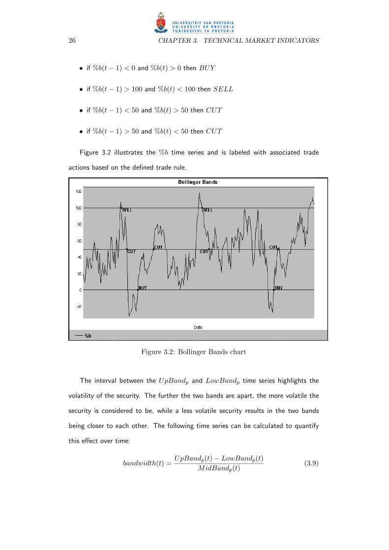
• if %b(t− 1) < 0 and %b(t) > 0 then BUY
• if %b(t− 1) > 100 and %b(t) < 100 then SELL
• if %b(t− 1) < 50 and %b(t) > 50 then CUT
• if %b(t− 1) > 50 and %b(t) < 50 then CUT
Figure 3.2 illustrates the %b time series and is labeled with associated trade
actions based on the defined trade rule.
Figure 3.2: Bollinger Bands chart
The interval between the UpBandp and LowBandp time series highlights the
volatility of the security. The further the two bands are apart, the more volatile the
security is considered to be, while a less volatile security results in the two bands
being closer to each other. The following time series can be calculated to quantify
this effect over time:
bandwidth(t) =UpBandp(t)− LowBandp(t)
MidBandp(t)(3.9)

3.4. MOVING AVERAGE CONVERGENCE/DIVERGENCE 27
Since the value bandwidth(t) quantifies the volatility of the security at time t,
bandwidth(t) can be used to identify and understand changes in supply and de-
mand for the underlying security.
3.4 Moving Average Convergence/Divergence
This section covers the Moving Average Convergence/Divergence indicator. A de-
tailed description of the indicator is given together with associated mathematical
formulae, default parameter values, and derived trading rules.
3.4.1 Description
The Moving Average Convergence/Divergence (MACD) indicator was developed by
Appel in 1979 [7] as a stock market timing device, utilising market momentum and
trend. MACD has proved to be best used in trending markets rather than choppy
non-trending markets. It is more efficient for longer term primary trends rather than
daily or secondary trends.
3.4.2 Rules and Interpretation
A short and long period exponential moving average (EMA) is calculated on the
security price. The difference between the two values is referred to as the price
momentum. A second time series is calculated by applying another EMA on the
price momentum using a smaller period than the ones originally used on the security
price. These two time series formulate the MACD indicator, defined as:
PriceMomentum(t) = EMAa(price)− EMAb(price) (3.10)
MomentumTrigger(t) = EMAc(PriceMomentum) (3.11)
EMAp(t) = price(t)(
2p + 1
)+
∑tj=t−p+1 price(j)
p
(100− 2
p + 1
)(3.12)

28 CHAPTER 3. TECHNICAL MARKET INDICATORS
where a,b and c indicate the periods to be used for the exponential moving average
calculations, where b > a > c. Appel recommended using a 12 day period for the fast
exponential moving average and a 26 period for the slow exponential moving average
to calculate the price momentum. A 9 day period was used for the exponential moving
average in the MomentumTrigger time series [7]. The short period EMA time
series will be referred to as the fast EMA, since it reacts quicker to price movements
compared to the second EMA time series. For the same reason, the large period
EMA will be referred to as the slow EMA.
The PriceMomentum time series oscillates around the zero axis, highlighting
positive and negative market momentum. Positive momentum indicates that the
average price for the fast EMA exceeds that of the slow EMA, highlighting a rise in
the underlying price. In this case the security is over-bought, highlighting a bullish
period. Negative momentum indicates a bearish period because the fast EMA has
fallen below that of the slow EMA, which highlights that the security is over-sold,
leading to a fall in the security price. The direction of the price momentum is also
used to indicate the strength of a bullish/bearish trend. A negative price momentum
with a negative gradient indicates a strong bearish period and a period where it would
possibly be a bad time to buy. A positive price momentum having a positive gradient
indicates that there is a strong bullish trend. When the price momentum shifts from
a positive to a negative value or vice versa, a trend reversal is indicated which is used
to generate a CUT action. The following trade rules are defined for MACD:
• if PriceMomentum(t− 1) < 0 and PriceMomentum(t) > 0 then CUT
• if PriceMomentum(t− 1) > 0 and PriceMomentum(t) < 0 then CUT
The MomentumTrigger time series in combination with the PriceMomentum
time series provides the necessary information required to enable trade entry. The
trading actions are returned when there is a crossover of these two time series in the

3.4. MOVING AVERAGE CONVERGENCE/DIVERGENCE 29
following way:
• if PriceMomentum(t−1) < MomentumTrigger(t−1) and PriceMomentum(t) >
MomentumTrigger(t) then BUY
• if PriceMomentum(t−1) > MomentumTrigger(t−1) and PriceMomentum(t) <
MomentumTrigger(t) then SELL
These actions enable the exploitation of short-term trends to realise profits. The
short-term trends may be up-trends or down-trends during periods of positive or
negative price momentum. Figure 3.3 illustrates the MACD indicator, with the trade
rules applied on the time series and all trade actions labelled.
Figure 3.3: MACD chart
Additional information is extracted from PriceMomentum(t) when the direction
of movement of the security price diverges from the direction of movement of the
price momentum. A bullish period is indicated when there is positive divergence in
the case where the security price is falling while PriceMomentum(t) is in an up-

30 CHAPTER 3. TECHNICAL MARKET INDICATORS
trend. A bearish period is indicated in the case of negative divergence where the
security price is rising while PriceMomentum(t) is in a down-trend.
3.5 Relative Strength Index
This section covers the Relative Strength Index. A detailed description of the indicator
is given together with associated mathematical formulae, default parameter values,
and derived trading rules.
3.5.1 Description
The Relative Strength Index (RSI) was introduced by Wilder in 1978 [162]. RSI
returns a value that continuously oscillates, tracking price strength and ultimately
displaying the velocity and momentum of a security price. This is done by comparing
the magnitude of a security’s recent gains to the magnitude of its recent losses.
3.5.2 Rules and Interpretation
RSI is calculated using:
RSIp(t) = 100(
1− 11 + RSp(t)
)(3.13)
RSp(t) =TotalGainp(t)TotalLossp(t)
(3.14)
TotalGainp(t) =t∑
j=t−p+1
(price(j)− price(j − 1) > 0) (3.15)
TotalLossp(t) =
∣∣∣∣∣∣
t∑
j=t−p+1
(price(j)− price(j − 1) < 0)
∣∣∣∣∣∣(3.16)
Note that if averageloss = 0, then RSI = 100 by definition.
In the above p is the number of periods used for calculating averageloss and
averagegain. A default value of 14 was used by Wilder [162]. Larger values for p
3.5. RELATIVE STRENGTH INDEX 31
result in smoother RSI curves, while small values for p result in large volatility in the
curve.
Two fixed levels need to be defined to aid the interpretation of RSI, namely an
upper level (Lupper) and a lower level (Llower). Wilder recommended the upper level
to be set at 70 and the lower level to be set at 30. When RSI is above the upper level
and then falls below the upper level, this is considered as a warning of a potential
trend reversal, meaning that a bearish reaction of the underlying security is to be
expected. Alternatively, a bullish reaction is expected when RSI is below the lower
and then rises above the lower level. These two levels also represent over-bought and
over-sold levels respectively.
A mid level (Lmid) for RSI is at 50, which can also be used to further interpret
RSI. Values above 50 indicate that average gains are more than average losses, which
can be used as a confirmation of a bullish trend. Bearish trends can be confirmed
when RSI falls below 50, since the average losses are more than the average gains.
The following RSI trading rules are defined given the behaviour of the RSI time
series:
• if RSI(t− 1) < Llower and RSI(t) > Llower then BUY
• if RSI(t− 1) > Lupper and RSI(t) < Lupper then SELL
• if RSI(t− 1) < Lmid and RSI(t) > Lmid then CUT
• if RSI(t− 1) > Lmid and RSI(t) < Lmid then CUT
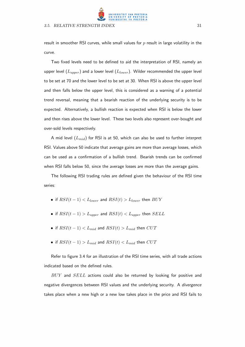
Refer to figure 3.4 for an illustration of the RSI time series, with all trade actions
indicated based on the defined rules.
BUY and SELL actions could also be returned by looking for positive and
negative divergences between RSI values and the underlying security. A divergence
takes place when a new high or a new low takes place in the price and RSI fails to

32 CHAPTER 3. TECHNICAL MARKET INDICATORS
Figure 3.4: Relative Strength Index chart
exceed its previous high or low respectively. Usually, divergences that occur after
an over-bought or over-sold security can be used to define more reliable rules. A
negative divergence during a period where the security is over-bought would entail
a SELL action while a BUY action would be returned when a positive divergence
takes place during a period where the underlying security is over-sold. It is said that
a ”failure swing” is completed when the RSI value turns and falls below its last low,
or rises higher than its last high, thus confirming a reversal.
3.6 Conclusion
This chapter covered the technical market indicators that form the technical analysis
tools of choice to be used in this study. Four technical market indicators were pre-
sented together with corresponding mathematical formulae, default parameters and
derived trading rules. The indicators selected were Aroon, Bollinger Bands, Relative
Momentum Index and Moving Average Convergence/Divergence: these indicators

3.6. CONCLUSION 33
are used in the remainder of this thesis.
Chapter 4
Computational Intelligence
Paradigms
The work in this thesis involves a number of computational intelligence (CI) paradigms,
which are covered in this chapter. Three main CI paradigms are presented, namely
artificial neural networks, particle swarm optimisation and co-evolution. Section 4.1
focuses on artificial neural networks, presenting artificial neurons, activation functions
and architectures. Neural network learning approaches are presented in section 4.1.5.
A brief introduction to evolutionary computation is made in section 4.2. Particle
swarm optimisation is covered in section 4.3, presenting neighbourhood topologies,
the PSO algorithm and a discussion on various PSO related parameters. Co-evolution
is covered in section 4.4. Two types of co-evolution are described, namely compet-
itive and cooperative co-evolution. The work produced in this study focuses on
competitive co-evolution, which is discussed in more detail in section 4.4.2. Other
co-evolution related topics that are covered include competitive fitness, fitness evalu-
ation, fitness sampling and the hall of fame. Relevant applications for each paradigm
are provided, highlighting financial applications that are related to this study.
34

4.1. ARTIFICIAL NEURAL NETWORKS 35
4.1 Artificial Neural Networks
This section explains artificial neural networks (ANN). The section briefly describes
the human brain and how ANNs were inspired by modelling the brain. The structure
and functionality of ANNs are explained together with different learning approaches
applicable to ANNs.
4.1.1 The Human Brain
The human brain consists of nerve cells called neurons that form connections with
one another, called synapses. These neurons form countless modules of networks
that are extremely complex. It is estimated that these networks contain more than
one hundred billion neurons for an adult brain and trillions of synapses [43], capable
of emitting electrical and chemical signals. It is the firing of these signals throughout
the neural complexity of the brain that allows intelligent behaviour. The human brain
is undoubtedly the most complex and advanced processor in the world today, able
to process in a non-linear parallel manner. The brain can process visual, acoustic
and sensory information immaculately, but this only partly describes its abilities - and
not even this functionality has been reproduced with today’s advanced technology.
Replicating the human brain is an inconceivable task today and it will take decades of
technological advancements for humanity to come anywhere close to such an effort.
The following books are recommended to the interested reader on neural networks
[16, 111].
4.1.2 Artificial Neurons
The artificial neural network (ANN) was inspired by studies of the human brain and
attempts to model its functionality. The artificial neuron (AN) forms the smallest
functional component of the ANN, similar to the biological neurons in the brain.
Each AN receives signals, either from other ANs, or the environment, and emits an

36 CHAPTER 4. COMPUTATIONAL INTELLIGENCE PARADIGMS
output signal by combining all the received signals. Each connection has a weight
value associated to it, which determines the strength of received signals. Each neuron
utilises a mathematical function that allows received signals to be transformed into
a single signal, which is emitted. These functions are referred to as an activation
function. Figure 4.1 illustrates the structure of an AN.
Figure 4.1: Artificial neuron
4.1.3 Activation Functions
Figure 4.2 illustrates four commonly used activation functions. As mentioned previ-
ously and shown by figure 4.1, the input into an activation function is an aggregate of
all signals received in different strengths. These strengths are determined by weights
that are associated with the connecting neurons. The formula for each of the illus-
trated activation functions is given as:
(a) Linear function (figure 4.2(a)):
F (τ) = βτ (4.1)
(b) Sigmoid function (figure 4.2(b)):
F (τ) =1
1 + e−λτ(4.2)

4.1. ARTIFICIAL NEURAL NETWORKS 37
(c) Hyperbolic tangent function (figure 4.2(c)):
F (τ) =2
1 + e−λτ− 1 (4.3)
(d) Gaussian function (figure 4.2(d)):
F (µ) = e−µ2/σ2(4.4)
where τ defines the net inputs, β is a constant defining the gradient of the linear
function, λ defines the steepness of the sigmoid and hyperbolic functions, σ2 defines
the variance of the Gaussian distribution and µ the mean.
4.1.4 Architecture
A single AN is capable of learning simple linearly separable functions [49] and forms
the smallest structural component of an ANN. An AN exhibits relatively simple be-
haviour when it functions on its own. A structure capable of learning highly complex
non-linearly separable functions can be constructed by combining a number of neurons
together. An ANN is traditionally structured in three layers of neurons, consisting of
input, hidden and output neurons, all of which are fully interconnected. This type of
ANN is the most straightforward in its structure and is referred to as a feed forward
neural network (FFNN).
The complexity of the network may be increased by adding neurons to a layer or
with the connection of neurons between adjacent layers. It has been proven that only
one hidden layer containing sufficient number of neurons can approximate any given
continuous function [18, 78, 79, 84]. Additionally, complexity may be increased by
connecting neurons that do not belong to adjacent layers. For the purpose of this
study, a standard FFNN is used.

38 CHAPTER 4. COMPUTATIONAL INTELLIGENCE PARADIGMS
(a) Linear (b) Sigmoid
(c) Hyperbolic tangent (d) Gaussian
Figure 4.2: Activation functions
Signals are presented to the input layer of the ANN and the signals are passed on
to connected ANs. The propagation of signals through each layer of the ANN results
in an output signal from each AN in the output layer. When a vector of inputs is
presented describing a specific state, the NN produces an answer described by its
outputs. An ANN can be seen as a nonlinear function that aims to map a set of
inputs to a set of outputs. Figure 4.3 illustrates the structure of a traditional ANN.
Special care always needs to be taken to avoid overfitting during the training of
an ANN. Overfitting may occur when the ANN structure is oversized, there is noise
in the training data or when an ANN is trained for too long. Overfitting implies
that the ANN structure contains excess degrees of freedom, allowing noisy data to

4.1. ARTIFICIAL NEURAL NETWORKS 39
Figure 4.3: Artificial neural network
be memorised by the structure. This results in favourable outputs produced for data
patterns on which the ANN has been trained with, and less favourable outputs pro-
duced for newly introduced inputs not included in the training process [49]. Different
methods have been developed to aid architecture optimization, which include pruning
and growing. Pruning is a method that removes neurons that have an unfavourable
effect on the learning abilities of the ANN [48, 105, 119]. Pruning involves starting
with a large ANN and then removing redundant and irrelevant weights, hidden units
and output units. Growing is a different approach to architecture selection, where a
small ANN structure is created that contains a minimal number of ANs, then me-
thodically adds ANs to the structure [65, 74, 80, 100]. More work has been done on
the issues of generalisation and overfitting by Amari et al. [4] and Muller et al. [120].
In general, overfitting can be avoided by separating the input and expected output
patterns into two disjointed sets, namely an in-sample set and an out-sample set.
The ANN is trained using the in-sample set, while its predictive quality is measured
against the out-sample set. An ANN is then selected by choosing a set-up where it
performs satisfactorily on both sets, indicating that the ANN has learnt all patterns
that have been presented during training and it has the ability to generalise over the
patterns that were not used whilst training.
40 CHAPTER 4. COMPUTATIONAL INTELLIGENCE PARADIGMS
4.1.5 Learning Approaches
An ANN does not possess any adaptive behaviour on its own, but its practicality
comes into play through the use of various algorithms designed to alter and adjust
the weights of the connections throughout the network. The process of adjusting
weight values is referred to as artificial neural network learning . Three major learning
paradigms exist which are described below:
• Supervised learning: This type of learning requires prior knowledge of the
problem domain. Supervised learning requires a training set of data patterns
consisting of inputs and target outputs. Supervised learning adjusts the weights
of the ANN such that the error between expected output and actual ANN
output is minimised. This type of learning is mostly done via gradient descent
optimisation (GD). A well-known and widely used GD algorithm was developed
by Werbos [160]. The algorithm developed by Werbos utilises backpropagation,
which propagates an error signal from the output layer through to the input
layer, adjusting weights accordingly. Other learning algorithms relevant to this
category includes generalised delta [112], Widrow-Hoff [23], scaled conjugate
gradient learning rules [118] and particle swarm optimisation [44, 71, 73, 81,
93, 115, 139, 158]. This learning paradigm is applicable to pattern recognition,
regression and classification problems [16, 104].
• Unsupervised learning: This type of learning only requires a vector of inputs,
but not any associated desired outputs. In general, this learning paradigm
attempts to discover patterns and features without any external help. Ap-
plications related to unsupervised learning in general include clustering [97],
classification [109, 33] and compression [32]. Kohonens’ self-organising maps
and learning vector quantizer (LVQ) [97] falls within this category. The latest
unsupervised neural network learning technique is that with the use of particle
4.1. ARTIFICIAL NEURAL NETWORKS 41
swarm optimisation [63, 116, 128], which is the form of learning used in this
study.
• Reinforcement learning: In this paradigm an actual data set consisting of
inputs and outputs does not exist for learning purposes. The ANN interacts
with its environment and based on its performance, the ANN is awarded or
penalised. Awards and penalties are represented by positive or negative signals
that adjust the weights of the ANN. Over time the network adapts and even-
tually produces outputs that are favourable. This learning type is applicable
to sequential decision-making tasks and control related problems in general.
LVQ-II by Kohonen [97] and Q-Learning by Watkins [159] are two popular
reinforcement learning algorithms.
4.1.6 Artificial Neural Network Applications
ANNs have extensively been applied in a wide range of real-world problems. This
includes the fields of medicine [96, 107], data mining [33, 109], data compression [40,
54], pattern recognition [32, 101, 104], gaming [25, 63, 128, 149] and robotics [57,
106]. Out of all computational intelligence paradigms, ANNs have played the most
important role in the field of finance, with numerous applications in trading bonds
[119], foreign exchange [164] and stocks [46, 102, 165]. ANN trading applications
take into consideration market information with the objective of determining price
direction in order to carry highly profitable trades at minimum risk. Stock trading
applications in particular are relevant to the work in this thesis. With regards to
neural networks in the financial sector, the following books are recommended [39,
114, 142, 146, 166].

42 CHAPTER 4. COMPUTATIONAL INTELLIGENCE PARADIGMS
4.2 Evolutionary Computation
Evolutionary computation (EC) is a paradigm within computation intelligence where
population-based metaheuristic optimisation techniques are used. EC was inspired
by Darwinian evolution, described as early as 1859 [36]. Mechanisms such as re-
production, mutation and elitism are frequently used in EC, highlighting concepts
of evolutionary biology as the driving force behind such techniques. Barricelli [12]
and Fraser [64] were the first in the 1950s to develop and apply EC. Other work fol-
lowed by Schwefel [141], Holland [75, 76], Fogel [59, 60, 61] and Rechenberg [135].
All aforementioned work introduced a form of evolutionary computation completely
disjointedly, which today forms the basis upon which EC is built. With regards to
evolutionary computation, the interested reader is prompted to the following work
by Back [9, 10]. EC algorithms include genetic algorithms (GA) [64, 68, 75, 76],
genetic programming (GP) by Koza [99], evolutionary strategies [135, 141], evolu-
tionary programming by Fogel [59, 60, 61], cultural evolution by Reynolds [136] and
co-evolution which is extensively covered in section 4.4.
EC is implemented as a simulation in which a population of solutions to a specific
problem is continuously evolved and improved over time. Solutions in an EC context
are referred to as chromosomes. A fitness function is defined which possibly forms
the most important component of EC. The fitness function maps a chromosome to
a scalar value that represents the quality of a solution. The ability to determine and
compare the quality of solutions is essential to elitism, which is an operation that
allows the preservation of the best solutions within a population. Another important
operation of EC is that of reproduction. Reproduction allows the combination of two
or more solutions to form new solutions. The original solutions are referred to as
parents while newer solutions are referred to as offspring. The process of combining
the parents is called crossover . Offspring solutions are often randomly mutated ,
which allows the maintenance of diversity within a population to avoid premature

4.2. EVOLUTIONARY COMPUTATION 43
convergence. Usually the mutation is larger at the beginning of the algorithm to
allow a global exploration of the search space and decreases over time to focus the
exploration more locally on specific solutions [49]. The quality of the offspring is
dependent on the selection of the parents, which is an extensively studied topic
[49, 55, 69]. Algorithm 1 provides pseudo-code for an EC algorithm. Each iteration
of the algorithm is referred to as a generation.
Algorithm 1 General Evolutionary Algorithm
1. Generate a population of p random solutions.
2. While no convergence:
a) Evaluate each solution in the population using the fitness function.
b) Use elitism to select e best solutions and preserve them unchanged.
c) Produce p-e new solutions via reproduction and randomly mutatethem.
d) Create a new population by grouping the elitism and reproductionsolutions together.
Convergence is reached in the following cases:
• the maximum number of generations is reached,
• the average or maximum fitness value does not change significantly over acertain number of generations, or
• an acceptable solution has been evolved that returns a satisfactory fitness.
There are multiple applications of GA and GP in the financial sector. Interested
readers are referred to [28]. Financial applications more relevant to technical trading
include foreign exchange trading [41, 124, 123, 152] and stock market trading [3, 14,
15, 122].
44 CHAPTER 4. COMPUTATIONAL INTELLIGENCE PARADIGMS
4.3 Particle Swarm Optimisation
This section discusses the basic particle swarm optimisation algorithm. The dynamics,
different topologies and parameters relevant to the algorithm are covered. The section
ends with some existing PSO applications in the financial world.
4.3.1 PSO Dynamics
Particle swarm optimisation (PSO) is a population based optimisation approach,
introduced by Kennedy and Eberhart [91, 92]. A PSO consists of a swarm of particles,
where each particle represents a potential solution. It aims to model the social
behaviour of a flock of birds, where the particles within the swarm can ”fly” within a
multi-dimensional search space in a methodical and organised manner. The position
of each particle is determined according to the experience of the particle itself and
neighbouring particles. The particle position is updated using the following equation:
−→x i(t) = −→x i(t− 1) +−→v i(t) (4.5)
where −→x i(t) is the position of particle i at time step t and −→v i(t) is the velocity
vector of particle i at time step t.
The velocity vector, −→v i, dictates the velocity and direction of the particle that
drives the optimisation process. Based on the velocity, each particle moves towards
the direction of its personal best position, −→y i, and the neighbourhood best position,
−→z i. The new position of the particle is additionally influenced by two acceleration
coefficients, which are used to scale up or down the influence of the personal best
and neighbourhood best position. The factor associated to the personal best position
is called the cognitive factor , while the one associated to the neighbourhood best
is called the social factor . The following equation is used to update the particle
velocity:
−→v i(t) = w−→v i(t− 1) +−→ρ1(−→y i −−→x i(t)) +−→ρ2(−→z i −−→x i(t)) (4.6)
4.3. PARTICLE SWARM OPTIMISATION 45
−→ρ1 = c1−→r1 (4.7)
−→ρ2 = c2−→r2 (4.8)
where w is an inertia weight, −→ρ1 is the cognitive factor, −→ρ2 is the social factor. c1 and
c2 are positive acceleration constants used to scale the contribution of the cognitive
and social components respectively. r1 , r2 are random values in the range [0,1],
sampled from a uniform distribution. These random values introduce a stochastic
element to the algorithm. More detail on these are discussed in section 4.3.3.
A fitness function, f , needs to be defined to map the particle position vector into
a scalar value. This will allow the evaluation of the particle quality that will help find
the personal and neighbourhood best solutions. Pseudocode for a PSO is given in
algorithm 2. The following references [29, 50, 94, 157] provide extensive information
on PSO.
4.3.2 PSO Topologies
In the context of a PSO, a population of solutions is referred to as a swarm and the in-
dividual solutions in the swarm as particles. Each particle within the swarm attempts
to discover the optimal solution by moving in different directions. The position of
a particle at any point in time is influenced by the position of its own best solution
(personal best) and the position of the best solution of all other particles with which
it exchanges knowledge (neighbourhood best). The social structure that determines
which particles share knowledge within a swarm is referred to as a neighbourhood
topology . Different social network structures can be formed, with the following three
topologies commonly used:
• Star topology: All particles exchange information with each other, forming a
single but fully interconnected social network. With this topology all particle
movements are affected by their own personal best solution and a global best

46 CHAPTER 4. COMPUTATIONAL INTELLIGENCE PARADIGMS
Algorithm 2 PSO
1. Initialise each particle in the swarm at a random position −→x i within thesearch space.
2. Initialise each particle velocity vector −→v i to zero.
3. Initialise each particle’s personal best position −→y i to its current position.
4. Repeat the following steps, t representing the current time step, while noconvergence:
a) Update each particle’s fitness using a fitness function f .
b) Update each particle’s personal best position −→y i:if f(−→x i(t)) > f(−→y i(t)) then −→y i(t) = −→x i(t)
c) Update the neighbourhood best position −→z i for each particle:if f(−→y i(t)) > f(−→z i(t)) then −→z i(t) = −→y i(t)
d) Update the position of each particle −→x i in the swarm using equation4.5.
e) Update the velocity −→v i of each particle in the swarm using equation4.6.
5. Assuming that a maximisation of fitness is performed, return the best so-lution defined by maxf(−→z i) of the entire swarm.
Convergence is reached in the following cases:
• the maximum number of iterations is reached,
• the average or maximum fitness value does not change significantly over acertain number of iterations, or
• an acceptable solution has been discovered that returns a satisfactory fit-ness.
solution. The global best solution forms the best solution of the entire swarm.
The first PSO algorithm developed used the star topology and was referred to
as the GBEST PSO. This is the simplest of topologies and has been shown
empirically to tend to premature convergence on a stationary point [44, 157].
The star topology is illustrated in figure 4.4(a).
• Ring topology: A neighbourhood size is defined for this topology, which deter-
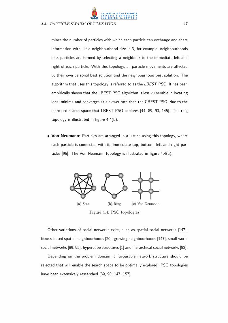
4.3. PARTICLE SWARM OPTIMISATION 47
mines the number of particles with which each particle can exchange and share
information with. If a neighbourhood size is 3, for example, neighbourhoods
of 3 particles are formed by selecting a neighbour to the immediate left and
right of each particle. With this topology, all particle movements are affected
by their own personal best solution and the neighbourhood best solution. The
algorithm that uses this topology is referred to as the LBEST PSO. It has been
empirically shown that the LBEST PSO algorithm is less vulnerable in locating
local minima and converges at a slower rate than the GBEST PSO, due to the
increased search space that LBEST PSO explores [44, 89, 93, 145]. The ring
topology is illustrated in figure 4.4(b).
• Von Neumann: Particles are arranged in a lattice using this topology, where
each particle is connected with its immediate top, bottom, left and right par-
ticles [95]. The Von Neumann topology is illustrated in figure 4.4(a).
(a) Star (b) Ring (c) Von Neumann
Figure 4.4: PSO topologies
Other variations of social networks exist, such as spatial social networks [147],
fitness-based spatial neighbourhoods [20], growing neighbourhoods [147], small-world
social networks [89, 95], hypercube structures [1] and hierarchical social networks [82].
Depending on the problem domain, a favourable network structure should be
selected that will enable the search space to be optimally explored. PSO topologies
have been extensively researched [89, 90, 147, 157].

48 CHAPTER 4. COMPUTATIONAL INTELLIGENCE PARADIGMS
4.3.3 PSO Parameters
The inertia weight, w, was introduced by Shi and Eberhart [143] to control the
exploration abilities of the swarm. The inertia weight is a means to control the step
size within the search space that is to be explored. Large values of w facilitate more
exploration, while smaller values focus the search on smaller regions of the search
space. The ability to focus the search locally or globally via the inertia weight was
followed by a natural extension of the static value to allow dynamic values [144].
An initial large value of w is used, which reduces over time. This allows an initial
exploration that focuses on smaller regions around possible solutions as the search
process progresses.
The cognitive and social components, as defined in equations 4.7 and 4.8, ad-
ditionally influence the exploration abilities of the PSO algorithm. c1 and c2 are
positive acceleration constants used to scale the contribution of the cognitive and
social components respectively. r1 , r2 are random values in the range [0,1], sampled
from a uniform distribution. These random values introduce a stochastic element to
the algorithm. To avoid velocities and positions exploding towards infinite values,
Kennedy has suggested maintaining the following relationship [88]:
c1 + c2 ≤ 4 (4.9)
Large values of c1 will steer the particle more towards the direction of the personal
best position, while larger c2 values would cause the particle to be steered more
towards the neighbourhood best position.
Convergence can be ensured by maintaining a relation combing the parameters
w, c1 and c2. The relation was defined by Van den Bergh through theoretical and
empirical analysis of the algorithms’ convergent behaviour [157]:
w >12(c1 + c2)− 1 (4.10)
with w ≤ 1.

4.3. PARTICLE SWARM OPTIMISATION 49
The topic of PSO convergence and analysis on the general properties of particle
exploration of a problem domain is an ongoing topic of research [30, 157].
4.3.4 PSO Applications
PSO has been successfully applied to train supervised and unsupervised neural net-
works. Each particle represents a neural network weight vector with the PSO attempt-
ing to minimise the mean squared error over a training set. PSO does not require
gradient information to function correctly, thus making it a candidate for numerous
problems where the gradient is either unavailable or too expensive to calculate.
The first supervised application on neural network training was done by Eberhart
and Kenedy [44, 93] by applying the basic PSO to the training of FFNNs. Many others
followed with studies that showed the success of PSO on supervised NN training. This
includes Mendes et al., who worked on the evaluation of the performance of different
neighbourhood topologies on the training of FFNNs [115], and Salerno who used
the basic PSO to train recurrent neural networks [139]. The ability of LBEST and
GBEST PSO to train FFNNs was evaluated by Hirata et al. [73] and Gudise and
Venayagamoorthy [71]. Another study on the training of NNs was done by Ismail
and Engelbrecht [81] and Van den Bergh and Engelbrecht [158] using product units.
Unsupervised neural network training has not enjoyed as much attention as super-
vised training. Xiao et al. used GBEST PSO to evolve weights for a self-organising
map [163]. PSO algorithms have also been used to co-evolve neural networks to ap-
proximate evaluation functions of game tree nodes by Messerschmidt and Engelbrecht
[116], Franken [63] and Papacostantis et al. [128].
Only in recent years has PSO been used in financial applications, with significant
success reported. Work has been to apply PSO to trading the stock market [125,
126, 127, 151], portfolio optimisation [27, 56, 86, 150] and credit scoring [66].

50 CHAPTER 4. COMPUTATIONAL INTELLIGENCE PARADIGMS
4.4 Co-evolution
This section provides a short background study on co-evolution. An introduction to
the paradigm is given, highlighting the differences between competitive and cooper-
ative co-evolution. Concepts such as fitness evaluation, fitness sampling and the hall
of fame are described. The section ends with a summary of different applications in
different fields, including financial applications.
4.4.1 Introduction
Co-evolution is the change in the genetic composition of two or more interdependent
species, in response to genetic composition change in one species [38]. It is a mutual
evolutionary influence, where each of the species involved exerts selective pressure
on each other, allowing the species to evolve and gradually adapt in turn. Co-
evolution can be seen as an iterative process, where the involved species participate
either in a competitive or cooperative environment, which eventually leads to the
gradual improvement of all involved. Therefore, as one specimen becomes superior
to another, the second evolves to overcome its inferiority and in turn become superior
to the first specimen. The first then repeats the same process, with the process
continuing indefinitely. Each specimen in turn offers different challenges, leading to
an evolutionary ”arms race” [38].
A generic example that depicts the two main different types of co-evolution is
given: species A and B in population P1, together have a competitive advantage
of some sort over species C and D in population P2. Species in population P2 are
forced to adapt in order to ensure their survival by evolving mechanisms to neutralise
the competitive advantage of species in population P1 or even better, to gain an
advantage of their own. This is done by species C and D cooperating with each
other and sharing knowledge they discover. Once species C and D have successfully
done so, species in population P1 repeat the same process which lead to a tit-for-

4.4. CO-EVOLUTION 51
tat relationship for an indefinite period, resulting in more adaptable, intelligent and
superior species.
The example above primarily demonstrates competitive co-evolution, where the
fitness of species in population P1 is an inverted fitness of the competing species in
population P2. A win for the former species ultimately means a failure for the latter.
This type of co-evolution is also referred to as predator-prey co-evolution and a fine
example in biology is described by Holland [77].
Co-evolution can also take place in a cooperative environment [132], referred
to as cooperative co-evolution, where all species work together in total cohesion.
This entails that the species work together as a team and as a single unit within a
population. In the example given, an increase in the fitness of specimen A would
entail the increase of fitness of specimen B, which forms part of the same population.
A win for the former specimen ultimately means a win for the latter. A cooperative
environment is also commonly referred to as symbiosis. The work in this thesis follows
a competitive co-evolutionary approach and thus the following section focuses on this
type of co-evolution only.
Co-evolutionary algorithms have two core differences from standard evolutionary
algorithms. Evolutionary algorithms operate in a static environment and solutions are
usually evaluated against an absolute fitness function. Co-evolutionary algorithms on
the other hand operate in a continuously changing environment, locally within each
population and globally over other populations. Because of this dynamic environment,
absolute fitness functions are difficult to define, but instead fitness is defined relatively,
by comparing individual specimens with each other.
4.4.2 Competitive Co-Evolution
Competitive co-evolution [5, 137, 138] takes place in an environment where two or
more agents directly compete against each other. It is a process that sees each agent

52 CHAPTER 4. COMPUTATIONAL INTELLIGENCE PARADIGMS
involved improve iteratively over time in an effort to overcome its competitors. Each
new generation sees improved agents with better qualities compared to previous gen-
erations: successful qualities get transferred to newer generations and are gradually
improved in turn.
It is important to note that with co-evolutionary algorithms, solutions are dis-
covered without any prior knowledge. The only information that is given to the
participating agents are the rules of the environment within which they can oper-
ate, but no objectives, strategies or general knowledge are provided. This is purely
an unsupervised training process, where agents are matched against each other and
are then evaluated relative to each other. The discovery of methodologies for ma-
chine learning within a competitive environment without the provision of any external
knowledge has been an ongoing effort over the past couple of decades [140].
4.4.3 Competitive Fitness
The fitness function used in co-evolutionary algorithms is referred to as competitive
fitness or relative fitness, and is not the same as absolute global fitness, used in
standard evolutionary algorithms. No prior knowledge is introduced via a fitness
function that could influence the behaviour of involved agents. The only knowledge
agents have is the rules of the environment within which they operate. The sole
driving force behind the process is the agents of one population performing better
than competing agents in other populations. Fitness is therefore purely a relative
function between competing agents, expressing the degree of superiority of one agent
over another. Therefore, competitive fitness reveals the ability of an agent within a
population, and is not relative to a global measurement.
Figure 4.5 depicts ideally how relative fitness may vary between two populations
during a co-evolutionary training process, while figure 4.6 depicts the ideal global
fitness of two populations. The relative fitness oscillates between two bands, with

4.4. CO-EVOLUTION 53
Figure 4.5: Co-evolution relative fitness
the one population overpowering the other in turn over time. In the case where the
two populations find themselves at extreme opposite ends, this indicates that the one
population is completely overpowered by the other population. The global fitness in
figure 4.6 reveals a similar ”arms race” pattern, but the difference is that the fitness
of each population increases over time. Global fitness reveals how the continuous
struggle of each population to overpower its rival population leads to the iterative
improvement of each population and the gradual improvement of both over time in
an ideal world.
4.4.4 Fitness Evaluation
Assume two populations of solutions P1 and P2 co-evolve in a competitive environ-
ment. There are three ways in which the fitness of a specific solution P1.−→x1 could be
evaluated relative to population P2:
• Simple Fitness [5, 8, 72]: A sample of individuals is taken from population
P2, and each one of these solutions is evaluated against P1.−→x1. The fitness

54 CHAPTER 4. COMPUTATIONAL INTELLIGENCE PARADIGMS
Figure 4.6: Co-evolution global fitness
of the solution P1.−→x1 is the number of solutions in the selected sample of P2
where P1.−→x1 was superior.
• Fitness Sharing [68]: Fitness sharing is used when it becomes necessary to
award solutions that contain unique characteristics. This is mainly done to
increase the diversity of solutions in a population so that a larger search space
is covered. Fitness sharing can be applied by calculating simple fitness and
then dividing this fitness by a value that represents the common characteristics
that the solution shares with other solutions within the same population.
• Competitive Fitness Sharing [62, 137]: Competitive shared fitness of P1.−→x1
is defined as:
P1.−→x1 =
P2.n∑
i=1
1N(P1, P2.xi)
(4.11)
where P2.n is the total number of individuals in P2 and N(P1, P2.xi) returns
the total number of agents in P1 that defeat P2.−→xi . Competitive shared fitness
awards agents in P1 that manage to beat agents in P2, where few other agents
in P1 managed to do so.

4.4. CO-EVOLUTION 55
4.4.5 Fitness Sampling
When it comes to selecting the sample against which a solution is to be evaluated,
one of the following fitness schemes can be selected [9]:
• Full competition [8]: Each solution competes against all other solutions. This
scheme is computationally demanding, since every possible pair is evaluated.
However, the fact that all solutions are evaluated against each other provides
better information regarding the solutions and a more accurate competitive
fitness is calculated. This in turn may enhance the overall performance of the
algorithm, since there is no possibility of disregarding good solutions.
• Random sampling: Random sampling is a scheme that allows each solution
to compete against a randomly selected number of solutions. One concern
when using random sampling, is that it may exclude favourable solutions in the
calculation of the competitive fitness.
• Bipartite sampling [72]: With bitrate sampling solutions are divided into two
teams, where each team competes against each other. Individuals are tested
against one of the teams resulting in less competitions.
• Tournament sampling [5]: Tournament selection uses relative fitness mea-
sures to select the best opponent individual. Different methods could be used
to setup a tournament sampling scheme. One approach would be creating
subsets of solutions and finding the best solution for each subset using relative
fitness. More subsets are then created using the best solutions and the process
is repeated until a final subset of solutions is created which will form the sample
solutions.
• Shared sampling: With shared sampling the sample solutions are selected as
the ones with the maximum competitive fitness.

56 CHAPTER 4. COMPUTATIONAL INTELLIGENCE PARADIGMS
4.4.6 Hall of Fame
It is important to retain the best solutions from one generation to another, when
a high selective pressure is required. With standard evolutionary algorithms, this is
achieved via elitism. For co-evolution, Rosin et al. [137, 138] introduced the “hall of
fame”, a mechanism that allows the perseverance of the best solutions throughout
evolution. A mechanism such as the hall of fame is necessary in co-evolution, since
potentially good solutions may be modified during training. Unlike standard evolu-
tionary algorithms that utilise a global fitness function and can easily retain the best
solutions, co-evolution may alter the best solution due to the relative fitness func-
tion in use. The solutions in the hall of fame may compete against newly evolved
solutions, which may result in the discovery of better solutions.
4.4.7 Applications
Co-evolution has found great applicability in the evolution of strategy-based models
for gaming. Applications can be found in a wide range of games, such as tic-tac-toe
[5, 6, 63, 116, 128], go [5], checkers [25, 26, 58, 63], backgammon [17, 34, 130, 131,
149], iterated prisoners dilemma [8, 63] and awari [37]. Other areas of application
include military purposes [35], classification by using evolving neural networks [72]
and controlling agents [98, 117].
More closely related to the topic of this study, a cooperative co-evolution algo-
rithm has been applied to find technical trading rules by evolving genetic programs
[14]. Co-evolution is not an extensively applied paradigm in the financial sector, with
other financial applications including the simulation of strategic behaviour in markets
[133] and co-evolving auction mechanisms [129].

4.5. CONCLUSION 57
4.5 Conclusion
The model defined in this work, which aims to discover intelligent trading agents,
combines three different CI paradigms. These are neural networks, particle swarm op-
timisation and co-evolution. The paradigms were described in this chapter, highlight-
ing financial applications that are relevant to this study. The FFNN was described,
which has been chosen as the architecture used in this thesis. Furthermore, PSO
was presented, which will form the unsupervised training technique used to train the
neural network agents. Additionally, PSO topologies and parameters were discussed.
Finally competitive co-evolution was covered, which is the environment within which
agents will compete against each other and progressively improve in the search for
the optimal trading agent.
Chapter 5
Security Trading Co-Evolutionary
PSO Model
This chapter presents a co-evolutionary particle swarm optimisation (CEPSO) model
that is used to discover security trading agents. Section 5.1 describes problems
with existing traditional technical market indicator (TMI) rule-based strategies. The
section highlights problems with TMI strategies and then defines objectives for a
new model to address such problems to improve efficiency. Section 5.2 describes the
trade simulation environment within which agent trading strategies are simulated.
A description of how trade actions are derived from FFNN output and how capital
gains/losses, transaction costs and returns are calculated follows. The model is listed
in section 5.3, including an overview of each step. Section 5.4 covers a fundamental
part of the CEPSO model, defining the competitive fitness function that is used in
the co-evolutionary environment. Finally, a detailed description of the CEPSO model
concludes the chapter in section 5.5.
58

5.1. TRADITIONAL METHODS AND PROBLEMS 59
5.1 Traditional Methods and Problems
Conventional TMI rule-based models require the careful selection of indicators and the
use of predefined rules that produce sound trade actions [13, 31]. Some examples of
such TMIs were presented in chapter 3. Such rule-based models are strictly defined
and are very difficult to fine-tune for individual stocks or different stock markets.
With just a few parameters to define each TMI, indicators leave much to be desired.
Because of the rigidity of such rules, TMIs are commonly used with default parameters
and in isolation from other indicators.
The model to be introduced in this thesis aims to discover trading strategies that
can offer advantages over conventional TMI rule-based strategies. The model should
allow the introduction of an arbitrary number of TMIs, which the model then makes
use of selectively. TMIs that are favourable and contribute positively to the quality
of discovered solutions should be weighted based on their contribution. No expert
trading knowledge should be required for training or to define trading rules. The
model should have the ability to search for strong solutions and discover complex
trading strategies for securities. Each strategy returned must derive high net profit
and low risk trading actions. The model should have the ability to detect trend
reversal patterns based on historical price data applied to the TMIs. Finding such
patterns in historical data will allow the return of trading strategies that could help
in the timing of trend reversals of securities on price data not used for training.
5.2 Trade Simulation Environment
Before describing the CEPSO model, it is necessary to define a trade simulation
environment within which strategies can be simulated and evaluated. This section
describes the components of such a simulation environment. Deriving trade actions,
calculating capital gains/losses, calculating transaction costs and calculating return
60 CHAPTER 5. SECURITY TRADING CO-EVOLUTIONARY PSO MODEL
on investment are covered in detail, enabling a trading strategy to be evaluated using
historical trade data.
5.2.1 Deriving Trade Actions
Given an arbitrary number of TMIs, it is important to describe the manner in which
trade actions are derived. A standard three layer FFNN is used for this purpose. The
sigmoid activation function is used for the hidden and output layer artificial neurons
(AN). The number of inputs used is dependent on the number of time series that are
produced by the selected TMIs that are considered, which is explained in more detail
in chapter 6.
The output layer consists of a single AN, which will be treated as a trend reversal
confidence value in the interval (0, 1). The aim of the trend reversal confidence is to
identify switches from up trends to down trends and vice versa, how trend switching is
identified is explained in this section. A trend reversal confidence time series, referred
to as σ, is produced by the FFNN by providing the values of the time series at each
time step and captures the reversal confidence value. Trade actions consist of the
actions in the set {BUY, SELL, CUT} and are derived from σ:
• if (σ(t) ≤ θ) then BUY
• if (σ(t) ≥ 1− θ) then SELL
• if (σ(t) > 0.3) and (σ(t) < 0.7) then CUT
• else no trade action is returned
where 0 < θ < 0.3 represents a threshold value of the sensitivity in triggering BUY
and SELL actions. The value of θ determines the risk factor that a trading strategy is
willing to take on. Small values of θ will result in less riskier trades taking place, while
a large θ will return more trades of higher risk. This study has taken the approach

5.2. TRADE SIMULATION ENVIRONMENT 61
of selecting a small θ. A BUY action entails buying the underlying security, while a
SELL action entails short selling the security. A CUT action signals getting out of
a position, if one is held. A CUT action means selling the bought stock or buying
back the stock that was sold short. An investable amount is defined to determine the
amount that is bought or short sold. The investable amount is the total monetary
amount available for the trading strategy to invest, which is discussed in more detail
in section 5.2.2.
Figure 5.1 depicts in detail how trade signals are derived from σ. The figure
illustrates the output of a FFNN, applied over a period in time. The value of σ(t)
oscillates between 0 and 1, indicating the confidence in the trend reversal of the
underlying security. Low σ(t) values close to 0 indicates high confidence that a
trend reversal from a down-trend to an up-trend is likely. The security in this case
is considered to be over-sold and a trend reversal, leading to a price increase, is
expected. A high σ(t) value close to 1 indicates a high confidence in the trend
reversal from an up-trend to a down-trend. In other words, the security is considered
Figure 5.1: Trend reversal confidence example

62 CHAPTER 5. SECURITY TRADING CO-EVOLUTIONARY PSO MODEL
to be over-bought and a drop in price is expected to take place. The actual trade
actions are derived in conjunction with a threshold value θ, which in the case of this
example is set to 0.1. The value of θ is a user- defined parameter that determines the
trade-triggering sensitivity. For (σ(t) > 0.3) and (σ(t) < 0.7) there is no confidence
in a reversal, indicating uncertainty about the direction of the price in the analysed
security.
At time interval 2, σ(t) penetrates the 1 − θ level, resulting in a SELL action
for the underlying security. The reasoning behind the derivation of a SELL action is
that there is a high confidence of a trend reversal from an up-trend to a down-trend
for the security. Since there is a high probability in a fall in price, the security is sold
short in an effort to take advantage of the possible price decrease. At time interval
19, σ(t) penetrates the θ level, causing a BUY action for the underlying security.
The action is derived because the trend reversal confidence from a down-trend to an
up-trend is very high. The security is bought in this case in an effort to benefit from
the possible price rise. A CUT signal is returned in the case where σ(t) is between
the levels 0.3 and 0.7. Around this mid-level there is much uncertainty with regards
to the trend reversal and the trading agent will avoid making any price speculations.
In the example presented by figure 5.1, CUT signals are returned at periods 12 and
28.
5.2.2 Calculating Capital Gains and Losses
An investable amount, used either to buy or short sell stocks, is defined. The in-
vestable amount is the total monetary amount available for the trading strategy to
invest in, for each BUY or SELL action derived. The investable amount can be
seen as the investment capital available to the agent. When the FFNN derives a
BUY action, the underlying stock is bought to the value of the investable amount.
Alternatively when the FFNN derives a SELL action, a short sell of the underlying

5.2. TRADE SIMULATION ENVIRONMENT 63
stock will take place to the value of the investable amount.
Deriving the trade actions for each time step results in the buying, selling short and
trade cutting of the stock at various time points. The number of bought or short
sold stocks per trade is calculated, based on the value of the investable amount.
Depending on how the stock price fluctuates, capital gains and capital losses are
calculated when the trade position is closed. A simple example of such a calculation
is given in table 5.1 as a demonstration, using an investable amount of $1,000,000.
The agent in the example enters a trade in a specific security, for the first time,
Table 5.1: Capital gains and losses calculation example.
Time Action Price Shares Capital Gains Capital Losses3 BUY $400 2500 - -7 CUT $500 2500 $250,000 -14 SELL $500 2000 - -22 CUT $200 2000 $600,000 -23 SELL $200 5000 - -29 CUT $500 5000 - $1,500,00035 BUY $500 2500 - -40 CUT $400 2500 - $200,000
Total $850,000 $1,700,000
at t = 3. No prior trading was done, with no capital gains or capital losses values
recorded. The agent buys the stock at a price of $400, investing an amount of
$1, 000, 000. A total of ($1, 000, 000/$400) = 2500 shares are bought, which are
then sold at t = 7. Given the increase in the stock price by $100, the agent realises
a capital gain of $250, 000. A short sell action follows at t = 14, at a price of $500
where 2000 shares are sold short. The price drops by $300 at t = 22, resulting
in a further realisation of $600, 000 as capital gain. A capital loss is incurred at
t = 29, when the price of 5000 short sold shares increases by $300, contributing to
a $1, 500, 000 loss. A further price drop of $100 from t = 35 to t = 40 results in
a capital loss worth $200, 000, because a total of 2000 shares were held. Given the

64 CHAPTER 5. SECURITY TRADING CO-EVOLUTIONARY PSO MODEL
sequence and timing of the agents’ trade actions in this example, capital gains worth
$850, 000 were accumulated and a capital loss of $1, 700, 000 was suffered. Overall,
a loss worth of $850, 000 was incurred.
5.2.3 Calculating Transaction Costs
Buying and short selling of stocks come with a transaction cost, payable to the
executing broker. It is necessary for such costs to be considered, since costs can
be a determining factor in the profitability of the discovered strategies. Transaction
costs vary from one broker to another and between different stock markets. For the
purposes of this thesis, a transaction cost of 5 basis points (BPS) on the invested
amount will be used for each trade entry and each trade exit. Additionally, 36.5 BPS
per annum on the invested amount will be used as a script lending fee. Based on an
investable amount of $1,000,000, this results in transaction costs of $500 per trade
entry, $500 per trade exit and $3650 per annum for script lending (or $10 per day).
Table 5.2 portrays an example of transaction costs, based on a simplistic scenario.
At t = 22 a script lending fee of $80 is payable for the eight days the stock was
borrowed, while an additional fee is payable at t = 29 for a further six days. In total,
transaction costs worth $4160 were payable to the executing broker for this example.
Table 5.2: Transaction costs calculation example.
Time Action Transaction Costs3 BUY $5007 CUT $50014 SELL $50022 CUT $500 + (8*$10) = $58023 SELL $50029 CUT $500 + (6*$10) = $56035 BUY $50040 CUT $500
Total $4160
5.3. THE CEPSO MODEL STEP-BY-STEP 65
5.2.4 Calculating Return on Investment
The return on investment, otherwise referred to as returns, is a ratio of the profits
or losses on an investment over the total capital invested. Returns are calculated for
a specific period of time, using the following equation:
returns =EMV −BMV
BMV(5.1)
where EMV is the value of the investment at the end of the period and BMV is
the value of the investment at the beginning of the period. It is common prac-
tice to annualise the returns, in order to make returns from different period lengths
comparable.
In the context of the trade simulation environment presented in this section, the
returns are calculated as the capital gains/losses over the investable amount:
returns =CG− CL
IA(5.2)
where CG are the capital gains, CL are the capital losses and IA is the investable
amount. For the example presented in table 5.1, the returns are -$850, 000/$1, 000, 000 =
−0.85 or -85% for the 40 days the strategy traded.
5.3 The CEPSO Model Step-by-Step
This section lists the steps of the CEPSO model, providing an introductory overview.
More details on the model is provided in section 5.5.
1. Calculate the TMI time series data, based on the security price data as described
in chapter 3. Divide the TMI time series data into two sets, namely an in-sample
and out-sample TMI time series data set. If the TMI time series consists of n
data points, the in-sample data set would consist of all sequential data points
from the beginning of the time series to m, and the out-sample data set all
sequential data points from m to n, where n > m.

66 CHAPTER 5. SECURITY TRADING CO-EVOLUTIONARY PSO MODEL
2. Create a single swarm of particles and randomly initialise the position of each
particle within the range [−r, r].
3. Set the velocity of each particle within the swarm to zero.
4. Initialise each particle’s personal best to its current position.
5. Repeat the following steps for a total of n epochs:
A. Use the current position vector of each particle within the swarm and create
a population of feed forward neural networks by assigning the particle
position vectors as FFNN weight vectors.
B. Using the in-sample TMI data set to derive the FFNN trend reversal con-
fidence time series.
C. Using the in-sample trend reversal confidence time series, calculate the
performance metrics for each solution within the population, by simulating
the derived BUY , SELL and CUT signals.
D. Calculate the competitive fitness for each solution using the in-sample
data. Each solutions’ performance metrics are considered in the calcu-
lation, which is derived from the in-sample data. More detail on how the
competitive fitness is calculated is given in section 5.4.
E. Add the best solution from the population to the hall of fame.
F. Update each particle’s fitness to the calculated competitive fitness of the
agent.
G. Update each particle’s personal best position.
H. Update the neighbourhood best position for each particle.
I. Update the velocity for each particle.
J. Update the position of each particle in the swarm.

5.4. COMPETITIVE FITNESS FUNCTION 67
6. Using the out-sample TMI data set, derive the FFNN trend reversal confidence
time series for each solution in the hall of fame.
7. Using the out-sample TMI confidence time series, calculate the performance
metrics for each solution in the hall of frame, by simulating the derived BUY ,
SELL and CUT signals.
8. The best solution within the hall of fame needs to be determined based on
the out-sample data. Calculate the competitive fitness for each solution in the
hall of fame using the out-sample data. Return the solution with the highest
competitive fitness for out-sample data as the best solution the model has
produced.
5.4 Competitive Fitness Function
Given a set of trade agents, a fitness value is assigned to each agent indicating its
relative strength or weakness with respect to other agents in the same set. The
competitive fitness introduced in this section is defined based upon two trade perfor-
mance metrics that are calculated for each agent, which includes a net profit and the
Sharpe ratio. It is important to note that these performance metrics can be calcu-
lated individually for each agent in complete isolation from other trade agents. The
performance metrics themselves are not the relative measures but merely represent
straightforward metrics of the performance of the agent.
The net profit of a trade agent is calculated by taking the capital gains of the
strategy and subtracting the capital losses and transaction costs. This profit and loss
(P&L) measure is defined as:
P&L = CG− CL− TC (5.3)
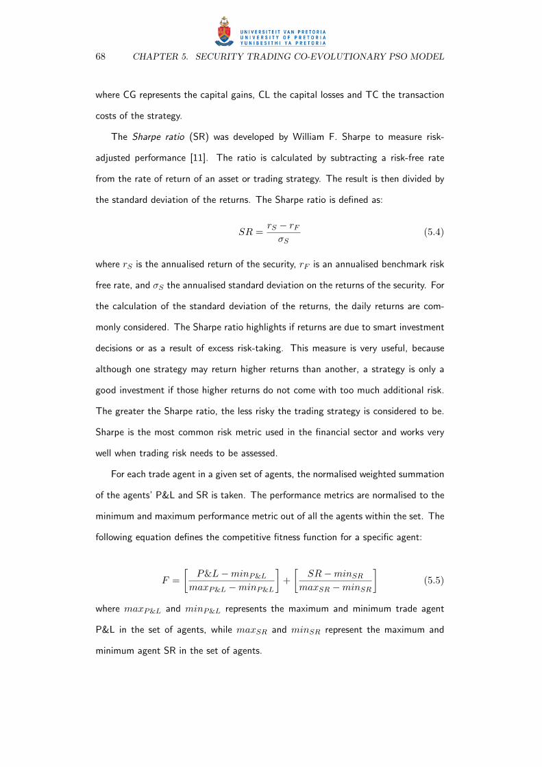
68 CHAPTER 5. SECURITY TRADING CO-EVOLUTIONARY PSO MODEL
where CG represents the capital gains, CL the capital losses and TC the transaction
costs of the strategy.
The Sharpe ratio (SR) was developed by William F. Sharpe to measure risk-
adjusted performance [11]. The ratio is calculated by subtracting a risk-free rate
from the rate of return of an asset or trading strategy. The result is then divided by
the standard deviation of the returns. The Sharpe ratio is defined as:
SR =rS − rF
σS(5.4)
where rS is the annualised return of the security, rF is an annualised benchmark risk
free rate, and σS the annualised standard deviation on the returns of the security. For
the calculation of the standard deviation of the returns, the daily returns are com-
monly considered. The Sharpe ratio highlights if returns are due to smart investment
decisions or as a result of excess risk-taking. This measure is very useful, because
although one strategy may return higher returns than another, a strategy is only a
good investment if those higher returns do not come with too much additional risk.
The greater the Sharpe ratio, the less risky the trading strategy is considered to be.
Sharpe is the most common risk metric used in the financial sector and works very
well when trading risk needs to be assessed.
For each trade agent in a given set of agents, the normalised weighted summation
of the agents’ P&L and SR is taken. The performance metrics are normalised to the
minimum and maximum performance metric out of all the agents within the set. The
following equation defines the competitive fitness function for a specific agent:
F =[
P&L−minP&L
maxP&L −minP&L
]+
[SR−minSR
maxSR −minSR
](5.5)
where maxP&L and minP&L represents the maximum and minimum trade agent
P&L in the set of agents, while maxSR and minSR represent the maximum and
minimum agent SR in the set of agents.
5.5. CEPSO MODEL DESCRIBED 69
The competitive fitness function attempts to evaluate the relative performance
of each solution within a set of solutions, by considering a weighted balance between
net profit and risk. The fitness function directs trading agents in making the highest
net profit at the lowest risk possible. By considering equation (5.3), the agent in
fact attempts to maximise capital gains and minimise capital losses together with
transaction costs. The consideration of equation (5.4) allows low risk solutions to
be returned by maximising strategy returns and minimising the standard deviation
of the returns. considering equation (5.5) closely, it can be deduced that a relative
fitness value of 2 represents a solution that is superior in P&L and SR in the set of
solutions, while a value of 0 represents the most inferior solution in the set. Note
that the competitive fitness value can not be used to compare solutions that were
derived from within different sets of solutions, since different maximum and minimum
performance metrics may exist in each separate set.
5.5 CEPSO Model Described
This section describes the CEPSO model in more detail. The first step of the CEPSO
model is data preparation. Price data is separated into two sets, an in-sample and
out-sample set. The former set is prepared to be used for training purposes, while
the latter is used to evaluate the generalisation ability of discovered strategies. Each
set is applied to the TMIs used in the model, deriving in-sample and out-sample TMI
time series data. If the TMI time series consists of n data points, the in-sample data
set would consist of all sequential data points from the beginning of the time series
to m and the out-sample data set all sequential data points from m to n, where
n > m.
PSO has been proven to be very effective as an unsupervised NN training algo-
rithm, as described in chapter 4, section 4.3.4. The CEPSO makes use of unsuper-
vised learning through competitive co-evolution to allow NN training. A single swarm

70 CHAPTER 5. SECURITY TRADING CO-EVOLUTIONARY PSO MODEL
of particles is created, each particle representing a security trade agent. For each par-
ticle in the swarm, the position is randomly initialised uniformly over the entire search
space. This will enable the algorithm to better converge to a strong solution. A range
from which random weight values can be selected was defined by Wessels and Barnard
[161] for this purpose. The ranges was defined as [ −1√fanin
, 1√fanin
], where fanin is
the number of connections leading to an AN. This initialisation of weights close to
zero has shown to be very efficient, facilitating convergence to optimal points within
the search space. The personal best position of each particle is set to the particle’s
initial position. A population of FFNNs is created by using the particle position vec-
tors as weight vectors. The trend reversal confidence signal for each neural network is
then computed for the in-sample TMI data during training, considering a historic time
window of size t. Trading actions that define BUY , SELL and CUT actions are
derived, as described in section 5.2.1. The trading actions are executed for each time
step, with capital gains, capital losses and transaction costs calculated, as explained
in section 5.2.
The performance of each particle (representing a FFNN) is measured using the
relative fitness function defined in equation (5.5). Based on the calculated perfor-
mance metrics, the competitive fitness for each FFNN strategy is computed using full
competition sampling, described in more detail in section 6.2.2. The fittest FFNN is
added to a hall of fame, allowing the perseverance of strong strategies throughout
the training process. A PSO algorithm is then executed to update each particle’s best
position. It is important to note that, since a competitive fitness is used to evaluate
the solutions within the swarm for each generation, the competitive fitness cannot
be used to compare solutions between different generations. The personal best posi-
tion of the particle is updated with the position with the highest competitive fitness,
comparing the current and existing personal best positions. The neighbourhood best
position for each solutions is then updated, together with the velocity and particle
5.6. CONCLUSION 71
position.
The training process takes place for a predefined total of n epochs, with each
epoch contributing the best in-sample strategy of the population to the hall of fame.
After the n epochs are executed, all the strategies in the hall of fame are evaluated
against each other, by using the competitive fitness function on all solutions within
the hall of fame. Previously the solutions were evaluated based on their out-sample
data, the objective with re-evaluating the hall of fame is to do so based on out-
sample data. The out-sample data is used in this case, with the highest fitness
solution returned as the best strategy.
5.6 Conclusion
This chapter presented the CEPSO model that forms the FFNN unsupervised trainer.
The chapter explained the reasoning behind the selection of the model and the ben-
efits over conventional TMI rule-based strategies. A trade simulation environment
was described that allows the simulation of trading strategies. The manner in which
trading actions are derived, the calculation of capital gains/losses, transaction costs
and returns are explained in detail with accompanying examples. A step-by-step list-
ing of the model then followed. The competitive fitness function was presented, used
in the competitive co-evolutionary environment to evaluate strategies against each
other. A detailed CEPSO model description then ended the section.

Chapter 6
Empirical Study
This chapter examines the performance of the co-evolutionary particle swarm opti-
misation (CEPSO) model. The model is applied to the stock price data of eight
different companies, discussed in section 6.1. The section also covers the technical
market indicator time series used and how the data is generally prepared for the
model. Section 6.2 covers the experimental procedure, defining objectives and intro-
ducing the initial CEPSO model set-up. Algorithm parameters and configurations are
examined in section 6.3, with the optimum model set-up discovered. The best dis-
covered strategies are compared against two benchmarks in section 6.4, highlighting
the effectiveness of the model.
6.1 Data Preparation
This section describes the data preparation for the empirical study, which includes
the stock data selection and the technical market indicators to which data is applied
to.
72

6.1. DATA PREPARATION 73
6.1.1 Stock Data
The top four US and UK companies by market capitalisation were selected, as defined
by the FT Global 500 [154]. The FT Global 500 is an annual snapshot of the largest
500 companies worldwide, ranked by market capitalisation. Its purpose is to highlight
how corporate fortunes change over time in different countries and industries. The
selection of the stocks was made based on the list published on the 31st March
2008. Refer to appendix C, table C.1 for a layout of the stocks used in this chapter,
together with their corresponding worldwide rank, country of origin, currency, industry
and market capitalisation. The daily price graphs for all eight companies are also
illustrated in appendix C, in the domicile currency of each company. The data for
a period of eight and a half years was used, which included data for the dates 1st
January 2000 to 30th June 2008. The in-sample data was selected as 75% of the data,
which consisted of the dates 1st January 2000 to 31st March 2006. The remaining
data was used as the out-sample data set, between the dates 1st April 2006 to 30th
June 2008.
The period 1st January 2000 to 30th June 2008 consists of a variety of stock
market crisis events, making it ideal for training purposes. It is ideal because during
these market events price movements were irrational and volatile, allowing the dis-
covery of agents that can deal with such extreme events. The date period that has
been selected includes the following market events:
• Dot-com bubble: The dot-com bubble roughly covered the period 1995-2001,
which saw a rapid increase of companies in the internet sector and other related
fields. It reached a climax on 10 March 2000, when the bubble “burst,” causing
dramatic falls in share prices in many involved companies, resulting in many of
the companies going bust.
• 9/11: The attacks on the World Trade Centre on 11 September 2001 had
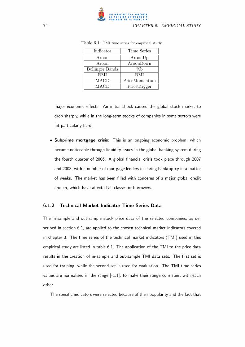
74 CHAPTER 6. EMPIRICAL STUDY
Table 6.1: TMI time series for empirical study.
Indicator Time SeriesAroon AroonUpAroon AroonDown
Bollinger Bands %bRMI RMI
MACD PriceMomentumMACD PriceTrigger
major economic effects. An initial shock caused the global stock market to
drop sharply, while in the long-term stocks of companies in some sectors were
hit particularly hard.
• Subprime mortgage crisis: This is an ongoing economic problem, which
became noticeable through liquidity issues in the global banking system during
the fourth quarter of 2006. A global financial crisis took place through 2007
and 2008, with a number of mortgage lenders declaring bankruptcy in a matter
of weeks. The market has been filled with concerns of a major global credit
crunch, which have affected all classes of borrowers.
6.1.2 Technical Market Indicator Time Series Data
The in-sample and out-sample stock price data of the selected companies, as de-
scribed in section 6.1, are applied to the chosen technical market indicators covered
in chapter 3. The time series of the technical market indicators (TMI) used in this
empirical study are listed in table 6.1. The application of the TMI to the price data
results in the creation of in-sample and out-sample TMI data sets. The first set is
used for training, while the second set is used for evaluation. The TMI time series
values are normalised in the range [-1,1], to make their range consistent with each
other.
The specific indicators were selected because of their popularity and the fact that

6.2. EXPERIMENTAL PROCEDURE 75
the time series they produce oscillate in a fixed range [31]. The oscillation in a fixed
range makes them practical in the context of neural networks, since they can easily
be normalised for use as neuron inputs. Furthermore, they expose a variety of price
properties throughout time, including supply, demand, momentum, volatility, trend,
sentiment and retracement.
6.2 Experimental Procedure
The empirical objectives that will be studied and analysed in this thesis are outlined
in section 6.2.1. The initial set-up of the CEPSO model is described in section
6.2.2. The default values used for financial parameters are initially described. The
section then describes neural network, PSO and co-evolution configurations used in
the empirical study.
6.2.1 Objectives
The following empirical objectives will be studied and analysed, with the in-sample
and out-sample performance considered:
• An analysis of different particle swarm optimisation (PSO) topologies and how
they affect the quality of discovered strategies.
• An investigation of swarm population size combinations with feed forward neu-
ral network (FFNN) hidden layer size. A study of how an increase in size of
swarm population size and hidden layer size affects the model, keeping in mind
issues of overfitting and computational complexity. These parameter combina-
tions are additionally investigated against different PSO topologies.
• An examination of the change in performance for different trading rule sensi-
tivity thresholds (θ).
76 CHAPTER 6. EMPIRICAL STUDY
• A study of whether the given model is successful in discovering optimal trading
agents, by comparing its performance against two benchmark strategies.
6.2.2 CEPSO Model Initial Set-up
Financial Parameter Configuration
An investable amount of 1,000,000 currency units is utilised in the trade simulation
environment, as described in chapter 5, section 5.2. This is the total capital available
for agents to buy or short sell stocks, on a trade-by-trade basis. The currency unit is
determined by the domicile currency of the stock. For US companies the US Dollar
(USD) is used, while the Pound Sterling (GBP) is used for UK companies.
For the Sharpe ratio calculations, an annual risk-free rate of 3% was used for the
US companies and 6% for the UK companies. The risk-free rates were chosen based
on the applicable interest rates for the US and UK at the time this empirical study
was conducted.
Neural Network Configuration
A standard three layer FFNN is used to produce the trend reversal confidence, from
which trading actions are derived. The sigmoid activation function are used for hidden
and output neurons.
The size of the FFNN input layer is six, which is the total number of TMI time
series as defined in table 6.1. The size of the FFNN hidden layer is investigated with
values of 2, 4, 6, 8 and 10 in section 6.3.1. Based on the results of the empirical study,
an investigation of more than 10 hidden units was not necessary. This is due to the
increased computational intensity that is introduced with no significant improvement
visible.
A single neuron forms the output layer of the neural network, which returns
a value in the range (0, 1), indicating a trend reversal confidence, as described in
6.3. EXPERIMENTAL ANALYSIS 77
section 5.2.1. The threshold, θ, used to derive trade actions from the FFNN output
is initially set to 0.05, but values of 0.1, 0.2 and 0.3 are examined in section 6.3.2.
Larger values are not considered, since 0.3 is the level at which CUT signals are
returned, as described in section 5.2.1.
PSO Configuration
The PSO algorithm is executed for a total of 350 epochs for each simulation. The
value φ for the inertia weight is set to 0.729844 and the acceleration constants c1 and
c2 are set to 1.496180. These three parameters satisfy the relation defined by van den
Bergh [157], ensuring convergent behaviour. The swarm size is investigated in this
empirical study, with values 10, 25, 50, 100, 150 and 200 in section 6.3.1. Different
PSO topologies, such as GBEST, LBEST and Von Neumann, are also studied in
section 6.3.1. A standard PSO algorithm is used, as introduced by Kennedy and
Eberhart [91, 92].
Co-evolutionary Configuration
A full competition fitness sampling is used, with other fitness sampling schemes
not considered. Full competition fitness sampling is used because it results in a
better estimation of relative fitness compared to schemes where only a sub-sample
of competing solutions is considered. The competitive fitness function defined in
equation (5.5) in section 5.4 normalises the performance metrics for all available
trading agents in each iteration, resulting in the most accurate estimation of relative
fitness.
6.3 Experimental Analysis
Appendix D depicts all the experimental result tables that this section refers to. An
overview of the experimental results is given below.

78 CHAPTER 6. EMPIRICAL STUDY
Tables D.1, D.2 and D.3 lists the average and standard deviation of the annualised
returns for the GBEST, LBEST and Von Neumann PSO topologies, together with
the combination for different particle swarm sizes and hidden neurons. The profit and
loss (P&L) and Sharpe ratio is tabled in the same fashion in tables D.4, D.5, D.6,
D.7, D.8 and D.9. A total of 30 simulations were executed for each permutation of
the three parameters (swarm size, hidden layer size and topology) for each company.
Performance associated to the increase of hidden layer neurons is depicted from left
to right, while the performance associated from top to bottom is relevant to the
increase of the PSO particle swarm size. The results for all eight company stocks
are combined in these tables, giving an overall view of returns, P&L and Sharpe
ratios regardless of the stock. By combining the companies together in these tables,
180 simulations result for each table entry. The reason why all eight companies are
combined together is to keep the number of tables to a manageable number, with
nine tables to compare instead of seventy two. The company-by-company results are
listed in tables D.10, D.11 and D.12 for the best swarm size and hidden layer set-up of
the Von Neumann and LBEST topologies. Table D.13 depicts the annualised returns
for different trend reversal confidence parameters on a company-by-company basis.
All tables clearly indicate the different parameter combinations used to produce
the results, on the top left column of each table. The top half of each table lists the
averages for the simulations, while the bottom half lists the standard deviations. The
left half lists the in-sample results, while the right half lists the out-sample results.
The averages of the average and standard deviation results are indicated in the last
column and last row of each table.
Solutions with combinations for the three parameters swarm size, hidden neuron
size and topology will be referred to using the following notation (swarm size, hidden
neuron size, topology). As an example, the solution (100, 6, Von Neumman) will
refer to a solution with a swarm size of 100, 6 neurons in the hidden layer using a
6.3. EXPERIMENTAL ANALYSIS 79
Von Neumann topology.
6.3.1 Topology vs. Swarm Size vs. Hidden Layer Size
Figure 6.1(b) illustrates together with the out-sample returns in tables D.1, D.2 and
D.3, that the returns of GBEST are considerably lower compared to Von Neumann
and LBEST. This can be explained by the fact that GBEST explores less compared
to the other topologies. Graph 6.1(a) indicates that GBEST has high in-sample
returns for large swarm size and hidden layer size combinations, which is due to the
overfitting of trained data.
The highest GBEST solution for out-sample data has a return of 10.34%, occur-
ring at (50, 10, GBEST). The Von Neumann and LBEST topologies both have their
highest return solutions over 13.0%. A solution with a return of over 13.0% occurs
once for the Von Neumann topology, at (200, 2, Von Neumann) with a return of
13.35%. The LBEST out-sample returns in table D.3 contains solutions with similar
quality at (150, 4, LBEST) and (200, 6, LBEST) with returns of 13.21% and 13.14%
respectively.
A 95% confidence interval using a two sample t-test is utilised for the following
comparison, based on 180 observations for each sample. The two sample t-test
is compared against a critical value of 1.97; t-test values larger than the critical
value are considered significantly different. The top Von Neumann solution based on
out-sample returns is significantly different to the GBEST solution, the t-test value
considering the two samples (50, 10, GBEST) and (200, 2, Von Neumann) is 1.99.
The top LBEST solution (150, 4, LBEST) falls short on the t-test at 1.95 against
GBEST and is therefore not significantly different when considering the out-sample
returns at a 95% confidence.
Examining tables D.4, D.5, D.6, D.7, D.8 and D.9 in conjunction with the figures
in 6.2, the following is observed:

80 CHAPTER 6. EMPIRICAL STUDY
(a) Returns in-sample
(b) Returns out-sample
Figure 6.1: Annualised returns (%) for each topology
• Von Neumann: The two highest out-sample P&L solutions consists of values
of 2,670,000 at (200, 2, Von Neumann) and 2,450,000 at (150, 2, Von Neu-
mann). The top two Sharpe solutions consist of 0.46 at (50, 8, Von Neumann)
and 0.45 at (200, 2, Von Neumann). Considering that (200, 2, Von Neumann)
has the highest returns, highest P&L and a high Sharpe ratio, it is chosen as
the favourite Von Neumann solution.

6.3. EXPERIMENTAL ANALYSIS 81
• LBEST: The top two P&L solutions, consists of 2,640,000 at (150, 4, LBEST)
and 2,630,000 at (200, 6, LBEST). The top three Sharpe solutions consist of
0.55 at (200, 6, LBEST) and 0.49 at both (150, 4, LBEST) and (200, 10,
LBEST). All three solutions have noteworthy performance features, but it is
solution (150, 4, LBEST) that stands out. The reason is because its P&L
and Sharpe performance is high using the smallest PSO particle swarm size
and the smallest number of hidden neurons out of all three solutions. Solution
(150, 4, LBEST) is selected as the favourite LBEST solution, since it is less
computationally expensive because of the small swarm and hidden layer size.
• GBEST: The top solution based on P&L is 2,070,000 with a Sharpe of 0.37.
The best GBEST solution based on all three performance metrics considered
is (50, 2, GBEST).
The best solutions for the Von Neumann and LBEST topologies are therefore
(200, 2, Von Neumann) and (150, 4, LBEST). Results of these topologies are com-
pared in tables D.10, D.11 and D.12 together with figures 6.3 on a company-by-
company basis. These three tables break down the performance for each solution
against each individual company for a more detailed comparison. The in-sample vs.
out-sample results and averages vs. standard deviation results are portrayed in the
same fashion as all previous tables.
The performance breakdown for each individual company shows that the two
selected configurations perform very similarly for out-sample and in-sample data,
with one topology slightly outperforming the other for some companies and vice
versa. Based on table D.10, the LBEST topology can be identified as having slightly
higher out-sample average returns for General Electric, AT&T, HSBC and BP. Exxon
Mobil, Microsoft, Vodafone and Rio Tinto Group have slightly higher out-sample
average returns for the Von Neumann topology. It must be pointed out that there
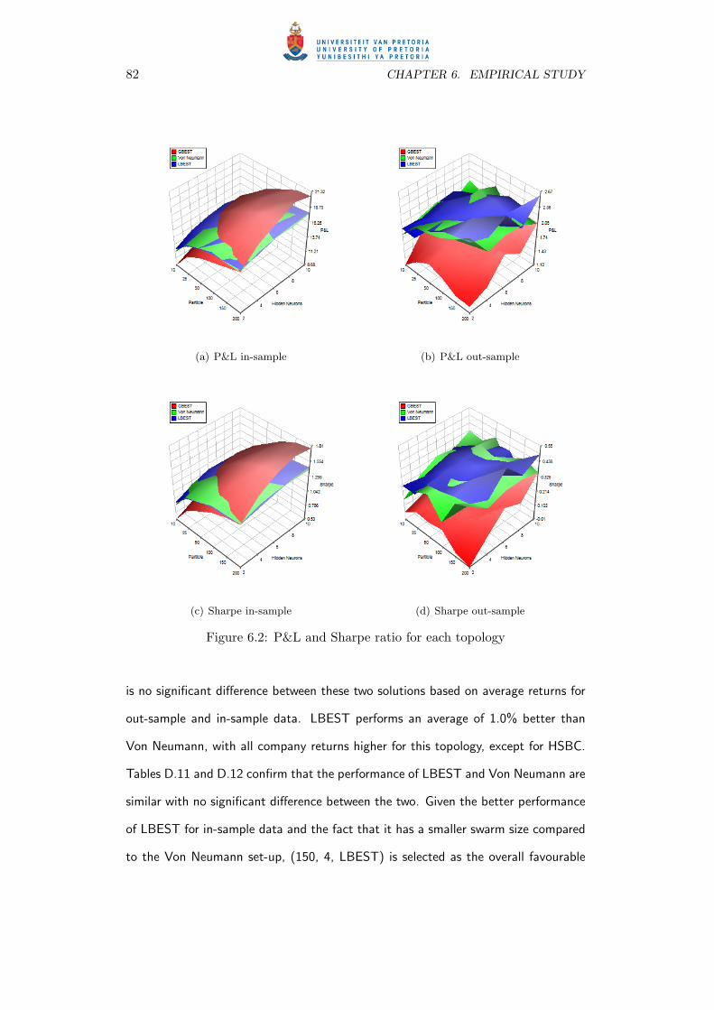
82 CHAPTER 6. EMPIRICAL STUDY
(a) P&L in-sample (b) P&L out-sample
(c) Sharpe in-sample (d) Sharpe out-sample
Figure 6.2: P&L and Sharpe ratio for each topology
is no significant difference between these two solutions based on average returns for
out-sample and in-sample data. LBEST performs an average of 1.0% better than
Von Neumann, with all company returns higher for this topology, except for HSBC.
Tables D.11 and D.12 confirm that the performance of LBEST and Von Neumann are
similar with no significant difference between the two. Given the better performance
of LBEST for in-sample data and the fact that it has a smaller swarm size compared
to the Von Neumann set-up, (150, 4, LBEST) is selected as the overall favourable
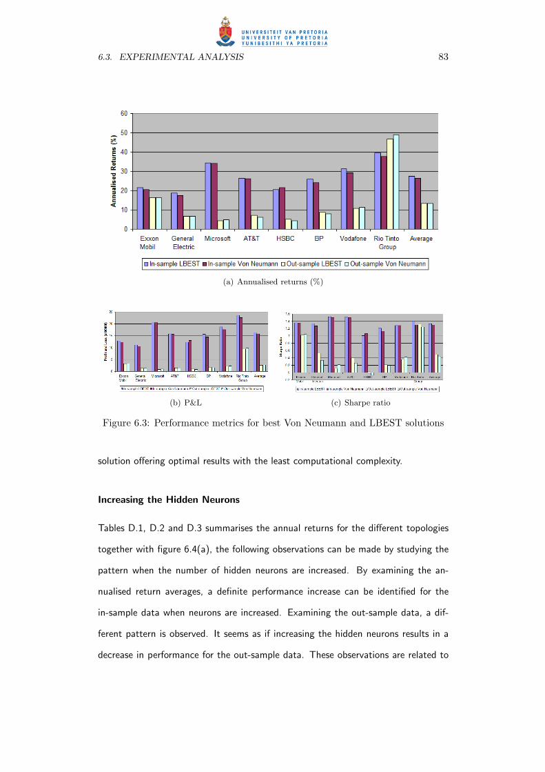
6.3. EXPERIMENTAL ANALYSIS 83
(a) Annualised returns (%)
(b) P&L (c) Sharpe ratio
Figure 6.3: Performance metrics for best Von Neumann and LBEST solutions
solution offering optimal results with the least computational complexity.
Increasing the Hidden Neurons
Tables D.1, D.2 and D.3 summarises the annual returns for the different topologies
together with figure 6.4(a), the following observations can be made by studying the
pattern when the number of hidden neurons are increased. By examining the an-
nualised return averages, a definite performance increase can be identified for the
in-sample data when neurons are increased. Examining the out-sample data, a dif-
ferent pattern is observed. It seems as if increasing the hidden neurons results in a
decrease in performance for the out-sample data. These observations are related to

84 CHAPTER 6. EMPIRICAL STUDY
the overfitting of data during the training process. The introduction of more neurons
to the neural network architecture allows more degrees of freedom, resulting in an
improvement of the in-sample data. This does not favour out-sample data, since
the neural network may be overfitting in-sample data patterns. For the given data,
more than six neurons in the hidden layer causes a substantial drop in performance
for out-sample data.
(a) Annualised returns (%) change for an increase in the hidden layer
(b) Annualised returns (%) change for an increase in the particle size
Figure 6.4: Performance Topologies

6.3. EXPERIMENTAL ANALYSIS 85
Increasing the Swarm Size
Tables D.1, D.2, D.3 and figure 6.4(b) indicate that there is a direct correlation
between swarm size and performance, for in-sample and out-sample data. This is
visible by observing the increase in annualised return averages for all three topologies
as the swarm size increases. This is attributed to the improved exploration capability
of the particle swarm, when more particles are introduced. The more particles, the
more information can be derived from the search space and is shared among parti-
cles, allowing better solutions to be found. The optimum swarm size is determined
by finding a size that offers a good trade-off between high performance and low
computational complexity. Based on the investigation conducted in this section, a
particle swarm size of 150 was found to be optimum for the LBEST topology.
6.3.2 Trading Sensitivity Threshold
A study is performed on the threshold values used to derive the trading actions from
the trend reversal confidence. The value of θ determines the risk factor that a trading
strategy is willing to take on. Small values of θ will result in less riskier trades taking
place, while a large θ will return more trades of higher risk. This study has taken
the approach of selecting a small θ, a value of 0.05 was used thus far. Table D.13
investigates larger threshold values, in an effort to increase annualised returns by
producing more trades with smaller confidence values.
The out-sample average annualised returns indicate that larger values contribute
to smaller returns. This highlights that lowering the confidence threshold yields
smaller returns even though more trading takes place. The corresponding average
annualised returns for θ values of 0.05, 0.1, 0.2 and 0.3 are 13.21, 13.09, 12.13
and 10.77. Since no benefits are seen with a change in the threshold, the optimal
parameter value remains as θ = 0.05.
86 CHAPTER 6. EMPIRICAL STUDY
6.4 Benchmarks
Each company stock price forms a different problem, so different model configurations
are suitable for different companies. The empirical procedure thus far aimed at
fine-tuning a general configuration that would be the most suitable for all eight
investigated companies. The best configuration for each individual company is not
chosen to be compared against the benchmarks, but rather the results derived from
the configuration that was optimum overall. The set-up (150, 4, LBEST) with
θ = 0.05 is chosen to be compared against the benchmarks.
6.4.1 Rule Based Results
A good combination of two technical market indicators is that of Bollinger Bands
and RSI, as suggested by John A. Bollinger [19]. The two indicators complement
each other very well and can be used to produce sound trading rules. Table 6.2
depicts the annualised results of using such rules on the eight selected companies.
The annualised returns of the trading rules are compared with the returns of the
agents discovered via the CEPSO model.
Comparing the strategies, the CEPSO strategies significantly outperform the rule-
based model for in-sample data. The returns are considerably higher for all eight
companies, which is to be expected since the in-sample data was used for training
and the neural network agent has taken full advantage of it. The out-sample results
highlight that the CEPSO strategies are superior for all companies, except for General
Electric and AT&T. In the case of General Electric, the CEPSO strategy produced
smaller annual returns by 3.14%, compared with the rule-based strategy. For AT&T
the performance of the benchmark is even larger, 13.02% better than CEPSO. For
the remaining six companies the CEPSO agent was superior, indicating that the
CEPSO model overall outperforms the Bollinger Bands/RMI strategy. On average
the CEPSO agents produces 21.24% more returns for the in-sample data and 9.09%
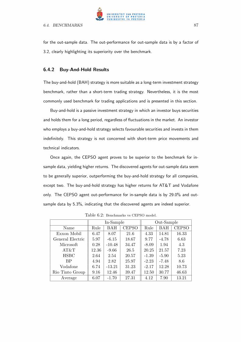
6.4. BENCHMARKS 87
for the out-sample data. The out-performance for out-sample data is by a factor of
3.2, clearly highlighting its superiority over the benchmark.
6.4.2 Buy-And-Hold Results
The buy-and-hold (BAH) strategy is more suitable as a long-term investment strategy
benchmark, rather than a short-term trading strategy. Nevertheless, it is the most
commonly used benchmark for trading applications and is presented in this section.
Buy-and-hold is a passive investment strategy in which an investor buys securities
and holds them for a long period, regardless of fluctuations in the market. An investor
who employs a buy-and-hold strategy selects favourable securities and invests in them
indefinitely. This strategy is not concerned with short-term price movements and
technical indicators.
Once again, the CEPSO agent proves to be superior to the benchmark for in-
sample data, yielding higher returns. The discovered agents for out-sample data seem
to be generally superior, outperforming the buy-and-hold strategy for all companies,
except two. The buy-and-hold strategy has higher returns for AT&T and Vodafone
only. The CEPSO agent out-performance for in-sample data is by 29.0% and out-
sample data by 5.3%, indicating that the discovered agents are indeed superior.
Table 6.2: Benchmarks vs CEPSO model.
In-Sample Out-SampleName Rule BAH CEPSO Rule BAH CEPSO
Exxon Mobil 6.47 8.07 21.6 4.33 14.81 16.33General Electric 5.97 -6.15 18.67 9.77 -4.78 6.63
Microsoft 0.28 -10.48 34.47 -8.09 1.94 4.3AT&T 12.36 -9.66 26.5 20.25 21.57 7.23HSBC 2.64 2.54 20.57 -1.39 -5.90 5.23
BP 4.94 2.82 25.97 -2.23 -7.48 8.6Vodafone 6.74 -13.21 31.23 -2.17 12.28 10.73
Rio Tinto Group 9.16 12.46 39.47 12.50 30.77 46.63Average 6.07 -1.70 27.31 4.12 7.90 13.21
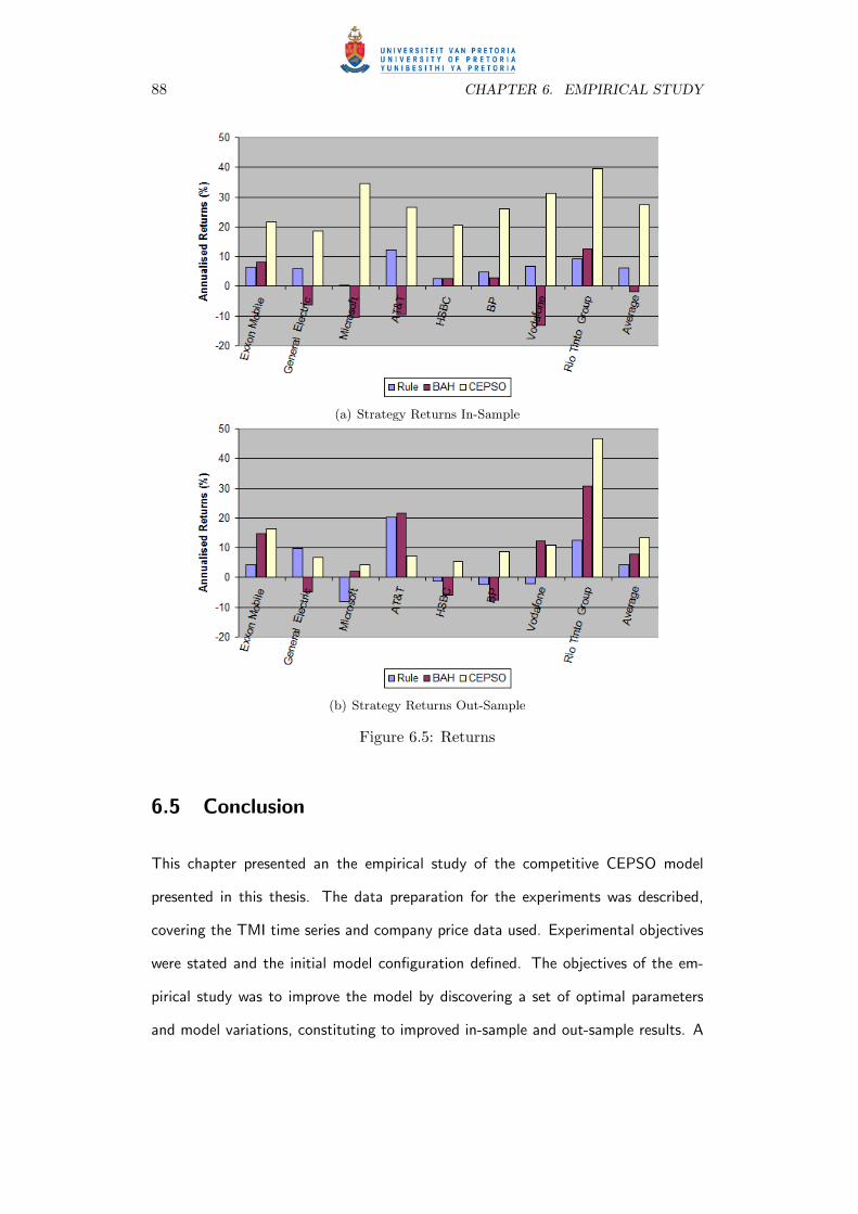
88 CHAPTER 6. EMPIRICAL STUDY
(a) Strategy Returns In-Sample
(b) Strategy Returns Out-Sample
Figure 6.5: Returns
6.5 Conclusion
This chapter presented an the empirical study of the competitive CEPSO model
presented in this thesis. The data preparation for the experiments was described,
covering the TMI time series and company price data used. Experimental objectives
were stated and the initial model configuration defined. The objectives of the em-
pirical study was to improve the model by discovering a set of optimal parameters
and model variations, constituting to improved in-sample and out-sample results. A

6.5. CONCLUSION 89
model configuration that consisted of a swarm size of 150 particles and a neural net-
work with four hidden neurons, using the LBEST topology with a reversal threshold
confidence value of θ = 0.05, performed optimally among the different topologies
investigated. The CEPSO strategy results were then compared against a TMI rule-
based and buy-and-hold strategy, with the CEPSO strategy proving to be superior to
both benchmarks. This shows that the model is in fact successful in discovering high
quality trading agents.
Chapter 7
Conclusion
This chapter serves as a conclusion to the thesis. Section 7.1 summarises the work
presented in the study, highlighting what has been achieved and noteworthy findings.
Section 7.2 comments on future research ideas that could potentially extend the work
produced in this study.
7.1 Summary
There were two main objectives laid out in the very beginning of the thesis. The
first objective was to study and define a co-evolutionary particle swarm optimisation
(CEPSO) model that could be used to optimise a neural network to detect trend
reversals, which could be utilised for security trading purposes. The second objective
was to examine whether technical market indicators could provide sufficient informa-
tion to derive intelligent trading models using historical stock price data.
Such a model was defined and applied to eight company stock prices. The model
was executed for different configurations, allowing the model’s exploration ability to
be investigated and iteratively improved. Four different technical market indicators
were used to transform the security prices and provided the necessary market-related
90

7.2. FUTURE RESEARCH 91
data to the model.
The discovered strategies reflected high profitability and low risk when they were
applied to newly introduced data not used for training. The solutions were compared
against two popular benchmarks and successfully outperformed them. The CEPSO
agents outperformed a rule-based benchmark by 9.09% and the buy-and-hold strategy
by 5.3% in terms of annualised returns. The agents managed to derive correct
trade actions successfully from the trend reversal confidence values produced. The
configuration that allowed the highest returns consisted of a PSO swarm of 150
particles, using the LBEST topology, four hidden layer neurons and a trend reversal
threshold value of θ = 0.05.
Furthermore, other secondary objectives were satisfied in this work. A thorough
background study on stock trading, technical market indicators and computational
intelligence paradigms was presented, upon which the CEPSO model was built. A
competitive fitness function was successfully defined and used as a measure for the
relative comparison of discovered strategies. This fitness function allowed solutions
to compete and co-evolve within a competitive environment.
7.2 Future Research
Other Technical Market Indicators
Four technical market indicators were considered in this work. A plethora of other
indicators could be considered and added to the model. This would be done in an
effort to exploit other market properties from security prices in order to improve
performance. Chaikin Volatility, Directional Movement Index, Elder Ray, Momen-
tum, Money Flow Index, Parabolic Stop and Reverse, Percentage Bands and Triple
Exponential Moving Average are just a few that could be considered.
92 CHAPTER 7. CONCLUSION
Using Fundamental Analysis
Adding concepts of fundamental analysis in conjunction with technical analysis could
be beneficial. Information could be extracted from financial statements and broker
reports and be provided to the agent to be considered together with the technical
market indicators.These two analytical methodologies have different advantages and
could complement each other if used together. Fundamental analysis favours long-
term investments, so it is sensible to state that short-term trading will not benefit
with the use of fundamentals. Long-term investments would be the main focus if
this task is undertaken.
Neural Network Architectures
Various neural network architectures exist, which might improve the trend reversal
confidence returned by the discovered trading agents. A standard feed forward neural
network is considered throughout this study, but other architectures such as prod-
uct unit, functional link, recurrent and time delay neural networks would be worth
examining.
PSO Algorithm Variations
A number of variations of the standard PSO algorithm exist. These variations offer
improved performance over the standard PSO algorithm that was used in this thesis,
that may contribute to better trading agents being discovered. These variations
offer better global optimisation of solutions and prevent stagnation on sub optimal
solutions.
Deriving Comprehensible Rules
Discovered neural network trading agents can only be used as a black box. It is im-
possible to understand how the trend reversal confidence is derived from the technical

7.2. FUTURE RESEARCH 93
market indicators. It is not favourable in the financial world to make use of trading
models that cannot be explained or understood. Deriving comprehensible rules from
neural network agents would be desirable, since a better understanding of the trading
strategy would make it more forthcoming. Additionally, comprehending discovered
strategies could help define better rules for deriving trading actions from the trend
reversal confidence, or even improve neural network configuration.
Defining PSO constraints
PSO solution constraints could be defined to control further the quality of the re-
turned strategies. For example, constraints applied to average trade length of so-
lutions could be used to define the term length of discovered solutions. Another
constraint could be placed on the number of trades the strategy produces, in order
to define the trading frequency. If low frequency trading is desired, an upper limit to
the number of trades could be placed that would force a smaller number of trades
per strategy.
Other Competitive Fitness Functions
The performance of the model could be improved by introducing different perfor-
mance metrics to the competitive fitness function. Measures such as maximum draw
down, internal rate of return and net present value could be considered. Furthermore,
different fitness functions could be considered altogether. A different competitive fit-
ness function may offer a better relative performance evaluation, contributing to a
better co-evolutionary environment.
Finding Multiple Solutions via Niching
The problem of convergence on sub-optimal solutions could further be addressed using
PSO niching. Niching would allow multiple solutions to be explored synchronously

94 CHAPTER 7. CONCLUSION
during training, increasing the probability of discovering global minima.

Bibliography
[1] A.M. Abdelbar and M. Mokhtar. Swarm optimisation with instinct-driven particles.
In Proceedings of the IEEE Congress on Evolutionary Computation, pages 777–782,
2003. [cited at p. 47]
[2] S. S. Alexander. Price movements in speculative markets: Trends or random walks.
Industrial Management Review, 2:7–26, 1961. [cited at p. 15]
[3] F. Allen and R. Karjalainen. Using genetic algorithms to find technical trading rules.
Journal of Financial Economics, 51(2):245–271, February 1999. [cited at p. 16, 43]
[4] S. Amari, N. Murata, K-R Muller, M. Finke, and H. Yanh. Asymptotic statistical theory
of overtraining and cross-validation. In Technical Report METR 95-06, Department of
Mathematical Engineering and Information University of Tokyo, 1995. [cited at p. 39]
[5] P. J. Angeline and J. B. Pollack. Competitive environments evolve better solutions
for complex tasks. In Proceedings of the 5th International Conference on Genetic
Algorithms, pages 264–270, Urbana-Champaign, IL, USA, 1993. [cited at p. 51, 53, 55,
56]
[6] P. J. Angeline and J. B. Pollack. Coevolving high-level representations. In C. G.
Langton, editor, Artificial Life III, volume 17, pages 55–71, Santa Fe, New Mexico,
1994. Addison-Wesley. [cited at p. 56]
[7] G. Appel. Technical analysis: Power tools for active investors. Financial Times /
Prentice Hall, ISBN 0131479024, 2005. [cited at p. 19, 27, 28, 119]
95
96 BIBLIOGRAPHY
[8] R. Axelrod. Genetic algorithms and simulated annealing, chapter The Evolution of
Strategies in the Iterated Prisoner’s Dilemma, pages 32–41. Morgan Kaufman, Los
Altos, CA, 1987. [cited at p. 53, 55, 56]
[9] T. Back, D. B. Fogel, and Z. Michaelewicz. Evolutionary computation 1: Basic al-
gorithms and operators. Taylor & Francis, ISBN 0750306645, 2000. [cited at p. 42,
55]
[10] T. Back, D. B. Fogel, and Z. Michaelewicz. Evolutionary computation 2: Advanced
algorithms and operations. Taylor & Francis, ISBN 0750306653, 2000. [cited at p. 42]
[11] C. R. Bacon. Practical portfolio performance measurement and attribution. Wiley ,
ISBN 0470856793, 2004. [cited at p. 68]
[12] N. A. Barricelli. Symbiogenetic evolution processes realised by artificial methods. 9:35–
36, 1957. [cited at p. 42]
[13] R. J. Jr Bauer and J. Dahlquist. Technical market indicators - analysis and performance.
John Wiley & Sons, ISBN 0471197211, 1998. [cited at p. 13, 16, 59]
[14] L. Becker and M. Seshadri. Cooperative coevolution of technical trading rules. Worces-
ter Polytechnic Institute, Computer Science Technical Report WPI-CS-TR-03-15, 2003.
[cited at p. 16, 43, 56]
[15] L. Becker and M. Seshadri. Gp-evolved technical trading rules can outperform buy and
hold. pages 26–30, Cary, North Carolina USA, September 2003. In Proceedings of the
Sixth International Conference on Computational Intelligence and Natural Computing,
Embassy Suites Hotel and Conference Center. [cited at p. 16, 43]
[16] C. M. Bishop. Neural networks for pattern recognition. Oxford University Press, ISBN
0198538642, 1995. [cited at p. 35, 40]
[17] A. D. Blair and J. B. Pollack. What makes a good co-evolutionary learning environ-
ment? Australian Journal of Intelligent Information Processing Systems, 4:166–175,
1997. [cited at p. 56]
[18] E. K. Blum and L. K. Li. Approximation theory and feedforward networks. Neural
Networks, 4(4):511–515, 1991. [cited at p. 37]

BIBLIOGRAPHY 97
[19] J. A. Bollinger. Bollinger on bollinger bands. McGraw-Hill, ISBN 0071373683, 2001.
[cited at p. 19, 23, 24, 86, 115]
[20] D. Braendler and T. Hendtlass. Improving particle swarm optimisation using the col-
lective movement of the swarm. IEEE Transactions on Evolutionary Computation, in
press. [cited at p. 47]
[21] W. Brock, J. Lakonishok, and B. LeBaron. Simple technical trading rules and the
stochastic properties of stock returns. Journal of Finance, 47(5):1731–64, December
1992. [cited at p. 15]
[22] S. J. Brown, A. Kumar, and W. N. Goetzmann. The dow theory: William peter
hamilton’s track record re-considered. 1998. [cited at p. 14, 15]
[23] N. Cesa-Bianchi, P. M. Long, and M. K. Warmuth. Worst-case quadratic loss bounds
for a generalisation of the widrow-hoff rule. In COLT ’93: Proceedings of the 6th
Annual Conference on Computational Learning Theory, pages 429–438, New York,
NY, USA, 1993. ACM Press. [cited at p. 40]
[24] T. S. Chande. A time price oscillator. Technical Analysis of Stocks & Commodities,
13:369–374, 1995. [cited at p. 19, 21, 115]
[25] K. Chellapilla and D. B. Fogel. Evolving neural networks to play checkers without
expert knowledge. IEEE Transactions on Neural Networks, 10(6):1382–1391, 1999.
[cited at p. 41, 56]
[26] K. Chellapilla and D. B. Fogel. Anaconda defeats hoyle 6-0: A case study competing
an evolved checkers program against commercially available software. In Proceedings
of the 2000 Congress on Evolutionary Computation, pages 857–863, La Jolla Marriott
Hotel La Jolla, California, USA, 2000. IEEE Press. [cited at p. 56]
[27] M. C. Chen, C. L. Lin, and A. P. Chen. Constructing a dynamic stock portfolio decision-
making assistance model: Using the taiwan 50 index constituents as an example. Soft
Comput., 11(12):1149–1156, 2007. [cited at p. 49]
[28] S. H. Chen. Genetic algorithms and genetic programming in computational finance.
Springer, ASIN B000WCT6Q0, 2002. [cited at p. 43]

98 BIBLIOGRAPHY
[29] M. Clerc. Particle swarm optimisation. ISTE, ISBN 1905209045, 2006. [cited at p. 45]
[30] M. Clerc and J. Kennedy. The particle swarm - explosion, stability and convergence in
a multidimensional complex space. IEEE Transactions on Evolutionary Computation,
6(1):58–73, 2002. [cited at p. 49]
[31] R. W. Colby. The encyclopedia of technical market indicators, second edition. McGraw-
Hill Professional, ISBN 0070120579, 2004. [cited at p. 13, 14, 16, 19, 20, 59, 75, 116]
[32] G. W. Cottrell. Extracting features from faces using compression networks: Face,
identity, emotion and gender recognition using holons. In Connection Models: Pro-
ceedings of the 1990 Summer School, San Mateo, CA, USA, 1990. Morgan Kaufmann.
[cited at p. 40, 41]
[33] M. W. Craven and J. W. Shavlik. Using neural networks for data mining. Future Gener.
Comput. Syst., 13(2-3):211–229, 1997. [cited at p. 40, 41]
[34] P. J. Darwen. Computationally intensive and noisy tasks: Co-evolutionary learning and
temporal difference learning on backgammon. In Proceedings of the 2000 Congress on
Evolutionary Computation, pages 872–879, La Jolla Marriott Hotel La Jolla, California,
USA, 2000. IEEE Press. [cited at p. 56]
[35] P. J. Darwen and X. Yao. Co-evolution in iterated prisoner’s dilemma with interme-
diate levels of cooperation: Application to missile defense. International Journal of
Computational Intelligence and Applications, 2(1):83–107, 2002. [cited at p. 56]
[36] C. R. Darwin. On the origins of species by means of natural selection or the preservation
of favoured races in the struggle for life. Murray, London 1859, 1859. [cited at p. 42]
[37] J. Davis and G. Kendall. An investigation, using coevolution, to evolve an awari player.
In Proceedings of Congress on Evolutionary Computation, pages 1408–1413, Hilton
Hawaiian Village Hotel, Honolulu, Hawaii, 2002. [cited at p. 56]
[38] R. Dawkins. The blind watchmaker. Longman, ISBN 0582446945, 1986. [cited at p. 50]
[39] G. J. Deboeck. Trading on the edge: Neural, genetic, and fuzzy systems for chaotic
financial markets: Neural, genetic and fuzzy systems for chaotic financial markets.
John Wiley & Sons , ISBN 0471311006, 1994. [cited at p. 41]
BIBLIOGRAPHY 99
[40] D. DeMers and G. W. Cottrell. Non-linear dimensionality reduction. In Advances
in Neural Information Processing Systems 5, [NIPS Conference], pages 580–587, San
Francisco, CA, USA, 1993. Morgan Kaufmann Publishers Inc. [cited at p. 41]
[41] M. A. H. Dempster, T. W. Payne, Y. Romahi, and G. W. P. Thompson. Computational
learning techniques for intraday FX trading using popular technical indicators. IEEE
Transactions on Neural Networks, 12(4):744–754, 2001. [cited at p. 16, 43]
[42] C. H. Dennis. Comment: The information content of daily market indicators. Journal
of Financial and Quantitative Analysis, 8(2):193–194, 1973. [cited at p. 15]
[43] A. R. Domasio. Scientific american book of the brain. The Lyons Press, ISBN
155821965X, 1999. [cited at p. 35]
[44] R. C. Eberhart, R. W. Dobbins, and P. Simpson. Computational intelligence pc tools.
Academic Press, ISBN 0122286308, 1996. [cited at p. 40, 46, 47, 49]
[45] R. D. Edwards and J. Magee. Technical analysis of stock trends, 8th edition. CRC
Press , ISBN 1574442929, 2001. [cited at p. 13, 16]
[46] B. Egeli, M. Ozturnan, and B. Badur. Stock market prediction using artificial neural
networks. Hawaii, USA, 1990. Proceedings of the 3rd Hawaii International Conference
on Business. [cited at p. 41]
[47] A. Elder. Come into my trading room: A complete guide to trading. John Wiley &
Sons, ISBN 0471225347, 2002. [cited at p. 19, 117]
[48] A. P. Engelbrecht. A new pruning heuristic based on variance analysis of sensitivity
information. In IEEE Transactions on Neural Networks, volume 12, pages 1386–1399,
2001. [cited at p. 39]
[49] A. P. Engelbrecht. Computational intelligence: An introduction. Wiley, ISBN
0470848707, 2002. [cited at p. 37, 39, 43]
[50] A. P. Engelbrecht. Fundamentals of computational swarm intelligence. Wiley, ISBN
0470091916, 2002. [cited at p. 45]

100 BIBLIOGRAPHY
[51] E. Fama. Random walks in stock market prices. volume 5, pages 55–59, 1965.
[cited at p. 15]
[52] E. Fama. Efficient capital markets: A review of theory and empirical work. The Journal
of Finance, 2:383–417, 1970. [cited at p. 15]
[53] E. Fama and M. E. Blume. Filter rules and stock market trading. Journal of Business,
39:226, 1965. [cited at p. 15]
[54] K. Fanghanel, R. Hein, K. Kollmann, and H. C. Zeidler. Optimising wavelet transform
coding using a neural network. In In Proceedings of the IEEE International Conference
on Information, Communications and Signal Processing, volume 3, pages 1341–1343,
Singapore, 1997. [cited at p. 41]
[55] S. G. Ficici, O. Melnik, and J. B. Pollack. A game-theoretic investigation of selection
methods used in evolutionary algorithms. In Proceedings of the 2000 Congress on
Evolutionary Computation, pages 880–887, La Jolla Marriott Hotel La Jolla, California,
USA, 2000. IEEE Press. [cited at p. 43]
[56] T. Fischer and A. Roehrl. Optimisation of performance measures based on expected
shortfall. Working paper, 2005. [cited at p. 49]
[57] D. Floreano and F. Mondada. Automatic creation of an autonomous agent: Genetic
evolution of a neural-network driven robot. In Proceedings of the Conference on Sim-
ulation of Adaptive Behavior, 1994. [cited at p. 41]
[58] D. B. Fogel. Blondie24: Playing at the edge of AI. San Francisco, CA, USA, 2001.
Morgan Kaufmann, ISBN 1558607838. [cited at p. 56]
[59] L. J. Fogel. Autonomous automata. Industrial Research, 4:14–19, 1962. [cited at p. 42]
[60] L. J. Fogel. On the optimisation of intellect. Los Angeles, USA, 1964. PhD Thesis,
University of California. [cited at p. 42]
[61] L. J. Fogel, A. J. Owens, and M. J. Walsh. Artificial intelligence through simulated
evolution. Wiley, ISBN 0471265160, 1966. [cited at p. 42]
BIBLIOGRAPHY 101
[62] S. Forrest, R. E. Smith, B. Javornik, and A. S. Perelson. Using genetic algorithms to ex-
plore pattern recognition in the immune system. Evolutionary Computation, 1(3):191–
211, 1993. [cited at p. 54]
[63] N. Franken. PSO-based coevolutionary game learning. Pretoria, South Africa, 2004.
MSc Thesis, Department of Computer Science, University of Pretoria. [cited at p. 41,
49, 56]
[64] A. S. Fraser. Simulation of genetic systems by automatic digital computers. Australian
Journal of Biological Science, 10:484–491, 1957. [cited at p. 42]
[65] B. Fritzke. Incremental learning of local linear mappings. In F. Fogelman, editor,
International Conference on Artificial Neural Networks, pages 217–222, Paris, France,
1995. EC2 & Cie. [cited at p. 39]
[66] L. Gao, C. Zhou, H. B. Gao, and Y. R. Shi. Credit scoring module based on neural
network with particle swarm optimisation. Advances in Natural Computation, 14:76–
79, 2006. [cited at p. 49]
[67] S. Godin. If you’re clueless about the stock market and want to know more. Kaplan
Publishing, ISBN 0793143675, 2001. [cited at p. 9]
[68] D. E. Goldberg and J. Richardson. Genetic algorithms with sharing for multimodal
function optimisation. In Proceedings of the Second International Conference on Ge-
netic Algorithms on Genetic algorithms and their Application, pages 41–49, Mahwah,
NJ, USA, 1987. Lawrence Erlbaum Associates, Inc. [cited at p. 42, 54]
[69] G. E. Goldberg and K. Deb. A comparative analysis of selection schemes used in genetic
algorithms. Foundations of Genetic Algorithms, pages 69–93, 1991. [cited at p. 43]
[70] B. Graham. The intelligent investor: The classic text on value investing. Collins, ISBN
0060752610, 2005. [cited at p. 16]
[71] V. G. Gudise and G. K. Venayagamoorthy. Comparison of particle swarm optimisation
and backpropagation as training algorithms for neural networks. In Proceedings of the
IEEE Swarm Intelligence Symposium, pages 110–117, 2003. [cited at p. 40, 49]

102 BIBLIOGRAPHY
[72] W.D. Hillis. Co-evolving parasites improve simulated evolution as an optimisation
procedure. pages 228–234, 1991. [cited at p. 53, 55, 56]
[73] N. Hirata, A. Ishigame, and H. Nishigaito. Neuro stabilising control based on lyapunov
method for power systems. In In SICE 2002. Proceedings of the 41st SICE Annual
Conference, volume 5, pages 3169–3171, 2002. [cited at p. 40, 49]
[74] Y. Hirose, K. Yamashita, and S. Hijiya. Back-propagation algorithm which varies
the number of hidden units. In Neural Networks, volume 2, pages 61–66, 1991.
[cited at p. 39]
[75] J. H. Holland. Outline for a logical theory of adaptive systems. Journal of the ACM,
3:297–314, 1962. [cited at p. 42]
[76] J. H. Holland. Adaptation in natural and artificial systems. First MIT Press Edition
1992, ISBN 0262581116, 1975. [cited at p. 42]
[77] J. H. Holland. Echo: Explorations of evolution in a miniature world. In 2nd Workshop
on Artificial Life, Santa Fe, New Mexico, 1990. [cited at p. 51]
[78] K. Hornik. Multilayer feedforward networks are universal approximators. In Neural
Networks, volume 2, pages 359–366, 1989. [cited at p. 37]
[79] K. Hornik, M. Stinchcombe, and H. White. Universal approximation of an unknown
mapping and its derivatives using multilayer feedforward networks. In Neural Networks,
volume 3, pages 551–560, 1990. [cited at p. 37]
[80] H. Huning. A node splitting algorithm that reduces the number of connections in a
hamming distance classifying network. In Proceedings of the International Workshop
on Artificial Neural Networks, pages 102–107, London, UK, 1993. Springer-Verlag.
[cited at p. 39]
[81] A. Ismail and A. P. Engelbrecht. Training product units in feedforward neural networks
using particle swarm optimisation. Proceedings of the International Conference on
Artificial Intelligence, 1999. [cited at p. 40, 49]
[82] S. Janson and M. Middendorf. A hierarchical particle swarm optimiser. In Proceedings
of the IEEE Congress on Evolutionary Computation, 2:770–776, 2003. [cited at p. 47]
BIBLIOGRAPHY 103
[83] M. C. Jensen and G. A. Bennington. Random walks and technical theories: Some
additional evidence. Journal of Finance, 25(2):469–82, May 1970. [cited at p. 15]
[84] L. K. Jones. Constructive approximations for neural networks by sigmoidal functions.
In Proceedings of the IEEE, volume 78, pages 1586–1589, 1990. [cited at p. 37]
[85] R. Jones. The trading game: Playing by the numbers to make millions. John Wiley
and Sons, ISBN 0471316989, 1999. [cited at p. 12]
[86] G. Kendall and Y. Su. A particle swarm optimisation approach in the construction of
optimal risky portfolios. In Proceedings of the 23rd International Multi-Conference
on Artificial Intelligence and Applications (IASTED 2005), pages 140–145, 2005.
[cited at p. 49]
[87] K. Kendall. Electronic and algorithmic trading technology: The complete guide. Aca-
demic Press, ISBN 0123724910, 2007. [cited at p. 12]
[88] J. Kennedy. The behaviour of particles. In Proceedings of the 7th International Con-
ference on Evolutionary Programming, pages 581–589, 1998. [cited at p. 48]
[89] J. Kennedy. Small worlds and mega minds: Effects of neighbourhood topology on
particle swarm performance. In Proceedings of the IEEE Congress on Evolutionary
Computation, volume 3, pages 1931–1938, 1999. [cited at p. 47]
[90] J. Kennedy. Stereotyping: Improving particle swarm performance with cluster analysis.
In Proceedings of the IEEE Congress on Evolutionary Computation, volume 2, pages
1507–1512, La Jolle, CA, USA, 2000. [cited at p. 47]
[91] J. Kennedy and R. C. Eberhart. A new optimiser using particle swarm optimization. In
Proceedings of the 6th International Symposium on Micromachine and Human Science,
pages 39–43, 1995. [cited at p. 44, 77]
[92] J. Kennedy and R. C. Eberhart. Particle swarm optimisation. In Proceedings of the
IEEE International Conference on Neural Networks, volume 4, pages 1942–1948, Perth,
Australia, 1995. [cited at p. 44, 77]

104 BIBLIOGRAPHY
[93] J. Kennedy and R. C. Eberhart. The particle swarm: Social adaptation in information-
processing systems, new ideas in optimisation. McGraw-Hill, ISBN 0077095065, 1999.
[cited at p. 40, 47, 49]
[94] J. Kennedy and R. C. Eberhart. Swarm intelligence. Morgan Kaufmann Publishers,
ISBN 1558605959, 2001. [cited at p. 45]
[95] J. Kennedy and R. Mendes. Population structure and particle swarm performance. In
Proceedings of the IEEE World Congress on Evolutionary Computation, pages 1671–
1676, Honolulu, Hawaii, 2002. [cited at p. 47]
[96] J. Khan, J. S. Wei, M. Ringner, L. H. Saal, M. Ladanyi, F. Westermann anf F. Berthold,
M. Schwab, C. R. Antonescu, C. Peterson, and P. S. Meltzer. Classification and
diagnostic prediction of cancers using gene expression profiling and artificial neural
networks. Nature Medicine, 7(6):673–679, 2001. [cited at p. 41]
[97] T. Kohonen. Self-organising maps. Springer Series in Information Sciences, ISBN
3540586008, 1995. [cited at p. 40, 41]
[98] J. R. Koza. Evolution and co-evolution of computer programs to control independently-
acting agents. In Proceedings of the 1st International Conference on Simulation of
Adaptive Behavior on From Animals to Animats, pages 366–375, Cambridge, MA,
USA, 1990. MIT Press. [cited at p. 56]
[99] J. R. Koza. Genetic programming: On the programming of computers by means of
natural selection. MIT Press, ISBN 0262111705, 1992. [cited at p. 42]
[100] T. Y. Kwok and D. Y. Yeung. Constructive feedforward neural networks for regression
problems: A survey. technical report hkust-cs95-43. Clear Water Bay, Kowloon, Hong
Kong, 1995. Department of Computer Science, Hong Kong University of Science and
Technology. [cited at p. 39]
[101] K. J. Lang, A. H. Waibel, and G. E. Hinton. A time-delay neural network architecture
for isolated word recognition. Neural Networks, 3(1):23–43, 1990. [cited at p. 41]
[102] R. Lawrence. Using neural networks to forecast stock market prices. Manitoba, BC,
Canada: Univ. of Manitoba, 1997. [cited at p. 41]

BIBLIOGRAPHY 105
[103] B. LeBaron. Technical trading rule profitability and foreign exchange intervention.
NBER Working Papers 5505, National Bureau of Economic Research, Inc, March 1996.
[cited at p. 15]
[104] Y. LeCun, B. Boser, J. S. Denker, D. Henderson, R. E. Howard, W. Hubbard, and
L. D. Jackel. Backpropagation applied to handwritten zip code recognition. Neural
Computation, 1(4):541–551, 1989. [cited at p. 40, 41]
[105] Y. LeCun, J. Denker, S. Solla, R. E. Howard, and L. D. Jackel. Optimal brain damage.
In D. S. Touretzky, editor, Advances in Neural Information Processing Systems II, San
Mateo, CA, 1990. Morgan Kauffman. [cited at p. 39]
[106] F. L. Lewis. Neural network control of robot manipulators. IEEE Expert: Intelligent
Systems and Their Applications, 11(3):64–75, 1996. [cited at p. 41]
[107] P. J. G. Lisboa. A review of evidence of health benefit from artificial neural networks
in medical intervention. Neural Netw., 15(1):11–39, 2002. [cited at p. 41]
[108] A. Lo and A. C. Mackinlay. Stock market prices do not follow random walks: Evidence
from a simple specification test. Rev. Financ. Stud., 1:41–66, 1988. [cited at p. 15]
[109] H. J. Lu, R. Setiono, and H. Liu. Effective data mining using neural networks. IEEE
Trans. On Knowledge And Data Engineering, 8:957–961, 1996. [cited at p. 40, 41]
[110] B. G. Malkiel. A random walk down wall street: Including a life-cycle guide to personal
investing. W. W. Norton and Company, ISBN 0393315290, 1996. [cited at p. 15]
[111] T. Masters. Practical neural network recipes in C++. Morgan Kaufmann, ISBN
0124790402, 1993. [cited at p. 35]
[112] J. L. McClelland and D. E. Rumelhart. Training hidden units: The generalised delta
rule. In Explorations in Parallel Distributed Processing, volume 3, pages 121–137. MIT
Press, 1988. [cited at p. 40]
[113] B. A. McDowell. The art of trading: Combining the science of technical analysis
with the art of reality-based trading. John Wiley and Sons, ISBN 0470187727, 2008.
[cited at p. 12]

106 BIBLIOGRAPHY
[114] P. D. McNelis. Neural networks in finance: Gaining predictive edge in the market.
Academic Press, ISBN 0124859674, 2005. [cited at p. 41]
[115] R. Mendes, P. Cortez, M. Rocha, and J. Neves. Particle swarms for feedforward neural
network training. In Proceedings of the IEEE Joint Conference on Neural Networks,
volume 2, pages 1895–1899, Honolulu, Hawaii, USA, 2002. [cited at p. 40, 49]
[116] L. Messerschmidt and A. P. Engelbrecht. Learning to play games using a PSO-based
competitive learning approach. In IEEE Transactions on Evolutionary Computation,
volume 8, page 280=288, 2002. [cited at p. 41, 49, 56]
[117] G. F. Miller and D. Cliff. Co-evolution of pursuit and evasion i: Biological and game-
theoretic foundations. In Technical Report CSRP311, University of Sussex, School of
Cognitive and Computing Sciences, Brighton, UK, 1994. [cited at p. 56]
[118] M. F. Moller. A scaled conjugate gradient algorithm for fast supervised learning. In
Neural Networks, volume 6, pages 525–533, 1993. [cited at p. 40]
[119] J. Moody and J. Utans. Architecture selection strategies for neural networks: Applica-
tion to corporate bond rating prediction. In Neural Networks in the Capital markets.
John Wiley & Sons, ISBN 0471943649, 1995. [cited at p. 39, 41]
[120] K-R Muller, M. Finke, N. Murata, K. Schulten, and S. Amari. A numerical study on
learning curves in stochastic multi-layer feed-forward networks. In Neural Computation,
volume 8, pages 1085–1106, 1995. [cited at p. 39]
[121] J. J. Murphy. Technical analysis of the financial markets: A comprehensive guide to
trading methods and applications. New York Institute of Finance, Prentice Hall Press,
ISBN 0735200661, 2002. [cited at p. 13, 16]
[122] C. J. Neely. Risk-adjusted, ex ante, optimal technical trading rules in equity markets.
International Review of Economics & Finance, 12(1):69–87, 2003. [cited at p. 16, 43]
[123] C. J. Neely and P. A. Weller. Intraday technical trading in the foreign exchange market.
Journal of International Money and Finance, 22(2):223–237, April 2003. [cited at p. 15,
16, 43]
BIBLIOGRAPHY 107
[124] C. J. Neely, P. A. Weller, and R. Dittmar. Is technical analysis in the foreign exchange
market profitable? a genetic programming approach. Working Papers 1996-006, Fed-
eral Reserve Bank of St. Louis, 1997. [cited at p. 16, 43]
[125] J. Nenortaite. A particle swarm optimisation approach in the construction of decision-
making model. Information technology and control 1A, 36:158–163, 2007. [cited at p. 16,
49]
[126] J. Nenortaite and R. Simutis. Stocks’ trading system based on the particle swarm
optimisation algorithm. Computational Science (ICCS 2004), pages 843–850, 2004.
[cited at p. 16, 49]
[127] J. Nenortaite and R. Simutis. Adapting particle swarm optimization to stock markets.
In ISDA ’05: Proceedings of the 5th International Conference on Intelligent Systems
Design and Applications, pages 520–525, Washington, DC, USA, 2005. IEEE Computer
Society. [cited at p. 16, 49]
[128] E. Papacostantis, A. P. Engelbrecht, and N. Franken. Coevolving probabilistic game
playing agents using particle swarm optimisation algorithms. In Proceedings of the IEEE
Evolutionary Computation in Games Symposium, pages 195–202, 2005. [cited at p. 41,
49, 56]
[129] S. Phelps, S. Parsons, P. McBurney, and E. Sklar. Coevolution of auction mechanisms
and trading strategies: Towards a novel approach to microeconomic design. In In Pro-
ceedings of the 2nd Workshop on Evolutionary Computation and Multi-Agent Systems,
New York, NY, 2002. [cited at p. 56]
[130] B. Pollack and A. D. Blair. Co-evolution in the successful learning of backgammon
strategy. volume 32, pages 225–240. Machine Learning, 1998. [cited at p. 56]
[131] J. B. Pollack, A. D. Blair, and M. Land. Coevolution of a backgammon player. In
C. G. Langton and K. Shimohara, editors, Artificial Life V: Proceedings of the 5th
International Workshop on the Synthesis and Simulation of Living Systems, pages 92–
98, Cambridge, MA, 1997. The MIT Press. [cited at p. 56]
108 BIBLIOGRAPHY
[132] M. A. Potter. The design and analysis of a computational model of cooperative coevo-
lution. Fairfax, VA, USA, 1997. PhD Thesis, George Mason University. [cited at p. 51]
[133] T. C. Price. Using co-evolutionary programming to simulate strategic behaviour in
markets. In Journal of Evolutionary Economics, volume 7, pages 219–254, 1997.
[cited at p. 56]
[134] M. J. Pring. Technical analysis explained : The successful investor’s guide to spot-
ting investment trends and turning points. McGraw-Hill, ISBN 0071381937, 1991.
[cited at p. 14]
[135] I. Rechenberg. Cybernetic solution path of an experimental problem. Farnbor-
ough, Hants, UK, 1965. Royal Aircraft Establishment, Library Translation no. 1222.
[cited at p. 42]
[136] R. G. Reynolds. An introduction to cultural algorithms. In Proceedings of the 3rd
Annual Conference on Evolutionary Computing, pages 131–139, San Diego, California,
USA, 1994. [cited at p. 42]
[137] C. D. Rosin and R. K. Belew. Methods for competitive co-evolution: Finding oppo-
nents worth beating. In Larry Eshelman, editor, Proceedings of the 6th International
Conference on Genetic Algorithms, pages 373–380, San Francisco, CA, 1995. Morgan
Kaufmann. [cited at p. 51, 54, 56]
[138] C. D. Rosin and R. K. Belew. New methods for competitive coevolution. Evolutionary
Computation, 5(1):1–29, 1997. [cited at p. 51, 56]
[139] J. Salerno. Using the particle swarm optimisation technique to train a recurrent neu-
ral model. In Proceedings of the 9th International Conference on Tools with Artifi-
cial Intelligence, pages 45–49, Washington, DC, USA, 1997. IEEE Computer Society.
[cited at p. 40, 49]
[140] A. Samuel. Some studies in machine learning using the game of checkers. IBM Journal
of Research and Development, 3:210–229, 1959. [cited at p. 52]
[141] H. P. Schwefel. Kybernetische evolution als strategie der experimentellen forschung in
der stromungstechnik. Diplomarbeit, Technische Universitat Berlin, 1959. [cited at p. 42]

BIBLIOGRAPHY 109
[142] J. Shadbolt and J. G. Taylor. Neural networks and the financial markets: Predict-
ing, combining and portfolio optimisation. Springer-Verlag, ISBN 1852335319, 2002.
[cited at p. 41]
[143] Y. Shi and R. C. Eberhart. A modified particle swarm optimiser. In Proceedings of
the IEEE World Conference on Computational Intelligence, pages 69–73, Anchorage,
Alaska, 1998. [cited at p. 48]
[144] Y. Shi and R. C. Eberhart. Parameter selection in particle swarm optimisation. In
Proceedings of the 7th International Conference on Evolutionary Programming VII,
pages 591–600, London, UK, 1998. Springer-Verlag. [cited at p. 48]
[145] Y. Shi and R. C. Eberhart. Empirical study of particle swarm optimisation. In Pro-
ceedings of the Congress on Evolutionary Computation, volume 3, pages 1945–1950,
Piscataway, NJ, USA, 1999. [cited at p. 47]
[146] K. Smith and J. N. D. Gupta. Neural networks in business: Techniques and applications.
GI Publishing, ISBN 1931777799, 2003. [cited at p. 41]
[147] P. N. Suganthan. Particle swarm optimiser with neighbourhood operator. In Proceed-
ings of the IEEE Congress on Evolutionary Computation, pages 1958–1961, Washington
D.C, USA, 1999. [cited at p. 47]
[148] Telegraph. Black box traders are on the march.
http://www.telegraph.co.uk/finance/2946240/Black-box-traders-are-on-the-
march.html. [cited at p. 12]
[149] G. Tesauro. Temporal difference learning and TD-Gammon. Commun. ACM, 38(3):58–
68, 1995. [cited at p. 41, 56]
[150] N. S. Thomaidis, T. Angelidis, V. Vassiliadis, and G. Dounias. Active portfolio man-
agement with cardinality constraints: An application of particle swarm optimization.
Working paper., 2008. [cited at p. 49]
[151] N. S. Thomaidis, M. Marinakis, M. Marinaki, and G. Dounias. Training neural network-
based models using trading-related objective functions. In Proceedings of the 3rd Eu-
110 BIBLIOGRAPHY
ropean Symposium on Nature-Inspired Smart Information Systems, St. Julians, Malta,
2007. [cited at p. 16, 49]
[152] J. D. Thomas and K. Sycara. The importance of simplicity and validation in genetic
programming for data mining in financial data. In Alex Alves Freitas, editor, Data Min-
ing with Evolutionary Algorithms: Research Directions, pages 7–11, Orlando, Florida,
18 1999. AAAI Press. [cited at p. 16, 43]
[153] Financial Times. City trusts computers to keep up with the news.
http://www.ft.com/cms/s/0/bb570626-ebb6-11db-b290-000b5df10621.html.
[cited at p. 12]
[154] Financial Times. Ft global 500. http://www.ft.com/reports/ft5002000. [cited at p. 73,
117, 123]
[155] International Herald Tribune. Artificial intelligence applied heavily to pick-
ing stocks. http://www.iht.com/articles/2006/11/23/business/trading.php?page=1.
[cited at p. 12]
[156] International Herald Tribune. Citigroup to expand electronic trading capabilities by buy-
ing automated trading desk. http://www.iht.com/articles/ap/2007/07/02/business/
NA-FIN-COM-US-Citigroup-Automated-Trading-Desk.php. [cited at p. 12]
[157] F. van den Bergh. An analysis of particle swarm optimisers. University of Pretoria,
South Africa, 2002. PhD Thesis, Department of Computer Science. [cited at p. 45, 46,
47, 48, 49, 77]
[158] F. van den Bergh and A. P. Engelbrecht. Using cooperative particle swarm optimisation
to train product unit neural networks. In Proceedings of the IEEE International Joint
Conference on Neural Networks, volume 1, pages 126–131, Washington DC, USA,
2001. [cited at p. 40, 49]
[159] J.C.H. Watkins and P. Dayan. Q-learning. Machine Learning, 8:279–292, 1992.
[cited at p. 41]
[160] P. J. Werbos. Beyond regression: New tools for prediction and analysis in the be-
havioural sciences. Boston, USA, 1974. PhD Thesis, Harvard University. [cited at p. 40]

BIBLIOGRAPHY 111
[161] L. F. A. Wessels and E. Barnard. Avoiding false local minima by proper initialisation of
connections. IEEE Transactions on Neural Networks, 3(6):899–882, 1992. [cited at p. 70]
[162] J. W. Jr Wilder. New concepts in technical trading systems. Greenboro, N.C. Trend
Research, ISBN 0894590278, 1978. [cited at p. 19, 30, 117, 119]
[163] X. Xiao, E. R. Dow, R. C. Eberhart Z. Ben Miled, and R.J. Oppelt. Gene clustering
using self-organising maps and particle swarm optimisation. In proceedings of the
second IEEE International Workshop on High Performance Computational Biology,
page 10, 2003. [cited at p. 49]
[164] J. Yao, Y. Li, and C. Tan. Forecasting the exchange rates of CHF vs USD using
neural networks. Journal of Computational Intelligence in Finance, 5(2):7–13, 1997.
[cited at p. 41]
[165] M. Zekic. Neural network applications in stock market predictions. In Proceedings of
the 9th International Conference on Information and Intelligent Systems, pages 255–
2633, 1998. [cited at p. 41]
[166] G. P. Zhang. Neural networks in business forecasting. Information Science Publishing,
ISBN 1591402158, 2003. [cited at p. 41]

Appendices
112
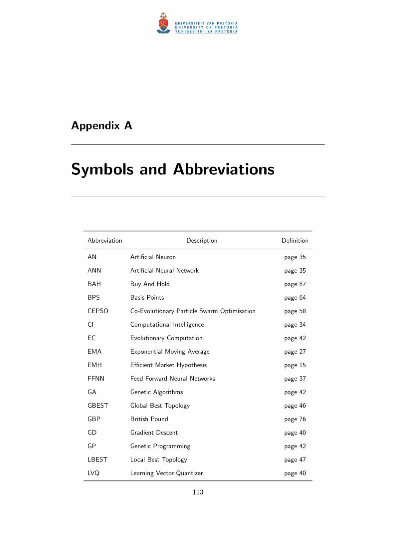
Appendix A
Symbols and Abbreviations
Abbreviation Description Definition
AN Artificial Neuron page 35
ANN Artificial Neural Network page 35
BAH Buy And Hold page 87
BPS Basis Points page 64
CEPSO Co-Evolutionary Particle Swarm Optimisation page 58
CI Computational Intelligence page 34
EC Evolutionary Computation page 42
EMA Exponential Moving Average page 27
EMH Efficient Market Hypothesis page 15
FFNN Feed Forward Neural Networks page 37
GA Genetic Algorithms page 42
GBEST Global Best Topology page 46
GBP British Pound page 76
GD Gradient Descent page 40
GP Genetic Programming page 42
LBEST Local Best Topology page 47
LVQ Learning Vector Quantizer page 40
113
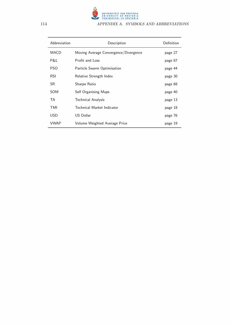
114 APPENDIX A. SYMBOLS AND ABBREVIATIONS
Abbreviation Description Definition
MACD Moving Average Convergence/Divergence page 27
P&L Profit and Loss page 67
PSO Particle Swarm Optimisation page 44
RSI Relative Strength Index page 30
SR Sharpe Ratio page 68
SOM Self Organising Maps page 40
TA Technical Analysis page 13
TMI Technical Market Indicator page 18
USD US Dollar page 76
VWAP Volume Weighted Average Price page 19

Appendix B
Financial Glossary
aroon: A technical market indicator introduced by Tushar S. Chande [24]. The in-
dicator attempts to quickly detect trend reversals and trend strengths. It measures
the number of time periods within a predefined time window frame, since the most
recent high price and low price. The main assumption this indicator makes is that a
security price will close at a high for the given period in an up-trend, and at a low
for the given period in a down-trend. Refer to chapter 3.
asset: A resource having economic value that an individual, corporation or country
owns or controls with the expectation that it will provide future benefit.
basis point: A basis point is 1/100th of a percentage point, or 0.01%. It is used as
a unit of measure in finance.
bear market: A market condition in which prices of securities are falling or are ex-
pected to fall. A lack of confidence surrounds such market conditions. The opposite
market condition is described as a bull market.
Bollinger bands: A technical market indicator created by John A. Bollinger [19]. It
addresses the issue of dynamic volatility by introducing adaptive bands that widen
during periods of high volatility and contract during periods of low volatility. Bollinger
Bands’ main purpose is to place the current price of a security into perspective, pro-
115

116 APPENDIX B. FINANCIAL GLOSSARY
viding a relative definition of high and low.
bond: A bond is a fixed interest financial asset, usually issued by the government
or large corporations. Bonds do not represent ownership, but rather a debt agree-
ment. An investor who buys a bond is actually lending capital to the issuer and fixed
amounts get paid back to the investor on specific end dates.
bubble: A temporary market condition created through excessive buying, resulting
in the dramatic increase of stock prices. Typically, these bubbles are followed by even
faster price drops due to sell-offs, which are referred to as a burst.
bull market: A market condition in which prices of securities are rising or are expected
to rise. Bull markets are characterized by optimism by investors. High confidence
and expectations surround the market that strong results will continue. The opposite
market condition is described as a bear market.
buy-and-hold strategy: A passive investment strategy in which an investor buys
securities and holds them for a long period, regardless of fluctuations in the market.
An investor who employs a buy-and-hold strategy, selects favourable securities and
invests in them indefinitely. This strategy is not concerned with short-term price
movements and technical indicators.
capital gain/loss: Capital gain is an increase in the value of an asset, giving it higher
worth than the purchase price. Capital loss entails the exact opposite, where there
is a decrease in the value of an asset.
Chaikin volatility: This is a technical market indicator introduced by Marc Chaikin
[31]. It attempts to determine the volatility of a given security by calculating percent-
age changes in the moving average of the high and low prices. Volatility is quantified
as a widening of the range between the two moving averages, hence larger percentage
values.
common stock: Refer to the definition of ordinary shares.
credit crunch: A credit crunch is a sudden reduction in the availability of loans/credit

117
or a sudden increase in the cost of obtaining a loan from financial institutions.
daily trend: A market trend that takes place within a single trading day.
demand: A consumer’s desire or willingness to pay for a good or service.
derivatives: These are financial instruments, like options and futures contracts, that
derive their value by reference to an underlying asset or index.
directional movement index: A technical market indicator created by J. Welles
Wilder [162]. This indicator is used to identify when a definable trend is present in
a security. The indicator defines two time series, one to highlight positive (upward)
movement or buying pressure and other to measures negative (downward) movement,
reflecting selling pressure.
efficient market hypothesis: An investment theory that states that it is impossible
to beat the market because stock market efficiency means that existing share prices
always incorporate and reflect all relevant information.
Elder ray: A technical market indicator developed by Dr Alexander Elder [47], used
to measure buying and selling pressures in the market. This indicator is composed of
two time series, one referred to as bull power and the other as bear power.
equity: Refer to the definition of stock.
executing broker: The broker or dealer that finalises and processes an order on
behalf of a client. Orders are sent to the broker and assessed for appropriateness. In
the case that an order is deemed practical, the executing broker will then carry out
the order.
FT global 500: An annual snapshot of the largest 500 companies worldwide, ranked
by market capitalisation. The intention is to highlight how corporate fortunes change
over time in different countries and industries. The list is maintained by the Financial
Times [154].
fundamental analysis: This involves the analysis of the company’s income sheets,
financial statements, management, company strategy, and generally any fundamental

118 APPENDIX B. FINANCIAL GLOSSARY
information about the company itself. Companies are generally valued based on all
fundamental data and if a company is discovered to be either undervalued or over-
valued, company stocks are bought or sold respectively.
hedge fund: A pooled investment fund, usually a private partnership, that seeks to
maximise absolute returns using a broad range of strategies.
index: An aggregate value produced by combining several stocks or other investment
vehicles together. Market indexes are intended to represent an entire stock market
or a sector and thus track the market’s changes over time.
internal rate of return: The internal rate of return is a capital budgeting metric
used in finance to decide whether investments should be made. It is an indicator of
the efficiency of an investment. It is an annualised effective compounded return rate
that can be earned on the invested capital.
investor: An individual who commits money to investment products with the expec-
tation of financial return. Generally, the primary concern of an investor is to minimise
risk while maximising return.
limited liability: A concept whereby a person’s financial liability is limited to a fixed
sum - most commonly, the value of their investment in a company or partnership.
liquidity: Describes the level to which a security can be traded without significantly
affecting price. A liquid security can undergo a high volume of trading without a
significant change in price.
market capitalisation: A measurement of wealth or economic size of a public com-
pany. It is calculated by multiplying the number of outstanding shares times the
current market price per share of the company.
market cycle: The period between two bull or bear markets.
market momentum indicator: The market momentum indicator is a calculation of
the difference between the current market price of a security and the price of the
same security a certain number of prior periods ago.

119
market volatility: This is the pace at which a security price moves higher and lower.
If the price of a security moves up and down rapidly over short time periods, it has
high volatility. If the price almost never changes, it has low volatility. If a security is
more volatile, it is also more risky.
maximum drawdown: The maximum drawdown is the maximum loss that a trad-
ing strategy has incurred in the past. From the maximum drawdown one can derive
a maximum drawdown period and maximum drawdown rate, which indicates the
amount of time and the number of trades required by the strategy to recover such a
loss. These risk measures are used to highlight the consequences of the worst case
loss scenario and how the strategy handles the scenario.
money flow index: The money flow index is a technical market indicator used to
determine the momentum in a trend by analysing the price and volume of a given
security. This is done by calculating the strength of money going in and out of a
security and can be used to predict trend reversal.
moving average divergence/convergence: A technical market indicator developed
by Gerald Appel[7] as a stock market timing device, utilising market momentum and
trend. It is used by traders to determine when to buy or sell a security, based on the
interaction between a line constructed from two exponential moving averages and a
trigger line.
net present value: Net present value is the present value of future cash in-flows mi-
nus the cost including cost of investment, calculated using an appropriate discounting
method.
ordinary share: The most common class of share representing the owners interest in
a company. It entitles the owner to a share of the corporation’s profits and a share
of the voting power in shareholder elections
parabolic stop and reverse: A technical market indicator by J. Welles Wilder [162].
This indicator utilises a trailing stop and reverse method to determine good trade

120 APPENDIX B. FINANCIAL GLOSSARY
exit and entry points.
perpetual claim: One of the characteristics of ordinary shares that allows individual
shareholders to liquidate their investments in the share of a company. This can only
by done by selling them to another investor.
primary trend: A primary trend consists of long-term price movements, usually a
month or longer.
profit and loss: The calculation of net profit on trading less fixed costs, such as
transaction costs.
return on investment: Refer to returns.
relative momentum index: One of the many technical market indicators introduced
by J. Welles Wilder. This indicator returns a tracking value of the price strength and
ultimately displays the velocity and momentum of a security price. This is done by
comparing the magnitude of a security’s recent gains to the magnitude of its recent
losses.
returns: The annual return on an investment, expressed as a percentage of the total
amount invested.
residual claim: Ordinary shareholders have a claim on the income and net assets of
the company after obligations to creditors, bond holders and preferred shareholders
have been met.
retracement: A reverse movement of the price or its rollback from the previous
maximum or minimum. This is generally a price movement in the opposite direction
of the previous trend.
risk: The quantifiable likelihood of loss or less-than-expected returns. It is the chance
that an investment’s actual return will be different than the one expected. It is usu-
ally measured using the historical returns or average returns for a specific security.
risk-free rate: The theoretical return attributed to an investment with zero risk. The
risk-free rate represents the interest on an investor’s money that is to be expected

121
from an absolutely risk-free investment over a specified period of time.
script lending: Script lending enables investors to borrow shares that they do not
own and then sell them to other market participants. The borrower pays a fee for the
service and is obliged to return the borrowed shares back to the owner upon request.
secondary trend: A secondary trend consists of price movements up to a month in
length.
security: An investment instrument issued by a corporation, government, or other
organization that offers evidence of debt or equity.
sentiment: A thought, view, or attitude of specialists as to the future direction of a
security or of the stock market itself.
share: Refer to the definition of stock.
Sharpe ratio: A ratio developed by Bill Sharpe to measure risk-adjusted perfor-
mance. It is calculated by subtracting the risk free rate from the rate of return for a
portfolio or security and dividing the result by the standard deviation of the returns.
short sell: refer to script lending.
stock: An instrument that signifies an ownership position in a corporation, and rep-
resents a claim on its proportional share in the corporation’s assets and profits.
stock dividends: A dividend is a share of a company’s profits that it pays to in-
vestors. Profits are not always divided to shareholders via dividends, it is common
for earnings to be retained and reinvested into the company.
stock market: A stock market represents the mechanism of organised trading of
securities. Stock markets allow buyers and sellers to get together and participate
in the exchange of securities in an efficient manner, while obeying certain rules and
regulations.
supply: The total amount of a good or services available for purchase at a certain
price.
technical analysis: Technical analysis is a technique where historic data primarily

122 APPENDIX B. FINANCIAL GLOSSARY
price and volume, is used to identify past trends and behaviour in tradable market
products. By understanding how these products have functioned in the past, techni-
cal traders attempt to utilise gained knowledge to forecast future price movements
that will enable them to enter and exit trades at the right time in order to realise a
profit.
technical market indicator: A time series that is derived from applying a mathe-
matical formula to the price data of a specific security. The indicator exposes certain
properties and behaviour that usually is not clear by inspecting the price only. Such
properties and behaviour provides a unique perspective on the strength and direction
of the underlying security’s future price.
trend: A long-term general movement direction or change in frequency of a security
price.
triple exponential moving average: A technical market indicator that attempts to
highlight momentum, displayed as an oscillator above and below a zero line. It com-
pares two triple smoothed exponential moving averages, and displays the difference
as a single line with positive and negative values.
volume: The number of shares or contracts traded in a security or an entire market
during a given period of time. It is simply the amount of shares that trade hands
from sellers to buyers as a measure of activity.
volume weighted average price: The volume weighted average price is the average
price at which a stock trades in a given period, weighted by the volume traded at
each price.

Appendix C
Stock Price Graphs
This appendix illustrates the price graphs of all eight stocks that were selected for the
experimental results for this thesis. The stocks were selected based on top market
capitalisation, as defined by the FT Global 500 [154]. The top four US and top four
UK companies were chosen using the capitalisation list published on the 31st March
2008. Table C.1 lists the stocks, together with their corresponding worldwide rank,
country, currency, industry and market capitalisation.
Table C.1: Stock selection for empirical study.
Rank Name Country Currency Industry Market Capital(USD million)
1 Exxon Mobil US USD Oil and Gas 452,5053 General Electric US USD Conglomerate 369,5697 Microsoft US USD Software Industry 264,1328 AT&T US USD Telecommunications 231,16815 HSBC UK GBP Banking 195,76816 BP UK GBP Oil and Gas 191,84428 Vodafone UK GBP Telecommunications 159,55330 Rio Tinto Group UK GBP Mining 154,860
123
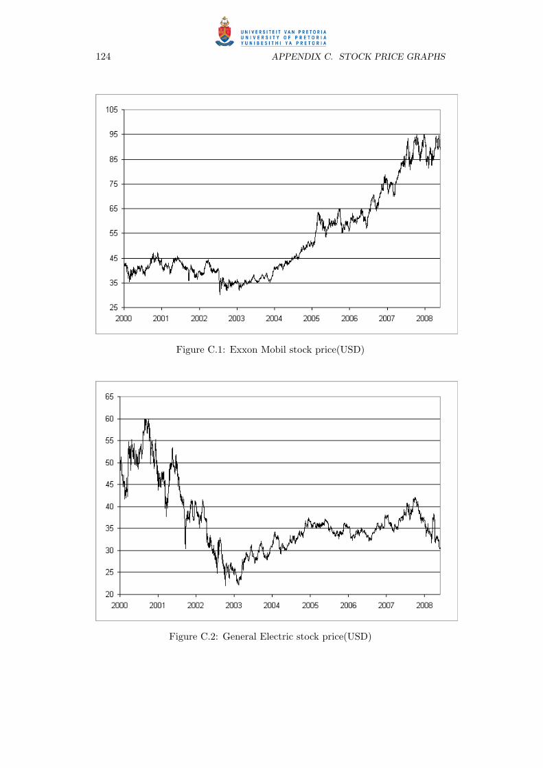
124 APPENDIX C. STOCK PRICE GRAPHS
Figure C.1: Exxon Mobil stock price(USD)
Figure C.2: General Electric stock price(USD)
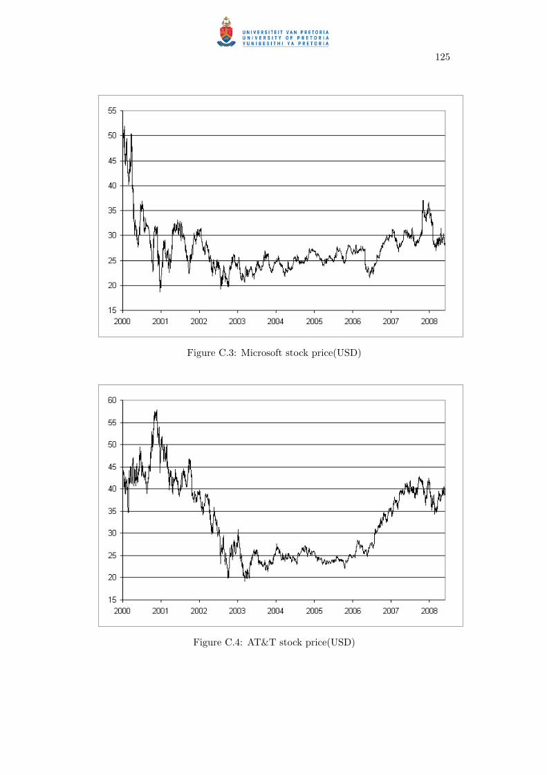
125
Figure C.3: Microsoft stock price(USD)
Figure C.4: AT&T stock price(USD)

126 APPENDIX C. STOCK PRICE GRAPHS
Figure C.5: HSBC stock price(GBP)
Figure C.6: BP stock price(GBP)
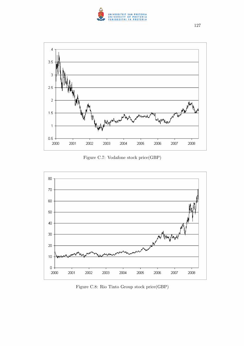
127
Figure C.7: Vodafone stock price(GBP)
Figure C.8: Rio Tinto Group stock price(GBP)

Appendix D
Empirical Study Tables
The tables in this appendix depict the empirical results for the investigated com-
petitive CEPSO model. Different tables depict results for different experiments. All
tables follow the exact same layout.
All tables display the different parameter combinations, which are indicated on
the top row and left most column of each table. The top half of each table lists the
averages for the simulated runs, while the bottom half list the standard deviations.
The left half lists the in-sample results, while the right half lists the out-sample results.
The averages of the average and standard deviation results are indicated in the last
column and row of each table.
128

129
Table D.1: Annualised returns (%) for the GBEST topology
Hidden Neurons (In-Sample) Hidden Neurons (Out-Sample)Particles 2 4 6 8 10 Avg 2 4 6 8 10 Avg
Retu
rns(
Avg) 10 14.42 16.84 21.48 22.72 23.47 19.78 5.57 8.03 7.65 9.1 9.15 7.9
25 19.64 22.41 26.05 27.5 26.55 24.43 6.96 8.44 8.37 9.02 9.8 8.5250 22.15 25.87 29.46 29.6 29.82 27.38 7.73 8.65 9.14 9.29 10.34 9.03100 23.59 28.23 31.16 32.34 31.81 29.43 7.27 8.78 8.85 9.3 8.76 8.59150 25.0 29.9 33.11 33.27 33.77 31.01 6.39 8.08 8.9 9.34 9.95 8.53200 26.56 30.83 33.28 35.49 34.32 32.09 6.33 7.04 9.29 8.16 10.3 8.23Avg 21.89 25.68 29.09 30.15 29.96 6.71 8.17 8.7 9.04 9.72
Retu
rns(
Std
) 10 7.65 8.54 9.11 8.36 8.81 8.49 13.5 14.83 11.97 13.51 12.96 13.3625 9.7 8.96 9.14 9.27 9.42 9.3 12.42 12.1 11.69 11.89 12.34 12.0950 10.03 9.74 9.36 9.29 10.67 9.82 13.12 12.32 12.27 11.79 12.32 12.36100 9.57 9.66 9.42 9.95 10.64 9.85 11.31 13.03 13.8 12.28 11.53 12.39150 9.44 9.58 9.92 10.28 10.29 9.9 11.39 13.21 13.48 12.83 11.83 12.55200 11.19 10.28 9.62 9.27 9.82 10.04 12.64 11.62 12.74 10.48 12.28 11.95Avg 9.6 9.46 9.43 9.4 9.94 12.4 12.85 12.66 12.13 12.21
Table D.2: Annualised returns (%) for the Von Neumann topology
Hidden Neurons (In-Sample) Hidden Neurons (Out-Sample)Particles 2 4 6 8 10 Avg 2 4 6 8 10 Avg
Retu
rns(
Avg) 10 18.39 21.55 22.6 21.32 21.12 21.0 8.95 9.7 10.26 9.43 10.55 9.78
25 23.17 24.55 24.18 23.65 22.82 23.67 10.74 9.93 10.08 10.52 10.0 10.2550 24.92 26.0 27.07 25.73 25.41 25.83 10.97 11.22 10.85 12.19 11.5 11.35100 26.54 27.05 28.41 27.84 27.13 27.39 11.45 11.55 10.98 11.42 9.63 11.0150 26.28 28.05 28.99 29.68 28.96 28.39 12.21 11.07 10.84 11.38 10.26 11.15200 26.38 28.53 29.25 28.94 29.59 28.54 13.35 10.86 11.3 11.1 10.17 11.36Avg 24.28 25.95 26.75 26.19 25.84 11.28 10.72 10.72 11.01 10.35
Retu
rns(
Std
) 10 9.08 8.3 8.13 8.15 8.18 8.37 14.33 12.35 13.47 11.37 12.2 12.7425 8.14 8.01 8.39 8.76 8.63 8.39 14.6 13.48 12.6 13.13 11.81 13.1350 8.31 8.26 8.5 9.01 9.2 8.65 14.46 13.82 13.89 13.53 12.87 13.71100 8.47 8.23 8.41 8.82 9.12 8.61 15.11 14.15 14.27 13.34 13.02 13.98150 8.11 8.43 9.1 8.7 9.09 8.68 15.21 13.46 13.2 13.77 12.06 13.54200 8.29 8.76 8.64 8.95 9.46 8.82 16.11 13.63 14.5 13.64 12.29 14.03Avg 8.4 8.33 8.53 8.73 8.95 14.97 13.48 13.66 13.13 12.38
Table D.3: Annualised returns (%) for the LBEST topology
Hidden Neurons (In-Sample) Hidden Neurons (Out-Sample)Particles 2 4 6 8 10 Avg 2 4 6 8 10 Avg
Retu
rns(
Avg) 10 19.21 21.84 23.17 23.84 22.52 22.11 9.67 9.58 10.14 10.42 9.35 9.83
25 22.81 24.59 25.94 25.65 26.41 25.08 9.54 10.57 11.17 10.75 9.78 10.3650 24.87 25.77 27.28 27.81 28.2 26.79 11.18 11.21 11.16 11.73 10.26 11.11100 25.91 27.23 28.49 28.26 29.19 27.82 12.19 10.68 11.42 11.96 11.22 11.49150 26.51 27.31 28.85 29.29 29.37 28.27 12.61 13.21 11.37 11.43 10.99 11.92200 27.19 27.92 29.35 29.67 29.9 28.8 12.98 12.21 13.14 10.83 12.98 12.43Avg 24.42 25.77 27.18 27.42 27.6 11.36 11.24 11.4 11.19 10.76
Retu
rns(
Std
) 10 7.87 7.53 7.63 7.71 8.2 7.79 13.12 13.36 13.52 13.62 11.2 12.9625 7.45 8.0 7.95 7.53 8.46 7.88 12.03 12.99 12.5 12.42 11.37 12.2650 8.25 7.83 8.32 7.81 8.67 8.18 13.72 13.29 12.27 14.12 12.61 13.2100 7.68 8.37 8.0 8.0 8.18 8.05 14.88 12.63 12.11 12.96 13.63 13.24150 7.69 8.27 8.23 8.82 8.47 8.3 14.14 15.38 12.5 13.45 12.45 13.59200 8.28 8.18 8.1 7.88 8.2 8.13 13.86 15.24 14.14 11.61 14.62 13.89Avg 7.87 8.03 8.04 7.96 8.36 13.62 13.82 12.84 13.03 12.65
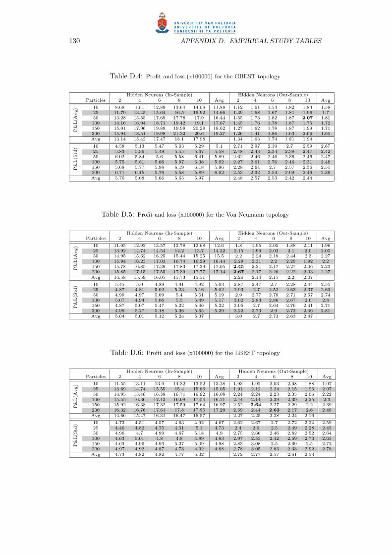
130 APPENDIX D. EMPIRICAL STUDY TABLES
Table D.4: Profit and loss (x100000) for the GBEST topology
Hidden Neurons (In-Sample) Hidden Neurons (Out-Sample)Particles 2 4 6 8 10 Avg 2 4 6 8 10 Avg
P&
L(A
vg) 10 8.68 10.1 12.89 13.64 14.08 11.88 1.12 1.61 1.53 1.82 1.83 1.58
25 11.79 13.45 15.64 16.5 15.92 14.66 1.39 1.68 1.67 1.81 1.96 1.750 13.28 15.55 17.69 17.78 17.9 16.44 1.55 1.73 1.82 1.87 2.07 1.81100 14.16 16.94 18.71 19.42 19.1 17.67 1.45 1.76 1.78 1.87 1.75 1.72150 15.01 17.96 19.89 19.98 20.28 18.62 1.27 1.62 1.78 1.87 1.99 1.71200 15.94 18.51 19.98 21.32 20.6 19.27 1.26 1.41 1.86 1.63 2.06 1.65Avg 13.14 15.42 17.47 18.1 17.98 1.34 1.63 1.74 1.81 1.94
P&
L(S
td) 10 4.58 5.13 5.47 5.03 5.29 5.1 2.71 2.97 2.39 2.7 2.59 2.67
25 5.83 5.36 5.49 5.55 5.67 5.58 2.48 2.43 2.34 2.38 2.47 2.4250 6.02 5.84 5.6 5.58 6.41 5.89 2.62 2.46 2.46 2.36 2.46 2.47100 5.75 5.81 5.66 5.97 6.38 5.92 2.27 2.61 2.76 2.46 2.31 2.48150 5.68 5.77 5.98 6.19 6.18 5.96 2.28 2.64 2.7 2.57 2.36 2.51200 6.71 6.15 5.76 5.58 5.89 6.02 2.53 2.32 2.54 2.09 2.46 2.39Avg 5.76 5.68 5.66 5.65 5.97 2.48 2.57 2.53 2.42 2.44
Table D.5: Profit and loss (x100000) for the Von Neumann topology
Hidden Neurons (In-Sample) Hidden Neurons (Out-Sample)Particles 2 4 6 8 10 Avg 2 4 6 8 10 Avg
P&
L(A
vg) 10 11.05 12.92 13.57 12.78 12.68 12.6 1.8 1.95 2.05 1.88 2.11 1.96
25 13.92 14.74 14.54 14.2 13.7 14.22 2.15 1.99 2.02 2.1 2.0 2.0550 14.95 15.62 16.25 15.44 15.25 15.5 2.2 2.24 2.18 2.44 2.3 2.27100 15.94 16.23 17.03 16.74 16.29 16.44 2.29 2.31 2.2 2.29 1.92 2.2150 15.78 16.85 17.39 17.83 17.39 17.05 2.45 2.21 2.17 2.27 2.06 2.23200 15.85 17.15 17.55 17.39 17.77 17.14 2.67 2.17 2.26 2.22 2.03 2.27Avg 14.58 15.59 16.05 15.73 15.51 2.26 2.14 2.15 2.2 2.07
P&
L(S
td) 10 5.45 5.0 4.89 4.91 4.92 5.03 2.87 2.47 2.7 2.28 2.44 2.55
25 4.87 4.81 5.02 5.23 5.16 5.02 2.93 2.7 2.52 2.63 2.37 2.6350 4.99 4.97 5.09 5.4 5.51 5.19 2.9 2.77 2.78 2.71 2.57 2.74100 5.07 4.94 5.06 5.3 5.49 5.17 3.02 2.83 2.86 2.67 2.6 2.8150 4.87 5.07 5.47 5.22 5.46 5.22 3.05 2.7 2.64 2.76 2.41 2.71200 4.99 5.27 5.18 5.36 5.65 5.29 3.22 2.73 2.9 2.72 2.46 2.81Avg 5.04 5.01 5.12 5.24 5.37 3.0 2.7 2.73 2.63 2.47
Table D.6: Profit and loss (x100000) for the LBEST topology
Hidden Neurons (In-Sample) Hidden Neurons (Out-Sample)Particles 2 4 6 8 10 Avg 2 4 6 8 10 Avg
P&
L(A
vg) 10 11.55 13.11 13.9 14.32 13.52 13.28 1.93 1.92 2.03 2.08 1.88 1.97
25 13.69 14.74 15.55 15.4 15.86 15.05 1.91 2.12 2.24 2.15 1.96 2.0750 14.95 15.46 16.38 16.71 16.92 16.08 2.24 2.24 2.23 2.35 2.06 2.22100 15.55 16.36 17.12 16.98 17.54 16.71 2.44 2.14 2.29 2.39 2.25 2.3150 15.92 16.38 17.32 17.59 17.64 16.97 2.52 2.64 2.27 2.29 2.2 2.39200 16.32 16.76 17.61 17.8 17.95 17.29 2.59 2.44 2.63 2.17 2.6 2.48Avg 14.66 15.47 16.31 16.47 16.57 2.27 2.25 2.28 2.24 2.16
P&
L(S
td) 10 4.73 4.51 4.57 4.63 4.92 4.67 2.62 2.67 2.7 2.72 2.24 2.59
25 4.46 4.82 4.75 4.51 5.1 4.73 2.4 2.6 2.5 2.49 2.28 2.4550 4.96 4.7 4.99 4.67 5.18 4.9 2.75 2.66 2.46 2.82 2.52 2.64100 4.63 5.01 4.8 4.8 4.89 4.83 2.97 2.53 2.42 2.59 2.73 2.65150 4.63 4.96 4.93 5.27 5.09 4.98 2.83 3.08 2.5 2.69 2.5 2.72200 4.97 4.92 4.87 4.73 4.92 4.88 2.78 3.05 2.83 2.33 2.92 2.78Avg 4.73 4.82 4.82 4.77 5.02 2.72 2.77 2.57 2.61 2.53
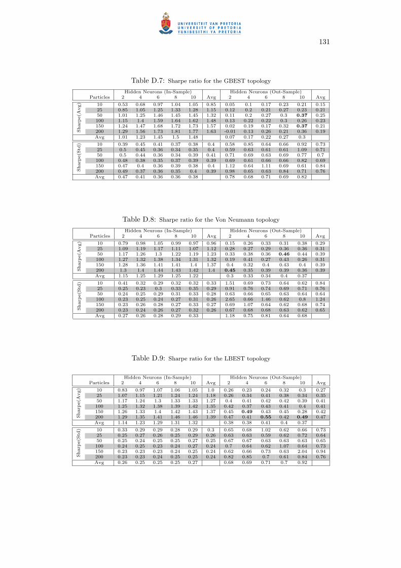
131
Table D.7: Sharpe ratio for the GBEST topology
Hidden Neurons (In-Sample) Hidden Neurons (Out-Sample)Particles 2 4 6 8 10 Avg 2 4 6 8 10 Avg
Sharp
e(A
vg) 10 0.53 0.68 0.97 1.04 1.05 0.85 0.05 0.1 0.17 0.23 0.21 0.15
25 0.85 1.05 1.25 1.33 1.28 1.15 0.12 0.2 0.21 0.27 0.23 0.2150 1.01 1.25 1.46 1.45 1.45 1.32 0.11 0.2 0.27 0.3 0.37 0.25100 1.15 1.4 1.59 1.64 1.62 1.48 0.13 0.22 0.22 0.3 0.26 0.23150 1.24 1.47 1.68 1.72 1.73 1.57 0.02 0.19 0.17 0.32 0.37 0.21200 1.29 1.56 1.73 1.81 1.77 1.63 -0.01 0.13 0.26 0.21 0.36 0.19Avg 1.01 1.23 1.45 1.5 1.48 0.07 0.17 0.22 0.27 0.3
Sharp
e(S
td) 10 0.39 0.45 0.41 0.37 0.38 0.4 0.58 0.85 0.64 0.66 0.92 0.73
25 0.5 0.45 0.36 0.34 0.35 0.4 0.59 0.63 0.61 0.61 1.09 0.7150 0.5 0.44 0.36 0.34 0.39 0.41 0.71 0.69 0.63 0.69 0.77 0.7100 0.48 0.38 0.35 0.37 0.39 0.39 0.69 0.61 0.66 0.66 0.82 0.69150 0.47 0.4 0.36 0.39 0.38 0.4 1.12 0.64 1.11 0.69 0.61 0.84200 0.49 0.37 0.36 0.35 0.4 0.39 0.98 0.65 0.63 0.84 0.71 0.76Avg 0.47 0.41 0.36 0.36 0.38 0.78 0.68 0.71 0.69 0.82
Table D.8: Sharpe ratio for the Von Neumann topology
Hidden Neurons (In-Sample) Hidden Neurons (Out-Sample)Particles 2 4 6 8 10 Avg 2 4 6 8 10 Avg
Sharp
e(A
vg) 10 0.79 0.98 1.05 0.99 0.97 0.96 0.15 0.26 0.33 0.31 0.38 0.29
25 1.09 1.19 1.17 1.11 1.07 1.12 0.28 0.27 0.29 0.36 0.36 0.3150 1.17 1.26 1.3 1.22 1.19 1.23 0.33 0.38 0.36 0.46 0.44 0.39100 1.27 1.32 1.38 1.34 1.31 1.32 0.19 0.41 0.27 0.43 0.26 0.31150 1.28 1.36 1.41 1.41 1.4 1.37 0.4 0.32 0.4 0.43 0.4 0.39200 1.3 1.4 1.44 1.43 1.42 1.4 0.45 0.35 0.39 0.39 0.36 0.39Avg 1.15 1.25 1.29 1.25 1.22 0.3 0.33 0.34 0.4 0.37
Sharp
e(S
td) 10 0.41 0.32 0.29 0.32 0.32 0.33 1.51 0.69 0.73 0.64 0.62 0.84
25 0.25 0.23 0.3 0.33 0.35 0.29 0.91 0.76 0.74 0.69 0.71 0.7650 0.24 0.25 0.29 0.31 0.33 0.28 0.63 0.66 0.65 0.63 0.64 0.64100 0.23 0.25 0.24 0.27 0.31 0.26 2.65 0.66 1.46 0.62 0.8 1.24150 0.23 0.26 0.28 0.27 0.33 0.27 0.69 1.07 0.64 0.62 0.68 0.74200 0.23 0.24 0.26 0.27 0.32 0.26 0.67 0.68 0.68 0.63 0.62 0.65Avg 0.27 0.26 0.28 0.29 0.33 1.18 0.75 0.81 0.64 0.68
Table D.9: Sharpe ratio for the LBEST topology
Hidden Neurons (In-Sample) Hidden Neurons (Out-Sample)Particles 2 4 6 8 10 Avg 2 4 6 8 10 Avg
Sharp
e(A
vg) 10 0.83 0.97 1.07 1.06 1.05 1.0 0.26 0.23 0.24 0.32 0.3 0.27
25 1.07 1.15 1.21 1.24 1.24 1.18 0.26 0.34 0.41 0.38 0.34 0.3550 1.17 1.24 1.3 1.33 1.33 1.27 0.4 0.41 0.42 0.42 0.39 0.41100 1.25 1.32 1.38 1.39 1.42 1.35 0.42 0.37 0.43 0.41 0.4 0.41150 1.26 1.33 1.4 1.42 1.43 1.37 0.45 0.49 0.43 0.45 0.28 0.42200 1.29 1.35 1.41 1.46 1.46 1.39 0.47 0.41 0.55 0.42 0.49 0.47Avg 1.14 1.23 1.29 1.31 1.32 0.38 0.38 0.41 0.4 0.37
Sharp
e(S
td) 10 0.33 0.29 0.29 0.28 0.29 0.3 0.65 0.68 1.02 0.62 0.66 0.73
25 0.25 0.27 0.26 0.25 0.29 0.26 0.63 0.63 0.59 0.62 0.72 0.6450 0.25 0.24 0.25 0.25 0.27 0.25 0.67 0.67 0.63 0.63 0.63 0.65100 0.24 0.25 0.23 0.24 0.27 0.24 0.7 0.64 0.62 1.07 0.64 0.73150 0.23 0.23 0.23 0.24 0.25 0.24 0.62 0.66 0.73 0.63 2.04 0.94200 0.23 0.23 0.24 0.25 0.25 0.24 0.82 0.85 0.7 0.61 0.84 0.76Avg 0.26 0.25 0.25 0.25 0.27 0.68 0.69 0.71 0.7 0.92
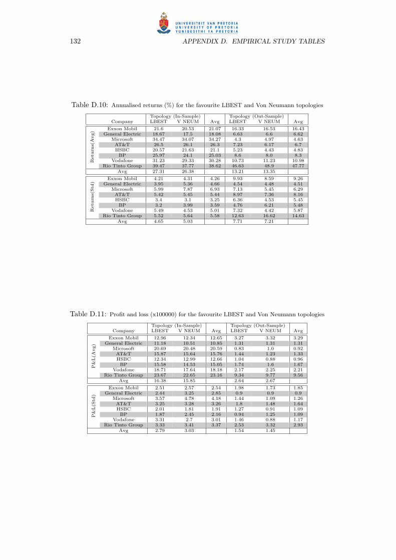
132 APPENDIX D. EMPIRICAL STUDY TABLES
Table D.10: Annualised returns (%) for the favourite LBEST and Von Neumann topologies
Topology (In-Sample) Topology (Out-Sample)Company LBEST V NEUM Avg LBEST V NEUM Avg
Retu
rns(
Avg)
Exxon Mobil 21.6 20.53 21.07 16.33 16.53 16.43General Electric 18.67 17.5 18.08 6.63 6.6 6.62
Microsoft 34.47 34.07 34.27 4.3 4.97 4.63AT&T 26.5 26.1 26.3 7.23 6.17 6.7HSBC 20.57 21.63 21.1 5.23 4.43 4.83BP 25.97 24.1 25.03 8.6 8.0 8.3
Vodafone 31.23 29.33 30.28 10.73 11.23 10.98Rio Tinto Group 39.47 37.77 38.62 46.63 48.9 47.77
Avg 27.31 26.38 13.21 13.35
Retu
rns(
Std
)
Exxon Mobil 4.21 4.31 4.26 9.93 8.59 9.26General Electric 3.95 5.36 4.66 4.54 4.48 4.51
Microsoft 5.99 7.87 6.93 7.13 5.45 6.29AT&T 5.42 5.45 5.44 8.97 7.36 8.16HSBC 3.4 3.1 3.25 6.36 4.53 5.45BP 3.2 3.99 3.59 4.76 6.21 5.48
Vodafone 5.49 4.53 5.01 7.32 4.42 5.87Rio Tinto Group 5.52 5.64 5.58 12.63 16.62 14.63
Avg 4.65 5.03 7.71 7.21
Table D.11: Profit and loss (x100000) for the favourite LBEST and Von Neumann topologies
Topology (In-Sample) Topology (Out-Sample)Company LBEST V NEUM Avg LBEST V NEUM Avg
P&
L(A
vg)
Exxon Mobil 12.96 12.34 12.65 3.27 3.32 3.29General Electric 11.18 10.51 10.85 1.31 1.31 1.31
Microsoft 20.69 20.48 20.59 0.83 1.0 0.92AT&T 15.87 15.64 15.76 1.44 1.23 1.33HSBC 12.34 12.99 12.66 1.04 0.88 0.96BP 15.58 14.53 15.05 1.74 1.6 1.67
Vodafone 18.71 17.64 18.18 2.17 2.25 2.21Rio Tinto Group 23.67 22.65 23.16 9.34 9.77 9.56
Avg 16.38 15.85 2.64 2.67
P&
L(S
td)
Exxon Mobil 2.51 2.57 2.54 1.98 1.73 1.85General Electric 2.44 3.25 2.85 0.9 0.9 0.9
Microsoft 3.57 4.78 4.18 1.44 1.09 1.26AT&T 3.25 3.28 3.26 1.8 1.48 1.64HSBC 2.01 1.81 1.91 1.27 0.91 1.09BP 1.87 2.45 2.16 0.94 1.25 1.09
Vodafone 3.31 2.7 3.01 1.46 0.88 1.17Rio Tinto Group 3.33 3.41 3.37 2.53 3.32 2.93
Avg 2.79 3.03 1.54 1.45
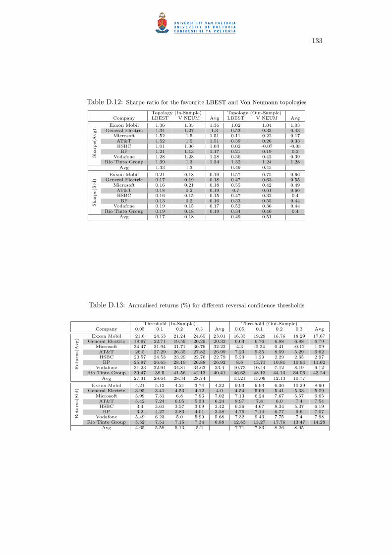
133
Table D.12: Sharpe ratio for the favourite LBEST and Von Neumann topologies
Topology (In-Sample) Topology (Out-Sample)Company LBEST V NEUM Avg LBEST V NEUM Avg
Sharp
e(A
vg)
Exxon Mobil 1.36 1.35 1.36 1.02 1.04 1.03General Electric 1.34 1.27 1.3 0.53 0.33 0.43
Microsoft 1.52 1.5 1.51 0.11 0.22 0.17AT&T 1.52 1.5 1.51 0.39 0.26 0.33HSBC 1.01 1.06 1.03 0.02 -0.07 -0.03BP 1.21 1.13 1.17 0.21 0.19 0.2
Vodafone 1.28 1.28 1.28 0.36 0.42 0.39Rio Tinto Group 1.39 1.3 1.34 1.32 1.24 1.28
Avg 1.33 1.3 0.49 0.45
Sharp
e(S
td)
Exxon Mobil 0.21 0.18 0.19 0.57 0.75 0.66General Electric 0.17 0.19 0.18 0.47 0.63 0.55
Microsoft 0.16 0.21 0.18 0.55 0.42 0.49AT&T 0.18 0.2 0.19 0.7 0.61 0.66HSBC 0.16 0.15 0.15 0.47 0.32 0.4BP 0.13 0.2 0.16 0.33 0.55 0.44
Vodafone 0.19 0.15 0.17 0.52 0.36 0.44Rio Tinto Group 0.19 0.18 0.19 0.34 0.46 0.4
Avg 0.17 0.18 0.49 0.51
Table D.13: Annualised returns (%) for different reversal confidence thresholds
Threshold (In-Sample) Threshold (Out-Sample)Company 0.05 0.1 0.2 0.3 Avg 0.05 0.1 0.2 0.3 Avg
Retu
rns(
Avg)
Exxon Mobil 21.6 24.53 21.24 24.65 23.01 16.33 19.29 16.76 18.29 17.67General Electric 18.67 22.71 19.59 20.29 20.32 6.63 6.76 6.88 6.88 6.79
Microsoft 34.47 31.94 31.71 30.76 32.22 4.3 -0.24 0.41 -0.12 1.09AT&T 26.5 27.29 26.35 27.82 26.99 7.23 5.35 8.59 5.29 6.62HSBC 20.57 24.53 23.29 22.76 22.79 5.23 1.29 2.29 2.65 2.97BP 25.97 26.65 28.19 26.88 26.92 8.6 13.71 10.81 10.94 11.02
Vodafone 31.23 32.94 34.81 34.63 33.4 10.73 10.44 7.12 8.19 9.12Rio Tinto Group 39.47 38.5 41.56 42.13 40.41 46.63 48.13 44.13 34.06 43.24
Avg 27.31 28.64 28.34 28.74 13.21 13.09 12.13 10.77
Retu
rns(
Std
)
Exxon Mobil 4.21 5.12 4.21 3.74 4.32 9.93 9.03 6.36 10.29 8.90General Electric 3.95 3.41 4.53 4.12 4.0 4.54 5.09 5.41 5.33 5.09
Microsoft 5.99 7.31 6.8 7.96 7.02 7.13 6.24 7.67 5.57 6.65AT&T 5.42 7.24 6.95 5.33 6.24 8.97 7.8 6.0 7.4 7.54HSBC 3.4 3.61 3.57 3.09 3.42 6.36 4.67 8.34 5.37 6.19BP 3.2 4.27 2.83 4.01 3.58 4.76 7.14 6.77 9.6 7.07
Vodafone 5.49 6.23 5.0 5.99 5.68 7.32 9.43 7.75 7.4 7.98Rio Tinto Group 5.52 7.51 7.15 7.34 6.88 12.63 13.27 17.76 13.47 14.28
Avg 4.65 5.59 5.13 5.2 7.71 7.83 8.26 8.05

Index
activation function, 36
aroon, 21
artificial neural network, 35
artificial neural network learning, 40
artificial neuron, 35
backpropagation, 40
biological neurons, 35
bollinger bands, 23
capital gain, 10
capital loss, 10
chromosome, 42
co-evolution, 50
cognitive factor, 44
common stock, 9
competitive co-evolution, 51
competitive fitness, 52
computational intelligence, 34
cooperative co-evolution, 51
crossover, 42
dept agreement, 9
divergence, 31
dow theory, 14
efficient markets hypothesis, 15
elitism, 42
equity, 9
evolutionary computation, 42
feed forward neural network, 37
FT Global 500, 73, 123
fundamental analysis, 16
gaussian activation function, 37
GBEST, 46
generation, 43
gradient descent, 40
hyberbolic tangent activation function, 37
LBEST, 47
learning vector quantizer, 40
limited liability, 10
linear activation function, 36
moving average convergence/divergence, 27
mutation, 42
ordinary shares, 9
overfitting, 38
ownership, 9
particle, 45
134

INDEX 135
particle swarm optimisation, 44
perpetual claim, 10
predator-prey co-evolution, 51
profit and loss, 67
pso neighbourhood topology, 45
reinforcement learning, 41
relative fitness, 52
relative strength index, 30
reproduction, 42
residual claim, 10
return on investment, 65
returns, 65
right to ownership, 9
ring topology, 46
script lending, 10
security, 9
self-organising maps, 40
share, 9
sharpe ratio, 68
short sell, 10
sigmoid activation function, 36
social factor, 44
star topology, 45
stock, 9
stock dividends, 10
stock market, 9
supervised learning, 40
swarm, 45
symbiosis, 51
synapses, 35
technical analysis, 13
technical market indicators, 18
unsupervised learning, 40
von neumann topology, 47