COMPASS ADJUSTMENT BY GPS AND TWO LEADING LINES

COMPASS ADJUSTMENT BY GPS AND TWO LEADING LINES

Jorge Moncunill Marimón (I)*, Aitor Martínez-Lozares, Ph.D (II), Agustí Martín

Mallofré, Ph.D (I), José Francisco González La Flor, Lieutenant Commander (reserve),

Ph.D. (I), Francisco Javier Martínez de Osés, Ph.D. (I)

(I) Department of Engineering and Nautical Sciences: UPC-Barcelona Tech. Pla de Palau,

18, 09003 Barcelona, Spain.

(II) Department of Navigation Science and Tecnology, Marine Engines and Naval

Architecture: Engineering School of Bilbao. María Díaz de Haro, 68, 48920 Portugalete

(Bizkaia), Spain.

* Correspondence author: [email protected]

Abstract:

The deviation card of a magnetic compass previously adjusted on two leading lines was

created using a GPS receiver.

During compass adjustment, the vessel follows magnetic courses using a gyroscopic

compass and taking into account magnetic declination and gyro error. A satellite

compass may also be used for the same purpose. However, some vessels are equipped

with neither gyroscopic nor satellite compass. In these cases, a minimum of five leading

lines must be considered, or a minimum of five bearings of conspicuous and distant points

or sun’s azimuths must be taken. This renders adjustment and creation of the deviation

card more laborious and time consuming. In order to expedite this process, a reliable

and practical method was developed to create the deviation card with courses over

ground given by a GPS receiver instead of the headings provided by a gyroscopic or

satellite compass. For this purpose, the stream factor, which, as in the ECDIS, also

includes other factors such as wind and waves, was considered. The method is valid for

all vessels, but is primarily intended for ships equipped with only magnetic compasses to

indicate the heading. Actual compass adjustment is carried out following two leadings

lines that coincide with or are close to magnetic cardinal courses separated by 90º.

Subsequently, courses over ground are taken when the vessel follows the main (four

cardinal and four quadrantal) compass headings to create the table of residual

deviations.

Keywords:

compass, adjustment, magnètic.

INTRODUCTION

The objective of this paper is the proper creation of the deviation card of a magnetic

compass previously adjusted on two leading lines using a GPS receiver.

Compass adjustment is necessary for the proper working of the magnetic compass, i.e.

the first nautical equipment mentioned in SOLAS V19. For many years, this procedure

has remained stagnant. However, with the emergence of new technologies, magnetic

compass applications and its adjustment techniques have once again become subjects of

research. In Spain, for example, there are four doctoral thesis focused on the improvement

of magnetic compass performance: Gaztelu-Iturri, 1999; Gea, 2003; Martinez-Lozares,

2009; Arribalzaga, 2016. This article follows this line of research in an attempt to simplify

the process of compass adjustment as well as enhance efficiency, focused in small crafts

that have a magnetic heading indicator only.

The paper is divided in seven sections. In section 1, the compass adjustment of small

crafts is explained. In sections 2, 3 and 4, the proposed method is approached, developed

and discussed respectively. In section 5, the application of the method is exposed,

according to the obtained results in section 4. Section 6 is focused on the determination

of necessary leading lines for the method’s application, taking as example, the fieldwork

carried out in the Barcelona harbour. Finally, in section 7, conclusions are drawn.

1.-INTRODUCTION TO COMPASS ADJUSTMENT

The process of compass adjustment has two phases: actual compass adjustment or

compensation, and creation of the table of residual deviations or deviation card. The

present work is mainly concerned with the latter. However, before this method is

presented, the following sub-sections explain how compensation is carried out in vessels

with only magnetic compasses to indicate heading.

1.1.-DEVIATION EQUATION [2] [6]

The deviation equation commonly applied is

'2cosE'2sinD'cosC'sinBA [i],

where

is the deviation, ꞌ is the compass course ( indicates the magnetic course; see section

2) and A, B, C, D, E are the approximate coefficients, with the exact coefficients being

the sines of the approximate ones.

Course deviation consists of three parts: constant deviation, A, which does not depend on

the course; semicircular deviation, B·sin ꞌ + C·cos ꞌ, which depends on the course, and

quadrantal deviation, D·sin 2ꞌ + E·cos 2ꞌ, which depends on twice the course. These

deviations are called semicircular and quadrantal deviations because they are repeated

with different sign every 180º and 90º, respectively, where 180º corresponds to half a

circle (semicircle) and 90º to a quarter of a circle (quadrant).

The semicircular deviation depends mainly on the hard irons of the ship (which have

permanent magnetism) and is corrected with magnets. On the other hand, the constant

and quadrantal deviations depend solely on and are corrected with the soft irons, which

do not have permanent magnetism but are induced according to their orientation within

the earth's magnetic field.

Considering ꞌ = 0º, 90º, 180º, 270º, the expressions of the deviations on the cardinal

courses are obtained as follows:

n = A + C + E e = A + B – E s = A – C + E w = A – B – E

Therefore, the deviations on the cardinal headings depend on the constant (coefficient A),

semicircular (coefficients B, C) and part of the quadrantal (coefficient E) deviation, with

the semicircular one being the main deviation.

1.2.-COMPENSATION DEVICES

The semicircular deviation of compasses in small crafts is compensated with a device that

fits the position of longitudinal and transversal magnets by turning one screw for the

longitudinal magnets and one for the transversal ones with an anti-magnetic screwdriver.

The polarity of magnets is indicated with colors: red for the north pole ends and blue or

green for the south pole ends.

As an example, Figures 1 and 2 show a small binnacle comprising a longitudinal magnet

(LM) on the port side with its north (red) end to aft and a transversal magnet (TM) on the

fore side with its north (red) end to starboard. In addition, there are two magnets arranged

in V-shape in the diametrically opposite position to the LM, and two more in the opposite

position to the TM; that is, opposite poles are located at the apex and ends of the V,

meaning that the latter form a magnet (V magnet). By adjusting the distance between the

V ends with a screwdriver-operated device, the magnetic moment of the V magnet is

changed because the distance between its poles is varied [1] [2]. Next, the magnets are

arranged in such a way that each V magnet and its corresponding simple magnet have

opposite polarities, and the magnetic moment of the V magnet at maximum distance

between its ends is twice that of the simple magnet, such that

i)-For no distance between ends of the V magnet, the resulting magnet is the simple

magnet.

ii)-For the maximum distance between ends of the V magnet, a magnet with the magnetic

moment of the simple magnet but the polarity of the V magnet is obtained.

iii)-For the middle distance between the ends of the V magnet, the resulting magnet is

null.

iv)-For intermediate distances, magnets with magnetic moments lower than that of the

simple magnet and polarities depending on the distance from the midpoint between ends

are obtained.

The quadrantal deviation can be compensated by installing soft iron correctors, such as

small spheres or cylinders, or boxes where several soft iron plates can be placed.

However, as this is not a common practice, this paper does not consider the compensation

of this deviation. It must be remembered, though, that the effect of the quadrantal

deviation is always included in the residual deviations.

Figure 1 (left). Compensating device: exterior view.

Figure 2 (right). Compensating device: internal arrangement of

the corrector magnets.

Source: Compass of the Barcelona School of Nautical Studies.

Another very common device consists in placing one (or two) longitudinal and one (or

two) transversal magnets that can rotate around their centers, as shown in Figure 3. In this

case, the horizontal component of the magnetic moment of the magnets is used to

compensate.

Figure 3. Compensating device with rotating magnets.

Source: The authors.

Notice that the longitudinal magnets are inside the transversal rotating cylinder and the

transversal magnets are inside the longitudinal rotating cylinder.

1.3.-COMPENSATION METHOD WITH TWO LEADING LINES

The ship follows a leading line that matches the magnetic east or west, or that is close to

one of these headings, and the position of the resulting longitudinal magnet is fitted by

turning the starboard screw to nullify the deviation, making the compass heading coincide

with the magnetic course of the leading line.

Analogously, the ship follows a leading line that matches or is close to the magnetic north

or south, and the position of the resulting transversal magnet is fitted by turning the fore

screw to make the compass heading be the magnetic course of the leading line.

1.4.-RESIDUAL DEVIATIONS

According to sub-section 1.3, when the deviations on two magnetic cardinal courses

separated by 90º are nullified, the effect of hard irons (reflected in coefficients B, C) is

minimized. However, this effect is not completely eliminated because the deviations on

the cardinal courses also depend on the constant deviation (coefficient A) and part of the

quadrantal one (coefficient E) (see sub-section 1.1). In addition, the effect of soft irons is

not compensated, either. Consequently, residual magnetic effects remain after the

compensation. [2] [6]

In small vessels, the procedure exposed in section 1.3 is usually enough to comply with

the requirement in [3], i.e. the deviation on any course must not exceed 4º for ships with

a length less than 82.5 m.

However, the residual deviations must be determined and reflected on the table (deviation

card) attached to the compass adjustment certificate, which must also be checked

regularly on board [4]. The proposed method is used to create this table, avoiding

following more leading lines and/or taking bearings of conspicuous and distant points of

land or sun’s azimuths, as indicated in [2] and [6], respectively.

2.-APPROACH OF THE METHOD

Coefficients A, B, C, D, E of the deviation equation [i], as well as the set and drift of the

current, are determined from the courses over ground indicated by the GPS when

following the eight main compass courses (the four cardinal and the four quadrantal ones).

The method is based on the triangle of speeds and types of courses, as shown in Figure 4.

References TN, MN, CN correspond to the true, magnetic and compass north, which are

the origins of the true (TC), magnetic () and compass course (ꞌ), respectively; is the

magnetic declination; , the deviation, and S, the vessel’s speed through the water. The

parameters of the current are set () and drift (d), where is expressed as a magnetic

course. Also, is the course difference due to the current: = COG – TC.

Figure 4. Types of courses and triangle of speeds.

TN MNCN

HEADING

S

'

TC

d

d

g

COG

S


3.-DEVELOPMENT OF THE METHOD

According to Figure 4, by the law of sines,

g

g

sinS

dsin

sin

d

sin

S

But + g= – , since they are opposite angles of a parallelogram. Then,

sinS

dsin

Developing,

sincosS

dcossin

S

dsin

cosS

d1

sinS

d

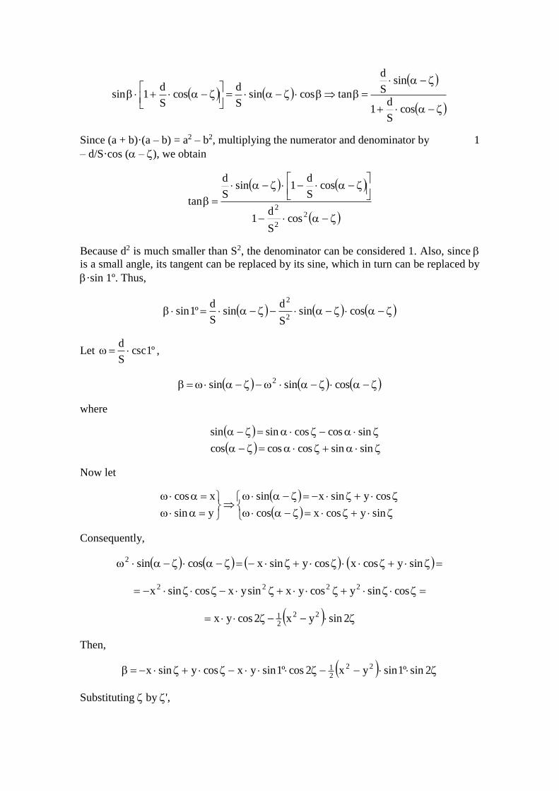
tancossinS

dcos

S

d1sin

Since (a + b)·(a – b) = a2 – b2, multiplying the numerator and denominator by 1

– d/S·cos ( – ), we obtain

2

2

2

cosS

d1

cosS

d1sin

S

d

tan

Because d2 is much smaller than S2, the denominator can be considered 1. Also, since

is a small angle, its tangent can be replaced by its sine, which in turn can be replaced by

·sin 1º. Thus,

cossinS

dsin

S

dº1sin

2

2

Let º1cscS

d ,

cossinsin 2

where

sinsincoscoscos

sincoscossinsin

Now let

sinycosxcos

cosysinxsin

ysin

xcos

Consequently,

sinycosxcosysinxcossin2

cossinycosyxsinyxcossinx 2222

2sinyx2cosyx 22

21

Then,

2sinº1sinyx2cosº1sinyxcosysinx 22

21

Substituting by ',

'2sinº1sinyx'2cosº1sinyx'cosy'sinx 22

21

The deviation is the difference between the magnetic course and the compass course, i.e.

= – ꞌ. Likewise, the magnetic course is the difference between the true course and

the magnetic declination, i.e. = TC – . Hence, = TC – – ꞌ, and TC is the difference

between the course over ground and : TC = COG . Therefore,

'COG

And the deviation equation is

'2cosE'2sinD'cosC'sinBA

Thus,

'2cosE'2sinD'cosC'sinBA'COG

Now let the pseudo-deviation () be defined as the difference between the course over

ground and the compass course: = COG – ꞌ. Then,

'2cosE'2sinD'cosC'sinBA

'sinx'2cosE'2sinD'cosC'sinBA

'2sinº1sinyx'2cosº1sinyx'cosy 22

21

Particularizing for the four cardinal compass courses, we obtain

º1sinyxyECAn [ii]

º1sinyxxEBAe [iii]

º1sinyxyECAs [iv]

º1sinyxxEBAw [v]

Consequently,

4A4wsen]iv[]iii[]ii[]i[

wsenA41 [vi]

xweBx2B2we]iv[]ii[21 [vii]

ysnCy2C2sn]iii[]i[21 [viii]

º1sinyx4E4wesn]iv[]ii[]iii[]i[

º1sinyxwesnE41 [ix]

And particularizing for the four quadrantal compass courses, we obtain

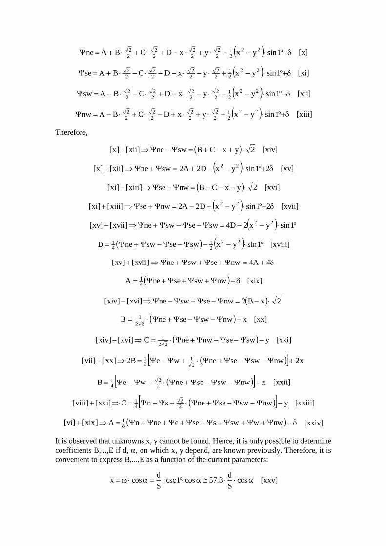
º1sinyxyxDCBAne 22

21

2

2

2

2

2

2

2

2 [x]

º1sinyxyxDCBAse 22

21

2

2

2

2

2

2

2

2 [xi]

º1sinyxyxDCBAsw 22

21

2

2

2

2

2

2

2

2 [xii]

º1sinyxyxDCBAnw 22

21

2

2

2

2

2

2

2

2 [xiii]

Therefore,

2yxCBswne]xii[]x[ [xiv]

2º1sinyxD2A2swne]xii[]x[ 22 [xv]

2yxCBnwse]xiii[]xi[ [xvi]

2º1sinyxD2A2nwse]xiii[]xi[ 22 [xvii]

º1sinyx2D4swseswne]xvii[]xv[ 22

º1sinyxswseswneD 22

21

41 [xviii]

4A4nwseswne]xvii[]xv[

nwswseneA41 [xix]

2xB2nwseswne]xvi[]xiv[

xnwswseneB22

1 [xx]

yswsenwneC]xvi[]xiv[22

1 [xxi]

x2nwswseneweB2]xx[]vii[2

121

xnwswseneweB2

2

41 [xxii]

ynwswsenesnC]xxi[]viii[2

2

41 [xxiii]

nwwswsseenenA]xix[]vi[81 [xxiv]

It is observed that unknowns x, y cannot be found. Hence, it is only possible to determine

coefficients B,...,E if d, , on which x, y depend, are known previously. Therefore, it is

convenient to express B,...,E as a function of the current parameters:

cosS

d3.57cosº1csc

S

dcosx [xxv]

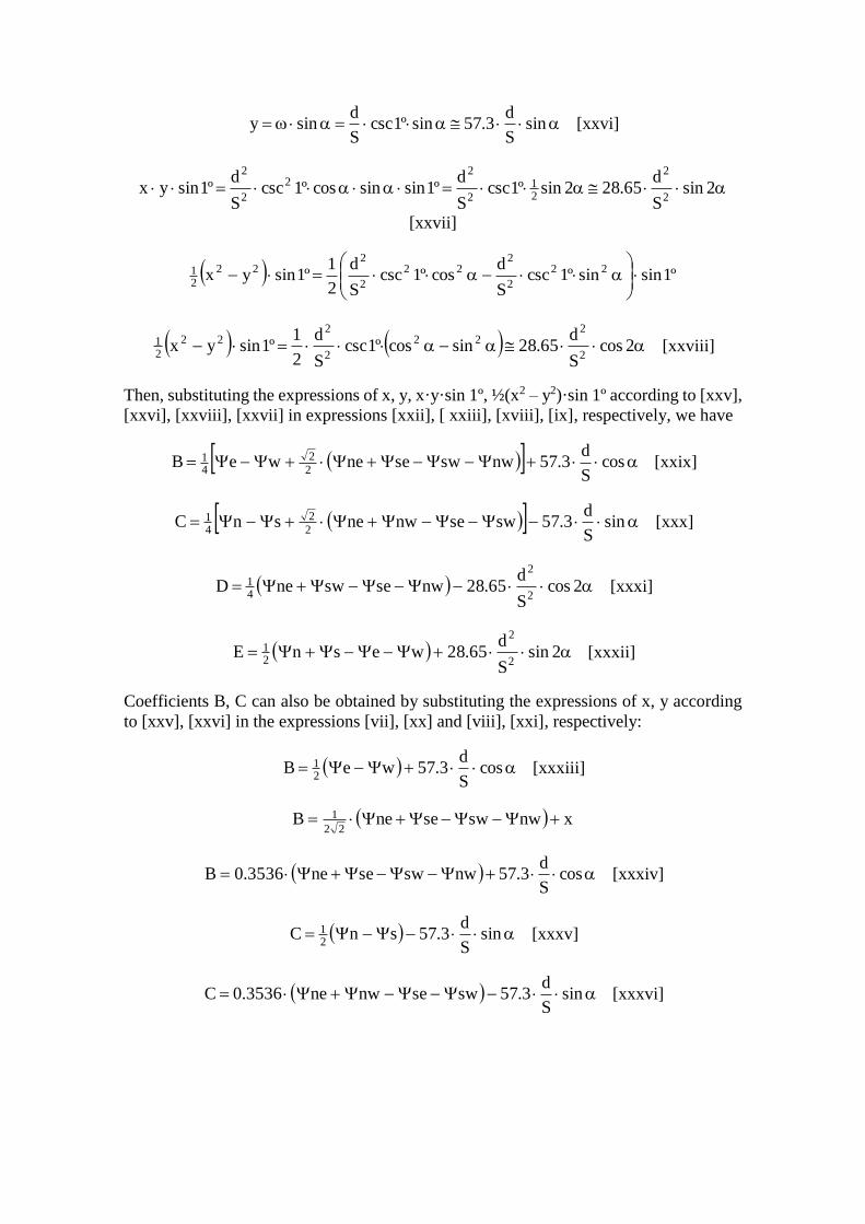
sinS

d3.57sinº1csc

S

dsiny [xxvi]

2sinS

d65.282sinº1csc

S

dº1sinsincosº1csc

S

dº1sinyx

2

2

21

2

22

2

2

[xxvii]

º1sinsinº1cscS

dcosº1csc

S

d

2

1º1sinyx 22

2

222

2

222

21

2cosS

d65.28sincosº1csc

S

d

2

1º1sinyx

2

222

2

222

21 [xxviii]

Then, substituting the expressions of x, y, x·y·sin 1º, ½(x2 – y2)·sin 1º according to [xxv],

[xxvi], [xxviii], [xxvii] in expressions [xxii], [ xxiii], [xviii], [ix], respectively, we have

cosS

d3.57nwswseneweB

2

2

41 [xxix]

sinS

d3.57swsenwnesnC

2

2

41 [xxx]

2cosS

d65.28nwseswneD

2

2

41 [xxxi]

2sinS

d65.28wesnE

2

2

21 [xxxii]

Coefficients B, C can also be obtained by substituting the expressions of x, y according

to [xxv], [xxvi] in the expressions [vii], [xx] and [viii], [xxi], respectively:

cosS

d3.57weB

21 [xxxiii]

xnwswseneB22

1

cosS

d3.57nwswsene3536.0B [xxxiv]

sinS

d3.57snC

21 [xxxv]

sinS

d3.57swsenwne3536.0C [xxxvi]

4.-DISCUSSION OF THE METHOD

Expressions [xxix], [xxx], [xxxiii], [xxxiv], [xxxv], [xxxvi] are not reliable for calculating

coefficients B, C because not knowing with precision the d/S ratio can lead to a

considerable error.

Nevertheless, it is observed that at a sufficient speed, the d2/S2 ratio is very small, and can

therefore be neglected in expressions [xxxi], [xxxii]. For example, for an already quite

critical ratio of S/d = 5 (i.e. a ship sailing at 5 knots with a 1 knot current, or a ship sailing

at 10 knots with a 2 knot current), the maximum error in the calculation of coefficients

D, E would be 1º. This maximum error is shown below for the S/d ratio:

Figure 5. Maximum error of coefficients D, E for the S/d ratio.

S/d 5 6 7 8 9 10 11 12

Max. error:

28.65·d2/S2 1.1460 0.7958 0.5847 0.4477 0.3537 0.2865 0.2368 0.1990

Source: The authors. I

These results show that the effect of the current can indeed be neglected in expressions

[xxxi], [xxxii]. Therefore,

nwseswneD41 [xxxvii]

wesnE41 [xxxviii]

In summary:

i)-Coefficient A can be determined from the pseudo-deviations without error. The

magnetic declination must also be applied (see [vi], [xix], [xxiv]).

ii)-Coefficients D, E can be determined solely from the pseudo-deviations but with a

small error which is negligible for sufficiently high speeds, i.e. for a ratio of S/d equal or

greater than 8, which causes an error less than 0.5º for each coefficient. Assuming a drift

of 1 knot or less, the minimum speed is 8 knots, and assuming a drift of 0.5 knots or less,

the minimum speed is 4 knots.

iii)-Coefficients B, C cannot be calculated with the pseudo-deviations because a

considerable error can be made.

On the other hand, coefficients B, C can be determined from coefficients A, E (calculated

from the pseudo-deviations) because

EAw,eBEBAw,e [xxxix]

EAs,nCECAs,n [xl]

where e,w and n,s can be considered the deviations on the leading lines which have

been nullified. Therefore,

EAB (+ leading line towards E; – leading line towards W)

EAC (+ leading line towards N; – leading line towards S)

Simplifying,

EA1B1180/TB1

[xli]

EA1C5.1180/TB2

[xlii]

where

[x] is the integer part of x, and TB1, TB2 are the true bearings, expressed in circular form

(from 0º to 360º), of the leading line close to the E or W and the leading line close to the

N or S, respectively.

5.-APPLICATION OF THE METHOD

The complete procedure to compensate the compass and create its table of the residual

deviations is as follows:

1.-The vessel must follow a leading line coincident with or close to the magnetic east or

west, and the deviation must be nullified. Next, the vessel must continue following the

leading line, and the course over ground indicated by the GPS must be noted down to

determine the pseudo-deviation, i.e. e,w = COG – '.

2.-Idem on a leading line coincident with or close to the magnetic north or south.

3.-The vessel must follow the other six main compass courses, and the course over ground

indicated by the GPS must be noted down to determine the pseudo-deviations.

4.-Coefficients A, D, E, B, C must be calculated using expressions [vi], [xxxvii],

[xxxviii], [xli], [xlii], respectively. Coefficient A can also be obtained by using [xix],

[xxiv].

5.-The table of the residual deviations must be created by applying the deviation equation

[i] to different compass courses, for example every 15º, as is the case of the deviation

card model of the Spanish regulation [5].

6.-DETERMINATION OF LEADING LINES

Two leading lines that coincide with or are as close as possible to magnetic cardinal

courses separated by 90º must be found. However, these leading lines cannot always be

determined on the chart (because one or both points are not on the chart), or if they can

be, they may be at a considerable distance. Alternatively, points that determine the

required leading lines can be selected despite not appearing on the chart, and then their

positions can be obtained from Google Maps and verified in situ, as done by Moncunill

and González La Flor in the outer northern area of the Barcelona harbour.

On January 16, 2020, the sailboat APHRODITE sailed the coastal waters between the

Besòs river mouth and the northern entrance to the Barcelona harbour, corresponding to

a distance of about 5 nautical miles. The voyage actually began and ended at El Masnou

marina (where the sailboat has her mooring), about 6 miles NE of the Besòs river mouth.

The meteorological conditions were as follows: on the way out, in the morning,

predominant onshore wind of force 2 on the Beaufort scale and rippled sea with a 0.5 m

swell from E; on the way back, in the afternoon, SW wind of force 3 and smooth sea;

good visibility and almost clear sky throughout the day. We sailed all the time, with the

occasional use of the engine.

The following leading lines, on which the points can be clearly distinguished, were

observed:

i)-Close to the W, southernmost chimney stack of former thermal power plant by the

Besòs river (point A) with the Tibidabo church (point B): IMAGE 1 (Figure 6).

ii)-Close to the W, second northernmost chimney stack of the Besòs combined cycle plant

(Endesa towers) (point C) with the Tibidabo church (point B): IMAGE 2 (Figure 7).

iii)-Close to the W, the Glòries tower (former Agbar tower) (point D) with the Collserola

telecommunications tower (point E): IMAGE 3 (Figure 8).

iv)-Close to the N, the Aigües del Besòs tower (point F) between two emblematic

buildings: IMAGE 4 (Figure 9). A ship's position was taken as the second point when the

ship was following the leading line (point G).

v)-Close to the N, the La Catalana de Gas tower (point H) with the Glòries tower (point

D): IMAGE 5 (Figure 10).

Figure 6. IMAGE 1: Leading line A–B, close to the W.


Figure 7. IMAGE 2: Leading line C–B, close to the W.


Figure 8. IMAGE 3: Leading line D–E, close to the W.


Figure 9. IMAGE 4: Leading line G–F, close to the N.


Figure 10. IMAGE 5: Leading line H–D, close to the N.


Since the sailboat has a magnetic heading indicator only, it was impossible to determine

exactly the true bearing of each leading line. Therefore, the positions of points A,...,H,

must be taken to obtain them.

These positions, which were taken from Google Maps and verified in situ, are shown in

the table below. They were rounded to the fourth decimal place of sexagesimal degree (in

latitude, 0.0001º corresponds to 11 m). Differences between both positions (Google Maps

and verified in situ) are due to the impossibility to access the central point of the buildings.

As for the position provided by the GPS (point G), it is shown as it appears on the screen,

i.e. rounded to the third decimal place of sexagesimal minute (0.001ꞌ = 1.852 m).

Figure 11. Position of the points of the obtained leading lines.

Point Google Maps In situ verification

A: Three Besòs chimney stacks 41.4266º 2.2345º 41.4263º 2.2342º

B: Tibidabo church 41.4220º 2.1187º 41.4217º 2.1192º

C: Endesa towers 41.4191º 2.2296º 41.4185º 2.2303º

D: Glòries tower (Agbar tower) 41.4038º 2.1895º 41.4037º 2.1896º

E: Collserola tower 41.4170º 2.1143º 41.4180º 2.1151º

F: Aigües del Besòs tower 41.4060º 2.2117º 41.4061º 2.2119º

G: Sea, following the leading line * * * 41º23.319’N

2º12.828’E

H: La Catalana de Gas tower 41.3838º 2.1926º 41.3837º 2.1925º


The true bearing (TB) of each leading line can be determined in three diferent ways:

i)-Plotting the points on the chart and drawing the leading lines.

ii)-Using dead reckoning formulae.

iii)-Using the loxodrome equation.

With the help of a spreadsheet, it was finally decided to use the loxodrome equation, from

which it follows that

2122

12

12ARSEMICIRCUL

k360MM

MMTBcos

,

where

TBSEMICIRCULAR, i.e. the arccosine provided by calculators and spreadsheets, is between

0º and 180º; M1, M2 are the meridional parts, expressed in sexagesimal degrees, of the

closest point of the leading line and the furthest one, respectively;1, 2 are the positive

(E) or negative (W) longitude, expressed in sexagesimal degrees, of the closest point of

the leading line and the furthest one, respectively, and k is the integer (0, 1 or –1) such

that the absolute value of 2 – 1 + 360·k is inferior or equal to 180º. In this case, k = 0.

Likewise, with beingthe latitude of a point, expressed in sexagesimal degrees, and

positive or negative depending on whether it is N or S, respectively, its meridional part

(M) is

21º45tanln

º180M

Finally, the true bearing expressed in circular form (from 0º to 360º) is TBSEMICIRCULAR if

2 – 1 + 360·k is positive, or 360º – TBSEMICIRCULAR if it is negative. TBSEMICIRCULAR was

obtained from a cosine and not a tangent (using the most common formula in Navigation)

because, unlike the tangent function, the cosine function is continuous such that errors in

the spreadsheet are avoided with the arccosine.

The obtained true bearings, rounded to half sexagesimal degree, are shown in the

following table:

Figure 12. True bearings of the obtained leading lines.

A–B C–B D–E G–F H–D

267 271.5 283 355 353.5


The practical value of the magnetic declination (i.e. rounded to half sexagesimal degree)

for the indicated day, taking the breakwater end at the north mouth of the Barcelona

harbour (41.3577, 2.1854, Google Maps) as the reference position, is 1º.

According to the World Magnetic Model WMM (2019-24), as used by NOAA

(https://www.ngdc.noaa.gov/geomag/calculators/magcalc.shtml), = 1.23ºE ± 0.34º.

According to the International Geomagnetic Reference Field IGRF-12 (2015) Model, as

used by Natural Resources Canada (https://geomag.nrcan.gc.ca/calc/mfcal-en.php),

= 1.107º.

It is worth recalling that the magnetic declination varies very slowly, both in time and

space (except near the geographical and magnetic poles), and therefore the value of 1º is

valid for the entire area considered.

Hence, the magnetic bearings are

Figure 13. Magnetic bearings of the obtained leading lines.

A–B C–B D–E G–F H–D

266 270.5 282 354 352.5


https://www.ngdc.noaa.gov/geomag/calculators/magcalc.shtml

https://geomag.nrcan.gc.ca/calc/mfcal-en.php

The two closest to the magnetic bearings N and W are selected:

G–F: Aigües del Besòs tower between two emblematic buildings: IMAGE 4 (Figure 9)

C–B: second northernmost chimney stack of the Besòs combined cycle plant (Endesa

towers) with the Tibidabo church: IMAGE 2 (Figure 7)

In addition, the leading line C–B has the advantage over A–B that it is closer to G–F.

7.-CONCLUSIONS

The proposed method enables a rigorous and practical compensation to be carried out on

vessels that have a magnetic heading indicator only. In order to perform the actual

compass adjustment, two leading lines as close as possible to magnetic cardinal courses

separated by 90º must be known, and to create the deviation card, a GPS receiver is used.

References:

[1] Arribalzaga Aurre, J. Sistema de compensación simplificado del desvío semicircular

para bitácora con compás de clase “A”. [Simplified compass adjustment system of the

sem icircular deviation for a binnacle with class "A" compass]. Doctoral Thesis,

University of the Basque Country, Department of Nautical Sciences and Marine Systems

Engineering, 2016. Date of access: July 2020. Available from:

<http://hdl.handle.net/10810/21147 >

[2] Gaztelu-Iturri Leicea, R. Compensación de la aguja náutica: curso de compensador

[Compensation of the magnetic compass: course on compass adjuster] Vitoria: Servicio

Central de Publicaciones del Gobierno Vasco, 1999. ISBN-10: 8445715070; ISBN-13:

9788445715079

[3] International Organization for Standardization. ISO 25862:2019: Ships and marine

technology: marine magnetic compasses, binnacles and azimuth reading devices.

Genève: ISO, 2019.

[4] Lushnikov, E.M.; Pleskacz, K. (2012). Analysis of problems related to the use of

ship’s course indicators. Scientific journals of the Maritime University of Szczecin,

Szczecin, Poland: Maritime University of Szczecin, 2012. 29 (101) pp. 122–125. Date of

access: July 2020. Available from: <http://repository.scientific-

journals.eu/handle/123456789/341>

[5] Spain. Ministry of Public Works and. Ministerial order of 14 December 1992 on

compass adjustment. In: Boletín oficial del Estado. Madrid: BOE, 8 January 1993, no. 7,

pp. 416–418

[6]-National Geospatial–Intelligence Agency. Handbook of magnetic compass

adjustment (Formerly Pub. No. 226). Bethesda, Maryland, USA: National Geospatial–

Intelligence Agency, 2004. Date of access: July 2020. Available from:

<https://bit.ly/338GRE6>

http://hdl.handle.net/10810/21147

http://repository.scientific-journals.eu/handle/123456789/341

http://repository.scientific-journals.eu/handle/123456789/341

https://bit.ly/338GRE6

COMPASS ADJUSTMENT BY GPS AND TWO LEADING LINES

Documents

Transcript of COMPASS ADJUSTMENT BY GPS AND TWO LEADING LINES