3OURNAL OF GEOPHYSICAL RESEARCH, VOL. 93, NO. C12, PAGES 15,374-15,388, DECEMBER 15, 1988

Comparison of Shuttle Imaging Radar-B Ocean Wave Image Spectra With Linear Model Predictions Based on Aircraft Measurements

FRANK M. MONALDO

Applied Physics Laboratory, Johns Hopkins University, Laurel, Maryland

DAVID R. LYZENGA

College of Marine Studies, University of Delaware, Newark

During October 1984, coincident shuttle imaging radar-B synthetic aperture radar (SAR) imagery and wave measurements from airborne instrumentation were acquired. The two-dimensional wave spectrum was measured by both a radar ocean wave spectrometer and a surface contour radar aboard the aircraft. In this paper we compare two-dimensional SAR image intensity variance spectra with these independent measures of ocean wave spectra to verify previously proposed models of the relationship between such SAR image spectra and ocea•n wave spectra. The results illustrate both the functional relationship between SAR image spectra and ocean wave spectra and the limitations imposed on the imaging of short-wavelength, azimuth-traveling waves.

1. INTRODUCTION

The first spaceborne synthetic aperture radar (SAR) used to estimate ocean wave spectra from space was aboard the Seasat satellite in 1978. In spite of the short (3 months) life of the satellite, substantial quantities of SAR wave imagery were ac- quired. The relatively modest portion of th9se data, which were fully digitally processed to produce geometrically and radi•ometrically corrected SAR imagery and associated image intensity variance spectra, revealed a general correlation be- tween the location of spectral peaks in the image spectra and independent surface measurements and wave model predic- tions [Beal et al., 1983, 1986a, b].

However, the lack of independently measured, two- dimensional wave spectra with wave number and angular res- olution comparable to those of SAR image spectra precluded verification of any thorough description of the relationship between SAR image intensity variance spectra and ocean wave slope or height variance spectra.

Additionally, the imaging of azimuth-traveling (traveling parallel to the satellite ground track) waves in Seasat SAR imagery was observed to be limited. Two-dimensional image spectra clearly exhibited a loss of spectral response at large azimuth wave numbers. The effect was observed to become

more pronounced in higher sea state conditions, making the measurement of short azimuth-traveling waves the most sig- nificant limitation on the use of spaceborne SAR wave imag- ery to estimate ocean wave spectra [Beal et al., 1986a; Mon- aldo and Beal, 1986' Alpers et al., 1986].

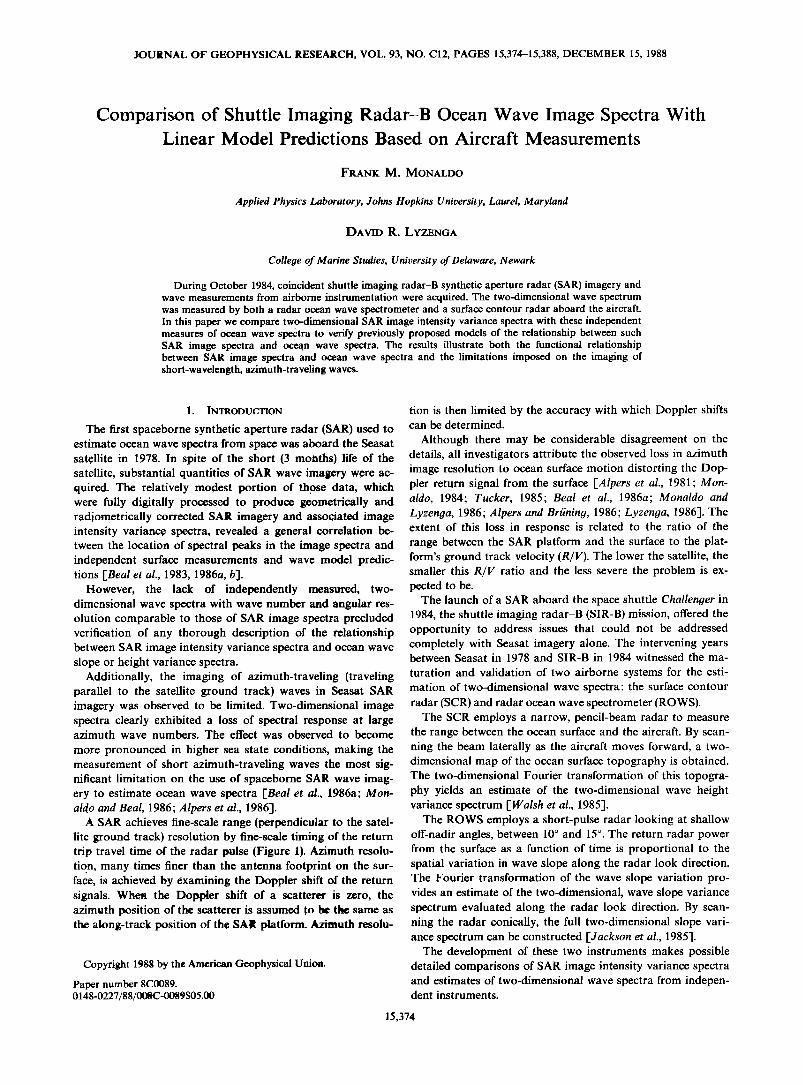
A SAR achieves fine-scale range (perpendicular to the satel- lite ground track) resolution by fine-scale timing of the return trip travel time of the radar pulse (Figure t). Azimuth resolu- tion, many times finer than the antenna footprint on the sur- face, is achieved by examining the Doppler shift of the return signals. When the Doppler shift of a scatterer is zero, the azimuth position of the scatterer is assumed •to he the same as the along-track position of the SAg platform. Azimuth resotu-

Copyright 1988 by the American Geophysical Union.

Paper number 8C0089. 0148-0227/88/008C-•89505.•

tion is then limited by the accuracy with which Doppler shifts can be determined.

Although there may be considerable disagreement on the details, all investigators attribute the observed loss in azimuth image resolution to ocean surface motion distorting the Dop- pler return signal from the surface [Alpers et al., 1981; Mon- aldo, 1984; Tucker, 1985; Beal et al., 1986a; Monaldo and Lyzenga, 1986; Alpers and Briining, 1986; Lyzenga, 1986]. The extent of this loss in response is related to the ratio of the range between the SAR platform and the surface to the plat- form's ground track velocity (R/V). The lower the satellite, the smaller this R/l/ ratio and the less severe the problem is ex- pected to be.

The launch of a SAR aboard the space shuttle Challenger in 1984, the shuttle imaging radar-B (SIR-B) mission, offered the opportunity to address issues that could not be addressed completely with Seasat imagery alone. The intervening years between Seasat in 1978 and SIR-B in 1984 witnessed the ma-

turation and validation of two airborne systems for the esti- mation of two-dimensional wave spectra: the surface contour radar (SCR) and radar ocean wave spectrometer (ROWS).

The SCR employs a narrow, pencil-beam radar to measure the range between the ocean surface and the aircraft. By scan- ning the beam laterally as the aircraft moves forward, a two- dimensional map of the ocean surface topography is obtained. The two-dimensional Fourier transformation of this topogra- phy yields an estimate of the two-dimensional wave height variance spectrum [Walsh et al., 1985].

The ROWS employs a short-pulse radar looking at shallow off-nadir angles, between 10 ø and 15 ø. The return radar power from the surface as a function of time is proportional to the spatial variation in wave slope along the radar look direction. The Fourier transformation of the wave slope variation pro- vides an estimate of the two-dimensional, wave slope variance spectrum evaluated along the radar look direction. By scan- ning the radar conically, the full two-dimensional slope vari- ance spectrum can be constructed [Jackson et al., 1985].

The development of these two instruments makes possible detailed comparisons of SAR image intensity variance spectra and estimates of two-dimensional wave spectra from indepen- dent instruments.

15,374

MONALDO AND LYZENGA: WAVE IMAGE SPECTRA AND MODEL PREDICTIONS 15,375

ii%?•,'-' ..'"--"• 0 = •/2

Ran Fig. 1. SAR geometry. The nadir look angle is O. The wave propaga-

tion angle with respect to azimuth is 05.

An additional opportunity provided by the SIR-B mission was associated with the low altitude of the shuttle orbit. The

shuttle Challenger flew at an altitude of 230 km during the SIR-B mission, as compared with the 800-km altitude of Seasat. The reduced range-to-velocity ratio of the shuttle SAR platform was expected to alleviate the problem of decreased azimuth response caused by ocean surface motion. In addi- tion, the extent of the observed azimuth response from SIR-B SAR image spectra could be compared with theoretical pre- dictions.

To avail ourselves of the advantage of the unique op- portunity offered by the SIR-B mission, an experiment was conducted off the southern coast of Chile. This location was

chosen because during the October mission of SIR-B, rela- tively high sea states were expected at far southern latitudes. Spatially and temporally coincident SAR wave imagery and aircraft measurements of two-dimensional wave spectra by a ROWS and SCR, mounted aboard a NASA P-3 aircraft, were acquired over 5 days during the experiment.

Preliminary comparisons of suitably corrected SAR image intensity variance spectra and SCR and ROWS wave spectra have shown good agreement [-Beal et al., 1986b]. It was ob- served that raw SAR image intensity variance spectra are gen- erally similar to measured ocean wave slope variance spectra. Although the SAR image spectra from SIR-B showed substan- tially improved azimuth response as compared with Seasat spectra, on at least one of the four carefully examined data sets, SAR image spectra were so distorted that it was impossi- ble, or at best marginally possible, to extract reasonably good estimates of wave spectra.

The data sets with severely distorted spectra were acquired on a day with only moderate sea states, when the significant wave height H s was less than 2 m. However, the azimuth components of the wavelengths of some of the wave systems present were short enough to be severely influenced by azi- muth resolution effects. The three data sets for which the wave

spectra were accurately extracted were acquired during days having larger sea states, from 2.8-m to 4.6-m significant wave height, but with azimuth wavelengths which were long enough to avoid significant azimuth resolution degradation. The in- teresting result is that because shortest-wavelength waves are associated with low to moderate sea states, it is low sea state

as opposed to high sea state conditions which may be the most problematic for SAR wave imaging.

Monaldo and Lyzenga [1986] proposed a generalized pro- cedure for converting SAR image intensity variance spectra into ocean wave slope or height variance spectra. This pro- cedure was shown to produce spectra in good general agree- ment with the ROWS slope variance and SCR height variance spectra.

One limitation of comparing SAR estimates of wave spectra with independent measures of the wave spectra is the finite dynamic range of and noise in the SAR image spectrum. Con- verting SAR image spectra into estimates of wave spectra usu- ally involves artificially boosting the SAR spectral response at large azimuth wave numbers. This process is possible as long as the residual spectral information is substantially greater than the spectral noise. However, when the spectral signal-to- noise ratio is small, this procedure tends to amplify the noise and obscure comparisons.

In this paper we attempt to circumvent this limitation by using SCR and ROWS wave spectra to produce estimates of SAR image intensity variance spectra. This procedure gener- ally involves decreasing spectral response, particularly at large azimuth wave numbers. Thus spectral noise is also reduced. We are able in this way to more extensively explore the re- lationship between SAR image spectra and ocean wave spec- tra.

The organization of this paper will be as follows. First, we will summarize the general theory regarding the relationship between SAR image intensity variance spectra and ocean wave spectra. Second, SAR image spectra from SIR-B will be sys- tematically compared with predicted image spectra computed from the SCR and ROWS wave spectra. Finally, we will apply an optimization procedure to explore the azimuth wave number dependence of the mapping between SAR image in- tensity variance spectra and ocean wave slope or height vari- ance spectra.

2. THE MODEL

As early as 1977, the primary mechanisms that permit SARs to image ocean waves had been identified •Elachi and Brown, 1977]. Alpers et al. ['1981] formally proposed a composite, linear systems approach to the understanding of SAR wave imagery. (See also Monaldo and Beal [-1986].) This approach was modified and simplified by Monaldo and Lyzenga [1986] to establish a specific procedure for converting SAR image spectra into estimates of wave spectra. The procedure was successfully applied to SAR image intenstiy variance spectra from the SIR-B mission.

Although we recognize that significant nonlinearities may exist in certain regimes of the SAR imaging process, the logi- cal first step is to evaluate the range of conditions over which a linear systems approach can yield useful results. We are encouraged by the fact that the obvious manifestations of non- linearity, such as the appearance of harmonics in the spec- trum, are conspicuously absent in the existing data. Numerical simulations [-e.g., Lyzenga, 1986] also suggest that even in cases where nonlinearities are expected, the imaging process can be treated as a quasi-linear system in which the primary effects of the nonlinearity are subsumed within the dynamic response function, as will be described below.

Further, if SAR wave image spectra are to be more than a curiosity, then the assumption of linearity must be a valid first approximation. If such an assumption is not valid, or if non-

15,376 MONALDO AND LYZENGA' WAVE IMAGE SPECTRA AND MODEL PREDICTIONS

linear aspects of wave imaging can not be parameterized in a linear systems model, then it is not, in general, possible to infer an ocean wave spectrum from a SAR image spectrum. Regard - less of how piquant investigators may find continued examina- tion of SAR wave imagery or the constru•ct!on of theoretical edifices to explain imaging processes, unless there exists a sub- stantial class of situations for which a linear systems approach is valid, continued study of SAR wave imaging seems fruitless.

Alpers et al. [1981, 1986] proposed a linearity parameter E, given by

Since the stationary response correction and noise subtraction are routinely applied to the SAR image spectra we will deal With here, we designate a corrected image intensity variance spectrum as Si'([c ) where

Sit(•) = F•,'(•)Sh(• ) (4)

The relationship betw•n this corrected spectrum and the wave height variance spectrum is expressed by

S,'(•) = [S,(•)- S,,(fc)]/Hs(• ) (5)

r7= 4 (sin 2 0 sin 2 •p + cos 2 0)•/•21cos c)[k3/2H s (I) where g is the acceleration due to gravity, 0 is the radar inci- dence angle, and k and •b are ocean wave number magnitude and propagation direction, respectively (see Figure 1). FOr r7 >_ 0.3, the imaging process is lab,e. led nonlinear. Table 1 is a listing of the estimated •- values for the wave systems examined in this paper. Of the seven systems listed, five?:'fall in the linear regime as defined by Alpers et al. [1981, 1986], one is margin- ally nonlin•iar, and one is severely nonlinear. As we shall see,

where

Fh'([c) = Hd(ka) l RsAR(• ) 12 (6)

2,2. SAR Modulation Transfer Function

The relationship between ocean surface wave height and apparent radar cross section, for a SAR image at nominal resolution, can be described by a SAR "modulation transfer function," Rs^R(•). The dominant scattering mechanism for off- nadi r microwave radars is a Bragg resonance interaction [Wright, 1966, 1978]. The effects of other types of scattering,

the systems labeled as marginally or severely nonlinear are the ones which are most distoried by the imaging process. Yet in i.e., specular scattering and wedge scattering, are discussed by no case is a harmonic of the primary wave system peak found. . Hasselmann et al, [1985]. High surface radar cross sections are ß obtained for surfaces with roughness on the scale of the radar

Following the linear sys,tems model as discussed by Mon- wavelength. In the case of the L band Seasat and SIR-B SARs, aldo a•nd Lyzenga [1986], a two-dimensional SAR image spec- the wavelength was approximately 30 cm. The real or appar- trum, S•(•), is related to the ocean 'surface he•ight: Vafia nee:" ent modification of such roughness by long (> 50 m) waves spectrum, S,(•), by a total system height transfer function, renders the long waves visible in SAR imagery. A complete F•(•), i.e.,

Si([c ) = F,(•}S,(f) + Sn(•) t2)

where •. is the wave number vector, composed of azimuth wave number k a and range wave number k r, and Sn(•) is the speckle noise spectrum contribution. The total system transfer function specifies how a two-dimensibnal ocean wave height variance spectrum maps into an image intensity variance spec- trum at each azimuth and range wave number. II•the absence of noise or limitation in dynamic range, this total system transfer function permits conversion interchangeab!y between image spectra and wave height spectra.

A linear systems approach allows us to describe the total system height transfer function as a product of functions, each of which is representative of a different aspect of the total system. Here we break up F•,(•) into the product of thre• functions,

Ft,(• ) = Hs(fc)Hd(ka) l RsA•(• ) I • (3)

where Hs([C ) is the stationary response function, Ha(k•) is the dynam!c response function, and I RsA•(fc)12 is the square of the SAR modulation transfer function.

Each of these constituent functions is described in the fol-

lowing sections.

2.1. Stationary Response Function

The first function on the right-hand side of (3), Hs(/C ), is called the "stationary" response function. Any system with finite spatial resolution will exhibit a falloff in spectral re- sponse at high wave numbers, associated with this finite reso- 3 lution. Correction for this transfer function is described exten:,. sively in the literature [Beal et aL, 1983]. It is now common to 4 find raw SAR image intensity variance Spectra corrected for

5 this stationary respQns•e. In addition, Mønaldo and Lyzenga [1986] outline a procedure for subtraction of speckle noise.

discussion of various imaging processes is also given by Hassel- mann et al. [1985].

2.2.1. Tilt modulation. There are two mechanisms, identi-

fied here, for the imaging of the range-traveling waves' tilt modulation and hydrodynamic modulation. Tilt modulation results from the variation of ocean surface cross section with

local radar incidence, i.e., the changing aspect of the small- scale surface roughness with radar incidence. Essentially, the parts of the ocean surface that are titled toward the radar return more electromagnetic energy than those that are tilted away from the radar.

The tilt modulation transfer function R t is given by the fractional modulation in radar cross section, a o, as a function of surface wave height [Alpers et al., 1981]. Since wave slope

equals toe product of wave height and wave number, R t can be written as

R t = k r • e i•/2 (7) o' o

where kr is the range component wave number of the long ocean wave and 0 is the incidence angle. The exponential term

TABLE 1. Ocean Wave Data

Total

Flight Significant Day Date, 1984 Wave Height, m

,

Approximate Wavelength, m

Oct. 9 2.8 180 Oct. 10 1.7 150

70

Oct. I1 4.6 225 125

Oct. 12 3.6 350 120

0.36

0.11

0.53

0.17 0.29 0.21

MONALDO AND LYZENGA: WAVE IMAGE SPECTRA AND MODEL PREDICTIONS 15,377

.... 2õ,2 50m ' • '• o • --'•1

o lOO

Azimuth

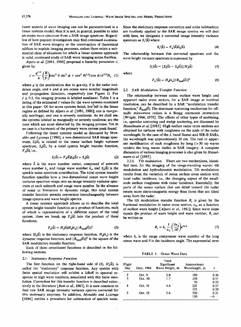
Fig. 2. Two-dimensional plot of the square of the SAR modula. tion transfer function, I RSAR(/C)12, with center of plot at 0 m-• wave number. Maximum displayed wave number is 2•r/(50 m). Units are square meters. Parameters are as follows: R/V = 35 s, 0 = 20 ø, HH polarization.

indicates that the phase of the modulation is 90 ø out of phase with the long wave crest.

The Bragg scattering model [Wright, 1966], when evaluated for reflection from a perfectly conducting rough surface, yields a backscattering cross section expressed by

a o = 16•rko4(1 q- sin 2 0)2S(2ko sin 0) (8)

where k 0 is radar wave number and S(2k o sin 0) is the wave height-density spectrum at Bragg wave number, 2k o sin 0. The "plus or minus" sign refers to VV and HH polarization, re- spectively. Seasat and SIR-B SARs were polarized HH. By assuming a Phillips spectrum for the short surface waves, i.e., S = Ak -4, it can be shown that tilt modulation transfer func- tion is given by

I 4cot0 ] Rt = kr 1 __+ sin 2 0' ei•r/2 (9)

Equation (9) applies for a perfectly conducting surface, which is a good approximation for the ocean surface at small inci- dence angles.

2.2.2. Hydrodynamic modulation. Hydrodynamic modula- tion refers to the hydrodynamic modulation of radar wave- length scale waves by long ocean surface waves. The nature of this interaction is still an active area of investigation [Phillips, 1981' Plant and Keller, 1983' Irvine, 1983]. However, esti- mates based on action conservation [e.g., Phillips, 1981] indi- cate that for typical radar look angles from spaceborne SARs (<30ø), the hydrodynamic term is roughly a factor of 2 smaller than the tilt term.

2.2.3. Velocity-bunching modulation. One mechanism by which azimuth-traveling waves are made visible in SAR imag- ery is known as "velocity bunching." As was mentioned before, a SAR achieves high azimuth resolution by utilizing the Dop- pler shifts of return radar signals. If a particular scattering element has a component of velocity, vr, parallel to the radar slant range direction, then the apparent azimuth position of the scattering element in the SAR image will be shifted by a distance equal to (R/V)v• [Harger, 1970; Raney, 1971].

The areas of small-scale roughness, acting as scatterers on

the ocean surface, are moved in a circular pattern by the "orbital" motion induced by long ocean waves. This periodic movement of the scatterers causes spatially periodic azimuth displacements. In turn, these azimuth displacements of scatter- ing elements concentrate and i'educe the apparent density of scatterers at the ipatial frequency of the long wave. Azimuth- traveling waves are thus rendered visible in SAR imagery [Alpers and Rufena.ch, 1979; Swift and Wilson, 1979].

The magnitude of the prbportionality constant relating long wave height and the fractional modulation of SAR image in- tensity caused by velocity bunching is given by

R,, = • (gk)•/2ka(sin2 0 sin 2 qb + cos 20)•/2e i/• (10)

A=Oorrt

where 0 eind qb are as defined in (1). This intensity modulation is either approximately in phase or 180 ø out of phase with the

lon• wai,.e crest, depending on whether the azimuth compo- nent o(the wave is traveling antiparallel or parallel to the SAR platform velocity vector. For small nadir incidence angles 0, (10) reduces to

I R• = • (gk)•/2ka cos 0 e i• A = 0 or rt (11)

The square of SAR modulation transfer function, I RSAR(•C)12, is the squared coherent sum of the contributions from each imaging mechanism. In determining the expression for the SAR modulation transfer function, hydrodynamic modulation was neglected because it is dominated by the tilt modulation term for small incidence angles. In addition, since the phases of the tilt modulation term R t and the velocity-bunching term R,, differ by -+-90 ø, the squared coherent sum is given by

In, 2 + in,,i 2 __ i Rs^•(•) 2

[i 4cøtø I(½) 1 1 __+ sin 2 0 kr2 + g cos 0 kka 2 (12)

Figure 2 is a contour plot of the square of the SAR modula- tion transfer function, { RSAR(/C)12, as a function of azimuth and range wave number. The center of the plot corresponds to zero wave number (infinite wavelength), and the outer circle corresponds to a wave number 2rt/(50 m). For this plot, HH polarization, a 20 ø radar incidence angle, and a range-to- velocity ratio of 35 s, corresponding to SIR-B SAR parame- ters, were assumed. The value of the SAR modulation transfer

function increases with wave number. The most rapid increase is along the azimuth wave number direction. Along this direc- tion the function is proportional to wave number cubed, whereas along the range direction it is proportional to wave number squared.

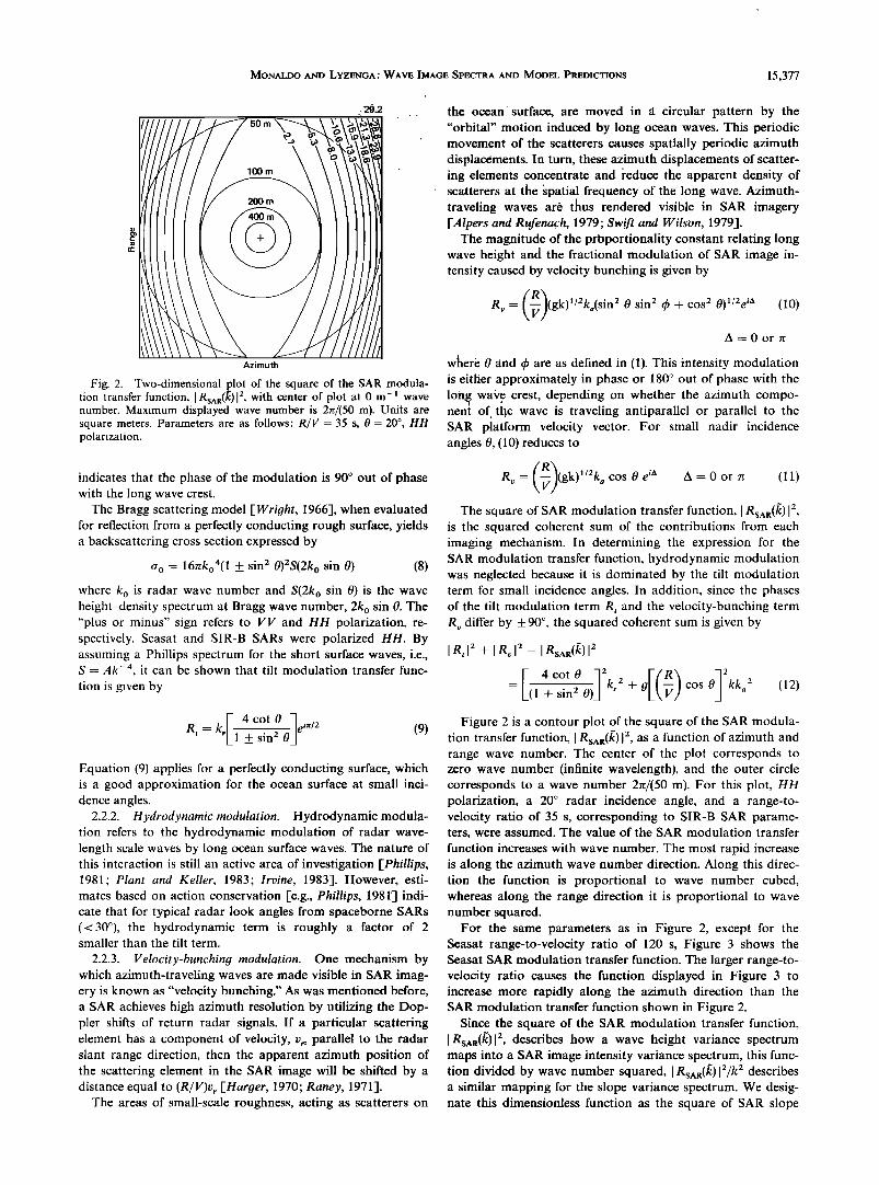
For the same parameters as in Figure 2, except for the Seasat range-to-velocity ratio of 120 s, Figure 3 shows the Seasat SAR modulation transfer function. The larger range-to- velocity ratio causes the function displayed in Figure 3 to increase more rapidly along the azimuth direction than the SAR modulation transfer function shown in Figure 2.

Since the square of the SAR modulation transfer function, I RsAR(•)I 2, describes how a wave height variance spectrum maps into a SAR image intensity variance spectrum, this func- tion divided by wave number squared, I RSAR(/C ) [2/k2 describes a similar mapping for the slope variance spectrum. We desig- nate this dimensionless function as the square of SAR slope

15,378 MONALDO AND LYZENGA.' WAVE IMAGE SPECTRA AND MODEL PREDICTIONS

320

//////• 5o m•"•• ,./•'•/•/•

lOOm s• •

Azimuth

Fig. 3. Two-dimensional plot of the square of the SAR modula- tion transfer function, I RsAR(• ) 12, with center of plot at 0 m-x wave number. Maximum displayed wave number is 2•r/(50 m). Units are square meters. Parameters are as follows: R/V = 120 s, 0 = 20 ø, HH polarization.

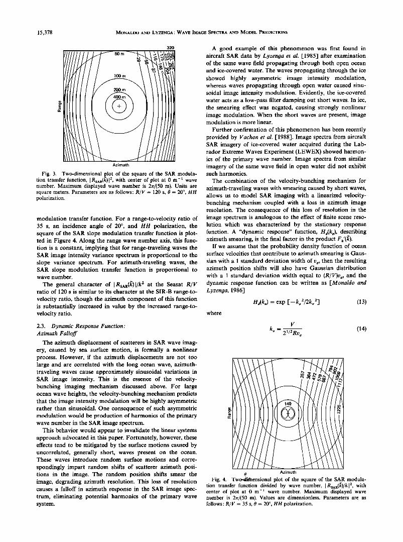
modulation transfer function. For a range-to-velocity ratio of 35 s, an incidence angle of 20 ø, and HH polarization, the square of the SAR slope modulation transfer function is plot- ted in Figure 4. Along the range wave number axis, this func- tion is a constant, implying that for range-traveling waves the SAR image intensity variance spectrum is proportional to the slope variance spectrum. For azimuth-traveling waves, the SAR slope modulation transfer function is proportional to wave number.

The general character of I RsA•t(•)l/k 2 at the Seasat R/V ratio of 120 s is similar to its character at the SIR-B range-to- velocity ratio, though the azimuth component of this function is substantially increased in value by the increased range-to- velocity ratio.

2.3. Dynamic Response Function: Azimuth Falloff

The azimuth displacement of scatterers in SAR wave imag- ery, caused by sea surface motion, is formally a nonlinear process. However, if the azimuth displacements are not too large and are correlated with the long ocean wave, azimuth- traveling waves cause approximately sinusoidal variations in SAR image intensity. This is the essence of the velocity- bunching imaging mechanism discussed above. For large ocean wave heights, the velocity-bunching mechanism predicts that the image intensity modulation will be highly asymmetric rather than sinusoidal. One consequence of such asymmetric modulation would be production of harmonics of the primary wave number in the SAR image spectrum.

This behavior would appear to invalidate the linear systems approach advocated in this paper. Fortunately, however, these effects tend to be mitigated by the surface motions caused by uncorrelated, generally short, waves present on the ocean. These waves introduce random surface motions and corre-

spondingly impart random shifts of scatterer azimuth posi- tions in the image. The random position shifts smear the image, degrading azimuth resolution. This loss of resolution causes a falloff in azimuth response in the SAR image spec- trum, eliminating potential harmonics of the primary wave system.

A good example of this phenomenon was first found in aircraft SAR data by Lyzenga et al. [1985] after examination of the same wave field propagating through both open ocean and ice-covered water. The waves propagating through the ice showed highly asymmetric image intensity modulation, whereas waves propagating through open water caused sinu- soidal image intensity modulation. Evidently, the ice-covered water acts as a low-pass filter damping out short waves. In ice, the smearing effect was negated, causing strongly nonlinear image modulation. When the short waves are present, image modulation is more linear.

Further confirmation of this phenomenon has been recently provided by Vachon et al. [1988]. Image spectra from aircraft SAR imagery of ice-covered water acquired during the Lab- rador Extreme Waves Experiment (LEWEX) showed harmon- ics of the primary wave number. Image spectra from similar imagery of the same wave field in open water did not exhibit such harmonics.

The combination of the velocity-bunching mechanism for azimuth-traveling waves with smearing caused by short waves, allows us to model SAR imaging with a linearized velocity- bunching mechanism coupled with a loss in azimuth image resolution. The consequence of this loss of resolution in the image spectrum is analogous to the effect of finite scene reso- lution which was characterized by the stationary response function. A "dynamic response" function, Hd(ka), describing azimuth smearing, is the final factor in the product Fh'(•).

If we assume that the probability density function of ocean surface velocities that contribute to azimuth smearing is Gaus- sian with a 1 standard deviation width of %, then the resulting azimuth position shifts will also have Gaussian distribution with a 1 standard deviation width equal to (R/V)v,,, and the dynamic response function can be written as [Monaldo and L yzenga, 1986]

where

Hd(ka) = exp [-- ka2/2k. 2] (13)

V - (14) k,, 2•/2Rv,,

:,•?, Azimuth Fig. 4. Twoi.•ilnensional plot of the square of the SAR modula-

tion transfer function divided by wave number, I Rs^R(k)/kl 2, with center of plot at 0 m -x wave number. Maximum displayed wave number is 2rc/(50 m). Values are dimensionless. Parameters are as follows: R/V = 35 s, 0 = 20 ø, HH polarization.

MONALDO AND LYZENGA' WAVE IMAGE SPECTRA AND MODEL PREDICTIONS 15,379

•6 /V = 35 s

.J /V = 120 s

10-31 • • • 0 2 4 6 8

Significant wave height (m)

25

50

1 O0

200

4O0

800

1600

3200

10

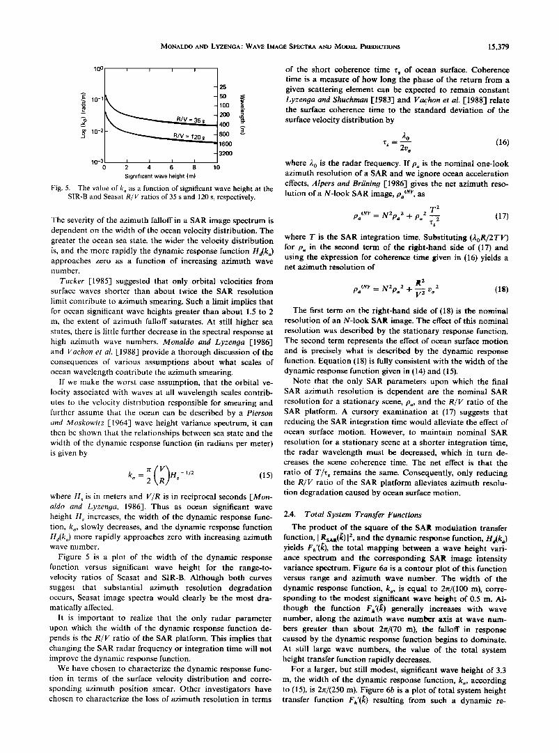
Fig. 5. The value of k, as a function of significant wave height at the SIR-B and Seasat R/V ratios of 35 s and 120 s, respectively.

The severity of the azimuth falloff in a SAR image spectrum is dependent on the width of the ocean velocity distribution. The greater the ocean sea state, the wider the velocity distribution is, and the more rapidly the dynamic response function Ha(ka) approaches zero as a function of increasing azimuth wave number.

Tucker [1985] suggested that only orbital velocities from surface waves shorter than about twice the SAR resolution

limit contribute to azimuth smearing. Such a limit implies that for ocean significant wave heights greater than about 1.5 to 2 m, the extent of azimuth falloff saturates. At still higher sea states, there is little further decrease in the spectral response at high azimuth wave numbers. Monaldo and Lyzenga [1986] and Vachon et al. [1988] provide a thorough discussion of the consequences of various assumptions about what scales of ocean wavelength contribute the azimuth smearing.

If we make the worst case assumption, that the orbital ve- locity associated with waves at all wavelength scales contrib- utes to the velocity distribution responsible for smearing and further assume that the ocean can be described by a Pierson and Moskowitz [1964] wave height variance spectrum, it can then be shown that the relationships between sea state and the width of the dynamic response function (in radians per meter) is given by

k.=• H s

where H., is in meters and V/R is in reciprocal seconds [Mon- aldo and Lyzenga, 1986]. Thus as ocean significant wave height Hs increases, the width of the dynamic response func- tion, k,, slowly decreases, and the dynamic response function Hd(k,) more rapidly approaches zero with increasing azimuth wave number.

Figure 5 is a plot of the width of the dynamic response function versus significant wave height for the range-to- velocity ratios of Seasat and SIR-B. Although both curves suggest that substantial azimuth resolution degradation occurs, Seasat image spectra would clearly be the most dra- matically affected.

It is important to realize that the only radar parameter upon which the width of the dynamic response function de- pends is the R/V ratio of the SAR platform. This implies that changing the SAR radar frequency or integration time will not improve the dynamic response function.

We have chosen to characterize the dynamic response func- tion in terms of the surface velocity distribution and corre- sponding azimuth position smear. Other investigators have chosen to characterize the loss of azimuth resolution in terms

of the short coherence time r s of ocean surface. Coherence time is a measure of how long the phase of the return from a given scattering element can be expected to remain constant Lyzenga and Shuchman [1983] and Vachon et al. [1988] relate the surface coherence time to the standard deviation of the

surface velocity distribution by

;to ß • - (16)

where )•o is the radar frequency. If/% is the nominal one-look azimuth resolution of a SAR and we ignore ocean acceleration effects, Alpers and Brfi'ning [1986] gives the net azimuth reso- lution of a N-look SAR image, p•(•)', as

T 2 •Oa(N)' = m2t9a2 q- }Oa2 2 (17)

r s

where T is the SAR integration time. Substituting (2oR/2TV) for Pa in the second term of the right-hand side of (17) and using the expression for coherence time given in (16) yields a net azimuth resolution of

R 2

pa (N)' = N2pa 2 q- •'• l)a 2 (18) The first term on the right-hand side of (18) is the nominal

resolution of an N-look SAR image. The effect of this nominal resolution was described by the stationary response function. The second term represents the effect of ocean surface motion and is precisely what is described by the dynamic response function. Equation (18) is fully consistent with the width of the dynamic response function given in (14) and (15).

Note that the only SAR parameters upon which the final SAR azimuth resolution is dependent are the nominal SAR resolution for a stationary scene, p,, and the R/V ratio of the SAR platform. A cursory examination at (17) suggests that reducing the SAR integration time would alleviate the effect of ocean surface motion. However, to maintain nominal SAR resolution for a stationary scene at a shorter integration time, the radar wavelength must be decreased, which in turn de- creases the scene coherence time. The net effect is that the

ratio of T/z s remains the same. Consequently, only reducing the R/V ratio of the SAR platform alleviates azimuth resolu- tion degradation caused by ocean surface motion.

2.4. Total System Transfer Functions

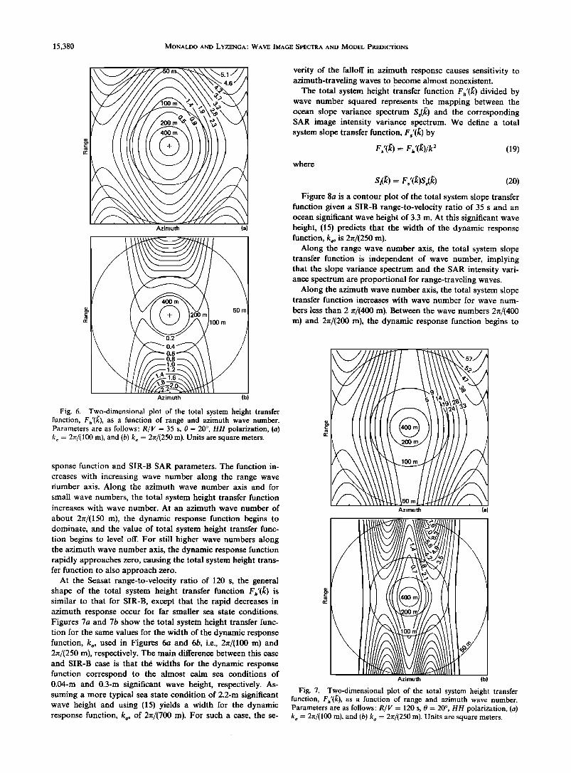
The product of the square of the SAR modulation transfer function, I RSA•(/• ) 12, and the dynamic response function, Ha(ka) yields Fh'(•), the total mapping between a wave height vari- ance spectrum and the corresponding SAR image intensity variance spectrum. Figure 6a is a contour plot of this function versus range and azimuth wave number. The width of the dynamic response function, k,, is equal to 2n/(100 m), corre- sponding to the modest significant wave height of 0.5 m. Al- though the function Fh'(•) generally increases with wave number, along the azimuth wave number axis at wave num- bers greater than about 2•r/(70 m), the falloff in response caused by the dynamic response function begins to dominate. At still large wave numbers, the value of the total system height transfer function rapidly decreases.

For a larger, but still modest, significant wave height of 3.3 m, the width of the dynamic response function, k,, according to (15), is 2rc/(250 m). Figure 6b is a plot of total system height transfer function F•'(•) resulting from such a dynamic re-

15,380 MONALDO AND LYZENGA: WAVE IMAGE SPECTRA AND MODEL PREDICTIONS

50 m

Azimuth (a)

Azimuth (b)

Fig. 6. Two-dimensional plot of the total system height transfer function, Fh'(•), as a function of range and azimuth wave number. Parameters are as follows: R/l/- 35 s, 0- 20 ø, HH polarization, (a) k• = 2•z/(100 m), and (b) k• = 2•z/(250 m). Units are square meters.

sponse function and SIR-B SAR parameters. The function in- creases with increasing wave number along the range wave number axis. Along the azimuth wave number axis and for small wave numbers, the total system height transfer function increases with wave number. At an azimuth wave number of

about 2re/(150 m), the dynamic response function begins to dominate, and the value of total system height transfer func- tion begins to level off. For still higher wave numbers along the azimuth wave number axis, the dynamic response function rapidly approaches zero, causing the total system height trans- fer function to also approach zero.

At the Seasat range-to-velocity ratio of 120 s, the general shape of the total system height transfer function F,'(•) is similar to that for SIR-B, except that the rapid decreases in azimuth response occur for far smaller sea state conditions. Figures 7a and 7b show the total system height transfer func- tion for the same values for the width of the dynamic response function, ks, used in Figures 6a and 6b, i.e., 2re/(100 m) and 2zr/(250 m), respectively. The main difference between this case and SIR-B case is that the widths for the dynamic response function correspond to the almost calm sea conditions of 0.04-m and 0.3-m significant wave height, respectively. As- suming a more typical sea state condition of 2.2-m significant wave height and using (15) yields a width for the dynamic response function, k s, of 2•z/(700 m). For such a case, the se-

verity of the falloff in azimuth response causes sensitivity to azimuth-traveling waves to become almost nonexistent.

The total system height transfer function F,'(•) divided by wave number squared represents the mapping between the ocean slope variance spectrum Ss(fC ) and the corresponding SAR image intensity variance spectrum. We define a total system slope transfer function, Fs'(• ) by

F•'(•c) = F•,'(•)/k 2 (19) where

s,(k) = rs'(k)s•(k) (20)

Figure 8a is a contour plot of the total system slope transfer function given a SIR-B range-to-velocity ratio of 35 s and an ocean significant wave height of 3.3 m. At this significant wave height, (15) predicts that the width of the dynamic response function, ks, is 2zr/(250 m).

Along the range wave number axis, the total system slope transfer function is independent of wave number, implying that the slope variance spectrum and the SAR intensity vari- ance spectrum are proportional for range-traveling waves.

Along the azimuth wave number axis, the total system slope transfer function increases with wave number for wave num-

bers less than 2 re/(400 m). Between the wave numbers 2re/(400 m) and 2re/(200 m), the dynamic response function begins to

Azimuth (a)

Azimuth (b)

Fig. 7. Two-dimensional plot of the total system height transfer function, Fh'(fc), as a function of range and azimuth wave number. Parameters are as follows: R/l/= 120 s, 0 = 20 ø, HH polarization, (a) k• = 2r•/(100 m), and (b) k• = 2•z/(250 m). Units are square meters.

MONALDO AND LYZENGA.' WAVE IMAGE SPECTRA AND MODEL PREDICTIONS 15,381

g

Azimuth

/

168 15o m 100 m[ 200 m1111•5_0_ 4 I ........... 1--- \ [ IIl[•ll• 561 !

Azimuth (b)

Fig. 8. Two-dimensional plot of the total system slope-transfer function I:,'(l•) as a function of azimuth and range wave number. Parameters are as follows: 0 = 20", HH polarization, H., = 3.3 m, (a) R V- 35 s, k,- 27r/(250 m). and (b) R/V = 120 s, k• = 27¾(700 m). Values of contours are dimensionless.

play an important role, causing the total system slope transfer function to be essentially independent of wave number. In this limited azimuth region the slope variance and intensity vari- ance spectra are proportional. At still larger wave numbers along the azimuth wave number axis, the dynamic response function dominates, causing the net transfer function to rap- idly decrease to zero with increasing wave number.

Figure 8b is contour plot of the total system slope transfer function Fs'(fc ) at the Seasat range-to-velocity ratio of 120 s and a significant wave height of 3.3 m. The dynamic response function width at this significant wave height and range-to- velocity ratio is 2•/(700 m), according to (15). The function portrayed in Figure 8b is very similar in structure to that in Figure 8a, except that the increased range-to-velocity ratio has dramatically reduced the sensitivity to azimuth-traveling waves.

3. CONVERSION OF SCR AND ROWS WAVE SPECTRA

INTO SAR IMAGE SPECTRA

Ocean wave data were acquired from a NASA P-3 aircraft, spatially and temporally coincident with SIR-B SAR imagery, off the southern coast of Chile from October 8 through Oc- tober 12, 1984. (see Table 1.) Two-dimensional ocean wave spectra are available from the SCR and/or ROWS for the last

4 days of the experiment. We will concentrate here on these last 4 days. Two other instruments aboard the aircraft, the Advanced Airborne Flight Experiment (AAFE) altimeter and the AOL airborne optical lidar (AOL) provided estimates of ocean significant wave height and one-dimensional wave height variance spectra, respectively [Beal et al., 1986b-I.

In this section we will apply the total system height transfer function Fh'([i ) to SCR wave height variance spectra and the total system slope transfer function to ROWS wave slope vari- ance spectra and then compare the resulting predicted image spectra with observed SIR-B SAR image intensity variance spectra.

3.1. Flight Day 2: October 9

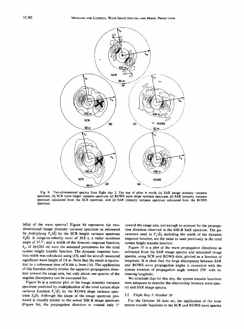
Figure 9a is a contour plot of an average spectrum com- posed of eight SIR-B SAR image intensity variance spectra from SAR imagery acquired on October 9, 1984. The eight constituent spectra were computed from eight contiguous 6.4 km by 6.4 km image frames. Peaks in the contour plot indi- cate the presence of image intensity fluctuations at the wave number and propagation direction location of the spectral peak. SAR image spectra exhibit a radial symmetry. Since it is impossible to determine from a single image the direction of wave propagation to within a 180 ø ambiguity, each wave system is represented by two peaks at the same wave number but at propagation directions exactly 180 ø apart.

In the particular spectrum shown in Figure 9a there is a single wave system represented by two symmetric peaks. The peak spectral density occurred at a wavelength of 180 m and an angle from 38 •' counterclockwise from the range wave number direction. The 38 ø off-range propagation direction corresponds, in this case, to a propagation direction of 49 ø west of north. For simplicity, for this day, we will refer only to the peak in the upper half plane of the spectrum.

Figure 9b is the corresponding height variance spectrum as measured by the SCR. The dominant wave system is measured to have a wavelength about the same as that measured by the SAR, but the observed propagation direction is 69 ø west of north. The SAR has apparently rotated the observed propaga- tion direction about 20 ø toward the range wave number direc- tion. This type of rotation has also been observed in Seasat image spectra [-Monaldo, 1984].

Note that the two companion peaks in the SCR spectrum are not symmetric as they are in the SAR spectrum. When an aircraft-mounted SCR flies over the ocean surface, it does not

measure the ocean surface instantaneously. As a result, it is possible to examine SCR data and remove the expected 180 ø ambiguity in propagation direction. When the correction pro- cedure is applied to SCR spectra, the peak at the true propa- gation direction is enhanced, and the fictitious one is dimin- ished. The fictitious peaks in the SCR spectra are marked with an "X."

Figure 9c is the corresponding ROWS slope variance spec- trum for this day. The wavelength of the dominant wave system as measured by the ROWS agrees with both the SCR and SAR estimates. However, the wave system is observed to be propagating from 76 ø west of north. The SAR appears to have rotated the apparent direction of propagation by 26 ø toward the range direction with respect to the ROWS esti- mated direction.

Can this rotation by the SAR be explained by the total system height transfer function Fh'(fc ) and the total system slope transfer function F.•'(•) and/or the natural spatial varia-

15,382 MONALDO AND LYZENGA; WAVE IMAGE SPECTRA AND MODEL PREDICTIONS

õ• (d)

Fig. 9. Two-dimensional spectra from flight day 2. The top of plots is north. (a) SAR image intensity variance spectrum, (b) SCR wave height variance spectrum, (c) ROWS wave slope variance spectrum, (d) SAR intensity variance spectrum calculated from the SCR spectrum, and (e) SAR intensity variance spectrum calculated from the ROWS spectrum.

bility of the wave spectra? Figure 9d represents the two- dimensional image intensity variance spectrum as estimated by multiplying Fn'(fc ) by the SCR height variance spectrum Sn(k). A range-to-velocity ratio of 39.8 s, a radar incidence angle of 37.7 ø, and a width of the dynamic response function, k•, of 2rr/(262 m) were the assumed parameters for the total system height transfer function. The dynamic response func- tion width was calculated using (15), and the aircraft measured significant wave height of 2.8 m. Note that the result is equiva- lent to a coherence time of 0.166 s, from (16). The application of this function clearly rotates the apparent propagation direc- tion toward the range axis, but only about one quarter of the angular discrepancy can be accounted for.

Figure 9e is a contour plot of the image intensity variance spectrum predicted by multiplication of the total system slope variance function Fs'(fc), by the ROWS slope variance spec- trum Ss(fC ). Although the shape of the image spectrum pro- duced is visually similar to the actual SIR-B image spectrum (Figure 9a), the propagation direction is rotated only 5 ø

toward the range axis, not enough to account for the propaga- tion direction observed in the SIR-B SAR spectrum. The pa- rameters used in Fs'(fc), including the width of the dynamic response function, are the same as used previously in the total system height transfer function.

Figure 10 is a plot of the wave propagation directions as estimated from the SAR image spectra and simulated image spectra, using SCR and ROWS data, plotted as a function of longitude. It is clear that the large discrepancy between SAR and ROWS wave propagation angles is consistent with the system rotation of propagation angle toward 270 ø with in- creasing longitude.

We conclude that for this day, the system transfer functions were adequate to describe the relationship between wave spec- tra and SAR image spectra.

3.2. Flight Day 3: October 10

For the October 10 data set, the application of the total system transfer functions to the SCR and ROWS wave spectra

MONALDO AND LYZENGA' WAVE IMAGE SPECTRA AND MODEL PREDICTIONS 15,383

350 -

0• 340

330

r' 320

• 318 -

•_ 290

• 28•

27• -81

+ SRR

o SCR

. RONS

+ ++ + o +

+ + +

+ +++ +++ + o + +

++++ B- o o

o o

I I I I 1

-80 -79 -78 -77 -76 -75

Longitude (degs)

Fig. 10. Wave system propagation directions as estimated from SAR image spectra and SCR- and ROWS-simulated image spectra plotted versus the longitude of the location from which the spectra were obtained.

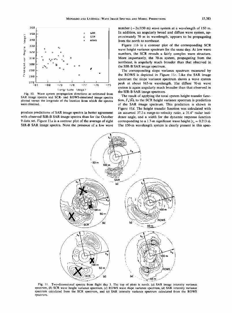
produce predictions of SAR image spectra in better agreement with observed SIR-B SAR image spectra than for the October 9 data set. Figure 1 la is a contour plot of the average of eight SIR-B SAR image spectra. Note the presence of a low wave

number (•-, 2rr/150 m) wave system at a wavelength of 150 m. In addition, an angularly broad and diffuse wave system, ap- proximately 70 m in wavelength, appears to be propagating from the north to northeast.

Figure llb is a contour plot of the corresponding SCR wave height variance spectrum for the same day. At low wave numbers, the SCR reveals a fairly complex wave structure. More importantly, the 70-m system, propagating from the northeast, is angularly much broader than that observed in the SIR-B SAR image spectrum.

The corresponding slope variance spectrum measured by the ROWS is depicted in Figure 11c. Like the SAR image spectrum the slope variance spectrum shows a wave system peak at about 165-m wavelength. The diffuse 70-m wave system is again angularly much broader than that observed in the SIR-B SAR image spectrum.

The result of applying the total system height transfer func- tion, Fh'(•), to the SCR height variance spectrum is prediction of the SAR image spectrum. This prediction is shown in Figure 1 l d. The height transfer function was calculated with an assumed 37.2-s range-to-velocity ratio, a 31.4 ø radar inci- dence angle, and a width for the dynamic response function corresponding to a 1.7-m significant wave height (r s = 0.213 s). The 150-m wavelength system is clearly present in this spec-

q•.• (d) Fig. 11. Two-dimensional spectra from flight day 3. The top of plots is north. (a) SAR image intensity variance

spectrum, (b) SCR wave height variance spectrum, (c) ROWS wave slope variance spectrum, (d) SAR intensity variance spectrum calculated from the SCR spectrum, and (e) SAR intensity variance spectrum calculated from the ROWS spectrum.

15,384 MONALDO AND LYZENGA: WAVE IMAGE SPECTRA AND MODEL PREDICTIONS

(e) •.. ROWS '---..

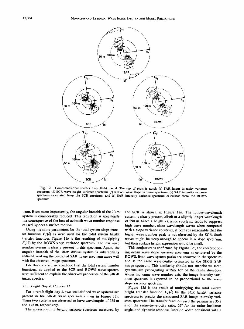
Fig. 12. Two-dimensional spectra from flight day 4. The top of plots is north. (a) SAR image intensity variance spectrum, (b) SCR wave height variance spectrum, (c) ROWS wave slope variance spectrum, (d) SAR intensity variance spectrum calculated from the SCR spectrum, and (e) SAR intensity variance spectrum calculated from the ROWS spectrum.

trum. Even more importantly, the angular breadth of the 70-m system is considerably reduced. This reduction is specifically the consequence of the loss of azimuth wave number response caused by ocean surface motion.

Using the same parameters for the total system slope trans- fer function Fs'(• ) as were used for the total system height transfer function, Figure 11e is the resulting of multiplying F•'(•) by the ROWS slope variance spectrum. The low wave number system is clearly present in this spectrum. Again, the angular breadth of the 70-m diffuse system is substantially reduced, making the predicted SAR image spectrum agree well with the observed image spectrum.

For this data set, we conclude that the total system transfer functions, as applied to the SCR and ROWS wave spectra, were sufficient to explain the observed properties of the SIR-B image spectra.

3.3. Flight Day 4: October 11

For aircraft flight day 4, two well-defined wave systems are present in the SIR-B wave spectrum shown in Figure 12a. These two systems are observed to have wavelengths of 225 m and 125 m, respectively.

The corresponding height variance spectrum measured by

the SCR is shown in Figure 12b. The longer-wavelength system is clearly present, albeit at a slightly longer wavelength of 290 m. Since a height variance spectrum tends to suppress high wave number, short-wavelength waves when compared with a slope variance spectrum, it perhaps reasonable that the higher wave number peak is not observed by the SCR. Such waves might be steep enough to appear in a slope spectrum, but their surface height expression would be small.

This conjecture is confirmed by Figure 12c, the correspond- ing ocean wave slope variance spectrum as estimated by the ROWS. Both wave system peaks are observed in the spectrum and at the same wavelengths estimated in the SIR-B SAR image spectrum. This similarity should not surprise us. Both systems are propagating within 45 ø of the range direction. Along the range wave number axis, the image intensity vari- ance spectrum is expected to be proportional to the wave slope variance spectrum.

Figure 12d is the result of multiplying the total system height transfer function Fh'(• ) by the SCR height variance spectrum to predict the associated SAR image intensity vari- ance spectrum. The transfer function used the parameters 35.2 s for the range-to-velocity ratio, 26 ø for the radar incidence angle, and dynamic response function width consistent with a

MONALDO AND LYZENGA' WAVE IMAGE SPECTRA AND MODEL PREDICTIONS 15,385

•l•m•A• •/ • SCR• (a) (-b)-

(c) (d)

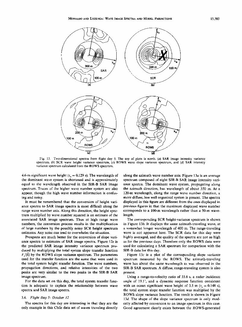
Fig. 13. Two-dimensional spectra from flight day 5. The top of plots is north. (a) SAR image intensity variance spectrum, (b) SCR wave height variance spectrum, (c) ROWS wave slope variance spectrum, and (d) SAR intensity variance spectrum calculated from the ROWS spectrum.

4.6-m significant wave height (r s = 0.129 s). The wavelength of the dominant wave system is shortened and is approximately equal to the wavelength observed in the SIR-B SAR image spectrum. Traces of the higher wave number system are also appear, though the high wave number information is confus- ing and noisy.

It must be remembered that the conversion of height vari- ance spectra to SAR image spectra is most difficult along the range wave number axis. Along this direction, the height spec- trum multiplied by wave number squared is an estimate of the associated SAR image spectrum. Thus at high range wave numbers, the conversion process results in the multiplication of large numbers by the possibly noisy SCR height spectrum estimates. Any noise can tend to overwhelm the situation.

Prospects are much better for the conversion of slope vari- ance spectra to estimates of SAR image spectra. Figure 12e is the predicted SAR image intensity variance spectrum pro- duced by multiplying the total system slope transfer function Fs'(• ) by the ROWS slope variance spectrum. The parameters used for the transfer function are the same that were used in

the total system height transfer function. The wave numbers, propagation directions, and relative intensities of the two peaks are very similar to the two peaks in the SIR-B SAR image spectrum.

For the data set on this day, the total system transfer func- tion is adequate to explain the relationship between wave spectra and SAR image spectra.

3.4. Flight Day 5: October 12

The spectra for this day are interesting in that they are the only example in this Chile data set of waves traveling directly

along the azimuth wave number axis. Figure 13a is an average spectrum composed of eight SIR-B SAR image intensity vari- ance spectra. The dominant wave system, propagating along the azimuth direction, has wavelength of about 350 m. At a 120-m wavelength, along the range wave number direction, a more diffuse, less well organized system is present. The spectra displayed in this figure are different from the ones displayed in previous figures in that the maximum displayed wave number corresponds to a 100-m wavelength rather than a 50-m wave- length.

The corresponding SCR height-variance spectrum is shown in Figure 13b. It displays the same azimuth-traveling wave, at a somewhat longer wavelength of 400 m. The range-traveling wave is not apparent here. The SCR data for this day were highly averaged, and the quality of the spectra are not as high as for the previous days. Therefore only the ROWS data were used for calculating a SAR spectrum for comparison with the SIR-B data for this day.

Figure 13c is a plot of the corresponding slope variance spectrum measured by the ROWS. The azimuth-traveling wave has about the same wavelength as was observed in the SIR-B SAR spectrum. A diffuse, range-traveling system is also present.

Using a range-to-velocity ratio of 33.8 s, a radar incidence angle of 19.1 ø, and a dynamic response function consistent with an ocean significant wave height of 3.5 m (r s = 0.148 s), the total system slope transfer function was multiplied by the ROWS slope variance function. The result is shown in Figure 13d. The shape of the slope variance spectrum is only mod- estly affected by conversion to an image spectrum in this case. Good agreement clearly exists between the ROWS-generated

15,386 MONALDO AND LYZENGA' WAVE IMAGE SPECTRA AND MODEL PREDICTIONS

1.0 I I I I I I

0.8- -

0.6- -

0.4

0.2

O0 I 0.02 0.04 0.06 0.08 0.10 0.12

Wavenumber (rads/m)

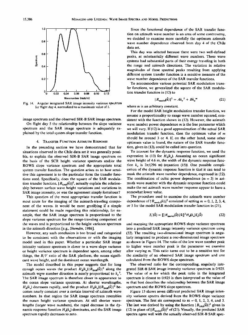
Fig. 14. Angular integrated SAR image intensity variance spectrum for flight day 4, normalized to a maximum value of 1.

image spectrum and the observed SIR-B SAR image spectrum. On flight day 5 the relationship between the slope variance

spectrum and the SAR image spectrum is adequately ex- plained by the total system slope transfer function.

4. TRANSFER FUNCTION AZIMUTH RESPONSE

In the preceding section we have demonstrated that for situations observed in the Chile data set it was generally possi- ble, to explain the observed SIR-B SAR image spectrum on the basis of the SCR height variance spectrum and/or the ROWS slope variance spectrum and the appropriate total system transfer function. The question arises as to how sensi- tive this agreement is to the particular form the transfer func- tions used. Specifically, does the square of the SAR modula- tion transfer function, I RSAR(f0 12, actually explain the relation- ship between surface wave height variations and variations in SAR image intensity, or was the agreement simply fortuitous?

This question of the most appropriate transfer function is most acute for the imaging of the azimuth-traveling compo- nent of the waves. It would be most gratifying if a simple statement could be made regarding this relationship, for ex- ample, that the SAR image spectrum is proportional to the slope variance spectrum for the range-traveling component ot the waves and is proportional to the height variance spectrum in the azimuth direction [e.g., Shemdin, 1986].

However, any such conclusion is too broad and categorical to be consistent with the observations or with the imaging model used in this paper. Whether a particular SAR image intensity variance spectrum is closer to a wave slope variance or height variance spectrum is dependent upon, among other things, the R/l/ ratio of the SAR platform, the ocean signifi- cant wave height, and the dominant ocean wavelength.

The model described in this paper suggests that for long enough ocean waves the product H,•(k,)IRsAR(•)] 2 along the azimuth waive number direction is nearly proportional to ka 3. The SAR image spectrum is therefore closer in appearance to the ocean slope variance spectrum. At shorter wavelengths, H,•(k,) decreases rapidly, and the product H,•(k,)lRsAR(fC)[2 be- comes nearly constant over a certain interval of azimuth wave numbers. In that region the SAR image spectrum resembles the ocean height variance spectrum. At still shorter wave- lengths (larger wave numbers), the rapid decrease in the dy- namic response function Ha(k,) dominates, and the SAR image spectrum rapidly decreases to zero.

Since the functional dependence of the SAR transfer func- tion on azimuth wave number is an area of some controversy, we decided to examine more carefully the optimum azimuth wave number dependence observed from day 4 of the Chile data set.

This day was selected because there were two well-defined peaks, at substantially different wave numbers. These wave systems had substantial parts of their energy traveling in both the range and azimuth directions. The variation in relative magnitudes of these spectral peaks resulting from applying different system transfer function is a sensitive measure of the wave number dependence of the SAR transfer functions.

To accommodate various potential SAR modulation trans- fer functions, we generalized the square of the SAR modula- tion transfer function in (12) to

] amodel(• ) 12 -- Akr 2 + aka m (21)

where m is an arbitrary constant. For the model SAR height modulation transfer function, we

assume a proportionality to range wave number squared, con- sistent with the function shown in (12). However, the azimuth wave number power dependence m is the free parameter which we will vary. If (12) is a good approximation of the actual SAR modulation transfer function, then the optimum value of m should be around 3 or 4. If, on the other hand, some other optimum value is found, the nature of the SAR transfer func- tion, given in (12), could be called into question.

To account for the dynamic response function, we used the expression in (13) for Ha(k,). Assuming an ocean significant wave height of 4.6 m, the width of the dynamic response func- tion ks is 2rc/(296 m) (equation (15)). One possible compli- cation of the dynamic response function is that it can tend to mask the azimuth wave number dependence, expressed in (12). The combination of cubic power dependence (m = 3) in azi- muth wave number with the dynamic response function could make the net azimuth wave number response appear to have a somewhat lower value.

The procedure used to examine the azimuth wave number dependence of[Rmod½l(k ) [2 consisted of setting m = 0, 1, 2, 3, 4, or 5 for the model SAR modulation transfer function in (21),

Si'(•) = I-I amodel(•)I/kj2Ha(k,•)Ss(•z) (22)

and mapping the appropriate ROWS slope variance spectrum into a predicted SAR image intensity variance spectrum using (22). The resulting two-dimensional image spectrum is angu- larly integrated to produce a one-dimensional image spectrum as shown in Figure 14. The ratio of the low wave number peak to higher wave number peak is the parameter we examine after varying m. This ratio turns out to be a sensitive test for the similarity of an observed SAR image spectrum and one calculated from the ROWS slope spectrum.

The observed ratio for the corresponding, angularly inte- grated SIR-B SAR image intensity variance spectrum is 0.925. The value of m for which the peak ratio in the integrated spectrum is closest to 0.925 is then interpreted as the value of m that best describes the relationship between the SAR image spectrum and the ROWS slope spectrum.

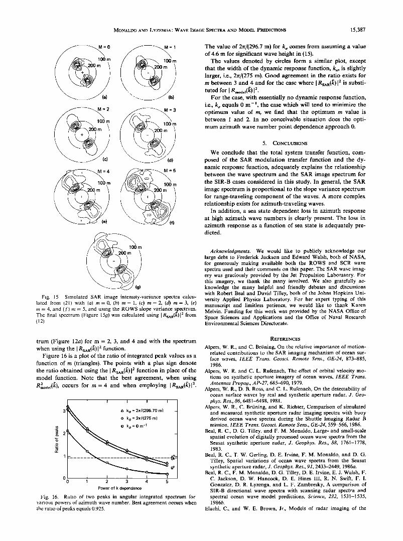
Figure 15 shows seven different predicted SAR image inten- sity variance spectra derived from the ROWS slope variance spectrum. The first six correspond to m = 0, 1, 2, 3, 4, and 5. The last was derived by using the function I RSAR(F0 12 given in (12) in place of I Rmoael(fc) 12 of (21). Visually, the predicted SAR spectra agree well with the actually observed SIR-B SAR spec-

MONALDO AND LYZENGA' WAVE IMAGE SPECTRA AND MODEL PREDICTIONS 15,387

0

00,m /A• c••,200, m

•• (c)

rn 100 rn Om

100m

•-- • (g) Fig. 15. Simulated SAR image intensity-variance spectra calcu-

lated from (21) with (a) m = 0, (b) m = 1, (c) m = 2, (d) m = 3, (e) m = 4, and (œ)m = 5, and using the ROWS slope variance spectrum. The final spectrum (Figure 15g) was calculated using IRsAR(•)I 2 from (12).

The value of 2rr/(296.7 m) for k•, comes from assuming a value of 4.6 m for significant wave height in (15).

The values denoted by circles form a similar plot, except that the width of the dynamic response function, k•,, is slightly larger, i.e., 2rr/(275 m). Good agreement in the ratio exists for m between 3 and 4 and for the case where I RSA.(•)12 is substi- tuted for I Rmoae](k ) 12.

For the case, with essentially no dynamic response function, i.e., k•, equals 0 m-•, the case which will tend to minimize the optimum value of m, we find that the optimum m value is between 1 and 2. In no conceivable situation does the opti- mum azimuth wave number point dependence approach 0.

5. CONCLUSIONS

We conclude that the total system transfer function, com- posed of the SAR modulation transfer function and the dy- namic response function, adequately explains the relationship between the wave spectrum and the SAR image spectrum for the SIR-B cases considered in this study. In general, the SAR image spectrum is proportional to the slope variance spectrum for range-traveling component of the waves. A more complex relationship exists for azimuth-traveling waves.

In addition, a sea state dependent loss in azimuth response at high azimuth wave numbers is clearly present. The loss in azimuth response as a function of sea state is adequately pre- dicted.

Acknowledgments. We would like to publicly acknowledge our large debt to Frederick Jackson and Edward Walsh, both of NASA, for generously making available both the ROWS and SCR wave spectra used and their comments on this paper. The SAR wave imag- ery was graciously provided by the Jet Propulsion Laboratory. For this imagery, we thank the many involved. We also gratefully ac- knowledge the many helpful and friendly debates and discussions with Robert Beal and David Tilley, both of the Johns Hopkins Uni- versity Applied Physics Laboratory. For her expert typing of this manuscript and limitless patience, we would like to thank Karen Melvin. Funding for this work was provided by the NASA Office of Space Sciences and Applications and the Office of Naval Research Environmental Sciences Directorate.

trum (Figure 12a) for m = 2, 3, and 4 and with the spectrum when using the I RSAR(/C ) 12 function.

Figure 16 is a plot of the ratio of integrated peak values as a function of m (triangles). The points with a plus sign denote the ratio obtained using the I RSAR(/C)12 function in place of the model function. Note that the best agreement, when using

2 ~ Rmodel(k), occurs for m = 4 and when employing IRsAR(/C) I 2.

3 • /x k o = 2rr/(296.70 m) - •.• o ko= 2rr/(275 m)

• 2 -

._o

0 I I I I 0 1 2 3 4 5

Power of k dependence

Fig. 16. Ratio of two peaks in angular integrated spectrum for various powers of azimuth wave number. Best agreement occurs when the ratio of peaks equals 0.925.

REFERENCES

Alpers, W. R., and C. Brfining, On the relative importance of motion- related contributions to the SAR imaging mechanism of ocean sur- face waves, IEEE Trans. Geosci. Remote Sens., GE-24, 873-885, 1986.

Alpers, W. R. and C. L. Rufenach, The effect of orbital velocity mo- tions on synthetic aperture imagery of ocean waves, IEEE Trans. Antennas Propag., AP-27, 685-690, 1979.

Alpers, W. R., D. B. Ross, and C. L. Rufenach, On the detectability of ocean surface waves by real and synthetic aperture radar, J. Geo- phys. Res., 86, 6481-6498, 1981.

Alpers, W. R., C. Brtining, and K. Richter, Comparison of simulated and measured synthetic aperture radar imaging spectra with buoy derived ocean wave spectra during the Shuttle Imaging Radar B mission, IEEE Trans. Geosci. Remote Sens., GE-24, 559-566, 1986.

Beal, R. C., D. G. Tilley, and F. M. Monaldo, Large- and small-scale spatial evolution of digitally processed ocean wave spectra from the Seasat synthetic aperture radar, J. Geophys. Res., 88, 1761-1778, 1983.

Beal, R. C., T. W. Gerling, D. E. Irvine, F. M. Monaldo, and D. G. Tilley, Spatial variations of ocean wave spectra from the Seasat synthetic aperture radar, J. Geophys. Res., 91, 2433-2449, 1986a.

Beal, R. C., F. M. Monaldo, D. G. Tilley, D. E. Irvine, E. J. Walsh, F. C. Jackson, D. W. Hancock, D. E. Hines III, R. N. Swift, F. I. Gonzalez, D. R. Lyzenga, and L. F. Zambresky, A comparison of SIR-B directional wave spectra with scanning radar spectra and spectral ocean wave model predictions, Science, 232, 1531-1535, 1986b.

Elachi, C., and W. E. Brown, Jr., Models of radar imaging of the

15,388 MONALDO AND LYZENGA.' WAVE IMAGE SPECTRA AND MODEL PREDICTIONS

ocean surface waves, IEEE Trans. Antennas Propag., AP-25, 84-95, 1977.

Harger, R. O., Synthetic Aperture Radar Systems, 37 pp., Academic, San Diego, Califi, 1970.

Hasselmann, K., R. K. Raney, W. J. Plant, W. Alpers, R. A. Shuch- man, D. R. Lyzenga, C. L. Rufenach, and M. J. Tucker, Theory of synthetic aperture imagery radar imaging of waves: A MARSEN view, d. Geophys. Res., 90, 4659-4686, 1985.

Irvine, D. E., The interaction of long gravity waves and short waves in the presence of wind, Ph.D. dissertation, Johns Hopkins Univer- sity, Baltimore, Md., 1983.

Jackson, F. C., W. T. Walton, and P. L. Baker, Aircraft and satellite measurement of ocean wave directional spectra using scanning beam microwave radars, d. Geophys. Res., 90, 987-1004, 1985.

Lyzenga, D. R., Numerical simulation of synthetic aperture radar image spectra for ocean waves, IEEE Trans. Geosci. Remote Sens., GE-24, 863-872, 1986.

Lyzenga, D. R., and R. A. Shuchman, Analysis of scatterer motion effects in MARSEX X band SAR imagery, d. Geophys. Res., 88, 9769-9775, 1983.

Lyzenga, D. R., R. A. Shuchman, J. D. Lyden, and C. L. Rufenach, SAR imaging of waves in water and ice: Evidence for velocity bunching, d. Geophys. Res., 90, 1031-1036, 1985.

Monaldo, F. M., Improvement in the estimate of dominant wave- length and direction from spaceborne SAR image spectra when corrected for ocean surface movement, IEEE Trans. Geosci. Remote Sens., GE-22, 603-608, 1984.

Monaldo, F. M., and R. C. Beal, Limitations of the Seasat SAR in high sea states, in Wave Dynamics and Radio Probing of the Ocean Surface, edited by O. M. Phillps and K. Hasselmann, pp. 423-442, Plenum, New York, 1986.

Monaldo, F. M., and D. R. Lyzenga, On the estimation of wave slope- and height-variance spectra from SAR imagery, IEEE Trans. Geosci. Remote Sens., GE-24, 543-551, 1986.

Phillips, O, M., The structure of short gravity waves on the ocean surface, in Spaceborne Synthetic Aperture Radar for Oceanography, edited by R. C. Beal, P.S. DeLeonibus, and I. Katz, Johns Hopkins University Press, Baltimore, Md., 1981.

Pierson, W. J., and L. Moskowitz, A proposed spectral form for fully developed wind seas based on the similarity theory of S. A. Kitaigo- rodskii, d. Geophys. Res., 69, 5181-5190, 1964.

Plant, W. J., and W. C. Keller, Parametric dependence of ocean wave-radar modulation transfer functions, d. Geophys. Res., 88, 9747-9756, 1983.

Raney, K., Synthetic aperture imaging of radar and moving targets, IEEE Trans. Aerosp. Electron. Syst., AES-7, 499-505, 1971.

Shemdin, O. H., Im•estigation of Physics of Synthetic Aperture Radar in Ocean Remote Sensing, Toward Interim Report, vol. 1, Data Sum- mary and Earl)' Results, 97 pp., Jet Propulsion Laboratory, Pasa- dena, Calif., 1986.

Swift, C. T., and L. R. Wilson, Synthetic aperture radar imaging of ocean waves, IEEE Trans. Antennas Propag., AP-27, 725-729, 1979.

Tucker, M. J., The imaging of waves by satellite synthetic aperture radar: The effects of surface motion, Int. d. Remote Sens., 6, 1059- 1074, 1985.

Vachon, P. W., R. B. Olsen, C. E. Livingston, and N. G. Freeman, Airborne SAR observations of the ocean surface during LEWEX, IEEE Trans. Geosci Remote Sens., 15, 548-561, 1988.

Walsh, E. J., D. W. Hines III, R. N. Swift, and J. F. Scott, Directional wave spectra measured with the surface contour radar, d. Phys. Oceanogr., 15, 566-592, 1985.

Wright, J. W., Backscattering from capillary waves with application to sea clutter, IEEE Trans. Antennas Propag., AP-14, 749-754, 1960.

Wright, J. W., Detection of ocean waves by microwave radar: The modulation of gravity-capillary waves, Boundary Layer Meteorol., 13, 87-105, 1978.

D. R. Lyzenga, College of Marine Studies, University of Delaware, Newark, DE 19716.

F. M. Monaldo, Applied Physics Laboratory, Johns Hopkins Uni- versity, Johns Hopkins Road, Laurel, MD 20707.

(Received August 10, 1987; accepted November 13, 1987.)