Comparison of different electrical machines for Belt Driven Alternator Starters

Dan Hagstedt

Doctoral Dissertation Department of Measurement Technology and

Industrial Electrical Engineering

2013

Department of Measurement Technology and Industrial Electrical Engineering

Lund University

Box 118

SE-221 00 LUND

SWEDEN

http://www.iea.lth.se

ISBN: 978-91-88934-59-8

CODEN:LUTEDX/(TEIE-1067)/1-166/(2013)

© Dan Hagstedt, 2013

Printed in Sweden by Media-Tryck, Lund University

Lund 2013

iii

Abstract

In this thesis focus is on the electromagnetic design of a synchronous machine suited for a belt driven alternator and starter (BAS) in a micro hybridisation of a mid size passenger car. The BAS needs to provide a high cranking torque to start the combustion engine, especially in a cool condition where the requirements is highest. Beside the high cranking torque is it desirable to have a high power performance over a wide speed range.

The thesis compares four potential excitations of a synchronous machine: the permanently magnetized (PMSM), the electrically magnetized (EMSM), the EMSM with series magnetisation (SMSM) and the hybrid magnetized (HMSM). Those are treated both theoretically and with numerical analyses, where the numerical calculations uses finite element analyses (FEA). The fundamental boundary conditions, as current density set by thermal limitations are based on a deep analysis of an existing Lundell alternator. This is presented with computational fluid dynamic (CFD) and finite volume analysis (FVA) in order to give knowledge on the heat dissipation of the alternator. A complete loss separation of the alternator is discussed and presented, both by calculations and experimental work.

The SMSM is a new configuration of an electrically excited synchronous machine with the field winding in series with the phase windings via a rectifier. This thesis shows the relation on both the magnetical and the electrical connection between the stator and the rotor. The power and torque characteristics are highlighted.

The thesis presents an electromagnetic design and experimental evaluation of a compact HMSM. A relatively simple and compact slip ring less rotor with EM and PM excitation is proposed, analysed and tested. A series of 3D FE transient computations are made in order to estimate efficiency at different operation points and with different types of rotor cores: solid iron and powder composite core. A rotor with the solid iron core is built and tested including different aspects of torque and power loss production.

iv

Acknowledgements

First of all I would like to acknowledge Mats Alaküla who, as supervisor and friend, have guided and supported me through many obstructions and decisions.

I will give a great thanks to my assistant supervisor Avo Reinap who, like a magician, conjure away hours of fruitful discussions in the great world of electrical machines.

Special thanks to my friends and colleagues, Jonas Ottoson and Tomas Bergh, who have followed me in my work from the very first day. Your friendship and support have meant a lot to me.

Thanks to all colleagues in my research group, for good support and discussions, and a special thank to Getachew Darge.

I am very grateful for the work that Svante Bouvin brought into the production of the prototype.

In the good relation with the industries I have collaborated with, I would like to acknowledge Lars Hoffman from the former automotive industry SAAB and Lasse Rydén at Volvo Trucks.

To my wife Maria and my children Oline and Fredrik, thanks for your support and love.

Lund, February 2012

Dan Hagstedt

v

vi

Contents

CHAPTER 1 INTRODUCTION ............................................................. 8

1.1 MOTIVATION........................................................................ 8

1.2 OBJECTIVES AND METHOD................................................. 11

1.3 REVIEW OF PREVIOUS WORK ............................................. 12

1.4 CONTRIBUTIONS ................................................................ 13

1.5 OUTLINE OF THE THESIS .................................................... 13

1.6 AUTHORS PUBLICATIONS................................................... 14

CHAPTER 2 THEORY ON MACHINES SUITABLE FOR BAS APPLICATIONS............................................................. 17

2.1 CONSTRUCTION ................................................................. 17

2.2 SYNCHRONOUS MACHINE EQUATIONS............................... 22

2.3 THE PERMANENTLY MAGNETIZED SYNCHRONOUS

MACHINE - PMSM............................................................. 27

2.4 EMSM ............................................................................... 32

2.5 SMSM................................................................................ 36

2.6 HMSM............................................................................... 45

2.7 SUMMARY.......................................................................... 49

CHAPTER 3 ANALYSIS OF AN ALTERNATOR ............................ 54

3.1 REFERENCE ALTERNATOR................................................. 54

3.2 MECHANICAL LOSSES ........................................................ 55

3.3 ELECTRICAL AND MAGNETO STATIC LOSSES ..................... 66

3.4 THERMAL........................................................................... 75

3.5 SUMMARY.......................................................................... 92

CHAPTER 4 COMPARISON OF PMSM, EMSM AND SMSM....... 95

4.1 SIMULATION ENVIRONMENT.............................................. 97

vii

4.2 CHARACTERISTICS............................................................104

4.3 SUMMARY ........................................................................113

CHAPTER 5 ALTERNATIVELY CONSTRUCTION WITH HYBRID MAGNETIZATION ROTOR......................116

5.1 STRUCTURE COMPARISON ................................................117

5.2 ALTERNATIVE CLAW-POLE DESIGNS ................................118

5.3 MATERIAL COMPARISON ..................................................119

5.4 SIMULATIONS ...................................................................122

5.5 CHARACTERISTICS............................................................130

5.6 SUMMARY ........................................................................139

CHAPTER 6 ASSESSMENT OF THE HYBRID MAGNETIZATION ROTOR ...........................................................................142

6.1 MACHINE DATA AND CONSTRUCTION ..............................142

6.2 LABORATORY SETUP ........................................................146

6.3 LABORATORY VALIDATIONS ............................................148

6.4 SUMMARY ........................................................................158

CHAPTER 7 CONCLUDING REMARKS AND FUTURE WORK160

REFERENCES ......................................................................................165

Chapter 1 Introduction

1.1 Motivation

The topic addressed in this thesis emanates from security of oil supply and preservation of environment with respect to road transportation. A global consensus states that peak oil has passed, or is about to pass, and thus we can expect gradually increasing oil prices. One way to delay the end of commercial oil is to reduce the need for oil, e.g. by reducing fuel consumption of vehicles. Thus, a lot of focus is today laid on fuel-efficient solutions and alternative energy supply for the transportation of tomorrow. One way to reduce the fuel consumption is to use some kind of hybridization technology mixing combustion drive and electric drive in the same vehicle.

The electric hybridization is one type of hybridization and can be classified as micro- mild- and full hybridization. This definition is a bit weak with diffuse limits between the classes. A micro hybrid is a vehicle with a so-called Stop&Go function, turning off the ICE when standing still. This requires a slightly stronger starter motor. A mild hybrid has an electric traction motor able not only to start the ICE but to provide tractive power to the vehicle for shorter periods of time but is mainly used to assist the combustion engine to work more efficiently. A full hybrid is even stronger than the mild hybrid and able to drive the vehicle in all different driving situations only with the electrical machine, in limited time, i.e. serve as an electric vehicle with limited range – typically a few kilometres. With a longer range, like a few 10’s of kilometres, the same vehicle can be referred to as a Plug In hybrid.

9

During the last years the vehicles have become more and more equipped with different types of electrical sub systems. It can be safety systems or comfort systems such as plant varying climate control in different positions inside the vehicle, electrical adjustable seats/mirrors/lights/distance sensors/lane keeping cameras/… etc. A lot of traditionally mechanically driven loads are replaced with electrical driven like water pumps/breaks/servo steering/ventilation fan etc. The increasing electric load requires increasing generator power and efficiency. A common alternator in a car is relatively cheap with a rather low efficiency - as low as 50 percent. The low cost of the conventional Lundell generator and low fuel costs has given low motivation for development of high efficient generators. This project is about such a development, in particular as Belt driven Alternator Starter (BAS).

A belt driven alternator starter (BAS) is an electrical machine that both work as a starter for the internal combustion engine (ICE) and as an alternator in the vehicle [15][16]. It is connected directly to the shaft of the ICE via a belt transmission, illustrated in Figure 1.1, i.e. replacing the ordinary alternator.

Figure 1.1 The placement schematic view of a BAS

For a micro hybrid the electrical machine will not only work as a BAS, it

10

will also support the combustion engine during lower speed in addition to the Stop&Go function. The suitable power of this machine, for a smaller sized passenger car, is suggested to be 5 kW and presented in “Belt driven Alternator and Starter with a Series Magnetized Synchronous Machine drive” [9]. Using a 5 kW BAS for the investigated size of the vehicle the fuel consumption in urban drive can be reduced up to 24 percent [9]. If the average fuel consumption is calculated for the European standard (1999/100 EC), the fuel consumption is reduced around 12 percent in total. The distribution between urban- and highway drive is 37 and 63 percent respectively for the European standard.

The main disadvantage of a BAS solution is that it is directly connected to the combustion engine, which means that it is not possible to drive the BAS as a machine without the ICE. This means that in a situation like a traffic jam, where the speed is slow enough to drive the vehicle without the ICE, the ICE will work as a mechanical load to the machine. If the ICE has adjustable valves that make it possible to reduce the cylinder compression the mechanical load that the ICE represent will decrease. For a flywheel alternator and starter (FAS) [17] or similar solution, if it is connected via clutch to the ICE, the system is possible to run without the ICE. But instead it requires more engagement to the existing ICE since it is embedded into the ICE. A BAS solution are easier to implement since it is possible to keep the existing ICE and basically replace the alternator with the BAS, in case that it is not to large in size. This makes it to a more cost-efficient solution compared to the FAS in an already developed production line.

Besides, the environment under the bonnet in the car close to the ICE is dirty, damp and can reach temperatures up to 120 °C. The BAS should also be able to start the combustion engine in a temperature as low as –40 °C, when the oil viscosity is high, leading to extraordinary high torque requirements.

To keep the size of the electrical machine down for a given maximum crankshaft torque, the machine usually has a gear ratio of about 3:1 to the ICE crankshaft. This means that the alternator starter runs with a speed three times higher than the combustion engine. When using the BAS together with either a petrol or diesel combustion engine, the speed range

11

is usually limited by the combustion engine. The operating speed range of a petrol engine varies typically between 700 – 6000 rpm while for the diesel engine it varies between 700 - 4500 rpm. In order to accomplish light hybridization of the vehicle, further than only stop and go capability, the power has to be increased to 5 kW [9] compared to common alternator power of 1.5 kW. These criteria set the main specifications of an alternator starter to be designed in this thesis:

Crank torque of at lest 55 Nm at -40oC

Nominal power, 5 kW

Speed range 0 - 18000 rpm

Base speed 3000rpm

1.2 Objectives and method

The objective with this thesis is to investigate a micro hybridization of a smaller sized car with a Belt driven Alternator and Starter (BAS) with the focus on evaluation and comparison of different types of electrical machines that are possible to use in a BAS application. The machine types selected for the study are the Permanently Magnetized Synchronous Machine (PMSM), the Electrical Magnetized Synchronous Machine (EMSM), the Series Magnetized Synchronous Machine (SMSM) and the Hybrid Magnetized Synchronous Machine HMSM. The SMSM is a new type of machine configuration.

Parts of the work presented in this PhD thesis started as a subpart of a project financed by “Statens energimyndighet” (STEM), the Swedish Energy Agency. The work started as an investigation of an SMSM in a BAS application. Another subpart of that project is made by Tomas Bergh and is about the control and the power electronics for a SMSM in a BAS application. This is published in the licentiate thesis “Belt driven Alternator and Starter with a Series Magnetized Synchronous Machine drive” [9]. These two sub project have in common a Simulink based study on optimizing the power rating of the BAS for a given application.

As an addition to the work done in the STEM-funded BAS project, another

12

project funded by the Strategic Research Foundation (SSF) in their program Pro Viking on Design and Manufacturing of Integrated Actuators (DAMIA), part I and II, has been the basis for the HMSM study presented in this thesis.

1.3 Review of previous work

BAS During the beginning at the last decade (2000), the BAS concept as a micro hybrid solutions started [15][16].

Today there are a couple of BAS solutions available on the market, e.g. by Hitachi and Valeo [10]. The Valeo system named StARS is a synchronous claw pole machine with a power of 2.5kW at a 14V system. It is a common Lundell alternator with permanent magnets in between the rotor claws to minimize magnetic flux leakage within the rotor circuit. Hitachi has a BAS solution called motor generator unit (MGU). It is like Valeos a permanent magnet enhanced Lundell machine with peak power of 4kW in a motor mode and 5kW in generator mode.

SMSM The SMSM (Series Magnetized Synchronous Machine) is a concept where the three phase currents are lead through a Rectifier to the field winding, thus eliminating the need for a field supply in an EMSM. This concept complicates the mathematical model and control but reduces the cost for power electronics. The SMSM concept is invented and patented by professor Mats Alaküla at the department of Industrial Electrical Engineering and Automation at the faculty of engineering of Lund University. The SMSM was mentioned in Dr David Martinez PhD thesis, [8], and the research results is published in a number of publications [9][11][12][13].

HMSM Many papers and reports are published, during the last decade (2000), within the field of hybrid excitations in electrical machines [44][45][46][47][48][49][50]. Even the BAS systems from Valeo and Hitachi mentioned above are forms of hybrid excitation with field boost

13

using permanent magnets.

1.4 Contributions

The contribution of this thesis is:

A comparative design study of which type of synchronous machine that suits best in a BAS application.

The characteristics of the SMSM, as torque versus speed and power versus speed characteristic.

The placement of the voltage-limit locus in the rotor oriented reference frame for different machines is discussed.

The characteristics and the design strategy for the HMSM is presented and discussed.

A contribution to a machine design tool developed at IEA at Lund University.

The thermal behavior of a conventional alternator is investigated.

A new type of a slip-ringless hybrid magnetized rotor is developed and tested.

A proper choice of machine size is discussed.

1.5 Outline of the Thesis

The thesis begins with a literature study and a review of machine design and the BAS concept. The theory of the different machine types is described and developed, as well as an analysis of an existing alternator, with its characteristics, losses and the thermal behaviour respectively. It is followed by developing a software machine designing tool, with a possibility to scan a large amount of different variables and machine structures. This is to simplify design and comparison between different types of synchronous machines. The software program is written in Matlab for pre- and post- processing and uses the finite element software FEMM

14

for magneto static calculations with the finite element method. With the help of this machine designing tool a comparison of three different machines, which all are possible as a BAS, is done. The three investigated machines are the PMSM, the EMSM and the SMSM. An alternative rotor construction with HMSM is developed and verified with a manufactured prototype.

In Chapter 2 the fundamentals about the synchronous machine in form of theory is described. It describes, with equations, the four machine types, PMSM, EMSM, SMSM and HMSM.

In Chapter 3 a conventional alternator that is used as a reference is described and analyzed, with its characteristics and the heat dissipations. It is split as a mechanical and an electrical treatment of losses, where theory is validated by measurements.

In Chapter 4 a simulation study and a comparison is made between PMSM, EMSM and SMSM. A number of parameter with equal boundary conditions, for all the machine types, is scanned to give a fair comparison.

In Chapter 5 an alternative rotor is proposed, which is a compact slip-ring less HMSM solution suited for a BAS application. A comparison is also made between a solid iron construction and a soft magnetic composite (SMC) construction of the rotor.

In Chapter 6 the prototyping and experimental work is described to validate the HMSM rotor model treated in chapter 5. The experimental work is done by dynamic loading of known rotational inertia.

In Chapter 7 a conclusion of the work is given, with a discussion and also a proposal for future work.

1.6 Authors publications

There are some publications made during the project, some of them is parts of this thesis and some is related and common with other projects and will not be included in this thesis.

Related and support the thesis:

15

Chapter 1

Bergh, T., Hagstedt, D., Alaküla, M., Karlsson, P. (2006), “Modeling and presentation of the series magnetized synchronous machine”. SPEEDAM 2006 International Symposium on Power Electronics, Electrical Drives, Automation and Motion, Taormina, Italy, 23-26 May, 2006.

Chapter 2

Hagstedt, D. (2006), “A BAS application of a series magnetized synchronous machine”. International Conference on Electrical Machines, IEMC'06 Conference, Crete, Greece, 2-5 September, 2006.

Chapter 4

Hagstedt, D., Márquez, F., Alaküla, M. (2008), “A comparison between PMSM, EMSM and SMSM in a BAS application ”. International Conference on Electrical Machines (ICEM2008), Vilamoura, Portugal, Sept. 6-9, 2008.

Reinap, A., Hagstedt, D., Márquez, F., Loayza, Y., Alaküla, M. (2008), “Development of a radial flux machine design environment”. International Conference on Electrical Machines (ICEM2008), Vilamoura, Portugal, Sept. 6-9, 2008.

Chapter 5 and 6

Hagstedt, D., Reinap, A., Ottosson, J., Alaküla, M. (2012), “Design and Experimental Evaluation of a Compact Hybrid Excitation Claw-Pole Rotor”. International Conference on Electrical Machines (ICEM2012), Marseille, France, Sept. 2-5, 2012.

Non supporting publications of the thesis:

Reinap, A., Hagstedt, D., Högmark, C., Alaküla, M. (2012), “Sub-optimization of a claw-pole structure according to material properties of soft magnetic materials”. IEEE Transactions on Magnetics, vol. 48, no. 4, pp. 1681-1684.

16

Reinap, A., Hagstedt, D., Högmark, C., Alaküla, M. (2011), “Evaluation of a Semi Claw-Pole Machine with SM2C Core”. International Electrical Machines and Drives Conference (IEMDC2011), Niagara Falls, Ontario, Canada, May 15-18, 2011.

Otosson, J., Alaküla, M., Hagstedt, D. (2011), “Electro-thermal Simulations of a Power Electronic Inverter for a Hybrid Car”. International Electrical Machines and Drives Conference (IEMDC2011), Niagara Falls, Ontario, Canada, May 15-18, 2011.

Chapter 2 Theory on machines suitable for BAS applications

Electrical machine design face two fundamental challenges: cost efficient production and high energy conversion efficiency. Regarding the performance and the specific characteristics of a machine, that is suitable for the BAS application, the energy conversion efficiency is vital due to its direct impact on fuel consumption of the vehicle. Therefore a generalised theory of a doubly fed machine is used to compare and to evaluate different machine topologies. As the difference on topologies lies mainly on the rotor excitation, the stator is chosen identical for the selected topologies. Moreover, the generalised theory of the doubly fed machines is taking advantage of a two phase system, which describes the saliency and the magnetisation of the machine parts. It is important not to loose the connection to the real 3-phase winding arrangement in the stator or the practical solution of realising excitation for the rotor. For that reason the machine construction (2.1) is broadly and briefly described in prior of establishing the equation system (2.2) that gives the adequate comparison of different topologies (2.3-2.7).

2.1 Construction

There are many different kind of electrical machines, from small sized machines in home electronics and toys to large sized machines for industrial purposes or power system generators. In small scale machines as in toys the Direct Current (DC) machine is the most common. They are suitable in a system that already uses a DC voltage source. DC machines can be separated into two categories, brushless and the one with brushes. The one with brushes uses those to commutate the DC current

18

mechanically into AC current in the armature windings. The brushless DC is basically the same as a synchronous machine, with some differences in how to control the machine. AC machines are the dominating type and the most important version of these is the Induction Machine (IM) where magnetization is provided by the stator winding and preserved during load by an induction of rotor currents balancing the stator side load currents. Another AC machine is the Electrically Magnetized Synchronous Machine (EMSM) magnetized from the rotor equipped with a magnetizing winding that generally needs a supply of currents via slip rings. The Permanently Magnetized Synchronous Machine (PMSM) is similar to the EMSM but with the magnetizing winding replaced by Permanent Magnets. Reluctance Machines in various forms are also AC machines but utilize only the rotor saliency to create torque and all magnetization is made from the stator.

In this thesis some of these fundamental concepts for electrical machines are combined. Permanent and Electric Magnetization is used in the HMSM machine and a field current supply without slip rings using the same source as the stator currents is used in the SMSM and HMSM.

When it comes to vehicular application, then the size of the electrical machine is both more restricted and less standardized than the machines for industrial applications or household appliances. Also the range of considerable operation points is usually broader and the need for a power density is higher compared to the aforementioned sectors. Even if the constructional layout of the machines is similar and the inverter controlled supply makes all topologies considerable, including the doubly excited synchronous machines,, the combinations can become more attractive in terms of power density and functionality.

Any electrical machine has a limitation due to the maximum allowed power of either the power supply or the machine itself. The current limitation is often related to the cooling capability of the stator windings and the voltage limitation to the voltage source and the winding insulation. Apart from the mechanical limitations and the speed ratings for the specified voltage, the limitation of power and current becomes convenient when normalizing machine parameters, current, voltage etc. to rating point. Before introducing the equation system, which is used to compare the different machine topologies suitable for the BAS application, the main constructional aspects of the machine parts are shortly discussed.

19

The rotor design is partly a compromise between options like

1. Selection between permanent, temporal (electric) and combined hybrid excitation,

2. Supply arrangement to the temporal (electric) magnetization by choosing separate or series excitation with electric (slipring) or magnetic (slipringless) connection to the rotor.

Therefore several of the machines studied in this thesis represent unique engineering solutions to pick the best properties of the different technologies, like in the SMSM and HMSM.

Stator The stator is the non-rotating part of the machine. For synchronous machines the stator is usually configured with three phase windings. The design of the stator, as for the design of the whole machine, is about balancing the need for magneto motive force to run magnetic flux through the machine against the electric current loading to create torque. In this balance the geometry, material properties, number of phases, number of slots, skew, winding distribution etc are the parameters that can be changed to maximize the torque capability and minimize losses, torque ripple (e.g. cogging) and induced voltage harmonics within given specifications on size, materials and speed.

20

Figure 2.1 A 2-pole full pitch three phase stator winding

It is not always size or cost effective to have distributed windings due to end winding overhangs and more complex winding procedure when manufacturing the machine. Distributed windings are more common in high cost machines with special purpose that require low harmonics. This also holds for fractional pitch windings. Figure 2.1 shows one stator with a full pitch winding (180°) and Figure 2.2 one with a 120° pitch winding also called a single tooth winding. If the stator uses a 120° winding, the windings end turns between the phases does not cross/overlap each other. This leads to a reduction of the copper losses in the end turns compared to a full pitch winding, but also to a lower flux linkage with the rotor. The single tooth winding is usually easier to manufacture and thus cheaper, and gives often a shorter end winding region in the machine and thus more active stator length but less flux linkage. The choice of a full pitch or single tooth winding is a typical example of design parameters in the winding design that the machine designer must consider.

21

Figure 2.2 A 2pole machine with a 120° single tooth winding

Rotor The rotating part of a machine is the rotor. The rotor is designed to EITHER provide the bulk of the magnetization of the stator-rotor-circuit OR a difference in reluctance/saliency in two magnetically orthogonal directions, in order to maximize torque production. In many cases, like in modern electrically or permanently magnetized synchronous machines both the magnetization and the reluctance difference are designed into the rotor circuit.

With a built in magnetization of the rotor it is desirable to be able to change this magnetization during operation. This requires an electrical magnetization, which on the other hand requires a supply of so called field current to a winding that normally rotates with the rotor – requiring some kind of slip ring solution for field current supply. Permanent magnetization does not need any slip rings or a supply of field current but it is on the other hand not possible to change during operation and on top of that also relatively expensive.

The rotor design is partly a compromise between options like these and several of the machines studied in this thesis represent unique engineering solutions to pick the best properties of the different technologies, like in the SMSM and HMSM.

22

2.2 Synchronous machine equations

The mathematical equations for a synchronous machine are expressed starting with a three phase machine with a two pole rotor. There is symmetry of 120 electrical degrees between the phases. A sketch of the machine with the mutual fluxes is presented in Figure 2.3. Figure 2.3.a. shows the magnetic flux linked with the respective phases, colored with blue for phase a, red for phase b and green for phase c. Figure 2.3.b. shows the mutual flux contribution from the rotor magnets. The leakage fluxes are not illustrated in Figure 2.3 a and b. Each phase voltage corresponds to the resistive voltage drop over the phase winding and the induced voltage. The induced voltage is the time-derivates of the total induced flux linkage ψ, collected by the winding with N effective turns (ψ=N ϕ). Which is the summation of the mutual fluxes from the rotor ϕfm and the three stator fluxes ϕam, ϕbm and ϕcm. It also contains its own leaking flux. The equation for each phase, labeled a, b and c, is presented in equation 2.1.

dt

dRiu

dt

dRiu

dt

dRiu

scaa

sbaa

saaa

(2.1)

Where u is the phase voltage, R, i and ψ the resistance, the phase current and the flux linkage respectively.

23

Figure 2.3 Phase produced fluxes and the field flux

The flux linkage in each phase that contributes from the stator fluxes can be separated into three parts. Each separate part is linked to each one of the adjacent phases (2.2). The expression for the stator produced flux linkage obtained in phase a is then:

amaasa (2.2)

Where sa is the total flux linked with phase a, a is the leakage flux linkage of phase winding a, a is the mutual flux connecting the three stator windings and finally m is the flux linkage of phase a originating from the magnets. The expression above is the same for all phases and can be presented for phase b and c as well.

Transformation to xy- frame Essential for an easier control of the machine, but also to clarify the mathematical model of the machine, it is common to express a multi phase’s machine into an equivalent two phase machine with rotational coordinates [20]. This is called Park’s transformation. The first step is to transform the phase magnitudes into vectors that are equivalent to the coordinates in the imaginary complex plane, here named to -

coordinates. For a two pole machine with three phases the expresses for the transformation into - coordinates is:

24

3

4

3

2

3

4

3

2

3

4

3

2

3

2

3

2

3

2

j

sc

j

sbsasss

j

c

j

bas

j

c

j

bas

eej

eieiiijii

eueuuujuu

abc

(2.3)

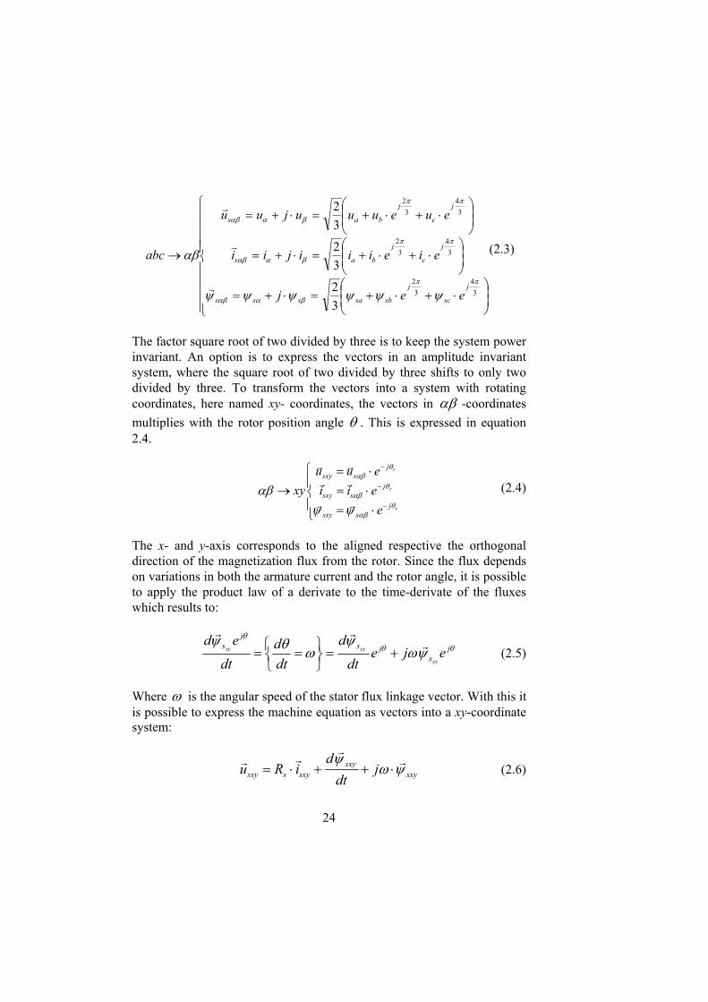
The factor square root of two divided by three is to keep the system power invariant. An option is to express the vectors in an amplitude invariant system, where the square root of two divided by three shifts to only two divided by three. To transform the vectors into a system with rotating coordinates, here named xy- coordinates, the vectors in -coordinates

multiplies with the rotor position angle . This is expressed in equation 2.4.

r

r

r

jssxy

jssxy

jssxy

e

eii

euu

xy

(2.4)

The x- and y-axis corresponds to the aligned respective the orthogonal direction of the magnetization flux from the rotor. Since the flux depends on variations in both the armature current and the rotor angle, it is possible to apply the product law of a derivate to the time-derivate of the fluxes which results to:

xy xy

xy

js s j j

s

d e dde j e

dt dt dt

(2.5)

Where is the angular speed of the stator flux linkage vector. With this it is possible to express the machine equation as vectors into a xy-coordinate system:

sxysxy

sxyssxy jdt

diRu

(2.6)

25

Where the flux linkage vector, sxy , is the resultant of the stator flux

linkage, produced both by the magnetization flux from the rotor m and

the stator phases, and the leaking flux in the stator.

msxysxysxy

(2.7)

The torque is the cross product of the stator flux linkage excluding the leakage flux ( sxy

) and the stator currents, expressed in equation 2.8.

sxsysysxsymsxymsxy iiiiT )( (2.8)

Where the differences between the stator produced fluxes gives a reluctance torque, i.e. if the reluctance in the x-direction is different from the reluctance in the y-direction. The vector equation 2.6, with the inductances can be presented in respective stator voltage as:

msxsxsy

syssy

sysysx

sxssx

dt

diRu

dt

diRu

(2.9)

The vector length of the armature current si

and the voltage su

is the

products of respective vector magnitude in the xy-direction, and are presented in equation 2.10 and 2.11 respectively.

22

sysxs iii

(2.10)

22

sysxs uuu

(2.11)

Parameter normalization The characteristic presentations in this chapter are done with the parameters normalized. This is done on the basis of the maximum stator

26

current max,si

and voltage max,su

respectively. The maximum equals one

per unit. The normalization of the magnetisation flux, inductances and torque is based on a PM-machine with no reluctance torque and with the center of the voltage-limit line at the maximum current-line. Those limit lines is further discussed and explained in the next section.

The normalization is:

base

basebase

bases

basesbase

snmnbase

base

basesbase

sbases

sbases

ZL

i

uZ

iTT

u

uu

ii

,

,

max,,

,

max,,

max,,

Inserting these base units in equations 2.10 and 2.11 gives:

basebase

sxsysysxsym

basebase

sxymsxy

base

basesbase

msxsx

basesbase

sy

basesbase

sys

bases

sy

basesbase

sysy

basesbase

sx

basesbase

sxs

bases

sx

i

iii

i

i

T

T

dt

d

iZ

iR

u

u

dt

d

iZ

iR

u

u

)(

,,,,

,,,,

In the following sections these equations should be used in their p.u. forms for the synchronous machine voltage equation

pum

pusx

pusx

pupusy

base

pusy

pus

pusy

pusy

pusy

pupusx

base

pusx

pus

pusx

dt

diRu

dt

diRu

1

1

27

and for the torque equation

pusx

pusy

pusy

pusx

pusy

pum

pusxy

pum

pusxy

pu iiiiT

)(

However, for the sake of simplicity, the index “pu” is left out.

2.3 The Permanently Magnetized Synchronous Machine - PMSM

The permanent magnetized machine is as the name says a machine that uses permanent magnets for the main magnetization of the machine. In the late 1900's, the popularity of the PM- machines increased, hand in hand with the great improvement of the performance of the magnets, also called high-energy magnets. This trend has then slowed during the last years by the price increase of those magnets.

By using high-energy magnets it is possible to make machines with a high shear stress e.g. tangential mechanic force density in Newton per square meter in the air gap. This gives a possibility to designee machines with a high torque per unit volume. The main disadvantage of those high torque permanent magnet machines is the cost of those high-energy magnets and difficulties to accomplish a low field weakening ratio. The low field weakening ratio is related to the low inductance of the machine due to the low permeability of the magnets located in the main flux paths. The field weakening characteristics of the PM- machine is illustrated and discussed in the section characteristics. Using smaller magnets, for a certain size of the machine, in order to increase the field weakening ratio effects decrease the amount of torque. To minimize the torque reduction effects, with smaller magnets, it is common with a magnet arrangement in a way that provides a reluctance torque [22]. One common solution for PM-machines, in the vehicular industry, is the v-embedded permanent magnet machine with air pockets. The v-embedded PM-machine is used in the simulated comparison study presented in Chapter 4.

Characteristics To illustrate the theoretical and an ideal characteristics, in this section, the resistive respective the iron losses is neglected. The permeability is set to

28

infinite which means that the saturation effects are ignored. With the saturation ignored the flux linkage is linear to the armature currents. This means that the expression of the flux linkage with any winding, can be expressed with a constant inductance L and a current i.

* * *·L i (2.12)

The magnitude of the stator voltage vector with those assumptions and in steady state, based on the equations 2.9 and 2.11, is:

2222

sysysxsxms iLiLu (2.13)

The torque equation 2.8 is:

sxsysysxsym iiLLiT )( (2.14)

Based on the equations 2.13 and 2.14, the characteristics of a synchronous machine can be presented by a circle diagram in the xy- current plane and with a torque versus speed diagram [2][20][22][23].

With a maximum voltage it is possible to calculate the current combinations that allows for certain speed levels of the machine. Those could be shown graphically as constant speed curves in the plan that the x- and y- current constitute. Every value on the current in x- direction gives two maximum possible currents in the y- direction. One positive and one negative which is for motor- or generator- operation respectively. The voltage-limit lines for a PMSM appear as circles or ellipses in where the area shrinks when the speed increases. This is illustrated in Figure 2.4, where each curve is for a certain speed. Figure 2.4 only shows the first and second quadrant which is when the machine operates as a motor. When the machine runs as a generator, in the ideal case, the curves in third and the forth quadrant is mirrored from the first and the second quadrant in the x-axis. The center of the voltage-limit locus ellipses due to the permanent magnetization flux linkage ψm in relation to the armature flux linkage ψsx, i.e. the elliptic center is when the resultant stator flux linkage in x-directions equals zero. The decrease of the resultant stator flux linkage in the x-direction is obtained in the region when the x-current is negative and is named as the field weakening region. This means, the higher the pm flux

29

from rotor is compare to the stator inductance Lsx, the more negative current in the x-direction is needed to reach the center of the ellipse.

The shape of the voltage ellipse is due to the relation between the both stator inductances, as one can see in equation 2.13. If the inductance in x- direction is larger than the one in the y- direction the ellipse will be standing in the plane, i.e. wider in the y- direction. The opposite is obtained if the inductance in the y- direction is larger then the one in the x- direction. If the inductances are equal to each other it has the shape of a circle. As one can see in Figure 2.4 the inductance in the y-direction is larger than the inductance in x-direction. The center of the voltage-limit ellipse in the figure is 1.1 per unit of the maximum negative current.

-2 -1.5 -1 -0.5 0 0.5 1 1.5 20

0.5

1

1.5

2

current isx

p.u.

curr

ent

i sy p

.u.

maximum current-line

Voltage-limit lines

Figure 2.4. Voltage-limit ellipse for a PMSM with 1.1m p.u. and with a

saliency ratio 33.1 p.u

Also a specific torque of the machine can be obtained with different current combinations. This is illustrated in Figure 2.5 a,b and c, where the torque increases in the positive y-direction. The ratio between the stator inductances is common to present as the saliency ratio ξ which is the inductance in y-direction divided by the induction in x-direction. Figure 2.5a shows the constant torque lines for a PMSM where the inductance in

30

the x- direction is smaller than the one in the y- direction, i.e. the saliency ratio ξ >1, which gives a positive reluctance torque in the field weakening region. Figure 2.5b, shows torque lines when the inductances are equal to each other, ξ =1, and the magnetization flux linkage only contributes to the torque i.e. the reluctance torque is zero. Figure 2.5c shows the constant torque lines when the inductance in x- direction is greater than in the y- direction, ξ <1. This gives a positive reluctance torque in the first quadrant. The black dotted line in Figure 2.5a, b and c is the maximum allowed amplitude of the stator currents. The black cross in the three cases in Figure 2.5 indicates respective maximum possible torque.

-1 0 10

0.5

1

=1.3333

i sy p

.u.

isx

p.u.-1 0 1

0

0.5

1

=1

i sy p

.u.

isx

p.u.-1 0 1

0

0.5

1

=0.66667i sy

p.u

.

isx

p.u.

Figure 2.5. PMSM constant torque lines for different saliency ratio

The current vector has to be within the voltage-limit ellipse, which shrinks towards the center off the ellipse with increasing speed. This means that that the maximum output torque decreases accordingly. It is possible to keep a constant torque until the speed exceeds the base speed, which is when the voltage-limit ellipse line crosses the maximum torque line and the maximum current line. This is when the voltage-limit ellipse illustrated in Figure 2.4 is crossing the maximum torque spot marked with a black dot in Figure 2.5. When the speed continues to increase, the current in the x-direction has to be more negative to increase the field weakening which has an impact of the current in the y-direction to keep the total amount of current within the limits. This affects the torque, which decreases as well. When the negative current in the x-direction equals the maximum current no further field weakening is possible. The field weakening ratio is the relation between the maximum speed and the base speed, i.e. the maximum speed divided by the base speed.

31

In order to visualize the mechanical output it is common to present the machine characteristic in a torque versus speed diagram. Figure 2.6 shows two cases of different pm magnetization. The green colored curve is when the center point of the voltage-limit ellipse lays in the negative x-current of 1.1 p.u, which corresponds to the one in Figure 2.4. The dark green colored curve is when the center point is twice the maximum current i.e. 2 p.u. Figure 2.6 shows that a high magnetization gives a high torque characteristic but with a lower field weakening ratio and a lower magnetization gives lower torque and higher field wakening ratio with the same saliency ratio [22].

Figure 2.6. Torque vs speed characteristic of a PMSM, different magnitude of magnetization

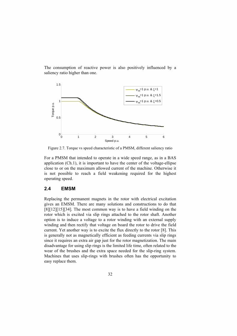
Figure 2.7 shows the torque versus speed characteristics for a machine with and without a reluctance torque. The magnetization flux is the same for all three curves, which is 1 p.u. The light green curve is for a machine without a reluctance torque and the dark green respective the black curve is with a reluctance torque. The black curve is for a saliency ratio of 0.5 and the dark olive curve is for a saliency ratio of 1.5. They have nearly the same characteristics which means that it doesn’t matter, in the ideal case, if the inductance in the y-direction is greater or smaller then the one in the x-direction. Regarding saturation this is not true, since an increase of the flux in the x-direction for a saturated machine will even saturate it more. With that point of view it is better to design a machine with a saliency ratio grater then one, i.e. a positive reluctance torque in the second quadrant.

0 1 2 3 4 5 60

0.5

1

1.5

2

2.5

Speed p.u.

Tor

que

p.u.

m=1.1 p.u. & =1.333

m=2 p.u. & =1.333

32

The consumption of reactive power is also positively influenced by a saliency ratio higher than one.

0 1 2 3 4 5 60

0.5

1

1.5

Speed p.u.

Tor

que

p.u.

m=1 p.u. & =1

m=1 p.u. & =1.5

m=1 p.u. & =0.5

Figure 2.7. Torque vs speed characteristic of a PMSM, different saliency ratio

For a PMSM that intended to operate in a wide speed range, as in a BAS application (Ch.1), it is important to have the center of the voltage-ellipse close to or on the maximum allowed current of the machine. Otherwise it is not possible to reach a field weakening required for the highest operating speed.

2.4 EMSM

Replacing the permanent magnets in the rotor with electrical excitation gives an EMSM. There are many solutions and constructions to do that [8][12][15][34]. The most common way is to have a field winding on the rotor which is excited via slip rings attached to the rotor shaft. Another option is to induce a voltage to a rotor winding with an external supply winding and then rectify that voltage on board the rotor to drive the field current. Yet another way is to excite the flux directly to the rotor [8]. This is generally not as magnetically efficient as feeding currents via slip rings since it requires an extra air gap just for the rotor magnetization. The main disadvantage for using slip rings is the limited life time, often related to the wear of the brushes and the extra space needed for the slip-ring system. Machines that uses slip-rings with brushes often has the opportunity to easy replace them.

33

The rotor geometry in an EMSM varies widely. It could be a salient pole structure with concentric coils with a radial flux principle or as in a common car alternator with a claw–pole structure with the transversal flux principle.

Since the EMSM has a separate winding for the field flux it is necessary to have a separate power supply and control for that. This is obviously an extra cost to the system.

The mathematical machine equations for an EMSM are nearly the same as the equations for the PMSM. It is only the magnetization flux that changes from a permanent flux to a temporal current dependent flux. This means that the flux linkage ψm from the rotor in the equations 2.8 and 2.9 above is replaced with the excitation flux linkage that is result of excitation current if and the mutual field inductance Lfm.

The voltage equation (NOT p.u. in this case) for the field circuit is:

( ) f sxf f f fm f fm

di diu R i L L L

dt dt (2.15)

Where Lf λ is the leakage inductance in the field winding, and the last term is the induced voltage due to an alteration in the stator current isx.

Characteristics Variable magnetization makes the EMSM a more controllable machine than the PMSM. Instead of field weakening the machine with a reversed flux from the stator it is possible to decrease the rotor flux itself. This gives an advantage at high speed applications since it is the mechanical limits of the machine that sets the maximum speed not the permanent magnetization. The calculated characteristics of the EMSM in this section are as the characteristics for the PMSM above, with ignored losses and saturations.

The voltage-limit ellipse for the EMSM is like the one for the PMSM but with an adjustable center point related to the variable excitation current. This is illustrated in Figure 2.8, where the different colors are for different excitations. The black voltage-limit lines are for the normalized

34

magnetization flux with if set to one per unit, which in this case is the field current that gives a stator flux linkage of ψbase to the machine at no load. The blue and the red voltage-limit lines are for an excitation current if of 0.5 and 0.1 per unit respectively. All three cases have a saliency ratio of 1.33.

-2 -1.5 -1 -0.5 0 0.5 1 1.5 20

0.5

1

1.5

2

current isx

p.u.

curr

ent

i sy p

.u.

if=0.1p.u.i

f=0.5p.u.

if=1p.u.

Figure 2.8. EMSM voltage ellipses with different magnetization current

The torque characteristics are also depending on the amount of the excitation. Figure 2.9 illustrates the constant torque curves for the same three cases above, i.e. with an excitation current of respective 0.1, 0.5 and 1 per unit and with a saliency ratio of 1.33. The maximum possible torque, corresponding to the maximum current (black dotted curve), is decreasing with a lower excitation current. In the figure those maximum torque is marked with a black cross. As the three excitation cases shows in the figures, the shapes of the curves are different for each case. The black one when the field current is one per unit is identical to the PMSM in Figure 2.5, with the same saliency ratio. When the field current is 0.1 per unit (red lines) it mainly the reluctance torque that gives the torque. This is also seen in the shape of the lines witch is similar to the lines for a pure reluctance machine.

35

-1 0 10

0.5

1

if=0.1 p.u.

Tmax

=0.24077 p.u.i sy

p.u

.

isx

p.u.-1 0 1

0

0.5

1

if=0.5 p.u.

Tmax

=0.58083 p.u.

i sy p

.u.

isx

p.u.-1 0 1

0

0.5

1

if=1 p.u.

Tmax

=1.0496 p.u.

i sy p

.u.

isx

p.u.

Figure 2.9. EMSM, constant torque lines for different magnetization current,

maximum torque indicated with +

The freedom of different field currents makes it theoretically possible to design the magnetization much higher than the largest demagnetization from the stator, even for a machine for high speed applications, i.e. the center point of the voltage-limit ellipse is further away on the negative x-axis than the border of the maximum current circle. In the reality the maximum excitation current is of course limited by the cooling conditions for the field winding.

The torque versus speed characteristic of the EMSM is illustrated in Figure 2.10. The different excitation current if in the figure shows how the characteristics of the EMSM would be if the excitation current is constant and the field weakening is achieved by the stator current in same way as the PMSM above. As one can see in the figure, it is possible to boost the magnetization with a higher excitation current and still have the opportunity to decrease the field in relation to the increase of speed. There are two ways of field weakening the EMSM, either by a negative stator current in the x-direction or by reduction of the excitation current. The proper choice in different operating points would be for the most efficient one, i.e. the local maximum derivate of the power.

36

0 1 2 3 4 5 6 7 8 9 100

0.2

0.4

0.6

0.8

1

1.2

1.4

1.6

1.8

2

Speed p.u.

Tor

que

p.u.

if=1 p.u.

if=1.25 p.u.

if=1.5 p.u.

Figure 2.10. Torque vs speed characteristic of an EMSM with different excitation

current

2.5 SMSM

The Series magnetized synchronous machine is an electrically magnetized synchronous machine with the field winding in series with the stator windings, by means of a rectifier [9]. The midpoint of the star-connected stator winding (Y-connection) is opened and, in its simplest implementation, connected to a three-phase diode rectifier which supplies the field winding asillustrated in Figure 2.11. The stator and the rotor are both electrically connected via the switch state of the rectifier and magnetically connected via the position of the rotor as for an EMSM. This complicates the mathematical modelling, but could be a possibility for simple rotor position identification in a sensorless/resolverless drive. The SMSM configuration of the machine eliminates the need for a separate field magnetizing circuit since the stator current goes through the field winding as well.

37

Figure 2.11. Circuit configuration of a EMSM and a SMSM

The field current depends on the modulus of the stator currents, not the phase voltage, illustrated in Figure 2.12. A mathematical expression for the field current fi is in equation 2.16.

2

a b cf

i i ii

(2.16)

Since the field current depends on the absolute value of the armature currents it always has a positive sign. This makes it possible to drive the SMSM with bipolar torque compared to the series magnetized DC machine, where the sign of the torque always is the same as the sign of the armature current.

Field weakening will occur, either when the stator current is reduced or by applying a demagnetizing stator current component, i.e. a negative current in the x-direction. Since the field current is the modulus of the phase currents there is a field current ripple with a frequency six times the frequency of the stator current as one can see in Figure 2.12. The average of the field current could be calculated over one sixth period of the current and gives equation (2.18).

phasephaseavef idii ˆ3)cos(ˆ3 6

6

,

(2.17)

38

Where phasei is the peak current of the phases.

-pi/2 0 pi/2 \pi 3pi/2 2pi

-1

0

1

T1 T2 T3 T4 T5 T6

if

ia

ib

ic

Figure 2.12. The field current and the three phase currents

The voltage over the field winding is:

dt

diRu f

frf

(2.18)

Where fR is the field winding resistance and the induced voltage due to

the time derivate of the field flux, f . The flux contains the stator mutual

flux and the self induced flux which consists of the leakage and the mutual flux respectively. Those three fluxes give the equation:

fmf (2.19)

Where m is the mutual stator flux, and f the leakage flux.

Equations in the xy-frame Depending on the stator phase currents there are 6 (different) possible conduction states of the bridge rectifier [9][13].The stator flux, created by the phase currents, as a vector could indicate in which conducting state the rectifier is. This is illustrated in Figure 2.13, where the 1T up to 6T is the

39

label for these six states. The figure also displays which diodes that are conducting in which state. The expression for the excitation current as a function of the stator current sxi and syi is presented in equation 2.20. A

more detailed derivation of the equation is to be fount in the technical report “Belt driven Alternator and Starter with a Series Magnetized Synchronous Machine drive” by Tomas Bergh [9].

1 2

2 1

· ( ) · ( ) ·2 6 2 2

· ( ) · ( ) ·2 2 2 6

f sx

sy

k ki cos sin i

k kcos sin i

(2.20)

The in equation 2.20 is the rotating angle of the stator created flux, the value of 1k and 2k is related to the conducting states of the diode rectifier.

The expression for 1k and 2k is:

1

2

2 a b c

b c

k k k k

k k k

Where ak , bk and ck could be ether -1 or 1 for lower diode conducting or

upper diode conducting respectively. Table 2.1 shows which sign those have in which conducting state.

Figure 2.13. Statements of the conducting diodes

40

Table 2.1 Diode conducting state

1T 2T 3T 4T 5T 6T

ak 1 1 -1 -1 -1 1

bk -1 1 1 1 -1 -1

ck -1 -1 -1 1 1 1

The average of the field current as a function of the stator currents in xy-coordinates is expressed in equation 2.21.

sxyavef

phasesxy

phaseavef

iiii

ii

6

ˆ2

3

ˆ3

,

,

(2.21)

With the average excitation current the magnetization flux linkage in equation 2.8 and 2.9 is represented by:

mfsxym Li

6 (2.22)

In equation (2.22) Lmf is the mutual field winding inductance. The voltage drop of the field is with the average current:

2 2

2 26 6 sx sy sxf f sx sy fm fm

d i i diu R i i L L

dt dt

(2.23)

Characteristics Due to the unusual relation between the stator currents and the field current the characteristics of the SMSM differ from the characteristics of the EMSM. The characteristics of the SMSM in this section are calculated

41

with ignored losses and saturation as in the case for the characteristics for the PMSM and EMSM above. The characteristics in this section use the average current in the equation 2.21 above. It also has a saliency ratio of 1.33.

The voltage-limit lines are shown in Figure 2.14, where the blue solid line is when the mutual flux from field winding equals the stator flux with a maximum negative x-current, i.e. the same excitation flux linkage as the EMSM with excitation a field current upi f .0.1 . The red dashed line

corresponds to a field winding inductance of 1.2 p.u.

-1.5 -1 -0.5 0 0.5 1 1.50

0.5

1

1.5

i sy p

.u.

isx

p.u.

Ismax

Lmf

=1p.u.

Lmf

=1.2p.u.

Figure 2.14. SMSM voltage ellipses with different maximum magnetization field

winding inductance.

As one can see in the figure, a higher field winding inductance requires that the armature current decreases in higher speeds. This is due to the active reduction of the magnetization flux linkage.

The constant torque lines in the xy-current framework, which are illustrated in Figure 2.15, are rather different from the EMSM and PMSM cases above. This difference is related to the relationship between the armature and excitation current. When the armature current is low the

42

excitation current is low which results in a low torque, as the armature current increases the excitation current and torque do the same.

-1.5 -1 -0.5 0 0.5 1 1.50

0.5

1

1.5

i sy p

.u.

isx

p.u.

Ismax

Lmf

=1p.u.

Lmf

=1.2p.u.

Figure 2.15. SMSM constant torque lines with different magnetization field

winding inductance. Igen, borde det inte stå Lmf=1 pu.

It si shown in Figure 2.15 that the higher the field winding inductance (red dashed line vs blue solid line) the higher the torque. In the figure, the torque lines in both cases equals to the same torque level ladder.

The torque versus speed characteristics of the SMSM is plotted in Figure 2.16. It is obvious that the field winding inductance differ from each other. For the case when the field winding inductance corresponds to 1 p.u., the field weakening behavies in the same way as in the case with an EMSM and PMSM with the same field winding inductance. This means the center point of the voltage-limit ellipse, in xy-current framework, is at the maximum current line. In the case where the field winding inductance of the SMSM is 1.2 p.u (red dashed line), the field weakening at higher speed requires a reduction of the armature current. This leads to a steeper negative slope of the torque characteristic in field weakening region, compared to the case when the field winding inductance is 1p.u..

43

0 1 2 3 4 5 6 7 8 9 100

0.5

1

1.5T

orqu

e p.

u.

Speed p.u.

Lmf

=1p.u.

Lmf

=1.2p.u.

Figure 2.16. SMSM voltage ellipses with different magnetization field winding

inductance

Matching the stator and field windings The relationship between the armature current and the excitation current as the equation 2.20 and 2.21 describes, is due to the physical connection between the stator windings and the field winding via the diode rectifier (Figure 2.11b). This makes a relation between the magnetization flux

linkage m and the absolute value of the stator current vector si

as:

sfsm iNNk (2.24)

Where sN and fN are the number of turns in the stator windings and the

field winding respectively, and k is the magnetic coupling factor related to the rest of machine design. With the selected relation between the numbers of winding turns, it is possible to configure the field winding inductance of the SMSM. If the number of turns in the stator winding is fixed, it is possible to strengthen the mutual field flux by adding more winding turns in the rotor winding. This has of course a limitation with the maximum possible heat dissipation of the rotor. Within that limitation it is possible to

44

achieve an optimization for a specific operating point. Therefore the optimal operation range of the machine can be selected by the choice of winding configuration.

0 1 2 3 4 5 6 7 8 9 100

0.2

0.4

0.6

0.8

1

Pow

er p

.u.

Speed p.u.

Lmf

=1p.u.

Lmf

=1.2p.u.

Figure 2.17. SMSM output power with different magnetization field winding

inductance

As an example, as shown in Figure 2.16, the torque is higher at low speed with the higher field winding inductance but is lower at high speed. This could be a good choice for a machine that prioritize high cranking torque and high torque in lower speeds and still have a good possibility to reach and transfer power at a higher speeds. The same configuration recalculated to the output power is plotted in Figure 2.17. As one can see the machine with the lower field winding inductance (blue line) has nearly a constant output power beyond the base speed compared to the one with the higher field winding inductance (red dashed line) that has a peak of the power around the base speed. A constant output power could be a good choice for a machine working in the whole speed range.

With additional technology, the two torque and power characteristics could be combined, but this is out of the scope of this thesis.

45

2.6 HMSM

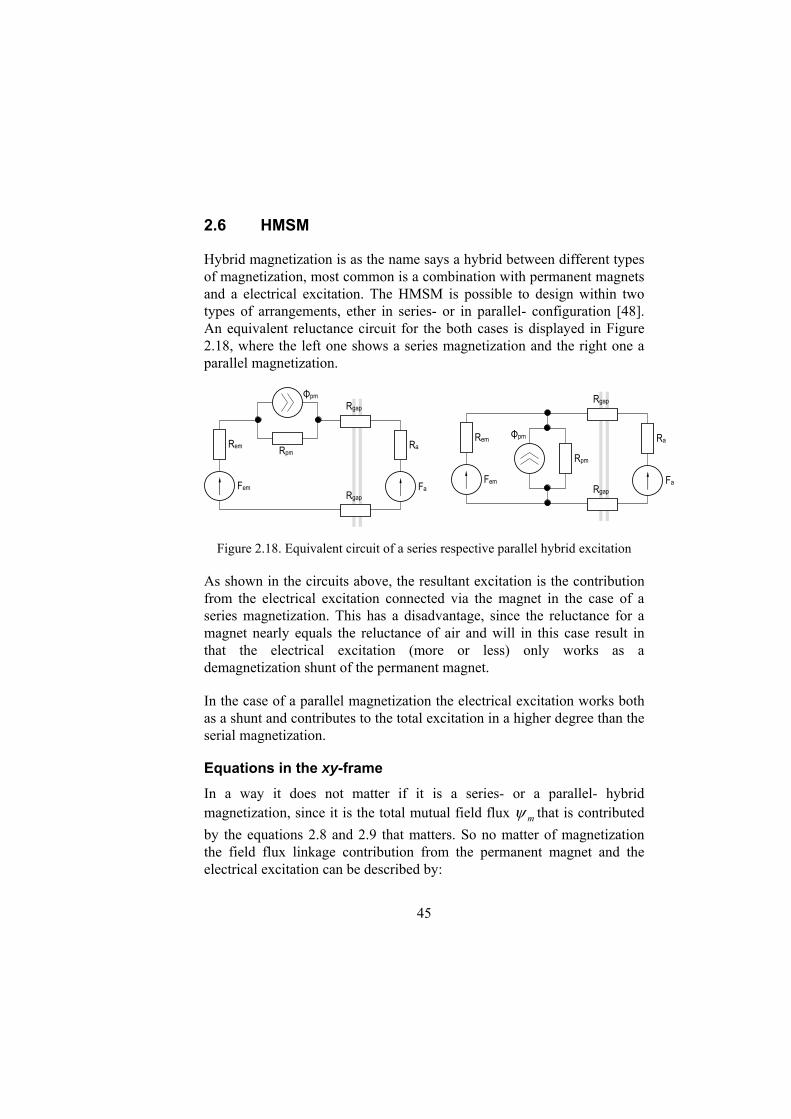
Hybrid magnetization is as the name says a hybrid between different types of magnetization, most common is a combination with permanent magnets and a electrical excitation. The HMSM is possible to design within two types of arrangements, ether in series- or in parallel- configuration [48]. An equivalent reluctance circuit for the both cases is displayed in Figure 2.18, where the left one shows a series magnetization and the right one a parallel magnetization.

Φpm Rgap

Rgap Fem

Rem

Fa

Ra Rpm

Φpm

Rgap

Rgap Fem

Rem

Fa

Ra

Rpm

Figure 2.18. Equivalent circuit of a series respective parallel hybrid excitation

As shown in the circuits above, the resultant excitation is the contribution from the electrical excitation connected via the magnet in the case of a series magnetization. This has a disadvantage, since the reluctance for a magnet nearly equals the reluctance of air and will in this case result in that the electrical excitation (more or less) only works as a demagnetization shunt of the permanent magnet.

In the case of a parallel magnetization the electrical excitation works both as a shunt and contributes to the total excitation in a higher degree than the serial magnetization.

Equations in the xy-frame In a way it does not matter if it is a series- or a parallel- hybrid magnetization, since it is the total mutual field flux m that is contributed

by the equations 2.8 and 2.9 that matters. So no matter of magnetization the field flux linkage contribution from the permanent magnet and the electrical excitation can be described by:

46

empmm (2.25)

Where pm and em are the mutual field flux from the permanent magnet

and the electrical excitation respectively. The relation between the mutual flux from the magnets and the maximum field flux can be seen as a hybridization ratio [48].

maxmax fmfpm

pm

m

pm

iL

(2.26)

The electrical excitation flux linkage em is replaced by the corresponding

excitation current fi and the inductance mfL .

Characteristics The characteristic of the HMSM is as well as the excitation a combination of a PMSM and an EMSM. It can be seen as a PMSM that has a possibility to shunt the magnetization or as an EMSM provided with an offset of the magnetization. In this section, as in the previous sections for the other machines, the characteristics are based on no losses and no saturation.

Figure 2.19 shows the voltage ellipse characteristics of the HMSM. The three different magnetization cases correspond to three different combinations of excitation current. The fundament is a PM magnetization of 1.5 p.u. (blue solid line). This corresponds to a zero field current which means that the mutual field flux only corresponds to the permanent magnets pmm . Consequently the machine is running as a PMSM with

a permanet magnetization of 1.5 p.u. The magnetization of 2 p.u. (red dashed line) and 1 p.u. (green dashed line) in Figure 2.19 corresponds to the case where the field current is positive and negative respectively. This gives a field enhancing and a field weakening respectively. In the case of a positive excitation current the mutual field flux is a contribution of both the permanent magnet and a positive electrical excitation. When the field current is negative the mutual field flux are decreased with the one corresponded to the electrical excitation.

47

-2.5 -2 -1.5 -1 -0.5 00

0.2

0.4

0.6

0.8

1

1.2

1.4

1.6

1.8

2

isx

p.u.

i sy p

.u.

m = 1.5pm

+ 0.5em = 2 p.u.

m = 1.5pm

+ 0em = 1.5 p.u.

m = 1.5pm

- 0.5em = 1 p.u.

Figure 2.19. HMSM voltage ellipses at different magnetization field winding

excitation and α=0.75

As one can see in the figure the center point of the voltage-limit ellipse has the possibility to be controlled by the field current. In this case the mutual field flux is the contribution from the permanent magnet and electric excitation a distribution of 1.5 p.u. and 0.5 p.u. respectively, which makes it possible to work within 1 to 2 p.u. in total excitation flux linkage.

The constant torque lines in the xy-frame are presented in Figure 2.20, where lines are with equidistant values and are the same in all three cases. It is obvious that the torque is connected to the field current as well. As the figure shows, a certain torque are achieved with different armature currents for the three cases, i.e. for a positive and a negative field current it requires less respective higher armature current to reach the torque as the fundamental one.

48

-1.5 -1 -0.5 0 0.5 1 1.50

0.5

1

1.5

i sy p

.u.

isx

p.u.

m = 1.5pm

+ 0.5em = 2 p.u.

m = 1.5pm

+ 0em = 1.5 p.u.

m = 1.5pm

- 0.5em = 1 p.u.

Figure 2.20. HMSM constant torque lines at different magnetization field winding

excitation and α=0.75

The difference between the constant torque lines, between the three cases, increases with a higher order of torque i.e. the slope of the torque as a function of the current is steeper with higher magnetization.

Figure 2.21 show the torque versus speed characteristics of the HMSM. The three colors, red, blue and green corresponds to respective case of the field winding excitation above. With the possibility to change the excitation it is possible to achieve a combination of the two PMSM characteristics shown in Figure 2.6. i.e. both the high torque characteristic and the high speed characteristic. In the beginning at cranking and at low speed the machine runs with full magnetization (red line), when the speed reduces to the lower speed where less magnetization results into higher torque it is possible to decrease the magnetization current (blue line) and in the end at high speed drive it is possible to run with minimum magnetization (green line).

Worth noticing is that the HMSM can be optimized for different applications. When the electrical excitation is zero there is no power loss in the field winding which results in a higher efficiency at these regions. In

49

the case where the machine works in a narrow speed range most of the time it is beneficial to design the machine such that the fundamental PM magnetization is enough in that speed.

0 1 2 3 4 5 6 70

0.5

1

1.5

2

Tor

que

p.u.

Speed p.u.

m = 1.5pm

+ 0.5em = 2 p.u.

m = 1.5pm

+ 0em = 1.5 p.u.

m = 1.5pm

- 0.5em = 1 p.u.

Figure 2.21. HMSM torque vs speed characteristics

The advantage of a HMSM compared to the PMSM and the EMSM is that it is possible to achieve relatively high power density like in the PMSM, which normally is difficult to achieve with the EMSM due to the limitation in field current, but have the EMSMs possibility to high speed operation.

2.7 Summary

The benefits with the different machines topologies discussed above, in a BAS application, are not obvious to see. The reasons are that a BAS application requires two outer boundaries in the specification of the performance. It needs a high cranking torque in a low temperature condition and must be able to run at a high speed and still provide power conversion. For the high cranking situation the torque is an intermittent torque where the heat situation is totally different to the nominal drive. This makes it possible to run the machine in a temporary overload before the system reaches the temperature limit. The maximum speed sets the

50

limitation of the permanent magnetisation which is uncontrollable in the PMSM case. But it is possible in the other three topologies, even if it is limited for the HMSM.

A comparison of the different machine topologies, with assumed boundaries, is presented in Figure 2.22. The normalized parameter is the same as the ones in previous sections and the criteria of BAS application follows the specification in chapter 1. This gives a minimum field weakening ratio of 6 and the cranking torque to 3.5 times the nominal torque.

0 1 2 3 4 5 6 7 8 9 100

0.2

0.4

0.6

0.8

1

1.2

1.4

1.6

1.8

2

Tor

que

p.u.

Speed p.u.

PM: normalized

PM: Lsy=2 p.u.

PM: pm=1.1667 p.u.

EMSM: em=1.5 p.u.

EMSM: em=0.5 p.u.

SMSM: em=1.5 p.u.

HMSM: pm=1.5 p.u., =0.75

Figure 2.22. Machine comparison on nominal torque vs speed characteristic

The black line in Figure 2.22 corresponds to the normalized PM-machine which has a permanent magnetization of 1 p.u. and the saliency ratio of 1. Since the pm magnetization is 1 p.u., which means that the centre of the voltage-limit lines lies on the maximum current line, the maximum speed is infinity. The jade colored line is for a PM configuration with 1 p.u. in magnetization and a saliency ratio of 2. An inductance of 2 p.u. is in this section set as an upper boundary of the inductance. To achieve higher saliency ratio then 2, for the PM machine, it requires that the x-directed

51

inductance decreases. This has a negative effect on the field weakening possibility. Since a saliency ratio greater than one is possible in all the compared machine topologies, it will be omitted in all other configurations than this.

The light green dotted line in Figure 2.22 is a PMSM with a PM magnetization of 1.1667, which is the maximum PM magnetization to have a field weakening ratio greater than 6. The maximum magnetizations expressed in equation 2.13, and with the normalized values it gives:

1667.116/1max,max

max,max sxsx

sm iL

u

(2.27)

A higher magnetization in the PM configuration results to machine with less field weakening ratio then this BAS specification.

The excitation flux linkage limitation of an EMSM, and a SMSM, is related to capability of heat dissipation of the excitation winding. To cover this in the comparison, the boundary condition is set to 0.5 and 1.5 p.u., represented as low and high heat dissipation respectively. The light red and dark red lines in Figure 2.22 shows the EMSM with respective boundary condition. As one can see in the figure reaches the EMSM with a field winding excitation of 0.5 p.u. only to the half of the reference torque, but the one with 1.5 p.u. to 1.5 of the reference torque.

The SMSM with a maximum field winding excitation of 1.5 p.u. is represented by the light blue dotted line, as one can see is the slope steeper in the field weakening region than in the EMSM case. This is related to coupling between the excitation- and the armature- current. In a case where the maximum field strength is equal or below 1 p.u. the torque versus speed characteristics is the same for both the SMSM and EMSM.

The last machine topology presented in Figure 2.22 is the HMSM, which characteristic corresponds to the brown dashed line in the figure. It is for a HMSM with an excitation level of 1.5 and 0.5 p.u. balanced between the permanent magnet and electric excitation respectively, i.e. hybridization ratio α=0.75. The HMSM has the highest base torque and also the possibility to field weakening to an infinity speed.

52

The power versus speed characteristics for the different machine configurations is displayed in Figure 2.23. It is possible to see that the PMSM with 1,1667 p.u. and the SMSM with 1.5 p.u. in the maximum field winding excitation only provides a peak in the maximum power decreasing with speed in field weakening when the others are able to keep it constant. Even if the EMSM only contributes to maximum power after the maximum speed is reached.

0 1 2 3 4 5 6 7 8 9 100

0.2

0.4

0.6

0.8

1

Pow

er p

.u.

Speed p.u.

PM: normalized

PM: Lsy=2 p.u.

PM: pm=1.1667 p.u.

EMSM: em=1.5 p.u.

EMSM: em=0.5 p.u.

SMSM: em=1.5 p.u.

HMSM: pm=1.5 p.u., =0.75

Figure 2.23. Machine comparison on nominal power vs speed characteristic

The different machine topologies have different capabilities to a cranking torque with a boost of the current. Due to the possibility of boosting both the excitation and the armature current, there is an advantage to boost the torque in a HMSM, EMSM and SMSM in comparison to the PMSM. Table 2.2 contains the torque capability of the different topologies, with the same configurations as discussed above. The table contains the base torque Tb held with a nominal current, the cranking torque Tc held with twice the nominal current and the last column the needed current to achieve the cranking torque of 3.5. p.u.

The EMSM with a field winding excitation of 1.5 p.u. is the one that can

53

achieve the highest cranking torque with twice the nominal current, but has nearly the same required current to fulfill the cranking torque of 3.5. in comparison to the HMSM. A pure PMSM without any reluctance torque is the least appropriated configuration in this application.

Table 2.2 Torque capability

Tb Tc with 2xIsmax Ic at Tc=3.5 p.u.

PM: normalized 1 2 3.5

PM: Lsy=2p.u. 1.299 3.52 1.99

PM: m =1.1667 p.u. 1.1667 2.33 3

EMSM: em =1.5 p.u. 1.5 6 1.53

EMSM: em =0.5 p.u. 0.5 2 2.65

SMSM: em =1.5 p.u. 1.5 6 1.53

SMSM: em =1p.u. 1 4 1.87

HMSM: pm =1.5 p.u. α=0.75 2 5 1.54

The aspects of losses and saturations which are neglected in this chapter plays a significant role in the selection process of which one that are the most convenient one in a BAS application. This is further investigated in chapter 4 where a comparison, considering the losses and saturations, between the PMSM, SMSM and EMSM is presented.

54

Chapter 3 Analysis of an alternator

In this chapter an alternator is analyzed with respect to different physical properties, like losses and performance. The losses are separated in to three main types, mechanical losses, electrical losses and magnetical losses, indicating the origin of the losses.

3.1 Reference Alternator

The alternator used as a reference, in this chapter, is a common Lundell alternator used in a Swedish Long Haul truck. It has a rated charging capacity of 3kW. The nominal output voltage and current is rated to 28V DC and 110A respectively. It consists of a delta connected three phase claw pole machine rectified via a full bridge diode rectifier. A circuit schematic is illustrated in Figure 3.1.

Figure 3.1. Circuit diagram of the alternator.

55

3.2 Mechanical losses

Mechanical losses are the losses that appear when the rotor is rotating, and they are by nature related to the speed. The mechanical losses consists mainly of

Ventilation losses

Bearing losses

Slip-ring losses

The ventilation losses represent air friction and originate from both the mounted cooling fan blades and the rotor structure itself. The contribution from the rotor structure is not considered in this thesis.

Fan blade calculations The air stream around the end turns of the stator windings, of the alternator, is created by the fan blades that are attached to the ends of the rotor. It consists of 12 blades on each side of the rotor; one side is pictured in Figure 3.3. The picture also includes lines made in Matlab, this to support the measuring of the physical dimensions of the blades. The fan can be classified as a centrifugal fan, which means that the air flow enters in an axial direction into the centre and passes over the blades before the exit in a radial direction. Fan losses originate from the drag force cased by frictions of the fluid, the fluid acceleration and the pressure change of the fluid. This section will neglect the drag force made by friction losses.

To calculate the performance of a centrifugal fan, such as outlet velocity of a fluid and the required shaft torque, the fluid movement is separated into two movements. The fluid has a rotational movement as well as a movement along the blade [24][25]. This is illustrated in Figure 3.2.a.

56

Figure 3.2. a) Velocity vectors. b) Arbitrary pipe

The velocity in the tangential direction of the fan blade has prefix and the the velocity in the radial direction index . The absolute velocity of the fluid, presented as v, is achieved by a vector summation of the both velocity vectors. A specific rotational speed of the blade requires a specific torque on the shaft that depends on both the change in velocity v and the change in pressure along the blade.

To calculate the torque created by a fluid flow across an arbitrary pipe attached to point C, illustrated in Figure 3.2.b, it is possible to use the geometry of the entrance and the exit of the pipe [24][25]. The force at the inlet and the outlet, projected to respective plane perpendicular to the centum axel, multiplied to respective radius gives the torque in point C.

2 2 2 1 1 1 1 1 1 1 2 2 2 2( cos cos ) ( cos cos )T m r v r v A p r A p r (3.1)

Where m is the mass flow rate of the fluid, which are equal for both the inlet and the outlet of the arbitrary pipe. In the equation the prefix 1 and 2 represent the inlet and the outlet. The other terms in the equation are r for the radius, v for the fluid velocity, p for the pressure and A for the cross section area. This equation is applicable on a fan blade as well and since the fan blades normally are placed so that the pressure vectors, at the inlet and the outlet, points through the centre of the shaft axel the second part in the equation is equal to zero. A reduction of equation 3.1 and a multiplication of the angular speed give an expression for the fan blade

57

power.

2 2 2 1 1 1( cos cos )P m r v rv (3.2)

The total power required for running a centrifugal fan, is the sum of the required power for each blade.

The equations for the velocities w respective u, is derived from the equations for respective movement. In the rotational direction at a certain radius the expression in the xy- coordinates are:

cos( )

sin( )

x r

y r

(3.3)

Where θ is the angle, which references to the x-axis and are positive in a counterclockwise direction. The velocities in the x- and y- directions are achieved as the time derivate of the movement equations. This gives the velocity as a function of the angular speed:

2 2

sin( )

cos( )

x

y

x y

dx dx du r

dt d dtdy dy d

u rdt d dt

u u u

(3.4)

To get the velocity vector along the fan blade, we do exactly the same procedure. Since a fan blade of the alternator is formed straight and tilted with a certain attack angle, see Figure 3.3, the movement equation in xy- coordinates is represented as:

r x

r y

x a c

y b c

(3.5)

58

Where a, b and c are constants and θr is the reverse angel compare to θ. θr is positive in a clockwise direction, this due to the relative movement in the opposite direction compare to the angular speed .

2 2 1 1

2 1

2 2 1 1

2 1

2 2

cos( ) cos( )

sin( ) sin( )

r rx

r r r

r ry

r r r

x y

r rdxw

d

r rdyw

d

w w w

(3.6)

To estimate the total amount of power, all the fan blades, with their configuration of length and attack angle, is measured and calculated. The specific blade dimensions for each of the twelve blades are listed in Table 3.1. The blade angle is the difference between the inlet and the outlet angle of the fane blade and is presented as θ2 - θ1 in the table. The inlet radius Rin of the fan blades vary from blade to blade, where the outer radius of the blades is the same. The inlet area Ain uses for calculating the mass flow rate.

With these dimensions and the solutions of the equations above a theoretical result compared to an experimental work is plotted in Figure 3.4. The measurements are made with the alternator as load, connected via a torque sensor to second machine. To avoid any kind of circulating currents, the diode rectifier is disconnected and the phase windings are unleashed from the delta connection. The alternator phases are connected to an oscilloscope, and with help of a negative excitation current the remanence is demagnetized to zero. The torque is measured at seven different speeds.

Due to a limitation in speed with the driving machine in the laboratory setup, it is only possible to measure up to a speed of 6000 rpm. The measured values are plotted as blue dots and the blue dashed line represent the result of a polynomial coefficients cubic spline interpolation of these values. The calculated fan losses are in the figure represented by the black solid line.

59

As shown in figure 3.4, the theoretical values are slightly lower than the measured ones. This is expected since all mechanical losses are not considered in the theoretical part. Examples are the bearing losses but also the fan losses created by the rotor geometry it self, which probably are the most significant parts of the difference in figure 3.4.

Figure 3.3. Picture and measuring lines of the fan blades

Table 3.1 Blade dimensions, radius R [mm], area A [mm2] and angle θ [deg]

Fb1 Fb2 Fb3 Fb4 Fb5 Fb6

θ2- θ1 14 14 14 14 13 9

Rin 35.2 35.2 35.2 35.2 36.8 39.9

Ain 284.0 309.9 309.9 309.9 278.7 331.7

Fb7 Fb8 Fb9 Fb10 Fb11 Fb12

θ2- θ1 12 12 11 11 11 11

Rin 37.6 36.8 37.6 37.6 37.6 37.6

Ain 247.9 260.7 238.7 220.3 220.3 220.3

60

Figure 3.4. Calculated fan losses and measured mechanical losses

Slip rings The slip ring unit consists of two main parts, where one is a rotating sliding surface also called the ring and the other a brush resting on the ring with a certain amount of pressure. Both the rings and the brushes are available in different materials for different applications and operating conditions. In the current alternator the slip ring unit consists of two copper rings with a graphite brush each. This thesis will only consider this setup of slip ring unit.

Then slip ring has a rather complex operating state. Example of phenomenon that appear in the slip ring units physicals properties is tunnel effects, connection resistance, electrical breakdown of oxidation and water films[27][28]. The losses are due to both the mechanical losses, frictional losses, and the excitation losses. It is categorized in both this section 3.2 and the next section 3.3. The mechanical frictional losses emanates from on the friction between the ring and the brush. This is expressed with equation 3.7.

61

2ms nP n p A v (3.7)

In the equation, n is the number of brushes per ring, μ the friction coefficient, v the peripheral velocity on the ring, pn the attached pressure on the brush and A the brush area. The friction coefficient is in the range of 0.1 – 0.2 [28] for a graphite and copper unit, in the current size. This varying in range is due to environmental conditions, and a thin water film which normally occurs at the surface of the copper rings [27].

The copper rings of the unit have a diameter dring and a force Fbrush that are applied on the brushes which makes it possible to rewrite equation 3.7 to:

2

2 ringbrushms

dFP (3.8)

The connection between the ring surface and the brush is located to a number of microscopic spots, also called a-spots [27]. Those are in the beginning or after a stop covered via a thin layer of oxides on the ring. This oxide layer has an electrical breakdown, fritting, at a voltage of approximately 106 V/cm [26]. Due to the physically small size of the a-spot area, there is in the reality a voltage approximately around 0.3 V over the whole brush. The fritting process creates a metallic connection at the a-spots and results in that the resistance decreases about 90%. When the current increases the metallic connection also increases. This makes the resistivity of the slip ring unit becomes non-linear, e.g. the resistance decreases with an increase of the current. When the slip ring rotates, not in dry air or with high currents, a thin film of water occurs which leads to an increase of the voltage drop over the contact between the ring and the brush.

If we consider a rotating unit in a conducting state within normal conditions of humidity and currents, due to all physical effects mentioned above, a constant voltage drop over the surface is assumed. With this assumption, and including the resistivity of the brush, an equation of the electrical losses of the slip ring unit is described by:

bbbdes IIRVP )(2 (3.9)

62

Where dV is the voltage drop over one brush, bR the resistance of the brush

and bIbI the current through the brush. The factor two in both equation

3.7 and 3.9 represents the two brushes in one unit.

Figure 3.5 shows the mechanical losses Pms and the electrical losses Pes for the slip ring unit regarded in the equations and assumptions above.

0 2000 4000 6000 8000 10000 12000 14000 16000 180000

5

10

15

20

25

Loss

es [

W]

Speed [RPM]

P

ms

Pes

Pms

+Pes

Figure 3.5. Slip ring losses as a function of rotational speed with constant current

The copper rings has a diameter of 13.45mm, the brushes has an area of 24mm2 and a length of 25 mm. The resistivity of the brushes and the average voltage drop are 25 μΩm and 1.7 V respectively, where the voltage drop is over both surfaces and the values is picked from a manufacturers data table [28] of a corresponding slip ring unit. The measured force on one brush is 2.94N and the used values for the friction coefficient and the brush current are 0.2 and 2.5A respectively.

Bearings The losses of a ball bearing depends on several factors such as the type of

63

bearing, if it is a deep groove ball bearing, angular contact or needle roller bearings etcetera. The losses are also affected by the size of the bearing, the lubrication and not at least the rotational speed [28]. In high rotational speeds sliding effects, gyroscopically and centrifugal momentum effects starts to play a significant role of the losses as well. Many bearing manufactures have empirical built equations and constants to express the losses for a specific type of a bearing in a certain dimension and speed. The bearing losses are described with the equation 3.10, [30][31]:

310)( dsealsrrrsishb TTTTP (3.10)

Trr is the rolling friction torque, Ts is the sliding friction , Tseal is the seal frictions torque and Td the frictions torque cased by drag losses in a oil bath lubrication.

The two bearings in the present alternator consist of sealed and grease lubricated single row groove ball bearings. This means that the friction torque cased by drag losses in a oil bath lubrications, Td, is equal to zero in equation 3.10.

The magnitudes and units for all constants and symbols in the equations concerning the bearings in this section are listed in Table 3.2. The equations will consistently in this section be valid for a bearing type of single row groove ball bearings and with load in only a radial direction. This means that the load in an axial direction is neglected and will be set to zero.

Rolling friction

The rolling friction torque depends on the load of the bearing, i.e. the acting force in both radial Fr and axial Fa directions, the viscosity v of the lubrication and the type and the dimension of the bearing. The equation for the rolling friction moment, when Fa = 0, is:

6.054.096.11 )( nvFdRT rmrr (3.11)

where R1 is a geometry constant, dm the mean diameter of the inner diameter d and the outer diameter D and the rotational speed n of the

64

bearing.

As shown in the equation 3.10 the rolling friction torque Trr is scaled by the two factors ϕish and ϕrs. Those factors are due to the inlet shear heating and kinematic replenishment of the lubrication, [30], and will not be discussed in this thesis. The equations are:

64.028.19 )(1084.11

1

vdn mish (3.12)

Respective:

)(2

)(

1

dD

KdDnvK

rsZ

rs

e

(3.13)

Krs is the replenishment constant depending on the lubrication and Kz a constant depending on the geometry. The replenishment constant for grease lubrication is 6·10-8.

Sliding friction

The movement of the balls, in a ball bearing, that consists of sliding instead of rolling creates as the name says sliding frictions. These effect is relative small in the bearings used in the alternator, it is in a order of about a half percent of the total losses. The equation for the sliding friction torque is:

3/526.0

1 rmss FdST (3.14)

where S1 is a geometry related constant and μs is the sliding friction coefficient.

Seal friction

The seal frictions are due to the friction in the contact spot between the not rotating seal and the rotating part of the bearing. It is in this case, for the alternator, the losses that has the highest impact of the bearing losses. The

65

equation for the seal friction moment is:

21 SsSseal KdKT (3.15)

where KS1 and KS2 are constants depending on the bearing type and seal type respectively, ds is the counter face diameter of the seal and β an exponent depending on both the seal type and the bearing type.

Calculations

The losses calculations are done by the equations above and multiplied by the angular speed to get the losses. All data are listed in Table 3.2 and the used viscosity is 20 mm2/s. The result is presented in Figure 3.6 and consists of the losses for respective bearing and the total losses.

Table 3.2 Bearing data, bearing 1 (B1) and bearing 2 (B2)

1R md rF ZK s 1S 1SK 2SK sd

B1 4.1e-7 26 100 3.1 0.05 0.00373 0.028 2 23 2,25

B2 3.7e-7 32 100 3.1 0.05 0.00284 0.023 2 26.5 2,25

Unit mm N mm

The total bearing losses at 3000 rpm is around 25W which matches the measured losses presented both in Figure 3.4 and Figure 6-7. The losses in Figure 3.4 is for the claw-pole alternator rotor with fan blades where the difference between the measurements and the calculated fan losses depends on the bearing losses, mechanical slip ring losses and the drag force of the rotor claws. In Figure 6-7 the dynamic measurements are done on another rotor, without fan blades and slip rings but with the same bearings, so the difference is only due to the rotor drag force.

66

0 1000 2000 3000 4000 5000 6000 7000 8000 90000

10

20

30

40

50

60

70

Loss

es [

W]

Speed [RPM]

Pb1

Pb2

Pb1

+Pb1

Figure 3.6. Bearing losses versus speed

3.3 Electrical and magneto static losses

Winding losses For electrical machines where the magnetic flux mainly flows in the iron material, without leaking too much of its flux through the winding, the winding losses dominates the resistive losses. Magnetic flux that alternates through the windings creates eddy currents which give rise to unwanted losses in the windings. This is not so common in well designed machines built with laminated steel cores that has a high permeability and are god conductors of a magnetic flux. In machines built with lower permeability materials this eddy currents can be significant.

Resistive losses depends on the current i through a winding with a certain length l, cross section area A and the resistivity ρ of the winding material.

22 iA

liRP (3.16)

67

The resistivity has a relation to the thermal state of the material and will vary at different temperatures. It depends on temperature as presented in equation 3.17.

201)( 20 TkT (3.17)

ρ20 is the resistivity of the material at a homogenous temperature of 20oC, kρ a temperature coefficient and T the homogenous temperature of the material in degree of Celsius. The resistivity of copper is 17.5 nΩm and the temperature coefficient is 0.0040. A temperature rise of 100 oC thus increases the copper conductor losses by 39 %.

Resistive measurements

Measurements of the winding resistance are made, both for the excitation winding in the rotor and for the stator windings, by a 4-wire method to achieve as accurate results as possible, since the stator resistance is

relatively low. The measurements are made at a temperature of 22 Co . The result is presented in Table 3.3

Table 3.3 Winding data, for the three stator windings and the rotor winding

saR sbR scR fR

Resistance [ ] 0.093 0.093 0.092 8.51

Area [mm2] 2.4 2.4 2.4 0.28

Length (calculated) [m] 13.18 13.18 13.04 142

The area of the windings is calculated from the measured conductor diameter, with a calliper. The length of the winding is calculated as a function of the resistivity and its dependency of the temperature in equation 3.16 and 3.17.

Phase currents

To calculate the winding losses, it is necessary to know the currents in the windings. The excitation current can be seen as a pure DC current supplied

68

from the excitation controller, which is attached to the alternator and control the rectified DC voltage to 28V. The conducting state of a diode rectifier is strongly dependent on both the source and its load [21]. In this case it is a machine as source and is connected to a battery which is in parallel to the load. It is of interest to look at the nominal operation of the alternator, where the output of rectifier is a DC -current and -voltage with values of 110A and 28V respectively.

Due to the relative high stator inductance and the high frequency of the alternator the stator currents tends to be close to sinusoidal waveforms. In Figure 3.7 the result of an LT Spice simulation of the line currents of the alternator, including the three phase diode rectifier, in nominal drive at 3000 rpm is presented. This results is in line with Vlado Ostovic results in "A Magnetic-Equivalent-Circuit-Based Performance Computation of a Lundell Alternator”[34].

0.025 0.026 0.027 0.028 0.029 0.03 0.031-150

-100

-50

0

50

100

150

Time [s]

Cur

rent

[A

]

idc

iL1

iL2

iL3

Figure 3.7. Line current and DC current in LtSpice

With these assumptions, that the line currents are sinusoidal, the mean value of the output DC current can be obtained from the mean value of an arbitrary line current integrated over one sixth of a full period.

69

LLdc idii ˆ3)cos(ˆ3 6

6

(3.18)

With the relation between the line current and the phase current, in a delta- connection, the phase current is expressed as a function of the mean DC current as:

dcL

Ph ii

i 333

ˆˆ

(3.19)

With a mean value of 110A as the DC current, the equation gives the peak phase current to 66.5A.

Losses and distribution

With respect to the resistance measured and presented above, the resistive losses are calculated. The current in the stator windings, by the specification of the alternator, has a nominal peak value of 66.5A and the excitation current is 2.5A. This means that the winding losses in the stator are:

2

20 2

ˆ2013

sw

cucusw

swscu

ITk

A

lP (3.20)

and the winding losses in the rotor by:

220 201 fwcucu

fw

fwfcu ITk

A

lP (3.21)

where the index sw and fw indexes the stator and the rotor winding respectively.

The winding temperature is varying dependent on the load of the alternator as well as the ambient temperature and the speed of the alternator. The speed of the alternator and the ambient temperature are the fundamentals

70

of the cooling condition that is discussed in section 3.4. To classify a certain alternator installed into a vehicle, with full warranty from the alternator manufacture, the vehicle manufacture has to run it in full load, i.e. installed into present vehicle and driving it in a rolling road simulator during under maximum conditions and full electric load of the alternator. Under those conditions the winding temperature in the stator can reach a temperature of 220oC [57]. Figure 3.8 shows the resistive winding losses in a temperature range between 0 oC and 200 oC with the nominal current.

0 20 40 60 80 100 120 140 160 180 2000

200

400

600

800

1000

1200

Temperature T [oC]

Cup

per

loss

es P

[W]

Pscu

Pfcu

Figure 3.8. Resistive winding losses in stator respective rotor at nominal stator current as a function of temperature

The part of the stator windings that contributes to the force action, i.e. the active part that is in stator stack, is the lesser part of the total winding. One stator winding with a length of 13.18 m runs in 12 slots with 11 turns. With a stator stack length of 36mm this means that 4.75m, or 36 %, of the winding is active and the rest of the winding consists of end turns. This in turn means that 36 percent of the winding losses are related to the active part of the winding and 64 percent of the losses to the end turns of the stator windings.

71

Iron losses The iron losses of a material can be divided into three types of losses I) the hysteresis losses, II) the eddy current losses and III) the anomalous losses respectively [32][33]. The hysteresis losses are due to, as the name implies, magnetic hysteresis of the material which simplified can be explained as the energy lost when remagnetizing the core material. Thus the hysteresis losses are proportional to the area of the hysteresis loop. An example of a hysteresis loop presented as a BH-curve, for steel material ss-1650, is shown in Figure 6-6a. The hysteresis losses are:

dfVPH (3.22)

Where V is the volume [m3], f the flux change frequency [Hz], H the field intensity [Am].

The eddy current losses; resistive losses in the material resulting from circulating induced eddy currents. Those eddy currents arise as a result of a fluctuation in the magnetic field of the material, sized to keep the magnetic field derivative zero. This is due to the Faradays law of induction.

c A

dAdt

dEdl (3.23)

Where E is the electric field [V/m]. Based on the resistive losses and the current density J, due to the electric field and the resistivity, it is possible to achieve an expression of the eddy current losses. The resistive losses and the current density are expressed as:

2iA

lP ,

E

J

This gives the eddy current losses as a function of the electric field:

2EVPE (3.24)

72

where is the resistivity [ m ].

The iron loss that consists of anomalous losses is the most complex losses phenomena in the material. It is not explained in this thesis, but the anomalous losses is related to a change in the domain walls of the material, and can be calculated by losses separation [32][33].

Since the rotor parts are used as a magnetic DC- circuit, the iron losses consist only of eddy current losses. Those occurs when the rotor claws passes the stator teeth at some speed. The flux density is increased at the rotor claw area where one stator tooth is placed at the moment. This since the tooth is linking the flux in a better way then the air in between the teeth. This means that the flux in the claw, near the surface, is varying when the claw passes the stator teeth and eddy current occur.

Simulations

The simulations are based on numerical finite element (FE) calculations in the software Maxwell 3d. The analysis is magnetic transient calculations in a time domain equal to a rotor rotation of 60 steps at one degree each. The iron losses are separated into rotor and stator losses respectively and use two different solvers. Since the iron losses in the rotor is due to eddy currents these are calculated by the Maxwell's built in eddy current solver. The iron losses in the stator use Maxwell's core losses solver, based on Steinmetz equations [42]. Figure 3.9 shows the Maxwell FE-model used to calculate the iron losses.

The armature and excitation current in the simulations corresponds to the nominal currents and the load angle is 90 deg. The rotor material in the model is steel 1008 and the stator material is laminated carbon steel based on Surahammars M600-100A1N, which have a thickness of 1mm.

73

Figure 3.9. FE-model in Maxwell 3d.

Numerically calculated iron losses, separated into stator losses and rotor losses, for the present alternator are presented in Figure 3.10 down below. As one can see the stator losses are about twice as big as the rotor losses. This is in line with other published results on iron losses in a Lundell alternator, [35] [36].

74

1500 2000 2500 3000 3500 4000 4500 5000 5500 60000

100

200

300

400

500

600

700

800

Fe

Loss

es [

W]

Speed [RPM]

Protor

Pstator

Figure 3.10. Calculated iron losses versus speed, with nominal current.

Rectifier losses A relatively high proportion of the total losses of an alternator are located in the three phase diode rectifier, which purpose is to establish a DC current to the battery. The reason is that an alternator in a vehicle is manufactured for a low voltage relatively to the amount of power. This makes the armature current unproportionally high.

During the operation for the rectifier there are two or three diodes, of six, conducting at the same time. In the reference alternator due to the relatively high inductance in the stator windings, mentioned in the previous section, there are three diodes conducting at the same time at a nominal drive situation. The losses for one diode during one period is related to the RMS value for the line current in half of the period and zero in the second half of the period. In the second half period, the losses are distributed to the opposite diode for the present phase. This means that the losses for one pair of the diodes are equal to the voltage drop of one diode multiplied with the RMS value of the line current. This is only true with the assumption above and if the switching loss of the diode is neglected.

75

The total diode losses of the whole rectifier are in this case three times higher, since there is three pair of diodes:

2

ˆ

2

ˆ3 LL

dddiod

iiRVP

(3.25)

where Vd is the intrinsic voltage drop of the diode and Rd the resistance of the diode.

The total voltage drop of one diode, according to the manufactures data sheet, is 1.1 V with 100 A at 25 oC. Unfortunately the intrinsic voltage drop and the diode resistance are not separated in the data sheet, but with the assumption that the intrinsic voltage drop Vd is approximately 0.6V the diode resistance is Rd = 5mΩ.

With those values inserted into the equation 3.25 above results in a total diode loss of 246 W of the three phase rectifier.

The temperature coefficient for a semiconductor is dependent on the forward current [38]. It is negative for a low current and positive for a high current. This means that it could be hard to estimate the temperature dependency of the losses in a diode.

3.4 Thermal

The thermal behaviour of a machine is set by its ability to heat dissipation and the related thermal conductivity of the machine parts. Heat dissipations appear in three forms, one as the conduction of the cooling medium, the second as the convections at the surface and the third as radiation. Which one that dominates depends on the machine construction. In this case, where the machine is a common Lundell alternator, the heat dissipation is dominated by convection. This since the cooling system of the alternator is based on a forced convection with air, which is provided by the airstream created by the fan blades discussed in section 3.2. The dissipation by radiation in the alternator are less than 1% of the total heat dissipation in its working range, and thus the radiation is neglected in this thesis and in the thermal model of the alternator discussed in this chapter.

Most of the heat in the alternator is crated by the losses in the stator windings and the stator iron losses, which are declared in the sections

76

above. The heat generated by the losses in the rectifier is disconnected from the rest of the alternator, this since the placement of the rectifier is outside on the relatively well cooled machine cage.

Convection The heat dissipation by forced convection is based on the heat exchange between the solid and the fluid when the fluid streams on the surface of the solid. The amount of heat dissipation depends on the velocity, the conductivity of the fluid and also the temperature difference between the fluid and the surface of the solid.

Figure 3.11. a) Fluid stream over a surface. b) Fluid velocity profile from surface. c) Fluid temperature profile from surface

Figure 3.11a) shows a fluid stream, with the fluid velocity Uf, over a surface. Figure 3.11b) and c) shows a typical velocity- and a temperature- profile of a fluid at an arbitrary point, p1, on the surface. The velocity- and the temperature- profiles describes the change in velocity respective the temperature from the surface to a distance y. The thickness of the profiles, also called the thickness of the boundary layer, is the distance from the surface where the velocity respective the temperature is 99 percent of the top layer.. The relative thickness of the temperature boundary layer to the thickness of the boundary layer of the velocity is commonly described by the dimensionless Prandtl number, Pr, named by Ludwig Prandtl. In the case where the fluid is a gas the Prandtl number is close to one, with means that the thickness of the velocity- and temperature- boundary layer is equal to each other. The boundary layer of the velocity depends on the shape and the structure of the surface and if the fluid flow is laminar or if it is turbulent. A thinner boundary layer of the velocity results to a thinner temperature boundary layer which in turn leads to a higher convection but

77

in cost of higher sheer stress and fan power.

The convection heat dissipation Qconv as a function of the average convection coefficient h and the temperature difference over an area A is:

)(. fsconv TTAhQ (3.26)

Where Ts and Tf is the temperature of the surface and the fluid respective. The convection coefficient in a specific point, as in point p1 in Figure 3.11, is related to the thickness of the boundary layer of temperature in that point. The convection coefficient is determined by the temperature gradient at the surface in that specific point, and can be expressed by:

0

yfs

f

y

T

TT

kh (3.27)

Where kf is the thermal conductivity of the fluid. The mean of the convection coefficient of a surface is reached by an integration of h over the whole surface. For complex geometries and surfaces, as in the case of electrical machines, it is impossible to do analytical calculations of the convections which exclusively have to be done by numerical calculations. To calculate the thermal behaviour of the whole machine it is necessary to make both the computational fluid dynamics (CFD) calculations and the numerical heat transfer of the machine. To achieve the most accurate result of this kind of thermal calculations it is necessary to use a full model that handle both at the same time, but it demands high computing -power and -time. This since a high number of nodes in the mesh is needed. The CFD calculations require a high resolution of the mesh especially in those regions where the velocity boundary layer is thin and so do the solid parts that consist of small details with different materials. To avoid huge meshes the model in this section consists of two separate models. One for the CFD calculations, where the boundary layer is the surface of the solid parts of the machine, and the other one for the numerical heat transfer in the machine.

78

Figure 3.12. Alternator geometry for the CFD and heat transfers analysis.

Figure 3.12 shows the geometry used for the CFD and the numerical heat transfer calculations, where the blue and the red dashed lines indicate the regions used for the CFD and the stator heat transfer model respectively. For the CFD model is an air model built with solid parts as mould, i.e. a solid of air is created where the machine solids erodes and forms the cavities in the air solid. The mesh of the CFD model is shown in Figure 3.17.

79

0 2000 4000 6000 8000 10000 12000 14000 16000 18000-20

0

20

40

60

80

100

120

Rad

ial A

ir ve

loci

ty [m

/s]

Speed [rpm]0 2000 4000 6000 8000 10000 12000 14000 16000 18000

0

0.2

0.4

0.6

0.8

1

1.2

1.4

mas

s flo

w r

ate

[kg/

s]

Figure 3.13. Calculated air velocity and the mass flow rate at the fan blade exit

Fluid dynamics In order to have the convection coefficients, for the winding end turns and the other machine parts that are affected by the air stream, it is necessary to compute the fluid dynamics of the alternator. The CFD model in this study is a static CFD model, instead of a rotating mesh for the fan blades on the rotor. A non rotating mesh is used with a radial air velocity at the inlet boundary. This is done to simplify the model further and to reduce the complexity of the mesh of the model. All calculations and simulations in this section use the properties of air at a temperature of 80 oC and assuming a laminar flow over a smooth surface.

Stator

The machine model is in this case symmetrised to one twentieth of the full machine and a cylindrical cut at a radius that corresponds to the outer radius of the fan blades. The inlet air velocity of the model is calculated from the velocity equations in section 3.2, and the result as a function of the rational speed of the rotor is presented in Figure 3.13. The figure also shows the mass flow rate of the air corresponding to the speed. To find out

80

the convection coefficients for the walls a constant surface temperature case is studied. Figure 3.14 and Figure 3.15 shows the air stream and the convection coefficients on the surfaces respectively, this at an air velocity of 25 m/s which corresponds to a rotating speed of 4386 rpm.

Figure 3.14. Inlet air stream of 25 m/s

The Blue walls in Figure 3.14 correspond to the walls of the solid parts of the machine. As one can see, the CFD model is only treating the air and the walls not the solid parts of the machine which appears as cavities in the model. The air steam is entering the bottom of model, which corresponds to the exit of the fan blades, and passes through and beside the end turns of the windings before exit of the machine house. The main part of the air stream passes the gable of the end turns and less is passed in between the stator slot exit of the windings. Despite this, the convection is relatively good due to the narrow passage that locally increases the air speed. As one can see in Figure 3.15 the convection is highest in the spot where the passage is thinnest.

81

Figure 3.15. Convection coefficients at a air velocity of 25 m/s

During the calculations, for a mean value of the convection coefficients, the surface is divided into different sectors. This to have a relatively god approximation of the differences in convection between the surfaces. The sectors are listed in Table 3.4 and the labels are shown in Figure 3.15. The result, from the CFD calculations, of the mean convection coefficients at different air speed are shown into Figure 3.16. As one can see, the slope of the mean values for the convection is relatively stable without much deflection in the most cases, with exception to the convection of the housing cage and the stator wall labelled hcs and hsw respectively. This due to the turbulences and the lack in mesh resolution at the region in the corner, label A in Figure 3.17, where the housing and the stator stack encounter each other.

One of the main struggles with CFD calculations is the mesh at the surfaces and at instable regions. Due to the relation between the

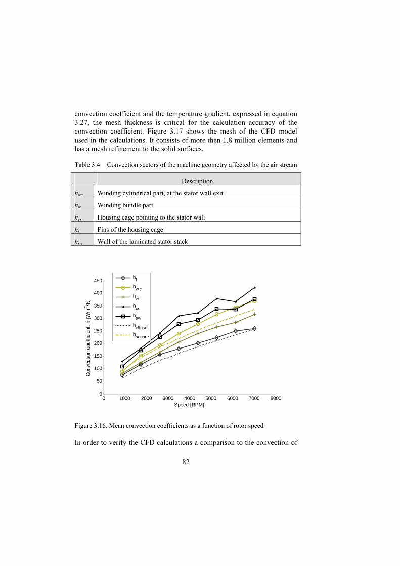
82

convection coefficient and the temperature gradient, expressed in equation 3.27, the mesh thickness is critical for the calculation accuracy of the convection coefficient. Figure 3.17 shows the mesh of the CFD model used in the calculations. It consists of more then 1.8 million elements and has a mesh refinement to the solid surfaces.

Table 3.4 Convection sectors of the machine geometry affected by the air stream

Description

hwc Winding cylindrical part, at the stator wall exit

hw Winding bundle part

hcs Housing cage pointing to the stator wall

hf Fins of the housing cage

hsw Wall of the laminated stator stack

0 1000 2000 3000 4000 5000 6000 7000 80000

50

100

150

200

250

300

350

400

450

Speed [RPM]

Con

vect

ion

coef

ficie

nt:

h [W

/m2 /K

]

h

f

hw c

hw

hcs

hsw

hellipse

hsquare

Figure 3.16. Mean convection coefficients as a function of rotor speed

In order to verify the CFD calculations a comparison to the convection of

83

known geometries in the literature [39][40], is displayed in the diagram (hellipse, hsquare, Figure 3.16). There are only two places of the alternator model that has representative structures to known and published structures. Those are the square shaped fins of the housing and the winding end turns at the exit from the stator that could by seen as an elliptic shape. The equation for the average convection coefficient of a forced convection over those shapes is:

D

kh

3/1m PrReC (3.28)

Where the k is the conductivity of the fluid, Re the Reynolds number, D the dynamic diameter, C and m constants due to the specific shape. The Reynolds number is calculated by:

v

DU Re (3.29)

Where U is the fluid velocity and v the kinematic viscosity which is expressed as the viscosity divided by the density of the fluid.

The constants C and m for a square respective an elliptic shape is presented in Table 3.5, which also tells in which range of the Reynolds number where those values are valid. Those values are developed by experimental work and where the forced convection is by a gas.

Table 3.5 Empirical correlation constants

C m Range of Re

Square shape 0.248 0.612 5000 - 100000

Elliptic shape 0.102 0.675 2500 - 15000

The calculated result of the convection coefficient using the constants in Table 3.5 is presented by dotted lines in Figure 3.16. As one can se the correlation between the numerical simulations and the calculations is within an acceptable range.

84

In the parts that are not cooled by the air stream from the fan the convection coefficients are set to 10 W/m2K which is close to the natural convection of a cylinder with the same diameter as the machine hosing. Convection in the air-gap is based on David A. Howey´s article named Air-Gap Convection in Rotating Electrical Machines [41].

)1ln(

2

m

m

h

r

gr

g

D

kh

(3.30)

Where Dh, g and rm is the hydraulic diameter the air-gap length and annulus gap radius respectively. The hydraulic diameter is in this case twice the air-gap length. This equation is applicable in the case when the Taylor number is lower then the critical Taylor number, which are 41.19. The Taylor number is calculated by:

v

grT m

am

5.15.0 (3.31)

Where ω is the angular speed of the rotor. The critical Taylor number is reached at a rotational speed around 6000 rpm.

85

Figure 3.17. CFD mesh of the air

Rotor

The convection of the rotor is separated into four sections and convection coefficients are estimated from empirical equations found in articles and literature [39][40][41]. The sections are illustrated in Figure 3.18. The rotor gable is divided into two regions, one is before the fan blades and the other at the entrance and after the blades. Those regions are marked with red and green respectively. The blades of the fan blades are not included in the model. The other two regions for the convection on the rotor is the air gap and the top surface of the winding, those are marked with blue and purple respectively. The convection in the air gap is the same as the stator model since those interact to each other, i.e. the heat transfer is in between those two gap surfaces.

86

Figure 3.18. Convection regions of the rotor

The convection at the surface of the rotor winding is seen as a cylinder with zero axial air flow. Which means that the only convection due to the rotation of the surface. The equation for calculation of the convection coefficient is [41]:

8.0Re03.0 erw D

kh (3.32)

where k and D is the conductivity of the fluid and the diameter of the cylinder, which in this case is the outer diameter of the winding. This equation is applicable for Reynolds number Re < 1.1e5 and Prandtl number Pr ≈ 0.7. The Reynolds number is calculated by:

Dv

uuze

22

Re (3.33)

where uz and uθ is the fluid velocity in axial respective rotational direction. The rotational velocity is calculated by:

87

2

Du (3.34)

A Reynolds number of 1.1e5 corresponds in this case to a rotational speed just below 6000 rpm.

The region before the fan blades at the cylinder gable (red section) is treated as the convection of a so-called "free disk" [41]. With Reynolds number below 1.5e5 is the convection coefficient calculated by:

v

khrgb

35.0 (3.35)

The Reynold number can be calculated by:

v

R2

Re

(3.36)

where R is the radius. Because of the square root of the Reynolds number is the radius cancelled in equation 3.35. Reynolds numbers less then 1.5e5 is in this case at speeds lower than 24000 rpm.

In the region of the rotor gable above the fan blades entrance (blue section), the air velocity is dominated by the air stream created by the fan blades. The convection in this region is assumed to be equal to laminar forced convection of a flat plate [39][40]. The convection coefficient is calculated by:

3/1PrRe664.0 L

khrgt (3.37)

where L is the length of the plate. The Reynolds number is in this case calculated by:

v

UL fRe (3.38)

88

where Uf is the bulk velocity of the air. In this case is the velocity Uf assumed to be the average air velocity over the region. The length L corresponds to the difference between the gap radius and the radius at the entrance of the fan blades.

Heat transfer The model for the heat transfer uses the convection coefficients as a boundary condition at the surfaces. Internal heat generation is applied at the windings, the stator and rotor cores respectively whose values depends on the respective losses. The conductivity for respective material in the machine is listed in Table 3.7. It would be quiet impossible to create the model with each single turn of the winding, since the requirement of an extremely high resolution of the mesh which leads to very long calculation times. Instead all winding turns are modelled as a single winding with a corresponding bulk insulation at the surface. The cross section area of the single winding and the insulation is equal the total amount of copper area of all windings and the insulation with respective insulation of each winding and the air and epoxy in between. This result in a constant temperature of the winding and a temperature distribution concentrated to the insulation due to the low thermal conductivity of the insulation in relation to the copper. The bulk conductivity of the insulation is calculated as a mixture of epoxy and air with the same percentage. The temperature onto the surface and the maximum winding temperature would be the same as if the simulations consisted of all windings separated.

The thermal model is validated with two different measurements, one in a test bench done by the author and one at a full load test where the alternator is installed in a Long Haul truck done by Volvo Global Trucks Technology (GTT), Vehicle Engineering (VE).

The measurements made by the author, is with the alternator connected to power electronics and driven as a motor. Four temperature probes are mounted at different places on the stator and the armature windings. Two is placed on the winding end turns, and are labelled T1 and T2. The location of T1 and T2 is at the bottom and the top of the winding end-turns respectively. They are wedged in between different winding turns in the outermost layer. The other two temperature probes, T3 and T4 are located in one of the stator slots and at the stator back respectively. The one in the

89

stator slot is in between the slot insulation and the windings. All the four locations are marked with black dots in Figure 3.19.

The temperature probes are type K thermocouple and are sampled by and are connected to a thermocouple module (NI9213) in a FPGA system (CompactRIO) from National Instruments. They are calibrated and have an error less then 0.3oC at the boiling point of water.

The alternator, driven as machine, is controlled for both a constant speed and constant resistive losses in the armature. The speed controller controls the current in the y-direction and the controller for the resistive losses by the current in the x- direction. Since the resistance is dependent on the temperature the armature losses is continuously calculated with equation 3.20 and the temperature held by probe T3.

Figure 3.19. Thermal stator

Table 3.6 Stator temperatures at 1900 rpm

T1 [oC] T2 [oC] T3 [oC] T4 [oC]

Measured 59.3 69.0 79.5 82.5

Simulation 49.6 52.4 64.9 67.4

Simulation 53.7% 54.5 57.8 76.9 82.5

90

To validate the simulation model one measurement is compared; this is for a rotational speed of 1900rpm and with the resistive losses of 102W. The iron losses in the stator are simulated in the magnetic transient model used in the section 3.3 above, which gives the result 83 Watt. With this iron losses the temperature difference between the measured and the simulated ones are relative large. The iron losses needs to be increased by 53.7% for the stator core temperature in the model to equal the measured one. This is not unbelievable since iron losses in the magnetic transient model does not consider the transversal flux and is analysed with sinusoidal currents [36]. The results from the measurement and the two different simulations are presented in Table 3.6. The temperatures are measured in steady state with an ambient temperature of 22oC.

The measurements by Volvo Global Trucks Technology, Vehicle Engineering [57], where the alternator is installed in a Long Haul truck and the alternator runs in full load gives a winding temperature of 222oC, this with an ambient temperature of 40oC. The alternator speed is within 3000 and 6000rpm

1500 2000 2500 3000 3500 4000 4500 5000 5500 6000220

225

230

235

240

245

250

255

260

265

Speed [RPM]

Win

ding

tem

pera

ture

: T

[ o C

]

Fe sim. correction 54%

Fe sim

Figure 3.20. Winding hot spot temperature regarded on speed

91

Figure 3.20 shows the diagram of the numerical analysis of the alternator in full load condition at different speeds, with and without the correction of the iron losses. As one can see, the temperature gradient is highly negatively at low speeds and in the case with the corrected losses is the gradient zero around 4000 rpm. This could be explained by, that the model is for a laminar air stream over a smooth surface or that the iron losses are set to high. The most of the calculated convection coefficients above have the boundary of a laminar flow around 6000 rpm. With an unsmooth surface those boundaries are lower, which results in a transition to a turbulent flow at an earlier stage. The convection highly improves with a turbulent flow which would decrease the temperature.

Table 3.7 Material data used in the model

Density

[kg/m3]

Conductivity

[W/mC]

Specific Heat

[J/kgC]

Air 1.1614 0.0183 1007

Epoxy and insulation 1900 0.294 1150

Cast Iron (rotor) 7200 83 165

Laminated steel (stator) 7850 30(xy) 2(z) 434

Aluminum (cage) 2689 237.5 951

Copper (windings) 8933 400 385

Equivalent insulation 850 0.15 1078

The numerical analysed rotor temperature at full load and a speed of 3000rpm is illustrated in Figure 3.21. Due to the complexity of measuring the temperature on a rotating body and lack of required laboratory equipments the rotor model is not validated with any measurements.

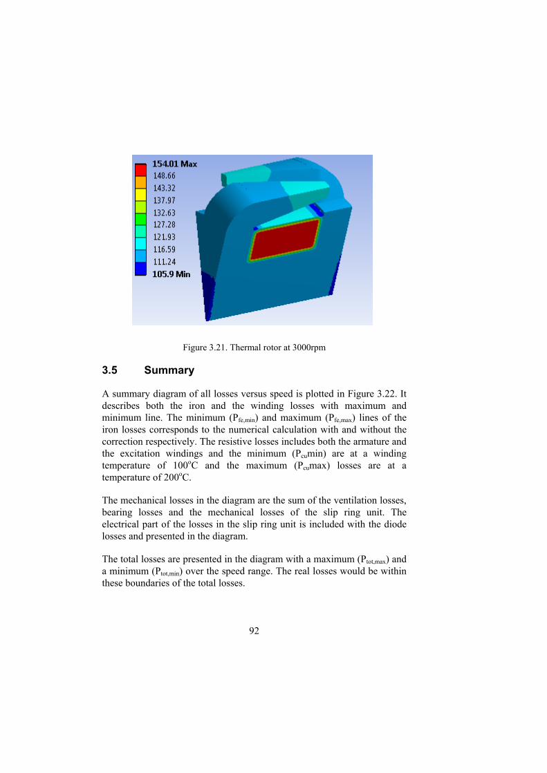
92

Figure 3.21. Thermal rotor at 3000rpm

3.5 Summary

A summary diagram of all losses versus speed is plotted in Figure 3.22. It describes both the iron and the winding losses with maximum and minimum line. The minimum (Pfe,min) and maximum (Pfe,max) lines of the iron losses corresponds to the numerical calculation with and without the correction respectively. The resistive losses includes both the armature and the excitation windings and the minimum (Pcumin) are at a winding temperature of 100oC and the maximum (Pcumax) losses are at a temperature of 200oC.

The mechanical losses in the diagram are the sum of the ventilation losses, bearing losses and the mechanical losses of the slip ring unit. The electrical part of the losses in the slip ring unit is included with the diode losses and presented in the diagram.

The total losses are presented in the diagram with a maximum (Ptot,max) and a minimum (Ptot,min) over the speed range. The real losses would be within these boundaries of the total losses.

93

1500 2000 2500 3000 3500 4000 4500 5000 5500 60000

500

1000

1500

2000

2500

3000

3500

Speed [RPM]

ELo

sses

: P

[W

]

P

tot max

Ptot

min

Pcu

max

Pcu

min

PFe

max

PFe

min

Pdiode & slip

Pmec

Figure 3.22. Calculated alternator losses

The efficiency of the alternator, based on the losses above and a load power of 3000W, is plotted in the diagram shown in Figure 3.23. As one can see, is the efficiency within 68% and 50% which is reasonably values [35][36].

94

3000 3500 4000 4500 5000 5500 600048

50

52

54

56

58

60

62

64

66

68

Speed [RPM]

Eff

icie

ncy:

[

%]

Max

Min

Figure 3.23. Calculated alternator efficiency with maximal power

95

Chapter 4 Comparison of PMSM, EMSM and SMSM

Based on knowledge of the alternator (chapter 3) and the targets for BAS application (chapter 1) the generalised theory (chapter 2) is proved against the principles of machine design, where the size and materials of the machines are specified. Simulation environment consist of pre and post processor at different levels where the construction is optimised and different operation points are analysed. Based on finite element analysis (FEA) the realistic and limiting features such as magnetic leakage, electric resistivity, magnetic saturation, power losses are included, which were excluded in the idealised generalised results in chapter 2. As a result, the machine characteristics for PMSM, EMSM, SMSM are presented, compared and discussed related to their suitability for the BAS application regarding:

Efficiency

Torque characteristics

Power characteristics

Power losses analysis

Several calculations are made in order to account for different load cases (variations of both load and operation frequency), as well as different machine concepts.

A conventional car alternator, with a power of 1.5kW, is considered in

96

order to establish the bases for the derivation of a heat transfer model that could be applied later for the estimation of the power loss distribution and the thermal sizing of the machines. Since the car alternator does not have a closed housing, the values for the dissipated heat flux through the external surfaces of both rotor and stator are nearly the same. This assumption will serve as a ground for the calculations of all the machines involved in the study. An ambient temperature of 100 °C and a maximum winding temperature of 130 °C are assumed during nominal operation of the machine, according to the conditions in the combustion engine compartment.

Current boost possibility The highest cranking torque is required at low temperatures, down to – 40 C. At this temperature, the cooling capabilities of the machine are considerably improved.

According to the law of energy balance, the summation of the power equals zero, a thermal lumped-parameter of a solid could be expressed by:

dissipation suppliedstorage

0c p losses

dTQ m c P

dt

(4.1)

The dissipation of the solid due to the cooling method and the thermal conductivity of the solid, where the storage power is according to the specific heat cp and the mass m of the solid. The supplied heating power is in this case the iron- and the resistive- losses respectively. Equation 4.1 is common to see as a thermal equivalent circuit with an analogy to an electric circuit of a capacitor in parallel to a resistance. This can be presented as:

0alosses

th

T T dTC P

R dt

(4.2)

Where Ta is an ambient temperature, C the thermal capacitance and Rth the thermal resistance.

97

Assuming steady state and that the thermal resistance does not change, the current allowed at –40 C is 2.38 times higher than the nominal current at 100 C, according to equation 4.2 which gives.

n

ncuth T

TIIPRT

(4.3)

Where delta ∆T represents the temperature difference between the winding and the ambient air, Pcu the copper losses, and I and In are the nominal current for –40 C and 100 C respectively.

4.1 Simulation environment

The simulation software tool is created to speedup the simulations and analysis for different sizes and types of radial flux machines [14]. It is structured and written in the Matlab for automatically generating the geometry and all necessary input parameters ether to FEMM or Vector Fields. Those are software that uses the finite element method (FEM) for both magneto static, quasi-static electromagnetic and thermal calculations. The main program handles the geometry with a parameterization of all dimensions as an input. Such as number of slots, number of poles, material selection, copper fill factor, current density etc.

The design environment is based on Matlab/(Octave) environment, which calls numeric field analysis by FEMM, sets up the numeric model and returns the magnet or the thermal numerical solution. Then the post processing is handled in Matlab as well. A roadmap of the design environment is illustrated in Figure 4.1.

98

Figure 4.1. Roadmap of the design environment.

The first stage is the initialization of the simulations, setting the criteria of the geometry properties (geom), material definitions (md), boundary conditions (bnd) and also the selection of the parameter sweep. The second stage is a rough optimization with the main purpose to estimate the best performance of a machine on a basis of a couple of design parameters. This kind of sensitivity study is an iterative process where a number of design parameters are changed successively so that the outcome can be easily visualised. When the outcome of the rough optimization fulfils the design requirements then an extended FEM analysis is done to give a full performance characterization sheet of the machine.

Rough optimization The rough optimization consists of two steps in order to find the machine performance over a set of selected parameters. The first stage is to find the current density, based on the thermal boundary condition. And the second stage finds the maximum of the torque and speed respectively.

The boundary conditions are the same for all combinations as well as the material properties.

Current density

In order to find the current density in the windings, both the core losses and the heat dissipation has to be considered. The boundary condition for the heat dissipation from the cooling surface is set to a constant heat flux of 5800 W/m2, which corresponds a convection coefficient of 200W/m2K

99

and a temperature difference of 30 oC between the ambient respective the surface temperature. This is done in order to consider the axial cooling surfaces of the machine, such as housing parts, that is not directly presented on 2D xy-plane. During this rough stage the winding end turns are neglected. The overhanging end-turns are assumed to have their own heat balance that does not contribute to heating of the stator. This means that the heat losses generated and dissipated by the end turns gives assumingly lower maximum temperature than the winding that is placed into the slot (look at Figure 3.19). This assumption works until the cooling of the end-turns is relatively more intensive than the cooling of the rest of the machine.

The whole process of finding the current density occurs in three steps:

I. Calculate the current density in the rotor (not relevant in the PMSM)

II. Calculating the total losses of the stator with different current densities

III. Calculate the current density in the stator windings.

The iron losses of the rotor are neglected. This since the core is made of laminated steel and the losses will be negligibly small. With only resistive losses in the rotor the winding temperature is linearly related to the power. The initial winding temperature Ti is held by a thermal FEM calculation using the initial winding heating power Pi. The corrected winding power is then calculated based on the liner relation to the temperature, where the winding temperature T0 at zero power equals the ambient temperature. With the winding temperature, length, area and power known it is possible to calculate the current density based on the resistivity of copper.

Since the total stator losses consist of both the iron losses and the resistive losses a magneto static FEM calculation is needed to estimate the iron losses. The core losses are calculated by Steinmetz equation for sinusoidal excitation, [42], based on the flux density from the magneto static calculation and the initialized base speed. The iron losses and the resistive losses are computed for five different current densities, two lower and two higher then the initial one. This is done with the maximum current vector in the y-direction. Those five sets of power losses are used to compute

100

respective winding temperature.

Then if the maximal allowed temperature is within the computed values of the losses, the accurate current density is held by the correct power which is interpolated by a cubic-spline interpolation from those five values.

Maximum torque and speed

To achieve the maximum possible torque of the machine, the eventual reluctance torque has to be considered. In order to do this, the numerical magneto static FEM model is computed with the current vector directed for six different load angles. The vector follows the maximum current circle in the xy-frame second quadrant and starts in the y-direction, continue with next step and ends at an angle of 45 degree from the y-direction. The maximum torque is then predicted with cubic-spline interpolation based on those values.

To avoid the effects of the cogging torque, which could have an impact of the result [14], all the torques given by the six current vectors is the mean value over different rotor positions.

In the case when the PMSM is calculated, the maximum speed is estimated by computing the model with the maximum current vector pointing in the negative x-direction. This gives the maximal possible field weakening (chapter 2).

Finite element scan through A series of magneto static calculations are made in order to obtain the static characteristics of the machine and create the foundations to the postprocessor. The data of interest are:

Torque map over several positions and operation points T=f(isx, isy, θe)

Flux linkage map over several positions and operation points ψ=f(isx, isy, θe)

Flux density map over a machine geometry. several positions and operation points B(x,y)=f(isx, isy, θe)

101

Previously the amount of computations in the rough optimization is made by 13 FE analyses per machine configuration. At this scan through the current combinations is a 9x5 matrix of the isx and isy respectively. They are scanned through at 7 different positions θe of the rotor with respect to the stator. As the machine has the symmetric 3-phase configuration, the simulations are made over 60 electrical degrees.

Postprocessor The postprocessor uses the FE-analyses in order to get the machine characteristics which are presented in torque and power versus speed diagrams respectively. This post processing is made in five main steps.

The first step converts the rotor position or angle dependency of the torque, flux linkage and flux density to projected values in xy-coordinates. The torque and the projected flux are handed by the average of the different angels and the flux densities are equal to the maximum values for a selected part of the machine. The flux linkage is transferred into the xy- coordinates by the equations 2.4 and 2.5.

With the properties independent of the rotor position, the second step is to calculate the resistance and the maximum speed for each current combination. The winding resistance is calculated with equation 3.16 and 3.17, and uses the resistivity of copper at 130 oC. To get the total length of the windings, each winding end turn is estimated and added. This is calculated by the arc length of the end turn multiplied with a curvature factor:

p

isew N

Dl (4.4)

Where lew is the length of one end turn, Dis the diameter of the midpoint in the slot, Np the number of poles and the σ a curvature factor. The curvature factor in this study is set into 1.6 [1]. With the winding resistance known and the flux linkage respective the maximum voltage is the maximum speed for each current combination calculated from equation 2.10 and 2.12.

102

The third step in the post processor is to find the torque and speed range of the machine from the pre-calculated maps of flux and torque as a function of current. The operational torque speed range is limited between three boundaries consisting by:

I. The line created by the maximum torque for minimum current (also known as maximum-torque-per-ampere – MTPA line), with start at zero current and end at the maximum torque point on the current limit line.

II. The maximum current circle in the field weakening region. With start at the maximum torque point and end at either the maximum field weakening point or at the third boundary. This is determined if the centre of the voltage-limit lines lays outward or inward the current-limit line.

III. The line created by the maximum torque per flux linkage (also known as minimum-flux-per-torque – MTPF). With start at crossing of the current-limit line and ends at the maximum speed point. This boundary is only valid if it is within the maximum current region.

These boundaries is commonly used in control strategies of synchronous motor drives, widely described in many papers and literatures [18][19][20][22][23], and will not be described further in this thesis.

Within these boundaries a matrix with different torque and speed combinations is interpolated from the fundamental matrixes of torque, maximum speed, flux density and flux linkage. Figure 4.2 shows an example, where every black dot corresponds to a cell in torque versus speed matrix. Each cell contains information of the flux linkage, currents and flux density.

103

0 2000 4000 6000 8000 10000 120000

2

4

6

8

10

12

14

Speed [rpm]

Tor

que

[Nm

]

Figure 4.2. Torque and speed mapping.

At the fourth step, each cell is supplemented with the losses and the efficiency. The resistive losses are defined by multiplying the resistance with the current squared. The iron losses are calculated with the Steinmetz equation [42].

VfBCfBCfBCP aeE

hfeh 5.15.122 (4.5)

Where Eh, C* are material related constants and B, f, V is the flux density, frequency and the volume of the iron sample.

In the case when the machine is an EMSM or SMSM the slip ring losses are added, and so are the diode losses of the rectifier in the SMSM. The slip ring losses are calculated with equation 3.8 and 3.9, and the diode losses by equation 3.25.

The remaining losses, as the mechanical losses, are the same for all three machine types and are canceled in this comparative study. This do not affects the comparison between the different machine types but gives an

104

unrealistic high efficiency of the machines.

The fifth and last step in the postprocessor is to illustrate the machine characteristics with a torque versus speed diagram that contains the efficiency regions. Also the maximum output power is displayed.

4.2 Characteristics

The objective of this section is to compare between an EMSM, a SMSM and a V-shaped embedded PMSM for the specified BAS application in chapter 1 by using the simulation environment described above. The machine specifications are:

Nominal power of 5000 kW

Maximum Voltage 108V

Intermittent cranking torque > 55 Nm

Speed range 0-18000rpm

The modelled EMSM and SMSM are a 12-pole, three-phase machine with 180-degrees distributed windings in the stator and salient poles in the rotor, Figure 4.3a. The length of the machine is 60 mm and the outer radius of the stator is 85 mm. Besides, a slotting factor of 0.5 is considered for the stator core. The same design criteria and specification conditions are applied to the PMSM, Figure 4.8. The material in both the rotor and the stator core is M235-35A, laminated carbon steel with a thickness of 0.35mm. The material constants for the iron losses is listed in Table 4.1

Table 4.1 Material constants to iron loss calculations of M235-35A

Eh Ch Ce Ca

1.7266 161.9738 0.3387 0.1464

105

EMSM In order to find the optimal relation between the air gap radius and the inner radius of the rotor with respect to the outer radius of the machine several alternatives are analyzed. As a result from the described process of rough optimization, Figure 4.3b shows the maximum torque produced for each of the air gap and rotor inner radius considered.

0.35 0.4 0.45 0.5

0.65

0.7

0.75

0.8

Relative inner radius, ri/ro

Re

lativ

e ai

r ga

p ra

diu

s, r

g/r

o

Torque, T [Nm]

10

1012

12

12

12

13

13

13

1314.5

14.5

14.5

14.5

15

15

Figure 4.3. a) EMSM and SMSM geometry for 1 pole.b) Maximum produced torque for different rg/ro and ri/ro ratios

From Figure 4.3b it can be deduced that the optimal ratio between the air gap radius and the outer radius is located around 0.78. Besides, for a constant air gap radius, the torque increases as the rotor inner radius decreases, since the rotor slot depth increases, allowing more copper and thus more current loading in the rotor winding. The black dot in Figure 4.3b represents the alternative selected for the comparative study. In order to reach at least 55 Nm of cranking torque at –40 C the current supplied to the machine needs to be 1.35 times higher than the maximum allowed current for continuous operation at that temperature, i.e. 3.21 times higher than the nominal current at 100 C. This is illustrated in Figure 4.4

Figure 4.5 presents the torque and output power characteristics as well as the efficiency map for the machine configuration selected from Figure 4.3b. For each operating point (torque – speed combination) the magnetizing current is selected in order to maximize the efficiency. This is made by running the scan through and post processing for various

106

excitation currents, and then select the one with the highest efficiency for each torque and speed combination. The slightly jagged lines of the efficiency and the power in Figure 4.5 contribute to the restricted resolution of the variance in the excitation.

-3.21 -2.38 -1 0 1 2.38 3.210

1

2.38

3.21

Constant torque lines

isx

i sy

03.77565

7.5513111.32715.102618.878322.6539

26.429630.205233.9809

37.75

65

41.53

22

45.30

78

49.083552.859156.634860.4105

Figure 4.4. Constant torque contours and current needed to reach the cranking torque under low temperature conditions for the EMSM.

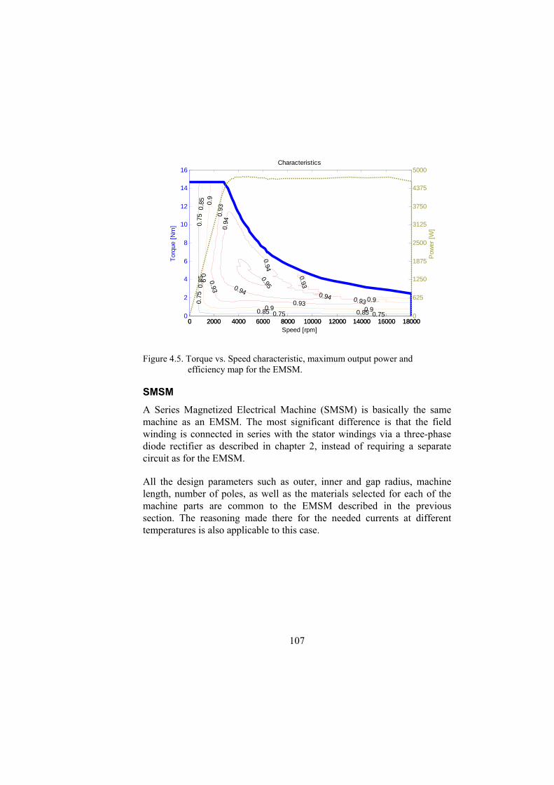
107

0.75

0.75

0.75 0.75

0.85

0.85

0.85 0.85

0.9

0.9

0.9 0.9

0.9

0.93

0.93

0.930.93

0.93

0.94

0.940.94

0.940.95

Characteristics

Speed [rpm]

Tor

que

[Nm

]

0 2000 4000 6000 8000 10000 12000 14000 16000 180000

2

4

6

8

10

12

14

16

0 2000 4000 6000 8000 10000 12000 14000 16000 180000

625

1250

1875

2500

3125

3750

4375

5000

Pow

er [

W]

Figure 4.5. Torque vs. Speed characteristic, maximum output power and efficiency map for the EMSM.

SMSM A Series Magnetized Electrical Machine (SMSM) is basically the same machine as an EMSM. The most significant difference is that the field winding is connected in series with the stator windings via a three-phase diode rectifier as described in chapter 2, instead of requiring a separate circuit as for the EMSM.

All the design parameters such as outer, inner and gap radius, machine length, number of poles, as well as the materials selected for each of the machine parts are common to the EMSM described in the previous section. The reasoning made there for the needed currents at different temperatures is also applicable to this case.

108

-1 -0.75 -0.5 -0.25 0 0.25 0.5 0.75 10

0.25

0.5

0.75

1

Constant and Torque lines

Relative current, isx

Rel

ative

curren

, isy

Figure 4.6. xy current combinations giving the maximum torque at different speeds for the SMSM.

As a result of the thermal and magnetostatic FE analysis described in scan through and postprocessor, Figure 4.6 shows the combinations of xy current that provide the maximum torque for different speeds, while Figure 4.7 shows the torque vs. speed characteristic, as well as the maximum output power and the efficiency map for the SMSM considered.

109

0 2000 4000 6000 8000 10000 12000 14000 16000 180000

2

4

6

8

10

12

14

16Characteristics

Speed [rpm]

Tor

que

[Nm

]

0.75

0 .75

0.85

0.85

0.9

0.9

0.93

0.930.93 0

0.94

0.94

0.940.94 0.0.95

0 2000 4000 6000 8000 10000 12000 14000 16000 180000

625

1250

1875

2500

3125

3750

4375

5000

Pow

er [

W]

Figure 4.7. Torque vs. Speed characteristic, maximum output power and efficiency map for the SMSM.

The relation between the magnetization flux linkage ψm and the absolute value of the armature current vector is described and discussed in equation 2.24 in chapter 2.5. The SMSM solution in this section uses a relation where the maximum armature current provides the magnetization flux linkage as high as possible. This gives the highest magnitude of the maximum torque but is punishing the output power in the upper speed region. As one can se in Figure 4.7 the power characteristics is fairly constant within the speed region of 3000-8000rpm and are, due to the reduction in magnitude of the armature current, decreasing above that speed. The point, where the amplitude of the armature current is reduced, can be seen in Figure 4.6 which is where the current leaves the maximum current line in the second quadrant. To have a constant power characteristic of the SMSM the number of rotor windings must be reduced, i.e. a decrease of the excitation inductance. This leads both to a lower torque capability and a lower peak power, which has to be considered in a specific designee task. In this specification the focus is on the cranking torque and the high speed possibility, not the performance of the power in the upper speed region.

110

PMSM The PMSM included in the comparison is based on the same stator as the EMSM and the SMSM. The rotor, however, has V-shaped embedded permanent magnets with air pockets in the extremes of the magnets. The V-shaped magnet arrangement and the inclusion of air pockets in the design is motivated by the increase in reluctance torque achieved, which besides of contributing to a better torque density of the machine, discussed in chapter 2. Figure 4.8 illustrates the stator and rotor geometry analyzed in this case.

Different magnet lengths and angles are scanned in order to find the best magnet configuration for the rotor. Two design parameters, namely dmi (distance from the axial center to the lowest corner of the magnet) and dpn (distance from the symmetry line between the 2 magnets to the closest corner of the magnet) are varied successively in order to evaluate their effect in the performance of the machine.

Figure 4.8. PMSM geometry for 1 pole.

This kind of sensitivity study is similar to that performed in section EMSM when the rg/ro and ri/ro ratios were to be selected. The results for the scanning process are shown on Figure 4.9a and b where the maximum torque and the maximum speed are shown respectively, for the different

111

combinations of dmi and dpn considered.

5.9 6 6.1 6.235.9

35.95

36

36.05

36.1

36.15

36.2

Relative, dmi [%]

Rel

ativ

e ,

dpn

[%]

Torque, T [Nm]

13.713.7

13.813.813.8

13.8

13.9

13.913.9

13.9

14

14

14

14

14.1

14.1

14.2

14.35.9 6 6.1 6.2

35.9

35.95

36

36.05

36.1

36.15

36.2

Relative, dmi [%]

Re

lativ

e , d

pn [%

]

Max Speed, [RPM]

16000

16000

16000

18000

18000 18000

18000

20000

2000020000

20000

22000 22000

Figure 4.9. a) Maximum produced torque for different dmi and dpn combinations. b) Maximum attainable speed for different dmi and dpn combinations.

16 combinations of dmi – dpn values have been scanned in the aforementioned process in order to find the best magnet configuration. Those combinations are represented by black crosses in Figure 4.9a and b. The black dots in the figures represent the dmi – dpn combination that provides the highest torque among those who fulfil the maximum speed requirement.

A more refined mesh, with higher resolution for the dmi and dpn variations could have been used in order to obtain more accurate results at a higher computational cost. An insufficient number of nodes in the mesh could mislead to an erroneous choice of the magnet configuration, since the constant torque and speed lines are calculated by interpolation between this nodes.

112

-5.95 -2.38 -1 0 1 2.38 5.950

1

2.38

3.21

Constant torque lines

isx

i sy

0 0 03.20146 3.

2014

6

3.20

146

6.40292

6.40

292

6.40

292

9.60

438

9.60

438

9.6043812

.805

8

12.80

5812.8058

16.0

073

16.00

73

16.0073

19.2

088

19.2

08819.2088

22.4

102

22.4

102

22.4102

25.6

117

25.6

117

25.6117

28.8

131

28.8

13128.8131

32.0

146

32.0

146

32.0146

35.2

16

35.2

16

35.216

38.4

175

38.4

175

41.6

19

41.619

44.8

204

44.820448

.02

19

48.021951

.22

33

51.223354

.42

48

54.424857.6263

60.8277

Figure 4.10. Constant torque contours and current needed to reach the cranking torque under low temperature conditions for the PMSM.

As it is specified for the BAS application, in order to reach at least 55 Nm of cranking torque at –40 C the machine has to be overexcited. However, in a PMSM only the stator current can be controlled, so all the extra power needed has to be supplied through the armature winding (chapter 2).

Under these assumptions, the needed current is 2.5 times higher than the maximum allowed current for continuous operation at that temperature, i.e. 5.95 times higher than the nominal current at 100 C as can be deduced from Figure 4.10.

Finally, the torque vs. speed characteristic, the maximum output power and the efficiency map are presented in Figure 4.11 for the PMSM considered in the comparative study.

113

0 2000 4000 6000 8000 10000 12000 14000 16000 180000

2

4

6

8

10

12

14

16Characteristics

Speed [rpm]

Tor

que

[Nm

]

0.75

0.75

0.75 0.75

0.85

0.85

0.85

0.85

0.9

0.9

0.9

0.93

0.93

0.93

0.94

0.94

0.94

0.95

0.95

0 2000 4000 6000 8000 10000 12000 14000 16000 180000

625

1250

1875

2500

3125

3750

4375

5000

Pow

er [

W]

Figure 4.11. Torque vs. Speed characteristic, maximum output power and efficiency map for the EMSM.

The compromises of the PMSM are between the torque capability and the speed capability. This PMSM is chosen to have as high cranking torque as possible but still with the possibility to reach the maximum speed in the specification. To improve the torque with larger permanent magnets would decrease the maximum speed below the requirements. Since the machine is designed with the cranking torque in mind magnetization is so strong that the center of the voltage-limit locus is outside the maximum current locus in the xy- current frame works. This results in a power characteristic with a high peak around 5000 rpm and a rapid decrease in power with an increase in speed. To get a flatter power characteristic of the machine the magnetization from the permanent magnets must be reduced, which will press down the torque capability of the machine.

4.3 Summary

The results from the simulations in this chapter show that the characteristics of the different machine topologies match the theoretical characteristics in chapter 2. The designed EMSM, SMSM and PMSM

114

provide nearly the same power output around the base speed. When it comes to the field weakening region than the compromise between the torque and field weakening capability of a PMSM does not completely match the requirements for BAS application. When it comes to EMSM then the variable field excitation is the reason for the perfect mach of the machine characteristics for the BAS application. Still the main concern is related to rotor supply and cooling. The rational arrangement of rotor supply brings EMSM down to SMSM with a more limited choice for the excitation current. A comparison of the power capability of SMSM in Figure 2.17 and Figure 4.7 and also the voltage-limit lines in Figure 4.6 shows that the electric excitation creates higher mutal flux linkage than the maximum field weakening that the stator is able to create. Apart from the electromagnetic torque component the designed machines also have a contribution of reluctance torque. The constant torque lines in Figure 4.4, Figure 4.6 and Figure 4.10 shows that all three machine configurations have a positive reluctance torque in the second quadrant.

Apart from the constant power region, the other design criterion for the BAS application is the cranking torque. The cranking current is 85% higher for the PMSM than for the EMSM and SMSM which means that the cranking time is shorter for the PMSM, since the stator winding temperature will increase faster for the PMSM. In comparison to the theoretical current boost for cranking, a higher current is needed in the case when saturation is considered. The EMSM and SMSM should have a cranking current just below two times the nominal current, but has 3.21. The PMSM should have a cranking current between two and three times the nominal current, but has 5.95. This due to the saturation effects, which requires higher current to achieve a high magnetic flux.

When focusing on power output and the power conversion efficiency, then the power is constant beyond the base speed for the EMSM, while the output power decreases at the higher speeds for SMSM and the PMSM due to limited field weakening regulation. As one can see in Figure 4.5, the efficiency of the PMSM is highest around the base speed but drops drastically at higher speed. This due to the active field weakening with the armature currents, which creates both resistive losses and iron losses. In the EMSM and the SMSM case the field weakening is created by a decrease of the excitation, which relives and reduces both the armature

115

current and the flux density of the machine.

116

Chapter 5 Alternatively construction with Hybrid Magnetization rotor

The hybrid magnetized synchronous machines (HMSM), as theoretically described in section 2.6, allows a torque boosting not only for warm and cold cranking but also at a high speed operation and efficient electromagnetic energy conversion at a very wide speed range with enhanced reliability [49]. The benefits are achieved by easily controlled excitation field – strengthening and weakening [54]. The implementation of the excitation coil costs power density compared to PMSM but improves efficient energy conversion and control over the very wide speed range.

This section discusses the design, EM and PM excited slip-ring less rotor. The main focuses of this work is on the magnetic design and power losses leaving the space for a future more extensive thermal analyses. First a review of previous research and HMSM designes are discussed. Thereafter an alternative rotor solution is presented and the hybridization ratio of the excitation is discussed. Thereafter, a rough design of the rotor EM and PM excitation is given by combining axi-symmetric 2D FE analysis together with equivalent circuit that represents the stator and also a modulator of the rotor core. On the basis of the rough design the final rotor construction is determined for the further 3D FE transient electromagnetic analyses and also for the prototyping.

117

5.1 Structure comparison

A hybrid excitation with both permanent magnets and field coils can completely be implemented either in the stator side in the AC magnetic core or in the rotor or even in combination [43]. Common for the different topologies is the avoidance of slip-rings for higher reliability and also better volumetric material utilization. [43]-[49]

Two different solutions of the excitation design, for a Parallel HESM, are presented in Figure 5.1. The first design (a) is one that uses parts of the machine gables for the DC excitation circuit [48] and the second design is one (b) with an extended axial excitation solution [44]. Both has some advantages and disadvantages. The advantage of the first one is the large diameter of the excitation coils and its close contact to the machine gable, which gives a good electromagnetic flux capability and good thermal capability respectively. The disadvantage is that the gable needs to be in a soft magnetic material and has to be as thick as the magnetic circuit requires and also encases the other machine parts. The magnetic DC- circuit also uses a rather long flux path which reduces electromagnetic flux capability. Since the magnetic gables insulate the rest of the machine parts, such as the stator, it could have an impact on the cooling capability of the machine. The advantage of the second solution, the one with the axial excitation shown in Figure 5.1.b, is that the DC-circuit is free and not affecting the outer parts of the machine. In fact that it is possible to use any kind of cooling system and material in the machine house gables. On the other hand the disadvantage is that it extends the machine length, in this case with a factor of 2.5.

118

Figure 5.1. EM excitation via a) housing gables [48] b) external magnetic circuit [44]. (both figures is copied from the referenced articles)

5.2 Alternative claw-pole designs

The utilization of permanent magnets for a conventional claw-pole rotor improves the performance including the layouts for a series, parallel and combined hybrid excitation. Several designs of claw-pole rotors with magnets have been investigated [50][10]. The benefits is a reduction of the flux leakage between the claws and a hybrid magnetising [50]. In common, the magnets are placed in between the claws which are a strategically good place from a magnetising point of view, however compromising manufacturability. Regarding the magnet, the rotor structure is exactly the same. I.e. the DC- winding is wrapped around the claw-pole core and shaft and are excited via slip-rings.

The target of this work is a relative easily manufactured slip-ringless rotor with a parallel hybrid excitation. The axial length is the same as the stator stack but is possible to extend to the double, by mirroring it, whiteout any impact on the magnetic design. This gives the possibility to use a stator configuration that is twice as long as the original one.

The rotor design, with a hybrid excitation and the existing stator, is illustrated in Figure 5.2. The excitation part consists of a stationary excitation coil and a rotating single piece permanent magnet, illustrated in light orange and purple respectively. For an easy manufacturing point of view, the magnet and the winding are shaped as a toroid. The magnet is

119

mounted between two rotating claw-pole structured cores which are illustrated in light blue in the figure. The excitation winding is mounted to a stationary core, dark blue in the figure, that linkage the flux via air gaps between the two rotating claw-pole cores. The stationary core has a fringe in the bottom, this to facilitate the manufacturing procedure of the winding which wraps directly around the core. The bottom fringe also turned out to improve the magnetic circuit during the demagnetization, which is shown in later sections.

Figure 5.2. Section of machine layout with hybrid excited rotor. The arrows demonstrate the flux paths of the permanent magnet and the

electromagnet origin of magnetisation.

5.3 Material comparison

Claw-pole structures have relatively high losses, discussed in section 3.3, due to the high eddy current losses in the solid iron. In the coming sections different rotor materials and their effect on the losses and the magnetic performance of the rotor is studied. The rotor materials in the 3D simulation study consider the solid low carbon steel type SAE 1008 and the soft magnetic composite (SMC) named Somaloy 500 1P.

Permeability

The BH- characteristics for three different materials are plotted and illustrated in Figure 5.3. The two materials mentioned above, steel 1008

120

are presented with the light green boxed line and the Somaloy 500 1P are presented with the darker green diamonds line. Respective BH-data is used in the simulations in the study at the subsequent section, and the BH- data is provided by the manufactures of respective material. The light brown curve in Figure 5.3 is for the material ss-1650, which is used in the machine prototype presented in Chapter 6. This BH-characteristic are measured by a toroid sample and presented in that section 6.3. As one can see, the ss-1650 is in between of the other two where steel 1008 have the highest magnetic performance and the Somaloy 500 the lowest performance.

0 0.5 1 1.5 2 2.5 3 3.5 4 4.5 5

x 104

0

0.5

1

1.5

2

H [A/m]

B [T

]

ss-1650

Somaloy 500 1P

Steel 1008

Figure 5.3. BH- characteristic

Iron losses

Table 5.1 shows the material data of the three soft magnet materials plotted in Figure 5.3. It also contains two other SMC materials with the name Somaloy 700 1p and 3P respectively. Those two SMC materials represent at the time of writing this text the newest composite that is recommended by the manufacturer in a magnetic construction. They are not used in any simulation in this thesis, but are for reference included in

121

the table.

The resistivity impact on the losses is seen in equation 3.24. Where the losses is proportional to the inverse of the resistivity and proportional to the volume, which means that the losses is less with higher resistivity for a given volume. The volume itself is dependent on the skin depth [32] of the circulating eddy currents. This is proportional to the square root of the resistivity and can be calculated by:

rf

0

(5.1)

where f and μ is the frequency and the material permeability respectively. This means that the eddy current losses with the skin depth considered is proportional to the inverse of the square root of the resistivity.

Table 5.1 Material data

Somaloy

500

Somaloy

700 3P

Somaloy 700 1P

Steel 1008 SS-1650

Density [kg/m3] 7630 - - 7872 7872

Resistivity [µΩm] 70

(Used 10)

200 400 0.143

(Used 0.5)

0.168

TRS [MPa] - 125 40 310 - 350 565 - 625

The resistivity of Somaloy 500 is around 100 times higher than the resistivity of Steel 1008. This means that the losses are about 10 tims higher for the Steel 1008 if the flux density respective the permeability is the same in the both materials, which it is not.

Unfortunately are the simulations with Steel 1008 done with a resistivity 0.5 μΩm instead of 0.143 μΩm which is the resistivity given by the material supplier. This results in a reduction of the simulated rotor losses, which would be higher if the correct resistivity were used. The resistivity

122

of SMC Somaloy used in the simulations is lower than the manufacturers specified resistivity which is around 70µΩm. This means that the losses would be even lower if the resistivity is higher.

Mechanical strength

The mechanical strength differs between soft magnetic composite and solid soft magnetic steel. Table contains the transverse rupture strength of the different material. Transverse rupture strength (TRS) is an ISO standard to test, by bending, the mechanically strength of a material.

As shown in Table 5.1 the composite (Somaloy) has less mechanic strength than the carbon steel (1008 and ss-1650). This will have an impact on the mechanical strength of the rotor if a SMC material is used. The mechanical strength of the rotor design is in this thesis not considered and will not be further discussed.

5.4 Simulations

The alternative construction, the slip-ringless and compact hybrid excitation claw pole rotor described in section 5.2, is numerical analyzed in both 2D- and 3D- finite element method (FEM) simulations.

FEM- optimization in 2 dimensions To get as close to an optimal rotor solution as possible an axi-symmetric equivalent 2D FE model is used. A simulation in two dimensions is much faster than a simulation in tree dimensions. This makes it possible to scan a wider span of different geometrical dimensions and material properties that would be nearly impossible within a 3D simulation, due to the computation time.

The 2D model consists of a real rotor geometry (excluding claws) and an equivalent counterpart of a claw-pole structure, air-gap and stator. This is illustrated in Figure 5.4 where the equivalent circuit is within the red dashed line. The other parts are the same in 2D respective 3D. To find the right equivalent circuit dimensions the average of the cross section area and the average length of the claw structure and the stator are calculated. This corresponds to the average cross sections area and length of the ones in the equivalent circuit in the 2D axi-symmetric model. This means that

123

the reluctance in the models is nearly equal in the both cases. The lack of accuracy between the both cases is that the flux leakage between the rotor teeth is neglected in the 2D model. This means that the 2D model is less accurate in the saturated situations where a possible flux leakage will occur.

Figure 5.4. Equivalent 2D model of the 3D- structure

Batch and boundaries

The simulations are done with the equivalent circuit in a single rotor position, which means that the stator and the claws of the rotor is the same during all simulations. The boundaries for the non-equivalent circuit are also restricted, where the outer dimensions as the radius and the length of the rotor is set to a single value, as well as the inner radius Ra is set to 10 mm which corresponds to a 20 mm non-magnetic shaft. The rotor length and the inner radius of the equivalent circuit are 32mm and 45.4mm respectively.

A range of magnet dimensions, width Wm and length Lm, combined with a

124

range of winding slot areas are analyzed. There is a comparison when the rotor uses slip-rings or not and for different rotor materials as well.

Simulation results

Figure 5.5 a,b, and Figure 5.6a, show the magnetization flux linkage Ψm as a function of the magnet width and the inner radius of the winding at different current densities of the excitation. The magnet width Wm and the inner coil radius Rc are scanned in between 1-15mm and 12-28mm respectively.

10

20

30

0

5

10

150.01

0.02

0.03

0.04

0.05

0.06

Rc [mm]

J=10 [A/m2]

wm [mm]

m [V

/s]

10

20

30

0

5

10

15-0.05

0

0.05

0.1

0.15

Rc [mm]

J = -10 [A/m2]

wm [mm]

m [V

/s]

Figure 5.5. Parameter sweep of the rotor inner core and the magnet width. a) flux linkage at J=10 A/mm2. b) flux linkage at J=-10 A/mm2

At Figure 5.5a, which is for the maximum excitation current density (10 A/mm2), it is possible to see that the flux linkage has a local maximum in all magnet width configurations. This corresponds to an optimal winding slot area. Large enough to suppress the PM-flux linkage to the excitation core and contribute to field strength without saturating and increase the reluctance in the inner rotor core too much. The lowest flux linkage in Figure 5.5a is obtained when the magnet width is 1mm and the inner coil radius is 12mm. This corresponds roughly to an EMSM with a rotor core thickness of 2mm, which is highly saturated.

125

The red dot in Figure 5.5 and Figure 5.6 indicates the selected geometry for the further investigation in 3D simulations and prototyping.

Figure 5.5b shows the flux linkage with an excitation of -10A/mm2, this is for minimum excitation. The flux linkage is nearly independent of the excitation current for a magnet width of 15mm. The rotor is dominated by the permanent magnet and can be treated as a PM rotor. The green line in Figure 5.5b shows the combination of Ra and Wm that result to zero excitation. This means that the combinations that is beneath this line gives a negative field strength, which is of no interest.

10

20

30

0

5

10

150

0.02

0.04

0.06

Rc [mm]

J = 0 [A/m2]

wm [mm]

m [V

/s]

10

20

30

0

5

10

150

0.2

0.4

0.6

0.8

1

Rc [mm]

hybridization ratio

wm [mm]

Figure 5.6. Parameter sweep of the rotor inner core and the magnet width. a) flux linkage at J=0 A/mm2. b) hybridization ratio

In Figure 5.6a the field current is zero, i.e. the excitation only comes from the permanent magnet. Figure 5.6b shows the hybridization ratio, which is calculated by equation 2.26 in chapter 2. The hybridization ratio is equal to the result presented in Figure 5.6a divided by the results in Figure 5.5a. The hybridization ratio for the selected configuration (red dot) is 0.64.

All the results presented in the figures above are calculated for a core width (wc in Figure 5.4) of 11mm. The simulation batch is done with different core width as well, but it is this configuration that contributes to the highest field strength within a proper field hybridization ratio.

126

The thickness of the magnet, in Figure 5.4 declared as the length Lm, has an impact of the magnet performance of the rotor construction. Figure 5.7a shows the flux linkage as a result of different magnet length and different current densities. As one can see, the flux linkage (Ψm) is nearly constant for a given current density, excepted for a magnet thickness (Lm) below 3mm where the flux linkage decreases. In this case the flux from the electric excitation is weakening the permanent magnetisation which is not able to maintain a strong total magnetization.

-10

0

10

0

5

100

1

2

3

x 10-3

J [A/mm2]

wm = 10 [mm], R

c = 19 [mm]

Lm [mm]

m [V

/s]

-10

0

10

0

5

10-8

-6

-4

-2

0

x 105

J [A/mm2]

wm = 10 [mm], R

c = 19 [mm]

Lm [mm]

Hm [A

/m]

Figure 5.7. Parameter sweep of the rotor inner core and the magnet width

To take into account that the permanent magnet do not demagnetizes below its breaking point [2], has the maximum applied magnetization field of the magnet been considered. Figure 5.7b shows the applied magnetization field Hm, contributed from the electric excitation, over the magnet. The negative signs due to that the applied magnetization field has the opposite direction of the magnetic flux of the magnet. It is obviously the highest excitation current density that results to largest variation and the highest negative magnetization field Hm.

The applied magnetization field Hm versus the magnet thickness Lm at a current density of 10 A/mm2 is plotted with a green line in the diagram presented in Figure 5.8. The figure also contains the demagnetization

127

characteristics (blue lines) of the magnet at three different magnet temperatures. The demagnetization characteristics are held by data from the magnet supplier.

The upper part of the demagnetization lines, above the “knee”, is the recoil region. This recoil region is when the permanent magnet is able to recover to the full magnet strength. If the demagnetization is deeper than the knee, the magnet will recoil to lower remanence and the magnet is permanently weakened.

-18 -16 -14 -12 -10 -8 -6 -4 -2 0

x 105

0

1

2

Bm

[T]

Hm [A/m]

20 oC

80 oC

140 oC

-18 -16 -14 -12 -10 -8 -6 -4 -2 0

x 105

0

5

10

L m

Figure 5.8. Demagnetization characteristics of magnet (blue) and the applied magnetization field with different magnet width (green)

If the length of the magnet is chosen to 1mm and the magnet temperature is 140oC, as we can see in Figure 5.8, then the magnet will be destroyed when the excitation current reaches a density of 10 A/mm2.

Since the prise of the magnet increases with an increase of the magnet length, there is a trade off between the price and the demagnetization capability. Due to the high environmental temperature under the bonnet of a vehicle and the losses of the machine a high magnet temperature has to

128

be considered. Relating to the results and the data in Figure 5.8 a proper choice is of the magnet length is above 3mm. The chosen magnet length for the 3D simulations and the prototype is 6mm, which gives a strong demagnetization capability and increases the durability of the machine for experimental work.

Figure 5.9 shows the mutual flux linkage versus the excitation current density in the field winding conductor with two different materials in the rotor, Somaloy 500 and the Steel 1008 respectively.

-10 -8 -6 -4 -2 0 2 4 6 8 100.015

0.02

0.025

0.03

0.035

0.04

0.045

0.05

0.055

J [A/mm2]

m [V

/s]

Somaloy 500

Steel 1008

Figure 5.9. Comparison of different material solutions

It is obviousl that the rotor with steel 1008 gives a stronger magnetisation than the one with Somaloy 500. This is in line with the BH- characteristics of the materials presented in Figure 5.3, where steel 1008 have higher permeability and higher flux density in saturation.

Both plots in Figure 5.9 are for the geometric combination which is marked with the red dot in previous figures, and has a magnet length of 6mm.

129

FEM- simulations in 3 dimensions A series of 3D FE transient electromagnetic analyses are carried out in order to model the electromagnetic energy conversion at a number of points in the motoring operation. The main focus is on the torque boosting where the stator current and the excitation current are changed simultaneously in sequence of 0, 0.75, 1.0, 1.5 and 2.38 times of the nominal current. The armature field is kept initially at a 90 degree angle to the excitation field. In addition the phase of the stator current is changed from the initial state by an additional angle of 9 electrical degrees at the time in order to analyse the contribution the reluctance torque due to the rotor saliency at the nominal conditions. Furthermore the analysis are made for the rotor that is made of the solid iron Steel 1008 and from a soft magnetic composite Somaloy 500 same as the 2D simulations above. The stator is laminated carbon steel based on Surahammars M600-100A1N, the same as used in chapter 3.3.

Environment Having the focus on accurate power loss modelling requires adequate information of material properties and loss models incorporated to numeric field computation tool [51]. The eddy current losses in the rotor are calculated with transient-nonlinear solver where a number of attempts are made in order to validate the results when considering the simulation time, convergence speed and the accuracy of the results (chapter 3.3). The power losses in the stator core are calculated after the solution is converged and based on a conventional loss model that uses the power loss coefficients extracted from the material data provided by the supplier.

The 3D model uses the geometrical proportion which was selected from in the 2D simulations and the model is shown in Figure 5.2. The machine specifications are listed in Table 5.2. The permanent magnet width in the model is smaller than the core, as shown in Figure 5.2. This is done in order have the same cross section area of the permanent magnet in the model as the one in the prototype, which uses 48 permanent magnets in segments to create the toroid shaped magnet.

Table 5.2 Machine specification

Quantity Value

130

Outer diameter, Do [mm] 142

Axial air gap length Ho, [mm] 34

Outer diameter of rotor Dr, [mm] 111

Axial rotor length Lr, [mm] 34

Number of poles, Np 12

Number of turns per stator phase, Nts 11

Number of magnets 1

Total magnet surface area, Am [mm2] 2256

Number of turns in excitation coil, Ntf 780

Nominal speed, n [rpm] 3000

Nominal stator current, Is [A] 95

Nominal excitation current, If [A] 1.8

The armature current used in the comparison is 43% higher than the original armature currents in the alternator. This is a result of a mistake in the calculation, where the current was calculated for a nominal power of 5 kW instead of 3 kW. If this current is used in more than an intermittent drive would it lead to a thermal overload, compared to the originate alternator.

5.5 Characteristics

Magnetization control

To see the effects on the flux linkage between the excitation and the stator, the simulation model is run with open stator winding and with different excitation current. This is in line with the 2D simulations above and gives an excitation characteristic of the machine and its hybridization ratio.

Figure 5.10a shows the mutual field flux peak to peak versus the excitation current for the rotor made of solid steel 1008. The excitation current is within -1.8A and 1.8A which corresponds to the min and max value of the current density in the 2D simulations. The hybridization ratio is in this case 0.55 comparing to 0.64 in the 2D calculations. This is due flux fringing in the bottom of the stationary excitation core which gives a

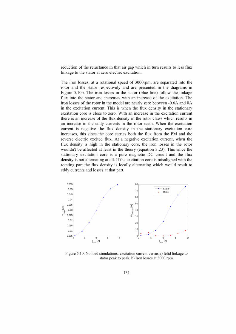
131

reduction of the reluctance in that air gap which in turn results to less flux linkage to the stator at zero electric excitation.

The iron losses, at a rotational speed of 3000rpm, are separated into the rotor and the stator respectively and are presented in the diagrams in Figure 5.10b. The iron losses in the stator (blue line) follow the linkage flux into the stator and increases with an increase of the excitation. The iron losses of the rotor in the model are nearly zero between -0.6A and 0A in the excitation current. This is when the flux density in the stationary excitation core is close to zero. With an increase in the excitation current there is an increase of the flux density in the rotor claws which results in an increase in the eddy currents in the rotor teeth. When the excitation current is negative the flux density in the stationary excitation core increases, this since the core carries both the flux from the PM and the reverse electric excited flux. At a negative excitation current, when the flux density is high in the stationary core, the iron losses in the rotor wouldn't be affected at least in the theory (equation 3.23). This since the stationary excitation core is a pure magnetic DC circuit and the flux density is not alternating at all. If the excitation core is misaligned with the rotating part the flux density is locally alternating which would result to eddy currents and losses at that part.

-2 -1 0 1 20.005

0.01

0.015

0.02

0.025

0.03

0.035

0.04

0.045

0.05

0.055

m

pp [

V/s

]

Imag

[A]-2 -1 0 1 2

0

10

20

30

40

50

60

70

80

Imag

[A]

Fe lo

sses

[W

]

Stator

Rotor

Figure 5.10. No load simulations, excitation current versus a) felid linkage to stator peak to peak, b) Iron losses at 3000 rpm

132

In Figure 5.10b it is possible to see that the simulated iron losses in the rotor are increased with an excitation current below -0.6A. This is an effect of the discretized mesh around the air gap of the stationary excitation core which will give a small alternating flux density in these air gap regions.

Torque boost

Torque, power losses in the stator and in the rotor core and flux linkage are calculated over an electric period, while the excitation current in the rotor coil and the armature current in the stator currents are increased gradually. The armature field is kept orthogonal to the excitation field and the purpose of the field strengthening together with the increased stator current is to analyse the influence of the magnetic saturation and to study the increase of the torque ripple of the machine.

0 1 2 3 4-5

0

5

10

15

20

25

30

35

time, t [ms]

torq

ue,

T(t

) [N

m]

0.0

0.75

1.01.5

2.38

0 1 2 3 4-0.08

-0.06

-0.04

-0.02

0

0.02

0.04

0.06

0.08

time, t [ms]

flux

linka

ge,

(t)

[Vs]

0.0

0.75

1.01.5

2.38

Figure 5.11. Simulation results of different magnitudes of currents a) Torque over an electric period. b) Flux linkage over an electric period

Figure 5.11a shows the torque over an electric period with the different magnitudes of the currents, both the armature and the excitation. The magnitude of the currents, both field and stator currents, are changed in steps from 0 to 2.38 times the nominal currents and where 0 for zero currents, armature and excitation, and 2.38 is for over currents of 2.38 times the nominal currents. No time has been devoted to devise any kind of optimization on the shape of the rotor claws and their teeth. This could

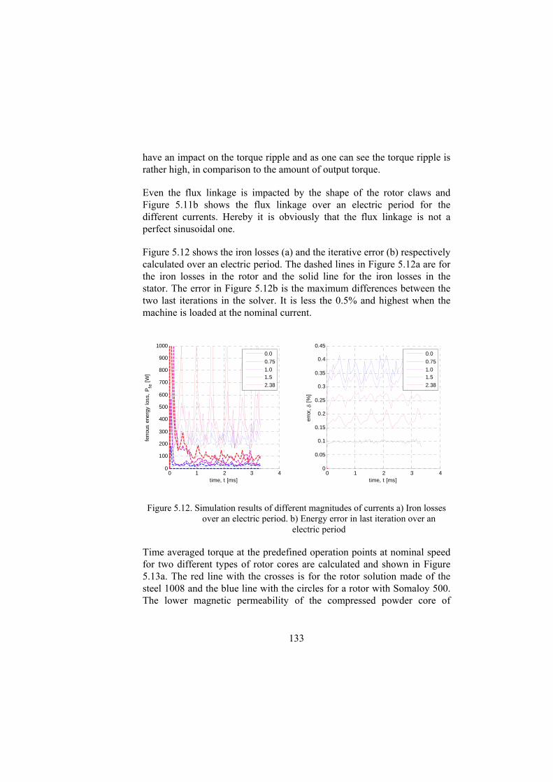
133

have an impact on the torque ripple and as one can see the torque ripple is rather high, in comparison to the amount of output torque.

Even the flux linkage is impacted by the shape of the rotor claws and Figure 5.11b shows the flux linkage over an electric period for the different currents. Hereby it is obviously that the flux linkage is not a perfect sinusoidal one.

Figure 5.12 shows the iron losses (a) and the iterative error (b) respectively calculated over an electric period. The dashed lines in Figure 5.12a are for the iron losses in the rotor and the solid line for the iron losses in the stator. The error in Figure 5.12b is the maximum differences between the two last iterations in the solver. It is less the 0.5% and highest when the machine is loaded at the nominal current.

0 1 2 3 40

100

200

300

400

500

600

700

800

900

1000

time, t [ms]

ferr

ous

ener

gy lo

ss,

Pfe

[W

]

0.0

0.75

1.01.5

2.38

0 1 2 3 40

0.05

0.1

0.15

0.2

0.25

0.3

0.35

0.4

0.45

time, t [ms]

erro

r,

[%

]

0.0

0.75

1.01.5

2.38

Figure 5.12. Simulation results of different magnitudes of currents a) Iron losses over an electric period. b) Energy error in last iteration over an

electric period

Time averaged torque at the predefined operation points at nominal speed for two different types of rotor cores are calculated and shown in Figure 5.13a. The red line with the crosses is for the rotor solution made of the steel 1008 and the blue line with the circles for a rotor with Somaloy 500. The lower magnetic permeability of the compressed powder core of

134

Somaloy-500, seen in Figure 5.3, result in lower torque output from the machine. At the same time the higher loading influences less the machine output and this is due to the negligible eddy current effects in the rotor and also smaller difference of permeability when entering the machine core into the saturation.

The torque in the both cases is tending to be concave to the current boost more than convex which is the theoretical case when the saturation is neglected.

Figure 5.13b shows the average error in each calculation, unfortunately the error is missing for the solid steel 1008 at the current magnitude of 0.75 respective 2.38. This since those points is calculated on a computer where the error was not recorded. Even though all the error points are not included the trends of error are that it is largest around the nominal current where the saturation is near the knee of the BH- curve.

0 0.5 1 1.5 2 2.5-5

0

5

10

15

20

25

30

loading, x [times]

aver

age

torq

ue,

T [

Nm

]

solid rotor core

powder rotor core

0 0.5 1 1.5 2 2.50.05

0.1

0.15

0.2

0.25

0.3

0.35

0.4

loading, x [times]

aver

age

erro

r,

[%

]

solid rotor core

powder rotor core

Figure 5.13. a) Torque versus x of nominal current b) Simulation error versus x of nominal current

The flux distribution of the machine with solid rotor core and maximum current loadings is shown in Figure 5.14. This outcome indicates that both the rotor and the stator core are magnetically loaded nearly to the saturation.

135

Figure 5.14. Flux density distribution at maximum selected current loading in the excitation coil and armature windings

When comparing the eddy current losses in the rotor; the powder core rotor has approximately 6 times smaller power losses than the solid rotor core Figure 5.15.b. The power losses in the stator core Figure 5.15.a is almost independent on the type of the rotor core, which means that the rotor establishes nearly the same magnetisation of the stator as the torque and the flux linkage are nearly the same, seen in Figure 5.13.

0 0.5 1 1.5 2 2.50

50

100

150

200

250

300

350

400

450

loading, x [times]

pow

er lo

sses

in t

he s

tato

r co

re,

Pfe

st [

W]

solid rotor core

powder rotor core

0 0.5 1 1.5 2 2.50

100

200

300

400

500

600

700

loading, x [times]

pow

er lo

sses

in t

he r

otor

cor

e, P

fest

[W

]

solid rotor core

powder rotor core

Figure 5.15. a) Iron losses in stator versus x of nominal current. b) Iron losses in rotor versus x of nominal current.

136

The eddy currents in the surface of the rotor teeth, which is the basis for the iron losses in the rotor, is larger in magnitude for the rotor made of steel 1008 compared to the one made of Somaloy 500. This is illustrated in Figure 5.16 a) and b) which shows the simulated eddy currents in the teeth for respective material. Figure 5.16a) shows results for the rotor consisting of Somaloy 500 and Figure 5.16b) for the rotor consisted of steel 1008. The simulations are at nominal load and with a rotational speed of 3000 rpm. As shown in the figures the current density for SMC and steel is 0.1A/mm2 and 15A/mm2 respectively (Figure 5.16). This is more than two orders of magnitude different between them. It is also noticeable that the eddy currents occur by the stator slots which are in line with the theory [3].

Figure 5.16. Eddy currents in the rotor teeth, a) Somaloy 500 b) Steel 1008

Load angle

So far the armature field is kept at a 90 degree angle to the excitation field and the further investigation is to determine the optimal loading angle when considering the rotor saliency and the availability of the reluctance torque in the machine. The load angle is changed in six steps and between 90 and 135 degree. The simulation results are shown in the diagram in Figure 5.17, where the x-axis show the angle 0 to 50 which means that the load angle extended above 90 degrees.

137

Again the two different rotor cores are compared, the powder core presented with blue circles and the solid iron core with red crosses. As one can see in Figure 5.17a) Somaloy 500 provides less torque compared to steel 1008. It generates less eddy current losses too, which can be seen in Figure 5.17b). It can be noticed in Figure 5.17 that the optimal current angle is nearly the same at 36 degrees and the eddy current losses decrease faster for the solid rotor core than for the powder rotor core when increasing the load angle from 0 to 36 electrical degrees.

The iron losses in the stator core are not dramatically affected by the variation of the load angle. It increases in the both cases with about 15% from 0 to 45 degree and has a maximum with the load angle of 36 degree.

0 10 20 30 40 5013.5

14

14.5

15

15.5

16

16.5

17

load angle, [degrees]

aver

age

torq

ue,

T av [

Nm

]

solid rotor core

powder rotor core

0 10 20 30 40 500

50

100

150

200

250

load angle, [degrees]

pow

er lo

sses

in t

he r

otor

cor

e, P

fert [

W]

solid rotor core

powder rotor core

Figure 5.17. a) Average torque versus load angle. b) Iron losses in rotor core versus load angle.

The increase of torque with the increased load angle, utilizing the reluctance torque, is 18% for the solid core and 21% for the powder core. This is rather high, but the reason is that the reluctance in the y-direction is due to the flux path in the rotor teeth, i.e. the flux in y-direction goes from one side of the rotor teeth to the other side of the same tooth. This makes the reluctance relatively small compared to the reluctance in the x-direction where the fluxes goes through the claw down via the excitation air gaps and back through the second claw, i.e. it passes two air gaps more

138

than the flux in y-direction.

Recalculating and scaling

The size and the current density in previous section is not representative to the comparison of the PMSM, the EMSM and the SMSM in chapter 4. The current density is too high and the size is too small, both in the radial direction and in length of the air gap. Thus the 3D model is resized to match the other machines and the armature currents are equivalent to same current density. The new properties are listed in Table 5.3.

The resized machine consists of two identical rotor parts which is mirrored and axially stacked after each other. This means that it has two excitation winding and two toroid shaped (one piece) permanent magnets. The permanent magnets are larger in the radial direction than the one in the previous section, both since the rotor are resized and also by that the cavity of the magnet slot is fully used. This was not the case in the previous section where the magnet was scaled to fit the multi piece magnet in the prototype.

Table 5.3 Resized machine specification

Quantity Value

Axial air gap length Ho, [mm] 68

Outer diameter of stator Ds, [mm] 171

Outer diameter of rotor Dr, [mm] 132.6

Axial rotor length Lr, [mm] 68

Number of poles, Np 12

Number of turns per stator phase, Nts 11

Number of turns in excitation coil, Ntf 780

Nominal speed, n [rpm] 3000

Nominal stator current, Is [A] 52

Nominal excitation current, If [A] 1.8

139

The 3D FE simulation model, using the axial symmetry of the rotor, consists of only one half of the machine and the result is multiplied by a factor of two. The rotor consists of Somaloy 500 in the rotating parts and the stationary excitation core is by steel 1008.

To reduce the calculation time the simulations are made without the solvers for the iron losses used at the numerical calculations in the previous section. The number of rotational positions is reduced and goes from 0 to 9 degree with a resolution of 1 degree.

The simulation result gives an average excitation flux linkage Ψm of 0.042Wb and 0.029Wb when the armature currents are 1.8A and 0A respectively. This corresponds to a hybridization ratio of 0.65.

The centre of the voltage-limit ellipse is with a negative excitation current within the maximum current circle (chapter 2). This makes the maximum speed of the machine, viewed in the electric limitation, to infinity. This means that it is the mechanical limitation that set the maximum speed.

The average torque at different load angles with the nominal currents and two times the nominal currents give the peak torque at 108 and 117 degree respectively. The average nominal torque of the whole machine is 31.5Nm and the intermittent current boost of 2 times the nominal current gives a torque of 68.7Nm. A linear interpolation between these torques, results to a required current boost of 1.63 times the nominal current to fulfil the specified cranking torque of 55Nm (chapter 1). Contribution of the reluctance torque in the cases of the nominal and two times the nominal currents are 9% and 17% respectively.

5.6 Summary

The 2D simulation, with the equivalent circuit, shows the potential to reduce the computational time in an evolution of a 3D machine. The computational time for the result presented as the surface graph in Figure 5.5a is around 10 minutes for the 2D model and consists of 255 number of simulations. A simulation of 6 points for the 3D model takes 7 days, which means that it would take 42.5 weeks to do all 255 points in the 3D model instead of 10 minutes in the 2D model.

140

For the iron losses there are an advantage with using SMC in this rotor. The reduction in iron losses at the simulated nominal current is 77% in the rotor and 31% in the total iron losses. This with a torque reduction of 5% compared to the solid iron rotor.

A comparison between the machines in chapter 4 and the two different sizes of the machine in this chapter 5 is listed in Table 5.4. The comparison is with the active length, outer stator radius Rout, air gap radius Rgap, air gap area Ag, active volume Vout, nominal torque Tn, shear stress F/Ag, nominal torque per volume Tn/V and the current boost factor Icrank which is x times the nominal currents. The active volume is calculated by the active length and the outer stator radius and does not considering any winding end turns and machine housing at all. All machines have the same armature current density.

Table 5.4 Machine comparison

EMSM SMSM PMSM HMSM I HMSM II

Length [m] 60e-3 60e-3 60e-3 68e-3 68e-3

Rout [m] 85e-3 85e-3 85e-3 70e-3 85e-3

Rgap [m] 66.3e-3 66.3e-3 66.3e-3 56e-3 66.3e-3

Ag [m2] 25e-3 25e-3 25e-3 23.9e-3 28.3e-3

Vout [m3] 13.6e-4 13.6e-4 13.6e-4 10.4e-4 15.4e-4

Tn [Nm] 14.5 14.5 13.9 13.8 31.4

F/Ag [N/m2] 8.75e3 8.75e3 8.39e3 10.30e3 16.72e3

Tn/V [Nm/m3] 10.6e3 10.6e3 10.2e3 13.2e3 20.3e3

Icrank (x In) 3.21 3.21 5.95 4.04 1.63

The HMSM I and II is the original size and the resized hybrid magnetization model respectively. They have a slightly longer active length than the other ones in Table 5.4. The air gap radius and outer stator radius for the HMSM II is the same as the EMSM, SMSM and PMSM.

Both the shear stress and the torque per volume are around two times

141

higher for the HMSM II in comparisons to the EMSM, SMSM and PMSM. This is in line with the theory in chapter 2. The required current boost to achieve the specified cranking torque indicates a clear advantage for the hybrid magnetization.

142

Chapter 6 Assessment of the hybrid magnetization rotor

In this chapter the machine is studied from an experimental point of view. Experimental verification methods and implementation of the methods are described. The outcome of the experimental work is presented and compared to the numerical analysis in Chapter 5.

6.1 Machine data and construction

An experimental rotor is built and tested with an existing stator and parts from a standard automotive Lundell alternator, analysed in Chapter 3. The rotor is made of solid steel SS1650 where the magnetic characteristics, BH-curve, are measured by a toroid chap sample of the material. The steel SS1650 for the prototype is chosen to simplify manufacturing of the rotor and reduce the construction time of the prototype.

The machine design specification used in the theoretical design (the 3D simulation model, see also Table 5.2) and the prototype specifications are both listed in Table 6.1. The differences between the prototype and simulation model, beside the rotor material, is the axial rotor length and the multi piece magnet. The active rotor length, i.e. the air gap length, is the same in both cases. Like with the theoretical design in Chapter 5 the nominal armature current is higher than the nominal current of the original alternator (66.5 A). This does not effect the validation but would give, as mentioned in Chapter 5, a higher temperature in continues drive.

143

Table 6.1 Machine specification

Quantity Theoretical design

Prototype

Outer diameter, Do [mm] 142 142

Axial air gap length Ho, [mm] 34 34

Outer diameter of rotor Dr, [mm] 111 111

Axial rotor length Lr, [mm] 34 54

Number of poles, Np 12 12

Number of magnets 1 28

Total magnet surface area, Am [mm2] 2256 2240

Number of turns per stator phase, Nts 11 11

Number of turns in excitation coil, Ntf 780 780

Supply voltage, Udc,[V] 1 108

Nominal speed, n [rpm] 3000 3000

Nominal stator current, Is [A] 95 95

Nominal excitation current, If [A] 1.8 1.8

The complete rotor is shown in Figure 6-1, where a) is the theoretical design (CAD) model and b) the manufactured prototype. There is an axial difference between the prototype and the theoretical design from chapter 5. Both the rotational part (A) and the non rotational part (B) are extended in axial direction. This is done in order to enable a non magnetic screw joint to the shaft (E) respective the fixture (D) without a reduction of the soft magnetic material, which would increase the reluctance. Instead it leads to a small decrease of the reluctance which improves the demagnetisation of the rotor. Since the changes in the reluctance is in the bottom part and not in the claws of the rotor, the impact on the maximum magnetization is negligible. Those screw joints are chosen for an easy assembly and the opportunity to an easy disassembly of the parts in the prototype. In a non prototype production the claw structure would probably be attached to the rotor shaft by press fit, as the regular alternator.

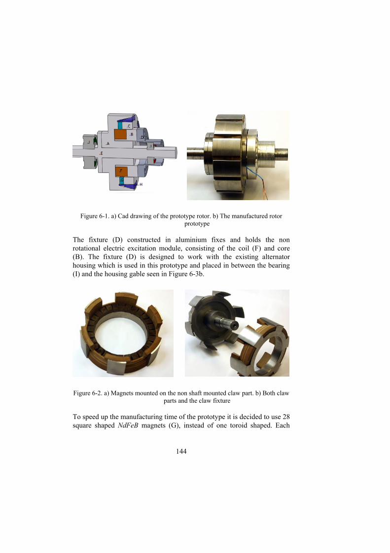
144

Figure 6-1. a) Cad drawing of the prototype rotor. b) The manufactured rotor prototype

The fixture (D) constructed in aluminium fixes and holds the non rotational electric excitation module, consisting of the coil (F) and core (B). The fixture (D) is designed to work with the existing alternator housing which is used in this prototype and placed in between the bearing (I) and the housing gable seen in Figure 6-3b.

Figure 6-2. a) Magnets mounted on the non shaft mounted claw part. b) Both claw parts and the claw fixture

To speed up the manufacturing time of the prototype it is decided to use 28 square shaped NdFeB magnets (G), instead of one toroid shaped. Each

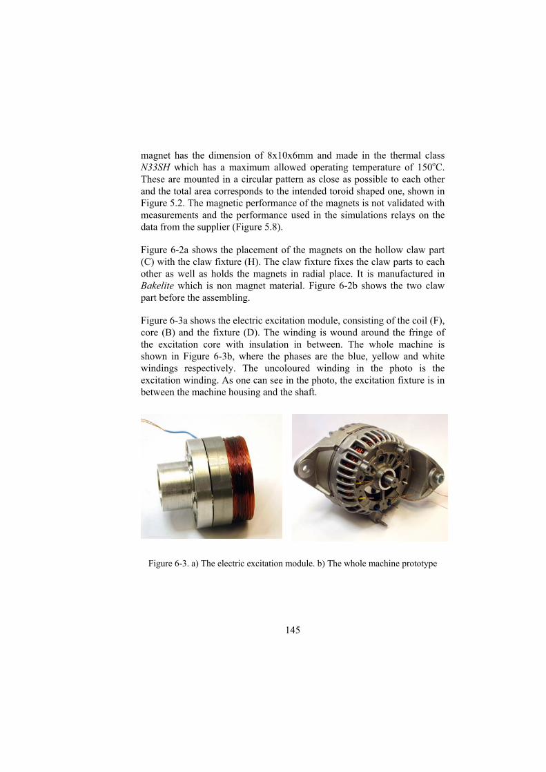
145

magnet has the dimension of 8x10x6mm and made in the thermal class N33SH which has a maximum allowed operating temperature of 150oC. These are mounted in a circular pattern as close as possible to each other and the total area corresponds to the intended toroid shaped one, shown in Figure 5.2. The magnetic performance of the magnets is not validated with measurements and the performance used in the simulations relays on the data from the supplier (Figure 5.8).

Figure 6-2a shows the placement of the magnets on the hollow claw part (C) with the claw fixture (H). The claw fixture fixes the claw parts to each other as well as holds the magnets in radial place. It is manufactured in Bakelite which is non magnet material. Figure 6-2b shows the two claw part before the assembling.

Figure 6-3a shows the electric excitation module, consisting of the coil (F), core (B) and the fixture (D). The winding is wound around the fringe of the excitation core with insulation in between. The whole machine is shown in Figure 6-3b, where the phases are the blue, yellow and white windings respectively. The uncoloured winding in the photo is the excitation winding. As one can see in the photo, the excitation fixture is in between the machine housing and the shaft.

Figure 6-3. a) The electric excitation module. b) The whole machine prototype

146

6.2 Laboratory setup

The photo in Figure 6-4 shows the machine rigged into the test bench. The machine is connected to a switched three phase power supply for dynamic testing [55] with known external inertias. A resolver is attached to the rotor axel in the rear of the machine. It is connected via a clutch and the resolver is capsulated in to an aluminium house which is mounted to the machine housing via three distance pins; the whole arrangement can be seen in the photo.

The laboratory setup uses a FPGA system (CompactRIO) from National Instruments for both the measurements and the control of the machine. Several I/O modules from National Instruments are mounted to the slots in the CompactRIO, each module is name by NI and a module specific number.

There are two different types of modules that are used for the angular measurement by resolver: a) resolver excitation input (Analogue out) NI9263 and b) the transformed resolver outputs (Analogue in) NI9223, respectively. The phase currents are measured by two LEM modules connected and sampled with a NI9215 module. The DC link voltage is sampled by NI9205 and the pulse width modulation (PWM) signal, to the power electronics, uses a NI9401 module.

The field current is supplied via a variable auto-transformer and diode bridge where additional inductor is connected to smooth the DC current. The DC current is measured by a common multimeter.

147

Figure 6-4. Prototype rigged for dynamic loading tests

The phase current in the laboratory setup is limited by the maximum range of the LEM modules to 120A.

The stator supply is a PWM switched voltage source inverter (VSI) controlled by vector control in the rotor reference frame (x,y) [20]. The reference of the current vector is set in polar coordinates by the length and the load angle respectively. The current vector is then transformed into the x- and y-current references used in the current control loop.

Dynamic loading

The measurements of the machine currents, rotor position, switching states of inverter voltage and dc-link voltage are done by acceleration/deceleration testing with a dynamic load [55] where two discs with known inertia are mounted on the shaft. By changing the known inertia, adding or removing the discs, it is possible to verify the inertia of the rotor and estimate acceleration torque at specified operation points of different sets of stator currents. In Figure 6-4 one disc is mounted.

148

The torque is related to the moment of the inertia and the angular acceleration is:

dt

dJT

(6.1)

where ω is the angle velocity, J and T the momentum of the inertia and torque respectively. Momentum of inertia of each disc is 18.27e-3Kgm2, by measuring the rotational acceleration with one respective two discs is the remaining momentum of inertia calculated to 3.37Kgm2. This is the moment of inertia of both the rotor respective the resolver and the clutches.

6.3 Laboratory validations

To validate the simulations in Chapter 5, a number of different laboratory measurements are done. One of the most important inputs is the evaluation of the BH-characteristic of the construction steel that is used for the prototype but not known in prior to 3D FEA. Both a toroid shaped measurement sample and the construction of the rotor prototype comes from the same piece of material. The toroid shaped sample of the material is used to get the magnetic performances of the material (SS_1650).

Rotor material properties To verify the magnetic properties of the SS_1650 steel used to build the prototype rotor, measurements are done on a 5mm thick toroid sample of SS-1650 with an outer and inner diameter of 50mm and 40mm respectively, see Figure 6-5. The primary winding (excitation) has 41 turns (Np) and the secondary winding (pickup) has 60 turns (Ns), both windings are uniformly distributed throughout the toroid.

By excitation of the primary winding, with an oscillating current ip, and measurement of the voltage vs over the secondary winding the BH- characteristics can be obtained [56]. The applied magnetization field H is:

core

pp

l

tiNtH

)()(

(6.2)

149

where lcore is the mean length of the core. The magnetic flux density is calculated by:

dttv

NAtB s

score

)(1

)( (6.3)

where Acore is the cross section area of the toroid core. The integral of the measured voltage vs is done by discretization of the sampled values.

Figure 6-5 Test sample for determination of magnetic properties of the rotor

materials SS-1650.

The measurement is sampled in 10kHz and the excitation current frequency is 0.45Hz. This low frequency is to avoid the effects of iron losses as much as possible.

The measured B-H characteristics of the material and the characteristics used in the design work in chapter 5 are shown in Figure 6-6. The mean calculation of the BH -loop is calculated as the mean value of the maximum respective minimum value of the flux density for each magnitude of applied magnetization field H.

150

-1.5 -1 -0.5 0 0.5 1 1.5

x 104

-2

-1.5

-1

-0.5

0

0.5

1

1.5

2

H [A/m]

B [T

]

Measured

Mean

0 1 2 3 4 5

x 104

0

0.5

1

1.5

2

H [A/m]

B [T

]

ss-1650

Somaloy 500 1P

Steel 1008

Figure 6-6. a) Measured BH characteristic and b) BH- characteristic used in design

The figure shows that the material SS-1650 used in the prototype has a lower magnetic performance than the material steel 1008, which is used in the simulations. This has an impact on the performance of the machine. A lower magnetic permeability of the prototype leads to less flux linkage in comparison to the simulations. This reduces the torque capability of the machine.

Losses Two different kinds of measurements are done in order to separate the mechanical and the electromagnetic losses from each other. The both measurements are using dynamic tests with deceleration of the machine with no armature currents and one loading disc.

Mechanical losses

The mechanical test is done without any excitation, i.e. the rotor is assembled without magnets and there are no current in the excitation winding. To reach an initial speed of the prototype, an external machine is connected driving up the speed and are then disconnected to start the deceleration.

151

140 160 180 200 220 240 2600

50

100

150

200

250

300

350

400

450Measure deceleration

Ang

ular

spe

ed [

rad/

s]

Time [s]

Measured

Polynomial curve fitting

0 1000 2000 3000 4000 50000

10

20

30

40

50

60

70Mec. losses

Pm

ec [

W]

Speed [rpm]

Figure 6-7. a) Deceleration of the prototype. b) Mechanical losses

Figure 6-7a show a measured deceleration of the prototype (blue solid line), with the initial rotational speed of 430 rad/s. The red dashed line in Figure 6-7a shows a fourth degree polynomial curve fitting of the measured values, the curve fitting using the least square approach. The polynomial coefficients from the curve fitting are used with equation 6.1 to calculate the mechanical losses shown in Figure 6-7b.

The mechanical losses are dominated by the bearings, discussed in chapter 3.2, this since the rotor is without fan blades and has minimal cavities in between the claws.

Electro magnetic losses

For the experimental validation of the electromagnetic iron losses the permanent magnets are inserted into the rotor. The test procedure is the same as for the measurements of the mechanical losses above, i.e. deceleration from an initial speed down to zero speed. This is done for different excitation currents in all cases without armature currents. The mechanical losses are subtracted from each result which gives the electro magnetic iron losses for each excitation. Figure 6-8a shows the measured respective the simulated iron losses versus the excitation current at 3000rpm, where the measurements and the simulations are plotted with black stars and blue line with dots respectively.

152

-2 -1 0 1 20

20

40

60

80

100

120

140

160

Imag

[A]

Fe lo

sses

[W

]

Simulated

Measured

Figure 6-8.a) No load iron losses at 3000rpm. b) Simulated flux density on the stator teeth

As one can see in the figure the measured losses are higher, with a positive excitation, than the simulated losses. This can be explained by a number of different losses increases respective error factors, such as an increase of the losses of the bearings with an increase of the loading and the losses data of the material in the simulation model. It is likely that the lack of the transversal flux related iron losses in the stator solver of the 3D simulation is the most dominating reason to the differences. The solver only considers the radial and tangential fluxes in a lamination sheet and not a transversal flux perpendicular to the sheet surface. This means that the eddy current in the sheet plane is not considered at all. The phenomena are related to the stator model which is a solid model with a lamination definition. To calculate a laminated stator model, consisting of each lamination sheet and with a mesh good enough to accurate solve the eddy currents in the sheet plane would require incredible computing time and computer resources.

As one can see in Figure 6-8b there is a higher flux density in the edge of the stator closest to the back of each claw pole. This indicates that there are transversal fluxes in the stator of the claw pole machine.

The bearing at the excitation module, shown with the label (I) in the Figure 6-1a, is an angular contact ball bearing. This is chosen since there is a reluctance force acting on the electric excitation module in the axial

153

direction of this design. The increase of this force leads to an increase of the losses in the bearing as well. This is independent on the direction of the fluxes in the excitation module, since there is always a pulling force that act on the module. This means that there is nearly the same magnitude of force with the excitation current of 1.8A respective -1.8A where the magnitude of the magnetic flux through the module is nearly the same. The total losses with the excitation current of -1.8A is below 10W which indicates that the increase of the bearing related losses with a positive excitation current is not the dominateing one in the difference of the losses between the model and the prototype.

Excitation flux linkage The magnetic performance of the SS-1650 is slightly weaker than for the steel 1008. This has an impact on the machine performances as the flux linkage. This section compares the simulations with experimental work of the excitation flux linkage. Both with the waveform of the induced flux in one stator phase and the magnitude of the flux linkage regarded on the excitation current.

All experiments are done with the prototype in idling via an external machine and the induced voltage is measured in all phases with an oscilloscope. The phases are measured stand alone, i.e. not connected to each other.

Figure 6-9a show a capture by the oscilloscope of the induced voltage for one phase over one electric period. It is possible to see that the waveform is far from a pure sinusoidal wave with only the fundamental frequency and it consists of many harmonics. This is not surprising, both since the rotor claw teeth are not optimized as mention before and the stator windings are not sinusoidally distributed between the slots.

The induced phase voltage u depends on the excitation flux linkage ѱm as:

dt

du m (6.4)

Based on this equation the flux linkage is solved by integrating the measured phase voltage. Figure 6-9b show the measured and simulated

154

flux linkage versus the rotor position θ. The measured is plotted by the solid blue line and the simulated with the dashed line. As one can see the measured flux linkage is weaker than the simulated one. The magnitude of the peak is about 11% lower for the measured flux linkage compare to the simulated. This is in line with the difference between the flux density around the saturation knee of materials SS-1650 and steel 1008; which is 10% lower at 4000A/m2 in the BH- characteristics shown in Figure 5.3 and Figure 6-6b. The waveform is nearly the same between the simulated and the measured flux linkage in Figure 6-9b.

-2.5 -2 -1.5 -1 -0.5 0 0.5 1

x 10-3

-50

-40

-30

-20

-10

0

10

20

30

40

50

Time [s]

Ua [

V]

Figure 6-9. a) Measured induced phase voltage. b) Measured and simulated flux linkage versus rotor angle

In Figure 6-10 the measured peak to peak stator flyx linkage value are plotted versus the excitation current (black stars). It also contains diagrams of both 2D and 3D simulations with the two materials steel 1008 and SS-1650. The red solid line and the blue line with dots represent simulations with the 2D and the 3D model respectively, where the rotor consists of steel 1008. The black stars and the black dotted line represent the measurements and the 2D simulations with the rotor in SS-1650.

155

-2 -1.5 -1 -0.5 0 0.5 1 1.5 20

0.01

0.02

0.03

0.04

0.05

0.06

m

pp [

V/s

]

If [A]

Sim.3d Steel 1008

Sim.2d Steel 1008Sim.2d Steel ss1650

Measured

Figure 6-10. Excitation flux linkage peak to peak versus excitation current

Each star in the figure is for one phase and one measurement; this explains the proliferation of the results.

In comparison between the 2D and the 3D simulations, with steel 1008, the magnitude of the flux linkage are same with the excitation current above 0.5A and differs below. The difference has to do with the missing fringe of the excitation core and a non-magnetic axel in the 2D model. This improves the flux paths in the lower region of the rotor part which works as a shunt by the electric excitation discussed in chapter 5. The magnitude of the measured flux linkage of the prototype with the SS-1650 in the rotor is less in comparison to the simulation with steel 1008., but has the nearly the same magnitude to the upper excitations of the 2D simulations with the same rotor material. Due to the simplification of the 2D model in the region with a negative excitation current the simulations differs from the measurements. A simulation with the 3D model and with the same material as the prototype would probably match each other. Due to lack of time is this unfortunately not done, and are left to future work.

The measured hybridization ratio (Ch2) is about 0.54 for the prototype.

156

This is nearly the same ratio as the 3D simulations in chapter 5.5 where the permanent magnet is equivalent to the magnets in the prototype.

Characteristics This section treats the validation of the torque characteristics of the model by the comparison between the prototype and the 3D model. It is done with different load angle and by scaling of the nominal current, which is used in the simulations shown in section 5.5.

Load angle and torque boost

The measurements are done with dynamic loading of one disc. Figure 6-11a shows the acceleration of the machine using nominal currents, both in the excitation and the armature. The torque is calculated by equation 6.1 where the rotational acceleration by the same polynomial curve fitting as in the previous section (Losses). The acceleration process starts with a light acceleration in reverse speed direction followed by a full acceleration in forward direction up to 4000rpm. This is done in order to have a stable acceleration in the zero speed point, which is the basically the way to calculate the cranking torque.

0.5 1 1.5 2 2.5 3 3.5 4

0

500

1000

1500

2000

2500

3000

3500

4000

4500

Spe

ed [

rpm

]

time [s]

0 5 10 15 20 25 30 35 40 450

2

4

6

8

10

12

14

16

18

20

22

Load angle, [deg]

Tor

que,

T [

N]

1.25

1

0.750.5

0.25

Figure 6-11. Measurments; a) the acceleration of the prototype at nominal currents and a relative load angle of 45 b) Torque at different load angle and

with different current scaling of the nominal currents.

Figure 6-11b shows the measured torque versus the relative load angle, i.e. the angle beyond the 90 degree. The different diagrams represent the

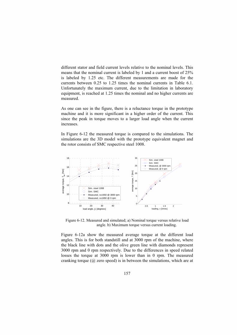
157

different stator and field current levels relative to the nominal levels. This means that the nominal current is labeled by 1 and a current boost of 25% is labeled by 1.25 etc. The different measurements are made for the currents between 0.25 to 1.25 times the nominal currents in Table 6.1. Unfortunately the maximum current, due to the limitation in laboratory equipment, is reached at 1.25 times the nominal and no higher currents are measured.

As one can see in the figure, there is a reluctance torque in the prototype machine and it is more significant in a higher order of the current. This since the peak in torque moves to a larger load angle when the current increases.

In Figure 6-12 the measured torque is compared to the simulations. The simulations are the 3D model with the prototype equivalent magnet and the rotor consists of SMC respective steel 1008.

10 20 30 408

10

12

14

16

18

load angle, [degrees]

aver

age

torq

ue,

T av [

Nm

]

Sim. steel 1008

Sim. SMC

Measured, ss1650 @ 3000 rpm

Measured, ss1650 @ 0 rpm

0.5 1 1.5 20

5

10

15

20

25

30

loading, x [times]

aver

age

torq

ue,

T [

Nm

]

Sim. steel 1008

Sim. SMCMeasured, @ 3000 rpm

Measured, @ 0 rpm

Figure 6-12. Measured and simulated; a) Nominal torque versus relative load angle. b) Maximum torque versus current loading.

Figure 6-12a show the measured average torque at the different load angles. This is for both standstill and at 3000 rpm of the machine, where the black line with dots and the olive green line with diamonds represent 3000 rpm and 0 rpm respectively. Due to the differences in speed related losses the torque at 3000 rpm is lower than in 0 rpm. The measured cranking torque (@ zero speed) is in between the simulations, which are at

158

3000rpm, with respective rotor material. The measured torque at 3000 rpm is lower than the both simulations.

In Figure 6-12b the maximum average torque is plotted in relation the relative stator and field current. The maximum torques for each current loading is the torque achieved at the load angle that gives the maximum torque (reluctance torque included). In this figure both the measured torque at 0 rmp and 3000 rpm are plotted, this with a green line with diamonds and a black line with dots, respectively. As one can see the characteristics of the measurements and simulations are equal, but the measurements are slightly lower in comparison to the simulations.

6.4 Summary

In this chapter the simulations are validated with measurements. The prototype machine tends to have the same shape of the characteristics of both the torque and flux linkage, but with a slightly lower performance than the simulation model based on the different steel (1008) compared to the prototype (SS-1650). The simulated machine both has higher magnetic performance of the rotor material and do not consider all losses, such as the mechanical losses and the iron losses calculations contributed to the transversal flux in the stator.

The mechanical losses are measured to ~35W at 3000 rpm (Figure 6-7) and the iron losses, due to transversal magnetic flux in the stator, are ~80W higher at the same speed (Figure 6-8). This is equal to a torque reduction of 0.37 Nm for the prototype compared to the simulation model. The excitation flux linkage of the prototype is in 7…11% lower than simulation model in the interval 0-1.8A of the excitation current (Figure 6-10). At zero relative load angle (no reluctance torque) and the maximum excitation current (1.8A) the torque reduction would be 7%. i.e. equal to the same reduction of the excitation flux linkage (equation 2.14). This would give a torque reduction of 1 Nm for the prototype in comparison to the simulation model with steel 1008, Table 6.2.

Table 6.2 Machine comparison, prototype versus simulation model

Prototype Simulation Δ [Nm] Δ [%]

159

SS-1650 Steel 1008

T (0o load angle) [Nm] 12.7 14.32 -1.62 -11.3

T (36o load angle) [Nm] 15.84 16.98 -1.14 -6.7

T (reluctance) [Nm] 3.14 2.66 + 0.48 18.0

T (reluctance) [%] 24.7 18.5 6.3 +34

Table 6.2 lists some of the results of the simulation model, the prototype machine and the differences between them. With a zero load angle the torque difference is 1.62Nm. This match the reasoning above with the added magnitude of the losses and the reduction of excitation flux linkage. The reluctance torque is 18% higher for the prototype in comparison to the model, this due to the improvement of the differences between the reluctance in the x- respective y- direction with a lower magnetic performance material in the rotor.

160

Chapter 7 Concluding Remarks and Future Work

Fore different machine concepts are analysed, theoretically with numerical calculation, in order to compare them in terms of their suitability for a BAS application. The results of the analysis for each of the machines are presented in a graphical format and in tables, allowing the designer to compare them in an easy and convenient way. The losses and heat dissipation is analysed for a common Lundell alternator in order to create the founding of the comparison study. Experimental work has verified the analytical models and assumptions in the thesis. A new compact hybrid magnetized synchronous machine is numerically analysed and validated by a prototype. The numerical calculation considers different rotor material in order to reduce the eddy current related iron losses in the rotor.

Regarding the torque capabilities and characteristics, the EMSM and the SMSM are similar to each other. They have identical torque characteristics if the centre of the voltage limit locus is within the maximum current range but differs if it is outward. When it is outward the maximum current range the torque characteristics are only similar over the first part of the speed range (lower speeds). This before an active field weakening, dependent on the voltage limitation, of the excitation is needed. Since the armature and the excitation winding are connected to each other in the SMSM, whereby the excitation and armature current are the same, both are reduced in field weakening the machine below the voltage limitation. In the numerical analyses of the SMSM in chapter 4 the breakpoint of the active field weakening is approximately at a speed of 9000 rpm where the current supplied to the stator winding of the SMSM has to be reduced to keep down the voltage level. For this reason the EMSM at higher speeds able to

161

provide a slightly higher torque than the SMSM. In other words the SMSM is limited for a high power in the whole speed range, if the excitation flux is higher than the maximum field weakening flux of the armature currents.

The lack of a separate field weakening with the excitation (SMSM) in high frequencies could be solved by capacitors connected between the phases before the connection to the rectifier. This is not treated in this thesis but would decrease the currents to the rectifier in relation to the frequency, equal to a low pass filter.

The advantage of the PMSM and the SMSM compare to the EMSM and the HMSM is the lack of an external power supply to the excitation. On the other hand, the PMSM does not have the possibility to decrease the excitation field as the three other alternatives, so in order to be able to run at high speeds, the permanent magnet excitation has to be kept to a reasonable value. This results in lower torque capabilities especially at high speeds if the PMSM is optimized for a high cranking torque. Attending to the efficiency of the machine, the PMSM has a higher efficiency and higher output power at mid speed range. However, when the speed increases, the efficiency drops faster for the PMSM than for the two electrical and the hybrid magnetized alternatives.

Among the electrically magnetized machines, the EMSM is able to provide higher output power than the SMSM, since the field current can be controlled separately, enabling an additional degree of freedom that makes it possible to keep the active stator current at high level at high speeds, just reducing the field current.

Concerning the cranking torque, the PMSM requires higher current levels which limits the time over which the cranking torque can be delivered. The HMSM has, in this study, the highest cranking torque for the least stator current which gives the advantage to the HMSM in a BAS application. For the SMSM and EMSM the cooling capability of the excitation winding is one of the main issues in a designe, setting one of the limitations on the excitation strength which plays a major role in a BAS application. The SMSM and EMSM in this thesis have the strength of the magnetization that place the centre of the voltage limit locus slightly outside the

162

maximum current line. Whit an improvement of the cooling capability of the rotor entails the possibility of increase the nominal excitation current and the magnetization. This would lead the EMSM and possibly the SMSM to be more competitive to the HMSM, this also since the lack of permanent magnets.

A future work for the EMSM and SMSM would be to improve the magnetization strength and also investigate or develop a slip-ringless solution.

The HMSM solution in this thesis has three main advantages in comparison to the other three machines. The first and maybe the most important role in the BAS application is to provide a high power factor and torque capability over a wide speed range. The second advantage is the slip-ring less solution, not used in the PMSM either, which are in many cases an issue for its sensitivity to the environment and the need for maintenance. This would in the author's opinion, not play a big role in a vehicle where many wear parts is used. The third advantage is the manufacturability and compactness of the rotor. Without winding end turns, it has the opportunity to increase the active magnetic axial length within a certain volume or be used in a more compact stator solution. A future work on this HMSM would be to design the excitation module and the nearby claw pole structure in a way that the axial forces, related to the reluctant force, would be cancelled. It would be interesting to build a second prototype based on the resized HMSM presented in chapter 5 which fulfil the requirements of the BAS specification and uses SMC in the contraction. To verify the study of different rotor materials in chapter 5, it would be interesting to build a prototype in SMC as well.

My subjective opinion The PMSM is with the high and also increasing prize of the permanent magnets and the lack of performance not suitable as a BAS. The HMSM is the maybe the most suitable one, the advantage is the high power density which is makes it possible to achieve the specification in a compact design. But the disadvantage is the use of permanent magnets, the future pricing of which is unsure. Both the EMSM and SMSM have the potential to work as a BAS, especially if the possibility of improving the current density in the rotor and a slip-ringless solution is further investigated.

163

Prerequisite for the use of a SMSM in a BAS with a high power factor during a wider range is the use of low pass filtering the excitation current.

The FEA in chapter 5 show the potential to use 2D simulations in the evolution of a 3D machine. It makes it possible to scan through a wider range of machine dimensions and different material properties in a more reasonable time than if it is done in a 3D model only. In this thesis an equivalent 2D structure is used, where the reluctance corresponds to the one in the 3D structure. This would be possible to replace by a reluctance equivalent boundary condition, based on a number of 3D FEA.

.

165

References

[1] T. A. Lipo, “Introduction to AC Machine Design”, Department of Electrical and Computer Engineering , Universiry of Wisconsin, USA, 1996.

[2] J. R. Hendershot Jr and TJE. Miller, “Design of Brushless Permanent-Magnets Motors”, Magna Physics Publishing and Clarendon Press, Oxford, 1994

[3] J. Pyrhönen, T. Jokinen and V. Hrabovcova, "Design of Rotating Electrical Machines", John Wiley & Sons, Ltd. 2008, ISBN: 978-0-470-69516-6

[4] “Comparing the Benefits and Impacts of Hybrid Electric Vehicle Options”, EPRI, Palo Alto,CA: 2001, 1000349.

[5] Y. Gao, M. Ehsani and J. Miller, “Hybrid Electric Vehicle: Overview and State of the art”, IEEE International Symposium on Industrial Electronics, Vol.1, pp 307-315, 2005.

[6] J. Heywood, “Internal Combustion Engine Fundamentals”, McGraw-Hill, New York, NY, USA, 1989.

[7] M. Alaküla, C. Andersson, K. Jonasson and B. Simonsson, “Hybrid Drive Systems for Vehicles part 1”, Department of Industrial Electrical Engineering and Automation, Lund University, Lund, 2006.

[8] D. Martinez, “Modelling and Control of Electrical Machines - With Applications to Iron-powder Machines and Acoustic Noise”, PhD Thesis, Department of Industrial Electrical Engineering and Automation, Lund University, Lund, Sweden, 2004.

[9] T. Bergh, “Belt driven Alternator and Starter with a Series Magnetized Synchronous Machine drive”, Licentiate Thesis, Department of Industrial Electrical Engineering and Automation, Lund University, Lund, Sweden, 2006.

166 References

166

[10] D. Richard, Y. Dubel, "Valeo StARS Technology: A Competitive Solution for Hybridization", Power Conversion Conference (PCC 07), Nagoya, 2-5 April, 2007

[11] Hagstedt, D., “A BAS application of a series magnetized synchronous machine”. International Conference on Electrical Machines, IEMC'06 Conference, Crete, Greece, 2-5 September, 2006.

[12] Hagstedt, D., Márquez, F., Alaküla, M., “A comparison between PMSM, EMSM and SMSM in a BAS application ”. International Conference on Electrical Machines (ICEM2008), Vilamoura, Portugal, Sept. 6-9, 2008

[13] Bergh, T., Hagstedt, D., Alaküla, M., Karlsson, P., “Modeling and presentation of the series magnetized synchronous machine”. SPEEDAM 2006 International Symposium on Power Electronics, Electrical Drives, Automation and Motion, Taormina, Italy, 23-26 May, 2006.

[14] Reinap, A., Hagstedt, D., Márquez, F., Loayza, Y., Alaküla, M., “Development of a radial flux machine design environment”. International Conference on Electrical Machines (ICEM2008), Vilamoura, Portugal, Sept. 6-9, 2008.

[15] S. Chen, B. Lequesne, R. R. Henry, Y. Xue, J. J. Ronning, “Design and Testing of a Belt-Driven Induction Starter-Generator”, IEEE Transaction on Industry Applications, vol. 38, n. 6, 1525-1533, November/December 2002.

[16] R. R. Henry, B. Lequesne, S. Chen, J. Ronning, Y. Xue, “Belt-Driven Starter-Generator for Future 42-Volt Systems”, SAE Int. Congr. Detroit, SAE Paper 2001-01-0728, Mars 2001.

[17] J.M. Miller, A.R. Gale, P.J. McCleer, F. Leonardi, J.H. Lang, "Starter-Alternator for Hybrid Electric Vehicle: Comparison of Induction and Variable Reluctance Machines and Drives", IEEE Industry Applications Conference, , vol.1, Oct. 1998, pp. 513-523

[18] S. Marimoto, Y. Takeda, T. Hirasa, K. Taniguchi, “Expansion of Operating Limits for Permanent Magnet Motor by Current Vector Control Considering Inverter Capacity”, IEEE Transaction on Industry Applications, Sep/Oct 1990, pp. 866-871.

References 167

167

[19] J.-M. Kim, S.-K. Sul, “Speed Control of Interior Permanent Magnet Synchronous Motor Drive for the Flux Weakening Operation”, IEEE Trans. Industry Applications, Jan./Feb. 1997, pp. 43-48.

[20] M. Alaküla; “Power Electronic Control”, Department of Industrial Electrical Engineering and Automation, Lund University, Sweden, 2003, pp. 101-103.

[21] N. Mohan, T. M. Undeland, W. P. Robbins, "Power Electronics, Converters, Applications, and Design",John Wiley & Sons, inc, 2003, ISBN 0-471-252693-9

[22] W. L. Soong, T. J. E. Miller, "Field-weakening performance of brushless synchronous AC motor drives", IEE Proc.-Electr. Power Appl., Vol. 141, No. 6, November 1994

[23] N. Bianchi, S. Bolognani, "Parameters and Volt-Ampere Ratings of a Synchronous Motor Drive for Flux-Weakening Applications", IEEE Transactions on Power Electronics, Vol. 12, No. 5, September 1997

[24] H. Alvarez, "Energiteknik Del 1", Studentlitteratur, Lund, 1990, ISBN 91-44-31471-X

[25] Y. Nakayama, R. F. Boucher, "Introduktion to Fluid Mechanics", YOKENDO CO. LTD, Tokyo, 1998, ISBN 0 340 67649 3

[26] E. I. Shobert, “Electrical Resistance of Carbon Brushes on Copper Rings”, Power Apparatus and Systems, Part III. Transactions of the American Institute of Electrical Engineers, vol. 73, pp. 788-799, Jan. 1954

[27] F. Magnussen, E. Nordlund, S. Châtelet, C. Sadarangani, “Measurements of slip ring units for characterization of performance”, Royal Institute of Technology (KTH), Sweden

[28] Morgan AM&T, "Book 1 How to Select Carbon Brushes for Motors and Generators"

[29] T. A . Harris, M. N . Kotzalas, “Essential Concepts of Bearing Technology”, Fifth Edition, CRC Press 2006, ISBN: 978-0-8493-7183-7

168 References

168

[30] T. Cousseau, B. Graca, A. Campos, J. Seabra, “Friction torque in grease lubricated thrust ball bearings”, Tribology International, 44, pp. 523-531, 2011.

[31] SKF General Catalogue 6000 EN, November 2005

[32] H. Skarrie; “Design of Powder Core Inductors”, Licentiate Thesis, Department of Industrial Electrical Engineering and Automation, Lund University, Lund, Sweden, 2001.

[33] G. Bertotti, “Hysteresis in Magnetism”, Elsevier inc. 1998, ISBN: 978-0-12-093270-2.

[34] V. Ostevic, J. M. Miller, V. K. Garg, R. D. Schultz, S. H. Swales “A Magnetic-Equivalent-Circuit-Based Performance Computation of a Lundell Alternator”, IEEE Transaction on Industry Applications, v 35 ,n 4, pp. 825–830, July/August 1999

[35] S. Küppers, G. Henneberger, “Numerical Procedures for the Calculation and Design of Automotive Alternators”, IEEE Transaction on magnetics, v 33,n 2, pp. 2022–2025, March 1997

[36] A. Gimeno, G. Friedrich, K. El-kadri-benkara, “Experimental and numerical evaluation of iron losses in a claw pole car generator” IEEE, International Conference on Electrical Machines (ICEM) , Rome, 2010

[37] L. Hultman, O. Andersson, ”Advances in SMC Technology - Materials and Applications”, EURO PM2009, Copenhagen, Denmark, Oct 13, 2009

[38] B. W. Williams, "Power electronics, devices drivers applications and passive components" McGraw-Hill, 1992

[39] Cengel, Y.A., “Heat and Mass Transfer: A Practical Approach,” 3/e, McGraw-Hill, 2007

[40] B. Sundén, "Värmeöverföring", Studentlitteratur, 2006

[41] D. A. Howey, P. R. N. Childs, A. S. Holmes, "Air-Gap Convection in Rotating Electrical Machines", IEEE Transactions on Industrial Electronics, VOL. 59, No. 3, March 2012.

[42] D. M. Ionel, M. Popescu, S. J. Dellinger, TJE Miller, R. J. Heideman, M. I. McGilp,_" Factors Affecting the Accurate Prediction of Core Losses in Electrical Machines", Electric

References 169

169

Machines and Drives, 2005 IEEE International Conference on 15-15 May 2005, pp. 1625 – 1632.

[43] K. T. Chau, C. C. Chan, and C. Liu, “Overview of permanent-magnet brushless drives for electric and hybrid electric vehicles,” IEEE Trans Ind Electron, v 55, n 6, pp. 2246–2257, Jun. 2008.

[44] Z. Zhuoran, Y. Yan, S. Yang and Z. Bo “Principle of Operation and Feature Investigation of a New Topology of Hybrid Excitation Synchronous Machine” IEEE Trans Trans Magn, v 44, n 9, pp. 2174–2180, Sep. 2008.

[45] E. Sulaiman, T. Kosaka and N. Matsui “High Power Density Design of 6-Slot-8-Pole Hybrid Excitation Flux Switching Machine for Hybrid Electric Vehicles” IEEE Trans Trans Magn, v 47, n 10, pp. 4453–4456, Oct. 2011.

[46] E. Sulaiman, T. Kosaka and N. Matsui “Design and Performance of 6-Slot-8-Pole Hybrid Excitation Flux Switching Machine for Hybrid Electric Vehicles” IEEE, The 2010 International Power Electronics Conference , 2010.

[47] W. Shanming, X. Yonghong, W. Xiangheng, S. Pengsheng, H. Shaogang and Z. Anming "State of the Art of Hybrid Excitation Permanent Magnet Synchronous Machines" IEEE ICEMS, pp. 1004-1009, Oct. 2010.

[48] Y. Amara, L. Vido, M. Gabsi, E. Hoang, A. Hamid Ben Ahmed, and M. Lecrivain, "Hybrid Excitation Synchronous Machines: Energy-Efficient. Solution for Vehicles Propulsion," IEEE Trans Vehicular Technology, v 58, n 5, pp. 2137-2149, Jun. 2009.

[49] C. Liu, K. T. Chau, and J. Z. Jiang, "A Permanent-Magnet Hybrid Brushless Integrated Starter–Generator for Hybrid Electric Vehicles", IEEE Trans Ind Electronics, v 57, n 12, pp 4055-4064, Dec 2010

[50] W. Li and S. Huang, "Analysis and Design of Hybrid Excitation Claw-pole Generator", Electric Power Components and Systems, 39:7, pp 680-695, Apr 2011

[51] C. Kaehler and G. Henneberger "Transient 3-D FEM computation of eddy-current losses in the rotor of a claw-pole alternator", IEEE Trans Magn, v 40, p.1362 , 2004.

170 References

170

[52] S. Kuppers and G. Hennenberger, "Numerical procedures for the calculation and design of automotive alternators", IEEE Tran. Magn, v 33, p.2022, 1997.

[53] G. Henneberger, S. Kuppers, I. Ramesohl, “Numerical calculation, simulation and design optimisation of claw pole alternators for automotive application”, IEE Colloquium on Machines for Automotive Applications, Digest No. 1996/166, pp. 3/1-3/5

[54] L. Kefsi, Y. Touzani, M. Gabsi, "Hybrid Excitation Synchronous Motor Control with a new Flux Weakening Strategy" IEEE Vehicle Power and Propulsion Conference (VPPC). sep. 2010

[55] Loayza, Y., Reinap, A., Alaküla, M. (2011), “Performance and efficiency evaluation of FPGA controlled IPMSM under dynamic loading”. 8th IEEE International Symposium on Diagnostics for Electrical Machines, Power Electronics and Drives (SDEMPED), Bologna, Italy, September 5-8, 2011.

[56] W.L. Soong, " BH Curve and Iron Loss Measurements for Magnetic Materials", Power Engineering Briefing Note Series, PEBN #5, 12 May 2008

[57] Ryden, L., Technical Leader Electrical Components, Volvo Global Trucks Technology (GTT), Vehicle Engineering (VE) (Personal communication)

171