Comparing the Functional Independence Measure and the interRAI/MDS for use in the functional assessment of older adults 

      by 

Christine Glenny          

A  thesis  presented to the University of Waterloo 

in fulfilment of the  thesis requirement for the degree of  

Master of Science in  

Health Studies and Gerontology      

Waterloo, Ontario, Canada, 2009  

©Christine Glenny 2009

ii  

Author’s Declaration

I hereby declare that I am the sole author of this thesis. This is a true copy of the thesis, including any required final revisions, as accepted by my examiners.

I understand that my thesis may be made electronically available to the public.

iii  

Abstract

Background: The rehabilitation of older persons is often complicated by increased frailty and

medical complexity – these in turn present challenges for the development of health information

systems. Objective investigation and comparison of the effectiveness of geriatric rehabilitation

services requires information systems that are comprehensive, reliable, valid, and sensitive to

clinically relevant changes in older persons. The Functional Independence Measure is widely

used in rehabilitation settings – in Canada this is used as the central component of the National

Rehabilitation Reporting System of the Canadian Institute of Health Information. An alternative

system has been developed by the interRAI consortium. We conducted a literature review to

compare the development and measurement properties of these two systems and performed a

direct empirical comparison of the operating characteristics and validity of the FIM motor and

the ADL items on the PAC in a sample of older adults receiving rehabilitation. Methods: For the

first objective english language literature published between 1983 (initial development of the

FIM) and 2008 was searched using Medline and CINAHL databases, and the reference lists of

retrieved articles. Additionally, attention was paid to the ability of the two systems to address

issues particularly relevant to older rehabilitation clients, such as medical complexity,

comorbidity, and responsiveness to small but clinically meaningful improvements. For the

second objective we used Rasch analysis and responsiveness statistics to investigate and compare

the instruments dimensionality, item difficulty, item fit, differential item function, number of

response options and ability to detect clinically relevant change. Results: The majority of FIM

articles studied inpatient rehabilitation settings; while the majority of interRAI/MDS articles

focused on nursing home settings. There is evidence supporting the reliability of both

instruments. There were few articles that investigated the construct validity of the

interRAI/MDS. The analysis showed that the FIM may be slightly more responsive than the

iv  

PAC, especially in the MSK patients. However, both scales had similar limitations with regards

the large ceiling effect and many unnecessary response options. Conclusions: Additional

psychometric research is needed on both the FIM and MDS, especially with regard to their use in

different settings and ability to discriminate between subjects with functional higher ability.

 

   

v  

Acknowledgements

I would like to thank my advisor, Dr. Paul Stolee for the numerous opportunities with

which he provided me during the course of my Master’s degree. My committee members, Dr.

Janice Husted and Dr. Mary Thompson also have my most sincere appreciation for their input.

I would also like to thank the Ontario Rehabilitation Research Advisory Network

(ORRAN) and Health Canada: Primary Health Transitions Fund for funding this project. Also

everyone involved in the data collection process especially Dr. Katherine Berg.

Many professors and members of staff in the Department of Health Studies and

Gerontology have contributed to my success. I thank them for making my experience at the

University of Waterloo such an enjoyable one.

Finally, a thank you to my family, friends and colleagues for their continued supported and

encouragement.

   

vi  

 

List of Tables  xiList of Figures  xii

CHAPTER 1: Introduction and Background 1.0   Introduction  2 

1.1   Background  3 

  1.1.1    Inpatient Rehabilitation of Older Persons  3 

    A          Musculoskeletal Rehabilitation Units versus Geriatric Rehabilitation           Unit    

3 

  1.1.2    Relevant Functional Assessment Instruments  4 

  1.1.3    National Rehabilitation Reporting System  5 

    A           Functional Independence Measure  5 

  1.1.4    interRAI/MDS Instruments  6 

    A           Measuring Activities of Daily Living with interRAI instruments  7 

    B          Measuring Cognitive Impairment with interRAI Instruments  7 

  1.1.5    Properties of Health and Functional Assessment Measures  8 

    A           Reliability              8 

    B          Validity  9 

    C          Responsiveness  9 

  1.1.6    Measurement Theory  10 

    A           Classical Test Theory  10 

    B           Rasch     11 

1.2   Study Rationale and Research Objectives 12 

  1.2.1    Study Rationale  12 

  1.2.2    Research Objectives  14 

  1.2.3    Analysis Plan 

 

 

14 

 

vii  

CHAPTER 2: Objective 1 2.0  Objective 1: Methods  17 

  2.0.1    Criteria for considering studies in this review  17 

  2.0.2    Search methods for identification of studies  18 

  2.0.3    Data collection and analysis  19 

2.1   Objective 1: Results  20 

  2.1.1    Reliability  21 

    A          Reliability of the FIM  22 

    B         Reliability of the MDS  24 

  2.1.2    Validity  26 

    A        Validity of the FIM  27 

    B        Validity of the MDS  29 

    C        Validity of the FIM and the MDS  31 

  2.1.3    Overall comments and Conclusions  31 

CHAPTER 3: Objective 2 Methods 3.0   Data   36 

  3.0.1    Data Source  36 

  3.0.2    Study Population  36 

  3.0.3    Data Collection Procedure  36 

  3.0.4    Data Collect Tools  37 

  3.0.5    Power Calculation  38 

  3.06    Scale Preparation  39 

3.1    Construct Theory  40 

3.2    Sample Description  41 

3.3    Research Questions  42 

3.4   Statistical Analysis  43 

  3.4.1    Principal Component Analysis  43 

viii  

  3.4.2    Common‐Persons Equating  44 

  3.4.3    Distribution Maps  45 

  3.4.4    Point Measure Correlations  46 

  3.4.5    Person/Item Fit Statistics  46 

  3.4.6    Category Probability Curves   47 

  3.4.7    Summary of Category Structure  47 

  3.4.8    Differential Item Functioning  48 

  3.4.9    Responsiveness statistics: Standardized Response Mean and Effect Size  48 

CHAPTER 4: Objective 2 Results 4.0   Sample Description  52 

4.1   Sub‐objective A  53 

  4.1.1    1. Do the items for one unidimentional construct  53 

  4.1.2    2. Does item difficulty correspond with subject ability  56 

  4.1.3    3. Does the empirical data fit the Rasch model  60 

  4.1.4    4. Can the number of response options be decreased to improve the validity of the measure? 

62 

  4.1.5    5. Is the level of difficulty of each item consistent across different impairment groups and overtime? 

65 

  4.1.6    Overall Conclusions  68 

  4.1.7    Scale Modifications  69 

    A           FIM  69 

    B           PAC  73 

4.2   Sub‐objective B  76 

  4.2.1    6. Which functional outcome measure is most appropriate in this sample with respect to the range in difficulty of the items relative to the ability of the subjects 

76 

4.3   Sub‐objective C  79 

  4.3.1    7. Which instrument is the most responsive in this sample?  79 

  4.3.2    8. Does responsiveness of each functional outcome measure change in      different samples of this population 

80 

    A                By Unit  80 

ix  

    B                By Age   81 

    C                By FCI  

82 

CHAPTER 5: Strengths and Limitation 5.1    Strengths  85 

5.2    Limitations  85 

CHAPTER 6: Conclusions  

6.1    Overall Conclusions  89 

6.2    Implications  91 

6.3   Recommendations for the Future 92 

References          

Appendix  Chapter 1 

 

  1.1  National Rehabilitation Reporting System (NRS)  106   1.2  Response option definitions for the FIM  115   1.3  interRAI Post AcuteCare (PAC)  116   1.4  interRAI ADL subscales  123   1.5  Definitions and interpretations of commonly used statistics for measuring 

reliability and validity 124 

Chapter 2     2.1  Literature review summary tables  125 

Chapter 3     3.1  Item codes for the FIM and the PAC  145   3.2  Construct theory  146   3.3  Functional Comorbidity Index and corresponding interRAI PAC items  149   3.4  “Rules of Thumb” for Principal Component Analysis  150   3.5  How to calculate 95% confidence intervals for SRM  151 

Chapter 4     4.1  Sample characteristics for Toronto vs London  152   4.2  Sample characteristics for GRU vs MSK  155   4.3  Frequency distributions  157   4.4  Standardized residual construct plots and item loadings (unmodified 

instruments) 167 

x  

  4.5  Multiple Item Characteristic Curves (unmodified instruments)  175   4.6  Variable Maps (Original instruments, pre CPA)  183   4.7  Item fit explanations (Original instruments)  187   4.8  How to collapse response options – admission data  192   4.9  Tally for how to collapse response options – admission data  212   4.10  Response option output for combined admission and discharge data  214   4.11  Underused response options for combined admission and discharge data  234   4.12  Uniform DIF (original instruments)  235   4.13  Non‐uniform DIF explanations  275   4.14  Separation of FIM and PAC items into self care and transfer subscales  277   4.15  Scatter plots for self care and transfer subscales   278   4.16  Item fit for modified instruments   282   4.17  Variable maps for modified instruments  284   4.18  Common person analysis of original instruments  288   4.19  Adjusted variable maps  292   4.20  Common person analysis of original instruments  295             

                          

 

xi  

 

List of Tables  Table 2.1 Summary of validity and reliability studies of the FIM and MDS  21   Table 2.2: FIM and MDS reliability findings by setting  22   Table 2.3: FIM and MDS reliability findings by type of rater  22   Table 2.4: Summary of results for the interrater reliability of the FIM  24   Table 2.5: FIM and MDS validity studies by setting  26   Table 2.6: Summary of results for the responsiveness of the FIM  29   Table 3.1: Research Questions and Statistical Methods  42   Table 4.1: Results of Principal Component Analysis for the Unmodified Scales  53   Table 4.2: Summary of Variable Maps for the Unmodified Scales  56   Table 4.3: Item Fit Statistics for the Unmodified Scales    60   Table 4.4: Uniform DIF analysis for Unmodified Instruments  66   Table 4.5: Summary of Results  68   Table 4.6: FIM Split Scales Correlation Coefficients  70   Table 4.7: Impact of removing STAIR on the dimensionality of the FIM   71   Table 4.8: Effect of combining response options on the dimensionality of the FIM  72   Table 4.9: PAC Split Scale Correlation Coefficients  74   Table 4.10: Impact of removing STAIR on the dimensionality of the PAC  74   Table 4.11: Effect of combining response options on the dimensionality of the PAC  76   Table 4.12: Responsiveness Statistics of the original and modified instruments  79   Table 4.13: Responsiveness Statistics of the original and modified instruments by age  81   Table 4.13: Responsiveness Statistics of the original and modified instruments by FCI 

                    

83 

xii  

 

List of Figures  Figure 2.1: Results of search strategy  20      

1  

Chapter 1:

Introduction and Background

2  

1.0 Introduction

Measuring and reporting health outcomes have become an essential component guiding

the development and evolution of health care systems. As the focus of health care changes to

adapt to the aging population, aggregate data from health assessment systems can be used to

inform policy decisions regarding service use and best practices (McKnight and Powell, 2000).

One area that already serves a disproportionately larger number of older adults is post acute

rehabilitation (PAC; Landi et al., 2002). There is a need for accurate assessment in this

population as it can have significant implications for the patient’s level of health care utilization

and future quality of life (Katz and Stroud, 1989). For example, Gosselin and colleagues (2008)

showed that the functional status of older patients is improved by rehabilitation services and the

majority of older adults who receive rehabilitative care are able to return to their previous living

environment. Despite some encouraging research in this area (Gosselin et al., 2008; Ergeletzis et

al., 2002; Hardy and Gill, 2005), there are limited data that focus on measuring rehabilitation

outcomes in older adults (Demers et al., 2004). One major challenge is that the performance of

currently available assessment systems is not well understood in this population.

Development of valid and reliable outcome measures for use with older adults is

complicated by frailty, comorbidity, and heterogeneity in this population. Geriatric patients are

different from their younger counterparts as they tend to have lower functional status on

admission and higher clinical complexity due to multicausal disability and intercurrent medical

conditions (Gosselin et al., 2008; Wells et al., 2003; Patrick et al., 2001). Older adults are an

extremely diverse population and represent a wide range of physical and cognitive abilities

(Landi et al., 2002). To address these obstacles, Wells and colleagues (2003) recommended that

standardized tools should be used for diagnosis, assessment and outcome measurement in

3  

geriatric rehabilitation. Instruments that are designed for younger, healthier, and more

homogenous groups are unlikely to have the same psychometric properties with older adults

(Landi et al., 2002) and additional research is required specifically related to the performance of

assessment tools and outcome measures in older populations of rehabilitation patients.

1.1 Background

1.1.1 Inpatient Rehabilitation of Older Persons

The primary focus of inpatient rehabilitation of older adults is to restore and/or maintain

physical functioning (Patrick et al., 2001). This is accomplished by striving to recover the

individual’s ability to perform activities of daily living (ADLs) and improve their quality of life

(Demers et al., 2004). In this population, small gains in one or several areas may result in large

overall improvements in functional status (Patrick et al., 2001). The benefits of geriatric

rehabilitation include preservation of the individual’s functional autonomy and prevention of

unnecessary use of health services including recurrent admissions (Stolee et al., 2004; Stott et al.,

2006). In contrast to long-term care or complex continuing care, the length of stay tends to be

short, with discharge dependent on the speed in which the person returns to a reasonable level of

independence. Rehabilitation of older adults can be distinguished from other age groups by the

large amount of patient variation (Demers et al., 2004). This is due to higher burden of comorbid

diseases and greater prevalence of cognitive impairment (Borrie et al., 2001).

A. Musculoskeletal Rehabilitation Units versus Geriatric Rehabilitation Units

Musculoskeletal Rehabilitation Units (MSK) and Geriatric Rehabilitation Units

(GRU) are two types of rehabilitation units in Ontario. MSKs specialize in musculoskeletal

4  

conditions such as arthritis, joint replacement and loss of physical functioning as a result of

stroke (torontorehab.on.ca; Knoefel et al., 2003). They serve adults over the age of 18; however,

as with many other types of health care services, their primary patient population tends to be

older adults (torontorehab.on.ca; Knoefel et al., 2003). GRUs care exclusively for older adults

and their patients tend to be admitted from acute care settings (torontorehab.on.ca). Knoefel and

colleagues (2003) compared the functional status and medical complexity of patients in GRUs

and MSKs. They found that, as expected, GRU patients were, on average, older than MSK

patients (Mean ages: 81 yrs vs 68.5 yrs) and were more medically complex (2003). GRU patients

were significantly more functionally impaired on admission and achieved less functional gains

during longer inpatient stays (2003). Both units had an equal proportion of orthopaedic patients

(1/3 of the patient populations) and 50% and 20% of the MSK and GRU patients respectively,

were classified as stroke (2003). The researchers suggested that due to the large difference in

patient characteristics, specially designed rehabilitations programs are necessary for medically

complex older adults (2003).

1.1.2 Relevant Functional Assessment Instruments for Rehabilitation Settings

Prior to the development of functional assessment instruments, information collected was

not precise enough to be used in clinical research and care planning (Katz and Stroud, 1989).

Assessment was mostly qualitative in nature and based on the judgement of a clinician (1989).

Researchers and clinicians identified the need for assessment instruments that could provide

meaning and quantitative precision to describe the magnitude and severity of functional

impairment (1989). This began with the development of a list of activities of daily living (ADL)

that were based on a combination of theoretical and empirical information and included six basic

5  

areas; bathing, dressing, toileting, transferring, continence and feeding (Katz, 1963). In the time

since, many generic and targeted functional assessment instruments have been developed using

various combinations of ADLs (Granger et al., 1986; Morris et al., 1990; Hebert et al., 1988;

Mahoney and Barthel et al., 1963). Researchers who focus on measuring physical functioning in

older adults have also suggested toolkits (Auger et al., 2007; Demers et al., 2005),

multidisciplinary teams (Wells et al., 2003; Stott, et al., 2006) and/or individualized approaches

(Stolee et al., 1999) for accurate assessment in these highly variable geriatric populations.

1.1.3 National Rehabilitation Reporting System

The National Rehabilitation Reporting System (NRS) (Appendix 1.1) is a minimum set

of client data regarding socio-demographic, administrative and functional status information

from inpatient rehabilitation facilities (www.cihi.ca). It was developed in Canada by the

Canadian Institute of Health Information (CIHI) based on consultations with over 350 experts in

the field and the results of a multi-province pilot study (cihi.ca). NRS data is submitted to CIHI

that subsequently produces reports that focus on rehabilitation indicators such as: average

admission/discharge function score, average length of stay by rehabilitation client group and

average days waiting for admission/discharge to and from rehabilitation (cihi.ca). The Functional

Independence Measure (FIM; Granger et al., 1983) is the major source of functional status data

in the NRS.

A. Functional Independence Measure (FIM)

The Functional Independence Measure (FIM) was developed in 1983 by a task

force assigned by the American Congress of Rehabilitation Medicine/American Academy of

Physical Medicine and Rehabilitation that was headed by Carl Granger and Byron Hamilton

6  

(Granger et al., 1986). It was designed to measure physical and cognitive disability and focuses

on burden of care (1986). The main objective in the development of the FIM was to create a

generic measure the can be administered by clinicians and non-clinicians to assess patients in all

age groups with a wide variety of diagnoses (1986). The FIM contains a total of 18 items.

Thirteen of these items constitute the motor subscale (FIM motor) and the remaining five items

make up the cognitive subscale (FIM cognitive) (Granger et al., 1993b). The motor subscale

collects information involving self care, sphincter control, mobility and locomotion and the

cognitive subscale focuses on communication and social cognition. The items are all scored

using a seven point ordinal scale that is based on the amount of assistance that is required for the

patient to perform the activity (Appendix 1.2;1993b). High scores on the FIM describe patients

that have a high level of independence and require a small amount of assistance (1993b). The

sum of all 18 items gives a total score that ranges from 18-126 (1993b).

1.1.4 interRAI/MDS instruments

interRAI is an international research consortium that develops comprehensive assessment

tools that are especially intended for older adult populations (Gray et al., 2009;

www.interrai.org). These Resident Assessment Instruments (RAIs) are used internationally in a

wide variety of health care settings for a large number of applications including care planning,

outcome measurement and quality indicators (RAI/MDS 2.0 User Manual, 2005). Currently

there are 12 RAI tools designed for use in rehabilitation, long term care, home care and other

settings across the health care continuum (Gray et al., 2009). The instruments consist of over 300

items covering a large array of patient characteristics including functional status, admission

history, medical conditions and other information (RAI/MDS 2.0 User Manual, 2005). All of the

7  

tools contain a proportion of common items that are intended to facilitate communication in

multiple health care settings (Hirdes et al., 2008; Gray et al., 2009). Each individual tool also

includes specialized items exclusive to that setting (2008). The tool specifically designed for use

in rehabilitation is the interRAI Post Acute Care (PAC; Appendix 1.3; Morris et al., 2004;

interrai.org).

A. Measuring Activities of Daily Living with interRAI instruments

Physical functioning is measured by a range of ADL items that can be summed to

form several ordinal ADL scales (Morris et al., 1999) (Appendix 1.4). These items were

designed to measure activities across a wide range of functional independence levels to enable

the detection of functional changes in individuals with both high and low levels of functioning

(1999). Each item is scored on the basis of the amount of assistance required for performance

with higher scores indicating greater dependence (1999). Currently there has been no consensus

on a single standard ADL subscale for the interRAI instruments (1999; Graney & Engle, 2000;

Phillips et al., 1993; Phillips and Morris, 1997; Landi et al., 2000).

B. Measuring Cognitive Impairment with interRAI instruments

Cognitive functioning can be estimated using the interRAI instruments in two

ways: the 5 item Cognitive Performance Scale (CPS; Morris et al., 1994) or the 11 item MDS

Cognition Scale (MDS-COGS; Hartmaier et al., 1995). Both are ordinal scales, the CPS ranges

from 0 (intact) to 6 (very severe impairment) and the MDS-COGS ranges from 0 (cognitively

intact) to 10 (very severe impairment). These scales were both developed based on their

correlation with, and ability to predict scores of, existing cognition scales, including the Mini-

8  

Mental State Exam (Folstein et al., 1975), Test for Severe Impairment (Albert & Cohen, 1992)

and the Global Deterioration Scale (Reisberg et al., 1998; Folstein et al., 1975; Albert & Cohen,

1992).

1.1.5 Properties of Health and Functional Assessment Measures

A. Reliability

Reliability is an indicator of the tool’s consistency (Streiner, 1993). There are three major

types of reliability used to describe different attributes of a test. Internal consistency measures

the average correlation between all items on a tool and is commonly expressed with Cronbach’s

α (1993). Intrarater reliability, also called test-retest reliability, is an indicator of the tests’

stability overtime when it is administered by the same rater (Streiner and Norman, 2003). If a

tool has good intrarater reliability, subjects who have not changed during the testing period (the

time frame between two assessments) should achieve the same score on both tests. Interrater

reliability indicates the consistency of a tool when it is administered by different raters (2003).

Interrater reliability is a more conservative estimate because it includes two possible sources of

error, different raters and possible changes in the subject ability over the testing period (Streiner,

1993). The Pearson correlation coefficient is a commonly used to indicate reliability; however, it

must be interpreted carefully because it measures consistency in association, but not in

agreement, therefore it is not sensitive to systematic biases between the observations (1993).

Intra-class correlation coefficients (ICC) and kappa coefficients are preferred for measuring

absolute agreement for dichotomous items, and weighted kappa is recommended for

polychotomous items because it can measure partial agreement between the different response

categories (Appendix 1.5; Streiner and Norman, 2003).

9  

B. Validity

Examining the validity of an instrument determines whether the tool measures what it

was designed to measure (Streiner, 1993). There are four major types of validity. Face validity is

an estimate of whether the tool appears to measure the intended concept (Streiner and Norman,

2003). This type of validity is usually assessed during the initial stages of development, and is

often a qualitative measure based on expert opinion. Content validity assesses whether the tool

targets all of the relevant topics related to the concept being measured and that there are no

irrelevant items (Streiner, 1993). Often this is measured using a content validity matrix which is

a tally of relevant topics measured by each item (1993). Criterion validity is the third major type

and can be divided into two categories; concurrent and predictive (Streiner and Norman, 2003).

Concurrent criterion validity measures the correlation of the tool with other tools that measure

the same concepts, preferably a “gold standard” when it exists (2003). Predictive criterion

validity examines whether the tool can predict future outcomes (2003). Finally, construct validity

investigates whether the tool correlates with a theorized construct (Streiner, 1993). It is

determined by the accumulation of evidence over multiple hypothesis based investigations

(1993).

C. Responsiveness

Responsiveness is the ability of a tool to identify and measure changes over time

if real clinically relevant changes have occurred (De Groot et al., 2006). Reliability is a necessary

but not sufficient condition for responsiveness (Streiner and Norman, 2003). This means that for

a tool to detect change over time it must be able to 1) measure consistently when no change has

occurred (reliable), 2) detect clinically relevant change when it has occurred (responsive) (2006).

10  

In order to accurately measure responsiveness, the investigator must use the tool in a population

that is expected to change over time (Brooks et al., 2006). If the population does not experience

true change over time, then the tool will be unresponsive due to the lack of change in the

population rather than the lack of detection by the measure. One disadvantage of generic health

status measures, like the FIM and PAC, is that the tools may contain items that are not expected

to change after treatment and as a result the responsiveness of the entire measure will be reduced

(Wright et al., 1997).

A number of methods have been proposed for the analysis of responsiveness

(Husted et al., 2000; Wright et al., 1997), however there is currently no consensus for a “goal

standard” measure of responsiveness (Husted et al., 2000). Due to this inconsistency, it is

suggested that multiple measures be used in a single study to allow for the interpretation of

trends across different recommended statistics (Beaton et al., 2007).

1.1.6 Measurement Theory

A. Classical Test Theory

Classical Test Theory (CTT), also referred to as Classical Measurement Theory,

is based on the assumption that a subject’s observed score (raw score, X) is composed of their

“true score” (T) and a component of measurement error (E):

X = T + E

It assumes that if there were no measurement errors, a true score could be obtained for every

subject (Kline, 2005). It also assumes that random error is normally distributed and therefore the

mean error for an infinite number of subjects is zero. Another property of CTT is that it assumes

that individual error is random and that it is not related to the subjects true score (2005). This

11  

theory results in the ability to make accurate estimates of T for populations but not for

individuals (2005). Another major limitation of this model is that it wrongly assumes that all

subjects and items have identical properties and consequently all items can be measured at the

interval level (2005).

B. Rasch

Rasch analysis is a statistical technique, based on log-odds transformations, that

uses ordinal data from classically designed measurement tools to construct interval measures

(Linacre, 2009). A shared linear continuum, measured in logits (log-odds units, a single Rasch

unit), is develop by characterizing subjects based on their performance on the tool (referred to as

the subject ability) and the items based on their rate of endorsement by the subjects (referred to

as the item difficulty) (2009). The Rasch models are log-linear models based on the probability

(P) that a subject (n) with the ability Bn will succeed on item i in category j that has difficulty

level Di. The “calibration” measure for category j (Fj) is the point where categories j-1 and j are

equally probable relative to the measure of the item.

Dichotomous model: loge (Pni1/Pni0) = Bn– Di

Polytomous “Partial Credit” model: log (Pnij/Pni(j-1) = Bn - Di – Fij = Bn - Dij

By forcing the ordinal data into a linear model, it becomes possible to evaluate

how well the empirical data (observed data) correspond to the model (referred to as “fit”). This is

a powerful tool for instrument development because it allows the investigator to quantify their

assumption that the items can be measured at the interval level and provides information on how

12  

to modify the instrument to become a more accurate estimate of the model’s interval scale

(2009).

1.2 Study Rationale and Research Objectives

1.2.1 Study Rationale

The overall purpose of this research was to directly compare the psychometric properties

of the FIM and the interRAI PAC when they are used to measure functional status in older adults

receiving rehabilitation. Components of these instruments collect parallel information (Williams

et al., 1997) and have been used widely with older persons. It is important for outcome measures

used in rehabilitation to be validated in this context because older adults represent a substantial

proportion of the rehabilitation patient population. They have different patient characteristics

than younger adults which makes it unlikely that the measurement properties of assessment tools

will be consistent between the two populations. Also, the higher heterogeneity and medical

complexity of older persons present challenges for consistent outcome measurement. One of the

reasons for this is that it is difficult to determine if the instrument is measuring true differences

between the subjects or merely random variability in the sample.

For the first stage of this project, past research focusing on the reliability and validity of

both instruments was accumulated and synthesized. There have been no publications to date that

review the psychometric properties of both tools. This information can be used for this analysis,

1) to develop a construct prior to the Rasch analysis and 2) to determine the representativeness of

our sample, and in the future to determine if results are compatible with the current knowledge

on the topic. It can also be used to identify gaps in the literature and guide future research.

13  

Second, admission and discharge data collected with both instruments was analysed for

the same group of patients. To our knowledge, this was the first dataset that has the same sample

of subjects assessed with the complete version of both tools. This is beneficial because the

construct validity of the functional assessment items could be compared directly. Also, additional

items on the instruments can be used to divide the sample into meaningful subpopulations to

determine if the tool has the same properties in patients with different characteristics.

Specifically, the data were collected from two different types of rehabilitation units: MSK and

GRU. These choices of rehabilitation units allow for the comparison of the scales when they are

used in patients with differing levels of clinical complexity.

In contrast to long-term care or complex continuing care, patients admitted to post acute

rehabilitation settings have a higher potential for future improvement. Length of stay tends to be

relatively short and the primary focus of care relates to functional improvements, with discharge

dependent on the speed in which the person returns to a reasonable level of independence. Based

on these characteristics, post acute rehabilitation is the ideal setting to measure the

responsiveness of functional outcome measures.

It was especially important to determine the responsiveness of tools used to measure

functional status in older adults because small changes on the tool’s scale may represent very

large, clinically relevant, changes in reality. For example, a small change on a tool’s scale can

mean the difference between discharge to a long-term care facility or to home care.

This research is consistent with the priorities of the Canadian Consensus Workshop on

Geriatric Rehabilitation because it investigated “mandated systems” and “best assessment tools”

(Stolee et al., 2004). Comparing the relative merits of the two systems could provide an initial

step towards the identification of a standard measure. Having a single valid tool for measuring

14  

functional impairment in older adults would help to guide service use, identify best practices and

improve communication between health care professionals.

1.2.2 Research Objectives

This thesis had two related objectives:

Objective 1: To conduct a systematic review of previously published literature

and compare the development and psychometric properties of the FIM and the

interRAI/MDS as functional assessment measures in older adults (50+).

Objective 2: To perform a direct empirical comparison of the operating

characteristics and validity of the FIM motor and the ADL items on the PAC in a

sample of older adults receiving rehabilitation.

A) To use Rasch methods to develop 1) a new scale using PAC items and

2) a revised version of the FIM motor subscale that will independently

measure functional impairment in MSK and GRU patients

B) To directly compare the construct validity of the original and newly

developed subscales for measuring functional impairment in MSK and

GRU patients

C) To measure and compare the responsiveness of the original and newly

developed subscales in MSK and GRU patients

1.2.3 Analysis Plan

For the first objective, information regarding the reliability and validity of the tools was

gathered and summarized to appraise current understanding and identify areas where future

15  

research is needed. This information was also use to develop a Construct Theory, an essential

first step for the Rasch analysis. In an effort to meet the second objective, eight research

questions were prepared. These helped to guide the analysis through developing new FIM and

PAC summary scales, investigating their construct validity, and directly comparing their

appropriateness as functional outcome measures including an evaluation of their responsiveness.

16  

Chapter 2:

Objective 1

17  

2.0 Objective 1: Methods

To date few researchers have attempted to collect and synthesize this information, and

there have been no reviews that are both systematic and inclusive. For this reason, a detailed

search strategy was developed and all studies meeting the inclusion/exclusion criteria were

included in the review regardless of their methodological merit.

2.0.1 Criteria for considering studies in this review

All relevant English language articles that were published between January 1983

(the initial development of the FIM) and June 2008 were included in this review. The following

inclusion and exclusion criteria were established to determine article relevance:

Inclusion criteria

1) The study population includes older adults (50+)

2) The main focus of the article is on some aspect related to the development

and/or measurement properties of the FIM and/or MDS instruments

Exclusion criteria

1) The article focuses on child, adolescent and/or young adult populations

2) The article does not contain original data, statistical analysis and results

3) The article is a review of previously published work

4) The article solely focuses on patients with spinal cord injuries and/or traumatic

brain injuries

18  

5) The article reports experimental versions of the FIM and/or MDS used to

assess the properties of additional items/short forms not currently used in clinical

practice

6) The instruments are used in the study as the intervention (i.e., to test the effects

of a comprehensive assessment on patient outcomes)

7) The article does not relate to MDS items/subscales that are comparable to FIM

items

2.0.2 Search methods for identification of studies

Published material was identified using the MEDLINE and CINAHL databases

using the following search strategy:

MEDLINE database

1) Functional Independence Measure [TIAB] OR FIM [TIAB] Limits: Published in 1983 to 2008

2) Minimum Data Set [TIAB] OR MDS [TIAB]OR interRAI [TIAB] OR Resident Assessment Instrument [TIAB] Limits: Published in 1983 to 2008

3)

Reproducibility of Results [MeSH] OR reliability [TIAB] OR interrater [TIAB] OR intrarater [TIAB] OR test retest [TIAB] OR internal consistency [TIAB] OR validity [TIAB] OR criterion [TIAB] OR construct [TIAB] OR content [TIAB] OR responsiveness [TIAB] OR clinically relevant change [TIAB] OR clinically important change [TIAB] OR development [TIAB] OR psychometric [TIAB] OR performance [TIAB] OR validation [TIAB] OR dimentionality [TIAB] OR structure [TIAB] Limits: Published in 1983 to 2008

4) Delirium, Dementia, Amnestic, Cognitive Disorders [MeSH] OR Activities of daily living [MeSH] OR functional assessment [TIAB] OR cognitive [TIAB] OR cognitively [TIAB] OR cognitive performance scale [TIAB] OR function [TIAB] OR physical [TIAB] OR activities of daily living [TIAB] OR ADL [TIAB] OR motor function [TIAB] Limits: Published in 1983 to 2008

5) 1 AND 3 AND 4 6) 2 AND 3 AND 4

19  

CINAHL database

1) Functional Independence Measure OR FIM Limits: Published in 1983 to 2008

2) Minimum Data Set OR MDS OR interRAI OR Resident Assessment Instrument [TIAB] Limits: Published in 1983 to 2008

3)

Reliability and Validity OR reliability OR interrater OR intrarater OR test retest OR internal consistency OR validity OR criterion OR construct [TIAB] OR content [TIAB] OR responsiveness [TIAB] OR clinically relevant change [TIAB] OR clinically important change [TIAB] OR development [TIAB] OR psychometric [TIAB] OR performance [TIAB] OR validation [TIAB] OR dimentionality [TIAB] OR structure [TIAB] Limits: Published in 1983 to 2008

4) Delirium, Dementia, Amnestic, Cognitive Disorders [MH+] OR Activities of Daily Living [MH+] OR functional assessment [TIAB] OR cognitive [TIAB] OR cognitively [TIAB] OR cognitive performance scale [TIAB] OR function [TIAB] OR physical [TIAB] OR activities of daily living [TIAB] OR ADL [TIAB] OR motor function [TIAB] Limits: Published in 1983 to 2008

5) S1 AND S3 AND S4 6) S2 AND S3 AND S4

The reference lists of the retrieved articles were also examined for additional relevant

papers.

2.0.3 Data collection and analysis

Guided by the inclusion and exclusion criteria, the first author (CG) eliminated irrelevant

articles based on the title of the publication and the content of its abstract. All potentially

relevant articles were retrieved and reviewed. As a reliability check, any article that was

retrieved but later found to be irrelevant was reviewed by the second author (PS). When the

relevance was questionable, the two authors discussed the paper to arrive at a final conclusion.

For each of the selected articles, information was gathered and charted using the

reliability and validity criteria proposed by Streiner (1993). The reliability and validity categories

reported the study sample and setting, methods, findings and conclusions in chart form. Internal

consistency, interrater and intrarater reliabilities were included in the reliability category and

20  

face, content, criterion and construct validities were included in the validity category. Also,

particular attention was given to responsiveness as a component of validity.

2.1 Objective 1: Results

The initial keyword search identified 944 articles, of which 850 were excluded based on

review of the title and abstract. Eight additional articles were identified by handsearching the

reference lists of articles obtained in the initial search. Of the 94 articles retrieved for further

review, 27 were excluded based on relevance and 9 were excluded as they were reviews of

previously published works (Figure 2.1).

944 Articles

94 Articles

Retrieved and Reviewed

Total Sample = 66 Articles

Figure 2.1: Results of search strategy

MEDLINE and CINAHL

Potentially eligible studies identified by search with duplicates removed

Appeared relevant based on title and abstract (see inclusion and exclusion criteria)

- 27 Articles Irrelevant,

reviewed by second author

+ 8 Articles Reference lists of relevant articles

- 9 Articles Review articles, no original data

21  

Forty articles focused on the FIM, 26 focused on the MDS, and 1 article investigated both

instruments. Appendix 2.1 summarize the total sample of articles that met the criteria for this

review

Table 2.1 Summary of validity and reliability studies of the FIM and MDS Reliability Validity

Internal Consistency Intrarater Interrater Total Criterion Construct Content Face Total

FIM 6 2 5 13 14 26 0 1 41 MDS/interRAI 5 1 12 18 12 7 0 1 20

* Some articles discuss multiple types of reliability and validity; therefore, totals do not correspond with the total number of articles in the sample

2.1.1 Reliability

Thirty-one of the articles in the sample investigated the reliability of the instruments. The

FIM and MDS were independently discussed in 13 and 18 articles respectively. A nearly equal

number of FIM articles investigated internal consistency and interrater reliability, while most

MDS articles focused on interrater reliability. For both instruments, few articles investigated

intrarater reliability (Table 2.2). Four of the FIM articles focused on inpatient rehabilitation

populations and five studied community residents mostly receiving home care. A large majority

of MDS articles focused on nursing home residents and no articles were found that solely

focused on inpatient rehabilitation. Clinicians were commonly used as raters for both

instruments, where only 3 FIM and 2 MDS articles used researchers to assess the participants

(Table 2.3).

22  

Table 2.2: FIM and MDS reliability findings by setting

Setting FIM MDS

Internal Consistency

Intrarater Interrater Total Internal consistency

Intrarater Interrater Total

Living at home 2 1 2 5 1 0 0 1 Inpatient Rehab. 3 0 1 4 0 0 0 0 Neurorehabilitation 0 0 1 1 0 0 0 0 Nursing home/SNF 1 0 0 1 3 0 8 11 Multilevel retirement 0 0 0 0 0 0 1 1 Acute care 0 0 0 0 0 1 0 1 Psychiatric care 0 0 0 0 1 0 0 1 Multiple settings 0 1 1 2 0 0 3 3

Total 6 2 5 13 5 1 12 18 Table 2.3: FIM and MDS reliability findings by type of rater

Rater

FIM MDS Internal

Consistency Intrarater Interrater Total Internal

consistency Intrarater Interrater Total

Clinician 6 0 4 10 3 1 12 16 Researcher 0 2 1 3 1 0 0 1 Both 0 0 0 0 1 0 0 1

Total 6 2 5 13 5 1 12 18

A. Reliability of the FIM

Internal consistency was high for the FIM total score (α = 0.88-0.97), domains (motor α =

0.86-0.98, cognitive α = 0.68-0.95), and subscales (α = 0.68-0.96); and the FIM was found to

have greater consistency than other tools commonly used in inpatient rehabilitation (Hsueh et al.,

2002). Dallmeijer and colleagues (2005) concluded that the FIM motor has slightly higher

internal consistency than the FIM cognitive; however, this result was not replicated in other

studies (Jette et al., 2005; Stineman et al., 1996). Contradictory evidence was found regarding

the internal consistency of the FIM in different impairment groups (Dallmeijier et al., 2005;

Stineman et al., 1996; Dodds et al., 1993). In an inpatient rehabilitation setting, Dodds and

colleagues (1993) found that the internal consistency of FIM items varied by impairment group,

especially for the locomotion subscale. This may suggest that all FIM items are not relevant for

all impairment types, or that the instrument is not functioning consistently for different types of

23  

patients (Streiner, 1993). Conversely, Stineman and colleagues (1996) investigated this

relationship in a sample of community residents and concluded that internal consistency was

excellent and no items should be removed for any of the 20 Uniform Data System for Medical

Rehabilitation (UDSMR) impairment types (Granger et al., 1986). The inconsistency between

these two articles may be due to different distributions and severities of impairment types in

inpatient rehabilitation and community settings. This may suggest that all FIM items are relevant

in higher functioning groups (community residents) but not in lower functioning groups (patients

in inpatient rehabilitation).

Two articles investigated the intrarater reliability of the FIM. In both articles, the

participants were assessed by researchers, and both concluded that the FIM total and domain

scores have very high reliability (FIM total r = 0.94-0.98, motor r = 0.90-0.97, cognitive r =

0.80-0.99; Ottenbacher et al., 1994; Daving et al., 2001). As researchers have different

background knowledge and are likely to receive different, more intense training programs prior

to conducting assessments, this may have artificially inflated the results leading to the high and

more narrow range of estimates of interrater reliability. Using researchers instead of clinician

raters also limited their investigation of the source of error in the natural environment.

Five additional articles also concluded that the FIM was reliable when they focused on

interrater reliability. Of these studies, 2 investigated populations of home care clients (Daving et

al., 2001; Ottenbacher et al., 1994) and 3 examined patients receiving rehabilitation in multiple

settings (Fricke et al., 1992; Hamilton et al., 1994; Kidd et al., 1994). Table 2.4 summarises the

statistical results of these 5 studies.

24  

Table 2.4: Summary of results for the interrater reliability of the FIM FIM

total FIM

motor FIM

cognitive FIM subscales FIM items

ICC 0.80-0.99

0.91-0.99

0.91-0.99 0.89-0.98 -

Percent agreement

43.5-65.1

- - - 54-79 (motor); 14-46 (cog)

Weighted Kappa

- - - - 0.24-0.58 (motor); -0.07-0.27 (cog)

Kappa - - - - 0.54-0.84 (all items) The interrater reliability was highest when both raters were present at the same interview which,

raters participated in FIM training prior to conducting their first assessment, raters met UDSMR

criteria, and the testing period was short (Dallmeijer et al., 2005; Daving et al., 2001; Fricke et

al., 1992; Hamilton et al., 1994; Kidd et al., 1995; Ottenbacher et al., 1994). Daving and

colleagues (2001) used clinicians to investigate the reliability of the FIM in community residents.

They found that the reliability ranged from poor to excellent where the least reliable assessments

were completed at different times by different raters. In this study the motor items were shown to

have higher interrater reliability (PA = 54-79; wκ = 0.24-0.58) than the cognitive items (PA =

24-46; wκ = -0.07-0.27). As the interrater reliability of the FIM was generally high in other

settings, an intrarater reliability study should be conducted to determine if clinicians assessing

community residents are the source of this inconsistency.

B. Reliability of the MDS

During the development of MDS instruments unreliable items were progressively

eliminated resulting in increasing reliability estimates overtime (Morris et al., 1990; Hawes et al.,

1995). Five articles investigated the internal consistency of functional status related outcome

measures in the MDS. In all 5 studies, the researchers concluded that the scale(s) investigated

25  

was(were) internally consistent. However, because many of the characteristics – including

subjects, setting, and raters – are different between the studies, and reliability is dependent on

such variations (Streiner & Norman, 2003), it is not currently possible to develop generalization

across these articles in regards to patterns in consistency.

Zimmerman and colleagues (2007) were the only group to investigate the intrarater

reliability of an MDS subscale. They concluded that the MDS-COGS was only moderately

reliable and found that the relative amount of within and between rater error changed for the

MDS-COGs depending on which cut-point was used. For the first cut-point (0 vs >1) the

intrarater reliability (κ = 0.59) was much higher than the interrater reliability (κ = 0.29) and for

the second cut-point (0-1 vs >2) the intrarater reliability decreased slightly (κ = 0.43) but was

approximately equal to the interrater reliability (κ = 0.46). This suggests that the error introduced

by the instrument was relatively stable at both points; however, there was more error introduced

by the rater at the first cut-point than the second.

High interrater reliability has been repeatedly shown for MDS items in nursing

home settings (Individual items r = 0.75-0.99, κ = 0.56-0.84, wκ = 0.33-1.0). Many of these

studies investigated the reliability of MDS items in isolation and did not assess the reliability of

embedded outcome measures such as the CPS and the various ADL scales. This may be a result

of intentions to preserve the ability to use various combinations of individual items over time and

across different settings, while retaining evidence of their reliability. When the properties of

summative scales were assessed, there was a lack of consistency in the number and combination

of items used to form the physical and cognitive outcome measures. These inconsistencies are

problematic because scales that contain different items may have different measurement

properties (Streiner & Norman, 2003) therefore making it difficult to accumulate and compare

26  

the results from multiple studies. More research is needed to develop or select a consistent ADL

subscale for the MDS.

2.1.2 Validity Sixty-one of the articles in the sample investigated the validity of the instruments. The

FIM and the MDS were independently discussed in 41 and 20 articles respectively. Almost two-

thirds of the FIM articles investigated construct validity, and most of the remaining focused on

concurrent and predictive criterion validity. The majority of MDS articles studied concurrent

criterion validity and seven articles investigated construct validity. For both instruments, no

articles focused on content validity and one article for each tool studied face validity. Eight

articles investigated the responsiveness of the FIM, only three articles investigated the

responsiveness of the MDS. The majority of FIM articles focused on inpatient rehabilitation and

the remaining studied populations in a variety of health care settings including home care,

neurorehabilitation, nursing homes, and acute care (Table 2.5). Almost three quarters of the

MDS articles investigated the validity of the tool in nursing home residents and no articles

exclusively focused on patients in rehabilitation settings.

Table 2.5: FIM and MDS validity studies by setting

Setting FIM MDS Criterion Construct Content Face Total Criterion Construct Content Face Total

Living at home 4 3 0 0 7 2 0 0 0 2 Inpatient Rehab. 6 18 0 1 25 0 0 0 0 0 Neurorehabilitation 2 1 0 0 3 0 0 0 0 0 Nursing home/SNF 0 1 0 0 1 8 5 0 1 14 Multilevel retirement 0 1 0 0 1 1 0 0 0 1 Acute care 1 1 0 0 2 0 0 0 0 0 Psychiatric care 0 0 0 0 0 0 0 0 0 0 Multiple settings 1 1 0 0 2 1 2 0 0 3

Total 14 26 0 1 41 12 7 0 1 20

27  

A. Validity of the FIM

For both instruments face validity was investigated during development and early

implementation (Granger et al., 1986; Morris et al., 1990). To examine the face validity of the

FIM, a wide variety of raters (including: occupational therapists, physiotherapists, nurses,

doctors, speech pathologists, recreation therapists, social workers, and researchers) assessed

patients from an inpatient rehabilitation facility (1986). Following their assessment, each rater

was surveyed regarding the necessity of each FIM item and the adequacy of the total scale

(1986). This resulted in the revision of multiple existing items, the addition of two new items,

and the increase of response options from four to seven (1986).

Ten FIM articles assessed concurrent criterion validity. Three of these focused on

alternative methods of FIM administration and found that caregivers of home care patients can

accurately report FIM items, and patient or nurse interviews are useful assessment alternatives to

direct patient observation in a neurorehabilitation setting (Cotter et al., 2000; Cotter et al., 2008;

Brosseau et al., 1995). Seven articles focused on the correlation of the FIM with other functional

assessment instruments. They found that the FIM correlates with various instruments used in

home care, acute care, and inpatient rehabilitation including the Barthel Index (BI) and the

Functional Autonomy Measurement System (SMAF) (Hebert et al., 1988; Ottenbacher et al.,

1994; Aitken & Bohannon, 2001; Desrosiers et al., 2003; Hsueh et al., 2002; Kidd et al., 1995;

Brosseau et al., 1996). Four articles investigated predictive criterion validity of the FIM and

found that in a home care setting the FIM can predict burden of care but not life satisfaction, and

in inpatient rehabilitation settings the FIM can consistently predict discharge location, length of

stay, and discharge function (Granger et al., 1993a; Black et al., 1999; Heinemann et al., 1999;

Ockowski & Barreca, 1993).

28  

Of the twenty-six articles that assessed the construct validity of the FIM, seven used

factor analysis to investigate the instruments’ dimensionality. Three of the seven articles

concluded that the FIM has a bidimensional structure defined by the motor and cognitive

domains (Brosseau et al., 1996; Stineman et al., 1996; Dallmeijer et al., 2005), and the remaining

four articles concluded that the FIM has a multidimensional structure defined by three to five

factors (Dickson & Kohler, 1995; Jette et al., 2005; Ravaud et al., 1999; Stineman et al., 1997).

All of the articles consistently found the cognitive domain to have a unidimensional structure and

any additional factors were contained in the motor domain (Dickson & Kohler, 1995; Jette et al.,

2005; Ravaud et al., 1999; Stineman et al., 1997).

Eight articles investigated the construct validity of the FIM using Rasch analysis. These

had mostly consistent findings: eating and stair climbing were seen to be the easiest and most

difficult FIM motor items respectively; expression and problem solving are the easiest and most

difficult FIM cognitive items; bowel, bladder, eating, and stair climbing are common “misfit”

items on the FIM motor; the distribution of FIM scores has a sigmoidal structure and the number

of response options should be reduced (Dallmeijer et al., 2005; Linacre et al., 1994; Lundgren-

Nilsson et al., 2005a; Lundgren-Nilsson et al., 2005b; Lundgren-Nilsson et al., 2006; Pollak et

al., 1996; Granger et al., 1993b; Grimby et al., 1996). The three articles that assessed the

dimensionality of the FIM using Rasch support bidimensional constructs defined by the motor

and cognitive domains (Linacre et al., 1994; Pollak et al., 1996; Granger et al., 1993). Six articles

used Rasch analysis to investigate differential item functioning (DIF) (Dallmeijer et al., 2005;

Linacre et al., 1994; Lundgren-Nilsson et al., 2005a; Lundgren-Nilsson et al., 2005b; Granger et

al., 1993b; Grimby et al., 1996). These articles consistently found evidence of DIF between

impairment groups, however, they disagreed on its clinical relevance. Dallmeijer and colleagues

29  

(2005) concluded that FIM scores have limited comparability across impairment groups which

must only be performed after adjustment for DIF. The remaining five studies concluded that the

DIF was not large enough to have clinical implications and could be easily predicted based on

patient characteristics.

Eight articles investigated the responsiveness of the FIM (Table 2.6) and mostly

estimated clinically relevant change using effect size and standardized response mean statistics.

All of these articles focused on patients in neurorehabilitation or inpatient rehabilitation settings

and consistently found that the FIM total, FIM motor, and FIM motor subscales are responsive

and the FIM cognitive and FIM cognitive subscales are not responsive in this population (Aitken

& Bohannon et al., 2001; Cano et al., 2006; Desrosiers et al., 2003; Dodds et al., 1993; Hsueh et

al., 2002; Schepers et al., 2006; Van der Putten et al., 1999; Wallace et al., 2002). The FIM was

also found to be as responsive as other functional assessment instruments used in inpatient

rehabilitation including the BI.

Table 2.6: Summary of results for the responsiveness of the FIM FIM total FIM

motor FIM motor subscales

FIM motor items

FIM cognitive

FIM cognitive subscales

ES 0.50-0.84 0.50-0.91 0.50-0.80 0.27-0.82 0.47 0.03-0.45 SRM - 0.62-0.94 0.77-1.54 - - 0.05-0.06

B. Validity of the MDS

Similar to the FIM, one article formally assessed the face validity of the MDS (Morris et

al., 1990). In a nursing home setting, following resident assessment with the MDS, trained nurses

were asked to comment on the relevance of each MDS item and their response options (1990).

The nurses felt that the multicategory items were crucial for care planning and a one-point

difference on each item represented a clinically relevant change (1990).

30  

The large majority of MDS articles focused on concurrent criterion validity. These

articles repeatedly found scores on the CPS, MDS-COGS, and a variety of ADL subscales to

correlate with other instruments commonly used in home care and nursing homes including the

Mini Mental State Exam (MMSE), Global Deterioration Scale (GDS), Lawton Index (Lawton &

Brody, 1969), and the BI (Landi et al., 2000; Kwan et al., 2000).

Of the four articles that focused on construct validity, one investigated the structure of the

MDS using a confirmatory factor analysis (Casten et al., 2008). They hypothesized a model with

6 factors; cognitive, ADL, time use, social quality, depression and problem behaviours. Five of

the six factors were confirmed in the group of residents with higher cognitive functioning while

none of these factors were confirmed in the lower functioning group. Their analysis showed that

the structure of the hypothesized ADL factor was “radically different” between the two groups.

They concluded that the MDS had differential item functioning by cognitive impairment and that

error is introduced when you use this instrument to compare groups with different cognitive

status.

The remaining three articles examined the responsiveness of the MDS and each used

different criteria for defining clinically relevant change in populations of nursing home residents.

Carpenter and colleagues (2006) defined a one-point change as clinically meaningful (based on

Morris et al., 1990) and found that the ADL-Long Form was responsive over three months and

six months. Morris and colleagues (1999) collected data on longitudinal change rates in nursing

home residents and based on average expected decline defined clinically meaningful change as

4% of one standard deviation over three months and 13% of one standard deviation over six

months, and also found three ADL scales contained within the MDS (the ADL-long form, ADL-

short form, and ADL-hierarchy scale; 1999) to be responsive. Lastly, Snowden and colleagues

31  

(1999) used effect size to estimate the responsiveness of the CPS and a 6-item summative ADL

subscale in nursing home residents enrolled in the Alzheimer’s Disease Patient Registry

(ADPR). They concluded that the CPS (ES = 0.60) was slightly more responsive and the ADL

subscale (ES = 0.024) was dramatically less responsive than the cognition (MMSE ES = 0.39)

and ADL (Dementia Rating Scale; DRS ES = 0.77) outcome measures currently used by the

ADPR (1999).

C. Validity of the FIM and the MDS

Only one study directly compared the FIM and the MDS 2.0 in the same article (Jette et

al., 2003). Using Rasch analysis they investigated whether setting specific functional assessment

instruments (FIM, OASIS, MDS 2.0 and PF-10 (ADL component of the Short Form-36)) used in

post acute care contain differences that prevent their use across different health care settings

(2003). Data were mostly obtained from retrospective chart review and samples were compared

where each participant was assessed for one of the outcome measures of interest. They found that

many FIM and MDS items cluster around the centre of the functional difficulty range, the range

of content coverage was wider for the MDS than the FIM, and the MDS measures functional

ability most precisely at the low end of the dimension whereas the FIM is more precise in the

low to moderate dimension (2003). They concluded that both instruments were well suited for

their specific application but neither instrument is well equipped across all settings (2003).

2.1.3 Overall Comments and Conclusions

For both the FIM and the MDS, the majority of articles used samples from the same type

of health care setting. Over half of the FIM studies were conducted in inpatient rehabilitation

settings and almost two-thirds of the MDS articles were conducted with nursing home residents.

Also, as MDS instruments are composed of similar items, psychometric data for a single MDS

32  

instrument, usually the MDS 2.0, were often extrapolated to other MDS instruments. This may

not be appropriate as reliability and validity estimates are dependent on variation in the sample

on which the instrument was tested (Streiner & Norman, 2003) and the individual MDS

instruments are designed and intended to be used on samples with different characteristics. This

implies that while the MDS instruments have excellent reliability estimates in a sample of

nursing home residents, these results might not be obtained in a different sample with dissimilar

characteristics. In a recent study, however, Hirdes and colleagues (2008) showed that the

reliability of individual MDS items was consistent across multiple settings. This study provides

important evidence supporting the reliability of the MDS in applications across the health care

continuum. Nonetheless, as both the FIM and the MDS are designed to be generic instruments,

future research with both instruments is needed in a wider range of health care settings to

determine if their psychometric properties are equivalent across different settings and client

groups.

For both the FIM and the MDS, few articles were located that investigated intrarater

reliability. Traditionally, it is more practical and economical to assess interrater reliability as it

includes more sources of error: the raters are different and the participant being assessed may

have changed over the testing period (Streiner, 1993). As a result, intrarater reliability is

necessary but not sufficient for interrater reliability. However, intrarater reliability can be used to

further investigate the source of low interrater reliability. For example, if an instrument has low

interrater reliability and high intrarater reliability it may mean that the raters have been trained

inadequately, resulting in inconsistent evaluations (Streiner, 1993).

Streiner and Norman (2003) discuss that validity evidence from a series of converging

experiments is superior to the results of one study. This is due to the inability of a single study to

33  

investigate definitively all aspects of an instrument’s hypothetical construct and that conclusions

regarding the validity of an instrument may vary with the sample, setting and many other factors

(Streiner, 1993; Streiner and Norman, 2003). Therefore, the validity of an instrument is

established by the accumulation of evidence across multiple studies. In this sample, there were

twice as many studies investigating the validity of the FIM as the MDS. Both the FIM and the

MDS have been repeatedly shown to correlate with commonly used assessment instruments in

this area. However, because the outcome measures contained in both instruments were developed

using these previously existing assessment tools (McDowell & Newell, 1996; Cohen & Marino,

2000; Hartmaier et al., 1995; Morris et al., 1994) and there is no ‘gold standard’ instrument for

measuring functional status in older adults, these investigations are not sufficient to establish the

validity of either instrument. Relative to the FIM articles, the MDS articles were especially

lacking in studies that focus on construct validity. There is a need for future research to

investigate the construct validity of functionally related outcome measures contained in the MDS

including assessment of dimensionality, floor and ceiling effects, differential item functioning

and responsiveness. Additional research is also needed on the construct validity of the FIM to

investigate inconsistent findings regarding dimensionality and differential item functioning.

It is especially important to determine the responsiveness of tools used to measure

functional status in older adults because small changes on the tool’s scale may represent very

large, clinically relevant, changes in quality of life. As there is currently no consensus on a “gold

standard” measure of responsiveness (Husted et al., 2000), it is suggested that multiple measures

of responsiveness be used in a single study to allow for the interpretation of patterns across

different recommended statistics (Beaton et al., 1997). The methods used to measure the

responsiveness of the FIM and the MDS differed widely across studies and very few studies

34  

applied more than one responsiveness statistic to the same sample. More research is needed to

determine the responsiveness of the FIM and MDS.

 

   

35  

Chapter 3:

Objective 2 Methods

36  

3.0 Data

3.0.1 Data Source

This objective involved an analysis of secondary data. The data were collected between

October 2005 and April 2006 as a component of an observational cohort study. The intended

purpose of these data was to determine how well the NRS and the PAC capture clinical

complexity and predict patient outcomes.

3.0.2 Study Population

Participants were recruited from both the MSK and GRU at London Parkwood Hospital

and Toronto Rehabilitation Institute. London Parkwood has a 20-bed MSK and a 30-bed GRU

that both target frail older person with multiple comorbidities. Patients are mostly admitted from

acute care and typical length of stay is 4-8 weeks. The Toronto Rehabilitation Institute GRU

admits approximately 200 patients per year and the MSK admits approximately 850 patients per

year. Guided by previous literature in this area, subjects from GRU and MSK will be treated as

separate populations and analysed independently (Knoefel et al., 2004).

3.0.3 Data Collection Procedure

Managers at each of the rehabilitation units identified designated health professionals on

staff from the program to participate in the study. As the NRS is currently mandated for

rehabilitation units in Ontario, the FIM motor was collected in its usual manner for each

institution. Also, prior to the data collection period staff members, identified as assessors,

received an orientation and standard training on the study methodology and documentation for

using the interRAI PAC instrument.

37  

Consecutive patients admitted to the GRU and MSK units during the study period were

approached by a clinician and asked to participate in the study. All consenting patients and their

proxies were enrolled. Patients who did not speak English and did not have an English speaking

proxy were excluded.

NRS and interRAI PAC data were measured and recorded for every participant on

admission and discharge.

3.0.4 Data Collection Tools

National Rehabilitation Reporting System

Please see section 2.3 for a detailed description of the NRS (Appendix 1.1). The

FIM motor subscale is used to assess functional impairment and will be the focus of this

analysis. Additional items on the NRS will be used to describe the sample.

interRAI Post Acute Care (PAC)

The PAC (Appendix 1.3) is designed for use in general rehabilitation hospitals

(interrai.org). The instrument is intended for short stay patients who have the capacity for future

functional and cognitive improvements (interrai.org). PAC items have been shown to be reliable

in this population (Hirdes, 2008), however there are no peer-reviewed publications to date which

exclusively focus on older adults or examined the validity of the functional assessment items.

The PAC does not currently have a single definitive subscale to assess functional impairment.

See the section on Scale Preparation for a description of items that will be used in this analysis.

Additional items on the PAC will be used to describe the sample.

38  

3.0.5 Power Calculation

A power calculation was completed to determine if the samples size was sufficient to

measure the responsiveness of the scales. The FIM motor subscale was used to determine sample

size as the number of PAC items to be used in this analysis was currently unknown a priori. A

post hoc sample size calculation will be conducted for the PAC and revised subscales to

determine if power was sufficient for this analysis. Equation 1 below is the appropriate power

calculation for use with paired means (Taylor, 1983).

Equation 1: ZB = [Δ]/[σd√(1/n)] - Zα

“ZB” represents the percentile corresponding to the power which is the probability that the

trial will detect the effect if it exists, in this case a clinically significant change in the FIM motor

score, and is the value that will be solved for in the equation. “Zα” represents the standard normal

deviate corresponding to the probability of making a type 1 error. This value was set at 1.96,

which corresponds to 95% probability that the observed difference was not due to chance alone

(in a 2 tailed distribution). “Δ” represents the true difference between the means which in this

case is the change in score on the FIM motor subscale that represents a clinically relevant

difference. Jaeschke and colleagues (1989) found that for a 7 point scale a mean change in score

of approximately 0.5 per item represents a meaningful clinically important difference. As the

FIM motor subscale has 13 items this value was set at 6.5. “n” represent the sample size, we used

the lowest sample size obtained, 35 participants from the Toronto GRU, in order to ensure the

most conservative estimate of power. Lastly, “σd” represents the standard deviation (SD) of the

difference, which was estimated based on published data as 10.6 (Herskovitz et al., 2007). This

39  

estimate is from a sample of geriatric rehabilitation patients assessed with the FIM on admission

and discharge (LOS 33.2+/- 21.4). This choice will likely result in a conservative estimate of

power because previous literature with stroke rehabilitation patients indicates that the SD of the

difference is lower for the FIM motor than for the FIM total (Schepers et al., 2006; van der

Putten et al., 1999; Streppel and Van Harten, 2002). Equation 2 shows the substitution of the

numeric values discussed above into Equation 1.

Equation 2: ZB = [6.5]/[10.6√(1/31)] – 1.96

ZB = 1.45

The value for ZB is 1.45. This value corresponds to over 90% power which means that in

a sample of 31 participants there is more than a 90% probability that a clinically significant

difference in the FIM motor score will be detected if it exists. The value for power is 10-15%

higher than what is typically acceptable in health status research, therefore the sample size is

large enough to measure the responsiveness of the FIM motor subscale.

3.0.6 Scale Preparation

Prior to the analysis, it was necessary to identify all possible functional assessment items

on the PAC. To determine which items should be included, previous literature (Graney & Engle,

2000; Hawes et al., 1995; Hirdes et al., 2008; Morris et al., 1999), items from earlier interRAI

ADL scales (Morris et al., 1999) and items on the FIM were all considered. The PAC items that

were chosen to be included in the analysis were: all ADL Self-Performance items (F1A-F1J),

Stairs (F5F_P), and all Continence items (G1,G4; Appendix 3.1). For the stair item, on the

40  

instrument it is possible to code both the subject’s performance (carried out activity during the

last 3 days) and capacity (based on presumed ability to carry out activities by the assessor), as all

other items included were performance measures only, the stair capacity item will not be

included (Appendix 3.1).

The PAC and the FIM have opposite response option coding structures. On the

FIM, the subject’s functional independence increases as the response option numbers increase

and on the PAC the subject’s functional independence decreases as the response option numbers

increase. To compare the scales using Rasch analysis it was necessary for their response options

to have a corresponding direction of increasing functional independence. In the conventional

Rasch analysis, item difficulty increases with the numeric value of the response option, therefore,

the PAC was reversed scaled prior to the analysis so zero indicates total dependence and six

indicates independence.

3.1 Construct Theory

Information from the literature review was used to develop a Construct Theory

(Appendix 3.1). Similar to a hypothesis, this is a description of what we expected to find in the

analysis (Linacre, 2009). The scope and level of detail included both depended on the status of

previous research on the topic; as expected there was more information available for the FIM

than the PAC. Also most of the FIM evidence was from previous research using Rasch analysis,

while predictions for the PAC were based on best available evidence as no articles were found

that used Rasch analysis to investigate the PAC. The theory was compared to the findings to

determine if they are consistent or contradictory. It was expected that the data would mostly

endorse the theory; however, inconsistencies provide useful information for interpreting the

41  

results. These contradictions may lead us to alter our original construct theory or bring about

questions regarding the quality of our data or analysis.

3.2 Sample Description

Prior to the analysis, frequency counts of key indicators and plots of sample

distributions were examined for two main reasons. First, this allowed for identification of

possible confounding variables that could bias the analysis leading to false interpretation.

Second, Bond and Fox (2001) recommend when using Principal Component Analysis (PCA) ten

subjects per response option are required for accurate interpretation of the results. The key

indicators that were included in this investigation are: gender, age, location (Toronto vs London),

length of stay, comorbid status, mean baseline and discharge scores for each measure, mean

difference scores for each measure and rehabilitation efficiency (functional improvement/length

of stay). The subject’s cognitive status has been shown to have an effect on the measurement

properties of both instruments (Dallmeijer et al., 2005; Phillips et al., 1993; Casten et al., 1998).

Cognitive status was measured using the FIM cognitive subscale and the CPS on the PAC

(Morris et al., 1994). Level of comorbidity has been shown to be a significant predictor of

rehabilitation success (Press et al., 2007) and has been identified as an important variable for

triaging older adults in rehabilitation (Knoefel et al., 2003). In this study the Functional

Comorbidity Index (Groll et al., 2005) was used to measure the subject’s comorbid status.

Twelve of the eighteen items have equivalents on the PAC (Appendix 3.2). This index was

chosen because physical functioning, instead of mortality, was used as the outcome measure

during development which makes it more sensitive in subjects with both high and low levels

functioning (2005).

42  

3.3 Research Questions

Table 3.1 lists eight research questions that were developed to guide the analysis.

Each analysis was done separately and results compared for GRU and MSK patients.

Table 3.1: Research Questions and Statistical Methods Research Question Statistical Methods

Sub-objective A 1. Do the items form one unidimensional construct?

Principal Component Analysis

2. Does item difficulty correspond with subject ability?

Distribution Maps

3. Do the empirical data fit the Rasch model?

Point Measure Correlations, Person/Item Fit Statistics

4. Can the number of response options be decreased to improve the validity of the measure?

Category Probability Curves, Summary of Category Structure

5. Is the level of difficulty of each item consistent across different impairment groups and overime?

Uniform and non-uniform differential item functioning (DIF)

Sub-objective B 6. Which functional outcome measure is most appropriate in this sample with respect to the range in difficulty of the items relative to the ability of the subjects?

Common-Persons Equating, Distribution maps

Sub-objective C 7. Which instrument is the most responsive in this sample?

Responsiveness Statistics: Standardized Response Mean and Effect Size

8. Does the responsiveness of each functional outcome measure change in different subsamples of this population?

Responsiveness Statistics: Standardized Response Mean

43  

3.4 Statistical Analysis

The following section describes statistical methods that were used in this analysis.

Despite the fact that each method is described individually, interpretations and conclusions were

based on accumulated evidence from multiple methods. Also, as the Rasch model readjusts to fit

changes to the data, an iterative pattern was used during the scale modification process to assess

the impact of small sequential adjustment. Statistical methods were conducted using the Rasch

measurement software, Winsteps, version 3.67.0, and statistical software, SPSS, version 17.0

(IOM, 2008; SPSS inc., 2008)

3.4.1 Principal Component Analysis of Residuals (PCA)

An important assumption of the Rasch model and an implicit principle of measurement is

that a summative tool measures only one attribute or dimension at a time (Bond and Fox, 2001).

Variation in Rasch data is due to item response patterns that are different from the pattern

expected by the model (Linacre, 2009). All tools will contain some degree of variation either

caused by multidimensionality or simply due to random error (noise) in the data. The purpose of

a PCA is to determine if variation caused by multidimensionality is large enough that the items

should be divided into separate tools, one for each dimension (2009). The first component

always represents the Rasch model, where all of the items on the scale are contained on one

dimension (in this case functional impairment). The existence of secondary dimensions

(contrasts) is determined by comparing the variance explained by the measure (i.e., the Rasch

model) with the unexpected variance explained by the contrasts (i.e., the secondary dimensions).

Appendix 3.3lists the “Rules of Thumb” that were applied in this analysis. Standardized residual

construct plots and item loadings were also used to understand the dimensionality of the scale.

44  

Each point on the plot represents an item placed according to its loading value and item

difficulty. If the scale depicted by the plot is unidimensional, we expected to see random scatter

with few extreme high loadings. Lastly, we considered the multiple item characteristic curves

(ICCs) as an additional pictorial reference to aid in the interpretation of dimensionality and

number of response options. These depict the model curves for more than one item on the scale

which allowed us to compare their baseline, end-point and shape (slope). Where multiple

dimensions were expected the positive and negative loadings from the PCA were cross-plotted to

further investigate their significance.

3.4.2 Common-Persons Equating

Common-Persons Equating can be used when the same group of subjects are assessed on

two tools (Winsteps). The purpose of this investigation is to determine if both tools, each

measuring a single dimension, are measuring the same dimension (Bond and Fox, 2001). First

the relationship between the person measures (subject’s Rasch score, in logits) on each tool were

illustrated by cross-plotting them on a single graph. These plots and correlation coefficients (r)

were analysed to determine if the total scores of the two instruments were related. Then the slope

and intercepts of the empirical line, created by the person measures, were compared to an

identity line that represents a 1-1 comparison between the tools. Using the Winsteps control file

and the information provided on the graph, one tool was used as the baseline (will keeps its own

logits) and the logit scale of the other tool was adjusted (eg. Fahrenheit-Celsius conversion).

After this adjustment, it was possible to directly compare item and person measures between the

two analyses.

45  

3.4.3 Distribution Maps

Distribution maps are graphical illustrations of a hierarchy of items and subjects on the

logit scale, arranged from easiest (less able subjects) at the bottom of the graph to hardest (more

able subject) at the top of the graph. The left side represents a frequency distribution of subjects

by ability and the right side represents a frequency distribution of the items by difficulty. The

graph is centred so that the mean difficulty for the items (the location where the average response

to the question is the middle response option on your scale) is at 0 logits (Linacre, 2009). The

relative placement of the subjects’ mean ability and the vertical spread of the subjects in relation

to the items, was used to illustrate the appropriateness of the tool for this sample.

The vertical placement of the items (and subjects) approximates placement on the linear

Rasch dimension, meaning that a larger increase in ability is necessary to move between items

with a wide vertical break than a narrow vertical break (2009). Large breaks in the item

distribution were used to identify “poorly defined testing regions”, where a large range of subject

ability was measured by a small number of items (2009). A cluster of subjects at the top or

bottom of the graph where no items are located were used to indicate ceiling and floor effects

respectively.

Horizontal placement on a distribution map depicts the frequency at that level of

difficulty (ability), meaning that two (or more) items (subjects) that are aligned horizontally have

the same level of difficulty (ability) (2009). This was used to identify redundant items.

After the scales were adjusted using Common-Persons Equating, the items from both

tools were displayed on one Distribution Map with a common logit scale. These combination

maps were used to directly compare the distribution of item difficulty to make judgements

regarding the appropriateness of each tool for measuring functional impairment in this sample.

46  

3.4.4 Point Measure Correlations

For an item to fit the Rasch model, the subjects who score in the upper response options

should be subjects who have high total person measures (2009). Point Measure Correlations are

indicators of this relationship for each item. For this investigation, items with small correlations

that noticeably deviate from the expected value (correlation expected if the item fit the Rasch

model perfectly) were identified for further investigation.

3.4.5 Person/Item Fit Statistics

Fit Statistics indicate the percent variation between the response patterns observed in the

data to those predicted by the Rasch model (Bond and Fox, 2001). Outfit statistics detect outliers

in the data and infit statistics identify general unpredictability (Linacre, 2009). In this study,

person and item fit statistics were used to diagnose outlying subjects and items with

unpredictable response patterns and determine their impact on the measurement error associated

with the tool. Items with fit statistics ranging between 1.5 and 2.0 or less than 0.5 indicated items

that are less productive for the scale (eg. repetitive items) but are unlikely to distort our

interpretation. Items with fit statistics greater than 2.0 may distort or degrade our interpretation

and their removal from the scale was considered. Infit and outfit statistics that range between 0.5

and 1.5 indicate that the item is “productive for measurement” . Scalograms (list of unexpected

values by item and subject) and ICCs were also be use to aid the diagnosis by illustrating the

relationship between the observed and expected responses.

47  

3.4.6 Category Probability Curves

Category Probability Curves are graphs where the x-axis is the person measure along the

latent variable and the y-axis is the probability of selecting each item response option

(Winsteps). For every measure, one response option will always be most probable (Linacre,

2009). To justify their existence, each response option must be the most probable at some point

along the latent variable (2009). A threshold (also called a crossover point) is the location where

the probability distributions of two response options intersect (2009). In this analysis, disordered

thresholds (when the crossover points are not sequentially ordered across the x-axis) were used

to identify response options that that are never most probable. These suggest the subject’s

inability to discriminate between the current set of response options and leads to increased

random error in the measure (2009). The curves were used to identify items for further

investigation in the Summary of Category Structure analysis.

3.4.7 Summary of Category Structure

The Summary of Category Structure analysis provides information regarding the

subject’s observed and expected values for each item response category (2009). The observed

column reports the number of subjects who choose each response option (Winsteps). Ideally, this

should show a smooth distribution of counts with one peak, imitating the probability curve from

the previous analysis (Linacre, 2009). The observed average column indicates the mean person

measure for that category; an asterisk is used to identify values where the mean person measure

does not increase as predicted by the model (person ability does not increase with item

48  

difficulty). Where necessary, this table was used to investigate the impact of collapsing

(combining) unused and/or disordered response options.

3.4.8 Differential Item Functioning

An analysis of Differential Item Functioning (DIF) determines if there is a change in the

level of difficulty for each item depending on the group of subjects responding to the tool (2009).

For a summative scale to be clinically useful the total score must translate into a meaningful

description of the subject on the latent variable (2009). If DIF is present the subject description

inferred from the total score will change depending on the sample. In addition DIF, also called

item bias, can indicate that the tool does not have the same measurement properties across

different groups of subjects, therefore their scores are not directly comparable (2009). For this

study, uniform (assumes DIF is constant across subject ability) and non-uniform (does not

assume DIF is constant across subject ability) DIF were investigated Uniform DIF contrast

greater than 0.5 logits were considered significant (Winsteps).

3.4.9 Responsiveness Statistics: Standardized Response Mean and Effect Size

Responsiveness was measured using the Standardized Response Mean (SRM) and Effect

Size (ES). SRM is a responsiveness index that represents the ratio of the change (signal) over the

variability of scores in patients who are clinically stable (Liang et al., 1990) It is calculated by

dividing the observed mean difference in scores by the standard deviation of the mean difference

in scores (1990). This value provides an estimate of change in the measure that is standardized

relative to the between-patient variability in change scores (Husted, 2000). This statistic is

preferred over other statistics used to calculate responsiveness, such as paired t tests and relative

49  

efficiency, because it does not use the standard error of the mean to represent variance in the

denominator which significantly decreases the dependence of the measure on sample size

(Beaton et al, 1997). SRM values of 0.2, 0.5, and 0.8 represent small, moderate and large values

for responsiveness respectively (Husted et al, 2000). Confidence intervals were also determined

based on the assumption that difference scores follow a normal distribution (Appendix 3.4;

Beaton et al, 1997; Zou et al., 2005) This is a considerable advantage of SRM for use in this

study because confidence intervals are a valuable tool for comparing the two scales within a

single patient group (Husted et al., 2000). SRM is also often used in the literature for this

application making it an advantageous choice for ease interpretation with other studies.

Similar to SRM, ES is also a ratio of true change over the between patient variability

(Cohen, 1977). The numerators are the same, both equalling the observed mean difference in

score. The denominators are different, for ES the measure of variability is the standard deviation

of baseline scores (Husted et al., 2000). Thus, the effect size is influenced by the level of

variability between the patients at baseline (2000). Similarly to SMR, ES 0.2, 0.5 and 0.8

represent small, moderate and large values of responsiveness, respectively. ES is also often used

in the literature, which facilitates its interpretability (2000).

As ES values are influenced by variation in baseline scores, the literature suggests that

this statistic only be used to compare the responsiveness of two measures in a homogeneous

study population (De Groot et al., 2006). Therefore it is appropriate to use ES to compare the

responsiveness of the tools in the total population and in subgroups of the total population;

however, it is not appropriate to compare the responsiveness of one measure in two different

types of populations that do not have equal variability at baseline. For example, it is not

appropriate to use an ES measure to compare the responsiveness of the FIM in the population

50  

from the MSK and the population from the GRU. This is because the ES value will be affected

by a combination of the variability in the baseline scores due to measurement error (the measure

of variance that would be present if the same population was used), and a variability in baseline

scores due to true differences in the characteristics of the populations. This would result in

different values for ES depending on the levels of heterogeneity of the populations selected by

the investigator.

51  

Chapter 4:

Objective 2 Results

52  

4.0 Sample Description Appendix 4.1 shows the sample characteristics from the Toronto and London populations

separated by unit. For both the GRU and MSK groups the PAC scores were slightly lower at the

London site than the Toronto site especially at admission. Overall, few differences were found

between the groups so we concluded that it was appropriate to combine the data from the two

sites.

We also compared the sample characteristics between the GRU and MSK groups. As

expected we found the GRU patients were older, had less variability in age, were more

physically impaired on admission and achieved similar functional gains to the MSK group over a

longer period of time (Appendix 4.2). The GRU group also tended to have more comorbid

conditions than the GRU group. Two thirds of MSK patients scored less than 1 on the FCI, while

close to half of the MSK patients scored 3 or more. Both groups had very few individuals who

were cognitively impaired; most of them were in the GRU group. No one declined in functional

status between admission and discharge in the MSK group and very few people declined in the

GRU. Based on our review of the literature, this population appears to be representative of GRU

and MSK patients (Knoefel et al., 2003; Rolland et al., 2004; Diamond et al., 1995; McCloskey

et al., 2004; Doods et al., 1993; Lundgren-Nilsson et al., 2005b).

Frequency distributions of the responses to each item and key summary indicators were

observed for both groups (Appendix 4.3). The GRU group had a wider distribution of responses

at both admission and discharge. At discharge there were clusters of responses near the more

independent options for both scales, especially in the MSK. Also, some items had less than ten

subjects in each response category.

53  

4.1 Sub-objective A 4.1.1 1. Do the items form one unidimensional construct? Table 4.1 presents the results of the principal component analysis for the unmodified

instruments. Appendix 3.4 lists the “Rules of Thumb” that were provided by the Winsteps

Software and used throughout the interpretation of these results. Appendix 4.4 shows the

standardized residual construct plots and item loadings for each group described below.

Appendix 4.5 shows the multiple ICC graphs for each group.

Table 4.1: Results of Principal Component Analysis for the Unmodified Scales FIM PAC Raw

variance explained by measures

Raw unexplained variance (total)

Unexplained variance in 1st construct (Eigen value)

Raw variance explained by measures

Raw unexplained variance (total)

Unexplained variance in 1st construct (Eigen value)

GRU ADM 59.3% 40.7% 8.5% (2.7) 65.2% 34.8% 7.3% (2.7) DIS 73.2% 26.8% 5.5% (2.7) 69.9% 30.1% 7.1% (3.1)

MSK ADM 57.6% 42.4% 8.3% (2.6) 62.7% 37.3% 8.3% (2.7) DIS 47.8% 52.2% 8.7% (2.2) 57.1% 42.9% 21.1% (2.7)

FIM GRU

The variance explained by the model was good at admission and increased to

excellent at discharge. Both plots showed a slight gap between positive and negative

loadings with few items having loading values close to zero. Neither plot showed an

obvious pattern of outlying items. At both admission and discharge the self care items

had positive loading values and the sphincter, transfer and locomotion items had negative

loading values, with the exception of T_TUB at both times. The multiple ICCs showed

that the items in the main cluster are functioning in a more consistent way at discharge

than admission. This pattern was reflected by the large increase in the raw variance

explained by the measure at discharge.

54  

MSK Differing from the GRU, the variance explained by the model decreased from

admission to discharge; however, at both times it remained in the good range. On

admission, all of the items except for STAIR were concentrated in the lower range of

item difficulty. The remaining locomotion and transfer items formed an obvious cluster,

all having high positive loadings and item difficulty ranging from -0.1 – 0.1. At

discharge, STAIR, BLADR and EATING switched to the construct defined by the

transfer and locomotion items. All of the items were scattered in a very narrow range of

item difficulty, and STAIR was an obvious outlier with both the highest positive loading

and greatest item difficulty. The large decrease in the raw variance explained by the

measure between admission and discharge was reflected in the multiple ICCs; at

discharge there was extreme variation in the baseline score for each item.

PAC GRU

The variance explained by the model increased slightly within the good range

between admission and discharge. The explained variance was moderately higher than the

FIM at admission and slightly lower than the FIM at discharge. All the transfer items

except for STAIR (WALK, T_TOIL, LOCO) formed on obvious cluster with high

positive loadings. STAIR had noticeably greater difficulty than the other items. At

discharge TOIL_U joined the transfer items which, similar to the admission plot, formed

a tight cluster with high positive loadings. Overall the negatively loaded items had a more

narrow range of loading values at discharge than admission.

MSK

Similar to the FIM, the variance explained by the model decreased slightly within

the good range from admission to discharge. The variance explained by the model was

55  

moderately higher than the FIM at admission and almost 10 percent higher at discharge.

On admission, Winsteps classified STAIR as a useless item (little or no variance) and it

was automatically removed from the model. The remaining transfer items formed an

obvious cluster with high positive loadings. At discharge, STAIR was included in the

model and had a noticeably higher item difficulty than the other items. TOIL_U joined

the remaining transfer items which, similar to the admission plot, formed a tight cluster

with high positive loadings. The majority of the negatively loaded items had clearly

lower values at discharge than admission. As with the FIM, the multiple ICCs showed

that the large decrease in the raw variance explained by the measure at discharge can be

attributed to the extreme variation in the baseline score for each item.

Conclusion

Overall, the variance explained by the model and the Eigen values for the first construct

are in the good range for all groups. This provides support that the items in the FIM and the PAC

both form unidimensional constructs making them appropriate for further Rasch analysis and

provides evidence for the validity of both summative scales. However, in all groups some or all

of the items related to locomotion and transfer appeared to be more closely related to each other

than the remaining items on both the FIM and the PAC. It also showed early evidence that the

STAIR item may not fit with the other items on the both instruments. These patterns will be

examined further in the subsequent analysis to determine if it is appropriate to separate these

items to improve the functioning, utility and validity of the instruments.

56  

4.1.2 2. Does item difficulty correspond with subject ability?

Table 4.2 summarises some key features of the variable maps for the unmodified

instruments. Appendix 4.6 contains the variable maps for all groups.

Table 4.2: Summary of Variable Maps for the Unmodified Scales FIM PAC Easiest

item

Most difficult item

Mean item difficulty is ___ mean subject ability

Floor effect

Ceiling effect

Easiest item

Most difficult item

Mean item difficulty is ___ mean subject ability

Floor Effect

Ceiling effect

GRU ADM F_EAT F_STAIR  Greater than

Slight Slight P_BOW P_STAIR Almost equal to

No Slight

DIS F_EAT  F_STAIR  Less than Slight Large P_BOW P_STAIR Less than No Large MSK ADM F_EAT  F_STAIR  Almost

equal to No No P_BOW

and P_EAT

P_BATH Less than No Large

DIS F_D_UB F_STAIR  Less than No Large P_BOW P_STAIR Less than No Large FIM GRU

On admission the mean item difficulty was slightly higher than subject ability.

There were also few items in the low range of subject ability, this indicated that the scale

was lacking in its ability to discriminate between subjects with very low physical

functioning. However, overall the spread of item difficulty corresponded closely with the

ability of the subjects. This provided evidence that for a group of subjects with this range

of physical functioning, the FIM will accurately measure their ability. Few subjects had

higher ability than the most difficult item; this implied that, for most subjects, the scale

will be able to respond to future improvements. The number of subjects characterized

with higher ability than the most difficult item drastically increased at discharge. There

was only one item (STAIR) that was more difficult than the mean subject ability. The

remaining items formed a cluster in the low ability region where there were few subjects

relative to the number of items. This showed that the FIM was unable to accurately

57  

discriminate between subjects with comparatively high levels of physically functioning in

this sample. The mean item difficulty was close to one standard deviation lower than the

mean subject ability, indicating that the scale is too easy for this group of subjects. To

improve the scale more items are needed that are able to discriminate between subjects

with higher ability and fewer items are needed in the lower ability range. The difficulty

order of the items remained mostly constant between admission and discharge with the

exception of BATH. This item appeared to be considerably more difficult at discharge

than on admission.

MSK

At admission, the mean item difficulty was approximately equal to the mean

subject ability in this sample. However, the mean item difficulty was highly skewed by

the large gap between STAIR and the remaining items. Eleven of thirteen items were

clustered between one standard deviation above and below the mean, and STAIR was

even more difficult than two standard deviations above the mean. At both admission and

discharge there was a tight cluster of redundant items in the low range of subject ability.

At discharge the distribution of item difficulty relative to subject ability was more

accurately reflected by a mean item difficulty more than one standard deviation below the

mean subject ability. The gap between STAIR and the remaining items was no longer

present; however, it was replaced by a large group of subjects with greater ability than the

most difficult item (referred to as a ceiling effect). The items below the mean difficulty

became even more redundant as the number of subjects they discriminate between

significantly decreased. Similar to the GRU on discharge, to improve the FIM for MSK

patients on admission and discharge, more items are needed that discriminate between

58  

subjects with higher levels of physical functioning and fewer items are required in the

lower ability range. Similar to the GRU, the order of item difficulty remained relatively

consistent between admission and discharge, with the exception of EATING which was

not the easiest item in this population at discharge. This change was likely due to the

small number of subjects in the low range of ability inaccurately defining item difficulty

(i.e., low variability).

PAC GRU

This group followed a similar pattern to FIM MSK group. At admission the mean

item difficulty was approximately equal to the mean subject ability; however, item

difficulty was highly skewed by the large gap between STAIR and the remaining items.

Unlike the FIM group, this gap remained at discharge. At both admission and discharge

there was a tight cluster of redundant items in the low range of subject ability which

became even more redundant as the number of subjects they discriminate between

significantly decreased at discharge. This increased redundancy and overall

improvements in the subject’s physically functioning increased the mean subject ability

relative to item difficulty at discharge. The order of item difficulty did not remain as

consistent between admission and discharge as the previous groups. Again this change

was likely due to the small number of subjects in the low range of ability inaccurately

defining item difficulty. This observation will be investigated further in the subsequent

analysis on differential item functioning.

MSK

59  

In this group there was a large ceiling effect at both admission and discharge. On

admission the mean item difficulty was almost one standard deviation below the mean

subject ability and decreased further to almost two standard deviations below at

discharge. The ceiling effect was especially concerning at admission because for a large

proportion of this sample the PAC will be unable to accurately measure future

improvements. On admission, Winsteps classified STAIR as a worthless item and it was

removed from the model. This means that on admission the observed responses to the

STAIR item did not have enough variability to contribute to the development of the

model so it was removed. Consistent with the pattern in the previous groups, the

redundancy of the items increased at discharge as the number of subjects they

discriminate between significantly decreased and the item difficulty order was less rigid.

Conclusion Both scales suffered from ceiling effects, especially on discharge. The majority of the

items on both scales are only able to discriminate between subjects in a very narrow and low

range of physical functioning. New, more difficult items need to be added to both scales or the

existing items need to be altered to become more difficult in order to accurately measure

physical functioning in this population. In all but one case STAIR was the most difficult item,

however, lack of response variability and large gaps between the difficulty of this item and the

remaining scale provided further evidence that this item may not belong on either the FIM or the

PAC. The remaining items tended to form a redundant cluster in the low region of subject ability.

This suggested that these items all require the same level of subject ability for achievement. It

may be possible to eliminate some of these repetitive items without decreasing the scales ability

to discriminate in this range of physical functioning.

60  

4.1.3 3. Does the empirical data fit the Rasch model? Table 4.3 displays fit statistics for both instruments. The first column contains point

measure correlations (PTMEA COOR) less than 0.40. The remaining three columns report

parameter-level mean-square fit statistics (MNSQ FIT) categorized by the range of their values

as defined by the Winsteps Software (section 3.4.5). Appendix4.7 contains relevant scalograms

and item characteristic curves (ICC) to illustrate poor fitting items.

Table 4.3: Item Fit Statistics for the Unmodified Scales FIM PAC PTMEA

COOR. <0.40

MNSQ FIT >2.0 (Infit,Outfit)

MNSQ FIT 1.5-2.0 (Infit,Outfit)

MNSQ FIT <0.50 (Infit,Outfit)

PTMEA COOR. <0.40

MNSQ FIT >2.0 (Infit,Outfit)

MNSQ FIT 1.5-2.0 (Infit,Outfit)

MNSQ FIT <0.50 (Infit,Outfit)

GRU ADM F_EAT (0.33) F_STAIR (0.38)

F_STAIR (1.15, 5.10) F_BLADR (1.86, 2.00)

F_BOWEL (1.61, 1.98) F_EAT (1.80, 1.88)

F_TOIL (0.39, 0.41)

P_STAIR (0.07) P_BLADR (0.30) P_BOWEL (0.39) P_EAT (0.39)

P_STAIR (3.37, 9.90) P_BLADR (2.31, 3.50) P_BOWEL (1.79, 3.58) P_EAT (1.79, 2.02)

- -

DIS

-

F_STAIR (2.08, 1.91) F_BLADR (2.05, 1.76)

F_BOWEL (1.71, 1.76) F_WALK

(1.32, 1.55)

F_T_TOIL (0.41, 0.48) -

P_BOWEL (2.72, 4.35) P_BLADR (2.26, 4.33)

P_STAIR (1.64, 1.60)

P_TOIL_U (0.47, 0.44) P_T_TOIL (0.36, 0.32)

MSK ADM F_STAIR (0.22) F_EAT (0.37)

-

F_BLADR (1.41, 1.94) F_WALK (1.34, 1.81)

-

P_BOWEL (0.36)

P_BOWEL (2.21, 6.30) P_BLADR (1.99, 5.41)

P_BED_M (1.11, 1.67) P_BATH

(1.58, 1.58)

-

DIS F_WALK (0.33) F_EAT (0.36)

F_WALK (2.23, 3.92) F_STAIR (1.34, 2.33)

F_BOWEL (1.64, 1.13)

-

P_BOWEL (0.21) P_EAT (0.29) P_BLADR (0.33)

P_STAIR (1.51, 4.75) P_BLADR (2.78, 3.38) P_BOWEL (1.61, 2.05) -

P_BED_MO (0.65, 0.38) P_T_TOIL (0.58, 0.27) P_WALK (0.58, 0.37) P_TOIL_U (0.57, 0.19) P_D_UB (0.57, 0.47) P_LOCO (0.54, 0.30)

FIM None of the FIM items had negative point measure correlations. This means that there are

no items on the FIM that when the subject’s total score increases their item score decreases. Very

few FIM items had low positive correlations. EAT and STAIR were common low correlating

items. This pattern was expected as EAT was the easiest item and STAIR was the most difficult

item on the scale. For these items, there is often less variability in subject’s score (i.e., most

61  

achieve the easiest item and fail the most difficult item) and greater potential for distortion from

outlying subjects. WALK had a relatively low correlation in the MSK group at discharge

indicating the need for further investigation.

STAIR, BLADR and WALK were identified as poor fitting items on the FIM. The most

concerning items were STAIR in the GRU group on admission and WALK in the MSK at

discharge. In the GRU group on admission, STAIR had a high outfit statistic. This often

indicates outliers or extreme responses. The scalogram and ICC showed that a few subjects with

low ability scored unexpectedly well on this difficult item. The ICC showed a very steep slope

which is also evidence of low subject variability. As discussed above, this is a common affect for

the scale’s easiest and most difficult items. In the MSK group on discharge WALK had

moderately high infit and outfit statistics. The scalogram and the ICC showed modest

unpredictable responses across the entire range of subject ability. WALK was also a common

item in the group with fit statistics between 1.5 and 2. This may be an indication that WALK

functions differently than the other items on the scale. This interpretation corresponds with the

evidence provided by the principal component analysis.

PAC Similar to the FIM, none of the PAC items had negative point measure correlations.

BOWEL and BLADR were common low correlating items in multiple groups and STAIR had an

exceptionally low correlation in the GRU group on admission.

STAIR, BOWEL and BLADR were identified as poor fitting items on the PAC. STAIR

was the most difficult item for all groups; therefore, it was expected to have poor fit due to low

variability and distortion from outlying subjects. This pattern was observed in the GRU group on

admission. Conversely, in the MSK group at discharge, there were a large number of subjects in

62  

the ability range of the STAIR item. In this case the poor fit statistics were affected by

unpredictable response patterns and outlying subjects especially in subjects with lower functional

ability. High infit and outfit statistics were observed for the BLADR and BOWEL items in all

groups. This was expected prior to the analysis because the response option definitions do not

follow a continuous pattern. The second option (Control with any catheter or ostomy) does not

represent a sequential step between the first (Continent) and the third option (Infrequently

incontinent). However, the evidence indicating poor fit in these items does not appear to be

caused by this. BOWEL was the easiest item for all groups and consequently poor fit was due to

high outfit statistics. The scalograms and ICCs for the BLADR item all also showed strings of

highly unpredictable responses and outlying subjects. All three of these items were considered

for removal from the scale and carefully considered throughout latter methods.

4.1.4 4. Can the number of response options be decreased to improve the validity of the measure? Initially, as described in the proposal, only admission data were used to investigate the

appropriateness of the response options for this population. It was rationalized that the

instrument must first function properly at admission in order to provide accurate assessment

through to discharge. Item category averages for the scale and category probability curves for

each item were analysed for the groups. For both instruments all groups showed a large number

of unused response options and disordered thresholds for most items. Category averages also

showed little consensus of overall functioning and different difficulty ranges for each response

option for most items. Using the category probability curves it was estimated that the ideal

number of response options for the majority of items was either three or four. A summary of

category structure analysis was then completed to determine the ideal way to collapse the

63  

response options into three and four category structures for each item (Appendix4.8). The results

were then tallied in an effort to gain majority consensus for a three and four category structure

that could be applied to all of the items in each scale (Appendix4.9). It was determined that the

items were functioning improperly in numerous different ways and no obvious consensus could

be reached.

In an effort to gain further understanding of how the response options were functioning,

the frequency distribution for each item was analysed. It was determined that for many items at

admission the majority of subjects responded in the more dependent categories (1, 2, 3) and at

discharge the majority of subjects responded in the more independent categories (5, 6, 7;

Appendix4.3). As both instruments were designed for a group of subjects with a wider range of

physical functioning than either the admission or discharge groups separately, we decided to

combine the admission and discharge data to better represent this population. It is important to

acknowledge that this sample will have less subject variability than a sample composed of

statistically independent individuals and to account for this in the interpretation of the results.

Appendix4.10 contains the category averages, category probability curves and summary

category structure tables for the combined data. For both instruments the category averages

showed fewer missing items and fewer disordered thresholds. The category probability curves

and summary category structure showed fewer disordered thresholds and overall appeared less

chaotic. Underused response options (relative to other options for that item, often less than 10

responses) were identified and tallied for each group (Appendix4.11).

Also, for both instruments the difficulty spread between categories was wider for more

extreme options (0-1, 5-6-7) than the middle options (2-3-4). For example, this implies that a

greater increase in physical functioning is required to move between 6-7 than between 2-3 on the

64  

FIM. This pattern was also reflected by the sigmoidal shape of the multiple ICCs. This pattern

could have been caused by many phenomena including the definitions of the response options,

psychological effects deterring clinicians from giving patients a perfect score, or other factors. It

is also likely to be one of the factors causing the large group of subjects in the ability range well

over the most difficult items for both instruments. As a result the scales are not differentiating

between subjects with high functional ability as accurately as possible.

For the PAC it was found that for 9 of the 13 items in the MSK group and 5 of the 13

items in the GRU group, totally dependent (0) was classified as an underused category. The

category probability curves showed that the distributions for the middle response options were

often overlapping/contained within each other. It was also found in both groups that the category

designated for incompletion (8) represented a different level of physical functioning than the

total independent group (6). In the MSK group, 8 tended to be more difficult than 6 (i.e., subjects

was scored incomplete tended to have higher ability than subjects who were classified as totally

dependent) and in the GRU group, 6 tended to be more difficult than 8 (i.e., subjects who scored

incomplete tended to have lower ability than subjects who were classified as totally dependent).

BLADR and BOWEL still showed obvious disordered thresholds and unused response options in

both groups suggesting they may not be functioning the same way as the other items in the

model. Also, the middle response option (3) was commonly classified as underused; especially

for the transfer items. Collapsing the middle categories to decrease number of response options

may improve the overall functioning of the instrument.

For the FIM we found that for the items in the self care subscale, for both the MSK and

the GRU, the lower response options (more dependent) were commonly underused. Two or more

of the most dependent categories were underused in three and four of the GRU and MSK groups

65  

respectively. In the GRU group BLADR and BOWEL still showed obvious disordered

thresholds and unused response options suggesting they may not be functioning the same way as

the other items in the model. In the MSK group BLADR had a similar pattern to the GRU group;

however, BOWEL appeared to fit more closely with the other items in the model. The most

extreme response options (1, 7) were underused for all three transfer items and WALK in the

MSK group. Also in this group an even larger improvement was required to achieve the most

independent option (7) for these items than the other items on the scale. In the GRU group the

category probability curves clearly showed a tendency for the middle categories (3, 4, 5) to

overlap. For the MSK group there was less consensus; overlapping categories were equally

common for all response options. From this evidence it appears that there are fewer

commonalities regarding item functioning between the GRU and MSK groups for the FIM than

in the PAC. This may lead to difficulties in the attempt to decrease the number of response

options to enhance scale functioning in both groups.

4.1.5 5. Is the level of difficulty of each item consistent across different impairment groups and overtime? Differential item functioning (DIF) was initially examined by plotting uniform DIF and

comparing the DIF contrast for each item (Appendix4.12). Table 4.4 lists the items for each

group where the DIF contrast was greater than 0.50.

66  

Table 4.4: Uniform DIF analysis for Unmodified Instruments FIM PAC Item DIF

Contrast Probability Item DIF

Contrast Probability

Gender GRU T1 EAT T_TOIL

0.57 0.54

0.4900 0.0119

EAT 0.86 0.0060

MSK T1 STAIR 0.85 0.3746 EAT BOWEL

0.89 0.74

0.0451 0.0573

GRU T2 - - - - - - MSK T2 BLADR

BOWEL T_TOIL

0.73 0.84 0.68

0.0034 0.1180 0.1195

TOIL_U BED_MO

0.83 1.16

0.3551 0.2315

Unit Time 1 T_TUB STAIR

1.04 1.64

0.0000 0.0000

BATH EAT

STAIR

0.53 0.52 1.41

0.0001 0.0241 0.0028

Time 2 TOIL BOWEL

0.56 0.88

0.0029 0.0000

EAT BOWEL

0.69 0.52

0.0159 0.0632

Time GRU BLADR T_BCW T_TOIL T_TUB STAIR

0.59 0.60 0.61 0.51 0.89

0.0000 0.0004 0.0006 0.0016 0.0000

BLADR 1.18 0.0000

MSK EAT BLADR T_BCW T_TOIL STAIR

1.06 1.17 0.76 0.50 1.01

0.0000 0.0000 0.0004 0.0126 0.0006

STAIR BLADR BOWEL

1.05 1.41 1.17

0.0002 0.0000 0.0000

Age All T1 STAIR 0.97 0.0000 STAIR 0.53 0.1142 GRU T1 GROOM

BATH D_UB

BLADR T_TUB WALK STAIR

0.78 0.98 0.71 0.82 0.67 0.58 1.11

0.0042 0.0001 0.0021 0.0000 0.0177 0.0032 0.0016

- - -

MSK T1 STAIR 1.32 0.1310 - - - All T2 BOWEL 0.73 0.0003 EAT 0.85 0.0028 GRU T2 - - - - - - MSK T2 EAT

BOWEL WALK

0.83 0.88 0.95

0.0826 0.0101 0.0028

P_HYG EAT

0.54 1.75

0.1215 0.0002

FCI All T1 STAIR 0.91 0.0000 EAT STAIR

0.62 0.61

0.0098 0.0891

GRU T1 BATH 0.52 0.0620 BOWEL 1.18 0.0000 MSK T1 STAIR 0.57 0.6886 BOWEL

EAT 0.91 1.90

0.0277 0.0011

ALL T2 - - - - - - GRU T2 EAT

GROOM T_TOIL

0.70 0.65 0.62

0.0516 0.0448 0.2900

BED_MO EAT

BOWEL BLADR

0.84 0.54 0.61 1.17

0.1460 0.2958 0.0074 0.0021

MSK T2 GROOM T_TOIL

0.62 0.52

0.0873 0.7646

EAT BOWEL

0.71 0.68

0.0788 0.1462

Items with DIF contrast more than 0.50 were found in most groups for both instruments.

There were considerably more items listed for the FIM than the PAC. This difference may be a

67  

result of the response options for each item on the FIM functioning in a less consistent manner

than the response options on the PAC. This would cause the FIM items to have less predictable

response patterns leading to more noise in the data.

For the items where uniform DIF was identified, graphs depicting non uniform DIF were

investigated. For almost all items on both instruments the apparent DIF could be accounted for

by two explanations (Appendix 4.13). The first was that the responses to the item had very low

variability and the DIF contrast was highly skewed by few individuals. For example, FIM

STAIR in the MSK group at admission had a significant uniform DIF contrast by gender. The

item appeared to be more difficult for females than males. The non-uniform DIF graph showed

that almost all participants achieved the same score on this item with the exception of one male

who scored in a higher response category (Appendix 4.13A). As this subject’s score was

different from the remaining population, their score had a large impact on the DIF contrast and

caused the item to appear less difficult for males than females. The second explanation was that

the item had a very unpredictable response pattern and that the apparent DIF was caused by noise

in the data. For example, P_BLADR displayed uniform DIF by time; it appeared to be more

difficult at discharge relative to admission. The non-uniform DIF graph (Appendix 4.13B)

showed that the response pattern was very erratic and did not fit the pattern expected by the

model.

One uniform DIF pattern was found that may not be a result of low variability or poor

fitting items. Uniform DIF by time was found for the transfer items on the FIM in both the GRU

and the MSK. These items appeared to be slightly easier at admission and slightly more difficult

at discharge than expected by the model. The non uniform DIF analysis showed that these items

were moderately unpredictable however, supporting this pattern (Appendix 4.13C). This is a

68  

particularly relevant pattern to investigate because if it reflects actual DIF than it could lead to

underestimating the responsiveness of the FIM. Though this pattern may truly exist, it may also

be due to the greater improvement in physical functioning required to move between response

options in the more independent region of the scale.

4.1.6 Overall Conclusions Table 4.5 gives a general summary of the results for the five research questions focusing

on suggestions for scale modifications. Overall the results were more consistent across the

different research questions for the PAC than the FIM. The inconsistent results for the FIM may

be due to a number of factors including greater random error and/or the overall impact of a few

scaling problems.

Table 4.5: Summary of Results Research Question FIM PAC

1) Dimensionality

• “Good” range for all groups • Transfer/locomotion items may represent

a second dimension • STAIR functions differently from other

items

• “Good” range for all groups • Transfer/locomotion items may represent a

second dimension • STAIR functions differently from other

items 2) Range of difficulty

• Ceiling effects • STAIR was much more difficult than the

other items on the scale • Cluster of redundant items in low

functioning region

• Ceiling effects • STAIR was much more difficult than the

other items on the scale • Cluster of redundant items in low

functioning region 3) Item fit • STAIR is a poor fitting item

• WALK is a moderately poor fitting item • STAIR, BLADR and BOWEL are poor

fitting items 4) Response Options

• Should reduce number of RO • Greater overall improvement is required

to move between more extreme RO than middle category options (sigmoidal)

• BLADR is an unpredictable item • BOWEL is an unpredictable item in GRU

but not MSK

• Should reduce number of RO, starting with the middle categories

• Greater overall improvement is required to move between more extreme RO than middle category options (sigmoidal)

• BLADR and BOWEL are unpredictable items

5) DIF • Possible DIF for transfer items by time, may be caused by too many RO

• No DIF

69  

4.1.7 Scale Modifications One of the dominant findings from the analysis of the original instruments was that both

scales are not accurately differentiating between subjects with high levels of functioning. Many

subjects were depicted on the variable maps with higher ability than the most difficult items and

the majority of items formed a repetitive cluster in the lower region of the continuum. To modify

the scale in order to improve this outcome either the current items or response definitions would

need to be altered to increase their difficulty and/or new, more difficult items would need to be

added to the scales. As the focus of this thesis is to modify the scales using Rasch analysis,

neither of these options will be explored. However, if our goal was to modify the scales using

any means possible, increasing the difficulty level of the scales to correspond with the ability of

the subjects would be the first undertaking as it would influence many of the subsequent

modifications.

FIM

Modifications were applied to the FIM in three main steps:

1) Investigation of multiple dimensions using split scales

2) Removal of misfitting items

3) Modification of response options

As the Rasch model will readjust to the data after each scale modification, the impact of small

adjustments was iteratively monitored throughout the process.

1) Investigation of multiple dimensions using split scales

The dimensionality analyses of the unmodified FIM showed that the transfer and

locomotion items may be more closely related to each other than the remaining items on the

70  

instrument. The significance of this pattern was investigated by dividing the items into two

scales (Appendix 4.14) and cross plotting them to determine if they are describing different

information about the same group of subjects. If each scale provides distinct information it is not

appropriate to combine them in one summative scale. Table 4.6 and Appendix 4.15 show the

scatter plots and correlation coefficients (PCC) from this analysis.

Table 4.6: FIM Split Scales Correlation Coefficients FIM Split Scales Correlation Coefficients (PCC) GRU on Admission 0.63 High GRU on Discharge 0.72 High MSK on Admission 0.57 Moderate MSK on Discharge 0.44 Moderate

Moderate to high correlations were found for all groups. This supports the

unidimensionality of the FIM because it indicates that both scales provide consistent information

about the subjects. The correlation coefficient was lowest for the MSK group on discharge; this

was likely a result of the large ceiling effect causing inaccurate assessment of this group and not

evidence of multidimensionality. It is appropriate to combine the items to form one summative

scale.

2) Removal of misfitting items When investigating the FIM three items showed evidence of poor fit: STAIR, BOWEL

and BLADR. When poor fitting items are removed, the model adjusts to achieve the best

possible infit and outfit statistics for the remaining items. Therefore, removing one poor fitting

item will change the fit statistics of other items on the scale. This adjustment could improve or

weaken the fit of these items. This means that items should be removed individually rather than

in groups. STAIR was chosen as the first item to remove from the FIM because it showed the

71  

most consistent pattern of poor fit across multiple analyses. Table 4.7, Appendix 4.16 and

Appendix 4.17 show the impact of removing STAIR on dimensionality, fit and item difficulty

respectively.

Table 4.7: Impact of removing STAIR on the dimensionality of the FIM Unmodified FIM STAIR Removed Model

Variance 1st construct (Eigen value) Model

Variance1st construct (Eigen value)

GRU ADM 59.3% 8.5% (2.7) 62.4% 8.3% (2.6) DIS 73.2% 5.5% (2.7) 74.5% 5.1% (2.4)

MSK ADM 57.6% 8.3% (2.6) 57.3% 9.1 (2.5) DIS 47.8% 8.7% (2.2) 51.6% 8.0 (2.0)

Overall when STAIR was removed there were very slight improvements to the

dimensionality of the FIM; with the exception of the MSK group on admission that remained the

same. Removing this item also had little to no impact on the fit or difficulty of the remaining

items. Because STAIR is such a poor fitting item and its removal did not negatively impact the

remaining items on the scale, STAIR should be removed from the FIM.

BLADR and BOWEL were borderline poor fitting items prior to removing STAIR from

the instrument. After removing STAIR, the infit and outfit statistics for these items did not

worsen. At this point in the analysis there was no conclusive evidence supporting their removal.

Therefore we decided to investigate the impact of modifying the number of response categories

prior to making a final conclusion regarding their removal.

3) Modification of Response Options

Based on the analysis of the original FIM instrument we decided to investigate the impact

of collapsing response options on the overall functioning of the instrument. We started by

combining the third and fourth categories (3-4). These categories were combined first because in

72  

the GRU two, three and four were all equally common overlapping and underused categories and

in the MSK three and four were slightly more common than two. After combining 3-4, the

second category became extremely evident as underused and was rarely the most probable option

on the category probability curves for either the GRU or the MSK groups. As three was already

combined with four, we decided to combine one and two (1122345).

We also decided to investigate a second strategy for collapsing the response options

where we combined 2-3 and 4-5 (1223345). This option was investigated because 1) the overall

interpretation of the original response options suggested that the middle categories should be

collapsed, 2) previous literature with ADL scales showed that it is a better model to separate the

most extreme category from the middle categories (Zhu et al., 2007) and 3) the multiple ICCs

showed the least amount of horizontal progression between these categories for all groups. Table

4.8, Appendix 4.15 and Appendix 4.16 show the impact of combining the response options on

dimensionality, fit and item difficulty respectively.

Table 4.8: Effect of combining response options on the dimensionality of the FIM STAIR Removed STAIR Removed

Collapsed 1122345 STAIR Removed

Collapsed 1223345 Model

Variance 1st construct (Eigen value)

Model Variance

1st construct (Eigen value)

Model Variance

1st construct (Eigen value)

GRU ADM 62.4% 8.3% (2.6) 58.2% 9.2% (2.6) 60.5% 9.1% (2.8) DIS 74.5% 5.1% (2.4) 70.9% 5.9% (2.4) 72.4% 5.7% (2.5)

MSK ADM 57.3% 9.1 (2.5) 56.3% 9.5% (2.6) 51.7% 9.2% (2.4) DIS 51.6% 8.0 (2.0) 52.8% 7.8% (2.0) 55.4% 7.7% (2.1)

The variance explained by the model was slightly lower for the collapsed scales than the

original scale in all groups except for the MSK at discharge. In the first three groups this likely

reflects the slight loss of information that occurred from decreasing the number of response options.

In the MSK group at discharge, combining categories at the lower end of the scale decreased the

impact of the more dependent options relative to the more independent options which likely

73  

artificially decreased the influence of the ceiling effect. This effect was also shown in the variable

maps; in groups where the ceiling effect was present, the mean item difficulty and mean subject

ability became closer together. In some groups decreasing the number of response options also

decreased the number of repetitive items and induced an overall wider spread of subject ability.

This provides some evidence that decreasing the number of response options could improve

differentiation between subjects.

The infit and outfit statistics of all the items, including BOWEL and BLADR, either

remained the same or improved when the number of response options was decreased. We

concluded that BOWEL and BLADR had acceptable item fit in most categories and should

remain in the model. Removing these items would likely have a negative effect on

responsiveness. This is because the slight decrease in variance (denominator) achieved by

removing moderately poor functioning items would not compensate for the loss of potential

achievement (numerator). This was also the rationale for not removing repetitive items; however,

it may be appropriate to remove these items if additional items are added to the scale.

Decreasing the number of response categories did not have an impact on the suspected

DIF by time for the transfer items. These items were still slightly more difficult than expected at

discharge. Overall, the FIM fit the unidimensional, interval Rasch model best when STAIR was

removed and the middle categories (2-3 and 4-5) were collapsed.

PAC

The same three steps were applied to investigate modifications to the PAC

1) Investigation of multiple dimensions using split scales

The dimensionality analyses of the unmodified PAC also showed that the transfer and

locomotion items may be more closely related to each other than the remaining items on the

74  

instrument. The same strategy was applied to investigate the significance of this pattern. Table

4.9 and Appendix 4.15 show the scatter plots and correlation coefficients (PCC) developed from

this analysis.

Table 4.9: PAC Split Scale Correlation Coefficients PAC Split Scales Correlation Coefficients GRU on Admission 0.68 High GRU on Discharge 0.69 High MSK on Admission 0.60 Moderate MSK on Discharge 0.47 Moderate

Similar to the FIM, moderate to high correlations were found for all groups. This

indicates that the self care and the transfer/locomotion subscales provide consistent information

about the subjects which supports a unidimensional model for the PAC. Again the correlation

coefficient was lowest for the MSK group on discharge. As with the FIM, this was likely a result

of the large ceiling effect causing inaccurate assessment of this group and not evidence of

multidimensionality.

2) Removal of misfitting items During the original investigation, there was clear, persistent evidence that STAIR,

BLADR and BOWEL did not fit the model and should be removed from the scale. Table 4.10,

Appendix 4.16 and Appendix 4.17 show the impact of sequentially removing these items on

dimensionality, fit and item difficulty respectively

Table 4.10: Impact of removing STAIR on the dimensionality of the PAC

Unmodified PAC STAIR Removed STAIR, Bladder Removed

Stair, Bladder and Bowel Removed

Model Variance

1st construct (Eigen value)

Model Variance

1st construct (Eigen value)

Model Variance

1st construct (Eigen value)

Model Variance

1st construct (Eigen value)

GRU ADM 65.2% 7.3% (2.7) 59.8% 9.2% (2.7) 57.9% 10.8% (2.8) 68.3% 9.4% (3.0) DIS 69.9% 7.1% (3.1) 68.6% 8.3 %(3.2) 70.4% 8.5% (3.2) 79.0% 6.5% (3.1)

MSK ADM 62.7% 8.3% (2.7) 65.3% 7.8% (2.7) 62.0% 9.2% (2.7) 65.8% 9.3% (2.7) DIS 57.1% 21.1% (2.7) 49.4% 11.3%(2.7) 50.7% 12.2% (2.7) 68.3% 9.2% (2.9)

75  

When STAIR was removed from the scale the variance explained by the model slightly

decreased for most groups and the infit and outfit statistics drastically increase for BOWEL and

BLADR. After all three poor fitting items were removed the dimensionality and the number of

items that fit the model improved for all groups. Because STAIR, BOWEL and BLADR were

such poor fitting items and removing them improved the overall functioning of the scale, these

items should be removed from the PAC. BED_MO and TOIL_U were common repetitive items

in three of the four groups. Currently these items will not be considered for removal as the

negative impact to the responsiveness would likely overshadow any benefits; however, this

conclusion should be reassessed if new items are added to the scale.

3) Modification of Response Options First, we reassessed the current number of response options with the poor fitting items

removed (note: the response option numbers discussed in this section are reversed scales from

the definitions on the instrument). The overall findings were consistent with the original results.

The category averages still showed the middle response options (1-2-3) clustering close together

and often disordered and relatively large gaps in functional improvement between the extreme

response options. We decided to sequentially decrease the number of response options in the

middle region and assess the effect on the overall functioning of the instrument (54321100;

43221100)). The third model tested was developed by the interRAI consortium as a strategy for

calculating the ADL Long Form (44321100; Morris et al., 1999). This model combines the

extreme categories while the middle categories remain separated. Table 4.11, Appendix 4.16 and

Appendix 4.17 show the impact of each model on dimensionality, fit and item difficulty

respectively.

76  

Table 4.11: Effect of combining response options on the dimensionality of the PAC Stair, Bladder and

Bowel Removed 00123456

Stair, Bladder and Bowel Removed,

Collapsed 54321100

Stair, Bladder and Bowel Removed, Collapsed

43221100

Stair, Bladder and Bowel Removed, Collapsed

44321100

Model Variance

1st construct (Eigen value)

Model Variance

1st construct (Eigen value)

Model Variance

1st construct (Eigen value)

Model Variance

1st construct (Eigen value)

GRU ADM 68.3% 9.4% (3.0) 68.2% 9.8% (3.1) 65.2% 10.3% (3.0) 68.4% 9.5% (3.0) DIS 79.0% 6.5% (3.1) 77.1% 7.1% (3.1) 74.7% 7.6% (3.0) 76.6% 7.7% (3.3)

MSK ADM 65.8% 9.3% (2.7) 65.3% 9.3% (2.7) 61.5% 9.6% (2.5) 66.3% 8.3% (2.5) DIS 68.3% 9.2% (2.9) 67.9% 9.2% (2.9) 66.6 % 9.6% (2.9) 67.5% 11.8% (3.3)

Little to no improvement was found for any of the models tested. This implies that even

though the majority of items are not functioning properly with the current number of response

options, there is no consensus on how to collapse them to improve the overall functioning of the

instrument. To further the investigation the responsiveness of each model was compared.

4.2 Sub-objective B

4.2.1 6. Which functional outcome measure is most appropriate in this sample with respect to the range in difficulty of the items relative to the ability of the subjects? The first step for the common person analysis was to investigate whether both tools were

measuring the same dimension – functional impairment. Appendix 4.18 contains scatter plots

and correlation coefficients depicting the relationship between the instruments for each group.

The total scores for the FIM and the PAC were highly to very highly correlated in the GRU.

Both scatter plots showed a clear linear association with few points outside the 95% confidence

interval for the line of best fit. In the MSK on admission the two instruments were moderately to

highly correlated. The scatter plot still showed an obvious linear pattern however the points were

not as tightly clustered as in the GRU. Lastly, the total scores for the two instruments had a very

low correlation in the MSK group on discharge. The scatter plot showed mostly random scatter

in the positive region of the plot. This result may have been cause by inaccurate assessment from

77  

both scales in this group. For both the FIM and the PAC the MSK group on discharge was the

most functionally independent group; therefore, they were the most affected by the ceiling effect.

Because there were few items on both scales differentiating between the subjects at this level of

functioning, it is doubtful that their total scores accurately reflected their ability and are likely to

have high amounts of error. These findings provide evidence that the FIM and the PAC were

measuring the same dimension in both GRU groups and in the MSK on admission, but there was

not sufficient evidence that they were measuring the same dimension in the MSK group on

discharge. This indicated that we were able to continue the analysis with all groups except for the

MSK group on discharge.

The next step in the common persons analysis was to compare the empirical line, created

by the data, to the identity line, which represents a 1-1 comparison between the instruments

(Appendix4.18). This information will allow us to compare the mean item difficulty for the two

instruments and determine how to adjust the measures to achieve a 1-1 logit comparison. The

empirical intercept with the x-axis was 0.25, 0.06 and 0.66 in the GRU group on admission,

discharge and the MSK group on admission respectively. This indicated that the mean item

difficulty was slightly higher for the FIM in both groups on admission and equal in the GRU

group on discharge. The slope of the empirical line was 1.02, 1.01 and 0.84 in the GRU group on

admission, discharge and MSK group on admission respectively. This indicated that the in the

GRU groups one logit increase on the FIM is equal to a one logit increase on the PAC and in the

MSK group on admission a one logit increase on the FIM is equal to a 0.84 logit increase on the

PAC.

When these modifications were applied to create directly comparable variable maps for

the two instruments (Appendix4.19), they appeared very minor. The variable maps showed that

78  

in the GRU group on discharge and the MSK group on admission, the majority of the items are

concentrated in the same range of functional ability for both instruments. In the GRU group at

admission the cluster of FIM items extended across the entire range of subject ability and the

cluster of PAC items ended slightly lower than this range. This may be evidence that the FIM

was a better instrument for subjects in the higher ability range of this sample; however, this

difference is likely to be very minor. The pattern of the subject distribution was very similar for

both instruments in all groups. When the placement of individual items was compared between

the tools, in the GRU groups corresponding items (items assessing similar activities) were

generally slightly more difficult on the FIM than the PAC and there were more repetitive items

on the PAC than the FIM. In the MSK group the placement of corresponding items and level of

repetition was more similar between the instruments.

The common person analysis was repeated with the modified version of both instruments

to investigate the impact on their relationship (Appendix 4.20). The correlations for the modified

instruments were equal to the correlations for the original instruments so MSK group at

discharge was also eliminated from this analysis. The slope of the empirical line decreased

slightly for all 3 groups meaning that the relationship between the instruments deviated more

from the 1-1 logit comparison. For the GRU groups the intercepts with the x-axis were the same

as in the original instruments. In the MSK group, the intercept decreased from 0.66 to 0.0

meaning that there was no longer a difference in mean item difficulty between the instruments.

As the variable maps for the modified instruments were very similar to the variable maps of the

original instruments, they were not separately analysed.

79  

4.3 Sub-objective C 4.3.1 7. Which Instrument is the most responsive in this sample? Table 4.12 lists the responsiveness statistics for the original and modified instruments. Table 4.12: Responsiveness Statistics of the original and modified instruments GRU MSK SRM (95% CI) ES SRM (95%CI) ES FIM 1.31

(1.58, 1.03) 1.68

2.25

(2.59,1.91) 2.12

FIM –S 1223345

1.37 (1.65, 1.08)

1.85

2.23 (2.57, 1.89)

2.16

PAC 1.29 (1.57, 1.01)

1.64

1.89 (2.20, 1.58)

1.57

PAC-SBB 1.22 (1.49, 0.95)

1.48

1.56 (1.83, 1.28)

1.33

PAC-SBB 54321100

1.37 (1.65, 1.09)

1.70

1.67 (1.95, 1.39)

1.43

PAC-SBB 43221100

1.41 (1.70, 1.12)

1.91

1.81 (2.11, 1.51)

1.60

PAC-SBB 44321100

1.23 (1.50, 0.96)

1.38

1.29 (1.54, 1.04)

1.12

In this population, both instruments were responsive in all groups. The modified version

of the FIM was equally responsive both in the GRU and the MSK. For the PAC, the

responsiveness decreased when STAIR, BLADR and BOWEL items were removed and then

progressively increased as the number of middle response categories were removed; however,

the 95% confidence intervals overlapped in almost all cases. The PAC was least responsive when

both extreme categories were collapsed (the strategy currently used to score the ADL Long

Form).

The FIM was equally responsive to the original PAC (containing STAIR, BOWEL and

BLADR) in the GRU and may have been slightly more responsive in the MSK (overlapping CI).

When STAIR, BOWEL and BLADR were removed from the PAC, the FIM was equally

responsive in the GRU and significantly more responsive in the MSK (CI did not overlap). When

80  

the middle categories on the PAC were combined, the FIM was equally responsive in the GRU

and may be slightly more responsive in the MSK (overlapping CI).

Overall, both instruments had large responsiveness statistics in all groups. The original

and modified versions of the FIM and the PAC were equally responsive in the GRU and the FIM

instruments appeared to be slightly more responsive than the PAC instruments in the MSK.

4.3.2 8) Does the responsiveness of each functional outcome measure change in different subgroups of this population? A By Unit In all cases ES was higher than the SRM in the GRU and lower than the SRM in the

MSK. This was caused by the ES being affected by variability in the population at admission;

there was more variability in the GRU than the MSK. Because this difference is an unknown

combination of the variability in the baseline scores due to measurement error (the measure of

variance that would be present if the same population was used), and a variability in baseline

scores due to true differences in the characteristics of the populations, it is not appropriate to use

ES to compare responsiveness of the same instrument in different populations.

Both the FIM and the FIM modified are significantly more responsive in the MSK than

the GRU. In both cases this was due to more change and less variability in the MSK group.

Similarly, the original PAC and all the modifications except for the one currently used to

calculate the ADL Long Form were more responsive in the MSK than the GRU. For these

instruments there was also always less variability in the MSK group; however, for both the

original PAC and the PAC with STAIR, BLADR and BOWEL removed, the change score was

equal in both units. When interpreting these results it is important to consider that the length of

81  

stay (LOS) was significantly longer and more variable in the in the GRU group than the MSK

group and that factors affecting LOS may not be the same in both units.

B By Age

Both the MSK and the GRU populations were split into two groups above and below the

median age for that unit. Median age was used to determine the cut-point to ensure that sample

size did not affect the width of the confidence intervals between groups. The median age for the

GRU was 82 and the median age for the MSK was 77. Table 4.13 lists the responsiveness

statistics the original and modified instruments by age

Table 4.13: Responsiveness Statistics of the original and modified instruments by age GRU MSK Below median age

(n=46) SRM (95% CI) ES

Above median age (n=47) SRM (95% CI) ES

Below median age (n=57) SRM (95% CI) ES

Above median age (n=58) SRM (95% CI) ES

FIM 1.25(1.64, 0.86) 1.67

1.36 (1.76, 0.96) 1.65

2.27 (2.27, 1.78) 2.09

2.50 (3.02, 1.98) 2.53

FIM –S 1223345

1.29 (1.68, 0.90) 1.91

1.40 (1.80, 1.00) 1.81

1.98 (2.42, 1.53) 1.92

2.58 (3.12, 1.98) 2.87

PAC(+) 1.29 (1.68, 0.90) 1.66

1.33 (1.72, 0.94) 1.53

1.73 (2.14, 1.32) 1.52

1.91(2.34, 1.48) 1.49

PAC-SBB 1.26 (1.64, 0.87) 1.56

1.30 (1.69, 0.90) 1.53

1.44 (1.81, 1.07) 1.21

1.76 (2.17, 1.35) 1.40

PAC-SBB 54321100

1.33 (1.72, 0.93) 1.70

1.41 (1.82, 1.00) 1.67

1.49 (1.86, 1.11) 1.33

1.90 (2.33, 1.46) 1.60

PAC-SBB 43221100

1.33 (1.72, 0.93) 1.91

1.47 (1.88, 1.06) 1.87

1.61 (2.00, 1.22) 1.44

2.10 (2.56. 1.64) 1.85

PAC-SBB 44321100

1.23 (1.61, 0.85) 1.39

1.23 (1.61, 0.85) 1.34

1.23 (1.57, 0.89) 1.09

1.40 (1.76, 1.04) 1.18

In the GRU both instruments were equally responsive in all groups. In the MSK the FIM

was more responsive in all groups; this difference was significant between the original FIM and

the PAC modification currently used to score the ADL Long Form (44321100). For both

instruments the responsiveness was greater for the older half than the younger half. For the GRU

82  

there was less change and less variability in the older group. In the MSK there was more change

in the older group and equally variability in both populations. The relationship in the MSK may

be a result of the ceiling effect and/or the sigmoidal pattern of the response options. Earlier in the

analysis we found that more functional improvement was required to move between response

categories for the extreme options (5-6-7) than the middle options. It is possible that the older

groups are more often moving between categories in the middle region of the scale and the

younger groups are moving between categories at the top of the scale. If this were true it would

be more difficult for the younger groups to show improvement on the scale than the younger

groups leading to the lower change score in the younger group and thus lower responsiveness.

The older groups may also appear to be more responsive when the groups are split by age

because the units do not have equal distributions of clinically complex patients. Patients with

comorbid conditions are more likely to be admitted to the GRU which would result in relatively

healthier individuals in the older group in the MSK and relatively less health individuals in the

younger group in the GRU. As the responsiveness of the instruments is affected by clinical

complexity (see below) this could have influenced these unexpected findings by age.

D By FCI

The data for the GRU and MSK groups were combined to compare the responsiveness by

FCI score. This was done because the sample sizes of the FCI groups within the separate units

were very different and each group was not always large enough to measure responsiveness. The

segregation of subjects in the low and high FCI groups was very similar to the MSK and GRU

groups respectively. For this reason we expected to see very similar patterns in responsiveness

statistics as when the subjects were separated by unit. Table 4.13 lists the responsiveness

statistics the original and modified instruments by FCI score

83  

Table 4.13: Responsiveness Statistics of the original and modified instruments by FCI GRU and MSK <2 FCI (n=100)

SRM (95% CI) ES

≥2 FCI (n=108) SRM (95% CI)

ESFIM 2.04(2,39, 1.69)

1.98 1.50 (1.78, 1.22) 1.73

FIM –S 1223345

1.90 (2.23, 1.57) 1.99

1.54 (1.81, 1.26) 1.78

PAC(+) 1.54 (1.83, 1.25) 1.59

1.51 (1.79, 1.23) 1.32

PAC-SBB 1.44 (1.72, 1.16) 1.46

1.37 (1.63, 1.11) 1.24

PAC-SBB 54321100

1.57 (1.86, 1.28) 1.57

1.43 (1.70, 1.16) 1.37

PAC-SBB 43221100

1.71 (2.02, 1.40) 1.73

1.50 (1.78, 1.22) 1.52

PAC-SBB 44321100

1.25 (1.51, 0.99) 1.27

1.23 (1.48, 0.98) 1.11

In this population, both instruments were responsive in all groups. As expected the two

groups followed the same patterns as the comparison between the GRU and MSK groups. The

only exception was that in the GRU group there was always less variability in admission score

than change score (ES>SRM) and in the MSK group there was always more variability in

admission score than change score (ES<SRM). When the groups were split by FCI, the

relationship between the variability of admission and change scores was unpredictable in the

group with more co morbidities and the variability was equal across both scores in the group

with less co-morbid conditions.

   

84  

Chapter 5:

Strengths and Limitations

85  

5.0 Strengths

The predominant strength of this study was that it used high quality data. Trained

clinicians collected all of the assessment information at admission and discharge. Full NRS and

PAC data were collected for all of the participants; there was no loss to follow up. The sample

size calculation indicated there were an adequate number of participants for the desired analysis.

Additional items on both tools were used to give a detailed description of the participants and

showed that this sample was representative of typical MSK and GRU populations.

The results are also likely to be a true reflection of actual FIM and PAC implementation

because they were collected by clinicians instead of researchers. When researchers, who may

complete a very detailed and unrealistic training program, assess participants outside of the

authentic clinical environment, reliability and validity may be overestimated.

Another major strength of this research is that multiple statistical methods were

used to interpret the data. For example, multiple research questions were used for the first sub-

objective to verify, iterate and explore each result. This helped to enhance our understanding of

the data and decreased the likelihood that the statistical findings were misinterpreted.

5.1 Limitations

Several limitations of this research are recognized. In relation to the first

objective, although a detailed search strategy was developed to locate articles that fit the criteria for the

review, it is possible that studies that did not principally focus on the psychometric properties of the MDS

or the FIM could contain additional information on the reliability and validity of the tools. Also, all

studies meeting the inclusion/exclusion criteria were included in the review regardless of their

86  

methodological merit. As we were aware of no prior attempt to collect and synthesize this information our

aim was to be as comprehensive and inclusive as possible.

For the second objective, secondary data were used for the analysis. As the data were not

specifically collected for all of the analysis of interest it did not contain all desired variables. For

example, the data did not contain all of the items in the Functional Comorbidity Index. However,

the purpose of this research corresponded with the original objective for the data which was to

compare the two instruments. Also, due to the fact that the NRS is regularly used by the staff

and the PAC is not, there may be an artificial difference in the quality of assessment between the

two tools. The difference in PAC scores between the sites may be evidence of this phenomenon.

The effect of this limitation was managed by the use of an experienced and thoroughly trained

clinician assessor and by the use of responsiveness measures that control for variation in change

baseline scores.

Small sample size may have also been limiting to this research. Though there were an

adequate number of participants to investigate responsiveness, there may have been too few

subjects to infer conclusive results from the Rasch analysis. The frequency distributions by

response options showed that the categories for some items contained fewer than ten participants.

However, this lack of variability in the data may not have been prevented by increasing the

sample size, as there were enough participants in each group for the potential of ten subjects per

category. Another limitation of this project was that the instruments were modified and the

effects of these modifications were investigated in the same group of subjects. Ideally, to limit

the probability that our conclusions are solely applicable to this sample, a different group of

subjects should be used to investigate the effect of our recommended scale modifications.

By combining the admission and discharge data to investigate the response options, we

artificially developed a population of subjects that would have less variability than a true

87  

population composed of all independent samples. Since the results for this portion of the

analysis were neither obvious nor definitive, different conclusions may have been reached with a

more variable group of subjects.

Very few subjects in this population had declining functional status between admission

and discharge. This limited our investigation to only focus on the responsiveness of the

instruments to improvement in functional status. Lastly, the calculation of the confidence

interval for SRM was dependent on the assumption that change scores were normally distributed

in this population. Based on the actual frequency distributions, this assumption was accurate in

the GRU but not in the MSK due to the ceiling effect. This may have distorted our estimate of

the width of the confidence intervals for SRM in the MSK group.

88  

Chapter 6:

Conclusions

89  

6.0 Overall Conclusions

For the first objective we assembled and compared available evidence of the reliability

and validity of two major systems for the functional assessment of older adults. Consistent with

the findings of other reviews (Poss et al., 2008; Ottenbacher et al., 1996), we found substantial

evidence of the reliability and validity of the FIM and of the reliability of the MDS. However,

for both instruments the majority of articles repeatedly used samples from the same type of

health care settings. This is problematic because reliability and validity estimates are dependent

on variation in the sample on which the instrument was tested and both instruments were

designed to be used across multiple care settings. Psychometric studies were also lacking for the

MDS in articles that focus on construct validity and for both instruments in articles that

measured responsiveness. Lastly, no literature was found that presented a direct empirical

comparison of both tools in the same population.

Based on the results of the literature review, a construct theory was completed in order to

develop hypotheses for our analysis. Following the analysis we found that many of our results

were consistent with what was expected for the FIM but very few of the predictions were

accurate for the PAC. This was likely due to the vastly disproportionate amount of literature

available focusing on the construct validity of the instruments in an inpatient rehabilitation

setting.

Consistent with our construct theory for the FIM, we found that the number of response

options should be reduced for both instruments. We also found that the majority of items in both

instruments have a sigmoidal structure where the amount of improvement in physical functioning

necessary to move between response options is greater for the extreme categories relative to the

middle categories. Based on both of these findings we concluded that the middle category

90  

response options may need to be collapsed to improve the overall functioning of the instrument.

Also consistent with the FIM literature we found that STAIR, BOWEL, and BLADR were poor

fitting items on both instruments. Our analysis supported that only STAIR should be removed

from the FIM and all three poor fitting items should be removed from the PAC. Lastly, we found

that both instruments were responsive in this population. As expected, the FIM and the PAC

were both more responsive in the group with less comorbid conditions. The instruments were

equally responsive in the GRU, and the FIM was more responsive than the PAC in the MSK.

A major finding that was not commonly discussed in the literature was the presence of a

large ceiling effect for both instruments, especially at discharge. This effect was likely caused by

a combination of the sigmoidal pattern discussed above and a lack of items in the upper region of

subject ability. As most patients were expected to improve in this setting, it is logical to assume

that many of them will approach the higher regions of the scale at discharge. However, in this

case some subjects were being admitted to rehabilitation with greater ability than many of the

items on the scales and an unusually high proportion of subjects were concentrated within a few

points of a perfect score. These findings indicate that the scales were unable to discriminate

between subjects once they reached the higher range of physical functioning and therefore may

underestimate change in this population. These findings are not likely to be exclusive to this

group of patients as the literature suggests that this sample was representative of all GRU and

MSK patients.

Lastly, we were only able to achieve modest improvements through scale modifications.

This may have been a result of attempting to improve the scales without first correcting the

ceiling effect. It may also imply limitations of the software; for example that it is a powerful tool

91  

for identifying potential problems with measurement scales, but difficult to accumulate the

findings and develop impactful strategies for improvement.

Overall, the FIM preformed slightly better than the PAC; however, modifications are

necessary to improve the functioning of both instruments. We found considerably more literature

supporting the validity of the FIM than MDS instruments, including the PAC. As well, our

analysis showed that the FIM may be slightly more responsive than the PAC, especially in the

MSK patients. However, both scales had similar limitations with regards the large ceiling effect

and many unnecessary response options. It is also important to consider that this analysis only

included the ADL items on the PAC and that this instrument is composed of additional, more

comprehensive items that could improve its validity. The compatibility of the PAC with interRAI

instruments used in other health care settings to improve communication should also be

considered before determining which tool is the most appropriate outcome measure for this

population.

6.1 Implications

After considering the strengths and limitations of this research, the study maintains a

comprehensive approach to its objectives and yielded important implications. The first objective

synthesized research in the area, provided an accessible format to appraise current understanding,

and offered direction for future research. The second objective adds to the current knowledge in

the field of functional assessment by focusing directly on measuring rehabilitation outcomes in

older adults. Geriatric rehabilitation has the potential to improve the quality of life for its

participants; valid outcome measures encourage this result by generating informative data that

can be used to direct care planning. This study provided empirical rationale and direction

92  

towards identification of one informative functional assessment measure developed from

interRAI items. The complete data set for both instruments also allowed for a direct and

comprehensive comparison. This was especially valuable for determining the responsiveness of

tools, which is extremely relevant for this population because small changes on the tool’s scale

may represent very large, clinically relevant, changes in reality. Overall the results of this study

may support efforts to improve outcomes and quality of life for older adults in inpatient

rehabilitation settings.

6.2 Recommendations for the Future The following is a list of recommendations based on the findings of this research:

• Future research with both instruments is needed in a wider range of health care

settings to determine if their psychometric properties are equivalent across

different settings and client groups

• More psychometric studies are needed to investigate the construct validity of the

PAC and the responsiveness of both instruments

• To improve the responsiveness and the ability of the scales to discriminate

between subjects with higher ability, research is needed to develop more difficult

items

• More research is needed on how to collapse the middle range of response options

to improve the overall functioning of both instruments 

93  

 

 

References

94  

References

Aitken DM, Bohannon RW: Functional independence measure versus short form-36: Relative responsiveness and validity. International Journal of Rehabilitation Research.Internationale Zeitschrift Fur Rehabilitationsforschung.Revue Internationale De Recherches De Readaptation 2001, 24(1):65-68.

Albert M, Cohen C: The test for severe impairment: an instrument for the assessment of

patients with severe cognitive dysfunction. J Am Geriatr Soc 1992; 40:449-53. Auger C, Demers L, Desrosiers J, Giroux F, Ska B, and Wolfson C: Applicability of

a toolkit for geriatric rehabilitation outcomes. Disability and Rehabilitation 2007, 29(2): 97-109.

Beaton DE, Hogg-Johnson S, Bombardier C: Evaluating changes in health status: reliability

and responsiveness of five geriatric health status measures in workers with musculoskeletal disorders. Journal of Clinical Epidemiology 1997, 50(1):79-93.

Black TM, Soltis T, Bartlett C: Using the functional independence measure instrument to

predict stroke rehabilitation outcomes. Rehabilitation Nursing : The Official Journal of the Association of Rehabilitation Nurses 1999, 24(3):109-14,121.

Bond TG & FOX CM: Applying the Rasch model: fundamental measurement in human

sciences. New York: Lawrence Erlbaum Associates; 2001. Borrie M, Stolee P, Knoefel F and Wells J: Synthesis research in geriatric rehabilitation:

Final report. Submitted to the Ontario Ministry of Health and Long-term Care; 2001.

Brooks D, Davis AM, Naglie G: Validity of 3 physical performance measures in

inpatient geriatric rehabilitation. Archives of Physical Medicine and Rehabilitation 2006, 87: 105-110.

Brosseau L, Philippe P, Boulanger Y: The functional independence measure: Validity of selected assessment methods applied to stroke survivors. Topics in Geriatric Rehabilitation 1995, 11(1):75-85

Brosseau L, Potvin L, Philippe P, Boulanger Y, Dutil E: The construct validity of the functional independence measure as applied to stroke patients. Physiotherapy Theory & Practice 1996, 12(3):161-171.

Bunc WH, Dvonch VM: The "value" of functional independence measure scores. American Journal of Physical Medicine & Rehabilitation / Association of Academic Physiatrists 1994, 73(1):40-43.

95  

Canadian Institute of Health Information: Resident Assessment Instrument (RAI) MDS 2.0 and RAPs Canadian Version: User Manual. Ottawa: Canadian Institute of Health Information; 2005.

Cano SJ, O'Connor RJ, Thompson AJ, Hobart JC: Exploring disability rating scale responsiveness II: Do more response options help? Neurology 2006, 67(11):2056-2059.

Carpenter GI, Hastie CL, Morris JN, Fries BE, Ankri J: Measuring change in activities of daily living in nursing home residents with moderate to severe cognitive impairment. BMC Geriatrics 2006, 6:7.

Carpenter GI, Teare GF, Steel K, Berg K, Murphy K, Bjornson J, et al: A new assessment for elders admitted to acute care: Reliability of the MDS-AC. Aging (Milan, Italy) 2001, 13(4):316-330.

Casten R, Lawton MP, Parmelee PA, Kleban MH: Psychometric characteristics of the minimum data set I: Confirmatory factor analysis. Journal of the American Geriatrics Society 1998, 46(6):726-735.

CIHI [www.cihi.ca]

Cohen-Mansfield J, Taylor L, McConnell D, Horton D: Estimating the cognitive ability of nursing home residents from the minimum data set. Outcomes Management for Nursing Practice 1999, 3(1):43-46.

Cohen, J: Statistical analysis for the behavioural sciences. New York: Academic Press; 1987.

Cohen ME, Marino RJ: The tools of disability outcomes research functional status measures. Archives of Physical Medicine and Rehabilitation 2000, 81(12 Suppl 2):S21-9.

Cotter EM, Burgio LD, Stevens AB, Roth DL, Gitlin LN: (2002). Correspondence of the functional independence measure (FIM) self-care subscale with real-time observations of dementia patients' ADL performance in the home. Clinical Rehabilitation 2002, 16(1):36-45.

Cotter EM, Burgio LD, Roth DL, Gerstle J, Richardson P: (2008). Comparison of caregiver and occupational therapist ratings of dementia patients' performance of activities of daily living. Journal of Applied Gerontology 2008, 27(2):215-225.

Dallmeijer AJ, Dekker J, Roorda LD, Knol DL, van Baalen B, de Groot V, et al.: Differential item functioning of the functional independence measure in higher performing neurological patients. Journal of Rehabilitation Medicine : Official Journal of the UEMS European Board of Physical and Rehabilitation Medicine 2005, 37(6):346-352.

Daving Y, Andren E, Nordholm L, Grimby G: Reliability of an interview approach to the functional independence measure. Clinical Rehabilitation 2001, 15(3):301-310.

96  

De Groot IJ, Post MW, VanHeuveln T, van Den Burg LH, Lindeman E: Measurement of decline of functioning in persons with amyotrophic lateral sclerosis: responsiveness and possible applications of the Functional Independence Measure, Barthel Index, rehabilitation Activities Profile and Frenchay activities Index. Amyotrophic Lateral Sclerosis 2006, 7(3), 167-172.

Demers L, Desrosiers J, Ska B, Wolfson N, Nikolova R, Pervieux I, Auger C: Assembling a toolkit to measure geriatric rehabilitation outcomes, 2005, 84: 460-472.

Demers L, Ska B, Desrosiers J, Alix , Wolfson C: Development of a conceptual framework for the assessment of geriatric rehabilitation outcomes. Archives of Gerontology and Geriatrics 2004, 38:221-237.

Desrosiers J, Rochette A, Noreau L, Bravo G, Hebert R, Boutin C: Comparison of two functional independence scales with a participation measure in post-stroke rehabilitation. Archives of Gerontology and Geriatrics 2003, 37(2):157-172.

Dickson HG, Kohler F: The functional independence measure: A comparative validity and reliability study. Disability and Rehabilitation 1995, 17(8):456.

Diamond PT, Holroyd S, Macciocchi SN, Felsenthal G: Prevalence of depression and outcome on the geriatric rehabilitation unit. American Journal of Physical Medicine and Rehabilitation 1995, 74(3):214-217.

Dodds TA, Martin DP, Stolov WC, Deyo RA: A validation of the functional independence measurement and its performance among rehabilitation inpatients. Archives of Physical Medicine & Rehabilitation 1993, 74(5):531-536.

Ergeletzis D, Kevorkian CG, Rintala D: Rehabilitation of the older stroke patient. American Journal of Physical Medicine & Rehabilitation 2002, 81(12):881-889.

Folstein MF, Folstein SE, McHugh PR: “Mini-mental state”: A practical method for grading the cognitive state of patients for the clinician. J Psychiatr Res 1975, 12:189-98.

Fricke J, Unsworth C, Worrell D: Reliability of the functional independence measure with occupational therapists. Australian Occupational Therapy Journal 1993, 40(1):7-15.

Gosman-Hedstrom G, Svensson E: Parallel reliability of the functional independence measure and the barthel ADL index. Disability and Rehabilitation 2000, 22(16):702-715.

Gosselin S, Desrosiers J, Crriveau H, Herbert R, Rochette A, Provencher V, Cote S, Tousignant M: Outcomes during and after impatient rehabilitation: Comparisonbetween adults and older adults. Journal of Rehabilitation Medicine 2008, 40(1):55-60.

Graney MJ, Engle VF: Stability of performance of activities of daily living using the MDS. The Gerontologist 2000, 40(5):582-586.

97  

Granger CV, Cotter AC, Hamilton BB, Fiedler RC: Functional assessment scales: A study of persons after stroke. Archives of Physical Medicine and Rehabilitation 1993a, 74(2):133-138.

Granger CV, Hamilton BB, Zielezny M, Sherwin FS: Advances in functional assessment in medical rehabilitation. Topics in Geriatric Rehabilitation 1986, 1(3):59-74.

Granger CV, Hamilton BB, Linacre JM, Heinemann AW, Wright BD: Performance profiles of the functional independence measure. American Journal of Physical Medicine & Rehabilitation / Association of Academic Physiatrists 1993b, 72(2):84-89.

Gray LC, Berg K, Fries BE, Henrard JC, Hirdes JP, Steel K, Morris JN: Sharing clinical information across care settings: the birth of an integrated assessment system. BMC Health Serv Res 2009, 9(1):71.

Grimby G, Gudjonsson G, Rodhe M, Sunnerhagen KS, Sundh V, Ostensson ML: The functional independence measure in sweden: Experience for outcome measurement in rehabilitation medicine. Scandinavian Journal of Rehabilitation Medicine 1996, 28(2):51-62.

Groll DL, To T, Bombardier C and Wright JG: The development of a comorbidity

index with physical function as the outcome. Journal of Clinical Epidemiology 2005, 58: 595-602. 

Gruber-Baldini AL, Zimmerman SI, Mortimore E, Magaziner J: The validity of the minimum data set in measuring the cognitive impairment of persons admitted to nursing homes. Journal of the American Geriatrics Society 2000, 48(12):1601-1606.

Hamilton BB, Laughlin JA, Fiedler RC, Granger CV: Interrater reliability of the 7-level functional independence measure (FIM). Scandinavian Journal of Rehabilitation Medicine 1994, 26(3):115-119.

Hardy SE, Gill TM: Factors associated with recovery of independence among newly disabled older persons. Arch Intern Med 2005, 165:106-112.

Hartmaier SL, Sloane PD, Guess HA, Koch GG: The MDS cognition scale: A valid instrument for identifying and staging nursing home residents with dementia using the minimum data set. Journal of the American Geriatrics Society 1994, 42(11):1173-1179.

Hartmaier SL, Sloane PD, Guess HA, Koch GG, Mitchell CM, Phillips CD: Validation of the minimum data set cognitive performance scale: Agreement with the mini-mental state examination. The Journals of Gerontology.Series A, Biological Sciences and Medical Sciences 1995, 50(2):M128-33.

Hawes C, Morris JN, Phillips CD, Mor V, Fries BE, Nonemaker S: Reliability estimates for the minimum data set for nursing home resident assessment and care screening (MDS). The Gerontologist 1995, 35(2):172-178.

98  

Hebert R, Carrier R, Bilodeau A: The functional autonomy measurement system (SMAF); description and calidation of an instrument for the measurement of handicaps. Age and Ageing 1988, 17:293-302.

Heinemann AW, Linacre J M, Wright BD, Hamilton BB, Granger C: Prediction of rehabilitation outcomes with disability measures. Archives of Physical Medicine and Rehabilitation 1994, 75(2):133-143.

Heinemann A W, Linacre JM, Wright BD, Hamilton BB, Granger C: (1993). Relationships between impairment and physical disability as measured by the functional independence measure. Archives of Physical Medicine and Rehabilitation 1993, 74(6):566-573.

Hershkovitz A, Kalandariov Z, Hermush V, Weiss R, Brill S: Factors affecting the

short term rehabilitation outcomes of disabled elderly patients with proximal hip fracture. Archives of Physical Medicine and Rehabilitation 2007, 88: 916-921. 

Hirdes JP, Fries BE, Morris JN, Steel K, Mor V, et al: (1999) Integrated health information systems based on the RAI/MDS series of instruments. Health Care Managament Forum 1999, 12(4):30-40.

Hirdes JP, Ljunggren G, Morris JN, Frijters DH, Finne Soveri H, Gray L, et al.: Reliability of the interRAI suite of assessment instruments: A 12-country study of an integrated health information system. BMC Health Services Research 2008, 8:277.

Hirdes JP, Smith TF, Rabinowitz T, Yamauchi K, Perez E, Telegdi NC, et al: The resident assessment instrument-mental health (RAI-MH): Inter-rater reliability and convergent validity. The Journal of Behavioral Health Services & Research 2002, 29(4):419-432.

Hsueh IP, Lin JH, Jeng JS, Hsieh CL: (2002). Comparison of the psychometric characteristics of the functional independence measure, 5 item barthel index, and 10 item barthel index in patients with stroke. Journal of Neurology, Neurosurgery, and Psychiatry 2002, 73(2):188-190.

Husted JA, Cook RJ, Farewell VT, Gladman DD: Methods for assessing responsiveness: a critical review and recommendations. Journal of Clinical Epidemiology 2000, 53:495-668.

interRAI [www.interrai.org]

Jaeschke R, et al: Measurement of health status, Ascertaining the minimal clinically important difference. Controlled Clinical Trials 1989, 10: 407-415.

Jette AM, Haley SM, Ni P: Comparison of functional status tools used in post-acute care. Health Care Financing Review 2003, 24(3):13-24.

99  

Jette DU, Warren RL, Wirtalla C: Functional independence domains in patients receiving rehabilitation in skilled nursing facilities: Evaluation of psychometric properties. Archives of Physical Medicine and Rehabilitation 2005, 86(6):1089-1094.

Katz S, Stroud MW: Functional assessment in geriatrics: A review of progress and

directions. Journal of the American Geriatrics Society 1989, 37:267-271.

Katz S, Ford AB, Moskowitz RW, Jackson BA, Jaffe MW: Studies of illness in the aged. The index of ADL: A standardized measure of biological and psychological function. Journal of the American Medical Association 1963, 185: 914-9.

Kidd D, Stewart G, Baldry J, Johnson J, Rossiter D, Petruckevitch A, et al: The functional independence measure: A comparative validity and reliability study. Disability and Rehabilitation 1995, 17(1):10-14.

Kline TJB: Psychological testing: A practical approach to design and evaluation. Thousand Oaks, CA: Sage Publications; 2005.

Knoefel FD, Helliwell B, Seabrook JA, Borrie MJ, Stolee P and Wells JL: A comparison of functional independence and medical complexity in geriatric and physical medicine rehabilitation in-patients. Geriatrics Today 2004, 6: 90-94.

Kwan C, Chi I, Lam T, Lam K, Chou K: Validation of minimum data set for home care assessment instrument (MDS-HC) for hong kong chinese elders. Clinical Gerontologist 2000, 21(4):35-48.

Lai JS, Eton DT: Clinically meaningful gaps. Rasch Measurement Transactions 2002, 14(4):850.

Landi F, Bernabei R, Russo A, Zuccala G, Onder G, Carosella L, Cesari M, Cocchi, A: Predictors of rehabilitation outcomes in frail patients treated in a geriatric hospital. Journal of the American Geriatrics Society 2002, 50:679-684.

Landi F, Tua E, Onder G, Carrara B, Sgadari A, Rinaldi C, et al.: Minimum data set for home care: A valid instrument to assess frail older people living in the community. Medical Care 2000, 38(12):1184-1190.

Lawton MP, Brody EM: Assessment of older people: Self-maintaining and instrumental activities of daily living. Gerontologist 1969, 3:179-186.

Lawton MP, Casten R, Parmelee PA, Van Haitsma K, Corn J, Kleban MH: Psychometric characteristics of the minimum data set II: Validity. Journal of the American Geriatrics Society 1998, 46(6):736-744.

Liang MH, Fossel AH, Larson MG: Comparison of five health status instruments for orthopaedic evaluation. Medical Care 1990, 28: 635-642.

100  

Linacre JM, Heinemann AW, Wright BD, Granger CV, Hamilton BB: The structure and stability of the functional independence measure. Archives of Physical Medicine and Rehabilitation 1994, 75(2):127-132.

Linacre JM: Practical Rasch Measurement [www.statistics.com]

Lundgren-Nilsson A, Grimby G, Ring H, Tesio L, Lawton G, Slade A, et al: Cross-cultural validity of functional independence measure items in stroke: A study using rasch analysis. Journal of Rehabilitation Medicine : Official Journal of the UEMS European Board of Physical and Rehabilitation Medicine 2005b, 37(1):23-31.

Lundgren-Nilsson A, Sunnerhagen KS, Grimby G: Scoring alternatives for FIM in neurological disorders applying rasch analysis. Acta Neurologica Scandinavica 2005a, 111(4):264-273.

Lundgren-Nilsson A, Tennant A, Grimby G, Sunnerhagen KS: Cross-diagnostic validity in a generic instrument: An example from the functional independence measure in scandinavia. Health and Quality of Life Outcomes 2006, 4:55.

Mahoney FL, Barthel DA: Functional evaluation: The Barthel Index. Maryland State Medical Journal 1965, 14:61-65.

McDowell I, Newell C: Measuring Health. New York: Oxford University Press; 1996.

McCloskey R: Functional and self-efficacy changes of patients admitted to a geriatric rehabilitation unit. Issues and innovations in Nursing Practice 2004, 46(2).186-193

McKnight C, Powell C: Outcome measures in the rehabilitation of older adults. Reviews in Clinical Gerontology 2001, 11(1):83-94.

Meng XL, Rosenthal R, Rubin DB: Comparing correlated correlation coefficients. Psychology Bulletin 1992, 111:172-175.

Morris JN, Fries BE, Mehr DR, Hawes C, Phillips C, Mor V, et al.: MDS cognitive performance scale. Journal of Gerontology 1994, 49(4):M174-82.

Morris JN, Fries BE, Morris SA: (1999). Scaling ADLs within the MDS. The Journals of Gerontology.Series A, Biological Sciences and Medical Sciences 1999, 54(11):M546-53.

Morris JN, Fries BE, Steel K, Ikegami N, Bernabei R, Carpenter GI, et al: Comprehensive clinical assessment in community setting: Applicability of the MDS-HC. Journal of the American Geriatrics Society 1997a, 45(8):1017-1024.

Morris JN, Hawes C, Fries BE, Phillips CD, Mor V, Katz S, et al.: Designing the national resident assessment instrument for nursing homes. The Gerontologist 1990, 30(3):293-307.

101  

Morris JN, Nonemaker S, Murphy K, Hawes C, Fries BE, Mor V, et al: A commitment to change: Revision of HCFA's RAI. Journal of the American Geriatrics Society 1997b, 45(8):1011-1016.

Morris JN, Jones RN, Fries BE, Hirdes JP: Convergent validity of minimum data set-based performance quality indicators in postacute care settings. American Journal of Medical Quality : The Official Journal of the American College of Medical Quality 2004, 19(6):242-247.

Mu Z, Zhang Z, Hirdes JP, Stolee P: Using machine learning algorithms to guide rehabilitation planning for home care clients. BMC Medical Informatics and Decision Making 2007, 7(41).

Ottenbacher KJ, Hsu Y, Granger CV, Fiedler RC: (1996). The reliability of the Functional Independence Measures: A quantitative review. Archives of Physical Medicine and Rehabilitation 1996, 77:1226-1232.

Oczkowski WJ, Barreca S: The functional independence measure: Its use to identify rehabilitation needs in stroke survivors. Archives of Physical Medicine and Rehabilitation 1993, 74(12):1291-1294.

Ottenbacher KJ, Mann WC, Granger CV, Tomita M, Hurren D, Charvat B: Inter-rater agreement and stability of functional assessment in the community-based elderly. Archives of Physical Medicine and Rehabilitation 1994, 75(12):1297-1301.

Patrick L, Knoefel F, Gaskowski P, Rexroth D: Medical complexity and rehabilitation efficiency in geriatric inpatients. Journal of the American Geriatrics Society 2001, 49:1571-1477.

Phillips CD, Chu CW, Morris JN, Hawes C: Effects of cognitive impairment on the reliability of geriatric assessments in nursing homes. Journal of the American Geriatrics Society 1993, 41(2):136-142.

Phillips CD, Morris JN: The potential for using administrative and clinical data to analyze outcomes for the cognitively impaired: An assessment of the minimum data set for nursing homes. Alzheimer Disease and Associated Disorders 1997, 11 Suppl 6:62-167.

Pollak N, Rheault W, Stoecker JL: Reliability and validity of the FIM for persons aged 80 years and above from a multilevel continuing care retirement community. Archives of Physical Medicine and Rehabilitation 1996, 77(10):1056-1061.

Poss JW, Jutan NM, Hirdes JP, Fires BE, Morris JN, Teare GF, Reidel K: A review of evidence on the reliability and validity of Minimum Data Set data. Healthcare Management Forum 2008, 21(1):33-9.

Press Y, Grinshpun Y, Berzak A, Friger M, Clarfield M: The effect of comorbidity on the rehabilitation process in elderly patients after hip fracture. Archives of Gerontology and Geriatrics 2007, 45: 281-294.

102  

Ravaud JF, Delcey M, Yelnik A: Construct validity of the functional independence measure

(FIM): Questioning the unidimensionality of the scale and the "value" of FIM scores. Scandinavian Journal of Rehabilitation Medicine 1999, 31(1):31-41.

Reisberg B, Ferris SH, de Leon MJ, Crook T: Global deterioration scale (GDS). Psychopharmacol Bull 1998, 24:661-663.

Rogers CR, Gwinn SM, Holm M: Comparing activities of daily living assessment instruments: FIMTM, MDS, OASIS, MDS-PAC. Physical & Occupational Therapy in Geriatrics 2001, 18(3):1-25.

Rolland Y, Pillard F, Lauwers-Cances V, Busquere F, Vellas B Lafont C: Rehabilitation outcome of elderly patients with hip fracture and cognitive impairment. Disability and Rehabilitation 2004, 26(7), 425-431.

Stineman MG, Jette A, Fiedler R, Granger C: Impairment-specific dimensions within the functional independence measure. Archives of Physical Medicine and Rehabilitation 1997, 78(6):636-643.

Schepers VP, Ketelaar M, Visser-Meily JM, Dekker J, Lindeman E: Responsiveness of functional health status measures frequently used in stroke research. Disability and Rehabilitation 2006, 28(17):1035-1040.

Sgadari A, Morris JN, Fries BE, Ljunggren G, Jonsson PV, DuPaquier JN, et al: Efforts to establish the reliability of the resident assessment instrument. Age and Ageing 1997, 26 Suppl 2:27-30.

Snowden M, McCormick W, Russo J, Srebnik D, Comtois K, Bowen J, et al: Validity and responsiveness of the minimum data set. Journal of the American Geriatrics Society 1999, 47(8):1000-1004.

Stineman MG, Shea JA, Jette A, Tassoni CJ, Ottenbacher KJ, Fiedler R, et al: The functional independence measure: Tests of scaling assumptions, structure, and reliability across 20 diverse impairment categories. Archives of Physical Medicine and Rehabilitation 1996, 77(11):1101-1108.

Stolee P, Borrie MJ, Cook S, Hollomby J: A research agenda for geriatric rehabilitation: the Canadian consensus. Geriatrics Today 2004, 7(2): 38-42.

Stolee P, Stadnyk K, Myers AM, Rockwood K: An individualized approach to outcome measurement in geriatric rehabilitation. J Gerontol A Biol Sci Med Sci 1999, 54(12):M641-7.

Stott DJ, Buttery AK, Bowman A, Agnew R, Burrow K, Mitchell SL, Ramsay S, Knight PV: Comprehensive geriatric assessment and home-based rehabilitation for

elderly people with a history of recurrent non-elective hospital admissions. Age and Ageing 2006, 35: 487-491.

103  

Streiner DL, Norman GR: Health measurement scales: A practical guide to their development and use. 3rd ed. New York: Oxford University Press; 2003.

Streiner DL: A checklist for evaluating the usefulness of rating scales. Canadian Journal of Psychiatry 1993, 38:140-148.

Streppel KRM, Van Harten W: The functional independence measure used in a dutch rehabilitating stroke population; a pilot study to assess progress. International Journal of Rehabilitation Research 2002, 25(2):87-91.

Taylor DW: The calculation of sample size and power in the planning of experiments. Hamilton Ontario: McMaster University; 1983.

Toronto Rehabilitation Institute [www.torontorehab.on.ca/patient/msk/index.htm ;

www.torontorehab.on.ca/patient/geriatric/index.htm] 2006. van der Putten JJ, Hobart JC, Freeman JA, Thompson AJ: Measuring change in disability after

inpatient rehabilitation: Comparison of the responsiveness of the barthel index and the functional independence measure. Journal of Neurology, Neurosurgery, and Psychiatry 1999, 66(4):480-484.

van der Steen JT, Volicer L, Gerritsen DL, Kruse RL, Ribbe MW, Mehr DR: Defining severe dementia with the minimum data set. International Journal of Geriatric Psychiatry 2006, 21(11):1099-1106.

Wallace D, Duncan PW, Lai SM: Comparison of the responsiveness of the barthel index and the motor component of the functional independence measure in stroke: The impact of using different methods for measuring responsiveness. Journal of Clinical Epidemiology 2002, 55(9):922-928.

Warren RT, Currie GA: Comparing OASIS, FIM, and MDS in assessing disability. Home Care Provider 1998, 3(1):47-50.

Wells JL, Seabrook JA, Stolee P, Borrie MJ, Knoefel F: State of the art in geriatric rehabilitation. Part 1: Review of frailty and comprehensive geriatric assessment.

Archives of Physical Medicine and Rehabilitation 2003, 84:890-897.

Williams BC, Li Y, Fries BE, Warren RL: Predicting patient scores between the functional independence measure and the minimum data set: Development and performance of a FIM-MDS “Crosswalk”. Archives of Physical Medicine and Rehabilitation 1997, 78:48-54.

Wright BD, Linacre JM, Smith RM, Heinemann AW, Granger CV: FIM measurement properties and rasch model details. Scandinavian Journal of Rehabilitation Medicine 1997, 29(4):267-272.

Wright J,Young N: A comparison of different indices of responsiveness. Journal of Clinical Epidemiology 1997, 50(3): 239-246.

104  

Zimmerman, S, Sloane PD, Williams CS, Dobbs D, Ellajosyula R, Braaten A, et al: Residential care/assisted living staff may detect undiagnosed dementia using the minimum data set cognition scale. Journal of the American Geriatrics Society 2007, 55(9):1349-1355.

 

105  

Appendix

106  

Appendix 1.1: National Rehabilitation Reporting System (NRS)

 

107  

 

 

 

 

108  

 

 

 

 

109  

 

 

 

 

110  

 

 

 

 

111  

 

 

 

 

112  

 

 

 

 

 

 

   

113  

Appendix 1.2: Response Option Definitions for the FIM

FIM total: NRS item 41 – item 58 FIM motor: NRS item 41 – item 53 FIM cognitive: NRS item 54 – item 58 FIM Response Option Definitions

1 Total assist (less than 25% independence)

2 Maximal assist (at least 25% independence)

3 Moderate assist (at least 50% independence)

4 Minimal assist (at least 75% independence)

5 Supervision

6 Modified independence

7 Complete independence

114  

Appendix 1.3: interRAI Post Acute Care (PAC)

 

 

 

115  

 

 

 

116  

 

 

 

117  

 

 

 

118  

 

 

 

119  

 

 

 

120  

 

 

 

121  

 

 

 

122  

 

   

123  

Appendix 1.4: interRAI ADL Subscales

ADL long form ADL short form ADL hierarchy Number of response options

4

4

7

Items dressing personal hygiene

toilet use locomotion on unit

transfer bed mobility

eating

personal hygiene toilet use

locomotion on unit eating

personal hygiene toilet use

locomotion on unit eating

124  

Appendix 1.5: Definitions and interpretations of commonly used statistics for measuring reliability and validity

Statistic (symbol) Definition Interpretation Additional comments Interclass correlation coefficient (ICC) Pearson’s correlation coefficient (r)

A measure of the extent to which the relationship between two variables can be described by a straight line

<0.40 low 0.40-0.60 moderate 0.60-0.80 high >0.80 very high

Measure of association not absolute agreement Liberal measure of reliability

Kappa (κ) The proportion responses that had exact agreement in relation to the proportion expected by chance for dichotomous items

< 0 Less than chance agreement 0.01–0.20 Slight agreement 0.21– 0.40 Fair agreement 0.41–0.60 Moderate agreement 0.61–0.80 Substantial agreement 0.81–0.99 Almost perfect agreement

Does not account for degree/level of disagreement More conservative measure of reliability

Weighted kappa (wκ) Extension of kappa that considers partial agreement Appropriate to uses with multilevel responses

If quadratic weights are used, weighted kappa is identical to ICC

Sensitivity Proportion of true positives

Dependent on what you are measuring

Specificity Proportion of true negatives

Percent Agreement Number of cases in which the raters agreed divided by the total number of ratings

Does not account for chance agreement

Cronbach’s alpha “Coefficient of consistency” Indicates how well a scale measures a unidimensional construct

>0.70 indicates good internal reliability

Corrected for agreement due to chance

Coefficient of determination (R2)

Proportion of variance accounted for by the statistical model

Dependent on what you are attempting to predict (relative)

Norman and Streiner, 2003; Viera and Garrett, 2005; Shavelson, 1996

125  

Appendix 2.1: Literature review summary tables Summary of articles that investigated the reliability of the FIM

Reference Sample and Setting

Description Results

Dallmeijer et al., 2005

533 participants living independently at home 295 post stroke (mean age 57.5 ) 150 with MS (mean age 38.3) 88 post TBI (mean age 35.3)

- Trained Physiatrists assessed all participants with the FIM by direct observation and patient interview - Investigated internal consistency using Cronbach’s alpha - Separately for each patient group; stroke, MS and TBI - Considered consistent when alpha >0.70

- For the patients with stroke, MS and TBI alpha for the FIM motor scale was 0.93, 0.89 and 0.98 respectively - For the patients with stroke, MS and TBI the alpha for the FIM cognitive scale were 0.78, 0.68 and 0.88 respectively

Daving et al., 2001

63 stroke survivors living at home Mean age 53

- Investigated the reliability of an interview approach for the FIM - Raters were 3 OTs and 1 nurse trained to use the FIM - 2 interviews 1) Independent assessments from 2 raters during the same interview in the patient’s home 2) Within 1 week on the first interview, independent assessment from 2 raters at the same interview in a clinic - Interrater reliability at the same and different interviews was assessed using unweighted kappa (wκ, <0.4 poor, 0.41-0.75 good, >0.75 excellent), percentage agreement (PA) (good >80%) and interclass correlation coefficient (ICC) (good > 0.75)

Same interview (2 pairs) Different interview (4 pairs)

All pairs

wκ PA wκ PA ICC Motor items 0.61 – 0.90 68 – 94 0.24 – 0.58 54 – 79 0.62 – 0.88 Cognitive items

0.26 – 0.61 41 – 68 -0.07 – 0.27

14 – 46 0.44 – 0.72

- Concluded: - FIM assessment showed high interrater reliability in both settings - The interrater reliability was lowest when assessment were done at different times by different raters

Dodds et al., 1993

11,102 patients from 20 inpatient rehabilitation facilities Mean age 65

- Each patient was assessed with the FIM by a member of the rehabilitation team at admission and discharge - Investigated internal consistency using Cronbach’s alpha - Considered consistent when alpha >0.70

- FIM total at admission α = 0.93 - FIM total at discharge α = 0.95 - Lower consistency for locomotion subscale (ambulation and stair climbing) 0.68, especially for SCI (0.41) and amputees (0.34) - Concluded: overall the FIM total has high internal consistency

Fricke et al., 1993

40 Occupational therapists 4 videos of stroke patients receiving rehabilitation in multiple settings

- Divided OTs according to experience with the FIM Experienced = >2 months using the FIM, Inexperienced = <2 months using the FIM - Randomly assigned the 2 groups to FIM training and non-training groups for a total of 4 groups: experienced and trained, experienced and untrained, inexperienced and trained, inexperienced and untrained - The trained arm received a 1 hour session including guided instruction, practice and video produced by the UDS - All participants and one expert (from UDS) rated 4 videos of stoke rehab patients - Assessed interrater reliability using ICC, percent agreement, disagreement rate and discrepancies b/w the rater and the expert

1) Percent agreement Range 57-74%, all activities 65%

Trained experienced

Untrained experienced

Trained inexperienced

Untrained inexperience

ICC 0.89 0.89 0.93 0.80 Percent agreement

43.5% 60.5% 65.1% 54.7%

Disagreement rate1

0.105 0.084 0.076 0.114

Discrepancies b/w rater and expert2

-0.36 0.00 -0.25 -0.12

126  

1fraction of the distance b/w the expert rating and OT rating, 2OT rating subtracted from expert rating Conclusion: “Ratings were most reliable when done by clinicians with no prior xperience, from the FIM training group”

Hamilton et al., 1994

1018 patients from 89 inpatient rehabilitation facilities

- 2 independent assessment by trained clinicians within 24 hours of admission - To examine interrater reliability, calculated ICC for FIM total, domains and subscales (one-way random effects ANOVA) and kappa (κ) for individual items (item level, 0.4 good agreement, 0.75 excellent agreement) - UDS developed a list of criteria for acceptable interrater reliability

- 24 of the 89 facilities included in the study met all UDS criteria for interrater reliability - Reported results for entire sample and only for the facilities that met the criteria

All Facilities Criterion facilities Total FIM ICC = 0.96 ICC = 0.99 FIM motor FIM cog

ICC = 0.96 ICC = 0.91

ICC = 0.99 ICC = 0.98

FIM subscales

ICC range = 0.89(Social cognition)-0.94 (Self-care)

ICC range = 0.97 (sphincter control, locomotion, communication) -0.98 (self-care, transfers, social cognition)

FIM items κ range = 0.54 (social interaction) -0.66 (stain climbing)

κ range = 0.69 (memory) – 0.84 (bladder management)

Concluded: high interrater reliability when used by clinicians meeting the USD criterion standards, further mastery training and testing in functional assessment seem necessary

Hsueh et al., 1998

118 inpatients receiving stroke rehabilitation Mean age 67.5

- Compared the internal consistency of the FIM motor, the original item Barthel Index (BI) and the BI-5 - Patients were assessed by an OT with both instruments (independently) within 24h of admission and discharge (counterbalanced sequence) - Used Cronbach’s alpha to measure internal consistency (adequate >0.70)

- Internal consistency was highest for the FIM motor ( α = 0.88 - 0.91), and acceptable for all 3 instruments (>0.71)

Jette et al., 2005

7536 residents from 70 skilled nursing facilities Mean age 76.3

- Trained clinicians assessed each patient with the FIM at admission and discharge - Calculated Cronbach’s alpha to investigate internal consistency (considered good where α > 0.70) for each of the 4 FIM domains of functional independence defined by Stineman and colleagues [46] : mobility, ADL, sphincter management and executive function

- Internal consistency was high for all four domains, ADL α = 0.89, sphincter management α = 0.91, mobility α = 0.76, executive function α = 0.96

Kidd et al., 1995

25 patients from a neurorehabilitation unit

- Assessed each patient with the FIM and the BI within 3 days of admission and discharge - 1st assessment by multidisciplinary team using best available information, 2nd assessment by researcher interviewing each patient, based solely on patient report - Used the method proposed by Bland and Altman (precision of agreement) to estimate interrater reliability

Mean difference b/w assessment methods admission discharge Change BI 0.8 (-4.72-3.12) 0.44 (-2.02-2.9) 1.24 (-2.19-4.67) FIM 2.56 (-15.3-10.18) 0.64(16.8-18.08) 3.20 (-6.67-13.07)

- Concluded: variation b/w the two methods that was “proportionately comparable” in both the FIM and the BI

Ottenbacher et al., 1994

20 community residents receiving assistance from a human service agency Mean age 75.7

- Investigated interrater and intrarater reliability of the FIM and IADL of the Multidimensional Functional Assessment of Older Adults - Assessment model based on the generalizability theory - Raters were trained members of the research team - On two occasions, the participants were assessed twice with both instruments, first by the same rater and then by a different rater (total of 4 assessments per participant) - Applied 2 different testing periods 1) ½ (n=10) short(S) 7-10 days 2) ½ (n=10) long(L) 4-6 weeks - Estimated reliability using ICC

ICC values Same rater Different rater Short interval Long interval Short interval Long interval FIM cog. .99 .96 .99 .94 FIM motor .97 .90 .99 .91 FIM total .98 .94 .99 .92

- As expected the ICC was higher for the short time interval than for the longer time interval - Concluded: the FIM is reliable across raters and overtime

127  

Summary of articles that investigated the validity of the FIM

Pollak et al., 1996

49 residents from a multilevel continuing care retirement community Mean age 89.7

- Each participant was evaluated on the FIM twice by a trained researcher - Testing period of 3 to 8 days - Used Rasch to converted FIM scores to FIM measures prior to analysis - Pearson’s Correlation Coefficient (PCC) and ICC for repeated measures were used to assess intrarater reliability

- Found high for the motor (ICC = 0.9) and cognitive (ICC = 0.8) domains - For higher functioning subjects (SNF), the reliability of the motor subscale (r =0.9) was higher than the cognitive subscale (r =0.6)

Ravaud et al., 1999

127 patients from a inpatient rehabilitation unit

- Trained clinicians assessed all patients on admission - Measured internal consistency of the total FIM using Cronbach’s alpha

- Concluded that the FIM total has high internal consistency (α = 0.93)

Stineman et al., 1996

93,829 patients discharged from 252 rehabilitation facilities

- Data provided by the UDS - Stratified patients by impairment category (using FIM-FRG system), all analysis were done separately for each impairment category - Examined internal consistency of the FIM total, motor and cognitive; identified items that were highly deterministic of functional status and examined if any items detracted from the overall consistency of the scale/subscale - Determined item-total correlations with Cronbach’s alpha for each item - Removed items with the lowest item-total correlation to evaluate the effect on the overall consistency of the scale

- Tub transfer, walking/wheelchair and stairs had low item total correlations in many impairment categories - No negative item-total correlations - The highest item-total correlations for the total population were in the mid 80s - Across the 20 impairment categories – alpha ranged from 0.88 to 0.97 for FIM total, .86-.97 for motor FIM and .86 -.95 for FIM cognitive - Internal consistency of the total scale/subscale remained generally the same when the lowest correlating item was removed - Concluded: the FIM has excellent internal consistency, no items should be removed

Reference Sample and Setting Description Results Aitken & Bohannon, 2001

28 orthopaedic patients admitted to a subacute setting for rehabilitation Mean age 69.1

- Assessed all patients with the FIM and Health-Rated Quality of Life (HRQOL SF-36) within 72 hours of admission and prior to discharge - Also tallied 5 rehabilitation variables (RV, physical therapy visits and units, occupational therapy visits and units and length of stay) for each patient - Estimated the responsiveness of both instruments using Kazis effect size (ES) and t-tests - Examined correlation of both tools to RV using the PCC

- FIM motor, all FIM motor subscales and FIM total were all responsive, with all ES scores between moderate (ES >0.50) and large (ES >0.80) - The FIM cognitive and FIM cognitive subscales were not responsive (ES = 0.09-0.25) - HRQOL SF-36 Physical was moderately responsive (ES = 0.55), all other HRQOL SF-36 subscales were not responsive (ES = 0.03-0.45) - FIM total, motor, self-care and locomotion all correlated (r = -0.403 to -0.692) with all RVs and no other FIM or HRQOL SF-36 measures was correlated with any RVs - Recommended FIM but not HRQOL SF-36 as an outcome measure in subacute rehab. settings

Black et al., 1999

234 stroke patients from an inpatients rehabilitation unit Mean age 68.8

- Investigated the relationship between FIM scores at discharge and discharge location - Divided the sample into 2 groups based on discharge location; 1) discharged home, 2) discharged to a skilled nursing facility (SNF) - To dichotomize FIM score, tested multiple cut points to determine which point resulted in the highest number of patients in the expected category (ie high FIM score discharged home and low FIM score discharged to SNF) - Compared the groups with a two-sample median test and chi square statistic

- Found a statistically significant difference between the median FIM admission and discharge scores for the two groups -Discharge FIM scores>80 are associated with discharge to home Sensitivity (0.94) and specificity (0.65)

Brosseau et al., 1995

89 inpatient and outpatient stroke survivors from a neurologic unit

-Compared 2 alternative FIM administration methods, patient interview (M1) and nurse interview (M2) to the gold standard patient observation (M3) - One physiotherapist was the interviewer/rater for all 3 methods, methods were completed in the same order for each patient and were all completed within a 72 hour period

- M1 and M2 both had high sensitivity (0.79-0.94) and specificity (0.67-1.0) relative to M3 - Higher inter-agreement for motor domain (ICC 0.8) than the cognitive domain (ICC 0.64) - Concluded that M3 should not be replaced by M1 or M2, but M1 and M2 are useful

128  

Mean age 69.8 - Dicotomized FIM item scales where 1-5 = no/dependent and 6,7 = yes/independent - Calculated sensitivity, specificity, positive and negative tests for M1 and M2 relative to M3 and ICC between M1 and M2

alternatives for the motor domain

Brosseau et al., 1996

152 stroke patients in acute hospital care Mean age 69

- Every participant was assessed on the FIM, Fugl-Meyer Test (motor status) and with an assessment tool published by the Ontario Society of Occupational Therapy (OSOT, cognitive status) by a trained PT within 72h of admission - Used a factor analysis to examine the dimensions included in the FIM (Principal Component Analysis, PCA) - Compared PCC to examine the association between the FIM motor and FIM cognitive with the Fugl-Meyer and the OSOT respectively

- 2 factors were found: life habits/ADL (FIM motor) and neuropsychological ability (FIM cog.) - They accounted for 76.2% of the total variance - The FIM motor and FIM cognitive showed positive association with the Fugl-Meyer and the OSOT respectively - Concluded: the FIM has a bidimentional structure - Concluded: FIM motor could be used alone or in combination with the FIM cognitive for clinical prediction purposes

Bunch & Dvonck, 1994

Conjoint analysis: 58 rehabilitation team members Multiple regression:142 patients receiving hip fracture rehabilitation

- Used conjoint analysis and multiple regression to investigate the equivalence (desirability) of the FIM subsections and assess the implications on the meaning of the FIM total score - Assessed the significance by contrasting the regression equation developed by the conjoint analysis with the regression equation developed with a sample of hip fracture patients

- 12% range in desirability across the 4 subsections tested - continence and mobility had uniform spacing (interval) - self care and communication were not linearly related (not interval) - The two regression equations produced the same result - Concluded: when other sources of error are considered the difference in desirability between the subsections is very small, and in practice FIM items can be summed to a meaningful total score (interval)

Cano et al., 2006

1,495 MS, stroke and SCI patients from a neurorehabilitation unit Mean age 48

- Assessed all participants with the FIM motor and the BI within 3 days of admission and 2 days of discharge - Examined item and total score distributions on admission and discharge - Assessed responsiveness of the items and total score using ES

Total scores - Ceiling effects were lower for the FIM motor than the BI (adm. = 0.4/1.7 and dis. = 5.4/27.8) - ES were similar for both measures ( FIM = 0.74, BI = 0.77) Item scores - Floor and ceiling effects were lower for all FIM items than comparable BI items - ES was higher for 2 BI items (Feeding, bathing) and 2 FIM items (bowels, walk/wheelchair use) equal for 4 items (grooming, toileting, bladder, stairs); FIM ES = 0.27-0.82, BI ES = 0.20 – 0.80 Concluded: the BI and the FIM are equally responsive to clinically relevant change

Cotter et al., 2002

21 participants with dementia living at home and their primary caregiver Mean age 62

- Aim was to determine if caregivers of dementia patients can validly report the patients ADL dependence and time spent providing ADL assistance - Caregivers assessed patients using the 6 FIM self-care subscale items and 1 mobility item (bed/chair/wheelchair transfer) (caregiver-reported, CR) and reported how much time in minutes was spent assisting with each ADL item - ADL performance was then videotaped in the home and two independent trained raters assessed the patient’s functional status using the same FIM items (observation derived, OD) - Correlation b/w the FIM scores was examined using Sperman’s rho and Wilcoxon signed-ranks - Correlation b/w the caregiver’s time estimate and the observed time from the videotape were examined using PCC and Wilcoxon signed-ranks

- The correlation of functional status b/w the CR and OD ranged from 0.620 and 0.909, and for 6 of the 7 items there was no statistically significant difference -There was a statistically significant difference b/w CR and OD for the transferring item (p = 0.0014) - According to the Wilcoxon signed ranks, all CR time estimates were larger than the OD assistance durations; with bathing, dressing below the waist and toileting being statistically different - On average the CR estimates were 2-3 times greater than the OD assistance durations - Concluded: caregivers can report the nature of their ADL assistance with reasonable accuracy, however due to consistent overestimates should but used with caution

Cotter et al., 2008

21 participants with dementia living at home and their primary caregiver Mean age: 62

- Aim was to determine if caregivers of dementia patients can validly report functional status - Caregivers assessed patients using 6 FIM self-care items and 1 mobility item (bed/chair/wheelchair transfer) (caregiver-reported, CG) - ADL performance was then videotaped in the home and two independent trained raters assessed the patient’s functional status using the same FIM items (observation derived, OD) - The videotaped data were then assessed by a blinded, trained OT (OT-rated,

- All correlations were positive and statistically significant at p<0.005 or better ADL CG/OD CG/OT OD/OT Bathing 0.904 0.884 0.924 Dressing above waist 0.910 0.891 0.893 Dressing below waist 0.818 0.915 0.933 Eating 0.862 0.717 0.809 Grooming 0.620 0.860 0.862 Toileting 0.858 0.795 0.909

129  

OT) - Correlation b/w the FIM scores was examined using Sperman’s rho (b/w 3 sets), ANOVA for overall FIM difference, and t-tests for each ADL item

Transferring 0.700 0.891 0.764 - Concluded: caregiver ratings are comparable to those obtained from a trained evaluator and caregivers can accurately describe the ADL functioning of their loved ones

Dallmeijer et al., 2005

533 participants living independently at home 295 post stroke (mean age 57.5 ) 150 with MS (mean age 38.3) 88 post TBI (mean age 35.3)

- Trained Physiatrists collected FIM score by direct observation and patient interview -Factor analysis - PCA follow by orthogonal rotation - Item considered to load on a factor if the factor loading was higher than 0.40 - Separately for each the motor and cognitive domain and each impairment group - Rasch analysis - First analysed pooled data to assess item fit in each domain - Second, examined differential item functioning (DIF) between impairment groups - To determine items difficulties are the same across the 3 impairment groups

- Low number of responses in the dependent categories - condensed number of item response categories from 7 to 3 where 1-5 = 1, 6 = 2 and 7 = 3 - In all groups found two factors, motor and cognitive - the motor factor accounted for 47%, 39% and 54% of the total variance in stroke, MS and TBI groups respectively - the cognitive factor explained 18%, 17% and 23% in the stroke, MS and TBI groups respectively - Concluded: the FIM has a 2 dimensional structure Rasch - pooled data: 2 misfit items in motor domain, bowel and bladder, removed for DIF - DIF was found in 7 of the 11 motor items and 4 of the 5 cognitive items - Concluded: there is limited comparability across impairment groups, must only be performed after adjustment for DIF

Desrosiers et al., 2003

132 post stroke patients from an inpatient rehabilitation unit Mean age 69.9

- Compared the association and responsiveness of the Functional Autonomy Measurement System (SMAF) and the FIM and the association of each instrument to a social participation measure after rehabilitation - All participants were assessed with the SMAF and the FIM on admission, 2 weeks post discharge and 6 months post discharge - At both post discharge assessments, the assessment of life habits (LIFE-H) was also administered - Calculated PCC to investigate association between scales, the relationships to the LIFE-H were further investigated with the method described by Meng and colleagues [61] - Responsiveness was measured using paired t-tests and SRM

- There were moderate to strong relationships ( alpha 0.65-0.96) between corresponding categories of the FIM and the SMAF

FIM items SMR SMAF items SMR Self care + sphincter control 0.77 ADL 0.88 Mobility + locomotion 1.54 Mobility 1.28 Communication 0.06 Communication 0.09 Social cognition 0.05 Mental function 0.08 - - IADL 0.97 Total score 0.97 Total score 1.20 - Total score IADL 1.04

- All corresponding FIM and SMAF categories were equally responsive with the exception of the SMAF total score that was significantly more responsive than the total FIM - The total SMAF and FIM are both highly related to the total LIFE-H, also corresponding components of the FIM and SMAF follow similar patterns of correlation to the LIFE-H components - 3 LIFE-H domains (education/employment, leisure and interpersonal relationships) were not related to either the SMAF or the FIM

Dickson & Kohler, 1995

515 patients from an inpatient rehabilitation unit 2 subgroups within the total group; 313 with neurological disorders and 41 with amputations

- Investigated the dimensionality of the FIM items - Correlation matrix of all FIM motor items - Calculated PCC - Factor analysis, PCA analysis to investigate the dimensional structure of the FIM motor - Eigenvalues >1 were used to identify factors

- Magnitude of correlation not consistent b/w items - strong correlations b/w transfer items, poor correlation b/w stair climbing and eating - For all 3 analyses more than one factor was required to explain the variance Percent Variance per Factor

1 2 3 4 5 6 Total pop. 63.886 10.137 6.959 4.038 3.310 2.767 Neuro. 67.124 11.097 6.096 3.286 2.872 2.388 Amputee 58.508 9.998 6.877 6.200 4.294 3.912

- For all patients and the group of patients with neurological conditions, 3 factor were required to explain 80% of the variance - For the group of patients with amputations, 4 factors were required to explain 80% of the variance

130  

- Concluded: the FIM total and FIM motor are both not unidimentional, therefore it is not appropriate to use Rasch analysis

Dodds et al., 1998

11,102 patients from a inpatient rehabilitation unit Mean age 65

- Developed multiple hypothesise to test the FIM’s ability to discriminate between patient characteristics and impairment type - Each patient was assessed with the FIM at admission and discharge -Also investigated responsiveness with paired t-tests

- All hypothesise were confirmed - Concluded: FIM is able to discriminate between impairment types - On average the patients showed 33% (6 points) improvement (p < 0.001) on the FIM - Responsiveness differed among types of impairments - Concluded: the FIM may be a responsive measure - Author notes interpretation of change scores is not clear and calls for further examination

Gosman-Hedstrom & Svensson, 2000

204 participants 3 months post-stroke in multiple settings Age 70+

- Each participant was assessed with the FIM and the BI by an OT - FIM items were condensed to 2-4 response options to correspond to the BI - Used rank invariant statistical method (item level comparison) to estimate correlation between the FIM and BI

- High concordance b/w FIM and BI - Monotonic agreement (0.978-1), percent agreement (0.62-0.97)

Granger et al., 1986

114 clinicians evaluated 110 rehabilitation patients

- Pilot test for face validity - An average of 3.5 clinicians partially assessed each participant - Raters from a wide variety of areas: OT, PT, nurses, doctors, speech pathologists, recreational therapists, social workers, researchers - After the rater assessed the patient they were asked 1) Are any items difficult to understand? 2) Are there any unnecessary items? 3) Should any items be added? - Also asked to rate the FIM on a 5 point global scale with respect to its adequacy as a measure of severity of disability (1 = poor – 5 = excellent)

- 12% of the raters agreed with the first question - item wording was revised - the number of response options was increased from 4 to 7 - modified dependence was segmented into supervision, minimal assistance and moderate assistance - Only 0.3% agreed with the second question, no items were eliminated - 30.7% agreed with the third question - 2 items were added - The average rating on the global scale was 3.2 (SD 0.55)

Granger et al., 1993a

21 participants discharged from inpatient rehabilitation (living in the community) Mean age 65.9

- Investigated whether FIM scores are able to predict: burden of care (minutes of care provided in the home/day), and subjects life satisfaction - Patient (or family member) completed a “Help at Home Journal”, recorded actual help received per day - Researcher (trained to administer the FIM) assessed patients at home by interview and patient observation - Selected specific items from other functional assessment scales including; Environmental Status Scale (ESS), Incapacity Status Scale (ISS), Long-range Evolution System (LES), Brief Symptom Inventory (BSI), Sickness Impact Profile (SIP), and assessed all patient with selected items - Calculated the PCC for each item, subscale, domain and full scale with the two dependent variables - Conducted simple regression, and multiple regression analyses (using the step-wise method) to determine the contribution of each item, subscale, domain and full scale to predicting the two dependent variables

- The FIM total and FIM motor scores showed high negative correlation with help received per day (PCC = -0.79 and PCC = -0.81 respectively), however did not correlate with general life satisfaction Multiple regression (R2)

Help in minutes/day FIMTUB, FIMGRM, FIMLOCOMO, FIMDRLO,SIPPHYS,FIMCPHM General life satisfaction BSIDEP, FIMDRLO, ISSVSN, FIMCOG, BSIHOS

.73, .89, .92, .95, .97, .98

.54, .75, .83, .91, .95 - Concluded: the FIM and the SIP are both useful in predicting burden of care and the FIM contributed to predicting the level of life satisfaction - A one point change on the FIM 18 and FIM 13 was equal to 2.19 and 2.37 minutes of help respectively

Granger, 1993b

REANALYSED Heinemann et al., [65] And Linacre et al., [66]

- Investigated operating characteristics and DIF of the FIM using Rasch analysis - First analysed the full data set as a single population, then analysed separately for USD defined impairment groups

- Found 2 dominant patterns of difficulty; motor and cognitive subscales - Easiest and hardest motor items are eating and stair climbing respectively - Easiest and hardest cog. items are expression and problem solving respectively - Major patterns were consistent across impairment groups, with few expected exceptions based on patient characteristics - For the same change in FIM score (ordinal), the change in FIM measure (interval) is less in the middle of the scale than at the top and bottom end

Grimby et al., 1996

579 patients from rehabilitation medicine wards in 3

- All participants were assessed by a rehabilitation team (physician, nurse, OT and PT) within 1 week of admission and 1 week of discharge - Divided the patients into 6 diagnostic groups

- Bowel and eating were the easiest motor items and stairs was the most difficult - For motor items, found good agreement between the diagnostic groups with few differences that could be explained by diagnostic characteristics

131  

hospitals Mean age 45

- Used Rasch to analyse possible DIF for the diagnostic groups and b/w admission and discharge assessments - Performed a multiple regression analysis with length of stay as the dependent variable and age, sex, FIM data and changes from admission to discharge as independent variables

- Memory and problem solving were the hardest among the cognitive items - The cognitive items were more “diagnosis sensitive” than the motor items - Found a sigmoidal relationship between FIM raw scores and FIM measures - Admission FIM accounted for up to nearly 50% of the variation in length of stay in a homogeneous sample such as stroke patients, but less than 40% in the total sample. - Concluded that FIM data can be used for comparison of patient status at admission and discharge in different rehabilitation units

Heinemann et al., 1993

27,669 rehabilitation patients Mean age 62.1

- Used Rasch to convert FIM scores to FIM measures and examine DIF across impairments groups - Hypothesis: the items on the FIM motor and cognitive domains each form one unidimentional scale with item difficulties being consistent across groups - Assessment by trained clinicians within 72 hours of admission and discharge - Analysed the motor and cognitive domains separately - Examined data for the entire sample and then separately for each of the 13 impairment groups (USD definitions)

- For the motor domain feeding and grooming were the easiest items, stair climbing, locomotion and tub/shower transfer are the most difficult items - For the cognitive domain comprehension and expression were the easiest items and problem solving was the most difficult - All items had acceptable fit, however in the motor domain bowel, bladder and stair fit less well - PCA showed that 95 and 92 percent of the variance is explained by the model for the motor and cognitive domains respectively - Item functioning was relatively equal across impairment groups, there were few exceptions that paralleled impairment characteristics - Specific suggestions for improving the FIM - reduce the number of transfer items, partially redundant - separate the bowel and bladder items further to distinguish cause for the incontinence - 3 items that have 2 modes – locomotion (wheelchair vs walking), comprehension (auditory vs visual) and expression (vocal vs nonvocal) and could read as separate items - develop an easier stair climbing item - “not tested” items could be assigned a value other than 1 to distinguish them from “total dependence” -Concluded: raw scores are not linear and should not be used in parametric statistical analysis

Heinemann et al., 1994

27,600 patients from 72 inpatient rehabilitation facilities Mean age 62.1 years

- Evaluated the extent to which functional status measures can be used to predict rehabilitation outcome and resource use - Hypothesis: 1) functional status at discharge could be predicted by admission function and 2) length of stay (LOS) could be predicted by admission functional status and promptness of admission following impairment - Assessment by trained clinicians within 72 hours of admission and discharge - Patients were separated by UDS-defined impairment types - Used Rasch to convert FIM scores to FIM measures prior to analysis - Performed multiple logistic regression with the clinical features (FIM scores and other patient characteristics determined by previous literature review) as the independent variables and discharge motor function, discharge cognitive function and LOS as the separate dependent variables

Percent variance

(range for impairment types)

Most powerful predictor

Other significant predictors

Discharge motor function

55 (47-71) FIMmotor on admission

Rehabilitation interruptions and onset admission interval

Discharge cognitive function

70 (46-85) FIMcog. on admission

Age, promptness of admission and frequency of rehabilitation interruptions

LOS 20(6-36) FIM motor on admission

Age, promptness of admission, cognitive function and frequency of rehabilitation interruptions

- Admission functional status was consistently related to discharge function and LOS - Motor function was a more important predictor of LOS than cognitive function for all impairment groups - Concluded: FIM should be used in the development of rehabilitation resource use models

Hsueh et al., 1998

118 stroke rehabilitation inpatients

- Investigated the concurrent criterion validity and responsiveness of the FIM motor, BI and BI-5 - Patients were assessed by an OT with both instruments (independently)

- B1-5 had significant floor effects at admission, 46.6% of the sample was in the floor Correlation with the FIM at admission and discharge

132  

Mean age 67.5

within 24h of admission and discharge (counterbalanced sequence) - Examined score ranges to assess floor and ceiling effects - Transformed both scales to range 0-100 by: 100* (observed score-minimum possible score)/score range - Used Spearman’s Correlation Coefficient and ICC to investigate the interaction across the measures (where ICC>0.75 indicated excellent agreement) - To measure responsiveness calculated the standardized response mean (SRM) - used Cohen’s criteria, >0.8 is large, 0.5-0.8 is moderate and 0.2-0.5 is small - used Wilcoxon matched pairs to evaluate significance

Admission (r, ICC) Discharge (r, ICC) BI-10 0.92, 0.83 0.94, 0.87 BI-5 0.74, 0.36 0.94, 0.74

Responsiveness SRM Wilcoxon Z (p value) FIM 1.3 7.5 (<0.001) BI-10 1.2 7.4(<0.001) BI-5 1.2 7.0 (<0.001)

- Concluded: BI and FIM both have acceptable and similar psychometric properties

Jette et al., 2005

7536 residents from 70 skilled nursing facilities Mean age 76.3

- Investigated the validity of using FIM items to derive 4 domains of functional independence defined by Stineman and colleagues [46] : mobility, ADL, sphincter management and executive function - Trained raters assessed each patient with the FIM at admission and discharge - Factor analysis (PCA) - Separately for each domain conducted an item level analysis (mean, SD, skewness), corrected item-total correlations ( >0.40 considered good correlation), and floor and ceiling effects

- Only 4 factors had eigenvalues above 1, the four factors accounted for 73.4% of the variance in functional independence - The items in each domain had similar SDs and distributions of items were not highly skewed - The item total correlations were higher within each domain than with items outside each domain - At admission, there were floor effects for sphincter management (34.4%) and mobility domains (43.1%) and ceiling effects for executive function domain (26.7%) - Concluded that the 4 FIM domains described by Stineman and colleagues [46] are valid for describing the functional independence of SNF residents

Kidd et al., 1995

25 patients from a neurorehabilitation unit

- All patients were independently assessed with the FIM and the BI by a multidisciplinary team within 3 days of admission and discharge - Converted FIM scores (ordinal) to FIM measures (interval, 0-100) - Dichotomized total FIM measures and BI scores at midpoint and constructed a 2-by-2 table to assess agreement - Calculated unweighted κ to measure the degree of agreement

- 14% of the items changed on the FIM, but did not change on the BI, 2% of the items changed on the BI but not on the FIM and 33% changed on both tools - κ: admission 0.92 (CI 0.77-1.0), discharge 0.88 (CI 0.66-1.0), change 0.78 (CI 0.49-1.0) - Concluded: there is reasonable agreement b/w the measures at admission and discharge, and only moderate agreement of change; the FIM has no psychometric advantages over the BI

Linacre et al., 1994

14,799 patients from a inpatient rehabilitation unit

- Obtain admission and discharge FIM ratings from the UDSMR - Used Rasch analysis to convert FIM ordinal scores to interval measures - Analysed the dimensionality of the FIM - assessing fit statistics(Fisherian acceptance testing) - Examined DIF between admission and discharge measures to establish whether it is appropriate to use the FIM to measure change over time

- Initial analysis on all 18 items - easiest item = eating, hardest item = stair - 2 of 5 cognitive item misfit - all fit stat. for cognitive items above 1, fit stat. for 8 of 13 motor items below 1 - Concluded: evidence of multidimensionality - Separated motor and cognitive items and re-analysed data - all cognitive items had acceptable fit - 4 motor items did not fit the model; bowel, bladder, stair, eating - eating and stair are the easiest and hardest items, therefore most likely to misfit - bowel and bladder likely physical and neurological components - range of item calibrations was greater when domains were separated, evidence that the tool is more discriminative - Concluded: 1) neither FIM motor or cognitive scores are linear (S shaped curves),2) there are slight differences in how tool functions at admission and discharge, however these are small enough to not be clinically relevant, therefore the FIM can be used to measure change over time

Lundgren-Nilsson et al., 2005a

1660 patients with stroke, TBI, SCI admitted to inpatient rehabilitation facilitates

- All participants were assess with the FIM by a trained rater on admission - Analysed the structural properties of the FIM’s response options using Rasch analysis (ie. investigated disordered thresholds) - Examined category probability curves for evidence of disordered thresholds, where necessary collapsed categories to determine the best model based on:

- For all 3 diagnosis, disordered thresholds were present when all 7 response options were used - A scale with 4 response options (complete dependence, modified independence, partial dependence, total dependence) is the best fit solution for all 3 diagnosis

133  

Mean age 48

person separation, disordered categories, distance of more than 1.4 logits between categories and item fit to the model

Lundgren-Nilsson et al., 2005b

2546 inpatients from 31 rehabilitation facilities within 6 different European countries Mean age 62

- Aimed to analyse the cross cultural validity of the FIM using the Rasch model - Initially data from each country was analysed separately and then pooled to assess cross-cultural differences - Examined output for disordered thresholds and collapsed middle categories uniquely for each item and country - Refit collapsed categories to the Rasch model for each country using standardized fit statistics for persons and items (acceptable range +/- 3.0) and a chi-square item-trait interaction statistic (non significant chi-square, >0.05) - DIF analysis within each country for age and gender, DIF analysis on pooled data for country - PCA of fit data to assess dimensionality

- Disordered thresholds were found especially for toileting, bladder and bowel management, transfer tub/shower, walk/wheelchair and stairs - In all countries there were few disordered thresholds in the FIM cognitive - Eating was the easiest item and transfer tub/shower and stairs were the most difficult items in most countries - Fit to the Rasch model varied by country for the motor scale, items fit the model in UK and item fit sequentially decreased in France, Belgium, Italy, Israel and Sweden respectively - FIM cognitive items fit the model in every country except Israel - The refit motor and cognitive scales for the individual countries were all free of DIF by gender and all but Sweden were free of DIF by age - In the pooled data only 5 of the 13 motor items had ordered thresholds, after collapsing the number of response categories varied from 2 to 7 across the items - Expression was the only cognitive item that had disordered thresholds in the pooled data - 7 of the motor items and 1 of the cognitive items showed DIF by country - After adjusting for DIF by country the pooled data fit the Rasch model - Concluded: FIM data for patients with stroke cannot be pooled in its raw form, or compared across countries; comparisons can only be made after adjusting for country specific DIF

Lundgren-Nilsson et al., 2006

471 patients from 9 inpatient rehabilitation facilities Age range 11-90

- Used Rasch techniques to investigate validity of the FIM - item response options: examine output for disordered thresholds and collapsed middle categories where necessary - item fit: positive residuals above 2.5 were considered to fit the model - DIF: b/w diagnostic group (stroke, TBI, SCI), used Tukey’s post hoc tests to determine where the DIF occurred when more than 2 groups were compared - Analysed the clinical meaning of the DIF - used a test equating technique to determine whether the meaning of the sum score reflected the same amount of independence in each group - used boundaries set by Lai and Eton [72]

- Item response options - For separate group data and pooled data, disordered thresholds were found for the majority of items - most item response options were reduced to 3 categories where, new 1 (old 1, 2) new 2 (old 3, 4, 5) new 3 (old 6, 7) - in the separate group data, SCI grooming and stairs were dichotomised, for TBI stairs was dichotomised - in the pooled data bladder and stairs were dichotomized - Item fit - Fit was assessed on re-scaled data - In the separate group data items, all items in the stroke and TBI group fit the model, in SCI bladder and bowel misfit - In the pooled data eating and bowel misfit the model - DIF - pooled data from all 3 groups was analysed for DIF, all items had DIF - Turkey’s post hoc showed that 9 of the 13 had DIF for SCI - due to the large amount of DIF items, SCI group was removed from the pooled data for further analysis - there were no misfit items in the pooled data when the SCI group was removed - DIF with SCI removed - 6 of the 13 items showed DIF - the scale was split for DIF items, making a new scale of 19 items - Analysis of the clinical significance of the DIF showed no clinical relevance - Concluded: number of item response options should be reduced, suggested that the reason for the DIF having no clinical relevance is that for the sum score the individual item’s DIF “balance out” - calls for further examination, SCI patients are different from stroke and TBI patients (not the same construct)

134  

Oczkowski & Barreca, 1993

113 patients from a stroke-specific rehabilitation program Mean age 65.7

- Investigate the potential of the FIM as a prognostic indicator of outcome - All patients were assessed on the FIM by a multidisciplinary team within 1 week of admission and then biweekly - Performed multiple logistic regression with the clinical features (demographic information, neurological characteristics, length of time from stroke onset, FIM scores) as the independent variables and the discharge location as the dependent variable

- Bladder and bowel incontinence on admission were predictive of discharge location - Gender, side of paralysis, hemianopsia, neglect, depression, aphasia and motivation were not predictive of discharge location - FIM scores on admission was the most powerful predictor of discharge location, admission postural staging and age were also significant predictors - Patients with admission FIM scores of 36 or less were never sent home, whereas all patient with FIM admission scores over 97 were discharged home - Concluded: It is possibly to use the FIM to classify stroke patients according to their needs

Ottenbacher et al., 1994

20 community residents receiving assistance from a human service agency Mean age 75.7

- Investigated association between the FIM and the Multidimensional Functional Assessment of Older Adults IADL scale - Raters were trained members of the research team - On two occasions the participants were assessed twice on both measures, first by the same rater and then by a different rater (total of 4 assessments per participant) - Calculate PCC to measure association

- The instruments were strongly correlated when both instruments were administered by the same rater (PCC=0.87) and when administered by different raters (PCC=0.83)

Pollak et al., 1996

49 residents from a multilevel continuing care retirement community Mean age 89.7

- Group subjects according to care setting: independent community, sheltered care, or skilled nursing facility - Each participant was evaluated twice by a trained researcher, 3 to 8 days between assessments - Rasch analysis was used, separately for the motor and cognitive domains, to converted FIM scores to FIM measures - Assessed item difficulties and fit statistics - Compared item difficulty calibrations (logits) found in this study with the those obtained by Linacre and colleagues [66] - Used two one way ANOVA to investigate the difference between the 3 groups

- The motor and cognitive domains are both unidimensional, linear scales - Eating and stair climbing were the easiest and hardest items on the motor domain respectively, and expression and problem solving were the easiest and hardest items on the cognitive domain - 3 misfit items on the motor scale: bladder management, bowel management and grooming, 1 misfit item on the cognitive subscale: memory - Significance difference between residential groups for both the motor (F (34.71), p<.05) and cognitive (F(12.42), p<.05) domains, provides evidence that the FIM measures level of assistance - Correlation of item with Linacre [66]: high for the motor subscale (r = 0.9) and low for the cognitive subscale (r = -0.3) - Suggests this is due to different populations

Ravaud et al., 1999

127 patients from a inpatient rehabilitation unit

- Trainer clinicians assessed all participants on admission - Analysed variable interdependence by constructing a correlation matrix b/w all individual items (Persons Correlation Coefficient) - Reasoned that if they are all measuring the same construct that they should all correlate with an alpha of at least 0.45 - Factor analysis to investigate the dimensionality of the FIM - PCA, analysed output before and after an orthogonal transformation

- Found that many of the items did not correlate with at least 0.45 - comprehension and expression show the lowest correlation with the other FIM items - results suggest that motor items involving limbs are independent of the cognitive items - PCA, before rotation - 2 factors, motor and cognitive domains, explain 63.7% of the variance - PCA, after orthogonal rotation - 4 factors (explained 76.5% of the variance) - F1 mobility and locomotion, F2 cognitive items, F3 self care items, F4 sphincter items - Conclusion: “neither the FIM nor the motor subscore are unidimensional

Schepers et al., 2006

163 post-stroke patients admitted to inpatient rehabilitation units Mean age 56

- Compared the responsiveness of several instruments used in stroke research: BI, FIM, Frenchay Activities Index (FAI) and Stroke Adapted Sickness Impact Profile 30 (SA-SIP 30) - All patients were assessed with the BI and the FIM at admission, 6 months (subacute phase, SP) and one year post stroke (chronic phase, CP), and assessed with the SA-SIP 30 and FAI at 6 months and one year post stroke - Responsiveness was measured using ES (small 0.2-0.5, moderate 0.5-0.8, large >0.8)

Effect size SP CP SP CP BI 0.98 0.52 SA-SIP30 total - 0.63 FIM total 0.84 0.47 SA-SIP30 physical - 0.53 FIM motor 0.89 0.51 SA-SIP30 psychological - 0.64 FIM cognitive 0.47 0.47 FAI - 0.59

- Concluded: the BI, FIM total, FIM motor, FAI, SA-SIP30 are responsive measures and recommend using the BI in the SP and the FAI and SA-SIP in the CP

135  

Stineman et al., 1996

93,829 patients discharged from 252 rehabilitation facilities

- Data provided by the UDS - Stratified patients by impairment category of the latest FIM-FRG system, 20 impairment categories, all analysis were done separately for each impairment category - Investigated the distribution of item-level responses and assessed whether any response options or items could be removed to improve the psychometric properties of the FIM but maintain clinical utility - looked for unused item response options and items that all participants responded the same - tallied the distribution of item responses in all 20 impairment groups - investigated floor and ceiling effects by identifying items that have an average response less than 3 or greater than 5, and items that have an average response that were greater or less than the means of all items by more than 2 SD - Factor analysis of explore 2 dimensional structure - PCC (orthogonal rotation), forced 2 factor solution - items were considered to belong to the factor were it had the highest loading, if it had a loading above .4 on both factors it was considered multidimentional - Multitrait scaling analysis to assess validity of the summation of the motor and cognitive domains - predetermined a series of 5 situations to validate the FIM as motor and cognitive summated subscales

-Analysis of item-level responses - consistent finding across all impairments - all response options were used for every item - item 6 “modified independence” was chosen less frequently then item 7 “total independence”, however found no psychometric benefit results from collapsing item 6 and 7, suggest they remain separate for clinical meaning - found no ceiling effects - in 3 of the impairment groups “stair” had a floor effect - Factor analysis - in 16 of the 20 impairment groups the items factored on to the motor and Cognitive domains - in the 4 remaining groups 6 or less items were multidimentional - Multitrait scaling - “Overall results support expression of the motor and cognitive FIM subscales as summated ratings”

Stineman et al., 1997

93,829 patients discharged from 252 rehabilitation facilities

- Data provided by the UDS - Stratified patients by impairment category of the latest FIM-FRG system, 20 impairment categories, all analysis were done separately for each impairment category - Factor analysis to investigate the existence of finer factors within the motor and cognitive domains - PCA (orthogonal rotation), did not numerically limit the factor solution - items were considered to belong to the factor where it had the highest loading - If/when impairment specific factors were identified, Cronbach’s alpha was calculated to determine internal consistency of the factor

- In 18 of the 20 impairment categories impairment specific structure was found beyond the motor dimension - The additional factors were always nested in the motor dimension, the cognitive factor remained undivided in all cases - 2 impairment categories loaded on 2 factors (motor and cognitive domain), 4 had 3 factors, 14 had 4 factors - The most common new factors found were; 16 categories had a mobility dimension (mobility and locomotion subsets), 13 had a self care dimension, 13 had a sphincter control dimension, 3 had an ADL dimension (self care + sphincter control) - Conclusion: there are multiple ways to divide the FIM into subscales, the appropriate subscale to use is dictated by the research question

Streppel & Van Harten, 2002

48 stroke patients at inpatient rehabilitation centre Mean age 61.3

- Part of a pilot study to find a suitable outcome measure for this sample - One OT assessed all participants within one week of admission and discharge - Calculated Standard error of measurement (SEM) based on Ottenbacher and colleagues [48] - SEM = SD root (1-r), were SD and r were test retest reliability of review, SEM = 13 (used this value as minimum important difference)

- Results, mean difference of admission and discharge scores = 19.3 - Only 55% exceeded a difference of 13 points - 26% of the sample had admission scores above 113, therefore no possibility of a >13 point difference – evidence of a ceiling effect in this population - When the 11 individuals that scored above 113 on admission were removed from the sample, 74% had a difference >13 points - Concluded: due to the ceiling effect, it is not suitable to use the FIM to measure change in this population

van der Putten et al., 1999

201 MS patients and 82 poststroke patients from an inpatient neurorehabilitation Mean age 48

- Compared the appropriateness and responsiveness of the FIM and the BI - Assessed all participants within 96 hours of admission and discharge with both tools - Appropriateness was examined based on score ranges, means, SD, and floor and ceiling effects, where floor and ceiling effects exceeding 20% were considered significant - Responsiveness was calculated using the ES

- FIM total, FIM motor and BI all had a wide range of scores (21-123, 13-91, 0-20), mean scores were near the midpoint of the scale (90.0, 57.6, 11.7) and small floor and ceiling effects (ranged from 0-8.5%) - FIM cog scores had low variability and were highly concentrated around the upper range of the scale (ceiling effect 13.4-17.9%) especially in MS patients - All ES were positive, indicating only improvement - ES for the FIM total, FIM motor and BI were all similar and higher in stroke patients

136  

 

Summary of articles that investigated the reliability of the interRAI/MDS

Reference Sample and Setting

Description Results

Carpenter et al., 2001

233 patient receiving acute care Mean age 78

- 2 independent assessments (MDS-AC), within 24 hours, by a trained nurse or doctor -153 patients within 48hours of admission, 80 patients within 48hours of discharge - Calculated percent agreement, κ (binary items) and wκ (wκ, multi-level items) to estimate interrater reliability (where κ >0.4 “sufficient for practical use”) - For average reliability estimates, items regarding pre-hospital status and inpatient status were separated

- Excluded items where 90% or more of the subjects had the same response - Average reliability estimates - Pre-hospital 0.57 - In-hospital 0.58 - Exact percent agreement was 83% for pre-hospital ratings and 79% for in-hospital ratings - Concluded: the MDS AC achieved high reliability

Casten et al., 1998

733 residents from a nursing home with probable dementia Mean age 84.50

- Study aimed to mimic the clinical environment (ie training, time, etc.) - 2 independent assessments (MDS-2.0), both completed within 24hours - 1st rater = Care Coordinator, 2nd rater = Nurse from the institution’s quality assessment department - Calculated PCC and κ to investigate interrater reliability

Interrater Reliability Estimates r κ Cognition 0.80 0.63 ADL (10 items) 0.99 0.61 Time use 0.75 0.75 Social quality 0.94 0.74 Depression 0.89 0.56 Problem behaviours 0.95 0.84

(0.82, 0.91, 0.95) than MS patients (0.30, 0.34, 0.37); concluded that these scales are responsive - ES of the FIM cog was very low, concluded that this scale was not responsive

Wallace et al., 2002

372 stroke patients from a inpatient rehabilitation facility Mean age 69.7

- Assessed the responsiveness of the BI and FIM motor for evaluating recovery from stroke over the 1-3 month post-stroke period - Also assessed the impact of different methods for measuring responsiveness on instrument comparison - Trained nurses/physical therapist assessed all patients with the Rankin Scale, BI and FIM motor at baseline 1 and 3 months post stroke - Used the Rankin Scale to define clinically meaning full change - Divided participants in 3 groups based on the results of the Rankin scale - those who improved were labelled the “changers” - those who did not change were labelled “unchangers” - those who declined were excluded - Of the 459 eligible participants,154 were changers, 218 were unchangers and 87 were excluded - Calculated responsiveness by: area under ROC curve, Guyatt’s effect size, paired t test, standard response mean, Kazis effect size, and mixed model adjusted t statistic

Measures of Responsiveness FIM motor BI

ROC curve 0.675 0.650 Guyatt effect size 1.29 1.29 Paired t test 12.0 12.1 SRM 0.62 0.63 Kazis effect size 0.31 0.28 Mixed model adjustable t-statistic 10.6 10.9

- Both instruments are able to demonstrate change, no measure is clearly superior - Consistent findings with all methods of measuring responsiveness, no superior measures

137  

- Concluded: correlations between raters were high and kappas were “at least acceptable and generally high”

Graney & Engle, 2000

42 residents from 2 nursing homes Mean age 67.8

- Studied the equivalence of 3 independent assessments of the 13 MDS 2.0 ADL items (interrater reliability) - Each resident was assessed 3 times during a day shift for 7 days within 14 days of admission as per MDS directions - Raters: trained interviewers - Evaluated reliability using a two-way ANOVA for ranks where each participant was evaluated for evidence of within-subject difference

- There were no statistically significant within-subject difference among the 3 assessment for any of the 13 ADL measures (range of p values for the 13 items 0.305-0.996) - Concluded: fewer than the required 21 assessments (3/day for 7 days), can be used for accurate evaluation of residents’ ADL performance using the MDS 2.0

Gruber-Baldini et al., 2000

1900 residents from 59 nursing homes Mean age 81.6

- All residents were assessed with the MDS-Cognitive Performance Scale (CPS) and MDS-Cognition Scale (MDS-COGS) (MDS 2.0) within 21-65 days of admission by a trained member of the nursing home staff - Examined internal consistency using Cronbach’s alpha and PCC to measure item-total correlations

Internal

consistency Item-total correlations

CPS 0.70 0.06 (comatose) – 0.67 (decision making) MDS-COGS

0.85 0.32 (making oneself understood) – 0.81 (decision making skills)

- The alpha of the CPS improved to 0.80 when the comatose item was removed Hawes et al., 1995

123 residents from a nursing home

- Independently evaluated by 2 trained nurses (MDS 2.0) - Calculated a Spearman Brown ICC for each item to estimate interrater reliability - Defined excellent reliability as ICC >0.70 and adequate reliability as ICC>0.40

- Of all the items in the tool 89% ICC = 0.4 or higher, 63% ICC = 0.6 or higher - Dropped 22 items due to poor reliability - Of the 8 ADL items, all were found have excellent reliability, with an average reliability of 0.92 - Concluded: the reliability of MDS items are sufficient for research purposes

Hirdes et al., 2002

261 psychiatric patients in acute, long-term, geriatric, and forensic mental health beds in 14 hospitals Mean age 45.7

- Two raters independently assessed each participant (MDS-MH) within 24 hours for acute patients and 7 days for long term, geriatric and forensic patients - Raters: trained nurses, social workers and/or psychiatrists - Calculated wκ (where >0.40 acceptable and >0.70 excellent) and percent agreement to estimate interrater reliability - Select subscales (ADL-Long Form, IADL Summary, Depression Rating Scale) were evaluated for internal consistency using Cronbach’s alpha

- The average wκ for each section ranged from 0.39-0.78, with 1 (delirium), 23 and 5 sections having wκ values in the poor, adequate and excellent range respectively - The percent agreement for each section ranged from 58-95.7, with 21 of the 29 sections having >80% agreement Internal Consistency

Number of items Cronbach’s alpha ADL-LF 7 0.95 IADL 6 0.92 DRS 7 0.77

- Conclude: the majority of items demonstrated acceptable or higher average levels of interrater reliability

Hirdes et al., 2008

783 participants from 12 countries 246 LTCF, 220 HC, 126 PC, 102 PAC, 89 MH Age: 9.9% <65, 57.5% 65-85, 32.6% >85

- Investigated the reliability of the items from 5 interRAI instruments supporting home care (MDS-HC), long term care (MDS-LTC), mental health (MDS-MH) palliative care (MDS-PC) and post-acute care (MDS-PAC) - All participants were assessed with the appropriate instrument for their setting by 2 trained health professionals (ordinary clinical staff, external research staff, or both) independently within 72 hours - Analysed interrater reliability using κ for binary items and wκ for multi-level items (where <0.40 poor, 0.41-0.60 moderate, 0.61-0.80 substantial, >0.81 almost perfect)

- For the 161 items common to two or more instruments, mean κ = 0.75, LTCF had the highest mean κ (0.74) and the HC instrument had the lowest (0.69) - For specialized items (unique to individual instruments varied from 8-170 items) the PAC had the highest mean κ value (0.73) and the other instruments ranged between 0.63 and 0.68 - ADL items were amongst the most reliable values in the total sample with κ of 0.80 of better - The lowest mean κ values for individual items had moderated to substantial agreement (κ 0.60- 0.70) - The large majority of items performed well in all 5 settings - Concluded: interRAI instruments exceeded standard cut-offs for acceptable reliability and retained their reliability across care setting which provides evidence to support cross domain application of the instruments as part of an integrated health information system

Kwan et al., 2000

179 participants receiving home care Mean age 72.9

- Investigated the internal consistency for summative outcome measures from the Chinese version of the interRAI HC - Participants were assessed by two trained research assistants - Calculated Cronbach Coefficient

- Of the outcome measures investigated, Cronbach Coefficient ranged from 0.49-0.80 Outcome Measure Cronbach Coefficient

IADL-capacity 0.68 IADL involvement 0.68 Stamina 0.49 Communication 0.80

138  

Mood 0.69 Pain 0.73

- Concluded: internal consistency was acceptable to consider the potential of adopting MDS-HC for Chinese population

Morris et al., 1990

383 residents from a nursing home

- Each resident was independently assessed (MDS-2.0) by two trained nurses - 1 worked at that facility, 1 employed by the project - 3 strategies to determine interrater reliability 1) percentage agreement 2)association b/w the judgements of pairs of assessors for the same items - Phi associative statistic dichotomous item, and Rio statistic for multi-level items 3) ICC - Items with low interrater reliability (<0.40) were eliminated unless they had strong clinical relevance

- Overall >55% of items tested achieve reliabilities of 0.40 (ICC) Reliability of ADL items

Dichotomous ADL items Multilevel ADL items 1) Percent Agreement 78.0-92.4 perfect:33.3-55.2, within 1: 73.3-89.6 2) Association 0.0-0.19 0.61-0.88 3) ICC -0.15-0.32 0.75-0.81

- All dichotomous ADL items had low reliabilities - bedfast was the only dichotomous item retained (and altered) as it is important for care planning, all others were dropped - All multi-level ADL items were found to have high interrater reliability

Morris et al., 1997a

241 clients receiving home care 187 residents from a nursing home Mean age 79.6

- Compared the interrater reliability of items in the MDS-2.0 and MDS-HC - Independent assessments by 2 trained clinicians within a 7 day period - Calculated wκ for each item

- For the items contained in both scales (47% of the items on the MDS-HC) Mean wκ MDS 2.0 = 0.75 MDS HC = 0.74 - For the items contained in the MDS-HC but not in the MDS2.0 Mean wκ = 0.70 - Concluded: MDS items perform equally as well in a home care setting as in a nursing home

Morris et al., 1997b

187 residents from 21 nursing facilities Mean age 80.6

- Each resident had independent dual assessments using a draft version MDS 2.0 administer by trained nurses - Calculated wκ to estimate interrater reliability (where <0.40 poor, 0.40-0.75 adequate, >0.75 excellent)

- Of the 42 new items added 1, 20 and 21 had poor, adequate, and excellent reliability respectively - The reliability of the revised items ranged from 0.33-0.72 and was significantly higher than the reliabilities for the items they replaced. - For the 82 items that did not change, revisions to process instructions, item definitions, or examples resulted in an 18% increase in the average wκ from 0.67 to 0.79 - Concluded: the findings support the reliability of the new and revised assessment items

Morris et al., 1999

175,920 residents from a nursing home

- Independent assessments (MDS 2.0) by 2 trained nurses within a 7 day period - Examined the internal consistency of the ADL Long Form and ADL Short Form with Cronbach’s alpha - Calculated wκ for each ADL item separately to investigate interrater reliability - Defined wκ over 0.75 evidence of excellent reliability

- ADL Long Form α = 0.94, ADL Short Form α = 0.90 - wκ range for ADL items 0.87-0.94 (excellent reliability)

Phillips et al., 1993

147 residents from a nursing home

- Assessed the impact of the patients cognitive status on the interrater reliability of the MDS 2.0 - Selected a purposive sample of 40 MDS 2.0 items - these items were used to construct 5 summary indices; all items, functional status and continence, communication and sensory abilities, psychotropic drug and restraint use, and sad mood and behaviour - Used the CPS to classify residents by cognitive status, 2 groups each intact and impaired - Independent assessment by 2 trained nurses - Calculated an indices of disagreement by adding the total number of

Average disagreement b/w assessors Cognitively intact Cognitively impaired Statistically significant All items 7.4 10.3 <.001 Functional Status 2.7 3.6 .02 Communication 0.9 2.1 <.001 Drugs/restraints 0.4 0.6 .05 Mood/behaviour 3.5 3.8 .48 (not statistically

significant) - There was a significant effect of cognitive function for four of the five indices - the residents cognitive function is inversely related to interrater reliability - for all items, in residents who were cognitively impaired the level of disagreement

139  

disagreements - For multilevel items, counted exact agreement and disagreement only, did not account for gradations of disagreement - Used ANOVA to determine if there was a statistically significant difference b/w the number of disagreements in the intact and impaired groups - Developed a series of binary multivariate models to estimate the impact of patient’s cognitive status on the item reliability relative to other possible sources of error (type of assessor, resident’s ADL needs and resident’s LOS)

increased by 40% - Items that required subjective assessment decisions were more affected than those that relied on medical records - The multivariate models were completely consistent with the initial findings, in the same four indices cognitive impairment had a significant impact on reliability (accounted for the most of the variance)

Phillips & Morris, 1997

4 separate databases of nursing home residents 1) Research database, n = 2,000 2) Kansas database, n = 27,000 3) Mississippi database, n = 19,000 4) Washington database, n = 6,000

- Compared the internal consistency of MDS 2.0 data collected during a research study with that from 3 administrative data bases in which the data were collected by facility members - Analyzed 7 cognitive functioning items and 7 ADL items - Calculated PCC to investigate internal consistency of the items and scales

Internal consistency (α) Research Kansas Mississippi Washington COG ADL COG ADL COG ADL COG ADL Correlations among items

0.48-0.71

0.62-0.85

0.51-0.74

0.66-0.87

0.51-0.72

0.66-0.89

0.46-0.72

0.58-0.85

Alphas for additive scales

0.91 0.95 0.91 0.96 0.92 0.96 0.91 0.94

Item correlations with additive scales

0.63-0.81

0.63-0.81

0.66-0.80

0.71-0.90

0.67-0.85

0.74-0.90

0.71-0.84

0.77-0.90

- Concluded: there is very little variation in the data provided from a research database and from clinical/administrative databases

Sgadari et al., 1997

Residents in nursing homes, accumulation of results from 7 countries Age varied by country, range 24-129

- Each resident was independently assessed with the MDS 2.0 by 2 trained nurses within 1-14 days - Calculated ICC to estimate interrater reliability

- Results ranged by country from 0.76 (Sweden) 0.97 (Denmark) -Average reliability of ADL performance items range from 0.62-0.92 by country - Concluded: “vast majority of RAI items achieve adequate to excellent reliability in all the countries”

Zimmerman et al., 2007

166 residents from 14 residential care/assisted living (RC/AL) facilities without a diagnosis of dementia Mean age 83.6

- Investigated the inter and intrarater reliability of the MDS-COGS in screening for undetected dementia (MDS 2.0) - Each resident was assessed twice by the 2 staff members involved in their care (test period 2-5 days) - The two raters were not restricted from discussing the residents status but completed the MDS-COGS form independently - 2 MDS-COGS cut points were assessed 0 (no impairment) vs 1 or more (any impairment) and 0 to 1 vs 2 or more - Calculated unweighted κ to determine reliability

Interrater Reliability Intrarater Reliability Cut point κ 95% CI κ 95% CI 0 vs >1 0.29 0.13-0.44 0.59 0.37-0.81 0-1 vs >2 0.46 0.30-0.63 0.43 0.43-0.76

- Concluded: in this population of raters the MDS-COGS had moderate reliability

140  

Summary of articles that investigated the validity of the interRAI/MDS

Reference Sample and Setting

Description Results

Carpenter et al., 2006

7001 moderately demented and 4616 severely demented residents of a nursing home Mean age 85.6

- Aimed to assess the responsiveness of the MDS-ADL Long Form in adults with moderate and severe dementia - Used CPS to determine severity of dementia; moderate CPS score of 3,severe CPS score of 4 or 5 - Excluded any residents with known comorbid conditions - Defined clinically meaningful change as a one point change on the MDS-ADL, based on nurse debriefing sessions during the tools development [25] - Calculated mean change from baseline to 3 and 6 months, separately for moderately and severe dementia

- The moderately impaired group showed the greatest change in early and middle level ADL items, while the severe group showed the greatest loss in late loss ADL items - For the moderately impaired group the average ADL decline at 3 months was 1.02 points and at 6 months 1.78 (SD 4.4) points, (95% CI 1.67-1.91) - For the severely impaired group the average ADL decline at 3 months was 1.07 points and at 6 months 1.70 (SD 3.9)points, (95% CI 1.59-1.83) - Concluded: the instrument was capable of detecting clinically meaningful change in physically function in nursing home residents with moderate to severe dementia

Casten et al., 1998

733 residents of a nursing home Mean age 84.50

- Confirmatory factor analysis (MDS 2.0) - Hypothesized factor model has 6 factors; cognition, activities of daily living, time use, social quality, depression and problem behaviours - Separated sample into 4 groups - Used Group 1 and 2 to test the reproducibility of the hypothesized factor model in two heterogeneous groups - randomized the groups by level of cognitive impairment - hypothesize a factor model and develop it using a maximum likelihood solution adjusted for sample 1 - used sample 2 to test the model - Group 3 and 4 were divided by cognitive status, intact (higher cognitive functioning, S3) and impaired (lower cognitive functioning, S4), to compare the factor loading patterns related to cognitive status

- 5 of the 6 factors were confirmed in the high functioning residents and residents randomized by cognitive status - social quality was the 1 factor not confirmed in these groups - 0 of the 6 factors were confirmed in the low functioning group - Specifically for the ADL factor, when the intact group was compared to the impaired group they had “radically different” structure (chi-square = 76.6, p<.001) - Concluded: error is introduced when the MDS is used to compare groups with different cognitive status

Cohen-Mansfield et al., 1999

290 residents of a nursing home Mean age 87

- Investigated the correlation between the MDS 2.0 CPS and MDS-COGS with the Mini-Mental State Exam (MMSE) and the Global Deterioration Scale (GDS) - All participants were assessed with all 4 instruments on admission by trained nurses - Calculated PCC to investigate relationship

  CPS MDS-COGS MMSE -0.71 -0.75 GDS 0.75 0.77

- The CPS and the MDS-COG correlate strongly (0.93) - Both the CPS and the MDS-COGS are strongly correlated with the MMSE and GDS - The MDS-COGS correlated to the MMSE and the GDS slightly higher than the CPS

Gruber-Baldini et al., 2000

1900 residents from 59 nursing homes Mean age 81.6

- All residents were assessed with the CPS and MDS-COGS (MDS 2.0) within 21-65 days of admission by a trained nurse - Additional data were collected from: interviews with a proxy family member, friend or other person who knew the resident prior to admission (Blessed Dementia Scale Changes in Everyday Activities and Difficulty Subscales, BC), a member of the nursing staff most familiar with the resident (Psychogeriatric Dependency Rating Scale, PGDRS and Katz ADL Scale) and the resident (Mini Mental State Exam, MMSE) - Examined validity using PCC and f tests of means

- The correlation between the CPS and the MDS-COGS was 0.92 - The MDS-COGS and the CPS were correlated with the MMSE and the PGDRS orientation, ranging in absolute value from 0.63 to 0.68 - Assessing divergent validity, correlations of the MDS cognitive scales with the PGDRS behaviour ranged from 0.28-0.31 with more functional scales ranging from 0.37-0.50 - Concluded: compared with other instruments, the MDS-COGS and the CPS had moderate and similar validity for assessing cognitive impairment

Hartmaier et al., 1994

200 residents from 8 nursing homes Mean age 80.5

- Aimed to develop a new, continuous scale to assess cognitive impairment using MDS items - Each resident was assessed once with the Global Deterioration Scale (GDS) and the Mini Mental State Exam (MMSE) by a medical student

- The GDS tended to classify subjects as more cognitively impaired than the CPS - Fair agreement between GDS and CPS, wκ = 0.41 and percent agreement ranged from 0-50% - In this population, further examination of the GDS revealed, mild to moderated cognitive impairment were not discriminated, instead the first 4 GDS stages were being lumped into one stage. Concluded

141  

- Independently, a geriatric nurse assessed each resident on the CPS and additional MDS items thought to be related to cognitive functioning - Prior to the analysis, the sample was randomly split into two groups of 133 and 67 to allow for instrument development with the first group and validation with the second group - Investigated the agreement between the scales using weighted and unweighted κ - Performed a logistic regression analysis to identify additional (to the CPS) MDS items predictive of GDS stages of cognitive impairment - Modified the CPS with additional MDS items until wκ with 4-stage GDS was maximized - Examined the validity of the MDS-COGS (newly developed scale) against the GDS and MMSE in the second group by calculating Spearman correlation, weighted and unweighted κ, percent agreement, and sensitivity and specificity

that in this sample the GDS was not appropriately a 7-stage scale and continued the analysis using a 4-stage GDS scale. - Found “substantial” agreement between the 4-stage GDS and the CPS (κ = 0.76), but percent agreement remained low (50% of less) - Logistic regression revealed that many additional MDS items were predictive of GDS stages - Yielded a maximum wκ with the GDS by including 8 MDS items assessed on a 10-point continuous scale, wκ = 0.82

r κ wκ sensitivity specificity GDS 0.92 0.68 0.80 MMSE 0.88 0.82 0.95 0.88

Concluded: the MDS-COGS is a valid measure for the presence and severity of cognitive impairment in nursing home residents

Hartmaier et al., 1995

200 residents from 8 nursing homes Mean age 80.5

- Each resident was assessed once on the Mini-Mental State Exam (MMSE) by a medical student - Independent of the MMSE assessment, a geriatric research nurse assessed each resident on previously selected MDS cognitive items (CPS and addition MDS items considered to be related to cognitive impairment) - Examined the correlation b/w the two instruments with the Spearman Correlation Coefficient - Residents were classified into two groups 1) cognitively intact or 2) cognitively impaired based on crude (MMSE = 23) and education adjusted MMSE cut points - The CPS cut point for cognitive impairment was 2 or more - Assessed sensitivity and specificity based on MMSE and CPS cut points and developed ROC curves to illustrate the relationship - Examined the level of agreement b/w the two instruments with κ coefficients of concordance and calculated positive predictive values (PPV) and negative predictive values (NPV)

- The average MMSE scores appeared to drop in a stepwise fashion across the seven CPS levels - CPS level 0 (intact) and level 6 (very severe impairment) had an mean crude MMSE score of 24.2 (SD = 3.45), and 1.64 (SD = 3.53) respectively - Spearman Correlation Coefficient, r = -0.863, p>0.001 - For crude MMSE and CPS scores sensitivity and specificity measures were above 0.80, and after adjusting for education level sensitivity and specificity measures for the CPS compared with the MMSE were both 0.94 - Reproducibility was κ = 0.85 (95% CI 0.72-0.98) and κ = 0.76 (95% CI 0.53-0.99) for high and low education respectively. After adjusting for education level, agreement between the CPS and the MMSE was κ = 0.82 (95% CI 0.68-0.96) - The area under the ROC curve was 0.96 (95% CI 0.88-1.0), including excellent diagnostic accuracy of the CPS for the identification of cognitive impaired subjects - PPV was 0.97 (95% CI 0.93-1.0) and the NPV was 0.80 (95% CI 0.69-0.91) - Concluded: the CPS can be used to detect cognitive impairment of nursing home residents as defined by the MMSE

Hirdes et al., 2002

261 psychiatric patients in acute, long-term, geriatric, and forensic mental health beds in 14 hospitals Mean age 45.7

- Aims to presents illustrative evidence for validity of the MDS-MH - Two raters independently assessed each participant within 24 hours for acute patients and 7 days for long term geriatric and forensic patients - Raters: trained nurses, social workers and/or psychiatrists - Based on post hoc patterns of association investigated with ANOVA

- Patients age 65+ were significantly more cognitively impaired (higher CPS scores, t = 8.4, p<0.0001) and more disabled (higher ADL scores, t = 31.9 (p<0.0001) than their younger and middle-aged counterparts - Participants that had suicide attempts in the past 12 months and those who has suicidal ideation in the last 30 days had higher depression than those not showing these indicators of suicidality (t=6.59, p<0.0001 and t=7.54,p<0.001, respectively) - Clear tendency (χ2 = 5.81, df = 1, p = 0.016) for those with multiple admissions to adhere to their medication regimens less than 80% of the time (revolving door syndrome) - High score on CPS related to higher prevalence of behavioural disturbances - Conclude: the above points are evidence of validity

Kwan et al., 2000

37 clients receiving home care Age >65

- Investigated the concurrent validity of the Chinese version of the MDS-HC Clinical Assessment Protocols (CAPs) by comparing CAPs triggered by the MDS HC and CAPs diagnosed by a clinician - Participants were assessed by two trained research assistants and a clinician blinded to the MDS assessment - Agreement was examined by κ coefficient

- Of the 19 CAPs assessed, agreement was “perfect of substantial” for 4 CAPs (κ = 1.0-0.65), “slight” for 10 CAPs (κ = 0.54-0.27) and “poor” for 5 CAPs (κ = 0.19-0.00) - Specifically for the ADL-rehabilitation potential CAP κ = 0.65 and for the Cognition CAP κ = 0.34 - Concluded: this level of agreement indicated a good potential of adopting the MDS-HC in the Chinese population

142  

Landi et al., 2000

95 patients receiving home care Mean age 77.4

- Assessed agreement of the MDS-ADL Long Form with the BI, MDS-IADL with the Lawton index and the CPS with the MMSE - Every participant was independently assessed with all 4 instruments by trained nurses - All assessment were completed within one week - Analysed scatter plots and calculated the PCC for each pair

- All 3 scatter plots showed a linear relationship - 0.74 MDS-ADL and BI (p<0.001) - 0.81 MDS-IADL and Lawton index (p>0.001) - 0.81 CPS and MMSE (p>0.001) Concluded: there is a high association for all 3 comparisons

Lawton et al., 1998

513 nursing home residents Divided into 2 groups, intact (n=260) and cognitively impaired (n=253) Mean age 87

- Separate data sets of intact and impaired residents Intact – able to give a self report Impaired – not able to give a self report - All subjects were assessed with 10 MDS-ADL items, the Lawton physical self-maintenance scale and a number of other MDS and non-MDS items/instruments not related to functional assessment (not described here) - Separate analysis for intact and impaired group - Hypothesized that the 2 instruments would correlate, calculated PCC

Intact group r = 0.58 Impaired group r = 0.79 Concluded: Moderate to high association b/w the scales provides evidence for validity

Morris et al., 1990

383 nursing home residents

- During the development of the MDS 2.0, nurses were asked to fill out a control form and a problem sheet to collect information regarding the instruments validity after each assessment - the nurses commented on the relevance of each item (face validity)

- nurse’s felt multicategory items were crucial to care planning - they reported that a difference of one point defined an increase care requirement

Morris et al., 1994

Combined samples of 2, 172 residents from 269 nursing homes and 6, 663 residents from 176 nursing homes Mean age 85

- Aimed to use MDS items to develop a valid hierarchical scale that described cognitive performance - All residents were assessed with the MDS, MMSE and those who scored less than 10 on the MMSE were also assessed with the Test for Severe Impairment (TSI) by trained nursing staff - A team of facility nurses also independently judged each resident’s orientation status as an additional marker to assess the sensitivity and specificity of the MDS - Automatic Interactions Detection (AID)(a type of cluster analysis) was used to develop classes of residents with distinct profiles as defined by the cognitive criterion measures of the MMSE, TSI and a combination of the two instruments (dependent variables) - Theoretically defined cognitive and ADL measures on the MDS were used as independent variables for the model

- The accepted model (CPS) required 5 MDS variables (short term memory, cognitive skills for decision making, coma, making self understood and eating) with 7 response options that move progressively from relative independence (level 0) to extreme cognitive impairment (level 6) - Each response option is statistically distinct based on the AID - Based on judgements of facility nurses, 42% of the derivation sample were oriented, 30% were partially disoriented and 28% were disoriented - The sensitivity and specificity of the CPS ranged from 0.82-0.95 and 0.88-0.92 respectively, relative to clinical judgement - Concluded: the CPS provides a functional view of cognitive performance using readily available MDS data

Morris et al., 1999

175,920 residents from multiple nursing homes

- Tallied the distribution of response options for each item - Aimed to give initial information on how the ADL items may be arranged hierarchically in relation to loss of function using exploratory factor analysis and hypothesis testing - Examined what ADL items tended to moved from the independent to a non independent status first (estimate difficulty), and which residents were last able to retain an independent status - Hypothesis that can separate items based on hierarchy of loss – starting with early loss ADLS items and continuing with middle and late loss items - Also examining the probability of losing a specific ADL when you have already lost other ADLs (eg. if the participant has lost 2 other ADLs what is the likelihood that they have also lost hygiene) - Compared data on 3 different MDS-ADL subscales scale (long form, short form, self performance hierarchy) to compare they ability to measure change over 3 and 12 month periods - Defined clinically relevant change as a 4% decline of one standard

- Found all response options were used for every item - 3 factors emerged in the factor analysis Early loss: dressing and personal hygiene Middle Loss: toilet use, transfer and locomotion Late loss: bed mobility and eating - “Middle Loss” category was separated into 2 clinically relevant categories; toilet use and ovement

Mean Change Percent Change in Standard Deviation Units

3-month change ADL-Long Form ADL Short Form ADL Hierarchy

0.41 0.23 0.07

4.4 4.3 3.9

12-month change ADL-Long Form ADL Short Form ADL Hierarchy

1.28 0.72 0.23

13.8 13.4 12.6

Concluded: all 3 scales are responsive, however the ADL long form is better at detecting minor,

143  

deviation unit in 3 months and a 13% decline of one standard deviation unit in 12 months - also compared the proportion of residents that showed any change on each subscale

incremental changes

Morris et al., 2004

160 patients receiving home care (HC) and 350 patients from inpatient rehabilitation facilities, skilled nursing homes and long term care homes (SNH) Mean age HC 78 SNH 80

- Explored the validity of summary scales created from MDS-HC and MDS-PAC items by investigating their association with established research and clinical assessment tools including: FIM, Outcome and Assessment Information Set (OASIS), Frailty and Injuries: Cooperative Studies of Intervention Techniques trials (FICSIT), Centre for Epidemiologic Studies-Depression Scale (CESD), Cornell Scale for Depression in Dementia, Mini-Mental State Exam (MMSE), Rehabilitation Institute of Chicago Functional Assessment Scale (RIC-FAS), Hearing Handicap Inventory Screening Version (HHIE-S), pain severity analog scale, supplementary interview on bowel and bladder function developed for this project and the Medical Outcomes Study Short form (SF-36) - To minimize response burden the data collection instruments were shortened to a subset of the total scales and each respondent was assessed with 2-6 different subsets - Used PCC to examine “correspondence between scale scores or individual items” - Completed exploratory factor analyses and correlation matrixes when more than 2 summary measures were available

- The FIM and OASIS had similar levels of agreement with the MDS with most in the good to high range - CPS was strongly correlated with the MMSE (0.69), OASIS cognitive function (0.77) and OASIS confusion (0.77) - Forced 2-factor exploratory analysis of the MDS-ADL items resulted in the first factor being measured most strongly by the MDS-ADL-Hier. (r=0.96) - the FIM-Self-Care and OASIS ADL summaries were highly correlated with this factor (r=0.58 and 0.61, respectively) - Conclude: the results demonstrate the validity of MDS-derived summary measures with other research and standardized clinical assessment instruments

Phillips & Morris, 1997

4 separate databases of nursing home residents 1) Research database, n = 2,000 2) Kansas database, n = 27,000 3) Mississippi database, n = 19,000 4) Washington database, n = 6,000

- Compared validity of MDS 2.0 data collected during a research study with that from 3 administrative data bases collected by facility members - Assessed 7 cognitive functioning items and 7 ADL items - Calculated Spearman’s Rho to investigate the correlation between the cognitive scale and the ADL scales - Compared the internal consistency (α) of the ADL self-performance scale among populations with differing levels of cognitive impairment, types of raters and setting to investigate if ADL data are consistent across the subpopulations

- The correlation of the cognitive scale with the ADL scale was 0.50, 0.47, 0.55 and 0.44 in the Research, Kansas, Mississippi and Washington data respectively

Research data Kansas data Mississippi data Washington data Relatively impaired 0.92 0.94 0.94 0.92 Moderately impaired 0.92 0.94 0.94 0.93 Severely impaired 0.92 0.94 0.93 0.93

- Cognitive scale is moderately correlated with the ADL scale - The MDS 2.0 provides consistent ADL data across 3 impairment subgroups - Alpha coefficients do not vary across the 4 databases - Concluded that there is very little variation in the data provided from a research database and from clinical/administrative databases

Snowden et al., 1999

140 nursing home residents enrolled in the Alzheimer’s Disease Patient Registry Mean age 83.4

- Aimed to investigate the association b/w MDS 2.0 subscales to comparable subscales from Alzheimer’s Disease Patient Registry (ADPR) Measurement - CPS vs MMSE - MDS behaviours domain score (BDS) vs ADPR Physician behaviour checklist(PBC) - MDS-ADL vs Dementia Rating Scale (DRS for ADLs) - Maximum 90 days between assessments (mean 20.9 day, SD 22.9 days) - Assessment completed by a research nurse via interviews with the patient’s family and nursing staff

Association (ICC) - CPS vs MMSE = 0.45 - MDS-BDS vs ADPR Physician Behaviour checklist (PBC) scores = 0.50 - MDS-ADL vs Dementia Rating Scale (DRS) for ADLs = 0.59 - Repeated calculations using only APDR items that appeared to measure the same construct as the MDS items, only slight improvements on association - Responsiveness - CPS (ES = 0.60) > MMSE (ES = 0.39) - MDS-ADL (ES 0.024) < DRS-ADL (0.77) - MDS-BDS (ES 0.058) < ADPR Physician Behaviour Checklist (0.065) - the ES of the DRS was more than 10 times greater than the MDS-ADL, a sample size of >3000

144  

- 60 of the 140 residents were assessed at baseline and follow-up (average followuo 636 days (SD 131 days) - Calculated Spearman’s Correlation Coefficients to estimate correlation (where >0.80 excellent, 0.6-0.79 good, 0.4-0.59 fair, <0.40 poor) and ES to investigate responsiveness

would be required to measure change using the MDS-ADL

van der Steen et al., 2006

175 residents from a nursing home with moderate to severe dementia Mean age: 62.7

- Used the Bedford Alzheimer Nursing Severity-Scale (BAN-S) as a standard for defining severe dementia, against MDS-based definitions - Aimed to propose a new definition of severe dementia, based on MDS data - Participants were assessed with the MDS, BANS-S and MMSE within a four-week period by nursing home staff (BANS-S and MDS) - Used independent samples t-tests, Pearson’s chi-square and κ to investigate the association b/w the measures

- CPS scores were driven by only 3 of the 5 component items since 0 residents were comatose and only 3 lacked shot term memory - PCC b/w CPS and BANS-S scores was +0.50 - Half of all residents were assigned CPS scores of 5 - Mean BANS-S score increased with CPS score - Within the CPS categories, BANS-S score varied widely - CPS scored many more residents as severely cognitively impaired than the BANS-S - poor correlation b/w the CPS and the BANS-S score when CPS was over 5 (κ 0.36) - Addition of an ADL component to the CPS definition allows for improved distinction b/w moderate and severe dementia - Proposed a CPS score of 5 or 6 with a minimum score of at least 10 points on the MDS ADL-short form as an MDS-bas3ed definition of severe dementia

Zimmerman et al., 2007

166 residents from 14 residential care/assisted living (RC/AL) facilities without a diagnosis of dementia Mean age 83.6

- Investigated the sensitivity and specificity of the MDS-COGS in screening for undetected dementia - Each resident was first assessed with the MDS-COGS by the staff member who was most involved in their care and then underwent a neurological assessment by a trained psychologist - 2 MDS-COGS cut points were assessed 0 (no impairment) vs 1 or more (any impairment) and 0 to 1 vs 2 or more - Calculated positive and negative agreement to estimate sensitivity and specificity

Cut point Sensitivity 95% CI Specificity 95% CI 0 vs >1 0.67 0.55-0.80 0.84 0.76-0.91 0-1 vs >2 0.49 0.36-0.62 0.97 0.93-1.00

- The neurologist determined that 55 participants had probable dementia - 19% of those with an MDS-COGS score of 0 had a probable diagnosis of dementia, increasing to 46%, 78%, 91% and 100% as the MDS-COGS scores increased 1, 2, 3, and 4 or more - The first cut point provides the highest sensitivity but is less specific and the second cut point provides the highest specificity but is less sensitive - Concluded: the MDS-COGS will identify with high specificity a subset of residents with undetected dementia but caution needs to be exercised due to its low sensitivity as some with milder dementia will not be detected

Jette et al., 2003 *

485 patients receiving post acute care 199 from acute inpatient rehabilitation, 90 from transitional care units, 90 from community ambulatory services and 106 from home care Mean age 62.7

- Investigate whether the setting specific functional assessment instruments used in post acute care (PAC) each have fundamental differences that prevent their applicability across diagnosis, over time and across different PAC settings - Compared the FIM, OASIS, MDS 2.0 and PF-10 - Stratified patients by impairment group; neurological, musculoskeletal and medically complex and by severity of impairment; slight, moderate and severe to ensure a representative sample - Collected standardized assessment information via retrospective chart review when available; FIM total for patients in inpatient rehabilitation, 19 MDS items for persons in skilled nursing facilities and 19 OASIS-ADL items for persons receiving home care - Administer 10 physical functioning SF-36 to individuals receiving outpatient services where no standardized assessment information was available - Assessed all patients via personal interview with a newly developed core set of 58 activity items - Used minimum and maximum threshold values for each instrument to determine range of content coverage - Analysed item characteristic curves to determine the degree and location of information provided by each scale

- Across all instruments cognitive, communication, bowel and bladder were the easiest items for this sample to perform (require less functional ability to perform) - PF-10 contained the most difficult items (require more functional ability to perform) - “a substantial number” of FIM, OASIS and MDS items required an average range of functional ability – clustered around the midpoint of the functional ability continuum - Across these four instruments there was “substantial overlap” in content - The range of coverage was greatest for the MDS and the OASIS - Measurement precision - OASIS and MDS, greatest at the low end of the functional ability dimension - FIM, greatest at the low to moderate point on functional continuum - PF, greatest at the high end of the functional continuum - Specifically, the FIM was found to be most precise and relevant for PAC inpatients(low end of functional continuum) and the MDS covered content from the mid portion of the continuum having less coverage at both the high and low end - Concluded: each of the four instruments are well suited for its primary application, none appear to be well equipped across all settings

* Jette et al., 2003 contains validity information for both the FIM and the MDS

145  

Appendix 3.1: Item Codes  

FIM items  Number on Instrument  Rasch Number  Rasch Code Self‐Care Eating  N41  1  F_EAT Grooming  N42  2  F_GROM Bathing  N43  3  F_BATH Dressing ‐ Upper Body   N44  4  F_D_UB Dressing – Lower body  N45  5  F_D_LB Toileting  N46  6  F_TOIL Sphincter Bladder Management  N47  7  F_BLADR Bowel Management  N48  8  F_BOWEL Transfers Bed, Chair, Wheelchair  N49  9  F_T_BCW Toilet  N50  10  F_T_TOIL Tub, Shower  N51  11  F_T_TUB Locomotion Walk/Wheelchair  N52  12  F_WALK Stairs  N53  13  F_STAIRS   

PAC items  Number on instrument  Rasch Number  Rasch Code Bathing  F1A  1  P_BATH Personal Hygiene  F1B  2  P_P_HYG Dressing Upper Body  F1C  3  P_D_UB Dressing Lower Body  F1D  4  P_D_LB Walking  F1E  5  P_WALK Locomotion  F1F  6  P_LOCO Transfer Toilet  F1G  7  P_T_TOIL Toilet Use  F1H  8  P_TOIL_U Bed Mobility  F1I  9  P_BED_MO Eating  F1J  10  P_EAT Stairs  F5F_P  11  P_STAIRS Bladder Continence  G1  12  P_BLADR Bowel Continence  G4  13  P_BOWEL  

146  

Appendix 3.2: Construct Theory

Objective Construct Theory FIM PAC

Sub-objective A 1. Do the items form one unidimensional construct?

• All three articles that assessed the dimensionality of the FIM using Rasch analysis concluded that the FIM motor is defined by a unidimensional construct (Linacre et al., 1994; Pollak et al., 1996; Granger et al., 1993).

• 2 of these were from samples of inpatient rehabilitation patients (Linacre et al., 1994; Granger et al., 1993) and 1 was in a sample of residents from a multilevel retirement community (Pollak et al., 1996)

• The articles that investigated dimensionality using factor analysis had conflicting results

• Three of the seven articles, 1 from acute hospital care (Dallmeijer et al., 2005) and 2 from home care settings (Brosseau et al., 1996; Stineman et al., 1996), concluded that the FIM motor is unidimensional

• The remaining four articles, 3 from inpatient rehabilitation settings (Dickson & Kohler, 1995; Ravaud et al., 1999; Stineman et al., 1997) and 1 (Jette et al., 2005) from a sample of residents from a skilled nursing facility, concluded that the FIM motor has a multidimensional structure defined by 2 to 4 factors

• When additional factors were identified they were defined by the motor subscales.

• Focusing on the evidence using Rasch analysis, I expect the FIM motor to be defined by one unidimensional construct. However, as the evidence using factor analysis in inpatient rehabilitation settings supports a multidimensional structure, I will thoroughly explore this possibility especially by subscale.

• Morris and colleagues (1999) concluded that a scale of 7 ADL items in the MDS 2.0 was multidimensional. They defined three factors based on hierarchical loss of functioning

• Based on this evidence it is possible that I will find that the PAC ADL items are defined by a multidimentional construct

147  

2. Does item difficulty correspond with subject ability?

• Based on evidence from Rasch analysis (Granger et al., 1993; Grimby et al., 1996; Linacre et al., 1994; Lundgren-Nilsson et al., 2005c; Pollack et al., 1996), I expect that EATING will be the easiest item and STAIR CLIMBING will be the most difficult item.

• There is also some evidence that sphincter and locomotion items may be too difficult for this population (Jette et al., 2005; Stineman et al., 1996; van der Putten et al., 1998); however, as most articles did not make this conclusion, I expect that the difficult level of FIM items will correspond to subject ability.

• Morris and colleagues (1999) defined 3 factors within a 7 item ADL subscale

Early loss: dressing and personal hygiene Middle Loss: toilet use, transfer and locomotion Late loss: bed mobility and eating • Based on these findings, I expect that

EATING and BED MOBILITY will be the easiest items and DRESSING and PERSONAL HYGIENE will be the most difficult items.

3. Does the empirical data fit the Rasch model?

• Based on previous literature using Rasch analysis, I expect BOWEL, BLADDER, EATING, and STAIR CLIMBING to be poor fitting items on the FIM (Dallmeijier et al., 2005; Linacre et al., 1994; Lundgren-Nilsson et al., 2005a; Lundgren-Nilsson et al., 2005b; Pollak et al., 1996)

• As the easiest and most difficult items tend to be poor fitting items (Linacre 2009), I expect EATING, BED MOBILITY, DRESSING, and PERSONAL HYGIENE to be poor fitting items

4. Can the number of response options be decreased to improve the validity of the measure?

• Based on previous literature using Rasch analysis, I expect that some items may have disordered thresholds when seven response options are used and that it may be appropriate to reduce the number of response options for better fit (Lundgren-Nilsson et al., 2005a; Lundgren-Nilsson et al 2005b; Lundgren-Nilsson et al., 2006).

• When investigating the face validity of the MDS 2.0, Morris and colleagues (1990) found that the nurses believed multicategory items were crucial for care planning and a one-point difference on each item represented a clinically relevant change.

• Cautioned as these findings are based on clinical relevance in a nursing home population and not statistical analysis, I expect to find that most items have an appropriate number of response options.

5. Is the level of difficultly of each item consistent across different impairment groups and overtime?

• Based on evidence from Rasch analysis, I expect to find slight DIF that can be predicted by sample characteristics (Dallmeijer et al., 2005; Linacre et al., 1994; Lundgren-Nilsson et al., 2005a; Lundgren-Nilsson et al., 2005b; Granger et al., 1993; Grimby et al., 1996).

• Their analysis showed that the structure of the hypothesized ADL factor was “radically different” between the two groups. They concluded that the MDS had differential item functioning by cognitive impairment and that error is introduced when you use this instrument to compare groups with different cognitive status.

148  

Sub-objective B 6. Which functional outcome measure is most appropriate in this sample with respect to the range in difficulty of the items relative to the ability of the subjects?

• Based on the article by Jette and colleagues (2003), I expect to find that FIM and MDS items to have a similar range of content coverage, because the easiest items on the MDS scale used in this study were all cognitive items and when they are removed both instruments cover a similar difficulty range

• I make these predictions with caution as the same sample was not used for both instruments; the MDS items were collected in a sample of nursing home residents and the FIM items were collected in a sample of inpatient rehabilitation patients.

Sub-objective C 7. Which instrument is the most responsive in this sample?

• I expect the FIM to be responsive in this population (Aitken & Bohannon et al., 2001; Cano et al., 2006; Desrosiers et al., 2003; Dodds et al., 2003; Hsueh et al., 1998; Schepers et al., 2006; Van der Putten et al., 1998; Wallace et al., 2002)

• As all of the articles investigating the responsiveness of the MDS are in nursing home residents (expected to decrease in functional ability overtime), the studies have conflicting findings, and less rigorous methods, I cannot confidently make a prediction for the responsiveness of the MDS

8. Does the responsiveness of each functional outcome measure change in different subsamples of this population?

N/A N/A

   

149  

Appendix 3.3: Functional Comorbidity Index and corresponding interRAI PAC items

Functional Comorbidity Index interRAI PAC Arthritis (rheumatoid and osteoarthritis)

Osteoporosis Asthma

Chronic obstructive pulmonary disease (COPD), acquired respiratory distress

syndrome (ARDS), or emphysema

H_1_m Chronic obstructive pulmonary disears

Angina I_3_e Chest pain Congestive heart failure H_1_l Congestive health failure

Heart attack (myocardial infarct) Neurological disease (such as multiple

sclerosis or Parkinson’s) H_1_c,d,e,f,g,h

Stroke of TIA H_1_j Stroke/CVA Peripheral vascular disease

Diabetes type 1 and 2 H_1_t Diabetes mellitus Upper gastrointestinal disease (ulcer, hernia,

reflux) I_2_k Acid reflux

Depression DRS>3 Anxiety or panic disorder H_1_n Anxiety

Visual impairment (such as cataracts, glaucoma, macular degeneration)

D_5 Vision

Hearing impairment D_3 Hearing, D_4 Hearing aid used Degenerative disc disease (back disease,

stenosis)

Obesity and/or body mass index >30 J_1_a,b Height and Weight

150  

Appendix 3.4: “Rules of Thumb” for Principal Component Analysis

Rules of Thumb – evidence supporting the unidimensionality of the Rasch model

Variance explained by measures > 4 x 1st Contrast is a good

Variance explained by measures > 10 x 1st Contrast is excellent

Variance explained by measures > 50% is good.

Unexplained variance explained by 1st contrast (eigenvalue size) < 3.0 is good.

Unexplained variance explained by 1st contrast (eigenvalue size) < 1.5 is excellent.

Unexplained variance explained by 1st contrast < 5% is excellent.

 

151  

Appendix 3.5: Calculating 95% confidence intervals for SRM

 

Variance for SRM (V) = 1/n + SRM2/2(n‐1) 

95% CI = SRM +/‐ z1‐α/2√V 

 

Eg. FIM GRU 

  SRM = 20.8/15.9 = 1.3081761 

  V = 1/93 + (1.3081761)2/(2 * 92) = 0.0200532 

  95% CI = 1.3081761 +/‐ 1.96 * √(0.0200532) 

  (1.58, 1.03) 

 

152  

Appendix 4.1: Sample characteristics for Toronto vs London

Characteristic  GRU – Toronto GRU – London Number of Participants  34  59 Age 

MeanStandard deviation

Range

 80.2 8.0 

61‐98 

 82.0 6.0 

68‐95 Gender (Females:Males)  23:11  37:22 Functional Comorbidity Index 

MeanStandard Deviation

Range

 2.71 1.31 0‐6 

 2.22 1.40 0‐6 

Length of Stay Mean

Standard DeviationRange

 61.33 28.24 19‐124 

 50.24 35.32 19‐262 

Functional Status FIMmotor admission 

MeanStandard Deviation

Range

 45.5 14.9 17‐77 

 44.6 10.7 18‐62 

FIMmotor  discharge Mean

Standard DeviationRange 

 64.6 19.4 19‐88 

 66.3 15.5 13‐85 

Change in FIMmotor (T2‐T1) Mean

Standard DeviationRange

Number of People who improved (%)Number of people who declined (%)

 19.1 18.2 ‐38‐47 30 (88%) 4 (12%) 

 21.7 14.4 ‐35‐51 57 (97%) 2 (3%) 

FIM efficiency Mean

Standard DeviationRange

 0.406 0.448 

‐0.775‐1.550 

 0.546 0.473 

‐1.400‐1.714 PAC admission (‐SBB)* 

MeanStandard Deviation

Range

 36.0 13.6 2‐59 

 28.0 10.3 12‐53 

PAC discharge(‐SBB) Mean

Standard DeviationRange

 16.4 15.2 0‐54    

 10.9 13.2 0‐68 

153  

Change in PAC (‐SBB; T1‐T2) Mean

Standard DeviationRange

Number of People who improved (%) Number of people who declined (%)

 19.6 15.8 ‐17‐53 32 (94%) 2 (6%) 

 17.1 14.1 ‐46‐44 56 (95%) 3 (5%) 

PAC efficiency (‐SBB) Mean

Standard DeviationRange

 0.375 0.373 

‐0.386‐1.35 

 0.413 0.398 

‐1.520‐1.826 Cognitive Status FIM Cognitive on admission 

MeanStandard Deviation

Range

 27.03 5.32 15‐35 

 27.37 5.80 16‐35 

PAC CPS on admission Mean

Standard DeviationRange

 1.44 0.89 0‐3 

 1.02 1.12 0‐3 

* PAC items without STAIR, BOWEL, BLADDER 

Characteristic  MSK – Toronto (1) MSK – London (2)Number of Participants  57  58 Age 

MeanStandard deviation

Range

 74.2 9.9 

53‐99 

 78.5 10.1 

56‐101 Gender (Females:Males)  40:17  37:21 Functional Comorbidity Index 

MeanStandard Deviation

Range

 1.16 1.10 0‐4 

 1.21 1.10 0‐4 

Length of Stay Mean

Standard DeviationRange

 18.07 16.09 4‐80 

 27.51 15.05 7‐81 

Functional Status FIMmotor admission 

MeanStandard Deviation

Range

 54.5 11.3 26‐73 

 56.9 10.2 39‐59 

FIMmotor  discharge Mean

Standard DeviationRange 

 78.5 8.2 

45‐89 

 78.7 6.1 

45‐90 Change in FIMmotor (T2‐T1) 

Mean 

24.1  

21.8 

154  

Standard DeviationRange

10.8 5‐60 

9.5 5‐44 

FIM efficiency Mean

Standard DeviationRange

 1.94 1.41 

0.27‐8.0 

 0.93 0.48 

0.12‐2.73 PAC admission (‐SBB) 

MeanStandard Deviation

Range

 23.2 14.9 1‐59 

 18.6 8.4 6‐42 

PAC discharge (‐SBB) Mean

Standard DeviationRange

 5.0 8.0 0‐42 

 4.0 5.2 0‐30 

Change in PAC (‐SBB; T1‐T2) Mean

Standard DeviationRange

 18.2 12.4 1‐51 

 14.6 7.8 3‐36 

PAC efficiency (‐SBB) Mean

Standard DeviationRange

 1.38 1.31 

0.09‐6.5 

 0.60 0.38 

0.10‐2.57 Cognitive status FIM Cognitive on admission     M

Standard DeviationRange

 34.63 1.17 29‐35 

 33.78 2.10 26‐35 

CPS score on admission Mean

Standard DeviationRange

 0.33 0.72 0‐2 

 0.38 0.79 0‐3 

155  

Appendix 4.2: Sample Characteristics for GRU vs MSK

Characteristic  GRU  MSK Number of Participants  93  115 Age 

MeanStandard Deviation

Range

 81.4 6.7 

61‐96 

 76.4 10.2 

53‐101 Gender (Females:Males)  60:33  77:38 Functional Comorbidity Index 

MeanStandard Deviation

Range

 2.398 1.384 0‐6 

 1.182 1.097 0‐4 

Length of Stay Mean

Standard DeviationRange

 53.97 33.36 19‐262 

 23.01 16.19 4‐81 

Functional Status FIMmotor admission 

MeanStandard Deviation

Range

 44.9 12.4 17‐77 

 55.7 10.8 26‐79 

FIMmotor  discharge Mean

Standard DeviationRange 

 65.7 16.9 13‐88 

 78.6 7.2 

45‐90 Change in FIMmotor (T2‐T1) 

MeanStandard Deviation

RangeNumber of People who improved (%)Number of people who declined (%)

 20.8 15.9 ‐38‐51 87 (94%) 6 (6%) 

 22.9 10.2 5‐60 

115 (100%) 0 (0%) 

FIM efficiency Mean

Standard DeviationRange

 0.499 0.467 

‐1.40‐1.71 

 1.420 1.147 

0.12‐8.0 PAC admission (+SBB)* 

MeanStandard Deviation

Range

 40.8 12.9 10‐77 

 29.8 13.5 9‐75 

PAC discharge (+SBB) Mean

Standard DeviationRange

 19.6 17.0 0‐87 

 8.60 8.5 0‐42 

Change in PAC (+SBB; T1‐T2) Mean

Standard Deviation

 21.2 16.4 

 21.2 11.2 

156  

RangeNumber of People who improved (%)Number of people who declined (%)

‐55‐56 5 (5%) 

88 (95%) 

1‐57 115 (100%) 

0 (0%) PAC efficiency (‐SBB)** 

MeanStandard Deviation

Range

 0.400 0.388 

‐1.52‐1.83 

 0.976 1.022 

0.09‐6.50 Cognitive Status FIM Cognitive on admission 

MeanStandard Deviation

Range

 27.25 5.60 15‐35 

 34.20 1.75 26‐35 

CPS score on admission Mean

Standard DeviationRange

 1.17 1.09 0‐3 

 0.35 0.75 0‐3  

* PAC items with STAIR, BOWEL, BLADR ** PAC items without STAIR, BOWEL, BLADR    

157  

Appendix 4.3: Frequency distributions FIM GRU on Admission 

 

 

 

 

 

 

050

1 2 3 4 5 6 7

# of Participa

nts

Response Options

Eating_T1

050

1 2 3 4 5 6 7

# of Participa

nts

Response Options

Grooming_T1

050

1 2 3 4 5 6 7

# of Participa

nts

Response Options

Bathing_T1

050

1 2 3 4 5 6 7

# of Participa

nts

Response Options

Dressing UB_T1

050

1 2 3 4 5 6 7

# of Participa

nts

Response Options

Dressing LB_T1

050

1 2 3 4 5 6 7

# of Participa

nts

Response Options

Toileting_T1

0

50

1 2 3 4 5 6 7

# of Participa

nts

Response Options

Bladder_T1

0

50

1 2 3 4 5 6 7

# of Participa

nts

Response Options

Bowel_T1

0

50

1 2 3 4 5 6 7# of Participa

nts

Response Options

Transfer: Bed/Chair/WC_T1

0

50

1 2 3 4 5 6 7

# of Participa

nts

Response Options

Transfer: Toilet_T1

0

50

1 2 3 4 5 6 7

# of Participa

nts

Response Options

Transfer: Tub/Shower_T1

0

50

1 2 3 4 5 6 7

# of Participa

nts

Response Options

Locomotion: Walk/WC_T1

0

50

1 2 3 4 5 6 7

# of Participa

nts

Response Options

Locomotion: Stairs_T1

158  

FIM GRU on Discharge  

 

 

   

 

 

0

50

1 2 3 4 5 6 7

# of Participa

nts

Response Options

Eating_T2

0

50

1 2 3 4 5 6 7

# of Participa

nts

Response Options

Grooming_T2

0

50

1 2 3 4 5 6 7

# of Participa

nts

Response Options

Bathing_T2

0

50

1 2 3 4 5 6 7# of Participa

nts

Response Options

Dressing UB_T2

0

50

1 2 3 4 5 6 7

# of Participa

nts

Response Options

Dressing LB_T2

0

50

1 2 3 4 5 6 7

# of Participa

nts

Response Options

Toileting_T2

050

1 2 3 4 5 6 7

# of Participa

nts

Response Options

Bladder_T2

0

1 2 3 4 5 6 7

# of Participa

nts

Response Options

Bowel_T2

0

1 2 3 4 5 6 7

# of Participa

nts

Response Options

Transfer: Bed/Chair/WC_T2

0

50

1 2 3 4 5 6 7

# of Participa

nts

Response Options

Transfer: Toilet_T2

0

50

1 2 3 4 5 6 7# of Participa

nts

Response Options

Transfer: Shower_T2

0

50

1 2 3 4 5 6 7

# of Participa

nts

Response Options

Locomotion: Walk/WC_T2

0

50

1 2 3 4 5 6 7# of Participa

nts

Response Options

Locomotion: Stairs_T2

159  

FIM MSK on Admission  

     

   

 

   

 

0

50

100

1 2 3 4 5 6 7# of Participa

nts

Response Options

Eating_T1

0

100

1 2 3 4 5 6 7

# of Participa

nts

Response Options

Grooming_T1

0

50

100

1 2 3 4 5 6 7# of Participa

nts

Response Options

Bathing_T1

0

100

1 2 3 4 5 6 7

# of Participa

nts

Response Options

Dressing UB_T1

0

100

1 2 3 4 5 6 7

# of Participa

nts

Response Options

Dressing LB_T1

0

100

1 2 3 4 5 6 7# of Participa

nts

Response Options

Toileting_T1

0

50

100

1 2 3 4 5 6 7# of Participa

nts

Response Options

Bladder_T1

0

50

100

1 2 3 4 5 6 7# of Participa

nts

Response Options

Bowel_T1

0

50

100

1 2 3 4 5 6 7# of Participa

nts

Response Options

Transfer: Bed/Chair/WC_T1

0

50

100

1 2 3 4 5 6 7# of Participa

nts

Response Options

Transfer: Toilet_T1

0

50

100

1 2 3 4 5 6 7# of Participa

nts

Response Options

Transfer: Shower_T1

0

50

100

1 2 3 4 5 6 7# of Participa

nts

Response Options

Locomotion: Walk/WC_T1

0

50

100

1 2 3 4 5 6 7

# of Participa

nts

Response Options

Locomotion: Stairs_T1

160  

FIM MSK on Discharge  

     

   

   

 

0

100

1 2 3 4 5 6 7

# of Participa

nts

Response Options

Eating_T2

0

100

1 2 3 4 5 6 7

# of Participa

nts

Response Options

Grooming_T2

0

100

1 2 3 4 5 6 7

# of Participa

nts

Response Options

Bathing_T2

0

50

100

1 2 3 4 5 6 7

# of Participa

nts

Response Options

Dressing UB_T2

0

50

100

1 2 3 4 5 6 7

# of Participa

nts

Response Options

Dressing LB_T2

0

50

100

1 2 3 4 5 6 7

# of Participa

nts

Response Options

Toileting_T2

0

50

100

1 2 3 4 5 6 7# of Participa

nts

Response Options

Bladder_T2

0

50

100

1 2 3 4 5 6 7# of Participa

nts

Response Options

Bowel_T2

0

50

100

1 2 3 4 5 6 7# of Participa

nts

Response Options

Transfer: Bed/Chair/WC_T2

0

50

100

1 2 3 4 5 6 7# of Participa

nts

Response Options

Transfer: Shower_T2

0

50

100

1 2 3 4 5 6 7

# of Participa

nts

Response Options

Locomotion: Walk/WC_T2

0

50

100

1 2 3 4 5 6 7# of Participa

nts

Response Options

Locomotion: Stairs_T2

161  

 

PAC GRU on Admission  

     

   

   

 

   

0

50

1 2 3 4 5 6 7 8# of Participa

nts

Response Options

Bathing_T1

0

50

1 2 3 4 5 6 7 8# of Participa

nts

Response Options

Personal Hygiene_T1

0

50

1 2 3 4 5 6 7 8

# of Participa

nts

Response Options

Dressing UB_T1

0

50

1 2 3 4 5 6 7 8# of Participa

nts

Response Options

Dressing LB_T1

0

50

1 2 3 4 5 6 7 8# of Participa

nts

Response Options

Walking_T1

0

50

1 2 3 4 5 6 7 8

Ax# of P

articipa

nts

Response Options

Locomotion_T1

0

50

1 2 3 4 5 6 7 8

# of Participa

nts

Response Options

Transfer Toilet_T1

0

50

1 2 3 4 5 6 7 8

# of Participa

nts

Response Options

Toilet Use_T1

0

50

1 2 3 4 5 6 7 8# of Participa

nts

Response Options

Bed Mobility_T1

0

50

1 2 3 4 5 6 7 8

Axis Title

Response Options

Bowel_T1

0

50

1 2 3 4 5 6 7 8

# of Participa

nts

Response Options

Eating_T1

0

50

1 2 3 4 5 6 7 8

# of Participa

nts

Response Options

Stair_T1

0

50

1 2 3 4 5 6 7 8

#of P

articipa

nts

Response Options

Bladder_T1

162  

PAC GRU on Discharge  

 

 

   

 

   

050

1 2 3 4 5 6 7 8

# of Participa

nts

Response Options

Bathing_T2

050

1 2 3 4 5 6 7 8

# of Participa

nts

Response Options

Personal Hygiene_T2

0

1 2 3 4 5 6 7 8

# of Participa

nts

Response Options

Dressing UB_T2

0

50

1 2 3 4 5 6 7 8

# of Participa

nts

Response Options

Dressing LB_T2

0

50

1 2 3 4 5 6 7 8

# of Participa

nts

Response Options

Walking_T2

0

50

1 2 3 4 5 6 7 8

Ax# of P

articipa

nts

Response Options

Locomotion_T2

0

50

1 2 3 4 5 6 7 8

# of Participa

nts

Response Options

Transfer Toilet_T2

0

50

1 2 3 4 5 6 7 8

# of Participa

nts

Response Options

Toilet Use_T2

0

50

1 2 3 4 5 6 7 8# of Participa

nts

Response Options

Bed Mobility_T2

0

50

1 2 3 4 5 6 7 8

# of Participa

nts

Response Options

Eating_T2

0

50

1 2 3 4 5 6 7 8

# of Participa

nts

Response Options

Stair_T2

0

50

1 2 3 4 5 6 7 8

# of Participa

nts

Response Options

Bladder_T2

0

50

1 2 3 4 5 6 7 8

# of Participa

nts

Response Options

Bowel_T2

163  

PAC MSK on Admission  

     

   

 

   

   

0

100

1 2 3 4 5 6 7 8

# of Participa

nts

Response Options

Bathing_T1

0

100

1 2 3 4 5 6 7 8

# of Participa

nts

Response Options

Personal Hygiene_T1

0

1 2 3 4 5 6 7 8

# of Participa

nts

Response Options

Dressing UB_T1

0

100

1 2 3 4 5 6 7 8

# of Participa

nts

Response Options

Dressing LB_T1

0

100

1 2 3 4 5 6 7 8

# of Participa

nts

Response Options

Walking_T1

0

100

1 2 3 4 5 6 7 8

Ax# of P

articipa

nts

Response Options

Locomotion_T1

0

100

1 2 3 4 5 6 7 8

# of Participa

nts

Response Options

Transfer Toilet_T1

0

100

1 2 3 4 5 6 7 8

# of Participa

nts

Response Options

Toilet Use_T1

0

100

1 2 3 4 5 6 7 8# of Participa

nts

Response Options

Bed Mobility_T1

0

1 2 3 4 5 6 7 8

# of Participa

nts

Response Options

Eating_T1

0

1 2 3 4 5 6 7 8

# of Participa

nts

Response Options

Stair_T1

0

1 2 3 4 5 6 7 8

# of Participa

nts

Response Options

Bladder_T1

0

100

1 2 3 4 5 6 7 8

3 of Participa

nts

Response Options

Bowel_T1

164  

PAC MSK on Discharge  

     

   

     

     

   

0

100

1 2 3 4 5 6 7 8

# of Participa

nts

Response Options

Bathing_T2

0

100

1 2 3 4 5 6 7 8

# of Participa

nts

Response Options

Personal Hygiene_T2

0

100

1 2 3 4 5 6 7 8

# of Participa

nts

Response Options

Dressing UB_T2

0

100

1 2 3 4 5 6 7 8

# of Participa

nts

Response Options

Dressing LB_T2

0

100

1 2 3 4 5 6 7 8

# of Participa

nts

Response Options

Walking_T2

0

100

1 2 3 4 5 6 7 8

Ax# of P

articipa

nts

Response Options

Locomotion_T2

0

100

1 2 3 4 5 6 7 8

# of Participa

nts

Response Options

Transfer Toilet_T2

0

100

1 2 3 4 5 6 7 8

# of Participa

nts

Response Options

Toilet Use_T2

0

100

1 2 3 4 5 6 7 8# of Participa

nts

Response Options

Bed Mobility_T2

0

100

1 2 3 4 5 6 7 8

# of Participa

nts

Response Options

Eating_T2

0

100

1 2 3 4 5 6 7 8

# of Participa

nts

Response Options

Stair_T2

0

100

1 2 3 4 5 6 7 8

# of Participa

nts

Response Options

Bladder_T2

0

100

1 2 3 4 5 6 7 8

# of PArticipan

ts

Response Options

Bowel_T2

165  

Sample Characteristics  

  

    

  

    

0

20

40

60

50‐59 60‐69 70‐79 80‐89 90‐99 100+

# of Participa

nts

Age

MSK_Age

0

20

40

60

50‐59 60‐69 70‐79 80‐89 90‐99 100+

# of Participa

nts

Age

GRU_Age

‐10

10

30

50

0 1 2 3 4 5 6# of Participa

nts

FCI score on admission

FCI GRU on Admission

0

20

40

60

0 1 2 3 4 5 6# of Participa

nts

FCI score on Admission

FCI MSK on Admission

0204060

# of Participa

nts

FIM score on admission

MSK_FIM adm

0102030

# of Participa

nts

FIM score on admission

GRU_FIM adm

0

20

40

60

# of Participa

nts

FIM Score on discharge

MSK_FIM dis

0

10

20

30

# of Participa

nts

FIM score on discharge

GRU_FIM dis

166  

   

   

   

       

01020304050

<‐1

0‐9

10‐19

20‐29

30‐39

40‐49

50‐59

60‐69

70‐79

80‐89

90‐99

100‐10

5

# of Participa

nts

FIM Change (T2‐T1)

MSK_FIM change

0

10

20

30

<‐1

0‐9

10‐19

20‐29

30‐39

40‐49

50‐59

60‐69

70‐79

80‐89

90‐99

100‐10

5

# of Participa

nts

FIM Change (T2‐T1)

GRU_FIM change

020406080

100

0‐9 10‐19 20‐29 30‐39 40‐49 50‐59 60‐69

# of Participa

nts

PAC score on admission

MSK_PAC adm

020406080

100

0‐9 10‐19 20‐29 30‐39 40‐49 50‐59 60‐69# of Participa

nts

PAC score on admission

GRU_PAC adm

01020304050

<‐1 0‐9 10‐1920‐2930‐3940‐4950‐5960‐69

# of Particiap

nts

PAC Change (T1‐T2)

MSK_PAC Change

020406080

100

0‐9 10‐19 20‐29 30‐39 40‐49 50‐59 60‐69

# of Participa

nts

PAC score on discharge

MSK_PAC dis

020406080

100

0‐9 10‐19 20‐29 30‐39 40‐49 50‐59 60‐69

# of Participa

nts

PAC scores on discharge

GRU_PAC dis

01020304050

<‐1 0‐9 10‐1920‐2930‐3940‐4950‐5960‐69

# of Participa

nts

PAC Change

GRU_PAC Change

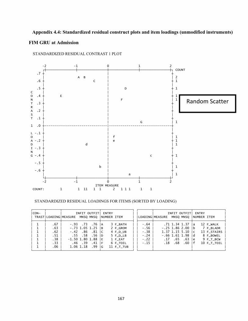
167  

Appendix 4.4: Standardized residual construct plots and item loadings (unmodified instruments)

FIM GRU at Admission STANDARDIZED RESIDUAL CONTRAST 1 PLOT

-2 -1 0 1 2 ┌┼───────────────┼───────────────┼───────────────┼───────────────┼┐ COUNT .7 ┼ | ┼ │ A B | │ 2 .6 ┼ C | ┼ 1 │ | │ .5 ┼ | D ┼ 1 C │ | │ O .4 ┼ E | ┼ 1 N │ | F │ 1 T .3 ┼ | ┼ R │ | │ A .2 ┼ | ┼ S │ | │ T .1 ┼ | ┼ │ | G │ 1 1 .0 ┼--------------------------------|--------------------------------┼ │ | │ L -.1 ┼ | ┼ O │ | f │ 1 A -.2 ┼ | e ┼ 1 D │ d | │ 1 I -.3 ┼ | ┼ N │ | │ G -.4 ┼ | c ┼ 1 │ | │ -.5 ┼ | ┼ │ b | │ 1 -.6 ┼ | ┼ │ | a │ 1 └┼───────────────┼───────────────┼───────────────┼───────────────┼┘ -2 -1 0 1 2 ITEM MEASURE COUNT: 1 1 11 1 1 2 1 1 1 1 1

STANDARDIZED RESIDUAL LOADINGS FOR ITEMS (SORTED BY LOADING) ┌──────┬───────┬───────────────────┬────────────────┐ ┌───────┬───────────────────┬────────────────┐ │CON- │ │ INFIT OUTFIT│ ENTRY │ │ │ INFIT OUTFIT│ ENTRY │ │ TRAST│LOADING│MEASURE MNSQ MNSQ │NUMBER ITEM │ │LOADING│MEASURE MNSQ MNSQ │NUMBER ITEM │ ├──────┼───────┼───────────────────┼────────────────┤ ├───────┼───────────────────┼────────────────┤ │ 1 │ .67 │ -.93 .73 .76 │A 3 F_BATH │ │ -.64 │ .71 1.34 1.37 │a 12 F_WALK │ │ 1 │ .63 │ -.73 1.05 1.25 │B 2 F_GROM │ │ -.56 │ -.25 1.86 2.00 │b 7 F_BLADR │ │ 1 │ .62 │ -.42 .86 .81 │C 4 F_D_UB │ │ -.38 │ 1.37 1.15 5.10 │c 13 F_STAIRS │ │ 1 │ .51 │ .55 .58 .56 │D 5 F_D_LB │ │ -.24 │ -.66 1.61 1.98 │d 8 F_BOWEL │ │ 1 │ .38 │ -1.50 1.80 1.88 │E 1 F_EAT │ │ -.22 │ .17 .65 .63 │e 9 F_T_BCW │ │ 1 │ .33 │ .46 .39 .41 │F 6 F_TOIL │ │ -.15 │ .18 .68 .60 │f 10 F_T_TOIL │ │ 1 │ .06 │ 1.06 1.18 .99 │G 11 F_T_TUB │ │ │ │ │ └──────┴───────┴───────────────────┴────────────────┘ └───────┴───────────────────┴────────────────┘

Random Scatter

168  

FIM GRU at Discharge

STANDARDIZED RESIDUAL CONTRAST 1 PLOT -2 -1 0 1 2 ┌┼───────────────┼───────────────┼───────────────┼───────────────┼┐ COUNT .7 ┼ B | A ┼ 2 │ | C │ 1 .6 ┼ | ┼ │ | │ C .5 ┼ | ┼ O │ D | │ 1 N .4 ┼ | ┼ T │ | E │ 1 R .3 ┼ | ┼ A │ | │ S .2 ┼ | ┼ T │ | │ .1 ┼ | ┼ 1 │ | F │ 1 .0 ┼-----G--------------------------|--------------------------------┼ 1 L │ | │ O -.1 ┼ | ┼ A │ | │ D -.2 ┼ | f ┼ 1 I │ e | │ 1 N -.3 ┼ d | ┼ 1 G │ | │ -.4 ┼ | c ┼ 1 │ | │ -.5 ┼ | ┼ │ b | a │ 2 └┼───────────────┼───────────────┼───────────────┼───────────────┼┘ -2 -1 0 1 2 ITEM MEASURE COUNT: 1 1 1 1 11 1 1 1 11 1 1

STANDARDIZED RESIDUAL LOADINGS FOR ITEMS (SORTED BY LOADING) ┌──────┬───────┬───────────────────┬────────────────┐ ┌───────┬───────────────────┬────────────────┐ │CON- │ │ INFIT OUTFIT│ ENTRY │ │ │ INFIT OUTFIT│ ENTRY │ │ TRAST│LOADING│MEASURE MNSQ MNSQ │NUMBER ITEM │ │LOADING│MEASURE MNSQ MNSQ │NUMBER ITEM │ ├──────┼───────┼───────────────────┼────────────────┤ ├───────┼───────────────────┼────────────────┤ │ 1 │ .70 │ .68 .89 .96 │A 3 F_BATH │ │ -.54 │ 1.54 2.08 1.91 │a 13 F_STAIRS │ │ 1 │ .68 │ -.42 .65 .53 │B 4 F_D_UB │ │ -.53 │ -.22 .72 .68 │b 9 F_T_BCW │ │ 1 │ .65 │ .60 .79 .94 │C 5 F_D_LB │ │ -.41 │ .11 .41 .48 │c 10 F_T_TOIL │ │ 1 │ .47 │ -.97 .80 .72 │D 2 F_GROM │ │ -.32 │ -.86 1.71 1.79 │d 8 F_BOWEL │ │ 1 │ .37 │ .41 .58 .81 │E 6 F_TOIL │ │ -.24 │ -.20 2.05 1.76 │e 7 F_BLADR │ │ 1 │ .03 │ .78 .99 1.19 │F 11 F_T_TUB │ │ -.22 │ .23 1.32 1.55 │f 12 F_WALK │ │ 1 │ .01 │ -1.68 .88 1.54 │G 1 F_EAT │ │ │ │ │ └──────┴───────┴───────────────────┴────────────────┘ └───────┴───────────────────┴────────────────┘

169  

FIM MSK at Admission

STANDARDIZED RESIDUAL CONTRAST 1 PLOT -2 -1 0 1 2 3 4 ┌┼──────────┼──────────┼──────────┼──────────┼──────────┼──────────┼┐ COUNT .7 ┼ A | ┼ 1 │ | │ .6 ┼ C | B ┼ 2 │ | D │ 1 C .5 ┼ | ┼ O │ | │ N .4 ┼ | ┼ T │ | │ R .3 ┼ | ┼ A │ | │ S .2 ┼ | ┼ T │ | │ .1 ┼ | ┼ 1 │ | │ .0 ┼----------------------|--------------------------------------------┼ L │ | E │ 1 O -.1 ┼ F | G ┼ 2 A │ | │ D -.2 ┼ | f ┼ 1 I │ | │ N -.3 ┼ | ┼ G │ e d | │ 2 -.4 ┼ c | ┼ 1 │ | │ -.5 ┼ b | ┼ 1 │ a | │ 1 -.6 ┼ | ┼ └┼──────────┼──────────┼──────────┼──────────┼──────────┼──────────┼┘ -2 -1 0 1 2 3 4 ITEM MEASURE COUNT: 1 111 111 1 121 1

STANDARDIZED RESIDUAL LOADINGS FOR ITEMS (SORTED BY LOADING) ┌──────┬───────┬───────────────────┬────────────────┐ ┌───────┬───────────────────┬────────────────┐ │CON- │ │ INFIT OUTFIT│ ENTRY │ │ │ INFIT OUTFIT│ ENTRY │ │ TRAST│LOADING│MEASURE MNSQ MNSQ │NUMBER ITEM │ │LOADING│MEASURE MNSQ MNSQ │NUMBER ITEM │ ├──────┼───────┼───────────────────┼────────────────┤ ├───────┼───────────────────┼────────────────┤ │ 1 │ .70 │ -.16 .85 .85 │A 9 F_T_BCW │ │ -.55 │ -.56 .99 .95 │a 2 F_GROM │ │ 1 │ .61 │ .43 .96 .99 │B 11 F_T_TUB │ │ -.48 │ -.87 1.08 1.09 │b 4 F_D_UB │ │ 1 │ .60 │ -.42 .64 .65 │C 10 F_T_TOIL │ │ -.42 │ -.71 .93 .95 │c 8 F_BOWEL │ │ 1 │ .56 │ .45 1.34 1.81 │D 12 F_WALK │ │ -.36 │ -.80 1.41 1.94 │d 7 F_BLADR │ │ │ │ │ │ │ -.35 │ -1.48 1.31 1.42 │e 1 F_EAT │ │ │ │ │ │ │ -.19 │ .37 .73 .72 │f 5 F_D_LB │ │ │ │ │ │ │ -.09 │ 3.59 1.28 .28 │G 13 F_STAIRS │ │ │ │ │ │ │ -.09 │ -.37 .71 .70 │F 6 F_TOIL │ │ │ │ │ │ │ -.05 │ .52 1.01 1.01 │E 3 F_BATH │ └──────┴───────┴───────────────────┴────────────────┘ └───────┴───────────────────┴────────────────┘

170  

FIM MSK at Discharge

STANDARDIZED RESIDUAL CONTRAST 1 PLOT -1 0 1 2 ┌┼─────────────────────┼─────────────────────┼─────────────────────┼┐ COUNT │ | │ .7 ┼ | A ┼ 1 │ | │ .6 ┼ | ┼ │ | │ .5 ┼ | ┼ C │ | │ O .4 ┼ | ┼ N │ | │ T .3 ┼ B | ┼ 1 R │ | │ A .2 ┼ C | ┼ 1 S │ | D │ 1 T .1 ┼ | E ┼ 1 │ G | F │ 2 1 .0 ┼----------------------|--------------------------------------------┼ │ | │ L -.1 ┼ | ┼ O │ | │ A -.2 ┼ | ┼ D │ | f │ 1 I -.3 ┼ e | ┼ 1 N │ | │ G -.4 ┼ | ┼ │ | │ -.5 ┼ d | ┼ 1 │ | c │ 1 -.6 ┼ b | ┼ 1 │ | a │ 1 -.7 ┼ | ┼ └┼─────────────────────┼─────────────────────┼─────────────────────┼┘ -1 0 1 2 ITEM MEASURE COUNT: 1 1 2 1 1 1 11 1 11 1

STANDARDIZED RESIDUAL LOADINGS FOR ITEMS (SORTED BY LOADING) ┌──────┬───────┬───────────────────┬────────────────┐ ┌───────┬───────────────────┬────────────────┐ │CON- │ │ INFIT OUTFIT│ ENTRY │ │ │ INFIT OUTFIT│ ENTRY │ │ TRAST│LOADING│MEASURE MNSQ MNSQ │NUMBER ITEM │ │LOADING│MEASURE MNSQ MNSQ │NUMBER ITEM │ ├──────┼───────┼───────────────────┼────────────────┤ ├───────┼───────────────────┼────────────────┤ │ 1 │ .72 │ 1.00 1.34 2.33 │A 13 F_STAIRS │ │ -.65 │ .17 .97 .96 │a 3 F_BATH │ │ 1 │ .32 │ -.41 1.36 1.07 │B 7 F_BLADR │ │ -.60 │ -.62 .79 .66 │b 2 F_GROM │ │ 1 │ .20 │ -.31 .83 1.01 │C 1 F_EAT │ │ -.53 │ .10 .63 .67 │c 5 F_D_LB │ │ 1 │ .14 │ .64 .86 1.00 │D 11 F_T_TUB │ │ -.52 │ -.49 .90 .79 │d 6 F_TOIL │ │ 1 │ .08 │ .22 .73 .70 │E 9 F_BCW │ │ -.29 │ -.77 .79 1.12 │e 4 F_D_UB │ │ 1 │ .07 │ .57 2.23 3.92 │F 12 F_WALK │ │ -.24 │ .38 .72 .67 │f 10 F_T_TOIL │ │ 1 │ .04 │ -.50 1.64 1.13 │G 8 F_BOWEL │ │ │ │ │ └──────┴───────┴───────────────────┴────────────────┘ └───────┴───────────────────┴────────────────┘

171  

PAC GRU at Admission

STANDARDIZED RESIDUAL CONTRAST 1 PLOT -2 -1 0 1 2 3 ┌┼────────────┼────────────┼────────────┼────────────┼────────────┼┐ COUNT │ | A │ 1 .8 ┼ | B ┼ 1 │ | │ .7 ┼ | ┼ │ | │ .6 ┼ | ┼ │ | │ C .5 ┼ | C ┼ 1 O │ | │ N .4 ┼ | ┼ T │ | │ R .3 ┼ | ┼ A │ | │ S .2 ┼ | ┼ T │ | │ .1 ┼ | ┼ 1 │ | │ .0 ┼-------------------------DE---------------------------------------┼ 2 L │ F | │ 1 O -.1 ┼ G | f ┼ 2 A │ | e │ 1 D -.2 ┼ | ┼ I │ | d │ 1 N -.3 ┼ | ┼ G │ | │ -.4 ┼ | ┼ │ | │ -.5 ┼ c | ┼ 1 │ | │ -.6 ┼ | ┼ │ b a | │ 2 -.7 ┼ | ┼ └┼────────────┼────────────┼────────────┼────────────┼────────────┼┘ -2 -1 0 1 2 3 ITEM MEASURE COUNT: 1 1 1 1 111 121 1 1

STANDARDIZED RESIDUAL LOADINGS FOR ITEMS (SORTED BY LOADING) ┌──────┬───────┬───────────────────┬────────────────┐ ┌───────┬───────────────────┬────────────────┐ │CON- │ │ INFIT OUTFIT│ ENTRY │ │ │ INFIT OUTFIT│ ENTRY │ │ TRAST│LOADING│MEASURE MNSQ MNSQ │NUMBER ITEM │ │LOADING│MEASURE MNSQ MNSQ │NUMBER ITEM │ ├──────┼───────┼───────────────────┼────────────────┤ ├───────┼───────────────────┼────────────────┤ │ 1 │ .83 │ .33 .72 .69 │A 6 P_LOCO │ │ -.65 │ -.19 .66 .64 │a 3 P_D_UB │ │ 1 │ .78 │ .38 .69 .63 │B 5 P_WALK │ │ -.64 │ -.37 .85 .78 │b 2 P_HYG │ │ 1 │ .50 │ .32 .63 .58 │C 7 P_T_TOIL │ │ -.49 │ -1.15 1.83 2.02 │c 10 P_EAT │ │ 1 │ .01 │ -.07 .75 .69 │D 9 P_BED_MO │ │ -.26 │ .21 .95 1.14 │d 1 P_BATH │ │ │ │ │ │ │ -.15 │ .58 .73 .69 │e 4 P_D_LB │ │ │ │ │ │ │ -.11 │ 2.37 3.37 9.90 │f 11 P_STAIRS │ │ │ │ │ │ │ -.10 │ -.81 2.31 7.90 │G 12 P_BLADR │ │ │ │ │ │ │ -.03 │ -1.58 1.79 3.58 │F 13 P_BOWEL │ │ │ │ │ │ │ -.01 │ -.03 .89 .84 │E 8 P_TOIL_U │ └──────┴───────┴───────────────────┴────────────────┘ └───────┴───────────────────┴────────────────┘

172  

PAC GRU at Discharge

STANDARDIZED RESIDUAL CONTRAST 1 PLOT -2 -1 0 1 2 3 ┌┼────────────┼────────────┼────────────┼────────────┼────────────┼┐ COUNT .9 ┼ A | ┼ 1 │ B | │ 1 .8 ┼ | ┼ │ C | │ 1 C .7 ┼ | ┼ O │ | │ N .6 ┼ D | ┼ 1 T │ | │ R .5 ┼ | ┼ A │ | │ S .4 ┼ | ┼ T │ | │ .3 ┼ | ┼ 1 │ E | │ 1 .2 ┼ | ┼ L │ | │ O .1 ┼ F | ┼ 1 A │ | │ D .0 ┼--------------------------|---------------------------------------┼ I │ | │ N -.1 ┼ | G ┼ 1 G │ | │ -.2 ┼ | f ┼ 1 │ | e │ 1 -.3 ┼ d c | ┼ 2 │ a | b │ 2 └┼────────────┼────────────┼────────────┼────────────┼────────────┼┘ -2 -1 0 1 2 3 ITEM MEASURE COUNT: 1 211112 1 1 1 1

STANDARDIZED RESIDUAL LOADINGS FOR ITEMS (SORTED BY LOADING) ┌──────┬───────┬───────────────────┬────────────────┐ ┌───────┬───────────────────┬────────────────┐ │CON- │ │ INFIT OUTFIT│ ENTRY │ │ │ INFIT OUTFIT│ ENTRY │ │ TRAST│LOADING│MEASURE MNSQ MNSQ │NUMBER ITEM │ │LOADING│MEASURE MNSQ MNSQ │NUMBER ITEM │ ├──────┼───────┼───────────────────┼────────────────┤ ├───────┼───────────────────┼────────────────┤ │ 1 │ .88 │ -.12 .60 .47 │A 5 P_WALK │ │ -.35 │ -1.18 2.72 4.35 │a 13 P_BOWEL │ │ 1 │ .87 │ -.32 .36 .32 │B 7 P_T_TOIL │ │ -.34 │ .17 2.26 4.33 │b 12 P_BLADR │ │ 1 │ .77 │ -.39 1.16 .70 │C 6 P_LOCO │ │ -.29 │ -.15 .79 .74 │c 3 P_D_UB │ │ 1 │ .59 │ -.27 .47 .44 │D 8 P_TOIL_U │ │ -.28 │ -.56 .84 .75 │d 2 P_P_HYG │ │ 1 │ .26 │ -.48 .60 .43 │E 9 P_BED_MO │ │ -.26 │ .29 .85 1.06 │e 4 P_D_LB │ │ 1 │ .11 │ -.50 .96 .96 │F 10 P_EAT │ │ -.18 │ .81 1.03 1.05 │f 1 P_BATH │ │ │ │ │ │ │ -.10 │ 2.70 1.64 1.60 │G 11 P_STAIRS │ └──────┴───────┴───────────────────┴────────────────┘ └───────┴───────────────────┴────────────────┘

173  

PAC MSK at Admission

STANDARDIZED RESIDUAL CONTRAST 1 PLOT -2 -1 0 1 2 ┌┼───────────────┼───────────────┼───────────────┼───────────────┼┐ COUNT │ | A │ 1 .8 ┼ | ┼ │ | B C │ 2 .7 ┼ | ┼ │ | │ .6 ┼ | ┼ C │ | │ O .5 ┼ | ┼ N │ | │ T .4 ┼ | ┼ R │ | │ A .3 ┼ | ┼ S │ | │ T .2 ┼ | ┼ │ | │ 1 .1 ┼ D | ┼ 1 │ | │ L .0 ┼-------------------------------E|--------------------------------┼ 1 O │ | │ A -.1 ┼ F | ┼ 1 D │ f e | │ 2 I -.2 ┼ | ┼ N │ | │ G -.3 ┼ |d ┼ 1 │ | │ -.4 ┼ b | c ┼ 2 │ | │ -.5 ┼ | ┼ │ | │ -.6 ┼ | ┼ │ | a │ 1 └┼───────────────┼───────────────┼───────────────┼───────────────┼┘ -2 -1 0 1 2 ITEM MEASURE COUNT: 2 21 1 1 11 11 1

STANDARDIZED RESIDUAL LOADINGS FOR ITEMS (SORTED BY LOADING) ┌──────┬───────┬───────────────────┬────────────────┐ ┌───────┬───────────────────┬────────────────┐ │CON- │ │ INFIT OUTFIT│ ENTRY │ │ │ INFIT OUTFIT│ ENTRY │ │ TRAST│LOADING│MEASURE MNSQ MNSQ │NUMBER ITEM │ │LOADING│MEASURE MNSQ MNSQ │NUMBER ITEM │ ├──────┼───────┼───────────────────┼────────────────┤ ├───────┼───────────────────┼────────────────┤ │ 1 │ .84 │ .46 .68 .63 │A 5 P_WALK │ │ -.65 │ 1.55 1.58 1.58 │a 1 P_BATH │ │ 1 │ .75 │ .37 .52 .52 │B 7 P_T_TOIL │ │ -.39 │ -1.33 1.32 1.18 │b 10 P_EAT │ │ 1 │ .74 │ .55 1.02 .97 │C 6 P_LOCO │ │ -.39 │ .65 .83 .80 │c 4 P_D_LB │ │ 1 │ .09 │ -.25 1.99 5.41 │D 12 P_BLADR │ │ -.29 │ .06 1.11 1.67 │d 9 P_BED_MO │ │ │ │ │ │ │ -.16 │ -.31 .81 .83 │e 2 P_P_HYG │ │ │ │ │ │ │ -.14 │ -1.33 2.21 6.30 │f 13 P_BOWEL │ │ │ │ │ │ │ -.11 │ -.34 .74 .73 │F 3 P_D_UB │ │ │ │ │ │ │ -.02 │ -.08 .70 .59 │E 8 P_TOIL_U │ └──────┴───────┴───────────────────┴────────────────┘ └───────┴───────────────────┴────────────────┘

174  

PAC MSK at Discharge

STANDARDIZED RESIDUAL CONTRAST 1 PLOT -1 0 1 2 ┌┼─────────────────────┼─────────────────────┼─────────────────────┼┐ COUNT │ A | │ 1 .8 ┼ B C | ┼ 2 │ | │ .7 ┼ | ┼ │ | │ C .6 ┼ D | ┼ 1 O │ | │ N .5 ┼ | ┼ T │ | │ R .4 ┼ | ┼ A │ | │ S .3 ┼ | ┼ T │ | │ .2 ┼ | ┼ 1 │ | │ .1 ┼ | ┼ L │ E | │ 1 O .0 ┼----------------------|--------------------------F-----------------┼ 1 A │ fG | │ 2 D -.1 ┼ |e ┼ 1 I │ | d │ 1 N -.2 ┼ | ┼ G │ c | b │ 2 -.3 ┼ | ┼ │ | │ -.4 ┼ | ┼ │ | │ -.5 ┼ |a ┼ 1 └┼─────────────────────┼─────────────────────┼─────────────────────┼┘ -1 0 1 2 ITEM MEASURE COUNT: 1 321 1 2 1 1 1

STANDARDIZED RESIDUAL LOADINGS FOR ITEMS (SORTED BY LOADING) ┌──────┬───────┬───────────────────┬────────────────┐ ┌───────┬───────────────────┬────────────────┐ │CON- │ │ INFIT OUTFIT│ ENTRY │ │ │ INFIT OUTFIT│ ENTRY │ │ TRAST│LOADING│MEASURE MNSQ MNSQ │NUMBER ITEM │ │LOADING│MEASURE MNSQ MNSQ │NUMBER ITEM │ ├──────┼───────┼───────────────────┼────────────────┤ ├───────┼───────────────────┼────────────────┤ │ 1 │ .85 │ -.41 .54 .30 │A 6 P_LOCO │ │ -.48 │ .06 2.78 3.38 │a 12 P_BLADR │ │ 1 │ .80 │ -.46 .58 .27 │B 7 P_T_TOIL │ │ -.27 │ 1.87 1.51 4.75 │b 11 P_STAIRS │ │ 1 │ .80 │ -.18 .58 .37 │C 5 P_WALK │ │ -.26 │ -.74 1.61 2.05 │c 13 P_BOWEL │ │ 1 │ .59 │ -.45 .57 .19 │D 8 P_TOIL_U │ │ -.14 │ .29 .99 1.00 │d 1 P_BATH │ │ 1 │ .04 │ -.37 .57 .47 │E 3 P_D_UB │ │ -.12 │ .02 .79 .78 │e 4 P_D_LB │ │ 1 │ .01 │ 1.21 1.20 1.41 │F 10 P_EAT │ │ -.06 │ -.44 .90 .66 │f 2 P_P_HYG │ │ │ │ │ │ │ -.03 │ -.41 .65 .38 │G 9 P_BED_MO │ └──────┴───────┴───────────────────┴────────────────┘ └───────┴───────────────────┴────────────────┘ 

   

175  

Appendix 4.5: Multiple item characteristic curves (unmodified instruments)

FIM GRU at Admission  

 

   

176  

FIM MSK on Admission 

 

   

177  

FIM GRU at Discharge 

 

   

178  

FIM MSK on Discharge 

 

   

179  

PAC GRU on Admission 

 

   

180  

PAC MSK on Admission 

 

   

181  

PAC GRU on Discharge 

 

   

182  

PAC MSK on Discharge 

 

   

183  

Appendix 4.6: Variable Maps (Original instruments, pre CPA)

FIM GRU on Admission FIM GRU on Discharge PERSONS - MAP - ITEMS <more>|<rare> 7 + | | | 6 + | | | 5 + | | | 4 + | | | 3 + | | X | 2 + | X T|T X | F_STAIRS 1 XX + F_T_TUB XXXXXX |S F_WALK XXXXXXX S| F_D_LB F_TOIL XXXXXXXX | F_T_BCW F_T_TOIL 0 XXXXXXXXXX +M XXXXXXXXXX | F_BLADR XXXXXXXX M| F_D_UB XXXXXXXXXX |S F_BOWEL F_GROM -1 XXXXXX + F_BATH XXXXXX S| XXXXXXXXXX |T F_EAT XXX | -2 + XX T| | XX | -3 + | | | -4 + | | | -5 + | | | -6 + | | | -7 + <less>|<frequ>

PERSONS - MAP - ITEMS <more>|<rare> 7 + | | | 6 + | | XX | 5 + | | T| 4 XX + | X | XXX | 3 XXX + XX S| XXXX | XXXXXXXXXX | 2 XXXXXX + XXXXXXXX |T XXXX | F_STAIRS XXXXXXXXX M| 1 XXXXXX + XXXXX |S F_BATH F_T_TUB XXXXXX | F_D_LB F_TOIL XXXXXX | F_WALK 0 X +M F_T_TOIL XXX S| F_BLADR F_T_BCW XX | F_D_UB X |S F_BOWEL -1 XX + F_GROM XX | | X T|T F_EAT -2 + XX | X | | -3 + | X | | -4 + | | | -5 + | | | -6 + | | | -7 + <less>|<frequ>

 

 

Ceiling effect 

Least able subjects 

Most able subjects  Hardest Items

Easiest Items

184  

FIM MSK on Admission FIM MSK on Discharge PERSONS - MAP - ITEMS <more>|<rare> 7 + | | | 6 + | | | 5 + | | | 4 + | X | F_STAIRS | 3 + | XX |T T| 2 XX + XXX | XXXXX | XXX S|S 1 XXXXXXXXXXXX + XXXXXXXX | XXXXXXXXXXXXXXX | F_BATH F_T_TUB F_WALK XXXXXXXXXXXXXX M| F_D_LB 0 XXXXXXXXX +M XXXXXXXXXXXX | F_TOIL F_T_BCW XXXXXXXXXXX | F_GROM F_T_TOIL XXXX S| F_BLADR F_BOWEL F_D_UB -1 XXXXX + XXXXX |S X T| F_EAT XXX | -2 + | |T | -3 + | | | -4 + | | | -5 + | | | -6 + | | | -7 + <less>|<frequ>

PERSONS - MAP - ITEMS <more>|<rare> 7 X + | X | | 6 + | | X | 5 + | | X | 4 + T| X | | 3 XXX + | XXXXXXXXXXXXXXX S| | 2 XXXXXX + XXXXXXXXXX | XXXXXXXXXXXX M| XXXXXXXXXXXXXXXX | XXXXXXXXXXXXXXXXXXXXXXXX +T F_STAIRS XXXXXXX | F_T_TUB XXXXXX |S F_T_TOIL F_WALK XXXX S| F_BATH F_BCW 0 X +M F_D_LB | F_EAT X |S F_BLADR F_BOWEL F_GROM F_TOIL X T| F_D_UB -1 XXX +T | | | -2 + | | | -3 + | | | -4 + | | | -5 + | | | -6 + | | | -7 + <less>|<frequ>

185  

PAC GRU on Admission PAC GRU on Discharge PERSONS - MAP - ITEMS <more>|<rare> 7 + | | | 6 + | | | 5 + | | | 4 + | | | 3 + X | X | | P_STAIRS 2 + XX |T XX T| XXX | 1 XXX +S XXXX S| XXXXXX | P_D_LB P_WALK XXXXXX | P_BATH P_LOCO P_T_TOIL 0 XXXXXXXX +M P_BED_MO P_TOIL_U XXXXXXXXXXXXXXXXX M| P_D_UB P_HYG XXXXXXXXXXXXXX | XXXXXXXXX | P_BLADR -1 XXXXXXX S+S XXXX | P_EAT XXX | P_BOWEL |T -2 XX T+ | | X | -3 + | | | -4 + | | | -5 + | | | -6 + | | | -7 + <less>|<frequ>

PERSONS - MAP - ITEMS <more>|<rare> 7 X + | | | 6 + | | X | 5 + | XX | | 4 XX T+ | | XXXXX | 3 X + S| P_STAIRS XXXXXX | XXXX | 2 XXXXXXXX + XXX |T XXXXXXXXX | XXXXXXXXXXX M| 1 XXXXXXX +S XXXXX | P_BATH XXXXXXXXX | XXX | P_BLADR P_D_LB 0 XXX S+M P_WALK XXX | P_D_UB P_TOIL_U P_T_TOIL XX | P_BED_MO P_EAT P_LOCO P_P_HYG X | -1 XX +S XX | P_BOWEL X T| |T -2 + X | | | -3 + | | | -4 + | | | -5 + | | | -6 + | | | -7 X + <less>|<frequ>

186  

PAC MSK on Admission PAC MSK on Discharge PERSONS - MAP - ITEMS <more>|<rare> 7 + | | | 6 + | | | 5 + X | | | 4 + X | | X T| 3 XX + XX | X | XXXXXXX | 2 XXXXXXXXXXX S+ XXXXXX | XXX |T P_BATH XXXXXXXXXXXXXXXXX | 1 XXXXXXXXXXXXXXX M+ XXXXXXXX |S P_D_LB XXXXXXXXXX | P_LOCO P_WALK XXXXX | P_T_TOIL 0 XXXXXXXXX +M P_BED_MO P_TOIL_U XXXXX S| P_BLADR P_D_UB P_P_HYG XXX | XXXXX |S -1 + T| P_BOWEL P_EAT X |T | -2 + | X | X | -3 + | | | -4 + | | | -5 + | | | -6 + | | | -7 + <less>|<frequ>

PERSONS - MAP - ITEMS <more>|<rare> 7 XXXXXXXXX + | | | 6 + | | | 5 + | | | 4 + | XXXXXXX T| | 3 XXXXXXXX + | XXXXXXXXXXXXXX S| XXXXXXXX | 2 XXXX + XXXXXXXXXX M| P_STAIRS XXXXXX |T XXXXXXXXXXXXXXXXX | P_EAT 1 XXXXXXXX + XXXXXXX S|S XXXXXXX | XXX | P_BATH 0 X +M P_BLADR P_D_LB XXX T| P_D_UB P_WALK XX | P_BED_MO P_LOCO P_P_HYG P_TOIL_U P_T_TOIL X |S P_BOWEL -1 + | |T | -2 + | | | -3 + | | | -4 + | | | -5 + | | | -6 + | | | -7 + <less>|<frequ>

187  

Appendix 4.7: Item fit explanations (Original instruments)

FIM GRU on Admission Scalogram MOST UNEXPECTED RESPONSES ITEM MEASURE |PERSON |22174367174485839624616851 7212 2313 |393990162583225309848024813126016756 high------------------------------------ 1 F_EAT -1.50 D|..1...................7....4.......1 3 F_BATH -.93 e|4................................... 2 F_GROM -.73 F|....74..7......4.....2...2.........1 8 F_BOWEL -.66 C|........2.3.3.3.....12.2........7... 4 F_D_UB -.42 f|....7..........3..3................. 7 F_BLADR -.25 B|......2..2.2.2..22....1.......6..565 10 F_T_TOIL .18 d|...................................5 12 F_WALK .71 E|.1.2...1.............7.55.4.43.3.... 11 F_T_TUB 1.06 G|1.............4....3....33.......... 13 F_STAIRS 1.37 A|.....................7...43......... |--------------------------------low- |221743671744858396246168513721212313 |39399016258322530984802481 1260 6756  

Item Characteristic Curve

 

Easiest Item 

Hardest Item 

Least able subjectsMost able subjects

Very steep 

Red line = Expected Responses 

Blue line = Observed Responses  95% Confidence Interval

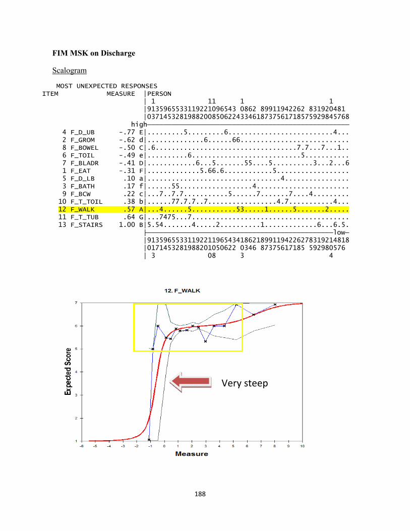
188  

FIM MSK on Discharge

Scalogram

MOST UNEXPECTED RESPONSES ITEM MEASURE │PERSON │ 1 11 1 1 │9135965533119221096543 0862 89911942262 831920481 │03714532819882008506224334618737561718575929845768 high────────────────────────────────────────────────── 4 F_D_UB -.77 E│.........5.........6..........................4... 2 F_GROM -.62 d│..............6......66........................... 8 F_BOWEL -.50 C│.6...................................7.7...7...1.. 6 F_TOIL -.49 e│..........6...........................5........... 7 F_BLADR -.41 D│............6...5.......55....5..........3...2...6 1 F_EAT -.31 F│.............5.66.6............5.................. 5 F_D_LB .10 a│.................................4................ 3 F_BATH .17 f│......55..................4....................... 9 F_BCW .22 c│...7..7.7...........5......7.......7....4......... 10 F_T_TOIL .38 b│......77.7.7..7.................4.7...........4... 12 F_WALK .57 A│...4......5...........53.....1......5.......2..... 11 F_T_TUB .64 G│...7475...7....................................... 13 F_STAIRS 1.00 B│5.54.......4.....2..........1.............6...6.5. ├──────────────────────────────────────────────low─ │91359655331192211965434186218991194226278319214818 │0171453281988201050622 0346 87375617185 592980576 │ 3 08 3 4

Very steep

189  

PAC MSK at Discharge

MOST UNEXPECTED RESPONSES ITEM MEASURE │PERSON │ 1 1 1 1 │5443157835219657971 0851314753082342 61 │5523578926010597421547847879116514087968 high──────────────────────────────────────── 13 P_BOWEL -.74 C│........................2...1........... 7 P_T_TOIL -.46 e│...........................4............ 8 P_TOIL_U -.45 c│..............................4......... 2 P_P_HYG -.44 F│...............4.......3........3....... 6 P_LOCO -.41 a│.........................4.4............ 9 P_BED_MO -.41 f│.................................2...... 3 P_D_UB -.37 b│....5................................... 5 P_WALK -.18 d│.........................4.4............ 4 P_D_LB .02 G│....555...........3...3...3........6.... 12 P_BLADR .06 B│.......3.....1..31.110..1...0..1...5.5.5 1 P_BATH .29 E│........333............2.........6...... 10 P_EAT 1.21 D│5555................................6.6. 11 P_STAIRS 1.87 A│...........00.0.........6...544...3....6 ├────────────────────────────────────low─ │5443157835219657971518513147531823427618 │5523178926010597421 0784787911051408 96 │ 5 1 4 6

190  

PAC MSK at Discharge

MOST MISFITTING RESPONSE STRINGS ITEM OUTMNSQ │PERSON │ 1 1 1 1 │5443157835219657971 0851314753082342 61 │5523578926010597421547847879116514087968 high──────────────────────────────────────── 11 P_STAIRS 4.75 A│...........00.0.........6...544...3....6 12 P_BLADR 3.38 B│.......3.....1..31.110..1...0..1...5.5.5 13 P_BOWEL 2.05 C│........................2...1........... 10 P_EAT 1.41 D│5555................................6.6. 1 P_BATH 1.00 E│........333............2.........6...... 2 P_P_HYG .66 F│...............4.......3........3....... 4 P_D_LB .78 G│....555...........3...3...3........6.... 9 P_BED_MO .38 f│.................................2...... 7 P_T_TOIL .27 e│...........................4............ 5 P_WALK .37 d│.........................4.4............ 8 P_TOIL_U .19 c│..............................4......... 3 P_D_UB .47 b│....5................................... 6 P_LOCO .30 a│.........................4.4............ ├────────────────────────────────────low─ │5443157835219657971518513147531823427618 │5523178926010597421 0784787911051408 96 │ 5 1 4 6

191  

PAC GRU at Admission

MOST UNEXPECTED RESPONSES ITEM MEASURE │PERSON │ 2343799664772648518565565375123327261123 │23499531913739214880149237885315624009562 high───────────────────────────────────────── 13 P_BOWEL -1.58 C│......33.......22..2.1.....22..0.......5. 10 P_EAT -1.15 D│...............6....6.....6..0..0.......3 12 P_BLADR -.81 B│..04.1..1112.01..0....0.........5545.55.. 2 P_HYG -.37 G│................................0........ 3 P_D_UB -.19 b│........6................................ 9 P_BED_MO -.07 f│.......................6................. 8 P_TOIL_U -.03 F│................0..0....0...........4.... 1 P_BATH .21 E│.2..0.................................... 7 P_T_TOIL .32 a│................................5........ 6 P_LOCO .33 d│........0....6....6.............4........ 5 P_WALK .38 c│.............6..................4........ 4 P_D_LB .58 e│............0............................ 11 P_STAIRS 2.37 A│0.....................1..1....6.......... ├─────────────────────────────────────low─ │22343799664772648518565565375123327261123 │ 3499531913739214880149237885315624009562

192  

Appendix 4.8: How to collapse response options – admission data

FIM GRU on Admission OBSERVED AVERAGE MEASURES FOR PERSONS (unscored) (BY OBSERVED CATEGORY) -3 -2 -1 0 1 2 3 ├─────────┼─────────┼─────────┼─────────┼─────────┼─────────┤ NUM ITEM │ 1 7 3 4 2 5 6 │ 13 F_STAIRS │ │ │ 1 2 3 4 5 │ 11 F_T_TUB │ │ │ 1 3 247 5 6 │ 12 F_WALK │ 1 2 3 4 5 6 7 │ 5 F_D_LB │ 1 2 3 4 5 67 │ 6 F_TOIL │ │ │ 1 2 3 4 5 6 7 │ 10 F_T_TOIL │ │ │ 1 3 2 45 6 7 │ 7 F_BLADR │ 1 2 3 4 5 6 7 │ 4 F_D_UB │ │ │ 1 25 3 4 6 7 │ 8 F_BOWEL │ 1 2 3 4 5 7 6 │ 2 F_GROM │ 1 2 3 54 │ 3 F_BATH │ │ │ │ │ 4 5 16 7 │ 1 F_EAT ├─────────┼─────────┼─────────┼─────────┼─────────┼─────────┤ NUM ITEM -3 -2 -1 0 1 2 3 1 1 2 24343315 64152644335341224111 1 1 PERSONS T S M S T

ITEM NUMBER: 1 F_EAT

ITEM DIFFICULTY MEASURE OF -1.50 ADDED TO MEASURES ┌───────────────────┬────────────┬────────────┬┬─────────┬────────┐ │CATEGORY OBSERVED│OBSVD SAMPLE│INFIT OUTFIT││STRUCTURE│CATEGORY│ │LABEL SCORE COUNT %│AVRGE EXPECT│ MNSQ MNSQ││CALIBRATN│ MEASURE│ ├───────────────────┼────────────┼────────────┼┼─────────┼────────┤ │ 1 1 2 2│ -.21 -2.51│ 4.53 8.41││ NONE │( -3.26)│ 1 │ 2 2 0 0│ │ .00 .00││ NULL │ -2.84 │ 2 │ 3 3 0 0│ │ .00 .00││ NULL │ -2.55 │ 3 │ 4 4 2 2│ -1.86*-1.27│ 1.90 .99││ -1.38 │ -2.28 │ 4 │ 5 5 45 48│ -.78 -.74│ 1.24 1.05││ -2.62 │ -1.68 │ 5 │ 6 6 32 34│ -.16 -.16│ .99 1.12││ 1.39 │ .51 │ 6 │ 7 7 12 13│ .32 .41│ 1.01 .95││ 2.61 │( 2.38)│ 7 └───────────────────┴────────────┴────────────┴┴─────────┴────────┘

For 4 RO Combine:1-4, 5, 6, 7 For 3 RO Combine:1-5, 6, 7

Eg. Unused Response 

193  

ITEM NUMBER: 2 F_GROM

ITEM DIFFICULTY MEASURE OF -.73 ADDED TO MEASURES ┌───────────────────┬────────────┬────────────┬┬─────────┬────────┐ │CATEGORY OBSERVED│OBSVD SAMPLE│INFIT OUTFIT││STRUCTURE│CATEGORY│ │LABEL SCORE COUNT %│AVRGE EXPECT│ MNSQ MNSQ││CALIBRATN│ MEASURE│ ├───────────────────┼────────────┼────────────┼┼─────────┼────────┤ │ 1 1 2 2│ -2.21 -2.14│ 1.01 .75││ NONE │( -4.05)│ 1 │ 2 2 5 5│ -1.47 -1.71│ 1.23 2.51││ -2.11 │ -2.63 │ 2 │ 3 3 2 2│ -1.18 -1.29│ 1.16 .67││ .15 │ -2.04 │ 3 │ 4 4 12 13│ -.88 -.84│ 1.05 .94││ -2.13 │ -1.53 │ 4 │ 5 5 67 72│ -.33 -.27│ .93 .89││ -1.55 │ .19 │ 5 │ 6 6 3 3│ 1.59 .32│ .25 .15││ 3.86 │ 2.10 │ 6 │ 7 7 2 2│ .63* .97│ 1.22 1.37││ 1.78 │( 3.27)│ 7 └───────────────────┴────────────┴────────────┴┴─────────┴────────┘

For 4 RO Combine: 1-3, 4, 5, 6-7 For 3 RO Combine: 1-3, 4, 5-7

ITEM NUMBER: 3 F_BATH

ITEM DIFFICULTY MEASURE OF -.93 ADDED TO MEASURES ┌───────────────────┬────────────┬────────────┬┬─────────┬────────┐ │CATEGORY OBSERVED│OBSVD SAMPLE│INFIT OUTFIT││STRUCTURE│CATEGORY│ │LABEL SCORE COUNT %│AVRGE EXPECT│ MNSQ MNSQ││CALIBRATN│ MEASURE│ ├───────────────────┼────────────┼────────────┼┼─────────┼────────┤ │ 1 1 5 5│ -2.15 -1.59│ .50 .65││ NONE │( -4.05)│ 1 │ 2 2 23 25│ -1.15 -1.07│ .61 .58││ -1.92 │ -2.02 │ 2 │ 3 3 24 26│ -.61 -.58│ .81 .70││ .07 │ -.72 │ 3 │ 4 4 21 23│ .30 -.09│ .66 .98││ .73 │ .26 │ 4 │ 5 5 20 22│ .24* .37│ .94 .89││ 1.12 │( 1.64)│ 5 └───────────────────┴────────────┴────────────┴┴─────────┴────────┘

For 4 RO Combine: 1, 2, 3, 4-7 For 3 RO Combine: 1-2, 3-4, 5-7

ITEM NUMBER: 4 F_D_UB

ITEM DIFFICULTY MEASURE OF -.42 ADDED TO MEASURES ┌───────────────────┬────────────┬────────────┬┬─────────┬────────┐ │CATEGORY OBSERVED│OBSVD SAMPLE│INFIT OUTFIT││STRUCTURE│CATEGORY│ │LABEL SCORE COUNT %│AVRGE EXPECT│ MNSQ MNSQ││CALIBRATN│ MEASURE│ ├───────────────────┼────────────┼────────────┼┼─────────┼────────┤ │ 1 1 4 4│ -2.15 -1.86│ .67 .64││ NONE │( -3.68)│ 1 │ 2 2 7 8│ -1.60 -1.43│ .57 .43││ -1.78 │ -2.35 │ 2 │ 3 3 15 16│ -.93 -1.03│ .97 .90││ -1.57 │ -1.55 │ 3 │ 4 4 14 15│ -.43 -.58│ .88 .96││ -.32 │ -.85 │ 4 │ 5 5 45 48│ -.19 -.09│ 1.24 1.17││ -1.09 │ .40 │ 5 │ 6 6 6 6│ .79 .40│ .51 .69││ 2.58 │ 2.00 │ 6 │ 7 7 2 2│ 1.51 .96│ .64 .68││ 2.19 │( 3.40)│ 7 └───────────────────┴────────────┴────────────┴┴─────────┴────────┘

For 4 RO Combine: 1-2, 3-4, 5, 6-7 For 3 RO Combine: 1-3, 4-5, 6-7

Eg. Disordered Threshold 

194  

ITEM NUMBER: 5 F_D_LB

ITEM DIFFICULTY MEASURE OF .55 ADDED TO MEASURES ┌───────────────────┬────────────┬────────────┬┬─────────┬────────┐ │CATEGORY OBSERVED│OBSVD SAMPLE│INFIT OUTFIT││STRUCTURE│CATEGORY│ │LABEL SCORE COUNT %│AVRGE EXPECT│ MNSQ MNSQ││CALIBRATN│ MEASURE│ ├───────────────────┼────────────┼────────────┼┼─────────┼────────┤ │ 1 1 25 27│ -1.31 -1.25│ .70 .74││ NONE │( -2.15)│ 1 │ 2 2 18 19│ -.97 -.79│ .53 .59││ -1.24 │ -.98 │ 2 │ 3 3 11 12│ -.36 -.37│ .53 .41││ -.63 │ -.33 │ 3 │ 4 4 22 24│ .11 .02│ .51 .38││ -1.41 │ .32 │ 4 │ 5 5 14 15│ .47 .38│ .64 .61││ .11 │ 1.31 │ 5 │ 6 6 2 2│ 1.19 .79│ .44 .57││ 1.98 │ 2.31 │ 6 │ 7 7 1 1│ 2.19 1.32│ .28 .30││ 1.20 │( 3.51)│ 7 └───────────────────┴────────────┴────────────┴┴─────────┴────────┘

For 4 RO Combine: 1-3, 4, 5, 6-7 For 3 RO Combine: 1-2, 3-4, 5-7

ITEM NUMBER: 6 F_TOIL

ITEM DIFFICULTY MEASURE OF .46 ADDED TO MEASURES ┌───────────────────┬────────────┬────────────┬┬─────────┬────────┐ │CATEGORY OBSERVED│OBSVD SAMPLE│INFIT OUTFIT││STRUCTURE│CATEGORY│ │LABEL SCORE COUNT %│AVRGE EXPECT│ MNSQ MNSQ││CALIBRATN│ MEASURE│ ├───────────────────┼────────────┼────────────┼┼─────────┼────────┤ │ 1 1 23 25│ -1.54 -1.27│ .35 .56││ NONE │( -2.28)│ 1 │ 2 2 19 20│ -.84 -.82│ .41 .33││ -1.31 │ -1.02 │ 2 │ 3 3 14 15│ -.31 -.41│ .27 .16││ -.77 │ -.37 │ 3 │ 4 4 13 14│ -.01 -.04│ .30 .18││ -.61 │ .17 │ 4 │ 5 5 17 18│ .43 .30│ .47 .41││ -.60 │ .91 │ 5 │ 6 6 6 6│ 1.09 .67│ .41 .52││ 1.06 │ 2.21 │ 6 │ 7 7 1 1│ 1.14 1.16│ .77 1.02││ 2.23 │( 3.98)│ 7 └───────────────────┴────────────┴────────────┴┴─────────┴────────┘

For 4 RO Combine: 1, 2-3, 4-5, 6-7 For 3 RO Combine: 1-2, 3-4, 5-7

ITEM NUMBER: 7 F_BLADR

ITEM DIFFICULTY MEASURE OF -.25 ADDED TO MEASURES ┌───────────────────┬────────────┬────────────┬┬─────────┬────────┐ │CATEGORY OBSERVED│OBSVD SAMPLE│INFIT OUTFIT││STRUCTURE│CATEGORY│ │LABEL SCORE COUNT %│AVRGE EXPECT│ MNSQ MNSQ││CALIBRATN│ MEASURE│ ├───────────────────┼────────────┼────────────┼┼─────────┼────────┤ │ 1 1 14 15│ -1.56 -1.46│ .85 .84││ NONE │( -2.84)│ 1 │ 2 2 21 23│ -.59 -1.09│ 3.03 3.52││ -1.42 │ -1.35 │ 2 │ 3 3 3 3│ -.87* -.74│ .17 .11││ 1.28 │ -.83 │ 3 │ 4 4 7 8│ -.28 -.40│ 1.39 1.36││ -1.16 │ -.47 │ 4 │ 5 5 26 28│ -.35* -.06│ 2.33 2.30││ -1.28 │ .02 │ 5 │ 6 6 16 17│ .15 .29│ 2.06 2.68││ .85 │ 1.12 │ 6 │ 7 7 6 6│ .76 .70│ .76 1.00││ 1.72 │( 2.80)│ 7 └───────────────────┴────────────┴────────────┴┴─────────┴────────┘

For 4 RO Combine: 1, 2, 3-5, 6-7 For 3 RO Combine: 1-2, 3-5, 6-7

195  

ITEM NUMBER: 8 F_BOWEL

ITEM DIFFICULTY MEASURE OF -.66 ADDED TO MEASURES ┌───────────────────┬────────────┬────────────┬┬─────────┬────────┐ │CATEGORY OBSERVED│OBSVD SAMPLE│INFIT OUTFIT││STRUCTURE│CATEGORY│ │LABEL SCORE COUNT %│AVRGE EXPECT│ MNSQ MNSQ││CALIBRATN│ MEASURE│ ├───────────────────┼────────────┼────────────┼┼─────────┼────────┤ │ 1 1 12 13│ -1.69 -1.66│ 1.09 1.63││ NONE │( -2.49)│ 1 │ 2 2 5 5│ -.66 -1.37│ 3.13 6.44││ .03 │ -1.73 │ 2 │ 3 3 6 6│ -.39 -1.11│ 2.67 4.00││ -.76 │ -1.36 │ 3 │ 4 4 1 1│ -.18 -.80│ 1.58 1.97││ 1.49 │ -1.06 │ 4 │ 5 5 28 30│ -.64* -.41│ 1.44 .96││ -3.28 │ -.65 │ 5 │ 6 6 32 34│ -.05 .02│ 1.44 1.20││ .33 │ .62 │ 6 │ 7 7 9 10│ .53 .50│ 1.63 1.04││ 2.18 │( 2.72)│ 7 └───────────────────┴────────────┴────────────┴┴─────────┴────────┘

For 4 RO Combine: 1-4, 5, 6, 7 For 3 RO Combine: 1-3, 4-5, 6-7

ITEM NUMBER: 9 F_T_BCW

ITEM DIFFICULTY MEASURE OF .17 ADDED TO MEASURES ┌───────────────────┬────────────┬────────────┬┬─────────┬────────┐ │CATEGORY OBSERVED│OBSVD SAMPLE│INFIT OUTFIT││STRUCTURE│CATEGORY│ │LABEL SCORE COUNT %│AVRGE EXPECT│ MNSQ MNSQ││CALIBRATN│ MEASURE│ ├───────────────────┼────────────┼────────────┼┼─────────┼────────┤ │ 1 1 11 12│ -1.43 -1.54│ .99 .93││ NONE │( -2.95)│ 1 │ 2 2 11 12│ -1.55*-1.11│ .45 .52││ -1.50 │ -1.72 │ 2 │ 3 3 23 25│ -.78 -.69│ .47 .34││ -1.81 │ -.91 │ 3 │ 4 4 16 17│ -.15 -.24│ .84 .86││ -.27 │ -.15 │ 4 │ 5 5 29 31│ .27 .19│ .55 .60││ -.79 │ 1.10 │ 5 │ 6 6 2 2│ 1.07 .65│ .51 .68││ 2.92 │ 2.41 │ 6 │ 7 7 1 1│ 2.19 1.22│ .36 .31││ 1.45 │( 3.61)│ 7 └───────────────────┴────────────┴────────────┴┴─────────┴────────┘

For 4 RO Combine: 1-2, 3, 4-5, 6-7 For 3 RO Combine: 1-2, 3-4, 5-7

ITEM NUMBER: 10 F_T_TOIL

ITEM DIFFICULTY MEASURE OF .18 ADDED TO MEASURES ┌───────────────────┬────────────┬────────────┬┬─────────┬────────┐ │CATEGORY OBSERVED│OBSVD SAMPLE│INFIT OUTFIT││STRUCTURE│CATEGORY│ │LABEL SCORE COUNT %│AVRGE EXPECT│ MNSQ MNSQ││CALIBRATN│ MEASURE│ ├───────────────────┼────────────┼────────────┼┼─────────┼────────┤ │ 1 1 16 17│ -1.57 -1.50│ .77 .64││ NONE │( -2.43)│ 1 │ 2 2 7 8│ -1.39 -1.13│ .21 .16││ -.66 │ -1.52 │ 2 │ 3 3 13 14│ -.90 -.75│ .50 .28││ -1.74 │ -.98 │ 3 │ 4 4 16 17│ -.10 -.33│ .34 .61││ -.93 │ -.43 │ 4 │ 5 5 38 41│ .08 .10│ .98 1.03││ -1.16 │ .95 │ 5 │ 6 6 2 2│ 1.07 .57│ .50 .77││ 3.10 │ 2.45 │ 6 │ 7 7 1 1│ 2.19 1.17│ .41 .28││ 1.39 │( 3.64)│ 7 └───────────────────┴────────────┴────────────┴┴─────────┴────────┘

For 4 RO Combine: 1-2, 3, 4-5, 6-7 For 3 RO Combine: 1-3, 4, 5-7

196  

ITEM NUMBER: 11 F_T_TUB

ITEM DIFFICULTY MEASURE OF 1.06 ADDED TO MEASURES ┌───────────────────┬────────────┬────────────┬┬─────────┬────────┐ │CATEGORY OBSERVED│OBSVD SAMPLE│INFIT OUTFIT││STRUCTURE│CATEGORY│ │LABEL SCORE COUNT %│AVRGE EXPECT│ MNSQ MNSQ││CALIBRATN│ MEASURE│ ├───────────────────┼────────────┼────────────┼┼─────────┼────────┤ │ 1 1 71 76│ -.66 -.69│ 1.69 2.29││ NONE │( -.40)│ 1 │ 2 2 5 5│ -.14 -.12│ .74 .34││ 1.20 │ .42 │ 2 │ 3 3 10 11│ .10 .31│ 1.28 .93││ -1.65 │ .98 │ 3 │ 4 4 4 4│ .58 .67│ 1.01 .73││ .35 │ 1.60 │ 4 │ 5 5 3 3│ 1.20 1.10│ .59 .42││ .10 │( 2.77)│ 5 └───────────────────┴────────────┴────────────┴┴─────────┴────────┘

For 4 RO Combine: 1, 2, 3-4, 5-7 For 3 RO Combine: 1-2, 3, 4-7

ITEM NUMBER: 12 F_WALK

ITEM DIFFICULTY MEASURE OF .71 ADDED TO MEASURES ┌───────────────────┬────────────┬────────────┬┬─────────┬────────┐ │CATEGORY OBSERVED│OBSVD SAMPLE│INFIT OUTFIT││STRUCTURE│CATEGORY│ │LABEL SCORE COUNT %│AVRGE EXPECT│ MNSQ MNSQ││CALIBRATN│ MEASURE│ ├───────────────────┼────────────┼────────────┼┼─────────┼────────┤ │ 1 1 39 42│ -1.05 -1.05│ 1.35 1.95││ NONE │( -1.49)│ 1 │ 2 2 19 20│ -.34 -.59│ 1.31 .90││ -.81 │ -.50 │ 2 │ 3 3 4 4│ -.67* -.21│ 1.76 2.01││ .45 │ -.06 │ 3 │ 4 4 7 8│ -.20 .12│ 1.81 1.89││ -1.31 │ .34 │ 4 │ 5 5 21 23│ .40 .41│ .95 .76││ -1.55 │ 1.09 │ 5 │ 6 6 2 2│ 1.31 .77│ .53 .47││ 2.22 │ 2.37 │ 6 │ 7 7 1 1│ -.32* 1.27│ 4.78 2.73││ .99 │( 3.60)│ 7 └───────────────────┴────────────┴────────────┴┴─────────┴────────┘

For 4 RO Combine: 1, 2, 3-6, 7 For 3 RO Combine: 1, 2-4, 5-7

ITEM NUMBER: 13 F_STAIRS

ITEM DIFFICULTY MEASURE OF 1.37 ADDED TO MEASURES ┌───────────────────┬────────────┬────────────┬┬─────────┬────────┐ │CATEGORY OBSERVED│OBSVD SAMPLE│INFIT OUTFIT││STRUCTURE│CATEGORY│ │LABEL SCORE COUNT %│AVRGE EXPECT│ MNSQ MNSQ││CALIBRATN│ MEASURE│ ├───────────────────┼────────────┼────────────┼┼─────────┼────────┤ │ 1 1 83 89│ -.56 -.58│ .93 .95││ NONE │( .23)│ 1 │ 2 2 2 2│ .55 .01│ .24 .01││ 2.09 │ .73 │ 2 │ 3 3 2 2│ -.06* .40│ 1.28 2.73││ -1.15 │ 1.00 │ 3 │ 4 4 2 2│ .10 .67│ 1.24 7.76││ -.82 │ 1.21 │ 4 │ 5 5 1 1│ 1.14 .92│ .27 .05││ .12 │ 1.45 │ 5 │ 6 6 2 2│ 1.82 1.23│ .06 .04││ -.99 │ 1.90 │ 6 │ 7 7 1 1│ -.32* 1.60│ 4.63 9.90││ .74 │( 3.35)│ 7 └───────────────────┴────────────┴────────────┴┴─────────┴────────┘  

For 4 RO Combine: 1-4, 5, 6, 7 For 3 RO Combine: 1, 2-4, 5-7

197  

FIM MSK on Admission OBSERVED AVERAGE MEASURES FOR PERSONS (scored) (ILLUSTRATED BY AN OBSERVED CATEGORY) -2 -1 0 1 2 3 4 ├─────────┼─────────┼─────────┼─────────┼─────────┼─────────┤ NUM ITEM │ 1 2 3 │ 13 F_STAIRS │ │ │ │ │ 2 1 3 4 5 6 7 │ 3 F_BATH │ 3 1 2 4 5 6 │ 12 F_WALK │ 2 1 3 4 5 6 │ 11 F_T_TUB │ 12 3 4 5 6 7 │ 5 F_D_LB │ │ │ 12 34 5 6 │ 9 F_T_BCW │ 1 2 3 45 6 7 │ 6 F_TOIL │ 2 13 4 5 6 │ 10 F_T_TOIL │ 2 3 4 5 6 7 │ 2 F_GROM │ 2 13 4 5 6 7 │ 8 F_BOWEL │ 2 1 3 546 7 │ 7 F_BLADR │ 3 4 1 5 6 7 │ 4 F_D_UB │ │ │ 4 3 5 6 7 │ 1 F_EAT ├─────────┼─────────┼─────────┼─────────┼─────────┼─────────┤ NUM ITEM -2 -1 0 1 2 3 4 1 3 1 43214 254437254413735822211 41 22 1 1 1 PERSONS T S M S T

ITEM NUMBER: 1 F_EAT

ITEM DIFFICULTY MEASURE OF -1.48 ADDED TO MEASURES ┌───────────────────┬────────────┬────────────┬┬─────────┬────────┐ │CATEGORY OBSERVED│OBSVD SAMPLE│INFIT OUTFIT││STRUCTURE│CATEGORY│ │LABEL SCORE COUNT %│AVRGE EXPECT│ MNSQ MNSQ││CALIBRATN│ MEASURE│ ├───────────────────┼────────────┼────────────┼┼─────────┼────────┤ │ 3 3 1 1│ -.92 -1.32│ 1.28 1.26││ NONE │( -3.79)│ 3 │ 4 4 2 2│ -1.42* -.97│ .56 .47││ -.38 │ -2.62 │ 4 │ 5 5 23 20│ -.23 -.48│ 1.39 1.60││ -1.70 │ -1.56 │ 5 │ 6 6 25 22│ .32 .07│ 1.26 1.55││ 1.18 │ -.36 │ 6 │ 7 7 64 56│ .50 .68│ 1.42 1.30││ .90 │( 1.02)│ 7 └───────────────────┴────────────┴────────────┴┴─────────┴────────┘

For 4 RO combine: 1-4, 5, 6, 7 For 3 RO combine: 1-4, 5-6, 7

198  

ITEM NUMBER: 2 F_GROM

ITEM DIFFICULTY MEASURE OF -.56 ADDED TO MEASURES ┌───────────────────┬────────────┬────────────┬┬─────────┬────────┐ │CATEGORY OBSERVED│OBSVD SAMPLE│INFIT OUTFIT││STRUCTURE│CATEGORY│ │LABEL SCORE COUNT %│AVRGE EXPECT│ MNSQ MNSQ││CALIBRATN│ MEASURE│ ├───────────────────┼────────────┼────────────┼┼─────────┼────────┤ │ 2 2 2 2│ -1.34 -1.25│ .93 .86││ NONE │( -3.48)│ 2 │ 3 3 5 4│ -.86 -.88│ 1.01 1.12││ -1.44 │ -2.21 │ 3 │ 4 4 14 12│ -.43 -.38│ .90 .90││ -1.11 │ -1.32 │ 4 │ 5 5 61 53│ .16 .15│ .92 .94││ -1.02 │ -.02 │ 5 │ 6 6 13 11│ .74 .65│ .74 .60││ 2.51 │ 1.28 │ 6 │ 7 7 20 17│ 1.22 1.26│ 1.13 1.03││ 1.07 │( 2.48)│ 7 └───────────────────┴────────────┴────────────┴┴─────────┴────────┘

For 4 RO combine: 1-3,4-5, 6, 7 For 3 RO combine: 1-3, 4-6, 7

ITEM NUMBER: 3 F_BATH

ITEM DIFFICULTY MEASURE OF .52 ADDED TO MEASURES ┌───────────────────┬────────────┬────────────┬┬─────────┬────────┐ │CATEGORY OBSERVED│OBSVD SAMPLE│INFIT OUTFIT││STRUCTURE│CATEGORY│ │LABEL SCORE COUNT %│AVRGE EXPECT│ MNSQ MNSQ││CALIBRATN│ MEASURE│ ├───────────────────┼────────────┼────────────┼┼─────────┼────────┤ │ 1 1 4 3│ -.68 -1.09│ 1.60 1.60││ NONE │( -3.17)│ 1 │ 2 2 7 6│ -1.23* -.66│ .28 .27││ -1.97 │ -1.89 │ 2 │ 3 3 39 34│ -.06 -.14│ .95 .96││ -2.64 │ -.74 │ 3 │ 4 4 29 25│ .36 .35│ 1.21 1.20││ -.12 │ .49 │ 4 │ 5 5 31 27│ .77 .84│ 1.08 1.07││ .00 │ 1.81 │ 5 │ 6 6 3 3│ 1.64 1.48│ .66 .70││ 2.96 │ 2.97 │ 6 │ 7 7 2 2│ 2.41 2.28│ .92 1.00││ 1.77 │( 4.18)│ 7 └───────────────────┴────────────┴────────────┴┴─────────┴────────┘

For 4 RO combine: 1-2, 3,-4, 5, 6-7 For 3 RO combine: 1-2, 3-4, 5-7

ITEM NUMBER: 4 F_D_UB

ITEM DIFFICULTY MEASURE OF -.87 ADDED TO MEASURES ┌───────────────────┬────────────┬────────────┬┬─────────┬────────┐ │CATEGORY OBSERVED│OBSVD SAMPLE│INFIT OUTFIT││STRUCTURE│CATEGORY│ │LABEL SCORE COUNT %│AVRGE EXPECT│ MNSQ MNSQ││CALIBRATN│ MEASURE│ ├───────────────────┼────────────┼────────────┼┼─────────┼────────┤ │ 1 1 1 1│ -.22 -1.47│ 1.98 3.29││ NONE │( -3.25)│ 1 │ 2 2 0 0│ │ .00 .00││ NULL │ -2.52 │ 2 │ 3 3 6 5│ -.98* -.88│ .89 .92││ -2.52 │ -1.98 │ 3 │ 4 4 16 14│ -.40 -.38│ .85 .87││ -.75 │ -1.31 │ 4 │ 5 5 56 49│ .13 .13│ .99 .96││ -.51 │ -.04 │ 5 │ 6 6 11 10│ .53 .61│ 1.97 1.30││ 2.86 │ 1.11 │ 6 │ 7 7 25 22│ 1.19 1.18│ .94 .91││ .92 │( 2.23)│ 7 └───────────────────┴────────────┴────────────┴┴─────────┴────────┘

For 4 RO combine: 1-4, 5, 6, 7 For 3 RO combine: 1-4, 5, 6-7

199  

ITEM NUMBER: 5 F_D_LB

ITEM DIFFICULTY MEASURE OF .37 ADDED TO MEASURES ┌───────────────────┬────────────┬────────────┬┬─────────┬────────┐ │CATEGORY OBSERVED│OBSVD SAMPLE│INFIT OUTFIT││STRUCTURE│CATEGORY│ │LABEL SCORE COUNT %│AVRGE EXPECT│ MNSQ MNSQ││CALIBRATN│ MEASURE│ ├───────────────────┼────────────┼────────────┼┼─────────┼────────┤ │ 1 1 5 4│ -.96 -1.04│ 1.18 1.20││ NONE │( -3.15)│ 1 │ 2 2 13 11│ -1.01* -.61│ .36 .36││ -2.16 │ -1.64 │ 2 │ 3 3 25 22│ -.19 -.13│ .63 .62││ -1.40 │ -.60 │ 3 │ 4 4 39 34│ .45 .32│ .58 .55││ -.72 │ .41 │ 4 │ 5 5 19 17│ .68 .74│ 1.02 1.00││ .88 │ 1.37 │ 5 │ 6 6 10 9│ 1.35 1.26│ .81 .79││ 1.26 │ 2.35 │ 6 │ 7 7 4 3│ 2.32 1.95│ .59 .60││ 2.14 │( 3.86)│ 7 └───────────────────┴────────────┴────────────┴┴─────────┴────────┘

For 4 RO combine: 1-2, 3, 4-5, 6-7 For 3 RO combine: 1-2, 3-5, 6-7

ITEM NUMBER: 6 F_TOIL

ITEM DIFFICULTY MEASURE OF -.37 ADDED TO MEASURES ┌───────────────────┬────────────┬────────────┬┬─────────┬────────┐ │CATEGORY OBSERVED│OBSVD SAMPLE│INFIT OUTFIT││STRUCTURE│CATEGORY│ │LABEL SCORE COUNT %│AVRGE EXPECT│ MNSQ MNSQ││CALIBRATN│ MEASURE│ ├───────────────────┼────────────┼────────────┼┼─────────┼────────┤ │ 1 1 4 3│ -1.37 -1.15│ .55 .65││ NONE │( -3.27)│ 1 │ 2 2 11 10│ -1.08 -.82│ .43 .41││ -1.64 │ -1.69 │ 2 │ 3 3 10 9│ -.52 -.44│ .69 .65││ -.17 │ -.90 │ 3 │ 4 4 21 18│ .12 -.06│ .88 .81││ -.62 │ -.33 │ 4 │ 5 5 24 21│ .19 .30│ .65 .45││ .36 │ .26 │ 5 │ 6 6 20 17│ .74 .67│ .85 .89││ 1.03 │ 1.00 │ 6 │ 7 7 25 22│ 1.25 1.18│ .82 .87││ 1.05 │( 2.23)│ 7 └───────────────────┴────────────┴────────────┴┴─────────┴────────┘

For 4 RO combine: 1, 2-3, 4-5, 6-7 For 3 RO combine: 1-3, 4-5, 6-7

ITEM NUMBER: 7 F_BLADR

ITEM DIFFICULTY MEASURE OF -.80 ADDED TO MEASURES ┌───────────────────┬────────────┬────────────┬┬─────────┬────────┐ │CATEGORY OBSERVED│OBSVD SAMPLE│INFIT OUTFIT││STRUCTURE│CATEGORY│ │LABEL SCORE COUNT %│AVRGE EXPECT│ MNSQ MNSQ││CALIBRATN│ MEASURE│ ├───────────────────┼────────────┼────────────┼┼─────────┼────────┤ │ 1 1 3 3│ -1.07 -1.33│ 1.35 1.20││ NONE │( -3.04)│ 1 │ 2 2 3 3│ -1.61*-1.09│ .16 .14││ -.42 │ -1.95 │ 2 │ 3 3 10 9│ -.61 -.77│ 1.51 1.76││ -1.34 │ -1.34 │ 3 │ 4 4 5 4│ .34 -.40│ 2.17 4.36││ .90 │ -.86 │ 4 │ 5 5 30 26│ .20* -.01│ 1.14 2.87││ -1.19 │ -.35 │ 5 │ 6 6 20 17│ .29 .40│ 1.31 1.08││ 1.40 │ .40 │ 6 │ 7 7 44 38│ .71 .91│ 1.73 1.38││ .65 │( 1.59)│ 7 └───────────────────┴────────────┴────────────┴┴─────────┴────────┘

For 4 RO combine: 1-4, 5, 6, 7 For 3 RO combine: 1-3, 4-6, 7

200  

ITEM NUMBER: 8 F_BOWEL

ITEM DIFFICULTY MEASURE OF -.71 ADDED TO MEASURES ┌───────────────────┬────────────┬────────────┬┬─────────┬────────┐ │CATEGORY OBSERVED│OBSVD SAMPLE│INFIT OUTFIT││STRUCTURE│CATEGORY│ │LABEL SCORE COUNT %│AVRGE EXPECT│ MNSQ MNSQ││CALIBRATN│ MEASURE│ ├───────────────────┼────────────┼────────────┼┼─────────┼────────┤ │ 1 1 1 1│ -1.22 -1.45│ 1.33 .98││ NONE │( -3.84)│ 1 │ 2 2 3 3│ -1.46*-1.25│ .74 .56││ -1.75 │ -2.37 │ 2 │ 3 3 6 5│ -1.12 -.95│ .75 .35││ -1.09 │ -1.65 │ 3 │ 4 4 4 3│ -.18 -.55│ 1.19 2.00││ .35 │ -1.20 │ 4 │ 5 5 20 17│ -.03 -.06│ .96 .96││ -1.21 │ -.69 │ 5 │ 6 6 75 65│ .48 .50│ .98 .96││ -.40 │ 1.19 │ 6 │ 7 7 6 5│ 1.39 1.29│ .88 1.07││ 4.10 │( 4.50)│ 7 └───────────────────┴────────────┴────────────┴┴─────────┴────────┘

For 4 RO combine: 1, 2-5, 6, 7 For 3 RO combine: 1-2, 3-5, 6-7

ITEM NUMBER: 9 F_T_BCW

ITEM DIFFICULTY MEASURE OF -.16 ADDED TO MEASURES ┌───────────────────┬────────────┬────────────┬┬─────────┬────────┐ │CATEGORY OBSERVED│OBSVD SAMPLE│INFIT OUTFIT││STRUCTURE│CATEGORY│ │LABEL SCORE COUNT %│AVRGE EXPECT│ MNSQ MNSQ││CALIBRATN│ MEASURE│ ├───────────────────┼────────────┼────────────┼┼─────────┼────────┤ │ 1 1 5 4│ -.99 -1.06│ 1.10 1.10││ NONE │( -3.09)│ 1 │ 2 2 11 10│ -.96 -.66│ .46 .42││ -1.50 │ -1.66 │ 2 │ 3 3 24 21│ -.03 -.19│ 1.04 1.03││ -1.04 │ -.69 │ 3 │ 4 4 32 28│ .09 .26│ 1.21 1.12││ -.09 │ .22 │ 4 │ 5 5 29 25│ .80 .71│ .63 .64││ .74 │ 1.34 │ 5 │ 6 6 14 12│ 1.49 1.33│ .82 .86││ 1.89 │( 3.02)│ 6 └───────────────────┴────────────┴────────────┴┴─────────┴────────┘

For 4 RO combine: 1-2, 3-4, 5, 6-7 For 3 RO combine: 1-2, 3-4, 5-7

ITEM NUMBER: 10 F_T_TOIL

ITEM DIFFICULTY MEASURE OF -.42 ADDED TO MEASURES ┌───────────────────┬────────────┬────────────┬┬─────────┬────────┐ │CATEGORY OBSERVED│OBSVD SAMPLE│INFIT OUTFIT││STRUCTURE│CATEGORY│ │LABEL SCORE COUNT %│AVRGE EXPECT│ MNSQ MNSQ││CALIBRATN│ MEASURE│ ├───────────────────┼────────────┼────────────┼┼─────────┼────────┤ │ 1 1 2 2│ -.55 -1.14│ 1.72 1.60││ NONE │( -3.92)│ 1 │ 2 2 11 10│ -1.08* -.75│ .43 .44││ -2.24 │ -2.13 │ 2 │ 3 3 24 21│ -.48 -.26│ .57 .52││ -.87 │ -.88 │ 3 │ 4 4 30 26│ .22 .21│ .64 .66││ .17 │ .10 │ 4 │ 5 5 33 29│ .79 .67│ .48 .48││ .76 │ 1.24 │ 5 │ 6 6 15 13│ 1.50 1.28│ .68 .77││ 2.17 │( 3.00)│ 6 └───────────────────┴────────────┴────────────┴┴─────────┴────────┘

For 4 RO combine: 1-2, 3-4, 5, 6-7 For 3 RO combine: 1-3, 4, 5-7

201  

ITEM NUMBER: 11 F_T_TUB

ITEM DIFFICULTY MEASURE OF .43 ADDED TO MEASURES ┌───────────────────┬────────────┬────────────┬┬─────────┬────────┐ │CATEGORY OBSERVED│OBSVD SAMPLE│INFIT OUTFIT││STRUCTURE│CATEGORY│ │LABEL SCORE COUNT %│AVRGE EXPECT│ MNSQ MNSQ││CALIBRATN│ MEASURE│ ├───────────────────┼────────────┼────────────┼┼─────────┼────────┤ │ 1 1 9 8│ -.63 -.90│ 1.38 1.36││ NONE │( -2.70)│ 1 │ 2 2 15 13│ -.94* -.42│ .34 .34││ -1.61 │ -1.30 │ 2 │ 3 3 40 35│ .17 .07│ .96 .95││ -1.59 │ -.19 │ 3 │ 4 4 27 23│ .67 .52│ .80 1.09││ .26 │ .89 │ 4 │ 5 5 19 17│ .87 1.02│ 1.16 1.15││ .68 │ 2.11 │ 5 │ 6 6 5 4│ 1.75 1.74│ .83 .86││ 2.26 │( 3.94)│ 6 └───────────────────┴────────────┴────────────┴┴─────────┴────────┘

For 4 RO combine: 1-2, 3, 4-5, 6-7 For 3 RO combine: 1-3, 4, 5-7

ITEM NUMBER: 12 F_WALK

ITEM DIFFICULTY MEASURE OF .45 ADDED TO MEASURES ┌───────────────────┬────────────┬────────────┬┬─────────┬────────┐ │CATEGORY OBSERVED│OBSVD SAMPLE│INFIT OUTFIT││STRUCTURE│CATEGORY│ │LABEL SCORE COUNT %│AVRGE EXPECT│ MNSQ MNSQ││CALIBRATN│ MEASURE│ ├───────────────────┼────────────┼────────────┼┼─────────┼────────┤ │ 1 1 18 16│ -.46 -.64│ 1.44 1.17││ NONE │( -2.34)│ 1 │ 2 2 40 35│ .00 -.18│ 1.29 1.20││ -1.65 │ -.44 │ 2 │ 3 3 6 5│ -.84* .21│ 1.66 4.76││ 1.47 │ .24 │ 3 │ 4 4 12 10│ .42 .54│ 1.32 1.39││ -.77 │ .69 │ 4 │ 5 5 27 23│ .80 .89│ 1.10 1.56││ -.55 │ 1.37 │ 5 │ 6 6 12 10│ 1.46 1.44│ 1.60 3.27││ 1.51 │( 3.15)│ 6 └───────────────────┴────────────┴────────────┴┴─────────┴────────┘

For 4 RO combine: 1-3, 4, 5, 6-7 For 3 RO combine: 1, 2-4, 5-7

ITEM NUMBER: 13 F_STAIRS

ITEM DIFFICULTY MEASURE OF 3.59 ADDED TO MEASURES ┌───────────────────┬────────────┬────────────┬┬─────────┬────────┐ │CATEGORY OBSERVED│OBSVD SAMPLE│INFIT OUTFIT││STRUCTURE│CATEGORY│ │LABEL SCORE COUNT %│AVRGE EXPECT│ MNSQ MNSQ││CALIBRATN│ MEASURE│ ├───────────────────┼────────────┼────────────┼┼─────────┼────────┤ │ 1 1 113 98│ .24 .24│ 1.54 1.16││ NONE │( 2.53)│ 1 │ 2 2 1 1│ 1.57 1.19│ 1.07 .18││ 1.83 │ 3.59 │ 2 │ 3 3 1 1│ 2.03 2.33│ 1.29 .37││ -1.83 │( 4.66)│ 3 └───────────────────┴────────────┴────────────┴┴─────────┴────────┘

For 4 RO combine: 1, 2, 3, 4-7 For 3 RO combine: 1, 2, 3-7

202  

PAC GRU on Admission OBSERVED AVERAGE MEASURES FOR PERSONS (unscored) (BY CATEGORY SCORE) -3 -2 -1 0 1 2 3 |---------+---------+---------+---------+---------+---------| NUM ITEM | 6 1 0 0 3 | 11 P_STAIRS | | | | | 0 1 2 3 4 5 6 | 4 P_D_LB | 0 0 21 3 4 6 5 | 5 P_WALK | 0 01 23 5 4 6 | 6 P_LOCO | 0 1 2 3 4 5 6 | 7 P_T_TOIL | 0 1 20 34 5 | 1 P_BATH | 10 2 3 4 5 6 | 8 P_TOIL_U | 0 1 2 3 4 5 6 | 9 P_BED_MO | 0 1 23 4 5 6 | 3 P_D_UB | 0 1 2 3 4 5 6 | 2 P_HYG | | | 0 231 4 5 0 | 12 P_BLADR | | | 3 0 4 . 5 6 | 10 P_EAT | | | 0 4 2 1 5 3 | 13 P_BOWEL |---------+---------+---------+---------+---------+---------| NUM ITEM -3 -2 -1 0 1 2 3 1 11 33 432 86659426115422 2121 22 2 1 1 PERSONS T S M S T 0 10 20 40 60 70 80 90 99 PERCENTILE

ITEM NUMBER: 1 P_BATH

ITEM DIFFICULTY MEASURE OF .21 ADDED TO MEASURES ┌───────────────────┬────────────┬────────────┬┬─────────┬────────┐ │CATEGORY OBSERVED│OBSVD SAMPLE│INFIT OUTFIT││STRUCTURE│CATEGORY│ │LABEL SCORE COUNT %│AVRGE EXPECT│ MNSQ MNSQ││CALIBRATN│ MEASURE│ ├───────────────────┼────────────┼────────────┼┼─────────┼────────┤ │ 0 0 12 13│ -1.18 -1.06│ 1.01 1.41││ NONE │( -2.64)│ 6 │ 1 1 16 17│ -.85 -.66│ .43 .39││ -1.34 │ -1.28 │ 5 │ 2 2 28 30│ -.12 -.35│ .92 1.47││ -1.27 │ -.40 │ 4 │ 3 3 11 12│ .23 .01│ .92 1.07││ .55 │ .33 │ 3 │ 4 4 23 25│ .35 .55│ 1.23 1.19││ -.69 │ 1.58 │ 2 │ 5 5 3 3│ 1.46 1.31│ .53 .89││ 2.75 │( 4.08)│ 1 └───────────────────┴────────────┴────────────┴┴─────────┴────────┘

For 4 RO collapse: 0, 1-3,4, 5-6 For 3 RO collapse: 0-1, 2-4, 5-6

ITEM NUMBER: 2 P_HYG

ITEM DIFFICULTY MEASURE OF -.37 ADDED TO MEASURES ┌───────────────────┬────────────┬────────────┬┬─────────┬────────┐ │CATEGORY OBSERVED│OBSVD SAMPLE│INFIT OUTFIT││STRUCTURE│CATEGORY│ │LABEL SCORE COUNT %│AVRGE EXPECT│ MNSQ MNSQ││CALIBRATN│ MEASURE│ ├───────────────────┼────────────┼────────────┼┼─────────┼────────┤ │ 0 0 2 2│ -1.91 -1.69│ .91 .81││ NONE │( -3.85)│ 6 │ 1 1 6 6│ -1.33 -1.15│ .54 .41││ -2.13 │ -2.31 │ 5 │ 2 2 12 13│ -.81 -.78│ 1.04 .93││ -1.28 │ -1.46 │ 4 │ 3 3 10 11│ -.37 -.47│ .85 .86││ -.07 │ -.85 │ 3 │ 4 4 40 43│ -.15 -.11│ .78 .67││ -1.32 │ .01 │ 2 │ 5 5 21 23│ .52 .47│ 1.03 .95││ 1.17 │ 2.05 │ 1 │ 6 6 2 2│ 2.03 1.34│ .54 .74││ 3.63 │( 4.41)│ 0 └───────────────────┴────────────┴────────────┴┴─────────┴────────┘

For 4 RO collapse: 0-2,3,4,5-6 For 3 RO collapse: 0-1, 2-4, 5-6

203  

ITEM NUMBER: 3 P_D_UB

ITEM DIFFICULTY MEASURE OF -.19 ADDED TO MEASURES ┌───────────────────┬────────────┬────────────┬┬─────────┬────────┐ │CATEGORY OBSERVED│OBSVD SAMPLE│INFIT OUTFIT││STRUCTURE│CATEGORY│ │LABEL SCORE COUNT %│AVRGE EXPECT│ MNSQ MNSQ││CALIBRATN│ MEASURE│ ├───────────────────┼────────────┼────────────┼┼─────────┼────────┤ │ 0 0 5 5│ -1.82 -1.38│ .45 .51││ NONE │( -3.22)│ 6 │ 1 1 10 11│ -1.01 -.91│ .67 .62││ -1.63 │ -1.82 │ 5 │ 2 2 16 17│ -.55 -.60│ .81 .70││ -1.03 │ -1.04 │ 4 │ 3 3 16 17│ -.37 -.31│ .77 .64││ -.27 │ -.39 │ 3 │ 4 4 33 35│ .04 .07│ .69 .64││ -.67 │ .51 │ 2 │ 5 5 8 9│ 1.03 .63│ .52 .50││ 1.94 │ 1.70 │ 1 │ 6 6 5 5│ 1.58 1.37│ .77 .87││ 1.66 │( 3.07)│ 0 └───────────────────┴────────────┴────────────┴┴─────────┴────────┘

For 4 RO collapse: 0-1,2-3,4, 5-6 For 3 RO collapse: 0-1, 2-4, 5-6

ITEM NUMBER: 4 P_D_LB

ITEM DIFFICULTY MEASURE OF .58 ADDED TO MEASURES ┌───────────────────┬────────────┬────────────┬┬─────────┬────────┐ │CATEGORY OBSERVED│OBSVD SAMPLE│INFIT OUTFIT││STRUCTURE│CATEGORY│ │LABEL SCORE COUNT %│AVRGE EXPECT│ MNSQ MNSQ││CALIBRATN│ MEASURE│ ├───────────────────┼────────────┼────────────┼┼─────────┼────────┤ │ 0 0 21 23│ -1.01 -.94│ .90 .93││ NONE │( -2.00)│ 6 │ 1 1 14 15│ -.74 -.59│ .45 .37││ -.92 │ -.93 │ 5 │ 2 2 16 17│ -.21 -.31│ .79 .68││ -1.16 │ -.31 │ 4 │ 3 3 19 20│ .07 .02│ .71 .61││ -.91 │ .31 │ 3 │ 4 4 17 18│ .37 .48│ .83 .77││ -.23 │ 1.22 │ 2 │ 5 5 4 4│ 1.51 1.11│ .25 .36││ 1.66 │ 2.33 │ 1 │ 6 6 2 2│ 2.52 1.77│ .26 .34││ 1.57 │( 3.70)│ 0 └───────────────────┴────────────┴────────────┴┴─────────┴────────┘

For 4 RO collapse: 0-1, 2-3, 4, 5-6 For 3 RO collapse: 0-1, 2-4, 5-6

ITEM NUMBER: 5 P_WALK

ITEM DIFFICULTY MEASURE OF .38 ADDED TO MEASURES ┌───────────────────┬────────────┬────────────┬┬─────────┬────────┐ │CATEGORY OBSERVED│OBSVD SAMPLE│INFIT OUTFIT││STRUCTURE│CATEGORY│ │LABEL SCORE COUNT %│AVRGE EXPECT│ MNSQ MNSQ││CALIBRATN│ MEASURE│ ├───────────────────┼────────────┼────────────┼┼─────────┼────────┤ │ 0 0 18 19│ -1.17 -1.00│ .66 .67││ NONE │( -2.11)│ 6 │ 1 1 12 13│ -.55 -.65│ .90 .68││ -.79 │ -1.05 │ 5 │ 2 2 18 19│ -.51 -.39│ .39 .30││ -1.31 │ -.48 │ 4 │ 3 3 7 8│ -.25 -.10│ .51 .33││ .31 │ .03 │ 3 │ 4 4 34 37│ .45 .33│ .66 .71││ -1.86 │ 1.02 │ 2 │ 5 5 1 1│ 2.38 .97│ .01 .01││ 3.78 │ 2.23 │ 1 │ 6 6 3 3│ 1.50* 1.68│ 1.30 .95││ -.14 │( 3.26)│ 0 └───────────────────┴────────────┴────────────┴┴─────────┴────────┘

For 4 RO collapse: 0-1, 2, 3-5, 6 For 3 RO collapse: 0-2,3-4, 5-6

204  

ITEM NUMBER: 6 P_LOCO

ITEM DIFFICULTY MEASURE OF .33 ADDED TO MEASURES ┌───────────────────┬────────────┬────────────┬┬─────────┬────────┐ │CATEGORY OBSERVED│OBSVD SAMPLE│INFIT OUTFIT││STRUCTURE│CATEGORY│ │LABEL SCORE COUNT %│AVRGE EXPECT│ MNSQ MNSQ││CALIBRATN│ MEASURE│ ├───────────────────┼────────────┼────────────┼┼─────────┼────────┤ │ 0 0 24 26│ -1.02 -.92│ .84 .98││ NONE │( -1.80)│ 6 │ 1 1 11 12│ -.60 -.60│ .48 .31││ -.30 │ -.87 │ 5 │ 2 2 15 16│ -.43 -.35│ .25 .17││ -1.12 │ -.37 │ 4 │ 3 3 6 6│ -.28 -.08│ .73 .48││ .36 │ .08 │ 3 │ 4 4 31 33│ .51 .31│ .54 .62││ -1.87 │ .84 │ 2 │ 5 5 1 1│ .25* .86│ 1.30 1.34││ 3.68 │ 1.85 │ 1 │ 6 6 5 5│ 1.37 1.52│ 1.53 1.03││ -.75 │( 2.85)│ 0 └───────────────────┴────────────┴────────────┴┴─────────┴────────┘

For 4 RO collapse: 0-1, 2, 3-5, 6 For 3 RO collapse: 0-1, 2-3, 4-6

ITEM NUMBER: 7 P_T_TOIL

ITEM DIFFICULTY MEASURE OF .32 ADDED TO MEASURES ┌───────────────────┬────────────┬────────────┬┬─────────┬────────┐ │CATEGORY OBSERVED│OBSVD SAMPLE│INFIT OUTFIT││STRUCTURE│CATEGORY│ │LABEL SCORE COUNT %│AVRGE EXPECT│ MNSQ MNSQ││CALIBRATN│ MEASURE│ ├───────────────────┼────────────┼────────────┼┼─────────┼────────┤ │ 0 0 11 12│ -1.46 -1.12│ .46 .54││ NONE │( -2.66)│ 6 │ 1 1 17 18│ -.73 -.73│ .73 .56││ -1.67 │ -1.29 │ 5 │ 2 2 11 12│ -.45 -.45│ .31 .17││ -.48 │ -.65 │ 4 │ 3 3 16 17│ -.22 -.15│ .60 .47││ -1.01 │ -.08 │ 3 │ 4 4 33 35│ .40 .29│ .51 .53││ -1.00 │ 1.05 │ 2 │ 5 5 3 3│ 1.01 .97│ 2.44 1.78││ 2.69 │ 2.44 │ 1 │ 6 6 2 2│ 2.16 1.73│ .60 .63││ 1.45 │( 3.67)│ 0 └───────────────────┴────────────┴────────────┴┴─────────┴────────┘

For 4 RO collapse: 0, 1-2, 3-5, 6 For 3 RO collapse: 0, 1-3, 4-6

ITEM NUMBER: 8 P_TOIL_U

ITEM DIFFICULTY MEASURE OF -.03 ADDED TO MEASURES ┌───────────────────┬────────────┬────────────┬┬─────────┬────────┐ │CATEGORY OBSERVED│OBSVD SAMPLE│INFIT OUTFIT││STRUCTURE│CATEGORY│ │LABEL SCORE COUNT %│AVRGE EXPECT│ MNSQ MNSQ││CALIBRATN│ MEASURE│ ├───────────────────┼────────────┼────────────┼┼─────────┼────────┤ │ 0 0 14 15│ -1.00 -1.12│ 1.41 1.41││ NONE │( -2.19)│ 6 │ 1 1 9 10│ -1.06* -.78│ .18 .13││ -.47 │ -1.25 │ 5 │ 2 2 10 11│ -.56 -.53│ .83 .76││ -.73 │ -.76 │ 4 │ 3 3 12 13│ -.42 -.29│ .84 .67││ -.57 │ -.34 │ 3 │ 4 4 29 31│ .03 .03│ .79 .75││ -1.00 │ .28 │ 2 │ 5 5 13 14│ .54 .53│ .79 .81││ 1.09 │ 1.45 │ 1 │ 6 6 6 6│ 1.63 1.24│ .51 .73││ 1.68 │( 3.04)│ 0 └───────────────────┴────────────┴────────────┴┴─────────┴────────┘

For 4 RO collapse: 0-2,3- 4, 5,6 For 3 RO collapse: 0-2, 3-4, 5-6

205  

ITEM NUMBER: 9 P_BED_MO

ITEM DIFFICULTY MEASURE OF -.07 ADDED TO MEASURES ┌───────────────────┬────────────┬────────────┬┬─────────┬────────┐ │CATEGORY OBSERVED│OBSVD SAMPLE│INFIT OUTFIT││STRUCTURE│CATEGORY│ │LABEL SCORE COUNT %│AVRGE EXPECT│ MNSQ MNSQ││CALIBRATN│ MEASURE│ ├───────────────────┼────────────┼────────────┼┼─────────┼────────┤ │ 0 0 10 11│ -1.20 -1.14│ .86 .86││ NONE │( -2.79)│ 6 │ 1 1 19 20│ -.84 -.76│ .84 .77││ -1.51 │ -1.31 │ 5 │ 2 2 6 6│ -.59 -.49│ .11 .07││ .60 │ -.68 │ 4 │ 3 3 19 20│ -.29 -.24│ .53 .40││ -1.45 │ -.19 │ 3 │ 4 4 22 24│ .14 .10│ .75 .68││ -.16 │ .44 │ 2 │ 5 5 10 11│ .91 .59│ .30 .35││ 1.18 │ 1.38 │ 1 │ 6 6 7 8│ 1.19 1.26│ 1.27 1.15││ 1.34 │( 2.77)│ 0 └───────────────────┴────────────┴────────────┴┴─────────┴────────┘

For 4 RO collapse: 0,1-3, 4, 5-6 For 3 RO collapse: 0-1, 2-4, 5-6

ITEM NUMBER: 10 P_EAT

ITEM DIFFICULTY MEASURE OF -1.15 ADDED TO MEASURES ┌───────────────────┬────────────┬────────────┬┬─────────┬────────┐ │CATEGORY OBSERVED│OBSVD SAMPLE│INFIT OUTFIT││STRUCTURE│CATEGORY│ │LABEL SCORE COUNT %│AVRGE EXPECT│ MNSQ MNSQ││CALIBRATN│ MEASURE│ ├───────────────────┼────────────┼────────────┼┼─────────┼────────┤ │ 0 0 2 2│ -.83 -2.22│ 3.51 9.79││ NONE │( -2.78)│ 6 │ 1 1 0 0│ │ .00 .00││ NULL │ -2.39 │ 5 │ 2 2 0 0│ │ .00 .00││ NULL │ -2.13 │ 4 │ 3 3 1 1│ -2.80* -.95│ 3.44 1.60││ -.61 │ -1.90 │ 3 │ 4 4 24 26│ -.64 -.56│ 1.05 .91││ -2.78 │ -1.54 │ 2 │ 5 5 57 61│ -.03 -.06│ .88 .99││ -.04 │ .56 │ 1 │ 6 6 8 9│ .68 .77│ 1.02 1.08││ 3.44 │( 3.41)│ 0 ├───────────────────┼────────────┼────────────┼┼─────────┼────────┤ │MISSING 1 1│ -.22 │ ││ │ │ └───────────────────┴────────────┴────────────┴┴─────────┴────────┘

For 4 RO collapse: 0-3, 4, 5, 6 For 3 RO collapse: 0-3, 4, 5-6

ITEM NUMBER: 11 P_STAIRS

ITEM DIFFICULTY MEASURE OF 2.37 ADDED TO MEASURES ┌───────────────────┬────────────┬────────────┬┬─────────┬────────┐ │CATEGORY OBSERVED│OBSVD SAMPLE│INFIT OUTFIT││STRUCTURE│CATEGORY│ │LABEL SCORE COUNT %│AVRGE EXPECT│ MNSQ MNSQ││CALIBRATN│ MEASURE│ ├───────────────────┼────────────┼────────────┼┼─────────┼────────┤ │ 0 0 89 96│ -.19 -.25│ 3.79 2.24││ NONE │( 1.46)│ 6 │ 1 1 2 2│ -.36* .51│ .88 1.86││ 1.55 │ 1.97 │ 5 │ 2 2 0 0│ │ .00 .00││ NULL │ 2.22 │ 4 │ 3 3 1 1│ 2.38 1.95│ .00 .00││ -1.45 │ 2.39 │ 3 │ 4 4 0 0│ │ .00 .00││ NULL │ 2.56 │ 2 │ 5 5 0 0│ │ .00 .00││ NULL │ 2.79 │ 1 │ 6 6 1 1│ -.70* 2.52│ 6.18 9.90││ -.10 │( 3.21)│ 0 └───────────────────┴────────────┴────────────┴┴─────────┴────────┘

For 4 RO collapse: 0, 1-4, 5, 6 For 3 RO collapse: 0, 1-2, 3-6

206  

ITEM NUMBER: 12 P_BLADR

ITEM DIFFICULTY MEASURE OF -.81 ADDED TO MEASURES ┌───────────────────┬────────────┬────────────┬┬─────────┬────────┐ │CATEGORY OBSERVED│OBSVD SAMPLE│INFIT OUTFIT││STRUCTURE│CATEGORY│ │LABEL SCORE COUNT %│AVRGE EXPECT│ MNSQ MNSQ││CALIBRATN│ MEASURE│ ├───────────────────┼────────────┼────────────┼┼─────────┼────────┤ │ 0 0 8 9│ -.71 -1.20│ 2.95 9.90││ NONE │( -3.06)│ 5 │ 1 1 19 20│ -.37 -.83│ 2.45 5.43││ -1.05 │ -1.35 │ 4 │ 2 2 8 9│ -.59* -.59│ 1.37 1.44││ .97 │ -.78 │ 3 │ 3 3 5 5│ -.48 -.37│ 1.16 .55││ .80 │ -.46 │ 2 │ 4 4 8 9│ -.13 -.11│ 2.01 1.99││ .09 │ -.10 │ 1 │ 5 5 45 48│ .10 .37│ 2.25 2.89││ -.81 │( .54)│ 0 └───────────────────┴────────────┴────────────┴┴─────────┴────────┘

For 4 RO collapse: 0, 1, 2-4, 5 For 3 RO collapse: 0, 1-3, 4-5

ITEM NUMBER: 13 P_BOWEL

ITEM DIFFICULTY MEASURE OF -1.58 ADDED TO MEASURES ┌───────────────────┬────────────┬────────────┬┬─────────┬────────┐ │CATEGORY OBSERVED│OBSVD SAMPLE│INFIT OUTFIT││STRUCTURE│CATEGORY│ │LABEL SCORE COUNT %│AVRGE EXPECT│ MNSQ MNSQ││CALIBRATN│ MEASURE│ ├───────────────────┼────────────┼────────────┼┼─────────┼────────┤ │ 0 0 3 3│ -1.62 -1.84│ 1.72 1.73││ NONE │( -3.00)│ 5 │ 1 1 1 1│ -.26 -1.40│ 2.78 7.74││ 1.06 │ -2.11 │ 4 │ 2 2 7 8│ -.68*-1.06│ 1.54 2.99││ -1.59 │ -1.66 │ 3 │ 3 3 2 2│ .48 -.77│ 1.96 9.84││ 1.92 │ -1.35 │ 2 │ 4 4 2 2│ -.91* -.47│ .18 .01││ .95 │ -1.00 │ 1 │ 5 5 78 84│ -.07 .01│ 1.99 1.74││ -2.34 │( -.44)│ 0 └───────────────────┴────────────┴────────────┴┴─────────┴────────┘

For 4 RO collapse: 0, 1, 2-4, 5 For 3 RO collapse: 0, 1-2, 3-5

207  

PAC MSK on Admission OBSERVED AVERAGE MEASURES FOR PERSONS (unscored) (BY CATEGORY SCORE) -3 -2 -1 0 1 2 3 4 5 |------+------+------+------+------+------+------+------| NUM ITEM | 10 2 0 34 56 | 1 P_BATH | | | | | 0 1 2 43 5 6 | 4 P_D_LB | 1002 3 4 5 6 | 6 P_LOCO | 0 01 2 3 4 5 6 | 5 P_WALK | 0 0 1 2 3 4 5 6 | 7 P_T_TOIL | | | 0 1 324 5 6 | 9 P_BED_MO | 0 120 3 4 5 6 | 8 P_TOIL_U | 0 04213 5 | 12 P_BLADR | 0 1 2 3 4 5 6 | 2 P_P_HYG | 0 1 2 3 45 6 | 3 P_D_UB | | | | | 0 3 1 2 5 | 13 P_BOWEL | 1 4 53 6 | 10 P_EAT |------+------+------+------+------+------+------+------| NUM ITEM -3 -2 -1 0 1 2 3 4 5 1 11 1 231233733555996121665341 2 2 1 1 1 PERSONS T S M S T 0 10 20 30 50 70 80 90 99 PERCENTILE

ITEM NUMBER: 1 P_BATH

ITEM DIFFICULTY MEASURE OF 1.55 ADDED TO MEASURES ┌───────────────────┬────────────┬────────────┬┬─────────┬────────┐ │CATEGORY OBSERVED│OBSVD SAMPLE│INFIT OUTFIT││STRUCTURE│CATEGORY│ │LABEL SCORE COUNT %│AVRGE EXPECT│ MNSQ MNSQ││CALIBRATN│ MEASURE│ ├───────────────────┼────────────┼────────────┼┼─────────┼────────┤ │ 0 0 19 17│ .30 -.38│ 2.67 2.58││ NONE │( -1.21)│ 6 │ 1 1 6 5│ -.32* .26│ .89 1.09││ -.42 │ -.23 │ 5 │ 2 2 30 26│ .44 .70│ 1.29 1.29││ -2.68 │ .49 │ 4 │ 3 3 20 17│ 1.29 1.11│ 1.35 1.81││ -.24 │ 1.17 │ 3 │ 4 4 20 17│ 1.38 1.54│ 1.38 1.33││ -.23 │ 1.95 │ 2 │ 5 5 18 16│ 2.08 2.10│ 1.00 1.02││ .36 │ 3.45 │ 1 │ 6 6 2 2│ 2.33 3.12│ 1.23 1.20││ 3.21 │( 5.90)│ 0 └───────────────────┴────────────┴────────────┴┴─────────┴────────┘

For 4 RO combine: 0-1, 2, 3-4, 5-6 For 3 RO combine: 0-1, 2, 3-6

ITEM NUMBER: 2 P_P_HYG

ITEM DIFFICULTY MEASURE OF -.31 ADDED TO MEASURES ┌───────────────────┬────────────┬────────────┬┬─────────┬────────┐ │CATEGORY OBSERVED│OBSVD SAMPLE│INFIT OUTFIT││STRUCTURE│CATEGORY│ │LABEL SCORE COUNT %│AVRGE EXPECT│ MNSQ MNSQ││CALIBRATN│ MEASURE│ ├───────────────────┼────────────┼────────────┼┼─────────┼────────┤ │ 0 0 2 2│ -2.60 -2.11│ .09 .17││ NONE │( -3.01)│ 6 │ 1 1 1 1│ -.79 -1.19│ 1.02 .74││ -.70 │ -2.00 │ 5 │ 2 2 5 4│ -.45 -.40│ .85 .87││ -2.06 │ -1.34 │ 4 │ 3 3 9 8│ -.07 .12│ .66 .62││ -.41 │ -.72 │ 3 │ 4 4 29 25│ .74 .65│ .89 .90││ -.48 │ .08 │ 2 │ 5 5 51 44│ 1.16 1.24│ 1.08 .98││ .68 │ 1.60 │ 1 │ 6 6 18 16│ 2.26 2.04│ .75 .87││ 2.96 │( 3.82)│ 0 └───────────────────┴────────────┴────────────┴┴─────────┴────────┘

For 4 RO combine: 0-2, 3-4, 5, 6 For 3 RO combine: 0-1, 3-4, 5-6

208  

ITEM NUMBER: 3 P_D_UB

ITEM DIFFICULTY MEASURE OF -.34 ADDED TO MEASURES ┌───────────────────┬────────────┬────────────┬┬─────────┬────────┐ │CATEGORY OBSERVED│OBSVD SAMPLE│INFIT OUTFIT││STRUCTURE│CATEGORY│ │LABEL SCORE COUNT %│AVRGE EXPECT│ MNSQ MNSQ││CALIBRATN│ MEASURE│ ├───────────────────┼────────────┼────────────┼┼─────────┼────────┤ │ 0 0 2 2│ -2.60 -2.05│ .11 .20││ NONE │( -3.09)│ 6 │ 1 1 1 1│ -.79 -1.07│ .80 .70││ -.57 │ -2.04 │ 5 │ 2 2 9 8│ -.42 -.29│ .74 .70││ -2.50 │ -1.23 │ 4 │ 3 3 8 7│ -.10 .20│ .29 .20││ .42 │ -.50 │ 3 │ 4 4 32 28│ .82 .69│ .87 .83││ -.61 │ .28 │ 2 │ 5 5 34 30│ 1.06 1.22│ 1.22 .99││ 1.23 │ 1.41 │ 1 │ 6 6 29 25│ 2.09 1.91│ .68 .79││ 2.03 │( 3.04)│ 0 └───────────────────┴────────────┴────────────┴┴─────────┴────────┘

For 4 RO combine: 0-1, 2-4, 5, 6 For 3 RO combine: 0, 1-3, 4-6

ITEM NUMBER: 4 P_D_LB

ITEM DIFFICULTY MEASURE OF .65 ADDED TO MEASURES ┌───────────────────┬────────────┬────────────┬┬─────────┬────────┐ │CATEGORY OBSERVED│OBSVD SAMPLE│INFIT OUTFIT││STRUCTURE│CATEGORY│ │LABEL SCORE COUNT %│AVRGE EXPECT│ MNSQ MNSQ││CALIBRATN│ MEASURE│ ├───────────────────┼────────────┼────────────┼┼─────────┼────────┤ │ 0 0 4 3│ -1.38 -1.18│ .98 .95││ NONE │( -2.95)│ 6 │ 1 1 11 10│ -.25 -.14│ .74 .71││ -2.27 │ -1.29 │ 5 │ 2 2 26 23│ .34 .43│ .86 .83││ -1.35 │ -.08 │ 4 │ 3 3 26 23│ 1.10 .90│ .78 .65││ .02 │ .86 │ 3 │ 4 4 23 20│ 1.17 1.34│ 1.01 .96││ .59 │ 1.62 │ 2 │ 5 5 13 11│ 2.00 1.80│ .52 .46││ 1.48 │ 2.44 │ 1 │ 6 6 12 10│ 2.54 2.48│ .93 .96││ 1.53 │( 3.72)│ 0 └───────────────────┴────────────┴────────────┴┴─────────┴────────┘

For 4 RO collapse: 0, 1-2, 3-4, 5-6 For 3 RO combine: 0, 1-2, 3-6

ITEM NUMBER: 5 P_WALK

ITEM DIFFICULTY MEASURE OF .46 ADDED TO MEASURES ┌───────────────────┬────────────┬────────────┬┬─────────┬────────┐ │CATEGORY OBSERVED│OBSVD SAMPLE│INFIT OUTFIT││STRUCTURE│CATEGORY│ │LABEL SCORE COUNT %│AVRGE EXPECT│ MNSQ MNSQ││CALIBRATN│ MEASURE│ ├───────────────────┼────────────┼────────────┼┼─────────┼────────┤ │ 0 0 7 6│ -.82 -.94│ 1.32 1.14││ NONE │( -2.24)│ 6 │ 1 1 10 9│ -.46 -.17│ .39 .29││ -1.33 │ -.83 │ 5 │ 2 2 13 11│ .02 .26│ .33 .23││ -.68 │ -.15 │ 4 │ 3 3 4 3│ .33 .66│ .67 .47││ 1.17 │ .36 │ 3 │ 4 4 52 45│ 1.17 1.07│ .50 .54││ -2.17 │ 1.05 │ 2 │ 5 5 6 5│ 1.63 1.53│ .63 .51││ 2.99 │ 2.01 │ 1 │ 6 6 23 20│ 2.20 2.16│ .93 .94││ .01 │( 3.07)│ 0 └───────────────────┴────────────┴────────────┴┴─────────┴────────┘

For 4 RO collapse: 0-1, 2-3, 4-5, 6 For 3 RO combine: 0-1, 2-3, 4-6

209  

ITEM NUMBER: 6 P_LOCO

ITEM DIFFICULTY MEASURE OF .55 ADDED TO MEASURES ┌───────────────────┬────────────┬────────────┬┬─────────┬────────┐ │CATEGORY OBSERVED│OBSVD SAMPLE│INFIT OUTFIT││STRUCTURE│CATEGORY│ │LABEL SCORE COUNT %│AVRGE EXPECT│ MNSQ MNSQ││CALIBRATN│ MEASURE│ ├───────────────────┼────────────┼────────────┼┼─────────┼────────┤ │ 0 0 10 9│ -.35 -.76│ 2.36 2.83││ NONE │( -1.81)│ 6 │ 1 1 9 8│ -.43* -.09│ .34 .28││ -.83 │ -.62 │ 5 │ 2 2 13 11│ .02 .31│ .28 .22││ -.80 │ -.03 │ 4 │ 3 3 4 3│ .33 .69│ .79 .54││ 1.13 │ .43 │ 3 │ 4 4 49 43│ 1.20 1.08│ .46 .54││ -2.17 │ 1.06 │ 2 │ 5 5 5 4│ 1.63 1.52│ .75 .56││ 3.03 │ 1.94 │ 1 │ 6 6 25 22│ 2.05 2.12│ 1.50 1.27││ -.36 │( 2.97)│ 0 └───────────────────┴────────────┴────────────┴┴─────────┴────────┘

For 4 RO collapse: 0-1, 2-3, 4-5, 6 For 3 RO combine: 0-1, 2-3, 4-6

ITEM NUMBER: 7 P_T_TOIL

ITEM DIFFICULTY MEASURE OF .37 ADDED TO MEASURES ┌───────────────────┬────────────┬────────────┬┬─────────┬────────┐ │CATEGORY OBSERVED│OBSVD SAMPLE│INFIT OUTFIT││STRUCTURE│CATEGORY│ │LABEL SCORE COUNT %│AVRGE EXPECT│ MNSQ MNSQ││CALIBRATN│ MEASURE│ ├───────────────────┼────────────┼────────────┼┼─────────┼────────┤ │ 0 0 6 5│ -1.22 -1.02│ .83 .79││ NONE │( -2.42)│ 6 │ 1 1 10 9│ -.34 -.21│ .46 .36││ -1.45 │ -.93 │ 5 │ 2 2 12 10│ -.04 .23│ .32 .25││ -.53 │ -.21 │ 4 │ 3 3 8 7│ .45 .63│ .33 .28││ .47 │ .33 │ 3 │ 4 4 45 39│ 1.07 1.03│ .40 .46││ -1.26 │ .99 │ 2 │ 5 5 7 6│ 1.84 1.47│ .16 .17││ 2.74 │ 1.85 │ 1 │ 6 6 27 23│ 2.17 2.08│ .72 .80││ .03 │( 2.89)│ 0 └───────────────────┴────────────┴────────────┴┴─────────┴────────┘

For 4 RO collapse: 0, 1, 2-4, 5-6 For 3 RO combine: 0, 1-3, 4-6

ITEM NUMBER: 8 P_TOIL_U

ITEM DIFFICULTY MEASURE OF -.08 ADDED TO MEASURES ┌───────────────────┬────────────┬────────────┬┬─────────┬────────┐ │CATEGORY OBSERVED│OBSVD SAMPLE│INFIT OUTFIT││STRUCTURE│CATEGORY│ │LABEL SCORE COUNT %│AVRGE EXPECT│ MNSQ MNSQ││CALIBRATN│ MEASURE│ ├───────────────────┼────────────┼────────────┼┼─────────┼────────┤ │ 0 0 5 4│ -1.48 -1.32│ .80 .77││ NONE │( -2.19)│ 6 │ 1 1 3 3│ -.56 -.50│ .54 .41││ -.28 │ -1.20 │ 5 │ 2 2 7 6│ -.36 -.08│ .50 .46││ -1.05 │ -.63 │ 4 │ 3 3 12 10│ .30 .29│ .63 .47││ -.36 │ -.15 │ 3 │ 4 4 23 20│ .64 .69│ .54 .33││ -.08 │ .39 │ 2 │ 5 5 18 16│ 1.16 1.13│ .59 .53││ 1.23 │ 1.09 │ 1 │ 6 6 47 41│ 1.81 1.73│ .94 .93││ .53 │( 2.21)│ 0 └───────────────────┴────────────┴────────────┴┴─────────┴────────┘

For 4 RO collapse: 0-2, 3, 4, 5-6 For 3 RO combine: 0-2, 3-4, 5-6

210  

ITEM NUMBER: 9 P_BED_MO

ITEM DIFFICULTY MEASURE OF .06 ADDED TO MEASURES ┌───────────────────┬────────────┬────────────┬┬─────────┬────────┐ │CATEGORY OBSERVED│OBSVD SAMPLE│INFIT OUTFIT││STRUCTURE│CATEGORY│ │LABEL SCORE COUNT %│AVRGE EXPECT│ MNSQ MNSQ││CALIBRATN│ MEASURE│ ├───────────────────┼────────────┼────────────┼┼─────────┼────────┤ │ 0 0 3 3│ -1.89 -1.33│ .48 .67││ NONE │( -3.31)│ 6 │ 1 1 11 10│ -.46 -.31│ .46 .50││ -2.13 │ -1.42 │ 5 │ 2 2 18 16│ .58 .19│ 2.25 6.20││ -.59 │ -.21 │ 4 │ 3 3 11 10│ .57* .57│ .62 .45││ .82 │ .38 │ 3 │ 4 4 15 13│ .90 .92│ .73 .58││ .38 │ .81 │ 2 │ 5 5 16 14│ 1.13 1.30│ 1.29 .82││ .98 │ 1.33 │ 1 │ 6 6 41 36│ 1.83 1.84│ 1.02 1.02││ .54 │( 2.32)│ 0 └───────────────────┴────────────┴────────────┴┴─────────┴────────┘

For 4 RO collapse: 0, 1, 2-3, 4-6 For 3 RO combine: 0-1, 2-3, 4-6

ITEM NUMBER: 10 P_EAT

ITEM DIFFICULTY MEASURE OF -1.33 ADDED TO MEASURES ┌───────────────────┬────────────┬────────────┬┬─────────┬────────┐ │CATEGORY OBSERVED│OBSVD SAMPLE│INFIT OUTFIT││STRUCTURE│CATEGORY│ │LABEL SCORE COUNT %│AVRGE EXPECT│ MNSQ MNSQ││CALIBRATN│ MEASURE│ ├───────────────────┼────────────┼────────────┼┼─────────┼────────┤ │ 1 1 1 1│ -2.51 -2.55│ 1.15 .57││ NONE │( -3.46)│ 5 │ 2 2 0 0│ │ .00 .00││ NULL │ -2.82 │ 4 │ 3 3 1 1│ .81 -1.49│ 2.23 3.20││ -1.87 │ -2.40 │ 3 │ 4 4 3 3│ -.09* -.08│ .86 .79││ -.53 │ -1.95 │ 2 │ 5 5 88 77│ .85 .87│ 1.99 1.19││ -1.63 │ .01 │ 1 │ 6 6 22 19│ 1.80 1.82│ 1.01 1.01││ 4.03 │( 3.81)│ 0 └───────────────────┴────────────┴────────────┴┴─────────┴────────┘

For 4 RO collapse: 0-1, 2-4, 5, 6 For 3 RO combine: 0-4, 5, 6

ITEM NUMBER: 12 P_BLADR

ITEM DIFFICULTY MEASURE OF -.25 ADDED TO MEASURES ┌───────────────────┬────────────┬────────────┬┬─────────┬────────┐ │CATEGORY OBSERVED│OBSVD SAMPLE│INFIT OUTFIT││STRUCTURE│CATEGORY│ │LABEL SCORE COUNT %│AVRGE EXPECT│ MNSQ MNSQ││CALIBRATN│ MEASURE│ ├───────────────────┼────────────┼────────────┼┼─────────┼────────┤ │ 0 0 7 6│ -.91 -.94│ 2.03 3.49││ NONE │( -2.34)│ 5 │ 1 1 13 11│ .26 -.26│ 2.14 9.90││ -.92 │ -.66 │ 4 │ 2 2 3 3│ .34 .08│ 2.05 2.19││ 1.63 │ -.19 │ 3 │ 3 3 4 3│ .50 .41│ 1.12 .88││ .20 │ .09 │ 2 │ 4 4 1 1│ .17* .81│ .46 .02││ 2.24 │ .39 │ 1 │ 5 5 87 76│ 1.29 1.38│ 2.00 2.46││ -3.15 │( .88)│ 0 └───────────────────┴────────────┴────────────┴┴─────────┴────────┘

For 4 RO collapse: 0, 1, 2-4, 5 For 3 RO combine: 0, 1-4, 5

211  

ITEM NUMBER: 13 P_BOWEL

ITEM DIFFICULTY MEASURE OF -1.33 ADDED TO MEASURES ┌───────────────────┬────────────┬────────────┬┬─────────┬────────┐ │CATEGORY OBSERVED│OBSVD SAMPLE│INFIT OUTFIT││STRUCTURE│CATEGORY│ │LABEL SCORE COUNT %│AVRGE EXPECT│ MNSQ MNSQ││CALIBRATN│ MEASURE│ ├───────────────────┼────────────┼────────────┼┼─────────┼────────┤ │ 0 0 2 2│ -2.05 -2.19│ .67 .35││ NONE │( -2.89)│ 5 │ 1 1 1 1│ .17 -1.45│ 3.08 8.10││ .16 │ -1.84 │ 4 │ 2 2 2 2│ .70 -.71│ 1.84 9.90││ -.42 │ -1.38 │ 3 │ 3 3 2 2│ -.36* -.22│ 1.00 .08││ .87 │ -1.06 │ 2 │ 4 4 0 0│ │ .00 .00││ NULL │ -.72 │ 1 │ 5 5 108 94│ 1.07 1.11│ 4.17 9.90││ -.60 │( -.17)│ 0 └───────────────────┴────────────┴────────────┴┴─────────┴────────┘

For 4 RO collapse: 0-1, 2-3, 4-5 For 3 RO combine: 0, 1-4, 5

 

212  

Appendix 4.9: Tally for how to collapse response options – admission data

Tally for Collapsing RO to 4 FIM 

Possible Options  Tally 1‐4, 5, 6, 7  6 1‐2, 3‐4, 5, 6‐7  4 1‐2, 3, 4‐5, 6‐7  3 1‐3, 4, 5, 6‐7  3 1‐3, 4‐5, 6, 7  1 1, 2, 3, 4‐7  2 1, 2‐3, 4‐5, 6‐7  2 1, 2‐5, 6, 7  1 1‐2, 3, 4‐5, 6‐7  1 1, 2, 3‐4, 5‐7  1 1, 2, 3‐5, 6‐7  1 1,2,3‐6,7  1  PAC 

Possible Options  Tally 0, 1‐3, 4, 5‐6  2 (7 point items) 0‐2, 3, 4, 5‐6  2 0‐1, 2‐3, 4, 5‐6  2 0, 1‐2, 3‐4, 5‐6  1 0‐3, 4, 5, 6  1 0, 1‐2, 3‐5, 6  1 0‐1, 2, 3‐5, 6  2 0, 1, 2‐3, 4‐6  1 0, 1, 2‐4 ,5‐6  1 0, 1‐4, 5, 6  1 0‐1, 2, 3‐4, 5‐6  1 0‐2, 3‐4, 5, 6  1 0‐1, 2‐3, 4‐5, 6  2 0‐1, 2‐4, 5, 6  2 

0, 1, 2‐4, 5  3 (6 point items) 0‐1, 2‐3, 4‐5  1 (6 point items)     

213  

Tally for Collapsing RO to 3  FIM 

Possible Options  Tally 1‐5, 6, 7  1 1‐3, 4, 5‐7  3 1‐2, 3‐4, 5‐7  6 1‐3, 4‐5, 6‐7  2 1‐2, 3, 4‐7  1 1, 2‐4, 5‐7  3 1‐2, 3‐5, 6‐7  1 1‐4, 5, 6‐7  2 1‐3, 4‐6, 7  2 1‐2, 3‐5, 6‐7  2 1, 2, 3‐7  1  PAC 

Possible Options  Tally 0‐1, 2‐4, 5‐6  7 0‐2, 3‐4, 5‐6  3 0‐1, 2‐3, 4‐6  4 0, 1‐3, 4‐6  3 0‐3, 4, 5‐6  1 0, 1‐2, 3‐6  2 0‐1, 2, 3‐6  1 

0, 1‐3, 4‐5  1 0, 1‐2, 3‐5  1 0‐4, 5, 6  2  

214  

4.10: Response option output for combined admission and discharge data

FIM GRU Admission and Discharge

OBSERVED AVERAGE MEASURES FOR PERSONS (unscored) (BY OBSERVED CATEGORY) -4 -3 -2 -1 0 1 2 3 4 5 6 ├─────┼─────┼─────┼─────┼─────┼─────┼─────┼─────┼─────┼─────┤ NUM ITEM │ 1 234 5 6 7 │ 13 F_STAIRS │ │ │ 1 2 3 4 5 6 7 │ 11 F_T_TUB │ 1 2 3 4 5 6 7 │ 5 F_D_LB │ 1 2 3 45 6 7 │ 3 F_BATH │ │ │ 1 2 34 5 6 7 │ 6 F_TOIL │ 12 3 4 5 6 7 │ 10 F_T_TOIL │ 1 3 24 5 6 7 │ 12 F_WALK │ 12 3 4 5 6 7 │ 9 F_T_BCW │ │ │ │ │ 1 2 3 45 6 7 │ 4 F_D_UB │ │ │ 1 3 0 245 6 7 │ 7 F_BLADR │ 1 2 3 4 5 6 7 │ 2 F_GROM │ │ │ 1 2 5 34 6 7 │ 8 F_BOWEL │ │ │ 4 1 5 6 7 │ 1 F_EAT ├─────┼─────┼─────┼─────┼─────┼─────┼─────┼─────┼─────┼─────┤ NUM ITEM -4 -3 -2 -1 0 1 2 3 4 5 6 1 1 11 1 1 1111121 3884605629900951694364304 23 31 2 2 PERSONS T S M S T 0 10 20 30 40 60 70 80 90 99 PERCENTILE

SUMMARY OF CATEGORY STRUCTURE. Model="R" FOR GROUPING "0" ITEM NUMBER: 1 F_EAT ITEM DIFFICULTY MEASURE OF -1.46 ADDED TO MEASURES ┌───────────────────┬────────────┬────────────┬┬─────────┬────────┐ │CATEGORY OBSERVED│OBSVD SAMPLE│INFIT OUTFIT││STRUCTURE│CATEGORY│ │LABEL SCORE COUNT %│AVRGE EXPECT│ MNSQ MNSQ││CALIBRATN│ MEASURE│ ├───────────────────┼────────────┼────────────┼┼─────────┼────────┤ │ 1 1 3 2│ -1.37 -2.90│ 3.32 8.83││ NONE │( -3.36)│ 1 │ 2 2 0 0│ │ .00 .00││ NULL │ -2.92 │ 2 │ 3 3 0 0│ │ .00 .00││ NULL │ -2.63 │ 3 │ 4 4 4 2│ -1.73*-1.20│ .94 .67││ -2.21 │ -2.33 │ 4 │ 5 5 70 38│ -.43 -.43│ 1.17 1.03││ -2.23 │ -1.55 │ 5 │ 6 6 57 31│ .62 .55│ 1.01 2.07││ 1.70 │ .77 │ 6 │ 7 7 52 28│ 1.76 1.89│ 1.16 1.12││ 2.74 │( 2.58)│ 7 └───────────────────┴────────────┴────────────┴┴─────────┴────────┘

215  

SUMMARY OF CATEGORY STRUCTURE. Model="R" FOR GROUPING "0" ITEM NUMBER: 2 F_GROM ITEM DIFFICULTY MEASURE OF -.82 ADDED TO MEASURES ┌───────────────────┬────────────┬────────────┬┬─────────┬────────┐ │CATEGORY OBSERVED│OBSVD SAMPLE│INFIT OUTFIT││STRUCTURE│CATEGORY│ │LABEL SCORE COUNT %│AVRGE EXPECT│ MNSQ MNSQ││CALIBRATN│ MEASURE│ ├───────────────────┼────────────┼────────────┼┼─────────┼────────┤ │ 1 1 3 2│ -2.66 -2.51│ 1.07 .90││ NONE │( -4.18)│ 1 │ 2 2 7 4│ -1.46 -1.80│ 1.42 2.20││ -2.16 │ -2.63 │ 2 │ 3 3 4 2│ -1.11 -1.21│ 1.15 1.31││ -.12 │ -1.96 │ 3 │ 4 4 17 9│ -.64 -.61│ 1.09 .97││ -1.55 │ -1.41 │ 4 │ 5 5 106 57│ .05 .18│ .69 .53││ -1.25 │ .13 │ 5 │ 6 6 10 5│ 1.90 1.21│ .27 .16││ 3.86 │ 1.74 │ 6 │ 7 7 39 21│ 2.43 2.32│ .80 .74││ 1.21 │( 2.85)│ 7 └───────────────────┴────────────┴────────────┴┴─────────┴────────┘

SUMMARY OF CATEGORY STRUCTURE. Model="R" FOR GROUPING "0" ITEM NUMBER: 3 F_BATH ITEM DIFFICULTY MEASURE OF .64 ADDED TO MEASURES ┌───────────────────┬────────────┬────────────┬┬─────────┬────────┐ │CATEGORY OBSERVED│OBSVD SAMPLE│INFIT OUTFIT││STRUCTURE│CATEGORY│ │LABEL SCORE COUNT %│AVRGE EXPECT│ MNSQ MNSQ││CALIBRATN│ MEASURE│ ├───────────────────┼────────────┼────────────┼┼─────────┼────────┤ │ 1 1 8 4│ -2.24 -1.75│ .48 .64││ NONE │( -3.84)│ 1 │ 2 2 30 16│ -1.04 -.94│ .57 .56││ -3.27 │ -1.87 │ 2 │ 3 3 35 19│ -.26 -.31│ 1.11 1.18││ -1.41 │ -.57 │ 3 │ 4 4 40 22│ .82 .36│ 1.15 1.34││ -.76 │ .40 │ 4 │ 5 5 44 24│ .75* 1.23│ 1.20 1.05││ .04 │ 1.61 │ 5 │ 6 6 24 13│ 2.42 2.22│ .40 .50││ 1.68 │ 3.40 │ 6 │ 7 7 5 3│ 4.05 3.46│ .57 .65││ 3.72 │( 5.55)│ 7 └───────────────────┴────────────┴────────────┴┴─────────┴────────┘

SUMMARY OF CATEGORY STRUCTURE. Model="R" FOR GROUPING "0" ITEM NUMBER: 4 F_D_UB ITEM DIFFICULTY MEASURE OF -.41 ADDED TO MEASURES ┌───────────────────┬────────────┬────────────┬┬─────────┬────────┐ │CATEGORY OBSERVED│OBSVD SAMPLE│INFIT OUTFIT││STRUCTURE│CATEGORY│ │LABEL SCORE COUNT %│AVRGE EXPECT│ MNSQ MNSQ││CALIBRATN│ MEASURE│ ├───────────────────┼────────────┼────────────┼┼─────────┼────────┤ │ 1 1 7 4│ -2.28 -2.07│ .67 .62││ NONE │( -3.45)│ 1 │ 2 2 9 5│ -1.55 -1.38│ .56 .40││ -1.53 │ -2.18 │ 2 │ 3 3 18 10│ -.83 -.86│ .88 .81││ -1.39 │ -1.42 │ 3 │ 4 4 23 12│ -.05 -.31│ 1.11 1.14││ -.42 │ -.72 │ 4 │ 5 5 79 42│ .24 .39│ .95 .70││ -.80 │ .49 │ 5 │ 6 6 11 6│ 1.14 1.29│ .65 .57││ 3.21 │ 1.72 │ 6 │ 7 7 39 21│ 2.58 2.33│ .48 .49││ .94 │( 2.83)│ 7 └───────────────────┴────────────┴────────────┴┴─────────┴────────┘

216  

SUMMARY OF CATEGORY STRUCTURE. Model="R" FOR GROUPING "0" ITEM NUMBER: 5 F_D_LB ITEM DIFFICULTY MEASURE OF .66 ADDED TO MEASURES ┌───────────────────┬────────────┬────────────┬┬─────────┬────────┐ │CATEGORY OBSERVED│OBSVD SAMPLE│INFIT OUTFIT││STRUCTURE│CATEGORY│ │LABEL SCORE COUNT %│AVRGE EXPECT│ MNSQ MNSQ││CALIBRATN│ MEASURE│ ├───────────────────┼────────────┼────────────┼┼─────────┼────────┤ │ 1 1 33 18│ -1.36 -1.24│ .62 .66││ NONE │( -2.02)│ 1 │ 2 2 21 11│ -.81 -.65│ .44 .40││ -1.13 │ -.91 │ 2 │ 3 3 19 10│ .08 -.16│ 1.34 1.34││ -.96 │ -.27 │ 3 │ 4 4 34 18│ .35 .36│ .65 .60││ -1.15 │ .34 │ 4 │ 5 5 39 21│ .88 1.04│ .58 .54││ -.11 │ 1.25 │ 5 │ 6 6 24 13│ 2.30 1.88│ .36 .83││ 1.28 │ 2.48 │ 6 │ 7 7 16 9│ 2.78 2.86│ .84 .92││ 2.08 │( 4.09)│ 7 └───────────────────┴────────────┴────────────┴┴─────────┴────────┘

S UMMARY OF CATEGORY STRUCTURE. Model="R" FOR GROUPING "0" ITEM NUMBER: 6 F_TOIL ITEM DIFFICULTY MEASURE OF .43 ADDED TO MEASURES ┌───────────────────┬────────────┬────────────┬┬─────────┬────────┐ │CATEGORY OBSERVED│OBSVD SAMPLE│INFIT OUTFIT││STRUCTURE│CATEGORY│ │LABEL SCORE COUNT %│AVRGE EXPECT│ MNSQ MNSQ││CALIBRATN│ MEASURE│ ├───────────────────┼────────────┼────────────┼┼─────────┼────────┤ │ 1 1 32 17│ -1.50 -1.26│ .38 .53││ NONE │( -2.07)│ 1 │ 2 2 21 11│ -.72 -.68│ .32 .23││ -.95 │ -.92 │ 2 │ 3 3 21 11│ -.08 -.23│ .72 .63││ -.88 │ -.31 │ 3 │ 4 4 19 10│ .15 .23│ .28 .17││ -.33 │ .20 │ 4 │ 5 5 40 22│ .74 .81│ .47 .36││ -.67 │ .87 │ 5 │ 6 6 28 15│ 1.92 1.59│ .42 1.19││ 1.11 │ 1.97 │ 6 │ 7 7 25 13│ 2.59 2.57│ .73 .88││ 1.73 │( 3.54)│ 7 └───────────────────┴────────────┴────────────┴┴─────────┴────────┘

SUMMARY OF CATEGORY STRUCTURE. Model="R" FOR GROUPING "0" ITEM NUMBER: 7 F_BLADR ITEM DIFFICULTY MEASURE OF -.64 ADDED TO MEASURES ┌───────────────────┬────────────┬────────────┬┬─────────┬────────┐ │CATEGORY OBSERVED│OBSVD SAMPLE│INFIT OUTFIT││STRUCTURE│CATEGORY│ │LABEL SCORE COUNT %│AVRGE EXPECT│ MNSQ MNSQ││CALIBRATN│ MEASURE│ ├───────────────────┼────────────┼────────────┼┼─────────┼────────┤ │ 0 0 2 1│ -.52 -2.23│ 7.91 7.54││ NONE │( -5.17)│ 0 │ 1 1 19 10│ -1.61*-1.35│ .61 .66││ -3.36 │ -2.84 │ 1 │ 2 2 34 18│ -.20 -.83│ 3.37 4.85││ -1.02 │ -1.05 │ 2 │ 3 3 4 2│ -.78* -.43│ .25 .22││ 2.15 │ -.52 │ 3 │ 4 4 9 5│ .05 -.06│ 1.53 1.48││ -.42 │ -.16 │ 4 │ 5 5 40 22│ .03* .38│ 2.24 2.04││ -.70 │ .28 │ 5 │ 6 6 31 17│ .80 1.06│ 2.25 1.92││ 1.59 │ 1.15 │ 6 │ 7 7 47 25│ 2.16 2.09│ .82 .92││ 1.76 │( 2.60)│ 7 └───────────────────┴────────────┴────────────┴┴─────────┴────────┘

217  

SUMMARY OF CATEGORY STRUCTURE. Model="R" FOR GROUPING "0" ITEM NUMBER: 8 F_BOWEL ITEM DIFFICULTY MEASURE OF -1.15 ADDED TO MEASURES ┌───────────────────┬────────────┬────────────┬┬─────────┬────────┐ │CATEGORY OBSERVED│OBSVD SAMPLE│INFIT OUTFIT││STRUCTURE│CATEGORY│ │LABEL SCORE COUNT %│AVRGE EXPECT│ MNSQ MNSQ││CALIBRATN│ MEASURE│ ├───────────────────┼────────────┼────────────┼┼─────────┼────────┤ │ 0 0 1 1│ -2.13 -2.42│ .52 .89││ NONE │( -5.99)│ 0 │ 1 1 18 10│ -1.62 -1.65│ 1.47 2.05││ -3.73 │ -2.82 │ 1 │ 2 2 6 3│ -.70 -1.21│ 2.43 3.84││ .84 │ -1.50 │ 2 │ 3 3 9 5│ -.04 -.89│ 2.63 4.85││ -.31 │ -1.14 │ 3 │ 4 4 2 1│ .08 -.55│ 1.56 1.92││ 1.93 │ -.85 │ 4 │ 5 5 38 20│ -.29* -.09│ 1.72 1.45││ -2.12 │ -.45 │ 5 │ 6 6 58 31│ .57 .64│ 1.38 1.11││ .97 │ .61 │ 6 │ 7 7 54 29│ 1.84 1.86│ 1.25 1.04││ 2.43 │( 2.52)│ 7 └───────────────────┴────────────┴────────────┴┴─────────┴────────┘

SUMMARY OF CATEGORY STRUCTURE. Model="R" FOR GROUPING "0" ITEM NUMBER: 9 F_T_BCW ITEM DIFFICULTY MEASURE OF .13 ADDED TO MEASURES ┌───────────────────┬────────────┬────────────┬┬─────────┬────────┐ │CATEGORY OBSERVED│OBSVD SAMPLE│INFIT OUTFIT││STRUCTURE│CATEGORY│ │LABEL SCORE COUNT %│AVRGE EXPECT│ MNSQ MNSQ││CALIBRATN│ MEASURE│ ├───────────────────┼────────────┼────────────┼┼─────────┼────────┤ │ 1 1 15 8│ -1.47 -1.67│ 1.07 1.01││ NONE │( -2.82)│ 1 │ 2 2 13 7│ -1.55*-1.06│ .41 .50││ -1.33 │ -1.62 │ 2 │ 3 3 25 13│ -.75 -.60│ .50 .42││ -1.61 │ -.89 │ 3 │ 4 4 22 12│ -.13 -.12│ .66 .48││ -.37 │ -.29 │ 4 │ 5 5 38 20│ .22 .51│ .45 .27││ -.51 │ .44 │ 5 │ 6 6 60 32│ 1.78 1.45│ .27 .47││ .36 │ 2.13 │ 6 │ 7 7 13 7│ 2.66 2.76│ .91 1.10││ 3.46 │( 4.72)│ 7 └───────────────────┴────────────┴────────────┴┴─────────┴────────┘

SUMMARY OF CATEGORY STRUCTURE. Model="R" FOR GROUPING "0" ITEM NUMBER: 10 F_T_TOIL ITEM DIFFICULTY MEASURE OF .36 ADDED TO MEASURES ┌───────────────────┬────────────┬────────────┬┬─────────┬────────┐ │CATEGORY OBSERVED│OBSVD SAMPLE│INFIT OUTFIT││STRUCTURE│CATEGORY│ │LABEL SCORE COUNT %│AVRGE EXPECT│ MNSQ MNSQ││CALIBRATN│ MEASURE│ ├───────────────────┼────────────┼────────────┼┼─────────┼────────┤ │ 1 1 21 11│ -1.57 -1.57│ .78 .68││ NONE │( -2.34)│ 1 │ 2 2 10 5│ -1.46 -1.04│ .21 .34││ -.90 │ -1.40 │ 2 │ 3 3 14 8│ -.78 -.64│ .42 .21││ -1.54 │ -.90 │ 3 │ 4 4 17 9│ -.11 -.19│ .47 .47││ -.98 │ -.46 │ 4 │ 5 5 50 27│ .09 .44│ .76 .41││ -1.34 │ .23 │ 5 │ 6 6 69 37│ 1.83 1.51│ .27 .58││ .24 │ 2.77 │ 6 │ 7 7 5 3│ 3.06 3.12│ .91 1.09││ 4.52 │( 5.99)│ 7 └───────────────────┴────────────┴────────────┴┴─────────┴────────┘

218  

SUMMARY OF CATEGORY STRUCTURE. Model="R" FOR GROUPING "0" ITEM NUMBER: 11 F_T_TUB ITEM DIFFICULTY MEASURE OF .85 ADDED TO MEASURES ┌───────────────────┬────────────┬────────────┬┬─────────┬────────┐ │CATEGORY OBSERVED│OBSVD SAMPLE│INFIT OUTFIT││STRUCTURE│CATEGORY│ │LABEL SCORE COUNT %│AVRGE EXPECT│ MNSQ MNSQ││CALIBRATN│ MEASURE│ ├───────────────────┼────────────┼────────────┼┼─────────┼────────┤ │ 0 0 1 1│ -2.50 -1.72│ .66 1.85││ NONE │( -6.67)│ 0 │ 1 1 84 45│ -.63 -.66│ 1.30 2.22││ -6.41 │ -1.96 │ 1 │ 2 2 7 4│ -.16 -.04│ .24 .18││ 1.30 │ .11 │ 2 │ 3 3 18 10│ .17 .48│ .93 .83││ -1.57 │ .59 │ 3 │ 4 4 24 13│ 1.23 1.09│ .61 .54││ -.36 │ 1.12 │ 4 │ 5 5 40 22│ 1.88 1.84│ .62 .59││ .09 │ 2.37 │ 5 │ 6 6 10 5│ 2.78 2.75│ 1.10 .92││ 2.80 │ 4.36 │ 6 │ 7 7 2 1│ 3.51 4.09│ 1.62 1.39││ 4.15 │( 6.26)│ 7 └───────────────────┴────────────┴────────────┴┴─────────┴────────┘

SUMMARY OF CATEGORY STRUCTURE. Model="R" FOR GROUPING "0" ITEM NUMBER: 12 F_WALK ITEM DIFFICULTY MEASURE OF .17 ADDED TO MEASURES ┌───────────────────┬────────────┬────────────┬┬─────────┬────────┐ │CATEGORY OBSERVED│OBSVD SAMPLE│INFIT OUTFIT││STRUCTURE│CATEGORY│ │LABEL SCORE COUNT %│AVRGE EXPECT│ MNSQ MNSQ││CALIBRATN│ MEASURE│ ├───────────────────┼────────────┼────────────┼┼─────────┼────────┤ │ 0 0 1 1│ -2.50 -1.99│ .56 1.49││ NONE │( -6.39)│ 0 │ 1 1 46 25│ -1.03 -1.04│ 1.37 3.44││ -5.46 │ -2.74 │ 1 │ 2 2 25 13│ -.24 -.51│ 1.41 .90││ -.31 │ -.51 │ 2 │ 3 3 5 3│ -.48* -.11│ .99 .93││ 1.13 │ -.10 │ 3 │ 4 4 10 5│ -.14 .28│ 1.93 2.09││ -.79 │ .22 │ 4 │ 5 5 36 19│ .62 .84│ 1.03 .64││ -.92 │ .68 │ 5 │ 6 6 61 33│ 1.94 1.79│ .40 .61││ .57 │ 3.36 │ 6 │ 7 7 2 1│ 2.44 3.40│ 8.39 .91││ 5.77 │( 7.05)│ 7 └───────────────────┴────────────┴────────────┴┴─────────┴────────┘

SUMMARY OF CATEGORY STRUCTURE. Model="R" FOR GROUPING "0" ITEM NUMBER: 13 F_STAIRS ITEM DIFFICULTY MEASURE OF 1.23 ADDED TO MEASURES ┌───────────────────┬────────────┬────────────┬┬─────────┬────────┐ │CATEGORY OBSERVED│OBSVD SAMPLE│INFIT OUTFIT││STRUCTURE│CATEGORY│ │LABEL SCORE COUNT %│AVRGE EXPECT│ MNSQ MNSQ││CALIBRATN│ MEASURE│ ├───────────────────┼────────────┼────────────┼┼─────────┼────────┤ │ 0 0 1 1│ -2.50 -1.52│ .89 .85││ NONE │( -6.80)│ 0 │ 1 1 134 72│ -.09 -.20│ 3.19 3.66││ -6.93 │ -1.08 │ 1 │ 2 2 4 2│ .61 .68│ .47 .38││ 2.55 │ 1.26 │ 2 │ 3 3 4 2│ .90 1.32│ 1.49 4.39││ -.21 │ 1.57 │ 3 │ 4 4 5 3│ .92 1.80│ 2.44 9.90││ .12 │ 1.85 │ 4 │ 5 5 20 11│ 2.09 2.20│ 1.74 .85││ -.62 │ 2.30 │ 5 │ 6 6 15 8│ 2.57 2.74│ 1.69 1.13││ 1.50 │ 3.82 │ 6 │ 7 7 3 2│ 3.34 3.81│ 6.74 9.90││ 3.60 │( 6.01)│ 7 └───────────────────┴────────────┴────────────┴┴─────────┴────────┘

219  

FIM MSK Admission and Discharge Data OBSERVED AVERAGE MEASURES FOR PERSONS (unscored) (BY OBSERVED CATEGORY) -2 -1 0 1 2 3 4 5 6 7 8 ├─────┼─────┼─────┼─────┼─────┼─────┼─────┼─────┼─────┼─────┤ NUM ITEM │ 1 23 45 6 │ 13 F_STAIRS │ │ │ │ │ 132 4 5 6 7 │ 12 F_WALK │ 21 3 4 5 6 7 │ 11 F_T_TUB │ │ │ │ │ 12 34 5 6 7 │ 9 F_T_BCW │ 2 1 3 4 5 6 7 │ 3 F_BATH │ 12 3 4 5 6 7 │ 5 F_D_LB │ 2 13 4 5 6 7 │ 10 F_T_TOIL │ │ │ │ │ 1 2 3 45 6 7 │ 6 F_TOIL │ 23 145 6 7 │ 8 F_BOWEL │ 123 4 5 6 7 │ 7 F_BLADR │ 2 3 4 5 6 7 │ 2 F_GROM │ 3 41 5 6 7 │ 4 F_D_UB │ │ │ 4 3 5 6 7 │ 1 F_EAT ├─────┼─────┼─────┼─────┼─────┼─────┼─────┼─────┼─────┼─────┤ NUM ITEM -2 -1 0 1 2 3 4 5 6 7 8 11 1 11 111 11 1 31 4535500849034463744635220 6 5 3 1 1 1 2 1 PERSONS T S M S T 0 10 20 30 40 50 60 70 80 90 99 PERCENTILE

SUMMARY OF CATEGORY STRUCTURE. Model="R" FOR GROUPING "0" ITEM NUMBER: 1 F_EAT ITEM DIFFICULTY MEASURE OF -1.54 ADDED TO MEASURES ┌───────────────────┬────────────┬────────────┬┬─────────┬────────┐ │CATEGORY OBSERVED│OBSVD SAMPLE│INFIT OUTFIT││STRUCTURE│CATEGORY│ │LABEL SCORE COUNT %│AVRGE EXPECT│ MNSQ MNSQ││CALIBRATN│ MEASURE│ ├───────────────────┼────────────┼────────────┼┼─────────┼────────┤ │ 3 3 1 0│ -1.03 -1.31│ 1.16 1.16││ NONE │( -3.89)│ 3 │ 4 4 2 1│ -1.50* -.96│ .52 .46││ -.30 │ -2.75 │ 4 │ 5 5 31 14│ -.19 -.48│ 1.35 3.13││ -1.94 │ -1.66 │ 5 │ 6 6 37 16│ .69 .27│ 1.40 1.56││ 1.21 │ -.36 │ 6 │ 7 7 158 69│ 1.61 1.76│ 1.49 1.35││ 1.03 │( 1.06)│ 7 └───────────────────┴────────────┴────────────┴┴─────────┴────────┘

220  

SUMMARY OF CATEGORY STRUCTURE. Model="R" FOR GROUPING "0" ITEM NUMBER: 2 F_GROM ITEM DIFFICULTY MEASURE OF -.77 ADDED TO MEASURES ┌───────────────────┬────────────┬────────────┬┬─────────┬────────┐ │CATEGORY OBSERVED│OBSVD SAMPLE│INFIT OUTFIT││STRUCTURE│CATEGORY│ │LABEL SCORE COUNT %│AVRGE EXPECT│ MNSQ MNSQ││CALIBRATN│ MEASURE│ ├───────────────────┼────────────┼────────────┼┼─────────┼────────┤ │ 2 2 2 1│ -1.43 -1.29│ .87 .81││ NONE │( -3.56)│ 2 │ 3 3 5 2│ -1.00 -.94│ .93 .98││ -1.27 │ -2.32 │ 3 │ 4 4 16 7│ -.62 -.50│ .77 .72││ -1.12 │ -1.46 │ 4 │ 5 5 65 28│ -.06 .08│ .54 .33││ -.86 │ -.33 │ 5 │ 6 6 36 16│ 1.43 1.05│ .82 .82││ 1.89 │ .93 │ 6 │ 7 7 105 46│ 2.29 2.31│ 1.13 1.06││ 1.35 │( 2.25)│ 7 └───────────────────┴────────────┴────────────┴┴─────────┴────────┘

SUMMARY OF CATEGORY STRUCTURE. Model="R" FOR GROUPING "0" ITEM NUMBER: 3 F_BATH ITEM DIFFICULTY MEASURE OF .23 ADDED TO MEASURES ┌───────────────────┬────────────┬────────────┬┬─────────┬────────┐ │CATEGORY OBSERVED│OBSVD SAMPLE│INFIT OUTFIT││STRUCTURE│CATEGORY│ │LABEL SCORE COUNT %│AVRGE EXPECT│ MNSQ MNSQ││CALIBRATN│ MEASURE│ ├───────────────────┼────────────┼────────────┼┼─────────┼────────┤ │ 1 1 4 2│ -.85 -1.13│ 1.41 1.37││ NONE │( -3.34)│ 1 │ 2 2 9 4│ -1.17* -.73│ .41 .42││ -1.97 │ -2.01 │ 2 │ 3 3 40 17│ -.29 -.27│ .69 .67││ -2.22 │ -.91 │ 3 │ 4 4 44 19│ .66 .35│ 1.62 1.59││ -.31 │ .23 │ 4 │ 5 5 49 21│ .93 1.27│ 1.05 1.03││ .46 │ 1.27 │ 5 │ 6 6 45 20│ 2.30 2.12│ .51 .49││ 1.58 │ 2.42 │ 6 │ 7 7 38 17│ 3.09 3.11│ .99 .99││ 2.47 │( 4.03)│ 7 └───────────────────┴────────────┴────────────┴┴─────────┴────────┘

SUMMARY OF CATEGORY STRUCTURE. Model="R" FOR GROUPING "0" ITEM NUMBER: 4 F_D_UB ITEM DIFFICULTY MEASURE OF -1.03 ADDED TO MEASURES ┌───────────────────┬────────────┬────────────┬┬─────────┬────────┐ │CATEGORY OBSERVED│OBSVD SAMPLE│INFIT OUTFIT││STRUCTURE│CATEGORY│ │LABEL SCORE COUNT %│AVRGE EXPECT│ MNSQ MNSQ││CALIBRATN│ MEASURE│ ├───────────────────┼────────────┼────────────┼┼─────────┼────────┤ │ 1 1 1 0│ -.41 -1.51│ 1.88 2.70││ NONE │( -3.34)│ 1 │ 2 2 0 0│ │ .00 .00││ NULL │ -2.60 │ 2 │ 3 3 7 3│ -1.01* -.92│ .88 .91││ -2.37 │ -2.06 │ 3 │ 4 4 18 8│ -.49 -.48│ .96 .89││ -.62 │ -1.40 │ 4 │ 5 5 62 27│ .00 .05│ .83 1.46││ -.43 │ -.28 │ 5 │ 6 6 22 10│ .89 .95│ 1.33 .61││ 2.53 │ .79 │ 6 │ 7 7 119 52│ 2.24 2.20│ .87 .87││ .89 │( 1.92)│ 7 └───────────────────┴────────────┴────────────┴┴─────────┴────────┘

221  

SUMMARY OF CATEGORY STRUCTURE. Model="R" FOR GROUPING "0" ITEM NUMBER: 5 F_D_LB ITEM DIFFICULTY MEASURE OF .16 ADDED TO MEASURES ┌───────────────────┬────────────┬────────────┬┬─────────┬────────┐ │CATEGORY OBSERVED│OBSVD SAMPLE│INFIT OUTFIT││STRUCTURE│CATEGORY│ │LABEL SCORE COUNT %│AVRGE EXPECT│ MNSQ MNSQ││CALIBRATN│ MEASURE│ ├───────────────────┼────────────┼────────────┼┼─────────┼────────┤ │ 1 1 5 2│ -1.09 -1.08│ 1.05 1.03││ NONE │( -3.36)│ 1 │ 2 2 16 7│ -1.00 -.70│ .45 .47││ -2.21 │ -1.77 │ 2 │ 3 3 26 11│ -.40 -.30│ .52 .44││ -1.14 │ -.75 │ 3 │ 4 4 41 18│ .22 .19│ .53 .45││ -.68 │ .06 │ 4 │ 5 5 27 12│ .61 .97│ .76 .51││ .81 │ .84 │ 5 │ 6 6 77 34│ 2.10 1.92│ .42 .48││ .25 │ 2.05 │ 6 │ 7 7 37 16│ 3.09 3.04│ .90 .95││ 2.97 │( 4.28)│ 7 └───────────────────┴────────────┴────────────┴┴─────────┴────────┘

SUMMARY OF CATEGORY STRUCTURE. Model="R" FOR GROUPING "0" ITEM NUMBER: 6 F_TOIL ITEM DIFFICULTY MEASURE OF -.53 ADDED TO MEASURES ┌───────────────────┬────────────┬────────────┬┬─────────┬────────┐ │CATEGORY OBSERVED│OBSVD SAMPLE│INFIT OUTFIT││STRUCTURE│CATEGORY│ │LABEL SCORE COUNT %│AVRGE EXPECT│ MNSQ MNSQ││CALIBRATN│ MEASURE│ ├───────────────────┼────────────┼────────────┼┼─────────┼────────┤ │ 1 1 4 2│ -1.45 -1.21│ .52 .62││ NONE │( -3.36)│ 1 │ 2 2 11 5│ -1.19 -.91│ .42 .38││ -1.54 │ -1.84 │ 2 │ 3 3 12 5│ -.68 -.58│ .59 .52││ -.30 │ -1.08 │ 3 │ 4 4 22 10│ -.14 -.23│ .74 .55││ -.49 │ -.55 │ 4 │ 5 5 26 11│ .06 .23│ .61 .43││ .34 │ .00 │ 5 │ 6 6 54 24│ 1.43 1.09│ .73 .99││ .41 │ .81 │ 6 │ 7 7 100 44│ 2.21 2.32│ 1.26 1.15││ 1.58 │( 2.35)│ 7 └───────────────────┴────────────┴────────────┴┴─────────┴────────┘

SUMMARY OF CATEGORY STRUCTURE. Model="R" FOR GROUPING "0" ITEM NUMBER: 7 F_BLADR ITEM DIFFICULTY MEASURE OF -.75 ADDED TO MEASURES ┌───────────────────┬────────────┬────────────┬┬─────────┬────────┐ │CATEGORY OBSERVED│OBSVD SAMPLE│INFIT OUTFIT││STRUCTURE│CATEGORY│ │LABEL SCORE COUNT %│AVRGE EXPECT│ MNSQ MNSQ││CALIBRATN│ MEASURE│ ├───────────────────┼────────────┼────────────┼┼─────────┼────────┤ │ 1 1 4 2│ -.84 -1.31│ 1.86 2.42││ NONE │( -3.06)│ 1 │ 2 2 5 2│ -.81 -1.04│ 1.81 4.56││ -.64 │ -1.90 │ 2 │ 3 3 13 6│ -.56 -.74│ 1.48 2.66││ -1.09 │ -1.29 │ 3 │ 4 4 5 2│ .06 -.41│ 1.72 2.20││ 1.14 │ -.84 │ 4 │ 5 5 41 18│ .51 .01│ 1.68 3.71││ -1.56 │ -.33 │ 5 │ 6 6 36 16│ .83 .79│ 1.46 1.09││ 1.24 │ .46 │ 6 │ 7 7 125 55│ 1.87 2.10│ 2.23 1.62││ .91 │( 1.77)│ 7 └───────────────────┴────────────┴────────────┴┴─────────┴────────┘

222  

SUMMARY OF CATEGORY STRUCTURE. Model="R" FOR GROUPING "0" ITEM NUMBER: 8 F_BOWEL ITEM DIFFICULTY MEASURE OF -.69 ADDED TO MEASURES ┌───────────────────┬────────────┬────────────┬┬─────────┬────────┐ │CATEGORY OBSERVED│OBSVD SAMPLE│INFIT OUTFIT││STRUCTURE│CATEGORY│ │LABEL SCORE COUNT %│AVRGE EXPECT│ MNSQ MNSQ││CALIBRATN│ MEASURE│ ├───────────────────┼────────────┼────────────┼┼─────────┼────────┤ │ 1 1 2 1│ -.58 -1.46│ 2.33 9.39││ NONE │( -3.45)│ 1 │ 2 2 4 2│ -1.21*-1.24│ 1.17 1.74││ -1.35 │ -2.14 │ 2 │ 3 3 6 3│ -1.22* -.95│ .60 .22││ -.81 │ -1.58 │ 3 │ 4 4 4 2│ -.39 -.59│ 1.00 1.78││ .32 │ -1.21 │ 4 │ 5 5 20 9│ -.26 -.04│ .87 .65││ -1.26 │ -.79 │ 5 │ 6 6 153 67│ 1.19 1.14│ 1.00 1.09││ -.86 │ .93 │ 6 │ 7 7 40 17│ 2.71 2.82│ 1.01 1.09││ 3.96 │( 4.37)│ 7 └───────────────────┴────────────┴────────────┴┴─────────┴────────┘

SUMMARY OF CATEGORY STRUCTURE. Model="R" FOR GROUPING "0" ITEM NUMBER: 9 F_T_BCW ITEM DIFFICULTY MEASURE OF .40 ADDED TO MEASURES ┌───────────────────┬────────────┬────────────┬┬─────────┬────────┐ │CATEGORY OBSERVED│OBSVD SAMPLE│INFIT OUTFIT││STRUCTURE│CATEGORY│ │LABEL SCORE COUNT %│AVRGE EXPECT│ MNSQ MNSQ││CALIBRATN│ MEASURE│ ├───────────────────┼────────────┼────────────┼┼─────────┼────────┤ │ 1 1 5 2│ -1.10 -1.13│ 1.02 1.01││ NONE │( -3.20)│ 1 │ 2 2 11 5│ -1.07 -.78│ .44 .44││ -2.14 │ -1.81 │ 2 │ 3 3 25 11│ -.27 -.39│ .99 .80││ -1.80 │ -.91 │ 3 │ 4 4 35 15│ -.14 .08│ .86 .55││ -.90 │ -.15 │ 4 │ 5 5 31 14│ .53 .88│ .47 .32││ .16 │ .63 │ 5 │ 6 6 113 49│ 2.14 2.01│ .49 .56││ -.25 │ 2.83 │ 6 │ 7 7 9 4│ 4.55 4.07│ .74 .85││ 4.93 │( 6.43)│ 7 └───────────────────┴────────────┴────────────┴┴─────────┴────────┘

SUMMARY OF CATEGORY STRUCTURE. Model="R" FOR GROUPING "0" ITEM NUMBER: 10 F_T_TOIL ITEM DIFFICULTY MEASURE OF .15 ADDED TO MEASURES ┌───────────────────┬────────────┬────────────┬┬─────────┬────────┐ │CATEGORY OBSERVED│OBSVD SAMPLE│INFIT OUTFIT││STRUCTURE│CATEGORY│ │LABEL SCORE COUNT %│AVRGE EXPECT│ MNSQ MNSQ││CALIBRATN│ MEASURE│ ├───────────────────┼────────────┼────────────┼┼─────────┼────────┤ │ 1 1 2 1│ -.72 -1.20│ 1.58 1.40││ NONE │( -4.00)│ 1 │ 2 2 11 5│ -1.19* -.84│ .42 .46││ -2.87 │ -2.27 │ 2 │ 3 3 26 11│ -.64 -.43│ .52 .43││ -1.65 │ -1.08 │ 3 │ 4 4 33 14│ .04 .05│ .68 .67││ -.59 │ -.22 │ 4 │ 5 5 39 17│ .54 .87│ .44 .27││ .10 │ .62 │ 5 │ 6 6 106 46│ 2.13 2.00│ .39 .47││ .28 │ 2.74 │ 6 │ 7 7 12 5│ 4.39 3.82│ .66 .80││ 4.73 │( 5.99)│ 7 └───────────────────┴────────────┴────────────┴┴─────────┴────────┘

223  

SUMMARY OF CATEGORY STRUCTURE. Model="R" FOR GROUPING "0" ITEM NUMBER: 11 F_T_TUB ITEM DIFFICULTY MEASURE OF 1.03 ADDED TO MEASURES ┌───────────────────┬────────────┬────────────┬┬─────────┬────────┐ │CATEGORY OBSERVED│OBSVD SAMPLE│INFIT OUTFIT││STRUCTURE│CATEGORY│ │LABEL SCORE COUNT %│AVRGE EXPECT│ MNSQ MNSQ││CALIBRATN│ MEASURE│ ├───────────────────┼────────────┼────────────┼┼─────────┼────────┤ │ 1 1 9 4│ -.79 -.97│ 1.23 1.22││ NONE │( -2.86)│ 1 │ 2 2 16 7│ -1.03* -.56│ .35 .35││ -2.36 │ -1.49 │ 2 │ 3 3 42 18│ -.11 -.08│ .60 .50││ -2.32 │ -.46 │ 3 │ 4 4 45 20│ .89 .61│ 1.04 1.20││ -.86 │ .54 │ 4 │ 5 5 40 17│ 1.25 1.57│ 1.23 1.04││ .17 │ 1.52 │ 5 │ 6 6 72 31│ 2.58 2.45│ .68 .80││ .40 │ 3.78 │ 6 │ 7 7 5 2│ 4.47 4.83│ .89 1.43││ 4.97 │( 7.10)│ 7 └───────────────────┴────────────┴────────────┴┴─────────┴────────┘

SUMMARY OF CATEGORY STRUCTURE. Model="R" FOR GROUPING "0" ITEM NUMBER: 12 F_WALK ITEM DIFFICULTY MEASURE OF 1.26 ADDED TO MEASURES ┌───────────────────┬────────────┬────────────┬┬─────────┬────────┐ │CATEGORY OBSERVED│OBSVD SAMPLE│INFIT OUTFIT││STRUCTURE│CATEGORY│ │LABEL SCORE COUNT %│AVRGE EXPECT│ MNSQ MNSQ││CALIBRATN│ MEASURE│ ├───────────────────┼────────────┼────────────┼┼─────────┼────────┤ │ 1 1 20 9│ -.51 -.74│ 1.76 5.19││ NONE │( -2.42)│ 1 │ 2 2 41 18│ -.20 -.37│ 1.41 1.64││ -2.53 │ -.66 │ 2 │ 3 3 7 3│ -.49* -.03│ 2.06 7.57││ .31 │ -.07 │ 3 │ 4 4 13 6│ .41 .40│ 1.10 2.46││ -1.71 │ .31 │ 4 │ 5 5 37 16│ .66 1.16│ 1.48 1.00││ -1.56 │ .80 │ 5 │ 6 6 109 48│ 2.28 2.22│ .85 1.49││ -.68 │ 4.02 │ 6 │ 7 7 2 1│ 6.70 5.40│ .61 .44││ 6.18 │( 8.54)│ 7 └───────────────────┴────────────┴────────────┴┴─────────┴────────┘

SUMMARY OF CATEGORY STRUCTURE. Model="R" FOR GROUPING "0" ITEM NUMBER: 13 F_STAIRS ITEM DIFFICULTY MEASURE OF 2.09 ADDED TO MEASURES ┌───────────────────┬────────────┬────────────┬┬─────────┬────────┐ │CATEGORY OBSERVED│OBSVD SAMPLE│INFIT OUTFIT││STRUCTURE│CATEGORY│ │LABEL SCORE COUNT %│AVRGE EXPECT│ MNSQ MNSQ││CALIBRATN│ MEASURE│ ├───────────────────┼────────────┼────────────┼┼─────────┼────────┤ │ 1 1 130 57│ .16 .20│ .80 .74││ NONE │( .86)│ 1 │ 2 2 17 7│ 1.68 1.16│ 1.68 .62││ .63 │ 1.52 │ 2 │ 3 3 5 2│ 1.70 1.80│ .61 .17││ .65 │ 1.86 │ 3 │ 4 4 9 4│ 2.37 2.14│ 1.15 1.23││ -.70 │ 2.14 │ 4 │ 5 5 30 13│ 2.57 2.47│ 1.31 9.90││ -1.00 │ 2.56 │ 5 │ 6 6 38 17│ 3.00 3.22│ 1.41 1.89││ .42 │( 3.79)│ 6 └───────────────────┴────────────┴────────────┴┴─────────┴────────┘

224  

PAC GRU Admission and Discharge Data 

OBSERVED AVERAGE MEASURES FOR PERSONS (unscored) (BY CATEGORY SCORE) -3 -2 -1 0 1 2 3 4 5 ├──────┼──────┼──────┼──────┼──────┼──────┼──────┼──────┤ NUM ITEM │ 00 1 2 3 4 .6 │ 11 P_STAIRS │ │ │ │ │ 0 1 02 34 5 6 │ 1 P_BATH │ 0 1 2 34 5 6 │ 4 P_D_LB │ │ │ 0 0 213 4 5 6 │ 5 P_WALK │ 0 0 1 23 4 5 6 │ 6 P_LOCO 0 0 1 2 3 4 5 6 │ 7 P_T_TOIL 0 10 23 4 5 6 │ 8 P_TOIL_U │ 0 1 2 34 5 6 │ 3 P_D_UB │ 0 12 3 4 5 6 │ 9 P_BED_MO │ 0 42 10 3 5 │ 12 P_BLADR │0 1 2 3 4 5 6 │ 2 P_HYG │ │ 0 3 0 4 . 5 6 │ 10 P_EAT 0 0 21 453 │ 13 P_BOWEL ├──────┼──────┼──────┼──────┼──────┼──────┼──────┼──────┤ NUM ITEM -3 -2 -1 0 1 2 3 4 5 111 1 1 21 13555472208867968172294636 34 6 1 5 2 2 2 PERSONS T S M S T 0 10 20 40 50 60 70 80 90 99 PERCENTILE

SUMMARY OF CATEGORY STRUCTURE. Model="R" FOR GROUPING "0" ITEM NUMBER: 1 P_BATH ITEM DIFFICULTY MEASURE OF .80 ADDED TO MEASURES ┌───────────────────┬────────────┬────────────┬┬─────────┬────────┐ │CATEGORY OBSERVED│OBSVD SAMPLE│INFIT OUTFIT││STRUCTURE│CATEGORY│ │LABEL SCORE COUNT %│AVRGE EXPECT│ MNSQ MNSQ││CALIBRATN│ MEASURE│ ├───────────────────┼────────────┼────────────┼┼─────────┼────────┤ │ 0 0 18 10│ -1.14 -.94│ .77 .86││ NONE │( -2.37)│ 6 │ 1 1 19 10│ -.66 -.51│ .64 .71││ -1.57 │ -1.13 │ 5 │ 2 2 37 20│ .03 -.13│ .87 .92││ -1.79 │ -.31 │ 4 │ 3 3 30 16│ .84 .39│ 1.25 1.53││ -.48 │ .45 │ 3 │ 4 4 47 26│ .98 1.18│ 1.37 1.27││ -.49 │ 1.50 │ 2 │ 5 5 23 13│ 1.99 2.17│ 1.03 1.07││ 1.59 │ 3.03 │ 1 │ 6 6 10 5│ 3.27 3.22│ 1.01 1.05││ 2.73 │( 4.82)│ 0 └───────────────────┴────────────┴────────────┴┴─────────┴────────┘  

225  

SUMMARY OF CATEGORY STRUCTURE. Model="R" FOR GROUPING "0" ITEM NUMBER: 2 P_HYG ITEM DIFFICULTY MEASURE OF -.63 ADDED TO MEASURES ┌───────────────────┬────────────┬────────────┬┬─────────┬────────┐ │CATEGORY OBSERVED│OBSVD SAMPLE│INFIT OUTFIT││STRUCTURE│CATEGORY│ │LABEL SCORE COUNT %│AVRGE EXPECT│ MNSQ MNSQ││CALIBRATN│ MEASURE│ ├───────────────────┼────────────┼────────────┼┼─────────┼────────┤ │ 0 0 2 1│ -1.81 -1.64│ .99 .91││ NONE │( -3.95)│ 6 │ 1 1 7 4│ -1.22 -1.12│ .63 .52││ -2.00 │ -2.37 │ 5 │ 2 2 15 8│ -.78 -.71│ .87 .75││ -1.04 │ -1.46 │ 4 │ 3 3 17 9│ -.25 -.34│ 1.26 1.24││ -.02 │ -.82 │ 3 │ 4 4 51 28│ .01 .13│ .75 .64││ -.59 │ -.05 │ 2 │ 5 5 54 29│ .90 .97│ .80 .63││ 1.08 │ 1.29 │ 1 │ 6 6 38 21│ 2.55 2.26│ .57 .73││ 2.57 │( 3.19)│ 0 └───────────────────┴────────────┴────────────┴┴─────────┴────────┘  

SUMMARY OF CATEGORY STRUCTURE. Model="R" FOR GROUPING "0" ITEM NUMBER: 3 P_D_UB ITEM DIFFICULTY MEASURE OF -.15 ADDED TO MEASURES ┌───────────────────┬────────────┬────────────┬┬─────────┬────────┐ │CATEGORY OBSERVED│OBSVD SAMPLE│INFIT OUTFIT││STRUCTURE│CATEGORY│ │LABEL SCORE COUNT %│AVRGE EXPECT│ MNSQ MNSQ││CALIBRATN│ MEASURE│ ├───────────────────┼────────────┼────────────┼┼─────────┼────────┤ │ 0 0 8 4│ -1.64 -1.25│ .45 .50││ NONE │( -2.90)│ 6 │ 1 1 12 7│ -.91 -.81│ .61 .55││ -1.28 │ -1.63 │ 5 │ 2 2 19 10│ -.39 -.47│ .85 .74││ -.95 │ -.92 │ 4 │ 3 3 25 14│ -.02 -.12│ 1.18 1.20││ -.43 │ -.34 │ 3 │ 4 4 46 25│ .18 .38│ .72 .53││ -.35 │ .39 │ 2 │ 5 5 36 20│ 1.22 1.20│ .59 .65││ 1.15 │ 1.49 │ 1 │ 6 6 38 21│ 2.58 2.35│ .58 .71││ 1.85 │( 3.07)│ 0 └───────────────────┴────────────┴────────────┴┴─────────┴────────┘  

SUMMARY OF CATEGORY STRUCTURE. Model="R" FOR GROUPING "0" ITEM NUMBER: 4 P_D_LB ITEM DIFFICULTY MEASURE OF .49 ADDED TO MEASURES ┌───────────────────┬────────────┬────────────┬┬─────────┬────────┐ │CATEGORY OBSERVED│OBSVD SAMPLE│INFIT OUTFIT││STRUCTURE│CATEGORY│ │LABEL SCORE COUNT %│AVRGE EXPECT│ MNSQ MNSQ││CALIBRATN│ MEASURE│ ├───────────────────┼────────────┼────────────┼┼─────────┼────────┤ │ 0 0 25 14│ -.93 -.86│ .99 1.04││ NONE │( -2.00)│ 6 │ 1 1 18 10│ -.71 -.48│ .29 .25││ -.83 │ -.91 │ 5 │ 2 2 24 13│ -.03 -.15│ .97 .96││ -1.10 │ -.27 │ 4 │ 3 3 31 17│ .38 .24│ .91 1.01││ -.71 │ .28 │ 3 │ 4 4 28 15│ .54 .83│ .91 .70││ .13 │ .96 │ 2 │ 5 5 33 18│ 1.72 1.65│ .46 .96││ .57 │ 1.98 │ 1 │ 6 6 25 14│ 2.84 2.67│ .45 .70││ 1.93 │( 3.69)│ 0 └───────────────────┴────────────┴────────────┴┴─────────┴────────┘  

226  

SUMMARY OF CATEGORY STRUCTURE. Model="R" FOR GROUPING "0" ITEM NUMBER: 5 P_WALK ITEM DIFFICULTY MEASURE OF .08 ADDED TO MEASURES ┌───────────────────┬────────────┬────────────┬┬─────────┬────────┐ │CATEGORY OBSERVED│OBSVD SAMPLE│INFIT OUTFIT││STRUCTURE│CATEGORY│ │LABEL SCORE COUNT %│AVRGE EXPECT│ MNSQ MNSQ││CALIBRATN│ MEASURE│ ├───────────────────┼────────────┼────────────┼┼─────────┼────────┤ │ 0 0 25 14│ -1.05 -.92│ .70 .69││ NONE │( -1.88)│ 6 │ 1 1 12 7│ -.47 -.57│ .78 .59││ -.08 │ -.95 │ 5 │ 2 2 21 11│ -.47 -.29│ .31 .28││ -1.07 │ -.46 │ 4 │ 3 3 9 5│ -.16 .00│ .54 .33││ .62 │ -.06 │ 3 │ 4 4 47 26│ .36 .43│ .52 .34││ -1.53 │ .45 │ 2 │ 5 5 16 9│ 1.35 1.11│ .30 .36││ 1.75 │ 1.23 │ 1 │ 6 6 54 29│ 2.27 2.15│ .59 .73││ .31 │( 2.37)│ 0 └───────────────────┴────────────┴────────────┴┴─────────┴────────┘  

SUMMARY OF CATEGORY STRUCTURE. Model="R" FOR GROUPING "0" ITEM NUMBER: 6 P_LOCO ITEM DIFFICULTY MEASURE OF .04 ADDED TO MEASURES ┌───────────────────┬────────────┬────────────┬┬─────────┬────────┐ │CATEGORY OBSERVED│OBSVD SAMPLE│INFIT OUTFIT││STRUCTURE│CATEGORY│ │LABEL SCORE COUNT %│AVRGE EXPECT│ MNSQ MNSQ││CALIBRATN│ MEASURE│ ├───────────────────┼────────────┼────────────┼┼─────────┼────────┤ │ 0 0 29 16│ -1.00 -.88│ .74 .79││ NONE │( -1.70)│ 6 │ 1 1 11 6│ -.52 -.55│ .53 .35││ .22 │ -.86 │ 5 │ 2 2 17 9│ -.29 -.29│ .50 .44││ -.89 │ -.42 │ 4 │ 3 3 8 4│ -.18 -.02│ .65 .38││ .55 │ -.08 │ 3 │ 4 4 43 23│ .39 .36│ .43 .32││ -1.56 │ .35 │ 2 │ 5 5 14 8│ 1.04 .99│ .64 .40││ 1.73 │ 1.03 │ 1 │ 6 6 62 34│ 2.06 2.02│ 1.56 1.54││ -.06 │( 2.10)│ 0 └───────────────────┴────────────┴────────────┴┴─────────┴────────┘  

S UMMARY OF CATEGORY STRUCTURE. Model="R" FOR GROUPING "0" ITEM NUMBER: 7 P_T_TOIL ITEM DIFFICULTY MEASURE OF -.08 ADDED TO MEASURES ┌───────────────────┬────────────┬────────────┬┬─────────┬────────┐ │CATEGORY OBSERVED│OBSVD SAMPLE│INFIT OUTFIT││STRUCTURE│CATEGORY│ │LABEL SCORE COUNT %│AVRGE EXPECT│ MNSQ MNSQ││CALIBRATN│ MEASURE│ ├───────────────────┼────────────┼────────────┼┼─────────┼────────┤ │ 0 0 14 8│ -1.39 -1.04│ .41 .54││ NONE │( -2.57)│ 6 │ 1 1 21 11│ -.68 -.65│ .62 .52││ -1.17 │ -1.21 │ 5 │ 2 2 15 8│ -.39 -.35│ .25 .16││ -.09 │ -.60 │ 4 │ 3 3 17 9│ -.15 -.04│ .45 .30││ -.25 │ -.13 │ 3 │ 4 4 46 25│ .32 .39│ .35 .20││ -.76 │ .42 │ 2 │ 5 5 16 9│ 1.12 1.09│ .94 .59││ 1.84 │ 1.21 │ 1 │ 6 6 55 30│ 2.31 2.13│ .39 .58││ .42 │( 2.33)│ 0 └───────────────────┴────────────┴────────────┴┴─────────┴────────┘  

227  

SUMMARY OF CATEGORY STRUCTURE. Model="R" FOR GROUPING "0" ITEM NUMBER: 8 P_TOIL_U ITEM DIFFICULTY MEASURE OF -.13 ADDED TO MEASURES ┌───────────────────┬────────────┬────────────┬┬─────────┬────────┐ │CATEGORY OBSERVED│OBSVD SAMPLE│INFIT OUTFIT││STRUCTURE│CATEGORY│ │LABEL SCORE COUNT %│AVRGE EXPECT│ MNSQ MNSQ││CALIBRATN│ MEASURE│ ├───────────────────┼────────────┼────────────┼┼─────────┼────────┤ │ 0 0 18 10│ -.98 -1.05│ 1.30 1.23││ NONE │( -2.10)│ 6 │ 1 1 12 7│ -.97 -.69│ .15 .11││ -.32 │ -1.15 │ 5 │ 2 2 12 7│ -.47 -.42│ .61 .47││ -.42 │ -.68 │ 4 │ 3 3 15 8│ -.34 -.14│ .56 .37││ -.38 │ -.31 │ 3 │ 4 4 41 22│ .16 .25│ .62 .52││ -.84 │ .18 │ 2 │ 5 5 30 16│ .89 .92│ .56 .36││ 1.00 │ 1.01 │ 1 │ 6 6 56 30│ 2.23 2.04│ .47 .71││ .96 │( 2.36)│ 0 └───────────────────┴────────────┴────────────┴┴─────────┴────────┘  

SUMMARY OF CATEGORY STRUCTURE. Model="R" FOR GROUPING "0" ITEM NUMBER: 9 P_BED_MO ITEM DIFFICULTY MEASURE OF -.24 ADDED TO MEASURES ┌───────────────────┬────────────┬────────────┬┬─────────┬────────┐ │CATEGORY OBSERVED│OBSVD SAMPLE│INFIT OUTFIT││STRUCTURE│CATEGORY│ │LABEL SCORE COUNT %│AVRGE EXPECT│ MNSQ MNSQ││CALIBRATN│ MEASURE│ ├───────────────────┼────────────┼────────────┼┼─────────┼────────┤ │ 0 0 13 7│ -1.04 -1.07│ .97 .94││ NONE │( -2.64)│ 6 │ 1 1 22 12│ -.80 -.69│ .69 .60││ -1.15 │ -1.23 │ 5 │ 2 2 9 5│ -.67 -.41│ .31 .77││ .59 │ -.64 │ 4 │ 3 3 21 11│ -.22 -.13│ .35 .20││ -.88 │ -.24 │ 3 │ 4 4 28 15│ .12 .23│ .60 .29││ -.01 │ .19 │ 2 │ 5 5 25 14│ .77 .84│ .33 .19││ .86 │ .82 │ 1 │ 6 6 66 36│ 2.08 1.91│ .55 .70││ .60 │( 1.99)│ 0 └───────────────────┴────────────┴────────────┴┴─────────┴────────┘  

SUMMARY OF CATEGORY STRUCTURE. Model="R" FOR GROUPING "0" ITEM NUMBER: 10 P_EAT ITEM DIFFICULTY MEASURE OF -1.12 ADDED TO MEASURES ┌───────────────────┬────────────┬────────────┬┬─────────┬────────┐ │CATEGORY OBSERVED│OBSVD SAMPLE│INFIT OUTFIT││STRUCTURE│CATEGORY│ │LABEL SCORE COUNT %│AVRGE EXPECT│ MNSQ MNSQ││CALIBRATN│ MEASURE│ ├───────────────────┼────────────┼────────────┼┼─────────┼────────┤ │ 0 0 2 1│ -.73 -2.18│ 3.38 9.90││ NONE │( -2.85)│ 6 │ 1 1 0 0│ │ .00 .00││ NULL │ -2.45 │ 5 │ 2 2 0 0│ │ .00 .00││ NULL │ -2.18 │ 4 │ 3 3 2 1│ -2.38* -.88│ 1.55 .40││ -1.39 │ -1.94 │ 3 │ 4 4 34 19│ -.40 -.34│ .92 .92││ -2.33 │ -1.55 │ 2 │ 5 5 113 62│ .65 .58│ .89 1.02││ -.01 │ .75 │ 1 │ 6 6 32 17│ 2.01 2.20│ 1.13 1.16││ 3.73 │( 3.72)│ 0 ├───────────────────┼────────────┼────────────┼┼─────────┼────────┤ │MISSING 1 1│ -.17 │ ││ │ │ └───────────────────┴────────────┴────────────┴┴─────────┴────────┘  

228  

SUMMARY OF CATEGORY STRUCTURE. Model="R" FOR GROUPING "0" ITEM NUMBER: 10 P_EAT ITEM DIFFICULTY MEASURE OF -1.12 ADDED TO MEASURES ┌───────────────────┬────────────┬────────────┬┬─────────┬────────┐ │CATEGORY OBSERVED│OBSVD SAMPLE│INFIT OUTFIT││STRUCTURE│CATEGORY│ │LABEL SCORE COUNT %│AVRGE EXPECT│ MNSQ MNSQ││CALIBRATN│ MEASURE│ ├───────────────────┼────────────┼────────────┼┼─────────┼────────┤ │ 0 0 2 1│ -.73 -2.18│ 3.38 9.90││ NONE │( -2.85)│ 6 │ 1 1 0 0│ │ .00 .00││ NULL │ -2.45 │ 5 │ 2 2 0 0│ │ .00 .00││ NULL │ -2.18 │ 4 │ 3 3 2 1│ -2.38* -.88│ 1.55 .40││ -1.39 │ -1.94 │ 3 │ 4 4 34 19│ -.40 -.34│ .92 .92││ -2.33 │ -1.55 │ 2 │ 5 5 113 62│ .65 .58│ .89 1.02││ -.01 │ .75 │ 1 │ 6 6 32 17│ 2.01 2.20│ 1.13 1.16││ 3.73 │( 3.72)│ 0 ├───────────────────┼────────────┼────────────┼┼─────────┼────────┤ │MISSING 1 1│ -.17 │ ││ │ │ └───────────────────┴────────────┴────────────┴┴─────────┴────────┘  

SUMMARY OF CATEGORY STRUCTURE. Model="R" FOR GROUPING "0" ITEM NUMBER: 12 P_BLADR ITEM DIFFICULTY MEASURE OF -.45 ADDED TO MEASURES ┌───────────────────┬────────────┬────────────┬┬─────────┬────────┐ │CATEGORY OBSERVED│OBSVD SAMPLE│INFIT OUTFIT││STRUCTURE│CATEGORY│ │LABEL SCORE COUNT %│AVRGE EXPECT│ MNSQ MNSQ││CALIBRATN│ MEASURE│ ├───────────────────┼────────────┼────────────┼┼─────────┼────────┤ │ 0 0 14 8│ -.64 -.97│ 2.42 9.90││ NONE │( -2.84)│ 5 │ 1 1 34 18│ .12 -.59│ 3.84 9.90││ -1.20 │ -1.04 │ 4 │ 2 2 12 7│ -.22* -.30│ 1.42 4.55││ 1.05 │ -.41 │ 3 │ 3 3 13 7│ .74 -.01│ 1.93 9.90││ .21 │ -.06 │ 2 │ 4 4 9 5│ -.31* .47│ 3.32 1.12││ 1.02 │ .31 │ 1 │ 5 5 102 55│ 1.17 1.48│ 3.02 4.15││ -1.07 │( .97)│ 0 └───────────────────┴────────────┴────────────┴┴─────────┴────────┘  

SUMMARY OF CATEGORY STRUCTURE. Model="R" FOR GROUPING "0" ITEM NUMBER: 13 P_BOWEL ITEM DIFFICULTY MEASURE OF -1.38 ADDED TO MEASURES ┌───────────────────┬────────────┬────────────┬┬─────────┬────────┐ │CATEGORY OBSERVED│OBSVD SAMPLE│INFIT OUTFIT││STRUCTURE│CATEGORY│ │LABEL SCORE COUNT %│AVRGE EXPECT│ MNSQ MNSQ││CALIBRATN│ MEASURE│ ├───────────────────┼────────────┼────────────┼┼─────────┼────────┤ │ 0 0 5 3│ -1.41 -1.65│ 1.74 2.19││ NONE │( -2.74)│ 5 │ 1 1 1 1│ -.20 -1.25│ 2.86 5.86││ 1.54 │ -1.92 │ 4 │ 2 2 10 5│ -.20 -.92│ 1.85 9.90││ -2.00 │ -1.49 │ 3 │ 3 3 4 2│ .74 -.61│ 2.02 9.90││ 1.53 │ -1.18 │ 2 │ 4 4 5 3│ .66* -.17│ .90 7.67││ .75 │ -.82 │ 1 │ 5 5 159 86│ .76 .88│ 2.26 1.87││ -1.82 │( -.22)│ 0 └───────────────────┴────────────┴────────────┴┴─────────┴────────┘  

229  

PAC MSK Admission and Discharge Data

OBSERVED AVERAGE MEASURES FOR PERSONS (unscored) (BY CATEGORY SCORE) -3 -2 -1 0 1 2 3 4 5 ├──────┼──────┼──────┼──────┼──────┼──────┼──────┼──────┤ NUM ITEM │ 0 0 1 2 3 4 5 6 │ 11 P_STAIRS │ │ │ │ │ 01 20 3 4 5 6 │ 1 P_BATH │ │ │ │ │ 0 1 2 43 5 6 │ 4 P_D_LB │ 0102 3 4 5 6 │ 6 P_LOCO │ 0 0 1 2 3 4 5 6 │ 5 P_WALK │ 0 0 1 2 3 4 5 6 │ 7 P_T_TOIL │ 0 02 413 5 │ 12 P_BLADR │ 0 1 324 5 6 │ 9 P_BED_MO │ 0 102 3 4 5 6 │ 8 P_TOIL_U │ 0 21 3 4 5 6 │ 3 P_D_UB │ 0 1 2 3 4 5 6 │ 2 P_P_HYG │ │ │ 0 3 21 5 │ 13 P_BOWEL │ 1 4 3 5 6 │ 10 P_EAT ├──────┼──────┼──────┼──────┼──────┼──────┼──────┼──────┤ NUM ITEM -3 -2 -1 0 1 2 3 4 5 111 1 1 1 1 11 1 42243758890123538474489070 4 8 4 8 7 9 PERSONS T S M S T 0 10 20 30 40 50 60 70 80 90 99 PERCENTILE

SUMMARY OF CATEGORY STRUCTURE. Model="R" FOR GROUPING "0" ITEM NUMBER: 1 P_BATH ITEM DIFFICULTY MEASURE OF 1.12 ADDED TO MEASURES ┌───────────────────┬────────────┬────────────┬┬─────────┬────────┐ │CATEGORY OBSERVED│OBSVD SAMPLE│INFIT OUTFIT││STRUCTURE│CATEGORY│ │LABEL SCORE COUNT %│AVRGE EXPECT│ MNSQ MNSQ││CALIBRATN│ MEASURE│ ├───────────────────┼────────────┼────────────┼┼─────────┼────────┤ │ 0 0 20 9│ .02 -.46│ 1.99 1.99││ NONE │( -1.42)│ 6 │ 1 1 7 3│ -.42* .10│ .60 .69││ -.21 │ -.49 │ 5 │ 2 2 33 15│ .30 .50│ 1.12 1.08││ -2.37 │ .17 │ 4 │ 3 3 36 16│ 1.19 .98│ 1.34 1.58││ -.48 │ .84 │ 3 │ 4 4 43 19│ 1.67 1.65│ 1.15 1.12││ .00 │ 1.66 │ 2 │ 5 5 50 23│ 2.34 2.49│ 1.23 1.20││ .79 │ 2.82 │ 1 │ 6 6 32 14│ 3.35 3.36│ 1.03 1.02││ 2.27 │( 4.63)│ 0 └───────────────────┴────────────┴────────────┴┴─────────┴────────┘

230  

SUMMARY OF CATEGORY STRUCTURE. Model="R" FOR GROUPING "0" ITEM NUMBER: 2 P_P_HYG ITEM DIFFICULTY MEASURE OF -.60 ADDED TO MEASURES ┌───────────────────┬────────────┬────────────┬┬─────────┬────────┐ │CATEGORY OBSERVED│OBSVD SAMPLE│INFIT OUTFIT││STRUCTURE│CATEGORY│ │LABEL SCORE COUNT %│AVRGE EXPECT│ MNSQ MNSQ││CALIBRATN│ MEASURE│ ├───────────────────┼────────────┼────────────┼┼─────────┼────────┤ │ 0 0 2 1│ -2.76 -2.26│ .08 .16││ NONE │( -3.15)│ 6 │ 1 1 1 0│ -.88 -1.23│ .92 .73││ -.50 │ -2.14 │ 5 │ 2 2 6 3│ -.54 -.41│ .77 .70││ -1.97 │ -1.47 │ 4 │ 3 3 13 6│ .21 .04│ 1.21 1.80││ -.35 │ -.83 │ 3 │ 4 4 33 15│ .51 .53│ .80 .74││ -.06 │ -.08 │ 2 │ 5 5 68 31│ 1.00 1.30│ .84 .38││ .76 │ 1.02 │ 1 │ 6 6 98 44│ 2.74 2.53│ .61 .75││ 2.12 │( 2.78)│ 0 └───────────────────┴────────────┴────────────┴┴─────────┴────────┘

SUMMARY OF CATEGORY STRUCTURE. Model="R" FOR GROUPING "0" ITEM NUMBER: 3 P_D_UB ITEM DIFFICULTY MEASURE OF -.53 ADDED TO MEASURES ┌───────────────────┬────────────┬────────────┬┬─────────┬────────┐ │CATEGORY OBSERVED│OBSVD SAMPLE│INFIT OUTFIT││STRUCTURE│CATEGORY│ │LABEL SCORE COUNT %│AVRGE EXPECT│ MNSQ MNSQ││CALIBRATN│ MEASURE│ ├───────────────────┼────────────┼────────────┼┼─────────┼────────┤ │ 0 0 2 1│ -2.76 -2.13│ .09 .20││ NONE │( -3.29)│ 6 │ 1 1 2 1│ -.42 -1.03│ 1.44 1.40││ -1.07 │ -2.07 │ 5 │ 2 2 9 4│ -.56* -.31│ .61 .54││ -1.59 │ -1.28 │ 4 │ 3 3 11 5│ -.20 .11│ .32 .21││ .24 │ -.62 │ 3 │ 4 4 40 18│ .62 .58│ .79 .55││ -.43 │ .08 │ 2 │ 5 5 50 23│ 1.11 1.31│ .97 .68││ 1.22 │ 1.05 │ 1 │ 6 6 107 48│ 2.62 2.48│ .65 .78││ 1.63 │( 2.53)│ 0 └───────────────────┴────────────┴────────────┴┴─────────┴────────┘

SUMMARY OF CATEGORY STRUCTURE. Model="R" FOR GROUPING "0" ITEM NUMBER: 4 P_D_LB ITEM DIFFICULTY MEASURE OF .28 ADDED TO MEASURES ┌───────────────────┬────────────┬────────────┬┬─────────┬────────┐ │CATEGORY OBSERVED│OBSVD SAMPLE│INFIT OUTFIT││STRUCTURE│CATEGORY│ │LABEL SCORE COUNT %│AVRGE EXPECT│ MNSQ MNSQ││CALIBRATN│ MEASURE│ ├───────────────────┼────────────┼────────────┼┼─────────┼────────┤ │ 0 0 4 2│ -1.54 -1.25│ .88 .87││ NONE │( -3.15)│ 6 │ 1 1 13 6│ -.36 -.23│ .64 .66││ -2.14 │ -1.46 │ 5 │ 2 2 27 12│ .10 .25│ .66 .61││ -.98 │ -.32 │ 4 │ 3 3 34 15│ .89 .67│ 1.15 1.14││ -.06 │ .49 │ 3 │ 4 4 31 14│ .92 1.19│ .65 .39││ .73 │ 1.15 │ 2 │ 5 5 35 16│ 2.05 1.93│ .52 .81││ 1.14 │ 1.88 │ 1 │ 6 6 77 35│ 2.91 2.86│ .88 .95││ 1.31 │( 3.11)│ 0 └───────────────────┴────────────┴────────────┴┴─────────┴────────┘

231  

SUMMARY OF CATEGORY STRUCTURE. Model="R" FOR GROUPING "0" ITEM NUMBER: 5 P_WALK ITEM DIFFICULTY MEASURE OF .12 ADDED TO MEASURES ┌───────────────────┬────────────┬────────────┬┬─────────┬────────┐ │CATEGORY OBSERVED│OBSVD SAMPLE│INFIT OUTFIT││STRUCTURE│CATEGORY│ │LABEL SCORE COUNT %│AVRGE EXPECT│ MNSQ MNSQ││CALIBRATN│ MEASURE│ ├───────────────────┼────────────┼────────────┼┼─────────┼────────┤ │ 0 0 7 3│ -.98 -1.01│ 1.11 .97││ NONE │( -2.49)│ 6 │ 1 1 13 6│ -.44 -.26│ .55 .44││ -1.31 │ -.98 │ 5 │ 2 2 13 6│ -.16 .10│ .30 .21││ -.19 │ -.34 │ 4 │ 3 3 4 2│ .11 .43│ .52 .29││ 1.32 │ .10 │ 3 │ 4 4 60 27│ .80 .86│ .47 .30││ -2.19 │ .62 │ 2 │ 5 5 16 7│ 1.55 1.53│ .41 .28││ 2.37 │ 1.39 │ 1 │ 6 6 108 49│ 2.66 2.57│ .66 .77││ .00 │( 2.46)│ 0 └───────────────────┴────────────┴────────────┴┴─────────┴────────┘

SUMMARY OF CATEGORY STRUCTURE. Model="R" FOR GROUPING "0" ITEM NUMBER: 6 P_LOCO ITEM DIFFICULTY MEASURE OF .21 ADDED TO MEASURES ┌───────────────────┬────────────┬────────────┬┬─────────┬────────┐ │CATEGORY OBSERVED│OBSVD SAMPLE│INFIT OUTFIT││STRUCTURE│CATEGORY│ │LABEL SCORE COUNT %│AVRGE EXPECT│ MNSQ MNSQ││CALIBRATN│ MEASURE│ ├───────────────────┼────────────┼────────────┼┼─────────┼────────┤ │ 0 0 11 5│ -.53 -.81│ 1.82 2.15││ NONE │( -1.90)│ 6 │ 1 1 10 5│ -.47 -.19│ .47 .39││ -.57 │ -.77 │ 5 │ 2 2 14 6│ -.14 .14│ .26 .19││ -.57 │ -.24 │ 4 │ 3 3 4 2│ .11 .45│ .60 .32││ 1.33 │ .15 │ 3 │ 4 4 57 26│ .82 .86│ .46 .30││ -2.23 │ .63 │ 2 │ 5 5 12 5│ 1.39 1.51│ .39 .13││ 2.50 │ 1.34 │ 1 │ 6 6 113 51│ 2.61 2.53│ .96 .93││ -.46 │( 2.35)│ 0 └───────────────────┴────────────┴────────────┴┴─────────┴────────┘

SUMMARY OF CATEGORY STRUCTURE. Model="R" FOR GROUPING "0" ITEM NUMBER: 7 P_T_TOIL ITEM DIFFICULTY MEASURE OF .02 ADDED TO MEASURES ┌───────────────────┬────────────┬────────────┬┬─────────┬────────┐ │CATEGORY OBSERVED│OBSVD SAMPLE│INFIT OUTFIT││STRUCTURE│CATEGORY│ │LABEL SCORE COUNT %│AVRGE EXPECT│ MNSQ MNSQ││CALIBRATN│ MEASURE│ ├───────────────────┼────────────┼────────────┼┼─────────┼────────┤ │ 0 0 6 3│ -1.36 -1.12│ .74 .73││ NONE │( -2.59)│ 6 │ 1 1 11 5│ -.40 -.31│ .59 .50││ -1.28 │ -1.12 │ 5 │ 2 2 13 6│ -.21 .06│ .28 .21││ -.30 │ -.42 │ 4 │ 3 3 10 5│ .21 .39│ .26 .16││ .47 │ .06 │ 3 │ 4 4 51 23│ .74 .81│ .42 .25││ -1.06 │ .58 │ 2 │ 5 5 13 6│ 1.45 1.45│ .19 .11││ 2.45 │ 1.27 │ 1 │ 6 6 117 53│ 2.59 2.49│ .54 .69││ -.28 │( 2.25)│ 0 └───────────────────┴────────────┴────────────┴┴─────────┴────────┘

232  

SUMMARY OF CATEGORY STRUCTURE. Model="R" FOR GROUPING "0" ITEM NUMBER: 8 P_TOIL_U ITEM DIFFICULTY MEASURE OF -.33 ADDED TO MEASURES ┌───────────────────┬────────────┬────────────┬┬─────────┬────────┐ │CATEGORY OBSERVED│OBSVD SAMPLE│INFIT OUTFIT││STRUCTURE│CATEGORY│ │LABEL SCORE COUNT %│AVRGE EXPECT│ MNSQ MNSQ││CALIBRATN│ MEASURE│ ├───────────────────┼────────────┼────────────┼┼─────────┼────────┤ │ 0 0 5 2│ -1.62 -1.42│ .72 .69││ NONE │( -2.34)│ 6 │ 1 1 3 1│ -.67 -.57│ .48 .37││ -.11 │ -1.36 │ 5 │ 2 2 9 4│ -.38 -.18│ .60 .48││ -1.13 │ -.79 │ 4 │ 3 3 13 6│ .08 .14│ .58 .33││ -.06 │ -.34 │ 3 │ 4 4 26 12│ .42 .51│ .56 .30││ -.05 │ .12 │ 2 │ 5 5 23 10│ .78 1.10│ .60 .13││ 1.22 │ .71 │ 1 │ 6 6 142 64│ 2.32 2.23│ .68 .78││ .12 │( 1.71)│ 0 └───────────────────┴────────────┴────────────┴┴─────────┴────────┘

SUMMARY OF CATEGORY STRUCTURE. Model="R" FOR GROUPING "0" ITEM NUMBER: 9 P_BED_MO ITEM DIFFICULTY MEASURE OF -.25 ADDED TO MEASURES ┌───────────────────┬────────────┬────────────┬┬─────────┬────────┐ │CATEGORY OBSERVED│OBSVD SAMPLE│INFIT OUTFIT││STRUCTURE│CATEGORY│ │LABEL SCORE COUNT %│AVRGE EXPECT│ MNSQ MNSQ││CALIBRATN│ MEASURE│ ├───────────────────┼────────────┼────────────┼┼─────────┼────────┤ │ 0 0 3 1│ -2.03 -1.46│ .43 .64││ NONE │( -3.43)│ 6 │ 1 1 11 5│ -.59 -.42│ .45 .46││ -1.93 │ -1.60 │ 5 │ 2 2 20 9│ .34 .02│ 1.94 4.43││ -.53 │ -.47 │ 4 │ 3 3 13 6│ .27* .33│ .49 .25││ .85 │ .07 │ 3 │ 4 4 17 8│ .56 .69│ .59 .22││ .48 │ .46 │ 2 │ 5 5 24 11│ .86 1.26│ 1.00 .23││ .84 │ .92 │ 1 │ 6 6 133 60│ 2.39 2.32│ .71 .79││ .28 │( 1.82)│ 0 └───────────────────┴────────────┴────────────┴┴─────────┴────────┘

SUMMARY OF CATEGORY STRUCTURE. Model="R" FOR GROUPING "0" ITEM NUMBER: 10 P_EAT ITEM DIFFICULTY MEASURE OF -1.57 ADDED TO MEASURES ┌───────────────────┬────────────┬────────────┬┬─────────┬────────┐ │CATEGORY OBSERVED│OBSVD SAMPLE│INFIT OUTFIT││STRUCTURE│CATEGORY│ │LABEL SCORE COUNT %│AVRGE EXPECT│ MNSQ MNSQ││CALIBRATN│ MEASURE│ ├───────────────────┼────────────┼────────────┼┼─────────┼────────┤ │ 1 1 1 0│ -2.67 -2.71│ 1.19 .60││ NONE │( -3.62)│ 5 │ 2 2 0 0│ │ .00 .00││ NULL │ -2.98 │ 4 │ 3 3 1 0│ .50 -1.58│ 2.14 2.71││ -1.71 │ -2.57 │ 3 │ 4 4 3 1│ -.29* -.08│ .82 .80││ -.32 │ -2.13 │ 2 │ 5 5 132 60│ 1.12 1.04│ 1.48 1.56││ -1.75 │ -.36 │ 1 │ 6 6 84 38│ 2.40 2.54│ 1.06 1.04││ 3.78 │( 3.32)│ 0 └───────────────────┴────────────┴────────────┴┴─────────┴────────┘

233  

SUMMARY OF CATEGORY STRUCTURE. Model="R" FOR GROUPING "0" ITEM NUMBER: 11 P_STAIRS ITEM DIFFICULTY MEASURE OF 3.02 ADDED TO MEASURES ┌───────────────────┬────────────┬────────────┬┬─────────┬────────┐ │CATEGORY OBSERVED│OBSVD SAMPLE│INFIT OUTFIT││STRUCTURE│CATEGORY│ │LABEL SCORE COUNT %│AVRGE EXPECT│ MNSQ MNSQ││CALIBRATN│ MEASURE│ ├───────────────────┼────────────┼────────────┼┼─────────┼────────┤ │ 0 0 146 66│ .83 .81│ 1.19 1.05││ NONE │( 1.48)│ 6 │ 1 1 3 1│ 1.63 1.65│ .36 .19││ 2.12 │ 2.08 │ 5 │ 2 2 13 6│ 2.34 2.24│ .70 .24││ -2.52 │ 2.45 │ 4 │ 3 3 10 5│ 2.61 2.69│ 1.52 1.05││ -.28 │ 2.80 │ 3 │ 4 4 32 14│ 3.18 3.13│ .96 .82││ -1.27 │ 3.33 │ 2 │ 5 5 3 1│ 3.50 3.59│ 3.67 5.40││ 2.71 │ 4.11 │ 1 │ 6 6 14 6│ 3.63 3.99│ 2.73 9.90││ -.76 │( 5.10)│ 0 └───────────────────┴────────────┴────────────┴┴─────────┴────────┘

SUMMARY OF CATEGORY STRUCTURE. Model="R" FOR GROUPING "0" ITEM NUMBER: 12 P_BLADR ITEM DIFFICULTY MEASURE OF -.19 ADDED TO MEASURES ┌───────────────────┬────────────┬────────────┬┬─────────┬────────┐ │CATEGORY OBSERVED│OBSVD SAMPLE│INFIT OUTFIT││STRUCTURE│CATEGORY│ │LABEL SCORE COUNT %│AVRGE EXPECT│ MNSQ MNSQ││CALIBRATN│ MEASURE│ ├───────────────────┼────────────┼────────────┼┼─────────┼────────┤ │ 0 0 10 5│ -.30 -.78│ 2.81 9.90││ NONE │( -2.31)│ 5 │ 1 1 21 10│ .74 -.16│ 2.73 9.90││ -.97 │ -.62 │ 4 │ 2 2 3 1│ .09* .14│ 1.46 .67││ 2.13 │ -.14 │ 3 │ 3 3 10 5│ 1.01 .44│ 1.42 9.90││ -.73 │ .15 │ 2 │ 4 4 2 1│ .73* .93│ 1.76 .17││ 2.46 │ .46 │ 1 │ 5 5 175 79│ 1.84 2.00│ 2.51 3.07││ -2.88 │( .99)│ 0 └───────────────────┴────────────┴────────────┴┴─────────┴────────┘

SUMMARY OF CATEGORY STRUCTURE. Model="R" FOR GROUPING "0" ITEM NUMBER: 13 P_BOWEL ITEM DIFFICULTY MEASURE OF -1.30 ADDED TO MEASURES ┌───────────────────┬────────────┬────────────┬┬─────────┬────────┐ │CATEGORY OBSERVED│OBSVD SAMPLE│INFIT OUTFIT││STRUCTURE│CATEGORY│ │LABEL SCORE COUNT %│AVRGE EXPECT│ MNSQ MNSQ││CALIBRATN│ MEASURE│ ├───────────────────┼────────────┼────────────┼┼─────────┼────────┤ │ 0 0 2 1│ -2.18 -2.19│ .40 .34││ NONE │( -3.22)│ 5 │ 1 1 2 1│ .91 -1.24│ 2.83 9.90││ -.44 │ -1.90 │ 4 │ 2 2 4 2│ .81* -.56│ 1.91 9.90││ -.25 │ -1.30 │ 3 │ 3 3 3 1│ -.28* -.13│ .89 .07││ 1.24 │ -.95 │ 2 │ 4 4 0 0│ │ .00 .00││ NULL │ -.59 │ 1 │ 5 5 210 95│ 1.65 1.69│ 3.11 6.92││ -.55 │( -.03)│ 0 └───────────────────┴────────────┴────────────┴┴─────────┴────────┘

234  

 

Appendix 4.11: Tally of underused response options   FIM 

  GRU  MSK EAT  1234  1234 GROM  123  123 BATH  1  12 D_UB  12  123 D_LB  ‐  1 TOIL  ‐  1 BLADR  34  124 BOWEL  234  1234 T_BCW  ‐  17 T_TOIL  7  17 T_TUB  27  17 WALK  7  17 STAIRS  2347  34   PAC 

  GRU  MSK BATH  0  1 P_HYG  01  012 D_UB  0  0 D_LB  ‐  03 WALK  3  3 LOCO  3  0 T_TOIL  ‐  012 TOIL_U  ‐  0 BED_MOEAT  3  012 EAT  0123  01234 STAIRS  156  156 BLADR  4  24 BOWEL  01234  01234  

235  

Appendix 4.12: Uniform DIF (original instruments)

FIM_GRU_adm vs dis

DIF class specification is: DIF=@TIME ┌─────────────────────────────────────────────────────────────────────────────────────────────────────┐ │ PERSON DIF DIF PERSON DIF DIF DIF JOINT Welch MantelHanzl ITEM │ │ CLASS MEASURE S.E. CLASS MEASURE S.E. CONTRAST S.E. t d.f. Prob. Prob. Size Number Name │ ├─────────────────────────────────────────────────────────────────────────────────────────────────────┤ │ ADM -1.61 .14 DIS -1.30 .15 -.31 .21 -1.52 183 .1308 .7313 -. 1 F_EAT │ │ DIS -1.30 .15 ADM -1.61 .14 .31 .21 1.52 183 .1308 .7313 +. 1 F_EAT │ │ ADM -.78 .13 DIS -.86 .13 .08 .18 .45 183 .6498 .3604 .69 2 F_GROM │ │ DIS -.86 .13 ADM -.78 .13 -.08 .18 -.45 183 .6498 .3604 -.69 2 F_GROM │ │ ADM .57 .11 DIS .73 .12 -.16 .16 -.96 183 .3360 .6859 -.62 3 F_BATH │ │ DIS .73 .12 ADM .57 .11 .16 .16 .96 183 .3360 .6859 .62 3 F_BATH │ │ ADM -.44 .10 DIS -.37 .12 -.07 .16 -.44 183 .6580 .1380 -. 4 F_D_UB │ │ DIS -.37 .12 ADM -.44 .10 .07 .16 .44 183 .6580 .1380 +. 4 F_D_UB │ │ ADM .66 .09 DIS .66 .11 .00 .14 .00 182 1.000 .5159 -.57 5 F_D_LB │ │ DIS .66 .11 ADM .66 .09 .00 .14 .00 182 1.000 .5159 .57 5 F_D_LB │ │ ADM .43 .09 DIS .43 .11 .00 .14 .00 181 1.000 .0511 -. 6 F_TOIL │ │ DIS .43 .11 ADM .43 .09 .00 .14 .00 181 1.000 .0511 +. 6 F_TOIL │ │ ADM -.84 .08 DIS -.25 .10 -.59 .13 -4.53 180 .0000 .2112 -. 7 F_BLADR │ │ DIS -.25 .10 ADM -.84 .08 .59 .13 4.53 180 .0000 .2112 +. 7 F_BLADR │ │ ADM -1.22 .08 DIS -.96 .13 -.26 .16 -1.67 174 .0958 .0358 -. 8 F_BOWEL │ │ DIS -.96 .13 ADM -1.22 .08 .26 .16 1.67 174 .0958 .0358 +. 8 F_BOWEL │ │ ADM .32 .09 DIS -.28 .14 .60 .16 3.64 175 .0004 .0015 .69 9 F_T_BCW │ │ DIS -.28 .14 ADM .32 .09 -.60 .16 -3.64 175 .0004 .0015 -.69 9 F_T_BCW │ │ ADM .52 .09 DIS -.09 .15 .61 .18 3.48 170 .0006 .0094 .37 10 F_T_TOIL│ │ DIS -.09 .15 ADM .52 .09 -.61 .18 -3.48 170 .0006 .0094 -.37 10 F_T_TOIL│ │ ADM 1.11 .12 DIS .60 .11 .51 .16 3.20 183 .0016 .0027 -.69 11 F_T_TUB │ │ DIS .60 .11 ADM 1.11 .12 -.51 .16 -3.20 183 .0016 .0027 .69 11 F_T_TUB │ │ ADM .27 .08 DIS -.06 .13 .32 .15 2.13 175 .0343 .0102 +. 12 F_WALK │ │ DIS -.06 .13 ADM .27 .08 -.32 .15 -2.13 175 .0343 .0102 -. 12 F_WALK │ │ ADM .52 .10 DIS 1.41 .09 -.89 .13 -6.64 183 .0000 .0465 -. 13 F_STAIRS│ │ DIS 1.41 .09 ADM .52 .10 .89 .13 6.64 183 .0000 .0465 +. 13 F_STAIRS│ └─────────────────────────────────────────────────────────────────────────────────────────────────────┘ Size of Mantel-Haenszel slice = .010 logits

‐2

‐1.5

‐1

‐0.5

0

0.5

1

1.5

2

DIF M

easure (d

iff.)

ITEM

PERSON DIF plot (DIF=@TIME)

ADM

DIS

More difficult at discharge than admission More difficult 

at admission than discharge More difficult 

at discharge than admission 

236  

FIM_MSK_adm vs dis

DIF class specification is: DIF=@TIME ┌─────────────────────────────────────────────────────────────────────────────────────────────────────┐ │ PERSON DIF DIF PERSON DIF DIF DIF JOINT Welch MantelHanzl ITEM │ │ CLASS MEASURE S.E. CLASS MEASURE S.E. CONTRAST S.E. t d.f. Prob. Prob. Size Number Name │ ├─────────────────────────────────────────────────────────────────────────────────────────────────────┤ │ ADM -1.76 .13 DIS -.70 .19 -1.06 .22 -4.74 218 .0000 .0080 -. 1 F_EAT │ │ DIS -.70 .19 ADM -1.76 .13 1.06 .22 4.74 218 .0000 .0080 +. 1 F_EAT │ │ ADM -.74 .10 DIS -.86 .17 .12 .20 .58 213 .5594 .6799 +. 2 F_GROM │ │ DIS -.86 .17 ADM -.74 .10 -.12 .20 -.58 213 .5594 .6799 -. 2 F_GROM │ │ ADM .21 .10 DIS .26 .11 -.05 .15 -.35 225 .7240 .7420 .00 3 F_BATH │ │ DIS .26 .11 ADM .21 .10 .05 .15 .35 225 .7240 .7420 .00 3 F_BATH │ │ ADM -1.05 .10 DIS -.97 .17 -.08 .20 -.42 210 .6738 .1141 -. 4 F_D_UB │ │ DIS -.97 .17 ADM -1.05 .10 .08 .20 .42 210 .6738 .1141 +. 4 F_D_UB │ │ ADM .19 .09 DIS .08 .13 .11 .16 .70 216 .4867 .1511 -. 5 F_D_LB │ │ DIS .08 .13 ADM .19 .09 -.11 .16 -.70 216 .4867 .1511 +. 5 F_D_LB │ │ ADM -.56 .08 DIS -.41 .16 -.15 .18 -.83 203 .4049 .9419 -. 6 F_TOIL │ │ DIS -.41 .16 ADM -.56 .08 .15 .18 .83 203 .4049 .9419 +. 6 F_TOIL │ │ ADM -1.02 .09 DIS .15 .13 -1.17 .15 -7.60 218 .0000 .0323 -. 7 F_BLADR │ │ DIS .15 .13 ADM -1.02 .09 1.17 .15 7.60 218 .0000 .0323 +. 7 F_BLADR │ │ ADM -.76 .11 DIS -.50 .18 -.26 .21 -1.20 211 .2306 .0297 -. 8 F_BOWEL │ │ DIS -.50 .18 ADM -.76 .11 .26 .21 1.20 211 .2306 .0297 +. 8 F_BOWEL │ │ ADM .53 .09 DIS -.23 .19 .76 .21 3.61 196 .0004 .0698 +. 9 F_T_BCW │ │ DIS -.23 .19 ADM .53 .09 -.76 .21 -3.61 196 .0004 .0698 -. 9 F_T_BCW │ │ ADM .26 .09 DIS -.24 .18 .50 .20 2.52 204 .0126 .2651 +. 10 F_T_TOIL│ │ DIS -.24 .18 ADM .26 .09 -.50 .20 -2.52 204 .0126 .2651 -. 10 F_T_TOIL│ │ ADM 1.05 .09 DIS .97 .13 .08 .16 .53 221 .5980 .7154 +. 11 F_T_TUB │ │ DIS .97 .13 ADM 1.05 .09 -.08 .16 -.53 221 .5980 .7154 -. 11 F_T_TUB │ │ ADM 1.31 .07 DIS .92 .19 .40 .20 1.97 189 .0505 .0358 +. 12 F_WALK │ │ DIS .92 .19 ADM 1.31 .07 -.40 .20 -1.97 189 .0505 .0358 -. 12 F_WALK │ │ ADM 3.03 .28 DIS 2.02 .07 1.01 .29 3.49 165 .0006 .0011 +. 13 F_STAIRS│ │ DIS 2.02 .07 ADM 3.03 .28 -1.01 .29 -3.49 165 .0006 .0011 -. 13 F_STAIRS│ └─────────────────────────────────────────────────────────────────────────────────────────────────────┘ Size of Mantel-Haenszel slice = .010 logits

‐2

‐1

0

1

2

3

4

DIF M

easure (d

iff.)

ITEM

PERSON DIF plot (DIF=@TIME)

ADM

DIS

237  

PAC_GRU_adm vs dis

DIF class specification is: DIF=@TIME ┌─────────────────────────────────────────────────────────────────────────────────────────────────────┐ │ PERSON DIF DIF PERSON DIF DIF DIF JOINT Welch MantelHanzl ITEM │ │ CLASS MEASURE S.E. CLASS MEASURE S.E. CONTRAST S.E. t d.f. Prob. Prob. Size Number Name │ ├─────────────────────────────────────────────────────────────────────────────────────────────────────┤ │ ADM .70 .09 DIS .95 .11 -.25 .15 -1.68 180 .0938 .4774 .00 1 P_BATH │ │ DIS .95 .11 ADM .70 .09 .25 .15 1.68 180 .0938 .4774 .00 1 P_BATH │ │ ADM -.56 .10 DIS -.77 .14 .21 .17 1.26 175 .2082 .8882 -. 2 P_P_HYG │ │ DIS -.77 .14 ADM -.56 .10 -.21 .17 -1.26 175 .2082 .8882 +. 2 P_P_HYG │ │ ADM -.15 .09 DIS -.12 .12 -.03 .15 -.21 177 .8369 .1634 -. 3 P_D_UB │ │ DIS -.12 .12 ADM -.15 .09 .03 .15 .21 177 .8369 .1634 +. 3 P_D_UB │ │ ADM .49 .08 DIS .49 .11 .00 .14 .00 178 1.000 .5427 .00 4 P_D_LB │ │ DIS .49 .11 ADM .49 .08 .00 .14 .00 178 1.000 .5427 .00 4 P_D_LB │ │ ADM .16 .08 DIS -.12 .12 .28 .14 2.02 173 .0454 .2469 +. 5 P_WALK │ │ DIS -.12 .12 ADM .16 .08 -.28 .14 -2.02 173 .0454 .2469 -. 5 P_WALK │ │ ADM .17 .07 DIS -.32 .12 .49 .14 3.44 169 .0007 .0013 +. 6 P_LOCO │ │ DIS -.32 .12 ADM .17 .07 -.49 .14 -3.44 169 .0007 .0013 -. 6 P_LOCO │ │ ADM .02 .08 DIS -.28 .12 .30 .14 2.10 173 .0370 .0549 +. 7 P_T_TOIL│ │ DIS -.28 .12 ADM .02 .08 -.30 .14 -2.10 173 .0370 .0549 -. 7 P_T_TOIL│ │ ADM -.11 .08 DIS -.19 .12 .08 .14 .54 171 .5911 .3438 -. 8 P_TOIL_U│ │ DIS -.19 .12 ADM -.11 .08 -.08 .14 -.54 171 .5911 .3438 +. 8 P_TOIL_U│ │ ADM -.16 .07 DIS -.46 .13 .30 .15 2.03 169 .0437 .2450 -.37 9 P_BED_MO│ │ DIS -.46 .13 ADM -.16 .07 -.30 .15 -2.03 169 .0437 .2450 .37 9 P_BED_MO│ │ ADM -1.19 .17 DIS -1.03 .18 -.16 .25 -.65 180 .5151 .8179 -. 10 P_EAT │ │ DIS -1.03 .18 ADM -1.19 .17 .16 .25 .65 180 .5151 .8179 +. 10 P_EAT │ │ ADM 2.96 .26 DIS 2.75 .10 .20 .28 .74 153 .4594 .0135 +. 11 P_STAIRS│ │ DIS 2.75 .10 ADM 2.96 .26 -.20 .28 -.74 153 .4594 .0135 -. 11 P_STAIRS│ │ ADM -.79 .08 DIS .39 .11 -1.18 .13 -9.11 176 .0000 .0071 -. 12 P_BLADR │ │ DIS .39 .11 ADM -.79 .08 1.18 .13 9.11 176 .0000 .0071 +. 12 P_BLADR │ │ ADM -1.49 .12 DIS -1.06 .18 -.43 .21 -2.02 173 .0454 .3723 -. 13 P_BOWEL │ │ DIS -1.06 .18 ADM -1.49 .12 .43 .21 2.02 173 .0454 .3723 +. 13 P_BOWEL │ └─────────────────────────────────────────────────────────────────────────────────────────────────────┘ Size of Mantel-Haenszel slice = .010 logits

‐2

‐1.5

‐1

‐0.5

0

0.5

1

1.5

2

2.5

3

3.5

DIF M

easure (d

iff.)

ITEM

PERSON DIF plot (DIF=@TIME)

ADM

DIS

238  

PAC_MSK_adm vs dis

DIF class specification is: DIF=@TIME ┌─────────────────────────────────────────────────────────────────────────────────────────────────────┐ │ PERSON DIF DIF PERSON DIF DIF DIF JOINT Welch MantelHanzl ITEM │ │ CLASS MEASURE S.E. CLASS MEASURE S.E. CONTRAST S.E. t d.f. Prob. Prob. Size Number Name │ ├─────────────────────────────────────────────────────────────────────────────────────────────────────┤ │ ADM 1.07 .08 DIS 1.20 .11 -.13 .14 -.92 211 .3565 .6628 -.87 1 P_BATH │ │ DIS 1.20 .11 ADM 1.07 .08 .13 .14 .92 211 .3565 .6628 .87 1 P_BATH │ │ ADM -.57 .10 DIS -.69 .18 .12 .21 .60 198 .5463 .3935 .99 2 P_P_HYG │ │ DIS -.69 .18 ADM -.57 .10 -.12 .21 -.60 198 .5463 .3935 -.99 2 P_P_HYG │ │ ADM -.58 .10 DIS -.39 .16 -.19 .19 -1.02 201 .3111 .0018 .00 3 P_D_UB │ │ DIS -.39 .16 ADM -.58 .10 .19 .19 1.02 201 .3111 .0018 .00 3 P_D_UB │ │ ADM .30 .08 DIS .23 .13 .07 .15 .49 205 .6218 .9230 .00 4 P_D_LB │ │ DIS .23 .13 ADM .30 .08 -.07 .15 -.49 205 .6218 .9230 .00 4 P_D_LB │ │ ADM .17 .08 DIS -.07 .15 .24 .17 1.42 192 .1584 .8662 .58 5 P_WALK │ │ DIS -.07 .15 ADM .17 .08 -.24 .17 -1.42 192 .1584 .8662 -.58 5 P_WALK │ │ ADM .27 .07 DIS .01 .15 .26 .17 1.51 189 .1318 .8440 .79 6 P_LOCO │ │ DIS .01 .15 ADM .27 .07 -.26 .17 -1.51 189 .1318 .8440 -.79 6 P_LOCO │ │ ADM .08 .08 DIS -.23 .16 .31 .18 1.72 187 .0865 .9630 -. 7 P_T_TOIL│ │ DIS -.23 .16 ADM .08 .08 -.31 .18 -1.72 187 .0865 .9630 +. 7 P_T_TOIL│ │ ADM -.30 .08 DIS -.45 .20 .14 .21 .67 181 .5009 .3549 -1.61 8 P_TOIL_U│ │ DIS -.45 .20 ADM -.30 .08 -.14 .21 -.67 181 .5009 .3549 1.61 8 P_TOIL_U│ │ ADM -.21 .07 DIS -.46 .18 .26 .19 1.34 181 .1832 .2158 -.95 9 P_BED_MO│ │ DIS -.46 .18 ADM -.21 .07 -.26 .19 -1.34 181 .1832 .2158 .95 9 P_BED_MO│ │ ADM -1.54 .20 DIS -1.59 .22 .06 .29 .20 217 .8449 .3913 .98 10 P_EAT │ │ DIS -1.59 .22 ADM -1.54 .20 -.06 .29 -.20 217 .8449 .3913 -.98 10 P_EAT │ │ ADM 3.96< .27 DIS 2.91 .08 1.05 .28 3.81 172 .0002 .0001 +. 11 P_STAIRS│ │ DIS 2.91 .08 ADM 3.96< .27 -1.05 .28 -3.81 172 .0002 .0001 -. 11 P_STAIRS│ │ ADM -.47 .09 DIS .94 .13 -1.41 .16 -8.89 204 .0000 .0278 -. 12 P_BLADR │ │ DIS .94 .13 ADM -.47 .09 1.41 .16 8.89 204 .0000 .0278 +. 12 P_BLADR │ │ ADM -1.55 .17 DIS -.37 .21 -1.17 .27 -4.41 214 .0000 .0895 -. 13 P_BOWEL │ │ DIS -.37 .21 ADM -1.55 .17 1.17 .27 4.41 214 .0000 .0895 +. 13 P_BOWEL │ └─────────────────────────────────────────────────────────────────────────────────────────────────────┘ Size of Mantel-Haenszel slice = .010 logits

‐2

‐1.5

‐1

‐0.5

0

0.5

1

1.5

2

2.5

3

3.5

DIF M

easure (d

iff.)

PERSON DIF plot (DIF=@TIME)

ADM

DIS

239  

FIM_T1_GRU_gender

DIF class specification is: DIF=@GENDER ┌─────────────────────────────────────────────────────────────────────────────────────────────────────┐ │ PERSON DIF DIF PERSON DIF DIF DIF JOINT Welch MantelHanzl ITEM │ │ CLASS MEASURE S.E. CLASS MEASURE S.E. CONTRAST S.E. t d.f. Prob. Prob. Size Number Name │ ├─────────────────────────────────────────────────────────────────────────────────────────────────────┤ │ 1 -1.13 .23 2 -1.70 .18 .57 .29 2.00 75 .0490 .8331 +. 1 F_EAT │ │ 2 -1.70 .18 1 -1.13 .23 -.57 .29 -2.00 75 .0490 .8331 -. 1 F_EAT │ │ 1 -.82 .24 2 -.69 .16 -.13 .28 -.46 71 .6504 .9093 -. 2 F_GROM │ │ 2 -.69 .16 1 -.82 .24 .13 .28 .46 71 .6504 .9093 +. 2 F_GROM │ │ 1 -.87 .19 2 -.97 .14 .10 .24 .42 74 .6733 .9573 +. 3 F_BATH │ │ 2 -.97 .14 1 -.87 .19 -.10 .24 -.42 74 .6733 .9573 -. 3 F_BATH │ │ 1 -.42 .19 2 -.42 .13 .00 .23 .00 73 1.000 .2891 -. 4 F_D_UB │ │ 2 -.42 .13 1 -.42 .19 .00 .23 .00 73 1.000 .2891 +. 4 F_D_UB │ │ 1 .51 .16 2 .55 .12 -.04 .20 -.18 74 .8604 .7742 -.37 5 F_D_LB │ │ 2 .55 .12 1 .51 .16 .04 .20 .18 74 .8604 .7742 .37 5 F_D_LB │ │ 1 .46 .15 2 .46 .11 .00 .19 .00 74 1.000 .4064 .00 6 F_TOIL │ │ 2 .46 .11 1 .46 .15 .00 .19 .00 74 1.000 .4064 .00 6 F_TOIL │ │ 1 .00 .14 2 -.38 .10 .38 .18 2.12 73 .0370 .1083 .00 7 F_BLADR │ │ 2 -.38 .10 1 .00 .14 -.38 .18 -2.12 73 .0370 .1083 .00 7 F_BLADR │ │ 1 -.78 .15 2 -.61 .10 -.17 .18 -.94 72 .3514 .3523 -.69 8 F_BOWEL │ │ 2 -.61 .10 1 -.78 .15 .17 .18 .94 72 .3514 .3523 .69 8 F_BOWEL │ │ 1 -.13 .18 2 .32 .12 -.45 .22 -2.10 72 .0390 .3027 .69 9 F_T_BCW │ │ 2 .32 .12 1 -.13 .18 .45 .22 2.10 72 .0390 .3027 -.69 9 F_T_BCW │ │ 1 -.19 .17 2 .35 .11 -.54 .21 -2.58 71 .0119 .1307 -. 10 F_T_TOIL│ │ 2 .35 .11 1 -.19 .17 .54 .21 2.58 71 .0119 .1307 +. 10 F_T_TOIL│ │ 1 1.33 .22 2 .90 .15 .43 .27 1.59 73 .1161 .2185 +. 11 F_T_TUB │ │ 2 .90 .15 1 1.33 .22 -.43 .27 -1.59 73 .1161 .2185 -. 11 F_T_TUB │ │ 1 .69 .15 2 .71 .11 -.02 .18 -.11 75 .9113 .9644 -. 12 F_WALK │ │ 2 .71 .11 1 .69 .15 .02 .18 .11 75 .9113 .9644 +. 12 F_WALK │ │ 1 1.59 .24 2 1.23 .15 .36 .28 1.29 71 .1999 .4795 +. 13 F_STAIRS│ │ 2 1.23 .15 1 1.59 .24 -.36 .28 -1.29 71 .1999 .4795 -. 13 F_STAIRS│ └─────────────────────────────────────────────────────────────────────────────────────────────────────┘ Size of Mantel-Haenszel slice = .010 logits

‐2

‐1.5

‐1

‐0.5

0

0.5

1

1.5

2

DIF M

easure (d

iff.)

ITEM

PERSON DIF plot (DIF=@GENDER)

1

2

1 = Males 

2 = Females

240  

FIM_T1_MSK_gender

DIF class specification is: DIF=@GENDER ┌─────────────────────────────────────────────────────────────────────────────────────────────────────┐ │ PERSON DIF DIF PERSON DIF DIF DIF JOINT Welch MantelHanzl ITEM │ │ CLASS MEASURE S.E. CLASS MEASURE S.E. CONTRAST S.E. t d.f. Prob. Prob. Size Number Name │ ├─────────────────────────────────────────────────────────────────────────────────────────────────────┤ │ 1 -1.64 .24 2 -1.40 .15 -.24 .28 -.86 80 .3922 .1080 -. 1 F_EAT │ │ 2 -1.40 .15 1 -1.64 .24 .24 .28 .86 80 .3922 .1080 +. 1 F_EAT │ │ 1 -.63 .19 2 -.53 .13 -.10 .23 -.44 83 .6626 .6632 -.69 2 F_GROM │ │ 2 -.53 .13 1 -.63 .19 .10 .23 .44 83 .6626 .6632 .69 2 F_GROM │ │ 1 .34 .18 2 .61 .13 -.27 .22 -1.21 84 .2298 .0852 .51 3 F_BATH │ │ 2 .61 .13 1 .34 .18 .27 .22 1.21 84 .2298 .0852 -.51 3 F_BATH │ │ 1 -.87 .18 2 -.87 .12 .00 .22 .00 82 1.000 .1545 +. 4 F_D_UB │ │ 2 -.87 .12 1 -.87 .18 .00 .22 .00 82 1.000 .1545 -. 4 F_D_UB │ │ 1 .31 .17 2 .40 .11 -.10 .20 -.49 84 .6225 .7579 .14 5 F_D_LB │ │ 2 .40 .11 1 .31 .17 .10 .20 .49 84 .6225 .7579 -.14 5 F_D_LB │ │ 1 -.16 .14 2 -.46 .10 .30 .17 1.75 84 .0830 .0731 +. 6 F_TOIL │ │ 2 -.46 .10 1 -.16 .14 -.30 .17 -1.75 84 .0830 .0731 -. 6 F_TOIL │ │ 1 -.74 .15 2 -.83 .11 .09 .18 .50 84 .6184 .9993 1.61 7 F_BLADR │ │ 2 -.83 .11 1 -.74 .15 -.09 .18 -.50 84 .6184 .9993 -1.61 7 F_BLADR │ │ 1 -.71 .19 2 -.71 .14 .00 .24 .00 85 1.000 .6408 .41 8 F_BOWEL │ │ 2 -.71 .14 1 -.71 .19 .00 .24 .00 85 1.000 .6408 -.41 8 F_BOWEL │ │ 1 -.19 .17 2 -.16 .12 -.03 .21 -.13 83 .8969 .6376 1.10 9 F_T_BCW │ │ 2 -.16 .12 1 -.19 .17 .03 .21 .13 83 .8969 .6376 -1.10 9 F_T_BCW │ │ 1 -.25 .18 2 -.51 .12 .26 .21 1.23 83 .2226 .2236 .00 10 F_T_TOIL│ │ 2 -.51 .12 1 -.25 .18 -.26 .21 -1.23 83 .2226 .2236 .00 10 F_T_TOIL│ │ 1 .46 .18 2 .43 .12 .02 .21 .12 83 .9084 .8165 -.25 11 F_T_TUB │ │ 2 .43 .12 1 .46 .18 -.02 .21 -.12 83 .9084 .8165 .25 11 F_T_TUB │ │ 1 .35 .14 2 .49 .10 -.14 .17 -.83 82 .4107 .2491 -. 12 F_WALK │ │ 2 .49 .10 1 .35 .14 .14 .17 .83 82 .4107 .2491 +. 12 F_WALK │ │ 1 3.20 .53 2 4.05 .79 -.85 .96 -.89 109 .3746 13 F_STAIRS│ │ 2 4.05 .79 1 3.20 .53 .85 .96 .89 109 .3746 13 F_STAIRS│ └─────────────────────────────────────────────────────────────────────────────────────────────────────┘ Size of Mantel-Haenszel slice = .010 logits

‐2

‐1

0

1

2

3

4

5

DIF M

easure (d

iff.)

ITEM

PERSON DIF plot (DIF=@GENDER)

1

2

1 = Males 

2 = Females

241  

FIM_T2_GRU_gender

DIF class specification is: DIF=@GENDER ┌─────────────────────────────────────────────────────────────────────────────────────────────────────┐ │ PERSON DIF DIF PERSON DIF DIF DIF JOINT Welch MantelHanzl ITEM │ │ CLASS MEASURE S.E. CLASS MEASURE S.E. CONTRAST S.E. t d.f. Prob. Prob. Size Number Name │ ├─────────────────────────────────────────────────────────────────────────────────────────────────────┤ │ 1 -1.45 .25 2 -1.81 .19 .36 .31 1.15 76 .2521 .2793 +. 1 F_EAT │ │ 2 -1.81 .19 1 -1.45 .25 -.36 .31 -1.15 76 .2521 .2793 -. 1 F_EAT │ │ 1 -.94 .22 2 -.99 .16 .06 .27 .21 73 .8367 .5284 -. 2 F_GROM │ │ 2 -.99 .16 1 -.94 .22 -.06 .27 -.21 73 .8367 .5284 +. 2 F_GROM │ │ 1 .49 .20 2 .78 .15 -.29 .25 -1.16 74 .2516 .1475 -.69 3 F_BATH │ │ 2 .78 .15 1 .49 .20 .29 .25 1.16 74 .2516 .1475 .69 3 F_BATH │ │ 1 -.27 .20 2 -.50 .15 .23 .25 .93 74 .3577 .1756 +. 4 F_D_UB │ │ 2 -.50 .15 1 -.27 .20 -.23 .25 -.93 74 .3577 .1756 -. 4 F_D_UB │ │ 1 .69 .18 2 .55 .14 .14 .23 .63 76 .5319 .7103 1.79 5 F_D_LB │ │ 2 .55 .14 1 .69 .18 -.14 .23 -.63 76 .5319 .7103 -1.79 5 F_D_LB │ │ 1 .56 .17 2 .32 .14 .24 .22 1.10 77 .2748 .6255 -.69 6 F_TOIL │ │ 2 .32 .14 1 .56 .17 -.24 .22 -1.10 77 .2748 .6255 .69 6 F_TOIL │ │ 1 -.05 .15 2 -.30 .13 .25 .20 1.25 78 .2148 .2691 1.10 7 F_BLADR │ │ 2 -.30 .13 1 -.05 .15 -.25 .20 -1.25 78 .2148 .2691 -1.10 7 F_BLADR │ │ 1 -.93 .20 2 -.82 .16 -.11 .26 -.43 77 .6692 .4380 -.69 8 F_BOWEL │ │ 2 -.82 .16 1 -.93 .20 .11 .26 .43 77 .6692 .4380 .69 8 F_BOWEL │ │ 1 -.54 .25 2 -.05 .18 -.49 .31 -1.58 73 .1191 .1619 -. 9 F_T_BCW │ │ 2 -.05 .18 1 -.54 .25 .49 .31 1.58 73 .1191 .1619 +. 9 F_T_BCW │ │ 1 -.09 .28 2 .22 .20 -.31 .34 -.90 74 .3698 .1238 -. 10 F_T_TOIL│ │ 2 .22 .20 1 -.09 .28 .31 .34 .90 74 .3698 .1238 +. 10 F_T_TOIL│ │ 1 .81 .19 2 .76 .15 .05 .24 .22 77 .8240 .7681 .00 11 F_T_TUB │ │ 2 .76 .15 1 .81 .19 -.05 .24 -.22 77 .8240 .7681 .00 11 F_T_TUB │ │ 1 .16 .19 2 .28 .16 -.12 .26 -.46 78 .6434 .5343 .41 12 F_WALK │ │ 2 .28 .16 1 .16 .19 .12 .26 .46 78 .6434 .5343 -.41 12 F_WALK │ │ 1 1.37 .16 2 1.62 .11 -.25 .20 -1.30 71 .1971 .5870 -. 13 F_STAIRS│ │ 2 1.62 .11 1 1.37 .16 .25 .20 1.30 71 .1971 .5870 +. 13 F_STAIRS│ └─────────────────────────────────────────────────────────────────────────────────────────────────────┘ Size of Mantel-Haenszel slice = .010 logits

‐2

‐1.5

‐1

‐0.5

0

0.5

1

1.5

2

DIF M

easure (d

iff.)

ITEM

PERSON DIF plot (DIF=@GENDER)

1

2

1 = Males 

2 = Females

242  

FIM_T2_MSK_gender

DIF class specification is: DIF=@GENDER ┌─────────────────────────────────────────────────────────────────────────────────────────────────────┐ │ PERSON DIF DIF PERSON DIF DIF DIF JOINT Welch MantelHanzl ITEM │ │ CLASS MEASURE S.E. CLASS MEASURE S.E. CONTRAST S.E. t d.f. Prob. Prob. Size Number Name │ ├─────────────────────────────────────────────────────────────────────────────────────────────────────┤ │ 1 -.55 .42 2 -.24 .21 -.31 .47 -.66 70 .5107 .4730 .22 1 F_EAT │ │ 2 -.24 .21 1 -.55 .42 .31 .47 .66 70 .5107 .4730 -.22 1 F_EAT │ │ 1 -.49 .33 2 -.66 .21 .17 .39 .45 78 .6554 .4757 .46 2 F_GROM │ │ 2 -.66 .21 1 -.49 .33 -.17 .39 -.45 78 .6554 .4757 -.46 2 F_GROM │ │ 1 -.16 .22 2 .29 .12 -.46 .25 -1.81 73 .0741 .1543 -.12 3 F_BATH │ │ 2 .29 .12 1 -.16 .22 .46 .25 1.81 73 .0741 .1543 .12 3 F_BATH │ │ 1 -.91 .37 2 -.72 .19 -.20 .41 -.48 71 .6352 .7360 1.25 4 F_D_UB │ │ 2 -.72 .19 1 -.91 .37 .20 .41 .48 71 .6352 .7360 -1.25 4 F_D_UB │ │ 1 -.16 .27 2 .20 .16 -.36 .32 -1.14 75 .2562 .3039 .48 5 F_D_LB │ │ 2 .20 .16 1 -.16 .27 .36 .32 1.14 75 .2562 .3039 -.48 5 F_D_LB │ │ 1 -.68 .35 2 -.42 .18 -.26 .39 -.67 72 .5037 .8394 .59 6 F_TOIL │ │ 2 -.42 .18 1 -.68 .35 .26 .39 .67 72 .5037 .8394 -.59 6 F_TOIL │ │ 1 .08 .18 2 -.64 .16 .73 .24 3.01 89 .0034 .0022 .56 7 F_BLADR │ │ 2 -.64 .16 1 .08 .18 -.73 .24 -3.01 89 .0034 .0022 -.56 7 F_BLADR │ │ 1 .12 .27 2 -.72 .19 .84 .33 2.57 82 .0118 .3808 -.04 8 F_BOWEL │ │ 2 -.72 .19 1 .12 .27 -.84 .33 -2.57 82 .0118 .3808 .04 8 F_BOWEL │ │ 1 -.04 .45 2 .30 .24 -.35 .51 -.68 73 .4977 .6029 -. 9 F_BCW │ │ 2 .30 .24 1 -.04 .45 .35 .51 .68 73 .4977 .6029 +. 9 F_BCW │ │ 1 -.13 .38 2 .55 .20 -.68 .43 -1.58 72 .1195 .3339 .92 10 F_T_TOIL│ │ 2 .55 .20 1 -.13 .38 .68 .43 1.58 72 .1195 .3339 -.92 10 F_T_TOIL│ │ 1 .38 .26 2 .73 .14 -.35 .30 -1.18 73 .2433 .2127 .19 11 F_T_TUB │ │ 2 .73 .14 1 .38 .26 .35 .30 1.18 73 .2433 .2127 -.19 11 F_T_TUB │ │ 1 .62 .33 2 .57 .20 .05 .38 .14 77 .8927 .8088 -. 12 F_WALK │ │ 2 .57 .20 1 .62 .33 -.05 .38 -.14 77 .8927 .8088 +. 12 F_WALK │ │ 1 1.11 .13 2 .96 .08 .14 .16 .92 78 .3597 .5399 1.15 13 F_STAIRS│ │ 2 .96 .08 1 1.11 .13 -.14 .16 -.92 78 .3597 .5399 -1.15 13 F_STAIRS│ └─────────────────────────────────────────────────────────────────────────────────────────────────────┘ Size of Mantel-Haenszel slice = .010 logits

‐1.5

‐1

‐0.5

0

0.5

1

1.5

DIF M

easure (d

iff.)

ITEM

PERSON DIF plot (DIF=@GENDER)

1

2

1 = Males 

2 = Females

243  

PAC_T1_GRU_gender

DIF class specification is: DIF=@GENDER ┌─────────────────────────────────────────────────────────────────────────────────────────────────────┐ │ PERSON DIF DIF PERSON DIF DIF DIF JOINT Welch MantelHanzl ITEM │ │ CLASS MEASURE S.E. CLASS MEASURE S.E. CONTRAST S.E. t d.f. Prob. Prob. Size Number Name │ ├─────────────────────────────────────────────────────────────────────────────────────────────────────┤ │ 1 .25 .17 2 .19 .12 .06 .21 .30 73 .7635 .7406 -.69 1 P_BATH │ │ 2 .19 .12 1 .25 .17 -.06 .21 -.30 73 .7635 .7406 .69 1 P_BATH │ │ 1 -.41 .18 2 -.37 .13 -.03 .22 -.15 72 .8835 .6286 -. 2 P_HYG │ │ 2 -.37 .13 1 -.41 .18 .03 .22 .15 72 .8835 .6286 +. 2 P_HYG │ │ 1 -.27 .16 2 -.15 .11 -.13 .20 -.63 73 .5318 .5944 .00 3 P_D_UB │ │ 2 -.15 .11 1 -.27 .16 .13 .20 .63 73 .5318 .5944 .00 3 P_D_UB │ │ 1 .53 .15 2 .61 .11 -.08 .19 -.42 74 .6739 .8946 .00 4 P_D_LB │ │ 2 .61 .11 1 .53 .15 .08 .19 .42 74 .6739 .8946 .00 4 P_D_LB │ │ 1 .23 .15 2 .45 .11 -.22 .18 -1.20 73 .2338 .0501 .69 5 P_WALK │ │ 2 .45 .11 1 .23 .15 .22 .18 1.20 73 .2338 .0501 -.69 5 P_WALK │ │ 1 .18 .14 2 .41 .10 -.23 .17 -1.34 74 .1853 .6323 -.69 6 P_LOCO │ │ 2 .41 .10 1 .18 .14 .23 .17 1.34 74 .1853 .6323 .69 6 P_LOCO │ │ 1 .06 .16 2 .44 .11 -.38 .20 -1.93 72 .0574 .2468 .00 7 P_T_TOIL│ │ 2 .44 .11 1 .06 .16 .38 .20 1.93 72 .0574 .2468 .00 7 P_T_TOIL│ │ 1 .05 .14 2 -.06 .10 .11 .17 .66 73 .5116 .4284 +. 8 P_TOIL_U│ │ 2 -.06 .10 1 .05 .14 -.11 .17 -.66 73 .5116 .4284 -. 8 P_TOIL_U│ │ 1 -.18 .14 2 -.01 .10 -.18 .18 -1.00 73 .3228 .8416 -. 9 P_BED_MO│ │ 2 -.01 .10 1 -.18 .14 .18 .18 1.00 73 .3228 .8416 +. 9 P_BED_MO│ │ 1 -.72 .21 2 -1.57 .22 .86 .30 2.82 83 .0060 .0940 +. 10 P_EAT │ │ 2 -1.57 .22 1 -.72 .21 -.86 .30 -2.82 83 .0060 .0940 -. 10 P_EAT │ │ 1 2.44 .34 2 2.27 .36 .17 .49 .34 84 .7379 .8185 -. 11 P_STAIRS│ │ 2 2.27 .36 1 2.44 .34 -.17 .49 -.34 84 .7379 .8185 +. 11 P_STAIRS│ │ 1 -.57 .13 2 -.93 .10 .37 .16 2.24 73 .0278 .9398 +. 12 P_BLADR │ │ 2 -.93 .10 1 -.57 .13 -.37 .16 -2.24 73 .0278 .9398 -. 12 P_BLADR │ │ 1 -1.28 .18 2 -1.76 .16 .48 .24 2.02 80 .0464 .0752 +. 13 P_BOWEL │ │ 2 -1.76 .16 1 -1.28 .18 -.48 .24 -2.02 80 .0464 .0752 -. 13 P_BOWEL │ └─────────────────────────────────────────────────────────────────────────────────────────────────────┘ Size of Mantel-Haenszel slice = .010 logits

‐2

‐1.5

‐1

‐0.5

0

0.5

1

1.5

2

2.5

3

DIF M

easure (d

iff.)

ITEM

PERSON DIF plot (DIF=@GENDER)

1

2

1 = Males 

2 = Females

244  

PAC_T1_MSK_gender

DIF class specification is: DIF=@GENDER ┌─────────────────────────────────────────────────────────────────────────────────────────────────────┐ │ PERSON DIF DIF PERSON DIF DIF DIF JOINT Welch MantelHanzl ITEM │ │ CLASS MEASURE S.E. CLASS MEASURE S.E. CONTRAST S.E. t d.f. Prob. Prob. Size Number Name │ ├─────────────────────────────────────────────────────────────────────────────────────────────────────┤ │ 1 1.55 .15 2 1.55 .10 .00 .18 .00 83 1.000 .7345 +. 1 P_BATH │ │ 2 1.55 .10 1 1.55 .15 .00 .18 .00 83 1.000 .7345 -. 1 P_BATH │ │ 1 -.28 .20 2 -.31 .14 .03 .24 .12 83 .9029 .9674 .93 2 P_P_HYG │ │ 2 -.31 .14 1 -.28 .20 -.03 .24 -.12 83 .9029 .9674 -.93 2 P_P_HYG │ │ 1 -.44 .19 2 -.29 .12 -.15 .22 -.68 81 .4999 .9801 .00 3 P_D_UB │ │ 2 -.29 .12 1 -.44 .19 .15 .22 .68 81 .4999 .9801 .00 3 P_D_UB │ │ 1 .60 .16 2 .68 .11 -.09 .19 -.45 84 .6547 .6692 1.07 4 P_D_LB │ │ 2 .68 .11 1 .60 .16 .09 .19 .45 84 .6547 .6692 -1.07 4 P_D_LB │ │ 1 .46 .15 2 .46 .10 .00 .18 .00 83 1.000 .3705 -. 5 P_WALK │ │ 2 .46 .10 1 .46 .15 .00 .18 .00 83 1.000 .3705 +. 5 P_WALK │ │ 1 .76 .14 2 .45 .10 .30 .17 1.77 84 .0807 .6353 +. 6 P_LOCO │ │ 2 .45 .10 1 .76 .14 -.30 .17 -1.77 84 .0807 .6353 -. 6 P_LOCO │ │ 1 .42 .15 2 .34 .10 .07 .18 .41 83 .6840 .6408 .90 7 P_T_TOIL│ │ 2 .34 .10 1 .42 .15 -.07 .18 -.41 83 .6840 .6408 -.90 7 P_T_TOIL│ │ 1 -.28 .17 2 .00 .10 -.28 .20 -1.40 79 .1661 .6832 .69 8 P_TOIL_U│ │ 2 .00 .10 1 -.28 .17 .28 .20 1.40 79 .1661 .6832 -.69 8 P_TOIL_U│ │ 1 -.12 .15 2 .14 .09 -.26 .18 -1.49 81 .1406 .5289 1.04 9 P_BED_MO│ │ 2 .14 .09 1 -.12 .15 .26 .18 1.49 81 .1406 .5289 -1.04 9 P_BED_MO│ │ 1 -1.95 .37 2 -1.06 .24 -.89 .44 -2.03 82 .0451 .2058 -.69 10 P_EAT │ │ 2 -1.06 .24 1 -1.95 .37 .89 .44 2.03 82 .0451 .2058 .69 10 P_EAT │ │ 1 -.06 .15 2 -.34 .11 .28 .19 1.47 86 .1450 .3554 +. 12 P_BLADR │ │ 2 -.34 .11 1 -.06 .15 -.28 .19 -1.47 86 .1450 .3554 -. 12 P_BLADR │ │ 1 -.90 .25 2 -1.64 .29 .74 .39 1.92 103 .0573 .6922 -. 13 P_BOWEL │ │ 2 -1.64 .29 1 -.90 .25 -.74 .39 -1.92 103 .0573 .6922 +. 13 P_BOWEL │ └─────────────────────────────────────────────────────────────────────────────────────────────────────┘ Size of Mantel-Haenszel slice = .010 logits

‐2.5

‐2

‐1.5

‐1

‐0.5

0

0.5

1

1.5

2

DIF M

easure (d

iff.)

ITEM

PERSON DIF plot (DIF=@GENDER)

1

2

1 = Males 

2 = Females

245  

PAC_T2_GRU_gender

DIF class specification is: DIF=@GENDER ┌─────────────────────────────────────────────────────────────────────────────────────────────────────┐ │ PERSON DIF DIF PERSON DIF DIF DIF JOINT Welch MantelHanzl ITEM │ │ CLASS MEASURE S.E. CLASS MEASURE S.E. CONTRAST S.E. t d.f. Prob. Prob. Size Number Name │ ├─────────────────────────────────────────────────────────────────────────────────────────────────────┤ │ 1 .67 .18 2 .89 .14 -.22 .23 -.97 74 .3331 .9880 .00 1 P_BATH │ │ 2 .89 .14 1 .67 .18 .22 .23 .97 74 .3331 .9880 .00 1 P_BATH │ │ 1 -.71 .23 2 -.46 .17 -.24 .29 -.85 74 .3975 .1944 -. 2 P_P_HYG │ │ 2 -.46 .17 1 -.71 .23 .24 .29 .85 74 .3975 .1944 +. 2 P_P_HYG │ │ 1 .09 .18 2 -.31 .15 .40 .23 1.71 78 .0910 .0296 +. 3 P_D_UB │ │ 2 -.31 .15 1 .09 .18 -.40 .23 -1.71 78 .0910 .0296 -. 3 P_D_UB │ │ 1 .21 .17 2 .34 .13 -.13 .22 -.62 75 .5368 .8997 -. 4 P_D_LB │ │ 2 .34 .13 1 .21 .17 .13 .22 .62 75 .5368 .8997 +. 4 P_D_LB │ │ 1 -.01 .17 2 -.19 .15 .17 .23 .77 77 .4448 .6027 +. 5 P_WALK │ │ 2 -.19 .15 1 -.01 .17 -.17 .23 -.77 77 .4448 .6027 -. 5 P_WALK │ │ 1 -.61 .20 2 -.26 .15 -.35 .25 -1.39 73 .1691 .9553 +. 6 P_LOCO │ │ 2 -.26 .15 1 -.61 .20 .35 .25 1.39 73 .1691 .9553 -. 6 P_LOCO │ │ 1 -.24 .18 2 -.37 .15 .13 .23 .55 77 .5868 .6459 -. 7 P_T_TOIL│ │ 2 -.37 .15 1 -.24 .18 -.13 .23 -.55 77 .5868 .6459 +. 7 P_T_TOIL│ │ 1 -.20 .18 2 -.31 .15 .11 .23 .48 77 .6340 .5543 +. 8 P_TOIL_U│ │ 2 -.31 .15 1 -.20 .18 -.11 .23 -.48 77 .6340 .5543 -. 8 P_TOIL_U│ │ 1 -.66 .21 2 -.37 .15 -.29 .25 -1.14 73 .2578 .3115 -. 9 P_BED_MO│ │ 2 -.37 .15 1 -.66 .21 .29 .25 1.14 73 .2578 .3115 +. 9 P_BED_MO│ │ 1 -.64 .34 2 -.43 .25 -.21 .43 -.49 73 .6256 .0405 -. 10 P_EAT │ │ 2 -.43 .25 1 -.64 .34 .21 .43 .49 73 .6256 .0405 +. 10 P_EAT │ │ 1 2.66 .17 2 2.70 .13 -.04 .21 -.17 74 .8644 .6989 +. 11 P_STAIRS│ │ 2 2.70 .13 1 2.66 .17 .04 .21 .17 74 .8644 .6989 -. 11 P_STAIRS│ │ 1 .26 .15 2 .10 .13 .16 .20 .81 78 .4229 .7684 +. 12 P_BLADR │ │ 2 .10 .13 1 .26 .15 -.16 .20 -.81 78 .4229 .7684 -. 12 P_BLADR │ │ 1 -.90 .25 2 -1.40 .26 .49 .36 1.37 82 .1732 .2964 +. 13 P_BOWEL │ │ 2 -1.40 .26 1 -.90 .25 -.49 .36 -1.37 82 .1732 .2964 -. 13 P_BOWEL │ └─────────────────────────────────────────────────────────────────────────────────────────────────────┘ Size of Mantel-Haenszel slice = .010 logits

‐2

‐1.5

‐1

‐0.5

0

0.5

1

1.5

2

2.5

3

DIF M

easure (d

iff.)

ITEM

PERSON DIF plot (DIF=@GENDER)

1

2

1 = Males 

2 = Females

246  

PAC_T2_MSK_gender

DIF class specification is: DIF=@GENDER ┌─────────────────────────────────────────────────────────────────────────────────────────────────────┐ │ PERSON DIF DIF PERSON DIF DIF DIF JOINT Welch MantelHanzl ITEM │ │ CLASS MEASURE S.E. CLASS MEASURE S.E. CONTRAST S.E. t d.f. Prob. Prob. Size Number Name │ ├─────────────────────────────────────────────────────────────────────────────────────────────────────┤ │ 1 .17 .20 2 .34 .12 -.17 .24 -.71 70 .4799 .2649 .30 1 P_BATH │ │ 2 .34 .12 1 .17 .20 .17 .24 .71 70 .4799 .2649 -.30 1 P_BATH │ │ 1 -.09 .25 2 -.58 .18 .49 .31 1.57 77 .1201 .1409 .00 2 P_P_HYG │ │ 2 -.58 .18 1 -.09 .25 -.49 .31 -1.57 77 .1201 .1409 .00 2 P_P_HYG │ │ 1 -.37 .29 2 -.37 .16 .00 .33 .00 67 1.000 .6921 +. 3 P_D_UB │ │ 2 -.37 .16 1 -.37 .29 .00 .33 .00 67 1.000 .6921 -. 3 P_D_UB │ │ 1 .24 .20 2 -.06 .14 .30 .25 1.23 75 .2227 .0651 .14 4 P_D_LB │ │ 2 -.06 .14 1 .24 .20 -.30 .25 -1.23 75 .2227 .0651 -.14 4 P_D_LB │ │ 1 .09 .27 2 -.24 .15 .33 .31 1.08 69 .2858 .0100 +. 5 P_WALK │ │ 2 -.24 .15 1 .09 .27 -.33 .31 -1.08 69 .2858 .0100 -. 5 P_WALK │ │ 1 -.31 .31 2 -.41 .15 .10 .34 .30 63 .7666 .1390 +. 6 P_LOCO │ │ 2 -.41 .15 1 -.31 .31 -.10 .34 -.30 63 .7666 .1390 -. 6 P_LOCO │ │ 1 -.39 .32 2 -.46 .17 .07 .36 .20 65 .8450 .7307 +. 7 P_T_TOIL│ │ 2 -.46 .17 1 -.39 .32 -.07 .36 -.20 65 .8450 .7307 -. 7 P_T_TOIL│ │ 1 -1.21 .87 2 -.38 .18 -.83 .89 -.93 45 .3551 .5465 .00 8 P_TOIL_U│ │ 2 -.38 .18 1 -1.21 .87 .83 .89 .93 45 .3551 .5465 .00 8 P_TOIL_U│ │ 1 -1.47 .94 2 -.31 .17 -1.16 .96 -1.21 44 .2315 .4986 .00 9 P_BED_MO│ │ 2 -.31 .17 1 -1.47 .94 1.16 .96 1.21 44 .2315 .4986 .00 9 P_BED_MO│ │ 1 .84 .40 2 1.37 .26 -.52 .48 -1.09 72 .2784 .0664 -.35 10 P_EAT │ │ 2 1.37 .26 1 .84 .40 .52 .48 1.09 72 .2784 .0664 .35 10 P_EAT │ │ 1 1.63 .13 2 1.99 .09 -.36 .16 -2.19 75 .0314 .2173 .69 11 P_STAIRS│ │ 2 1.99 .09 1 1.63 .13 .36 .16 2.19 75 .0314 .2173 -.69 11 P_STAIRS│ │ 1 .30 .17 2 -.07 .14 .38 .22 1.73 81 .0882 .5704 +. 12 P_BLADR │ │ 2 -.07 .14 1 .30 .17 -.38 .22 -1.73 81 .0882 .5704 -. 12 P_BLADR │ │ 1 -.16 .31 2 -.89 .24 .73 .39 1.87 79 .0647 .6547 -. 13 P_BOWEL │ │ 2 -.89 .24 1 -.16 .31 -.73 .39 -1.87 79 .0647 .6547 +. 13 P_BOWEL │ └─────────────────────────────────────────────────────────────────────────────────────────────────────┘ Size of Mantel-Haenszel slice = .010 logits

‐2

‐1.5

‐1

‐0.5

0

0.5

1

1.5

2

2.5

DIF M

easure (d

iff.)

ITEM

PERSON DIF plot (DIF=@GENDER)

1

2

1 = Males 

2 = Females

247  

FIM_T1_GRU vs MSK

DIF class specification is: DIF=@UNIT ┌─────────────────────────────────────────────────────────────────────────────────────────────────────┐ │ PERSON DIF DIF PERSON DIF DIF DIF JOINT Welch MantelHanzl ITEM │ │ CLASS MEASURE S.E. CLASS MEASURE S.E. CONTRAST S.E. t d.f. Prob. Prob. Size Number Name │ ├─────────────────────────────────────────────────────────────────────────────────────────────────────┤ │ GRU -1.63 .12 MSK -2.04 .13 .41 .18 2.33 205 .0209 .0214 .88 1 F_EAT │ │ MSK -2.04 .13 GRU -1.63 .12 -.41 .18 -2.33 205 .0209 .0214 -.88 1 F_EAT │ │ GRU -1.11 .12 MSK -1.03 .12 -.08 .16 -.46 203 .6427 .1190 -.49 2 F_GROM │ │ MSK -1.03 .12 GRU -1.11 .12 .08 .16 .46 203 .6427 .1190 .49 2 F_GROM │ │ GRU .15 .11 MSK .38 .10 -.23 .15 -1.52 200 .1296 .0017 .00 3 F_BATH │ │ MSK .38 .10 GRU .15 .11 .23 .15 1.52 200 .1296 .0017 .00 3 F_BATH │ │ GRU -.72 .10 MSK -.93 .10 .22 .14 1.52 203 .1295 .4666 .41 4 F_D_UB │ │ MSK -.93 .10 GRU -.72 .10 -.22 .14 -1.52 203 .1295 .4666 -.41 4 F_D_UB │ │ GRU .38 .10 MSK .38 .09 .00 .13 .00 199 1.000 .0412 -.22 5 F_D_LB │ │ MSK .38 .09 GRU .38 .10 .00 .13 .00 199 1.000 .0412 .22 5 F_D_LB │ │ GRU .03 .09 MSK -.30 .08 .33 .12 2.86 200 .0046 .0015 .55 6 F_TOIL │ │ MSK -.30 .08 GRU .03 .09 -.33 .12 -2.86 200 .0046 .0015 -.55 6 F_TOIL │ │ GRU -.52 .08 MSK -.75 .08 .23 .12 1.98 204 .0487 .0017 -.44 7 F_BLADR │ │ MSK -.75 .08 GRU -.52 .08 -.23 .12 -1.98 204 .0487 .0017 .44 7 F_BLADR │ │ GRU -.75 .09 MSK -.58 .10 -.18 .14 -1.29 205 .1990 .8767 .40 8 F_BOWEL │ │ MSK -.58 .10 GRU -.75 .09 .18 .14 1.29 205 .1990 .8767 -.40 8 F_BOWEL │ │ GRU .17 .10 MSK .60 .09 -.43 .14 -3.12 201 .0021 .0001 -.39 9 F_T_BCW │ │ MSK .60 .09 GRU .17 .10 .43 .14 3.12 201 .0021 .0001 .39 9 F_T_BCW │ │ GRU .13 .10 MSK .58 .09 -.45 .14 -3.30 201 .0012 .0000 -.74 10 F_T_TOIL│ │ MSK .58 .09 GRU .13 .10 .45 .14 3.30 201 .0012 .0000 .74 10 F_T_TOIL│ │ GRU 1.49 .13 MSK .45 .08 1.04 .15 6.83 187 .0000 .0000 .59 11 F_T_TUB │ │ MSK .45 .08 GRU 1.49 .13 -1.04 .15 -6.83 187 .0000 .0000 -.59 11 F_T_TUB │ │ GRU .72 .09 MSK 1.07 .08 -.34 .12 -2.91 197 .0041 .3301 .00 12 F_WALK │ │ MSK 1.07 .08 GRU .72 .09 .34 .12 2.91 197 .0041 .3301 .00 12 F_WALK │ │ GRU 1.11 .12 MSK 2.75 .20 -1.64 .23 -7.09 202 .0000 .0006 -. 13 F_STAIRS│ │ MSK 2.75 .20 GRU 1.11 .12 1.64 .23 7.09 202 .0000 .0006 +. 13 F_STAIRS│ └─────────────────────────────────────────────────────────────────────────────────────────────────────┘ Size of Mantel-Haenszel slice = .010 logits

‐3

‐2

‐1

0

1

2

3

DIF M

easure (d

iff.)

ITEM

PERSON DIF plot (DIF=@UNIT)

GRU

MSK

248  

FIM_T2_GRU vs MSK

DIF class specification is: DIF=@UNIT ┌─────────────────────────────────────────────────────────────────────────────────────────────────────┐ │ PERSON DIF DIF PERSON DIF DIF DIF JOINT Welch MantelHanzl ITEM │ │ CLASS MEASURE S.E. CLASS MEASURE S.E. CONTRAST S.E. t d.f. Prob. Prob. Size Number Name │ ├─────────────────────────────────────────────────────────────────────────────────────────────────────┤ │ GRU -1.63 .15 MSK -1.97 .20 .34 .25 1.37 205 .1734 .3357 -.02 1 F_EAT │ │ MSK -1.97 .20 GRU -1.63 .15 -.34 .25 -1.37 205 .1734 .3357 .02 1 F_EAT │ │ GRU -.90 .13 MSK -1.32 .17 .43 .21 2.03 205 .0439 .4055 -.27 2 F_GROM │ │ MSK -1.32 .17 GRU -.90 .13 -.43 .21 -2.03 205 .0439 .4055 .27 2 F_GROM │ │ GRU .52 .11 MSK .36 .11 .16 .16 .99 203 .3213 .0476 .26 3 F_BATH │ │ MSK .36 .11 GRU .52 .11 -.16 .16 -.99 203 .3213 .0476 -.26 3 F_BATH │ │ GRU -.36 .11 MSK -.80 .17 .44 .20 2.16 204 .0320 .9147 .41 4 F_D_UB │ │ MSK -.80 .17 GRU -.36 .11 -.44 .20 -2.16 204 .0320 .9147 -.41 4 F_D_UB │ │ GRU .61 .11 MSK .44 .13 .17 .17 1.01 205 .3143 .9544 -.47 5 F_D_LB │ │ MSK .44 .13 GRU .61 .11 -.17 .17 -1.01 205 .3143 .9544 .47 5 F_D_LB │ │ GRU .41 .10 MSK -.15 .15 .56 .18 3.02 204 .0029 .1080 .28 6 F_TOIL │ │ MSK -.15 .15 GRU .41 .10 -.56 .18 -3.02 204 .0029 .1080 -.28 6 F_TOIL │ │ GRU -.28 .10 MSK -.01 .13 -.27 .16 -1.66 205 .0979 .2262 .14 7 F_BLADR │ │ MSK -.01 .13 GRU -.28 .10 .27 .16 1.66 205 .0979 .2262 -.14 7 F_BLADR │ │ GRU -1.01 .14 MSK -.13 .14 -.88 .20 -4.38 204 .0000 .0220 -1.46 8 F_BOWEL │ │ MSK -.13 .14 GRU -1.01 .14 .88 .20 4.38 204 .0000 .0220 1.46 8 F_BOWEL │ │ GRU -.21 .15 MSK .27 .20 -.48 .25 -1.94 205 .0538 .0004 -1.32 9 F_T_BCW │ │ MSK .27 .20 GRU -.21 .15 .48 .25 1.94 205 .0538 .0004 1.32 9 F_T_BCW │ │ GRU .03 .15 MSK .44 .19 -.40 .25 -1.63 205 .1043 .0546 -. 10 F_T_TOIL│ │ MSK .44 .19 GRU .03 .15 .40 .25 1.63 205 .1043 .0546 +. 10 F_T_TOIL│ │ GRU .80 .11 MSK .39 .13 .41 .17 2.45 205 .0151 .0027 1.06 11 F_T_TUB │ │ MSK .39 .13 GRU .80 .11 -.41 .17 -2.45 205 .0151 .0027 -1.06 11 F_T_TUB │ │ GRU .23 .12 MSK .53 .18 -.30 .22 -1.39 204 .1666 .9833 1.54 12 F_WALK │ │ MSK .53 .18 GRU .23 .12 .30 .22 1.39 204 .1666 .9833 -1.54 12 F_WALK │ │ GRU 1.68 .09 MSK 1.95 .07 -.27 .11 -2.36 193 .0191 .3147 .00 13 F_STAIRS│ │ MSK 1.95 .07 GRU 1.68 .09 .27 .11 2.36 193 .0191 .3147 .00 13 F_STAIRS│ └─────────────────────────────────────────────────────────────────────────────────────────────────────┘ Size of Mantel-Haenszel slice = .010 logits

‐2.5

‐2

‐1.5

‐1

‐0.5

0

0.5

1

1.5

2

2.5

DIF M

easure (d

iff.)

ITEM

PERSON DIF plot (DIF=@UNIT)

GRU

MSK

249  

PAC_T1_GRU vs MSK

DIF class specification is: DIF=@UNIT ┌─────────────────────────────────────────────────────────────────────────────────────────────────────┐ │ PERSON DIF DIF PERSON DIF DIF DIF JOINT Welch MantelHanzl ITEM │ │ CLASS MEASURE S.E. CLASS MEASURE S.E. CONTRAST S.E. t d.f. Prob. Prob. Size Number Name │ ├─────────────────────────────────────────────────────────────────────────────────────────────────────┤ │ GRU .72 .10 MSK 1.25 .09 -.53 .13 -4.07 201 .0001 .0125 -.28 1 P_BATH │ │ MSK 1.25 .09 GRU .72 .10 .53 .13 4.07 201 .0001 .0125 .28 1 P_BATH │ │ GRU -.44 .10 MSK -.66 .11 .22 .15 1.45 205 .1494 .1083 .41 2 P_HYG │ │ MSK -.66 .11 GRU -.44 .10 -.22 .15 -1.45 205 .1494 .1083 -.41 2 P_HYG │ │ GRU -.22 .09 MSK -.60 .10 .37 .13 2.81 205 .0054 .0024 .41 3 P_D_UB │ │ MSK -.60 .10 GRU -.22 .09 -.37 .13 -2.81 205 .0054 .0024 -.41 3 P_D_UB │ │ GRU .50 .09 MSK .50 .09 .00 .13 .00 201 1.000 .2340 .37 4 P_D_LB │ │ MSK .50 .09 GRU .50 .09 .00 .13 .00 201 1.000 .2340 -.37 4 P_D_LB │ │ GRU .24 .08 MSK .19 .08 .05 .12 .44 203 .6587 .3149 -. 5 P_WALK │ │ MSK .19 .08 GRU .24 .08 -.05 .12 -.44 203 .6587 .3149 +. 5 P_WALK │ │ GRU .26 .08 MSK .26 .08 .00 .11 .00 203 1.000 .5756 -.41 6 P_LOCO │ │ MSK .26 .08 GRU .26 .08 .00 .11 .00 203 1.000 .5756 .41 6 P_LOCO │ │ GRU .07 .09 MSK .07 .09 .00 .12 .00 203 1.000 .1071 -.11 7 P_T_TOIL│ │ MSK .07 .09 GRU .07 .09 .00 .12 .00 203 1.000 .1071 .11 7 P_T_TOIL│ │ GRU -.16 .08 MSK -.36 .09 .20 .12 1.70 205 .0901 .1012 -.53 8 P_TOIL_U│ │ MSK -.36 .09 GRU -.16 .08 -.20 .12 -1.70 205 .0901 .1012 .53 8 P_TOIL_U│ │ GRU -.22 .08 MSK -.14 .08 -.08 .12 -.72 203 .4726 .8738 -.47 9 P_BED_MO│ │ MSK -.14 .08 GRU -.22 .08 .08 .12 .72 203 .4726 .8738 .47 9 P_BED_MO│ │ GRU -1.18 .15 MSK -1.69 .17 .52 .23 2.27 204 .0241 .0816 .69 10 P_EAT │ │ MSK -1.69 .17 GRU -1.18 .15 -.52 .23 -2.27 204 .0241 .0816 -.69 10 P_EAT │ │ GRU 2.28 .33 MSK 3.68< .33 -1.41 .46 -3.03 203 .0028 .1185 -. 11 P_STAIRS│ │ MSK 3.68< .33 GRU 2.28 .33 1.41 .46 3.03 203 .0028 .1185 +. 11 P_STAIRS│ │ GRU -.80 .08 MSK -.61 .09 -.18 .12 -1.55 205 .1235 .8228 +. 12 P_BLADR │ │ MSK -.61 .09 GRU -.80 .08 .18 .12 1.55 205 .1235 .8228 -. 12 P_BLADR │ │ GRU -1.58 .12 MSK -1.58 .17 .00 .21 .00 204 1.000 .4730 +. 13 P_BOWEL │ │ MSK -1.58 .17 GRU -1.58 .12 .00 .21 .00 204 1.000 .4730 -. 13 P_BOWEL │ └─────────────────────────────────────────────────────────────────────────────────────────────────────┘ Size of Mantel-Haenszel slice = .010 logits

‐2

‐1

0

1

2

3

4

DIF M

easure (d

iff.)

ITEM

PERSON DIF plot (DIF=@UNIT)

GRU

MSK

250  

PAC_T2_GRU vs MSK

DIF class specification is: DIF=@UNIT ┌─────────────────────────────────────────────────────────────────────────────────────────────────────┐ │ PERSON DIF DIF PERSON DIF DIF DIF JOINT Welch MantelHanzl ITEM │ │ CLASS MEASURE S.E. CLASS MEASURE S.E. CONTRAST S.E. t d.f. Prob. Prob. Size Number Name │ ├─────────────────────────────────────────────────────────────────────────────────────────────────────┤ │ GRU .77 .10 MSK .77 .11 .00 .15 .00 194 1.000 .8787 .20 1 P_BATH │ │ MSK .77 .11 GRU .77 .10 .00 .15 .00 194 1.000 .8787 -.20 1 P_BATH │ │ GRU -.49 .13 MSK -.68 .17 .19 .21 .89 194 .3730 .6621 .16 2 P_P_HYG │ │ MSK -.68 .17 GRU -.49 .13 -.19 .21 -.89 194 .3730 .6621 -.16 2 P_P_HYG │ │ GRU -.09 .11 MSK -.37 .15 .28 .19 1.51 193 .1333 .3752 +. 3 P_D_UB │ │ MSK -.37 .15 GRU -.09 .11 -.28 .19 -1.51 193 .1333 .3752 -. 3 P_D_UB │ │ GRU .27 .10 MSK .10 .12 .17 .16 1.09 194 .2777 .6771 .87 4 P_D_LB │ │ MSK .10 .12 GRU .27 .10 -.17 .16 -1.09 194 .2777 .6771 -.87 4 P_D_LB │ │ GRU -.06 .11 MSK -.03 .14 -.03 .18 -.15 194 .8774 .3648 .47 5 P_WALK │ │ MSK -.03 .14 GRU -.06 .11 .03 .18 .15 194 .8774 .3648 -.47 5 P_WALK │ │ GRU -.30 .12 MSK -.06 .15 -.24 .19 -1.28 194 .2025 .5335 .69 6 P_LOCO │ │ MSK -.06 .15 GRU -.30 .12 .24 .19 1.28 194 .2025 .5335 -.69 6 P_LOCO │ │ GRU -.26 .11 MSK -.35 .16 .08 .19 .45 192 .6559 .5170 -. 7 P_T_TOIL│ │ MSK -.35 .16 GRU -.26 .11 -.08 .19 -.45 192 .6559 .5170 +. 7 P_T_TOIL│ │ GRU -.17 .11 MSK -.58 .19 .41 .22 1.90 187 .0592 .0773 .00 8 P_TOIL_U│ │ MSK -.58 .19 GRU -.17 .11 -.41 .22 -1.90 187 .0592 .0773 .00 8 P_TOIL_U│ │ GRU -.42 .12 MSK -.42 .17 .00 .21 .00 192 1.000 .0312 .69 9 P_BED_MO│ │ MSK -.42 .17 GRU -.42 .12 .00 .21 .00 192 1.000 .0312 -.69 9 P_BED_MO│ │ GRU -.38 .19 MSK -1.08 .21 .69 .29 2.43 194 .0159 .0715 .99 10 P_EAT │ │ MSK -1.08 .21 GRU -.38 .19 -.69 .29 -2.43 194 .0159 .0715 -.99 10 P_EAT │ │ GRU 2.30 .09 MSK 2.56 .08 -.26 .12 -2.10 189 .0371 .5754 -. 11 P_STAIRS│ │ MSK 2.56 .08 GRU 2.30 .09 .26 .12 2.10 189 .0371 .5754 +. 11 P_STAIRS│ │ GRU .20 .10 MSK .46 .12 -.26 .15 -1.71 194 .0880 .6353 +. 12 P_BLADR │ │ MSK .46 .12 GRU .20 .10 .26 .15 1.71 194 .0880 .6353 -. 12 P_BLADR │ │ GRU -1.12 .18 MSK -.60 .22 -.52 .28 -1.87 194 .0632 .7051 +. 13 P_BOWEL │ │ MSK -.60 .22 GRU -1.12 .18 .52 .28 1.87 194 .0632 .7051 -. 13 P_BOWEL │ └─────────────────────────────────────────────────────────────────────────────────────────────────────┘ Size of Mantel-Haenszel slice = .010 logits

‐1.5

‐1

‐0.5

0

0.5

1

1.5

2

2.5

3

DIF M

easure (d

iff.)

ITEM

PERSON DIF plot (DIF=@UNIT)

GRU

MSK

251  

FIM_T1_ALL_age

DIF class specification is: DIF=@AGE ┌─────────────────────────────────────────────────────────────────────────────────────────────────────┐ │ PERSON DIF DIF PERSON DIF DIF DIF JOINT Welch MantelHanzl ITEM │ │ CLASS MEASURE S.E. CLASS MEASURE S.E. CONTRAST S.E. t d.f. Prob. Prob. Size Number Name │ ├─────────────────────────────────────────────────────────────────────────────────────────────────────┤ │ 1 -1.93 .14 2 -1.75 .12 -.18 .18 -1.02 200 .3088 .0553 .08 1 F_EAT │ │ 2 -1.75 .12 1 -1.93 .14 .18 .18 1.02 200 .3088 .0553 -.08 1 F_EAT │ │ 1 -1.21 .12 2 -.95 .11 -.26 .16 -1.62 203 .1066 .4354 .00 2 F_GROM │ │ 2 -.95 .11 1 -1.21 .12 .26 .16 1.62 203 .1066 .4354 .00 2 F_GROM │ │ 1 .47 .11 2 .11 .10 .36 .15 2.40 203 .0172 .0593 .01 3 F_BATH │ │ 2 .11 .10 1 .47 .11 -.36 .15 -2.40 203 .0172 .0593 -.01 3 F_BATH │ │ 1 -1.00 .11 2 -.69 .10 -.31 .14 -2.17 202 .0310 .0905 .00 4 F_D_UB │ │ 2 -.69 .10 1 -1.00 .11 .31 .14 2.17 202 .0310 .0905 .00 4 F_D_UB │ │ 1 .38 .10 2 .38 .09 .00 .13 .00 203 1.000 .6386 .49 5 F_D_LB │ │ 2 .38 .09 1 .38 .10 .00 .13 .00 203 1.000 .6386 -.49 5 F_D_LB │ │ 1 -.23 .09 2 -.10 .08 -.13 .11 -1.14 202 .2548 .4087 -.41 6 F_TOIL │ │ 2 -.10 .08 1 -.23 .09 .13 .11 1.14 202 .2548 .4087 .41 6 F_TOIL │ │ 1 -.74 .09 2 -.57 .07 -.17 .12 -1.46 199 .1458 .0940 -.13 7 F_BLADR │ │ 2 -.57 .07 1 -.74 .09 .17 .12 1.46 199 .1458 .0940 .13 7 F_BLADR │ │ 1 -.65 .11 2 -.70 .09 .05 .14 .39 201 .6961 .3614 .69 8 F_BOWEL │ │ 2 -.70 .09 1 -.65 .11 -.05 .14 -.39 201 .6961 .3614 -.69 8 F_BOWEL │ │ 1 .46 .10 2 .35 .09 .11 .14 .76 202 .4469 .2426 .11 9 F_T_BCW │ │ 2 .35 .09 1 .46 .10 -.11 .14 -.76 202 .4469 .2426 -.11 9 F_T_BCW │ │ 1 .44 .10 2 .31 .09 .14 .14 .99 202 .3209 .1028 .18 10 F_T_TOIL│ │ 2 .31 .09 1 .44 .10 -.14 .14 -.99 202 .3209 .1028 -.18 10 F_T_TOIL│ │ 1 .77 .10 2 .84 .09 -.07 .13 -.53 204 .5948 .4713 -.41 11 F_T_TUB │ │ 2 .84 .09 1 .77 .10 .07 .13 .53 204 .5948 .4713 .41 11 F_T_TUB │ │ 1 1.01 .09 2 .86 .08 .15 .12 1.28 203 .2024 .4536 +. 12 F_WALK │ │ 2 .86 .08 1 1.01 .09 -.15 .12 -1.28 203 .2024 .4536 -. 12 F_WALK │ │ 1 2.38 .17 2 1.41 .10 .97 .19 5.02 186 .0000 .0577 +. 13 F_STAIRS│ │ 2 1.41 .10 1 2.38 .17 -.97 .19 -5.02 186 .0000 .0577 -. 13 F_STAIRS│ └─────────────────────────────────────────────────────────────────────────────────────────────────────┘ Size of Mantel-Haenszel slice = .010 logits

‐2.5

‐2

‐1.5

‐1

‐0.5

0

0.5

1

1.5

2

2.5

3

DIF M

easure (d

iff.)

ITEM

PERSON DIF plot (DIF=@AGE)

1

2

1 = <Mean 

2 = >Mean

252  

FIM_T2_ALL_age

DIF class specification is: DIF=@AGE ┌─────────────────────────────────────────────────────────────────────────────────────────────────────┐ │ PERSON DIF DIF PERSON DIF DIF DIF JOINT Welch MantelHanzl ITEM │ │ CLASS MEASURE S.E. CLASS MEASURE S.E. CONTRAST S.E. t d.f. Prob. Prob. Size Number Name │ ├─────────────────────────────────────────────────────────────────────────────────────────────────────┤ │ 1 -1.85 .20 2 -1.70 .15 -.15 .24 -.61 196 .5456 .3503 .31 1 F_EAT │ │ 2 -1.70 .15 1 -1.85 .20 .15 .24 .61 196 .5456 .3503 -.31 1 F_EAT │ │ 1 -1.06 .16 2 -1.06 .12 .00 .20 .00 199 1.000 .0470 .84 2 F_GROM │ │ 2 -1.06 .12 1 -1.06 .16 .00 .20 .00 199 1.000 .0470 -.84 2 F_GROM │ │ 1 .51 .12 2 .39 .10 .12 .16 .77 202 .4401 .2516 .28 3 F_BATH │ │ 2 .39 .10 1 .51 .12 -.12 .16 -.77 202 .4401 .2516 -.28 3 F_BATH │ │ 1 -.67 .16 2 -.44 .11 -.24 .19 -1.21 194 .2263 .8741 .14 4 F_D_UB │ │ 2 -.44 .11 1 -.67 .16 .24 .19 1.21 194 .2263 .8741 -.14 4 F_D_UB │ │ 1 .69 .13 2 .45 .11 .24 .17 1.44 199 .1521 .0060 1.36 5 F_D_LB │ │ 2 .45 .11 1 .69 .13 -.24 .17 -1.44 199 .1521 .0060 -1.36 5 F_D_LB │ │ 1 .16 .14 2 .25 .10 -.09 .18 -.50 195 .6173 .9691 -.02 6 F_TOIL │ │ 2 .25 .10 1 .16 .14 .09 .18 .50 195 .6173 .9691 .02 6 F_TOIL │ │ 1 -.10 .13 2 -.23 .10 .14 .16 .83 195 .4070 .9370 .46 7 F_BLADR │ │ 2 -.23 .10 1 -.10 .13 -.14 .16 -.83 195 .4070 .9370 -.46 7 F_BLADR │ │ 1 -.20 .15 2 -.93 .13 .73 .20 3.66 203 .0003 .1078 .40 8 F_BOWEL │ │ 2 -.93 .13 1 -.20 .15 -.73 .20 -3.66 203 .0003 .1078 -.40 8 F_BOWEL │ │ 1 -.08 .20 2 -.04 .15 -.04 .25 -.16 196 .8767 .5129 1.14 9 F_T_BCW │ │ 2 -.04 .15 1 -.08 .20 .04 .25 .16 196 .8767 .5129 -1.14 9 F_T_BCW │ │ 1 .29 .20 2 .11 .15 .18 .25 .74 198 .4586 .1484 .97 10 F_T_TOIL│ │ 2 .11 .15 1 .29 .20 -.18 .25 -.74 198 .4586 .1484 -.97 10 F_T_TOIL│ │ 1 .35 .14 2 .79 .10 -.43 .17 -2.54 196 .0119 .0102 -.42 11 F_T_TUB │ │ 2 .79 .10 1 .35 .14 .43 .17 2.54 196 .0119 .0102 .42 11 F_T_TUB │ │ 1 .55 .17 2 .21 .13 .35 .21 1.66 197 .0983 .1037 -.70 12 F_WALK │ │ 2 .21 .13 1 .55 .17 -.35 .21 -1.66 197 .0983 .1037 .70 12 F_WALK │ │ 1 1.72 .09 2 1.97 .08 -.24 .12 -2.11 202 .0363 .0081 -.23 13 F_STAIRS│ │ 2 1.97 .08 1 1.72 .09 .24 .12 2.11 202 .0363 .0081 .23 13 F_STAIRS│ └─────────────────────────────────────────────────────────────────────────────────────────────────────┘ Size of Mantel-Haenszel slice = .010 logits

‐2.5

‐2

‐1.5

‐1

‐0.5

0

0.5

1

1.5

2

2.5

DIF M

easure (d

iff.)

ITEM

PERSON DIF plot (DIF=@AGE)

1

2

1 = <Mean 

2 = >Mean

253  

FIM_T1_GRU_age

DIF class specification is: DIF=$S1W1 ┌─────────────────────────────────────────────────────────────────────────────────────────────────────┐ │ PERSON DIF DIF PERSON DIF DIF DIF JOINT Welch MantelHanzl ITEM │ │ CLASS MEASURE S.E. CLASS MEASURE S.E. CONTRAST S.E. t d.f. Prob. Prob. Size Number Name │ ├─────────────────────────────────────────────────────────────────────────────────────────────────────┤ │ 1 -1.22 .20 2 -1.70 .18 .49 .27 1.80 81 .0754 .9078 -. 1 F_EAT │ │ 2 -1.70 .18 1 -1.22 .20 -.49 .27 -1.80 81 .0754 .9078 +. 1 F_EAT │ │ 1 -.32 .18 2 -1.10 .19 .78 .26 2.94 85 .0042 .0619 +. 2 F_GROM │ │ 2 -1.10 .19 1 -.32 .18 -.78 .26 -2.94 85 .0042 .0619 -. 2 F_GROM │ │ 1 -.28 .20 2 -1.26 .14 .98 .24 4.05 75 .0001 .0007 .00 3 F_BATH │ │ 2 -1.26 .14 1 -.28 .20 -.98 .24 -4.05 75 .0001 .0007 .00 3 F_BATH │ │ 1 .02 .17 2 -.69 .14 .71 .22 3.18 79 .0021 .0208 +. 4 F_D_UB │ │ 2 -.69 .14 1 .02 .17 -.71 .22 -3.18 79 .0021 .0208 -. 4 F_D_UB │ │ 1 .73 .17 2 .46 .12 .27 .20 1.33 74 .1867 .0148 +. 5 F_D_LB │ │ 2 .46 .12 1 .73 .17 -.27 .20 -1.33 74 .1867 .0148 -. 5 F_D_LB │ │ 1 .37 .16 2 .51 .11 -.13 .19 -.69 74 .4941 .2900 -. 6 F_TOIL │ │ 2 .51 .11 1 .37 .16 .13 .19 .69 74 .4941 .2900 +. 6 F_TOIL │ │ 1 -.81 .15 2 .01 .10 -.82 .18 -4.60 74 .0000 .0079 -. 7 F_BLADR │ │ 2 .01 .10 1 -.81 .15 .82 .18 4.60 74 .0000 .0079 +. 7 F_BLADR │ │ 1 -.76 .14 2 -.61 .11 -.15 .18 -.82 76 .4164 .4762 -. 8 F_BOWEL │ │ 2 -.61 .11 1 -.76 .14 .15 .18 .82 76 .4164 .4762 +. 8 F_BOWEL │ │ 1 -.03 .17 2 .28 .12 -.31 .21 -1.45 75 .1505 .4146 -. 9 F_T_BCW │ │ 2 .28 .12 1 -.03 .17 .31 .21 1.45 75 .1505 .4146 +. 9 F_T_BCW │ │ 1 .28 .16 2 .12 .12 .16 .20 .81 75 .4222 .2592 +. 10 F_T_TOIL│ │ 2 .12 .12 1 .28 .16 -.16 .20 -.81 75 .4222 .2592 -. 10 F_T_TOIL│ │ 1 1.52 .24 2 .84 .14 .67 .28 2.43 70 .0177 .0116 +. 11 F_T_TUB │ │ 2 .84 .14 1 1.52 .24 -.67 .28 -2.43 70 .0177 .0116 -. 11 F_T_TUB │ │ 1 .32 .15 2 .90 .11 -.58 .19 -3.04 75 .0032 .0143 -. 12 F_WALK │ │ 2 .90 .11 1 .32 .15 .58 .19 3.04 75 .0032 .0143 +. 12 F_WALK │ │ 1 1.02 .15 2 2.13< .30 -1.11 .34 -3.26 90 .0016 .0355 -. 13 F_STAIRS│ │ 2 2.13< .30 1 1.02 .15 1.11 .34 3.26 90 .0016 .0355 +. 13 F_STAIRS│ └─────────────────────────────────────────────────────────────────────────────────────────────────────┘ Size of Mantel-Haenszel slice = .010 logits

‐2

‐1.5

‐1

‐0.5

0

0.5

1

1.5

2

2.5

DIF M

easure (d

iff.)

ITEM

PERSON DIF plot (DIF=$S1W1)

1

2

1 = <Mean 

2 = >Mean

254  

FIM_T1_MSK_age

DIF class specification is: DIF=@AGE ┌─────────────────────────────────────────────────────────────────────────────────────────────────────┐ │ PERSON DIF DIF PERSON DIF DIF DIF JOINT Welch MantelHanzl ITEM │ │ CLASS MEASURE S.E. CLASS MEASURE S.E. CONTRAST S.E. t d.f. Prob. Prob. Size Number Name │ ├─────────────────────────────────────────────────────────────────────────────────────────────────────┤ │ 1 -1.37 .20 2 -1.54 .16 .17 .26 .67 109 .5027 .9294 +. 1 F_EAT │ │ 2 -1.54 .16 1 -1.37 .20 -.17 .26 -.67 109 .5027 .9294 -. 1 F_EAT │ │ 1 -.68 .16 2 -.46 .15 -.22 .22 -1.01 111 .3126 .7571 +. 2 F_GROM │ │ 2 -.46 .15 1 -.68 .16 .22 .22 1.01 111 .3126 .7571 -. 2 F_GROM │ │ 1 .73 .15 2 .34 .14 .39 .21 1.90 111 .0606 .1466 .69 3 F_BATH │ │ 2 .34 .14 1 .73 .15 -.39 .21 -1.90 111 .0606 .1466 -.69 3 F_BATH │ │ 1 -1.03 .15 2 -.73 .14 -.29 .21 -1.42 110 .1586 .5809 -. 4 F_D_UB │ │ 2 -.73 .14 1 -1.03 .15 .29 .21 1.42 110 .1586 .5809 +. 4 F_D_UB │ │ 1 .42 .14 2 .33 .13 .09 .19 .46 111 .6482 .5558 .69 5 F_D_LB │ │ 2 .33 .13 1 .42 .14 -.09 .19 -.46 111 .6482 .5558 -.69 5 F_D_LB │ │ 1 -.34 .12 2 -.37 .11 .03 .16 .17 110 .8645 .7241 +. 6 F_TOIL │ │ 2 -.37 .11 1 -.34 .12 -.03 .16 -.17 110 .8645 .7241 -. 6 F_TOIL │ │ 1 -.93 .14 2 -.72 .11 -.21 .18 -1.17 107 .2458 .2648 -. 7 F_BLADR │ │ 2 -.72 .11 1 -.93 .14 .21 .18 1.17 107 .2458 .2648 +. 7 F_BLADR │ │ 1 -.71 .19 2 -.71 .14 .00 .24 .00 107 1.000 .8002 -.69 8 F_BOWEL │ │ 2 -.71 .14 1 -.71 .19 .00 .24 .00 107 1.000 .8002 .69 8 F_BOWEL │ │ 1 -.16 .15 2 -.16 .13 .00 .19 .00 110 1.000 .8029 .69 9 F_T_BCW │ │ 2 -.16 .13 1 -.16 .15 .00 .19 .00 110 1.000 .8029 -.69 9 F_T_BCW │ │ 1 -.47 .15 2 -.39 .13 -.08 .20 -.41 110 .6833 .5841 .69 10 F_T_TOIL│ │ 2 -.39 .13 1 -.47 .15 .08 .20 .41 110 .6833 .5841 -.69 10 F_T_TOIL│ │ 1 .52 .15 2 .36 .13 .16 .20 .80 111 .4241 .9993 +. 11 F_T_TUB │ │ 2 .36 .13 1 .52 .15 -.16 .20 -.80 111 .4241 .9993 -. 11 F_T_TUB │ │ 1 .45 .12 2 .45 .11 .00 .16 .00 111 1.000 .7726 .00 12 F_WALK │ │ 2 .45 .11 1 .45 .12 .00 .16 .00 111 1.000 .7726 .00 12 F_WALK │ │ 1 4.15 .74 2 2.83 .46 1.32 .87 1.52 103 .1310 .3173 +. 13 F_STAIRS│ │ 2 2.83 .46 1 4.15 .74 -1.32 .87 -1.52 103 .1310 .3173 -. 13 F_STAIRS│ └─────────────────────────────────────────────────────────────────────────────────────────────────────┘ Size of Mantel-Haenszel slice = .010 logits

‐2

‐1

0

1

2

3

4

5

DIF M

easure (d

iff.)

ITEM

PERSON DIF plot (DIF=@AGE)

1

2

1 = <Mean 

2 = >Mean

255  

FIM_T2_GRU_age

DIF class specification is: DIF=@AGE

┌─────────────────────────────────────────────────────────────────────────────────────────────────────┐ │ PERSON DIF DIF PERSON DIF DIF DIF JOINT Welch MantelHanzl ITEM │ │ CLASS MEASURE S.E. CLASS MEASURE S.E. CONTRAST S.E. t d.f. Prob. Prob. Size Number Name │ ├─────────────────────────────────────────────────────────────────────────────────────────────────────┤ │ 1 -1.44 .21 2 -1.90 .21 .46 .30 1.55 90 .1247 .3102 +. 1 F_EAT │ │ 2 -1.90 .21 1 -1.44 .21 -.46 .30 -1.55 90 .1247 .3102 -. 1 F_EAT │ │ 1 -1.00 .19 2 -.97 .18 -.03 .26 -.10 90 .9183 .8582 +. 2 F_GROM │ │ 2 -.97 .18 1 -1.00 .19 .03 .26 .10 90 .9183 .8582 -. 2 F_GROM │ │ 1 .72 .17 2 .64 .16 .07 .24 .31 90 .7590 .7716 -. 3 F_BATH │ │ 2 .64 .16 1 .72 .17 -.07 .24 -.31 90 .7590 .7716 +. 3 F_BATH │ │ 1 -.50 .18 2 -.36 .16 -.14 .24 -.59 90 .5555 .6154 +. 4 F_D_UB │ │ 2 -.36 .16 1 -.50 .18 .14 .24 .59 90 .5555 .6154 -. 4 F_D_UB │ │ 1 .66 .16 2 .55 .15 .11 .22 .49 90 .6220 .6872 +. 5 F_D_LB │ │ 2 .55 .15 1 .66 .16 -.11 .22 -.49 90 .6220 .6872 -. 5 F_D_LB │ │ 1 .47 .16 2 .36 .15 .10 .22 .48 90 .6300 .7618 +. 6 F_TOIL │ │ 2 .36 .15 1 .47 .16 -.10 .22 -.48 90 .6300 .7618 -. 6 F_TOIL │ │ 1 .02 .14 2 -.39 .14 .41 .20 2.08 90 .0403 .5447 +. 7 F_BLADR │ │ 2 -.39 .14 1 .02 .14 -.41 .20 -2.08 90 .0403 .5447 -. 7 F_BLADR │ │ 1 -.67 .18 2 -1.03 .17 .35 .25 1.41 90 .1608 .4632 +. 8 F_BOWEL │ │ 2 -1.03 .17 1 -.67 .18 -.35 .25 -1.41 90 .1608 .4632 -. 8 F_BOWEL │ │ 1 -.22 .22 2 -.22 .20 .00 .29 .00 90 1.000 .0636 +. 9 F_T_BCW │ │ 2 -.22 .20 1 -.22 .22 .00 .29 .00 90 1.000 .0636 -. 9 F_T_BCW │ │ 1 -.05 .25 2 .22 .21 -.28 .33 -.85 89 .3980 .4313 +. 10 F_T_TOIL│ │ 2 .22 .21 1 -.05 .25 .28 .33 .85 89 .3980 .4313 -. 10 F_T_TOIL│ │ 1 .53 .18 2 .98 .15 -.46 .23 -1.95 89 .0539 .0687 -. 11 F_T_TUB │ │ 2 .98 .15 1 .53 .18 .46 .23 1.95 89 .0539 .0687 +. 11 F_T_TUB │ │ 1 .15 .19 2 .29 .17 -.14 .26 -.55 89 .5814 .8498 +. 12 F_WALK │ │ 2 .29 .17 1 .15 .19 .14 .26 .55 89 .5814 .8498 -. 12 F_WALK │ │ 1 1.37 .13 2 1.73 .13 -.36 .19 -1.95 90 .0539 .1200 -. 13 F_STAIRS│ │ 2 1.73 .13 1 1.37 .13 .36 .19 1.95 90 .0539 .1200 +. 13 F_STAIRS│ └─────────────────────────────────────────────────────────────────────────────────────────────────────┘ Size of Mantel-Haenszel slice = .010 logits

‐2.5

‐2

‐1.5

‐1

‐0.5

0

0.5

1

1.5

2

DIF M

easure (d

iff.)

ITEM

PERSON DIF plot (DIF=@AGE)

1

2

1 = <Mean 

2 = >Mean

256  

FIM_T2_MSK_age

DIF class specification is: DIF=@AGE ┌─────────────────────────────────────────────────────────────────────────────────────────────────────┐ │ PERSON DIF DIF PERSON DIF DIF DIF JOINT Welch MantelHanzl ITEM │ │ CLASS MEASURE S.E. CLASS MEASURE S.E. CONTRAST S.E. t d.f. Prob. Prob. Size Number Name │ ├─────────────────────────────────────────────────────────────────────────────────────────────────────┤ │ 1 -.90 .42 2 -.07 .22 -.83 .47 -1.75 95 .0826 .1634 -. 1 F_EAT │ │ 2 -.07 .22 1 -.90 .42 .83 .47 1.75 95 .0826 .1634 +. 1 F_EAT │ │ 1 -.33 .26 2 -.82 .24 .49 .35 1.39 110 .1662 .0331 1.45 2 F_GROM │ │ 2 -.82 .24 1 -.33 .26 -.49 .35 -1.39 110 .1662 .0331 -1.45 2 F_GROM │ │ 1 .42 .16 2 -.01 .14 .42 .21 2.00 109 .0481 .0672 .36 3 F_BATH │ │ 2 -.01 .14 1 .42 .16 -.42 .21 -2.00 109 .0481 .0672 -.36 3 F_BATH │ │ 1 -.81 .29 2 -.73 .20 -.08 .35 -.22 104 .8280 .3431 .24 4 F_D_UB │ │ 2 -.73 .20 1 -.81 .29 .08 .35 .22 104 .8280 .3431 -.24 4 F_D_UB │ │ 1 .22 .21 2 .03 .18 .19 .28 .68 108 .4957 .8563 .78 5 F_D_LB │ │ 2 .03 .18 1 .22 .21 -.19 .28 -.68 108 .4957 .8563 -.78 5 F_D_LB │ │ 1 -.51 .27 2 -.46 .20 -.05 .33 -.16 105 .8751 .4464 -1.13 6 F_TOIL │ │ 2 -.46 .20 1 -.51 .27 .05 .33 .16 105 .8751 .4464 1.13 6 F_TOIL │ │ 1 -.55 .22 2 -.33 .14 -.23 .26 -.87 103 .3842 .3868 -. 7 F_BLADR │ │ 2 -.33 .14 1 -.55 .22 .23 .26 .87 103 .3842 .3868 +. 7 F_BLADR │ │ 1 .08 .26 2 -.81 .21 .88 .34 2.62 107 .0101 .0715 .95 8 F_BOWEL │ │ 2 -.81 .21 1 .08 .26 -.88 .34 -2.62 107 .0101 .0715 -.95 8 F_BOWEL │ │ 1 -.04 .37 2 .36 .26 -.40 .45 -.89 104 .3768 .8665 .15 9 F_BCW │ │ 2 .36 .26 1 -.04 .37 .40 .45 .89 104 .3768 .8665 -.15 9 F_BCW │ │ 1 .56 .28 2 .26 .24 .31 .36 .84 109 .4031 .3196 .18 10 F_T_TOIL│ │ 2 .26 .24 1 .56 .28 -.31 .36 -.84 109 .4031 .3196 -.18 10 F_T_TOIL│ │ 1 .46 .21 2 .76 .16 -.30 .26 -1.16 106 .2474 .2291 .14 11 F_T_TUB │ │ 2 .76 .16 1 .46 .21 .30 .26 1.16 106 .2474 .2291 -.14 11 F_T_TUB │ │ 1 1.12 .21 2 .17 .23 .95 .31 3.05 111 .0028 .0478 .69 12 F_WALK │ │ 2 .17 .23 1 1.12 .21 -.95 .31 -3.05 111 .0028 .0478 -.69 12 F_WALK │ │ 1 .75 .12 2 1.16 .09 -.41 .15 -2.66 106 .0090 .0115 -1.43 13 F_STAIRS│ │ 2 1.16 .09 1 .75 .12 .41 .15 2.66 106 .0090 .0115 1.43 13 F_STAIRS│ └─────────────────────────────────────────────────────────────────────────────────────────────────────┘ Size of Mantel-Haenszel slice = .010 logits

‐1.5

‐1

‐0.5

0

0.5

1

1.5

DIF M

easure (d

iff.)

ITEM

PERSON DIF plot (DIF=@AGE)

1

2

1 = <Mean 

2 = >Mean

257  

PAC_T1_ALL_age

DIF class specification is: DIF=@AGE ┌─────────────────────────────────────────────────────────────────────────────────────────────────────┐ │ PERSON DIF DIF PERSON DIF DIF DIF JOINT Welch MantelHanzl ITEM │ │ CLASS MEASURE S.E. CLASS MEASURE S.E. CONTRAST S.E. t d.f. Prob. Prob. Size Number Name │ ├─────────────────────────────────────────────────────────────────────────────────────────────────────┤ │ 1 1.10 .10 2 .92 .09 .18 .13 1.39 203 .1649 .8772 .69 1 P_BATH │ │ 2 .92 .09 1 1.10 .10 -.18 .13 -1.39 203 .1649 .8772 -.69 1 P_BATH │ │ 1 -.62 .11 2 -.48 .10 -.14 .15 -.93 201 .3553 .1253 .31 2 P_HYG │ │ 2 -.48 .10 1 -.62 .11 .14 .15 .93 201 .3553 .1253 -.31 2 P_HYG │ │ 1 -.54 .10 2 -.29 .09 -.24 .13 -1.82 201 .0695 .0285 -.71 3 P_D_UB │ │ 2 -.29 .09 1 -.54 .10 .24 .13 1.82 201 .0695 .0285 .71 3 P_D_UB │ │ 1 .58 .09 2 .43 .09 .15 .13 1.21 203 .2281 .3122 -.13 4 P_D_LB │ │ 2 .43 .09 1 .58 .09 -.15 .13 -1.21 203 .2281 .3122 .13 4 P_D_LB │ │ 1 .16 .09 2 .25 .08 -.09 .12 -.78 202 .4339 .7439 -.69 5 P_WALK │ │ 2 .25 .08 1 .16 .09 .09 .12 .78 202 .4339 .7439 .69 5 P_WALK │ │ 1 .26 .09 2 .26 .08 .00 .12 .00 202 1.000 .3335 -.53 6 P_LOCO │ │ 2 .26 .08 1 .26 .09 .00 .12 .00 202 1.000 .3335 .53 6 P_LOCO │ │ 1 .10 .09 2 .05 .08 .05 .12 .39 202 .6957 .0570 1.10 7 P_T_TOIL│ │ 2 .05 .08 1 .10 .09 -.05 .12 -.39 202 .6957 .0570 -1.10 7 P_T_TOIL│ │ 1 -.29 .09 2 -.23 .08 -.06 .12 -.48 201 .6331 .7011 .00 8 P_TOIL_U│ │ 2 -.23 .08 1 -.29 .09 .06 .12 .48 201 .6331 .7011 .00 8 P_TOIL_U│ │ 1 -.06 .09 2 -.27 .08 .21 .12 1.79 202 .0747 .1175 .43 9 P_BED_MO│ │ 2 -.27 .08 1 -.06 .09 -.21 .12 -1.79 202 .0747 .1175 -.43 9 P_BED_MO│ │ 1 -1.64 .19 2 -1.28 .16 -.36 .25 -1.45 199 .1489 .1330 .11 10 P_EAT │ │ 2 -1.28 .16 1 -1.64 .19 .36 .25 1.45 199 .1489 .1330 -.11 10 P_EAT │ │ 1 3.26 .25 2 2.73 .22 .53 .34 1.59 202 .1142 .3527 -. 11 P_STAIRS│ │ 2 2.73 .22 1 3.26 .25 -.53 .34 -1.59 202 .1142 .3527 +. 11 P_STAIRS│ │ 1 -.77 .10 2 -.69 .07 -.08 .12 -.65 197 .5173 .3834 -. 12 P_BLADR │ │ 2 -.69 .07 1 -.77 .10 .08 .12 .65 197 .5173 .3834 +. 12 P_BLADR │ │ 1 -1.64 .15 2 -1.53 .13 -.11 .19 -.57 201 .5692 .9688 +. 13 P_BOWEL │ │ 2 -1.53 .13 1 -1.64 .15 .11 .19 .57 201 .5692 .9688 -. 13 P_BOWEL │ └─────────────────────────────────────────────────────────────────────────────────────────────────────┘ Size of Mantel-Haenszel slice = .010 logits

‐2

‐1

0

1

2

3

4

DIF M

easure (d

iff.)

ITEM

PERSON DIF plot (DIF=@AGE)

1

2

1 = <Mean 

2 = >Mean

258  

PAC_T2_ALL_age

DIF class specification is: DIF=@AGE ┌─────────────────────────────────────────────────────────────────────────────────────────────────────┐ │ PERSON DIF DIF PERSON DIF DIF DIF JOINT Welch MantelHanzl ITEM │ │ CLASS MEASURE S.E. CLASS MEASURE S.E. CONTRAST S.E. t d.f. Prob. Prob. Size Number Name │ ├─────────────────────────────────────────────────────────────────────────────────────────────────────┤ │ 1 .77 .12 2 .77 .10 .00 .15 .00 190 1.000 .8739 -.16 1 P_BATH │ │ 2 .77 .10 1 .77 .12 .00 .15 .00 190 1.000 .8739 .16 1 P_BATH │ │ 1 -.76 .17 2 -.44 .12 -.33 .21 -1.54 184 .1242 .4049 -.69 2 P_P_HYG │ │ 2 -.44 .12 1 -.76 .17 .33 .21 1.54 184 .1242 .4049 .69 2 P_P_HYG │ │ 1 -.34 .15 2 -.09 .11 -.25 .18 -1.38 185 .1689 .0268 -.69 3 P_D_UB │ │ 2 -.09 .11 1 -.34 .15 .25 .18 1.38 185 .1689 .0268 .69 3 P_D_UB │ │ 1 .08 .13 2 .28 .10 -.20 .16 -1.24 186 .2155 .3967 -.27 4 P_D_LB │ │ 2 .28 .10 1 .08 .13 .20 .16 1.24 186 .2155 .3967 .27 4 P_D_LB │ │ 1 .06 .13 2 -.14 .11 .20 .17 1.17 191 .2454 .1172 .19 5 P_WALK │ │ 2 -.14 .11 1 .06 .13 -.20 .17 -1.17 191 .2454 .1172 -.19 5 P_WALK │ │ 1 -.27 .14 2 -.18 .12 -.09 .19 -.50 188 .6178 .3076 .19 6 P_LOCO │ │ 2 -.18 .12 1 -.27 .14 .09 .19 .50 188 .6178 .3076 -.19 6 P_LOCO │ │ 1 -.20 .14 2 -.35 .12 .14 .18 .79 189 .4278 .1919 .41 7 P_T_TOIL│ │ 2 -.35 .12 1 -.20 .14 -.14 .18 -.79 189 .4278 .1919 -.41 7 P_T_TOIL│ │ 1 -.29 .14 2 -.29 .12 .00 .19 .00 189 1.000 .6159 1.39 8 P_TOIL_U│ │ 2 -.29 .12 1 -.29 .14 .00 .19 .00 189 1.000 .6159 -1.39 8 P_TOIL_U│ │ 1 -.25 .14 2 -.55 .13 .29 .20 1.50 192 .1358 .0139 +. 9 P_BED_MO│ │ 2 -.55 .13 1 -.25 .14 -.29 .20 -1.50 192 .1358 .0139 -. 9 P_BED_MO│ │ 1 -.25 .21 2 -1.10 .19 .85 .28 3.02 192 .0028 .0088 1.14 10 P_EAT │ │ 2 -1.10 .19 1 -.25 .21 -.85 .28 -3.02 192 .0028 .0088 -1.14 10 P_EAT │ │ 1 2.45 .09 2 2.45 .08 .00 .13 .00 191 1.000 .1788 -.41 11 P_STAIRS│ │ 2 2.45 .08 1 2.45 .09 .00 .13 .00 191 1.000 .1788 .41 11 P_STAIRS│ │ 1 .30 .13 2 .30 .09 .00 .16 .00 184 1.000 .4617 -. 12 P_BLADR │ │ 2 .30 .09 1 .30 .13 .00 .16 .00 184 1.000 .4617 +. 12 P_BLADR │ │ 1 -.99 .22 2 -.93 .19 -.06 .28 -.21 190 .8367 .7681 +. 13 P_BOWEL │ │ 2 -.93 .19 1 -.99 .22 .06 .28 .21 190 .8367 .7681 -. 13 P_BOWEL │ └─────────────────────────────────────────────────────────────────────────────────────────────────────┘ Size of Mantel-Haenszel slice = .010 logits

‐1.5

‐1

‐0.5

0

0.5

1

1.5

2

2.5

3

DIF M

easure (d

iff.)

ITEM

PERSON DIF plot (DIF=@AGE)

1

2

1 = <Mean 

2 = >Mean

259  

PAC_T1_GRU_age

DIF class specification is: DIF=@AGE ┌─────────────────────────────────────────────────────────────────────────────────────────────────────┐ │ PERSON DIF DIF PERSON DIF DIF DIF JOINT Welch MantelHanzl ITEM │ │ CLASS MEASURE S.E. CLASS MEASURE S.E. CONTRAST S.E. t d.f. Prob. Prob. Size Number Name │ ├─────────────────────────────────────────────────────────────────────────────────────────────────────┤ │ 1 .29 .14 2 .13 .14 .16 .20 .81 90 .4189 .5813 +. 1 P_BATH │ │ 2 .13 .14 1 .29 .14 -.16 .20 -.81 90 .4189 .5813 -. 1 P_BATH │ │ 1 -.35 .14 2 -.40 .15 .06 .21 .27 90 .7857 .4535 -. 2 P_HYG │ │ 2 -.40 .15 1 -.35 .14 -.06 .21 -.27 90 .7857 .4535 +. 2 P_HYG │ │ 1 -.17 .13 2 -.21 .13 .04 .19 .22 90 .8267 .9536 +. 3 P_D_UB │ │ 2 -.21 .13 1 -.17 .13 -.04 .19 -.22 90 .8267 .9536 -. 3 P_D_UB │ │ 1 .63 .13 2 .54 .12 .09 .18 .53 90 .5995 .4461 +. 4 P_D_LB │ │ 2 .54 .12 1 .63 .13 -.09 .18 -.53 90 .5995 .4461 -. 4 P_D_LB │ │ 1 .32 .13 2 .43 .12 -.11 .17 -.61 90 .5410 .2818 .69 5 P_WALK │ │ 2 .43 .12 1 .32 .13 .11 .17 .61 90 .5410 .2818 -.69 5 P_WALK │ │ 1 .40 .12 2 .28 .11 .12 .16 .73 90 .4679 .3590 -.69 6 P_LOCO │ │ 2 .28 .11 1 .40 .12 -.12 .16 -.73 90 .4679 .3590 .69 6 P_LOCO │ │ 1 .41 .13 2 .24 .13 .17 .18 .94 90 .3489 .2961 +. 7 P_T_TOIL│ │ 2 .24 .13 1 .41 .13 -.17 .18 -.94 90 .3489 .2961 -. 7 P_T_TOIL│ │ 1 -.10 .12 2 .04 .11 -.14 .16 -.85 90 .3959 .3937 -. 8 P_TOIL_U│ │ 2 .04 .11 1 -.10 .12 .14 .16 .85 90 .3959 .3937 +. 8 P_TOIL_U│ │ 1 .00 .12 2 -.13 .12 .13 .17 .80 90 .4270 .5196 +. 9 P_BED_MO│ │ 2 -.13 .12 1 .00 .12 -.13 .17 -.80 90 .4270 .5196 -. 9 P_BED_MO│ │ 1 -1.15 .22 2 -1.15 .22 .00 .31 .00 89 1.000 .8493 -.69 10 P_EAT │ │ 2 -1.15 .22 1 -1.15 .22 .00 .31 .00 89 1.000 .8493 .69 10 P_EAT │ │ 1 2.43 .34 2 2.29 .34 .13 .49 .27 90 .7855 .1165 +. 11 P_STAIRS│ │ 2 2.29 .34 1 2.43 .34 -.13 .49 -.27 90 .7855 .1165 -. 11 P_STAIRS│ │ 1 -.94 .11 2 -.70 .10 -.24 .15 -1.57 90 .1195 .1622 -. 12 P_BLADR │ │ 2 -.70 .10 1 -.94 .11 .24 .15 1.57 90 .1195 .1622 +. 12 P_BLADR │ │ 1 -1.72 .17 2 -1.43 .16 -.29 .23 -1.25 90 .2144 .7939 +. 13 P_BOWEL │ │ 2 -1.43 .16 1 -1.72 .17 .29 .23 1.25 90 .2144 .7939 -. 13 P_BOWEL │ └─────────────────────────────────────────────────────────────────────────────────────────────────────┘ Size of Mantel-Haenszel slice = .010 logits

‐2

‐1.5

‐1

‐0.5

0

0.5

1

1.5

2

2.5

3

DIF M

easure (d

iff.)

ITEM

PERSON DIF plot (DIF=@AGE)

1

2

1 = <Mean 

2 = >Mean

260  

PAC_T1_MSK_age

DIF class specification is: DIF=@AGE ┌─────────────────────────────────────────────────────────────────────────────────────────────────────┐ │ PERSON DIF DIF PERSON DIF DIF DIF JOINT Welch MantelHanzl ITEM │ │ CLASS MEASURE S.E. CLASS MEASURE S.E. CONTRAST S.E. t d.f. Prob. Prob. Size Number Name │ ├─────────────────────────────────────────────────────────────────────────────────────────────────────┤ │ 1 1.55 .13 2 1.55 .11 .00 .17 .00 111 1.000 .4899 -. 1 P_BATH │ │ 2 1.55 .11 1 1.55 .13 .00 .17 .00 111 1.000 .4899 +. 1 P_BATH │ │ 1 -.43 .18 2 -.22 .15 -.21 .23 -.90 109 .3702 .1604 .00 2 P_P_HYG │ │ 2 -.22 .15 1 -.43 .18 .21 .23 .90 109 .3702 .1604 .00 2 P_P_HYG │ │ 1 -.45 .16 2 -.26 .13 -.20 .21 -.94 109 .3469 .5972 -.06 3 P_D_UB │ │ 2 -.26 .13 1 -.45 .16 .20 .21 .94 109 .3469 .5972 .06 3 P_D_UB │ │ 1 .72 .13 2 .59 .12 .13 .18 .73 111 .4684 .9723 -.69 4 P_D_LB │ │ 2 .59 .12 1 .72 .13 -.13 .18 -.73 111 .4684 .9723 .69 4 P_D_LB │ │ 1 .49 .13 2 .44 .11 .05 .17 .29 111 .7726 .1444 +. 5 P_WALK │ │ 2 .44 .11 1 .49 .13 -.05 .17 -.29 111 .7726 .1444 -. 5 P_WALK │ │ 1 .50 .12 2 .59 .11 -.09 .16 -.54 110 .5930 .8322 -. 6 P_LOCO │ │ 2 .59 .11 1 .50 .12 .09 .16 .54 110 .5930 .8322 +. 6 P_LOCO │ │ 1 .34 .13 2 .39 .11 -.05 .17 -.31 110 .7540 .6723 +. 7 P_T_TOIL│ │ 2 .39 .11 1 .34 .13 .05 .17 .31 110 .7540 .6723 -. 7 P_T_TOIL│ │ 1 -.17 .14 2 -.02 .11 -.15 .18 -.85 109 .3983 .2587 .37 8 P_TOIL_U│ │ 2 -.02 .11 1 -.17 .14 .15 .18 .85 109 .3983 .2587 -.37 8 P_TOIL_U│ │ 1 .29 .12 2 -.12 .11 .40 .16 2.52 110 .0131 .2513 .00 9 P_BED_MO│ │ 2 -.12 .11 1 .29 .12 -.40 .16 -2.52 110 .0131 .2513 .00 9 P_BED_MO│ │ 1 -1.46 .32 2 -1.24 .26 -.23 .41 -.56 108 .5784 .3512 .21 10 P_EAT │ │ 2 -1.24 .26 1 -1.46 .32 .23 .41 .56 108 .5784 .3512 -.21 10 P_EAT │ │ 1 -.33 .15 2 -.19 .12 -.14 .19 -.73 108 .4660 .7427 +. 12 P_BLADR │ │ 2 -.19 .12 1 -.33 .15 .14 .19 .73 108 .4660 .7427 -. 12 P_BLADR │ │ 1 -1.19 .25 2 -1.43 .25 .24 .35 .69 112 .4887 .2591 +. 13 P_BOWEL │ │ 2 -1.43 .25 1 -1.19 .25 -.24 .35 -.69 112 .4887 .2591 -. 13 P_BOWEL │ └─────────────────────────────────────────────────────────────────────────────────────────────────────┘ Size of Mantel-Haenszel slice = .010 logits

‐2

‐1.5

‐1

‐0.5

0

0.5

1

1.5

2

DIF M

easure (d

iff.)

ITEM

PERSON DIF plot (DIF=@AGE)

1

2

1 = <Mean 

2 = >Mean

261  

PAC_T2_GRU_age

DIF class specification is: DIF=@AGE ┌─────────────────────────────────────────────────────────────────────────────────────────────────────┐ │ PERSON DIF DIF PERSON DIF DIF DIF JOINT Welch MantelHanzl ITEM │ │ CLASS MEASURE S.E. CLASS MEASURE S.E. CONTRAST S.E. t d.f. Prob. Prob. Size Number Name │ ├─────────────────────────────────────────────────────────────────────────────────────────────────────┤ │ 1 .69 .16 2 .92 .15 -.23 .22 -1.04 88 .3011 .1455 -. 1 P_BATH │ │ 2 .92 .15 1 .69 .16 .23 .22 1.04 88 .3011 .1455 +. 1 P_BATH │ │ 1 -.49 .19 2 -.61 .19 .12 .27 .43 88 .6714 .0369 +. 2 P_P_HYG │ │ 2 -.61 .19 1 -.49 .19 -.12 .27 -.43 88 .6714 .0369 -. 2 P_P_HYG │ │ 1 -.25 .17 2 -.06 .16 -.18 .23 -.80 88 .4268 .8673 +. 3 P_D_UB │ │ 2 -.06 .16 1 -.25 .17 .18 .23 .80 88 .4268 .8673 -. 3 P_D_UB │ │ 1 .14 .16 2 .42 .14 -.28 .21 -1.31 88 .1921 .2513 -.69 4 P_D_LB │ │ 2 .42 .14 1 .14 .16 .28 .21 1.31 88 .1921 .2513 .69 4 P_D_LB │ │ 1 .05 .15 2 -.33 .18 .38 .23 1.65 88 .1021 .3239 +. 5 P_WALK │ │ 2 -.33 .18 1 .05 .15 -.38 .23 -1.65 88 .1021 .3239 -. 5 P_WALK │ │ 1 -.46 .17 2 -.31 .18 -.15 .24 -.60 88 .5501 .5344 +. 6 P_LOCO │ │ 2 -.31 .18 1 -.46 .17 .15 .24 .60 88 .5501 .5344 -. 6 P_LOCO │ │ 1 -.23 .16 2 -.42 .17 .19 .23 .81 88 .4180 .4467 +. 7 P_T_TOIL│ │ 2 -.42 .17 1 -.23 .16 -.19 .23 -.81 88 .4180 .4467 -. 7 P_T_TOIL│ │ 1 -.17 .16 2 -.38 .17 .20 .23 .86 88 .3912 .0723 +. 8 P_TOIL_U│ │ 2 -.38 .17 1 -.17 .16 -.20 .23 -.86 88 .3912 .0723 -. 8 P_TOIL_U│ │ 1 -.38 .16 2 -.60 .19 .21 .25 .85 88 .3983 .1030 +. 9 P_BED_MO│ │ 2 -.60 .19 1 -.38 .16 -.21 .25 -.85 88 .3983 .1030 -. 9 P_BED_MO│ │ 1 -.57 .29 2 -.43 .28 -.14 .41 -.34 88 .7319 .5410 .00 10 P_EAT │ │ 2 -.43 .28 1 -.57 .29 .14 .41 .34 88 .7319 .5410 .00 10 P_EAT │ │ 1 2.63 .15 2 2.75 .14 -.12 .21 -.58 87 .5642 .2609 -. 11 P_STAIRS│ │ 2 2.75 .14 1 2.63 .15 .12 .21 .58 87 .5642 .2609 +. 11 P_STAIRS│ │ 1 .26 .15 2 .10 .14 .16 .21 .76 88 .4488 .6709 +. 12 P_BLADR │ │ 2 .10 .14 1 .26 .15 -.16 .21 -.76 88 .4488 .6709 -. 12 P_BLADR │ │ 1 -1.38 .28 2 -.97 .25 -.40 .38 -1.07 88 .2895 .8185 +. 13 P_BOWEL │ │ 2 -.97 .25 1 -1.38 .28 .40 .38 1.07 88 .2895 .8185 -. 13 P_BOWEL │ └─────────────────────────────────────────────────────────────────────────────────────────────────────┘ Size of Mantel-Haenszel slice = .010 logits

‐2

‐1.5

‐1

‐0.5

0

0.5

1

1.5

2

2.5

3

DIF M

easure (d

iff.)

ITEM

PERSON DIF plot (DIF=@AGE)

1

2

1 = <Mean 

2 = >Mean

262  

PAC_T2_MSK_age

DIF class specification is: DIF=@AGE ┌─────────────────────────────────────────────────────────────────────────────────────────────────────┐ │ PERSON DIF DIF PERSON DIF DIF DIF JOINT Welch MantelHanzl ITEM │ │ CLASS MEASURE S.E. CLASS MEASURE S.E. CONTRAST S.E. t d.f. Prob. Prob. Size Number Name │ ├─────────────────────────────────────────────────────────────────────────────────────────────────────┤ │ 1 .14 .17 2 .39 .13 -.25 .22 -1.12 97 .2652 .2861 -.26 1 P_BATH │ │ 2 .39 .13 1 .14 .17 .25 .22 1.12 97 .2652 .2861 .26 1 P_BATH │ │ 1 -.80 .30 2 -.26 .18 -.54 .34 -1.56 91 .1215 .9434 -. 2 P_P_HYG │ │ 2 -.26 .18 1 -.80 .30 .54 .34 1.56 91 .1215 .9434 +. 2 P_P_HYG │ │ 1 -.59 .26 2 -.25 .17 -.34 .31 -1.09 93 .2795 .0870 -. 3 P_D_UB │ │ 2 -.25 .17 1 -.59 .26 .34 .31 1.09 93 .2795 .0870 +. 3 P_D_UB │ │ 1 -.13 .20 2 .11 .14 -.23 .25 -.93 95 .3533 .2810 .98 4 P_D_LB │ │ 2 .11 .14 1 -.13 .20 .23 .25 .93 95 .3533 .2810 -.98 4 P_D_LB │ │ 1 -.03 .20 2 -.28 .18 .25 .27 .91 100 .3640 .1814 +. 5 P_WALK │ │ 2 -.28 .18 1 -.03 .20 -.25 .27 -.91 100 .3640 .1814 -. 5 P_WALK │ │ 1 -.38 .22 2 -.41 .17 .03 .28 .10 98 .9221 .6287 +. 6 P_LOCO │ │ 2 -.41 .17 1 -.38 .22 -.03 .28 -.10 98 .9221 .6287 -. 6 P_LOCO │ │ 1 -.34 .23 2 -.53 .19 .19 .30 .64 100 .5231 .5780 +. 7 P_T_TOIL│ │ 2 -.53 .19 1 -.34 .23 -.19 .30 -.64 100 .5231 .5780 -. 7 P_T_TOIL│ │ 1 -.23 .25 2 -.61 .24 .38 .34 1.10 102 .2748 .4576 .00 8 P_TOIL_U│ │ 2 -.61 .24 1 -.23 .25 -.38 .34 -1.10 102 .2748 .4576 .00 8 P_TOIL_U│ │ 1 -.18 .24 2 -.58 .23 .40 .33 1.21 102 .2293 .0544 +. 9 P_BED_MO│ │ 2 -.58 .23 1 -.18 .24 -.40 .33 -1.21 102 .2293 .0544 -. 9 P_BED_MO│ │ 1 2.19 .33 2 .45 .30 1.75 .44 3.93 101 .0002 .0015 .77 10 P_EAT │ │ 2 .45 .30 1 2.19 .33 -1.75 .44 -3.93 101 .0002 .0015 -.77 10 P_EAT │ │ 1 1.87 .12 2 1.87 .10 .00 .15 .00 99 1.000 .3891 -.69 11 P_STAIRS│ │ 2 1.87 .10 1 1.87 .12 .00 .15 .00 99 1.000 .3891 .69 11 P_STAIRS│ │ 1 -.07 .19 2 .12 .13 -.19 .24 -.79 95 .4287 .8761 -. 12 P_BLADR │ │ 2 .12 .13 1 -.07 .19 .19 .24 .79 95 .4287 .8761 +. 12 P_BLADR │ │ 1 -.87 .37 2 -.66 .24 -.21 .44 -.47 93 .6393 .5930 +. 13 P_BOWEL │ │ 2 -.66 .24 1 -.87 .37 .21 .44 .47 93 .6393 .5930 -. 13 P_BOWEL │ └─────────────────────────────────────────────────────────────────────────────────────────────────────┘ Size of Mantel-Haenszel slice = .010 logits

   

‐1.5

‐1

‐0.5

0

0.5

1

1.5

2

2.5

DIF M

easure (d

iff.)

ITEM

PERSON DIF plot (DIF=@AGE)

1

2

1 = <Mean 

2 = >Mean

263  

FIM_T1_ALL_FCI

DIF class specification is: DIF=@FCI ┌─────────────────────────────────────────────────────────────────────────────────────────────────────┐ │ PERSON DIF DIF PERSON DIF DIF DIF JOINT Welch MantelHanzl ITEM │ │ CLASS MEASURE S.E. CLASS MEASURE S.E. CONTRAST S.E. t d.f. Prob. Prob. Size Number Name │ ├─────────────────────────────────────────────────────────────────────────────────────────────────────┤ │ 0 -1.95 .14 1 -1.73 .12 -.21 .18 -1.17 202 .2440 .1830 -.14 1 F_EAT │ │ 1 -1.73 .12 0 -1.95 .14 .21 .18 1.17 202 .2440 .1830 .14 1 F_EAT │ │ 0 -1.17 .12 1 -.99 .11 -.18 .16 -1.12 204 .2630 .7683 .00 2 F_GROM │ │ 1 -.99 .11 0 -1.17 .12 .18 .16 1.12 204 .2630 .7683 .00 2 F_GROM │ │ 0 .22 .11 1 .33 .10 -.12 .15 -.77 205 .4403 .8474 .10 3 F_BATH │ │ 1 .33 .10 0 .22 .11 .12 .15 .77 205 .4403 .8474 -.10 3 F_BATH │ │ 0 -.95 .11 1 -.73 .10 -.22 .14 -1.52 204 .1300 .1947 .69 4 F_D_UB │ │ 1 -.73 .10 0 -.95 .11 .22 .14 1.52 204 .1300 .1947 -.69 4 F_D_UB │ │ 0 .40 .09 1 .35 .09 .06 .13 .43 205 .6680 .0368 .41 5 F_D_LB │ │ 1 .35 .09 0 .40 .09 -.06 .13 -.43 205 .6680 .0368 -.41 5 F_D_LB │ │ 0 -.25 .08 1 -.08 .08 -.17 .11 -1.46 205 .1445 .3425 -.07 6 F_TOIL │ │ 1 -.08 .08 0 -.25 .08 .17 .11 1.46 205 .1445 .3425 .07 6 F_TOIL │ │ 0 -.61 .09 1 -.64 .08 .02 .12 .21 203 .8349 .4062 .16 7 F_BLADR │ │ 1 -.64 .08 0 -.61 .09 -.02 .12 -.21 203 .8349 .4062 -.16 7 F_BLADR │ │ 0 -.73 .11 1 -.65 .09 -.07 .14 -.51 199 .6080 .6164 -.69 8 F_BOWEL │ │ 1 -.65 .09 0 -.73 .11 .07 .14 .51 199 .6080 .6164 .69 8 F_BOWEL │ │ 0 .53 .10 1 .29 .10 .24 .14 1.71 205 .0883 .0573 -.04 9 F_T_BCW │ │ 1 .29 .10 0 .53 .10 -.24 .14 -1.71 205 .0883 .0573 .04 9 F_T_BCW │ │ 0 .49 .10 1 .26 .09 .23 .14 1.70 204 .0913 .0710 .02 10 F_T_TOIL│ │ 1 .26 .09 0 .49 .10 -.23 .14 -1.70 204 .0913 .0710 -.02 10 F_T_TOIL│ │ 0 .62 .09 1 1.01 .10 -.39 .13 -2.93 205 .0038 .0290 .00 11 F_T_TUB │ │ 1 1.01 .10 0 .62 .09 .39 .13 2.93 205 .0038 .0290 .00 11 F_T_TUB │ │ 0 1.08 .08 1 .77 .08 .32 .12 2.71 205 .0072 .3802 -.80 12 F_WALK │ │ 1 .77 .08 0 1.08 .08 -.32 .12 -2.71 205 .0072 .3802 .80 12 F_WALK │ │ 0 2.44 .19 1 1.47 .12 .97 .22 4.38 194 .0000 .1031 +. 13 F_STAIRS│ │ 1 1.47 .12 0 2.44 .19 -.97 .22 -4.38 194 .0000 .1031 -. 13 F_STAIRS│ └─────────────────────────────────────────────────────────────────────────────────────────────────────┘ Size of Mantel-Haenszel slice: MHSLICE = .010 logits

‐2.5

‐2

‐1.5

‐1

‐0.5

0

0.5

1

1.5

2

2.5

3

DIF M

easure (d

iff.)

ITEM

PERSON DIF plot (DIF=@FCI)

0

1

264  

FIM_T2_ALL_FCI

DIF class specification is: DIF=@FCI ┌─────────────────────────────────────────────────────────────────────────────────────────────────────┐ │ PERSON DIF DIF PERSON DIF DIF DIF JOINT Welch MantelHanzl ITEM │ │ CLASS MEASURE S.E. CLASS MEASURE S.E. CONTRAST S.E. t d.f. Prob. Prob. Size Number Name │ ├─────────────────────────────────────────────────────────────────────────────────────────────────────┤ │ 0 -2.04 .20 1 -1.59 .14 -.45 .24 -1.85 198 .0662 .0165 -.80 1 F_EAT │ │ 1 -1.59 .14 0 -2.04 .20 .45 .24 1.85 198 .0662 .0165 .80 1 F_EAT │ │ 0 -1.21 .16 1 -.97 .12 -.24 .21 -1.15 199 .2505 .5858 .26 2 F_GROM │ │ 1 -.97 .12 0 -1.21 .16 .24 .21 1.15 199 .2505 .5858 -.26 2 F_GROM │ │ 0 .40 .12 1 .47 .10 -.08 .16 -.48 203 .6343 .8285 .22 3 F_BATH │ │ 1 .47 .10 0 .40 .12 .08 .16 .48 203 .6343 .8285 -.22 3 F_BATH │ │ 0 -.70 .16 1 -.42 .11 -.27 .20 -1.40 196 .1637 .9781 -.18 4 F_D_UB │ │ 1 -.42 .11 0 -.70 .16 .27 .20 1.40 196 .1637 .9781 .18 4 F_D_UB │ │ 0 .54 .13 1 .54 .10 .00 .17 .00 200 1.000 .1782 .67 5 F_D_LB │ │ 1 .54 .10 0 .54 .13 .00 .17 .00 200 1.000 .1782 -.67 5 F_D_LB │ │ 0 .10 .15 1 .27 .10 -.18 .18 -1.00 196 .3209 .8401 -.41 6 F_TOIL │ │ 1 .27 .10 0 .10 .15 .18 .18 1.00 196 .3209 .8401 .41 6 F_TOIL │ │ 0 .02 .12 1 -.31 .10 .32 .16 2.07 201 .0394 .7038 -.52 7 F_BLADR │ │ 1 -.31 .10 0 .02 .12 -.32 .16 -2.07 201 .0394 .7038 .52 7 F_BLADR │ │ 0 -.41 .17 1 -.73 .12 .32 .21 1.51 197 .1314 .6597 -.29 8 F_BOWEL │ │ 1 -.73 .12 0 -.41 .17 -.32 .21 -1.51 197 .1314 .6597 .29 8 F_BOWEL │ │ 0 .06 .22 1 -.08 .14 .13 .26 .51 194 .6129 .2109 .37 9 F_BCW │ │ 1 -.08 .14 0 .06 .22 -.13 .26 -.51 194 .6129 .2109 -.37 9 F_BCW │ │ 0 -.01 .24 1 .24 .14 -.25 .28 -.91 187 .3662 .5996 .22 10 F_T_TOIL│ │ 1 .24 .14 0 -.01 .24 .25 .28 .91 187 .3662 .5996 -.22 10 F_T_TOIL│ │ 0 .40 .14 1 .76 .10 -.36 .17 -2.10 199 .0373 .0986 -.27 11 F_T_TUB │ │ 1 .76 .10 0 .40 .14 .36 .17 2.10 199 .0373 .0986 .27 11 F_T_TUB │ │ 0 .48 .18 1 .27 .12 .21 .22 .96 192 .3376 .8483 .51 12 F_WALK │ │ 1 .27 .12 0 .48 .18 -.21 .22 -.96 192 .3376 .8483 -.51 12 F_WALK │ │ 0 1.97 .07 1 1.73 .08 .24 .11 2.18 205 .0301 .2189 -.02 13 F_STAIRS│ │ 1 1.73 .08 0 1.97 .07 -.24 .11 -2.18 205 .0301 .2189 .02 13 F_STAIRS│ └─────────────────────────────────────────────────────────────────────────────────────────────────────┘ Size of Mantel-Haenszel slice: MHSLICE = .010 logits

‐2.5

‐2

‐1.5

‐1

‐0.5

0

0.5

1

1.5

2

2.5

DIF M

easure (d

iff.)

ITEM

PERSON DIF plot (DIF=@FCI)

0

1

265  

PAC_T1_ALL_FCI

DIF class specification is: DIF=@FCI ┌─────────────────────────────────────────────────────────────────────────────────────────────────────┐ │ PERSON DIF DIF PERSON DIF DIF DIF JOINT Welch MantelHanzl ITEM │ │ CLASS MEASURE S.E. CLASS MEASURE S.E. CONTRAST S.E. t d.f. Prob. Prob. Size Number Name │ ├─────────────────────────────────────────────────────────────────────────────────────────────────────┤ │ 0 1.12 .09 1 .89 .09 .23 .13 1.77 205 .0783 .3359 +. 1 P_BATH │ │ 1 .89 .09 0 1.12 .09 -.23 .13 -1.77 205 .0783 .3359 -. 1 P_BATH │ │ 0 -.69 .12 1 -.43 .10 -.26 .15 -1.74 201 .0832 .0819 .36 2 P_HYG │ │ 1 -.43 .10 0 -.69 .12 .26 .15 1.74 201 .0832 .0819 -.36 2 P_HYG │ │ 0 -.55 .10 1 -.28 .09 -.27 .13 -2.02 203 .0446 .1516 -.29 3 P_D_UB │ │ 1 -.28 .09 0 -.55 .10 .27 .13 2.02 203 .0446 .1516 .29 3 P_D_UB │ │ 0 .50 .09 1 .50 .09 .00 .13 .00 205 1.000 .2424 -.06 4 P_D_LB │ │ 1 .50 .09 0 .50 .09 .00 .13 .00 205 1.000 .2424 .06 4 P_D_LB │ │ 0 .24 .09 1 .19 .08 .06 .12 .47 204 .6368 .0746 .00 5 P_WALK │ │ 1 .19 .08 0 .24 .09 -.06 .12 -.47 204 .6368 .0746 .00 5 P_WALK │ │ 0 .23 .08 1 .29 .08 -.06 .11 -.54 204 .5902 .5496 .24 6 P_LOCO │ │ 1 .29 .08 0 .23 .08 .06 .11 .54 204 .5902 .5496 -.24 6 P_LOCO │ │ 0 .11 .09 1 .04 .08 .07 .12 .56 204 .5763 .5114 -.37 7 P_T_TOIL│ │ 1 .04 .08 0 .11 .09 -.07 .12 -.56 204 .5763 .5114 .37 7 P_T_TOIL│ │ 0 -.34 .09 1 -.19 .08 -.15 .12 -1.30 203 .1939 .0905 -.10 8 P_TOIL_U│ │ 1 -.19 .08 0 -.34 .09 .15 .12 1.30 203 .1939 .0905 .10 8 P_TOIL_U│ │ 0 -.13 .08 1 -.23 .08 .10 .12 .84 205 .4045 .7024 -.14 9 P_BED_MO│ │ 1 -.23 .08 0 -.13 .08 -.10 .12 -.84 205 .4045 .7024 .14 9 P_BED_MO│ │ 0 -1.81 .19 1 -1.18 .15 -.62 .24 -2.61 199 .0098 .1927 -.42 10 P_EAT │ │ 1 -1.18 .15 0 -1.81 .19 .62 .24 2.61 199 .0098 .1927 .42 10 P_EAT │ │ 0 3.54 .37 1 2.83 .18 .71 .42 1.71 180 .0891 .2205 +. 11 P_STAIRS│ │ 1 2.83 .18 0 3.54 .37 -.71 .42 -1.71 180 .0891 .2205 -. 11 P_STAIRS│ │ 0 -.63 .09 1 -.79 .08 .16 .12 1.34 203 .1804 .9653 +. 12 P_BLADR │ │ 1 -.79 .08 0 -.63 .09 -.16 .12 -1.34 203 .1804 .9653 -. 12 P_BLADR │ │ 0 -1.34 .14 1 -1.72 .13 .38 .19 2.04 205 .0423 .7850 +. 13 P_BOWEL │ │ 1 -1.72 .13 0 -1.34 .14 -.38 .19 -2.04 205 .0423 .7850 -. 13 P_BOWEL │ └─────────────────────────────────────────────────────────────────────────────────────────────────────┘ Size of Mantel-Haenszel slice: MHSLICE = .010 logits

‐3

‐2

‐1

0

1

2

3

4

DIF M

easure (d

iff.)

ITEM

PERSON DIF plot (DIF=@FCI)

0

1

266  

PAC_T2_ALL_FCI

DIF class specification is: DIF=@FCI ┌─────────────────────────────────────────────────────────────────────────────────────────────────────┐ │ PERSON DIF DIF PERSON DIF DIF DIF JOINT Welch MantelHanzl ITEM │ │ CLASS MEASURE S.E. CLASS MEASURE S.E. CONTRAST S.E. t d.f. Prob. Prob. Size Number Name │ ├─────────────────────────────────────────────────────────────────────────────────────────────────────┤ │ 0 .69 .12 1 .83 .10 -.14 .16 -.87 190 .3856 .3594 -.39 1 P_BATH │ │ 1 .83 .10 0 .69 .12 .14 .16 .87 190 .3856 .3594 .39 1 P_BATH │ │ 0 -.63 .18 1 -.52 .12 -.11 .21 -.51 184 .6094 .8738 .61 2 P_P_HYG │ │ 1 -.52 .12 0 -.63 .18 .11 .21 .51 184 .6094 .8738 -.61 2 P_P_HYG │ │ 0 -.39 .16 1 -.10 .10 -.30 .20 -1.51 179 .1319 .1696 1.22 3 P_D_UB │ │ 1 -.10 .10 0 -.39 .16 .30 .20 1.51 179 .1319 .1696 -1.22 3 P_D_UB │ │ 0 .14 .13 1 .24 .10 -.10 .16 -.63 186 .5268 .8559 -.02 4 P_D_LB │ │ 1 .24 .10 0 .14 .13 .10 .16 .63 186 .5268 .8559 .02 4 P_D_LB │ │ 0 -.15 .17 1 -.02 .10 -.12 .19 -.63 177 .5301 .5032 .44 5 P_WALK │ │ 1 -.02 .10 0 -.15 .17 .12 .19 .63 177 .5301 .5032 -.44 5 P_WALK │ │ 0 -.22 .17 1 -.22 .11 .00 .20 .00 178 1.000 .6088 .24 6 P_LOCO │ │ 1 -.22 .11 0 -.22 .17 .00 .20 .00 178 1.000 .6088 -.24 6 P_LOCO │ │ 0 -.26 .16 1 -.29 .11 .04 .19 .19 181 .8498 .0981 .41 7 P_T_TOIL│ │ 1 -.29 .11 0 -.26 .16 -.04 .19 -.19 181 .8498 .0981 -.41 7 P_T_TOIL│ │ 0 -.38 .18 1 -.26 .11 -.12 .21 -.55 175 .5816 .1175 .32 8 P_TOIL_U│ │ 1 -.26 .11 0 -.38 .18 .12 .21 .55 175 .5816 .1175 -.32 8 P_TOIL_U│ │ 0 -.62 .22 1 -.36 .11 -.26 .24 -1.07 168 .2846 .9266 -1.10 9 P_BED_MO│ │ 1 -.36 .11 0 -.62 .22 .26 .24 1.07 168 .2846 .9266 1.10 9 P_BED_MO│ │ 0 -.81 .22 1 -.64 .19 -.17 .29 -.59 191 .5561 .8611 .30 10 P_EAT │ │ 1 -.64 .19 0 -.81 .22 .17 .29 .59 191 .5561 .8611 -.30 10 P_EAT │ │ 0 2.41 .09 1 2.50 .09 -.09 .13 -.71 193 .4792 .0697 .00 11 P_STAIRS│ │ 1 2.50 .09 0 2.41 .09 .09 .13 .71 193 .4792 .0697 .00 11 P_STAIRS│ │ 0 .64 .11 1 .07 .10 .56 .15 3.82 192 .0002 .2174 +. 12 P_BLADR │ │ 1 .07 .10 0 .64 .11 -.56 .15 -3.82 192 .0002 .2174 -. 12 P_BLADR │ │ 0 -.17 .18 1 -1.36 .19 1.18 .26 4.49 194 .0000 .2085 +. 13 P_BOWEL │ │ 1 -1.36 .19 0 -.17 .18 -1.18 .26 -4.49 194 .0000 .2085 -. 13 P_BOWEL │ └─────────────────────────────────────────────────────────────────────────────────────────────────────┘ Size of Mantel-Haenszel slice: MHSLICE = .010 logits

‐2

‐1.5

‐1

‐0.5

0

0.5

1

1.5

2

2.5

3

DIF M

easure (d

iff.)

ITEM

PERSON DIF plot (DIF=@FCI)

0

1

267  

FIM_T1_GRU_FCI

DIF class specification is: DIF=@FCI ┌─────────────────────────────────────────────────────────────────────────────────────────────────────┐ │ PERSON DIF DIF PERSON DIF DIF DIF JOINT Welch MantelHanzl ITEM │ │ CLASS MEASURE S.E. CLASS MEASURE S.E. CONTRAST S.E. t d.f. Prob. Prob. Size Number Name │ ├─────────────────────────────────────────────────────────────────────────────────────────────────────┤ │ 0 -1.37 .29 1 -1.54 .16 .16 .33 .50 50 .6175 .2720 -. 1 F_EAT │ │ 1 -1.54 .16 0 -1.37 .29 -.16 .33 -.50 50 .6175 .2720 +. 1 F_EAT │ │ 0 -1.22 .31 1 -.62 .14 -.60 .34 -1.75 45 .0865 .1194 -. 2 F_GROM │ │ 1 -.62 .14 0 -1.22 .31 .60 .34 1.75 45 .0865 .1194 +. 2 F_GROM │ │ 0 -1.32 .24 1 -.81 .13 -.52 .27 -1.91 50 .0620 .0988 -. 3 F_BATH │ │ 1 -.81 .13 0 -1.32 .24 .52 .27 1.91 50 .0620 .0988 +. 3 F_BATH │ │ 0 -.74 .23 1 -.33 .12 -.41 .26 -1.58 48 .1209 .0254 -. 4 F_D_UB │ │ 1 -.33 .12 0 -.74 .23 .41 .26 1.58 48 .1209 .0254 +. 4 F_D_UB │ │ 0 .40 .19 1 .60 .11 -.20 .22 -.91 51 .3662 .5073 -. 5 F_D_LB │ │ 1 .60 .11 0 .40 .19 .20 .22 .91 51 .3662 .5073 +. 5 F_D_LB │ │ 0 .37 .18 1 .49 .11 -.12 .21 -.59 52 .5582 .7663 +. 6 F_TOIL │ │ 1 .49 .11 0 .37 .18 .12 .21 .59 52 .5582 .7663 -. 6 F_TOIL │ │ 0 .06 .17 1 -.35 .10 .42 .19 2.16 51 .0353 .1206 +. 7 F_BLADR │ │ 1 -.35 .10 0 .06 .17 -.42 .19 -2.16 51 .0353 .1206 -. 7 F_BLADR │ │ 0 -.73 .18 1 -.66 .10 -.06 .21 -.31 48 .7570 .4191 +. 8 F_BOWEL │ │ 1 -.66 .10 0 -.73 .18 .06 .21 .31 48 .7570 .4191 -. 8 F_BOWEL │ │ 0 .32 .20 1 .12 .12 .20 .23 .87 51 .3883 .7305 -.69 9 F_T_BCW │ │ 1 .12 .12 0 .32 .20 -.20 .23 -.87 51 .3883 .7305 .69 9 F_T_BCW │ │ 0 .18 .20 1 .18 .11 .00 .23 .00 49 1.000 .9432 +. 10 F_T_TOIL│ │ 1 .18 .11 0 .18 .20 .00 .23 .00 49 1.000 .9432 -. 10 F_T_TOIL│ │ 0 1.00 .21 1 1.10 .16 -.10 .26 -.37 60 .7116 .8577 -. 11 F_T_TUB │ │ 1 1.10 .16 0 1.00 .21 .10 .26 .37 60 .7116 .8577 +. 11 F_T_TUB │ │ 0 .97 .16 1 .61 .10 .36 .19 1.88 53 .0651 .1431 +. 12 F_WALK │ │ 1 .61 .10 0 .97 .16 -.36 .19 -1.88 53 .0651 .1431 -. 12 F_WALK │ │ 0 1.56 .25 1 1.27 .15 .29 .30 .98 52 .3336 .4129 +. 13 F_STAIRS│ │ 1 1.27 .15 0 1.56 .25 -.29 .30 -.98 52 .3336 .4129 -. 13 F_STAIRS│ └─────────────────────────────────────────────────────────────────────────────────────────────────────┘ Size of Mantel-Haenszel slice: MHSLICE = .010 logits

‐2

‐1.5

‐1

‐0.5

0

0.5

1

1.5

2

DIF M

easure (d

iff.)

ITEM

PERSON DIF plot (DIF=@FCI)

0

1

268  

FIM_T1_MSK_FCI

DIF class specification is: DIF=@FCI ┌─────────────────────────────────────────────────────────────────────────────────────────────────────┐ │ PERSON DIF DIF PERSON DIF DIF DIF JOINT Welch MantelHanzl ITEM │ │ CLASS MEASURE S.E. CLASS MEASURE S.E. CONTRAST S.E. t d.f. Prob. Prob. Size Number Name │ ├─────────────────────────────────────────────────────────────────────────────────────────────────────┤ │ 0 -1.56 .16 1 -1.35 .20 -.21 .26 -.82 93 .4161 .8546 -. 1 F_EAT │ │ 1 -1.35 .20 0 -1.56 .16 .21 .26 .82 93 .4161 .8546 +. 1 F_EAT │ │ 0 -.59 .13 1 -.50 .18 -.09 .23 -.40 89 .6869 .7196 +. 2 F_GROM │ │ 1 -.50 .18 0 -.59 .13 .09 .23 .40 89 .6869 .7196 -. 2 F_GROM │ │ 0 .52 .13 1 .52 .18 .00 .22 .00 89 1.000 .9272 .59 3 F_BATH │ │ 1 .52 .18 0 .52 .13 .00 .22 .00 89 1.000 .9272 -.59 3 F_BATH │ │ 0 -.87 .13 1 -.87 .17 .00 .21 .00 90 1.000 .7603 -. 4 F_D_UB │ │ 1 -.87 .17 0 -.87 .13 .00 .21 .00 90 1.000 .7603 +. 4 F_D_UB │ │ 0 .48 .11 1 .15 .16 .33 .20 1.67 88 .0991 .0665 +. 5 F_D_LB │ │ 1 .15 .16 0 .48 .11 -.33 .20 -1.67 88 .0991 .0665 -. 5 F_D_LB │ │ 0 -.37 .10 1 -.37 .13 .00 .17 .00 90 1.000 .4551 +. 6 F_TOIL │ │ 1 -.37 .13 0 -.37 .10 .00 .17 .00 90 1.000 .4551 -. 6 F_TOIL │ │ 0 -.80 .11 1 -.77 .14 -.03 .18 -.17 92 .8684 .3038 -. 7 F_BLADR │ │ 1 -.77 .14 0 -.80 .11 .03 .18 .17 92 .8684 .3038 +. 7 F_BLADR │ │ 0 -.83 .15 1 -.55 .17 -.28 .23 -1.22 97 .2260 .4782 .00 8 F_BOWEL │ │ 1 -.55 .17 0 -.83 .15 .28 .23 1.22 97 .2260 .4782 .00 8 F_BOWEL │ │ 0 -.16 .12 1 -.18 .16 .02 .20 .11 89 .9162 .8932 .00 9 F_T_BCW │ │ 1 -.18 .16 0 -.16 .12 -.02 .20 -.11 89 .9162 .8932 .00 9 F_T_BCW │ │ 0 -.38 .12 1 -.51 .17 .13 .21 .63 89 .5334 .3622 -.37 10 F_T_TOIL│ │ 1 -.51 .17 0 -.38 .12 -.13 .21 -.63 89 .5334 .3622 .37 10 F_T_TOIL│ │ 0 .36 .12 1 .58 .17 -.22 .21 -1.03 88 .3055 .3262 -. 11 F_T_TUB │ │ 1 .58 .17 0 .36 .12 .22 .21 1.03 88 .3055 .3262 +. 11 F_T_TUB │ │ 0 .51 .10 1 .33 .14 .18 .17 1.10 89 .2744 .9196 +. 12 F_WALK │ │ 1 .33 .14 0 .51 .10 -.18 .17 -1.10 89 .2744 .9196 -. 12 F_WALK │ │ 0 3.42 .49 1 3.99< 1.34 -.57 1.43 -.40 66 .6886 13 F_STAIRS│ │ 1 3.99< 1.34 0 3.42 .49 .57 1.43 .40 66 .6886 13 F_STAIRS│ └─────────────────────────────────────────────────────────────────────────────────────────────────────┘ Size of Mantel-Haenszel slice: MHSLICE = .010 logits

‐2

‐1

0

1

2

3

4

5

DIF M

easure (d

iff.)

ITEM

PERSON DIF plot (DIF=@FCI)

0

1

269  

FIM_T2_GRU_FCI

DIF class specification is: DIF=@FCI ┌─────────────────────────────────────────────────────────────────────────────────────────────────────┐ │ PERSON DIF DIF PERSON DIF DIF DIF JOINT Welch MantelHanzl ITEM │ │ CLASS MEASURE S.E. CLASS MEASURE S.E. CONTRAST S.E. t d.f. Prob. Prob. Size Number Name │ ├─────────────────────────────────────────────────────────────────────────────────────────────────────┤ │ 0 -2.20 .31 1 -1.50 .17 -.70 .35 -1.99 50 .0516 .0090 -. 1 F_EAT │ │ 1 -1.50 .17 0 -2.20 .31 .70 .35 1.99 50 .0516 .0090 +. 1 F_EAT │ │ 0 -1.48 .28 1 -.82 .15 -.65 .32 -2.06 48 .0448 .0281 -. 2 F_GROM │ │ 1 -.82 .15 0 -1.48 .28 .65 .32 2.06 48 .0448 .0281 +. 2 F_GROM │ │ 0 .61 .25 1 .68 .14 -.06 .28 -.23 50 .8226 .9692 -. 3 F_BATH │ │ 1 .68 .14 0 .61 .25 .06 .28 .23 50 .8226 .9692 +. 3 F_BATH │ │ 0 -.66 .26 1 -.35 .14 -.30 .29 -1.04 48 .3034 .4119 -. 4 F_D_UB │ │ 1 -.35 .14 0 -.66 .26 .30 .29 1.04 48 .3034 .4119 +. 4 F_D_UB │ │ 0 .69 .23 1 .58 .13 .11 .26 .41 49 .6816 .3905 +. 5 F_D_LB │ │ 1 .58 .13 0 .69 .23 -.11 .26 -.41 49 .6816 .3905 -. 5 F_D_LB │ │ 0 .41 .24 1 .41 .12 .00 .27 .00 48 1.000 .9643 -.69 6 F_TOIL │ │ 1 .41 .12 0 .41 .24 .00 .27 .00 48 1.000 .9643 .69 6 F_TOIL │ │ 0 .25 .18 1 -.35 .11 .60 .22 2.77 53 .0077 .6510 .00 7 F_BLADR │ │ 1 -.35 .11 0 .25 .18 -.60 .22 -2.77 53 .0077 .6510 .00 7 F_BLADR │ │ 0 -1.12 .37 1 -.82 .13 -.30 .39 -.77 41 .4456 .6317 -. 8 F_BOWEL │ │ 1 -.82 .13 0 -1.12 .37 .30 .39 .77 41 .4456 .6317 +. 8 F_BOWEL │ │ 0 -.33 .39 1 -.22 .16 -.11 .42 -.25 42 .8001 .7814 +. 9 F_T_BCW │ │ 1 -.22 .16 0 -.33 .39 .11 .42 .25 42 .8001 .7814 -. 9 F_T_BCW │ │ 0 -.46 .55 1 .16 .16 -.62 .58 -1.07 37 .2900 .7822 +. 10 F_T_TOIL│ │ 1 .16 .16 0 -.46 .55 .62 .58 1.07 37 .2900 .7822 -. 10 F_T_TOIL│ │ 0 .61 .26 1 .82 .13 -.21 .29 -.72 47 .4760 .8531 .00 11 F_T_TUB │ │ 1 .82 .13 0 .61 .26 .21 .29 .72 47 .4760 .8531 .00 11 F_T_TUB │ │ 0 -.04 .41 1 .27 .13 -.31 .43 -.71 39 .4842 .3668 .41 12 F_WALK │ │ 1 .27 .13 0 -.04 .41 .31 .43 .71 39 .4842 .3668 -.41 12 F_WALK │ │ 0 1.86 .15 1 1.38 .11 .48 .19 2.54 57 .0138 .1198 +. 13 F_STAIRS│ │ 1 1.38 .11 0 1.86 .15 -.48 .19 -2.54 57 .0138 .1198 -. 13 F_STAIRS│ └─────────────────────────────────────────────────────────────────────────────────────────────────────┘ Size of Mantel-Haenszel slice: MHSLICE = .010 logits

‐2.5

‐2

‐1.5

‐1

‐0.5

0

0.5

1

1.5

2

2.5

DIF M

easure (d

iff.)

ITEM

PERSON DIF plot (DIF=@FCI)

0

1

270  

FIM_T2_MSK_FCI

DIF class specification is: DIF=@FCI ┌─────────────────────────────────────────────────────────────────────────────────────────────────────┐ │ PERSON DIF DIF PERSON DIF DIF DIF JOINT Welch MantelHanzl ITEM │ │ CLASS MEASURE S.E. CLASS MEASURE S.E. CONTRAST S.E. t d.f. Prob. Prob. Size Number Name │ ├─────────────────────────────────────────────────────────────────────────────────────────────────────┤ │ 0 -.31 .24 1 -.31 .30 .00 .39 .00 91 1.000 .6468 -.11 1 F_EAT │ │ 1 -.31 .30 0 -.31 .24 .00 .39 .00 91 1.000 .6468 .11 1 F_EAT │ │ 0 -.40 .21 1 -1.02 .32 .62 .38 1.62 83 .1092 .0873 .70 2 F_GROM │ │ 1 -1.02 .32 0 -.40 .21 -.62 .38 -1.62 83 .1092 .0873 -.70 2 F_GROM │ │ 0 .17 .13 1 .17 .17 .00 .22 .00 89 1.000 .3465 .31 3 F_BATH │ │ 1 .17 .17 0 .17 .13 .00 .22 .00 89 1.000 .3465 -.31 3 F_BATH │ │ 0 -.77 .22 1 -.77 .26 .00 .33 .00 92 1.000 .2127 -.22 4 F_D_UB │ │ 1 -.77 .26 0 -.77 .22 .00 .33 .00 92 1.000 .2127 .22 4 F_D_UB │ │ 0 .12 .17 1 .07 .22 .05 .28 .18 90 .8561 .1312 .55 5 F_D_LB │ │ 1 .07 .22 0 .12 .17 -.05 .28 -.18 90 .8561 .1312 -.55 5 F_D_LB │ │ 0 -.49 .21 1 -.46 .25 -.02 .32 -.07 93 .9416 .8258 -.54 6 F_TOIL │ │ 1 -.46 .25 0 -.49 .21 .02 .32 .07 93 .9416 .8258 .54 6 F_TOIL │ │ 0 -.46 .16 1 -.32 .18 -.14 .24 -.57 93 .5721 .0079 -.39 7 F_BLADR │ │ 1 -.32 .18 0 -.46 .16 .14 .24 .57 93 .5721 .0079 .39 7 F_BLADR │ │ 0 -.41 .21 1 -.58 .23 .17 .31 .56 97 .5801 .2808 .83 8 F_BOWEL │ │ 1 -.58 .23 0 -.41 .21 -.17 .31 -.56 97 .5801 .2808 -.83 8 F_BOWEL │ │ 0 .22 .28 1 .22 .33 .00 .43 .00 93 1.000 .9302 .81 9 F_BCW │ │ 1 .22 .33 0 .22 .28 .00 .43 .00 93 1.000 .9302 -.81 9 F_BCW │ │ 0 .16 .25 1 .68 .26 -.52 .36 -1.43 97 .1546 .7646 .98 10 F_T_TOIL│ │ 1 .68 .26 0 .16 .25 .52 .36 1.43 97 .1546 .7646 -.98 10 F_T_TOIL│ │ 0 .51 .16 1 .86 .20 -.35 .26 -1.39 92 .1687 .4455 -.59 11 F_T_TUB │ │ 1 .86 .20 0 .51 .16 .35 .26 1.39 92 .1687 .4455 .59 11 F_T_TUB │ │ 0 .76 .21 1 .33 .26 .43 .33 1.30 91 .1984 .0939 +. 12 F_WALK │ │ 1 .33 .26 0 .76 .21 -.43 .33 -1.30 91 .1984 .0939 -. 12 F_WALK │ │ 0 1.00 .09 1 1.00 .12 .00 .15 .00 88 1.000 .5823 -.65 13 F_STAIRS│ │ 1 1.00 .12 0 1.00 .09 .00 .15 .00 88 1.000 .5823 .65 13 F_STAIRS│ └─────────────────────────────────────────────────────────────────────────────────────────────────────┘ Size of Mantel-Haenszel slice: MHSLICE = .010 logits

‐1.5

‐1

‐0.5

0

0.5

1

1.5

DIF M

easure (d

iff.)

ITEM

PERSON DIF plot (DIF=@FCI)

0

1

271  

PAC_T1_GRU_FCI

DIF class specification is: DIF=@FCI ┌─────────────────────────────────────────────────────────────────────────────────────────────────────┐ │ PERSON DIF DIF PERSON DIF DIF DIF JOINT Welch MantelHanzl ITEM │ │ CLASS MEASURE S.E. CLASS MEASURE S.E. CONTRAST S.E. t d.f. Prob. Prob. Size Number Name │ ├─────────────────────────────────────────────────────────────────────────────────────────────────────┤ │ 0 .06 .19 1 .26 .11 -.20 .22 -.87 52 .3860 .6664 -. 1 P_BATH │ │ 1 .26 .11 0 .06 .19 .20 .22 .87 52 .3860 .6664 +. 1 P_BATH │ │ 0 -.55 .22 1 -.32 .12 -.23 .25 -.94 49 .3518 .8511 +. 2 P_HYG │ │ 1 -.32 .12 0 -.55 .22 .23 .25 .94 49 .3518 .8511 -. 2 P_HYG │ │ 0 -.34 .19 1 -.14 .11 -.20 .22 -.90 51 .3703 .7346 -. 3 P_D_UB │ │ 1 -.14 .11 0 -.34 .19 .20 .22 .90 51 .3703 .7346 +. 3 P_D_UB │ │ 0 .46 .17 1 .62 .10 -.16 .20 -.81 52 .4221 .2129 .00 4 P_D_LB │ │ 1 .62 .10 0 .46 .17 .16 .20 .81 52 .4221 .2129 .00 4 P_D_LB │ │ 0 .57 .17 1 .31 .10 .26 .20 1.31 51 .1968 .1599 .00 5 P_WALK │ │ 1 .31 .10 0 .57 .17 -.26 .20 -1.31 51 .1968 .1599 .00 5 P_WALK │ │ 0 .45 .16 1 .29 .09 .16 .19 .83 51 .4081 .8882 .00 6 P_LOCO │ │ 1 .29 .09 0 .45 .16 -.16 .19 -.83 51 .4081 .8882 .00 6 P_LOCO │ │ 0 .51 .18 1 .25 .10 .25 .21 1.24 52 .2214 .2784 -. 7 P_T_TOIL│ │ 1 .25 .10 0 .51 .18 -.25 .21 -1.24 52 .2214 .2784 +. 7 P_T_TOIL│ │ 0 -.09 .16 1 -.01 .09 -.08 .19 -.45 51 .6552 .2092 -. 8 P_TOIL_U│ │ 1 -.01 .09 0 -.09 .16 .08 .19 .45 51 .6552 .2092 +. 8 P_TOIL_U│ │ 0 -.10 .16 1 -.07 .10 -.03 .19 -.18 52 .8562 .6772 +. 9 P_BED_MO│ │ 1 -.07 .10 0 -.10 .16 .03 .19 .18 52 .8562 .6772 -. 9 P_BED_MO│ │ 0 -1.33 .36 1 -1.11 .17 -.22 .40 -.55 45 .5839 .6952 .00 10 P_EAT │ │ 1 -1.11 .17 0 -1.33 .36 .22 .40 .55 45 .5839 .6952 .00 10 P_EAT │ │ 0 2.37 .74 1 2.37 .25 .00 .78 .00 39 1.000 .3346 +. 11 P_STAIRS│ │ 1 2.37 .25 0 2.37 .74 .00 .78 .00 39 1.000 .3346 -. 11 P_STAIRS│ │ 0 -.73 .15 1 -.84 .09 .11 .18 .62 51 .5399 .8770 +. 12 P_BLADR │ │ 1 -.84 .09 0 -.73 .15 -.11 .18 -.62 51 .5399 .8770 -. 12 P_BLADR │ │ 0 -1.55 .25 1 -1.58 .13 .03 .28 .12 49 .9044 .4310 +. 13 P_BOWEL │ │ 1 -1.58 .13 0 -1.55 .25 -.03 .28 -.12 49 .9044 .4310 -. 13 P_BOWEL │ └─────────────────────────────────────────────────────────────────────────────────────────────────────┘ Size of Mantel-Haenszel slice: MHSLICE = .010 logits

‐2

‐1.5

‐1

‐0.5

0

0.5

1

1.5

2

2.5

3

DIF M

easure (d

iff.)

ITEM

PERSON DIF plot (DIF=@FCI)

0

1

272  

PAC_T1_MSK_FCI

DIF class specification is: DIF=@FCI ┌─────────────────────────────────────────────────────────────────────────────────────────────────────┐ │ PERSON DIF DIF PERSON DIF DIF DIF JOINT Welch MantelHanzl ITEM │ │ CLASS MEASURE S.E. CLASS MEASURE S.E. CONTRAST S.E. t d.f. Prob. Prob. Size Number Name │ ├─────────────────────────────────────────────────────────────────────────────────────────────────────┤ │ 0 1.61 .10 1 1.42 .15 .20 .18 1.10 87 .2760 .9520 -. 1 P_BATH │ │ 1 1.42 .15 0 1.61 .10 -.20 .18 -1.10 87 .2760 .9520 +. 1 P_BATH │ │ 0 -.39 .14 1 -.18 .18 -.21 .23 -.89 91 .3733 .3047 1.79 2 P_P_HYG │ │ 1 -.18 .18 0 -.39 .14 .21 .23 .89 91 .3733 .3047 -1.79 2 P_P_HYG │ │ 0 -.38 .13 1 -.25 .17 -.13 .21 -.61 90 .5439 .7602 -.24 3 P_D_UB │ │ 1 -.25 .17 0 -.38 .13 .13 .21 .61 90 .5439 .7602 .24 3 P_D_UB │ │ 0 .69 .11 1 .59 .15 .10 .19 .51 88 .6083 .0856 1.39 4 P_D_LB │ │ 1 .59 .15 0 .69 .11 -.10 .19 -.51 88 .6083 .0856 -1.39 4 P_D_LB │ │ 0 .46 .10 1 .49 .15 -.02 .18 -.12 87 .9029 .5182 +. 5 P_WALK │ │ 1 .49 .15 0 .46 .10 .02 .18 .12 87 .9029 .5182 -. 5 P_WALK │ │ 0 .47 .10 1 .73 .14 -.26 .17 -1.53 88 .1299 .2484 -. 6 P_LOCO │ │ 1 .73 .14 0 .47 .10 .26 .17 1.53 88 .1299 .2484 +. 6 P_LOCO │ │ 0 .37 .10 1 .37 .15 .00 .18 .00 88 1.000 .6353 .00 7 P_T_TOIL│ │ 1 .37 .15 0 .37 .10 .00 .18 .00 88 1.000 .6353 .00 7 P_T_TOIL│ │ 0 -.12 .11 1 -.01 .15 -.11 .18 -.59 90 .5579 .2989 -.69 8 P_TOIL_U│ │ 1 -.01 .15 0 -.12 .11 .11 .18 .59 90 .5579 .2989 .69 8 P_TOIL_U│ │ 0 .11 .10 1 -.05 .14 .15 .17 .90 86 .3713 .5152 -.04 9 P_BED_MO│ │ 1 -.05 .14 0 .11 .10 -.15 .17 -.90 86 .3713 .5152 .04 9 P_BED_MO│ │ 0 -1.66 .25 1 -.75 .32 -.91 .41 -2.24 91 .0277 .0966 .00 10 P_EAT │ │ 1 -.75 .32 0 -1.66 .25 .91 .41 2.24 91 .0277 .0966 .00 10 P_EAT │ │ 0 -.22 .11 1 -.33 .17 .11 .20 .55 83 .5836 .3510 +. 12 P_BLADR │ │ 1 -.33 .17 0 -.22 .11 -.11 .20 -.55 83 .5836 .3510 -. 12 P_BLADR │ │ 0 -.93 .18 1 -2.83 .53 1.90 .55 3.42 64 .0011 .7815 +. 13 P_BOWEL │ │ 1 -2.83 .53 0 -.93 .18 -1.90 .55 -3.42 64 .0011 .7815 -. 13 P_BOWEL │ └─────────────────────────────────────────────────────────────────────────────────────────────────────┘ Size of Mantel-Haenszel slice: MHSLICE = .010 logits

‐3.5

‐3

‐2.5

‐2

‐1.5

‐1

‐0.5

0

0.5

1

1.5

2

DIF M

easure (d

iff.)

ITEM

PERSON DIF plot (DIF=@FCI)

0

1

273  

PAC_T2_GRU_FCI

DIF class specification is: DIF=@FCI ┌─────────────────────────────────────────────────────────────────────────────────────────────────────┐ │ PERSON DIF DIF PERSON DIF DIF DIF JOINT Welch MantelHanzl ITEM │ │ CLASS MEASURE S.E. CLASS MEASURE S.E. CONTRAST S.E. t d.f. Prob. Prob. Size Number Name │ ├─────────────────────────────────────────────────────────────────────────────────────────────────────┤ │ 0 .73 .24 1 .83 .12 -.10 .27 -.38 44 .7084 .3513 .00 1 P_BATH │ │ 1 .83 .12 0 .73 .24 .10 .27 .38 44 .7084 .3513 .00 1 P_BATH │ │ 0 -.77 .33 1 -.51 .15 -.26 .36 -.71 41 .4787 .5183 -. 2 P_P_HYG │ │ 1 -.51 .15 0 -.77 .33 .26 .36 .71 41 .4787 .5183 +. 2 P_P_HYG │ │ 0 -.44 .29 1 -.09 .13 -.35 .32 -1.09 40 .2827 .0237 -. 3 P_D_UB │ │ 1 -.09 .13 0 -.44 .29 .35 .32 1.09 40 .2827 .0237 +. 3 P_D_UB │ │ 0 .16 .23 1 .32 .12 -.16 .26 -.62 44 .5415 .5038 .69 4 P_D_LB │ │ 1 .32 .12 0 .16 .23 .16 .26 .62 44 .5415 .5038 -.69 4 P_D_LB │ │ 0 -.15 .29 1 -.12 .12 -.03 .31 -.09 40 .9268 .0303 .69 5 P_WALK │ │ 1 -.12 .12 0 -.15 .29 .03 .31 .09 40 .9268 .0303 -.69 5 P_WALK │ │ 0 -.16 .29 1 -.43 .13 .27 .32 .85 41 .4009 .1374 .69 6 P_LOCO │ │ 1 -.43 .13 0 -.16 .29 -.27 .32 -.85 41 .4009 .1374 -.69 6 P_LOCO │ │ 0 -.24 .27 1 -.32 .13 .08 .29 .28 42 .7823 .0539 +. 7 P_T_TOIL│ │ 1 -.32 .13 0 -.24 .27 -.08 .29 -.28 42 .7823 .0539 -. 7 P_T_TOIL│ │ 0 -.14 .27 1 -.29 .13 .15 .30 .49 42 .6301 .0221 -.69 8 P_TOIL_U│ │ 1 -.29 .13 0 -.14 .27 -.15 .30 -.49 42 .6301 .0221 .69 8 P_TOIL_U│ │ 0 -1.25 .55 1 -.40 .13 -.84 .57 -1.49 31 .1460 .4142 -. 9 P_BED_MO│ │ 1 -.40 .13 0 -1.25 .55 .84 .57 1.49 31 .1460 .4142 +. 9 P_BED_MO│ │ 0 -.90 .43 1 -.39 .23 -.52 .49 -1.06 45 .2958 .3600 .21 10 P_EAT │ │ 1 -.39 .23 0 -.90 .43 .52 .49 1.06 45 .2958 .3600 -.21 10 P_EAT │ │ 0 2.50 .19 1 2.77 .12 -.27 .23 -1.20 47 .2344 .1393 -. 11 P_STAIRS│ │ 1 2.77 .12 0 2.50 .19 .27 .23 1.20 47 .2344 .1393 +. 11 P_STAIRS│ │ 0 .62 .19 1 .00 .12 .61 .22 2.79 50 .0074 .0581 +. 12 P_BLADR │ │ 1 .00 .12 0 .62 .19 -.61 .22 -2.79 50 .0074 .0581 -. 12 P_BLADR │ │ 0 -.18 .30 1 -1.35 .20 1.17 .36 3.25 51 .0021 .3980 -. 13 P_BOWEL │ │ 1 -1.35 .20 0 -.18 .30 -1.17 .36 -3.25 51 .0021 .3980 +. 13 P_BOWEL │ └─────────────────────────────────────────────────────────────────────────────────────────────────────┘ Size of Mantel-Haenszel slice: MHSLICE = .010 logits

‐2

‐1.5

‐1

‐0.5

0

0.5

1

1.5

2

2.5

3

DIF M

easure (d

iff.)

ITEM

PERSON DIF plot (DIF=@FCI)

0

1

274  

PAC_T2_MSK_FCI

 

DIF class specification is: DIF=@FCI ┌─────────────────────────────────────────────────────────────────────────────────────────────────────┐ │ PERSON DIF DIF PERSON DIF DIF DIF JOINT Welch MantelHanzl ITEM │ │ CLASS MEASURE S.E. CLASS MEASURE S.E. CONTRAST S.E. t d.f. Prob. Prob. Size Number Name │ ├─────────────────────────────────────────────────────────────────────────────────────────────────────┤ │ 0 .21 .13 1 .43 .17 -.22 .22 -1.03 85 .3082 .8848 -.58 1 P_BATH │ │ 1 .43 .17 0 .21 .13 .22 .22 1.03 85 .3082 .8848 .58 1 P_BATH │ │ 0 -.38 .20 1 -.51 .24 .13 .31 .44 86 .6634 .2858 +. 2 P_P_HYG │ │ 1 -.51 .24 0 -.38 .20 -.13 .31 -.44 86 .6634 .2858 -. 2 P_P_HYG │ │ 0 -.42 .19 1 -.30 .21 -.12 .28 -.43 90 .6660 .5471 1.10 3 P_D_UB │ │ 1 -.30 .21 0 -.42 .19 .12 .28 .43 90 .6660 .5471 -1.10 3 P_D_UB │ │ 0 .05 .15 1 -.01 .19 .05 .24 .22 85 .8283 .7365 .66 4 P_D_LB │ │ 1 -.01 .19 0 .05 .15 -.05 .24 -.22 85 .8283 .7365 -.66 4 P_D_LB │ │ 0 -.30 .20 1 -.05 .19 -.25 .27 -.91 94 .3665 .4646 -. 5 P_WALK │ │ 1 -.05 .19 0 -.30 .20 .25 .27 .91 94 .3665 .4646 +. 5 P_WALK │ │ 0 -.57 .21 1 -.26 .18 -.32 .28 -1.16 96 .2490 .2914 -. 6 P_LOCO │ │ 1 -.26 .18 0 -.57 .21 .32 .28 1.16 96 .2490 .2914 +. 6 P_LOCO │ │ 0 -.41 .20 1 -.51 .22 .11 .30 .36 89 .7199 .6385 +. 7 P_T_TOIL│ │ 1 -.51 .22 0 -.41 .20 -.11 .30 -.36 89 .7199 .6385 -. 7 P_T_TOIL│ │ 0 -.50 .25 1 -.40 .24 -.10 .35 -.28 94 .7770 .5102 +. 8 P_TOIL_U│ │ 1 -.40 .24 0 -.50 .25 .10 .35 .28 94 .7770 .5102 -. 8 P_TOIL_U│ │ 0 -.41 .23 1 -.41 .24 .00 .33 .00 92 1.000 .6949 -. 9 P_BED_MO│ │ 1 -.41 .24 0 -.41 .23 .00 .33 .00 92 1.000 .6949 +. 9 P_BED_MO│ │ 0 1.44 .26 1 .73 .38 .71 .47 1.54 80 .1286 .0788 .85 10 P_EAT │ │ 1 .73 .38 0 1.44 .26 -.71 .47 -1.54 80 .1286 .0788 -.85 10 P_EAT │ │ 0 1.81 .09 1 2.01 .14 -.20 .16 -1.20 79 .2352 .1429 .69 11 P_STAIRS│ │ 1 2.01 .14 0 1.81 .09 .20 .16 1.20 79 .2352 .1429 -.69 11 P_STAIRS│ │ 0 .22 .13 1 -.21 .18 .44 .22 1.94 81 .0563 .7858 +. 12 P_BLADR │ │ 1 -.21 .18 0 .22 .13 -.44 .22 -1.94 81 .0563 .7858 -. 12 P_BLADR │ │ 0 -.30 .22 1 -1.98> 1.12 1.68 1.14 1.48 49 .1462 .2253 +. 13 P_BOWEL │ │ 1 -1.98> 1.12 0 -.30 .22 -1.68 1.14 -1.48 49 .1462 .2253 -. 13 P_BOWEL │ └─────────────────────────────────────────────────────────────────────────────────────────────────────┘ Size of Mantel-Haenszel slice: MHSLICE = .010 logits 

‐2.5

‐2

‐1.5

‐1

‐0.5

0

0.5

1

1.5

2

2.5

DIF M

easure (d

iff.)

ITEM

PERSON DIF plot (DIF=@FCI)

0

1

275  

Appendix 4.13: Non-uniform DIF explanations

A) FIM T1 MSK STAIRS DIF by gender 

 

B) PAC GRU Admission vs Discharge 

 

Low variability 

Outlier 

276  

C) FIM GRU Admission vs Discharge 

 

Admission (Blue) is consistently below difficulty expected by the model and discharge (Red) is consistently above difficulty expected by the model 

277  

Appendix 4.14: Item Codes  

FIM items  PAC items Self‐Care   Eating  Bathing Grooming  Personal Hygiene Bathing  Dressing Upper Body Dressing ‐ Upper Body   Dressing Lower Body Dressing – Lower body  Bed Mobility Toileting  Eating Bladder Management  Bladder Continence Bowel Management  Bowel Continence    Transfer   Bed, Chair, Wheelchair  Walking Toilet  Locomotion Tub, Shower  Transfer Toilet Walk/Wheelchair  Toilet Use Stairs  Stairs    

278  

Appendix 4.15: Scatter plots for self care and transfer subscales

 

  PCC = 0.63   

 

  PCC = 0.72 

‐4

‐3

‐2

‐1

0

1

2

3

4

‐14 ‐13 ‐12 ‐11 ‐10 ‐9 ‐8 ‐7 ‐6 ‐5 ‐4 ‐3 ‐2 ‐1 0 1 2 3 4 5 6 7 8

Mea

sure

s (F

IM_T

1_G

RU

_SS_

pfile

.txt)

Measures (FIM_T1_GRU_TL)

FIM_T1_GRU_TL & FIM_T1_GRU_SS_pfile.txt

‐6

‐5

‐4

‐3

‐2

‐1

0

1

2

3

4

5

6

7

8

‐12 ‐11 ‐10 ‐9 ‐8 ‐7 ‐6 ‐5 ‐4 ‐3 ‐2 ‐1 0 1 2 3 4 5 6 7 8 9 10 11 12 13 14Mea

sure

s (F

IM_T

2_G

RU

_SS_

pfile

.txt)

Measures (FIM_T2_GRU_TL)

FIM_T2_GRU_TL & FIM_T2_GRU_SS_pfile.txt

279  

 

  PCC = 0.57 

 

  PCC = 0.44 

‐4

‐3

‐2

‐1

0

1

2

3

4

5

6

7

‐9 ‐8 ‐7 ‐6 ‐5 ‐4 ‐3 ‐2 ‐1 0 1 2 3 4 5 6 7 8 9 10

Mea

sure

s (F

IM_T

1_M

SK_S

S_pf

ile.tx

t)

Measures (FIM_T1_MSK_TL)

FIM_T1_MSK_TL & FIM_T1_MSK_SS_pfile.txt

‐3

‐2

‐1

0

1

2

3

4

5

6

7

8

9

10

11

‐4 ‐3 ‐2 ‐1 0 1 2 3 4 5 6 7 8 9 10 11

Mea

sure

s (F

IM_T

2_M

SK_S

S_pf

ile.tx

t)

Measures (FIM_T2_MSK_TL)

FIM_T2_MSK_TL & FIM_T2_MSK_SS_pfile.txt

280  

 

  PCC = 0.68  

 

  PCC = 0.68 

‐4

‐3

‐2

‐1

0

1

2

3

4

5

6

‐11 ‐10 ‐9 ‐8 ‐7 ‐6 ‐5 ‐4 ‐3 ‐2 ‐1 0 1 2 3 4 5 6 7 8 9 10Mea

sure

s (P

AC

_T1_

GR

U_S

S_pf

ile.tx

t)

Measures (PAC_T1_GRU_TL)

PAC_T1_GRU_TL & PAC_T1_GRU_SS_pfile.txt

‐6

‐5

‐4

‐3

‐2

‐1

0

1

2

3

4

5

6

7

8

‐9 ‐8 ‐7 ‐6 ‐5 ‐4 ‐3 ‐2 ‐1 0 1 2 3 4 5 6 7 8 9 10 11Mea

sure

s (P

AC

_T2_

GR

U_S

S_pf

ile.tx

t)

Measures (PAC_T2_GRU_TL)

PAC_T2_GRU_TL & PAC_T2_GRU_SS_pfile.txt

281  

 

  PCC = 0.60 

 

  PCC = 0.47

‐4

‐3

‐2

‐1

0

1

2

3

4

5

6

7

8

‐11 ‐10 ‐9 ‐8 ‐7 ‐6 ‐5 ‐4 ‐3 ‐2 ‐1 0 1 2 3 4 5 6 7 8 9 10 11 12 13 14 15 16

Mea

sure

s (P

AC

_T1_

MSK

_SS_

pfile

.txt)

Measures (PAC_T1_MSK_TL)

PAC_T1_MSK_TL & PAC_T1_MSK_SS_pfile.txt

‐2

‐1

0

1

2

3

4

5

6

7

8

‐5 ‐4 ‐3 ‐2 ‐1 0 1 2 3 4 5 6 7 8 9 10 11 12 13 14 15 16 17

Mea

sure

s (P

AC

_T2_

MSK

_SS_

pfile

.txt)

Measures (PAC_T2_MSK_TL)

PAC_T2_MSK_TL & PAC_T2_MSK_SS_pfile.txt

281 

282  

Appendix 4.16: Item fit for modified instruments

FIM STAIR Removed STAIR Removed Collapsed 1122345

STAIR Removed Collapsed 1223345

PTME COOR <0.40

MNSQ FIT >2.0

MNSQ FIT 1.5-2.0

MNSQ FIT <0.50

PTME COOR <0.40

MNSQ FIT >2.0

MNSQ FIT 1.5-2.0

MNSQ FIT <0.50

PTME COOR <0.40

MNSQ FIT >2.0

MNSQ FIT 1.5-2.0

MNSQ FIT <0.50

PTME COOR <0.40

MNSQ FIT >2.0

MNSQ FIT 1.5-2.0

MNSQ FIT <0.50

GRU ADM F_EAT (0.33) F_STAI (0.38)

F_STAIR (1.15, 5.10) F_BLAD (1.86, 2.00)

F_BOWEL (1.61, 1.98) F_EAT (1.80, 1.88)

F_TOIL (1.39, 1.41)

F_EAT (0.34)

F_BLADR (1.89, 2.06)

F_BOWEL (1.56, 1.92) F_EAT (1.82, 1.87) F_WALK (1.47, 1.63)

F_TOIL (1.47, 1.63)

F_T_TUB (0.41, 0.50)

F_BLADR (1.74, 1.79) F_BOWEL (1.50, 1.51) F_EAT (1.50, 1.52)

F_TOIL (0.49, 0.44)

- -

F_EAT (1.71, 1.67)

F_TOIL (0.50, 0.49)

DIS

-

F_STAIR (2.08, 1.91) F_BLADR (2.05, 1.76)

F_BOWEL (1.71, 1.76) F_WALK

(1.32, 1.55)

F_T_TOIL (0.41, 0.48) -

F_BLADR (2.09, 2.03) F_BOWE (1.79, 2.08)

-

F_T_TOIL (0.41, 0.50)

- F_BLADR (1.87, 2.38)

F_BOWEL (1.59, 1.80)

F_EAT (1.11, 1.58)

F_T_TOIL (0.44, 0.52)

-

F_BOWEL (1.80, 2.18)

F_EAT (1.29, 1.78) F_BLADR (1.53, 1.56)

-

MSK ADM F_STAI (0.22) F_EAT (0.37)

-

F_BLADR (1.41, 1.94) F_WALK (1.34, 1.81)

-

EAT (0.37)

-

F_BLADR (1.38, 1.94) F_WALK (1.32, 1.77)

-

F_BLADR (1.17, 2.54) F_WALK (1.40, 2.10)

F_EAT (1.46, 1.56)

F_EAT (0.38)

F_BLADR (1.34, 2.13)

F_EAT (1.54, 1.80) -

DIS F_WALK (0.33) F_EAT (0.36)

F_WALK (2.23, 3.92) F_STAIR (1.34, 2.33)

F_BOWEL (1.64, 1.13) -

F_EAT (0.33) F_WALK (0.35)

F_WALK (2.49, 3.23)

F_BOWEL (1.79, 1.19) -

F_EAT (0.36) F_WALK (0.38)

F_WALK (1.76, 2.46)

-

F_WALK (1.85, 2.22)

F_EAT (1.08, 1.93) -

PAC Stair Removed Stair and bladder removed Stair, bladder and bowel removed PTME

COOR <0.40

MNSQ FIT >2.0

MNSQ FIT 1.5-2.0

MNSQ FIT <0.50

PTME COOR <0.40

MNSQ FIT >2.0

MNSQ FIT 1.5-2.0

MNSQ FIT <0.50

PTME COOR <0.40

MNSQ FIT >2.0

MNSQ FIT 1.5-2.0

MNSQ FIT <0.50

PTME COOR <0.40

MNSQ FIT >2.0

MNSQ FIT 1.5-2.0

MNSQ FIT <0.50

GRU ADM P_STAIR (0.07) P_BLAD (0.30) P_BOWE (0.39) P_EAT (0.39)

P_STAIRS (3.37, 9.90) P_BLADR (2.31, 3.50) P_BOWEL (1.79, 3.58) P_EAT (1.79, 2.02)

- -

P_BLAD (0.30) P_BOWE (0.28) P_EAT (0.39)

P_BLADR (2.36, 9.73) P_BOWEL (1.81, 3.85) P_EAT (1.86, 2.06)

- -

P_BLADR (0.30) P_EAT (0.39)

P_BLADR (2.63, 9.90) P_EAT (2.08, 2.05)

- - P_EAT (0.39)

P_EAT (2.03, 2.37)

- -

DIS

-

P_BOWEL (2.72, 4.35) P_BLADR (2.26, 4.33)

P_STAIRS (1.64, 1.60)

P_TOIL_U (0.47, 0.44) P_T_TOIL (0.36, 0.32)

P_BOWE (0.38)

P_BLADR (2.46, 8.02) P_BOWEL (2.71, 6.80) -

P_TOIL_U (0.48, 0.41) P_T_TOIL (0.37, 0.30) P_B_MO

(0.61, 0.44)

- P_BLADR (2.86, 9.90)

- P_TOIL_U (0.64, 0.43) P_T_TOIL (0.54, 0.43) P_B_MO

(0.49, 0.39)

- -

P_TOIL_U (0.75, 1.74) P_LOCO (1.51, 0.75)

P_T_TOIL (0.43, 0.32) P_B_MO (0.62, 0.44)

MSK ADM P_BOWEL (0.36)

P_BOWEL (2.21, 6.30) P_BLADR (1.99, 5.41)

P_BED_M (1.11, 1.67) P_BATH

(1.58, 1.58) -

P_BOWEL (2.22, 6.40) P_BLADR (2.00, 5.48)

P_BED_M

(1.12, 1.68)

P_BATH (1.59, 1.59)

-

P_EAT (0.35)

P_BLADR (2.11, 6.88)

P_BED_M (1.13, 1.69) P_BATH

(1.61, 1.63)

P_EAT (0.38)

-

P_BATH (1.74, 1.77) P_BED_M (1.22, 1.76) -

DIS P_BOWE (0.21) P_EAT (0.29) P_BLAD (0.33)

P_STAIRS (1.51, 4.75) P_BLADR (2.78, 3.38) P_BOWEL (1.61, 2.05) -

P_BED_MO (0.65, 0.38) P_T_TOIL (0.58, 0.27) P_WALK (0.58, 0.37) P_TOIL_U (0.57, 0.19) P_D_UB (0.57, 0.47) P_LOCO (0.54, 0.30)

P_BOWE (0.36) P_EAT (0.45)

P_BLADR (2.79, 3.83)

P_BLADR (1.89, 0.93) P_EAT (1.40, 1.55)

P_T_TOIL (0.62, 0.34) P_WALK (0.66, 0.49) P_TOIL_U (0.58, 0.19) P_D_UB (0.62, 0.40) P_LOCO (0.59, 0.43)

P_BLADR (0.39) P_EAT (0.37)

P_BLADR (3.17, 4.28)

P_EAT (1.41, 1.57)

P_T_TOIL (0.66, 0.34) P_WALK (0.66, 0.49) P_TOIL_U (0.61, 0.19) P_D_UB (0.64, 0.40) P_LOCO (0.61, 0.43)

P_EAT (0.39)

P_EAT (1.67, 2.16)

P_TOIL_U (0.74, 0.20)

283  

 

 

Stair, bladder and bowel removed Stair, Bladder and Bowel Removed Collapsed 54321100

Stair, Bladder and Bowel Removed, Collapsed 43221100

Stair, Bladder and Bowel Removed, Collapsed 44321100

PTME COOR <0.40

MNSQ FIT >2.0

MNSQ FIT 1.5-2.0

MNSQ FIT <0.50

PTME COOR <0.40

MNSQ FIT >2.0

MNSQ FIT 1.5-2.0

MNSQ FIT <0.50

PTME COOR <0.40

MNSQ FIT >2.0

MNSQ FIT 1.5-2.0

MNSQ FIT <0.50

PTME COOR <0.40

MNSQ FIT >2.0

MNSQ FIT 1.5-2.0

MNSQ FIT <0.50

GRU ADM P_EAT (0.39)

P_EAT (2.03, 2.37) - - - - P_EAT

(1.96, 1.99) - - - P_EAT (1.77, 1.76) - P_EAT

(0.35) P_EAT (2.13, 1.83)

- -

DIS

- -

P_TOIL_U (1.74. 0.75) P_LOCO (1.51, 0.75)

P_T_TOIL (0.43, 0.32) P_B_MO (0.62, 0.44)

- - P_TOIL_U (0.75, 1.74)

P_T_TOIL (0.49, 0.82)

P_TOIL_U (0.80, 2.09)

P_EAT (1.56, 1.42)

P_T_TOIL (0.44, 0.29)

- -

P_LOCO (1.53, 1.36)

P_T_TOIL (0.61, 0.32) P_B_MO (0.62, 0.44)

MSK ADM P_EAT (0.38) -

P_BATH (1.74, 1.77) P_BED_M (1.22, 1.76)

-

P_EAT (0.37)

P_BED_M (1.31, 1.77)

P_EAT (0.37)

P_BATH (1.34, 1.74) P_BED_M (1.56, 1.56)

- P_EAT (2.45, 2.88)

P_BED_M (1.17, 1.80)

DIS P_EAT (0.39)

P_EAT (1.67, 2.16)

P_TOIL_U (0.74, 0.20)

P_EAT (0.39)

P_EAT (1.67, 2.16)

P_T_TOIL (0.49, 0.82) P_TOIL_U (0.85, 0.21)

P_EAT (0.39)

P_EAT (1.71, 2.62)

P_T_TOIL (0.72, 0.37)

- P_P_HYG (1.38, 2.34)

- -

 

284  

Appendix 4.17: Variable maps for modified instruments

GROUP  Unadjusted FIM  STAIR Removed Stair Removed Collapsed 1122345 Stair Removed Collapsed 1223345FIM_T1 GRU

PERSONS - MAP - ITEMS <more>|<rare> 4 + | | | 3 + | | X | 2 + | X T|T X | F_STAIRS 1 XX + F_T_TUB XXXXXX |S F_WALK XXXXXXX S| F_D_LB F_TOIL XXXXXXXX | F_T_BCW F_T_TOIL 0 XXXXXXXXXX +M XXXXXXXXXX | F_BLADR XXXXXXXX M| F_D_UB XXXXXXXXXX |S F_BOWEL F_GROM -1 XXXXXX + F_BATH XXXXXX S| XXXXXXXXXX |T F_EAT XXX | -2 + XX T| | XX | -3 + | | | -4 + | | | -5 + | | | -6 + | | | -7 + <less>|<frequ>

PERSONS - MAP - ITEMS <more>|<rare> 4 + | | | 3 + | X | | 2 + | X T|T X | F_T_TUB 1 XXXXXXX + XXX |S F_D_LB F_WALK XXXXXXXX S| F_TOIL XXXXXXXX | F_T_BCW F_T_TOIL 0 XXXXXXXXXXX +M XXXXXXXXXXX M| F_BLADR F_D_UB XXXXX | F_BOWEL F_GROM XXXXXXXX |S F_BATH -1 XXXXXXXX + XXXXXXXX S| XXXXXXX |T F_EAT XX | -2 XX + T| | XX | -3 + | | | -4 + | | | -5 + | | | -6 + | | | -7 + <less>|<frequ>

PERSONS - MAP - ITEMS <more>|<rare> 4 + | | | 3 + | X | | 2 +T T| X | F_T_TUB | 1 XXX +S F_D_LB F_WALK XXXX | F_TOIL XXX | F_T_BCW F_T_TOIL XXXXXXXX S| 0 X +M XXXXXXXXXXX | F_BLADR F_D_UB XXXX | F_GROM XXXXXXXXXX | F_BATH -1 XXXXXX M+S F_BOWEL X | XXXXXXXX | XXXXXX | -2 XX +T XXXXX | F_EAT XXXXXXXXXXX S| | -3 XXX + X | | T| -4 X + | XX | | -5 + X | | | -6 + | | | -7 + <less>|<frequ>

PERSONS - MAP - ITEMS <more>|<rare> 4 + | X | | 3 + | T| X |T 2 + XXXXXX | XXX | F_T_TUB XXX |S F_WALK 1 XXX S+ F_D_LB F_TOIL XXXX | F_T_TOIL XXXX | F_T_BCW XXXXX | 0 XXXXXXXX +M XXXXXX | F_BLADR F_D_UB XXXXX | XXX M| F_BOWEL F_GROM -1 XXXX + X |S XXXXXX | XXXXXXXXX | F_EAT -2 X + XXXXXX S|T F_BATH XXXX | XXXXX | -3 XX + X | | T| -4 + | XX | | -5 + | | | -6 + | | | -7 + <less>|<frequ>

FIM GRU T2 PERSONS - MAP - ITEMS <more>|<rare> 6 + | | XX | 5 + | | T| 4 XX + | X | XXX | 3 XXX + XX S| XXXX | XXXXXXXXXX | 2 XXXXXX + XXXXXXXX |T XXXX | F_STAIRS XXXXXXXXX M| 1 XXXXXX + XXXXX |S F_BATH F_T_TUB XXXXXX | F_D_LB F_TOIL XXXXXX | F_WALK 0 X +M F_T_TOIL XXX S| F_BLADR F_T_BCW XX | F_D_UB X |S F_BOWEL -1 XX + F_GROM XX | | X T|T F_EAT -2 + XX | X | | -3 + | X | | -4 + | | | -5 + | | | -6 + | | | -7 +

ERSONS - MAP - ITEMS <more>|<rare> 6 + | XX | | 5 T+ | | XX | 4 + XXXX | XXXXXX | S| 3 XXXXXX + XXXXX | XXXXXXX | XX | 2 XXX + XXX | XXXXXXX M|T XXXXXXXX | 1 XXXX + F_T_TUB XXXXXXXXX |S F_BATH F_D_LB XXXX | F_TOIL XXXXX | F_T_TOIL F_WALK 0 XX +M F_BLADR F_T_BCW XX S| F_D_UB XX | XX |S F_BOWEL F_GROM -1 X + XX | |T F_EAT X | -2 X T+ X | X | | -3 + | X | | -4 + | | | -5 + | | | -6 + | | | -7 +

PERSONS - MAP - ITEMS <more>|<rare> 6 + | | | 5 + XX T| | | 4 + XX | | XXXX | 3 XXXXXX + S| XXXXXX | XXXXX | 2 XXXXXX +T F_T_TUB XXXX | XX | XXX | 1 XXXXX +S F_BATH F_WALK XXXXXX M| XXXXXXX | F_D_LB XXXX | F_TOIL 0 XXXXXXX +M F_BLADR F_T_TOIL XXX | | F_T_BCW XXXXXX | F_D_UB -1 X +S F_BOWEL XX S| F_GROM X | F_EAT X | -2 X +T X | X | X | -3 + X T| | X | -4 + X | | X | -5 + | | X | -6 + | | | -7 X +

PERSONS - MAP - ITEMS <more>|<rare> 6 + T| XX | | 5 + | | XXX | 4 XXX + | XXXXXXXXX S| | 3 XXXXXX + XXXX | XXXXX | XXX | 2 XX + F_T_TUB X |T XXXXXXX | XXX M| 1 XXXXXX +S XXXX | F_EAT F_WALK XXXXX | F_D_LB XXXXX | F_BATH F_TOIL 0 XX +M XXXX | F_GROM XX | F_BLADR F_T_TOIL XX | -1 +S F_BOWEL F_T_BCW XXX S| F_D_UB | X |T -2 X + X | X | | -3 XX + | T| X | -4 + X | X | | -5 X + | | | -6 + X | |

285  

FIM MSK T1 PERSONS - MAP - ITEMS <more>|<rare> 6 + | | | 5 + | | | 4 + | X | F_STAIRS | 3 + | XX |T T| 2 XX + XXX | XXXXX | XXX S|S 1 XXXXXXXXXXXX + XXXXXXXX | XXXXXXXXXXXXXXX | F_BATH F_T_TUB F_WALK XXXXXXXXXXXXXX M| F_D_LB 0 XXXXXXXXX +M XXXXXXXXXXXX | F_TOIL F_T_BCW XXXXXXXXXXX | F_GROM F_T_TOIL XXXX S| F_BLADR F_BOWEL F_D_UB -1 XXXXX + XXXXX |S X T| F_EAT XXX | -2 + | |T | -3 + | | | -4 + | | | -5 + <less>|<frequ>

PERSONS - MAP - ITEMS <more>|<rare> 6 + | | | 5 + | | | 4 . + | | | 3 . + . | T| .# | 2 # + .## | .## S| ##### |T 1 .####### + ####### | F_BATH F_D_LB F_T_TUB F_WALK .###### M|S .#### | F_T_BCW 0 .##### +M F_TOIL .### | F_GROM F_T_TOIL .## S|S F_BLADR F_BOWEL F_D_UB .## | -1 ## + . T|T F_EAT .# | | -2 + | | | -3 + | | | -4 + | | | -5 + | <less>|<frequ> EACH '#' IS 2.

PERSONS - MAP - ITEMS <more>|<rare> | 6 + | | | 5 + | | | 4 + X | | | 3 + X | X T| | 2 XXX + XX |T XXXXXX | XXX S| F_BATH 1 XXXXXXXXXXXXX +S F_D_LB F_T_TUB F_WALK XXXXXXXXXXX | XXXXXXXXXXX | XXXXXXXXXXXX M| F_T_BCW 0 XXXX +M F_TOIL F_T_TOIL XXXXXXXXXXXXX | XXXXXXX | F_BOWEL XXXXXXXX | F_BLADR F_GROM -1 X S+S F_D_UB XXXX | XXXXXXX | F_EAT X |T -2 X + X T| | X | -3 XXX + | | | -4 + | | | -5 + | <less>|<frequ>

PERSONS - MAP - ITEMS | 6 + | | . | 5 + | | | 4 + | . | | 3 . T+ # | | #### | 2 # + ### S| .### |T ##### | F_BATH 1 ## + .######## |S F_D_LB F_T_TUB F_WALK ### M| .### | F_GROM 0 .####### +M F_T_BCW .# | F_TOIL .### | F_BOWEL F_T_TOIL .# S|S F_BLADR F_D_UB -1 ### + .# | . |T F_EAT # | -2 . T+ | # | | -3 + | | | -4 + | | | -5 + | <less>|<frequ> EACH '#' IS 2.

FIM MSK T2 PERSONS - MAP - ITEMS <more>|<rare> 7 X + | X | | 6 + | | X | 5 + | | X | 4 + T| X | | 3 XXX + | XXXXXXXXXXXXXXX S| | 2 XXXXXX + XXXXXXXXXX | XXXXXXXXXXXX M| XXXXXXXXXXXXXXXX | XXXXXXXXXXXXXXXXXXXXXXXX +T F_STAIRS XXXXXXX | F_T_TUB XXXXXX |S F_T_TOIL F_WALK XXXX S| F_BATH F_BCW 0 X +M F_D_LB | F_EAT X |S F_BLADR F_BOWEL F_GROM F_TOIL X T| F_D_UB -1 XXX +T | | | -2 + | | | -3 + | | | -4 + | | | -5 + | | | -6 + | | | -7 + <less>|<frequ>

PERSONS - MAP - ITEMS <more>|<rare> 7 ## + | | | 6 + | | | 5 + .# T| | | 4 .# + | | .## S| 3 + .######## | | .####### | 2 + ######## M| ##### | .### | 1 ###### +T #### | F_T_TUB F_WALK .# S|S F_T_TOIL ### | F_BATH F_BCW F_D_LB 0 . +M | F_EAT . |S F_BLADR F_BOWEL F_GROM F_TOIL . | F_D_UB -1 # T+T . | | | -2 + | | | -3 + | | | -4 + | | | -5 + | | | -6 + | | | -7 + <less>|<frequ> EACH '#' IS 2

PERSONS - MAP - ITEMS <more>|<rare> 7 ## + | | | 6 + | | | 5 + .# | T| | 4 + .# | | | 3 .## S+ | .######## | | 2 .####### + | .######## M|T ##### | 1 .### + F_T_TUB F_WALK ###### |S F_BCW F_T_TOIL .#### | # S| F_BATH 0 ## +M F_D_LB . | . | F_BLADR F_BOWEL F_EAT . |S F_D_UB F_TOIL -1 + F_GROM . T| |T .# | -2 + | | | -3 + | | | -4 + | | | -5 + | | | -6 + | | | -7 + <less>|<frequ> EACH '#' IS

PERSONS - MAP - ITEMS <more>|<rare> 7 ## + | | . | 6 + | | # T| 5 + | | .# | 4 + S| ### | | 3 ######### + | ######### | | 2 .###### M+ |T F_T_TUB .######## | .#### | 1 ### + F_WALK ## |S . S| F_BATH F_D_LB F_T_TOIL ## | F_BCW 0 . +M .# | F_EAT F_GROM | |S F_BLADR F_TOIL -1 + F_BOWEL . T| F_D_UB . | |T -2 + .# | | | -3 + | | | -4 + | | | -5 + | | | -6 + | | | -7 + <less>|<frequ> EACH '#' IS 2.

286  

GROUP  Unadjusted PAC  STAIR Removed STAIR and bowel removed Stair, bladder and bowel Removed PAC_T1 GRU

PERSONS - MAP - ITEMS <more>|<rare> 5 + | | | 4 + | | | 3 + X | X | | P_STAIRS 2 + XX |T XX T| XXX | 1 XXX +S XXXX S| XXXXXX | P_D_LB P_WALK XXXXXX | P_BATH P_LOCO P_T_TOIL 0 XXXXXXXX +M P_BED_MO P_TOIL_U XXXXXXXXXXXXXXXXX M| P_D_UB P_HYG XXXXXXXXXXXXXX | XXXXXXXXX | P_BLADR -1 XXXXXXX S+S XXXX | P_EAT XXX | P_BOWEL |T -2 XX T+ | | X | -3 + | | | -4 + | | | -5 + | | | -6 + | | | -7 + <less>|<frequ>

PERSONS - MAP - ITEMS <more>|<rare> 5 + . | | | 4 + | | | 3 + . | | | 2 # T+ # | .# |T # | 1 .# S+ #### |S P_D_LB .## | P_BATH P_LOCO P_T_TOIL P_WALK #### | P_BED_MO P_TOIL_U 0 ##### M+M P_D_UB P_HYG ######## | .###### | ### |S -1 ## S+ P_BLADR P_EAT ### | |T P_BOWEL # | -2 T+ | . | | -3 + | | | -4 + | | | -5 + | | | -6 + | | | -7 + <less>|<frequ> EACH '#' IS 2.

PERSONS - MAP - ITEMS <more>|<rare> 5 + . | | | 4 + | | | 3 + . | | | 2 # T+ # | # | .# |T 1 ## S+ ## | P_D_LB .## |S P_LOCO P_T_TOIL P_WALK .### | P_BATH 0 #### M+M P_BED_MO P_D_UB P_TOIL_U ######### | P_HYG .##### |S .### | P_BLADR -1 .### + .# S|T P_EAT ## | . | -2 + . T| . | | -3 . + | | | -4 + | | | -5 + | | | -6 + | | | -7 + <less>|<frequ> EACH '#' IS 2.

PERSONS - MAP - ITEMS <more>|<rare> . | 5 + | | | 4 + | | . | 3 . + | T| . | 2 # + # | # | ### S|T 1 .# + ### |S P_D_LB # | P_LOCO P_T_TOIL P_WALK .### | P_BATH 0 # +M P_BED_MO P_TOIL_U ### M| P_D_UB ######### | P_HYG .### |S -1 ## + .## |T .## S| .# | P_EAT -2 .# + . | . | # | -3 . T+ . | | | -4 + | | | -5 + | | | -6 + | | | -7 + <less>|<frequ> EACH '#' IS 2.

PAC GRU T2 PERSONS - MAP - ITEMS <more>|<rare> 7 X + | | | 6 + | | X | 5 + | XX | | 4 XX T+ | | XXXXX | 3 X + S| P_STAIRS XXXXXX | XXXX | 2 XXXXXXXX + XXX |T XXXXXXXXX | XXXXXXXXXXX M| 1 XXXXXXX +S XXXXX | P_BATH XXXXXXXXX | XXX | P_BLADR P_D_LB 0 XXX S+M P_WALK XXX | P_D_UB P_TOIL_U P_T_TOIL XX | P_BED_MO P_EAT P_LOCO P_P_HYG X | -1 XX +S XX | P_BOWEL X T| |T -2 + X | | | -3 + | | | -4 + | | | -5 + | | | -6 + | | | -7 X +

PERSONS - MAP - ITEMS <more>|<rare> 7 XXXXX + | | | 6 + | | | 5 + XX | | T| 4 + XXXXXXX | | XXXXXX | 3 S+ XXXXXXX | XX | XXX | 2 XXXXXXX + XXXXX | XXXXXXXX M| XXXX | P_BATH 1 XXXXXX +T XXXXXXX | XXXXXXXX |S P_D_LB XX | P_BLADR 0 XX S+M P_D_UB P_TOIL_U P_T_TOIL P_WALK XXX | P_BED_MO P_EAT P_LOCO P_P_HYG XX |S XX | -1 XX +T P_BOWEL X T| | | -2 + X | | | -3 + | | | -4 + | | | -5 + | | | -6 + | | | -7 X + <less>|<frequ

PERSONS - MAP - ITEMS <more>|<rare> 7 XXXXX + | | | 6 + | | | 5 + XX | T| | 4 XXXXXXXX + | | XXXXXX | 3 S+ XXXXXX | XX | XXXX | 2 XXXXXXX + XXXXXXXXXX | XX M| XXXXXXXX | P_BATH 1 XXX +T XXXXXXX | XXXXXXX |S P_D_LB X | P_BLADR 0 XXX S+M P_D_UB P_WALK XXX | P_EAT P_LOCO P_TOIL_U P_T_TOIL X |S P_BED_MO P_P_HYG X | -1 X +T X | XX T| | -2 X + X | | | -3 + | | | -4 + | | | -5 + | | | -6 + | | | -7 X + <less>|<frequ>

PERSONS - MAP - ITEMS <more>|<rare> 7 XXXXXXX + | | | 6 XX T+ | | | 5 + XXXXXXXXX | | XXXXXXX | 4 S+ | XXXXXXX | XXXX | 3 + XX | XXX | XXXXXX | 2 XXXXX M+ XXX | XXXXXX | P_BATH XXX |T 1 XXX + XXXXXXX | P_D_LB X |S XXX | 0 X S+M P_D_UB P_WALK XX | P_EAT P_TOIL_U P_T_TOIL XXX |S P_BED_MO P_LOCO P_P_HYG X | -1 X + |T XXX | X | -2 T+ | | X | -3 + | X | | -4 + | | | -5 + | | | -6 + | | | -7 X + <less>|<frequ

287  

PAC MSK T1

PERSONS - MAP - ITEMS <more>|<rare> 5 + X | | | 4 + X | | X T| 3 XX + XX | X | XXXXXXX | 2 XXXXXXXXXXX S+ XXXXXX | XXX |T P_BATH XXXXXXXXXXXXXXXXX | 1 XXXXXXXXXXXXXXX M+ XXXXXXXX |S P_D_LB XXXXXXXXXX | P_LOCO P_WALK XXXXX | P_T_TOIL 0 XXXXXXXXX +M P_BED_MO P_TOIL_U XXXXX S| P_BLADR P_D_UB P_P_HYG XXX | XXXXX |S -1 + T| P_BOWEL P_EAT X |T | -2 + | X | X | -3 + | | | -4 + | | | -5 + | | | -6 + | | | -7 + <less>|<frequ>

PERSONS - MAP - ITEMS <more>|<rare> 5 + . | | | 4 + . | | . T| 3 # + # | . | .### | 2 .##### S+ ### | .# |T P_BATH .######## | 1 .####### M+ #### |S P_D_LB ##### | P_LOCO P_WALK .## | P_T_TOIL 0 .#### +M P_BED_MO P_TOIL_U .## S| P_BLADR P_D_UB P_P_HYG .# | .## |S -1 + T| P_BOWEL P_EAT . |T | -2 + | . | . | -3 + | | | -4 + | | | -5 + | | | -6 + | | | -7 + <less>|<frequ> EACH '#' IS 2.

PERSONS - MAP - ITEMS <more>|<rare> 5 + X | | | 4 + X | | X T| 3 XX + | XXX | XXXX | 2 XXXXXXXX S+ XXXXXXXXX | XXXXX | P_BATH XXXXXXXXXXXX |T 1 XXXXXXXXXXX M+ XXXXXXXXXXXXX |S XXXXXXXXXX | P_D_LB P_LOCO XXXXXXXXX | P_T_TOIL P_WALK 0 XXXXXXXXX +M P_BED_MO XXXX S| P_TOIL_U XXX | P_BLADR P_P_HYG XX |S P_D_UB -1 XXXXX + P_EAT T|T X | | -2 + | | | -3 + | X | | -4 + | | | -5 + | | | -6 + | | | -7 X + <less>|<frequ>

PERSONS - MAP - ITEMS 5 + . | | | 4 + . | T| . | 3 # + # | . | .#### S| 2 .##### + ### | .## |T P_BATH ##### | 1 ####### M+ .#### |S .#### | P_D_LB P_LOCO .## | P_T_TOIL P_WALK 0 .### +M #### S| P_BED_MO P_TOIL_U # | .# |S P_D_UB P_P_HYG -1 . + P_EAT .# | # T|T . | -2 + | | | -3 + | | . | -4 + | | | -5 + | | | -6 + | | | -7 . + <less>|<frequ> EACH '#' IS 2.

PAC MSK T2

PERSONS - MAP - ITEMS <more>|<rare> 7 XXXXXXXXX + | | | 6 + | | | 5 + | | | 4 + | XXXXXXX T| | 3 XXXXXXXX + | XXXXXXXXXXXXXX S| XXXXXXXX | 2 XXXX + XXXXXXXXXX M| P_STAIRS XXXXXX |T XXXXXXXXXXXXXXXXX | P_EAT 1 XXXXXXXX + XXXXXXX S|S XXXXXXX | XXX | P_BATH 0 X +M P_BLADR P_D_LB XXX T| P_D_UB P_WALK XX | P_BED_MO P_LOCO P_P_HYG P_TOIL_U P_T_TOIL X |S P_BOWEL -1 + | |T | -2 + | | | -3 + | | | -4 + | | | -5 + | | | -6 + | | | -7 + <less>|<frequ>

PERSONS - MAP - ITEMS <more>|<rare> 7 .########## + | | | 6 + | | | 5 + | | T| 4 + | ########## | | 3 S+ | .######### | | 2 .#### M+ ### | P_EAT #### | .# |T 1 .### + ##### S| .## |S P_BATH | P_BLADR P_D_LB 0 .# +M P_WALK .# | P_BED_M P_D_UB P_LOCO P_P_HYG P_TOIL_ P_T_TOI T|S . | P_BOWEL -1 + |T | | -2 + | | | -3 + | | | -4 + | | | -5 + | | | -6 + | | | -7 + <less>|<frequ> EACH '#' IS 2.

PERSONS - MAP - ITEMS <more>|<rare> 7 .########## + | | | 6 + | | | 5 + | | T| 4 + | ########## | | 3 S+ | .######### | | 2 .#### M+ ### | P_EAT #### | .# |T 1 .#### + #### S|S ## | P_BATH . | P_BLADR P_D_LB 0 # +M # | P_D_UB P_P_HYG P_WALK # T| P_BED_MO P_LOCO P_TOIL_U P_T_TOIL |S -1 + . |T | | -2 + | | | -3 + | | | -4 + | | | -5 + | | | -6 + | | | -7 + <less>|<frequ> EACH '#' IS 2.

PERSONS - MAP - ITEMS <more>|<rare> 7 .########### + | | | 6 + T| | | 5 + | ########### | S| 4 + | ########### | | 3 + ##### | M| P_EAT ### | 2 ### +T . | .# | ## | 1 .## S+S . | P_BATH .# | # | P_D_LB 0 . +M . | P_WALK # T| P_BED_MO P_D_UB P_P_HYG P_TOIL_U . | P_LOCO P_T_TOIL -1 . +S | | | -2 +T | . | | -3 + | | | -4 + | | | -5 + | | | -6 + | | | -7 + <less>|<frequ> EACH '#' IS 2.

288  

Appendix 4.18: Common person analysis of original instruments

GRU T1 (BEFORE calibration) 

 Identity slope  1Empirical slope   1.02Empirical intercept with x‐axis  0.25Correlation Coefficient  0.752467

GRU T1 (AFTER calibration) 

 

Identity slope  1Empirical slope   1.00Empirical intercept with x‐axis  0.00

‐4

‐3

‐2

‐1

0

1

2

3

4

‐4 ‐3 ‐2 ‐1 0 1 2 3 4

Mea

sure

s (F

IM_T

1_G

RU

_pfil

e.tx

t)

Measures (PAC_T1_GRU)

PAC_T1_GRU & FIM_T1_GRU_pfile.txt

‐4

‐3

‐2

‐1

0

1

2

3

4

‐4 ‐3 ‐2 ‐1 0 1 2 3

Mea

sure

s (F

IM_T

1_G

RU

_pfil

e.tx

t)

Measures (PAC_T1_GRU)

PAC_T1_GRU & FIM_T1_GRU_pfile.txt

289  

GRU T2 (BEFORE calibration) 

 Identity slope  1Empirical slope   1.01Empirical intercept with x‐axis  0.06Correlation Coefficient  0.807206

GRU T2 (AFTER calibration) 

 

Identity slope  1Empirical slope   1.00Empirical intercept with x‐axis  0.00 

‐7‐6‐5‐4‐3‐2‐1012345678

‐7 ‐6 ‐5 ‐4 ‐3 ‐2 ‐1 0 1 2 3 4 5 6 7 8

Mea

sure

s (F

IM_T

2_G

RU

_pfil

e.tx

t)

Measures (PAC_T2_GRU)

PAC_T2_GRU & FIM_T2_GRU_pfile.txt

‐7‐6‐5‐4‐3‐2‐1012345678

‐7 ‐6 ‐5 ‐4 ‐3 ‐2 ‐1 0 1 2 3 4 5 6 7 8

Mea

sure

s (F

IM_T

2_G

RU

_pfil

e.tx

t)

Measures (PAC_T2_GRU)

PAC_T2_GRU & FIM_T2_GRU_pfile.txt

290  

MSK T1 (BEFORE calibration) 

 Identity slope  1Empirical slope   0.84Empirical intercept with x‐axis  0.66Correlation Coefficient  0.609866

MSK T1 (AFTER calibration) 

 

Identity slope  1Empirical slope   1.00Empirical intercept with x‐axis  0

‐3

‐2

‐1

0

1

2

3

4

‐4 ‐3 ‐2 ‐1 0 1 2 3 4 5 6

Mea

sure

s (F

IM_T

1_M

SK_p

file.

txt)

Measures (PAC_T1_MSK)

PAC_T1_MSK & FIM_T1_MSK_pfile.txt

‐3

‐2

‐1

0

1

2

3

4

‐4 ‐3 ‐2 ‐1 0 1 2 3 4Mea

sure

s (F

IM_T

1_M

SK_p

file.

txt)

Measures (PAC_T1_MSK)

PAC_T1_MSK & FIM_T1_MSK_pfile.txt

291  

MSK T2 (BEFORE calibration) 

 Correlation Coeeficient  0.383878

 

 

 

 

 

 

 

‐2

‐1

0

1

2

3

4

5

6

7

8

9

10

‐2 ‐1 0 1 2 3 4 5 6 7 8 9 10

Mea

sure

s (F

IM_T

2_M

SK_p

file.

txt)

Measures (PAC_T2_MSK)

PAC_T2_MSK & FIM_T2_MSK_pfile.txt

292  

Appendix 4.19: Adjusted variable maps

FIM GRU on Admission PAC GRU on Admission PERSONS - MAP - ITEMS <more>|<rare> 7 + | | | 6 + | | | 5 + | | | 4 + | | | 3 + | | X | 2 + | X T|T X | F_STAIRS 1 XX + F_T_TUB XXXXXX |S F_WALK XXXXXXX S| F_D_LB F_TOIL XXXXXXXX | F_T_BCW F_T_TOIL 0 XXXXXXXXXX +M XXXXXXXXXX | F_BLADR XXXXXXXX M| F_D_UB XXXXXXXXXX |S F_BOWEL F_GROM -1 XXXXXX + F_BATH XXXXXX S| XXXXXXXXXX |T F_EAT XXX | -2 + XX T| | XX | -3 + | | | -4 + | | | -5 + | | | -6 + | | | -7 + <less>|<frequ>

PERSONS - MAP - ITEMS <more>|<rare> 7 + | | | 6 + | | | 5 + | | | 4 + | | | 3 + | X | X | P_STAIRS 2 + | XX T|T XX | 1 XXX + XXX |S XXXX S| XXXXXX | P_D_LB P_WALK 0 XXXXXX + P_BATH P_LOCO P_T_TOIL XXXXXXXX |M P_BED_MO P_TOIL_U XXXXXXXXXXXXXXXXX M| P_D_UB XXXXXXXXXXXXXX | P_HYG -1 XXXXXXXXX + P_BLADR XXXXXXX S|S XXXX | P_EAT XXX | P_BOWEL -2 + XX T|T | | -3 X + | | | -4 + | | | -5 + | | | -6 + | | | -7 + <less>|<frequ>

293  

FIM GRU on Discharge PAC GRU on Discharge PERSONS - MAP - ITEMS <more>|<rare> 7 + | | | 6 + | | XX | 5 + | | T| 4 XX + | X | XXX | 3 XXX + XX S| XXXX | XXXXXXXXXX | 2 XXXXXX + XXXXXXXX |T XXXX | F_STAIRS XXXXXXXXX M| 1 XXXXXX + XXXXX |S F_BATH F_T_TUB XXXXXX | F_D_LB F_TOIL XXXXXX | F_WALK 0 X +M F_T_TOIL XXX S| F_BLADR F_T_BCW XX | F_D_UB X |S F_BOWEL -1 XX + F_GROM XX | | X T|T F_EAT -2 + XX | X | | -3 + | X | | -4 + | | | -5 + | | | -6 + | | | -7 + <less>|<frequ>

PERSONS – MAP - ITEMS <more>|<rare> 7 X + | | | 6 + | | X | 5 + | XX | | 4 T+ XX | | XXXXX | 3 + X S| P_STAIRS XXXXXX | XXXX | 2 XX + XXXXXXXXX |T XXXXXXXXX | XXXXXXXXX M| 1 XXXXXXX + XXXX |S P_BATH XXXXXXXXX | XXXXXX | P_D_LB 0 XXX S+M P_BLADR X | P_D_UB P_TOIL_U P_WALK XXXX | P_BED_MO P_EAT P_LOCO P_P_HYG P_T_TOIL X | -1 XX +S XX | P_BOWEL X T| | -2 +T | X | | -3 + | | | -4 + | | | -5 + | | | -6 + | | | -7 X + <less>|<frequ>

294  

FIM MSK on Admission PAC MSK on Admission PERSONS - MAP - ITEMS <more>|<rare> 7 + | | | 6 + | | | 5 + | | | 4 + | X | F_STAIRS | 3 + | XX |T T| 2 XX + XXX | XXXXX | XXX S|S 1 XXXXXXXXXXXX + XXXXXXXX | XXXXXXXXXXXXXXX | F_BATH F_T_TUB F_WALK XXXXXXXXXXXXXX M| F_D_LB 0 XXXXXXXXX +M XXXXXXXXXXXX | F_TOIL F_T_BCW XXXXXXXXXXX | F_GROM F_T_TOIL XXXX S| F_BLADR F_BOWEL F_D_UB -1 XXXXX + XXXXX |S X T| F_EAT XXX | -2 + | |T | -3 + | | | -4 + | | | -5 + | | | -6 + | | | -7 + <less>|<frequ>

PERSONS - MAP - ITEMS <more>|<rare> 7 + | | | 6 + | | | 5 + | | | 4 + | X | | 3 + X | | X T| 2 XX + XX | XXXXX | XXXXXXXX S| 1 XXXXXXXXX + XXXXXX |T P_BATH XXXXXXXXXXXXXXXXX | XXXXXXXXXXXXXXX M| 0 XXXXXXXXXXXXX +S P_D_LB P_LOCO XXXXXXXX | P_T_TOIL P_WALK XXXXXXXXXX |M P_BED_MO P_TOIL_U XXXXXX S| P_BLADR P_D_UB P_P_HYG -1 XXXX + XXXX |S T| X |T P_BOWEL P_EAT -2 + | | XX | -3 + | | | -4 + | | | -5 + | | | -6 + | | | -7 + <less>|<frequ>

295  

Appendix 4.20: Common person analysis of original instruments

 

Identity slope  1 Empirical slope  0.80 Empirical intercept with x‐axis  0.20 Correlation coefficient  0.74  

 

 

Identity slope  1 Empirical slope  0.83 Empirical intercept with x‐axis  0.98 Correlation coefficient  0.79  

‐6‐5‐4‐3‐2‐1012345

‐8 ‐7 ‐6 ‐5 ‐4 ‐3 ‐2 ‐1 0 1 2 3 4 5 6 7

FIM

_T1_

GR

U

PAC_T1_GRU

PAC_T1_GRU_modified & FIM_T1_GRU_modified

‐10‐9‐8‐7‐6‐5‐4‐3‐2‐1012345678

‐11 ‐10 ‐9 ‐8 ‐7 ‐6 ‐5 ‐4 ‐3 ‐2 ‐1 0 1 2 3 4 5 6 7 8 9 10

FIM

_T2_

GR

U

PAC_T2_GRU

PAC_T2_GRU_modified & FIM_T2_GRU_modified

296  

 

Identity slope  1 Empirical slope  0.68 Empirical intercept with x‐axis  0 Correlation coefficient  0.59  

 

Correlation coefficient  0.41  

‐6‐5‐4‐3‐2‐10123456

‐9 ‐8 ‐7 ‐6 ‐5 ‐4 ‐3 ‐2 ‐1 0 1 2 3 4 5 6 7 8

FIM

_T1_

MSK

PAC_T1_MSK

PAC_T1_MSK_modified & FIM_T1_MSK_modified

‐6‐5‐4‐3‐2‐101234567891011

‐7 ‐6 ‐5 ‐4 ‐3 ‐2 ‐1 0 1 2 3 4 5 6 7 8 9 10 11 12 13FIM

_T2_

MSK

PAC_T2_MSK

PAC_T2_MSK_modified &FIM_T2_MSK_modified