Worcester Polytechnic InstituteDigitalCommons@WPI

Mechanical Engineering Faculty Publications Department of Mechanical Engineering

1-1-2008

Comparing Mathematical and HeuristicApproaches for Scientific Data AnalysisAparna S. Varde

Shuhui Ma

Mohammed D. Maniruzzaman

David C. Brown

Elke A. Rundensteiner

See next page for additional authors

Follow this and additional works at: http://digitalcommons.wpi.edu/mechanicalengineering-pubsPart of the Mechanical Engineering Commons

This Article is brought to you for free and open access by the Department of Mechanical Engineering at DigitalCommons@WPI. It has been acceptedfor inclusion in Mechanical Engineering Faculty Publications by an authorized administrator of DigitalCommons@WPI.

Suggested CitationVarde, Aparna S. , Ma, Shuhui , Maniruzzaman, Mohammed D. , Brown, David C. , Rundensteiner, Elke A. , Sisson, Richard D. (2008).Comparing Mathematical and Heuristic Approaches for Scientific Data Analysis. AI EDAM-Artificial Intelligence For Engineering DesignAnalysis and Manufacturing, 22(1), 53-69.Retrieved from: http://digitalcommons.wpi.edu/mechanicalengineering-pubs/51

AuthorsAparna S. Varde, Shuhui Ma, Mohammed D. Maniruzzaman, David C. Brown, Elke A. Rundensteiner, andRichard D. Sisson Jr.

This article is available at DigitalCommons@WPI: http://digitalcommons.wpi.edu/mechanicalengineering-pubs/51

Comparing mathematical and heuristic approachesfor scientific data analysis

APARNA S. VARDE,1 SHUHUI MA,2 MOHAMMED MANIRUZZAMAN,3 DAVID C. BROWN,4

ELKE A. RUNDENSTEINER,4 AND RICHARD D. SISSON, JR.51Mathematics and Computer Science, Virginia State University, Petersburg, Virginia, USA2Tiffany & Company, Cumberland, Rhode Island, USA3Materials Science, Worcester Polytechnic Institute, Worcester, Massachusetts, USA4Computer Science, Worcester Polytechnic Institute, Worcester, Massachusetts, USA5Manufacturing and Materials Science, Worcester Polytechnic Institute, Worcester, Massachusetts, USA

(RECEIVED December 8, 2006; ACCEPTED June 4, 2007)

Abstract

Scientific data is often analyzed in the context of domain-specific problems, for example, failure diagnostics, predictiveanalysis, and computational estimation. These problems can be solved using approaches such as mathematical modelsor heuristic methods. In this paper we compare a heuristic approach based on mining stored data with a mathematical ap-proach based on applying state-of-the-art formulae to solve an estimation problem. The goal is to estimate results of scien-tific experiments given their input conditions. We present a comparative study based on sample space, time complexity, anddata storage with respect to a real application in materials science. Performance evaluation with real materials science data isalso presented, taking into account accuracy and efficiency. We find that both approaches have their pros and cons in com-putational estimation. Similar arguments can be applied to other scientific problems such as failure diagnostics and predic-tive analysis. In the estimation problem in this paper, heuristic methods outperform mathematical models.

Keywords: Comparative Study; Computational Estimation; Heat Treating of Materials; Heuristic Methods; MathematicalModeling

1. INTRODUCTION

Scientific data in domains such as materials science is oftenanalyzed in the context of domain-specific applications. Anexample is computational estimation, where the results of ex-periments are estimated without conducting real experimentsin a laboratory. Another application is failure diagnostics,where existing cases are used to diagnose causes of failuressuch as distortion in materials. A related application is predic-tive analysis, where process variables are predicted a priori toassist parameter selection so as to optimize the real processes.

This paper describes the use of mathematical and heuristicapproaches in such scientific data analysis. The goal is to per-form a comparative study between these two approaches. Weconsider a domain-specific computational estimation prob-lem. The domain of focus is the heat treating of materials(Stolz, 1960). The result of a heat treating experiment isplotted as a heat transfer curve. Scientists are interested in

estimating this curve given experimental input conditions(Sisson et al., 2004). We present a detailed study of selectedmathematical and heuristic approaches as potential solutionsto this problem.

Mathematical models for estimation are based on formulaederived from theoretical calculations (Stolz, 1960; Beck et al.,1985). They provide definite solutions under certain situ-ations. However, existing mathematical models are often inapplicable under certain circumstances (Maniruzzaman et al.,2006). For example, in heat treating there is a direct–inverseheat conduction model for estimating heat transfer curves(Beck et al., 1985). However, if the real experiment is not con-ducted, this model requires initial time–temperature inputs tobe given by domain experts each time the estimation is per-formed. This is not always feasible.

Heuristic methods are often based on approximation. Aheuristic by definition is a rule of thumb likely to lead tothe right answer but not guaranteed to succeed (Russell &Norvig, 1995). However, heuristic methods are applicablein some situations where mathematical models cannot beused or do not provide adequate solutions. In our earlier

Reprint requests to: Aparna S. Varde, Mathematics and Computer Science,Virginia State University, 1 Hayden Drive, Petersburg, VA 23806, USA.E-mail: avarde@vsu.edu

Artificial Intelligence for Engineering Design, Analysis and Manufacturing (2008), 22, 53–69. Printed in the USA.Copyright # 2008 Cambridge University Press 0890-0604/08 $25.00DOI: 10.1017/S0890060408000048

53

work (Varde et al., 2006b) we have proposed a heuristicapproach based on integrating the data mining techniquesof clustering and classification as a solution to a computa-tional estimation problem. When applied to estimating heattransfer curves, this approach works well in many situationswhere mathematical models in heat treatment are not foundto be satisfactory because of lack of inputs.

In this paper, we present a comparative study betweenmathematical and heuristic approaches in estimation takinginto account sample space, time complexity, and data storage.Sample space refers to the number of experiments that can beestimated under various conditions. Time complexity relatesto the computation of the mathematical models or heuristicmethods in terms of execution time. Data storage refers tothe amount of data stored in the database in each approach.

We also provide performance evaluation with real datafrom the heat treating domain considering accuracy and effi-ciency. The accuracy of the estimated results refers to howclose the estimation is to the result of a real laboratory experi-ment. The efficiency of the approach relates to how fast it canperform the estimation.

It is found that both mathematical and heuristic approacheshave their advantages and disadvantages. For the given esti-mation problem in this paper, we find that heuristic methodsare generally better than existing mathematical models.

The arguments made for computational estimation can alsobe considered valid in the context of the other applicationssuch as failure diagnostics tools (Scientific Forming Technol-ogies, 1995) and predictive analysis systems (Varde et al.,2004). Detailed discussion about each of these is beyondthe scope of this paper.

The following contributions are made in this work:

1. A description of mathematical and heuristic approachesin computational estimation.

2. A comparative study based on sample space, time com-plexity, and data storage.

3. A performance evaluation with real data from the heattreating of materials.

The rest of this article is organized as follows. Section 2explains the computational estimation problem. Section 3describes a mathematical approach to solve the given prob-lem, and Section 4 describes a heuristic solution. Section 5presents a comparative assessment of the approaches withrespect to sample space, data storage, and time complexity.Section 6 discusses the performance evaluation of eachapproach in terms of accuracy and efficiency. Section 7 out-lines related work. Section 8 states the conclusions.

2. COMPUTATIONAL ESTIMATION PROBLEM

In scientific domains such as materials science and mechanicalengineering, experiments are performed in the laboratory withspecified input conditions and the results are often plottedas graphs. The term graph in this paper refers to a two-

dimensional plot of a dependent versus an independent vari-able depicting the behavior of process parameters. Thesegraphs serve as good visual tools for analysis and comparisonof the processes. Performing real laboratory experiments andplotting such graphs consumes significant time and resources,motivating the need for computational estimation.

We explain this with an example from the domain of heattreating of materials that inspired this work. Heat treating is afield in materials science that involves the controlled heatingand rapid cooling of a material in a liquid or gas medium toachieve desired mechanical and thermal properties (Stolz,1960).

Figure 1 shows an example of the input conditions andthe resulting graph in a laboratory experiment in quenching,namely, the rapid cooling step in heat treatment (Stolz,1960). The quenchant name refers to the cooling mediumused, for example, T7A and HoughtoQuenchG. The partmaterial name incorporates the characteristics of the partsuch as its alloy content and composition, for example,ST4140 and Inconel600. Note that the part may have thick,thin, or no oxide layer on its surface. A sample of the partcalled the probe is used for quenching, and has certain shapeand dimensions characterized by the probe type. Duringquenching, the quenchant is maintained at a given tempera-ture and may be subjected to a certain level of agitation,that is, high or low. All these parameters are recorded as inputconditions of the quenching experiment.

The result of the experiment is plotted as a graph called aheat transfer coefficient curve. This depicts the heat transfercoefficient h versus part temperature T. The heat transfer co-efficient measures the heat extraction capacity of the pro-cess, and depends on the cooling rate and other parameterssuch as part density, specific heat, area, and volume. Theheat transfer curve characterizes the experiment by repre-senting how the material reacts to rapid cooling (Stolz, 1960).

For instance, in the material ST4140, which is a kind of steel,heat transfer coefficient curves with steep slopes imply fast heatextraction capacity. The corresponding input conditions couldbe used to treat this steel in an application that requires such acapacity. Materials scientists are interested in this type of anal-ysis to assist decision making about corresponding processes.

However, to perform such analysis, conducting the actualexperiment in the laboratory takes 5–6 h. The concerned re-sources require a capital investment of thousands of dollarsand recurring costs worth hundreds of dollars (Sisson et al.,2004).

It is thus desirable to computationally estimate in an experi-ment the resulting graph given the input conditions. The esti-mation problem is as follows:

† Given: the input conditions of a scientific experiment† Estimate: the resulting graph depicting the output of the

experiment

We describe the solutions to this estimation problem takinginto account mathematical and heuristic approaches.

A.S. Varde et al.54

3. MATHEMATICAL MODELING APPROACH

Mathematical models are often derived in a domain-specificmanner. We explain mathematical modeling with referenceto the problem of estimating heat transfer curves (Ma et al.,2004; Maniruzzaman et al., 2006). This problem translatesto estimating heat transfer coefficients as a function of tem-perature. The estimation method presented here is based onthe extension of the sequential function specification method(Beck et al., 1985).

The mathematical model we describe relates to processesknown as direct and inverse heat conduction (Stolz, 1960).Although there are other mathematical models in the litera-ture, we discuss just this model in detail. The argumentsapplied here in the context of comparative analysis can alsobe extended in principle to other mathematical models.

3.1. The direct problem

The first step of the analysis is to develop a direct solution forthe heat conduction problem, that is, to determine probetemperature given other input conditions. We consider aone-dimensional, nonlinear heat conduction problem in acylindrical coordinate system. The Center for Heat TreatingExcellence (CHTE) probe (3/8-in. diameter, 1.5-in. length)is used in this study (Ma et al., 2004).

The differential heat equation can be expressed as

@2T(r, t)@r2

þ 1r

@T

@r¼ 1

a

@T(r, t)@t

, (1a)

with boundary conditions

k@T(r, t)@r

¼ h[T(r, t)� T1], (1b)

@T(0, t)@r

¼ 0, (1c)

and initial condition

T(r, 0) ¼ T0: (1d)

Here, T(r, t) is the temperature, which is the function of radiusand time; h is the heat transfer coefficient; T1 is the quenchanttemperature; and k and a are the respective thermal conduc-tivity and thermal diffusivity of the material being studied.

The direct problem is thus concerned with calculating theprobe temperature at the different locations when the surfaceheat transfer coefficient, specific heat, thermal conductivity,and boundary conditions are known. The above direct heatconduction problem is solved using a technique called thefinite difference method. This method is explained in detailin Ma et al. (2004).

3.2. The inverse problem

The next step of the analysis is known as the inverse problem.In this problem, the surface heat transfer coefficient h(T ) isregarded as being unknown, but everything else in Eqs.(1a) –(1d) is known. In addition, the temperature readings atthe geometric center of the probe from the quenching experi-ment are considered available. Let the temperature reading bedenoted by Y(0, t). Then the estimation of surface heat trans-fer coefficient can be obtained by minimizing the followingfunctional:

J[h] ¼ðt¼tf

t¼0

[T(0, t)� Y(0, t)]2dt: (2)

where J[h] is the functional to be minimized, T(0, t) is the cal-culated temperature at the geometric center of the probe ob-tained by solving the direct problem using a finite differencemethod, Y(0, t) is the experimentally measured temperature,and tf is the final time for the whole quenching process.

3.3. Steepest descent method (SDM)

The SDM is an iterative process used for the estimation of thetransient heat transfer coefficient. This method primarily in-volves minimizing the J[h] functional. The computationalprocedure to implement this method will be explainedSection 3.4.

Fig. 1. An example of input conditions and a graph. [A color version of this figure can be viewed online at www.journals.cambridge.org]

Approaches for scientific data analysis 55

In this method the change in heat transfer coefficient fromcomputation step n to n þ 1 can be expressed as

h nþ1 ¼ h n � b nP n; (3)

Here,b n is the search step size in going from iteration n to nþ 1,and P n is the direction of descent (i.e., search direction) given by

P n ¼ J 0 n (4)

To determine the search step and the search direction, weneed two concepts, namely, a sensitivity problem and anadjoint problem.

3.3.1. Sensitivity problem

The sensitivity problem involves replacing T with T þ DTin the direct heat conduction differential equation, then sub-tracting the direct problem from the resultant expressionand neglecting the second-order terms.

@ 2DT(r, t)@r 2

þ 1r

@DT

@r¼ 1

a

@DT(r, t)@t

, (5a)

hDT � k@DT

@r¼ Dh(T1 � T), (5b)

@DT(0, t)@r

¼ 0, (5c)

DT(r, 0) ¼ 0: (5d)

Here, Eq. (5a) is the differential equation for the sensitivityproblem, Eqs. (5b) and (5c) are used for the boundary condi-tions, and Eq. (5d) is the initial condition. This sensitivityproblem can also be solved by a finite difference method.The functional can be rewritten as follows:

J[h nþ1] ¼ðt¼tf

t¼0

[T(h n � b nP n)� Y]2dt: (6)

If the temperature term T(hn 2 bnP n) is linearized by a Tay-lor expansion, then the above equation takes the form

J[h nþ1] ¼ðt¼tf

t¼0

[T(h n)� b nDT(P n)� Y]2dt: (7)

Taking the first-order derivative of the J[h nþ1] expression interms of b n, then the search step size can be expressed as

b n ¼

ðt¼tf

t¼0[T(0, t)� Y(0, t)]DTdtðt¼tf

t¼0[DT]2dt

: (8)

The sensitivity problem DT can be solved using Eqs. (5a)–(5d) by letting Dh¼ P n, T(0, t) is the solution from the direct

problem, and Y(0, t) is taken from the experiment (Ma et al.,2004).

3.3.2. Adjoint problem

The theorem of the adjoint problem can be explained asfollows. The minimum or maximum of function f (x) subjectto the constraints function gj(x) that is not on the boundary ofthe region where f (x) and gj(x) are defined can be found byintroducing p new parameters l1, l2, . . . , lp and solvingthe system

@

@xif (x)þ

Xp

j¼1ljgj(x)

!¼ 0: (9a)

In our case, because there is only one constraint function,the adjoint problem is formed by multiplying Eq. (9a) bythe Lagrange multiplier l(r, t), integrating over the wholespace and time domain and adding the functional. Thefollowing expression results:

J[h] ¼ðt

[T � Y]2dt

þðð

r,t

l(r, t) �a @ 2T(r, t)@r 2

þ 1r

@T

@r� @T(r, t)

@t

� �� �dtdr:

(9b)

Similar to the formation of the sensitivity problem, DJ isobtained by perturbing h by Dh and T by DT in Eq. (9b), sub-tracting from the resultant expression, and neglecting thesecond-order terms.

DJ ¼ðt

[2(T � Y)DTdt þðð

r,t

al �r2Tdr �ðð

r,t

l �rTdr: (10)

Green’s second identity is applied to the second term inEq. (10), the initial and boundary conditions for the sensitivityproblem (5b)–(5d) are utilized, and the integral term includingDT is allowed to go to zero. The adjoint problem can be formu-lated as follows:

@ 2l(r, t)@r 2

þ 1r

@l

@r¼ 1

a

@l(r, t)@t

: (11a)

With final and boundary conditions

�lhþ k@l

@r¼ 2 k

a(T � Y), (11b)

@l(0, t)@r

¼ 0, (11c)

l(r, tf ) ¼ 0: (11d)

Note that the adjoint problem is a final condition problem,which means l ¼ 0 at t ¼ tf , instead of the regular initial

A.S. Varde et al.56

condition problem, but the final condition problem can betransformed into the initial condition problem by letting t ¼

tf 2 t.After the introduction of the adjoint problem, the following

term is left from the functional expression:

DJ ¼ðt

al

kDh(T � T1)dt: (12)

From the definition of the search step size bn,

DJ ¼ðt

J 0Dhdt: (13)

Comparing Eqs. (12) and (13), the following expression forthe gradient of the functional is the result:

J 0 [h] ¼ al

k(T � T1): (14)

3.3.3. Stopping criterion

From Huang et al. (2003) the traditional check condition isspecified as

J[hnþ1] , 1: (15)

where the stopping criteria 1 is a small value. This check condi-tions assumes that there are no errors is measurement. However,in practice, the measured temperature data may contain errors.Therefore, the stopping criteria 1 is obtained as follows by usinga discrepancy principle, which takes the standard deviation intoaccount:

1 ¼ s 2tf : (16)

Here s is the standard deviation of the measurement, which isassumed to be a constant.

3.4. Computational procedure

The computational procedure Ma et al. (2004) for the solutionof the problem by SDM can be summarized as follows:

1. Pick an initial guess for h at iteration n for all the timesteps.

2. Solve the direct problem T(r, t) given by Eqs. (1a)–(1d)for all the time steps using the guessed h at iteration n asthe boundary condition.

3. Examine the stopping criteria indicated by Eq. (16),continue if not satisfied.

4. Solve the adjoint problem l(r, t) given by Eqs. (11a)–(11d).

5. Calculate gradient of functional J 0[h] in Eq. (14) andsearch direction in Eq. (4).

6. Solve the sensitivity problem DT(r, t) given by Eqs.(5a)–(5d) by letting Dh ¼ P n.

7. Compute the search step size b n from Eq. (8).8. Estimate the new h nþ1 from Eq. (3) and return to step 1.

This summarizes the mathematical approach for solvingthe computational estimation problem. We now explain ourheuristic approach.

4. HEURISTIC APPROACH BASEDON DATA MINING

The term heuristic originates from the Greek word heures-kein, meaning “to find” or “to discover” (Russell & Norvig,1995). Newell et al. (1988) stated that “A process that maysolve a given problem but offers no guarantees of doing sois called a heuristic for that problem.” Nevertheless, heuristicmethods in the literature often provide good solutions tomany problems.

We have proposed a heuristic estimation approach calledAutoDomainMine (Varde et al., 2006b). The assumption inthis approach is that data from existing experiments hasbeen stored in a database.

4.1. AutoDomainMine: A heuristic approachfor estimation

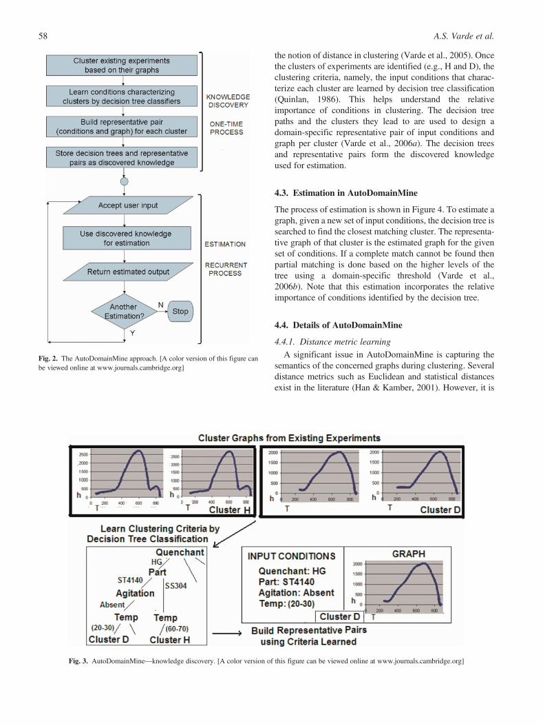
The AutoDomainMine approach is based on data mining. Itinvolves a one-time process of knowledge discovery frompreviously stored data and a recurrent process of using thediscovered knowledge for estimation. This approach is illus-trated in Figure 2.

AutoDomainMine discovers knowledge from existing ex-perimental data by integrating the two data mining techniquesof clustering and classification. It follows a typical learningstrategy of materials scientists. They often perform analysisby grouping experiments based on the similarity of the result-ing graphs and reasoning about the causes of similarity groupby group in terms of the impact of the input conditions on thegraphs (Sisson et al., 2004). This learning strategy is auto-mated for knowledge discovery in AutoDomainMine (Vardeet al., 2006b). Clustering is the process of placing a set of ob-jects into groups of similar objects (Han & Kamber, 2001).This is analogous to the grouping of experiments done byscientists. Classification is a form of data analysis that canbe used to extract models to predict categories (Mitchell,1997). An analogy can be drawn here with the scientistsreasoning about the similarity group by group. Hence, thetwo data mining techniques are integrated for knowledgediscovery as described below.

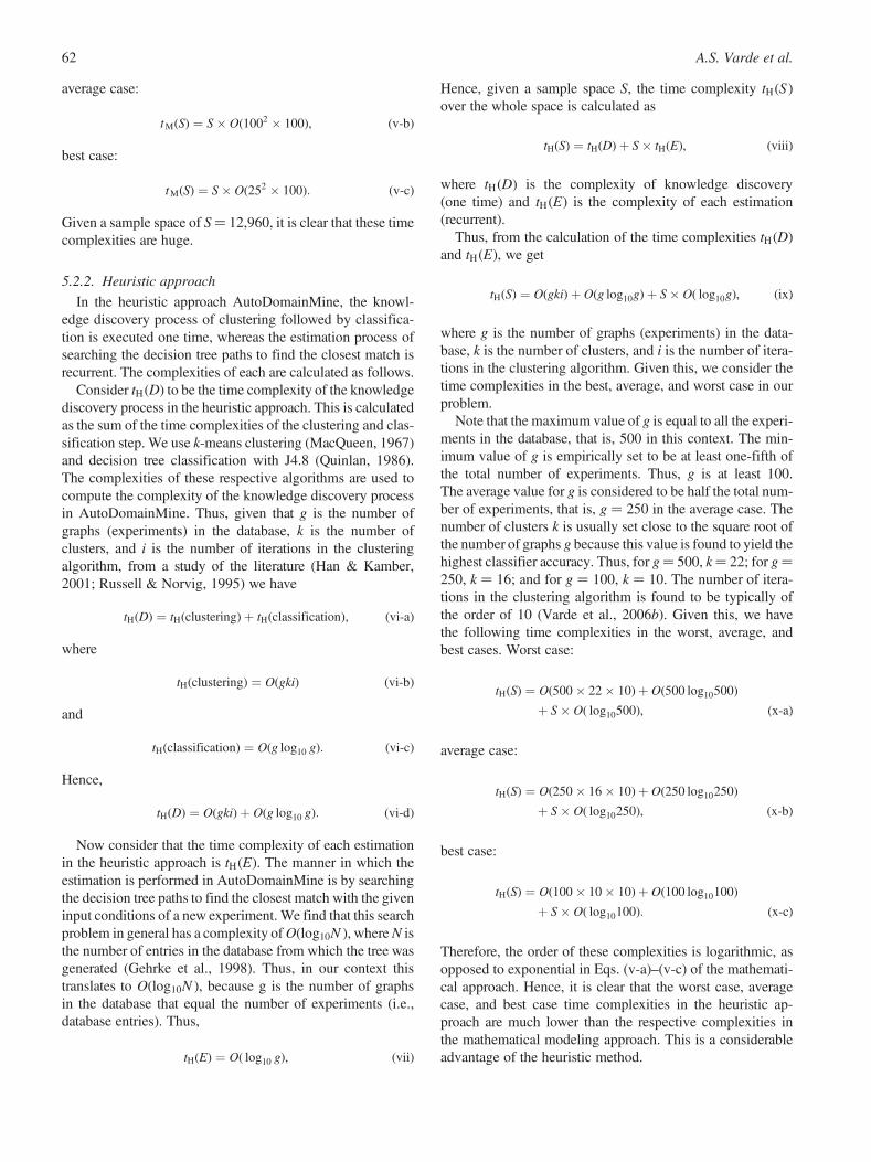
4.2. Knowledge discovery in AutoDomainMine

The knowledge discovery process is shown in Figure 3. Clus-tering is first performed over the graphs obtained from exist-ing experiments. Any clustering algorithm in the literaturecan be used such as the k-means algorithm (MacQueen,1967). We use a semantics-preserving distance metric as

Approaches for scientific data analysis 57

the notion of distance in clustering (Varde et al., 2005). Oncethe clusters of experiments are identified (e.g., H and D), theclustering criteria, namely, the input conditions that charac-terize each cluster are learned by decision tree classification(Quinlan, 1986). This helps understand the relativeimportance of conditions in clustering. The decision treepaths and the clusters they lead to are used to design adomain-specific representative pair of input conditions andgraph per cluster (Varde et al., 2006a). The decision treesand representative pairs form the discovered knowledgeused for estimation.

4.3. Estimation in AutoDomainMine

The process of estimation is shown in Figure 4. To estimate agraph, given a new set of input conditions, the decision tree issearched to find the closest matching cluster. The representa-tive graph of that cluster is the estimated graph for the givenset of conditions. If a complete match cannot be found thenpartial matching is done based on the higher levels of thetree using a domain-specific threshold (Varde et al.,2006b). Note that this estimation incorporates the relativeimportance of conditions identified by the decision tree.

4.4. Details of AutoDomainMine

4.4.1. Distance metric learning

A significant issue in AutoDomainMine is capturing thesemantics of the concerned graphs during clustering. Severaldistance metrics such as Euclidean and statistical distancesexist in the literature (Han & Kamber, 2001). However, it is

Fig. 2. The AutoDomainMine approach. [A color version of this figure canbe viewed online at www.journals.cambridge.org]

Fig. 3. AutoDomainMine—knowledge discovery. [A color version of this figure can be viewed online at www.journals.cambridge.org]

A.S. Varde et al.58

not known a priori which metric(s) would best preserve se-mantics if used as the notion of distance in clustering. Expertsat best have vague notions about the relative importance ofregions on the graphs but do not have a defined metric.State-of-the-art distance learning approaches (e.g., Hinne-burg et al. 2000, Xing et al., 2003) are either not applicableor not accurate enough in this context. We therefore proposean approach called LearnMet (Varde et al., 2005) to learnsemantics-preserving distance metrics for graphs. This isillustrated in Figure 5.

A LearnMet metric D is a weighted sum of componentswhere each component is an individual metric such as Euc-lidean distance, statistical distance, or a domain-specific crit-ical distance (Varde et al., 2005), and its weight gives itsrelative importance in the domain. LearnMet iteratively com-pares a training set of actual clusters given by experts withpredicted clusters obtained from any fixed clustering algo-rithm, for example, k-means (MacQueen, 1967). In the firstiteration, a guessed metric D is used for clustering using fun-damental knowledge of the domain. This metric is adjustedbased on error between predicted and actual clusters using a

weight adjustment heuristic (Varde et al., 2005) until erroris below a given threshold or a maximum number of epochsis reached. The metric with error below threshold or withminimum error among all epochs is returned as the learnedmetric. The output of LearnMet is used as the notion ofdistance for the graphs.

4.4.2. Designing cluster representatives

Another important issue in AutoDomainMine is capturingrelevant data in each cluster while building representatives.A default approach of randomly selecting a representativepair of input conditions and graph per cluster is not found tobe effective in preserving the necessary information. Becauseseveral combinations of conditions lead to a single cluster,randomly selecting any one as a representative causes informa-tion loss. Randomly selected representatives of graphs do notincorporate semantics and ease of interpretation based on userinterests.

State-of-the-art approaches (e.g., Helfman & Hollan, 2001;Janecek & Pu, 2004), do not build cluster representatives as ap-propriate for our needs. Hence, we propose an approach called

Fig. 4. AutoDomainMine—estimation. [A color version of this figure can be viewed online at www.journals.cambridge.org]

Fig. 5. The LearnMet approach. [A color version of this figure can be viewed online at www.journals.cambridge.org]

Approaches for scientific data analysis 59

DesRept (Varde et al., 2006a) to design domain-specific clus-ter representatives. This approach is depicted in Figure 6.

In DesRept, two design methods of guided selection andconstruction are used to build candidate representatives show-ing various levels of detail in the cluster, where each candidatecaptures a certain aspect of domain semantics. Candidates arecompared using our proposed DesRept encodings for condi-tions and graphs analogous to the minimum descriptionlength principle (Rissanen, 1987). In minimum descriptionlength, the goal is to minimize the sum of encoding a theoryand examples using the theory. In DesRept, the theory refersto a cluster representative, whereas the examples refer to theother objects within the cluster. Thus, a DesRept encodingconsists of the sum of storing a cluster representativeand the distance of all other cluster objects from thatrepresentative. In correspondence, the criteria in the DesReptencodings are complexity of the representative itself and in-formation loss based on its distance from other cluster objects.Weights are assigned to these two criteria based on user inter-ests in targeted applications. The winning candidate for eachcluster is considered to be the one with the lowest encoding.This candidate is returned as the designed cluster representa-tive. The designed representatives are used for estimation inthe AutoDomainMine approach (Varde et al., 2006b).

4.4.3. Implementation of heuristic approach

The main tasks in implementing this heuristic estimationapproach based on data mining are described below. The pro-gramming language used for implementation is Java withMySQL for the databases.

† The learning strategy in AutoDomainMine of discover-ing knowledge for estimation by integrating clusteringand classification is implemented using the k-meansalgorithm for clustering (MacQueen, 1967) and theJ4.8 algorithm for decision tree classification (Quinlan,1986). Parameters in these algorithms such as the valuesof k are variable and are altered during the evalution ofthe approach as will be elaborated in Section 6.

† LearnMet is implemented for learning semantics-preserving distance metrics for graphs, in particular, its

weight adjustment heuristic. The clustering algorithmused within LearnMet is also k-means (MacQueen, 1967).

† DesRept is implemented for designing domain-specificcluster representative pairs along with the DesReptEncodings for evaluating them. The clusters are ob-tained from the k-means algorithm (MacQueen, 1967)and the decision tree paths leading to the clusters areobtained using the J4.8 algorithm for decision treeclassification (Quinlan, 1967).

Thus, the AutoDomainMine approach has been used tobuild a software tool called AutoDomainMine (Varde et al.,2006b), which is a trademark of the CHTE that supportedthis research. This approach has been rigorously evaluatedwith real data from the heat treating domain with the helpof formal user surveys. It has been found to provide effectiveestimation as per the requirements of the users.

5. COMPARATIVE STUDY

We now compare the approaches based on sample space, timecomplexity, and data storage.

5.1. Sample space

The sample space of any estimation problem is the number ofcases it can estimate (Russell & Norvig, 1995). We explainthe calculation of the sample space with reference to ourestimation problem.

5.1.1. Sample space calculation

The sample space is calculated as a product of the numberof possible values of each experimental input condition. Eachinput condition is described by an attribute that gives its nameand a value that gives its content. Thus, we have, samplespace

S ¼YA

c¼1

Vc, (i)

where A is the total number of attributes (conditions) and Vc isthe number of possible values of the conditions.

Consider the example of estimating heat transfer curves. Inthis example, the input conditions are the following:

1. quenchant name: T7A, DurixolV35, and so forth2. part material: ST4140, SS304, and so forth3. agitation level: absent, high, low4. oxide layer: none, thin, thick5. probe type: CHTE, IVF, and so forth6. quenchant temperature: 08–2008C

Note that there are 500 experiments stored in the database.The number of possible values of each of these based on thestored experiments is as follows:

Fig. 6. The DesRept approach. [A color version of this figure can be viewedonline at www.journals.cambridge.org]

A.S. Varde et al.60

1. quenchant name: nine values2. part material: four values3. agitation level: three values4. oxide layer: three values5. probe type: two values6. quenchant temperature: 20 ranges

Thus, the total sample space provided by the 500 storedexperiments is given by a product of these values. Hence,we have sample space ¼ 9�4�3�3�2�20 ¼ 12,960.

We now discuss this with reference to our mathematicaland heuristic approaches.

5.1.2. Mathematical approach

In this approach, the estimation of heat transfer coefficientsis performed using the direct and inverse heat conductionequations. However, to apply these equations, data on timeand temperature is needed. If the real laboratory experimentis not conducted then this data is typically supplied bydomain experts (Maniruzzaman et al., 2006).

Thus, in this process domain expert intervention is neededeach time the estimation is performed. Thus, to cover a sam-ple space of 12,960 experiments, the domain experts wouldneed to provide the time–temperature inputs 12,960 times,which seems rather infeasible. Besides the fact that supplyingthese inputs is time consuming and cumbersome, it is notalways possible for the experts to guess them based on ex-perimental input conditions. This is a major drawback ofthe mathematical approach related to sample space.

However, a major advantage of this approach is that noother data on previous experiments needs to be stored inadvance to cover this sample space. The state of the art for-mulae can be directly applied.

The advantage and disadvantage are further clarified as wediscuss the heuristic solution.

5.1.3. Heuristic approach

The heuristic solution approach to the given estimationproblem is AutoDomainMine (Varde et al., 2006b). In thisapproach, when the input conditions of a new experimentare submitted, the decision tree paths are traced to find theclosest match. The representative graph of the correspondingcluster is conveyed as the estimated result. When an exactmatch is not found, a partial match is conveyed using higherlevels of the tree. Thus, even if data on all the possible com-binations of inputs is not available, an approximate answercan still be provided.

Hence, to cover the sample space of the estimation it is notnecessary to supply time–temperature data for each newexperiment whose results are to be estimated. The estimationcan be performed simply by supplying the input conditions ofthe new experiment. Thus, the whole sample space of 12,960experiments can be covered without domain expert interven-tion each time the estimation is performed. This is an advan-tage of the heuristic approach with reference to the samplespace criterion.

However, to perform the estimation in AutoDomainMine,data from existing laboratory experiments needs to be storedin the database. This forms the basis for knowledge discoveryand estimation. This is a drawback of the heuristic approach.However, the amount of data from existing experiments canbe much lower than the sample space. For example, in heattreating the number of experiments stored is 500. Withthis, AutoDomainMine gives an accuracy of approximately90–95%, as elaborated later in this paper.

5.2. Time complexity

The time complexity of any approach refers to the executiontime of the technique used for computation. We discuss thiswith reference to the mathematical and heuristic approaches.

5.2.1. Mathematical approach

In the direct–inverse heat conduction mathematical model,the time complexity tM(E) of each estimation (Ma et al.,2004) is given as

tM(E) ¼ O(n2 � i), (ii)

where n is the number of time–temperature data points sup-plied and i is the number of iterations for convergence tominimal error. Each such data point corresponds to measure-ment of heat transfer coefficient at one instance of time.

In the given problem the maximum number of data pointssupplied would be 1500 and the minimum number would be25. On an average, 100 data points are supplied. The numberof iterations for convergence is typically found to be on theorder of 100 (Ma et al., 2004).

Thus, we have the following time complexities. Worst case:

tM(E) ¼ O(15002 � 100), (iii-a)

average case:

tM(E) ¼ O(1002 � 100), (iii-b)

best case:

tM(E) ¼ O(252 � 100): (iii-c)

Because the data points need to be provided for each estima-tion, the time complexity tM(S ) over the whole sample space Sis given by

tM(S) ¼ S� tM(E), (iv)

where tM(E) is the time complexity of each estimation.Thus, we have the following time complexities over the

whole sample space for the worst, average, and best cases.Worst case:

tM(S) ¼ S� O(15002 � 100), (v-a)

Approaches for scientific data analysis 61

average case:

tM(S) ¼ S� O(1002 � 100), (v-b)

best case:

tM(S) ¼ S� O(252 � 100): (v-c)

Given a sample space of S¼ 12,960, it is clear that these timecomplexities are huge.

5.2.2. Heuristic approach

In the heuristic approach AutoDomainMine, the knowl-edge discovery process of clustering followed by classifica-tion is executed one time, whereas the estimation process ofsearching the decision tree paths to find the closest match isrecurrent. The complexities of each are calculated as follows.

Consider tH(D) to be the time complexity of the knowledgediscovery process in the heuristic approach. This is calculatedas the sum of the time complexities of the clustering and clas-sification step. We use k-means clustering (MacQueen, 1967)and decision tree classification with J4.8 (Quinlan, 1986).The complexities of these respective algorithms are used tocompute the complexity of the knowledge discovery processin AutoDomainMine. Thus, given that g is the number ofgraphs (experiments) in the database, k is the number ofclusters, and i is the number of iterations in the clusteringalgorithm, from a study of the literature (Han & Kamber,2001; Russell & Norvig, 1995) we have

tH(D) ¼ tH(clustering)þ tH(classification), (vi-a)

where

tH(clustering) ¼ O(gki) (vi-b)

and

tH(classification) ¼ O(g log10 g): (vi-c)

Hence,

tH(D) ¼ O(gki)þ O(g log10 g): (vi-d)

Now consider that the time complexity of each estimationin the heuristic approach is tH(E). The manner in which theestimation is performed in AutoDomainMine is by searchingthe decision tree paths to find the closest match with the giveninput conditions of a new experiment. We find that this searchproblem in general has a complexity of O(log10N ), where N isthe number of entries in the database from which the tree wasgenerated (Gehrke et al., 1998). Thus, in our context thistranslates to O(log10N ), because g is the number of graphsin the database that equal the number of experiments (i.e.,database entries). Thus,

tH(E) ¼ O( log10 g), (vii)

Hence, given a sample space S, the time complexity tH(S )over the whole space is calculated as

tH(S) ¼ tH(D)þ S� tH(E), (viii)

where tH(D) is the complexity of knowledge discovery(one time) and tH(E) is the complexity of each estimation(recurrent).

Thus, from the calculation of the time complexities tH(D)and tH(E), we get

tH(S) ¼ O(gki)þ O(g log10g)þ S� O( log10g), (ix)

where g is the number of graphs (experiments) in the data-base, k is the number of clusters, and i is the number of itera-tions in the clustering algorithm. Given this, we consider thetime complexities in the best, average, and worst case in ourproblem.

Note that the maximum value of g is equal to all the experi-ments in the database, that is, 500 in this context. The min-imum value of g is empirically set to be at least one-fifth ofthe total number of experiments. Thus, g is at least 100.The average value for g is considered to be half the total num-ber of experiments, that is, g ¼ 250 in the average case. Thenumber of clusters k is usually set close to the square root ofthe number of graphs g because this value is found to yield thehighest classifier accuracy. Thus, for g¼ 500, k¼ 22; for g¼250, k ¼ 16; and for g ¼ 100, k ¼ 10. The number of itera-tions in the clustering algorithm is found to be typically ofthe order of 10 (Varde et al., 2006b). Given this, we havethe following time complexities in the worst, average, andbest cases. Worst case:

tH(S) ¼ O(500� 22� 10)þ O(500 log10500)

þ S� O( log10500), (x-a)

average case:

tH(S) ¼ O(250� 16� 10)þ O(250 log10250)

þ S� O( log10250), (x-b)

best case:

tH(S) ¼ O(100� 10� 10)þ O(100 log10100)

þ S� O( log10100): (x-c)

Therefore, the order of these complexities is logarithmic, asopposed to exponential in Eqs. (v-a)–(v-c) of the mathemati-cal approach. Hence, it is clear that the worst case, averagecase, and best case time complexities in the heuristic ap-proach are much lower than the respective complexities inthe mathematical modeling approach. This is a considerableadvantage of the heuristic method.

A.S. Varde et al.62

5.3. Data storage

The data storage criterion refers to the quantity of data thatneeds to be stored from existing experiments to execute theapproach.

5.3.1. Mathematical approach

This approach uses the applicable formulae and the inputssupplied by domain experts each time the estimation is per-formed. No data from previously performed experiments isutilized in the computation. Hence, in theory, the quantityof data stored for this approach is zero. Thus, given that Q re-fers to the quantity of data, we find that in the mathematicalmodel, Q¼ 0. This is a big advantage of the mathematical ap-proach.

However, note that the experts, although providing initialtime–temperature inputs to this model, may refer to existingexperiments. Thus, in practice, data stored from previouslyperformed experiments could perhaps be useful in mathemat-ical modeling, but this data storage is not a requirement of themodel per se, which gives this approach an edge over theheuristic approach.

5.3.2. Heuristic approach

This uses the existing experiments in the database forknowledge discovery and estimation. Given that g is the num-ber of graphs (experiments) in the database, n is the number ofdata points stored per graph, and A is the number of attributesstored for each experiment, the quantity Q of data stored in theheuristic approach is given as

Q ¼ g� n� A: (xi)

The heuristic approach cannot work without data from pre-vious experiments. This is one of the situations where themathematical model wins over the heuristic method.

Theoretically, there is no bound on the minimum quantityof data that needs to be stored in order to perform the estima-tion heuristically. However, the more the data from existingexperiments, the more accurate is the estimation. This isbecause a greater number of experiments are available forknowledge discovery by clustering and classification and agreater number of decision tree paths can be searched forestimation. In addition, the more distinct the input conditionsare, the better it is for the heuristic approach. This is because agreater number of distinct paths can be identified in thedecision tree to more classify new experiments.

Note that in scientific domains experiments are often de-signed using the Taguchi metrics (Roy et al., 2001). In Tagu-chi design, experimental parameters are intelligently selectedsuch that one experiment can effectively cover approximatelythree experiments in terms of the ranges of the inputs and thecorresponding results. This enhances the sample space. It istherefore desirable that Taguchi metrics be used for theexperimental setup to provide more data for the heuristicapproach.

6. PERFORMANCE EVALUATION

The approaches have been evaluated for accuracy and effi-ciency with real data from the domain of heat treating ofmaterials. A summary of the evaluation is presented here.

6.1. Accuracy

Accuracy is a quality measure that refers to how close the es-timated result is to the output of a real experiment. Evaluationof accuracy is explained with reference to each approach in-dividually.

6.1.1. Mathematical approach

We present excerpts from the study of the accuracy of themathematical approach. The objective of the study is to pre-dict the surface heat transfer coefficient from the known tem-perature at the geometric center of the CHTE probe. In thisstudy a few numerical examples are presented below to illus-trate the ability of the SDM in predicting the surface heattransfer coefficient.

The first test case shows a CHTE ST4140 cylindrical probewith 3/8-in. diameter and 1.5-in. length quenched in themineral oil Houghton G. Specific heat and thermal con-ductivity as a function of temperature are utilized in the cal-culation. Figure 7 shows the heat transfer coefficient h(T )from two methods, namely, lumped parameter analysis (Maet al., 2002) and the inverse analysis described here.

Figure 8 shows another case of the estimated heat transfercoefficient of the same CHTE ST4140 steel probe quenchedin mineral oil T-7-A. The difference between Figure 9 andFigure 8 is that the curve in Figure 9 includes the Leidenfrostpoint, which is one of the important parameters to character-ize the quenching process. The selection of this test case is toensure that the inverse analysis can successfully predict theheat transfer coefficient curve with a Leidenfrost point.Figure 9 shows the comparison results from the lumpedparameter analysis and the inverse analysis. The inverseanalysis does give a heat transfer coefficient curve with aLeidenfrost point, which shifts to the higher temperaturecompared with that from the lumped parameter analysis.

The third test case is for a wrought aluminum 2024 probewith the same dimension quenched in polymer solution Aqua260. The results are shown in Figure 9. As can be seen, thecurves from both the lumped parameter analysis and the in-verse analysis are almost on top of each other. This is becausethe thermal conductivity is much higher for aluminum alloythan that for steel, which makes the heat extraction ratemuch greater for aluminum quenching.

Likewise, several tests are conducted with different inputconditions using the 500 laboratory experiments stored inthe database. Based on the tests conducted, the domain ex-perts conclude that the estimation accuracy of the mathemati-cal models in general is found to be in the range of approxi-mately 85–90%. This means that in 85–90% of the tests, theestimated result matches the real result of the corresponding

Approaches for scientific data analysis 63

laboratory experiment. However, this is subject to the avail-ability of good time–temperature inputs from experts.

6.1.2. Heuristic approach

The accuracy of the heuristic model is evaluated with formalsurveys conducted by the targeted users of the system. The usersrun tests with the AutoDomainMine tool. These tests are con-ducted using various values of experimental parameters. The

clustering seeds are altered for randomization, different valuesof k are used in the k-means algorithm for clustering anddecision tree parameters in the J4.8 algorithm are altered. Weshow below a few examples from our rigorous evaluation ofAutoDomainMine. The holdout strategy (Russell & Norvig,1995) is used for evaluation. Among the 500 experiments inthe heat treating database, 400 are used for training the techniqueand the remaining 100 are kept aside as the distinct test set.

Fig. 7. The heat transfer coefficient for the CHTE ST4140 probe quenched in Houghton G. [A color version of this figure can be viewedonline at www.journals.cambridge.org]

Fig. 8. The heat transfer coefficient for the CHTE ST4140 probe quenched in T-7-A. [A color version of this figure can be viewed online atwww.journals.cambridge.org]

A.S. Varde et al.64

Tests are conducted as follows. In each test, the users enterthe input conditions of a real experiment from the distinct testset. They observe the estimated output of AutoDomainMineand compare it with the output of the corresponding real ex-periment. If the real and estimated results are close enough asper user satisfaction, then the estimation is considered to becorrect. Accuracy is then reported as the percentage of correctestimations over all the tests conducted.

We target the users of various applications of Auto-DomainMine such as parameter selection (Sisson et al.,2004), simulation tools (Lu et al., 2002), decision supportsystems (Varde et al., 2003), and intelligent tutors (Bierman& Kamsteeg, 1988). Accuracy is reported in the context ofeach application. Sample screen-dumps from the evaluationare demonstrated here.

Figure 10 shows an example of how the user enters theinput conditions of an experiment in the test set. The Auto-DomainMine system estimates the heat transfer curve that

would be obtained. The estimated output is shown in Figures11–13. Figure 11 depicts the most likely heat transfer curvethat would be obtained from the input conditions in Figure10. This conveys to the user the most probable estimated out-put. Figure 12 shows the average heat transfer curve with pre-diction limits for the same input conditions. This enables theuser to get an idea of the estimated average output along withvariations that may occur if the real experiment were con-ducted. Figure 13 goes one level deeper to illustrate the esti-mated ranges of heat transfer that would occur with the giveninput conditions. This allows the user to see all the potentialvalues of the estimated output that would occur based on ananalysis of existing data.

The users compare the estimated output in all the levelswith the real output of the corresponding experiment con-ducted with the same input conditions. Figure 14 shows thereal heat transfer curve obtained for the input conditions inFigure 10. Upon comparing the real and estimated heat

Fig. 9. The heat transfer coefficient for the CHTE aluminum 2024 probe quenched in Aqua260. [A color version of this figure can beviewed online at www.journals.cambridge.org]

Fig. 10. An example of user input to AutoDomainMine. [A color version of this figure can be viewed online at www.journals.cambridge.org]

Approaches for scientific data analysis 65

transfer curves, the users conclude that the estimation is cor-rect. Because the estimation provided by AutoDomainMineshows the expected output including its estimated ranges,the real result is more likely to fall within these ranges (as op-posed to the output provided by the mathematical models).This, in turn, is likely to increase the accuracy of the estima-tion in most cases.

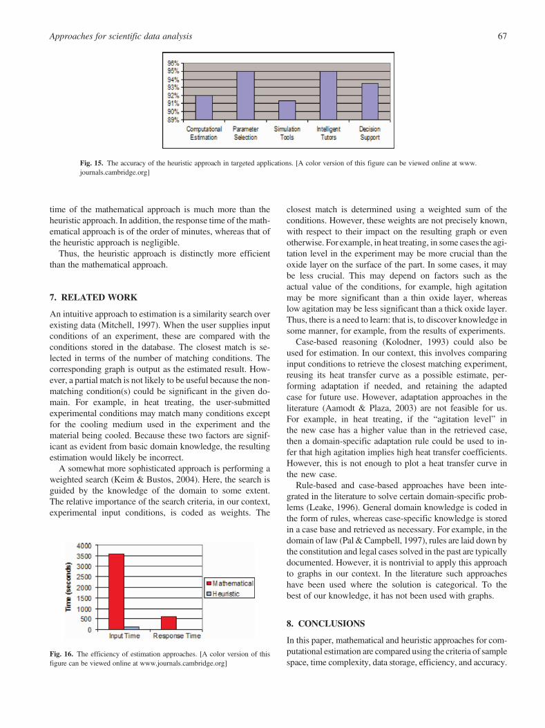
Likewise, upon conducting tests with all the data in the testset, the estimation accuracy of AutoDomainMine is found tobe in the range of 90–95% (Varde et al., 2006b). This isevident from an analysis of the survey results. Figure 15shows the accuracy of the heuristic approach AutoDomain-Mine in the context of computational estimation and its tar-geted applications. Note that the accuracy has been evaluatedby users in the context of the applications of estimation.Hence, we analyze the responses of the users with respect tothe given applications and report accuracy accordingly. Forexample, among 100 tests conducted by parameter selectionusers, 95 are found to be accurate, and hence, the accuracyin that application is reported as 95%. The accuracy of thecomputational estimation on the whole is the percentage ofaccurate tests among all the tests conducted by users in allthe applications. This effectively represents the overall estima-

tion accuracy of AutoDomainMine. Figure 15 shows that theoverall accuracy is 92%.

Therefore, on the whole, we find that the estimation ac-curacy in the heuristic approach is somewhat higher than thatin the mathematical approach.

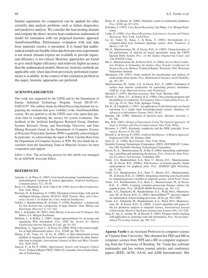
6.2. Efficiency

Efficiency refers to the amount of time taken to perform theestimation, that is, the setup time for supplying the inputsand the response time of the tool (Fig. 16). We record theamount of time taken to supply inputs for each test in boththe mathematical and heuristic approaches. Note that in themathematical approach, in addition to experimental inputconditions, experts need to provide initial values for time–temperature. Thus, the time taken to provide these additionalinputs is also recorded. The response time of each approach interms of how long it takes to produce the output, given the in-puts, is observed as well.

Figure 12 shows average input and response times of themathematical and heuristic approaches. We find that input

Fig. 11. The most probable estimated output. [A color version of this figurecan be viewed online at www.journals.cambridge.org]

Fig. 13. Potential ranges of estimated output. [A color version of this figurecan be viewed online at www.journals.cambridge.org]

Fig. 12. The average estimated output with variations. [A color version ofthis figure can be viewed online at www.journals.cambridge.org]

Fig. 14. The heat transfer curve from the real experiment. [A color version ofthis figure can be viewed online at www.journals.cambridge.org]

A.S. Varde et al.66

time of the mathematical approach is much more than theheuristic approach. In addition, the response time of the math-ematical approach is of the order of minutes, whereas that ofthe heuristic approach is negligible.

Thus, the heuristic approach is distinctly more efficientthan the mathematical approach.

7. RELATED WORK

An intuitive approach to estimation is a similarity search overexisting data (Mitchell, 1997). When the user supplies inputconditions of an experiment, these are compared with theconditions stored in the database. The closest match is se-lected in terms of the number of matching conditions. Thecorresponding graph is output as the estimated result. How-ever, a partial match is not likely to be useful because the non-matching condition(s) could be significant in the given do-main. For example, in heat treating, the user-submittedexperimental conditions may match many conditions exceptfor the cooling medium used in the experiment and thematerial being cooled. Because these two factors are signif-icant as evident from basic domain knowledge, the resultingestimation would likely be incorrect.

A somewhat more sophisticated approach is performing aweighted search (Keim & Bustos, 2004). Here, the search isguided by the knowledge of the domain to some extent.The relative importance of the search criteria, in our context,experimental input conditions, is coded as weights. The

closest match is determined using a weighted sum of theconditions. However, these weights are not precisely known,with respect to their impact on the resulting graph or evenotherwise. For example, in heat treating, in some cases the agi-tation level in the experiment may be more crucial than theoxide layer on the surface of the part. In some cases, it maybe less crucial. This may depend on factors such as theactual value of the conditions, for example, high agitationmay be more significant than a thin oxide layer, whereaslow agitation may be less significant than a thick oxide layer.Thus, there is a need to learn: that is, to discover knowledge insome manner, for example, from the results of experiments.

Case-based reasoning (Kolodner, 1993) could also beused for estimation. In our context, this involves comparinginput conditions to retrieve the closest matching experiment,reusing its heat transfer curve as a possible estimate, per-forming adaptation if needed, and retaining the adaptedcase for future use. However, adaptation approaches in theliterature (Aamodt & Plaza, 2003) are not feasible for us.For example, in heat treating, if the “agitation level” inthe new case has a higher value than in the retrieved case,then a domain-specific adaptation rule could be used to in-fer that high agitation implies high heat transfer coefficients.However, this is not enough to plot a heat transfer curve inthe new case.

Rule-based and case-based approaches have been inte-grated in the literature to solve certain domain-specific prob-lems (Leake, 1996). General domain knowledge is coded inthe form of rules, whereas case-specific knowledge is storedin a case base and retrieved as necessary. For example, in thedomain of law (Pal & Campbell, 1997), rules are laid down bythe constitution and legal cases solved in the past are typicallydocumented. However, it is nontrivial to apply this approachto graphs in our context. In the literature such approacheshave been used where the solution is categorical. To thebest of our knowledge, it has not been used with graphs.

8. CONCLUSIONS

In this paper, mathematical and heuristic approaches for com-putational estimation are compared using the criteria of samplespace, time complexity, data storage, efficiency, and accuracy.

Fig. 15. The accuracy of the heuristic approach in targeted applications. [A color version of this figure can be viewed online at www.journals.cambridge.org]

Fig. 16. The efficiency of estimation approaches. [A color version of thisfigure can be viewed online at www.journals.cambridge.org]

Approaches for scientific data analysis 67

Similar arguments for comparison can be applied for otherscientific data analysis problems such as failure diagnosticsand predictive analysis. We consider the heat treating domainand compare the direct–inverse heat conduction mathematicalmodel for estimation with our proposed heuristic approachAutoDomainMine. Performance evaluation with real datafrom materials science is presented. It is found that mathe-matical models are feasiblewhen data from previous experimentsis not stored, domain experts are available to provide inputs,and efficiency is not critical. Heuristic approaches are foundto give much higher efficiency and relatively higher accuracythan the mathematical models. However, heuristic methods areapplicable only when data from previously performed experi-ments is available. In the context of the estimation problem inthis paper, heuristic approaches are preferred.

ACKNOWLEDGMENTS

This work was supported by the CHTE and by the Department ofEnergy Industrial Technology Program Award DE-FC-07-01ID14197. The authors thank the Metal Processing Institute for or-ganizing the seminars that gave visibility to the AutoDomainMinesystem. We are grateful to all the CHTE users who spent their pre-cious time in completing the surveys for system evaluation. Thefeedback of the Artificial Intelligence Research Group, DatabaseSystems Research Group, and Knowledge Discovery and DataMining Research Group in the Department of Computer Scienceat Worcester Polytechnic Institute (WPI) is gratefully acknowledged.In particular, we acknowledge the input of Prof. Carolina Ruiz fromthe Department of Computer Science at WPI. We also thank the re-searchers from the Quenching Team in Materials Science for theircooperation and support.

Editor’s Note: The reviewing process for this article was managedby an AIEDAM Associate Editor.

REFERENCES

Aamodt, A., & Plaza, E. (2003). Case based reasoning: foundational issues,methodological variations & system approaches. Artificial IntelligenceCommunications 7(1), 39–59.

Beck, J.V., Blackwell, B., & St. Clair, C.R. (1985). Inverse Heat Conduction.New York: Wiley.

Bierman, D., & Kamsteeg, P. (1988). Elicitation of knowledge with and forintelligent tutoring systems. IICAI-03: IEEE Systems, Man, and Cyber-netics Society’s 1st Indian Int. Conf. Artificial Intelligence.

Gehrke, J., Ramakrishnan, R., & Ganti, V. (1998). Rainforest—a frameworkfor fast decision tree construction of large datasets. Data Mining andKnowledge Discovery 4, 127–162.

Han, J., & Kamber, M. (2001). Data Mining: Concepts and Techniques. SanMateo, CA: Morgan Kaufmann.

Helfman, J., & Hollan, J. (2001). Image representations for accessing andorganizing Web information. Proc. SPIE Int. Society for OpticalEngineering Internet Imaging II Conf., pp. 91–101.

Hinneburg, A., Aggarwal, C., & Keim, D. (2000). What is the nearest neigh-bor in high dimensional spaces. Proc. VLDB, pp. 506–515.

Huang, C.-H., Yuan, I.C., & Ay, H. (2003). A three-dimensional inverseproblem in imaging the local heat transfer coefficients for plate finned-tube heat exchangers. International Journal of Heat and Mass Transfer4(6), 3629–3638.

Janecek, P., & Pu, P. (2004). Opportunistic Search with Semantic FisheyeViews, Technical Report TR IC/2004/42. Lausanne: Swiss Federal Insti-tute of Technology.

Keim, D., & Bustos, B. (2004). Similarity search in multimedia databases.Proc. ICDE, pp. 873–874.

Kolodner, J. (1993). Case-Based Reasoning. San Mateo, CA: Morgan Kauf-mann.

Leake, D. (1996). Case-Based Reasoning: Experiences, Lessons and FutureDirections. New York: AAAI Press.

Lu, Q., Vader, R., Kang, J., & Rong, Y. (2002). Development of acomputer-aided heat treatment planning system. Heat Treatment ofMetals 3, 65–70.

Ma, S., Maniruzzaman, M., & Sisson, R.D., Jr. (2002). Characterization ofthe performance of mineral oil based quenchants using the CHTEQuench Probe System. Proc. 1st Int. Surface Engineering Congr. and13th IFHTSE Congr.

Ma, S., Maniruzzaman, M., & Sisson, R.D., Jr. (2004). Inverse Heat Conduc-tion Problem in Estimating the Surface Heat Transfer Coefficients bySteepest Descent Method, Technical Report. Worcester, MA: WorcesterPolytechnic Institute.

MacQueen, J.B. (1967). Some methods for classification and analysis ofmultivariate observations. Proc. Mathematical Statistics and Probability,pp. 281–297.

Maniruzzaman, M., Varde, A.S., & Sisson, R.D., Jr. (2006). Estimation ofsurface heat transfer coefficients for quenching process simulation.ASM Int. Conf. Materials Science and Technology.

Mitchell, T. (1997). Machine Learning. New York: McGraw–Hill.Newell, A., Shaw, J.C., & Simon, H.A. (1988). Chess playing programs and

the problem of complexity. In Computer Chess Compendium (Levy, D.,Ed.), pp. 29–42. New York: Springer–Verlag.

Pal, K., & Campbell, J. (1997). An application of rule-based and case-basedreasoning in a single legal knowledge-based system. Database forAdvances in Information Systems 28(4), 48–63.

Quinlan, J.R. (1986). Induction of decision trees. Machine Learning 1,81–106.

Roy, R.K. (2001). Design of Experiments Using The Taguchi Approach: 16Steps to Product and Process Improvement. New York: Wiley.

Rissanen, J. (1987). Stochastic complexity and the MDL principle. Econ-ometric Reviews 6, 85–102.

Russell, S., & Norvig, P. (1995). Artificial Intelligence: A Modern Approach.Englewood Cliffs, NJ: Prentice–Hall.

Stolz, G., Jr. (1960). Heat Transfer. New York: Wiley.Scientific Forming Technologies Corporation. (2005). DEFORM-HT. Colum-

bus, OH: Scientific Forming Technologies Corporation.Sisson, R., Jr., Maniruzzaman, M., & Ma, S. (2004). Quenching: understand-

ing, controlling and optimizing the process. Proc. Center for Heat Treat-ing Excellence Fall Seminar, Columbus, OH.

Varde, A.S., Rundensteiner, E.A., Ruiz, C., Brown, D.C., Maniruzzaman,M., & Sisson, R.D. (2006a). Effectiveness of domain-specific clusterrepresentatives for graphical plots. Proc. SIGMOD IQIS Workshop,pp. 31–36.

Varde, A.S., Rundensteiner, E.A., Ruiz, C., Brown, D.C., Maniruzzaman,M., & Sisson, R.D., Jr. (2006b). Integrating clustering and classificationfor estimating process variables in materials science. AAAI Poster Track.

Varde, A.S., Rundensteiner, E.A., Ruiz, C., Maniruzzaman, M., & Sisson,R.D., Jr. (2005). Learning semantics-preserving distance metrics forgraphical plots. Proc. SIGKDD MDM Workshop, pp. 107–112.

Varde, A.S., Takahashi, M., Rundensteiner, E.A., Ward, M.O., Maniruzza-man, M., & Sisson, R.D., Jr. (2003). QuenchMinerTM: decision supportfor optimization of heat treating processes. IICAI, pp. 993–1003.

Varde, A.S., Takahashi, M., Rundensteiner, E.A., Ward, M.O., Maniruzza-man, M., & Sisson, R.D., Jr. (2004). A priori algorithm and game-of-life for predictive analysis in materials science. International Journalof Knowledge-Based & Intelligent Engineering Systems 8(4), 213–228.

Xing, E., Ng, A., Jordan, M., & Russell, S. (2003). Distance metric learningwith application to clustering with side information. Proc. Neural Infor-mation Processing Systems, pp. 503–512.

Aparna Varde is an Assistant Professor in computer scienceat Virginia State University. She obtained her PhD and MS incomputer science from WPI and a BE in computer engineer-ing from the University of Bombay. Dr. Varde has softwaretrademarks and has written journal articles and conferencepapers (IEEE, ACM, AAAI, and ASM International). Her

A.S. Varde et al.68

professional activities include serving as a reviewer for thejournals Data and Knowledge Engineering, Transactionson Knowledge and Data Engineering, and Information Sys-tems; as Co-Chair of the PhD Workshop in the ACM Confer-ence on Information and Knowledge Management; and as aPC Member of SIAM’s Data Mining Conference and theMultimedia Data Mining Workshop in the ACM Conferenceon Knowledge Discovery and Data Mining. She is workingon research projects mostly in scientific data mining.

Shuhui Ma is a Manufacturing Engineer at Tiffany andCompany. She has a BS in physical chemistry from BeijingUniversity of Science and Technology and an MS and aPhD in materials science and engineering from WPI. She isa member of Sigma Xi, ASM, and TMS. Dr. Ma was therecipient of the 2006 Bodycote/HTS best paper award.

Mohammed Maniruzzaman is currently a ResearchAssistant Professor of mechanical engineering at WPI. Hehas a BSc and an MS degree in mechanical and a PhD inmaterials science and engineering. He is a member of theASM, TMS, and Sigma Xi. Dr. Maniruzzaman’s main re-search interest is the application of mathematical modelingto materials processing, with special emphasis on alloy heattreatment and molten metal treatment.

David C. Brown is a Professor of computer science and has acollaborative appointment as a Professor of mechanical en-gineering at WPI. He has BSc, MSc, MS, and PhD degrees incomputer science and is a member of the ACM, IEEE ComputerSociety, AAAI, ASME, and IFIP WG 5.2. He is the Editor inChief of the Cambridge University Press journal Artificial Intel-ligence for Engineering Design, Analysis and Manufacturing,

and he is on the editorial boards of several other journals.Dr. Brown’s research interests include computational modelsof engineering design and the applications of artificial intelli-gence to engineering and manufacturing.

Elke Rundensteiner is a Professor of computer science atWPI. She is a well-known expert in databases. Her currentresearch includes stream data management, data integrationand warehousing, and visual information exploration. Shehas over 280 publications in these areas. Her research hasbeen funded by government agencies and industry, includ-ing NSF, NIH, IBM, Verizon, GTE, HP, and NEC. Dr.Rundensteiner has been the recipient of numerous honors,including NSF Young Investigator, Sigma Xi OutstandingSenior Faculty Researcher, and WPI Trustees’ OutstandingResearch and Creative Scholarship awards. She serves onthe program committees of prestigious conferences and is theAssociate Editor and Special Issue Editor of several journals.

Richard D. Sisson, Jr., is the George F. Fuller Professor andDirector of Manufacturing and Materials Engineering at WPI.He received his BS in metallurgical engineering fromVirginia Polytechnic Institute and an MS and a PhD in metal-lurgical engineering from Purdue University. Dr. Sisson’steaching and research has focused on the applications ofthermodynamics and kinetics to materials processing anddegradation phenomena in metals and ceramics. He becamea Fellow of ASM International in 1993. He received theWPI Trustees Award as Teacher of the Year in 1987. In2006 he was inducted into Virginia Tech’s College ofEngineering Excellence. In 2007 he received the WPIChairman’s Exemplary Faculty Award.

Approaches for scientific data analysis 69