ilable at ScienceDirect

Atmospheric Environment 42 (2008) 8412–8421

Contents lists ava

Atmospheric Environment

journal homepage: www.elsevier .com/locate/atmosenv

Comparing air quality in Italy, Germany and Poland using BC indexes

Olha Bodnar b, Michela Cameletti a, Alessandro Fasso a,*, Wolfgang Schmid b

a Department of Information Technology and Mathematical Methods, University of Bergamo, Via Marconi 5, 24044, Dalmine (BG), Italyb Department of Statistics, Europa Universitat Viadrina, Frankfurt (Oder), Germany

a r t i c l e i n f o

Article history:Received 24 April 2008Received in revised form 21 July 2008Accepted 12 August 2008

Keywords:Particulate mattersTropospheric ozoneEnvironmental time seriesUnbalanced monitoring networksNetwork heterogeneity index

* Corresponding author. Tel.: þ39 035 205 2323; fE-mail address: alessandro.fasso@unibg.it (A. Fas

1352-2310/$ – see front matter � 2008 Elsevier Ltddoi:10.1016/j.atmosenv.2008.08.005

a b s t r a c t

In this paper we discuss air quality assessment in three Italian, German and Polish regionsusing the index methodology proposed by Bruno and Cocchi. This analysis focuses first ofall on the air quality in each of the considered countries, and then adopts a more generalapproach in order to compare pollution severity and toxicity. In this context, air qualityindexes are a powerful data-driven tool since they are easily calculated and summarizea complex phenomenon, such as air pollution, in indicators which are immediatelyunderstandable. The use of a unique index should be encouraged in a global Europeanperspective where all countries are commonly involved in assessing air quality and takingproper measures for improving it. In particular, the main objective of this work is toevaluate the index performances in distinguishing different health risk related air pollu-tion patterns.

� 2008 Elsevier Ltd. All rights reserved.

1. Introduction

Air quality is known to be an important issue for bothgovernments and citizens. On one hand, the latter areinterested in detailed and timely air quality informationregarding their own country. For example, the EuropeanEnvironment Agency (2007) gives detailed behavioral hintsfor high tropospheric ozone events. On the other hand, theEU member states have to comply with European andnational directives, which fix limit values and alertthresholds for the main air pollutants and provide criteriaand reference methods for measuring them. On thissubject, see the EU Council Directive 1999/30/EC, relating topollutant limit values, and the EU Council Directive 1996/62/EC, on ambient air quality assessment and management.

In this framework a simple and effective tool, such as anair quality index, is needed for giving timely informationabout air quality in order to assess compliance with refer-ence standards and evaluate the effects of emission controlpolicies. Air quality indexes are easily computed and

ax: þ39 035 562 779.so).

. All rights reserved.

synthesize multiple and multiscale measurements ina standardized indicator that provides timely and easilyunderstandable information. Their use is suggested, forexample, by the U.S. Environmental Protection Agency(EPA) which publishes national guidelines for theircomputing and reporting (U.S. EPA, 2003).

Although the European directives define the measure-ment methods for various pollutants, there are differencesamong the national monitoring networks in terms ofspatial distribution of the different instruments and, hence,of the monitored pollutants. Moreover, especially with longtime series and trend analysis, network characteristicschange both in space and time, thus giving rise to hetero-geneous networks (Fasso et al., 2007).

From the scientific investigation point of view, airquality indexes can be used for preliminary analysis in airquality spatio-temporal modeling and mapping or inimpact assessment of air pollution exposure (Bellini et al.,2007; Englert, 2004; Pope, 2000). Moreover, indexes can beused as sub-indicators in composite indicators, see e.g.Saisana et al. (2005) and references therein. RecentlyLagona (2005) and Chiu et al. (revision submitted) haveproposed an approach to indexes by means of the latentfactors of a Hidden Markov Model. Although it is

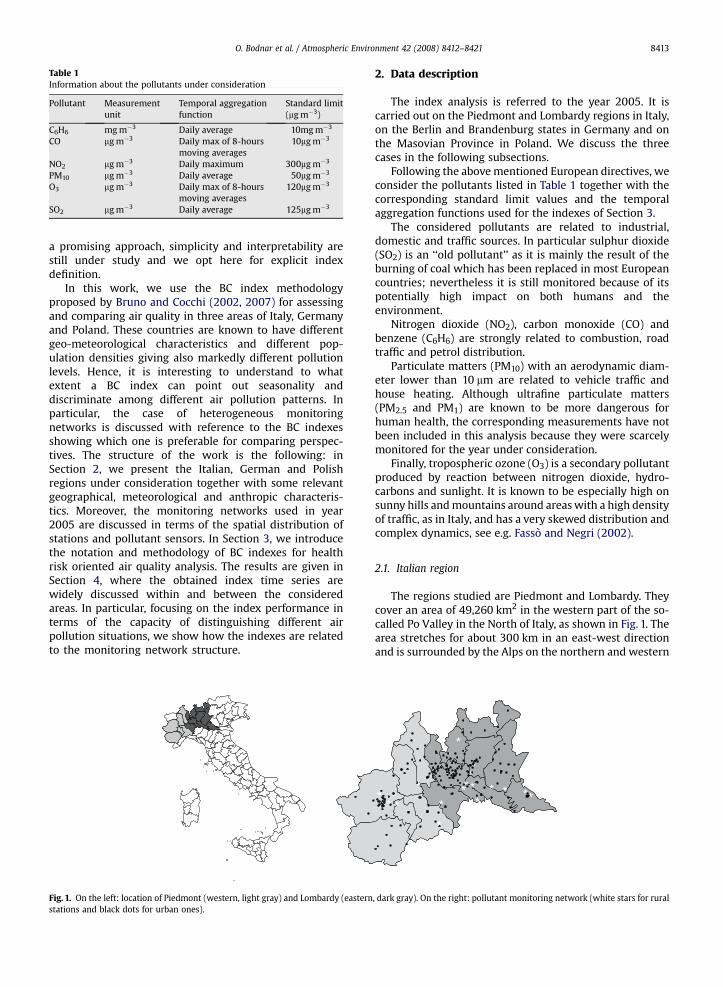
Table 1Information about the pollutants under consideration

Pollutant Measurementunit

Temporal aggregationfunction

Standard limit(mg m�3)

C6H6 mg m�3 Daily average 10mg m�3

CO mg m�3 Daily max of 8-hoursmoving averages

10mg m�3

NO2 mg m�3 Daily maximum 300mg m�3

PM10 mg m�3 Daily average 50mg m�3

O3 mg m�3 Daily max of 8-hoursmoving averages

120mg m�3

SO2 mg m�3 Daily average 125mg m�3

O. Bodnar et al. / Atmospheric Environment 42 (2008) 8412–8421 8413

a promising approach, simplicity and interpretability arestill under study and we opt here for explicit indexdefinition.

In this work, we use the BC index methodologyproposed by Bruno and Cocchi (2002, 2007) for assessingand comparing air quality in three areas of Italy, Germanyand Poland. These countries are known to have differentgeo-meteorological characteristics and different pop-ulation densities giving also markedly different pollutionlevels. Hence, it is interesting to understand to whatextent a BC index can point out seasonality anddiscriminate among different air pollution patterns. Inparticular, the case of heterogeneous monitoringnetworks is discussed with reference to the BC indexesshowing which one is preferable for comparing perspec-tives. The structure of the work is the following: inSection 2, we present the Italian, German and Polishregions under consideration together with some relevantgeographical, meteorological and anthropic characteris-tics. Moreover, the monitoring networks used in year2005 are discussed in terms of the spatial distribution ofstations and pollutant sensors. In Section 3, we introducethe notation and methodology of BC indexes for healthrisk oriented air quality analysis. The results are given inSection 4, where the obtained index time series arewidely discussed within and between the consideredareas. In particular, focusing on the index performance interms of the capacity of distinguishing different airpollution situations, we show how the indexes are relatedto the monitoring network structure.

Fig. 1. On the left: location of Piedmont (western, light gray) and Lombardy (easternstations and black dots for urban ones).

2. Data description

The index analysis is referred to the year 2005. It iscarried out on the Piedmont and Lombardy regions in Italy,on the Berlin and Brandenburg states in Germany and onthe Masovian Province in Poland. We discuss the threecases in the following subsections.

Following the above mentioned European directives, weconsider the pollutants listed in Table 1 together with thecorresponding standard limit values and the temporalaggregation functions used for the indexes of Section 3.

The considered pollutants are related to industrial,domestic and traffic sources. In particular sulphur dioxide(SO2) is an ‘‘old pollutant’’ as it is mainly the result of theburning of coal which has been replaced in most Europeancountries; nevertheless it is still monitored because of itspotentially high impact on both humans and theenvironment.

Nitrogen dioxide (NO2), carbon monoxide (CO) andbenzene (C6H6) are strongly related to combustion, roadtraffic and petrol distribution.

Particulate matters (PM10) with an aerodynamic diam-eter lower than 10 mm are related to vehicle traffic andhouse heating. Although ultrafine particulate matters(PM2.5 and PM1) are known to be more dangerous forhuman health, the corresponding measurements have notbeen included in this analysis because they were scarcelymonitored for the year under consideration.

Finally, tropospheric ozone (O3) is a secondary pollutantproduced by reaction between nitrogen dioxide, hydro-carbons and sunlight. It is known to be especially high onsunny hills and mountains around areas with a high densityof traffic, as in Italy, and has a very skewed distribution andcomplex dynamics, see e.g. Fasso and Negri (2002).

2.1. Italian region

The regions studied are Piedmont and Lombardy. Theycover an area of 49,260 km2 in the western part of the so-called Po Valley in the North of Italy, as shown in Fig. 1. Thearea stretches for about 300 km in an east-west directionand is surrounded by the Alps on the northern and western

***

** * **

**

*

*

****

**

, dark gray). On the right: pollutant monitoring network (white stars for rural

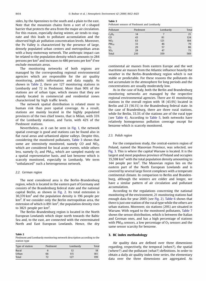
Table 3Pollutant sensors of Piedmont and Lombardy

Pollutant Piedmont Lombardy Total

C6H6 14 7 21CO 43 81 124NO2 63 121 184PM10 33 46 79O3 29 57 86SO2 28 47 75Total 210 359 569

O. Bodnar et al. / Atmospheric Environment 42 (2008) 8412–84218414

sides, by the Apennines to the south and a plain to the east.Note that the mountain chains form a sort of c-shapedbarrier that protects the area from the major air circulation.For this reason, especially during winter, air tends to stag-nate and this leads to pollutant accumulation and theobserved high air pollution concentration levels. Moreover,the Po Valley is characterized by the presence of large,densely populated urban centers and metropolitan areaswith a busy motorway network. The anthropic impact canbe related to the population density which amounts to 284persons per km2 and increases to 486 persons per km2 if weexclude mountain areas.

The monitoring networks of both regions aremanaged by the corresponding regional environmentalagencies which are responsible for the air qualitymonitoring, public information and data supply. Asshown in Table 2, there are 127 monitoring stations inLombardy and 72 in Piedmont. More than 90% of thestations are of urban type, which means that they aremainly located in commercial and residential zonescharacterized by high traffic levels.

The network spatial distribution is related more tohuman risk than pure spatial coverage. As a result,stations are mainly located in the highly populatedprovinces of the two chief towns, that is Milan, with 33%of the Lombardy stations, and Turin, with 42% of thePiedmont stations.

Nevertheless, as it can be seen in Fig. 1, the networkspatial coverage is good and stations can be found also inflat rural areas and urbanized alpine valleys. Despite this,considering the monitored pollutants, Table 3 shows thatsome are intensively monitored, namely CO and NO2,which are considered for local acute events, while othersless, namely O3 and PM10, which are sampled mainly ona spatial representative basis, and last benzene which isscarcely monitored, especially in Lombardy. We term‘‘unbalanced’’ such a heterogeneous network.

2.2. German region

The next considered area is the Berlin–Brandenburgregion, which is located in the eastern part of Germany andconsists of the Brandenburg federal state and the nationalcapital Berlin, as shown in Fig. 2. Its total extension is30,370 km2 and the population density is 196 people perkm2. If we consider only the Berlin metropolitan area, theextension of which is 891 km2, the population density risesto 3821 people per km2.

The Berlin–Brandenburg region is located in the NorthEuropean Lowlands which slope north towards the BalticSea and, to the east, are connected with the exterminatedNorth and East European Lowlands. Hence, the dry

Table 2Piedmont and Lombardy monitoring network description according to thestation type

Type of station Piedmont Lombardy Total

Rural 6 12 18Urban 66 115 181Total 72 127 199

continental air masses from eastern Europe and the wetmaritime air masses from the Atlantic influence heavily theweather in the Berlin–Brandenburg region which is notstable or predictable. For these reasons the pollutants donot accumulate in the atmosphere for long periods and theconcentrations are usually moderately low.

As in the case of Italy, both the Berlin and Brandenburgmonitoring networks are managed by the respectiveregional environmental agencies. There are 41 monitoringstations in the overall region with 18 (43.9%) located inBerlin and 23 (56.1%) in the Brandenburg federal state. Inthe case of Brandenburg, there are three rural stations,while for Berlin, 33.3% of the stations are of the rural type(see Table 4). According to Table 5, both networks haverelatively homogeneous pollution coverage except forbenzene which is scarcely monitored.

2.3. Polish region

For the comparison study, the central-eastern region ofPoland, named the Masovian Province, was selected, seeFig. 3. This is where the capital Warsaw is located. It is thelargest and most populous province of Poland and occupies35,598 km2 with the total population density amounting to144 people per km2. The Masovian region lies on theeastern part of the North European Lowlands and iscovered by several large forest complexes with a temperatecontinental climate. In comparison to Berlin and Branden-burg, although the winters are colder and longer, wehave a similar pattern of air circulation and pollutantaccumulation.

According to the regulations concerning the nationalmonitoring of the environment, 21 monitoring stations hadenough data for year 2005 (see Fig. 2). Table 6 shows thatthere is just one station of the rural type while the others areurban stations. Moreover, six stations (29%) are situated inWarsaw. With regard to the monitored pollutants, Table 7shows the sensor distribution, which is between the Italianand German ones, and has a high percentage of stationswith PM10 sensors, a low percentage of O3 sensors and thesame sensor scarcity for benzene.

3. BC index methodology

Air quality data are defined over three dimensionsregarding, respectively, the temporal (when?), the spatial(where?) and the pollutant (what?) definitions. In order toobtain a daily air quality index time series, the elementarydata over the three dimensions are aggregated. As

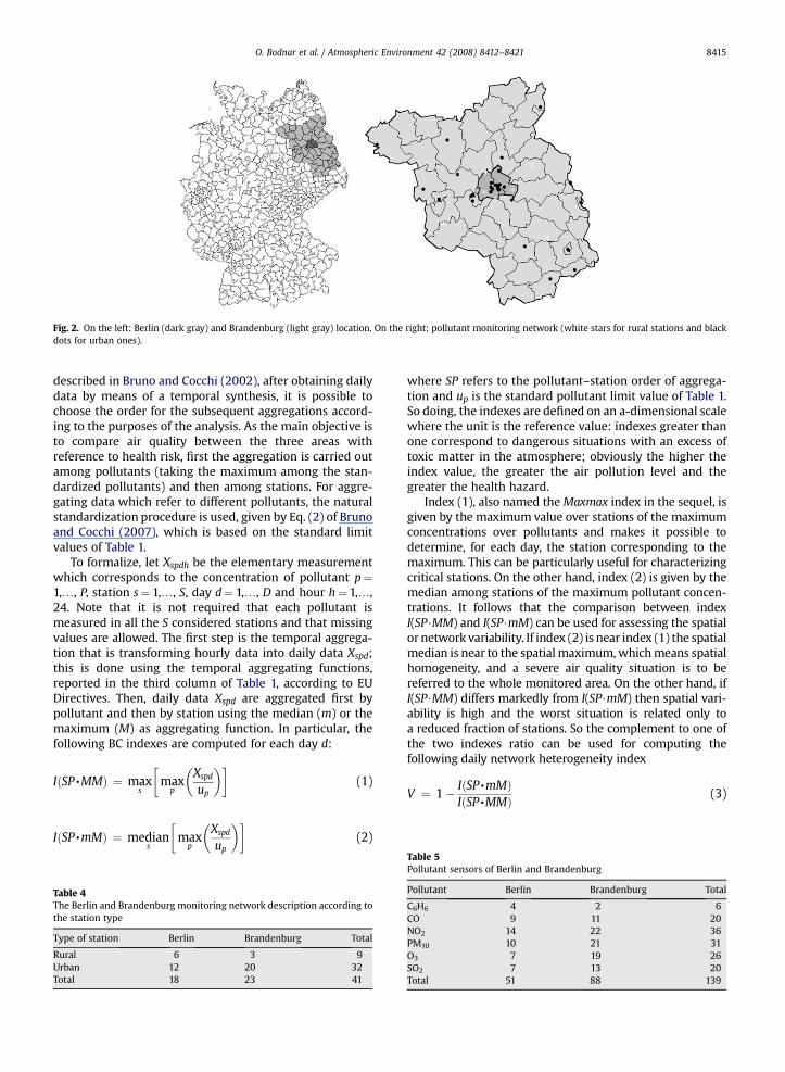
Fig. 2. On the left: Berlin (dark gray) and Brandenburg (light gray) location. On the right: pollutant monitoring network (white stars for rural stations and blackdots for urban ones).

Table 5

O. Bodnar et al. / Atmospheric Environment 42 (2008) 8412–8421 8415

described in Bruno and Cocchi (2002), after obtaining dailydata by means of a temporal synthesis, it is possible tochoose the order for the subsequent aggregations accord-ing to the purposes of the analysis. As the main objective isto compare air quality between the three areas withreference to health risk, first the aggregation is carried outamong pollutants (taking the maximum among the stan-dardized pollutants) and then among stations. For aggre-gating data which refer to different pollutants, the naturalstandardization procedure is used, given by Eq. (2) of Brunoand Cocchi (2007), which is based on the standard limitvalues of Table 1.

To formalize, let Xspdh be the elementary measurementwhich corresponds to the concentration of pollutant p¼1,., P, station s¼ 1,., S, day d¼ 1,., D and hour h¼ 1,.,24. Note that it is not required that each pollutant ismeasured in all the S considered stations and that missingvalues are allowed. The first step is the temporal aggrega-tion that is transforming hourly data into daily data Xspd;this is done using the temporal aggregating functions,reported in the third column of Table 1, according to EUDirectives. Then, daily data Xspd are aggregated first bypollutant and then by station using the median (m) or themaximum (M) as aggregating function. In particular, thefollowing BC indexes are computed for each day d:

IðSP,MMÞ ¼ maxs

�max

p

�Xspd

up

��(1)

IðSP,mMÞ ¼ medians

�max

p

�Xspd

up

��(2)

Table 4The Berlin and Brandenburg monitoring network description according tothe station type

Type of station Berlin Brandenburg Total

Rural 6 3 9Urban 12 20 32Total 18 23 41

where SP refers to the pollutant–station order of aggrega-tion and up is the standard pollutant limit value of Table 1.So doing, the indexes are defined on an a-dimensional scalewhere the unit is the reference value: indexes greater thanone correspond to dangerous situations with an excess oftoxic matter in the atmosphere; obviously the higher theindex value, the greater the air pollution level and thegreater the health hazard.

Index (1), also named the Maxmax index in the sequel, isgiven by the maximum value over stations of the maximumconcentrations over pollutants and makes it possible todetermine, for each day, the station corresponding to themaximum. This can be particularly useful for characterizingcritical stations. On the other hand, index (2) is given by themedian among stations of the maximum pollutant concen-trations. It follows that the comparison between indexI(SP$MM) and I(SP$mM) can be used for assessing the spatialor network variability. If index (2) is near index (1) the spatialmedian is near to the spatial maximum, which means spatialhomogeneity, and a severe air quality situation is to bereferred to the whole monitored area. On the other hand, ifI(SP$MM) differs markedly from I(SP$mM) then spatial vari-ability is high and the worst situation is related only toa reduced fraction of stations. So the complement to one ofthe two indexes ratio can be used for computing thefollowing daily network heterogeneity index

V ¼ 1� IðSP,mMÞIðSP,MMÞ (3)

Pollutant sensors of Berlin and Brandenburg

Pollutant Berlin Brandenburg Total

C6H6 4 2 6CO 9 11 20NO2 14 22 36PM10 10 21 31O3 7 19 26SO2 7 13 20Total 51 88 139

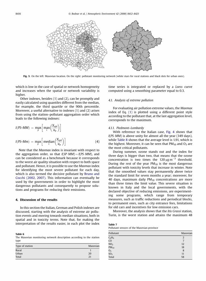
Fig. 3. On the left: Masovian location. On the right: pollutant monitoring network (white stars for rural stations and black dots for urban ones).

O. Bodnar et al. / Atmospheric Environment 42 (2008) 8412–84218416

which is low in the case of spatial or network homogeneityand increases when the spatial or network variability ishigher.

Other indexes, besides (1) and (2), can be promptly andeasily calculated using quantiles different from the median,for example, the third quartile or the 90th percentile.Moreover, a useful alternative to indexes (1) and (2) arisesfrom using the station–pollutant aggregation order whichleads to the following indexes:

IðPS,MMÞ ¼ maxp

�max

s

�Xspd

up

��

IðPS,MmÞ ¼ maxp

�median

s

�Xspd

up

��(4)

Note that the Maxmax index is invariant with respect tothe aggregation order, so that I(SP$MM)¼ I(PS$MM), andcan be considered as a benchmark because it correspondsto the worst air quality situation with respect to both spaceand pollutant. Hence, it is possible to use the Maxmax indexfor identifying the most severe pollutant for each day,which is also termed the decisive pollutant by Bruno andCocchi (2002, 2007). This information can eventually beused by the governments in order to highlight the mostdangerous pollutants and consequently to propose solu-tions and programs for reducing their emissions.

Table 7

4. Discussion of the results

In this section the Italian, German and Polish indexes arediscussed, starting with the analysis of extreme air pollu-tion events and moving towards median situations, both inspatial and in toxicity terms. Note that, for making theinterpretation of the results easier, in each plot the index

Table 6The Masovian monitoring network description according to the stationtype

Type of station Masovian

Rural 1Urban 20Total 21

time series is integrated or replaced by a Loess curvecomputed using a smoothing parameter equal to 0.3.

4.1. Analysis of extreme pollution

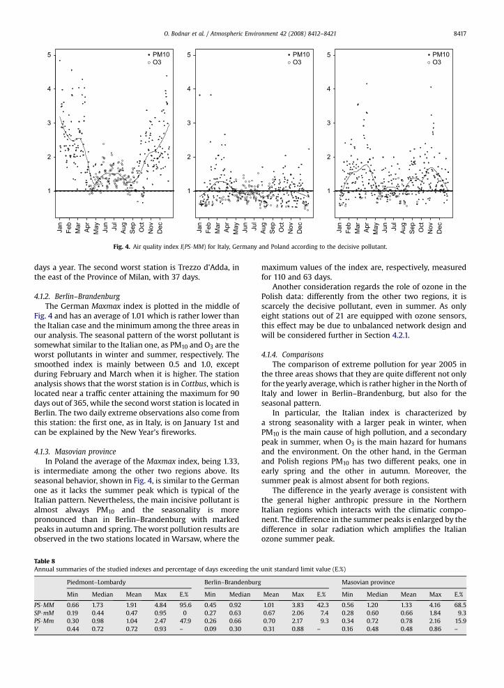
For evaluating air pollution extreme values, the Maxmaxindex of Eq. (1) is plotted using a different point styleaccording to the pollutant that, at the last aggregation level,corresponds to the maximum.

4.1.1. Piedmont–LombardyWith reference to the Italian case, Fig. 4 shows that

I(PS$MM) is above unity for almost all the year (349 days),while Table 8 shows that the average level is 1.91, which isthe highest. Moreover, it can be seen that PM10 and O3 arethe most critical pollutants.

During summer, ozone stands out and the index forthree days is bigger than two, that means that the ozoneconcentration is two times the 120 mg m�3 threshold.During the rest of the year PM10 is the most dangerouspollutant with toxicity levels that increase in winter. Notethat the smoothed values stay permanently above twicethe standard limit for seven months a year; moreover, for40 days, maximum daily PM10 concentrations are morethan three times the limit value. This severe situation isknown in Italy and the local governments, with thedeclared objective of reducing emissions, are experiment-ing some programs, which range from temporarymeasures, such as traffic reductions and periodical blocks,to permanent ones, such as city entrance fees, limitationsfor old cars and incentives for low emission cars.

Moreover, the analysis shows that the Itis Grassi station,Turin, is the worst station and attains the maximum 48

Pollutant sensors of the Masovian province

Pollutant Masovian

C6H6 2CO 7NO2 12PM10 18O3 8SO2 11Total 58

1

2

3

4

5 PM10O3

Jan

Feb

Mar Apr

May JunJul

Aug

SepOct

NovDec

PM10O3

Jan

Feb

Mar Apr

May JunJul

Aug

SepOct

NovDec

PM10O3

Jan

Feb

Mar Apr

May JunJul

Aug

SepOct

NovDec

1

2

3

4

5

1

2

3

4

5

Fig. 4. Air quality index I(PS$MM) for Italy, Germany and Poland according to the decisive pollutant.

O. Bodnar et al. / Atmospheric Environment 42 (2008) 8412–8421 8417

days a year. The second worst station is Trezzo d’Adda, inthe east of the Province of Milan, with 37 days.

4.1.2. Berlin–BrandenburgThe German Maxmax index is plotted in the middle of

Fig. 4 and has an average of 1.01 which is rather lower thanthe Italian case and the minimum among the three areas inour analysis. The seasonal pattern of the worst pollutant issomewhat similar to the Italian one, as PM10 and O3 are theworst pollutants in winter and summer, respectively. Thesmoothed index is mainly between 0.5 and 1.0, exceptduring February and March when it is higher. The stationanalysis shows that the worst station is in Cottbus, which islocated near a traffic center attaining the maximum for 90days out of 365, while the second worst station is located inBerlin. The two daily extreme observations also come fromthis station: the first one, as in Italy, is on January 1st andcan be explained by the New Year’s fireworks.

4.1.3. Masovian provinceIn Poland the average of the Maxmax index, being 1.33,

is intermediate among the other two regions above. Itsseasonal behavior, shown in Fig. 4, is similar to the Germanone as it lacks the summer peak which is typical of theItalian pattern. Nevertheless, the main incisive pollutant isalmost always PM10 and the seasonality is morepronounced than in Berlin–Brandenburg with markedpeaks in autumn and spring. The worst pollution results areobserved in the two stations located in Warsaw, where the

Table 8Annual summaries of the studied indexes and percentage of days exceeding the

Piedmont–Lombardy Berlin–Brandenburg

Min Median Mean Max E.% Min Median

PS$MM 0.66 1.73 1.91 4.84 95.6 0.45 0.92SP$mM 0.19 0.44 0.47 0.95 0 0.27 0.63PS$Mm 0.30 0.98 1.04 2.47 47.9 0.26 0.66V 0.44 0.72 0.72 0.93 – 0.09 0.30

maximum values of the index are, respectively, measuredfor 110 and 63 days.

Another consideration regards the role of ozone in thePolish data: differently from the other two regions, it isscarcely the decisive pollutant, even in summer. As onlyeight stations out of 21 are equipped with ozone sensors,this effect may be due to unbalanced network design andwill be considered further in Section 4.2.1.

4.1.4. ComparisonsThe comparison of extreme pollution for year 2005 in

the three areas shows that they are quite different not onlyfor the yearly average, which is rather higher in the North ofItaly and lower in Berlin–Brandenburg, but also for theseasonal pattern.

In particular, the Italian index is characterized bya strong seasonality with a larger peak in winter, whenPM10 is the main cause of high pollution, and a secondarypeak in summer, when O3 is the main hazard for humansand the environment. On the other hand, in the Germanand Polish regions PM10 has two different peaks, one inearly spring and the other in autumn. Moreover, thesummer peak is almost absent for both regions.

The difference in the yearly average is consistent withthe general higher anthropic pressure in the NorthernItalian regions which interacts with the climatic compo-nent. The difference in the summer peaks is enlarged by thedifference in solar radiation which amplifies the Italianozone summer peak.

unit standard limit value (E.%)

Masovian province

Mean Max E.% Min Median Mean Max E.%

1.01 3.83 42.3 0.56 1.20 1.33 4.16 68.50.67 2.06 7.4 0.28 0.60 0.66 1.84 9.30.70 2.17 9.3 0.34 0.72 0.78 2.16 15.90.31 0.88 – 0.16 0.48 0.48 0.86 –

1 2 3 4 5

0.0

0.2

0.4

0.6

0.8

1.0

ItalyGermanyPoland

0.0 0.5 1.0 1.5

0.0ItalyGermanyPoland

0.0 0.5 1.0 1.5 2.0

0.0ItalyGermanyPoland

0.2

0.4

0.6

0.8

1.0

0.2

0.4

0.6

0.8

1.0

Fig. 5. Empirical distribution function for I(PS$MM), I(SP$mM) and I(PS$Mm).

O. Bodnar et al. / Atmospheric Environment 42 (2008) 8412–84218418

Moreover, the one-winter-peak pattern in Italy isrelated to the long periods of weather stability which arecommon in December and January and is different from theNorth European pattern of Berlin where autumn and springare more stable and dryer seasons, favoring a moderatepollution accumulation.

In terms of pollution severity, 95.6% of the year 2005 (349days) the Piedmont–Lombardy index I(PS$MM) exceededthe unit standard limit value, whilst this percentage for theGerman and Polish regions was 42% (155 days) and 68% (250days). It follows that in Northern Italy extreme toxic eventsare more likely to occur, while in Berlin–Brandenburgpollution levels are less severe. The pollution in the Maso-vian region is intermediate but there is an additionaluncertainty related to a sparser monitoring network. Theseconsiderations are also confirmed by the empirical distri-bution functions plotted in the left part of Fig. 5. It can be

0.5

1.0

1.5

2.0

0.5

1.0

1.5

2.0

Jan

Feb

Mar Apr

May JunJul

Aug

SepOct

NovDec Jan

Feb

Mar Apr

May JunJul

Fig. 6. Air quality index I(SP$mM) fo

seen that the Italian curve is dominated by the German andPolish ones; it is the slowest curve in reaching the upperlimit one and this is related to a greater index variability.

4.2. Analysis of median pollution

In this section, the use of the two aggregating strategiesfor the median indexes of Eq. (2) and (4) are compared. Thefirst one can be recommended for balanced networks, andits capability of understanding spatial variability is illus-trated. Vice versa, the second one results more stable orrobust with respect to unbalanced multisensor networkdesigns.

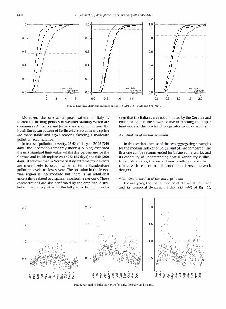
4.2.1. Spatial median of the worst pollutantFor analyzing the spatial median of the worst pollutant

and its temporal dynamics, index I(SP$mM) of Eq. (2),

Jan

Feb

Mar Apr

May JunJul

Aug

SepOct

NovDec

Aug

SepOct

NovDec

0.5

1.0

1.5

2.0

r Italy, Germany and Poland.

0.0

0.2

0.4

0.6

0.8

1.0Jan

Feb

Mar Apr

May JunJul

Aug

SepOct

NovDec Jan

Feb

Mar Apr

May JunJul

Aug

SepOct

NovDec Jan

Feb

Mar Apr

May JunJul

Aug

SepOct

NovDec

0.0

0.2

0.4

0.6

0.8

1.0

0.0

0.2

0.4

0.6

0.8

1.0

Fig. 7. Network heterogeneity index V for Italy, Germany and Poland.

O. Bodnar et al. / Atmospheric Environment 42 (2008) 8412–8421 8419

together with the network heterogeneity index V given byEq. (3), is used.

Fig. 6 shows that for the Italian case it results that theindex is always lower than one, with an average given inTable 8, which is the lowest of the three areas and contra-dicts the conclusions in the previous section. Such a biasfollows from the unbalanced design of the Italian networkwhich has only 79 PM10 sensors out of 199 stations. Thisnetwork design bias is also suggested by the high values ofthe spatial, or network, variability index V, plotted in Fig. 7,whose mean is the highest for the Italian data.

As shown by Fig. 7 and Table 8, the German and Polishdata have a lower spatial or network heterogeneity index V,especially for Berlin–Brandenburg. The behavior of theindex I(SP$mM) is closer to the Maxmax indexof the previoussection. Here the average of I(SP$mM) is slightly lower forthe Polish data than the Berlin–Brandenburg data. Once

0.5

1.0

1.5

2.0

2.5

Jan

Feb

Mar Apr

May JunJul

Aug

SepOct

NovDec Jan

Feb

Mar Apr

May JunJul

0.5

1.0

1.5

2.0

2.5

Fig. 8. Air quality index I(PS$Mm) fo

again, the result is disregarded as the network heteroge-neity index V in Masovian region is rather higher than theGerman one, suggesting that the Masovian network is moreunbalanced than the German one for the I(SP$mM) index.

To reinforce the conclusion that the high values of ItalianV are related to network design rather than genuine spatialvariability, the same analysis was carried out for somerepresentative provinces out of the 19 single provinces ofPiedmont–Lombardy. The detailed figures are not reportedhere for the sake of brevity; nevertheless, the results areessentially the same as the aggregate level. In particular,there are high values for V even at the provincial level con-firming the idea of network heterogeneity by design.

4.2.2. Worst median pollutantThe second approach to median pollution is based on

the index I(PS$Mm) of Eq. (4). As it takes the median among

Aug

SepOct

NovDec Jan

Feb

Mar Apr

May JunJul

Aug

SepOct

NovDec

0.5

1.0

1.5

2.0

2.5

r Italy, Germany and Poland.

0.0

0.5

1.0

1.5

2.0

2.5

3.0

3.5 I(PS.MM)=I(SP.MM)I(PS.mM)I(PS.Mm)I(SP.mM)I(SP.Mm)

Jan

Feb

Mar Apr

May JunJul

Aug

SepOctNovDec

I(PS.MM)=I(SP.MM)I(PS.mM)I(PS.Mm)I(SP.mM)I(SP.Mm)

Jan

Feb

Mar Apr

May JunJul

Aug

SepOctNovDec

I(PS.MM)=I(SP.MM)I(PS.mM)I(PS.Mm)I(SP.mM)I(SP.Mm)

Jan

Feb

Mar Apr

May JunJul

Aug

SepOctNovDec

0.0

0.5

1.0

1.5

2.0

2.5

3.0

3.5

0.0

0.5

1.0

1.5

2.0

2.5

3.0

3.5

Fig. 9. Index comparison for Italy, Germany and Poland.

O. Bodnar et al. / Atmospheric Environment 42 (2008) 8412–84218420

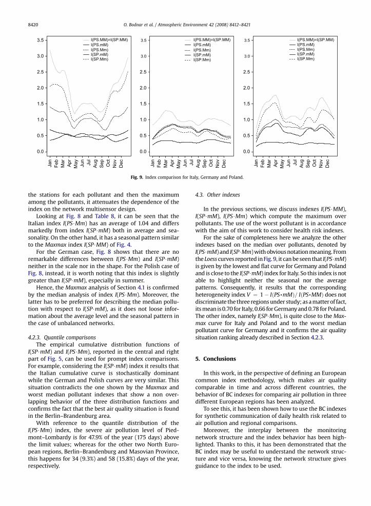
the stations for each pollutant and then the maximumamong the pollutants, it attenuates the dependence of theindex on the network multisensor design.

Looking at Fig. 8 and Table 8, it can be seen that theItalian index I(PS$Mm) has an average of 1.04 and differsmarkedly from index I(SP$mM) both in average and sea-sonality. On the other hand, it has a seasonal pattern similarto the Maxmax index I(SP$MM) of Fig. 4.

For the German case, Fig. 8 shows that there are noremarkable differences between I(PS$Mm) and I(SP$mM)neither in the scale nor in the shape. For the Polish case ofFig. 8, instead, it is worth noting that this index is slightlygreater than I(SP$mM), especially in summer.

Hence, the Maxmax analysis of Section 4.1 is confirmedby the median analysis of index I(PS$Mm). Moreover, thelatter has to be preferred for describing the median pollu-tion with respect to I(SP$mM), as it does not loose infor-mation about the average level and the seasonal pattern inthe case of unbalanced networks.

4.2.3. Quantile comparisonsThe empirical cumulative distribution functions of

I(SP$mM) and I(PS$Mm), reported in the central and rightpart of Fig. 5, can be used for prompt index comparisons.For example, considering the I(SP$mM) index it results thatthe Italian cumulative curve is stochastically dominantwhile the German and Polish curves are very similar. Thissituation contradicts the one shown by the Maxmax andworst median pollutant indexes that show a non over-lapping behavior of the three distribution functions andconfirms the fact that the best air quality situation is foundin the Berlin–Brandenburg area.

With reference to the quantile distribution of theI(PS$Mm) index, the severe air pollution level of Pied-mont–Lombardy is for 47.9% of the year (175 days) abovethe limit values; whereas for the other two North Euro-pean regions, Berlin–Brandenburg and Masovian Province,this happens for 34 (9.3%) and 58 (15.8%) days of the year,respectively.

4.3. Other indexes

In the previous sections, we discuss indexes I(PS$MM),I(SP$mM), I(PS$Mm) which compute the maximum overpollutants. The use of the worst pollutant is in accordancewith the aim of this work to consider health risk indexes.

For the sake of completeness here we analyze the otherindexes based on the median over pollutants, denoted byI(PS$mM) and I(SP$Mm) with obvious notation meaning. Fromthe Loess curves reported in Fig. 9, it can be seen that I(PS$mM)is given by the lowest and flat curve for Germany and Polandand is close to the I(SP$mM) index for Italy. So this index is notable to highlight neither the seasonal nor the averagepatterns. Consequently, it results that the correspondingheterogeneity index V ¼ 1� IðPS,mMÞ= IðPS,MMÞ does notdiscriminate the three regions under study; as a matter of fact,its mean is 0.70 for Italy, 0.66 for Germany and 0.78 for Poland.The other index, namely I(SP$Mm), is quite close to the Max-max curve for Italy and Poland and to the worst medianpollutant curve for Germany and it confirms the air qualitysituation ranking already described in Section 4.2.3.

5. Conclusions

In this work, in the perspective of defining an Europeancommon index methodology, which makes air qualitycomparable in time and across different countries, thebehavior of BC indexes for comparing air pollution in threedifferent European regions has been analyzed.

To see this, it has been shown how to use the BC indexesfor synthetic communication of daily health risk related toair pollution and regional comparisons.

Moreover, the interplay between the monitoringnetwork structure and the index behavior has been high-lighted. Thanks to this, it has been demonstrated that theBC index may be useful to understand the network struc-ture and vice versa, knowing the network structure givesguidance to the index to be used.

O. Bodnar et al. / Atmospheric Environment 42 (2008) 8412–8421 8421

In particular, it turns out that the BC index based on thespatial median of the maximum among pollutants of eachstation, denoted by I(SP$mM), may be used for describingand comparing the mean pollution if the network isbalanced. This index may be coupled with a spatial networkheterogeneity index for assessing the variability betweenstations and the balanced network hypothesis.

Moreover, it has been shown that two indexes, namelythe Maxmax index and the worst median pollutant index,which is denoted by I(PS$Mm), are more robust withrespect to network design and can be used to describe andcompare different regions. In particular, they highlightvarious properties of daily pollution, such as the particularseasonality behavior of Northern Italy, which is character-ized by different pollutants in different seasons and winterand summer peaks.

Acknowledgments

The authors would like to thank the Umweltbundesamt(Fachgebiet II 5.2, Immissionssituation), the LandesumweltamtBrandenburg (Abt. Immissionsschutz), the Berliner LuftguteMessnetz (BLUME) and the Chief Inspectorate of Environ-mental Protection (Department of Monitoring, Assessment andOutlooks, Warsaw) for the help and given support.

The work of M. Cameletti and A. Fasso was partiallysupported by the PRIN project n.2006131039 and theRegione Piemonte CIPE project 2004.

The authors wish also to thank two anonymousreviewers for their valuable comments and suggestions.

References

Bellini, P., Baccini, M., Biggeri, A., Terracini, B., 2007. The meta-analysis ofthe Italian studies on short-term effects of air pollution (MISA): oldand new issues on the interpretation of the statistical evidences.Environmetrics 18, 219–229.

Bruno, F., Cocchi, D., 2002. A unified strategy for building simple airquality indexes. Environmetrics 13, 243–261.

Bruno, F., Cocchi, D., 2007. Recovering information from synthetic airquality indexes. Environmetrics 18, 345–359.

Chiu, G., Guttorp, P., Westveld, A. A latent health factor index via gener-alized linear mixed models, with application to ecological healthassessment, submitted for publication.

Englert, N., 2004. Fine particles and human health – a review of epide-miological studies. Toxicology Letters 149, 235–242.

European Environment Agency, 2007. How can I protect my health?Available at: http://www.eea.europa.eu/maps/ozone/whatcanIdo.

Fasso, A., Cameletti, M., Nicolis, O., 2007. Air quality monitoring usingheterogeneous networks. Environmetrics 18, 245–264.

Fasso, A., Negri, I., 2002. Nonlinear statistical modelling of high frequencyground ozone data. Environmetrics 13, 225–241.

Lagona, F., 2005. Air quality indices via non homogeneous hidden markovmodels. Contributed Papers. In: Proceedings of the ItalianStatistical SocietyConference on Statistics and Environment. CLEUP, Padova, pp. 91–94.

Pope, C., 2000. Review: epidemiological basis for particulate air pollutionhealth standards. Aerosol Science and Technology 32, 4–14.

Saisana, M., Saltelli, A., Tarantola, S., 2005. Uncertainty and sensitivityanalysis techniques as tools for the quality assessment of compositeindicators. Journal of the Royal Statistical Society A 168, 307–323.

U.S. EPA, 2003. Guideline for the Reporting of Daily Air Quality – Air QualityIndex. Availableat: http://airnow.gov/index.cfm?action¼static.publications.