arX

iv:0

912.

2336

v1 [

q-bi

o.N

C]

11

Dec

200

9

A comparative study of different integrate & fire neurons: spontaneous activity,

dynamical response, and stimulus-induced correlation

Rafael D. Vilela1, 2 and Benjamin Lindner1

1 Max-Planck-Institut fur Physik Komplexer Systeme, Nothnitzer Str. 38 01187 Dresden, Germany2Centro de Matematica, Computacao e Cognicao,

Universidade Federal do ABC, 09210-170, Santo Andre, SP, Brazil

(Dated: December 11, 2009)

Stochastic integrate & fire (IF) neuron models have found widespread applications in computa-tional neuroscience. Here we present results on the white-noise-driven perfect, leaky, and quadraticIF models, focusing on the spectral statistics (power spectra, cross spectra, and coherence functions)in different dynamical regimes (noise-induced and tonic firing regimes with low or moderate noise).We make the models comparable by tuning parameters such that the mean value and the coefficientof variation of the interspike interval match for all of them. We find that, under these conditions,the power spectrum under white-noise stimulation is often very similar while the response char-acteristics, described by the cross spectrum between a fraction of the input noise and the outputspike train, can differ drastically. We also investigate how the spike trains of two neurons of thesame kind (e.g. two leaky IF neurons) correlate if they share a common noise input. We showthat, depending on the dynamical regime, either two quadratic IF models or two leaky IFs are morestrongly correlated. Our results suggest that, when choosing among simple IF models for networksimulations, the details of the model have a strong effect on correlation and regularity of the output.

I. INTRODUCTION

Neurons communicate information via short-lastingdischarges of the electrical potential across their mem-brane. The excitability mechanism by which these spikesare generated relies on the dynamics of voltage-gated ionchannels in the neural membrane and is well understood[1, 2]. To study the dynamics of large neural networks, adetailed description of the single neuron’s dynamics, al-though in principle possible, is impractical and one mustresort to simpler models of neural spike generation gov-erned by only one or two dynamical variables per neuron[3]. In particular in stochastic versions, that take into ac-count the large variability of neural spiking, these modelscan be also helpful to study basic aspects of signal trans-mission by single neurons.

One class of commonly used simplified models com-prises integrate & fire (IF) neurons with white noise cur-rent. In IF models a spike is generated if the voltagereaches a firing threshold (inducing also a reset of thevoltage); the voltage obeys the one-dimensional dynam-ics

v = f(v) + s(t) + µ +√

2Dξ(t) (1)

where s(t) is a time-dependent stimulus while µ and Dare the mean and the noise intensity of the input current(ξ(t) is white Gaussian noise). Variants of the model dif-fer by the function f(v). A fine-tuned choice of f(v) maypermit a rather accurate prediction of both experimentalsubthreshold voltage fluctuations and spike statistics un-der noisy stimulation in vitro and in vivo (see [4, 5, 6, 7, 8]for some recent convincing examples). Simple choices likea constant, linear, or quadratic function leading to theperfect (PIF), leaky (LIF), or quadratic (QIF) model,respectively, allow for an analytical calculation of one orthe other spike statistics and may be also numericallysimpler to simulate in large-scale networks. Models likeEq. (1) have been used in analytical studies of (i) condi-tions for asynchronous or oscillatory activity in recurrentnetworks [9, 10, 11, 12]; (ii) the transmission of rapid sig-nals [13, 14, 15, 16]; (iii) the variability of spontaneous

activity [17, 18, 19, 20]; (iv) noise-induced resonancesin the spontaneous activity [19, 21], and in the responseto external stimuli [14, 22]; and (v) oscillations in re-current networks induced by spatially correlated stimuli[23, 24, 25], to name but a few.

Most of the phenomena studied depend strongly onthe choice of f(v). As an example, consider the effect ofcoherence resonance, which refers to the existence of anoptimal noise intensity D that maximizes the regularityof the spike train, seen, for instance, as a minimum ofthe coefficient of variation (CV) vs noise intensity: onlythe leaky [19, 21] but not the perfect or quadratic IFmodels [20] show such a minimum. It has, furthermore,been shown that LIF and QIF differ strongly in their re-sponse to fast (high-frequency) periodic signals [15, 16].Despite these discussions, however, a systematic compar-ison among the commonly used IF models is still missing.In this paper, we want to fill this gap.

If one wishes to compare different IF models, the firstquestion is how the input parameters µ and D should bechosen in the respective model. Already the most ba-sic firing statistics of a certain IF model, the firing rate(quantifying the spike train’s intensity) and the interspikeinterval’s coefficient of variation (characterizing the vari-ability of the spiking) depend strongly and in a model-specific way on µ and D [17, 19, 20, 26, 27]. The authorshave recently shown that this basic firing statistics, i.e.rate and CV, determine uniquely the input parametersµ and D for the three most common IF models men-tioned above (perfect, leaky, and quadratic IF neurons).This offers a natural way of unambiguously defining fir-ing regimes for these models. Moreover, setting the firingregime by means of prescribing rate and CV allows for afair comparison of the higher-order statistics of differentIF models. In this way, we can, for example, consider anLIF neuron and a QIF neuron that both show a moder-ate firing rate (e.g. 10Hz) and medium variability (say,a CV of about 0.5) and compare how these two neuronsdiffer in their spontaneous and driven activity. This ap-proach of assuming the same basic firing statistics andcomparing higher-order statistics is complementary to a

2

previous set-up which was entirely based on the firingrate dependence on input current [15].

What is the most important output statistics of noisyIF neurons once the firing rate and CV are fixed? In mostof the above analytical approaches, two single-neuroncharacteristics appear to be essential: (i) the spike trainpower spectrum of spontaneous activity and (ii) the re-sponse to weak stimuli (e.g. to a weak periodic signals(t) = ε cos(ωt)). In a more recent theory of recurrentnetworks [25], the knowledge of a third simple propertyis needed that goes beyond the properties of a single neu-ron: the degree of correlations that can be induced in twouncoupled neurons that share some common noisy stim-ulus. This latter property has attracted attention of itsown and has been recently studied experimentally (see[28] and references therein) and theoretically [25, 29, 30]in particular in the limit of a weak input correlation.

In the present paper, we study the spontaneous powerspectrum, the linear response function (susceptibility),and the two-neuron correlations induced by a commonstimulus for the perfect, leaky, and quadratic IF modelsand a variety of firing regimes. In section II, we introducethe three IF models studied and define the firing regimes.In section III, we present results on spontaneous activ-ity of single neurons. We show that typically IF neuronspresent similar power spectra when they are in the samefiring regime. In section IV, we study the dynamicalresponse of single neurons. We recover characteristic dif-ferences between the susceptibility of the LIF and QIFdiscussed previously (see, e.g. [15]), as well as betweenLIF and PIF [31], and show in addition that the spectralcoherence between spike train and external signal is basi-cally low-pass for all three models. Section V is devotedto the study of two neurons driven in part by commonnoise. In this case, linear response theory leads to a goodapproximation for the cross-spectra between the two out-put spike trains when the common noise makes up onlya small fraction of the total noise. Coherence functionsof the two output spike trains are again low-pass andresemble qualitatively the input-output coherence func-tions discussed before. Finally, we discuss the correlationcoefficient of the spike count for the LIF and QIF modelsfor a weak common noise and show analytically in theappendix that this correlation coefficient is equal to theinput correlation for the PIF model. We summarize ourresults and draw some conclusions in section VI.

II. MODELS AND FIRING REGIMES

A. Integrate-and-fire neuron models

In this paper we consider IF neurons subjected tostochastic voltage-independent input current, i.e., addi-tive white Gaussian noise which can be justified in theso-called diffusion approximation [26, 32, 33]. We willconsider exclusively models driven by white noise, settingthe term s(t) in Eq. (1) to zero; a fraction of the inputnoise will later be regarded as a stimulus or as commonnoise.

For a leaky integrate-and-fire neuron, the current bal-ance equation reads

CmV = −gL(V − VL) + µ +√

2Dξ(t), (2)

if V (t) = Vth then spike at ti = t & V → Vr

where Cm is the capacitance of the cell membrane, gLand VL are leak conductance and leak reversal potential,respectively, and µ and D are the mean and the intensityof the white Gaussian input noise current. The secondline describes the fire-and-reset rule upon reaching thethreshold Vth.

With the simple transformation v = (V − VL)/(Vth −Vr) and the new parameters τm = Cm/gL (membrane

time constant), µ = µ/gL, and D = D/g2L, this reads

τmv = −v + µ +√

2Dξ(t), (3)

if v(t) = vth then spike at ti = t & v → vr

where the threshold and reset are now at vth = 1 andvr = 0. When measuring time in multiples of the mem-brane time constant, i.e. t = t/τm, this model is equiva-

lent to Eq. (1) with a rescaled noise intensity D = D/τm

and with f(v) = −v. Note that µ +√

2Dξ(t) in thisrescaled model has not the physical dimensions of anelectric current anymore and that is why we will referto it here with the more general term ’input’.

If the leak term gL(V − VL) is small compared to themean input current, we may be justified to neglect it. Allprevious transformations can be repeated (including thedivision by the leak conductance gL) and thus we end upwith

τmv = µ +√

2Dξ(t), (4)

if v(t) = vth then spike at ti = t & v → vr

which corresponds after rescaling of time again to Eq. (1)but this time with f(v) ≡ 0. This is the perfect integrate-and-fire (PIF) model with white noise (also known asrandom-walk model of neural firing) [32, 34].

If the noise-free neuron is close to a dynamical bi-furcation, specifically, close to a saddle-node bifurca-tion from quiescence to tonic firing, another form of theintegrate-and-fire neuron contains a quadratic nonlinear-ity [12, 18, 20, 36, 37, 38]

CmV = a(V − V0)2 + µ +

√

2Dξ(t), (5)

if V (t) = ∞ then spike at ti = t & V → −∞In this case one chooses threshold and reset at infinitybecause the slow dynamics in V makes the exact (largebut finite) values of Vr and Vth irrelevant. Note alsothat V in this case can be but has not to be a voltage— in general, it is the variable of the center manifold[38]; correspondingly, the factor Cm on the left-hand-side can be taken as a convention. For infinite reset andthreshold values, this dynamics can be brought into asimplified standard form by choosing a new variable v =a(V − V0)/gL and new parameters µ = aµ/g2

L and D =Da2/g4

L:

τmv = v2 + µ +√

2Dξ(t), (6)

if v(t) = ∞ then spike at ti = t & v → ∞

which corresponds in rescaled time t = t/τm and noise

intensity D = D/τm to Eq. (1) with f(v) = v2. In simu-lations of this standard form of this quadratic integrate-and-fire neuron (QIF), one uses large but finite threshold

3

and reset such that – by further increasing their values –the results (ISI statistics, spike train power spectra, etc.)do not change anymore within the desired accuracy (say,curves do not change in line thickness). For the effectof finite values of reset and threshold values on the ISIstatistics, see [20].

Note that both in the PIF and the QIF the intro-duction of the membrane time scale is arbitrary — wecould equally well compare to PIF and QIF models inwhich τm would be replaced by a multiple or a fractionof this time (changing then also the input parameters, ofcourse). The choice of τm has been made previously forthe PIF [44] and we follow here this convention also forthe QIF.

Our approach of comparing different IF models hereis complementary to others in which the input currentis assumed to be known and the parameters of the spe-cific models (e.g. Eq. (2) and Eq. (5)) are fitted to yielda given ISI statistics. Here we start with the standardmodels Eq. (3), Eq. (4), and Eq. (6) and ask for the in-put parameters that yield a given rate (in units of theinverse membrane time constant) and a given CV. Al-though this may seem to be unusual in an experimentalsituation where one has control over the input current,it appears to be a reasonable approach in vivo where theeffective input current and its noise intensity is set by thesynaptic background and thus unknown.

B. Firing regimes

In order to make different IF models comparable, wemust first specify the correspondence between their pa-rameters. For instance, in a comparison between LIFand QIF, we should first decide which pair (D, µ) for thefirst model corresponds to which pair (D, µ) for the sec-ond. Here we do this by defining different firing regimesin terms of fixed rate and coefficient of variation of thespike trains. In order words, D and µ in different modelsare chosen as to yield a given firing rate

r =1

〈T 〉 (7)

and a given coefficient of variation

R =

√

〈T 2〉 − 〈T 〉2〈T 〉 , (8)

where T is the interspike interval. Throughout this paper〈·〉 denotes averaging over realizations of the stochasticprocess. Note that, since time is measured in units ofthe membrane time constant, all the rates are in unitsof the inverse of this constant. For instance, for a mem-brane time constant of 10ms, a nondimensional rate of 1corresponds to 100Hz.

The pair of parameters (D, µ) for a given model thatyields a certain regime is therefore determined by theintersection between one countour line for the rate andone contour line for the CV. However, it is not clear apriori whether at most one such intersection exists. Thisproblem was recently addressed by us [39]. We showedthat, given fixed rate and CV, there can be at most oneassociated pair (D, µ) for the three IF models studied inthis paper.

0.001 0.01 0.1D (PIF)

0

0.2

0.4

0.6

0.8

1

1.2

(

PIF)

µ

r = 1

r = 0.7

r = 0.4

r = 0.1

R = 0.1 R = 0.3

R = 0.5

R = 0.7

A B C

D E F

G H

I

0.01 0.1D (LIF)

0.7

0.8

0.9

1

1.1

1.2

1.3

1.4

1.5

1.6

1.7

(L

IF)

µ

r = 1

r = 0.7

r = 0.4

r = 0.1

R = 0.1

R = 0.3

R = 0.5

R = 0.7

AB

C

D E

F

G

H

I

1 10 100D (QIF)

0

2

4

6

8

10

(

QIF

)µ

A B

C

D E

FG

H

I

r = 1

r = 0.7

r=0.4

r = 0.1

R =0.1

R =0.3

R =0.5

R =0.7

FIG. 1: Contour lines for rate (black) and CV (gray) inparameter space for the different models. Regimes A-I aredefined by intersections of these contour lines.

Fig. 1 displays some contour lines for the rate and CVfor the three models considered here. There are differentways to determine these contour lines. They can be ob-tained analytically (see [39]). Here we have determinedthem numerically, as explained in section III B. In Fig. 1we also define 9 specific regimes, labeled A-I, which westudy in some detail here. The corresponding values for

4

the rate and CV in these regimes are:

Regime A B C D E F G H I

rate 1 1 1 0.7 0.7 0.7 0.4 0.4 0.1

CV 0.1 0.3 0.5 0.1 0.3 0.5 0.3 0.5 0.7

III. SINGLE NEURONS: SPONTANEOUS

ACTIVITY

A. Measures

The output spike train y can be modelled as a sumof delta peaks at the time instants when the voltage de-scribed by Eq. (1) reaches the threshold value:

y(t) =∑

j

δ(t − tj), (9)

where tj is the instant when the j-th spike occurs.The spontaneous activity of the IF neurons studied

here corresponds to a renewal point process. Each in-terspike interval is an independent random variable. Inprocesses of this type, all the information on the statisticsis contained in the probability density of the ISI.

In this paper, we will quantify the neuron’s correlationstatistics by means of power and cross-spectra. We startby defining the Fourier transform of the zero-averagespike train as:

y(f) =

∫ T

0

dt′e2πift′(y(t′) − 〈y(t′)〉). (10)

The power spectrum of the spike train will be the quan-tity used in this paper to characterize the spontaneousactivity of the IF neurons. It is given by:

Sy(f) = limT→∞

1

T〈yy∗〉, (11)

where T is the realization time window. For renewalpoint processes, the relation between the power spectrumof the spike train and the Fourier transform of the prob-ability density of the ISI, F (f), is given by [40]:

Sy(f) =1

〈T 〉1 − |F (f)|2|1 − F (f)|2 . (12)

We note that analytical expressions for F (f) are known inthe cases of PIF and LIF (equivalently, often the Laplacetransform is stated that yields the Fourier transform fora negative imaginary argument). In this work, we willonly use that for the PIF, which is given by [31, 41]:

F (PIF)(f) = exp

[

(vth − vr)

(

µ

2D−√

µ2

4D2− 2ifπ

D

)]

.

(13)

10-1

100

101

0.01

0.1

1

10

PIFLIFQIF

10-1

100

101

0

0.5

1

1.5

2

10-1

100

101

00.20.40.60.8

11.21.4

10-1

100

101

0.01

0.1

1

10

10-1

100

101

0

0.2

0.4

0.6

0.8

1

1.2

10-1

100

101

0

0.2

0.4

0.6

0.8

1

10-1

100

101

f

0

0.2

0.4

0.6

0.8

10-1

100

101

f

0

0.1

0.2

0.3

0.4

0.5

10-2

10-1

100

f

0

.05

0.1

A B C

D E F

G H I

SS

Sy

yy

FIG. 2: Power spectra of the spike trains for the three modelsin the nine firing regimes defined in Fig. 1.

B. Results

In Fig. 2, we show the power spectra for the three mod-els in regimes A-I. These spectra were obtained analyti-cally via Eqs. (12) and (13) for the PIF and numericallyfor LIF and QIF using the algorithm recently introducedby Richardson [42]. We observe that the power spectraof different models in the same regime are in general verysimilar. In Regimes A and D, which are characterized bylow variability (CV equal to 0.1), the power spectra vir-tually coincide. In the other regimes, the power spectracoincide in the limits of low and large frequencies, and de-viate to some extent in the intermediate-frequency range.

The coincidence of the power spectra for different mod-els in the same regime in the low and large frequency lim-its is not surprising. In fact, for renewal point processesone can show [40] that:

limf→0

Sy(f) = rR2 (14)

and

limf→∞

Sy(f) = r. (15)

Since each regime is defined by fixing the rate and CV, weconclude from Eq. (14) and Eq. (15) that the power spec-tra for different models should indeed coincide in theselimits. In fact, we have used these relations and the abovementioned algorithm for the numerical determination ofthe power spectrum [42] to obtain the contour lines dis-played in Fig. 1.

To quantify the differences between the power spectraof different models, we define the maximal relative differ-ence ∆Sj,k

y between the power spectra of models j and k

5

0

0.05

0.1

0.15

0.2

0.25

0.3

0.35

0.4

(a)

D (LIF)

µ (L

IF)

0.01 0.1

0.9

1

1.1

1.2

1.3

1.4

1.5

1.6

1.7

0

0.05

0.1

0.15

0.2

0.25

0.3

0.35

0.4

(b)

D (QIF)

µ (Q

IF)

1 10 100

0

2

4

6

8

10

0 0.02 0.04 0.06 0.08 0.1 0.12 0.14 0.16 0.18 0.2

(c)

D (QIF)

µ (Q

IF)

1 10 100

0

2

4

6

8

10

FIG. 3: (Color online) Maximal (over all frequencies) relative

difference of power spectra ∆SPIF,LIFy (a), ∆S

PIF,QIFy (b),

and ∆SLIF,QIFy (c). The contour lines for rate and CV are

the same as those depicted in Fig. 1.

over all frequencies as:

∆Sj,ky = maxf

(

|S(j)y − S

(k)y |

(S(j)y + S

(k)y )/2

)

. (16)

In Fig. 3 we plot ∆SPIF,LIFy , ∆S

PIF,QIFy , and

∆SLIF,QIFy . The first observation we make is that the

power spectra of the PIF matches those of the LIF andQIF in the parameter regions where the PIF is a good

model, i.e., for large µ and small D [cf. Fig. 3(a) and(b)]. Second, when comparing the LIF with the QIF(Fig. 3(c)), we conclude that the power spectra of thesemodels are practically coincident if the noise intensity issmall and their relative difference increases with D, dis-playing moderate differences for very large noise inten-sity. There is a nontrivial dependence on µ as well, butthe dependence on D is the dominant one. Remarkably,this rule of thumb whereby the power spectra differencesbetween LIF and QIF increase with the noise intensityis valid for both tonic (µQIF > 0) and noise-induced

(µQIF < 0) firing regimes.

IV. SINGLE NEURONS: DYNAMICAL

RESPONSE

A. Measures

In this section, we are interested in the response ofsingle neurons to a small stimulus. This can be accom-plished in several ways, e.g., by adding a small term withsinusoidal time dependence to Eq. (1). Alternatively, andthis is the procedure adopted here, one can regard a frac-tion of the noise term in Eq. (1) as the external stimulus.This choice will allow for a straightforward connectionbetween the single neuron’s response presented in thissection and two-neuron correlations under common noisediscussed in section V. We thus rewrite Eq. (1) as:

v = f(v) + µ +√

2(1 − c)Dξi(t) +√

2cDξc(t), (17)

where the noise terms ξi(t) and ξc(t) are white Gaussianand described by:

〈ξi(t)〉 = 〈ξc(t)〉 = 〈ξi(t)ξc(t′)〉 = 0,

〈ξc(t)ξc(t′)〉 = 〈ξi(t)ξi(t

′)〉 = δ(t − t′), (18)

and c (playing the role of a relative signal amplitude) isa number between 0 and 1. When addressing the singleneuron’s response, we read Eq. (17) as describing a cer-

tain neuron subjected to intrinsic noise√

2(1 − c)Dξi(t)and driven by an external (noisy) stimulus:

s(t) =√

2cDξc(t). (19)

To characterize the neuron’s response to the stimulus,we use the cross-spectrum between the spike train y andthe stimulus s(t),

Sys(f) = limT→∞

1

T〈ys∗〉, (20)

and the coherence function with respect to s,

γ2(f) =|Sys|2SySs

, (21)

where Ss = 2cD is the power spectrum of s. One shouldnote that the coherence function is restricted to the in-terval 0 < γ2(f) < 1.

6

B. Single neuron’s response

The cross-spectra (20) can be calculated, for small c,from linear response theory. The idea is to consider theterm

√2cDξc as a small perturbation of the term µ in

the stochastic system

v = f(v) + µ +√

2(1 − c)Dξi(t). (22)

This does not seem feasible at first sight, since ξc hasinfinitely large variance. To show that linear responsecan be applied in this case, we formally consider ξc as aband pass white noise with flat spectrum of height 2cDand cutoff frequency fmax. Its variance is then equal to2cDfmax. This variance can be kept small even in thelimit of fmax → ∞ (white noise) if we impose that cdecreases sufficiently fast, i.e., c ≪ µ/2Dfmax. There-fore ξc can be indeed considered a small perturbation.Linear response theory [43] then leads to the followingapproximation:

〈y(f)〉 = χD,µ(f)√

2cDξc(f), (23)

where χD,µ is the susceptibility of the system which canbe estimated from the cross spectrum between input sig-nal and spike train via the well-known relation

χD,µ =Sys(f)

2cD=

limT→∞〈〈y√

2cDξ∗c 〉ξi〉ξc

2cD, (24)

Closed analytical forms for χ exist for the PIF [44] andLIF [13, 14], and are given respectively by:

χPIF =µ2

vth − vr

1 −√

1 − 8πifD/µ2

4πifD(25)

and

χLIF =r2πif/

√D

2πif − 1

D2πif−1

(

µ−vth√D

)

− eδD2πif−1

(

µ−vr√D

)

D2πif

(

µ−vth√D

)

− eδD2πif

(

µ−vr√D

) ,

(26)where the rate r for the LIF is given by

r(µ, D) =

(

√π

∫ (µ−vr)/√

2D

(µ−vth)/√

2D

dzez2

erfc(z)

)−1

, (27)

the abbreviation δ reads

δ =v2

R − v2T + 2µ(vth − vr)

4D, (28)

and Da(z) is the parabolic cylinder function [45]. Forthe QIF, χ can be obtained numerically from the Fokker-Planck equation [46].

C. Results

Since Eq. (24) is valid for arbitrary c, the cross-spectrum Sys is fully characterized by the susceptibilityχD,µ. We have studied the susceptibility for the threemodels in regimes A-I. The susceptibility for the PIF was

10-1

100

101

102

10-3

10-2

10-1

100

101

PIFLIFQIF

10-1

100

101

10-1

100

101

10-1

100

101

10-3

10-2

10-1

100

101

10-1

100

101

10-1

100

101

10-1

100

101

f

10-3

10-2

10-1

100

101

10-1

100

101

f10

-110

010

1

f

A B C

D E F

G H I

|χ|

|χ|

|χ|

FIG. 4: Gain (|χ|) as a function of frequency for the threemodels in the Regimes A-I.

10-2

10-1

100

101

102

-60-30

0306090

120150180 PIF

LIFQIF

10-2

10-1

100

101

102

10-2

10-1

100

101

102

10-2

10-1

100

101

-60-30

0306090

120150180

10-2

10-1

100

101

10-2

10-1

100

101

10-2

10-1

100

101

f

-60-30

0306090

120150180

10-2

10-1

100

101

f10

-210

-110

010

1

f

A B C

D E F

G H I

Phas

e [o ]

Ph

ase

[o ]

Phas

e [o ]

FIG. 5: Phase lag of the linear response (i.e. − arg(|χ|)) as afunction of frequency for the three models in the Regimes A-I.Due to numerical constraints, the phase of the QIF model isnot shown in the large frequency range, where it asymptotesto 180o.

determined using Eq. (25), while the susceptibility for theLIF and QIF was determined by integrating the Fokker-Planck equation with the algorithm presented in [42, 46].It turns out that this numerical integration is faster thanthe evaluation of Eq. (26) using standard softwares.

In Fig. 4, we show the gain |χ| as a function of the fre-

7

quency for the three models in Regimes A-I. The gain istypically larger for the LIF and is in all regimes at leastone order of magnitude smaller for the QIF. In regimesA and D, where the firing is most regular, the gain dis-plays peaks for the LIF (close to the firing frequency andits higher harmonics) and QIF (only close to its firingfrequency) but not for the PIF. As observed in [15], inthe large frequency limit the gain decays as a power lawwith exponent 0.5 for the LIF and 2 for the QIF. FromEq. (25), we see that the exponent for the PIF is also 0.5.

In Fig. 5, we display the phase φ for the different mod-els. It is defined such that χ = |χ|eiφ. For the PIF, itis in all regimes close to zero for small frequencies andincreases monotonically. Its saturation value, attained inthe limit f → ∞, is φ = 45o. Except for the limits ofsmall and large frequencies, the behavior of the LIF canbe markedly different. In particular in Regimes A andD, the phase oscillates around zero in a certain rangeenclosing the eigenfrequency. It first becomes negative.Close to the eigenfrequency it changes signal, and repeatsthis oscillatory behavior a few times before approachingits asymptotic value of 45o. Finally, the behavior of thephase for the QIF is similar to the one of the LIF, exceptthat the asymptotic value at large frequencies is remark-ably larger - equal to 180o. The asymptotic behaviors forthe LIF and QIF were also discussed in [15].

10-2

10-1

100

101

102

0

0.2

0.4

0.6

0.8

1

γ 2 /c

PIFLIFQIF

10-2

10-1

100

101

102

10-2

10-1

100

101

102

10-2

10-1

100

101

0

0.2

0.4

0.6

0.8

1

γ 2 /c

10-2

10-1

100

101

10-2

10-1

100

101

10-2

10-1

100

101

f

0

0.2

0.4

0.6

0.8

1

γ 2 /c

10-2

10-1

100

101

f10

-310

-210

-110

010

1

f

A B C

D E F

G H I

FIG. 6: Coherence function γ2 for the three models in theRegimes A-I. Note that, in Regime I, the coherence of theQIF is larger than that of LIF for small frequencies.

We now turn to the coherence function γ2 that weshow in multiples of c for the different models in Fig. 6.Although the gain of the three models differed by morethan one order of magnitude and showed different reso-nances, their coherence functions are rather similar anddisplay a low-pass behavior. Therefore PIF, LIF, andQIF transmit most information in a low-frequency bandof the stimulus. Going to the limit of vanishing frequen-cies, the PIF will transmit most information: as can be

explicitely shown [31], γ2 for the PIF approaches themaximum value c in the limit of zero frequency, a fea-ture not shared by neither LIF nor QIF. Furthermore,the coherence function at low frequencies can be largerfor the LIF as compared to the QIF (regimes A-H) and,conversely, larger for the QIF as compared to the LIF(regime I). As we will argue in the next section, this fea-ture also affects which of these models will display largertwo-neuron correlations under common noise stimulus.

V. TWO-NEURON CORRELATIONS UNDER

COMMON STIMULUS

A. Measures

We now study two neurons of the same model sub-jected to individual noise and also to common noise. Forthis purpose we consider the following modification ofEq. (17):

vi = f(vi) + µ +√

2(1 − c)Dξi(t) +√

2cDξc(t), (29)

where the subscript i stands for the neuron’s index andcan attain the values 1 and 2. Eqs. (18) remain valid,and we now also have:

〈ξ1(t)ξ2(t′)〉 = 0. (30)

To characterize the correlations between the outputspike trains of two different neurons, we will use theircross-spectrum,

Sy1y2(f) = lim

T→∞

1

T〈y1y

∗2〉, (31)

and their coherence function,

Γ2(f) =|Sy1y2

|2Sy1

Sy2

. (32)

Another important measure of correlation between twospike trains is the correlation coefficient of the spikecount. The spike counts n1 and n2 are the numbers ofspikes elicited by neurons 1 and 2, respectively, over atime window of length T . Their correlation coefficient isdefined as:

ρT =〈n1n2〉 − 〈n1〉〈n2〉

√

〈n21〉 − 〈n1〉2

√

〈n22〉 − 〈n2〉2

(33)

and its range lies between -1 and 1. In the importantlimit of large time windows, one can prove the followingrelation between this correlation coefficient and the zerofrequency values of the cross- and power-spectra of thespike train [28]:

ρ ≡ limT→∞

ρT = limf→0

Sy1y2(f)

√

Sy1(f)Sy2

(f). (34)

8

B. Small input correlation

We now calculate Sy1y2(f) in the case of small c. Using

Eq. (23), we obtain:

Sy1y2(f) = lim

T→∞

1

T〈〈〈y1y

∗2〉ξ1

〉ξ2〉ξc

=

limT→∞

1

T〈〈y1〉ξ1

〈y∗2〉ξ2

〉ξc= 2cD|χD,µ|2, (35)

where the averages were taken first over ξ1 (with frozenξ2 and ξc), then over ξ2 (with frozen ξc), and finally overrealizations of ξc. Eq. (35) has been already used in theliterature [24, 25].

Since the limit of χ at zero frequency is given by drdµ ,

for small input correlation Eq. (34) has the simple form[28]:

ρ =2cD

∣

∣

∣

drdµ

∣

∣

∣

2

rR2. (36)

Eqs. (21), (24), (34), and (35) imply that, for smallc, the correlation coefficient of the spike count is equalto the limit value of the coherence function γ2 at zerofrequency.

C. Results

Our analysis of the two-neuron correlation relies pri-marily on simulations of the stochastic differential equa-tions (Eq. (29)) and the evaluation of the cross-spectra(Eq. (31)). This is computationally considerably moredemanding than the simple integration of the Fokker-Planck equation and the evaluation of the analytical ex-pressions leading to the results presented in the previoussections. For this reason we now restrict ourselves to theanalysis of regimes C and I only. However, this sufficesto lead us to three important conclusions, which we nowstate. First, as Figs. 7 and 8 show, linear response the-ory leads to good approximations for the cross-spectraSy1y2

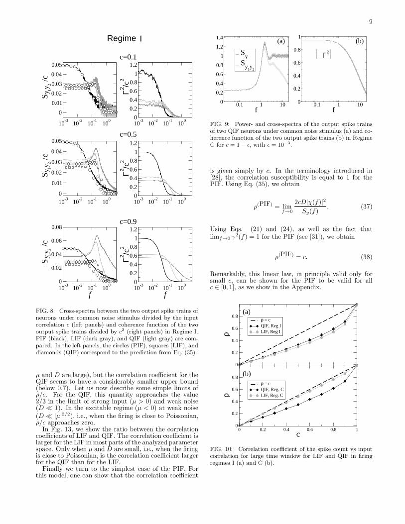
for small c (e.g., c=0.1). Second, we note fromFig. 9 that, as the input correlation c approaches 1, theconvergence of Sy1y2

to Sy and of Γ2(f) to the maxi-mum value 1 (for all f) is very slow. This convergenceis more pronouncedly slow for large frequencies, whichcorresponds to the fact that a tiny amount of individ-ual noise is enough to produce a finite difference in thespiking times of the two neurons. Third, the coherencefunction in the important limit of small frequencies islarger for the LIF in regime C as compared to the QIFand, conversely, larger for the QIF as compared to theLIF in regime I.

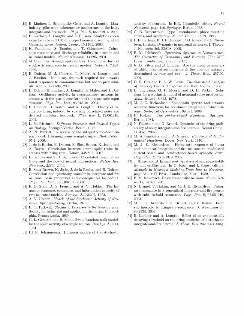
In view of the discussion in section VA, we concludethat the correlation coefficient ρ of the spike count in thelimit of large time windows is larger for the LIF than forthe QIF in regime C and larger for the QIF than for theLIF in regime I. In Fig. 10, this is shown to occur for cin the whole range 0 ≤ c ≤ 1. We also observe that anapproximately linear dependence holds in a fairly broadrange in Regimes C and I for both models.

10-1

100

101

0

0.1

0.2

0.3

y y

10-1

100

101

0

0.2

0.4

0.6

0.8

1

1.2

Γ2 /c2

10-1

100

101

0

0.1

0.2

0.3

0.4

y y

10-1

100

101

0

0.2

0.4

0.6

0.8

1

1.2

Γ2 /c2

10-1

100

101

f

0

0.2

0.4

0.6

y y

10-1

100

101

f

0

0.2

0.4

0.6

0.8

1

1.2

Γ2 /c2

Regime C

c=0.1

S

/c

1 2

c=0.5

c=0.9S

/

cS

/

c1

21

2

FIG. 7: Cross-spectra between the two output spike trains ofneurons under common noise stimulus divided by the inputcorrelation c (left panels) and coherence function of the twooutput spike trains divided by c2 (right panels) in Regime C.PIF (black), LIF (dark gray), and QIF (light gray) are com-pared. In the left panels, the circles (PIF), squares (LIF), anddiamonds (QIF) correspond to the prediction from Eq. (35).

In order to provide a complete picture of the corre-lation coefficient not only for two specific regimes butrather in a fairly broad region of the parameter space,we show in Fig. 11 and Fig. 12 the ratio ρ/c as a func-tion of µ and D for the LIF and QIF, respectively. Theywere estimated on the basis of the Eq. (36) and are ex-pected to be correct for small input correlation c. Forthe LIF, we have calculated the terms in Eq. (36) fromthe exact analytical expressions (see e.g. [39]). For theQIF we resorted to the numerical algorithm of Refs. [46]and [42].

We note from that for both LIF and QIF the corre-lation coefficient falls sharply when the Poissonian firingregime (low D and µ) is approached. Also remarkable isthe fact that, at least in the studied parameter regions,the correlation coefficient for the LIF can approach 1 (if

9

10-3

10-2

10-1

100

0

0.01

0.02

0.03

0.04

0.05

y y

10-3

10-2

10-1

100

0

0.2

0.4

0.6

0.8

1

1.2

Γ2 /c2

10-3

10-2

10-1

100

0

0.01

0.02

0.03

0.04

0.05

y y

10-3

10-2

10-1

100

0

0.2

0.4

0.6

0.8

1

1.2

Γ2 /c2

10-3

10-2

10-1

100

f

0

0.02

0.04

0.06

0.08

y y

10-3

10-2

10-1

100

f

0

0.2

0.4

0.6

0.8

1

1.2

Γ2 /c2

Regime I

c=0.1

S

/c

1 2

c=0.5

c=0.9

S

/c

S

/c

1 2

1 2

FIG. 8: Cross-spectra between the two output spike trains ofneurons under common noise stimulus divided by the inputcorrelation c (left panels) and coherence function of the twooutput spike trains divided by c2 (right panels) in Regime I.PIF (black), LIF (dark gray), and QIF (light gray) are com-pared. In the left panels, the circles (PIF), squares (LIF), anddiamonds (QIF) correspond to the prediction from Eq. (35).

µ and D are large), but the correlation coefficient for theQIF seems to have a considerably smaller upper bound(below 0.7). Let us now describe some simple limits ofρ/c. For the QIF, this quantity approaches the value2/3 in the limit of strong input (µ > 0) and weak noise(D ≪ 1). In the excitable regime (µ < 0) at weak noise(D ≪ |µ|3/2), i.e., when the firing is close to Poissonian,ρ/c approaches zero.

In Fig. 13, we show the ratio between the correlationcoefficients of LIF and QIF. The correlation coefficient islarger for the LIF in most parts of the analyzed parameterspace. Only when µ and D are small, i.e., when the firingis close to Poissonian, is the correlation coefficient largerfor the QIF than for the LIF.

Finally we turn to the simplest case of the PIF. Forthis model, one can show that the correlation coefficient

0.1 1 10f

0

0.2

0.4

0.6

0.8

1

1.2

1.4

Sy

Sy

1y

2

0.1 1 10f

0

0.2

0.4

0.6

0.8

1

Γ2

(b)(a)

FIG. 9: Power- and cross-spectra of the output spike trainsof two QIF neurons under common noise stimulus (a) and co-herence function of the two output spike trains (b) in RegimeC for c = 1 − ǫ, with ǫ = 10−3.

is given simply by c. In the terminology introduced in[28], the correlation susceptibility is equal to 1 for thePIF. Using Eq. (35), we obtain

ρ(PIF) = limf→0

2cD|χ(f)|2Sy(f)

. (37)

Using Eqs. (21) and (24), as well as the fact thatlimf→0 γ2(f) = 1 for the PIF (see [31]), we obtain

ρ(PIF) = c. (38)

Remarkably, this linear law, in principle valid only forsmall c, can be shown for the PIF to be valid for allc ∈ [0, 1], as we show in the Appendix.

0

0.2

0.4

0.6

0.8

ρ

ρ = cQIF, Reg ILIF, Reg I

0 0.2 0.4 0.6 0.8 1c

0

0.2

0.4

0.6

0.8

ρ

ρ = cQIF, Reg. CLIF, Reg. C

(a)

(b)

FIG. 10: Correlation coefficient of the spike count vs inputcorrelation for large time window for LIF and QIF in firingregimes I (a) and C (b).

10

0 0.1 0.2 0.3 0.4 0.5 0.6 0.7 0.8 0.9 1

0.001 0.01

0.1

0.8 1

1.2 1.4

1.6 1.8

0 0.1 0.2 0.3 0.4 0.5 0.6 0.7 0.8 0.9

1

ρ /c

D

µ

FIG. 11: (Color online) Correlation coefficient (divided byc) of the spike counts at large time windows for the LIF as afunction of both D and µ.

0

0.1

0.2

0.3

0.4

0.5

0.6

0.7

0.1 1

10 100

0

2

4

6

8

10

0 0.1 0.2 0.3 0.4 0.5 0.6 0.7

ρ /c

D

µ

FIG. 12: (Color online) Correlation coefficient (divided byc) of the spike counts at large time windows for the QIF as afunction of both D and µ.

VI. CONCLUSIONS

We have provided an extensive comparison of threeimportant IF models in different firing regimes, as de-termined by given firing rate and CV. We have shownthat the spontaneous activity of the LIF and QIF neu-rons virtually coincide in regimes characterized by weakinput noise and deviates moderately for larger values ofthe input noise. The dynamical response behavior, how-ever, strongly differs among different models, even in thesame firing regimes. This was discussed in the limit oflarge stimulus frequencies in [15] and extended here forthe entire frequency range.

An important feature of the single neuron’s responsecharacteristics is that, depending on the firing regime,it can be stronger at a given frequency for the LIF ascompared to the QIF or the other way around. We haveshown that this implies, as long as the linear responsetheory holds true (i.e., for small c), that either two LIFor two QIF neurons can display larger low-frequency cor-relations when driven in part by common noise. Alto-gether our findings indicate that the successful use of a

0.7

0.8

0.9

1

1.1

1.2

1.3

1.4

1.5

1.6

1 10 100D (QIF)

0

2

4

6

8

10

µ (Q

IF)

FIG. 13: (Color online) Ratio between the correlation co-efficients of the spike counts of LIF and QIF in the limit oflarge time windows. The contour lines for rate and CV arethe same as those depicted in Fig. 1.

certain IF model to reproduce the spontaneous activityof biological neurons does not at all guarantee that thecorrelations in the activity of a population of such neu-rons will be also well described. More important for thelatter are the dynamical response characteristics of thesingle neuron to an external stimulus.

We have also characterized a large portion of the phys-iologically relevant parameter space of the studied IFmodels and concluded that the correlations in the spiketrains of two LIFs, as characterized by the correlationcoefficient for the spike count, are in most cases largerthan the corresponding correlations of two QIFs. An im-portant exception, however, exists: when the firing ap-proaches the Poissonian regime, the correlations betweenQIF neurons become larger than those of two LIF neu-rons.

It constitutes an interesting open problem to performthe same studies as done here for other IF models, e.g.the exponential IF model introduced in [15]. Finally, anextensive comparison between type I [18, 20, 47] and typeII [48, 49, 50] neurons as regards to spontaneous activity,dynamical response, and two-neuron correlation undercommon stimulus is still lacking and is expected to shedlight on the problem of how large neuronal populationsencode and transmit information.

VII. ACKNOWLEDGMENT

We would like to thank Magnus J. E. Richardson forhelp on his algorithm from [42] prior to publication.

APPENDIX A: CORRELATION COEFFICIENT

FOR THE PIF FOR ARBITRARY c

Here we show that the correlation coefficient for thePIF is for an input correlation c ∈ [0, 1] given by:

ρ(PIF) = c. (A1)

11

For this purpose, we track the non-reset voltage of thePIF described by:

vi = µ +√

1 − cξi(t) +√

cξc(t), (A2)

and observe that, in the limit of large times, the rela-tive error in approximating the spike count ni(t) by thisunresetted voltage vi(t) approaches zero, i.e.:

limt→∞

ni(t) − vi(t)

(ni(t) + vi(t))/2= 0. (A3)

Eq. (A3) holds true because the difference between thespike count and the non-reset voltage is a number be-tween 0 and 1 (assuming vth − vr = 1). In other words,the numerator appearing in the limit of Eq. (A3) remainsbounded between 0 and 1 for all t, while the denominatorgoes to infinity as t → ∞.

Approximating the spike count ni(t) by this unresettedvoltage vi(t), we obtain an alternative formula for thecorrelation coefficient for the spike count of the PIF:

ρ(PIF) = limt→∞

〈v1(t)v2(t)〉 − 〈v1(t)〉〈v2(t)〉√

(〈v21(t)〉 − 〈v1(t)〉2)(〈v2

2(t)〉 − 〈v2(t)〉2).

(A4)To calculate the right-hand side of Eq. (A4), we use theformal solution of Eq. (A2), given by:

vi(t) =

∫ t

0

(µ +√

1 − cξi(t′) +

√cξc(t

′))dt′. (A5)

Substituting Eq. (A5) in Eq. (A4) and using Eqs. (18)and (30), we obtain Eq. (A1).

APPENDIX B: NUMERICAL METHODS

The contour lines for the rate for both LIF and QIF,as well as the respective power spectra, were obtained byresorting to the numerical algorithm of Ref. [42]. Forthe LIF (QIF), the rate and CV were calculated for thepoints on a roughly 2000 × 2000 (103 × 103) grid overthe (D, µ) region displayed in Fig. 1. The integrationstep for the numerical evaluation of the Fokker-Planckequation (see [42]) was equal to 10−4 for the LIF and10−3 for the QIF, with the threshold and reset at ±∞being numerically replaced by ±500 for the latter. TheCV was estimated by assuming that the power spectrumat a frequency 103 times smaller than the firing rate wasequal to rR2 (see Eq. (14)) for both LIF and QIF.

The gain and phase for the linear response of LIF andQIF were computed using the algorithm of Ref. [46], withthe same integration steps (as well as reset and thresholdvalues for the QIF) as above. Finally, the cross-spectraSy1y2

were obtained from a fast Fourier transform algo-rithm after integrating the stochastic diferential equa-tions Eq. (29) with a time step of 10−3. For the LIF,a correction based on the probability that the voltagereached the threshold and decreased below it within thetime interval dt was implemented (see [51]).

[1] B. Hille. Ion channels of excitable membranes. Sinauer,Sunderland, 2001.

[2] C. Koch. Biophysics of Computation - Information Pro-

cessing in Single Neurons. Oxford University Press, NewYork, Oxford, 1999.

[3] W. Gerstner and W. Kistler. Spiking Neuron Models.Cambridge, Cambridge, UK, 2002.

[4] L. Badel, S. Lefort, R. Brette, C. C. H. Petersen, W. Ger-stner, and M. J. E. Richardson. Dynamic I-V curves arereliable predictors of naturalistic pyramidal-neuron volt-age traces. J. Neurophysiol., 99:656, 2008.

[5] R. Jolivet, R. Kobayashi, A. Rauch, R. Naud, S. Shi-nomoto, and W. Gerstner. A benchmark test for a quan-titative assessment of simple neuron models. J. Neurosci.

Methods, 169:417, 2008.[6] R. Jolivet, F. Schurmann, T. K. Berger, R. Naud,

W. Gerstner, and A. Roth. The quantitative single-neuron modeling competition. Biol. Cybern. 99:417,2008.

[7] A. Rauch, G. La Camera, H. R. Luscher, W. Senn, andS. Fusi. Neocortical pyramidal cells respond as integrate-and-fire neurons to in vivo-like input currents. J. Neuro-

physiol., 90:1598, 2003.[8] P. Lansky, P. Sanda, and J. F. He. The parameters of

the stochastic leaky integrate-and-fire neuronal model. J.

Comput. Neurosci. 21:211, 2006.[9] L. F. Abbott and C. van Vreeswijk. Asynchronous states

in a network of pulse-coupled oscillators. Phys. Rev. E,48:1483, 1993.

[10] D. J. Amit and N. Brunel. Dynamics of a recurrent net-

work of spiking neurons before and following learning.Network: Comput. Neural Syst., 8:373, 1997.

[11] N. Brunel. Dynamics of sparsely connected networks ofexcitatory and inhibitory spiking neurons. J. Comput.

Neurosci., 8:183, 2000.[12] D. Hansel and G. Mato. Existence and stability of persis-

tent states in large neuronal networks. Phys. Rev. Lett.,86:4175, 2001.

[13] N. Brunel, F. S. Chance, N. Fourcaud, and L. F. Abbott.Effects of synaptic noise and filtering on the frequencyresponse of spiking neurons. Phys. Rev. Lett., 86:2186,2001.

[14] B. Lindner and L. Schimansky-Geier. Transmission ofnoise coded versus additive signals through a neuronalensemble. Phys. Rev. Lett., 86:2934, 2001.

[15] N. Fourcaud-Trocme, D. Hansel, C. van Vreeswijk, andN. Brunel. How spike generation mechanisms determinethe neuronal response to fluctuating inputs. J. Neurosci.,23:11628, 2003.

[16] B. Naundorf, T. Geisel, and F. Wolf. Dynamical responseproperties of a canonical model for type-i membranes.Neurocomputing, 65:421, 2005.

[17] L. M. Ricciardi and L. Sacerdote. The Ornstein-Uhlenbeck process as a model for neuronal activity. Biol.

Cybernetics, 35:1, 1979.[18] B. S. Gutkin and G. B. Ermentrout. Dynamics of mem-

brane excitability determine interspike interval variabil-ity: A link between spike generation mechanisms andcortical spike train statistics. Neural Comp., 10:1047,1998.

12

[19] B. Lindner, L. Schimansky-Geier, and A. Longtin. Max-imizing spike train coherence or incoherence in the leakyintegrate-and-fire model. Phys. Rev. E, 66:031916, 2002.

[20] B. Lindner, A. Longtin, and A. Bulsara. Analytic expres-sions for rate and CV of a type I neuron driven by whiteGaussian noise. Neural. Comp., 15:1761, 2003.

[21] K. Pakdaman, S. Tanabe, and T. Shimokawa. Coher-ence resonance and discharge reliability in neurons andneuronal models. Neural Networks, 14:895, 2001.

[22] M. Stemmler. A single spike suffices: the simplest form ofstochastic resonance in neuron models. Network, 7:687,1996.

[23] B. Doiron, M. J. Chacron, L. Maler, A. Longtin, andJ. Bastian. Inhibitory feedback required for networkburst responses to communication but not to prey stim-uli. Nature, 421:539, 2003.

[24] B. Doiron, B. Lindner, A. Longtin, L. Maler, and J. Bas-tian. Oscillatory activity in electrosensory neurons in-creases with the spatial correlation of the stochastic inputstimulus. Phys. Rev. Lett., 93:048101, 2004.

[25] B. Lindner, B. Doiron, and A. Longtin. Theory of os-cillatory firing induced by spatially correlated noise anddelayed inhibitory feedback. Phys. Rev. E, 72:061919,2005.

[26] L. M. Ricciardi. Diffusion Processes and Related Topics

on Biology. Springer-Verlag, Berlin, 1977.[27] A. N. Burkitt. A review of the integrate-and-fire neu-

ron model: I. homogeneous synaptic input. Biol. Cyber.,95:1, 2006.

[28] J. de la Rocha, B. Doiron, E. Shea-Brown, K. Josic, andA. Reyes. Correlation between neural spike trains in-creases with firing rate. Nature, 448:802, 2007.

[29] E. Salinas and T. J. Sejnowski. Correlated neuronal ac-tivity and the flow of neural information. Nature Rev.

Neurosci., 2:539, 2001.[30] E. Shea-Brown, K. Josic, J. de la Rocha, and B. Doiron.

Correlation and synchrony transfer in integrate-and-fireneurons: basic properties and consequences for coding.Phys. Rev. Lett., 100:108102, 2008.

[31] R. B. Stein, A. S. French, and A. V. Holden. The fre-quency response, coherence, and information capacity oftwo neuronal models. Biophys. J., 12:295, 1972.

[32] A. V. Holden. Models of the Stochastic Activity of Neu-

rones. Springer-Verlag, Berlin, 1976.[33] H. C. Tuckwell. Stochastic Processes in the Neuroscience.

Society for industrial and applied mathematics, Philadel-phia, Pennsylvania, 1989.

[34] G. L. Gerstein and B. Mandelbrot. Random walk modelsfor the spike activity of a single neuron. Biophys. J., 4:41,1964.

[35] P.I.M. Johannesma. Diffusion models of the stochastic

activity of neurons. In E.R. Caianiello, editor, Neural

Networks, page 116. Springer, Berlin, 1968.[36] G. B. Ermentrout. Type I membranes, phase resetting

curves, and synchrony. Neural. Comp., 8:979, 1996.[37] P. E. Latham, B. J. Richmond, P. G. Nelson and S. Niren-

berg. Intrinsic Dynamics in neuronal networks. I. Theory.J. Neurophysiol. 83:808, 2000.

[38] E. M. Izhikevich. Dynamical Systems in Neuroscience:

The Geometry of Excitability and Bursting (The MITPress, Cambridge, London, 2007).

[39] R. D. Vilela and B. Lindner. Are the input parametersof white-noise-driven integrate & fire neurons uniquelydetermined by rate and cv? J. Theor. Biol., 257:90,2009.

[40] D. R. Cox and P. A. W. Lewis. The Statistical Analysis

of Series of Events. Chapman and Hall, London, 1966.[41] H. Sugiyama, G. P. Moore, and D. H. Perkel. Solu-

tions for a stochastic model of neuronal spike production.Math. Biosci., 8:323, 1970.

[42] M. J. E. Richardson. Spike-train spectra and networkresponse functions for non-linear integrate-and-fire neu-rons. Biological Cybernetics , 99:381, 2008.

[43] H. Risken. The Fokker-Planck Equation. Springer,Berlin, 1984.

[44] N. Fourcaud and N. Brunel. Dynamics of the firing prob-ability of noisy integrate-and-fire neurons. Neural Comp.,14:2057, 2002.

[45] M. Abramowitz and I. A. Stegun. Handbook of Mathe-

matical Functions. Dover, New York, 1970.[46] M. J. E. Richardson. Firing-rate response of linear

and nonlinear integrate-and-fire neurons to modulatedcurrent-based and conductance-based synaptic drive.Phys. Rev. E, 76:021919, 2007.

[47] J. Rinzel and B. Ermentrout. Analysis of neural excitabil-ity and oscillations. In C. Koch and I. Segev, editors,Methods in Neuronal Modeling:From Ions to Networks,page 251. MIT Press, Cambridge, Mass., 1989.

[48] E. M. Izhikevich. Resonate-and-fire neurons. Neural Net-

works, 14:883, 2001.[49] N. Brunel, V. Hakim, and M. J. E. Richardson. Firing-

rate resonance in a generalized integrate-and-fire neuronwith subthreshold resonance. Phys. Rev. E, 67:051916,2003.

[50] M. J. E. Richardson, N. Brunel, and V. Hakim. Fromsubthreshold to firing-rate resonance. J. Neurophysiol.,89:2538, 2003.

[51] B. Lindner and A. Longtin. Effect of an exponentiallydecaying threshold on the firing statistics of a stochasticintegrate-and-fire neuron. J. Theor. Biol. 232:505 (2005).