Comparative Analysis of CFD Models for dense Gas-Solid Systems

Comparative Analysis of CFD Models of DenseGas–Solid Systems

B. G. M. van Wachem, J. C. Schouten, and C. M. van den BleekDelftChemTech, Chemical Reactor Engineering Section, Delft University of Technology,

2628 BL Delft, The Netherlands

R. KrishnaDept. of Chemical Engineering, University of Amsterdam, 1018 WV Amsterdam, The Netherlands

J. L. SinclairSchool of Chemical Engineering, Purdue University, West Lafayette, IN 47907

Many gas ] solid CFD models ha®e been put forth by academic researchers, go®ern-ment laboratories, and commercial ®endors. These models often differ in terms of boththe form of the go®erning equations and the closure relations, resulting in much confu-sion in the literature. These ®arious forms in the literature and in commercial codes arere®iewed and the resulting hydrodynamics through CFD simulations of fluidized beds

( )compared. Experimental data on fluidized beds of Hilligardt and Werther 1986 , Ke-( ) ( ) ( )hoe and Da®idson 1971 , Darton et al. 1977 , and Kuipers 1990 are used to quanti-

tati®ely assess the ®arious treatments. Predictions based on the commonly used go®ern-( ) ( )ing equations of Ishii 1975 do not differ from those of Anderson and Jackson 1967

in terms of macroscopic flow beha®ior, but differ on a local scale. Flow predictions arenot sensiti®e to the use of different solid stress models or radial distribution functions, asdifferent approaches are ®ery similar in dense flow regimes. The application of a differ-ent drag model, howe®er, significantly impacts the flow of the solids phase. A simplifiedalgebraic granular energy-balance equation is proposed for determining the granulartemperature, instead of sol®ing the full granular energy balance. This simplification doesnot lead to significantly different results, but it does reduce the computational effort ofthe simulations by about 20%.

Introduction

Gas]solid systems are found in many operations in thechemical, petroleum, pharmaceutical, agricultural, biochemi-cal, food, electronic, and power-generation industries. Com-

Ž .putational fluid dynamics CFD is an emerging techniquefor predicting the flow behavior of these systems, as it is nec-essary for scale-up, design, or optimization. For example,

Ž .Barthod et al. 1999 have successfully improved the perform-ance of a fluidized bed in the petroleum industries by means

Correspondence concerning this article should be addressed to B. G. M. vanWachem.

Current address for B. G. M. van Wachem and J. C. Schouten: Laboratory ofChemical Reactor Engineering, Eindhoven University of Technology, P. O. Box 513,5600 MB Eindhoven, The Netherlands.

Ž .of CFD calculations. Sinclair 1997 gives an extensive intro-duction on applying CFD models for gasrsolid risers. Al-though single-phase flow CFD tools are now widely and suc-cessfully applied, multiphase CFD is still not because of thedifficulty in describing the variety of interactions in these sys-tems. For example, to date there is no agreement on the ap-propriate closure models. Furthermore, there is still noagreement on even the governing equations. In addition, pro-posed constitutive models for the solid-phase stresses and theinterphase momentum transfer are partially empirical.

CFD models of gas]solid systems can be divided into twogroups, Lagrangian models and Eulerian models. Lagrangianmodels, or discrete particle models, calculate the path and

May 2001 Vol. 47, No. 5AIChE Journal 1035

motion of each particle. The interactions between the parti-Žcles are described by either a potential force soft-particle

. Ždynamics, Tsuji et al., 1993 or by collision dynamics hard-.particle dynamics, Hoomans et al., 1995 . The drawbacks of

the Lagrangian approach are the large memory requirementsand the long calculation time and, unless the continuous

Ž .phase is described using direct numerical simulations DNS ,empirical data and correlations are required to describe thegas]solid interactions. Eulerian models treat the particlephase as a continuum and average out motion on the scale ofindividual particles, thus enabling computations by thismethod to treat dense-phase flows and systems of realisticsize. As a result, CFD modeling based on this Eulerianframework is still the only feasible approach for performingparametric investigation and scale-up and design studies.

This article focuses on the Eulerian approach and com-pares the two sets of governing equations, the different clo-sure models, and their associated parameters that are em-ployed in the literature to predict the flow behavior ofgas]solid systems. Unfortunately, many researchers proposegoverning equations without citing, or with incorrectly citing,a reference for the basis for their equations. Both Anderson

Ž . Ž .and Jackson 1967 and Ishii 1975 have derived multiphaseflow equations from first principles, but the inherent assump-tions in these two sets of governing equations constrain thetypes of multiphase flows to which they can be applied. Oneof the objectives of our current contribution is to show how

Ž .these two treatments differ; it is shown that Ishii’s 1975treatment is appropriate for a dispersed phase consisting of

Ž .fluid droplets, and that Anderson and Jackson’s 1967 treat-ment is appropriate for a dispersed phase consisting of solidparticles. In the case of a solid dispersed phase, many re-searchers and commercial CFD codes employ kinetic theoryconcepts to describe the solid-phase stresses resulting fromparticle]particle interactions. Various forms of the constitu-tive models based on these concepts have been applied in theliterature. The qualitative and quantitative differences be-tween these are shown in this article. The predictions of CFDsimulations of bubbling fluidized beds, slugging fluidizedbeds, and bubble injection into fluidized beds incorporatingthese various treatments are compared to the ‘‘benchmark’’

Ž .experimental data of Hilligardt and Werther 1986 , KehoeŽ . Ž . Ž .and Davidson 1971 , Darton et al. 1977 , and Kuipers 1990 .

Governing EquationsMost authors who refer to the origin of their governing

Ž .equations refer to the work of Anderson and Jackson 1967Ž . Ž .or Ishii 1975 . Anderson and Jackson 1967 and Jackson

Ž . w Ž .x1997 with correction in Jackson 1998 use a formal math-ematical definition of local mean variables to translate thepoint Navier-Stokes equations for the fluid and the Newton’sequation of motion for a single particle directly into contin-uum equations representing momentum balances for the fluid

Ž .and solid phases, as earlier suggested by Jackson 1963 . Thepoint variables are averaged over regions that are large withrespect to the particle diameter, but small with respect to thecharacteristic dimension of the complete system. A weighting

Ž .function, g N xy yN , is introduced in forming the local aver-ages of system point variables, where N xy yN denotes theseparation of two arbitrary points in space. The integral of g

over the total space is normalized to unity:

`24p g r r dr s1. 1Ž . Ž .H

0

The ‘‘radius’’ l of function g is defined by

`l 2 2g r r dr s g r r dr , 2Ž . Ž . Ž .H H0 l

If l is chosen to satisfy a< l < L, where a is the particleradius and L is the shortest macroscopic length scale, aver-ages defined should not depend significantly on the particu-lar functional form of g or its radius.

Ž .The gas-phase volume-fraction e x and the particlegŽ .number density n x at point x are directly related to the

weighting function g :

e x s g N xy yN dV 3Ž . Ž . Ž .g H yVg

n x s g N xy x N , 4Ž . Ž .Ž .Ý pp

where V is the fluid-phase volume, and x is the position ofg pthe center of particle p. The local mean value of the fluid-phase point properties, - f ) , is defined byg

e x - f ) x s f y g N xy yN dV . 5Ž . Ž . Ž . Ž . Ž .g Hg yVg

The solid-phase averages are not defined like the fluid-phase averages, since the motion of the solid phase is deter-mined with respect to the center of the particle, and averageproperties need only depend on the properties of the particleas a whole. Hence, the local mean value of the solid-phasepoint properties is defined by

n x - f ) x s f N xy x N . 6Ž . Ž . Ž .Ž .Ýs s pp

The average space and time derivatives for the fluid andsolid phases follow from the preceding definitions. The aver-aging rules are then applied to the point continuity and mo-mentum balances for the fluid. For the solid phase, the aver-aging rules are applied to the equation of motion of a singleparticle p:

©sr V s s y n y ds q f q r V g , 7Ž . Ž . Ž .H Ýs p g y q p s p t Sp q / p

where © is the particle velocity, r is the particle density, Vs s pis the volume of particle p, s is the gas-phase stress tensor,gS denotes the surface of particle p, and f represents thep q presultant force exerted on the particle p from contacts withother particles.

The resulting momentum balances for the fluid and solidphases, dropping the averaging brackets -) on the vari-

May 2001 Vol. 47, No. 5 AIChE Journal1036

ables, are as follows:

r e © q© ?=© s= e sŽ .g g g g g g g t

y s ? n y g N xy yN ds q r e g 8Ž . Ž .HÝ g y g gSpp

r e © q© ?=© s g N xy x N s n y dsŽ .HÝg s s s s p g y t Spp

q=?s q r e g . 9Ž .s s s

The first term on the righthand side of the gas-phase equa-tion of motion represents the effect of stresses in the gasphase, the second term on the righthand side represents thetraction exerted on the gas phase by the particle surfaces,and the third term represents the gravity force on the fluid.The first term on the righthand side of the solid-phase equa-tion of motion represents the forces exerted on the particlesby the fluid, the second term on the righthand side repre-sents the force due to solid]solid contacts, which can be de-scribed using concepts from kinetic theory, and the third termrepresents the gravity force on the particles. The averagedshear tensor of the gas phase can be rewritten with the New-tonian definition as

mg Ts sy P Iq =© q =© , 10Ž .Ž .g g g geg

where the gas-phase volume-fraction is introduced in the vol-ume process.

Note that the forces due to fluid traction are treated dif-ferently in the fluid-phase and solid-phase momentum bal-ances. In the particle phase, only the resultant force actingon the center of the particle is relevant; the distribution ofstress within each particle is not needed to determine its mo-tion. Hence, in the solid-phase momentum balance, the re-sultant forces due to fluid traction acting everywhere on thesurface of the particles are calculated first, after which theseare averaged to the particle centers. In the fluid-phase mo-mentum balance, the traction forces at all elements offluid]solid interaction are calculated, and then are averagedto the location of the surface elements. Hence, the fluid-phasetraction term is given as

s ? n y g N xy yN ds s g N xy x N s ? n y dsŽ . Ž .H HÝ Ýg y p g yS Sp pp p

2y=? a g N xy x N s ? n y n y ds qO = ,Ž . Ž . Ž .HÝ p g y½ 5Spp

11Ž .

which is a result of a Taylor series expansion in g N xy yNabout the center of the particle with radius a. Here terms ofŽ 2.O = and higher have been neglected. Note that the first

term on the righthand side of Eq. 11 is the same as the fluidtraction term in the particle-phase momentum balance. The

Table 1. Governing Equations Applied to Gas–Solid Flow

Continuity equationseg Ž .q=? e © s0g g tes Ž .q=? e © s0s s t

( )Momentum equations of Jackson 1997 © bg Ž .r q© ?=© s=?t y=P y © y© q r gg g g g g s g t eg

© © bgs Ž .r e q© ?=© y r e q© ?=© s © y©s s s s g s g g g s t t eg

Ž .qe r y r g q=?t y=Ps s g s sin alternative form:

©g Ž .r e q© ?=© se =?t ye =P y b © y© qe r gg g g g g g g g s g g t ©s Ž .r e q© ?=© se =?t ye =P q=?t y=P q b © y©s s s s s g s s s g s t

qe r gs s

( )Momentum equations of Ishii 1975 ©g Ž .r e q© ?=© sye =P q=?e t qe r g y b © y©g g g g g g g g g g s t ©s Ž .r e q© ?=© sye =P q=?e t qe r g q b © y©s s s s s s s s s g s t

Ž .applied to gas-solid flow Enwald et al., 1996 : ©g Ž .r e q© ?=© sye =P q=?e t qe r g y b © y©g g g g g g g g g g s t

©s Ž .r e q© ?=© sye =P q=?t y=P qe r g q b © y©s s s s s s s s s g s t

Definitions2

Ž .t s2m D q l y m tr D Ii i i i i iž /31 Tw Ž . xD s =© q =©i i i2

Note: The explanation of the symbols can be found in the Notation.

difference in the manner in which the resultant forces due tofluid tractions act on the surfaces of the particles is a key

Ž . Ž .distinction between the Jackson 1997 and Ishii 1975 for-Ž .mulations. In the Ishii 1975 formulation, applicable to fluid

droplets, the fluid-droplet traction term is the same in thegas phase and the dispersed-phase governing equations.

The integrals involving the traction on a particle surfaceŽ .have been derived by Nadim and Stone 1991 and are given

Ž .in Jackson 1997 as

bg N xy x N s ? n y ds s © y© q r e gŽ . Ž .HÝ p g y g s g seS gpp

D ©f gq r e 12Ž .g s Dt

=? a g N xy x N s ? n y n y ds sy= e P ,Ž . Ž . Ž .HÝ p g y s gSpp

13Ž .

where b is the interphase momentum transfer coefficient.The final equations of motion for both phases according to

Ž .Jackson 1997 are shown in Table 1, both in the form as


originally presented in his article, and in an equivalent alter-native form, which is merely a linear combination of the orig-inal equations.

Ž .In Ishii’s 1975 formulation, the fluid and dispersed phasesare averaged over a fixed volume. This volume is relativelylarge compared to the size of individual molecules or parti-

Ž .cles. A phase indicator function is introduced, X r , which isunity when the point r is occupied by the dispersed phase,and zero if it is not. Averaging over this function leads to thevolume fraction of both phases:

1e s X r dV , 14Ž . Ž .Hs rV V

where V is the averaging volume. Since both the continuousand dispersed phases are liquids, they are treated the samein the averaging process. Hence, the momentum balances forboth phases are the same,

e r -© )k k kq=? e r -© )-© )Ž .k k k k t

sy= e - P ) q=? e -t ) qe r g q M , 15Ž .Ž . Ž .k k k k k k k

where k is the phase number and M is the interphase mo-kmentum exchange between the phases, with M q M s0. Ing s

Ž .the Ishii 1975 formulation, the distribution of stress withinboth phases is important since the dispersed phase is consid-ered as fluid droplets. Hence, ‘‘jump’’ conditions are used todetermine M . The interphase momentum transfer is definedkas

1M sy P n y n ?tŽ .Ýk k k k kLjj

1s - P )y P n y- P ) n y nŽ .ŽÝ ki k k ki k kLjj

? -t )yt q n ? -t ) , 16Ž ..Ž .ki k k ki

where L is the interfacial area per unit volume, P is thej kpressure in the bulk of phase k, - P ) is the average pres-kisure of phase k at the interface, t denotes the shear stresskin the bulk, and -t ) represents the average shear stresski

Ž . Žat the interface. The terms - P )y P n and n ? -tki k k k ki. Ž .)yt are identified by Ishii 1975 as the form drag andk

the skin drag, respectively, making up the total drag force.The other terms can be written out as

M sdragq - P )=e q - P )y- P ) =eŽ .k k k ki k k

y =e ? -t ). 17Ž .Ž .k ki

Ž .According to Ishii and Mishima 1984 , the last term onthe righthand side is an interfacial shear term and is impor-

Ž .tant in a separated flow. According to Ishii 1975 , the termŽ .- P )y- P ) only plays a role when the pressure atki kthe bulk is significantly different from that at the interface, asin stratified flows. For many applications both terms are neg-

ligible, and

M sdragq - P )=e . 18Ž .k k k

The momentum equations for the gas phase and the dis-Ž .persed phase following the original work of Ishii 1975 are

shown in Table 1. Many researchers and commercial codesŽ .modify Ishii’s 1975 equations to describe gas]solid flows

Ž .such as Enwald et al., 1996 . These modified equations areŽ .also shown in Table 1. When Ishii’s 1975 equations are ap-

plied to gas]solid flows, the solid-phase stress tensor is notmultiplied by the solid volume fraction, since the volume-fraction functionality is already accounted for in the kinetictheory description.

Ž . Ž .Comparing the Ishii 1975 and Jackson 1997 momentumŽ .balances, the differences are twofold. First, Jackson 1997

includes the solid volume fraction multiplied by the gradientof the total gas-phase stress tensor in the solid-phase mo-

Ž .mentum balance, whereas Ishii 1975 only includes the solidvolume-fraction multiplied by the gradient of the pressure.

Ž .Second, in the Ishii 1975 approach in the gas-phase mo-mentum balance, the pressure carries the gas volume fractionoutside the gradient operator; the shear stress carries the gasvolume fraction inside the gradient operator. In JacksonŽ .1997 both stresses are treated equally with respect to thegas volume fraction and the gradient operators. When thegas-phase shear stress plays an important role, these differ-ences may be significant near large gradients of volume frac-tion, that is, near bubbles or surfaces.

Closure RelationsKinetic theory

Closure of the solid-phase momentum equation requires adescription for the solid-phase stress. When the particle mo-tion is dominated by collisional interactions, concepts from

Ž .gas kinetic theory Chapman and Cowling, 1970 can be usedto describe the effective stresses in the solid phase resulting

Ž .from particle streaming kinetic contribution and direct col-Ž .lisions collisional contribution . Constitutive relations for the

solid-phase stress based on kinetic theory concepts have beenŽ .derived by Lun et al. 1984 , allowing for the inelastic nature

of particle collisions.Analogous to the thermodynamic temperature for gases,

the granular temperature can be introduced as a measure ofthe particle velocity fluctuations.

1X2

Us -© ). 19Ž .s3

Since the solid-phase stress depends on the magnitude ofthese particle-velocity fluctuations, a balance of the granular

3Ž .energy Q associated with these particle-velocity fluctua-2

tions is required to supplement the continuity and momen-tum balance for both phases. This balance is given as

3 e r Q q=? e r Q© s y=P Iqt :=©Ž . Ž .s s s s s s s sž /2 t

y=? k =Q yg y J , 20Ž .Ž .s s s


where the first term on the righthand side represents the cre-ation of fluctuating energy due to shear in the particle phase,the second term represents the diffusion of fluctuating en-ergy along gradients in Q, g represents the dissipation duesto inelastic particle]particle collisions, and J represents thesdissipation or creation of granular energy resulting from theworking of the fluctuating force exerted by the gas throughthe fluctuating velocity of the particles. Rather than solvingthe complete granular energy balance given in Eq. 20, some

Žresearchers Syamlal et al., 1993; Boemer et al., 1995; Van.Wachem et al., 1998, 1999 assume the granular energy is in a

steady state and dissipated locally, and neglect convection anddiffusion. Retaining only the generation and the dissipationterms, Eq. 20 simplifies to an algebraic expression for thegranular temperature:

0s y=P Iqt :=© yg . 21Ž .s s s sž /Because the generation and dissipation terms dominate indense-phase flows, it is anticipated that this simplification isa reasonable one in dense regions of flow.

Solid-phase stress tensorThe solids pressure represents the normal solid-phase

forces due to particle]particle interactions. In the literaturethere is general agreement on the form of the solids pres-

Ž .sure, given by Lun et al. 1984 as

P s r e Q 1q2 1q e g ew xŽ .s s s 0 s

s r e Qq2 g r e 2Q 1q e . 22Ž . Ž .s s 0 s s

The first part of the solids pressure represents the kineticcontribution, and the second part represents the collisionalcontribution. The kinetic part of the stress tensor physicallyrepresents the momentum transferred through the system byparticles moving across imaginary shear layers in the flow;the collisional part of the stress tensor denotes the momen-tum transferred by direct collisions.

The solids bulk viscosity describes the resistance of theparticle suspension against compression. In the literature,there also is general agreement on the form of the solids bulk

Ž .viscosity, given by Lun et al. 1984 as

4 Q2l s e r d g 1q e . 23Ž . Ž .(s s s s 03 p

However, the kinetic theory description for the solids shearviscosity often differs between the various two-fluid models.

Ž .Gidaspow 1994 does not account for the inelastic nature ofparticles in the kinetic contribution of the total stress, as Lun

Ž .et al. 1984 do, claiming this correction is negligible. TheŽ .solids shear viscosity of Syamlal et al. 1993 neglects the ki-

netic or streaming contribution, which dominates in dilute-Ž .phase flow. Hrenya and Sinclair 1997 follow Lun et al.

Ž .1984 , but constrain the mean free path of the particle by adimension characteristic of the actual physical system. This is

Ž .opposed to the Lun et al. 1984 theory, which allows the

mean free path to tend toward infinity, and the solids viscosi-ties tends toward a finite value as the solid volume fractiontends to zero. Hence, by constraining the mean free path, the

Ž .limit of the Hrenya and Sinclair 1997 shear viscosity expres-sion correctly tends to zero as the solid volume fraction ap-

Ž .proaches zero. In dense solid systems e )0.05 , there is nosŽ .difference in the predicted solids viscosity of Lun et al. 1984

Ž . Ž .and Hrenya and Sinclair 1997 . The Syamlal et al. 1993solids shear viscosity also tends to zero as the solid volumefraction tends to zero. In this case, however, this solids shear

Table 2. Solids Shear Viscosity

( )Lun et al. 19848

Ž .1q h 3hy2 e gs 0'5 t Q 1 8es 5m s r d qs s s ž /96 hg 5 2yhž /0

7682 xq he gs 025p

2Ž .Ž .4 Q 1 r d g 1q e 3r2 ey1r2 es s 0 s2 'Ž .s e r d g 1q e q Qp(s s s 0 Ž .5 p 15 3r2y1r2 eŽ .1 r d e 3r4eq1r4 10 r ds s s s s' 'q Qp q Qp

Ž . Ž .Ž .6 3r2y er2 96 1q e 3r2y1r2 e g0

( )Syamlal et al. 1993'4 Q e d r p Qs s s2 Ž .m s e r d g 1q e q(s s s s 0 Ž .5 p 6 3y e

2Ž .Ž .1q 1q e 3ey1 e gs 05

Ž .Ž .4 Q 1 1q e 3r2 ey1r22 2'Ž .s e r d g 1q e q Qp r d g e(s s s 0 s s 0 sŽ .5 p 15 3r2y er2

'1 e d r p Qs s sq

Ž .12 3r2y er2

( )Gidaspow 1994'5 p

2'2 r d Qs s4 Q 4962 Ž . Ž .m s e r d g 1q e q ? 1q g e 1q e(s s s s 0 0 sŽ .5 p 1q e g 50

4 Q 12 2'Ž . Ž .s e r d g 1q e q Qp r d g 1q e e(s s s 0 s s 0 s5 p 15

1 10 r ds s' 'q Qp r d e q Qps s s Ž .6 96 1q e g0

( )Hrenya and Sinclair 1997

' Ž .5 p Q 1 1 8e 1q8r5h 3hy2 e gs s 0m s r d qs s s l ž /96 hg 5 2yhm f pž /01q

R768

2q he gs 025p2Ž . Ž .4 Q 1 r d g 1q e 3r2 ey1r2 es s 0 s2 'Ž .s e r g 1q e q Qp(s s 0 Ž .5 p 15 3r2y er2

lm f pr d e 1r2 1q q3r4ey1r4s s s ž /ž /1 R'q Qp

l6 m f pŽ .3r2y1r2 e 1qž /R10 r ds s'q Qp

l96 m f pŽ .Ž .1q e 3r2y1r2 e g 1q0 ž /R

Note: The symbols can be found in the Notation.


Figure 1. Comparison of solids shear viscosities fromdifferent kinetic theory models: es0.9, emaxs0.65.

viscosity limit is reached because the kinetic contribution tothe solids viscosity is neglected.

Table 2 presents the forms for the solids shear viscosity aspresented in the original articles as well as in an equivalentform so that all of the models can be easily compared. Figure1 shows a comparison of the constitutive models for the solidsshear viscosity as a function of the solid volume fraction. Allmodels yield the same solids shear viscosity at high solids vol-

Ž .ume fractions. Syamlal et al. 1993 deviate from the othersfor solid volume fractions less than 0.3. Hrenya and SinclairŽ .1997 show a rapid decrease in solids shear viscosity at ex-tremely small particle concentrations.

Conducti©ity of granular energySimilar to the solids shear viscosity, the solids thermal con-

ductivity, k , consists of a kinetic contribution and a colli-Ž .sional contribution. Gidaspow 1994 differs from Lun et al.

Ž .1984 only in the dependency of the solids thermal conduc-Ž .tivity on the coefficient of restitution. Syamlal et al. 1993

neglect the kinetic contribution to the thermal conductivity.Ž . Ž .Hrenya and Sinclair 1997 follow Lun et al. 1984 , but con-

strain the mean free path of the particle by a dimension char-acteristic of the actual system. Hence, the limit of their con-ductivity expression, as with the shear viscosity, correctly tendsto zero when approaching zero solid volume fraction. Syamlal

Ž .et al. 1993 also correctly predict zero for the conductivity atzero solid volume fraction by neglecting the kinetic contribu-tion.

Table 3 presents the forms for the solids thermal conduc-tivity as presented in the original articles, as well as in anequivalent form so that all of the closure models can be eas-ily compared. Figure 2 shows a quantitative comparison ofthe constitutive models for the solids thermal conductivity asa function of the solid volume fraction. All models yield thesame thermal conductivity at high solid volume fraction.

Ž .Syamlal et al. 1993 deviate from the others for solids vol-Ž .ume fraction less than 0.3. Hrenya and Sinclair 1997 show a

Table 3. Solids Thermal Conductivities

( )Lun et al. 19842' Ž .25 p Q 8 96e 1q12r5h 4hy3 e gs s 0

k s r d qs s ž / ž /128 hg 5 41y33h0

5122q he gs 025p

2 2Ž . Ž .Q 9 r d g 1r2qer2 2 ey1 es s 0 s2 'Ž .s2e r d g 1q e q Qp(s s s 0 Ž .p 8 49r16y33r16e2Ž .15 e r d e r2q1r4eq1r4s s s'q Qp

Ž .16 49r16y33r16e25 r ds s'q Qp

Ž .Ž .64 1q e 49r16y33r16e g0

( )Syamlal et al. 1993'15d r e Qp 12 16s s s 2 Ž . Ž .k s 1q h 4hy3 e g q 41y33h he gs 0 s 0Ž .4 41y33h 5 15p

2 2Ž . Ž .Q 9 r d g 1r2q er2 2 ey1 es s 0 s2 'Ž .s2e r d g 1q e q Qp(s s s 0 Ž .p 8 49r16y33r16e15 e r ds s s'q Qp

Ž .32 49r16y33r16e

( )Gidaspow 199475 'k s r d p Qdil s s384

22 6 Q

2Ž . Ž .k s 1q 1q e g e k q2e r d g 1q e (0 s dil s s s 0Ž .1q e g 5 p02 2Ž . Ž .Q 9 r d g 1r2q er2 2 ey1 es s 0 s2 'Ž .s2e r d g 1q e q Qp(s s s 0 Ž .p 8 49r16y33r16e

lm f p2e r d e r2q1r4eq1r4qs s s ž /15 R'q Qpl16 m f pŽ .49r16y33r16e 1qž /R

25 r ds s'q Upl64 m f pŽ .Ž .1q e 49r16y33r16e 1q g0ž /R

Note: The symbols can be found in the Notation.

Figure 2. Comparison of solids thermal conductivityfrom different kinetic theory models: es0.9,e s0.65.max


rapid decrease in thermal conductivity at extremely smallparticle concentration.

Dissipation and generation of granular energyŽ .Jenkins and Savage 1983 represent the dissipation of

granular energy due to inelastic particle]particle collisions as

4 Q2 2g s3 1y e e r g Q y=? © . 24Ž . Ž .(s s s 0 sž /d ps

For small mean-field gradients associated with a slight parti-cle inelasticity, the term =? © is typically omitted, as in Luns

Ž .et al. 1984 :

e 2r gs s 02 3r2g s12 1y e Q . 25Ž . Ž .s 'd ps

The rate of energy dissipation per unit volume resulting fromthe action of the fluctuating force exerted by the gas throughthe fluctuating velocity of the particles is given by J ss

X X X X X XŽ . Ž .b © ? © y© ? © . According to Gidaspow 1994 , the term © ? ©s s g s s sX Xis equal to 3U. The second term, © ? © , is neglected by Gi-g s

Ž . Ž .daspow 1994 . However, Louge et al. 1991 have proposed aŽ .closure for this second term based on the work of Koch 1990

for the dilute flow regime, which we apply here:

2bd © y©Ž .s g s

J s b 3Qy . 26Ž .s '4e r p Qs s

X XŽ .Using the closure of Louge et al. 1991 for © ? © , we haveg sfound that this term is of the same order of magnitude as

X X© ? © . It should be noted, however, that the term as proposeds sŽ .by Louge et al. 1991 is originally meant for the dilute flow

regime and does not tend to zero at closest solids packing.Ž .Therefore, Sundaresan private communication, 1999 has

proposed dividing this term by the radial distribution func-tion to correct the closure in this limit of closest solids pack-ing.

Ž .Recently, Sangani et al. 1996 have derived an equationX X Ž .for © ? © , and Koch and Sangani 1999 have derived an equa-s s

X Xtion for © ? © , especially for dense solid flows. With theseg scorrelations, the expression for the rate of energy dissipationresulting from fluctuations is

22b d © y©m e Q Ž .s g ss s UJ s 3 R y S , 27Ž .s diss2 'd 4e r p Qs s s

where R can be interpreted as the effective drag coeffi-disscient, which is determined as a result of a fit of numerical

Ž . Usimulations Sangani et al., 1996 , and S is an energy source:

1U 2S s R b , 28Ž .s'2 p

where R represents the energy source due to a specifiedsmean force acting on the particles and is obtained by a fit ofnumerical simulations. When the solids volume fraction ap-proaches the maximum packing limit, R tends to zero.s

Table 4. Radial Distribution Function

( )Carnahan and Starling 196921 3e es s

g s q q0 2 31ye Ž . Ž .2 1ye 2 1yes s s

( )Lun and Sa®age 1986 y2 .5e s,maxes

g s 1y0 ž /es, max

( )Sinclair and Jackson 1989 y11r3es

g s 1y0 ž /es, max

( )Gidaspow 1994 y11r33 es

g s 1y0 ž /5 es, max

Radial distribution functionThe solid-phase stress is dependent on the radial distribu-

Ž .tion function at contact. Lun et al. 1984 employed the Car-Ž .nahan and Starling 1969 expression for the radial distribu-

Ž .tion function. The Carnahan and Starling 1969 expression,however, does not tend toward the correct limit at closestsolids packing. Because particles are in constant contact atthe maximum solid volume fraction, the radial distributionfunction at contact tends to infinity. Therefore, alternative

Ž .expressions to the Carnahan and Starling 1969 expressionŽ .have been proposed by Gidaspow 1994 , Lun and Savage

Ž . Ž .1986 , and Sinclair and Jackson 1989 , which tend to thecorrect limit at closest packing. These various forms of theradial distribution function are given in Table 4 and are plot-ted in Figure 3 as a function of the solid volume fraction,along with the data from molecular simulations of Alder and

Ž .Wainright 1960 and the data from experiments of GidaspowŽ . Ž .and Huilin 1998 . The expression of Gidaspow 1994 most

closely coincides with the data over the widest range of solidŽ .volume fractions. The expression of Gidaspow 1994 , how-

Figure 3. Radial distribution functions: computational( )data of Alder and Wainright 1960 vs. experi-

( )mental data of Gidaspow and Huilin 1998 .


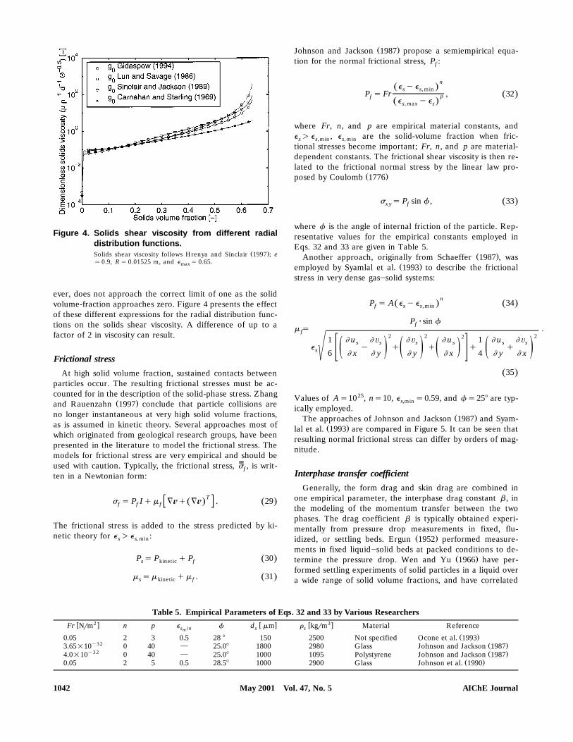
Figure 4. Solids shear viscosity from different radialdistribution functions.

Ž .Solids shear viscosity follows Hrenya and Sinclair 1997 ; es0.9, R s 0.01525 m, and e s 0.65.max

ever, does not approach the correct limit of one as the solidvolume-fraction approaches zero. Figure 4 presents the effectof these different expressions for the radial distribution func-tions on the solids shear viscosity. A difference of up to afactor of 2 in viscosity can result.

Frictional stressAt high solid volume fraction, sustained contacts between

particles occur. The resulting frictional stresses must be ac-counted for in the description of the solid-phase stress. Zhang

Ž .and Rauenzahn 1997 conclude that particle collisions areno longer instantaneous at very high solid volume fractions,as is assumed in kinetic theory. Several approaches most ofwhich originated from geological research groups, have beenpresented in the literature to model the frictional stress. Themodels for frictional stress are very empirical and should beused with caution. Typically, the frictional stress, s , is writ-ften in a Newtonian form:

Ts s P Iqm =©q =© . 29Ž . Ž .f f f

The frictional stress is added to the stress predicted by ki-netic theory for e )e :s s, min

P s P q P 30Ž .s kinetic f

m sm qm . 31Ž .s kinetic f

Ž .Johnson and Jackson 1987 propose a semiempirical equa-tion for the normal frictional stress, P :f

ne yeŽ .s s, min

P s Fr , 32Ž .pfe yeŽ .s, max s

where Fr, n, and p are empirical material constants, ande )e , e are the solid-volume fraction when fric-s s, min s, mintional stresses become important; Fr, n, and p are material-dependent constants. The frictional shear viscosity is then re-lated to the frictional normal stress by the linear law pro-

Ž .posed by Coulomb 1776

s s P sin f , 33Ž .x y f

where f is the angle of internal friction of the particle. Rep-resentative values for the empirical constants employed inEqs. 32 and 33 are given in Table 5.

Ž .Another approach, originally from Schaeffer 1987 , wasŽ .employed by Syamlal et al. 1993 to describe the frictional

stress in very dense gas]solid systems:

nP s A e ye 34Ž . Ž .f s s, min

P ? sin ffm s .f

2 2 221 u ® ® u 1 u ®s s s s s se y q q q qs) ž /ž / ž / ž /6 x y y x 4 y x

35Ž .

Values of As1025, ns10, e s0.59, and f s258 are typ-s,minically employed.

Ž .The approaches of Johnson and Jackson 1987 and Syam-Ž .lal et al. 1993 are compared in Figure 5. It can be seen that

resulting normal frictional stress can differ by orders of mag-nitude.

Interphase transfer coefficientGenerally, the form drag and skin drag are combined in

one empirical parameter, the interphase drag constant b , inthe modeling of the momentum transfer between the twophases. The drag coefficient b is typically obtained experi-mentally from pressure drop measurements in fixed, flu-

Ž .idized, or settling beds. Ergun 1952 performed measure-ments in fixed liquid]solid beds at packed conditions to de-

Ž .termine the pressure drop. Wen and Yu 1966 have per-formed settling experiments of solid particles in a liquid overa wide range of solid volume fractions, and have correlated

Table 5. Empirical Parameters of Eqs. 32 and 33 by Various Researchers2 3w x w x w xFr Nrm n p e f d mm r kgrm Material References in s sm

Ž .0.05 2 3 0.5 28 8 150 2500 Not specified Ocone et al. 1993y3 2 Ž .3.65=10 0 40 } 25.08 1800 2980 Glass Johnson and Jackson 1987

y3 2 Ž .4.0=10 0 40 } 25.08 1000 1095 Polystyrene Johnson and Jackson 1987Ž .0.05 2 5 0.5 28.58 1000 2900 Glass Johnson et al. 1990


Figure 5. Different expressions for the frictional normalstress.

their data and those of others for solids concentrations, 0.01Ž .Fe F0.63. Syamlal et al. 1993 use the empirical correla-s

Ž .tions of Richardson and Zaki 1954 and Garside and Al-Bi-Ž .bouni 1977 to determine the terminal velocity in fluidized

and settling beds expressed as a function of the solid volumefraction and the particle Reynolds number. From the termi-nal velocity, the drag force can be readily computed.

Ž .The drag model of Gidaspow 1994 follows Wen and YuŽ .1966 for solid volume fractions lower than 0.2 and Ergun

Ž .1952 for solid volume fractions larger than 0.2. The motiva-Ž .tion for this hybrid drag description of Gidaspow 1994 is

Ž .unclear because the Wen and Yu 1966 expression includesexperimental drag data for solid volume fractions larger than0.2. Moreover, a step change in the interphase drag constantis obtained at the ‘‘crossover’’ solid volume fraction of 0.2,which can possibly lead to difficulties in numerical conver-gence. The magnitude of this discontinuity in b increases withincreasing particle Reynolds number. The drag coefficientsare summarized in Table 6 and are compared quantitativelyin Figure 6 for a range of solid volume fractions at a fixedparticle Reynolds number.

SimulationsThe impact on the predicted flow patterns of the differ-

ences in the governing equations and constitutive models arecompared for the test cases of a freely bubbling fluidized-bed,a slugging fluidized bed, and a single bubble injection into afluidized bed. The particles in a fluidized bed move accord-ing to the action of the fluid through the drag force, andbubbles and complex solid mixing patterns result. Typically,the average solid volume fraction in the bed is fairly large,averaging about 40%, whereas in the the freeboard of the

Ž . Žfluidized bed the top there are almost no particles e fsy6.10 .The simulations in this work were carried out with the

commercial CFD code CFX 4.2 from AEA Technology, Har-Ž .well, UK, employing the Rhie-Chow Rhie and Chow, 1983

algorithm for discretization. For solving the difference equa-

Table 6. Drag Coefficients( )Wen and Yu 1966

Ž .1ye e r N© y© N3 s s g g s y2.65Ž .b s C 1yeD s4 dsŽ .Rowe 1961

24 0.687ŽŽ . . Ž .1q0.15 1ye Re if 1ye Re -1,000s p s pŽ .Re 1yep sC sD d r N© y© Ns g g s¼ Ž .0.44 Re s if 1ye Re G1,000p s pmg

( ) ( )Gidaspow 1994 applies the Ergun 1952 equation for higher ®olume fractions:2e m e r N© y© N7s g s g g s

150 q if e )0.2g2Ž . 4 d1ye d ss sb s

Ž .1ye e r N© y© N3 s s g g s¼ y2 .65Ž .C 1ye if e F0.2D s s4 ds

( )Syamlal et al. 1993Ž .e 1ye r3 s s g

b s C N© y© ND g s24 V dr sŽ .Dalla Valle 1948

2Vr

C s 0.63q4.8(D ž /ReŽ .Garside and Al-Dibouni 1977

1 2 2'Ž . Ž .V s ay0.06 Req 0.06 Re q0.12 Re 2by a q ar 24.14Ž .as 1yes

1.28Ž .0.8 1ye if e G0.15s sbs

2.65½ Ž .1ye if e -0.15s s


Ž .tions, the higher-order total variation diminishing TVDscheme, Superbee is used. This TVD scheme incorporates a

Žmodification to the higher-order upwind scheme second or-.der . The time discretization is done with the second-order

backward-difference scheme. The solution of the pressurefrom the momentum equations requires a pressure correctionequation, correcting the pressure and the velocities after each

Ž .iteration; for this, the SIMPLE Patankar, 1980 algorithm isemployed. The calculated pressure is used to determine thedensity of the fluid phase; the simulations are performed al-lowing for compressibility of the gas phase. The grid spacingwas determined by refining the grid until average propertieschanged by less than 4%. Due to the deterministic chaoticnature of the system, the dynamic behavior always changeswith the grid. The simulations of the slugging fluidized bedand the freely bubbling fluidized bed were carried out for 25s of real time. After about 5 s of real time, the simulation hasreached a state in which averaged properties stay unchanged.Averaged properties, such as bubble size and bed expansion,were determined by averaging over the last 15 s of real timein each simulation. A bubble is defined as a void in the solidphase with a solid volume fraction less than 15%. The bubblediameter is defined as the diameter of a circle having thesame surface as the void in the solid phase; this is called theequivalent bubble diameter.

Boundary conditionsAll the simulations are carried out in a two-dimensional

rectangular space in which front and back wall effects areneglected. The left and right walls of the fluidized bed aretreated as no-slip velocity boundary conditions for the fluidphase, and the free-slip velocity boundary conditions are em-ployed for the particle phase. A possible boundary conditionfor the granular temperature follows Johnson and JacksonŽ .1987 :

n ? k=Q sŽ .

'pr e 3Q 3Qs s X 2 2w N© N y 1y e , 36Ž .Ž .slip w1r3 2es6e 1ys, max ž /es, max

where the lefthand side represents the conduction of granu-lar energy to the wall, the first term on the righthand siderepresents the generation of granular energy due to particleslip at the wall, and the second term on the righthand siderepresents dissipation of granular energy due to inelastic col-lisions. Another possibility for the boundary condition for the

Ž .granular temperature is proposed by Jenkins 1992 :

n ? k=Q sy© ? My D , 37Ž . Ž .slip

where the exact formulations of M and D depend upon theamount of friction and sliding occurring at the wall region.Simulations we have done with an adiabatic boundary condi-

Ž .tion at the wall =Qs0 show very similar results.ŽThe boundary condition at the top of the freeboard fluid-

.phase outlet is a so-called pressure boundary. The pressure

Figure 6. Different expressions for the interphase dragcoefficient as a function of solid volume-frac-tion: Re s45.p

at this boundary is fixed to a reference value, 1.013=105 Pa.Neumann boundary conditions are applied to the gas flow,requiring a fully developed gas flow. For this, the freeboardof the fluidized bed needs to be of sufficient height; this isvalidated through the simulations. In the freeboard, the solidvolume fraction is very close to zero, and this can lead tounrealistic values for the particle-velocity field and poor con-vergence. For this reason, a solid volume fraction of 10y6 isset at the top of the freeboard. This way the whole freeboardis filled with a very small number of particles, which givesmore realistic results for the particle phase velocity in thefreeboard, but does not influence the behavior of the flu-idized bed itself.

The bottom of the fluidized bed is made impenetrable forthe solid phase by setting the solid phase axial velocity tozero. For the freely bubbling fluidized bed and the sluggingfluidized bed, Dirichlet boundary conditions are employed atthe bottom with a uniform gas inlet velocity. To break thesymmetry in the case of the bubbling and slugging beds, ini-tially a small jet of gas is specified at the bottom lefthandside of the geometry. In the case of the bubble injection, aDirichlet boundary condition is employed at the bottom ofthe fluidized bed. The gas inlet velocity is kept at the mini-mum fluidization velocity, except for a small orifice in thecenter of the bed, at which a very large inlet velocity is speci-fied. Finally, the solid-phase stress, as well as the granulartemperature at the top of the fluidized bed, are set to zero.

Initial conditionsInitially, the bottom part of the fluidized bed is filled with

particles at rest with a uniform solid volume fraction. The gasflow in the bed is set to its minimum fluidization velocity. Inthe freeboard a solid volume fraction of 10y6 is set, as ex-plained earlier. The granular temperature is initially set to10y10 m2? sy2.

Test CaseWith increasing gas velocity above the minimum fluidiza-

tion velocity, U , bubbles are formed as a result of the in-m f


Figure 7. Computational grid of simulated fluidizedbeds with the gas inlet boundary condition.Ž . Ž .a Freely bubbling fluidized bed; b slugging fluidized bed,Ž .c bubble injection into a fluidized bed.

herent instability of the gas]solid system. The behavior ofthe bubbles significantly affects the flow phenomena in thefluidized bed, that is, solid mixing, entrainment, and heat andmass transfer. The test cases in this comparative study areused to investigate the effect of different closure models andgoverning equations on the bubble behavior and bed expan-sion. Simulation results of each test case are compared to

Ž .generally accepted experimental data and semi empiricalmodels. The system properties and computational parame-ters for each of the test cases are given in Table 7; the com-

putational meshes are also shown in Figure 7. The test casesare discussed in greater detail in the following sections.

Freely bubbling fluidized bedsIn the freely fluidized-bed case, the gas flow is distributed

uniformly across the inlet of the bed. Small bubbles form atthe bottom of the fluidized bed that rise, coalesce, and eruptas large bubbles at the fluidized-bed surface. In order to

Ž .evaluate model predictions, we use the Darton et al. 1977bubble model for bubble growth in freely bubbling fluidizedbeds. This model is based upon preferred paths of bubbleswhere the distance traveled by two neighboring bubbles be-fore coalescence is proportional to their lateral separation.

Ž .Darton et al. 1977 have validated their model with mea-surements of many researchers. Their proposed bubble-growth equation for Geldart type B particles is

0.80.4 y0.2D s0.54 UyU hq4 A g , 38' Ž .Ž . Ž .b m f 0

where D is the bubble diameter, h is the height of the bub-bble above the inlet of the fluidized bed, U is the actual super-ficial gas inlet velocity, and A is the ‘‘catchment area’’ that0characterizes the distributor. For a porous-plate gas distribu-

Ž .tor, Darton et al. 1977 propose 4 A s0.03 m.' 0Ž .Werther and Molerus 1973 have developed a small capac-

itance probe and the statistical theory to measure the bubblediameter and the bubble rise velocity in fluidized beds usingthis probe. This capacitance probe can be placed in the flu-idized bed at different heights and radial positions in the bed.The bubble rise velocity is determined by placing two verti-cally spaced probes and correlating the obtained data. Thecapacitance probe measures the bubbles passing it, that is,the bubble is pierced by the capacitance probe. The durationof this piercing is dependent upon the size of the bubble, therise velocity of the bubble, and the vertical position of thebubble relative to the probe.

Ž .Hilligardt and Werther 1986 have done many measure-ments of bubble size and bubble velocity under various con-ditions using the probe developed by Werther and MolerusŽ .1973 and have correlated their data in the form of the

Ž .Davidson and Harrison 1963 bubble model. Hilligardt and

Table 7. System Properties and Computational Parameters

Freely Bubbling Slugging Bubble Injection intoŽ .Parameter Description Fluidized Bed Fluidized Bed Fluidized Bed Kuipers, 1990

3w xr kgrm Solid density 2,640 2,640 2,660s3w xr kgrm Gas density 1.28 1.28 1.28g

y5 y5 y5w xm Pa ? s Gas viscosity 1.7=10 1.7=10 1.7=10gw xd mm Particle diameter 480 480 500s

e Coefficient of restitution 0.9 0.9 0.9e Max. solid volume fraction 0.65 0.65 0.65max

w xU mrs Minimum fluidization velocity 0.21 0.21 0.25m fw xD m Inner column diameter 0.5 0.1 0.57Tw xH m Column height 1.3 1.3 0.75t

w xH m Height at minimum fluidization 0.97 0.97 0.5m fe Solids volume fraction 0.42 0.42 0.402s, m f

at minimum fluidizationy3 y3 y3w xD x m x-mesh spacing 7.14=10 6.67=10 7.50=10y3 y3 y2w xD y m y-mesh spacing 7.56=10 7.43=10 1.25=10


Werther propose a variant of the Davidson and HarrisonŽ .1963 model for predicting the bubble rise velocity as a func-tion of the bubble diameter,

u sc UyU qwn gd , 39' Ž .Ž .b m f b

where w is the analytically determined square root of theFroude number of a single rising bubble in an infinitely large

Ž .homogeneous area. Pyle and Harrison 1967 have deter-mined that w s0.48 for a two-dimensional geometry, whereasin three dimensions the Davies-Taylor relationship gives w s0.71. The symbols c and n , added by Hilligardt and WertherŽ .1986 , are empirical coefficients based on their data, whichare dependent upon the type of particles and the width andheight of the fluidized bed. For the particles and geometry

Ž .employed in this study, Hilligardt and Werther 1986 pro-pose c f0.3 and n f0.8. Proposals of values for c and nunder various fluidization conditions, determined by simula-

Ž .tions, are given by Van Wachem et al. 1998 .Ž .Hilligardt and Werther 1986 also measured bed expan-

sion under various conditions. Predictions of the bed expan-sion from the simulations are compared to these data.

Slugging fluidized bedsIn the case of the slugging fluidized beds, coalescing bub-

bles eventually reach a diameter of 70% or more of the col-umn diameter, resulting from either a large inlet gas velocityor a narrow bed. The operating conditions employed in thesimulations correspond to the slugging conditions reported

Ž .by Kehoe and Davidson 1971 , who present a detailed studyof slug flow in fluidized beds. The experiments of Kehoe and

Ž .Davidson 1971 were performed in slugging fluidized beds of2.5-, 5-, and 10-cm diameter columns using Geldart B parti-cles from 50-mm to 300-mm diameter and with superficial gasinlet velocities of up to 0.5 mrs. X-Ray photography was usedto determine the rise velocity of slugs and to determine the

Ž .bed expansion. Kehoe and Davidson 1971 use their data tovalidate two different equations for the slug rise velocity, bothbased on two-phase theory:

wu sUyU q gD 40' Ž .slug m f T2

wu sUyU q 2 gD , 41' Ž .slug m f T2

where w is the analytically determined square root of theFroude number of a single rising bubble. Equation 40 is theexact two-phase theory solution, and Eq. 41 is a modificationof Eq. 40, based on the following observations:

Ž .1. For fine particles -70 mm the slugs travel symmetri-cally up in the fluidized bed, so the slug rise velocity is in-creased by coalescence.

Ž .2. For coarser particles )70 mm the slugs tend to moveup the walls, which also increases their velocity.

Ž .According to Kehoe and Davidson 1971 , Eqs. 40 and 41give upper and lower bounds on the slug rise velocity. Fur-

Ž .thermore, Kehoe and Davidson 1971 measured the maxi-Ž .mum bed expansion H during slug flow. They validatedmax

their theoretical analysis, which led to the result that

H y H UyUmax m f m fs , 42Ž .

H um f bub

where u is the rise velocity of a slug without influence ofbubthe gas phase,

wu s gD 43' Ž .bub T2

or

wu s 2 gD , 44' Ž .bub T2

corresponding to Eqs. 40 and 41. Hence, they also proposeupper and lower bounds on the maximum bed expansion.

Bubble injection in fluidized bedsSingle jets entering a minimum fluidized bed through a

narrow single orifice provide details of bubble formation andŽ .growth. Such experiments were carried out by Kuipers 1990 .

Ž .Kuipers 1990 reported the shape of the injected bubble aswell as the quantitative size and growth of the bubble withtime using high-speed photography. The superficial gas-inletvelocity from the orifice was Us10 mrs, and the orifice wasds1.5=10y2 m wide.

Results and DiscussionPredictions based on simulations of these three test cases

are used to compare the different governing and closuremodels. For this comparative study, only one particular clo-sure model is varied at a time, to determine the sensitivity ofthe model predictions to that particular closure. No couplingeffects were investigated. The default governing equations are

Ž .those given by Jackson 1997 , and the default closure modelsŽ .are the solid-phase stress of Hrenya and Sinclair 1997 , theŽ .radial distribution function of Lun and Savage 1986 , the

Ž .frictional model of Johnson and Jackson 1987 with empiri-Ž .cal values given by Johnson et al. 1990 , the complete

granular energy balance neglecting J , and the drag coeffi-sŽ .cient model of Wen and Yu 1966 . For animations of some

of the simulations, please refer to our W ebsitehttp:rrwww.tcp.chem.tue.nlr;scrrwachemrcompare.html.

Go©erning equationsSimulations of the slugging bed case were performed with

Ž . Ž .both the Ishii 1975 and the Jackson 1997 governing equa-tions. Figure 8 shows the predicted maximum bed expansionwith increasing gas velocity during the slug flow and the two

Ž .correlations of Kehoe and Davidson 1971 . Figure 9 showsthe increasing slug rise velocity with increasing gas velocity.Clearly, the exact formulation of the governing equation doesnot have any significant influence on the prediction of thesemacroscopic engineering quantities, and both CFD modelsdo a good job at predicting these quantities. Microscopically,however, there does seem to be a difference in the predic-


Figure 8. Predicted maximum expansion of a sluggingfluidized bed with increasing gas velocity with

( )the governing equations of Jackson 1997( )and Ishii 1975 , and the additional term J ins

the granular energy equation.The predictions are compared with the two-phase theory as

Ž .proposed and validated by Kehoe and Davidson 1971 .

tions, as indicated in Figure 10. The flow of the gas phase inareas of large solid volume-fraction gradient is slightly differ-ent, leading to a different solids distribution. Specifically,

Ž .Figure 10 shows that the Jackson 1997 governing equationsproduce a more round-nosed bubble shape than the IshiiŽ .1975 equations, because the path of the gas phase is differ-ent.

Figure 9. Predicted slug rise velocity with increasinggas velocity with the governing equations of

( ) ( )Jackson 1997 and Ishii 1975 , and the addi-tional term J in the granular energy equation.sThe predictions are compared with the two-phase theory as

Ž .proposed and validated by Kehoe and Davidson 1971 . Theconstant w s 0.48.

Figure 10. Rising bubble in a slugging fluidized bed( )predicted by a employing the governing

( ) ( )equations of Jackson 1997 , and by b em-ploying the governing equations of Ishii( )1975 at the same real time; the lines arecontours of equal solid volume fraction.

Solids stress modelsThe exact solid-phase stress description does not influence

either the freely bubbling or the slugging fluidized-bed pre-dictions, as is expected from Figure 1; this figure shows thatbetween 0.4 and 0.6 solids volume fraction, which is domi-nant in the cases studied, all solids-phase stress predictionsare equal. Moreover, the influence of the radial distributionupon the stress does not give rise to any variation in the pre-dictions of the engineering quantities associated with thesesimulations; the variation of the solids phase stress as a func-tion of radial distribution function, shown in Figure 4, is smallbetween 0.4 and 0.6 solids volume fraction, as long as the

Ž .Carnahan and Starling 1969 equation is not employed. Fromthe magnitude of the terms on the solid-phase momentumbalance during simulations of fluidized beds, it can be con-cluded that gravity and drag are the dominating terms andthat solids-phase stress predicted by kinetic theory plays aminor role.

Drag modelsCoordinating with results of the comparison of the drag

Ž .models shown in Figure 6, the Syamlal et al. 1993 drag leadsto a lower predicted pressure drop and lower predicted bedexpansion than the other two drag models. Figure 11 showsthe average simulated bed expansion employing different drag


Figure 11. Predicted bed expansion as a function of gasvelocity based on different drag models andwith and without frictional stress.The predictions are compared to the experimental data of

Ž .Hilligardt and Werther 1986 . The spread in the simula-Ž .tion data with the drag model of Gidaspow 1994 is indi-

cated by the line.

models in the freely bubbling fluidized-bed case, comparedŽ .to measurements of Hilligardt and Werther 1986 . The drag

Ž .model of Syamlal et al. 1993 underpredicts the bed expan-sion compared to the findings of Hilligardt and WertherŽ .1986 , and therefore also underpredicts the gas holdup inthe fluidized bed.

Figure 12 shows the simulated bubble size as a function ofthe bed height when employing different drag models, com-

Ž .pared with the Darton et al., 1977 equation. Although the

Figure 12. Predicted bubble size as a function of bedheight at Us0.54 mrrrrrs based on differentdrag models and compared to the correla-

( )tion of Darton et al. 1977 .The vertical lines indicate the spread of the simulatedbubble size.

Figure 13. Predicted bubble rise velocity as a functionof the bubble diameter at U s 0.54 mrrrrrsbased on different drag models and com-pared to the experimental correlation of Hilli-

( )gardt and Werther 1986 .The vertical lines indicate the spread of the simulatedbubble rise velocity.

spread in the simulations is fairly large, all of the investigateddrag models are in agreement with the equation put forth by

Ž .Darton et al. 1977 . Figure 13 shows the predicted bubblerise velocity employing different drag models in a freely bub-bling fluidized bed, compared to the empirical correlation of

Ž .Hilligardt and Werther 1986 . All of the investigated dragmodels are in fairly good agreement with the empirical corre-lation.

Because the bubble sizes predicted by the different dragmodels are all close, while the predicted bed expansion dif-fers between the models, variations in the predicted solid-volume fraction of the dense phase exist between the models,

Ž .with the Syamlal et al. 1993 drag model predicting the high-est solid volume fraction in the dense phase.

Figure 14 shows the quantitative bubble-size prediction fora single jet entering a minimum fluidized bed based on the

Ž . Ž .drag models of Wen and Yu 1966 and Syamlal et al. 1993 ,which are compared to the experimental data of KuipersŽ .1990 . Moreover, in Figure 15 we show the resulting qualita-tive predictions of the bubble growth and shape, and also

Ž .compare these with photographs by Kuipers 1990 . The WenŽ .and Yu 1966 drag model yields better agreement withŽ .Kuipers’ 1990 findings for both the bubble shape and size

Ž .than the Syamlal et al. 1993 drag model. The Syamlal et al.Ž .1993 drag model underpredicts the bubble size and pro-duces a bubble that is more circular in shape than in the

Ž .experiments of Kuipers 1990 and in the simulations withŽ .the Wen and Yu 1966 drag model.

Frictional stressFrictional stresses can increase the total solid-phase stress

by orders of magnitude, and is an important contributing forcein dense gas]solid modeling. The simulation of the single jet


Figure 14. Bubble diameter as a function of time for abubble formed at a single jet of Us10 mrrrrrs.A comparison is made between the experiments of KuipersŽ .1990 , model simulations using the drag coefficient of Wen

Ž .and Yu 1966 with and without frictional stress, and modelsimulations using the interphase drag constant of Syamlal

Ž .et al. 1993 .

entering a fluidized bed reveals that the size of the bubble isnot significantly influenced by the frictional stress, as shownin Figure 14. However, Figure 11 shows that the predictedbed expansion in the freely bubbling fluidized bed is signifi-cantly less without frictional stress. Moreover, the number ofiterations for obtaining a converged solution is almost dou-bled when frictional stress is omitted. Without frictionalstress, there is less air in the dense phase, the maximum

Figure 15. Experimental and simulated bubble shapeassociated with a single jet at Us10 mrrrrrsand at t s0.10 s and t s0.20 s.

Ž .Comparison is made between the a experiment of KuipersŽ . Ž .1990 ; b model simulation using the interphase drag

Ž . Ž .constant of Wen and Yu 1966 ; c model simulation usingŽ .the interphase drag constant of Syamlal et al. 1993 .

Žachieved solids packing is higher maximum achieved solids.volume fraction increased from 0.630 to 0.649 , and the bed

expansion is less. Moreover, the solid-phase stress in thedense regions are significantly decreased because the pre-dicted granular temperature in the dense region of flow is

Ž y5 2 y2 .very low Qf10 m ? s due to the magnitude of the dis-sipation term. When frictional stress is neglected in the simu-lations, convergence difficulty arises because the maximumsolid volume fraction specified in the radial distribution func-tion is approached and the derivative of the radial distribu-tion function near maximum solid volume fraction is ex-tremely steep. In order to still obtain convergence, we havewritten the radial distribution function as a Taylor series ap-proximation at very high solid volume fraction. Adding fric-tional stress in the simulations prevents this problem, be-cause then the solid volume fraction does not approach themaximum packing value.

Granular energy balanceThe influence of the additional generation and dissipation

term J in the granular energy balance is determined in thescase of the slugging fluidized bed. Figure 8 shows the predic-tions of the maximum bed expansion as a function of increas-ing gas velocity for simulations with and without this addi-tional term. Figure 9 also shows the predicted rise velocity ofthe slugs with and without this additional term J . Althoughsthis additional term J results in as much as 20% highers

Žgranular temperature values granular temperature increased2 y2 2 y2 .from 0.138 m ? s to 0.165 m ? s , this does not seem to

influence the predicted bed expansion or the slug rise veloc-Ž .ity. The exact formulation of J Eq. 26 or 27 does not play as

role in the predicted granular temperature.Simulations of slugging fluidized beds were also performed

using the simplified algebraic granular energy equation, Eq.21. There were no differences in predicted bed expansion,bubble size, or bubble rise velocity due to this simplificationvs. using the full granular energy balance. This simplifiedequation gives rise to deviations from full granular energy-balance predictions of as much as 10% in the granular tem-

Ž 2 y2perature granular temperature decreased from 0.138 m ? s2 y2 .to 0.0127 m ? s . The computational effort for solving the

complete granular energy equation is about 20% higher thancalculating the granular temperature from the algebraicequation. More simulation results of the freely bubbling flu-idized bed case with the algebraic equation are given in van

Ž .Wachem et al. 1998 .

ConclusionsIn this article we have compared different formulations that

are employed in CFD models for gas]solid flow in the Eule-rianrEulerian framework. We discussed the basis for the for-mulation of the two different sets of governing equationscommon to the two-fluid literature with respect to the natureof the dispersed phase. It is shown in detail that the model-ing of gas]solid flows requires different governing equationsthan the modeling of gas]liquid flows. We also have com-pared various closure models both quantitatively and qualita-tively. For example, we have shown how the hybrid drag model

Ž .proposed by Gidaspow 1994 produces a discontinuity in the


drag coefficient, how an order-of-magnitude difference in thenormal stress is predicted by the various frictional stress

Ž .models, and how the Syamlal et al. 1993 model predicts alower bed expansion than with the other drag models.

Finally, we have studied the impact of the two governingequations and the various closure models on simulation pre-dictions in three fluidized-bed test cases. It is shown that theresulting predictions based on the two sets of governingequations are similar on an engineering scale, but are differ-ent in terms of microscopic features associated with individ-ual bubbles or localized solids distributions. It is also shownthat the model predictions are not sensitive to the use of dif-ferent solids stress models or radial distribution functions. Indense-phase gas]solid flow, the different approaches in thekinetic theory modeling predict similar values for the solid-phase properties. From an analysis of the individual terms onthe momentum balance of the solid-phase momentum bal-ance during the simulations, it can be concluded that gravityand drag are the most dominating terms; this is why the twodifferent sets of governing equations predict similar results,and why the exact solid-phase stress prediction is of minorimportance. At a very high volume fraction, frictional stresscan influence the hydrodynamic prediction due to its largemagnitude. Simplifying the granular energy balance by re-taining only the generation and dissipation terms is a reason-able assumption in the case of fluidized-bed modeling andreduces the computational effort by about 20%. Finally, themanner in which the drag force is modeled has a significantimpact on the simulation results, influencing the predictedbed expansion and the solids concentration in the dense-phase regions of the bed.

AcknowledgmentsŽ .The investigations were supported in part by the Netherlands

Ž .Foundation for Chemical Research SON , with financial aid fromŽ .the Netherlands Organization for Scientific Research NWO . This

support is largely acknowledged. B.G.M. van Wachem gratefully ac-knowledges the financial support of the Netherlands Organization

Ž .for Scientific Research NWO , the Stimulation fund for Internation-Ž .alization SIR , DelftChemTech, the Delft University Fund, and the

Ž .Reactor Research Foundation RR , for the expenses for visitingPurdue University.

NotationAsempirical constant

A scatchment area of distributor, m20

C sdrag coefficientDd sparticle diameter, ms

y1D sstrain rate tensor, ssDsdiameter, m

D sinner column diameter, mTescoefficient of restitutionf sfluid-phase point property

Fr sempirical material constant, N ?my2

Ž .g r sweighting functiong sgravitational constant, m ? sy2

g sradial distribution function0hsheight of bubble in fluidized bed, m

H sminimum fluidization bed height, mm fH scolumn height, mt

J sfluctuating velocityrforce correlation, kg ?my3 ? sy1

Lsinterfacial area per unit volume, my1

Msinterphase momentum exchange, N ? sy1

nsempirical constant in frictional stressnsnumber densitynsnormal vector, m

psempirical constant in frictional stressP spressure, N ?my2

r spoint in space, mRscharacteristic length scale, m

ResReynolds numberSssurface, m2

tstime, sŽ . y1Usinlet superficial gas velocity, m ? s

U sminimum fluidization velocity, m ? sy1m f

©svelocity vector, m ? sy1

V svolume, m3

V sratio of terminal velocity of a group of particles to that of anrisolated particle

xsposition vector, mX sphase indicator

D xsx-mesh spacing, mD ysy-mesh spacing, m

Greek lettersb sinterphase drag constant, kg ?my3 ? sy1

e svolume fractionŽ .hs1r2 1q e

f sangle of internal frictionw ssquare root of the Froude number

wX sspecularity coefficientg sdissipation of granular energy, kg ?my3 ? sy1

k ssolids thermal conductivity, kg ?my1 ? sy1

lssolids bulk viscosity, Pa ? sl smean free path, mm f p

mssolids shear viscosity, Pa ? sn sempirical coefficientc sempirical coefficientr sdensity, kg ?my3

y2s stotal stress tensor, N ?my2t sviscous stress tensor, N ?m

Qsgranular temperature, m2 ? sy2

Subscriptsbsbubble

bubssingle bubbledilsdilute

f sfrictionalg sgas phaseisinterface

kseither phasemf sminimum fluidization

minsminimum; kick-in valuemax smaximum

psparticlesssolids phase

slipsslipslug sslug

wswall

Literature CitedAlder, B. J., and T. E. Wainwright, ‘‘Studies in Molecular Dynamics:

II. Behaviour of a Small Number of Elastic Spheres,’’ J. Chem.Ž .Phys., 33, 1439 1960 .

Anderson, T. B., and R. Jackson, ‘‘A Fluid Mechanical DescriptionŽ .of Fluidized Beds,’’ Ind. Eng. Chem. Fundam., 6, 527 1967 .

Barthod, D., M. Del Pozo, and C. Mirgain, ‘‘CFD-Aided Design Im-Ž .proves FCC Performance,’’ Oil Gas J., 66 1999 .

Boemer, A., H. Qi, U. Renz, S. Vasquez, and F. Boysan, ‘‘EulerianComputation of Fluidized Bed Hydrodynamics}A Comparison ofPhysical Models,’’ Proc. of the Int. Conf. on FBC, Orlando, FL, p.

Ž .775 1995 .Carnahan, N. F., and K. E. Starling, ‘‘Equations of State for Non-At-

Ž .tracting Rigid Spheres,’’ J. Chem. Phys., 51, 635 1969 .Chapman, S., and T. G. Cowling, The Mathematical Theory of Non-

Ž .Uniform Gases, Cambridge Univ. Press, 3rd Ed., Cambridge 1970 .


Coulomb, C. A., ‘‘Essai sur Une Application des Regles de Maximis´et Minimis a Quelques Problemes de Statique, Relatifs a l’Archi-` ` ´tecture,’’ Acad. R. Sci. Mem. Math, Phys. Di®ers. Sa®ants, 7, 343`Ž .1776 .

Ž .Dalla Valle, J. M., Micromeritics, Pitman, London 1948 .Darton, R. C., R. D. LaNauze, J. F. Davidson, and D. Harrison,

‘‘Bubble Growth Due to Coalescence in Fluidized Beds,’’ Trans.Ž .Inst. Chem. Eng., 55, 274 1977 .

Davidson, J. F., and D. Harrison, Fluidized Particles, Cambridge Univ.Ž .Press, Cambridge 1963 .

Enwald, H., E. Peirano, and A. E. Almstedt, ‘‘Eulerian Two-PhaseFlow Theory Applied to Fluidization,’’ Int. J. Multiphase Flow, 22,

Ž .21 1996 .Ergun, S., ‘‘Fluid Flow through Packed Columns,’’ Chem. Eng. Prog.,

Ž .48, 89 1952 .Garside, J., and M. R. Al-Dibouni, ‘‘Velocity-Voidage Relationship

for Fluidization and Sedimentation,’’ Ind. Eng. Chem. Proc. Des.Ž .De®., 16, 206 1977 .

Gidaspow, D., Multiphase Flow and Fluidization, Academic Press, SanŽ .Diego 1994 .

Gidaspow, D., and L. Huilin, ‘‘Equation of State and Radial Distri-bution Functions of FCC Particles in a CFB,’’ AIChE J., 44, 279Ž .1998 .

Hilligardt, K., and J. Werther, ‘‘Local Bubble Gas Hold-Up and Ex-pansion of GasrSolid Fluidized Beds,’’ Ger. Chem. Eng., 9, 215Ž .1986 .

Hoomans, B. P. B., J. A. M. Kuipers, W. J. Briels, and W. P. M. vanSwaaij, ‘‘Discrete Particle Simulation of Bubble and Slug Forma-tion in a Two-Dimensional Gas-Fluidised Bed: A Hard-Sphere

Ž .Approach,’’ Chem. Eng. Sci., 51, 99 1996 .Hrenya, C. M., and J. L. Sinclair, ‘‘Effects of Particle-Phase Turbu-

Ž .lence in Gas-Solid Flows,’’ AIChE J., 43, 853 1997 .Ishii, M., Thermo-Fluid Dynamic Theory of Two-Phase Flow, Direc-

tion des Etudes et Recherches d’Electricite de France, Eyrolles,´Ž .Paris 1975 .

Ishii, M., and K. Mishima, ‘‘Two-Fluid Model and HydrodynamicŽ .Constitutive Relations,’’ Nucl. Eng. Des., 82, 107 1984 .

Jackson, R., ‘‘The Mechanics of Fluidized Beds: Part I: The Stabilityof the State of Uniform Fluidization,’’ Trans. Inst. Chem. Eng., 41,

Ž .13 1963 .Jackson, R., ‘‘Locally Averaged Equations of Motion for a Mixture

of Identical Spherical Particles and a Newtonian Fluid,’’ Chem.Ž .Eng. Sci., 52, 2457 1997 .

Ž .Jackson, R., ‘‘Erratum,’’ Chem. Eng. Sci., 53, 1955 1998 .Jenkins, J. T., ‘‘Boundary Conditions for Rapid Granular Flow: Flat,

Ž .Frictional Walls,’’ J. Appl. Mech., 59, 120 1992 .Jenkins, J. T., and S. B. Savage, ‘‘A Theory for the Rapid Flow of

Identical Smooth, Nearly Elastic, Spherical Particles,’’ J. FluidŽ .Mech., 130, 187 1983 .

Johnson, P. C., and R. Jackson, ‘‘Frictional-Collisional ConstitutiveRelations for Granular Materials, with Application to Plane Shear-

Ž .ing,’’ J. Fluid Mech., 176, 67 1987 .Johnson, P. C., P. Nott, and R. Jackson, ‘‘Frictional-Collisional

Equations of Motion for Particulate Flows and Their ApplicationŽ .to Chutes,’’ J. Fluid Mech., 210, 501 1990 .

Kehoe, P. W. K., and J. F. Davidson, ‘‘Continuously Slugging Flu-Ž .idised Beds,’’ Inst. Chem. Eng. Symp. Ser., 33, 97 1971 .

Koch, D. L., ‘‘Kinetic Theory for a Monodisperse Gas-Solid Suspen-Ž .sion,’’ Phys. Fluids A, 2, 1711 1990 .

Koch, D. L., and A. S. Sangani, ‘‘Particle Pressure and MarginalStability Limits for a Homogeneous Monodisperse Gas-FluidizedBed: Kinetic Theory and Numerical Simulation,’’ J. Fluid Mech.,

Ž .400, 229 1999 .

Kuipers, J. A. M., A Two-Fluid Micro Balance Model of Fluidized Beds,Ž .PhD Thesis, Univ. of Twente, Twente, The Netherlands 1990 .

Louge, M. Y., E. Mastorakos, and J. T. Jenkins, ‘‘The Role of Parti-cle Collisions in Pneumatic Transport,’’ J. Fluid Mech., 231, 345Ž .1991 .

Lun, C. K. K., and S. B. Savage, ‘‘The Effects of an Impact VelocityDependent Coefficient of Restitution on Stresses Developed by

Ž .Sheared Granular Materials,’’ Acta Mech., 63, 15 1986 .Lun, C. K. K., S. B. Savage, D. J. Jefferey, and N. Chepurniy, ‘‘Kinetic

Theories for Granular Flow: Inelastic Particles in Couette Flowand Slightly Inelastic Particles in a General Flowfield,’’ J. Fluid

Ž .Mech., 140, 223 1984 .Nadim, A., and H. A. Stone, ‘‘The Motion of Small Particles and

Ž .Droplets in Quadratic Flows,’’ Stud. Appl. Mech., 85, 53 1991 .Ocone, R., S. Sundaresan, and R. Jackson, ‘‘Gas-Particle Flow in a

Duct of Arbitrary Inclination with Particle-Particle Interactions,’’Ž .AIChE J., 39, 1261 1993 .

Patankar, S. V., Numerical Heat Transfer and Fluid Flow, Hemi-Ž .sphere, New York 1980 .

Ž .Pyle, D. L., and D. Harrison, Chem. Eng. Sci., 22, 531 1967 .Rhie, C. M., and W. L. Chow, ‘‘Numerical Study of the Turbulent

Flow Past an Airfoil with Trailing Edge Separation,’’ AIAA J1, 21,Ž .1527 1983 .

Richardson, J. F., and W. N. Zaki, ‘‘Sedimentation and Fluidisation:Ž .I,’’ Trans. Inst. Chem. Eng., 32, 35 1954 .

Rowe, P. N. ‘‘Drag Forces in a Hydraulic Model of a Fluidized Bed:Ž .II,’’ Trans. Inst. Chem. Eng., 39, 175 1961 .

Sangani, A. S., G. Mo, H.-K. Tsao, and D. L. Koch, ‘‘Simple ShearFlows of Dense Gas-Solid Suspensions at Finite Stokes Numbers,’’

Ž .J. Fluid Mech., 313, 309 1996 .Schaeffer, D. G., ‘‘Instability in the Evolution Equations Describing

Ž .Incompressible Granular Flow,’’ J. Differ. Eqs., 66, 19 1987 .Sinclair, J. L., ‘‘Hydrodynamic Modelling,’’ Circulating Fluidized Beds,

J. R. Grace, A. A. Evidan, and T. M. Knowlton, eds., Blackie,Ž .London, p. 149 1997 .

Sinclair, J. L., and R. Jackson, ‘‘Gas-Particle Flow in a Vertical PipeŽ .with Particle-Particle Interactions,’’ AIChE J., 35, 1473 1989 .

Syamlal, M., W. Rogers, and T. J. O’Brien, ‘‘Mfix DocumentationTheory Guide,’’ U.S. Dept. of Energy, Office of Fossil Energy,

Ž .Tech. Note 1993 .Tsuji, Y., T. Kawaguchi, and T. Tanaka, ‘‘Discrete Particle Simula-

tion of Two-Dimensional Fluidized Bed,’’ Powder Technol., 77, 79Ž .1993 .

Van Wachem, B. G. M., J. C. Schouten, R. Krishna, and C. M. vanden Bleek, ‘‘Eulerian Simulations of Bubbling Behaviour in Gas-

Ž .Solid Fluidised Beds,’’ Comput. Chem. Eng., 22, s299 1998 .Van Wachem, B. G. M., J. C. Schouten, R. Krishna, and C. M. van

den Bleek, ‘‘Validation of the Eulerian Simulated Dynamic Be-haviour of Gas-Solid Fluidised Beds,’’ Chem. Eng. Sci., 54, 2141Ž .1999 .

Wen, C. Y., and Y. H. Yu, ‘‘Mechanics of Fluidization,’’ Chem. Eng.Ž .Prog. Symp. Ser., 62, 100 1966 .

Werther, J., and O. Molerus, ‘‘The Local Structure of Gas FluidizedBeds I. A Statistically Based Measured System,’’ Int. J. Multiphase

Ž .Flow, 1, 103 1973 .Zhang, D. Z., and R. M. Rauenzahn, ‘‘A Viscoelastic Model for

Ž .Dense Granular Flows,’’ J. Rheol., 41, 1275 1997 .

Manuscript recei®ed Dec. 7, 1999, and re®ision recei®ed Oct. 9, 2000.


Comparative Analysis of CFD Models for dense Gas-Solid Systems

Documents

Transcript of Comparative Analysis of CFD Models for dense Gas-Solid Systems