Combined vs. Separate Views in Matrix-based Graph Analysis and Comparison

Alan G. Melville, Martin Graham, Jessie B. Kennedy School of Computing

Edinburgh Napier University Edinburgh, United Kingdom

{a.melville, m.graham, j.kennedy}@napier.ac.uk

Abstract—While much work has been done in the area of visualization for analysis of graphs, relatively little research exists into how best to use visualization for comparing graphs. We have developed a suite of general graph comparison questions that can be tailored to specific data sets, and compared the use of superimposed and juxtaposed views of graph matrices on an example data set. Our observations indicate that combined views are more useful in comparing general graphs, allowing for greater user accuracy in determining differences and their effects.

Keywords-Graph comparison, matrix visualisation

I. INTRODUCTION Data sets from such widely varying areas as biomedical

interactions, social networks, ontologies and software architectures can all be usefully represented in terms of the vertices and edges that make up a graph. As a result of this, the use of visualization techniques to assist in graph analysis has become commonplace over the last few years. So far this has concentrated on the analysis of single graphs - however more recently the requirement to analyze many graphs has become important. For example, with the increasing use of ontologies, users now need to understand how different ontologies compare, and software engineers need to understand how changes between revisions of code bases affect method call graphs, leading to an increasing demand for a reliable means of comparing graphs.

Graph comparison is a well-known problem in mathematics and computer science, with many algorithmic means of comparing structural similarities and differences in graphs. However, what we are concerned with is the visualization and thus visual comparison of multiple graphs, and what basic approach is best for finding differences between them.

To this end, this paper describes an experiment to compare two modes of visualizing multiple graphs in a matrix format – either as juxtapositions of separate matrix views or superimpositions into one combined matrix view. The aim of the experiment was to determine which of these two approaches, if any, would be more effective in allowing users to answer questions of a set of multiple graphs.

The rest of the paper is organized as follows: Section II describes previous work in comparative graph visualisation, Section III outlines a set of generic graph comparison

questions, and Section IV outlines the methodology behind using these questions in evaluating differences between juxtaposed and superimposed views of the graph as matrices. The final sections discuss the results and conclusions of this evaluation.

II. PREVIOUS WORK A review of existing research into single graph

visualizations shows that there are two distinct alternatives for effectively representing a general graph: as a node-link diagram, and as an adjacency matrix of the graph. Both have strengths and weaknesses in single graph analysis which have been widely explored [1; 2; 3]. Research has also been undertaken into determining the best method to use for some types of graphs: Ghoniem et al. [4] examined locally sparse social networks, while Keller et al. [5] looked at connectivity models and the design structure matrix familiar to engineers. This research has shown that matrix-based displays are preferable to node-link displays for large or locally dense graphs and non-path-finding tasks. Node-link displays are better in general for smaller and simpler graphs and for path-finding. Other work has thus combined parts of these different representations such as Henry and Fekete [6] who overlay path-following edges on a matrix representation, and then alternatively [7] render dense sub-graphs as embedded matrices within a larger node-link representation.

For multiple graph visualizations, while there has been work done on the visualization and comparison of specific restricted graph types, such as planar graphs [8; 9] and trees [10; 11; 12], the general graph case has not been widely examined. Sairaya et al. [13] examined the issue of graphs associated with time series data and how best to indicate changes to the graph data at points in the time line; Telea et al. [14] looked at combining the graphs of RDF schemas with instances of the schemas, but in both cases the visualizations considered means of making alterations to node representations in order to show similarities or differences. Whilst these were effective, such alterations are data dependant rather than independent of both data type and graph type.

Collins and Carpendale [15] produced a comparison tool that used connections between node-link displays shown as pages of a book. The limitation of such a tool for lies primarily in the fact that only two pages can be adjacent to a

graph at any given time, thus limiting the number of graphs compared to three (one against two others).

Other research in this area has tended to look at some means of merging graphs for comparative purposes, [16; 17] and considered how best to compare node-link displays. Erten et al.’s [8] work in particular concluded that for collections of small graphs shown as node-link views, a combined view was superior to a juxtaposition of separate graph views for discovering similarities and differences between the set of graphs. Meanwhile, Beck and Diehl’s recent work [18] showed the relations within and between multiple revisions of source code, combined into a single matrix view.

Freire et al.’s ManyNets [19] approaches multiple graphs from a different angle. It gives a table-based summary of statistics for large numbers of graphs, with graphs as rows and graph metrics as columns. Thus, the graphs can be sorted and compared on the basis of metrics such as edge counts, densities, in and out-degrees etc. in the same way a spreadsheet can be sorted.

Given that Erten et al. [8] had shown the superiority of a combined node-link view over separate node-link views for multiple graphs, we decided to investigate whether the same held true for the other main visualization method for graphs – the matrix. Thus, our aim was to determine whether a combined matrix would prove superior both in terms of user preference and of performance when compared to juxtaposed matrices.

III. GRAPH COMPARISON As noted above, visual graph comparison has so far

focused on node-link displays. We considered that since we are attempting to compare differences and similarities of graphs rather than analyze the information and structure of them or perform path-finding-based tasks, the intuitive nature of the node-link display would not necessarily have any advantage over the more abstract adjacency matrix. Since adjacency matrices are by definition planar, we examined means of comparing planar views. Erten et al covered three possible ways of laying out small planar graphs [8]; side-by-side, combined into a single planar view, and stacked one upon the other like a deck of cards. The recent IV seminar at Dagstuhl [20] looked at the first two of these options, describing them as juxtaposed and superimposed respectively, and also considered the uses of showing only the differences between data sets, possibly in an abstracted format.

We found during preliminary testing that the stacking option was quite confusing even for planar graphs of only fifteen or so nodes and accordingly decided to disregard this approach. We designed and built a visualization tool which enables comparison of graphs in matrix format both as juxtaposed single graphs and as a superimposed combine view. Using this tool we are able to visualize multiple general graphs in terms of their adjacency matrices. By offering a filter option to toggle common edges invisible, we are able also to allow a purely difference-based visualization.

Another issue we encountered was that of the stability of a matrix across multiple representations. In the superimposed

state we show all the nodes that ever occur in the set of graphs along the appropriate axes, as all will come into consideration even if some are present in just one of the graphs. With regard to the juxtaposed matrices we have the issue of whether to show each matrix with just the nodes that occur in a particular graph, or to insert dummy rows/columns for nodes that do occur in other graphs but not in the current graph, which would preserve a consistent layout of nodes on the axes across all the juxtaposed representations.. The issue has been explored for dynamic node-link graphs by Purchase and Samra [21], who concluded that placement should either be fixed globally or per graph, either was not significantly better than the other, but definitely not a halfway blend of the two. We decided in the end to display only the nodes that were present in each individual graph.

To aid in the rationale behind the graph comparison test, we identified a series of ‘standard’ graph comparison questions. These could then be couched in terms of any experimental data set in order to produce a series of testable comparison tasks.

The general case graph comparison questions we considered were:

• Given a specific vertex in one graph, find it in a second

graph; • Given a specific vertex in one graph, find its equivalent

in a second graph by o Comparing its edges sets in and out o Comparing those vertices to which it is

connected as an origin o Comparing those vertices to which it is

connected as a target • Given an identifiable edge in one graph, find it in a

second graph; • Given an identifiable edge in one graph find its

equivalent in a second graph o Compare its origin o Compare its target

• Given multiple graphs, find the similarities between them in terms of

o Common vertices o Common edges o Common sub-graphs

• Given a given sub-graph in one graph, find its equivalent(s) in another graph

The experiment was intended to discover whether it was

more effective comparing graphs when the matrix views were juxtaposed (laid out side-by-side in separate views), or combined into a single matrix view which allowed the individual graphs to be compared and contrasted in one view.

IV. METHOD We tested a group of eighteen students, thirteen male and

five female, with two sets of questions based on the generic tasks. We used both different types of visualization, and to

eliminate bias the order in which the two visualizations were tested was varied between testers. We also included some initial questions on finding nodes in single graphs to allow users to familiarise themselves with the software.

After completing the first set of questions each tester attempted to answer the second set of questions using the visualization which they had not yet tried. After completing the tests, the testers were asked for comments and to express a preference for the type of visualization.

A. Data Set The data set used in this experiment consisted of sports

results, specifically the results of the annual SuperBowl game that decides which is the best team in America’s National Football League. The graph shows teams as vertices and the games as directed edges from the winner to the loser. This data set was chosen for several reasons: • It is easily comprehensible by non-expert users; • It is small (29 vertices and 43 edges) enough to manage

the number of differences to test our questions with, but complex enough to require testers take care when finding and interpreting those differences;

• The node-link graphs produced from this data set are non-planar with sufficient edge crossings and occlusion

to justify using matrix representations; • It can be represented in different ways, allowing for

direct comparison between versions; • It has the rare property of uniquely identifiable edges,

where the identity is not dependent on the vertices at either end – each edge is a SuperBowl game with a specific number. This enabled our users to more easily identify each specific difference and us to evaluate user accuracy.

We chose to use two graphs based on historic data which would enable information about the teams to be directly obtained from the comparison process. We then added a further two ahistorical graphs where results and opponents had in some cases been altered.

Thus, one pair of graphs (historic and altered) represented the teams by their current location (or in the case of the New York teams NYG or NYJ respectively). Thus in this representation, the Colts are shown as IND as their current home is Indianapolis, the Rams as STL (St Louis), and so on.

The second pair of graphs showed the teams by their home location when the game in question was played. For example, the Colts were shown as BAL (Baltimore) for

Figure 1. Four graphs of SuperBowl results juxtaposed as individual matrix visualizations.

SuperBowls III and V, but IND for SuperBowl XLI; the Rams under LA for SuperBowl XIV, and STL for SuperBowls XXXIV and XXXVI and so on. This also meant that the two New York teams were shown under the same.

We then couched the generic questions we’d identified in terms of this data set. For example, rather than ask “which vertex has the highest out-degree?” we ask “which team won the greatest number of SuperBowls?” Likewise we ask “which graph shows a different loser than Denver Broncos (DEN) against the New York Giants (NYG/NY), and what is the team abbreviation?” (ans : graph 4 shows CLE as the target of the edge NY-CLE).

B. Juxtaposed vs Superimposed Visualizations The experiment compared and contrasted two distinct

modes of visualizing multiple graphs in matrix form. One, the juxtaposition mode, showed one matrix per graph, divided as small multiples on the screen. The second displayed a single matrix visualization within which all the graphs were displayed in a combined structure. For all matrices, the vertices were shown on the axes and the edges as blocks within a grid. Where more than one edge (either a multi-edge in one graph, or multiple edges originating from different graphs) connected the same vertices, the blocks were reduced in size and offset from each other so that all edges were visible. Hovering the pointer over a filled block in the grid brought up a larger scale detail of the edge(s) in that block.

The juxtaposed visualization showed the test graphs in separate windows. These windows were linked so that a vertex or group of vertices selected in one graph would be highlighted in the others, and an edge or group of edges highlighted in one graph would likewise be highlighted in the others.

All the windows showed all vertices for all graphs (see Fig. 1). Given that an adjacency matrix shows all its vertices on each of its axes, this was necessary to more easily enable direct comparison where one graph contained a vertex (for example NY, representing New York) which was not present in the other. A visual comparison is much more difficult if the same vertices are not present in all views. In addition it is much easier to compare multiple matrices if all the vertices are placed in the same order; this means that edges joining a given two vertices always appear in the same position in the view.

Due to the choice of graphs used, we were able to more or less bypass the issue of vertex mapping, although it should be noted that LA in the game-time based graphs maps to both STL and OAK (in specific instances) in the current location graphs rather than to LA.

While the default setting of the axes placed vertices in degree order, which of course varied between the graphs, a facility was provided to enable re-ordering of the vertices on either or both axes. This facility was not linked between the views, since a user might wish to reorder the vertices in only one view at a time. The initial ordering was chosen specifically to make it easy to answer the first questions in each set, most of which to some extent involved finding vertices of given degree and were intended to give users practice in manipulating the visualizations.

A further feature of the views allowed a user to double click on any given vertex on either axis and by so doing to ‘pull’ all the edges associated with that vertex towards that axis. Thus if a user wished to see how many games a team had won, they could double click the team on the y-axis; to see how many losses, a double click on the x-axis would be used. This perforce reordered the axes and was again not

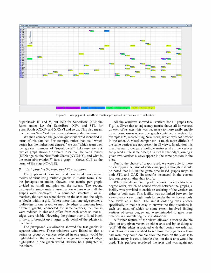
Figure 2. Four graphs of SuperBowl results superimposed into one matrix visualization.

linked, although the vertex selected would highlight in the other graph.

The second visualization superimposed the matrices into a single combined view (see Figure 2) using the combined vertex set. The same colours were used for each graph as were used in the juxtaposed view.

The functionality of this visualization was identical to that of the other visualizations with the addition of two buttons which enabled a user to toggle the visibility of any graph off or on at will. An example of this representation is shown in Fig. 2.

Finally we added a filter facility. This enabled users to select one graph and make its common edges with any or all of the others invisible. This facility takes advantage of the common vertex set to search each vertex in turn to determine if has multiple edges to other vertices from different graphs. In effect this gives a difference visualization mode to both the juxtaposed and superimposed states. Fig. 3 shows the filter in action in the superimposed view.

Figure 3. Superimposed matrices with filter.

We found that all our users utilised these facilities at some point, but none suggested that we link the reordering so that reordering an axis in one view would automatically do the same in the other.

V. RESULTS The results showed that in terms of user preference, 13

out of the 18 testers preferred the combined view; only 4 preferred the separate windows and 1 had no preference.

The task-based results showed: In determining which of the four graphs had a specific

difference (a single edge)

View type Result Superimposed Mean = 0.78; SD = 0.42; n=18 Juxtaposed Mean = 0.56; SD = 0.5; n=18

In determining difference between vertices on a given

edge (representation of SB V, the Colts as BAL or IND)

View type Result Superimposed Mean = 0.83; SD = 0.30; n=18 Juxtaposed Mean = 0.66; SD = 0.47; n=18

In determining a difference in vertices, the change being

made in graph four where the SuperBowl game between NYG and DEN was instead between NYG and CLE.)

View type Result

Superimposed Mean = 0.83; SD =0.30; n=18 Juxtaposed Mean = 0.56; SD =0.5; n=18

These results show a statistically significant

improvement in accuracy for the superimposed visualization over the juxtaposed one. On the other hand, both visualizations scored almost identically in both finding a given vertex/edge in different graphs, and in determining the differences between in and out degree of any given vertex between graphs.

As shown by the figures above, it was in the area of finding equivalency (of both edges and vertices) that the superposition proved superior. Our testers found it very difficult to find which difference related where in the juxtaposed views, and much preferred (and were more correct) using the superimposed matrices.

VI. CONCLUSIONS AND FUTURE WORK Our main finding is that when comparing small graphs

with matrix visualizations, it is significantly more effective to combine the visualizations into a single view rather than to link separate views; the accuracy of the comparison was better by nearly 50% in the former case.

This mirrors the same result Erten et al found for small planar graphs with node-link displays, the combined view being superior to that of the separate views. Likewise, Andrews et al [17] results were similar although with smaller ranges of difference.

We can therefore state that a combined tool for multiple graph comparison should be based around a superimposition of the graphs to be compared, regardless of whether the display technique is to be node-link or matrix-based.

We should be careful not to over-generalize this finding of a combined view being superior to separate views for comparison tasks. While the result of combining several general graphs is itself another general graph (in effect, a graph is its own plural), it may not apply to other data types, since combining them does not result in data of the same type. For example, the aggregate of multiple trees is a non tree-like graph of some description, and combining multiple data tables results in a data cube.

Future work may examine superposition versus juxtaposition versus differencing of other data types to determine if the above result holds for them also.

REFERENCES [1] H.C. Purchase. "Metrics for Graph Drawing Aesthetics," Journal of

Visual Languages and Computing, vol. 13(5) October 2002, pp.501-516, doi:10.1006/jvlc.2002.0232.

[2] H.C. Purchase, D. Carrington and J.-A. Allder. "Empirical Evaluation of Aesthetics-based Graph Layout," Empirical Software Engineering, vol. 7(3) 2002, pp.233-255, doi:10.1023/A:1016344215610.

[3] H.-J. Schulz and H. Schumann. "Visualizing Graphs - A Generalized View," Proc. 10th IEEE International Conference on Information Visualisation, IEEE Computer Society Press, 5-7 July 2006, pp.166-173, doi:10.1109/IV.2006.130.

[4] M. Ghoniem, J.-D. Fekete and P. Castagliola. "A Comparison of the Readability of Graphs Using Node-Link and Matrix-Based Representations," Proc. IEEE InfoVis, IEEE Computer Society Press, 10-12 October 2004, pp.17-24, doi:10.1109/INFOVIS.2004.1.

[5] R. Keller, C.M. Eckert and P.J. Clarkson. "Matrices or node-link diagrams: which visual representation is better for visualising connectivity models?," Information Visualization, vol. 5(1) 2006, pp.62-76, doi:10.1057/palgrave.ivs.9500116.

[6] N. Henry and J.-D. Fekete. "MatLink: Enhanced Matrix Visualization for Analyzing Social Networks," Proc. Interact, Springer, 10-14 September 2007, pp.288-302, doi:10.1007/978-3-540-74800-7_24.

[7] N. Henry, J.-D. Fekete and M. McGuffin. "NodeTrix: A Hybrid Visualization of Social Networks.," IEEE Transactions on Visualization and Computer Graphics, vol. 13(6) 2007, pp.1302-1309, doi:10.1109/TVCG.2007.70582.

[8] C. Erten, S.G. Kobourov, V. Le and A. Navabi. "Simultaneous Graph Drawing: Layout Algorithms and Visualization Schemes," Proc. Graph Drawing, Springer-Verlag, 21-24 September 2003, pp.437-449, doi:10.1007/978-3-540-24595-7_41.

[9] P. Brass, E. Cenek, C.A. Duncan, A. Efrat, C. Erten, D.P. Ismailescu, et al. "On simultaneous planar graph embedding," Computational Geometry: Theory and Applications, vol. 36(2) 2007, pp.117-130, doi:10.1016/j.comgeo.2006.05.006.

[10] J.Y. Hong, J. D'Andries, M. Richman and M. Westfall. "Zoomology: Comparing Two Large Hierarchical Trees," Proc. IEEE InfoVis Poster Compendium, IEEE Computer Society Press, 19-21 October 2003, pp.120-121.

[11] T. Munzner, F. Guimbretière, S. Tasiran, L. Zhang and Y. Zhou. "TreeJuxtaposer: Scalable Tree Comparison using Focus+Context with Guaranteed Visibility," ACM Transactions on Graphics, vol. 22(3) July 2003, pp.453-462, doi:10.1145/882262.882291.

[12] M. Graham and J. Kennedy. "Exploring Multiple Trees through DAG Representations," IEEE Transactions on Visualization and Computer Graphics, vol. 13(6) November 2007, pp.1294-1301, doi:10.1109/TVCG.2007.70556.

[13] P. Saraiya, P. Lee and C. North. "Visualization of Graphs with Associated Timeseries Data," Proc. IEEE InfoVis, IEEE Computer Society Press, 23-25 October 2005, pp.225-232, doi:10.1109/INFOVIS.2005.37.

[14] A. Telea, F. Frasincar and G.-J. Houben. "Visualisation of RDF(S)-based Information," Proc. International Conference on Information Visualization, IEEE Computer Socierty Press, 16-18 July 2003, pp.294-299, doi:10.1109/IV.2003.1217993.

[15] C. Collins and S. Carpendale. "VisLink: Revealing Relationships Amongst Visualizations," IEEE Transactions on Visualization and Computer Graphics, vol. 13(6) Nov/Dec 2007, pp.1192-1199, doi:10.1109/TVCG.2007.70611

[16] S. Diehl, C. Görg and A. Kerren. "Preserving the Mental Map using Foresighted Layout," Proc. Joint Eurographics-IEEE TVCG Symposium on Visualization, Springer Verlag, 28-30 May 2001, pp.175-184.

[17] K. Andrews, M. Wohlfahrt and G. Wurzinger. "Visual Graph Comparison," Proc. 13th International Conference on Information Visualisation, IEEE Computer Society Press, 15-17 July 2009, pp.62-67, doi:10.1109/IV.2009.108.

[18] F. Beck and S. Diehl. "Visual Comparison of Software Architectures," Proc. 5th International Symposium on Software Visualization (SOFTVIS), ACM Press, 25-26 October 2010, pp.183-192, doi:10.1145/1879211.1879238.

[19] M. Freire, C. Plaisant, B. Shneiderman and J. Golbeck. "ManyNets: An Interface for Multiple Network Analysis and Visualization," Proc. ACM Conference on Human Factors in Computing Systems (CHI), ACM Press, 10-15 April 2010, pp.213-222, doi:10.1145/1753326.1753358.

[20] A. Kerren, C. Plaisant and J.T. Stasko. "Executive Summary of Dagstuhl Seminar on Information Visualization". Retrieved 21 March, 2011, from http://drops.dagstuhl.de/opus/volltexte/2010/2760/pdf/10241_executive_summary.2760.pdf

[21] H.C. Purchase and A. Samra. "Extremes Are Better: Investigating Mental Map Preservation in Dynamic Graphs," Proc. 5th International Conference on Diagrammatic Representation and Inference, Springer-Verlag Berlin Heidelberg, 19-21 September 2008, pp.60-73, doi:10.1007/978-3-540-87730-1.