Color and Flow Based Superpixels for 3D Geometry Respecting Meshing

Mohamad Motasem Nawaf 1 Md. Abul Hasnat 1 Desire Sidibe 2 Alain Tremeau 1

1 Universite Jean Monnet, Laboratoire Hubert Curien UMR CNRS 5516, Saint-Etienne, France2 Universite de Bourgogne, Le2i UMR CNRS 6306, Le Creusot, France

mohamad.motasem.nawaf@univ-st-etienne.fr

Abstract

We present an adaptive weight based superpixel segmen-tation method for the goal of creating mesh representationthat respects the 3D scene structure. We propose a newfusion framework which employs both dense optical flowand color images to compute the probability of boundaries.The main contribution of this work is that we introduce anew color and optical flow pixel-wise weighting model thattakes into account the non-linear error distribution of thedepth estimation from optical flow. Experiments show thatour method is better than the other state-of-art methods interms of smaller error in the final produced mesh.

1. IntroductionSuperpixels (SPs) can be defined as an over-

segmentation of an image which is obtained by dividingthe image into small homogeneous color/texture regions sothat each of them belongs to only one object/surface. SPshas been widely used in many computer vision tasks suchas object detection [17], depth estimation [16, 8, 7, 15],occlusion boundaries detection [6, 21] and scene segmen-tation [2, 9, 18, 22]. In this paper, our goal is to use SPsas a tool to decompose a scene into triangle mesh, so thatthe mesh respects the 3D geometry of the scene. A trianglemesh comprises a set of triangles that are connected bytheir common edges or corners. We are motivated by thefact that many graphics software (e.g. Google earth) rep-resents 3D world structure by meshes. Moreover, modernsoftware packages and hardware devices can operate moreefficiently on meshes compared to the massive cloud ofpoints. Also, meshes have an advantage of being compactto represent continuous structure. Therefore, our aim is topropose a method that is applicable to any active/passive3D reconstruction application. In particular, a methodthat models the output (e.g. point cloud) to a mesh withminimum loss of precision.

SPs are mainly computed using color information of animage [3, 2, 11]. Recently, depth and/or flow information

have been used with color [22, 10, 18]. We believe thatflow information is an essential source based on the fact thatspatially uniform regions have continuous flow while occlu-sion boundaries are often associated with flow disturbances.Hence, flow information can be used to detect boundaries.Moreover, in combining color and flow, false boundaries incolor based segmentation could be identified.

In our method, we mainly target outdoor scenes, wherethe popular structured light based depth sensors fails dueto sunlight. Alternatively, we rely on flow and depth infor-mation obtained from a pair of images of the target scene.Hence, we propose a fusion scheme that incorporates adense optical flow and color images to compute SPs andgenerate the mesh. In contrary with the methods proposedin the literature [10, 22], our fusion method takes into ac-count (a) the non-linear error distribution of the depth esti-mation obtained using optical flow; (b) the fact that it has alimited range; and (c) that it could not be computed in partsof the image due to the view change between two images.To incorporate such information, we introduce a pixel-wiseweighting to be used while fusing boundary informationusing optical flow and color. Hence, our contribution is anovel locally adaptive weighting approach.

We assess the quality of SP segmentation for the goal of3D meshing by analyzing the error introduced by the meshgenerated based on such segmentation, with respect to theoriginal depth map. Figure 1 shows an example of an inputimage pair, obtained SPs and corresponding mesh (last rowin the Figure). The mesh is obtained by dividing the imageinto a set of triangles that covers the whole image, and eachtriangle lies completely in one SP (more details in Section3.5). Our method is evaluated and compared to state-of-artSPs methods using the KITTI dataset [4] which is providedwith depth ground truth.

The paper is organized as follows: In Section 2 wediscuss some related work, including color and color-depth/flow based approaches. Section 3 shows an overviewof the system, with a focus on computing the pixel-wiseweighting and the way it is involved to compute the proba-bility of boundaries, generating SPs and the mesh. In Sec-

Pair of color images

Sparse points correspondences

Dense optical flow (𝑢𝑢, 𝑣𝑣)

𝑅𝑅|𝑇𝑇 {𝐻𝐻1:4}

Local image homographies Possible correspondences map

Rough depth estimation Pixel-wise weights

𝐺𝐺𝐺𝐺𝐺𝐺(𝑢𝑢, 𝑣𝑣, 𝐿𝐿, 𝑎𝑎, 𝑏𝑏,𝑊𝑊𝑢𝑢,𝑣𝑣,𝐿𝐿,𝑎𝑎,𝑏𝑏 , 𝑠𝑠)

Superpixels Meshing Generalized boundary probability

Figure 1. Overview of the proposed method.

tion 4 we evaluate our method against the state of the artmethods. Finally, in Section 5 we conclude our work.

2. Related WorkA wide range of SPs generation methods use color, tex-

ture and position information as features. An early examplefor color based SPs method is the graph-based model [3].In this method, the pixels are represented as nodes and theedges are computed as the similarity between nodes. Then,SPs are obtained by applying the minimum spanning treealgorithm. This method has been widely adopted to repre-sent 3D scenes structure [16, 8, 7]. In this method, thereis no restriction on the shape/number/alignment of the re-sulting SPs. In contrast, a remarkable property in severalother SPs methods is that they consider the regularity andthe arrangement of the SPs. For instance, the simple lineariterative clustering (SLIC) method [2] introduces a new dis-tance measure that involves the position of the pixel as wellas color. This distance measure is taken into account when alabel is assigned to each pixel. Hence, there is a limit on thesize of the formed SPs subject to a regularization parameter.

Among the methods that tends to produce a grid alignedSPs are SEEDS (Superpixels Extracted via Energy-DrivenSampling) [21] and Turbopixels [11]. SEEDS uses a fixednumber of uniformly distributed seeds (rectangular shapeclusters) for initialization, and then refines the boundariesbetween them based on minimizing an energy function thatconsists of a color distribution and boundary terms. Op-posite way, Turbopixels method starts with rectangular griddistributed clusters centers and then it grows them basedon a Boundary Velocity which is computed from local im-age gradients. These regularity aware methods produce SPswith relatively similar size and regular shape, and the out-put is more or less aligned to a grid. For meshing purposes,having such property is not necessary as it does not reflectthe real world structure. Moreover, it produces unnecessaryadditional number of SPs which will result in more meshfaces (e.g. an extreme case if we have a single homoge-

neous surface in the image). In our method, the numberof SPs varies based on the nature of scene. Moreover, thesize of SPs is not limited. Whereas including flow infor-mation helps to improve the segmentation as will be shownin the experimental results in Section 4. For more detailsabout color-based SPs methods we refer the reader to [2].

Recently, due to the increasing use of depth information(obtained from different types of sensors) for computer vi-sion tasks, SPs generation including depth appears as animportant issue. Specially, it is important to know how toincorporate/fuse depth, and what SPs method to use. Sev-eral methods [9, 22] already exist for this purpose. Forinstance, the method proposed in [9] fuses depth informa-tion in the watershed based SPs algorithm. Their fusion ap-proach takes the maximum of the Laplacian computed froma grayscale and depth image. In [22] the authors proposed aSLIC [2] based method where they incorporate depth in thedistance function. Both methods use global weight for eachchannel/layer (e.g. color and depth). That means all pixelsof a particular channel have the same weight. However, weargue that weight should be assigned locally since the depthuncertainty is not uniform throughout the whole image.

3. Superpixels Generation SchemeThe block diagram of our proposed method is illustrated

in Figure 1. Starting from a pair of color images, we com-pute a dense optical flow and also sparse feature points cor-respondences. These sparse feature points are used to re-cover the relative motion of the two images, and to computelocal homographies that are used to define a mask of theoverlap between the two images. Together with a roughdense estimation obtained from the optical flow, we use therelative motion parameters and the mask of overlap to com-pute the pixel-wise weights for each optical flow direction.Then, we employ a global boundary probability generatorthat takes as input: (a) the two channels of the optical flow;(b) the three layers of one input color image (in CIELABcolor space) and (c) the pixel-wise and layer-wise learned

(a)

(b)

Figure 2. Depth maps computed using same first image and (a) animage shifted horizontally (stereo); (b) Image obtained with dom-inant forward motion (Epipole near the center, borders problem).

weights. This step is followed by watershed segmentationto generate the superpixels (SPs). Finally, a mesh represen-tation is obtained based on the SPs. Each of these steps isdescribed in the following subsections.

3.1. Relative Motion Recovery

An accurate relative motion [R|T ] is needed to computea depth map, to estimate the pixel-wise weights and also toperform a minor outliers correction of the optical flow. Forthis purpose, we use a traditional approach by first perform-ing SIFT feature points matching [13] on the image pair,and estimating the fundamental matrix using RANSAC pro-cedure. Then, given the camera intrinsic parameters, wecompute the Essential matrix that encodes the rotation andtranslation (up to scale) between the two images.

3.2. Dense Optical Flow and Depth Map Estimation

The usage of optical flow in this work is essential. Ithelps identifying the spatial uniformity in the scene andhence it works as a complement to color images. We adoptthe dense optical flow underlying median filtering methodproposed in [19] (We use the publicly available code [1]).Among the proposed variations, we use Classic-C method(Classical optical flow objective function with Charbonnierpenalty term and 5x5 median filtering window size), whichshowed to have better occlusions handling and flow de-noising. Additionally, we perform a minor outliers detec-tion and correction based on the recovered fundamental ma-trix. Given the dense points correspondences obtained bythe optical flow, we compute a simple first-order geomet-ric error (Sampson distance) for each point. We allow morerelaxed (3-5 times) distance threshold compared to the av-erage distance of the selected inliers model computed usingthe sparse SIFT features (in the previous Section). The flowvectors that exceed this threshold are replaced by linearlyinterpolated new values.

For dense depth map computation, we apply the directlinear transformation (DLT) triangulation method followedby structure only bundle adjustment, which involves mini-mizing a geometric error function as described in [5]. Weuse the Levenberg-Marquardt based framework proposed in[12]. In the special case of close to degenerated configura-tions (e.g. epipole inside the image), computing the depthmap in the epipole’s neighboring is difficult. In this par-ticular case we calculate a rough relative depth map by re-moving spatial correlation from the magnitude of the opticalflow. This correlation results from the presence of x and yin the optical flow equation (see Equation 2). To remove thiscorrelation, we first search for the correlation center (cx, cy)by maximizing the following pairwise correlation formula:

arg maxcxcy

∑ij

√(i− cx)

2+ (j − cy)

2.√u2ij + v2ij (1)

where i and j are the image coordinates, u and v are theoptical flow components. Then, we divide each point in theoptical flow magnitude by the euclidean distance to imagecenter shifted by [cx cy]. Figure 2(b) shows an example ofa depth map computed using this method. The input imagesin this case are taken by the same camera moving forward.We believe that the depth map obtained by this approachis good enough to extract boundary information comparedwith the normal case (e.g. Figure 2(a)).

3.3. Pixel-Wise Optical Flow Channels Weighting

The desired pixel-wise weighting should reflect the un-certainty in depth information obtained from the opticalflow. The weights are computed based on: (a) the error dis-tribution of depth estimation as a function of the optical flowerror; and (b) handling the occlusions on the boundaries ofthe image. There are several error sources that disturb thedepth estimation from images. In the scope of this paper,we only consider the error made during computing pixelscorrespondences (or flow vector) which is assumed to beuniform in the image. Our aim is to establish an uncertaintymeasure of the depth based on the aforementioned error. Weassume that we have relatively larger translational shift thanrotational between the image pair. By this assumption wedo not lose generality as it is the case in most realistic con-figurations. The optical flow (u, v) for a point (X,Y, Z)in the three dimensional world, in case of translational dis-placement T (TX , TY , TZ) between two views, is given by:[

uv

]=

s

Z

[TZx− TXfTZy − TY f

](2)

here s is a constant related to camera intrinsics. f is thefocal length. (x, y) is the projection of P in the imageplane. Z axis is normal to image plane and pointing for-ward. Based on this equation we can compute the error in

(a) (b) (c) (d)

Figure 3. Original image (a), and the obtained boundaries probability based on optical flow (b), color (c), both color and optical flow (d).

(a) (b) (c) (d)

Figure 4. Examples of superpixel segmentation (a,b). Exemplar 3D mesh (c) and the corresponding textured 3D model of the scene (d)

estimated depth as a function of error in optical flow as:

[rurv

]=

∂Z∂u∂Z∂v

= s

−fTXZ2

(xTZ − fTX)2

−fTY Z2

(yTZ − fTX)2

(3)

This equation shows that the estimated depth error is non-linear. Also, note that the depth computed from larger opti-cal flow introduces less error compared with small one. Weuse this fact to establish our uncertainty measure. There-fore, we assign an uncertainty value for the optical flowinversely proportional to the estimated depth in that pointaccording to Equation 3. However, due to the discretizedconfiguration (pixels array representation), this is only validup to a certain distance limit where differences in depth be-yond a given point are not recognizable by the computer vi-sion system. Formally, by considering that the flow vectoris defined by a linear system composed of two types of com-ponents; Z dependent and non Z dependent terms [15]. Wedefine a blind zone as the set of points where the Z depen-dent terms contribute to the optical flow less than one pixel.Hence, we build a pixel-wise uncertainty map for each opti-cal flow channel based on Equation 3 and by considering theaforementioned remark by assigning zero weight for pixelsin the blind zone. Computationally, the depth Z is com-puted as an average of Gaussian window centered at the re-lated pixel in the depth map. This helps to handle the noisydepth specially on the occlusion boundaries.

Another issue we consider is that in each of the input im-ages, and due to the change of view point, some parts in theboundary in one image does not exist in the other (no cor-respondence). The optical flow computed in those parts isobtained by data propagation, which is generally erroneous(see the noisy boundaries in Figure 2(b)). Hence, we pro-ceed to find these parts in order to take them into account inthe computed uncertainty map. For this purpose, based onthe sparse feature points (obtained in Section 3.1), we com-pute the correspondences of the four image corners in theother image. Hence, we calculate four local 2D to 2D pointshomographies for each of the four corners using n nearest

feature points such that: pi2 = Hipi

1 {i = 1 : 4}. Here pi1 is

the feature point homogeneous coordinates in the first im-age, which belongs to the set of n nearest points (n ∼ 50)to the corner i. Hi is the corresponding 3 × 3 homogra-phy. We compute the homographies by using RANSACwith DLT simple fitting. We assume that the selected pointshave small depth variations. However, using RANSAC herehelps to reject the points whose depth is far from the meandepth. We estimate a frame of possible correspondences byapplying the inverse of the computed homographies on eachcorner. All the points that belong to this frame are projectedin both images, Figure 6 illustrates this step. By generatinga binary mask C based on the computed frame, we write theoverall pixel-wise weighting for optical flow channels as:[

Wu

Wv

]=

[(C + αC)Ru

(C + αC)Rv

](4)

where α controls the impact of the pixels that do not belongto possible correspondences area defined by C, and R. is aunit normalized error matrix computed as r. (given in Equa-tion 3). In order to allow contributions from color channelsto fulfill the parts with high uncertainty in flow channels,we assign the pixel-wise weight for color channels as:

WLAB = 1− β√

W2u + W2

v (5)

here β is a normalizer that imposes WLAB ∈ [0..1].

3.4. Generalized Boundary Probability

In order to compute the probability of boundaries, we ex-tend the generalized boundary detection method proposedin [10]. We select this method due to several advantagessuch as: (a) significantly lower computational cost w.r.t. thestate of the art methods and (b) ability to combine differ-ent types of information (e.g. color and depth) through eas-ily adaptable layer-wise integration. Most importantly, theclosed form formulation of this method allows us to easilyincorporate our proposed locally adaptive weights.

Consider that we have an image with K layers whereeach layer has an associated boundary. Now for each layer,

1 2 3 4 5

·104

5 · 10−2

0.1

0.15

0.2

0.25

Number of mesh vertices

Relativemeanerror

LABUV-PWLABUV-GW

UVLABSLIC

SLIC-UVTurbopixelsGraph-based

1

(a) Depth error vs. number of vertices

0 200 400 600 800 1,000 1,200

2 · 10−2

4 · 10−2

6 · 10−2

8 · 10−2

0.1

0.12

0.14

Number of superpixels

LABUV-PWLABUV-GW

UVLABSLIC

SLIC-UVTurbopixelsGraph-based

2

(b) Depth error vs. number of superpixels

LABUV-PW

LABUV-GW U

VLAB

SLIC

SLIC-UV

Turbopixels

Graph-based

5

10

4.57

8.7 8.91 8.78

5.58 5.08 5.22

13.16

Overallrelativeerror%

(c) Overall relative mean error

Figure 5. Experimental results

let us denote n = [nx, ny] the boundary normal, b =[b1, ..., bK ] the boundary heights and J = n>b the rank-12 ×K matrix. Then, the boundary detection is formulatedas computing ‖b‖ which defines the boundary strength. Theclosed form solution [10] computes ‖b‖ as the square rootof the largest eigenvalue of a matrix M = JJ>, where theunknown matrix J is computed from known values of twomatrices P and X as: J ≈ P>X. The matrix P associatesthe position information and the matrix X associates eachlayer information. Therefore, we can redefine the matrix M

for a pixel p as: Mp =(P>Xp

) (P>Xp

)>. Note that we

can compute ‖b‖ for an image (using P and X) only if thelayers are properly scaled. Usually, the scale for each layersi is learned [10] from annotated images. However, we alsoinclude the pair-wise weighting matrix Wi (Equations 4, 5).Therefore, we construct the matrix Mp =

∑i siWi,pMi,p,

where Mi defines a matrix for the ith layer. In our approachwe use the following layers: L∗, a∗ and b∗ (CIELAB colorcomponents) and optical flow channels u and v.

Figure 3(d) shows an illustration of a boundary proba-bility estimated using our method. It shows the advantageof the pixel-wise weighing such as removing strong falseboundaries originated from color (Figure 3(c)). It also al-lows to complete far details that are not present in the blindzone of the flow-based boundary probability (Figure 3(b)).

3.5. Superpixels Formation and Mesh Generation

We apply watershed algorithm [20] on the probabilityof boundaries [14] in order to produce SPs. The numberof the resulting SPs could be roughly controlled by apply-ing variable window size median filtering on the boundaryprobability map. After obtaining the SPs we convert themto a standard mesh representation (VRML). To this aim,we apply the following procedure on a binary edge mapformed from SPs; First we detect all the segments that form

a straight line in the edge map. Then, for each of the de-tected segments we only keep the two ends. The remainingedges are the vertices of the mesh. The mesh faces are thenformed by the known Delaunay triangulation manifestingon each SP’s vertices. This way guarantees that a triangleis contained in only one SP. Converting the 2D mesh to 3Dmesh is then straightforward by knowing the 3D locationsof all vertices. Figure 4(c) shows a 3D mesh example com-puted using the SPs shown in Figure 4(a).

4. ExperimentsTo evaluate our method we use the KITTI dataset [4]

which contains outdoor scenes obtained using a mobile ve-hicle. The dataset provides depth data obtained using laserscanner (∼ 80m). This enables us to test our fusion model,and in particular the efficiency of the pixel-wise weighting.We select our test images1 to cover most possible cameraconfigurations (stereo, forward motion, rotation, etc.).

We evaluate the performance of our method (LABUV-PW) compared to the following methods: SLIC [2], SLIC-UV (an extended SLIC 2 that includes optical flow), Tur-bopixels [11] and graph-based [3]. Moreover, to show theimpact of the pixel-wise weighting we test a variation of ourmethod that uses a global weight (learned according to [10])per layer (LABUV-GW). Additionally, we include individ-ual results for color only (LAB) and optical flow (UV).

The evaluation is carried out by producing multiple seg-mentations with variable numbers of SPs that covers a cer-tain range (∼ 25−2000) for each test image. Each segmen-tation is converted into 2D mesh according to the methodshown in Section 3.5. Then, based on the ground truth depthmap, we obtain the 3D location of the mesh vertices, henceit becomes a 3D mesh. Next, we calculate a relative depth

1Raw data section, sequences # 0001-0013, 0056, 0059, 0091-0106.2Implemented based on the new measure proposed in [22]

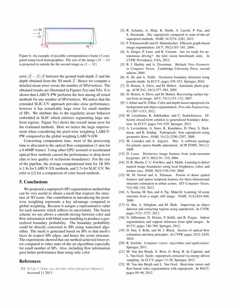
HHi

-1i

O

MI

Figure 6. An example of possible correspondences frame O com-puted using local homographies. The rest of the image (M − O)is projected to outside the the second image as (I −M)

error |Z − Z|/Z between the ground truth depth Z and thedepth obtained from the 3D mesh Z. Hence we compute adetailed mean error versus the number of SPs/vertices. Theobtained results are illustrated in Figures 5(a) and 5(b). It isshown that LABUV-PW performs the best among all testedmethods for any number of SPs/vertices. We notice that theextended SLIC-UV approach provides close performance,however it has remarkably large error for small numberof SPs. We attribute this to the regularity aware behaviorembedded in SLIC which enforces segmenting large uni-form regions. Figure 5(c) shows the overall mean error forthe evaluated methods. Here we notice the large improve-ment when considering the pixel-wise weighting LABUV-PW compared to the global weighing LABUV-GW.

Concerning computation time, most of the processingtime is allocated to the optical flow computation (1 min fora 0.46MP frame). Using other GPU-assisted or acceleratedoptical flow methods caused the performance to drop down(due to less quality of occlusions boundaries). For the restof the pipeline, the average computational time for 1K SPsis 1.9s for LABUV-XX methods, and 2.7s for SLIC-UV. Werefer to [2] for a comparison of color based methods.

5. ConclusionsWe proposed a superpixel (SP) segmentation method that

can be very useful to obtain a mesh that respects the struc-ture of 3D scene. Our contribution in introducing the pixel-wise weighting represents a key advantage compared toglobal weighting. Because it assigns a representative valuefor each measure which reflects its uncertainty. The fusionscheme we use allows a smooth mixing between color andflow information with blind zone handling to produce a gen-eralized boundary probability. The boundary probabilitycould be directly converted to SPs using watershed algo-rithm. The mesh is generated based on SPs so that mesh’sfaces do respect SPs edges, and hence the scene structure.The experiments showed that our method achieved lower er-ror compared to other state-of-the art algorithms especiallyfor small number of SPs. Also, including flow informationgave better performance than using only color.

References[1] http://www.cs.brown.edu/people/dqsun/,

Accessed 11 2013.

[2] R. Achanta, A. Shaji, K. Smith, A. Lucchi, P. Fua, andS. Susstrunk. Slic superpixels compared to state-of-the-artsuperpixel methods. PAMI, 34:2274–2282, 2012.

[3] P. Felzenszwalb and D. Huttenlocher. Efficient graph-basedimage segmentation. IJCV, 59(2):167–181, 2004.

[4] A. Geiger, P. Lenz, and R. Urtasun. Are we ready for au-tonomous driving? the kitti vision benchmark suite. InCVPR, Providence, USA, 2012.

[5] R. I. Hartley and A. Zisserman. Multiple View Geometryin Computer Vision. Cambridge University Press, secondedition, 2004.

[6] X. He and A. Yuille. Occlusion boundary detection usingpseudo-depth. In ECCV, pages 539–552. Springer, 2010.

[7] D. Hoiem, A. Efros, and M. Hebert. Automatic photo pop-up. ACM ToG, 24(3):577–584, 2005.

[8] D. Hoiem, A. Efros, and M. Hebert. Recovering surface lay-out from an image. IJCV, 75(1):151–172, 2007.

[9] I. Jebari and D. Filliat. Color and depth-based superpixels forbackground and object segmentation. Procedia Engineering,41:1307–1315, 2012.

[10] M. Leordeanu, R. Sukthankar, and C. Sminchisescu. Ef-ficient closed-form solution to generalized boundary detec-tion. In ECCV, pages 516–529. Springer, 2012.

[11] A. Levinshtein, A. Stere, K. Kutulakos, D. Fleet, S. Dick-inson, and K. Siddiqi. Turbopixels: Fast superpixels usinggeometric flows. PAMI, 31(12):2290–2297, 2009.

[12] M. Lourakis and A. Argyros. Sba: A software packagefor generic sparse bundle adjustment. ACM TOMS, 36(1):2,2009.

[13] D. Lowe. Distinctive image features from scale-invariantkeypoints. IJCV, 60(2):91–110, 2004.

[14] D. R. Martin, C. C. Fowlkes, and J. Malik. Learning to detectnatural image boundaries using local brightness, color, andtexture cues. PAMI, 26(5):530–549, 2004.

[15] M. M. Nawaf and A. Tremeau. Fusion of dense spatialfeatures and sparse temporal features for three-dimensionalstructure estimation in urban scenes. IET Computer Vision,7(5):302–310, 2013.

[16] A. Saxena, M. Sun, and A. Ng. Make3d: Learning 3d scenestructure from a single still image. PAMI, 31(5):824–840,2009.

[17] G. Shu, A. Dehghan, and M. Shah. Improving an objectdetector and extracting regions using superpixels. In CVPR,pages 3721–3727, 2013.

[18] N. Silberman, D. Hoiem, P. Kohli, and R. Fergus. Indoorsegmentation and support inference from rgbd images. InECCV, pages 746–760. Springer, 2012.

[19] D. Sun, S. Roth, and M. J. Black. Secrets of optical flowestimation and their principles. In CVPR, pages 2432–2439,2010.

[20] R. Szeliski. Computer vision: algorithms and applications.Springer, 2011.

[21] M. Van den Bergh, X. Boix, G. Roig, B. de Capitani, andL. Van Gool. Seeds: superpixels extracted via energy-drivensampling. In ECCV, pages 13–26. Springer, 2012.

[22] M. Van den Bergh and L. Van Gool. Real-time stereo andflow-based video segmentation with superpixels. In WACV,pages 89–96, 2012.