Cognitive Gateway to Promote Interoperability, Coverage and ...
174
Cognitive Gateway to Promote Interoperability, Coverage and Throughput in Heterogeneous Communication Systems Qinqin Chen Dissertation submitted to the faculty of the Virginia Polytechnic Institute and State University in partial fulfillment of the requirements for the degree of Doctor of Philosophy In Electrical Engineering Charles W. Bostian (Chair) Allen B. MacKenzie Michael S. Hsiao Claudio da Silva Tonya L. Smith‐Jackson December 8, 2009 Blacksburg, Virginia Keywords: software defined radio, cognitive radio, cognitive gateway, dynamic spectrum access, waveform, signal classification, synchronization, interoperability, signaling, link scheduling, DiffServ, queuing Copyright 2009, Qinqin Chen
-
Upload
khangminh22 -
Category
Documents
-
view
1 -
download
0
Transcript of Cognitive Gateway to Promote Interoperability, Coverage and ...

Cognitive Gateway to Promote Interoperability, Coverage and Throughput in Heterogeneous Communication Systems
Qinqin Chen
Dissertation submitted to the faculty of the Virginia Polytechnic Institute and State University in partial fulfillment of the requirements for the degree of
Doctor of Philosophy
In Electrical Engineering
Charles W. Bostian (Chair) Allen B. MacKenzie Michael S. Hsiao Claudio da Silva
Tonya L. Smith‐Jackson
December 8, 2009 Blacksburg, Virginia
Keywords: software defined radio, cognitive radio, cognitive gateway, dynamic spectrum access, waveform, signal classification, synchronization, interoperability,
signaling, link scheduling, DiffServ, queuing
Copyright 2009, Qinqin Chen

Cognitive Gateway to Promote Interoperability, Coverage and Throughput in Heterogeneous Communication Systems
Qinqin Chen
ABSTRACT
With the reality that diverse air interfaces and dissimilar access networks coexist, accompanied by the trend that the dynamic spectrum access (DSA) is allowed and gradually employed, cognition and cooperation form the promising framework to achieve the ideality of seamless ubiquitous connectivity in future communication networks. In this dissertation, cognitive gateway (CG), conceived as a special cognitive radio (CR) node, is proposed and designed to facilitate universal interoperability among incompatible waveforms. Located in places where various communication nodes and diverse access networks coexist, the CG can be easily set up and works like a network server with the differentiated service (Diffserv) architecture to provide automatic traffic relaying and link establishment. The author extracts a scalable “source‐CG‐destination” snapshot from the entire network and investigates the key enabling technologies for such a snapshot. CG features providing universal interoperability, which is enabled by the generic waveform representation format and the reconfigurable software defined radio platform. According with the trend of all IP‐based solution for the future communication systems, the term “waveform” in this dissertation has been defined as a protocol stack specification suite. The author gives a generic waveform representation format based on the five‐layer TCP/IP protocol stack architecture. This format can represent the waveforms used by Ethernet, WiFi, cellular system, P25, cognitive radios etc. A significant advantage of CG over other interoperability solutions lies in its autonomy, which is contributed to by appropriate signaling processes and automatic waveform identification. The service process in a CG is usually initiated by the users who send requests by their own waveforms. These requests are transmitted during the signaling procedures. The complete operating procedure of a CG has been depicted as a waveform‐oriented cognition loop, which is primarily executed by waveform identifier, scenario analyzer, central controller, and waveform converter together. The author details the service process initialized by a primary user (e.g. legacy public safety radio) and that initialized by a secondary user (e.g. CR), and describes the signaling procedures between CG and clients for the accomplishment of CG discovery, user registration and un‐registration, link establishment, communication resumption, service termination, route discovery, etc. From the waveforms conveyed during the signaling procedures, the waveform identifier extracts the parameters that can be used for a CG to identify the source waveform and the destination waveform. These parameters are called

iii
“waveform indicators”. The author analyzes the four types of waveforms of interest and outlines the waveform indicators for different types of communication initiators. In particular, a multi‐layer waveform identifier is designed for a CG to extract the waveform indicators from the signaling messages. For the physical layer signal recognition, a Universal Classification Synchronization (UCS) system has been invented. UCS is conceived as a self‐contained system which can detect, classify, synchronize with a received signal and provide all parameters needed for physical layer demodulation without prior information from the transmitter. Currently, it can accommodate the modulations including AM, FM, FSK, MPSK, QAM and OFDM. The design and implementation details of a UCS have been presented. The designed system has been verified by over‐the‐air (OTA) experiments and its performance has been evaluated by theoretical analysis and software simulation. UCS can be ported to different platforms and be applied for various scenarios. An underlying assumption for UCS is that the target signal is transmitted continually. However, it is not the case for a CG since the detection objects of a CG are signaling messages. In order to ensure higher recognition accuracy, signaling efficiency, and lower signaling overhead, the author addresses the key issues for signaling scheme design and their dependence on waveform identification strategy. In a CG, waveform transformation (WT) is the last step of the link establishment process. The resources required for transformation of waveform pairs, together with the application priority, constitute the major factors that determine the link control and scheduling scheme in a CG. The author sorts different WT into five categories and describes the details of implementing the typical four types of WT (including physical layer analog ↔ analog gateway, up to link layer digital ↔ digital gateway, up‐to‐network‐layer digital gateway, and Voice over IP (VoIP) – an up to transport layer gateway) in a practical CG prototype. The issues including resource management and link scheduling have also been addressed. The dissertation presents the CG prototype implemented on the basis of GNU Radio plus multiple USRPs. In particular, the service process of a CG is modeled as a two‐stage tandem queue, where the waveform identifier queues at the first stage can be described as M/D/1/1 models and the waveform converter queue at the second stage can be described as G/M/K/K model. Based on these models, the author derives the theoretical block probability and throughput of a CG. Although the “source‐CG‐destination” snapshot considers only neighboring nodes which are one‐hop away from the CG, it is scalable to form larger networks. CG can work in either ad‐hoc or infrastructure mode. Utilizing its capabilities, CG nodes can be placed in different network architectures/topologies to provide auxiliary connectivity. Multi‐hop cooperative relaying via CGs will be an interesting research topic deserving further investigation.

iv
Acknowledgements Upon the completion of this dissertation, there are lots of people I would like to thank. First of all, I would like to express my sincere gratitude to my advisor, Dr. Charles W. Bostian. In spring 2006, when I was looking for a graduate research assistantship opportunity, he opened a door to me. Thus, in fall 2006 I successfully transferred to Virginia Tech, joined the warm “family” in the Center for Wireless Telecommunications, and started an unforgettable journey as to “cognitive radio”. Throughout my graduate study in Virginia Tech, Dr. Bostian has been much more than an advisor in academic research. In my mind, he is a “cognitive” supervisor, or more accurately speaking, he is like a kindly, wise “father” of the CWT “family”. Every student is his “child” with particular characteristics. He is aware of the particularities of his “children”, provides different guidance to them, explores maximally the potentials and capabilities of each of them, and tries to keep the good relationship and cooperation among them. To me, he offers tremendous encouragement, support, and help. He has given me credits for any effort and improvement I made; he has been always giving me positive, timely responses to any of my requests; he has been giving me lots of chances to express my ideas and to practice my abilities; he has been giving me great freedom to do what I want to do in the style I feel comfortable. With all his help I have overcome a lot of difficulties I encountered, and grown up to be an individual who is able to independently perform professional research work. I feel honored to be his supervisee. And what I learned from Dr. Bostian will be beneficial to my future life. In addition to Dr. Charles W. Bostian, I would like to thank Dr. Allen B. MacKenzie, Dr. Michael Hsiao, Dr. Claudio da Silva, and Dr. Tonya Smith‐Jackson, my committee members, for their precious suggestions and support in my research. In particular, I would like to extend my gratitude to Dr. Allen B. MacKenzie, who gave me to opportunity to take his course on “Cognitive Radios, Cognitive Networks, and Dynamic Spectrum Access”, from which I widened my knowledge, and improved my skills to read and write technical papers in English. I also want to extend thanks to Dr. Claudio da Silva since his clear explanation in the course, “Stochastic Signals and Systems”, made me master the knowledge necessary for my research work. In addition, I would like to express my gratitude to Dr. Yaling Yang, who served in my qualifying examination and taught me the knowledge about computer networks. Next, I would like to thank Judy Hood for her kindness, patience, and enormous help to me. She makes me feel at ease in the lab. In addition, she has been not only helping me
v
go through the administrative and operational processes, logistics, but also helping me a lot in improving my written and spoken English. It has been a great pleasure for me to work closely with a number of outstanding colleagues in CWT. During the first year of joining CWT, Bin Le and Thomas W. Rondeau led me into the magic kingdom of “cognitive radio” and GNU Radio, and offered me a great deal of help. Both of them are exceptional Ph.D. graduates. They have become my role models and their dissertations have become important references in my work afterwards. I would like to give special thanks to Ying Wang, a Ph.D. student who graduated in September 2009. Just like what she said, we complement each other and make a good team. During the three years after joining CWT, we have been worked together most closely. We got new ideas after brainstorming; we came to an agreement after intense discussions; we supported each other to conquer difficulties; we stayed up late to make demonstrations happen; we shared happiness and setbacks; we are good friends. Without her, there will not be so many joys and achievements. Particular thanks also go to Bin Li, Feng (Andrew) Ge, Alex Young, Mark D. Silvius, and Terry Brisebois. From them, I have learned a lot of things I did not know before. I also appreciate the friendship and kindly assistance they offered to me. In addition to aforementioned colleagues, I would like to thank others including Sujit Nair, Almohanad Fayez, Aravind Radhakrishnan, Gladstone Marballie, Rohit Rangnekar, Paco Garcia, Jana, Mustafa Y. ElNainay, Yongsheng (Sam) Shi, Daniel Firend, Xueqi Cheng, Nannan He, and Gyuhyun Kwon. It is they who make my Ph.D. study a fun journey and make every deadline a finish line. I cannot forget the help of Dr. Zhongfeng Wang, my advisor in Oregon State University, who led me into the area of VLSI design and taught me lots of research skills. In addition, Zhiqiang Cui, my colleague in OSU, offered considerable help on my life and study. Without them, I cannot work through the big difficulties that I faced when I just came to a foreign country. I would like to give a thousand thanks to them. Finally, I am as ever, especially indebted to my parents and soul mate, Yihong Yang, for their unlimited love and support in my life.

vi
Grant Information
This material is based upon work supported by the National Science Foundation under Grant CNS‐0519959. Any opinions, findings and conclusions or recommendations expressed in this material are those of the author(s) and do not necessarily reflect the views of the National Science Foundation (NSF). This project is supported by Award No. 2005‐IJ‐CX‐K017 awarded by the National Institute of Justice, Office of Justice Programs, US Department of Justice. The opinions, findings, and conclusions or recommendations expressed in this dissertation are those of the author(s) and do not necessarily reflect the views of the Department of Justice.

vii
TABLE OF CONTENTS
Table of Figures ................................................................................................................................ x
List of Tables .................................................................................................................................. xiii
List of Acronyms ............................................................................................................................ xiv
Chapter 1: Introduction ................................................................................................................... 1
1.1 Research Motivation & Problem Statement ......................................................................... 1
1.2 Research Background & State of the Art ............................................................................... 3
1.3 CWT Public Safety Cognitive Radio ........................................................................................ 9
1.4 About This Dissertation ....................................................................................................... 14
1.5 Contributions ....................................................................................................................... 14
1.6 What distinguishes my work from PSCR? ............................................................................ 16
1.7 Dissertation Organization .................................................................................................... 16
Chapter 2: Cognitive Gateway Overview ...................................................................................... 18
2.1 Introduction and Objectives ................................................................................................ 18
2.2 Specifications and Scope ..................................................................................................... 20
2.3 Cognitive Gateway Functional Architecture and System Operating Procedure ................. 21
2.4 An Overview of Building Functional Cognitive Gateway Systems ....................................... 25
2.4.1 Waveform Representation ........................................................................................... 25
2.4.2 Waveform Identification and Scenario Analysis ........................................................... 27
2.4.3 Database ....................................................................................................................... 29
2.4.4 Waveform Transformation ........................................................................................... 29
2.4.5 Link Control................................................................................................................... 29
2.4.6 Generic Interfaces ........................................................................................................ 30
2.5 The Intention and Extension of Cognitive Gateway ............................................................ 32
Chapter 3: Signaling Schemes and Waveform Identification ........................................................ 33
3.1 Waveform Indicator Selection ............................................................................................. 33
3.2 A Complete Service Process ................................................................................................ 35
3.3 Introduction to Waveform Identification ............................................................................ 41
3.4 Universal Classifier and Synchronizer .................................................................................. 42
3.4.1 Introduction .................................................................................................................. 42
3.4.2 Background and State Of The Art ................................................................................. 45
viii
3.4.3 System Overview .......................................................................................................... 45
3.4.4 System Design and Implementation ............................................................................ 47
3.4.4.1 Spectrum Sensing .............................................................................................. 48
3.4.4.2 Signal Capture .................................................................................................... 48
3.4.4.3 Channel Estimation and Equalization ................................................................ 49
3.4.4.4 Modern Wireless Communications Modulations and Scenarios ...................... 50
3.4.4.5 Narrowband and Wideband Categorization...................................................... 51
3.4.4.6 Narrowband Categorization .............................................................................. 53
3.4.4.7 Bandwidth estimation ....................................................................................... 60
3.4.4.8 Symbol timing and coarse classification ............................................................ 61
3.4.4.9 Carrier synchronization and fine classification .................................................. 67
3.4.4.10 OFDM signal scenario and application .............................................................. 71
3.4.4.11 Estimation of symbol length and CP length ....................................................... 72
3.4.4.12 Carrier Synchronization for OFDM Signals ........................................................ 74
3.4.4.13 Verification Schemes for UCS System ................................................................ 75
3.4.5 UCS Prototypes and Performance Evaluation .............................................................. 76
3.4.6 Conclusion and Discussion ........................................................................................... 84
3.5 Comparison between UCS and ASC ..................................................................................... 88
3.6 Signaling Process and Mechanisms ..................................................................................... 91
3.7 Discussion ............................................................................................................................ 99
Appendix 3‐A ............................................................................................................................. 99
Appendix 3‐B ........................................................................................................................... 100
Chapter 4: Waveform Transformation and Link Scheduling ....................................................... 102
4.1 Waveform Transformation ................................................................................................ 102
4.1.1 WT Categorization ...................................................................................................... 102
4.1.2 WT at the Physical Layer ............................................................................................ 103
4.1.3 WT up to the Link Layer .............................................................................................. 105
4.1.4 WT up to the Network Layer ...................................................................................... 108
4.1.5 Voice over IP ............................................................................................................... 110
4.2 Resource Management and Scheduling ............................................................................ 112
4.3 Conclusion and Discussion ................................................................................................ 117
Chapter 5: Prototype and Performance Evaluation .................................................................... 119
ix
5.1 Over‐The‐Air Prototype ..................................................................................................... 119
5.2 Miscellaneous Implementation Details ............................................................................. 123
5.3 OTA Experimental Results ................................................................................................. 129
5.4 Theoretical Performance Evaluation Using Queuing Theory ............................................ 130
Appendix 5‐A ........................................................................................................................... 136
Appendix 5‐B ........................................................................................................................... 140
Chapter 6: Conclusions ................................................................................................................ 143
6.1 Dissertation Summary ....................................................................................................... 143
6.2 Future Work ...................................................................................................................... 149
Bibliography ................................................................................................................................. 151

x
Table of Figures Figure 1.1: State & Local Public Safety Spectrum ........................................................................................... 2 Figure 1.2: CWT Cognition Cycle. ©2007 Bin Le. Reprinted, with permission, from B. Le, "Building a
Cognitive Radio: From Architecture Definition to Prototype Implementation," Ph.D. Dissertation, in Dept. of Electrical & Computer Engineering. 2007, Virginia Polytechnic Institute and State University: Blacksburg, VA. ..................................................................................................................................... 7
Figure 1.3: CWT PSCR Node Block Diagram. ©2007 Bin Le. Reprinted, with permission, from B. Le, "Building a Cognitive Radio: From Architecture Definition to Prototype Implementation," Ph.D. Dissertation, in Dept. of Electrical & Computer Engineering. 2007, Virginia Polytechnic Institute and State University: Blacksburg, VA. ........................................................................................................ 10
Figure 1.4: CWT PSCR Node with Subsystem Implementation Details. ©2007 Bin Le. Reprinted, with permission, from B. Le, "Building a Cognitive Radio: From Architecture Definition to Prototype Implementation," Ph.D. Dissertation, in Dept. of Electrical & Computer Engineering. 2007, Virginia Polytechnic Institute and State University: Blacksburg, VA. ............................................................... 11
Figure 1.5: Hierarchical Two‐plane Structure of CWT SDR Platform. ©2007 Bin Le. Reprinted, with permission, from B. Le, "Building a Cognitive Radio: From Architecture Definition to Prototype Implementation," Ph.D. Dissertation, in Dept. of Electrical & Computer Engineering. 2007, Virginia Polytechnic Institute and State University: Blacksburg, VA. ............................................................... 12
Figure 1.6: MAC/PHY Reconfigurable Waveform Framework ...................................................................... 13 Figure 1.7: Framework System‐level Block Diagram—Digital Waveform. ©2007 Bin Le. Reprinted, with
permission, from B. Le, "Building a Cognitive Radio: From Architecture Definition to Prototype Implementation," Ph.D. Dissertation, in Dept. of Electrical & Computer Engineering. 2007, Virginia Polytechnic Institute and State University: Blacksburg, VA. ............................................................... 13
Figure 2.1: Hyperball Nature‐inspired Computer Network Invented by Philip Emeagwali .......................... 18 Figure 2.2: Add CGs to Provide Seamless Connectivity ................................................................................ 19 Figure 2.3: (a) “Source‐CG‐Destination” Snapshot; (b) CG Design Objective ............................................... 20 Figure 2.4: Node Specifications and Icons .................................................................................................... 20 Figure 2.5: Cognitive Gateway Block Diagram .............................................................................................. 21 Figure 2.6: A Scenario Using a Cognitive Gateway. ©2008 Software Defined Radio Forum. Reprinted, with
permission, from Q. Chen et al., “Cognitive Gateway Design to Promote Universal Interoperability,” in Software Defined Radio Technical Conference. October 26‐30, 2008: Washington, DC................. 22
Figure 2.7: CG Functional Loop‐‐Waveform‐Oriented Processing Loop ....................................................... 23 Figure 2.8: A Generic Cognitive Radio Architecture. ©2007 Thomas W. Rondeau. Reprinted, with
permission, from T. W. Rondeau, "Application of Artificial Intelligence to Wireless Communications," Ph.D. Dissertation, in Dept. of Electrical & Computer Engineering. 2007, Virginia Polytechnic Institute and State University: Blacksburg, VA. ................................................................................................. 25
Figure 2.9: UCS Function Block Diagram for Narrowband Signals. ©2008 Software Defined Radio Forum. Reprinted, with permission, from Q. Chen et al., “Cognitive Gateway Design to Promote Universal Interoperability,” in Software Defined Radio Technical Conference. October 26‐30, 2008: Washington, DC. ................................................................................................................................. 28
Figure 2.10: Generic API and Link Control. ©2008 Software Defined Radio Forum. Reprinted, with permission, from Q. Chen et al., “Cognitive Gateway Design to Promote Universal Interoperability,” in Software Defined Radio Technical Conference. October 26‐30, 2008: Washington, DC................. 30
Figure 3.1: A Process of Interoperating LPSRs from Different Departments via a CG .................................. 36 Figure 3.2: Finite State Machine of a CR Node ............................................................................................. 37 Figure 3.3: Generalized Flow‐graph of a CG ................................................................................................. 40 Figure 3.4: Logical flow for a WR to extract the waveform indicators listed in Table 3.1 ............................ 41 Figure 3.5: Role of UCS in DSA ...................................................................................................................... 44

xi
Figure 3.6: Cognitive Receiver System Structure .......................................................................................... 46 Figure 3.7: UCS Functional Block Diagram .................................................................................................... 47 Figure 3.8: Use Autocorrelation to Differentiate OFDM and Narrowband Signals ...................................... 52 Figure 3.9: Narrowband Categorization Flow Chart ..................................................................................... 54 Figure 3.10: Time Varying Phase Plot Comparing FM and DBPSK ................................................................ 57 Figure 3.11: Instantaneous Frequency Histogram of C4FM ......................................................................... 60 Figure 3.12: PSD for A DQPSK Signal ............................................................................................................ 61 Figure 3.13: Histogram of DBPSK PSD .......................................................................................................... 61 Figure 3.14: Block Diagram for Symbol Timing and Coarse Classification .................................................... 61 Figure 3.15: Illustration of Determining Symbol Rate Candidate Space S .................................................... 63 Figure 3.16: Illustration of Symbol Timing Impact to the Received Signal ................................................... 63 Figure 3.17: Variance Curves Implying Global Optimal Symbol Timing Position .......................................... 65 Figure 3.18: Pulse Shaping of Raised Cosine Function ................................................................................. 67 Figure 3.19: Carrier Synchronization Block Diagram for One Iteration ........................................................ 67 Figure 3.20: Constellation Diagram of An M‐ary QAM (M=16) Signal Set .................................................... 68 Figure 3.21: Multiple‐Iteration Frequency Tracking Algorithm with Loop Gain Adaptation ........................ 69 Figure 3.22: Results of UCS (a|b|c) .............................................................................................................. 70 Figure 3.23: Fine Classification Based on Instantaneous Phase Distribution Histogram .............................. 70 Figure 3.24: Original OFDM Signal and Two Schemes for Changing the Bandwidth of an OFDM Signal ..... 71 Figure 3.25: Overview of OFDM Synchronization and Parameter Extraction .............................................. 72 Figure 3.26: Estimation of CP Length ........................................................................................................... 72 Figure 3.27: Convolution of Symbol and Cyclic Prefix .................................................................................. 73 Figure 3.28: Serials to Parallel of OFDM in Transmitter Side ....................................................................... 73 Figure 3.29: Comparison between the Effect of Frequency Offset on OFDM Signal and QPSK Signal ........ 74 Figure 3.30: Platforms for OTA Experiments ................................................................................................ 76 Figure 3.31: OTA Demo Setup for UCS 1.0 ................................................................................................... 77 Figure 3.32: OTA Demo Setup for UCS 2.0 ................................................................................................... 77 Figure 3.33: Wideband/Narrowband Error Detection Probability ............................................................... 78 Figure 3.34: Illustration for Probability of Mistaking Jump/Non‐Jump Points Decision Caused by Noise ... 79 Figure 3.35: Probability of Mistaking Jump/Non‐Jump Points ..................................................................... 80 Figure 3.36: Probability of Mistaken Continuous‐Phase/Discontinuous‐Phase Differentiation .................. 80 Figure 3.37: Symbol Timing Error Rate for Narrow Band Signal ................................................................... 81 Figure 3.38: Probability of Mistaken MPSK/16QAM Differentiation ............................................................ 83 Figure 3.39: Average Running Timing under Different SNR Conditions ....................................................... 84 Figure 3.40: Heterogeneous Design Flow for GPP/DSP/FPGA Hybrid Architecture ..................................... 86 Figure 3.41: Use Two WARP‐Based UCS Sensors to Determine a Signal Emitter’s Geolocation .................. 86 Figure 3.42: OTA Demo Setup for a Simplified DCCS Prototype. ©2009 Ying Wang. Reprinted, with
permission, from Y. Wang, "Dynamic Cellular Cognitive System," Ph.D. Dissertation, in Dept. of Electrical & Computer Engineering. 2009, Virginia Polytechnic Institute and State University: Blacksburg, VA. ................................................................................................................................... 87
Figure 3.43: OTA Demo Setup for Cooperative Spectrum Sensing in a Heterogeneous Cognitive Radio Network. ©2009 Feng Ge. Reprinted, with permission, from F. Ge, " Software Radio‐Based Decentralized Dynamic Spectrum Access Networks: A Prototype Design and Enabling Technologies," Ph.D. Dissertation, in Dept. of Electrical & Computer Engineering. 2009, Virginia Polytechnic Institute and State University: Blacksburg, VA. ................................................................................................. 87
Figure 3.44: Two‐Stage Adaptive Signal Classification System. ©2007 Bin Le. Reprinted, with permission, from B. Le, "Building a Cognitive Radio: From Architecture Definition to Prototype Implementation," Ph.D. Dissertation, in Dept. of Electrical & Computer Engineering. 2007, Virginia Polytechnic Institute and State University: Blacksburg, VA. ................................................................................................. 88
Figure 3.45: Signaling Procedure Instantiation for CR Nodes ....................................................................... 92 Figure 3.46: Illustration of the Transmission Manners of CR “request” Messages for WR Processing
Strategy ① .......................................................................................................................................... 95 Figure 3.47: Correct WR Rate at Different Transmission Symbol Rates for Different Packet Lengths ......... 97

xii
Figure 3.48: Average WR Time at Different Transmission Symbol Rates for Different Packet Lengths ....... 98 Figure 4.1: Instantiation of a Physical Layer Analog ↔ Analog Gateway (one‐way) ................................. 103 Figure 4.2 : Flow‐graph of a Physical Layer Analog ↔ Analog Gateway ................................................... 104 Figure 4.3: USRP RFX900 Transceiver Daughterboard. Reprinted, with permission from Ettus Research LLC.
.......................................................................................................................................................... 104 Figure 4.4: MAC FSM for a Physical Layer Analog ↔ Analog Gateway ..................................................... 105 Figure 4.5 : CR Protocol Stack Model Based on GNU Radio plus OS .......................................................... 106 Figure 4.6: Instantiation of an up to Link Layer Digital ↔ Digital Gateway (one‐way) ............................. 106 Figure 4.7 : Flow‐graph of an up to Link Layer Digital ↔ Digital Gateway ................................................ 107 Figure 4.8: MAC Main Loop of an up to Link Layer Digital ↔ Digital Gateway (side 0) ............................ 108 Figure 4.9 : Instantiation of an up‐to‐Network‐Layer Digital Gateway (one‐way) ..................................... 109 Figure 4.10: Flow‐graph of an up to Network Layer Digital ↔ Digital Gateway ....................................... 110 Figure 4.11 : Voice over IP – an up to Transport Layer Gateway (one‐way) .............................................. 111 Figure 4.12: Logic view of packet classification and traffic conditioning at the end router ....................... 113 Figure 4.13: Instantiation of a Diffserv Architecture in Ethernet ............................................................... 114 Figure 4.14 : Weighted Fair Queuing (WFQ) for a Single‐server Waveform Identifier ............................... 116 Figure 4.15: WFQ for a Single (or multiple)‐server Waveform Transformation ......................................... 117 Figure 4.16: Extended CG Functional Loop with Link‐layer Optimization .................................................. 118
Figure 5.1: OTA Experiment Setup When an FRS radio is a communication initiator ................................ 120 Figure 5.2: OTA Experiment Setup When a CGN is a communication initiator .......................................... 121 Figure 5.3: OTA Experiment Setup for a Multi‐hop Case ............................................................................ 123 Figure 5.4: Software/Hardware Architecture of Implemented CG Node ................................................... 126 Figure 5.5: Software/Hardware Architecture of Implemented CR Node ................................................... 126 Figure 5.6: CR User State Diagram Maintained by CGN ............................................................................. 127 Figure 5.7: Modeling a CG by a Two‐stage Tandem Queue ....................................................................... 131 Figure 5.8: Time diagram of arrivals and service completion events ......................................................... 131 Figure 5.9: Markov Chain Model of a CG .................................................................................................... 133
xiii
List of Tables
Table 2.1: Reference Waveform Format (A SAMPLE). ©2008 Software Defined Radio Forum. Reprinted, with permission, from Q. Chen et al., “Cognitive Gateway Design to Promote Universal Interoperability,” in Software Defined Radio Technical Conference. October 26‐30, 2008: Washington, DC. ................................................................................................................................. 27
Table 2.2: Reference Waveform Platform Format (A SAMPLE) .................................................................... 31
Table 3.1: Waveform Indicators ................................................................................................................... 34 Table 3.2: Notations ..................................................................................................................................... 47 Table 3.3: Modulation Types of Interest ...................................................................................................... 50 Table 3.4: User Scenarios Description .......................................................................................................... 51 Table 3.5: Categorizing the Narrowband Modulations ................................................................................ 54 Table 3.6: Determination of Candidate Symbol Sets Space SS ..................................................................... 64 Table 3.7: Comparison between ASC and UCS ............................................................................................. 88 Table 3.8: ASC modulation classification performance using temporal statistics (AWGN). ©2007 Bin Le.
Reprinted, with permission, from B. Le, "Building a Cognitive Radio: From Architecture Definition to Prototype Implementation," Ph.D. Dissertation, in Dept. of Electrical & Computer Engineering. 2007, Virginia Polytechnic Institute and State University: Blacksburg, VA. .................................................. 90
Table 3.9: UCS probability of success under different SNR values (AWGN) ................................................. 90 Table 3.10: A Control Message Format And Its Sub‐Field Definition ........................................................... 95 Table 3.11: Correct Detection Rate for WR (total iterations: 20) ................................................................. 96 Table 3.12: Correct Parameter Detection Rate (total iterations: 50) .......................................................... 97 Table 3.13: Average Processing Time (seconds) for Parametric Extraction (total iterations: 50) ................ 98 Table 3.14: Legacy Public Safety Waveforms ............................................................................................. 100 Table 3.15: P25 Waveforms........................................................................................................................ 101
Table 4.1: Waveform Transformation Categorization ................................................................................ 102 Table 4.2 : Linux Kernel IP Routing Tables .................................................................................................. 110 Table 4.3 : Hardware & Software Resources Required for WT .................................................................. 111 Table 4.4: USRP Table Example .................................................................................................................. 112 Table 4.5: Link Priority Specification .......................................................................................................... 113 Table 4.6: Cognitive Gateway analogies to DiffServ Architecture .............................................................. 114
Table 5.1: Control Messages Exchanged between CRN and CGN .............................................................. 124 Table 5.2: Representation of “communication channel preference” ........................................................ 127 Table 5.3: Dynamic Tables Maintained by a CGN ....................................................................................... 128 Table 5.4: Experiment Setup Specifications ............................................................................................... 129 Table 5.5: Link Set‐up Time for the Waveform Pair of “CRN↔SNET” ....................................................... 130

xiv
List of Acronyms
AM API ASC ASIC AWGN BW CAI CBR CC CDMA CE C4FM CG CGN CP CPFSK CQPSK CR CRN CSMA/CA CTCSS CWT DBPSK DCCS DDC DiffServ DSA DSP DST DySPAN 8PSK E2R ESNR FCC FDMA FEC FFT FCFS FM FPGA FRS FSM GA GMSK
Amplitude Modulation Application Programming Interfaces Adaptive Signal Classification Application Specific Integrated Circuit Additive White Gaussian Noise Bandwidth Common Air Interface Case Based Reasoning Central Controller Code Division Multiple Access Cognitive Engine Continuous 4‐level Frequency Modulation Cognitive Gateway Cognitive Gateway Node Cyclic Prefix Continuous Phase Frequency Shift Keying Compatible Quadrature Phase Shift Keying Cognitive Radio Cognitive Radio Node Carrier Sense Multiple Access with Collision Avoidance Continuous Tone Coded Squelch System Center for Wireless Telecommunications Differential Binary Phase Shift Keying Dynamic Cellular Cognitive System Digital Down Converter Differentiated Service Dynamic Spectrum Access Digital Signal Processor (or Processing) Destination Dynamic Spectrum Access Network 8 Phase Shift Keying End‐to‐End Reconfigurability Expected Signal to Noise Ratio Federal Communications Commission Frequency Division Multiple Access Forward Error Correction Fast Fourier Transform First‐Come First‐Served Frequency Modulation Field Programmable Gate Array Family Radio Service Finite State Machine Genetic Algorithm Gaussian Minimum Shift Keying

xv
GPP GSM GUI HTTP IETF IPICS IRIS ISM ISSI KNN LAN LMR LPSR MAC MFSK MIMO ML MOD MPSK MySQL NIJ CommTech OCON‐ANN OFDM OFDMA OS OSA OSSIE OTA P25 PCN PHY Layer PHB PLL PSCR PSD PSTN PTT PU QAM QoS QPSK OSI RX RoIP 16QAM SDR SDRF SFF
General Purpose Processor Global System for Mobile Communications Graphic User Interface Hypertext Transfer Protocol Internet Engineering Task Force IP Interoperability and Collaboration System Implementing Radio In Software Industrial Scientific Medical Inter‐RF Subsystem Interface K‐Nearest Neighbor Local Area Network Land Mobile Radio Legacy Public Safety Radio Medium Access Control M‐ary Frequency Shift Keying Multiple‐Input and Multiple‐Output Maximum Likelihood Modulation M‐ary Phase Shift Keying My Structured Query Language National Institute of Justice Communications Technology One‐Class‐One‐Network Artificial Neural Network Orthogonal Frequency Division Multiplexing Orthogonal Frequency Division Multiple Access Operating System Opportunistic Spectrum Access Open Source SCA Implementation – Embedded Over The Air Project 25 Picocell Cognitive‐radio Node Physical Layer Per‐Hop Behavior Phase Lock Loop Public Safety Cognitive Radio Power Spectral Density Public Switched Telephone Network Push To Talk Primary User Quadrature Amplitude Modulation Quality of Service Quadrature Phase Shift Keying Open System Interconnection Receiver Radio over IP 16 Quadrature Amplitude Modulation Software Defined Radio Software Defined Radio Forum Small Form Factor
xvi
SISO SMTP SN SNR SoR SQL SRC SU TCP/IP TDMA TWG TX UCS UHF USRP UWB VHDL VHSIC VHF VIDA VoIP WAN WARP WFQ WI WiFi WiMAX WLAN WMN WR WSGA WT WWAN WWRF XML
Single Input Single Output Simple Mail Transfer Protocol Serial Number Signal to Noise Ratio Statement of Requirements Structured Query Language Source Secondary User Transmission Control Protocol/Internet Protocol Time Division Multiple Access Technical Working Group Transmitter Universal Classification Synchronization Ultra High Frequency Universal Software Radio Peripheral Ultra Wideband VHSIC Hardware Description Language Very‐High‐Speed Integrated Circuit Very High Frequency Voice, Interoperability, Data and Access Voice over IP Wide Area Network Wireless open‐Access Research Platform Weighted Fair Queuing Waveform Identification Wireless Fidelity Worldwide Interoperability for Microwave Access Wireless Local Area Network Wireless Mesh Network Waveform Recognition Wireless System Genetic Algorithm Waveform Transformation Wireless Wide Area Network Wireless World Research Forum eXtensible Makeup Language

1
Chapter 1: Introduction 1.1 Research Motivation & Problem Statement
In this dissertation, a research work on “cognitive gateway design to promote interoperability, coverage and throughput in heterogeneous communication systems” will be presented. This work was initially motivated by the significant insufficiencies of current land mobile radio (LMR) networks for public safety communications, demonstrated in the disaster scenarios like 9.11, Hurricane Katrina, and the London subway bombing [1]. In these cases, the lack of communication interoperability is a crucial problem; responders from different agencies such as law enforcement, fire department and emergent medical service are unable to communicate directly across disciplines and jurisdictions, and the reinforcement responders from other regions cannot connect to the dispatch facilities via local infrastructure, including base stations and repeaters. It is because public safety entities of different forces work on different spectrum bands, which are statically allocated in fragments (as shown in Figure 1.1), but the legacy public safety radios cannot cover all the bands and flexibly switch between different bands. In addition, when the aforementioned disasters occurred, the terrestrial communication infrastructure (such as PSTN, WLAN access points, Internet backbone, cellular network, as well as base stations/repeater sites for public safety usage) was destroyed, and cannot be immediately recovered afterwards. As a result, for both first responders and besieged people, the communications between the disaster‐hit area and the outside, and within that area became problematic. (1) The remaining functional infrastructure, if accessible, was overloaded, hence could not provide efficient services; (2) The cooperation among various terminals was not attained. The major reasons lie in three aspects. Technically, the utilization of unitary‐function communication devices impeded the opportunities of seeking auxiliary service from those nearby available, however inaccessible, nodes to reach remote entities. For example, the conventional public safety mobile radios only support voice conveyance in a manner of analog FM Push‐to‐Talk (PTT) with CTCSS (Continuous Tone‐Coded Squelch System) capability at a dedicated RF frequency range. This unitary functionality not only cannot facilitate interoperability, but also cannot meet public safety agencies’ increasing demands for data, image, and video [2]. In addition, the human factor, that the different users did not reach an agreement on the signaling procedure and adhere to a common information exchange protocol in advance [3], is a fairly important reason; while limited and fragmented budget cycles and funding is another key issue hampering emergency response wireless communications.

2
The shortcomings of traditional public safety communications described above indicate the essentiality of developing a truly interoperable communications system for responders to successfully perform day‐to‐day routine tasks and mission‐critical duties; while the particularities of public safety communications, which will be outlined next, imply that it is a challenging goal. The public safety communication system in disaster “hot spots” can be characterized as follows. (1) It incorporates heterogeneous communication entities, the mainstay of which is LMR and fixed terrestrial communication infrastructure, if still exists, is a plus. (2) It has a dynamic topology because of the mobility of the involved radios. (3) It contains multiple communication modes: unicast, multicast, and broadcast. (4) Therein, the number of users and the amount of users’ communication requests dramatically increase, but available resources are inadequate. It is obvious that the infrastructure suffering destruction is not able to provide satisfying quality of service (QoS) for the number of users exceeding its capacity.
Figure 1.1: State & Local Public Safety Spectrum Figure Source: National Criminal Justice Reference Service website
SAFECOM [2], a communications program of the US Department of Homeland Security, has developed and released a two‐volume Statement of Requirements (SoR), qualitative and quantitative respectively, for public safety communications [3]. These documents provide an important reference for evaluating the capabilities of new industrial products and the suitability of emerging technologies for future public safety communication systems [4]. The first and foremost functional requirement is interoperability. What is interoperability? SAFECOM defines it as “the ability of emergency response officials to share information via voice and data signals on demand, in real time, when needed, and
3
as authorized.” In [5], the author enumerates several definitions of interoperability, “ranging from purely generic interpretations to highly technical interpretations that apply to specific types of hardware, software, or systems”, a representative one of which is the definition adopted by the FCC: “an essential communications link within public safety and public service wireless communications systems which permits units from two or more different entities to interact with one another and to exchange information according to a prescribed method in order to achieve predictable results”. This definition contains two factors important for the achievement of interoperability: standards‐based design and QoS. Standards‐based design requires all entities to comply with the same operating protocol or a common air interface. Because of the heterogeneous nature of public safety communication systems, it is reasonable to provide different QoS for traffic of different levels of priority, which should be taken into consideration when we design link‐layer scheduling schemes and network‐layer routing protocols. Other requirements of interest include scalability, efficient spectrum utilization, adequate signal coverage, improved reliability, and higher data rate etc. It is worth mentioning that SAFECOM SoR specifies two types of scalability feature requirements that public safety communication systems need to meet. They are vertical scalability and horizontal scalability. The former refers to a communication system’s “capability of dynamic scaling to accommodate a growing number of users on a constrained network”; the latter stands for the ability to “scale in terms of coverage area in a very cost‐efficient manner while still maintaining high availability and reliability, as well as vertical scalability”[3]. Actually, the preceding analysis for public safety cases miniatures the important issues to be considered in next generation wireless communication systems: (1) supporting a variety of ubiquitous advanced services, at least including both voice and data, is a desired characteristic of future wireless systems; (2) realizing seamless connectivity for heterogeneous communication networks and terminals is necessary [6, 7]. As a typical application scenario, the public safety communication system contains specific entities (or nodes), and imposes its own requirements for security, reliability.
1.2 Research Background & State of the Art
As summarized in [5], “the ultimate goal of a public safety network is to provide assured, secure and seamless communications that are accessible anytime and anywhere with maximum interoperability and adaptability.” To achieve this goal, we first need to

4
realize ubiquitous interoperability; while the accomplishment of interoperability is not merely a matter of physical layer. We deem that lack of interoperability is essentially due to waveform incompatibility no matter whether it is caused by the difference in carrier frequencies, modulation formats, signaling protocols, or by other operating parameters. “Waveform” is one of the most important concepts that will be addressed and mentioned through all the chapters of this dissertation. Before uncovering the long story about “cognitive gateway”, we would like to give our definition to “waveform”: the term “waveform” is defined as a protocol stack specification suite, namely a set of parameters describing the format of a communication signal (physical layer) and its related processing protocols (link layer, network layer, etc.). This definition is based on a five‐layer reference model, aiming at the generic format which allows extension and facilitates universal interoperability. The waveform types considered in our work include, but are not limited to, Family Radio Service (FRS), Project 25 (P25) [8], Wireless Fidelity (WiFi), Bluetooth, Software Defined Radio (SDR), and Cognitive Radio (CR). From the methodological point of view, there are two types of solutions to the interoperability problem: requiring that (1) all the communication systems comply with a common standard; or that (2) each communication node is able to accommodate all the existing waveforms. A good example that combines the ideas in (1) and (2) is the Project 25 (P25). “Project 25 is a multi‐phase, multi‐year project to establish a standards profile for the operations and functionality of new digital narrowband private LMR systems needed to satisfy the service, feature, and capability requirements of the public safety communications community for procuring and operating interoperable LMR equipment” [9]. P25 introduces specific definitions for critical system interfaces, which include the Common Air Interface (CAI), the Inter‐RF Subsystem Interface (ISSI), the interface for the world‐wide PSTN, the interface for host and network (such as TCP/IP) connectivity. The key benefits offered by P25 technology include interoperability, backwards compatibility with standard analog FM radios, encryption capability, improved audio quality and spectrum efficiency [10]. The full implementation of P25 depends on the ubiquitous usage of P25‐compliant radio systems. This may take many years to be accomplished. Currently, the ISSI and other interfaces are still under development and phase‐2 specifications are still in discussion, thus manufacturers mainly provide radios supporting phase‐1 functionalities. The IP‐based solution is an alternative method that enables interoperability for disparate public safety networks. The standardized Internet Protocol Suite (TCP/IP) has
5
been successfully used in the Internet to provide worldwide interconnection of computer networks. Because of its popularity and maturity, IP technology has become a practical choice in the design of interoperable systems. The Internet protocol allows various users that have different radio or computer systems to interconnect with each other by interfacing at a common networking level [5]. The basic idea is: each of the disparate communication networks is equipped with elements (e.g. gateways) that translate its outgoing information into IP‐based traffic for transmission via the Internet and convert the ingoing IP‐traffic back to the format supported by this network. The remainder of the network then performs the overall transport functions without modification. Thus, the terms like Voice‐over‐IP (VoIP) and Radio‐over‐IP (RoIP) came on the scene. Furthermore, IP‐based interoperable systems offer advantages including resiliency, scalability, flexibility, and capability of graceful evolution to next generation networks, therefore they have been gaining acceptance by more vendors. For instance, Cisco IP Interoperability and Collaboration System (IPICS) has been marketed as “an easy‐to‐use, scalable, comprehensive solution for communications interoperability” [11]. Harris Corporation has introduced P25IP system [12] and VIDA (Voice, Interoperability, Data and Access) [13]. The former combines the global ubiquitous IP infrastructure standard with the P25 digital over‐the‐air protocol; while the latter is a flexible, scalable, IP‐based network solution that provides connectivity between existing systems [14] (including OpenSky, NetworkFirst, EDACS, and P25IP) and future systems. Actually, another important technology, Software Defined Radio (SDR), has been applied to the suite of Harris VIDA network radios. The term software radio (also known as SDR) was coined by Joseph Mitola III in 1991 to “signal the shift from digital radio to multiband multimode software‐defined radios where ‘80%’ of the functionality is provided in software, versus the ‘80%’ hardware of the 1990's” [15]. The primary strength of SDR is its reconfigurability of altering operating characteristics, spanning not only transceiving parameters at the physical layer but also the information handling features at upper layers, via software changes [5, 16]. This capability enables waveform agility in communication nodes, which are able to flexibly switch between different existing waveforms and be upgraded to accommodate future new waveforms, and thus facilitates the universal interoperability among different radio systems. Making full use of the advantages of SDR in public safety communication systems, most of the requirements specified in SoR [3] can be met.
Since its introduction, SDR technology has gained lots of attention. For example, research regarding the reconfigurability of wireless communication systems is ongoing in working group 6 of the Wireless World Research Forum (WWRF) [17], in the Software

6
Defined Radio Forum (SDRF) [18], and in the European FP6 project End‐to‐End Reconfigurability (E²R) [19]. The SDR Forum™, established in 1996, has become an annual pageant attracting the attendance of worldwide service providers, operators, manufacturers, developers, regulatory agencies, and academia. It has played a significant role in promoting the success of next generation radio technologies. Some industrial companies have released SDR‐based equipment. In early 2008, Thales Communications introduced LibertyTM multiband software‐defined LMR for government agencies and first responders [20]. In early 2009, the Liberty radio became the first U.S. Federal Communications Commission (FCC)‐approved multiband radio covering the entire public safety bands (136‐174 MHz, 380‐520 MHz, 700 MHz, and 800 MHz). Its operating modes include P25‐conventional, P25‐trunked, and legacy analog. In addition, the RF‐1033M radio from Harris Corporation is another multiband (VHF‐low: 30‐50 MHz, VHF‐high: 136‐174 MHz, UHF: 380‐512 MHz) multimode (analog FM/AM and P25‐conventional) LMR featuring software‐enabled upgrades and feature enhancements [21]; while the next‐generation Harris Unity™ XG‐100 Multiband Radio extends the frequency range of the RF‐1033M to cover the 700/800 MHz bands and provides full P25 compliance [22]. Both of these products aimed at enabling interoperability for the public safety communications market. The advent of these products has fully proved the feasibility of Joseph Mitola III’s idea of software radio, though SDR ever sounded like an impossible dream due to hardware insufficiency at the time when it was proposed. Although it possesses a good many advantages, a software‐defined radio cannot work well when encountering unknown waveforms which are not included in the existing repository. It also cannot dynamically, efficiently adapt to the changes of its surrounding environments, especially when working in the license‐exempt spectrum bands and the dynamic spectrum access (DSA) [23, 24] allowed scenarios. For instance, the user holding a Liberty radio cannot talk to the person who uses a RF‐1033M radio operating at VHF‐low band; without an agreement in advance, they cannot automatically switch to the common operating mode to keep compliance with each other. Therefore, a smarter radio should be created to overcome the deficiencies of software radios. Cognitive radio (CR) [25‐27], introduced by Joseph Mitola III in 1999, is an attractive technology that belongs to the second type of solutions. Its operation was first described in terms of a feedback loop in [25]. CR is conceived as a flexible and reconfigurable radio guided by intelligent processing to sense its surroundings, learn from experience and knowledge, and adapt the communications system to provide optimized radio resources utilization and desired QoS. Our CWT (Center for Wireless Telecommunications at Virginia Tech) [28] team builds CR as a SDR operating under the

7
control of an intelligent software package called a cognitive engine (CE) [29‐31]. The operating processes of a CR can be detailed by the cognition cycle [32] shown in Figure 1.2. Therein, a CR will act like a person, with the abilities of sensing, synthesizing, reasoning, learning, decision making and acting etc. These features enable CR a powerful tool for solving two major problems in wireless communications. One is accessing the spectrum efficiently and dynamically, which will be addressed soon. The other one is implementing interoperability, for example, talking to legacy radios using a variety of incompatible waveforms [33].
Figure 1.2: CWT Cognition Cycle. ©2007 Bin Le. Reprinted, with permission, from B. Le, "Building
a Cognitive Radio: From Architecture Definition to Prototype Implementation," Ph.D. Dissertation, in Dept. of Electrical & Computer Engineering. 2007, Virginia Polytechnic Institute
and State University: Blacksburg, VA.
So far we have presented lots of technical efforts made to improve interoperability. Yet, interoperability is not only a “technical thing”, but also a “people thing”. These two perspectives never can be completely separated because policies should assort with the actual technology level and techniques should comply with the established regulations. When we are targeting seamless connectivity in heterogeneous communication networks, FCC spectrum regulation policies and channel designation strategies inevitably become the key factors we need to take into consideration. Under the conventional static spectrum management policies, spectrum resource is superficially scarce, yet substantially underutilized. Thus, the persistently increasing subscribers cannot be

8
accommodated and their demands for various high‐data‐rate high‐quality services cannot be met. The exacerbation of these problems has driven the FCC and researchers to explore methods for improving the efficiency of spectrum utilization. The major efforts include: (1) allocating more frequency bands (For example, “the FCC has been proactive in predefining a set of non‐Federal, or national, interoperability channels in designated public safety spectrum bands … that could serve as a basis for initial on‐the‐scene coordination and resolution of local interoperability issues” [5]), (2) increasing available communications channels within limited spectrum bands (e.g. narrow‐banding public safety communication channels from conventional 25kHz to 12.5kHz in P25 Phase 1 and 6.25kHz in Phase 2 [10]), (3) shifting from traditional “command and control” mechanisms toward more market based mechanisms [34] has gradually become a desirable trend of the fundamental spectrum regulatory reforms, (4) the FCC is promoting technology advancement such as SDR and CR to enable DSA. In recent years, DSA has become one of the hottest topics, and there has been tremendous progress in the research and development of DSA. The IEEE Dynamic Spectrum Access Networks (DySPAN) symposium, first held in 2005, has emerged as the preeminent event to gather international spectrum regulators, economists, engineers, network architects, researchers and academic scholars together to share cutting edge research and demonstrations in this area [35]. Reference [24] summarized three models for DSA strategies. They are dynamic exclusive use model, open sharing model (e.g. the case for the unlicensed industrial, scientific, and medical (ISM) band), and hierarchical access model including spectrum underlay (e.g. UWB) and spectrum overlay [26] (e.g. opportunistic spectrum access (OSA)). OSA allows secondary users (SU, unlicensed) to opportunistically access the spectrum “holes” without causing interference to the primary users (PU, licensed). DSA can be exploited in the systems like public safety, cellular access networks to improve communication opportunities, system capacity, and network throughput. In order for a heterogeneous network to fulfill or optimize the benefits promised by DSA, we need (1) appropriate schemes for power allocation and spectrum management, (2) efficient protocols for medium access control (MAC) and routing, and (3) “smart” radios able to automatically “identify and exploit local and instantaneous spectrum availability in a nonintrusive manner” [24]. The third requirement can be met by utilizing cognitive radios, but pure software radios are not qualified. DSA is not the focus of this dissertation, but it is a fairly important factor that influences the behavior of both primary users and secondary users in a heterogeneous network. For example, when one of a pair of secondary users, who were in communication,
9
switches to an unoccupied channel after detecting the occurrence of primary users, it not only needs to change RF carrier frequency, but also may need to change other physical layer parameters including transmission power, modulation, signal bandwidth, and even upper‐layer settings like MAC and routing methods. Based on our definition for waveform, failure to track the changes of each other will result in waveform incompatibility, hence the loss of interoperation. All these factors have made CR technology a necessary and inevitable choice to combat the problems described in section 1.1. A CR is capable of generating any waveforms supported by the available radio hardware and software resources. Ideally, it can accommodate all the existing waveforms. So, if the technologies have been advanced enough that all the existing communication systems could be replaced by CRs with affordable prices, seamless communications at anytime, anywhere will become reality. However, CR “belongs to an emerging class of applications with the processing requirements of a supercomputer but the power constraints of a mobile terminal” [36], nevertheless the capabilities of current DSP processors fall behind the conception for cognitive functionalities. So, different communication systems will co‐exist for a long time before coming to the end of their normal life cycles, even if they cannot interoperate with each other. Therefore, we propose a cognitive gateway (CG) [37] to bridge incompatible waveforms. Our proposed CG is designed on the basis of CR concept. It follows the cognition loop shown in Figure 1.2, and hence inevitably has some similarities with the public safety cognitive radio (PSCR) [29, 38] developed earlier in our laboratory. As the foundation of forming the idea of cognitive gateway, our CWT PSCR system will be briefly introduced in an individual Section 1.3. More details about the CWT PSCR can be found in [29].
1.3 CWT Public Safety Cognitive Radio
Beginning in 2005, the CWT of Virginia Tech was sponsored by the National Institute of Justice (NIJ) to apply CR technology to public safety interoperability problem [39]. Our first PSCR prototype was successfully demonstrated at NIJ Communications Technology (CommTech) Technical Working Group (TWG) Meeting & Program Review in Las Vegas, Nevada on April 24, 2007. The demonstrated PSCR node can operate at three different modes to meet the requirements of public safety applications [29, 38, 40]. • Scan mode: in this mode, the PSCR is able to sense the frequency band of interest,
detect and identify existing family radio service (FRS) or public safety waveforms and networks, and report to the user to enable the awareness of the radio environment.

10
• Talk mode: this mode exhibits PSCR’s capability of flexible waveform and link reconfiguration. When the PSCR operator clicks on a displayed entry identifying a particular radio or network, the radio is able to immediately configure itself and establish a link with the selected radio or network to provide voice or data services.
• Gateway mode: this mode provides the interoperable communication. The PSCR takes two recognized but incompatible FRS or public safety waveforms and serves as a gateway to bridge them together.
The PSCR system block diagram is shown in Figure 1.3. The PSCR consists of four major subsystems. Figure 1.4 illuminates the PSCR node architecture with subsystem implementation details. “The kernel part is the CE that is implemented as a public safety application specific version, where the solution making module is a CBR‐GA (case based reasoning‐genetic algorithm) chain. Because public safety communications use pre‐defined standards‐based waveforms, customized waveforms are not always needed from a GA solution search. However, a GA is enabled to improve the link performance by adjusting parameters of these public safety waveforms. Thus the GA solution improvement module can be switched on/off accordingly.”[29]
Figure 1.3: CWT PSCR Node Block Diagram. ©2007 Bin Le. Reprinted, with permission, from B. Le, "Building a Cognitive Radio: From Architecture Definition to Prototype Implementation," Ph.D. Dissertation, in Dept. of Electrical & Computer Engineering. 2007, Virginia Polytechnic
Institute and State University: Blacksburg, VA.

11
The second subsystem is the graphical user interface (GUI). It provides users the operating and displaying interfaces for the three aforementioned working modes. The backend processing of the GUI integrates the central control of the CE. It also features a full Java implementation for portability. The third subsystem is the PSCR knowledge base, implemented as a standard MySQL database, to support waveform recognition and solution making. In the SQL database, the standard dictionary that stores legacy public safety waveforms provides a look‐up table for case‐matching and the configuration dictionaries provide waveform and radio platform configuration components for the CE solution maker. It deserves mentioning that for the purpose of radio environment awareness, the spectrum sweeper uses FFT‐based Welch periodogram method [41], and the signal classifier adopts K‐nearest neighbor (KNN) algorithm and one‐class‐one‐network artificial neural network (OCON‐ANN) at different classification stages [42‐44].
Figure 1.4: CWT PSCR Node with Subsystem Implementation Details. ©2007 Bin Le. Reprinted,
with permission, from B. Le, "Building a Cognitive Radio: From Architecture Definition to Prototype Implementation," Ph.D. Dissertation, in Dept. of Electrical & Computer Engineering.
2007, Virginia Polytechnic Institute and State University: Blacksburg, VA. The fourth subsystem is the SDR platform for waveform implementation, called waveform framework, together with the general radio interface between CE and this radio platform. The PSCR waveform framework was built on the basis of GNU Radio1 [45]
1 GNU Radio is a free software toolkit for learning, building, and deploying Software‐Defined Radios.
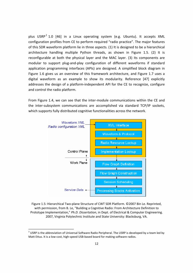
12
plus USRP2 1.0 [46] in a Linux operating system (e.g. Ubuntu). It accepts XML configuration profiles from CE to perform required “radio practice”. The major features of this SDR waveform platform lie in three aspects. (1) It is designed to be a hierarchical architecture handling multiple Python threads, as shown in Figure 1.5. (2) It is reconfigurable at both the physical layer and the MAC layer. (3) Its components are modular to support plug‐and‐play configuration of different waveforms if standard application programming interfaces (APIs) are designed. A simplified block diagram in Figure 1.6 gives us an overview of this framework architecture, and Figure 1.7 uses a digital waveform as an example to show its modularity. Reference [47] explicitly addresses the design of a platform‐independent API for the CE to recognize, configure and control the radio platform. From Figure 1.4, we can see that the inter‐module communications within the CE and the inter‐subsystem communications are accomplished via standard TCP/IP sockets, which supports fully distributed cognitive functionalities across the network.
Figure 1.5: Hierarchical Two‐plane Structure of CWT SDR Platform. ©2007 Bin Le. Reprinted, with permission, from B. Le, "Building a Cognitive Radio: From Architecture Definition to
Prototype Implementation," Ph.D. Dissertation, in Dept. of Electrical & Computer Engineering. 2007, Virginia Polytechnic Institute and State University: Blacksburg, VA.
2 USRP is the abbreviation of Universal Software Radio Peripheral. The USRP is developed by a team led by Matt Ettus. It is a low‐cost, high‐speed USB‐based board for making software radios.

13
Figure 1.6: MAC/PHY Reconfigurable Waveform Framework
Figure Source: references [29, 48]
Figure 1.7: Framework System‐level Block Diagram—Digital Waveform. ©2007 Bin Le. Reprinted,
with permission, from B. Le, "Building a Cognitive Radio: From Architecture Definition to Prototype Implementation," Ph.D. Dissertation, in Dept. of Electrical & Computer Engineering.
2007, Virginia Polytechnic Institute and State University: Blacksburg, VA.
14
1.4 About This Dissertation
In this document, a cognitive gateway is designed to facilitate universal interoperability between incompatible waveforms. Our eventual goal is to make a dynamic heterogeneous communication network work effectively and efficiently with the addition of cognitive gateways. The solution addressed in this dissertation can be briefly described as follows. Located in a network incorporating heterogeneous communication radios, the users send requests by their own waveforms, and then cognitive gateways are capable of automatically establishing links between incompatible radios and routing messages to the expected destination, along a path composed of links which support different waveforms. In some specific scenarios, CG can act as signal repeater, network gateway, or waveform gateway to provide extended service coverage area and improved system throughput. The advantages of CG over other interoperability solutions, which require the manipulations of operators, lie in its universality and autonomy, which is enabled by a software defined radio incorporating waveform‐oriented processing and automatic waveform identification. Two steps should be taken to fulfill the proposed solution. At the first step, we consider only the users with one‐hop distance to a cognitive gateway. This consideration is reasonable because “source‐CG‐destination” is a typical network snapshot. Therein, we focus on designing a powerful network node with special cognitive capabilities and also the necessary signaling schemes between a CG and its one‐hop neighboring users. The key enabling technologies for this step, including waveform‐oriented processing loop, waveform identification, waveform transformation, waveform representation, and multiple‐link scheduling will be detailed in Chapter 2~4. Chapter 5 introduces the proof‐of‐concept prototype for the “source‐CG‐destination” snapshot, containing multiple links and the performance of such a system is also evaluated. Utilizing its capabilities, CG nodes can be placed in different network architectures/topologies to provide auxiliary connectivity. At the second step, we need to solve the multi‐hop relaying problem in a heterogeneous network.
1.5 Contributions
The contributions provided in this dissertation are summarized as follows. (1) We design a cognitive gateway node to facilitate universal interoperability and automatic relaying in a heterogeneous network, and describe its operating procedure by a waveform‐oriented cognition loop. We build and test a proof‐of‐concept prototype.

15
(2) We define “waveform” as a protocol stack specification suite and give a generic waveform representation format, which has a flexible, hierarchical, and platform‐independent architecture. (3) We analyze the commonly used waveforms and identify their waveform indicators, which are usually selected from the existing features or information embedded in the waveforms that a node can support. The waveform indicators are used for a CG to identify the waveform pair (including source waveform and destination waveform). (4) We develop a universal classification synchronization (UCS) system, implement it in the costly Anritsu MS2781A Signature Signal Analyzer and also an inexpensive SDR platform (i.e. USRP 1.0 plus GNU Radio), demonstrate its functions over‐the‐air, and evaluate its theoretical performance. In addition, we initialize the idea of implementing UCS on a GPP/DSP/FPGA hybrid platform. UCS performs automatic signal recognition, synchronization, and provides necessary parameters for transceiver configuration, demodulation without any a priori knowledge of the signal. (UCS was developed jointly by Ying Wang and me. Each of us applied it to different problems in our own dissertation.) It serves as the key component of CG’s waveform identifier. In addition, we design the signaling schemes between CG and various users. Specifically, we discuss the design trade‐offs among signaling message’s transmission manner (which means what the appropriate symbol rate, modulation, message length, repeating time should be chosen), signal‐to‐noise ratio (SNR), and waveform identifier’s accuracy and processing speed. (5) We implement the physical layer digital gateway, which currently uses two USRP 1.0 boards and is able to bridge two waveforms that are different in carrier frequency, modulation type. The up‐to‐network layer digital gateway, which bridges two waveforms coming from different subnets, has also been implemented. We integrate these functions and the multiple‐link multiple‐USRP management capabilities and implement the prototype for “source‐CG‐destination” snapshot. Our CG prototype will provide a test‐bed to verify the feasibility and practical performance of the vast MAC algorithms, channel allocation schemes, and network architectures proposed for DSA and cognitive network. (6) We design the method for multi‐USRP management, model CG as a differentiated service (Diffserv) system and evaluate its service performance by queuing theory.

16
1.6 What distinguishes my work from PSCR?
In this section, I will illuminate how my work goes beyond PSCR from the following aspects: (1) CG provides automatic waveform identification and link establishment, instead of manual operations in PSCR. (2) CG adopts a deterministic waveform identifier, which not only possesses the abilities of a PSCR sensor, but also provides extra abilities of fine classification and parameter estimation during and after symbol timing and carrier synchronization. Therefore, a CG is able to acquire more information for waveform recognition and handle more waveforms than PSCR. More details about the comparison between UCS and the classifier used in PSCR will be given in Chapter 3. (3) CG facilitates extensive interoperation between different waveforms, extending PSCR gateway mode, which only bridges different analog FM waveforms at the physical layer, to more complicated scenarios, which contain physical layer digital gateways, up‐to‐network layer gateways, and support the gateway function through the five layers. (4) The capability of managing multiple USRP motherboards and multiple links, not used in PSCR, has been enabled in CG. (5) CG enables the self‐organization self‐formation capability. It can either serve as a base station when the dynamic heterogeneous network operates at infrastructure mode or perform as an ad‐hoc relay to improve the throughput in a DSA‐allowed network. (6) CG has relatively more complete networking features. A series of topics including link strategy selection, link‐selection, routing are considered.
1.7 Dissertation Organization
This dissertation is organized into six chapters. Chapter 1 opens with research motivation and problem statement, followed by the introduction to research background, including the existing efforts made for improving communications interoperability. In particular, our first PSCR prototype demonstrated at NIJ CommTech TWG Meeting & Program Review in 2007 has been introduced and compared with the proposed cognitive gateway. Chapter 2 gives an overview of proposed cognitive gateway system. We first describe its functional architecture and system operating procedure. Next, we introduce the primary components constituting a complete cognitive gateway node, and their respective functionalities. These components include waveform identifier, scenario analyzer, waveform and user databases, decision maker, central controller (including logic link controller and resource manager), generic system API, and waveform converter.

17
In Chapter 3, we detail the design for waveform identification. The waveform identification module has two tasks, namely environment observation and user request awareness. This chapter covers the contribution point (2)‐(4). Chapter 4 addresses the implementation details for waveform conversion (including physical layer analog/digital gateway and up‐to‐network layer digital gateway), and investigates the strategies for multiple‐link and multiple‐USRP management. Chapter 5 introduces the proof‐of‐concept prototype for the “source‐CG‐destination” snapshot. We build a simplified CG on the open source GNU Radio, using a Linux system for its software platform and USRPs for its hardware platform. In our prototype, a CG can bridge the waveforms transmitted over different platforms, which include Walkie‐talkies for family radio service (FRS), P25 radios, USRP boards, as well as commercial‐off‐the‐shelf 802.11 WiFi chips, and 802.3 Ethernet adapters. The performance of such a system is also evaluated in this chapter. In addition, we discuss the CG configuration deduction problem. The last chapter, Chapter 6, summarizes the conclusions made in the preceding chapters, and envisions future work and possible extension, for example, the employment of CG will be beneficial to other applications including cooperative relay, DSA, etc.
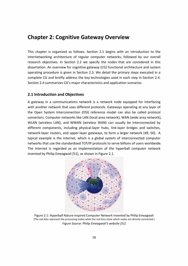
18
Chapter 2: Cognitive Gateway Overview This chapter is organized as follows: Section 2.1 begins with an introduction to the internetworking architecture of regular computer networks, followed by our overall research objectives. In Section 2.2 we specify the nodes that are considered in this dissertation. An overview for cognitive gateway (CG) functional architecture and system operating procedure is given in Section 2.3. We detail the primary steps executed in a complete CG and briefly address the key technologies used in each step in Section 2.4. Section 2.4 summarizes CG’s major characteristics and application scenarios.
2.1 Introduction and Objectives
A gateway in a communications network is a network node equipped for interfacing with another network that uses different protocols. Gateways operating at any layer of the Open System Interconnection (OSI) reference model can also be called protocol converters. Computer networks like LAN (local area network), WAN (wide area network), WLAN (wireless LAN), and WWAN (wireless WAN) can usually be interconnected by different components, including physical‐layer hubs, link‐layer bridges and switches, network‐layer routers, and upper‐layer gateways, to form a larger network [49, 50]. A typical example is the Internet, which is a global system of interconnected computer networks that use the standardized TCP/IP protocols to serve billions of users worldwide. The Internet is regarded as an implementation of the hyperball computer network invented by Philip Emeagwali [51], as shown in Figure 2.1.
Figure 2.1: Hyperball Nature‐inspired Computer Network Invented by Philip Emeagwali (The red dots represent the processing nodes while the red lines show which nodes are directly connected.)
Figure Source: Philip Emeagwali’s website [51]

19
As mentioned in Chapter 1, the object of our interest is a heterogeneous communication network, not limited to IP‐based LANs and WLANs. Our objective is seamless connectivity among the various involved communication nodes. But because of nodes’ incompatibility and insufficient coverage range, the heterogeneous network is actually a broken “fishing net”. So, mending the “holes” in the broken “fishing net” becomes our major job in this dissertation. We introduce cognitive gateways to construct new links to fill the “holes”. This interesting job is abstracted and illuminated by the graphs in Figure 2.2.
Figure 2.2: Add CGs to Provide Seamless Connectivity
(Dots and lines denote nodes and links, respectively. Different colors stand for different types of nodes and waveforms. But note that these colors do not mean the graph coloring strategies for channel allocation [24].
CGs are colored in orange.)
Cognitive gateways (CG) are conceived as a kind of special cognitive radio (CR) node which will facilitate universal interoperability between incompatible waveforms used by a variety of heterogeneous communication systems. In our solution, CGs are network nodes with routing ability. That means cognitive gateways are capable of automatically detecting users’ requests and routing their messages to the expected destination. In this sense, CGs are analogous to the routers of the Internet. Since we are considering a DSA‐enabled radio environment, the routing path is composed of links which may use different waveforms. This opens the multi‐hop routing problem in a dynamic heterogeneous network. It is an issue related to network topology and architecture. For the convenience of our discussion, we extract the “source‐CG‐destination” snapshot, shown in Figure 2.3(a), from the entire network, namely, we only consider the nodes with one‐hop distance to a CG. This snapshot is embodied in both infrastructure and ad‐hoc modes. No matter how many hops exist between the source and a CG, only the last hop of inbound route is considered by the CG; similarly, no matter how many hops exist between a CG and the destination, only the first hop of outbound route is considered by

the on dsign
2.2
In testaCG mak(PS)compubdevnodnod
CG. We widesigning analing schem
Figur
Specifica
he snapshoablishment is able to aking, logic li) communimmunicationblic safety raeloped CR des can intedes used in o
ill keep thea network nmes betwee
re 2.3: (a) “S
ations and
ot displayedrequests a
automaticalink control,cation inten initiating adios, P25‐cnodes. Oureroperate wour discussi
se assumptnode with sen a CG and
ource‐CG‐De(*PS st
d Scope
d in Figure nd sets up ly execute w and waveferoperabilitynodes, inc
compliant rr goal, illumwith each otion and give
Figure 2.4: N
20
tions from Cspecial cogn its one‐hop
estination” Stands for pub
2.3(a), the an affiliatiowaveform iform transfoy problemscluding thrradios, IP‐baminated in Fther via thee their corre
Node Specific
Chapter 2 tnitive capabp neighbori
Snapshot; (b)blic safety.)
communicaon with a Cidentificatioormation. Ms, we primee standarased WiFi aFigure 2.3(b aid of CGsesponding i
cations and I
to Chapter bilities and ng nodes.
) CG Design O
ation initiatCG when neon, scenarioMotivated bmarily consid systems,and Etherneb), is that t. In Figure 2icons.
cons
5, where walso the ne
Objective
tor broadcaecessary; tho analysis, dby the publider four ty i.e., conveet nodes, anhese four t2.4, we out
we focus ecessary
asts link hen this decision c safety ypes of entional nd user‐types of tline the

21
2.3 Cognitive Gateway Functional Architecture and System Operating Procedure
A complete CG node is composed primarily of nine modules as shown in Figure 2.5. These are the waveform identifier, scenario analyzer, waveform and user databases, decision maker, forwarding & routing tables, central controller (including logic link controller and resource manager), generic application programming interfaces (APIs), and waveform converter. This architecture follows CWT’s cognition loop in Figure 1.4 and is quite similar to that of the CRs developed in our laboratory. The biggest differences lie in four aspects. (1) Using its available hardware and software resources, a CG is responsible for establishing as many communication links with a specified quality of service as needed between incompatible waveforms, so (2) it needs to identify the types of both source and destination waveforms, and (3) it requires a protocol to manage the establishment, maintenance, and termination of logic links. (4) It needs a procedure for user registration and authentication. Thus, the design for CGs has some difference from the discussion presented in [29‐31], although similarities inevitably exist. The key technologies used in CG will be addressed in detail.
Figure 2.5: Cognitive Gateway Block Diagram
In our research, cognitive gateways are located in a network incorporating heterogeneous communication nodes. Those that comply with the same or similar standard are able to communicate with each other directly, via repeaters, or intra‐standard gateways; while those following different standards need inter‐standard gateways to bridge them. According to our “waveform” definition, repeaters, intra‐
Waveform Identification Scenario Analysis
P25 Radio Platforms
Internet ProtocolStack Suite
Frame Analyzer
UCS
Physical Layer Demodulator
Standard Waveform Database
Cognitive Waveform Database
Platform for Waveform Identification
Destination Waveform Identifier
Source Unit Identifier
QoS Requirements
Central Controller Resource Manager
Logic Link Controller
Authorized or Registered
User Database
Generic API
Waveform Transformation
Cognitive Radio Platforms
Other Waveform Platforms
Case-based Decision
Maker
c
Forwarding & Routing Tables

22
standard gateways, and inter‐standard gateways all implement the same function — waveform transformation. These are specific forms of CG in different application scenarios to improve interoperability and extend communications coverage. Specifically speaking, “intra‐standard gateways” bridge the nodes using the same waveform type but different parametric values. For example, the police officers from different cities use legacy analog FM narrowband handheld radios operating at distinct frequencies. Therein an “intra‐standard gateway” is enough to facilitate their voice communications. Besides, the gateway routers interconnecting different TCP/IP LANs also belong to “intra‐standard gateways”. In Figure 2.6, we describe a scenario where the CG acts as an inter‐standard gateway to bridge legacy public safety systems, P25 enabled systems, IP‐based wireless LANs, and user‐developed CR systems.
Figure 2.6: A Scenario Using a Cognitive Gateway. ©2008 Software Defined Radio Forum. Reprinted, with permission, from Q. Chen et al., “Cognitive Gateway Design to Promote
Universal Interoperability,” in Software Defined Radio Technical Conference. October 26‐30, 2008: Washington, DC.
A gateway is the intersection point for different systems. It has multiple identities and interfaces. The CG shown in Figure 2.6 is wireless. It uses software/hardware (such as GNU Radio [45] plus Universal Software Radio Peripheral (USRP) [46]) similar to wireless network cards to transmit and receive signals over the air. Its interface to an IP‐based network should have an IP address; its interface to a P25 system should have an address and identification which can be recognized by P25 radios; its interface to a CR network should be known to CR nodes. For each subnet using this CG, if a node within one subnet wants to send data to another node belonging to a different subnet, it only needs to send the data to the CG which can reach the desired destination. This principle is analogous to that used in IP‐based network: a very popular example is connecting a

23
LAN to the Internet or a WAN [50]. But a CG has to do much more than replacing the original source address with the new one. A CG needs to recognize the incoming waveform to determine whether it is a signal it should forward or drop, which waveform the next‐hop relay should employ, and which waveform platforms it should launch to implement waveform transformation. The complete operating procedure of a CG can be depicted by the waveform‐oriented processing loop in Figure 2.6.
Figure 2.7: CG Functional Loop‐‐Waveform‐Oriented Processing Loop
Basically, the waveform identification module consists of a signal classifier, physical layer demodulator, and frame analyzer. It works with the two waveform databases (a standard waveform database and a cognitive waveform database) to identify the waveform coming into the CG. The signal classifier determines physical layer parameters like carrier frequency, bandwidth, modulation type, and symbol rate. In most cases, these parametric values are sufficient for waveform identification. If not, the physical layer demodulator will be configured by these parametric values to extract the link layer frames; then, the frame analyzer will deduce the frame format to help decide the source waveform type. Meanwhile, the source and destination addresses or identifiers will be extracted and fed into the next block—the scenario analyzer. Referring to the user database, the scenario analyzer identifies the waveform pair that the CG needs to interconnect. We call this link establishment request an application. Applications from authorized users will be placed in the waiting queue of the central controller. After the scenario analysis step, the decision maker first checks the forwarding & routing tables to
24
choose the next‐hop candidates, and then it determines the next‐hop node and the waveform that will be used for this hop, taking into consideration capabilities of candidate nodes, availability of needed resources, concurrency of ongoing links, and the priority of this application. Based on the decision result, the central controller will allocate appropriate resources to implement the applications and meet their priorities and QoS requirements to the best of their ability. Then, the system configuration profiles and necessary control commands will be generated to launch corresponding platforms or components for implementing waveform transformation, thereby establishing communication links between different waveform platforms. Because of its wireless nature, a CG can only provide service to the users within its effective range. Its user database contains all the users within its service group. This service group mainly includes pre‐authorized public safety radios, wireless IP nodes, and registered CR nodes. When a new CR node appears, it will broadcast registration request messages and affiliate itself with one of the CG nodes who respond to its requests. In this way it is able to join and quit the service group of an available CG, and the CG’s user database will be updated accordingly. Our goal is to make the whole system automatic after the initial human setup. Therefore, appropriate signaling mechanisms should be designed. Our requirements for signaling scheme design are embodied in the four aspects as follows. (1) Minimal or no changes should be made to the standard systems. (2) The waveform sent by a user should contain the necessary information for a CG to process the link establishment request. (3) The signaling messages should be transmitted in a manner that can be recognized by a CG with high accuracy. (4) The overhead for signaling process should be as low as possible. Because of the heterogeneity of communication initiators, CGs use different signaling methods to fit different types of users. For instance, the legacy public safety analog FM radio signal, unlike the digital signals generated by the packet‐switch system, does not carry destination information by default. We detail the design trade‐offs between signaling schemes and waveform identification in Chapter 3. It is worth mentioning that the maintenance of real‐time forwarding tables and routing table is necessary for a CG to provide effective and efficient bridging/relaying services. A forwarding table includes destination indication value, destination waveform type, and the CG interface where the incoming information should be forwarded to. Since different types of communication initiators adopt different destination indicators, CG maintains forwarding table for each of them. The routing table usually stores the routes to particular network destinations, and metrics associated with those routes. Typically in

25
the Internet, this information contains the topology of the network immediately around it. But in a CG, we exploit a waveform‐guided routing method, where the next‐hop nodes and the waveform used for each link of the route need to be determined. The route selection has to consider not only network topologies, but also the radio environment, capabilities of SU, and activities of PU. The details about CG forwarding tables and routing tables are addressed in Chapter 4.
2.4 An Overview of Building Functional Cognitive Gateway Systems
In this section, we will separately introduce the major components that constitute a CG. Before diving into the details for each module, we first show how to present a waveform because waveforms are the processing objects through the whole procedure of a CG.
2.4.1 Waveform Representation
The waveforms used in standard systems have been well defined, but a CR system is distinguished by waveform agility and there is not a uniform specification for its mechanisms or protocols. Considering that the IP‐based networks form the backbone infrastructure and that the OSI reference model has been widely and successfully used, we decided to describe the waveforms according to the five‐layer protocol stack architecture. Our definition for “waveform” in Chapter 1 is based just on the above considerations.
Figure 2.8: A Generic Cognitive Radio Architecture. ©2007 Thomas W. Rondeau. Reprinted, with
permission, from T. W. Rondeau, "Application of Artificial Intelligence to Wireless Communications," Ph.D. Dissertation, in Dept. of Electrical & Computer Engineering. 2007,
Virginia Polytechnic Institute and State University: Blacksburg, VA. In our discussion, we assume that the CR nodes constituting a CR network follow the generic CR architecture shown in Figure 2.8. This architecture determines the waveform format for CR. Actually it is challenging to develop (1) CR nodes with complete stack
Application
Comm. Sys.
Transport
Network
User Domain
Link / MAC
Physical
CognitiveEngine
PolicyEngine
Operational Cognitive Radio Platform
External Environment and RF Channel
Policy Domain

26
architecture and functionalities, and (2) necessary mechanisms/protocols for communications among nodes following the same or different standards. These two tasks are very important to CG design, but they contain too many issues, which cannot be fully addressed in a few words. Hence, we only list here the key issues to be considered as follows.
Supported applications and corresponding QoS, security and reliability requirements
Transport layer protocols Routing algorithms Addressing and mobility management Unit identification, database management Channel utilization scheme, logic link control Frame architecture and message formats for inter‐ and intra‐system communication REM (radio environmental map) acquisition Except the second bullet, the other issues have been discussed to certain degrees in some sections of this dissertation. In Table 2.1, we give a reference format that can represent typical existing waveforms like standard 802.11b and 802.11g, and P25 waveforms complying with the standard CAI. The five layers are denoted as PHY, LINK, NET, TRAN, APPL, respectively. The given format has a hierarchical architecture, where the concrete format of the lower tier is subject to change based on the higher tier specification. For example, the traditional analog public safety waveform does not have NET and TRAN layers at all. This architecture possesses several advantages: (1) clear hierarchy/layering is efficient for parameter extraction at the system configuration stage; (2) it is flexible to adapt to different waveforms and open for future modification. Actually, many parameters of the standard waveforms use fixed default values, and some “knobs” outlined in Table 2.1 do not exist in the standard waveforms. Therefore, when a waveform profile containing these “knobs” is generated for system (re)configuration, a parser does not need to extract all the parametric values. This will speed up the system configuration step. In addition, this waveform representation method is platform independent. No matter which vendor the device is from, no matter whether the CR is built on GNU Radio, IRIS (Implementing Radio in Software) [52], or OSSIE (Open Source SCA Implementation ‐ Embedded) [53], this format works. In CWT, we select extensible markup language (XML) to describe a waveform.

27
Table 2.1: Reference Waveform Format (A SAMPLE). ©2008 Software Defined Radio Forum. Reprinted, with permission, from Q. Chen et al., “Cognitive Gateway Design to Promote
Universal Interoperability,” in Software Defined Radio Technical Conference. October 26‐30, 2008: Washington, DC.
Tiers (high low) Parameters (or Knobs)
2.Waveform
Type
Options: C
R, W
iFi, P2
5, Con
ventional Pub
lic Safety
TX
PHY RF Tx carrier frequency, Tx power
MOD Modulation type and index, Symbol rate, Roll off, Differential coding
FEC∗ (e.g. RS) Number of input symbols, Number of output symbols
LINK
MAC∗ protocol (e.g. CSMA)
Carrier sense threshold,Contention window, Minimum back‐off delay
Frame Frame size, Frame type
NET Protocol Network protocol (IPv4 or IPv6)
IP address allocation protocol Routing protocol
IP packet Packet size TRAN Protocol TCP or UDP
APPL
Service∗ type Application protocol (e.g. HTTP, SMTP)
Encryption Encryption key RX Similar as the format for TX
* Type options for Medium Access Control (MAC) Protocol: CSMA/CA, PTT, ALOHA etc. Type options for FEC: convolutional coding, block coding (including Reed‐Solomon (shortened as “RS” in Table 2.1, BCH, Golay, Hamming). Service type could be audio, video, multimedia, data etc.
2.4.2 Waveform Identification and Scenario Analysis
The waveform identification module not only identifies the incoming waveform type but also provides the REM to the central controller as the reference for medium access control. The output of waveform identifier will be a subset of the complete waveform representation addressed in Section 2.4.1; while the information fed into the central controller by the scenario analyzer may be a set like (node A: waveform A: network A, node B: network B, high priority), which means node A from network A, which is using waveform A, requested to establish communication link with node B in network B, and this application has a high priority. Note that waveform A is a combined entry from the waveform database. If a signal from an unwanted user is detected, the CG will discard it. The waveform identification step employs our newly developed universal classification, synchronization (UCS) system [54, 55] to implement the physical‐layer signal recognition,

28
and the physical layer demodulation when necessary. Our UCS system currently supports a variety of modulations, including analog AM and FM, and M‐ary PSK, QAM, FSK, and standard OFDM. The system block diagram for narrowband signals is shown in Figure 2.9. It can automatically interpret features of the received signal to accomplish classification, synchronization and demodulation without knowing any prior modulation information. As we add more modems to our software repository, more modulations will be included.
Figure 2.9: UCS Function Block Diagram for Narrowband Signals. ©2008 Software Defined Radio Forum. Reprinted, with permission, from Q. Chen et al., “Cognitive Gateway Design to Promote Universal Interoperability,” in Software Defined Radio Technical Conference. October 26‐30,
2008: Washington, DC. (*Bandwidth estimation varies for different modulation groups.)
Under the traditional static spectrum policies a spectrum sensing module, which is able to provide signal location information in the frequency domain (including center frequency and bandwidth) is almost sufficient for waveform identification. However, the introduction of market based spectrum policies and the adoption of CR, DSA result in the occurrence of new waveforms and increase the difficulty and complexity for identifying standard waveforms. Thereby, in some cases, information in addition to the physical‐layer parameters must be extracted from the link layer frames to provide more accurate waveform identification, and also to guide the posterior steps. For example, a CG needs to know the destination address and waveform in order to determine how the API should be configured, and which interface the received data should be forwarded to. We therefore take advantage of a multi‐layer waveform identifier. The platform for waveform identification can be a stand‐alone MATLAB‐enabled Anritsu MS2781A Signature Signal Analyzer [56] running Windows, a sensor implemented over GNU Radio plus USRP in Linux and embedded in the same host as the central controller, or a Lyrtech SFF SDR platform [57] connected to a PC.
Spectrum Sensing
Phase Continuous vs. Phase Non‐continuous
Categorization
Amplitude‐modulated vs.Phase/freq‐modulated
Categorization
Analog Freq‐Modulated vs. Digital
Freq‐modulated
Bandwidth Estimation∗
Incoming Signals
AM, FM or FSK MPSK or QAM
FM or FSK
FSK
FM
AMSymbol Timing
& Coarse Classification
MPSK QAM
Carrier Sync.
FineClassification
Digital Demod.
MPSK
AMFM
Analog Demodulation
CTCSS Tone Recognition
Demodulated FM Signal
Demodulated AM Signal

29
2.4.3 Database
We have four databases serving the CG: standard waveform database, CR waveform database, user database, and the system resource database contained in the resource manager. The waveform databases are organized as hierarchical architectures with “knobs” whose values are obvious for waveform differentiation. Instead of outlining all the combinations, we list all the possible values for each “knob”. The user database includes IDs for authorized users and the address sets used in different subnets. Since a CG provides services for wireless mobile users within its contributing range, the users’ mobility will result in the update of this database. The system resource database contains the usage situation of CPU, memory, power, and waveform platforms. Thus, it is a dynamic database.
2.4.4 Waveform Transformation
Waveform transformation could be much easier if we have corresponding waveform modems. That means we can first demodulate the received signal and extract the payload, then encapsulate and modulate the payload into another waveform format, then transmit it. Besides the payload, we also need to extract the necessary information required for re‐transmission (e.g. destination address, destination ID). Repeaters and intra‐standard gateways usually bridge the waveforms which have different physical layer parameters, such as carrier frequency, modulation, symbol rate etc. As to the inter‐standard gateway exploited in Figure 2.6, instead of making great efforts to develop the modems for standard P25 waveforms and 802.11b, g waveforms under the open source software environment like GNU Radio, we directly make use of inexpensive WiFi chips for PHY‐ and LINK‐layer processing, and the built‐in protocol stack, well supported by operating system, for upper‐layer processing. We also use the E.F.Johnson 5300 ES Series Mobile Radio platform [58], which provides an interface to be controlled by a PC. If GNU Radio is assumed as the software platform for CR implementation, we can build a TUN/TAP (a virtual point‐to‐point and Ethernet device) [59] to create an interface “gr#”, which is similar to the interface “eth#” for Ethernet or “wlan#” for WiFi. These different interfaces can be bridged at the network layer. The information for hardware configuration is generated based on current application (i.e. the waveform pair), link status, resource occupancy, and routing & forwarding table.
2.4.5 Link Control
One of the big challenges for CG implementation is the link control. A CG may manage multiple links. A finite state machine (FSM) based link control protocol is essential to smooth link configuring, switching, establishment, maintenance, and termination. We

30
need to determine the states and actions for FSM. The central controller sends a command (such as load, reload, start, stop, pause) to guide the target waveform platforms’ behavior while the waveform converter returns link status to the central controller. The FSM design also takes into account the MAC protocols used for each waveform transformation link. The format of link status can be expressed as: Link 1 (waveform platform A waveform platform B): busy. The number of links that a CG can handle during a given period of time depends on its capabilities and available software/hardware resource. In some cases, the sensor of a CG competes for the waveform platform for CR. In addition, a CG for a wireless communication system is different from the gateway used in wired networking system in the aspect that the multiple waveform platforms cannot be simultaneously employed if the signals are transmitted at the same or close channels due to the self‐interference problem. For those links that can coexist, multiple threads are created. The performance of a CG will be evaluated by the metrics link throughput, delays, and packet loss rate.
Figure 2.10: Generic API and Link Control. ©2008 Software Defined Radio Forum. Reprinted,
with permission, from Q. Chen et al., “Cognitive Gateway Design to Promote Universal Interoperability,” in Software Defined Radio Technical Conference. October 26‐30, 2008:
Washington, DC.
2.4.6 Generic Interfaces
A CG can be implemented in a distributed manner, where the modules connected to the central controller may be located in the same or different hosts. As shown in Figure 2.5, a series of APIs are needed to convey information between the directly associated functional modules. “Sockets” can serve as the tunnel for the information conveyance.

31
As the scheduler of the whole CG, the central controller uses a general method to describe the attached modules. This description may include a set like (module name, host name or address, port number). A distributed implementation enables the concurrent operation of multiple functional modules. The major task of the generic API in Figure 2.5 is to convey information between the central controller and the waveform converter. A reconfigurable, flexible API that balances among generality, efficiency, and complexity is an ideal choice for CG. Generally, the information for hardware configuration, waveform pair specification, and system link behavior control is transmitted via this generic API. Just like the idea for a generic waveform representation in Section 2.4.1, this generic API targets all the layers of a protocol stack and thus can be configured to meet the specific requirements for different applications. The generic API between the center controller and the waveform converter is composed of three parts: waveform pair configuration API, platform pair configuration API, and control API. A complete generic API can be simply expressed as: (waveform A: platform A, waveform B: platform B, link control command). The waveform representation refers to Table 2.1, while the waveform platform format refers to Table 2.2. Both the waveform profile and its corresponding platform profile will be greatly simplified if the waveform pair uses standard waveforms. A block diagram shown in Figure 2.10 describes the link status control and the generic API.
Table 2.2: Reference Waveform Platform Format (A SAMPLE)
Hierarchy Parameters (or Knobs)
Waveform∗ platform
(e.g. GNU Radio plus USRP)
PHY
TX
Tx_USRP_subdev_spec, Tx_USRP_pga_gain, Tx_USRP_interp, Tx_samples_per_symbol
RX
Rx_USRP_subdev_spec, Rx_USRP_pga_gain, Rx_USRP_decim, Rx_samples_per_symbol
USB fusb_block_size, fusb_nblocks
LINK
TUN Device [11]
Tun_device_filename, IFF_TUN, IFF_TAP, IFF_NO_PI, IFF_ONE_QUEUE
NET
Interface gr0
IP address 192.168.100.6 Name Host name, USRP 1.0 serial number or USRP 2.0 MAC address
* Type options for waveform platform: GNU Radio+USRP, OS+WiFi chip, E.F.Johnson 5300.

32
Different platforms may use different operating systems and different languages. We select extensible markup language (XML) to describe the configuration profiles because of the following reasons: (1) it is open and flexible to be modified; (2) it has a hierarchical architecture, which matches our proposed generic waveform format; (3) it is readable by both machine and human beings; (4) By a simple data parser, the XML format can be mapped to the waveform platform‐specific format regardless of programming languages (such as C++, Python, Java) used in the waveform platforms. The generic API suite represented in XML format has been successfully applied to our PSCR and UCS system for information exchange. The former employs Python and C++ running on a Linux operating system (OS), while the latter uses MATLAB in both Windows and Linux OS.
2.5 The Intention and Extension of Cognitive Gateway
In this chapter, our introduction to CG focuses on the “node” level. As an intelligent “node”, CG possesses the following characteristics: (1) Universal interoperability enabled by the generic waveform representation format and the reconfigurable software defined radio platform; (2) Autonomy facilitated by the automatic waveform identifier and waveform‐oriented cognition loop; (3) Extendable and upgradable to accommodate more waveforms; (4) Cognition: CG adapts to the radio environments, and adjusts itself to minimize resources competition, improve nodes cooperation. Besides, we endow CG with routing ability. The “Source‐CG‐Destination” snapshot can be scaled in different network architectures to provide larger communication coverage. In Chapter 5, we will present the prototype built to verify the functionalities of a CG. With the above capabilities, CG can be beneficial to a variety of application scenarios. Here we give three examples. (1) In “hot spots”, CGs can be easily set up to facilitate the communications, for both first responders and besieged people, between the disaster‐hit area and the outside (or edge infrastructure), and within that area. (2) CGs can act as mesh routers in wireless mesh networks (WMNs) [60‐64]. (3) CGs can be utilized in a DSA‐enabled system to improve throughput. (4) CGs can work at both peer‐to‐peer and infrastructure mode to assist cooperative relay [65‐70]. Furthermore, with the reality that diverse air interfaces and dissimilar access networks coexist, accompanied by the trend that the DSA is allowed and gradually employed, cognition and cooperation form the promising framework to achieve the ideality of seamless ubiquitous connectivity in future communication networks [71, 72].

33
Chapter 3: Signaling Schemes and Waveform Identification Admittedly, the CG waveform identifier plays an important role in the entire process of providing a complete service, yet the success of a complete service also needs appropriate signaling schemes between CG and users (or clients). In this chapter, we will detail the key issues including waveform indicator selection, a complete service, waveform identification, and signaling processes. Further, we will analyze the trade‐offs between control message design and CG processing strategy for waveform identification (WI), with the objective of balancing the signaling efficiency and the WI accuracy.
3.1 Waveform Indicator Selection
When we introduced the operating procedure of the cognitive gateway system in Chapter 2, we made two assumptions as follows. (1) The communication initiator knows the existence of CGs even though it may not know where they are. (2) If requesting the service from CGs, the clients will send waveforms containing the necessary information for a CG to process their requests. The rationality of the second assumption is confirmed only after we analyze the four types of waveforms of interest, including legacy public safety, P25, WiFi & Ethernet, and user‐developed cognitive radio (CR). From these waveforms, we extract the parameters that can be used for a CG to identify the source waveform and the destination waveform. These parameters are called “waveform indicators”, outlined in Table 3.1. The selection of waveform indicators primarily follows two principles: (1) Make use of the existing features or information embedded in the waveforms that a node can support; if changes are inevitable and necessary, minimal changes should be made. For standard waveforms, the change might be a new utilization method of the existing features. For example, in some specific scenarios, the CTCSS (Continuous Tone‐Coded Squelch System) of a legacy analog FM public safety waveform can be used to indicate different requests and destinations. But we need to emphasize that these kind of changes should be agreed to by all the communication nodes involved. For the user‐developed CRs, the changes might be different transmission manners like the time interval between consecutive packets or the size of an individual packet. Usually, these changes are made to facilitate the cooperation between clients and CGs, hence smoothing the service processes. (2) The information that can indicate the waveform type should be represented in a format which can be interpreted by a CG with satisfactory accuracy and acceptable time consumption. In the next section, we will address how the detailed service process
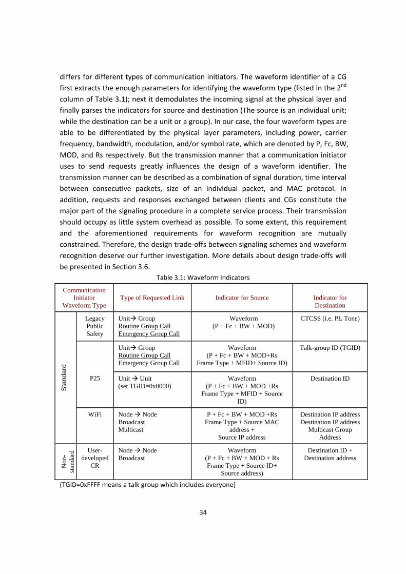
34
differs for different types of communication initiators. The waveform identifier of a CG first extracts the enough parameters for identifying the waveform type (listed in the 2nd column of Table 3.1); next it demodulates the incoming signal at the physical layer and finally parses the indicators for source and destination (The source is an individual unit; while the destination can be a unit or a group). In our case, the four waveform types are able to be differentiated by the physical layer parameters, including power, carrier frequency, bandwidth, modulation, and/or symbol rate, which are denoted by P, Fc, BW, MOD, and Rs respectively. But the transmission manner that a communication initiator uses to send requests greatly influences the design of a waveform identifier. The transmission manner can be described as a combination of signal duration, time interval between consecutive packets, size of an individual packet, and MAC protocol. In addition, requests and responses exchanged between clients and CGs constitute the major part of the signaling procedure in a complete service process. Their transmission should occupy as little system overhead as possible. To some extent, this requirement and the aforementioned requirements for waveform recognition are mutually constrained. Therefore, the design trade‐offs between signaling schemes and waveform recognition deserve our further investigation. More details about design trade‐offs will be presented in Section 3.6.
Table 3.1: Waveform Indicators
Communication Initiator
Waveform Type
Type of Requested Link
Indicator for Source
Indicator for Destination
Stan
dard
Legacy Public Safety
Unit Group Routine Group Call Emergency Group Call
Waveform (P + Fc + BW + MOD)
CTCSS (i.e. PL Tone)
P25
Unit Group Routine Group Call Emergency Group Call
Waveform (P + Fc + BW + MOD+Rs
Frame Type + MFID+ Source ID)
Talk-group ID (TGID)
Unit Unit (set TGID=0x0000)
Waveform (P + Fc + BW + MOD +Rs
Frame Type + MFID + Source ID)
Destination ID
WiFi Node Node Broadcast Multicast
P + Fc + BW + MOD +Rs Frame Type + Source MAC
address + Source IP address
Destination IP address Destination IP address
Multicast Group Address
Non
-st
anda
rd User-
developed CR
Node Node Broadcast
Waveform (P + Fc + BW + MOD + Rs Frame Type + Source ID+
Source address)
Destination ID + Destination address
(TGID=0xFFFF means a talk group which includes everyone)

35
3.2 A Complete Service Process
In this section, we detail a complete service process using specific examples. Recall the node specifications in Figure 2.4; the communication initiator is either a primary user (e.g. public safety radio) or a secondary user (e.g. CR node). The primary users (PUs) are pre‐authorized clients; while the secondary users (SUs) need to register to the nearest available CG before being able to get services. Amongst the PUs, the conventional public safety radios use pre‐assigned fixed channels (the P25 trunking system is different [73, 74]) with no need to worry about causing interference to SUs, but the SUs dynamically access the unoccupied channels with the caution of avoiding interference to PUs. In addition, requests from the PU are treated by CGs as higher priorities than those from the SU. Moreover, the PUs and SUs usually possess different capabilities. It is their difference in privileges, channel utilization, and capabilities that makes the service process initialized by a PU different from that initialized by a SU.
For the convenience of our discussion, the four waveform types (legacy public safety, P25, IP‐based, and CR) of our interest are simply denoted by waveform types A, B, C, and D, respectively (as shown in Figure 2.3(b)). Figure 3.1 illuminates a process where in a legacy public safety radio (LPSR) interoperates with the legacy public safety radio(s) from another department with the aid of a CG. When a legacy public safety user is a communication initiator, it sets the CTCSS value to correspond with the communication target, and then pushes the button to send its request. The CG that detects this request first identifies the source waveform type, which is LPSR from Department A in our example, on the basis of extracted parametric combination (P, Fc, BW, MOD). Next, the CG configures itself to do FM demodulation and calculates FFT to get the value of CTCSS. For instance, the CTCSS value is 1. After checking the local forwarding table for the source of waveform type A, the CG knows the destined communication target is LPSR Department B. Therefore, the CG needs to establish a physical layer analog gateway link and forward the incoming traffic to the outgoing interface 1. If the waveform pair is other than (LPSR LPSR), the corresponding link establishment process will be different from that shown in Figure 3.1. The waveform conversion for various waveform pairs will be detailed in Chapter 4.

36
Figure 3.1: A Process of Interoperating LPSRs from Different Departments via a CG
Next, we will address the complete service process initialized by a CR. CRs dynamically share the spectrum as SUs and the entire process is much more complicated than the cases when PUs are communication initiators. Before it is able to get services provided by CGs, a CR needs to register to a CG. In our case, CGs can be fixed or mobile. We do not employ a proactive CG discovery method (where the CGs periodically broadcast their existence, and the users choose one to join service group) because a CG does not have a fixed control channel for broadcasting, and hence this method will increase the complexity of both CGs and CRs. Instead, a reactive CG discovery mechanism [75] is exploited. The CR node chooses a vacant channel to broadcast a request registration message; each of the CG nodes that receive this message will unicast a response message which contains its ID. If the CG is multiple hops away from the requesting CR node, its response message should also include the information for the CR node to set up a route to the CG. The requesting CR node may select a CG using different criteria, for instance, the minimum number of hops, the closest distance, or the shortest delay. Actually, the solution to “which CG will be the best choice” varies with the real‐time channel capacity, traffic loads, delays, congestion etc. But this is beyond our scope. In our implemented prototype, the CR node that requests registration unicasts an acknowledgement message to the CG from which it gets the earliest reply to confirm its decision. The CG which gets the acknowledgement updates its user database by adding a new entry including the user’s ID, geolocation (if provided), and the channel where the user is currently residing. In addition, because of network dynamics and user migration,

37
the cognitive gateways within neighborhood periodically exchange information to keep their user databases and routing tables up‐to‐date. Therefore, the registration process provides convenience for user tracking and network resource (particularly spectrum) management.
Figure 3.2: Finite State Machine of a CR Node
During the process of registration, a CR node follows the finite state machine (FSM) in Figure 3.2. It uses a carrier sense multiple access (CSMA) MAC protocol with a back‐off time upper limit of th2. The major factors that impact the value of th2 are channel utilization, packet size, and packet transmission rate. It is important that if PU occurs, a CR node must immediately vacate its ongoing transceiver path and move to an unoccupied channel to transmit messages. In addition, another time threshold th1 is set to determine when a CR node should re‐send its request message. That means if a CR node did not get any response from CG within a time period of th1 after sending the request message, it will resend its request. The value of th1 is primarily determined by the processing delay in the CG. Once the acknowledgement has been sent out, the CR node stays in that channel until a new application emerges. In fact, during the signaling process for registration, link establishment, link resuming, and link termination, a CR node adopts the same flow‐graph exhibited in Figure 3.2. Further, the wireless communications between CR nodes can also be described by the FSM in Figure 3.2. After joining in the served user group of the CG (say “CG1”), a CR node named “CR1” sends link establishment request to CG1, expressing its desire to communicate with another CR node – “CR2”. The link establishment request message informs CG1 of the target destination ID (i.e. CR2), preferred channel list and modulation, and CR1’s current

38
geolocation. The preferred channel list reflects the channel availability in CR1’s surroundings and it will be used for channel negotiation before the communications. Upon extracting the destined node ID from the received message, CG1 first checks its user database, then its routing table. The checking results have two possibilities. (1) There is neither an entry for CR2 in its local user database nor a route to CR2 in its routing table. CG1 will inquire of its neighboring cognitive gateways. If the inquiry result is “no”, CG1 will notify CR1 that CR2 is not in service; if CR2 is found to be registered with another reachable cognitive gateway called “CG2”, a communication route that is composed by three parts, namely CR1↔ CG1, CG1↔ CG2, and CG2 ↔ CR2, needs to be set up. (2) CR2 is also affiliated with CG1. In this case, CG1 will calculate the distance between CR1 and CR2 based on the geo‐locations in the user database. If either CR1 or CR2 is out the effective communication range of the other, the communications between CR1 and CR2 will need the relaying of CG1; otherwise, CR1 will in principle communicate with CR2 directly, i.e. CR1↔ CR2. For the one‐hop links like CR1↔ CG1, CG2CR2, and CR1↔ CR2, a simple channel negotiation based on communication nodes’ preference and spectrum observation records will be made to determine which channel they should occupy for communications. There are three possible results from channel
negotiation: ① no vacant channel is available; ② there is a common channel usable by
the two communication nodes; ③ there is no common channel for the two CR nodes, but the communications can be bridged by CG1, which means the route between CR1 and CR2 contains two links (CR1↔ CG1↔ CR2), operating at different channels (or even different modulations and symbol rates in some cases). In addition, internal IP addresses are allocated to the pair of CR nodes during the pre‐link establishment signaling process. So far, we have mentioned channels for signaling and for communications. We use a small portion of our interested spectrum band for signaling, and the remainder for communications. The separation of signaling and communication channels eases the waveform recognition process. Both of these two parts are further divided into several sub‐channels. Therefore, the SUs dynamically share the multiple control channels for signaling. Without a fixed division for control channels, CR users are capable of flexibly finding signaling opportunities based on their carrier sensing results. This is another method for SUs to access the signaling spectrum band. A CG maintains the status of the registered CR users and also tracks the channel where each CR user showed for the last time. The tracking is necessary for a CG to contact a CR user who will act as a callee in the requested application. The tracking is achievable because during a complete service process, a CR user will choose an available control

39
channel to exchange control messages with the CG (who provides services to it) every time when its status is changed. To simplify the processing of a CG, CR users are only allowed to send control messages in the channels assigned for signaling. Using specific examples, we have detailed the operation flow of clients and CG during the service process for registration and link establishment. The communication resuming will happen if an on‐going communication which involves at least one SU is interrupted by PUs; and the link termination will occur if the clients have finished their communications, thus the occupied resources can be released. After a signaling process, the established link may go through a CG or not. The links that exclude CGs usually happen (1) between two CR users or (2) between a CR user and a primary user. In these scenarios, it is the users themselves who will terminate the links. For case (1), the two CR users need to send control messages to inform the CG, which they registered with, of “channel release”. For case (2), the CR user needs to send control messages to inform the CG of “communication completion”. For the variety of links including a CG, the CG center controller will launch/terminate corresponding waveform transformation (WT) flow‐graphs, which will be described in Section 4.1. A termination is executed when the center controller decides to utilize limited resources to serve for an application with higher priority or when the center controller gets the “communication completion” notice via a socket from the WT flow‐graph. A generalized flow‐graph in Figure 3.3 depicts the major operations of a CG. It includes the process for all the four types of waveforms of our interest.

40
Figure 3.3: Generalized Flow‐graph of a CG
(*WFQ stands for Weighted Fair Queuing. The leaky bucket and WFQ will be addressed in Chapter 4.)

41
3.3 Introduction to Waveform Identification
In a cognitive gateway, “waveform” is extracted as the object of the gateway’s entire processing loop. This cognition loop starts with “waveform identification (WI)” (also called “waveform recognition (WR)”). The major functions of a CG waveform identifier include: • User request awareness & waveform pair identification: extract necessary
parameters from the detected request signal and work with scenario analysis module to identify the waveform pair (source waveform and destination waveform);
• Environment observation: provide the radio environment information as the reference for medium access control and channel negotiation.
The fundamental requirement for the WR in a CG is that the waveforms of our interest can be recognized and identified to the extent that is enough for the CG’s decision making and link configuration. The design of WR becomes a challenging task for the following reasons: • The traditional static spectrum regulation policy has gradually evolved into s market
based spectrum policy. • The adoption of CR and DSA technologies result in the occurrence of new waveforms. • Standard waveforms coexist with user‐developed CR waveforms. • Different types of users use different signaling methods. In order to ensure higher
recognition accuracy and signaling efficiency, we need to tackle lots of trade‐offs. Figure 3.4 illuminates the logical flow for a WR to extract the waveform indicators listed in Table 3.1.
Figure 3.4: Logical flow for a WR to extract the waveform indicators listed in Table 3.1

42
As described in Chapter 2, CG uses a multi‐layer waveform identifier, where the physical layer signal recognition is implemented by the universal classification, synchronization (UCS) system. UCS is a joint work by Ying Wang and the author of this dissertation. Both of us will include it in our dissertations as an important part of our contributions. Our UCS work has been presented and accepted for publication in [55]. This work, with the addition of some recent updates, will appear in its entirety in Section 3.4. Section 3.4 is not organized the same way as other materials in this dissertation, but instead is an independent section. While this procedure might seem a bit unusual, our advisor felt that the work is of such significance it should appear in full, rather than simply being cited as a reference in both documents. An underlying assumption for the work to be addressed in the next section is that the target signal is transmitted continually, which guarantees the UCS system can capture enough signal samples for recognition. However, in most cases the target signals of a CG may not necessarily follow a continuous transmission manner. In particular, when the detection objects are control signals, it will be difficult to pick appropriate parameters for UCS. In Section 3.6, we will discuss the key issues in the design of signaling mechanisms and their relationship with waveform identification.
3.4 Universal Classifier and Synchronizer
Extracting parameters from a received signal and auto‐demodulating based on these parameters without prior information from the transmitter can be beneficial to Dynamic Spectrum Access (DSA), Cognitive Radio, and many other applications. Universal Classifier and Synchronizer (UCS) is conceived as such a self‐contained system which can detect, classify, synchronize with a received signal and provide all parameters needed for physical layer demodulation. The accommodated modulations include AM, FM, FSK, MPSK, QAM and OFDM. UCS can be used in different multi‐user access schemes. The designed system has been verified by a prototype using GNU Radio in Linux plus a Universal Software Radio Peripheral (USRP), as well as other software defined radio (SDR) platforms. Performance for key components and the entire system has been evaluated by theoretical analysis, Over the Air (OTA) experiments and computer simulations.
3.4.1 Introduction
Signal classification has many applications in wireless communications for both civilian and military purposes [76]. An M‐ary hypothesis testing problem is commonly posed to detect and classify a signal [77]. In our system, we are not only focusing on the existence and type of the signal, but also extracting its physical layer features for

43
demodulation. A software‐based design at IF or quasi‐baseband of a cognitive radio makes it able to automatically change configuration settings based on varying channel environments and user requirements. A radio equipped with UCS can respond to this change so that the continuity of communication can be guaranteed. UCS has the ability to demodulate signals without benefit of priori information and forms the heart of a truly cognitive receiver [54]. In the DSA scenario, a pair of cognitive transceivers occupies a certain channel as secondary users until a primary user appears. The secondary users must immediately move to an unoccupied channel. In order for this pair of cognitive radios to stay tuned in to continue communicating, either an out‐of‐band control channel needs to be used to negotiate setting information, or a pre‐defined channel changing protocol needs to be complied with to achieve automatic coordination. The former increases system overhead in control message conveyance and control channel management. The latter also has drawbacks. The primary users’ behavior and channel environment conditions are not fully predictable, while under a pre‐defined channel changing protocol the secondary users have to alter their settings in a fixed manner, in order to maintain the link. Thus the allowance for a radio to cognitively change its key physical layer parameters according to the channel environment is dramatically limited. Therefore, by sole use of a pre‐defined channel changing protocol, optimal resource utilization cannot be achieved. With UCS integrated in the radio, the aforementioned drawbacks can be conquered because the receiver can automatically extract necessary parameters from the detected signal and continue the previous communication. Such a system can be employed in DSA‐enabled scenarios to promote throughput, simplify channel management, optimize resource utilization, and provide better robustness under varying conditions, without increasing overhead. For example, if the changed channel is different from the previous one in terms of bandwidth, Signal to Noise Ratio (SNR) or other propagation features, the physical layer parameters can be changed for better performance without interrupting the communication. The parameters include carrier frequency, modulation type, symbol rate etc. As shown in Figure 3.5, during the DSA resource optimization process, unlike the conventional communication scenarios with pre‐agreement, the communication waveform is shuffled like a Rubik's Cube, and UCS is in hand to put it back in proper order. Another example of UCS’s applications is that UCS can accommodate multiple devices or support a variety of modulation settings. Whenever some resources become unavailable, the transmitter can switch to use other resources and the receiver with UCS will automatically follow it.

44
The remainder of this paper is organized as follows. In Section 3.4.2, we present our objectives after introducing the research background and state of the art. Section 3.4.3 begins with a description of the general cognitive receiver model, followed by the overview of our UCS system. We address the design and implementation details for each module of the UCS system in Section 3.4.4. Section 3.4.5 describes the UCS prototype and evaluates the performance for several key components and the entire system by theoretical analysis, OTA experiments and computer simulations. Conclusions and some discussions are made in Section 3.4.6.
Figure 3.5: Role of UCS in DSA Figure Source: reference [78]

45
3.4.2 Background and State Of The Art
As a branch of SIGINT [76], signal classification became an attractive research topic in 1980s. Because of the recently increasing interest in cognitive radio, signal classification is gaining more attention. The methodologies and technologies in this area can be roughly divided into three categories, (a) Maximum Likelihood (ML) based, (b) feature‐extraction based, and (c) cyclostationary feature based [29]. Method (a) classifies by comparing the likelihood of candidate signal and modulation types. Reference [79] is a classic article that talks about the optimal classification rules. Reference [80] is about asynchronous classification for MFSK. Method (b) directly extracts phase or amplitude features from the target signal in order to differentiate modulations. Zero crossing and wavelet technology are quite frequently involved in this area [81‐83]. Some papers combine (a) and (b) to get better performance. For example, in Reference [84], both ML and extracted features are used for OFDM signal detecting and classification in cognitive radio. Method (c) is attractive for DSA applications because of its ability to detect and classify signals at low signal to noise ratios [85]. The methods mentioned above have excellent performance in certain scenarios. The scenario conditions include channel types, signal types, and equipment. Our objective is to design a universal signal classification and synchronization system which can analyze a signal’s physical layer features with minimal prior information and application limits and can demodulate the signal using the acquired information.
3.4.3 System Overview
UCS has been developed and implemented to identify signals including AM, FM, MPSK, QAM, MFSK and OFDM. The system is constructed to run on USRP [46] with the GNU Radio [45] software toolkit. It is reconfigurable to provide adaptivity in various environments, extendable to accommodate more signal types, and transplantable to other platforms, such as Anritsu MS 2781A Signal Analyzer, Lyrtech Small Form Factor (SFF) SDR platform, Rice University WARP (Wireless open‐Access Research Platform) [86]. A fully developed UCS system with a reconfigurable demodulator can function as a cognitive receiver to classify, synchronize with and demodulate new signals. The system structure is shown in Figure 3.6. A complete cognitive receiving loop starts from signal awareness. The hardware is initially set with a wide frequency span at a center frequency we are interested in, and then zoomed in to the band where a possible signal exists. It is then reset to a reasonable sampling rate, and capture time. The channel estimation and equalization process is launched afterwards. This module is used to classify the channel type and make the necessary compensation. The next step is called

46
suite categorization and is used to determine the signal type. If the signal is analog, then it is sample based, which means we must demodulate it sample by sample, like FM and AM. If the signal is MPSK or QAM, then it is symbol based, which requires symbol timing and synchronization before demodulation. If the signal is wideband, for example OFDM, then it is block based, which means the demodulation is done block by block. If a signal cannot be clearly assigned to one of these three categories (sample, symbol, or block based) with information that has been extracted by the process described above, “knobs” [30, 31] like sampling rate will be “turned” to reconfigure the hardware for data re‐collection. Otherwise, the signal is identified as one of the aforementioned three types and then fed to the corresponding reasoning module, where the parameters needed for demodulation are estimated. Three possible results will be returned by the verification process: “reclassify,” “ready to configure,” and “unknown signal type.” If the parameters pass verification, they will be marked as “ready to configure” and formatted in an XML file [30, 31] to configure the demodulator and one complete loop is finished. If they do not pass, but the problem can be fixed by changing the hardware settings, the verification module will send “knobs” to reconfigure the hardware and the loop will be executed again. If the problem cannot be fixed, the result will be “unknown signal type”, and the signal will be stored in a database for future classification.
Figure 3.6: Cognitive Receiver System Structure
The system block diagram shown in Figure 3.7 includes all the modules implemented in UCS prototype. In the next section, we will describe the details of each module. The entire structure of UCS prototype can be understood as 4 branches and 3 phases. The 4
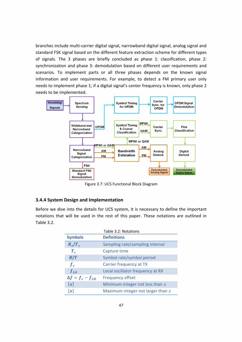
47
branches include multi‐carrier digital signal, narrowband digital signal, analog signal and standard FSK signal based on the different feature extraction scheme for different types of signals. The 3 phases are briefly concluded as phase 1: classification, phase 2: synchronization and phase 3: demodulation based on different user requirements and scenarios. To implement parts or all three phases depends on the known signal information and user requirements. For example, to detect a FM primary user only needs to implement phase 1; if a digital signal’s center frequency is known, only phase 2 needs to be implemented.
Figure 3.7: UCS Functional Block Diagram
3.4.4 System Design and Implementation
Before we dive into the details for UCS system, it is necessary to define the important notations that will be used in the rest of this paper. These notations are outlined in Table 3.2.
Table 3.2: Notations Symbols Definitions
/ Sampling rate/sampling interval Capture time / Symbol rate/symbol period Carrier frequency at TX Local oscillator frequency at RX
Frequency offset Minimum integer not less than Maximum integer not larger than

48
3.4.4.1 Spectrum Sensing Spectrum sensing has two purposes: it provides signal location information in the frequency domain (including center frequency and bandwidth), and also describes the spectrum occupation for the radio environmental map, which is important for DSA. In UCS, after the transceiver RF front‐end has been set at the carrier frequency estimated by the spectrum sensing module, the sensed signal will be down‐converted to IF or quasi‐baseband. Then each sample will be expressed as a complex number for subsequent processing. The amplitude and phase of this complex signal contain important information for classification, synchronization and demodulation. The spectrum sensing method adopted in UCS is energy detection based on power spectral density (PSD). From the PSD distribution, in the frequency ranges where the SNR is larger than a certain threshold, we consider that a signal exists. The threshold is defined as the acceptable SNR for UCS to get the correct modulation information extraction. The Welch’s method [87] can be used to estimate PSD with reduced noise. 3.4.4.2 Signal Capture Two factors that determine how to capture a signal for analysis are sampling rate and capture duration, which represent bandwidth and resolution respectively in the frequency domain. The captured signal data needs to be detailed enough to guarantee the accuracy of further information abstraction as well as brief enough to simplify the complexity and decrease the effect of fading channels. The settings of these two parameters in the signal collection device influence the entire UCS procedure. Sampling rate equal to twice the bandwidth of the interested signal is enough for waveform recovery. In our case, between waveform recovery and information demodulation, a series of other processes are required in order to acquire symbol rate, center frequency and other physical layer features. Is it necessary to increase sampling rate even higher in order to obtain these parameters? We will prove in Section 3.4.4.8 that in order to extract the correct symbol rate, sampling rate has to be larger than max 2 , , where is the threshold sampling rate required for symbol rate estimation. The value of the threshold is related to the pulse shaping used on the transmitter side. Capture time is another key factor to be considered. There are several restrictions for capture time. To simplify the calculation, capture time will be chosen as the minimum value which satisfies the following restrictions:
1. : is the frequency resolution required by the signal.
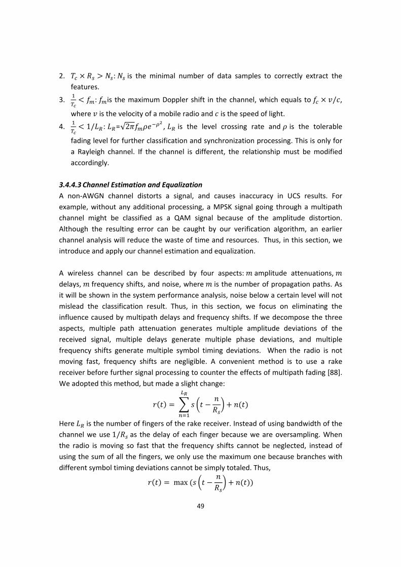
49
2. : is the minimal number of data samples to correctly extract the features.
3. : is the maximum Doppler shift in the channel, which equals to / ,
where is the velocity of a mobile radio and is the speed of light.
4. 1/ : =√2 , is the level crossing rate and is the tolerable
fading level for further classification and synchronization processing. This is only for a Rayleigh channel. If the channel is different, the relationship must be modified accordingly.
3.4.4.3 Channel Estimation and Equalization A non‐AWGN channel distorts a signal, and causes inaccuracy in UCS results. For example, without any additional processing, a MPSK signal going through a multipath channel might be classified as a QAM signal because of the amplitude distortion. Although the resulting error can be caught by our verification algorithm, an earlier channel analysis will reduce the waste of time and resources. Thus, in this section, we introduce and apply our channel estimation and equalization. A wireless channel can be described by four aspects: amplitude attenuations, delays, frequency shifts, and noise, where is the number of propagation paths. As it will be shown in the system performance analysis, noise below a certain level will not mislead the classification result. Thus, in this section, we focus on eliminating the influence caused by multipath delays and frequency shifts. If we decompose the three aspects, multiple path attenuation generates multiple amplitude deviations of the received signal, multiple delays generate multiple phase deviations, and multiple frequency shifts generate multiple symbol timing deviations. When the radio is not moving fast, frequency shifts are negligible. A convenient method is to use a rake receiver before further signal processing to counter the effects of multipath fading [88]. We adopted this method, but made a slight change:
Here is the number of fingers of the rake receiver. Instead of using bandwidth of the channel we use 1/ as the delay of each finger because we are oversampling. When the radio is moving so fast that the frequency shifts cannot be neglected, instead of using the sum of all the fingers, we only use the maximum one because branches with different symbol timing deviations cannot be simply totaled. Thus,
max

50
The output of the modified rake receiver is a clean signal ready for further processing. 3.4.4.4 Modern Wireless Communications Modulations and Scenarios UCS is designed for practical systems. It is necessary to give a summary of the commonly used signal types and multi‐user access schemes in modern wireless communications. Listing commonly used signal types helps clarify the research focus of UCS. In this paper, user scenarios analysis mainly focuses on single and multiuser access schemes. User scenarios analysis is beneficial for balancing UCS system implementation phase level and computation complexity. Currently, the most frequently used communication systems include: cellular, Wi‐Fi, WiMAX, public safety radios, and, customized cognitive radios. The goal of UCS is to extract physical layer features. The physical layer modulations for each standard are listed in Table 3.3, and the multiuser schemes for each standard are listed in Table 3.4.
Table 3.3: Modulation Types of Interest Communication System Physical Layer Modulation Types
Adopted
GSM GMSKGPRS GMSK3G CDMA4G(WiMAX) OFDMWi‐Fi OFDMPublic Safety Radio FM, C4FM, CQPSKCustomized waveforms for cognitive radio
FM, AM, MPSK, QAM, OFDM
From Table 3.3, we can see that the waveforms of interest include GMSK, CDMA, OFDM, FM, C4FM (Continuous 4 level FM), MPSK, QAM, etc. Among all these modulation types, we do not include CDMA in the UCS system because processing CDMA requires the spreading code. In standard communication systems, parameters are fixed; and in customized waveforms, the parameters are prone to change with varying environments. Our system can deal with both situations. In Table 3.4, multiuser access schemes fall into two categories: pre‐defined multi‐user schemes, which include TDMA, FDMA, CSMA and OFDMA, and primary/secondary user scenarios. One of the main purposes of UCS in cognitive radio is to accurately recognize the target of on‐going communication. Because of multiuser scenarios, other radios’ behavior will impact this recognition process. The basic principle of UCS is to extract

51
physical layer features so that any signal can be demodulated. Technically, if a signal can be demodulated, the identification of the signal is not a problem, and then a multiuser scheme will not prevent UCS application. However, either due to computation complexity or real time requirements, it is not a smart idea to run entire UCS on each of the signals appearing in the spectrum. As illustrated in Figure 3.7, running necessary phases instead of entire UCS system is more efficient. For example, for a standard primary user, the spectrum location and modulation setting are pre‐defined and fixed. This means that for a decided frequency, the primary user features are assured. If it is established that the signal is not a primary user, UCS will be called to determine the signal type, and if the detected signal type might be the type for the target of on‐going communication, the next step synchronization and demodulation will be continued to identify the secondary user.
Table 3.4: User Scenarios Description
Communication System Multi‐user Access Scheme
GSM Mixed TDMA and FDMAGPRS Unused TDMA channels in GSM 3G CDMA4G(WiMAX) OFDMAWi‐Fi CSMA/CAPublic Safety Radio Random Access or TrunkingCustomized waveforms for cognitive radio
DSA
3.4.4.5 Narrowband and Wideband Categorization As mentioned in system overview, all considered signals in UCS system fall into one of three categories: sample‐based, symbol‐based or block‐based signals. These can also be viewed as analog signals, digital signals and wideband signals. Because these three categories have different processing methodologies, they need to be differentiated before further processing. This section is to differentiate wideband signal and narrowband signal, and the next section focuses on further categorization for narrowband signals. A wideband signal is a signal whose period duration is longer than the maximum delay of the channel, which causes frequency selective fading. Spread spectrum and dividing the entire channel into multiple orthogonal sub‐channels are the two commonly used methods to resist this fading. In this paper, we refer to the former as a CDMA signal and to the latter as an OFDM signal. As mentioned in Section 3.4.4.4, CDMA signal could not be detected by UCS system because its processing requires the

52
spreading code. Thus, an alternative way to achieve the narrowband and wideband categorization is OFDM signal identification. To identify a signal as OFDM, we correlate the incoming signal with itself [89]. To illustrate this situation, we did OTA experiments for MPSK, analog FM and OFDM signal; the results are shown in Figure 3.8. The correlated output is different in the case of narrowband modulations and OFDM modulation. This difference is due to the cyclic prefix present in the OFDM signal, which gives us multiple peaks as opposed to a single peak in narrowband modulations. Will the peak be distinct enough to serve as the foundation for differentiation? The following calculation shows the identification accuracy under different SNR’s. The duration of an OFDM symbol is , where is the symbol duration without
the cyclic prefix and is the duration of cyclic prefix.
A continuous‐time OFDM signal at baseband can be written as [90]:
Here is the OFDM symbol at the th subcarrier and Γ denotes the set of
user subcarriers. Channel delay and frequency shift will not influence the ratio between the cyclic prefix peak and noise floor. It can be proved that it is sufficient to distinguish between narrowband and wideband signals. The detailed analysis appears in Section 3.4.5. Narrowband signals and wideband signals have different processing methodologies. We introduce narrowband signal classification and synchronization from Section 3.4.4.6 to Section 3.4.4.9, and wideband signal classification and synchronization from Section 3.4.4.10 to Section 3.4.4.12.
Figure 3.8: Use Autocorrelation to Differentiate OFDM and Narrowband Signals

53
3.4.4.6 Narrowband Categorization This section is divided into several sub‐sections, each subsequent sub‐section building on the information described in the previous sub‐section. The first sub‐section describes the general formulation of the narrowband waveforms that are currently categorized and provides a general categorization scheme for these waveforms. The second sub‐section describes the algorithm for performing the actual categorization of a narrowband signal and provides a general set of metrics for categorization thresholds as affected by noise as well as other irregularities that appear in mobile systems. It is important to understand that it is this coarse signal classification which will make the subsequent processing, e.g. symbol timing, carrier synchronization, and demodulation, much more efficient. Narrowband generalization Prior to providing the categorization of current waveforms of interest, it is efficient to describe these waveforms using a general structure. The general form is defined as:
cos 2 where and are the amplitude and phase of the waveform, respectively. Note that although the amplitude and phase are described as time‐varying for all waveforms, it is possible that for some waveforms these are constants. Analog and digital non‐linear modulation Both FM and continuous‐phase FSK (CPFSK) signals may be represented in the time domain by
, cos 2 2 (3‐1) where is the message signal, also called the modulating signal [91], and the constant represents the frequency sensitivity of the modulator [92]. In FM, is
continuous; in CPFSK, contains discontinuities, but its integral is continuous. Analog and digital linear modulation The other modulations (AM, PSK, QAM) belong to the linear modulation family, which can be expressed in the time domain as follows [91]. exp 2
cos 2 arg (3‐2)
Here, arg means the phase component of the modulating signal . For the convenience of the posterior analysis, we represent a full AM signal by: 1 cos 2 (3‐3), where is a constant that determines the percentage modulation [92].

54
General categorization for narrowband modulations By qualitatively analyzing their features (including instantaneous phase, amplitude, and frequency) embodied in equation (3‐1)~(3‐3), the aforementioned narrowband modulations can be sorted into the categories shown in Table 3.5.
Table 3.5: Categorizing the Narrowband Modulations Continuous phase Discontinuous phase
Constant amplitude Varying amplitude
Single-value envelope
Multiple-value envelope
Continuous freq.
Discrete freq. AM
MPSK
QAM
FM CPFSK Categorization algorithm and criteria
Table 3.5 gives a general outline of what features to look for when attempting to categorize a received signal. It is also the theoretical basis for the feature‐based categorization algorithms, one of which is interpreted by the flow‐graph in Figure 3.9.
Figure 3.9: Narrowband Categorization Flow Chart

55
In the real systems, signals’ features may differ from their theoretical counterparts due to distortion caused by noise and imperfections (including Doppler shift, frequency offset between transmitter and receiver etc.). It is important to take into consideration these effects when we derive the quantitative thresholds for the criteria used for the feature‐based categorization algorithm, based on theoretical analysis and experimental settings. Effects of noise to narrowband signals The additive filtered noise at the receiver’s band‐pass filter output can be defined by [92]:
cos 2 sin 2 cos 2
Here the envelope / is Rayleigh distributed, and the phase
tan / is uniformly distributed over 2 radians. The addition of
noise will change the envelope and (or) phase of the signals as follows: cos 2 , where
2 cos ,
tansin
cos 3 4
The envelope and phase for different modulations are listed as follows:
Modulation Type Envelope Phase
AM 1 0
FM or CPFSK 2
MPSK or QAM arg
When SNR makes the receiver operate satisfactorily, the signal’s amplitude level | | is large compared with the noise envelope. Then, with reasonable approximations, can be simplified as:
sin
Establishing discontinuous vs. continuous phase by counting phase jump points Suppose the frequency offset is Δ ; the Doppler shift of the channel, if it exists, is ; the initial phase of the transmitted signal is , the phase change introduced by noise and the delay of the channel is Δ . Then, the instantaneous phase of the down‐converted signal at the receiver side will be 2 Δ Δ . If we totally captured samples using the even sampling interval 1/ , the phase

56
change between the and the 1 sample is composed of four parts expressed
as follows and indicated by circled numbers ①‐④:
① 2 Δ After spectrum sensing, the received signal is down‐converted to quasi‐baseband. In our case, the frequency offset |∆ | from DC is around 2 . In order to handle signals with bandwidth up to several hundred , the sampling rate is usually set to be greater than the Nyquist rate 2, i.e. 200 . Therefore, the phase change caused by the frequency offset within one sampling period is |2 Δ | 0.02 .
② 2 The Doppler shift differs in different application scenarios. In the terrestrial cases, the employed carrier frequencies may vary in a very wide range from VHF, UHF to SHF, and the relative velocity between the transmitter and the receiver can be 0~60 mph. For example, when
4.9 , 60 , the Doppler shift is 436 . In most cases, the phase change
accumulated by the Doppler shift within one sampling period is much less than 2 0.00436 .
③ Δ Δ From equation (3‐4), we can see that noise causes tiny phase changes between two consecutive samples. For narrow band signals, channel delay is much smaller than the symbol interval; the phase changing caused by channel delay is also a small value.
④ The phase changes contributed by modulated information depend upon the modulation scheme. From equation (3‐1), we can see that the difference between the instantaneous
phases of two adjacent samples for FM or CPFSK is 2 . Considering
that the maximum frequency deviation, expressed as max , is usually 2500Hz
for narrowband FM, and 5000Hz for wideband FM, we can get:
2 2 max 0.05
For M‐ary CPFSK, 2 2 1 , which is less than 0.018
for P25 C4FM (its maximum frequency deviation is 1800Hz) if we choose 1/200 . For other modulations, the absolute value sets of the phase difference between successive samples are listed as follows. AM: 0 BPSK: 0, QPSK: 0, /2, , 3 /2
8PSK: 0, , , , , , ,
16QAM:

57
0, 0.1476, 0.2048, 0.2952, 0.3524, 0.5,
0.6476, 0.7048, 0.7952, 0.8524, 1, 1.1476,1.2048, 1.2952, 1.3524, 1.5, 1.6476, 1.7952
(3‐5)
When the phase change between the two adjacent samples is larger than a certain threshold , it can be considered that this is a phase discontinuity caused by
information present in the signal and we call it the “phase jump point”. The value of should make the aforementioned signals distinguishable in their phases, which
means within the same period of collecting time, a discontinuous‐phase signal has a much larger number of phase jump points than a continuous‐phase signal does. Therefore, the sensed narrowband signal can be sorted into the discontinuous‐phase or continuous‐phase group by comparing the number of phase jump points with a
reasonable threshold . In Figure 3.10, the phase of a FM signal is compared with
that of a BPSK signal.
Figure 3.10: Time Varying Phase Plot Comparing FM and DBPSK
The above analysis provides us a theoretical range for the threshold of phase jump
points . . 0.1476 0.2048 , referring to formula (3‐5). Next, we
will deduce for the phase‐based categorization.
Samples within one symbol contain the same phase information. The jumping occurs when the adjacent samples belong to two different symbols, if these two symbols represent different information. Thus, the number of phase jump points out of the
number of captured samples equals to the number of symbol changes within the capture time / . Let 1/ ( is the symbol rate) denotes the symbol duration time. The number of symbols within is / . Because the number of symbol changes within an L‐length symbol stream can be any value within a finite set at a certain probability, is actually a discrete random
58
variable with finite possible values. Based on the derivation in Appendix 3‐A, we get the
ratio of to for MPSK and M‐ary QAM as follows.
·1
When / is fixed, the smaller is, the smaller the value of / is. Thus, the
threshold should be less than / · /2. Based on the analysis in the “Signal Capture” section, the sampling rate is chosen to be several times the roughly estimated bandwidth , which is output from the spectrum sensing module. Constant vs. varying amplitude The phase‐continuous family mainly includes AM, FM, and CPFSK. We distinguish these three modulations by their different envelope characteristics. FM or CPFSK has a constant envelope, but the envelope of an AM signal changes with the modulating signal; the distribution range of an FM or CPFSK envelope is consequently much less than that of an AM. Thus, the envelope variance can be the criterion for the second‐stage categorization shown in Figure 3.9. The corresponding threshold for this criterion will be derived as follows. At large SNR, can be simplified as . The envelope variance will be:
,
Therefore, the envelope variance threshold can be chosen from the range of .
Continuous vs. discrete frequency Next, we will calculate the instantaneous frequency of down‐converted FM or CPFSK signal, which can be expressed by:
Δ 1cos
cos sin2 ·
The above equation tells that will be discontinuous due to the discontinuities of in CPFSK, but this is not the case for FM. This difference between FM and CPFSK
signals can be evaluated in terms of several different metrics: (1) The ratio of instantaneous frequency’s standard deviation ( ) to its mean value ( ),
which is expressed by:
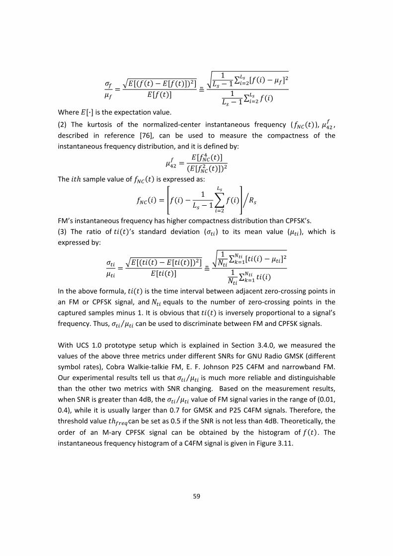
59
11 ∑
11 ∑
Where · is the expectation value. (2) The kurtosis of the normalized‐center instantaneous frequency ( ), , described in reference [76], can be used to measure the compactness of the instantaneous frequency distribution, and it is defined by:
The sample value of is expressed as:
11
FM’s instantaneous frequency has higher compactness distribution than CPFSK’s. (3) The ratio of ’s standard deviation ( ) to its mean value ( ), which is expressed by:
1 ∑
1 ∑
In the above formula, is the time interval between adjacent zero‐crossing points in an FM or CPFSK signal, and equals to the number of zero‐crossing points in the captured samples minus 1. It is obvious that is inversely proportional to a signal’s frequency. Thus, ⁄ can be used to discriminate between FM and CPFSK signals. With UCS 1.0 prototype setup which is explained in Section 3.4.0, we measured the values of the above three metrics under different SNRs for GNU Radio GMSK (different symbol rates), Cobra Walkie‐talkie FM, E. F. Johnson P25 C4FM and narrowband FM. Our experimental results tell us that ⁄ is much more reliable and distinguishable than the other two metrics with SNR changing. Based on the measurement results, when SNR is greater than 4dB, the ⁄ value of FM signal varies in the range of (0.01, 0.4), while it is usually larger than 0.7 for GMSK and P25 C4FM signals. Therefore, the threshold value can be set as 0.5 if the SNR is not less than 4dB. Theoretically, the
order of an M‐ary CPFSK signal can be obtained by the histogram of . The instantaneous frequency histogram of a C4FM signal is given in Figure 3.11.

60
Figure 3.11: Instantaneous Frequency Histogram of C4FM
3.4.4.7 Bandwidth estimation Bandwidth estimation can provide a range for symbol rate estimation for a digital signal, as well as filter bandwidth for an analog signal. The accuracy of bandwidth estimation influences the efficiency of the entire system, especially symbol rate estimation time. In our system, we designed a histogram algorithm to replace the traditional 3 bandwidth estimation method. For an MPSK or a QAM signal, which normally use raised‐cosine pulse shaping, if the lower cutoff frequency for bandwidth calculation could start from the starting frequency of the pulse shaping, and the upper cutoff frequency ends at the ending frequency, then 1 _ . Thus, given the roll off value, we can estimate symbol rate more accurately than by using 3 bandwidth estimation method. In Figure 3.12, we take QPSK as an example to illustrate. The intersection of the PSD plot and the straight line indicates the lower and upper frequency bounds of the desired signal spectrum. The joint point is where the PSD dramatically changes, and can be found by analyzing the histogram of PSD. Figure 3.13 shows the histogram of the PSD of a DBPSK signal. We use it as an example to explain how to find SNR and the threshold from a PSD histogram. On the left side, there is a Gaussian like distribution; this is the histogram for noise. The abscissa of local maximum PSD indicates the mean of noise power, and its reciprocal is equal to the current SNR since the received signal is normalized. On the right side, the relatively centralized distribution is the signal. The straight line, where the locally minimal histogram number is, indicates the threshold for
estimation.
-4 -3 -2 -1 0 1 2 3 40
10
20
30
40
50
60
61
Figure 3.12: PSD for A DQPSK Signal
Figure 3.13: Histogram of DBPSK PSD
3.4.4.8 Symbol timing and coarse classification Symbol timing is a key technology in communication systems. It includes both symbol rate searching and symbol synchronization in our system. Figure 3.14 gives the block diagram for symbol timing and coarse classification. The accuracy of bandwidth estimation will determine the range of searching space.
Figure 3.14: Block Diagram for Symbol Timing and Coarse Classification

62
Define the estimated bandwidth, which is the output of the Bandwidth Estimation module, as (Hz), the sampling rate as (Hz), the real bandwidth as , and true symbol rate as . Estimated symbol rate is:
/ 1 _ where _ is the roll off value of the root raised cosine filter used at the transmitter. The number of samples per symbol is expressed as:
may not be an integer. For the next step’s processing convenience, the value of
samples per symbol needs to be an integer. Thus, equals to the integer part of ,
and we need to resample the sample stream, which was collected at the original sampling rate , according to the redefined sampling rate :
The value of is not accurate enough to be used to calculate symbol rate directly. We therefore need to analyze the accuracy of the symbol rate estimation to set a candidate space for fine symbol rate estimation and symbol timing. Space is determined by two factors: the maximum bandwidth estimation error and the tolerated error of the symbol rate when demodulating. Figure 3.15 illustrates the process of determining symbol rate candidate space S. Suppose 2 equals to the value of the maximum element in the candidate space minus the value of the minimum element, and equals the difference between the two adjacent elements, then is defined as:
/ , / , … , , … , / , / ] Define as the maximum bias error between and , i.e.
| | In order to find the correct symbol rate, we let , which guarantees . Suppose the maximum tolerated symbol rate error for the subsequent synchronization is , then 2 , such that
where is the element of . So far, the candidate space is defined. For each element of , we have a new resampling rate: , where
= / . is a vector in which each element represents the resampling rate corresponding to each element in . Next, we are going to explain how we search for the best symbol rate and finish symbol timing synchronization at the same time. Figure 3.16 shows a snapshot of samples for a DBPSK signal at quasi‐baseband, which was collected by the Anritsu Signature signal analyzer in the OTA experiment. There are 8 samples per symbol. Dots indicate the sampling points. Red points indicate the correct

63
symbol timing. Black points indicate the incorrect symbol timing. As we can see, only when both symbol rate and the symbol timing moment are correct, the chosen samples have very small variance, while the other set has relatively large variance. We need to calculate two parameters from this result: number of samples per symbol and timing position within a symbol.
Figure 3.15: Illustration of Determining Symbol Rate Candidate Space S
_ is defined as the vector including the quasi‐baseband complex samples
collected at sampling rate within capture time .
Figure 3.16: Illustration of Symbol Timing Impact to the Received Signal
2680 2690 2700 2710 2720 2730 2740
0
0.2
0.4
0.6
0.8
1
1.2
1.4
1.6

64
Each element of space is a candidate for the correct symbol rate. _ is the samples stream after resampling _ by . is defined as the space
for candidate symbol set. The number of elements in is ∑ / .
Each element of is a vector, which is expressed by
_ |
where 1,2, … ,2 / 1, 1,2, … , .
is the candidate space for optimal symbol timing. Each element of is potentially a correctly sampled symbol set. Our target is the optimum one. Before searching for the optimal symbol set, we need to first distinguish QAM from MPSK (Figure 3.17).
Table 3.6: Determination of Candidate Symbol Sets Space SS
Symbol rate candidate
Samples/ symbol
Samplingrate
Samplesvector
Candidate symbol set SS
sampling_r Samples_V
S1 SPS1 S1*SPS1 Samples_V1 SS1={Samples_V1(1), Samples_V1(SPS1+1), Samples_V1(2*SPS1+1), …, Samples_V1(n*SPS1+1),…} SS2={Samples_V1(2), Samples_V1(SPS1+2), Samples_V1(2*SPS1+2), …, Samples_V1(n*SPS1+2),…} … … SSj={Samples_V1(j), Samples_V1(SPS1+j), Samples_V1(2*SPS1+j), …, Samples_V1(n*SPS1+j),…} … … SSSPS1={Samples_V1(SPS1), Samples_V1(2*SPS1), …, Samples_V1(n*SPS1),…} Number of candidate symbol sets for S1 is SPS1.
S2 SPS2 S2*SPS2 Samples_V2 SSSPS1+j={Samples_V2(m)|(m mod SPS2)=j} j=1,2,3,…, SPS2. Number of candidate symbol sets for S2 is SPS2.
…… …… …… …… ……
The total number of elements in SS is ∑ /
QAM and MPSK can be differentiated by analyzing their envelopes. The desired envelope of MPSK symbols is a single constant value, and the desired envelope of QAM

65
is a set of several constant values. In other word, if we cluster samples’ envelope in each element of , and the clustered result is centralized around one constant value, then it is MPSK. If not, then according to the number of centralized values, we can classify the samples as 16QAM (3 values), 64 QAM (9 values), etc. The number of the centralized values is called the envelope order. Because only one element of space is the correctly sampled symbol set, if the received signal is MPSK, for example, other elements’ envelope order may be equivalent to or greater than 1 due to the incorrect sampling. Each element’s envelope order is calculated and saved in a vector called . Based on the clustering result, we calculate the variance for each of the symbol clusters and add them to get the total variance. The variance is saved in vector . The minimal value of this vector is marked as min Sampling at the right position will guarantee the highest SINR (Signal to Interference plus Noise Ratio). We therefore consider that min has the best symbol timing. The corresponding symbol rate is found at the same time. min and will be fed to the next module, as well as the min , which is important for information removal in carrier synchronization.
Figure 3.17: Variance Curves Implying Global Optimal Symbol Timing Position
1 1.5 2 2.5 3 3.5 40
0.01
0.02
0.03
0.04
0.05
0.06
D8PSK
Best SymbolRate Candidate
Optimal Timing Position
1 2 3 4 5 6 7 82
4
6
8
10
12 x 10-3
16QAM
Optimal Timing Position
Best SymbolRate Candidate
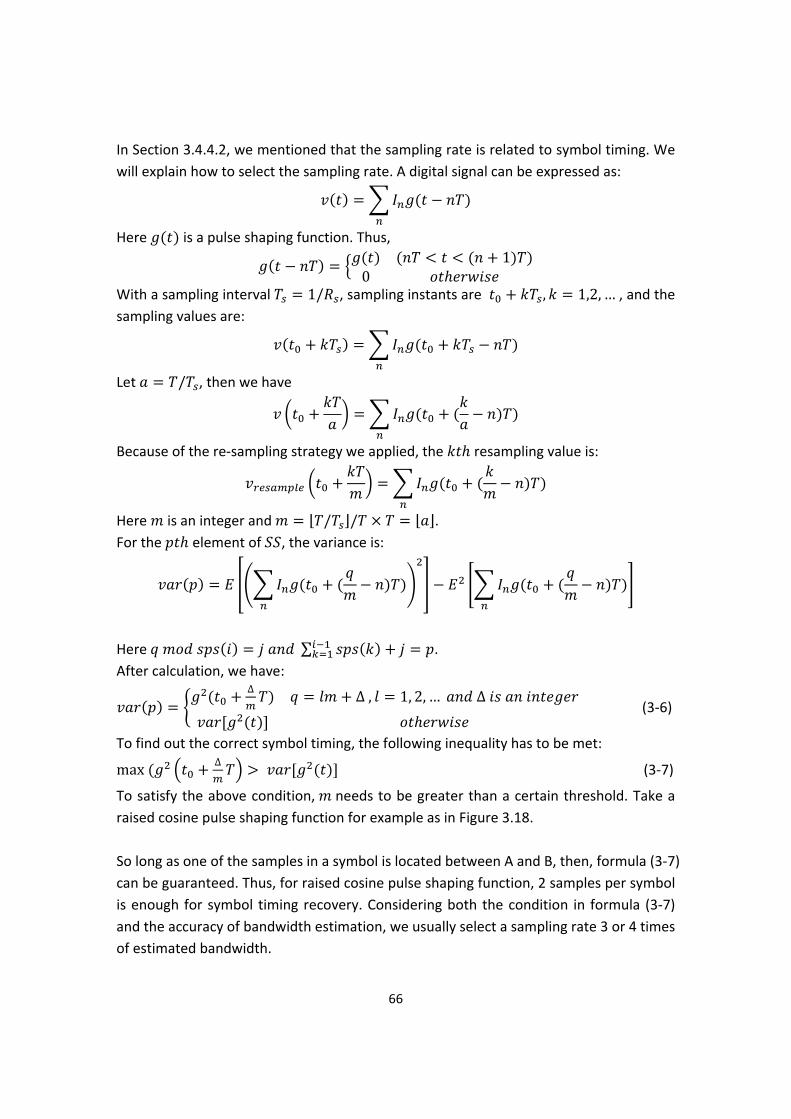
66
In Section 3.4.4.2, we mentioned that the sampling rate is related to symbol timing. We will explain how to select the sampling rate. A digital signal can be expressed as:
Here is a pulse shaping function. Thus, 1
0
With a sampling interval 1/ , sampling instants are , 1,2, … , and the sampling values are:
Let / , then we have
Because of the re‐sampling strategy we applied, the resampling value is:
Here is an integer and / / . For the element of , the variance is:
Here ∑ . After calculation, we have:
∆ ∆ , 1, 2, … ∆ (3‐6)
To find out the correct symbol timing, the following inequality has to be met:
max ∆ (3‐7)
To satisfy the above condition, needs to be greater than a certain threshold. Take a raised cosine pulse shaping function for example as in Figure 3.18. So long as one of the samples in a symbol is located between A and B, then, formula (3‐7) can be guaranteed. Thus, for raised cosine pulse shaping function, 2 samples per symbol is enough for symbol timing recovery. Considering both the condition in formula (3‐7) and the accuracy of bandwidth estimation, we usually select a sampling rate 3 or 4 times of estimated bandwidth.

67
Figure 3.18: Pulse Shaping of Raised Cosine Function
3.4.4.9 Carrier synchronization and fine classification When the modulation types and parameters are known, a Phase Lock Loop (PLL) can be used to accomplish carrier synchronization. This is necessary to overcome equipment limitations. For example, typical of low cost SDR platforms, the USRP has an inaccurate oscillator which will generate a frequency offset – in this case less than 2 kHz. Phase offset is caused by noise, channel delay, and different phase references in the transmitter and receiver. In the UCS scenario, both the order of MPSK and the center frequency are unknown. As a result, the methods described above will not produce accurate results. In [93], we designed the Universal Synchronization Algorithm, which doesn’t need to know the order of MPSK. The key idea is that we remove the information before the symbols get into the PLL. The carrier synchronization architecture is composed of five parts: information removal, frequency estimation, frequency rectification, phase estimation, and phase rectification, as shown in Figure 3.19.
Figure 3.19: Carrier Synchronization Block Diagram for One Iteration

68
In M‐ary PSK modulation, the amplitude of the transmitted signal is constrained to remain constant, thereby yielding a circular constellation [91]. In addition, the M constellation points of an MPSK signal uniformly distribute on a single circle. This means the phase difference, contributed by the information‐bearing elements, between any two adjacent symbols of a MPSK signal, can be represented as · 2 / , where n is an integer and M is the order of a MPSK signal. Therefore, it is convenient to use a phase‐based method to remove information for MPSK. However, in QAM the amplitude also varies along with the phase. The constellation points of a QAM signal uniformly distribute on squares. Therefore, it seems that a QAM signal does not possess the same phase features as MPSK, and we’ll need a square‐slicer to cluster the symbols. We observe that the constellation points of a QAM signal also lie on circles. For example, in ideal conditions, the constellation points of a 16QAM signal distribute on three circles (Figure 3.20), while 64QAM has nine circles. For 16QAM, the phases of points on the inner (the 1st) and outer (the 3rd) circles have the same distribution as a QPSK signal. Therefore, we can select the symbols on the 1st and 3rd circles of 16QAM, or the 1st, 3rd, and 9th circles of 64QAM for phase‐based information removal. When the SNR is sufficient, the symbol timing and coarse classification module will provide an accurate envelope order, and a properly designed envelope‐slicer will pick out the desired points for information removal.
Figure 3.20: Constellation Diagram of An M‐ary QAM (M=16) Signal Set
The loop gain of the PLL is a critical parameter for which we need to account. The PLL will not converge if the loop gain is less than the actual frequency offset Δ . When the value of loop gain is less than3Δ , the PLL will converge on a very accurate result and output a frequency offset estimation. Therefore, in UCS, we use multiple iterations to achieve better estimation precision and adaptive loop gain to ensure the convergence of our algorithm, called “Multiple‐iteration frequency tracking algorithm with loop gain adaptation”, which is illustrated in Figure 3.21. This algorithm is implemented by a while loop. At each iteration of the while loop, the loop gain is updated on the basis of the just estimated _ . This adaptive scheme improves the robustness and reliability of our frequency tracking algorithm. For the while loop, we chose the

69
maximum iterations _ and, variance of the phases of the information‐removed points _ as the criteria. With the increase in the number of iterations, the residual frequency offset should become smaller and smaller. Thereby, where
_ develops a trend of reduction and its value becomes less than a threshold _ , we can attain clear constellation points. The setting of _
is based on the result presented in [94]. _ is related to the symbol rate and
SNR.
Figure 3.21: Multiple‐Iteration Frequency Tracking Algorithm with Loop Gain Adaptation
The final result for frequency offset estimate is the ultimate value of _ ,which has been updated by _ _ _ at iteration of the while loop. Applying the above schemes to our carrier frequency offset estimation algorithm, the error between _ and the actual frequency offset is within 1 Hz. Finally, we can get a clear constellation diagram. Figure 3.22 shows the constellation diagrams for 8PSK and 16QAM at different processing stages: the first column figures display the snapshots of constellation points (samples) before symbol timing. In the middle, the symbol stream output from the symbol timing module is plotted. The third column contains the constellation diagrams for synchronized samples.

70
Figure 3.22: Results of UCS (a|b|c)
From the instantaneous phase distribution histogram of a carrier‐synchronized signal, we can easily estimate the bits per symbol of MPSK or M‐QAM, as shown in Figure 3.23. Thus, the fine classification after carrier synchronization has been achieved.
Figure 3.23: Fine Classification Based on Instantaneous Phase Distribution Histogram
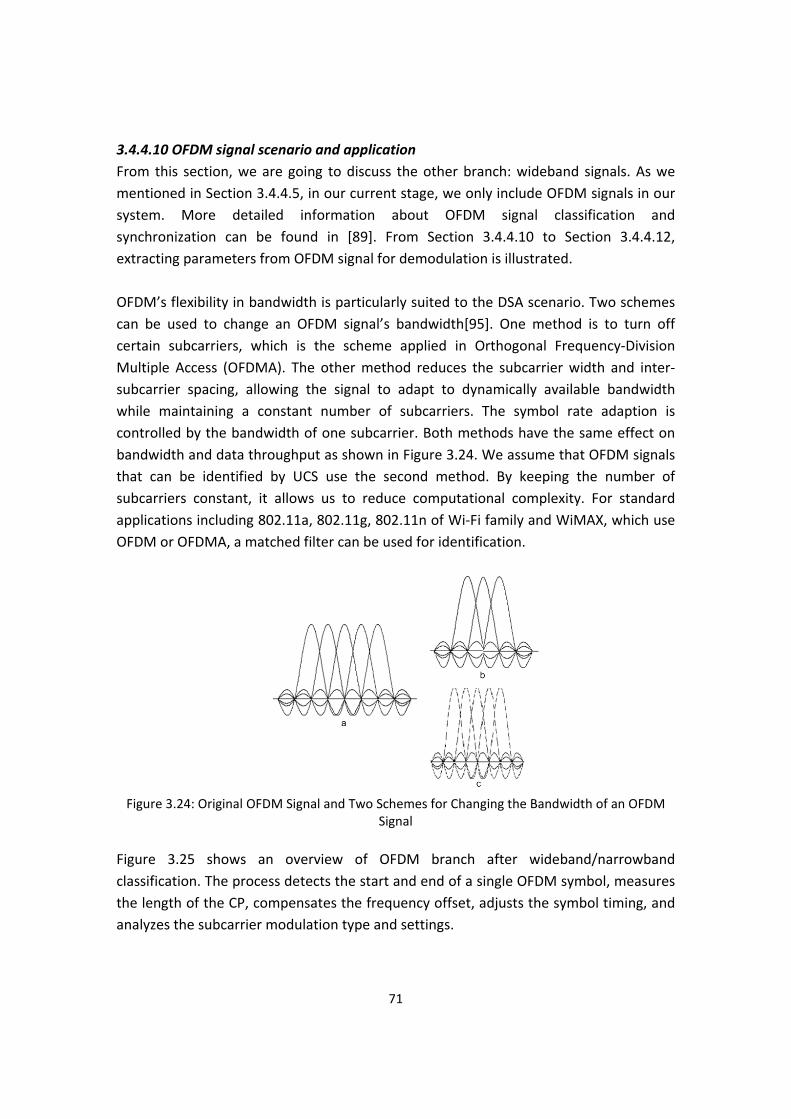
71
3.4.4.10 OFDM signal scenario and application From this section, we are going to discuss the other branch: wideband signals. As we mentioned in Section 3.4.4.5, in our current stage, we only include OFDM signals in our system. More detailed information about OFDM signal classification and synchronization can be found in [89]. From Section 3.4.4.10 to Section 3.4.4.12, extracting parameters from OFDM signal for demodulation is illustrated. OFDM’s flexibility in bandwidth is particularly suited to the DSA scenario. Two schemes can be used to change an OFDM signal’s bandwidth[95]. One method is to turn off certain subcarriers, which is the scheme applied in Orthogonal Frequency‐Division Multiple Access (OFDMA). The other method reduces the subcarrier width and inter‐subcarrier spacing, allowing the signal to adapt to dynamically available bandwidth while maintaining a constant number of subcarriers. The symbol rate adaption is controlled by the bandwidth of one subcarrier. Both methods have the same effect on bandwidth and data throughput as shown in Figure 3.24. We assume that OFDM signals that can be identified by UCS use the second method. By keeping the number of subcarriers constant, it allows us to reduce computational complexity. For standard applications including 802.11a, 802.11g, 802.11n of Wi‐Fi family and WiMAX, which use OFDM or OFDMA, a matched filter can be used for identification.
Figure 3.24: Original OFDM Signal and Two Schemes for Changing the Bandwidth of an OFDM
Signal
Figure 3.25 shows an overview of OFDM branch after wideband/narrowband classification. The process detects the start and end of a single OFDM symbol, measures the length of the CP, compensates the frequency offset, adjusts the symbol timing, and analyzes the subcarrier modulation type and settings.

72
Figure 3.25: Overview of OFDM Synchronization and Parameter Extraction
3.4.4.11 Estimation of symbol length and CP length By correlating the incoming signal with itself, we are able to separate an OFDM symbol into a data part and a cyclic prefix part. From Figure 3.8, we observe that the OFDM plot has three distinct peaks. The two smaller peaks are due to the presence of the cyclic prefix. The length of the data part of a symbol is the distance between the highest peak and the smaller peak. The number of samples between these two peaks is defined as ; then the data part duration at the receiver side is / , where is sampling rate. For finding the CP length, we convolve the data part of an OFDM symbol with the rest of the OFDM symbol as shown in Figure 3.26. The CP’ copy in data part will overlap with CP. This will result in a peak as shown in Figure 3.27. The position of the peak determines the length of the CP.
Figure 3.26: Estimation of CP Length

73
Figure 3.27: Convolution of Symbol and Cyclic Prefix
Meanwhile, we also get the data part of an OFDM symbol. This part is called . When we use the data part of an OFDM symbol for carrier synchronization and per‐subcarrier symbol timing, it is necessary to have an integer numbers of samples per MPSK signal symbol which is acquired after FFT and parallel‐to‐serial conversion. To meet the requirement of integer number of samples per symbol, we need to resample . Figure 3.27 shows the serial to parallel (S/P) processing at the transmitter side. is symbol duration before S/P, 1/ and is the symbol rate at the transmitter side. is the number of subcarriers. Thus, the data part duration is / .
Figure 3.28: Serials to Parallel of OFDM in Transmitter Side
The data part duration at the transmitter side is the same as that at the receiver side. Thus, we have:
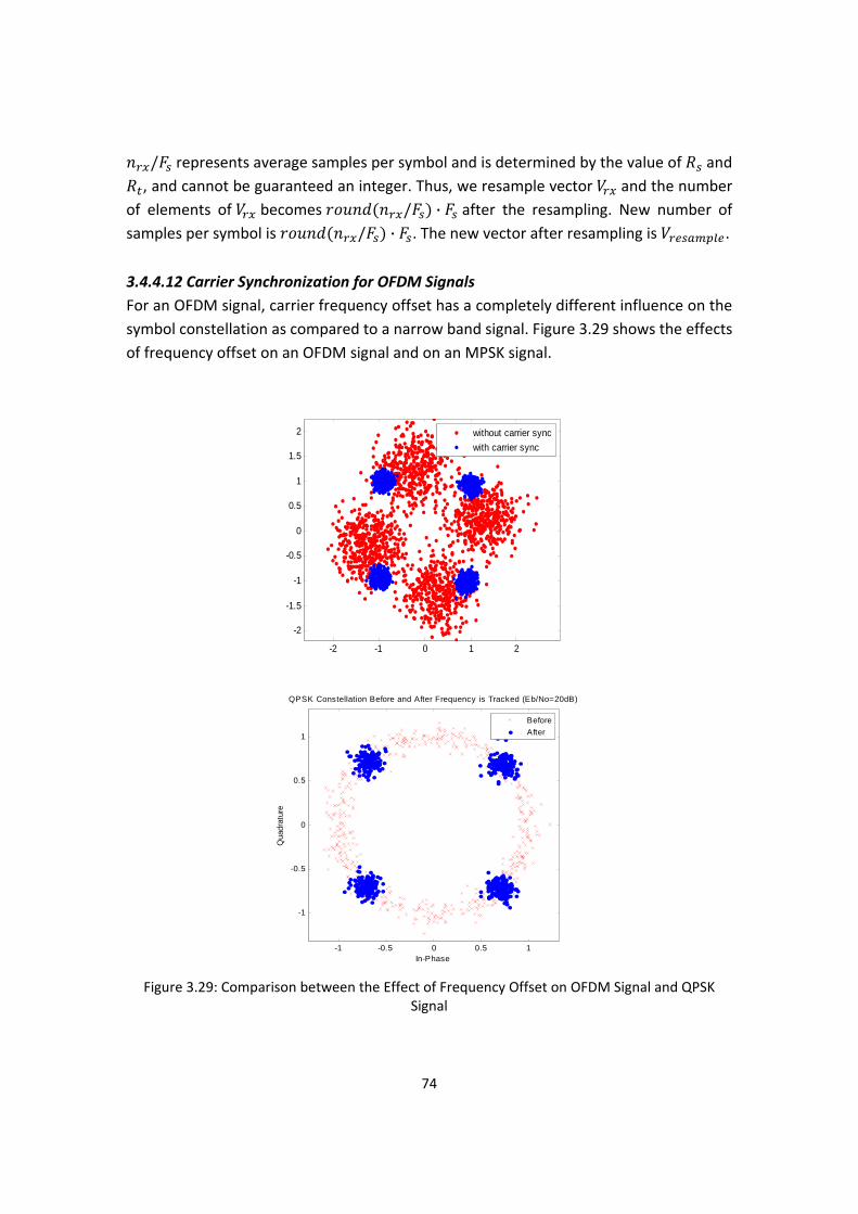
74
/ represents average samples per symbol and is determined by the value of and , and cannot be guaranteed an integer. Thus, we resample vector and the number
of elements of becomes / · after the resampling. New number of samples per symbol is / · . The new vector after resampling is .
3.4.4.12 Carrier Synchronization for OFDM Signals For an OFDM signal, carrier frequency offset has a completely different influence on the symbol constellation as compared to a narrow band signal. Figure 3.29 shows the effects of frequency offset on an OFDM signal and on an MPSK signal.
Figure 3.29: Comparison between the Effect of Frequency Offset on OFDM Signal and QPSK
Signal
-1 -0.5 0 0.5 1
-1
-0.5
0
0.5
1
Qua
drat
ure
In-Phase
QPSK Constellation Before and After Frequency is Tracked (Eb/No=20dB)
BeforeAfter
-2 -1 0 1 2
-2
-1.5
-1
-0.5
0
0.5
1
1.5
2 without carrier syncwith carrier sync

75
In Figure 3.29, the comparison is based on the assumption that the symbol rate is correct. Frequency offset causes an OFDM constellation to spread with errors in both amplitude and phase. The frequency offset introduces only phase errors in MPSK signals. The reason for this difference is that frequency offset becomes a timing delay after FFT at the OFDM receiver. This delay will lead to incorrect symbol timing, which will spread the signal constellation. The frequency offset estimation algorithm is designed as follows. The step size of the frequency offset is defined as ∆ , and the range of the frequency offset estimated is defined as . We search from to using step size ∆ . As we
compensate for frequency offset, the variance of the amplitude of the symbols changes. The minimal variance corresponds to the carrier frequency offset. 3.4.4.13 Verification Schemes for UCS System Low SNR decreases the accuracy of both the bandwidth estimation and of the phase values of the received samples. The former will increase the range of searching space in symbol timing step, and the latter will decrease the synchronization accuracy. Both of them will increase the average time consumed for one iteration of correct signal recognition. In our system, which is distinguished from other communication systems operating with bit errors, the final result can only be either right or wrong. Thus, a verification scheme is necessary for our system. There are three parts of verification embedded in our system: noise versus signal verification, symbol timing verification (bandwidth estimation verification), and carrier synchronization verification. If a result does not pass the aforementioned verification, it will be treated as incorrect, and the system will automatically discard the results and recollect data for recalculation. Therefore, the introduction of verification will in fact increase the average time consumed per correct calculation, although it can provide a very high correct rate. Accordingly, we can convert the tradeoff of SNR versus correct rate into the tradeoff of SNR versus average iteration time by always keeping the correct rate high. This section involves two parts; the first is to explain the verification algorithm and the other to discuss the relationship between SNR and average consuming time. Noise versus signal verification is located right after channel estimation. The objective of this function is a pre‐decision on whether the captured data will be successfully processed by the system. The failure case occurs when only noise has been captured or the collected signal has a SNR lower than system tolerance. In Figure 3.13, the ration between the right peak position value and the left peak position is considered as Expected SNR (ESNR). Only a signal with ESNR larger than a certain threshold will be

76
considered. We use ESNR instead of SNR because ESNR is not influenced by the oversampling rate, while SNR is. The threshold is determined by system running environment and user requirement. The second verification is symbol timing verification. In the symbol timing section, we defined the range for searching. And if it has reached this range, but no satisfactory solution has been found, we drew the conclusion that the data should be discarded and new data should be collected. This part of verification only existed in narrowband signal branches, and not for OFDM. The third verification is for carrier synchronization. We define a threshold for loop iterations. If the loop iterations have reached the threshold and not satisfied the criterion, we concluded that the data should be discarded and new data should be collected.
3.4.5 UCS Prototypes and Performance Evaluation
UCS has been implemented and tested over the air. The platforms available for OTA experiments are exhibited in Figure 3.30. The UCS 1.0 implemented in the Anritsu MS2781A Signature Signal Analyzer focuses on demonstrating the classification and synchronization functions of UCS. The UCS 2.0 transplants the system to GNU radio and USRP platform, which dramatically decrease the equipment expense. In UCS 3.0, now under development, the system will be transplanted to a Lyrtech SFF radio platform, which integrates DSP and FPGA design and can greatly speed the entire UCS process. The OTA demonstration setup for UCS 1.0 and UCS 2.0 is shown in Figure 3.31 and Figure 3.32. In this section, we focus on UCS 2.0.
Figure 3.30: Platforms for OTA Experiments

77
CR1 and CR 2 are two cognitive radio nodes based on GNU Radio with USRP as their hardware platform. Narrowband signals, including FM, AM, MPSK (M=2,4,8), QAM(16) and OFDM are transmitted by CR1. CR2 will receive the signal over the air from CR1 via the antenna. All the information required for the CR2 to correctly demodulate the signal is extracted by the UCS algorithm and stored in XML format. The updated XML file will be used to (re)configure the radio framework of CR2. Then the connection between CR1 and CR2 can be created, and they commence communications.
Figure 3.31: OTA Demo Setup for UCS 1.0
Figure 3.32: OTA Demo Setup for UCS 2.0
How to assess a system is at least as important as actually building it. We evaluate our system from three aspects: accuracy, SNR requirement and time consumption. The decision making in our system is step by step, thus, our analysis and evaluation are also step based. Next, we will give the performance curves for the four key steps in UCS system: wideband/narrowband, narrowband categorization, symbol timing, and carrier synchronization.

78
Figure 3.33 shows the error probability of wideband/narrowband signal differentiation under different SNR with different product values of sampling rate and guard interval. As we can see, it is related to the number of samples within a cyclic prefix period. The larger the product of sampling rate and guard interval is, the lower the error rate is under the same SNR. Thus, we can conclude that normally, the SNR requirements for correctly differentiating between narrowband and wideband signals with high probability are not tight, and thus easy to meet.
Figure 3.33: Wideband/Narrowband Error Detection Probability
As seen in Table 3.5, narrowband signal categorization includes several steps. Here, we mainly analyze the performance of phase‐based grouping at different SNR. The probability of mistaken continuous‐phase/discontinuous‐phase differentiation is: For mistaken continuous‐phase to discontinuous‐phase:
1 1 1
For mistaken discontinuous‐phase to continuous‐phase:
1
11

79
Here, is the average number of jump points for each modulation type, is the probability that a non‐jump point is mistaken to be a jump point, is the probability that a jump point is mistaken to be non‐jump point. As explained in Figure 3.34,
can be expressed as:
2
Where is the angle for a jump point and is a function that
1arccos
2
arccos 2 2
Figure 3.34: Illustration for Probability of Mistaking Jump/Non‐Jump Points Decision Caused by
Noise
In Figure 3.34, we only provide the condition of ; other conditions are similar to it.
is the cdf function of a Rayleigh distribution with , and is the pdf function. In our system, 0.2 and /8. Figure 3.35 shows the distribution of
and under different SNR and Figure 3.36 shows the performance of the continuous‐phase/discontinuous‐phase classifier under different SNR. We can see that for digital signals, the SNR requirement for this step is very low; however, for analog, an error rate less 10 than requires a SNR larger than 8 dB.
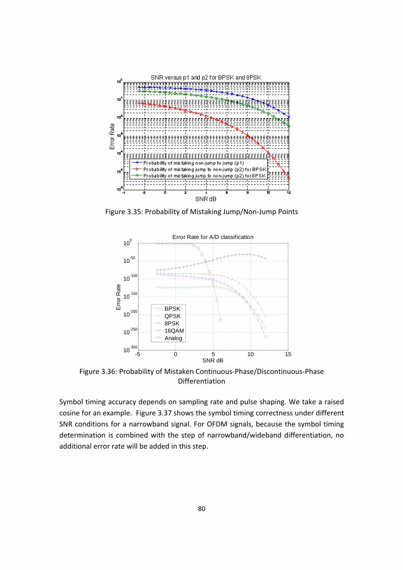
80
Figure 3.35: Probability of Mistaking Jump/Non‐Jump Points
Figure 3.36: Probability of Mistaken Continuous‐Phase/Discontinuous‐Phase
Differentiation Symbol timing accuracy depends on sampling rate and pulse shaping. We take a raised cosine for an example. Figure 3.37 shows the symbol timing correctness under different SNR conditions for a narrowband signal. For OFDM signals, because the symbol timing determination is combined with the step of narrowband/wideband differentiation, no additional error rate will be added in this step.
-5 0 5 10 1510-300
10-250
10-200
10-150
10-100
10-50
100
SNR dB
Erro
r Rat
e
Error Rate for A/D classification
BPSKQPSK8PSK16QAMAnalog
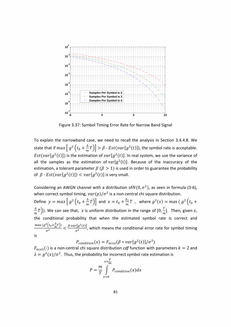
81
Figure 3.37: Symbol Timing Error Rate for Narrow Band Signal
To explain the narrowband case, we need to recall the analysis in Section 3.4.4.8. We
state that if ∆ · ), the symbol rate is acceptable.
is the estimation of . In real system, we use the variance of all the samples as the estimation of var g t . Because of the inaccuracy of the estimation, a tolerant parameter 1 is used in order to guarantee the probability of · is very small. Considering an AWGN channel with a distribution of 0, , as seen in formula (3‐6), when correct symbol timing, / is a non‐central chi square distribution.
Define ∆ and ∆
, where max ∆
. We can see that, is uniform distribution in the range of 0, . Then, given ,
the conditional probability that when the estimated symbol rate is correct and ∆
·, which means the conditional error rate for symbol timing
is /
· is a non‐central chi square distribution cdf function with parameters 2 and / . Thus, the probability for incorrect symbol rate estimation is
-5 0 5 1010
-7
10-6
10-5
10-4
10-3
10-2
10-1
100
Samples Per Symbol is 2Samples Per Symbol is 3Samples Per Symbol is 4

82
Here, SNR represents the ratio between signal power and noise power, expressed as a numerical ratio and not in dB. In Figure 3.37, 1.4 and a raised cosine filter with
0.35 is used, which are also the settings used in our implemented system. As we can see in Figure 3.37, the number of samples per symbol does influence the performance. In our implemented system, we use samples per symbol between 3 and 4. For QAM signal, the calculation for variance is based on cluster. SNR requirement will be larger than 5dB in order to reach error rate less than10 . Figure 3.37 doesn’t include verification, and our implemented system with verification has lower SNR requirement, around 3dB to 4 dB. As we described in Section 3.4.4.8, MPSK and M‐ary QAM signals are distinguished by analyzing the envelope values of the symbol stream that is output from the Symbol Timing module. For 16QAM, its constellation points lie on three circles. From the inner circle to the outer circle, we use the 1st, 2nd, 3rd to denote the corresponding circle, respectively. Therefore, sorting the 16QAM symbol points (complex) into circles is a three‐hypothesis testing problem. After derivation, we get the performance curves plotted under different SNR with different threshold values ( 0.50 , 0.52 , 0.54 , 0.56 , 0.58 , 0.60 ), as shown in Figure 3.38. is the number of symbols. Without knowing the modulation type, these symbols are clustered into three groups no matter the incoming signal is MPSK or 16QAM. For symbol clustering, the normalized complex symbols will first be scaled to match the three circles’ radius of an ideal 16QAM signal. The clustering principles are related to the symbol envelope :
1 , 1 1 1 √6 2 , 2 2 1 √6 √14 3 , 3 3 1 √14
1,2,3 denotes the number of symbols that are sorted into the circle range. Thus, if 2 , the signal is judged as MPSK, otherwise, it will be 16QAM. Figure 3.38 tells that the threshold should be changed with the varying of SNR to meet corresponding requirement to error probability. Carrier synchronization for narrow band signals is required to compensate the frequency offset so that the symbol stream has the least phase variance. It has the same performance as a standard phase lock loop [88, 96, 97]. For OFDM signal, it is to find the least amplitude variance. The searching step of a frequency offset matters to the accuracy of the frequency offset, as well as to subcarrier synchronization. In our implemented system, we use a frequency offset step of 100 .
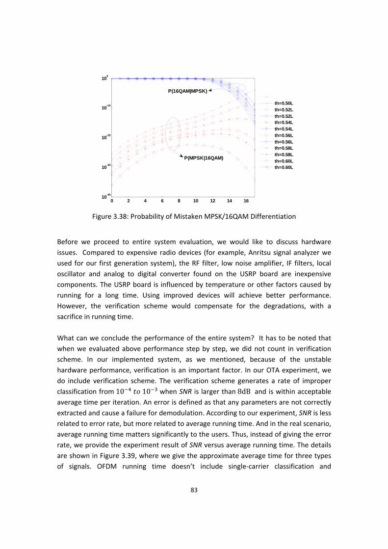
83
Figure 3.38: Probability of Mistaken MPSK/16QAM Differentiation
Before we proceed to entire system evaluation, we would like to discuss hardware issues. Compared to expensive radio devices (for example, Anritsu signal analyzer we used for our first generation system), the RF filter, low noise amplifier, IF filters, local oscillator and analog to digital converter found on the USRP board are inexpensive components. The USRP board is influenced by temperature or other factors caused by running for a long time. Using improved devices will achieve better performance. However, the verification scheme would compensate for the degradations, with a sacrifice in running time. What can we conclude the performance of the entire system? It has to be noted that when we evaluated above performance step by step, we did not count in verification scheme. In our implemented system, as we mentioned, because of the unstable hardware performance, verification is an important factor. In our OTA experiment, we do include verification scheme. The verification scheme generates a rate of improper classification from 10 10 when SNR is larger than 8dB and is within acceptable average time per iteration. An error is defined as that any parameters are not correctly extracted and cause a failure for demodulation. According to our experiment, SNR is less related to error rate, but more related to average running time. And in the real scenario, average running time matters significantly to the users. Thus, instead of giving the error rate, we provide the experiment result of SNR versus average running time. The details are shown in Figure 3.39, where we give the approximate average time for three types of signals. OFDM running time doesn’t include single‐carrier classification and
0 2 4 6 8 10 12 14 1610-40
10-30
10-20
10-10
100
th=0.50Lth=0.52Lth=0.52Lth=0.54Lth=0.54Lth=0.56Lth=0.56Lth=0.58Lth=0.58Lth=0.60Lth=0.60L
P(MPSK|16QAM)
P(16QAM|MPSK)

84
synchronization time and it is based on simulation. The digital and analog curves are based on OTA experiment.
Figure 3.39: Average Running Timing under Different SNR Conditions
3.4.6 Conclusion and Discussion
In Section 3.4, we have discussed the design and implementation of a universal classifier and synchronizer, and evaluated its performance in terms of accuracy, SNR, and speed. It has been verified in both theoretical analysis and practical experiments that the system works with high accuracy. The UCS prototype developed with an inexpensive SDR platform (USRP plus GNU Radio) can observe the environment, make decisions and autonomously act on those decisions. With the aforementioned advantages, a UCS can serve as a very accurate sensor in a complex, distributed cognitive radio or network, or act as an independent physical layer cognitive receiver. UCS is portable. According to users’ requirements for cost, device size, accuracy, and processing speed, a compromise decision should be made on the specific platform where the UCS will be ported. Signal feature extraction and analysis in UCS include many digital signal processing (DSP) tasks, which can contribute to the majority of the computation load of a system employing it. These DSP functions can be implemented in software executed by general purpose processors (GPP) or on a variety of digital hardware platforms consisting of ASICs, FPGAs, and DSPs. GNU Radio, which is GPP‐based, is a widely used open source software toolkit for learning about, building, and deploying software defined radios. The Anritsu MS2781A Signature Signal Analyzer is a powerful platform equipped with high performance RF components that runs MATLAB on Windows. The initial UCS was tested, verified and demonstrated using the Anritsu MS2781A Signature Signal Analyzer over the air (OTA). Although it provides a very simple and convenient development environment, this MATLAB‐based platform is not
8 10 12 14 16 18 200
1
2
3
4
5
6SNR versus Average Running Time
SNR dB
Ave
rage
Run
ning
Tim
e S
BPSKOFDM withour subcarrier classification and syncFM

85
ideal to be a portable CR terminal due to its high cost and bulky size. Thus, GNU Radio running on a Linux system connected to an inexpensive Universal Software Radio Peripheral (USRP) becomes an attractive candidate for the implementation of UCS. The functionalities of UCS have been fully implemented on this SDR platform. However, the conventional GPPs cannot handle the high computational complexity arising from adding more waveforms and increasing the spectrum band to be observed. Therefore, our attention is moved to the reconfigurable digital hardware platforms which are able to support the required high number of calculations per clock cycle. Based on the comparison in [16], a DSP represents the most generalized type of hardware that can be programmed to perform various functions, while an ASIC is the most specialized piece of hardware and can be used only in the specific application for which it has been designed. An FPGA offers a compromise in flexibility and power consumption between and an ASIC and a DSP. The lowest programmability of an ASIC makes it not appropriate for the implementation of our SDR system. The low complexity signal processing tasks can be fulfilled by a DSP, but an FPGA is more efficient for implementing the logic‐intensive modules and will offer much higher throughput when technologies like concurrency, pipelining, parallel processing, folding and unfolding, and look‐ahead operation have been exploited for optimization. In our laboratory, we have analyzed the computational features of UCS algorithm and designed a GPP/DSP/FPGA hybrid architecture to achieve the optimal trade‐offs between flexibility, modularity, scalability, and performance. Some students in our laboratory have made a good practice on the Lyrtech SFF SDR platform to realize a hybrid implementation of UCS [98, 99]. This can be called UCS 3.0. Figure 3.40 illustrates the heterogeneous design flow for this hybrid architecture. This platform provides the convenience for developers to use Xilinx System Generator to generate hardware code from Simulink blocks, instead of writing VHDL code. Actually, the VLSI design technologies can be applied to optimize the FPGA implementation of the algorithm. The performance of this hybrid design should be estimated using metrics including throughput, logic gate counts, critical paths, and total processing time. In addition, it would be meaningful to compare the resource requirements, processing speed for implementing the same functionalities of UCS on different platforms such as Anritsu MATLAB‐based, GNU Radio plus USRP based, and the GPP/DSP/FPGA hybrid. If available, these results will be a helpful reference for the users to choose appropriate implementation platform. UCS 1.0, 2.0, and 3.0 all belong to Single Input Single Output (SISO) systems. If a multiple‐input and multiple‐output (MIMO) version of UCS could be implemented, overlapping signals from different emitters may be separated by locations. For example, when implemented in WARP boards with beamforming capability, two UCS sensors can
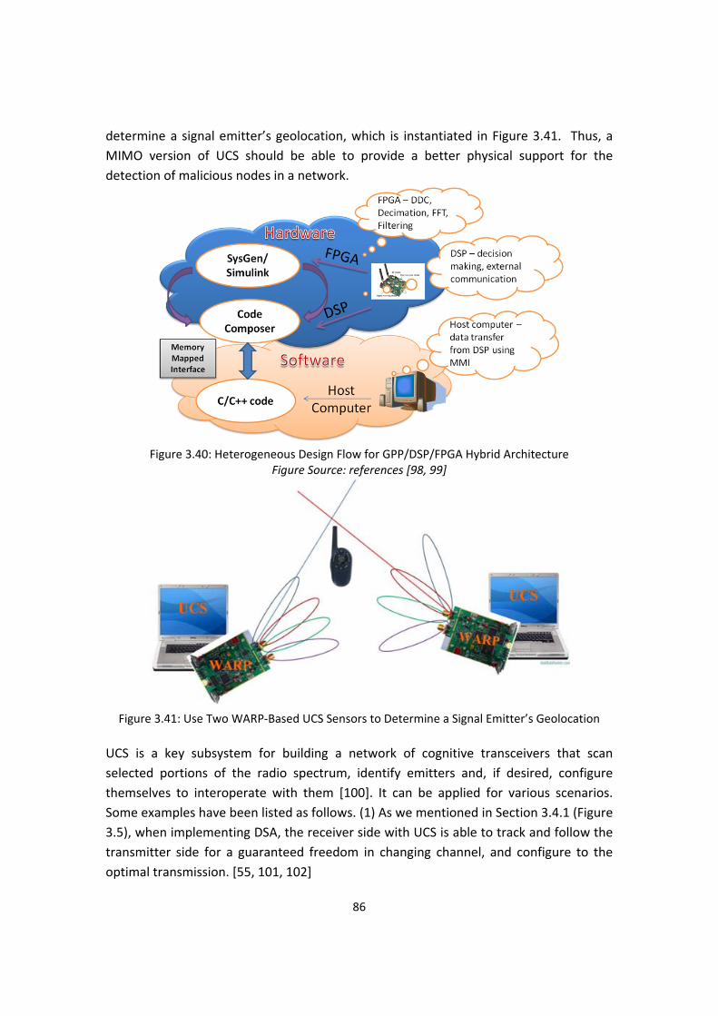
86
determine a signal emitter’s geolocation, which is instantiated in Figure 3.41. Thus, a MIMO version of UCS should be able to provide a better physical support for the detection of malicious nodes in a network.
Figure 3.40: Heterogeneous Design Flow for GPP/DSP/FPGA Hybrid Architecture
Figure Source: references [98, 99]
Figure 3.41: Use Two WARP‐Based UCS Sensors to Determine a Signal Emitter’s Geolocation
UCS is a key subsystem for building a network of cognitive transceivers that scan selected portions of the radio spectrum, identify emitters and, if desired, configure themselves to interoperate with them [100]. It can be applied for various scenarios. Some examples have been listed as follows. (1) As we mentioned in Section 3.4.1 (Figure 3.5), when implementing DSA, the receiver side with UCS is able to track and follow the transmitter side for a guaranteed freedom in changing channel, and configure to the optimal transmission. [55, 101, 102]

(2) Cogprot
Figwithof
(3) an atermfreq
FigRad
Tec
UCS can begnitive Systtotype of D
gure 3.42: Oh permissionElectrical & C
UCS implemad‐hoc sensminal probquency rang
gure 3.43: OTio Network. Decentral
chnologies,"
e used for Ptem). FigurCCS [103].
TA Demo Se, from Y. WaComputer En
mented in dsor networlem, boostge coverage
TA Demo Set©2009 Fengized DynamiPh.D. Disser
Polytech
PCN (picocere 3.42 giv
tup for a Simang, "Dynamngineering. 2
different plak for coopet the overe [104]”, as
tup for Coopg Ge. Reprintc Spectrum Artation, in Denic Institute
87
ell cognitiveves the OT
mplified DCCSic Cellular Co2009, VirginiaBlacksburg,
atforms canerative specall spectrushown in Fi
erative Spected, with perAccess Netwept. of Electrand State U
e radio nodTA experim
S Prototype.ognitive Systa PolytechniVA.
n function actrum sensm sensing igure 3.43.
ctrum Sensinrmission, froworks: A Protrical & Compniversity: Bla
de) in DCCSment setup
©2009 Yingtem," Ph.D. Dc Institute an
as distributeing to “oveperforman
g in a Heteroom F. Ge, " Sootype Designuter Engineeacksburg, VA
S (Dynamic p for a sim
g Wang. RepDissertation,nd State Uni
ed sensors ercome thence, and i
ogeneous Cooftware Radin and Enabliering. 2009, VA.
Cellular mplified
rinted, in Dept. versity:
to form hidden ncrease
ognitive io‐Based ng Virginia

(4) extrrout
3.5
In SSafetheiidensystFigufuncplatthe
FipeI
Com
For this disract informting. [105, 1
Comparis
Section 1.6,ety Cognitivir waveformntification, wtem, inventure 3.44. Mctionalities tform and iaspects list
Stag Stag Stagigure 3.44: Trmission, froImplementat
V
monalities (((
ssertation, mation from106]
son betwe
, we enumve Radio (Pm identifierswhile the seted by Bin ore details of ASC hantegrated ited in Table
ge 0: Adaptivege 1: Modulatge 2: ModulatTwo‐Stage Adom B. Le, "Bution," Ph.D. DVirginia Polyt
Ta
(1) Feature‐b(2) Not know(3) Use powe
in a dynamm waveform
een UCS a
erated thePSCR). An ims. A CG usesensor of a PLe. The bloabout ASC ave been pinto our PSe 3.7.
e segmentatiotion classification classificadaptive Signauilding a CogDissertation,technic Instit
ble 3.7: Com
ASC
based signal wing any prioer spectrum
88
mic heterogms for cogn
and ASC
major traimportant ds the UCS toPSCR adoptock diagramcan be fou
partially impSCR system
on and pre‐pration before cation after caral Classificatignitive Radio, in Dept. of tute and Stat
mparison bet
classificationor modulatiodensity to d
eneous netnitive gatew
its that madifference bo implements the Adaptm of a comnd in [42, 4plemented . Here, we
rocessing arrier synchrorrier synchronion System. ©: From ArchiElectrical & Cte University
ween ASC an
n on informatioetermine sig
twork, UCSways’ unit
ake CG go between CGnt the physictive Signal C
mplete ASC 43] and Chaon a GNUcompare U
onization nization ©2007 Bin Ltecture DefiComputer Eny: Blacksburg
nd UCS
on from the tgnal location
can automidentificati
beyond theG and PSCRcal layer waClassificatiosystem is gapter 3 of [2U Radio‐basUCS with AS
Le. Reprintednition to Prongineering. 2g, VA.
UCS
transmitter s and level
matically ion and
e Public R lies in aveform on (ASC) given in 29]. The sed SDR SC from
d, with ototype 2007,
side

Sim
Fe
FeUsag
ThDete
milarities O((R(((
Used eatures
①②
③
④
⑤
⑥
U
eature ge Mode
MwpDct
hreshold ermination
Lts
T
Off‐line: (1)Determine (2)Determine Real‐time: (3) Calculate t(4) Compare t(5) Categorize
① Power sp② The stand
of the ins③ The stand
of the diramplitud
④ The standanalytica
⑤ The standphase of
⑥ The standvalue of t
UCS needs to
Multiple featuweight factorsparallel architDeterminate wcontribution ttraining ANN.
Le’s training isthresholds reqspecific radio
Thresholds sh
ASC
the appropriathe threshold
these featuresthese calculate the signal int
pectrum densidard deviationstantaneous adard deviationrect value of te; dard deviationl phase value dard deviationthe signal; dard deviationthe phase cha
employ more
ASC
ures for each ss for each featecture (OCONweight for eacto classificatio
s an off‐line mquired at the environment
hould be deter
89
ate features td;
s for incominged results witto the corresp
ty (PSD)n of the directmplitude; n of the envelhe instantane
n of the directof the signal;n of the differ
n of the absolnge
e robust featu
signal, needinture, a kind oN‐ANN); ch feature’s on based on
method to acqKNN stage, uns.
rmined based
hat can differ
g signals; th the threshoponding class.
t value
ope eous
t
ential
ute
①②
③
④
res when app
ng f
Oneminhier
quire nder
We(emsyst
on both theo
rentiate the si
old; .
PSDthe direct anthe signal; the direct vainstantaneouthe different*The term “dire
plied to fading
e distinguishanimal principlerarchical arch
mainly use fimpirical valuestem.
oretical and ex
UCS
gnals;
nalytical phase
alue of the us amplitude;tial value of thect value” is from
g channels.
UCS
ble feature one, itecture; (Figu
xed thresholds) in current U
xperimental r
e value of
; he phase m [76].
ne step,
ure 3.9)
ds UCS
esults.

90
Pros: • Convenient for reconfiguration; • Adaptive to SNR changes; • Parallel architecture is more efficient for
FPGA implementation Cons:
• Parallel architecture needs to properly assign the weights for each feature.
• Need off‐line training • Require more resources (both software
and hardware) for calculation when the candidate modulations increase;
• Implemented testbeds [107] do not include synchronization part, so they:
• Cannot provide symbol rate estimate; • Cannot differentiate the high‐order
MPSK signals.
Pros:• Hierarchical architecture is efficient for GPP‐
based implementation, • Don’t need training to determine feature
weights. • Combine synchronization (carrier, frame,
symbol), symbol rate estimation into the general classification process, thus classify the higher order modulations and extract the parameters for demodulation;
• Back reconfigure the system settings according to real‐time feedback.
Cons: • May need to change the system architecture
as more candidate modulations are added. • Currently, UCS has been tested in the regular
lab environment, but not been tested in multi‐path fading channels.
Table 3.8 and Table 3.9 give the modulation classification performance under different SNR values for ASC and UCS, respectively. Table 3.8: ASC modulation classification performance using temporal statistics (AWGN). ©2007 Bin Le. Reprinted, with permission, from B. Le, "Building a Cognitive Radio: From Architecture Definition to Prototype Implementation," Ph.D. Dissertation, in Dept. of Electrical & Computer
Engineering. 2007, Virginia Polytechnic Institute and State University: Blacksburg, VA.
Table 3.9: UCS probability of success under different SNR values (AWGN)
MOD SNR&Platform
AM FM C4FM BPSK QPSK 8PSK 16QAM
Anritsu 20 dB 100 100 100 100 100 100 100
USRP 20 dB N/A 100 88.00 100 95.83 95.00 N/A

91
3.6 Signaling Process and Mechanisms
As we introduced in Section 3.2, a series of signaling procedures between CG and clients is necessary for the accomplishment of CG discovery, user registration and un‐registration, link establishment, communication resumption, service termination, route discovery, etc. Figure 3.45 illustrates the signaling procedure between a CG and two CR nodes. In this example, CR1 proactively initializes the service process, and both CR1 and CR2 belong to the served user group of CG1. To make the signaling process work successfully, we need to determine (or design): (1) Modulation, symbol rate, the bandwidth of each signaling sub‐channel, and control channel access method for CR nodes; (2) Control messages exchanged between CR nodes and CG; (3) Transmission manner that a communication initiator uses to send control messages; (4) CG processing strategies, especially how UCS is utilized in waveform identification. These are the primary issues that should be considered for the design of signaling mechanisms. And the time consumed for signaling and WI is an important portion of the “call set‐up time” or “link establishment time”, which is one of the metrics for evaluating the performance of a CG. Different communication initiators use different waveforms to send their requests: legacy public safety radios choose a desired CTCSS and then Push‐to‐Talk; P25 has its own specifications for various operations; standard IP‐capable nodes follow their own mechanisms; the CR nodes send control messages (packets). When we use UCS 2.0, the average time consumed in extracting (Fc, MOD=FM) for a legacy public safety user is 600ms. After this, we need to capture another 500ms of data to determine the value of CTCSS. Thus, in order for a CG that employs UCS 2.0 to figure out the waveform pair indicators, a legacy public safety user should make the radio’s signal last at least 1.1 seconds, within which the 600ms portion can be shortened if a faster processing platform would be used, while the 500ms portion has almost no room for reduction because it depends on the resolution required to distinguish between different CTCSS tones. Next, we will address the aforementioned four issues when the communication initiator is a CR node. According to our OTA experimental results for UCS, when the target emitter is continuously transmitting BPSK signal, the probability of successful classification is the highest amongst the other listed digital modulations under the same SNR conditions. In addition, the control messages are usually much shorter than the communication traffic messages. Thus, considering other higher‐order modulations with the same symbol rate,

92
transmitting a control message in BPSK will not sacrifice much time. Further, at the same SNR, the performance of a BPSK coherent receiver is equivalent to a QPSK coherent receiver and better than other higher‐order MPSK coherent receivers. And the demodulation of DBPSK signal is easier than other higher‐order MPSK signals, which can save time on request processing. Therefore, we choose DBPSK as the modulation for control message exchange between CR and CG.
Figure 3.45: Signaling Procedure Instantiation for CR Nodes

93
In Section 2.3, we propose four requirements for signaling scheme design. Here, we restate them as follows. (1) Minimal or no changes should be made to the standard systems. (2) The waveform sent by a user should contain the necessary information for a CG to process the link establishment request. (3) The signaling messages should be transmitted in a manner that can be recognized by a CG with high accuracy. (4) The overhead for the signaling process should be as low as possible. The first two requirements have been validated in Section 3.1. The latter two requirements will serve as the fundamental principles for our control message design. From Figure 3.45 we can see that the signaling between a CR user and a CG is a three‐way control message exchange process, where the “request” message is the object from which a CG can extract enough information to identify waveform pair. The “request” message should be transmitted in a manner good both for physical layer waveform recognition and for receiving the message; while the “acknowledgement” message should be transmitted in a manner good for receiving the message only. The minimum durations required for these two types of control message may be different. They are expressed by and , respectively.
Generally speaking, the longer the signal lasts, the more accurate the waveform recognition results will be. In the practical experiments, we found that the physical layer waveform recognition module, configured with the parameter settings (including sampling rate, capture time) that are good for UCS demo system, cannot correctly identify the waveform parameters (including Fc, BW, MOD, Rs) from the short “request” messages. However, continuously transmitting the “request” messages is a great waste of the precious spectrum resource, and it will overwhelm the channel. Thus the CG that detects the request cannot get a chance to send response back. In most channel models with variable length messages, the probability of error‐free reception diminishes in inverse proportion with increasing message length. In other words it's easier to receive a short message than a longer message. Therefore, we need to determine an appropriate “request” message duration. Because a CR node does not synchronize with a CG, a CG may not capture the complete “request” messages from a CR. The luckiest case is . The value of depends on the waveform identification strategy in a
CG. In a practical CG, the WR logic flow in Figure 3.4 can be implemented with different processing strategies, two of which are described and compared as follows.

94
① The CG provides only one waveform identifier (using a USRP for data collection) to detect “requests” from waveform types A, B, and D. The waveform identifier watches the spectrum bands (e.g. 462MHz‐464MHz and 762MHz‐764MHz) where PUs and SUs coexist, locates the newly appeared signal, and extracts its parameters including Fc, BW (Rs), and MOD. If the incoming signal possesses the similar physical layer parametric settings as that for one of the pre‐determined “request” messages, CG will configure a receiver or transceiver corresponding to the identified source waveform type and launch it for further processing; otherwise, the CG will discard this incoming signal. Pros: Higher accuracy for identifying source waveform type; Cons: Need to implement symbol timing, carrier synchronization, and fine classification, so more time will be consumed on the step‐by‐step parameter extraction, which will lead to longer service time for WR and link set‐up.
② The CG provides two waveform identifiers (using USRPs for data collection) to detect user “requests”. One of the waveform identifiers serves for waveform type A and B; the other one serves for waveform type D and watches only the small portion of spectrum band, which is shared by CR users for signaling. The former needs to figure out the rough estimate for Fc, BW, and modulation category (FM or CPFSK). The latter estimates only Fc, BW. If the BW is approximately equivalent to that of a pre‐determined signaling channel for CR users, CG will launch a digital transceiver process to interpret the messages. If the occurred signal cannot be successfully demodulated or understood, the transceiver process will be terminated after a reasonable period of time.
Pros: Compared with ①, ② spends less time on physical‐layer parameter extraction (no need to do symbol timing, symbol rate estimation, and carrier synchronization). Thus, the service time for WR and link set‐up time will be shorter. Cons: Higher false alarm probability of identifying a CR user’ request messages, and more resources consumption for WR.
If the CG adopts the processing strategy ①, the waveform identifier needs to collect data twice. Thus, is the time interval that is counted from the point when the waveform identifier begins to collect data for spectrum sensing to the point when the waveform identifier finishes collecting data for classification. In this case, the aforementioned equation may not be correct. As illustrated in Figure 3.46,
the two data capture periods and are separated by the spectrum sensing processing period . Therefore, the “request” messages can be transmitted in a variety of manners to cover and . It is not easy to give deterministic mathematic results to describe the acceptable transmission manner, which includes a combination of signal duration, time interval between consecutive packets, and size of an individual packet.
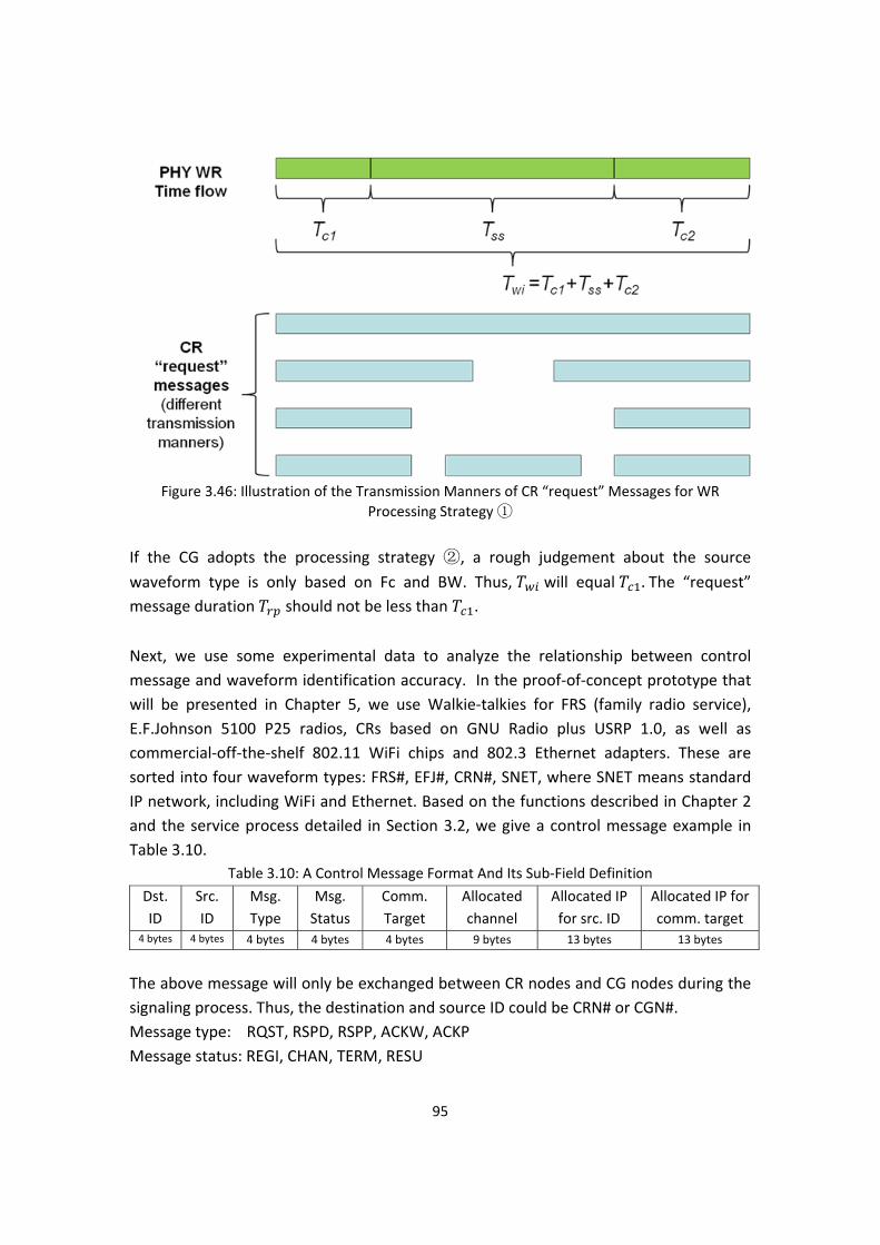
95
Figure 3.46: Illustration of the Transmission Manners of CR “request” Messages for WR
Processing Strategy ①
If the CG adopts the processing strategy ②, a rough judgement about the source
waveform type is only based on Fc and BW. Thus, will equal . The “request” message duration should not be less than .
Next, we use some experimental data to analyze the relationship between control message and waveform identification accuracy. In the proof‐of‐concept prototype that will be presented in Chapter 5, we use Walkie‐talkies for FRS (family radio service), E.F.Johnson 5100 P25 radios, CRs based on GNU Radio plus USRP 1.0, as well as commercial‐off‐the‐shelf 802.11 WiFi chips and 802.3 Ethernet adapters. These are sorted into four waveform types: FRS#, EFJ#, CRN#, SNET, where SNET means standard IP network, including WiFi and Ethernet. Based on the functions described in Chapter 2 and the service process detailed in Section 3.2, we give a control message example in Table 3.10.
Table 3.10: A Control Message Format And Its Sub‐Field Definition
Dst. ID
Src. ID
Msg. Type
Msg. Status
Comm. Target
Allocated channel
Allocated IP for src. ID
Allocated IP for comm. target
4 bytes 4 bytes 4 bytes 4 bytes 4 bytes 9 bytes 13 bytes 13 bytes
The above message will only be exchanged between CR nodes and CG nodes during the signaling process. Thus, the destination and source ID could be CRN# or CGN#. Message type: RQST, RSPD, RSPP, ACKW, ACKP Message status: REGI, CHAN, TERM, RESU
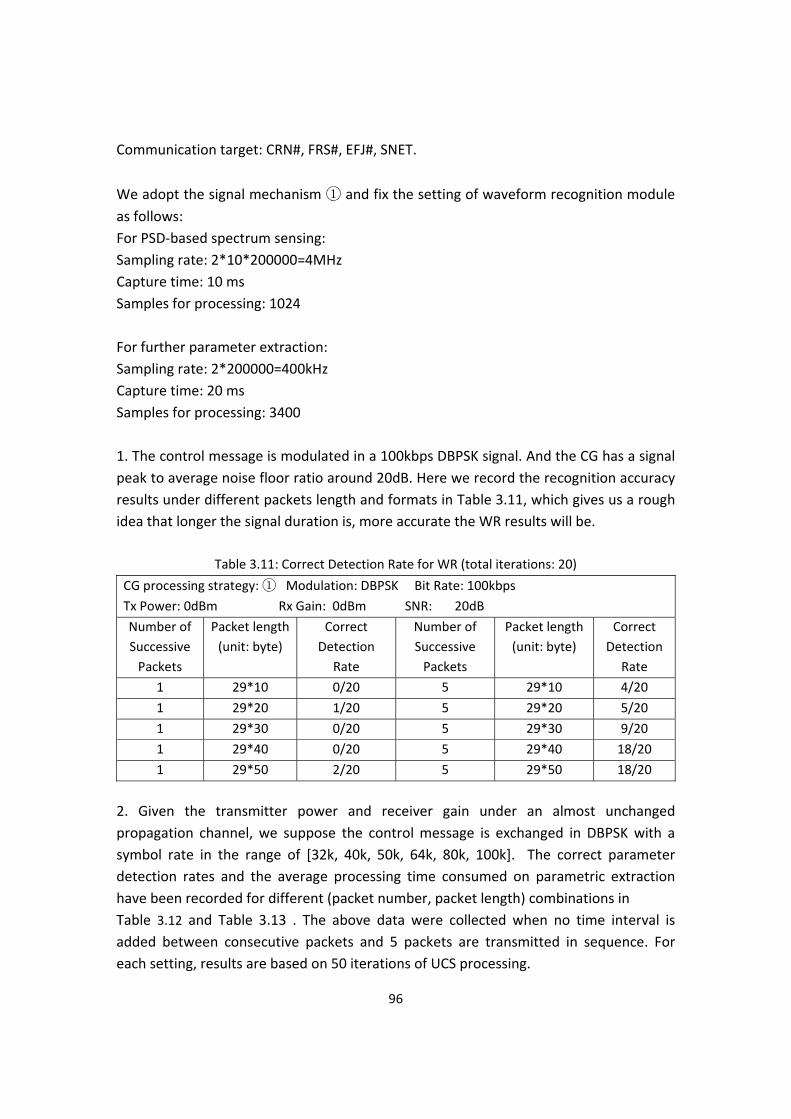
96
Communication target: CRN#, FRS#, EFJ#, SNET.
We adopt the signal mechanism ① and fix the setting of waveform recognition module as follows: For PSD‐based spectrum sensing: Sampling rate: 2*10*200000=4MHz Capture time: 10 ms Samples for processing: 1024 For further parameter extraction: Sampling rate: 2*200000=400kHz Capture time: 20 ms Samples for processing: 3400 1. The control message is modulated in a 100kbps DBPSK signal. And the CG has a signal peak to average noise floor ratio around 20dB. Here we record the recognition accuracy results under different packets length and formats in Table 3.11, which gives us a rough idea that longer the signal duration is, more accurate the WR results will be.
Table 3.11: Correct Detection Rate for WR (total iterations: 20)
CG processing strategy: ① Modulation: DBPSK Bit Rate: 100kbps
Tx Power: 0dBm Rx Gain: 0dBm SNR: 20dB
Number of Successive Packets
Packet length (unit: byte)
Correct Detection
Rate
Number of Successive Packets
Packet length (unit: byte)
Correct Detection
Rate
1 29*10 0/20 5 29*10 4/20
1 29*20 1/20 5 29*20 5/20
1 29*30 0/20 5 29*30 9/20
1 29*40 0/20 5 29*40 18/20
1 29*50 2/20 5 29*50 18/20
2. Given the transmitter power and receiver gain under an almost unchanged propagation channel, we suppose the control message is exchanged in DBPSK with a symbol rate in the range of [32k, 40k, 50k, 64k, 80k, 100k]. The correct parameter detection rates and the average processing time consumed on parametric extraction have been recorded for different (packet number, packet length) combinations in Table 3.12 and Table 3.13 . The above data were collected when no time interval is added between consecutive packets and 5 packets are transmitted in sequence. For each setting, results are based on 50 iterations of UCS processing.

97
Table 3.12: Correct Parameter Detection Rate (total iterations: 50)
CG processing strategy: ① Control message modulation: DBPSK
Tx Power: 0dBm Rx Gain: 0dBm SNR: 20dB
Symbol Rate Packet length
32k 40k 50k 64k 80k 100k
Number of Successive Packets:
5
29*10 35/50 25/50 12/50 13/50 14/50 10/50
29*20 50/50 50/50 49/50 28/50 25/50 18/50
29*30 50/50 50/50 50/50 47/50 46/50 33/50
29*40 50/50 50/50 48/50 48/50 48/50 43/50
29*50 50/50 50/50 48/50 45/50 46/50 41/50
Figure 3.47: Correct WR Rate at Different Transmission Symbol Rates for Different Packet
Lengths We can draw two conclusions from the curves plotted in Figure 3.47. (1) At a certain packet length, the data collected at different symbol rate reflects the principle shown in Figure 3.37. That is “the higher the symbol rate, the fewer the number of samples per symbol, and thus the worse the WR performance”. (2) At the same symbol rate, longer packets have longer lasting periods, the chances of a WR capturing enough date will be higher, thus more accurate the WR results will be.

98
Table 3.13: Average Processing Time (seconds) for Parametric Extraction (total iterations: 50)
CG processing strategy: ① Control message modulation: DBPSK
Tx Power: 0dBm Rx Gain: 0dBm SNR: 20dB
Symbol Rate packet length
32k
40k
50k
64k
80k
100k
Number of Successive Packets:
5
29*10 1.5011 1.5248 2.99 2.5515 2.4214 3.306
29*20 1.3416 1.168 1.6153 2.5096 2.0196 2.75
29*30 1.2998 1.1016 1.2828 1.9847 1.7126 2.3482
29*40 1.307 1.1718 1.3758 2.0823 1.9542 2.5584
29*50 1.292 1.111 1.3777 2.2324 1.8465 2.3798
Figure 3.48: Average WR Time at Different Transmission Symbol Rates for Different Packet
Lengths
From Figure 3.48, it is obvious that the symbol rate of 40kbaud is a good value to choose. Combining the results in these two figures and the principle of “it is easier to receive a short message than a longer one”, we can choose the following parameters for “request”
message transmission if the CG adopts the processing strategy ①. Symbol rate for control message transmission: 40kbaud Packet number in sequence: 5

99
Packet length: 29*30 Based on the transmission symbol rate and roll‐off value, the bandwidth for each signaling channel can be determined. The above selection makes the bandwidth of a CR “request” signal distinguishable from that of a legacy public safety signal and that of a P25 signal.
3.7 Discussion
The success of a service process highly depends on the correct waveform identification. Higher WI accuracy is usually obtained with a sacrifice of time, which will increase the “call set‐up time” or “link set‐up time”. We compared two different processing strategies for a CG’s waveform identification. To some extent, it provides a useful reference for the practical implementation of a CG system. Yet, the processing speed of current MATLAB‐based UCS system cannot meet the requirement for a shorter “link set‐up time”. There are a variety of methods to improve this. An example is the GPP/DSP/FPGA hybrid implementation of UCS mentioned in Section 3.4.6. In addition, continuously running the sensor will consume lots of power, which is not practical for the battery powered terminals. Thus, power consumption will limit the mobility of CG nodes.
Appendix 3‐A
Before starting the derivation, it is reasonable to make two assumptions: (1) For MPSK and M‐ary QAM, each of the M possible symbol states occurs with the same probability 1/M; (2) Within a symbol stream, the occurrence of each symbol is independent of other symbols. Define a sequence of discrete random variables , , , , , , where 1, means the number of phase jump points that the occurrence of the th symbol in the ‐length symbol stream will contribute to . Thus, the discrete random variable
can be represented by:
The assumptions in (1) and (2) imply that , , , , , are independent, discrete random variables with the probability mass function as follows:
0 1 , when 1; 0 1/ 1 1 1/ , when 2, .
Therefore, the mean value of will be:

100
1 ·1
Since , the ratio of to will be:
1·
1
In the real system, we usually choose an oversampling rate in the range of [3, 8], and capture several hundred or thousand of samples. Thus, it is reasonable to conclude
/ 1/ , and the above equation can be approximately simplified as:
·1
3 8
It is worth mention that the above analysis ignores the cases where long strings of the same symbol are contained in the captured symbol stream. However, the value of
/ , derived under the restriction that the maximum allowed length of
consecutively identical symbols is 3, almost equals to the result in equation (3‐8).
Appendix 3‐B
We analyze the waveforms used by legacy public safety radios and P25‐compliant radios, and summarize the specific parameters in Table 3.14 and Table 3.15, respectively.
Table 3.14: Legacy Public Safety Waveforms
Waveform Type: Legacy Public Safety
TX
PHY Tx power (P) Tx carrier frequency (Fc): Refer to Figure 1.1 Bandwidth (BW): 25kHz
Modulation (MOD): FM + CTCSS
LINK Medium access method: Push to Talk
NET N/A
TRAN N/A
APPL voice
RX Similar as the format for TX

101
Table 3.15: P25 Waveforms
Waveform Type: P25
TX
PHY RF Power level (P): FM analog = P25 digital equipment, currently
Spectrum (Fc): VHF (136‐174MHz), UHF(403‐512MHz, 806‐870MHz), 700 MHz (746 – 806MHz)
Bandwidth (BW): 25kHz, 12.5kHz, 6.25kHz Modulation (MOD): C4FM(deviation ±1.8kHz, ±0.6kHz),
FM, CQPSK Digital full channel rate: 9600 bits/s (symbol rate Rs=4.8 baud) Channel coding: interleaving and linear block codes such
as Hamming codes, Golay codes, Reed‐Solomon codes, Primitive BCH, and shortened cyclic codes.
LINK Multiplexing: FDMA and/or TDMA (phase 2)
NET N/A
TRAN N/A
APPL voice (unit call, group call), data
RX Similar as the format for TX
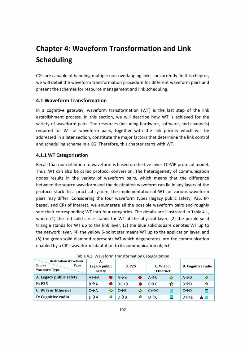
102
Chapter 4: Waveform Transformation and Link Scheduling CGs are capable of handling multiple non‐overlapping links concurrently. In this chapter, we will detail the waveform transformation procedure for different waveform pairs and present the schemes for resource management and link scheduling.
4.1 Waveform Transformation
In a cognitive gateway, waveform transformation (WT) is the last step of the link establishment process. In this section, we will describe how WT is achieved for the variety of waveform pairs. The resources (including hardware, software, and channels) required for WT of waveform pairs, together with the link priority which will be addressed in a later section, constitute the major factors that determine the link control and scheduling scheme in a CG. Therefore, this chapter starts with WT.
4.1.1 WT Categorization
Recall that our definition to waveform is based on the five‐layer TCP/IP protocol model. Thus, WT can also be called protocol conversion. The heterogeneity of communication nodes results in the variety of waveform pairs, which means that the difference between the source waveform and the destination waveform can lie in any layers of the protocol stack. In a practical system, the implementation of WT for various waveform pairs may differ. Considering the four waveform types (legacy public safety, P25, IP‐based, and CR) of interest, we enumerate all the possible waveform pairs and roughly sort their corresponding WT into four categories. The details are illustrated in Table 4.1, where (1) the red solid circle stands for WT at the physical layer, (2) the purple solid triangle stands for WT up to the link layer, (3) the blue solid square denotes WT up to the network layer, (4) the yellow 5‐point star means WT up to the application layer, and (5) the green solid diamond represents WT which degenerates into the communication enabled by a CR’s waveform adaptation to its communication object.
Table 4.1: Waveform Transformation Categorization Destination Waveform
Source Type Waveform Type
A: Legacy public
safety
B: P25
C: WiFi or Ethernet
D: Cognitive radio
A: Legacy public safety A↔A A B A C A D B: P25 B A B↔B B C B D C: WiFi or Ethernet C A C B C↔C C D D: Cognitive radio D A D B D C D↔D
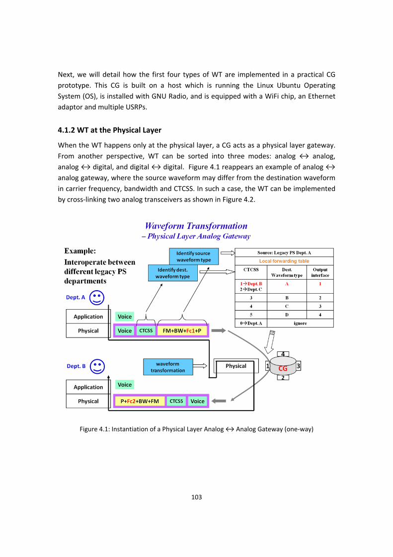
103
Next, we will detail how the first four types of WT are implemented in a practical CG prototype. This CG is built on a host which is running the Linux Ubuntu Operating System (OS), is installed with GNU Radio, and is equipped with a WiFi chip, an Ethernet adaptor and multiple USRPs.
4.1.2 WT at the Physical Layer
When the WT happens only at the physical layer, a CG acts as a physical layer gateway. From another perspective, WT can be sorted into three modes: analog ↔ analog, analog ↔ digital, and digital ↔ digital. Figure 4.1 reappears an example of analog ↔ analog gateway, where the source waveform may differ from the destination waveform in carrier frequency, bandwidth and CTCSS. In such a case, the WT can be implemented by cross‐linking two analog transceivers as shown in Figure 4.2.
Figure 4.1: Instantiation of a Physical Layer Analog ↔ Analog Gateway (one‐way)

104
Figure 4.2 : Flow‐graph of a Physical Layer Analog ↔ Analog Gateway The above architecture was initially developed to bridge two push‐to‐talk FM radios with different bandwidths and carrier frequencies in the gateway mode of a PSCR. Later the CTCSS function was added. Basically, this gateway employs two pairs of transmitter (TX) paths and receiver (RX) paths for waveform 0 and waveform 1, respectively. Each transceiver needs a USRP daughter board, covering the desired frequency. We use the transceiver daughter board displayed in Figure 4.3 [108]. There are two options for using this board as a RF transceiver. (1) Connecting one antenna to the single TX/RX port for both transmitting and receiving, and enabling the automatic TX/RX switching mode, we can make the gateway in Figure 4.2 work in “half‐duplex”. This means two one‐way communication links (i.e. RX0 TX1 and RX1 TX0) cannot work simultaneously. But it is acceptable because the radios operate at the push‐to‐talk mode. In addition, the automatic TX/RX switching function is quite useful for the CSMA‐based packet transmission. (2) Connecting antennas to both TX/RX and RX2 ports, and using the TX/RX port for transmitting and the RX2 port for receiving make a “full‐duplex” mode possible. But we did not use this mode in our experiments.
Figure 4.3: USRP RFX900 Transceiver Daughterboard. Reprinted, with permission from Ettus
Research LLC. Figure Source: reference [108]

105
The software part was built on the basis of GNU Radio modules. The output of demodulator 0 is fed into the input of modulator 1, and vice versa. GNU Radio based implementation provides a great reconfigurability; thus it is not difficult to make the gateway architecture to accommodate different waveforms. Probe 0 and Probe 1 are used to detect energy at channel 0 and channel 1, respectively. According to the carrier sensing results, the four paths, which are abbreviated as TX0, RX0, TX1, and RX1, are controlled by a MAC illustrated in Figure 4.4 to establish target links or terminate the flow‐graph. The control of paths is facilitated by setting the corresponding USRP sub‐device in “enable” or “disable” state and adjusting the gain values for the LNAs and amplifiers. For this gateway, at each time, only two of the four paths can simultaneously run. The possible combinations include RX0 & RX1, RX0&TX1, and RX1&TX0.
Figure 4.4: MAC FSM for a Physical Layer Analog ↔ Analog Gateway
A USRP mother board can hold two daughter boards. The two daughter boards required for a physical layer analog ↔ analog gateway can dwell in the same mother board or different mother boards. It is important to note that once one side of a USRP is running, you cannot configure the other side unless you stop the running side.
4.1.3 WT up to the Link Layer
For the digital gateway cases, we let each CR node have an internal IP address (for example, a Class C IPv4 address like 192.168.200.1) allocated by the CG which the CR is affiliated with. The IP address is bound with a TUN/TAP [109] interface which is displayed as “gr#” in the operating system. The protocol stack architecture of a CR is shown in Figure 4.5, where the TUN/TAP are virtual network drivers that provide a
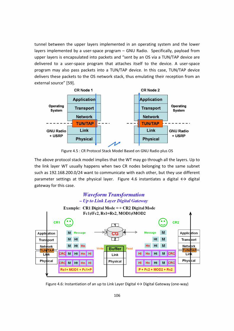
106
tunnel between the upper layers implemented in an operating system and the lower layers implemented by a user‐space program – GNU Radio. Specifically, payload from upper layers is encapsulated into packets and “sent by an OS via a TUN/TAP device are delivered to a user‐space program that attaches itself to the device. A user‐space program may also pass packets into a TUN/TAP device. In this case, TUN/TAP device delivers these packets to the OS network stack, thus emulating their reception from an external source” [59].
Figure 4.5 : CR Protocol Stack Model Based on GNU Radio plus OS
The above protocol stack model implies that the WT may go through all the layers. Up to the link layer WT usually happens when two CR nodes belonging to the same subnet such as 192.168.200.0/24 want to communicate with each other, but they use different parameter settings at the physical layer. Figure 4.6 instantiates a digital ↔ digital gateway for this case.
Figure 4.6: Instantiation of an up to Link Layer Digital ↔ Digital Gateway (one‐way)

107
Figure 4.7 : Flow‐graph of an up to Link Layer Digital ↔ Digital Gateway
To implement an up to link layer digital ↔ digital WT, we need to set up two digital transceivers as shown in Figure 4.7, both of which adopt the CSMA MAC protocol. In addition, we use four files (or buffers, or memories). “Ch0_Rx_payload” and “Ch1_Tx_payload” are accessed when the signal flows from Side 0 to Side 1. When Side 0 receives payloads, it first stores these payloads into “Ch0_Rx_payload” as a backup, then accumulates them in a string variable called “to_be_relayed_payload”, once “Ch1_Tx_payload” has be emptied by Side 1 the content of this string variable will be written into “Ch1_Tx_payload”, and then the variable “to_be_relayed_payload” will be set as an empty string to accept new payloads received by Side 0; when Side 1 detects that the size of “Ch1_Tx_payload” has increased to a threshold value, it will read the payloads from the file and send them in the format of waveform 1 once channel 1 is clear. When the signal flows from Side 1 to Side 0, the process of accessing “Ch1_Rx_payload” and “Ch0_Tx_payload” is similar to the foregoing explanation. The backup files ‐“Ch0_Rx_payload” and “Ch1_Rx_payload”‐ are necessary when the transmission rates of two sides are different. (When choosing the per‐hop waveform, it is better if the bit rates at the two sides are the same.) In addition, if the sizes of these two files will remain unchanged within a pre‐set time threshold, the two sides can break from their MAC loops. These files will be deleted after the application (waveform 0 ↔ waveform 1) is over. The MAC main loop at Side 0 is illustrated by the FSM in Figure 4.8. We need two transceiver daughter boards to implement the aforementioned digital gateway. Currently, we run two processes for Side 0 and Side 1, respectively. And the USRP sub‐device configuration for each side is made separately. Therefore, these two daughter boards should dwell in different mother boards. Otherwise, errors will occur.

108
Figure 4.8: MAC Main Loop of an up to Link Layer Digital ↔ Digital Gateway (side 0)
4.1.4 WT up to the Network Layer
If a CR node (e.g. CR1) wants to communicate with another CR node (e.g. CR2) out of the subnet it belongs to or with a standard IP node (WiFi [110] or Ethernet) which is within or beyond the subnet CR1 belongs to, WT up to the network layer will happen in a CG. The achievement of such a gateway benefits from the convenience provided by the Linux OS. The Linux kernel supports the prevalent TCP/IP protocol. In particular, it provides handy commands for the user to revise routing tables and iptables [111] to bridge different network interfaces. Taking the advantages of a Linux OS, Silvius et al [112] have successfully implemented and demonstrated CWT Smart Radio 2008 architecture’s ability to configure and control multiple adapter types, including 802.11 WiFi (wlan#), 802.15.1 Bluetooth (pan#), 802.3 Ethernet (eth#), and USRP plus GNU
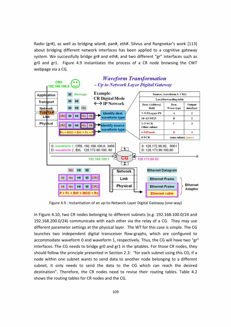
109
Radio (gr#), as well as bridging wlan#, pan#, eth#. Silvius and Rangnekar’s work [113] about bridging different network interfaces has been applied to a cognitive gateway system. We successfully bridge gr# and eth#, and two different “gr” interfaces such as gr0 and gr1. Figure 4.9 instantiates the process of a CR node browsing the CWT webpage via a CG.
Figure 4.9 : Instantiation of an up‐to‐Network‐Layer Digital Gateway (one‐way)
In Figure 4.10, two CR nodes belonging to different subnets (e.g. 192.168.100.0/24 and 192.168.200.0/24) communicate with each other via the relay of a CG. They may use different parameter settings at the physical layer. The WT for this case is simple. The CG launches two independent digital transceiver flow‐graphs, which are configured to accommodate waveform 0 and waveform 1, respectively. Thus, the CG will have two “gr” interfaces. The CG needs to bridge gr0 and gr1 in the iptables. For those CR nodes, they should follow the principle presented in Section 2.3: “for each subnet using this CG, if a node within one subnet wants to send data to another node belonging to a different subnet, it only needs to send the data to the CG which can reach the desired destination”. Therefore, the CR nodes need to revise their routing tables. Table 4.2 shows the routing tables for CR nodes and the CG.

110
Figure 4.10: Flow‐graph of an up to Network Layer Digital ↔ Digital Gateway
Table 4.2 : Linux Kernel IP Routing Tables Node Destination Gateway Genmask Flags Metric Ref Use Iface
CR1 192.168.100.2
192.168.100.0 0.0.0.0 255.255.255.0 U 0 0 0 gr0
0.0.0.0 192.168.100.1 0.0.0.0 UG 0 0 0 gr0
CG gr0:
192.168.100.1 gr1:
192.168.200.1
192.168.100.0 0.0.0.0 255.255.255.0 U 0 0 0 gr0
192.168.200.0 0.0.0.0 255.255.255.0 U 0 0 0 gr1
128.173.88.0 0.0.0.0 255.255.252.0 U 0 0 0 eth0
169.254.0.0 0.0.0.0 255.255.0.0 U 1000 0 0 eth0
0.0.0.0 128.173.88.1 0.0.0.0 UG 100 0 0 eth0
CR2 192.168.200.2
192.168.200.0 0.0.0.0 255.255.255.0 U 0 0 0 gr0
0.0.0.0 192.168.200.1 0.0.0.0 UG 0 0 0 gr0
4.1.5 Voice over IP
Ge et al [114] implemented a simply half‐duplex Voice over IP (VoIP) function via UDP sockets. The flow‐graph for implementing such a VoIP connection is illustrated in Figure 4.11. Although the quality of service (QoS) cannot be guaranteed, this relaying method provides a convenient solution to increasing the voice communication range. This type of WT is also necessary in a CG system.

111
Figure 4.11 : Voice over IP – an up to Transport Layer Gateway (one‐way)
The implementation of various WT in a CG has created necessary conditions to achieve the objectives proposed in Section 2.1. The four types of WT detailed in this section primarily employ inexpensive devices – USRPs and flexible open source toolkit – GNU Radio. As a summary of this section, we list the hardware & software resources required for each type of WT in Table 4.3, which will serve as an important basis for resource management and decision making.
Table 4.3 : Hardware & Software Resources Required for WT WT Type Hardware (for two ways) Software (for two ways)
Physical Layer Analog ↔ Analog WT
Two USRP daughter boards,one or two mother board(s)
analog gateway path in Figure 4.2
Up to Link Layer Digital ↔ Digital WT
Two USRP daughter boards,two mother boards
Two digital transceiver paths (Figure 4.7) with the MAC in Figure 4.8
Up to Network Layer Digital ↔ Digital WT
(CR ↔ Standard IP node)
One USRP daughter board,one mother board;
WiFi chip or Ethernet adaptor
One digital transceiver path with a CSMA MAC and a TUN/TAP
Up to Network Layer Digital ↔ Digital WT (2 CRs from 2 subnets)
Two USRP daughter boards,two mother boards
Two digital transceiver paths, each of which uses a CSMA MAC and a TUN/TAP
(Figure 4.10)
Up to Transport Layer Analog ↔ Digital WT
One USRP daughter board,one mother board;
WiFi chip or Ethernet adaptor
One analog transceiver path and UDP socket (Figure 4.11)
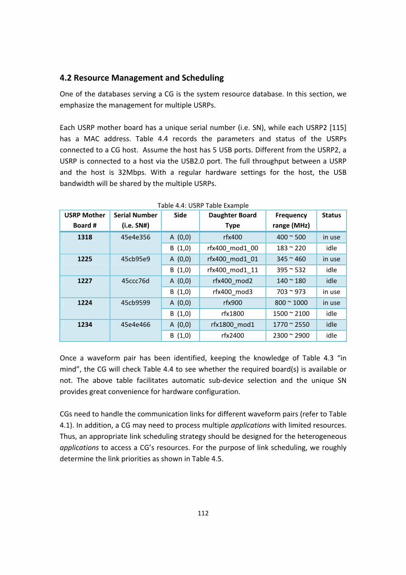
112
4.2 Resource Management and Scheduling
One of the databases serving a CG is the system resource database. In this section, we emphasize the management for multiple USRPs. Each USRP mother board has a unique serial number (i.e. SN), while each USRP2 [115] has a MAC address. Table 4.4 records the parameters and status of the USRPs connected to a CG host. Assume the host has 5 USB ports. Different from the USRP2, a USRP is connected to a host via the USB2.0 port. The full throughput between a USRP and the host is 32Mbps. With a regular hardware settings for the host, the USB bandwidth will be shared by the multiple USRPs.
Table 4.4: USRP Table Example USRP Mother
Board # Serial Number
(i.e. SN#) Side Daughter Board
Type Frequency range (MHz)
Status
1318 45e4e356 A (0,0) rfx400 400 ~ 500 in use
B (1,0) rfx400_mod1_00 183 ~ 220 idle
1225 45cb95e9 A (0,0) rfx400_mod1_01 345 ~ 460 in use
B (1,0) rfx400_mod1_11 395 ~ 532 idle
1227 45ccc76d A (0,0) rfx400_mod2 140 ~ 180 idle
B (1,0) rfx400_mod3 703 ~ 973 in use
1224 45cb9599 A (0,0) rfx900 800 ~ 1000 in use
B (1,0) rfx1800 1500 ~ 2100 idle
1234 45e4e466 A (0,0) rfx1800_mod1 1770 ~ 2550 idle
B (1,0) rfx2400 2300 ~ 2900 idle
Once a waveform pair has been identified, keeping the knowledge of Table 4.3 “in mind”, the CG will check Table 4.4 to see whether the required board(s) is available or not. The above table facilitates automatic sub‐device selection and the unique SN provides great convenience for hardware configuration. CGs need to handle the communication links for different waveform pairs (refer to Table 4.1). In addition, a CG may need to process multiple applications with limited resources. Thus, an appropriate link scheduling strategy should be designed for the heterogeneous applications to access a CG’s resources. For the purpose of link scheduling, we roughly determine the link priorities as shown in Table 4.5.
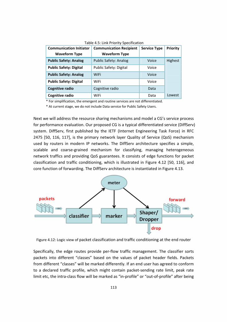
113
Table 4.5: Link Priority Specification Communication Initiator
Waveform Type Communication Recipient
Waveform Type Service Type Priority
Public Safety: Analog Public Safety: Analog Voice Highest
Lowest
Public Safety: Digital Public Safety: Digital Voice
Public Safety: Analog WiFi Voice
Public Safety: Digital WiFi Voice
Cognitive radio Cognitive radio Data
Cognitive radio WiFi Data * For simplification, the emergent and routine services are not differentiated. * At current stage, we do not include Data service for Public Safety Users.
Next we will address the resource sharing mechanisms and model a CG’s service process for performance evaluation. Our proposed CG is a typical differentiated service (DiffServ) system. DiffServ, first published by the IETF (Internet Engineering Task Force) in RFC 2475 [50, 116, 117], is the primary network layer Quality of Service (QoS) mechanism used by routers in modern IP networks. The DiffServ architecture specifies a simple, scalable and coarse‐grained mechanism for classifying, managing heterogeneous network traffics and providing QoS guarantees. It consists of edge functions for packet classification and traffic conditioning, which is illustrated in Figure 4.12 [50, 116], and core function of forwarding. The DiffServ architecture is instantiated in Figure 4.13.
Figure 4.12: Logic view of packet classification and traffic conditioning at the end router
Specifically, the edge routes provide per‐flow traffic management. The classifier sorts packets into different “classes” based on the values of packet header fields. Packets from different “classes” will be marked differently. If an end user has agreed to conform to a declared traffic profile, which might contain packet‐sending rate limit, peak rate limit etc, the intra‐class flow will be marked as “in‐profile” or “out‐of‐profile” after being

114
compared with the negotiated traffic profile by the metering function. The in‐profile packets should receive their priority marking and ensured forwarding service, but whether the out‐of‐profile packets should be delayed, remarked, dropped, or forwarded depends on the employed policy, which is not specified in the DiffServ. The core routers provide per‐class traffic management. They perform the per‐hop behavior (PHB) [116, 118], including buffering and scheduling packets transmission based on marking at edge. PHB results in a different observable forwarding performance behavior, but it does not specify what mechanisms to use to ensure required PHB performance behavior.
Figure 4.13: Instantiation of a Diffserv Architecture in Ethernet
Recalling our description of a CG in Chapter 2 and Chapter 3, the components of a CG function analogous to the elements of a DiffServ architecture for IP networks. Their mapping relationship is enumerated in Table 4.6.
Table 4.6: Cognitive Gateway analogies to DiffServ Architecture DiffServ Architecture Cognitive Gateway
arriving packets (standard IP packets) user requests (analog signal or digital packets)
classifier waveform identifier
marker + meter scenario analyzer
shaper/dropper Partial of center controller + decision maker
per‐hop behavior (PHB) center controller + decision maker + waveform transformation
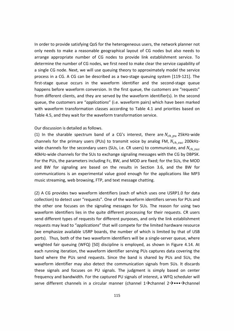
115
In order to provide satisfying QoS for the heterogeneous users, the network planner not only needs to make a reasonable geographical layout of CG nodes but also needs to arrange appropriate number of CG nodes to provide link establishment service. To determine the number of CG nodes, we first need to make clear the service capability of a single CG node. Next, we will use queuing theory to approximately model the service process in a CG. A CG can be described as a two‐stage queuing system [119‐121]. The first‐stage queue occurs in the waveform identifier and the second‐stage queue happens before waveform conversion. In the first queue, the customers are “requests” from different clients, and they are served by the waveform identifier(s). In the second queue, the customers are “applications” (i.e. waveform pairs) which have been marked with waveform transformation classes according to Table 4.1 and priorities based on Table 4.5, and they wait for the waveform transformation service. Our discussion is detailed as follows. (1) In the sharable spectrum band of a CG’s interest, there are _ 25kHz‐wide
channels for the primary users (PUs) to transmit voice by analog FM, _ 200kHz‐wide channels for the secondary users (SUs, i.e. CR users) to communicate, and _ 40kHz‐wide channels for the SUs to exchange signaling messages with the CG by DBPSK. For the PUs, the parameters including Fc, BW, and MOD are fixed; for the SUs, the MOD and BW for signaling are based on the results in Section 3.6, and the BW for communications is an experimental value good enough for the applications like MP3 music streaming, web browsing, FTP, and text message chatting. (2) A CG provides two waveform identifiers (each of which uses one USRP1.0 for data collection) to detect user “requests”. One of the waveform identifiers serves for PUs and the other one focuses on the signaling messages for SUs. The reason for using two waveform identifiers lies in the quite different processing for their requests. CR users send different types of requests for different purposes, and only the link establishment requests may lead to “applications” that will compete for the limited hardware resource (we emphasize available USRP boards, the number of which is limited by that of USB ports). Thus, both of the two waveform identifiers will be a single‐server queue, where weighted fair queuing (WFQ) [50] discipline is employed, as shown in Figure 4.14. At each running iteration, the waveform identifier serving PUs captures data covering the band where the PUs send requests. Since the band is shared by PUs and SUs, the waveform identifier may also detect the communication signals from SUs. It discards these signals and focuses on PU signals. The judgment is simply based on center frequency and bandwidth. For the captured PU signals of interest, a WFQ scheduler will serve different channels in a circular manner (channel 1 channel 2 ••• channel
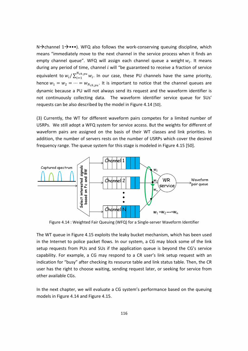
116
N channel 1 •••). WFQ also follows the work‐conserving queuing discipline, which means “immediately move to the next channel in the service process when it finds an empty channel queue”. WFQ will assign each channel queue a weight . It means during any period of time, channel will “be guaranteed to receive a fraction of service
equivalent to / ∑ _ . In our case, these PU channels have the same priority,
hence _ . It is important to notice that the channel queues are
dynamic because a PU will not always send its request and the waveform identifier is not continuously collecting data. The waveform identifier service queue for SUs’ requests can be also described by the model in Figure 4.14 [50]. (3) Currently, the WT for different waveform pairs competes for a limited number of USRPs. We still adopt a WFQ system for service access. But the weights for different of waveform pairs are assigned on the basis of their WT classes and link priorities. In addition, the number of servers rests on the number of USRPs which cover the desired frequency range. The queue system for this stage is modeled in Figure 4.15 [50].
Figure 4.14 : Weighted Fair Queuing (WFQ) for a Single‐server Waveform Identifier
The WT queue in Figure 4.15 exploits the leaky bucket mechanism, which has been used in the Internet to police packet flows. In our system, a CG may block some of the link setup requests from PUs and SUs if the application queue is beyond the CG’s service capability. For example, a CG may respond to a CR user’s link setup request with an indication for “busy” after checking its resource table and link status table. Then, the CR user has the right to choose waiting, sending request later, or seeking for service from other available CGs. In the next chapter, we will evaluate a CG system’s performance based on the queuing models in Figure 4.14 and Figure 4.15.
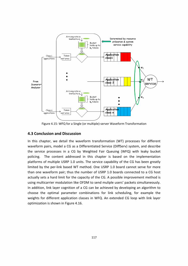
117
Figure 4.15: WFQ for a Single (or multiple)‐server Waveform Transformation
4.3 Conclusion and Discussion
In this chapter, we detail the waveform transformation (WT) processes for different waveform pairs, model a CG as a Differentiated Service (DiffServ) system, and describe the service processes in a CG by Weighted Fair Queuing (WFQ) with leaky bucket policing. The content addressed in this chapter is based on the implementation platforms of multiple USRP 1.0 units. The service capability of the CG has been greatly limited by the per‐link based WT method. One USRP 1.0 board cannot serve for more than one waveform pair; thus the number of USRP 1.0 boards connected to a CG host actually sets a hard limit for the capacity of the CG. A possible improvement method is using multicarrier modulation like OFDM to send muliple users’ packets simultaneously. In addition, link layer cognition of a CG can be achieved by developing an algorithm to choose the optimal parameter combinations for link scheduling, for example the weights for different application classes in WFQ. An extended CG loop with link layer optimization is shown in Figure 4.16.

118
Figure 4.16: Extended CG Functional Loop with Link‐layer Optimization

119
Chapter 5: Prototype and Performance Evaluation In this chapter, we will first introduce the cognitive gateway (CG) prototype implemented on the basis of GNU Radio plus multiple USRPs, and next give the system performance data measured from the over‐the‐air (OTA) experiments in a laboratory environment. In addition, we model a cognitive gateway as a two‐stage tandem queue and derive its theoretical performance using queuing theory.
5.1 Over‐The‐Air Prototype
Recall that when we introduced the CG design objective in Section 2.1, we extracted the “source‐CG‐destination” snapshot, where different types of nodes and links are denoted by dots and lines with different colors. CGs are colored in orange. Conventional public safety radios, P25‐compliant radios, standard IP‐based nodes, and user‐developed cognitive radio nodes (CRNs) are colored in blue, red, violet, and green, respectively. The link between a client and a CG has the same color as the client because the link employs the waveforms supported by the client and the CG adopts the client’s preference. We have set up different OTA experiments (from Figure 5.1 to Figure 5.3) to validate the proposed functionalities for CG. In these figures, we also provide the “dots and lines” connections for the corresponding setups. Figure 5.1 shows the OTA experiment setup when an FRS radio acts as a communication initiator, which is indicated by a blue arrow. With this setup, we have successfully tested the following functions. (1) CGN1 (i.e. cognitive gateway node 1) is able to extract the CTCSS value from the signal emitted by an FRS Walkie‐Talkie, which operates at the 462MHz band. (2) Based on the specific CTCSS value, CGN1 sets up the corresponding peer‐to‐peer links between the waveform pairs including:
• FRS Walkie‐Talkie and EFJ P25 portable radio (analog mode), which works at the 774~776MHz band;
• FRS Walkie‐Talkie and WiFi node; (3) CRN1 and CRN2, which are allowed to dynamically share the spectrum band of 462~464MHz with FRS radios, register to CGN1 by control message exchanges. (4) The FRS radio wants to broadcast voice messages to the cognitive radio nodes. CGN1 identifies the request from this FRS radio, and informs both CRN1 and CRN2 that they should turn to the analog FM mode and listen on the channel where the FRS radio works.

120
Figure 5.1: OTA Experiment Setup When an FRS radio is a communication initiator
When a cognitive radio node acts as a communication initiator, the OTA experiment in Figure 5.2 has been set up to test the functions of implemented CG and CR nodes. The testing scenarios and corresponding steps are listed as follows. Scenario 1: CRN1 ↔ CRN2, same subnet, same (Fc, MOD, Rs) (1)CRN1 randomly chooses a clear control channel and broadcasts its request for registration. (2)CGN1 detects the registration request from CRN1, and sends CRN1 the registration response messages containing its ID, which is “CGN1” in this case. (3)CRN1 gets the response from CGN1, and sends CGN1 the registration acknowledgement (ACK) messages. Then CRN1 will stay at the control channel and listen. (4)CGN1 adds an entry for CRN1 in its user database after receiving the ACK messages from CRN1. (5)CRN1 wants to communicate with CRN2. It randomly chooses a clear control channel and sends its request for link establishment to CGN1. The request includes CRN1’s preference for communication channels (Fc), modulations (MOD), and symbol rates (Rs). (6)CGN1 receives the link establishment request from CRN1, but it does not find CRN2 in its user database. Then, CGN1 informs CRN1 that CRN2 is not in service yet. (7)CRN2 registers to CGN1. The registration procedure follows the steps from (1) to (4).
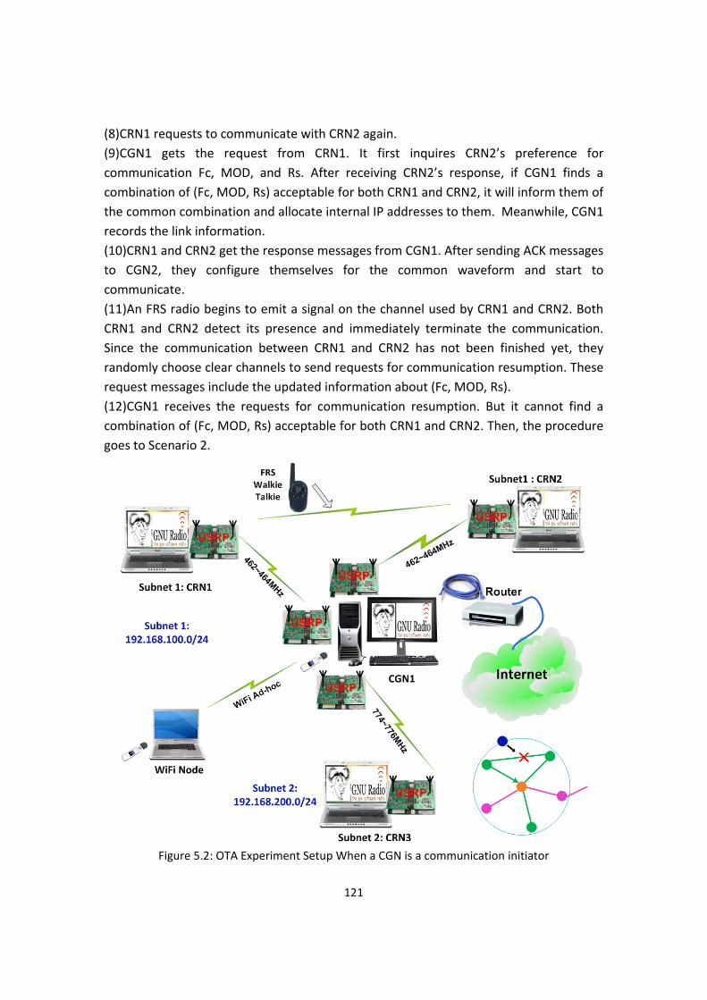
121
(8)CRN1 requests to communicate with CRN2 again. (9)CGN1 gets the request from CRN1. It first inquires CRN2’s preference for communication Fc, MOD, and Rs. After receiving CRN2’s response, if CGN1 finds a combination of (Fc, MOD, Rs) acceptable for both CRN1 and CRN2, it will inform them of the common combination and allocate internal IP addresses to them. Meanwhile, CGN1 records the link information. (10)CRN1 and CRN2 get the response messages from CGN1. After sending ACK messages to CGN2, they configure themselves for the common waveform and start to communicate. (11)An FRS radio begins to emit a signal on the channel used by CRN1 and CRN2. Both CRN1 and CRN2 detect its presence and immediately terminate the communication. Since the communication between CRN1 and CRN2 has not been finished yet, they randomly choose clear channels to send requests for communication resumption. These request messages include the updated information about (Fc, MOD, Rs). (12)CGN1 receives the requests for communication resumption. But it cannot find a combination of (Fc, MOD, Rs) acceptable for both CRN1 and CRN2. Then, the procedure goes to Scenario 2.
Figure 5.2: OTA Experiment Setup When a CGN is a communication initiator
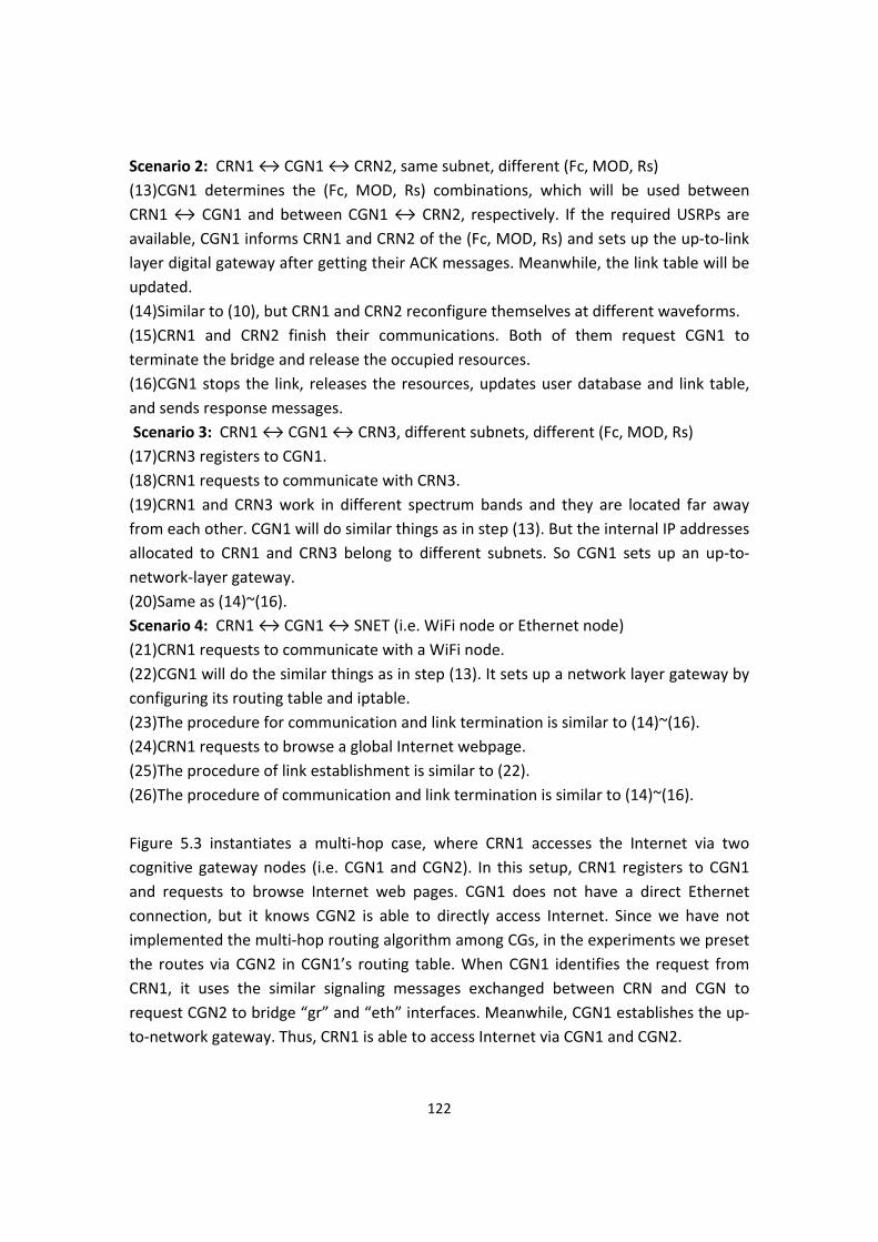
122
Scenario 2: CRN1 ↔ CGN1 ↔ CRN2, same subnet, different (Fc, MOD, Rs) (13)CGN1 determines the (Fc, MOD, Rs) combinations, which will be used between CRN1 ↔ CGN1 and between CGN1 ↔ CRN2, respectively. If the required USRPs are available, CGN1 informs CRN1 and CRN2 of the (Fc, MOD, Rs) and sets up the up‐to‐link layer digital gateway after getting their ACK messages. Meanwhile, the link table will be updated. (14)Similar to (10), but CRN1 and CRN2 reconfigure themselves at different waveforms. (15)CRN1 and CRN2 finish their communications. Both of them request CGN1 to terminate the bridge and release the occupied resources. (16)CGN1 stops the link, releases the resources, updates user database and link table, and sends response messages. Scenario 3: CRN1 ↔ CGN1 ↔ CRN3, different subnets, different (Fc, MOD, Rs) (17)CRN3 registers to CGN1. (18)CRN1 requests to communicate with CRN3. (19)CRN1 and CRN3 work in different spectrum bands and they are located far away from each other. CGN1 will do similar things as in step (13). But the internal IP addresses allocated to CRN1 and CRN3 belong to different subnets. So CGN1 sets up an up‐to‐network‐layer gateway. (20)Same as (14)~(16). Scenario 4: CRN1 ↔ CGN1 ↔ SNET (i.e. WiFi node or Ethernet node) (21)CRN1 requests to communicate with a WiFi node. (22)CGN1 will do the similar things as in step (13). It sets up a network layer gateway by configuring its routing table and iptable. (23)The procedure for communication and link termination is similar to (14)~(16). (24)CRN1 requests to browse a global Internet webpage. (25)The procedure of link establishment is similar to (22). (26)The procedure of communication and link termination is similar to (14)~(16). Figure 5.3 instantiates a multi‐hop case, where CRN1 accesses the Internet via two cognitive gateway nodes (i.e. CGN1 and CGN2). In this setup, CRN1 registers to CGN1 and requests to browse Internet web pages. CGN1 does not have a direct Ethernet connection, but it knows CGN2 is able to directly access Internet. Since we have not implemented the multi‐hop routing algorithm among CGs, in the experiments we preset the routes via CGN2 in CGN1’s routing table. When CGN1 identifies the request from CRN1, it uses the similar signaling messages exchanged between CRN and CGN to request CGN2 to bridge “gr” and “eth” interfaces. Meanwhile, CGN1 establishes the up‐to‐network gateway. Thus, CRN1 is able to access Internet via CGN1 and CGN2.

123
Figure 5.3: OTA Experiment Setup for a Multi‐hop Case
5.2 Miscellaneous Implementation Details
The control messages exchanged between CRN and CGN during the signaling processes for different scenarios have been summarized in Table 5.1. The given messages can also be used between CG nodes. The control message format in Table 5.1 is a little bit different from that shown in Table 3.10. The major difference lies in the “communication channel preference” field. For example, when CRN1 contains “100100101” in this field of its request message for communication with CRN2, it means CRN1 operates at band 1 and the communication channels numbered “1”, “3” and “6” will be acceptable for communications. In the experiment, we let band 1 start from 462MHz, and assign up to eight communication channels for CR nodes, each of which has a bandwidth of 200kHz. The meaning of the “communication channel preference” field is explained in Table 5.2. Since it is impossible for a CG node to sense all the channel occupancy conditions surrounding those CR nodes who register to this CG, a CG needs to collect the channel availability information from both the communication initiator and the recipient. The method given in Table 5.2 is convenient for the channel negotiation in a CG. The common channels can be selected by a simple logic “AND” operation.

124
Table 5.1: Control Messages Exchanged between CRN and CGN Scenarios Control Messages
Nodes Behavior
Message direction
Dst. ID Src.ID
Msg.Type
Msg. Status
Comm. Target
Comm. channel preference
IP for src. ID IP for comm. target
Register
CRN1 FFFF CRN1 RQST REGI 0000 000000000CRN1 CGN1 CRN1 CGN1 RSPD REGI 0000 000000000CRN1 CGN1 CGN1 CRN1 ACKW REGI 0000 000000000
Request
link setup with CRN2
Case 1: the desired destination CRN2 is not in service (i.e. CRN2 has not registered yet per CGN1’s knowledge)
CRN1 CGN1 CGN1 CRN1 RQST CHAN CRN2 100100101
CRN1 CGN1 CRN1 CGN1 RSPD CHAN CRN2 FFFFFFFFF
CRN1 CGN1 CGN1 CRN1 ACKW CHAN CRN2 FFFFFFFFF
Case 2: CRN2 has registered to CGN1, but it is in communication.
CRN1 CGN1 CGN1 CRN1 RQST CHAN CRN2 100100101CRN1 CGN1 CRN1 CGN1 RSPD CHAN CRN2 BBBBBBBBBCRN1 CGN1 CGN1 CRN1 ACKW CHAN CRN2 BBBBBBBBB
Case 3: CRN1 ↔ CRN2 Both CRN1 and CRN2 registered to CGN1, and they belong to the same subnet. There is a common channel they can use for direct comm.
CRN1 CGN1 CGN1 CRN1 RQST CHAN CRN2 100100101CRN2 CGN1 CRN2 CGN1 RQST CHAN CRN1 101100001CRN2 CGN1 CGN1 CRN2 RSPD CHAN CRN1 101000001CRN1 CGN1 CRN1 CGN1 RSPD CHAN CRN2 100000001 192.168.100.2 192.168.100.3CRN1 CGN1 CGN1 CRN1 ACKW CHAN CRN2 100000001 192.168.100.2 192.168.100.3CRN2 CGN1 CRN1 CGN1 RSPP CHAN CRN1 100000001 192.168.100.3 192.168.100.2CRN2 CGN1 CGN1 CRN1 ACKP CHAN CRN1 100000001 192.168.100.3 192.168.100.2
Case 4: CRN1 ↔ CGN1 ↔ CRN2 Both CRN1 and CRN2 registered to CGN1, and they belong to the same subnet. There is No common channel they can use for direct comm. But they can comm. via CGN1.
CRN1 CGN1 CGN1 CRN1 RQST CHAN CRN2 100100101CRN2 CGN1 CRN2 CGN1 RQST CHAN CRN1 101100001CRN2 CGN1 CGN1 CRN2 RSPD CHAN CRN1 101001000CRN1 CGN1 CRN1 CGN1 RSPD CHAN CRN2 100000001 192.168.100.2 192.168.100.3CRN1 CGN1 CGN1 CRN1 ACKW CHAN CRN2 100000001 192.168.100.2 192.168.100.3CRN2 CGN1 CRN1 CGN1 RSPP CHAN CRN1 101000000 192.168.100.3 192.168.100.2CRN2 CGN1 CGN1 CRN1 ACKP CHAN CRN1 101000000 192.168.100.3 192.168.100.2
Source ID: CRN#, CGN# Message type: RQST, RSPD, RSPP, ACKW, ACKP Destination ID: CRN#, CGN# Message status: REGI, CHAN, TERM, RESU Communication target: CRN#, FRS#, EFJ#, SNET

125
Table 5.1: Control Messages Exchanged between CRN and CGN (Continued) Scenarios Control Messages
Nodes Behavior
Message direction
Dst. ID
Src.ID
Msg.Type
Msg. Status
Comm. Target
Comm. channel
preference
IP for src. ID IP for comm. target
Request link setup with CRN2
Case 5: CRN1 ↔ CGN1 ↔ CRN2 Both CRN1 and CRN2 registered to CGN1, and they belong to different subnets. They can comm. via CGN1. CGN1 needs to set up an up‐to‐network layer gateway.
CRN1 CGN1 CGN1 CRN1 RQST CHAN CRN2 100100101CRN2 CGN1 CRN2 CGN1 RQST CHAN CRN1 201000001CRN2 CGN1 CGN1 CRN2 RSPD CHAN CRN1 201001000CRN1 CGN1 CRN1 CGN1 RSPD CHAN CRN2 100000001 192.168.100.2 192.168.200.3CRN1 CGN1 CGN1 CRN1 ACKW CHAN CRN2 100000001 192.168.100.2 192.168.200.3CRN2 CGN1 CRN1 CGN1 RSPP CHAN CRN1 201000000 192.168.200.3 192.168.100.2CRN2 CGN1 CGN1 CRN1 ACKP CHAN CRN1 201000000 192.168.200.3 192.168.100.2
Request to access Internet
Case 1: CRN1 ↔ CGN1 ↔ SNET CRN1 registered to CGN1, and CGN1 has a direct Ethernet connection.
CRN1 CGN1 CGN1 CRN1 RQST CHAN SNET 100100101
CRN1 CGN1 CRN1 CGN1 RSPD CHAN SNET 100000001 192.168.100.2 192.168.100.1
CRN1 CGN1 CGN1 CRN1 ACKW CHAN SNET 100000001 192.168.100.2 192.168.100.1
Case 2: CRN1 ↔ CGN1 ↔CGN2 ↔ SNET CRN1 registered to CGN1. CGN1 does not have a direct Ethernet connection, but CGN2 has.
CRN1 CGN1 CGN1 CRN1 RQST CHAN SNET 100100101CGN2 CGN1 CGN2 CGN1 RQST CHAN SNET 301000001 192.168.300.2CGN2 CGN1 CGN1 CGN2 RSPD CHAN SNET 301001000 192.168.300.3 192.168.300.2CGN2 CGN1 CGN2 CGN1 ACKW CHAN SNET 301000000 192.168.300.2 192.168.300.3CRN1 CGN1 CRN1 CGN1 RSPD CHAN SNET 100000001 192.168.100.2 192.168.100.1CRN1 CGN1 CGN1 CRN1 ACKW CHAN SNET 100000001 192.168.100.2 192.168.100.1
Request link setup
General cases: There is no channel available. Or all the USRPs of CGN1 have been occupied.
CRN1 CGN1 CGN1 CRN1 RQST CHAN CRN#/SNET 100100101 CGN1 checks the availability of channels and USRPs.
CRN1 CGN1 CRN1 CGN1 RSPD CHAN CRN#/SNET 000000000CRN1 CGN1 CGN1 CRN1 ACKW CHAN CRN#/SNET 000000000
Terminate comm. link
CRN1 CGN1 CGN1 CRN1 RQST TERM CRN#/SNET ######### 192.168.###.# 192.168.###.#CRN1 CGN1 CRN1 CGN1 RSPD TERM CRN#/SNET ######### 192.168.###.# 192.168.###.#CRN1 CGN1 CGN1 CRN1 ACKW TERM CRN#/SNET ######### 192.168.###.# 192.168.###.#
Resume interrupted link The messages are similar to those for the link set‐up cases. The MSG status should be changed to “RESU”.

126
Figure 5.4: Software/Hardware Architecture of Implemented CG Node
Figure 5.5: Software/Hardware Architecture of Implemented CR Node
127
Table 5.2: Representation of “communication channel preference”
Band Communication channel availability
channel 8 channel 7 channel 6 channel 5 channel 4 channel 3 channel 2 channel 1
1 0 0 1 0 0 1 0 1
2 0 1 0 0 1 0 0 0
The software/hardware architectures of implemented CGN and CRN are given in Figure 5.4 and Figure 5.5, respectively. The main functions of both CGN and CRN start with opening a listening socket. Based on the command and/or data received from the socket, the main function will enter one of its finite states and execute the corresponding tasks under that state. To perform the tasks, the main function may need to launch other processes. For example, both CGN and CRN need a signaling executor to take charge of the control message exchanges. The control messages contain the information which will determine the direction of the main programs. In certain situations the signaling executors will send back data to the main function via sockets. Appendix 5‐A provides the screen snapshots for CGN and CRN. These screen snapshot are obtained during the service procedure for a waveform pair of CRN SNET. The flow‐graph of a CGN refers to Figure 3.3. Although the WFQ scheduling scheme for multiple links and the periodic information exchange among CGs have not been implemented in the current prototype, we have developed the dynamic tables in the central controller for the purpose of managing user status, requested applications, and link status. The entry formats of these tables are given in Table 5.3. Figure 5.6 shows the diagram of CR user states maintained by CGN and the transition relationship between these states.
Figure 5.6: CR User State Diagram Maintained by CGN

128
Table 5.3: Dynamic Tables Maintained by a CGN
Cognitive radio node status table (example) CRN ID Registered CGN# Used band# Current Fc (Hz) Status Internal IP address Last modified time
CRN1 CGN1 band1 462100000 registered/rqst_pend/got_channel/in_comm
192.168.100.2 01:23:27.238652
Status table of requested applications (example) Waveform pair Priority level WT type Status Last modified time
CRN1 CRN2 pending/processed 01:23:27.238652
Link status table (example) Waveform pair Status src_ch ↔ dst_ch src_ip ↔ dst_ip src_mod ↔ dst_mod src_rs ↔ dst_rs Last modified time
CRN1 CRN2 started/ended/resumed
4621000000 ↔4625000000
192.168.100.2↔192.168.100.3
DBPSK ↔DBPSK 100k ↔100k 01:23:27.238652
Internal IP addresses for the Nodes at Band# (example) Internal IP address Node ID Net mask Flag Interface Last modified time
192.168.100.2 CRN1 255.255.255.0 RU gr0 01:23:27.238652
192.168.100.1 CGN1 255.255.255.0 GW gr0 01:23:27.278732

129
5.3 OTA Experimental Results
The link setup time depends on the service ability of a cognitive gateway node and also the population of users. Link setup time should be counted from the instant when the user begins to send “request” till the instant when the communication link is ready. For a CR user, the link setup time should be the sum of the following time slots: (1) The time for a CR user to find an available channel, and this is related to the number of channels and the arriving rate of users (including PU and SU); (2) Waiting time before getting served; (3) Service time (i.e. request processing time). In the laboratory conditions, I measure the link (call) set‐up time at a given system setting. It is easy to measure the link set‐up time when there is no resource (including channel, CGN’s hardware and processing ability) competition. So this result should be the minimal required link set‐up time, which can only be a reference time. Since it is hard to realize all the possible scenarios in the laboratory conditions, it is necessary to do a theoretical analysis to help evaluate CG’s performance.
Table 5.4: Experiment Setup Specifications CRN1
Computer Dell Inspiron 6400Intel Centrino Duo, each of the two processors is T2500 @2.00GHz
CGN1
Computer
Dell Precision 390 Desktop Intel Core 2 Duo CPU, each of the two processors is [email protected] cache size: 2048KB
CRN1 & CGN1
Operating system Ubuntu 7.10
Software PYTHON scripts, GNU Radio
Radio peripheral USRP
Using the above settings and waveform identification strategy ① addressed in Section 3.6, the link set‐up time for the waveform pair of “FRS↔FRS”, without resource competition, has been measured. The result is 3.55078 seconds. And a majority of the link set‐up time for the “FRS↔FRS” pair has been consumed in the waveform identification stage, which takes 3.5107s. We captured the MATLAB time report in Appendix 5‐B. From the results we can see that data collection and loading samples from hard disk consume lots of time. This portion of time consumption can be greatly reduced by employing memory‐based data access methods. In addition, we measured the link set‐up time when CRN1 requested to access Internet, which means the waveform pair of “CRN↔SNET”. The measurement result is 2.7 seconds, which is detailed in Table 5.5. These results are collected in CRN1 when CGN1 adopts waveform

130
identification strategy ②. The control messages are transmitted by DBPSK with a symbol rate of 40k baud.
Table 5.5: Link Set‐up Time for the Waveform Pair of “CRN↔SNET” Processes in CRN1 System Time in CRN1 Where is the time displayed?
The command “request SNET” is received by the FSM of CRN1.
1260951102.9 Interface for the FSM of CRN1
CRN1 gets the response from CGN1. “Channel” and “IP address” have been
allocated. 1260951104.44
Interface for callback information displaying in CRN1
The FSM of CRN1 gets the command “start_comm” from “Signaling Executor”.
1260951104.51 Interface for the FSM of CRN1
The FSM of CRN1 informs its operator of “The requested link has been set up and it is ready for starting the application program.”
1260951105.6 Interface for callback information displaying in CRN1
Link Set‐up Time is: 1260951105.6‐1260951102.9=2.7 seconds
5.4 Theoretical Performance Evaluation Using Queuing Theory
The service process of a CG can be modeled as the two‐stage tandem queue [119, 121] displayed in Figure 5.7. As we addressed in Section 4.2, both Queue 1 and Queue 2 are single‐server queues, which employ evenly weighted fair queuing (WFQ) discipline. Queue 1 has _ traffic flows, which are characterized as independent Poisson arrival
processes of primary users’ (PUs’) requests with the same mean rate of . Since the waveform identifier cyclically serves the requests from different channels and instantaneously switches from one channel to the next after a deterministic service time of , it can be modeled as a single equivalent queue with a specific service discipline. The arrival process to this queue is the sum of the _ independent Poisson traffic
flows; thus it is still a Poisson process and its mean rate is _ [119]. It is important
to note that the service time is the time that the WR spends in identifying an FRS signal and extracting its CTCSS value. Thus, under the same signal‐to‐noise ratio (SNR) level and the same implementation platform for WR, the service time can be approximately regarded as a constant value. Additionally, in a CG, the requests arrived during the service time will not be buffered. Therefore, Queue 1 can be described as an M/D/1/1 model [119, 122]. The request arrivals and WR service completion events happening in Queue 1 are depicted by the time diagram in Figure 5.8. The applications (i.e. waveform pairs) that are figured out in Queue 1 will arrive in Queue 3. It is necessary to analyze the service completion process of Queue 1. We can see that the process of served arrivals is a

131
process with the generic renewal time equal to , where is the residual inter‐arrival time excluding the fixed service time [122]. Because of the memoryless property of the exponential distribution, is exponential with a mean value of 1/ _ . The
served arrival departs Queue 1 after a deterministic service time . Thus, the service completion process (i.e. the departure process) in terms of the inter‐arrival time between subsequent service completion events is also a process with the generic renewal time equal to .
Figure 5.7: Modeling a CG by a Two‐stage Tandem Queue
Figure 5.8: Time diagram of arrivals and service completion events

132
An M/D/1/1 queue has only two states because the departing event will always leave the system empty until the next request arrives. This leads to the equilibrium state probabilities for Queue 1 at any arbitrary instant to be
,1
11
1 ,
,_
1 _ 1
In the above equations, _ is the traffic intensity offered to Queue 1. The
blocking probability and the throughput (i.e. carried traffic) of Queue 1 will be:
, , 1 , , 1 , 1
In a similar way, Queue 2 can be modeled as an M/D/1/1 queue. The equilibrium state probabilities for Queue 2 at any arbitrary instant are:
,1
1 , , 1 , _
And the blocking probability and the throughput of Queue 2 will be:
, , 1 , , 1 , 1
Next, we will consider a simplified case for Queue 3. As shown in Figure 5.7, we consider only three application classes for Queue 3. Specifically, application class 1 is “FRS FRS” pairs, which are from Queue 1; application class 2 is “CRN# SNET” pairs from Queue 2; application class 3 is “CRN# CRN#” pairs (whose communication links are setup via CG) from Queue 2. The first two application classes need only one USRP board, while application class 3 needs two USRP boards. To model Queue 3, we make some assumptions: (1) there are three USRP boards available for waveform transformation, which means Queue 3 has three servers; (2) the service processes for these three application classes are exponentially distributed with mean values of 1/ , 1/ , 1/ , respectively; (3) the mean arrival rates of these three application classes are , ,
, respectively; (4) if the three servers are all busy, the new arrivals will be blocked; (5) for simplicity, a first‐come‐first‐served (FCFS) discipline is applied to Queue 3. Thus, Queue 3 can be modeled as a G/M/3/3 queue [119, 120] with three classes of applications. The states of Queue 3 and the transition between these states can be approximately described by the Markov chain in Figure 5.9, where the circles stand for the states. For example, “state 0” means all the servers are idle; “state 1_1” means there is one server working and this server is working for application class 1; “state 3_13” means all three servers are busy, one of them is working for application class 1 and two of them are serving application class 3. Queue 3 has 13 states in total. The block

133
probability equals the sum of the probabilities for “state 3_13”, “state 3_23”, “state 3_111”, “state 3_112”, “state 3_122”, and “state 3_222”.
Figure 5.9: Markov Chain Model of a CG
From Figure 5.9, we can get thirteen equilibrium state equations.
, , _ , _ , _
, _ , , _ · 2 , _ , _
, _ , , _ · 2 , _ , _
, _ 2 , _ , _ · 3 , _
, _ , _ , _ , _ · 2 , _ · 2
, _ 2 , _ , _ , _ · 3
, _ , , _ , _
, _ , _ · 3
, _ , _ · 3
, _ 2 , _ , _
, _ 2 , _ , _
, _ , _ , _
, _ , _ , _ In addition, the sum of all the state probabilities should equal 1. Based on these equations, we can get a matrix equation in (4‐1), i.e. , where is a 13×13 matrix,

134
is a column vector including the 13 state probabilities for Queue 3, and b is a constant column vector including 13 numbers. If | | 0, the matrix equation (4‐1) has a deterministic solution:
| || | 1,2,3, … , 13
is the kth element of the column vector , and is obtained by replacing the kth column of the matrix A by the constant column vector b. In Queue 3, the block probabilities for the three application classes are:
_ _ , _ , _ , _ , _ , , _
_ , _ , _ , _ , _ , , _
_ 1 , , _ , _ The above analysis for Queue 3 is based on an FIFS service discipline. When priorities are taken into account, the analysis process follows that of [123‐125].
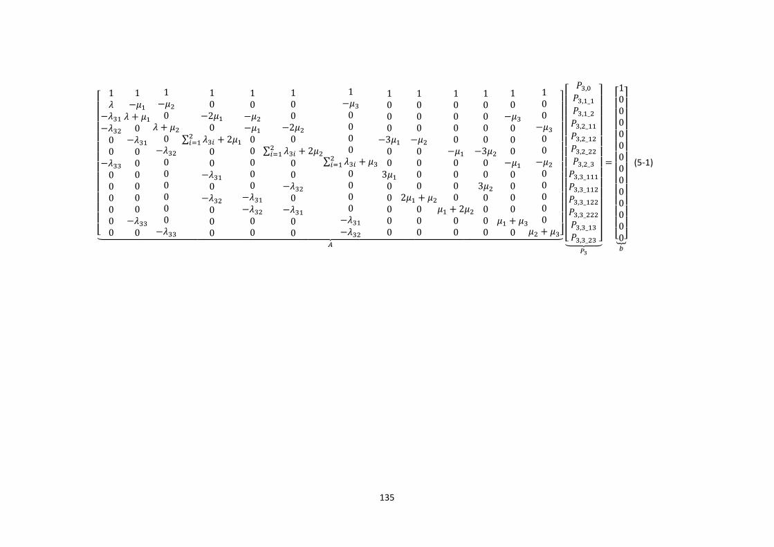
135
1
00
000000
1
0
000000
0
1
0
0
000000
1020
∑ 200
0
000
10
00000
00
10020
∑ 200
0
00
1
0000
∑0000
1000300
300000
1000
0000
2000
10000
0000
200
10000300
30000
10
000
0000
0
100
00
00000
,
, _
, _
, _
, _
, _
, _
, _
, _
, _
, _
, _
, _
10000000000000
(5‐1)

136
Appendix 5‐A
Screen snapshots for a cognitive radio node (CRN):
(1) Interface for a CR user to input commands:
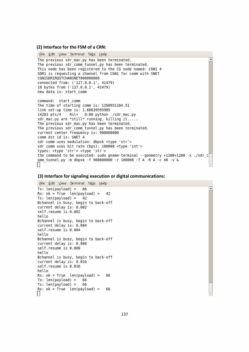
137
(2) Interface for the FSM of a CRN:
(3) Interface for signaling execution or digital communications:

138
(4) Interface for callback information displaying in a CRN:
Screen snapshots captured during the procedure that a CRN is browsing the Internet webpage via a CGN:

139
Screen snapshot for a cognitive gateway node (CGN):
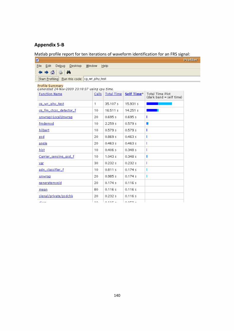
140
Appendix 5‐B
Matlab profile report for ten iterations of waveform identification for an FRS signal:
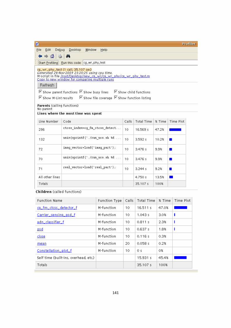
141

142

143
Chapter 6: Conclusions 6.1 Dissertation Summary
Originally motivated by the lack of communication interoperability problem encountered by the public safety first responders in the disaster scenarios, and later inspired by the sound vision of future wireless mobile communication system in 4G, the author of this dissertation aims at designing a class of special cognitive nodes, named “Cognitive Gateways (CGs)”, which can be easily set up and work in either ad‐hoc or infrastructure mode to provide seamless ubiquitous connectivity among heterogeneous communication systems complying with dissimilar air interfaces or standards. On the road towards this challenging goal, the author has made the following contributions in this dissertation. A cognitive gateway has been proposed, designed, built, and tested to facilitate universal interoperability among incompatible waveforms. Located in places where various communication nodes and diverse access networks coexist, the CG works like a network server with the differentiated service (DiffServ) architecture to provide automatic traffic relaying and link establishment. The service process in a CG is usually initiated by the users who send requests by their own waveforms. The complete operating procedure of a CG has been depicted as a waveform‐oriented cognition loop, which is primarily executed by eight modules together. These modules are waveform identifier, scenario analyzer, waveform & user databases, decision maker, forwarding & routing tables, central controller (including logic link controller and resource manager), generic application programming interfaces (APIs), and waveform converter. The major functions of a CG waveform identifier include user request awareness, waveform pair identification, and environment observation. The waveform identifier extracts necessary parameters from the detected request signal and works with the scenario analyzer to identify the waveform pair (source waveform and destination waveform) that the CG needs to interconnect. In addition, it provides the radio environment information as the reference for waveform negotiation. After checking the local forwarding and routing tables and performing a waveform negotiation process, the decision maker and central controller determine the route between the requested waveform pair and the waveforms that will be used for each link of this route, taking into consideration capabilities of nodes in the route, availability of needed resources, concurrency of ongoing links, and the priority of this application. Based on the decision result, the central controller will allocate appropriate resources to implement the application and

144
meet its QoS requirements to the best of a CG’s ability. Then, the system configuration profiles and necessary control commands will be generated to launch corresponding platforms for waveform transformation, thereby establishing communication links between different users. For the convenience of discussion, the “source‐CG‐destination” snapshot has been extracted from the entire network. Although this snapshot considers only neighboring nodes which are one‐hop away from the CG, it is scalable to form larger networks. From Chapter 2 to Chapter 5, the author has investigated the key enabling technologies for such a snapshot. This dissertation considers primarily enabling the interoperation of four types of nodes (i.e. legacy public safety radios, P25‐compliant radios, standard TCP/IP‐based nodes, and user‐developed cognitive radio nodes) via the aid of CGs, but actually cognitive gateways are extendable and upgradable to accommodate more waveforms. The declared universal interoperability is enabled by the generic waveform representation format and the reconfigurable software defined radio platform. The important term “waveform” has been defined as a protocol stack specification suite in Chapter 1. This definition accords with the trend of all IP‐based solution for the future communication systems. In Chapter 2, the author gives a generic waveform representation format based on the five‐layer TCP/IP protocol stack architecture. This format can represent the waveforms used by Ethernet, WiFi, cellular system, P25, cognitive radios (CRs), etc. This architecture possesses three advantages: (1) clear hierarchy/layering is efficient for parameter extraction at the system configuration stage; (2) it is flexible to adapt to different waveforms and open for future modification; (3) it is platform independent. In addition, the similar idea has been applied to the design of the generic API to meet specific requirements for different applications. The generic APIs play an important role in conveying the information for waveform pair configuration, platform pair configuration, and link behavior control. A reference representation format for GNU Radio plus USRP based waveform platform format is also given in this Chapter. Because of the reasons enumerated at the end of Section 2.4, XML has been selected to describe the configuration profiles. A significant advantage of CG over other interoperability solutions lies in its autonomy, which is contributed to by appropriate signaling processes and automatic waveform identification. In the proposed “source‐CG‐destination” snapshot, if requesting the services from CGs, the clients will send waveforms containing the necessary information for a CG to process their requests. These requests are transmitted during the signaling procedures. A series of signaling procedures between CG and clients is necessary for the accomplishment of CG discovery, user registration and un‐registration, link

145
establishment, communication resumption, service termination, route discovery, etc. From the waveforms conveyed during the signaling procedures, the waveform identifier extracts the parameters that can be used for a CG to identify the source waveform and the destination waveform. These parameters are called “waveform indicators”. The above issues have been detailed in Chapter 3 and here are the summaries.
• Waveform indicator selection: the author analyzed the four types of waveforms of interest and confirmed the rationality of containing waveform indicators in a user’s requests. The selection of waveform indicators primarily follows two principles: (1) make use of the existing features or information embedded in the waveforms that a node can support; if changes are inevitable and necessary, minimal changes should be made. For standard waveforms, the change might be a new utilization method of the existing features. For the user‐developed CRs, the changes might be different transmission manners like the time interval between consecutive packets or the size of an individual packet. (2) The information that can indicate the waveform type should be represented in a format which can be interpreted by a CG with satisfactory accuracy and acceptable time consumption. In Section 3.1, the author outlines the waveform indicators for different types of communication initiators.
• A complete service process: the detailed service process differs for different types of communication initiators. In our discussion, user‐developed cognitive radio users are allowed to dynamically share the spectrum licensed to public safety radios as secondary users. Thus, the communication initiator is either a primary user (PU) or a secondary user (SU). The difference in privileges, channel utilization methods, and capabilities make the service process initialized by a PU different from that initialized by a SU. In particular, the author details the service process initialized by a legacy public safety radio (LPSR) and that initialized by a CR. An LPSR sets the CTCSS (Continuous Tone‐Coded Squelch System) value to correspond with the communication target, and then pushes the button to send its request. For a CR, the entire process is much more complicated. CR exploits a reactive CG discovery mechanism by choosing a vacant signaling channel (i.e. control channel) to broadcast a request registration message. The registration process provides convenience for user tracking and network resource (particularly spectrum) management. In addition, the author describes the MAC layer flow‐graph adopted by a CR node during the signaling process for registration, link establishment, link resuming, and link termination, and during its communications with other CR nodes. Further, the author analyzes the possible cases that may happen when a CR user requests to communicate with another CR user and also the possible outcomes of

146
channel negotiation performed between the CG and CR source & destination. Furthermore, channel division, and the operations for communication resumption and link termination have been briefly addressed. As a summary of Section 3.2, the author gives a generalized flow‐graph which depicts the major operations of a CG and includes the process for all the four types of waveforms of interest.
• Waveform identification: CG uses a multi‐layer waveform identifier to extract the waveform indicators from the signaling messages. The physical layer signal recognition is implemented by the Universal Classification Synchronization (UCS) system. UCS is a joint work by Ying Wang and the author of this dissertation. Both of us have included it in our dissertations as an important part of our contributions. UCS is conceived as a self‐contained system which can detect, classify, synchronize with a received signal and provide all parameters needed for physical layer demodulation without prior information from the transmitter. Currently, it can accommodate the modulations including AM, FM, FSK, MPSK, QAM and OFDM. Also, it can be used in different multi‐user access schemes. UCS is reconfigurable to provide adaptivity in various environments, extendable to accommodate more signal types, and transplantable to different platforms. In Section 3.4, the design and implementation details of a UCS have been presented. The designed system has been verified by a prototype using GNU Radio in Linux plus a Universal Software Radio Peripheral (USRP), as well as using MATLAB in a Windows‐based Anritsu MS 2781A Signal Analyzer. In addition, performance for key components and the entire system has been evaluated in terms of accuracy, signal‐to‐noise ratio (SNR), and speed by theoretical analysis, computer simulations, and Over the Air (OTA) experiments. Furthermore, the author compares the features of different candidate platforms and discusses how to make a compromise decision on the specific platform where the UCS will be ported according to users’ requirements for cost, device size, accuracy, and processing speed. In CWT, the computational features of UCS algorithm have been analyzed and a GPP/DSP/FPGA hybrid architecture has been designed to achieve the optimal trade‐offs between flexibility, modularity, scalability, and performance. Some students in CWT have made a good practice on the Lyrtech Small Form Factor (SFF) SDR platform to realize a hybrid implementation of UCS. With the aforementioned advantages, a UCS can be applied for various scenarios such as dynamic spectrum access (DSA), dynamic cellular cognitive system (DCCS), and distributed ad‐hoc sensor network.
• Comparison between UCS and ASC: CG possesses the abilities of a Public Safety Cognitive Radio (PSCR), but it goes beyond the PSCR. An important difference

147
between CG and PSCR lies in their waveform identifiers. A CG uses the UCS to implement the physical layer waveform identification, while the sensor of a PSCR adopts the Adaptive Signal Classification (ASC) system, invented by Bin Le. In Section 3.5, the author makes an interesting comparison between UCS and ASC from different aspects.
• Signaling process and mechanisms: an underlying assumption for UCS is that the target signal is transmitted continually, which guarantees the UCS system can capture enough signal samples for recognition. However, in most cases the detection objects of a CG are signaling messages, which may not be transmitted continuously, thus it will be difficult to pick appropriate parameters for UCS. Generally speaking, the longer the signal lasts, the more accurate the waveform recognition results will be. But in most channel models, it is easier to receive a short message than a longer message. In order to ensure higher recognition accuracy, signaling efficiency, and lower signaling overhead, the author has addressed the key issues for signaling scheme design and their dependence on waveform identification strategy in Section 3.6. Specifically, the author analyzed the relationship between the durations of signaling messages for both LPSR & CR and the processing time required for different waveform identification strategies. In addition, the author gave a reference control message format for CR nodes. Further, based on the OTA experiment results under a certain waveform identification strategy, the author determined the modulation, symbol rate, transmission manner (including number of packets in sequence, size of a unit packet) that should be used for signaling messages.
Departing from the service queue of the waveform identifier(s), the accepted waveform pairs will enter the service queue of the waveform transformation (WT) system. In a CG, waveform transformation is the last step of the link establishment process. The resources (including hardware, software, and channels) required for transformation of waveform pairs, together with the application priority, constitute the major factors that determine the link control and scheduling scheme in a CG. In Chapter 4, the author first enumerates all the possible waveform pairs generated by the four waveform types of interest and roughly sorts their corresponding WT into five categories. Next, with the aid of the transceiver flow‐graphs and MAC layer state diagrams, the author describes the details of implementing the typical four types of WT (including physical layer analog ↔ analog gateway, up to link layer digital ↔ digital gateway, up‐to‐network‐layer digital gateway, and Voice over IP (VoIP) – an up to transport layer gateway) in a practical CG prototype. This CG is built on a host which is running the Linux Ubuntu Operating

148
System (OS), is installed with GNU Radio, and is equipped with a WiFi chip, an Ethernet adaptor and multiple USRPs. As the important basis for resource management, a CG needs to “keep in mind” the hardware and software resources required for each type of WT. In addition, the resource manager of a CG maintains a table which contains the mapping relationship between mother board serial number (SN), daughter board sides & types, and daughter board frequency ranges for each USRP connected to the CG host, and the real‐time status of those USRP boards. Such a table facilitates automatic sub‐device selection and the unique SN provides great convenience for hardware configuration. When a CG needs to process multiple applications with limited resources, the resource manager plays very important roles. The author finds that a CG can be regarded as a DiffServ system because the components of a CG function analogous to the elements of a DiffServ architecture for IP networks. Furthermore, a CG has been described as a two‐stage tandem queuing system. The first‐stage queue occurs in the waveform identifier and the second‐stage queue happens before waveform conversion. In the first queue, the customers are “requests” from different clients, and they are served by the waveform identifier(s). In the second queue, the customers are “applications” (i.e. waveform pairs) which have been marked with WT classes and link priorities, and they wait for the waveform transformation service. Each stage of the tandem queue employs a weighted fair queuing (WFQ) discipline. In Chapter 5, the author has introduced the CG prototype implemented on the basis of GNU Radio plus multiple USRPs and presents the test steps for the three different OTA experiments which are set up to validate the proposed functionalities for CG. In particular, the author provides miscellaneous implementation details for a CG prototype: (1) the control messages exchanged between CRN and CGN during the signaling processes for different scenarios; (2) the “communication channel preference” field embedded in a control message for channel negotiation; (3) the software/hardware architectures of implemented CGN and CRN; (4) the entry formats of dynamic tables maintained by the CG center controller for the purpose of managing user status, requested applications, link status, and internal IP addresses. One of the metrics used to evaluate a CG’s performance is link setup time, which depends on the service ability of a cognitive gateway node and also the population of users. In the laboratory conditions, the author measured the link (call) set‐up time at a given OTA experiment setting when there is no resource competition. So this result should be the minimal required link set‐up time. Since it is hard to realize all the possible scenarios in the laboratory conditions, it is necessary to do theoretical analysis to aid the performance evaluation for evaluate CGs. In the last section of Chapter 5, the service process of a CG is modeled as a two‐stage tandem queue, where the waveform identifier queues at the first stage can be

149
described as M/D/1/1 models and the waveform converter queue at the second stage can be described as G/M/K/K model. Based on these models, the author derives the theoretical block probability and throughput of a CG.
6.2 Future Work
The dissertation ends in this chapter, but the research work related to cognitive gateway deserves further investigation. In this section, the author will briefly address some thoughts about future work.
• Implement an MIMO version of UCS: it has been mentioned in Section 3.4.6 that UCS 1.0, 2.0, and 3.0 all belong to Single Input Single Output (SISO) systems. If a multiple‐input and multiple‐output (MIMO) version of UCS could be implemented, overlapping signals from different emitters may be separated by locations. Thus, a MIMO version of UCS should be able to provide a better physical support for the detection of malicious nodes in a network. In addition, the results provided in Section 3.4 are based on AWGN channels. However, the practical wireless communication channels suffer from multipath fading effects, which can be combated by the MIMO technology. Thus, an MIMO version of UCS will be more useful in practical applications.
• Traffic engineering and network planning: in Section 5.4, the author has modeled a CG as a two‐stage tandem queue and made a preliminary analysis about its theoretical performance in terms of block probability and throughput. The purpose of doing so is to provide the theoretical basis for network planning. Network planning includes at least two aspects: (1) given the populations of different types of users and the capabilities of CGs, how should the network planner arrange appropriate resources (e.g. number of CGs, number of servers in each CG) to meet the requirements for QoS; (2) considering the limitations for transmission power and/or effective communication ranges of CGs and different users, how should the network planner place the CGs. The first aspect contains traffic engineering, which is usually tackled by queuing theory. The solution to the second one may require the knowledge of graph theory. In Section 5.4, the author has simplified the link scheduling discipline, employed by the second stage queue, from WFQ to FIFS. In the future, it is necessary to quantize the WT classes and link priorities into the weights of WFQ and analyze a CG’s performance when it employs the WFQ discipline.
• Enable the link layer cognition in a CG: there are different link scheduling disciplines existing, such as FCFS, priority queuing, Round Robin, and WFQ. In

150
addition, the scheduling mechanism may follow a preemptive, non‐preemptive, work‐conserving, or non‐work conserving manner. Furthermore, a scheduling discipline like WFQ may choose different weights for the various application classes. Thus, in the link layer of a CG, there are lots of “knobs” that can be tuned. The future work should include the implementation of different scheduling schemes and the development of a genetic algorithm to choose the optimal parameter combinations for link scheduling at specific application scenarios. Therefore, the link layer cognition of a CG can be achieved.
• Improve the performance of a CG: the performance of a “source‐CG‐destination” snapshot can be evaluated in terms of call (or link) setup time, call block probability, link capacity, and carried throughput. The OTA experimental results in Section 5.3 indicate that a majority of the link setup time has been consumed at the waveform recognition (WR) stage. Therefore, the WR strategy should be simplified; the method for data collection and sample loading should be greatly improved; the WR module should be moved to a speedy platform. As mentioned in Section 4.3, The service capability of the CG has been greatly limited by the single‐carrier based WT method. A possible improvement method is using multicarrier modulation like OFDM to send muliple users’ traffic simultaneously. Further, in the cases that there are multiple types of users, OFDMA could serve as a possible solution. It will be a useful work to calculate the system capacities under different WT methods.
• Cognition and cooperation: the CG proposed in this dissertation can be applied to cooperative traffic relaying for both PUs and SUs, thus the network throughput can be greatly improved. When the author details the service process initialized by CR users, there are three possible outcomes from channel negotiation. It is obvious that the introduction of CG in the third case will help to throughput improvement. Researchers have done lots of interesting work about cooperative relaying [65, 66, 69, 126]. For example, reference [126] gives an overview about several cooperative protocols, such as amplify‐and‐forward relaying, two‐way relaying, coherent relaying, and decode‐and‐forward relaying etc. We can utilize different levels of CGs’ capabilities into different cases. Cognition together with cooperation in wireless communication network is a promising research field [65, 69]. Two of the specific research topics are relay selection [127] and waveform determination for each relaying link. These are also related to the next‐hop selection problem in multi‐hop routing [128].

151
Bibliography [1] R. Taylor, “Public safety communication systems requirements and designs,” in 2007
Virginia Tech Symposium on Wireless Personal Communications tutorial presentations. June 6‐8, 2007, Virginia Tech: Blacksburg, VA.
[2] SAFECOM. Available from: http://www.safecomprogram.gov/SAFECOM/. [3] Statement of Requirements (SoR). Available from:
http://www.safecomprogram.gov/SAFECOM/library/technology/1258_statementof.htm. [4] Y. Zhang, J. Luo, and H. Hu, Chapter 16: Wireless Mesh Networks for Public Safety and
Disaster Recovery Applications (by M. Portmann), in Wireless Mesh Networking: Architectures, Protocols and Standards. Auerbach Publications, Taylor & Francis Group: New York, 2007.
[5] B. Lane, on‐line tech topics about Public Safety. Available from: http://www.fcc.gov/pshs/techtopics/.
[6] C. Siva Ram Murthy and B. S. Manoj, Ad Hoc wireless networks: architectures and protocols. Prentice Hall PTR: Upper Saddle River, NJ, 2004.
[7] Y. K. Kim and R. Prasad, 4G Roadmap and Emerging Communication Technologies. Artech House, 2005
[8] Project 25 website. Available from: http://www.p25.com/. [9] APCO Project 25 Statement of Requirements (SoR). Available from:
http://www.apcointl.org/frequency/project25/documents/SOR‐2009.pdf. [10] Daniels Electronics Ltd., P25 Radio Systems Training Guide. Available from:
http://www.apcointl.org/frequency/project25/documents/TG‐001‐2‐0‐0_P25_Training_Guide.pdf.
[11] Cisco IP Interoperability and Collaboration System (IPICS). Available from: http://www.cisco.com/en/US/products/ps10165/Products_Sub_Category_Home.html.
[12] Harris P25. Available from: http://www.macom‐wireless.com/products/p25/Default.asp. [13] Harris VIDA (Voice, Interoperability, Data and Access). Available from:
http://www.macom‐wireless.com/vida.asp. [14] Harris RF Communication Products. Available from: http://www.macom‐
wireless.com/default.asp. [15] Joseph Mitola III homepage. Available from: http://web.it.kth.se/~maguire/jmitola/. [16] J. H. Reed, Software Radio: A Modern Approach to Radio Engineering. Pearson Education,
2002. [17] Wireless World Research Forum, Working Group 6. Available from: http://wg6.ww‐
rf.org/. [18] Software Defined Radio (SDR) Forum. Available from: http://www.sdrforum.org/. [19] European FP6 project End‐to‐End Reconfigurability (E²R). Available from:
http://www.e2r.motlabs.com. [20] Thales Communications Inc. Liberty™ Multiband Land Mobile Radio (LMR). Available
from: http://www.thalesliberty.com/about_liberty.asp.

152
[21] Harris Corporation RF1033M Multiband Multimode Land Mobile Radio (LMR). Available from: http://www.rfcomm.harris.com/talkasone/RF1033M.asp.
[22] Harris Corporation Harris Unity™ XG‐100 Multiband Radio. Available from: http://www.rfcomm.harris.com/talkasone/Unity_XG‐100.asp.
[23] T. C. Clancy III, “Dynamic spectrum access in cognitive radio networks,” Ph.D. dissertation. 2006, University of Maryland, College Park.
[24] Q. Zhao and B. M. Sadler, "A survey of dynamic spectrum access," IEEE Signal Processing Magazine, May 2007. 24(3): pp. 79‐89.
[25] J. Mitola III and G. Q. Maguire Jr, "Cognitive radio: making software radios more personal. Personal Communications," IEEE Wireless Communications, 1999. 6(4): pp. 13‐18.
[26] J. Mitola III, “Cognitive radio for flexible mobile multimedia communications," in 1999 IEEE International Workshop on Mobile Multimedia Communications (MoMuC'99).
[27] J. Mitola III, “Cognitive radios: An integrated agent architecture for software defined radio,” Ph.D. dissertation. 2000, Royal Institute of Technology, Sweden.
[28] Center for Wireless Telecommunications (CWT) at Virginia Tech. Available from: http://www.cognitiveradio.wireless.vt.edu/dokuwiki/doku.php?id=home.
[29] B. Le, "Building a Cognitive Radio: From Architecture Definition to Prototype Implementation," Ph.D. Dissertation, in Dept. of Electrical & Computer Engineering. 2007, Virginia Polytechnic Institute and State University: Blacksburg, VA.
[30] T. W. Rondeau, "Application of Artificial Intelligence to Wireless Communications," Ph.D. Dissertation, in Dept. of Electrical & Computer Engineering. 2007, Virginia Polytechnic Institute and State University: Blacksburg, VA.
[31] B. Le, T. W. Rondeau, and C.W. Bostian, "Cognitive radio realities". Wireless Communications and Mobile Computing, November 2007. 7(9): pp. 1037‐1048.
[32] B. Le, C.W.Bostian, D. Maldonado, Radio Domain Cognition ‐ A System Approach in Theory and Implementation. Virginia Tech Intellectual Properties (VTIP) No. 05.077. October 31, 2005.
[33] J. H. Reed and C. W. Bostian, “Understanding the Issues in Software Defined Cognitive Radio”.
[34] J. M. Chapin and W. H. Lehr, “The path to market success for dynamic spectrum access technology," IEEE Communications Magazine, May 2007: pp. 96‐103.
[35] IEEE Dynamic Spectrum Access Networks (DySPAN) symposium. Available from: http://www.ieee‐dyspan.org/.
[36] Y. Lin, H. Lee, M.Woh, Y. Harel, S. Mahlke, T. Mudge, C. Chakrabarti, and K. Flautner, , "SODA: A high‐performance DSP architecture for software‐defined radio," IEEE Micro, January‐February 2007. 27(1): pp. 114‐123.
[37] Q. Chen and C.W. Bostian, “Cognitive Gateway Design to Promote Universal Interoperability,” in Software Defined Radio Technical Conference. October 26‐30, 2008: Washington, DC.
153
[38] B. Le, F.A.G. Rodriguez, Q. Chen, B. Li, F. Ge, M. ElNainay, T.W. Rondeau, and C.W. Bostian,, “A Public Safety Cognitive Radio Node,” in Software Defined Radio Technical Conference. November 5‐9, 2007: Denver, Colorado.
[39] C. W. Bostian, "A prototype public safety cognitive radio for universal interoperability,". 2006, Center for Wireless Telecommunications, Wireless @ Virginia Tech: Blacksburg, VA.
[40] C. W. Bostian, "A prototype public safety cognitive radio for universal interoperability: update and demonstration," presented at NIJ Communications Technology (CommTech) Technical Working Group (TWG) Meeting & Program Review. April 2007: Las Vegas, Nevada.
[41] N. Ghani and R. Lamontagne. “Neural networks applied to the classification of spectral features for automatic modulation recognition,” in IEEE Proc. for Military Communication (MILCOM) Conference. 1993.
[42] B. Le, T. W. Rondeau, D. Maldonado, C. W. Bostian. “Modulation Identification Using Neural Network for Cognitive Radios,” in Software Defined Radio Forum Technical Conference. 2005. Anaheim, CA.
[43] B. Le, T. W. Rondeau, D. Maldonado, D. Scaperoth, C. W. Bostian. “Signal Recognition for Cognitive Radios,” in Software Defined Radio Forum Technical Conference. November 2006. Orlando, FL.
[44] B. Le and C. W. Bostian, Adaptive Signal Classification for Cognitive Radios, Virginia Tech Intellectual Properties (VTIP) 07‐094.
[45] GNU Radio. Available from: http://www.gnu.org/software/gnuradio/. [46] Ettus Research. Available from: http://www.ettus.com/. [47] B. Le, T. W. Rondeau, and C. W. Bostian, "General radio interface between cognitive
radio algorithms and software defined radio platforms," in Software Defined Radio Technical Conference. 2007: Denver, CO.
[48] Q. Chen, “Reconfigurable SDR platform design,” qualifying exam document, Virginia Tech. May 3, 2007.
[49] A. S. Tanenbaum, Computer networks. the 4th ed. 2003, Upper Saddle River, NJ: Prentice Hall PTR.
[50] J. F. Kurose and K. W. Ross, Computer networking: a top‐down approach featuring the Internet. the 3rd ed. 2005, Boston: Pearson/Addison Wesley.
[51] Philip Emeagwali's vision of hyperball computer for weather forecasting. Available from: http://emeagwali.com/essays/technology/weather/computing‐the‐weather.html.
[52] P. Sutton, L.E.D., K. E. Nolan. “A Reconfigurable Platform for Cognitive Networks,” in the 1st International Conference on Cognitive Radio Oriented Wireless Networks and Communications. June 8‐10, 2006.
[53] OSSIE (Open Source SCA Implementation ‐ Embedded). Available from: http://ossie.mprg.org/.
[54] Q. Chen, Y. Wang, C.W. Bostian, "Universal Classifier Synchronizer Demodulator," in the 1st international workshop on Dynamic Spectrum Access and Cognitive Radio Networks (DSA‐CRN’08) joint with the 27th IEEE IPCCC. December 7‐9, 2008: Austin, TX.

154
[55] Y. Wang, Q. Chen, and C.W. Bostian, "Universal Classifier and Synchronizer," accepted by International Journal of Autonomous and Adaptive Communications Systems (IJAACS).
[56] Anritsu MS2781A Signature Signal Analyzer. Available from: http://www.us.anritsu.com/products.
[57] Lyrtech Small Form Factor (SFF) SDR platform. Available from: http://www.lyrtech.com/. [58] EFJohnson 5300 ES Mobile Radio. Available from:
http://www.efjohnson.com/products/5300ES.asp. [59] TUN/TAP. Available from: http://vtun.sourceforge.net/tun/. [60] I. F. Akyildiz, X. Wang, and W. Wang, "Wireless mesh networks: a survey," Computer
Networks, 15 March 2005. 47(4): p. 445‐487. [61] i. F. Akyildiz and X. Wang, Wireless mesh networks. 2009, United Kingdom: John Wiley &
Sons Ltd. [62] Y. Zhang, J. Luo, H. Hu, Wireless mesh networking: architectures, protocols and
standards. 2007, New York: Auerbach Publications. [63] L. Gavrilovska and R. Prasad, Ad hoc networking towards seamless communications.
2006, the Netherlands: Springer. [64] E. Hossain and K. K. Leung, Wireless mesh networks: architectures and protocols. 2008:
Springer. [65] N. Devroye, M. Vu, and V. Tarokh, "Cognitive Radio Networks: Information Theory Limits,
Models and Design," in IEEE Signal Proc. Magazine, Special Issue on Cognitive Radios. November 2008. pp. 12‐23.
[66] Q. Zhang, J. Jia, and J. Zhang, "Cooperative relay to improve diversity in cognitive radio networks", in IEEE Communications Magazine. February 2009. pp. 111‐117.
[67] J. Jia, J. Zhang, and Q. Zhang, "Cooperative Relay for Cognitive Radio Networks," in IEEE INFOCOM. April 19‐25, 2009. Rio de Janeiro, Brazil.
[68] N. Devroye, P. Mitran, O.‐S. Shin, H. Ochiai, and V. Tarokh, ''Cooperation and Cognition in Wireless Networks,'' SK Telecom Review, special issue on 4G Spectrum and System Engineering issues, February 2007.
[69] O.‐S. Shin, N. Devroye, P. Mitran, H. Ochiai, S. S. Ghassemzadeh, H. T. Kung, and V. Tarokh, "Cooperation, Competition and Cognition in Wireless Networks: From Theory to Implementation", in Cooperation in Wireless Networks: Principles and Applications. 2006, Springer.
[70] Y. Zhang, H. Chen, and M. Guizani, Cooperative wireless communications. 2009, Boca Raton, FL: Auerbach Publications, Taylor & Francis Group.
[71] K. R. Chowdhury and I. F. Akyildiz, "Cognitive wireless mesh networks with dynamic spectrum access," IEEE Journal on Selected Areas in Communications, 2008. 26(1): pp. 168‐181.
[72] M. D. Katz and F. H.P. Fitzek, "Cooperative and Cognitive Networks: A Motivating Introduction," in Cognitive Wireless Networks: Concepts, Methodologies and Visions Inspiring the Age of Enlightenment of Wireless Communications (Editors: M.D.K. Frank and H. P. Fitzek). 2007, Springer Netherlands.
[73] P25 radio systems: training guide. 2007: Daniels Electronics Ltd.

155
[74] Public Safety Wireless Network: Comparison of Conventional and Trunked Systems. May 1999. Available from: http://www.safecomprogram.gov/SAFECOM/library/technology/1179_conventionaland.htm.
[75] N. Bayer, D. Sivchenko, B. Xu, S. Hischke, and J. Habermann, "Integration of Heterogeneous Ad Hoc Networks with the Internet," in Proc. of International Conference on Wireless Ad Hoc Networks. 2005. London, UK.
[76] E. Azzouz and A.K. Nandi, Automatic modulation recognition of communication signals. 1996, Boston: Kluwer Academic Publishers.
[77] N. Warke and G.C. Orsak, "A universal methodology for signal classification in non‐Gaussian environments," in Sixth IEEE Digital Signal Processing Workshop. 1994: Yosemite National Park, CA.
[78] Y. Wang, C. W. Bostian, and C.d. Silva, , "Universal Classification and Synchronization," in Microsoft Cognitive Wireless Networking Summit Poster. 2008: Snoqualmie, Washington.
[79] A. Polydoros and K. Kim, "On the detection and classification of quadrature digital modulations in broad‐band noise," IEEE Transactions on Communications, 1990. 38(8): pp. 1199‐1211.
[80] B. F. Beidas and C.L. Weber, "Asynchronous classification of MFSK signals using the higher order correlation domain," IEEE Transactions on Communications, 1998. 46(4): pp. 480‐493.
[81] P. Jahankhani, V. Kodogiannis and K. Revett, "EEG signal classification using wavelet feature extraction and neural networks," in IEEE John Vincent Atanasoff 2006 International Symposium on Modern Computing. October 3‐6, 2006: Sofia, Bulgaria. pp. 120‐124.
[82] S.‐Z. Hsue and S.S. Soliman, "Automatic modulation classification using zero crossing". Radar and Signal Processing, IEE Proceedings F, Dec 1990. 137(6): pp. 459‐464.
[83] A. Prochazka and J. Kukal and O. Vysata, "Wavelet transform use for feature extraction and EEG signal segments classification", in 3rd International Symposium on Communications, Control and Signal Processing (ISCCSP) 2008. March 12‐14, 2008: St. Julians. pp. 719‐722.
[84] T. Yucek and H. Arslan, "OFDM signal identification and transmission parameter estimation for cognitive radio applications," in 2007 IEEE Global Telecommunications Conference (GLOBECOM '07). Nov. 26‐30, 2007. Washington, DC.
[85] K. Kim et al., "Cyclostationary approaches to signal detection and classification in cognitive radio", in 2nd IEEE International Symposium on New Frontiers in Dynamic Spectrum Access Networks, 2007 (DySPAN 2007). April 17‐20, 2007: Dublin, Ireland. pp. 212‐215.
[86] Rice University WARP (Wireless open‐Access Research Platform). Available from: http://warp.rice.edu/index.php.
[87] P. D. Welch, "The Use of Fast Fourier Transform for the Estimation of Power Spectra: A Method Based on Time Averaging Over Short, Modified Periodograms," IEEE Transactions on Audio Electroacoustics, June 1967. AU‐15: pp. 70 ‐ 73.
156
[88] J. G. Proakis and M. Salehi, Communication Systems Engineering. 2002: Prentice Hall. [89] Y. Wang et al., "OFDM signal classification and synchronization for cognitive radio
systems," in SDR Forum Technical Conference. 2008: Washington D.C. [90] T. Yucek and H. Arslan, "OFDM signal identification and transmission parameter
estimation for cognitive radio applications," in 2007 IEEE Global Telecommunications Conference (GLOBECOM '07). Nov. 26‐30, 2007. Washington, DC.
[91] T. S. Rappaport, Wireless Communications Principles and Practice. 2002: Prentice Hall. [92] J. G. Proakis, Communication Systems. 2003: Prentice HallPrentice Hall. [93] Y. Wang, Q. Chen, and C. W. Bostian, "Universal synchronizer design for cognitive radio,"
in SDR Forum Technical Conference. 2007: Denver, CO. [94] N. M. Blachman, "Gaussian noise part II : distribution of phase change of narrow‐band
noise plus sinusoid," IEEE Transactions on Information Theory, 1988. 34(6): pp. 1401‐1405.
[95] R. Chandra et al, "Adapting channel widths to improve application performance," 2008. [96] J .G. Proakis, Digital Communications. 2001: McGraw‐Hill Companies, Inc. [97] S. Haykin, Communication Systems. 2003: John Wiley & Sons, Inc. [98] S. Nair, A. Fayez, G. Marballie, and C. W. Bostian, "Broadband Parallel RF Sensor Using
Lyrtech SFF SDR Platform," in PIRANA Meeting. October 2008, BBN Technologies: Boston, MA.
[99] S. Nair, A. Fayez, G. Marballie, Y. Wang, Q. Chen, and C. W. Bostian, “Universal Classification Synchronization (UCS) on a FPGA/DSP/GPP SDR Platform,” in the Wireless @ Virginia Tech 2009 Symposium on Wireless Personal Communications. June 3‐5, 2009: Blacksburg, VA.
[100] C. W. Bostian and Q. Chen, "Signal Recognition, Synchronization, and Demodulation: The VT UCS System," in DARPA‐SN‐09‐60 Machine Learning for Behavioral Control of Cognitive Radios (ML BCCR) Workshop. September 21‐22, 2009: Stevens Institute of Technology Hoboken, NJ.
[101] Y. Wang, Q. Chen, A. Young, T. Brisebois, S. Nair, A. Fayes, M. Silvius, F. Ge, G. Marballie, and C. W. Bostian, “Universal Classification and Synchronization (UCS),” in NIJ Communications Technology (CommTech) Technical Working Group Meeting and Program Review. March 31‐April 3, 2008: Boulder, CO.
[102] Y. Wang, Q. Chen, A. Young, T. Brisebois, S. Nair, A. Fayes, M. Silvius, F. Ge, G. Marballie, and C. W. Bostian, “Universal Classification and Synchronization,” in Microsoft Research Cognitive Wireless Networking Summit. June 5‐6, 2008: Snoqualmie, Washington.
[103] Y. Wang , Q. Chen, A. Young, B. Li, T. Brisebois, S. Nair, X. Cheng, N. He, G. Kwon, R. Rangnekar, A. Fayez, F. Ge, M. D. Silvius, G. Marballie, A. Radhakrishnan, and C. W. Bostian, “Dynamic Cellular Cognitive Radio: Rapidly Deployable Networking with DSA for Public Safety,” in IEEE DySPAN 2008 (demonstration session). October 14‐17, 2008: Chicago, Illinois.
[104] F. Ge, R. Rangnekar, A. Radhakrishnan, et al, “A Heterogeneous Cognitive Radio Network Enabling Dissimilar Cooperative Spectrum Sensing, Dynamic Spectrum Access,

157
Interoperability," in IEEE DySPAN 2008 (demonstration session). October 14‐17, 2008: Chicago, Illinois.
[105] Q. Chen and C. W. Bostian, "Cognitive Gateway Design to Promote Interoperability, Coverage and Throughput in Heterogeneous Communication Systems," in the poster competition of the Paul E. Torgersen Graduate Student Research Excellence Award. April, 2009, Virginia Tech: Blacksburg, VA.
[106] Q. Chen and C. W. Bositan, "Cognitive Gateway Design to Promote Interoperability, Coverage and Throughput in Heterogeneous Communication Systems," in the Wireless @ Virginia Tech 2009 Symposium on Wireless Personal Communications. June 3‐5, 2009: Blacksburg, VA.
[107] B. Le, P. Garcia, Q. Chen, Y. Wang, T. W. Rondeau, and C. W. Bostian, "Waveform agility of cognitive radios in Anritsu SignatureTM and CWT2 SDR platform," in Software Defined Radio Technical Conference. November 13‐17, 2006: Orlando, FL.
[108] Ettus Research, Datasheet for the transceiver daughter boards, the XCVR2450 and RFX‐series. Available from: http://www.ettus.com/downloads/er_ds_transceiver_dbrds_v5b.pdf.
[109] Virtual Point‐to‐Point(TUN) and Ethernet(TAP) devices. Available from: http://vtun.sourceforge.net/tun/.
[110] M.S. Gast, 802.11 wireless networks: the definition guide. the 2nd edition ed. 2006: O'Reilly Media, Inc.
[111] IptablesHowTo, Ubuntu documentation. Available from: https://help.ubuntu.com/community/IptablesHowTo.
[112] M. D. Silvius, T. Brisebois, Q. Chen, A. Fayez, F. Ge, B. Li, G. Marballie, S. Nair, R. Rangnekar, Y. Shi, Y. Wang, A. Young, and C. W. Bostian, “Communications from an Infrastructure Damaged Area: Smart Radio Challenge 2008 Final Report,” in Project Report: Wireless@Virginia Tech‐‐CWT. September 30, 2008.
[113] M. D. Silvius, R. Rangnekar, A. B. MacKenzie, and C. W. Bostian, “An Educational Testbed Illustrating Ad‐Hoc Networking and Software Defined Radio,” in Unpublished Whitepaper. November 28, 2008.
[114] F. Ge, A. Young, B. Li, T. Brisebois, Q. Chen, A. Fayes, S. Bates, M. EI Nainay, G. Kwon, M. Silvius, G. Marballie, Y. Wang, S. Nair, Y. Shi, et al, "A Public Safety Cognitive Radio," in NIJ Communications Technology (CommTech) Technical Working Group Meeting and Program Review. March 31‐April 3, 2008: Boulder, CO.
[115] Ettus Research, USRP2 motherboard datasheet. Available from: http://www.ettus.com/downloads/ettus_ds_usrp2_v2.pdf.
[116] An architecture for Differentiated Services, December 1998. Available from: http://tools.ietf.org/html/rfc2475.
[117] New Terminology and Clarifications for Diffserv, April 2002.Available from: http://tools.ietf.org/html/rfc3260.
[118] Per Hop Behavior Identification Codes, June 2001. Available from: http://tools.ietf.org/html/rfc3140.

158
[119] G. Giambene, Queuing theory and telecommunications: networks and applications. 2005: Springer.
[120] J. N. Daigle, Queuing theory with applications to packet telecommunication. 2005: Springer.
[121] D. Denteneer and J.S.H Leeuwaarden, Multiaccess, reservations & queues. 2008: Springer.
[122] B. Blaszczyszyn and B. Radunovic, "M/D/1/1 loss system with interference and applications to transmit‐only sensor networks," in 5th International Symposium on Modeling and Optimization in Mobile, Ad Hoc and Wireless Networks and Workshops (WiOpt 2007). April 16‐20, 2007: Limassol, Cyprus.
[123] M. Iftikhar, B.L., M. Caglar,. "An Analytical Model Based on G/M/1 with Self‐Similar Input to Provide End‐to‐End QoS in 3G Networks," in Proceedings of the 4th ACM international workshop on Mobility management and wireless access (MobiWAC'06) . October 2006. Terromolinos, Spain.
[124] M. Iftikhar, B. Landfeldt, and M. Caglar, "Traffic engineering and QoS control between wireless diffserv domains using PQ and LLQ," in Proceedings of the 5th ACM international workshop on Mobility management and wireless access ( MobiWac '07). October 2007. Chania, Crete Island, Greece.
[125] M. Iftikhar, T. Singh, B. Landfeldt, and M. Caglar, "Multiclass G/M/1 queuing system with self‐similar input and non‐preemptive priority," Computer Communications, March 2008. 31(5): pp. 1012‐1027.
[126] S. Berger, M. Kuhn, A. Wittneben, T. Unger, and A. Klein, "Recent advances in amplify‐and‐forward two‐hop relaying," in IEEE Communications Magazine. July 2009. pp. 50‐56.
[127] S.H. Nam, M. Vu, and V. Tarokh, "Relay Selection Methods for Wireless Cooperative Communications," in 42nd Annual Conference on Information Sciences and Systems, 2008 (CISS'08). March 19‐21, 2008: Princeton, NJ. pp. 859‐864.
[128] S. Biswas and R. Morris, "ExOR: opportunistic multi‐hop routing for wireless networks," in ACM SIGCOMM 2005. August 21‐26, 2005: Philadelphia, PA.