Claudine Hermann
279
Claudine Hermann Claudine Hermann (born 1945) is retired Professor of Physics at Ecole Polytechnique, the most renowned French engineering school. Her research domain was optics of solids. She is alumna of Ecole Normale Supérieure de Jeunes Filles and her PhD (1976) is in solid state physics. She was the first woman ever appointed Professor at Ecole Polytechnique (1992). Since then, in parallel with her activities in physics, she has been studying the situation of women scientists in Western Europe and promoting science for girls, by papers and conferences, in France and abroad. She has worked in team for many years with the late Huguette Delavault, a retired Mathematics Professor at Paris University. She was a member of the expert group that produced the so called 'ETAN report' ('Science policies in the European Union : Promoting excellence thourhg mainstreaming gender equality') of the Directorate General Research of the European Commission on women in research in academia in Western Europe (2000). She was one of the two French members of the group of civil servants on Women and Science at DG Research (Helsinki group) (1999-2005). She is a member of the Board of Administration of the European Platform of Women Scientists. She is a co-founder and the first president of the association Femmes et Sciences (French Women and Science association), she is now the vice-president of the association. She is a member of the Board of administration of the EADS Foundation and a member of the Scientific Board of the Science Museum La Villette (Paris). She is the author of 80 referred papers in Physics and 30 in the field of Women and Science. She is frequently giving conferences, in France and abroad, on the scientific and technical education of girls and on the situation of women scientists, in Europe and in France. She is married, mother of three sons, and grand-mother of three grand-sons and a grand- daughter.
-
Upload
khangminh22 -
Category
Documents
-
view
1 -
download
0
Transcript of Claudine Hermann

Claudine Hermann
Claudine Hermann (born 1945) is retired Professor of Physics at
Ecole Polytechnique, the most renowned French engineering school.
Her research domain was optics of solids. She is alumna of Ecole
Normale Supérieure de Jeunes Filles and her PhD (1976) is in solid
state physics. She was the first woman ever appointed Professor at
Ecole Polytechnique (1992).
Since then, in parallel with her activities in physics, she has been
studying the situation of women scientists in Western Europe and
promoting science for girls, by papers and conferences, in France and
abroad. She has worked in team for many years with the late Huguette Delavault, a retired
Mathematics Professor at Paris University. She was a member of the expert group that
produced the so called 'ETAN report' ('Science policies in the European Union : Promoting
excellence thourhg mainstreaming gender equality') of the Directorate General Research of
the European Commission on women in research in academia in Western Europe (2000). She
was one of the two French members of the group of civil servants on Women and Science at
DG Research (Helsinki group) (1999-2005). She is a member of the Board of Administration
of the European Platform of Women Scientists.
She is a co-founder and the first president of the association Femmes et Sciences (French
Women and Science association), she is now the vice-president of the association.
She is a member of the Board of administration of the EADS Foundation and a member of the
Scientific Board of the Science Museum La Villette (Paris).
She is the author of 80 referred papers in Physics and 30 in the field of Women and Science.
She is frequently giving conferences, in France and abroad, on the scientific and technical
education of girls and on the situation of women scientists, in Europe and in France.
She is married, mother of three sons, and grand-mother of three grand-sons and a grand-
daughter.

Statistical Physics

Advanced Texts in Physics
This program of advanced texts covers a broad spectrum of topics that are ofcurrent and emerging interest in physics. Each book provides a comprehensive andyet accessible introduction to a field at the forefront of modern research. Assuch, these texts are intended for senior undergraduate and graduate students at theM.S. and Ph.D. levels; however, research scientists seeking an introduction toparticular areas of physics will also benefit from the titles in this collection.

Claudine Hermann
Statistical PhysicsIncluding Applicationsto Condensed Matter
With 63 Figures

Claudine HermannLaboratoire de Physique de la Matiere CondenseeEcole Polytechnique91128 [email protected]
Library of Congress Cataloging-in-Publication Data is available.
ISBN 0-387-22660-5 Printed on acid-free paper.
© 2005 Springer Science+Business Media, Inc.All rights reserved. This work may not be translated or copied in whole or in part without thewritten permission of the publisher (Springer Science+Business Media, Inc., 233 Spring Street,New York, NY 10013, USA), except for brief excerpts in connection with reviews or scholarlyanalysis. Use in connection with any form of information storage and retrieval, electronic adapta-tion, computer software, or by similar or dissimilar methodology now known or hereafter devel-oped is forbidden.The use in this publication of trade names, trademarks, service marks, and similar terms, even ifthey are not identified as such, is not to be taken as an expression of opinion as to whether ornot they are subject to proprietary rights.
Printed in the United States of America. (MPY)
9 8 7 6 5 4 3 2 1 SPIN 10955284
springeronline.com

Table of Contents
Introduction xi
Glossary xv
1 Statistical Description of Large Systems. Postulates 11.1 Classical or Quantum Evolution of a Particle ; Phase Space . . 2
1.1.1 Classical Evolution . . . . . . . . . . . . . . . . . . . . . 21.1.2 Quantum Evolution . . . . . . . . . . . . . . . . . . . . 41.1.3 Uncertainty Principle and Phase Space . . . . . . . . . . 41.1.4 Other Degrees of Freedom . . . . . . . . . . . . . . . . . 5
1.2 Classical Probability Density ; Quantum Density Operator . . . 51.2.1 Statistical Approach for Macroscopic Systems . . . . . . 61.2.2 Classical Probability Density . . . . . . . . . . . . . . . 81.2.3 Density Operator in Quantum Mechanics . . . . . . . . 9
1.3 Statistical Postulates ; Equiprobability . . . . . . . . . . . . . . 101.3.1 Microstate, Macrostate . . . . . . . . . . . . . . . . . . 101.3.2 Time Average and Ensemble Average . . . . . . . . . . 111.3.3 Equiprobability . . . . . . . . . . . . . . . . . . . . . . . 12
1.4 General Properties of the Statistical Entropy . . . . . . . . . . 151.4.1 The Boltzmann Definition . . . . . . . . . . . . . . . . 151.4.2 The Gibbs Definition . . . . . . . . . . . . . . . . . . . . 151.4.3 The Shannon Definition of Information . . . . . . . . . 18
Summary of Chapter 1 . . . . . . . . . . . . . . . . . . . . . . . . . . 19Appendix 1.1 . . . . . . . . . . . . . . . . . . . . . . . . . . . . . . . 21Appendix 1.2 . . . . . . . . . . . . . . . . . . . . . . . . . . . . . . . 27Appendix 1.3 . . . . . . . . . . . . . . . . . . . . . . . . . . . . . . . 29
2 The Different Statistical Ensembles. General Methods 312.1 Energy States of an N -Particle System . . . . . . . . . . . . . . 322.2 Isolated System in Equilibrium : “Microcanonical Ensemble” . 352.3 Equilibrium Conditions for Two Systems in Contact . . . . . . 36
2.3.1 Equilibrium Condition : Equal β Parameters . . . . . . 362.3.2 Fluctuations of the Energy Around its Most Likely Value 37
v

vi Table of Contents
2.4 Contact with a Heat Reservoir, “Canonical Ensemble” . . . . . 402.4.1 The Boltzmann Factor . . . . . . . . . . . . . . . . . . . 412.4.2 Energy, with Fixed Average Value . . . . . . . . . . . . 422.4.3 Partition Function Z . . . . . . . . . . . . . . . . . . . . 442.4.4 Entropy in the Canonical Ensemble . . . . . . . . . . . 452.4.5 Partition Function of a Set of Two Independent Systems 46
2.5 Grand Canonical Ensemble . . . . . . . . . . . . . . . . . . . . 482.5.1 Equilibrium Condition : Equality of Both T ’s and µ’s . 492.5.2 Heat Reservoir and Particles Reservoir . . . . . . . . . . 502.5.3 Grand Canonical Probability and Partition Function . . 512.5.4 Average Values . . . . . . . . . . . . . . . . . . . . . . . 522.5.5 Grand Canonical Entropy . . . . . . . . . . . . . . . . . 53
2.6 Other Statistical Ensembles . . . . . . . . . . . . . . . . . . . . 53Summary of Chapter 2 . . . . . . . . . . . . . . . . . . . . . . . . . 55Appendix 2.1 . . . . . . . . . . . . . . . . . . . . . . . . . . . . . . . 57
3 Thermodynamics and Statistical Physics 593.1 Zeroth Law of Thermodynamics . . . . . . . . . . . . . . . . . . 603.2 First Law of Thermodynamics . . . . . . . . . . . . . . . . . . . 60
3.2.1 Work . . . . . . . . . . . . . . . . . . . . . . . . . . . . 613.2.2 Heat . . . . . . . . . . . . . . . . . . . . . . . . . . . . . 633.2.3 Quasi-Static General Process . . . . . . . . . . . . . . . 63
3.3 Second Law of Thermodynamics . . . . . . . . . . . . . . . . . 643.4 Third Law of Thermodynamics . . . . . . . . . . . . . . . . . . 663.5 The Thermodynamical Potentials ; the Legendre Transformation 67
3.5.1 Isolated System . . . . . . . . . . . . . . . . . . . . . . . 673.5.2 Fixed N , Contact with a Heat Reservoir at T . . . . . . 693.5.3 Contact with a Heat and Particle Reservoir at T . . . . 703.5.4 Transformation of Legendre ; Other Potentials . . . . . . 72
Summary of Chapter 3 . . . . . . . . . . . . . . . . . . . . . . . . . . 75
4 The Ideal Gas 794.1 Introduction . . . . . . . . . . . . . . . . . . . . . . . . . . . . . 794.2 Kinetic Approach . . . . . . . . . . . . . . . . . . . . . . . . . . 80
4.2.1 Scattering Cross Section, Mean Free Path . . . . . . . . 804.2.2 Kinetic Calculation of the Pressure . . . . . . . . . . . . 81
4.3 Classical or Quantum Statistics ? . . . . . . . . . . . . . . . . . 834.4 Classical Statistics Treatment of the Ideal Gas . . . . . . . . . 85
4.4.1 Calculation of the Canonical Partition Function . . . . . 854.4.2 Average Energy ; Equipartition Theorem . . . . . . . . . 874.4.3 Free Energy ; Physical Parameters (P, S, µ) . . . . . . . 894.4.4 Gibbs Paradox . . . . . . . . . . . . . . . . . . . . . . . 90
4.5 Conclusion . . . . . . . . . . . . . . . . . . . . . . . . . . . . . 91Summary of Chapter 4 . . . . . . . . . . . . . . . . . . . . . . . . . . 93Appendix 4.1 . . . . . . . . . . . . . . . . . . . . . . . . . . . . . . . 95

Table of Contents vii
Appendix 4.2 . . . . . . . . . . . . . . . . . . . . . . . . . . . . . . . 103
5 Indistinguishability, the Pauli Principle 1135.1 Introduction . . . . . . . . . . . . . . . . . . . . . . . . . . . . . 1145.2 States of Two Indistinguishable Particles . . . . . . . . . . . . . 116
5.2.1 General Case . . . . . . . . . . . . . . . . . . . . . . . . 1165.2.2 Independent Particles . . . . . . . . . . . . . . . . . . . 116
5.3 Pauli Principle ; Spin-Statistics Connection . . . . . . . . . . . 1195.3.1 Pauli Principle ; Pauli Exclusion Principle . . . . . . . . 1195.3.2 Theorem of Spin-Statistics Connection . . . . . . . . . . 120
5.4 Case of Two Particles of Spin 1/2 . . . . . . . . . . . . . . . . . 1215.4.1 Triplet and Singlet Spin States . . . . . . . . . . . . . . 1215.4.2 Wave Function of Two Spin 1/2 Particles . . . . . . . . 123
5.5 Special Case of N Independent Particles . . . . . . . . . . . . . 1245.5.1 Wave Function . . . . . . . . . . . . . . . . . . . . . . . 1245.5.2 Occupation Numbers . . . . . . . . . . . . . . . . . . . . 125
5.6 Return to the Introduction Examples . . . . . . . . . . . . . . 1265.6.1 Fermions Properties . . . . . . . . . . . . . . . . . . . . 1265.6.2 Bosons Properties . . . . . . . . . . . . . . . . . . . . . 126
Summary of Chapter 5 . . . . . . . . . . . . . . . . . . . . . . . . . . 129
6 General Properties of the Quantum Statistics 1316.1 Use of the Grand Canonical Ensemble . . . . . . . . . . . . . . 132
6.1.1 2 Indistinguishable Particles at T , Canonical Ensemble . 1326.1.2 Description in the Grand Canonical Ensemble . . . . . . 133
6.2 Factorization of the Grand PartitionFunction . . . . . . . . . . 1346.2.1 Fermions and Bosons . . . . . . . . . . . . . . . . . . . . 1346.2.2 Fermions . . . . . . . . . . . . . . . . . . . . . . . . . . 1356.2.3 Bosons . . . . . . . . . . . . . . . . . . . . . . . . . . . . 1356.2.4 Chemical Potential and Number of Particles . . . . . . . 136
6.3 Average Occupation Number ;Grand Potential . . . . . . . . . . 1366.4 Free Particle in a Box ; Density of States . . . . . . . . . . . . . 138
6.4.1 Quantum States of a Free Particle in a Box . . . . . . . 1386.4.2 Density of States . . . . . . . . . . . . . . . . . . . . . . 143
6.5 Fermi-Dirac Distribution ; Bose-Einstein Distribution . . . . . . 1476.6 Average Values of Physical Parameters at T . . . . . . . . . . . 1486.7 Common Limit of the Quantum Statistics . . . . . . . . . . . . 149
6.7.1 Chemical Potential of the Ideal Gas . . . . . . . . . . . 1496.7.2 Grand Canonical Partition Function of the Ideal Gas . . 151
Summary of Chapter 6 . . . . . . . . . . . . . . . . . . . . . . . . . . 153
7 Free Fermions Properties 1557.1 Properties of Fermions at Zero Temperature . . . . . . . . . . . 155
7.1.1 Fermi Distribution, Fermi Energy . . . . . . . . . . . . . 1557.1.2 Internal Energy and Pressure at Zero Temperature . . . 158

viii Table of Contents
7.1.3 Magnetic Properties. Pauli Paramagnetism . . . . . . . 1597.2 Properties of Fermions at Non-Zero Temperature . . . . . . . . 160
7.2.1 Temperature Ranges and Chemical Potential Variation . 1607.2.2 Specific Heat of Fermions . . . . . . . . . . . . . . . . . 1637.2.3 Thermionic Emission . . . . . . . . . . . . . . . . . . . . 165
Summary of Chapter 7 . . . . . . . . . . . . . . . . . . . . . . . . . . 169Appendix 7.1 . . . . . . . . . . . . . . . . . . . . . . . . . . . . . . . 171
8 Elements of Bands Theory and Crystal Conductivity 1758.1 What is a Solid, a Crystal ? . . . . . . . . . . . . . . . . . . . . 1768.2 The Eigenstates for the Chosen Model . . . . . . . . . . . . . . 177
8.2.1 Recall : the Double Potential Well . . . . . . . . . . . . 1778.2.2 Electron on an Infinite and Periodic Chain . . . . . . . 1808.2.3 Energy Bands and Bloch Functions . . . . . . . . . . . . 182
8.3 The Electron States in a Crystal . . . . . . . . . . . . . . . . . 1848.3.1 Wave Packet of Bloch Waves . . . . . . . . . . . . . . . 1848.3.2 Resistance ; Mean Free Path . . . . . . . . . . . . . . . . 1848.3.3 Finite Chain, Density of States, Effective Mass . . . . . 185
8.4 Statistical Physics of Solids . . . . . . . . . . . . . . . . . . . . 1898.4.1 Filling of the Levels . . . . . . . . . . . . . . . . . . . . 1898.4.2 Variation of Metal Resistance versus T . . . . . . . . . . 1908.4.3 Insulators’ Conductivity Versus T ; Semiconductors . . . 191
8.5 Examples of Semiconductor Devices . . . . . . . . . . . . . . . 1968.5.1 The Photocopier : Photoconductivity Properties . . . . 1968.5.2 The Solar Cell : an Illuminated p − n Junction . . . . . 1968.5.3 CD Readers : the Semiconductor Quantum Wells . . . . 197
Summary of Chapter 8 . . . . . . . . . . . . . . . . . . . . . . . . . . 199
9 Bosons : Helium 4, Photons,Thermal Radiation 2019.1 Material Particles . . . . . . . . . . . . . . . . . . . . . . . . . . 201
9.1.1 Thermodynamics of the Boson Gas . . . . . . . . . . . . 2029.1.2 Bose-Einstein Condensation . . . . . . . . . . . . . . . . 203
9.2 Bose-Einstein Distribution of Photons . . . . . . . . . . . . . . 2069.2.1 Description of the Thermal Radiation ; the Photons . . 2069.2.2 Statistics of Photons, Bosons in Non-Conserved Number 2079.2.3 Black Body Definition and Spectrum . . . . . . . . . . . 2109.2.4 Microscopic Interpretation . . . . . . . . . . . . . . . . . 2129.2.5 Photometric Measurements : Definitions . . . . . . . . . 2149.2.6 Radiative Balances . . . . . . . . . . . . . . . . . . . . . 2179.2.7 Greenhouse Effect . . . . . . . . . . . . . . . . . . . . . 218
Summary of Chapter 9 . . . . . . . . . . . . . . . . . . . . . . . . . . 221
Solving Exercises and Problems of Statistical Physics 223
Units and Physical Constants 225

Table of Contents ix
A few useful formulae 229
Exercises and Problems 231Ex. 2000 : Electrostatic Screening . . . . . . . . . . . . . . . . . . . . 233Ex. 2001 : Magnetic Susceptibility of a “Quasi-1D” Conductor . . . 234Ex. 2002 : Entropies of the HC Molecule . . . . . . . . . . . . . . . 236Pr. 2001 : Quantum Boxes and Optoelectronics . . . . . . . . . . . . 237Pr. 2002 : Physical Foundations of Spintronics . . . . . . . . . . . . 245
Solution of the Exercises and Problems 251Ex. 2000 : Electrostatic Screening . . . . . . . . . . . . . . . . . . . . 253Ex. 2001 : Magnetic Susceptibility of a “Quasi-1D” Conductor . . . 255Ex. 2002 : Entropies of the HC Molecule . . . . . . . . . . . . . . . 258Pr. 2001 : Quantum Boxes and Optoelectronics . . . . . . . . . . . . 259Pr. 2002 : Physical Foundations of Spintronics . . . . . . . . . . . . 266
Index 275

Introduction
A glosssary at the end of this introduction defines the terms specific to Statis-tical Physics. In the text, these terms are marked by an asterisk in exponent.
A course of Quantum Mechanics, like the one taught at Ecole Polytechnique,is devoted to the description of the state of an individual particle, or possiblyof a few ones. Conversely, the topic of this book will be the study of systems∗
containing very many particles, of the order of the Avogadro number N , forexample the molecules in a gas, the components of a chemical reaction, theadsorption sites for a gas on a surface, the electrons of a solid. You certainlypreviously studied this type of system, using Thermodynamics which is ruledby “exact” laws, such as the ideal gas one. Its physical parameters, that can bemeasured in experiments, are macroscopic quantities like its pressure, volume,temperature, magnetization, etc.
It is now well-known that the correct microscopic description of the state ofa system, or of its evolution, requires the Quantum Mechanics approach andthe solution of the Schroedinger equation, but how can this equation be solvedwhen such a huge number of particles comes into play ? Printing on a listingthe positions and velocities of the N molecules of a gas would take a timemuch longer that the one elapsed since the Big Bang ! A statistical descriptionis the only issue, which is the more justified as the studied system is larger,since the relative fluctuations are then very small (Ch. 1).
This course is restricted to systems in thermal equilibrium∗ : to reach suchan equilibrium it is mandatory that interaction terms should be present inthe hamiltonian of the total system : even if they are weak, they allow energyexchanges between the system and its environment (for example one may beconcerned by the electrons of a solid, the environment being the ions of thesame solid). These interactions provide the way to equilibrium. This approachtakes place during a characteristic time, the so-called “relaxation time”, witha range of values which depends on the considered system (the study of off-equilibrium phenomena, in particular transport phenomena, is another branch
xi

xii Introduction
of the field of Statistical Physics, which is not discussed in this book). Whetherthe system is in equilibrium or not, the parameters accessible to an experi-ment are just those of Thermodynamics. The purpose of Statistical Physicsis to bridge the gap between the microscopic modeling of the system and themacroscopic physical parameters that characterize it (Ch. 2).
The studied system can be found in a great many states, solutions of theQuantum Mechanics problem, which differ by the values of their microscopicparameters while satisfying the same specified macroscopic physical condi-tions, for example a fixed number of particles and a given temperature. Theaim is thus to propose statistical hypotheses on the likehood for a particularmicroscopic state or another one to be indeed realized in these conditions :the statistical description of systems in equilibrium is based on the postulateon the quantity statistical entropy : it should be maximum consistently withthe constraints on the system under study. The treated problems concern allkinds of degrees of freedom : translation, rotation, magnetization, sites oc-cupied by the particles, etc. For example, for a system made of N spins, ofgiven total magnetization M , from combinatory arguments one will look forall the microscopic spin configurations leading to M ; then one will make thebasic hypothesis that, in the absence of additional information, all the possibleconfigurations are equally likely (Ch. 2). Obviously it will be necessary to ve-rify the validity of the microscopic model, as this approach must be consistentwith the laws and results of Thermodynamics (Ch. 3)
It is specified in the Quantum Mechanics courses that the limit of ClassicalMechanics is justified when the de Broglie wavelength associated with thewavefunction is much shorter than all the characteristic dimensions of theproblem. When dealing with free indistinguishable mobile particles, the cha-racteristic length to be considered is the average distance between particles,which is thus compared to the de Broglie wavelength, or to the size of a typicalwave packet, at the considered temperature.
According to this criterion, among the systems including a very large numberof mobile particles, all described by Quantum Mechanics, two types will thusbe distinguished, and this will lead to consequences on their Statistical Physicsproperties :
– in dilute enough systems the wave packets associated with two neighboringparticles do not overlap. In such systems, the possible potential energy of aparticle expresses an external field force (for example gravity) or its confine-ment in a finite volume. This system constitutes THE “ideal gas” : this meansthat all diluted systems of mobile particles, subjected to the same externalpotential, have the same properties, except for those related to the particlemass (Ch. 4) ;

Introduction xiii
– in the opposite case of a high density of particles, like the atoms of a li-quid or the electrons of a solid, the wave packets of neighboring particles dooverlap. Quantum Mechanics analyzes this latter situation through the Pauliprinciple : you certainly learnt a special case of it, the Pauli exclusion prin-ciple, which applies to the filling of atomic levels by electrons in Chemistry.The general expression of the Pauli principle (Ch. 5) specifies the conditionson the symmetry of the wavefunction for N identical particles. There are onlytwo possibilities and to each of them is associated a type of particle :
- on the one hand, the fermions, such that only a single fermion can be in agiven quantum state ;- on the other hand, the bosons, which can be in unlimited number in adetermined quantum state.
The consequences of the Pauli principle on the statistical treatment of non-interacting indistinguishable particles, i.e., the two types of Quantum Statis-tics, that of Fermi-Dirac and that of Bose-Einstein, are first presented in verygeneral terms in Ch. 6.
In the second part of this course (Ch. 7 and the following chapters), examplesof systems following Quantum Statistics are treated in detail. They are veryimportant for the physics and technology of today. Some properties of fermionsare presented using the example of electrons in metallic (Ch. 7) or, moregenerally, crystalline (Ch. 8) solids.
Massive boson particles, in conserved number, are studied using the examplesof the superfluid helium and the Bose-Einstein condensation of atoms. Finally,the thermal radiation, an example of a system of bosons in non-conservednumber, will introduce us into very practical current problems (Ch. 9).
A topic in physics can only be fully understood after sufficient practice. Aselection of exercises and problems with their solution is presented at the endof the book.
This introductory course of Statistical Physics emphasizes the microscopicinterpretation of results obtained in the framework of Thermodynamics andillustrates its approach, as much as possible, through practical examples : thusthe Quantum Statistics will provide an opportunity to understand what is aninsulator, a metal, a semiconductor, or what is the principle of the greenhouseeffect that could deeply influence our life on earth (and particularly that ofour descendants !).
The content of this book is influenced by the previous courses of Statisti-cal Physics taught at Ecole Polytechnique : the one by Roger Balian Frommicrophysics to macrophysics : methods and application to statistical physics,volume I translated by D. ter Haar and J.F. Gregg, volume II translated by D.

xiv Introduction
ter Haar, Springer Verlag Berlin (1991), given during the 1980s ; the course byEdouard Brézin during the 1990s. I thank them here for all that they broughtto me in the stimulating field of Statistical Physics.
Several discussions in the present book are inspired from the course by F.Reif Fundamentals of Statistical and Thermal Physics, Mac Graw-Hill (1965),a not so recent work, but with a clear and practical approach, that shouldsuit students attracted by the “physical” aspect of arguments. Many otherPhysical Statistics text books, of introductory or advanced level, are editedby Springer. This one offers the point of view of a top French scientific GrandeEcole on the subject.
The present course is the result of a collective work of the Physics Depart-ment of Ecole Polytechnique. I thank the colleagues with whom I worked thepast years, L. Auvray, G. Bastard, C. Bachas, B. Duplantier, A. Georges,T. Jolicoeur, M. Mézard, D. Quéré, J-C. Tolédano, and particularly my co-workers from the course of Statistical Physics “A”, F. Albenque, I. Antoniadis,U. Bockelmann, J.-M. Gérard, C. Kopper, J.-Y. Marzin, who brought theirsuggestions to this book and with whom it is a real pleasure to teach.
Finally, I would like to thank M. Digot, M. Maguer and D. Toustou, from thePrinting Office of Ecole Polytechnique, for their expert and good-humoredhelp in the preparation of the book.

Glossary
We begin by recalling some definitions in Thermodynamics that will be veryuseful in the following. For convenience, we will also list the main definitions ofStatistical Physics, introduced in the next chapters of this book. This sectionis much inspired by chapter 1, The Language of Thermodynamics, from thebook Thermodynamique, by J.-P. Faroux and J. Renault (Dunod, 1997).
Some definitions of Thermodynamics :
The system is the object under study ; it can be of microscopic or macroscopicsize. It is distinguished from the rest of the Universe, called the surroundings.
A system is isolated if it does not exchange anything (in particular energy,particles) with its surroundings. The parameters (or state variables) are in-dependent quantities which define the macroscopic state of the system : theirnature can be mechanical (pressure, volume), electrical (charge, potential),thermal (temperature, entropy), etc. If these parameters take the same valueat any point of the system, the system is homogeneous. The external parame-ters are independent parameters (volume, electrical or magnetic field) whichcan be controlled from the outside and imposed to the system, to the ex-perimental accuracy. The internal parameters cannot be controlled and mayfluctuate ; this is the case for example of the local repartition of density underan external constraint. The internal parameters adjust themselves under theeffect of a modification of the external parameters.
A system is in equilibrium when all its internal variables remain constant intime and, in the case of a system which is not isolated, if it has no exchangewith its surroundings : that is, there is no exchange of energy, of electriccharges, of particles. In Thermodynamics it is assumed that any system, sub-mitted to constant and uniform external conditions, evolves toward an equili-brium state that it can no longer spontaneously leave afterward. The thermalequilibrium between two systems is realized after exchanges between them-selves : this is not possible if the walls which separate them are adiabatical,i.e., they do not transmit any energy.
xv

xvi Glossary
In a homogeneous system, the intensive parameters, such as its temperature,pressure, the difference in electrical potential, do not vary when the systemvolume increases. On the other hand, the extensive parameters such as thevolume, the internal energy, the electrical charge are proportional to the vo-lume.
Any evolution of the system from one state to another one is called a pro-cess or transformation. An infinitesimal process corresponds to an infinitelysmall variation of the external parameters between the initial state and thefinal state of the system. A reversible transformation takes place through acontinuous set of equilibrium intermediate states, for both the system andthe surroundings, i.e., all the parameters defining the system state vary conti-nuously : it is then possible to vary these parameters in the reverse directionand return to the initial state. A transformation which does not obey thisdefinition is said to be irreversible.
In a quasi-static transformation, at any time the system is in internal equi-librium and its internal parameters are continuously defined. Contrarly to areversible process, this does not imply anything about the surroundings butonly means that the process is slow enough with respect to the characteristicrelaxation time of the system.
Some definitions of Statistical Physics :
A configuration defined by the data of the microscopic physical parameters,given by Quantum or Classical Mechanics, is a microstate.
A configuration defined by the data of the macroscopic physical parameters,given by Thermodynamics, is a macrostate.
An ensemble average is performed at a given time on an assembly of systemsof the same type, prepared in the same macroscopic conditions.
In the microcanonical ensemble, each of these systems is isolated and itsenergy E is fixed, that is, it is lying in the range between E and E + δE.It contains a fixed number N of particles.
In the canonical ensemble, each system is in thermal contact with a largesystem, a heat reservoir, which imposes its temperature T ; the energy of eachsystem is different but for macroscopic systems the average 〈E〉 is definedwith very good accuracy. Each system contains N particles.
In the canonical ensemble the partition function is the quantity that normsthe probabilities, which are Boltzmann factors. (see Ch. 2)
In the grand canonical ensemble, each system is in thermal contact with a heat

Glossary xvii
reservoir which imposes its temperature T , the energy of each system beingdifferent. The energies of the various systems are spread around an averagevalue, defined with high accuracy in the case of a macroscopic system. Eachsystem is also in contact with a particle reservoir, which imposes its chemicalpotential : the number of particles differs according to the system, the averagevalue 〈N〉 is defined with high accuracy for a macroscopic system.

Chapter 1
Statistical Description ofLarge Systems. Postulatesof Statistical Physics
The aim of Statistical Physics is to bridge the gap between the microscopicand macroscopic worlds. Its first step consists in stating hypotheses aboutthe microscopic behavior of the particles of a macroscopic system, i.e., withcharacteristic dimensions very large with respect to atomic distances ; theobjective is then the prediction of macroscopic properties, which can be mea-sured in experiments. The system under study may be a gas, a solid, etc.,i.e., of physical or chemical or biological nature, and the measurements maydeal with thermal, electrical, magnetic, chemical, properties. In the presentchapter we first choose a microscopic description, either through Classical orQuantum Mechanics, of an individual particle and its degrees of freedom. Thephase space is introduced, in which the time evolution of such a particle isdescribed by a trajectory : in the quantum case, this trajectory is defined witha limited resolution because of the Heisenberg uncertainty principle (§ 1.1).Such a description is then generalized to the case of the very many particlesin a macroscopic system : the complexity arising from the large number ofparticles will be suggested from the example of molecules in a gas (§ 1.2). Forso large numbers, only a statistical description can be considered and § 1.3presents the basic postulate of Statistical Physics and the concept of statis-tical entropy, as introduced by Ludwig Boltzmann (1844-1906), an Austrianphysicist, at the end of the 19th century.
1

2 Chapter 1. Statistical Description of Large Systems
1.1 Classical or Quantum Evolutionof a Particle ; Phase Space
For a single particle we describe the time evolution first in a classical frame-work, then in a quantum description. In both cases, this evolution is conve-niently described in the phase space.
1.1.1 Classical Evolution
px
t1
xO
t0
Fig. 1.1 : Trajectory of a particle in the phase space.
Consider a single classical particle, of momentum p0, located at the coordinater0 at time t0. It is submitted to a force F0(t). Its time evolution can bepredicted through the Fundamental Principle of Dynamics, since
dp
dt= F (t) (1.1)
This evolution is deterministic since the set (r, p) can be deduced at any latertime t. One introduces the one-particle “phase space”, at six dimensions, ofcoordinates (x, y, z, px, py, pz). The data (r, p) correspond to a given point ofthis space, the time evolution of the particle defines a trajectory, schematizedon the Fig. 1.1 in the case of a one-dimension space motion. In the particularcase of a periodic motion, this trajectory is closed since after a period theparticle returns at the same position with the same momentum : for examplethe abscissa x and momentum px of a one-dimension harmonic oscillator of

Classical or Quantum Evolution of a Particle 3
mass m and frequency ω are linked by :
p2x
2m+
12mω2x2 = E (1.2)
In the phase space this relation is the equation of an ellipse, a closed trajec-tory periodically described (Fig. 1.2). Another way of determining the time
pxpx
xEO
t0
t1
Fig. 1.2: Trajectory in the phase space for a one-dimension harmonicoscillator of energy E.
evolution of a particle is to use the Hamilton equations (see for example thecourse of Quantum Mechanics by J.-L. Basdevant and J. Dalibard, includinga CDROM, Springer, 2002) : the motion is deduced from the position r andits corresponding momentum p. The hamiltonian function associated with thetotal energy of the particle of mass m is given by :
h =p2
2m+ V (r) (1.3)
where the first term is the particle kinetic energy and V is its potential energy,from which the force in (1.1) is derived. The Hamilton equations of motionare given by : ⎧⎪⎨
⎪⎩r =
∂h
∂p
p = −∂h
∂r
(1.4)
and are equivalent to the Fundamental Relation of Dynamics (1.1).
Note : Statistical Physics also applies to relativistic particles which have adifferent energy expression.

4 Chapter 1. Statistical Description of Large Systems
1.1.2 Quantum Evolution
It is well known that the correct description of a particle and of its evolutionrequires Quantum Mechanics and that to the classical hamiltonian function hcorresponds the quantum hamiltonian operator h. The Schroedinger equationprovides the time evolution of the state |ψ〉 :
i∂|ψ〉∂t
= h|ψ〉 (1.5)
The squared modulus of the spatial wave function associated with |ψ〉 givesthe probability of the location of the particle at any position and any time.Both in Classical and Quantum Mechanics, it is possible to reverse the timedirection, i.e., to replace t by −t in the motion equations (1.1), (1.4) or (1.5),and thus obtain an equally acceptable solution.
1.1.3 Uncertainty Principle and Phase Space
You know that Quantum Mechanics introduces a probabilistic character, evenwhen the particle is in a well-defined state : if the particle is not in an ei-genstate of the measured observable A, the measurement result is uncertain.Indeed, for a single measurement the result is any of the eigenvalues aα of theconsidered observable. On the other hand, when this measurement is repro-duced a large number of times on identical, similarly prepared systems, theaverage of the results is 〈ψ|A|ψ〉, a well-defined value.
px
h
xO
Fig. 1.3: A phase space cell, of area h for a one-dimension motion, correspondsto one quantum state.

Classical Probability Density ; Quantum Density Operator 5
In the phase space, this quantum particle has no well-defined trajectory since,at a given time t, in space and momentum coordinates there is no longer anexact position, but a typical extent of the wave function inside which thisparticle can be found.
Another way of expressing this difficulty is to state the Heisenberg uncertaintyprinciple : if the particle abscissa x is known to ∆x, then the correspondingcomponent px of its momentum cannot be determined with an accuracy betterthan ∆px, such that ∆x · ∆px ≥ /2, where = h/2π, h being the Planckconstant. The “accuracy” on the phase space trajectory is thus limited, inother words this trajectory is “blurred” : the phase space is therefore dividedinto cells of area of the order of h for a one-dimension motion, h3 if the problemis in three dimensions, and the state of the considered particle cannot bedefined better than within such a cell (Fig. 1.3). This produces a discretizationof the phase space. (In the case of a classical particle, it is not a priori obviousthat such a division is necessary, and if it is the case, that the same cell areashould be taken. It will be stated in § 1.2.2 that, for sake of consistency at theclassical limit of the quantum treatment, this very area should be chosen.)
1.1.4 Other Degrees of Freedom
Up to now we have only considered the degrees of freedom related to theparticle position, which take continuous values in Classical Mechanics andare described by the spatial part of the wave function in Quantum Mecha-nics. If the particle carries a magnetic moment, the wave function includes anadditional component, with discrete eigenvalues (see a Quantum Mechanicscourse).
1.2 Classical Probability Density ; QuantumDensity Operator
When considering a macroscopic system, owing to the extremely large numberof parameters, the description of the particles’ evolution can only be donethrough a statistical approach. The tools are different for either the classicalor the quantum description of the particles’ motion.

6 Chapter 1. Statistical Description of Large Systems
1.2.1 Necessity of a Statistical Approachfor Macroscopic Systems
The physical parameters referring to individual particles, the evolution ofwhich was described in the above section, are measured at the atomic scale(distances of the order of a Bohr radius of the hydrogen atom, i.e., a tenthof a nm, energies of the order of a Rydberg or of an electron-volt, charac-teristic times in the range of the time between two collisions in a gas, thatis about 10−10 sec for N2 in standard conditions). For an object studied inThermodynamics or measured in usual laboratory conditions, the scales arequite different : the dimensions are currently of the order of a mm or a cm,the energies are measured in joules, the measurement time is of the order ofa second. Thus two very different ranges are evidenced : the microscopic one,described by Classical or Quantum Mechanics laws, unchanged when rever-sing the direction of time ; the macroscopic range, which is often the domainof irreversible phenomena, as you learnt in previous courses. Now we will seewhat are the implications when shifting from the microscopic scale to the ma-croscopic one. For that we will first consider the case of a few particles, thenof a number of particles of the order of the Avogadro number.
If the physical system under study contains only a few particles, for examplean atom with several electrons, the behavior of each particle follows the Me-chanics laws given above. Once the position and momentum of each particleare known at t = t0, together with the hamiltonian determining the systemevolution, in principle one can deduce r and p at any further time t (yet thecalculations, which are the task of Quantum Chemistry in particular, quicklybecome very complex).
Thus in principle the problem can be solved, but one is facing practical diffi-culties, which quickly become “impossibilities”, as soon as the system understudy contains “many” particles. Indeed in Molecular Dynamics, a branchof Physics, the evolution of particle assemblies is calculated according tothe Classical Mechanics laws, using extremely powerful computers. However,considering the computing capacities available today, the size of the sampleis restricted to several thousands of particles at most.
Consider now a macroscopic situation, like those described by Thermodyna-mics : take a monoatomic gas of N molecules, where N = 6.02 × 10²³ is theAvogadro number, and assume that at time t0 the set of data (r0, p0) is knownfor each particle. Without prejudging the time required for their calculation,just printing the coordinates of all these molecules at a later time t, witha printer delivering the coordinates of one molecule per second, would take2 × 1016 years ! The information issued in one day would be for 105 mole-cules only. Another way to understand the enormity of such an informationon N molecules is to wonder how many volumes would be needed to print it.
Classical Probability Density ; Quantum Density Operator 7
The answer is : many more than the total of books manufactured since thediscovery of printing !
One thus understands the impossibility of knowing the position and momen-tum of each particle at any time. In fact, the measurable physical quanti-ties (for example volume, pressure, temperature, magnetization) only rarelyconcern the properties of an individual molecule at a precise time : if the re-cent achievements of near-field optical microscopy or atomic-force microscopyindeed allow the observation of a single molecule, and only in very specificand favorable cases, the duration of such experiments is on a “human” scale(in the range of a second). One almost always deals with physical quanti-ties concerning an assembly of molecules (or particles) during the observationtime.
“It is sufficient for the farmer to be certain that a cloud burst and watered theground and of no use to know the way each distinct drop fell. Take anotherexample : everybody understands the meaning of the word “granite”, even ifthe shape, chemical composition of the different crystallites, their compositionratios and their colors are not exactly known. We thus always use conceptswhich deal with the behavior of large scale phenomena without considering theisolated processes at the corpuscular scale.” (W. Heisenberg, “Nature in thecontemporary physical science, ” from the French translation, p.42 Idées NRF,Paris (1962)).
Besides, some of the observed macroscopic properties may have no microscopicequivalent :
“Gibbs was the first one to introduce a physical concept which can apply to anatural object only if our knowledge of this object is incomplete. For exampleif the motions and positions of all the molecules in a gas were known, speakingof the temperature of this gas would no longer retain a meaning. The tempera-ture concept can only be used when a system is insufficiently determined andstatistical conclusions are to be deduced from this incomplete knowledge.” (W.Heisenberg, same reference, p.45).
It is impossible to collect the detailed information on all the molecules of a gas,anyway all these data would not really be useful. A more global knowledgeyielding the relevant physical parameters is all that matters : a statisticalapproach is thus justified from a physical point of view. Statistics are directlyrelated to probabilities, i.e., a large number of experiments have to be repeatedeither in time or on similar systems (§ 1.2.2). Consequently, one will haveto consider an assembly (or an “ensemble”) consisting of a large number ofsystems, prepared in a similar way, in which the microscopic structures differand the measured values of the macroscopic parameters are not necessarilyidentical : the probability of occurrence of a particular “event” or a particular

8 Chapter 1. Statistical Description of Large Systems
measurement is equal to the fraction of the ensemble systems for which itoccurs (see § 1.3.2).
1.2.2 Classical Probability Density
The hamiltonian is now a function of the positions and momenta of the Nparticles, i.e., H(r1, . . . ri, . . . rN , p1, . . . pi, . . . pN).
Using a description analogous to that of the one-particle phase space of § 1.1.1,the system of N classical particles now has a trajectory in a new phase space,at 6N dimensions since there are 3N space and 3N momenta coordinates.As it is impossible to exactly know the trajectory, owing to the lack of in-formation on the coordinates of the individual particles (see § 1.2.1), onecan only speak of the probability of finding the system particles at timet in the neighborhood of a given point of the phase space, of coordinates
(r1, . . . ri, . . . rN , p1, . . . pi, . . . pN ) toN∏
i=1
d3rid3pi.
On this phase space, a measure dτ and a probability density D haveto be defined. Then the probability will be given by D(r1, . . . , ri, . . . ,p1, . . . , pi, . . . t)dτ .
From the Liouville theorem (demonstrated in Appendix 1.1) the phase space
elementary volumeN∏
i=1
d3rid3pi is conserved for any time t during the par-
ticles evolution. A consequence is that for a macroscopic equilibrium, theonly situation considered in the present book, the probability density is time-independent.
The elementary volume of the N -particle phase space is homogeneous to anaction to the power 3N , that is, [mass × (length)2 × (time)−1]3N , and thushas the same dimension as h3N , the Planck constant to the same power. Theinfinitesimal volume will always be chosen large with respect to the volumeof the elementary cell of the N -particle phase space, so that it will contain alarge number of such cells. (The volume of the elementary cell will be chosenas h3N , from arguments similar to the ones for a single particle.) Finally, dτmay depend on N , the particle number, through a constant CN .
Here we will take dτ =CN
h3N
N∏i=1
d3rid3pi. The quantity dτ is thus dimension-
less and is related to the “number of states” inside the volume d3rid3pi ; the
constant CN is determined in § 4.4.3 and 6.7 so that dτ should indeed give

Classical Probability Density ; Quantum Density Operator 9
the number of states in this volume : this choice has a interpretation in thequantum description, and the continuity between classical and quantum des-criptions is achieved through this choice of CN .
The classical probability density D(r1, . . . ri, . . . , p1, . . . , pi, . . . , t) is then de-fined : it is such that D(r1, . . . ri, . . . , p1, . . . , pi, . . . , t) ≥ 0, and∫
D(r1, . . . ri, . . . , p1, . . . pi, . . . , t)dτ = 1 (1.6)
on the whole phase space.
The average value at a given time t of a physical parameter A(ri, pi, t) is thencalculated using :
〈A(t)〉 =∫
A(ri, pi, t)D(ri, pi, t)dτ (1.7)
In the same way, the standard deviation σA, representing the fluctuation ofthe parameter A around its average value at a given t, is calculated from :
(σA(t))2 = 〈A2(t)〉 − 〈A(t)〉2 =∫ [
A(ri, pi, t) − 〈A(ri, pi, t)〉]2
D(ri, pi, t)dτ
(1.8)
1.2.3 Density Operator in Quantum Mechanics
By analogy with the argument of § 1.1.2, if at time t0 the total system is inthe state |ψ〉, now with N particles, the Schroedinger equation allows one todeduce its evolution through :
i∂|ψ〉∂t
= H |ψ〉 (1.9)
where H is the hamiltonian of the total system with N particles.
It was already pointed out that, when the system is in a certain state |ψ〉, theresult of a single measurement of the observable A on this system is uncertain(except when |ψ〉 is an eigenvector of A) : the result is one of the eigenvaluesaα of A, with the probability |〈ψ|ϕα〉|2, associated with the projection of |ψ〉on the eigenvector |ϕα〉 corresponding to the eigenvalue aα (that we take hereto be nondegenerate, for sake of simplicity). If the measurement is repeatedmany times, the average of the results is 〈ψ|A|ψ〉.
Now another origin of uncertainty, of a different nature, must also be includedif the state of the system at time t is already uncertain. Assume that the

10 Chapter 1. Statistical Description of Large Systems
macroscopic system may be found in different orthonormal states |ψn〉, withprobabilities pn (0 ≤ pn ≤ 1). In such a case the results average for repeatedmeasurements will be :
〈A〉 =∑
n
pn〈ψn|A|ψn〉 =∑
n
pn〈ψn|ψn〉〈ψn|A|ψn〉 = Tr (DA) (1.10)
The density operator, defined by
D =∑
n
pn|ψn〉〈ψn| (1.11)
has been introduced (its properties are given in Appendix 1.2). This operatorincludes both our imperfect knowledge of the system’s quantum state, throughthe pn factors, and the fluctuations related to the quantum measurement,which would already be present if the state |ψn〉 was certain (this state appearsthrough its projector |ψn〉〈ψn|). One verifies that
Tr (DA) =∑n′
∑n
pn〈ψn′ |ψn〉〈ψn|A|ψn′〉 = 〈A〉 (1.12)
since 〈ψn′ |ψn〉 = δn′n.
In the current situations described in the present course, the projection states|ψn〉 will be the eigenstates of the hamiltonian H of the N -particle totalsystem, the eigenvalues of which are the accessible energies of the system. Inthe problems considered the operator D will thus be diagonal on such a basis :each energy eigenstate |ψn〉 will simply be weighted by its probability pn.
Now hypotheses are required to obtain an expression of D(ri, pi, t) in theclassical description, or of the probabilities pn in the quantum one.
1.3 Statistical Postulates ; Equiprobability
We should now be convinced that a detailed microscopic treatment is impos-sible for a system with a very large number of particles : we will have to limitourselves to a statistical approach. It is necessary to define the microscopicand macroscopic states to which this description will apply.
1.3.1 Microstate, Macrostate
A configuration defined by the data of microscopic physical parameters (forexample, positions and momenta of all the particles ; quantum numbers cha-racterizing the state of each particle ; magnetization of each paramagnetic

Statistical Hypotheses ; Equiprobability 11
atom localized in a solid) is a microstate∗.1 A configuration defined by thevalue of macroscopic physical parameters (total energy, pressure, tempera-ture, total magnetization, etc.) is a macrostate∗. Obviously a macrostate isalmost always realized by a very large number of microstates : for example,in a paramagnetic solid, permuting the values of the magnetic moments oftwo fixed atoms creates a new microstate associated with the same macro-state. Assume that each magnetic moment can only take two values : +µ and−µ. The number of microstates W (p) all corresponding to the macrostateof magnetization M = (2p − N)µ, in which p magnetic moments µ are in agiven direction and N − p in the opposite direction, is the number of choicesof the p moments to be reversed among the total of N . It is thus equal to
CpN =
N !p!(N − p)!
. Since N is macroscopic and in general p too, CpN is a very
large number.
The scope of this book is the analysis of systems in equilibrium∗ : this meansthat one has waited long enough so that macroscopic physical parameters nowkeep the same values in time within very small fluctuations (the macrostate isfixed), whereas microscopic quantities may continue their evolution. Besides,even when the system is not isolated∗ from its surroundings, if it has reachedequilibrium, by definition there is no algebraical transport out of the systemof matter, energy, etc.
The approach toward equilibrium is achieved through interactions, bringingvery small amounts of energy into play, yet essential to thermalization : in asolid, for example, electrons reach an equilibrium, among themselves and withthe ions, through the collisions they suffer, for example, on ions vibrating atnon-vanishing temperature, or impurities. Here the characteristic time is veryshort, of the order of 10−14 sec in copper at room temperature. For otherprocesses this time may be much longer : the time for a drink to reach itsequilibrium temperature in a refrigerator is of the order of an hour. If thesystem has no measurable evolution during the experiment, it is consideredto be in equilibrium.
1.3.2 Time Average and Ensemble Average
Once equilibrium is reached, the time average of a physical parameter, which islikely to fluctuate in a macrostate, is calculated using the classical probabilitydensity (1.7) or the quantum density operator (1.11), that is, for example
1The words marked by an asterisk are defined in the glossary preceding Chapter 1.

12 Chapter 1. Statistical Description of Large Systems
〈A〉 =1T
∫ t′+T
t′dt
∫A(ri, pi, t)D(ri, pi, t)dτ, (1.13)
Would the same result be obtained by calculating the average at a given timeon an assembly of macrostates prepared in a similar way ? A special case,allowing this issue to be understood, is that of an isolated system, of constanttotal energyE. In the N -particle phase space, the condition of constant energydefines a 6N − 1-dimension surface. The points representing the various sys-tems prepared at the same energy E are on this surface. Is the whole surfacedescribed ? What is the time required for that ? This equivalence of the timeaverage with the average on an ensemble of systems prepared in the same wayis the object of the ergodic theorem, almost always applicable and that wewill assume to be valid in all the cases treated in this course.
In Statistical Physics, the common practice since Josiah Willard Gibbs (1839-1903) is indeed to take the average, at a fixed time, on an assembly (an en-semble) of systems of the same nature, prepared under the same macroscopicconditions : this is the so-called ensemble average. As an example, consider asystem, replicated a large number of times, which is exchanging energy witha reservoir. The energy distribution between the system and the reservoir dif-fers according to the replica whereas, as will be shown in § 2.3.1, the systemtemperature is always that of the heat reservoir. Let N be the number ofprepared identical systems, where N is a very large number. We consider aphysical parameter f that can fluctuate, in the present case the energy ofeach system. Among the N systems, this parameter takes the value fl in Nl
of them ; consequently, the ensemble average of the parameter f will be equalto
〈fN 〉 =1N
∑l
Nlfl (1.14)
When N tends to infinity, Nl/N tends to the probability pl to achieve thevalue fl and the ensemble average tends to the average value calculated usingthese probabilities :
limN→∞
〈fN 〉 = 〈f〉 =∑
l
plfl (1.15)
1.3.3 Equiprobability
On daily experience ( !), when throwing a die, in the absence of any otherinformation, it is commonly assumed that every face is equally likely to occur,so that the probability of occurrence of a given face (1 for example) is 1/6.

Statistical Hypotheses ; Equiprobability 13
In Statistical Physics, an analogous postulate is stated : one assumes thatin the absence of additional information, for an isolated system of energyranging between E and E + δE, where δE is the uncertainty, all the accessiblemicrostates are equally probable. (In a classical description, this is equivalent tosaying that all the accessible phase space cells are equiprobable.) Consideringthe example of the magnetic moments, this means that, to obtain the samemagnetization value, it is equally likely to have a localized magnetic momentreversed on a particular site or on another one.
The larger the number of accessible states, the larger the uncertainty or disor-der, the smaller the information about the system : a measure of the disorderis the number of accessible states, or the size of the accessible volume, of thephase space.
Ω/2 Ω/2
Fig. 1.4 : Joule-Gay-Lussac expansion.
Consider for example a container of volume Ω, split into two chambers ofvolume Ω/2 each, isolated from its surroundings (Fig. 1.4). If the gas at equi-librium is completely located inside the left chamber, the disorder is smallerthan if, at the same conditions, the equilibrium occurs in the total volumeΩ. Opening the partition between the two chambers, in the so-called Joule-Gay-Lussac free expansion, means relaxing the constraint on the molecules tobe located in the left chamber. This is an irreversible∗ process2 as the pro-bability for a spontaneous return, at a later time, to the situation where theN molecules all lie in the left chamber is extremely low (2−N). It appearsthat a macroscopic initial state distinct from equilibrium will most probablyevolve toward a larger disorder, although the fluctuations in equilibrium areidentical when the direction of time is reversed. The direction of time definedin Statistical Physics is based on the idea that a statistically improbable statewas built through an external action, requiring the expending of energy.
The basic postulate of Statistical Physics, stated by Ludwig Boltzmann in1877 for an isolated system, consists in defining a macroscopic quantity fromthe number of accessible microstates. This is the statistical entropy S, given
2A very interesting discussion on the character of the time direction and on irreversi-bility in Statistical Physics can be found in the paper by V. Ambegaokar and A.A. Clerk,American Journal of Physics, vol 67, p. 1068 (1999).

14 Chapter 1. Statistical Description of Large Systems
by
S = kB lnW (E) (1.16)
Here W (E) is the number of microstates with an energy value between E andE+δE ; the constant kB is a priori arbitrary. To make this statistical definitionof the entropy coincide with its thermodynamical expression (see § 3.3), oneshould take kB equal to the Boltzmann constant, which is the ratio of the idealgas constant R = 8.31 J/K to the Avogadro number N = 6.02×10²³, that is,kB = R/N = 1.38×10⁻²³J/K. This is what will be taken in this course. Takethe example of the localized magnetic moments of a solid in the presence of anexternal magnetic field B : in the configuration where p moments are parallelto B and N − p moments are in the opposite direction, the magnetization isM = (2p−N)µ and the magnetic energy E = − M · B = (N −2p)µ · B. It was
shown in § 1.3.1 that in such a case W (E) =N !
p!(N − p)!. For a large system,
using the Stirling formula for the factorial expansion, one gets
S = kB lnW (E) =kBN
2
ïÅ1 +
E
NµBB
ãln
Å2
1 + (E/NµBB)
ã
+Å1 − E
NµBB
ãlnÅ
21 − (E/NµBB)
ãò (1.17)
When two independent, or weakly coupled, subsystems are associated, withrespective numbers of microstates W1 and W2, the number of microstates ofthe combined system is W = W1 · W2, since any microstate of subsystem 1can be associated with any microstate of 2. Consequently, S = S1 + S2, sothat S is additive∗. A special case is obtained when the two subsystems areidentical, then S = 2S1, that is, S is extensive∗.
Formula (1.16) is fundamental in that it bridges the microscopic world (W )and the macroscopic one (S). It will be shown in § 3.3 that S is indeed identicalto the entropy defined in Thermodynamics.
Before stating the general properties of the statistical entropy S as defined by(1.16), we first discuss those ofW (E). The aim is to enumerate the microstatesof given energy E, to the measurement accuracy δE. The number of accessiblestates is related to both the number of particles and to the number of degreesof freedom of each particle. It is equal to the accessible volume of the phasespace, to the factor CN/h3N (§ 1.2.2).
The special case of free particles, in motion in a macroscopic volume, is treatedin Appendix 1.3. This example of macroscopic system allows one to unders-tand : i) the extremely fast variation of W (E) with E, as a power of theparticle number N , assumed to be very large (a similar fast variation is alsoobtained for an assembly of N particles subjected to a potential) ; ii) the to-

General Properties of the Statistical Entropy 15
tally negligible effect of δE in practical cases ; iii) the effective proportionalityof lnW (E), and thus of S, to N .
In the general case, the particles may have other degrees of freedom (in theexample of diatomic molecules : rotation, vibration), they may be subjectedto a potential energy, etc. Results i), ii), iii) are still valid.
1.4 General Properties of the StatisticalEntropy
As just explained on a special case, the physical parameter that contains thestatistical character of the system under study is the statistical entropy. Wenow define it on more general grounds and relate it to the information on thesystem.
1.4.1 The Boltzmann Definition
The expression (1.16) of S given by Boltzmann relies on the postulate of equalprobability of the W accessible microstates of an isolated system. S increasesas the logarithm of the microstates number.
1.4.2 The Gibbs Definition
A more general definition of the statistical entropy was proposed by Gibbs :
S = −kB
∑i
pi ln pi (1.18)
This definition applies to an assembly of systems constructed under the samemacroscopic conditions, made up in a similar way according to the processdefined in § 1.3.2 ; in the ensemble of all the reproduced systems, pi is theprobability to attain the particular state i of the system, that is, the microstatei. It is this Gibbs definition of entropy that will be used in the remaining partof this course. For example, for systems having reached thermal equilibriumat temperature T , we will see that the probability of realizing a microstate i ishigher, the lower the microstate energy (pi is proportional to the Boltzmannfactor, introduced in § 2.4.1). The Boltzmann expression (1.16) of the entropyis a special case, which corresponds to the situation where all W microstatesare equiprobable, so that the probability of realizing each of them is pi = 1/W .

16 Chapter 1. Statistical Description of Large Systems
Then :
S = −kB ln1W
(∑
i
pi) = kB lnW (1.19)
It is not possible to proceed the other way and to deduce the general Gibbsdefinition from the particular Boltzmann definition. Yet let us try to relatethe Gibbs and the Boltzmann definitions using a particular example : we areconsidering a system made up of n1 + n2 equiprobable microstates regroupedinto two subsystems 1 and 2. Subsystem 1 contains n1 microstates, its probabi-lity of realization is p1 = n1/(n1 +n2). In the same way, subsystem 2 containsn2 microstates, its probability of realization is equal to p2 = n2/(n1 + n2).
From the Boltzmann formulation, the statistical entropy of the total systemis
Stot = kB ln(n1 + n2) (1.20)
This entropy is related to the absence of information on the microstate of thetotal system in fact realized :
– we do not know whether the considered microstate belongs subsystem 1 or2 : this corresponds to the entropy S12, which is the Gibbs term that we wantto find in this example ;
– a part S1 of the entropy expresses the uncertainty inside system 1 owing toits division into n1 microstates
S1 = p1(kB lnn1) (1.21)
and is weighted by the probability p1.
In the same way S2 comes from the uncertainty inside system 2
S2 = p2(kB lnn2) (1.22)
Since the various probabilities of realization are multiplicative, the correspon-ding entropies, which are related to the probabilities through logarithms, areadditive :
Stot = S1 + S2 + S12 (1.23)
kB ln(n1 + n2) =n1
n1 + n2kB lnn1 +
n2
n1 + n2kB lnn2 + S12

General Properties of the Statistical Entropy 17
Then the S12 term is given by
S12 = kB
Ån1 + n2
n1 + n2
ãln(n1 + n2)
− kB
Ån1
n1 + n2
ãlnn1 − kB
Ån2
n1 + n2
ãlnn2
= −kBn1
n1 + n2ln
n1
n1 + n2− kB
n2
n1 + n2ln
n2
n1 + n2
= −kB(p1 ln p1 + p2 ln p2)
(1.24)
Indeed this expression is the application of the Gibbs formula to this particularcase.
On the other hand, expression (1.16) of the Boltzmann entropy is a specialcase of SGibbs, which makes (1.18) maximum : the information on the system
is the smallest when all W microstates are equiprobable and pi =1Wfor each
i. The Boltzmann expression is the one that brings S to its maximum withthe constraint of the fixed value of the system energy.
The expression (1.18) of S, as proposed by Gibbs, satisfies the following pro-perties :
S ≥ 0, for 0 ≤ pi ≤ 1 and ln pi ≤ 0
S = 0 if the system state is certain : then p = 1 for this particular state, 0 forthe other ones.
S is maximum when all pi’s are equal.
S is additive : indeed, when two systems 1 and 2 are weakly coupled, so that
⎧⎪⎪⎨⎪⎪⎩
S1 = −kB
∑i
p1i ln p1i
S2 = −kB
∑j
p2j ln p2j(1.25)
by definition, the entropy of the coupled system will be written :
Stot = −kB
∑l
pl ln pl (1.26)
Now, since the coupling is weak, each state of the total system is characterized

18 Chapter 1. Statistical Description of Large Systems
by two particular states of subsystems 1 and 2 and pl = p1ip2j . Consequently,
Stot = −kB
∑i,j
p1ip2j(ln p1i + ln p2j)
= −kB
[∑i
p1i ln p1i
( ∑j
p2j
)+
∑j
p2j ln p2j
( ∑i
p1i
)](1.27)
= S1 + S2
One thus finds the additivity of S, its extensivity being a special case thatis obtained by combining two systems of the same density, but of differentvolumes.
1.4.3 The Shannon Definition of Information
We just saw that the more uncertain the system state, or the larger the numberof accessible microstates, the larger S ; in addition, S is zero if the system stateis exactly known. The value of S is thus related to the lack of information onthe system state.
The quantitative definition of information, given by Claude Shannon (1949),is closely copied from the Gibbs definition of entropy.3 It analyzes the capacityof communication channels. One assumes that there are W possible distinctmessages, that si (i = 0, 1, . . .W − 1) is the content of the message numberi, and that the probability for si to be emitted is pi. Then the informationcontent I per sent message is
I = −W−1∑i=0
pi log2 pi (1.28)
This definition is, to the constant kBln2, the same as that of the Gibbs entropy,since log2pi = lnpi/ln2.
The entropy is also related to the lack of information : probabilities are at-tributed to the various microstates, since we do not exactly know in whichof them is the studied system. These probabilities should be chosen in such away that they do not include unjustified hypotheses, that is, only the knownproperties of the system are introduced, and the entropy (the missing informa-tion) is maximized with the constraints imposed by the physical conditions ofthe studied system. This is the approach that will be chosen in the argumentsof § 2.3, 2.4, and 2.5.
3See the paper by J. Machta in American Journal of Physics, vol 67, p.1074 (1999), whichcompares entropy, information, and algorithmics using the example of meteorological data.

Summary of Chapter 1
The time evolution of an individual particle is associated with a trajectory inthe six-dimensional phase space, of coordinates (r, p). The Heisenberg uncer-tainty principle and the classical limit of quantum properties require that aquantum state occupies a cell of area h3 in this space. At a given time t anN -particle state is represented by a point in the 6N -dimensional phase space.
The classical statistical description of a macroscopic system utilizes a proba-bility density, such that the probability of finding the system of N particles
in the neighborhood of the point (r1, . . . , rN , p1, . . . , pN ), toN
Πi=1
d3rid3pi, is
equal to
D(r1, . . . , rN , p1, . . . , pN )CN
h3N
N∏i=1
d3ridpi
where CN is a constant depending on N only.
In Quantum Mechanics the density operator
D =∑
n
pn|ψn〉〈ψn|
is introduced, which contains the uncertainties related both to the incompleteknowledge of the system and to the quantum measurement.
A configuration defined by the data of the microscopic physical parametersis a microstate. A macrostate is defined by the value of macroscopic physicalparameters ; it is generally produced by a very large number of microstates.
This course will only deal with Statistical Physics in equilibrium.
The time average of a fluctuating physical parameter is generally equivalentto the average on an assembly of identical systems prepared in the same way(“ensemble average”).
One assumes that, in the absence of additional information, in the case of an
19

20 Summary of Chapter 1
isolated system of energy between E and E+δE, where δE is the uncertainty,all the W (E) accessible microstates are equally probable. The statistical en-tropy S is then defined by
S = kB lnW (E)
where kB = R/N is the Boltzmann constant, with R the ideal gas constantand N the Avogadro number.
The general definition of the statistical entropy, valid for an ensemble average,is
S = −kB
∑i
pi ln pi
where pi is the probability of occurrence of the particular microstate i of thesystem. The expression for an isolated system is a special case of the latterdefinition. The statistical entropy is an extensive parameter, which is equalto zero when the microscopic state of the system is perfectly known.

Appendix 1.1
The Liouville Theorem in Classical Mechanics
There are two possible ways to consider the problem of the evolution bet-ween the times t and t + dt of an ensemble of systems taking part in theensemble average, each of them containing N particles, associated with thesame macrostate and prepared in the same way. To one system, in its parti-cular microstate, corresponds one point in the 6N -dimensional phase space.Either we may be concerned with the time evolution of systems containedin a small volume around the considered point (§A) ; or we may evaluate thenumber of systems that enter or leave a fixed infinitesimal volume of the phasespace during a time interval (§ B). In both approaches it will be shown thatthe elementary volume of the phase space is conserved between the times tand t + dt.
A. Time evolution of an ensemble of systems
At time t the systems occupy the phase space volume dτ around the point withcoordinates (q1, . . . qi, . . . , q3N , p1, . . . pi, . . . , p3N ) (Fig. 1.5). The infinitesimal
volume has the expression dτ = CN
3N∏i=1
dpidqi, where CN is a constant that
only depends on N .
To compare this volume to the one at the instant t + dt, one has to evaluate
the products3N∏i=1
dpi(t)dqi(t) and3N∏i=1
dpi(t + dt)dqi(t + dt), that is, to calculate
the Jacobian of the transformation⎧⎪⎪⎨⎪⎪⎩
pi(t) → pi(t + dt) = pi(t) + dt · ∂pi(t)∂t
qi(t) → qi(t + dt) = qi(t) + dt · ∂qi(t)∂t
(1.29)
21

22 Appendix 1.1
pi
qiO
t + dt
dτ ′
dτ
t
Fig. 1.5: The different systems, which were located in the volume dτ of the6N -dimensional phase space at t, are in dτ ′ at t + dt.
i.e., the determinant of the 6N × 6N matrix⎡⎢⎢⎢⎣
∂qi(t + dt)∂qj(t)
∂pi(t + dt)∂qj(t)
∂qi(t + dt)∂pj(t)
∂pi(t + dt)∂pj(t)
⎤⎥⎥⎥⎦ (1.30)
The Hamilton equations are used, which relate the conjugated variables qi
and pi through the N -particle hamiltonian and are the generalization of Eq.(1.4) : ⎧⎪⎪⎨
⎪⎪⎩∂qi
∂t=
∂H
∂pi
∂pi
∂t= −∂H
∂qi
(1.31)
One deduces ⎧⎪⎪⎨⎪⎪⎩
qi(t + dt) = qi(t) + dt · ∂H
∂pi
pi(t + dt) = pi(t) − dt · ∂H
∂qi
(1.32)
and in particular ⎧⎪⎪⎨⎪⎪⎩
∂qi(t + dt)∂qj(t)
= δij + dt · ∂2H
∂qj∂pi
∂pi(t + dt)∂pj(t)
= δij − dt · ∂2H
∂pj∂qi
(1.33)

Appendix 1.1 23
The obtained determinant is developed to first order in dt :
Det(1 + dt · M) = 1 + dt ·Tr M + O(dt2)
with
Tr M = −3N∑i=1
∂2H
∂pi∂qi+
3N∑i=1
∂2H
∂pi∂qi= 0 (1.34)
Consequently, the volume around a point of the 6N -dimensional phase spaceis conserved during the time evolution of this point ; the number of systemsin this volume, i.e., D(. . . qi, . . . , . . . pi, . . . , t)dτ , is also conserved.
B. Number of systems versus time in a fixed volume dτof the phase space
In the volume dτ = CN
3N∏i=1
dqi · dpi, at time t, the number of systems present
is equal to
D(q1, . . . qi, . . . q3N , p1, . . . pi, . . . p3N )dτ (1.35)
Each system evolves over time, so that it may leave the considered volumewhile other systems may enter it.
p1
q1O
q1(t)dt
dq1
dp1
(q1(t) +∂q1(t)∂q1
dq1) dt
Fig. 1.6: In the volume dq1 · dp1 (thick line), between the times t and t + dt,the systems which enter were in the light grey rectangle at t ; those whichleave the volume were in the dark grey hatched rectangle. It is assumed thatq1(t) is directed toward the right.
Take a “box”, like the one in Fig. 1.6 which represents the situation for the onlycoordinates q1, p1. If only this couple of conjugated variables is considered, the

24 Appendix 1.1
problem involves a single coordinate q1 in real space (so that the velocity q1
is necessarily normal to the “faces” at constant q1) and we determine thevariation of the number of systems on the segment for the q1 coordinate[q1, q1 + dq1].
Considering this space coordinate, between the times t and t + dt, one cal-culates the difference between the number of systems which enter the vo-lume through the faces normal to dq1 and the number which leave throughthe same faces : the ones which enter were at time t at a distance of thisface smaller or equal to q1(t)dt (light grey area on the Fig.), their density isD(q1 −dq1, . . . qi, . . . q3N , p1, . . . pi, . . . p3N ). Those which leave were inside the
volume, at a distanceÅq1(t) +
∂q1(t)∂q1
dq1
ãdt from the face (dark grey hatched
area).
The resulting change, between t and t + dt and for this set of faces, of thenumber of particles inside the considered volume, is equal to
−∂(q1(t)D)∂q1
dq1dt (1.36)
For the couple of “faces” at constant p1, an analogous evaluation is performed,also contributing to the variation of the number of particles in the considered“box.” Now at 3N dimensions, for all the “faces,” the net increase of thenumber of particles in dτ during the time interval dt is
−3N∑i=1
∂(Dqi(t))∂qi
dqidt −3N∑i=1
∂(Dpi(t))∂pi
dpidt (1.37)
This is related to a change in the particle density in the considered volume
through to∂D
∂tdtdτ . Thus the net rate of change is given by
∂D
∂t= −
3N∑i=1
Å∂D
∂qiqi +
∂D
∂pipi
ã−
3N∑i=1
D
Å∂qi
∂qi+
∂pi
∂pi
ã(1.38)
From the Hamilton equations, the factor of D is zero and the above equationis equivalent to
dD
dt=
∂D
∂t+
3N∑i=1
Å∂D
∂qiqi +
∂D
∂pipi
ã= 0 (1.39)
wheredD(q1, . . . , qi, . . . q3N , p1, . . . , pi, . . . p3N )
dtis the time derivative of the
probability density when one moves with the representative point of the sys-tem in the 6N -dimensional phase space. This result is equivalent to the oneof §A.

Appendix 1.1 25
As an example, consider the microcanonical ensemble, in which the densityD is a constant for the energies between E and E + δE, zero elsewhere. ThedensityD is function of the sole energy, a constant in the microcanonical case,so that its derivative with respect to energy is zero between E and E + δE.Then D is independent of the coordinates qi and of the momenta pi, and from(1.39) it is time-independent.

Appendix 1.2
Properties of the Density Operator in QuantumMechanics
The operator D defined by
D =∑
n
pn|ψn〉〈ψn|
where pn is the probability to realize the microstate |ψn〉, has the followingproperties :
i) it is hermitian : D = D+
Indeed, for any operator |u〉,
〈u|D|u〉 =∑
n
pn|〈u|ψn〉|2 = 〈u|D+|u〉 (1.40)
ii) it is defined positive
〈u|D|u〉 =∑
n
pn|〈u|ψn〉|2 ≥ 0 (1.41)
iii) it is normed to unity, since
Tr D =∑
n
pn = 1 (1.42)
27

Appendix 1.3
Estimation of the Number of Microstatesfor Free Particles Confined Within a Volume Ω
Take the example of a free point particle, of energy and momentum linked
byp2
2m= ε ; in three dimensions, the particle occupies the volume Ω. The
constant energy surfaces correspond to a constant p. In the 6-dimensional(r, p) phase space for a single particle, the volume associated with the energiesbetween ε and ε + δε is equal to : Ω4πp2δp = Ω4πp.pδp, with
δε =pδp
m, that is, δp =
…m
2εδε (1.43)
For a single particle, the number of accessible states between ε and ε + δε isproportional to Ωp · pδp, i.e., Ωε1/2δε, i.e., also to Ωε(3/2)−1δε.
For N independent free particles, the constant-energy sphere of the 6N -dimensional phase space contains all the states of energy smaller or equal to E,where E is of the order of Nε. The volume of such a sphere varies in ΩNp3N .The searched microstates, of energy between E and E + δE, correspond to avolume of the order of ΩNp3N−1δp, that is, ΩNp3N−2δE, for pδp ∝ δE. Thenumber W (E) of microstates with energy between E and E + δE is propor-tional to this volume, i.e.,
W (E) =Å
ΩΩ0
ãN ÅE
E0
ã3N/2 δE
E(1.44)
where the constants Ω0 and E0 provide the homogeneity of the expressionand where δE, the uncertainty on the energy E, is very much smaller thanthis energy value.
The increase of W (E) versus energy and volume is extremely fast : for
29

30 Appendix 1.3
example, if N is of the order of the Avogadro number, N ,
W (E) =Å
ΩΩ0
ã6×10²³ ÅE
E0
ã9×10²³δE
E(1.45)
which is such a huge number that it is difficult to imagine it ! The logarithmin the definition of the Boltzmann entropy S is here :
lnW (E) = N lnΩΩ0
+Å
3N
2
ãln
E
E0+ ln
δE
E(1.46)
E is of the order of N times the energy of an individual particle. For N inthe N range, the dominant terms in lnW (E) are proportional to N : indeedfor an experimental accuracy δE/E of the order of 10−4, the last logarithmis equal to −9.2 and is totally negligible with respect to the two first terms,of the order of 1023.
Note : the same type of calculation, which estimates the number of accessiblestates in a given energy range, will also appear when calculating the densityof states for a free particle (§ 6.4).

Chapter 2
The Different StatisticalEnsembles. GeneralMethods in StatisticalPhysics
In the first chapter we convinced ourselves that the macroscopic properties ofa physical system can only be analyzed through a statistical approach, in theframework of Statistical Physics.
Practically, the statistical description of a system with a very large number ofparticles in equilibrium, and the treatment of any exercise or problem of Sta-tistical Physics, always follow the two steps (see the section General methodfor solving exercises and problems, at the end of Ch. 9) :
– First, determination of the microscopic states (microstates) accessible bythe N -particles system : this is a Quantum Mechanics problem, which maybe reduced to a Classical Mechanics one in some specific cases. § 2.1 willschematically present the most frequent situations.
– Second, evaluation of the probability for the system to be in a particularmicrostate, in the specified physical conditions : it is at this point that thestatistical description comes in.
To solve this type of problem, one has to express that in equilibrium the sta-tistical entropy is maximum, under the constraints defined by the physicalsituation under study : the system may be isolated, or in thermal contact
31

32 Chapter 2. The Different Statistical Ensembles. General Methods
with a heat reservoir (a very large system, which will dictate its tempera-ture), the system may exchange particles or volume with another system,and so forth. The experimental conditions define the constraint(s) from theconservation laws adapted to the physical situation (conserved total energy,conserved number of particles, etc.). In this chapter, the most usual statisticalensembles will be presented : “microcanonical” ensemble in § 2.2, “canonical”ensemble in § 2.4, “grand canonical” ensemble in § 2.5, using the names in-troduced at the end of the 19th century. In all these statistical ensembles,one reproduces the considered system in a thought experiment, thus realizingan assembly of macroscopic objects built under the same initial conditions,which allows average values of fluctuating physical parameters to be defined.For a given physical condition, one will decide to use the statistical ensemblemost adapted to the analysis of the problem.
However, as will be shown, for systems with a macroscopic number of particles(the only situation considered in this book), there is equivalence, to a extre-mely small relative fluctuation, between the various statistical ensembles thatwill be described here : in the case of a macroscopic system, a measurement willnot distinguish between a situation in which the energy is fixed and anotherone in which the temperature is given. It is only the convenience of treatmentof the problem that will lead us to choose one statistical ensemble rather thananother. (On the contrary for systems with a small number of particles, orof size intermediate between the microscopic and macroscopic ranges, the so-called “mesoscopic systems,” nowadays much studied in Condensed MatterPhysics, the equivalence between statistical ensembles is not always valid.)
2.1 Determination of the Energy Statesof an N-Particle System
For an individual particle i in translation, of momentum pi and mass m,under a potential energy Vi(ri), the time-independent Schroedinger equation(eigenvalues equation) is
hi|ψαi
i 〉 =
Çpi
2
2m+ Vi(ri)
å|ψαi
i 〉
= εαi
i |ψαi
i 〉(2.1)
where αi expresses the different states accessible to this particle.
As soon as several particles are present, one has to consider their interactions,which leads to a several-body potential energy. Thus, the hamiltonian for Nparticles in motion, under a potential energy and mutual interactions, is given

Energy States of an N-Particle System 33
by
H =∑
i
pi2
2m+ Vi(ri) +
∑i<j
Vij(ri, rj) (2.2)
This is the case, for example, for the molecules of a gas, confined within alimited volume and mutually interacting through Van der Waals interactions ;this is also the situation of electrons in solids in attractive Coulombic inter-action with the positively charged nuclei (Vi term), and in repulsion betweenthemselves (Vij term). The latter interactions, expressed in the Vij ’s, are es-sential in the approach toward thermal equilibrium through the transitionsthey induce between microscopic states, but they complicate the solution ofthe N -particle eigenstate problem. Now they mostly correspond to energyterms very small with respect to those associated with the remaining part ofthe hamiltonian.
An analogous problem is faced when one is concerned by the magnetic mo-ments of a ferromagnetic material : the hamiltonian of an individual electronicintrinsic magnetic moment located in a magnetic field is given by
h = −µB · B (2.3)
where the Bohr magneton operator µB is related to the spin operator S by :
µB = − e
mS (2.4)
and has for eigenvalues∓e/2m (see a course of QuantumMechanics). The ha-miltonian of an ensemble of magnetic moments in a magnetic field B contains,in addition to terms similar to h, other terms expressing their mutual inter-actions, i.e.
H = −∑
i
µBi · B +∑i<j
Jij µBi · µBj (2.5)
where Jij is the coupling term between the moments localized at sites i andj. According to the site i or j, the moment orientation is different.
All these types of hamiltonians, in which several-particle terms appear, aregenerally treated through approximations, which allow them to be reduced tothe simplest situation where H is written as a sum of similar hamiltonians,each concerning a single particle. There are several methods to achieve sucha reduction :
– either neglecting the interactions between particles in the equilibrium state,as they correspond to very small energies. As a consequence, in the aboveexample of the gas molecules, the only term included in the potential energy

34 Chapter 2. The Different Statistical Ensembles. General Methods
expresses the confinement with a box (confinement potential) or an externalfield (gravity) ; the particles are then considered as “free” ;
– or using the so-called “mean field” treatment : each particle is subjected toa mean effect from the other ones. This will be a repulsive potential energy inthe case of the Coulombic interaction between electrons in a solid, an effectivemagnetic field equivalent to the interactions from the other magnetic momentsin the case of a ferromagnetic material ;
– or changing of variable in the hamiltonian H , in order to decouple thevariables, so that H may be re-written as a sum of terms (“normal modes”defining quasi-particles, for example, in the problem of the atomic vibrationsin a crystal at a given temperature).
From now on, let us assume that the total-system hamiltonian is indeed ex-pressed as the sum of similar individual-particle hamiltonians
H =∑
i
hi , with hiψαi
i (ri) = εαi
i ψαi
i (ri) (2.6)
Then it will only be necessary to solve the problem for an individual particle :indeed you learnt in Quantum Mechanics that the solution of
Hψ(r1, r2, . . . , rN ) = Eψ(r1, r2, . . . , rN ) (2.7)
is
( ∑j
hj
)( N∏i=1
ψαi
i (ri))
=( ∑
j
εαj
j
)( N∏i=1
ψαi
i (ri))
(2.8)
i.e.,
E =∑
i
εαi
i , ψ(r1, r2, . . . , rN ) =N∏
i=1
ψαi
i (ri) (2.9)
The total energy of the system is the sum of the individual particle energiesand the N -particle eigenfunction is the product of the eigenfunctions for eachsingle particle.
In the first three chapters of this book, the problems studied will concerndiscrete variables (for example„ spin magnetic moments) or particles distin-guishable by their fixed coordinates, like the atoms of a solid vibrating aroundtheir equilibrium position at finite temperature. The systems with translationdegrees of freedom will be analyzed in the classical framework in chapter 4(ideal gas), or in the framework of the Quantum Statistics from chapter 5 untilthe end of the course : in the Quantum Statistics description of the accessible

Isolated System in Equilibrium : “Microcanonical Ensemble” 35
microstates, one has to account for the indistinguishability of the particles, asexpressed by the Pauli principle.
In all that follows, we will assume that the microscopic states of the conside-red system are known. We are going to rely on the hypothesis of maximumentropy, as introduced in chapter 1, § 1.3 and § 1.4, under the specific physicalconstraints due to the given experimental conditions ; we will then deduce thesystem macroscopic properties, using Statistical Physics.
2.2 Isolated System in Equilibrium :“Microcanonical Ensemble”
In such a system one assumes that there is no possible exchange with its sur-roundings (Fig. 2.1) : the volume is fixed, the number of particles N is given,the total energy assumes a fixed value E, i.e., its lies in the range between EE + δE, where δE is the uncertainty. This situation is called “microcanonicalensemble.” It is the framework of application of the Boltzmann hypothesis ofequiprobability of the W (E) accessible microstates (§ 1.3.3). The probabilityto realize any of these microstates is equal to 1/W (E) ; the statistical entropyS is maximum under these conditions (with respect to the situation wherethe probabilities would not be equal) and is given by
S = kB lnW (E) (2.10)
E to δE
Fig. 2.1 : Isolated system. Its energy has a fixed value.
To solve this type of problem, one has to determineW (E) : this means perfor-ming a combinatory calculation of the number of occurrences of the macrosco-pic energy E from the various configurations of the microscopic components ofthe system. For example, for an ensemble of localized magnetic moments loca-ted in an external magnetic field, to each fixed value of E corresponds a valueof the macroscopic magnetization. The corresponding number of microstatesW (E) was evaluated in § 1.3.1. The other physical macroscopic parameters

36 Chapter 2. The Different Statistical Ensembles. General Methods
are deduced from S and its partial derivatives (see § 3.5). In particular a mi-crocanonical temperature is defined from the partial derivative of S versusE : 1/T = ∂S/∂E.
2.3 Equilibrium Conditions for Two Systemsin Contact, Only Exchanging Energy
A
E
A′
∂S′
∂E′ = kBβ′∂S
∂E= kBβ
Fig. 2.2: The systems A and A′ only exchange energy, the combined systemA0=A+A′ is isolated.
Two distinct systems A and A′ are brought into thermal contact. The systemA0, made up of the combination of A and A′ (Fig. 2.2) is the isolated system,to which we can apply the above approach, i.e. look for the maximum ofits statistical entropy. The systems in contact, A and A′, can only exchangeenergy and are weakly coupled, which means that a possible interaction energyis neglected. We can also say that the system A under study has the constraintto be coupled to A′, the total energy E + E′ being conserved. This is a verycommon situation, like the one of a drink can in a refrigerator, the ensemble(can-refrigerator) being taken as thermally insulated from the room in whichthe refrigerator stands, the room representing the surrondings.
2.3.1 Equilibrium Condition : Equal β Parameters
The total energy and the total statistical entropy are shared between A andA′ :
E0 = E + E′ (2.11)
SA0(E0, E) = SA(E) + SA′(E0 − E) (2.12)
From the Boltzmann relation (2.10), the equation (2.12) is equivalent to
W0(E0, E) = WA(E) · WA′(E0 − E) (2.13)

Equilibrium Conditions for Two Systems in Contact 37
since for weakly coupled systems the number of microstates of the combinedsystem is the product of the numbers of microstates of the two subsystems.
After a long enough time has elapsed, the combined system (can-refrigerator)A0 reaches an equilibrium situation. Since the combination A0 of the twosystems A and A′ is an isolated system, in equilibrium its entropy is maximumwith respect to the exchange of energy between A and A′ :
SA0(E0, E) = SA(E) + SA′(E0 − E) (2.14)
∂SA0(E0, E)∂E
= 0 , i.e.,∂SA0(E0, E)
∂E=
∂SA(E)∂E
+∂SA′(E0 − E)
∂E= 0
(2.15)
Once the equilibrium has been reached :
∂SA(E)∂E
= −∂SA′(E0 − E)∂E
=∂SA′(E′)
∂E′ (2.16)
The obtained equilibrium condition is that the partial derivative of entropyversus energy takes the same value in both systems in contact, A and A′, allthe other parameters (volume, etc.) being kept constant. This derivative willbe written :
∂S
∂E= kBβ (2.17)
where kB is the Boltzmann constant.
In equilibrium, reached for an energy value of system A equal to E = E, onethus has
β = β′ (2.18)
We know that the entropy S and the energy E are both extensive* parame-ters : by definition the values of extensive parameters are doubled when thesystem volume Ω is doubled together with the number N of particles, whilethe density N/Ω, an intensive* parameter, is maintained in such a transfor-mation. In such a process, the parameter β is not changed, it is an intensiveparameter having the dimension of reciprocal energy, the dimension of kBβbeing a reciprocal temperature. In § 3.3 the partial derivative of the entropyversus energy will be identified with 1/T , where T is the absolute temperature,so that (2.18) expresses that in equilibrium T = T ′.
2.3.2 Fluctuations of the Energy Around its Most LikelyValue
The number of microstates of the total system A0 realizing the splittingof the energies [E in A, E0 − E in A′] is proportional to the product

38 Chapter 2. The Different Statistical Ensembles. General Methods
WA(E) · WA′(E0 − E). The probability of occurrence of the correspondingmicrostate is
p(E, E0 − E) =WA(E)WA′ (E0 − E)∑
E
WA(E)WA′ (E0 − E)=
WA(E)WA′(E0 − E)Wtot(E0)
(2.19)
Let us consider the variation of this probability versus E around the valueE achieving the entropy maximum with respect to an energy exchange bet-ween A and A′. In (2.19), only the numerator is a function of E, since thedenominator is a sum over all the possible values of E.
For a macroscopic system, W (E) increases very fast with E, as already ve-rified on the example of free particles in Appendix 3 of Chapter 1. On theother hand, WA′(E0 − E) strongly decreases with E if A′ is macroscopic.Their product goes through a very steep maximum, corresponding to thestate of maximum probability of the combined system, reached for E = E.This energy is very close to the average value 〈E〉 of the energy in system A,as the probability practically vanishes outside the immediate vicinity of E.The probability variation around E is much faster than that of its logarithm,which varies versus E in the same way as
SA0(E) = kB ln[WA(E)WA′ (E0 − E)] (2.20)
because the combined system A0 is isolated.
Note that in the particular case of a free-particle system, where W (E) ∼ EN
(see Appendix 3, Chapter 1), β =Å
∂S
∂E
ãΩ
is of the order of N/E. Since the
total energy is of the order E, the average energy per particle is of the order1/β = kBT , to a numerical factor of order unity. The average energy of a freeparticle at temperature T is thus of order kBT .
Now we look for the probability variation versus the energy of system Afor E close to the most likely value E. The logarithm of this probability isproportional to the entropy of the combined system SA0(E), considered as afunction of E, as A0 is an isolated system to which the Boltzmann formulaSA0(E) = kB lnW0(E) applies.
In equilibrium, the entropy of the combined system A0 is maximum withrespect to an energy exchange between the two systems ; the entropy of A0
can be developed around this maximum, for E − E small :
SA0(E) = SA0(E) +Å
∂SA0
∂E
ãE
(E − E) +12
Å∂2SA0
∂E2
ãE
(E − E)2 (2.21)
+ O((E − E)3
)

Equilibrium Conditions for Two Systems in Contact 39
Here the first derivative is equal to zero and the second derivative is negative,as the extremum is a maximum. This second derivative includes the contri-butions of both A and A′ and is equal to :
∂2SA0
∂E2=
∂2SA
∂E2+
∂2SA′
∂E′2 = kB
Å∂β
∂E+
∂β′
∂E′
ã= −kBλ0 (2.22)
All these terms are calculated for E = E. In fact, since β = 1/kBT , sta-ting that ∂β/∂E is negative means that the internal energy increases withtemperature : this is always realized in practical cases.1.
From the entropy properties (2.21) and (2.22), using the Boltzmann relationone deduces those of the number of accessible microstates :
W0(E) ≈ W0(E) exp[ − λ0(E − E)2/2
](2.23)
The probability of realizing the state with the sharing of the energies [E insystem A and E0 − E in system A′] is proportional to W0(E). It is given by
p(E, E0 − E) ≈ p(E, E0 − E) exp( − λ0(E − E)2/2
)(2.24)
This is a Gaussian function around the equilibrium state E. Its width ∆E =1/
√λ0 depends of the size of the total system likeÅ
∂β
∂E+
∂β′
∂E′
ã−1/2
(2.25)
that is, like the square root of a number of particles, since E and E′ areextensive and the parameters β and β′ intensive. The relative width ∆E/Evaries as a reciprocal number of particles. For a macroscopic system, where NandN ′ ∼ 1023, this relative width is of the order of 10−11, thus unmeasurable :the fluctuations of the energy of system A around its equilibrium value arepractically null. This is equivalent to saying that, for a system with a verylarge number of particles, situations i), in which the energy of A is exactlyequal to the value E, and ii), in which system A reached an equilibriumenergy E through exchanges with a heat reservoir, lead to the same physicalmeasurement of the energy.
1When the total energy has an upper bound, as in the case of the spins in a paramagneticsolid, the maximum energy is reached when all the magnetic moments are antiparallel to theapplied magnetic field. In the vicinity of this maximum, adding energy produces a decreasein entropy, so that (2.17) leads to a negative β, thus to a “ negative temperature.” Howeverin the situation of a real paramagnetic solid, the spin degree of freedom is in equilibriumwith the other degrees of freedom, like the ones related to the atoms’ vibrations aroundtheir equilibrium positions. For the latter ones, the energy is not limited and for the wholesolid, the total energy indeed increases with temperature.

40 Chapter 2. The Different Statistical Ensembles. General Methods
2.4 System in Contact with a Heat Reservoir,“Canonical Ensemble”
When two systems are brought into thermal contact, one being much largerthan the other (the can is much smaller than the refrigerator) (Fig. 2.3), thelarger system behaves like a heat reservoir of energy E0 − E close to E0, theenergy E of the other system thus being very small. The statistical entropy,and, consequently, the parameter β of the larger system, are close to those ofthe total system :Å
∂SA′
∂E′
ãE0−E
=Å
∂SA′(E)∂E
ãE0
− E
Å∂2SA′(E)
∂E2
ãE0
+ O(E2) (2.26)
= kBβ0 − E
Å∂2SA′(E)
∂E2
ãE0
+ O(E2) (2.27)
A
E
A′
β′
Fig. 2.3: The system A is in contact with the heat reservoir A′ which dictatesits parameter β′ to A.
When the equilibrium is reached, the parameter β of the smaller system isadjusted to the parameter β′ of the larger system, which itself takes a valueclose to that of the parameter β0 of the ensemble : the larger system acts as aheat reservoir or thermostat, a body that keeps its value of β and dictates thisparameter to the smaller system (we will see in chapter 3 that this is equivalentto saying that it keeps its temperature when put in thermal contact : forexample, in equilibrium the can takes the temperature of the refrigerator).The smaller system A can be a macroscopic system, sufficiently smaller thanA′, or even a single microscopic particle, like an individual localized magneticmoment inside a paramagnetic solid, with respect to which the rest of themacroscopic solid plays the role of a reservoir.
The situation in which the system under study is in thermal contact with aheat reservoir that gives its temperature T to the system is called “canonical,”since it is a very frequent situation among the studied problems. The ensemble

Canonical Ensemble 41
of systems in contact with the heat reservoir, on which we will calculate theensemble average, is the “canonical ensemble.”
2.4.1 The Boltzmann Factor
We are thus in the situation where a smaller system A is coupled to a largersystem A′ that dictates its value of the parameter β, which is close to thevalue for the combined isolated system.
First consider the probability pi that a specific microstate i of system A, ofenergy Ei, is produced. It only depends on the properties of the heat reservoirand is the ratio of the number of microstates Wres(E0 − Ei) of the reservoirwith this energy to the sum of all the numbers of microstates for all thereservoir energies E0 − Ei :
pi =Wres(E0 − Ei)∑i
Wres(E0 − Ei)(2.28)
Wres(E0−Ei) is calculated in the microcanonical ensemble for the given energyE0 − Ei and is related to Sres(E0 − Ei) through the Boltzmann relation
lnWres(E0 − Ei) =1
kBSres(E0 − Ei) (2.29)
Indeed, once the reservoir energy E0 −Ei is fixed, the different microstates inthis situation are equally likely.
Since
Sres(E0 − Ei) = SA′(E0) − Ei
Å∂SA′
∂E′
ãE′=E0
+ . . . (2.30)
lnWres(E0 − Ei) = lnWA′(E0) − Eiβ0 + . . . (2.31)
= constant− β0Ei + . . .
the probability of occurrence of this microstate is proportional toWres(E0 − Ei), i.e.,
pi = C exp(−β0Ei) (2.32)
In the probability pi there appears the exponential of the energy Ei of thesystem. This is the so-called “Boltzmann factor” (1871), or “canonical dis-tribution,” an expression that will be used very often in this course, everytime we will study an ensemble of distinguishable particles, in fixed number
N , of given temperature T =1
kBβ(the case of indistinguishable particles will

42 Chapter 2. The Different Statistical Ensembles. General Methods
be treated in the framework of the Quantum Statistics in chapter 5 and thefollowing ones). As an example, Fig. 2.4 schematizes the Boltzmann factor fora 4-microstate system.
E
β1
p4
p3
p2
p1E1
E2
E3
E4
E
β2 = 0, 5β1
(T2 = 2T1)p4
p3
p2
p1E1
E2
E3
E4
Fig. 2.4: The considered system has four microstates of energies E1 to E4.The abscissae are proportional to the probabilities of occurrence of one of themicrostates, for two different values of β (or of the temperature).
If the total number of microstates of system A corresponding to the sameenergy E is W (E), then the probability that system A, coupled to A′, has theenergy E, is equal to :
p(E) = C′W (E) exp(−β0E) (2.33)
where W (E) is the degeneracy (the number of ways to realize this energy)of the state of energy E. The probability p(E) is the product of the functionW (E), very rapidly increasing with energy for a macroscopic system, by adecreasing exponential : the probability has a very steep maximum for E = E.
2.4.2 Energy, with Fixed Average Value
We now show that another condition, i.e., the constraint of a given averagevalue 〈E〉 of the energy of a system A, leads to a probability law analogous to

Canonical Ensemble 43
the one just found. The only difference is that the value of β, now a parameter,should be adjusted so that the average of energy indeed coincides with thegiven value 〈E〉.
We have to maximize the statistical entropy of A while the value 〈E〉 is given.We thus have to realize
SA = −kB
∑i
pi ln pi maximum, under the constraints
⎧⎪⎪⎨⎪⎪⎩
∑i
pi = 1∑i
piEi = 〈E〉(2.34)
A general mathematical method allows one to solve this type of problem, it isthe method of Lagrange multipliers explained in Appendix 2.1 : parametersare introduced, which are the Lagrange multipliers (here β). These parametersare adjusted at the end of the calculation, in order that the average values beequal to those given by the physical properties of the system, here the valueof the average energy.
One thus obtains for the probability of occurrence of the microstate of energyEi :
pi =exp(−βEi)∑i
exp(−βEi)(2.35)
that is, an expression of the “Boltzmann-factor” type (2.32) but here β doesnot characterize the temperature of a real heat reservoir. It is rather determi-ned by the condition that the average energy of the system A should be theone given by the problem conditions, that is :
∑i
Ei exp(−βEi)
∑i
exp(−βEi)= 〈E〉 (2.36)
This method of the Lagrange multipliers is followed in some Statistical Physicscourses to obtain the general expression of the Boltzmann factor (for example,those given at Ecole polytechnique by R. Balian, E. Brézin, or A. Georges andM. Mézard).

44 Chapter 2. The Different Statistical Ensembles. General Methods
2.4.3 Partition Function Z
The probability for the system in contact with a heat reservoir to be in a stateof energy Ei is
pi =e−βEi
ZN, withβ =
1kBT
(2.37)
The term
ZN =∑
i
e−βEi (2.38)
which allows one to norm the Boltzmann factors is called the “canonical par-tition function for N particles” (in German “Zustandssumme,” which means“sum over the states”).
Formulae (2.37) and (2.38) are among the most important ones ofthis course !
The complete statistical information on the considered problem is containedin its partition function, since from Z and its partial derivatives all the averagevalues of the physical macroscopic parameters of the system can be calculated.We will show this property now on the examples of the average energy andthe energy fluctuation around its average (for the entropy see § 2.4.5). Indeed,the average energy is given by
〈E〉 =∑
i
piEi =∑
i
Eiexp(−βEi)
Z
= − 1Z
∂Z
∂β= −∂ lnZ
∂β
(2.39)
It appears here that lnZ is extensive like 〈E〉.
To determine the energy fluctuation around its average value, one calculates
(∆E)2 = 〈E − 〈E〉〉2 = 〈E2〉 − 〈E〉2 (2.40)
A procedure similar to that of (2.39) is followed to find 〈E2〉 :
〈E2〉 =∑
i
piE2i =
∑i
E2i
exp(−βEi)Z
=1Z
∂2Z
∂β2(2.41)
(∆E)2 =1Z
∂2Z
∂β2− 1
Z2
Å∂Z
∂β
ã2
=∂
∂β
Å1Z
∂Z
∂β
ã=
∂2 lnZ
∂β2(2.42)
One verifies here that, since lnZ varies as the number of particles of the systemand β is intensive, ∆E varies as N1/2 and ∆E/E as N−1/2 (in agreement

Canonical Ensemble 45
with the result of § 2.3.2), which corresponds to an extremely small value ina macroscopic system : for N = 1023, ∆E/E is of the order of 10−11 !
Note 1 : A demonstration (outside the framework of the present course, see,for example, R. Balian chapter 5 § 5) can be done of the equivalence betweenall the statistical ensembles in the case of macroscopic systems : it is valid inthe “thermodynamical limit,” which consists in simultaneously having severalparameters tending toward infinity : the volume Ω (which means in particularthat it is very much larger than typical atomic volumes), the particle numberN and the other extensive parameters, while keeping constant the particledensity N/Ω and the other intensive parameters. In such a limit, it is equi-valent to impose an exact value of a physical parameter (like the energy inthe microcanonical ensemble) or an average value of the same parameter (theenergy in the canonical ensemble).
In fact, the technique is simpler in the canonical ensemble, where lnZ is cal-culated on all the states without any restriction, than in the microcanonicalensemble, where the calculation of lnW (E) requires the limitation to therange of energies between E and E + δE. Besides, for macroscopic systemsone understands that the predicted physical results, using either the microca-nonical or the canonical statistical ensemble, cannot be distinguished throughmeasurements.
Note 2 : The value of ZN “gives a hint” at the number of microstates that canbe achieved at the experiment temperature. Indeed at very low temperature,where βEi → ∞, only the fundamental state E0 is realized and ZN = 1. Onthe other hand, at high temperature where βEi → 0, many terms are of theorder of unity, corresponding to practically equally likely states.
2.4.4 Entropy in the Canonical Ensemble
We just showed that, using the partition function, we can calculate the averageenergy of system A at temperature T , together the fluctuation around thisaverage energy. We now have to express the statistical entropy of A in theseconditions. Here the probabilities of occurrence of the different microstates arenot equal, since they depend of their respective energies through Boltzmannfactors. Thus the definition of the statistical entropy to be used is no longerthat of Boltzmann, but rather the one of Gibbs :
SA = −kB
∑i
pi ln pi (2.43)

46 Chapter 2. The Different Statistical Ensembles. General Methods
with
pi =1Z
e−βEi ,∑
i
pi = 1 (2.44)
Consequently,
SA = −kB
∑i
pi(− lnZ − βEi) (2.45)
SA = kB(ln Z + β〈E〉) = kB lnZ + kBβU (2.46)
The average energy 〈E〉 of the macroscopic system is identified to the internalenergy U of Thermodynamics (see § 3.2).
Note that, for a large system in which the energy fluctuation is relatively verysmall around 〈E〉, the probability of occurrence of this energy value is veryclose to unity. The number of occurrences of this average energy isW (〈E〉), sothat the Gibbs entropy (2.43) practically reduces to the Boltzmann entropy(2.10) for this value 〈E〉.
2.4.5 Partition Function of a Set of Two IndependentSystems with the Same β Parameter (Same T )
In § 2.1 we saw that, in the N -particle problems solved in this book, we alwaysdecompose the hamiltonian of the total system into a sum of hamiltonians forindividual particles ; a particle may have several degrees of freedom, whenceanother sum of hamiltonians. The energy of a microstate is thus a sum ofenergies and now we see the consequence of this property on the partitionfunction of such a system in thermal equilibrium.
This situation is schematized by simply considering a system A made up oftwo independent subsystems A1 and A2, both in contact with a heat reservoirat temperature T . A particular microstate of A1 has the energy E1i, whilethe energy of A2 is E2j and the energy of A is Eij . Then⎧⎪⎪⎪⎪⎪⎪⎪⎪⎪⎪⎨
⎪⎪⎪⎪⎪⎪⎪⎪⎪⎪⎩
Eij = E1i + E2j
Z = Z1Z2 =∑ij
exp−β(E1i + E2j) , with β =1
kBT
lnZ = lnZ1 + lnZ2
〈E〉 = 〈E1〉 + 〈E2〉S = S1 + S2
(2.47)

Canonical Ensemble 47
This property is very often used : when the energies of two independentsystems at the same temperature sum, the corresponding partition functionsmultiply. Consequently, in the case of distinguishable independent particleswith several degrees of freedom, one will separately calculate the partitionfunctions for the various degrees of freedom of an individual particle ; thenone will multiply the factors corresponding to the different degrees of freedomand particles to obtain the partition function Z of the total system. Finally,in the special case of the ideal gas, one will introduce the factor CN into Z(see § 4.4.3 and 6.7).
Take the example of the vibrations of atoms around their equilibrium posi-tions, owing to thermal motion, in a solid in thermal equilibrium at tempera-ture T : this is a very classical exercise and here we only sketch its solution.In the model proposed by Einstein (1907), one assumes that the atoms, innumber N , are points and that they are all attracted toward their respectiveequilibrium position with the same restoring constant, that is, with the samefrequency ω. The value of ω depends of the mechanical properties of the solid,in particular of its stiffness. Then the hamiltonian for a particular atom inmotion is given by
hi =p 2
i
2m+
12mω2r 2
i = hxi + hyi + hzi (2.48)
It is the sum of three hamiltonians of the “harmonic-oscillator” type, identicalfor each coordinate. The eigenvalues of the hamiltonian hxi relative to thecoordinate x of site i are
Enxi =
(nxi +
12)ω (2.49)
The contribution to the partition function of this degree of freedom is equalto
zxi =∑
n
exp(−β(nxi + 1/2)ω) (2.50)
The partition function for the total system is the product of 3N terms similarto this one. The average energy is deduced using (2.39), it is equal to 3Ntimes the average value for the coordinate x of site i.
The parameter accessible to experiment is the specific heat at constant volumeCv, defined as the derivative of the average energy with respect to tempera-ture. The above solution gives for this lattice contribution
Cv =3NkB(Θ/T )2
(eΘ/T − 1)2, taking
ω
kB= Θ (2.51)
This expression is sketched on Fig. 2.5.

48 Chapter 2. The Different Statistical Ensembles. General Methods
Cv/3NkB
T/Θ1O
1
Fig. 2.5: Variation of Cv versus temperature, according to the Einstein model.The dots are experimental data for diamond, the solid line is calculated forΘ = 1320 K (after A. Einstein, Annalen der Physik vol.22, p.186 (1907)).
Its high temperature limit Cv = 3NkB = 25 J.K−1mol−1 is independent of ω,thus universal : this is the Dulong and Petit law (1819), valid for metals atroom temperature.
The low temperature limit Cv → 0 for T → 0 is in agreement with experi-ment. However, the above law of variation of Cv is not experimentally verified.The Einstein model is improved by introducing a repartition of characteristicfrequencies in a solid instead of a single ω : this is the Debye model (1913),in which Cv is proportional to T 3 at very low temperatures. The agreementwith experiment then becomes excellent for insulators, whereas for metals anadditional term is due to the mobile electron contribution to the specific heat(see § (7.2.2)).
2.5 Exchange of Both Energy and Particles :“Grand Canonical Ensemble”
Here we consider two coupled systems A and A′, separated by a porous par-tition through which energy and particles can be exchanged, the combinedsystem A0 being isolated from its surroundings (Fig. 2.6). An example of sucha situation is water molecules under two phases, liquid and gas, contained in

Grand Canonical Ensemble 49
∂S
∂N= −kBα E ∂S′
∂N ′ = −kBα′
A′
∂S′
∂E′ = kBβ′N
∂S
∂E= kBβ
A
Fig. 2.6 : The two systems A and A′ exchange energy and particles.
a thermally insulated can of fixed volume, the water molecules belonging toeither phase. One can also study hydrogen molecules as a free gas in equili-brium with hydrogen molecules adsorbed on a solid palladium catalyst surfacetogether with the total system being thermally insulated and the total numberof molecules fixed.
We have to state that the entropy is maximum at equilibrium, following anapproach very similar to the one of 2.3.1.
2.5.1 Equilibrium Condition : Equality of BothTemperatures and Chemical Potentials
One writes that the maximum of entropy for the combined system A0 = A+A′
takes place at constant total energy and fixed total number of particles, i.e.,
SA0(E0, N0) = SA(E, N) + SA′(E′, N ′) maximum (2.52)
under the two constraints ⎧⎨⎩
E0 = E + E′
N0 = N + N ′(2.53)
Let us express the condition of entropy maximum of A0 :
SA0(E0, N0) = SA(E, N) + SA′(E0 − E, N0 − N) (2.54)
With respect to an energy exchange between the two systems :Å∂SA0(E, N)
∂E
ãN
= 0 ,
i.e.,Å
∂SA0(E, N)∂E
ãN
=Å
∂SA(E, N)∂E
ãN
+Å
∂SA′(E0 − E, N0 − N)∂E
ãN
= 0
(2.55)

50 Chapter 2. The Different Statistical Ensembles. General Methods
With respect to a particles exchange :Å∂SA0(E, N)
∂N
ãE
= 0
i.e.,Å
∂SA0(E, N)∂N
ãE
=Å
∂SA(E, N)∂N
ãE
+Å
∂SA′(E0 − E, N0 − N)∂N
ãE
= 0.
(2.56)
The thermal equilibrium condition (2.55) again provides the results of § 2.3.1,that is, β = β′. The condition (2.56) on N implies thatÅ
∂SA(E, N)∂N
ãE
= −Å
∂SA′(E0 − E, N0 − N)∂N
ãE
=Å
∂SA′(E′, N ′)∂N ′
ãE′
(2.57)
The second equilibrium condition is the equality, in the systems A and A′ incontact, of the partial derivatives of the entropy versus the number of particles,all the other parameters being kept constant. This derivative will be writtenÅ
∂S
∂N
ãΩ,E
= −kBα (2.58)
where kB is the Boltzmann constant. It will be seen in § 3.5.1 that the para-meter α is related to the chemical potential µ through α = βµ = µ/kBT .
The equilibrium condition between systems A and A′ thus simultaneouslyimplies ⎧⎪⎨
⎪⎩β = β′ , i.e., T = T ′
α = α′ , i.e.,µ
T=
µ′
T ′
(2.59)
that is, the equality of both the temperatures and the chemical potentials inboth systems. Thus in equilibrium the chemical potential of hydrogen is thesame, whether in gas phase or adsorbed on the catalyst, and the temperaturesare the same in both phases.
2.5.2 Heat Reservoir and Particles Reservoir ; GrandCanonical Probability and Partition Function
Similarly to the approach of § 2.4, one now considers that the system A understudy is macroscopic, but much smaller that the system A′ (Fig. 2.7). Conse-quently, the parameters α′ and β′ of system A′ are almost the same as those

Grand Canonical Ensemble 51
of the combined system A0, and are very little modified when system A variesin energy or in number of particles : with respect to A the system A′ behaveslike a heat reservoir and a particle reservoir, it dictates both its temperatureβ′ = 1/kBT ′ and its chemical potential α′ = µ/kBT ′ to A.
A
E α′
A′
β′N
Fig. 2.7: The system A is in contact with the heat reservoir and particlesreservoir A′, which dictates its parameters α′ and β′ to A.
This situation in Statistical Physics, in which the system under study A iscoupled to a heat reservoir that dictates its value of β, i.e., its temperature,and to a particle reservoir that gives the value of α, is called the “grandcanonical ensemble.”
2.5.3 Grand Canonical Probability Law and PartitionFunction
Now both the energy Ei and the number of particles Ni of the consideredsystem enter into the Boltzmann-type probability pi. Indeed, consider theprobability pi to reach a particular microstate i of A, of energy Ei and particlenumber Ni. It is related to the ability for the reservoir to realize this physicalsituation at given energy and number of particles, that is, to the numberWres(E0 −Ei, N0−Ni) of equally likely microstates, and thus to the reservoirentropy, through the Boltzmann entropy relation. Now
Sres(E0 − Ei, N0 − Ni) = SA0(E0, N0) − Ei
Å∂Sres∂E
ãE0,N0
− Ni
Å∂Sres∂E
ãE0,N0
+ . . .
(2.60)
thus
lnWres(E0 − Ei, N0 − Ni) = lnWres(E0, N0) − Eiβ0 + Niα0 + . . . (2.61)
The probability of occurrence of this microstate is proportional to Wres, i.e.,
p(Ei, Ni) =1
ZGexp(−β0Ei + α0Ni) (2.62)

52 Chapter 2. The Different Statistical Ensembles. General Methods
which defines the grand partition function ZG, the quantity which norms theprobabilities. It is now a sum over all energies and numbers of particles thatcan be achieved ; this sum can also be regrouped according to the differentnumbers of particles :
ZG =∑
i
e−βEi+αNi =∑N
eαNZN (2.63)
The canonical partition function ZN for N particles, as defined in (2.38),
ZN =∑
i
e−βEi (2.64)
thus appears in ZG with a weight equal to expαN .
(Note that in (2.63) the sum is performed over all microstates i with anarbitrary number of particles, whereas in (2.64) the sum is only over thestates with N particles, with N fixed.)
2.5.4 Average Values
Using p(Ei, Ni) one calculates the average energy and the average numberof particles of system A : this is conveniently performed from the partialderivatives of ZG. The approach is the same as in (2.39) :
〈E〉 =∑
i
Eip(Ei, Ni) =∑
i
Eiexp(−βEi + αNi)
ZG= − 1
ZG
∂ZG
∂β= −∂ lnZG
∂β
(2.65)
〈N〉 =∑
i
Nip(Ei, Ni) =∑
i
Niexp(−βEi + αNi)
ZG= +
1ZG
∂ZG
∂α=
∂ lnZG
∂α
(2.66)
To determine the energy fluctuations around its average value, one proceedsin a way similar to the calculation in the canonical ensemble (eqs. (2.41) and(2.42)). Let us calculate the fluctuation of the particle number in system A :
〈N2〉 =∑
i
N2i p(Ei, Ni) =
1ZG
∂2ZG
∂α2(2.67)
(∆N)2 = 〈N2〉 − 〈N〉2 =1
ZG
∂2ZG
∂α2−Å
1ZG
∂ZG
∂α
ã2
(2.68)
=∂
∂α
Å1
ZG
∂ZG
∂α
ã=
∂2 lnZG
∂α2

Other Statistical Ensembles 53
Since lnZG is extensive as it increases like 〈E〉 or 〈N〉 (see (2.65) and (2.66)),(∆N)2 varies proportionaly with the size of the system, or with its averagenumber of particles. Consequently, ∆N/N is of the order 〈N〉−1/2, it is thusvery small for a macroscopic system.
Thus by differentiating ZG one obtains the average physical parameters 〈E〉and 〈N〉 and their fluctuations around these averages : in fact ZG, whichexpresses the probabilities, contains the complete information on the system.
2.5.5 Grand Canonical Entropy
Using the Gibbs definition
S = −kB
∑i
pi ln pi (2.69)
one calculates the entropy in the grand canonical ensemble. Here
pi =1
ZGe−βEi+αNi ,
∑i
pi = 1 (2.70)
Consequently,
S = −kB
∑i
pi(− lnZG − βEi + αNi) (2.71)
S = kB(ln ZG + β〈E〉 − α〈N〉) = kB lnZG + kBβU − kBα〈N〉 (2.72)
In the present definition of the grand canonical ensemble, we have considereda macroscopic system in contact with a heat reservoir and a particle reservoir.The grand canonical ensemble is also used when the system under study isspecified by the average values of both its energy and its particle number andone then needs to determine β and α = βµ : the argument is the extension ofthe one in § 2.4.2. We will use the grand canonical ensemble in particular forthe study of the Quantum Statistics : the Pauli principle introduces limitationsto the occupation of the quantum states, which will be more convenientlyexpressed in this ensemble.
2.6 Other Statistical Ensembles
As you imagine, one can generalize to various physical situations the approachconsisting of considering two weakly coupled systems A and A′, the combinedsystem being isolated, i.e., the total parameters being fixed. In particular one

54 Chapter 2. The Different Statistical Ensembles. General Methods
can study systems A and A′ exchanging both energy and volume, the totalvolume Ω0 = Ω + Ω′ being fixed.
The equilibrium condition now implies that the partial derivatives of the en-tropy
( ∂S
∂E
)N,Ω
= kBβ and(∂S
∂Ω
)N,E
= kBγ (2.73)
take the same value in both systems. Thermodynamics will show, in § 3.5.1,that kBγ = P/T where P is the pressure, so that the new equilibrium condi-tion will be ®
T = T ′
P = P ′ (2.74)
that is, in equilibrium the systems A and A′ will have the same temperatureand the same pressure. If A′ is much larger than A, it will give its pressure toA.
The chemistry experiments performed in isothermal and isobar conditions(for example, at room temperature and under the atmospheric pressure) arein such a condition. Then
p(Ei, Ωi) =1
ZT,Pexp(−βEi − γΩi) =
1ZT,P
expÅ− Ei
kBT− PΩi
kBT
ã(2.75)
i represents the microstate in which the system has the energy Ei and occupiesthe volume Ωi. A new partition function ZT,P is defined by
ZT,P =∑
i
exp(−βEi − γΩi) (2.76)
(In fact the sum over the volume, a continuous variable, is rather an integral.)The entropy is deduced :
S = −kB
∑i
p(Ei, Ωi)(− lnZT,P − βEi − γΩi) (2.77)
S = kB(lnZT,P + β〈E〉 + γ〈Ω〉) (2.78)
Summary of Chapter 2
In this chapter the general method for solving problems in Statistical Physicsis presented.
– First one needs to determine the quantum states of the system. In the caseswe will consider, the system hamiltonian can be decomposed into a sum ofsimilar one-particle terms
H =∑
i
hi
Until chapter 4, the particles will be assumed to be distinguishable.
– Only in a second step does one choose a statistical ensemble adapted tothe physical conditions of the problem (or the most convenient to solve theproblem, since for macroscopic systems one cannot measure the fluctuationsresulting from the choice of a specific ensemble rather than another one). Oneexpresses that the entropy is maximum in equilibrium, under the constraintsset by the physical conditions.
According to the chosen ensemble, a mathematical quantity deduced from theprobabilities allows one to obtain the macroscopic physical parameters thatcan be measured in experiments :
– the microcanonical ensemble is used to treat the case of an isolated system :the number of microstatesW (E) all producing the same macrostate of energyin the range between E and E + δE, allows the entropy to be obtained
S = kB lnW (E)
– the canonical ensemble is adapted to the case of a system with a fixednumber of particles N , in contact with a heat reservoir at temperature T .
The probability to be in a microstate of energy Ei is then given by the Boltz-mann factor :
pi =e−βEi
ZN, with β =
1kBT
55

56 Summary of Chapter 2
The canonical partition function for N particles is defined by
ZN =∑
i
e−βEi
It is related to the average energy through
〈E〉 = − 1Z
∂Z
∂β= −∂ lnZ
∂β
– the grand canonical ensemble corresponds to the situation of a system incontact with a heat reservoir and a particle reservoir. The grand canonicalpartition function is introduced :
ZG =∑N
eαNZN
The probability to be in a microstate of both energy Ei and number of par-ticles Ni is given by
p(Ei, Ni) =1
ZGexp(−βEi + αNi)
The average energy and the average number of particles are then deduced :
〈E〉 = − 1ZG
∂ZG
∂β= −∂ lnZG
∂β, 〈N〉 =
1ZG
∂ZG
∂α=
∂ lnZG
∂α

Appendix 2.1
Lagrange Multipliers
One looks for the extremum of a function with several variables, satisfyingconstraints. Here we just treat the example of the entropy maximum with afixed average value of the energy, i.e.,
S = −kB
∑i
pi ln pi maximum, under the constraints
⎧⎪⎨⎪⎩
∑i
pi = 1∑i
piEi = 〈E〉 (2.79)
The process consists in introducing constants, the Lagrange multipliers, hereλ and β, the values of which will be determined at the end of the calculation.Therefore one is looking for the maximum of the auxiliary function :
F (p1, . . . , pi, . . . ) = −∑
i
pi ln pi + λ(∑
i
pi − 1) − β(∑
i
Eipi − 〈E〉) (2.80)
which expresses the above conditions, with respect to the variables pi. This iswritten
∂F
∂pi= −(ln pi + 1) + λ − βEi = 0 (2.81)
The solution is
ln pi = −βEi + λ − 1 (2.82)
Consequently,
pi = (eλ−1) e−βEi (2.83)
57

58 Appendix 2.1
The constants λ and β are then obtained by expressing the constraints :
•∑
i
pi = 1 , whence
eλ−1∑
i
e−βEi = 1 (2.84)
eλ−1 =1∑
i
e−βEi=
1Z
(2.85)
•∑
i
piEi = 〈E〉 , i.e., (2.86)
1Z
∑i
Eie−βEi = 〈E〉 (2.87)
which is indeed expression (2.36).
Note that, if the only constraint is Σipi = 1, the choice of the pi maximizing S
indeed consists in taking all the pi equal ; this is what is done for an isolatedsystem using the Boltzmann formula.

Chapter 3
Thermodynamics andStatistical Physics inEquilibrium
In Chapter 1 we stated the basic principles of Statistical Physics, which relyon a detailed microscopic description and on the hypothesis, for an isolatedsystem, of the equiprobability of the different microscopic occurrences of agiven macroscopic state ; the concept of statistical entropy was also introdu-ced. In Chapter 2 the study was extended to other systems in equilibrium, inwhich the statistical entropy is maximized, consistently with the constraintsdefined by the physical conditions of the problem. It is now necessary to linkthis statistical entropy S and the entropy which appears in the second law ofThermodynamics and that you became familiar with in your previous studies.It will be shown in this chapter that these two entropies are identical.
Thus the purpose of this chapter will first be (§ 3.1 to 3.4), mostly in theequilibrium situation, to rediscover the laws of Thermodynamics, which rulethe behavior of macroscopic physical properties. This will be done in theframework of the hypotheses and results of Statistical Physics, as obtainedin the first two chapters of this book. Then we will be able to use at bestthe different thermodynamical potentials (§ 3.5), each of them being directlyrelated to a partition function, that is, to a microscopic description. They areconvenient tools to solve the Statistical Physics problems.
We are going to state the successive laws of Thermodynamics and to see howeach one is interpreted in the framework of Statistical Physics. The examplechosen in Thermodynamics will be the ideal gas, the properties of which you
59

60 Chapter 3. Thermodynamics and Statistical Physics
studied in previous courses. Its study in Statistical Physics will be presentedin the next chapter 4.
3.1 Zeroth Law of Thermodynamics
According to this law, if two bodies at the same temperature T are broughtinto thermal contact, i.e. can exchange energy, they remain in equilibrium.
In Statistical Physics, we saw in (2.3.1) that if two systems are free to exchangeenergy, the combined system being isolated, the equilibrium condition is thatthe partial derivative of the statistical entropy versus energy should take thesame value in each system :
∂S
∂E= kBβ,
∂S′
∂E′ = kBβ′; β = β′ (3.1)
It was suggested that this partial derivative of the entropy is related to itstemperature, as will be more precisely shown below in § 3.3.
3.2 First Law of Thermodynamics
Its statement is as follows :
Consider an infinitesimal process of a system with a fixed number of particles,exchanging an infinitesimal work δW and an infinitesimal amount of heat δQwith its surroundings. Although both δW and δQ depend on the sequence ofstates followed by the system, the sum
dU = δW + δQ (3.2)
only depends on the initial state and the final state, i.e., it is independent ofthe process followed. This states that dU is the differential of a state functionU , which is the internal energy of the system.
A property related to this first law is that the internal energy of an isolatedsystem remains constant, as no exchange of work or heat is possible :
dU = 0 (3.3)
In this Statistical Physics course, we introduced the energy of a macroscopicsystem : in the microcanonical ensemble it is given exactly ; in the canonicalor grand canonical ensemble its value is given by the average
〈E〉 = U =∑
i
piEi (3.4)

First Law of Thermodynamics 61
where pi is the probability of occurrence of the state of energy Ei. The diffe-rential of the internal energy
dU =∑
i
pidEi +∑
i
Eidpi (3.5)
consists in two terms that we are going to identify with the two contributionsin dU , i.e., δW and δQ. For this purpose, two particular processes will first beanalyzed, in which either work (§ 3.2.1) or heat (§ 3.2.2) is exchanged with thesurroundings. Then the case of a quasi-static general process will be considered(§ 3.2.3).
3.2.1 Work
E E
E4 + dE4
E3 + dE3
E2 + dE2
E1 + dE1
xj + dxjxj
E1
E2
E3
E4
Fig. 3.1: Modification of the energies of the considered system when theexternal parameter varies from xj to xj + dxj .
The quantum states of a system are the solutions of a hamiltonian whichdepends of external parameters xj characteristic of the system : for example,you learnt in Quantum Mechanics, and will see again in chapter 6, that agas molecule, free and confined within a fixed volume Ω, assumes for energy

62 Chapter 3. Thermodynamics and Statistical Physics
eigenvalues 2k2/2m, where the allowed values of k depend of the container
volume like Ω−1/3 ; as for the probabilities of realizing these eigenstates, theyare determined by the postulates of Statistical Physics.
Mechanical work will influence these external parameters : for example, themotion of a piston modifies the volume of the system, thus shifting its quanti-zed states. More generally, if only the external parameters of the hamiltonianare modified from xj to xj + dxj , the energy of the eigenstates is changedand a particular eigenvalue Ei of the hamiltonian becomes Ei + dEi in sucha process (Fig. 3.1).
The variation of the average energy of the system is then
∂U
∂xjdxj = −Xjdxj (3.6)
where Xj is the generalized force corresponding to the external parameter xj .
In the special case of a gas, the variation of internal energy in a dilatation dLis equal to
∂U
∂LdL = −FdL = −PSdL = −PdΩ (3.7)
Here P is the external pressure that acts on the system surface S ; it is equalto the pressure of the system in the case of a reversible process (Fig. 3.2).This internal energy variation is identified with the infinitesimal work receivedby the gas. In such a situation the variation dL of the characteristic lengthmodifies the accessible energies.
P dΩdL
Ω
S
Fig. 3.2 : Dilatation of the volume Ω submitted to the external pressure P .
In general the variation of average energy resulting from the variation of theexternal parameters is identified with the infinitesimal work
δW = −∑
j
Xjdxj (3.8)
and corresponds to the term∑
i
pidEi

First Law of Thermodynamics 63
3.2.2 Heat
Assume that energy is brought into the system, while no work is delivered :the external parameters of the hamiltonian are unchanged, the energy levelsEi remain identical. The average energy of the system increases, now dueto higher probabilities of occurrence of the system states of higher energy.The probabilities pi are modified and now the variation of internal energy isidentified with the infinitesimal heat absorbed :
δQ =∑
i
Eidpi (3.9)
A way to confirm this identification of∑i
Eidpi is to consider a very slow pro-
cess in which no heat is exchanged with the surroundings, that is, the systemis thermally insulated : this is an adiabatic∗ process. In Thermodynamics,such a process is done at constant entropy. In Statistical Physics, it can alsobe shown that the statistical entropy is conserved in this process :
S = −kB
∑i
pi ln pi = constant (3.10)
Consequently,
∑i
dpi ln pi +∑
i
pidpi
pi= 0 (3.11)
Now as∑i
pi = 1, one has∑i
dpi = 0, whence
∑i
ln pidpi = 0 (3.12)
One replaces ln pi by its expression in the canonical ensemble
ln pi = −βEi − lnZ (3.13)
and deduces ∑i
Eidpi = 0 (3.14)
which is indeed consistent with the fact that the heat δQ exchanged with thesurroundings is zero in an adiabatic process.
3.2.3 Quasi-Static General Process
Consider an infinitesimal quasi-static∗ process of a system, that is, slow en-ough to consist in a continuous and reversible∗ sequence of equilibrium states.

64 Chapter 3. Thermodynamics and Statistical Physics
In the differential dU one still identifies the work with the term arising fromthe variation of the hamiltonian external parameters in this process. The com-plementary contribution to dU is identified with δQ, the heat exchanged withthe surroundings in the process.
3.3 Second Law of Thermodynamics
Let us recall its statement :
Let us consider a system with a fixed numberN of particles, in thermal contactwith a heat source at temperature T . The system exchanges an amount of heatδQ with this source in an infinitesimal quasi-static process. Then the entropyvariation dSthermo of the considered system is equal to
dSthermo =δQ
T(3.15)
Although δQ depends on the particular path followed, the extensive quantitydSthermo is the differential of a state function, which thus only depends on theinitial and final states of the considered process.
Besides, in a spontaneous, i.e. without any contribution from the surroun-dings, and irreversible process, the entropy variation dSthermo is positive orzero.
The general definition of the entropy in Statistical Physics is that of Gibbs :
S = −kB
∑i
pi ln pi (3.16)
Let us first examine the interpretation of an irreversible process in StatisticalPhysics. An example is the free expansion of a gas into vacuum, the so-called“Joule-Gay-Lussac expansion” : a N -molecule gas was occupying a volumeΩ (Fig. 3.3a), the partition is removed, then the gas occupies the previouslyempty volume Ω′ (Fig. 3.3b). The combined system is isolated and removingthe partition requires a negligible amount of work. The accessible volumebecomes Ω+Ω′ and it is extremely unlikely that the molecules again gather inthe sole volume Ω. In such a process, which is irreversible in Thermodynamics,the accessible volume for the particles has increased, that is, the constrainton their positions has been removed ; the number of cells of the one-particlephase space (r, p) has increased with the accessible volume in this process.
Let us now consider an infinitesimal reversible process, corresponding to amere modification of the probabilities of occurrence of the same accessible

Second Law of Thermodynamics 65
Ω Ω′ Ω Ω′
b)a)
Fig. 3.3 : Joule-Gay-Lussac expansion into vacuum.
microstates. dS is obtained by differentiating (3.16) :
dS = −kB
(∑i
ln pidpi +∑
i
pi
pidpi
)
= −kB
∑i
ln pidpi
(3.17)
since, as probabilities are normalized,∑
i
dpi = 0.
To be more precise, let us work in the canonical ensemble, in which the systemis submitted to this process at constant number of particles, remaining at everytime t in thermal equilibrium with a heat reservoir at the temperature T (t).The probability to realize the microstate of energy Ei is equal to (see (2.37)) :
pi(t) =e−β(t)Ei(t)
Z, i.e., ln pi(t) = −β(t)Ei(t) − lnZ(t) (3.18)
Then
dS = kBβ(t)∑
i
Ei(t)dpi (3.19)
From the above interpretation of the infinitesimal heat δQ, (3.19) can also bewritten
dS = kBβ(t)δQ (3.20)
This expression is to be compared to (3.15). The statistical entropy definedby (3.16) and the thermodynamical entropy (3.15) can be identified under thecondition that kBβ, defined by (3.1) as the partial derivative of the statistical
entropy S versus energy, is identical to1T, the reciprocal of the thermodyna-
mical temperature :
kBβ ≡ 1T
(3.21)

66 Chapter 3. Thermodynamics and Statistical Physics
Indeed the integrand factor, which allows one to transform δQ into the totaldifferential dS, is unique to a constant, which justifies this identification.
3.4 Third Law of Thermodynamics
The second law allows one to calculate entropy variations. From the third law,or Walther Nernst (1864-1941)’s law, the absolute value of S can be obtained :
When the absolute temperature T of a system tends to zero, its entropy tendsto zero.
From a microscopic point of view, when the temperature vanishes, the par-ticles gather into the accessible states with the lowest energies.
If the minimum energy corresponds to a single state E0, the probability ofoccupation of this fundamental state tends to unity while those for the otherstates vanish. Then the microscopic description becomes certain and the en-tropy vanishes : for example, when the temperature tends to zero in a mono-atomic ideal gas, one expects the molecules to be in a state of kinetic energyas small as possible (yet different from zero, because of the Heisenberg un-certainty principle) ; in the case of electrons in a solid, as will be studied inchapter 7, the fundamental state is nondegenerate too.
Let us now consider a material which has two equivalent states at low tempe-rature, with the same minimal energy, for example, two allotropic crystallinespecies, each occurring with the probability 1/2. When T tends to zero, thecorresponding entropy tends to
S0 = kB ln 2 (3.22)
This quantity is different from zero, yet it is not extensive so that S0/Nbecomes negligible. This is very different from the situation at finite T whereS/N is finite and S extensive.
Thus the statement of the Nernst law consistent with Statistical Physics isthat S/N tends to zero for N large when the temperature tends to the absolutezero.
Notice that, in the case of the paramagnetic solid at zero external magneticfield and very low temperature, one would expect to find S/N = kB ln 2, incontradiction with the Nernst law. In fact, this spin system cannot be strictlyin zero magnetic field because of the nuclear magnetic interactions that arealways present (but are not very efficient at higher temperature where otherphenomena imply much larger amounts of energy) : under the effect of these

The Thermodynamical Potentials ; the Legendre Transformation 67
nuclear interactions the system is no longer at zero magnetic field and becomesordered when T tends to zero.
The present sections have put in correspondence the laws of Thermodynamicsand the statistical approach of chapters 1 and 2. Their conclusion is that thedescription based on Statistical Physics and its postulates is indeed equivalentto the three laws of Thermodynamics.
3.5 The Thermodynamical Potentialsand their Differentials ;the Legendre Transformation
Now that we have identified the statistical entropy to the thermodynamicalentropy, we can take advantage of our background in Thermodynamics tointroduce the thermodynamical potential adapted to the considered physi-cal situation, and relate it to the statistical description and to the physicalparameters. The thermodynamical potential will be a function of the para-meters determined by the experimental conditions and in equilibrium it willbe extremum.
3.5.1 Isolated System
Here the entropy S is the thermodynamical potential to consider. During aspontaneous evolution toward equilibrium, S increases and reaches its maxi-mum in equilibrium.
In the microcanonical description, the entropy is related to the number W ofmicrostates of energies lying in the range between E and E + dE by
S = kB lnW (3.23)
dS and dU are linked through the differential expressions of the first andsecond laws of Thermodynamics :
dS =δQ
T=
dU
T− δW
T(3.24)
so that
1T
=Å
∂S
∂U
ãN,Ω
(3.25)

68 Chapter 3. Thermodynamics and Statistical Physics
In the case of the ideal gas where
δW = −PdΩ (3.26)
dS =dU
T+
PdΩT
(3.27)
The differential expression (3.27) shows that S, calculated for a fixed numberN of particles, is a function of the variables U and Ω, both extensive. Thepressure is deduced from the partial derivative of S versus the volume :
P
T=
Å∂S
∂Ω
ãN,U
=Å
kB∂ lnW (U)∂Ω
ãN,U
(3.28)
Note : we suggested in the Appendix 3 of chapter 1 that, in the case of freeparticles, the number of microstates associated with the energy E was of theform
W (E) ∝ ΩNχ(E) (3.29)
so that
P
T=
ÅkB∂ lnW (U)
∂Ω
ãN,U
=kBN
Ω(3.30)
PΩ = NkBT (3.31)
Here we find the ideal gas law, that will be again established in the nextchapter.
After having studied a given system, we now consider another similar system,with the same energy U and under the same volume Ω, which only differs byits number of particles equal to N + dN . Its entropy is now S(U, Ω, N) + dS,and we write
dS = − µ
TdN (3.32)
This defines the chemical potential µ, related to the entropy variation of thesystem when an extra particle is added, at constant internal energy and vo-lume. The chemical potential is an intensive parameter. For a classical idealgas, if N increases, one expects S to increase, so that µ is negative.
Then, including the dependence in the particles number, the differential of Sfor the ideal gas is written
dS =dU
T+
PdΩT
− µdN
T(3.33)

The Thermodynamical Potentials ; the Legendre Transformation 69
S is a function of extensive variables only ; the partial derivative of S versusN is equal to Å
∂S
∂N
ãΩ,U
= −µ
T(3.34)
We previously showed in § 2.5.1 that if the two systems are exchanging par-ticles, in equilibrium
∂S
∂N= −kBα (3.35)
takes the same value in both systems.
These two partial derivatives of the entropy versus the number of particlescan be identified, so that
α =µ
kBT(3.36)
Besides, from the differential (3.33) of S expressed for the ideal gas one de-duces the expression of the differential of its energy U :
dU = −PdΩ + TdS + µdN (3.37)
The last term can be interpreted as a “chemical work.”
3.5.2 System with a Fixed Number of Particles, inContact with a Heat Reservoir at Temperature T
We are going to show that the corresponding thermodynamical potential is theHelmholtz free energy F , which is minimum in equilibrium and is related tothe N -particle canonical partition function ZN . Indeed the general definition(3.16) of S applies, with now probabilities pi equal to
pi =1
ZNexp(−βEi) and β =
1kBT
(3.38)
Then ∑i
pi ln pi =∑
i
pi
Å− Ei
kBT
ã− ln ZN
= − U
kBT− lnZN
(3.39)
Consequently, in the canonical ensemble,
S =U
T+ kB lnZN (3.40)
U − TS = −kBT lnZN (3.41)

70 Chapter 3. Thermodynamics and Statistical Physics
Now in Thermodynamics the free energy F is defined by
F = U − TS (3.42)
whence we deduce the relation between the thermodynamical potential F ,and the partition function ZN expressing the Statistical Physics properties :
F = −kBT lnZN (3.43)
Let us write the differential of the thermodynamical potential F in the casewhere the infinitesimal work is given by δW = −∑
jXjdxj (see eq. 3.8) :
dF = dU − TdS − SdT
= −∑
j
Xjdxj + δQ + µdN − TdS − SdT (3.44)
Now δQ = TdS, so that
dF = −∑
j
Xjdxj − SdT + µdN (3.45)
The interpretation of (3.45) is that, in a specific infinitesimal reversible pro-cess at constant temperature and fixed number of particles, the free energyvariation is equal to the work received by the system, whence the name ofHelmholtz “free energy,” i.e., available energy, for this thermodynamical po-tential.
For a gas, the infinitesimal work is expressed as a function of pressure, so that
dF = −PdΩ − SdT + µdN (3.46)
The entropy, the pressure, and the chemical potential are obtained as partialderivatives F or of lnZN :
S = −Å
∂F
∂T
ãN,Ω
=Å
∂(kBT lnZN )∂T
ãN,Ω
(3.47)
P = −Å
∂F
∂Ω
ãN,T
=Å
∂(kBT lnZN )∂Ω
ãN,T
(3.48)
µ =Å
∂F
∂N
ãΩ,T
= −Å
∂(kBT lnZN )∂N
ãΩ,T
(3.49)
3.5.3 System in Contact with Both a Heat Reservoirat Temperature T and a Particle Reservoir
It was shown in 2.5.1 that, during such an exchange of energy and particles,the parameters taking the same value in equilibrium in both the system and

The Thermodynamical Potentials ; the Legendre Transformation 71
the reservoir are kBβ = 1/T and kBα = µ/T : two Lagrange parametersthus come into the probabilities, which do not only depend on the energybut also on the number of particles. Thus the probability of occurrence of amacroscopic state of energy Ei and number of particles Ni can be written (see§ 2.5.3, eqs. (2.62) and (2.63)) :
pi(Ei, Ni) =1
ZGexp(−βEi + αNi) (3.50)
so that ∑i
pi ln pi =∑
i
pi
Å− Ei
kBT+ αNi − lnZG
ã(3.51)
= − U
kBT+ α〈N〉 − lnZG (3.52)
Consequently,
S =U
T− αkB〈N〉 + kB lnZG (3.53)
U − TS − αkBT 〈N〉 = −kBT lnZG (3.54)
where 〈N〉 is the average number of particles in the system under study.
The thermodynamical potential introduced here is the grand potential A,defined by
A = U − TS − µ〈N〉 = F − µ〈N〉 (3.55)
It is related to the grand canonical partition function through
A = −kBT lnZG (3.56)
The differential of A is deduced from its definition :
dA = dF − µd〈N〉 − 〈N〉dµ (3.57)
= −∑
j
Xjdxj − SdT − 〈N〉dµ (3.58)
Like the other thermodynamical potentials, A is extensive. The only extensivevariable in A is the one in the infinitesimal work. In the case of a gas, it isthe volume so that
A = −PΩ (3.59)
The entropy S and the average number of particles 〈N〉 are obtained bycalculating the partial derivatives of A.
As a conclusion of this section on the thermodynamical potentials, rememberthat to a fixed physical situation, corresponding to data on specific externalparameters, is associated a particular thermodynamical potential, which isextremum in equilibrium.

72 Chapter 3. Thermodynamics and Statistical Physics
3.5.4 Transformation of Legendre ;Other Thermodynamical Potentials
In § 3.5.2 and § 3.5.3 we saw two different physical situations, associated withtwo thermodynamical potentials with similar differentials, except for a changein one variable. The mathematical process that shifts from F (N) to A(µ) iscalled “transformation of Legendre.”
The general definition of such a transformation is the following : one goesfrom a function Φ(x1, x2, ...) to a function
Γ = Φ(x1, x2, ...) − x1y1, with y1 =∂Φ∂x1
(3.60)
the new function Γ is considered as a function of the new variable y1. Becauseof the change of variable and of function, the differentials of Φ and of Γ arerespectively :
dΦ =∂Φ∂x1
dx1 +∂Φ∂x2
dx2 + . . . (3.61)
dΓ =∂Γ∂y1
dy1 +∂Γdx2
dx2 + . . . (3.62)
Now
∂Γ∂y1
=∂Γ∂x1
· ∂x1
∂y1=
Å∂Φ∂x1
− ∂Φ∂x1
− x1∂y1
∂x1
ã· ∂x1
∂y1= −x1 (3.63)
Consequently,
dΓ = −x1dy1 +∂Φ∂x2
dx2 + . . . (3.64)
The partial derivatives of Γ versus the variables x2 . . . are not modified withrespect to those of Φ for the same variables.
In this process one has shifted from the variables (x1, x2 . . . xn) to the va-riables (y1, x2 . . . xn). This is indeed the transformation that was performedfor example, when shifting from U(S) to F (T ), the other variables Ω, N beingconserved, or when shifting from F (N) to A(µ), the variables Ω and T beingunchanged.
Other thermodynamical potentials can be defined in a similar way, a specificpotential corresponding to each physical situation. For example, a frequentsituation in Chemistry is that of experiments performed at constant tempera-ture and constant pressure (isothermal and isobaric condition) : the exchangesoccur between the studied system A and the larger system A′ which acts as

The Thermodynamical Potentials ; the Legendre Transformation 73
an energy and volume reservoir. We saw that the equilibrium condition, ex-pressing the maximum of entropy of the combined system with respect toexchanges of energy and volume, corresponds to the equality of the tempera-tures and the pressures in both systems. The corresponding thermodynamicalpotential is the Gibbs free enthalpy G, in which the number of particles isfixed :
G = U − TS + P 〈Ω〉dG = 〈Ω〉dP − SdT + µdN
(3.65)
This potential is defined from the free energy F
F = U − TS
dF = −PdΩ − SdT + µdN(3.66)
using a transformation of Legendre on the set of variables (volume Ω andpressure P ), that is
G = F + P 〈Ω〉 (3.67)
The chemical potential is interpreted here as the variation of the free enthalpyG when one particle is added to the system, at constant pressure and tem-perature. The free enthalpy, extensive like all thermodynamical potentials,depends of a single extensive variable, so that
G = µN (3.68)
The chemical potential µ is here the free enthalpy per particle.
The free enthalpy is related to the partition function which includes all thepossible values of energy and volume of the considered system (see § 2.6) :
ZT,P =∑
i
e−βEi − γΩi (3.69)
Note 1 : each time a transformation of Legendre is performed, an extensivevariable is replaced by an intensive one. Now a thermodynamical potentialhas to be extensive, so that it should retain at least one extensive variable.Consequently, there is a limit to the number of such tranfomations yielding anew thermodynamical potential.
Note 2 : Appendix 4.1 presents a practical application of thermodynamicalpotentials to the study of chemical reactions.

Summary of Chapter 3
We have expressed the laws of Thermodynamics in the language of StatisticalPhysics.
– Zeroth law :
For two systems A and A′ in thermal equilibrium
1T
= kBβ =Å
∂S
∂E
ãN,Ω
= kBβ′ =1T ′
– First law :
The differential of the average energy of a system :
dU = d
(∑i
piEi
)=
∑i
pidEi +∑
i
Eidpi
is split into two terms.
The infinitesimal work is related to the modification of the energy states ofthe system due to the change of external parameters (volume, etc.)
δW =∑
i
pidEi
The infinitesimal heat exchanged δQ is associated with variations of probabi-lities of occurrence of the microstates
δQ =∑
i
Eidpi
– Second law :
We have identified the thermodynamical entropy with the statistical en-tropy as introduced in the first chapters of this book and have shown that
kBβ =1T.
75

76 Summary of Chapter 3
In Statistical Physics, an irreversible process corresponds to an increase of thenumber of accessible microstates for the considered system, and consequentlyto an increase of disorder and of entropy.
– Third law :
The entropy per particle S/N vanishes when the temperature tends to theabsolute zero.
– The adapted thermodynamical potential depends on the considered physi-cal situation, it is extremum in equilibrium. It is related to the microscopicparameters of Statistical Physics through the partition function ; its partialderivatives give access to the measurable physical parameters. Using a trans-formation of Legendre, one gets a new thermodynamical potential, with onenew variable (see the table next page).

Summary of Chapter 3 77
Ensemble
Microcanonical
Canonical
GrandCanonical
Physical
isolatedsystem
exchangeofenergywitha
exchangeofenergywitha
Conditions
Eto
δEheatreservoiratfixed
Nheatreservoirandofparticleswitha
particlereservoir
Lagrange
Parameter(s)
β=
1
kB
Tβ
=1
kB
T,α
=βµ
=µ
kB
T
Statistical
Wmicroscopic
Description
configurationsat
EZ
N(β
)=
∑microstates
e−β
En
ZG
(α,β
)=
∑ N
eαN
ZN
(β)
Thermodynamical
S=
kB
lnW
F=
−kB
Tln
ZN
A=
−kB
Tln
ZG
Potential
F=
U−
TS
A=
U−
TS−
µN
Thermodynamical
dS
=P T
dΩ
+dU T
−µ T
dN
dF
=−P
dΩ−
SdT
+µdN
dA
=−P
dΩ−
SdT−
Ndµ
Parameters
1 T=
( ∂S
∂U
) Ω,N
...
S=
−( ∂
F
∂T
) Ω,N
...
〈N〉=
−Å ∂
A
∂µ
ã Ω,T
(averagevalue)

Chapter 4
The Ideal Gas
4.1 Introduction
After having stated the general methods in Statistical Physics and bridgedits concepts with your previous background in Thermodynamics, we are nowgoing to apply our know-how to the molecules of a gas, with no mutual in-teraction. The properties of such a gas, called “ideal gas” (“perfect gas” inFrench) are discussed in Thermodynamics courses. Here the contribution ofStatistical Physics will be evidenced : starting from a microscopic descrip-tion in Classical Mechanics, it allows to explain the observed macroscopicproperties.
A few notions of kinetic theory of gases will first be introduced in § 4.2 and § 4.3we will discuss to what extent classical Statistical Physics, as used up to thispoint in this book, can apply to free particles. This chapter is “doubly clas-sical” since, like in the three preceding chapters, Classical Statistics is used,but now for particles with an evolution described by Classical Mechanics :both the states themselves and their occurrence are classical. The canonicalensemble is chosen in § 4.4 to solve the statistical properties of the ideal gasand physical consequences are deduced ; in the Appendices, all that we learntin this chapter and the preceding ones is applied in a practical problem : theinterpretation of chemical reactions in gas phase is done in Thermodynamics(Appendix 4.1) and in Statistical Physics (Appendix 4.2).
79

80 Chapter 4. The Ideal Gas
4.2 Kinetic Approach
This section, which has no relation with Quantum Mechanics or StatisticalPhysics in equilibrium, will allow us to obtain insight into the simplest physicalparameters describing the motion of molecules in a gas, and to introduce someorders of magnitude. If necessary, we will refer to the Thermodynamics courseson the ideal gas.
4.2.1 Scattering Cross Section, Mean Free Path
Consider a can filled with a gas, in the standard conditions of temperatureand pressure (T = 273 K, P = 1 atmosphere). Each molecule has a radius r,defined by the average extension of the valence orbitals, i.e., a fraction of ananometer. If in its motion a molecule comes too close to another one, therewill be a collision. One defines the scattering cross section which is the circleof radius r around a molecule, inside which no other molecule can penetrate.
r
d
l=
ντ
Fig. 4.1: Definitions of the scattering cross section and of the mean free path.
The mean distance between two collisions l, or mean free path, is deducedfrom the mean volume per particle Ω/N and the scattering cross section by
l(πr2) =ΩN
= d3 (4.1)
where d is the average distance between particles (Fig. 4.1). From l, onededuces the mean time τ between two collisions, or collision time, by writing
l = ντ (4.2)
where ν is the mean velocity at temperature T , of the order of√
kBT/m (seethe justification in § 4.4.2).

Kinetic Approach 81
For nitrogen molecules with r = 0.42 nm, at 273 K and under a pressure ofone atmosphere one finds l ≈ 70 nm, ν ≈ 300m.sec−1, τ ≈ 2 × 10⁻¹⁰ sec.The length l is to be compared with the average distance between particlesd = 3.3 nm. These values show that in the gas collisions are very frequent atthe time scale of a measure, which ensures that equilibrium is rapidly reachedafter a perturbation of the gas ; at the molecular scale distances covered bet-ween collisions are very large (of the order of a hundred times the size of amolecule), thus the motion of each molecule mostly occurs as if it was alone,that is, free.
4.2.2 Kinetic Calculation of the Pressure
Let us now recall the calculation, from kinetic arguments, of the pressure ofa gas, i.e., of the force exerted on a wall of unit surface by the molecules.The aim is to evaluate the total momentum transferred to this wall by themolecules impinging on it during the time interval ∆t : indeed in this chapterClassical Mechanics does apply, so that the total force on the wall is given bythe Fundamental Equation of Dynamics :
Ftotal =∑
i
∆pi
∆t(4.3)
Here the momentum brought by particle i is ∆pi. The resulting force is normalsince the wall is at rest, it is related to the pressure P and to the consideredwall surface S through
|Ftotal| = PS (4.4)
One will now evaluate the total momentum transferred to the surface, whichis the difference between the total momentum of the particles which reach thewall and that of the particles which leave it (Fig. 4.2).
The incident particles, with pz > 0, bring a total momentum∑
i
pif(r, pi, t)
to the wall, chosen as xOy plane.
The probability density in equilibrium f(r, pi, t) is assumed to be stationary,homogeneous, and isotropic in space (hypotheses stated by James Clerk Max-well in 1859). It thus reduces to an even function f(p) versus the three com-ponents of the momentum and satisfies to∫
f(p)d3p = 1 (4.5)
Consider the particles, of momentum equal to p to d3p, incident on the surfaceS during the time interval ∆t. They are inside an oblique cylinder along the

82 Chapter 4. The Ideal Gas
pz
m∆t
z
p′
O
pS
Fig. 4.2 : Collisions of molecules on a wall.
direction of p, of basis S, height pz
m∆t and volume
Spz
m∆t (the direction z is
chosen along the normal to the surface). For a particles density ρ = N/Ω, thenumber of incident particles is
Spz
m∆t ρf(p)d3p (4.6)
Each of them transfers its momentum p to the wall. The total momentumbrought by the incident particles is thus equal to
∑inc
∆pi =Sm
∆tρ
∫pz>0
pzpf(p)d3p (4.7)
This sum is restricted to the particles traveling toward the surface, of momen-tum pz > 0.
A similar calculation leads to the total momentum of the particles whichleave the surface, or in other words “were reflected,” by the wall. The volume
is S (−pz)m
∆t, the total momentum taken from the wall is equal to
∑refl
∆pi =Sm
∆tρ
∫pz<0
(−pz)pf(p)d3p (4.8)
The net total momentum transferred to the wall is obtained by integrating on

Classical or Quantum Statistics ? 83
all values of momentum pz, i.e.,
∑inc
∆pi −∑refl
∆pi =Sm
∆tρ
∫pzpf(p)d3p (4.9)
Because the probability is an even function, the integrals in pxpz and in pypz
vanish, so that the integral reduces to the z component, normal to the surface :(∑inc
∆pi −∑rEfl
∆pi
)z
= 2S ∆tρ
∫p2
z
2mf(p)d3p (4.10)
It is related to the average value of the contribution to the kinetic energy ofthe motion along Oz : since the distribution of momenta is taken as isotropic,this is one third of the average value of the total kinetic energy Ec. One candeduce the expression of the normal force on the wall and thus of the pressure :
Ftotal = 2Sρ〈Ec〉
3(4.11)
P = 2ρ〈Ec〉
3(4.12)
As you already know, and will be again shown in this chapter in § 4.4.2,the average kinetic energy per particle in a monoatomic ideal gas, with onlytranslational degrees of freedom, is equal to
〈Ec〉 =≠
p2
2m
∑=
Æp2
x + p2y + p2
z
2m
∏=
32kBT (4.13)
Consequently, the pressure is related to the particles density and to the tem-perature through
P = 2ρ13· 32kBT = ρkBT =
N
ΩkBT (4.14)
a relation which is the well-known ideal gas law.
This type of kinetic calculation will be used in chapter 9 on thermal radia-tion ; in the case of nonequilibrium Statistical Physics, it also allows one toestimate the order of magnitude of transport coefficients (for example, thermalconductivity, viscosity).
4.3 Classical or Quantum Statistics ?
We now consider the range of validity of Classical Statistical Physics forstudying the properties of a gas of free molecules.

84 Chapter 4. The Ideal Gas
It is well known that the correct treatment of the particles motion must bedone in Quantum Mechanics, so that the motion of a particle should not bedescribed in terms of a trajectory but rather of a probability of presence de-duced from a wave function. Moreover, the specific question raised by theQuantum Statistics, as will be seen in Chapter 5, is that of the indistingui-shability of the particles.
But you also learnt that Classical Mechanics can however be used when thesize of the considered system, here the average distance between two particles,is much larger than the characteristic dimension of the wave function, here itswavelength (in the opposite situation, the description in Quantum Mechanicsis mandatory).
Let us first evaluate the characteristic dimension, at a given temperature T , ofthe wavelength of the molecules’ wave function. The momenta distribution isa function of T : it was just recalled that the mean kinetic energy per particle
of an ideal gas is equal to32kBT in thermal equilibrium at temperature T ,
which gives »〈p2〉 =
√3mkBT (4.15)
Using the Louis de Broglie relation (1926),
λ =h
p(4.16)
to the root-mean-square value (4.15) of the momentum, one associates thewavelength λ of a free particle wave function, where h is the Planck constant.In order to simplify the forthcoming expressions of § 4.4, the thermal de Brogliewavelength is defined here by
λth =√
3√2π
h√〈p2〉 =h√
2πmkBT(4.17)
To know which of the Classical or Quantum Statistics applies, one thus com-pares λth to the average distance d between particles, of the order of (Ω/N)1/3.
If λth d, λ3th
ΩN, the classical statistics is applicable. Then
h√2πmkBT
Å
ΩN
ã1/3
(4.18)
h Å
ΩN
ã1/3 √2πmkBT (4.19)
This is a high temperature or low density regime.

Classical Statistics Treatment of the Ideal Gas 85
On the other hand, for λth ≥ d, the treatment of the present chapter is nolonger valid and a quantum analysis is necessary (see Chapter 5 and followingones).
Take the example of a nitrogen gas in standard conditions of temperature andpressure : Ω = 22.4 liters for N = 6.02× 10²³ molecules and T = 273 K. Thequantity to be compared to h = 6.63× 10⁻³⁴ J.sec is equal here to 1× 10⁻³¹.Indeed the regime is classical. On the other hand, when at constant pressurethe temperature is lowered to a few kelvins, the thermal L. de Broglie wa-velength and the average distance between particles become comparable forgases of low atomic mass like helium (under the condition that they are not so-lid under these conditions !). In fact the right member of (4.19) is also written(kBT/P )1/3(2πmkBT )1/2 and thus varies like m1/2T 5/6. Classical Statisticsis then no longer valid (see chapter 9).
In the next section we will study the ideal gas by the classical “Maxwell-Boltzmann” statistics and thus assume that the condition λth d is fulfilled.Consequently, a classical description of the motion and of the phase space canbe used (see § (1.1)) : until the next chapter we forget Quantum Mechanics...
4.4 Classical Statistics Treatment of the IdealGas in the Canonical Ensemble
As explained in chapter 2, the statistical treatment of a macroscopic systemwill give the same physical results, whether performed in the microcanonical,canonical or grand canonical ensemble. In the ideal gas case, the microcanoni-cal ensemble leads to somewhat more complicated calculations. The treatmentcould be done in the grand canonical ensemble ; here we will choose the ca-nonical ensemble. We follow the general method (see chapter 3) consisting infirst calculating the canonical partition function Zc (§ 4.4.1), then deducingthe average energy (§ 4.4.2) and the free energy F (§ 4.4.3) the partial deri-vatives of which provide the thermodynamical parameters pressure, entropyand chemical potential.
4.4.1 Calculation of the Canonical Partition Function
We are concerned here by N monoatomic molecules, confined into a volumeΩ, with energies reduced to their translational kinetic energies within thisvolume. Consequently, the probability of occurrence of the state in which themolecule i is within the volume d3ri around ri, with the momentum pi to

86 Chapter 4. The Ideal Gas
d3pi, is given by
1Zc
exp
[−β
∑i
Åp2
i
2m+ V (ri)
ã]∏i
CNd3rid3pi
h3N(4.20)
To express the confinement, the potential energy is taken as zero inside thevolume Ω, infinite outside it. The canonical partition function for N particles,which normalizes the probabilities to unity, is calculated using the measureof the 6N -dimensional phase space introduced in § 1.2.2 and expressed in theabove formula. (Remember that CN is a constant which only depends on thenumber of particles.)
Zc =∫
exp
(−β
∑i
Åp2
i
2m+ V (ri)
ã)∏i
CNd3rid3pi
h3N(4.21)
As already seen in § 2.4.5 of chapter 2, since the total energy consists in a sumof similar one-particle terms, the partition function is a product of terms :
Zc = CN (z1)N (4.22)
with
z1 =∫
expï−β
Åp21
2m+ V (r1)
ãòd3r1d
3p1
h3(4.23)
=∫
e−βV (r1)d3r1
∫e−βp2
1/2m d3p1
h3(4.24)
(Do not forget the CN factor of the phase space measure !)
If the potential only expresses that the molecule remains within the volume Ω,the integral in r1 is equal to Ω (the exponential is equal to one in the allowedvolume, zero outside it).
Note : If the potential is position-dependent, as in the case of a gas in equi-librium in the gravity field, the probability of presence and the density bothvary in exp(−βV (r)) and the integral in r1 is different from Ω (it is propor-tional to the characteristic extension of the potential energy).
From now we assume that the gas is confined, with a uniform probability ofpresence within the allowed volume.
The integral in momentum is reduced into the product of three Gaussianintegrals, each one concerning a single coordinate :
∫exp
Å−β
p21
2m
ãd3p1
h3=
ñ∫ +∞
−∞exp
Å−β
p21x
2m
ãdp1x
h
ô3
(4.25)

Classical Statistics Treatment of the Ideal Gas 87
Homogeneity considerations predict a result with a dimension (momentum/h)3.Now the characteristic momentum in the exponential is
»mβ =
√mkBT . The
mathematical appendix at the end of this book gives the value of the dimen-sionless Gaussian integral. Finally
z1 =Ωh3
(2πmkBT )3/2 =Ω
λ3th
(4.26)
where the thermal de Broglie wavelength, defined in § 4.3, is expressed. Onededuces the N -particle canonical partition function
Zc = CN
ÅΩh3
ãN
(2πmkBT )3N/2 = CN
ÅΩλ3th
ãN
(4.27)
that we will use to calculate the free energy F . But before that we will calculatethe average value of the N -molecule kinetic energy, using Maxwell’s originalmethod.
4.4.2 Average Energy ; Equipartition Theorem
In the absence of potential energy other than the confinement one, the internalenergy in the sense of Thermodynamics reduces to this average kinetic energy.By definition :
〈Ec〉 =
∫ ∑i
pi2
2m exp
ñ−β(
∑j
pj2
2m + V (rj))
ô∏i
CN d3rid3pi
h3N
∫exp
ï−β(
∑i
pi2
2m + V (ri))ò∏
i
CN d3rid3pi
h3N
(4.28)
The integrals of this complicated expression factorize both in the numeratorand in the denominator, the particle i playing a specific role :
〈Ec〉 =∑
i
∫d3rid
3pi
h3
pi2
2mexp
ñ−β(
pi2
2m+ V (ri))
ô(4.29)
×
∏j =i
∫ CN d3rjd3pj
h3 exp[−β( p2
j
2m + V (rj))]
∏j
∫ CN d3rjd3pj
h3 expî−β( pj
2
2m + V (rj))ó
As for particle i, one separates the terms corresponding to the three degreesof freedom xi, yi and zi. A sum of 3N analogous terms appears :
〈Ec〉 = 3N
∫ +∞−∞
p2x
2m exp(−β
p2x
2m
)dpx∫ +∞
−∞ expÄ−β
p2x
2m
ädpx
(4.30)

88 Chapter 4. The Ideal Gas
For each of these terms, an integration by parts allows one to transform the
numerator term into the denominator one to the factor12β
=kBT
2, for
∫ +∞
−∞
p2x
2mexp
Å−β
p2x
2m
ãdpx =
12β
∫ +∞
−∞exp
Å−β
p2x
2m
ãdpx (4.31)
Consequently,
U =3N
2β=
32NkBT (4.32)
In fact this calculation is valid in the Maxwell-Boltzmann Classical Statisticsfor the average value of any energy term expressed as a quadratic degree of
freedom, for example an elastic potential energy of the type12kix
2i , for which
ki > 0. Indeed one will always perform an integration by parts of a second-degree term in energy in the numerator to express the corresponding factorof the denominator partition function, which will provide the factor kBT/2.But this property is not valid for a polynomial of degree different than two,for example for an anharmonic term in x3
i .
This result constitutes the “theorem of energy equipartition”, established byJames C. Maxwell as early as 1860 :
For a system in canonical equilibrium at temperature T , the ave-rage value of the energy per particle and per quadratic degree of
freedom is equal to12kBT .
We have already used this property several times, in particular in § 4.3 tofind the root-mean-square momentum of the ideal gas at temperature T . It isalso useful to determine the thermal fluctuations of an oscillation, providing
a potential energy in12kx2 for a spring, in
12Cϑ2 for a torsion pendulum,
and more generally to calculate the average value at temperature T of ahamiltonian of the form
h =∑
i
aix2i +
∑j
bjp2j (4.33)
where ai is independent of xi, bj does not depend of pj , and all the coeffi-cients ai and bj are positive (which allows to use this property for an energydevelopment around a stable equilibrium state).
A case of application of the energy equipartition theorem is the specific heatat constant volume associated to U . We recall its expression
Cv =Å
∂U
∂T
ãΩ,N
(4.34)

Classical Statistics Treatment of the Ideal Gas 89
In the case of a monoatomic ideal gas, Cv only contains the contribution of
the three translation degrees of freedom and is thus equal to32NkB.
4.4.3 Free Energy ; Physical Parameters (P, S, µ)
We saw in chapter 3 that the canonical partition function Zc is related to thefree energy through
F = U − TS = −kBT lnZc (4.35)
In the case of an ideal gas, the differential of F is
dF = −PdΩ − SdT + µdN (4.36)
The volume Ω and the number of particles N are extensive variables, thetemperature T is intensive. The chemical potential, already introduced in §3.5.3, is here the variation of free energy of the system at fixed temperatureand volume when one particle is added.
Substituting the expression of Zc obtained in § 4.4.1, one obtains :
F = −kBT
ÅN ln
Ωh3
(2πmkBT )3/2 + lnCN
ã(4.37)
F = −NkBT
Åln
ΩNh3
(2πmkBT )3/2 + lnN +1N
lnCN
ã(4.38)
For the potential F to be extensive, the quantity between brackets must be
intensive. This dictates that the ratioΩNshould appear in the first term and
that the remaining terms should be constant :
lnN +1N
lnCN = constant (4.39)
i.e.,
lnCN = −N lnN + constant× N (4.40)
From now on, we will take
CN =1
N !, i.e. lnCN = −N lnN + N + O(ln N) (4.41)
so that the constant in Eq. (4.39) is equal to unity. This choice will be justifiedin § 4.4.4 by a physical argument, the Gibbs paradox, and will be demonstratedin § 6.7. Then
F = −NkBT
ïlnÅ
ΩNh3
(2πmkBT )3/2
ã+1
ò= −NkBT ln
ÅeΩ
Nλ3th
ã(4.42)

90 Chapter 4. The Ideal Gas
One deduces the pressure, the entropy and the chemical potential of the as-sembly of N particles :
P = −Å
∂F
∂Ω
ãN,T
=NkBT
Ω(4.43)
S = −Å
∂F
∂T
ãN,Ω
= NkB lnÅ
ΩNλ3
th
ã+
52NkB (4.44)
µ =Å
∂F
∂N
ãT,Ω
= −kBT lnÅ
ΩNλ3
th
ã(4.45)
One identifies the first of these relations as the ideal gas law, that we now justre-demonstrated using Statistical Physics.
The expression obtained for S(Ω, N, T ) is extensive but does not satisfy theNernst principle, since it does not vanish when the temperature tends to zero :the entropy would become very negative if the de Broglie thermal wavelengthwas becoming too large with respect to the mean distance between particles.This confirms what we already expressed in § 4.3, that is, the ideal gas modelis no longer valid at very low temperature.
In the validity limit of the ideal gas model, λth d is equivalent to Ω/Nλ3th
very large, thus to µ very negative (µ → −∞).
Remember that the measure of the classical N -particle phase space must be
taken equal to1
N !
N∏i=1
d3rid3pi
h3to ensure the extensivity of the thermodyna-
mical potentials F and S. This will be justified in chapter 6 : the factor CN
expresses the common classical limit of both Quantum Statistics.
4.4.4 Gibbs Paradox
At the end of the 19th century, John Willard Gibbs used the following physicalargument to deduce the requirement of the constant CN = 1
N ! in the expres-sion of the infinitesimal volume of the phase space : consider two containersof volumes Ω1 and Ω2, containing under the same density and at the sametemperature T , respectively, N1 and N2 molecules of gas (Fig. 4.3). One thenopens the partition which separates the two containers, the gases mix andthe final total entropy is compared to the initial total one. If the gases in thetwo containers were of different chemical natures, the disorder and thus theentropy increase. On the other hand, if both gases are of the same nature andthe molecules indistinguishable, the entropy is unchanged in the process.
The detailed calculation of the different terms in the total entropy, before

Conclusion 91
N1 et N2
of the same natureΩ1 + Ω2
N1 + N2
T
S = S1 + S2
N1 et N2
of different natures
Ω1 + Ω2
N1 , N2
T
S > S1 + S2
N1
Ω1=
N2
Ω2
T
S1
N1
Ω1 Ω2
N2
S2
T
Fig. 4.3: Mixture of two gases at the same temperature and with the samedensity.
and after opening the partition, is simple and uses the partial derivative withrespect of temperature of expression (4.38) of the free energy, including theconstant CN : if one assumes that CN = 1, there will be a variation of thetotal entropy even for a mixture of molecules of the same nature. When oneintroduces the factor CN = 1/N !, the result corresponds to the physical pre-diction. The choice of this factor is not surprising once one considers thatmolecules of the same chemical nature are indistinguishable : for a system ofN indistinguishable particles, there are N ! possible permutations of these par-ticles among their one-particle states, providing the same macroscopic state.In order to account only once for this state in the enumeration that will leadto the physical predictions, among others of the entropy, it is natural to choosethe value CN = 1/N !.
4.5 Conclusion
Using Statistical Physics, we have been able to find again the well-knownresults of Thermodynamics on the ideal gas and to justify them. It seemsinteresting, now that we come to the end of the study of Classical Statistics,to present the respective contributions of Thermodynamics (Appendix 4.1)and of Statistical Physics (Appendix 4.2) on a practical example. This will bedone on the analysis of the chemical reactions.
In the Statistical Physics part, one will show in details the various microscopicterms of the hamiltonian of a gas of diatomic molecules ; this allows one to

92 Chapter 4. The Ideal Gas
understand the origin of a law very commonly used in Chemistry, that is, thelaw of mass action. Enjoy your reading !
Reading these two Appendixes is not a prerequisite to understan-ding the next chapters.

Summary of Chapter 4
First we have presented some orders of magnitude, relative to nitrogen mole-cules in standard conditions of temperature and pressure. They justify thatthe hypotheses of the ideal gas, of molecules with no mutual interaction, isreasonable : indeed the distances traveled by a molecule between collisionsare very large with respect to a molecule radius and the characteristic time toreach equilibrium is very short as compared to a typical time of measurement.
Then the kinetic calculation of a gas pressure was recalled.
The domain of validity of the ideal gas model, in the framework of bothClassical Mechanics and Classical Statistics, is the range of high temperaturesand low densities : the criterion to be fulfilled is
h Å
ΩN
ã1/3 √2πmkBT , or λth =
h√2πmkBT
d =Å
ΩN
ã1/3
where λth is the thermal de Broglie wavelength and d the mean distancebetween particles.
The statistical treatment of the ideal gas is done in this chapter in the cano-nical ensemble, the N -particle canonical partition function is given by
Zc = CN
ïÅΩh3
ã(2πmkBT )3/2
òN
To ensure that the free energy and the entropy are extensive and to solve theGibbs paradox, one must take CN = 1/N !.
The average value at temperature T of the energy associated to a quadratic
degree of freedom is equal to12kBT (theorem of the equipartition of energy).
This applies in particular to the kinetic energy terms for each coordinate.
The chemical potential of the ideal gas is very negative ; its entropy does notsatisfy to the third law of Thermodynamics (but the ideal gas model is nolonger valid in the limit of very low temperatures).
93
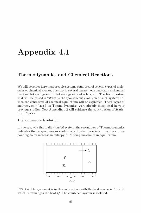
Appendix 4.1
Thermodynamics and Chemical Reactions
We will consider here macroscopic systems composed of several types of mole-cules or chemical species, possibly in several phases : one can study a chemicalreaction between gases, or between gases and solids, etc. The first questionthat will be raised is “What is the spontaneous evolution of such systems ?” ;then the conditions of chemical equilibrium will be expressed. These types ofanalyses, only based on Thermodynamics, were already introduced in yourprevious studies. Now Appendix 4.2 will evidence the contribution of Statis-tical Physics.
1. Spontaneous Evolution
In the case of a thermally isolated system, the second law of Thermodynamicsindicates that a spontaneous evolution will take place in a direction corres-ponding to an increase in entropy S, S being maximum in equilibrium.
A′
Q
A
Atot
T0
Fig. 4.4: The system A is in thermal contact with the heat reservoir A′, withwhich it exchanges the heat Q. The combined system is isolated.
95
96 Appendix 4.1
Chemical reactions are mostly done at constant temperature : one then hasto consider the case of a system A in thermal contact with a heat reservoirA′ at temperature T0 (Fig. 4.4). The combined system Atot, made of A andA′ is an isolated system, the entropy Stot of which increases in a spontaneousprocess :
∆Stot ≥ 0 (4.46)
The entropy variation of the combined system
∆Stot = ∆S + ∆S′ (4.47)
can be expressed as a function of parameters of the system A alone.
Indeed, if the amount of heat Q is given to A by the heat reservoir, thereservoir absorbs −Q and its entropy variation is equal to ∆S′ = −Q/T0 :the transfer of Q does not produce a variation of T0 and one can imagine areversible sequence of isothermal transformations at T0 producing this heatexchange.
Besides, the internal energy variation in A, i.e., ∆U , is, from the first law ofThermodynamics,
∆U = W + Q (4.48)
whereW is the work operated in the considered transformation. Consequently,
∆Stot = ∆S − (∆U − W )T0
=−∆F0 + W
T0(4.49)
where, by definition, F0 = U − T0S, which is identical to the Helmholtz freeenergy F = U − TS of system A if the temperature of A is that of theheat reservoir (in an off-equilibrium situation T differs from T0 and F is notidentical to F ).
From the condition of spontaneous evolution one deduces that
−∆F0 ≥ (−W ) (4.50)
which expresses that the maximum work that may be delivered by A in areversible process is (−∆F0), whence the name of “free energy.”
If the volume of system A is maintained constant and there is no other typeof work,W = 0, so that the condition for spontaneous evolution is then givenby
∆F0 ≤ 0 (4.51)

Appendix 4.1 97
This condition for a system in contact with a heat reservoir replaces thecondition ∆Stot ≥ 0 for an isolated system.
A more realistic situation is the one in which system A is kept at constanttemperature and constant pressure. This is the case in laboratory experimentswhen a chemical reaction is performed at fixed temperature T0 and under theatmospheric pressure P0 : system A is exchanging heat and work with a verylarge reservoirA′, which can thus give energy to A without any modification ofT0 and also exchange a volume ∆Ω with A without any change of its pressureP0 (Fig. 4.5).
A′ A
Q
T
∆ΩP
Atot
P0
T0
Fig. 4.5: System A is in contact with the larger system A′, with which it isexchanging the amount of heat Q and the volume ∆Ω.
Similarly, one considers that the combined system made of A and A′ is isola-ted, so that in a spontaneous process
∆Stot = ∆S + ∆S′ ≥ 0 (4.52)
If A absorbs Q from A′, ∆S′ = −Q/T0, where T0 is again the temperature ofA′.
The variation of internal energy of A includes the received heat Q, the me-chanical work −P0∆Ω received by A from A′, and alsoW ∗, work of any otherorigin (electrical for example) that A may have received :
∆U = Q − P0∆Ω + W ∗ (4.53)
Consequently,
∆Stot = ∆S − Q
T0=
T0∆S − (∆U + P0∆Ω − W ∗)T0
(4.54)
i.e., ∆Stot =−∆G0 + W ∗
T0(4.55)

98 Appendix 4.1
Here we defined G0 = U + P0Ω − T0S, which identifies to the Gibbs freeenthalpy of system A, that is, G = U + PΩ− TS, when P = P0 and T = T0.
A spontaneous evolution will be expressed through the condition
−∆G0 + W ∗ ≥ 0 (4.56)
When all the external parameters of system A, except its volume, are keptfixed, W ∗ is null and the condition of spontaneous evolution is then
∆G0 ≤ 0 (4.57)
Consequently, when a system is in contact with a reservoir so that it remainsat fixed temperature and pressure and can exchange work only with thisreservoir, the stable equilibrium is characterized by the condition of minimumof G0.
2. Chemical Equilibrium, Law of Mass Action : ThermodynamicalApproach
Consider a homogeneous system (for example in gaseous phase) with severaltypes of molecules : here we will study the dissociation reaction of iodine vaporat temperatures in the 1000 K range :
I2 2I
In this reaction the number of iodine atoms is conserved between the speciescorresponding to the two members of the chemical equation, which can alsobe expressed in the form
2I− I2 = 0
the species disappearing in the reaction carrying a negative sign, the one ap-pearing a positive one. In the same way, the most general chemical equilibriumwill be written
n∑i=1
biNi = 0 (4.58)
The bi are the integral coefficients of the balanced reaction for the Bi mole-cules. The number Ni of molecules of Bi type in the system is changed if theequilibrium is displaced but the total number of atoms of each species in thesystem is conserved. The variations of the numbers Ni are thus proportionalto the coefficients bi of the chemical equilibrium
dNi = bi dλ for any i
where dλ is a proportionality constant. dNi is positive for the molecules ap-pearing, negative for those vanishing in the reaction.

Appendix 4.1 99
Consider a chemical equilibrium at fixed temperature T and pressure P , thuscharacterized by dG(T, P ) = 0. In such conditions the equilibrium is expressedby :
dG =n∑
i=1
dGi =n∑
i=1
(−SidT + ΩidP + µidNi)
At fixed T and P, dG =n∑
i=1
µidNi = 0
(4.59)
Here µi =Å
∂G
∂Ni
ãT,P
is the chemical potential of species Bi. Replacing dNi
by its expression versus λ, one obtains the relation characterizing the equili-brium :
n∑i=1
biµi = 0 (4.60)
The chemical potentials depend on the experimental conditions, in particularon the concentrations of the different species. Assume that these reagents areideal gases and look for the dependence of µi on the partial pressure Pi of oneof these gases.
Since Gi is extensive and depends on a single extensive parameter Ni, thenumber of molecules of the species i, then one must have
Gi = µiNi (4.61)
The dependence in temperature and pressure of µi is thus that of Gi. For anideal gas, at fixed temperature,
Gi = Ui + PiΩ − TSi (4.62)
introducing the partial pressure Pi of species i, such that PiΩ = NikBT .Consequently,
dGi = −SidT + ΩdPi + µidNi (4.63)
Å∂Gi
∂Pi
ãT,Ni
= Ni
Å∂µi
∂Pi
ãT,Ni
= Ω =NikBT
Pi(4.64)
i.e., by integrating (4.64),
µi = µ0i (T ) + kBT ln
Pi
P0(4.65)

100 Appendix 4.1
where µ0i (T ) is the value of the chemical potential of species i at temperature
T and under the standard pressure P0.
The general condition of chemical equilibrium is thus given by
n∑i=1
biµ0i + kBT
n∑i=1
lnÅ
Pi
P0
ãbi
= 0 (4.66)
One writes
∆G0m
N =n∑
i=1
biµ0i (4.67)
∆G0m, the molar free enthalpy at the temperature T of the reaction, is the
difference between the molar free enthalpy of the synthesized products andthat of the used reagents, N is the Avogadro number.
One also defines
Kp =n∏
i=1
ÅPi
P0
ãbi
(4.68)
For example, in the dissociation equilibrium of iodine molecules,
Kp =(PI/P0)2
(PI2)/P0(4.69)
One recognizes in Kp the constant of mass action.
The above equation gives
Kp = e−∆G0m/RT (4.70)
where R = NkB is the ideal gases constant, R = 8.31 J.K−1. From the tablesof free enthalpy values deduced from experiments, one can deduce the value ofKp. From the experimental study of a chemical equilibrium at temperatureT , one can also deduce the value of Kp, and thus of ∆G0
m, at temperatureT : if the temperature of the experiment is modified from T to T ′, the partialpressures are changed, Kp(T ) becomes Kp(T ′), such that
lnKp(T ′) = −∆G0m(T ′)/RT ′ (4.71)
By definition, at a given T , ∆G0m = ∆H0 − T∆S0, where ∆H0 is the molar
enthalpy of the reaction and ∆S0 its entropy variation. If T and T ′ are closeenough, one makes the approximation that neither ∆H0 nor ∆S0 noticeablyvary between these temperatures. Then
lnKp(T ′) − lnKp(T ) = −∆H0
Å1
RT ′ −1
RT
ã(4.72)

Appendix 4.1 101
i.e., also
d ln Kp(T )dT
=∆H0
RT 2(4.73)
From the enthalpy ∆H0, one can predict the direction of displacement of theequilibrium when the temperature increases : if∆H0 > 0, that is, the enthalpyincreases in the reaction and the reaction is endothermal, the equilibrium isthus displaced toward the right side when T increases. This is in agreementwith the principle of Le Châtelier :
If a system is in stable equilibrium, any spontaneous change ofits parameters must lead to processes which tend to restore theequilibrium.
As an application, the experimental data below on the dissociation of iodineallow to deduce the enthalpy of this reaction in the vicinity of 1000 K.
For a fixed total volume of 750.0 cm3, in which a total number n of moleculesI2 was introduced at temperature T , the equilibrium pressure is P :
T (K) 973 1 073 1 173P (10−2 atm) 6.24 7.50 9.18n(10−4 moles) 5.41 5.38 5.33
As an exercise, one can calculate Kp at each temperature and verify that∆H0 = 157 kJ.mole−1. This reaction is endothermal.
The example presented here suggests the rich domain, but also the limitationsof the applications of Thermodynamics in Chemistry : Thermodynamics doesnot reduce to a game between partial derivatives, as some students may be-lieve ! It allows one to predict the evolution of new reactions, from tablesdeduced from measures. However, only the contribution of Statistical Phy-sics allows us to predict these evolutions from the sole spectroscopic dataand microscopic models. It is this latter approach that will be followed now.Thanks to the understanding acquired in this first part of the Statistical Phy-sics course, we will be able to deduce the constant of mass action from thequantum properties of the chemical species of the reaction.

Appendix 4.2
Statistical Physics and Chemical Reactions
The same example of dissociation of the iodine molecule at 1000 K, in gasphase, will now be treated by applying the general methods of StatisticalPhysics. The calculations will be completely developed, which may be regar-ded as tedious but yet they are instructive !
1. Energy States : The Quantum Mechanics Problem
Iodine I is a monoatomic gas, its only degrees of freedom are those of trans-lation. The electronic structure of its fundamental state is 2P3/2 (notation2S+1LJ : orbital state = 1 whence the notation P ; spin 1/2, i.e., 2S +1 = 2 ;total kinetic moment equal to J = 3/2, therefore the degeneracy 4). Iodinehas a nuclear moment J=5/2.
The hamiltonian of the iodine atom in the gas phase is therefore given by
HI = HI transl + HI elec + HI nucl (4.74)
The molecule I2 has six degrees of freedom, which can be decomposed intothree degrees of translation of its center of mass, two of rotation and one ofvibration :
HI2 = HI2transl + Hrot + Hvibr + HI2elec + HI2nucl (4.75)
Since this molecule is symmetrical, one should account for the fact that thetwo iodine atoms are indistinguishable inside the molecule and thus the phy-sics of the system is invariant in a rotation of 180 degrees around an axisperpendicular to the bond in its middle.
The fundamental electronic state of molecular iodine is not degenerate. It lieslower than the fundamental electronic state of atomic iodine. The dissociationenergy, necessary at zero temperature to transform a molecule into two iodine
103

104 Appendix 4.2
atoms, is equal to Ed = 1.542 eV, which corresponds to 17,900 K : one shouldbring Ed/2 per atom to move from the state I2 to the state I.
The nuclear spin of iodine has the value J = 5/2, both under the atomic andmolecular forms ; one assumes that no magnetic field is applied.
The splittings between energy levels of I or I2 are known from spectroscopicmeasures : Raman or infrared techniques give access to the distances bet-ween rotation or vibration levels ; the distance between electronic levels aregenerally in the visible (from 1.5 eV to 3 eV) or the ultraviolet range.
One now expresses the eigenvalues of the different terms of HI and HI2 .
a. Translation States
One has to find the hamiltonian eigenstates : in the case of the iodine atomof mass mI,
Htr =p2
2mI+ V (r) (4.76)
where V (r) is the confinement potential limiting the particle presence to arectangular box of volume Ω = LxLyLz.
The eigenstates are plane waves ψ = (exp ik ·r)/√Ω ; the k values are quanti-zed and for the Born-Von Kármán periodic limit conditions [ψ(x+Lx) = ψ(x)](see § 6.4.2) the k components satisfy :
kxLx = nx2π ; kyLy = ny2π ; kzLz = nz2π
with nx, ny, nz positive, negative or null integers.
The corresponding energies are :
ε I tr =
2
2mIk2
=h2
2mI
ñÅnx
Lx
ã2
+Å
ny
Ly
ã2
+Å
nz
Lz
ã2ô (4.77)
The translation energies εI2 tr of the molecule I2 are obtained by replacing mIby mI2 in the above expression of εItransl.
All these states are extremely close : if Ω is of the order of 1 cm3 and thedimensions of the order of 1 cm, the energy of the state nx = 1, ny = nz = 0is given by, for I (mI = 127 g)
13.6 eV× mHmI
·Å
a0
Lx
ã2
= 13.6 × 1127
× (0.53 × 10−8)2 = 3 × 10⁻¹⁸eV !

Appendix 4.2 105
The distances between energy levels are in the same range, thus very smallwith respect to kBT , for T = 1000K.
This discussion implies that the ideal gas model is valid at room temperaturefor I and I2 (still more valid than for N2, since these molecules are heavier).The partition functions for their translation states will take the form (4.26)-(4.27).
b. Rotation States
The iodine molecule is linear (Fig. 4.6), its inertia momentum around an
axis normal to the bond is I = 2m
ÅRe
2
ã2
= µR2e with µ = mI/2 and Re
the equilibrium distance between the two nuclei. Since mI = (127/N )g thismomentum is particularly large at the atomic scale.
The rotation hamiltonian is
Hrot =12I
J2 (4.78)
and shows that the problem is isotropic in the center of mass frame.
Re
mImI
Fig. 4.6 : Structure of the I2 molecule.
Its eigenvalues are :
εrot(J) =
2J(J + 1)2I
= hcBJ(J + 1), where B =
4πcIis given in cm−1
(4.79)
(one recalls the definition hν = hc/λ = hcσ ; the unit cm−1 for σ is particu-larly adapted to infrared spectroscopy).
The selection rules ∆J = ±1 for allowed electric dipolar transitions betweenrotation levels correspond to εrot(J + 1) − εrot(J) = hc · 2B(J + 1).
For iodine B = 0.0373 cm−1, 2hcB/kB = 0.107 K, to be compared to HCwhere B = 10.6 cm−1, 2hcB/kB = 30.5 K.
The rotation levels are thus still very close at the thermal energy scale.

106 Appendix 4.2
c. Vibration States
In a first approximation the vibration hamiltonian of the molecule I2 can bedescribed as a harmonic oscillator hamiltonian, with a parabolic potentialwell centered at the equilibrium distance Re between the two nuclei, that is,V (R) = 1
2K(R−Re)2 (Fig. 4.7). (In this figure a realistic potential is sketchedin full line ; the dotted line represent its approximated harmonic potential.)
ε
RRe
3
21
n = 0
Fig. 4.7 : Potential well associated to the vibration of the molecule I2.
Hvibr =p2
R
2µ+
12K(R − Re)2 (4.80)
with pR = −i∂
∂R, µ being the reduced mass of the system. In this approxi-
mation, the vibration energies are given by
εvibr(n) =Ån +
12
ãω with ω =
K
µ(4.81)
The transitions ∆ε = ω = hcσv are in the infrared domain. For I2 σv =214.36 cm−1, which corresponds to λ = 46.7µm or hcσv/kB = 308 K (for F2
the corresponding temperature is 1280 K).
d. Electronic States
The splitting between fundamental and excited states, for both I and I2, is ofthe order of a few eV, corresponding to more than 10,000 K.
The origin of the electronic energies (Fig. 4.8) is taken at the I2 fundamentalstate, so that the energy of the I fundamental state is EI, with 2EI = Ed =1.542 eV, where Ed is the dissociation energy.

Appendix 4.2 107
εe2
εe1
εe0
I2
g = 1
ε′e1
ε′e0
EI
I
g = 4
Fig. 4.8 : Electronic states of I2 and I.
e. Iodine Nuclear Spin
It is J = 5/2 on both species I and I2.
2. Description of the Statistical State of the System : Calculationof the Partition Functions
It was stated in Ch.2 that for a macroscopic system the predictions for theexperimental measurements of physical parameters were the same whateverthe chosen statistical ensemble. Here we will work in the canonical ensemble,where the calculations are simpler.
At temperature T , the number of iodine molecules is NI2 , the number of atomsproduced by the dissociation of the molecules NI. The partition function fora single iodine molecule is written zI2 , that of an isolated atom zI. Because ofthe particles indistinguishability, the total canonical partition function Zc isgiven by :
Zc =1
NI2 !(zI2)
NI21
NI!(zI)NI (4.82)
It is related to the free energy F of the system
F = −kBT lnZc (4.83)
the partial derivatives of which, with respect to the numbers of particles, arethe chemical potentials :
µI2 =∂F
∂NI2= −kBT ln
ÅzI2NI2
ãµI = −kBT ln
ÅzINI
ã(4.84)
Since the total energy of an iodine atom or molecule is a sum of contributions,the partition function of a corresponding atom or a molecule is a product of

108 Appendix 4.2
factors : thus for an I2 molecule
εI2 = εI2 tr + εrot(J) + εvibr(n) + εel + εnucl (4.85)
zI2 = zI2tr · zrot · zvibr · zel · znucl (4.86)
with :
zI2 tr =1h3
∫d3r
∫d3p e−βp2/2mI2 (4.87)
zrot =∑
J
gJe−βεJ =∑
J
(2J + 1)e−βhcBJ(J+1) (4.88)
zvibr =∑
v
gve−βεv =
∑n
e−βω(n+ 12 ) (4.89)
zel =∑
e
gee−βεe (4.90)
znucl = (2J + 1)2 for I2, znucl = 2J + 1 for I (4.91)
The factors gr, gv, ge express the degeneracies of the rotation, vibration andelectronic energy levels. The value of the nuclear spin is J , there are twonuclei in I2.
One will first evaluate the various partition functions, noting that a largevalue of the partition function is related to a large number of accessible states.The examined chemical potentials will be sums of terms, associated with thedifferent z factors. Note that one has to calculate
zI2NI2
(orzINI) (see (4.84)),
thus to divide a single factor of zI2 by NI2 : we will associate the factor NI2 tothe sole translation factor, then it no longer comes into the partition functionsfor the other degrees of freedom. (The indiscernability factor is thus includedin the translation degree of freedom.) Then :
lnzI2NI2
= lnztr I2NI2
+ ln zrot + ln zvibr + ln zel + ln znucl (4.92)
a. Translation
The calculation of ztr I was already done for the ideal gas :
ztr I = Ω ·Å
2πmIkBT
h2
ã3/2
=Ω
(λth I)3=
NIkBT
Pi· 1(λth I)3
(4.93)
Pi is the partial pressure, such that PiΩ = NIkBT and λth I is the thermalde Broglie wavelength at T for I. Since we are in the classical framework, ztr I

Appendix 4.2 109
must be very large. Numerically λth, expressed in picometers (10−12 m), isgiven by
λth =1749
(TK × mg·mole−1)1/2· 10−12 m
At 1000 K, for the iodine atom mI = 127g, λth I = 4, 91 10−12 m.
In the same condition, for the I2 molecule, λth I2 = 3.47 10−12 m.
For a partial pressure equal to the atmospheric pressure and a temperatureT = 1000 K, one obtains
zI tr = 1.15 × 10⁹NI
zI2 tr = 3.26 × 10⁹NI2
These numbers are huge !
b. Rotation
The factor 2J + 1 is the degeneracy of the energy level hcBJ(J + 1). Besides,the linear molecule I2 is symmetrical, so that after a 180 degree rotation onegets a new state, indistinguishable from the initial one (this would not be thecase for HC for example). One thus has to divide the above expression (4.88)by two. This is equivalent to saying that the wave function symmetry allowsto keep only half of the quantum states.
Since the energy distance between rotation levels is small with respect to kBT ,one can replace the discrete sum by an integral
12
∑J
(2J + 1)e−βhcBJ(J+1) 12
∫ ∞
0
(2J + 1)e−βhcBJ(J+1)dJ
12
1βhcB
=kBT
2hcB
(4.94)
This approximation implies that zrot is a large number. Numerically, thecontribution of zrot, equal to 1/2βhcB, is the ratio 1000 K/0.107 K=9346.
c. Vibration
zvibr = e−βω/2∞∑
n=0
e−βωn =e−βω/2
1 − e−βω(4.95)
At 1000 K, for I2, the term βω is 0.308 : the quantum regime is valid andthis expression cannot be approximated. It has the value 3.23.

110 Appendix 4.2
d. Electronic Term
ze =∑
e
gee−βεe (4.96)
Owing to the large distances between electronic levels, one will only considerthe fundamental level, four times degenerated for I, nondegenerated for I2.
At 1000 K, the term zeI is equal to 4 e−(Ed/2kBT ) = 4e−8.94 = 5.25 × 10⁻⁴,whereas for the same choice of energy origin zeI2
= 1.
3. Prediction of the Action of Mass Constant
Let us return to the definition relations (4.68) to (4.70) of Appendix 4.1,
Kp = exp(−∆G0m/RT ) = exp(−
n∑i=1
biµ0i /kBT ) (4.97)
where the µ0i are the chemical potentials under the atmospheric pressure. For
our example :
Kp = exp[−(2µ0I − µ0
I2)/kBT ] (4.98)
The chemical potentials are expressed versus the partition functions calculatedabove :
1kBT
(2µ0I − µ0
I2) = −2[lnÅ
z0I trNI
ã+ ln zeI ] + ln
Åz0I2 trNI2
ã+ ln zrot + ln zvib
(4.99)
Here the translation partition functions are calculated under the atmosphe-ric pressure (standard pressure) ; the terms associated to the nuclear spins2 ln(2J + 1) exactly compensate and ln ze I2 = 0.
From the data of the previous section one obtains :
lnz0I trNI
= 20.87 , ln zeI = −7.56
lnz0I2 tr
NI2= 21.91 , ln zrot = 9.14 , ln zvibr = 1.17
Kp = e−5.6 3.7 × 10⁻³

Appendix 4.2 111
One can also predict, from the calculation of the temperature variation of Kp,a value for the enthalpy of the iodine dissociation reaction :
d lnKp
dT=
∆H
RT 2(4.100)
i.e.,
d
dT
Ç−2µ0I + µ0
I2
kBT
å=
∆H
RT 2(4.101)
∆H is thus deduced from the logarithmic derivatives versus T , at constant P ,of the different partition functions : the translation partition functions vary
like T 5/2, zrot like T , zvibr likeÅsinh
βω
2
ã−1
. Consequently,
∆H
RT 2= 2
d
dT
ïlnÅ
z0I trNI
ã+ ln zeI
ò− d
dT
ïlnÅ
z0I2 trNI2
ã+ ln zrot + ln zvibr
ò(4.102)
= 2ï
52T
+Ed
2kBT 2
ò−ï
52T
+1T
+ω
2kBT 2coth
βω
2
ò(4.103)
that is,
∆H =3RT
2+ N
ÅEd − ω
2coth
βω
2
ã(4.104)
The obtained value of ∆H is close to that of the dissociation energy per mole :∆H = 152 kJ/mole. The Kp and ∆H values, calculated from spectroscopicdata, are very close to those deduced from the experiment quoted in theAppendix 4.1 (Kp 3.4 · 10−3 at 1000 K, ∆H = 158 kJ/mole).
The discrepancies come in particular from the approximations done in thedecomposition of the degrees of freedom of the iodine molecule : we assu-med that the vibration and rotation were independent (rigid rotator model) ;moreover, the potential well describing vibration is certainly not harmonic.
Obviously, for an experiment performed at constant temperature T and vo-lume Ω, the equilibrium constant Kv could have been calculated in a similarway and the free energy F would have been used. The variation of Kv withtemperature provides the variation ∆U of internal energy in the chemicalreaction.
4. Conclusion
Through these examples, which were developed in detail, the contribution ofStatistical Physics in the prediction of chemical reactions was shown. As just

112 Appendix 4.2
seen now, if the Statistical Physics concepts refer to very fundamental notions,this discipline (sometimes at the price of lengthy calculations !) brings usefuldata to solve practical problems.

Chapter 5
Indistinguishability,the Pauli Principle(Quantum Mechanics)
The preceding chapter presented properties of the ideal gas which are validin the limit where the average value, at temperature T , of the de Brogliewavelength is small with respect to the average distance between the particlesin motion. Another way to express the same concept is to consider that thewave functions of two particles have a very small probability of overlappingin such conditions.
From now on, we will work in the other limit, in which collisions betweenparticles of the same nature are very likely. In the present chapter the Quan-tum Mechanics properties applicable to this limit will be recalled. In Quan-tum Mechanics courses (see for example the one by J.-L. Basdevant and J.Dalibard) it is stated that, for indistinguishable particles, the Pauli prin-ciple must be added to the general postulates of Quantum Mechanics. Infact here we are only re-visiting this principle but ideas are better unders-tood when they are tackled several times ! In chapter 6 the consequences inStatistical Physics will be drawn on the properties obtained in the presentchapter 5.
In the introduction (§ 5.1) we will list very different physical phenomena, as-sociated with the property of indistinguishability, which will be interpretedat the end of the chapter in the framework of Statistical Physics. To intro-duce the issue, in § 5.2 some properties of the quantum states of two, thenseveral, identical particles, will be recalled. In § 5.3, the Pauli principle and
113

114 Chapter 5. Indistinguishability, the Pauli Principle
its particular expression, the Pauli exclusion principle, will be stated ; thetheorem of spin-statistics connection will allow one to recognize which typeof statistics is applicable according to the nature of the considered particlesand to distinguish between fermions and bosons. In § 5.4, the special case oftwo identical particles of spin 1/2 will be analyzed. These results will be ex-tended to an arbitrary number of particles in § 5.5 and the description of a Nindistinguishable particle state through the occupation numbers of its variousenergy levels will be introduced : this is much more convenient than using theN -particle wave function. It is this approach that will be used in the followingchapters of this book. Finally in § 5.6 we will return to the examples of theintroduction and will interpret them in the framework of the Pauli principle.
5.1 Introduction
It is possible to distinguish fixed particles of the same nature, by specifyingtheir coordinates : this is the case of magnetic moments localized on sites ofa paramagnetic crystal, of hydrogen molecules adsorbed on a solid catalyst.They are then distinguishable through their coordinates.
(1) (2)
D
θθ
c)b)a)
Fig. 5.1: Two identical particles, a) represented by the wave packets whichdescribe them in their center-of-mass frame, b) suffer a collision. c) After thecollision, the wave function is spread in a ring-shaped region the radius ofwhich increases with time. When a particle is detected in D, it is impossibleto know whether it was associated with wave packet (1) or (2) prior to thecollision.
On the other hand, two electrons in motion in a metal, two protons in anucleus, or more generally all particles of the same chemical nature, identical,in motion and thus likely to collide, cannot be distinguished by their physicalproperties : these identical particles are said to be indistinguishable. Indeed,as explained in Quantum Mechanics courses, if these particles, the evolutionof which is described through Quantum Mechanics, do collide, their wave

Introduction 115
functions overlap (fig. 5.1). Then, after the collision it is impossible to knowwhether (1′) originated from (1) or from (2), since the notion of trajectorydoes not exist in Quantum Mechanics (Fig. 5.2).
(1)
(1′)
D
(2)
(2′)
a)
(1)
(2′)
D
(2)
(1′)
b)
Fig. 5.2: Representation in term of “trajectory” of the event describedon Fig. 5.1. The two particles being identical, one cannot distinguishbetween a) and b).
The quantum treatment of such systems refers to the Pauli principle. Thisprinciple allows the interpretation of a great variety of chemical and physicalphenomena, among which are
1. the periodic classification of the elements ;
2. the chemical binding ;
3. the ferromagnetism of some metals, like iron or cobalt, that is, theirability to evidence a macroscopic magnetization even in the absence ofan external magnetic field ;
4. the superconductivity of some solids, the electrical resistance of whichstrictly vanishes below a temperature called “critical temperature” ;
5. the special behavior of the isotope 42He, which becomes superfluid for
temperatures lower than a critical temperature Tc, equal to 2.17 K un-der the atmospheric pressure : this means that no viscosity is restrainingits motion ; the isotope 3
2He does not show such a property ;
6. the stimulated light emission and the laser effect.

116 Chapter 5. Indistinguishability, the Pauli Principle
5.2 States of Two Indistinguishable Particles(Quantum Mechanics)
5.2.1 General Case
When N particles are indistinguishable, the physics of the system and the N -particle hamiltonian are unchanged by permutation of some of these particles.Consequently, the hamiltonian commutes with any permutation operator bet-ween these particles, so that they have a common basis of eigenvectors. It canbe shown that any permutation of N particles can be decomposed into a pro-duct of exchanges of two particles. Thus it is helpful to begin by recalling theproperties of the operator which exchanges the particles of a system consistingin particle 1 at r1 and particle 2 at r2 :
P12ψ(r1, r2) = ψ(r2, r1) (5.1)
The operator P12 must satisfy :
(P12)2 = 1 (5.2)
since after two exchanges one returns to the initial state. This implies thatthe eigenvalue eiα of P12 must fulfill the condition :
e2iα = 1, i.e., eiα = ±1 (5.3)
i) If
eiα = +1, ψ(r2, r1) = ψ(r1, r2) (5.4)
the eigenstate is symmetrical in the exchange (or transposition) of particles 1and 2.
ii) If
eiα = −1, ψ(r2, r1) = −ψ(r1, r2) (5.5)
the wave function is antisymmetrical in the transposition of the two particles.
5.2.2 Independent Particles
If the indistinguishable particles are independent, the total hamiltonian for allthe particles is written as a sum of one-particle hamiltonians :
HN =N∑
i=1
hi (5.6)

States of two Indistinguishable Particles (Quantum Mechanics) 117
The eigenstates of each one-particle hamiltonian satisfy :
hiχn(ri) = εnχn(ri) (i = 1, 2) (5.7)
The index n corresponds to the considered quantum state, for example forthe electron of a hydrogen atom n = 1s, 2s, 2p . . . ; the particle i is located atri.
The one-particle eigenstate at the lowest energy (fundamental state) satisfies
h1χ1(r1) = ε1χ1(r1) (5.8)
The energy ε2 of the one-particle first excited state is such that
h1χ2(r1) = ε2χ2(r1) (5.9)
Since the particles are assumed to be independent, the eigenstates of thetwo-particle hamiltonian H12 can be easily expressed with respect to the one-particle solutions :
H12ψnn′(r1, r2) = εnn′ψnn′(r1, r2) (5.10)
with
εnn′ = εn + εn′ and ψnn′(r1, r2) = χn(rn)χn′(r2) (5.11)
Indeed remember that
(h1 + h2)χn(r1)χn′(r2) = εnχn(r1)χn′(r2) + χn(r1)εn′χn′(r2)= (εn + εn′)χn(r1)χn′(r2)
(5.12)
so that the two-particle energy is the sum of the one-particle energies and thetwo-particle wave function is the product of the one-particle wave functions.Any linear combination of wave functions corresponding to the same energyεn + εn′ is also a solution of H12.
Here one is looking for eigenfunctions with a symmetry determined by theindistinguishability properties.
In the two-particle fundamental state, each individual particle is in its funda-mental state (fig. 5.3), this two-particle state has the energy 2ε1, it is nonde-generate. Its wave function satisfies
H12ψ11sym(r1, r2) = 2ε1ψ11sym(r1, r2) (5.13)
It is symmetrical and can be written
ψ11sym(r1, r2) = χ1(r1)χ1(r2) . (5.14)

118 Chapter 5. Indistinguishability, the Pauli Principle
ε2 ε2
ε1ε1
fundamental state first excitedstate
Fig. 5.3 : Occupation of two levels by two indistinguishable particles.
In the two-particle first excited state, the total energy is ε1 + ε2. This state isdoubly degenerate, as two distinct independent states can be built (particle 1in ε1, particle 2 in ε2 or the opposite). But since the particles are indistingui-shable, one cannot tell which of the two particles is in the fundamental state.Thus one looks for solutions which are common eigenstates of H12 and P12.The acceptable solutions are :
for the symmetrical first excited state
ψ12sym(r1, r2) =1√2(χ1(r1)χ2(r2) + χ2(r1)χ1(r2)) (5.15)
for the antisymmetrical first excited state
ψ12asym(r1, r2) =1√2(χ1(r1)χ2(r2) − χ2(r1)χ1(r2)) (5.16)
These wave functions (5.14) to (5.16) are determined, to a phase factor.
Now consider the case of N particles.
The total energy of the system, which is the eigenvalue of HN , is then equalto
εN =N∑
i=1
εni (5.17)
The eigenfunction is a product of one-particle eigenfunctions,
ψN (r1, . . . , rN ) =N
Πi=1
χni(ri) (5.18)
Any permutation of N particles can be decomposed into a product of ex-changes of particles by pair, it thus admits the eigenvalues +1 or −1 :
Pψ(r1, r2, . . . ri, . . . rN ) = σψ(r1, r2, . . . ri, . . . , rN ) (5.19)

Pauli Principle ; Spin-Statistics Connection 119
with σ = ±1.
σ = +1 is associated with an “even” permutation
σ = −1 is associated with an “odd” permutation
Although the decomposition of the permutation into a product of exchangesis not unique, the value of σ is well determined.
Among the eigenfunctions of the permutation operators, two types will bedistinguished : either the wave function is completely symmetrical, i.e., it isunchanged by any permutation operator ; or it is a completely antisymmetricaleigenfunction which satisfies (5.19) and changes its sign for an odd permuta-tion, but is not changed for an even permutation. The eigenfunctions, commonto the permutation operators and to the hamiltonian HN of the N indistin-guishable particles, will necessarily be of one of these two types.
5.3 Pauli Principle ;Spin-Statistics Connection
5.3.1 Pauli Principle ; Pauli Exclusion Principle
The Pauli (1900-1958) principle is a postulate which is stated as follows :
The wave function of a set of N indistinguishable particles obeys either of thetwo properties below :
– either it is completely symmetrical, i.e., its sign does not change by permu-tation of two arbitrary particles : then these particles are called bosons ;
– or it is completely antisymmetrical, and thus its sign is modified by permu-tation of two particles : these particles are fermions.
The property verified by the wave function only depends on the type of theconsidered particles, it is independent of their number N and of the particularstate Ψ they occupy.
This principle is verified by all chemical types of particles. In particular, everytime a new type of elementary particle was discovered, these new particlesindeed satisfied the Pauli principle.
A special case of the Pauli principle is the Pauli exclusion principle : Twofermions cannot be in the same quantum state. Indeed, if they were in the

120 Chapter 5. Indistinguishability, the Pauli Principle
same one-particle state Ψ, the antisymmetrical expression of the wave functionwould be :
ψ(1, 2) =1√2[ψ(1)ψ(2) − ψ(2)ψ(1)] = 0 (5.20)
One now needs to determine which particles, called “fermions”, satisfy theFermi-Dirac statistics, and which particles, the “bosons”, follow the Bose-Einstein statistics. There is no intuitive justification to the following theorem,which provides the answer to this question.
5.3.2 Theorem of Spin-Statistics Connection
The particles with an integral or zero spin (S/ = 0, 1, 2 . . . ) arebosons. The wave function for N bosons is symmetrical in thetransposition of two of them.The particles with an half-integral spin (S/ = 1/2, 3/2, 5/2 . . .)are fermions. The N -fermions wave function is antisymmetricalin the transposition of two of them.
Among the elementary particles, electrons, protons, neutrons, neutrinos,muons have a spin equal to 1/2 ; the spin of photons is 1, the spin of me-sons is 0 or 1.
When these particles are combined into one or several nuclei, the total angularmomentum takes into account all the orbital momenta and the spin intrinsicmomenta. In Quantum Mechanics courses it is shown that the addition of twoangular momenta J1 and J2 gives a parameter which has the properties of anew angular momentum, with a quantum number J varying between | J1−J2 |and | J1 + J2 | by unity steps. If two integral or half-integral momenta areadded, only integral values of J are obtained ; if an integral J1 is added to ahalf-integral J2, the sum J is half-integral. It is the quantum number J whichis identified with the spin of the ensemble.
More generally if a composite particle contains an even number of elementaryparticles of half-integral spin, its total angular moment (or its total spin)is integral, this is a boson ; if it contains an odd number, its total angularmoment is half-integral, and the composite particle is a fermion.
For example, the atom 42He has two electrons, two protons and two neutrons,
i.e., six particles of half-integral spin : it is a boson. On the other hand, theatom 3
2He is composed of two electrons, two protons but a single neutron,thus it is a fermion. The statistical properties of these two isotopes are verydifferent (see the Introduction of this chapter, example 5), whereas the che-

Case of Two Particles of Spin 1/2 121
mical properties, determined by the number of electrons that can participatein chemical bonds, are the same.
5.4 Case of Two Particles of Spin 1/2
Here the properties of the wave functions of two indistinguishable particlesof spin 1/2 are recalled, this is in particular the case for two electrons. Fromthe theorem of spin-statistics connection, this wave function must be anti-symmetrical with respect to the transposition of these two particles. Now,in addition to their spin degree of freedom, these two particles also have anorbital degree of freedom concerning the space coordinates ; from QuantumMechanics courses, the wave function for a single particle of this type canbe decomposed into tensor products concerning the space and spin variables.The most general form of decomposition is :
ψ(r1, r2; σ1, σ2) = ψ++(r1, r2)| + +〉 + ψ+−(r1, r2)| + −〉+ ψ−+(r1, r2)| − +〉 + ψ−−(r1, r2)| − −〉 (5.21)
5.4.1 Triplet and Singlet Spin States
Let us first assume, for simplification, that this decomposition is reduced toa single term, i.e.,
ψ(r1, r2; σ1, σ2) = ψ(r1, r2) ⊗ |σ1, σ2〉, with σ1, σ2 = ±1/2 (5.22)
Since we are dealing with fermions, the two-particle wave function changessign when particles 1 and 2 are exchanged. This sign change can occur in twodifferent ways :
– either it is the space part ψ(r1, r2) of the wave function which is antisym-metrical in this exchange, the spin function remaining unchanged ;
– or it is |σ1, σ2〉 which changes its sign in this exchange, the space functionremaining unchanged.
Consider the spin states. Each particle has two possible spin states, noted | ↑〉or | ↓〉. There are thus four basis states for the set of two spins, which can bechosen as
| ↑↑〉, | ↑↓〉, | ↓↑〉, | ↓↓〉 (5.23)
(the order of notation is : particle 1, then particle 2).

122 Chapter 5. Indistinguishability, the Pauli Principle
From these states one deduces four new independent states, classified accor-ding to their symmetry, that is, their behavior when exchanging the spins ofthe two particles.
There are three symmetrical states, unchanged when the role of particles 1and 2 is exchanged :
⎧⎪⎪⎪⎪⎨⎪⎪⎪⎪⎩
| ↑↑〉 = |11〉1√2
(| ↑↓〉 + | ↓↑〉) = |10〉| ↓↓〉 = |1 − 1〉
(5.24)
They constitute the triplet state of total spin S = 1, with projectionson the quantization axis Oz described by the respective quantum numbersSz = +1, 0,−1 : the eigenvalue of the squared length of this spin is equal toS(S + 1)2, i.e., 2
2 when the eigenvalue of the projection along Oz is Sz,i.e., , 0 or −.
There remains an antisymmetrical state, which changes its sign in the ex-change of the two spins, this is the singlet state
1√2
(| ↑↓〉 − | ↓↑〉) = |00〉 (5.25)
in which S = Sz = 0.
Even when the two-particle hamiltonian does not explicitly depend on spin,orbital wave functions with different symmetries and possibly different energyeigenvalues are associated with the triplet and singlet states : for example, inthe special case treated in § 5.2.2 the fundamental state, with a symmetricalorbital wave function [see Eq. (5.14)], must be a spin singlet state, whereasin the first excited state one can have a spin triplet. This energy splittingbetween the symmetrical and antisymmetrical orbital solutions is called theexchange energy or exchange interaction.
The exchange interaction is responsible of ferromagnetism, as understood byWerner Heisenberg (1901-1976) as early as 1926 : indeed the dipolar inter-action between two magnetic moments a fraction of a nm apart, each of theorder of the Bohr magneton, is much too weak to allow the existence of anordered phase of magnetization at room temperature. On the contrary, owingto the Pauli principle, in ferromagnetic systems the energy splittings betweenstates with different spins correspond to separations between different orbitallevels. These are of a fraction of an electron-volt, which is equivalent to tem-peratures of the order of 1000 K, since these states are the ones responsiblefor valence bindings.

Case of Two Particles of Spin 1/2 123
In a ferromagnetic solid, magnetism can originate from mobile electrons inmetals like in Fe, Ni, Co, or from ions in insulating solids, as in the magnetiteiron oxide Fe3O4, and the spin can differ from 1/2. However this interactionbetween the spins, which relies on the Pauli principle, is responsible for theenergy splitting between different orbital states : one state in which the totalmagnetic moment is different from zero, corresponding to the lower tempera-ture state, and the other one in which it is zero.
5.4.2 General Properties of the Wave Functionof Two Spin 1/2 Particles
It has just been shown that, because of the Pauli principle, space wave func-tions are associated with the triplet states, which are changed into their oppo-site in the exchange of the two particles (antisymmetrical wave function). Tothe singlet state is associated a symmetrical wave function. The most generalwave function for two spin 1/2 particles will be written, for a decompositiononto the triplet and singlet states :
ψA11|11〉 + ψA
10|10〉 + ψA1−1|1 − 1〉 + ψS
00|00〉
The wave functions of the type ψA11 are spatial functions of r1 and r2, the
upper index recalls the symmetry of each component.
The same wave function can be expressed on the spin basis |σ1, σ2〉, accountingfor expressions (5.24) and (5.25) of the triplet and singlet wave functions. Onethus obtains :
ψ(r, r2; σ1, σ2) = ψA11| + +〉 +
ψA10 + ψS
00√2
| + −〉 +ψA
10 − ψS00√
2| − +〉
+ ψA1−1| − −〉 (5.26)
It thus appears, by comparing to the general expression (5.21), that the Pauliprinciple dictates symmetry conditions on the spin 1/2 components :
• ψ++(r1, r2) and ψ−−(r1, r2) must be antisymmetrical in the exchangeof particles 1 and 2
• ψ+−(r1, r2) and ψ−+(r1, r2) do not have a specific symmetry, but theirsum is antisymmetrical and their difference symmetrical.

124 Chapter 5. Indistinguishability, the Pauli Principle
5.5 Special Case of N Independent Particles ;Occupation Numbers of the States
In the general case of an N -identical-particle system, the Pauli principle dic-tates a form for the N -particle wave function and occupation conditions forthe energy levels which are very different in the case of fermions or bosons. Inthis part of the course, we are only interested by independent particles : thissituation is simpler and already allows a large number of physical problemsto be solved.
5.5.1 Wave Function
Fermions :
We have seen that two fermions cannot be in the same quantum state andthat their wave function must be antisymmetrical in the transposition of thetwo particles. We consider independent particles, the N -particle wave functionof which takes the form of a determinant called “Slater determinant,” whichindeed ensures the change of sign by transposition and the nullity if twoparticles are in the same state :
ψ(r1, . . . , rN ) ∝
∣∣∣∣∣∣∣χ1(r1) χ2(r1) χN (r1)...
......
χ1(rN )... χN (rN )
∣∣∣∣∣∣∣ (5.27)
If a state is already occupied by a fermion, another one cannot be added.A consequence is that at zero temperature all the particles cannot be in theminimum energy state : the different accessible levels must be filled, beginningwith the lowest one, each time putting one particle per level and thus eachtime moving to the next higher energy level. The process stops when the N th
and last particle is placed in the last occupied level : in Chemistry this processis called the “Aufbau principle” or construction principle ; in solids, the lastoccupied state at zero temperature is called the Fermi level and is usuallynoted εF (see chapters 7 and 8).
Bosons :
On the other hand, the wave function for N bosons is symmetrical ; in par-ticular it is possible to have all the particles on the same level of minimumenergy at zero temperature.

Special Case of N Independent Particles ; Occupation Numbers 125
5.5.2 Occupation Numbers
TheN -fermion (orN -boson) wave functions are complicated to write because,as soon as a particle is put in a state of given energy, this induces conditions onthe available states for the other particles ; then the antisymmetrization of thetotal wave function has to be realized for the fermions (or the symmetrizationfor the bosons). Since these particles are indistinguishable, the only interestingdatum in Statistical Physics is the number of particles in a defined quantumstate.
Instead of writing theN -particle wave function, which will be of no use in whatfollows, we will described the system as a whole by the occupation numbersof its different states, this is the so-called “Fock basis” : these one-particlestates correspond to distinct εk, which can have the same energy but differentindexes if the state is degenerate (for example two states of the same energyand different spins will have different indexes k and k′) ; the states are orderedby increasing energies (Fig. 5.4).
εk nk
n3
n2
n1ε1
ε2
ε3
Fig. 5.4 : Definition of the occupation numbers of the one-particle states.
The notation |n1,2 , . . . nk, . . . 〉 will express the N -particle state in which n1
particles occupy the state of energy ε1, n2 that of energy ε2, . . . nk the stateof energy εk. One must satisfy
n1 + n2 + . . . + nk + . . . = N (5.28)
the total number of particles in the system. Under these conditions, the totalenergy of the N -particle system is given by
n1ε1 + n2ε2 + . . . + nkεk + . . . = EN (5.29)
From the Pauli principle
• for fermions : nk = 0 or 1 (5.30)
• for bosons : nk = 0, 1, 2 . . .∞ (5.31)

126 Chapter 5. Indistinguishability, the Pauli Principle
This description will be used in the remainder of the course. The whole physi-cal information is included in the Fock notation. Indeed one cannot tell whichparticle is in which state, this would be meaningless since the particles areindistinguishable. The only thing that can be specified is how many particlesare in each one-particle state.
5.6 Return to the Introduction Examples
Now we are able to propose a preliminary interpretation of the physical phe-nomena described in the introduction, § 5.1, some of which will be analyzedin more detail in the following chapters :
5.6.1 Fermions Properties
1. In the periodic classification of the elements, the atomic levels are filledwith electrons which are fermions. In a given orbital level only twoelectrons of distinct spin states can be placed, i.e., according to thePauli principle they are in the singlet spin state.
2. When a chemical bond is created, the electrons coming from the twoatoms of the bond go into the atomic levels originating from the couplingbetween the levels of the separated atoms. The resulting bonding andantibonding states must also be populated by electrons in different spinstates, thus in the singlet spin state.
3. The ferromagnetism arises, as already mentioned, from the energy dif-ference between the singlet and the triplet spin states for a pair of elec-trons. If the fundamental state presents a macroscopic magnetization,it must be made from microscopic states with a nonzero spin. In fact,in a ferromagnetic metal such as iron or nickel, the spins of two ironnuclei couple through conduction electrons which travel from nucleus tonucleus.
5.6.2 Bosons Properties
4. In superconductivity the electrons of a solid couple by pairs due totheir interaction with the solid vibrations. These pairs, called “Cooperpairs,” are bosons which gather into the same fundamental state at lowtemperature, thus producing the phenomenon of superconductivity.
5. In the same way the 4He atoms are bosons, which can occupy the samequantum state below a critical temperature (see chapter 9). Their ma-

Return to the Introduction Examples 127
croscopic behavior expresses this collective property, whence the absenceof viscosity.
6. Photons are also bosons and the stimulated emission, a specific propertyof bosons in nonconserved number, will be studied in § 9.2.4.

Summary of Chapter 5
In Quantum Mechanics, the hamiltonian describing the states of identicalparticles is invariant under a permutation of these particles, the states beforeand after permutation are physically indistinguishable. This means that thehamiltonian commutes with any permutation operator : one first looks forthe permutations eigenstates, which are also eigenstates of the N -particlehamiltonian.
In the case of two indistinguishable particles the symmetrical and antisymme-trical eigenstates have been described. These states have a simple expressionin the case of independent particles.
Any permutation of N particles can be decomposed into a product of ex-changes (or transpositions) of particles by pair : a permutation is thus eithereven or odd.
The Pauli principle postulates that the wave functions for N identical particlescan only be, according to the particle’s nature, either completely symmetrical(bosons) or completely antisymmetrical (fermions) in a permutation of theparticles. In particular, because their wave function is antisymmetrical, twofermions cannot occupy the same quantum state (“Pauli exclusion principle”).
The theorem of spin-statistics connection specifies that the particles of half-integral total spin, the fermions, have an antisymmetrical wave function ; theparticles of integral or zero total spin, the bosons, have a completely symme-trical wave function.
In the case of two spin-1/2 particles, the triplet spin state, symmetrical, andthe singlet spin state, antisymmetrical, have been described. The spin com-ponent of the wave function has to be combined with the orbital part, theglobal wave function being antisymmetrical to satisfy the Pauli principle.
In Statistical Physics, to account for the Pauli principle, the state of N par-ticles will be described using the occupation numbers of the various energy
129

130 Summary of Chapter 5
levels, rather than by its wave function. A given state can be occupied at mostby one fermion, whereas the number of bosons that can be located in a givenstate is arbitrary.

Chapter 6
General Properties of theQuantum Statistics
In chapter 5 we learnt the consequences, in Quantum Mechanics, of the Pauliprinciple which applies to indistinguishable particles : they will now alwaysbe taken as independent, that is, without any mutual interaction.
We saw that it is very difficult to express the conditions stated by the Pauliprinciple on the N -particle wave function ; on the other hand, a descriptionthrough occupation numbers |n1, n2, . . . , nk, . . . 〉 of the different quantumstates ε1, ε2, . . . εk . . . accessible to these indistinguishable particles is muchmore convenient. In fact we assume that the states are nondegenerate and ifthere are several states with the same energy, we label them with differentindexes. Besides, it was stated that there exists two types of particles, the fer-mions with a half-integral spin, which cannot be more than one in any givenone-particle state εk, whereas the bosons, with an integral or zero spin, canbe in arbitrary number in any one single-particle quantum state.
In the present chapter we return to Statistical Physics (except in § 6.4, whichis on Quantum Mechanics) : after having presented the study technique ap-plicable to systems referring to Quantum Statistics, we determine the averagenumber of particles, at a given temperature, on an energy state of the consi-dered system : this number will be very different for fermions and bosons.
This chapter presents general methods and techniques to analyze, using Statis-tical Physics, the properties of systems of indistinguishable particles followingthe Quantum Statistics of either Fermi-Dirac or Bose-Einstein, while the follo-wing chapters will study these statistics more in detail on physical examples.
131

132 Chapter 6. General Properties of the Quantum Statistics
In § 6.1, we will show how the statistical properties of indistinguishable in-dependent particles are more conveniently described in the grand canonicalensemble. In § 6.2 we will explain how the grand canonical partition functionZG is factorized into terms, each one corresponding to a one-particle quan-tum state. In § 6.3 the Fermi-Dirac and the Bose-Einstein distributions willbe deduced, which give the average number of particles of the system occu-pying a quantum state of given energy at temperature T , and the associatedthermodynamical potential, the grand potential, will be expressed.
The § 6.4 will be a (long) Quantum Mechanics parenthesis, it will be shownthere that a macroscopic system, with extremely close energy levels, is conve-niently described by a density of states, that will be calculated for a freeparticle. In § 6.5, this density of states will be used to obtain the averagevalue, at fixed temperature, of physical parameters in the case of indistin-guishable particles. Finally, in § 6.6, the criterion used in § 4.3 to define thedomain of Classical Statistics will be justified and it will be shown that theMaxwell-Boltzmann Classical Statistics is the common limit of both QuantumStatistics when the density decreases or the temperature increases.
6.1 Use of the Grand Canonical Ensemble
In chapter 5 we learnt the properties requested for the wave function of Nindistinguishable particles, when these particles are fermions or when they arebosons. (From the present chapter until the end of the book, the study will belimited to indistinguishable and independent particles.) Now we look for thestatistical description of such a system in thermal equilibrium at temperatureT and first show, on the example of two particles, that the use of the canonicalensemble is not convenient.
6.1.1 Two Indistinguishable Particles in ThermalEquilibrium : Statistical Descriptionin the Canonical Ensemble
Consider a system of two indistinguishable particles. The one-particle energylevels are noted ε1, . . . , εk, . . . , and are assumed to be nondegenerate (a dege-nerate level is described by several states at the same energy but with differentindexes). The canonical partition function for a single particle at temperatureT is written :
Z1 =∑
k
e−βεk with β =1
kBT(6.1)

Use of the Grand Canonical Ensemble 133
Now consider the two particles. For a given microscopic configuration, thetotal energy is εi +εj. After having recalled the results for two distinguishableparticles, we will have to separately consider the case of fermions and that ofbosons.
We have seen in § 2.4.5 that for distinguishable particles
Z2disc = (Z1)2 (6.2)
since there is no limitation to the levels occupation by the second particle.
Fermions cannot be more than one to occupy the same state. Consequently,as soon as the level of energy εi is occupied by the first particle, the secondone cannot be on it. Thus
Z2fermions =12
∑i=j
e−β(εi+εj) =∑i<j
e−β(εi+εj) (6.3)
Let us compare Z2fermions to (Z1)2 :
(Z1)2 =
(∑i
e−βεi
) (∑j
e−βεj
)=
∑i
e−β2εi + 2∑i<j
e−β(εi+εj) (6.4)
(Z1)2 =∑
i
e−β2εi + 2Z2fermions (6.5)
In the case of bosons, in addition to the configurations possible for the fer-mions, the two particles can also lie on the same level :
Z2bosons =∑i≤j
e−β(εi+εj) (6.6)
Let us relate (Z1)2 to Z2bosons :
(Z1)2 = Z2bosons +12
∑i=j
e−β(εi+εj) (6.7)
(Z1)2 = Z2bosons + Z2fermions (6.8)
It was easy to determine the levels available for the particles in this examplebecause they were only two. For three particles one must then consider whichrestrictions appear for the third one because of the levels occupied by the firsttwo particles. For N particles one should again proceed step by step, but thismethod is no longer realistic !
6.1.2 Description in the Grand Canonical Ensemble
To avoid complicated conditions on the occupation numbers nk one will workin the grand canonical ensemble, assuming in a first step that the total number

134 Chapter 6. General Properties of the Quantum Statistics
of particles of the system is arbitrary. Thus one will calculate ZG and the grandpotential A ; then the value of the Lagrange parameter α = βµ (or that ofthe chemical potential µ) will be fixed in such a way that the average numberof particles 〈N〉, deduced from the statistical calculation, coincides with thereal number of particles in the system. We know (§ 2.5.4) that the relativefluctuation on N introduced by this procedure is of the order of 1/
√N , that
is, of the order of a few 10−12 for N of the order of the Avogadro number.
6.2 Factorization of the Grand PartitionFunction
6.2.1 Fermions and Bosons
By definition
ZG(α, β) =∞∑
N=0
eαNZN(β) =∞∑
N=0
eβµNZN(β) (6.9)
where N is one of the numbers of particles and where α and the chemicalpotential are related by α = βµ. The canonical partition function ZN (β)corresponding to N particles is given by
ZN (β) =∑
n
e−βEn (6.10)
Let us introduce the occupation numbers nk of the quantum states εk :
ZG =∞∑
N=0
eβµ
∑k
nk
Ñ ∑∑
nk=N
e−β
∑k
nkεk
é(6.11)
with
∑k
nk = N (6.12)
and the energy for this configuration of the N particles being given by
∑k
nkεk = EN (6.13)

Factorization of the Grand Partition Function 135
As the sum is performed over all the total numbers N and all the particledistributions in the system, ZG is also written
ZG =∑
|n1...nk>e
βµ∑
k
nk−β∑k
nkεk
(6.14)
=∑
|n1...nk>e
β∑k
nk(µ−εk)
(6.15)
In the latter expression, one separates the contribution of the state ε1 : thisis the term ∑
n1
eβ(µ−ε1)n1 (6.16)
which multiplies the sum concerning all the other states, with n1 taking allpossible values. One then proceeds state after state, so that ZG is written asa product of factors :
ZG =∞∏
k=1
(∑nk
eβ(µ−εk)nk
)(6.17)
Each factor concerns a single state εk and its value depends on the numberof particles which can be located in this state, i.e., of the nature, fermions orbosons, of the considered particles. Note that, since ZG is a product of factors,lnZG is a sum of terms, each concerning a one-particle state of the type εk.
6.2.2 Fermions
In this case, the quantum state εk is occupied by 0 or 1 particle : there areonly two terms in
∑nk, the contribution of the state εk in ZG is the factor
1 + exp β(µ − εk), whence
ZG fermions =∞∏
k=1
(1 + eβ(µ−εk)) (6.18)
6.2.3 Bosons
The state εk can now be occupied by 0, 1, 2,... particles, so that nk variesfrom zero to infinity. The contribution in ZG of the state εk is thus the factor
∞∑nk=0
eβ(µ−εk)nk =1
1 − eβ(µ−εk)(6.19)

136 Chapter 6. General Properties of the Quantum Statistics
This geometrical series can be summed only if exp(α − βεk) is smaller thanunity, a condition to be fulfilled by all the states εk. One will thus have toverify that µ < ε1, where ε1 is the one-particle quantum state with the lowestenergy, i.e., the fundamental state. This condition is also expressed throughα = βµ as α < βε1.
Then the grand partition function takes the form :
ZG bosons =∞∏
k=1
11 − eβ(µ−εk)
(6.20)
6.2.4 Chemical Potential and Number of Particles
The grand canonical partition function ZG is associated with the grand po-tential A such that
A = −kBT lnZG (6.21)
As specified in § 3.5.3, the partial derivatives of the grand partition functionprovide the entropy, the pressure and the average number of particles N :
dA = −SdT − PdΩ − Ndµ (6.22)
In particular the constraint on the total number of particles of the system isexpressed from :
N = −Å
∂A
∂µ
ãT,Ω
(6.23)
6.3 Average Occupation Number ;Grand Potential
From the grand partition function ZG one deduces average values at tempe-rature T of physical parameters of the whole system, but also of the state εk.In particular the average value of the occupation number 〈nk〉 of the state ofenergy εk is obtained through
〈nk〉 =
∑nk
nk eβ(µ−εk)nk
∑nk
eβ(µ−εk)nk= − 1
β
∂ lnZG
∂εk(6.24)

Average Occupation Number ; Grand Potential 137
For fermions, the average occupation number, the so-called “Fermi-Dirac dis-tribution,” is given by
〈nk〉FD =1
eβ(εk−µ) + 1=
1eβεk−α + 1
with α = βµ (6.25)
For bosons, this average number is “the Bose-Einstein” distribution whichtakes the form
〈nk〉BE =1
eβ(εk−µ) − 1=
1eβεk−α − 1
(6.26)
Note : Remember the sign difference in the denominator between fermions andbosons ! Its essential physical consequences are developed in the next chapters.
The average occupation numbers are related to factors in the grand partitionfunction ZG : indeed one will verify that
11 − 〈nk〉FD
= 1 + eβ(µ−εk) (6.27)
1 + 〈nk〉BE =1
1 − eβ(µ−εk)(6.28)
which are the respective contributions of the level εk to ZG, in the cases offermions or bosons.
These occupation numbers yield the average values, at given temperature,thus at fixed β, of physical parameters.
Thus the average number of particles is related to α and β, which appear inf(ε), through
〈N〉 =∑
k
〈nk〉 (6.29)
The total energy of the system at temperature T is obtained from
U =∑
k
εk〈nk〉 (6.30)
The grand potential A is expressed, like the ZG factors, versus the occupationnumbers of the states of energy εk :
A = +kBT∑
k
ln(1 − 〈nk〉) fermions (6.31)
A = −kBT∑
k
ln(1 + 〈nk〉) bosons (6.32)

138 Chapter 6. General Properties of the Quantum Statistics
6.4 Free Particle in a Box ; Density of States(Quantum Mechanics)
The different physical parameters, like the average number of particles 〈N〉,the internal energy U , the grand potential A, were expressed above as sumsof contributions arising from the discrete one-particle levels. Now we will firstrecall what these states are for a free particle confined within a volume of ma-croscopic characteristic dimensions, i.e., of the order of a mm or a cm (§ 6.4.1) :such dimensions are extremely large with respect to atomic distances, so thatthe characteristic energy splittings are very small (§ 6.4.1a). The boundaryconditions (§ 6.4.1b) of the wave function imply quantization conditions, thatwe are going to express in two different ways. However, for both quantizationconditions the same energy density of states D(ε) is defined (§ 6.4.2), suchthat the number of allowed states between energies ε and ε + dε is equal toD(ε) dε.
6.4.1 Quantum States of a Free Particle in a Box
a) Eigenstates
By definition a free particle feels no potential energy (except the one expres-sing the possible confinement) We first consider that the free particle canmove through the entire space. Its hamiltonian is given by
h =p 2
2m(6.33)
We are looking for its stationary states (see a course on QuantumMechanics) :the eigenstate |ψ〉 and the corresponding energy ε satisfy
p 2
2m|ψ〉 = ε|ψ〉 (6.34)
i.e.,
− 2
2m∆ψ(r) = εψ(r) (6.35)
The time-dependent wave function is then deduced :
Ψ(r, t) = ψ(r) exp(−iεt/) (6.36)
It is known that the three space variables separate in eq. (6.35) and that it isenough to solve the one-dimension Schroedinger equation
− 2
2m
d2ψ(x)dx2
= εxψ(x) (6.37)

Free Particle in a Box ; Density of States 139
which admits two equivalent types of solutions :
i) either
ψ(x) =1√Lx
exp ikxx (6.38)
with kx > 0, < 0 or zero. The time-dependent wave function
Ψ(x, t) =1√Lx
exp i
Åkxx − εxt
ã(6.39)
with εx =
2k2x
2m= ωx is a progressive wave : when the time t increases,
a state of given phase propagates toward increasing x’s for kx > 0, towarddecreasing x’s for kx < 0 ; the space wave function is a constant for kx = 0.
ii) or
ψ(x) = A cos kxx + B sinkxx (6.40)
where A and B are constants.
The time-dependent wave function
Ψ(x, t) = (A sin kxx + B cos kxx) expÅ−i
εxt
ã(6.41)
corresponds to the same energy εx or the same pulsation ωx as in (6.39).The solution of progressive-wave type (6.39) is found again if one choosesA = 1/
√Lx, B = iA. For real coefficients A and B, when changing the space
origin in x there is indeed separation of the space and time variables in (6.41).Then a state of given space phase does not propagate in time, such a wave isstationary.
At three dimensions the kinetic energy terms along the three coordinates addup in the hamiltonian ; the energy is equal to
ε = εx + εy + εz (6.42)
and the wave function is the product of three wave functions, each concerninga single coordinate.
Now we are going to express, through boundary conditions on the wave func-tion, that the particle is confined within the volume Ω. This will yield quan-tization conditions on the wave vector and the energy.

140 Chapter 6. General Properties of the Quantum Statistics
b) Boundary Conditions
The volume Ω containing the particles has a priori an arbitrary shape. Ho-wever, it can be understood that each particle in motion is most of the timeat a large distance from the container walls, so that the volume propertiesare not sensitive to the surface properties as soon as the volume is large en-ough. It is shown, and we will admit it, that the Statistical Physics propertiesof a macroscopic system are indeed independent of the shape of the volumeΩ. For convenience we will now assume that Ω is a box (Lx, Ly, Lz), withmacroscopic dimensions of the order of a mm or a cm.
We consider a one-dimension problem, on a segment of length Lx. The pre-sence probability of the particle is zero outside the interval [O, Lx], in theregion where the particle cannot be found. There are two ways to express thiscondition :
i) Stationary boundary conditions :
To indicate that the particle cannot leave the interval, one assumes that inx = 0 and x = Lx potential barriers are present, which are infinitely highand thus impossible to overcome. Thus the wave function vanishes outsidethe interval [O, Lx] and also at the extremities of the segment, to ensure itscontinuity at these points ; since it vanishes at x = 0, it must be of the formψ(x) = A sin kxx (Fig. 6.1). The cancellation at x = Lx yields
kxLx = nxπ (6.43)
where nx is an integer, so that
kx = nxπ
Lx(6.44)
The wave vector is an integer multiple ofπ
Lx, it is quantized.
For such values of kx, the time-dependent wave function is given by
Ψ(x, t) = A sinkxx expÅ−i
εxt
ã(6.45)
One understands that the physically distinct allowed values are restricted tonx > 0 : indeed taking nx < 0 is just changing the sign of the wave function,which does not change the physics of the problem. The value nx = 0 is to berejected since a wave function has to be normalized to unity and thus cannotcancel everywhere. In the same way ky and kz are quantized by the conditionsof cancellation of the wave function on the surface : finally the allowed vectorsk for the particle confined within the volume Ω are of the form
k =Ånx
π
Lx, ny
π
Ly, nz
π
Lz
ã(6.46)

Free Particle in a Box ; Density of States 141
ψ(x)
x
LxO
Fig. 6.1: The free-particle wave function is zero outside the interval ]O, Lx[.
the three integers nx, ny, nz being strictly positive. In the space of the wavevectors (Fig. 6.2), the extremities of these vectors are on a rectangular lattice
defined by the three vectorsÅ
π
Lx
i,π
Ly
j,π
Lz
k
ã. The unit cell built on these
vectors isπ3
LxLyLz=
π3
Ω.
kz
π
Ly
π
Lz
ky
kx
πL x
Fig. 6.2: Quantization of the k-space for boundary conditions of thestationary-wave type. Only the trihedral for which the three k-componentsare positive is to be considered.
ii) Periodical boundary [Born-Von Kármán (B-VK)] conditions :
Here again one considers that when a solid is macroscopic, all that dealswith its surface has little effect on its macroscopic physical parameters likeits pressure, its temperature. The solid will now be closed on itself (Fig. 6.3)and this will not noticeably modify its properties : one thus suppresses surface

142 Chapter 6. General Properties of the Quantum Statistics
effects, of little importance for a large system. Then at a given x the propertiesare the same, and the wave function takes the same value, whether the particlearrives at this point directly or after having traveled one turn around beforereaching x :
ψ(x + Lx) = ψ(x) (6.47)
OLx
x
Fig. 6.3 : The segment [0, Lx] is closed on itself.
This condition is expressed on the progressive-wave type wave function (6.39)through
exp ikx(x + Lx) = exp ikxx (6.48)
for any x, so that the condition to be fulfilled is
kxLx = n′x2π (6.49)
that is, kx = n′x
2π
Lx(6.50)
where n′x is integer. The same argument is repeated on the y and z coordinates.
The wave vector k is again quantized, with basis vectors twice larger than forthe condition i) above for stationary waves, the allowed values now being
k =Ån′
x
2π
Lxn′
y
2π
Lyn′
z
2π
Lz
ã(6.51)
The integers n′x, n′
y, n′z are now positive, negative or null (Fig. 6.4). Indeed
the time-dependent wave function is written, to a phase,
Ψ(r, t) =1√Ω
exp i(k.r − ωt), with ω = ε =
2k2
2m(6.52)
Changing the sign of k, thus of the integers n′i, produces a new wave which
propagates in the opposite direction and is thus physically different. If one ofthese integers is zero, this means that the wave is constant along this axis.

Free Particle in a Box ; Density of States 143
kz
2π
Ly
2π
Lz
ky
kx
2πL x
Fig. 6.4: Quantization of the k-space for the periodic (B-VK) boundaryconditions. Note that each dimension of the elementary box is twice thatcorresponding to the stationary boundary conditions (Fig. 6.2), and thatnow the entire space should be considered.
6.4.2 Density of States
Under these quantization conditions what is the order of magnitude of theobtained energies, and of the spacing of the allowed levels. As an exampleconsider the framework of the periodic boundary conditions. The quantizedallowed energies are given by
ε =
2
2m
ñn′2
x
Å2π
Lx
ã2
+ n′2y
Å2π
Ly
ã2
+ n′2z
Å2π
Lz
ã2ô
(6.53)
For Lx for the order of 1 mm, a single coordinate and a mass equal to that ofthe proton,
2
2m
Å2π
Lx
ã2
= 13.6 eV.(2π)2
1840.
Å0.5 × 10⁻¹⁰
10−3
ã2
∼= 8 × 10⁻¹⁶ eV (6.54)
For a mass equal to that of the electron, the obtained value, 1840 times larger,is still extremely small at the electron-volt scale !
The spacing between the considered energy levels is thus very small as com-pared to any realistic experimental accuracy, as soon as Lx is macroscopic,that is, large with respect to atomic distances (the Bohr orbit of the hydrogenatom is associated with energies in the electron-volt range, see the above es-

144 Chapter 6. General Properties of the Quantum Statistics
timation). If the stationary boundary conditions had been chosen, the energysplitting would have been four times smaller.
The practical question which is raised is : “What is the number of availablequantum states in a wave vector interval d3k around k fixed, or in an energyinterval dε around a given ε ?” It is to answer this question that we are goingto now define densities of states, which summarize the Quantum Mechanicsproperties of the system. It is only in a second step (§ 6.5) that StatisticalPhysics will come into play through the occupation factors of these accessiblestates.
a) Wave Vector and Momentum Densities of States(B-VK Conditions) :
One is estimating the number of quantum states dn of a free particle, confinedwithin a volume Ω, of wave vector between k and k + d3k, the volume d3k
being assumed to be large as compared to(2π)3
Ω. The wave vector density of
states Dk(k) is defined by
dn = Dk(k)d3k (6.55)
We know that the allowed states are uniformly spread in the k-space andthat, in the framework of the B-VK periodic boundary conditions, for each
elementary volume(2π)3
Ωthere is a new quantum state (Fig. 6.4) : indeed a
parallelepiped has eight summits, shared between eight parallelepipeds. Thesearched number dn is thus equal to
dn =d3k
(2π)3/Ω=
Ω(2π)3
d3k , (6.56)
which determines
Dk(k) =Ω
(2π)3(6.57)
The above estimation has been done from the Schroedinger equation solutionsrelated to the space variable r (orbital solutions). If the particle carries a spins, to a given solution correspond 2s+1 states with different spins, degeneratein the absence of applied magnetic field, which multiplies the above value ofthe density of states [Eq. (6.57)] by (2s+1). Thus for an electron, of spin 1/2,there are two distinct spin values for a given orbital state. For a free particle,its wave vector and momentum are related by
p = k d3p = 3d3k (6.58)

Free Particle in a Box ; Density of States 145
The number dn of states for a free particle of momentum vector between pand p + d3p, confined within the volume Ω, is written, from eq. (6.56),
dn =Ω
(2π)3d3p
3=
Ωh3
d3p = Dp(p)d3p (6.59)
Here the (three-dimensional) momentum density of states has been definedthrough
Dp(p) =Ωh3
(6.60)
Note that the distance occupied by a quantum state, on the momentum axisof the phase space corresponding to the one-dimension motion of a single
particle, ish
Lx. This is consistent with the fact that a cell of this phase space
has the area h and that here ∆x = Lx, since, the wave function being ofplane-wave type, it is delocalized on the whole accessible distance.
b) Three-Dimensional Energy Density of States (B-VK Condi-tions) :
The energy of a free particle only contains the kinetic term inside the allowedvolume, it only depends of its momentum or wave vector modulus :
ε =
2k2
2m=
p2
2m(6.61)
All the states corresponding to a given energy ε are, in the k-space, at the
surface of a sphere of radius k =…
2mε
2. If one does not account for the
particle spin, the number of allowed states between the energies ε and ε + dεis the number of allowed values of k between the spheres of radii k and k+dk,
dk being related to dε through dε =
2
mkdk. (For clarity in the sketch, Fig.
6.5 is drawn in the case of a two-dimensional problem.)
The concerned volume is 4πk2dk, the number dn of the searched states, wi-thout considering the spin variable, is equal to
Ω(2π)3
4πk2dk =Ω
(2π)34πk.kdk (6.62)
=Ω
2π2
…2mε
2
m
2dε (6.63)
Thus a density of states in energy is obtained, defined by dn(ε) = D(ε) dε,with
D(ε) = CΩ√
ε with C =(2s + 1)
4π2
Å2m
2
ã3/2
(6.64)

146 Chapter 6. General Properties of the Quantum Statistics
ky
ε + dε
kx
2π
Lx
2π
Ly
O
ε
Fig. 6.5: Number of states of energy between ε and ε + dε, (two-dimensionalproblem).
This expression of the energy density of states, which includes the spin de-generacy, is valid for any positive energy ; the density of states vanishes forε < 0, since then no state can exist, the energy being only of kinetic originfor the considered free particle.
c) Densities of States (Stationary-Waves Conditions)
We have seen that, in the case of stationary-wave conditions, all the physi-cally distinct solutions are obtained when restricting the wave vectors choiceto those with all three positive components. The volume corresponding to thestates of energies between ε and ε+dε must thus be limited to the correspon-ding trihedral of the k-space. This is the 1/8th of the space between the two
spheres of radii k and k + dk, i.e.,184πk2dk, dk being still related to dε by
dε =
2
mkdk (6.65)
However the wave vector density of states is eight times larger for thestationary-wave quantization condition than for the B-VK condition (the al-lowed points of the k-space are twice closer in the x, y and z directions). Thenone obtains a number of orbital states, without including the spin degeneracy,of
dn′ =Ωπ3
184πk2dk (6.66)

Fermi-Dirac Distribution ; Bose-Einstein Distribution 147
The density D(ε) thus has exactly the same value than in b) when the spindegeneracy (2s + 1) is introduced.
One sees that both types of quantization condition are equivalent for a ma-croscopic system. In most of the remaining parts of this course, the B-VKconditions will be used, as they are simpler because they consider the wholewave vector space. Obviously, in specific physical conditions, one may have touse the stationary-wave quantization conditions.
Notes :
In presence of a magnetic potential energy, which does not affect the orbitalpart of the wave function, the density of states Dk(k) is unchanged. On thecontrary, D(ε) is shifted (see § 7.1.3).
As an exercise, we now calculate the energy density of states for free particlesin the two- or one-dimension space. The relations between ε and k, betweendε and dk are not modified [(6.61) and (6.65)].
– The two-dimension elementary area is 2πkdk, the k -density of states
is given byLxLy
(2π)2without taking the spin in account and the energy
density of states is a constant.
– In one dimension, the elementary length is 2dkx (kx and −kx correspond
to the same energy, whence the factor 2), the kx-density of states isL
2π
without spin, and D(ε) varies like1√ε. D(ε) diverges for ε tending to
zero but its integral, which gives the total number of accessible statesfrom ε = 0 to ε = ε0, is finite.
6.5 Fermi-Dirac Distribution ;Bose-Einstein Distribution
We have just seen that, for a macroscopic system, the accessible energy levelsare extremely close and have defined a density of states, which is a discretefunction of energy ε : in the large volume limit, it is as if D(ε) was a functionof the continuous variable ε.
Let us now return to Statistical Physics in the framework of the large volumeslimit. From the average number of occupation 〈nk〉 (see § 6.3) of an energylevel εk, one defines the energy function “ occupation factor” or “distribution,”of Fermi-Dirac or of Bose-Einstein according to the nature of the considered

148 Chapter 6. General Properties of the Quantum Statistics
particles :
fFD(ε) =1
eβ(ε−µ) + 1=
1eβε−α + 1
(6.67)
fBE(ε) =1
eβ(ε−µ) − 1=
1eβε−α − 1
(6.68)
Recall that α and the chemical potential µ are related by α = βµ with
β =1
kBT.
The consequences of the expression of their distribution will be studied indetails in chapter 7 for free fermions and in chapter 9 for bosons.
6.6 Average Values of Physical Parametersat T in the Large Volumes Limit
On the one hand, the energy density of states D(ε) summarizes the Quan-tum Mechanical properties of the system, i.e., it expresses the solutions of theSchroedinger equation for an individual particle. On the other hand, the dis-tribution f(ε) expresses the statistical properties of the considered particles.To calculate the average value of a given physical parameter, one writes thatin the energy interval between ε and ε + dε, the number of accessible statesis D(ε)dε, and that at temperature T and for a parameter α or a chemicalpotential µ, these levels are occupied according to the distribution f(ε) (ofFermi-Dirac or Bose-Einstein). Thus
N =∫ +∞
−∞D(ε)f(ε) dε (6.69)
U =∫ +∞
−∞εD(ε)f(ε) dε (6.70)
The temperature and the chemical potential are included inside the distribu-tion expression. In fact the first equation allows one to determine the chemicalpotential value.
To obtain the grand potential, one generalizes to a large system relations(6.31) and (6.32) that were established for discrete parameters :
A = +kBT
∫ +∞
−∞D(ε) ln(1 − f(ε)) dε for fermions (6.71)
A = −kBT
∫ +∞
−∞D(ε) ln(1 + f(ε)) dε for bosons (6.72)

Common Limit of the Quantum Statistics 149
6.7 Common Limit of the Quantum Statistics
6.7.1 Chemical Potential of the Ideal Gas
In the case of free particles (fermions or bosons) of spin s, confined in a volumeΩ, one expresses the number of particles (6.69) using the expression (6.64) ofthe density of states D(ε) :
N =(2s + 1)Ω(2m)3/2
4π23
∫ +∞
0
√εdε
eβε−α ∓ 1(6.73)
where, in the denominator, the sign− is for bosons and the sign+ for fermions.If the temperature is finite, the dimensionless variable of the integral is βε = x,so that this relation can be written :
N
Ω=
Å2mkBT
2
ã3/2 (2s + 1)4π2
∫ +∞
0
√xdx
ex−α ∓ 1(6.74)
The physical parameters are then put into the left member, which depends ofthe system density and temperature as
N
Ω4π2
(2π)31
2s + 11
23/2
Åh2
mkBT
ã3/2
=N
Ω
√π
21
2s + 1(λth)3 = constant
N
Ωλ3th
(6.75)
The thermal de Broglie wavelength λth appears, as defined in § 4.3. The quan-tity (6.75) must be equal to the right member integral, which is a function ofα such that
u∓(α) =∫ ∞
0
√xdx
ex−α ∓ 1(6.76)
In fact (6.75) expresses, to the factor√
π/2(2s+1), the cube of the ratio of thethermal de Broglie wavelength λth to the average distance between particlesd = (Ω/N)1/3. It is this comparison which, in § 4.3, had allowed us to definethe limit of the classical ideal gas model. Since (6.75) and (6.76) are equal,one obtains :
u∓(α) =1
2s + 1
√π
2N
Ω(λth)3 (6.77)
The integral u∓(α) can be numerically calculated versus α, it is a monotonousincreasing function of α for either Fermi-Dirac (FD) or Bose-Einstein (BE)Quantum Statistics (Fig. 6.6). We already know the sign or the value of u(α)for some specific physical situations :
It was noted in § 6.2.2 that the expression of f(ε) for Bose-Einstein statisticsimplies that α < βε1, i.e., α < 0 for free bosons, since then ε1 is zero. We

150 Chapter 6. General Properties of the Quantum Statistics
u±(α) uFD
u+(α) = uFD
u−(α) = uBE
constantN
Ωλ3th
αOαFDαBE
classical limit
uBE
Fig. 6.6: Sketch of the function u±(α) and determination of α from thephysical data of the considered system.
will see in chapter 9 of this book that, in some situations, α vanishes, thusproducing the Bose-Einstein condensation, which is a phase transition.
In the case of free fermions at low temperature, it will be seen in the nextchapter that µ is larger than ε1, which is equal to zero, i.e., α > 0.
When α tends to minus infinity, the denominator term takes the same expres-sion for both fermions and bosons. The integration is exactly performed :
u∓(α) eα
∫ +∞
0
√xe−xdx = eα
√π
2 1 (6.78)
Considering the expression of the right member of 6.76, this limit does occurif the particle density n = N/Ω tends to zero or the temperature tends toinfinity.
In the framework of this classical limit, one deduces
eα =N
Ωλ3th
(2s + 1)(6.79)
which allows one to express the chemical potential µ, since α = µ/kBT . One

Common Limit of the Quantum Statistics 151
finds, if the spin degeneracy is neglected, i.e., if one takes 2s + 1 = 1,
µ = −kBT ln
ñΩN
Å2πmkBT
h2
ã3/2ô
(6.80)
the very expression obtained in § 4.4.3 for the ideal gas.
6.7.2 Grand Canonical Partition Functionof the Ideal Gas
Let us look for the expression of A in the limit where α tends to minusinfinity. For both fermions and bosons, one gets the same limit, by developingthe Naperian logarithm to first order : it is equal to
A = −kBT∑
k
eα−βεk (6.81)
= −kBTeα∑
k
e−βεk (6.82)
One recognizes the one-particle partition function
z1 =∑
k
e−βεk (6.83)
(its value for the ideal gas was calculated in § 4.4.1), whence
A = −kBTeαz1 (6.84)
By definition
A = −kBT lnZG, (6.85)
thus in the common limit of both Quantum Statistics, i.e., in the classicallimit conditions, ZG is equal to
ZG = exp(eαz1) =∑N
eαN zN1
N !(6.86)
Now the general definition of the grand canonical partition function ZG, usingthe N -particle canonical partition function ZcN , is
ZG =∑N
eαNZcN (6.87)
This shows that in the case of identical particles, for sake of consistency, theN -particles canonical partition function must contain the factor 1/N !, the

152 Chapter 6. General Properties of the Quantum Statistics
“memory” of the Quantum Statistics, to take into account the indistinguisha-bility of the particles :
ZcN =1
N !zN1 (6.88)
This factor ensures the extensivity of the thermodynamical functions, like S,and allows to solve the Gibbs paradox (there is no extra entropy when twovolumes of gases of the same density and the same nature are allowed to mixinto the same container.) (see § 4.4.3).
Notes :
The above reasoning allows one to grasp how, in the special case of free par-ticles, one goes from a quantum regime to a classical one.
We did not specify to which situation corresponds the room temperature,the most frequent experimental condition. We will see that for metals, forexample, it corresponds to a very low temperature regime, of quantum nature(see chapter 7).

Summary of Chapter 6
To account for the occupation conditions of the energy states as stated bythe Pauli principle, it is simpler to work in the grand canonical ensemble, inwhich the number of particles is only given in average : then, at the end ofthe calculation, the value of the chemical potential is adjusted so that thisaverage number coincides with the real number of particles in the system.As soon as the system is macroscopic, the fluctuations around the averageparticle number predicted in the grand canonical ensemble are much smallerthan the resolution of any measure.
The grand partition function gets factorized by energy level and takes a dif-ferent expression for fermions and for bosons.
Remember the distribution, which provides the average number of particles,of chemical potential equal to µ, on the energy level ε at temperature T =1/kBβ :
for fermionsfFD(ε) =
1expβ(ε − µ) + 1
(6.89)
for bosonsfBE(ε) =
1expβ(ε − µ) − 1
(6.90)
For a free particle in a box, we calculated the location of the allowed energylevels. The periodic boundary conditions of Born-Von Kármán (or in an ana-logous way the stationary-waves conditions) evidence quantized levels, andfor a box of macroscopic dimensions (“large volume limit”), the allowed levelsare extremely close. One then defines an energy density of states such thatthe number of allowed states between ε and ε + dε is equal to
dn = D(ε)dε (6.91)
For a free particle in the three-dimensional space D(ε) ∝ √ε.
153

154 Summary of Chapter 6
In the large volume limit the average values at temperature T of physicalparameters are expressed as integrals, which account for the existence of al-lowed levels through the energy density of states and for their occupation bythe particles at this temperature through the distribution term :
N =∫ +∞
−∞D(ε)f(ε) dε (6.92)
U =∫ +∞
−∞εD(ε)f(ε) dε (6.93)
We showed how for free particles the Classical Statistics of the ideal gas isthe common limit of the Fermi-Dirac and Bose-Einstein statistics when thetemperature is very high and/or the density very low. The factor 1/N ! inthe canonical partition function of the ideal gas is then the “memory” of theQuantum Statistics properties.

Chapter 7
Free Fermions Properties
We now come to the detailed study of the properties of the Fermi-Dirac quan-tum statistics. First at zero temperature we will study the behavior of freefermions, which shows the consequences of the Pauli principle. Then we willbe concerned by electrons, considered as free, and will analyze two of theirproperties which are temperature-dependent, i.e., their specific heat and the“ thermionic” emission. In the next chapter we will understand why this freeelectron model indeed properly describes the properties of the conductionelectrons in metals.
In fact, in the present chapter we follow the historical order : the properties ofelectrons in metals, described by this model, were published by Arnold Som-merfeld (electronic specific heat, Spring 1927) and Wolfang Pauli (electronsparamagnetism, December 1926), shortly after the statement of the Pauliprinciple at the beginning of 1925.
7.1 Properties of Fermionsat Zero Temperature
7.1.1 Fermi Distribution, Fermi Energy
The Fermi-Dirac distribution, presented in § 6.5, gives the average value ofthe occupation number of the one-particle state of energy ε, and is a functionof the chemical potential µ. Its expression is
f(ε) =1
eβ(ε−µ) + 1=
12
ï1 − tanh
β(ε − µ)2
ò(7.1)
155

156 Chapter 7. Free Fermions Properties
It is plotted in Fig. 7.1 and takes the value12for ε = µ for any value of β and
thus of the temperature. This particular point is a center of inversion of thecurve, so that the probability of “nonoccupation” for µ−δε, i.e., 1−f(µ−δε),has the same value as the occupation probability for µ + δε, i.e., f(µ + δε).
At the point ε = µ the tangent slope is −β
4: the lower the temperature, the
larger this slope.
f
2 kBT1 − f(ε)
εµ0
11 − f
f(ε)
Fig. 7.1 : Variation versus energy of f(ε) and 1 − f(ε).
In particular when T tends to zero, f(ε) tends to a “step function” (Heavisidefunction). One usually calls Fermi energy the limit of µ when T tends to zero ;it is noted εF , its existence and its value will be specified below. Then oneobtains at T = 0 : ®
f(ε) = 1 if ε < εF
f(ε) = 0 if ε > εF
(7.2)
At T = 0 K the filled states thus begin at the lowest energies, and end at εF ,the last occupied state. The states above εF are empty. This is in agreementwith the Pauli principle : indeed in the fundamental state the particles arein their state of minimum energy but two fermions from the same physicalsystem cannot occupy the same quantum state, whence the requirement toclimb up in energy until the particles all located.
In the framework of the large volume limit, to which this course is limited,the total number N of particles in the system satisfies
N =∫ ∞
0
D(ε)f(ε)dε (7.3)
where D(ε) in the one-particle density of states in energy. This conditiondetermines the µ value.

Properties of Fermions at Zero Temperature 157
At zero temperature, the chemical potential, then called the “Fermi energyεF ,”, is thus deduced from the condition that
N =∫ εF
0
D(ε)dε (7.4)
The number N corresponds to the hatched area of Fig. 7.2.
f(ε)
D(ε)
εεF0
T = O K
Fig. 7.2: Density of states D(ε) of three-dimensional free particles anddetermination of the Fermi energy at zero temperature. The hatched areaunder the curve provides the number N of particles in the system.
For a three-dimensional system of free particles, with a spin s = 1/2, from(6.64)
D(ε) =Ω
2π23(2m)3/2
√ε for ε > 0
D(ε) = 0 for ε ≤ 0(7.5)
The integral (7.4) is then equal to
N =23
Ω2π23
(2m)3/2ε3/2F (7.6)
that is,
εF =
2
2m
Å3π2 N
Ω
ã2/3
(7.7)
This expression leads to several comments :

158 Chapter 7. Free Fermions Properties
– N and Ω are extensive, thus εF is intensive ;
– εF only depends on the density N/Ω ;
– the factor of 2/2m in (7.7) is equal to k2F , where kF is the Fermi wave
vector : in the k-space the surface corresponding to the constant energyεF , called “Fermi surface,” contains all the filled states. In the case offree particles, it is a sphere, the “Fermi sphere,” of radius kF . One canalso define the momentum pF = kF =
√2mεF . Then expression (7.6)
can be obviously expressed versus kF or pF for spin-1/2 particles :
N =2Ω
(2π)343πk3
F =2Ωh3
4π
3p3
F (7.8)
The first factor is equal to Dk(k) (resp. Dp(p)), the one-particle densityof states in the wave vector- (resp. momentum-) space.Expression (7.8) is also directly obtained by writing :
N =∫ kF
0
Dk(k)d3k .
– εF corresponds, for metals, to energies of the order of a few eV. In-deed, let us assume now (see next chapter) that the only electrons tobe considered are those of the last incomplete shell, which participatein the conduction. Take the example of copper, of atomic mass 63.5 gand density 9 g/cm3. There are thus 9N/63.5 = 0.14N copper atomsper cm3, N being the Avogadro number. Since one electron per copperatom participates in conductivity, the number of such electrons per cm3
is of 0.14N = 8.4 × 10²²/cm3 i.e., 8.4 × 1028/ m3. This corresponds toa wave vector kF = 1.4× 10¹⁰ m−1, and to a velocity at the Fermi level
vF =kF
mof 1.5 × 10⁶ m/sec. One deduces εF = 7 eV.
Remember that the thermal energy at 300 K, kBT , is close to 25 meV, sothat the Fermi energy εF corresponds to a temperature TF such that kBTF =εF , in the 104 or 105 K range according to the metal (for copper 80, 000 K) !
7.1.2 Internal Energy and Pressure of a Fermi Gasat Zero Temperature
The internal energy at zero temperature is given by
U =∫ εF
0
εD(ε)dε (7.9)

Properties of Fermions at Zero Temperature 159
For the three-dimensional density of states (7.5), U is equal to :
U =25
Ω2π23
(2m)3/2ε5/2F (7.10)
i.e., by expressing N using (7.6),
U =35NεF (7.11)
Besides,
P = −Å
∂U
∂Ω
ãN
(7.12)
From (7.10) and (7.7), U varies like N5/3Ω−2/3, so that at constant particlesnumber N
P =23
U
Ω(7.13)
For copper, one obtains P = 3.8 × 10¹⁰ N/m2 = 3.7 × 10⁵ atmospheres.This very large pressure, exerted by the particles on the walls of the solidwhich contains them, exists even at zero temperature. Although the stateequation (7.13) is identical in the cases of fermions and of the ideal gas, thetwo situations are very different : for a classical gas, when the temperaturetends to zero, both the internal energy and the pressure vanish. For fermions,the Pauli principle dictates that levels of nonzero energies are filled. Thefact that electrons in the same orbital state cannot be more than a pair,and of opposite spins, leads to their mutual repulsion and to a large averagemomentum, at the origin of this high pressure.
7.1.3 Magnetic Properties. Pauli Paramagnetism
A gas of electrons, each of them carrying a spin magnetic moment equal tothe Bohr magneton µB , is submitted to an external magnetic field B. If N+
is the number of electrons with a moment projection along B equal to +µB,N− that of moment −µB, the gas total magnetic moment (or magnetization)along B is
M = µB(N+ − N−) (7.14)
The density of statesDk(k) is the same as for free electrons. Since the potentialenergy of an electron depends on the direction of its magnetic moment, thetotal energy of an electron is
ε± =
2k2
2m∓ µBB (7.15)

160 Chapter 7. Free Fermions Properties
The densities of states D+(ε) and D−(ε) now differ for the two magneticmoment orientations, whereas in the absence of magnetic field,D+(ε) = D−(ε) = D(ε)/2 : here®
D+(ε) = 12D(ε + µBB)
D−(ε) = 12D(ε − µBB)
(7.16)
Besides, the populations of electrons with the two orientations of magneticmoment are in equilibrium, thus they have the same chemical potential.
The solution of this problem is a standard exercise of Statistical Physics.Here we just give the result, in order to comment upon it : one obtains themagnetization
M = µB · µBB · D(εF ) (7.17)
This expresses that the moments with the opposite orientations compensate,except for a small energy range of width µBB around the Fermi energy. The
corresponding (Pauli) susceptibility, defined by limB→0
1µ0Ω
M
B, is equal to
χ =1µ0
32
N
Ωµ2
B
εF=
1µ0
32
N
Ωµ2
B
kBT· kBT
εF(7.18)
with µ0 = 4π × 10−7. It is reduced with respect to the classical result (Curielaw) by a factor of the order of kBT/εF , which expresses that only a verysmall fraction of the electrons participate in the effect (in other words, onlya few electrons can reverse their magnetic moment to have it directed alongthe external field).
7.2 Properties of Fermions at Non-ZeroTemperature
7.2.1 Temperature Ranges and Chemical PotentialVariation
At nonvanishing temperature, one again obtains the chemical potential µ po-sition from expression (7.3), which links µ to the total number of particles :
N =∫ ∞
0
D(ε)f(ε)dε
=∫ ∞
0
D(ε)1
eβ(ε−µ) + 1dε (7.3)

Properties of Fermions at Non-Zero Temperature 161
f(ε)
D(ε)
εµ εF0
T TF
f(ε)D(ε)
Fig. 7.3 : Determination of the chemical potential µ for T TF .
Relation (7.3) implies that µ varies with T . Fig. 7.3 qualitatively shows forkBT εF the properties which will be calculated in Appendix 7.1. Indeedthe area under the curve representing the product D(ε)f(ε) gives the numberof particles. At T = 0 K, one has to consider the area under D(ε) up tothe energy εF ; at small T , a few states above µ are filled and an equivalentnumber below µ are empty. Since the function D(ε) is increasing, to maintainan area equal to N, µ has to be smaller than εF , of an amount proportionalto D′(µ).
The exact relation allowing one to deduce µ(T ) for the two Quantum Statisticswas given in (6.74) : recalling that α = βµ, and substituting (7.5) into (7.3)one obtains for fermions∫ ∞
0
√xdx
exp(x − α) + 1= 2π2 · N
Ω
Å
2
2mkBT
ã3/2
(7.19)
=23
ÅεF
kBT
ã3/2
(7.20)
In the integral we defined βε = x.
Thus α is related to the quantity εF /kBT = TF /T .
– When T vanishes, the integral (7.19) tends to infinity : the exponentialin the denominator no longer plays any role since α tends to infinity(εF is finite and β tends to infinity). The right member also tends to

162 Chapter 7. Free Fermions Properties
infinity. One thus has to return to equation (7.4).
– We have just studied the low temperature regime T TF , which takesplace in metals at room temperature (TF ∼ 104 K) and corresponds toFig. 7.3.
In astrophysics, the “white dwarfs” enter in this framework. They arestars at the end of their existence, which have already burnt all theirnuclear fuel and therefore have shrunk. Their size is of the order of aplanet (radius of about 5000 km) for a mass of 2 × 1030 kg (of theorder of that of the sun), their temperature T of 107 K. Their highdensity in electrons determines εF . TF being in the 109 K range, thelow temperature regime is achieved !
This regime for which the Quantum Statistics apply is called the “de-generate” (in opposition to “classical”) regime : as already mentionedabout Pauli paramagnetism, and will be seen again below, the “active”particles all have an energy close to µ, this is almost as if this level wasdegenerate in the Quantum Mechanics meaning.
– On the other hand, when T TF , the integral (7.19) vanishes. Thisis realized either at low density (εF small), or at given density when Ttends to infinity. Then e−α tends to infinity, and since α = βµ with βtending to zero, this implies that µ tends to −∞. One then finds theMaxwell-Boltzmann Classical Statistics, as discussed in § 6.7.2.
– Between these two extreme situations, µ thus decreases from εF to −∞when the ratio T/TF increases.
When studying systems at room temperature, the regime is degenerate in mostcases. For properties mainly depending on the Pauli principle, one can considerthen to be at zero temperature. This is the situation when filling the electronicshells in atoms according to the “Aufbau (construction) principle”, widelyused in Chemistry courses : the Quantum Mechanics problem is first solvedin order to find the one-electron energy levels of the considered atom. Thesolutions ranked in increasing energies are the states 1s, 2s, 2p, 3s, 3p, 4s, 3d,etc. (except some particular cases for some transition metals). These levelsare then filled with electrons, shell after shell, taking into account the leveldegeneracy (K shell, n = 1, containing at most two electrons, L shell of n = 2,with at most eight electrons, etc.). Since the energy splittings between levelsare of the order of a keV for the deep shells and of an eV for the valence shell,the thermal energy remains negligible with respect to the energies coming intoplay and it is as if the temperature were zero.
On the other hand, if one is interested in temperature-dependent properties,like the specific heat or the entropy, which are derivatives versus temperatureof thermodynamical functions, more exact expressions are required and atlow temperature one will proceed through limited developments versus thevariable T/TF .

Properties of Fermions at Non-Zero Temperature 163
7.2.2 Specific Heat of Fermions
The very small contribution of electrons to a metal specific heat, which followthe Dulong and Petit law (see Ch. 2, § (2.4.5)) only introducing the vibrationsof the lattice atoms, presented a theoretical challenge in the 1910s. This leadto a questioning of the electron conduction model, as proposed by Paul Drudein 1900.
To calculate the specific heat Cv =Å
∂U
∂T
ãN,Ω
of a fermions assembly, one
needs to express the temperature dependence of the internal energy.
One can already make an estimate of Cv from the observation of the shape ofthe Fermi distribution : the only electrons which can absorb energy are thoseoccupying the states in a region of a few kBT width around the chemicalpotential, and each of them will increase its energy by an amount of the orderkBT to reach an empty state.
The number of concerned electrons is thus ∼ kBT · D(µ) and for a three-
dimensional system at low temperature (kBT
εF 1, so that µ and εF are
close),
N ∼∫ µ
0
D(ε)dε ∝ µ3/2 , (7.21)
i.e.,dN
dµ=
32
N
µ= D(µ) (7.22)
The total absorbed energy is thus of the order of
U ∼ÅkBT · 3
2N
µ
ã· kBT (7.23)
Consequently,
Cv =dU
dT∼ NkB
ÅkBT
µ
ã(7.24)
These considerations evidence a reduction of the value of Cv with respect tothe classical value NkB in a ratio of the order kBT/µ 1, because of thevery small number of concerned electrons.
The exact approach refers to a general method of calculation of the inte-grals in which the Fermi distribution enters : the Sommerfeld development.The complete calculation is given in Appendix 7.1. Here we just indicate itsprinciple.
At a temperature T small with respect to TF , one looks for a limited develop-ment in T/TF of the fermions internal energy U , which depends of T , and of

164 Chapter 7. Free Fermions Properties
the chemical potential, itself temperature-dependent. The searched quantity
Cv =Å
dU
dT
ãN,Ω
is then equal to
Cv =32NkB · π2
3
ÅkBT
εF
ã(7.25)
which is indeed of the form (7.24), as far as µ is not very different from εF
(see Appendix 7.1).
The first factor in (7.25) is the specific heat of a monoatomic ideal gas ; thelast factor is much smaller than unity in the development conditions, it rangesbetween 10−3 and 10−2 at 300 K (for copper it is 3.6 × 10⁻³) and expressesthe small number of effective electrons.
The electron’s specific heat in metals is measured in experiments performedat temperatures in the kelvin range. In fact the measured total specific heatincludes the contributions of both the electrons and the lattice
Ctotalv = Celv + C latticev (7.26)
The contribution Clatticev of the lattice vibrations to the solid specific heat wasstudied in Ch. 2, § 2.4.5. The Debye model was mentioned, which correctlyinterprets the low temperature results by predicting that Clatticev is proportio-nal to T 3, as observed in non-metallic materials. The lower the temperature,the less this contribution will overcome that of the electrons.
The predicted variation versus T for Ctotalv is thus given by
Ctotalv = γT + aT 3 (7.27)
Ctotalv
T= γ + aT 2 (7.28)
with, from (7.25),
γ = NkBπ2
2kB
εF(7.29)
From the measurement of γ one deduces a value of εF of 5.3 eV for copperwhereas in § 7.1.1 we calculated 7 eV from the value of the electrons concen-tration, using (7.7). In the case of silver the agreement is much better sincethe experiment gives εF = 5.8 eV, close to the prediction of (7.7).
The possible discrepancies arise from the fact that the mass m used in thetheoretical expression of the Fermi energy was that of the free electron. Now aconduction electron is submitted to interactions with the lattice ions, with thesolid vibrations and the other electrons. Consequently, its motion is altered,

Properties of Fermions at Non-Zero Temperature 165
which can be expressed by attributing it an effective mass m∗. This conceptwill be explained in § 8.2.3 and § 8.3.3.
Defining
εF =
2
2m∗
Å3π2 N
V
ã2/3
, (7.30)
one deduces from these experiments a mass m∗ = 1.32m for copper, m∗ =1.1m for silver, where m is the free electron mass.
Note that the fermion entropy can be easily deduced from the developmentof the Appendix : we saw that A = −PΩ (see § 3.5.3), so that, according to
(7.13), A = −23U . Besides, from (3.5.3), S = −
Å∂A
∂T
ãµ,Ω
. One deduces
S = NkBπ2
2kBT
εF= Cv (7.31)
The electrons entropy thus satisfies the third law of Thermodynamics since itvanishes with T .
7.2.3 Thermionic Emission
ε
V
εF
01f(ε)
0
Fig. 7.4: Potential well for the electrons of a metal. In order to extract anelectron at zero temperature, one illuminates the solid with a photon of energyhigher than V − εF .
The walls of the “potential box” which confines the electrons in a solid arenot really infinitely high. The photoelectrical effect, evidenced by Heinrich

166 Chapter 7. Free Fermions Properties
Hertz (1887), and interpreted by Albert Einstein (this was the argument forEinstein’s Nobel prize in 1921), allows one to extract electrons from a solid,at room temperature, by illumination with a light of high enough energy : forzinc, a radiation in the near ultraviolet is required (Fig. 7.4).
The energy’s origin is here the state of a free electron with zero kinetic energy,i.e., with such a convention the Fermi level has a negative energy. The potentialbarrier is equal to V . To extract an electron at zero temperature, a photonmust bring it at least V − εF , an energy usually in the ultraviolet range.
When heating this metal to a high temperature T , the Fermi distributionis spreading toward little negative or even positive energies, so that a fewelectrons are then able to pass the potential barrier and become free (Fig.7.5). One utilizes tungsten heated to about 3000 K to make the filamentsof the electrons cannons of TV tubes or electronic microscopes, as its fusiontemperature is particularly high (3700 K).
ε
V
µ
1/2f(ε)
0
Fig. 7.5: Filling of the electronic states in a metal heated to a hightemperature T .
One way to calculate the thermal current consists in expressing that a particleescapes the metal only if it can overcome the potential barrier, i.e. if its kineticenergy in the direction perpendicular to the surface, taken as z axis, is largeenough. It should satisfy
p2
2m≥ p2
z
2m≥ V (7.32)
We know that the electronic energies, and thus V and V −µ, are of the orderof a few eV : whatever the filament temperature, the system is in a regime

Properties of Fermions at Non-Zero Temperature 167
where kBT remains small with respect to the concerned energies, and wherekBT
εF 1. Consequently, µ is still close to εF , and in the Fermi distribution
f(ε) =1
expβÄ
p2
2m − µä
+ 1(7.33)
the denominator exponent is large for the electrons likely to be emitted.
The Fermi distribution can then be approximated by a Maxwell-Boltzmanndistribution
f(ε) eβµe−β p2
2m (7.34)
There remains to estimate the number ∆n of electrons moving toward thesurface ∆S during a time ∆t. This is a standard problem of kinetic theory ofgases (the detailed method of calculation is analogous to the kinetic calcula-tion of the pressure, § 4.2.2).
One obtains a total current jz = ∆n/∆S∆t equal to
jz =∆n
∆S∆t=
2h3
2πm(kBT )2e−β(V −µ) (7.35)
This expression shows the very fast variation of the thermal emission currentwith the temperature T , in T 2e−(V −µ)/kBT . It predicts that a 0.3 × 0.3 mm2
tungsten tip emits a current of 15 mA at 3000 K and of only 0.8µA at2000 K.
Practically, to obtain a permanent emission current, one must apply an ex-ternal electric field : in the absence of such a field, the first electrons emittedinto vacuum create a space charge, associated with an antagonistic electricfield, which prevents any further emission.
Another way of calculating the emitted current consists in considering thatin the TV tube, in the absence of applied electrical potential, an equilibriumsets up at temperature T between the tungsten electrons which try to escapethe metal and those outside the metal that try to enter it.
The equilibrium between electrons in both phases is expressed through theequality of their chemical potentials. Now, outside the solid the electronconcentration is very small, so that one deals with a classical gas which fol-lows the Maxwell-Boltzmann statistics. The electron current toward the solidis calculated like for an ideal gas. When an electric field is applied, this currentvanishes but the emission current, which is its opposite, remains.
Note that, in order to be rigorous, all these calculations should take intoaccount the energy levels of the metal and its surface, which would be very

168 Chapter 7. Free Fermions Properties
complicated ! Anyhow, the above estimates qualitatively describe the effectand lead to correct orders of magnitude.
On this example of the thermionic emission we have shown a practical appli-cation, in which electrons follow the high temperature limit of the Fermi-Diracstatistics.

Summary of Chapter 7
The properties of free fermions are governed by the Fermi-Dirac distribution :
fFD(ε) =1
expβ(ε − µ) + 1
At zero temperature the fermions occupy all the levels of energy lower orequal to εF , the Fermi energy, which is defined as the chemical potential µ forT = 0 K.
The number N of particles of the system and the Fermi energy are linked atT = 0 K through
N =∫ εF
0
D(ε)dε
This situation, related to the Pauli principle, induces large values of the in-ternal energy and of the pressure of a system of N fermions.
An excitation, of thermal or magnetic origin, of a fermions system, only affectsthe states of energy close to µ or εF . Consequently, the fermions’ magneticsusceptibility and specific heat are reduced with respect to their values in aclassical system. In the case of the specific heat, the reduction is a ratio of theorder of kBT/µ, where µ is the chemical potential, of energy close to εF .
The magnetic susceptibility and the specific heat of electrons in metals arewell described in the framework of the free electrons model developed in thischapter.
169

Appendix 7.1
Calculation of Cv Through the SommerfeldDevelopment
The specific heat Cv =Å
dU
dT
ãN,Ω
of fermions is deduced from the expression
of the internal energy U(T ) versus temperature.
We have therefore to calculate, at nonvanishing temperature,
N =∫ ∞
0
f(ε)D(ε)dε (7.36)
U =∫ ∞
0
εf(ε)D(ε)dε (7.37)
that is, more generally,
〈g(ε)〉 =∫ +∞
−∞g(ε)D(ε)f(ε)dε =
∫ +∞
−∞ϕ(ε)f(ε)dε (7.38)
where ϕ(ε) is assumed to vary like a power law of ε for ε > εminimum, to benull for smaller values of ε.
We know that, owing to the shape of the Fermi distribution,
limT→0
〈g(ε)〉 =∫ εF
−∞ϕ(ε)dε (7.39)
We write the difference
∆ =∫ +∞
−∞ϕ(ε)f(ε)dε −
∫ µ
−∞ϕ(ε)dε (7.40)
which is small when kBT µ (βµ 1). This difference introduces ϕ′(µ) : ifϕ′(µ) is zero, because of the symmetry of f(ε) around µ, the contributions on
171

172 Appendix 7.1
both sides of µ compensate. Besides, we understood in § 7.2.1 that, to maintainthe same N when the temperature increases, µ gets closer to the origin, fora three-dimensional system for which ϕ′(µ) > 0 when D(ε) is different fromzero (ϕ(ε) ∝ √
ε).
Let us write ∆ explicitly :
∆ =∫ µ
−∞dεϕ(ε)f(ε) −
∫ µ
−∞dεϕ(ε) +
∫ ∞
µ
dεϕ(ε)f(ε) (7.41)
=∫ µ
−∞dεϕ(ε)
Å1
eβ(ε−µ) + 1− 1
ã+
∫ ∞
µ
dεϕ(ε)1
eβ(ε−µ) + 1(7.42)
Here a symmetrical part is played by either the empty states below µ [theprobability for a state to be empty is 1 − f(ε)], or the filled states above µ,all in small numbers if the temperature is low.
We take β(ε − µ) = x, βdε = dx
∆ = −∫ 0
−∞
dx
βϕ
ŵ +
x
β
ã1
1 + e−x+
∫ ∞
0
dx
βϕ
ŵ +
x
β
ã1
1 + ex(7.43)
= −∫ ∞
0
dx′
βϕ
ŵ − x′
β
ã1
1 + ex′ +∫ ∞
0
dx
βϕ
ŵ +
x
β
ã1
1 + ex(7.44)
=∫ ∞
0
dx
β
11 + ex
ïϕ
ŵ +
x
β
ã− ϕ
ŵ − x
β
ãò(7.45)
=1β
∫ ∞
0
dx
1 + ex· 2
ñϕ′(µ)
x
β+
ϕ(3)(µ)3!
Åx
β
ã3
+ . . .
ô(7.46)
=∞∑
n=0
ϕ(2n+1)(µ)β2n+2
In (7.47)
with
In =2
(2n + 1)!
∫ ∞
0
dxx2n+1
ex + 1(7.48)
The integrals In are deduced from the Riemann ζ functions (see the section“A few useful formulae”). In particular at low temperature the principal term
of ∆ is equal toπ2
6(kBT )2ϕ′(µ).
Let us return to the calculation of the specific heat Cv. For the internal energyof nonrelativistic particles, ϕ(ε) = ε · Kε1/2 = Kε3/2 for ε > 0, ϕ(ε) = 0 forε < 0. Then
U(T ) =∫ µ
0
Kε3/2dε +π2
6(kBT )2(Kε3/2)′µ + O(T 4) (7.49)

Appendix 7.1 173
but µ depends on T since
N =∫ µ
0
Kε1/2dε +π2
6(kBT )2(Kε1/2)′µ + O(T 4) =
∫ εF
0
Kε1/2dε (7.50)
expresses the conservation of the particles number.
One deduces from (7.50) :
µ(T ) = εF
ñ1 − π2
12
ÅkBT
εF
ã2ô
+ O(T 4) (7.51)
Replacing the expression of µ(T ) into U(T ), one gets :
U(T ) − U(T = 0) Kε5/2F
π2
6
ÅkBT
εF
ã2
= NεFπ2
4
ÅkBT
εF
ã2
(7.52)
One deduces Cv :
Cv =dU
dT=
32NkB · π2
3
ÅkBT
εF
ã(7.53)

Chapter 8
Elements of Bands Theoryand Crystal Conductivity
The previous chapter on free fermions allowed us to interpret some propertiesof metals. We considered that each electron was confined within the solid bypotential barriers, but did not introduce any specific description of its inter-actions with the lattice ions or with the other electrons. This model is notvery realistic, in particular it cannot explain why some solids are conductingthe electrical current and others are not : at room temperature, the conduc-tivity of copper is almost 108 siemens (Ω−1 ·m−1) whereas that of quartz isof 10−15 S, and of teflon 10−16 S. This physical parameter varies on 24 ordersof magnitude according to the material, which is absolutely exceptional innature.
Thus we are going to reconsider the study of electrons in solids from the startand to first address the characteristics of a solid and of its physical description.As we now know, the first problem to solve is a quantum mechanical one, andwe will rely on your previous courses. In particular we will be concerned by aperiodic solid, that is, a crystal (§ 8.1). We will see that the electron eigenstatesare regrouped into energy bands, separated by energy gaps (§ 8.2 and § 8.3).
We will have to introduce here very simplifying hypotheses : in Solid StatePhysics courses, more general assumptions are used to describe electronicstates of crystals.
Using Statistical Physics (§ 8.4) we will see how electrons are filling energybands. We will understand why some materials are conductors, other onesinsulators. We will go more into details on the statistics of semiconductors,
175

176 Chapter 8. Elements of Bands Theory and Crystal Conductivity
of high importance in our everyday life, and will end by a brief description ofthe principles of a few devices based on semiconductors (§ 8.5).
8.1 What is a Solid, a Crystal ?
A solid is a dense system with a specific shape of its own. This definitionexpresses mechanical properties ; but one can also refer to the solid’s visualaspect, shiny in the case of metals, transparent in the case of glass, colored forpainting pigments. These optical properties, as well as the electrical conduc-tion and the magnetic properties, are due to the electrons. In a macroscopicsolid with a volume in the cm3 range, the numbers of electrons and nucleipresent are of the order of the Avogadro number N = 6.02 × 10²³.
The hamiltonian describing this solid contains for each particle, either elec-tron or nucleus, its kinetic energy, and its potential energy arising from itsCoulombic interaction with all the other charged particles. It is easily guessedthat the exact solution will be impossible to get without approximations (andstill very difficult to obtain using them !).
One first notices that nuclei are much heavier than electrons and, conse-quently, much less mobile : either the nuclei motion will be neglected byconsidering that their positions remain fixed, or the small oscillations of thesenuclei around their equilibrium positions (solid vibrations) will be treated se-parately from the electron motions, so that the electron hamiltonian H willnot include the nuclei kinetic energy. H will then be given by
H =NZ∑i=1
p2
i
2m− Ze2
4πε0
NZ∑i=1
N∑n=1
1
|ri − Rn|+
12
e2
4πε0
NZ∑i,j=1
1|ri − rj | (8.1)
where Z is the nuclear charge ; the nth nucleus is located at Rn and theelectron i at ri. The second term expresses the Coulombian interaction of allthe electrons with all the nuclei, the third one the repulsion among electrons.
Besides, we will assume that the solid is a perfect crystal, that is, its atoms areregularly located on the sites Rn of a three-dimensional periodic lattice. Thiswill simplify the solution of the Quantum Mechanical problem, but many ofour conclusions will also apply to disordered solids.
The repulsion term between electrons in H depends of their probabilities ofpresence, in turn given by the solution of the hamiltonian : this is a difficultself-consistent problem. The Hartree method, which averages the electronicrepulsion, and the Hartree-Fock method, which takes into account the wavefunction antisymmetrization as required by the Pauli principle, are used to

The Eigenstates for the Chosen Model 177
solve this problem by iteration, but they lead to complicated calculations.Phenomena like ferromagnetism, superconductivity, Mott insulators, mixed-valence systems, are based on the interaction between electrons ; however inmost cases one can account of the repulsion between electrons in a crystalthrough an average one-electron periodic term and we will limit ourselvesto this situation in the present course. Then it will be possible to split thehamiltonian H into one-electron terms, this is the independent-electron ap-proximation :
H =N∑
i=1
hi (8.2)
with
hi =p2
i
2m+ V(ri) (8.3)
The potential V(ri) has the lattice periodicity, it takes into account the attrac-tions and repulsions on electron i and is globally attractive. The eigenvaluesof H are the sums of the eigenenergies of the various electrons.
Our task will consist in solving the one-electron hamiltonian hi. We willintroduce an additional simplification by assuming that the lattice is one-dimensional, i.e., V(ri) = V(xi). This will allow us to extract the essentialcharacteristics, at the cost of simpler calculations.
In the “electron in the box” model that we have used up to now, V(xi) onlyexpressed the potential barriers limiting the solid, and thus leveled out thepotential of each atom. Here we will introduce the attractive potential on eachlattice site. The energy levels will derive from atomic levels, rather than fromthe free electron states which were the solutions in the “box” case.
8.2 The Eigenstates for the Chosen Model
8.2.1 Recall : the Double Potential Well
First consider an electron on an isolated atom, located at the origin. Its ha-miltonian h is given by
h =p2
2m+ V (x) (8.4)
where V is the even Coulombian potential of the nucleus (Fig. 8.1).

178 Chapter 8. Elements of Bands Theory and Crystal Conductivity
One of its eigenstate is such that :
hϕ(x) = ε0ϕ(x) (8.5)
ϕ(x) is an atomic orbital, of s-type for example, which decreases from theorigin with a characteristic distance λ. We will assume that the other orbitalsdo not have to be considered in this problem, since they are very distant inenergy from ε0.
V
|ϕ|2
x
λ
Fig. 8.1: Coulombian potential of an isolated ion and probability of presenceof an electron on this ion.
Let us add another nucleus, that we locate at x = d (Fig. 8.2). The hamil-tonian, still for a single electron now sharing its presence between the twoions,
h =p2
2m+ V (x) + V (x − d) (8.6)
In the case of two 1s-orbital initial states, this corresponds to the descriptionof the H+
2 ion (two protons, one electron).
One follows the standard method on the double potential well of the Quan-tum Mechanics courses and defines |ϕL〉 and |ϕR〉, the atomic eigenstatesrespectively located on the left nucleus (at x = 0 ) and the right nucleus (atx = d) : ⎧⎪⎪⎪⎪⎪⎨
⎪⎪⎪⎪⎪⎩
ñp2
2m+ V (x)
ô|ϕL〉 = ε0|ϕL〉
ïp2
2m+ V (x − d)
ò|ϕR〉 = ε0|ϕR〉
(8.7)

The Eigenstates for the Chosen Model 179
V
xε0 + A
ε0 − A
0 d
Fig. 8.2: Potential due to two ions of the same nature, distant of d andcorresponding bound states.
Owing to the symmetry of the potential in (8.6) with respect to the pointx = d/2, whatever d the eigenfunctions of h can be chosen either symmetricalor antisymmetrical with respect to this mid-point. However, if d is very largewith respect to λ, the coupling between the two sites is very weak, h has twoeigenvalues practically equal to ε0 and if at the initial time the electron is onone of the nuclei, for example the left one L, it will need a time overcoming theobservation possibilities to move to the right one R. One can then considerthat the atomic states (8.7) are the eigenstates of the problem (althoughstrictly they are not).
On the other hand, you learnt in Quantum Mechanics that if d is not too largewith respect to λ, the L and R wells are coupled by the tunnel effect, whichis expressed through the coupling matrix element
−A = 〈ϕR|H |ϕL〉 , A > 0 (8.8)
which decreases versus d approximately like exp(−d/λ).
The energy degeneracy is then lifted : the two new eigenvalues of h are equal
to ε0−A, corresponding to the symmetrical wave function |ψS〉 =1√2(|ϕL〉+
|ϕR〉), and ε0 +A, of antisymmetrical wave function |ψA〉 =1√2(|ϕL〉− |ϕR〉)
(Fig. 8.2). These results are valid for a weak enough coupling (A |ε0|).
For a stronger coupling (d ∼ λ) one should account for the overlap of thetwo atomic functions, expressed by 〈ϕL|ϕR〉 different from zero. Anyway theeigenstates are delocalized between both wells. For H+
2 they correspond to thebonding and antibonding states of the chemical bound.

180 Chapter 8. Elements of Bands Theory and Crystal Conductivity
8.2.2 Electron on an Infinite and Periodic Chain
In the independent electrons model, the hamiltonian describing a single elec-tron in the crystal is given by
hcrystal =p2
2m+
+∞∑n=−∞
V (x − xn) (8.9)
where xn = nd, is the location of the nth nucleus. The potentials sum isperiodic and plays the role of V(ri) in formula (8.3) (Fig. 8.3).
V
0 d 2d nd
x
Fig. 8.3 : Potential periodic of a crystal.
One is looking for the stationary solution, such that
hcrystalψ(x) = εψ(x) (8.10)
If the nuclei are far enough apart, there is no coupling : although the eigens-tates are delocalized, if at the initial time the electron is on a given nucleus,an infinite time would be required for this electron to move to the neighboringnucleus. The state of energy ε = ε0 is N times degenerate. On the other hand,in the presence of an even weak coupling, the eigenstates are delocalized. Weare going to assume that the coupling is weak and will note :
hcrystal = hn +∑n′ =n
V (x − n′d) (8.11)
to show the atomic hamiltonian on the specific site n.
To solve the eigenvalue problem, by analogy with the case of the double po-tential well, we will work in a basis of localized states, which are not theeigenstates of the considered infinite periodic chain. Now every site plays a si-milar role, the problem is invariant under the translations which change x intox + nd = x + xn. The general basis state is written |n〉, it corresponds to thewave function φn(x) located around xn and is deduced through the translationxn from the function centered at the origin, i.e., φn(x) = φ0(x − xn).
These states are built through orthogonalization from the atomic functionsϕ(x − xn) in order to constitute an orthonormal basis : 〈n′|n〉 = δnn′ (this is

The Eigenstates for the Chosen Model 181
the so-called “Hückel model”). The functions φn(x) depend on the coupling.When the atoms are very distant, φn(x) is very close to ϕ(x−xn), the atomicwave function. In a weak coupling situation, where the tunnel effect only takesplace between first neighbors, φn(x) is still not much different from the atomicfunction.
One looks for a stationary solution of the form
|ψ〉 =∑
n
cn|n〉 (8.12)
One needs to find the coefficients cn, expected to all have the same norm,since every site plays the same role :
hcrist
( +∞∑n=−∞
cn|n〉)
= ε( +∞∑
n=−∞cn|n〉
)(8.13)
One proceeds by analogy with the solution of the double-well potential pro-blem : one assumes that the hamiltonian only couples the first neighboringsites. Then the coupling term is given by
〈n|hcrist|n + 1〉 = 〈n − 1|hcrist|n〉 = −A (8.14)
For atomic s-type functions ϕ(x) A is negative.
By multiplying (8.13) by the bra 〈n|, one obtainscn−1〈n|hcryst|n − 1〉 + cn〈n|hcryst|n〉 + cn+1〈n|hcryst|n + 1〉 = cnε (8.15)
Now
〈n|hcryst|n〉 = 〈n|hn|n〉 + 〈n|∑n′ =n
V (x − n′d)|n〉
= ε0 + α ε0
(8.16)
The term α, which is the integral of the product of |φn(x)|2 by the sum ofpotentials of sites distinct from xn, is very small in weak coupling conditions[it varies in exp(−2d/λ), whereas A is in exp(−d/λ)]. It will be neglected withrespect to ε0.
The coefficients cn, cn−1 and cn+1 are then related through
−cn−1A + cnε0 − cn+1A = cnε (8.17)
One obtains analogous equations by multiplying (8.13) by the other bras,whence finally the set of coupled equations :⎧⎪⎨
⎪⎩. . . . . .
−cn−1A + cnε0 − cn+1A = cnε
− cnA + cn+1ε0 − cn+2A = cn+1ε
(8.18)

182 Chapter 8. Elements of Bands Theory and Crystal Conductivity
8.2.3 Energy Bands and Bloch Functions
The system (8.18) assumes a nonzero solution if one chooses cn as a phase :
cn = exp(ik · nd) (8.19)
where k, homogeneous to a reciprocal length, is a wave vector and nd thecoordinate of the considered site.
By substituting (8.19) into (8.17) one obtains the dispersion relation, or dis-persion law, linking ε and k :
ε(k) = ε0 − 2A coskd (8.20)
ε(k) is an even function, periodic in k, which describes the totality of its values,i.e. the interval [ε0−2A, ε0 +2A], when k varies from −π/d to π/d (Fig. 8.4).The domain of accessible energies ε constitutes an allowed band ; a value of εchosen outside of the interval [ε0 − 2A, ε0 + 2A] does not correspond to a k-value, it belongs to a forbidden domain. The range −π/d ≤ k < π/d is called“the first Brillouin zone,” a concept introduced in 1930 by Léon Brillouin, aFrench physicist ; it is sufficient to study the physics of the problem. Note that
−π/dε(k)
π/dk
4 A
ε0 − 2 A
ε0
ε0 + 2 A
Fig. 8.4 : Dispersion relation in the crystal.
in the neighborhood of k = 0, ε(k) ε0 − 2A + Ad2k2 + . . . which looks likethe free electron dispersion relation, if an effective mass m∗ is defined suchthat
2/2m∗ = Ad2. This mass also expresses the smaller or larger difficultyfor an electron to move under the application of an external electric field, dueto the interactions inside the solid it is subjected to.
The wave function associated with ε(k) is given by
ψk(x) =+∞∑
n=−∞exp iknd · φ0(x − nd) (8.21)

The Eigenstates for the Chosen Model 183
This expression can be transformed into
ψk(x) = exp ikx ·+∞∑
n=−∞exp−ik(x − nd) · φ0(x − nd) (8.22)
which is the product of a plane wave by a periodic function uk(x), of periodd : indeed, for n′ integer,
uk(x + n′d) =+∞∑
n=−∞exp−ik(x + n′d − nd) · φ0(x + n′d − nd)
=+∞∑
n′′=−∞exp−ik(x − n′′d) · φ0(x − n′′d) = uk(x)
(8.23)
This type of solution of the Schroedinger stationary equation
ψk(x) = eikx · uk(x) (8.24)
can be generalized, for a three-dimensional periodic potential V (r), into
ψk(r) = eik·r · uk (8.25)
This is the so-called Bloch function, from the name of Felix Bloch, who, inhis doctoral thesis prepared in Leipzig under the supervision of Werner Hei-senberg and defended in July 1928, was the first to obtain the expression ofa crystal wave function, using a method analogous to the one followed here.The expression results from the particular form of the differential equation tobe solved (second derivative and periodic potential) and is justified using theFloquet theorem.
Expression (8.21) of ψk(x), established in the case of weak coupling betweenneighboring atomic sites, can be interpreted as a Linear Combination of Ato-mic Orbitals (LCAO), since the φ0’s then do not differ much from the atomicsolutions ϕ. This model is also called “tight binding” as it privileges the ato-mic states. When the atomic states of two neighboring sites are taken asorthogonal, this is the so-called “Hückel model.”
The ψk(x) functions are delocalized all over the crystal. The extreme energystates, at the edges of the energy band, correspond to particular Blochfunctions : the minimum energy state ε0 − 2A is associated with ψ0(x) =∑+∞
n=−∞ φ0(x−nd), the addition in phase of each localized wave function : thisis a situation comparable to the bonding symmetrical state of the H+
2 ion ; thestate of energy ε0+2A is associated with ψπ/d(x) =
∑+∞n=−∞(−1)nφ0(x−nd),
alternate addition of each localized wave function and is analogous to the an-tibonding state of the H+
2 ion.

184 Chapter 8. Elements of Bands Theory and Crystal Conductivity
One can notice that the band width 4A obtained for an infinite chain is onlytwice the value of the energy splitting for a pair of coupled sites. The reason isthat, in the present model, a given site only interacts with its first neighborsand not with the more distant sites
Note : the dispersion relation (8.20) and the wave function (8.24), that weobtained under very specific hypotheses, can be generalized in the case ofthree-dimensional periodic solids, as can be found in basic Solid State Physicscourses, like the one taught at Ecole Polytechnique.
8.3 The Electron States in a Crystal
8.3.1 Wave Packet of Bloch Waves
Bloch waves of the (8.21) or (8.24) type are delocalized and thus cannotdescribe the amplitude of probability of presence for an electron, as thesewaves cannot be normalized : although a localized function φ0(x) can benormed, ψk(x) spreads to infinity.
To describe an electron behavior, one has to build a packet of Bloch waves
Ψ(x, t) =∫ +∞
−∞g(k)eikxuk(x)e−iε(k)t/dk (8.26)
centered around a wave vector k0, of extent ∆k small with respect to π/d.From the Heisenberg uncertainty principle, the extent in x of the packet willbe such that ∆x · ∆k ≥ 1, i.e., ∆x d : the Bloch wave packet is spreadingover a large number of elementary cells.
8.3.2 Resistance ; Mean Free Path
It can be shown that an electron described by a wave packet (8.26), in mo-tion in a perfect infinite crystal, keeps its velocity value for ever and thus isnot diffused by the periodic lattice ; in fact the Bloch wave solution alreadyincludes all these coherent diffusions. Then there is absolutely no resistanceto the electron motion or, in other words, the conductivity is infinite.
A static applied electric field E modifies the electron energy levels ; the pro-blem is complex, one should also account for the effect of the lattice ionswhich are also subjected to the action of E and interact with the electron.Experimentally one notices in a macroscopic crystal that the less its defects,

The Electron States in a Crystal 185
like dislocations or impurities, the higher its conductivity. An infinite perfectthree-dimensional crystal would have an infinite conductivity, a result predic-ted by Felix Bloch as early as 1928. (These simple considerations do not applyto the recently elaborated, low-dimensional, systems.)
The real finite conductivity of crystals arises from the discrepancies to theperfect infinite lattice : thermal motion of the ions, defects, existence of thesurface. In fact in copper at low temperature one deduces from the conducti-vity value σ = ne2τ/m the mean time τ between two collisions and, introdu-cing the Fermi velocity vF (see §7.1.1), one obtains a mean free path = vF τof the order of 40 nm, that is, about 100 interatomic distances. This doesshow that the lattice ions are not responsible for the diffusion of conductionelectrons.
8.3.3 Finite Chain, Density of States, Effective Mass
V (x)
d 2d Nd (N + 1)dx
0
Fig. 8.5 : Potential for a N -ions chain.
A real crystal is spreading over a macroscopic distance L = Nd (Fig. 8.5) (thedistance L is measured with an uncertainty much larger than the interatomicdistance d ; one can thus always assume that L contains an integer numberN of interatomic distances). Obviously, if only the coupling to the nearestneighbors is considered, for most sites there is no change with respect to thecase of the infinite crystal. Thus the eigenstates of the hamiltonian for thefinite crystal :
hcrystal =p2
2m+
N∑n=1
V (x − xn) (8.27)
should not differ much from those of the hamiltonian (8.9) for the infinitecrystal : we are going to test the Bloch function obtained for the infinitecrystal as a solution for the finite case.
On the other hand, for a macroscopic dimension L the exact limit conditionsdo not matter much. It is possible, as in the case of the free electron model,to close the crystal on itself by superposing the sites 0 and Nd and to express

186 Chapter 8. Elements of Bands Theory and Crystal Conductivity
the periodic limit conditions of Born-Von Kármán :
ψ(x + L) = ψ(x) (8.28)
ψk(x + L) = eik(x+L)uk(x + L) = eikLψk(x) (8.29)
as L contains an integer number of atoms, i.e. an integer number of atomicperiods d, and uk(x) is periodic. One thus finds the same quantization condi-tion as for a one-dimensional free particle : k = p2π/L, where p is an integer,associated with an one-dimension orbital density of states L/2π ; the corres-ponding three-dimensional density of states is Ω/(2π)3, where Ω is the crystalvolume. These densities are doubled when one accounts for the electron spin.
The solutions of (8.27) are then⎧⎪⎨⎪⎩
ε = ε0 − 2A coskd
ψk(x) = 1√N
∑Nn=1 exp iknd · φ0(x − nd)
with k = p · 2πL p integer
(8.30)
When comparing to the results (8.20) and (8.21) for the infinite crystal, onefirst notices that ψk(x) as given by (8.30) is normed. Moreover ε is now quan-tized (Fig. 8.6) : to describe the first Brillouin zone
(−π
d≤ k <
π
d
)all the
different states are obtained for p ranging between −N
2and +
N
2− 1 (or
between −N − 12
andN − 1
2− 1 if N is odd, but because of the order of
magnitude of N , ratio of the macroscopic distance L to the atomic one d, thisdoes not matter much !). On this interval there are thus N possible states, i.e.,as many as the number of sites. Half of the states correspond to waves pro-pagating toward increasing x’s (k > 0), the other ones to waves propagatingtoward decreasing x’s.
Note that if the states are uniformly spread in k, their distribution is notuniform in energy. One defines the energy density of states D(ε) such that thenumber of accessible states dn, of energies between ε and ε + dε, is equal to
dn = D(ε)dε (8.31)
One will note that, at one dimension, to a given value of ε correspond twoopposite values of kx, associated with distinct quantum states. By observingFig. 8.6, it can be seen that D(ε) takes very large values at the vicinity of theband edges (ε close to ε0 ± 2A) ; in fact at one dimension D(ε) has a specificbehavior [D(ε) diverges at the band edges, but the integral∫ ε
εmin
D(ε′)dε′ (8.32)

The Electron States in a Crystal 187
ε(k)
kπ/d
02π
N d=
2π
L−π/d
ε0 − 2 A
ε + 2 A
Fig. 8.6 : Allowed states in the energy band, for a N electrons system.
remains finite]. When this model is extended to a three-dimensional system,one finds again a “quasicontinuous” set of very close accessible states, uni-formly located in k (but not in energy), in number equal to that of the initialorbitals (it was already the case for two atoms for which we obtained thebonding and antibonding states).
V
x
2sband
1sband1s
2s
Fig. 8.7: In a N atom crystal, to each atomic state corresponds a band thatcan accommodate 2N times more electrons than the initial state.
In a more realistic case, the considered atom has several energy levels(1s, 2s, 2p, ...). Each energy level gives rise to a band, wider if the atomic statelies higher in energy (Fig. 8.7). The widths of the bands originating from thedeep atomic states are extremely small, one can consider that these atomiclevels do not couple. On the other hand, the width of the band containingthe electrons involved in the chemical bond is always of the order of severalelectron-volts.

188 Chapter 8. Elements of Bands Theory and Crystal Conductivity
Again each band contains N times more orbital states than the initial atomicstate, that is, 2N times more when the electron spin is taken into account.The density of states in k is uniform. One defines an energy density of statesD(ε) such that
dn = D(ε)dε = 2Å
L
2π
ã3
d3k at three dimensions (8.33)
The area under the curve representing the density of states of each band isequal to 2N times the number of electrons acceptable in the initial atomicorbital : 2N for s states, 6N for p states, etc. (Fig. 8.8). The allowed bandsare generally separated by forbidden bands, except when there is an overlapbetween the higher energy bands, which are broadened through the coupling(3s and 3p on the Fig. 8.8).
D(ε)1s
2s2p
3s, 3p
ε
Fig. 8.8 : Density of states of a crystal.
It can be shown that in the vicinity of a band extremum, the tangent of theD(ε) curve is vertical. In particular, at the bottom of a band the density ofstate is rather similar to the one of a free electron in a box [see (6.64)], for
which we obtained D(ε) =Ω
2π23(2m)3/2
√ε, m being the free electron mass.
Here again one will define the effective mass in a given band, this time fromthe curvature of D(ε) [this mass is the same as the one in § 8.2.3, introducedfrom the dispersion relation (8.20)]. Indeed, setting
D(ε) Ω2π23
(2m∗)3/2√
ε − ε0 (8.34)
in the vicinity of ε0 at the bottom of the band is equivalent to taking fordispersion relation
ε − ε0 2k2
2m∗ , i.e.,
2
m∗ =d2ε
dk2(8.35)

Statistical Physics of Solids 189
The effective mass is linked to the band width : from the dispersion relation(8.20) for instance, one obtains around k = 0
1m∗ =
2Ad2
2(8.36)
One can understand that the electrons of the deep bands are “very heavy,” andthus not really mobile inside the lattice, that is, they are practically localized.
Note : in non crystalline (or amorphous) solids, like amorphous silicon, thecoupling between the atomic states also produces energy bands.
8.4 Statistical Physics of Solids
Once the one-electron quantum states determined, one has to locate the Nelectrons in these states, in the framework of the independent electrons model.
8.4.1 Filling of the Levels
At zero temperature, the Pauli principle dictates one to fill the levels from thelowest energy one, putting two electrons, with different spin states, on eachorbital state until the N electrons are exhausted. We now take two examples,that of lithium (Z = 3), and that of carbon (Z = 6) crystallized into thediamond form.
In lithium, each atom brings 3 electrons, for the whole solid there are 3Nelectrons to be located. The 1s band is filled by 2N electrons. The comple-mentary N electrons are filling the 2s band up to its half, until the energyε = εF , the Fermi energy, which lies 4.7 eV above the bottom of this band.Above εF , any state is empty at T = 0 K.
When a small amount of energy is brought to the solid, for example using avoltage source of a few volts, the electrons in the 2s band in the vicinity of εF
can occupy states immediately above εF , whereas 1s electrons cannot react,having no empty states in their neighborhood. This energy modification ofelectrons in the 2s band produces a global macroscopic reaction, expressedby an electric current, to the electric field : lithium is a metal or a conductor,the 2s band is its conduction band.
In diamond, the initial electronic states are not the 2s and 2p states of theatomic carbon but their sp3 tetrahedral hybrids (as in CH4) which separateinto bonding hybrids with 4 electrons per atom (including spin) and antibon-

190 Chapter 8. Elements of Bands Theory and Crystal Conductivity
ding hybrids also with 4 electrons. In the crystal, the bonding states consti-tute a 4N -electron band, the same is true for the antibonding states. The4N electrons of the N atoms exactly fill the bonding band, which containsthe electrons participating in the chemical bond, whence the name of valenceband. The band immediately above, of antibonding type, is the conductionband. It is separated from the valence band by the band gap energy, notedEg : Eg = 5.4 eV for diamond and at T = 0 K the conduction band is empty,the valence band having exactly accommodated all the available electrons. Un-der the effect of an applied voltage of a few volts, the valence electrons cannotbe excited through the forbidden band, there is no macroscopic reaction, thediamond is an insulator.
Like carbon, silicon and germanium also belong to column IV of the perio-dic table, they have the same crystalline structure, they are also insulators.However these latter atoms are heavier, their crystal unit cells are larger andthe characteristic energies smaller : thus Eg = 1.1 eV in silicon and 0.75 eVin germanium.
Remember that a full band has no conduction, the application of an electricfield producing no change of the macroscopic occupation of the levels. Thisis equally valid for the 1s band of the lithium metal and at zero temperaturefor the valence band of insulators like Si or Ge.
8.4.2 Variation of Metal Resistance versus Temperature
We now are able to justify the methods and results on metals of the previouschapter, by reference to the case of lithium discussed above : their bandsconsist in one or several full bands, inactive under the application of an electricfield, and a conduction band partly filled at zero temperature. The density ofstates at the bottom of this latter band is analogous to that of an electron in abox, under the condition that the free electron mass is replaced by the effectivemass at the bottom of the conduction band. Indeed we already anticipatedthis result when we analyzed the specific heats of copper and silver (7.2.2).
The electrical conductivity σ is related to the linear effect of an applied field Eon the conduction electrons. An elementary argument allows one to establishits expression σ = ne2τ/m∗, where n is the electron concentration in theconduction band, e the electron charge, τ the mean time between two collisionsand m∗ the effective mass. A more rigorous analysis, in the framework of thetransport theory, justifies this formula which is far from being obvious : theonly excitable electrons are in the vicinity of the Fermi level, their velocity inthe absence of electric field is vF .
The phenomenological τ term takes into account the various mechanisms

Statistical Physics of Solids 191
which limit the conductivity : in fact the probabilities of these different inde-pendent mechanisms are additive, so that
1τ
=1
τvibr+
1τimp
+ · · · (8.37)
1/τvibr corresponds to the probability of diffusion by the lattice vibrations,which increases almost linearly with the temperature T , 1/τimp to the dif-fusion by neutral or ionized impurities, a mechanism present even at zerotemperature.
Then
1σ
= ρ =m∗
ne2
Å1
τvibr+
1τimp
+ · · ·ã
ρ = ρvibr(T ) + ρimp + · · ·(8.38)
Thus the resistivity terms arising from the various mechanisms add up, thisis the empirical Matthiessen law, stated in the middle of the 19th century.
Consequently, the resistance of a metal increases with temperature accordingto a law practically linear in T , the dominating mechanism being the elec-tron’s diffusion on the lattice vibrations. This justifies the use of the plati-num resistance thermometer as a secondary temperature standard between−183 C and +630 C.
8.4.3 Variation of Insulator’s ConductivityVersus Temperature ; Semiconductors
a) Concentrations of Mobile Carriers in Equilibriumat Temperature T
We have just seen that at zero temperature an electric field has no effect on aninsulator, since its valence band is totally full and its conduction band empty.However there are processes to excite such systems. The two main ones are :
– an optical excitation : a photon of energy hν > Eg will promote anelectron from the valence band into the conduction band. This is theabsorption phenomenon, partly responsible for the color of these solids.It creates a nonequilibrium thermal situation.
– a thermal excitation : the thermal motion is also at the origin of transi-tions from the valence band to the conduction band. We are now goingto detail this latter phenomenon, which produces a thermal equilibriumat temperature T .

192 Chapter 8. Elements of Bands Theory and Crystal Conductivity
When an electron is excited from the valence band, this band then makesa transition from the state (full band) to the state (full band minus oneelectron), which allows one to define a quasi-particle, the “hole,” which is thelack of an electron. We already noted in chapter 7.1.1 the symmetry, due tothe shape of the Fermi distribution, between the occupation factor f(ε) ofenergy states above µ, and the probability 1 − f(ε) of the states below µ forbeing empty. The following calculation will show the similarity between theelectron or hole role.
The electrons inside the insulator follow the Fermi-Dirac statistics and atzero temperature the conduction band is empty and the valence band full.This means that εF lies between εv, the top of the valence band and εc, theminimum of the conduction band. At weak temperature T (kBT Eg) oneexpects that the chemical potential µ still lies inside the energy band gap.
We are going to estimate n(T ), the number of electrons present at T in theconduction band and p(T ), the number of electrons missing (or holes present)in the valence band, and to deduce the energy location µ(T ) of the chemicalpotential. These very few carriers will be able to react to an applied electricfield E : indeed in the conduction band the electrons are very scarce at usualtemperatures and they are able to find vacant states in their close neighbo-rhood when excited by E ; in the same way the presence of several holes inthe valence band permits the valence electrons to react to E.
The volume concentration n(T ) of electrons present in the conduction bandat temperature T in the solid of volume Ω is such that
Ωn(T ) =∫ εcmax
εc
D(ε)f(ε)dε =∫ εcmax
εc
D(ε)1
exp β(ε − µ) + 1dε (8.39)
where εc is the energy of the conduction band minimum, εcmax the energy ofits maximum.
One assumes, and it will be verified at the end of the calculation, that µ isdistant of this conduction band of several kBT , which leads to β(εc −µ) 1,so that one can approximate f(ε) by a Boltzmann factor. Then
Ωn(T ) ∫ εcmax
εc
D(ε)e−β(ε−µ)dε (8.40)
Because of the very fast exponential variation, the integrand has a significantvalue only if ε−εc does not exceeds a few kBT . Consequently, one can extendthe upper limit of the integral to +∞, as the added contributions are abso-lutely negligible. Moreover, only the expression of D(ε) at the bottom of theconduction band really matters : we saw in (8.34) that an effective mass, heremc, can be introduced, which expresses the band curvature in the vicinity of

Statistical Physics of Solids 193
ε = εc. Whence
n(T ) ∫ ∞
εc
12π23
(2mc)3/2√
ε − εce−β(ε−µ)dε (8.41)
=1
2π23e−β(εc−µ)(2mckT )3/2
∫ ∞
0
√xe−xdx
= 2Å
2πmckBT
h2
ã3/2
expÅ−εc − µ
kBT
ã(8.42)
In the same way one calculates the hole concentration p(T ) in the valenceband, the absence of electrons at temperature T being proportional to thefactor 1 − f(ε) :
Ωp(T ) =∫ εv
εvmin
D(ε)[1 − f(ε)]dε (8.43)
One assumes that µ is at a distance of several kBT from εv, the maximum ofthe valence band, of minimum εvmin. The neighborhood of εv is the only regionthat will intervene in the integral calculation because of the fast decrease of1 − f(ε) e−β(µ−ε). In this region D(ε) is parabolic and is approximated by
D(ε) Ω2π23
(2mv)3/2√
εv − ε (8.44)
where mv > 0, the “hole effective mass,” expresses the curvature of D(ε) inthe neighborhood of the valence band maximum. One gets :
p(T ) = 2Å
2πmvkBT
h2
ã3/2
expÅ−µ − εv
kBT
ã(8.45)
In the calculations between formulae (8.40) and (8.45) we did not make anyassumption about the way n(T ) and p(T ) are produced. These expressionsare general, as is the product of (8.42) by (8.45) :
n(T ) · p(T ) = 4Å
2πkBT
h2
ã3
(mcmv)3/2 expÅ− Eg
kBT
ã(8.46)
with Eg = εc − εv.
b) Pure (or Intrinsic) Semiconductor
In the case of a thermal excitation, for each electron excited into the conduc-tion band a hole is left in the valence band. One deduces from (8.46) :
n(T ) = p(T ) = ni(T ) = 2Å
2πkBT
h2
ã3/2
(mcmv)3/4 expÅ− Eg
2kBT
ã(8.47)

194 Chapter 8. Elements of Bands Theory and Crystal Conductivity
For this intrinsic mechanism, the variation of ni(T ) versus temperature isdominated by the exp(−Eg/2kBT ) term. In fact, here the thermal mechanismcreates two charge carriers with a threshold energy Eg.
The very fast variation of the exponential is responsible for the distinctionbetween insulators and semiconductors. Indeed at room temperature T = 300K, which corresponds to approximately 1
40 eV, let us compare the diamondsituation where Eg = 5.2 eV [exp(−Eg/2kBT ) = exp(−104) = 6.8 × 10−46]and that of silicon, where Eg = 1.1 eV [exp(−22) = 2.8 × 10⁻¹⁰]. In 1 cm3 ofdiamond, there is no electron in the conduction band, whereas ni(T ) is equalto 1.6 × 10¹⁶m−3 at 300 K in silicon.
A semiconductor is an insulator with a “not too wide” band gap, which al-lows the excitation of some electrons into the conduction band at room tem-perature. The most commonly used semiconductors, apart from silicon, aregermanium and gallium arsenide GaAs (Eg = 1.52 eV).
The chemical potential of an intrinsic semiconductor is determined by substi-tuting expression (8.47) of ni(T ) into (8.41). One obtains :
µ =εc + εv
2+
34kBT ln
mv
mc(8.48)
The Fermi level εF , which is the chemical potential at T = 0 K, lies in themiddle of the band gap and µ does not move much apart from this locationwhen T increases (kBT Eg). Consequently, the hypotheses that µ lies veryfar from the band edges as compared to kBT , made when calculating n(T )and p(T ), are valid.
Under the effect of an external electric field, both electrons and holes par-ticipate in the electrical current : indeed the current includes contributionsfrom both the conduction and the valence bands. As will be studied in SolidState Physics courses, the holes behave like positive charges and the totalelectrical conductivity in the semiconductor is the sum of the valence bandand conduction band currents :
σ = σn + σp
=Å
ne2 τn
mc+ pe2 τp
mv
ã (8.49)
Here τn (respectively τp) is the electron (respectively hole) collision time.
The temperature variation of σ in an intrinsic semiconductor is dominated bythe variation of exp(−Eg/2kT ), the other factors varying like powers of T .Consequently, σ increases very fast with T , thus its reciprocal, the resistivityand the measured resistance of a semiconductor decrease with temperaturebecause the number of carriers increases.

Statistical Physics of Solids 195
c) Doped Semiconductor
The density of intrinsic carriers at room temperature is very weak and practi-cally impossible to attain : for instance in silicon about 1 electron out of 1012
is in the conduction band due to thermal excitation. To achieve the intrinsicconcentration the studied sample should contain neither impurities nor de-fects ! It is more realistic to control the conductivity by selected impurities,the dopants.
Thus phosphorus atoms can be introduced into a silicon crystal : phosphorusis an element of column V of the periodic table, which substitutes for siliconatoms in some lattice sites. Each phosphorus atom brings one more electronthan required by the tetrahedral bonds of Si. At low temperature this electronremains localized near the phosphorus nucleus, on a level located 44 meVbelow the bottom of the conduction band. When the temperature increases,the electron is ionized into the conduction band. Phosphorus is a donor.
The concentration of conduction electrons will be determined by the concen-tration ND in P atoms, of typical value ND ∼ 1022m−3, chosen much largerthan the intrinsic and the residual impurity concentrations, but much smallerthan the Si atoms concentration.
In such a material, because of (8.46), the hole concentration is very small withrespect to ni, the current is carried by the electrons, the material is called ofn-type.
In a symmetrical way, the substitution in the silicon lattice of a Si atom bya boron atom creates an acceptor state : boron, an element of column III ofthe periodic table, only has three peripheral electrons and thus must captureone extra electron in the valence band to satisfy the four tetrahedral bonds ofthe crystal. This is equivalent to creating a hole, which, at low temperature,is localized 46 meV above the silicon valence band and at higher temperatureis delocalized inside the valence band.
In boron-doped silicon, the conductivity arises from the holes, the semicon-ductor is of p-type.
In Solid State Physics courses, the statistics of doped semiconductors is stu-died in more detail : one finds in particular that the chemical potential µmoves versus temperature inside the band gap (in a n-type material, at lowtemperature it is close εc, in the vicinity of the donors levels and returnsto the middle of the band gap, like in an intrinsic material, at very hightemperature). The semiconductors constituting the electronic compounds aregenerally doped.

196 Chapter 8. Elements of Bands Theory and Crystal Conductivity
8.5 Examples of Semiconductor Devices
Here we only give a flavor of the variety of configurations and uses. In spe-cialized Solid State Physics courses, one will describe in more details thesemiconductors properties. The aim here is to show that, just using the basicelements of the present chapter, one can understand the principle of operationof three widespread devices.
8.5.1 The Photocopier : Photoconductivity Properties
Illuminating a semiconductor by light of energy larger than Eg promotes anelectron into the conduction band and leaves a hole in the valence band. Theconductivity increase is ∆σ, proportional to the light flux. In the xerographyprocess, the photocopier drum is made of selenium which, under the illumi-nation effect, shifts from a very insulator state to a conducting state. Thisproperty is utilized to fix the pigments (the toner black powder) which arenext transferred to the paper and then cooked in an oven to be stabilized onthe paper sheet.
8.5.2 The Solar Cell : an Illuminated p − n Junction
When, in the same solid, a p region is placed next to a n region, the electronsof the n region diffuse toward the holes of the p region : some of these mobilecharges neutralize and a so-called space charge region becomes emptied ofmobile carriers. The dopants still remain in the region, their charged nucleicreate an electric field which prevents any additional diffusion. This effectcan also be interpreted from the requirement of equal chemical potentials inthe n and p region at equilibrium : in the neighborhood (a few µm) of theregion of doping change, there prevails an intense internal electric field Ei. Ifthe sun is illuminating this region, the excited electron and hole, of oppositecharges, are separated by Ei. An external use circuit will take advantage ofthe current produced by this light excitation. We will reconsider these devices,called “solar cells,” at the end of next chapter when we will deal with thermalradiation.

Examples of Semiconductor Devices 197
8.5.3 Compact Disk Readers :Semiconductor Quantum Wells
It was seen in § 8.3.3 that starting from the energy levels of the constitutingatoms one gets the energy bands of a solid. Their location depends of theinitial atomic levels, thus of the chemical nature of the material. For almostthirty years it has been possible, in particular using Molecular Beam Epitaxy(MBE), to sequentially crystallize different semiconductors, which have thesame crystal lattice but different chemical composition : a common exampleis GaAs and Ga1−xAlxAs.
In such semiconductor sandwiches the bottom of the conduction band (or thetop of the valence band ) does not lie at the same energy in GaAs and inGa1−xAlxAs. One thus tailors quantum wells, to fashion. Their width usuallyranges from 5 to 20 nm, their energy depth is of a few hundreds of meV,and the energies of their localized levels is determined by their “geometry,”as taught in Quantum Mechanics courses.
These quantum wells are much used in optoelectronics, for example as diodesor lasers emitters, in the telecommunication networks by optical fibers, asreaders of compact disks, of code-bars in supermarkets, etc.

Summary of Chapter 8
One has first to study the quantum states of a periodic solid. By analogy withthe problem of the double potential well of the Quantum Mechanics course,one considers an electron on an infinite periodic chain, in a model of inde-pendent electrons, of the Linear Combination of Atomic Orbitals type. Thehamiltonian eigenstates are Bloch states, the eigenenergies are regrouped intoallowed bands separated by forbidden bands (or band gaps). The importantparameter is the coupling term between neighboring sites.
In a perfect crystal, the velocity of an electron would be maintained forever.
The finite macroscopic dimension of a crystal allows one to define a densityof states and to show that the number of orbital states is the product of thenumber of cells in the crystal by the number of orbital states correspondingto each initial atomic state. Filling these states together with considering thespin properties, allows one to distinguish between insulators and metals.
We calculated the number of mobile carriers of an insulator versus tempera-ture. The resistance of an insulator exponentially decreases when T increases,the resistance of a metal increases almost linearly with T .
A semiconductor is an insulator with a “rather small” band gap energy.
199

Chapter 9
Bosons : Helium 4,Photons,Thermal Radiation
We learnt in chapter 5 that bosons are particles of integer or null spin, witha symmetrical wave function, i.e. which is unmodified in the exchange of twoparticles. Bosons can be found in arbitrary number on a one-particle state ofgiven energy εk. We are going now to discuss in more detail the properties ofsystems following the Bose-Einstein statistics. We will begin with the case ofmaterial particles and take the example of 42He, the helium isotope made up oftwo protons and two neutrons. The Bose-Einstein condensation occurring inthis case is related to the helium property of superfluidity. Then we will studythe statistics in equilibrium of photons, relativistic particles of zero mass. Thephoton statistics has an essential importance for our life on the earth throughthe greenhouse effect. Moreover, it played a major conceptual part : indeedit is in order to interpret the experimental thermal radiation behavior thatMax Planck (1858-1947) produced the quanta hypothesis (1901). Finally wewill take a macroscopic point of view and stress the importance of thermalradiation phenomena in our daily experience.
9.1 Material Particles
The ability of bosons of given non-zero mass to gather on the same level undera low enough temperature yields to a phase transition, the Bose-Einsteincondensation.
201

202 Chapter 9. Bosons : Helium 4, Photons, Thermal Radiation
9.1.1 Thermodynamics of the Boson Gas
Let us recall the average occupation number 〈nk〉 [Eq.(6.26)] by bosons ofchemical potential µ, of the energy level εk at temperature T =
1kBβ
:
〈nk〉 =1
eβ(εk−µ) − 1(9.1)
As nk is positive or zero, the denominator exponent should be positive forany εk, which implies that the chemical potential µ must be smaller than anyεk, including ε1, the energy of the fundamental state. At fixed T and µ, 〈nk〉decreases when εk increases. The µ value is fixed by the condition
∑k
〈nk〉 = N (9.2)
where N is the total particles number of the considered physical system.
From 〈nk〉 one can calculate all the thermodynamical parameters and in par-ticular the average energy :
U =∑
k
εk〈nk〉 (9.3)
the grand potential A and its partial derivatives S and P
A = −kBT∑
k
ln(1 + 〈nk〉) (9.4)
dA = −PdΩ − SdT − Ndµ (9.5)
In the large volume limit, (9.1) is replaced by the Bose-Einstein distribution,a continuous function given by
f(ε) =1
eβ(ε−µ) − 1(9.6)
The physical parameters are calculated in this case using the density of statesD(ε), then expressing the constraint replacing (9.2) on the particles numberand verifying that µ < ε1. Here (§ 9.1) one is concerned by free bosons, with no
mutual interaction, therefore their energy is reduced to ε =p2
2m(apart from
the “box” potential producing the quantization, leading to the expression ofD(ε)), so that ε1 = 0 and µ < 0.
Then for particles with a spin s, in the three-dimensional space, one gets,

Material Particles 203
taking D(ε) = CΩ√
ε, where C =2s + 14π2
Å2m
2
ã3/2
[cf. Eq. (6.64)],
N =∫ ∞
0
f(ε)D(ε)dε = CΩ∫ ∞
0
√εdε
eβ(ε−µ) − 1(9.7)
U =∫ ∞
0
εf(ε)D(ε)dε = CΩ∫ ∞
0
ε3/2dε
eβ(ε−µ) − 1(9.8)
A = −kBT
∫ ∞
0
ln[1 + f(ε)]D(ε)dε
A = CΩkBT
∫ ∞
0
√ε ln[1 − e−β(ε−µ)]dε (9.9)
= −23CΩ
∫ ∞
0
ε3/2dε
eβ(ε−µ) − 1(9.10)
Integrating (9.9) by parts, one finds (9.10) which is equal to (9.8) to the factor
−23, so that
A = −23U = −PΩ (9.11)
This is the state equation of the bosons gas, that is,
P =23
U
Ω(9.12)
which takes the same form as for the fermions (7.13), although the physicalproperties are totally different.
9.1.2 Bose-Einstein Condensation
The above expressions are only valid when the condition µ < 0 is fulfilled (seeabove). Now when T decreases at constant density N/Ω, since β increases thedifferences (ε−µ) must decrease in order that N/Ω keeps its value (9.7). Thismeans that µ gets closer to zero.
Now consider the limit situation µ = 0. Relation (9.7) then becomes
N = CΩ∫ ∞
0
√εdε
eβε − 1(9.13)
N =CΩ
β3/2B
∫ ∞
0
√xdx
ex − 1=
CΩ
β3/2B
I
Å12
ã(9.14)
i.e., using the mathematical tables of the present book,
N =CΩ
β3/2B
· 2, 315 (9.15)

204 Chapter 9. Bosons : Helium 4, Photons, Thermal Radiation
Relation (9.15) defines a specific temperature TB = 1/kBβB which is onlyrelated to the density n = N/Ω :
TB =1
kB
ÅN
CΩ1
2, 315
ã2/3
(9.16)
=6, 63
2
2mkB
n2/3
(2s + 1)2/3(9.17)
In (9.17) C was replaced by its expression C =2s + 14π2
Å2m
2
ã3/2
, in which the
spin of the 42He particles is zero.
The temperature TB, or Bose temperature, would correspond in the abovecalculation to µ = 0, whereas the situation of § 9.1.1 is related to µ < 0. Sincethe integrals in (9.7) and (9.13) are both equal to N/CΩ, to maintain thisvalue constant it is necessary that β (corresponding to µ < 0) be smaller thanβB (associated to µ = 0). Consequently, (9.7) is only valid for T > TB. Whenlowering the temperature to TB, µ tends to zero, thus getting closer to thefundamental state of energy ε1 = 0.
For T < TB the analysis has to be reconsidered : the population of level ε1
has to be studied separately, as it would diverge if one were using expression(9.1) without caution ! Now the population N1 of ε1 is at most equal to N .Expression (9.1) remains valid but µ cannot be strictly zero.
Assume that N1 is a macroscopic number of the order of N :
N1 =1
eβ(ε1−µ) − 1=
1e−βµ − 1
(9.18)
The corresponding value of µ is given by :
e−βµ = 1 +1
N1
µ −kBT
N1
(9.19)
µ is very close to zero because it is the ratio of a microscopic energy to amacroscopic number of particles. The first excited level ε2 has the energy
2
2mL2∝ Ω−2/3, whereas the chemical potential is in Ω−1, so that µ is very
small as compared to ε2.
The N − N1 particles which are not located in ε1 are distributed among theexcited states, for which one can take µ = 0 without introducing a large error,

Material Particles 205
and adapt the condition (9.7) on the particle number
N − N1 = CΩ∫ ∞
ε2
√εdε
eβε − 1(9.20)
CΩ∫ ∞
ε1=0
√εdε
eβε − 1(9.21)
Indeed shifting the limit of the integral from ε2 to ε1 is adding a relativecontribution to (9.20) of the order of (ε2/kBT )1/2. Since the volume Ω ismacroscopic, this quantity is very small, ε2 being much less than kBT .
One recognizes in (9.21) the integral (9.13) under the condition of replacingβB by β. Whence :
N
T3/2B
=N − N1
T 3/2(9.22)
N1 = N
ñ1 −
ÅT
TB
ã3/2ô
(9.23)
Thus, when lowering the temperature, different regimes take place :
– as long as T > TB, the chemical potential is negative and the particlesare distributed among all the microscopic states of the system accordingto the Bose-Einstein distribution (9.6) ;
– when T = TB, µ almost vanishes (it is very small but negative) ;– when T < TB, the particles number N1 on the fundamental level be-comes macroscopic, this is the “Bose condensation.” One thus realizes amacroscopic quantum state. The distribution of particles on the excitedlevels corresponds to µ 0. When T continues to decrease, N1 increasesand tends to N when T tends to zero ; µ is practically zero.
Going through TB corresponds to a phase transition : for T < TB the Bosegas is degenerate, which means that a macroscopic particles number is locatedin the same quantum state. This corresponds for 4
2He to the superfluid state.The phenomenon of helium superfluidity is very complex and the interactionsbetween atoms, neglected up to now, play a major part in this phase. Theabove calculation predicts a transition to the superfluid state at 3.2 K instandard conditions (4He specific mass =140 kg/m3 under the atmosphericpressure) whereas the transition occurs at Tλ = 2.17 K. This is a second-orderphase transition (the free energy is then finite, continuous and derivable ; thespecific heat is discontinuous).
The superconductivity of some solids also corresponds to a Bose condensation(2003 Nobel prize of A. Abrikosov and V. Ginzburg). It was possible to ob-serve the atoms’ Bose condensation by trapping and cooling atomic beams attemperatures of the order of a mK in “optical molasses” (1997 Nobel pricesof S. Chu, C. Cohen-Tannoudji and W.D. Phillips).

206 Chapter 9. Bosons : Helium 4, Photons, Thermal Radiation
9.2 Bose-Einstein Distribution of Photons
Our daily experience teaches us that a heated body radiates, as is the case fora radiator heating a room or an incandescent lamp illuminating us through itsvisible radiation. Understanding these mechanisms, a challenge at the end ofthe 19th century, was at the origin of M. Planck’s quanta hypothesis (1901).For more clarity we will not follow the historical approach but rather use thetools provided by this course. Once the results obtained, we will return to theproblems Planck was facing.
9.2.1 Description of the Thermal Radiation ;the Photons
Consider a cavity of volume Ω heated at temperature T (for example an oven)and previously evacuated. The material walls of this cavity are made of atoms,the electrons of which are promoted into excited states by the energy from theheat source. During their deexcitation, these electrons radiate energy, underthe form of an electromagnetic field which propagates inside the cavity, isabsorbed by other electrons associated to other atoms, and so forth, and thisprocess leads to a thermal equilibrium between the walls and the radiationenclosed inside the cavity.
If the cavity walls are perfect reflectors, classical electromagnetism teaches usthat the wave electrical field E is zero inside the perfect conductor and normalto the wall on the vacuum side (due to the condition that Etangential is conti-nuous), and that the corresponding magnetic field B must be tangential. Inorder to produce the resonance of this cavity and to establish stationary waves,the cavity dimension L should contain an integer number of half-wavelengthsλ. The wave vector k = 2π/λ and L are then linked.
An electromagnetic wave, given in complex notation by E(ω,k) exp i(k ·r−ωt)is characterized by its wave vector k and its frequency ω ; it can have two in-dependent polarization states (either linear polarizations along two perpendi-cular directions, or left or right circular polarizations) on which the directionof the electric field in the plane normal to k is projected. Finally its intensityis proportional to | E(ω,k)|2.
Since the interpretation of the photoelectric effect by A. Einstein in 1905, ithas been known that the light can be described both in terms of waves andof particles, which are the photons. The quantum description of the electro-magnetic field is taught in advanced Quantum Mechanics courses. Here weonly specify that the photon is a relativistic particle of zero mass, so that

Bose-Einstein Distribution of Photons 207
the general relativistic relation between the energy ε and the momentum p,ε =
√p2c2 + m2
0c4, where c is the light velocity in vacuum, reduces in this
case to ε = pc. Although the photon spin is equal to 1, due to its zero massit only has two distinct spin states. The set of data consisting in p and thephoton spin value defines a mode.
The wave parameters k and ω and the photon parameters are related throughthe Planck constant, as summarized in this table :
electromagnetic wave particle : photonwave vector k p = k momentumfrequency ω ε = ω energyintensity | E(k, ω)|2 number of photonspolarization (2 states) spin (2 values)
Let us return to the cavity in thermal equilibrium with the radiation itcontains : its dimensions, in Ω1/3, are very large with respect to the wave-length of the considered radiation. The exact surface conditions do not mattermuch : as in the particles case (see § 6.4.1b) ), rather than using the stationarywave conditions, we prefer the periodic limit conditions (“Born-Von Kármán”conditions) : in a thought experiment we close the system on itself, whichquantizes k and consequently, p and the energy. Assuming the cavity is a boxof dimensions Lx, Ly, Lz, one obtains :
k = (kx, ky, kz) = 2π
Ånx
Lx,ny
Ly,nz
Lz
ã(9.24)
where nx, ny, nz are positive or negative integers, or zero.
Then
p = h
Ånx
Lx,ny
Ly,nz
Lz
ã(9.25)
ε = pc = ω = hν (9.26)
9.2.2 Statistics of Photons, Bosons in Non-ConservedNumber
In the photon emission and absorption processes of the wall atoms, the numberof photons varies, and there are more photons when the walls are hotter :in this system the constraint on the conservation of particles number, thatexisted in § 9.1, is lifted. This constraint was defining the chemical potentialµ as a Lagrange multiplier, which no longer appears in the probability law forphotons, i.e., the chemical potential is zero for photons.

208 Chapter 9. Bosons : Helium 4, Photons, Thermal Radiation
Let us consider the special case where only a single photon mode is possible,i.e., a single value of p, of the polarization and of ε in the cavity at thermalequilibrium at temperature T . Any number of photons is possible, thus thepartition function z(ε) is equal to
z(ε) =∞∑
n=0
e−βnε =1
1 − e−βε(9.27)
and the average energy at T of the photons in this mode is given by
〈n〉ε = − 1z(ε)
∂z(ε)∂β
=ε
eβε − 1
For the occupation factor of this mode, one finds again the Bose-Einsteindistribution in which µ = 0, i.e.
f(ε) =1
eβε − 1(9.28)
[Note that in the study of the specific heat of solids (see § 2.4.5) a factorsimilar to (9.28) appeared : in the Einstein and Debye models the quantizedsolid vibrations are described by harmonic oscillators. Changing the vibrationstate of the solid from
(n + 1
2
)ω to
(n + 1
2 + 1)
ω is equivalent to creatinga quasi-particle, called a phonon, which follows the Bose-Einstein statistics.The number of phonons is not conserved].
If now one accounts for all the photons modes, for amacroscopic cavity volumeΩ, one can define the densities of states Dk(k), Dp(p), D(ε) such that thenumber dn of modes with a wave vector between k and k +dk is equal to dn :
dn = 2 · Ω(2π)3
d3k = Dk(k)d3k
dn = 2 · Ωh3
d3p = Dp(p)d3p
that is,
Dk(k) =Ω
4π3, Dp(p) =
2Ωh3
(9.29)
The factor 2 expresses the two possible values of the spin of a photon of fixedk (or p).
Since the energy ε only depends of the modulus p, one obtains D(ε) from
D(ε)dε = 2Ωh3
4πp2dp = 8πΩ
h3c3ε2dε
D(ε) =8πΩh3c3
ε2
(9.30)

Bose-Einstein Distribution of Photons 209
In this “large volume limit”, one can express the thermodynamical parame-ters.
The thermodynamical potential to be considered here is the free energy F(since µ = 0)
F = −kBT lnZ = kBT
∫ ∞
0
ln(1 − e−βε)D(ε)dε (9.31)
The internal energy is written
U =∫ ∞
0
εD(ε)f(ε)dε
=∫ ∞
0
8πΩh3c3
ε3
eβε − 1dε =
∫ ∞
0
8πΩc3
hν3dν
eβhν − 1
(9.32)
i.e.,
U =∫ ∞
0
Ωu(ν)dν
with
u(ν) =8πh
c3
ν3
eβhν − 1(9.33)
The photon spectral density in energy u(ν) is defined from the energy contribu-tion dU of the photons present inside the volume Ω, with a frequency betweenν and ν + dν :
dU = Ωu(ν)dν (9.34)
The expression (9.33) of u(ν) is called the Planck law .
The total energy for the whole spectrum is given by
U =8πΩh3c3
(kBT )4∫ ∞
0
x3dx
ex − 1(9.35)
where the dimensionless integral is equal to Γ(4)ζ(4) with Γ(4) = 3! and
ζ(4) =π4
90(see the section “Some useful formulae” in this book). Introducing
= h/2π, the total energy becomes
U =π2
15Ω
(kBT )4
(c)3(9.36)
The free energy U and the internal energy F are easily related : in theintegration by parts of (9.31), the derivation of the logarithm introduces

210 Chapter 9. Bosons : Helium 4, Photons, Thermal Radiation
the Bose-Einstein distribution, the integration of D(ε) provides a term inε3/3 = ε . ε2/3. This exactly gives
F = −U
3= −π2
45Ω
(kBT )4
(c)3
[to be compared to (9.11), which is valid for material particles with a densityof states in ε1/2, whereas the photons density varies in ε2]. Since
dF = −SdT − PdΩ (9.37)
one deduces
S = −Å
∂F
∂T
ãΩ
=4π2
45kBΩ
ÅkBT
c
ã3
(9.38)
P = −Å
∂F
∂Ω
ãT
= −F
Ω(9.39)
P =π2
45(kBT )4
(c)3(9.40)
The pressure P created by the photons is called the radiation pressure.
9.2.3 Black Body Definition and Spectrum
The results obtained above are valid for a closed cavity, in which a measu-rement is strictly impossible because there is no access for a sensor. One iseasily convinced that drilling a small hole into the cavity will not perturb thephotons distribution but will permit measurements of the enclosed thermalradiation, through the observation of the radiation emitted by the hole. Be-sides any radiation coming from outside and passing through this hole willbe trapped inside the cavity and will only get out after thermalization. Thissystem is thus a perfect absorber, whence its name of black body.
In addition we considered that thermal equilibrium at temperature T is rea-ched between the photons and the cavity. In such a system, at steady-state,for each frequency interval dν, the energy absorbed by the walls exactly ba-lances their emitted energy, which is found in the photon gas in this frequencyrange, that is, Ωu(ν)dν. Therefore the parameters we obtained previously forthe photon gas are also those characterizing the thermal emission from mat-ter at temperature T , whether this emission takes place in a cavity or not,whether this matter is in contact with vacuum or not. We will then be ableto compare the laws already stated, and in the first place the Planck law, toexperiments performed on thermal radiation.

Bose-Einstein Distribution of Photons 211
The expression (9.33) of u(ν) provides the spectral distribution of the thermalradiation versus the parameter β, i.e. versus the temperature T . For any T ,u(ν) vanishes for ν = 0 and tends to zero when ν tends to infinity. Thevariable is in fact βhν and one finds that the maximum of u(ν) is reached forβhνmax = 2.82, that is,
νmax = 2.82kBT
h(9.41)
Relation (9.41) constitutes the Wien law.
When T increases, the frequency of the maximum increases and for T1 < T2
the whole curve u(ν) for T2 is above that for T1 (Fig. 9.1).
u(ν)J.s.m−3
T1 < T2 < T3
ν
1014Hz40
5.10−15
T3 = 6000K
T2
T1
Fig. 9.1: Spectral density in energy of the thermal radiation for severaltemperatures.
For small values of ν, u(ν) kBT · 8π
c3ν2 (9.42)
for ν large, u(ν) 8πh
c3ν3e−βhν (9.43)
At the end of the 19th century, photometric measures allowed one to ob-tain the u(ν) curves with a high accuracy. Using the then available Maxwell-Boltzmann statistics, Lord Rayleigh and James Jeans had predicted that theaverage at temperature T of the energy of oscillators should take the form(9.42), in kBTν2. If this latter law does describe the low-frequency beha-vior of the thermal radiation, it predicted an “ultraviolet catastrophe” [u(ν)would be an increasing function of ν, thus the UV and X emissions shouldbe huge]. Besides, theoretical laws had been obtained by Wilhem Wien andexperimentally confirmed by Friedrich Paschen : an exponential behavior at

212 Chapter 9. Bosons : Helium 4, Photons, Thermal Radiation
high frequency like in (9.43) and the law (9.41) of the displacement of the dis-tribution maximum. It was the contribution of Max Planck in 1900 to guessthe expression (9.33) of u(ν), assuming that the exchanges of energy betweenmatter and radiation can only occur through discrete quantities, the quanta.Note that the ideas only slowly clarified until the advent in the mid 1920’s ofQuantum Mechanics, such as we know it now. It it remarkable that the paperby Bose, proposing the now called “Bose-Einstein statistics,” preceded by afew months the formulation by Erwin Schroedinger of its equation !
The universe is immersed within an infrared radiation, studied in cosmo-logy, the distribution of which very accurately follows a Planck law forT = 2.7 K. It is in fact a “fossil” radiation resulting from the cooling, byadiabatic expansion of the universe, of a thermal radiation at a temperatureof 3000 K which was prevailing billions of years ago : according to expression(9.38) of the entropy, an adiabatic process maintains the product ΩT 3. Theuniverse radius has thus increased of a factor 1000 during this period.
The sun is emitting toward us radiation with a maximum in the very nearinfrared, corresponding to T close to 6000 K. A “halogen” bulb lamp is emit-ting a radiation corresponding to the temperature of its tungsten filament(around 3000 K), which is immersed in a halogen gas to prevent its evapora-tion. We ourselves are emitting radiation with a maximum in the far infrared,corresponding to our temperature close to 300 K.
9.2.4 Microscopic Interpretation of the Bose-EinsteinDistribution of Photons
Another schematic way to obtain the Bose-Einstein distribution, and conse-quently, the Planck law, consists in considering that the walls of the containerare made of atoms with only two possible energy levels ε0 and ε1 separatedby ε1 − ε0 = hν, and in assuming that the combined system (atoms-photonsof energy hν) is at thermal equilibrium (Fig. 9.2). It is possible to rigorouslycalculate the transition probabilities between ε0 and ε1 (absorption), or bet-ween ε1 and ε0 (emission) under the effect of photons of energy hν. This isdone in advanced Quantum Mechanics courses. Here we will limit ourselves toa more qualitative argument, admitting that in Quantum Mechanics a transi-tion is expressed by a matrix element, which is the product of a term 〈1|V |0〉specific of the atoms with another term due to the photons. Besides, we willadmit that an assembly of n photons of energy hν is described by a harmonicoscillator, with energy levels splitting equal to hν, lying in the state |n〉.
The initial state contains N0 atoms in the fundamental state, N1 atoms inthe state ε1, and n photons of energy hν.

Bose-Einstein Distribution of Photons 213
BEFORE
N1
hν
N0
N1
N0
N1
hν
N0
E1
E0
E1
E0
E1
E0
AFTER
N1 + 1
N0 − 1
N1 − 1hν
N0 + 1
N1 − 1
hν
N0 + 1
absorption
spontaneous
emission
induced
emission
Fig. 9.2: Absorption, spontaneous and induced emission processes foran assembly of two-level atoms in thermal equilibrium with photons.
In the absorption process (Fig. 9.2 top), the number of atoms in the state ofenergy ε0 becomes N0 − 1, while N1 changes to N1 + 1 ; a photon is utilized,thus the photons assembly shifts from |n〉 to |n − 1〉. This is equivalent toconsidering the action on the state |n〉 of the photon annihilation operator,i.e., according to the Quantum Mechanics course,
a|n〉 =√
n |n − 1〉 (9.44)
The absorption probability per unit time P is proportional to the number ofatoms N0 capable of absorbing a photon, to the square of the matrix elementappearing in the transition, and is equal, to a multiplicative constant, to :
Pa = N0 |〈1|V |0〉|2 |〈n − 1|a|n〉|2 (9.45)
= N0 |〈1|V |0〉|2 n (9.46)
This probability is, as expected, proportional to the number n of presentphotons.

214 Chapter 9. Bosons : Helium 4, Photons, Thermal Radiation
In the emission process (Figs. 9.2 middle and bottom), using a similar argu-ment, since the number of photons is changed from n to n + 1, one considersthe action on the state |n〉 of the photon creation operator :
a+|n〉 =√
n + 1 |n + 1〉 (9.47)
The emission probability per unit time Pe is proportional to the number ofatoms N1 that can emit a photon, to the square of the matrix element of thistransition and is given by
Pe = N1 |〈0|V |1〉|2 |〈n + 1|a+|n〉|2 (9.48)
= N1 |〈0|V |1〉|2 (n + 1) (9.49)
We find here that Pe is not zero even when n = 0 ( spontaneous emission), butthat the presence of photons increases Pe (induced or stimulated emission) :another way to express this property is to say that the presence of photons“stimulates” the emission of other photons. The induced emission was intro-duced by A. Einstein in 1916 and is at the origin of the laser effect. Rememberthat the name “laser” stands for Light Amplification by Stimulated Emissionof Radiation.
In equilibrium at the temperature T , n photons of energy hν are present : theabsorption and emission processes exactly compensate, thus
N0n = N1(n + 1) (9.50)
Besides, for the atoms in equilibrium at T , the Maxwell-Boltzmann statisticsallows one to write
N1
N0= e−βhν (9.51)
One then deduces the value of n
n =1
eβhν − 1(9.52)
which is indeed the Bose-Einstein distribution of photons. This yields u(ν, T )through the same calculation of the photons modes as above [formulae (9.29)to (9.33)].
This approach, which is based on advanced Quantum Mechanical results,has the advantage of introducing the stimulated emission concept and thedescription of an equilibrium from a balance between two phenomena.
9.2.5 Photometric Measurements : Definitions
We saw that a “black body” is emitting radiation corresponding to the thermalequilibrium in the cavity at the temperature T . A few simple geometrical

Bose-Einstein Distribution of Photons 215
considerations allow us to relate the total power emitted by a black body toits temperature and to introduce the luminance, which expresses the “color”of a heated body : we will then be able to justify that all black bodies at thesame given temperature T are characterized by the same physical parameterand thus that one can speak of THE black body.
Let us first calculate the total power P emitted through the black-body aper-ture in the half-space outside the cavity. We consider the photons of frequencyν, to dν, which travel through the aperture of surface dS and have a velocitydirected toward the angle θ to dω with the normal n to dS. The number ofthese photons which pass the hole during dt are included in a cylinder of basisdS and height c cos θdt (Fig. 9.3). They carry an energy
dS
dω
n
cdt
θ
Fig. 9.3: Radiation emitted through an aperture of surface dS in a cone dωaround the direction θ.
d2P · dt =dω
4πc cos θ dt dS u(ν)dν (9.53)
The total power P radiated into the half-space, by unit time, through a holeof unit surface is given by
P =∫ π
2
0
cos θ sin θdθ
∫ 2π
0
dϕ
4π
∫ ∞
0
c u(ν, T )dν (9.54)
P =c
4U
Ω=
π2
60(kBT )4
3c2= σT 4 (9.55)
This power varies like T 4, this is the Stefan-Boltzmann law. The Stefanconstant σ is equal to 5.67 × 10⁻⁸ watts · m−2· kelvins−4. At 6000 K, theapproximate temperature of the sun surface, one gets P = 7.3×10⁷ W· m−2 ;at 300 K one finds 456 W·m−2.
Another way to handle the question is to analyze the collection process ofthe radiation issued from an arbitrary source by a detector. It is easy to

216 Chapter 9. Bosons : Helium 4, Photons, Thermal Radiation
understand that the collected signal first depends on the spectral response ofthe detector : for instance, a very specific detector is our eye, which is onlysensitive between 0.4 µm and 0.70 µm, with a maximum of sensitivity in theyellow-green at 0.55 µm. Therefore specific units have been defined in visualphotometry, which take into account the physiological spectral response.
But the signal also depends on geometrical parameters, such as the detectorsurface dS′, the solid angle under which the detector sees the source or, equi-valently, the source surface dS and the source-detector distance together withtheir respective directions (Fig. 9.4).
A physical parameter, the luminance L, characterizes the source : in the visibledetection range the colors of two sources of different luminances are seen asdifferent (a red-hot iron does not have the same aspect as the sun or as anincandescent lamp ; a halogen lamp looks whiter that an electric torch).
To be more quantitative, in energetic photometry one defines the infinitesimalpower d2P received by the elementary surface dS′ of a detector from thesurface dS of a source (Fig. 9.4) by the equation
d2P = LdS cos θdωdν = LdScos θ cos θ′
r2dS′dν = LdS′ cos θ′dω′dν (9.56)
dS dS′
M ′
n′n
M θ
dωdω′
θ′
Fig. 9.4: Definition of the geometrical parameters of the source and detector.
The surface element of the source is centered on M , the detection element onM ′, with MM ′ = r ; θ is the angle between MM ′ and the normal n to dS,dω the solid angle under which the detector is seen from the source dS. Onenotices that the definition is fully symmetrical and that alternatively one canintroduce dS′, the solid angle dω′ under which the source is seen from thedetector, the angle θ′ between M ′M and the normal to dS′ in M ′.
The luminance depends of T , ν and possibly of θ, the direction of the emission,that is, L(ν, T, θ).
When the source is a black body of surface dS in thermal equilibrium at thetemperature T , the power emitted toward dS′ in the frequency range (ν, ν+dν)

Bose-Einstein Distribution of Photons 217
is calculated from (9.53)
d2P =c
4πu(ν, T ) dS cos θ dω dν (9.57)
The comparison between (9.56) and (9.57) allows one to express the blackbody luminance L0 versus u(ν, T ) :
L0(ν, T ) =c
4πu(ν, T ) (9.58)
Thus all black bodies at the same temperature T have the same luminance,which allows one to define the black body. It is both the ideal source anddetector since, once the equilibrium has been reached, it absorbs any radiationthat it receives and re-emits it. Its luminance does not depend on the directionθ of emission. Formulae (9.56) and (9.57) also express that the surface whichcomes into play is the apparent surface, i.e., the projection dS cos θ of theemitting surface on the plane perpendicular to MM ′. For this whole surfacethe luminance is uniform and equal to
c
4πu(ν, T ) : this is the Lambert law
which explains why the sun, a sphere radiating like the black body, appearsto us like a planar disk.
The heated bodies around us are generally not strictly black bodies, in themeaning that (9.58) is not fulfilled : their luminance(L(ν, T, θ)) not only de-pends on the frequency and the temperature, but also on the emission direc-tion. Besides, we saw that the black body is “trapping” any radiation whichenters the cavity : it thus behaves like a perfect absorber, which is not themost general case for an arbitrary body.
9.2.6 Radiative Balances
Consider an arbitrary body, exchanging energy only through radiation andhaving reached thermal equilibrium : one can only express a balance statingthat the absorbed power is equal to the emitted power (in particular a transpa-rent body neither absorbs nor emits energy). Assume that the studied body isilluminated by a black body and has an absorption coefficient a(ν, T, θ) (equalto unity for the black body). If the studied body does not diffuse light, thatis, radiation is only reemitted in the image direction of the source, and if itremains at the frequency it was absorbed, one obtains the relation
L0(ν, T )a(ν, T, θ)absorption
=c
4πu(ν, T )a(ν, T, θ) = L(ν, T,−θ)
emission(9.59)
after simplifying the geometrical factors.
Relation (9.59) links the black body luminance L0(ν, T ) to that of the consi-dered body, of absorption coefficient a(ν, T, θ). The black body luminance is

218 Chapter 9. Bosons : Helium 4, Photons, Thermal Radiation
larger than, or equal to, that of any thermal emitter at the same temperature,the black body is the best thermal emitter. This is the Kirchhoff law.
In the case of a diffusing body (reemitting radiation in a direction otherthan −θ) or of a fluorescent body (reemitting at a frequency different fromthat of its excitation), one can no longer express a detailed balance, angleby angle or frequency by frequency, between the ambient radiation and thebody radiation. However, in steady-state regime, the total absorbed power isequal to the emitted power and the body temperature remains constant. Theapplicable relation is deduced from (9.59) after integration over the anglesand/or over the frequencies.
One can also say that the power, assumed to be emitted by a black body,received by the studied body at thermal equilibrium at T , is either absorbed(and thus reemitted since T remains constant), or reflected. For instance fora diffusing body one writes :
received power = emitted power + reflected power
which implies for the luminances :
L0(ν, T ) = L(ν, T ) + [L0(ν, T )− L(ν, T )]L0(ν, T ) = L(ν, T ) + [1 − a(ν, T )]L0(ν, T )
(9.60)
This is another way to obtain (9.59).
These types of balances are comparisons between the body luminance L andthe black body luminance L0 : if the interpretation of the L0 expression re-quires Quantum Mechanics, the comparisons of luminances are only based onbalances and were discovered during the 19th century.
More generally speaking, the exchanges of energy are taking place accordingto three processes : conduction, convection and radiation. Whereas the firsttwo mechanisms require a material support, radiation which occurs throughphotons can propagate through vacuum : it is thanks to radiation that weare in contact with the universe. Through the intersideral vacuum, stars areilluminating us and we can study them by analyzing the received radiation.Our star, the sun, is sending a power of the order of a kW to each 1 m2
surface of earth. The researches on solar energy try to make the best use ofthis radiation, using either thermal sensors, or photovoltaic cells (“solar cells”)(see §8.5.2) which directly convert it into electricity.
9.2.7 Greenhouse Effect
Before interpreting the radiative balance of the earth, let us consider thegreenhouse effect which allows one to maintain inside a building, made of

Bose-Einstein Distribution of Photons 219
glass formerly, often of plastics nowadays, a temperature higher than the oneoutside and thus favors particular vegetables or flowers cultivation (Fig. 9.5).The origin of the effect arises from the difference in absorption properties ofthe building walls for the visible and infrared radiations.
In the visible range, where the largest part of the radiation emitted by the sunis found, the walls are transparent, so that the sun radiation can reach theground, where it is absorbed. The ground in turn radiates like a black body,with its frequency maximum in the infrared [Wien law, equation (9.41)].
Now the walls are absorbing in the in-frared, they reemit a part of this radia-tion toward the ground, the tempera-ture of which rises, and so on. At equi-librium the ground temperature is thusTG. If a steady state has been reached,the power getting into the greenhouse,i.e., P0, is equal to the one that is get-ting out of it :
Wall inglass orplasticsa
T ′GGroundTG
P0
Fig. 9.5: Principle of thegreenhouse effect.
P0 = σST 4G(1 − a)
if S is the ground surface and a the absorption coefficient, by the walls, of theground infrared radiation. In the absence of greenhouse, the ground tempera-ture would be T ′
G, such that
P0 = σST ′4G
The temperature TG inside the greenhouse is higher than T ′G since
TG =T ′
G
(1 − a)1/4
Here we assumed a perfect transparency of the walls in the visible and noreflection by the walls both in the visible and the infrared.
“The greenhouse effect” related to a possible climate global warming is anexample of radiative balance applied to the earth. The earth is surrounded bya layer of gases, some of which corresponding to molecules with a permanentdipolar moment, due to their unsymetrical arrangement of atoms : this is thecase for H2O,CO2,O3, etc. Thus the vibration and rotation spectra of thesemolecules evidence an infrared absorption.
The sun illuminates the earth with thermal radiation, the maximum of itsspectrum being located in the visible [Eq. (9.41)] ; this radiation is warming

220 Chapter 9. Bosons : Helium 4, Photons, Thermal Radiation
the ground. The earth, of temperature around 300 K, reemits thermal ra-diation toward space, the frequency maximum of this reemission is in theinfrared. A fraction of the earth radiation is absorbed by the gases around theearth, which in turn reemit a fraction of it, and so on. Finally, according tothe same phenomenon as the one described above for a greenhouse, the earthreceives a power per unit surface larger than the one it would have reachedit if there had only been vacuum around it ; its average temperature is 288 K(instead of 255 K if it had been surrounded by vacuum).
The global climate change, possibly induced by human activity, is related toan increase in concentration of some greenhouse effects gases (absorbing fluo-rocarboned compounds, which are now forbidden for use, and mainly CO2). Ifthe absorption coefficient increases, the ground temperature will vary in thesame way. This will produce effects on the oceans level, etc. . . 1
More advanced studies on the greenhouse effect account for the spectra ofabsorption or transparency of the gases layer around the earth according totheir chemical species, etc.
In our daily life, we are surrounded by radiating objects like heating radiators,incandescent lamps. On the contrary we wish other objects to maintain theirenergy without radiating : this is the case, in particular, for thermos bottles,Dewar cans. We foresee here a very vast domain with technological, ecologicaland political involvements !
1The Intergovernmental Panel on Climate Change, established by the World Meteorolo-gical Organization and the United Nations Environment program, is assessing the problemof potential global climate change. An introduction brochure can be downloaded from itswebsite (www.ipcc.ch).

Summary of Chapter 9
The chemical potential µ of material non-interacting particles following theBose-Einstein statistics is located below their fundamental state ε1.
The occupation factor by material bosons of an energy level ε is equal to
f(ε) =1
eβ(ε−µ) − 1
At given density N/Ω, below a temperature TB, which is a function of N/Ω,the Bose condensation takes place : a macroscopic number of particles thenoccupies the fundamental state ε1, that is, the same quantum state. Thethermodynamical properties in this low temperature range are mainly due tothe particles still in the excited states.
The superfluidity of helium 4, the superconducting state of some solids,are examples of systems in the condensed Bose state, which is observedfor T < TB.
Photons are bosons in non-conserved number, their Bose-Einstein distributionis given by
f(ε) =1
eβε − 1The Planck law expresses the spectral density in energy or frequency of pho-tons in an empty cavity of volume Ω, in the frequencies range [ν, ν + dν] :
dU = Ωu(ν)dν = Ω8πh
c3
ν3dν
eβhν − 1
This law gives the spectral distribution of the “black body” radiation, i.e., ofthermal radiation at temperature T = 1/kBβ.
The black body is the perfect thermal emitter, its luminance is proportionalto u(ν). The thermal emission of a body heated at temperature T correspondsto a luminance at maximum equal to that of the black body.
221

222 Summary of Chapter 9
The greenhouse effect arises from the properties of the walls enclosing thegreenhouse : higher transparency in the visible and larger infrared absorption.This phenomenon is also applicable to the radiation balance of the earth.

General Method forSolving Exercisesand Problems
At the risk of stating obvious facts, we recall here that the text of a statisticalphysics exercise or problem is very precise, contains all the required informa-tion and that each word really matters.
Therefore it is recommended to first read the text with the highestattention.
The logic of the present course will always be apparent, i.e, you have to askyourself the two following questions, in the order given here :
1. What are the microstates of the studied system ?
2. Which among these microstates are achieved in the problem conditions ?
1. The first question is generally solved through Quantum Mechanics,which reduces to Classical Mechanics in special cases (the ideal gas, forexample).
Mostly this is equivalent to the question : “What are the energy states of thesystem ?” In fact they are often specified in the text.
At this stage there are three cases :
– distinguishable particles (for example of fixed coordinates) : see thefirst part of the course
– classical mobile particles : see the chapter on the ideal gas
– indistinguishable particles : see the second part of the course, in whichthe study is limited to the case of independent particles.
223

224 General Method for Solving Exercises and Problems
2. The second question specifically refers to Statistical Physics.
According to the physical conditions of the problem one will work in theadapted statistical ensemble :
– isolated system, fixed energy and fixed particles number : microcanonicalensemble
– temperature given by an energy reservoir and fixed number of particles :canonical ensemble
– system in contact with an energy reservoir (which dictates its tempera-ture) and a particles reservoir (which dictates its chemical potential) :grand canonical ensemble
The systems of indistinguishable particles obeying the Pauli principle andstudied in the framework of this course are solved in the grand-canonicalensemble. Their chemical potential is then set in such a way that the averagenumber of particles coincides with the real number of particles given by thephysics of the system.

Units and physicalconstants
(From R. Balian, “From microphysics to macrophysics : methods and appli-cations of statistical physics”, Springer Verlag Berlin (1991))
We use the international system (SI), legal in most countries and adoptedby most international institutions. Its fundamental units are the meter (m),the kilogram (kg), the second (sec), the ampere (A), the kelvin (K), the mole(mol), and the candela (cd), to which we add the radian (rad) and the stera-dian (sr).
The derived units called by specific names are : the hertz (Hz = s−1), thenewton (N = m kg sec−2), the pascal (Pa = N m−2), the joule (J = N m), thewatt (W = J sec−1), the coulomb (C = A s), the volt (V = W A−1), the farad(F = C V−1), the ohm (Ω = V A−1), the siemens (S = A V−1), the weber(Wb = V s), the tesla (T = Wb m−2), the henry (H = Wb A−1), the Celsiusdegree (C), the lumen (lm = cd sr), the lux (lx = lm m−2), the becquerel (Bq= sec−1), the gray (Gy = J kg−1) and the sievert (Sv = J kg−1).
The multiples and submultiples are indicated by the prefixes deca (da = 10),hecto (h = 102), kilo (k = 103) ; mega (M = 106), giga (G = 109), tera (T =1012), peta (P = 1015), exa (E = 1018) ; deci (d = 10−1), centi (c = 10−2),milli (m = 10−3) ; micro (µ = 10−6), nano (n = 10−9), pico (p = 10−12),femto (f = 10−15), atto (a = 10−18).
225

226 Units and physical constants
Constants of electromagnetic µ0 = 4π × 10−7NA−2 (defines the ampere)units ε0 = 1/µ0c
2, 1/4πε0 9 × 10⁹ N m2 C−2
light velocity c = 299 792 458 m sec−1 (defines the meter)c 3 × 10⁸ m sec−1
Planck constant h = 6.626 × 10⁻³⁴ J secDirac constant = h/2π 1.055 × 10⁻³⁴ J sec
Avogadro number N 6.022× 10²³ mol−1 (by definition,the mass of one mole of 12C is 12 g)
Atomic mass unit 1 u=1 g/N 1.66 × 10⁻²⁷ kg(or dalton or amu)
neutron and proton masses mn 1.0014mp 1.0088 uelectron mass m 1 u/1823 9.11 × 10⁻³¹ kg
Elementary charge e 1.602 × 10⁻¹⁹ CFaraday constant N e 96 485C mol−1
Bohr magneton µB = e/2m 9.27 × 10⁻²⁴ J T−1
nuclear magneton e/2mp 5 × 10⁻²⁷ J T−1
Fine structure constant α =e2
4πε0c 1
137Hydrogen atom :Bohr radius a0 =
mcα=
4πε02
me2 0.53 Å
binding energy E0 =
2
2ma20
=m
22
Åe2
4πε0
ã2
13.6 eVRydberg constant R∞ = E0/hc 109 737 cm−1
Boltzmann constant kB 1.381× 10⁻²³ J K−1
molar constant of the gas R = NkB 8.316 J K−1mol−1
Normal conditions :pressure 1 atm=760 torr= 1.01325× 10⁵Patemperature Triple point of water : 273.16 K
( definition of the kelvin) or 0.01C(definition of the Celsius scale)
molar volume 22.4 × 10⁻³m3 mol−1
Gravitation constant G 6.67 × 10⁻¹¹m3 kg−1 sec−2
gravity acceleration g 9.81 m sec−2
Stefan constant σ =π2k4
603c2
5.67 × 10⁻⁸ W m−2 K−4

Units and physical constants 227
Definition of the photometric A light power of 1 W,units at the frequency of 540 THz,
is equivalent to 683 lm
Energy units and equivalences : 1 erg = 10−7 J (not IS)1 kWh=3.6×10⁶ J
electrical potential 1 eV ↔ 1.602× 10⁻¹⁹ J↔ 11 600 K(electron-volt)heat (calorie) 1 cal = 4.184 J (not SI ; specific
heat of 1 g water)chemical binding 23 kcal mol−1 ↔ 1 eV (not SI)temperature (kBT ) 290K ↔ 1
40 eV (standard temperature)
mass (mc2) 9.11 × 10⁻³¹ kg ↔ 0.511 MeV (elec-tron at rest)
wave number (hc/λ) 109 700 cm−1 ↔ 13.6 eV (Rydberg)frequency (hν) 3.3 × 10¹⁵ Hz ↔ 13.6 eV
It is useful to remember these equivalencies to quickly estimate orders ofmagnitude.
Various non-SI units 1 ångström (Å)=10−10 m (atomic scale)1 fermi (fm)=10−15 m (nuclear scale)1 barn (b)=10−28 m2
1 bar=105 Pa1 gauss (G)=10−4 T1 marine mile=1852 m1 knot=1 marine mile per hour 0.51 m sec−1
1 astronomical unit (AU) 1.5 × 10¹¹ m(Earth-Sun distance)1 parsec (pc) 3.1 × 10¹⁶ m (I UA/sec arc)1 light-year 0.95 × 10¹⁶ m
Data on the Sun Radius 7 × 10⁸ m=109 earth radiiMass 2 × 1030 kgAverage density 1.4 g cm−3
Luminosity 3.8 × 1026 W

A few useful formulae
Normalization of a Gaussian function :∫ +∞
−∞dx e−ax2
=…
π
a
The derivation of this formula with respect to a yields the moments of theGauss distribution.
Euler gamma function :
Γ(t) ≡∫ ∞
0
xt−1e−xdx = (t − 1)Γ(t − 1)
∫ ∞
0
(1 − x)s−1xt−1dx =Γ(s)Γ(t)Γ(s + t)
Γ(t)Γ(1 − t) =π
sinπt, Γ
Å12
ã=
√π
Stirling formula :
t! = Γ(t + 1) ∼t→∞ tt e−t
√2πt
Binomial series :
(1 + x)t =∞∑
n=0
xn
n!Γ(t + 1)
Γ(t + 1) − n)=
∞∑n=0
(−x)n
n!Γ(n − t)Γ(−t)
, |x| < 1
Poisson formula :
+∞∑n=−∞
f(n) =+∞∑
l=−∞f(2πl) ≡
+∞∑l=−∞
∫ +∞
−∞dxf(x)e2πilx
229

230 A few useful formulae
Euler-Maclaurin formula :
1ε
∫ a+ε
a
dxf(x) ≈ 12[f(a) + f(a + ε)] − ε
12f ′(x) |a+ε
a +ε3
720f ′′′(x) |a+ε
a + . . .
≈ f(a + 12ε) +
ε
24f ′(x) |a+ε
a − 7ε3
5760f ′′′(x) |a+ε
a + . . .
This formula allows one to calculate the difference between an integral and asum over n, for a = nε.
Constantse 2.718, π 3.1416
γ ≡ lim(1 + ... +1n− lnn) 0.577 Euler constant.
Riemann zeta function :
ζ(t) ≡∞∑
n=1
1nt
,
∫ ∞
0
xt−1dx
ex − 1= Γ(t)ζ(t)
∫ ∞
0
xt−1dx
ex + 1= (1 − 2−t+1)Γ(t)ζ(t)
t 1.5 2 2.5 3 3.5 4 5ζ 2.612 1
6π2 1.341 1.202 1.127 190π4 1.037
Dirac distribution :
12π
∫ +∞
−∞dx eixy/a = δ(y/a) = |a|δ(y)
1|a|
+∞∑=−∞
e2πiy/a = δ(y/a)
limt→∞
sin tx
x= lim
t→∞1 − cos tx
tx2= πδ(x)
f(x)δ(x) = f(0)δ(x) , f(x)δ′(x) = −f ′(0)δ(x) + f(0)δ′(x)
If f(x) = 0 at the x = xi points, one has
δ[f(x)] =∑
i
1|f ′(xi)|δ(x − xi)

Exercises and Problems
A course can only be fully understood after practice through exercises andproblems. There are many excellent collections of classical exercises in Statis-tical Physics. In what follows, we reproduce original texts which were recentlygiven as examinations at Ecole Polytechnique. An examination of StatisticalPhysics at Ecole Polytechnique usually consists in an exercise and a problem.As examples, you will find here the exercises given in 2000, 2001 and 2002and the problems of 2001 and 2002 which were to be solved by the studentswho had attended the course presented in this book.
Electrostatic Screening : exercise 2000Magnetic Susceptibility of a “Quasi-1D” Conductor : exercise 2001Entropies of the HC Molecule : exercise 2002Quantum Boxes and Optoelectronics : problem 2001Physical Foundations of Spintronics : problem 2002
231

Exercise 2000 : Electrostatic Screening 233
Exercise 2000 : Electrostatic Screening
I. Let us consider N free fermions of mass me and spin 1/2, without anymutual interaction, contained in a macroscopic volume Ω maintained at tem-perature T .
I.1. Recall the equation relating N/Ω to the chemical potential µ of thesefermions through the density of states in k (do not calculate the integral).
I.2. In the high temperature and low density limit recall the approximateintegral expression relating N/Ω to µ (now calculate the integral).
I.3. The same fermions, at high temperature and small density, are now sub-mitted to a potential energy V (r). Express the total energy of one such particleversus k. Give the approximate expression relating N to µ and V (r).
I.4. Deduce that the volume density of fermions is given by
n(r) = n0 exp(−βV (r)) ,
where β = 1/kBT and n0 is a density that will be expressed as an integral.
I.5. Show that at very small potential energy, such that βV (r) 1 for anyr, then n0 = N/Ω.
II. From now on, we consider an illuminated semiconductor, of volume Ω,maintained at temperature T . It contains N electrons, of charge −e, in itsconduction band together with P = N holes (missing electrons) in its valenceband. The holes will be taken as fermions, of spin 1/2, mass mh and charge+e. We assume that the high temperature limit is realized.
Assume that a fixed point chargeQ is present at the coordinates origin, which,if alone, would create an electrostatic potential :
Φext(r) =Q
4πε0εrr
where εr is the relative dielectric constant of the considered medium.
In fact, the external chargeQ induces inhomogeneous charge densities −en(r)and +ep(r) inside both fermion gases. These induced charges in turn generateelectrostatic potentials, which modify the densities of mobile charges, and soon.
You are going to solve this problem by a self-consistent method in the followingway : let Φtot(r) be the total electrostatic potential, acting on the particles.

234 Exercises and Problems
II.1. Express the potential energies, associated with Φtot(r), to which the elec-trons and the holes are respectively subjected. Deduce from I. the expressionsn(r) and p(r) of the corresponding densities of mobile particles.
II.2. The electrostatic potential Φtot(r) is a solution of the Poisson equation,in which the charge density includes all the charges of the problem. Admitthat the charge density Qδ(r) is associated with the point charge Q locatedat r, where δ(r) is the Dirac delta distribution.
Show that, in the high temperature limit and to the lowest order in Φtot(r),the total electrostatic potential is solution of
∆Φtot(r) =Φtot(r)
λ2− Qδ(r)
ε0εr
where λ is a constant that will be expressed versus N/Ω and T . What is theunit of λ ?
II.3. Estimate λ for N/Ω = 1022 m−3, T = 300 K, εr = 12.4.
II.4. The solution of this equation is
Φtot(r) =Q exp(−r/λ)
4πε0εrr
Indicate the physical implications of this result in a few sentences.
Exercise 2001 : Magnetic Susceptibility of a“Quasi-1D”
I. Consider an assembly of N magnetic ions at temperature T inside a volumeΩ. These ions are independent and distinguishable. The electronic structureof an ion consists in a fundamental non-degenerate level |0〉, of energy ε0, anda doubly degenerate excited state of energy ε0 +λ. Under the effect of a staticand uniform magnetic field B, the fundamental level remains at the energyε0 while the excited level splits into two sublevels |+〉 and |−〉 of respectiveenergies ε0 + λ + γB and ε0 + λ − γB.
I.1. Without any calculation, plot the location of the states |0〉, |+〉 and |−〉versus the applied magnetic field, in the following special cases :
a) λ = 0 , kBT γBb) λ kBT γBc) kBT λ γBd) γB λ kBT

Exercise 2001 : Magnetic Susceptibility of a “Quasi-1D” Conductor 235
In each case indicate which states are occupied at temperature T .
I.2. Calculate the system free energy, assuming that the only degrees of free-dom are those, of electronic origin, related to the three levels |0〉, |+〉 and |−〉.Deduce the algebraic expressions of the system magnetizationM = −∂F
∂Band
of its susceptibility χ = limB→0M
ΩB(Ω is the volume).
I.3.On the expressions of the magnetization and of the susceptibility obtained
in I.2. only discuss the limit cases a), b), c), d) of question I.1 (takeγB
kBT=
x). Verify that the obtained results are in agreement with the qualitativeconsiderations of I.1.
I.4. The figure below represents the variation versus temperature of the pa-ramagnetic susceptibility of the organic “quasi-one-dimensional” compound[HN(C2H5)3](TCNQ)2. Using the results of the present exercise can you qua-litatively interpret the shape of this curve ?
Sus
cept
ibili
ty
Temperature (K)
Fig. 1: Magnetic susceptibility of the quasi-one-dimensional organic com-pound versus temperature.
II. Let a paramagnetic ion have a total spin S. You will admit that, in presenceof a static and uniform magnetic field B, the levels of this ion take the energiesεl = lγB, where −S ≤ l ≤ S, with l = −S, (−S + 1), (−S + 2), . . . + S.
Consider an ion at thermal equilibrium at the given temperature T . Calculate

236 Exercises and Problems
its free energy f and its average magnetic moment m = − ∂f
∂B.
Write the expressions of the magnetization in the following limit cases : highand low magnetic fields ; high and low temperatures. In each situation give abrief physical comment.
Exercise 2002 : Entropies of the HC Molecule
1. Let a three-dimensional ideal gas be made of N monoatomic moleculesof mass m, confined inside the volume Ω and at temperature T . Withoutdemonstration recall the expressions of its entropy S3D and of its chemicalpotential µ3D.
2. For a two-dimensional ideal gas of N ′ molecules, mobile on a surface A,of the same chemical species as in 1., give the expressions, versus A, m andT , of the partition function Z2D, the entropy S2D and the chemical potentialµ2D. To obtain these physical parameters, follow the same approach as in thecourse.
Which of these parameters determines whether a molecule from the ideal gasof question 1. will spontaneously adsorb onto surface A ?
3. Let us now assume that each of the N molecules from the gas is adsorbedon surface A. What is, with respect to the gas phase, the variation per moleof translation entropy if the molecules now constitute a mobile adsorbed filmon A ?
4. Numerically calculate the value of S3D (translation entropy) for one moleof HC, of molar mass M=36.5, at 300K under the atmospheric pressure.Calculate S2D (translation entropy on a plane) for one mole of such a gas,adsorbed on a porous silicon surface : assume that, due to the surface corru-gation, the average distance between molecules on the surface is equal to 1/30of the distance in the gas phase considered above.
5. In fact, in addition to its translation degrees of freedom, the HC moleculepossesses rotation degrees of freedom. Write the general expression of thepartition function ofN molecules of this gas versus ztr and zrot, the translationand rotation partition functions for a single molecule, accounting for the factthat the molecules are indistinguishable. The expressions of ztr and zrot willbe calculated in the next questions.
6. In this question one considers a molecule constrained to rotate in a planearound a fixed axis. Its inertia moment with respect to this axis is IA. The

Problem 2001 : Quantum Boxes and Optoelectronics 237
rotation angle φ varies from 0 to 2π, the classical momentum associated withφ is pφ. The hamiltonian for one molecule corresponding to this motion isgiven by
h =p2
φ
2IA
The differential elementary volume of the corresponding phase space isdφ dpφ/h, where h is the Planck constant. Calculate the partition functionz1rot.
7. In the case of the linear HC molecule, of inertia moment I, free to rotatein space, the rotation hamiltonian for a single molecule is written, in sphericalcoordinates,
h =p2
θ
2I+
p2φ
2I sin2 θ
Here θ is the polar angle (0 ≤ θ ≤ π), φ the azimuthal angle (0 ≤ φ ≤ 2π) ;pθ (respectively pφ) is the momentum associated with θ (respectively φ). Thevolume element of the phase space is now equal to dφ dpφ dθ dpθ/h2. Calculatethe corresponding partition function z2rot.
Show that the dependence in temperature and in inertia moment obtained forz2rot is the expected one, when this expression of the rotation energy is takeninto account. Verify that the expression found for z2rot is in agreement withthe one given in the course for a linear molecule in the classical approximation(be careful, the HC molecule is not symmetrical).
8. Numerically calculate the rotation entropy by mole at 300K of a HC mole.
Take I = 2.7 × 10−40 g · cm 2.
Problem 2001 : Quantum Boxesand Optoelectronics
For more clarity, comments are written in italics and questions in standardcharacters.
Semiconducting quantum boxes are much studied nowadays, because of theirpossible applications in optoelectronics. The aim of the present problem is tostudy the rate of spontaneous emission and the radiative efficiency in quantumboxes : these are two important physical parameters for the elaboration ofemission devices (quantum–boxes lasers). We will particularly focus on theexperimental dependence of these parameters.
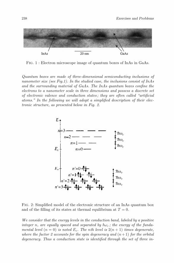
238 Exercises and Problems
Fig. 1 : Electron microscope image of quantum boxes of InAs in GaAs.
Quantum boxes are made of three-dimensional semiconducting inclusions ofnanometer size (see Fig.1). In the studied case, the inclusions consist of InAsand the surrounding material of GaAs. The InAs quantum boxes confine theelectrons to a nanometer scale in three dimensions and possess a discrete setof electronic valence and conduction states ; they are often called “artificialatoms.” In the following we will adopt a simplified description of their elec-tronic structure, as presented below in Fig. 2.
Fig. 2: Simplified model of the electronic structure of an InAs quantum boxand of the filling of its states at thermal equilibrium at T = 0.
We consider that the energy levels in the conduction band, labeled by a positiveinteger n, are equally spaced and separated by ωc ; the energy of the funda-mental level (n = 0) is noted Ec. The nth level is 2(n + 1) times degenerate,where the factor 2 accounts for the spin degeneracy and (n+1) for the orbitaldegeneracy. Thus a conduction state is identified through the set of three in-

Problem 2001 : Quantum Boxes and Optoelectronics 239
teger quantum numbers |n, l, s〉, with n > 0 and 0 ≤ l ≤ n, s = ±12. The first
valence states are described in a similar way, with analogous notations (Ev,ωv, n′, l′, s′).
I. Quantum Box in Thermal Equilibrium
At zero temperature and thermal equilibrium, the valence states are occupiedby electrons, whereas the conduction states are empty. We are going to showin this section that the occupation factor of the conduction states of the quan-tum box in equilibrium remains small for temperatures up to 300K. Therefore,only in this part, the electronic structure of the quantum box will be roughlydescribed by just considering the conduction and valence band levels lying nea-rest to the band gap. Fig.3 illustrates the assumed electronic configuration ofthe quantum box at zero temperature.
Fig. 3 : Electronic configuration at T = 0.
I.1. Give the average number of electrons in each of these two (spin-degenerate) levels versus β = 1/kBT , where T is the temperature, and thechemical potential µ .
I.2. Find an implicit relation defining µ versus β, by expressing the conser-vation of the total number of electrons in the thermal excitation process.
I.3. Show that, in the framework of this model, µ is equal to (Ec + Ev)/2independently of temperature.
I.4. Estimate the average number of electrons in the conduction level at 300Kand conclude. For the numerical result one will take Ec − Ev = 1 eV.
In optoelectronic devices, like electroluminescent diodes or lasers, electronsare injected into the conduction band and holes into the valence band of thesemiconducting active medium : the system is then out of equilibrium. Thereturn toward equilibrium takes place through electron transitions from theconduction band toward the valence band, which may be associated with lightemission.

240 Exercises and Problems
Although the box is not in equilibrium, you will use results obtained in thecourse (for systems in equilibrium) to study the distribution of electrons in theconduction band, and that of holes in the valence band. Consider that, in-side a given band, the carriers are in equilibrium among themselves,with a specific chemical potential for each band. This is justified by thefact that the phenomena responsible for transitions between conduction states,or between valence states, are much faster than the recombination of electron-hole pairs.
One now assumes in sections II and III that the quantum boxexactly contains one electron-hole pair (regime of weak excitation) :the total number of electrons contained in all the conduction states is thusequal to 1 ; the same assumption is valid for the total number of holes presentin the valence states.
II. Statistical Study of the Occupation Factor of theConduction Band States
II.1. Write the Fermi distribution for a given electronic state |n, l, s〉 versusβ = 1/kBT and µ, the chemical potential of the conduction electrons. Showthat this distribution factor fn,l,s only depends of the index n ; it will bewritten fn in the following.
II.2. Expressing that the total number of electrons is 1, find a relation betweenµ and β.
II.3. Show that µ < Ec.
II.4. Show that fn is a decreasing function of n. Deduce that
fn ≤ 1(n + 1)(n + 2)
(Hint : give an upper bound and a lower bound for the population of electronicstates of energy smaller or equal to that of level n).
II.5. Deduce that for states other than the fundamental one, it is very rea-sonable to approximate the Fermi-Dirac distribution function by a Maxwell-Boltzmann distribution and this independently of temperature. Deduce thatthe chemical potential is defined by the following implicit relation :
12
= g(β, w) , with w = eβ(µ−Ec)
and g(β, w) =w
w + 1+ w
∑n≥1
(n + 1)e−βnωc (1)

Problem 2001 : Quantum Boxes and Optoelectronics 241
II.6. Show that the function g defined in II.5 is an increasing function of wand a decreasing function of β. Deduce that the system fugacity w decreaseswhen the temperature increases and that µ is a decreasing function of T .
II.7. Specify the chemical potential limits at high and low temperatures.
II.8. Deduce that beyond a critical temperature Tc – to be estimated only inthe next questions – it becomes legitimate to make a Maxwell-Boltzmann-typeapproximation for the occupation factor of the fundamental level.
II.9. Now one tries to estimate Tc. Show that expression (1) can also bewritten under the form :
12
=w
w + 1− w +
w
(1 − e−βωc)2(2)
[Hint : as a preliminary, calculate the sum χ(β) =∑
n≥1e−βnωc and compare
it to the sum entering into equation (1)].
II.10. Consider that the Maxwell-Boltzmann approximation is valid for the
fundamental state if f0 ≤ 1e + 1
. Hence deduce Tc versus ωc.
II.11. For a temperature higher than Tc show that :
fn = e−βnωc(1 − e−βωc)2
2(3)
III. Statistics of holes
III.1.Give the average number of electrons in a valence band state |n′, l′, s′〉of energy En′ , versus the chemical potential µv of the valence electrons.
(Recall : µv is different from µ because the quantum box is out of equilibriumwhen an electron-hole pair is injected into it.)
III.2. Deduce the average number of holes hn′,l′,s′ present in this valencestate of energy En′ . Show that the holes follow a Fermi-Dirac statistics, if oneassociates the energy −En′ to this fictitious particle. Write the hole chemicalpotential versus µv.
It will thus be possible to easily adapt the results of section II, obtained forthe conduction electrons, to the statistical study of the holes in the valenceband.
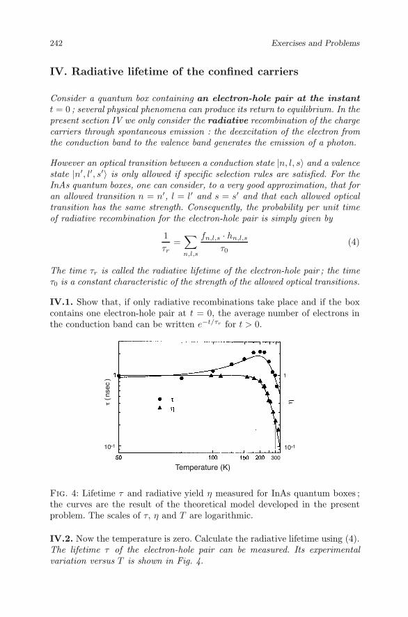
242 Exercises and Problems
IV. Radiative lifetime of the confined carriers
Consider a quantum box containing an electron-hole pair at the instantt = 0 ; several physical phenomena can produce its return to equilibrium. In thepresent section IV we only consider the radiative recombination of the chargecarriers through spontaneous emission : the deexcitation of the electron fromthe conduction band to the valence band generates the emission of a photon.
However an optical transition between a conduction state |n, l, s〉 and a valencestate |n′, l′, s′〉 is only allowed if specific selection rules are satisfied. For theInAs quantum boxes, one can consider, to a very good approximation, that foran allowed transition n = n′, l = l′ and s = s′ and that each allowed opticaltransition has the same strength. Consequently, the probability per unit timeof radiative recombination for the electron-hole pair is simply given by
1τr
=∑n,l,s
fn,l,s · hn,l,s
τ0(4)
The time τr is called the radiative lifetime of the electron-hole pair ; the timeτ0 is a constant characteristic of the strength of the allowed optical transitions.
IV.1. Show that, if only radiative recombinations take place and if the boxcontains one electron-hole pair at t = 0, the average number of electrons inthe conduction band can be written e−t/τr for t > 0.
nsec
Fig. 4: Lifetime τ and radiative yield η measured for InAs quantum boxes ;the curves are the result of the theoretical model developed in the presentproblem. The scales of τ, η and T are logarithmic.
IV.2. Now the temperature is zero. Calculate the radiative lifetime using (4).The lifetime τ of the electron-hole pair can be measured. Its experimentalvariation versus T is shown in Fig. 4.

Problem 2001 : Quantum Boxes and Optoelectronics 243
IV.3. Assume that at low temperature one can identify the lifetime τ and theradiative lifetime τr. Deduce τ0 from the data of Fig. 4.
IV.4. From general arguments show that the radiative lifetime τr is longerfor T = 0 than for T = 0. (Do not try to calculate τr in this question.)Now the temperature is in the 100–300K range. For InAs quantum boxes, somestudies show that the energy spacing ω between quantum levels is of the orderof 15 meV for the valence band and of 100 meV for the conduction band.
IV.5. Estimate Tc for the conduction electrons and the valence holes using theresult of II.10. Show that a zero temperature approximation is valid at roomtemperature for the distribution function of the conduction states. What isthe approximation then valid for the valence states ?
IV.6. Deduce the dependence of the radiative lifetime versus temperature Tfor T > Tc.
IV.7. Compare to the experimental result for τ shown in Fig. 4. Which va-riation is explained by our model ? What part of the variation remains unex-plained ?
IV.8. From the experimental values of τ at T = 200 K and at T = 0 K deducean estimate of the energy spacing between hole levels. Compare to the valueof 15 meV suggested in IV.4.
V. Non-Radiative Recombinations
trap
trap
Fig. 5 : A simple two-step mechanism of non-radiative recombination.
The electron-hole pair can also recombine without emission of a photon (non-radiative recombination). A simple two-step mechanism of non-radiativerecombination is schematized as follows : (a) a trap located in the neighborhoodof the quantum box captures the electron ; (b) the electron then recombines with

244 Exercises and Problems
the hole, without emission of a photon. The symmetrical mechanism relyingon the initial capture of a hole is also possible. One expects that such a phe-nomenon will be the more likely as the captured electron (or hole) lies in anexcited state of the quantum box, because of its more extended wave functionof larger amplitude at the trap location.
The radiative and non-radiative recombinations are mutually independent.Write 1/τnr for the probability per unit time of non-radiative recombinationof the electron-hole pair ; the total recombination probability per unit time isequal to 1/τ .
The dependence of the emission quantum yield η of the InAs quantum boxesis plotted versus T in the Fig. 4 above : η is defined as the fraction of recom-binations occuring with emission of a photon.
V.1. Consider a quantum box containing an electron-hole pair at the instantt = 0. Write the differential equation describing the evolution versus time ofthe average number of electrons in the conduction band, assuming that theelectron-hole pair can recombine either with or without emission of radiation.
V.2. Deduce the expressions of τ and η versus τr and τnr.
V.3. Comment on the experimental dependence of η versus T . Why is itconsistent with the experimental dependence of τ ?
Assume that the carriers, electrons or holes, can be trapped inside the non-radiative recombination center only if they lie in a level of the quantum boxof large enough energy (index n higher than or equal to n0). Write the non-radiative recombination rate under the following form :
1τnr
= γ∑
n≥n0,l,s
(fn,l,s + tn,l,s) (5)
V.4. From the experimental results deduce an estimate of the index n0 forthe InAs quantum boxes.
[Hint : work in a temperature range where the radiative recombination rateis negligible with respect to the non-radiative recombination rate and write asimple expression versus 1/T , to first order in η, then in ln η. You can assume,and justify the validity of this approximation, that the degeneracy of any levelof index higher than or equal to n0 can be replaced by 2(n0 + 1)].
This simple description of the radiative and non-radiative recombination pro-cesses provides a very satisfactory understanding of the experimental depen-dences of the electron-hole pairs lifetime and of the radiative yield of the InAs

Problem 2002 : Physical Foundations of Spintronics 245
quantum boxes (see Fig. 4). These experimental results and their modelingare taken from a study performed at the laboratory of Photonics and Nano-structures of the CNRS (French National Center of Scientific Research) atBagneux, France.
Problem 2002 : Physical Foundationsof Spintronics
A promising research field in material physics consists in using the electronspin observable as a medium of information (spintronics). This observablehas the advantage of not being directly affected by the electrostatic fluctua-tions, contrarly to the space observables (position, momentum) of the elec-tron. Thus, whereas in a standard semiconductor the momentum relaxationtime of an electron does not exceed 10−12 sec, its spin relaxation time canreach 10−8 sec. Here we will limit ourselves to the two-dimensional motionof electrons (quantum well structure). The electron effective mass is m. Theaccessible domain is the rectangle [0, Lx]× [0, Ly] of the xOy plane. The per-iodic limit conditions will be chosen at the edge of this rectangle. Part II canbe treated if the results indicated in part I are assumed.
Part I : Quantum Mechanics
Consider the motion of an electron described by the hamiltonian
H0 =p
2
2m+ α (σxpx + σy py) α ≥ 0
where p = −i∇ is the momentum operator of the electron and the σi (i =x, y, z) represent the Pauli matrices. Do not try to justify this hamiltonian.Assume that at any time t the electron state is factorized into a space partand a spin part, the space part being a plane wave of wave vector k. Thisnormalized state is thus written
eik·r√LxLy
[a+(t)|+〉 + a−(t)|−〉] =eik·r√LxLy
Åa+(t)a−(t)
ã(1)
with |a+(t)|2 + |a−(t)|2 = 1 (2)
where |±〉 are the eigenvectors of σz . One will write kx = k cosφ, ky = k sin φ,with k ≥ 0, 0 ≤ φ < 2π.

246 Exercises and Problems
I.1. Briefly justify that one can indeed search a solution of the Schroedingerequation under the form given in (2), where k and φ are time-independent.Write the evolution equations of the coefficients a±(t).
I.2
(a) For fixed k and φ, show that the evolution of vectorÅ
a+(t)a−(t)
ãdes-
cribing the spin state can be put under the form : i ddt
Åa+(t)a−(t)
ã=
Hs
Åa+(t)a−(t)
ãwhere Hs is a 2× 2 hermitian matrix, that will be expli-
citly written versus k, φ, and the constants α, and m.
(b) Show that the two eigenenergies of the spin hamiltonian Hs are : E± =
2k2
2m± αk with the corresponding eigenstates :
|χ+〉 =1√2
Å1
eiφ
ã|χ−〉 =
1√2
Å1
−eiφ
ã(3)
(c) Deduce that the set of |Ψk,±〉 states :
|Ψk,+〉 =eik·r√2LxLy
Å1
eiφ
ã|Ψk,−〉 =
eik·r√2LxLy
Å1
−eiφ
ã(4)
with ki = 2πni/Li (i = x, y and ni positive, negative or null integers)constitute a basis, well adapted to the problem, of the space of theone-electron states.
I.3 Assume that at t = 0 the state is of the type (2) and write ω = αk.
(a) Decompose this initial state on the |Ψk,±〉 basis.(b) Deduce the expression of a±(t) versus a±(0).I.4 One defines sz(t), the average value at time t of the z-component of theelectron spin Sz = (/2) σz . Show that :
sz(t) = sz(0) cos(2ωt) + sin(2ωt) Im(a+(0)∗ a−(0) e−iφ
)I.5 The system is installed in a magnetic field B lying along the z-axis. Theeffect of B on the orbital variables is neglected. The hamiltonian thus becomesH = H0 − γBSz.
(a) Why does the momentum k remain a good quantum number ? Deducethat, for a fixed k, a spin hamiltonian H
(B)s can still be defined. You
will express it versus Hs, γ, B and σz .
(b) Show that the eigenenergies of H(B)s are
E(B)± =
2k2
2m±
»α2k2 + γ2B2/4

Problem 2002 : Physical Foundations of Spintronics 247
(c) Consider a weak field B (γB αk). The expression of the eigenvectorsof Hs to first order in B are then given by
|χ(B)+ 〉 = |χ+〉 − γB
4αk|χ−〉 |χ(B)
− 〉 = |χ−〉 +γB
4αk|χ+〉
Deduce that the average values of Sz in the states |χ(B)± 〉 are
〈χ(B)+ |Sz |χ(B)
+ 〉 = −γB
4αk〈χ(B)
− |Sz|χ(B)− 〉 = +
γB
4αk
(d) What are the values of |χ(B)± 〉 and of the matrix elements 〈χ(B)
± |Sz|χ(B)± 〉,
in the case of a strong field B (such that γB αk).
Part II : Statistical Physics
In this part, we are dealing with the properties of an assembly of N electrons,assumed to be without any mutual interaction, each of them being submittedto the hamiltonian studied in Part I. We will first assume that there is nomagnetic field ; the energy levels are then distributed into two branches asobtained in I.2 :
E±(k) =
2k2
2m± αk (5)
with k = |k|. We will write k0 = mα/ and ε0 = 2k2
0/(2m) = mα2/2.
II.1.We first consider the case α = 0. Briefly recall why the density of statesD0(ε) of either branch is independent of ε for this two-dimensional problem.Show that D0(ε) = mLxLy/(2π
2).
II.2.We return to the real problem with α > 0 and now consider the branchE+(k).
(a) Plot the dispersion law E+(k) versus k. What is the energy range εaccessible in this branch ?
(b) Express k versus k0, ε0, m, and the energy ε for this branch. Deducethe density of states :
D+(ε) = D0(ε)Å1 −
…ε0
ε + ε0
ã(6)
Plot D+(ε)/D0(ε) versus ε/ε0.
II.3. One is now interested by the branch E−(k).
(a) Plot E−(k) versus k and indicate the accessible energy range.How many k’s are possible for a given energy ε ?

248 Exercises and Problems
(b) Show that the density of states of this branch is given by
ε < 0 : D−(ε) = 2D0(ε)…
ε0ε + ε0
ε > 0 : D−(ε) = D0(ε)Å1 +
…ε0
ε + ε0
ã(7)
II.4. In the rest of the problem, the temperature is taken as zero.
(a) Qualitatively explain how the Fermi energy changes with the electronsnumber N . Show that if N is small enough, only the branch E− is filled.
(b) What is the value of the Fermi energy εF when the E+ branch beginsto be filled ? Calculate the number of electrons N∗ at this point, versusLx, Ly, m, and ε0.
(c) Where are the wave vectors k corresponding to the filled states εF < 0located ?
II.5. Assume in what follows that εF > 0.
(a) What are the wave vectors k for the occupied states in either branchE± ?
(b) Calculate the Fermi wave vectors k+F and k−
F versus εF , k0, ε0, m and .
(c) For N > N∗, calculate N − N∗ and deduce the relation :
N =LxLym
π2(2ε0 + εF )
II.6. A weak magnetic field is now applied on the sample.
(a) Using the result of I.5, explain why the Fermi energy does not vary tofirst order in B.
(b) Calculate the magnetization along z of the electrons gas, to first orderin B.
II.7. Now one analyzes the possibility to maintain a magnetization in thesystem for some time in the absence of magnetic field. At time t = 0, eachelectron is prepared in the spin state |+〉z. The magnetization along z is thusM(0) = N/2. For a given electron, the evolution of sz(t) in the absence ofcollisions was calculated in I.4. Now this evolution is modified due to the effectof collisions. Because of the elastic collisions of an electron on the materialdefects, its k wave vector direction may be randomly modified. These collisionsare modeled assuming that :
– they occur at regular times : t1 = τ , t2 = 2τ ,..., tn = nτ ,...
– the angle φn characterizing the k direction between the nth and the(n + 1)th collision is uniformly distributed over the range [0, 2π[ anddecorrelated from the previous angles φn−1, φn−2, ..., and thus from thecoefficients a±(tn).
– the angles φn corresponding to different particles are not correlated.

Problem 2002 : Physical Foundations of Spintronics 249
Under these assumptions, the total magnetization after many collisions canbe calculated by making an average over angles for each electron. One writess(t) for the average of sz(t) over the angles φn.Show that s(tn+1) = cos(2ωτ) s(tn).
II.8. One assumes that ωτ 1.
(a) Is there a large modification of the average spin s between two collisions ?
(b) One considers large times t with respect to the interval τ between twocollisions. Show that the average spin s(t) exponentially decreases andexpress the characteristic decrease time td versus ω and τ .
(c) Take two materials : the first one is a good conductor (a few collisionstake place per unit time), the second one is a poor conductor (manycollisions occur per unit time). In which of these materials is the averagespin better “protected,” i.e., has a slower decrease ? Comment on theresult.
(d) For τ = 10−12 sec and ω=5 µeV, estimate the spin relaxation time td.
II.9. To maintain a stationary magnetization in the population of N spins,one injects g± electrons per unit time, of respective spins sz = ±/2 into thesystem. For each spin value, the electrons leave the system with a probabilityper unit time equal to 1/tr. Besides, one admits that the relaxation mechanismstudied in the previous question is equivalent to the exchange between the+ and − spin populations : a + spin is transformed into a − spin with aprobability per unit time equal to 1/td, and conversely a − spin is transformedinto a + spin with a probability per unit time equal to 1/td. One calls f±(t)the populations of each of the spin states at time t, td is the spin relaxationtime.
(a) Write the rate equations on df±/dt. What are the spin populations f∗±in steady state ?
(b) Deduce the relative spin population, that is, the quantity P =f∗+ − f∗
−f∗+ + f∗−
.
In what type of material will the magnetization degrade not too fast ?

Solution of the Exercisesand Problems
Electrostatic Screening : exercise 2000Magnetic Susceptibility of a “Quasi-1D” Conductor : exercise 2001Entropies of the HC Molecule : exercise 2002Quantum Boxes and Optoelectronics : problem 2001Physical Fundations of Spintronics : problem 2002
251

Exercise 2000 : Electrostatic Screening 253
Exercise 2000 : Electrostatic Screening
I.1. The density N/Ω and the chemical potential µ are related by
N
Ω=
1Ω
∫D(k)fFD(k)d3k =
14π3
∫ +∞
0
4πk2dk
exp β
Å
2k2
2me− µ
ã+ 1
I.2. In the high temperature and low density limit, the exponential in thedenominator of the Fermi-Dirac distribution is large with respect to 1, sothat
N
Ω 1
4π3
∫ +∞
0
e−β
Å
2k2
2me− µ
ã4πk2dk
N
Ω 2eβµ
Å2πmekBT
h2
ã3/2
I.3. The total energy in presence of a potential is written
ε =
2k2
2me+ V (r)
At high temperature and low density
N 14π3
∫Ω
e−βV (r)d3r
∫ +∞
0
4πk2dk e−β
Å
2k2
2me− µ
ã
I.4. By definition one has
N =∫
Ω
n(r)d3r
one thus identifies n(r) to
n(r) = n0 e−βV (r)
with
n0 =1
4π3
∫ +∞
0
4πk2dk e−β
Å
2k2
2me− µ
ã
I.5. If βV (r) 1 for any r, n is uniform, i.e.,
n = n0 =N
Ω

254 Solution of the Exercises and Problems
II.1. The potential energy of an electron inside the electrostatic potentialΦtot(r) is −e Φtot(r), the energy of a hole +e Φtot(r). The electron and holedensities are respectively equal to
n(r) = n0 exp[−β(−e Φtot(r)]
p(r) = p0 exp[−β(+e Φtot(r)]
with n0 = p0 =N
Ω.
II.2. The total density of charges at r is equal to e[p(r) − n(r)]. The chargelocalized at the origin also enters into the Poisson equation :
∆Φtot(r) +e[p(r) − n(r)]
ε0εr+
Qδ(r)ε0εr
= 0
In the high temperature limit and to the lowest order
p(r) − n(r) = n0
[e−βeΦtot(r) − eβeΦtot(r)
] −2n0 eβΦtot(r)
Whence the equation satisfied by Φtot(r) :
∆Φtot(r) =2n0 e2β
ε0εrΦtot(r) − Q
ε0εrδ(r)
One writes λ2 =ΩN
ε0εrkBT
2e2, this is the square of a length.
II.3. IfN
Ω= 1022 m−3 T = 300 K, εr = 12.4, then λ = 30 nm.
II.4. The effect of the charge located at the origin cannot be felt beyond adistance of the order of λ : at a larger distance Φtot(r) is rapidly constant,the electron and hole densities are constant andopposite. The mobile electronsand holes have screened the charge at the origin.

Exercise 2001 : Magnetic Susceptibility of a “Quasi-1D” Conductor 255
Exercise 2001 : Magnetic Susceptibility of a“Quasi-One-Dimensional” Conductor
I.1.
a) λ = 0 kBT γB b) λ kBT γB
ε
| + 1 >
|0 >B
| − 1 >
0ε0
Three levels in ε0 for B = 0Comparable occupationsof the three levels
ε | + 1 >
| − 1 >
|0 >B
0ε0
ε0 + λ
At the temperature T ,the upper levelsare weakly occupied
c) kBT λ γB
ε | + 1 >
| − 1 >
|0 >B
0ε0
ε0 + λ
Comparable occupations of the three states at T .Little influence of λ, this caseis almost equivalent to a)
d) γB λ kBT
ε | + 1 >
|0 >B
| − 1 >0
ε0
ε0 + λ
Only level | − 1〉 is populated.The magnetization is saturated, each
ion carries a moment +γ

256 Solution of the Exercises and Problems
I.2. State |0〉, energy ε0
|+〉 ε0 + λ + γB|−〉 ε0 + λ − γB
For a single ion :
z = e−βε0 + e−β(ε0+λ+γB) + e−β(ε0+λ−γB)
= e−βε0 [1 + e−β(λ+γB) + e−β(λ−γB)]
For the whole system : Z = (z)N
F = −kBT lnZ
= −NkBT¶−βε0 + ln
î1 + e−β(λ+γB) + e−β(λ−γB)
ó©= Nε0 − NkBT ln
î1 + e−β(λ+γB) + e−β(λ−γB)
óM = −∂F
∂B= Nγ
[e−βλ+βγB − e−βλ−βγB
]1 + e−β(λ+γB) + e−β(λ−γB)
For B → 0, M ∼ Nγ2βγBe−βλ
1 + 2e−βλi.e.,
χ =2Nγ2βe−βλ
Ω(1 + 2e−βλ)
I.3. Discussion of the limit cases :(a) λ = 0
M = Nγex − e−x
1 + ex + e−xwith x = βγB
In the limit x → 0, one obtains χ =2Nγ2
3ΩkBT(Curie law).
(b) βλ 1 βγB = x
M Nγe−βλ(ex − e−x)
χ 2Nγ2e−βλ
ΩkBT
(Curie law attenuated by the thermal activation towards the magneticlevel).
(c) 1 βλ x
M Nγ[x − βλ + βλ + x]3
=2Nγ2βB
3
χ =2Nγ2
3ΩkBT
This situation is analogous to a).

Exercise 2001 : Magnetic Susceptibility of a “Quasi-1D” Conductor 257
(d) βγB βλ 1M Nγ
The magnetization is saturated.
I.4. The high temperature behavior of χ in the figure suggests a Curie law.
The expression of χ obtained in I.2. vanishes for β → ∞ and for β → 0. Itis positive and goes through a maximum for β of the order of 1
λ (exactly for1−βλ+2e−βλ = 0, i.e., βλ = 1.47). From the temperature of the χ maximumλ can be deduced.
Note : in fact, for the system studied in the present experiment, the ε0 + λlevel contains 3 states, and not 2 like in this exercise based on a simplifiedmodel.
II.
z =+S∑−S
e−lβγB = eβSγB2S∑l=0
e−lβγB = eβSγB 1 − e−(2S+1)βγB
1 − e−βγB
f = −kBT ln z = −kBT
ñSβγB + ln
1 − e−(2S+1)x
1 − e−x
ôwith x = βγB
m = − ∂f
∂B= −∂f
∂xγβ = γS + kBT
(2S + 1)γβe−(2S+1)x
1 − e−(2S+1)x− kBTβγe−x
1 − e−x
m
γ= S +
2S + 1e(2S+1)x − 1
− 1ex − 1
3 limits : x → +∞ x → −∞ x → 0
(a) x → +∞ (high positive field, low temperature)m
γ→ S saturation
(b) x → −∞ (high negative field, low temperature)m
γ→ S − (2S + 1) + 1 = −S saturation
(c) x → 0 : (low field, high temperature).
One expectsm to be proportional to B, which allows to define a susceptibility.Therefore one has to developm up to the term in x, which requires to express

258 Solution of the Exercises and Problems
the denominators to third order.
m
γ S +
2S + 1(2S + 1)x + (2S + 1)2 x2
2 + (2S + 1)3 x3
6 + ...− 1
x + x2
2 + x3
6 + . . .
m
γ x
S(S + 1)3
=γBS(S + 1)
3kBT(Curie law)
Exercise 2002 : Entropies of the HC Molecule
1.S3D = NkB ln
ïΩ
Nh3(2πmkBT )3/2
ò+
52NkB
µ3D = −kBT lnï
ΩNh3
(2πmkBT )3/2
ò2.
Z2D =1
N ′!
ÅA
h22πmkBT
ãN ′
S2D = N ′kB lnï
A
N ′h2(2πmkBT )
ò+ 2N ′kB
µ2D = −kBT lnï
A
N ′h2(2πmkBT )
òA molecule is spontaneously adsorbed if µ2D < µ3D.
3. If the adsorbed film is mobile on the surface :
∆S = S2D − S3D
∆S = NkB lnï
Ah
Ω(2πmkBT )1/2
ò− 1
2NkB
4. For the only translation degrees of HC :
S3D = 152.9 J.K−1
S2D = 48.2 J.K−1
The average 3D distance is of 3.3 nm, it is 0.11 nm between molecules on thesurface (which is less than an interatomic distance, but one has also to ac-count for the large corrugation of the surface).

Problem 2001 : Quantum Boxes and Optoelectronics 259
5.ZN =
1N !
(zrot)N (ztr)N
6.
φ
z1rot =∫∫
dφdpφ
hexp
Ç−βp2
φ
2IA
å
=2π
h
∫ +∞
−∞dpφ exp
Ç−βp2
φ
2IA
å=
2π
h
√2πIAkBT
7.
z2rot =∫∫∫∫
dθdpθdφdpφ
h2exp
Å−βp2
θ
2I
ãexp
Ç− βp2
φ
2I sin2 θ
å
=8π2
h2IkBT
The expression in the course iskBT
2hcB=
4π2
h2IkBT , for a symmetrical mo-
lecule, such that its physical situation is identical after a 180 rotation. ButHC is not symmetrical
8. Rotation entropy of HC :
Frot = −NkBT ln z2rot
(the factor for indistinguishability is included inside the translation term).
Srot = −∂Frot∂T
= NkB
ïln z2rot + T
∂ ln z2rot∂T
òSrot = 33.3 J ·K−1
Problem 2001 : Quantum Boxesand Optoelectronics
I.1. Owing to the spin degeneracies one has
〈nEc〉 =2
eβ(Ec−µ) + 1and 〈nEv 〉 =
2eβ(Ev−µ) + 1

260 Solution of the Exercises and Problems
I.2. At any temperature 〈nEc〉 + 〈nEv〉 = 2, in the present approximation inwhich the total number of electrons is 2. It follows that
1eβ(Ec−µ) + 1
+1
eβ(Ev−µ) + 1= 1 , an implicit relation between µ and β
I.3. This equation can be reexpressed, noting x = eβµ, y = eβEc and z =eβEv :
x
y + x+
x
z + x= 1
that is, zx + yx + 2x2 = zy + zx + yx + x2, x2 = yz, whence the result
µ =Ec + Ev
2, independently of temperature.
I.4. One immediately deduces from I.3
〈nEc〉 =2
eβ(Ec−µ) + 1=
2
eβ(Ec−Ev)
2 + 1
At 300 K with Ec − Ev = 1 eV, 〈nEc〉 =2
e20 + 1= 4 × 10⁻⁹.
At 300 K, at thermal equilibrium, the probability for the conduction levels tobe occupied is thus extremely small.
II.1.fnls =
1eβ(Enls−µ) + 1
As the energy Enls only depends of n, consequently we will write fnls = fn.
II.2. Noting gn for the degeneracy of state n, one has
〈n〉 = 1 =∑
n
gn fn =∑
n
2(n + 1)fn
an implicit relation between µ and β.
II.3. If one had µ > Ec, 2f0 would be larger than 1, in contradiction with〈n〉 = 1.
II.4. En is an increasing function of n, as is also eβ(En−µ), whence the result.One has f0 < 1/2, and fn+1 < fn, so that :
1 ≥n∑
i=0
gi fi >
n∑i=0
gi fn = 2fn
n∑i=0
(n + 1) = 2fn(n + 1)(n + 2)
2
i.e., fn ≤ 1(n + 1)(n + 2)

Problem 2001 : Quantum Boxes and Optoelectronics 261
II.5. The relation obtained in II.4 implies f1 ≤ 16, f2 ≤ 1
12, etc. One then
deduces that in f1 one has eβ(E1−µ) > 5, in f2 eβ(E2−µ) > 11, which justifiesthe use of the Maxwell-Boltzmann approximation, i.e.,
fnls =1
eβ(Enls−µ) + 1≈ e−β(En−µ)
for any excited state.
Taking into account the validity of this approximation, the implicit relationbetween µ and β becomes
1 = 2f0 + 2∞∑
n=1
(n + 1)e−β(En−µ)
With En = Ec+nωc, and w = e−β(Ec−µ), this expression can be transformedinto
12
= g(β, w) =1
w−1 + 1+ w
∞∑n=1
(n + 1)e−βnωc
=w
w + 1+ w
∞∑n=1
(n + 1)e−βnωc (1)
II.6. Obviously g is a decreasing function of β at fixed w. Moreover,∂g
∂w=
1(w + 1)2
+∞∑
n=1
(n + 1)e−βnωc > 0, thus g is an increasing function
of w. When T increases, β decreases. For g to remain constant [equal to 1/2from (1)], the fugacity w must decrease when T increases.
Since w = e−β(Ec−µ),∂w
∂T= w
1kT 2
(Ec − µ) + β∂µ
∂T. From II.3., µ < E0 = Ec
and the first term of the right member is > 0. Consequently,∂w
∂T< 0 implies
∂µ
∂T< 0.
II.7. From equation (1),
– when β → 0,∞∑
n=1
(n + 1)e−βnωc tends to infinity, thus the solution w must
tend to 0. Then µ tends to −∞. (One finds back the classical limit at hightemperature) ;
– when T → 0, the sum tends to 0 and (1) becomes12
=w
w + 1, so that w
tends to 1 in this limit : the low temperature limit of µ is then E0 = Ec.

262 Solution of the Exercises and Problems
II.8. f0 =1
w−1 + 1. At low temperature, w tends to 1 and f0 tends to 1/2,
whereas at high temperature w tends to 0 and the Maxwell-Boltzmann sta-tistics is then applicable to the 0 level. Since w is a monotonous function ofT , this latter limit must be valid beyond a critical temperature Tc, so thatthen eβ(E0−µ) 1 (w 1).
II.9. The function χ =∞∑
n=1
e−βnωc is equal toe−βωc
1 − e−βωc=
1eβωc − 1
. Its
derivative∂χ
∂β= −ωc
∞∑n=1
ne−βnωc
allows to conveniently calculate the sum in the right member of (1), which isequal to :
∞∑n=1
(n + 1)e−βnωc = χ − 1ωc
∂χ
∂β=
1eβωc − 1
+eβωc
(eβωc − 1)2
=2eβωc − 1
(eβωc − 1)2= −1 +
e2βωc
(eβωc − 1)2= −1 +
1(1 − e−βωc)2
whence the result (2).
II.10. This condition is equivalent to w < 1/e, and at T = Tc one has w = 1/e.For w = 1/e, (2) becomes
1 +e(e − 1)2(e + 1)
=1[
1 − exp(− ωc
kBTc
)]2
i.e.,2(e + 1)
e2 + e + 2=
[1 − exp
(− ωc
kBTc
)]2
which provides :
ωc
kTc= − ln
(1 −
2(e + 1)
e2 + e + 2
)
Numerically kBTc = 0.65 ωc.
II.11. For T > Tc, the Maxwell-Boltzmann statistics is applicable to the
fundamental state and consequently to any state. f0 =1
w−1 + 1can be ap-
proached by w, which allows to write (2) as :
12
=w
(1 − e−βωc)2

Problem 2001 : Quantum Boxes and Optoelectronics 263
It follows that
fn = e−β(E0+nωc−µ) = we−βnωc = e−βnωc(1 − e−βωc)2
2(3)
III.1. The average number of electrons in a state of spin s′ of energy E inthe valence band is also the Fermi-Dirac distribution function :
〈n〉 =1
eβ(E−µv) + 1
III.2.
hn′′s′ = 1 − 〈n〉 =eβ(E−µv)
eβ(E−µv) + 1=
1e−β(E−µv) + 1
=1
eβ(−E+µv) + 1
hn′′s′ is indeed an expression of the Fermi-Dirac statistics, under the condi-tion of writing Et = −E. The holes chemical potential is then given byµt = −µv.
The results on the electrons in questions II.1. to II.11. apply to the holes(provided this transposition for the energy and for µ).
IV.1. If all recombinations are radiative,
dn
dt= − n
τr
whence the result : n = n0 e−t/τr with n0 = 1.
IV.2. At T = 0, both f0 and h0 are equal to 1/2, all the other occupationfactors being equal to zero.
Consequently, one has :
1τr
=f0,0,1h0,0,1 + f0,0,−1h0,0,−1
τ0=
2f0h0
τ0=
12τ0
i.e., τr = 2τ0
IV.3. One deduces from the figure τr = 2τ0 = 1 nsec, that is, τ0 = 0.5 nsec.
IV.4. At any temperature one has
1τr
=∑n,l,s
fn,l,shn,l,s
τ0(4)
Moreover the average numbers of electrons and holes are equal to 1. As theoccupation factors are spin-independent, for a given value of s one gets :
∑n,l
fn =∑n′,l′
hn′ =12

264 Solution of the Exercises and Problems
One deduces : ∑n,l
fnhn ≤(∑
n,l
fn
)( ∑n′,l′
hn′)
=14
This limit being reached at T = 0, one then finds that at any temperaturethe radiative lifetime is larger than or equal to its value at T = 0.
IV.5. For the electrons ωc 100 meV, whereas ωv 15 meV for theholes. Tc is thus of the order of 780 K for the electrons and 117 K for theholes. Expression (2) shows that when kBT ω, w is of the order of 1,which indeed constitutes the zero temperature approximation. The Maxwell-Boltzmann approximation is valid for any hole state if T > Tc = 117 K, fromII.10.
IV.6. One thus has f0 = 1/2 and all the other fn’s are equal to zero, whereasfrom (3),
h0 =(1 − e−βωv)2
2One then deduces that the only active transition is associated to the levels|001〉 and |00 − 1〉 (like at zero temperature) and that
1τr
=2f0h0
τ0=
h0
τ0=
(1 − e−βωv)2
2τ0
IV.7. This model allows one to qualitatively understand the increase of theradiative lifetime with temperature, due to the redistribution of the hole pro-bability of presence on the excited levels. This is indeed observed above 250K,a temperature range in which a decrease of the lifetime is observed in the ex-periment.
IV.8. At 200 K one approximately gets τr(T ) = 2τr(0), that is,
(1 − e−βωv)2 =12, which gives
βωv = − ln(1 − 1√
2
)
i.e., a splitting between holes levels of 1.23 kBT for T = 200 K, that is, of20 meV.
V.1. The probability per unit time of radiative recombination is1τr. This
means that the variation of the average number of electrons per unit time,due to these radiative recombinations, is given by
d〈n〉dt
= −〈n〉τr

Problem 2001 : Quantum Boxes and Optoelectronics 265
In presence of non radiative recombinations at the rate1
τnr, the total variation
becomes :d〈n〉dt
= −〈n〉τr
− 〈n〉τnr
V.2. This allows to define the total lifetime τ by
d〈n〉dt
= −〈n〉τr
− 〈n〉τnr
= −〈n〉τ
i.e.,1τ
=1τr
+1
τnr
and a radiative yield η equal to the ratio between the number of radiativerecombinations per unit time and the total number of recombinations perunit time :
η =〈n〉τr
〈n〉τ
=τ
τr=
1τr
1τr
+ 1τnr
=1
1 + τr
τnr
V.3. When only radiative recombinations are present, τnr → ∞ and theradiative yield η is equal to 1, independently of the value of the radiativelifetime. Here the yield strongly decreases above 200 K, whereas it is constantfor T < 150 K. This implies that a nonradiative recombination mechanismbecomes active for T > 200 K.
Correlatively, this is consistent with the decrease of the total lifetime τ in thesame temperature range, whereas the results of question IV.6. show that theradiative lifetime should increase with temperature.
V.4. We found in V.2 : η =1τr
1τr
+ 1τnr
.
In this expression1
τnr= γ
∑n≥n0,l,s
(fn,l,s + hn,l,s). At sufficiently high tem-
perature, around 350 K, τ ≈ 0.5 nsec whereas τr > 2 nsec. In this regime,the nonradiative recombinations determine τ , and η ≈ τnr
τr. Besides, only the
hole levels of index n0 > 0 are occupied, they satisfy a Maxwell-Boltzmannstatistics. This allows to write, using (3),
1τnr
= γ∑
n≥n0
2(n + 1)e−βnωv(1 − e−βωv)2
2

266 Solution of the Exercises and Problems
Taking an orbital degeneracy equal to n0 + 1 for each excited level, one has
1τnr
= γ(1 − e−βωv)2
22(n0 + 1)e−βn0ωv
∑n≥0
e−βnωv
= γ(1 − e−βωv)(n0 + 1)e−βn0ωv
Using the result of IV.6,
1η
=γ(1 − e−βωv)(n0 + 1)e−βn0ωv
(1−e−βωv )2
2τ0
= 2γτ0(n0 + 1)e−βn0ωv
(1 − e−βωv)
≈ 2γτ0(n0 + 1)e−βn0ωv
In this temperature range ln(η) = constant+n0ωv
kT.
The slope of η(T ) provides an approximation for n0 : between 200 and 350 K
lnÅ
η200Kη350K
ã= ln(10) =
n0ωv
kB
Å1
200− 1
350
ãwhich yields a value of n0 ranging between 5 and 6.
Problem 2002 : Physical Foundationsof Spintronics
Part I : Quantum Mechanics
I.1. A state having a plane wave eik·r for space part is an eigenstate of themomentum operator, with the eigenvalue k. The effect of the hamiltonianon this type of state gives :
H
ñeik·r√LxLy
Åa+
a−
ãô=
eik·r√LxLy
ï
2k2
2m
Åa+
a−
ã+ kα
Åe−iφ a−eiφ a+
ãòOne thus sees that, if the coefficients a± verify the evolution equations
ia± =
2k2
2ma± + kα e∓iφ a∓
the proposed eigenvector is a solution of the Schroedinger equationi|ψ〉 = H |ψ〉.

Problem 2002 : Physical Foundations of Spintronics 267
I.2.
(a) For fixed k and φ, one is restricted to a two-dimensional problem, onlyon the spin variables, and the hamiltonian is equal to
Hs =
2k2
2mId + kα
Å0 e−iφ
eiφ 0
ãwhere Id represents the identity matrix.
(b) It can be immediately verified that the two proposed vectors are eigen-vectors of Hs with the eigenenergies E±.
(c) The space of the one-electron states is the tensor product of the spaceassociated to the electron motion in the rectangle [0, Lx] × [0, Ly] withthe spin space. The functions eik·r/
√LxLy are an orthonormal basis
of the orbital space, provided that the choice of k allows this functionto satisfy the periodical limit conditions : this requires ki = 2πni/Li,with ni positive, negative or null integer. As for the two vectors |χ±〉,they constitute a basis of the spin space. Thus the vectors |Ψk,±〉 are anorthonormal eigenbasis of the hamiltonian H0.
I.3.
(a) The development of the initial spin state on the pair of eigenstates |χ±〉is Å
a+(0)a−(0)
ã=
12
(a+(0) + a−(0)e−iφ
)Å 1eiφ
ã+
12
(a+(0) − a−(0)e−iφ
)Å 1−eiφ
ãThe initial state (orbital ⊕ spin) is thus given by
|Ψ〉 =a+(0) + a−(0)eiφ
√2
|Ψk,+〉 +a+(0) − a−(0)eiφ
√2
|Ψk,−〉 .
(b) One deduces that the electron spin state at time t is characterized byÅa+(t)a−(t)
ã=
e−iE+t/
2(a+(0) + a−(0)e−iφ
)Å 1eiφ
ã+
e−iE−t/
2(a+(0) − a−(0)e−iφ
)Å 1−eiφ
ãAfter development, one finds
a±(t) = e−i2k2t / 2m(a±(0) cos(ωt) − ia∓(0)e∓iφ sin(ωt)
).

268 Solution of the Exercises and Problems
I.4. A simple calculation gives
sz(t) =
2(|a+(t)|2 − |a−(t)|2)
=
2[cos(2ωt)
(|a+(0)|2 − |a−(0)|2 )+2 sin(2ωt) Im
(a∗+(0)a−(0)e−iφ
)]One then deduces the result announced in the text.
I.5.(a) The new term in the hamiltonian, arising from the magnetic field, com-mutes with the momentum operator. One can thus always look for ei-
genstates of the form eik·rÅ
a+
a−
ã, where
Åa+
a−
ãis a two-component
vector providing the spin state. The hamiltonian determining the evo-lution of this spin is written in the |±〉z basis :
H(B)s = Hs − γB
2σz =
2k2
2mId +
Å −γB/2 kαe−iφ
kαeiφ γB/2
ã(b) One verifies that the eigenenergies of the above matrix are those givenin the text.
(c) One notices that 〈χ±|Sz|χ±〉 = 0 and that 〈χ±|σz |χ∓〉 = 1. One deducesthe formulae given in the text.
(d) For a large B, the eigenstates of H(B)s are practically equal to the
eigenstates |±〉z of Sz. More precisely, for γ < 0 (electron), one has|χ(B)
± 〉 ±|±〉z. Consequently, 〈χ(B)± |Sz |χ(B)
± 〉 ±/2.
Part II : Statistical Physics
II.1. For α = 0, one has E± = 2k2/(2m). The number of quantum states in
a given spin state, with a wave vector of coordinates in the range (kx to kx
+dkx ; ky to ky + dky) is equal to
d2N =LxLy
(2π)2dkxdky =
LxLy
(2π)2k dk dφ
i.e., by integration over the angle φ :
dN =LxLy
2πkdk =
LxLy
2π
m
2dε
The density of states is thus independent of the energy ε and equal toD0(ε) = LxLym/(2π
2).

Problem 2002 : Physical Foundations of Spintronics 269
II.2.
(a) The dispersion law in this branch is written
E+(k) =
2(k + k0)2
2m− ε0
This corresponds to a portion of parabola, plotted in Fig.1. The spec-trum of the allowed energies is [0,∞[.
Dispersion relations
k0kF
0
E
+
E +
E
kF
k1 k 2
Fig. 1 : Typical behavior of the dispersion laws E±(k) in either branch.
(b) For the branch ε = E+(k),
k = −k0 +…
2m
2(ε + ε0)
and thus
D+(ε) =LxLy
2πk
dk
dε= D0(ε)
Å1 −
…ε0
ε + ε0
ãThe corresponding curve is plotted in 2.

270 Solution of the Exercises and Problems
1 0 1 2 3 4 5 6 7 8 9 10E
0
1
2
3
4
D(E
)
Fig. 2: Densities of states D+/D0 (lower curve) and D−/D0 (upper curve),plotted versus ε/ε0.
II.3.(a) For the branch ε = E−(k),
E−(k) =
2(k − k0)2
2m− ε0
the variation of which is given in Fig.1. The spectrum of the permittedenergies is [−ε0,∞].– For −ε0 < ε ≤ 0, there are two possible wavevector moduli k for agiven energy ε :
k1,2 = k0 ±…
2m
2(ε + ε0)
– For ε > 0, there is a single allowed wavevector modulus :
k = k0 +…
2m
2(ε + ε0)
(b) One then deduces, for ε > 0
D−(ε) = D0(ε)Å
1 +…
ε0ε + ε0
ãand for ε < 0 (adding both contributions corresponding for either signin the k1,2 formula) :
D−(ε) = 2D0(ε)…
ε0ε + ε0

Problem 2002 : Physical Foundations of Spintronics 271
The corresponding curve is plotted in Fig. 2.
II.4.(a) Assume that the electrons are accommodated one next to the other inthe available energy levels. Since the temperature is taken to be zero,the first electron must be located on the fundamental level, the secondone on the first excited level, and so forth. Thus the first levels to befilled are those of the E− branch, with k around k0, the Fermi energy εF
being a little larger than −ε0 for N small. When N increases, the energyεF also increases. It reaches 0 when all the states of the E− branch, ofwave vectors ranging between 0 and 2k0, are filled. For larger numbersof electrons, both branches E± are filled.
(b) The E+ branch remains empty until εF reaches the value εF = 0. Thereare then
N∗ =∫ 0
−ε0
D−(ε)dε =2LxLym
π2ε0
electrons on the E− branch.(c) In the E− branch, the filled states verify E−(k) < εF , i.e.,
k1 < k < k2 with :
k1,2 = k0 ±…
2m
2(εF + ε0)
(see the dashed lines in Fig.1). The extremities of the corresponding kvectors are thus located inside a ring, limited by two Fermi “surfaces”consisting of the circles of respective radii k1 and k2.
II.5.(a) When N is larger than N∗, one has to add the extra N − N∗ electronsin both branches, up to the Fermi level. The situation is then given bythe dotted line in Fig.1. For either E± branch, the extremities of thewave vectors k corresponding to the filled states are located inside thedisk defined by E±(k) < εF .
(b) For the E+ (resp. E−) branch, the radius of the disk corresponding tothe occupied states is determined by E+(k+
F ) = εF (resp. E−(k−F ) = εF ),
with :
k±F = ∓k0 +
…2m
2(εF + ε0)
In either branch, the Fermi “surface” is a circle for this two-dimensionalproblem.
(c) One finds :
N − N∗ =∫ εF
0
(D+(ε) + D−(ε)) dε =LxLym
π2εF

272 Solution of the Exercises and Problems
One then deduces the relation between the electrons number and theFermi energy :
N =LxLym
π2(2ε0 + εF )
II.6.
(a) The energies E(B)± in either branch only vary to second order in B, i.e.,
one has E(B)± = E0± + O(B2). This implies that the Fermi energy too
only varies to second order in B.
(b) The total magnetization at zero temperature is the sum of the averagevalues of Sz in each filled quantum state, i.e.,
M =∑
k<k+F
〈Ψ(B)k,+
|Sz|Ψ(B)k,+
〉 +∑
k<k−F
〈Ψ(B)k,−|Sz |Ψ(B)
k,−〉
= −∫ k+
F
0
γB
4αk
LxLy
2πkdk +
∫ k−F
0
γB
4αk
LxLy
2πkdk
One thus finds :
M =γB
4α
LxLy
2π(k−
F − k+F ) =
LxLy
4πγBm
II.7. One returns to the expression of question I.4, replacing a±(0) by a±(tn)and a±(t) by a±(tn+1). One averages over the angle φn, using the fact thatthis angle is not correlated to a±(tn) : a∗
+(tn) a−(tn) e−iφn = 0. One thusfinds that the term in sin(2ωτ) does not contribute and then gets the relationgiven in the text : s(tn+1) = cos(2ωτ) s(tn).
II.8.
(a) If ωτ 1, then cos(2ωτ) 1 − 2ω2τ2. The change of s(t) in a timeinterval τ between two collisions is then weak.
(b) In the time interval t τ , the number of collisionsn = t/τ 1 takes place (the fact that t is not an exact multiple ofτ plays a negligible role). Consequently,
s(t) = s(0) (cos(2ωτ))n = s(0) exp (n ln(cos(2ωτ)))
Using ln(cos(2ωτ)) ln(1 − 2ω2τ2) −2ω2τ2, one obtainss(t) = s(0) e−t/td with td = 1/(2ω2τ).
(c) The shorter τ , the longer td. Paradoxically, a poor conductor, in whichthe time interval between collisions is very short, leads to a longer spinrelaxation time than a good conductor. This surprising result can beput together with the quantum Zenon effect, in which one finds that afrequent observation of a system prevents its evolution.

Problem 2002 : Physical Foundations of Spintronics 273
(d) One finds ω = 7.6 × 10⁹ sec−1 and td = 8.7 × 10⁻⁹ sec. As announ-ced in the introduction of the text, the spin relaxation time td can bemuch longer than the interval τ between collisions, corresponding to therelaxation time of the electron velocity.
II.9. Let us write the rate equation for the spins + and − populations :df+
dt= g+ − f+
tr− f+
td+
f−td
df−dt
= g− − f−tr
− f−td
+f+
td
In steady-state regime, one has df+/dt = df−/dt = 0, which leads to
f∗+ =
Å1tr
+1td
ãg+ +
1td
g−
1tr
2 +2
trtd
f∗− =
Å1tr
+1td
ãg− +
1td
g+
1tr
2 +2
trtd
and thus
P =g+ − g−g+ + g−
1
1 + 2trtd
To maintain a high polarization, at fixed injection rate, one must minimizethe denominator, and thus select a material in which td is as large as possible,consequently in which collisions occur very frequently. Examples of these de-velopments, together with references, may be found in the paper in PhysicsToday volume 52 (1999) p.33.

Index
adiabatic process, 63
bandallowed, 182conduction, 189, 190forbidden, 182theory (elements), 182valence, 190
band gap, 190black bodydefinition, 210radiation, 215spectrum, 210
Bloch function, 183Boltzmann Factor, 41Bose-Einstein condensation, 203,
205Bose-Einstein distribution, 137, 147Bose-Einstein distribution of pho-
tons, 206, 212Bose-Einstein statistics, 201bosons, 120, 124boundary conditionsBorn-Von Kármán, 141periodical, 141stationary, 140
Brillouin zone, 182, 186
chemicalequilibrium, 98potential, 49, 68reactions, 95reactions and statistical phy-
sics, 103chemical bond, 126classical statistics (validity), 83
collision, 80, 115collision time, 80collisions, 248common limit of the Quantum Sta-
tistics, 149, 150Compact Disk reader, 197conductor, 189cross section, 80crystal
eigenstates, 182energy bands, 182finite, 185hamiltonian, 176infinite (periodic chain), 180
density of states in a crystalenergy, 188wavevector, 186
density of states of free particlesenergy, 145, 146momentum, 144wave vector, 144
density operator in Quantum Me-chanics, 10, 27
diamond, 189dispersion law, 182, 247donor, 195dopant, 195double potential well, 177
effective masselectron, 182, 188hole, 193
electrical conductivity, 194electrostatic screening, 233emission
275

276 Index
induced, 214spontaneous, 214stimulated, 214
energy, 186band, 182fixed average value, 42fluctuations around its most
likely value, 37energy states of a molecule
electronic, 106rotation, 105translation, 104vibration, 106
energy states of an N -particle sys-tem, 32
ensembleaverage, 12, 19canonical, xvi, 40grand canonical, xvi, 51microcanonical, xvi, 35
ensemble average, xvienthalpy, 100entropy
and information (Shannon),18
canonical ensemble, 45grand canonical ensemble, 53HC molecule, 236statistical (Boltzmann defini-
tion), 13statistical (Gibbs definition,
15equilibrium, xv, 11equilibrium conditions, xvequilibrium conditions between two
systemsexchanging energy, 36exchanging energy and par-
ticles, 48equipartition theorem, 87equiprobability, 12equivalence between statistical en-
sembles, 45exchange
energy, 122
interaction, 122
Fermienergy, 156sphere, 158surface, 158
Fermi-Diracstatistics, 155
Fermi-Dirac distribution, 137, 147,155
fermions, 120, 124free, 155paramagnetism, 159properties at non-zero tempe-
rature, 160properties at zero tempera-
ture, 155specific heat, 163
ferromagnetism, 115, 122, 126Fock basis, 125fossil radiation, 212free energy, 70, 89, 96free enthalpy, 73, 98free particles, 34
number of microstates, 29quantum states in a box, 138
GaAs, 197, 238germanium, 190Gibbs Paradox, 90global climate change, 220grand partition function factoriza-
tion for indistinguishableparticles, 134
grand potential, 71, 137, 202greenhouse effect, 218
Hückel model, 181hamiltonian
N -particle, 32Hartree method, 176Hartree-Fock method, 176heat, 63
elementary statistical defini-tion, 63

Index 277
heat reservoir, 40helium 4, 126Bose-Einstein condensation, 203
hole, 192effective mass, 193
ideal gascanonical partition function,
85canonical statistical treatment,
85limit of the Quantum Statis-
tics, 150independent-electron approximation,
177insulator, 190
Joule-Gay-Lussac expansion, 13,64
Kirchhoff law, 218
Lagrange multipliers, 57Lambert law, 217laser effect, 214law of mass actionin statistical physics, 110in thermodynamics, 98
Le Châtelier principle, 101linear combination of atomic orbi-
tals, 183Liouville Theorem, 21luminance, 216
macrostate, xvi, 11magnetic susceptibilityfermions, 160quasi-1D Conductor, 234
Matthiessen law, 191Maxwell-Boltzmann statistics, 85mean field treatment, 34mean free path, 80metal, 189methods in statistical physics, 31,
223microstate, xvi, 11
number for free particles, 29molecular beam epitaxy, 197
Nernst law, 66non-radiative recombination, 243
occupation numbers, 125
paramagnetismCurie, 160Pauli, 160quasi-1D conductor, 235
parameters, xvextensive, xviexternal, xvintensive, xviinternal, xv
particlesdistinguishable, 114free, 34indistinguishable, 114, 116
partition functioncanonical, 44grand canonical, 50, 52rotation, 109translation, 108vibration, 109
Pauli paramagnetisme, 159Pauli principle, 119periodic classification of the ele-
ments, 126phase space, 2phase transition, 205phonon, 208photoconductivity, 196photocopier, 196photons
density of states, 208spectral density in energy, 209states, 206statistics, 207
Planck law, 209postulates of Statistical Physics,
13postulates of the Statistical Phy-
sics, 13

278 Index
pressure kinetic calculation, 81probability density (classical), 8process, xvi
quantum boxes, 237quantum statistics, 131
classical limit, 149, 150
radiation pressure, 210radiative
balance, 217, 219lifetime, 242recombination, 242yield, 244
resistance, 184variation with temperature (me-
tal), 191variation with temperature (se-
miconductor), 194
semiconductor, 194n-type, 195p-type, 195p − n junction, 196quantum well, 197doped, 195intrinsic, 193pure, 193statistics, 192
silicon, 190singlet state of two spins, 122Slater determinant, 124solar cell, 196, 218Sommerfeld development, 171specific heat
Einstein model, 47Debye model, 48electrons, 163ideal gas, 88lattice, 47
spin relaxation time, 249spin-statistics connection, 120spintronics, 245statistics
Bose-Einstein, 201
classical, 83Fermi-Dirac, 155Maxwell-Boltzmann, 85quantum, 131
Stefan-Boltzmann law, 215superconductivity, 126, 205system, xi, xv
isolated, xv, 35
temperature, 40, 65thermal
de Broglie wavelength, 84equilibrium, xi, xvradiation, 210
thermionic emission, 165thermodynamical potentials, 67thermodynamics
first law, 60second law, 64third law, 66zeroth law, 60
thermostat, 40tight-binding approximation, 183time average, 11transformation
infinitesimal, xviirreversible, xviof Legendre, 72quasi-static, xvireversible, xvi
triplet state of two spins, 122
valenceband, 190
white dwarfs, 162Wien law, 211with temperature, 191work, 61
(elementary) statistical defini-tion, 62