CLASSIFICATION RULES IN STANDARDIZED PARTITION ...

CLASSIFICATION RULES IN STANDARDIZED

PARTITION SPACES

Revised Version of the thesis

of the same title that was submitted at the

UNIVERSITY OF DORTMUND

DORTMUND

JULY, 2002

revised

SEPTEMBER, 2002

By

Ursula Maria Garczarek

from Ulm

Acknowledgements

I received a lot of support of many kinds in accomplishing this work. I want

to express my gratitude to all the people and organizations that contributed.

• Thanks for financial support:

to the Deutsche Forschungsgemeinschaft, Sonderforschungsbereich 475.

Some of the results of this thesis have been preprinted as technical reports

(Sondhauss and Weihs, 2001b,c; Garczarek and Weihs, 2002) in the Sonder-

forschungsbereich 475.

• Thanks for support in realizing the simulation study in Chapter 6:

to Karsten Lubke.

• Thanks for proofreading and comments:

to Thorsten Bernholt, Anja Busse, Martina Erdbrugge, Uwe Ligges, Ste-

fan Ruping, Christin Schafer, and Winfried Theis.

• Thanks for maintaining my computer:

to Uwe Ligges and Matthias Schneider.

• Thanks for help on R and LATEX:

to Uwe Ligges, Brian Ripley, Winfried Theis,

• Thanks for discussions on various aspects of statistics and/or machine

learning:

to the members of project A4 of the SFB475: Peter Brockhausen, Thomas

Fender, Ursula Gather, Thorsten Joachims, Katharina Morik, Ursula

Robers, Stefan Ruping and Claus Weihs,

and also to Claudia Becker, Thorsten Bernholt, Manfred Jaeger, Joachim

Kunert, Tobias Scheffer, Detlef Steuer, and Winfried Theis.

v

vi

• Thanks for support in managing the administrative aspects of life:

to Anne Christmann, Peter Garczarek, Myriel Gelhaus, Nicole Radtke,

Winfried Theis, Claus Weihs, and Thorsten Ziebach.

• Thanks for support in daily life:

to Anja Busse, Claudia Becker, Anne Christmann, Martina Erdbrugge,

Peter Garczarek, Myriel Gelhaus, Martin Kappler, Rolf Klein, Peter

Koschinski, Uwe Ligges, Heinz-Jurgen Metzger, Michael Meyners, Detlef

Steuer, Winfried Theis, and Claus Weihs.

Over and above: thanks for love and patience to Peter Garczarek and

Myriel Gelhaus, groundwork of everything else.

Dortmund, Germany Ursula Garczarek

July, 2002

Table of Contents

Acknowledgements v

Table of Contents vii

Abstract x

Introduction 2

1 Preliminaries 6

1.1 Statistics, Machine Learning, and

Data Mining . . . . . . . . . . . . . . . . . . . . . . . . . . . . . 6

1.2 Basic Notation . . . . . . . . . . . . . . . . . . . . . . . . . . . 9

1.3 Decision Problems . . . . . . . . . . . . . . . . . . . . . . . . . 11

2 Statistics 14

2.1 Basic Definitions . . . . . . . . . . . . . . . . . . . . . . . . . . 14

2.2 Derivations of Expected Loss . . . . . . . . . . . . . . . . . . . . 21

2.2.1 Bayesian Approach . . . . . . . . . . . . . . . . . . . . . 21

2.2.2 Frequentist approach . . . . . . . . . . . . . . . . . . . . 27

2.2.3 Optimal Solutions . . . . . . . . . . . . . . . . . . . . . . 34

2.3 Learning Classification Rules . . . . . . . . . . . . . . . . . . . . 35

2.3.1 Plug-in Bayes Rules . . . . . . . . . . . . . . . . . . . . 40

2.3.2 Example: Linear and Quadratic Discriminant Classifiers 42

2.3.3 Predictive Bayes Rules . . . . . . . . . . . . . . . . . . . 46

2.3.4 Example: Continuous Naıve Bayes Classifier . . . . . . . 55

3 Machine Learning 59

3.1 Basic Definitions . . . . . . . . . . . . . . . . . . . . . . . . . . 59

3.2 Environment . . . . . . . . . . . . . . . . . . . . . . . . . . . . . 65

vii

viii

3.3 Representation . . . . . . . . . . . . . . . . . . . . . . . . . . . 66

3.3.1 Example: Univariate Binary Decision Tree . . . . . . . . 77

3.3.2 Example: Plug-in and Predictive Bayes Rules . . . . . . 82

3.3.3 Example: Support Vector Machines . . . . . . . . . . . . 85

3.4 Performance and Learning . . . . . . . . . . . . . . . . . . . . . 91

3.4.1 Ideal Concepts . . . . . . . . . . . . . . . . . . . . . . . 93

3.4.2 Example: Support Vector Machine . . . . . . . . . . . . 105

3.4.3 Realizable Concepts . . . . . . . . . . . . . . . . . . . . 108


3.4.5 Conclusion . . . . . . . . . . . . . . . . . . . . . . . . . . 115

3.5 Optimization and Search . . . . . . . . . . . . . . . . . . . . . . 116

3.5.1 Examples: Plug-in and Predictive Bayes Rules . . . . . . 117


3.5.3 Example: Univariate Binary Decision Tree . . . . . . . . 122

4 Summing-Up and Looking-Out 129

4.1 Classification Rule Learning and Concept Learning . . . . . . . 129

4.2 Best Rules Theoretically . . . . . . . . . . . . . . . . . . . . . . 130

4.3 Learnt Rules Technically . . . . . . . . . . . . . . . . . . . . . . 132

5 Introduction to Standardized Partition Spaces for the Com-

parison of Classifiers 135

5.1 Introduction . . . . . . . . . . . . . . . . . . . . . . . . . . . . . 135

5.2 The Standardized Partition Space . . . . . . . . . . . . . . . . . 138

5.3 The Bernoulli Experiment and the Correctness Probability . . . 139

5.4 Goodness Beyond Correctness Probability . . . . . . . . . . . . 142

5.5 Some Example . . . . . . . . . . . . . . . . . . . . . . . . . . . 144

5.6 Scaling . . . . . . . . . . . . . . . . . . . . . . . . . . . . . . . . 148

5.6.1 Justification . . . . . . . . . . . . . . . . . . . . . . . . . 155

5.7 Performance Measures for Accuracy and Ability to Separate . . 157

5.8 Applications . . . . . . . . . . . . . . . . . . . . . . . . . . . . . 161

5.9 Conclusions . . . . . . . . . . . . . . . . . . . . . . . . . . . . . 167

6 Comparing and Interpreting Classifiers in Standardized Par-

tition Spaces using Experimental Design 169

6.1 Introduction . . . . . . . . . . . . . . . . . . . . . . . . . . . . . 170

6.2 Experiment . . . . . . . . . . . . . . . . . . . . . . . . . . . . . 170

6.2.1 Classification Methods . . . . . . . . . . . . . . . . . . . 172

6.2.2 Quality Characteristics . . . . . . . . . . . . . . . . . . . 172

ix

6.2.3 Predictors . . . . . . . . . . . . . . . . . . . . . . . . . . 173

6.2.4 Factors . . . . . . . . . . . . . . . . . . . . . . . . . . . . 174

6.2.5 Experimental Design . . . . . . . . . . . . . . . . . . . . 175

6.3 Results . . . . . . . . . . . . . . . . . . . . . . . . . . . . . . . . 175

6.4 Influence Plots . . . . . . . . . . . . . . . . . . . . . . . . . . . 178

7 Dynamizing Classification Rules 180

7.1 Introduction . . . . . . . . . . . . . . . . . . . . . . . . . . . . . 181

7.2 Basic Notations . . . . . . . . . . . . . . . . . . . . . . . . . . . 182

7.3 Adaption of Static Classification Rules for Prediction of Cycle

Phases . . . . . . . . . . . . . . . . . . . . . . . . . . . . . . . . 183

7.3.1 ET: Method of Exact Transitions . . . . . . . . . . . . . 185

7.3.2 WET: Method of Weighted Exact Transitions . . . . . . 186

7.3.3 HMM: Propagation of Evidence for Probabilistic Classifiers188

7.3.4 Propagation of Evidence for Non

-Probabilistic Classifiers . . . . . . . . . . . . . . . . . . 190

7.4 Design of Comparison . . . . . . . . . . . . . . . . . . . . . . . 193

7.4.1 Data . . . . . . . . . . . . . . . . . . . . . . . . . . . . . 193

7.4.2 Design . . . . . . . . . . . . . . . . . . . . . . . . . . . . 194

7.4.3 Methods . . . . . . . . . . . . . . . . . . . . . . . . . . . 195

7.4.4 Linear Discriminant Analysis and Support Vector Ma-

chines . . . . . . . . . . . . . . . . . . . . . . . . . . . . 198

7.5 Results . . . . . . . . . . . . . . . . . . . . . . . . . . . . . . . . 200

7.6 Simulations . . . . . . . . . . . . . . . . . . . . . . . . . . . . . 203

7.6.1 Data . . . . . . . . . . . . . . . . . . . . . . . . . . . . . 203

7.6.2 Design . . . . . . . . . . . . . . . . . . . . . . . . . . . . 204

7.6.3 Results . . . . . . . . . . . . . . . . . . . . . . . . . . . . 205

7.7 Summary . . . . . . . . . . . . . . . . . . . . . . . . . . . . . . 210

8 Conclusions 212

A References for Implemented Classification Methods 215

Bibliography 219

Abstract

In this work we propose to represent classification rules in a so-called standard-

ized partition space. This offers a unifying framework for the representation

of a wide variety of classification rules.

Standardized partition spaces can be utilized for any processing of classifi-

cation rules that goes beyond their primal goal, the assignment of objects to

a fixed number of classes on the basis of observed predictor values.

An important secondary goal in many classification problems is to gain a

deeper understanding of the relationship between the predictors and the class

membership. A standard approach in this respect is to look at the induced

partitions by means of the decision boundaries in the predictor space. The

comparison of partitions generated by different classification methods for the

same problem is performed to detect procedure-invariantly confirmed relations.

In general, such comparisons serve for the representation of the different po-

tential relationships methods can model. In high-dimensional predictor spaces,

and with respect to a wide variety of classifiers with largely diverse decision

boundaries, such a comparison may be difficult to understand.

In these cases, we propose not to use the predictor space as a constant entity

for the comparison but to standardize decision boundaries and regions — and

to compare the classification rules with respect to the different patterns that

are generated by placing examples from some test set in these standardized

regions.

x

xi

This is possible for any rule that bases its assignment on some transfor-

mation of observed predictor values such that these transformations asses the

membership of the corresponding object in the classes. The main difficulty is

an appropriate scaling of membership values such that membership values of

different classification methods are comparable in size. We present a solution

to this problem.

Given appropriately scaled membership values we can rank classification

rules not only with respect to their ability to assign objects correctly to classes

but also with respect to their ability to quantify the membership of objects in

classes reliably. We introduce measures for the evaluation of the performance

of classification rules in this respect.

In designed simulation study we realize a comparative study of classification

rules to demonstrate the possibilities of the suggested method.

Another important secondary goal is the combination of the evidence on

the class membership with evidence from other sources. For that purpose,

we also propose to scale membership values into the standardized partition

space. Only in this case, the goal of the scaling is not the comparability

to other classification rules, but the compatibility with the information from

other sources. Therefore, we present an additional scaling procedure that

weights current membership information of objects in classes with information

about past memberships in dynamic domains. In a simulation study, various

combination strategies are compared.

1

The stone mind

Hogen, a Chinese Zen teacher, lived alone in a small temple in the

country. One day four traveling monks appeared and asked if

they might make a fire in his yard to warm themselves and sleep

for the night.

While they were building the fire, Hogen heard them arguing about

subjectivity and objectivity. He joined them and said: ”There

is a big stone. Do you consider it to be inside or outside your

mind?”

One of the monks replied ”From the Buddhist viewpoint everything

is an objectification of the mind, so I would say that the stone

is inside my mind.”

”Your head must be very heavy,” observed Hogen, ”if you are car-

rying around a stone like that in your mind.”

(taken from: 101 Zen Stories)

Introduction

In the days of data mining, the number of competing classification techniques

is growing steadily. These techniques are developed in different scientific com-

munities and on the basis of diverse theoretical backgrounds.

The aim of the theoretical part of this thesis is to introduce the main ideas

of some of these frameworks for classification to show that all of them are well-

founded, and nevertheless justifiable and questionable at the same time. As a

consequence, general superiority of one approach over the other can only be

shown and will only be valid within frameworks that consider the same criteria

of performance to be important.

For specific tasks, though, it is important to develop strategies to rank

the performance of classification rules to help data analysts in choosing an

appropriate classification method. In standard comparative studies, the term

’performance’ is largely restricted to the misclassification rate, because this

can be most easily formalized and measured. This is unsatisfactory, because

’performance’ of a classification rule can stand for much more than only its

ability to assign objects correctly to classes. This is, however, the only aspect

that is measured by the misclassification rate. Misclassification rates do not

cover the variety of demands on classification rules in practice.

2

3

In many practical applications of classification techniques it is important to

understand the interplay of predictors and class membership. Any classifica-

tion method finds its own coding for this interplay. Therefore, the comparison

and ranking of performance for different methods with respect to their abil-

ity to support the analysis of the relationship between class membership and

predictor values becomes very difficult. The important feature of the method

introduced in this thesis is the possibility of a standardized representation of

the classifiers quantitative assessment of membership.

The two main communities involved in classification for data mining ap-

plications are statisticians and machine learners. We describe classification as

it is approached in these communities. The initial point of this work is de-

termined by the characteristics of data mining applications and the definition

of the classification task in decision theoretic terms. These are presented in

Chapter 1.

In Chapter 2 the statistical view on decision problems is described. We

introduce two statistical frameworks in which decision problems can be solved,

namely the Bayesian approach in Section 2.2.1 and the so-called frequentist

approach in Section 2.2.2. The strategies to learn ’optimal’ classification rules

in these frameworks are outlined. To exemplify these approaches, we derive

the notation and the implementation of linear and quadratic discriminant clas-

sifiers and a continuous naıve Bayes classifier.

In Chapter 3 we describe the general approach to ”learning” in machine

learning. We embed the learning of classification rules in the corresponding

4

framework of concept learning. We devise a structure for comparable repre-

sentations of methods for concept learning and classification rule learning. To

link the statistical approach to the machine learning approach, the classifiers

introduced in Chapter 2 will be represented that way. We present various

aspects of performance that are important for concept learning, and different

theoretical frameworks that define good learning in these terms, namely the

probably approximately correct learning and the structural risk minimization

principle. To exemplify techniques from the machine learning community, the

representation and the learning of a decision tree classifier and a support vector

machine classifier will be developed.

Chapter 4 summarizes the classification rule learning and the concept learn-

ing. The demonstration of the various approaches in chapters 3 and 2 will show

that though the underlying principles of appropriate learning in these frame-

works are very different, and therefore classification rules gained with methods

following these principles may be very different, the basic type of the rules

is often similar: rules base their assignment of objects into classes on some

quantification of the membership in the classes and assign to the class with

highest membership.

This technical similarity yields the basis for standardized partition spaces.

The general idea and the implementation will be presented in Chapter 5. We

will provide performance measures that quantify the ability of classification

rules not only to assign objects correctly to classes but also to provide a more

differentiated assessment of higher or lower membership of individual objects

in classes. Original membership values are measured on different scales – we

5

will standardize these so that scaled membership values reflect the classifiers

characteristic of classification and give a realistic impression of the classifiers

performance.

We demonstrate the comparison of classification rules in standardized par-

titions spaces in a designed simulation study using statistical experimental

design in Chapter 6. Thereby, we introduce another aspect that is of impor-

tance for the comparison of classification rules: the use of informative data

for the detection of strengths and weaknesses of classification methods. We

will introduce a visualization of scaled membership values that can be used to

analyze the influence of predictors on the class membership.

In Chapter 7 we will show that an appropriate scaling of membership values

into the standardized partition space is not only useful for the comparison of

classification rules and the interpretation of the relationship between predictor

values and class membership, but also for the combination of evidence from

different sources. Current membership information of objects in classes and

information about past memberships can be elegantly combined and allow

for the dynamization of static classification rules and the incorporation of

background knowledge on dynamic structures.

We conclude with a summary and discussion of the thesis in Chapter 8.

Chapter 1

Preliminaries

1.1 Statistics, Machine Learning, and

Data Mining

Historically, statistics has its origins as accountancy for the state in the 18th

century, while the theory of machine learning has its origins in the beginnings

of artificial intelligence and cognitive science in the mid-1950s. Statistics has

shifted towards the study of distributions for finding information in data that

helps to solve a problem. Research in artificial intelligence focussed in the

60ties more on the representation of domain knowledge, and drifted slightly

apart from research in machine learning where researchers were more inter-

ested in general, domain independent methods. Nowadays, machine learning

plays again a central role in artificial intelligence. According to the American

Association for Artificial Intelligence (AAAI, 2000-2002): Machine learning

refers to a system capable of the autonomous acquisition and integration of

knowledge.

Data mining started as a subtopic of machine learning in the mid-1990s.

6

7

The term mainly refers to the secondary analysis of large databases and became

a hot topic, because development in database technology led to huge databases.

Owners of these databases view these as resources for information, and data

mining is concerned with the search for patterns and relationships in the data

by building models. Of course, the task to discover knowledge in data is much

older than the beginning of data mining, in statistics it is well known mainly

under the name explorative data analysis, other names are knowledge discovery

in databases, knowledge extraction, data archeology, data dredging , and so on....

New for statisticians is the size of the databases to work on: it goes into the

terabytes — millions or billions of records. Interdisciplinary team work thus

seems to be a good strategy to tackle data mining tasks, consisting of at least

machine learners, statisticians, and database experts. The different technical

languages and approaches to data analysis, yet, make team work difficult, and

often work is done in parallel and not together.

One aim of this work is to improve the mutual understanding. This thesis

focusses on one within the many tasks of data mining: classification. Mainly

statisticians and machine learners have contributed solutions to classification

problems — in parallel. We will present different approaches to the task.

Similarities and differences are worked out.

The many methods to solve classification problems raise another problem:

to decide for a given application, which method to use. Not only differ machine

learning and statistics in their ways to approach the classification task, but also

in their ways to evaluate methods, and to define, what a good method is. In

8

classification the compromise is to reduce good to mean having a high predic-

tion accuracy — but even prediction accuracy can be defined and evaluated in

many different ways. The second aim of this work is to provide a tool that can

be used to evaluate classification methods from statistics and machine learning

with respect to more goodness aspects, the standardized partition space.

One major endeavor in the presentation of classification approaches and in

the comparison of classification rules is to be precise about assumptions. This

has two reasons:

1. Being precise about assumptions is a basic necessity of interdisciplinary

work.

Within communities some assumptions are so common that they are

deemed common sense such that their justification is not questioned and

one feels no need to trace their effects. Or — knowledge about justifi-

cation and effect is presumed from former discussions within the com-

munity. These non-stated a-priori assumptions are one cause of major

misunderstandings when crossing the borders of communities.

2. In data mining applications many common assumptions are violated and

one has to be aware of the consequences thereof.

Data mining is concerned mainly with secondary data analysis, where

data has been collected according to some strategy serving some other

purpose, but not with regard to the data analysis. In consequence, com-

mon assumptions about the ”data generating process” are violated: In

9

particular the assumption that data items have been sampled indepen-

dently and from the same distribution does not hold. Data may be

collected with ”selection bias”, such that they are not representative for

an intended population for future events, and so on. Hand (1998) gives

an excellent overview of these problems and their consequences.

A first a-priori of this work stated clearly: we can not escape assumptions when

learning. It is the general problem of inductive inference that any learning has

to assume some relation between the past and the future. The way we set up

this relation will always influence the outcome of our learning process. One

fights windmills when fighting assumptions – one better is aware of them to

be able to change them.

1.2 Basic Notation

The following notation for sets and their elements is used throughout this work:

Abbr. Description

N Set of natural numbers. If possible, we use letters

from the middle of the Latin alphabet i, j, k, n, m

to denote natural numbers, small letters for count-

ing indices capital letter for the end-points, e.g.

n = 1, ..., N .

R Set of real numbers. If possible, we use letters

from the end of the Latin alphabet u, v, w, x, y, z

to denote real numbers.

R+ Set of positive real numbers.

R+0 Set of non-negative real numbers.

10

Abbr. Description

(a, b), [a, b]⊆R open and closed interval on R.

(a, b], [a, b),⊂R left open and right open interval on RRK , K∈N Set of K-dimensional vectors of real numbers. We

mark vectors with arrows, e.g. ~x∈RK . In general,

~x can be a row vector or a column vector. If it is

necessary to distinguish row vectors from column

vectors, row vectors will be marked with a single

quotation mark as in ~x′.

RK×N , K,N∈N Set of K×N -dimensional matrices of real numbers.

We use bold-face capital letters for matrices, e.g.

M∈RK×N . We note transposed matrices with a

single quotation mark, as in M′∈RN×K .

QK ⊂ RK×K Set of quadratic matrices, Q∈QK .

QK[pd] ⊂ QK Set of positive definite matrices.

QK[D] ⊂ QK Set of diagonal matrices, where only diagonal ele-

ments are non-zero.

e.g. U ⊂ R Subspaces of the real numbers. These sets will

always be denoted by bold-face letters, preferably

capital Latin letters.

e.g. Ω, S Set of arbitrary elements. These sets will always

be denoted by bold-face letters, preferably capital

and from the Greek alphabet, or as special case,

S. If possible, elements are noted with the corre-

sponding small letters.

e.g. |Ω|∈N ∪∞ (possibly infinite) potency of set Ω.

11

1.3 Decision Problems

Decision theory is concerned with the problem of decision making. Decision

theory is part of many different scientific disciplines. Typically, it is seen

to be a research area of mathematics, as a branch of game theory. It plays

an important role in Artificial Intelligence, e.g. in planning (Blythe, 1999)

and expert systems (Horvitz et al., 1988). In statistical decision theory one

is concerned with decisions under uncertainty, when there exists statistical

knowledge that can be used to quantify these uncertainties.

Standard formulations of decision problems use the following three basic

elements:

Definition 1.3.1 (Basic elements of Decision Problems).

Decision problems are formulated in terms of

state some true state from a set of states of the world, s∈S,action some chosen action from a set of possible actions a∈A,

loss a loss function L(, ) : S×A→R.

The loss L(s, a) quantifies the loss one experiences if one chooses action a while

the ”true state of the world” is s.

——————————————————-

The decision maker would like to choose the action with minimum loss, with

the difficulty that she is uncertain about the true state of the world.

12

In this work, one special instantiation of a decision problem plays the cen-

tral role: the classification problem.

Definition 1.3.2 (Classification Problem).

In a classification problem we want to assign some object ω∈Ω into one out

of G classes C := 1, ..., G. And we assume, any ω∈Ω belongs to one and

only one of these classes c(ω)∈C. We define the basic elements of classification

problems to be:

state the true class c(ω)∈C for the given ω∈Ω,action the assigned class c(ω)∈C,

loss some loss function L(, ) : C×C→R.

——————————————————-

The most common loss function for classification problems is the so-called zero-

one loss L[01](, ) : C×C→0, 1 where any wrong assignment is penalized

with one:

L[01](c, c) :=

0 if c = c,1 otherwise.

(1.3.1)

In statistics, the point estimation problem is another important decision prob-

lem. Some solutions of the classification problem involve solutions of point

estimation problems.

Definition 1.3.3 (Point estimation).

In general point estimation the goal is to decide about the value g of some

function g() : Θ→ Γ ⊆ RM , M∈N, of the unknown parameter θ∈Θ of some

distribution PV |θ. We call g(θ) the estimand, and the action g the ”estimate”.

For convenience of the presentation we will assume Θ ⊆ RM , and g : Θ→Θ

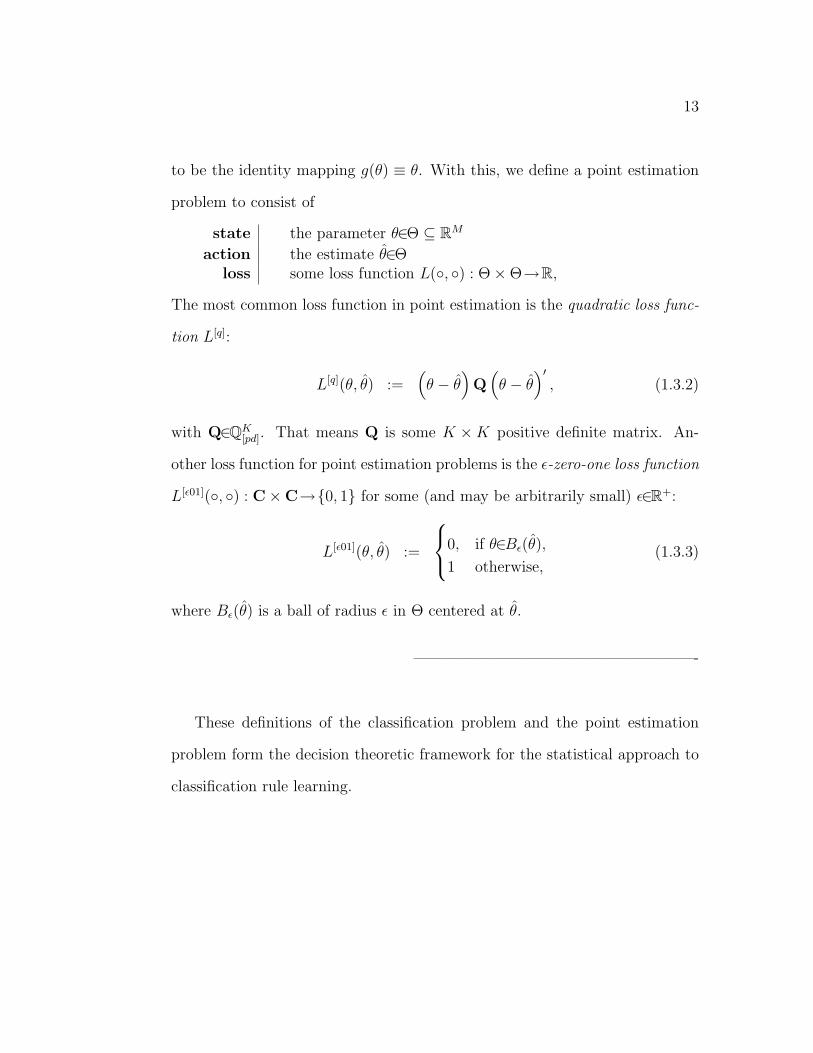
13

to be the identity mapping g(θ) ≡ θ. With this, we define a point estimation

problem to consist of

state the parameter θ∈Θ ⊆ RM

action the estimate θ∈Θloss some loss function L(, ) : Θ×Θ→R,

The most common loss function in point estimation is the quadratic loss func-

tion L[q]:

L[q](θ, θ) :=(θ − θ

)Q

(θ − θ

)′, (1.3.2)

with Q∈QK[pd]. That means Q is some K ×K positive definite matrix. An-

other loss function for point estimation problems is the ε-zero-one loss function

L[ε01](, ) : C×C→0, 1 for some (and may be arbitrarily small) ε∈R+:

L[ε01](θ, θ) :=

0, if θ∈Bε(θ),

1 otherwise,(1.3.3)

where Bε(θ) is a ball of radius ε in Θ centered at θ.

——————————————————-

These definitions of the classification problem and the point estimation

problem form the decision theoretic framework for the statistical approach to

classification rule learning.

Chapter 2

Statistics

We will describe statistical solutions to decision theoretic problems, based on

the presentations in Berger (1995) and Bernardo and Smith (1994), but also

Mood et al. (1974), Gelman et al. (1995), and Lehmann (1983). We will

describe two main decision theoretic schools, namely the Bayesian and the

frequentist or (classical) school. For a current overview and references to the

many more statistical frameworks, we refer to Barnett (1999).

2.1 Basic Definitions

In Definition 1.3.1, we follow Berger (1995) in assuming a certain ”true state

of the world”, as this is common and convenient. We want to focus on simi-

larities and differences of certain perspectives on decision problems, such that

a common definition of the basic elements seems inevitable. From a puristic

Bayesian point of view, though, we would rather prefer to define potentially

observable, yet currently unknown events upon some assumed external, ob-

jective reality. Therefore, Bernardo and Smith (1994) define slightly different,

but related basic elements of a decision problem. This is just one exemplary

14

15

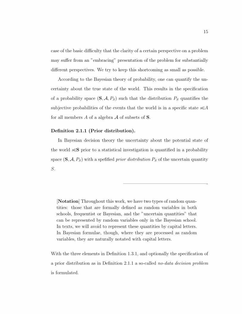
case of the basic difficulty that the clarity of a certain perspective on a problem

may suffer from an ”embracing” presentation of the problem for substantially

different perspectives. We try to keep this shortcoming as small as possible.

According to the Bayesian theory of probability, one can quantify the un-

certainty about the true state of the world. This results in the specification

of a probability space (S,A, PS) such that the distribution PS quantifies the

subjective probabilities of the events that the world is in a specific state s∈Afor all members A of a algebra A of subsets of S.

Definition 2.1.1 (Prior distribution).

In Bayesian decision theory the uncertainty about the potential state of

the world s∈S prior to a statistical investigation is quantified in a probability

space (S,A, PS) with a spefified prior distribution PS of the uncertain quantity

S.

——————————————————-

[Notation] Throughout this work, we have two types of random quan-

tities: those that are formally defined as random variables in both

schools, frequentist or Bayesian, and the ”uncertain quantities” that

can be represented by random variables only in the Bayesian school.

In texts, we will avoid to represent these quantities by capital letters.

In Bayesian formulae, though, where they are processed as random

variables, they are naturally notated with capital letters.

With the three elements in Definition 1.3.1, and optionally the specification of

a prior distribution as in Definition 2.1.1 a so-called no-data decision problem

is formulated.

16

To obtain information about the true state of the world a statistical investi-

gation is performed. This investigation is deemed a conceptual random ex-

periment with elementary events ω∈Ω and corresponding probability space

(Ω,A, P ). The events of this experiment are described by some random vari-

able X() : Ω → X ⊆ R, or by some random K-dimensional row vector

~X() : Ω→X ⊆ RK , K∈N, and X in this context is called sample space.

[Notation] We will denote real valued random quantities always with

capital letters, preferably Latin letters from near the end of the alpha-

bet. As an exception, we will use V to denote general random quanti-

ties, real-valued variables or vectors. Also, we use the corresponding

small letter to denote a value of the random quantity V = v, v∈X. We

only consider discrete and continuous random variables and possibly

mixed vectors of discrete and continuous random variables. Whenever

defining a function of a random variable, we assume it to be measur-

able. The distribution of a random quantity V∈X is denoted by PV ,

and the corresponding density with p(v), v∈X. We write V ∼ PV to

say, V is a random quantity with distribution PV . Ignoring subtleties

with respect to sets of measure zero, we use the terms ”distribution”

and ”density” interchangeable. In case of discrete random variables,

we define X to be minimal in the sense, that only values with positive

probability are included: X =v∈RK : p(v) > 0

. We note corre-

sponding integrals for integrable functions f : X→R with respect to

the counting measure and the Lebesgue measure both with

∫

X

f(v)p(v)dµ(v) =

∑v∈X f(v)p(v) discrete case,∫

Xf(v)p(v)dv continuous case.

(2.1.1)

If the distribution of V is dependent on some other quantity q, we

note this by PV |q and p(v|q), v∈X.

Of course, the outcome of the statistical investigation has to be informative

about the true state of the world s, or, in other terms, the probability distri-

bution P ~X of ~X has to depend upon s, denoted by P ~X|s, s∈S. This defines

17

”being informative” mainly from the perspective of the frequentist school in

statistics (see Section 2.2.2). From the Bayesian perspective being informa-

tive is translated the other way round: we know how our uncertainty prior

to the statistical investigation — coded in PS — changes after observing ~x.

The changed uncertainty is quantified in the so-called a-posteriori distribution

PS|~x, and PS|~x and PS differ at least for some ~x∈X. The update mechanism

for determining PS|~x for all ~x∈X in the Bayesian context is derived from the

specification of the joint distribution P ~X,S of S and ~X that can be decomposed

in the a-priori distribution PS and the sampling distribution which we also call

the informative distribution P ~X|s for all s∈S (see Section 2.2.1).

Therefore, it is no offence to the Bayesian formalism to describe the model

assumptions common to the Bayesian and the frequentist approaches on the

basis of P ~X|s. These model assumptions are comprised in a statistical model:

Definition 2.1.2 (Statistical Model).

A statistical model Λ codes the distributional assumptions about the dis-

tribution of a random vector ~X with counterdomain X in a triple

Λ :=(X,A,P ~X|S

),

where (X,A) is some measurable space, and P ~X|S :=

P ~X|s, s∈S

is a corre-

sponding class of distributions.

——————————————————-

Definition 2.1.3 (Statistical Investigation).

A statistical investigation consists of the data ~x and a representation of the

information content in ~x on s∈S. This is coded in a statistical model Λ that

18

specifies the distributional assumptions about the data generating process of ~x

in dependence on s∈S. And – optionally – the uncertainty about s is quantified

in a prior distribution PS. A statistical investigation thus consists of

information some observed data ~x,

representation Λ :(X,A,P ~X|S

)and optionally some

prior distribution PS.

We will indicate the origin of the density of a random variable ~X within a

certain statistical model by writing p(~x|s,Λ).

——————————————————-

The density of the sampling distribution p(~x|s,Λ) is sometimes perceived as a

function l~x(|Λ) : S→R+0 in s for fixed ~x:

l~x(s|Λ) := p(~x|s,Λ), s∈S. (2.1.2)

It is then called likelihood function.

On the basis of the formalization of decision problem in Chapter 1 and the

definition of a statistical investigation, we can now define a scheme for a com-

prised representation of various statistical approaches to classification that we

will use to clarify their similarities and distinctions:

Definition 2.1.4 (Scheme for Statistical Decision Problems). In this

work, statistical decision problem are instantiated by specifying the basic el-

ements of a decision problem 1.3.1 and modelling a statistical investigation

2.1.3.

19

state some true state from a set of states of the world, s∈S,action some chosen action from a set of possible actions a∈A,

loss a loss function L(, ) : S×A→R,information some observed data ~x,

representation some statistical Λ :(X,A,P ~X|S

)and optionally some

prior distribution PS.

——————————————————-

We do so to define the statistical classification problem and the statistical point

estimation problem.

Definition 2.1.5 (Statistical Classification Problem).

In a statistical classification problem, we want to assign some object ω∈Ωinto one and only one class c∈C. And we assume, any ω∈Ω belongs to one

and only one of these classes c(ω)∈C. We take measurements ~x(ω) on the

object. The measured entities are often called predictors, the corresponding

space X the predictor space. The information content of ~x(ω) on c(ω) is coded

in a statistical model Λ that specifies distributional assumptions about the

data generating processes for the measurements on objects belonging to each

of the classes c∈C, the class of informative distributions. In addition, the

uncertainty about the true class c(ω) of the object ω prior to the measurement

may be coded in the prior distribution PC . In its comprised form, the statistical

classification problem reads as follows:

state the true class c(ω)∈C for the given ω∈Ω,action the assigned class c(ω)∈C,

loss the zero-one loss function L = L[01],information some measurements ~x(ω),

representation Λ :(X,A,P ~X|C

)and optionally some prior distribution

PC .

20

——————————————————-

Definition 2.1.6 (Statistical Point Estimation Problem).

We set up the statistical point estimation problem by assuming ~xn∈X ⊆RK , n = 1, ..., N , to be the realization of a random sample of size N from a

population with distribution P ~X|θ∈P ~X|Θ for some θ∈Θ ⊆ RM . That is our sam-

ple space is given by XN := ×Nn=1X, and corresponding product measurable

space(XN ,AN

). The joint density p(~x1, ..., ~xN |θ) of a random sample factors

as follows:

p(~x1, ..., ~xN |θ) =N∏

n=1

p(~xn|θ).

The corresponding product distribution⊗N

n=1 P ~Xn=

⊗Nn=1 P ~X is denoted by

PN~X

. In other words, the random vectors ~X1, ~X2, ..., ~XN are identically and

independently distributed (i.i.d.), according to P ~X|θ for some θ∈Θ. The scheme

of the statistical point estimation problem reads as follows:

state the parameter θ∈Θ ⊆ RM ,

action the estimate θ∈Θ,loss some loss function L(, ) : Θ×Θ→R,

information ~xn∈RK , n = 1, ..., N ,representation Λ :(

X,A,P ~X|Θ)N

:=(XN ,AN ,

PN

~X|θ, θ∈Θ)

and optionally some prior distribution Pθ.

——————————————————-

A reasonable method to decide on an action in a statistical decision problem is

to look at the ”expected” loss of making a decision, dependent on the statistical

investigation, and to minimize it.

21

2.2 Derivations of Expected Loss

We will present two standard types of ”expected” loss, defined according to

the Bayesian and to the frequentist approach to statistical inference.

[Notation] Here and in the following, we will denote with E(g(V ))

the expected value of some integrable function g(V ) with respect to

the distribution PV of some random variable V∈X:

E(g(V )) :=

∫

X

g(v)p(v)dν(v).

If the distribution of V depends on some other quantity q this will be

denoted either with E(g(V )|q) or with EV |q(g(V )), whichever seems

to be more useful in a given situation.

2.2.1 Bayesian Approach

In the Bayesian context, PS quantifies the uncertainty we have about the state

of the world. This enables Bayesians to quantify the expected loss of some

action a∈A in a decision problem by the weighted average loss with respect to

the prior distribution PS:

ρ (a, PS) := E (L(S, a)) =

∫

S

L(s, a)p(s)dµ(s). (2.2.1)

After the investigation, given the observed data ~x, the uncertainty about

the state of the world is changed according to simple probability calculus ap-

plied on the distributional assumptions in Λ. In Λ the full Bayesian probability

model is defined, that is the joint probability distribution of the unknown state

22

of the world and the yet unobserved data of the statistical investigation:

p(s, ~x|Λ) = p(s|~x,Λ)p(~x|Λ)

= p(~x|s,Λ)p(s|Λ).

Typically this is done by specifying the prior distribution PS and the sampling

distribution P ~X|s. We denote the joint probability and its decomposition by

PS, ~X = PS ⊗ P ~X|S.

The update-mechanism on the basis of the full Bayesian model results in:

p(s|~x,Λ) =p(~x|s,Λ)p(s|Λ)

p(~x|Λ)(2.2.2)

=p(~x|s,Λ)p(s|Λ)∫

Sp(~x|s,Λ)p(s|Λ)dµ(s)

. (2.2.3)

The updated uncertainty is thus quantified in PS|~x,Λ, the so-called posterior

distribution.

When deciding for a∈A, we now expect a weighted average loss with respect

to the posterior distribution PS|~x,Λ:

ρ (a, PS|~x,Λ) = E (L(S, a)|~x,Λ) =

∫

S

L(s, a)p(s|~x,Λ)dµ(s).

Appropriate Bayesian modelling is an art of its own, elaborated extensively

in Bernardo and Smith (1994). The Bayesian school is often criticized for

the use of prior distributions, when there is not some knowledge (considered

objective) that justifies to possibly favor one state over the other. The influence

of a specific subjective prior on the final decision is from the perspective of

many scientists objectionable. For large data sets, though, there is not really a

problem: under appropriate (and typically fulfilled) conditions, when using the

Bayesian update mechanism for more and more data, the influence of the prior

23

distribution vanishes (Bernardo and Smith, 1994, Section 5.3). For moderate

sample sizes there exists a vast number of literature on how to define so-called

non-informative priors. Bernardo and Smith (1994, p. 357) call the search for

non-informative priors that ”let the data speak for themselves” or represent

”ignorance” the search for a Bayesian ”Holy Grail” . We share their view that

the search for a kind of ”objective” prior is misguided, as Put bluntly: data

cannot ever speak for themselves; (Bernardo and Smith, 1994, p. 298). With

careful consideration, what the unknown quantity of interest in an investigation

really is, what can be achieved are ”minimally informative” priors, chosen

relative to the information which can be supplied by a particular experiment.

The corresponding theory of reference priors is presented in Bernardo and

Smith (1994, Section 5.4).

In case of the statistical classification problem the reference prior and the

non-informative priors from any principle to derive non-informative priors co-

incide:

p(c) := 1/G, for all c∈C = 1, ..., G . (2.2.4)

In return to the effort of careful modelling, the basic Bayesian principle for

making a decision is very simple and straightforward:

Principle 2.2.1 (Conditional Bayesian Principle).

In any statistical decision problem, always choose an action a∈A that min-

imizes the Bayesian expected loss given the current knowledge:

a[B](L) := arg mina∈A

ρ(a, PS|~x,Λ)

(2.2.5)

24

The word ”conditional” emphasizes the fact that with the conditional Bayesian

principle, we are looking for the best decision conditional on a given body of

acquired knowledge, subject to the specific, observed data ~x. This is one of

the major differences to the frequentist approach, as you will see in Section

2.2.2.

Applying the conditional Bayesian principle to the statistical classification

problem set up in Definition 2.1.5 results in assigning the object ω with mea-

surement ~x(ω) to the class with lowest error probability (cp. (2.2.7)) and the

highest posterior probability (cp. (2.2.8)):

c[B] = arg minc∈C

ρ

(c, PC|~x,Λ

)

= arg minc∈C

E

(L[01](C, c)|~x,Λ

)(2.2.6)

= arg minc∈C

∫

C

L[01](c, c)p(c|~x,Λ)dµ(c)

= arg minc∈C

∑c∈Cc6=c

p(c|~x,Λ)

= arg minc∈C

1− p(c|~x,Λ) (2.2.7)

= arg maxc∈C

p(c|~x,Λ) . (2.2.8)

With the factorization

p(c|~x,Λ) =p(c, ~x|Λ)∑

g∈C p(g, ~x|Λ)=

p(c|Λ)p(~x|c,Λ)∑g∈C p(g, ~x|Λ)

,

and because the denominator does not depend on c, we present the final as-

signment as it is most often cited:

c[B] = arg maxc∈C

p(c|~x,Λ) (2.2.9)

= arg maxc∈C

p(c|Λ)p(~x|c,Λ) . (2.2.10)

25

Concerning the statistical point estimation problem, the posterior uncer-

tainty about the true parameter θ∈Θ is coded in Pθ|~x,Λ. If one wants to decide

for a single best estimate θ, this depends on the specified loss.

For the quadratic loss 1.3.2 the best estimate is the mean of the posterior

distribution (see Bernardo and Smith, 1994):

θ[B](L[q]) = arg minθ∈Θ

E(L[q](θ, θ)|~x,Λ

)(2.2.11)

= E (θ|~x,Λ) . (2.2.12)

The Bayes estimate with respect to the ε-zero-one loss given in (1.3.3) for

ε→0, ε > 0, is the mode of the posterior distribution (see Bernardo and Smith,

1994, and compare with (2.2.6) and (2.2.8)):

θ[B](L[ε01]) = limε→0+

arg minθ∈Θ

E(L[ε01](θ, θ)|~x,Λ

)(2.2.13)

= limε→0+

arg maxθ∈Θ

∫

Bε(θ)

p(θ|~x,Λ)dµ(θ). (2.2.14)

The mode of the posterior distribution is also called the maximum a-posteriori

estimate (MAP) of θ.

The conditional Bayesian principle is an implementation of another basic

principle of statistical inference, the so-called likelihood principle:

Principle 2.2.2 (Likelihood Principle).

Given a decision problem 1.3.1, all the information about the state of the

world that can be obtained from a statistical investigation is contained in the

likelihood function l~x(|Λ) for the actual observation ~x. Two likelihood func-

tions (from the same or different investigations) in statistical models Λ1 and

26

Λ2 contain the same information about the state of the world, if they are pro-

portional to each other:

l~x1(s|Λ1)

l~x2(s|Λ2)≡ r, r∈R, for all s∈S.

The maximum-likelihood point estimation follows another implementation

of the likelihood principle:

Definition 2.2.1 (Maximum Likelihood Estimation).

Let θ[ML]∈Θ be the parameter value under which the data ~x would have

had the highest probability of arising:

θ[ML] = arg maxθ∈Θ

l~x(θ|Λ),

If this parameter value exists, then according to the maximum likelihood prin-

ciple, this is the best estimate of θ.

——————————————————-

Note that this principle makes no use of any definition of loss, and has not

been derived as an optimal solution to a decision problem. Yet, maximum-

likelihood estimation is widely used, because it has high intuitive appeal and

often the resulting estimators have desirable properties also from the perspec-

tive of other approaches. In particular asymptotically, that is for N →∞ in

Definition 2.1.6, the maximum-likelihood estimation can be justified from the

Bayesian perspective (see Gelman et al., 1995), as well as from the frequentist

perspective (see Lehmann, 1983).

27

2.2.2 Frequentist approach

In the frequentist school, we think of the state of the world as being unknown

but fixed. The information in the data ~x of the statistical investigation is

modelled by assuming ~x to be the realization of some random vector ~X, dis-

tributed according to P ~X|s depending on s. According to the frequentist school

probabilities are the limiting values of relative frequencies in indefinitely long

sequences of repeatable (and identical) situations (Barnett, 1999, p.76). De-

spite the difficulties when formalizing this ”notion” of probability to some

”definition” (see also Barnett, 1999, Section 3.3) it is a notion that motivates

many statistical procedures. This is also true in statistical decision theory

where from a frequentist point of view the goal is no longer only to decide

for the best action given the one observed ~x at hand, which is targeted when

applying the conditional Bayesian principle. A frequentist wants to decide for

some action following some decision rule that minimizes what she expects to

lose if this rule was repeatedly used with varying random ~X∈X.

Definition 2.2.2 (Decision Rule).

Let A be the action space of some decision problem and X be the sample

space of some related statistical investigation.

A non-randomized decision rule is a function

δ() : X→A.

If ~x∈X is the observed value of the sample information, then δ(~x)∈A is the

action that will be taken. The space of all non-randomized decision rules will

be denoted by ∆.

28

A randomized decision rule

δ∗(, ) : X×AA→ [0, 1]

is — for given ~x∈X — a probability distribution PA|~x with corresponding mea-

surable space (A,AA). If ~x∈X is the observed value of the sample information,

then δ∗(~x,B) is the probability that some action a∈B ⊆ AA will be taken. The

space of all non-randomized decision rules will be denoted by ∆∗.

Decision rules for estimation problems are called estimators and decision

rules for classification classification rules.

——————————————————-

The expected loss in terms of the frequentist approach is the hypothetical

average loss, if we used the decision rule for the outcomes of the indefinitely

number of repetitions of the statistical investigation given constant true state

s:

Definition 2.2.3 (Frequentist Expected Loss, Risk Function).

The risk function of a randomized decision rule δ∈∆∗ is defined by

R(s, δ) = E ~X|s(E ~A

(L(s, δ( ~X, A))| ~X

)), (2.2.15)

which results for a non-randomized decision rule δ∈∆ in

R(s, δ) = E ~X|s(L(s, δ( ~X))

). (2.2.16)

——————————————————-

29

Now the difficulty is that we still do not really know, what is the best decision

rule and resulting action is, because the expected loss R(s, δ) – analogously

to the individual loss L(s, a) – is dependent on the unknown true state of the

world s∈S.

Actually, we can set up a no-data decision problem, where decision rules

are actions, and the risk function is the loss function. And the frequentist

wants to decide upon the best decision rule.

Of course, the best rule would minimize R(s, δ) for all values of s∈S among

all δ∈∆∗. Such a rule is called the uniformly best rule on ∆∗. Yet, for most

problems it is not possible to find such a rule. Sometimes on a restricted set of

rules δ∈∆[r] ⊂ ∆∗, though, a uniformly best rule exists. Of course, the restric-

tions should be such that we do not feel that important rules are cancelled

out, rather that we feel that any proper rule should fulfill this requirement

anyway. A very general restriction follows the so-called invariance principle.

Informally, the invariance principle is based on the following argument (cp.

Berger, 1995):

Principle 2.2.3 (Principle of Rational Invariance).

The action taken in a statistical decision problem should not depend on the

unit of measurement used, or other such arbitrarily chosen incidentals.

To present the formal invariance principle, we need to define ”arbitrarily

chosen incidentals”. Let two statistical decision problems be defined with

corresponding formal structures, I = 1, 2, by:

30

states sI∈SI ,actions aI∈AI ,losses LI : SI ×AI→R,

Informations ~xI∈XI ,

representations ΛI :(XI ,AI ,P ~XI |SI

).

These decision problems are said to have the same formal structure, if there

exist some one-to-one transformations g : S1 → S2 and h : A1 → A2 with

corresponding inverse transformations g−1 and h−1, such that the following

statements hold true for all s1∈S1, and a1∈A1:

L1(s1, a1) = L2 (g(s1), h(a1)) ,

P ~X1|s1= P ~X2|g(s1),

And also for all s2∈S2, and a2∈A2 it is true that:

L1

(g−1(s2), h

−1(a2))

= L2(s2, a2),

P ~X1|g−1(s2) = P ~X2|s2.

Based on this, the invariance principle says:

Principle 2.2.4 (Invariance Principle).

If two statistical decision problems have the same formal structure in terms

of state, action, loss, and representation without prior distribution, then the

same decision rule should be used in each decision problem.

The invariance principle is defined without requiring the prior to be in-

variant, thus from a Bayesian perspective it is not really an implementation

31

or the principle of rationale invariance. It can be shown that the frequen-

tist invariance principle is fulfilled when applying the conditional Bayesian

principle to statistical decision problems with certain reference (respectively

non-informative) priors. For details and examples, see Berger (1995, Section

6.6).

In case of point estimation problems with a convex loss function, e.g. the

quadratic loss function, we only need to consider non-randomized decision

rules, as for any randomized decision rule one can find a non-randomized de-

cision rule which is uniformly not worse. To find some uniformly best rule the

set of non-randomized rules ∆ is further restricted to the set of the so-called

unbiased decision rules:

Definition 2.2.4 (Unbiased Decision Rule). A non-randomized decision

rule δ : X→R for an estimation problem with estimand θ∈Θ is unbiased, if

E(δ( ~X) | θ

)= θ for all θ∈Θ.

——————————————————-

From a frequentist perspective, this restriction makes sense, because it ensures

that, for infinite replications of the experiment δ( ~X1), δ( ~X2),...,δ( ~XN),... the

amounts by which the decision rule over- and underestimates θ will balance.

Often, among unbiased estimators a uniformly best can be found (Lehmann,

1983).

If on the set of rules that we want to consider, no uniformly best rule exists,

we have to follow other strategies to define what is considered the overall best

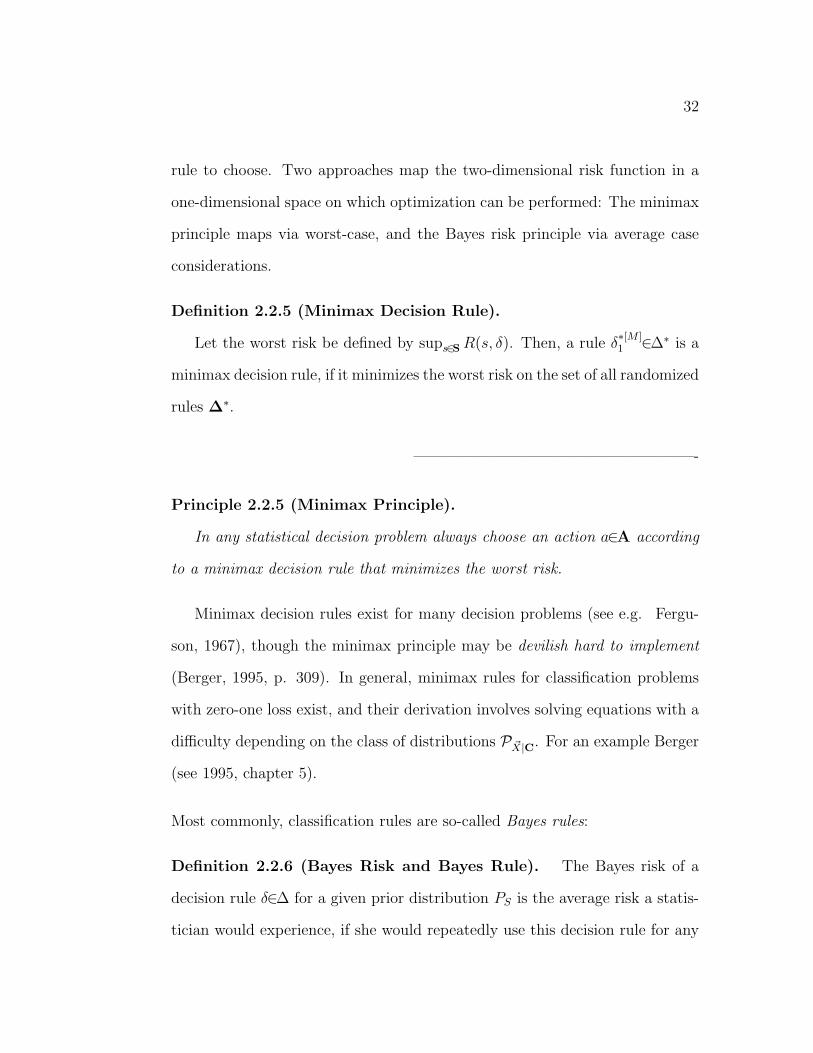
32

rule to choose. Two approaches map the two-dimensional risk function in a

one-dimensional space on which optimization can be performed: The minimax

principle maps via worst-case, and the Bayes risk principle via average case

considerations.

Definition 2.2.5 (Minimax Decision Rule).

Let the worst risk be defined by sups∈S R(s, δ). Then, a rule δ∗[M ]1 ∈∆∗ is a

minimax decision rule, if it minimizes the worst risk on the set of all randomized

rules ∆∗.

——————————————————-

Principle 2.2.5 (Minimax Principle).

In any statistical decision problem always choose an action a∈A according

to a minimax decision rule that minimizes the worst risk.

Minimax decision rules exist for many decision problems (see e.g. Fergu-

son, 1967), though the minimax principle may be devilish hard to implement

(Berger, 1995, p. 309). In general, minimax rules for classification problems

with zero-one loss exist, and their derivation involves solving equations with a

difficulty depending on the class of distributions P ~X|C. For an example Berger

(see 1995, chapter 5).

Most commonly, classification rules are so-called Bayes rules:

Definition 2.2.6 (Bayes Risk and Bayes Rule). The Bayes risk of a

decision rule δ∈∆ for a given prior distribution PS is the average risk a statis-

tician would experience, if she would repeatedly use this decision rule for any

33

potential realization of ~X:

r(PS, δ) = E (R(S, δ))

= ES

(E ~X|S

(L(S, δ( ~X))

))

A Bayes rule is any decision rule that minimizes this risk:

δ[B] = arg minδ∈∆

r(PS, δ)

——————————————————-

Principle 2.2.6 (Bayes Risk Minimization).

In any statistical decision problem with specified prior distribution PS, al-

ways choose an action a∈A according to a Bayes rule minimizing the Bayes

risk.

Choosing a Bayes rule only on the set of non-randomized decision rules, is

no restriction, because if a randomized Bayes rule δ∗[B]∈∆∗ with respect to a

prior distribution exists, there exists also a non-randomized Bayes rule δ[B]∈∆for this prior (cp. Ferguson, 1967, Section 1.8).

It might seem contradictious that Bayes rules are introduced as a frequen-

tist solution to the classification problem and not as a Bayesian solution. The

reason is that the characterizing difference between the Bayesian approach and

the frequentist approach is whether one wants to find best decision locally or

globally. The conditional Bayes principle favors local solutions – a best decision

given a quantification of the current uncertainty based on all available infor-

mation. And from the frequentist perspective one wants best global decisions

34

– a best rule prescribing the decision maker given any potential information

from the statistical investigation which decision to make.

2.2.3 Optimal Solutions

The basic idea about how actions should be chosen, differ a lot between the

conditional Bayesian principle and the Bayes risk principle. According to the

former, we only want to decide for the best action conditional on the observed

data, and according to the latter, we want to follow a decision rule that gives

minimum risk for indefinitely repetitions of the statistical investigation and

appendant decisions. Yet, trying to do the best locally also leads (only requir-

ing very little assumptions) to the best global rule. The assumptions have to

be such that we can apply the Fubini theorem for interchanging orders of inte-

gration for the calculation of expectations. Explicitly, the loss function has to

be a non-negative measurable function with respect to (S×X,A(S)×A(X)).

If that is fulfilled, we get

r(PS, δ) = ES

(E ~X|S

(L(S, δ( ~X))

))

= E ~X

(ES| ~X

(L(S, δ( ~X))

))

= E ~X

(ρ

(δ( ~X), PS| ~X

)), (2.2.17)

where ρ is the Bayesian expected loss given in equation (2.2.1). If for each

~x∈X that can be realized, we always decide for the action according to the

conditional Bayesian principle 2.2.1, we minimize the argument of E ~X() in

(2.2.17) for all ~x with positive density p(~x), and thus we minimize r(PS, ) for

δ∈∆ (see Berger, 1995, Section 4.4).

35

In consequence, Bayes rules are optimal solutions to a statistical classifi-

cation problem with informative distribution P ~X|C and class prior distribution

PC , both from a frequentist point of view as well as from a Bayesian point of

view.

Though the basic idea about how actions should be chosen, differ a lot be-

tween the Bayesian school and the frequentist school, an assignment to classes

with Bayes rules is an optimal solution of a statistical classification problem in

both schools. In the following, all the statistical classification rules considered

are Bayes rules with respect to zero-one loss L[01].

Combining the notation of a frequentist Bayes rule (2.2.17) and the Bayes

assignment (2.2.9), we will write Bayes rules with respect to a pecific statistical

model Λ in the following way:

c(~x|bay) = arg maxc∈C

p(c|Λ)p(~x|c,Λ) . (2.2.18)

These rules have lowest expected error rate on X, which corresponds with the

lowest error probability with respect to some randomly chosen object ω∈X.

And locally for any given measurement ~x(ω) it assigns to the class with the

highest posterior probability.

2.3 Learning Classification Rules

In the preceding sections we have shown that Bayes rules have desirable proper-

ties in solving statistical classification problems from the Bayesian perspective

as well as from the frequentist perspective — under the assumption that we

can specify the full Bayesian statistical model with prior distribution PC and

36

a class of informative distributions CP ~X|C.

Very often, such a specification is difficult to find. Firstly, a frequentist

definition of probability does not allow to code uncertainty about the class by

a distribution PC . Secondly, even more difficult it may be deemed to spec-

ify for each c, c∈C, a precise informative distribution P ~X|c. Only in very

special applications, like randomized experiments where chance is under con-

trol, a statistician of any school will feel comfortable with determining these

distributions from scratch and without additional information. In all other

cases, one would prefer to define all distributions PC and P ~X|c, c∈C, to be-

long to classes of distributions with unknown parameters, sayPC|~π, ~π∈Π

and

P ~X|θc, c∈C, θc∈Θ

. Or in other words, one specifies the joint distribution

PC, ~X|~π,θ with unknown parameters ~π∈Π and θ∈Θ.

In that way, when learning classification rules, not only ~X but also C

is modelled to be some random variable C : Ω→ C with probability space

(Ω,A, P ).

When the statistician has to learn classification rules from experience addi-

tional information about these unknown or uncertain parameters is available.

Definition 2.3.1 (Training Set).

The additional information that can be used to learn classification rules

from experience consists of a number of already observed objects with known

class membership, the so-called training set L:

L := (c, ~x)(ωn), ωn∈Ω, n = 1, ..., NL ,

= (cn, ~xn)n = 1, ..., NL ,

:= cn, ~xn, n = 1, ..., NL .

37

The third representation allows for statements like cn∈L or ~xn∈L, which are

often convenient.

——————————————————-

In the standard statistical approach, the training set L is treated to be a ran-

dom sample from the joint distribution PC, ~X|~π,θ, and the new object to assign

is deemed to be another independent random draw from that distribution.

This is typically not fulfilled in data mining applications (see Section 1.1), but

nonetheless the default way to proceed. Of course, if one knows about certain

dependencies among the objects, more sophisticated statistical models can and

should be deployed, see e.g. Chapter 7.

The class of distributions from which to choose PC is not controversial,

as it is a distribution over a finite number of potential outcomes c∈C. All

potential distributions are elements of the class of multinomial distributions

with unknown class probabilities πc ≥ 0, c∈C such that∑

c∈C πc = 1.

Definition 2.3.2 (Unit Simplex).

The space of vectors ~u with non-negative elements that sum up to one is a

so-called unit simplex, and will be denoted by UG ⊂ [0, 1]G.

——————————————————-

When we say, the class distribution PC is a multinomial distribution with

parameter n = 1 for the ”sample size” and parameter vector ~π∈UG for the

”class probabilities” this is slightly imprecise. It is actually the random unit

vector ~EC(C)∈UG that is multinomially distributed, with elements Ec(C), c∈C

38

defined as

Ec(C) := Ic(C) :=

1, if C = c, c∈C0 otherwise.

(2.3.1)

In general, IA : RM →0, 1 denotes the indicator function of some set A ⊆RM . And we represent the multinomial distribution with parameters 1 and ~π

by PC|~π = MN(1, ~π).

Definition 2.3.3 (Class and Class Indicators).

Let C be the random variable C() : Ω → C representing the class of

some object ω∈Ω with probability space (Ω,A, P ). The vector ~EC(C) given

in (2.3.1), is a one-to-one mapping of this random variable. We call it the

vector of class indicators.

——————————————————-

Defining an appropriate class for the informative distributions P ~X|θcwill be

dependent on the application.

Definition 2.3.4 (Statistical Classification Problem with Learning).

In a statistical classification problem with learning we are given a statistical

classification problem, but the representation of the information content of the

measurement on the classes is incomplete: the informative distribution P ~X|c is

specified in dependence on some parameter θc∈Θ with different but unknown

values for the classes P ~X|θc, c∈C. Whether Bayesian or non-Bayesian, the

prior class distribution PC is specified to be a multinomial distribution with

unknown class probabilities ~π: PC|~π = MN(1, ~π). This results in defining a

39

joint distribution PC, ~X|~π,θ∗ decomposed into PC, ~X|~π,θ∗ = MN(1, ~π)⊗P ~X|θC, with

θ∗∈ΘG, θC∈Θ . In the Bayesian approach, we quantify the uncertainty about

the parameters in the distribution P~π,θ1,...,θG.

The task is to assign a new object ω∈Ω to one of the classes, given these

incomplete distributional assumptions and some training data consisting of

NL objects with known classes and measurements. These are assumed to be a

random sample from the joint distribution PC, ~X|~π,θ∗ .

state the true class c(ωNL+1)∈C for the new object ωNL+1∈Ω,action the assigned class c(ωNL+1)∈C,

loss the zero-one loss function L = L[01],information some measurements ~x(ωNL+1),experience L = (cn, ~xn), n = 1, ..., NL,

representation Λ :(C×X,A,

MN(1, ~π)⊗ P ~X|θC

, ~π∈UG, θC∈Θ)NL+1

,

and , optionally, some prior distribution P~π,θ∗ .

——————————————————-

There are two basic strategies to solve a statistical classification problem

with learning:

• Decompose the task in two decision problems, one estimation problem for

the parameters, and one statistical classification problem for the assign-

ment and solve them one after the other. This results in so-called plug-in

Bayes rules, abbreviated with pib . This strategy will be described in

Section 2.3.1.

• Do not differentiate between ”experience and information”. Use both

as ”information”, and solve the ”problem with learning” as statistical

40

classification problem. This results in so-called predictive Bayes rules,

abbreviated with peb , and presented in Section 2.3.3.

2.3.1 Plug-in Bayes Rules

In the first approach, typically one estimates θ and ~π separately according

to some principle for point estimation, and then assigns to classes using the

resulting so-called plug-in Bayes rule.

For estimating the parameters of PC|~π, one counts the number of objects

in the training set L in each class. This results in the vector of frequencies

~fL∈NG, with elements defined by

fc|L =

NL∑n=1

Ic(cn), c∈C. (2.3.2)

The c1, .., cNLare assumed to be realizations of a random sample C1, ..., CNL

from MN(1, ~π), therefore the corresponding random vector of class frequencies

~F∈NG is distributed according to MN(NL, ~π).

1. Estimation of the parameters of the class distribution

state the parameter ~π∈UG,action the estimate ~πL∈UG,

loss some loss function L(, ) : UG ×UG→R,

information vector of observed frequencies ~fL∈NG,representation Λ1 :

(NG,A,

MN(NL, ~π) , ~π∈UG)

optionally someprior distribution P~π.

41

2. Estimation of the parameters θ of the informative distributions:

state the parameters θc∈Θ ⊆ RM , c∈Caction the estimates θc|L∈Θ,

loss some loss function L(, ) : Θ×Θ→R,information training set L := (cn, ~xn), n = 1, ..., NL

representation Λ2 :(XNL ,ANL ,

⊗NL

n=1P ~X|θcn, θcn∈Θ

)optionally some

prior distributions Pθc , c∈C.

3. Assignment:

state the true class c(ωNL+1)∈C for the given ωNL+1∈Ω,action the assigned class c(ωNL+1)∈C,

loss the zero-one loss function L = L[01],information some measurements ~x(ωNL+1),

representation Λ3 :(X,A,

P ~X|θc|L

, c∈C)

and PC|~πL.

The plug-in Bayes rule for the representation Λ = Λ1,Λ2,Λ3 is given

by:

c (~xNL+1|L,Λ) = arg maxc∈C

p(c|~xNL+1, θc|L~πL,Λ3

)(2.3.3)

= arg maxc∈C

p (c|~πL,Λ1) p

(~xNL+1|θc|L,Λ2

). (2.3.4)

In the next section, the plug-in procedure will be exemplified by introducing

two common classification methods in statistics: the linear and the quadratic

discriminant analysis.

42

2.3.2 Example: Linear and Quadratic Discriminant Clas-

sifiers

The origin of discriminant analysis goes back to Fisher (1936), who developed

a ”discriminant” rule for two classes. His original justification rests upon an

approach to classification as a special type of regression, with the predictors as

regressor variables and the class as regressand. And the Fisher linear discrimi-

nant function maximizes the separation between classes in a least-squares sense

on the set of all linear functions. Later, one revealed that the corresponding

classification rule was also a plug-in Bayes rule under the assumption that the

predictors are multivariate normally distributed with unequal means in the

classes and equal covariance matrices. For the prove, we refer to McLachlan

(1992).

The class distribution is both in linear and in quadratic discriminant anal-

ysis (LDA and QDA) modelled as being multinomial PC|~π = MN(1, ~π) with

unknown parameters ~π∈UG. The measurements ~x(ω) on some object ω∈Ωare modelled as realizations of continuous random vectors — the predictors —

from the space of real vectors, ~X∈X = RK . The sampling distributions P ~X|θc

are multivariate normal distributions with unequal mean vectors ~µc∈RK for

objects in different classes, c∈C. This is also called a gaussian modelling. LDA

and QDA differ in their assumption about the covariance matrices Σc, c∈C, of

the normal distributions: in QDA they may be different in the different classes,

in LDA one assumes the same covariances for the distributions in each class,

that is Σc ≡ Σ.

We implement LDA and QDA as plug-in Bayes rules. Thus, we have to do

43

point estimation for the parameters ~π and ~µc,Σc resp. Σ, c∈C.

1. Estimation of the parameters of the multinomial distribution

state the parameter, ~π∈UG,action the estimate ~πL∈UG,

loss quadratic loss function Lq,

information vector of observed frequencies ~fL∈NG,representation Λ1 :

(NG,A,

MN(N,~π) , ~π∈UG)

optionally someprior distribution P~π,

strategy direct computation of optimal solution with respect toquadratic loss respectively according to the maximumlikelihood principle.

The parameters ~π are estimated by the observed relative frequencies on the

training set L:

~πL :=~fL

NL

. (2.3.5)

The estimator ~πL is at the same time the maximum-likelihood estimator for ~π

and the uniformly best unbiased estimator with respect to the quadratic loss

(e.g. Lehmann, 1983).

2. Estimation of the parameters of the multivariate normal dis-

tributions:

state the parameters, µc∈RK , Σc∈QKpd, c∈C

action the potential estimates µc|L∈RK , Σc|L∈QKpd, c∈C,

loss quadratic loss function Lq defined for a vector of all pa-rameters,

information training set L := (cn, ~xn), n = 1, ..., NQDA-repr. Λ2 :

((RK)N ,AN ,

⊗Nn=1N (~µcn ,Σcn) , ~µcn∈RK ,Σcn∈QK

pd

).

LDA-repr. Λ2 :((RK)N ,AN ,

⊗Nn=1N (~µcn ,Σ) , ~µcn∈RK ,Σ∈QK

pd

),

strategy direct computation of optimal unbiased solutions ac-cording to the maximum likelihood principle.

We estimate the vector of means ~µc by the vector of the empirical means

of all objects belonging to class c on the learning set. The elements of ~µc|L are

44

given by:

µk,c|L :=

1

fc|L

NL∑n=1

(Ic(cn)xk,n) , c∈C. (2.3.6)

The resulting estimator(~µ1|L, ...~µG|L

)is at the same time the maximum-

likelihood estimator and the uniformly minimum risk estimator of (~µ1, ...~µG).

The maximum-likelihood estimator of the covariance matrices Σc of the

QDA-model is the empirical covariance matrix:

Σ[ML]c|L :=

1

fc|L

NL∑n=1

(Ic(cn)

(~xn−~µc|L

)′ (~xn−~µc|L

)), c∈C.

We follow the usual practice of estimating Σc with the unbiased estimator,

the so-called sample variance

Sc|L :=

fc|Lfc|L−1

Σ[ML]c|L (2.3.7)

The resulting estimator(~µ1|L, ...~µG|L,S

1|L , ...,SG|L

)is the uniformly minimum

risk estimator of (~µ1, ...~µG,Σ1, ...,ΣG) with respect to quadratic loss (McLach-

lan, 1992).

The maximum-likelihood estimator of the common covariance matrix Σ

of the LDA-model is the so-called pooled within-group empirical covariance

matrix:

Σ[ML]L

:=1

NL

G∑c=1

(fc|LΣ

[ML]c|L

).

We also use the unbiased variant for estimating the common covariance of the

LDA-model:

SL :=NL

NL−GΣ[ML]

L.

45

The final plug-in Bayes rule for the QDA is thus given by:

c (~x|L, qda) = arg maxc∈C

fc,L

NL

p(~x|~µc|L,Sc|L

), (2.3.8)

where p(|~µc|L,Sc|L

)is the density of the multivariate normal distribution:

p(~x|~µc|L,Sc|L

)=

(2π)−K2 det

(Sc|L

)−12 exp

(−1

2

(~x−~µc|L

)S−1

c|L(~x−~µc|L

)′)(2.3.9)

The joint faces fc,g of the partitions between two classes for these continuous

densities are given implicitly by the equations

p(c|~x, ~πL, ~µc|L,Sc|L

)= p

(g|~x, ~πL, ~µg|L,Sg|L

), c 6= g, c, g∈C.

The form of these borders is the origin of the names of the methods: After

taking the logarithm and some other minor transformations, one can see that

these implicit functions are in case of QDA quadratic functions of ~x.

The argmax rule of LDA is the same as the argmax rule of QDA, only

replacing the local sample variances by the pooled sample variances. This

simplifies the implicit functions such that they can be shown to be linear

functions of ~x (see McLachlan, 1992). For the sake of completeness, we also

display the argmax rule for the LDA:

c (~x|L, lda) = arg maxc∈C

fc,L

NL

p (~x|~µc,L,SL)

. (2.3.10)

with

p(~x|~µc|L,SL

)

= (2π)−K2 det (SL)−

12 exp

(−1

2

(~x−~µc|L

)S−1

L

(~x−~µc|L

)′). (2.3.11)

46

As McLachlan (1992, p.56) puts it, there are no compelling reasons for us-

ing the unbiased variants of the covariance estimators. If unbiasedness was

considered important, one should use unbiased estimators of the ratio of the

densities, because these determine the Bayes-rule. In his book, he presents

these estimators (McLachlan, 1992).

When learning classification rules, one is not so much interested in unbiased

point estimation, rather in best classifications. These would be achieved, if the

distributional assumptions were fulfilled, and we would use a predictive Bayes-

rule, not being based on point estimation at all.

In this work, though, we focus on typical data mining situations, where any

distributional assumptions may be considerably violated, therefore theoretical

justifications of the type above are all of minor importance. And standard

estimators are used for convention and convenience.

2.3.3 Predictive Bayes Rules

We announced to present two statistical solutions to solve a statistical classi-

fication problem with learning. The first follows frequentist strategies to solve

point estimation problems for the learning and then solves the classification

problem according to the principle of Bayes risk minimization. The second

strategy, the predictive Bayes rules, is an implementation of the conditional

Bayes principle. It aims at the best local class assignment given the current

knowledge about the situation, consisting of a specific prior uncertainty about

classes and their relation to measurements on objects quantified in P~π,θ, the

47

training data L that gives us additional information about that relation, and

some measurement ~x(ω)∈X on the object ω∈Ω we have to classify.

Decision Making Given the Prior Assume for now, we had solved the

problem to specify a prior distribution P~π,θ. Then decision making according

to the conditional Bayesian principle is straightforward. Experience and infor-

mation represent the current information on which to base the decision on the

classification problem:

state the true class c(ωNL+1)∈C for the given ωNL+1∈Ω,action the assigned class c(ωNL+1)∈C,

loss the zero-one loss function L = L[01],information learning set and measurement: (cn, ~xn), n = 1, ..., NL,

~xNL+1,

representation Λ :(C×X,A,

MN(1, ~π)⊗ P ~X|θC

, ~π∈UG, θC∈Θ)NL+1

,

and some prior distribution P~π,θ1,...,θG.

——————————————————-

Applying the conditional Bayesian principle with respect to the updated model

L,Λ, results in the following predictive Bayes rule:

c[B] (~x|L,Λ) = arg maxc∈C

p (c|~x,L,Λ)

= arg maxc∈C

p (c, ~x|L,Λ)

= arg maxc∈C

p (c|L,Λ) p (~x|c,L,Λ)

= arg maxc∈C

∫

U×Θ

p (c|~π,Λ) p (~x|θc,Λ) p (~π, θc|L,Λ) dµ(~π, θc)

.

Comparing the last line with the plug-in Bayes rule exposes the main difference

between the two approaches. With the plug-in Bayes rule, one assigns to

48

the class with the highest probability computed on the basis of individual

(best) estimates of the unknown parameters. Whereas the predictive Bayes

rule assigns to the class with the highest expected probability on the basis

of the a-posteriori distribution of the parameters. Asymptotically (that is for

N → ∞) ”good” point estimators converge to the true parameters, and in

most cases, the posterior distribution converges to a normal distribution with

all mass arbitrarily close to the true parameter. Therefore, for large N , the

assignments with both approaches will not be too different.

Specifying the Prior

The open problem is, how to specify the prior distributions. In the follow-

ing we will, as is commonly done, assume that prior to the investigation the

uncertainty about ~π and the θc, c∈C was independent. In addition, the prior

uncertainty of the parameter θc is assumed to be the same for all c∈C. Then

the prior distribution can be factorized P~π,θ1,...,ΘG= P~π ⊗PG

θ . In consequence,

the updating of the distribution of the parameters can also be decomposed:

p (~π, θ|L,Λ) =p (L|~π, θ) p (~π, θ|Λ)

k(L)

=1

k(L)

N∏n=1

p (cn, xn|~π, θ) p (~π|Λ) p (θ|Λ)

=1

k(L)

(N∏

n=1

p (cn|~π) p (~π|Λ)

)(N∏

n=1

p (xn|θcn) p (θcn |Λ)

).

This is often very helpful for the computation. It is not necessary to calculate

the constant term k(L), as it has no influence on the relative size of p (c|~x,L,Λ)

among the classes, and thus no influence on the final assignment into one of

49

the classes.

For defining the form of the prior distributions, we will use standard natural

conjugate prior modelling.

Definition 2.3.5 (Family of natural conjugate priors).

Let F :=p(|θ) : X→R+

0 , θ∈Θ

define the densities of the class of infor-

mative distributions, and P :=p() : θ→R+

0

a class of prior densities for

θ∈Θ. Then the class P is called conjugate for F if

p(θ|~x)∈P for all p(|θ)∈F and p()∈P .

This definition is vague so far, as e.g. the class of all distributions is conjugate

to any class of sampling distributions. If in addition, the densities belonging

to P are of the same functional form as the class of likelihood functions arising

from F , then P is called the natural conjugate prior family to F .

——————————————————-

With natural conjugate priors, not only the tractability of Bayesian updat-

ing is highly improved, but also the effects of prior and sample information can

be easily understood: we start with a certain functional form for the prior, and

we end up with a posterior of the same functional form, but with parameters

updated by the sample information.

Assume the class of prior distributions Pθ|Ψ :=p(|ψ) : Θ→R+

0 , ψ∈Ψ

to

be uniquely parameterized by parameters ψ∈Ψ. If Pψ is the natural conjugate

prior for the class of informative distributions

P ~X|Θ :=p(|θ,Λ) : X→R+

0 , θ∈Θ

50

according to some model Λ then for any ~x∈X and ψ∈Ψ there exists some ψ~x∈Ψ

such that the posterior distribution is a member of Pθ|Ψ. In terms of the update

mechanism given in equation (2.2.2) this reads:

p(θ|~x,Λ) =p(~x|θ,Λ)p(θ|ψ,Λ)

p(~x|Λ)(2.3.12)

= p(θ|ψ~x,Λ) (2.3.13)

This is not only useful for tracing the influence of the prior, but also the

prior can be translated into an equivalent sample that carries the same informa-

tion. That helps determining an appropriate prior. You will see an example in

the following subsection. A general outline involves the class of regular expo-

nential distributions, canonical parameters and the relationship with sufficient

statistics. We refer the interested reader to Bernardo and Smith (1994, Section

5.2.2).

Specifying the Prior for ~π

Bayesian modelling of the informative distribution and the corresponding prior

distribution varies for predictive Bayes rules – suitable solutions are highly

dependent on the given task. Common is the problem to model the class

distribution and the corresponding prior. We will present in the following a

minimal informative conjugate modelling thereof.

Remember, PC|~π is a multinomial distribution with class probabilities πc ≥0, c∈C such that

∑c∈C πc = 1.

The natural conjugate prior family for the multinomial model is the class

of Dirichlet priors D(~α) with ~α∈(R+)G. This multinomial-Dirichlet model will

51

play an important role later in standardized partition spaces (Chapter 5, thus

it will be described below quite detailed.

By comparing the density of the multinomial distribution MN(N,~π), and

the Dirichlet distribution D(~α), you see what is meant by requiring a natural

conjugate prior to have the same functional form as the likelihood function:

p(~n|~π) =Γ (NL+1)∏Gc=1 Γ (nc+1)

G∏c=1

πncc , ~π∈UG, (2.3.14)

p(~π|~α) =Γ (α0)∏Gc=1 Γ (αc)

G∏c=1

παc−1c , (2.3.15)

with ~n∈NG,∑G

c=1 nc =NL, ~π∈UG ~α∈(R+)G ∑G

c=1 αc =α0, and Γ() denoting

the Gamma function. It is obvious that the parameter vector ~α plays the role

of the frequency vector ~n.

Updating the prior with the observed class frequencies n1|L, ..., nG|L in the

data L, the elements of the parameter vector of the posterior Dirichlet distri-

bution are:

αc|L = αc + fc|L, c∈C.

In other terms, D(~α|L)=D(~α + ~fL

).

The relationship between prior and posterior is easy to understand: the

Dirichlet distribution gathers the information about ~π in the vector of so-far

”imagined” (~α) and observed frequencies (~fL) of the classes in the data, ~α+ ~fL.

The parameters αc, c∈C embody the same information on ~π as an sample of α0

outcomes of the experiment with observed frequencies αc, c∈C does. Therefore

α0 is the so-called equivalent sample size (ESS) of the prior uncertainty.

The mean vector and the covariances of the posterior Dirichlet distribution

52

are:

E (~π|~α,L) =~α+ ~fL

α0+NL

:= ~pL,

Σ (~π|~α,L) :=[σc,g|L

]c,g∈C ,

with

σc,c|~α,L =pc,L(1− pc,L)

1+NL+α0

and

σc,g|~α,L =−pc,Lpg,L

1+NL+α0

, g 6= c, c, g∈C.

Sometimes, one wants to know the marginal distribution of the sample

entity, in this case C, given the prior with parameters ~α and the training data

L:

p(c|L, ~α,Λ) =

∫

U

(p(c|~π,Λ)p(~π|L, ~α,Λ)dµ(~π)) .

This distribution is called the posterior predictive distribution. As in case

of the multinomial distribution, the random entity for which the posterior

distribution is described is not really C but rather the vector of class indicators

~E(C)∈UG (Definition 2.3.3).

In general, the marginal distribution of some frequency vector ~F given L

and ~α in this setting is a multinomial-Dirichlet distribution Md(F•, ~α+ ~fL

)

that differs from the multinomial distribution MN(F•,

~α+~fLα0+NL

), mainly by hav-

ing larger (absolute) values for the variances and covariances.

Yet, for the special case of only one new trial, namely the distribution of

53

~E(C), the multinomial-Dirichlet distribution Md(1, ~α + ~fL

)is also a multino-

mial distribution MN(1, ~α+~fL

αo+NL

). That is, the posterior predictive distribution

is defined by the probabilities:

p(c|L,Λ) =αc+fc|Lα0+NL

, c∈C. (2.3.16)

This results in the following central moments (Bernardo and Smith, 1994,

Appendix)):

E(

~E|~α+ ~fL

)=

~α+ ~fL

α0+NL

:= ~pL, (2.3.17)

Σ(

~E|~α+ ~fL

):=

[σc,g|L

]c,g∈C , with (2.3.18)

σc,c = pc|L(1− pc|L) and (2.3.19)

σc,g = pc|Lpg|L, g 6= c, c, g∈C (2.3.20)

Now assume, our training data was appropriately modelled to the the real-

ization of some some i.i.d. sample from that multinomial class distribution and

some sampling distribution. For example, let ω∈Ω be the realization of some

random draw from some population, where ~πΩ denotes the vector of relative

frequencies of objects in the classes in this population. Then, for NL →∞,

the observed relative frequencies converge to the true relative frequencies, and

so do the elements of the mean vector of the Dirichlet distribution, and the

(co)-variances converge to zero:

fc,L

NL

→πc,Ω,αc+fc,L

αo+NL

→πc,Ω, σc,g|L→0, c, g∈C. (2.3.21)

In other words, as it should be, with more and more independent examples,

our uncertainty about the true parameter of the class distribution vanishes,

and gets centered around the true parameter.

54

Form of the conjugate prior and update mechanism have been explained

and specified above, so the final decision is on the priors’ parameters. Stan-

dard minimal informative priors are achieved by setting all αc, c∈C, either to

be equal to one, ~α := ~1, or equal to zero, ~α := ~0. In the former the prior

distribution assigns equal density to all ~π∈UG, in the latter uniform improper

density is assigned to the vector of logarithms of the elements of ~π (Gelman

et al., 1995). The density is improper, as the integral over this density is in-

finity, which violates the probability assumptions. Many minimal informative

priors are improper, which is not deemed a problem, as long as one takes care

that the resulting posterior is proper.

For the two priors under consideration, the updated posterior is either

D(

~fL

)or D

(~fL+~1

). The more objects are presented in the training data,

the less important this difference is for any class assignment as this depends on

relative frequencies. With small data sizes and with ~α = ~0, we may run into

technical difficulties: for the posterior of the prior of zeros to be proper, at least

one object in each group has to be observed. That is the main reason, why we

in general prefer ~α = ~1. The critical question is, whether the defined classes

are such that we are sure there are objects of any class in the population.

If according to our prior knowledge, we can be sure of that, but we have no

(justifiable) idea, that any class should have a higher frequency than another,

then it seems appropriate to model this with an imaginative sample of one

object in each class.

In the preceding paragraphs we have given an outline of general Bayesian

conjugate modelling and a detailed description of the multinomial-Dirichlet

55

model. In the next section, we will present you a full description of a specific

predictive Bayes rule that exemplifies the complete procedure of predictive

Bayes rules.

2.3.4 Example: Continuous Naıve Bayes Classifier

The naıve Bayes classifier is based on distributional assumptions between the

class and observed facts on some object, and thus a statistical classification

rule. Yet, it is mainly used in information retrieval, a branch of computer

science. The use of the naıve Bayes in information retrieval can be traced

back to the early 60ties (Maron and Kuhns, 1960; Maron, 1961) for automatic

text categorization, and it is still the benchmark classifier in this field. For an

overview Lewis (see 1998). Typically, the observed facts — words in a text

— are modelled with high-dimensional vectors of binary random variables,

but in our applications we use a continuous — namely gaussian — modelling.

Therefore we call the resulting classifier a continuous naıve Bayes classifier

(CNB).

As usually, the class distribution is modelled as being multinomial PC|~π =

MN(1, ~π) with unknown parameters ~π∈UG.

Given the class, predictor variables are assumed to be stochastically in-

dependent and normally distributed with unequal and unknown means and

variances, P ~X|c = N (νc,Σc), c∈C. So far, the representation is the same as

for QDA. It is different, as we impose a restriction on the set of considered

covariance matrices: all Σc have to be diagonal matrices, Σc∈QK[D], c∈C.

56

By this, we assume for given class c∈C the elements X1, ..., XK of the K-

dimensional vector ~X to be independently distributed, each according to some

univariate normal distribution PXk|c = N(µk|c, σ2

k|c), k = 1, ..., K, c∈C. This

is the independence assumption that characterizes all naıve Bayes classifiers,

whatever the type (normal, exponential, Bernoulli, multinomial,...) of the

univariate sampling distributions PXk|c, k = 1, ..., K, c∈C may be. The assign-

ment according to the conditional Bayesian principle can thus be factorized in

K + 1 factors:

c(~x|cnb) = arg maxc∈C

p(c|cnb)p(~x|c, cnb)

= arg maxc∈C

p(c|cnb)

K∏

k=1

p(xk|c, cnb)

.

Each of the factors can be quite easily learnt from the training data. The name

can be understood in the light of this simplifying effect of the independence

assumption, when one uses it although one knows, it is not really valid. Quite

nicely, it often works despite that fact!

We will use the assumptions of the continuous naıve Bayes classifier to con-

struct a predictive Bayes rule. Thus, in addition to the distributional assump-

tions stated above, we need to define the prior distribution for the parameters

~π,µk,c, σk|c, k = 1, ..., K, c∈C. In a first step, we decompose this distribution

in independent distributions for ~π, and for each pair (µk|c, σk|c), k = 1, ..., K,

c∈C.

We set the prior for the distribution P~π of the parameters of the multinomial

distribution ~π to be a Dirichlet distribution D(~1). This results in a posterior

57

predictive distribution PC|L,~α being also multinomial with probabilities

p(c|L,Λ) =αc+fc|Lα0+NL

, c∈C.

This has been shown in the preceding subsection 2.3.3.

For each pair (µk|c, σ2k|c), k = 1, ..., K, c∈C we set up the standard minimal

informative conjugate prior for the univariate normal distribution as presented

in Gelman et al. (1995). Dropping the class and variable indices for now, the

joint distribution of (µ, σ2) is factorized as Pσ ⊗ Pµ|σ. Pσ is the scaled inverse

χ2 distribution with parameter ν0 ∈ R for the degrees of freedom and σ20 ∈ R+

for the scale, denoted by invχ2(ν, σ20) and the conditional distribution Pµ|σ2 is

some normal distribution with parameters µ0 ∈ R and σ2

κ0∈ R+.

The minimal informative starting prior is an improper distribution uniform

on (µk|c, log(σ2k|c)) or, equivalently,

p(µk|c, σ2k|c) ∝ (σ2

k|c)−1.

The joint posterior distribution p(µk|c, σ2k|c|L) is proportional to the likelihood

function multiplied by the factor σ−2:

p(µk|c, σ

2k|c|L

) ∝ σ−n−2k|c exp

(−

(NL − 1)S2k|c,L + NL(µk|c,L−µk|c)

2σ2k|c

),

where µk|c,L and S2k|c,L are the univariate realizations of the empirical mean

and the sample variance as defined in (2.3.6) and (2.3.7).

The resulting posterior predictive distribution p(xk|c,L, cnb) is a Student-

t-distribution T(µk|c,L,

√1+ 1

NLSk|c,L, fc|L−1

)with fc|L−1 degrees of freedom,

location µk|c,L, and scale√

1+ 1fc|L

Sk|c,L, k = 1, ..., K, c∈C.

58

The final predictive Bayes rule is given by

c(~x|L, cnb) = arg maxc∈C

αc+fc|Lα0+NL

K∏

k=1

p(xk|c,L, cnb)

, (2.3.22)

with

p(xk|c,L, cnb) = h(fc|L,Sk|c,L)

(1 +

1

fc|L

(xk − µk|c,L

Sk|c,L

)) fc|L+1

2

,

where h is some appropriate function. Important to notice in the equation

above is the dependency of the exponent only on the observed frequencies of

objects in the classes fc|L. In consequence, the functions representing the joint

faces of the partitions of X can in general not be simplified to be quadratic

forms, only if L is a balanced sample in each class. Nevertheless, pictures of

the resulting joint faces resemble much those of the plug-in QDA, where the

joint faces are quadratic forms.

Chapter 3

Machine Learning

We embed the learning of classification rules in the corresponding machine

learning framework of concept learning. A comparable representation of meth-

ods for concept learning and classification rule learning is developed. We

present various aspects of performance that are important for concept learning,

and different theoretical frameworks that define good learning in these terms.

3.1 Basic Definitions

As learning is the main concern of machine learning, defining what it means

is a crucial point. Typically one defines learning in a broad sense such that it

covers most intuitive ideas people have about learning. According to Langley

(1995) this reads as follows:

Definition 3.1.1 (Learning).

Learning is the improvement of performance in some environment through

the acquisition of knowledge resulting from experience in that environment.

——————————————————-

59

60

Defining learning in dependence of the improvement of performance is not

mandatory and is questioned e.g. by Michalski (1986). Such a definition is

exclusive for learning incidences, where learning happens without a predefined

goal – and such a predefinition is sometimes difficult to state in data mining in

general. Yet, for classification rule learning, the difficulty is not to define some

performance criterion, but rather that the most common definition of perfor-

mance – correctness – might not cover important aspects of performance one

might want to improve. In Chapter 5 we will introduce performance aspects

that go beyond the correctness. That is, we do not question the importance

of performance for classification rule learning, we broaden the notion of per-

formance, therefore, Definition 3.1.1 is a good choice for defining learning for

our purposes. The initial point for machine learning solutions to classification

tasks is concept learning. Mitchell (1997) defines concept learning as follows:

Definition 3.1.2 (Concept learning).

Concept learning is the problem of automatically inferring the general def-

inition of some concept, given examples labelled as members or nonmembers

of the concept. In other words, concept learning is inferring a boolean-valued

function from training examples of its input and output.

——————————————————-

Based on this definition, we can now compare the general set up of classi-

fication rule learning with concept learning: In the Definition 2.1.5 of the

statistical classification problem, we distinguish between the object ω and the

measurements on the object ~x(ω), the class c(ω) being deemed some other

61

characteristic of the object. This is common in statistics and uncommon in

machine learning. Indirectly, this already says the object ω is more than its

description ~x(ω), so that the idea of a deterministic relationship between the

object’s class c(ω) and its observations ~x(ω) is immediately questionable, as

we may lack valuable information about the object.

Quite differently, the starting point in machine learning is the inference

of some concept. Other than the term class, the term concept relates di-

rectly to an idea of something by combining all its characteristics or par-

ticulars; a construct (Webster’s Dictionary, 1994). (Just as a philosophical

note in the margin: obviously one can doubt, whether ”class” can ever be

a characteristic of some object in the world or whether it always will be

some concept humans have about objects in the world.) If the examples in

L = (cn, ~xn), n = 1, ..., NL (see Definition 2.3.1) are optimally chosen, each

input ~xn should provide all information about the combined ”characteristics

and particulars” of the associated concept with number cn, n = 1, ..., NL. And

in consequence, the assumption of a probabilistic relationship appears strange.

Relating concepts and their definitions to a statistical investigation: what

would happen, if all relevant information about the class membership was

present in ~x? Then, for the classification task, there is no need to distinguish

the object ω and the information ~x. Therefore, we will equate the ”optimal

description” with the ”object”. In data mining applications, the assumption

of optimal descriptions is most commonly relaxed to allow for noise corrupting

the input and also — potentially — the output. (Throughout this work we

will not assume the latter). To allow for noise we equate the non-optimal,

62

actually available descriptions with the observed measurements on the object

~x∈X. We distinguish ”ideal concepts” from ”realizable concepts”:

Definition 3.1.3 (Ideal and Realizable Concepts). We call concepts de-

fined in terms of some optimal descriptions ω∈Ω ideal concepts, and we will

represent them by their boolean functions ec(|Ω), c∈C.

Concepts in terms of potentially incomplete or corrupted, yet available,

descriptions ~x∈X, are called realizable concepts. The corresponding boolean

functions are denoted by ec(|X), c∈C.

In the notation of certain values of these functions, we drop the identifying

domain, if the instance symbol is not ambiguous, as e.g. in ec(~x) or ec(ω),

c∈C.

——————————————————-

In Section 2.3 we presented Bayes rules as the goal of statistical classifi-

cation rule learning. We argued at the end of Section 2.2.2 that randomized

Bayes rules can not be better than deterministic Bayes rules, and restricted the

optimization to be performed only on the set of non-randomized rules. That is,

though statisticians model a non-deterministic relationship between the obser-

vation ~x(ω) and the class c(ω), the learnt classification rule c(|L, bay) : X→C

is deterministic. In that sense, statistical classification rule learning is an in-

stance of concept learning as stated in Definition 3.1.2.

[Notation] As it is common in machine learning, in Definition 3.1.2

concepts are formally defined to be boolean-valued functions, and their

domain is equated with the ”input space” X. For the reasons given

above, we define the domain of ideal concepts to be the ”optimal input

63

space” Ω. In the statistical context we already saw that for the learn-

ing of classification rules, classes are modelled to be random variables

(Section 2.3). That is, they are also functions with domain Ω, the only

difference being that these functions correspond to a probability space

(Ω,A, P ). We assimilated the statistical and the machine learning’s

representation regarding the domain.

In this work we will mainly consider multi-class problems, where each

object belongs to one and only one class of a set of classes. In Langley

(1995) this is called the competitive framework for concepts, where an

optimal description can be an instance of one and only one out of a

finite number of competing concepts. We defined the counterdomain

of the class to be C = 1, ..., G, or alternatively, using the dual rep-

resentation with the vector of class indicators ~eC the counterdomain is

UG (cp. 2.3.3). In the same way, we define the set of competing con-

cepts to be numbered by c∈C = 1, ..., G, and we denote by ~eC∈UG

the vector of the logical values of the corresponding boolean functions.

This assimilates statistical and machine learning’s representation with

respect to the counterdomain. In Table 3.1 you find the synopsis of

the assimilated notation for concept and classification rule learning.

The Definition 3.1.1 of learning rests upon four rather vague terms, namely

performance, environment, knowledge, and experience. This vagueness is in-

tended for the definition to be broad. In the following sections we will clarify

the notion of these terms in the context of this work:

In Section 3.2 we acquire the environmental factors of concept learning

as they emerge from our definition of a classification problem and from the

characteristics of data mining applications.

In Section 3.3 we devise a structure for comparable representations of meth-

ods for concept learning and classification rule learning.

In Section 3.4 we present various aspects of performance that are important

for concept learning, and different theoretical frameworks that define good

64

Symbol Statistics Machine LearningΩ population optimal input space

ω ∈ Ω object optimal descriptionC set of classes set of concept numbers

c(ω) class of object ω number of the ideal concept ofwhich ω is an instance

ec(|Ω) class indicator function forclass c

ideal concept number c

~eC(|Ω) vector of class indicatorfunctions

vector of ideal competing con-cepts

X predictor space input space~x observed measurement of

predictorsnon-optimal description

ec(|X) class indicator function forassignments to class c

realizable competing conceptnumber c

~eC(|X) vector of class indicatorfunctions

vector of realizable competingconcepts

c(|X) classification rule matching rule for numbers of re-alizable competing concepts

Table 3.1: Assimilated notation

65

learning in these terms.

And finally, in Section 3.5 we present ways how to do a good job in learning

good concepts.

3.2 Environment

Among other things, the environment determines the task, aspects of the per-

formance criterion, the amount of supervision, whether the learning system

has to learn online or offline, and the strength of the regularities on which the

learning system can base its learning (cp. Langley, 1995).

Some aspects of this environment are fixed by the main topic of this work:

The classification problem as posed in Definition 1.3.2 determines the task

and partly the related performance criterion: the zero-one loss with respect to

the correctness of the classification of some presented object. As we have seen

in the development of the statistical approaches, though, there are different

ways to extent this concrete, individual loss to an ”expected” loss with respect

to the correctness of the classification of some object with unknown class.

The experience is presented in terms of a set of objects with known classes

(see Definition 2.3.1). This constitutes the manner of learning to be completely

supervised and offline.

In data mining applications, the strength of the regularities is one of the

big questions. Learning concepts is one tool utilized in the larger context of

the knowledge discovery process, where one tries to find out about regularities

and their strengths in the database. Particularly tricky about the regularity

question is that it is only partly predetermined by the domain and the data.

66

The perceived strength of regularity also depends on the language used to

describe the regularities.

An important characteristic of regularities is whether they are probabilistic

or deterministic. In their assumptions about this, approaches in statistics and

machine learning differ the strongest. Statisticians are trained to think in terms

of (genuinely) probabilistic relationships. One way to explain probabilistic

relationships is to assume a random sample of objects from some population.

If the entities among which we want to reveal relationships are characteristics of

these objects, this random draw induces a probabilistic relationship, including

deterministic relationships as special cases.

This approach stands in contrast to the cultural habit in the machine learn-

ing community. As one can see in Definition 3.1.2, starting point is typically

some deterministic relationship, which is — if necessary — softened to allow for

noise. As the potential causes of noise, one regards e.g. corrupted supervised

feedback or input description (cp. Langley (1995)).

3.3 Representation

The designer of a learning system has to decide upon the representation of the

experience and the acquired knowledge. With these choices, one determines the

capacity of the learning system, and of course this has an enormous influence

on the potential performance of the system.

Determining the Experimental Unit In the classification problem, the

first choice is about the unit that defines what an individual example is. In

67

Definition 1.3.2 this unit is represented by the ”object” ω. Chapter 7 is devoted

to an application, where this unit is defined in two different ways, and where

the change of the unit leads to considerably better predictions.

Representation of Individual Examples Once it is clear what a single

example is, to represent its characteristics we can employ

a) binary features, denoting the absence or presence of a certain fea-

ture,

b) nominal attributes that are similar to binary features, only that

they allow for more than two mutually exclusive features,

c) numeric attributes that take on real, integral, or ordinal values, or

d) relational literals that subsume featural, nominal, and numeric schemes.

The last representation is used for tasks that are inherently relational in nature

and require more sophisticated formalisms to be processed — like first-order

logic instead of propositional logic. The standard statistical framework is based

on propositional logic only, so that in this work relational literals play no role.

The consequences of the restriction to propositional logic in statistics can be

best understood in the motivation of current research developing systems to

overcome the deficiencies of it (Jaeger, 1997).

The class c∈1, ..., G is obviously represented by a nominal attribute. In

general, the characteristics used to determine the class in a classification prob-

lem can be represented by binary or nominal features, as well as by numeric

attributes. In the examples and applications in this work, though, these char-

acteristics are always represented by numeric attributes. This reflects the sta-

tistical background of the author. Numeric representations — and applications

where this is appropriate — are most common in statistics.

68

[Notation] For the assimilated notation, we will always assume the

input space X to be numeric, that is

X ⊆ RK , K∈N. (3.3.1)

Also, if optimal descriptions ω ∈ Ω are available, these are also rep-

resented numerically

Ω ⊆ RK , K∈N.

We will sometimes substitute ω by a vector ~w = ω∈Ω ⊆ RK when

optimal descriptions are available.

Using only numeric attributes is less restrictive as it seems, because

boolean or nominal attributes can always be translated into numeric

vectors in which the values are limited to 0 and 1.

Representation of Individual Concepts On the basis of descriptions of

examples one can start to describe individual concepts. Langley (1995) differ-

entiates between extensional and intensional descriptions of concepts.

Definition 3.3.1 (Extensional definitions and descriptions of a learn-

ing system).

An extensional definition of some realizable concept ec(|X) consists of an

enumeration of all descriptions that are positive examples of this concept

X[c] := ~x∈X : ec(~x) = 1 , c∈C.

In this context, ~x∈X are called extensional descriptions. Elements of the ex-

tensional descriptions ~x∈X[c] are also called instances or members of concept

number c, c∈C.

——————————————————-

69

We can only enumerate realizable concepts with finite potency∣∣X[c]

∣∣∈N to

formulate extensional definitions. Given some extensional description ~x, we

find out about its membership in concept number c by a simple match with

the list X[c]. For some infinite list X[c] this is clearly impossible in finite

time. To overcome this problem, intensional definitions are designed to be

more compact compared to such lists. In the following, we will develop a

representation of intensional definitions to relate them to statistical models.

Intensional definitions describe realizable concepts e.g. by logical combina-

tions of feature or attribute values. Certain (restricted) spaces of logical com-

binations are very common concept description languages in machine learning.

For example, the intensional definition of some realizable concept ec(|X) can

consist of conjunctions of constraints on individual attributes. Mitchell (1997)

denotes constraints on 6 nominal attributes for a certain concept by sixtupels

of the form

<?, a2, a3, ?, ?, ? > .

To be an instance of this concept, the ? say, these attributes can have any

value, the second and third attribute have to be equal to certain values, x2!= a2

and x3!= a3. This is only one of many ways to represent conjunctions of

constraints.

Our choice for representing constraints on individual attributes is a set of

boolean functions on individual features or attributes xk∈Xk, k = 1, ..., K, the

elements of the description ~x∈X = ×Kk=1Xk. The individual constraints in the

70

example above read as follows:

ec,k(xk) = 1, k = 1, 4, 5, 6,

ec,2(x2) = Ia2(x2),

ec,3(x3) = Ia3(x3),

and the corresponding intensional description consists of the logical values

ec,k, k = 1, ..., 6. In general, a set of individual constraints is noted as follows:

I [c] = ec,k() : Xk→0, 1 , k = 1, ..., K . (3.3.2)

Connecting Extensional and Intensional Description The information

in I [c] is not sufficient to define the corresponding concept ec(|X) so far. One

needs in addition some instructions how to combine the elements of the inten-

sional description I [c]. Langley (1995) calls these instructions the interpreter.

The interpreter allows to extend the intensional definition such that we can

determine for each ~x∈X whether it is a member or not a member of concept

number c. Implicitly, the intensional definition I [c] and the interpreter deter-

mine the partition of the input space into

X = X[c] ∪X\X[c], c∈C (3.3.3)

In machine learning these partitions are typically called decision regions, and

the joint faces between them decision boundaries.

71

A description like the one in (3.3.2) can be interpreted by the

1) the logical,

2) the threshold, or

3) the competitive approach.

In the logical approach the interpreter carries out an ’all or none’ matching

process. If and only if the extensional description ~x fulfills all conditions of the

elements of the intensional definition I [c], it is seen to be an instance of the

corresponding concept number c∈C:

ec(~x) =K∏

k=1

(ec,k(xk)).

Interpreted in this way, logical combinations result in a partition of the instance

space with decision boundaries that are parallel to the axes.

In the threshold approach the interpreter carries out a partial matching

process. Only some of the elements of the intensional definition must hold, or

more generally, a weighted sum of the individual functions must lie above a

certain threshold Tc∈R for a single c∈C:

ec(~x) = I(Tc,∞)

(K∑

k=1

wc,kec,k(xk)

)(3.3.4)

Here, extensional definitions are unions of extensional definitions of the type

that can be generated by the logical approach. This results in decision bound-

aries that are piecewise parallel to the axes.

So far, the interpreter matched an extensional description ~x ∈ X with a

single intensional definition I [c]. In this work, we consider a set of competing

concepts ec(|X), c∈C. Here, we have to ensure, that for each extensional de-

scription ~x one and only one ec(~x), c∈C is non-zero. We denote this restriction

72

by requiring the vector ~eC of the competing concepts ec, c∈C, to be a member

of the unit simplex, ~eC∈UG.

The appropriate interpreter follows the so-called competitive approach. For

each c∈C and ~x∈X the interpreter performs a partial matching, and computes

the competitive degree of match

m(, ) : C×X→R (3.3.5)

of the extensional description ~x with the intensional definitions I [c], c∈C. It

then selects the best competitor to be the best-matching concept. Thus, the

set of competing intensional concept definitions I [c], c∈C and an instruction

for the evaluation of the competitive degree of match determines for each ~x∈Xthe number of the concept c∈C it is matched with.

Different from the logical or the threshold approach, in the competitive ap-

proach decision regions are context-specific. That is with the same intensional

definition I [c], for example the set X[c] corresponding to the binary partition

with threshold approach X = X[c] ∪X\X[c], c∈C may be different to the set

X[c] in the competitive approach:

X =⋃c∈C

X[c], (3.3.6)

X[c] ∩X[c] = ∅, c 6= c, c, c∈C. (3.3.7)

For example, let I [c] be defined by a set of one-dimensional boolean func-

tions as in (3.3.2). The competitive degree of match m(c, ~x|one) can be mea-

sured by the same weighted sum of the elements as in (3.3.4) for the threshold

approach. Only the competitive interpreter compares the individual match

m(c, ~x|one) not with a fixed threshold Tc, but with the matches m(c, ~x|one)

73

of this description of the other concepts c 6= c, c, c∈C. The description ~x is

interpreted to be an instance of the concept with highest degree of match. The

number of the best-matching concept is determined by:

c(~x|one) = arg maxc∈C

m(c, ~x|one)

= arg maxc∈C

K∑

k=1

wc,kec,k(xk).

The threshold approach and the competitive approach can of course also be

used to interpret more complicated intensional definitions than the exemplify-

ing individual boolean valued functions in (3.3.2). We want to derive a general

framework to represent intensional concept definitions such that we can relate

them to statistical models. We have to introduce some more notation for that

purpose.

[Notation] In the machine learning literature, intensional definitions

are often expressed by logic syntax. In the assimilated representation

of statistical and machine learning approaches, we will represent them

as function spaces with domain X and counterdomain R, I [c]⊂F(X→R)

Based on the numeric representation of the examples (3.3.1) such that

X ⊆ RK , the elements of intensional concept definitions relevant in

this work can be represented by real-valued functions on subsets of

the predictor variables:

f(|υ) : X[M]→R, M ⊆ 1, ..., K , υ∈Υ,

with X[M] := ×k∈M Xk.

For each function on some subset of variables exists an extension on

the superset of all variables. Define ~x[M]∈X[M] in dependence of ~x∈Xsuch that for all k∈M the elements are equal, x

[M]k = xk. Then the

extension f(|υ,X) of f(|υ,X[M]) is achieved by requiring:

f(~x|υ,X) ≡ f(~x[M]|υ,X[M]) for all ~x∈X.

74

That way, we can define the functions of the intensional definitions to

be members from some class FΥ(X→R) with some parameterization

Υ which we always force to be unique. The parameter υ∈Υ contains

the definition of the actual domain X[M].

Definition 3.3.2 (Intensional concept definitions). We will represent

intensional concept definitions by a set of functions IΥc from some class of

functions FΥ(X→R) with unique parameters υ ∈ Υ:

IΥc := f(|υc), υc∈Υc ⊂ FΥ.

The set IΥc of functions may be finite or infinite, depending on the potency

|Υc|, c∈C.

——————————————————-

The instructions, how to combine the functions in IΥc to some real-valued

function mc∈F (X→R) that measures the individual degree of match of any

description with one of the competing concepts c∈C are subsumed in an oper-

ator t:

t : IΥc→F (X→R) .

The final competitive degree of match is given by the weighted individual

match.

75

This determines for any ~x∈X the matched concept number c∈C according

to the competitive interpreter:

Definition 3.3.3 (Best-matching competing concepts).

The number of the best-matching competitive concept for any description

~x∈X is determined by the following matching rule:

c (~x | t, ΥC, ~w) := arg maxc∈C

wc (tIΥc) (~x), (3.3.8)

with some operator t : IΥc → F (X→R), c∈C, ΥC := Υ1, ..., ΥG, and

~π := (π1, ..., πG).

The corresponding best-matching competing concepts ec

(|t, ΥC, ~π

), X →

0, 1 with

ec(~x|t, ΥC, ~π) := Ic (c (~x | t, ΥC, ~w)) , ~x∈X, c∈C,

are uniquely defined by two joint components relevant for all concepts, and

two concept-specific components.

The joint components that define competing concepts are:

J1) the functional class FΥ (X→R) for the intensional definitions IΥc⊂FΥ,

and

J2) the operator t : IΥc →F (X→R) for the instructions how to de-

termine the individual match m(c, ~x) of descriptions ~x∈X with the

intensional concept definition IΥc , c∈C.

These joint components determine the class of concepts that can be learnt

by a learning system running with these joint components. This class is called

the hypotheses space H:

H :=

h()∣∣∣∣∣

h(~x) := Ic (c (~x | t, ΥC, ~w)) ,

t, ΥC⊂ΥG, ~π∈RG, c∈C

(3.3.9)

76

The two concept specific components are typically the parameters the system

has to learn from the examples:

S1) the parameters Υc⊂Υ of the intensional definitions, and

S2) the weights πc∈R,

for each c∈C.

For ease of notation and whenever possible without loss of important infor-

mation the representational choices will be subsumed in either the name of

the method that is based on these choices (like e.g. lda , qda , and cnb in the

preceding chapter), or with met as placeholder.

——————————————————-

The intensional concept definitions I [c], c∈C, are the machine learning coun-

terpart of the statistical model Λ. And the statistical ’interpreters’ are the

evaluation instructions for deriving optimal class assignments according to

some principle, e.g. conditional Bayesian, Minimax, or Bayes Risk introduced

in Chapter 2.

In this section, we have structured the representation of best-matching

competing concepts to be able to present methods from machine learning and

methods from statistics in a comparable manner. In the following sections

we will do so for two methods from machine learning, namely decision trees

(Section 3.3.1) and support vector machines (Section 3.3.3, and the statistical

methods introduced in the preceding Chapter (Section 3.3.2)

77

3.3.1 Example: Univariate Binary Decision Tree

The first example for our way to represent intensional definitions will intro-

duce a standard method in the machine learning community : a decision tree.

Decision tree learning is one of the most widely used and practical methods for

inductive inference (Mitchell, 1997, pg. 52).

We will develop the intensional definition for a univariate binary decision

tree (TREE) on the basis of K numeric attributes. A basic assumption for

this definition is that for each attribute the order of its values has a meaning.

In other words, values xk∈R, k = 1, ..., K, of attributes are measured on an

ordinal or metric scale. A univariate binary decision tree matches descriptions

~x∈X ⊆ RK with concepts by sorting them down the tree along nodes with

numbers q∈N ⊂ N from the root node q := 1 to some leaf node, denoted by

q[l]∈N[l] ⊆N. The leaf nodes provide the information for the final matching

rule.

Each non-leaf node q∈N\N[l] specifies a split. A split in a univariate binary

tree depends on the value xk(q) the description ~x∈X yields on a specific indi-

vidual attribute k(q) ∈ 1, ..., K. The description ~x is processed down the left

branch, if the value is below or equal to a certain threshold value t(q)∈Xk(q),

and down the right branch otherwise. Thus each description ~x goes along some

path starting in the root node q = 1 and ending in the leaf node q[l](~x)∈N[l].

The path consists of a series of node numbers stored as an ordered subset of

N:

pt(~x) :=

1, q[p]2 (~x), q

[p]3 (~x), ..., q[l](~x)

⊆N. (3.3.10)

78

We define univariate binary decision trees, such that all nodes q ∈ N carry in-

formation about the degree of match between each concept and any description

~x that is processed through this node, q∈pt(~x). This information is provided

by the weights w(c, q). Relevant for the final decision are only the weights

w(c, q[l]) in leaf nodes q[l]∈N[l]: they provide the competitive degree of match

m(c, ~x) := w(c, q[l](~x)) of the description ~x with concept numbers c∈C. Of-

ten only weights in leaf nodes are given in a definition of a decision tree. We

include weights in split nodes in our definition, because these play a role in

learning decision trees.

Let D∈N denote the depth of a tree. The depth is the maximum number of

nodes along any path from the root node to a leaf node, not counting the leaf

node. Thus, D counts the binary splits along the longest path. Obviously, we

can have a maximum of 2D leaf nodes and a maximum of 2D+1 − 1 nodes all

together. Typically, not all potential nodes are elements of a decision tree, but

we assume a certain ”ghost numbering” of nodes as if all nodes were present.

In Figure 3.1 you see a scheme of that numbering for a tree of depth D = 3.

As a result of that numbering, paths are given by

q[p]1 = 1

q[p]2 ∈ 2, 3...

q[p]d+1 ∈

2q

[p]d , 2q

[p]d +1

...

q[l] := q[p]dmax

∈

2q[p]dmax−1, 2q

[p]dmax−1 + 1

With these preliminaries we can define univariate binary decision trees:

Definition 3.3.4 (Univariate Binary Decision Tree).

79

8 9 10\ 11\ 12 13 14 15

4 5 6 7

2 3

1©©©©©¼

HHHHHj¡

¡ª@

@R¡

¡ª@

@R

¢¢®

AAU

¢¢®

AAU

¢¢®

AAU

Figure 3.1: Pattern for numbering the nodes in a decision tree. Anypotential node is numbered from top to bottom and from left to right. Theactual nodes of a certain tree define the set N. If some potential node is nota member of the tree — like 10 and 11 in the tree above — their numbers arenot assigned. In the example N := 1, 2, 3, 4, 5, 6, 7, 8, 9, 12, 13, 14, 15.

Let N[a](D) be the set of the numbers of all potential nodes of trees with

depth D∈N, N[a](D) :=1, 2, ..., 2D+1−1

. We specify a univariate binary de-

cision tree for extensional descriptions ~x∈X⊆RK by:

1. D∈N : the depth of the tree

2. N⊆N[a](D): the set of numbers of the realized nodes in the tree,

3. ~k∈0, 1, ..., K2D+1−1: the respective numbers of inspected attributes

of a split, including the dummy ”0” if no attribute is inspected:

k(q) :

k(q) = 0, if q∈N[a](D)\N or q∈N[l]

k(q)∈1, ..., K else.

4. ~t∈R2D+1: the respective threshold values, with

t(q) :

t(q)∈X0 := 0 if k(q) = 0,

t(q)∈Xk(q) else.

5. W∈RG×(2D+1−1): a matrix of weights W[c, q] := w(c, q) for the com-

petitive degree of match between concepts and descriptions passing

through that node and w(c, q) = 0 for all ghost nodes q∈N[a](D)\NColumns of the matrix W : ~wq := (w(1, q), .., w(G, q)) represent the

weights of concepts per potential node in N[a](D). Rows provide

80

the weights of potential nodes ~wc :=(w(c, 1), ..., w(c, 2D+1−1)

)per

concept number c∈C.

——————————————————-

The functional class FΥ (X→R) for intensional definitions representable

by univariate binary decision trees can now be expressed as:

J1 : FΥ = FD,N,~k,~t, ~w

=

I(−∞,t(q)]

(|Xk(q)

),

t(q)∈Xk(q),

~k∈0, 1, ..., K2D+1−1 , ~wc∈R2D+1−1

q∈N[a](D), D∈N.

Except for the weight vector ~wc, all parameters of the concept definitions

are shared by all competing concepts. The shared parameters D,N, ~k,~t de-

termine the pt(~x) of a description ~x∈X from the root to its leaf node q[l](~x),

and the weights w(1, q[l](~x), ..., w(G, q[l](~x)) determine the competitive degree

of match.

The interpreter of these concept definitions is based on the tree operator:

J2 :⊔

T : ID,N,~k,~t, ~wc→ F(X → R)

that links each tree with the routine that determines for each ~x ∈ X the

concept’s weight in the leaf node: w(c, q[l](~x)). We describe this operator⊔T

by the algorithm that determines for any (correctly specified) univariate binary

decision tree and any corresponding ~x ∈ X the weights of all concepts in the

leaf node.

In Algorithm 3.3.1 we give the pseudo-(matlab)-code of this algorithm. The

variable tree is a structure with fields for D,~k,~t,W. The numbering according

81

to the scheme 3.1 allows to work along actual paths of the tree along nodes

q∈N without considering N explicitly.

Algorithm 3.3.1

function [nleaf,w]=find leafnode(x,tree)

q=1;

D=tree.D;

while q ≤ 2ˆ(D+1)-1k=tree.k(q);

t=tree.t(q);

w=tree.W(:,q);

if k 6= 0

if x(k) ≤ t

q=2*q;

else

q=2*q+1;

end

else

nleaf=q;

q=2ˆ(D+1);end

end

The concept specific parameter S1 in Definition 3.3.3 of intensional tree defini-

tions are the weight vectors ~wc∈R2D+1−1, c∈C. Typically, no additional concept

specific weight vectors (S2: πc∈R, c∈C) are used.

The final match of extensional descriptions ~x∈X with the competing con-

cepts with numbers c∈C is given by:

c(~x|tree) = arg maxc∈C

⊔T ID,N,~k,~t, ~w(~x)

= arg maxc∈C

w(c, q[l](~x))

82

3.3.2 Example: Plug-in and Predictive Bayes Rules

In this section, we will embed the two variants of Bayes rules — plug-in and

predictive — from statistics in the concept learning framework. In statistical

terms, the score of the informative density p(~x|θc,Λ) for a certain ~x∈X quan-

tifies the probability to observe ~x(ω) on some randomly generated object ω∈Ωthat is a member of class c. In machine learning terms, p(~x|θc,Λ) quantifies

the degree of match of some non-optimal description ~x with concept number

c.

Plug-in Bayes rules For a plug-in Bayes rule the common component J1

from Definition 3.3.3 is the class of the densities of the informative distributions

J1 : FΥ := FΘ = p (|θ,Λ) , θ∈Θ .

For LDA and QDA that is the class of all densities of multivariate normal

distributions in RK : (cp. with equations (2.3.9) and (2.3.11))

FΘ := FRK×QK[pd]

=

(2π)−

K2 det (Σ)−

12 exp

(−1

2(~x−~µ) Σ−1 (~x−~µ)′

), ~µ∈RK , Σ∈QK

[pd]

Each concept is defined by the estimated density of its informative distri-

bution:

Iθc|L =p(|θc|L,Λ

), θc|L∈Θ, c∈C.

In LDA and QDA these estimated densities have different mean vectors, in

LDA equal variances, in QDA unequal variances:

I~µc|L,SL=

p(|~µc|L,SL, lda,

), ~µc|L∈RK , SL∈QK

[pd], c∈C,

I~µc|L,Sc|L =p(|~µc|L,Sc|L, qda,

), ~µc|L∈RK , Sc|L∈QK

[pd], c∈C.

83

Represented in that way, only one function defines an individual concept,

and we do not really need to define J2 the operator to combine ”it”. (For the

sake of completeness we could say we use the identity mapping tIΥc = IΥc as

operator).

The concept specific parameters are the estimated parameters ~µc|L and —

in case of QDA — Sc|L of the multivariate normal distributions and the weights

πc|L∈R, estimated by the relative class frequencies (see 2.3.2):

S1(lda) : ~µc|L ∈ RK , c∈C,

S1(qda) : ~µc|L ∈ RK , Sc|L∈QK[pd], c∈C,

S2 πc|L =fc|LNL

, c∈C.

This results in the plug-in Bayes rules as given in (2.3.10) and (2.3.8).

The predictive Bayes rule of CNB is defined with the conjugate multi-

nomial Dirichlet model for the class distribution PC|~π independently of the

conjugate priors Pθc|ψ ≡ Pθ|ψ for the informative distributions for c∈C.

In general, for predictive Bayes rules the class of functions FΥ consists not

of the class of informative densities belonging for P ~X|Θ, but of its product with

the corresponding prior densitiy for Pθ|Ψ:

J1 : FΥ = FΘ,Ψ = p (|θ,Λ) p(θ|ψ), θ∈Θ, ψ∈Ψ

The particular independence assumption in the naıve Bayes classifier results

in intensional concept definitions based on functions for individual attributes,

along with the corresponding prior. In the CNB classifier as introduced in

Section 2.3.4 each of them is a univariate normal distribution N (µk, σ2k) with

standard minimal informative conjugate joint prior distribution for mean and

variance (µk, σ2k), k = 1, ..., K.

85

To remind, fc|L, c ∈ C is the observed frequency of examples in the classes.

The operator for predictive Bayes rules is the integral with respect to θ

that evaluates the mean posterior degree of match:

J2 :(tI [c]

)(~x) :=

∫Θ

p (~x|θ,Λ) p(θ|ψc|L,Λ)dµ(θ)

= p (~x|ψc,L,Λ) .

In case of the modelling of CNB with minimal informative priors this results

in (see Section 2.3.4):

(tI [c])(~x) =

∏Kk=1 p

(xk

∣∣∣∣µk|c,L,r

1+ 1fc|L

Sk|c,L, fc|L−1

).

with the densities from a Student-t-distribution with fc|L−1 degrees of freedom,

location µk|c,L, and scale√

1+ 1fc|L

Sk|c,L, k = 1, ..., K, c∈C. To remind, Sk|c,L,

k = 1, ..., K is the sample variance of variable Xk|c in the sub-sample of all

examples in L in class c, c∈C.

The competitive degree of match is measured by the product of class weight

and the mean posterior degree of match and results in the predictive Bayes

rules as given in (2.3.22):

c(~x|L, cnb) = arg maxc∈C

αc+fc|Lα0+NL

K∏

k=1

p

(xk

∣∣∣∣µk|c,L,r

1+ 1fc|L

Sk|c,L, fc|L−1

)

3.3.3 Example: Support Vector Machines

Support vector machines (SVM, Vapnik, 1995) separate descriptions belonging

to two competing concepts c∈C = 1, 2 by hyperplanes with a large margin

between the descriptions of the competing concepts. Support vector machines

are very popular in the machine learning community, which would certainly

not be the case if they were only about linear separation with hyperplanes.

86

With the ”kernel-trick”, though, one can map descriptions into a possibly infi-

nite dimensional Euclidean space and then do a linear separation in that space.

Actually, in current research support vector machines are approached as one

instantiation of the larger class of kernel machines, that include the fields of

gaussian process prediction, mathematical programming with kernels, regu-

larization networks, reproducing kernel Hilbert spaces, and related methods

(Scholkopf and Smola, 2000-2002).

The following derivation of the components J1, J2, S1, and S2 of the best-

matching competing concepts for support vector machines relies on the pre-

sentations in Scholkopf et al. (1995) and Burges (1998), though notation is

different.

Consider a hyperplane defined on the basis of the dot product ( · ) :

F×F→R in some (possibly infinite dimensional) Euclidian space F:

hp(f, θ) = , g∈F : f · g + θ = 0 (3.3.11)

for some f∈F and θ∈R. The pair of parameters (f, θ) defining the hyperplane so

far are not unique. Given a finite set of reference points GN := g1, ..., gN⊂F,

though, we can use these to pose a restriction that makes the parameters

unique:

N

minn=1

|f · gn + θ| != 1. (3.3.12)

This leads to the canonical form of the hyperplane with respect to the

reference points GN :

hp(GN , f, θ) =

g∈F : f · g + θ = 0,

N

minn=1

|f · gn + θ| = 1

.(3.3.13)

87

This canonical form induces two other parallel hyperplanes with equations

hp+(GN , f, θ) : f · g + θ =+1 (3.3.14)

hp−(GN , f, θ) : f · g + θ =−1 (3.3.15)

respectively. Per definition, no reference point lies between these hyperplanes.

This subspace plays an important role in the derivation of performance criteria

for the selection of best separating hyperplanes as you will see in Section 3.4.2.

Note here, that the distance between these hyperplanes – the so-called margin

– results in (see e.g. Burges, 1998):

mr(GN , f, θ) =2

‖f‖ . (3.3.16)

The space F can be the input space X∈RK itself, or the counterdomain of

some mapping Φ() : X→F.

Neither presentation of results nor calculation typically takes place in this

Euclidean space, only the linear separation of the mapped descriptions. We do

not need to perform calculations in this space, because one considers mappings

Φ() to which there exist some kernel function, which can be used to calculate

the dot product in that space:

K(~x, ~y) = Φ(~x) · Φ(~y), for all ~x, ~y∈X

Kernel functions that represent the dot product in some Euclidean space

can be found by checking the so-called Mercer’s condition (Burges, 1998, e.g.).

Standard kernels are e.g.polynomial kernels of fixed degree p∈N:

K (~x, ~y|p) =

(K∑

k=1

(xkyk) + 1

)p

,

88

or Gaussian radial basis functions with width parameter σ2:

K(~x, ~y|σ2

)= exp

(−∑K

k=1(xk − yk)2

2σ2

). (3.3.17)

Throughout this work, we use the support vector machine with Gaussian RBF

kernels K (, |σ2) :, X×X→R+0 .

Each hyperplane corresponds to a specific concept ec( | X), c∈C in the

following way: first find the smallest ball in the feature space that contains all

feature reference points of XN . Let

Bµ,R := ~x∈X : ‖Φ(~x)− µ‖ < R , µ∈F, R∈R

be any ball in the feature space with center µ and radius R. Then the smallest

ball containing all feature reference points of XN is given by:

B(XN) := arg min Bµ,R : Φ(~xn)∈Bµ,R, for all ~xn∈XN , µ∈F, R∈R

We call B(XN) the feature reference ball.

The domain of the decision function of support vector machine classifiers

is restricted to all descriptions within the feature reference ball. Descriptions

within the feature reference ball and above the hyperplane are defined to be

members of the concept, those below are non-members. That is, we define

ec

(~x | σ2,XN , ~w, θ)

):=

IR+ (K(~w, ~x) + θ | σ2) if ~x∈B(XN),

undefined otherwise.(3.3.18)

This is the standard threshold approach (3.3.4) with threshold T = 0 to the

interpretation of intensional definitions.

89

The class of all such canonical forms of hyperplanes within the correspond-

ing feature reference ball is the joint component J1 of the support vector

machine classifier:

J1 : FΥ = Fσ2,XN , ~w,θ (3.3.19)

=

~x∈B(XN) : K(~w, ~x|σ2) + θ = 0,

minNn=1 |K(~w, ~xn|σ2) + θ| = 1,

σ2∈R2, XN⊆X, ~w∈RK , θ∈R

(3.3.20)

To make individual concepts comparable, they should be defined on the

same domain. Therefore, the reference points should be shared. We also want

them to be based on the same kernel function with equal widths, that is σ2 is

also modelled by a joint parameter.

For a corresponding individual concept definition I [c] = Iσ2,XN , ~wc,θc we have

to fix the concept specific parameters S1:

S1 : ~wc∈RK , θc∈R.

To develop a competitive degree of match we interpret the value that is

compared to the threshold T =0 in (3.3.18) as measurement for the individual

degree of match. Thus the operator t : Iσ2,XN , ~wc,θc→F (X→R) is defined by

J2 : (tIσ2,XN , ~wc,θc) (~x)

=

K(~wc, ~x|σ2) + θc if ~x∈B(XN),

undefined otherwise.

Note that the absolute individual degree of match of valid descriptions

according to J2 divided by ‖Φ(~wc)‖ =√

K(~wc, ~wc) measures the perpendicular

distance to the concept’s hyperplane:

d(~x, I [c]) =|K(~wc, ~x|σ2) + θc|√

K(~wc, ~wc).

90

There exist several suggestions how to combine binary SVM to more competing

concepts (see e.g. Platt et al., 2000; Vogtlander and Weihs, 2000). We will use

the so-called one-against-rest-strategy, where each concept is defined as binary

competing concept against the comprised concept ”all others”, namely the

”rest”.

We take the view that the distances to the different hyperplanes can be

compared in size and represent the competitive degree of match:

c(~x|svm) =

arg maxc∈C

K(~wc,~x|σ2)+θc√

K(~wc, ~wc)

if ~x∈B(XN),


(3.3.21)

This makes (K(~wc, ~wc))−1

2 to be the concept weight factor S2, c∈C.

This can be justified, because the hyperplanes as we defined them lie in

the same space, namely the feature ball. One may think of other combinations

that take into account that smaller values of K(~wc, ~wc) can be interpreted to

signal a higher ”quality” of the hyperplane as separator as you will see later.

One can think of other weightings with this factor.

Bottom Line about Representation

We saw that for competing concepts in machine learning typically a competi-

tive interpreter is used to assess the competitive degree of match of descriptions

with the concepts’ individual intensional concept definitions IΥc . We derived

a representation of best-matching competing concepts based on two common

components namely the class of functions from which the intensional defini-

tions can be taken (J1), the instructions to assess individual degree of match

91

(J2) in general, and the concept specific parameters of the intensional defini-

tions (S1) and an additional weighting factor for each concept (S2). The final

matching rule is an argmax rule.

To some extent, the set of functions defined to be superset of the functions

in IΥc is arbitrary: one could always use tIΥc . Which functions are defined

to be the basic functions is important for two reasons:

1) it can be useful for the interpretation of concepts e.g. by revealing

the form of the decision boundaries,

2) it can organize the learning of concepts as we will see in the next

section.

3.4 Performance and Learning

The task a learning system has to perform when learning competing concepts

is to infer for each concept the corresponding ”boolean-valued function from

examples of its input and output” (Definition 3.1.2) — given that any input

is an instance of exactly one of the concepts.

According to our general representation for best-matching competing con-

cepts in Definition 3.3.3 the first step of learning is done by the developer of the

learning system by specifying the joint components J1 : FΥ and J2 : t. The

next step in learning consists in determining the concept specific parameters

S1 : Υc⊂Υ and S2 : wc∈R for c∈C on the basis of the examples in L.

If one wants to learn ’optimal’ parameters one has to define the perfor-

mance measure to rank different choices for the parameters according to their

performance.

92

In this respect, given any specification of these parameters, the performance

on matching some input ~x∗∈X with known number of the ”true” concept c∗ is

binary: either the learning systems output according to the learnt matching

rule is correct or not:

c (~x∗ | L, met)?= c∗.

In general, one can define different losses for mistakes in dependence of the

concepts that were mismatched, but in this work we will only consider the

zero-one loss. This is the common choice for the individual loss in classifica-

tion problems and is also the commonly chosen basic individual performance

measure in concept learning. Given the example (c∗, ~x∗):

L[01](c∗, c) :=

0 if c∗ = c (~x | L, met) ,1 otherwise.

As stated earlier, the divisive question is how to extent this concrete, in-

dividual loss to some ”expected” loss. As in the frequentist approach, in

concept learning the expected loss is defined with respect to the matching of

any hypothetical future description ~x ∈ X, and not conditional on one specific

description at hand as in the conditional Bayesian principle.

The expected loss in concept learning is normally called the expected error

rate or the error probability, respectively, as these two coincide for zero-one

loss as is shown e.g. in (2.2.7) and below in (3.4.2). This is the starting

point to make assumptions about the generating process of descriptions and

their relation to concepts, because these assumptions establish the basis to

”expect” something. The first assumption is about the relation of concepts and

descriptions: whether optimal descriptions are available or not. In machine

learning learning systems are typically first analyzed on the basis of ideal

93

concepts (Section 3.4.1), and then the derived statements are extended to

realizable concepts (Section 3.4.3).

3.4.1 Ideal Concepts

Let us assume ideal concepts ec(|Ω), c∈C, based on available optimal descrip-

tions ω∈Ω⊆RK . The performance of a learnt best-matching rule c ( | L, met) :=

c( | t, ΥC|L, ~wL

)can be understood in terms of its mean loss on the input

space:

L[01]Ω (c) :=

1

µ(Ω)

∫

Ω

L[01] (c(ω), c (ω | L, met)) dµ(ω) (3.4.1)

because 1µ(Ω)

is finite assuming µ to be either the counting measure or the

Lebesgue measure (cp. (2.1.1)).

According to this performance criterion, all potential descriptions are equally

treated, as the loss quantifying the error c(ω) 6= c[m](ω|L) in matching some

description ω gets the same weight 1µ(Ω)

for all ω∈Ω. This is an appropriate

choice to define some ”expected error rate”, if

1. the generation of future descriptions is completely under control

and we know they will be generated by a complete enumeration of

the input space without repetition, or

2. the random process that governs the generation of future descrip-

tions follows some uniform distribution on the input space such that

each description has the same probability to be generated.

Extending these assumptions, we can model future descriptions ω∈Ω to

be sampled from some population of descriptions according to some general

probability model (Ω,A, P ). Here, the distribution P can be any distribu-

tion on (Ω,A), such that there may be some descriptions ω∈Ω that have a

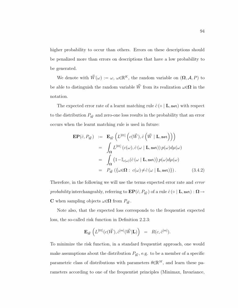
94

higher probability to occur than others. Errors on these descriptions should

be penalized more than errors on descriptions that have a low probability to

be generated.

We denote with ~W (ω) := ω, ω∈RK , the random variable on (Ω,A, P ) to

be able to distinguish the random variable ~W from its realization ω∈Ω in the

notation.

The expected error rate of a learnt matching rule c ( | L, met) with respect

to the distribution P ~W and zero-one loss results in the probability that an error

occurs when the learnt matching rule is used in future:

EP(c, P ~W ) := E ~W

(L[01]

(c( ~W ), c

(~W | L, met

)))

=

∫

Ω

L[01] (c(ω), c (ω | L, met)) p(ω)dµ(ω)

=

∫

Ω

(1−Ic(ω)(c (ω | L, met)

)p(ω)dµ(ω)

= P ~W (ω∈Ω : c(ω) 6= c (ω | L, met)) . (3.4.2)

Therefore, in the following we will use the terms expected error rate and error

probability interchangeably, referring to EP(c, P ~W ) of a rule c ( | L, met) : Ω→C when sampling objects ω∈Ω from P ~W .

Note also, that the expected loss corresponds to the frequentist expected

loss, the so-called risk function in Definition 2.2.3:

E ~W

(L[01](c( ~W ), c[m]( ~W |L)

)= R(c, c[m]).

To minimize the risk function, in a standard frequentist approach, one would

make assumptions about the distribution P ~W , e.g. to be a member of a specific

parametric class of distributions with parameters θ∈RM , and learn these pa-

rameters according to one of the frequentist principles (Minimax, Invariance,

95

Bayes,...). In machine learning, though, typically one wants to learn rules

without such a restriction on the distribution P ~W .

Yet, as long as we do not know neither P ~W nor the true ideal competing

concepts ~eC(|Ω), c∈C, we can not evaluate the performance of any learning

system with respect to the mean loss on the input space nor with respect

to the error probability. We have to find ways to relate these theoretical

performance criteria to something we can observe: performance measures. If

optimal descriptions are available, in the experience as well as in future, the

inductive learning hypothesis is a useful guide. Informally it says (Mitchell,

1997):

Principle 3.4.1 (Inductive Learning Hypothesis).

Any concept found to approximate the ideal concept well over a sufficiently

large set of training examples will also approximate the ideal concept well over

other unobserved examples.

Following this hypothesis, the performance measure for best-matching com-

petitive concepts is the empirical risk respectively the training error rate:

Definition 3.4.1 (Training Error Rate). The empirical risk of a set of

best-matching competitive concepts is the expected loss with respect to the

empirical distribution P ~W |L according to the examples L. For zero-one loss

this results in the training error rate:

EP(c, P ~WL) := E ~W |L(L[01](c( ~W ), c( ~W |L, met)

)

=1

NL

NL∑n=1

L[01] (cn, c(ωn|L, met) .

96

——————————————————-

Minimizing the training error rate EP(c, PC, ~X|L can be shown to be sound

given certain assumptions are fulfilled:

1. The descriptions ωL := ω1, ..., ωNL in the training set can be

interpreted to be realizations of some random sample from some

population with probability space (Ω,A, P ~W ). (i.i.d. assump-

tion)

2. The concept numbers cL := c1, ..., cNL of the training exam-

ples are assigned according to the true competing concepts ~eC∈U(supervised learning).

3. Future descriptions will be additional independent random draws

from the same population. Their unknown ”true” concept num-

bers will correspond to the same ”true” competing concepts ~eC∈UG

(structural stability).

4. Either Ω is a countable set, or the true concepts only have countable

discontinuities on Ω.

Assume, we do know nothing about the probability P ~W and optimal de-

scriptions are available. Let us split the error probability EP in two parts:

P ~W

(ω∈Ω : c(ω) 6= c[m](ω|L)

)

= P ~W

(ω∈L : c(ω) 6= c[m](ω|L)

)+ P ~W

(ω∈Ω\L : c(ω) 6= c[m](ω|L)

)

For countable spaces Ω and corresponding discrete distributions P ~W and with

more and more examples sampled from the distribution P ~W (that is NL →∞)

the second addend goes to zero, and obviously one should minimize the first

addend. But even for small training sets, preferring competing concepts ~eC|L

that make more errors on the training set than others can not be justified

without additional assumptions on P ~W or the true concepts ~eC. If we pre-

ferred some matching rule with more errors over one with fewer errors, the

97

first addend would obviously increase. And there is no information about the

behavior of the second addend to justify some believe that the second addend

becomes smaller with such a choice. We can follow the same reasoning for con-

tinuous distributions P ~W on uncountable spaces Ω assuming the corresponding

concepts only have countable discontinuities.

As we will see, this is different if only non-optimal descriptions are available.

For non-optimal descriptions minimizing the training error rate is not a good

strategy to achieve low error probability.

In broad hypotheses spaces typically there will be more than one hypothe-

sis that gives no training error. Within the subspace of hypotheses that make

no training error, so far we have no mean to distinguish its members with re-

spect to their error probability. And also, to compare learning systems, many

learning systems are able to output some hypothesis or a set of hypotheses

that make no training errors. Thus, minimum training error is no decisive per-

formance measure, neither to find the best hypothesis within some hypotheses

space, nor to compare the performance of different learning systems. We have

to combine the training error with other performance criteria and their mea-

sures to be able to rank further given we want to do so.

The so-called probably approximately correct (PAC) learning framework of-

fers a way to assess the quality of different learning systems in terms of the

computational resources required for high quality learning, which relates to the

number of training examples required for high quality learning. In addition,

results based on the PAC learning model provide useful insights regarding the

relative complexity of different learning problems in terms of the true concepts

98

to learn and regarding the rate at which generalization accuracy improves with

additional training examples (Mitchell, 1997).

The guarantee of the quality these learning systems have to issue is that a

learnt hypothesis for two competing concepts will probably be approximately

correct for any true concept from a certain class of concepts. In other words,

the error probability of the learnt hypothesis is bound to be below a certain

level, and the learning system has to learn such a hypothesis with a probability

above a certain level.

Definition 3.4.2 (PAC learnability).

Consider a class of ideal concepts C (Ω→0, 1)⊆F (Ω→0, 1) with Ω⊆RK , and some learner with hypotheses space H (Ω→0, 1). Then C is PAC

learnable by the learner using H, if for

— all concepts ec∈C,

— any distribution P ~W over Ω,

— any 0<ε< 12

— any 0<δ< 12

the learning system finds with probability P > (1− δ) some hypothesis h ∈ Hwith error probability EP(h, P ~W ) < ε.

——————————————————-

As it is common, this definition is in terms of the learning of only two

competing concepts. We have not found an extension to more competing

concepts under the assumption of ideal concepts, though we would expect

that it exists. Intuitively, it seems possible to extent it to the multi-class case

99

by some defined path for learning several binary matching rules and/or some

defined path for the final best matching from binary matching rules. We do not

go deeper into this, because the PAC learning model itself will play no further

role in this work, and is mainly introduced as a basis for the understanding

of the structural risk minimization framework we will now start to derive.

We present the structural risk minimization principle as it is given in Shawe-

Taylor et al. (1996) and Shawe-Taylor and Bartlett (1998): this framework

differs slightly from the original framework of Vapnik (1995) in that it makes

implicit priors on hypotheses space in the latter framework explicit.

In Definition 3.4.2 of PAC learnability we have to argue on the basis of

some fixed but unknown class of true concepts C. It is possible to bound the

error probability also without such a restriction.

General bounds can be derived on the basis of an analysis of the capacity of

hypotheses spaces to partition some finite set of descriptions into two groups:

Definition 3.4.3 (Growth function and VC-dimension).

Let H be a hypotheses space H(Ω→0, 1). Let ΩN := ω1, ..., ωN⊂Ω⊆RK be a set of descriptions in the input space. Let

H|ΩN:= (h(ω1), ..., h(ωN)) , h ∈ H⊆0, 1N

denote the set of all dichotomies on this set that can be induced by H.

The growth function GH() : N→N relates the size N of potential sets with

the maximum number of dichotomies that the hypotheses space can induce

over it:

GH(N) := max∣∣H|ΩN

∣∣ , ΩN∈ΩN

.

100

If GH(N) = 2N for some set ΩN all dichotomies on ΩN can be fitted by the

hypotheses space, we say H shatters ΩN . The Vapnik-Chernovenkis dimen-

sion VC-dimension finally determines the maximum size N up to which the

hypotheses space can shatter some set:

VC(H) := maxN : GH(N) = 2N

.

The Vapnik-Chernovenkis dimension measures the flexibility of the hypotheses

space and in that it is a specific measure of its complexity.

——————————————————-

The following bound on the error probability in dependence on the VC-

dimension is based on Shawe-Taylor et al. (1996):

Theorem 3.4.1 (Bound for the Error Probability in fixed Hypothe-

ses Space). Let H be some hypotheses space with VC(H) = d. Let the de-

scriptions ω1, ..., ωNL in L be the realizations of some random sample from

(Ω,A, P ~W ). If the learning system finds some hypothesis h∈H with no training

error, EP(h, P ~W |L) = 0, then with probability P≥ 1−δ the error probability

EP(h, P ~W ) will be smaller than the following bound:

bEP(NL, d, δ) =4d

NL

ln

(2eNL

d

)+

4

NL

(ln

(4

δ

)).

Some explanation Note that d must be much smaller than NL for the

bound to be meaningful in the sense that it is below the natural bound of one.

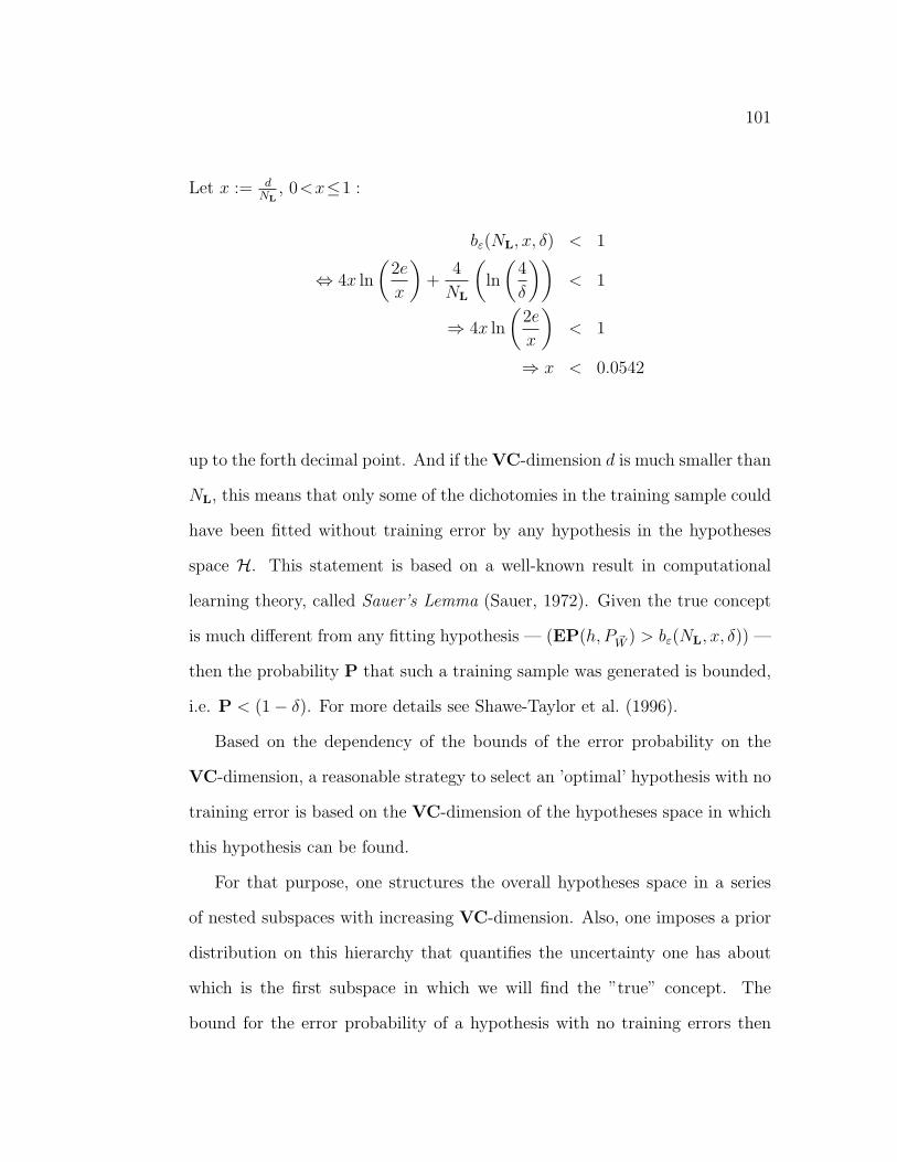
101

Let x := dNL

, 0<x≤1 :

bε(NL, x, δ) < 1

⇔ 4x ln

(2e

x

)+

4

NL

(ln

(4

δ

))< 1

⇒ 4x ln

(2e

x

)< 1

⇒ x < 0.0542

up to the forth decimal point. And if the VC-dimension d is much smaller than

NL, this means that only some of the dichotomies in the training sample could

have been fitted without training error by any hypothesis in the hypotheses

space H. This statement is based on a well-known result in computational

learning theory, called Sauer’s Lemma (Sauer, 1972). Given the true concept

is much different from any fitting hypothesis — (EP(h, P ~W ) > bε(NL, x, δ)) —

then the probability P that such a training sample was generated is bounded,

i.e. P < (1− δ). For more details see Shawe-Taylor et al. (1996).

Based on the dependency of the bounds of the error probability on the

VC-dimension, a reasonable strategy to select an ’optimal’ hypothesis with no

training error is based on the VC-dimension of the hypotheses space in which

this hypothesis can be found.

For that purpose, one structures the overall hypotheses space in a series

of nested subspaces with increasing VC-dimension. Also, one imposes a prior

distribution on this hierarchy that quantifies the uncertainty one has about

which is the first subspace in which we will find the ”true” concept. The

bound for the error probability of a hypothesis with no training errors then

102

will depend on the VC-dimension of the first subspace in the hierarchy the

hypothesis belongs to (see Shawe-Taylor and Bartlett, 1998):

Theorem 3.4.2 (Bound for the Error Probability in Structured Hy-

potheses Space). Consider some hierarchy of nested hypotheses spaces

H1⊆H2⊆ . . .⊆Hd⊆ . . . (3.4.3)

where VC(Hd) = d, d∈N. Letpd∈R+

0 , d∈N,∑∞

d=1 pd = 1

be some series

of non-negative numbers representing our prior uncertainty about which sub-

space to use. We call this the prior on the hypotheses structure. Let the de-

scriptions ω1, ..., ωNL in L be the realizations of some random sample from

(Ω,A, P ~W ). Let d be the minimum VC-dimension of some hypotheses space

Hd in which the learning system finds some hypothesis hd with no training

error, EP(hd, P ~W |L) = 0.

Then with probability P≥1−δ the error probability EP(hd, P ~W ) will not be

larger than the following bound:

bEP(NL, d, δ) =

4dNL

ln(

2eNL

d))

+ 4NL

(ln

(1pd

)+ ln

(4δ

))for pd > 0,

undefined otherwise,

provided d ≤ m.

Using the principle of structural risk minimization, the error bound is the

performance measure to rank different hypotheses in a large hypotheses space

among all those with no training errors:

Principle 3.4.2 (Structural Risk Minimization).

103

Given a hierarchy of nested hypotheses spaces and a prior on the structure

as in Theorem 3.4.2, and some hypotheses with no training errors on L, choose

that hypothesis hd∈Hd, d∈N that has the lowest bound bEP(NL, d, δ) for its error

probability EP(hd, P ~W ).

The prior pd > 0, d∈N, on the hypotheses structure has naturally to de-

crease for increasing d→∞ at least beyond some point D∈N to satisfy the

constraint∑∞

d=1 pd = 1. In other words, we bias our search towards hypothe-

ses spaces with low complexity in terms of their VC-dimension. In that way

the structural risk minimization principle is one implementation of the prin-

ciple of inductive inference:

Principle 3.4.3 (Ockham’s Razor).

”Pluralitas non est ponenda sine neccesitate” or ”plurality should not be

posited without necessity.” The words are those of the medieval English philoso-

pher and Franciscan monk William of Ockham (ca. 1285-1349). [...] Ock-

ham’s razor is also called the principle of parsimony. These days it is usually

interpreted to mean something like ”the simpler the explanation, the better” or

”don’t multiply hypotheses unnecessarily.” (Carroll, 1994-2002).

Though Ockham’s razor is almost globally successfully used, so far no-

one has succeeded to prove optimality of Ockham’s razor from first principles,

though attempts have been made. Wolpert (1992) demonstrates the counter-

evidence. Mitchell (1997) states two main problems that arise when trying to

prove Ockham’s razor in general:

1. within hypotheses spaces typically there does not exist an unique

definition of their length and one can define and justify different

104

orderings of the hypotheses on the basis of different definitions of

length, and

2. the definition of some ordering is even more arbitrary if one wants

to compare hypotheses from different hypotheses spaces.

For example for TREE, we can motivate to measure length in terms of the

depth of the tree D or the number of leaf nodes N[l] ⊆N. These definitions

are related, but induce different orderings on the set of trees. Among all trees

with no training errors, according to Ockham’s razor we could justify to select

different trees as ’the best’ whichever definition of length we use.

It might seem that the ordering according to the VC-dimension was unique

and ’the best’. Yet, there are many different ways to define nested structures

fulfilling (3.4.3) with increasing VC-dimension within the same hypotheses

space ∪∞d=1Hd ⊆ F (Ω → 0, 1). And there are other complexity measures,

also related to the spaces capability to fit dichotomies of the training set that

may even improve the error bounds in the sense that they are tighter (Shawe-

Taylor and Bartlett, 1998, ”fat shattering dimension”)

Mitchell (1997) speculates, why Ockham’s razor is so successful. In a very

broad interpretation, this says, Ockham’s razor works, because human beings

can only reason with short explanations, and thus evolution has made us to

perceive the world such that our internal representations of the world lead to

short descriptions.

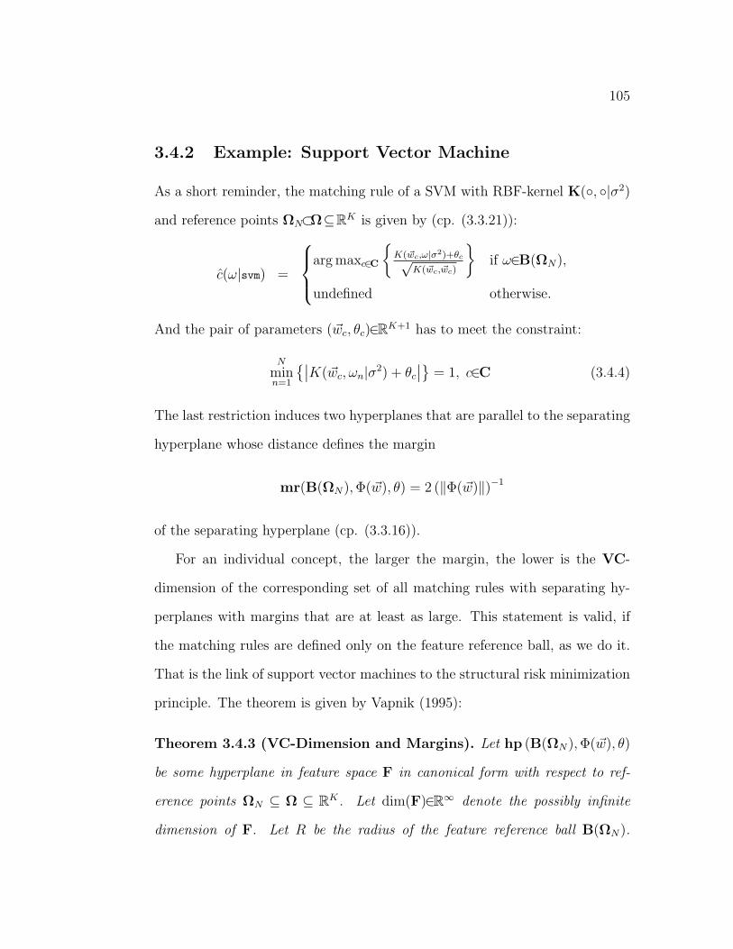
105

3.4.2 Example: Support Vector Machine

As a short reminder, the matching rule of a SVM with RBF-kernel K(, |σ2)

and reference points ΩN⊂Ω⊆RK is given by (cp. (3.3.21)):

c(ω|svm) =

arg maxc∈C

K(~wc,ω|σ2)+θc√

K(~wc, ~wc)

if ω∈B(ΩN),


And the pair of parameters (~wc, θc)∈RK+1 has to meet the constraint:

N

minn=1

∣∣K(~wc, ωn|σ2) + θc

∣∣ = 1, c∈C (3.4.4)

The last restriction induces two hyperplanes that are parallel to the separating

hyperplane whose distance defines the margin

mr(B(ΩN), Φ(~w), θ) = 2 (‖Φ(~w)‖)−1

of the separating hyperplane (cp. (3.3.16)).

For an individual concept, the larger the margin, the lower is the VC-

dimension of the corresponding set of all matching rules with separating hy-

perplanes with margins that are at least as large. This statement is valid, if

the matching rules are defined only on the feature reference ball, as we do it.

That is the link of support vector machines to the structural risk minimization

principle. The theorem is given by Vapnik (1995):

Theorem 3.4.3 (VC-Dimension and Margins). Let hp (B(ΩN), Φ(~w), θ)

be some hyperplane in feature space F in canonical form with respect to ref-

erence points ΩN ⊆ Ω ⊆ RK. Let dim(F)∈R∞ denote the possibly infinite

dimension of F. Let R be the radius of the feature reference ball B(ΩN).

106

Let the corresponding margin mr(B(ΩN), Φ(~w), θ) = 2 (‖Φ(~w)‖)−1 (3.3.16) be

bounded from below by the following constraint:

‖Φ(~w)‖ ≤ A∈R.

Then the hypotheses space HR(XN ) of matching rules restricted to the feature

reference ball (cp. (3.3.21) for arbitrary Kernel) has VC-dimension bounded

by

HR(XN ) ≤ minR2(XN)A2, dim(F)

+ 1.

Now assume we use the descriptions ω1, ...., ωNL in the training set L as

reference points ΩNL. And we define an ordering of the hypotheses space of all

hyperplanes within the feature ball ΩNLby decreasing size of the margin. We

have thus introduced a specific hierarchy on the hypotheses space of all such

hyperplanes.

A separating hyperplane with respect to the training set leads to a matching

rule with no training errors: all members of one concept have to lie above the

hyperplane, all members of the counter concept below. So far we use natural

numbers as concept numbers, for two competing concepts that is C = 1, 2.For separating hyperplanes it is more convenient to use another numbering,

namely:

y(c) :=

1 if c = 1,

−1 if c = 2.

With this coding, we can rewrite the restriction in (3.4.4) such that all ex-

amples of the training set that are members of concept 1 lie above (yn = 1),

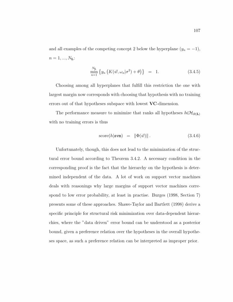
107

and all examples of the competing concept 2 below the hyperplane (yn = −1),

n = 1, ..., NL:

NL

minn=1

yn

(K(~w, ωn|σ2) + θ

)= 1. (3.4.5)

Choosing among all hyperplanes that fulfill this restriction the one with

largest margin now corresponds with choosing that hypothesis with no training

errors out of that hypotheses subspace with lowest VC-dimension.

The performance measure to minimize that ranks all hypotheses h∈HR(L)

with no training errors is thus

score(h|svm) = ‖Φ(~w)‖ . (3.4.6)

Unfortunately, though, this does not lead to the minimization of the struc-

tural error bound according to Theorem 3.4.2. A necessary condition in the

corresponding proof is the fact that the hierarchy on the hypothesis is deter-

mined independent of the data. A lot of work on support vector machines

deals with reasonings why large margins of support vector machines corre-

spond to low error probability, at least in practise. Burges (1998, Section 7)

presents some of these approaches. Shawe-Taylor and Bartlett (1998) derive a

specific principle for structural risk minimization over data-dependent hierar-

chies, where the ”data driven” error bound can be understood as a posterior

bound, given a preference relation over the hypotheses in the overall hypothe-

ses space, as such a preference relation can be interpreted as improper prior.

108

3.4.3 Realizable Concepts

Again we assume ideal concepts ec(|Ω), c∈C, based on optimal descriptions

ω∈Ω ⊆ RK . Yet, these optimal descriptions are not available and we will

have to match descriptions ~x∈X, with realizable concepts ec(|X), c∈C that

approximate the ideal concepts.

For non-optimal descriptions the mean loss on the input space (3.4.1) is

normally not considered as performance criterion.

In machine learning for non-optimal descriptions ~x∈X and numbers c∈C of

ideal competing concepts ~eC : Ω→UG one typically assumes some unknown

joint distribution over PC, ~X . To understand how this can be related to the

idea of ”noise corrupted descriptions”, we will give one possible explanation

here:

We can derive a probabilistic relation between non-optimal descriptions and

concept numbers by assuming that future optimal descriptions ω∈Ω are sam-

pled from some population of optimal descriptions according to some general

probability model (Ω,A(Ω), PW ).

This optimal description is the instance of the concept with number c(ω).

This defines some random variable C() : Ω→C on (Ω,A, P ). The corrupted

version of the optimal description ~x(ω) can be seen to be the output of a

function ~x = f(ω, e), with e ∈ E denoting some other event representing

”noise”: a random draw from (E,A(E), PE) . In that respect ~X(, ) is a

random variable on Ω×E with probability space(Ω×E,A(Ω)×A(E)), P ~W,E

).

Extending c(ω) := c(ω, e) for all e∈E and ω ∈ Ω, we can define C and ~X as

random variables on (Ω×E) with joint probability distribution PC, ~X .

109

The performance of a learnt best-matching rule

c(~x | t, ΥC|L, ~wL

)= c (~x | L, met) , ~x∈X

is most often defined analogously to (3.4.2) to be the expected error with

respect to the joint distribution PC, ~X :

EP(c[m], PC, ~X) := EC, ~X

(L[01]

(C, c[m]( ~X|L)

))(3.4.7)

:=

∫

C×XL[01]

(c, c[m](~x|L)

)p(c, ~x)dµ(c, ~x)

=

∫

X

∫

C

L[01](c, c[m](~x|L)

)p(c|~x)dµ(c)p(~x)dµ(~x)

= PW,E

((ω, e)∈Ω×E : c(ω) 6= c[m](f(ω, e)|L)

).

We already know the best matching rule that minimizes this expected error:

it is the Bayes rule c(|bay) in (2.2.18) with respect to the true probability

model τ specifying PC, ~X (see end of Section 2.2.2).

According to the true joint probability, there may be examples in the train-

ing set L such that

cn 6= arg maxc∈C

p(c| ~xn,Λ), n∈1, ..., NL .

If one tries to learn competing concepts that make no training errors these

examples lead astray from the best competing concepts. Thus, a learning

instruction that avoids to fit these ”non-typical” examples can lead to a rule

with lower error probability.

110

Misleading examples in the training set cause a problem known as the

overfitting problem. Overfit can be defined as follows (Mitchell, 1997, cp.):

Definition 3.4.4 (Overfit).

A learnt matching rule h := c(~x | t, ΥC|L, ~wL

)∈H from some hypotheses

space H overfits the training data L if there exists another matching rule

h := c(~x | t, ΥC|L, ~πL

)∈ H that makes more training errors, but has a lower

error probability:

EP(h, PC, ~X|L) < EP(h, PC, ~X|L)

EP(h, PC, ~X) > EP(h, PC, ~X)

——————————————————-

Note that in this definition of ”overfit” the performance of a matching rule

is compared to the performance of all matching rules from the same common

hypotheses space. Alternatively, one could define overfit in terms of the er-

ror probability of the Bayes rule with respect to the true joint probability

PC, ~X , the best, yet unknown rule. The practical use of the latter, though, is

void as we will never be able to calculate nor to estimate it without making

representational assumptions.

There are two basic strategies to fight overfitting:

1) split the training set L∗ in a learning set L and a validation set V.

Learn various hypotheses HL on the learning set according to some

”inner” performance measure and estimate the error probability

EP(h, PC, ~X) of these hypotheses by their empirical error rate on

the validation set, EP(h, PC, ~X|V). Use this as performance measure

to rank the hypotheses h∈HL

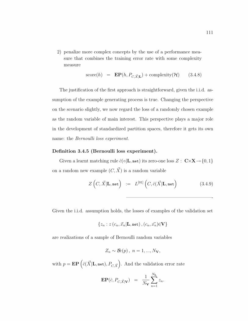
111

2) penalize more complex concepts by the use of a performance mea-

sure that combines the training error rate with some complexity

measure

score(h) = EP(h, PC, ~X|L) + complexity(H) (3.4.8)

The justification of the first approach is straightforward, given the i.i.d. as-

sumption of the example generating process is true. Changing the perspective

on the scenario slightly, we now regard the loss of a randomly chosen example

as the random variable of main interest. This perspective plays a major role

in the development of standardized partition spaces, therefore it gets its own

name: the Bernoulli loss experiment.

Definition 3.4.5 (Bernoulli loss experiment).

Given a learnt matching rule c(|L, met) its zero-one loss Z : C×X→0, 1on a random new example (C, ~X) is a random variable

Z(C, ~X|L, met

):= L[01]

(C, c( ~X|L, met

)(3.4.9)

——————————————————-

Given the i.i.d. assumption holds, the losses of examples of the validation set

zn : z (cn, ~xn|L, met) , (cn, ~xn)∈V

are realizations of a sample of Bernoulli random variables

Zn ∼ Be(p) , n = 1, ..., NV,

with p = EP(c( ~X|L, met), PC, ~X

). And the validation error rate

EP(c, PC, ~X|V) =1

NV

NL∑n=1

zn.

112

is a ”good” estimator of parameter p as it is the maximum-likelihood estimator

as well as the unbiased minimum variance estimator thereof.

The Bernoulli loss perspective is also useful to reason against the use of

the training error as some estimate of the error probability: after the examples

of the training set were used to learn the matching rule, it is inappropriate to

model them as outcomes of a random experiment at all.

And before learning, the training set is a random quantity, and the rule to

learn c[m](|L) and the losses Z1, ..., ZNLare both dependent on it:

Zn = Z(Cn, ~Xn

∣∣∣

(C1, ~X1), ..., (CNL, ~XNL

)

,L, met)

, n = 1, ..., NL.

= L[01]

(Cn, c( ~Xn|L, met)

∣∣∣∣L)

, n = 1, ..., NL.

The rule to learn is dependent on the learning set, and the losses depend on the

rule to learn and one of the examples in the learning set. These dependencies

induce a relationship among the examples and thus they do not form an i.i.d.

sample.

Justifications of the second approach all rest upon different formalizations

of Ockham’s razor (Principle 3.4.3). Most statistical model selection strategies

are based on Ockham’s razor, as Hansen and Yu (2001) put it into words it

is the soul of model selection. The minimum description length principle, the

minimum message length principle, model selection based on the Akaike infor-

mation criterion, or the Bayesian information criterion are all formalizations

of this idea. For an overview, see Hansen and Yu (2001).

The adaption of the structural risk minimization principle to non-optimal

descriptions also fits in that approach. The version of Theorem 3.4.2 that

113

allows for training errors provides the corresponding bound for the error prob-

ability. Shawe-Taylor and Bartlett (1998) introduce more priors there: in

Theorem 3.4.2 one specifies the prior pd, d∈N, on the structure, quantifying the

uncertainty which subspace in the hierarchy to use, now additionally within

each subspace Hd a prior with non-negative values qd,k :∑NL

n=1 qd,k = 1, for all

d∈N specifies the uncertainty on the number of errors a best hypothesis within

this subspace will make on some training data of size NL.

Theorem 3.4.4 (Bound for the Error Probability in Structured Hy-

potheses Space with Noise).

Again consider some hierarchy of nested hypotheses spaces

H1⊆H2⊆ . . .⊆Hd⊆ . . .

with VC(Hd) = d, d∈N. Let the non-negative numbers pd, d∈N, with∑∞

d=1 pd =

1 define a prior on the hypotheses structure, and for all d∈N let qd,k :∑NL

n=1 qd,k =

1 define a prior on the number of minimum training errors on a training set

of size NL of some hypothesis hd∈Hd, d∈N. Let the descriptions in L be the

realizations of a random sample according to the distribution PC, ~X .

If the learning system finds some hypothesis hd∈Hd with k training errors,

then with probability P≥1−δ its error probability EP(hd, PC, ~X) will be smaller

than the following bound:

bEP(NL, d, k, δ) =

2(

kNL

+ 2dNL

ln(

2eNL

d

)+ 2

NLln

(4

pdqd,kδ

))for qd,kpd > 0,


provided d ≤ NL.

114

These error bounds of structural risk are all very loose, and can not really

be understood in terms of some ”guarantee of quality” as they are typically

at least larger than 0.5 — which is the error probability we get if we match

descriptions with two competing concepts by tossing a fair coin.

Thus, we prefer the error bound to be interpreted as a performance measure

that combines training error with a founded penalty for the complexity to find

the point where Ockham’s razor shaves because further ”plurality would be

posited without necessity”.


To allow for noise in SVM classifiers, we only have to modify the restriction

(3.4.5)

NL

minn=1

yn

(K(~w, ωn|σ2) + θ

)= 1.

that was introduced to force the examples of the two competing concepts to

lie either all above or below the hyperplane.

One introduces so-called slack variables ξn ≥ 0, n = 1, ..., NL such that

description ~xn can lie on the wrong side if ξn > 0, n = 1, ..., NL. It is now

easier to write the description as individual constraints on each example:

yn

∣∣K(~w, ~xn|σ2) + θ∣∣ ≥ 1− ξn, n = 1, ..., NL. (3.4.10)

Note that in this representation one does not require any more the bound of

”1” to be reached. This is redundant, because by maximizing the margin we

will reach the bound anyway.

115

If an error occurs, the corresponding slack variable ξn exceeds unity. Thus

∑NL

n=1 ξn is an upper bound on the number of training errors.

And the performance measure is no longer based on the size of the mar-

gin alone, but combined with a penalty for training errors. We get another

performance measure according to the second basic strategy (3.4.8) to fight

overfitting. The self-evidence one entitles to this strategy is articulated by

Burges (1998), when he introduces it. The quotation is adapted to nomencla-

ture and notation in this work by the words and formula in squared brackets:

Hence, a natural way to assign an extra cost for errors is to change the [perfor-

mance measure] to be minimized from [‖Φ(~w)‖] to[‖Φ(~w)‖+ C

(∑NL

n=1 ξn

)],

where C[∈R] is a parameter to be chosen by the user, a larger C corresponding

to assigning a higher penalty to errors.

3.4.5 Conclusion

In machine learning the basic assumptions about the generating process of

data differ from those in statistics. In consequence, the principles of ”good”

learning differ, as well as measures to assess the performance of matching rules,

and hypotheses spaces in which to search for best matching rules.

Common to the approaches to classification rule learning and concept learn-

ing is the dependence of the performance measures on the i.i.d. assumption

of examples. They differ in the assumptions about the probability space on

which sampling takes place. In statistics the performance measures based on

expected loss depend on an assumed and often quite restrictive class of dis-

tributions. In machine learning, one tries to avoid this type of assumptions,

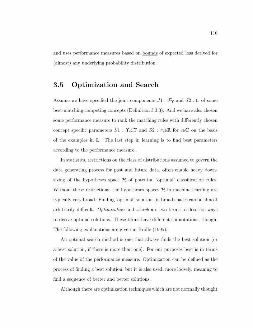
116

and uses performance measures based on bounds of expected loss derived for

(almost) any underlying probability distribution.

3.5 Optimization and Search

Assume we have specified the joint components J1 : FΥ and J2 : t of some

best-matching competing concepts (Definition 3.3.3). And we have also chosen

some performance measure to rank the matching rules with differently chosen

concept specific parameters S1 : Υc⊂Υ and S2 : πc∈R for c∈C on the basis

of the examples in L. The last step in learning is to find best parameters

according to the performance measure.

In statistics, restrictions on the class of distributions assumed to govern the

data generating process for past and future data, often enable heavy down-

sizing of the hypotheses space H of potential ’optimal’ classification rules.

Without these restrictions, the hypotheses spaces H in machine learning are

typically very broad. Finding ’optimal’ solutions in broad spaces can be almost

arbitrarily difficult. Optimization and search are two terms to describe ways

to derive optimal solutions. These terms have different connotations, though.

The following explanations are given in Bridle (1995):

An optimal search method is one that always finds the best solution (or

a best solution, if there is more than one). For our purposes best is in terms

of the value of the performance measure. Optimization can be defined as the

process of finding a best solution, but it is also used, more loosely, meaning to

find a sequence of better and better solutions.

Although there are optimization techniques which are not normally thought

117

of as search, and search methods which are not optimal or not defined as

optimizing anything, most often we are dealing with search methods which

seek to optimize a well-defined criterion, and usually we understand the search

method in terms of the way it approximates to an optimal search.

Bridle (1995) distinguishes combinatorial optimization problems, where a

solution is a sequence or more complicated data structure, from (non-linear)

continuous optimization problems, where a solution is a vector of real numbers.

We will reserve the term search for combinatorial problems and optimization

for continuous problems.

Implicitly, optimization is often assumed to be the easier task compared

to search in terms of computational resources needed, though this is of course

not true in general. In the following, we will sketch important features of

optimization and search relevant to this work while describing the implemented

optimization and search strategies of the examples LDA, QDA, CNB, SVM and

TREE.

3.5.1 Examples: Plug-in and Predictive Bayes Rules

The plug-in Bayes rules of LDA and QDA and predictive Bayes rules of CNB

are all solutions of optimization problems in the sense above. They possess

two important and quite desirable features:

1. they are optimal search methods, because they always find the or

a best solution, if such exist, and

2. they can be computed directly — analytically or numerically —

with standard algorithms.

118

The statistical models in which these strategies can be successfully pursued are

very restrictive. In particular, statisticians are confronted with combinatorial

problems if they are uncertain about structural components of the model dis-

tributions like e.g. which multivariate dependencies and/or which predictors

to consider. In general, whenever one has to learn intensional definitions with

basic function fυ∈FΥ(X→R), where the parameter υ∈Υ determines the actual

domain of fυ() : X[M]→R, one has to solve a combinatorial problem.

For example, we performed variable selection with LDA and QDA in (Sond-

hauss and Weihs, 2001b) for the problem of business cycle prediction that is

analyzed in Chapter 7. Given thirteen potential predictor variables (K = 13)

we selected the best two by exhaustive search on the space of all potential

combinations of two predictors(132

)= 78. If we had intended to find the best

subset of predictors among all subset of predictors, exhaustive search would

have become infeasible on the 213 = 8192 combinations.

For plug-in Bayes rules not only that these combinatorial problems can be

computationally demanding, but also we run into the difficulties of potential

overfit. The performance measures for best point estimation are only valid

for ranking within the hypotheses space corresponding to the statistical model

based on a fixed set of predictors, but not to rank hypotheses corresponding

to different statistical models. In (Sondhauss and Weihs, 2001b) we solved

this problem by a method related to the first strategy to fight overfitting:

cross validation. For each statistical model a best plug-in rule was learnt

on a sub-sample of the training data. Its performance was assessed by the

empirical error on the rest of the training data. This was repeated for different

119

partitions of the training data into learning set and validation set. The overall

performance measure used in cross validation is the average error rate on the

validation sets according to the various repetitions of the validation.

For predictive Bayes rules the appropriate strategy to rank hypotheses from

different statistical models consists of quantifying a prior over the statistical

models, and then performing standard Bayesian updating of these model priors

to select the best one. If these priors are motivated by some quantification of

the complexity of the models, Bayesian model selection and structural risk

minimization methods get close.


To find the best separating hyperplane to determine a SVM classifier, one first

has to specify the Kernel type (we use the Gaussian RBF-Kernel in (3.3.17)),

then the Kernel specific parameter (the width σ2 of the RBF-Kernel) and the

parameter C that controls the trade-off between margin maximization and

training error minimization (Section 3.4.4).

Given the Kernel and these parameters, the hypotheses space for SVM

matching rules is still very broad. One of the characteristics, the SVMs are

famous for, is the fact that the best concept specific parameters can neverthe-

less be found with guarantee by an optimization procedure in polynomial time

(Burges, 1998).

To minimize the performance measure

‖Φ(~w)‖+ C

(NL∑n=1

ξn

)(3.5.1)

120

derived in Section 3.4.4 under the constraints given in equation (3.4.10)

yn

∣∣K(~w, ~xn|σ2) + θ∣∣ ≥ 1− ξn, n = 1, ..., NL,

one can switch to a Lagrangian formulation of the problem. For a detailed

description see e.g. Burges (1998). As a consequence of the restrictions, the

feature parameter φ(~w) with minimum norm,

φ(~w)[opt] := arg minΦ(~w)∈F

‖Φ(~w)‖+ C

(NL∑n=1

ξn

)

can be written as a weighted sum of the features of the descriptions in the

training set:

φ(~w)[opt] :=

NL∑n=1

αnynΦ(~xn), (3.5.2)

with non-negative weights αn, n = 1, ..., NL. Only some descriptions ~xn∈Lhave a non-zero weight, C > αn > 0, namely those whose features lie on or

within the margins of the hyperplane and those that represent training errors.

The corresponding descriptions ~xn∈L : αn 6=0, n = 1, ..., NL are the so-called

support vectors.

The learnt matching rule that combines hyperplanes for concepts c∈Cagainst all others thus can be written as:

c(~x|L, svm)

=

arg maxc∈C

PNLn=1 αc,n|LK(~x,~xn|σ2)+θc|L√

K(~wc|L, ~wc|L)

if ~x∈B(XNL

),


(3.5.3)

Comparing SVM with RBF Kernel to other RBF classifiers, one sees that

support vectors play the role of RBF centers. A clear figure of merit of the

121

SVM is the principled way of choosing the number and the location of these

RBF centers (Scholkopf et al., 1997).

Yet not all parameters that define SVM are automatically learnt. We have

to choose the parameters (C, σ2). In the application in Chapter 7 we did no

search or optimization of these parameters. We set them to certain values that

performed well in a preliminary study. The original data set in the prelimi-

nary study is also part of the analysis in Chapter 7. Using the ”optimized”

values from preliminary studies on the same data later, certainly is not the

most proper way to do in a comparative study, because it gives the respective

classifier some advantage. But the other classifiers in this study were also to

even larger extends already optimized in this preliminary study and the main

question in Chapter 7 is about other properties, thus we did it nevertheless.

For the simulated data in Chapter 7, though, this is not only a very efficient

and but also a justified approach to use background knowledge to fix these

values.

To adjust (C, σ2) otherwise, one can use the Bernoulli loss experiment, and

any optimization method that finds extremal points of multidimensional func-

tions to minimize the validation error in dependence of (C, σ2). One example

is the gradient decent algorithm used by Chapelle et al. (2002) for (heavier)

SVM model selection. As many of these methods, the gradient decent algo-

rithm might get stuck in local minima, yet, it does not if the error surface is

convex. Nevertheless, given certain restrictions on the functions’ surface, these

algorithms are optimal optimization strategies. otherwise, they are heuristic

optimization strategies (Luenberger, 1973).

122

Based on model assumptions on the error surface, one can apply methods

from statistical experimental design to optimize parameters. We minimized the

validation set error with respect to the parameters (C, σ2) of a specific RBF

SVM in Garczarek et al. (2002) using experimental design with a quadratic loss

function: We assumed that the error EP(h(C, σ2), PC, ~X|V

)can be approxi-

mated by quadratic function of (log10(C),− loge(σ2)/K) restricted to the cube

[−1, 2]2. That way we restricted the search for the best parameters (C, σ2)

on the rectangle [ 110

, 100]× [Ke2 , Ke]. Defining 5 optimal experimental points

according to a central-composit plan for two variables (see e.g. Weihs and

Jessenberger, 1999) the quadratic function was fitted and optimal parameters

determined by the minimum of the fitted quadratic function on the rectangle.

3.5.3 Example: Univariate Binary Decision Tree

As we stated earlier, we are confronted with a combinatorial problem if the pa-

rameters υ∈Υ determine the actual domain X[M] of the basic functions fυ∈FΥ

of the intensional definitions.

In case of TREE the class of functions for the intensional definitions was

derived in Section 3.3.1 to be:

J1 : FΥ = FD,N,~k,~t, ~w

=

I(−∞,t(q)]

(|Xk(q)

),

t(q)∈Xk(q),

~k∈0, 1, ..., K2D+1−1 , ~wc∈R2D+1−1

q∈N[a](D), D∈N.

Thus, the parameter for the depth of the tree D, the parameters N ⊆1, 2, ..., 2D−1 − 1

representing the numbers of the actual nodes in the tree,

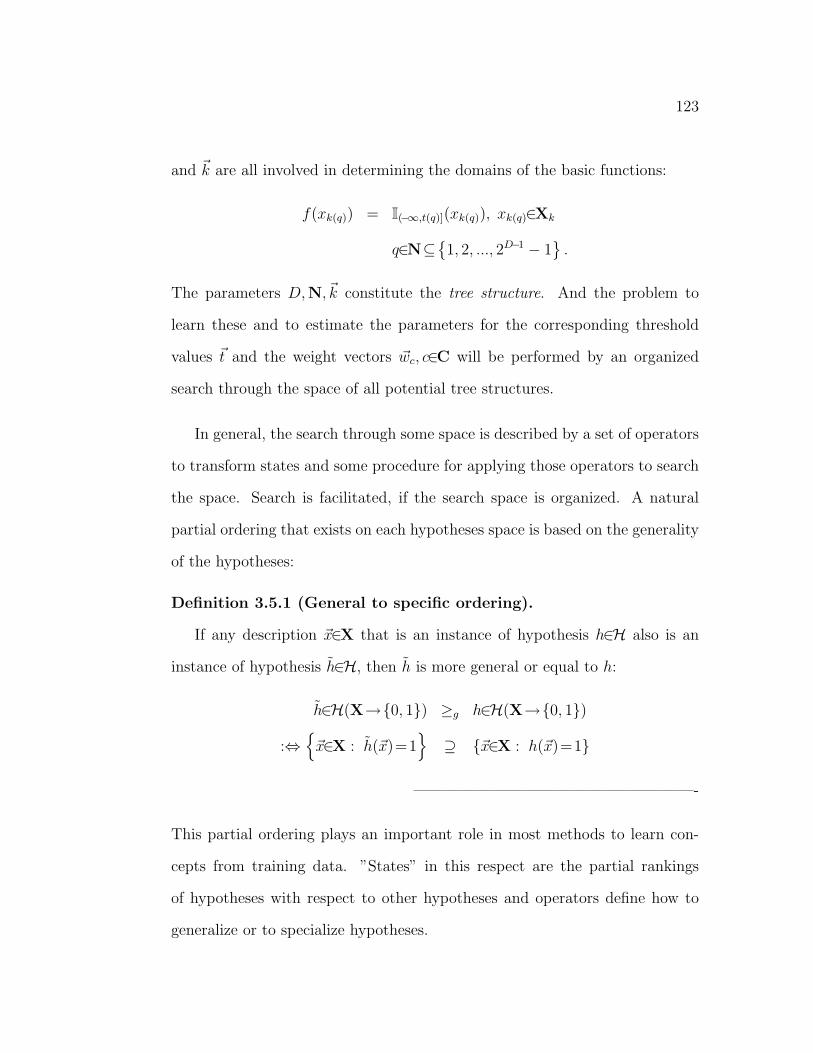
123

and ~k are all involved in determining the domains of the basic functions:

f(xk(q)) = I(−∞,t(q)](xk(q)), xk(q)∈Xk

q∈N⊆1, 2, ..., 2D−1 − 1

.

The parameters D,N, ~k constitute the tree structure. And the problem to

learn these and to estimate the parameters for the corresponding threshold

values ~t and the weight vectors ~wc, c∈C will be performed by an organized

search through the space of all potential tree structures.

In general, the search through some space is described by a set of operators

to transform states and some procedure for applying those operators to search

the space. Search is facilitated, if the search space is organized. A natural

partial ordering that exists on each hypotheses space is based on the generality

of the hypotheses:

Definition 3.5.1 (General to specific ordering).

If any description ~x∈X that is an instance of hypothesis h∈H also is an

instance of hypothesis h∈H, then h is more general or equal to h:

h∈H(X→0, 1) ≥g h∈H(X→0, 1)

:⇔~x∈X : h(~x)=1

⊇ ~x∈X : h(~x)=1

——————————————————-

This partial ordering plays an important role in most methods to learn con-

cepts from training data. ”States” in this respect are the partial rankings

of hypotheses with respect to other hypotheses and operators define how to

generalize or to specialize hypotheses.

124

On the basis of the general-to-specific ordering one can use strategies of

three basic types to find some hypothesis h∈H with no training errors:

1) Bottom-up strategies start with the most specific possible hypothe-

sis in H, minimally generalize this hypothesis if it fails to cover one

of the instances of the concept to learn in the training set, and stop

if it covers all examples that are instances of the concept to learn.

This hypothesis is the output of the search algorithm.

2) Top-down strategies start with the most general hypothesis in the

hypotheses space, minimally specialize this hypothesis as long as it

still covers some examples in the training data that do not belong

to the concept to learn, and stop if no non-members are covered

any more. This hypothesis is the output of the search algorithm.

3) Version space strategies combine both strategies, and a description

of all hypotheses in the hypotheses space that have no training error

is the output of these strategies.

Concept learning formulated as search problems and the development and

analysis of strategies form a central and basic part of machine learning research.

We refer to Mitchell (1997) and Langley (1995) for a general introduction into

this substantial field, and we restrict our attention to the decision tree learning.

The two core learning algorithms in decision tree learning ID3 (Quinlan,

1986) and its successor C4.5 (Quinlan, 1993) are both greedy top-down strate-

gies. The implementation we use rPart for ”Recursive Partitioning and Re-

gression Trees” is one variant thereof based on the CART system (Breiman

et al., 1984).

Top down says, we start with the empty tree and want to specialize. Greedy

says we specialize by stepping that way that maximizes some defined splitting

criterion the most within this single step — not looking further ahead, where

another choice might lead to an overall larger profit.

125

To present the strategy to learn a univariate binary decision tree for some

training set L, we show how to learn a tree with no training errors, and then

select the strategy to fight overfitting.

To start with, assume we were given some tree structure D,N, ~k and cor-

responding threshold values ~t. Let X[q]⊆X denote the set of all descriptions

that potentially pass through node q∈N :

X[q] := ~x∈X : q∈pt(~x) .

And L[q] ⊆X denote all training examples that pass through this node and

L[q,c]⊆X all those among them that are members of concept number c, c∈C:

L[q] := ~xn∈L : q∈pt( ~xn) , L[q,c] := cn, ~xn∈L : q∈pt( ~xn), cn = c

Define X[q,c] to be the analogue of L[q,c] on the input space X.

A good quantification of the degree of match w(c, q), c∈C, q∈N of some

description ~x passing through node q with concept number c would certainly

be its probability to belong to concept number c given it is processed through

node q:

w(c, q) :=P

C, ~X(X[q,c])P

C, ~X(X[q])

Of course we do not know these, but we can use the empirical counterparts as

estimates:

w(c, q|L) :=

∣∣L[q,c]∣∣

|L[q]| , c∈C, q∈N (3.5.4)

The vector ~wq[l]|L =(w(1, q[l]|L), ..., w(G, q[l]|L)

)∈UG defines a probability dis-

tribution on C.

126

A decision tree makes no error, if the leaf nodes n[l]∈N[l] in the tree are

”pure” in the sense that only examples that belong to one concept can be

found in a leaf node, that is, w(c, q[l]|L) = 1 for some c∈C Thus, our goal

are pure nodes where weight vectors are unit vectors. These have maximum

heterogeneity among all vectors ~w∈UG. Consequently, splitting criteria in

decision trees are based on measures for the heterogeneity of the weights in

the nodes. We use the empirical entropy in the nodes:

et(q|L) =∑c∈C

w(c, q|L) log2 w(c, q|L)

Starting in the root node n = 1, we have to find the predictor k to which

a threshold t(1)∈Xk(1) exists such that the two sets X[2] and X[3] induced by

the roots corresponding threshold function decrease the entropy:

f(xk(1)) = I(−∞,t(1)]

(|Xk(1)

)

L[2](k(1), t(1)) :=~xn∈L[1] : xk(1),n≤ t(1)

L[3](k(1), t(1)) :=~xn∈L[1] : xk(1),n >t(1)

with L[2](k(1), t(1)) ∪ L[3](k(1), t(1)) = L[1] = L To decrease the entropy the

weighted sum of entropies in the new leafs must be lower than the entropy of

the root node. The corresponding splitting criterion that we use is the so-called

information gain:

ig(q, k(q), t(q)|L)

= et(q|L)− et(2q|L, k(q), t(q))− et(2q + 1|L, k(q), t(q))

that can be defined for potential splits in any node.

127

The best pair k(1)∈1, ..., K and t(1)∈Xk(1) are found by exhaustive search.

This is possible for discrete as well as continuous attributes though theoreti-

cally the threshold value t(1)∈Xk(1) for a continuous attribute k(1) can take

on any value in the corresponding uncountable space Xk(1), ∈1, ..., K. Yet,

only a finite number of them can induce different partitions L[2](k(1), t(1)) ∪L[3](k(1), t(1)) = L[1] of the training examples in the previous node, and thus

we can

Going greedily from simple-to-complex and stopping with the first tree that

fits the data the search strategy induces a so-called search bias that prefers trees

that can be learnt greedily and that prefers short trees. The bias induced by

greediness has to be taken care of in trees where nodes can have more than two

successor nodes. If a node can split into as many successors as there are values

of discrete attributes, the greedy search combined with the information gain

measure would favor attributes with many values over those with fewer values.

One should use other splitting criteria then (see e.g. Mitchell, 1997). The bias

with respect to short trees is wanted, reasoning as usual with Ockham’s razor.

To avoid overfitting one can follow two basic strategies: doing post-pruning

or pre-pruning. Post-pruning will typically be based on a Bernoulli loss ex-

periment. Given some large tree with no training errors, find a subtree that

minimizes the validation error. Pre-pruning uses either statistical tests or some

combination of error and complexity penalty to decide in each node, whether

the potential benefit is large enough to justify the growth of the tree. We in-

troduced a hard complexity penalty: tree growth is stopped, if the number of

examples is below some minimum. This penalty parameter is optimized with

128

a Bernoulli loss experiment.

As a reward for the difficulty to solve variable selection problems, corre-

sponding hypotheses spaces offer the possibility to find good (in terms of error

probability) best-matching rules that are at the same time easy to interpret.

For example, the hypotheses space of TREE is flexible, therefore one may find

better rules than within very restricted spaces. And decision tree rules repre-

sent concepts that are decomposed in ”subconcepts” – the paths – based on

only small subsets of predictor variables – the predictor variables on a path.

Therefore, they are potentially easier to understand compared to concepts ac-

cording to flexible yet inherently high-dimensional hypotheses spaces like those

of neural networks and SVM.

——————————————————-

Chapter 4

Summing-Up and Looking-Out

The preceding chapters provide the theoretical basis for the development of

new methods that will take place in the following chapters. This Chapter

serves as transmitter.

4.1 Classification Rule Learning and Concept

Learning

In chapters 2 and 3, we introduced statistical approaches for learning classifi-

cation rules, and machine learning approaches for finding best-matching com-

peting concepts. We embedded the statistical learning of classification rules

in the concept learning framework. We derived an assimilated formulation of

the problem relevant in this work. This can be comprised as follows:

1. We consider classification problems that are based on some Kdimensional

real-valued vector ~x(ω)∈X ⊂ RK measured on objects ω∈Ω. The task is

to assign a new object ω∈Ω to one of the classes based on the informa-

tion in ~x, and training data consisting of NL objects with known classes

129

130

c1, ..., cNL and measurements ~x1, ..., ~xNL

.

2. We consider comparative concept matching problems based on descrip-

tions ~x∈X that are a corrupted versions of optimal descriptions ω∈Ω.

Optimal descriptions are instances of one concept out of a set of com-

peting ideal concepts ~eC() : Ω → UG. The task is to match a new

description ~x∈X with the number of the ideal concept c∈C given some

training data NL of corrupted descriptions ~x1, ..., ~xNL and the numbers

c1, ..., cNL of corresponding ideal concepts.

We do not continue to use both terminologies in parallel. We will express

ourselves in statistical technical terms, as we are more familiar with them.

4.2 Best Rules Theoretically

One of the main characteristics where machine learning and statistical ap-

proaches to classification rule learning differ, is the size of the hypotheses

spaces learnt classification rules may come from. As we have shown, this

difference is the impact of the different views on what can be or should be

expected.

The hypotheses spaces in statistics are typically downsized by distributional

assumptions on the underlying data generation process. If these assumptions

are valid, optimal classification rules in terms of error probability can be effi-

ciently learnt in these small spaces. Predictive Bayes rules are optimal in this

respect if the distributional assumptions about the sample distribution is valid

and the prior distribution is accepted. Plug-in Bayes rules are asymptotically

131

optimal if the distributional assumptions about the sample distribution are

valid.

In machine learning, mostly one does not pose a certain distributional as-

sumption other than there is some i.i.d. data generating process. One prefers

broad hypotheses spaces over smaller ones to avoid large representational bi-

ases. One problem in large hypotheses spaces is over-fitting and appropriate

performance measures have to be defined to avoid it. The other problem is the

computational effort to search in these spaces. Heuristic search strategies like

the ones for decision trees can find good solutions in the large spaces within

acceptable computational time, yet they do not necessarily find optimal solu-

tions in these spaces. In that way, search bias is favored over representational

bias. An important feature of the support vector machines is the fact that one

can guarantee to find optimal solutions with respect to the underlying per-

formance measure. Yet, the connection of the optimality with respect to this

performance measure to the true error probability of the learnt classification

rule is not clear. They can be connected by prior assumptions to the error

bounds in structural risk minimization. Yet, as long as these error bounds can

be far above one, and are not below 0.5 for two competing concepts, the op-

timality with respect to these error bounds does not give valuable guaranteed

information about the actual error probability of the learnt rule.

We presented the different approaches to show that each of them is jus-

tifiable and questionable at the same time. Even more so in data mining

applications, because all the underlying performance criteria and measures

rely on the assumption that the training data are appropriately modelled to

132

be the realization of some i.i.d. sample, and that future observations will be

generated according to the same process as the training data was.

In data mining applications the data generating process is not under con-

trol, neither according to a specific deterministic mechanism nor according to

a specific random mechanism. In consequence, we tape up the position that

all these approaches are justifiable heuristic search strategies.

4.3 Learnt Rules Technically

Technically, learnt rules from machine learning and statistics are very much

alike: most of them base their assignment of objects into classes on cer-

tain transformations of the respective observations for each of the considered

classes. As we have shown in Chapter 2 in statistics classification rules are typ-

ically learnt Bayes rules, and thus transformations are most commonly based

on the estimation of conditional class probabilities. In machine learning we

saw in Chapter 3 that transformations can be understood as an assessment of

the competitive degree of match of descriptions with concepts.

These transformations are taken from some hypotheses spaceH⊂F (X → C)

whose content depends on the representational choices defining the classifica-

tion method (Section 3.3). Given some training set L of examples, and on the

basis of a specific performance measure (Section 3.4) and a specific optimiza-

tion or search strategy (Section 3.5) ’optimal’ transformations are learnt:

m(c, |L,Λ) : X→R, c∈C.

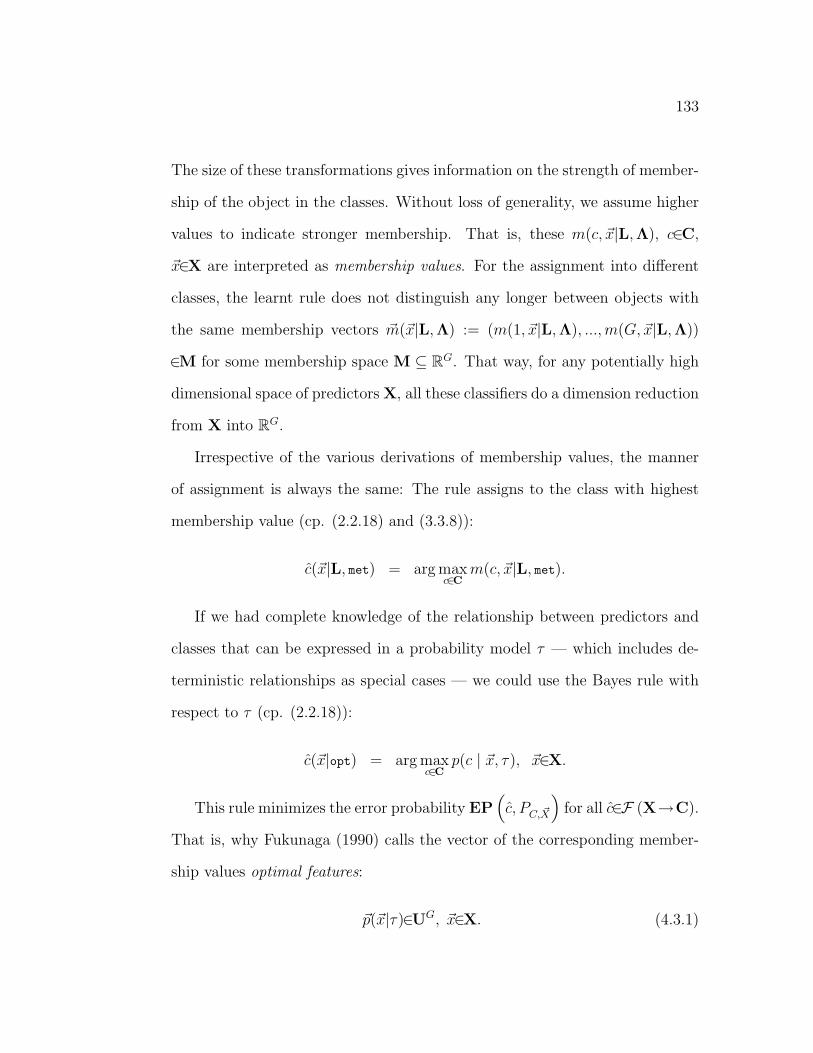
133

The size of these transformations gives information on the strength of member-

ship of the object in the classes. Without loss of generality, we assume higher

values to indicate stronger membership. That is, these m(c, ~x|L,Λ), c∈C,

~x∈X are interpreted as membership values. For the assignment into different

classes, the learnt rule does not distinguish any longer between objects with

the same membership vectors ~m(~x|L,Λ) := (m(1, ~x|L,Λ), ..., m(G,~x|L,Λ))

∈M for some membership space M ⊆ RG. That way, for any potentially high

dimensional space of predictors X, all these classifiers do a dimension reduction

from X into RG.

Irrespective of the various derivations of membership values, the manner

of assignment is always the same: The rule assigns to the class with highest

membership value (cp. (2.2.18) and (3.3.8)):

c(~x|L, met) = arg maxc∈C

m(c, ~x|L, met).

If we had complete knowledge of the relationship between predictors and

classes that can be expressed in a probability model τ — which includes de-

terministic relationships as special cases — we could use the Bayes rule with

respect to τ (cp. (2.2.18)):

c(~x|opt) = arg maxc∈C

p(c | ~x, τ), ~x∈X.

This rule minimizes the error probability EP(c, PC, ~X

)for all c∈F (X→C).

That is, why Fukunaga (1990) calls the vector of the corresponding member-

ship values optimal features:

~p(~x|τ)∈UG, ~x∈X. (4.3.1)

134

If these optimal features were known, we could use them to answer any

question of interest about the interplay of predictors and class membership.

The idea of standardized partition spaces as we will introduce them in the next

Chapter is motivated by the attempt to make any argmax rule comparable to

the ’true’ or ’optimal’ Bayes rule. We want to use learnt membership functions

of argmax classifiers as surrogates for optimal features.

Chapter 5

Introduction to StandardizedPartition Spaces for theComparison of Classifiers

In the preceding chapters, the main performance criterion for the comparison of

classification rules was the error probability and the corresponding appropriate

performance measure – the error rate on a validation set. In this chapter, we

will motivate, why one might want to go beyond that, and we will introduce

standardized partition spaces as means to do so.

5.1 Introduction

In the days of data mining, the number of competing classification techniques

is growing steadily. Thus, it is a worthy goal to rate the goodness of clas-

sification rules from a wide range of techniques related to diverse theoretical

backgrounds. Restricting the term goodness to what can be most easily for-

malized and measured is unsatisfactory. That is, ’goodness’ of a classification

rule can stand for much more than only its ability to assign future objects

135

136

correctly to classes — the correctness probability. This is, however, the only

aspect that is controlled by the most common performance measure, the error

rate. Error rates do not cover the variety of demands on classification rules in

practice.

In this context, Hand (1997) attaches importance to goodness concepts

regarding the rule’s quantitative assessment of the membership of objects in

classes. This assessment typically determines the final assignment into classes:

a high assessment (relative to the assessed membership in other classes) in the

assigned class should be justified (accuracy), the relative sizes of membership

in classes should reflect ’true’ conditional class probabilities (precision), and

membership values of objects in the different classes should be well-separated

(non-resemblance).

Beyond the reliable quantitative assessment of the membership of new ob-

jects in classes, in many practical applications of classification techniques it is

important that this assessment can be easily understood and is comprehensi-

ble. For that purpose one often is interested in the range of values of predictors

assigned to the same class. This relates to the rule’s induced partitions of the

predictor space (cp. (3.3.6)):

X =⋃c∈C

X[c],

X[c] ∩X[c] = ∅, c 6= c, c, c∈C.

It is not always the original space of measurement X in which considerations

about decision regions or boundaries are performed. In multi-dimensional

spaces XK , K∈N or/and with very flexible form of boundaries this often does

not lead to an improvement of understanding. In these cases, boundaries and

137

regions are often described in some feature space F of suitably derived features

Φ : X→F:

F =⋃c∈C

F[c],

F[c] ∩ F[c] = ∅, c 6= c, c, c∈C.

One example is the support vector machine. As has been shown in Chapter

3 the joint faces of the partitions of support vector machines in feature space

are hyperplanes, and their form in the original space is typically ”flexible” and

beyond human imagination if the dimension of the original space is greater than

three. Other examples of partitions described in feature spaces are common

in the visualization of decision regions of linear and quadratic discriminant

classifiers. For a more detailed discussion of this point, see Sondhauss and

Weihs (2001a).

If decision boundaries are described in some feature space, a direct com-

parison of the partitions from different classifiers would only be possible, if all

classification methods would deduce at least resembling entities as features.

This is not true when comparing methods from machine learning and statis-

tics.

Therefore, we will standardize the space of induced partitions with re-

spect to the joint faces between the partitions, such that in the corresponding

”feature” space we can compare and visualize the basic pattern of rules, and

additionally we can measure performance with respect to goodness aspects be-

yond the correctness probability. This idea was first introduced in Weihs and

Sondhauss (2000)

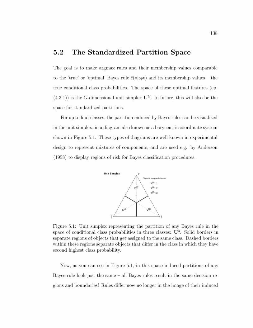
138

5.2 The Standardized Partition Space

The goal is to make argmax rules and their membership values comparable

to the ’true’ or ’optimal’ Bayes rule c(|opt) and its membership values – the

true conditional class probabilities. The space of these optimal features (cp.

(4.3.1)) is the G-dimensional unit simplex UG. In future, this will also be the

space for standardized partitions.

For up to four classes, the partition induced by Bayes rules can be visualized

in the unit simplex, in a diagram also known as a barycentric coordinate system

shown in Figure 5.1. These types of diagrams are well known in experimental

design to represent mixtures of components, and are used e.g. by Anderson

(1958) to display regions of risk for Bayes classification procedures.

1

2

3

Unit Simplex

X[1]

X[2]

X[3]

Objects’ assigned classes:

’X[1]’: 1

’X[2]’: 2

’X[3]’: 3

Figure 5.1: Unit simplex representing the partition of any Bayes rule in thespace of conditional class probabilities in three classes: U3. Solid borders inseparate regions of objects that get assigned to the same class. Dashed borderswithin these regions separate objects that differ in the class in which they havesecond highest class probability.

Now, as you can see in Figure 5.1, in this space induced partitions of any

Bayes rule look just the same – all Bayes rules result in the same decision re-

gions and boundaries! Rules differ now no longer in the image of their induced

139

partition, but where they place objects within these regions. Therefore, to

visualize the behavior of learnt rules in these coordinates, we have to display

some data points in these coordinates.

We use a test set T for that purpose. We require that the examples in

the test set data were not utilized by any method under consideration for the

learning of their rule, not as learning set L, and not as validation set V to

fight overfitting. Like in the Definition 2.3.1 of the training set we define the

test set such that it allows all statements cn∈T, ~xn∈T, and (cn, ~xn)∈T to be

valid:

T := (c, ~x)(ωn), ωn∈Ω, n = 1, ..., NT ,

:= (cn, ~xn), n = 1, ..., NT ,

:= cn, ~xn, n = 1, ..., NT .

5.3 The Bernoulli Experiment and the Cor-

rectness Probability

The basic view to analyze the behavior of some classification rule on the test

set is that of a Bernoulli experiment. Remember in Definition 3.4.5 we defined

the random variable

Z(C, ~X|L, met) := L[01](C, c( ~X|L, met)

)

that represents the zero-one loss of some learnt matching rule c(|L, met) on

some new randomly drawn example (C, ~X) according to PC, ~X . In standardized

partition spaces, we define performance in terms of success rather than in terms

140

of loss therefore the random variable of interest is the counterpart — the zero-

one gain:

G(C, ~X|L, met) := 1− L[01](C, c( ~X|L, met),

= IC(c( ~X|L, met)

).

Given the i.i.d. assumption holds on the test set, the gains with respect to the

examples in the test set are appropriately modelled as realizations of Bernoulli

random variables

Gn ∼ Be(CP

(c( ~X|L, met), PC, ~X

)), n = 1, ..., NT,

with

CP(c( ~X|L, met), PC, ~X

):= PC, ~X

((C, ~X) : c( ~X|L, met) = C

)

the correctness probability. And – analogously to the error probability and

the error rate – the correctness rate on the examples of the test set is an

appropriate empirical measure for the correctness probability:

CR := 1NT

∑(cn, ~xn∈T Icn(c(xn|L, met)

We are not so much interested in the overall correctness probability, but

more in the correctness probability with respect to the assignment into each

of the classes. Therefore, we divide the overall Bernoulli experiment for the

analysis of the gain with respect to any assignment in G Bernoulli experiments

for the analysis of potential gain with respect to the assignment into each class.

141

Let X[c](L, met), c∈C denote the induced partition on the predictor space

according to the rule c(~x|L, met), ~x∈X.

The conditional random variable G[c] : C×X[c](L, met)→0, 1:

G[c](C, ~X| ~X∈X[c](L, met),L, met)

:=

Ic(C)Ic

(c( ~X|L, met)

)if ~X∈X[c](L, met)


=

Ic(C) if ~X∈X[c](L, met),


is for each c∈C a Bernoulli random variable. Therefore, the gains of test set

examples in these regions can be modelled as realization of i.i.d. Bernoulli

random variables

Gn ∼ Be(CP

(c( ~X|L, met), PC, ~X

)), n = 1, ..., NT,

with

CP[c](c( ~X|L, met), PC, ~X

),

= PC, ~X

((C, ~X) : C = c, c( ~X|L, met) = c

),

=: PC, ~X|X[c]

((C, ~X) : C = c, ~X∈X[c]

),

the conditional correctness probability. And the corresponding empirical cor-

rectness rates will be called local correctness rates.

CR[c] := 1N

T[c]

∑cn∈T[c] Ic(cn)

142

5.4 Goodness Beyond Correctness Probability

We are focussing on the goodness concepts of accuracy, precision, and ability to

separate on refer to the concepts of inaccuracy, imprecision, and resemblance

of Hand (1997). There are two main differences. First, we use counterparts,

i.e. high values and not low values are desirable. Second, Hand restricts

his attention to probabilistic classifiers where membership values are equal

to estimated conditional class probabilities. Our aim is to generalize these

concepts to be applicable for a wider range of techniques, by using scaled

membership values instead of estimated conditional class probabilities.

Accuracy tells us something about the effectiveness of the rule in the assign-

ment of objects into classes. Measures of accuracy in the literature typically

assess whether true classes are the same as assigned classes. We call these

measures correctness measures to distinguish them from Hands measures of

accuracy that quantify the difference between a-posteriori class probabilities

of an observed example (1-0) and the estimated conditional class probabilities

of a probabilistic classifier. Given an accurate rule in the sense of Hand allows

to interpret the size of the estimated probability in the assigned class as a

reliable measure of the certainty we can have about that assignment. We want

scaled membership values to potentially allow for the same interpretation.

Ability to separate tells us, how well classes are distinguished, given the

transformations the classification rule uses to assess the membership of an

object in the classes. Measures of the ability to separate are based on the

diversity of the vectors of ’true’ conditional class probabilities among objects

assigned to different classes given their membership values. This is slightly

143

different from Hand’s concept of non-resemblance, where the diversity of the

’true’ conditional class probabilities among classes within probability vectors

given membership values is of interest. If the ability to separate is high, the

classifiers transformation for gaining membership vectors work out the charac-

teristic differences between classes. We want to use scaled membership vectors

to appropriately assess a classifiers ability to separate.

Precision tells us, how good the classification rule estimates ’true’ condi-

tional class probabilities. Measures compare the rule’s membership values with

’true’ conditional class probabilities. To measure precision, we obviously need

knowledge of ’true’ conditional class probabilities. Since our scaled member-

ship values should reflect as precisely as possible the information in the original

membership values and the rule’s performance on the test set, the empirical

precision will be enforced by our scaling procedure. Thus, scaled membership

values can not be used to assess precision, but mirror information of the rule’s

performance on the test set.

Note that Hand (1997) also defines separability which is substantially differ-

ent from the concepts above as it is a characteristic of classification problems

and not of rules. It tells us, how different the ’true’ conditional class proba-

bilities of objects are, given the observed features. Separability determines an

upper bound for any rule’s ability to separate. A measure for separability is

based on the diversity of ’true’ conditional class probabilities given the values

of the predictors of objects.

144

5.5 Some Example

For illustration, we generated two small data sets (27 examples each). Ex-

amples are generated according to three χ2(ν)-distributions with parameters

ν = 2, ν = 9, and ν = 29, respectively. Figure 5.2 shows the dot plot of the

realizations ~xn∈T from these classes, cn∈1, 2, 3 , with 1 : χ2(2), 2 : χ2(9),

and 3 : χ2(29).

0.3 1 2 5 10 20 40

ssssss

++++++

ooo

sss

ooo

+++ +++

oooooo

+++

ssssss

ooo ooo

sss

ooo

ssssss sss

ooo ooo ooo ooo

sss

+++

χ2(29)

χ2(9)

χ2(2)

Figure 5.2: Dotplot on a logarithmic scale for the realized test set samplesfrom the three χ2 distributions. There is small overlap between the samplessuch that they are non-separable.

The simplex on the left in Figure 5.3 presents the vectors of true conditional

class probabilities ~p(~xn|τ) of the realizations ~xn∈T. On the right you see the

respective estimated conditional class probability vectors ~p(~xn|L, qda), ~xn∈Taccording to the learnt plug-in Bayes rule of the QDA classifier as presented

in Chapter 2. Details of the implementation are given in the appendix.

The closer the marker of an example is to the class corner the higher is

its (estimated) probability in that class. The general shape of the position

of the markers in the two simplexes is parabolic. You can see e.g., that the

QDA classifier underestimates the class probability for objects in class χ2(2),

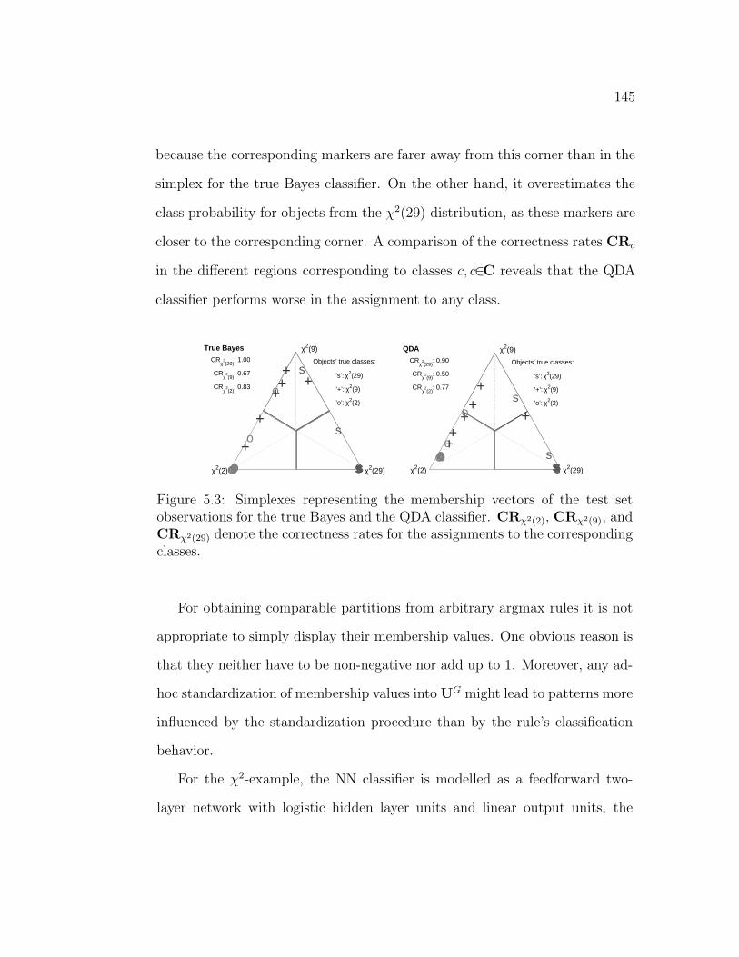
145

because the corresponding markers are farer away from this corner than in the

simplex for the true Bayes classifier. On the other hand, it overestimates the

class probability for objects from the χ2(29)-distribution, as these markers are

closer to the corresponding corner. A comparison of the correctness rates CRc

in the different regions corresponding to classes c, c∈C reveals that the QDA

classifier performs worse in the assignment to any class.

χ2(29)

χ2(9)

χ2(2)

True Bayes

CRχ

2(29)

: 1.00

CRχ

2(9)

: 0.67

CRχ

2(2)

: 0.83

ss

+

o so

++

oo

+

s

s

o

o

so ssooo s

+

s

o

+

Objects’ true classes:

’s’: χ2(29)

’+’: χ2(9)

’o’: χ2(2)

χ2(29)

χ2(9)

χ2(2)

QDA

CRχ

2(29)

: 0.90

CRχ

2(9)

: 0.50

CRχ

2(2)

: 0.77

sso

so

+

oo

+

sso

o

so

ssooo

s

+

+

+s

o

+


’s’: χ2(29)

’+’: χ2(9)

’o’: χ2(2)

Figure 5.3: Simplexes representing the membership vectors of the test setobservations for the true Bayes and the QDA classifier. CRχ2(2), CRχ2(9), andCRχ2(29) denote the correctness rates for the assignments to the correspondingclasses.

For obtaining comparable partitions from arbitrary argmax rules it is not

appropriate to simply display their membership values. One obvious reason is

that they neither have to be non-negative nor add up to 1. Moreover, any ad-

hoc standardization of membership values into UG might lead to patterns more

influenced by the standardization procedure than by the rule’s classification

behavior.

For the χ2-example, the NN classifier is modelled as a feedforward two-

layer network with logistic hidden layer units and linear output units, the

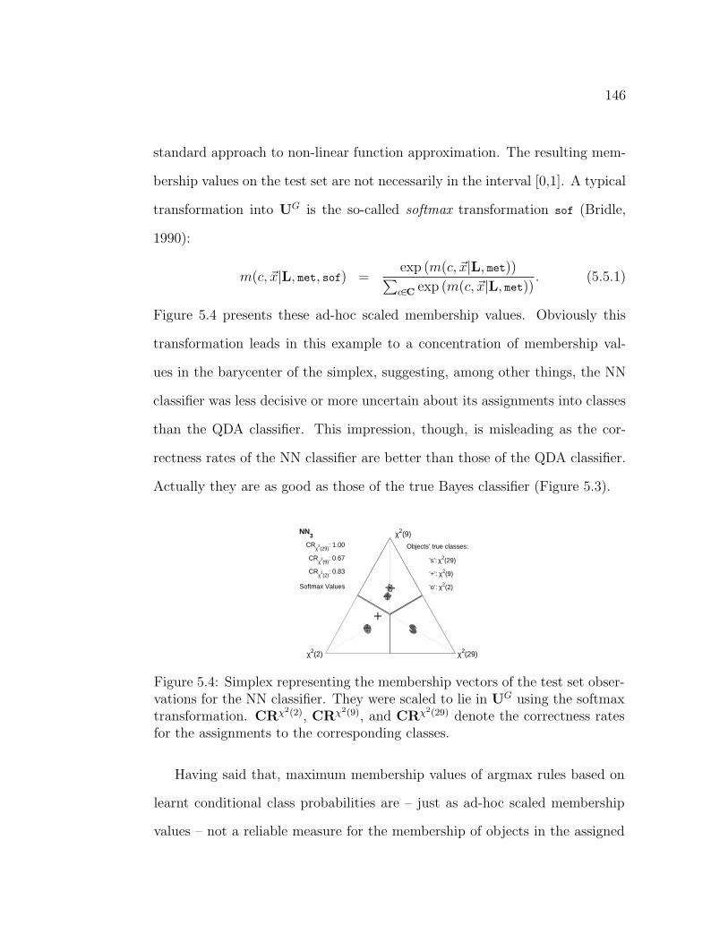
146

standard approach to non-linear function approximation. The resulting mem-

bership values on the test set are not necessarily in the interval [0,1]. A typical

transformation into UG is the so-called softmax transformation sof (Bridle,

1990):

m(c, ~x|L, met, sof) =exp (m(c, ~x|L, met))∑c∈C exp (m(c, ~x|L, met))

. (5.5.1)

Figure 5.4 presents these ad-hoc scaled membership values. Obviously this

transformation leads in this example to a concentration of membership val-

ues in the barycenter of the simplex, suggesting, among other things, the NN

classifier was less decisive or more uncertain about its assignments into classes

than the QDA classifier. This impression, though, is misleading as the cor-

rectness rates of the NN classifier are better than those of the QDA classifier.

Actually they are as good as those of the true Bayes classifier (Figure 5.3).

χ2(29)

χ2(9)

χ2(2)

NN3

CRχ

2(29)

: 1.00

CRχ

2(9)

: 0.67

CRχ

2(2)

: 0.83

Softmax Values

ss

+

o so

++

oo

+

ssoo so ssooo s+

so

+


’s’: χ2(29)

’+’: χ2(9)

’o’: χ2(2)

Figure 5.4: Simplex representing the membership vectors of the test set obser-vations for the NN classifier. They were scaled to lie in UG using the softmaxtransformation. CRχ2(2), CRχ2(9), and CRχ2(29) denote the correctness ratesfor the assignments to the corresponding classes.

Having said that, maximum membership values of argmax rules based on

learnt conditional class probabilities are – just as ad-hoc scaled membership

values – not a reliable measure for the membership of objects in the assigned

147

classes, and thus not a reliable measure for the correctness of the rule’s decision.

They give information on the rule’s performance from its own perspective only,

whereas for comparisons, we would prefer a more objective view.

You can see this in Figure 5.3 in the χ2-example . In the QDA simplex,

membership values of objects that get assigned to class χ2(29) are closer to the

χ2(29) corner than in the true Bayes simplex, because the QDA classifier gives

these objects a higher membership in that class. In terms of separateness

or non-resemblance, this incorrectly suggests that QDA was better in that

assignment than the true Bayes classifier. Only in simulation studies like this

we can know whether a higher separateness is justified by a real difference in

the characteristics of objects, or rather by an overestimation of the relevance

of differences by the classification method.

As both, non-probabilistic membership values and estimated class prob-

abilities, need to be scaled to reflect the rule’s true performance, from now

on we do no longer distinguish between membership values of probabilistic

classifiers and non-probabilistic classifiers, assuming the latter to be already

’appropriately’ standardized into the space UG. Appropriately for our pur-

poses means that for any ~x∈X at least the order of the membership values of

classes is kept whether it is based on the original membership values or on the

standardized ones. In this sense, the softmax transformation defined above is

a valid transformation. For classifiers with membership values not on a met-

ric scale, we recommend to use the ranks of m(~x, 1), ..., m(~x,G) for each ~x∈Xdivided by the number of classes G, as the relative distance between member-

ship values can not be interpreted. From now on we assume the membership

148

vectors ~m(~x|L, met), ~x∈X, to be members of the unit simplex, the placeholder

met subsuming the learning method and – if necessary – the ad-hoc scaling

method.

5.6 Scaling

As shown in the χ2 example, membership values have to be appropriately

scaled, before they can be used to assess the quality of a classification rule.

Otherwise, membership values are misleading. With our scaling procedure we

derive membership values where the size of the membership value of an object

assigned to some class can be interpreted as an indicator for the certainty, with

which the object really belongs to that class. In other words we are interested

mainly in the interpretation of the membership values in the assigned class.

In the following, these are called assignment values. We will denote them in

dependence of the class of the final assignment:

m[c](~x|L, met) :=

maxg∈C m(g, ~x|L, met) if c(~x|L, met) = c

undefined otherwise,(5.6.1)

for c∈C. If the assignment values of one classification rule are on average

higher than those of another classification rule, then for this to be justified,

the assignment into classes according to the first rule should be more reliable

than according to the latter. This is needed, if we want to go beyond the mere

use of correctness rates for the comparison of classification methods.

The assignment value of some new example (C, ~X) given ~X∈X[c](L, met) is

149

just like its gain a conditional random variable:

M [c]( ~X| ~X∈X[c](L, met),L, met)

:=

m[c]( ~X|L, met) if ~X∈X[c](L, met),


And thus, the assignment values of the test set examples in the regions can be

modelled as realization of random variables from distribution PM [c] .

We have two sources of information about the certainty of the assignment

of objects into classes:

1. the individual assessment of the membership of the objects in the classes

according to the membership values of the classification rule,

2. the observed performance with respect to these assignments on the test

set.

The former source has the disadvantage that it might be unreliable, the latter

the disadvantage that it results in statements of the average certainty whereas

we are interested in the certainty on individual assignments. Thus, we will use

the information on the actual performance to ”correct” the membership values

such that on average they reflect the actual behavior and such that relative

individual assessment is kept.

With these preliminaries, we can compare the information about the cor-

rectness probability as it is contained in the test set with the information about

the conceived correctness probability according to the classifier’s membership

values.

150

In a Bayesian setting, the correctness probability can be approached as an

uncertain parameter ϕ with a quantification of the current uncertainty about

it according to a conjugate prior distribution Pϕ. The Bernoulli distribution

is a special case of the binomial distribution, and the binomial-beta model is

the two-dimensional special case of the multinomial-Dirichlet model described

in subsection 2.3.3.

[Notation] In standard notation of the Beta distribution the param-

eters α and β correspond to the parameterization of the Dirichlet

distribution α1, α2 as we used it in Section 2.3.3. We will define

another parameterization in terms of the expected value of the Beta

distribution

p := E(γ|α, β) =α

α+β

and its equivalent sample size (cp. Section (2.3.3)) which we now refer

to as dispersion parameter:

N := α+β

One says N is the equivalent sample size only in context of the Binomial-

Beta learning of the uncertain parameter γ. Approaching the Beta

distribution in general (as we will do later) calling it ”dispersion” pa-

rameter is motivated by the fact that for fixed p the parameter N

determines the variance of the Beta distribution:

Var(γ|α, β) =αβ

(α+β)2(α+β+1)

=p(1− p)

N + 1

We can quantify the uncertainty about the correctness probability in each

region X[c] with the information in the sample in the test set for the corre-

sponding conditional Bernoulli experiment:

T[c](L, met) := (cn, ~xn)∈T : c(~xn|L, met) = c

151

Let NT[c] be the potency of T[c].

In standardized partition spaces and for the assessment of the information

about the classifiers correctness probability in the test set we use the minimal

informative improper prior (α0, β0) := (0, 0) rather than the other possible

choice (α0, β0) := (1, 1) which we said we would prefer in general in Section

2.3.3. We say something about the reasons to do so later.

With this prior, the posterior distributions Pϕ[c]|T[c] quantifying the uncer-

tainty about the correctness probabilities ϕ[c] for the assignment into classes

c∈C are Beta distributions Bt(pT[c] , NT[c]) where the expected value pT[c] is

quantified by the local correctness rate CR[c] in class c:

pT[c] :=1

NT[c]

∑

cn∈T[c]

Ic(cn)

= CR[c]

and the dispersion parameter NT[c] is quantified by the number of examples in

class c∈C.

We will model the distribution of the assignment value PM [c] also by a Beta

distribution, M [c] ∼ Bt(pM [c] , NM [c]) with unknown parameters pM [c]∈[0, 1] and

NM [c]∈N. We estimate these parameters by standard point estimation for that

task, namely the method of moments (cp. Gelman et al., 1995). Let

m[c] :=1

NT[c]

∑

~xn∈T[c]

m[c](~x|L, met)

S[c] :=1

NT[c] − 1

∑

~xn∈T[c]

(m[c](~xn|L, met)−m[c]

)2

be the sample mean and the sample variance of the assignment values for class

152

c. Then the parameters pM [c] and NM [c] can be estimated by:

pm[c] := m[c],

Nm[c] :=m[c]

(1−m[c]

)

S[c]− 1.

If the classifier’s assignment values were a reliable reflection of the uncer-

tainty of their assignments, then the estimated expected value should reflect

the local correctness rate CR[c] of the assignment to class c, as both are esti-

mators of the local correctness probability γ[c]. That is,

pm[c]

!≈ CR[c].

If that is not the case, membership values need to be scaled to be trusted as

quantifications to assess the certainty of assignments.

It is not necessary, though, that the two Beta distribution Bt(pm[c] , Nm[c])

and Bt(pT [c], NT [c]

)resemble also with respect to their dispersion parameters,

because these have different interpretations:

Bt(pT [c], NT [c]

)describes the uncertainty about the true value of the cor-

rectness probability γ[c]. The entity of interest is γ[c]. With respect to the

membership values the Beta distribution Bt(pm[c] , Nm[c]) describes the uncer-

tainty of individual assignments to classes from the perspective of the classifier.

The entities of interest are the individual assessments.

In the former context, the larger NT[c] is, the better, because the more

certain we are about γ. In the latter, smaller Nm[c] is preferable, if one can

reliably interpret the deviation from the mean in two respects:

1. if the assignment value is larger/lower than the mean then the assignment

is more/less certain than on average, and

153

2. if the assignment value is lower than the mean and this results in a higher

assessment of membership in another class then this should correspond

to a higher probability that this object belongs to that other class than

on average.

If membership values are reliable, then the dispersion parameter Nm[c] reflects

the (true) diversity of objects with respect to assessed membership.

Our scaling aims at scaled membership values that meet these requirements.

That is, we want to scale membership values such that they approximate a Beta

distribution with expected value CR[c] and ”appropriate” dispersion parameter

N . We iterate to find the best dispersion parameter N [c,opt]:

1. Define N := min NT[c] , NM [c] as the minimum dispersion parameter

and N := max NT[c] , NM [c] as the maximum dispersion parameter to

describe the diversity of assessed scaled membership in class c among all

objects that get assigned to class c. Do the following steps for all N∈N,

N≤N≤N :

(a) Let Fp,N denote the Beta distribution function with parameters

p,N . For all ~xn∈T[c], evaluate the equation

FCR[c],N (m(c, ~xn|L, met,T, N)) (5.6.2)

= Fpm[c] ,Nm[c]

(m(c, ~xn|L, met)) (5.6.3)

to yield m(c, ~xn|L, met,T, N). Scaled assignment values that solve

this equation approximate a Beta distribution Bt(CR[c], N

). This

is a basic trick mainly used when generating random numbers. The

trick is based on a fundamental property of any distribution PY with

154

continuous distribution function FY . According to this property the

transformation of Y with its own distribution function is uniformly

distributed

U := F (Y ) ⇒ U ∼ U [0, 1],

with U [0, 1] denoting the uniform distribution on the interval [0, 1].

And for an uniformly distributed random variable U ∼ U [0, 1] and

any continuous distribution function F of a distribution P it is true

that

F−1(U) ∼ P .

In consequence it is true that

F (F−1(Y )) ∼ P .

(b) Scaled membership vectors are members of the unit simplex

~m(~x|L, met,T, N)∈UG.

Therefore, after the scaling of the assignment value of some object

(cn, ~xn)∈T[c] the membership values m(g, ~xn|L, met) of this object in

the other classes g 6=c, g, c∈C have to be recalculated, such that the

scaled membership values in all classes sum up to one. We do this,

keeping the ratio of membership values in the other classes fixed:

m(g, ~xn|L, met,T, N)

:=1−m(c, ~x|L, met,T, N)

1−m(c, ~x|L, met)m(g, ~x|L, met).

155

(c) We calculate the average euclidian distance of the scaled member-

ship vector ~m(~xn|L, met,T, N) to the class indicator function of the

true class ~e(cn), (cn, ~xn)∈T[c]:

D(N) :=1

NT[c]

∑

(cn,xn)∈T[c]

∥∥~e(cn)− ~m(~x|L, met,T, N)∥∥

The smaller it is, the more reliable is the information on deviations

in dependency of N . We do not want to increase the number of false

assignments with our scaling, therefore we select as best N [c,opt] the

one that minimizes D(N) relative to the prediction error rate on

T[c] we would get, if we used m(|L, met,T, N) for prediction.

The scaled membership vectors with the optimal dispersion parameters

in each class are the scaled membership values we use in standardized

partition spaces:

~m(~x|L, met,T, sca)∈UG.

5.6.1 Justification

The scaled membership vectors ~m(~x|L, met,T, sca) describe the classification

performance of the rule, because on average the scaled memberships in the

assigned classes reflect the correctness of that decision, namely CR[c] and the

dispersion parameter N [c,opt] is chosen such that the reliable information of the

scattering of vectors around the mean is maximized, c∈C.

Given these properties, we can interpret the scaled membership values

m(s, ~x|L, met,V, sca) as some estimator for the probability to be in a certain

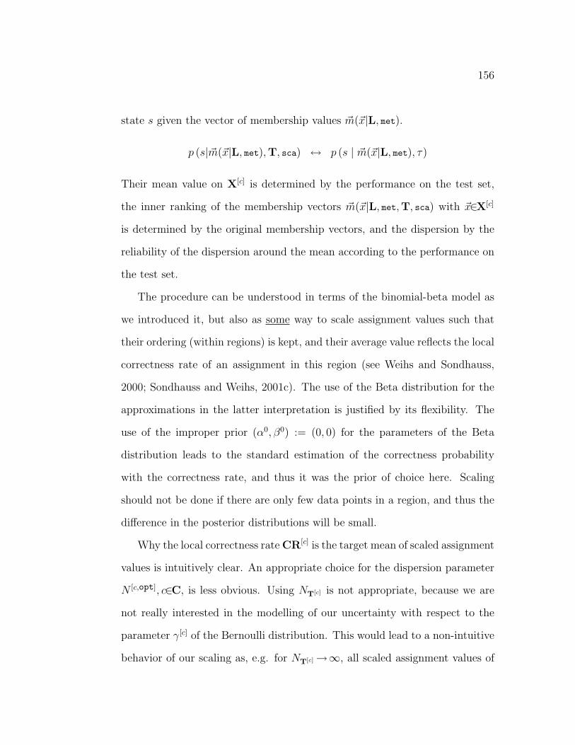
156

state s given the vector of membership values ~m(~x|L, met).

p (s|~m(~x|L, met),T, sca) ↔ p (s | ~m(~x|L, met), τ)

Their mean value on X[c] is determined by the performance on the test set,

the inner ranking of the membership vectors ~m(~x|L, met,T, sca) with ~x∈X[c]

is determined by the original membership vectors, and the dispersion by the

reliability of the dispersion around the mean according to the performance on

the test set.

The procedure can be understood in terms of the binomial-beta model as

we introduced it, but also as some way to scale assignment values such that

their ordering (within regions) is kept, and their average value reflects the local

correctness rate of an assignment in this region (see Weihs and Sondhauss,

2000; Sondhauss and Weihs, 2001c). The use of the Beta distribution for the

approximations in the latter interpretation is justified by its flexibility. The

use of the improper prior (α0, β0) := (0, 0) for the parameters of the Beta

distribution leads to the standard estimation of the correctness probability

with the correctness rate, and thus it was the prior of choice here. Scaling

should not be done if there are only few data points in a region, and thus the

difference in the posterior distributions will be small.

Why the local correctness rate CR[c] is the target mean of scaled assignment

values is intuitively clear. An appropriate choice for the dispersion parameter

N [c,opt], c∈C, is less obvious. Using NT[c] is not appropriate, because we are

not really interested in the modelling of our uncertainty with respect to the

parameter γ[c] of the Bernoulli distribution. This would lead to a non-intuitive

behavior of our scaling as, e.g. for NT[c] →∞, all scaled assignment values of

157

objects in that region approach the empirical mean CR[c] which approaches

the true correctness probability. The parameter N [c,opt] should rather have an

interpretation as a measure of the dispersion of assignment values. Because

of that, no huge scaling of assignment values near to true conditional class

probabilities should take place. This is an argument favoring the dispersion

parameter Nm[c] estimated with the original assignment values, but only for

probabilistic classifiers. For non-probabilistic classifiers Nm[c] is dependent on

the ad-hoc standardization of the corresponding membership vector into UG,

and might be misleadingly high or low. Our approach avoids unwarranted

large certainty parameters Nm[c] for each c∈C.

5.7 Performance Measures for Accuracy and

Ability to Separate

We now define measures for the rating of the performance of argmax classifi-

cation rules with respect to accuracy and ability to separate. These measures

are based on Euclidean distances between scaled membership vectors of test

set examples and specified corresponding corners of the simplex: either it is

the corner of the true class or it is the corner of the assigned class.

The definition in terms of these Euclidean distances is not only useful for

the understanding of the measures as such but also for a visualization of the

performance of classifiers for classification problems with up to four classes.

The measure of accuracy is based on the Euclidean distances between scaled

158

membership vectors ~m(~xn|L, met,T, sca) and the vector representing the corre-

sponding true class corner ~e(cn) for the examples (cn, ~xn)∈T. We standardize

the mean of these distances such that a measure of 1 is achieved if all vectors

lie in the correct corners, and zero if they all lie in the centroid of the simplex.

The measure of accuracy is thus:

Ac (met | L,T, sca) (5.7.1)

:= 1− G(G−1)

1NT

NT∑n=1

‖~e(cn)− ~m(~xn|L, met,T, sca)‖ (5.7.2)

On the basis of this performance measure, we can now compare the behavior

of the QDA classifier with the behavior of the NN classifier in the χ2-example.

In the scaled simplexes in Figure 5.5, the average distance of objects to the

assigned corners can be interpreted as the average correctness of such an as-

signment. The nearer objects are to the corner, the better the classifier is.

So we easily can see that the NN classifier is better in the assignment to the

χ2(2) and the χ2(29) class, because apparently most objects in these regions

are closer to these corners. The accuracy, though, is not that much better.

The reason is, that for some individual objects, the NN classifier has very high

assignment values, though the assignment is wrong. The measure of accuracy

penalizes this over-confidence.

Analogously, the measure of the ability to separate is based on the Eu-

clidean distances between scaled membership vectors ~m(~xn|L, met,T, sca) and

the vector representing the corresponding assigned class corner ~e(c (~xn | L, met)),

of the observed measurements ~xn∈T.

159

Note that in particular for poor classifiers the assignment of an observation

based on its scaled membership values might be different from the assignment

based on the original membership values, such that

c (~xn | L, met) = arg maxc∈C

m(c, ~xn|L, met)

6= arg maxc∈C

m(c, ~xn|L, met,T, sca)

and that we really want to use the original assignment in our definition.

We do this, because we want to measure the diversity of the scaled mem-

bership values of objects that are assigned to the same class of the original

classification rule. Only then, our measures are estimates for the behavior of

the rule on its induced partitions Xc(L, met), c∈C.

We standardize the mean of these distances in the same way as above, such

that our measure of the ability to separate is defined as:

AS (met | L,T, sca) (5.7.3)

:= 1− G(G−1)

1NT

NT∑n=1

‖~e(c(~xn|L, met))− ~m(~x|L, met,T, sca)‖ (5.7.4)

In the χ2-example, the ability to separate of the NN classifier (AS=0.78) is

noticeable higher than the ability to separate of the QDA classifier( AS=0.63)

as can be seen in Figure 5.6. The position of the membership values in their

simplexes reflects that fact: in particular the objects in the χ2(2) and the

χ2(29) areas are in the NN-simplex much closer to the corner than in the

QDA-simplex, and therefore better separated from the objects in the other

regions.

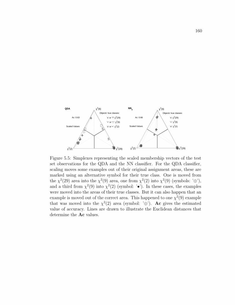
160

χ2(29)

χ2(9)

χ2(2)

QDA

Ac: 0.63

Scaled Values

sso

so

+

oo

⊕

s

soo

so

ssooo

s

⊕

+

⊕s

•+


’s’ or ’?’: χ2(29)

’+’ or ’⊕’: χ2(9)

’o’ or ’•’: χ2(2)

χ2(29)

χ2(9)

χ2(2)

NN3

Ac: 0.66

Scaled Values

ss

+

o so

++

oo

+

ssoo

sossooo s+

s

o

+


’s’: χ2(29)

’+’: χ2(9)

’o’: χ2(2)

Figure 5.5: Simplexes representing the scaled membership vectors of the testset observations for the QDA and the NN classifier. For the QDA classifier,scaling moves some examples out of their original assignment areas, these aremarked using an alternative symbol for their true class. One is moved fromthe χ2(29) area into the χ2(9) area, one from χ2(2) into χ2(9) (symbols: ’⊕’),and a third from χ2(9) into χ2(2) (symbol: ’•’). In these cases, the exampleswere moved into the areas of their true classes. But it can also happen that anexample is moved out of the correct area. This happened to one χ2(9) examplethat was moved into the χ2(2) area (symbol: ’⊕’). Ac gives the estimatedvalue of accuracy. Lines are drawn to illustrate the Euclidean distances thatdetermine the Ac values.

161

χ2(29)

χ2(9)

χ2(2)

QDA

AS: 0.63

Scaled Values

sso

so

+

oo

⊕

s

soo

so

ssooo

s

⊕

+

⊕s

•+


’s’ or ’?’: χ2(29)

’+’ or ’⊕’: χ2(9)

’o’ or ’•’: χ2(2)

χ2(29)

χ2(9)

χ2(2)

NN3

AS: 0.78

Scaled Values

ss

+

o so

++

oo

+

ssoo so ssooo s+

s

o

+


’s’: χ2(29)

’+’: χ2(9)

’o’: χ2(2)

Figure 5.6: Simplexes representing the scaled membership vectors of the testset observations for the QDA and the NN classifier. For the QDA classifier,scaling moves some objects out of their original assignment areas. These aremarked using an alternative symbol for their true class. AS gives the esti-mated value of the ability to separate. Dotted lines are drawn to illustrate theEuclidean distances that determine the AS values.

5.8 Applications

We use two benchmark problems from the UCI Repository (Blake and Merz,

1998) to show the potential benefit of standardized partition spaces for the

comparison of classification methods.

One is the well-known Iris data set which dates back to Fisher (1936).

The data set contains three classes of iris plant of 50 instances each, namely

Setosa, Virginica and Versicolor. Using length and width of the sepals and

petals of the plants, Setosa is linearly separable from the other two; Virginica

and Versicolor are not linearly separable from each other. Altogether, the

domain is very simple.

The other data set is the so-called Glass identification database created

by German (1987). For 214 glass splinter, the origin from one of seven types

of glass are to be identified. Refraction index and the weight percent in nine

oxides of elements like Sodium, Magnesium and others are measured. We

162

comprised the original seven classes to float processed window glass (fpW),

non-float processed window glass (nfW), and non-window glass (noW). This

domain is pretty difficult and classes are not easy to separate.

We split the Iris data in two halves for training and testing. As the iris data

set is balanced, we kept the balance in the test and training set, such that there

are 25 observations from each plant in each data set. From the glass data we

took a simple sample of about a third (72/214) of the observations for the test

set. This resulted in a frequency in the classes fpW/nfW/NoW of 51/55/36 in

the training set and 36/21/15 in the test set.

We compared a set of classification methods, that are quite different in the

assumptions they make about any underlying generating process of the data

as we elaborated in chapters 2-4: the classifiers from linear and quadratic dis-

criminant analysis (LDA, QDA), a continuous naıve Bayes classifier (CNB),

a Neural Network (NN), the k-Nearest neighbor classifier (k-NN), and a de-

cision tree classifier (TREE). Details of the implementation are given in the

appendix.

The main results on the iris data are presented in Table 5.1:

As expected, all classifiers perform pretty well on the Iris data set w.r.t.

correctness rate, accuracy, and ability to separate. In Figure 5.7 you see the

simplexes of the three best classifiers according to these measures. In the

simplexes you see at a glance that these classifiers can perfectly identify Setosa

plants: all scaled membership values of Setosa-objects lie strictly (except for

jittering) in the Setosa-corner, and all other objects lie on the side line between

Virginica and Versicolor. QDA misidentifies one Viginica plant as Versicolor,

163

Method CR Ac ASQDA 0.97 0.93 0.95LDA 0.96 0.91 0.93k-NN3 0.96 0.89 0.94NB 0.95 0.87 0.91TREE3 0.95 0.84 0.92NN4 0.92 0.77 0.88

Table 5.1: Performance of compared methods on the Iris database, ordered bydeclining correctness rate and accuracy. QDA, LDA, and k-NN3 are the threebest with respect to all performance measures, but the ranking differs whenthe ability to separate instead of the accuracy is used for ordering: LDA issecond best in accuracy and k-NN is second best in ability to separate.

and one Versicolor plant as Virginica, apparent from one ’+’ in Versicolor’s area

and one ’o’ in Virginica’s area. The scaled assignment values lie comparatively

near to the border between these areas, say, the QDA classifier detected these

assignments correctly as slightly ambiguous.

LDA and k-NN3 both have the same correctness rate, resulting from three

misclassifications: LDA misidentifies two Versicolors as Virginica and one Vir-

ginica as Versicolor, and k-NN3 does it vice versa. Objects are better separated

(more densely grouped) in the simplex of k-NN3. Thus, k-NN3 has a higher

ability to separate than LDA — simply because k-NN3 only has a few dis-

tinct membership vector values, namely(3+3−1

3

)= 10, corresponding to the

observable frequencies in three groups in a sample of three objects. On the

other side, k-NN3 has a lower accuracy than LDA, mainly because one of the

misspecified Virginicas (the ’o’ near the Versicolor’s corner) has in the training

set three Versicolor neighbors, and thus an original membership value of one

in the Versicolor class. Scaling does not move the objects in the Versicolor

region too much, because on average, k-NN3 is pretty successful in correctly

164

Sts

Vrs

Vrg

QDA

Ac: 0.93

AS: 0.95

Scaled Values

sssssssssssssssssssssssss

++++++++++++++++

+

+++++

++

ooo

oooooooo

oo

ooooooo

oooo+

o


’s’: Sts

’+’: Vrs

’o’: Vrg

Sts

Vrs

Vrg

k−NN3

Ac: 0.89

AS: 0.94

Scaled Values


++++++++++++++

+

+

+

++++

+

++

o

oo

oo

oo

oooo

oooooo

oooooo+

o

o


’s’: Sts

’+’: Vrs

’o’: Vrg

Sts

Vrs

Vrg

LDA

Ac: 0.91

AS: 0.93

Scaled Values


++++++++++++++++++++

+

++

ooooooooooo

oo

oooooo

o

oooo

++

o


’s’: Sts

’+’: Vrs

’o’: Vrg

Figure 5.7: Simplexes representing the scaled membership vectors of the QDA,the k-NN3 and the LDA classifiers of the iris test set observations. AS andAc give the estimated ability to separate and accuracy of these classifiers.

assigning to Versicolor:

p(Vrs | X[V rs](L, knn),T, sca

)=

23

25= 0.92

This value of 0.92 is not too far from the average original membership value

in this region,

m[V rs](T|L, knn) = 0.949.

The contribution of the misspecifying membership vector alone on the es-

timated accuracy Ac is approximately − 350

√2 ∼= −0.08.

Loosely speaking, the ability to separate is higher the lesser the classifier’s

membership vectors reflect the individuality of objects within regions. This is

what we want, if we are mainly interested in the commonness of objects in the

165

same region. Yet, at the same time, it raises the risk that ambiguous individu-

als are not detected as such, which decreases the accuracy of the classification

rule.

As expected, the overall performance is noticeably worse on the Glass

data compared to the Iris data set w.r.t. correctness rate (≤ 0.85), accuracy

(≤ 0.55), and ability to separate (≤ 0.72). With Figure 5.8 we mainly want to

demonstrate the importance of scaling for a comparison of probabilistic and

non-probabilistic classifiers. If we had measured the ability to separate of the

naıve Bayes classifier with its own estimates of class conditional probabilities

it would be very high, namely ASoT = 0.96, because most objects lie in the

corners. But this would not reflect the diversity of the vectors of ’true’ condi-

tional class probabilities given their membership values, but only the classifiers

own estimate thereof. And given the high rate of misclassifications, this is not

reliable. For the NN4 classifier, the softmax transformation in equation (5.5.1)

leads to concentration of objects in the barycenter of the simplex like in the

χ2-example. Thus, determining the accuracy and the ability to separate with

these values, would lead to very low estimates:

Ac(nn|L,T, sof) = 0.16, AS(nn|L,T, sof) = 0.26.

The arbitrariness of this may become apparent, when knowing that the softmax

transformation on the doubled values of the original membership values:

m(c, ~x|L, met, 2sof) :=exp (2m(c, ~x|L, met))∑c∈C exp (2m(c, ~x|L, met))

.

would have led to measures of accuracy

Ac(nn|L,T, 2sof) = 0.28, AS(nn|L,T, 2sof) = 0.49.

166

We can continue with this: on the basis of original membership values times

4 performance would seem to be even better with

Ac(nn|L,T, 4sof) = 0.38, AS(nn|L,T, 4sof) = 0.72.

These ad-hoc scalings are as appropriate as the softmax transformation with

factor 1 on the original membership values, thus, this is an example of the

earlier stated problem, that measuring accuracy and ability to separate on the

basis of ad-hoc scaled membership values reflects scaling procedure rather than

the behavior of the classification rule. One can take advantage of the depen-

dency of the softmax scaling on factorizing the original membership values to

find a scaling that is appropriate and meaningful in another context. This will

be shown in Chapter 7.

Method CR Ac ASTREE 0.85 0.55 0.72k-NN1 0.83 0.55 0.75NN 0.67 0.32 0.50QDA 0.67 0.31 0.34NB 0.67 0.27 0.44LDA 0.65 0.27 0.41

Table 5.2: Goodness of various methods on the glass database, ordered firstby declining correctness rate and second by declining accuracy. TREE andk-NN1 are by far the two best classifiers w.r.t. all three measures, but theinner ranking would be different, if we had used the ability to separate insteadof the correctness rate for the ordering.

167

fpW

nfW

NoW

Naive Bayes

CRfpW

: 0.69

CRnfW

: 0.43

CRNoW

: 0.89

ssssssss

+

sssssssso ssoo sss

+

sssso sso sooo ss

++

ss

++

ss+++

o

+

sos

+++o++

oo

+

o

+++

o

++


’s’: fpW

’+’: nfW

’o’: NoW

fpW

nfW

NoW

NN4

CRfpW

: 0.74

CRnfW

: 0.48

CRNoW

: 0.88

Softmax Values

sss

sssss

+ssssss

so

+s

+

s+

oss

+

+

ssoo sso

soo

s+

s

+

s

+

s

++

s

+

+

s

++o

+s

os

o

s

o

+

o ss+

o

+o+

o

+s


’s’: fpW

’+’: nfW

’o’: NoW

fpW

nfW

NoW

Naive Bayes

Ac: 0.27

AS: 0.44

Scaled Values

ssssssss⊕

ssssssss

o

ss

oo

sss⊕

ssss

o

ss

o

s

ooo

ss⊕

+

ss

+

⊕ss+++

•

+?

os

+++o++

o

•+

•

+++

o

++


’s’ or ’?’: fpW

’+’ or ’⊕’: nfW

’o’ or ’•’: NoW

fpW

nfW

NoW

NN4

Ac: 0.32

AS: 0.50

Scaled Values

sss

ssss

s

+

ssssss

s

o

+

s

+

s

+

oss

+

+

ssoo sso

s

oos

+

s

+

s

+

s

++

s

+

+

s

++

o+ ?

o?

o

s

o

+

o ??

+

o

+o+

o

+?


’s’ or ’?’: fpW

’+’ or ’⊕’: nfW

’o’ or ’•’: NoW

Figure 5.8: Simplexes representing the original and the scaled membershipvectors of the glass test set observations for the naıve Bayes and the NN4

classifier. AS and Ac give the estimated ability to separate and accuracy. Forboth classifiers, scaling moves some objects out of the assignment area of nfW.These are marked using an alternative symbol for their true class.

5.9 Conclusions

In this chapter, we introduced standardized partition spaces as means to com-

pare argmax classification rules.

With the scaling given in section 5.6, one can overcome at the same time the

arbitrariness of typical ad-hoc scaling procedures for non-probabilistic classi-

fiers, and the unreliability of heavily model-based class conditional estimates.

This is, because the empirical distribution of scaled membership vectors re-

flects the distribution of the original membership vectors corrected for the

information in the test set.

168

One can understand standardized partition spaces in terms of an inversion

of the standard approach to compare induced partitions of various classification

rules by means of the decision boundaries in the predictor space X — the joint

faces of the induced partitions. In high-dimensional predictor spaces, and with

respect to a wide variety of classifiers with very different decision boundaries,

such a comparison may be difficult to understand. In these cases, it can be

helpful not to use the predictor space as the constant entity for the comparison

but to standardize decision boundaries and regions — and to compare the

classification rules with respect to the different patterns they generate when

placing examples from some test set in these standardized regions.

The layout of examples in standardized partition spaces reflects the classi-

fiers characteristic of classification and give a realistic impression of the classi-

fiers performance on the test set. In this sense, standardized partition spaces

are a valuable tool for the comparison of rules with respect to their quantita-

tive assessment of the membership of objects in classes, in particular by means

of accuracy and ability to separate.

Chapter 6

Comparing and InterpretingClassifiers in StandardizedPartition Spaces usingExperimental Design

In this Chapter we realize the comparison of classification rules in standardized

partition spaces with the methods derived in Chapter 5. We will introduce a

visualization of scaled membership values that can be used to analyze the

influence of predictors on the class membership.

We demonstrate the use of standardized partitions spaces in analyzing the

astonishing phenomenon that simple classification methods do pretty well on

real data sets though their underlying premises about the true relation be-

tween predictors and classes can not reasonably be assumed to hold. We will

implement a screening experiment to detect the main influencing factors for

the performance of various classifiers.

169

170

6.1 Introduction

We will perform a simulation study to analyze the following problem:

Given a medium number of predictors, (10-20), and a potentially complex

relation between classes and predictors, one would expect flexible classification

methods like support vector machines or neural networks to do better than

simple methods like e.g. the linear discriminant analysis or cart. Nevertheless,

one often observes on real data sets, that the simple procedures do pretty well.

Our assumption is, that simple methods are more robust against instability,

and that the effect of instability superposes the effect of complexity of the

relation. By instability we mean the deviation from the assumption that the

collected data are an independent and identically distributed sample from a

certain joint distribution of predictors and classes.

We analyze this problem with a simulation study using experimental design.

6.2 Experiment

In general, influencing factors for the goodness of any classification methods

are data characteristics like the number of classes (we fix as three), the number

of predictor variables (we fix as 12), the number of training objects as such

(we vary), the number of training objects in classes (we use balanced design

only) the number of missing values (we ignore this factor at this stage), and

the form of the joint distribution of classes and predictors on objects.

Our main interest is on the influence of the form of the joint distribution

of classes and predictors on objects.

171

The form determines the shape of the optimal partition. The joint faces

fc,g of the partitions between two classes for continuous densities are given

implicitly by the equations

pτ (g|~x) = p(h|~x, τ), g 6= h, g, h∈C.

We view these implicit functions as random variables Yg,h := fg,h( ~X).

For a direct systematic scanning of this space of implicit functions via simu-

lations, we would have to fix various functions fg,h( ~X) of increasing complexity,

and determine from there possible joint distributions of C and ~X.

This is rather complicated, and moreover, the connection of this to some-

thing one can potentially know about the problem at hand, or see by explo-

ration of the data, is difficult to understand. Thus we do not want to model the

complexity of the relation via these implicit functions, but via the conditional

distributions P ( ~X|c, τ), c = 1, ..., G.

One aspect of the joint distribution is the dependency structure between

predictors. Often this makes the learning results less stable. Some classification

methods, like e.g. the naıve Bayes, even assume independence of variables. In

all cases, the analysis of the relevance of predictors for the detection of classes

is obscured by this inner dependency.

Concerning the shape of the bivariate distributions between one predictor

and the class, we define easiness from the perspective of the classifier from

a linear discriminant analysis: easy are linear functions fg,h, which we know

can be generated from multivariate normal distributions with equal covariance

matrices. These are the assumptions, a linear discriminant analysis is based

on. In that case, Yg,h — as a sum of normally distributed variables — is also

172

normally distributed.

To see the effect of instability on the different types of classification meth-

ods, we model instability by deflected observations accounting for three factors:

the percentage of deflected observations, the percentage of relevant variables

in which the deflection takes place and the direction of the deflection.

Deflection only takes place on the test data. Thus the ”true” generating

process for the test data differs from that of the training data.

6.2.1 Classification Methods

We compared a set of classification methods, that are quite different in the

assumptions they make about any underlying generating process of the data

as we elaborated in chapters 2 and 3: the classifiers from linear and quadratic

discriminant analysis (LDA, QDA), a continuous naıve Bayes classifier (CNB),

a Neural Network (NN), the k-Nearest neighbor classifier (k-NN), and a de-

cision tree classifier (TREE). In the appendix you find the description of the

implementation of these classification methods.

6.2.2 Quality Characteristics

The target values in our experiment are correctness rate (CR), accuracy (Ac),

and ability to separate (AS) just as we derived them in Chapter 5. The

more overlapping the true distribution are the more difficult is the problem as

such. Thus we use as target values not the performance measures as such but

their relation ratios (rCR, rAc, rAS) to the best that can be achieved: the

corresponding performance values of the Bayes rule with respect to the true

173

V G1 G2 G3 relevant for V G1 G2 G3 relevant forV1 0 -1.64 1.64 G2 vs G3 V7 0 -1 1 G2 vs G3V2 1.64 0 -1.64 G1 vs G3 V8 1 0 -1 G1 vs G3V3 -1.64 1.64 0 G1 vs G2 V9 -1 1 0 G1 vs G2V4 0 1.64 1.64 G1 vs rest V10 0 0 0 AnnoyanceV5 1.64 0 1.64 G2 vs rest V11 0 0 0 AnnoyanceV6 1.64 1.64 0 G3 vs rest V12 0 0 0 Annoyance

Table 6.1: Definition of Expectation of Predictors in Groups in the non-dependent case

probability model.

6.2.3 Predictors

We also want to demonstrate the use of scaled membership values for analyzing

the relevance of variables for the different classes. For that purpose we generate

our predictor variables such that we have a clear concept for the relevance at

least in the non-dependent case.

All univariate distributions have variance 1. They only differ in expecta-

tion, kurtosis and skewness. Table gives the defined expectations, which are

either zero, one, or the upper or lower 5%-quantile of the standard normal

distribution, u.05.= −1.64 and u.95

.= 1.64.

We fix this expectations for the normal and the non-normal case. The

resulting expectations, variances an covariances in the dependent case can be

calculated.

174

6.2.4 Factors

We define the low (level=-1) and the high level (level=1) for our experimental

design by looking at the easiness of the learning task.

The more training data we have, the more information we have to learn

classification rules, thus we consider the number of examples in the training

set as influencing factor TO. We set N = 1000 as low (difficulty) level and

N = 100 as high (difficulty) level.

To model the deviance of the true distribution from the normal distribution,

we use the Johnson System (Johnson, 1949), where random variables can be

generated such that they have pre-defined first four central moments. Low and

high skewness values (S: 0.12 and 1.152), and low and high kurtosis values (K:

2.7 and 5.0) are selected such that all combinations are valid, and that a wide

range of distributions in the skewness-kurtosis-plane is spanned.

On the low level of dependency Dp, we generate independent predictor

variables Xk, k = 1, ..., K. The high level of dependence is constructed by

calculating ”inverted” variables: Xk :=∑K

i=1 Xi −Xk, k = 1, ..., K.

We do want deflection to be the deviance from the ordinary, thus the chosen

high level of 40% for the percentage of deflected observations DO assures that

more than a half of the observations is ”ordinary”. We define the low level as

10%. For the low level of the percentage of deflected variables DV only one

of the nine relevant predictor variables is deflected, on the high level, all but

one.

The direction of deflection DD of an observation is either determined by

a shift of the value in each affected predictor variable towards its mean in the

175

Plan No. TO K S DP DO DV DD1 -1 -1 -1 -1 -1 -1 -12 -1 -1 1 -1 1 1 13 1 -1 -1 1 -1 1 14 1 1 -1 -1 1 -1 15 1 1 1 -1 -1 1 -16 -1 1 1 1 -1 -1 17 1 -1 1 1 1 -1 -18 -1 1 -1 1 1 1 -1

Table 6.2: Plackett-Burmann design for seven factors. In the experiment ac-cording to each plan, factors with ”-1” are set on low values, and those with”1” on high values.

true group of the observation, or away from it towards the nearest true mean

of this variable in another group.

6.2.5 Experimental Design

To do the screening for detecting the relevant factors for the relative perfor-

mance of the analyzed set of classifiers, we use a standard Plackett-Burman

design for the seven factors under investigation. It is presented in Table 6.2.

6.3 Results

In Table 6.3 we present the values of those coefficients of the approximated

linear response functions that are significant at a five percent level, the measure

of the fit of the linear model based on all factors R2, and based only on the

significant factors R25%.

For all performance measures and all classification methods, the size of the

training set is always significant. In general, all classification methods react

176

stronger in terms of the relative accuracy and the relative ability to separate,

than with respect to the relative correctness rate. This is not astonishing, be-

cause deviations from the underlying model always influence the quantification

of the class membership but have to reach a certain level to influence the class

assignment. In that sense, the performance measures derived in Chapter 5 are

more sensitive detectors of violated model assumptions than the correctness

rate is.

With respect to the starting question of this experiments about the good

performance of simple classification methods this is only confirmed for the

LDA classifier. Its negative reactions to any disturbance is always very small.

The TREE classifier though reacts quite strongly on dependency, as well as

the NB and the k-NN which all considered to be simple, yet often successful

methods. All of them react positively on kurtosis. The NN classifier is almost

as insensitive as the LDA classifier, only its accuracy suffers from deflected

observations and variables – indication that outlier detection would be an

important issue in neural networks if scaled membership values were to be

interpreted to analyze the relationship between predictors and classes.

The next step in the analysis of these classifiers will be the fitting of models

with interactions, especially for LDA, QDA, and NN, where the low R2-values

indicate that more complex models should be fitted. In such analyses, the

astonishing result that LDA also reacts positively on skewness, may turn out

to be the result of interactions. as the main effects or a Plackett-Burmann

plan are confounded with two-factor interactions (cp. Weihs and Jessenberger,

1999).

177

Met

h.

Cri

t.In

tc.

TO

KS

DP

DO

DV

DD

R2

R2 5%

LD

ArC

R.9

997

−.01

89−.

0071

.006

2.0

072

.89

.83

rAc

.997

3−.

0503

−.01

58.0

173

.017

5.8

7.8

1rA

S.9

99−.

0347

−.01

3.0

117

.014

2.8

9.8

2Q

DA

rCR

.996

3−.

0583

.90

.82

rAc

.991

7−.

1334

−.02

38.9

1.8

6rA

S.9

933

−.09

65−.

0192

.016

5.9

1.8

8T

RE

ErC

R.9

29−.

0966

.047

9−.

1171

.91

.90

rAc

.779

−.16

6.1

005

−.23

7.9

1.9

0rA

S.8

873

−.13

42.0

688

−.18

06.9

2.9

1N

BrC

R.9

99−.

1498

.124

1−.

2816

.97

.96

rAc

.997

3−.

2308

.166

5−.

5473

.073

3.9

7.9

7rA

S.9

983

−.24

06.1

926

−.43

81.9

7.9

6k-N

NrC

R.9

973

−.05

86.0

286

.016

7−.

0528

.012

9.9

8.9

8rA

c.9

927

−.13

45.0

933

−.12

13.9

3.9

1rA

S.9

967

−.09

83.0

426

.031

9−.

0868

.025

1.9

8.9

8N

NrC

R.9

76−.

0384

.013

9.7

3.6

5rA

c.9

247

−.08

94.0

396

−.04

01−.

0586

.74

.72

rAS

.965

7−.

06.0

212

.74

.67

Tab

le6.

3:D

escr

ipti

ons

ofth

eA

ppro

xim

ated

Res

pon

seFunct

ions

178

6.4 Influence Plots

We also want to demonstrate the use of scaled membership values for analyzing

the relevance of variables for the different classes. As an example, we plotted

the scaled membership values of the NN classifier against the ranks of V1,

V2, and V3 – variables designed to be relevant to the discrimination between

groups 2 and 3, groups 1 and 3, and groups 1 and 2 respectively (see Table

6.1). We propose to use the ranks rather than the predictor values as such

to be independent from the measurement scale of different predictors, and to

gain comparable plots for all predictor variables as it is done in Figure 6.1.

You see that the relevance of each of these variables for the separation

between the respective groups can easily be read off the membership-predictor

plots for plan No. 1, where all factors are set to their low values. Because of

the scaling, the high level of the assignment values reflect the fact that these

assignments can be trusted. Due to the black-box-nature of neural networks

this information could typically not be read off that easily.

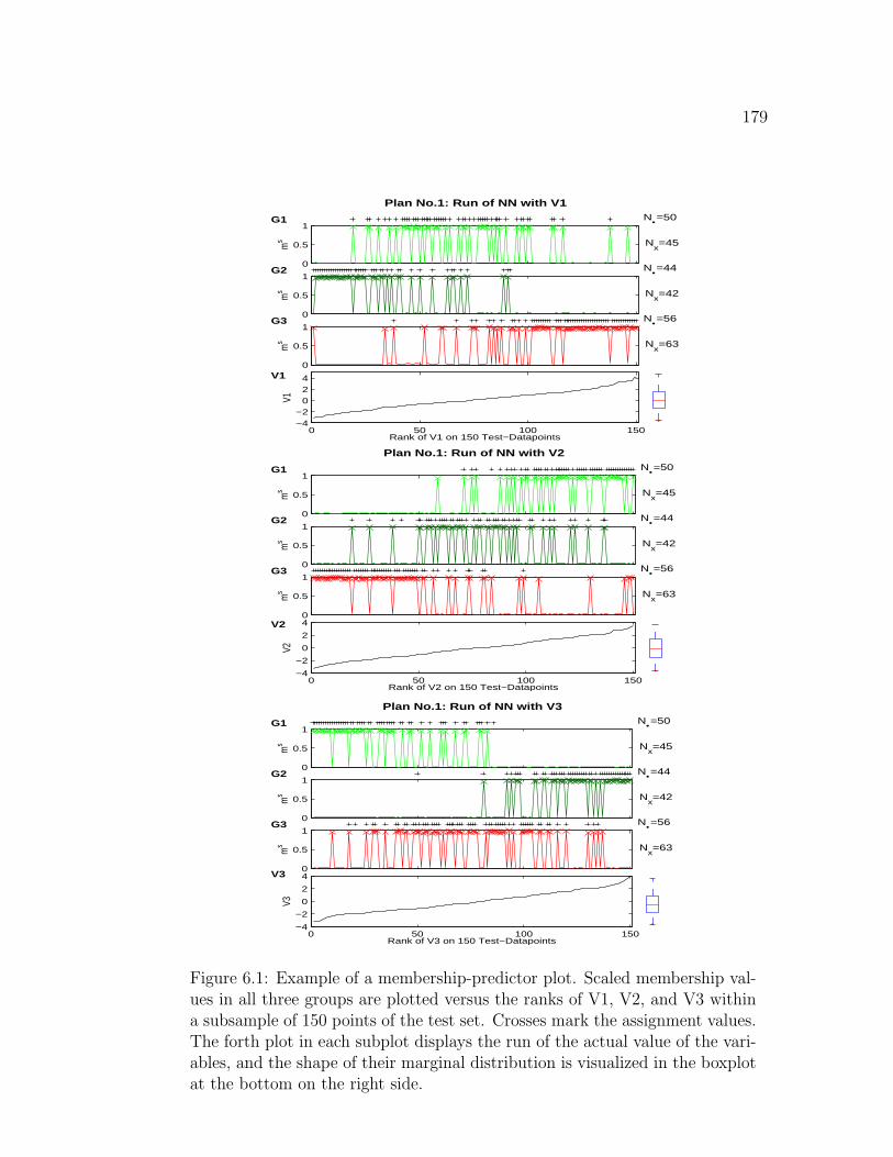
179

Plan No.1: Run of NN with V1N•=50G1

0

0.5

1

Nx=45m

sN•=44G2

0

0.5

1

Nx=42m

s

N•=56G3

0

0.5

1

Nx=63m

s

0 50 100 150−4−2

024V1

V1

Rank of V1 on 150 Test−Datapoints


0

0.5

1

Nx=45m

s

N•=44G2

0

0.5

1

Nx=42m

s

N•=56G3

0

0.5

1

Nx=63m

s

0 50 100 150−4

−2

0

2

4V2

V2



0

0.5

1

Nx=45m

s

N•=44G2

0

0.5

1

Nx=42m

s

N•=56G3

0

0.5

1

Nx=63m

s

0 50 100 150−4

−2

0

2

4V3

V3


Figure 6.1: Example of a membership-predictor plot. Scaled membership val-ues in all three groups are plotted versus the ranks of V1, V2, and V3 withina subsample of 150 points of the test set. Crosses mark the assignment values.The forth plot in each subplot displays the run of the actual value of the vari-ables, and the shape of their marginal distribution is visualized in the boxplotat the bottom on the right side.

Chapter 7

Dynamizing Classification Rules

In this chapter, we show how to combine evidence on the class membership

gained by static classification rules with background knowledge about a dy-

namic structure.

Combining current and past evidence is important in dynamic domains,

where the task is to predict the state of the system in different time periods.

We sometimes know that the succession of states is cyclic. This is for example

true for the prediction of business cycle phases, where an upswing is always

followed by upper turning points, and the subsequent downswing passes via

lower turning points over to the next upswing and so on.

We present several ideas how to implement this background knowledge

in popular static classification methods. We show that the basic strategy of

this work to scale membership values into the standardized partition space is

very useful for that purpose. Different from the preceding chapters, the goal

of the scaling in that respect is not the comparability to other classification

rules, but the compatibility with a coding of dynamic background informa-

tion as evidence. Therefore, we will present an additional scaling procedure

180

181

that weights current information of an objects membership in a class with

information about past memberships and compare the effect with the scaling

introduced in Chapter 5.

7.1 Introduction

In the literature, business cycles are typically either treated as a univariate phe-

nomenon and tackled by univariate time series methods, or they are modelled

as a multivariate phenomenon and tackled by static multivariate classification

methods (Meyer and Weinberg, 1975; Heilemann and Munch, 1996). As a con-

sequence, either the time-dependency or the interplay of different variables is

ignored. The same is true for many of the analyses of other cyclic phenomena

that are very common particularly in economy and in biology. In biology, the

importance is manifested by the fact that there is an own branch called chrono-

biology that studies biological rhythms, like e.g. menstruation (cp. Belsey and

Carlson, 1991), cyclic movements of the small bowel (cp. Aalen and Husebye,

1991), or sleep (cp. Guimaraes et al., 2001).

In a preliminary comparative study we showed that multivariate classi-

fication methods (ignoring knowledge of time dependencies) and a dynamic

Bayesian network that generalizes the Naive Bayes classifier for time depen-

dencies (ignoring dependencies between predictors) generated about the same,

unsatisfying, average prediction accuracy for the prediction of business cycle

phases.

That means, some static multivariate classification methods generated the

same error rates as the dynamic Bayesian network without using background

182

knowledge of time dependencies in business cycles. Therefore, there was hope

that in order to improve prediction accuracy for the multivariate methods

advantage could be taken of the cyclical structure of business cycle phases for

which the following pattern is true: lower turning points → upswing → upper

turning points → downswing → lower turning points → and so on.

In this thesis, we introduce and analyze several ideas on the incorporation

of this background knowledge in different types of classification rules. The gen-

eral problem of predicting cycles is formulated in Section 7.2. In Section 7.3

ideas on adapting static classification rules to cyclical structures are described.

The data used for learning and testing the prediction models for business cy-

cle phases and the design of comparison are presented in Section 7.4. Also we

introduce the model assumptions of the dynamic Bayesian network we devel-

oped for the prediction of business cycles and the considered static classifiers.

In Section 7.5 we present the performance of the implemented ideas for the

prediction of business cycle phases. To validate the findings, we performed

additional simulations that are presented in Section 7.6. And finally, conse-

quences are summarized in Section 7.7.

7.2 Basic Notations

As in the chapters before, we consider classification problems that are based on

some K-dimensional real-valued vector ~x(ω)∈X⊂RK measured on objects ω∈Ω.

And we want to decide about the class c(ω)∈C := 1, ...., G the object belongs

to. And we drop ω in our notations, unless it is useful for understanding.

Unlike before, in case of prediction of cycle phases, we classify not really

183

various objects, but rather one object — called system — in different time

periods t = 1, ..., T . And in each time period the system is situated in one out

of G possible states s∈S := 1, ..., G. We will further on no longer distinguish

between states and classes and denote both by s, and their space 1, ..., G by

S.

The chronological order of how the system passes through states is fixed:

Given the system is in time period t− 1 in state st−1 := s, it either stays there

or moves on to a certain other state s⊕ so that st∈s, s⊕⊂S, t = 1, ..., T . In

the following, we assume a corresponding numbering of states where s⊕=s+1

for s = 1, 2, ..., G−1 and s⊕=1 for s=G.

7.3 Adaption of Static Classification Rules for

Prediction of Cycle Phases

For multi-class problems, there are two distinct basic structures to decide on

a certain elementary class s∈S where the cyclical structure can easily be im-

plemented: multi-class argmax rules or certain compositions of binary argmax

rules.

Multi-class argmax rules use membership values for each elementary class

m(s, |L, met) : X→R, s∈S:

s = s(~x|L, met) = arg maxs∈S

m(s, ~x|L, met).

Other rules for multi-class problems define membership values not for ele-

mentary states but for various sets out of the product set over S, m : X→℘(S).

This is true, for example, if the final assignment is the result of a path of binary

184

argmax decisions, where in each step a decision is made between exactly two

elements of ℘(S).

Some of our strategies to ”dynamize” static rules by integrating knowledge

of a cyclic structure will rely on the assumption, that not only the size of

the assessed membership of one object in different classes can be meaningfully

compared but also the size of the membership values of different objects in the

same class. Some combinations of binary argmax rules fulfill this need, others

not. We will give examples of both:

One strategy from which we can easily read off membership values that are

comparable in size between objects, is the so-called one-against-rest strategy

introduced by Scholkopf et al. (1995) for SVM. Each class s is trained against

the other classes s := S\s. Thus G binary argmax rules are trained, each

on the complete training set L, by learning membership functions m(s, <

lset, et) and m(s, |L, met). As these membership functions are all based on

the same training set, their values are comparable in size and we can combine

them easily to a multi-class argmax rule by assigning to the class with the

highest value among m(s, |L, met), s∈S.

Not comparable in size are membership values of objects, when for the

learning of the membership functions each state is trained against every other

state with a binary SVM. The collection of G(G−1)2

membership functions

m((s, s′), |L(s, s′), met) : X→R, s′ = 1, ..., s− 1, s = 2, ..., G.

is learnt on different training sets, L(s, s′), s, s′⊂S only consisting in those

objects that belong to the relevant classes s and s′:

L(s, s′) = (sn, ~xn)∈L : sn∈s, s′⊂S

185

The max win strategy of Friedman (1996) and the decision directed acyclic

graphs (DDAG) of Platt et al. (2000) are of that type.

7.3.1 ET: Method of Exact Transitions

For any of the above mentioned argmax rules, we can take advantage of the

cyclical structure by restricting the comparison of membership values to ad-

missible transitions. That is, we start in the last known state of the system s0

and predict the next state by

s(~x1|s0,L, met) = arg maxs∈s0,s⊕0

m(s, ~x1|L, met).

For the consequent time periods t = 2, ..., T the predicted state st−1 from the

preceding time period is used as if it was the true one:

s(~xt|s0, s1, ..., st−1,L, met) = s(~xt|st−1,L, met)

= arg maxs∈st−1,s⊕t−1

m(s, ~xt|L, met).

This adaption was proposed by Weihs et al. (1999) for the prediction of

business cycle phases and is called classification with exact transitions (ET).

The classification with ET decomposes in two steps:

1. the information ”st−1” is used to decide on the set of admissible states

st∈st−1, s

⊕t−1

⊂S,

2. then, using the information in ~xt, we assign to that state s∈st−1, s

⊕t−1

with higher membership.

186

In the following, we will drop the time-index t and denote variables from time-

slice t− 1 with a minus: v− := vt−1, t = 2, ..., T , if statements are valid for all

t = 2, ..., T , and where indexing is not needed for understanding.

7.3.2 WET: Method of Weighted Exact Transitions

If a system is in a certain state s, the willingness to skip to s⊕ in the next time

period may be higher or lower than the inertia that keeps it in s. Thus, we

may gain further improvement of the rules, if we exploit the information that

our last assignment was into s− not only for the decision on the admissible

states, but also for the decision in which of them to assign now.

One idea is to weight membership values with an estimator of the willing-

ness to pass over, e.g. estimated transition probabilities from the training set

like observed frequencies:

m(s, ~x|s−,L, met) = w(s−, s)m(s, ~x|L, met)e.g.= p(s|s−,L, met)m(s, ~x|L, met).(7.3.1)

With such weighting, we assign to class s⊕ if the ratio of the membership

in s⊕ to the membership in s is higher than the ratio of the quantified inertia

that keeps the system in s to the quantified willingness to go from s→s⊕.

s(~x|s−,L, met) = arg maxs=s−,s⊕−

w(s−, s)m(s, ~x|L, met)

↔ s(~x|s−,L, met) =

s− if m(s−,~x|L,met)

m(s⊕−,~x|L,met)

w(s−,s−)

w(s−,s⊕−)≥ 1

s⊕− otherwise.

Therefore, a necessary condition for weighting is that membership values and

the willingness to skip or stay are measured on a ratio scale. Simple multiplica-

tion is used to combine these evidences, giving both of them same importance.

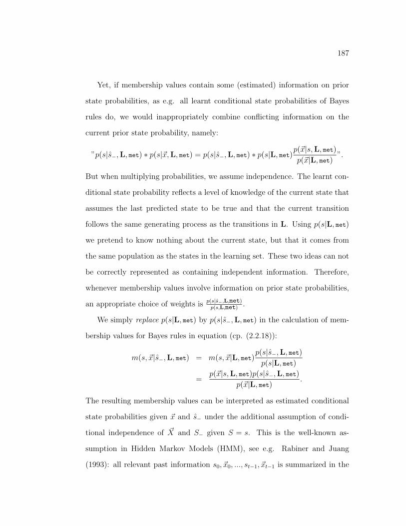
187

Yet, if membership values contain some (estimated) information on prior

state probabilities, as e.g. all learnt conditional state probabilities of Bayes

rules do, we would inappropriately combine conflicting information on the

current prior state probability, namely:

”p(s|s−,L, met) ∗ p(s|~x,L, met) = p(s|s−,L, met) ∗ p(s|L, met)p(~x|s,L, met)

p(~x|L, met)”.

But when multiplying probabilities, we assume independence. The learnt con-

ditional state probability reflects a level of knowledge of the current state that

assumes the last predicted state to be true and that the current transition

follows the same generating process as the transitions in L. Using p(s|L, met)

we pretend to know nothing about the current state, but that it comes from

the same population as the states in the learning set. These two ideas can not

be correctly represented as containing independent information. Therefore,

whenever membership values involve information on prior state probabilities,

an appropriate choice of weights is p(s|s−,L,met)p(s,L,met)

.

We simply replace p(s|L, met) by p(s|s−,L, met) in the calculation of mem-

bership values for Bayes rules in equation (cp. (2.2.18)):

m(s, ~x|s−,L, met) = m(s, ~x|L, met)p(s|s−,L, met)

p(s|L, met)

=p(~x|s,L, met)p(s|s−,L, met)

p(~x|L, met).

The resulting membership values can be interpreted as estimated conditional

state probabilities given ~x and s− under the additional assumption of condi-

tional independence of ~X and S− given S = s. This is the well-known as-

sumption in Hidden Markov Models (HMM), see e.g. Rabiner and Juang

(1993): all relevant past information s0, ~x0, ..., st−1, ~xt−1 is summarized in the

188

last state st−1 and is propagated solely through the transition probabilities

p(st|st−1) ≡ p(s|s−), st = 1, ..., G, t = 1, ..., T . The idea to combine static

probability classifiers with a Markov chain to build a dynamic classifier was

introduced by Koskinen and Oller (1998).

7.3.3 HMM: Propagation of Evidence for Probabilistic

Classifiers

Thus, from WET to the propagation in HMM models is only a small step for

any probabilistic static classifier. We add on the Markov chain and predict

states using the forward step in the forward-backward procedure for finding

the next state in HMMs (cp. Rabiner and Juang, 1993). The parameters of

the distributions in an HMM are the states’ transition probabilities and the

so-called emission probabilities of HMMs, the p(~x|s), ~x∈X, s∈S. We use the

observed frequencies on the training set L as estimators for the transition

probabilities, and the estimated conditional probabilities p(~x|s,L, met) of a

probabilistic classifier as emission probabilities.

We no longer propagate evidence assuming the predicted state was the true

one, but we propagate the probability that a certain state is true, given the

state s0 in time period t0 := 0 and the past observations of predictor variables.

The general justification of this strategy is based on probability calculus and

therefore relies on the interpretation of membership values as conditional class

probabilities.

189

The first step is the same as in WET. We predict s1 using ~x1 and s0:

s1 = s(~x1|s0,L, met) = arg maxs=s0,s⊕0

p(s|~x1, s0,L, met).

The next step is different. We do not assume s1 = s(~x1|s0,L, met) to be the true

state, but we propagate to be in state s0 with probability p(s0|~x1, s0,L, met)

and in state s⊕0 with probability (1−p(s0|~x1, s0,L, met)).

Thus, the joint probability to be in state s⊕0 in the second time period and

to observe ~x2 and ~x1 is the sum of the probabilities of the two paths that can

lead from s0 to s⊕0 : s0→s0→s⊕0 and s0→s⊕0 →s⊕0 :

p(s2, ~x2, ~x1|s0,L, met) =∑

s=s0,s⊕0

p(~x2|s2,L, met)p(s2|s,L, met)p(s, ~x1|s0,L, met).

Later, more than two states are possible and the joint probabilities are recur-

sively calculated by:

p(st, ~xt, ..., ~x1|s0,L, met)

=∑s∈S

p(~xt|st,L, met)p(st|s,L, met)p(s, ~xt−1, ..., ~x1|s0,L, met).

The argmax rule based on these membership values is the same as from the

derived conditional state probabilities:

p(st|~xt, ..., ~x1, s0,L, met) =p(st, ~xt, ..., ~x1|s0,L, met)∑s∈S p(s, ~xt, ..., ~x1|s0,L, met)

.

We will call these conditional state probabilities ”prior probabilities” of states

s∈S in time period t given all past information in time period t, namely

~xt−11 := ~x1, ..., ~xt−1 and s0.

Another possibility is to use the forward step of the viterbi-algorithm for

propagating the evidence (cp. Rabiner and Juang, 1993). This results in a

190

propagation only along the currently most probable path given the observa-

tional series ~xt1 and s0. We abbreviate these two HMM algorithms as HMM

SOP, meaning HMM propagation via the sum of paths, and HMM MPP mean-

ing HMM propagation along the most probable path.

7.3.4 Propagation of Evidence for Non

-Probabilistic Classifiers

In cases, where membership values are not estimated conditional probabilities,

technically we can apply the HMM SOP and the HMM MPP algorithms af-

ter any scaling of the membership values into the space of conditional class

probabilities U. Particularly in artificial neural networks (ANN) it is common

to scale membership vectors by the so-called softmax transformation (Bridle,

1990) that we introduced in Chapter 5 in equation (5.5.1):

m(s, ~x|L, met, sof) =exp (m(s, ~x|L, met))∑c∈S exp (m(c, ~x|L, met))

.

The whole field of ANN/HMM hybrid literature is concerned with aspects

of combining HMM propagation with evidence, a survey is given by Bengio

(1999). Note, that our problem differs essentially in two points from typical

ANN/HMM hybrid applications: the very small data size, and the goal to do

forward prediction only, because our challenge is to identify the current busi-

ness cycle phase, not a series of past ones. Typically, the latter is relatively

easy to do in business cycles. As we have to rely only on current and past in-

formation for the classification of the current state, many ANN/HMM Hybrid

procedures are not applicable.

191

All considerations about necessary characteristics of membership values for

the WET procedure also apply, if we want to use HMM propagation. There

is no problem, if the m(s, |L, met, sof) serve as good estimators for p(|s,Λ),

s∈S for some probability model Λ, like e.g. softmax-scaled discriminant func-

tions of LDA. If the assumptions Λ of a multivariate normal distribution of

predictors given the class and a common covariance matrix are justified, these

discriminant functions are shifted logarithms of class conditional probability

estimators (cp. McLachlan, 1992). In that case the softmax transformation

yields the probability estimators as such:

exp (ln(p(c|~x,L, lda)) + k)∑g∈S exp (ln(p(g|~x,L, lda)) + k)

=exp(k)p(c|~x,L, lda)∑g∈S exp(k)p(g|~x,L, lda)

= p(c|~x,L, lda)

with ln denoting the natural logarithm, and k∈R. Also, for an increasing num-

ber of independent training samples in L, and specific additional assumptions

about the algorithm and the underlying ”true” distribution, Hampshire and

Pearlmutter (1990) have shown that softmax-scaled ANN outputs converge to

conditional probability estimators.

But there is no general justification of the softmax transformation as lead-

ing to ”good” probability estimators in terms of e.g. unbiasedness or mini-

mum risk, nor any other general justification, why this transformation should

be chosen among all potential transformations from X to U. In particular

in small data sets like ours, where in addition the independence assumption

of the sample is violated, the interpretation of membership values from e.g.

ANNs as class conditional probabilities is risky. The same is true for estimated

conditional probabilities based on venturous probability model assumptions,

192

and there is no justification for this interpretation in case of softmax-scaled

membership values of SVMs. Yet, a good scaling is essential for successfully

combining static classifiers with HMM propagation (cp. Bengio, 1999). Thus,

we introduce two justified ways to do the scaling.

Scaling by aiming at probability estimators: P-Scaling

For the purpose of comparing static classification rules, we developed a scaling

sca such that scaled membership values m(s, ~x|L, met,V, sca) can be inter-

preted as an estimator p(s|~m(~x|L, met),V, sca) for the probability

p (s | ~m(~x|L, met), τ) to be in a certain state s given the vector of membership

values ~m(~x|L, met). The p-scaling is the scaling procedure described in Section

5.6.

Scaling by optimally weighting evidences: E-scaling

Alternatively to p-scaling, we scale membership values with a parameterized

softmax transformation. We minimize the error rate on the validation set

among all softmax transformation with a parameter κ:

m(s, ~x|L, met, sof(κ)) =exp (κm(s, ~x|L, met))∑c∈S exp (κm(c, ~x|L, met))

, κ∈R+.

We use the HMM algorithms to combine the evidence available in the obser-

vations ~xt−11 – quantified in the scaled membership values – with the prior

knowledge of the last known state s0. Analogously to the probabilistic case

we define and regard m(s| ~xt−11 , s0,L, met,V, sof(κ)) as the prior evidence

in time period t for state s given all past information.

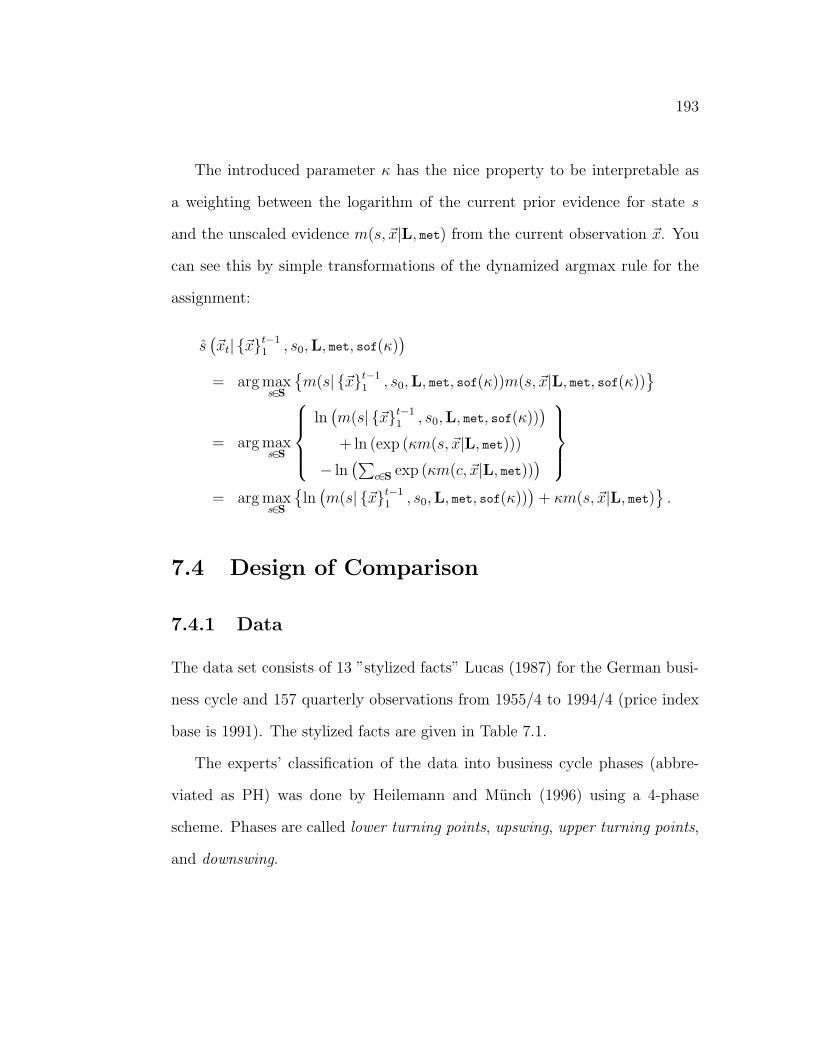
193

The introduced parameter κ has the nice property to be interpretable as

a weighting between the logarithm of the current prior evidence for state s

and the unscaled evidence m(s, ~x|L, met) from the current observation ~x. You

can see this by simple transformations of the dynamized argmax rule for the

assignment:

s(~xt| ~xt−1

1 , s0,L, met, sof(κ))

= arg maxs∈S

m(s| ~xt−1

1 , s0,L, met, sof(κ))m(s, ~x|L, met, sof(κ))

= arg maxs∈S

ln(m(s| ~xt−1

1 , s0,L, met, sof(κ)))

+ ln (exp (κm(s, ~x|L, met)))

− ln(∑

c∈S exp (κm(c, ~x|L, met)))

= arg maxs∈S

ln

(m(s| ~xt−1

1 , s0,L, met, sof(κ)))

+ κm(s, ~x|L, met)

.

7.4 Design of Comparison

7.4.1 Data

The data set consists of 13 ”stylized facts” Lucas (1987) for the German busi-

ness cycle and 157 quarterly observations from 1955/4 to 1994/4 (price index

base is 1991). The stylized facts are given in Table 7.1.

The experts’ classification of the data into business cycle phases (abbre-

viated as PH) was done by Heilemann and Munch (1996) using a 4-phase

scheme. Phases are called lower turning points, upswing, upper turning points,

and downswing.

194

IE real investment in equipment-grC real private consumption-grY real gross national product-grPC consumer price index-grPY real gross national product price deflator-grIC real investment in construction-grLC unit labor cost-grL wage and salary earners-grM1 money supply M1RL real long term interest rateRS nominal short term interest rateGD government deficitX net exports

Table 7.1: Our predictors of business cycle phases are based on economicaggregates that cover all important economic fields: real activity (labor market,supply/demand), prices, and monetary sphere. The abbreviation ’gr’ standsfor growth rates with respect to last year’s corresponding quarter.

7.4.2 Design

There are six full cycles in the considered quarters. All methods (have to)

rely on the assumption of structural stability over this period, though this is

not really valid. One goal of our analysis of business cycles was to uncover

the stable part of this process, valid in all six cycles. As an appropriate cross-

validation design to compare methods for that purpose, we decided to perform

a leave-one-cycle out (L1CO) analysis. Given our data D this cross-validation

resulted in six test sets Ti consisting in the observations in the i-th cycle and

corresponding training sets, L\i := D\Ti, i = 1, ..., 6.

For a fair comparison, all optimization in order to gain a rule has to be

done on each of the training sets separately. Rules are then compared with

respect to their prediction accuracy measured as the average prediction error

195

on the test sets:

APE :=1

6

6∑i=1

(1

Ti

Ti∑t=1

Ist(sL\i

t )

),

where sL\i

t is the predicted state at time period t of the i-th cycle using a

classification rule learnt on L\i, Ti is the number of time periods in the i-th

cycle, i = 1, ..., 6, and Is is the indicator function for state s∈S.

This gives an average error on a new cycle, which seems to be more appro-

priate as performance measure than the standard, namely the average error on

a single new observation. Cycles form a natural entity in the given task, and

the structural instability across cycles together with a performance measure

based on single observations would lead to an unwanted preference of methods

that predict well on long cycles.

Whenever model selection based on cross validation is part of a classifi-

cation method, we performed on each of the six training sets – each with

five cycles – an inner loop of leave-one-cycle out validation. This results in a

doubled leave-one-cycle out (DL1CO) strategy .

7.4.3 Methods

CRAKE

In our study, there is one classification method that is based on a multivariate

time-series model: the so-called Rake model of Sondhauss and Weihs (1999),

respectively the continuous Rake model (CRAKE). This is a dynamic Bayesian

network with two time-slices, where the multivariate distribution of predictors

and state in a time-slice is dependent on their realization in the preceding

196

time-slice in a certain way. The assumed stochastic independencies within a

time-slice reflect those of the Naive-Bayes classifier. The independence as-

sumptions between time-slices broaden those of HMMs to allow for time de-

pendencies between predictor variables. The Rake model is a multivariate

version of so-called Markov regime switching models (MRSM) introduced by

Hamilton (1989). These are typically applied for predicting switches between

two regimes based on one or a maximum of two predictor variables forming

auto-regressive processes of various depths and parameters depending on the

regimes(Diebold and Rudebusch, 1996).

In the Rake model (in the following denoting its model assumptions by π),

the distribution of each predictor variable Xt,k is modelled to be dependent

not only on the current state st (like in HMMs), but also on its predecessor

xk,t−1. Yet, it is assumed to be conditionally independent of all other past

and current variables (like in the Naive Bayes classifier), given st and xk,t−1.

Therefore, for all ~xt∈X, st∈S, k = 1, ..., K, t = 1, ..., T , it is true that:

pπ

(xk,t| st

0 , x1,t, ..., xK,t \xk,t, ~xt−11

)= pπ (xk,t|st, xk,t−1) .

And the current state St is conditionally independent of the past st−10 , ~xt−1

1

given the preceding state st−1, t = 1, ..., T :

pπ

(st| st−1

0 , ~xt−10

)= pπ (st|st−1) , st, st−1∈S.

This is different from the Naive Bayes classifier, where (non-conditional) inde-

pendence of St and the past is assumed, t = 1, ..., T .

The conditional independence assumptions in the Rake model lead to a

decomposition of the joint probabilities of state variable and predictor variables

197

in time-slice t given st−1 and ~xt−1, such that the conditional state probabilities

can be calculated as follows:

pπ (st|~xt, st−1, ~xt−1) =pπ (st|st−1) pπ(~xt|~xt−1, st)

pπ(~xt|~xt−1, st−1), t = 1, ..., T.

The joint conditional probabilities of the predictor variables decompose into

pπ(~xt|~xt−1, st) =K∏

k=1

pπ(xk,t|xk,t−1, st). (7.4.1)

Often, the local conditional distributions as defined in (7.4.1) in Bayesian

networks are discrete distributions. The growth rates of the stylized facts in our

data, though, would need to be discretized for that purpose. More naturally

they are modelled by continuous distributions. We assumed each predictor

variable Xk,t|xk,t−1, st to be normally distributed with autoregressive mean

µk,t = αk(st) + βk(st)xk,t−1 and variance σk(st) and estimated the parameters

according to Bayesian learning in the normal regression model(Gelman et al.,

1995).

For modelling the discrete and finite distribution of transitions S|s− for

each s−∈S we choose a Bayesian multinomial distribution model. The cyclic

structure is taken care of by an informative Dirichlet prior that sets inadmiss-

able probabilities to zero. For further details, see Gelman et al. (1995).

Exact forward propagation of evidence in dynamic Bayesian networks was

used to predict the phase of the cycle in time period t, t = 1, ..., T , given the

respective evidence of the past and the present:

st = arg maxs∈S

p(s| ~xt1 , s0,L, met)

198

7.4.4 Linear Discriminant Analysis and Support Vector

Machines

In the past, mainly static classification methods were used for the multivariate

prediction of business cycle phases. One reason is the fact that typically the last

true phase is not observed to do the prediction for the next one. It is only by

observing the continuing evolution of the economy for some more quarters that

it becomes apparent what phase the business cycle was in. Another reason for

using static methods is that we are not only reaching for a good prediction, but

also for a description of phases in terms of the stylized facts. Thus, methods

were applied that use as predictors observed entities, and for which we want

to understand the connection they have to business cycle phases.

The ideas of modifying static methods outlined in Section 7.3 now allow for

both, description and prediction: we describe phases using their membership

functions m(s, |L, met) : X→R, s∈S and we try to get better predictions by

combining this evidence with the knowledge on the cyclical structure.

Starting point of this investigation were the results on a comparative study

on the performance of various multivariate classification methods for the stable

prediction of business cycle phases (Sondhauss and Weihs, 2001b). ”Best”

results of 37% average prediction error were gained with a certain artificial

neural network (ANN) algorithm and a specific bootstrapped optimization

procedure added on QDA — both time consuming procedures. The good result

of the ANN is highly dependent on the randomly chosen starting values of the

parameters of the network, and could never be confirmed with other starting

values. With 43 % APE the performance of the simple LDA procedure based

199

on a selection of best two predictors was not much worse and comparable to the

performance of CRAKE. Thus there was hope by using the knowledge of the

cyclical structure to find a simple model that does a better job in extracting

the stable part of the multivariate phenomenon ”business cycles”.

The hope was justified: combining LDA with HMM propagation of evidence

and a DL1CO selection of the best two predictors, we found a model with a

lower APE than any of the more complex models, and in each of the six inner

loops of the DL1CO design, always the same two predictors were chosen as

the best, namely L and LC.

In this paper, we will concentrate on the comparison of the various methods

introduced in Section 3 to incorporate cyclic knowledge in general argmax

classifiers. Therefore, we picked from the various originally considered argmax

classifiers LDA, as it led to the best results, and a specific binary support vector

machine (SVM) representing non-probabilistic classifiers. We prefer SVM over

neural networks, because they do not suffer from the problem with the starting

values. The results of the various add-on strategies will be compared to those

with CRAKE, the fully dynamic model and motivator for dynamizing static

classifiers. We apply these methods to the complete set of 13 stylized facts,

and only to the two stable predictors, L, and LC, found with LDA. This will

reveal the discriminating reaction of these basic classifiers on noisy signals in

lower and higher dimensions.

The LDA as we realized it, is a Bayes rule with uniform class priors and

equal costs. Given the phase of a certain quarter st, the predictor variables ~Xt

are assumed to be distributed according to a multivariate normal distribution.

200

The distributions differ in the vector of means ~µt = ~µ(st) of the predictor

variables, but not in the arbitrary symmetric and positive definite covariance

matrix Σt ≡ Σ, t = 1, ..., T . We used the implementation in R (Ihaka and

Gentleman, 1996). For the e-scaling not the estimated conditional probabilities

were presented as membership values, but their logarithms for the reasons given

in Section 3.4.

The SVM was realized with radial basis function (RBF) kernels (cp. Vapnik,

1995; Scholkopf et al., 1995)) as implemented in the SVM toolbox 2.51 for

Matlab by Schwaighofer (2002).

More details on these classifiers are given in chapters 2 and 3.

One of the parameters in SVM with RBF-kernels, typically denoted by C,

controls the trade off between margin maximization and error minimization.

This was set to be the maximum of 10 and the number of predictors. The

second parameter defines the width of the RBF-kernel. This was set to be

equal to the number of the predictors. These settings were found to match

the findings in our preliminary studies, where we optimized the L1CO errors

in the inner loop of both of these parameters using experimental design with

a quadratic loss function.

7.5 Results

In Tables 7.2 and 7.3 you see the performance of the LDA, SVM, and CRAKE

procedures based on all predictors and based on two predictors.

Overall best for the prediction of business cycles is LDA using L and LC

as predictors only, when combined with an HMM SOP prediction and without

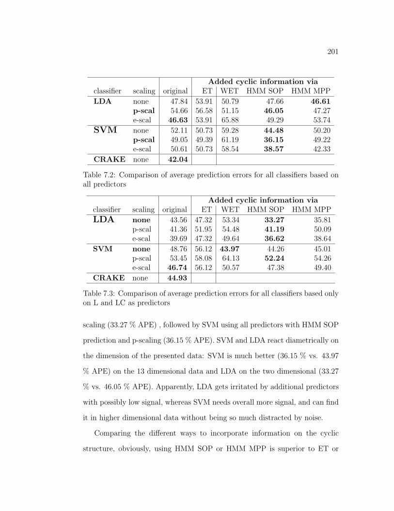
201

Added cyclic information viaclassifier scaling original ET WET HMM SOP HMM MPP

LDA none 47.84 53.91 50.79 47.66 46.61p-scal 54.66 56.58 51.15 46.05 47.27e-scal 46.63 53.91 65.88 49.29 53.74

SVM none 52.11 50.73 59.28 44.48 50.20p-scal 49.05 49.39 61.19 36.15 49.22e-scal 50.61 50.73 58.54 38.57 42.33

CRAKE none 42.04

Table 7.2: Comparison of average prediction errors for all classifiers based onall predictors




CRAKE none 44.93

Table 7.3: Comparison of average prediction errors for all classifiers based onlyon L and LC as predictors

scaling (33.27 % APE) , followed by SVM using all predictors with HMM SOP

prediction and p-scaling (36.15 % APE). SVM and LDA react diametrically on

the dimension of the presented data: SVM is much better (36.15 % vs. 43.97

% APE) on the 13 dimensional data and LDA on the two dimensional (33.27

% vs. 46.05 % APE). Apparently, LDA gets irritated by additional predictors

with possibly low signal, whereas SVM needs overall more signal, and can find

it in higher dimensional data without being so much distracted by noise.

Comparing the different ways to incorporate information on the cyclic

structure, obviously, using HMM SOP or HMM MPP is superior to ET or

202

true 4 4 4 4 4 4 4 1 1 1 1 1 1 1 1 1 1 1 1 1 2 2 2 2 3 3 3 3 3 3 3 3original 4 3 4 3 3 1 4 3 1 1 1 1 1 1 1 1 1 1 1 1 1 1 2 3 3 3 4 3 3 3 3 4ET 4 1 1 1 1 1 2 3 4 1 1 1 1 1 1 1 1 2 2 3 4 1 2 3 4 4 4 4 4 4 4 4WET 4 1 1 1 1 1 1 1 1 1 1 1 1 1 1 1 1 1 1 1 1 1 1 1 1 1 1 1 1 1 1 1

Table 7.4: P-scaled original static predictions of the BSVM classifier vs. thosewith ET or WET compared to the true phases in the fifth cycle. 4 is a lowerturning point, 1 an upswing, 2 an upper turning point, and 3 an downswing

WET, as well as to the original results. Actually, with ET of WET, most of

the times results are even worse than the original. At first, this was unex-

pected. Yet, looking at some specific series of predictions reveals the pitfalls

one can run into with these methods. A characteristic example is the course

of predictions of the SVM classifier presented in Table 7.4.

With ET once the classifier has mispredicted, it has big difficulties to pre-

dict the phase for the consequent quarters, because it is only allowed to com-

pare for example upper turning points (2) with downswing (3), where the

evidence in the predictor variables potentially indicates the true upswing (1).

After an error, either the classifier ’waits’ in the mispredicted state for the

cycle to pass that state, or it passes through all states, until prediction and

true state meet again. Obviously, WET simply sticks much too long in phase

1.

The issue-related problem to reveal the stable part of the multivariate phe-

nomenon ”business cycles” is solved by the good – compared to what we can

expect to achieve – performance of the LDA classifier with HMM SOP prop-

agation. Method-related, though, the results up to now were disappointing in

that no clear pattern of superiority of any method to incorporate cyclic infor-

mation can be read off Tables 7.2 and 7.3. Since this might be an artefact of

203

the sample systematic simulations were carried out, the designs and the results

of which will be discussed in the next section.

7.6 Simulations

The dependencies in economic aggregates themselves are dependent on polit-

ical frameworks and on world trade contracts, as well as on incidents as wars

and global crises. Within the time-period of our observation at least the oil

crises and the German Reunification will have had an influence of that type.

Thus, we do not expect our data on different quarters to really give us examples

of the same concept.

Yet, to see some examples from at least almost the same is necessary for any

learning (algorithm). Therefore, for the evaluation of methods, the instability

is disastrous: No method can be convincingly good, and differences in the

performance tell as much about the data as about the methods. Therefore, we

simulated data from stable processes.

7.6.1 Data

From the over countable space of processes, one will always be able to find

some process that supports the method, one is in favor of. Thus, to avert arbi-

trariness we selected three processes motivated from the original problem, and

with parameters estimated according to Bayesian learning from the original

problem. By Bayesian learning, we account for the uncertainty we have about

the estimated parameters.

204

The transition between phases is generated according to a Markov process.

For the likelihood distributions of the predictors, given the course of phases, we

use the distributional assumptions of three different generating models: LDA

based on all 13 predictors (GLDA), LDA based on L and LC as predictors only

(GLDL), and CRAKE based on all predictors (GCRA).

GLDL is chosen, because the classifier that estimated state conditional

probabilities according to that two-dimensional model performed best on our

real data set. GLDA will enable us to compare low dimensional and higher

dimensional behavior of our algorithms. And finally, GCRA as a generating

model was selected, because the performance of the corresponding classifier

was not too bad, and because random variables from this model violate of the

HMM assumption. Thus, we can see the effect of an extreme violation of the

HMM assumption on our algorithms.

We did 20 replications in our simulation. The series of phases of each

replication consists in six business cycles, and drives the observational series

in each of the three models.

7.6.2 Design

We compare the behavior of algorithms in two different cross-validation de-

signs:

1. DL1CO just as on the real data to understand the performance of our

algorithms on small data sets and

2. a learning- validation-, and test set (LVT) design. Here the data from

205

7 replications is used for learning, the data from the next seven replica-

tions for validation (used to optimize the scaling), and the data from the

remaining 6 replications is used to estimate the prediction error rates.

This analysis will show us the potential benefit of algorithms for large

data sets.

7.6.3 Results

DL1CO Design




CRAKE none 40.40

Table 7.5: Mean average percentages of prediction errors in 20 replications ofa DL1CO design on data generated according to GLDA




CRAKE none 30.19

Table 7.6: Mean average percentages of prediction errors in 20 replications ofa DL1CO design on data generated according to GLDL

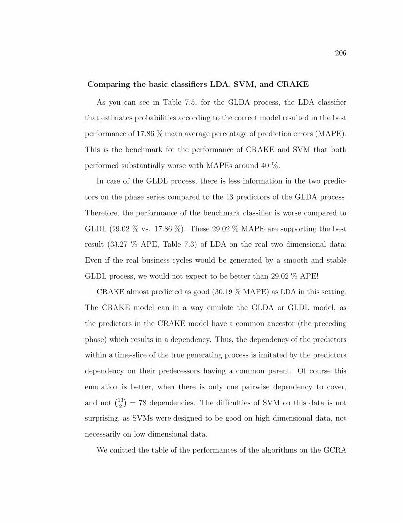
206

Comparing the basic classifiers LDA, SVM, and CRAKE

As you can see in Table 7.5, for the GLDA process, the LDA classifier

that estimates probabilities according to the correct model resulted in the best

performance of 17.86 % mean average percentage of prediction errors (MAPE).

This is the benchmark for the performance of CRAKE and SVM that both

performed substantially worse with MAPEs around 40 %.

In case of the GLDL process, there is less information in the two predic-

tors on the phase series compared to the 13 predictors of the GLDA process.

Therefore, the performance of the benchmark classifier is worse compared to

GLDL (29.02 % vs. 17.86 %). These 29.02 % MAPE are supporting the best

result (33.27 % APE, Table 7.3) of LDA on the real two dimensional data:

Even if the real business cycles would be generated by a smooth and stable

GLDL process, we would not expect to be better than 29.02 % APE!

CRAKE almost predicted as good (30.19 % MAPE) as LDA in this setting.

The CRAKE model can in a way emulate the GLDA or GLDL model, as

the predictors in the CRAKE model have a common ancestor (the preceding

phase) which results in a dependency. Thus, the dependency of the predictors

within a time-slice of the true generating process is imitated by the predictors

dependency on their predecessors having a common parent. Of course this

emulation is better, when there is only one pairwise dependency to cover,

and not(132

)= 78 dependencies. The difficulties of SVM on this data is not

surprising, as SVMs were designed to be good on high dimensional data, not

necessarily on low dimensional data.

We omitted the table of the performances of the algorithms on the GCRA

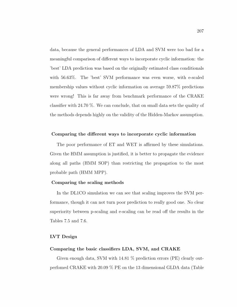
207

data, because the general performances of LDA and SVM were too bad for a

meaningful comparison of different ways to incorporate cyclic information: the

’best’ LDA prediction was based on the originally estimated class conditionals

with 56.63%. The ’best’ SVM performance was even worse, with e-scaled

membership values without cyclic information on average 59.87% predictions

were wrong! This is far away from benchmark performance of the CRAKE

classifier with 24.70 %. We can conclude, that on small data sets the quality of

the methods depends highly on the validity of the Hidden-Markov assumption.

Comparing the different ways to incorporate cyclic information

The poor performance of ET and WET is affirmed by these simulations.

Given the HMM assumption is justified, it is better to propagate the evidence

along all paths (HMM SOP) than restricting the propagation to the most

probable path (HMM MPP).

Comparing the scaling methods

In the DL1CO simulation we can see that scaling improves the SVM per-

formance, though it can not turn poor prediction to really good one. No clear

superiority between p-scaling and e-scaling can be read off the results in the

Tables 7.5 and 7.6.

LVT Design

Comparing the basic classifiers LDA, SVM, and CRAKE

Given enough data, SVM with 14.81 % prediction errors (PE) clearly out-

perfomed CRAKE with 20.09 % PE on the 13 dimensional GLDA data (Table

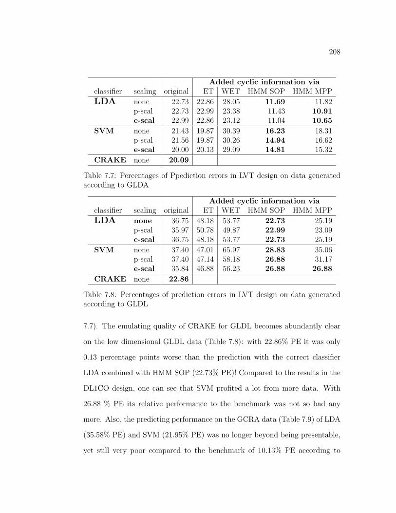
208




CRAKE none 20.09

Table 7.7: Percentages of Ppediction errors in LVT design on data generatedaccording to GLDA




CRAKE none 22.86

Table 7.8: Percentages of prediction errors in LVT design on data generatedaccording to GLDL

7.7). The emulating quality of CRAKE for GLDL becomes abundantly clear

on the low dimensional GLDL data (Table 7.8): with 22.86% PE it was only

0.13 percentage points worse than the prediction with the correct classifier

LDA combined with HMM SOP (22.73% PE)! Compared to the results in the

DL1CO design, one can see that SVM profited a lot from more data. With

26.88 % PE its relative performance to the benchmark was not so bad any

more. Also, the predicting performance on the GCRA data (Table 7.9) of LDA

(35.58% PE) and SVM (21.95% PE) was no longer beyond being presentable,

yet still very poor compared to the benchmark of 10.13% PE according to

209




CRAKE none 10.13

Table 7.9: Percentages of prediction errors in LVT design on data generatedaccording to CRAKE

CRAKE. SVM is substantially superior to LDA that obviously can not revert

the emulation of CRAKE on GLDL.

Comparing the different ways to incorporate cyclic information

With more data, HMM SOP no longer generally outperformed HMM MPP.

On the GLDA data and added on the conditional state probability estimators

in the true model (LDA) propagation along the most probable path was al-

ways superior, irrespective of the scaling. As HMM SOP based on the true

conditional state probabilities would result in the best Bayes predictions, this

is astonishing. HMM MPP rests upon sums of fewer yet basically the same

estimated probabilities as HMM SOP, thus a reduced variance of the predic-

tions is our working hypothesis about the causes of these findings. This would

support the intuitive appeal of the HMM MPP procedure to drop ”circumstan-

tial” evidences and to concentrate on the most probable. On the GCRA data,

where the HMM assumption is heavily violated, all of our ideas to incorporate

cyclic information was harm- instead of useful.

210

Comparing the scaling methods

For SVM, the improvement with scaled membership values levelled off at

about 1-2 percentage points of PE. E-scaling that optimizes the HMM com-

bination of evidence for prediction is better than p-scaling, even if the HMM

assumption is not justified. As it should in case of the LDA classifier, the e-

scaling parameter was approximately 0.9 for GLDA or equal to one for GLDL

that is, the softmax transformation resulted in (almost) identity mapping.

7.7 Summary

Summarizing, from the analysis of the results one might deduce the following

general conclusions on the incorporation of background knowledge of a cyclical

state structure into classification rules:

• Prediction based on classification with (weighted) exact transitions is

risky, because one false prediction might entail many succeeding errors.

• With HMM propagation we found a simple and convincing method to

extract the stable part of the business cycle process on the real data.

• Yet, when the basic HMM assumption that the past evidence of a multi-

variate time series is comprised in the current state was heavily violated,

in our simulations all of our ways to incorporate knowledge of the un-

derlying cyclical structure was harmful.

• Both scaling procedures did a good job on scaling membership values

211

from the non-probabilistic classifier SVM. E-scaling is easier and opti-

mizes propagation, therefore it is favorable for this purpose. There is no

risk in using it, because even if it is performed on the ”correct” estima-

tors, it does no harm.

• On the basis of very well scaled membership values, HMM propagation

along the most probable path is a worthy alternative to full HMM prop-

agation of evidence.

Chapter 8

Conclusions

In this thesis a general approach to the comparative presentation of classifica-

tion rules is introduced: an adequate scaling into the standardized partition

space. This offers a unifying framework for the representation of a wide variety

of classification rules.

For that purpose in chapters 2 and 3 we give a summary on varying theoret-

ical frameworks of classification techniques in statistics and machine learning.

By a schematic representation of their proceedings similarities and differences

are worked out. It becomes clear that the differences in their basic approaches

can be understood in terms of their different definitions of what is expected –

the ”expected loss”. The main impact these varying expectations have is on

the functional space in which potential classification rules lie.

Irrespective of the dissimilarity of the approaches on the theoretic level, on

the technical level their proceedings are quite similar: based on training data

membership functions are learnt that enable to quantify the membership of

some object in classes on the basis of its predictor values.

212

213

The unified representation of these membership functions in the standard-

ized partition space is presented in Chapter 5. Linchpin is the adequate scaling

of the values from different membership functions into this space. A method

that results in a presentation of membership assessments that reflect the clas-

sifiers characteristic of classification and give a realistic impression of the clas-

sifiers performance on a test set is introduced.

In the scaling procedure as we present it, the focus is on the membership

values in the assigned classes – the assignment values. The scaling of the mem-

bership values in the other classes is treated secondarily. It is both challenging

in theory and implementation to extend this such that scaled membership

values in all classes reflect the actual behavior of the classification rule.

The benefit of the presentation of classification rules in standardized parti-

tion spaces is manifold: firstly, it facilitates comparison of classification rules.

In standardized partition spaces one can motivate and visualize performance

criteria that enable to evaluate the quality of membership functions.

Given this quality is high, scaled membership values provide an excellent

basis for the analysis of the interplay of class membership and predictor values

that now can be presented in multifarious ways.

In Chapter 6 we demonstrate the comparison of classification rules in stan-

dardized partition spaces. This is intended to impart an impression of the

possibilities of the procedure.

In Chapter 7 we show that the unified presentation is not only useful for

the comparison of classification methods and for the interpretation of classifi-

cation rules. It can also be utilized to combine evidence on class membership

214

from varying sources. In Chapter 7 past and current information on class

membership are merged. This changes the aim of the scaling of membership

values and accordingly an alternative scaling procedure is shown to be better

for this purpose. Its superiority refers only partly to the prediction results –

they are better but not to a large extent. The main advantages are that it is

easier to perform and that it provides further insight into the way evidences

are combined.

Overall, this thesis gives a first insight into the possibilities of a unified rep-

resentation of classification rules in standardized partition spaces. It remains

to be seen in further application whether the effort of adequate scaling shows

as much profit as the author believes.

Appendix A

References for Implemented

Classification Methods

Linear and Quadratic Discriminant Analysis The general outline of

linear and quadratic discriminant analysis and the specific features of their

implementation we chose to use in this work are given in Sections 2.3.2, 3.3.2,

and 3.5.1. For the calculations we used the procedures lda and qda in R

(Ihaka and Gentleman, 1996) with standard moment estimation of means and

variances.

Continuous naıve Bayes The distributional assumptions and the learning

of parameters of the implemented continuous naıve Bayes classification method

are derived in Sections 2.3.4, 3.3.2, and 3.5.1. For the programming we used

Matlabr(Matlab).

215

216

Univariate Binary Decision Tree The representation of univariate binary

decision trees and the basic strategies for learning them have been described in

Sections 3.3.1 and 3.5.3. For the implementation, we use the rPart procedure

in R (Ihaka and Gentleman, 1996). The chosen splitting criterion is the ’infor-

mation’ split. We optimize the minimum number of observations in a leaf node

via lowest validation error. The validation set consists of a sampled quarter of

the training set. The final tree with optimized number of observations in the

leaf node is learnt on the complete training set.

Support Vector Machine Support vector machines as we use them are

described in Sections 3.3.3, 3.4.2, 3.4.4 and 3.5.2. We implemented support

vector machines with radial basis functions and solved the quadratic opti-

mization problem for the learning of the best separating hyperplane with the

(SVM) toolbox 2.51 for Matlab by Schwaighofer (2002). For selecting the best

parameter pair for the training error penalty and the width of the kernels, we

minimized the validation set error using experimental design, as described in

Section 3.5.2. The validation set consists of a sampled quarter of the training

set. The final hyperplane with optimized parameters is learnt on the complete

training set.

K-Nearest Neighbor The k-nearest neighbor procedure is a specific instance-

based learning method, where learning consists mainly of storing the presented

training data (Mitchell, 1997). For k-nearest neighbor learning one assumes

that objects that are ”near” to each other according to their predictor values

will most likely belong to the same class. The main representation task consists

217

in defining nearness on the space of predictor variables X. A second modelling

decision is about the number k of nearest neighbors one wants to consider.

This explains the ”k” in the name of the method. Given the notion of distance

and the number of neighbors to consider, some new object is assigned to the

class most of its neighbors belongs to. A detailed description can be found e.g.

in Mitchell (1997).

We implemented the k-nearest neighbor algorithm with Euclidian distance.

Overfitting is no problem in k-nearest neighbor learning, therefore we selected

the number k of neighbors by minimum training error among all natural num-

bers smaller or equal to the factorial of the number of classes.

Neural Network Alongside the implemented support vector machine, neu-

ral networks result in the most flexible decision boundaries in the predictor

space among the classification methods in this work. From a statistician’s

point of view, they can be understood in terms of a highly non-linear regres-

sion method. Support vector machines and neural networks are highly related

via their common ancestor: Rosenblatt’s perceptron (see Vapnik, 1995). Neu-

ral networks are inspired and built on the basis of a rough analogy to biological

learning systems that consist out of very complex webs of interconnected neu-

rons. For an introduction to neural networks, see (Mitchell, 1997), and for a

deeper understanding of neural networks as classifiers, see Bishop (1995).

We modelled the neural network as a feedforward two-layer network with

logistic hidden layer units and linear output units, the standard approach to

non-linear function approximation. For the optimization of the parameters of

the net given its structure, we used the Levenberg-Marquardt backpropagation

218

algorithm and minimized the mean squared error. We selected good starting

values and the best number of hidden nodes with respect to the error rates

of the learnt net on a validation set. The validation set consists in a sampled

quarter of the training set. The final net is learnt on the complete training

set using Bayesian regularization of the Levenberg-Marquardt training. For

details, see Demuth and Beale (1998)).

Bibliography

101 Zen Stories. The stone mind. In P. Reps, editor, Zen Flesh, Zen Bones: A

Collection of Zen and Pre-Zen Writings. Tuttle Publishing, Boston, 1957.

AAAI. Dynamic library of introductory information about ar-

tificial intelligence — machine learning, 2000-2002. URL

http://www.aaai.org/AITopics/html/machine.html.

O. O. Aalen and E. Husebye. Statistical analysis of repeated events forming

renewal processes. Statistics in Medicine, 10:1227–1240, 1991.

T. W. Anderson. An Introduction to Multivariate Statistical Analysis. John

Wiley & Sons, New York, 1958.

V. Barnett. Comparative Statistical Inference. John Wiley & Sons Ltd, Chich-

ester, 3 edition, 1999.

E. M. Belsey and N. Carlson. The description of mentrual bleeding patterns:

Toward fewer measures. Statistics in Medicine, 10:267–284, 1991.

Y. Bengio. Markovian models for sequential data. Neural Computing Surveys,

2:129–162, 1999.

J. O. Berger. Statistical Decision Theory and Bayesian Analysis. Springer-

Verlag, New York, 2 edition, 1995.

219

220

J. M. Bernardo and A. F. M. Smith. Bayesian Theory. John Wiley & Sons,

Chichester, 1994.

C. M. Bishop. Neural Networks for Pattern Recognition. Oxford University

Press, Oxford, England, 1995. ISBN 0-19-853864-2.

C. Blake and C. Merz. UCI repository of machine learning databases, 1998.

URL http://www.ics.uci.edu/∼mlearn/MLRepository.html.

J. Blythe. An overview of planning under certainty. In M. Wooldridge and

M. M. Veloso, editors, Artificial Intelligence Today: Recent Trends and De-

velopments, volume 1600 of Lecture Notes in Computer Science. Springer,

1999.

L. Breiman, J. H. Friedman, R. A. Olshen, and C. J. Stone. Classification and

Regression Trees. Wadsworth, Pacific Grove, 1984.

J. S. Bridle. Probabilistic interpretation of feedforward classification network

outputs, with relationships to statistical pattern recognition. In F. Fogelman

Soulie and J. Herault, editors, Neuro-computing: Algorithms, Architectures

and Applications, pages 227–236, Berlin, 1990. Springer.

J. S. Bridle. Optimization and search in speech and language processing, 1995.

C. J. C. Burges. A tutorial on support vector machines for pattern recognition.

Data Mining and Knowledge Discovery, 2(2):121–167, 1998.

R. T. Carroll. The skeptic’s dictionary, 1994-2002. URL

http://skepdic.com/homepage.html.

O. Chapelle, V. Vapnik, O. Bousquet, and S. Mukherjee. Choosing multiple

parameters for support vector machines. Machine Learning, 46(1-3):131–

159, 2002.

221

H. Demuth and M. Beale. Neural Network Toolbox User’s Guide, 1998.

F. X. Diebold and G. D. Rudebusch. Measuring business cycles: a modern

perspective. The Review of Economics and Statistics, 78:67–77, 1996.

T. S. Ferguson. Mathematica Statistics — A Decision Theoretic Approach.

Academic Press, New York, 1967.

R. A. Fisher. The use of multiple measurements in taxonomic problems. Annals

of Eugenics, 7(2):179–188, 1936.

J. H. Friedman. Another approach to polychotomous classification. Technical

report, Stanford Department of Statistics, 1996.

K. Fukunaga. Introduction to Statistical Pattern Recognitionen. Academic

Press, New York, 2nd edition, 1990.

U. Garczarek and C. Weihs. Comparing classifiers in standardized partition

spaces using experimental design. Technical report, SFB 475, University of

Dortmund, 2002. 21/02.

U. Garczarek, C. Weihs, and U. Ligges. Prediction of notes from vocal time

series. Technical report, SFB 475, University of Dortmund, 2002. to be

published ??/02.

A. Gelman, J. B. Carlin, H. S. Stern, and D. B. Rubin. Bayesian Data Analysis.

Chapman & Hall, New York, 1995.

B. German. Glass identification database, 1987. URL

http://www.ics.uci.edu/∼mlearn/MLRepository.html.

G. Guimaraes, J.-H. Peter, T. Penzel, and A. Ultsch. A method for automated

temporal knowledge acquisition applied to sleep related breathing disorders.

Artificial Intelligence in Medicine, 23:211–237, 2001.

222

J. D. Hamilton. A new approach to the anylysis of nonstationarity time series

and the business cycle. Econometrica, 57:357–384, 1989.

J. B. I. Hampshire and B. A. Pearlmutter. Equivalence proofs for multilayer

perceptron classifiers and the Bayesian discriminant function. In Proceedings

of the 1990 Connectionist Models Summer School, 1990. D. Touretzky, J.

Elman, T. Sejnowski, and G. Hinton, eds. Morgan Kaufmann, San Mateo,

CA., 1990.

D. J. Hand. Construction and Assessment of Classification Rules. John Wiley

& Sons, Chichester, 1997.

D. J. Hand. Data mining: statistics and more? The American Statistician,

52:112–118, 1998.

M. H. Hansen and B. Yu. Model selection and the principle of minimum

description length. Journal of the American Statistical Association, 96(454):

746–774, 2001.

U. Heilemann and H. J. Munch. West german business cycles 1963-1994:

A multivariate discriminant analysis. In CIRET–Conference in Singapore,

CIRET–Studien 50, 1996.

E. J. Horvitz, J. S. Breese, and M. Henrion. Decision theory in expert systems

and artificial intelligence. International Journal of Approximate Reasoning,

2:247–302, 1988.

R. Ihaka and R. Gentleman. R: A language for data analysis and graphics.

Journal of Computational and Graphical Statistics, 5(3):299–314, 1996.

M. Jaeger. Relational Bayesian networks. In Proceedings of the 13th Conference

on Uncertainty in Artificial Intelligence, pages 266–273. Morgan Kaufmann,

1997.

223

N. L. Johnson. Bivariate distributions based on simple translation systems.

Biometrika, 36:149–176, 1949.

L. Koskinen and L.-E. Oller. A hidden markov model as a dynamic bayesian

classifier, with an application to forecasting business-cycle turning points.

Technical report, National Institute of Economic Research, 1998. 59.

P. Langley. Elements of Machine Learning. Morgan Kaufmann, San Francisco,

CA, 1995.

E. L. Lehmann. Theory of Point Estimation. Springer-Verlag, New York, 1983.

D. D. Lewis. Naive (Bayes) at forty: The independence assumption in infor-

mation retrieval. In C. Nedellec and C. Rouveirol, editors, Proceedings of

ECML-98, 10th European Conference on Machine Learning, number 1398,

pages 4–15, Chemnitz, DE, 1998. Springer Verlag, Heidelberg, DE.

R. E. Lucas. Models of business cycles. Basil Blackwell, New York, 1987.

D. G. Luenberger. Introduction to Linear and Nonlinear Programming.

Addison-Wesley Publishing, Reading, Mass, 1973.

M. E. Maron. Automatic indexing: An experimental inquiry. Journal of the

Association for Computing Machinery, 8:404–417, 1961.

M. E. Maron and J. L. Kuhns. On relevance, probabilistic indexing and infor-

mation retrieval. Journal of the Association for Computing Machinery, 7:

216–244, 1960.

Matlab. Using Matlab, 1998.

G. J. McLachlan. Discriminant Analysis and Statistical Pattern Recognition.

Wiley, New York, 1992.

224

J. R. Meyer and D. H. Weinberg. On the classification of economic fluctuations.

Explorations in Economic Research, 2:167–202, 1975.

R. S. Michalski. Understanding the nature of learning: issues and research

directions. In R. S. Michalski, J. Carbonnel, and T. Mitchell, editors, Ma-

chine Learning: An Artificial Intelligence Approach, volume 2, pages 3–25.

Kaufmann, Los Altos, 1986.

T. M. Mitchell. Machine Learning. McGraw-Hill, Boston, Massachusetts, 1997.

A. M. Mood, F. A. Graybill, and D. C. Boes. Introduction to the Theory of

Statistics. McGraw-Hill, Singapore, 3 edition, 1974.

J. C. Platt, N. Cristianini, and J. Shawe-Taylor. Large margin dags for multi-

class classification. Advances in Neural Information Processing Systems, 12:

547–553, 2000.

J. R. Quinlan. Induction of decision trees. Machine Learning, 1:81–106, 1986.

J. R. Quinlan. C4.5: Programs for Machine Learning. Morgan Kaufmann,

San Mateo, CA, 1993.

L. Rabiner and B.-H. Juang. Fundamentals of Speech Recognition. Prentice

Hall Inc., New Jersey, 1993.

N. Sauer. On the density of families of sets. Journal of Combinatorial Theory

Series A, 13:145–147, 1972.

B. Scholkopf, C. J. C. Burges, and V. N. Vapnik. Extracting support data for a

given task. In U. M. Fayyad and R. Uthurusamy, editors, Procceedings of the

First International Conference on Knowledge Discovery and Data Mining,

pages 252–257. AAAI Press, Menlo Park, 1995.

225

B. Scholkopf and A. Smola. Kernel machines, 2000-2002. URL

http://www.kernel-machines.org/index.html.

B. Scholkopf, K.-K. Sung, C. J. C. Burges, F. Girosi, P. Niyogi, T. Poggio, and

V. Vapnik. Comparing support vector machines with Gaussian kernels to

radial basis function classiers. IEEE Transactions on Signal Processing, 45

(11):2758–2765, 1997. URL citeseer.nj.nec.com/sch97comparing.html.

A. Schwaighofer. Svm toolbox for matlab. http:// www.igi.tugraz.at

/aschwaig /software.html, 2002.

J. Shawe-Taylor and P. L. Bartlett. Structural risk minimization over data-

dependent hierarchies. IEEE Trans. on Information Theory, 44(5):1926–

1940, 1998.

J. Shawe-Taylor, P. L. Bartlett, R. C. Williamson, and M. Anthony. A frame-

work for structural risk minimisation. In Computational Learing Theory,

pages 68–76, 1996.

U. M. Sondhauss and C. Weihs. Dynamic bayesian networks for classification

of business cycles. Technical report, SFB 475, University of Dortmund, 1999.

17/99.

U. M. Sondhauss and C. Weihs. Combining mental fit and data fit for classi-

fication rule selection. Technical report, SFB 475, University of Dortmund,

2001a. 24/01.

U. M. Sondhauss and C. Weihs. Incorporating background knowledge for

better prediction of cycle phases. Technical report, SFB 475, University of

Dortmund, 2001b. 24/01.

U. M. Sondhauss and C. Weihs. Standardizing the comparison of partitions.

Technical report, SFB 475, University of Dortmund, 2001c. 31/01.

226

V. N. Vapnik. The Nature of Statistical Learning Theory. Springer-Verlag,

New York, 1995.

K. Vogtlander and C. Weihs. Business cycle prediction using support vector

methods. Technical report, SFB 475, University of Dortmund, 2000. 21/00.

Webster’s Dictionary. Webster’s Encyclopedic Unabridged Dictionary of the

English Language. Gramercy Books, New York, Avenel, 1994.

C. Weihs and J. Jessenberger. Statistische Methoden zur Qualitatssicherung

und -optimierung in der Industrie. Wiley-VCH, Weinheim, 1999.

C. Weihs, M. C. Rohl, and W. Theis. Multivariate classification of business

phases. Technical report, SFB 475, University of Dortmund, 1999. 26/99.

C. Weihs and U. M. Sondhauss. Business phase classification and prediction:

How to compare interpretability of classification methods? Technical report,

SFB 475, University of Dortmund, 2000. 24/00.

D. H. Wolpert. A rigorous investigation of ‘evidence’ and ‘Occam factors’ in

Bayesian reasoning. Technical Report 92-03-013, The Santa Fe Institute,

Santa Fe, 1992.

CLASSIFICATION RULES IN STANDARDIZED PARTITION ...

Documents

Transcript of CLASSIFICATION RULES IN STANDARDIZED PARTITION ...