
City Research Online - City, University of London
65
City, University of London Institutional Repository Citation: Blake, D., Wright, I. D. and Zhang, Y. (2008). Optimal funding and investment strategies in defined contribution pension plans under Epstein-Zin utility (Actuarial Research Paper No. 186). London, UK: Faculty of Actuarial Science & Insurance, City University London. This is the unspecified version of the paper. This version of the publication may differ from the final published version. Permanent repository link: https://openaccess.city.ac.uk/id/eprint/2317/ Link to published version: Actuarial Research Paper No. 186 Copyright: City Research Online aims to make research outputs of City, University of London available to a wider audience. Copyright and Moral Rights remain with the author(s) and/or copyright holders. URLs from City Research Online may be freely distributed and linked to. Reuse: Copies of full items can be used for personal research or study, educational, or not-for-profit purposes without prior permission or charge. Provided that the authors, title and full bibliographic details are credited, a hyperlink and/or URL is given for the original metadata page and the content is not changed in any way. City Research Online
-
Upload
khangminh22 -
Category
Documents
-
view
0 -
download
0
Transcript of City Research Online - City, University of London
City, University of London Institutional Repository
Citation: Blake, D., Wright, I. D. and Zhang, Y. (2008). Optimal funding and investment strategies in defined contribution pension plans under Epstein-Zin utility (Actuarial Research Paper No. 186). London, UK: Faculty of Actuarial Science & Insurance, City University London.
This is the unspecified version of the paper.
This version of the publication may differ from the final published version.
Permanent repository link: https://openaccess.city.ac.uk/id/eprint/2317/
Link to published version: Actuarial Research Paper No. 186
Copyright: City Research Online aims to make research outputs of City, University of London available to a wider audience. Copyright and Moral Rights remain with the author(s) and/or copyright holders. URLs from City Research Online may be freely distributed and linked to.
Reuse: Copies of full items can be used for personal research or study, educational, or not-for-profit purposes without prior permission or charge. Provided that the authors, title and full bibliographic details are credited, a hyperlink and/or URL is given for the original metadata page and the content is not changed in any way.
City Research Online

City Research Online: http://openaccess.city.ac.uk/ [email protected]

Faculty of Actuarial Science and Insurance
Actuarial Research Paper No. 186
Optimal Funding and Investment
Strategies in Defined Contribution Pension Plans under Epstein-Zin
Utility
David Blake Douglas Wright
Yumeng Zhang
October 2008 Cass Business School
106 Bunhill Row London EC1Y 8TZ Tel +44 (0)20 7040 8470
ISBN 978-1-905752-15-7 www.cass.city.ac.uk

“Any opinions expressed in this paper are my/our own and not necessarily those of my/our employer or anyone else I/we have discussed them with. You must not copy this paper or quote it without my/our permission”.

1
Optimal Funding and Investment Strategies
in Defined Contribution Pension Plans under
Epstein-Zin Utility
David Blake+, Douglas Wright∗ and Yumeng Zhang#
October 2008
Abstract
A defined contribution pension plan allows consumption to be redistributed from the plan
member’s working life to retirement in a manner that is consistent with the member’s personal
preferences. The plan’s optimal funding and investment strategies therefore depend on the
desired pattern of consumption over the lifetime of the member.
We investigate these strategies under the assumption that the member has an Epstein-Zin utility
function, which allows a separation between risk aversion and the elasticity of intertemporal
substitution, and we also take into account the member’s human capital.
We show that a stochastic lifestyling approach, with an initial high weight in equity-type
investments and a gradual switch into bond-type investments as the retirement date approaches
is an optimal investment strategy. In addition, the optimal contribution rate each year is not
constant over the life of the plan but reflects trade-offs between the desire for current
consumption, bequest and retirement savings motives at different stages in the life cycle,
changes in human capital over the life cycle, and attitude to risk.
Key words: defined contribution pension plan, funding strategy, investment strategy,
Epstein-Zin utility
+ Professor David Blake, Director of the Pensions Institute, Cass Business School, City University; ∗Dr. Douglas Wright, Senior Lecturer, Faculty of Actuarial Science and Insurance, Cass Business School, City
University; # Yumeng Zhang, Faculty of Actuarial Science and Insurance, Cass Business School, City University, y.zhang-
The authors are grateful to the Institute of Actuaries for financial support.

2
Optimal Funding and Investment Strategies in Defined
Contribution Pension Plans under Epstein-Zin Utility
1 Introduction
1.1 The role of the pension plan in allocating consumption across the
life cycle
A typical individual’s life cycle consists of a period of work followed by a period of
retirement. Individuals therefore need to reallocate consumption from their working life
– when the lifetime’s income is earned – to retirement – when there might be no other
resources available, except possibly a subsistence level of support from the state. A
defined contribution (DC) pension plan can achieve this reallocation in a way that is
consistent with the preferences of the individual plan member. There are three key
preferences to take into account.
The first relates to the desire to smooth consumption across different states of the nature
in any given time period. The second relates to the desire to smooth consumption across
different time periods. Saving for retirement involves the sacrifice of certain consumption
today in exchange for, generally, uncertain consumption in the future. This uncertainty
arises because both future labour income and the returns on the assets in which retirement
savings are invested are uncertain. The plan member therefore needs to form a view on
both the trade-off between consumption in different states of nature in the same time
period and the trade-off between consumption in different time periods. Attitudes to these
trade-offs will influence the optimal funding and investment strategies of the pension
plan.
In a DC pension plan, the member allocates part of the labour income earned each year to
the pension plan in the form of a contribution and, thus, builds up a pension fund prior to
retirement. Then, on retirement, the member uses a proportion of the accumulated
pension fund to purchase a life annuity. The decisions regarding the contribution rate

3
each year before retirement (i.e., the funding strategy) and the annuitisation ratio (i.e., the
proportion of the fund at retirement that is used to purchase a life annuity) are both driven
by the member’s preference between current and future consumption, as well as the
desire to leave a bequest, the third key preference that we need to take into account.
Should the member die before retirement, the entire accumulated pension fund will be
available to bequest; after retirement, only that part of the residual pension fund that has
not been either annuitised or spent can be bequested.
The investment strategy (i.e., the decision about how to invest the accumulated fund
across the major asset categories, such as equities and bonds) will influence the volatility
of the pension fund and, hence, consumption in different time periods, and so will be
influenced by the member’s attitude to that volatility.
In this paper, we investigate the optimal funding and investment strategies in a DC
pension plan.1 To do this, we use a model that differs radically from existing studies in
this field in three key respects.
The first key feature of the model is the assumption of Epstein-Zin recursive preferences
by the plan member. This enables us to separate relative risk aversion (RRA) and the
elasticity of intertemporal substitution (EIS). Risk aversion is related to the desire to
stabilise consumption across different states of nature in a given time period (e.g., an
individual with a high degree of risk aversion wishes to avoid consumption uncertainty in
that period, and, in particular, a reduction in consumption in an unfavourable state of
nature) and the EIS measures the desire to smooth consumption over time (e.g., an
individual with a low EIS wishes to avoid consumption volatility over time, and, in
particular, a reduction in consumption relative to the previous time period).2 Thus, risk
1 This research focuses on the investment and funding strategies for a DC plan during the accumulation
stage and the only form of saving we allow is pension saving. Non-pension saving, housing-related
investments and post-retirement investment strategies are beyond the scope of this study. 2 The EIS is defined as

4
aversion and EIS are conceptually distinct and, ideally, should be parameterised
separately. In this paper, we consider four different types of member according to
different RRA and EIS combinations, as shown in Table 1.1.
Table 1.1 Pension plan member types
High RRA (risk averse) Low RRA (risk tolerant)
Low EIS (likes consumption smoothing)
● risk-averse member
who dislikes consumption volatility over time
● low equity allocation, particularly as retirement approaches
● e.g., low income member with dependants
● risk-tolerant member
who dislikes consumption volatility over time
● high equity allocation at all ages
● e.g., low income member without dependants
High EIS (accepts consumption volatility)
● risk-averse member
who does not mind consumption volatility over time
● low equity allocation, particularly as retirement approaches
● e.g., high income member with dependants
● risk-tolerant member
who does not mind consumption volatility over time
● high equity allocation at all ages
● e.g., high income member without dependants
( )
( ) ( )( ) ( )
( )( ) ( )( )
1 2
1 21 2
1 2 1 2
1 2
/
ln //
/ ln /
/
ϕ = − = −
′ ′ ′ ′ ′ ′
t t
t tt t
t t t t
t t
d c c
d c cc c
d U c U c d U c U c
U c U c
,
where 1tc is consumption in period t1 and ( )1tU c′ is the marginal utility of 1tc , etc. The sign and size of
the EIS reflects the relationship between the substitution effect and income effect of a shock to a state variable, such
as an increase in the risk-free interest rate. The substitution effect is always negative, since current consumption
decreases when the risk-free rate increases because future consumption becomes relatively cheap and this encourages
an increase in savings. The income effect will be positive if an increase in the risk-free rate (which induces an increase
in wealth) leads to an increase in current consumption; it will be negative otherwise. If the income effect dominates, the
EIS will be negative and an increase in the risk-free rate leads to an increase in current consumption. If the substitution
effect dominates (which is the usual assumption), the EIS will be positive and an increase in the risk-free rate leads to a
decrease in current consumption. If the income and substitution effects are of equal and opposite sign, the EIS will be
zero and current consumption will not change in response to an increase in the risk-free rate: in other words,
consumption will be smooth over time in response to interest rate volatility.

5
Within the commonly used power utility framework, the coefficient of relative risk
aversion (RRA) is the reciprocal of EIS (see, for example, Campbell and Viceira (2002)).
This restriction has been criticised because it does not reflect empirical observations. For
example, based on the consumption capital asset pricing model,3 Schwartz and Torous
(1999) disentangle these two concepts using the term structure of asset returns. Using US
data, their best estimate for RRA is 5.65 (with a standard error of 0.22) and their best
estimate of the IES is 0.226 (with a standard error of 0.008). Thus, a high RRA is
associated with a low level of EIS, but the estimated parameter values do not have the
reciprocal relationship assumed by power utility. Blackburn (2006) also rejects the
reciprocal relationship on the basis of a time series of RRA and EIS parameters estimated
from observed S&P 500 option prices for a range of different expiry dates between 1996
and 2003.4
The second key feature of the model is the recognition that the optimal investment
strategy will depend not just on the properties of the available financial assets, but also on
the plan member’s human capital. A commonly used investment strategy in DC pension
plans is “deterministic lifestyling”. With this strategy, the pension fund is invested
entirely in high risk assets, such as equities, when the member is young. Then, at some
arbitrary date prior to retirement (e.g., 10 years), the assets are switched gradually (and
usually linearly) into lower risk assets such as bonds and cash. However, there has been
no strong empirical evidence to date demonstrating that this is an optimal strategy.
If equity returns are assumed to be mean reverting over time, then the lifestyle strategy of
holding the entire fund in equities for an extended period prior to retirement may be
justified, as the volatility of equity returns can be expected to decay over time (as a result
of the effect of “time diversification”). However, there is mixed empirical evidence about
whether equity returns are genuinely mean reverting: Blake (1996), Lo and Mackinley
(1988) and Poterba and Summers (1988) find supporting evidence for the UK and US,
3 Breeden’s 1979 extension of the traditional CAPM which estimates future asset prices based on aggregate
consumption rather than the return on the market portfolio. 4 In particular, Blackburn (2006) found that, over the period 1996 to 2003, the level of risk aversion changed
dramatically whilst the level of elasticity of intertemporal substitution stayed reasonably constant.

6
while Howie and Davies (2002) and Kim et al (1991) find little support for the
proposition in the same countries. We would therefore not wish an optimal investment
strategy to rely on the assumption of mean reversion holding true in practice.
A more appropriate justification for a lifestyle investment strategy comes from
recognising the importance of human capital in individual financial planning. Human
capital (i.e., the net present value of an individual’s future labour income) can be
interpreted as a bond-like asset in which future labour income is the “dividend” on the
individual’s implicit holding of human capital. Young pension plan members therefore
implicitly have a significant holding of bond-like assets and, thus, should weight the
financial element of their overall portfolio towards equity-type assets.5 But to date, there
has been no quantitative research exploring the human capital dimension in a DC pension
framework.
This paper presents an intertemporal model to solve the life-cycle asset allocation
problem for a DC pension plan member. The model assumes two assets (a risky equity
fund and a risk-free cash fund), a constant investment opportunity set (i.e., a constant
return on the risk-free asset, and a constant expected return and volatility on the risky
asset) and stochastic labour income. We consider two aspects of labour income risk: the
volatility of labour income and the correlation between labour income and equity returns
which determines the extent to which labour income affects portfolio choice (e.g., a
positive correlation reduces the optimal asset allocation to equities).
The third key feature of the model concerns the annuitisation decision at retirement. A
member with a strong “bequest” savings motive will not wish to annuitise all the
accumulated pension wealth. In our model, the member chooses to annuitise a proportion
of the accumulated pension fund at retirement by buying a life annuity which will
generate a return linked to bonds. We denote this proportion the “annuitisation ratio”.
This ratio is chosen to maximise the expected utility level at retirement when annuity
5 Note this argument might not be appropriate for more entrepreneurial individuals whose pattern of future labour
income growth corresponds more to equity than to bonds.

7
income replaces labour income. The member invests the residual wealth that is not
annuitised in higher returning assets in line with the RRA. The member can draw an
income from the residual wealth to enhance consumption in retirement, but, unlike the
life annuity, the residual wealth can be bequested when the individual dies.
Before considering the model in more detail, we will review Epstein-Zin utility.
1.2 Epstein-Zin utility
The classical dynamic asset allocation optimisation model was introduced by Merton
(1969, 1971), and shows how to construct and analyse optimal dynamic models under
uncertainty. Ignoring labour income, in a single risky asset and constant investment
opportunity setting, the optimal portfolio weight in the risky asset for an investor with a
power utility function ( ) ( )1
( ) 1U W W−
= −γ
γ (where W is wealth and γ is the
coefficient of relative risk aversion) is given by:
2
µα
γσ= [1]
where µ and 2σ are the excess return on the risky asset and the variance of the return on
the risky asset, respectively. The investment opportunity set is assumed to be constant.
Equation [1] is appropriate for a single-period myopic investor, rather than a long-term
investor such as a pension plan member. Instead of focusing on the level of wealth itself,
long-term investors focus on the consumption stream that can be financed by a given
level of wealth. As described by Campbell and Viceira (2002, p37), “they consume out of
wealth and derive utility from consumption rather than wealth”. Consequently, current
saving and investment decisions are driven by preferences between current and future
consumption.
8
To account for this, Epstein and Zin (1989) proposed the following discrete-time
recursive utility function,6 which has become a standard tool in intertemporal investment
models, but has not hitherto been applied to pension plans:
( ) ( )
11 1
1 11
11 1
11
ϕ ϕγϕ γβ β
− −−
− −+
= − +
t t t tV C E V [2]
where
• tV is the utility level at time t ,
• β is the individual’s personal discount factor for each year,
• tC is the consumption level at time t ,
• γ is the coefficient of relative risk aversion (RRA), and
• ϕ is the elasticity of intertemporal substitution (EIS).
The recursive preference structure in [2] is helpful in two ways: first, it allows a multi-
period decision problem to be reduced to a series of one-period problems (from time t to
time 1+t ); and second, as mentioned previously, it enables us to separate RRA and EIS.
Ignoring labour income, for an investor with Epstein-Zin utility, there is an analytical
solution7 for the optimal portfolio weight in the risky asset given by:
( )1 1
2 2
cov ,11
µα
γσ γ σ+ +−
= + − ×
t t ttt
t t
R V [3]
This shows that the demand for the risky asset is based on the weighted average of two
components. The first component is the short-term demand for the risky asset (or myopic
demand, in the sense that the investor is focused on wealth in the next period). The
second component is the intertemporal hedging demand, which is determined by the
6 Recursive utility preferences focus on the trade-off between current-period utility and the utility to be derived from all
future periods. Kreps and Porteus (1978) first developed a generalised iso-elastic utility function which distinguishes
attitudes to risk from behaviour toward intertemporal substitution. Following the KP utility function, Epstein and Zin
(1989, 1991) proposed a discrete-time recursive utility function that allows the separation of the risk aversion
parameter from the EIS parameter. Duffie and Epstein (1992) then extended the Epstein-Zin discrete recursive utility in
a continuous-time form called a stochastic differential utility (SDU) function. 7 For more details, see Merton (1973) and Campbell and Viceira (2002).
9
covariance of the risky asset return with the investor’s utility per unit of wealth over time.
Thus, ignoring labour income, the optimal portfolio weights are constant over time,
provided that the investment opportunity set remains constant over time (i.e., t =µ µ and
2 2
t =σ σ in [3]).
In a realistic life-cycle saving and investment model, however, labour income cannot be
ignored. It is risky and cannot be capitalised and traded. But, allowing for labour income
volatility in the optimisation process means that an analytical solution for the optimal
asset allocation cannot be obtained. To address this, the recent literature has employed a
number of numerical methods8 to approximate the solution of the dynamic portfolio
optimisation problem.
In the presence of income risk, the optimal portfolio weight in the risky asset is not
constant, but instead follows a lifestyle strategy, as shown by Coco et al. (2005). This can
be explained as follows: human capital or wealth can be thought of as the expected net
present value (NPV) of future labour income. Thus, an individual’s labour income can be
seen as the dividend on the individual’s implicit holding of human capital. The ratio of
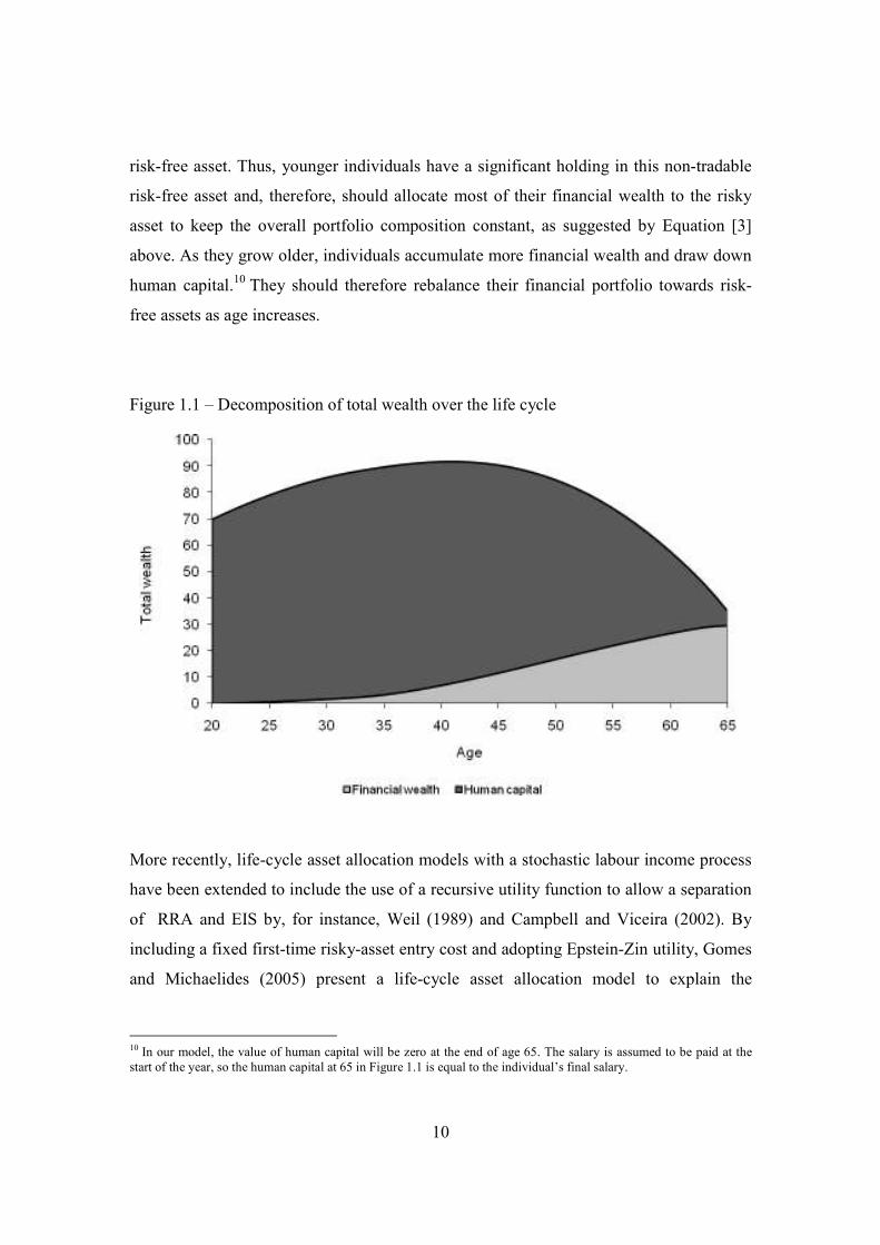
human to financial wealth9 is a crucial determinant of the life-cycle portfolio composition.
In early life, as shown in Figure 1.1, this ratio is large since the individual has had little
time to accumulate financial wealth and expects to receive labour income for many years.
Given that long-term average labour income growth is of a similar order of magnitude as
average long-run interest rates in the UK over the last century, as explained in Cairns et
al. (2006), labour income can be thought of as an implicit substitute to investing in the
8 By far, the most popular approach is value function iteration. Specifically, this involves the discretisation of the state
variables by setting up a standard equally-spaced grid and solves the optimisation for each grid point at the next-to-last
time period. The expectation term in the resulting Bellman equation is approximated by using quadrature integration
and then the dynamic optimisation problem can be solved by backward recursion. It is possible that the accumulated
state variable values from the previous time period are not represented by a grid point, in which case, an interpolation
method (e.g., bilinear, cubic spline, etc.) must be employed to approximate the value function. However, this approach
requires knowledge of the distribution of each of the shocks to the process, so that appropriate quadrature integration
(e.g., Gauss quadrature) can be used. Furthermore, this approach cannot handle a large number of state variables. To
overcome these limitations, Brandt et al. (2005) proposed a simulation method based on the recursive use of
approximated optimal portfolio weights. The idea is to estimate asset return moments using a large number of
simulated sample paths, and then to approximate the value function using a Taylor series expansion. If the return is
path-dependent, it is necessary to regress the return variable on the simulated state variables from previous time period,
before using the Taylor expansion with conditional return moments. 9 In our model, the only source of financial wealth is pension wealth, and we use these terms interchangeably.
10
risk-free asset. Thus, younger individuals have a significant holding in this non-tradable
risk-free asset and, therefore, should allocate most of their financial wealth to the risky
asset to keep the overall portfolio composition constant, as suggested by Equation [3]
above. As they grow older, individuals accumulate more financial wealth and draw down
human capital.10
They should therefore rebalance their financial portfolio towards risk-
free assets as age increases.
Figure 1.1 – Decomposition of total wealth over the life cycle
More recently, life-cycle asset allocation models with a stochastic labour income process
have been extended to include the use of a recursive utility function to allow a separation
of RRA and EIS by, for instance, Weil (1989) and Campbell and Viceira (2002). By
including a fixed first-time risky-asset entry cost and adopting Epstein-Zin utility, Gomes
and Michaelides (2005) present a life-cycle asset allocation model to explain the
10 In our model, the value of human capital will be zero at the end of age 65. The salary is assumed to be paid at the
start of the year, so the human capital at 65 in Figure 1.1 is equal to the individual’s final salary.

11
empirical observations of low stock market participation and moderate equity holdings
for participants11
.
Turning to DC pension plans, most of the existing literature investigates their optimal
dynamic asset allocation strategy by assuming a fixed contribution rate (e.g., 10% of
salary per annum prior to retirement) and maximising the utility of the replacement ratio
(i.e., pension as a proportion of final salary) at retirement (for example, Cairns et al.
(2006)) or by minimising the expected present value of total disutility 12 prior to
retirement (for example, Haberman and Vigna (2002)). The EIS is implicitly assumed to
be zero and there is no facility for adjusting the contribution rate in response to changes
in salary level or in asset performance. However, in practice, most DC plans allow
members to make additional voluntary contributions, and often set upper and lower limits
on the contribution rate per annum.
Our aim in this study is to investigate the optimal asset allocation strategy for a DC plan
member with Epstein-Zin utility, so that an individual member’s investment strategy
depends on the pattern of preferred consumption levels over the member’s entire lifetime.
We also derive the optimal profile of contribution rates over the accumulation stage of a
DC plan. The rest of the paper is structured as follows. Section 2 outlines the discrete-
time model with Epstein-Zin utility, including the parameter calibration process and
optimisation method used. In Section 3, we generate simulations of the two key state
variables (i.e., wealth and labour income) and derive the optimal funding and investment
strategies for the DC pension plan; we also conduct a sensitivity analysis of the results.
Section 4 concludes.
11 Gomes and Michaelides (2005, page 871) argue that the less risk-averse investors have a weaker incentive to pay the
fixed entry cost of equity investment, and therefore stock market participants in aggregate tend to be more risk averse.
12 The disutility is normally defined using the deviation of actual fund level from interim and final target fund levels.

12
2 The model
2.1 The model structure and optimisation problem
We propose a two-asset discrete-time model with a constant investment opportunity set.
To ensure conformity with a DC pension plan, a number of constraints need to be
specified:
(i) pension wealth can never be negative,
(ii) in any year prior to retirement, consumption must be lower than labour income,
(iii) short selling of assets is not allowed,
(iv) members are not allowed to borrow from future contributions.13
Members are assumed to join the pension plan at age 20 (denoted time 0=t below)
without bringing in any transfer value from a previous plan and the retirement age is
fixed at 65. We work in time units of one year and members are assumed to live to a
maximum age of 120ω = .
2.1.1 Preferences
We assume the plan member possesses the discrete-time recursive utility function
proposed by Epstein and Zin (1989):
( ) ( )
11 11 1
1 1
20 11
11
20 20 20 20 20 20 1 201 11
ϕ ϕγ γ
γϕβ βγ
− −
− −+ +
−−
+ + + + + + + +
= − + × + − × × −
t
t t t t t t t
W
bV p C E p V p b [4]
13 Some studies have assumed that the member can borrow from future contributions (i.e., to incorporate a loan in the
portfolio equal to the present value of future contributions). In this way, Boulier et al. (2001) and Cairns et al. (2006)
investigate the optimal asset allocation of DC pension plan with guaranteed benefit protection. However, there are
arguments against the use of this assumption. In most cases, this would not be allowed in practice. Also, the loan
amount depends on assumptions about the level of future contributions and, in practice, there can be a lot of uncertainty
about future contributions.

13
where
• 20+tV is the utility level at time t (or age 20 + t ),
• 20+tW is the wealth level at time t ,
• 20+tC is the consumption level at time t ,
• γ is the coefficient of relative risk aversion (RRA),
• ϕ is the elasticity of intertemporal substitution (EIS),
• β is the discount factor for each year, and
• 20+tp is the one-year survival probability at time t (i.e., the probability that a
member who is alive age 20 + t survives to age 20 1+ +t ).
The parameter b is the “bequest intensity” and determines the strength of the bequest
motive. If a member dies during the year of age 20 + t to 20 1+ +t , the deceased member
will give the remaining wealth at the end of the year, 120 ++tW , a utility measure of
( ) ( )1
20 1 1tb W b−
+ +× −γ
γ . Thus, a higher value of b implies that the member has a
stronger desire to bequest wealth on death.
In the final year of age ( )1,ω ω− , where we have 1 0ω− =p , equation [4] reduces to:
11 11 1
1 1
11
1 1 11
ϕ ϕγ γ
ω
ϕω ω ωβ
γ
− −
− −
−
− − −
= + × −
W
bV C E b [5]
which provides the terminal condition for the utility function.
2.1.2 Financial assets
We assume that there are two underlying assets in which the pension plan can invest:
(i) a risk-free asset (i.e., a cash fund), and
14
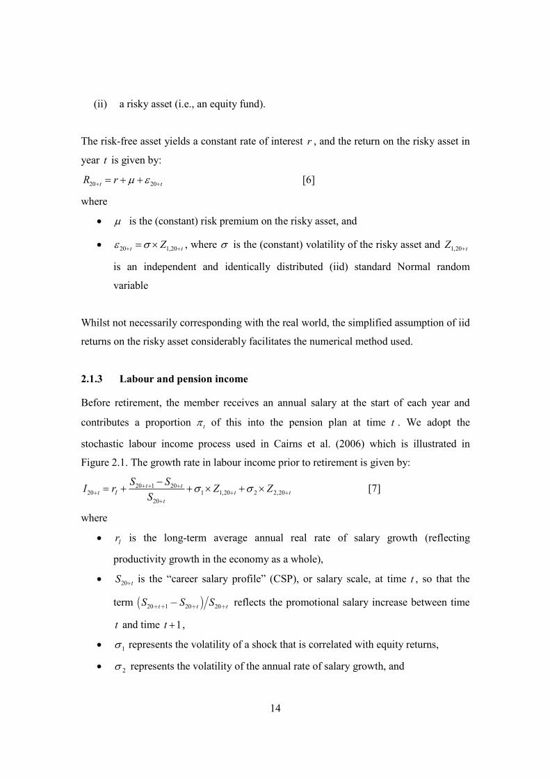
(ii) a risky asset (i.e., an equity fund).
The risk-free asset yields a constant rate of interest r , and the return on the risky asset in
year t is given by:
20 20µ ε+ += + +t tR r [6]
where
• µ is the (constant) risk premium on the risky asset, and
• 20 1,20ε σ+ += ×t tZ , where σ is the (constant) volatility of the risky asset and 1,20+tZ
is an independent and identically distributed (iid) standard Normal random
variable
Whilst not necessarily corresponding with the real world, the simplified assumption of iid
returns on the risky asset considerably facilitates the numerical method used.
2.1.3 Labour and pension income
Before retirement, the member receives an annual salary at the start of each year and
contributes a proportion π t of this into the pension plan at time t . We adopt the
stochastic labour income process used in Cairns et al. (2006) which is illustrated in
Figure 2.1. The growth rate in labour income prior to retirement is given by:
20 1 2020 1 1,20 2 2,20
20
σ σ+ + ++ + +
+
−= + + × + ×t t
t I t t
t
S SI r Z Z
S [7]
where
• Ir is the long-term average annual real rate of salary growth (reflecting
productivity growth in the economy as a whole),
• 20+tS is the “career salary profile” (CSP), or salary scale, at time t , so that the
term ( )20 1 20 20t t tS S S+ + + +− reflects the promotional salary increase between time
t and time 1+t ,
• 1σ represents the volatility of a shock that is correlated with equity returns,
• 2σ represents the volatility of the annual rate of salary growth, and
15
• tZ +20,2 is an iid standard Normal random variable.
Equations (6) and (7) are subject to a common stochastic shock, 1,20+tZ , implying that the
correlation between the growth rate in labour income and equity returns is given by
( )2 2
1 1 2+σ σ σ .
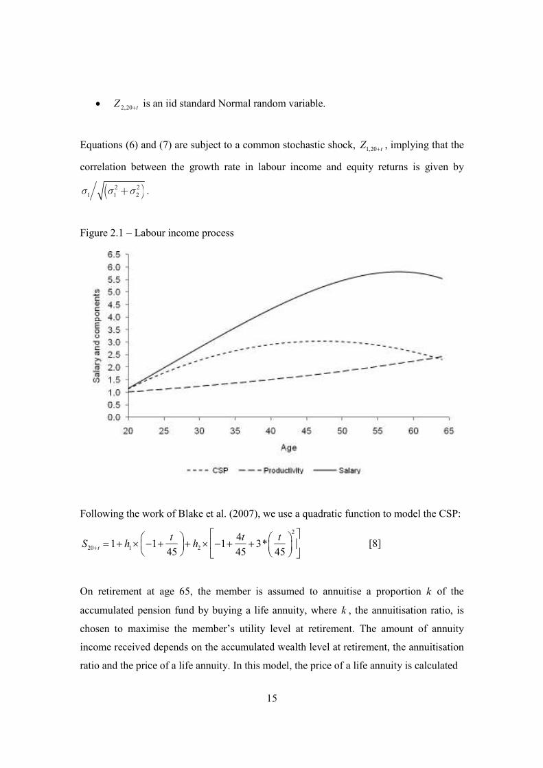
Figure 2.1 – Labour income process
Following the work of Blake et al. (2007), we use a quadratic function to model the CSP:
2
20 1 2
41 1 1 3*
45 45 45+
= + × − + + × − + + t
t t tS h h [8]
On retirement at age 65, the member is assumed to annuitise a proportion k of the
accumulated pension fund by buying a life annuity, where k , the annuitisation ratio, is
chosen to maximise the member’s utility level at retirement. The amount of annuity
income received depends on the accumulated wealth level at retirement, the annuitisation
ratio and the price of a life annuity. In this model, the price of a life annuity is calculated

16
using the risk-free return on the cash fund, so it is fixed over time and no annuity risk is
considered. After retirement, the member invests the residual wealth that is not
annuitised. Retirement income therefore comes from two sources: the annuity and
possible withdrawals from the residual fund until death.
2.1.4 Wealth accumulation
Before retirement, the growth in the member’s pension wealth will depend on the
investment strategy adopted, the investment returns on both the risk-free asset and the
risky asset, and the chosen contribution rate.
The contribution rate at time t is given by ( )20 20 20 20t t t tY C Y+ + + += −π (for 0 44≤ ≤t ),
where 20+tY is the labour income level at time t . We require the contribution rate to be
non-negative, so that 20 20+ +≥t tY C before retirement. The contribution rate is allowed to
vary over time, so that consumption in any period can adjust to changes in income level
and investment performance.
We also need to impose the restriction 20 0+ ≥tW (for 1000 ≤≤ t ), to ensure that the
wealth level is always non-negative at each age over the life cycle.
A proportion,20α +t
, of the member’s pension account is assumed to be invested in the
risky asset at time t . Then, for 0 43≤ ≤t (i.e., up to and including the year prior to
retirement), we have the following recursive relationship for the wealth process:
( ) ( )20 1 20 20 20 20 201π α µ ε+ + + + + + + = + × + + + t t t t t tW W Y r [9]
As mentioned above, we assume that that short selling of assets is not allowed and
therefore impose the restriction that 200 1α +≤ ≤t .

17
At the start of the year in which the member is aged between 64 and 65, the member
receives the final salary payment and makes the final contribution to the pension fund. So,
we have:
( ) ( )65 64 64 64 64 641π α µ ε− = + × + + + W W Y r [10]
At the end of this year, the member retires and chooses the annuitisation ratio k , giving a
residual wealth on retirement at exact age 65 of ( )65 651 −= − ×W k W . The annuitisation
ratio k is chosen to maximise the utility level at retirement. This control variable does
not appear in the utility function, but rather in the wealth constraint in the retirement year.
After retirement, the member invests a proportion 20α +t (for 45≥t ) of the residual
wealth (i.e., that which was not annuitised) in the risky asset and receives annuity
payments rather than labour income at the start of each year, provided that the member is
still alive. This implies that the recursive relationship for the wealth accumulation process
at this stage of the member’s life cycle is given by:
( )6520 1 20 20 20 20
65
1 α µ ε−
+ + + + + +
× = + − × + + +
ɺɺt t t t t
k WW W C r
a [11]
where 65aɺɺ is the price of a life annuity at age 65 (and, hence, 65 65k W a−× ɺɺ represents the
annual annuity income after retirement).
Finally, we must constrain consumption after retirement such that
( )20 20 65 65t tC W k W a−+ +≤ + × ɺɺ .
2.1.5 The optimisation problem and solution method
The model has three control variables: the asset allocation at time t , 20α +t , the
consumption level at time t , 20+tC , and the annuitisation ratio at retirement, k .

18
The optimisation problem is then:
( )20 20
20, ,
maxα + +
+t t
tC k
E V
subject to the following constraints:
(i) for 0 43≤ ≤t , we have:
a) a wealth accumulation process satisfying:
( ) ( )20 1 20 20 20 20 201 0π α µ ε+ + + + + + + = + × + + + ≥ t t t t t tW W Y r ,
b) an allocation to the risky asset satisfying 10 20 ≤≤ +tα , and
c) a contribution rate satisfying 20 0π + ≥t ;
(ii) for 44=t , we have:
a) a wealth accumulation process satisfying:
( ) ( ) ( )( )65 64 64 64 64 641 1 0π α µ ε = − × + × + + + ≥ W k W Y r ,
b) an allocation to the risky asset satisfying 640 1α≤ ≤ ,
c) a contribution rate satisfying 64 0π ≥ , and
d) an annuitisation ratio at age 65 satisfying 10 ≤≤ k ;
(iii) and, for 45≥t , we have:
a) a wealth accumulation process satisfying:
( )6520 1 20 20 20 20
65
1 0α µ ε−
+ + + + + +
× = + − × + + + ≥
ɺɺt t t t t
k WW W C r
a,
b) an allocation to the risky asset satisfying 10 20 ≤≤ +tα , and
c) consumption satisfying 6520 20
65
−
+ +
×≤ + ɺɺ
t t
k WC W
a.
19
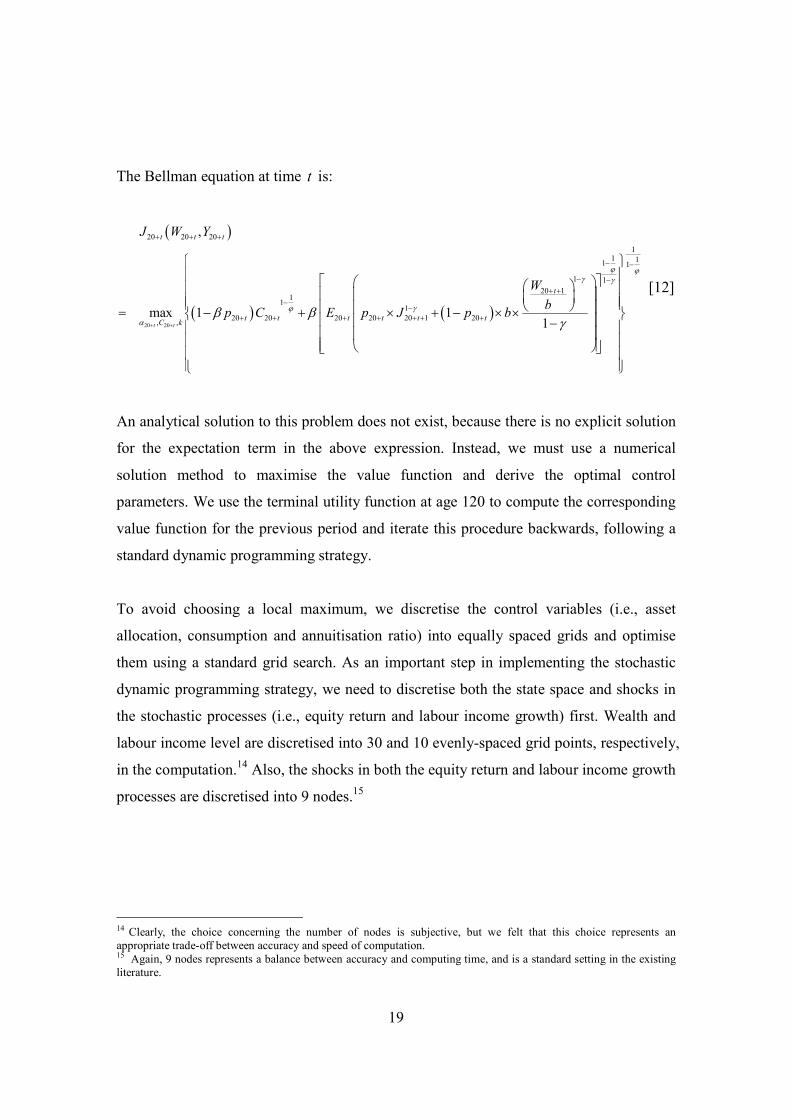
The Bellman equation at time t is:
( )
( ) ( )20 20
20 20 20
11 1
1 1
1 1
20 11
11
20 20 20 20 20 1 20, ,
,
max 1 11
ϕ ϕγ γ
γϕ
αβ β
γ+ +
+ + +
− −
− −+ +
−−
+ + + + + + +
= − + × + − × × −
t t
t t t
t
t t t t t tC k
J W Y
W
bp C E p J p b
[12]
An analytical solution to this problem does not exist, because there is no explicit solution
for the expectation term in the above expression. Instead, we must use a numerical
solution method to maximise the value function and derive the optimal control
parameters. We use the terminal utility function at age 120 to compute the corresponding
value function for the previous period and iterate this procedure backwards, following a
standard dynamic programming strategy.
To avoid choosing a local maximum, we discretise the control variables (i.e., asset
allocation, consumption and annuitisation ratio) into equally spaced grids and optimise
them using a standard grid search. As an important step in implementing the stochastic
dynamic programming strategy, we need to discretise both the state space and shocks in
the stochastic processes (i.e., equity return and labour income growth) first. Wealth and
labour income level are discretised into 30 and 10 evenly-spaced grid points, respectively,
in the computation.14
Also, the shocks in both the equity return and labour income growth
processes are discretised into 9 nodes.15
14 Clearly, the choice concerning the number of nodes is subjective, but we felt that this choice represents an
appropriate trade-off between accuracy and speed of computation. 15 Again, 9 nodes represents a balance between accuracy and computing time, and is a standard setting in the existing
literature.

20
The expected utility level at time t is then computed using these nodes and the relevant
weights attached to each (i.e., Gauss quadrature weights and interpolation nodes).16
The
advantage of using this set of nodes is that the state variables can be computed more
quickly and precisely; however, because we have a fine grid on the control variables and
a much coarser grid on the shocks, we may have some state variable values outside of the
grid points in the next time period. In this case, cubic spline interpolation is employed to
approximate the value function. While this approach does not significantly reduce the
accuracy of the results obtained, use of a much finer grid for the shocks in the equity
return and labour income growth processes would significantly increase computing time,
as mentioned previously.
For each age 20 + t prior to the terminal age of 120, we compute the maximum value
function and the optimal values for the control variables at each grid point. Substituting
these values in the Bellman equation, we obtain the value function of this period, which
is then used to solve the maximisation problem for the previous time period. Details of
the dynamic programming and integration process are given in Appendix 1. The
computations were performed in MATLAB.17
2.2 Parameter calibration
We begin with a standard set of baseline parameter values (all expressed in real terms)
presented in Table 2.1.
The constant net real interest rate, r , is set at 2% p.a., while, for the equity return process,
we consider a mean equity premium, µ , of 4% p.a. and a standard deviation, σ , of 20%
p.a.. Using an equity risk premium of 4% p.a. (as opposed to the historical average of
around 6%) is a common choice in recent literature (e.g., Fama and French (2002),
Gomes and Michaelides (2005)). This more cautious assumption reflects the fact that the
historical equity risk premium might be higher than can reasonably be expected in future,
and thus will reduce the weight given to equities in the optimal portfolios obtained. We
16
For more details, see Judd (1998, page 257-266). 17
http://www.mathworks.com/products/matlab/. The code is available on request from the authors.
21
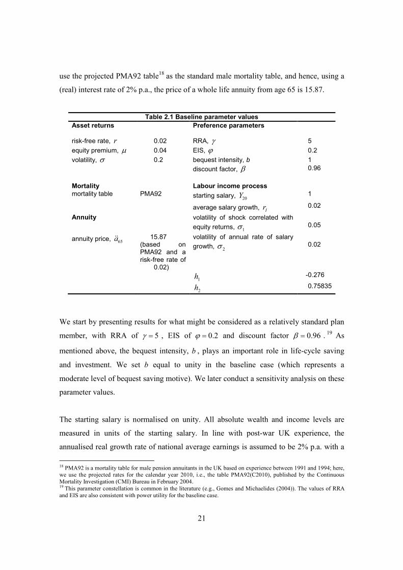
use the projected PMA92 table18
as the standard male mortality table, and hence, using a
(real) interest rate of 2% p.a., the price of a whole life annuity from age 65 is 15.87.
Table 2.1 Baseline parameter values
Asset returns
Preference parameters
risk-free rate, r 0.02 RRA, γ 5
equity premium, µ 0.04 EIS, ϕ 0.2
volatility, σ 0.2 bequest intensity, b 1
discount factor, β 0.96
Mortality Labour income process mortality table PMA92 starting salary,
20Y 1
average salary growth, Ir 0.02
Annuity volatility of shock correlated with
equity returns, 1σ
0.05
annuity price, 65ɺɺa 15.87
(based on PMA92 and a risk-free rate of
0.02)
volatility of annual rate of salary
growth, 2σ
0.02
1h -0.276
2h 0.75835
We start by presenting results for what might be considered as a relatively standard plan
member, with RRA of 5γ = , EIS of 0.2ϕ = and discount factor 0.96β = .19
As
mentioned above, the bequest intensity, b , plays an important role in life-cycle saving
and investment. We set b equal to unity in the baseline case (which represents a
moderate level of bequest saving motive). We later conduct a sensitivity analysis on these
parameter values.
The starting salary is normalised on unity. All absolute wealth and income levels are
measured in units of the starting salary. In line with post-war UK experience, the
annualised real growth rate of national average earnings is assumed to be 2% p.a. with a
18 PMA92 is a mortality table for male pension annuitants in the UK based on experience between 1991 and 1994; here,
we use the projected rates for the calendar year 2010, i.e., the table PMA92(C2010), published by the Continuous
Mortality Investigation (CMI) Bureau in February 2004. 19 This parameter constellation is common in the literature (e.g., Gomes and Michaelides (2004)). The values of RRA
and EIS are also consistent with power utility for the baseline case.
22
standard deviation of 2% p.a. (i.e., 0.02Ir = and 2 0.02=σ ). Following the work of
Blake et al. (2007), we estimate the CSP parameters 1h and 2h using average male salary
data (across all occupations) reported in the 2005 Annual Survey of Hours and Earnings.
The estimated values are 1 0.276= −h and 2 0.75835=h (see [8]).
3 Results
3.1 Baseline case
3.1.1 Optimal asset allocation assuming no bequest motive or labour income risk
As suggested by equation [3] above, the optimal portfolio composition should be constant
when there is no bequest motive and labour income risk is ignored. Figure 3.1 shows the
optimal equity weight for the final time period (i.e., year of age 119 to 120) with no
bequest motive. As expected, we can see that when the accumulated wealth level is large
(and labour income is small in comparison), the optimal asset allocation is close to the
result suggested in equation [3], so that we have:
120 120
2 2
cov( , )11 0.2
µα
γσ γ σ −
= + − × ≈
R V
This result shows that we can approximate an analytical solution numerically reasonably
accurately, thereby justifying the use of our grid search numerical method.
3.1.2 Simulation output
The output from the optimisation exercise is a set of optimal control variables (i.e., asset
allocation, 20α +t , and consumption level, 20+tC ) for each time period and the optimal
annuitisation ratio, k , at retirement age 65. We generate a series of random variables for
both the equity return and labour income shocks, and then generate 10,000 independent
simulations of wealth and labour income levels.

23
Figure 3.1 – Optimal equity allocation for the final time period
0
0.2
0.4
0.6
0.8
1
AnnuityWealth
Optimal equity allocation
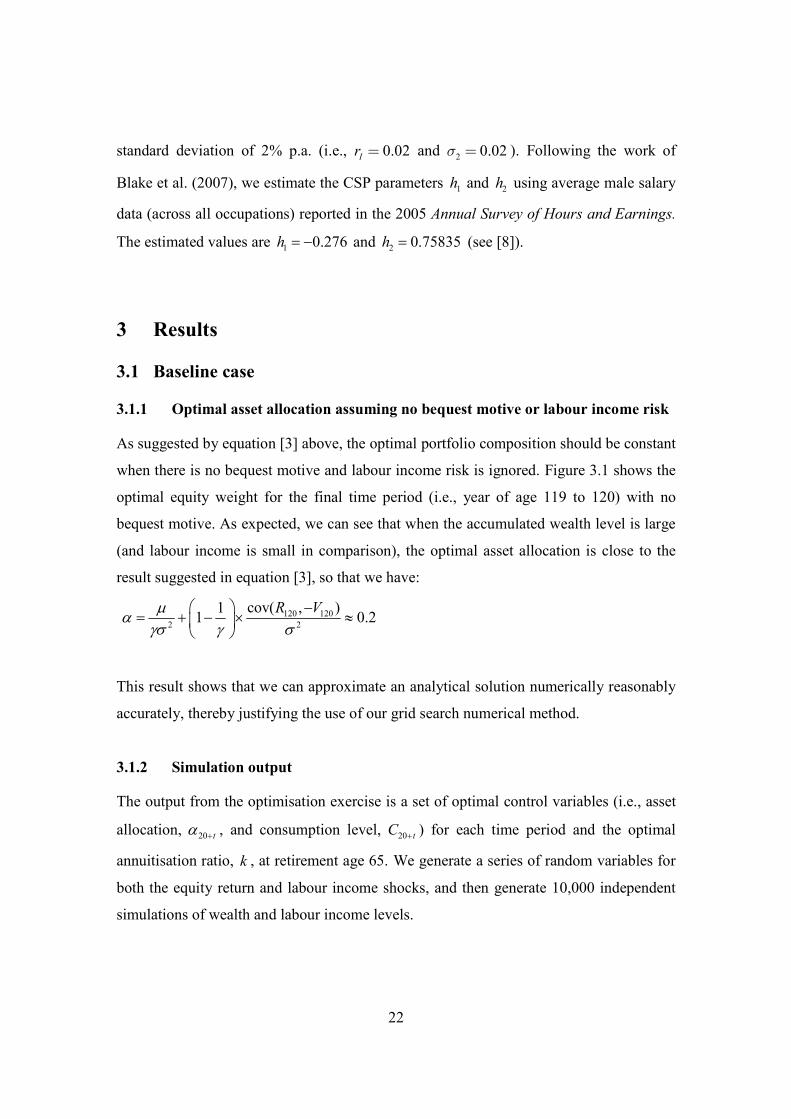
Figure 3.2 shows the simulation means of labour income and optimal wealth and
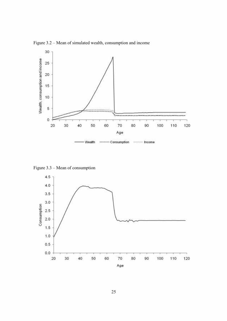
consumption levels for ages 20, 21, …, 120, and Figure 3.3 shows the consumption
profile on a larger scale. We have bequest and retirement saving motives in this model. In
the early years of the life cycle (i.e., up to age 45 or so), wealth accumulation is driven by
the bequest intensity (i.e., the extent of the desire to protect dependants if the member
dies) and by the attitude to risk (i.e., the degree of aversion to cutting consumption in
unfavourable states).20
Consumption increases smoothly during this period. Then, as the
member gets older, the retirement motive becomes more important as the member
recognises the need to build up the pension fund in order to support consumption after
retirement. From age 45 to the retirement age of 65, the retirement savings motive
dominates and the pension fund grows significantly. As a result, consumption remains
almost constant during this period.
20 This will become clearer in sections 3.2.1 and 3.2.2.

24
After retirement, there is a large fall in consumption compared with the period
immediately prior to retirement and thereafter consumption remains stable for the
remainder of the member’s lifetime. Evidence presented in Banks et al (1998) shows that
consumption tends to fall after retirement. Part of this is explained by the fact that work-
related expenses such as travel and clothes no longer need to be incurred. Part is
explained by the fact that precautionary balances need to be maintained to pay for lumpy
expenditures such as car repairs or home maintenance, given that working to pay for
these expenses is no longer an option. Part is also explained by the fact that retired people
tend to stay at home more and so spend less on high-cost items, such as restaurant meals
and holidays. We do not attempt to model these complex issues in a formal way. Instead,
we try to capture them in the post-retirement consumption constraint
( )( )20 20 65 65t tC W k W a−+ +≤ + × ɺɺ (i.e., for 45≥t ), given in section 2.1.4 above.
Consumption after retirement is therefore subject to a cash-in-hand constraint and cannot
exceed the sum of pension income and unannuitised wealth. The constraint is tighter the
higher the fraction, k, of pension wealth the member chooses to annuitize at age 65.
Given that k is a control variable, Figure 3.3 shows the optimal reduction in consumption
in retirement when k is chosen optimally (i.e., to maximise ( )64E V ).
The size of the fall in consumption at retirement when there is a cash-in-hand constraint
will be influenced by the level of non-pension wealth, such as discretionary savings or
housing. Since non-pension wealth does not need to be annuitized, it acts as a buffer that
can be used to smooth life-cycle consumption. Non-pension wealth is outside the scope
of the present paper.
25
Figure 3.2 – Mean of simulated wealth, consumption and income
Figure 3.3 – Mean of consumption
26
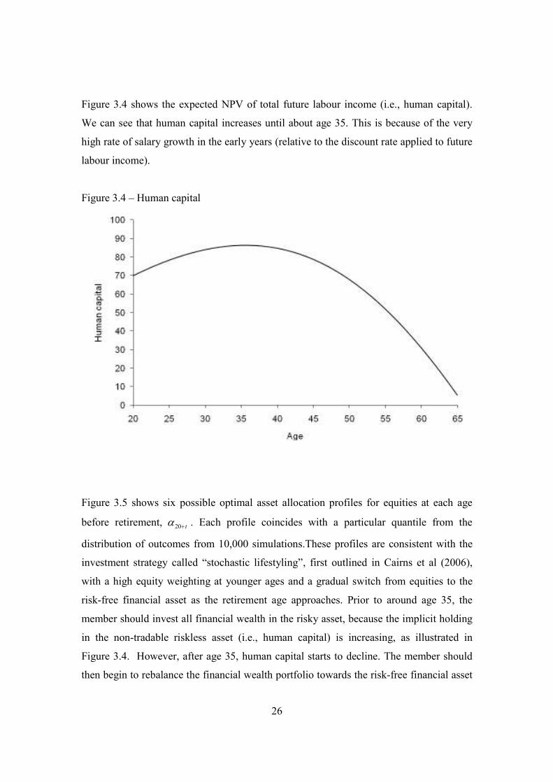
Figure 3.4 shows the expected NPV of total future labour income (i.e., human capital).
We can see that human capital increases until about age 35. This is because of the very
high rate of salary growth in the early years (relative to the discount rate applied to future
labour income).
Figure 3.4 – Human capital
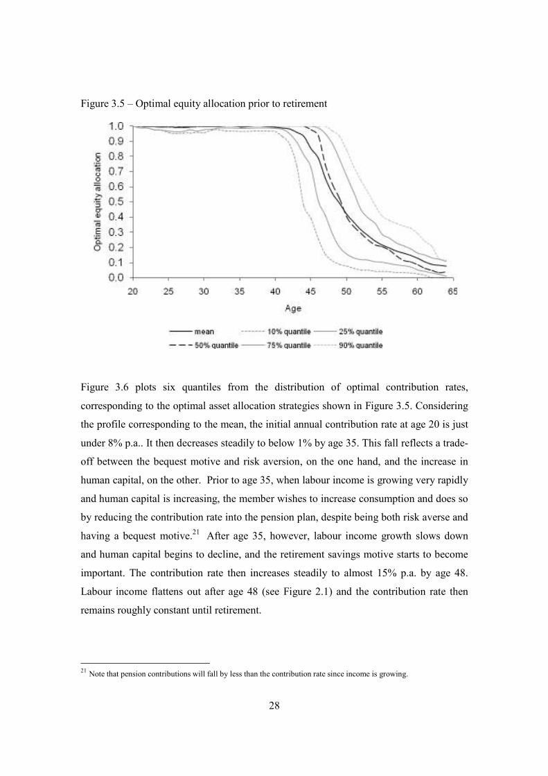
Figure 3.5 shows six possible optimal asset allocation profiles for equities at each age
before retirement, 20α +t . Each profile coincides with a particular quantile from the
distribution of outcomes from 10,000 simulations.These profiles are consistent with the
investment strategy called “stochastic lifestyling”, first outlined in Cairns et al (2006),
with a high equity weighting at younger ages and a gradual switch from equities to the
risk-free financial asset as the retirement age approaches. Prior to around age 35, the
member should invest all financial wealth in the risky asset, because the implicit holding
in the non-tradable riskless asset (i.e., human capital) is increasing, as illustrated in
Figure 3.4. However, after age 35, human capital starts to decline. The member should
then begin to rebalance the financial wealth portfolio towards the risk-free financial asset

27
to compensate for the decline in human capital. This is because the risk-free financial
asset and human capital are substitutes, with the degree of substitutability inversely
related to the correlation between labour income growth and equity returns,
( )2 2
1 1 2+σ σ σ .
The investment strategy is known as “stochastic lifestyling” because the optimal equity
weighting over the life cycle depends on the realised outcomes for the stochastic
processes driving the state variables, namely labour income and the risky financial asset.
The profiles have a similar shape which can be characterised as three connecting (and
approximately) linear segments. The first is a horizontal segment involving a 100%
equity weighting (approximately) from age 20 to an age somewhere in the range of 40-47.
The second is a steep downward segment that involves a reduction in equities to
somewhere between 10-40% over a seven year period. The third is a more gentle
downward sloping segment that reduces the equity weighting to somewhere between 0-
10% by the retirement age. It is important to note that the profiles in Figure 3.5 are not,
however, consistent with the more traditional “deterministic lifestyling” strategy, which
involves an initial high weighting in equities with a predetermined linear switch from
equities to cash in the period leading up to retirement (typically the preceding 5 or 10
years).
28
Figure 3.5 – Optimal equity allocation prior to retirement
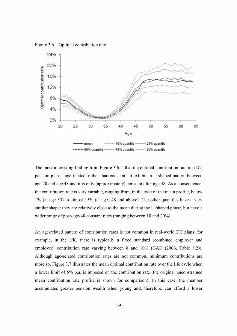
Figure 3.6 plots six quantiles from the distribution of optimal contribution rates,
corresponding to the optimal asset allocation strategies shown in Figure 3.5. Considering
the profile corresponding to the mean, the initial annual contribution rate at age 20 is just
under 8% p.a.. It then decreases steadily to below 1% by age 35. This fall reflects a trade-
off between the bequest motive and risk aversion, on the one hand, and the increase in
human capital, on the other. Prior to age 35, when labour income is growing very rapidly
and human capital is increasing, the member wishes to increase consumption and does so
by reducing the contribution rate into the pension plan, despite being both risk averse and
having a bequest motive.21
After age 35, however, labour income growth slows down
and human capital begins to decline, and the retirement savings motive starts to become
important. The contribution rate then increases steadily to almost 15% p.a. by age 48.
Labour income flattens out after age 48 (see Figure 2.1) and the contribution rate then
remains roughly constant until retirement.
21
Note that pension contributions will fall by less than the contribution rate since income is growing.
29
Figure 3.6 – Optimal contribution rate
The most interesting finding from Figure 3.6 is that the optimal contribution rate in a DC
pension plan is age-related, rather than constant. It exhibits a U-shaped pattern between
age 20 and age 48 and it is only (approximately) constant after age 48. As a consequence,
the contribution rate is very variable, ranging from, in the case of the mean profile, below
1% (at age 35) to almost 15% (at ages 48 and above). The other quantiles have a very
similar shape: they are relatively close to the mean during the U-shaped phase, but have a
wider range of post-age-48 constant rates (ranging between 10 and 20%).
An age-related pattern of contribution rates is not common in real-world DC plans: for
example, in the UK, there is typically a fixed standard (combined employer and
employee) contribution rate varying between 8 and 10% (GAD (2006, Table 8.2)).
Although age-related contribution rates are not common, minimum contributions are
more so. Figure 3.7 illustrates the mean optimal contribution rate over the life cycle when
a lower limit of 5% p.a. is imposed on the contribution rate (the original unconstrained
mean contribution rate profile is shown for comparison). In this case, the member
accumulates greater pension wealth when young and, therefore, can afford a lower
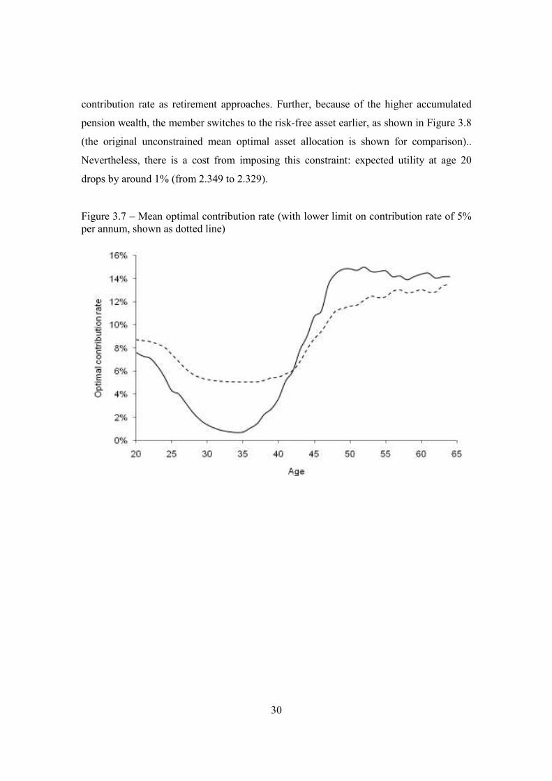
30
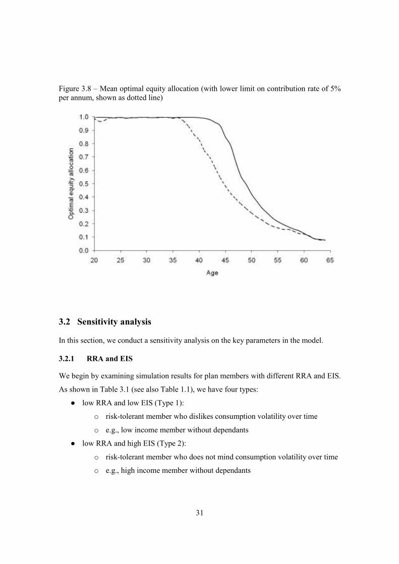
contribution rate as retirement approaches. Further, because of the higher accumulated
pension wealth, the member switches to the risk-free asset earlier, as shown in Figure 3.8
(the original unconstrained mean optimal asset allocation is shown for comparison)..
Nevertheless, there is a cost from imposing this constraint: expected utility at age 20
drops by around 1% (from 2.349 to 2.329).
Figure 3.7 – Mean optimal contribution rate (with lower limit on contribution rate of 5%
per annum, shown as dotted line)
31
Figure 3.8 – Mean optimal equity allocation (with lower limit on contribution rate of 5%
per annum, shown as dotted line)
3.2 Sensitivity analysis
In this section, we conduct a sensitivity analysis on the key parameters in the model.
3.2.1 RRA and EIS
We begin by examining simulation results for plan members with different RRA and EIS.
As shown in Table 3.1 (see also Table 1.1), we have four types:
● low RRA and low EIS (Type 1):
o risk-tolerant member who dislikes consumption volatility over time
o e.g., low income member without dependants
● low RRA and high EIS (Type 2):
o risk-tolerant member who does not mind consumption volatility over time
o e.g., high income member without dependants
32
● high RRA and low EIS (Type 3):
o risk-averse member who dislikes consumption volatility over time
o e.g., low income member with dependants
● high RRA and high EIS (Type 4):
o risk-averse member who does not mind consumption volatility over time
o e.g., high income member with dependants
The baseline case in Section 3.1 dealt with Type 3 (highlighted in Table 3.1), a member
with a high RRA and a low EIS (i.e., 5=γ and 0.2=ϕ ).
Table 3.1 RRA and EIS values for the different types of plan member
RRA, γ EIS, ϕ
Type 1 2 0.2
Type 2 2 0.5
Type 3 5 0.2
Type 4 5 0.5
Figure 3.9 shows the different patterns of optimal contribution rates corresponding to
these four types. For risk-tolerant members with low RRA (i.e., Types 1 and 2),
contributions prior to age 50 are negligible. From age 50 or so, the retirement savings
motive kicks in and contributions into the pension plan begin. The contribution rate is
lower for Type 1 (low EIS) than for Type 2 (high EIS) members (by approximately 3-4%
p.a.). This lower retirement savings intensity is the result of a stronger aversion to cutting
consumption: due to the lower EIS level, cuts in consumption needed to fund the pension
plan are more heavily penalised in the utility function of Type 1 members than of Type 2
members.
33
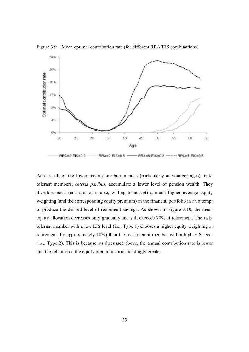
Figure 3.9 – Mean optimal contribution rate (for different RRA/EIS combinations)
As a result of the lower mean contribution rates (particularly at younger ages), risk-
tolerant members, ceteris paribus, accumulate a lower level of pension wealth. They
therefore need (and are, of course, willing to accept) a much higher average equity
weighting (and the corresponding equity premium) in the financial portfolio in an attempt
to produce the desired level of retirement savings. As shown in Figure 3.10, the mean
equity allocation decreases only gradually and still exceeds 70% at retirement. The risk-
tolerant member with a low EIS level (i.e., Type 1) chooses a higher equity weighting at
retirement (by approximately 10%) than the risk-tolerant member with a high EIS level
(i.e., Type 2). This is because, as discussed above, the annual contribution rate is lower
and the reliance on the equity premium correspondingly greater.
34
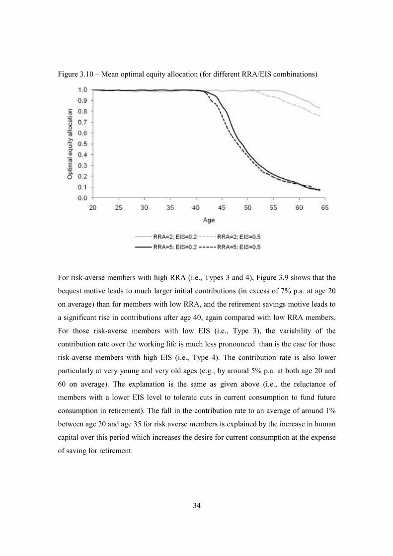
Figure 3.10 – Mean optimal equity allocation (for different RRA/EIS combinations)
For risk-averse members with high RRA (i.e., Types 3 and 4), Figure 3.9 shows that the
bequest motive leads to much larger initial contributions (in excess of 7% p.a. at age 20
on average) than for members with low RRA, and the retirement savings motive leads to
a significant rise in contributions after age 40, again compared with low RRA members.
For those risk-averse members with low EIS (i.e., Type 3), the variability of the
contribution rate over the working life is much less pronounced than is the case for those
risk-averse members with high EIS (i.e., Type 4). The contribution rate is also lower
particularly at very young and very old ages (e.g., by around 5% p.a. at both age 20 and
60 on average). The explanation is the same as given above (i.e., the reluctance of
members with a lower EIS level to tolerate cuts in current consumption to fund future
consumption in retirement). The fall in the contribution rate to an average of around 1%
between age 20 and age 35 for risk averse members is explained by the increase in human
capital over this period which increases the desire for current consumption at the expense
of saving for retirement.

35
As a result of higher contribution rates, risk-averse members accumulate a much higher
level of pension wealth and, as can be seen in Figure 3.10, switch away from equities
much earlier (from about age 40) and hold less than 10% of the pension fund in equities
at retirement on average.
For a given level of risk aversion, Figure 3.10 shows that a lower EIS leads to a higher
equity weighting during the later stages of the accumulation phase of the pension plan. At
first sight, this finding seems counterintuitive: surely individuals with a lower IES would
prefer a lower equity weighting in their pension fund and hence more stable contributions
over time? Constantinides (1990), for example, appeals to habit formation (i.e., the
complementarity between consumption in adjacent periods) for inducing a strong desire
for stable consumption and a correspondingly low demand for equities. However, in our
model, the retirement saving motive is important, since the only source of post-retirement
consumption in our model comes from the pension plan. During the accumulation phase,
a member with a low EIS is not willing to reduce current consumption in order to
increase plan contributions (to meet the retirement saving motive), but is willing to use a
higher equity weighting and the corresponding equity premium in an attempt to generate
the necessary retirement savings. Figure 3.10 shows that the retirement savings effect
dominates the habit formation effect in determining the equity weighting in the later
years of the accumulation phase (Gomes and Michaelides (2005) derived the same result).
3.2.2 Bequest motive
Investors with a desire to bequest wealth to their dependants on death would be expected
to save more than those who do not. Figure 3.11 shows the mean optimal pattern of
contribution rates for the baseline case of 5γ = and 0.2ϕ = and different bequest
intensities. When the bequest motive is absent (b = 0), members consume almost all of
their earnings in the early years of their working lives, and have very negligible
contributions into their pension plans. By contrast, members with a high bequest intensity
(b = 2.5) make very high contributions in the early years (14% at age 20). They also

36
make higher contributions throughout their working lives,22
but the differences after age
35 are much less.
Figure 3.12 shows that the optimal equity weight in the portfolio is lower, the higher the
bequest intensity. However, the effect is small because: first, the mortality rate does not
vary much before retirement, and second, and more importantly, the annuitisation ratio (k)
is a control variable in our model and, thus, a member with a high bequest intensity could
choose to annuitise a smaller ratio of the pension fund at retirement, instead of assuming
significant equity risk in an attempt to accumulate more wealth prior to retirement.23
Figure 3.11 – Mean optimal contribution rate (for different levels of bequest motive)
22 Although it is still pulled down to below 1% between ages 20 and 35 by the effect of the increase in human capital. 23 This is confirmed in Table 3.2 below.

37
Figure 3.12 – Mean optimal equity allocation (for different levels of bequest motive)
3.2.3 Personal discount factor
Figures 3.13 and 3.14 show the outcome from conducting a sensitivity analysis on β , the
individual’s personal discount factor, on the mean optimal contribution rate and asset
allocation.
Individuals with a low personal discount factor (or high personal discount rate) value
current consumption more highly than future consumption in comparison with
individuals with a high personal discount factor. This will lead, ceteris paribus, to a
lower contribution rate into the pension plan as shown in Figure 3.13. There will be a
correspondingly slower accumulation of financial wealth and therefore a higher ratio of
human to financial wealth throughout the working life. This, in turn, leads to an optimal
lifestyle strategy with a higher portfolio allocation to the risky asset throughout the
working life, together with a shorter switching period, as shown in Figure 3.14.
Figure 3.13 – Mean optimal contribution rate (for different levels of personal discount
factor, β )

38
Figure 3.14 – Mean optimal equity allocation (for different levels of personal discount
factor, β )

39
3.2.4 Correlation between labour income growth and equity returns
In our model, the degree of correlation between labour income growth and equity returns
is determined by ( )2 2
1 1 2+σ σ σ . When this correlation coefficient is high, human
capital and financial wealth will also be highly correlated. Although the ratio of human
capital to financial wealth will fall over the life cycle, it will do so more gradually when
the correlation coefficient is high than when it is low. As discussed earlier, this ratio is a
crucial determinant of portfolio composition over the life cycle: as it falls, so does the
optimal weight in equities. A more gradual decline in the ratio of human capital to
financial wealth will lead to a more gradual switch from equities to the risk-free financial
asset.
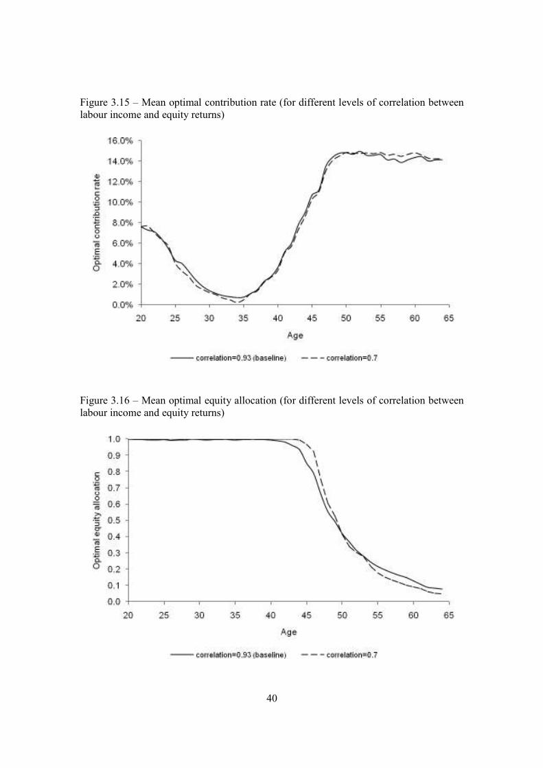
We assume a high correlation of 0.93 in our baseline case. Figures 3.15 and 3.16 show
the outcomes from conducting a sensitivity analysis on this correlation coefficient: we
lowered it to 0.70. The lower correlation coefficient has a negligible effect on the
optimal contribution rate (Figure 3.15), but leads to a later and steeper switch away from
equities (Figure 3.16).
40
Figure 3.15 – Mean optimal contribution rate (for different levels of correlation between
labour income and equity returns)
Figure 3.16 – Mean optimal equity allocation (for different levels of correlation between
labour income and equity returns)

41
3.2.5 Salary growth rate
Finally, Figure 3.17 shows the effect on the mean optimal equity allocation of increasing
the average annual real rate of salary growth, Ir , from 2% to 5%. The optimal equity
weighting is lower at most ages.
Figure 3.17 – Mean optimal equity allocation (different average annual real rate of salary
growth rates)
3.2.6 Annuitisation ratio
Although the annuitisation ratio, k, is part of the budget constraint not the utility function,
it is still a control variable in our model, and is chosen to maximise ( )64E V , conditional
on the values for RAA, EIS and the personal discount factor (see Section 2.1.5 above).
Table 3.2 shows the mean optimal values of k corresponding to different values for RAA,
EIS and the personal discount factors.
42
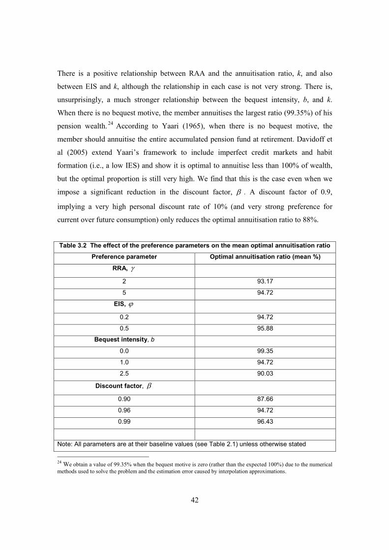
There is a positive relationship between RAA and the annuitisation ratio, k, and also
between EIS and k, although the relationship in each case is not very strong. There is,
unsurprisingly, a much stronger relationship between the bequest intensity, b, and k.
When there is no bequest motive, the member annuitises the largest ratio (99.35%) of his
pension wealth.24
According to Yaari (1965), when there is no bequest motive, the
member should annuitise the entire accumulated pension fund at retirement. Davidoff et
al (2005) extend Yaari’s framework to include imperfect credit markets and habit
formation (i.e., a low IES) and show it is optimal to annuitise less than 100% of wealth,
but the optimal proportion is still very high. We find that this is the case even when we
impose a significant reduction in the discount factor, β . A discount factor of 0.9,
implying a very high personal discount rate of 10% (and very strong preference for
current over future consumption) only reduces the optimal annuitisation ratio to 88%.
Table 3.2 The effect of the preference parameters on the mean optimal annuitisation ratio
Preference parameter Optimal annuitisation ratio (mean %)
RRA, γ
2 93.17
5 94.72
EIS, ϕ
0.2 94.72
0.5 95.88
Bequest intensity, b
0.0 99.35
1.0 94.72
2.5 90.03
Discount factor, β
0.90 87.66
0.96 94.72
0.99 96.43
Note: All parameters are at their baseline values (see Table 2.1) unless otherwise stated
24
We obtain a value of 99.35% when the bequest motive is zero (rather than the expected 100%) due to the numerical
methods used to solve the problem and the estimation error caused by interpolation approximations.

43
4 Conclusion
In this paper, we have examined optimal funding and investment strategies in a DC
pension plan using a life-cycle model that has been extended in three significant ways:
(i) the assumption of Epstein-Zin recursive preferences by the plan member which
enables a separation between the RRA and EIS,
(ii) the introduction of human capital as an asset class along with financial assets,
such as equities and cash, and
(iii) endogenising the decision about how much to annuitise at retirement.
We also considered two important motives for saving: bequest and retirement. In addition,
a plan member’s personal discount rate influenced the optimal strategies.
We found that the optimal funding strategy typically exhibits a U-shaped pattern for the
contribution rate in early working life and then stabilises in the period leading up to
retirement. The initial high level is explained by a high bequest intensity combined with a
high degree of risk aversion. The falling part of the U is explained by the increase in
human capital inducing an increase in consumption at the expense of savings, while the
rising part of the U is explained by the retirement savings motive. A higher personal
discount rate lowers contributions at each age, while preserving the general shape of the
optimal contribution profile. A lower bequest intensity reduces contributions to the
pension plan in early career and in the extreme case of a zero bequest intensity
completely eliminates them until mid-career when the retirement savings motive kicks in.
The effect of lower risk aversion is to delay the start of contributions into the pension
plan: contributions do not begin until late in the working life, but then increase steadily
until the retirement age. The effect of lower EIS is to reduce contributions into the plan at
all ages, since members with low EIS are reluctant to accept cuts in consumption to “pay
for” the pension contributions.

44
We found that the optimal investment strategy is stochastic lifestyling rather than the
more conventional deterministic lifestyling. While the optimal weighting in equities is
initially very high and subsequently declines as the retirement date approaches, it does
not do so in a predetermined manner as in the case of deterministic lifestyling. Instead the
optimal equity weighting over the life cycle depends on the realisations of the stochastic
processes determining labour income and equity returns. Stochastic lifestyling is justified
by recognising the importance of human capital and interpreting it as a bond-like asset
which deteriorates over the working life. An initial high weighting in equities is intended
to counterbalance human capital in the combined “portfolio” of human capital and
pension wealth. In time, the weighting in equities falls, while that in bonds rises as human
capital decays over time. When the correlation between labour income and equity returns
is high, human capital and pension wealth will also be more highly correlated; the
optimal switch away from equities over the life cycle will therefore be later and steeper.
The size of the pension fund is a crucial determinant of the optimal asset allocation. The
greater the pension wealth accumulated, the more conservative the optimal asset
allocation strategy will be, for a given RAA, EIS and discount rate. Also, the higher the
contribution rate, the earlier the switch out of equities can be made. In our model, risk-
tolerant members who value both current consumption over future consumption as
smooth consumption profiles over time (i.e., have a low RRA, a high discount rate and a
low EIS) accumulate the lowest pension wealth levels and therefore need to adopt the
most aggressive investment strategy.
Finally, we found that the optimal annuitisation ratio was typically very high, suggesting
that longevity protection is a hugely valuable feature of a well-defined DC pension plan
to a rational consumer. It was negatively related to the bequest intensity and the discount
rate, but not very sensitive to RRA or EIS.
The results in this paper have some important implications for the optimal design of DC
pension plans:

45
● An investment strategy involving a switch from equities to bonds as members
approach retirement is appropriate for DC pension plans, even when equity
returns are not mean reverting. However, the switch out from equities is not
predetermined, but depends on what happens to equity returns. Nevertheless,
the switch should typically be made earlier than in traditional lifestyle
strategies (i.e., from age 45 or so rather than age 55, which is more common
in practice). Also, the optimal equity weight in the portfolio typically never
reduces to zero (even immediately prior to retirement), as is common in
traditional lifestyle strategies.
● It is very important to incorporate the salary process in the optimal design of a
DC pension plan.25
For most people, their human capital will be bond-like in
nature and this will have a direct impact on the optimal contribution rate and
asset allocation decisions, in particular, justifying a high weight for equities in
the pension plan. However, for senior plan members whose salary levels
(including bonus and dividends from their own stock holdings) may have a
strong link with corporate profitability, their labour income growth rate may
be much higher than the risk-free rate of return and also be more volatile. In
this case, their human capital asset will be more equity-like in nature and so
the optimal investment strategy will be more geared towards the risk-free
asset (as shown in Figure 3.17).
● The results provide some justification for age-related contribution rates in DC
plans. Because members tend to prefer relatively smoothed consumption
growth, a plan design involving a lower contribution rate (e.g., 5% p.a. or less)
when members are young, and a gradually increasing contribution rate as
members get older (reaching on average 15% p.a. in the period prior to
retirement) offers higher expected utility than fixed age-independent
contribution rates. Greater contribution rate flexibility will be especially
welcomed by members with high EIS. Such members are more sensitive to
25 This was first pointed out by Blake et al (2007).

46
changes in financial incentives and thus are more desirous of flexible
contribution rates. If they were allowed to make additional voluntary
contributions (AVCs), the optimal asset allocation strategy would actually
become more conservative as they approach retirement.
● An annuity is an important component of a well-designed plan. The optimal
annuitisation ratio is very high, even when there is a strong bequest motive
and the plan member values current consumption highly. This is true despite
the well-known aversion to annuitisation documented in Friedman and
Warshawsky (1990) and Mitchell et al (1999).

47
References
Banks, James, Richard Blundell, and Sarah Tanner (1998) Is There a Retirement-Savings
Puzzle? American Economic Review, 88, 769-788.
Banks, James and Susann Rohwedder, 2001. “Life-cycle saving patterns and pension
arrangements in the UK”, Research in Economics, 55, 83-107.
Battocchio, Paolo and Francesco Menoncin, 2002. “Optimal pension management under
stochastic interest rate, wages, and inflation”, IRES (Institut de Recherches Economiques
et Sociales) working paper, http://www.ires.ucl.ac.be/DP/IRES_DP/2002-21.pdf.
Bhamra, Harjoat S. and Raman Uppal, 2006. “The role of risk aversion and intertemporal
substitution in dynamic consumption-portfolio choice with recursive utility”, Journal of
Economic Dynamics and Control, 6, 967-991.
Blackburn, Douglas W., 2006. “Option implied risk aversion and elasticity of
intertemporal substitution”, Indiana University working paper.
Blake, David, 1996. “Efficiency, risk aversion and portfolio insurance: An analysis of
financial asset portfolios held by investors in the United Kingdom, Economic Journal,
106, 1175-1192.
Blake, David, Andrew J.G. Cairns and Kevin Dowd, 2001. “PensionMetrics I: Stochastic
pension plan design and value at risk during accumulation phase”, Insurance:
Mathematics and Economics, 29, 187-215.
Blake, David, Andrew J.G. Cairns and Kevin Dowd, 2007. “The impact of occupation
and gender on pensions from defined contribution plans”, Geneva Papers on Risk &
Insurance, 32, 458-82
Boulier, Jean-Francois, Etienne Trussant and Daniele Florens, 1995. “A dynamic model
for pension funds management”, Proceedings of the 5th AFIR International Colloquium, 1,
361-384.
Boulier, Jean-Francois, ShaoJuan Huang and Gregory Taillard, 2001. “Optimal
management under stochastic interest rates: the case of a protected defined contribution
pension fund”, Insurance: Mathematics and Economics, 28, 173-189.
Brandt, Michael W., A. Goyal, P. Santa-Clara and J.R. Stroud, 2005. “A simulation
approach to dynamic portfolio choice with an application to learning about return
predictability”, Review of Financial Studies, 18, 831-874.
Breeden, Douglas T., 1979. “An intertemporal asset pricing model with stochastic
consumption and investment opportunities”,.Journal of Financial Economics, 7, 265-296.

48
Cagetti, Marco, 2003. “Wealth accumulation over the life cycle and precautionary
savings”, Journal of Business and Economic Statistics, 21, 339-353.
Cairns, Andrew J.G., 1994. “An introduction to stochastic pension plan modelling”,
presentation paper of workshop on Interest Rate Risk, Vancouver, 19-20 August, 1994,
http://www.ma.hw.ac.uk/~andrewc/papers/.
Cairns, Andrew J.G., 2000. “Some notes on the dynamics and optimal control of
stochastic pension fund models in continuous time”, Astin Bulletin, 30, 19-55.
Cairns, Andrew J.G, David Blake and Kevin Dowd, 2006. “Stochastic lifestyling:
Optimal dynamic asset allocation for defined contribution pension plans”, Journal of
Economic Dynamics and Control, 30, 843-877.
Campbell, John Y., João F. Cocco, Francisco J. Gomes and Pascal J. Maenhout, 1999.
“Investing retirement wealth: a life-cycle model”, NBER working paper 7029.
Campbell, John Y. and Luis M. Viceira, 2002. Strategic Asset Allocation: Portfolio
Choice for Long-Term Investors, Oxford University Press, Oxford.
Cardinale, M., G. Hatz, J. Kumar and J.M. Orszag, 2005. “Background risk and
pensions”, Sessional meeting, Institute of Actuaries, 28 November 2005,
http://www.actuaries.org.uk/files/pdf/sessional/sm20051128.pdf.
Cocco, João F., Francisco J. Gomes and Pascal J. Maenhout, 2005. “Consumption and
portfolio choice over the life-cycle”, The Review of Financial Studies,18, 491-533.
Constantinides, George, 1990. “Habit formation: A resolution of the equity premium
puzzle”, Journal of Political Economy, 98, 519-43.
Davidoff, Thomas, Brown, Jeffrey R. and Peter A. Diamond (2005) “Annuities and
Individual Welfare”, American Economic Review, 95, 1573-1590.
Deelstra, G., Martino Grasselli and P-F Koehl, 2000. “Optimal investment strategies in a
CIR framework”, Journal of Applied Probability, 37, 936-946.
Duffie, Darrell and Larry G. Epstein, 1992. “Stochastic differential utility”,
Econometrica, 60, 353-394.
Duman, Bernard, Raman Uppal and Tan Wang, 2000. “Efficient intertemporal allocations
with recursive utility”, Journal of Economic Theory, 93, 240-259.
Dynan, Karen, Jonathan Skinner and Stephen Zeldes, 2002. “The importance of bequest
and life-cycle saving in capital accumulation: A new answer”, The American Economic
Review, 92, 274-278.
49
El Karoui, N., S. Peng and M.C. Quenez, 1997. “Backward stochastic differential
equations in finance”, Mathematical Finance, 7, 1-71.
El Karoui, N., S. Peng and M.C. Quenez, 2001. “A dynamic maximum principle for the
optimization of recursive utilities under constraints”, The Annals of Applied Probability,
11, 664-693.
Epstein, L.G. and Stanley Zin, 1989. “Substitution, risk aversion, and the temporal
behavior of consumption and asset returns: A theoretical framework”, Econometrica 57,
937-969.
Epstein, L.G. and Stanley Zin, 1991. “Substitution, risk aversion, and the temporal
behavior of consumption and asset returns: An empirical investigation”, Journal of
Political Economics, 99, 263-286.
Fama, Eugene and Kenneth French (2002) “The equity premium”, Journal of Finance, 57,
637-659.
Friedman, Benjamin and Mark Warshawsky, 1990. “The cost of annuities: Implications
for saving behaviour and bequests”, Quarterly Journal of Economics, 105, 135-154.
Garcia, Philip, Stephen Bridges, David Hargreaves, Hui In Ng and Hemal Popat, 2004.
“Demand for DC products”, Finance and Investment Board Working Party, Institute of
Actuaries
Gomes, Francisco and Alexander Michaelides, 2004. “A human capital explanation for
an asset allocation puzzle”, UBS Pension Series 24, London School of Economics,
http://fmg.lse.ac.uk/pdfs/dp491.pdf
Gomes, Francisco and Alexander Michaelides, 2005. “Optimal life-cycle asset allocation:
Understanding the empirical evidence”, Journal of Finance, 60, 869-904.
GAD, 2006. Occupational Pension Schemes 2005, Government Actuary’s Department,
London.
Haberman, Steven and Elena Vigna, 2002. “Optimal investment strategies and risk
measures in defined contribution pension schemes”, Insurance: Mathematics and
Economics, 31, 35-69.
Hoek, John van der and Michael Sherris, 2001. “A class of non-expected utility risk
measures and implication for asset allocations”, Insurance: Mathematics and Economics,
28, 69-82.
50
Horneff, Wolfram J., Raimond H. Maurer and Michael Z. Stamos, 2006. “Life-cycle
asset allocation with annuity markets: Is longevity insurance a good deal?”, Goethe
University working paper.
Howie, Robert, Helen Davies, 2002. “Setting investment strategy for the long term: A
closer look at defined contribution investment strategy”, Faculty and Institute of
Actuaries, Finance and Investment Conference 2002,
http://www.actuaries.org.uk/files/pdf/library/proceedings/fin_inv/2002/Howie.pdf.
Josa-Fombellida, Ricardo and J.P. Rincon-Zapatero, 2001. “Minimization of risks in
pension funding by means of contributions and portfolio selection”, Insurance:
Mathematics and Economics, 29, 35-45.
Judd, Kenneth L., 1998. Numerical Methods in Economics, The MIT Press, Cambridge
MA.
Kim, Myung Jig , Charles R. Nelson, and Richard Startz, 1991. “Mean reversion in stock
prices? A reappraisal of the empirical evidence”, The Review of Economic Studies, 58,
Special Issue: The Econometrics of Financial Markets, 515-528.
Kreps, David M. and Evan L. Porteus, 1978. “Temporal resolution of uncertainty and
dynamic choice theory”, Econometrica, 46, 185-200.
Lo, Andrew W., and A.Craig Mackinley, 1988. “Stock prices doe not follow random
walks: Evidence from a simple specification test”, Review of Financial Studies, 1, 41-66.
Merton, Robert C., 1969. “Lifetime portfolio selection under uncertainty: The
continuous-time case”, Review of Economics and Statistics, 51, 247-257.
Merton, Robert C., 1971. “Optimum consumption and portfolio rules in a continuous-
time model”, Journal of Economic Theory, 3, 373-413.
Merton, Robert C., 1973. “An intertemporal capital asset pricing model”, Econometrica,
41, 867-887.
Mitchell, Olivia S., James Poterba, Mark Warshawsky, and J. R. Brown, 1999. “New
evidence on the money’s worth of individual annuities”, American Economic Review, 89,
1299-1318.
Annual Survey of Hours and Earnings (ASHE), Office for National Statistics, London,
2005.
Øksendal, Bernt, 1998. Stochastic Differential Equations, 5th
Edition, Springer, Berlin.
Poterba, James M., and Lawrence H. Summers, 1988. “Mean reversion in stock prices:
Evidence and Implications, Journal of Financial Economics, 22, 27-59.

51
Schwartz, Eduardo and Walter N. Torous, 1999. “Can we disentangle risk aversion from
intertemporal substitution in consumption”, Anderson School of Management, University
of California, http://repositories.cdlib.org/anderson/fin/25-99.
Vasiček, O.E., 1977. “An equilibrium characterisation of the term structure”, Journal of
Financial Economics, 5, 177-188.
Viceira, L., 2001. “Optimal portfolio choice for long-horizon investors with nontradable
labor income”, The Journal of Finance, 56, 2, 433-470.
Vigna, Elena and Steven Haberman, 2001. “Optimal investment strategy for defined
contribution pension schemes”, Insurance: Mathematics and Economics, 28, 233-262.
Von Neumann, J. and O. Morgenstern, 1944. Theory of Games and Economic Behavior,
Princeton University Press.
Weil, Philippe, 1989. “The equity-premium puzzle and the risk-free rate puzzle”, Journal
of Monetary Economics, 24, 401-421.
Weil, Philippe, 1990. “Non-expected utility in macroeconomics”, The Quarterly Journal
of Economics, 105, 1, 29-42.
Yaari, M., 1965. “Uncertain lifetime, life insurance and the theory of the consumer”,
Review of Economic Studies, 32, 137-150.
Yen, Simon H. and Yuan-kung Hsu Ku, 2003. “Dynamic asset allocation strategy for
intertemporal pension fund management with time-varying volatility”, Academia
Economic Papers, 31, 229-261.

52
Appendix 1 - Numerical solution for the dynamic programming and
integration process
The Epstein-Zin utility function at time t is as follows:
( ) ( )
11 11 1
1 1
20 11
11
20 20 20 20 20 20 1 201 11
ϕ ϕγ γ
γϕβ βγ
− −
− −+ +
−−
+ + + + + + + +
= − + × + − × × −
t
t t t t t t t
W
bV p C E p V p b
In the last period ( )1,ω ω− , where 1 0ω− =p , the terminal value function is given by:
( )1 1 1
11 1
1 1
1 1
11
1 1 1 200 ,0 1
max1ω ω ω
ϕ ϕγ γ
ω
ϕω ω ωα
βγ− − −
− −
− −
−
− − − +≤ ≤ ≤ ≤
= + × × −
TC W
W
bJ W C E b
The optimisation problem is then:
( )20 20
20, ,
maxα + +
+t t
tC k
E V
subject to the constraints given by:
• ( ) ( )20 1 20 20 20 20 201π α µ ε+ + + + + + + = + × + + + t t t t t tW W Y r , when 0 43≤ ≤t ;
• ( ) ( ) ( )( )65 64 64 64 64 641 1π α µ ε = − × + × + + + W k W Y r , when 44=t ;
• ( )6520 1 20 20 20 20
65
1 α µ ε−
+ + + + + +
× = + − × + + +
ɺɺt t t t t
k WW W C r
a, when 45≥t ;
• 200 1α +≤ ≤t
; and
• 10 ≤≤ k .

53
The Bellman equation is given by:
(a) for 430 ≤≤ t , we have:
( )
( ) ( )20 20
20 20 20
11 1
1 1
1 1
20 11
11
20 20 20 20 20 1 20,
,
max 1 11
ϕ ϕγ γ
γϕ
αβ β
γ+ +
+ + +
− −
− −+ +
−−
+ + + + + + +
= − + × + − × × −
t t
t t t
t
t t t t t tC
J W Y
W
bp C E p J p b
(b) for 44=t , we have:
( )
( ) ( )64 64
64 64 64
11 1
1 1
1 1
651
11
64 64 64 64 65 64, ,
,
max 1 11
ϕ ϕγ γ
γϕ
αβ β
γ
− −
− −
−−
= − + × + − × × −
C k
J W Y
W
bp C E p J p b
(c) and, for 45≥t , we have:
( )
( ) ( )20 20
20 20 20
11 1
1 1
1 1
20 11
11
20 20 20 20 20 1 20,
,
max 1 11
ϕ ϕγ γ
γϕ
αβ β
γ+ +
+ + +
− −
− −+ +
−−
+ + + + + + +
= − + × + − × × −
t t
t t t
t
t t t t t tC
J W Y
W
bp C E p J p b

54
To solve the non-linear expectation part in the Bellman equation above, i.e., ( )1
20 20 1
γ−+ + +t tE J ,
Gauss-Hermite quadrature is used to discretise 1Z and 2Z into 9 nodes, and the procedure
of discretising 1Z and 2Z is to substitute 1,2 mZ and 2,2 nZ for them respectively.
So, we have:
( ) ( )1, 2,
9 9 11 1
20 20 1 20 1 1, 2, 20 1, 20 1
1 1
2 , 2 ;γ
γ π−
− −+ + + + + + + + +
= =
≈ ∑∑ m nt t Z Z t m n t t
m n
E J w w J Z Z W Y
where 1,mZw ,
2,nZw and 1,mZ , 2,nZ are the Gauss-Hermite quadrature weights and nodes,
and π is the mathematical constant.
To avoid choosing a local maximum, we discretise both control variables (i.e.,
consumption and asset allocation) into 20 equally-spaced grids and optimise using a
standard grid search. Wealth and labour income level are discretised in 30 and 10
equally-spaced grids, respectively.
Substituting the expectation with the Gauss-Hermite approximated function in the
Bellman equation at time t , we compute the maximum value function and optimal
variables at each grid point. We then iterate the procedure back to age 20. For a point in
the state space other than grid points, cubic spline interpolation is employed to
approximate the optimal results.

FACULTY OF ACTUARIAL SCIENCE AND INSURANCE
Actuarial Research Papers since 2001
Report Number
Date Publication Title Author
135. February 2001. On the Forecasting of Mortality Reduction Factors.
ISBN 1 901615 56 1
Steven Haberman Arthur E. Renshaw
136. February 2001. Multiple State Models, Simulation and Insurer Insolvency. ISBN 1 901615 57 X
Steve Haberman Zoltan Butt Ben Rickayzen
137.
September 2001
A Cash-Flow Approach to Pension Funding. ISBN 1 901615 58 8
M. Zaki Khorasanee
138.
November 2001
Addendum to “Analytic and Bootstrap Estimates of Prediction Errors in Claims Reserving”. ISBN 1 901615 59 6
Peter D. England
139. November 2001 A Bayesian Generalised Linear Model for the Bornhuetter-Ferguson Method of Claims Reserving. ISBN 1 901615 62 6
Richard J. Verrall
140.
January 2002
Lee-Carter Mortality Forecasting, a Parallel GLM Approach, England and Wales Mortality Projections. ISBN 1 901615 63 4
Arthur E.Renshaw Steven Haberman.
141.
January 2002
Valuation of Guaranteed Annuity Conversion Options. ISBN 1 901615 64 2
Laura Ballotta Steven Haberman
142.
April 2002
Application of Frailty-Based Mortality Models to Insurance Data. ISBN 1 901615 65 0
Zoltan Butt Steven Haberman
143.
Available 2003
Optimal Premium Pricing in Motor Insurance: A Discrete Approximation.
Russell J. Gerrard Celia Glass
144.
December 2002
The Neighbourhood Health Economy. A Systematic Approach to the Examination of Health and Social Risks at Neighbourhood Level. ISBN 1 901615 66 9
Les Mayhew
145.
January 2003
The Fair Valuation Problem of Guaranteed Annuity Options : The Stochastic Mortality Environment Case. ISBN 1 901615 67 7
Laura Ballotta Steven Haberman
146.
February 2003
Modelling and Valuation of Guarantees in With-Profit and Unitised With-Profit Life Insurance Contracts. ISBN 1 901615 68 5
Steven Haberman Laura Ballotta Nan Want
147. March 2003. Optimal Retention Levels, Given the Joint Survival of Cedent and Reinsurer. ISBN 1 901615 69 3
Z. G. Ignatov Z.G., V.Kaishev R.S. Krachunov
148.
March 2003.
Efficient Asset Valuation Methods for Pension Plans. ISBN 1 901615707
M. Iqbal Owadally
149.
March 2003
Pension Funding and the Actuarial Assumption Concerning Investment Returns. ISBN 1 901615 71 5
M. Iqbal Owadally

Report Number
Date Publication Title Author
150.
Available August 2004
Finite time Ruin Probabilities for Continuous Claims Severities
D. Dimitrova Z. Ignatov V. Kaishev
151.
August 2004
Application of Stochastic Methods in the Valuation of Social Security Pension Schemes. ISBN 1 901615 72 3
Subramaniam Iyer
152. October 2003. Guarantees in with-profit and Unitized with profit Life Insurance Contracts; Fair Valuation Problem in Presence of the Default Option1. ISBN 1-901615-73-1
Laura Ballotta Steven Haberman Nan Wang
153.
December 2003
Lee-Carter Mortality Forecasting Incorporating Bivariate Time Series. ISBN 1-901615-75-8
Arthur E. Renshaw Steven Haberman
154. March 2004. Operational Risk with Bayesian Networks Modelling. ISBN 1-901615-76-6
Robert G. Cowell Yuen Y, Khuen Richard J. Verrall
155.
March 2004.
The Income Drawdown Option: Quadratic Loss. ISBN 1 901615 7 4
Russell Gerrard Steven Haberman Bjorn Hojgarrd Elena Vigna
156.
April 2004
An International Comparison of Long-Term Care Arrangements. An Investigation into the Equity, Efficiency and sustainability of the Long-Term Care Systems in Germany, Japan, Sweden, the United Kingdom and the United States. ISBN 1 901615 78 2
Martin Karlsson Les Mayhew Robert Plumb Ben D. Rickayzen
157. June 2004 Alternative Framework for the Fair Valuation of Participating Life Insurance Contracts. ISBN 1 901615-79-0
Laura Ballotta
158.
July 2004.
An Asset Allocation Strategy for a Risk Reserve considering both Risk and Profit. ISBN 1 901615-80-4
Nan Wang
159. December 2004 Upper and Lower Bounds of Present Value Distributions of Life Insurance Contracts with Disability Related Benefits. ISBN 1 901615-83-9
Jaap Spreeuw
160. January 2005 Mortality Reduction Factors Incorporating Cohort Effects. ISBN 1 90161584 7
Arthur E. Renshaw Steven Haberman
161. February 2005 The Management of De-Cumulation Risks in a Defined Contribution Environment. ISBN 1 901615 85 5.
Russell J. Gerrard Steven Haberman Elena Vigna
162. May 2005 The IASB Insurance Project for Life Insurance Contracts: Impart on Reserving Methods and Solvency Requirements. ISBN 1-901615 86 3.
Laura Ballotta Giorgia Esposito Steven Haberman
163. September 2005 Asymptotic and Numerical Analysis of the Optimal Investment Strategy for an Insurer. ISBN 1-901615-88-X
Paul Emms Steven Haberman
164. October 2005. Modelling the Joint Distribution of Competing Risks Survival Times using Copula Functions. I SBN 1-901615-89-8
Vladimir Kaishev Dimitrina S, Dimitrova Steven Haberman
165. November 2005.
Excess of Loss Reinsurance Under Joint Survival Optimality. ISBN1-901615-90-1
Vladimir K. Kaishev Dimitrina S. Dimitrova

Report Number
Date Publication Title Author
166. November 2005.
Lee-Carter Goes Risk-Neutral. An Application to the Italian Annuity Market. ISBN 1-901615-91-X
Enrico Biffis Michel Denuit
167. November 2005 Lee-Carter Mortality Forecasting: Application to the Italian
Population. ISBN 1-901615-93-6
Steven Haberman Maria Russolillo
168. February 2006 The Probationary Period as a Screening Device: Competitive Markets. ISBN 1-901615-95-2
Jaap Spreeuw Martin Karlsson
169.
February 2006
Types of Dependence and Time-dependent Association between Two Lifetimes in Single Parameter Copula Models. ISBN 1-901615-96-0
Jaap Spreeuw
170.
April 2006
Modelling Stochastic Bivariate Mortality ISBN 1-901615-97-9
Elisa Luciano Jaap Spreeuw Elena Vigna.
171. February 2006 Optimal Strategies for Pricing General Insurance.
ISBN 1901615-98-7 Paul Emms Steve Haberman Irene Savoulli
172. February 2006 Dynamic Pricing of General Insurance in a Competitive
Market. ISBN1-901615-99-5 Paul Emms
173. February 2006 Pricing General Insurance with Constraints.
ISBN 1-905752-00-8 Paul Emms
174. May 2006 Investigating the Market Potential for Customised Long
Term Care Insurance Products. ISBN 1-905752-01-6 Martin Karlsson Les Mayhew Ben Rickayzen
175. December 2006 Pricing and Capital Requirements for With Profit
Contracts: Modelling Considerations. ISBN 1-905752-04-0
Laura Ballotta
176. December 2006 Modelling the Fair Value of Annuities Contracts: The Impact of Interest Rate Risk and Mortality Risk. ISBN 1-905752-05-9
Laura Ballotta Giorgia Esposito Steven Haberman
177. December 2006 Using Queuing Theory to Analyse Completion Times in Accident and Emergency Departments in the Light of the Government 4-hour Target. ISBN 978-1-905752-06-5
Les Mayhew David Smith
178. April 2007 In Sickness and in Health? Dynamics of Health and Cohabitation in the United Kingdom. ISBN 978-1-905752-07-2
Martin Karlsson Les Mayhew Ben Rickayzen
179. April 2007 GeD Spline Estimation of Multivariate Archimedean
Copulas. ISBN 978-1-905752-08-9 Dimitrina Dimitrova Vladimir Kaishev Spiridon Penev
180. May 2007 An Analysis of Disability-linked Annuities.
ISBN 978-1-905752-09-6
Ben Rickayzen
181. May 2007 On Simulation-based Approaches to Risk Measurement in Mortality with Specific Reference to Poisson lee-Carter Modelling. ISBN 978-1-905752-10-2
Arthur Renshaw Steven Haberman

Report Number
Date Publication Title Author
182. July 2007 High Dimensional Modelling and Simulation with
Asymmetric Normal Mixtures. ISBN 978-1-905752-11-9 Andreas Tsanakas Andrew Smith
183. August 2007 Intertemporal Dynamic Asset Allocation for Defined
Contribution Pension Schemes. ISBN 978-1-905752-12-6 David Blake Douglas Wright Yumeng Zhang
184. October 2007 To split or not to split: Capital allocation with convex risk
measures. ISBN 978-1-905752-13-3 Andreas Tsanakas
185. April 2008 On Some Mixture Distribution and Their Extreme
Behaviour. ISBN 978-1-905752-14-0 Vladimir Kaishev Jae Hoon Jho
186. October 2008 Optimal Funding and Investment Strategies in Defined
Contribution Pension Plans under Epstein-Zin Utility. ISBN 978-1-905752-15-7
David Blake Douglas Wright Yumeng Zhang
187. May 2008 Mortality Risk and the Valuation of Annuities with
Guaranteed Minimum Death Benefit Options: Application to the Italian Population. ISBN 978-1-905752-16-4
Steven Haberman Gabriella Piscopo
Statistical Research Papers
1. December 1995. Some Results on the Derivatives of Matrix Functions. ISBN
1 874 770 83 2
P. Sebastiani
2. March 1996 Coherent Criteria for Optimal Experimental Design. ISBN 1 874 770 86 7
A.P. Dawid P. Sebastiani
3. March 1996 Maximum Entropy Sampling and Optimal Bayesian Experimental Design. ISBN 1 874 770 87 5
P. Sebastiani H.P. Wynn
4. May 1996 A Note on D-optimal Designs for a Logistic Regression Model. ISBN 1 874 770 92 1
P. Sebastiani R. Settimi
5. August 1996 First-order Optimal Designs for Non Linear Models. ISBN 1 874 770 95 6
P. Sebastiani R. Settimi
6. September 1996 A Business Process Approach to Maintenance: Measurement, Decision and Control. ISBN 1 874 770 96 4
Martin J. Newby
7. September 1996.
Moments and Generating Functions for the Absorption Distribution and its Negative Binomial Analogue. ISBN 1 874 770 97 2
Martin J. Newby
8. November 1996. Mixture Reduction via Predictive Scores. ISBN 1 874 770 98 0 Robert G. Cowell. 9. March 1997. Robust Parameter Learning in Bayesian Networks with
Missing Data. ISBN 1 901615 00 6
P.Sebastiani M. Ramoni
10.
March 1997. Guidelines for Corrective Replacement Based on Low Stochastic Structure Assumptions. ISBN 1 901615 01 4.
M.J. Newby F.P.A. Coolen
11. March 1997 Approximations for the Absorption Distribution and its Negative Binomial Analogue. ISBN 1 901615 02 2
Martin J. Newby
12. June 1997 The Use of Exogenous Knowledge to Learn Bayesian Networks from Incomplete Databases. ISBN 1 901615 10 3
M. Ramoni P. Sebastiani

Report Number
Date Publication Title Author
13. June 1997 Learning Bayesian Networks from Incomplete Databases.
ISBN 1 901615 11 1 M. Ramoni P.Sebastiani
14. June 1997 Risk Based Optimal Designs. ISBN 1 901615 13 8 P.Sebastiani
H.P. Wynn 15. June 1997. Sampling without Replacement in Junction Trees.
ISBN 1 901615 14 6
Robert G. Cowell
16. July 1997 Optimal Overhaul Intervals with Imperfect Inspection and Repair. ISBN 1 901615 15 4
Richard A. Dagg Martin J. Newby
17. October 1997 Bayesian Experimental Design and Shannon Information. ISBN 1 901615 17 0
P. Sebastiani. H.P. Wynn
18. November 1997. A Characterisation of Phase Type Distributions.
ISBN 1 901615 18 9 Linda C. Wolstenholme
19. December 1997 A Comparison of Models for Probability of Detection (POD)
Curves. ISBN 1 901615 21 9
Wolstenholme L.C
20. February 1999. Parameter Learning from Incomplete Data Using Maximum Entropy I: Principles. ISBN 1 901615 37 5
Robert G. Cowell
21. November 1999 Parameter Learning from Incomplete Data Using Maximum Entropy II: Application to Bayesian Networks. ISBN 1 901615 40 5
Robert G. Cowell
22. March 2001 FINEX : Forensic Identification by Network Expert Systems. ISBN 1 901615 60X
Robert G.Cowell
23. March 2001. Wren Learning Bayesian Networks from Data, using Conditional Independence Tests is Equivalant to a Scoring Metric ISBN 1 901615 61 8
Robert G Cowell
24. August 2004 Automatic, Computer Aided Geometric Design of Free-Knot, Regression Splines. ISBN 1-901615-81-2
Vladimir K Kaishev, Dimitrina S.Dimitrova, Steven Haberman Richard J. Verrall
25. December 2004 Identification and Separation of DNA Mixtures Using Peak Area Information. ISBN 1-901615-82-0
R.G.Cowell S.L.Lauritzen J Mortera,
26. November 2005. The Quest for a Donor : Probability Based Methods Offer Help. ISBN 1-90161592-8
P.F.Mostad T. Egeland., R.G. Cowell V. Bosnes Ø. Braaten
27. February 2006 Identification and Separation of DNA Mixtures Using Peak Area Information. (Updated Version of Research Report Number 25). ISBN 1-901615-94-4
R.G.Cowell S.L.Lauritzen J Mortera,
28. October 2006 Geometrically Designed, Variable Knot Regression
Splines : Asymptotics and Inference. ISBN 1-905752-02-4 Vladimir K Kaishev Dimitrina S.Dimitrova Steven Haberman Richard J. Verrall

Report Number
Date Publication Title Author
29. October 2006 Geometrically Designed, Variable Knot Regression
Splines : Variation Diminishing Optimality of Knots. ISBN 1-905752-03-2
Vladimir K Kaishev Dimitrina S.Dimitrova Steven Haberman Richard J. Verrall
30. November 2008 Scheduling Reentrant Jobs on Parallel Machines with a Remote Server. ISBN 978-1-905752-18-8
Konstantin Chakhlevitch Celia Glass
Papers can be downloaded from
http://www.cass.city.ac.uk/arc/actuarialreports.html

Faculty of Actuarial Science and Insurance
Actuarial Research Club
The support of the corporate members
• CGNU Assurance • English Matthews Brockman • Government Actuary’s Department
is gratefully acknowledged.
Copyright 2008 © Faculty of Actuarial Science and Insurance, Cass Business School
106 Bunhill Row, London EC1Y 8TZ.
ISBN 978-1-905752-15-7