The Ethical Implications of an Elite Press - City Research Online
Upload
khangminh22Category
view
0download
0
City, University of London Institutional Repository
Citation: Kham, A.Z. (1996). Frequency estimation of pre-stressed and composite floors. (Unpublished Doctoral thesis, City University London)
This is the accepted version of the paper.
This version of the publication may differ from the final published version.
Permanent repository link: https://openaccess.city.ac.uk/id/eprint/7929/
Link to published version:
Copyright: City Research Online aims to make research outputs of City, University of London available to a wider audience. Copyright and Moral Rights remain with the author(s) and/or copyright holders. URLs from City Research Online may be freely distributed and linked to.
Reuse: Copies of full items can be used for personal research or study, educational, or not-for-profit purposes without prior permission or charge. Provided that the authors, title and full bibliographic details are credited, a hyperlink and/or URL is given for the original metadata page and the content is not changed in any way.
City Research Online: http://openaccess.city.ac.uk/ [email protected]
City Research Online

FREQUENCY ESTIMATION
OFPRE-STRESSED AND COMPOSITE FLOORS
Dissertation
Submitted In Fulfilment Of The Requirement ForThe Degree
Of
Doctor Of Philosophy
By
ARSHAD ZAMAN KHAN
September 1996
CITYUniversity
SCHOOL OF ENGINEERING
Department Of Civil Engineering

CONTENTS
LIST OF TABLES 7
LIST OF FIGURES 9
ACKNOWLEDGEMENTS 12
DECLARATION 13
ABSTRACT 14
PUBLICATIONS 15
Chapter 1 INTRODUCTION 17
1.1 Floor Vibrations 18
1.1.1 Human Perception 19
1.1.2 Fundamental Frequency 20
1.1.3 Floor Damping 21
1.2 Estimating The Fundamental Frequency Of Floors 22
1.2.1 Equivalent Beam Method (EBM) 22
1.2.2 Plate Method (PM) 24
1.2.3 Static Deflection Method (SDM) 26
1.2.4 Concrete Society Method (CSM) 28
1.2.5 Finite Element Method (1-EM) 30
1.3 Objectives 32
1.4 The Scope Of This Thesis 33
1.5 Outline 33
Chapter 2 DYNAMIC TESTING 35
2.1 Modal Analysis 35
2.1.1 Digital Signal Processing 36
2.1.1.1 Sampling and Aliasing 39
2.1.1.2 Leakage 39
2.1.1.3 Windowing 40
2.1.1.4 Averaging 41
2

2.2 Hammer Testing ...................................................................................... 41
2.2.1 Equipment.. ................................................................................. 42
2.2.2 Procedure .................................................................................... 49
2.3 Data Processing ....................................................................................... 50
Chapter 3 EXPERIMENTAL RESULTS 52
3.1 Post-Tensioned Concrete 1-Way Spanning Solid Floor Slabs
WithBeams ...................................... 53
3.1.1 Wycombe Entertainment Centre Multi-Storey Car Park,
Level 1+ 54
3.1.2 Wimbledon Town Hall Development Car Park, Basement-1 56
3.1.3 The Hart Shopping Centre Car Park, Level-1 58
3.1.4 The Exchange Shopping Centre Multi-Storey Car Park,
Level-1 60
3.2 Post-Tensioned Concrete Solid Flat Slab Floors 62
3.2.1 Vantage West Car Park 63
3.2.2 The Hart Shopping Centre Car Park, Level-2 65
3.2.3 Nurdin & Peacock Office 67
3.2.4 Crown Gate Shopping Centre, Chapel Walk, Service Deck 69
3.2.5 St. Martin's Gate Multi-Storey Car Park, Level-4 71
3.2.6 Brindley Drive Multi-Storey Car Park, Level-4 73
3.2.7 Snow Hill Re-Development Livery Street Multi-Storey
Car Park, Level-1B 75
3.2.8 Snow RH Re-Development Livery Street Multi-Storey
Car Park, Level-lA 77
3.2.9 Island Site, Finsbury Pavement, Office, Level-4 (Flexible Panel).79
3.2.10 Island Site, Finsbury Pavement, Office, Level-4 (Stiff Panel) 81
3.2.11 Friars Gate Multi-Storey Car Park, Level-5 83
3.2.12 Tower Street Car Park 85
3.3 Pre-Tensioned Concrete Double-T Beam Floors 87
3.3.1 Trigonos Phase-V Multi-Storey Car Park, Level-6 88
3

3.3.2 Reading Station Re-Development Multi-Storey Car Park,
Level-10 90
3.3.3 Safeway Superstore Car Park 92
3.3.4 Toys R Us Multi-Storey Car Park #4, Level-7 94
3.3.5 Royal Victoria Place Multi-Storey Car Park, Level-3 96
3.4 Composite Steel-Concrete Slab Floors 98
3.4.1 The Millwall Football and Athletics Stadium, Senegal Fields,
West Stand, Hospitality Level 99
3.4.2 Worcester Central Development, Friary Walk Car Park,
Level-2 101
3.4.3 Braywick House Office 103
3.4.4 Premium Products Office 105
3.4.5 Tattersalls Grandstand Windsor Racing Stadium 107
3.4.6 St. George's RC Secondary School Office 109
3.4.7 BRE's Large Building Test Facility, Level-5 111
3.4.8 Guildford High School for Girls, Main Hall 113
Chapter 4 FINITE ELEMENT MODELLING 115
4.1 Post-Tensioned Concrete 1-Way Spanning Solid Floor Slabs
With Beams 116
4.1.1 Single-Panel vs Multi-Panel Models 120
4.1.2 Parametric Studies 128
4.1.2.1 Frequency vs Span/Depth Ratios 129
4.1.2.2 Frequency vs Deflection Relationship 131
4.2 Post-Tensioned Concrete Solid Flat Slab Floors 133
4.2.1 Single-Panel vs Multi-Panel Models 133
4.2.2 Parametric Studies 138
4.2.2.1 Frequency vs Span/Depth Ratios 138
4.2.2.2 Frequency vs Deflection Relationship 141
4.3 Pre-Tensioned Concrete Double-T Beam Floors 143
4.3.1 Single-Beam vs Multi-Beam Models 145
4.3.2 Parametric Studies 149
4
4.3.2.1 Frequency vs Beam Length 149
4.3.2.2 Frequency vs Deflection Relationship 150
4.4 Composite Steel-Concrete Slab Floors 152
4.4.1 Single-Panel Models 153
4.4.2 Parametric Studies 158
4.4.2.1 Frequency vs Slab Thickness 158
4.4.2.2 Frequency vs Deflection Relationship 159
Chapter 5 COMPARISONS 161
5.1 Post-Tensioned Concrete 1-Way Spanning Solid Floor Slabs
With Beams 161
5.1.1 Discussion 163
5.1.2 Equivalent Beam Span Length 164
5.2 Post-Tensioned Concrete Solid Flat Slab Floors 165
5.2.1 Discussion 165
5.2.2 Equivalent Beam Span Length 167
5.3 Pre-Tensioned Concrete Double-T Beam Floors 168
5.3.1 Discussion 168
5.4 Composite Steel-Concrete Slab Floors 169
5.4.1 Discussion 169
Chapter 6 CONCLUSIONS 171
6.1 Conclusions 171
6.1.1 Frequency Estimation Methods 171
6.1.2 Minimum Fundamental Frequency 174
6.1.3 Damping Estimation 175
6.1.4 Span/Depth Ratio and Static Deflections 176
6.1.5 Modified SDOF Formula 178
6.2 Recommendations 179
6.3 Future Research 180
5

REFERENCES AND BIBLIOGRAPHY 181
APPENDICES
AFloor TYPes 188
BTypical Calculations 190
C Typical FE Model Input File 202
6

LIST OF TABLES
Chapter 1
1.1 Design Frequency Limits, Bachmann (1992) 21
1.2 Recommended Damping Values 22
1.3 Variation of 22 with L - -. - , Blevins (1995) 25L
Y
Chapter 4
4.1 FE and Measured Fundamental Frequencies 122
4.2 FE and Measured Fundamental Frequencies 123
4.3 Span/Depth Ratios of the Tested Floors 130
4.4 FE Single Panel Deflections and Constant K 132
4.5 FE and Measured Fundamental Frequencies 133
4.6 Span/Depth Ratios of the Tested Floors 140
4.7 FE Single Panel Deflections and Constant K 142
4.8 Material Properties 144
4.9 FE and Measured Fundamental Frequencies 145
4.10 Proposed Spans for the Tested Floors 150
4.11 FE Single Beam Deflections and Constant K 151
4.12 FE and Measured Fundamental Frequencies 154
4.13 FE Single Panel Deflections and Constant K 160
Chapter 5
5.1 Comparison of Results for Beam and Slab Floors 162
5.2 Comparison of Results for Flat Slab Floors 166
5.3 Comparison of Results for Double-T Beam Floors 168
5.4 Comparison of Results for Composite Floors 170
7

Chapter 6
6.1 Fundamental Frequency Estimates 174
6.2 Damping Estimates 175
6.3 Maximum Span/Depth Ratios for Beam and Slab Floors 176
6.4 Maximum Span/Depth Ratios for Flat Slab Floors 177
6.5 Maximum Static Deflections and Constant K
for Modified SDOF Formula 178
8

LIST OF FIGURES
Chapter 2
2.1 3-D Representation of Vibrations 37
2.2 Transient Time History and Fourier Transform 38
2.3 Aliasing 39
2.4 Leakage 40
2.5 Hanning Window and its Effect on a Periodic Signal 41
2.6 Hammer Details 43
2.7 Time and Frequency Response of a Hammer Impact 44
2.8 Spectra for Various Hammer Tips 45
2.9 Accelerometer Details 47
2.10 Estimating Damping 51
Chapter 3
3.1 Typical Plan Layout and Cross-Section 53
3.2 Typical Transfer Function, Phase and Coherence Function 55
3.3 Typical Transfer Function, Phase and Coherence Function 57
3.4 Typical Transfer Function, Phase and Coherence Function 59
3.5 Typical Transfer Function, Phase and Coherence Function 61
3.6 Typical Plan Layout and Cross-Section 62
3.7 Typical Transfer Function, Phase and Coherence Function 64
3.8 Typical Transfer Function, Phase and Coherence Function 66
3.9 Typical Transfer Function, Phase and Coherence Function 68
3.10 Typical Transfer Function, Phase and Coherence Function 70
3.11 Typical Transfer Function, Phase and Coherence Function 72
3.12 Typical Transfer Function, Phase and Coherence Function 74
3.13 Typical Transfer Function, Phase and Coherence Function 76
9

3.14 Typical Transfer Function and Phase 78
3.15 Typical Transfer Function, Phase and Coherence Function 80
3.16 Typical Transfer Function, Phase and Coherence Function 82
3.17 Typical Transfer Function, Phase and Coherence Function 84
3.18 Typical Transfer Function, Phase and Coherence Function 86
3.19 Typical Plan Layout and Cross-Section 87
3.20 Typical Transfer Function, Phase and Coherence Function 89
3.21 Typical Transfer Function, Phase and Coherence Function 91
3.22 Typical Transfer Function, Phase and Coherence Function 93
3.23 Typical Transfer Function, Phase and Coherence Function 95
3.24 Typical Transfer Function, Phase and Coherence Function 97
3.25 Typical Plan Layout and Cross-Section 98
3.26 Typical Transfer Function, Phase and Coherence Function 100
3.27 Typical Transfer Function, Phase and Coherence Function 102
3.28 Typical Transfer Function, Phase and Coherence Function 104
3.29 Typical Transfer Function, Phase and Coherence Function 106
3.30 Typical Transfer Function, Phase and Coherence Function 108
3.31 Typical Transfer Function, Phase and Coherence Function 110
3.32 Typical Transfer Function, Phase and Coherence Function 112
3.33 Typical Transfer Function, Phase and Coherence Function 114
Chapter 4
4.1 Shell Element 117
4.2 Beam Element 118
4.3 Beam Section Model 118
4.4 Typical Floor Layout 121
4.5 Field vs FE Frequency 123
4.6 A Typical FE 1-Panel Model 125
4.7 A Typical FE 2-Panel Model 126
4.8 A Typical FE 3-Panel Model 127
4.9 Frequency vs Short Span/Depth Ratio 129
10
4.10 Frequency vs Long Span/Depth Ratio 129
4.11 Frequency vs Static Deflections 131
4.12 Field vs FE Frequency 134
4.13 A Typical FE 1-Panel Model 135
4.14 A Typical FE 2-Panel Model 136
4.15 A Typical FE 3-Panel Model 137
4.16 Frequency vs Short Span/Depth Ratio 138
4.17 Frequency vs Long Span/Depth Ratio 139
4.18 Frequency vs Static Deflections 141
4.19 Field vs FE Frequency 146
4.20 A Typical FE 1-Beam Model 147
4.21 A Typical FE 10-Beam Model 148
4.22 Frequency vs Beam Length 149
4.23 Frequency vs Static Deflections 150
4.24 Field vs FE Frequency 155
4.25 A Typical FE 1-Panel Model 156
4.26 A Typical FE 1- Panel Model 157
4.27 Frequency vs Slab Thickness 158
4.28 Frequency vs Static Deflections 159
Chapter 5
5.1 Estimation of Equivalent Span Length for EBM Formula 164
5.2 Estimation of Equivalent Span Length for EBM Formula 167
11

ACKNOWLEDGEMENTS
I believe that nothing is impossible with the will of ALLAH (SWT). Therefore, I only seek HIS will,
nothing more, nothing less, nothing else!
I would like to tender my grateful thanks and appreciations to my supervisor Prof L F Boswell, Head
of the Department, for his generous and continuous support, and guidance throughout the duration
of this research and, in particular, for his assistance in arranging the experimental kit. It has been a
privilege to work with him and I am enormously appreciative of his encouragement, useful
suggestions, criticism, help and advice. It N'as his special interest in my research that made possible
the results achieved and presented in this thesis.
The second most important contribution towards my research has been that of my wife, "Gul". She
has continually supported me throughout, not only morally but also physically by accompanying me
to all the sites and helping me to carry out the experiments. I am extremely indebted to Gul's help
during the experiments, without which the programme would not have been possible. My family
members in PAKISTAN have also shown great patience and perseverance and their prayers have
been of enormous value to me. Special thanks are due to my friend Dr Abdul-Lateef Bello for his
advice and prayers.
I would also like to thank the Ministry of Education of the Government of the Islamic Republic of
PAKISTAN for its financial support through a merit scholarship, award No. F.6-48/88-Sch.III.
Thanks are also due to the following governing bodies and trusts that provided financial assistance
in the later stages of the research:
a) The Committee of the Vice Chancellors and Principals, UK
b) Muslim Aid, UK
c) The Charles Wallace (PAKISTAN) Trust, UK
d) The Sir Ernest Cassel Educational Trust, UK
e) The Sir Richard Stapley Educational Trust, UK
The Leche Trust, UK
g) Corporation of London, UK
Finally, I would like to thank all those who assisted in various ways during my experimental
programme including the owners of all the structures tested. I am particularly thankful to Mr Sami
Khan of Bunyan Meyer & Partners for his useful comments from time to time. Last, but not least, I
am grateful to all my friends and colleagues for their invaluable support.
12

DECLARATION
1. I understand that I am the owner of this thesis and that the copyright rests
with me unless I specifically transfer it to another person.
2. I understand that the University requires that I deposit one copy of my thesis
in the Library where it shall be available for consultation and that photocopies
of it may be made available to those who wish to consult it elsewhere. I
understand that the Library, before allowing the thesis to be consulted either
in the original or in a photocopy, will require each person wishing to consult
it to sign a declaration that he or she recognises that the copyright of the
thesis belongs to me and that no quotation from it and no information derived
from it may be published without my prior written consent. I, therefore, grant
powers of discretion to the University Librarian to allow this thesis to be
copied in whole or in part without further reference to me. This permission
covers only single copies made for study purposes, subject to normal
conditions of acknowledgement.
3. I agree that my thesis shall be available for consultation in accordance with
paragraph 2 above.
Arshad Zaman Khan
2 September 1996
13

ABSTRACT
The modern trends towards economy and the use of high strength materials haveresulted in long spans and slender floors of low frequencies. These frequencies maybe within the range of the first few harmonics of daily life human activities. Thoughthe problem of resonance with walking vibrations, an activity most common on allfloors, is unlikely, high amplitude or persistent vibrations due to these low-levelexcitations may cause alarm to building occupants. There may also be some problemswith the most sensitive equipment. These uncomfortable vibrations are a serviceabilitylimit state problem and can only be avoided by ensuring a high floor fundamentalnatural frequency and damping. There is a need, therefore, for a method to accuratelypredict the fundamental natural frequency and damping of these floors and to ensurethat they are high enough to avoid any resonance or perceptibility problems.
Available analytical formulae for the estimation of fundamental natural frequency arenot directly applicable to actual floors due to various assumptions. The only methodthat may be reliably used for static or dynamic analyses is the finite element methodbecause it can conveniently model the three dimensional nature of structures andaccount for the various boundary conditions and material properties.
The research reported in this thesis consists of measuring fundamental naturalfrequencies and corresponding damping of a range of actual floors. The experimentalfrequencies have then been compared with those results which are based on theanalytical formulae and finite element method. The analytical methods suitable forvarious categories of floors have been identified. A new linear-elastic single panel orbeam finite element model, correlated with the experimental results, has beendeveloped for the accurate estimation of the fundamental natural frequency of thesefloors. The correct boundary conditions for various categories of floors have beenidentified. The single-degree-of-freedom (SDOF) formula for the estimation offundamental natural frequency using static deflections has been modified for thefloors tested. This modified SDOF formula can be used for convenient handcalculations by the consultants and designers who want a quick estimation offundamental natural frequency due to time and cost limitations. The formula may alsobe used to limit static deflections and, therefore, design loads for any choice of aminimum fundamental natural frequency. Also, new limits on span/depth ratios for flatslabs and span limits for double-T beam floors have been suggested. Similarly,minimum fundamental natural frequencies, damping ratios and maximum staticdeflections have been suggested for the floors tested. The single panel or beam modelmay also be used for various parametric studies, both for static and dynamic analyses.
14

PUBLICATIONS
The research reported in this thesis and its applications have been presented andpublished in the following papers at the time of submission:
1. "Predicting Fundamental Natural Frequency of Composite Floors"A Zaman; and L F BoswellJournal of Singapore Structural Steel Society, Vol. 6, No. 1, 1996, pages 37-43.
2. "Frequency Estimation of Long Span Floors"A Zaman; and L F Boswell2nd International Conference on Structural Dynamics Modelling: Test, Analysis,Correlation and Updating, Cumbria (UK), 3-5 July, 1996, pages 129-139.
3. "Review of AcceptabiliG) Criteria for the Vibration of Composite Floors"A Zaman; and L F BoswellInternational Seminar on Structural Assessment: The Role of Large and Full ScaleTesting, London (UK), 1-3 July, 1996, pages 48.1-48.8.
4. "Predicting Fundamental Natural Frequency of Conzposite Floors"A Zaman; and L F BoswellProceedings of the 4th Annual Mechanical Engineering Conference of ISME &2nd International Mechanical Engineering Conference, Shiraz (IRAN), 14-17 May1996, Vol. IV, pages 715-722.
5. "Dynamic Response Testing and Finite Element Modelling of the LBTF Steel-Framed Building Floors"A Zaman; and L F BoswellProceedings of the Second Cardington Conference: Fire, Static and DynamicTests at the Large Building Test Facility at Cardington (UK), 12-14 March 1996.
6. "Dynamic Behaviour of a Composite Beam Before and After Failure"A Zarnan; and L F BoswellOne day Seminar on Composites and Finite Elements in Infrastructure Design andRehabilitation at British Standards Institution in London, 1 November 1995, pages18-21
7 "Using FEM To Predict Floor Vibration Response"A Zaman; and L F BoswellProceedings of the NAFEMS 5th International Conference on Reliability of FiniteElement Methods for Engineering Applications, Amsterdam (TheNETHERLANDS), 10-12 May, 1995, pages 307-318.
15
8. "FE Modelling for Dynamic Analysis of Double-T Prestressed Floors"Arshad ZamanProceedings of StruCoMe 94, Paris (FRANCE), 22-24 November, 1994, pages499-510.
9. "Vibration Criteria for Unbonded Prestressed Concrete Floors"P Waldron; R G Caverson; M S Williams; and A ZamanProceedings of the FIP Symposium: Modern Prestressing Techniques and theirApplications, Kyoto (JAPAN), 17-20 October, 1993, Volume 2, pages 877-884.
10. "Comparison of Finite Element and Field Test Results for the Vibration ofConcrete Floors"M S Williams; A Zaman; P Waldron; and R G CaversonProceedings of the International Conference on Structural Dynamics Modelling:Test, Analysis and Correlation, Cranfield (UK), 7-9 July, 1993, pages 79-88.
16
Chapter 1 INTRODUCTION
The trend towards achieving longer spans with slender slab thicknesses and the use of
high strength steel and concrete to optimise strength and stiffness properties of floor
slabs have led to more economical but rather flexible structures. This has also made
long span floors susceptible to vibration problems from a serviceability point of view
due to everyday human activities. Moreover, it has caused concern that the dynamic
criterion may be of equal importance as the static criterion for design because of the
low floor frequencies and high amplitude vibrations.
It is widely recognised that the most important parameter in effecting a floor vibration
is the natural frequency of the floor. Slender long-span floors have low natural
frequencies (typically less than 10 Hz) and only the first or fundamental mode affects
the human perception of floor motion and thus serviceability. It is extremely
important to estimate this frequency as accurately as possible and to design the floor
for a fundamental natural frequency (hereafter called fundamental frequency) higher
than the lowest excitation frequency (for example, walking) to avoid any resonance
conditions or objectionable vibrations.
This Chapter examines the importance of floor vibrations and summarises the various
methods most commonly used for the estimation of the fundamental frequency of floors.
The aims and scope of the research are defined towards the end of the Chapter together
with an outline of the thesis.
17

1.1 Floor Vibrations
Long-span floor slabs are being used increasingly for office buildings and car parks for
reasons of economy, lower floor heights, and fast construction etc. These floors can be
either post-tensioned concrete: solid flat slabs with or without drop panels, 1-way
spanning solid slabs with beams, ribbed, or waffle; pre-tensioned concrete: double-T
beams; or composite steel-concrete slabs comprising of profiled steel decking (or sheeting)
as the permanent formwork to the underside of concrete slabs spanning between support
beams.
Post-tensioned concrete floors allow higher span/depth ratios whereas pre-tensioned
double-T beams allow longer spans. The major advantage of composite slab floors over
precast or in-situ concrete construction is the reduced construction period. Moreover,
steel decking is easy to handle, can be cut to length and is less susceptible to tolerance
problems. The shear connectors can be welded or fixed through the decking and the
attachments/openings for services can be easily made.
The use of slender sections due to improved methods of construction and design has,
however, produced floors which may be susceptible to vibrations. Low amplitude
vibration problems in long-span and light-weight composite floors have been encountered
and studied in recent years, Wyatt (1989). These vibrations are important at the
serviceability limit state only. They range from an uncomfortable environment or
annoyance for building occupants due to low amplitude excitations caused by a human
footfall or to the large amplitude vibrations caused by rhythmic group activities (i.e. high
floor accelerations or deflections). The serviceability limit state should, therefore, be
an important consideration in floor design.
Since there is a lack of experimental data on the dynamic behaviour of long-span
floors, their advantages, therefore, may be overshadowed if inadequate attention is given
to their dynamic serviceability and their vibrational behaviour is not properly
understood and taken into account at the design stage.
18
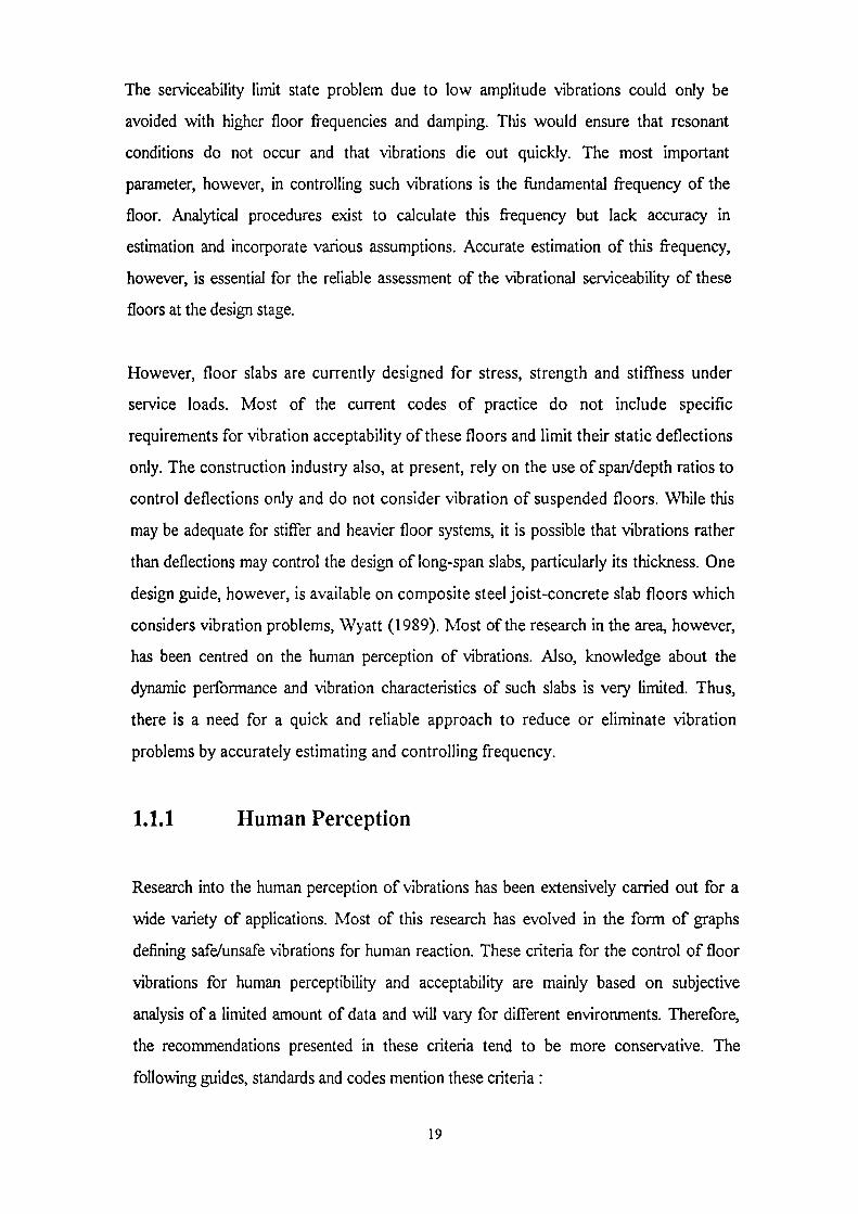
The serviceability limit state problem due to low amplitude vibrations could only be
avoided with higher floor frequencies and damping. This would ensure that resonant
conditions do not occur and that vibrations die out quickly. The most important
parameter, however, in controlling such vibrations is the fundamental frequency of the
floor. Analytical procedures exist to calculate this frequency but lack accuracy in
estimation and incorporate various assumptions. Accurate estimation of this frequency,
however, is essential for the reliable assessment of the vibrational serviceability of these
floors at the design stage.
However, floor slabs are currently designed for stress, strength and stiffness under
service loads. Most of the current codes of practice do not include specific
requirements for vibration acceptability of these floors and limit their static deflections
only. The construction industry also, at present, rely on the use of span/depth ratios to
control deflections only and do not consider vibration of suspended floors. While this
may be adequate for stiffer and heavier floor systems, it is possible that vibrations rather
than deflections may control the design of long-span slabs, particularly its thickness. One
design guide, however, is available on composite steel joist-concrete slab floors which
considers vibration problems, Wyatt (1989). Most of the research in the area, however,
has been centred on the human perception of vibrations. Also, knowledge about the
dynamic performance and vibration characteristics of such slabs is very limited. Thus,
there is a need for a quick and reliable approach to reduce or eliminate vibration
problems by accurately estimating and controlling frequency.
1.1.1 Human Perception
Research into the human perception of vibrations has been extensively carried out for a
wide variety of applications. Most of this research has evolved in the form of graphs
defining safe/unsafe vibrations for human reaction. These criteria for the control of floor
vibrations for human perceptibility and acceptability are mainly based on subjective
analysis of a limited amount of data and will vary for different environments. Therefore,
the recommendations presented in these criteria tend to be more conservative. The
following guides, standards and codes mention these criteria :
19
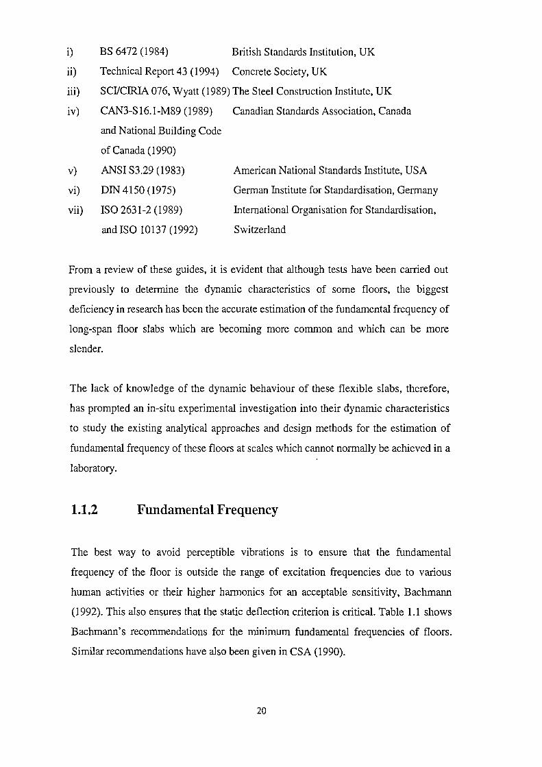
i) BS 6472 (1984) British Standards Institution, UK
ii) Technical Report 43 (1994) Concrete Society, UK
iii) SCl/CIRIA 076, Wyatt (1989) The Steel Construction Institute, UK
iv) CAN3-S16.1-M89 (1989) Canadian Standards Association, Canada
and National Building Code
of Canada (1990)
v) ANSI S3.29 (1983) American National Standards Institute, USA
vi) DIN 4150 (1975) German Institute for Standardisation, Germany
vii) ISO 2631-2 (1989) International Organisation for Standardisation,
and ISO 10137 (1992) Switzerland
From a review of these guides, it is evident that although tests have been carried out
previously to determine the dynamic characteristics of some floors, the biggest
deficiency in research has been the accurate estimation of the fundamental frequency of
long-span floor slabs which are becoming more common and which can be more
slender.
The lack of knowledge of the dynamic behaviour of these flexible slabs, therefore,
has prompted an in-situ experimental investigation into their dynamic characteristics
to study the existing analytical approaches and design methods for the estimation of
fundamental frequency of these floors at scales which cannot normally be achieved in a
laboratory.
1.1.2 Fundamental Frequency
The best way to avoid perceptible vibrations is to ensure that the fundamental
frequency of the floor is outside the range of excitation frequencies due to various
human activities or their higher harmonics for an acceptable sensitivity, Bachmann
(1992). This also ensures that the static deflection criterion is critical. Table 1.1 shows
Bachmann's recommendations for the minimum fundamental frequencies of floors.
Similar recommendations have also been given in CSA (1990).
20

Table 1.1:
Design Frequency Limits, Bachmann (1992)
Type of Structure Minimum Frequency (Hz)
Office Buildings 4.8 (Damping > 5%)
7.2 (Damping < 5%)
Gymnasia and Sports Halls:
Reinforced Concrete 7.5
Prestressed Concrete 8.0
Composite Steel-Concrete 8.5
Dancing and Concert Halls
(Without Fixed Seating):
Reinforced Concrete 6.5
Prestressed Concrete 7.0
Composite Steel-Concrete 7.5
Concert Halls, Theatres and
Spectator Galleries
(With Fixed Seating):
Classical or Soft Pop Music 3.4
Hard Pop Music 6.5
1.1.3 Floor Damping
Damping can arise from any structural or non-structural component and is, therefore,
extremely hard to predict theoretically. The above guides and recommendations are,
therefore, based on experience, observations and some measurements. Table 1.2 shows
these recommendations. A fair engineering judgement is required at the design stage to
allow for reasonable damping to control small vibrations.
21
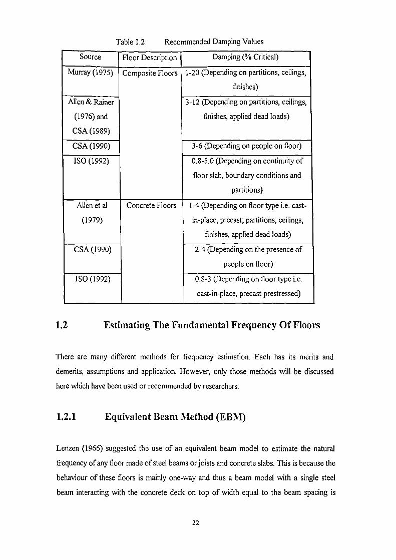
Table 1.2: Recommended Damping Values
Source Floor Description Damping (% Critical)_
Murray (1975) Composite Floors 1-20 (Depending on partitions, ceilings,
finishes)
Allen & Rainer
(1976) and
CSA (1989)
3-12 (Depending on partitions, ceilings,
finishes, applied dead loads)
CSA (1990) 3-6 (Depending on people on floor)
ISO (1992) 0.8-5.0 (Depending on continuity of
floor slab, boundary conditions and
partitions)
Allen et al
(1979)
Concrete Floors 1-4 (Depending on floor type i.e. cast-
in-place, precast; partitions, ceilings,
finishes, applied dead loads)
CSA (1990) 2-4 (Depending on the presence of
people on floor)
ISO (1992) 0.8-3 (Depending on floor type i.e.
cast-in-place, precast prestressed)
1.2 Estimating The Fundamental Frequency Of Floors
There are many different methods for frequency estimation. Each has its merits and
demerits, assumptions and application. However, only those methods will be discussed
here which have been used or recommended by researchers.
1.2.1 Equivalent Beam Method (EBM)
Lenzen (1966) suggested the use of an equivalent beam model to estimate the natural
frequency of any floor made of steel beams or joists and concrete slabs. This is because the
behaviour of these floors is mainly one-way and thus a beam model with a single steel
beam interacting with the concrete deck on top of width equal to the beam spacing is
22

considered to closely approximate the floor fundamental frequency using the following
equation, Blevins (1995):
f _ 22 1 Elj '
1
27r m L4
where A --- fundamental frequency of the floor;
A = it for a simply supported beam, Blevins (1995);
A, --- 4.73 for a fixed-ended beam, Blevins (1995);
El = flexural rigidity of the floor;
L = floor span;
m = mass/length of the floor = pA ;
P = density of the floor material;
A = area of cross-section of the floor.
Allen (1974) clarified that the above equation is particularly applicable for rigid support
conditions and extended the method to flexible support conditions by suggesting the use
of Dunkerly's Principle, Inman (1994), for each floor component as follows:
1_ 1 1j.1 2 — fc2, + f 2c2 ±
where fi = fundamental frequency of the total floor system;
f„ = first floor component frequency;
f, = second floor component frequency and so on.
Allen and Rainer (1976), Allen et al (1985), CSA (1989), Murray (1975), Pernica and
Allen (1982) have all applied this approach for estimating the fundamental frequency of
composite floors. Allen et al (1979) applied this formula to two concrete floors and noted
that the application of the formula is straightforward for simply supported precast T-
beams. For cast-in-place beam and slab systems, they used the formula based on an
(1.2)
23

assumed simply supported T-section and found that the assumption of simple supports
generally under-estimated the frequency. The British Standards Institution (BS8110:1985)
recommends a width of 0.75L— for the flange of this T-section where L is the beam span5
length. The width of beam, however, is not included in this assumption and, therefore,
should be added to this value for calculation purposes. For composite floors, Wyatt
(1989) suggested the effective width of slab to be the smaller of either —L
or beam4
spacing. Allen-Murray (1993), on the other hand, suggest the smaller of 0.4 L or
beam spacing.
Composite floor slabs with steel decking can normally be regarded as continuous and
resting over the supporting floor beams for dynamic analysis. The section properties
are, therefore, based on a transformed moment of inertia. This assumption is applied
even if the slab is not structurally connected to the beam flange, since the magnitude
of the impacts are not sufficient to overcome the friction force between the elements.
For the case of a girder supporting beams, it has been found that the beam seats are
sufficiently stiff to transfer the shear. Thus, a transformed moment of inertia
assumption can be used for the girder as well. But this will result in higher frequencies
than those obtained using the girder moment of inertia only assuming the beams as
point loads. However, there is no agreement on whether the beam supporting slab is
to be used for the system frequency or the girder supporting beams. Normally, the
smaller frequency will be assumed to be critical.
1.2.2 Plate Method (PM)
The fundamental frequency (f) of a rectangular plate having plan dimensions Lx and L.),
(Lx � 4) and thickness h is given by Blevins (1995) as:
A? I Eh' A - 27rL2x \I 12P(1– v2)
(1.3)
24

L2where 1 r 1+ —2- for a plate simply supported at its edges, Blevins (1995);
E = Young's modulus of elasticity;
p= density of the material of the plate;
v = Poisson's ratio.
For the case of a plate simply supported only at its corners, 2 can be obtained from Table
1.3 below.
Table 1.3:L
Variation of 22 with , Blevins (1995)Ly
L,
Ly
22
1.0 7.12
1.5 8.92
2.0 9.29
2.5 9.39
From Table 1.3, the variation of 22 with can be approximated by the following thirdL y
order polynomial equation (using trendline or least-squares curve-fitting):
22 1.5467 -L-'-[ Ly
3 ( ) 2
9.82— -L- + 20.803 L —5.41Ly
(1.4)Ly
Although most two-way floor systems can not be idealised as simply supported at their
edges or corners, it can be reasonably assumed that the displacements along column lines
are negligible in the first mode of vibration. This assumption, however, is only valid for
continuous floors with similar span dimensions in both directions.
25
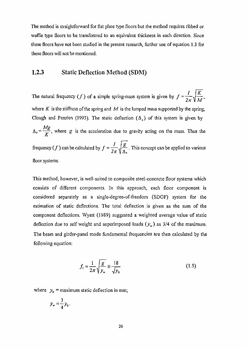
The method is straightforward for flat plate type floors but the method requires ribbed or
waffle type floors to be transformed to an equivalent thickness in each direction. Since
these floors have not been studied in the present research, further use of equation 1.3 for
these floors will not be mentioned.
1.2.3 Static Deflection Method (SDM)
1The naturalnatural frequency (f ) of a simple spring-mass system is given by f =— —
27r M '
where K is the stiffness of the spring and M is the lumped mass supported by the spring,
Clough and Penzien (1993). The static deflection (A s ) of this system is given by
MgA s = —K where g is the acceleration due to gravity acting on the mass. Thus the
1 igfrequency (f ) can be calculated by f =-27r —
A, . This concept can be applied to various
floor systems.
This method, however, is well-suited to composite steel-concrete floor systems which
consists of different components. In this approach, each floor component is
considered separately as a single-degree-of-freedom (SDOF) system for the
estimation of static deflections. The total deflection is given as the sum of the
component deflections. Wyatt (1989) suggested a weighted average value of static
deflection due to self weight and superimposed loads (y.) as 3/4 of the maximum.
The beam and girder-panel mode fundamental frequencies are then calculated by the
following equation:
r _ 1 lig _ 18
j1 — 2ir y., — Ify-;
where yo = maximum static deflection in mm;
3Y. = —4 Yo -
(1.5)
26

The system frequency is then assumed to be the lowest of the two modes calculated.
Other details are given in the design guide by The Steel Construction Institute, Wyatt
(1989).
Allen-Murray (1993) used the following formula for the fundamental frequency of the
beam and girder-panel modes for composite steel-concrete floor systems:
f, = 0.18j-f- (1.6)A,
where g = 9806.65 mm/sec2;
A, = static deflection of beam or girder in mm.
They also considered the critical mode to be the one with lowest frequency. However,
they suggested to calculate a combined mode if the beam span (Lb ) is less than 1/2
the girder span (Li ). For this mode the static deflections of both the beam and girder-
panel modes are added together before using equation 1.6. They assumed beams and
girders as simply supported for the purposes of estimating their deflections and the
modulus of elasticity of concrete as 1.35 times higher than the calculated value to
account for the increase in stiffness under dynamic loading.
For the combined mode, an effective beam-panel width (Bb ) should be determined
from equation 1.7 below and it should be less than 2j 4„fal , where Lt„,a is the total
floor length perpendicular to the beam
1
D) 4Bb = 2 (-- 4,
Db(1.7)
27

(1.8)
where D, is the slab rigidity given by IlL (Is is the slab moment of inertia per unit length
and n is the modular ratio) and Db is the beam rigidity given by ( lb is thespacing
beam moment of inertia and spacing is the distance between the centres of the
beams).
If the total floor length is less than the effective beam-panel width, the combined mode is
restricted and the system is effectively stiffened. This can be accounted for by reducing the
girder deflections ( A s ) to Sg as below:
Lswhere 0.5 <1.0.
Bb
Since it is very difficult to calculate deflections of two-way slab systems, this method can
be best used in conjunction with the Finite Element Method where static deflections of the
model can be closely approximated.
1.2.4 Concrete Society Method (CSM)
The Concrete Society (1994) has proposed the following formulae (Equations 1.9 - 1.13)
to calculate the natural frequency of a two-way slab in the x -direction; the characteristics
of the y -direction mode are determined by interchanging the x and y subscripts in these
equations. This approach assumes two independent orthogonal modes in the two span
directions and takes into account the effects of perimeter beams, the difference in stiffness
in the two orthogonal directions and the type of slab. The method yields two natural
frequencies corresponding to the two span directions.
28

It may be mentioned here that CSM determines the dynamic response of the fundamental
mode which is then multiplied by a factor to give the total dynamic response. However,
the method is based on EBM and there is no evidence of its validation against any
experimental data or other methods.
In the following equations, nx is the number of bays in the x -direction, each of span 4,
and ny is the number of bays in the y-direction, each of span L. The flexural stifthesses
of the slab spanning in the two directions are EI x and EI y respectively and m is the mass
per unit area. Equations for solid slabs will be given here; for others see the design
handbook on post-tensioned concrete floors, Concrete Society (1994).
Slabs with Perimeter Beams
The effective aspect ratio (A s ) of a slab panel is defined as:
nxL., y) 4
x Ly
This, in turn, is used to calculate a modification factor (k x ) given by:
k x = 1+7.2x (1.10)
The natural frequency of the slab with perimeter beams (f) is then given by:
fl = kx2E IEI.v
x rn
Slabs without Perimeter Beams
For slabs without perimeter beams the frequency given by equation 1.11 is modified by the
calculation of a frequency fb given by:
(1.9)
29

(1.12)
fic= f;—Cf.;— fb) (1.13)
The natural frequency of the slab without perimeter beams (fx ) is then given by:
1.2.5 Finite Element Method (FEM)
The finite element (FE) method was first developed in 1956. It is a powerful numerical
technique that uses variational and interpolation methods for modelling and solving
boundary value problems. The method is extremely useful for structures with unusual
geometric shapes.
A structure is made up of different members connected together. The FE method consists
of dividing each member of the structure into a finite number of elements of predictable
behaviour. Since the actual variation of the field variable (e.g. displacement, stress,
temperature, pressure, or velocity etc.) inside the continuum is not known, the variation
inside each element is assumed to be approximated by a simple function. These
approximating functions are defined in terms of the values of the unknown field variables
at the element nodes. The field equations for the whole continuum are then brought
together in an assembly procedure, resulting in global mass and stiffness matrices, which
describe the motion of the structure as a whole. Full details of the method are beyond the
scope of this thesis, see Zienkiewicz (1981).
The FE method is systematic and modular and may be implemented on a computer to
solve a wide range of practical vibration problems simply by changing the input to a
30

computer program. The method is capable of analysing higher modes of vibration and can
model complex geometries with varying boundary conditions. Several large established
commercial FE codes are available. However, the FE modelling of the floors in this
thesis was carried out by I-DEAS and ANSYS structural dynamic analysis packages.
The FE method provides improved accuracy in calculating the natural frequencies of
floors if the geometry and boundary conditions are correctly modelled. The degree of
refinement in results is, therefore, superior to the methods which have been discussed
previously. However, modelling the correct stiffness for all elements (geometry,
density and modulii of elasticity) and boundary conditions (joint and support
continuity) require experience and extensive modelling. Various models need to be
studied if a higher order of accuracy is desired. Due consideration should be given to
the small magnitude of dynamic deflections.
The FE method also allows sensitivity studies once the model is correlated with the
experimental results. The most common method of comparing frequencies of experimental
and analytical models is to plot them against each other. This plot should be a straight line
of slope ± 1 for perfectly correlated data. Any deviation suggests errors in material
properties, element type or boundary conditions. Therefore, several models need to be
studied before arriving at a reasonable correlation. The method also allows estimation of
static deflections and, therefore, frequency estimation using the static deflection approach.
The FE method is based on some assumptions (e.g. shape functions etc.) and
approximations (e.g. geometry and material properties). The FE modelling and analysis
may also be expensive and time consuming. Therefore, the FE results are not expected to
correlate exactly with the experimental results and for all practical purposes a reasonable
error is widely accepted by engineers.
This method has been previously successfully used for the validation of experimental
frequencies of a composite floor, Osborne and Ellis (1990). However, details on modelling
were not given because it was undertaken by a consultancy firm. Maguire and Severn
(1987) have used this method for frequency estimation of a chimney, two water tanks and
31

four bridge beams. They found good correlation of their FE results with their experimental
results. Gardner-Morse and Huston (1993) used this method for comparing their
experimental frequencies of a pedestrian bridge and found good correlation. More
recently, Chen and Aswad (1994) used this method to study the vibration of precast
double-T floors. However, they did not carry out any field measurements and only used
various loading functions in their study.
It has been established, therefore, that FEM can be successfully used for frequency
estimation of prototype structures. However, it has not been used for the estimation of
frequency of concrete floors. Moreover, the biggest uncertainty in the use of this method
for concrete and composite floors is the correct material properties. Therefore, this
method has been extensively studied in the present research to explore the possibility of
estimating fundamental frequency of floors using a very simple model and to study the
effect of various parameters on this frequency.
1.3 Objectives
The research carried out consisted of in-situ dynamic monitoring of 29 long-span floor
slabs of different structural configurations with the following objectives:
i) to examine the importance of vibrations in the design of long-span floor slabs;
ii) to determine experimentally the dynamic characteristics of these floors;
iii) to compare and evaluate the existing design guides and the most commonly used
analytical approaches for the calculation of fundamental frequency of floor slabs
and to identify the most appropriate method for the estimation of the fundamental
frequency of these floors;
iv) to study the use of the finite element method for frequency estimation of floors
and to develop an "accurate" model correlated against experimental results;
v) to carry out a parametric/sensitivity study of the FE-models in order to limit the
static deflections and span/depth ratios of long-span floors.
32

1.4 The Scope Of This Thesis
The research is limited to the fimdamental frequency estimation of the following structural
configurations of long-span suspended floor slabs:
i) Post-Tensioned Concrete 1-Way Spanning Solid Floor Slabs With Beams;
ii) Post-Tensioned Concrete Solid Flat Slab Floors;
iii) Pre-Tensioned Concrete Double-T Beam Floors;
iv) Composite Steel-Concrete Slab Floors.
Other types of floors (waffle, ribbed etc.) have not been included because they could not
be tested in a reasonable number to obtain reliable conclusions.
The dynamic testing is carried out under serviceability conditions and only the vertical
modes of vibrations are considered. The floors are assumed linear and elastic (due to small
deflections and low floor frequencies caused by everyday normal activities).
1.5 Outline
Chapter 2 presents a description of the dynamic testing and data analysis procedures. A
brief review of Modal Analysis is presented which is relevant to the present research. The
testing equipment is described along with various precautions and requirements.
Chapter 3 presents and discusses the results of all the field tests. Typical experimental
graphs (inertance transfer fimction, corresponding phase diagram and coherence function
plots) are given.
Chapter 4 discusses the use of Finite Element (FE) modelling and analyses for the
vibrations of long-span floor slabs. Results of various models are also compared for each
floor tested. Details of a parametric/sensitivity study of the FE models is also given.
33

Various plots (fundamental frequency versus span/depth ratios, span lengths and static
deflections) are presented which have been obtained from the results of the FE models.
Chapter 5 presents the comparison of experimental results with those obtained through the
various analytical methods discussed in Chapter 1 and Chapter 4.
Chapter 6 presents the conclusions and recommendations based on the research. Guidance
is provided by presenting the use of the various plots previously discussed in Chapter 4.
Suggestions for furthering the research are given at the end of the chapter.
A detailed list of references has been provided. Two appendices are added to provide
isometric sketches of the floor types tested with typical dimensions and calculations for
frequency estimation for one floor in each category.
34

Chapter 2 DYNAMIC TESTING
This Chapter presents the method of vibration measurement used for obtaining
experimental results for the floors tested. A brief review of the relevant parts of modal
analysis which have been used in the research is presented along with the data analysis
procedure.
2.1 Modal Analysis
This is a technique to determine experimentally the dynamic characteristics of structures.
Of major interest in the present research is the fundamental frequency of floors which is
extremely important in predicting and understanding their dynamic behaviour. Full details
of the method are beyond the scope of this thesis and, therefore, only the important and
relevant details will be briefly discussed here. For details, see Ewins (1995).
The main procedure is to excite the structure by means of an impulse hammer to measure
the input force and use an accelerometer to measure the resulting vibration response. The
force and acceleration signals are then Fourier transformed into frequency domain
functions, from which the frequency response functions (also called transfer functions) are
established. The modal parameters: which are the natural frequencies and damping ratios,
can then be estimated by curve-fitting.
The fundamental idea behind modal testing is that of resonance. If a structure is excited at
resonance, its response exhibits two distinct phenomena:
a) As the driving frequency approaches the natural frequency of the structure, the
amplitude at resonance rapidly approaches a sharp maximum value;
b) The phase of response shifts by 1800 as the frequency sweeps through resonance,
with the value of the phase at resonance being 90°.
35

(2.2)
(2.3)
(2.4)
These physical phenomena are used to determine the natural frequency of the structure
from measurements of the magnitude and phase of the structure's forced response.
Understanding modal testing requires knowledge of several areas. These include
instrumentation, signal processing, parameter estimation and vibration analysis. It is
important to understand some details of the signal processing performed by the spectrum
analyser in order to carry out valid experiments. These are presented below.
2.1.1 Digital Signal Processing
A periodic time signal or fimction x(t) of period T can be represented by an infinite
Fourier series of sinusoids of the form given by:
x(1) =a +E (a „cosnco r t +b „sin na )74)2 „=,
2/rwhere coT = and the Fourier or spectral coefficients ao , a„ and b„ are defined by: T
a° =-1F(t)di T o
2 Tra „ =— j F (t) cos nor tdt
T 0
b„ = —2 1F (t) sin 'icor tdtT 0
The spectral coefficients represent frequency-domain information about a given time
signal. These coefficients also represent the connection between Fourier analysis and
vibration experiments.
(2.1)
36

Frequency
-n-,'Time 1-Estory Analysis
Spectral Analysis
Figure 2.1 shows a 3-D graph illustrating the addition of sine waves to give a composite
waveform. Two of the axes are time and amplitude and the third is a frequency axis. These
different views along the time domain (time history) and frequency domain (frequency
response spectrum) allow for the visual separation of the individual components of the
waveform.
Vibration Amplitude
Time
-0a.....
...:Time Domain View
A A A
Frequency Domain View
Figure 2.1: 3-D Representation of Vibrations
The analysis done in modal testing is performed in the frequency domain, inside the
analyser. The analyser converts the analogue time-domain signal into digital frequency-
domain signals and then performs the required computations with these signals. The
method used to do this is called fast Fourier transform (FFT) which is essentially the
Fourier series analysis explained above.
37
Transient Time History
)1.— Fourier Transform
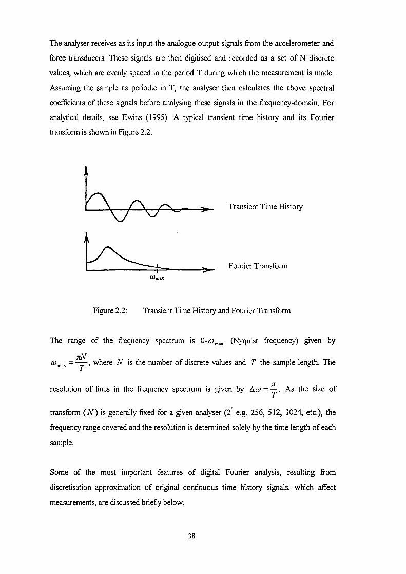
The analyser receives as its input the analogue output signals from the accelerometer and
force transducers. These signals are then digitised and recorded as a set of N discrete
values, which are evenly spaced in the period T during which the measurement is made.
Assuming the sample as periodic in T, the analyser then calculates the above spectral
coefficients of these signals before analysing these signals in the frequency-domain. For
analytical details, see Ewins (1995). A typical transient time history and its Fourier
transform is shown in Figure 2.2.
Figure 2.2: Transient Time History and Fourier Transform
The range of the frequency spectrum is 0- co n.,,,,, (Nyquist frequency) given by
rrNc o ." = — , where N is the number of discrete values and T the sample length. The
T
irresolution of lines in the frequency spectrum is given by Act) = —
T. As the size of
transform (N) is generally fixed for a given analyser (2n e.g. 256, 512, 1024, etc.), the
frequency range covered and the resolution is determined solely by the time length of each
sample.
Some of the most important features of digital Fourier analysis, resulting from
discretisation approximation of original continuous time history signals, which affect
measurements, are discussed briefly below.
38

2.1.1.1 Sampling And Aliasing
The signals are sampled at different equally spaced time intervals to produce a digital
record in the form of N set of numbers. Improper sampling time may cause an error called
aliasing when calculating digital Fourier transforms. Aliasing is the misrepresentation of
the analogue signal by the digital record. Thus, if the sampling rate is too slow, the digital
representation will cause high frequencies to appear as low frequencies (Figure 2.3). This
can be avoided by subjecting the analogue signal to an anti-aliasing filter which allows low
frequencies through, by maintaining a reasonably small sampling interval. A reasonable
sampling rate is two times the highest frequency of interest.
!Signal
Ali • A.. 11, •
ample Instant
Alias Frequency
Figure 2.3: Aliasing
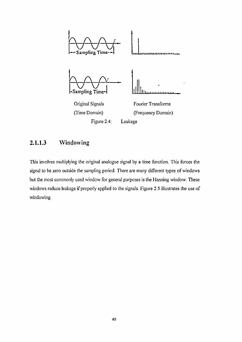
2.1.1.2 Leakage
The digital analysis is feasible only if the periodic signal is sampled over a finite time. The
digital Fourier transform of finite length signals assumes that the signal is periodic within
the sample record length. Thus the actual frequency leaks into a number of fictitious
frequencies because a complicated signal containing many different frequencies cannot
simply be cut at an integral multiple of its period. Leakage can be corrected by the use of a
window function. Figure 2.4 illustrates this phenomenon.
Time
39
1
'
bci_)scA7...
Sampling Time—1
Sampling Time.-!
Original Signals Fourier Transforms
(Time Domain) (Frequency Domain)
Figure 2.4: Leakage
2.1.1.3 Windowing
This involves multiplying the original analogue signal by a time function. This forces the
signal to be zero outside the sampling period. There are many different types of windows
but the most commonly used window for general purposes is the Harming window. These
windows reduce leakage if properly applied to the signals. Figure 2.5 illustrates the use of
windowing.
40

Raw Signal
Hanning Window
H°°-1---
Windowed Signal
1.1
Fourier Transform of Windowed Signal
Figure 2.5: Hanning Window and its Effect on a Periodic Signal
2.1.1.4 Averaging
It is necessary to perform an averaging process, involving several individual time records
or samples before a result is obtained which can be used with confidence. The two major
considerations which determine the number of averages required are the statistical
reliability and the removal of spurious random noise from the signals.
2.2 Hammer Testing
In this type of dynamic testing, the floor slabs are excited by an instrumented hammer with
a force transducer and the response is measured with an accelerometer. A spectrum
analyser is used to extract this information from the hammer signal and compare it to other
signals generated by an accelerometer located at various points of interest on the test
41

object. The analyser instantly displays the inertance transfer function, phase and coherence
functions which can be used to study the dynamic behaviour of the test structure.
Hammer testing has not been used previously in the case of suspended concrete slab
floors. However, it's use is more common in the case of the structural analysis of piles,
and modal analysis of mechanical parts (gear boxes, turbine blades etc.). It has been used
previously, though, for a composite floor, Osborne and Ellis (1990); a chimney, two water
tanks and four bridge beams, Maguire and Severn (1987); and a pedestrian bridge,
Gardner-Morse and Huston (1993). The method was employed for present research
because it is the simplest, quickest, easiest, inexpensive and most portable method
available. The use of hammer also avoids the mass loading problem. It has the added
advantage of being able to measure the force input. This normalised response
measurement per unit of force input, therefore, allows subsequent response calculations of
the floor slab for a given force. It is assumed, however, that the floors tested are linear and
excited only in their linear range. Further, the response of the floors which have been
excited by the hammer impulse is identical to the free vibration response to certain initial
conditions and contains excitations at a number of the floor's natural frequencies within a
selected frequency range.
2.2.1 Equipment
The equipment required to carry out the testing was very compact and straightforward to
use after initial familiarity. The following are the main components of the testing
equipment:
i) Instrumented Sledge Impulse hammer
This is a 5.4 kg (12 lbs) impact hammer (Figure 2.6) designed to excite the
suspended floor slabs into motion with a definable force impulse (Figure 2.7). It
has an integral piezo-electric force sensor/transducer of the Low Impedance
Voltage Mode (LIVM) type to generate the input force signal. This sensor utilises
self-generating quartz crystals to generate an output signal (in mV/1b) which is
exactly analogous to the impact force of the hammer when it strikes the testVf
42

890 mm75 mm Dia.
r- -iElectrical Connection - BNC Jack(Output Signal Through Cable)
+270 mm
Force Sensor
Impact tip (Soft - Brown)(Removable) (Medium - Green)
(Hard - Black)
43
Figure 2.6 Hammer Details
structure. The peak impact force is nearly proportional to the hammerhead mass
and the impact velocity. The stress created by the input force impulse results in a
strain (motion) in other parts of the test structure and the relationship between this
input stress and resulting strain define the transfer characteristics of the structure.
This signal thus quantifies the input or forcing function, identifying its phase,
amplitude and frequency content, necessary to describe exactly the mathematical
form of the impulse, by a spectrum analyser or fast Fourier transformation
techniques. The sensor is powered by the constant current type power source of
the spectrum analyser. The hammer contains an integral integrated-circuit (IC)
amplifier which converts the very high impedance voltage signal from the quartz
crystals to a low impedance level output signal which can be read out by spectrum
analyser. The hammer sensitivity is 1.17 mV/lb-F and its designed nominal full-
scale impact range is 5000 lbs-F with a maximum impulse of 8000 lbs-F.

Impact Force Pulse
(Time History)
Frequency Spectrum
I I II I IUseful 1 2 3
/----- 7,,Range .-1 ' T T
Frequency co
Figure 2.7: Time and Frequency Response of a Hammer Impact
Impact Tips
A hammer hit to the test structure excites a broad range of frequencies depending
on the impact tip used. This tip (soft, medium, hard, or tough) is attached to the
force sensor and transmits the force of the hammer strike into the sensor. It also
protects the sensor face from damage.
The upper frequency limit excited by the hammer is decreased by increasing the
hammerhead mass and is increased with increasing stiffness of the tip of the
hammer. The soft impact tip provides mostly the low frequency excitation while
the tough tip (being very rigid) gives greater high frequency content to the input
forcing function. As the hardness of the tip increases, the impact pulse rise time is
faster thereby producing a higher frequency energy spectrum. The choice of a tip
greatly depends on the response (low/high) in terms of frequency excitation in the
44
1-0
0I
0-01
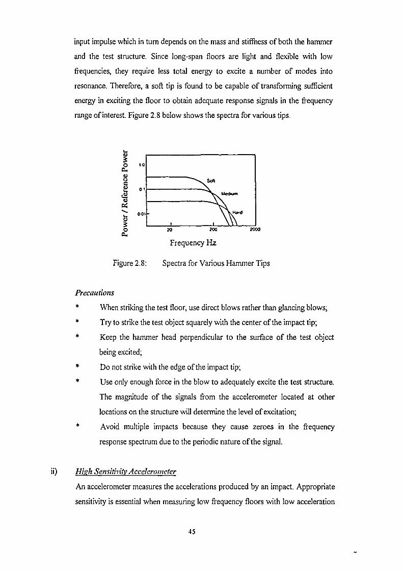
input impulse which in turn depends on the mass and stiffness of both the hammer
and the test structure. Since long-span floors are light and flexible with low
frequencies, they require less total energy to excite a number of modes into
resonance. Therefore, a soft tip is found to be capable of transforming sufficient
energy in exciting the floor to obtain adequate response signals in the frequency
range of interest. Figure 2.8 below shows the spectra for various tips.
_ Hald
Figure 2.8:
1 I
20 290
Frequency Hz
Spectra for Various Hammer Tips
Precautions
* When striking the test floor, use direct blows rather than glancing blows;
* Try to strike the test object squarely with the center of the impact tip;
* Keep the hammer head perpendicular to the surface of the test object
being excited;
* Do not strike with the edge of the impact tip;
* Use only enough force in the blow to adequately excite the test structure.
The magnitude of the signals from the accelerometer located at other
locations on the structure will determine the level of excitation;
* Avoid multiple impacts because they cause zeroes in the frequency
response spectrum due to the periodic nature of the signal.
ii) Hlell Sensitivitv Accelerometer
An accelerometer measures the accelerations produced by an impact. Appropriate
sensitivity is essential when measuring low frequency floors with low acceleration
45
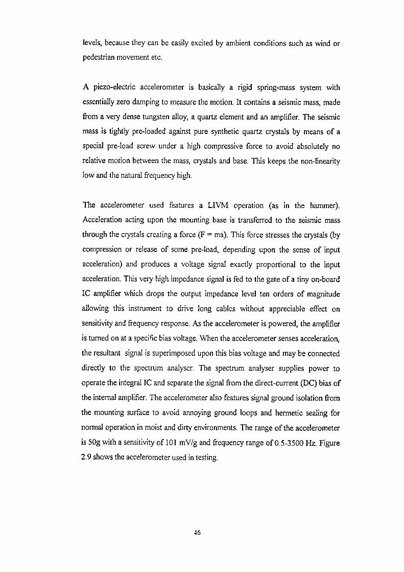
levels, because they can be easily excited by ambient conditions such as wind or
pedestrian movement etc.
A piezo-electric accelerometer is basically a rigid spring-mass system with
essentially zero damping to measure the motion. It contains a seismic mass, made
from a very dense tungsten alloy, a quartz element and an amplifier. The seismic
mass is tightly pre-loaded against pure synthetic quartz crystals by means of a
special pre-load screw under a high compressive force to avoid absolutely no
relative motion between the mass, crystals and base. This keeps the non-linearity
low and the natural frequency high.
The accelerometer used features a LIVM operation (as in the hammer).
Acceleration acting upon the mounting base is transferred to the seismic mass
through the crystals creating a force (F = ma). This force stresses the crystals (by
compression or release of some pre-load, depending upon the sense of input
acceleration) and produces a voltage signal exactly proportional to the input
acceleration. This very high impedance signal is fed to the gate of a tiny on-board
IC amplifier which drops the output impedance level ten orders of magnitude
allowing this instrument to drive long cables without appreciable effect on
sensitivity and frequency response. As the accelerometer is powered, the amplifier
is turned on at a specific bias voltage. When the accelerometer senses acceleration,
the resultant signal is superimposed upon this bias voltage and may be connected
directly to the spectrum analyser. The spectrum analyser supplies power to
operate the integral IC and separate the signal from the direct-current (DC) bias of
the internal amplifier. The accelerometer also features signal ground isolation from
the mounting surface to avoid annoying ground loops and hermetic sealing for
normal operation in moist and dirty environments. The range of the accelerometer
is 50g with a sensitivity of 101 mV/g and frequency range of 0.5-3500 Hz. Figure
2.9 shows the accelerometer used in testing.
46
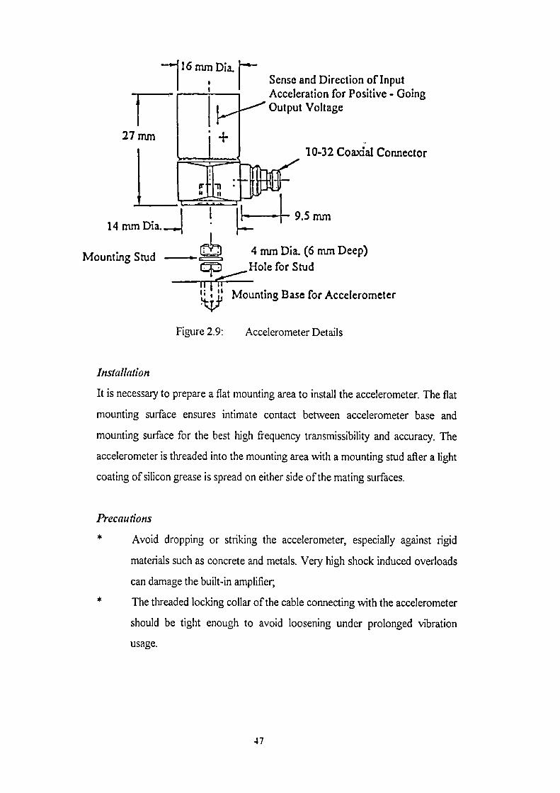
--116 mrn Dia.Sense and Direction of InputAcceleration for Positive - GoingOutput Voltage
27 mm
10-32 Coaxial Connector
9.5 mm14 mm Dia.
Mounting Stud
lir--Mounting Base for Accelerometer
4 mm Dia. (6 mm Deep)
Hole for Stud
Figure 2.9: Accelerometer Details
Installation
It is necessary to prepare a flat mounting area to install the accelerometer. The flat
mounting surface ensures intimate contact between accelerometer base and
mounting surface for the best high frequency transmissibility and accuracy. The
accelerometer is threaded into the mounting area with a mounting stud after a light
coating of silicon grease is spread on either side of the mating surfaces.
Precautions
Avoid dropping or striking the accelerometer, especially against rigid
materials such as concrete and metals. Very high shock induced overloads
can damage the built-in amplifier,
The threaded locking collar of the cable connecting with the accelerometer
should be tight enough to avoid loosening under prolonged vibration
usage.
47

iii) Cables
The hammer and accelerometer are connected to the spectrum analyser by cables.
Bayonet-Neal-Conkenal (BNC) sensor connectors are provided in the spectrum
analyser and at the end of the hammer handle to plug in the cable (Figure 2.6). The
accelerometer has a 10-32 connector and thus a BNC to 10-32 connector cable is
used to connect the accelerometer with the spectrum analyser (Figure 2.9).
Precautions
* Do not allow cables to hang loosely or vibrate unrestrained. Forces
generated by such motion may strain the accelerometer base causing
spurious output from the crystals;
* Avoid stressing the cables by tying them down to a fixed surface near the
accelerometer mounting area.
iv) Frequency Response Spectrum Analyser
This is an instrument used for data acquisition and detailed system analysis. The
analyser used acts as both a digital storage oscilloscope and as a FFT analyser
(converting a signal in the time domain to the frequency domain) with powerful
waveform processing capabilities. It manipulates data and calculates complex
mathematical processes. It is powered by an internal Nickel-Cadmium (NiCad)
battery which can be recharged. It allows the observation of input signals both in
the time and frequency domains. Data stored in the time domain can be further
reprocessed and stored in the frequency domain.
The analyser receives continuous analogue voltage signals from the output of the
transducers where it is proportional to both acceleration and force signals. These
signals are filtered, digitised and transformed into the frequency domain for
analysis. The analyser has facilities to perform analogue to digital signal
conversion, signal filtering for anti-aliasing effects, averaging, windowing,
calculating the transfer function, phase and coherence functions and post-
processing time-domain data to frequency-domain etc.
48

2.2.2 Procedure
The test procedure used in the experimental programme is very simple, repetitive and
quick. It can be explained in steps as follows:
Selection Of The Test Panel
A typical representative panel of the floor is identified. The selection depends on the plan
layout of the floor and dimensions. A panel with the longest spans would give the lowest
fundamental frequency and so every effort is made to select such a panel with the least
obstructions.
Marking The Test Grid
A grid of reasonable size is marked on the test panel. An aspect ratio of one or as close to
one as possible is maintained, depending on the size of the panel. The more grid points,
the more accurate are the average values of the experimental results.
Selecting The Accelerometer / Hanuner Impact Location
The accelerometer is placed on a grid point that gives good response (i.e. not near a nodal
line) at the natural frequencies of interest. The choice can be quickly made by testing a few
points. Normally, the midspan point gives the best response and the accelerometer is
placed at this point to measure the vibrations. In the case of floors with false flooring, the
accelerometer is moved from point to point on the grid and only a few floor panels are
removed near the midspan for exciting the floor with the hammer.
Exciting The Floor
The floor is excited with the hammer at the various grid points in turn. A minimum of five
impacts may be used at each grid point to obtain an average value of the response at these
locations.
Storing The Data
The spectrum analyser performs the analysis and provides plots of the transfer function,
phase and coherence fimctions. A frequency band-width of 25 Hz may be used for the
49

analyser for good resolution of low frequencies of the floors. Data for each test grid
location measured in the above manner is then stored on the spectrum analyser. It is later
transferred to a personal computer for further analyses to extract the dynamic properties.
2.3 Data Processing
After obtaining the transfer function and phase for each grid location for each test through
the spectrum analyser, the following procedure was used to extract the modal parameters
(fundamental natural frequencies and damping ratios) of all the test floors.
Cum-Fitting
A multi-degree-of-freedom (MDOF) curve-fit program, MODENT, was used to extract
the fundamental frequency and corresponding damping ratios for all the grid locations of
each test. For procedural details see MODENT (1993) manuals.
The MDOF curve-fitting used a least-squares approach and is carried out for each mode
of vibration in the region of its natural frequency. It can identify closely spaced modes
because the transfer function in the region of a mode is dominated by its resonating
frequency. In the frequency range around the resonant peak, it is assumed that the plot is
due to the response of a damped MDOF system due to a harmonic input at and near that
natural frequency. Thus frequencies are obtained by noting the location of the peaks and
examining the value of phase at these frequencies, which ideally should be 900.
The damping ratio ( n associated with each peak is determined by the Half-Power (Band
b — flaWidth) technique by the relation = g , Inman (1994), Figure 2.10.
2
50

11/(130)12
max.1-1(13) = IH(134)1
i !MU
iria30)1
0
P. Pa
Frequency Ratio p =Co„
Figure 2.10: Estimating Damping
Maximum amplitudes occur in damped vibrations when the forcing frequency (w) equals
the system's damped natural frequency, which is slightly smaller than the undamped
natural frequency (c n ). In Figure 2.10, and p„ are the frequency ratios at which the
1response amplitude is reduced to—,.--__ times its peak value, fid is the frequency ratio at
V2
which the maximum amplitude occur. The accuracy with which the damping ratio is
determined using this method depends on the frequency resolution in the original
frequency response data.
Averaging
The results for frequency and damping for each grid location were averaged to obtain a
reliable estimate of these properties.
Caution
Although the MODENT software estimates frequency and damping reliably by comparing
all the data files for each test grid location, in many cases, however, it is necessary to study
the phase diagrams closely. This is because of interference in the data due to unavoidable
ambient vibrations and noise. Therefore, every test was analysed a number of times for a
more reliable and average estimate of frequency and damping.
51

Chapter 3 EXPERIMENTAL RESULTS
This Chapter presents the field test results of the floor slabs tested in the experimental
programme. The experimental technique and methods of analysis have been presented in
Chapter 2.
Although the choice of floors was governed by availability, every effort was made to test
as many floors as possible. The floors tested are divided into four main categories as
follows:
i) Post-Tensioned Concrete 1-Way Spanning Solid Floor Slabs With Beams
ii) Post-Tensioned Concrete Solid Flat Slab Floors
iii) Pre-Tensioned Concrete Double-T Beam Floors
iv) Composite Steel-Concrete Slab Floors
Many owners of office buildings were reluctant to grant access for fear of causing alarm to
occupants. Therefore, most of the floors tested were either unoccupied offices at the time
or car parks. In many cases the designers and owners were reluctant to provide all
information including layout drawings and material properties. Most of those who did
provide drawings did not want them to be included in the thesis or published in the
research papers. Therefore, only a general plan layout drawing with a typical cross-section
is given for each category. Structural details for each floor are given individually along
with the experimental fundamental natural frequency. Although the main theme of the
research was the estimation of fundamental natural frequency, experimental damping
estimates are also given. Typical experimental graphs (transfer function, phase and
coherence function plots) are given for each individual floor. General comments on
individual floor testing and results are also given.
52

3.1 Post-Tensioned Concrete 1-Way Spanning Solid
Floor Slabs With Beams
Only four (4) floors of this type could be tested. All of them had beams along the long-
span direction. Figure 3.1 shows a general layout for this floor type with a typical
cross-section (see also Appendix A). Specific dimensions are given for each floor
individually.
II I I I I
—
I!
se
it
IIC1 C2
C4 C3•
-I-I
C00.V)
CTC0-J
C
It
I I I IShort Span Ls
Slab
I
i
LJ Beam
Column
D
Figure 3.1: Typical Plan Layout and Cross-Section
53

3.1.1 Wycombe Entertainment Centre Multi-Storey Car
Park, Level 1+
Structure Description (see Figure 3.1)
Location 1-Egh Wycombe
Typical panel Ls = 7.305 m, LL = 12.05 m
Beams D = 650 mm, W = 665 mm
Columns Cl = C2 = 300 mm x 800 mm
C3 = C4 = 1600 mm x 450 mm
Slab t=210 mm
Finishing 1'1 one
Test date Tuesday 21 April 1992
Test Results
Fundamental natural frequency
10.2 Hz
Floor damping
2.5 % critical
Continents
At the time of the test, there was some noise due to the construction work in progress at
the site and also due to the generator used for power supply to the testing equipment. The
accelerometer sensitivity was, therefore, increased to measure floor vibrations due to the
hammer impact. The effect of noise is visible in the coherence function.
Measurements were taken when no vehicle was parked on the floor. The presence of
vehicles could reduce the frequencies due to the added mass. The floor damping was low
but may be increased with the presence of vehicles. Low damping was also due to the fact
that the floor was newly constructed uncracked solid concrete with no finishes or
suspended ceilings etc.
54
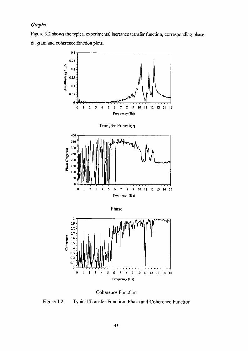
0 -A16;" r'r ' t1 2 3 4 5 6 7 8 9 10 11 12 13 14 15
0.25
0.05
400
350
300
E 250
200
150a.
100
50
0.9
0.8
0.7
0.6
0.5
0.4
0.3
02
0.1
Graphs
Figure 3.2 shows the typical experimental inertance transfer function, corresponding phase
diagram and coherence function plots.
0.3
Frequency (11z)
Transfer Function
0 1 2 3 4 5 6 7 8 9 10 11 12 13 14 15
Frequency (Hz)
Phase
0 1 2 3 4 5 6 7 8 9 10 11 12 13 14 15
Frequency (IIz)
Coherence Function
Figure 3.2: Typical Transfer Function, Phase and Coherence Function
55

3.1.2 Wimbledon Town Hall Development Car Park,
Basement-1
Structure Description (see Figure 3.1)
Location •. Wimbledon
Typical Panel Ls = 7.5 m, LI, = 14.0 m
Beams D = 500 mm, W = 1200 mm
Columns Cl = C2 = C3 = C4 = 500 mm x 500 mm
Slab t = 200 mm
Finishing None
Test Date Thursday 3 December 1992
Test Results
Fundamental natural frequency
5.8 Hz
Floor damping
2.1 % critical
Comments
The car park is close to the London Underground railway line and so the vibrations due to
the moving trains have affected the results. Again, the accelerometer sensitivity was
increased to measure hammer impacted floor vibrations. The effect of noise is visible in the
coherence function.
Measurements were taken when no vehicle was parked on the floor panel tested.
However, there were a few vehicles parked on other floor panels nearby. Their effect on
frequency and damping could not be ascertained because testing could not be repeated for
the case of no vehicle on the floor. However, the floor frequency and damping were quite
low and, therefore, resulted in perceptible vibrations. Low damping was also due to the
absence of any finishing and suspended ceilings etc.
56
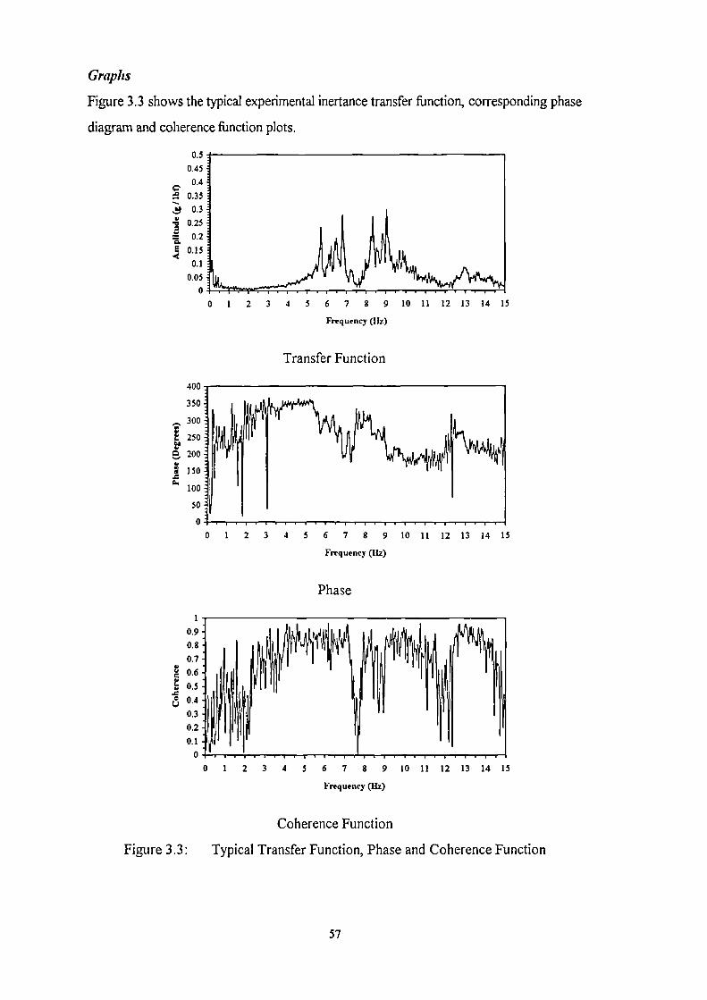
2 3 4 5 6 7 8 9 10 11 12 13 14 15
400
350
300
250
e, 200
I150a.
100
50
iv?
10.90.80.7-0.60.50.40.30.2 :10.1 441
Graphs
Figure 3.3 shows the typical experimental inertance transfer fimction, corresponding phase
diagram and coherence fimction plots.
0.5 0.45
0.442 0.35
0.3II 0.25
0.2—O.E 0.15
0.1
0 .0.05
Frequency (lb)
Transfer Function
0 1 2 3 4 5 6 7 8 9 10 11 12 13 14 15
Frequency (Hz)
Phase
1 2 3 4 5 6 7 8 9 10 11 12 13 14 15
Frequency (Hz)
Coherence Function
Figure 3.3: Typical Transfer Function, Phase and Coherence Function
57

3.1.3 The Hart Shopping Centre Car Park, Level-1
Structure Description (see Figure 3.1)
Location •. Fleet
Typical panel Ls = 7.2 m, LL = 8.0 m
Beams D = 375 mm, W = 1200 mm
Columns Cl = C2 = C3 = C4 = 300 mm x 600 mm
Slab t = 200 mm
Finishing Asphalt Layer
Test Date Sunday 6 December 1992
Test Results
Fundamental natural frequency
11.2Hz
Floor damping
1.9 % critical
Conunents
At the time of the test, there was a strong wind and light drizzle coming in through the
floor wall openings. This caused some ambient vibrations and, therefore, the
accelerometer sensitivity had to be increased. Also, some floor area was wet during testing
and thus any hammer impact on the wet area also produced noise due to splashing of
water. Data for a few grid points was, therefore, affected. It may, however, be noted that
the coherence fiinction plot shows a better response of floor when compared with
previous floors.
Measurements were taken when a few vehicles were parked near the test panel.
Moreover, other vehicles continued to move around the floor for parking and exiting
purposes. The floor damping, however, did not show any improvement due to the
presence of an asphalt layer, when compared with the previous car parks.
58

400
350
300
250DS
.200
150
100
50
0.90.8 -
0.7 -
0.6 -E, 0.5
0.4-
0.3 -
0.2 -
0.1
Graphs
Figure 3.4 shows the typical experimental inertance transfer function, corresponding
phase diagram and coherence function plots.
0.4
0.35 4
0.3
---ba 0.25
0.2
3. 0.15
0.1
0.05
0 0123 4 5 6 7 8 9 10 11 12 13 14 15
Frequency (Hz)
Transfer Function
0 1 2 3 4 5 6 7 8 9 10 11 12 13 14 15
Frequency (Hz)
Phase
2 3 4 5 6 7 8 9 10 11 12 13 14 15
Frequency (Hz)
Coherence Function
Figure 3.4: Typical Transfer Function, Phase and Coherence Function
6
59

3.1.4 The Exchange Shopping Centre Multi-Storey Car
Park, Level-1
Structure Description (see Figure 3.1)
Location Ilford
Typical panel Ls = 7.2 m, LI, = 15.6 m
Beams D = 700 mm, W = 600 min
Columns Cl = C2 = 600 mm x 400 mm
C3 = C4 = 400 rnm x 800 mm
Slab t = 160 mm
Finishing None
Test Date Thursday 10 December 1992
Test Results
Fundamental natural frequency
7.3 Hz
Floor damping
3.7 % critical
Comments
At the time of the test, there was a strong breeze coming in through the floor wall
openings. This caused some ambient vibrations and, therefore, the accelerometer
sensitivity had to be increased. The coherence function indicates the effect of this
disturbance.
Measurements were taken when no vehicle was parked on the floor. The floor damping
was more than that of previous floors, mainly due to the presence of a storage room near
the floor panel tested and the side ramp for vehicles. The presence of the storage room
and the ramp resulted in a breakage of the continuous nature of the floor and acted as
dampers.
60

1.5
1.2 -a.0
40.3 - \VI
o
400
350
300
I 250
.200
j 150
100
50
0
0.90.80.7
o..X 0.6 A
0.5 -
0.3 -0.20.1
o
trr
Graphs
Figure 3.5 shows the typical experimental inertance transfer function, corresponding
phase diagram and coherence function plots.
1 2 3 4 5 6 7 8 9 10 11 12 13 14 15
Frequency (Hz)
Transfer Function
0 1 2 3 4 5 6 7 8 9 10 11 12 13 14 15
Frequency (Hz)
Phase
1
0 1 2 3 4 5 6 7 8 9 10 11 12 13 14 15
Frequency (Hz)
Coherence Function
Figure 3.5: Typical Transfer Function, Phase and Coherence Function
61

3.2 Post-Tensioned Concrete Solid Flat Slab Floors
Only twelve (12) floors of this type could be tested. Figure 3.6 shows a general layout
for this floor type with a typical cross-section (see also Appendix A). Specific
dimensions are given for each floor individually.
Cl C2
-IJC00.
u)
cr.co
_1
C4 C3
Short Span Ls
Figure 3.6: Typical Plan Layout and Cross-Section
62

3.2.1 Vantage West Car Park
Structure Description (see Figure 3.6)
Location Hammersmith
Typical panel Ls = 7.2 m, LI, = 8.4 m
Slab t = 225 mm
Columns Cl = C2 = C3 = C4 =360 mm x 360 mm
Finishing None
Test date Friday 7 August 1992
Test Results
Fundamental natural frequency
8.1 Hz
Floor damping
4.6 % critical
Comments
The car park is close to the approach path of London's Heathrow Airport and motorway
M4. Therefore, noise and vibrations due to the flying aeroplanes and road traffic have
affected the results. The effect of noise is visible in the coherence function.
Measurements were taken when no vehicle was parked on the floor panel tested. The
floor damping could not be estimated accurately due to the closely spaced modes and the
interference due to noise in the data.
63
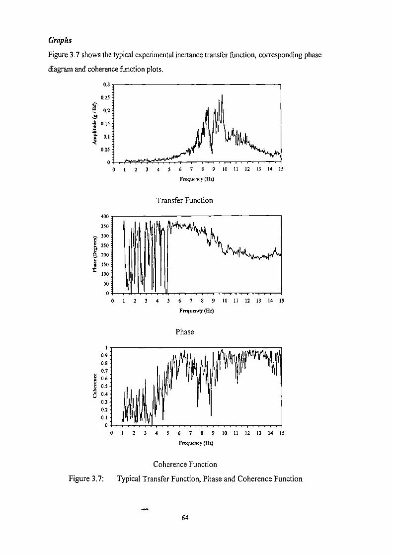
0.3
0.25
-.7.,
E
400
350
300
250 14I6., 200
i 150
e. 100
50
o ,
Graphs
Figure 3.7 shows the typical experimental inertance transfer function, corresponding phase
diagram and coherence function plots.
0 1 2 3 4 5 6 7 8 9 10 11 12 13 14 15
Frequency (11z)
Transfer Function
0 1 2 3 4 5 6 7 8 9 10 11 12 13 14 15
Frequency (Hz)
Phase
0 1 2 3 4 5 6 7 8 9 10 11 12 13 14 15
Frequency (Hz)
Coherence Function
Figure 3.7: Typical Transfer Function, Phase and Coherence Function
+.014
64

3.2.2 The Hart Shopping Centre Car Park, Level-2
Structure Description (see Figure 3.6)
Location Fleet
Typical panel Ls = 7.2 m, LL = 10.7 m
Slab t = 225 mm
Columns Cl = C2 = C3 = C4 = 300 mm x 600 mm
Finishing None
Test Date Sunday 6 December 1992
Test Results
Fundamental natural frequency
5.9 Hz
Floor damping
6.5 % critical
Comments
The test on this roof level car park had to be repeated three times due to severe weather
interruptions. The effect of strong wind on the test day is visible in the coherence function.
Measurements were taken when a few vehicles were parked near the floor panel tested.
There were also disturbances due to vehicles moving on the floor for parking/exiting
purposes. The high floor damping is due to the fact that the panel tested was close to the
shopping mall below with walls etc. which acted as dampers. Also, the floor had
suspended ceilings underneath.
65

400
350
17 300
250
e, 200
V 150
a. 100
50
0.9
0.8
0.7
0.6
0.5
0.4
0.3
0.2
0.1
Graphs
Figure 3.8 shows the typical experimental inertance transfer function, corresponding
phase diagram and coherence function plots.
0.5
0.45 -
0.4 -Cs
0.35
0.3 -I,
0.25 -a
0.2
E 0.15<2
0.1
0.05
0 , .
0 1 2 3 4 5 6 7 8 9 10 11 12 13 14 15
Frequency (Hz)
Transfer Function
0 1 2 3 4 5 6 7 8 9 10 11 12 13 14 15
Frequency (Hz)
Phase
2 3 4 5 6 7 8 9 10 11 12 13 14 15
Frequency (1h)
Coherence Function
Figure 3.8: Typical Transfer Function, Phase and Coherence Function
66

3.2.3 Nurdin & Peacock Office
Structure Description (see Figure 3.6)
Location London
Typical panel Ls = 7.2 m, LL = 7.2 m
Slab t = 225 mm
Columns CI = C2 = C3 = C4 = 450 nun x 450 mm
Finishing False Floor
Test Date Saturday 10 December 1994
Test Results
Fundamental natural frequency
10.1 Hz
Floor damping
7.1 % critical
Continents
This office floor was vacant at the time of the test. However, the office equipment,
furniture, false floors and carpets etc. contributed to the values of frequency and damping.
The results benefit from the quiet environment during the testing. This is reflected in the
coherence function plot. However, the coherence function plot does not correspond to the
grid point for which the transfer function and phase are given. This is due to the fact that
only two plots could be stored at a time on the spectrum analyser and they were chosen as
the transfer function and the corresponding phase diagram.
The spectrum analyser used for this test and all the remaining tests of this floor type
(section 3.2), was newly bought and was different from the one used for earlier tests
(sections 3.1, 3.2.1, and 3.2.2). The choice of this new spectrum analyser was the
additional features required for other purposes in the laboratory.
67

Graphs
Figure 3.9 shows the typical experimental inertance transfer function, corresponding
phase diagram and coherence function plots.
0.002
C 0.0015.o
0.001
0.0005
0 1 2 3 4 5 6 7 8 9 10 11 12 13 14 15
Frequency (Hz)
Transfer Function
400
350
300
E 250
E. 200
150
100
50
1 2 3 4 5 6 7 8 9 10 11 12 13 14 15
Frequency (11z)
Phase
10.9
0.8
0.7
0.6 -
0.5 -
0.4 -
0.3
0.2
0.1
0 1 2 3 4 5 6 7 8 9 10 11 12 13 14 15
Frequency (Hz)
Coherence Function
Figure 3.9: Typical Transfer Function, Phase and Coherence Function
68

3.2.4 Crown Gate Shopping Centre, Chapel Walk,
Service Deck
Structure Description (see Figure 3.6)
Location Worcester
Typical panel Ls=8.0 m,LL =8.0 m
Slab t = 375 mm
Columns CI = C2 = C3 = C4 = 400 mm x 400 mm
Finishing Asphalt layer
Test Date Wednesday 14 December 1994
Test Results
Fundamental natural frequency
12.7 Hz
Floor damping
1.0% critical
Comments
This floor was tested at night time when no vehicle was present on the floor. During the
test, the hammer impact tip broke down and another tip had to be used. The column
locations could not be accurately located due to accessibility problems to the floor below.
Therefore, some of the data was very poor possibly due to impact at or near column lines
and also due to a strong breeze at the time of the test. The coherence function, therefore,
shows a very poor floor response. The coherence function does not correspond to the grid
point for which the transfer function and phase are given, for reasons given earlier in
section 3.2.3.
The measured floor danping was below I% of critical but was assumed as 1%. This low
damping is due to the sharp first peak of the transfer function. It also shows that the
presence of an asphalt layer has little contribution to floor damping. This has already been
noted in section 3.1.3.
69

0.9
0.8
0.7
• 0.6
t 0.5
6 0.4 -
0.3
0.2 -
0.1
Graphs
Figure 3.10 shows the typical experimental inertance transfer fimction, corresponding
phase diagram and coherence fimction plots.
0.001
0.0009 -
0.0008 -
—11 0.0007 --..,9 0.0006
•
•
0.0005 -a
0.0004
0.0003 -0.0002 -
0.0001 -
0 1 2 3 4 5 6 7 8 9 10 11 12 13 14 15
Frequency (Hz)
Transfer Function
400
350
300
250
g 200
150
100
50
0 1 2 3 4 5 6 7 8 9 10 11 12 13 14 15
Frequency (11z)
Phase
1 2 3 4 5 6 7 8 9 10 11 12 13 14 15
Frequency (Hz)
Coherence Function
Figure 3.10: Typical Transfer Function, Phase and Coherence Function
70

3.2.5 St. Martin's Gate Multi-Storey Car Park, Level-4
Structure Description (see Figure 3.6)
Location Worcester
Typical panel Ls = 7.2 m, Li, = 8.4 m
Slab t = 250 mm
Columns Cl = C2 = C3 = C4 = 450 mm x 450 mm
Finishing None
Test Date Saturday 28 January 1995
Test Results
Fundamental natural frequency
9.1 Hz
Floor damping
1.0 % critical
Comments
This floor was tested at a time when vehicles were moving out of the car park. Therefore,
some of the data was very poor due to this disturbance. The floor is a liftslab type
construction with special connections at the column locations. The floor damping
measured was below 1% of critical but was assumed as 1%. The low floor damping is due
to the non-monolithic column connections in addition to the not well defined peaks. The
coherence function does not correspond to the grid point for which the transfer function
and phase are given, for reasons given earlier in section 3.2.3. The coherence function
shows the poor floor response due to the interference caused by the movement of
vehicles.
71

0.00045 4
0.0005 I
0.0004C.4 0.00035....
0.0003 1
43 0.00025 -1•=
0.00027i.i 0.00015 -
0.0001 -
0.00005 -
0 ,
Graphs
Figure 3.11 shows the typical experimental inertance transfer function, corresponding
phase diagram and coherence function plots.
1 2 3 4 5 6 7 8 9 10 11 12 13 14 15
Frequency (Hz)
Transfer Function
400
350
•300
p 250
A 200
.1 150a.
100
50
0
0 1 2 3 4 5 6 7 8 9 10 11 12 13 14 15
Frequency (Hz)
Phase
1
0 .9 -
0 .8 -
0.7
1 2 3 4 5 6 7 8 9 10 11 12 13 14 15
Frequency (Hz)
Coherence Function
Figure 3.11: Typical Transfer Function, Phase and Coherence Function
0
0
72
3.2.6 Brindley Drive Multi-Storey Car Park, Level-4
Structure Description (see Figure 3.6)
Location Birmingham
Typical panel Ls = 7.2 in, LL = 9.55 m
Slab t = 250 mm
Columns Cl = C2 = C3 = C4 = 400 mm x 400 mm
Finishing None
Test Date Saturday 28 January 1995
Test Results
Fundamental natural frequency
7.2 Hz
Floor damping
1.4 % critical
Comments
This floor was tested in the evening when no vehicle was parked on the floor. However,
there was a light breeze through the wall openings. The floor is a lifislab type construction
with special connections at the column locations. The results were not very clear to
interpret and, therefore, were analysed a number of times to obtain average values for
frequency and damping. The low floor damping is due to the non-monolithic column
connections. The coherence function, which shows the poor floor response, does not
correspond to the grid point for which the transfer function and phase are given, for
reasons given earlier in section 3.2.3.
73

0.0005
0.0004 -c
„y 0.0003 -
0.0002 -
0.0001 -
Graphs
Figure 3.12 shows the typical experimental inertance transfer function, corresponding
phase diagram and coherence function plots.
0 1 2 3 4 5 6 7 8 9 10 11 12 13 14 15
Frequency (Hz)
Transfer Function
400
350
300
250
200
150
100
50
0
0 2 3 4 5 6 7 8 9 10 11 12 13 14 15
Frequency (Hz)
Phase
0.5
0.4
0.3 :
0.2:
0.1
1 2 3 4 5 6 7 8 9 10 11 12 13 14 15
Frequency (Hz)
Coherence Function
Figure 3.12: Typical Transfer Function, Phase and Coherence Function
0
0
74

3.2.7 Snow Hill Re-Development Livery Street Multi-
Storey Car Park, Level-1B
Structure Description (see Figure 3.6)
Location Birmingham
Typical panel Ls = 7.5 m, LL = 8.0 m
Slab t = 225 mm
Columns Cl = C2 = C3 = C4 = 450 mm x 450 mm
Finishing None
Test Date Sunday 29 January 1995
Test Results
Fundamental natural frequency
8.6 Hz
Floor damping
1.0 % critical
Comments
This floor was tested at a time when no vehicle was parked on the floor. The car park is
close to the main road and, therefore, there was continuous noise of the traffic. Some of
the results were not very good and, therefore, they were analysed a few times before an
average estimate of frequency and damping was obtained. The coherence function, which
does not correspond to the grid points for which the transfer function and phase are given,
for reasons given earlier in section 3.2.3, shows the effect of noise and light breeze across
the car park.
The measured floor damping was below 1% of critical but was assumed as 1%. This is
due to the fact that the tested panel was near the middle of this large car park with no
partitions, suspended ceilings, and finishes etc.
75

400
350
,..... 300
i 250eatll 200
100
j150a.
50
,0 1 2 3 4 5 6 7 8 9 10 11 12 13 14 15
Frequency (11z)
o
1
i\
0.90.80.7
ao
ca' 0.6E 0.5xC., 0.4
0.30.20.1
Graphs
Figure 3.13 shows the typical experimental inertance transfer function, corresponding
phase diagram and coherence function plots.
0.0006
0.0005 -C., 0.0004 -—
..9SI
.0 0.0003 -a-6.e 0.0002 -
•E0.0001 -
0 1 2 3 4 5 6 7 8 9 10 11 12 13 14 15
Frequency (1h)
Transfer Function
Phase
I
o
o 1 2 3 4 5 6 7 8 9 10 11 12 13 14 15
Frequency (Hz)
Coherence Function
Figure 3.13: Typical Transfer Function, Phase and Coherence Function
76

3.2.8 Snow Hill Re-Development Livery Street Multi-
Storey Car Park, Level-IA
Structure Description (see Figure 3.6)
Location . Birmingham
Typical panel Ls = 7.5 m, Li. = 8.0 m
Slab t = 350 mm
Columns Cl = C2 = C3 = C4 = 450 mm x 450 mm
Finishing None
Test Date Sunday 29 January 1995
Test Results
Fundamental natural frequency
12.7 Hz
Floor damping
1.6 % critical
Comments
This floor was tested at a time when no vehicle was parked on the floor. The floor is the
next level below of the previous car park. The layout of the floor is identical to the
previous floor except the slab thickness. This increased stiffness raised the frequency and
also damping. The coherence function for this floor could not be measured due to the lack
of memory space of the spectrum analyser which had just been used for the previous floor.
Also, only a few grid points were measured for the same reason. The results were again
not very good due to various disturbances discussed earlier in section 3.2.7.
77

kvvi\gf
Graphs
Figure 3.14 shows the typical experimental inertance transfer function and corresponding
phase diagram plots. The coherence friction for this test could not be measured due to
lack of memory of the spectrum analyser.
0.0002
0.00018
0.00016
0.00014
„9 0.00012
0.0001
= 0.00008a.
0.00006
0.00004
0.00002
0
0 1 2 3 4 5 6 7 8 9 10 11 12 13 14 15
Frequency (Hz)
Transfer Function
400
350
1., 300
E 250La
A_. 200
150
100
50
0
0 1 2 3 4 5 6 7 8 9 10 11 12 13 14 15
Frequency (Hz)
Phase
Figure 3.14: Typical Transfer Function and Phase
78

3.2.9 Island Site, Finsbury Pavement, Office, Level-4
(Flexible Panel)
Structure Description (see Figure 3.6)
Location London
Typical panel Ls = 9.0 m, LI, = 9.0 m
Slab t = 300 mm
Columns Cl = C2 = C3 = C4 = 600 mm Diameter
(Assumed 600 mm x 600 mm)
Finishing None
Test Date Saturday 29 April 1995
Test Results
Fundamental natural frequency
8.4 Hz
Floor damping
1.0% critical
Comments
This floor was tested at a time when construction work was in progress at the site. The
site is located at the corner of a busy road junction. Therefore, the floor response was not
accurately measured. The coherence function shows the quality of the measurements.
Again, it does not correspond to the grid point for which the transfer function and phase
are given, for reasons given earlier in section 3.2.3.
The floor panel tested is close to a central opening which caused a breakage in the
continuous nature of the floor. The measured floor damping was less than 1% of critical
but was assumed as 1%. The reason for low damping is the sharp peak in the transfer
function.
79
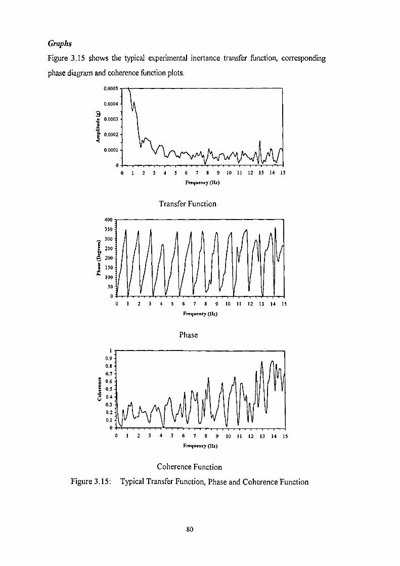
Graphs
Figure 3.15 shows the typical experimental inertance transfer function, corresponding
phase diagram and coherence function plots.
0.0005
0.0004 -
Sw 0.0003 -
0.0002
0.0001
2 3 4 5 6 7 8 9 10 11 12 13 14 15
Frequency (11z)
Transfer Function
/ ! i. . P . . .
0 1 2 3 4 5 6 7 8 9 10 11 12 13 14 15
Frequency (l1z)
Phase
0.9
0.8
0.7
1E
▪
'
•
0.6
0.5
Cc; 0.40.3
0.2
0.1
0 1 2 3 4 5 6 7 8 9 10 11 12 13 14 15
Frequency (11z)
Coherence Function
Figure 3.15: Typical Transfer Function, Phase and Coherence Function
400
350
„ 300
250
200
150
• 100
50
80
3.2.10 Island Site, Finsbury Pavement, Office, Level-4
(Stiff Panel)
Structure Description (see Figure 3.6)
Location London
Typical panel Ls = 7.5 m, LL = 9.0 m
Slab t = 300 mm
Columns Cl = C2 = C3 = C4 = 600 mm Diameter
(Assumed 600 mm x 600 mm)
Finishing None
Test Date Saturday 29 April 1995
Test Results
Fundamental natural frequency 10.6 Hz
Floor damping 1.3 % critical
Comments
This floor panel is adjacent to the previous panel tested but away from the central floor
opening. Therefore, the same comments apply here as for the previous floor in section
3.2.9.
81

0.0001 -
400
350
,... 300
250
; 200
i 150-I.
100
50
o . , . . . .
1
I \Io , 1
IV
0.9
0.8
0.74,
0.6
;n 0.540 0.4c.. )
0.3
0.2
0.1
o
I\
Graphs
Figure 3.16 shows the typical experimental inertance transfer function, corresponding
phase diagram and coherence function plots.
0.0005
0.0004 -.11e..9 0.0003 -a,
0 1 2 3 4 5 6 7 8 9 10 11 12 13 14 15
Frequency (1Iz)
Transfer Function
0 1 2 3 4 5 6 7 8 9 10 11 12 13 14 15
Frequency (Hz)
Phase
0 1 2 3 4 5 6 7 8 9 10 11 12 13 14 15
Frequency (Hz)
Coherence Function
Figure 3.16: Typical Transfer Function, Phase and Coherence Function
82

3.2.11 Friars Gate Multi-Storey Car Park, Level-5
Structure Description (see Figure 3.6)
Location Winchester
Typical panel Ls = 6.0 m, LL = 7.5 m
Slab t = 200 mm
Columns Cl = C2 = C3 = C4 = 250 mm x 450 mm
Finishing None
Test Date Wednesday 3 May 1995
Test Results
Fundamental natural frequency
10.3 Hz
Floor damping
1.5% critical
Comments
This car park is located near the city centre. However, the test was carried out when the
car park had been closed. The only disturbance that occurred was due to the light breeze
through the car park. Therefore, results are better and the quality of measurements is
reflected in the coherence fimction. The coherence function does not correspond to the
grid point for which the transfer function and phase are given, for reasons given earlier in
section 3.2.3.
The floor panel tested is part of the floor constructed as an extension of the existing car
park. The two floors are separated by a 50 mm expansion joint. The low damping is due
to the absence of any partitions, finishes and suspended ceilings etc.
83

I
i i -iv
\rIIIv
Iv%
ti'V
4
10.9
0.8 ,0.7 -
40.a. 0.6
0 .5 -
6 0.4 -
0.3 :
0.2-
0
0.1
0
PP\ 4
Graphs
Figure 3.17 shows the typical experimental inertance transfer function, corresponding
phase diagram and coherence function plots.
0 1 2 3 4 5 6 7 8 9 10 11 12 13 14 15
Frequency (Ih)
Transfer Function
400
350
300,-,
g 250
g 200
i 150
4 loo
50 1
o
o
I/Ar/
1 2 3 4 5 6 7 8 9 10 11 12 13 14 15
Frequency (11z)
Phase
1 2 3 4 5 6 7 8 9 10 11 12 13 14 15
Frequency (Hz)
Coherence Function
Figure 3.17: Typical Transfer Function, Phase and Coherence Function
84

3.2.12 Tower Street Car Park
Structure Description (see Figure 3.6)
Location Winchester
Typical panel Ls = 8.0 rn, Li, = 9.0 m
Slab t = 275 mrn
Columns Cl = C2 = C3 = C4 = 450 mm x 450 mm
Finishing None
Test Date Wednesday 3 May 1995
Test Results
Fundamental natural frequency
8.5 Hz
Floor damping
2.8 % critical
Comments
This car park is located near the city centre and close to a busy traffic roundabout. The car
park is open 24 hours and there was some vehicular movement throughout testing.
However, due to time constraints, the test had to be carried out. Every effort was,
however, made to record measurements when no vehicle moved on the floor panels
nearby. The coherence function shows the effect of disturbances due to vehicle movement,
noise on the adjacent road and strong breeze through the car park. The coherence function
does not correspond to the grid point for which the transfer function and phase are given,
for reasons given earlier in section 3.2.3.
85

1 2 3 4 5 6 7 8 9 10 11 12 13 14 15
0.003
0.0025C.o
0.002
40.0005
-a. 0.001
„I
400
350
,...‘ 300
250b/
(1). 200
j150
100
50
0? I 01 2 3 4 5 6 7 8 9 10 11 12 13 14 15
1 0.9:
0.8
0.7
0.6 :
0.5
0.4i
0). 32 WI\0.1
0
0
i
I
i AIIII 4
i II
I II I
I
1 2 3 4 5 6 7 8 9 10 11 12 13 14 15
Graphs
Figure 3.18 shows the typical experimental inertance transfer function, corresponding
phase diagram and coherence function plots.
Frequency (11z)
Transfer Function
Frequency (Hz)
Phase
Frequency (Hz)
Coherence Function
Figure 3.18: Typical Transfer Function, Phase and Coherence Function
86

1 1
1 1
ColumnI 1
1 1
-I - -r• n-
L Girder-•
I I I I I I
11111
II III
1 1
1 1
1 1
1 1 1 1
1 1 I I 1 I1
1 1 1 . 1
1 1 I I1 1 1
1 1 I II 1 1
Double—T Beams
1 I I 1 1 1
I I IInverted T Girder
1 1
50 mm
3.3 Pre-Tensioned Concrete Double-T Beam Floors
Only five (5) floors of this type could be tested. All of them consisted of double-T
beams supported on L-girders or inverted T-beams on neoprene bearing pads. Figure
3.19 shows a general layout for this floor type with a typical cross-section (see also
Appendix A). Specific dimensions are given for each floor individually.
Figure 3.19: Typical Plan Layout and Cross-Section
87

3.3.1 Trigonos Phase V Multi-Storey Car Park, Level-6
Structure Description (see Figure 3.19)
Location Swindon
Column Spacing 7.2 m
Beam Size D‘,„ = 550 mm, t,„, = 185 mm, t wb = 130 mm
Beam Length L = 16.045 m
Finishing 75 mm screed; 50 mm asphalt
Test date Monday 27 July 1992
Test Results
Fundamental natural frequency
4.9 Hz
Floor damping
2.1% critical
Comments
At the time of the test, there was a strong breeze on this roof floor. This caused some
ambient vibrations and, therefore, the accelerometer sensitivity had to be increased. The
coherence fimction indicates the effect of this disturbance.
Measurements were taken when no vehicles were parked on the floor. The floor
frequency was low due to its long span. There were many closely spaced modes and the
data had to be analysed a number of times to obtain an average estimate of the floor
frequency and damping.
88

0 1 2 3 4 5 6
7 8 9 10
0.3
0.25C'.0
0.2
i0.05
400
350
,-, 300
i 250orV 200
i 150re.
100
50
o
0.9 :0.8 :
6+ 0.7 :'a't.c6 0.4
0.3 :0.2 -0.1 -
Graphs
Figure 3.20 shows the typical experimental inertance transfer function, corresponding
phase diagram and coherence function plots.
Frequency (Hz)
Transfer Function
0 1 2 3 4 5 6
7 8 9
10
Frequency. (Ilz)
Phase
1 2 3 4 5 6
7 8 9
10
Frequency (IIz)
Coherence Function
Figure 3.20: Typical Transfer Function, Phase and Coherence Function
89

3.3.2 Reading Station Re-Development Multi-Storey Car
Park, Level-10
Structure Description (see Figure 3.19)
Location Reading
Column Spacing 7.2 m
Beam Size Dv, = 550 mm, t„t = 195 mm, twb = 140 mm
Beam Length L = 15.4 m
Finishing 75 mm screed
Test date Sunday 19 March 1995
Test Results
Fundamental natural frequency
5.6 Hz
Floor damping
1.0 % critical
Comments
Measurements were taken when no vehicle was parked on the floor. The floor frequency
was low due to its long span. This frequency was estimated after a number of analysis of
the data. The quality of the data was very poor due to interferences caused by wind and
noise. Also, floor damping could not be accurately estimated for the same reasons. It was
evaluated at a value below 1.0 % of critical but was assumed as 1.0 % critical. The
results have also been affected by the poor construction of the floor which showed
leakages at the beam junctions.
The spectrum analyser used for this test and all the remaining tests of this floor type
(section 3.3), was newly bought and was different from the one used for earlier tests
(sections 3.1, 3.2.1, 3.2.2 and 3.3.1). The reasons have already been discussed in section
3.2.3.
90

0.001
400
o
350
300
250
200
j150
100
50
Graphs
Figure 3.21 shows the typical experimental inertance transfer function, corresponding
phase diagram and coherence function plots.
0 1 2 3 4 5 6 7 8 9 10
Frequency (Hz)
Transfer Function
0 1 2 3 4 5 6 7 8 9 10
Frequency (11z)
Phase
0.9
0.8
0.7
0.6
0.5
0.4
0.3
0.2
0.1
0 1 2 3 4 5 6 7 8 9 10
Frequency (Hz)
Coherence Function
Figure 3.21: Typical Transfer Function, Phase and Coherence Function
91

3.3.3 Safeway Superstore Car Park
Structure Description (see Figure 3.19)
Location Sutton
Column Spacing 7.2 m
Beam Size = 550 mm, tv,t = 225 mm, twb = 170 mm
Beam Length L = 15.6 m
Finishing 75 mm screed
Test date Sunday 23 April 1995
Test Results
Fundamental natural frequency 5.5 Hz
Floor damping (average) 1.0 % critical
Comments
At the time of the test, there was a strong breeze on this roof floor. Also, light rain started
towards the end of the test. This caused some ambient vibrations and, therefore, the
accelerometer sensitivity had to be increased. The coherence function indicates the effect
of this disturbance. It, however, does not correspond to the grid point for which the
transfer function and phase are given, for reasons given earlier in section 3.2.3. The quality
of floor construction also affected the results, as discussed in section 3.3.2.
Measurements were taken when no vehicle was parked on the floor. The floor frequency
was low due to its long span. The reasons for low damping are the same as for the
previous floor (section 3.3.2).
92

400
350
300
E 250
200
150A.
100
50
A
Graphs
Figure 3.22 shows the typical experimental inertance transfer function, corresponding
phase diagram and coherence ffinction plots.
0.0005
0.0004 -C`.0
,N 0.00034.
— 0.0002S .
0.0001 -
1
2 3 4 5 6
7 8 9 10
Frequency (Hz)
Transfer Function
1 2 3 4 5 6 7 8 9 10
Frequency (11z)
Phase
0.9 -0 -
0.7
0.6
0.5
0 4
0.3
0.2
0.1
0 1 2 3 4 5 6 7 8 9 10
Frequency (Hz)
Coherence Function
Figure 3.22: Typical Transfer Function, Phase and Coherence Function
93

3.3.4 Toys R Us Multi-Storey Car Park # 4, Level-7
Structure Description (see Figure 3.19)
Location Basildon
Column Spacing 7.2 m
Beam Size D, = 450 mm, twt = 265 mm, twi, = 208 mm
Beam Length L = 15.7 m
Finishing 100 mm screed
Test date Wednesday 26 April 1995
Test Results
Fundamental natural frequency
4.6 Hz
Floor damping
3.4 % critical
Comments
Measurements were taken when no vehicle was parked on the floor. However, the odd
vehicle did move along the adjacent bay for entering/exiting purposes. The floor frequency
was low due to its long span. Damping estimate was higher than other floors of this type.
This was due to the closely spaced modes. Again, the quality of data was poor due to the
interferences caused by a light breeze and traffic noise. The poor floor construction has
also affected the results.
The coherence function does not correspond to the grid point for which the transfer
function and phase are given, for reasons given earlier in section 3.2.3. The quality of
measurements is reflected in the coherence function.
94
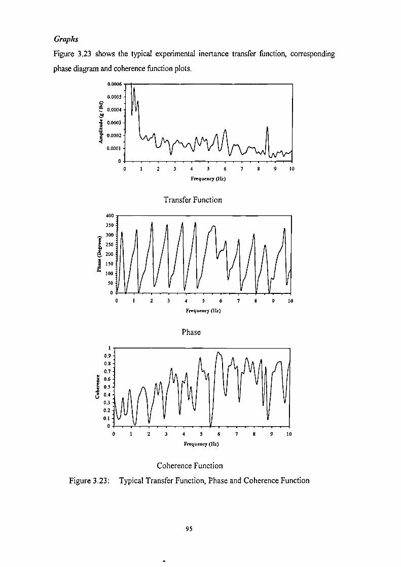
C.0.0004
0.0003 -
▪ 0.0002 -
0.0001 -
0.0006
0.0005 -
JVIIP
0 .9 -
0.8 :
0.7 :
▪ 0.6 :
F, 0.5
o 0.4
0 .3 -
0.2
0.1
Graphs
Figure 3.23 shows the typical experimental inertance transfer function, corresponding
phase diagram and coherence function plots.
2 3 4 5 6
Frequency (Hz)
7 8 9 10
Transfer Function
400
350
ss 300
250
200
150
100
50
0 1 2 3 4 5 6 7 8 9 10
Frequency (Hz)
Phase
0 1 2 4 5 6 7 8 9 10
Frequency (Hz)
Coherence Function
Figure 3.23: Typical Transfer Function, Phase and Coherence Function
95

3.3.5 Royal Victoria Place Multi-Storey Car Park,
Level-3
Structure Description (see Figure 3.19)
Location Tunbridge Wells
Column Spacing 7.2 m
Beam Size Dv, = 550 mm, twt = 195 mm, twb = 140 mm
Beam Length L = 15.4 m
Finishing 75 mm screed
Test date Sunday 30 April 1995
Test Results
Fundamental natural frequency
5.8 Hz
Floor damping (average)
1.0 % critical
Conunents
Measurements were taken when no vehicle was parked on the floor. However, the odd
vehicle did move along the adjacent bay for entering/exiting purposes. The floor frequency
was low due to its long span. Damping estimate was lower than 1.0 % of critical but was
assumed as 1.0 % critical. Again, the quality of data was poor. This is a particular feature
for double-T car parks which have been investigated. The reason is thought to be caused
by the floor construction techniques at the junction of two adjacent beams and also due to
noise etc. The data was, therefore, analysed a number of times for reasonable estimates of
the floor frequency and damping.
The coherence function does not correspond to the grid point for which the transfer
fiinction and phase are given, for reasons given earlier in section 3.2.3. It shows the quality
of measurements.
96

1 2 3 4 5 6 7 8 9 10
400
350
300..-.
g 250
g 200
i 150if.
100
50
Io ,
6 7 8 9 1040 1 2
0.9 -.
0.8 -.
0.7 -.
0.6 -
0.5 -.
0.4
0.3
0.21
1
o
Graphs
Figure 3.24 shows the typical experimental inertance transfer function, corresponding
phase diagram and coherence function plots.
0.018
0.016
c 0.014..o
0.012-......9 0.01-a..?, 0.008O...i 0.006
0.004 -
0.002 -
0
0
Frequency (11z)
Transfer Function
Frequency (11z)
Phase
0 1 2 3 4 5 6 7 8 9 10
Frequency (Hz)
Coherence Function
Figure 3.24: Typical Transfer Function, Phase and Coherence Function
97
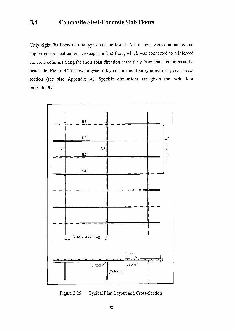
3.4 Composite Steel-Concrete Slab Floors
Only eight (8) floors of this type could be tested. All of them were continuous and
supported on steel columns except the first floor, which was connected to reinforced
concrete columns along the short span direction at the far side and steel columns at the
near side. Figure 3.25 shows a general layout for this floor type with a typical cross-
section (see also Appendix A). Specific dimensions are given for each floor
individually.
Figure 3.25: Typical Plan Layout and Cross-Section
98

3.4.1 The Millwall Football and Athletics Stadium, Senegal
Fields, West Stand, Hospitality Level
Structure Description (see Figure 3.25)
Location . London
Typical Panel Ls = 6.75 m, Li, = 8.3 m
Beams B1 -UB610x229x101
B2, B3 - UB356x127x33
B4 - UB305x102x28
Girders Gl, G2 -UB610x229x101
Profile CF70 (1.2)
Slab t = 130 mm
Finishing None
Test Date Monday 7 December 1992
Test Results
Fundamental natural frequency
12.6 Hz
Floor damping
1.0 % critical
Comments
This stadium was under construction at the time of the test. Therefore, the test was carried
out at night after the working shifts. However, the floor was wet at various locations and
only a few selected grid points could be tested. The response of the floor was quite good
as compared with many previous floors due to the quiet environment and absence of any
other disturbances. This is visible in the coherence function.
The floor damping is quite low and therefore resulted in perceptible vibrations. It is mainly
due to the sharp first peak of the transfer function, which in turn resulted due to the
absence of any partitions, finishes and suspended ceilings etc.
99

4.5
4
C' 3.5A
.... 3
..9 2.5‘2
= 2....S.'
10.5
o
E 15Q
400
350
•.., 300
250ee, 200
j150a.
100
50
o
1
i! .1
. ,
0 1 2 3 4 5 6 7 8 9 10 11 12 13 14 15
V i 1 V".10.9 -0.8 -
0.7
0.6
0.5 -.0.4 -
0.3
0.2
0.1
o
i
Graphs
Figure 3.26 shows the typical experimental inertance transfer function, corresponding
phase diagram and coherence function plots.
0 1 2 3 4 5 6 7 8 9 10 11 12 13 14 15
Frequency (11z)
Transfer Function
Frequency (11z)
Phase
0 1 2 3 4 5 6 7 8 9 10 11 12 13 14 15
Frequency (11z)
Coherence Function
Figure 3.26: Typical Transfer Function, Phase and Coherence Function
100

3.4.2 Worcester Central Development, Friary Walk Car
Park, Level-2
Structure Description (see Figure 3.25)
Location Worcester
Typical Panel Ls = 7.2 m, LL = 8.0 m
Beams B1 - UB914x305x253
B2, B3 - UB610x229x101
B4 - UB914x419x388
Girders Gl, G2 -UB610x229x101
Profile CF60 (1.2)
Slab t = 130 mm
Finishing None
Test Date Thursday 15 December 1994
Test Results
Fundamental natural frequency
8.1 Hz
Floor damping
3.2 % critical
Conunents
This car park was tested after the business hours. However, the floor panel tested was close to
the shopping mall where most of the shops were closing down and caused considerable
disturbance, which can be observed in the coherence function. The coherence function does not
correspond to the grid point for which the transfer function and phase are given, for reasons
given earlier in section 3.2.3. The floor frequency was obtained from an average sample of data
due to poor quality. The floor damping is relatively high when compared with the previous
floor of this type. The main reason for this was the nearby mall with shops at the lower levels
which acted as dampers.
The spectrum analyser used for this test and all the remaining tests of this floor type (section
3.4), was newly bought and was different from the one used for earlier tests (sections 3.1,
3.2.1, 3.2.2, 3.3.1 and 3.4.1). The reasons have already been discussed in section 3.2.3.
101

C.A—
.90.02'8.8a
N
0.001
0.0009
0.0008
0.0007 -
0.0006 1
0.0005
0.0004
0.0003
0.0002
0.0001
0 \Ai
\I
.- . .
9 10 11 12
. . •
13 14 15
/I
0 1 2 3 4 5 6 7 8
400
350
300
250
200
150
100
50
o
igI
1
1 iI
tII'
0.9 -.
0.8 -,
0.7 -
0.6 -
0.5 -
0.4 -
0.3 -
0.2 -
0.1t
Jo
Graphs
Figure 3.27 shows the typical experimental inertance transfer function, corresponding
phase diagram and coherence function plots.
0 1 2 3 4 5 6 7 8 9 10 11 12 13 14 15
Frequency (11z)
Transfer Function
Frequency (11z)
Phase
0 1 2 3 4 5 6 7 8 9 10 11 12 13 14 15
Frequency (Ilz)
Coherence Function
Figure 3.27: Typical Transfer Function, Phase and Coherence Function
102

3.4.3 Braywick House Office
Structure Description (see Figure 3.25)
Location Maidenhead
Typical Panel Ls = 9.0 m, LI, = 9.0 m
Beams BI, B4 - Cellform650x152x60
B2, B3 - Cellform650x152x52
Girders G1 - UB610x.305x238
G2 - UB610x229x140
Profile CF51 (1.2)
Slab t = 130 mm
Finishing None
Test Date Friday 24 February 1995
Test Results
Fundamental natural frequency 8.8 Hz
Floor damping 2.0 % critical
Comments
This floor was tested during construction hours. The floor was partly loaded with
construction material and some patchy water. Effects of noise and breeze are visible in the
coherence function plot. The coherence function does not correspond to the grid point for
which the transfer function and phase are given, for reasons given earlier in section 3.2.3.
The floor response was more accurately measured than the previous floor (section 3.4.2)
due to an increase in the sensitivity of the accelerometer. The floor damping is quite low
and, therefore, resulted in perceptible vibrations. It may increase when the construction
has finished due to the presence of planned suspended ceilings and boundary walls.
103

Graphs
Figure 3.28 shows the typical experimental inertance transfer function, corresponding
phase diagram and coherence function plots.
ao
0.0014
0.0012
0.001
0.0008 -
0.0006 -
0.0004 -
0.0002 -
1 2 3 4 5 6 7 8 9 10 11 12 13 14 15
Frequency (11z)
Transfer Function
400
350
300
250
g200
150
100
50
1 2 3 4 5 6 7 8 9 10 11 12 13 14 15
Frequency (11z)
Phase
1 .
0.8
0.7
ao
0.6 -
F., 0.5
0.4
0.3 -.
0.2 -
0.1 -
0
0 1 2 3 4 5 6 7 8 9 10 11 12 13 14 15
Frequency (11z)
Coherence Function
Figure 3.28: Typical Transfer Function, Phase and Coherence Function
104

3.4.4 Premium Products Office
Structure Description (see Figure 3.25)
Location Heathrow
Typical Panel Ls = 6.0 m, LI, = 9.0 m
B eams B1, B3 - UB356x127x33
B2 - UB406x140x39
Girders GI, G2 - UB533x210x92
Profile CF70 (1.2)
Slab t = 130 mm
Finishing False Floor
Test Date Thursday 2 March 1995
Test Results
Fundamental natural frequency
9.1 Hz
Floor damping
11.4 % critical
Comments
This building is located inside a cargo hanger near London's Heathrow Airport Terminal-
4. This newly built floor was being furnished. The floor had false flooring and was
carpeted recently. There were some partition walls being added. The test was carried out
after the working hours in an enclosed and quiet environment. However, most of the
furnishings and equipment was lying on the floor near the panel tested. The floor response
was measured by removing a flooring panel and placing the accelerometer on the bare
concrete. The floor damping is unexpectedly quite high due to the false floor and carpets
and partitions underneath.
The coherence function does not correspond to the grid point for which the transfer
function and phase are given, for reasons given earlier in section 3.2.3. It shows a good
floor response.
105

0.9
0.8 .
0.7 :0 .6 -
0.5
0.4
0.3
0.2
0.1
o
Graphs
Figure 3.29 shows the typical experimental inertance transfer function, corresponding
phase diagram and coherence function plots.
0.001
0.0009
0.0008C'-12 0.0007 --...
0.0006 -
•
▪▪
0.0005 -a 0.0004 -s.i 0.0003 -,
0.0002 -
0.0001 -
0
0 1 2 3 4 5 6 7 8 9 10 11 12 13 14 15
Frequency (11z)
Transfer Function
400
350
•..• 300
250
g200
i 1504
100
50
o0 1 2 3 4 5 6 7 8 9 10 11 12 13 14 15
Frequency (11z)
Phase
0 1 2 3 4 5 6 7 8 9 10 11 12 13 14 15
Frequency (Hz)
Coherence Function
Figure 3.29: Typical Transfer Function, Phase and Coherence Function
_
106
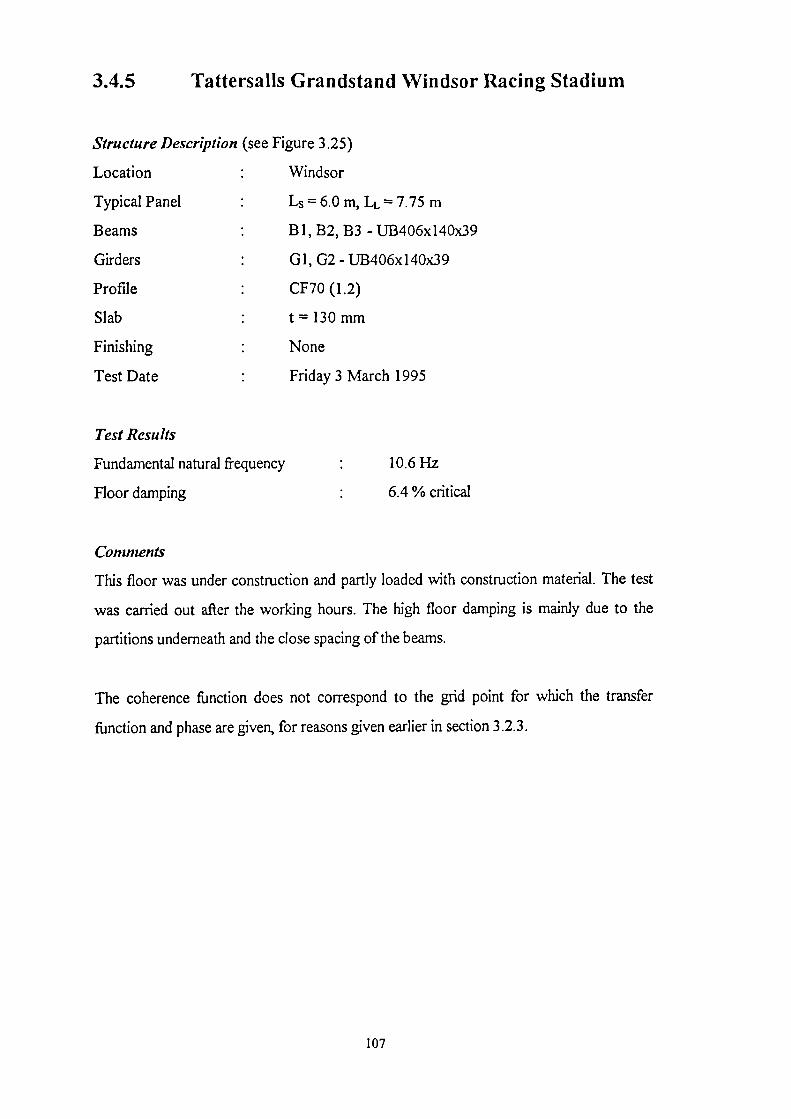
3.4.5 Tattersalls Grandstand Windsor Racing Stadium
Structure Description (see Figure 3.25)
Location Windsor
Typical Panel Ls = 6.0 m, LI, = 7.75 m
Beams BI, B2, B3 - UB406x140x39
Girders GI, G2 - UB406x140x39
Profile CF70 (1.2)
Slab t = 130 mrn
Finishing None
Test Date Friday 3 March 1995
Test Results
Fundamental natural frequency 10.6 Hz
Floor damping 6.4 % critical
Comments
This floor was under construction and partly loaded with construction material. The test
was carried out after the working hours. The high floor damping is mainly due to the
partitions underneath and the close spacing of the beams.
The coherence function does not correspond to the grid point for which the transfer
function and phase are given, for reasons given earlier in section 3.2.3.
107

0.001
0 1 2 3 4 5 6 7 8 9 10 11 12 13 14 15
400
350
300
250
g 200
j150
100
50
1 2 3 4 5 6 7 8 9 10 11 12 13 14 15
Graphs
Figure 3.30 shows the typical experimental inertance transfer function, corresponding
phase diagram and coherence function plots.
Frequency (Hz)
Transfer Function
Frequency (Hz)
Phase
0.9
0.8 :
0.7 :
0.6
0.5
0.4 :
0.3 -
0.2 :
0.1
0
0 1 2 3 4 $ 6 7 8 9 10 11 12 13 14 15
Frequency (11z)
Coherence Function
Figure 3.30: Typical Transfer Function, Phase and Coherence Function
108

3.4.6 St. George's RC Secondary School Office
Structure Description (see Figure 3.25)
Location London
Typical Panel Ls = 7.0 m, LL = 7.37 m
Beams Bl, B2, B3 - UB533x210x101
Girders GI, G2 -UB533x210x101
Profile CF70 (1.2)
Slab t = 200 mm
Finishing None
Test Date Friday 17 March 1995
Test Results
Fundamental natural frequency
14.0 Hz
Floor damping
2.7 % critical
Comments
This floor was under construction and partly loaded with construction material. Some rain
water was also corning in through the side walls at the time of the test. The results were,
therefore, affected and this can be observed in the coherence function. The high floor
frequency was primarily due to the heavy stiff beams and girders.
109

2 4 6 8 10 12 14 16 18 20
400
350
300
250
; 200
150
100
50
Graphs
Figure 3.31 shows the typical experimental inertance transfer function, corresponding
phase diagram and coherence function plots.
0.0004
C 0.0003
• 0.0002
/ 0.0001 -
0 2 4 6 8 10 12 14 16 18 20
Frequency (11z)
Transfer Function
Frequency (11z)
Phase
0 2 4 6 8 10 12 14 16 18 20
Frequency (1Iz)
Coherence Function
Figure 3.31: Typical Transfer Function, Phase and Coherence Function
110

3.4.7 BRE's Large Building Test Facility, Level-5
Structure Description (see Figure 3.25)
Location Cardington
Typical Panel Ls = 9.0 m, LL = 9.0 m
Beams Bl, B2, B3, B4 - UB305x165x40
Girders G1 -UB356x171x51
G2 - UB610x229x101
Profile CF70 (1.2)
Slab t = 130 mm
Finishing None
Test Date Monday 3 April 1995
Test Results
Fundamental natural frequency
6.4 Hz
Floor damping
3.6% critical
Comments
This panel was the least cracked of the other panels on the floor. The floor had been
subjected to excessive loading tests. These tests had caused cracking of concrete thereby
reducing the overall moment of inertia of the slab. This, therefore, resulted in a lower first
frequency and a slightly higher damping.
The coherence function does not correspond to the grid point for which the transfer
function and phase are given, for reasons given earlier in section 3.2.3. The building is
situated in a hanger and the testing environment was very quiet. However, a separate
vibration test of the whole building was being carried out at the time of this test. This
caused some disturbances which are visible in the coherence function.
111

0.0035
0.003
.0 0.0025
0.002
0.0015
0.001
0.0005
0
Graphs
Figure 3.32 shows the typical experimental inertance transfer function, corresponding
phase diagram and coherence function plots.
0 1 2 3 4 5 6 7 8 9 10 11 12 13 14 15
Frequency (Hz)
Transfer Function
400
350
300
250
200
.1 150
100
50
2 3 4 5 6 7 8 9 10 11 12 13 14 15
Frequency (11z)
Phase
0.9
0.8
0.7 -
0.6
0.5
0.4
0.3
0.2
0.1
0 1 2 3 4 5 6 7 8 9 10 11 12 13 14 15
Frequency (Hz)
Coherence Function
Figure 3.32: Typical Transfer Function, Phase and Coherence Function
112

3.4.8 Guildford High School for Girls, Main Hall
Structure Description (see Figure 3.25)
Location Guildford
Typical Panel Ls = 2.95 m, LL, = 17.0 m
Beams B1, B2 - UB610x229x140
Girders Not supporting slab
Profile CF70 (1.2)
Slab t = 130 mm
Finishing False Floor
Test Date Tuesday 4 April 1995
Test Results
Fundamental natural frequency
8.6 Hz
Floor damping
3.8 % critical
Comments
This is a continuous floor supported on closely spaced long-span beams only. The floor had
wooden false flooring and furniture for students. There were suspended ceilings underneath.
The damping of the floor is, therefore, relatively high when compared with other floors of this
type. The testing environment was ideal as it was carried out when the school had closed for
vacation. However, since the accelerometer could not be placed on the bare concrete surface
the results are not very good. This can be observed in the plot of the coherence function. The
impact of hammer on the wooden floor also produced noise which has affected the results as
visible from the coherence function plot The coherence function does not correspond to the
grid point for which the transfer function and phase are given, for reasons given earlier in
section 3.2.3.
The frequency of the floor was estimated after careful and repeated analysis of the data due to
its poor quality. This floor has also been tested by Westok Structural Services Ltd. Their
measurements indicated a fundamental frequency of 7.8 Hz, WSSL (1995). They had
connected the accelerometer to the steel beams which explains the difference in frequencies.
113

0.006
0.005 -C.al— 0.004 -......9a•13 0.003 -2E
-
0.002 -...
0.001 -
400
/1350 /ii /300_
! 250tie. 200j 150
100
50 /I
0
1
IE.eoU
0.9
0.8
0.7
0.6
0.5
0.4
0.3
0.2
0.1
o
Graphs
Figure 3.33 shows the typical experimental inertance transfer fimction, corresponding
phase diagram and coherence function plots.
0 1 2 3 4 5 6 7 8 9 10 11 12 13 14 15
Frequency (Ili)
Transfer Function
0 1 2 3 4 5 6 7 8 9 10 11 12 13 14 15
Frequency (l1z)
Phase
0 1 2 3 4 5 6 7 8 9 10 11 12 13 14 15
Frequency (11z)
Coherence Function
Figure 3.33: Typical Transfer Function, Phase and Coherence Function
114

Chapter 4 FINITE ELEMENT MODELLING
This Chapter presents the results of finite element (FE) modelling of all the floor slabs
tested in the experimental programme. Four different models are discussed according to
each category of floors which have been mentioned in Chapter 3. Material properties
pertinent to each floor category are given. Figures of typical models showing the boundary
conditions are given for each floor category with corresponding modelling details. FE
results for each floor are given individually along with the experimental fiindamental
natural frequency. Since the main theme of the research was the estimation of fundamental
frequency, only this is used in all comparisons and discussions. A parametric study of the
models leading to various curves for the control of natural frequency and deflections is
also given. These curves were used to modify the SDOF system formula for the estimation
of frequency using static deflections (f = —1
11—g
, see section 1.2.3) for each floor type2ff A,
and this is discussed for each floor category.
115

4.1 Post-Tensioned Concrete 1-Way Spanning Solid
Floor Slabs With Beams
The FE modelling of the four floors of this type was carried out using the I-DEAS and
ANSYS software packages. All these floors are continuous in both directions with
variable beam and column dimensions and span lengths in both directions. However,
the study was limited to 3x3 adjacent panels only (see Figure 3.1), to study the effect
of continuity of the floor on fundamental natural frequency and if a more detailed
model resulted in any accuracy. Models in steps of a single panel and upto 3x3 panels
where possible were, therefore, analysed. The High Wycombe car park floor could only
be studied upto 3x1 panels with the cantilever portion of slab. The Ilford car park
floor could be studied with an upto 2x2 panel model due to the unsymmetric layout
and other layout restrictions. Major details of modelling are as follows:
Geometry
The as-built dimensions (measured on-site) were used in modelling the floors (for the
reasons given in Chapter 3).
Boundary Conditions
The columns were modelled as fixed supports along their perimeter. This is the most
realistic approach considering that columns are cast monolithic with the concrete slab.
Element Type
Linear isotropic quadrilateral elastic thin shell elements were used for the slab (in the
horizontal plane) in the different models studied. The same shell elements (in the
vertical plane) and elastic beam elements were used for the beams to study their
effect. A brief discussion on both shell and beam elements follow. For full details, see
I-DEAS and ANSYS manuals.
116

k Tk
I
Shell Elements
The shell element has both bending and membrane capabilities. It has six degrees-of-
freedom (DOF) at each node: translations in the nodal x, y and z directions and
rotations about the nodal x, y and z axes. Both in-plane and normal loads are
permitted. The element is defined by four nodes, four thicknesses and the orthotropic
material properties. The element must not have a zero thickness or area. The four
nodes defining the element should lie in an exact flat plane: however, a small out-of-
plane tolerance is permitted so that the element may have a slightly warped shape.
The shell element used is referred to as the Thin Shell Element in I-DEAS and She1163
in ANSYS. Figure 4.1 shows the shell element.
nT1
%=.n411-,n Ir
n
uz
zp
.
Figure 4.1:
Beam Elements
The beam element is uniaxial with tension, compression, torsion and bending
capabilities. It has six DOF's at each node: translations in the nodal x, y and z
directions and rotations about the nodal x, y and z axes. The element is defined by
two nodes, the cross-sectional area, two area moments of inertia (Iyy and Li), two
thicknesses (ty and ti), an angle of orientation about the element x-axis, the torsional
moment of inertia (Ir) and the material properties. The beam element can have any
cross-sectional shape for which the moments of inertia can be computed. However, the
stresses are determined as if the distance between the neutral axis and the extreme fibre is
one-half of the corresponding thickness. The element thicknesses are used only in the
bending calculations. The beam element must lie in an X-Y plane and must not have a
T.;I1
Shell Element
117

zero length or area. The moments of inertia, however, may be zero. The beam element
is slightly stiffer than the shell element because it allows bending in one direction only.
The beam element used is referred to as the Beam Element in I-DEAS and 3-D
Beam4 in ANSYS. Figure 4.2 shows the beam element.
uz
Tz it
Figure 4.2: Beam Element
FE Modelling of Elements
The beams defined as shell elements of thickness B and depth D at the slab centroid 0
are shown in Figure 4.3. The centroid of the beams defined as beam elements of section
BxD was translated in the vertical plane from 0 to 0' to avoid any duplication of the area
covered by the slab shell elements (see Figure 4.3). The centroids of the beam and slab
elements were then connected by a rigid element between them to produce a reasonable
constraint for their displacements (see Figure 4.3). This procedure establishes the simplest
level of modelling that provides a reasonable representation of the dynamic characteristics
of these floors.
It
0'ID
4
Figure 4.3: Beam Section Model
118

Material Properties
Assumptions regarding material properties had to be made for reasons which have
given under "Geometry". Natural and normal weight aggregate concrete of Grade 40,
normally used in prestressed construction, was assumed in the FE analyses. The
following values for the material properties were used:
i) Density of concrete (pc ) 2400 Kg/m3
ii) Compressive strength of concrete (L, ) •. Grade 40 (i.e. 40 N/mm2)
iii) Modulus of elasticity of concrete (Er ) •. 34.79 ICN/mm2
The modulus of elasticity of concrete is the biggest uncertain variable in this type of
dynamic analysis. There are a number of equations available for its estimation and
none of them result in a single value, for example, Neville (1995), ACT (1994), etc. It
depends, therefore, on the analyst to choose any value of the modulus based on his
experience. However, in doing so, the following factors that would probably result in
a higher value for the modulus than estimated by any equation, must be considered:
i) Effect of creep and shrinkage of concrete over time;
ii) Gain in compressive strength of concrete over time;
iii) Effects of post-tensioning (discussed later);
iv) High value for modulus in dynamic motion.
Moreover, in the case of post-tensioned floors, the service loads do not normally
reach or exceed the design loads and, therefore, the concrete may be assumed
uncracked.
The British Standards BS8110:Part-I (1985) provide the equation El. = 5.5.0for
the estimation of modulus. However, a range of 22-34 ICN/mm2 with an average of 28
KN/mm2 is given in BS8110:Part-II (1985) for the modulus of Grade 40 concrete
based on its 28-day strength. Since the 28-day compressive strength of Grade 40
concrete increases by 25% over 1-year, BS8110:Part-I (1985), this range, therefore,
119

becomes 24.6-38.0 KN/mtn2 with an average of 31.3 KN/mm2. For simplicity of
calculation and considering the above factors affecting El., the above equation was
used to estimate E., for these floor slabs. Since the dynamic modulus of elasticity is
higher than the static by upto 21%, Chen and Aswad (1994), the results reported
here, based on the above assumption, may be considered to be conservative.
Post-Tensioning
The effect of post-tensioning was not modelled in this study as this was not the main
concern. However, it may be mentioned that post-tensioning enables the concrete
section to resist tension due to applied loading without cracking, thus increasing the
stiffness when compared with cracked sections which in turn would increase the
frequencies. Post-tensioned floors may be assumed to be uncracked mainly because of
the pre-compression and initial camber and the fact that the actual service loads are
normally less than the design loads. The increases in modulus of elasticity due to
strength gains, however, may be assumed to be offset by the prestress losses over
time.
Since there are a large number of uncertainties in floor vibrations, it may be assumed
that the modelling of post-tensioning will not lead to higher accuracies in frequency
estimation as compared to using the accurate estimates of the modulus of elasticity,
for example.
4.1.1 Single Panel vs Multi-Panel Models
It has been previously shown that a complete model of a composite floor leads to
accurate estimates of all frequencies, Osborne and Ellis (1990). However, the floor
analysed by Osborne and Ellis (1990) was a small building floor. In real life
structures, the layout may not be easy to model. The floor may not be symmetric and
may have different slab thicknesses and other structural element dimensions and
properties. Also, the floor layout may be so large that it may become difficult to
model the whole floor. Afterall, a very accurate analysis is not feasible in practice.
120

In order to develop simple analytical models, it is necessary to investigate more
detailed models to ensure that accuracy is not jeopardised. However, it may be
mentioned that most designers or consultants do not wish to spend extra time on
detailed finite element modelling. Also, most floor arrangements tested in this
research consisted of upto a maximum of three floor panels extending in one direction
and several in the other direction (Figure 4.4). Therefore, the floors tested were
modelled in steps of one panel and upto 3 x 3 panels only.
Figure 4.4: Typical Floor Layout
During modelling, the experimental results were used as a benchmark in order to
achieve accuracy. This type of analyses, called model tuning, was carried out because
it was not sure which element type or boundary condition would yield the closest
results. Although the material properties of concrete were a major factor of
uncertainty, these were kept constant throughout the analyses and for all the floors of
this type so that every modelling effects could be studied.
Table 4.1 compares the measured fundamental natural frequency of these floors with
the results of FE analyses for floor models with shell elements for both the slab and
beams.
121

Table 4.1: FE and Measured Fundamental Frequencies
Site Field Results
(Hz)
Finite Element Results (Hz)
1 Panel 2 x 2 Panels 3 x 3 Panels
High Wycombe 10.2 10.13 9.85 10.08
Wimbledon 5.8 6.10 6.45 6.45
Fleet 11.2 11.53 7.34 N/A
Ilford 7.3 7.34 7.12 N/A
It can be seen from Table 4.1 that a single-panel model closely approximates the
fundamental natural frequency of this floor type. Additional panels affect this frequency
because of the differences in dimensions or boundary conditions.
The most important point to note from Table 4.1 is the results for the Fleet floor which
has adjacent floor panels of different dimensions. Since it was not possible to test the most
flexible panel, the fundamental frequencies using the 2 x 2 panel model do not match the
experimental results. It may, therefore, be concluded that fundamental frequency is a
localised property and will change from panel to panel. Because these low floor
frequencies damp out quickly due to inherent damping, additional panels or a more
complete floor model would, therefore, not affect the fundamental natural frequency
significantly. Based on this conclusion, further studies were limited to a single panel
model only.
The comparison of field and FE results for the single-panel FE model with she]
elements is plotted in Figure 4.5.
122
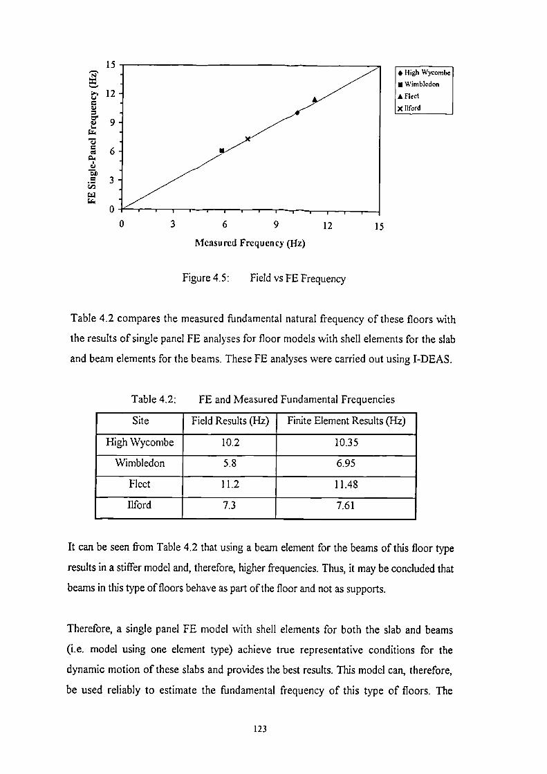
15• High Wycombe
• Wimbledon
• Fleet
X Ilford
0 3 6 9 12 15
Measured Frequency (Hz)
Figure 4.5: Field vs FE Frequency
Table 4.2 compares the measured fundamental natural frequency of these floors with
the results of single panel FE analyses for floor models with shell elements for the slab
and beam elements for the beams. These FE analyses were carried out using I-DEAS.
Table 4.2: FE and Measured Fundamental Frequencies
Site Field Results (Hz) Finite Element Results (Hz)
High Wycombe 10.2 10.35
Wimbledon 5.8 6.95
Fleet 11.2 11.48
Ilford 7.3 7.61
It can be seen from Table 4.2 that using a beam element for the beams of this floor type
results in a stiffer model and, therefore, higher frequencies. Thus, it may be concluded that
beams in this type of floors behave as part of the floor and not as supports.
Therefore, a single panel FE model with shell elements for both the slab and beams
(i.e. model using one element type) achieve true representative conditions for the
dynamic motion of these slabs and provides the best results. This model can, therefore,
be used reliably to estimate the fundamental frequency of this type of floors. The
123

model also allow the beams to bend in both orthogonal directions which is more realistic
because of their longer spans. Further studies have, therefore, been based on this
model.
Figures 4.6 to 4.8 below shows the typical 1-panel, 2-panel and 3-panel models for
the floor type under consideration.
124

n:c;
71:1.)u.=I:10
• •-n
V•4
125

126
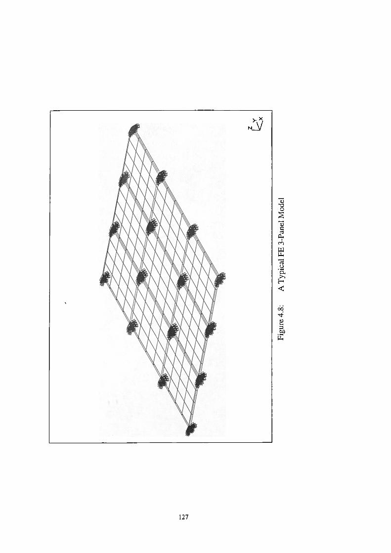
127

4.1.2 Parametric Studies
The single panel FE model was used to study the variation of fundamental frequency with
the span/depth ratios in both directions of the floor slab; and the maximum static
deflections. The thickness of the slab was the only variable changed in the model. Static
and dynamic analyses of the model then yielded maximum static deflections and floor
frequencies for each slab thickness, respectively. These analyses were carried out for self-
weight only and no super-imposed load was considered. In practice, any extra loading
would reduce the frequencies and increase the deflections. However, in the FE analyses
the inclusion of these loads would only affect the frequencies if they are modelled as an
equivalent slab thickness of density equal to that of concrete. This, however, would also
increase the stiffness and thus raise the frequencies. Thus, the effect of modelling the
super-imposed loads in this way are negligible and were, therefore, not considered.
The analyses were restricted to a maximum frequency range of interest of 15 Hz and,
therefore, slab thicknesses which resulted in higher frequencies were not used in studying
these variations. The analyses were, however, carried out below the minimum frequency
limits only to establish these limits. However, a minimum slab thickness of 125 mm was
used for all the floors to achieve lower frequencies. The upper limit of slab thickness
resulting in the maximum frequencies of 15 Hz was variable for all the floors, depending
on their span/depth ratios in each direction.
Since the Canadian Code, CSA (1985, 1989), requires a full dynamic analysis for floors
with fundamental frequencies below 6 Hz, this frequency was used as a minimum in the
parametric studies.
128
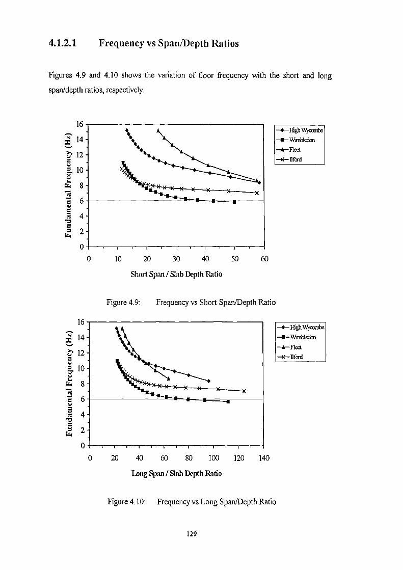
.1
.1
0 20 40 60 80 100 120
140
0
,
—4— lIgh WYcanhe--II— \Nimble:kit
—A—fleet
--X-11 fad
4.1.2.1 Frequency vs Span/Depth Ratios
Figures 4.9 and 4.10 shows the variation of floor frequency with the short and long
span/depth ratios, respectively.
16- -*— High WYconte—I—don—A—Fleet
- -X— Ilford
0
o 10 20 30 40 50 60
Short Span / Slab Depth Ratio
Figure 4.9: Frequency vs Short Span/Depth Ratio
Long Span / Slab Depth Ratio
Figure 4.10: Frequency vs Long Span/Depth Ratio
129

From Figures 4.9 and 4.10, it may be noted that the graphs of span/depth ratios against
floor fundamental frequencies follow a general trend but differ in shape due to the different
dimensions of the beams. The difference in the ordinates, however, is due to the different
stiffnesses caused by the span/depth ratios and beam and column dimensions of each floor.
It is clear from Figures 4.9 and 4.10 that a maximum span/depth ratio of 42 for the slab's
short span direction (normal to beams) and 78 for the slab's long span direction
(along beams), respectively, would ensure a minimum fundamental frequency of 6 Hz for
this floor type. It may be noted, therefore, that the Ilford floor donot satisfy this
requirement (see Table 4.3).
Assuming that the fundamental frequencies of the single-panel FE model are correct, it can
be concluded that all the floors tested satisfy the minimum frequency requirement.
However, the high frequency of Ilford floor even for higher short and long span/depth
ratios is due to the contribution of beams and the extra stiffness provided by columns. It
has been shown previously that beams behave as part of the floors and not as supports but
they increase local stiffness which plays an important role in using high span/depth ratios
for the slab. Generally, a lower span/depth ratio is obtained for a floor with a wide beam
of large cross-section area and a higher span/depth ratio is obtained for a floor with a
narrow beam of small cross-section area (see Table 4.1, Figures 4.9 and 4.10 and Table
4.3).
Table 4.3: Span/Depth Ratios of the Tested Floors
Site Short Span/Depth Ratio Long Span/Depth Ratio
High Wycombe 34.8 57. 4
Wimbledon 37.5 70.0
Fleet 36.0 40.0
Ilford 45.0 97.5
130

(4.1)
4.1.2.2 Frequency vs Deflection Relationship
Figures 4.11 shows the variation of floor frequency with maximum static deflections.
—*-- High Wycombe
—M-- Wimbledon
--i-- Fleet
—X-- Ilford
0
0 3 6 9 12 15
Maximum Static Deflections (mm)
Figure 4.11: Frequency vs Static Deflections
Figure 4.11 shows that the variation of static deflections against corresponding floor
frequency generally follows a consistent trend. The difference in the shape of these curves
is due to the different dimensions of the beams. A trendline least-squares curve-fit shows
that these relationships are of the following form:
Equation 4.1 is a modified form of the more well-known formula f = —1
III- for a2 71- As
SDOF spring-mass system (see also section 1.2.3). The constant K as determined by
curve-fitting is given in Table 4.4 below:
131
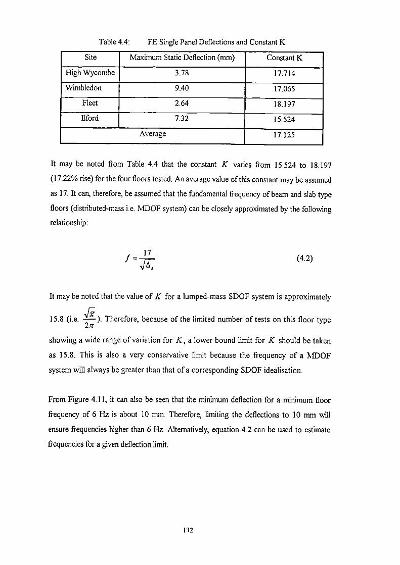
Table 4.4: FE Single Panel Deflections and Constant K
Site Maximum Static Deflection (mm) Constant K
High Wycombe 3.78 17.714
Wimbledon 9.40 17.065
Fleet 2.64 18.197
Ilford 7.32 15.524
Average 17.125
It may be noted from Table 4.4 that the constant K varies from 15.524 to 18.197
(17.22% rise) for the four floors tested. An average value of this constant may be assumed
as 17. It can, therefore, be assumed that the fundamental frequency of beam and slab type
floors (distributed-mass i.e. MDOF system) can be closely approximated by the following
relationship:
17f =
,j,:,
It may be noted that the value of K for a lumped-mass SDOF system is approximately
Nr15.8 (i.e. —f-). Therefore, because of the limited number of tests on this floor type
2ir
showing a wide range of variation for K, a lower bound limit for K should be taken
as 15.8. This is also a very conservative limit because the frequency of a MDOF
system will always be greater than that of a corresponding SDOF idealisation.
From Figure 4.11, it can also be seen that the minimum deflection for a minimum floor
frequency of 6 Hz is about 10 mm. Therefore, limiting the deflections to 10 mm will
ensure frequencies higher than 6 Hz. Alternatively, equation 4.2 can be used to estimate
frequencies for a given deflection limit.
(4.2)
132

4.2 Post-Tensioned Concrete Solid Flat Slab Floors
The FE modelling of the twelve floors of this type was carried out using ANSYS
software. All of these floors were continuous in both directions with variable column
dimensions and span lengths in both directions (see Figure 3.6). However, the study
was limited to 3x3 adjacent panels only, to study the effect of continuity of the floor
on the fundamental frequency and if a more detailed model improves the accuracy of the
result. Models in steps of a single panel and upto 3x3 panels where possible were,
therefore, analysed. Major details of modelling of this floor type are the same as those
discussed in section 4.1, except that in this case there are no beams to model.
4.2.1 Single Panel vs Multi-Panel Models
Table 4.5 compares the measured fundamental frequency of these floors with the
results of FE analyses for floor models with shell elements for the slab.
Table 4.5: FE and Measured Fundamental Frequencies
Site Fundamental Frequency (Hz)
Field Results Finite Element Results
1 Panel 2 x 2 Panels 3 x 3 Panels
Hammersmith 8.1 8.41 9.25 9.81
Fleet 5.9 6.18 6.58 N/A
London 10.1 10.96 12.21 12.81
Worcester 12.7 14.19 15.90 16.69
Worcester 9.1 9.98 10.70 N/A
Birmingham 7.2 8.00 8.61 8.66
Birmingham 8.6 9.28 10.03 10.18
Birmingham 12.7 14.44 15.61 15.84
London 8.4 9.48 10.53 N/A
London 10.6 11.15 10.53 N/A
Winchester 10.3 10.32 10.81 N/A
Winchester 8.5 9.19 9.80 9.94
133

-T-
2 3 4 5 6 7 8 9 10 11 12 13 14 15
15
1413
71=
u
12
5=471..
10
9
• 87.iclt
7
6
TAc
5
iii 4;14
,3
210
It can be seen from Table 4.5 that a single-panel model closely approximates the
fundamental frequency of this floor type. This conclusion is identical to that given in
section 4.1. Therefore, all other relevant comments in section 4.1.1 apply here as well.
Also, the 2 and 3-panel models show a consistent over-estimation of fundamental
frequency. This is considered to be caused by the dimensions and boundary conditions of
adjacent panels not always being the same.
The comparison of field and FE results for the single-panel FE model are plotted in
Figure 4.12.
• Hammersmith
• Fleet
• London
X Worcester
• Worcester
• Birmingham
+ Birmingham
- Birmingham
0 London
0 London
0 Winchester
A Winchester
Measu red Frequency (Hz)
Figure 4.12: Field vs FE Frequency
Figures 4.13 to 4.15 below shows the typical 1-panel, 2-panel and 3-panel models of
this floor type.
134

135

4t:
=toi..1.L...
136

137

—A— Hammersmith
—10--Fleet
—A—London
Worcester
--A— Worcester
—0—Birmingham
— I—Birmingham -
—e-- London
—6-- London
—a-- Winchester
—6— Winchester
4.2.2 Parametric Studies
The single panel FE model was used to study the variation of fundamental frequency with
the span/depth ratios in both directions of the floor slab; and the maximum static
deflections, in a manner similar to that given in section 4.1.2.
The thickness of slab only was varied in the model. Static and dynamic analyses of the
model then yielded maximum static deflections and floor frequencies for each slab
thickness, respectively.
4.2.2.1 Frequency vs Span/Depth Ratios
Figures 4.16 and 4.17 shows the variation of floor frequency with the short and long
span/depth ratios, respectively.
0
10
20
30
40 50
60
70
Short Span / Slab Depth Ratio
Figure 4.16: Frequency vs Short Span/Depth Ratio
It is clear from Figure 4.16 above that a maximum span/depth ratio of 33.5 for the short
span direction will ensure frequencies above 6 Hz.
138

2
,10 20 30 40 50
60
70
4
—•—liammersmith
—if—Fleet
- -&— London
—if— Worcester
—ik-- Worcester
—4--Birmingham
—I—Birmingham -
—e— London
—4-- London
—0— Winchester
—6— Winchester
Long Span / Slab Depth Ratio
Figure 4.17: Frequency vs Long Span/Depth Ratio
It is clear from Figure 4.17 above that a maximum span/depth ratio of 47.8 for the long
span direction will ensure frequencies above 6 Hz.
Figures 4.16 and 4.17 shows that the graphs of span/depth ratios against floor
fundamental frequencies follow a general trend and similar shape. This is due to the
homogeneous nature of the floor and absence of any beams. The difference in the
ordinates, however, is due to the different stiffnesses caused by the span/depth ratios and
column dimensions of each floor.
Therefore, in order to avoid fundamental frequencies below 6 Hz for this floor type, it is
necessary to use span/depth ratios of upto 33.5 for the short span direction and 47.8 for
the long span direction. It may be noted, therefore, that the Worcester floor (Test-4)
donot satisfy this requirement (see Table 4.6).
Assuming that the fundamental frequencies of the single-panel FE model are correct, it can
be concluded that all the floors tested satisfy the minimum frequency requirement.
However, the high frequency of Worcester floor (Test-4) even for a higher short
span/depth ratio is due to the extra stiffness provided by columns.
139

Table 4.6: Span/Depth Ratios of the Tested Floors
Site Short Span/Depth Ratio Long Span/Depth Ratio
Hammersmith 32.0 37. 3
Fleet 32.0 47.6
London 32.0 32.0
Worcester 35.6 35.6
Worcester 28.8 33.6
Birmingham 28.8 38.2
Birmingham 33.3 35.6
Birmingham 21.4 22.9
London 30.0 30.0
London 25.0 30.0
Winchester 30.0 37.5
Winchester 29.1 32.7
140

4.2.2.2 Frequency vs Deflection Relationship
Figures 4.18 shows the variation of floor frequency with maximum static deflections.
20
18 -
2 -
0
0 3 6 9 12 15 18 21 24 27 30 33 36
Maximum Static Deflections (mm)
Figure 4.18: Frequency vs Static Deflections
—4-1-Lammersmith
--A— London
- Worcester
—-II— Worcester
—0-- Bi rmingham
—f—Birmingham -
—A—London
—4—London
—13— Winchester
--A— Winchester
Figure 4.18 shows that the variation of static deflections against corr
frequency generally follows a consistent trend. A trendline least-squares
that these relationships are of the same form as equation 4.1 obtained
beam and slab type floors (see section 4.1.2.2). The constant K for
given in Table 4.7 below:
esponding floor
curve-fit shows
earlier for the
these floors is
141

Table 4.7: FE Single Panel Deflections and Constant K
Site Maximum Static Deflections (mm) Constant K
Hammersmith 4.89 18.607
Fleet 8.67 18.209
London 2.96 18.852
Worcester 1.75 18.795
Worcester 3.50 18.687
Birmingham 5.29 18.408
Birmingham 4.10 18.804
Birmingham 1.67 18.804
London 3.96 18.871
London 2.80 18.692
Winchester 3.24 18.573
Winchester 4.15 18.724
Average 18.669
It may be noted from Table 4.7 that the constant K varies from 18.209 to 18.871
(3.64% rise) for the twelve floors tested. An average value of this constant may be
assumed as 18.7. It can, therefore, be assumed that the fundamental frequency of flat slab
type floors can be closely approximated by the following relationship:
18.7(4.3)
It may be noted, however, that this constant depends on the type of floor (see section
4.1.2.2). The above results donot show a wide range of variation for K and, therefore, a
conservative lower bound limit for K may be taken as 18.
From Figure 4.18, it can also be seen that the maximum deflection for a minimum floor
frequency of 6 Hz is about 9 mm. Therefore, limiting the deflections to 9 mm will ensure
frequencies higher than 6 Hz. Alternatively, equation 4.3 can be used to estimate
frequencies for a given deflection limit.
142

4.3 Pre-Tensioned Concrete Double-T Beam Floors
The FE modelling of the five floors of this type was carried out using I-DEAS software.
All floors are made of precast Double-T beams placed on inverted T or L-shaped
girders. The topping in the form of screed or asphalt layer serves as a bond between
these beams. Therefore, the FE modelling of this floor type included a single-beam
model and upto ten adjacent beams to study the effect of adjacent beams on floor
fundamental frequency and to determine if a more detailed model improves the
accuracy of the results. Major details of modelling of this floor type are the same as those
discussed in section 4.1, except the following:
Boundary Conditions
The beams were modelled as simply supported. This is the most realistic approach
considering that these precast beams are placed on the girders supported by bearing
pads.
Element Type
Linear isotropic quadrilateral thin shell elements were used for the flanges and linear
isotropic beam elements were used for the webs in the different double-T models
studied (see Figure 3.19). The webs of the double-T beams were approximated by a
rectangular beam section. The beam and the shell elements were connected by rigid
elements to define the correct restraint conditions for their displacements. This
achieved true representative conditions for the dynamic motion of these simply
supported long-span beams which essentially behave as one-way bending along the
span.
143
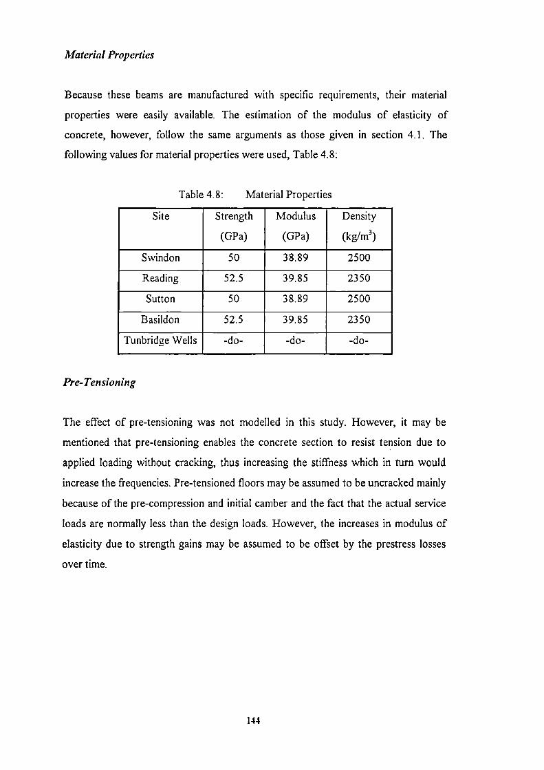
Material Properties
Because these beams are manufactured with specific requirements, their material
properties were easily available. The estimation of the modulus of elasticity of
concrete, however, follow the same arguments as those given in section 4.1. The
following values for material properties were used, Table 4.8:
Table 4.8: Material Properties
Site Strength
(GPa)
Modulus
(GPa)
Density
(kg/m3)
Swindon 50 38.89 2500
Reading 52.5 39.85 2350
Sutton 50 38.89 2500
Basildon 52.5 39.85 2350
Tunbridge Wells -do- -do- -do-
Pre-Tensioning
The effect of pre-tensioning was not modelled in this study. However, it may be
mentioned that pre-tensioning enables the concrete section to resist tension due to
applied loading without cracking, thus increasing the stiffness which in turn would
increase the frequencies. Pre-tensioned floors may be assumed to be uncracked mainly
because of the pre-compression and initial camber and the fact that the actual service
loads are normally less than the design loads. However, the increases in modulus of
elasticity due to strength gains may be assumed to be offset by the prestress losses
over time.
144

4.3.1 Single Beam vs Multi-Beam Models
Chen and Aswad (1994) have studied a series of beams in a floor model for the estimation
of frequencies. However, their studies are not based on experimental results. Since it has
been established earlier that a single-panel floor model closely approximates the
fundamental frequency of floors, this principle was applied to double-T beam type floors.
Therefore, FE models for the Swindon floor with one double-T beam and upto ten
adjacent double-T beams were studied for frequency estimation. In all FE models, the end
nodes representing beam elements were assumed to be simply supported. All other nodes
were free to move and rotate (see Figure 4.20). It was found that there was no effect of
adjacent beams on fundamental frequency and that the 1-beam model closely
approximates the fundamental frequency of the floor. Therefore, only the 1-beam model
was studied for all the remaining floors of this type.
Table 4.9 gives the measured fundamental frequency of these floors along with the
results of FE analysis.
Table 4.9: FE and Measured Fundamental Frequencies
Site Fundamental frequency (Hz)
Field Results FE Results
Swindon 4.9 4.6
Reading 5.6 5.2
Sutton 5.5 5.0
Basildon 4.6 4.4
Tunbridge Wells 5.8 5.2
It can be seen from Table 4.9 that a single-beam model closely approximates the
fundamental frequency of this floor type. The addition of adjacent beams do not affect this
frequency because they are of the same size. Because these low floor frequencies damp
out quickly due to inherent damping, additional beams or a more complete floor
model would, therefore, not affect the fundamental frequency significantly.
145

The comparison of field and FE results (Table 4.9) are plotted in Figure 4.19.
1 2 3 4 5 6 7 8 9 10
Measured Frequency (Hz)
Figure 4.19: Field vs FE Frequency
• Svinden
• Reading
• Suncn
• Basildcn
z Tunbridge Wells
Figure 4.19 above shows the close comparison of FE results with the experimental
results. It may be noted, however, that all the FE frequencies are lower-bound and,
therefore, conservative estimates.
Figure 4.20 and 4.21 shows the typical 1-beam and 10-beam models of this floor
type.
146

147

148

, i
4.3.2 Parametric Studies
The single-beam FE model was used to study the variation of fundamental frequency with
the beam length and the maximum static deflections, in a manner similar to that given in
section 4.1.2. In this study, only the length of the beam was varied and fundamental
frequency and static deflections evaluated.
Since the fundamental frequencies of double-T floors studied here were found to be below
6 Hz (Canadian Code requirement), a minimum fundamental frequency of 4.5 Hz was
chosen for satisfactory vibration response. This frequency is more than twice the average
walking frequency of 2 Hz and being not an exact multiple of walking frequency, is
unlikely to be excited by people walking. Therefore, this frequency was used as a
minimum in the parametric studies.
4.3.2.1 Frequency vs Beam Length
Figure 4.22 shows the variation of floor frequency with beam length.
--•— Sv,indon
—4—Reading/Wells
—ti— Sutton
—X— Basildon
6 8 10 12 14 16 18 20
Beam Length (m)
Figure 4.22: Frequency vs Beam Length
149

0
Table 4.10 gives the proposed span length limits based on a minimum fundamental
frequency of 4.5 Hz. It may be noted, however, that the experimental fundamental
frequency of the Basildon floor satisfy this requirement whereas its FE model result
doesnot.
Table 4.10: Proposed Spans for the Tested Floors
Site Original Span (m) Proposed Span (m)
Swindon 16.045 16.2
Reading 15.4 16.6
Sutton 15.6 16.4
Basildon 15.7 15.4
Tunbridge Wells,
15.4 16.6
4.3.2.2 Frequency vs Deflection Relationship
Figure 4.23 shows the variation of floor frequency with beam deflections.
—0— Svdndon
—s-- Reading/Wells
--et— Sutton
--X— Basildon
2 4 6 8 10 12 14
Maximum Static Deflections (mm)
Figure 4.23: Frequency vs Static Deflections
150

Figure 4.23 shows a single curve following an average relationship of the form of
equation 4.1, obtained earlier for beam and slab and flat slab type floors. The constant
K is given in Table 4.11 below.
Table 4.11: FE Single Beam Deflections and Constant K
Site Maximum Static Deflections (mm) Constant K
Swindon 15.0 17.72
Reading 11.5 17.72
Sutton 12.7 17.73
Basildon 16.6 17.73
Tunbridge Wells 11.5 17.72
Average 17.72
It may be noted from Table 4.11 that the constant K varies from 17.72 to 17.73
(0.06% rise) for the five floors tested. An average value of this constant may be
assumed as 17.7. Therefore, the fundamental frequency of double-T beam type floors
can be closely approximated by the following relationship:
17.7f= ,—
vAs
Since the above results donot show a wide range of variation for K, a conservative
lower bound limit for K may be taken as 17.5.
From Figure 4.23, it can also be seen that the maximum self-weight deflection for a
minimum fimdamental frequency of 4.5 Hz is about 8.5 mm. Therefore, limiting the
deflections to 8.5 mm will ensure frequencies higher than 4.5 Hz. Alternatively,
equation 4.4 can be used to estimate frequencies for a given deflection limit.
(4.4)
151

4.4 Composite Steel-Concrete Slab Floors
The FE modelling of the eight floors of this type was carried out using I-DEAS software.
All of these floors are continuous in both directions and are made of concrete slabs
supported on a steel profile which is welded to steel beams and girders (see Figure
3.25 and Appendix A.4). Based on previous floor modelling, only a single-panel of
these floors was modelled. Major details of modelling of this floor type are the same as
those discussed in section 4.1, except the following:
Boundary Conditions
The steel columns were modelled as simply supported at their centroid at the four
corners of the single-panel FE model. This is the most realistic approach considering
that the steel beams and girders are riveted to these columns. In the case of Millwall
Stadium floor, however, the two north columns were encased in a concrete column of
780 mm diameter. These were, therefore assumed fixed at the perimeter of the
column (assumed as 780 mm x 780 mm).
Element Type
Shell elements were used for the slab and beam elements were used for the beams and
girders (see section 4.1). The slab was modelled in two different ways: of uniform
slab thickness and of actual slab profile dimensions (for calculations, see Appendix
B.4). In both cases shell elements were used. In the case of actual slab profile,
however, the profile was modelled as shells in vertical plane (see section 4.1). The
beam and girder elements were connected to the shell elements by rigid elements to
represent the welded joints and define the correct constraint for their displacements.
152

Material Properties
Relevant data for the composite floors were taken from the brochures of Precision Metal
Forming Limited on Composite Floor Decking Systems [71]. The following material
properties were used in all calculations for these floors (see also section 4.1):
Concrete
Density (pc ) 1900 Kg/m3
Compressive strength (Li ) Grade 40 (i.e. 40 N/mm2)
Modulus of elasticity (E, ) 22 KN/mm2
The modulus of concrete (E, ) has been suggested by Wyatt (1989) as 22 ICN/nun2
for composite floors with light-weight concrete.
Steel
Density (ps ) 7820 Kg/m3
Modulus of elasticity (Es ) 206.8 ICN/rrun2
These values have been used as default for steel in I-DEAS and have, therefore, been
assumed for all calculation purposes.
4.4.1 Single Panel Models
Table 4.12 compares the measured fundamental frequency of these floors with the
results of single panel FE models. Results for both types of models studied are
included.
153
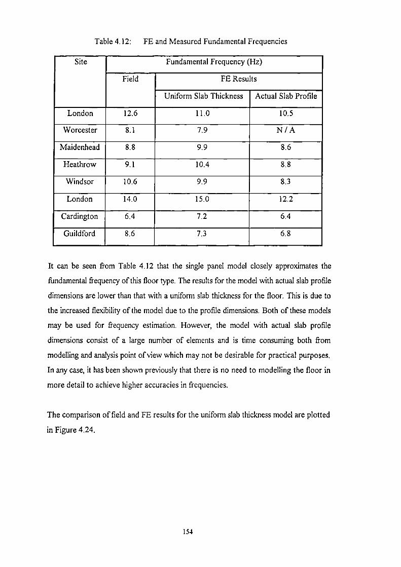
Table 4.12: FE and Measured Fundamental Frequencies
Site Fundamental Frequency (Hz)
Field FE Results
Uniform Slab Thickness Actual Slab Profile
London 12.6 11.0 10.5
Worcester 8.1 7.9 N/A
Maidenhead 8.8 9.9 8.6
Heathrow 9.1 10.4 8.8
Windsor 10.6 9.9 8.3
London 14.0 15.0 12.2
Cardington 6.4 7.2 6.4
Guildford 8.6 7.3 6.8
It can be seen from Table 4.12 that the single panel model closely approximates the
fundamental frequency of this floor type. The results for the model with actual slab profile
dimensions are lower than that with a uniform slab thickness for the floor. This is due to
the increased flexibility of the model due to the profile dimensions. Both of these models
may be used for frequency estimation. However, the model with actual slab profile
dimensions consist of a large number of elements and is time consuming both from
modelling and analysis point of view which may not be desirable for practical purposes.
In any case, it has been shown previously that there is no need to modelling the floor in
more detail to achieve higher accuracies in frequencies.
The comparison of field and FE results for the uniform slab thickness model are plotted
in Figure 4.24.
154
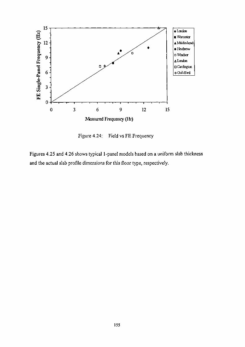
• Laxion
• Worcester
•
ivitidenhead
Heathrow
o Windsor
A Lcndon
0 Cardingtan
0 Guildford
0
3
6
9 12
15
Measured Frequency (Hz)
Figure 4.24: Field vs FE Frequency
Figures 4.25 and 4.26 shows typical 1-panel models based on a uniform slab thickness
and the actual slab profile dimensions for this floor type, respectively.
155

,..riesi
•zi
4.)u.=
tO
t.T.4
156

157
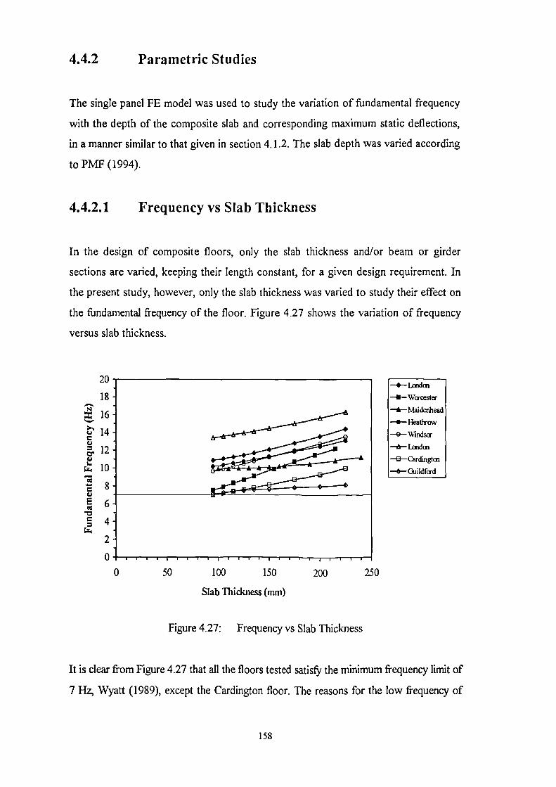
, • i r , I , , , ,
b_.-6-&-ii-6- ,.•
._.-4-•-*--
4.4.2 Parametric Studies
The single panel FE model was used to study the variation of fundamental frequency
with the depth of the composite slab and corresponding maximum static deflections,
in a manner similar to that given in section 4.1.2. The slab depth was varied according
to PMF (1994).
4.4.2.1 Frequency vs Slab Thickness
In the design of composite floors, only the slab thickness and/or beam or girder
sections are varied, keeping their length constant, for a given design requirement. In
the present study, however, only the slab thickness was varied to study their effect on
the fundamental frequency of the floor. Figure 4.27 shows the variation of frequency
versus slab thickness.
50 100 150 200 250
Slab Thickness (mm)
Figure 4.27: Frequency vs Slab Thickness
It is clear from Figure 4.27 that all the floors tested satisfy the minimum frequency limit of
7 Hz, Wyatt (1989), except the Cardington floor. The reasons for the low frequency of
20
18 -
`.1 16 -
ct" 14 -=4.,0.° 12 -
10 -
71. 8
1 6-c,§ 4.1.1
2 -
0 - 0
—4— Londcn
—ii— Wcrcester
—A—Maidenhead
--A— Heathrow
—e— Windsor
—6— London
—El— Cardingtcn
—0— Guildfcrd
158
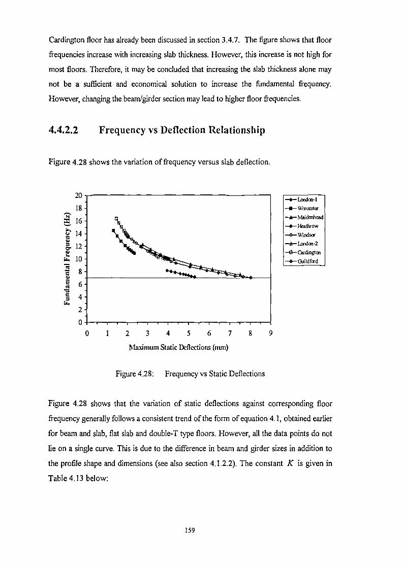
Cardington floor has already been discussed in section 3.4.7. The figure shows that floor
frequencies increase with increasing slab thickness. However, this increase is not high for
most floors. Therefore, it may be concluded that increasing the slab thickness alone may
not be a sufficient and economical solution to increase the fundamental frequency.
However, changing the beam/girder section may lead to higher floor frequencies.
4.4.2.2 Frequency vs Deflection Relationship
Figure 4.28 shows the variation of frequency versus slab deflection.
20 —A— Linda-1
—II— Wcreester
—A— Maidenhead
—A— Heathrow
—0—Windsor
—A— Londcn-2
—E3— Cardingtcn
—4— Guildford
6 7 8 9
Maximum Static Deflections (mm)
Figure 4.28: Frequency vs Static Deflections
Figure 4.28 shows that the variation of static deflections against corresponding floor
frequency generally follows a consistent trend of the form of equation 4.1, obtained earlier
for beam and slab, flat slab and double-T type floors. However, all the data points do not
lie on a single curve. This is due to the difference in beam and girder sizes in addition to
the profile shape and dimensions (see also section 4.1.2.2). The constant K is given in
Table 4.13 below:
159

Table 4.13: FE Single Panel Deflections and Constant K
Site Maximum Static Deflections (mm) Constant K
Uniform Slab Thickness Actual Slab Profile
London 2.28 2.41 14.996
Worcester 6.81 3.78 16.448
Maidenhead 4.04 8.60 19.982
Heathrow 3.45 8.78 19.437
Windsor 3.95 8.33 20.107
London 1.70 12.23 19.097
Cardington 7.65 6.59 20.087
Guildford _ 5.14 5.81 18.834
Average 18.624
It may be noted from Table 4.13 that the constant K varies from 14.996 to 20.107
(34.08% rise) for the eight floors tested. An average value of the constant K may be
assumed as 18.6. It can, therefore, be assumed that the fundamental frequency of
composite floors can be closely approximated by the following relationship:
18.6 (4.5)
The above results show a wide range of variation for K and since the minimum value
of this constant for a MDOF system is 15.8 (see section 4.1.2.2), a conservative
lower bound limit of K may be taken as 15.8.
From Figure 4.28, it can also be seen that the maximum deflection for a minimum floor
frequency of 7 Hz is about 5.5 mm. Therefore, limiting the deflections to 5.5 mm will
ensure frequencies higher than 7 Hz. Alternatively, equation 4.5 can be used to
estimate frequencies for a given deflection limit.
160

Chapter 5 COMPARISONS
This Chapter presents the comparisons of the experimental fundamental frequency of all
the floor slabs tested with the analytical methods given in Chapter 1. The results from only
the methods appropriate to each category are compared. This is followed by brief
comments on the use of each method. Typical calculations for each floor category are
given in Appendix B.
5.1 Post-Tensioned Concrete 1-Way Spanning Solid
Floor Slabs with Beams
Table 5.1 below compares the results obtained by the analytical methods with the
experimental results for the four floors of this type. Typical calculations for the High
Wycombe floor are given in Appendix B.1.
161

e".•
0
a)
f:21
\40
rei 'e.7-1 b() r7-1
•arLel 00
•n•11 kr)
..6ciN
cs1
tri
vi.<1"
n.0
0:5
'0•
LL4
••n11
v")kr)
en
kri
eu
1-4
tr) CN
00 ci
162

5.1.1 Discussion
Based on the results for the four floors given in Table 5.1 above, the estimation of
fimdamental frequency of this type of floor can be summarised as follows:
EBM: This method provides two estimates of the fimdamental frequency. The
simple support assumption for the equivalent beam always under-
estimates the fundamental frequency whereas the fixed support
assumption always over-estimates this frequency.
PM: This method provides two estimates of the fundamental frequency. The
simple support assumption does not produce consistent estimates of the
fundamental frequency whereas the corner support assumption always
under-estimates this frequency.
CSM: This method offers two estimates. One estimate along the short span
direction is always an under-estimate. The estimates using the long-span
direction is not consistent.
FEM: This method offers the closest possible estimates.
SDM: This method provides three estimates of the fundamental frequency. The
estimates may be based on the SDOF formula or the modified SDOF
formula developed in this research. In the SDOF formula, deflections may
be assumed for the EBM or PM approaches. For the EBM approach, the
simple support deflections always under-estimate the fundamental
frequency whereas the fixed support deflections always over-estimate this
frequency. The PM deflections are difficult to estimate and, therefore,
have not been used here. However, the modified SDOF formula using the
maximum deflection from the static analysis of the single panel FE model
provides the closest estimates.
163

0.6 0.7 0.8 0.9 1
5.1.2 Equivalent Beam Span Length
As noted in section 5.1.1, the EBM method for simple support conditions provide
frequency estimates lower than the experimental results whereas the fixed support
conditions provide higher estimates. Therefore, both the support conditions are not
correct if EBM approach is to be used for frequency estimation. However, the EBM
formula for simple supports could be used for frequency estimation if the beam span
length taking part in vibrations is correctly identified. Figure 5.1 shows the relationship for
the estimation of an equivalent span length for the EBM formula for simple supports for
the estimation of fundamental frequency of the floor.
Equivalent Span / Actual Span
—*— Ffigh Wycombe
—s— Wimbledon
—A— Fleet
—X— 11 ford
Figure 5.1: Estimation of Equivalent Span Length for EBM Formula
It may be noted from Figure 5.1 above that the EBM formula for the estimation of
fundamental frequency may be used reliably if the span length of the beam is reduced by a
factor between 0.825 and 0.925. The full length of the beam does not take part in
vibrations due to restraints or end conditions at the column supports. It also depends on
the slab thickness and beam cross-section area. Thus, if the EBM method is to be used
instead of a single-panel FE model, the length of beam should be multiplied by a factor
between 0.825 and 0.925. The choice is arbitrary because not enough experiments have
164

been carried out on this floor type. However, for conservative estimates, a factor of 0.925
or close to it may be used as a first approximation. Note, however, that the curves for the
High Wycombe and Wimbledon floors overlap.
5.2 Post-Tensioned Concrete Solid Flat Slab Floors
Table 5.2 below compares the results obtained by the analytical methods with the
experimental results for the twelve floors of this type. Typical calculations for the
Hammersmith floor are given in Appendix B.2.
5.2.1 Discussion
Based on the results for the twelve tests given in Table 5.2 above, the estimation of
fundamental frequency for this type of floor can be summarise as follows:
EBM: Same conclusions as in section 5.1.1.
PM: This method provides two estimates of the fundamental frequency. The
simple support assumption always over-estimate the fundamental
frequency whereas the corner support assumption generally under-
estimates this frequency (except in the case of Test # 6).
CSM: Same conclusions as in section 5.1.1.
FEM: Same conclusions as in section 5.1.1.
SDM: Same conclusions as in section 5.1.1.
165
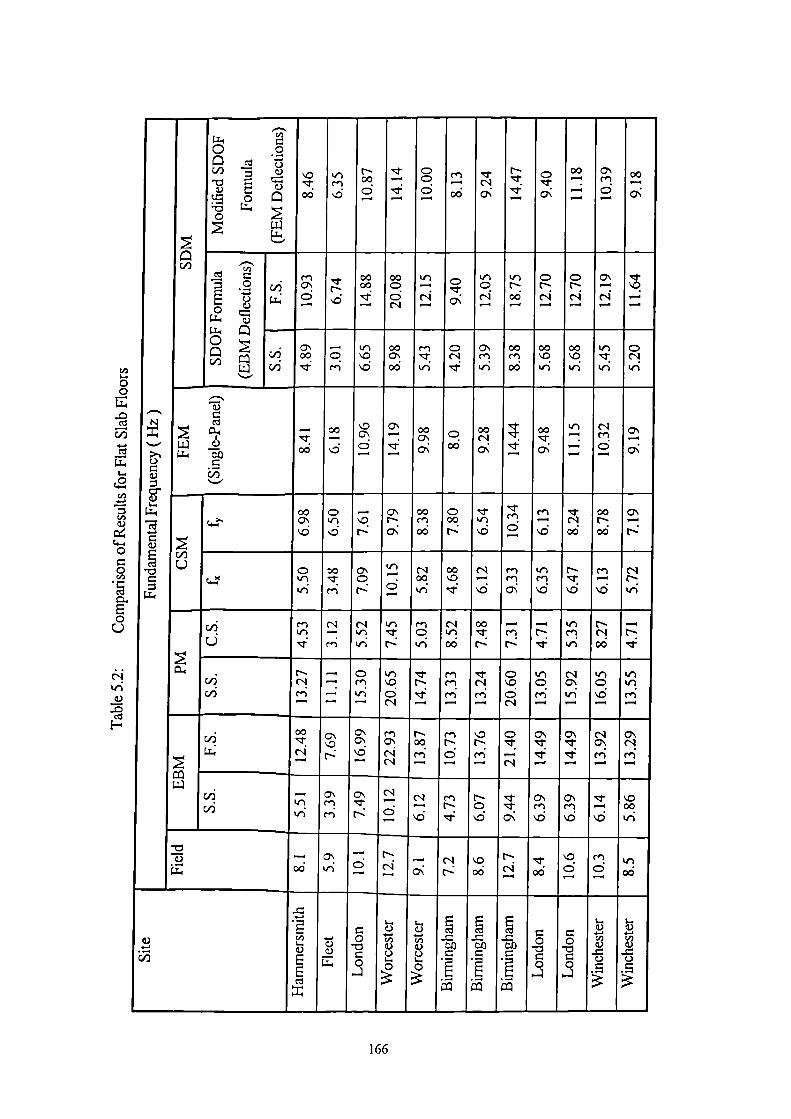
,`"•
.....,
co==
g"a:
t
g0=w
(.6-0
(:)En
Lx.
0
C)VI
-coi)-0o
....,.
ce/o
tt .15'= 0)
=! c-)
ca.
L.1.1
..,
,c)
,,,.zi:
v.,
,orn.
t--00
c:5
T1-.---.
4
CD0ci.
(4.,,06
.,j_c.sic::
r--'d-
4
c,,r,:j
00-:
-.
ONcv,6
00,
c:).
co=
0
0
CIU)
---,0c0. _.2.=
'-'q
envi ONr.„; c6
,J.(..,.
,a
00004
000co;
kr) c,.--. ,rN
Er,o
N
kr)c--.00
0r--
N
0r---N
0)-.c-4
S,--.
• anU,00CIS d:
--cp.en
Er,vc<5
oocnoci
en C•Zr Nkr; 'Ci
CsenEri
00enDO
00'0Eri
00kotri
If)vtr;
0Ntri
,--,a)C9
arij.) CULL' c
i./)......,
,..,;:r
06
00-
n..0ON
6
ON,-.4
COCDON
0: c'ci
00
0:
4
4
00
0:
t n
''''
N
6
ON
0;
coON<5
co'4n.6
--.6t-
ONt--o:
00 CDcn oooc; t.
'f)c:o
Tr(.,,
6
en,•1
kt6
1-N
cc;
ooN
06
ON,-1
c4.40V1
Er;.:1-en
ON0
r-:
tr)
•
(z)
N 0000 nID
kr; •ci:
N,--,n6
enenan
ix)env:5
r.-v.nth
en,-,v5
Nt---tri
c/i0
enkr)
.zi:
N.--.ri
Nkr)
kri
inNzl-
t--:
en NC) V)kri ot5
00.1-S
—.enS
,--.sv:
oilentr;
l---c..)ci
,-1s.1:
a.,C/iCii
hNr'i,—.
—---.—;—
cenLri—,
Lr,n.06c..4
'1- ent-- en•zr: ri,—. •nn•
..1-Nrei••n•
oVD6N
In0ee;vnI
NONtri1n1
trl0n.t59n1
Illt/1reirnI
01
viLL;
00'4.c‘i
cN
r.:
C.,‘ON
,1:5--
enONc,iN
t-- en00 t---ri 6.--, vnI
VDts-eeis n
CD'I'--.N
ON'4'.1:—
ON'I',:i,--i
NONeii1n1
ONNc4-;1n1
f.1.1vi
Vi
-Lntri
CTencn
ON-1-S
CI—
6
N (4-1--, sv5 .1:
sCn6
.1-d-on
CAenv:5
ONennci
'cl-,--1\a
n.000tri
-ti75. -fao
,--.oeS
cniri
--c:::5
N•
C`I•- - NCJn t--:
VDati
sc`i
•zr
c:(5vD6
cn6
kr)
v5
a).-;-..VI
..=
• "6"),-.0
E
•0
t.0
7.
-g
3
at6U
'5
at g6 - 5C..) =
t" 1CCI
g- go=
*Ef:4
g- 5C
*E(=CI
=0-0=
°
=°-0=
3
"6=
.5
'"6..=
.5
166

5.2.2 Equivalent Beam Span Length
Following on the reasons given in section 5.1.2, Figure 5.2 shows the relationship for the
estimation of an equivalent span length for the EBM formula for simple supports for the
estimation of fundamental frequency of flat slab floors.
C.)
CIJ
C.)
C.)
CV
COL1.1
5
4.5 -
4 -
3.5
3
2.5 -
2
1.5 -
'*•-•••oe*Mb 14..*
• ._ .• .• • •- -
i—0— Flamm ersm th
—II— Fleet
don—A-- Lon
Worcester--X—
Worcester--A--
--e— Birmingham
inB irm gh am
— Birmingham
Lon don—A—
London—0—
—e— Winchester
Win--A-- eh ester
1
0.5 -
0
,••• ••.;
0.5 0.6 0.7 0.8
0.9
1
Equivalent Span /Actual Span
Figure 5.2: Estimation of Equivalent Span Length for EBM Formula
As in section 5.1.2, it may be noted from Figure 5.2 above that the EBM formula for the
estimation of fundamental frequency may be used reliably if the span length of the beam is
reduced by a factor between 0.7 and 0.9. This relatively wide range is due to the fact that
these floor types do not have beams and are essentially 2-way slabs. The use of EBM
formula for these floors is not directly applicable. However, it may still be used for quick
and conservative estimates. Thus, if the EBM method is to be used instead of a single-
panel FE model, the length of beam should be multiplied by a factor between 0.7 and 0.9.
For conservative estimates, a factor of 0.9 or close to it may be used as a first
approximation.
167
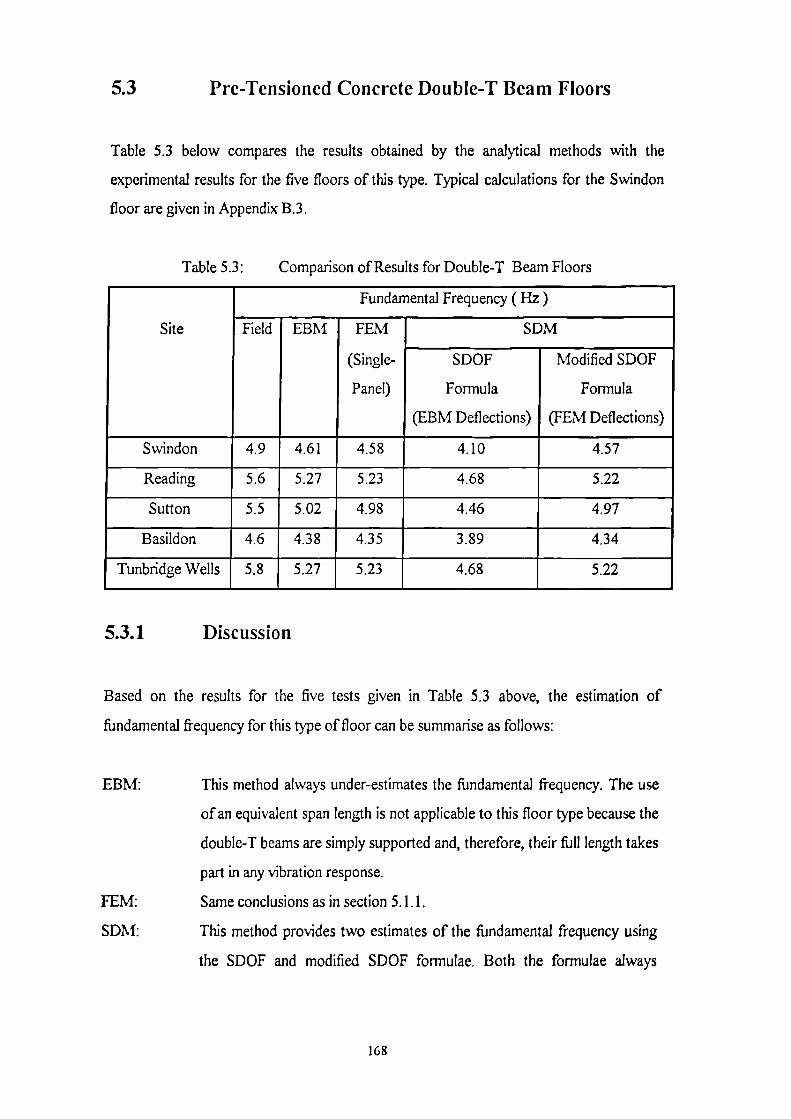
5.3 Pre-Tensioned Concrete Double-T Beam Floors
Table 5.3 below compares the results obtained by the analytical methods with the
experimental results for the five floors of this type. Typical calculations for the Swindon
floor are given in Appendix B.3.
Table 5.3: Comparison of Results for Double-T Beam Floors
Site
Fundamental Frequency ( Hz )
Field EBM FEM
(Single-
Panel)
SDM
SDOF
Formula
(EBM Deflections)
Modified SDOF
Formula
(FEM Deflections)
Swindon 4.9 4.61 4.58 4.10 4.57
Reading 5.6 5.27 5.23 4.68 5.22
Sutton 5.5 5.02 4.98 4.46 4.97
Basildon 4.6 4.38 4.35 3.89 4.34
Tunbridge Wells 5.8 5.27 5.23 4.68 5.22
5.3.1 Discussion
Based on the results for the five tests given in Table 5.3 above, the estimation of
fundamental frequency for this type of floor can be summarise as follows:
EBM: This method always under-estimates the fundamental frequency. The use
of an equivalent span length is not applicable to this floor type because the
double-T beams are simply supported and, therefore, their full length takes
part in any vibration response.
FEM: Same conclusions as in section 5.1.1.
SDM: This method provides two estimates of the fundamental frequency using
the SDOF and modified SDOF formulae. Both the formulae always
168

under-estimates the fundamental frequency but the modified SDOF
formula results are better of the two.
5.4 Composite Steel-Concrete Slab Floors
The results obtained from the analytical methods are compared with the experimental
results for the ten floors of this type in Table 5.4 below. Typical calculations for the
Millwall floor are given in Appendix B.4.
5.4.1 Discussion
Based on the results for the eight tests given in Table 5.4 above, the estimation of
fundamental frequency for this type of floor can be summarise as follows:
EBM: This method offers better estimates of the fundamental frequency for
the case of beam supporting slab only. The use of an equivalent span
length is not applicable to this floor type because the steel beams are
simply supported at girders (as shown in FE modelling) and, therefore,
their full length takes part in any vibration response.
Dunkerly: This method does not produce consistent estimates of the fundamental
frequency.
SDM: The three different approaches of this method do not produce consistent
estimates for the fundamental frequency. The Wyatt and Allen-Murray
estimates are reasonably close. However, the frequency estimation
using FE deflections are the closest of the three methods.
FEM: Same conclusions as in section 5.1.1. The uniform slab thickness model
is simple as compared to the actual slab profile model and requires
considerably less CPU time for analysis.
169

8
0
8
8
,--.
.......
ca)=cra.)
..4a.'
CO
LLI
--aZtd
a)•-c) t.
LI 2cil at,
-0°
Ill6—
<I
Z
vDco:
ooGO
enco;
N
c`i.1-n6
..
o0n6
0!4g
E.-,9 .5i7j c.)
:a[-,
-0°
C).—
ON
hCYnCI n
Tt.6
CNon
0`r'
N m
°c/)
enN
. •—nS
eno:
C6
-zr0:
e'l4
s.6
t-stoo;
>,vs=
aa)
C)a...oEoU
-17-',1)
1aa
En
c;nD
Lti•:t.
a:t---on
ED
ons;52:
ootri
.<4
z
t...(1)
-12073c...
Nv-i—.
.06—.
CT
4—.kr)
r•-;—.\O
4.—.00csic•si
N—;—•
<---4
E8
C.1:1
75c9
a-1
Ncsi—
m,a
--.(--i•—•
c)4.—.
4ci•—•
TI.c-.4CA
VD.6
0kri
co-0
C CI›N
(Nil0
0
ri
__.-4-•t--
N.._....,<---z
o.•Ch
ciN.cl s•r".
<--...z
'7a)
-00
t---.—
en
.6N.
c`if:)
6C \
0:c nv6
•:1 -.6
0tri
18
. —JDE0
C.)
/....N>1
.--
—.
Cnenkri
—.13
enCn
—.00 (Ni
kr)tri
Z
1...• ....
CD4•n•
•—•c;•n••n
07I:1...
0 \
N•n•
0•ct:•n•
Tr
c•--:vnI
\Co
c=5vnI
<
---Z
E
8
h c.si•.0
0(-it-4
kr) 0c6
o0.6
,I..0
oN4 •
'
-071• —
.0csi
,....c6
00otS
•—•0.n
.06
c)4
.4-n6
:
.0 •oO
;
C)
iii
i=0
-00
3
atr,3a)t-.)8
3
-0c%111)
-a.)C)
-0
0.....•gx
1-9,
.0=
• —
N
0-t:a3
=0Voc
• —"0
8
-t:D8
c—-03 .';
I II
170

Chapter 6 CONCLUSIONS
The main objective of the research was to study the various analytical techniques for the
estimation of fundamental frequency of floors. This Chapter presents a summary of the
findings of the research on frequency estimation based on the comparisons made in
Chapter 5. A brief discussion is included on damping estimation and conclusions of a
parametric study of the FE models. Recommendations are suggested and some
suggestions are made for future research.
6.1 Conclusions
6.1.1 Frequency Estimation Methods
The various analytical techniques for the estimation of the fundamental frequency of floors
were reviewed in Chapter 1. The fundamental frequency for all the floors tested was
calculated by these methods and compared with the experimental results in Chapter 5.
Each method was found to have a different application and suitability for different floor
types. The following is a summary of the use of each method for the floors tested.
Equivalent Bean: Method (EM
The EBM depends on a reasonable estimate of an equivalent beam span and an effective
slab width supported by the beam, which is recommended in the BS 8110 (1985), for
beam and slab, and flat slab floors. The choice of equivalent beam span depends on the
boundary conditions and may range between 0.825 and 0.925 for the beam and slab type
floors and between 0.7 and 0.9 for the flat slab type floors, respectively. A conservative
equivalent beam span and a higher effective slab width may result in closer frequency
estimates. In general, the EBM gives good estimates of fundamental frequency and may
be used if a conservative estimates of equivalent beam span and effective slab width are
used.
,
171

The beam formula for simple supports is directly applicable to double-T floors because the
double-T beam units are simply supported; this is an assumption in the derivation of the
formula. Therefore, for all practical purposes, the beam formula can be used to predict the
fundamental frequency of double-T floors. For composite floors, the results for both the
cases of beam supporting the slab and girder supporting the beams are not consistent and
depends on the layout and section dimensions. For simplicity, therefore, the case of beam
supporting the slab may be used for initial estimates of the fundamental frequency.
Plate Method (PM)
The PM is not directly applicable to all the floors because the boundary conditions of the
panels tested are not either simply supported or corner supported. Also, the columns
supporting these slabs are monolithic with the slab resulting in a very rigid connection
around their perimeter. Therefore, they cannot be assumed as point supports and should
be modelled as fixed supports around their perimeter. The inconsistency in the results is
also due to the summation of stifthesses in both the directions. The presence of beams in
one direction, in the case of beam and slab floors, for example, result in a higher relative
stiffness. The PM is not applicable to double-T and composite floors. In the absence of
any exact formula for all the practical cases, the PM in its present form (equation 1.3,
section 1.2.2) is not recommended for fundamental frequency estimation.
Concrete Society Method (CSM)
The CSM is similar to EBM. It offers two estimates for the fundamental frequency in
which the number of panels in each direction plays a very important role. The CSM does
not identify whether all the panels in each direction should be considered or only those
with similar dimensions and support conditions. Obviously, this selection leads to
inaccurate results because reducing the number of panels increases the frequencies and
vice-versa. The CSM is not applicable to double-T and composite floors. Since this
method is not based on any experimental evidence and its application does not lead to any
reliable conclusions, it is not recommended for use.
172

Finite Element Method (FEM)
The FEM offers the closest possible frequency estimates but depends to a large extent on
the material properties and boundary conditions of the floors. Since a single constant value
of the concrete strength and thus the modulus of elasticity of concrete was assumed for all
the floors except where notified (in the case of double-T beam floors), some of the
frequency estimation is not very close. Since the single-panel model developed shows
good correlation in most cases, it may be reasonably assumed that if the actual strengths
were known for all the floors, accurate estimates of the fundamental frequency would
have resulted. The FE model, however, allows the analyst to vary the different parameters
in order to achieve higher frequencies and/or lower static deflections. The FEM can be
easily employed on any available FE package and is strongly recommended for both
fundamental frequency and static deflection estimates.
Static Deflection Method (SDA.)
The SDM leads to inaccurate estimates of the fundamental frequency except in the case of
static deflections obtained from FE analysis. The SDM, however, can be used reliably only
after necessary modification of the SDOF system frequency formula. The SDM requires
estimates of the maximum static deflection of the floors which can either be selected
before design or calculated from FEM for a single-panel or beam models. The modified
SDOF formula, therefore, offers flexibility in either controlling frequency or deflections of
the floors at the design stage.
For composite floors, both Wyatt's and Allen-Murray's approaches lead to reasonable
estimates of fundamental frequency and may be used in the absence of a FE package.
Dunkerly's Formula
The application of Dunkerly's formula to both the EBM and SDM approaches always
lead to an under-estimation of fundamental frequency. Since the frequency estimation of
the system by this formula depends on the two estimates of frequency for the beam and
girder elements, the results are not always consistent. This is because most floors are
inherently continuous and cannot be separated into individual components, this was noted
173

in the case of beam and slab type floors (section 4.1.1). This formula is, therefore, not
recommended for any frequency estimation at all.
6.1.2 Minimum Fundamental Frequency
In order to control vibration problems, it is vitally important to ensure a high fundamental
frequency for the floors at the design stage. Table 6.1 below gives the estimated range,
average and the recommended minimum fundamental frequencies for the floors
tested. It may be noted, however, that the recommended minimum fundamental
frequencies are for general purpose buildings and are based on CSA (1990) and
Wyatt (1989) with due consideration to the economy of construction.
Table 6.1: Fundamental Frequency Estimates
Floor Type Fundamental Frequency (Hz)
Estimated Range Average Recommended Minimum
Beam and Slab 5.8-11.2 8.6 6.0
Flat Slab 5.9-12.7 9.4 6.0
Double-T Beam 4.6-5.8 5.3 4.5
Composite 6.4-14.0 9.8 7.0
From Table 6.1, it is clear that both the maximum estimated and average fundamental
frequencies are for composite floors. The above minimum fundamental frequencies
are recommended to avoid any objectionable vibrations due to walking at or near a
frequency of 2 Hz. This is because floor frequencies above the second harmonic of
walking frequency or not an exact multiple of that has been found to be difficult to
excite by normal daily life activities.
174

6.1.3 Damping Estimation
The inherent floor damping depends mainly on the material properties, suspended
ceilings, partition or support walls, false floors, and other floor attachments apart
from the loading on the floor including furniture etc. Damping estimates also depends
on the location of measurement because exciting a floor near a support wall would
not result in an accurate estimate of true damping as compared to excitation at the
midspan, for example. The estimation of damping using the Half-Power method
requires accurate estimation of half-power frequencies and the floor natural frequency
(see Figure 2.10). This, in turn, depends on the frequency resolution. Since it was not
possible to measure data for a high frequency resolution in some cases, the estimation
of damping in these cases is not accurate. Other reasons for such inaccuracies include
closely spaced modes, noise and other ambient vibrations in the data.
Another method of estimating damping accurately would be to excite the floor at its
fundamental frequency and allowing the vibration to decay. The log-decrement
method can then be used for estimating damping. However, this requires the prior
knowledge of the floor fundamental frequency which was the unknown in the present
research.
Table 6.2 below gives the estimated range and average values of damping for the
floors tested.
Table 6.2: Damping Estimates
Floor Type Damping Ratio (% Critical)
Estimated Range Average
Beam and Slab 1.9-3.7 2.6
Flat Slab 1.0-7.1 2.6
Double-T Beam 1.0-3.4 1.7
Composite 1.0-11.4 4.3
175

From Table 6.2, it is clear that both the maximum estimated and average damping
values are for composite floors. Therefore, although it is difficult to predict damping
at the design stage, a minimum damping ratio of 5% of critical is recommended for all
floors to ensure that all objectionable vibrations die out in a reasonable amount of
time.
6.1.4 Span / Depth Ratios and Static Deflections
In the parametric studies in Chapter 4, only the thickness of the floor slab was varied
in the case of beam and slab, flat slab and composite floors whereas the length of
beam was varied in the case of double-T beam floors. The following conclusions are
based on these studies.
Beam and Slab Floors
Based on the results of the four floors of this type, a lower span/depth ratio of the
slab was obtained for a floor with a wide beam of large cross-section area and a
higher span/depth ratio was obtained for a floor with a narrow beam of small cross-
section area. It may be mentioned here that the effect of the span/depth ratio of beams
on fundamental frequency was not studied in this research. Table 6.3 below shows the
estimated and recommended maximum span/depth ratios.
Table 6.3: Maximum Span/Depth Ratios for Beam and Slab Floors
Span Direction Maximum Span/Depth Ratios
Estimated Recommended
Short_
42 40
Long 78 70
The Concrete Society (1994) recommends a maximum span/depth ratio of 45 for
these slabs for spans less than 13 m and more than 6 m. This limit, however, is only
for the slab's long span direction whereas the limits given in Table 6.3 restricts both
the spans to avoid frequencies below 6 Hz.
... 176

Similarly, a static deflection limit of 10.0 mm was obtained for these floors. However,
these conclusions may not be generalised due to the limited amount of tests on this
floor type. Moreover, these conclusion are based on a minimum fundamental
frequency of 6 Hz and will be different for other choices of minimum frequency.
Flat Slab Floors
Table 6.4 below shows the estimated and recommended maximum span/depth ratios
based on the results of the twelve floors of this type.
Table 6.4: Maximum Span/Depth Ratios for Flat Slab Floors
Span Direction Maximum Span/Depth Ratios
Estimated Recommended
Short 33.5 30
Long 47.8 45
The Concrete Society (1994) recommends a maximum span/depth ratio of 44 for flat
slabs with drop panels for spans less than 13 m and more than 6 m. This limit,
however, is only for the slab's long span direction whereas the limits given in Table
6.4 restricts both the spans to avoid frequencies below 6 Hz.
Similarly, a static deflection limit of 9.0 mm was obtained for these floors. However,
these conclusions are based on a minimum fundamental frequency of 6 Hz and will be
different for other choices of minimum frequency.
Double-T Beam Floors
The dynamic behaviour of these floors depend on the span length of the beams and
their cross-sections. Based on the results of the five floors of this type, limits for their
span lengths have been suggested in section 4.3.2.1. Similarly, a static deflection limit
of 8.5 mm was obtained for these floors. However, these conclusions are based on a
minimum fundamental frequency of 4.5 Hz and will be different for other choices of
minimum frequency.
177

Composite Floors
The dynamic behaviour of these floors depend on the slab thickness and the beam or
girder sections. A static deflection limit of 5.5 mm was obtained for these floors,
based on a minimum fundamental frequency of 7 Hz. Based on the results of the eight
floors of this type, their dynamic behaviour may be improved by increasing the beam
or girder section irrespective of the slab thickness or a minimum fundamental
frequency (see section 4.4.2.1).
6.1.5 Modified SDOF Formula
It has been shown in Chapter 4 that the fundamental frequency of the floors tested
can be closely approximated by the following modified form of the SDOF system
frequency formula using static deflections:
KI =
\f,3J
where K is a constant dependent on the type of floor. The average value of this
constant, as estimated from the frequency versus deflection relationship for the floors
tested (see Chapter 4), and its recommended minimum values are given in Table 6.5
below. In addition, the estimated and recommended maximum static deflection limits
for these floors are also given in Table 6.5.
Table 6.5: Maximum Static Deflections and Constant K for Modified SDOF
Formula
Floor Type Maximum Static Deflections (mm),
K
Estimated Recommended Estimated
Average
Recommended
Minimum
Beam and Slab 10.0 9.0 17.0 15.8
Flat Slab 9.0 8.0 18.7 18.0
Double-T Beam 8.5 8.0 17.7 17.5
Composite 5.5 5.0 18.6 15.8
(6.1)
178

6.2 Recommendations
Following recommendations are suggested which are based on the author's
experience of vibration testing of floors and the comparisons given in Chapter 5:
Testing
1. The testing should always be carried out in a very quiet environment.
2. A minimum number of 512 samples should be used for acquiring vibration
data. This will result in smooth plots and, therefore, easy identification of
peaks in the transfer function.
3. A high sensitivity value should be used for the accelerometer when collecting
vibration data. This will ensure that only the floor response is being measured
and, therefore, will result in a clean data.
4. The vibration data should be analysed a number of times for an average
estimation of the dynamic characteristics.
5. When analysing the vibration data, the corresponding phase variation should
be closely studied to check the pattern and detect any closely spaced modes, if
any.
6. A backup data storage system should always be carried to the site to allow for
extra set of data points to be measured. This is because sometimes there may
be different floor types or panels available for testing on the site.
7 The layout dimensions should always be measured on site to check if the
original design has not been altered.
8. Every effort should be made to obtain the actual material properties used in
the design of the site being tested.
Frequency Estimation
1. The single-panel FE model developed in this thesis may be used at the design
stage for the estimation of the fundamental frequencies. The model allows the
variation of the different parameters in ensuring high floor frequencies and/or
lower static deflections.
179

2. The span/depth ratio limits obtained for beam and slab, and flat slab type
floors may be used as a guide at the design stage to avoid low fundamental
frequencies.
3. The span length limits obtained for double-T beam type floors may be used as
a guide at the design stage to avoid low fundamental frequencies.
4. Equation 6.1 may be used for the estimation of the fundamental frequency of
floors. Alternatively, the static deflections may be limited based on a minimum
fundamental frequency.
6.3 Future Research
Acceptable floor vibrations mainly depend on the floor fundamental frequency and
associated damping. It has been established that a single-panel FE model can be used
to predict the fundamental frequency of a floor, whereas a more detailed model of the
whole floor may be needed to estimate the higher floor frequencies. However, the
estimation of floor damping need to be investigated in detail and methods for ensuring
and enhancing the floor damping should be developed.
The span/depth ratios for beam and slab, flat slab and composite floors and span
length limits for double-T beam type floors should be further studied to include the
effect of floor accelerations due to various human activities. Therefore, acceleration
limits should be studied and developed for different floors in addition to the existing
deflection and span/depth ratio limitations.
Floors which have been designed for high fundamental frequency and damping
performance and low deflection and acceleration limits could have their dynamic
behaviour significantly improved.
180
REFERENCES AND BIBLIOGRAPHY
[1] ACI 318-89R-92. (1994). "Building Code Requirements for Reinforced
Concrete". ACI Manual of Concrete Practice Part 3: Use of Concrete in
Buildings - Design, Specifications and Related Topics, Detroit, Michigan, USA.
[2] ACI 363R-92. (1994). "State-of-the-art Report on High Strength Concrete".
ACT Manual of Concrete Practice Part 1: Materials and General Properties of
Concrete, Detroit, Michigan, USA.
[3] ANSI S3.29-1983 (1983). "Guide to the Evaluation of Human Exposure
to Vibrations in Buildings". American National Standards Institute, New
York, USA.
[4] Allen, D.E.; Murray, T.M. (1993). "Vibration of Composite Floors".
Proceedings of the Symposium on Structural Engineering in Natural Hazards
Mitigation, Irvine, CA, pages 1491-1496.
[5] Allen, D.E.; Murray, T.M. (1993). "Design Criterion for Vibrations Due to
Walking". AISC Engineering Journal, 4th Quarter, pages 117-129.
[6] Allen, D.E. (1990). "Building Vibrations From Human Activities". Concrete
International, Volume 12, Number 6, pages 66-73.
[7] Allen, D.E. (1990). "Floor Vibrations From Aerobics". Canadian Journal of
Civil Engineering, Volume 17, Number 5, pages 771-779.
[8] Allen, D.E.; Rainer, J.H.; Pemica, G. (1985). "Vibration Criteria For Assembly
Occupancies". Canadian Journal of Civil Engineering, Volume 12, Number 3,
pages 617-623.
[9] Allen, D.E.; Rainer, J.H.; Pernica, G. (1979). "Vibration Criteria For Long-
Span Concrete Floors". Proceedings of the ACI Symposium on Vibrations of
Concrete Structures, New Orleans, USA, pages 67-78.
[10] Allen, D.E.; Rainer, J.H. (1976). "Vibration Criteria For Long-Span Floors".
Canadian Journal of Civil Engineering, Volume 3, Number 2, pages 165-173.
[11] ASCE (1986). "Structural Serviceability: A Critical Appraisal and Research
Needs". Ad Hoc Committee on Serviceability Research, Committee on Research
181

of the Structural Division, ASCE Journal of the Structural Engineering, Volume
112, Number 12, pages 2646-2664.
[12] Bachmann, H. (1992). "Practical Cases Of Structures With Man-Induced
Vibrations". Proceedings of the Symposium/Workshop on Serviceability of
Buildings, 16-18 May 1988, Ottawa, Ontario, Canada, Volume I, pages 419-434.
[13] Bachmann, H. (1992). "Case Studies Of Structures With Man-Induced
Vibrations". ASCE Journal of the Structural Engineering, Volume 118, Number
3, pages 631-647.
[14] Bachmann, H. (1992). "Vibration Upgrading of Gymnasia, Dance Halls and
Footbridges". Structural Engineering International, Volume 2, Number 2, pages
118-124.
[15] Bachmann, H. (1984). "Vibration of Building Structures Caused by Human
Activities, Case Study Of a Gymnasium". National Research Council of
Canada (NRCC), NRC/CNR TT-2077.
[16] Bachmann, H. and Ammann, W. (1987). "Vibrations in Structures Induced by
Man and Machines". IABSE, Structural Engineering Document, Zurich,
Switzerland.
[17] Blevins, R.D. (1995). "Formulas for Natural Frequency and Mode Shape".
Krieger Publishing Company, Malabar, Florida, USA.
[18] Bolton, A. (1978). "Natural Frequencies of Structures for Designers". The
Structural Engineer, Volume 56A, Number 9, pages 245-253.
[19] BS 6472, (1984). "British Standard Guide To Evaluation Of Human
Exposure To Vibration In Buildings (1 Hz To 80 Hz)". British Standards
Institution, London, U.K.
[20] BS 8110 (1985). "Structural Use of Concrete: Part 1 - Code of Practice for
Design and Construction and Part 2 - Code of Practice for Special
Circumstances". British Standards Institution, London, U.K.
[21] CSA Standard CAN3-516.1-M89 (1989). "Steel Structures For Buildings
(Limit States Design) - Appendix G: Guide For Floor Vibrations". Canadian
Standards Association (CSA), NRCC, Rexdale, Ontario, Canada, pages 127-134.
182

[22] CSA Standard (1990). "Serviceability Criteria For Deflections And
Vibrations". The Supplement to the National Building Code of Canada (NBCC),
Commentary A to part 4, NRCC, pages 146-152.
[23] Chen, Y; Aswad, A. (1994). "Vibration Characteristics of Double Tee
Building Floors". PCI Journal, Volume 39, Number 1, pages 84-95.
[24] Chui, Y.H. and Smith, I. (1988). "A Serviceability Criterion to Avoid Human
Discomfort for Light-Weight Wooden Floors". Proceedings of the
Symposium/Workshop on Serviceability of Buildings, 16-18 May 1988, Ottawa,
Ontario, Canada, Volume I, pages 512-525.
[25] Clough, R.W. and Penzien, J. (1993). "Dynamics of Structures". McGraw-Hill
International Inc., New York, USA.
[26] Concrete Society (1994). "Post-Tensioned Concrete Floors: Design
Handbook". CS Technical Report Number 43.
[27] DIN 4150 (1975). "Vibrations in Civil Engineering. Part-2: Effects on
People in Buildings (In German)". German Institute for Standardisation,
Berlin, Germany.
[28] Ebrahimpour, A.; and Sack, R.L. (1988). "Crowd-Induced Dynamic Loads".
Proceedings of the Symposium/Workshop on Serviceability of Buildings, 16-18
May 1988, Ottawa, Ontario, Canada, Volume I, pages 451-464.
[29] Ebrahimpour, A.; and Sack, R.L. (1992). "Design Live Loads for Coherent
Crowd Harmonic Movements". ASCE Journal of the Structural Engineering,
Volume 118, Number 4, pages 1121-1136.
[30] Ellingwood, B; Tallin, A. (1984). "Structural Serviceability: Floor Vibrations".
ASCE Journal of Structural Engineering, Volume 110, Number 2, pages 401-418.
[31] Ellis, B.R. (1994). "Dynamic Testing". Proceedings of the First Cardington
Conference, Cardington, UK.
[32] Ellis, B.R.; and Ji, T. (1994). "Floor Vibration Induced by Dance-Type Loads:
Verification". The Structural Engineer, Volume 72, Number 3, pages 45-50.
[33] Elnimeiri, M. and Iyengar, H. (1989). "Composite Floor Vibrations: Predicted
and Measured". ASCE Structures Congress, May 1989, New York, USA, pages
487-493.
183

[34] Eriksson, P.E. (1994). "Vibration of Low-Frequency Floors - Dynamic Forces
and Response Prediction". PhD Thesis, Chalmers University of Technology,
Department of Structural Engineering, Goteborg, Sweden.
[35] Ewins, D.J. (1995) "Modal Testing: Theory And Practice". Research Studies
Press Ltd., Taunton, England, and John Wiley and Sons Inc., Chichester, England.
[36] Foschi, RO.; and Gupta, A. (1987). "Reliability of Floors Under Impact
Vibration". Canadian Journal of Civil Engineering, Volume 14, pages 683-689.
[37] Galambos, T.V. (1988). "Vibration of Steel Joist-Concrete Slab Floors".
Technical Digest Number 5, Steel Joist Institute, South Carolina, USA.
[38] Halvorsen, W.G.; Brown, D.L. (1977). "Impulse Technique For Structural
Frequency Response Testing". Sound and Vibration, pages 8-21.
[39] Inman, D.J. (1994). "Engineering Vibration". Prentice-Hall International, Inc.,
New Jersey, USA.
[40] Irwin, A.W. (1978). "Human Response to Dynamic Motion of Structures".
The Structural Engineer, Volume 56A, Number 9, pages 237-244.
[41] ISO 2631-2 (1989). "Evaluation of Human Exposure to Whole-Body
Vibration-Part 2: Human Exposure to Continuous and Shock-Induced
Vibrations in Buildings (1-80 Hz)". International Organisation for
Standardisation, Geneva, Switzerland.
[42] ISO 10137 (1992). "Bases for Design of Structures - Serviceability of
Buildings Against Vibration". International Organisation for Standardisation,
Geneva, Switzerland.
[43] Ti, T.; and Ellis, B.R. (1994). "Floor Vibration Induced by Dance-Type Loads:
Theory". The Structural Engineer, Volume 72, Number 3, pages 37-44.
[44] Lenzen, K.H. (1966). "Vibration Of Steel Joist Concrete Slab Floors". AISC
Engineering Journal, Volume 3, pages 133-136.
[45] Leon, M.R. and Alsamsam, A.M.I. (1993). "Performance and Serviceability of
Composite Floors". ASCE Symposium on Structural Engineering in Natural
Ha7ards Mitigation, New York, USA, pages 1479-1484.
[46] Maguire, J.R.; Severn, R.T. (1987). "Assessing The Dynamic Properties Of
Prototype Structures By Hammer Testing". Proceedings of The Institution of
Civil Engineers, Part 2, Volume 83, pages 769-784.
184

[47] Matthew, P.W.; and Bennett, D.F.H. (1990). "Economic Long-Span Concrete
Floors". British Cement Association, Publication 97.311.
[48] Matthews, C.M. and Montgomery, C.J. (1988). "Dynamic Study of a Stub
Girder Floor System". Proceedings of the Symposium/Workshop on
Serviceability of Buildings, 16-18 May 1988, Ottawa, Ontario, Canada, Volume I,
pages 465-476.
[49] Matthews, C.M. and Montgomery, C.J. (1988). "A Dance Floor with
Unsatisfactory Dynamic Response". Proceedings of the Symposium/Workshop
on Serviceability of Buildings, 16-18 May 1988, Ottawa, Ontario, Canada,
Volume I, pages 533-546.
[50] MODENT (1993). "Modal Analysis Program by ICATS - Reference
Manual". Imperial College of Science, Technology and Medicine, London, UK.
[51] Mouring, S.E.; and Ellingwood, B.R. (1994). "Guidelines to Minimise Floor
Vibrations from Building Occupants". ASCE Journal of the Structural
Engineering, Volume 120, Number 2, pages 507-526.
[52] Mouring, SE.; and Ellingwood, B.R. (1993). "Minimising Floor Vibration
Caused by Building Occupants". Proceedings of the International Colloquium
on Structural Serviceability of Buildings, Goteborg, Sweden, IABSE Reports,
Volume 69, pages 125-132.
[53] Murray, T.M.; and Allen, D.E. (1993). "Floor Vibrations: A New Design
Approach". Proceedings of the International Colloquium on Structural
Serviceability of Buildings, Goteborg, Sweden, IABSE Reports, Volume 69,
pages 119-124.
[54] Murray, T.M.; and Allen, D.E. (1993). "Floor Vibrations: A New Design
Approach". Proceedings of International Colloquium on Structural Serviceability
of Buildings, Sweden, IABSE Reports, Volume 69, pages 119-124.
[55] Murray, T.M. (1991). "Building Floor Vibrations". AISC Engineering Journal,
Volume 28, Number 3, pages 102-109.
[56] Murray, T.M. (1988). "Practical Aspects of Floor Serviceability Design".
Proceedings of the Symposium/Workshop on Serviceability of Buildings, 16-18
May 1988, Ottawa, Ontario, Canada, Volume I, pages 495-511.
185

[57] Murray, T.M. (1981). "Acceptability Criterion for Occupant-Induced Floor
Vibrations". AISC Engineering Journal, Volume 18, Number 2, pages 62-70.
[58] Murray, T.M. (1975). "Design To Prevent Floor Vibrations". AISC
Engineering Journal, Volume 12, Number 3, pages 82-87.
[59] NBCC (1990). "National Building Code of Canada", Ontario, Canada.
[60] Neville, A.M. (1995). "Properties of Concrete". Longman Group Ltd., Harlow,
England, UK.
[61] Ohlsson, S.V. (1988). "Ten Years of Floor Vibration Research - A Review of
Aspects and Some Results". Proceedings of the Symposium/Workshop on
Serviceability of Buildings, 16-18 May 1988, Ottawa, Ontario, Canada, Volume I,
pages 435-449.
[62] Onysko, D.M. (1988). "Performance and Acceptability of Wood Floors -
Forintek Studies". Proceedings of the Symposium/Workshop on Serviceability of
Buildings, 16-18 May 1988, Ottawa, Ontario, Canada, Volume I, pages 477-493.
[63] Osborne, K.P.; Ellis, B.R. (1990). "Vibration Design And Testing Of A Long-
Span Light-Weight Floor". The Structural Engineer, Volume 68, Number 10,
pages 181-186.
[64] Parmalee, R.A.; and Ramirez, M.R. (1987). "Dynamic Criteria for Human
Response to Floor Vibrations". Proceedings of the Structures Congress '87,
Orlando, Florida, USA, pages 448-454.
[65] Pernica, G.; Allen, D.E. (1982). "Floor Vibration Measurements In A
Shopping Centre". Canadian Journal of Civil Engineering, Volume 9, Number 2,
pages 149-155.
[66] PMF (1994). "ComFlor 51 and 70". Brochures on Composite Floor Decking
Systems, Precision Metal Forming Limited, UK.
[67] Rainer, J.H.; Allen, D.E.; and Pemica, G. (1988). "Dynamic Response of Floors
Due to People in Motion". Proceedings of the Symposium/Workshop on
Serviceability of Buildings, 16-18 May 1988, Ottawa, Ontario, Canada, Volume I,
pages 566-572.
[68] Rosenthal, I and Itskovitch, M. (1988). "Vibration Response of a Ribbed Slab
Floor to Dancing". Proceedings of the Symposium/Workshop on Serviceability
186
of Buildings, 16-18 May 1988, Ottawa, Ontario, Canada, Volume I, pages 526-
53 1
[69] Smith, I.; and Chui, Y.H. (1988). "Design of Light-Weight Wooden Floors to
Avoid Human Discomfort". Canadian Journal of Civil Engineering, Volume 15,
pages 254-262.
[70] Tolaymat, R.A. (1988). "A New Approach to Floor Vibration Analysis". AISC
Engineering Journal, pages 137-143.
[71] Tolaymat, RA. (1988). "An Automated Approach to Floor Vibration
Analysis". Proceedings of the Symposium/Workshop on Serviceability of
Buildings, 16-18 May 1988, Ottawa, Ontario, Canada, Volume I, pages 558-565.
[72] Wiss, J.F.; and Parmalee, R.A. (1974). "Human Perception of Transient
Vibrations". ASCE Journal of the Structural Engineering, Volume 100, Number
ST4, pages 773-787.
[73] WSSL (1995). "Advertisement - Westok Structural Services Limited". The
Structural Engineer, Vol. 74, No. 5/7, page A2.
[74] Wyatt, T.A. (1989). "Design Guide On The Vibration Of Floors". The Steel
Construction Institute, U.K., SCI Publication 076.
[75] Wyatt, T.A. (1985). "Floor Excitation by Rhythmic Vertical Jumping".
Engineering Structures, pages 208-210.
[76] Zienkiewicz, O.C. (1981). "The Finite Element Method". McGraw-Hill
International Inc., New York, USA.
187

c,
Appendix A
Floor Types
==-
This appendix presents typical isometric sketches for each of the four floor types
tested. Typical plan layout and cross-sections have already been given in Chapter 3.
For the composite floors, only the profiles used in the floors tested are given along
with their corresponding dimensions. For full structural details and dimensions, see
Chapter 3.
A.1 Post-Tensioned Concrete 1-Way Spanning Solid Floor Slabs with Beams
Beam and Slab Floor Banded Flat slab Floor
A.2 Post-Tensioned Concrete Solid Flat Slab Floors
••,•n•••
Solid Flat Slab Floor Solid Flat Slab Floor with Drop Panels
188
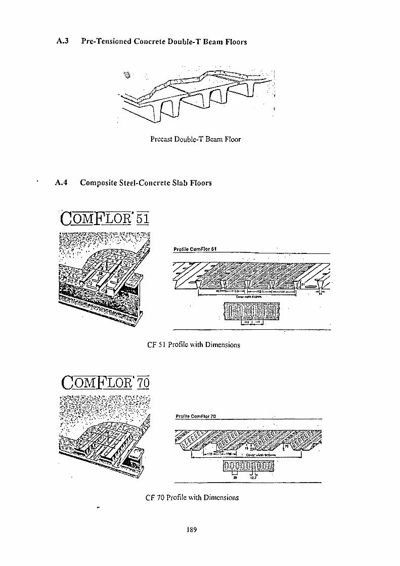
Profile ComFlor S1
Profile ComFlor 70
...
A.3 Pre-Tensioned Concrete Double-T Beam Floors
CF 51 Profile with Dimensions
COMFLOR: 70
CF 70 Profile with Dimensions
189
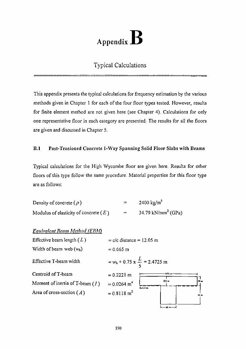
-1210 re
1441 re
Appendix BTypical Calculations
This appendix presents the typical calculations for frequency estimation by the various
methods given in Chapter 1 for each of the four floor types tested. However, results
for finite element method are not given here (see Chapter 4). Calculations for only
one representative floor in each category are presented. The results for all the floors
are given and discussed in Chapter 5.
B.1 Post-Tensioned Concrete 1 -Way Spanning Solid Floor Slabs with Beams
Typical calculations for the High Wycombe floor are given here. Results for other
floors of this type follow the same procedure. Material properties for this floor type
are as follows:
Density of concrete (p) = 2400 kg/m3
Modulus of elasticity of concrete (E) = 34.79 kN/mm2 (GPa)
Equivalent Beam Method (EBili)
Effective beam length (L) = c/c distance = 12.05 m
Width of beam web (wb) = 0.665 m
Effective 1-beam width L= wb + 0.75 x — = 2.4725 m
5
Centroid of 1-beam = 0.2221 m ?CPS on I1
??2.1 r•Moment of inertia of 1-beam (I) = 0.0264 m4
Invil 6146
Area of cross-section (A) = 0.8118 m2
I1*— 613 e• -I
190

_ 7r El _7.43 Hz (simple supports)
1Fundamental natural frequency
Fundamental natural frequency
2 pAL4
_ (4.73) 2 1 El
2 n- pA L4— 16.84 Hz (fixed supports)
Plate Method (PM)
Poisson ratio of concrete ( v) = 0.2
Slab thickness (h) = 0.21 m
Long span (Lx ) = 12.05 m
Short span (L) = 7.305 m
LE- 1.65
Ly
L2For simply supported plate, 22 = 7r 2 [ 1 + = 36.73
1.2y
22 .1 Eh 2Fundamental natural frequency — — 9.48 Hz
27rk2 12p(1— v2)
For corner supported plate,
22 = 1.5467x(1.65) 3 — 9.82x(1.65) 2 + 20.803x(1.65)— 5.41 .-- 9.13
22 11 Eh 2 Fundamental natural frequency = — 2.36 Hz
2n-L2x 12p(1— v2)
Concrete Society Method (CSM)
lx0.213 Moment of inertia of slab (Ix = ly — )— 0.00077175 m4/m
12
Number of spans along short span (nx ) = 3
Number of spans along long span (Fly ) = 1
nxLx2 x = — 1.8187
LyIC = 1 + AT
12x = 1.3023
191

Ay = — 1.6496nL
K= 1 + 1
= 1.3675ivy
For slabs with perimeter beams,
=1E1
y — 3.25 Hz2 pAL4,
71" 1 El x _ 9.29 Hzf—k
Y Y 2
1
pAL4,
Static Deflection Method (SDM)
Using the EBM values of area, length and moment of inertia with acceleration due to
gravity (g)= 9.80665 ni/sec2:
5pAgL4 Static deflection of equivalent beam (A) — — 5.71 mm (simple supports)
384E/
Fundamental natural frequency = —1
il—g
= 6.59 Hz27r As
pAgL4 Static deflection of equivalent beam (A, ) — — 1.14 mm (fixed supports)
384E/
Fundamental natural frequency = —1
= 14.75 Hz27r As
FE maximum static deflection (A s )) = 3.78 mm
17 Fundamental natural frequency — — 8.74 Hz
192

B.2 Post-Tensioned Concrete Solid Flat Slab Floors
Typical calculations for the Hammersmith floor are given here. Results for other
floors of this type follow the same procedure. Material properties for this floor type
are the same as for 1-Way Spanning Solid Post-Tensioned Concrete Slabs with
Beams, given in Appendix B.1.
Equivalent Beam Method (EMI).
Effective beam length (L) = cic distance (long span) = 8.4 m
Width of beam = 1.0 m
Area of beam (A) = 1 x 0.225 = 0.225 m2
_ lx0.225 3 _Moment of inertia (I) 0.00095 m4
12
7T 11El
4Fundamental natural frequency — — 5.51 Hz (simple supports)
2 pAL
_ (4.
2 pAL4
73) 2 li ElFundamental natural frequency — 12.48 Hz (fixed supports)
7r
Plate Method (P)'.i)
Poisson ratio of concrete ( v) = 0.2
Slab thickness (h) = 0.225 m
Long span ( Lx ) = 8.4 m
Short span ( Ly ) = 7.2 m
Lx.--' 1.17
LY
[For simply supported plate, 22 = ir 2 1+ 72-L2x = 23.30
22 li Eh 2 Fundamental natural frequency =
2n-L2., 12p(1— v2) — 13.27 Hz
193

For corner supported plate,
=1.5467x(1.17)3 — 9.82x(1.17) 2
Fundamental natural frequency
+ 20.803x(l.17) — 5.41 7.95
22Eh'— 4.53 Hz
1,1
27/1,2, 12p(1— v2)
Concrete Society Method (GSM)
Moment of inertia of slab (I = — lx0.2253
— 0.00095) m4/m12
Number of spans along short span (nx) 5
Number of spans along long span (n,) = 5
n x Lx 1= —4.28 K= 1 + 1-2x = 1.0544
Ly
— nL
Y = 5.831
Ay Ky= 1 + = 1.029422y
For slabs without perimeter beams,
fx,. 2 pAL4,
— 5.80 Hz
f;=kyn- 1E1 x
— 7.71 Hz2 pAL4,
2 pAL4fb — x — 4.44 Hz
/ L41+ —r
IL
fx = f:, - ( - fb)
( i
tlx
1\
ilv— 5.50 Hz
2
( i 1\
fy - (f; - fb)"v — 6.98 Hz
2

1Fundamental natural frequency = --g— = 10.93 Hz
27r A,
Static Deflection Method (OM)
Using the equivalent beam method values of area, length and moment of inertia with
acceleration due to gravity (g) = 9.80665 rrdsec2:
5pAge Static deflection of equivalent beam (A, ) — — 4.89 mm (simple supports)
384E/
Fundamental natural frequency = —1
1—g
= 7.13 Hz2Jr
1A,
pAgL4 Static deflection of equivalent beam (A s ) — —2.08mm (fixed supports)
384E/
FE maximum static deflections (A s ) = 4.89 mm
18.7 Fundamental natural frequency — — 8.46 Hz
laiK
195

r 1EI
2
1— 4.61 Hz
pAL4Fundamental natural frequency
B.3 Pre-Tensioned Concrete Double-T Beam Floors
Typical calculations for the Swindon floor are given here. Results for other floors of
this type follow the same procedure. The Plate and Concrete Society Methods donot
apply to this floor type. Material properties for this floor type are as follows:
Site p (kg/m3) E (kN/mm2)
Swindon, Sutton 2500 38.89
Reading, Basildon, Tunbridge wells 2350 39.85
Equivalent Beam Method (EMI)
Effective beam length (L) = c/c distance = 16.045 m
Area of beam (A)
= 0.4242 m2
Moment of inertia (I)
= 0.01559 m4
Static Deflection Method (SD111)
Using the equivalent beam method values of area, length and moment of inertia with
acceleration due to gravity (g)= 9.80665 m/sec2:
5pAgL4 Static deflection of T-beam (A s ) — — 14.8 mm
384E/
Fundamental natural frequency = --- (g± = 4.10 Hz2ir
1As
FE maximum static deflections (A s ) = 15.0 mm
17.7Fundamental natural frequency = —,--- — 4.57 Hz
VA,
—
196

—NA
380.41 nr,426 rnn
174.25 in ri
180 nr.
B.4 Composite Steel-Concrete Slab Floors
Typical calculations for the Millwall Stadium, London floor are given here. Results
for other floors of this type follow the same procedure. The Plate and Concrete
Society Methods donot apply to this floor type. Material properties for this floor type
are as follows:
Density of Concrete (Pc)
Modulus of Elasticity of Concrete (Er)
Density of Steel (ID.)
Modulus of Elasticity of Steel (E3)
Modular Ratio (17) = E
s
▪ 1900 kg/m3
• 22 kN/mm2
• 7820 kg/m3
• 206.8 kN/mm2
9.4
Equivalent Beam Method (EMI)
a) Beam (UB356x127x33) Supporting CF70 Profile Slab
Slab thickness (t) = least oft ' or t2 = 105 mm (see PMF (1994)):
112+164 55Profile based thickness: t1= 130 - x — 105 mm
2 300
Weight based thickness:2.07x1000
t2 x1000 = 110 mm9.80665x1900
Beam length (Lb )) = 6.75 m
Area of beam = 4180 mm2
Moment of inertia of beam = 8200,0000 mm4
Beam spacing (Sb) = 2.665 m
Effective slab width (ESW) = least of —Lb or Sb4
= 1.6875 m
SE W _ 180 mmTransformed width =
Centroid = 380.41 mm from base
Transformed moment of inertia (45 ) = 316305176.3 mm4
Beam mass/length (mB) = 33 kg/m
197

I.•,--- 020 ..., -1
L.-
6797 rftr%
-no-,
30/.1
'31
Supported mass (nib ) = S b XtX pc + mB
= 2.665 x 0.105 x 1900 + 33 = 564.6675 kg/m
Fundamental natural frequency of beam (fb) =
y
if E31Th — 11.73 Hz
2 mbL4b
b) Girder (UB610x229x101) Supporting Two Beams
Girder length (Lg ) = 8.3 m
Area of girder = 12920 mm2
Moment of inertia of girder = 75720,0000 mm4
Girder spacing (S g) = 6.75 m
LEffective slab width = least of --L or Sg = 2.075 m
4
ESTVTransformed width — — 220 mm
17
Centroid = 543.90 mm from base
Transformed moment of inertia ( 42 )= 1966082782 mm4
Girder mass/m (mG ) = 101 kg/m
Supported mass (m2 ) = 2 x mb x —4 + niGL2
= 2x 564.6675 x + 101 = 1019.4351 kg/m8.3
Fundamental natural frequency of girder (fg
) — 71- 1E sl T
g — 14.40 Hz2 m L4
g g
Dunkerlv's Formula
1 f — — 9.10 Hz
Ti_._ 1I fb2 42
198

Static Deflection Method (SDM)
a) Wyatt's Approach
For 1.2 mm thick CF70 profile deck (see PMF (1994)):
Neutral Axis (N.A.) of profile 30.32 mm from bottom
Area of profile 1585 mm2/m
Moment of inertia of profile 760000 mm4/m
1000x105x —
105 + 1585x(130– 30.32)
Slab N.A. – 9.4 2 – 58.36 mm from top1000
x105+15859.4
Moment of inertia of slab (IS):
1000 105 1000I = —x—+—x105x(58.36– —
105) 2 + 760000 + 1585x(130 – 30.32 – 58.36)2
s 9.4 12 9.4 2
Is = 14112351.23 mm4/m
Mode-1:
Mode-2:
Slab - Fixed between beams
Slab width = 1 m
Slab length (L5 ) = 2.665 m
Slab mass (ms )= 0.105 x 1900 = 199.5 kg/m2
Assuming acceleration due to gravity (g)= 9.80665 rn/sec2,
Static deflection of slab (A s ) – nisgE: _
0 0880585 mm384E,/,
Beam - Simply supported between girders
5mbgL4bStatic deflection of beam (L b ) – – 2.2882871 mm
384E5/7b
Total deflection (A T ) = A s + = 2.37634556 mm
18 Fundamental natural frequency------ – 11.68 Hz
IS;
Slab - Fixed between beams
Static deflection of slab (A, ) = 0.0880585 mm
Beam - Fixed between girders
199
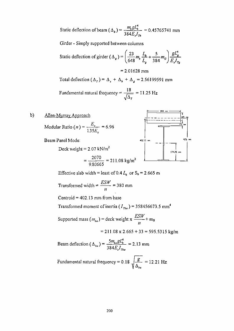
Static deflection of beam (A b ) — rnbgL4b – 0.45765741 mm384E5/Tb
Girder - Simply supported between columns
23 5 gL4gStatic deflection of girder (A —)=
171"
, 4,
+648 Lg 384 mGg
Es/ T
= 2.01628 mm
Total deflection (A T ) = A, + A b + Ag = 2.56199591 mm
18 Fundamental natural frequency – – 11.25 Hz
NrA;
380 n r,
b) Allen-Murray Approach
Modular Ratio (n) –Es
– 6.961.35E,
Beam Panel Mode:
Deck weight = 2.07 kN/m2
2070 – 211.08 kg/m2
_
9.80665
Effective slab width = least of 0.4 Lb or Sb = 2.665 m
ESWTransformed width – – 380 mm
12
Centroid = 402.13 mm from base
Transformed moment of inertia (/ Tba ) = 358456673.5 mm4
.Supported mass (n
ESW
a)= deck weight x -r MBn
= 211.08 x 2.665 + 33 = 595.5315 kg/m
Beam deflection (A ba ) — 51118'4 – 2.13 mm384E5/0
li gFundamental natural frequency = 0.18 = 12.21 Hz
200

G79. nn
475
Girder Panel Mode:
Effective slab width = least of 0.4 Lg or Sg
= 3.32m
S. E WTransformed width = — 475 mm
n 30L1 nn
Centroid = 601.8 mm from base I
Transformed moment of inertia (I Tga ) = 2273917335 mm4
Supported mass (mga )= 2 x nib x L--tg + mG = 1069.6 kg/m
5,7; eGirder deflection (A) — gag g — 1.38 mm
g 384E3 1 7. g a
1Fundamental natural frequency = 0.18 : = 15.18 Hz
Combined Mode:
Slab rigidity (D.,)= Is = 19051674.16 mm4/m
n
Beam rigidity (Db)— l
b — 134505318.4 mm4/mspacing
( gBeam panel effective width =2 —Ds
Lb = 7.68 m < —2
L3 Iola/Db
Since Lg = 8.3 m> 7.68 m
iFundamental natural frequency = 0.18 g
— 9.52 HzIiAb+Ag
c) Finite Element Method
For the constant slab thickness FE model:
FE maximum static deflections (A 5 ) = 2.28 mm
18.6 Fundamental natural frequency — — 12.32 Hz
VA,
107 net
201
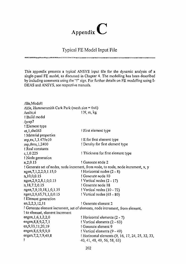
Appendix CTypical FE Model Input File
This appendix presents a typical ANSYS input file for the dynamic analysis of asingle-panel FE model, as discussed in Chapter 4. The modelling has been describedby including comments using the "I" sign. For further details on FE modelling using I-DEAS and ANSYS, see respective manuals.
/file,Modell/title, Hammersmith Cark Park (mesh size = 6x6)/units,si ! N, m, kg! Build model/prep7! Element typeet,l,she1163! Material propertiesmp,ex,1,3.479e10mp,dens,1,2400! Real constantsr,1,0.225! Node generationn,2,0.15! Generate set of nodes, nodengen,7,1,2,2,0,1.15,0n,10,0,0.15ngen,2,9,2,8,1,0,0.15n,18,7.2,0.15ngen,7,9,10,18,1,0,1.35ngen,2,9,65,71,1,0,0.15! Element generationen,2,2,3,12,11! Generate element increment,! to element, element incrementengen,1,6,1,2,2,0engen,8,8,9,2,7,1en,9,10,11,20,19engen,8,6,9,9,9,0engen,7,2,7,9,49,8
First element type
!
E for first element typeDensity for first element type
Thickness for first element type
Generate node 2increment, from node, to node, node increment, x, y
Horizontal nodes (2 - 8)Generate node 10Vertical nodes (2 - 17)Generate node 18Vertical nodes (10 - 72)Vertical nodes (65 - 80)
. Generate element 2set of elements, node increment, from element,
! Horizontal elements (2 - 7)1 Vertical elements (2 - 63)! Generate element 9! Vertical elements (9 - 49)! Horizontal elements (9, 16, 17, 24, 25, 32, 33,40, 41, 48, 49, 56, 58, 63)
202

! Boundary conditionsd,2,all ! Fix nodes 2, 8, 10, 11, 17, 18, 64, 65, 71, 72,!
74,80d,8,alld,10,alld,11,alld,17,alld,18,alld,64,alld,65,alld,71, alld,72,alld,74,alld,80,allFinish! Start solution/soluantype,modal ! Analysis type! Options (method, number of modes, from frequency, to frequency,! reduced modes, normalise)modopt,subsp,10,0,20„offmxpand,5,0,20,nosolveFinish! Start post-processing/postl
Note: Nodes 1, 9, 73, and 81 have not been modelled because they represent thecolumn centres at the four corners of the model and, therefore, would be fixed in thesame manner as the perimeter of these columns (nodes 2, 10, 11; 8, 17, 18; 64, 65,74; and 71, 72, 80).
The above input file is for the Hammersmith floor. Figure 4.11 shows this model.
203

Copyright © 2022 FDOKUMEN