City, University of London Institutional Repository

Citation: Ziai, Y. (1979). Statistical models of claim amount distributions in general insurance. (Unpublished Doctoral thesis, City University London)

This is the accepted version of the paper.

This version of the publication may differ from the final published version.

Permanent repository link: https://openaccess.city.ac.uk/id/eprint/8584/

Link to published version:

Copyright: City Research Online aims to make research outputs of City, University of London available to a wider audience. Copyright and Moral Rights remain with the author(s) and/or copyright holders. URLs from City Research Online may be freely distributed and linked to.

Reuse: Copies of full items can be used for personal research or study, educational, or not-for-profit purposes without prior permission or charge. Provided that the authors, title and full bibliographic details are credited, a hyperlink and/or URL is given for the original metadata page and the content is not changed in any way.

City Research Online: http://openaccess.city.ac.uk/ publications@city.ac.uk

City Research Online

STATISTICAL M DELS OF CLAIM ANIOLM DISTRIBUTIONS

IN GENEERL\L INSUIW CE.

by

YOUSSEF ZIA?, M. Sc., A. I. A.

A Thesis Submitted for the Degree of Doctor of Philosophy

Actuarial Science Division

Dept: to nt of hiatheratics

The City University, London.

009,9 1 DZ q-76S/90

April 19'79

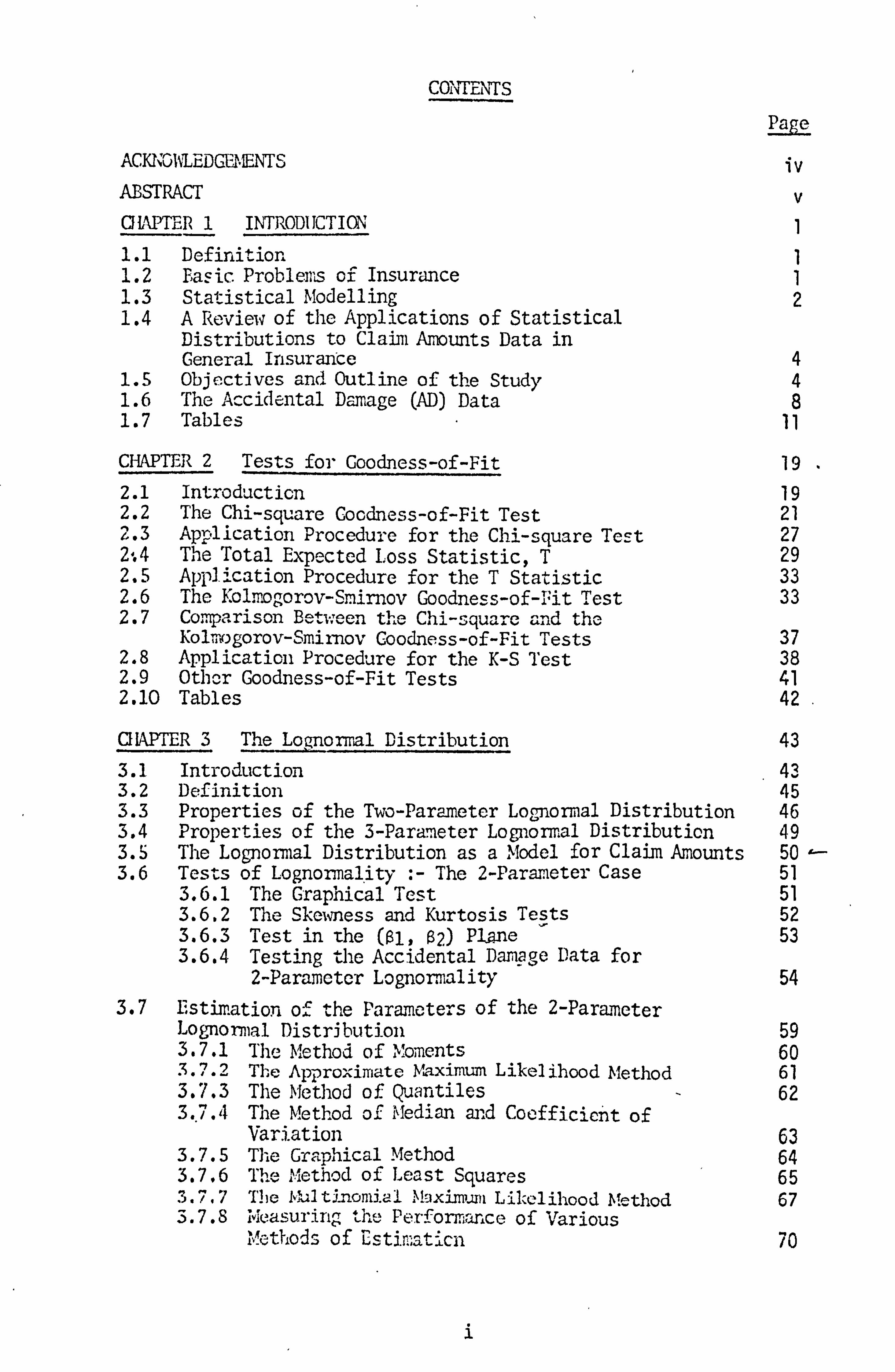
CONTENTS

ACKNOWLEDGEMENTS

ABSTRACT

QýAPTER 1 INTRODUCTION

1.1 Definition 1.2 Basic Problems of Insurance 1.3 Statistical Modelling 1.4 A Review of the Applications of Statistical

Distributions to Claim Amounts Data in General Insurance

1.5 Objectives and Outline of the Study 1.6 The Accidental Damage (AD) Data 1.7 Tables

CHAPTER 2 Tests for Goodness-of-Fit

2.1 Introducticn 2.2 The Chi-square Cocdness-of-Fit Test 2.3 Application Procedure for the Chi-square Test 2.4 The Total Expected Loss Statistic, T 2.5 Application Procedure for the T Statistic 2.6 The Kolmogorov-Smirnov Goodness-of-Pit Test 2.7 Comparison Between the Chi-square and the

Kolm gorov-Smirnov Goodness-of-Fit Tests 2.8 Application Procedure for the K-S Test 2.9 Other Goodness-of-Fit Tests 2.10 Tables

CQWPTER 3 The Lognormal Distribution

3.1 Introduction 3.2 Definition 3.3 Properties of the Two-Parameter Lognormal Distribution 3.4 Properties of the 3-Parameter Logformal Distribution 3.5 The Lognormal Distribution as a Model for Claim Amounts 3.6 Tests of Lognormality :- The 2-Parameter Case

3.6.1 The Graphical Test 3.6.2 The Skewness and Kurtosis Tests 3.6.3 Test in the (Bi, $2) Plane 3.6.4 Testing the Accidental Damage Data for

2-Parameter Lognormality

3.7 Estimation of the Parameters of the 2-Parameter Lognormal Distribution 3.7.1 The Method of Moments 3.7.2 The Approximate Maximum Likelihood Method 3.7,3 The Method of Quantiles 3., 7.4 The Method of Median and Coefficient of

Variation 3.7.5 The Graphical Method 3.7.6 The Method of Least Squares 3.7.7 The Mul tinomia1 >>aximuuri Likelihood Method 3.7.8 Measuring the Performance of Various

Methods of Cstimaticn

Pam

iv

V

1 1 2

4 4 8

11

19 19 21 27 29 33 33

37 38 41 42

43 43 45 46 49 50 51 51 52 53

54

59 60 61 62

63 64 65 67

70

1

Page 3.8 Application of the 2-Parameter Lognormal Model to the

Accidental Damage Data 7y

3.9 Prediction of the Claim Amount Distribution: - The 2-Parameter Lognormal Model 78

3.9.1 The Effects of Inflation on the Parameters of the Model 78

3.9.2 The Prediction Technique 79 3.9.3 Prediction for the AD Data 31

3.10 The 3-Parameter Lognormal Mode]. 84

3.11 Test of Lognormality: - The 3-Parameter Case 85

3.11.1 The Graphical Test 85 3.11.2 Testing the AD Data for 3-Parameter

Lognormality 86

3.12 Estimation of the Parameters of the 3-Parameter Lognormal Distribution 87

3.12.1 The Method of Least Squares 88 3.12.2 The Multinomial Maximum Likelihood Method 90

3.13 Application of the 3-Parameter Lognormal Model to the Al) Data

. 91

3.14 Prediction of the Claim Amount Distribution: - The 3-Parameter Lognormal Model 95

3.14.1 The Effects of Inflation on the Parameters of the Model 95

3.14.2 Prediction for the AD Data 96

3.15 Conclusions 98

3.16 Tables 99

CHAPTER 4 The Weibull Distribution 156

4.1 Introduction 156 4.2 Definition 157 4.3 Properties of the Weibull Distribution 158 4.4 The Graphical Test for the Weibull Distribution 160 4.5 The Weibull Graphical Test on the AD Data 163 4.6 Estij-, ation of the Parameters of the Weibull

Distribution 165 4.6.1 The Method of Least Squares 167 4.6.2 Multinomial Maximun Likelihood Method 169

4.7 Application of the Weibull Model to the AD Data 170 4.8 The Effects of Inflation on the Parameters

of the Weibull Model 175 4,9 Conclusions 176 4.10 Tables 177

CHAPTER 5 The Inverse Gaussian Distribution 186

5.1 Introduction 185 5.2 Definition 187 5.3 Properties of the Inverse Gaussian Distribution 189 5.4 Estimation of the Parc. rieters from Group: d Data 191

11

Pie

5.5 Application of the Inverse Gaussian Model to the AD Data 193

5.6 Prediction of the Claim Amount Distribution 197 5.6.1 The Effects of Inflation on the

Parameters of the Model 197 5.6.2 Prediction for the AD Data 198

5.7 Conclusions 199 5.8 Tables 200

CHAPTER 6 The Pareto Distribution 213

6.1 Introduction 213 6.2 Definition 213 6.3 Properties of the Pareto Distribution 214 6.4 The Graphical Test for the Pareto Distribution 215 6.5 The Pareto Graphical Test on the AD Data 216 6.6 Estimation of the Parameters of the Pareto

Distribution 218 6.7 The Effects of Inflation on the Parameters 220 6.8 Conclusions 0 221

CHAPTER 7 The Truncated Lognormal Distribution 223

7.1 Introduction 223 7.2 Definition and Some Properties of the Truncated

Lognormal Distribution 226 7.3 Estimation of Parameters 227 7.4 Applications to the AD Data 230 7.5 Conclusions 234 7.6 Tables 234

CHAPTER 8 The Gamma Distribution 250

8.1 Introduction 250 8.2 Definition and Some Properties of the Gamma

Distribution 253 8.3 Estimation of Parameters 257 8.4 Application of the Gamma Distribution to the AD

Square Root Data 258 8.5 The Effects of Inflation on the Parameters of the

Model 261 8.6 Prediction for the AD Square Root Data 261 8.7 Conclusions 262 8.8 Tables 264

CHAPTER 9 Summary of Conclusions 273

APPENDIX 278

REFE RENCES 313

111

ACKNOWLIDGEMEMS

I would like to express my gratitude to Professor Bernard Benjamin

for his helpful supervision, constructive criticism and kind

encouragement during the preparation of this thesis.

I am additionally grateful to Mr. Stewart Coutts for suggesting some

of the problems considered in this thesis and for his rigorous

criticism and constructive advice throughout.

The applications of. the theoretical aspects of this work are

demonstrated on actual data provided by a British insurance company

whose co-operation is gratefully acknowledged.

I would also like to thank the library staff of the Institute of

Actuaries and of the City University whose sympathetic assistance

aided my research.

Finally, I wish to record my appreciation of the work of

Miss Lancaster and Miss Williams in typing the manuscript.

iv

ABSTRACT

This work examines the following statistical distributions

as possible models for the distribution of claim amounts in general

insurance:

1- The lognormal

2- The Weibull

3- The inverse Gaussian (A new 3-parameter form is introduced)

4- The Pareto

5- The truncated lognormal as a model for large claim amounts)

6- The gamma (as a model for the distribution of the square root of claim amounts)

The properties. of the above distributions are investigated and various

methods of estimation of their parameters are explored. The method

of multinomial maxim mt likelihood for estimating the parameters is

favoured because data on claim amounts is generally in grouped

frequency format. To find these estimates a computing technique is

proposed which avoids solving a complicated set of non-linear

equations. A procedure which avoids solving non-linear equations

is also suggested for the least squares estimation of the 3-parameter

lognormal, 3-param_etor Weibull and the Pareto distribution of the

second kind. In order to show how the various methods work in

practice they are applied to an actual set of accidental damage claim

amounts. Goodness-of-fit tests are used to judge the agreement

between the model and sample valuos. The Chi-square and the

Kolmogorov-Sriirnov tests are reviewed and a new test statistic is

V

proposed which measures the overall agreement between the model

and sample values in monetary terms. The application procedures

for all these tests are described.

Inflation is likely to be the main cause of the increase in

the size of claim over time. Therefore, its effects on the

parameters of various models are examined. A method is suggested

for predicting the future distribution of claim amounts which

uses the parameters of a past model after being adjusted for

inflation. This predictive method is demonstrated on the

accidental damage data whenever a suitable model is found.

vi

7

CRU"TER 1

INI RODI TCTION'

1.1 Definition

General insurance' is defined as all classes of insurance

other than life insurance (or assurance). For a thorough comparison

between life and general insurance reference may be made to

Benjamin (1977). Fundamentally, general insurance has the following

distinguishing features as compared with life assurance:

1- Claim size not knoi%n in advance and often without limit.

2 -- Premium changes from year to year because contracts are

normally renewed annually.

3- More than one claim can arise under the same policy.

4- Volatility; large variances of both claim frequency

and claim amount especially the latter.

1.2 Basic Problems of Insurance

In insurance we are faced with the problems of charging

adequate premiums to cover a certain risk and the setting up of

reserves adequate to meet the cost of future claims with some margin

of profit. In life assurance, where the claim amount is i o:: n in

advance or can be determined by actuarial methods, these problems

have been solved by the use of the life table (which provides a

model for the probability of survival) in conjunction with discounting

functions. In general insurance, however, where the size of claim is

most usually not ie ot. n in advance, a prior estimate of the future

cost of claims is essential to the calculation of reserves. This

cost is a cc'mbinatic. -, of the frequency of claims and their size. it

- Sometimes referred to as Non-fife insurance.

I

is possible to treat each of these components of the cost separately

by collecting separate statistics on the frequency and size of claims.

In this work, we are concerned with the size of claims only. No claim

amount table exists for the calculation of the probability of

occurrence of a claim of a certain size.

1.3 Statistical Modelling _.

ý(''

It is ]mown that many random factors affect the size of the claim.

Statistical modelling is recognized as a rational tool of analysis for

problems in all areas of science and engineering where data variation

cannot be ignored. Therefore, it coninands considerable attention in

the solution of the basic insurance problems. Statistical modelling

assumes that there is a claim amount distribution underlying the

risk process. This distribution, once determined, enables us to

calculate the probability that if a claim occurs it will be not

greater than a: certain size. The shape of the claim amount distribution

is important in premiun determination and reserves calculations. As

Beard (1974) states, "a good theoretically derived model would be of

considerable help in dealing with practical estimation problems

arising frort the random fluctuations which arise in the relatively

small samples (in terms of the large claims) which commronly are all

that is available". In some classes of general insurance business

reinsurance is sought due to the likelihood of occurrence of very

large claims. In that case, the examination of the area (the

probability) under the upper tail of the distribution is necessary

for the insurance coy ; any's decision about 'retentioni' before

reinsurance. In motor insurance the policyholder may opt to pay

some first art of any on damage claim. ('voluntary excess') in

return. for a. reduction in the prerni. ta, i. The appropriate deduction,

1 -" That part of the risk which the insurance campany wishes to bear without help from the reinsures.

2

X-

in this case, may be calculated by examining the lower tail of the

claim amounts distribution. The essence of statistical modelling

approach is, therefore, to find a statistical distribution as a

model for the claim amounts experience of the particular class of

insurance in which we are interested. There are two stages involved.

At first we have to demonstrate from theoretical considerations of the

problem that a specific statistical distribution can model the claim

amounts experience. Sometimes it is not readily obvious how the

model could be theoretically derived and we have to start irnnediately,

from stage two. That is, by fitting our intuitive model to samples

of data from past experience and, perhaps, by using statistical

goodness-of-fit tests satisfy ourselves that the specific model

actually agrees with the claim amounts experience for our particular

class of business. Once we have found a model and gathered

sufficient Ielowledge about its parameters and how they behave with

respect to time, we will be able to use statistical techniques to

predict the distribution of the claim amounts arising during any

future period. This is our main objective in this approach.

In practice a solution to our problem, even starting from stage

two as mentioned above, is not easily obtainable because of many

undesirable factors such as insufficiency of the data, heterogeneity

of the data and data being only available in a certain form (e. g.

grouped or/and truncated). The empirical distributions of claim

amounts are by nature skewed to the right, i. e., there are many

small claims and much fewer larger claims. This leads us to the

examination of positively skewed statistical distributions as possible

models. It is also inrportant to study truncated distributions since

in practice, as in reinsurance, data on claims above a certain size

only may be available. Some of the models which have been more

often employed are referred to below.

3

1.4 A Review of the Applications of Statistical Distributions to Cl. a Amounts Data in General Insurance;

Studies have been made which involve fitting statistical

distributions to claim size data. Beard (1955) has fitted the

lognonnal to the American fire insurance property damage claim size

data. Beard 41957) gives a numerical example of the application of

the lognormal. and log-Pearson type I distributions to an experience

of fire ciairs in Denmark. In Beard (1964) a lognormal distribution

is fitted to a sample of settled. motor insurance claims, property

damage and liability claims mixed. Benckcrt (1962) fits lognormal

distributions to claims data from fire insurance, accident insurance

and motor third party insurance. Harding (1968) uses a truncated

lognorinal distribution as a model for the original amount of a claim

falling under the excess of loss reinsurance of motor business

contracts. Ferrara (1971) fits lognormal distributions to fire

insurance claim size data from several different industries. }3enckert

and Jung (1974) fit lognormal and Pareto distributions to data on

claims in fire insurance of dwelling houses reported between 1958

and 1969 by Swedish fire insurance companies. Finger (1976) uses the

lognormal distribution as a model for claim amounts in liability

insurance. Bickerstaff (1972) uses the lognormal as a model for the

distribution by size of auto collision claims.

The lognormal seems to be the most successfully used model in

general insurance. However, the above references do not deal extensively

with the various methods of estirating the parameters of the lognormal

distribution, and the efficiencies of these Methods, nor do they examine

some of the other skc: aed distributions.

1.5 Objectives and Cut line of the. Study

It vas, with the ubýýýýr. Yc; narl: s iii mind that the -present work was

4.

started. We study several skewed distributions as models for claim

amounts in general insurance. In order to show the applications of

these models in practice we apply their theoretical methods to a

set of real data fron motor insurance Accidental Damage (AD) claim

amounts. A description of the data will be provided in secticn

1.6.

Goodness-of-fit tests are used frequently in the present work

to examine the agreement between a model and sample values. Therefore,

in chapter 2 we consider several of these tests. The more widely

used Chi-square test is reviewed and a new test statistic is proposed

to supplement it. This statistic measures the overall agreement

between a model and sample values in monetary terms and, therefore,

its value can be easily interpreted. The importance of this

statistic is demonstrated in examining the agreement between

predicted and actual distributions since, in that case, it indicates

by how much we have overpredicted or underpredicted the total cost

of claims.

The Kolmogorov-Smirnov test for goodness-of-fit is a well established,

but less frequently used, test which is also reviewed in Chapter 2.

The application procedures for all three statistics are described and,

in later chapters, demonstrated on the AD data.

Because of the importance of the lognormal distribution in

general insurance it is extensively studied in Chapter 3. The two

and three parameter cases are considered. After defining the distribution

its properties are examined and a theoretical justification for the

emergence of the lognormal distribution as a model for claim amounts

is provided. Tests of 1ognormality and various estimation methods are

suggested for the two parameter. case when data only in grouped form

5

are available. These are later demonstrated on the AD data. A

computer simulation is carried out to measure the efficiency of

different methods of estimation. The multinomial maximum likelihood

(MML) method which is most suitable for grouped data is studied and,

with the wide availability of computers, a technique is suggested

for finding the estimates of the parameters. This iterative

procedure maximizes the loglikelihood function directly, via a

search for the optimum solution, starting from a set of initial

values. The effects of inflation on the parameters are then

considerecTand predictions are made for the distribution of claim

amounts, in a future period, by using different indices of wages

and prices. The agreement between the actual and predicted claim

amounts are tested by the goodness-of-fit tests described in

Chapter 2. The 3-parameter case is then studied. A method of

estimation which involves the least squares technique and a

search for the location parameter is suggested which avoids solving

non-linear equations. The method of IWL is also modified for the

3-parameter case. These methods are then applied to the AD data.

The effects of inflation on the parameters are studied and distributions

of claim amounts during future periods arc predicted.

In Chapter 4 the Weibull distribution which belongs to the

exponential family is studied. The two and three parameter cases are

examined, very much on the same lines as for the lognormal distribution.

The same methods of estimation as for the 3-parameter lognormal are

modified. for the 3-parameter. Weibull distribution.

Chapter 5 is devoted to the study of the inverse Gaussian (or inverse

normal) distribution. This is a skewed distribution with a shape

similar to the lognormal, the g aroma and the Weibull distributions .

Ü

Chhikara and Folks (1978) state that several sets of cmpirical data

wich they have investigated seem to be equally well represented

by the lognormal and the inverse Gaussian distributions. In the

absence of other considerations they recornend the use of the

inverse Gaussian distribution on the basis of the convenience of

working with it. Therefore, it seemed important to study and test

this distribution on the AD claims. Initially, the properties of

the distribution are examined and the methods of moments and ML

are suggested for the estimation of the parameters. These methods

are applied to the AD claims data and the effects of inflation are

investigated. We then introduce the 3-parameter version of this

distribution by bringing in a threshold parameter. No mention of

this case is made in chhikara and Folks (1978) or in Johnson and

Kotz (1970). We suggest using the MML method of estimation. This

method is then applied to the data. The effects of inflation on

the parameters are studied and predictions for future periods are

made and comapred with the actual experience by using goodness-of-

fit tests.

Chapter 6 looks at the Pareto distributions of the first and

second kinds. The properties and a graphical test are studied.

Various estimation methods are examined. In Chapter 7 we use the

method of MM to fit this distribution to the upper tail of the

AD claims data, i. e., claims greater than £600.

To study the tail of the claim amounts distribution, which

is of interest in reinsurance, we deal with the truncated lognormal

model in Chapter 7. The method of A'IL is developed and applied to

the truncated samples of AD data. The effects of truncation at

different points are studied.

7

In Chapter 8 we examine the ganuna distribution. Board (1978 -

personal co munication) suggests the gamma distribution as a model

for the distribution of the square root of the claim amount. We

would like to test this to see if by taking the square root of the

claim amount we can arrive at a better fitting model. For this

reason a different set of AD data was obtained where the claims

are grouped into different bands according to the square root of

their size. The data are better described in Chapter 8. The

properties of the gamm distribution are studied and the methods

of moments and rte, are suggested for the estimation of the parameters.

These are then applied to the data. The effects of inflation on the

parameters are studied and predictions for future periods arc made.

A final discussion and a sumnary of the findings of the study

are presented in Chapter 9.

The tables of results for every chapter are presented at the

end of the chapter.

All the computer programs used in this work have been written

by the author in Fortran 4 language and have been run via the

interactive terminals on the City University's ICL 1905E Computer.

The texts of the programs are presented in the Appendix.

1.6 The Accidental Damage (AD) Data

The important part of any data analysis is to have a reliable

set of data. Since we are looking for models of the distribution of

claim amounts we must be sure that the data used in the analysis has

been collected only from the experience of the particular class of

business we are investigating. In other words, the data must be

free from heterogeneity in every respect. In addition, a considerable

amount of data is required and we need to look at the experience

over several periods.

8

A miedium-sized, U. K., general insurance company provided its with

some data. of Accidental Damagel (AD), excluding windscreen, claim

amounts in respect of claims which occurred during certain periods

of time in the past. These periods are referred to as periods of

accident. T h-- portfolio from which these claims come was

comprehensively insured private cars. Data combined for all age

groups, vehicle groups, districts and type of use were available.

For claims iip to £570 we were given the number of open and settled

claims grouped in bands of £30, i. e. £i-30, £31-60, ........., £541-570.

For aniouiits greater than £571 details of the individual claims were

made available. After some investigation we grouped these in the

following bands:

£571 - £600, £601 - £700,701 - 5800, etc.

until the band containing the maximum claim amount (or amounts) was

reached.

Data was provided in respect of seven periods of accident. Each

period covers three months of the calendar year. Ile were given data

from the quarter starting on 1.10.1973 to the one ending on 30.6.1975.

For convenience sake we refer to the period, say, from 1.10.1973

to 31.12.1973 as '73/4th quarter'. There are, therefore, seven samples

of AD claim amounts each corresponding to one of the periods from

73/4th quarter to 75/2nd quarter. In each case the data had been collected

_ at least six months after the end of the period of accident. The

incurred but not reported (IBNR) claims are assumed to be so few as not

to present a problem. This is because experience (of the insurance

company) shows that almost all AD claims are reported and settled

within six months after the end of the period of accident. Zero

claims2 were not included in the data. 1- Damage to the policy holder's own vehicle. 2- Thee are those claims in respect Of s rich no pa ninety "l rn .

de by red or the insurance compan}' e: ' r ? 3eca1zse no na}ý, zcni is i eý, ui

because the insurance company recovers the cost fron: another insurer.

9

The relevant information for the construction of the Al. ) claim

amount samples were extracted from the computer print-outs of the

insurance company's claim files. These were then stored in data

subfiles on our computer.

Computer program P1 was written to print the frequency distribution

of a given sample of AD data. The sample cumulative distribution

function and various relevant sample statistics are also calculated

and printed out. The program was run with the AD samples and the

results are given in tables (1.1) to (1.7). In each table the

column headed by 'NCIII > LB. AMOUNT' gives the number of those claims

in the sairple whose amounts are greater than the amount given by the

lower boundary of each interval. From this information we can, for

example, see that in 73/4th quarter there were 89 claims with

amounts greater than £601. The tables show that the number of such

claims has increased over time. The total number of claims in each

sample is on average about 2600. For the calculation of the sample

moments we have assumed that in each interval all the claims are for

an amount equal to the mid-point of that interval. An inspection

of the insurance company's claim file showed that this assumption

was justified since the average amount of claim in each band was in

fact approximately equal to the mid-point of that claim amount interval.

For the calculation of the median and mode linear interpolations in

the claim amount intervals were used. From the tables we can see that the mean and the standard deviation of

the claim amounts have increased over time while the coefficient of

variation has rurw. ined quite stable at about 1.1. For each sample,

the frequency distribution, the coefficients of skewness and kurtosis

as well as the relative positions of the rode, the median and the mean

all indicate the skewness and sharp peakedness of the claim amounts

10

distribution. The sample statistics given in tables (1.1) to (1.7)

will be of use in later chapters.

1.7 Tables

11

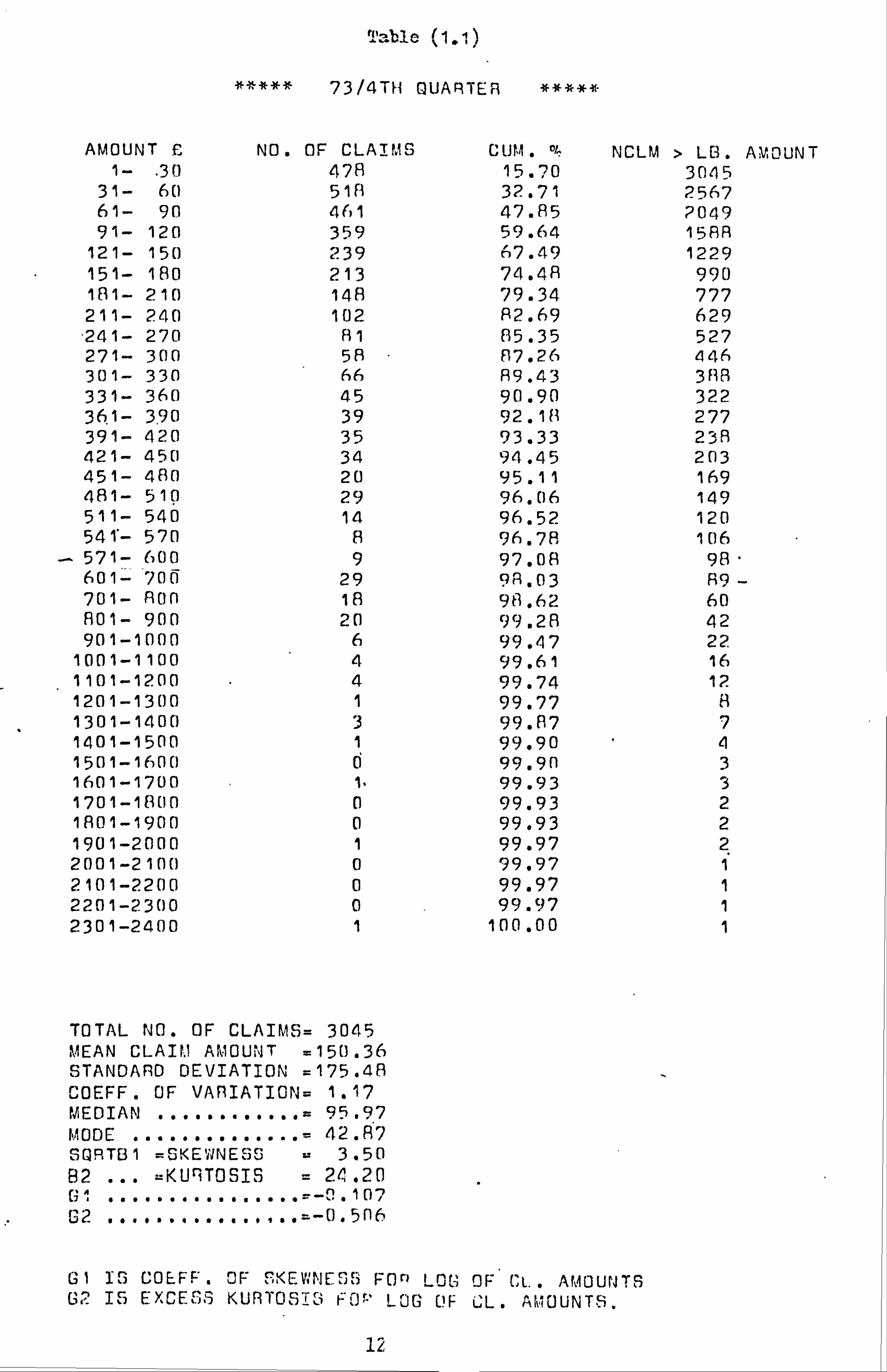
Table (1.1)

ý`## 73/4TH QUARTER

AMOUNT £ NO. OF CLAIMS CUM. %%: NCLM > LB. AMOUNT 1- . 30 478 15.70 3045

31- 60 518 32.71 2567 61- 90 461 47.85 2049 91- 120 359 59.64 1588

121- 150 239 67.49 1229 151- 180 213 74.48 990 181- 210 148 79.34 777 211- 240 102 82.69 629 -241- 270 81 85.35 527 271- 300 58 117.26 446 301- 330 66 89.43 3118 331- 360 45 90.90 322 361- 3.90 39 92.111 277 391- 420 35 93.33 238 421- 450 34 94.45 203 451- 480 20 95.11 169 481- 510 29 96.06 149 511- 540 14 96.52 120 541'- 570 8 96.78 106

- 571- 600 9 97.08 98 601- Inn 29 98,03 R9 - 701- Ron 18 9E1.62 60 801- 900 20 99.28 42 901-1000 6 99.47 22

1001-1100 4 99.61 16 1101-1200 4 99.74 12 1201-1300 1 99.77 a 1301-1400 3 99.87 7 1401-1500 1 99.90 4 1501-1600 [i 99.90 3 160 1-1700 1" 99.93 3 1701-1800 0 99.93 2 1801-1900 0 99.93 2 1901-2000 1 99.97 2 2001-2100 0 99.97 1 2101-2200 0 99.97 1 2201-23(10 0 99.97 1 2301-2400 1 100.00 1

TOTAL NO. OF CLAIMS= 3045 MEAN CLAIM AMOUNT =150.36 STANDARD DEVIATION =175.48 COEFF. OF VARIATION= 1.17 MEDIAN ............ = 95.97 MODE .............. = 42. A7 SQRT61 =SKEWNESS = 3.50 82 ... _KURTOSIS = 24.20

-^ 107 G2 ................ =-0.5f6

G1 13 COEFF . OF SKEWNES: i FOn L0C; OF (, l.. AfA 0UN TS G02 15 EXCESS KURTOSIS FO LOG OF C: L. AfOOUNT`i.

12

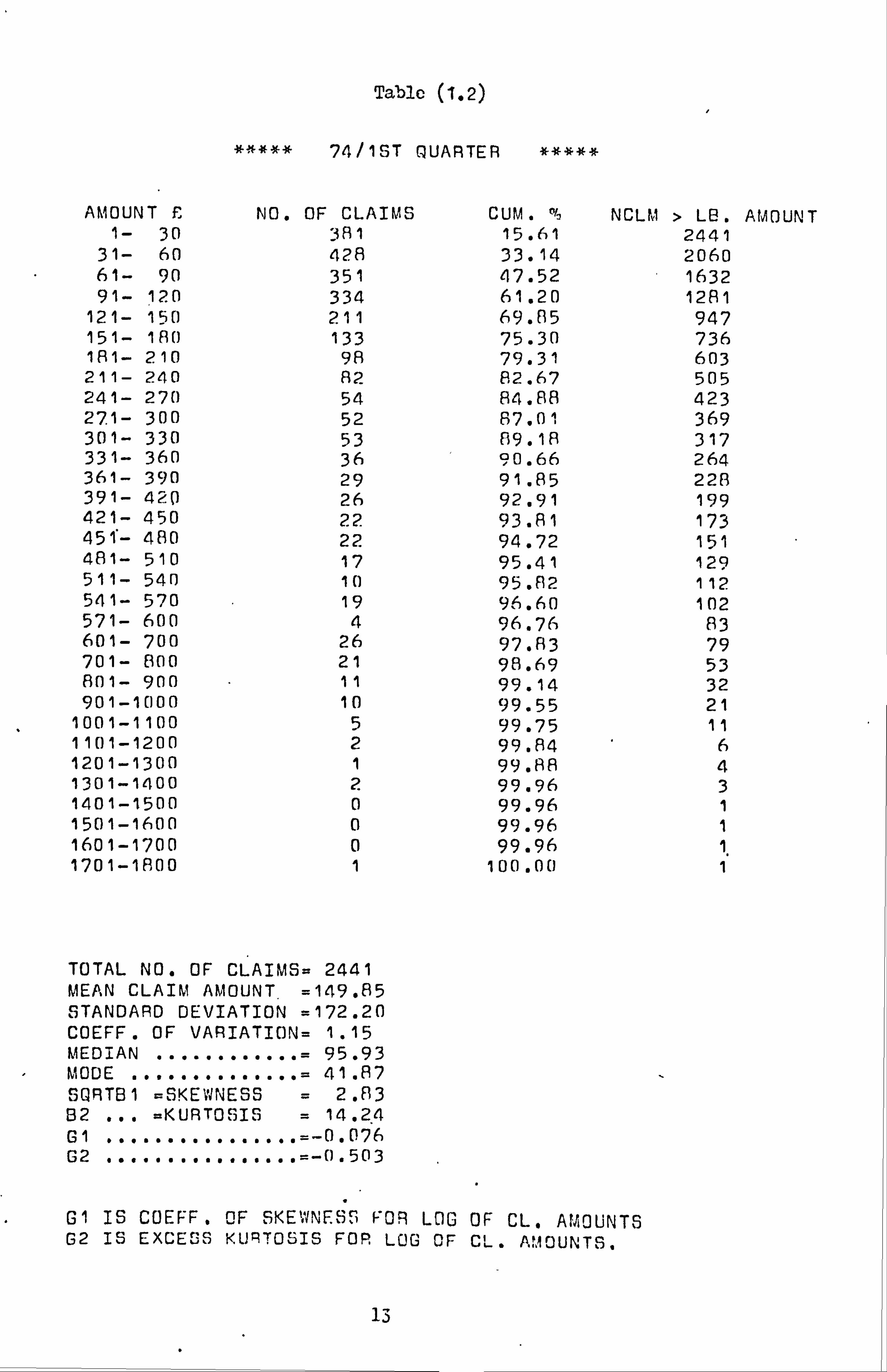
Table (1.2)

### 24/15T QUARTER #####

AMOUNT E NO. OF CLAIMS CUM. Of, NCLM > LB. AMOUNT 1- 30 381 15.61 2441

31- 60 428 33.14 2060 61- 90 351 47.52 1632 91- 120 334 61.20 1281

121- 150 211 69.05 947 151- 180 133 75.30 736 181- 210 98 79.31 603 211- 240 82 82.67 505 241- 270 54 84.88 423 27.1- 300 52 87.01 369 301- 330 53 09.18 317 331- 360 36 90.66 264 361- 390 29 91.85 22B 391- 420 26 92.91 199 421- 450 22 93.81 173 451- 480 22 94.72 151 481- 510 17 95.41 129 511- 540 1() 95.02 112 541- 570 19 96.60 102 571- 600 4 96.76 83 601- 700 26 97.83 79 701- 800 21 98.69 53 801- 900 11 99.14 32 901-1000 10 99.55 21

1001-1100 5 99.75 11 1101-1200 2 99.84 6 1201-1300 1 99.88 4 1301-1400 2 99.96 3 1401-1500 0 99.96 1 1501-1600 0 99.96 1 1601-1700 0 99.96 1 1701-1800 1 100.00 1

TOTAL NO. OF CLAIMS= 2441 MEAN CLAIM AMOUNT =149.85 STANDARD DEVIATION =172.20 COEFF. OF VARIATION= 1.15 MEDIAN ............ = 95.93 MODE .............. = 41.87 SQRTB I -SKEWNESS = 2.83 B2 ... =KURTOSIS = 14.24 G1 .............. .. =-0.076 G2 ................ =-0.503

G1 IS COEFF. OF SKEWNESS VOR LOG OF CL. AMOUNTS G2 IS EXCESS KUR70SIS FOR LOG OF CL. AMOUNTS.

13

Table (1.3)

#*### 74/2ND QUARTER -f*#**

AMOUNT NO. OF CLAIMS CUM. % NCLM > LO. 1- 30 351 14.73 2383

31- 60 380 30.68 2032 61- 90 382 46.71 1652 91- 120 295 59.09 1270

121- 150 211 67.94 975 151- 180 142 73.90 764 181- 210 114 7A. 68 622 211- 240 101 82.92 508 241- 270 57 85.31 407 271- 3(10 51 87.45 350 301- 330 39 89.09 299 331- 360 36 90.60 260 361- 390 25 91.65 224 391- 420 24 92.66 199 421- 450 27 93.79 175 451- 480 18 94.54 148 181- 510 21 95.43 130 511- 540 17 96.14 109 541- 570 12 96.64 92 571- 600 11 97.10 80 601- 700 30 98.36 69 701- 800 13 9E3.91 39 801- 900 11 99.37 26 901-1000 4 99.54 15

1001-1100 7 99.83 11 1101-1200 0 99.83 4 1201-1300 1 99.87 4 1301-1400 1 99.92 3 1401-1500 0 99.92 2 1501-1600 1 99.96 2 1601-1700 0 99.96 1 1701-1800 0 99.96 1 1801-1900 1 100.00 1

TOTAL NO. OF CLAIMS= 23R3 MEAN CLAIM AMOUNT =151.57 STANDARD DEVIATION =167.98 COEFF. OF VARIATION= 1.11 MEDIAN ............ = 98.4A MODE .............. = 61.17 SQRTB 1 =SKEWNESS =2 . 88 62 ... =KURTOSIS = 15.91 G1 ................ =-0.14 G2 ................ =--f). nb4

G1 IS COEFF . OF SKE WNES S) - Fon LO1Ga 0F CL . j«% MCUN'i'S G2 IS FOP LOG OF CL. AMOUNTS.

AMOUNT

14

Table (1.4)

*3*## /4/3RD 1UARTE9 #####

AMOUNT E NO. OF CLAIMS CUM. % NCLM > LB. AMOUNT 1- 30 362 12.93 2799

31- 60 427 28.19 2437 61- 90 383 41.87 2010 91- 120 356 54.59 1627

121- 150 283 64.70 1271 151- 180 194 71.63 9138 181- 210 137 76.53 794 211- 240 97 79.99 657 241- 270 86 83.07 560 271- 300 71 85.60 474 301- 330 64 87.89 403 331- 360 45 89.50 339 361- 390 44 91.07 294 391- 420 25 91.96 250 421- 450 26 92.89 225 451- 480 22 93.68 199 481- 510 25 94.57 177 511- 540 14 95.07 152 541- 570 14 95.57 138 571- 600 17 96.18 124

., _ 601- 700 32 97.32 107 701- 800 34 98.54 75 801- 900 17 99.14 41 901-1000 4 99.29 24

1001-1100 9 99.61 20 1101-1200 4 99.75 11 1201-1300 0 99.75 7 1301-1l00 1 99.79 7

1401-1500 3 99.89 6 1501-1600 0 99.89 3 1601-1700 1 99.93 3 1701-1800 0 99.93 2 1801-1900 0 99.93 2 1901-2000 0 99.93 2 2001-2100 0 99.93 2 2101-2200 1 99.96 2 2201-2300 0 99.96 1 2301-2400 0 99.96 1 2401-2500 0 99.96 1 2501-2600 1 100.00 1

TOTAL NO. OF CLAIMS= 2 MEAN CLAIM AMOUNT =166.13 STANDARD DEVIATION =1RR. 70 COEFF. OF VARIATION= 1.14 MEDIAN ............ =109.6 7 MODE .............. _ 48.39 SORTOI -SKEWNESS = 3.42 P. 2 ... =KUPPTOSIS = 24.04 G1 ................ =-0.179 G2 ................

G1 IS COEFF. OF SKEW'NE iii FOR LOG OF CL. AMOUNTS G2 IS EXCESS KURTOSIS FOR LOG OF CL, AMOUNTS.

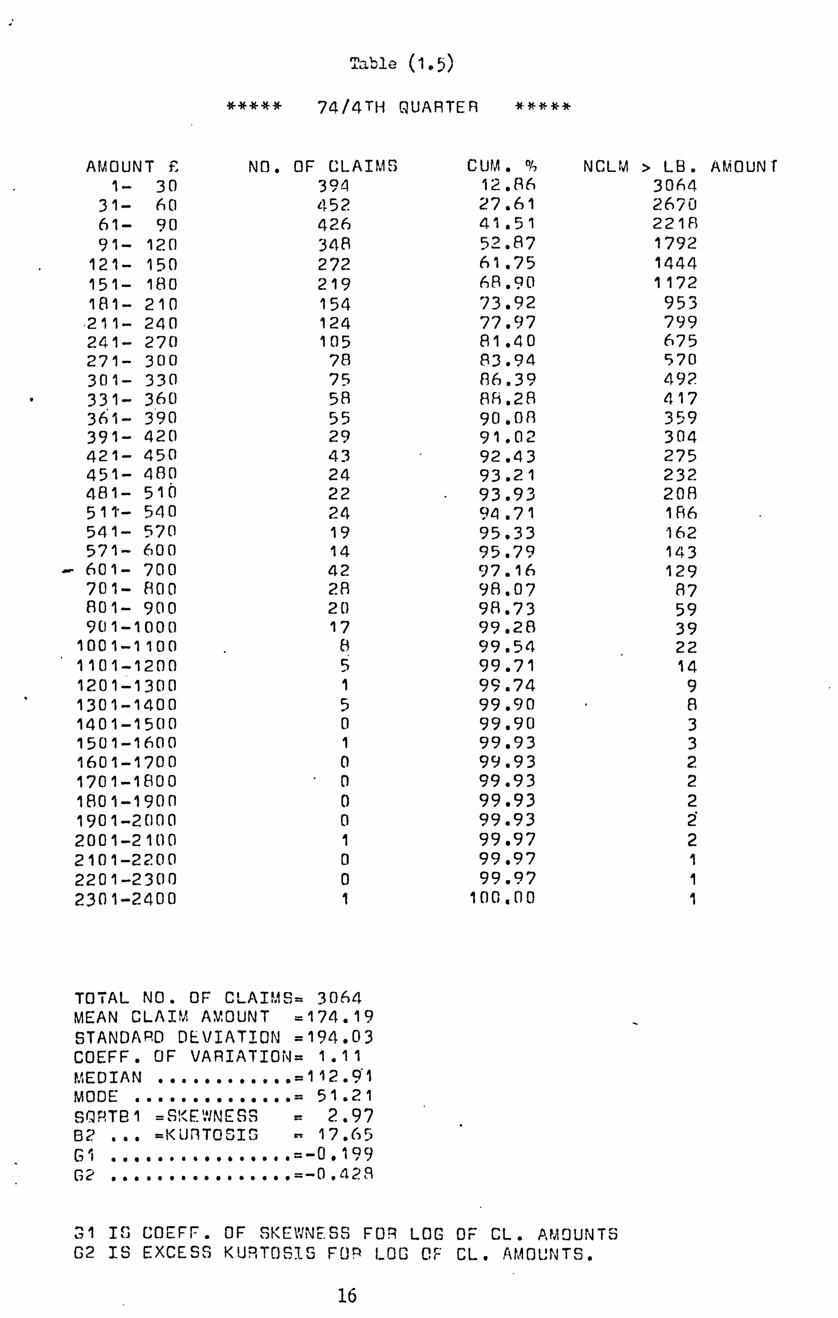
Table (1.5)

##### 74/4TH QUARTER #####

AMOUNT £ NO. OF CLAIMS CUM. % NCLM > LB. AMOUNT 1- 30 394 12.86 3064

31- 60 452 27.61 2670 61- 90 426 41.51 221A 91- 120 348 52.87 1792

121- 150 272 61.75 1444 151- 180 219 68.90 1172 181- 210 154 73.92 953 211- 240 124 77.97 799 241- 270 105 81.40 675 271- 300 78 83.94 570 301- 330 75 (36.39 492 331- 360 58 8h. 28 417 3611- 390 55 90.08 359 391- 420 29 91.02 304 421- 450 43 92.43 275 451- 480 24 93.21 232 481- 510 22 93.93 208 51 1'- 540 24 9A. 71 I A6 541- 570 19 95.33 162 571- 600 14 95.79 143

- 601- 700 42 97.16 129 701- 800 28 98.07 87 801- 900 20 98.73 59 901-1000 17 99.28 39

1001-1100 8 99.54 22 1101-1200 5 99.71 14 1201-1300 1 99.74 9 1301-1400 5 99.90 8 1401-1500 0 99.90 3 1501-1600 1 99.93 3 1601-1700 0 99.93 2 1701-1800 0 99.93 2 1801-1900 0 99.93 2 1901-2000 0 99.93 2 2001-2100 1 99.97 2 2101-2200 0 99.97 1 2201-2300 0 99.97 1 2301-2400 1 100.00 1

TOTAL NO. OF CLAIMS= 3064 MEAN CLAIM AMOUNT =174.19 STANDARD DEVIATION =194.03 COEFF. OF VARIATION= 1.11 MEDIAN ............ =112.91 MODE .............. = 51.21 SQFTB1 =SKEWNESS = 2.97 82 ... =KURTOSIS 17.65 Gi ................ =-0.199 Cc' ................ =-0.429

31 IS COEFF. OF SKEWNESS FOR LOG OF CL. AMOUNTS G2 IS EXCESS KURTOSIS FOR LOG OF CL. AMOUNTS.

16

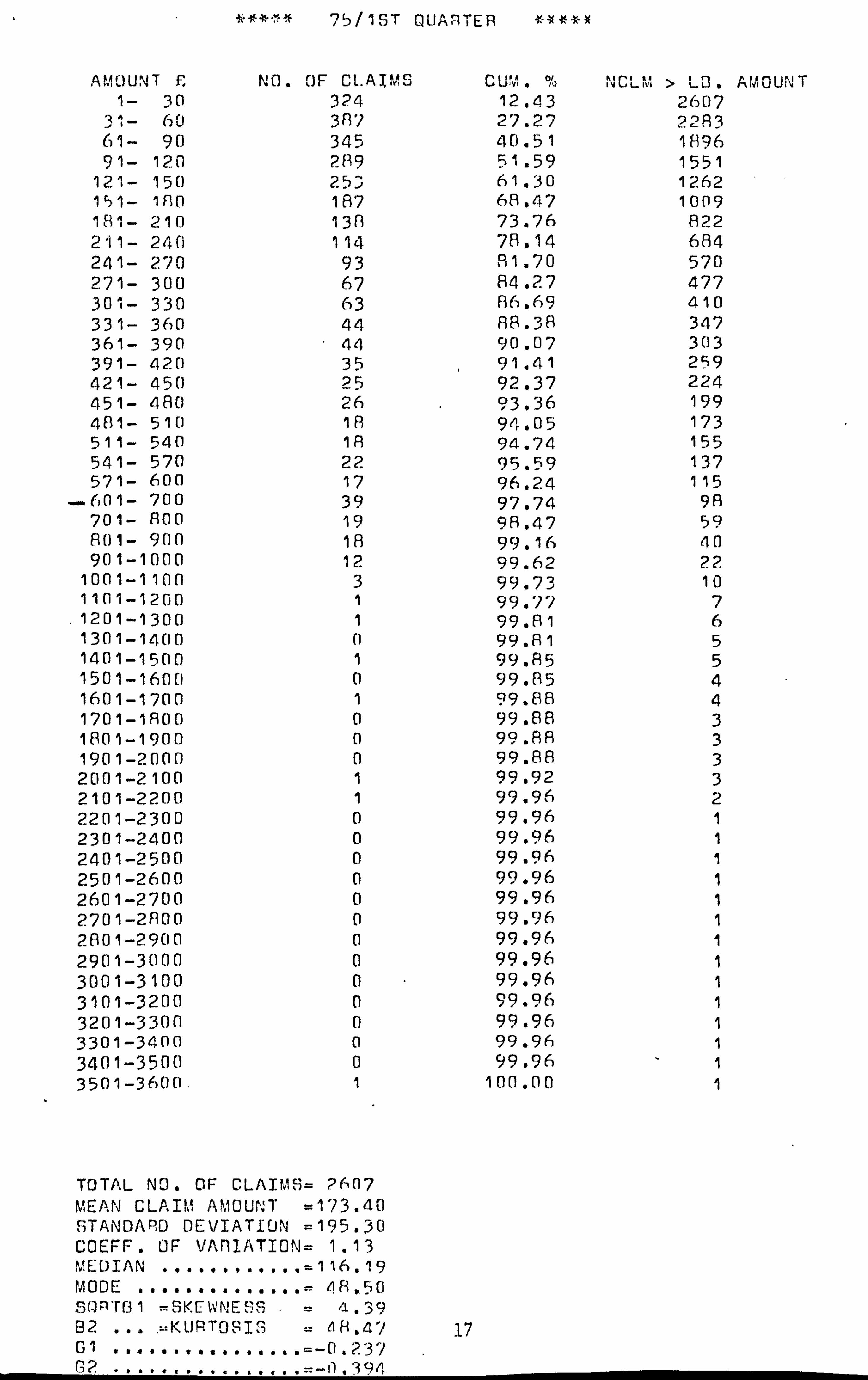
75/1ST QUARTER *-W ** *

AMOUNT £ NO. OF CLAIMS CUV" .% NCLkli > LU . 1- 30 324 12.43 2607

31- 60 31J 27.27 22133 61- 90 345 40.51 1896 91- 120 289 51.59 1551

121- 150 25D 61.30 1262 151- 1130 187 68.47 1009 181- 210 1313 73.76 822 211- 240 114 78.14 684 241- 270 93 91.70 570 271- 300 67 84.27 477 301- 330 63 136.69 410 331- 360 44 138.38 347 361- 390 44 90.07 303 391- 420 35 91.41 259 421- 450 25 92.37 224 451- 480 26 93.36 199 4131- 510 1R 94.05 173 511- 540 113 94.74 155 541- 570 22 95.59 137 571- 600 17 96.24 115 601- 700 39 97.74 98 701- 800 19 913.47 59 1301- 900 18 99.16 40 901-1000 12 99.62 22

1001-1100 3 99.73 10 1101-1200 1 99.71 7

. 1201-1300 1 99.81 6 1301-1400 0 99.81 5 1401-1500 1 99.85 5 1501-1600 0 99.85 4 1601-1700 1 99.68 4 1701-1800 0 99.88 3 1801-1900 0 99.88 3 1901-2000 0 99.88 3 2001-2100 1 99.92 3 2101-2200 1 99.96 2 2201-2300 0 99.96 1 2301-2400 0 99.96 1 2401-2500 0 99.96 1 2501-2600 0 99.96 1 2601-2700 0 99.96 1 2701-21100 0 99.96 1 2801-2900 0 99.96 1 2901-3000 0 99.96 1 3001-3100 0 99.96 1 3101-3200 0 99.96 1 3201-3300 0 99.96 1 3301-3400 0 99.96 1 3401-3500 0 99.96 1 3501-3600. 1 100.00 1

TOTAL NO. OF CLAIMS= 2607 MEAN CLAIM AMOUNT =173.40 STANDARD DEVIATION =195.30

AMOUNT

COEFF. OF VAf 1ATION= 1.13 MEDIAN ............ =116.19 MODE ..............: 48.50 Sran'rr31 -SKEWNESS /--' . 39 132 ... . =: KURTOFI = 18.4 -1 17 G1 ................ =-0.23) G2 ....... =-0 . 394

Tal P (1ý?,

# #'" 75/2ND QUARTER #9--*#

AMOUNT £ NO. OF CLAIMS CU", 1. % NCLM > LB. AMOUNT 1- 30 302 12.10 2495

31- 60 374 27.09 2193 61- 90 332 40.40 1819 91- 120 27? 51.50 1487

121- 150 235 60.92 1210 1'51- 180 167 6P, . 42 975 181- 210 122 73.31 7138 211- 240 110 77.72 666 241- 270 80 60.92 556 271- 300 72 83.81 476 301- 330 47 65.69 1104 331- 360 39 87.25 357 361- 39n 40 88.06 318 391- 420 3A 90.38 278 421- 450 29 91.54 240 451- 480 21 92.38 211 481- 510 30 93.59 190 511- 540 19 94.35 160 541- 570 17 95.0.3 141 571- 600 11 95.47 124 601- 700 36 96.91 113 701- 800 22 97.80 77 801- 900 22 98.68 55 901-1 [Ioo 11 99.12 33

1001-11(10 4 99.28 22 1101-1200 3 99.40 18 1201-1300 3 99.52 15 1301-1400 6 99.76 12 1401-1500 2 99.84 6 1501-1600 1 99.88 4 1601-1700 0 99.88 3 1701-1800 1 99.92 3 1801-1900 0 99.92 2 1901-2000 1 99.96 2 2001-2100 0 99.96 1 2101-2200 0 99.96 1 2201-2300 1 100.00 1

TOTAL NO. OF CLAIMS= 2495 MEAN CLAIM AMOUNT =180.08 STANDARD DE1/IATI_ON =204.79 COEFF. OF. VARIATION= 1.14 MEDIAN ............ =116.44 MODE .............. = 49.45 SQRTF31 =SKEWNESS = 3.07

02 ... =KURTOSIS = 17.70 Cl ................. -0.1R4 G2 ................ =-0.376

GI IS COEFF. OF FKF'WNES ; FOR LOG OF CL. AMOUNTS G2 IS EXCESS KURTO IS FOR LOG OF CL. AMOUNTS.

1$

CHAPTER 2

Tests for Goodness-of-Fit

2.1 Introduction

The natural order of any statistical analysis involving the

fitting of a theoretical distribution to a set of sample values is

to fit the theoretical model first and then to test its agreement

with the observed distribution of the sai le values. This problem

of testing "the goodness-of-fit" (i: e. the adherence of the model

to the data) will arise at various stages of the present work when

we consider different statistical distributions as models for the

distribution of claim amounts. Before considering the fitting

methods for various distributions it is deem: d convenient to devote

one chapter to the study of the theoretical bases and application

procedures of some goodness-of-fit tests.

Goodness-of-fit tests are performed to examine the agreement

between the theoretical distribution of a random variable and its

empirical distribution represented by a set of sample values. In

other words, if xl, x2,..., xn are independent observations of a

random variable X (for instance the claim amount) with an unknown

distribution function F(Lx), then we are required to test the null

hypothesis that

H: F (x) = F0 (x)

where Fo(x) is some particular distribution function. Any test of

110 is called a. test of fit. Hypotheses of fit, Ho, may be

classified as simple or composite. H0 is a sigle hypothesis if

it specifies the values of all the parameters of F0(x). If the

values of none of the parameters or only of some of them are specified

by the nufl hypothesis týýe?: is is called a composite }iypothc. sis.

19

The reason for formulating the null hypothesis of a test of

fit in terms of the distribution function is that the parametric

hypothesis testing methods do not provide the means of testing

whether observations come from a particular distribution with

unspecified paramieters. In addition, by our intuition we expect

that the distribution of sample observations would closely

approximate the true distribution (Kendall and Stuart (1973)).

It is in this sense that a goodness of fit test is a measure of

the discrepancy between the sample and theoretical distribution

functions. Savage (1953) characterizes a goodness of fit test by

the following four properties:

1- It is defined for samples from some large class of distributions.

2- The null hypothesis is either some specified distribution or

a class of distributions of which the functional form is

known.

3- For all null hypotheses, the test statistic used has the

same distribution (at least asymptotically).

4- The test is consistentl.

In our work a test of goodness of fit will be required in

two circumstances:

(i) Fitting and Testing

Let us assume that we have a sample of data representing the observed distribution of the claim amounts. We can

postulate the form of the population distribution of this variable and use one of the appropriate estimation techniques, for that particular distribution, to estimate its parameters and, thus specify it completely. We will

1- A test of hypothesis 1-I0 against a class of alternatives Hl- is said to be consistent if, c; en any member of Ht holds, the probability of rejecting Ho tends to 1 as scinpl e size (s) tends to infinity.

20

then need to test how well the theoretical and observed distributions agree. A good agreement will be taken as

evidence that the assuned family of distributions is the

correct form for the distribution of claim amounts. The null hypothesis in this case is of the composite type.

Pr', d. ýction and Testing,

We may predict a theoretical distribution, whose form and

parameters are-completely specified, as the distribution

of claim amounts in a particular period of accident

occurrence. If a set of data representing the observed distribution for the same period already exists, we will be

able to test how well the predicted and actual distributions

agree. In this situation the null hypothesis of test is of

a simple type. Evidence of a good fit can be used to

recommend a prediction technique and support the assumption

about the theoretical model.

In. this chapter several goodness of fit tests will be studied.

In Section 2.2 the Chi-square goodness of fit test will be dealt

with in detail. To supplement the Chi-square test, and to avoid

some of its shortcomings, a test statistic based on the weighted

sum of the actual minus expected number of claims, in different intervals,

will be proposed in section 2.4. The Kolmogorov-Smirnov test of

goodness of fit, which is generally believed to be more powerful than

the Chi-square test, will be studied in detail in section 2.6. Two

other test statistics will be mentioned in section 2.9 but because

they are not applicable to grouped data we will not study them in

detail.

2.2 The Chi-scauare Goodness-of-Fit Test

This was the first goodness of fit test and it was introduced

by Karl Pearson in 1900.

Let us assizie that we have a sample of n independent observations of

a random variable X, with distribution function F (x) . P'earson's

test involves grouping the observations into, say, k mutually

2' 1

exclusive categories such that nl be the number of observations in k

category i and n=E ni i=1

If the population distribution is completely specified by the null

hypothesis as F(x) = Fo(x) (i. e. the form and all the parameters of

Fo(x) are knouzi) and we assume that Iö is true, then the probability,

poi, of a random observation falling into any category i can be

calculated. If poi is multiplied by the total number of

observations, n, we will find the expected frequency of class i, say noi'

under the hypothesis H0. Apart from sampling variation there should

be close agreement between ni and nof, the observed and expected frequencies respectively. The Chi-square goodness of fit test

provides a probability basis for computing and deciding whether the

discrepancy is too large to have occurred by chance. The test

statistic, proposed by Pearson, is;

2 X2 =E

(ni noi) i=1 not

Large values of X2 indicate an overall lack of agreement between the

observed and expected distributions. The null hypothesis which

resulted in Hors should, therefore, be rejected for large values of

x2.

If when Ho is assumed true the sampling distribution of a test

statistic is known and tractable, tables of its percentage points

can be constructed. The sampling distribution of X2 is very

complicated when the sample size is finite, but Cramer (1946) has

shown that its limiting distribution, under Ho, is approximately

Chi-square, X2, with k-i degrees of freedom (we assured F0(x)

22

as completely specified).

In some situations the null hypothesis is composite such

that usually only the form of the postulated distribution is laiown

but not any, or some, of its parameters. If these parameters have

to be estimated from the sample data, then the limiting distribution

of X2 may depend on the method of estimation. With a poor method

of estimation X2 may frequently have a large value even if the

theory is correct (Cochran (1952)). In a general proof of the

distribution of X2 the method of estimation must be asserted. A

method that yields those values of the parameters which minimize

X2 (mininun Chi-square method) may seem the most suitable. Fisher

(1924) has shown that in the limit in large samples this method

becomes equivalent to the method of multinomial maxi mm likelihood.

The following theorem due to R. A. Fisher, states the principal

theoretical result for the distribution of the Chi-square test

" statistic when parameters of the distribution of X under the null

hypothesis, Fo(x), are estimated from the sample data.

Theorem

If Fo(x), whose form is known, has r ui iown parameters, and

if the corresponding multinomial maximum likelihood estimates

are substituted for the unimovm parameters, then X2 is

distributed, in the lint, as the Chi-square, x2,

distribution with k-r-1 degrees of freedom.

(A proof of this can be found in Cramer (1946)).

Cochran (1952) states that any efficient method of estimation gives

estimates which in the limit become identical with the maximtnn

likelihood estimates. Thus, the Chi-square distribution with the

appropriate reduction in the degrees of freedom is valid, as the

23

distribution of X2 statistic, for any efficient method of

estimation. If fully efficient ordinary maximum likelihood

estimators are used, then X2 does not have an as)mptotic

Chi-square distribution. There will be a partial recovery of

the r degrees of freedom lost by the multinomial inaximi

likelihood estimators and the distribution of the Chi-square

statistics, X2, will be bounded between a x2k-1 and a X2k-r-1 variable.

Therefore the critical values should be adjusted upwards. As

k becomes large x2k-1 and x2k-r-1 become so close together that

the difference can be ignored (Kendall and Stuart (1973)).

If individual observations are available in the sample, and

the null hypothesis is that they follow a continuous density function,

then the investigator must first group the observations into

different mutually exclusive classes. Cochran (1952) mentions that

the investigator has the choice of both the number of classes and

the division points between them, but that his choice will affect

the sensitivity of the test. According to Kendall and Stuart

(1973) the whole asymptotic theory of the Chi-square test is

valid as long as the k'classes into which the observations are

grouped are determined without reference to the observations

because there has been no provision in the theory for the class

boundaries themselves being random variables. A rule suggested

by Mann and Wald (1942) and by Gumbel (1943) is to choose the

classes so that the expected frequencies are all equal to n/k

where k, the nwnber of classes, is assumed given. Mann and Wald

(1942) have developed a technique for finding the optimum nuTa)cr of

classes for any sample size n such that the power of the test is

never less than 21. The problems of the choice of the number of

classes and class boundaries do not arise i hcn only a sample of

24

already grouped observations is available. Such is the case with

our Accidental Damage data and the above problems are therefore

pursued no further here.

In the derivation of the sampling distribution of the Chi-square

test statistic, a multinomial distribution is approximated by a

multinormal distribution (see Cramer (1946) or Kendall and Stuart (1973)).

When the nu:. ber of classes is large, and the expected frequencies are

small, this approximation may not be satisfactory. It has been

suggested by some authors that the expected frequency in any interval

should not be less than S. For any expected frequency less than

5, the usual procedure is to pool the adjacent classes together until

this condition is removed. The number of degrees of freedom should

then be calculated on the basis of the number of classes actually

used, after pooling together, in the calculation of X2. Since the

discrepancy between an observed and a postulated distribution is

often most apparent in the tails, the sensitivity of the Chi-square

test is likely to be decreased by excessive pooling at the tails

(Cochran (1952)). Consequently the rule of minimum expected

frequency of 5 should not be considered as inflexible. Cochran

(1942) has shown that there is little disturbance at the 5% level

when a single expected frequency is as low as 1. At 1% level the

same is true if the degrees of freedom of the Chi-square distribution

are greater than 6. He states that two expected frequencies as low

as 1 may be allowed with negligible disturbance to the 5% level.

The Oil-square goodness-of-fit test is commonly used when there

is no clear alternative hypothesis. This necessarily precludes the

computation of power. If there exists an alternative hypothesis,

then the distribution of X2 under the alternative hypothesis is

asymptotically a "non-central x2" with k-r-1 degrees of freedom

25 1

.ý

(where r pararieters have been estimated by the multinomial maximum

likelihood estimators) and a non-centrality parameter which depends

on the sample size. For the method of calculation of the limiting

power function of the test see Kendall and Stuart (1973).

The dependence of the power of the Chi-square test on the sample size

is a weakness of this test, since with a small sample, an alternative

hypothesis which has a large departure from the null hypothesis, Ho,

may have a small probability of yielding a significant value of

the test statistic. On the other hand, for a large sample, rather

small and unimportant departures from the null hypothesis are likely

to yield a significant value of the test statistic.

Xe are two major shortcomings of the Chi-square test. lVhen

testing the goodness-of-fit of a continuous distribution, grouping the

observations into classes necessarily implies the loss of information

by such grouping. Another shortcoming is that the X2 test statistic

is based on the squares of the deviations between the actual and

expected frequencies. This implies that the Chi-square test will not

be sensitive to the pattern of signs of the deviations.

? The Chi-square goodness-of-fit test is applicable to situations

in tthich the alternative hypotheses are expressed in vague and general

terms. Its main advantage is that when the hypothesized distribution

is not completely specified the test can still be performed, in the

same way as for a simple null hypothesis, simply by replacing the

unknown parameters with efficient estimators and reducing the degrees

of freedom. by the nmiber of estimated parameters.

It was mentioned that the Chi-square goodness-of-fit test ignores

the signs of deviations of the observed frequencies from the expected

ones. It is, therefore, sometimes informative to examine the pattern

of the signs of deviations. David (1947) has shown that if the null

hypothesis is simple then all patterns of signs are equiprobable. 26

Therefore, when 11 is simple, if the hypothetical. distribution is

the true population distribution, we expect the signs of deviations

to have a random pattern rather than form a few clusters of

deviations of the same signs. To test the randomness pattern of

the signs, it is possible to use the "runs"' test (see, for instance,

Bury (1975)). A simpler alternative method is to compare the number

of changes of signs of deviations with the number of non-changes. z

These two numbers should be approximately equal, provided that a

large number of deviations exists and the pattern of signs is

random (Benjamin and Haycocks(1970)).

For. a composite null hypothesis, where all the parameters have to

be estimated from the sample, Fraser (1950) has shown that all

patterns of signs of deviations are not equiprobable. Therefore,

the "runs" test for randomness or the simple comparison of the

number of changes and non-changes of signs cannot be applied in

' the case of a composite null hypothesis.

2.3 App ication Procedure for the Chi-square Test

The frequency distributions of our AD claim amounts samples,

which were presented in Chapter 1, are skewed to the right and in

grouped form. In this work, the Chi-square goodness-of-fit tests

will be performed in situations (i) and (ii) mentioned in section 2.1.

If estimates of the parameters of a hypothesized distribution are

required, they will be calculated from the grouped data, as given,

without any amalgamation of the intervals. there necessary, computer

programs will be written to provide result tables, giving the actual,

A, and the expected, E, frequencies as well. as deviations, A-E, for

1- A "r&", in this case, is defined as a sequence of consecutive plus signs or minus signs.

2- In the sequence ++T--+ there are two changes and three non-changes of signs.

27

every interval. The value of for any interval in which E

the expected frequency is greater than or equal to 5, as well as

the total of such values are also printed. For other intervals,

i. e. where E<5, enough intervals will have to be pooled together

to remove this condition. The values of LA-Fý2 for the pooled E

intervals will then have to be calculated, on an electronic desk

calculator, and added to the total already given in the table.

The number of degrees of freedom is calculated on the basis of the

number of intervals actually used in the calculation of the final

value of X2. Considering that the number of intervals used in the

calculation of X2 is always more than 20, the value of X2 is

expected to be large. Because of the skewness of the data the

major contributions to the value of X2 are from the intervals in

the lower tail of the distribution. The number of claims in the

upper tail of the distribution, for instance, claims of amounts

greater than £1200, is very small. IT erefore the contributions to

the total X2 from, at most one or two, pooled intervals in the upper

tail will be rather small, when compared with the value of X2, and

may be ignored in many instances. This means that the total of (A-E) 2

E values are calculated by the computer, for the intervals with

an expected frequency of greater than or equal to 5, may be safely

taken as the value of the Chi-square statistic: However, for the

calculation of the degrees of freedom, the number of pooled intervals

will be taken into account. The above procedure saves us many

unnecessary calculations on the desk calculator.

Let us now assume that x is the value of our test statistic and

v is its relevant n rber of degrees of freedom. We look up a table

of ci iulati. ve percentage points of the Chi-square distribution,

28

with v degrees of freedom, and note the probability, P, that a 2

xv random variable will exceed the value of our calculated X2.

In other words we find P such that

P= Pr (X2 ^ X2) v

We classify the result of the test, according to different values

of P, as follows:

If (i) P30.05

or (ii)0.01, P< 0.05

or (iii) 0.001 5P0.01

or (iv) p<0.001

then the difference between the observed and postulated distributions,

tinder the null hypothesis, based on the given sample is respectively:

(i) Not Significant

(ii) Almost Significant

Significant

(iv) Highly Significant

The above arbitrary classification is based on a 5% significance level.

A different level of significance, say 10%, may be used if stronger

confidence is required from the test.

2 .4 The Total Expected Loss Statistic, T

It is not just the sign of the deviations that are considered

important but their magnitude needs some attention too. It is generally

expected that for a good fit the mag itude of the deviations should be

small. For a random variable such as the claim amount whose distribution

is skewed to the right, the frcqucncies in the intervals of the lower

29

tail of the sample histogram will be much greater than those in

the upper tail intervals. Therefore, the magnitude of the

deviations in the lower tail intervals will be generally greater

than those in the upper tail. On the other hand, the claim amounts

are larger in the upper tail than in the lower. Therefore, it is

not very informative merely to look at the magnitude of the

deviations. The above can perhaps be explained better by providing

an example. Suppose that the (Actual-Expected) frequency in the

£1-130 interval is equal to +100. In money terms this difference

is on average equal to

100 x £15.5 = 11550

where 115.5 is the average claim amount in that interval. This is,

in monetary terms, equivalent to a deviation of only 1 in the

11501 - £1600 interval. We, therefore, suggest looking at the

weighted deviation for each interval where the weight is the average

amount of claim in the interval (the examination of our data showed

that the mid-point of each interval is approximately equal to the

average claim amount in that interval). We can also define the test

statistic T as"the sum of the weighted deviations, i. e.

k T

ii £i(ni-noi)

where fi is the mid-point of interval i, in

ni is the actual frequencyLinterval i,

not is the expected frequency in interval i,

and k is the number of intervals.

This statistic is a measure of overall agreement, in monetary terns,

between a hypothesized distribution and the actual sample values. For

a good fit we expect the value of T to be small. Every component of T,

such as 30

ti (n1-nol)

indicates, in money terms, a difference (or a loss) in interval i

which we should expect to find between the observed distribution

of claim amounts and its hypothesized distribution under the null

hypothesis. Hence we call T the total expected loss statistic.

As a better indicator of the difference between the observed and the

postulated distributions we can look at the ratio of T to the

total actual cost of claims (i. e. E

f. n. ) for the sample. For a i=l 11

good fit this ratio, expressed as a percentage, should be small.

To illustrate this point, suppose that the total actual cost of

claims for a sample of data, representing a particular period of

accidents, is equal to £1,000,000. If the above defined ratio is

equal to 2%, say, then the loss we would be incurring by adopting

the hypothesized distribution under H0 as the true distribution of

claim amounts would be equal to £20,000. It would then have to

be decided, on the basis of the situation at hand, whether such a

discrepancy can be allowed. When testing the goodness-of-fit of a

predicted model to actual data, T indicates, in monetary terms, how

far from reality our model is predicting. A set of values of T

calculated from samples of actual data collected in the past and

their predicted models can indicate the reliability and consistency

of a prediction technique. This knowledge will be valuable when

setting up reserves to meet the cost of future claims as calculated

from a predicted distribution of claim amounts. I

We have given some consideration to finding the sampling distribution

of this statistic. We may use the method of derivation of the asymptotic

distribution of the Chi-square test statistic and argue as follows:

If the null hypothesis is simple, so that all the parameters of the

31

postulated distribution are known, then the probability poi that an

observation (claim amount) will fall into interval i can be calculated

on the asswnption that Ho is true. In the derivation of the

asymptotic distribution of the Chi-square statistic it is shown that

the quantities (ni-npoi)/V are approximately unit normal

variates, and the x2 distribution emerges as the sum of the squares

of these quantities (see Kendall and Stuart (1973)). If the null

hypothesis is composite so that, say, r parameters have to be

estimated from the sample, then poi will be a function of the r

unknown parameters. In the proof of the asymptotic distribution of

the X2 statistic it is again shown that when the r unknown parameters

are estimated as the solution to a set of r homogeneous linear

equations in the ni (for instance, estimation by maximum likelihood

method), then the quantities (n. -npoi)/ ö will be unit normal

variates (see Kendall and Stuart (1973)). Therefore, for the

purpose of finding the sampling distribution of T, if the above condition

in the case of estimation of the parameters holds, we can take it that

in both cases of simple and composite hypotheses the quantities

(ni-noi) where not = npoi

are normally distributed with mean zero and variance noi, i. e.

N(O, noi).

Therefore, fi(n1-noi) are independent N(O, fi2noi)

for i=1,2....... k

and .kk T=

"E1 fi(ni-noi) is distributed as N(0, E fi2noi)

=1

It is thus possible to compare the standardized value of T with the

critical values of the standard normal distribution. To justify

32

the multinormal approximation to the multinomial distribution, as in

the case of the X2 statistic, we believe that the expected frequency

in each interval should be greater than or equal to S. If this is

not so, then enough intervals will need to be pooled together to

remove this condition.

2.5 Application Procedure for the T Statistic

In this work we shall use the statistic T in addition to the

formal Chi-square goodness-of-fit test. We are interested in T as a

measure of the discrepancy, in monetary terms, between the observed

and the postulated distributions. We shall not, therefore, concern

ourselves with its sampling distribution or making comparisons of

its standardized value with tables of standard normal cumulative

percentage points. Hence intervals will not be pooled in the

calculation of T. When fitting a distribution to a sample or

comparing a predicted distribution with an observed one, the

computer programs will produce a table of results. "Expected Loss",

as defined in 2.4, will be calculated for each interval and

printed in the table. The total expected loss, T, will also be

produced. The ratio of the total expected loss to the total actual

cost of claims, calculated as mentioned earlier in 2.4, will be

shown at the bottom of the table as a percentage.

2.6 * The Kolmogorov-Smirnov Goodness-of-Fit Test

Two criticisms of the Chi-square goodness-of-fit test when used

for continuous distributions' were the necessity for grouping the

individual observations and the adoption of large intervals for

small sample sizes. Both of these procedures result in loss of

information. Besides, when there are k intervals, the 2 test

33

statistic is based on k comparisons between the observed and

expected class frequencies, while there are n observations in the

sample. Therefore, in such circumstances, it is preferable to have

available test statistics based on individual observations. Several

goodness-of-fit test statistics exist which are based on the

individual sample observations and are functions of the deviations

between the observed cumulative distribution of the sample (the

empirical distribution function) and the cumulative distribution

function under the null hypothesis. Let us first define the

empirical distribution function:

For a sample of n random observations xl, x2,....., xn we define

the empirical distribution function Sn(x) as

0 x<x(1)

Ux) = r/n x(r) ,x< X(r+1)

1 x(n) ,x

The x(r) are the order statistics of the sample. Hence Sn(x) is

simply a step function which gives the proportion of the observations

less than or equal to x.

The best known statistic of the above form is the Kolmogorov-

&nirnov test statistic. his goodness-of-fit test was first proposed

by Kolmogorov in 1933 and then developed by Smirnov in 1939. If

ro(x) is assumed to be a continuous and completely specified

population distribution function under the null hypothesis and

Sn(x) to be the step function of the sample, then the test makes use

of the statistic

34

U3 max ( Sn (x) - Fo (x) 1 x

It is expected that SnCx), for a random sample of n independent

observations, is fairly close to the specified distribution function.

If it is not close enough, then the distribution under the null

hypothesis is not the correct population distribution.

The maximum deviation D is a random variable whose sampling

distribution is lcnoum and is independent of Fo(x), when the null

hypothesis holds, provided that F0(x) is continuous (Massey (1951)).

Therefore, D is a distribution free statistic. Its limiting

distribution was derived by Kolmogorov himself. Smirnov (1948)

gave a tabulation of the limiting distribution of D. Massey

(1950-a) provided the method for evaluating tha distribution of D

for small samples. Tables for determining the significance of D

in finite samples were given by Birnbaum (1952). A table of the

critical values of the test statistic D at different significance

levels for sample sizes n=1 to 20, n= 25,30,35 and n> 35

was given by Massey (1951). For the sake of convenience, the

critical values of D for large sample sizes (n > 35) are reported,

from his paper, in table (2.1) at the end of this chapter.

When data is only available in grouped form, it is possible to

calculate the deviations ISn(xi)- Fo(xi)I at each point xi'where

xi is the upper boundary of interval i. Massey (1951) states that

grouping the observations into intervals tends to 'Lower the value of

D, and he-assert. s that for grouped data the appropriate significance

levels are smaller than those given in his table. For ]arge sa-nples,

however, grouping causes little change in the appropriate

significance levels. If the nunber of categories is small, then

important chi.. gcs can be expected in the significance levels for any ýj

sample size. According to Massey (1951), the Kolmogorov-Smirnov

Statistic, D, is correctly used only if the distribution Fo(x) is

continuous and completely specified as regards form and all its

parameters. The distribution of the maximum deviation, D, is not

known when certain parameters of the distribution have to be

estimated from the sample values. When we estimate the parameters

of the population distribution from the data, we are in effect

adjusting these parameters according to the sample values, and

in consequence we should be making a closer fit of the hypothesized

distribution to the sample values. Hence we expect that at the

same significance level the critical value of D will be smaller

than when F0(x) is completely specified. Therefore, in these

circumstances, if the maximum absolute deviation exceeds the

critical value Da(n), corresponding to a significance level a and

read from an appropriate table of the critical values of D (for

large sample sizes, n, see table (2.1)), then we cansafely

reject the null hypothesis and conclude that the population

distribution is not Fo(x).

The distribution of the Kolmogorov-Smirnov test statistic

when the parameters of Fo(x) are estimated from the sample values

depends on the form of F0(x) and is very difficult to find analytically.

Monte Carlo techniques can be used to calculate the approximate

distribution function of this test statistic for each particular

family of distributions (say, normal) Fo(x) under the null

hypothesis. Lilliefors (1967) gives a table, based on Monte Carlo

calculations, for use with the Kolmogorov-Smirnov statistic when

testing whether a set of observations is from a normal population

whose; wean and variance are not specified but must be estimated from

36

the sample. He suggests using the sample mean and variance (with

denominator n-1) as estimates of the mean and variance of the normal

population to specify F0(x). For large sample sizes (n > 40) the

critical values of D at various significance levels are

reproduced, From his paper, in table (2.2) at the end of this

chapter.

Lilliefors (1969) gives a similar table to be used when testing

whether a set of observations is from an exponential population

with unspecified mean. He suggests using the sample mean as the

mean of the exponential population.

2.7 Comparison Between the Chi-square and the Kolmogoroy-Sminiov Goodness-of-Fit Tests

Massey (1951) argues that the Kolmogorov-Smirnov test may be

always more powerful than the Chi-square test. He also points out

that the K-S test, at least at the 50 per cent power level, will

detect smaller deviations between the observed and hypothesized

distributions than will the Chi-square test. Not enough is known

about the power of either test to justify the preference for using

X2 or D for testing a completely specified hypothesis (Birnbaum (1952)).

However, Massey (1950-b) has established a lower bound to the power

of the K-S test in large samples.

We recall that two criticisms of the Chi-square test were the

grouping of the observations when individual observations were

available and the adoption of large intervals for small samples. Both

of these procedures result im.. loss of information. The Kolmogorov-

mirnov test, however, uses individual observations and hence may

utilize information more cconpletely than the Chi-square test.

For very small samples the C'hi-square test is not applicable at all

37

because its sampling distribution is not distribution free for

finite sample sizes and is not known. The K-S test, however, may

be used for very small. samrles.

The major shortcoming of the K-S test is that when the

parameters of the postulated distribution must be estimated from

the sample values the test is not applicable because the sampling

distribution of D is not distribution free and is not known. In

such circumstances the limiting distribution of the Chi-square

is easily modified by reducing the degrees of freedom.

2.8 Application Procedure For K-S Test

In our work, we can apply the Kol ogorov-Smirnov test to examine

the goodness-of-fit of a predicted distribution of claim amounts

to actual data (i. e. in situation classified under (ii) in Section

2,1). In such cases the null hypothesis is of the simple form

and we can use critical values of D given, for large n, in table

(2.1). However, in situations classified under (i) in section

2.1, when we fit a distribution with unspecified parameters to a

sample of actual data, the null hypothesis will be composite and,

as mentioned earlier, we cannot in general use the K-S goodness-of-

fit test because tables of the critical values of D do not exist

in these circumstances. There is, however, an exception in the case

of the lognormal distribution.

We say a random variable X is distributed lognormally if and only if

Y= log X is distributed normally (see Chapter 3). Y= log X is a

one-to-one function and hcnce we can use a test of normality for Y

as a test of lognormality for X. Therefore, for the lognormal

distribution we may use the Kolm. ogorov-&nirnov test statistic along

with table (2.2) of its critical values for large sample sizes. As

38

we mentioned earlier, this table has been produced by Li. lliefors (1967)

by using Monte Carlo techniques, and it is for testing the

goodness-of-fit of a normal distribution with unknown mean and

variance.

We menti. oned earlier that if parameters are estimated from the

sample values then the critical values of the K-S statistic would be

smaller than those in the standard tables (of Massey (1951), for

instance). This provides us with a means of safely rejecting a

postulated distribution when its parameters have been estimated from

the sample. For this purpose we need only to check that the absolute

maximum deviation, D, exceeds the critical value Da(n), given in

table (2.1) for large n, to conclude that the hypothesized distribution

should be rejected at significance level a. If D does not exceed

Da(n) then we cannot decide whether the null hypothesis should be

rejected or accepted.

Our accidental damage data are in grouped form. Therefore, we

explain the method of calculating the Kolmogorov-S; nirnov test

statistic, D, for this type of data. Let us assume that n

observations have been grouped into k intervals such that xi and ni

are respectively the upper boundary and the observed frequency of

interval i. Suppose that under some null hypothesis the expected

frequency for each interval has been obtained and that for interval

i it is equal to noi. The above is all the information we need to

calculate the value of the K-S test statistic, D, without resorting

to the calculation of the empirical and theoretical distribution

functions. This is because we can easily show that

D max I Sn Cx1) - Fo fxi) x. 1

E max 1 31

(l. . -1°j) I

where i=1,2,...., k.

39

Therefore, if in a table which gives the above information, a

column for (Actual-Expected) frequencies exists, we can rapidly

calculate the D test statistic. For this purpose we need to add

the successive values in this column, starting from the first

interval, and to find the maximum absolute value of the cumulative

sums which we obtain. We then divide this maximum absolute value

by n, the sample size, and the result will be the value of the

K-S test statistic D.

Because the distribution of claim amounts is skewed to the right

we expect that the largest deviations of the observed from

expected frequencies would occur in the lower tail of the

distribution. The deviations usually change sign from every

interval, or every few intervals, to the next and so it is

expected that the maximum absolute deviation, in the cumulative

sum of the (Actual-Expected) frequencies, will occur somewhere in

the laver tail of the distribution. Therefore, we need only to add

the values of (Actual-Expected) frequencies for a few lower intervals

to be able to calculate D.

If the null hypothesis is simple, then we compare the value of

D with the critical values of its distribution given in table (2.1)

for large n. If Ho is composite and the distribution under the

mill hypothesis is the two-parameter lognormal distribution, then

we use table (2.2).

Let P= Pr (D(n) a D) where D(n) is some value in the table of the

critical values of D. In other words, P is the probability of finding

a value from the distribution of the K-S statistic which is greater

than that found from our sample. According to different values of

P we can classify the result of the test as follows:

40

if (1) P>0.05

or (ii) 0.01 ,P<0.05

or (iii) P<0.01

then the difference between the observed and the postulated

distributions, under the null hypothesis, based on the given

sample is respectively:

(i) Not Significant

(ii) Almost Significant

(iii) Significant

The above arbitrary classification is based on a 5% significance

level. A different level of significance, say 101o, may be adopted

if stronger confidence is required from the test.

2.9 Other Goodness-of-Fit Tests

There are two other goodness-of-fit tests which are, like the

Kohnogorov-Sr, tirnov test, based on the deviation between the sample

empirical distribution function and the hypothesized distribution

function. These are:

(i) Cramer-Von Mises

(ii) Anderson-Darling

test statistics. For the calculation of these statistics we require

the sample order statistics, and hence we need to know the values

of the individual observations. Most data on claim amounts,

including our own AD data, are only available in grouped frequency

form which does not allow the exact calculation of these statistics.

We therefore do not consider these statistics in the present work.

41

2.10 Tables Table (2.1)

Critical values of the Kolmogorov-&nirnov Statistic Da(n),

for testing completely specified distributions. sample size =n> 35

Level of significance Ca) 0.20 0.15 0.10 0.05 0.01

D Cn, 1.07 1.14 1.22 1.36 1.63 a Vn

Table (2.2)

Critical values of the Kolmogorov-Smirnov Statistic, Da(n),

for testing a normal distribution with unspecified mean and variance . sample size =n> 40

Level of significance (a) 0.20 0.15 0.10 0.05 0.01

D (n) 0.736 0.768 0.805 0.886 1.031 a

42

CHAPTER 3

The Lognormal Distribution

3.1 Introduction

Over the past century, the lognormal distribution has emerged as

one of the most widely applied distributions in practical statistical

work. Aitchison and Brown (1957) studied this distribution thoroughly

and in 1957 published a book entitled "The Lognormal Distribution"

in which almost all the results previously found by other people are

collated. An extensive bibliography is also included. Their review

of the literature shows that this distribution has successfully fitted

data from various branches of science and engineering. A core up to

date bibliography is provided by Johnson and Kotz (1970).

References to the application of the lognormal distribution in

the field of insurance were made in section 1.4. The papers by

Benckert (1962) and Ferrara (1971) s1--em most relevant to the present

work. In both papers, the lognormal distribution is fitted to several

sets of claim size data from different branches of general insurance.

The former, however, does not define or present the data and uses only

maximum likelihood estimation formulae when individual observations

are available. In the latter reference, grouped data are available and

the three parameter lognormal distribution is fitted by a combination

of the methods of quantiles and. least squares. We shall comment

further on this procedure when we consider the estimation problem of

the three parameter case.

Aitchison and Broun (1957) deal extensively with the estimation

problem where individual observatiors are available. Their treatment

of estimation from grouped data is, however, so brief that it is

contained in a few paragraphs.

43

Most data on claim amounts, including our accidental damage data,

are avail. abl' in grouped form only. A substantial part of this chapter

is, therefore, devoted to the problem of estimation from grouped data.

The two and three parameter lognormal distributions are initially

defined and some of their properties are derived. A theoretical

justification for the emergence of the lognormal model for the

distribution of claim amounts is put forward. In section 3.6, several

tests of lognormality for the 2-parameter case are examined and the

accidental damage data isthen tested. A simulation exercise is carried

out to see how these tests perform when applied to actual samples of

lognormal data. Estimation from grouped data, for the 2-parameter

distribution, is studied in section 3.7. Several methods are

considered and, in particular, a special technique is proposed for

estimating the parameters by the method of multinomial maximum likelihood.

A computer simulation is performed to measure the efficiency of various

methods of estimation. In 3.8, the 2-parameter model is fitted to the

accidental damage data and the results are analysed. The effects of

inflation on the parameters of the model are next discussed and a

technique for predicting the distribution of claim amounts during a

future period is suggested. This is then tested on our AD data. Several

indices of prices and wages are examined to find the appropriate index

for changes in the accidental damage claim amounts over time.

The 3-parameter case is dealt with next. A graphical test of

lognormality is suggested which provides us with an approximate method

of estimating the location parameter. In section 3.12, the estimation

problem for grouped data is considered. A special technique for

estimating the parameters by the method of least squares is suggested.

The multinomiial maximum likelihood method is also modified for the 3-

parameter case. These methods are then used to fit the 3-parameter

44

ix dcl. to our accidcntal dairage data. The results are analysed iii

? 7ýý

3.13. The theoretical effects of the rate of inflation on the

parameters of the model are studied in 3.14. Predictions are made

using accidental damage data from the far past and the results are

compared with actual data from the past. Finally, the findings of

this chapter will be discussed in the conclusion section 3.15.

3.2 Definition

A random variable X is said to be lognormally distributed if 2

and only if Y= log X is normally distributed. Let u and a be

the parameters, mean and variance respectively, of the distribution of

Y.. We denote its probability density and distribution functions by

i2 fN(y; It ,? ) and N(y; .1 ,ý) respectively, : here

2 cy; 11 to

f and

"N (y; , a2 )

for -co<y<o

_ (Q / )-1 exp 2(u )2] (3.2-i)

Y fN (t; u , Q2) dt (3.2-2)

2 -Go <It <a* ; 0<a <a*

The probability density function (p. d. f. ) of X can be derived, by

using the transformation Y= log X, as

fLN(X, u , ßs2) - (Qx�Z, r)-1 exp 2( log xe- )2 (3.2-3)

2 and its distribution function, LN(x; u ,c), will be

22' LN (x; u Q) =N (log x; u a) (3.2-4)

for x> 0; -c3 <u< co ;0<Q<

2 fLN(x; p , e) , as defined in (3.2-"3), is the p. d. f. of the two-parameter . Lognormal distribution. It is evideat that u and Q2 are not location

or scale parameters for X.

45

If we rearrange (3.2-3) into

f (a, U , c'2) = LQP (x/P) /] -ý exp {- 2[ log

6x/p 2}

(3.2-5)

where p= ell

then it becomes obvious that p= ell and a are the scale and shape

parameters respectively. It will be shown later that eu is the median

of the two-parameter lognormal distribution.

We can introduce a location parameter, c, into the model by replacing

x by x-c in (3.2-3). The parameter c serves as a threshold below which

a lognormal variable X is not realized. The p. d. f. of the three-

parameter lognormal distribution is therefore

fLN(x; c, u, Q2) ._[ o(x -- c)/ ] -1 cxpf -2[ lcg(x -ac) - u12} (s. z-6)

2 for x>c; -oo<u<c; 0<a <

and its distribution function will be

22 LN(x; c, u, cr) = N(log(x - c) ;u a) (3.2-7)

In the 3-parameter case it is log(X - c) which is distributed normally

and not log X.

3.3 Properties of the Two-Parameter Lognormal Distribution

The following results can easily be derived for the two-parameter

lognormal distribution (see, for instance, Aitchison and Brown (1957)).

The distribution is unimodal and has a mode at

Xmode = exp (u - a) (3.3-1)

The median of the distribution is at

xmedi = exp(P) (3.3-2)

Moments of all orders exist and in particular the rth moment of X

about zero is

46

of = E(Xr) = exp(ru +122 ra) (3.3-3)

Heyde (1903) has shown that this distribution cannot be uniquely

determined by its moments because there exist other distributions

with the same moment sequence as {er}

The mean of the distribution, which for simplicity we denote by a

is at

a= E(X) = ei = exp(u +2 (3.3-4)

The rth central moment, er , can be expressed in terms of the rth

and lower moments of X about zero. In particular

'-e'2 (3.3-5) e2 = e2 l

3 03 = e3 - 30,101 + 2011 '; (3.3-6)

24 04 = e4 - 4e1le3 + bei e2 - 3ei (3.3-7)

2 Hence the variance of X, denoted by 6, is

,' --- 2-22

Var(X) =ß e2 = exp(2u +a )(e a - 1)

which on using (3.3-4) gives

22222 g= aA where A= ea -1 (3.3-8)

From(3.3-8) it is obvious that A is the coefficient of variation 2

of the distribution which depends on a only.

From (3.3-6) and (3.3-7), 0 and o4 can be expressed in terms of a

and a as

03 =a3 (a 6+

3), ')8

4(X12 + . 6X10 + 35x + 167

64 + 3x 04 )

Hence the coefficients of skewness ard, kurtosis of the distribution,

1 and ß2 respectively, are

47

ri=3_ A3 +3>0 (3.3-9)

ý= q4

=a+ 6x6 + 15X4 + 16x +3>3 (3.3-10) 2 ß; 7

which indicate that all lognon l densities are skewed to the right

and that t}: --y are more peaked than their related normal densities.

2 For small values of A, and hence of a, i and ß2 are close to 0

and 3 respectively. In such cases, the central portion of a lognormal

frequency curve resembles a normal curve and may be approximated by it.

From(3.3-3) it is evident that er is a product of e4 and

.22 L-9- e2 which Laurent (1963) defines as the two "functional characteristics"

of the distribution. The mean and variance of the lognormal distribution

are non-functional in the sense that two lognormal populations may

have the same mean or variance although they have different parameters

and a22. This motivates the use of the median, ell , and the

function ca as measures of central tendency and dispersion respectively.

We can show that a simple relationship exists between the quantiles

of the same order of the lognorrral and the standard normal distributions. 2

Let zq and xq be the quantiles of order q of N(z; 0,1) and LN(x; u, o )

respectively. Then by definition 2

N(zq; 0,1) =q= LN (xq; ua)

i, e. =P (X , xq) =P (log X, log xq) =P (Y , log xq) (where Y= log X)

u lo; x -u

=P (Y -

log ä =P- (Z*

Q

(where Z is the standardized normal variable)

log xQ -u =N(p, i

48

logx -u Hence za = (3.3-11)

or xq = exp (u + azq) (3.3-12)

In particular, the median of N(z; 0,1) is at z0.50 = 0, hence

from (3.3-12) the median of the distribution of X is, as mentioned

earlier, at eu .

Before concluding this section, we may note that the relative

positions of the mode, the median and the mean, i. e. 2

eu-c' , eu and eu +° respectively

prövide additional evidence that all lognormal densities are positively

skewed.

3.4 Properties of the 3-Parameter Lognormal Distribution

The transformation x}x-c to obtain the 3-parameter distribution

is only a translation along the x-axis. It leaves the shape of the

frequency curve unchanged and only shifts it by an amount c along the

x-axis.

The location measures are, therefore, increased by c and hence

Xmode =c+ exp(tt - Q) (3.4-1)

Xmedian= o+ ex' (u) (3.4-2)

i aý "mean =c+ exp(u + r) (3.4-3)

The moments about the mean and the dispersion measures remain the

same as for the 2-parameter case. In particular the variance, ßz, and

the coefficients of skewness and kurtosis are the sa: re for both the

two and three parameter lognormal distributions because they are all

functicnr, of the central rrernents. The coefficient of variation becomes

49

A' where

IM

a== (3.4-4) i. e. +a = 1+c a

which is a function of all three parameters. 2

The relationship between quantiles of order q of LN(x ; c, u, cr) and

N (z ; 0,1) will, from (3.3-12). become

X=c+ exp(11 + azq) (3.4-5)

which is equivalent to zq =Q log(xq - c) - (3.4-6)

3.5 The Lognormal Distribution as a Model for Claim Amounts

Let X0 be the amount which an insurance company at the inception

of a policy expects to pay in case of a claim on that policy (X0 can be

considered closely related to the net premium). Suppose that there

are n factors which affect the size of a claim on this policy, such

as age, type of car, district, driving skill, climate, occupation, etc.

Let Xj be the size of claim due to the effect of factors 1 to j only.

If we assume that the effect of factor j is to irodify Xj_1 to Xj by

multiplying it by a random perturbation U), i. e.

xi x_1. U

No UlU2 ... Uj

then for a policy subject to n different factors we have

X1 = Xo ujU? ... n

where . {U1, U2, ... tin } is assumed to be a sequence of random

variables With knoN joint distribution. Consequently

50

n log X1= log Xo +I log U.

j =1 -

provided that the joint distribution of U's is such that the central limit

theorem applies to the sum of their logarithms, it follows that log Il will

tend to normality for large n. Hence the amount of the claim will be

(approximately) lognormally distributed . Ferrara (1971) and Finger (1976)

also justify the lognormal nadel with arguments very similar to the above.

3.6 Tests of Lognormality :- The 2-Parameter Case

An irportant step in the identification of the statistical model is

to test if our sample is likely to be from a population whose distribution

belongs to a particular family of distributions. In other words, we should,

as a first step, test if our sample is, say, from a logformal population.

At this stage we are not interested in the parameters of the model but would

just like to know if, on the basis of the saa'nple values, the assumption of

lognornality is reasonable enough to allow further analysis according to

this model.

We consider three tests for the lognormal distribution.

3.6.1 Graphical Test

From equation (3.3-11) , i. e.

Zq .Q

lO-ý Xq Q

it is obvious that the locus of the points (log xq , zq) is a straight

lire. 1'hen these points are calculated fron a sarple and plotted on a

rectangular co-ordinate system then, if the sample is frort a t1co parameter

lognonal populaticn, the points should lie approximately on a straight

line.

To calculate zcu, quintile of order q of N(z; 0,1) distribution, ' we need

51

to know q. This can be calculated from the sample empirical

distribution function which we define as

Total number of claims <x F(x) = P( %X x) ° Total number of claims in the sample

(3 6-1)

Therefore r(x) is simply the proportion of claims with amounts less

than or equal to x. If we express this ratio as a percentage, then we

call F(x) the sample cumulative percentage function. Hence, at the point

Xq in the sample we take q= F(xq) and enter a table of the cumulative

distribution function of the standard normal distribution in order toaind

the value of the variate za. The point (log xq , zq) is thus determined.

The use of a special graph paper called the "logarithmic probability

paper" makes the above task easier. This graph paper has one of its

axes graduated logarithmically while the other is graduated according to

a standard nonral probability scale. Hence we only need to know and

plot (xq, q%). The logarithmic axis converts xa to log xq while the

probability axis converts the percentage proportion q to its corresponding

standard normal variate za.

3.6.2 The Skewness and Kurtosis Tests

As mentioned earlier, if X has a lognomal distribution then log X

is normally distributed. This suggests that a test of normality for

log X is equivalent to a test of lognoYmality for X. Therefore, we

may apply the skewness and kurtosis tests of normality on the transfonned

values, log x, and infer from its result whether the original sample

values are from a lognormal population.

This test is based on g, and g2 , the sample coefficients of skewness

and excess kurtosis respectively, for the distribution of log, X, i. e.

In- g1 1

m2

(3.6-2)

52

and m4

g2 `2-3 (3.6-3) m2

where mr is the sample central moment of order r.

Exact expressions for means and variances of gl and g2 are given in

Cramer (1946) as :

Er (gl) _0 (3.6-4)

var(g1) _ (n6( n+3

(3.6-5)

E(92) =- n6l (3.6-6)

var(g2) = 24n(n-2)(n-3)

2 (3.6-7) (n+1) (n+3) (n+5)

where n is the sample size.

we can, therefore, see by how many standard deviations g1 and g2 differ

from their mean values. If the difference is less than, for instance,

three standard deviations, then it is not significant, while if it is

greater than or equal to, say, three standard deviations, then the difference

indicates significant deviation from the assumption of normality under

which the mean and variance have been calculated.

Geary and Pearson (1938) have given the 5% and 1% probability points of

gl and (g2 + 3) for various sample sizes. In large samples, however, the

rough test of normality provided by comparing gl and g2 with the

approximate values of their standard errors, namely /

and nn respectively, would be sufficient.

3.6.3 Test in the (ýl, ßz) Plane

Let ºýý1 and 62 be the coefficients of ske-mess and kurtosis,

53

respectively, for a distribution. Barton and Dennis (1952) divide the

(ßl, 02) plane into different regions of unir, ýodal frequency curves. They

show that in the (51, ß2) plane the lognormal distribution is represented

by a straight line. This information provides us with another test of

lognormality.

Suppose that we are given several samples of independent observations

on a random variable (say, claim amounts incurred during different

and b2 , i. e. the sample periods of accident). We can calculate V -b

coefficients of skewness and kurtosis respectively. In large samples,

V -bi. and b2 should be close to their population values ß and ß2.

Therefore, we can plot the points (bl, b2), calculated for different

samples, on a rectangular co-ordinate system of axes. If the underlying

distributions of the populations from which our samples were derived are

lognormal, we would expect the points (bl, b2) to lie, approximately,

on a straight line. Therefore, with the availability of several samples,

we can test whether the underlying model for the distribution of claim

amounts is lognormal.

3.6.4 Testing the Accidental Damage Data for 2-Parameter Lognornnalit

We first applied the graphical test. Accidental Damage data for

seven different periods of accident were presented in tables (1.1) to

(1.7). For each sar, -ple, data is in grouped form and the sample cumulative

percentage function, F(xl) qi%, has been calculated at each point

x. which is the claim amount equal to the upper boundary of interval i.

Considering the range of the claim amounts, the points (xi , qi) were

plotted on a 3-cycle logarithmic probability paper which has its log

axis (for claim anx)unt) graduated for increases of x up to one thousandfold.

The plots for different periods of accident are presented in figures

(3.1-a) and (3.1-b). To avoid producing a. too voluminous th3sis, these

54

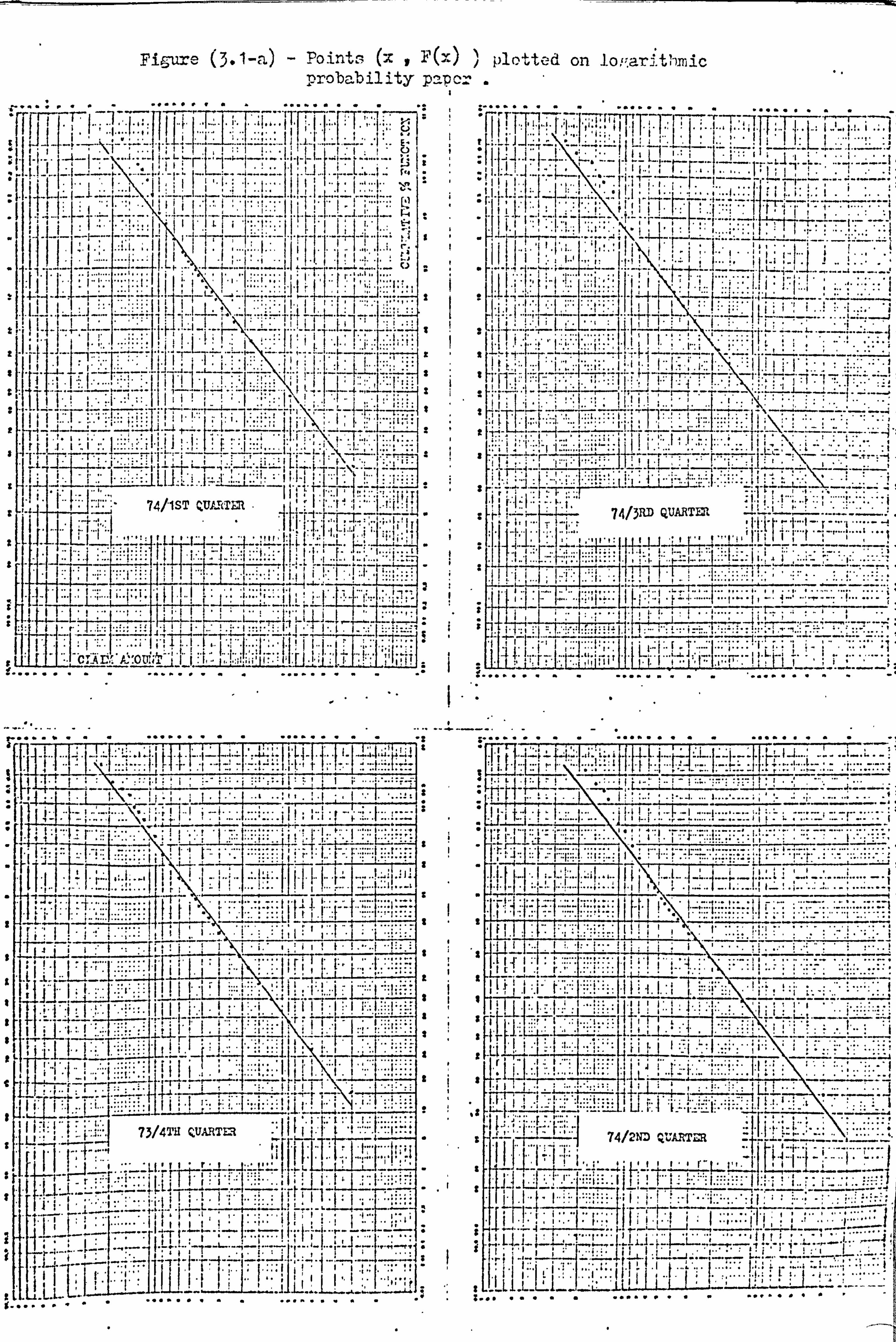
S S

Figure (3.1-a) - Points (x , F(-) ) plotted on lo, -. arithmic

probability paper .

N I'

117-17

F: T

74/iST QUARTER ;' ý'I'""'('" , ý. r. j.: l

777 f:. .tI: ,;; -ý. ̀ , fit. -:,

,i!. "', ,I:. I.., t--... '. -.

. ourl eLLLLL

arm T

'71-77-7 II ý_1fI! I mo-"j i

73/4 ýZUART

. 77

r. ...

ir

i-

t t

=i

l tS

zt

tt 1

S, -

tS

-'t

_; t

-S

i

}

'ji i

3 =

_-

__

::

:':

$it

S:

s=

_:

'_

=II

"_

-H :

"_

LY 71-

III .1 -j'r".

.. +ýI,

ý,

! ý..

", Ii''. 1 _- I ýI. I

II'

'"17ý ('...

Lý:. ý t'1 ý--

'i; I. i ý-II 1I..

-fit `ý -'i" 1 ii.

W

ý..,

i. i I

. «. ý. {..., _ýý__ý.

ý. Lýf_ý.

_L... _,. _. -t_

77

. _. , may. -tai. ..... _. ý .... ..:

ý:: "...:: ýý. ý_ ý. r ý_ -

ýf t 74/3RD QUARTER

..,

rý1+"ý;: ifli .

LL

:. j t.

ju"I: ý'.

1 1; !i

. -`-

'---`-

di

[L I

74/2ND ^L"ABT tIý.. ... ........

I " ý ý"ý '

{..:.?. ß. 1 1_:... 1. '... -. - ---ý, ý'!. L ýr . _. -ý ý iJ ý _ _ _

1 :A ß. 1 I

.+5... ..

T..... .

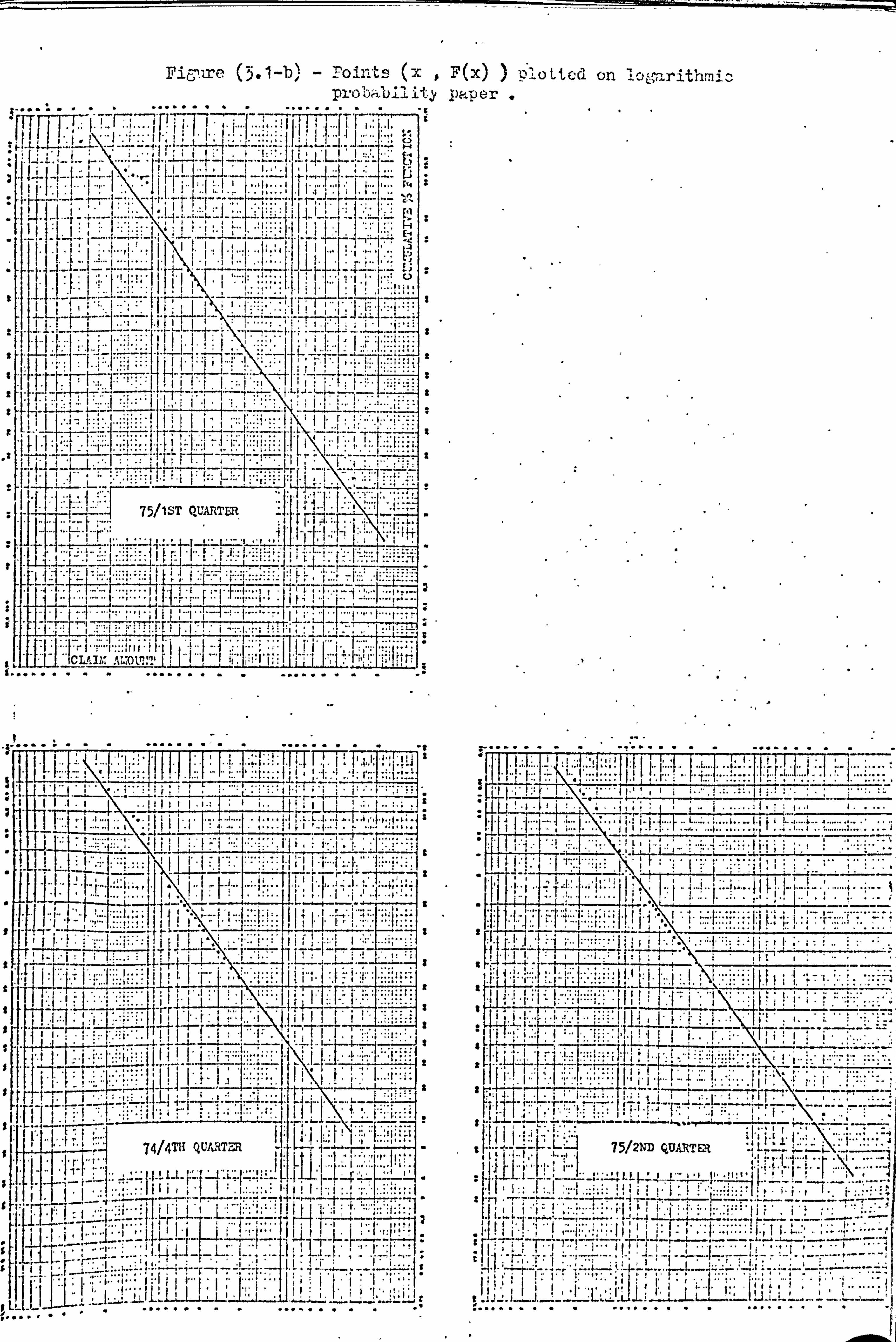
Fiý. ire (3. ! -b) - Poirts (x sr

(x) 'o tied on iagnrithrn! probability paper

4 T 1 T .

ýi i. «1'__l-

"'» . rl .IiII

ýý_ I

Imo,

. 'I^ . jý

.'i .4J. 1i _.

1: ý..

_ý.. i. ',:

ý';

7 -1

HL (1 ký;.. l... (.. %I:.

_li:;.. L

ýLI

44

j J

-' 75/1ST QUARTER TA

T :_ ITiý .

JI'_ 'I 111L! _l.

'T-ý"'ý'.. "`-'ý 11:.! _

... I" '.. t.. t

i

_-

s

a

V

c'

$ ,.....

...... . ý.

...... .! _..... ..... ...... _

I H

rte . 1..

FF..

...::..

1 .1

.; : ý.......:;., }. 1.:,...

?4 4TH QUARTa"Ft

LL

i

2

*

2

2

I

2

2

2

s

r ;.....

t.

ill

I

:I

F- I 4J.;

LL L

[7,

7512ND TERE L" ý-

'

IL" ,4i..

ý l. 1ý. ý_.. '. I:.: ý'ý"j j 1i. _ß ý .... _ý... l i. -+_ ; ;.....

-..

-; "ý-i

:........ ..

and other graphs have been reduced from their originals. jr, this case,

they have been reduced to 1

of their original size. However, for the

purpose of comparison between plots for different samples, it is more

convenient to present these graphs as in figures (3.1-a) and (3,1-b).

For each sample the points appear to lie approximately on a straight

line. We have fitted this line by eye. The pattern of formation of

the points about the line is the sane for all the samples. The deviations

from the line seem to be greater at the tails of the distribution.

It was deemed necessary to see what an actual sanp1e of two-

parameter lognormal observations from a population similar to those from

which our accidental damage data have been derived would look like when

plotted on the logarithmic probability paper. A computer simulation exercise

was, therefore, performed. We generated ten random samples each

consisting of 2500 lognormal observations from the population with

.2 4.5 and v=1; It will be shown later that these values of u and 2

are close to our estimates of the population parameters for the

accidental damage data. The size of each sample was adopted as 2500

because this figure is close to the size-of our AD samples.

For each simulated sample, the random lognormal variates were grouped

according to the same grouping format as for the AD samples, i. e. up to

600 in bands of 30 and afterwards in bards of 100. The computer program

P2 performed the task of simulation and then printed out a table of

grouped data with its corresponding sample cumulative percentage function.

The ten simulated samples, thus generated, were then each plotted on

logarithmic probability papers in the same way as described for the

accidental damage data. The plots are presented in figures (3.2-a),

(3.2-b) and (3.2-c).

In each case the points seem to lie approximately on the straight line

55

pure (5.2-e. ) - Fo int (. x ,) plotted on logarithmic I protabilitly paper.

(STI1ULATF. 'i) SEvý^FI3)

i- _t- 1

rk.

^'..

. ---

H i... 4 ci_ýýý. I.

'-1. ". ý_. r - ma ` "

-i

17

-Li

1" I I

ý 'Ii

" .ý 1

, L ý_ýj-"ý-

ý

LLSi . UL' w0 %VATION

7-7

i:

_x

x_ =Is

ý'-ý -_

1-7

-- . u--

ß. -.. r. 1.; '' I ..... ý.. ý.,. L.. ý_

... l.. _i-.. -1

I"

i

x

e

Y

ý;: ý... f a....... ....... ... :. i_ :ý_..:... .

::.:: .

::..... ._1

. t. I1

ii,, . 'ý I"!

i.. ,. i.:. i.; tL,... I .I,. i

.. i:. i...:

17-

-' ~i ;}; " . I. _ý...: _

'I ... -if I i.

ýTji

it.

77 7

ý,

r ;!

I.... ,. 4 '1"

. f.

i : i-Its. : L.. i::.. (:

flT r I

:i

s

s

s

s" s

sl

s sý

ss

.s

r

sý t.

DI:

r'ýTý, iýl"E: _ýT-.

ij" : -: ý i{ 'jIr: - ý` . G' _. ' - -ý = - - 1- - r-

ý 1 . 1. ý.

r' - -ý-7 -"r-. lý. r.

i

.i ý", i , 1:.. i. _: ý" 't -rýLiý_I_; ý_: ý. 1 .r ! , _. ý _... y_.. _-ýj

_ _ y

1

. 1.7. ý

.. ir. f...

'.

_r, ...., ý.

77

ý.. `.. a... ýýý"'T"ý. +.

ý i1..

r,

1... LýT_..

_;.... Y... ""ý.

2

i

0

s

e

sýý

ýJf

(3.2-^} - Points (x : `i, Y) jp1ottcd on 1crarit1=, ic

pros abil itv pr (SII4a1..

tirJ i'. ir? I

z. .. ---- t...... .

f7l

1-7

14.

77. I. ;

LL L ,Ir

{I.. r .1t ý": s.

FF1. «<f...

r1LL"i

' -I

;: IiI ii.

ý"jý. 1' I ; "" fl_T:

=1 ý1.: L"

`ý ý!

-1 . ý.

`

: i.:..; ..:

' ia..: 1. i..;

.

1.

--. I .. 1'

ýý. ...

. ýJ T ,L --T.

1

. ULL 4-L

I 1_jT;

°ý: _.

"

:. wl . 7-W

ýý :I t. f ... .'It, 1f., i,. E

i ' 1 ' -- } 1- 7 --

, i-r"-f-- ý :; i, 1ilfý! iI I`I

. ý.::

i. i i. i. 1i "? ii :I_. i.:.. ii ýtl; ý. : i:::

1Lý_J

. rr ý . I___. ý .

Y"'ý X4 1.. _: ß.,. _i: -. _

tom, _. _1 i 1! if! '" ...;.. ß. _t_1_

ýlýýý .: ýI ' I.

ý- i SIMUL ATED O

:

BS1ytVATI01

ý .

T 7,7, -177 lý

x i

z. x

=x

s"x

xx 1.

-i"c

's

-" s }

"s i

I

-. g.

:2"-

i'

s.

:Is

c =is

s= ss _. T

s

:_

.' _'

"s

`

4ý

I' I"_' i : Iý°_ : li`tý'i i ..... iii. I. i... l. t ....!

'! M1I..

I

-1. .. l'

"'l..:. ( 1.: 1:. ý..

ý' :...

ýl..:. ":

"-". I'. 1.1 .; ý_. ,_...

", --.. {

-IT id HiS, J: 1

'- i. ".; _; ý

''1.

ý. .

. ".. L...

i tip iý;..... .. L. li .l 44

I1: t

77

: 1. ß ; Jýý'I , -{

- .; {Ii. ` j{t : ýý1: 1 !ýi j" :I

F777- -7

li-.. ý_J ____

i; '; 1

..... ..... t ... ý_

. . ý, - : ýý. ý_. ý.... -. - ---- --

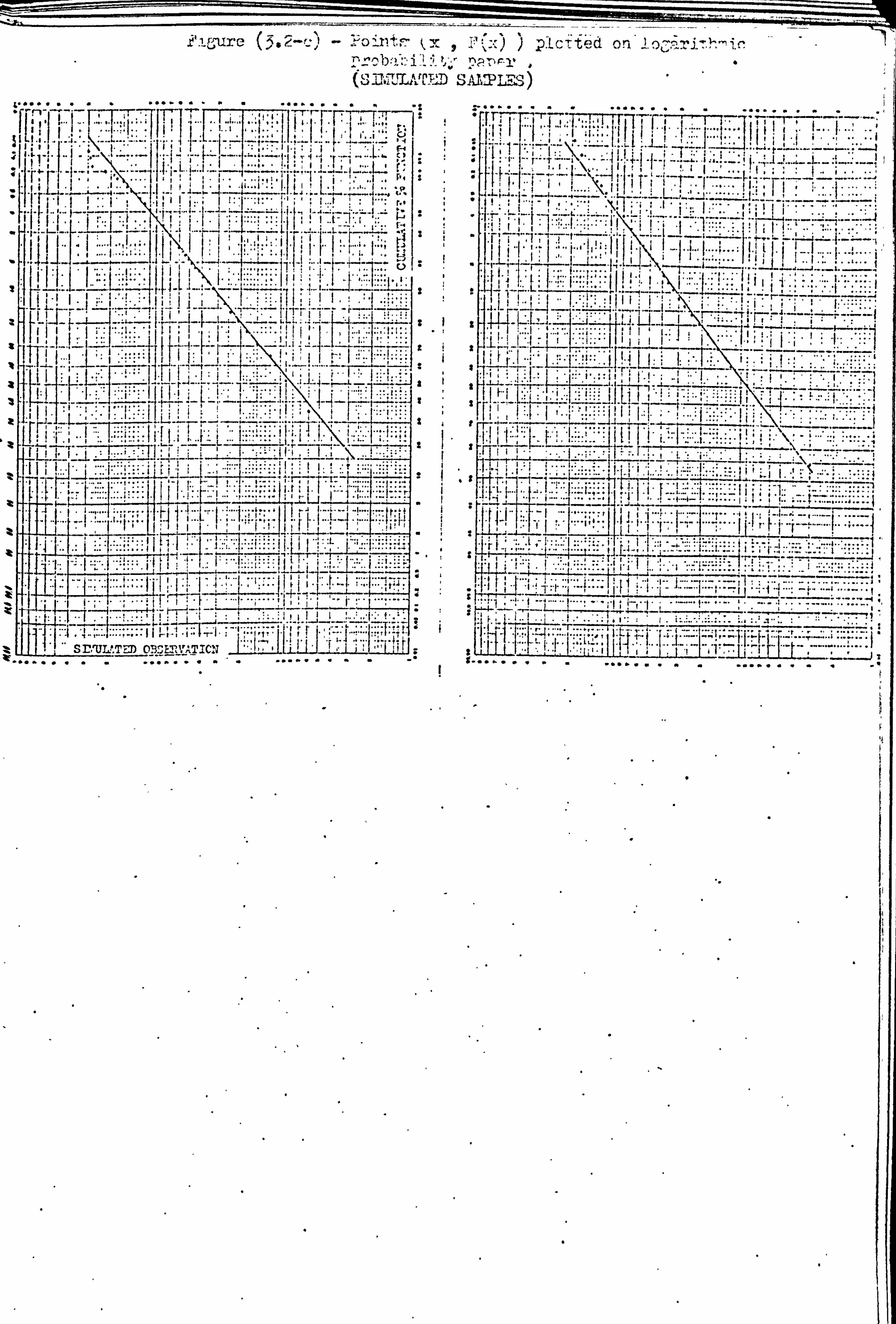
gure rroi=?: L

I i7- 71 Ifi"týj I

_I' , "tiý I i: ýý-!

' t: " !ýit. _i `; 'i"t..., r..

I TT

Ifl

; "" }ýr ýt`

Sr, OL? TM 0 If, I 9"HIMTICN

2

S

F(:: ) )p CTt°d on I7i? S! ~J 1t

A! iT LE2 )

77-

r" -t'- :

ý. ý. ".

Iý ýt-} -{--; __; ý.. i,:.. ---' }... ß_1_L.

_: __1_. _::

_r. l "ýJ. ý-i I_ýiIti

IT X77:

'

s: i=

sr$ ss

:

s

I .:

r

I

" i.

E

. ýýý". .,. . ur"" .. " .t f

F

" 'd

"t

which has been fitted by eye. In the lower tail of the distribution

the points seem to lie almost exactly on the line , unlike the behaviour

of the accidental damage samples. The pattern of the points in the

upper tail of the simulated samples is similar to that of the accidental

damage data, i. e. the deviations from the line are more marked. This

indicates that even from a sample of 2500 lognormal observations we

cannot obtain a close fit to the straight line in the upper tail of the

distribution. This is because the lognormal is a very skew distribution

and observations in the tail are scarce. Therefore, we need a much

larger sample size before we can see a true picture of the upper tail of

the distribution. Hence we can safely assume that the pattern of the

points in the upper tail of the accidental damage samples is by no means

unusual to the lognormal distribution and should, therefore, feel

satisfied that the distribution fits the upper tail reasonably well.

The simulated samples, however, tell a different story in the. lower

tail of the distribution. Here the points lie very much closely on

the straight line-and the deviations from it are much smaller than in

the case of the accidental damage samples. Therefore, the pattern of

the points in the lower tail of the accidental damage samples is not

consistent with that of the two-parameter lognormal distribution. We

believe that this inconsistency could be partly because of the in-

sufficiencies and inaccuracies of the data in the lower tail. Most

policy holders do not claim for small amounts for fear of losing their

full entitlement to no claim discount which, in some cases, is worth

more than the amount they may recover by a claim. Therefore, the data

in the lower intervals may be incomplete. On the whole, the assumption

of two-parameter lognorriality as tested by this method seems reasonable

enough to allow further analysis.

Two other tests of lognormality, mentioned in 3.6.2, are the

skewness and kurtosis tests of normality. The values of the coefficients

56

gl and g2 for each saq)le of the accidental damage data were calculated

by program Pl. These were presented in tables (1.1) to (1.7) and are

produced in table (3.1) at the end of this chapter. The standard

errors of these coefficients, for large samples, have been calculated

according to the formulae of section 3.6.2. These are presented in

table (3.1. ) as well. From this table it is apparent that in four periods,

namely 74/3rd quarter to 75/2nd quarter, the value of gl is greater than

three times its standard error. Therefore, in these four cases, the

underlying assumption of normality. for log X, and hence of two-parameter

lognormality for X (the claim amount) should be rejected. For the

remaining three periods, namely 73/4th quarter to 74/2nd quarter, the

lognormal assumption for the distribution of claim amounts is supported.

The values of g2 are significantly larger than their standard errors.

Therefore, this test suggests that the assumption of two-parameter log-

normality should be rejected. gl and g2 were calculated from grouped

data with the assumption made, in section 1.6, about the concentration

of the claims in each band at the mid-point of that band. This could

affect the values of gl and g2 calculated from grouped data. A

Sheppard's correction for the calculation of moments of log Xis not

applicable exactly because the intervals of log X are not of equal

length.

It was decided to put the ten simulated lognormal samples to these

tests. The values of g1 and g2 were calculated from the simulated

grouped data in exactly the sane way as for the accidental damage data.

Their standard errors for a sample of size 2500 were also calculated.

The results are presented in table (3.2). The values of gl compare

favourably with its standard error and, therefore, this test performs

very well. The values of g2 are in most cases acceptable, but in the

case of samples 1,7 and 8, E2 is greater than three times its standard

error.

57

Therefore, the coefficients g1 and g2, even when calculated from grouped

data, can be used to test normality for log X and, on the basis of the

simulated samples, it seems that gl can indicate normality more

accurately than g2. The comparison of the values of gl and g2 calculated

from accidental damage samples with those for the simulated samples shows

that the assumption of two-parameter lognonnality is, on the whole,

reasonable.

Another test of lognormality is the test in (ßl, ß2) plane

which was mentioned in section 3.4.3. The values of ºý1 and b2 for

the AD samples were calculated by program P1 and they were shown in

tables (1.1) to (1.7). Figure (3.3) shows a plot of the points (bl, b2).

These points, although some of them are very near each other, seem to

lie approximately on a straight line. This supports the assumption of

lognormality as the underlying model for the distribution of claim

amounts.

To see how this test performs when applied to actual lognormal

samples, bl and b2 were calculated for each of the ten simulated samples.

The points (bl, b2) are plotted in figure (3.4). They appear to lie

approximately on a straight line. Therefore, this test can be applied to

test lognormality. However, for reliable results we need a large

number of points and hence a large number of samples.

58

'l

Figure (3.3)'- Fart of the (bi 2) points for the Accidental Damaje data

5 1° " 20

ýiý

}GC

if

9a

70

6c

IC

6, ip 20 -"�0 A. u -0

Figure (3.4) - Plot of the (bl , ib2) Points for the o; TMulated samples.

3.7 Estimation of the Parameters of the 2-Parameter Lognormal

Distribution

Aitchison C-1-id Brown (1957) investigated thoroughly the problem of

estimating tho parameters of the lognormal distribution when the value

of each individual observation in the sample is available. Ibwever,

their treatment of the problem in the case of grouped data is very brief

and they point out that there are certain difficulties in the various

methods of estimation. In this section we study the problem of

estimation from grouped data. Some of the methods, described below,

have been modified from methods of estimation for when individual sample

values are given. Some others, such as the graphical, the least

squares, and the multinomial maximum likelihood methods are directly

suitable for grouped data.

Let us assume that we have a sample of grouped data where n independent

random observations on a random variable X (in our case, the claim

amount) have been grouped according to their size into k intervals.

Further, let ni be the number of observations (clams) in the class

interval (xi_1, xi) such that

k n=ýn;

1y i=1

It is usual, in the case of grouped data, to assume that all the values

within any interval are concentrated at the mean of the portion of the

distribution over that interval. If the distribution is the correct

rodcl for the population from which the sample values have been derived,

then for every relatively small interval, the mean of the portion of the

distribution over that interiral can be considered as equal to the mean

of sample values in the sp-me interval. Information on the average

amount of claim in any interval was provided by the insurance company.

This showed that for every interval the average amount was very nearly

59

equal to the value of the idd-point of that interval. We, therefore,

feel justified in asstrdng that within any interval (xi_l, xi) the

claims are concentrated at the point

iL (xi-1 * Yid

3.7.1 The Method of Moments

(3.7-1)

Let Sl and S2 be respectively the first and the second moments

of the sample values abcut zero, i. e.

1k S1 =n lýl

nixi (3.7-2)

k2 S2 nil nixi (3.7-3)

Estimation by the method of mments consists of putting S1 and S2 equal

to their corresponding theoretical values from the distribution. Hence,

by using equation (3.3-3) with r=1 and r=2 respectively, we will

have

S1 = exp (u +2 Q2 )

2 S2 = exp (2p + 2Q )

2 Solving the above sL'Tultareous equations for u: nd a we obtain

2S2 log S2

and

Q2 - log S2 -2 log Sl

(3.7-4)

(3.7-5)

(3.7-6)

(3.7-7)

^z 2 where u and Q are the estimates of p and a respectively. We have

given some consideration to the question of applying a Sheppard's

correction to the second sample moment. however, numerical investigations

60

showed that this correction does not have a significant impact on the

values of u and e2 . It has been suggested by some authors (see for

instance, Geary and Pearson (1938)) that unless the grouping interval

is more than one-third of the standard deviation of the sample, it is not

really necessary to apply any corrections to the moments. A glance at

tables (1.1) to (1.7) shows that for our AD samples the interval width

for the majority of the bands, containing some 9510 of the total number

of claims, is 30, while the standard deviation in each sample is at

least six times that. From the above considerations a correction to the

second moment is not deemed necessary.

3.7.2 The Approximate Maximum Likelihood Method

The word "approximate" in the title of this method is used because

of the assumption of concentration of the claims in every interval at

the mid-point of that interval. For a grouped sample, using the notation

already adopted, the likelihood function L is

2-kk -n1 " L= (2, ra)n/2 I1 xi exp 'ý' I ni (log xi -u )2 (3.7-8)

i. =1 2a i=l

I

2 The same values of u and a maximize both L and log L where

log L=-n log 27r -2 log Q2 k

nlog x-1 i=1 ii

2a

kz ill (log xi-u)

i=1

(3.7-9)

2 The values of u and a which r, mxlmize log L are the solutions of the follow-

ing two simultaneous equations,

u1°ß _0

loh I, =p 2

t: ence, it can be easily shoum that p and Q the estimates of u and 2

61

2 a respectively are

k

iý =nG 1=1

and

k ^ý_ 1 Cl` n i=1

n1 log xi

2 ^2 nl(log xi) -u (3.7-11)

3.7.3 The Method of Quantiles

The relationship (3.3-12) between the same order quantiles of the

lognormal and the standard normal distributions, namely

xq = eu+ a zq

is the basis of this method. Let xql and a2 be two different quantiles

of orders al and q2 caleulatcd from the sample. These can be either

selected as the upper boundaries of two different intervals or be

calculated by interpolation in the intervals of X. The corresponding

standard normal quantiles, zql and zq2 respectively, can be calculated

by reference to a table of N(0,1) distribution function. and a2 the 2

estimates of u and a respectively, are the solutions of the following

simultaneous equations

x= eu+ czai aý

A x eul azg2 q2

Hence z log x-z log x ^ _.

3c g' ch (3.7-12) zq2 - LQ1

and

ä2 log xa, log xq1 `2

Zq2 Zql

62

It can be shown that this method is most efficient when the two quantiles

are symmetrically placed (Aitchison and Brown (1957)). Let, therefore

ql =q and q2 =1-q where q< 1/2

then

zal =zq=- t, say, where t>0since q<1/2

and z2 = '1_a =

Hence u and Q2 will be

u=2( log xl_q + log xq )

and

(3.7-14)

ý2 4t2

(log xl_q - log xq) 2 (3.7-15)

Aitchison and Brown (1957) state that quantiles of order 27% and 73%

estimate u with 81% efficiency and quantiles of order 7% and 93% estimate 2

c with an efficiency of 65%. We will later use these two sets of 2

quantiles to estimate u and a from the AD samples. To obtain the values

of the c{uantiles linear interpolation in the intervals of x will be used.

3.7.4 The Method of Median and Coefficient of Variation

This is a very simple method which involves calculating the sample

median and coefficient of variation, xmedian and V respectively, and

putting them equal to their theoretical values fron the distribution.

To find xmedian' in the intervals of x may be necessary.

For the sanple coefficient of variation, V, we need to calculate the

sample mean and standard deviation. The expressions for the median and

coefficient of variation for the two-parameter lognormal distribution

were given by (3.3-2) and (3.3-8) respectively. Hence

inedian = ell

63

and 2 V_= (e - 1) 2

2 The estimates of i and a will therefore be

}log median (3.7-16)

and a2= log (1 + v2) (3.7-17 )

This method can be considered as a combination of the methods of moments

and quantiles.

3.7.5 The Graphical Method

This method is derived as a follow-up of the graphical test of

loiormality mentioned earlier in section 3.6.1. Therefore, we know that

the locus of the points (log xq, zq) is the straight line

Z. =1 log x- 11

Let us assume. that we have followed the procedure of section 3.6.1 and

plotted the points (log xq , zq) from a sample of grouped data. Let us

further assume that these points seem to lie approximately on a straight

line. We can fit this line to the points by eye. The inverse of the

gradient of the line will give an estimate of a and then from the intercept

of the line we find the estimate of p.

Aitchison and Brown (1957) suggest the following method when the

logarithmic probability paper has been used to plot the points :

From a table of the standard normal distribution function we notice that

116% Z158ö -1

and =_+1 284% 284.13%

0 Z5oä =

64

Therefore, if we put the logno: 7na1 population quantiles of orders 16 a,

50% and 84% equal to their corresponding values read from the straight

line we will have

u-Q x16%% =e

u X50$ =e

u+Q X84% =e

Hence from (3.5-18)

a u= log X50%

Then from (3.5-19)

ea _ X50%

x160

and from (3.5-20)

Q X84% e= X50%

a better estimate of eo would be

ee X50%

+ X84%

2. X16% X50%

Hence

(3.7-1ß)

(3.7-3.9)

(3.7-20)

(3.7-21)

X50*- 112 Z_ log 2(a+ X84% ) (3.7-22)

X16$ 50$

For grouped data, this method has the advantage that the data is already

in the form required by it.

3.7.6 The Method of Least Squares

This is a variation of the graphical method. Instead of fitting a

straight line by eye to the set of points (log xqj zq) we use the least

65

squares regression method to determine its equation. The theory of

linear regression tells us that if the ur_creighted least squares li:: c

through a set of m points (Ui, Vi), where i=1,2, ... , in , is

V= aU+b

then the coefficients a and b are

_W- uv

aÜÜ2

and b. = V- aU

mm where U= 1Iu V= 1 V.

M i=1 1m i=1 1

(3.7-23)

(3.7-24)

(3.7-25)

M2m

U=1 Ui and UV =1 UiV. m i_l m i=l i

As we mentioned earlier, the point (log x, z) lies on the straight

line

z=Q log x-Q (3.7-26)

Therefore, we can let

U. = log xal and Vi = zq. i

where xqi is the upper boundary of interval i, qi is the value of the

sample cumulative percentage function at the point äi and zqi is

the standard normal variate corresponding to qi, i. e.

Z qi 2

q1 exp 2) dt

The problem then is to calculate the coefficients a and b of the line

V= aU+b

66

If our grouped data consists of k intervals, then i takes integer

values frone 1 to k-1 because for the final interval ak =1 which

results in an indeterminate value of zq. The values of zq can be

obtained from a table of the standard normal cumulative distribution

function. If this estimation procedure is programmed on the computer, an

approximate formula for calculating zq from q should be used. Hastings

(1968) gives the following approximate fornula for calculating the

standard normal variate ,z, from ,p, the area under the upper tail

of its - frequency curve :

where

- 2.515517 + 0.802853t + 0.010328r

Z=t 1+1.432788t + 0.1ß9269r + 13 8rt (3.7-27

p_ 27r)-1

r. = log 2

P

J"0 exp (- 22)de

z

and t=

, 0<p<0.5

To use this formula in conjunction with the estimation method, we have

to take p=1- qi where qi is as defined above.

Let, therefore, V= aU +b be the equation of the least squares line

where a and b have been calculated according to the formulae (3.7-24) and

(3.7-25). A comparison between the equation of this line and that of

its equivalence given by (3.7-26) shows that

a= l/Q and b- --u/a

a Hence u=- b/a

and a2 _ a-2

(3.7-28)

0 (3.7-29)

3.7.7 The Mhultinomial Maximum Likelihood method

This is by far the nxost suitable method for estimation of the

67

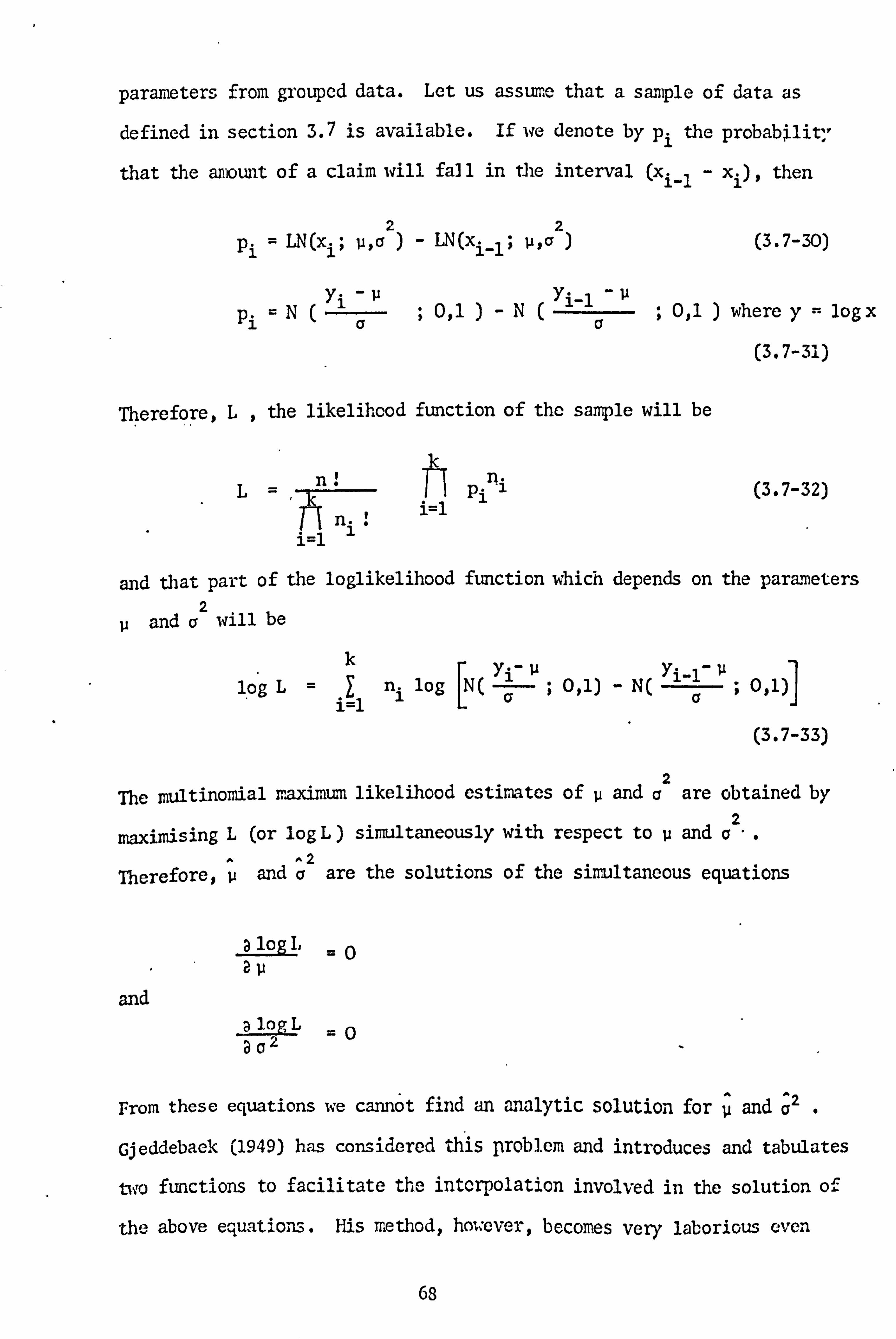
parameters from grouped data. Let us asswre that a sample of data as

defined in section 3.7 is available. If we denote by pi the probabilit; "

that the amount of a claim will fall in the interval (xi_1 - xi), then

22 pi = LN(x1; u, Q )' LN(Xi-1; u, a )

"_ -u pi=N(a ; 0,1)-N (

Y'

Therefore, L, the likelihood function of the sample will be

(3.7-3i)

n: n. L= Pi i (3.7-32)

n i=1

i=1 1

and that part of the loglikelihood function which depends on the parameters 2

V and will be

k yi- u yi-1- u 'j log L== nl log

[N( 0,1) - N(

Q; 0,1) I

J i-1 (3.7-33)

2 The multinomial raximun likelihood estimates of u and a are obtained by

2 maximising L (or log L) simultaneously with respect to µ and a

2 Therefore, u and a are the solutions of the simultaneous equations

alogL =0

and alogL =0 a02

From these equations we cannot find an analytic solution for u and Q2

Gjeddebaek (1949) has considered this problem and introduces and tabulates

No functions to facilitate the interpolation involved in the solution of

the above equations. His mrýethod, however, becomes very laborious even

(3.7-30)

; 0,1 ) where y- lag x

68

when the number of intervals is greater than 3. It is possible to

use an iterative procedure to solve the system of non-linear equations 2

in u and a. Tallis and Young (1962) apply this method in the case of

the 3-parameter lognormal distribution.

We instead propose the use of an iterative method which maximizes 2

log L itself with respect to the parameters u and a. There are now

many computer routines-available for maximizing a general function of 1

severable variables. We use one such routine provided by the NAG library

of programs. This routine minimizes the function - log L (i. e. it

maximizes log L) with respect to the unlaiown parameters by using a revised

quasi-Newton method implemented by Gill and Murray (1972). Analytical

derivatives of the function need not be supplied. To start the iterative

process the initial values for u and a- are obtained by one of the

simpler estimation methods described earlier. The procedure uses

estimates of the gradient and curvature of the objective function to

generate a sequence of points which are intended to converge to a 4 42

local maximum of log L. V and a thus obtained can then be used as the

starting point in order to make sure that they are indeed the optimum

points. If on inspecting a maximum found by the routine it is suspected

that a 'better' solution exists, the remedy is to re-run the routine

from another starting point closer to the expected solution. With the

wide availability of the computer this is very much easier than the

methods of Gjedd. ebaek or Tallis-and Young.

In conclusion, we point out that there is another suitable method

of estimation from grouped data which is called 'the modified Chi-square

minimum method'. This involves minimizing a modified Chi-square type

statistic with respect to the unknown parameters. Cramer (1946).

1- Nottingham Algoritiunic Group

69

however, shows that this method is identical with the iruitinomial

naximtn likelihood method. Therefore, we shall not consider the

modified Cri-square minimum meted in this work.

3.7.8 Measuring the Performance of Various Methods of Estimation

A simulation exercise was carried out to see how well different

methods of estimation perform in practice. 100 samples, each of size

2500, were generated from the lognormal population with parameters 2

u=4.5 and a=I. These values for the parameters will be shown to

be close to the values for our accidental damage (AD) data. The size

of the simulated samples, 2500 , is typical of the size of our accidental

damage samples. In this way, simulated samples resembling the actual

AD samples were produced. The computer program P3 was written for this

task and samples of data grouped in the same format of intervals as for

the accidental damage data were created.

We define the numerical measures of efficiency of a particular method of 2

estimating u and a as

N Eff(p) =R CUl u)2 (3.7-34)

i=1

Eff (Q2) N0-a )2 (3.7-35) i=1

where u=4.5 $ a2 =1 and N= 100, and a1 are the estimates of

and a2respectively, arrived at by the method in question from

sample i.. For each pair of estimates (p ,Q we can find, from

forrulae (3.3-4) and (3.3-8)9 ai and $i which are the estimates of

a and a the mean and standard deviation of the lognormal distribution

respectively. ., i and ßi are then considered as estimates obtained

70

by the same method of esti. ̂ mation which was used to find ui and cri from

sample i. Because a and 0 are functions-of both u and a, it is 2

important to kiow how well a particular , method of estimation performs in estimating a and ß. 't'herefore, we can similarly define measures of

efficiency for a and ß as

N 12 Eff(a) =N1 (ai - a) (3.7-36)

i=1

N Eff(ß) - (ßi - ß)2 (3.7-37)

i=1

2 where, from 4.5 and a=1 we have, a= 148.41 and 8= 194.54.

Men comparing two different methods of estimating a certain parameter,

the one whose calculated measure of efficiency is smaller will be fudged

as more efficient and hence will be preferred. 2

The computer program P4 was written to estimate u and a, from

each of the 100 simulated samples, by the Methods of moments, approximate

maximum likelihood, 27 and 73% quantiles, 7 and 93% quantiles, median and

coefficient of variation and the least squares regression. The graphical.

method was excluded from the exercise because the task of plotting 100

sets of data points would have been very laborious. Besides, 'the

efficiency of this method depends on how experienced the analyst is in

using the graph paper and fitting the line by eye. The multinomial

maximum likelihood method was not included because it is the most

suitable method for estimating the parameters from grouped data and is,

therefore, sure to be very efficient. 2

Program P4 produced estimates of p, v, a and e, by various methods,

from each sample and calculated the efficiency of each method in

estimating each parameter. Table (3.3) Shows the results of this

simulation exercise. It is apparent that amongst the methods considered

71

the approximate it . xirumi Likelihood is the Timst efficient in estimating

the parameters from the particular type of data we are dealing, with. The

method of ?7 and 73% quantiles is the second best and nits use should be

recommended when simplicity in calculations rather than maximum accuracy

is the criterion. The efficiency of the method of median and coefficient

of variation for estimating u is the same as that of the method of 27 and 2

73% quantiles, and for estimating e is the same as that of the method Ilk

of moments. Therefore, the median can be used to obtain a good estimate

of v. The method of 7 and 93% quantiles is not very accurate for our

type of data. The methods of it inents and least squares regression

-" appear to perform with nearly the same degree of accuracy.

3.8-Application of the 2-Parameter Lognormal Model to the Accidental

Damage Data

The results of the tests of lognorrality carried out in section 3.6.4

seemed reasonable enough to encourage us to fit the two-parameter log-

normal model. to the accidental damage data presented in tables (1.1) to

(1.7). An extensive computer program, PS , was written to estimate the 2

parameters i and a by all the methods described in section 3.7, except

the methods of median and coefficient of variation and multinoi.. ia1

maxiim. m likelihood. The former method was excluded because it can be

considered as a combination of the methods of moments and quantiles.

The latter will be dealt with separately. For each sample of data

supplied as input, the program provides six relevant tables of results.

For a particular period of accident, nsitily the 4th quarter of 1973

which was presented in table (1.1), the results of a run of program P5

are presented in tables (3.4-a) to (3.4-f). The first table, (3.4 -s),

presents the estimates of u and a by different methods as well as some

of their corresponding relevant distribution statistics. Table (3.4-b)

72

gives the expected number of claims, in each interval, calculated by

using various sets of estimates. A table of actual minus expected.

frequencies is produced as table (3.4-c). To allow the calculation or

the'Chi-square statistic, values of (A

E E) for each interval up

to ? 000 and each set of parameters are presented in table (3.4-d).

It was considered that for claim arounts greater than X1000 the expected

number of claims in each interval would be less than 5. The total i

of the (AEE

values for each method of estimation and for intervals

up to £1000 is provided, but these-totals need to be adjusted for

intervals above £1000. To allow comparison between the actual cost of

claims and that expected under the model by different methods of

estimation, table (3.4-e) is produced. Each entry in this table is the

product of the number of claims in an interval, and the average anount

of claim in the sane interval (tr e average is assumed to be equal to te

mid-point of the interval). Table (3.4-f) provides the expected loss

and the T statistic, as defined in section 2.4 of chapter 2.

Program P5 was run with data from other periods of accident as well. To

avoid inclusion of a large number of tables, only the first table of

each run, similar to table (3.4-a) are presented here in tables (3.5) 'Co

(3.10). Relevant statistics such as the Chi-square, the T and the ratio

of T to total actual cost have been added to each of these tables.

Let us now closely examine the results produced for 73/4th quarter.

A glance at table (3.4-a) shows that with the exception of the method of

7 and 93% quantiles all the methods have produced almost similar results.

Estimates of u are about 4.5 and of a2 about 0.9. The skewness and

kurtosis of the frequency curve of the model are greater than those of the

sample (see table (1.1)), hence indicating that the frequency curve of

the model has a ]onger tail and is more peaked than the histogram of the

sample values. Table (3.4-c) indicates that the disagreement between

73

the actual and expected number of claims is more marked in a few of the

lo: -: er tail intervals. These differences are smallest for the approximate

maximrai likelihood ; method. Table (3.4-d) in fact shows that the Chi-

square statistic is smallest for that method although all the values of

this statistic indicate a significant difference between the sample

values and the model. It can be observed that the major contribution

to the Chi-square statistic is from one or two cells in the lower tail

of the distribution. We may recall that when we tested the data for

lognormality, the points in the lower tail did not fit the straight

line very well. We blamed the insufficiencies of the data in the lower

tail intervals for this behaviour. The fit of the model to the data

would have been very satisfactory if it were not for these one or two

large contributions. In chapter 7, where we investigate the truncated

lognormal distribution, the effects of discarding various intervals in

the lower tail will be studied.

Table (3.4-e) indicates that despite the large Chi-square values, the

total cost of claims from the sample and the model are fairly close to

each other. It is also inferred that although in terms of the number

of claims only about 4% of the total lies in the upper tail, (greater

than £600), in terms of the cost of claims about 17% of the total comes

from the upper tail. Table (3.4-f) shows that the total expected loss

is not, in fact, very large, except for 7 and 93% quantiles method and

that the ratio of T to the total actual cost is quite small.

For the method of approximate maximum likelihood we can apply the

Kolmogorev-Smirnov test of goodness-of-fit in conjunction with table

(2.2). The value of this statistic is D=0.023 which gives P <0"01 (see

section 2.8) . Therefore this test, like the Chi-square, indicates

significant differences between the model and the actual Sanple.

74

I

For other periods of accident results similar to those of the 73/4th

quarter can be observed fron tables (3.5) to (3.1o).

The above analysis supports the findings of the simulation exercise of

section 3.7.8. Pinongst the methods considered, the approximate

maximum likelihood gives the best fit of the model to the actual data

in terms of the goodness-of-fit tests. The fact that for each sample,

the Chi-square statistic is smallest for this method is not surprising

if we recall the remarks of chapter 2 about the estimation method

and its effects on the Chi-square statistic. The method of 27 and

73% quantiles also produces satisfactory results and its use is recommended

when a quick solution is required.

Before commenting on the-suitability of this model for our type of data

we will consider the estimation of the parameters by the method of

multinomi. al maximum likelihood.

Program P6 estimates the parameters by the technique described in

section 3.7.7 and provides a table of results. For our accidental

damage data, the results are presented in tables (3.11) to (3.17). For

each sample, estimates of u and a2, and the values of the mean and

standard deviation of the claim amount are provided. The tables are self-

explanatory. If, for each sample, we compare the results of this method

with those of the approximate maxiiraua likelihood, we will notice that

the estimates are very close to each other but a slightly better fit

has been provided by the present method. The Chi-square and the total

expected loss statistics are smaller for each sample. The values of the

Chi-square statistic still indicate significant differences between

the model and the sample values. This can be seen to be supported by

the Kolmogorov-Smirnov statistic. The actual minus expected frequencies

are again large in just a few of the intervals and the pattern appears

75

to be consistent for all the samples. It is, however, encouraging that

the values of the test statistics are not drastically large but

that they are just about significant.

The analysis so far shows that the method of multinomial maximum

likelihood, as we expected, produces more satisfactory results when

estimating the parameters from grouped data. Therefore, guided by this

information, it will be the principal method which we shall use throughout

the forthcoming stages of the present work.

To see how closely the frequency curve of the model approximates

the histogram of the sample values, computer program P7 was written to

plot both of them. The graphs for various samples are presented in

figures (3.5.1) to (3.5.7).

(This section is continued after Figure (3.5.7)).

76

t{ ý'.. tiaýýr C'J

73.

77

1,.

1f;:

17.

16

13.

12.

11.

13.

S.

7:

61

31 2

6

l4-1 '. i

: 2.

ý.

h'' . tr..

Eigare (3.5.1)

hI , TC: rPAM or 73. '1111 GUA1 Tf. F L TA P. ND ""PAf.

L(ý;, Nhf`': AL P. D. r. W'il1, MULTN. NAXL. f'AP4M! 11 ..

MCwýt. SIE. SICMA

2 20 -i(l, ; 270 2eO -ý3, " 260 1 2t, 1Ü 1C S1O 51C 370 (>CC 1

OF 73%1TF+ GUARTE. R DATA AND 2-PAP.:

F. C. E". WITH FILLTN. MAXL. PAP. AiE. TCks

SIGMA SL'. =i.:: 55

iýýIj: i{S`ý1: : ý: ýi '. '% . I1ý~

ýý ýý (3-5-2)

IFr.?. ai_4k '( 4

2I.

2o 'l

s.

1 f; =7. IFS

IJ

13.

12

3 22 Gf1 ; 2u afi ; CC 213 ?T.. 7C. cC 2.2 2aG 9c0 15e 9c;.. 51

mac,? _, ': cýý

Z.

f, (X

CUAPTr. P C; TA AND 7-PAP.

ri tU. LTN .I A)(L . PAP. API': TC. R .

SIGNA SQ. -. a . 257

-': rr

NI+TC': PAN or "1'IL', T (JUMr1-I' CATA fNL1 : -PW.

LOC"NOR! '. AL f . CO. r . Gl tti i: uLTN. I! AXL . PAI'"hll! 11'. K4,

or, (ý f; ;2 fl, f, : ". tý :4 I'l, :

: ':, Figure (3-5-311,

22 HISIC: F', AI1 Or- 7"1/2N("I :; t1AF*ICR L' TA AND . -PAS:.

iý. L03NOF. MAL P. i. r. '.! Illy ilU11N. MXt_. r. AF'ßtVýTFRt; 1'

tii i MC+wý1 . '" i6 SIC"T7r 5O. -l . "';?

1(. I . 7.

1 rl'

1S:

lw

13.

12.

11.

C',

E:

5. .

3.

2:

6ý g0,12C X56 T£; 3 213 24.0 27C :? ZO 3< 21, C _3 120 13 18,1 5<., 1C 57< Ef'E

1? ý1 ý. E'i

Z.

ý,

G4; ß

'TER DATA AND 2-PPM..

ILTN. f1AXL. PF. r Ar'-JrFG

SIGMA SO. -i.:: 3

-z : ci OX4 -1 L:

F. ure (3.5.4)

!t I "'. ' ]V+ ýý f

. s.

F; I , tt1 . ('\ft ; 'F 'i 1' :. GAf '[$ EINTA ANU '-. i'AP. 1

ßt7 LOL"NC''`tt. f'W1 1h ULI N . h! AXt.,

19 r1c_y_q. fý? ' :, Trt1A ýyL, "'=1 .ý 11

1C. 17.

16

In

13.

11.

9

3. 2.

ý 50 12 ý. P . 6; 'I 212 24[a 270 210(1 2: T 35 ":: 7 1 F' 20 1'" 1c 513 59[: 5? i b 3f Co

x1a-1 5. ee

1 . 5C

i. Cp

2. ßfr.

1.

G(11C;

HISTCLR; 41 Cr 79/3; r, ý-LAP. TC. R DATA AND 2-PAP.

LO; NCr"AL P. C. r. WITH MULTN. MAXL . PA. RAM': TFRS:

MEW-1. G37 SIGMA SO . -1.. ^.. '1

I -

. '

.; e ; 2;

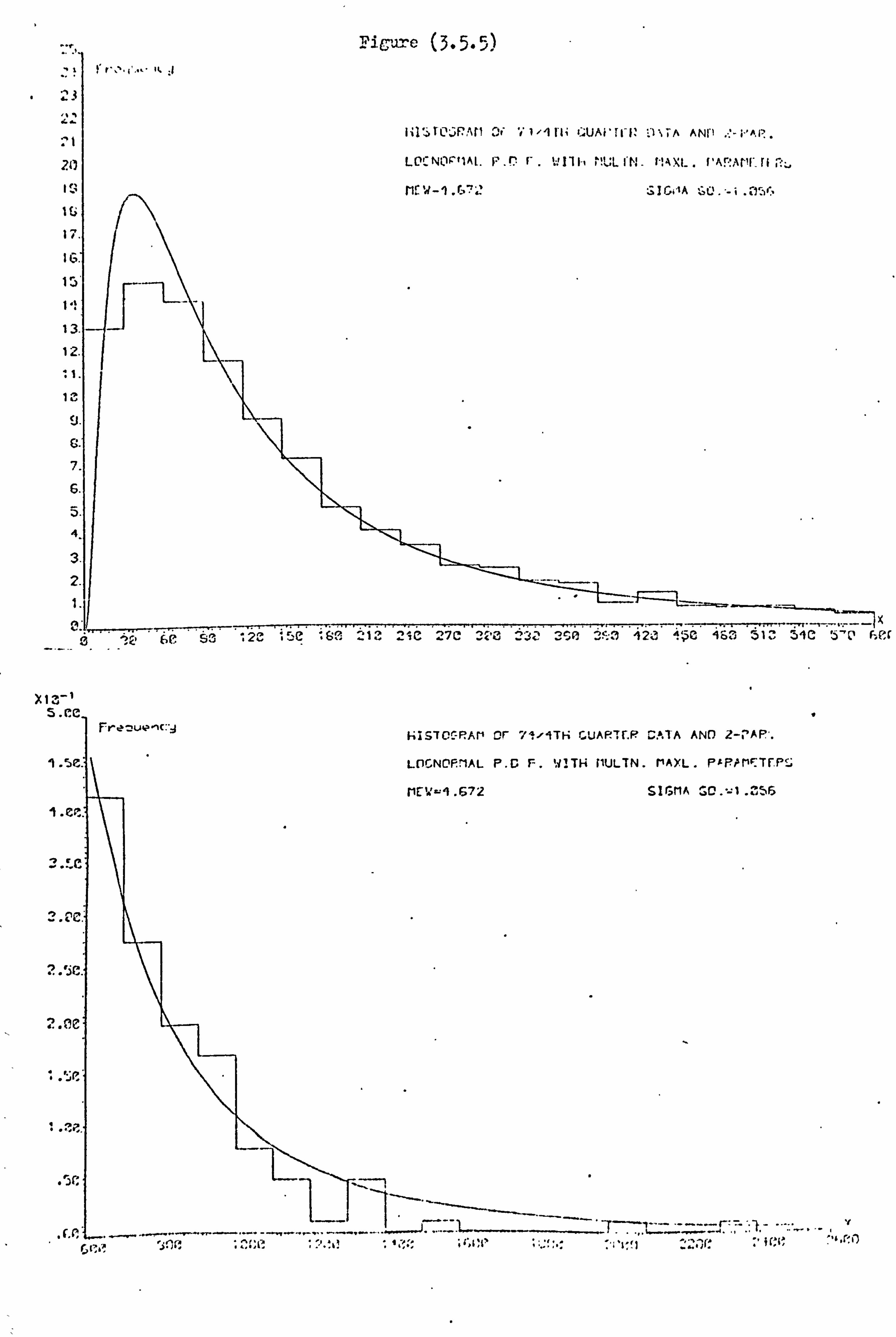
Pip. -are (3.5.5)

'ArIF fi icy

?i 51. ̂ . 51C 5-0 F P.:

Xlü-ý 5. ce

Frr-±uvnc:

9. Se.

2.: C

...

STCC-PAM Or 7 . '1TFi GUART1 DATA AND 1-i AP. '.

GNQF.! 1AL P. C F. WITH (1ULTN. f+AXL. PAPPMý: TFPý;

W--. 571 SIGMA ýc. -1.0,55

2 13 ff .

I. ' _. *---"-" ---.. --. -...

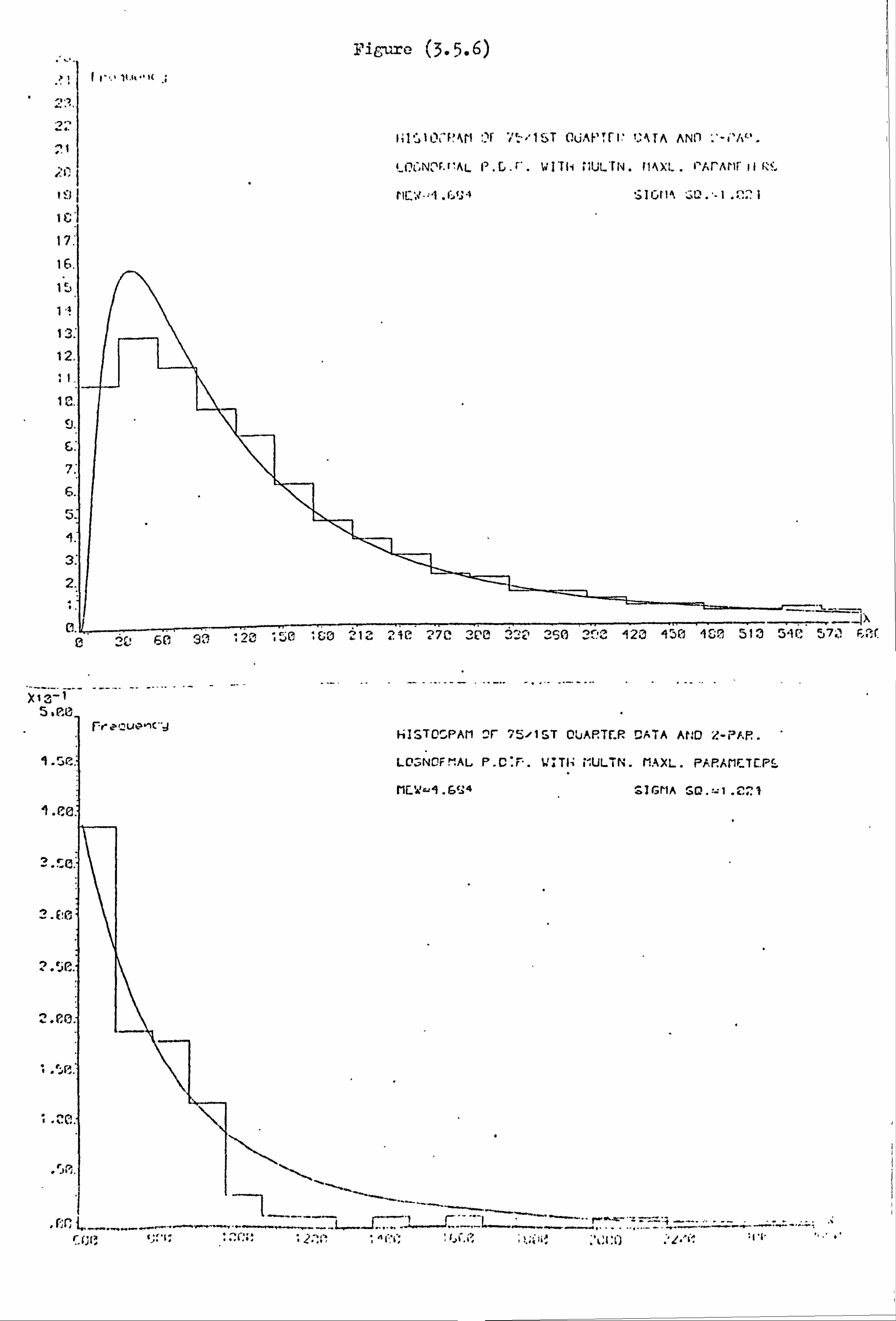
r

7,

ii

1i

1

i

1

1

Figure (3.5.6)

A ; Mr

X13-t 5 .e

FreuC

9

4 . cO-

0

Qt:

{iIGTO. PAM ^` :5 1ST CIAP. Tf_P. DATA AND 'l. -PAP..

LO NOFMAL P. C: P. WITH i-, ULTN. MA)(L. PAPAMETC. P:,

MLWa J. 6cý; 4 SIGMA SGG. --1. C^}

- ; :0 : i. IT

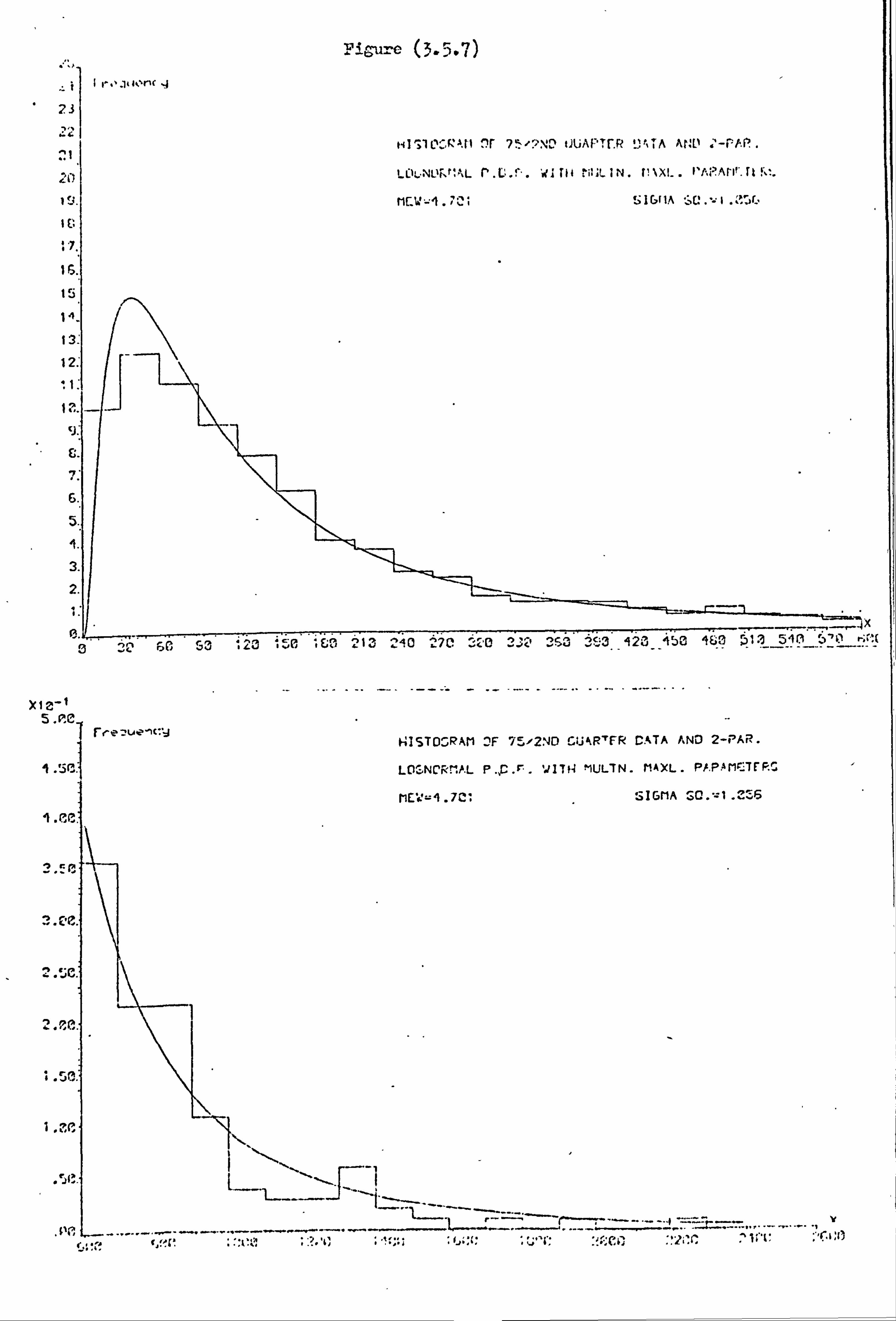
2

2i

ti

ti

p

i

I: t'.

t

Fibure (3.5.7)

:(

x, a-, 5M,

9 . 'ý

9. (;

7 r.

7"C

- s" "

4". J

/. J

1.?

CATA AND 2-PAR.

MAXI.. PA. PAMC-TFF. G

SIGMA SO. -I. 2ý6

: "; c : yt' c: """ �". " i;

(section 3.8 continued)

The multinomial maxinnm likelihood estimates have been used to plot

the frequency curve. To -represent clearly the behaviour of the tail of

the distribution, each curve consists of two parts. The graph at the

top of the page represents the distribution up to £600 claim amounts,

i. e. the lower tail. The bottom graph shows the upper tail of the

distribution, i. e. claim amounts greater than £600.

As previous results indicated, the discrepancy between the frequency

curve and the histogram for each sample is more marked at the lower

tail of the distribution. The possible reasons for this were mentioned

earlier. The curve appears to model the histogram satisfactorily at

the middle part and the upper tail of the distribution. The distinct

mode and the long tail of the histogram are both portrayed by the frequency

curve. The graphs show that shifting the curve, slightly, along the x

axis (i. e. a 3-parameter lognormal model) or ignoring the lower tail

(i. e. a truncated distribution) would produce models which would fit

the actual data more closely.

Judging by the results of the foregoing analysis, we are not

satisfied that the two-parameter lognormal distribution is the correct

model for the distribution of accidental damage claim amounts. However,

the analysis has been constructive in showing how the model should be

applied in practice. It has also been shown that, for our data, a

modification of the model would provide better results. To complete the

work on the two-parameter lognormal distribution we will study, in the

next section, the effect of inflation on the parameters of the model

and will suggest a means of-predicting the model of the future

distribution of claim amounts.

77

3.9 Prediction of the Claim Amount Distribution :- The 2-Parameter

Lognormal Model

We are interested in the cost of future claims for both the

calculation of premium rates and the setting up of reserves. -lie

cannot, therefore, wait until all the claims have been notified and

settled in order to find the cost of the claims. One way of solving

this problem is by predicting the cost of the future claims. In this

section we will suggest a technique by which the distribution of the

claim amounts during any future period can be predicted. From this

distribution, and assuming that we have a knowledge of the number of

claims in the particular period , all the required information about the

cost of claims can be obtained. The technique will be tested by using

past data. The performance of this method will be examined by goodness-

of-fit tests. In particular, the total expected loss statistic, T,

will indicate, in monetary terns, how accurately the technique is

performing in predicting the total cost of future claims.

3.9.1 The Effects of Inflation on the Parameters ' of' the' Mädel

In practice, it is usually observed that the same kind of claim

costs more to settle than it previously did in the past. From tables

(1.1) to (1.7) we can see that the mean claim amount has increased from

one quarter to the next. It is generally believed that inflation is

the main cause of the increase in the cost of claims over time. The

increase may be due to other apparent factors the real roots of which lie

in inflation. For instance, in the third party liability claims, the

decision of the courts in awarding higher Compensations stems from the

rise in the cost of living and higher wages.

Let us assume that the effect of inflation is to increase a claim of

size X to X(1 + i) after a period of time where i is the effective rate

78

of inflation during that period. If we assume that the distribution

of X is the two-parameter lognormal with parameters 2 (u, a ), by a

transformation of variables it can be shown that X(1 + i) is distributed 2

as the two-parameter lognormal with parameters (p +d, a ) where we call

d= log(1 + i) the force of inflation. Therefore, inflation affects 2

only p and leaves a unchanged. If we look at the multinomial maxirum

likelihood estimates ofp , given in tables (3.11) to (3.17), we notice

that they have generally increased from one period to the next. The

mean and the standard deviation of the lognormal distribution, a and 2

respectively, are functions of both p and a (see section 3.3) and hence

inflation increases both of them over time. After a period of time in

which i is the effective rate of inflation, a and 0 will be increased to

a(1 + i) and ß(1 + i) respectively. Tables (3.11) to (3.17) show that

the mean and the standard deviation of the claim amounts have increased

from one period to the next.

3.9.2 The Prediction Technique

For our accidental damage claims, investigation shows that nearly

70% of the total cost of claims are reported and settled within the actual

period (quarter) of accident. Another 25% are settled by the end of the

second quarter. Therefore, it is reasonable to assume that all AD claims

are settled in the middle of the period of accident. Hence, if the

distribution of claim amounts during a period A, for instance, is 2

LN(x; u, a ), their distribution during a future period B will be

LN(x; p+o, a2) where it is assumed that the rate of inflation from the

middle of period A to the middle of period B is i and that d= log(1 + i).

If sizeable parts of the total cost of claims are settled over various

periods and, furthenrorc, if they take a] ong time after the end of the

period of accident to be se. ttied (e. g. for the third party liability

79

claims), then the rate of settlement irrst be taken into consideration.

A co, bined rate of inflation and settlement will be required for

prediction purposes.

Other factors such as seasonality may be affecting the nwrber and

amount of claims during different periods of the year. For instance, in

autumn and : winter, due to the bad weather conditions, it is likely to

have more accidents and more claims for larger amounts. The data of

tables (1.1) to (1.7) show that the number of claims for the 4th quarter

of the year is greater than for the other quarters. To nullify the

effects of such factors we suggest that each period of accident should

be used to predict the distribution of claim amounts during the same

period but in a future year(s). For instance, the model for the first

quarter of 1974 should be used to predict that for the first quarter of

1975 , etc.

We can use our available AD data to test this technique for three

different periods of accident, namely, we can use

73/4th quarter to predict 74/4th quarter,

74/1st quarter to predict 75/1st quarter,

and 74/2nd quarter to predict 75/2nd quarter.

The question remains as to what should be the appropriate rate of inflation.

It would be advantageous if we could show that changes in the parameters

of the model, over time, correspond to changes in the value of a particular

index of prices or wages. We shall consider three such indices

1- Me General Index of Retail Prices.

2- The Index of Average Earnings, Miscellaneous Services.

3- The Index of Motor Vehicles Repair Costs.

indices 1 and 2 are published in the "Monthly Digest of Statistics"

which is a publication of the Central Statistical. Office. Two of the

constituents of index 2 are the wages of rotor repairers and garages.

80

Index 3 is based on the experience of the Royal Insurance Company and is

published by the Economic Advisory Group which is part of the British

Insurance Association. The value of this index at the beginning of evti

quarter of the year is given. By taking the average of the index values

at the beginning and at the end of every quarter we can find the average

index for that particular quarter. For indices 1 and 2 we take the

average of the monthly values as the value of the index for each quarter.

The percentage change in the value of an index from-one quarter to a

future quarter indicates the rate of inflation to be used for prediction

purposes. After we have predicted the distribution of claim amounts for

one of the quarters mentioned above we can perform goodness-of-fit

tests between the predicted and actual distributions. A consistently.

good fit for different quarters will not only show the success of the

prediction technique but will also indicate the particular index which

should be used when predicting the distribution of accidental damage

claim anbunts. Naturally, we have to use a forecast value of that index

for periods in the future.

3.9.3 Prediction for the AD Data

To test the prediction technique, for the two-parameter lognormal

model, we wrote computer program P8. We considered it important to see,

first of all, what the predicted distribution would be like if inflation

was ignored. For the three quarters mentioned in the previous section,

the program was used with i=0. The results are presented in tables

(3.18) to (3.20). Let us look at table (3.18) for 74/4th quarter. The

program has produced a comprehensive table. The details of the predicted

quarter, the quarter used for predicticn and its parameters as well as

the rate of inflation and the index used for its calculation are provided.

81

The prediction parameters are computed and given as well as the actual

ones. The n,.; ans and the standard deviations of the predicted and

actual claim axrount distributions are also given. The output format for

the rest of the table is similar to tables (3.10) to (3.17) and the

column headings are self-explanatory. From tables (3.18) to (3.20) it

is clear that when inflation is ignored parameter p is underestimated

and the predicted mean and standard deviation of the claim amount are

much smaller than the actual ones. Therefore, we should expect a major

disagreement between the actual and the predicted distributions.

This is shown by the large values of the Chi-square and total expected

loss statistics. The large positive values of the total expected loss, T,

indicate that the distribution is heavily underpredicted when inflation

is ignored. Tables (3.21) to (3.23) show the results when inflation,

according to the Index of Motor Vehicles Repair Costs, is taken into

consideration. The results are now better, 'but still not quite satisfactory,

as the large values of the Chi-square and T statistics indicate. Here,

the negative values of T show that the distribution is over-predicted.

Next we used the Index of Average Earnings. The results are given in

tables (3.24) to (3.26). They show an improvement over the previous

index. The differences between the predicted and actual parameters are

smaller than before but the Chi-square statistics still show significant

differences between the predicted and actual distributions. The absolute

values of T are smaller but still show a large over-prediction. For

_the_GeneralIndex of Retail Prices, the results are presented in tables

(3.27) to (3.29). This index has produced the most satisfactory results

amongst the indices considered. The prediction and actual parameters

are close to each other and have produced the smallest values for the

Chi-square and T statistics. The Chi-square statistics stil]. indicate

significant differences between the predicted and actual distributions.

82

The total expected loss statistics, T, still indicate over-prediction.

If we calculate the values of the Kolmogorov-F. anirnov statistic, D,

from each of the tables (3.27) to (3.29) and compare them with the

critical values of D in table (2.1), we shall find that respectively

P 0.18 ,p0.15 and p 0.02 (see chapter 2, section 2.8).

Therefore, on the basis of this test, the differences between the

predicted and the actual distributions are not significant for the 74/4th

and 75/1st quarters but are significant for the 75/2nd quarter. The

large values of the Chi-square statistics are due to large contributions

from one or two lower tail intervals. If it had not been for these

intervals, the Chi-square values would have been satisfactory too.

This again indicates that we should consider a modification of the model.

The prediction technique performs satisfactorily, especially when used

in conjunction with the General Index of Retail Prices.

All the indices considered resulted in over-prediction. In predicting

the claims cost, and hence in reserving, it is better to over-predict and

be safe rather than under-predict and end up in a loss. However, there

must be a balance between over-prediction and tying up too much funds as

reserves. Therefore, we would prefer the General Index of Retail Prices

to the Index of Motor Vehicles Repair Costs. Besides, the former

results in closer agreement between the predicted and the actual

distributions. This indicates that changes, over time, in the amounts

of accidental damage claims correspond to charges in the General Index

of Retail Prices. The major cost of any repair, in particular for serious

accidents and hence for large claims, is for the replacement of the

damaged parts rather than for the labour charge. Therefore, it seems

reasonable that -accidental damage claim amounts should be subject to

inflation according to an index of prices rather than wages. The

inflation rates calculated prom the Index of Motor Vehicles Repair Costs

83

are too high. This index has been calculated from the experience of

just one company and we can see that it does not agree with the

experience of the company which has provided our data. One possible

reason could be that the forwwer company may be insuring more expensive

or luxurious cars. In the future stages of the present work we shall,

therefore, only use the General Index of Retail Prices in our predictions.

Before concluding this section it is not out of place to comment on

the importance of our proposed total expected loss statistic, T.

Table (3.27), for example, shows that we have predicted the total claims

cost with a difference (or an error) of £16,844 which is 3.16% of the

total actual cost. This is easily understood in a way that, say, the

Chi-square or the Ko1n gorov-S-nirnov statistics are not. It is thus that

we recommend the use of this statistic in actuarial work.

3.10 The 3-Parameter Lognormal model

our accidental damage data are from a portfolio of comprehensively

insured private motor cars. There is a voluntary excess, of amount c

(where c, 0), on these policies. For every claim of amount x+c, the

insured pays the amount c and the insurance company pays the amount X.

Therefore, it is reasonable to assume that the logarithm of the total

amount of claim, i. e. log(X + c), and not just log X, is distributed

normally.

In a portfolio, c nay have several different values. Our data

consists of payments by the insurance company only and the value of c

for every claim is not known. We assume that c is the same for all

policies and treat it as an unknown parameter. Hence, we are faced with

a 3-parameter lognormal distribution. This was defined in section 3.2

and some of its properties were given in section 3.4.

84

3.11 Test of Lo7ormality: - The 3-Parameter Case

3.11.1 The Graphical Test

It is useful to have a procedure for testing whether a given sample

of data is from a 3-parameter lognormal population. Aitchison and Brown

(1957) mention a graphical method of roughly estimating the unknown

location parmpeter c. We suggest using this method as a test of 3-

parameter legnormality.

From equation (3.4-6) we know that if the random variable X is distributed

2 as LN(x; -c , u, a ) then the locus of the points (log(x + c), z) is the

straight line

Zß log(x+ c) -0

Let us assume that we are given a sample of observations from a 3-

parameter log o=: al distribution. If the value of c was lcno wm, then the

set of points (log (x + c), z), calculated from the sample, should lie almost

on a straight, line (line 1 in figure (3.6)). If o is unknown, and we.

Z

Figure (3.6) - Straight line plot for a sample from the 3-parameter lognormal distribution

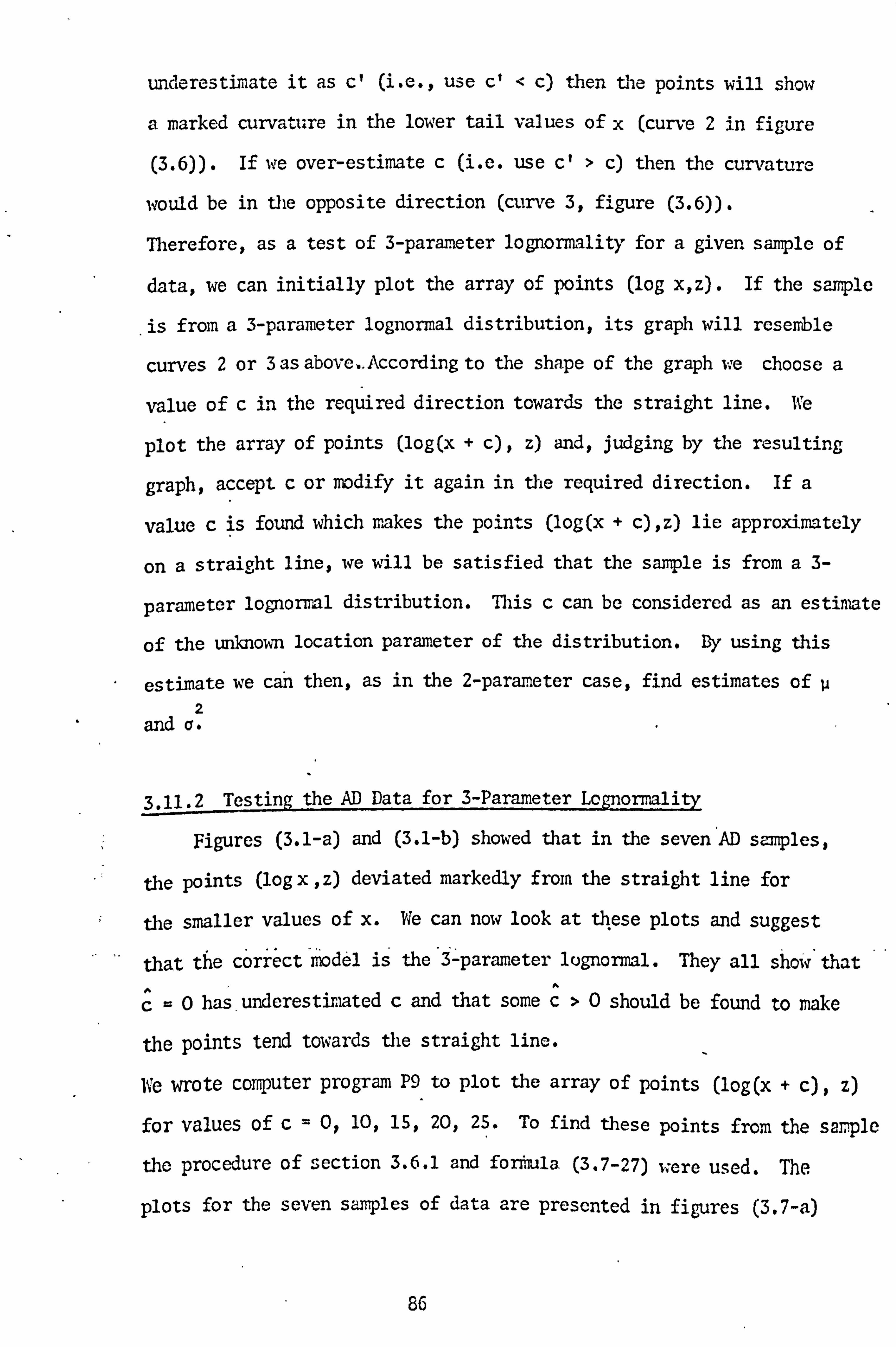
underestimate it as c' (i. e., use c' < c) then the points will show

a marked curvature in the lower tail values of x (curve 2 in figure

(3.6)). If we over-estimate c (i. e. use c' > c) then the curvature

would be in the opposite direction (curve 3, figure (3.6)).

Therefore, as a test of 3-parameter lognormality for a given sample of

data, we can initially plot the array of points (log x, z). If the sample

is from a 3-parameter lognormal distribution, its graph will resemble

curves 2 or 3 as above.. According to the shape of the graph we choose a

value of c in the required direction towards the straight line. We

plot the array of points (log(x + c), z) and, judging by the resulting

graph, accept c or modify it again in the required direction. If a

value c is found which makes the points (log(x + c), z) lie approximately

on a straight line, we will be satisfied that the sample is from a 3-

parameter lognormal distribution. This c can be considered as an estimate

of the unknown location parameter of the distribution. By using this

estimate we can then, as in the 2-parameter case, find estimates of 2

" and a.

3.11.2 Testing the AD Data for 3-Parameter Lognormality

Figures (3.1-a) and (3.1-b) showed that in the seven AD samples,

the points (log x, z) deviated markedly from the straight line for

the smaller values of x. We can now look at these plots and suggest

that the correct model is the 3-parameter lognormal. They all show' that

c=0 has, underestimated c and that some c>0 should be found to make

the points tend towards the straight line.

We wrote computer program P9 to plot the array of points (log(x + c), z)

for values of c=0,10,15,20,25. To find these points from the sarple

the procedure of section 3.6.1 and formula. (3.7-27) were used. The

plots for the seven samples of data are presented in figures (3.7-a)

86

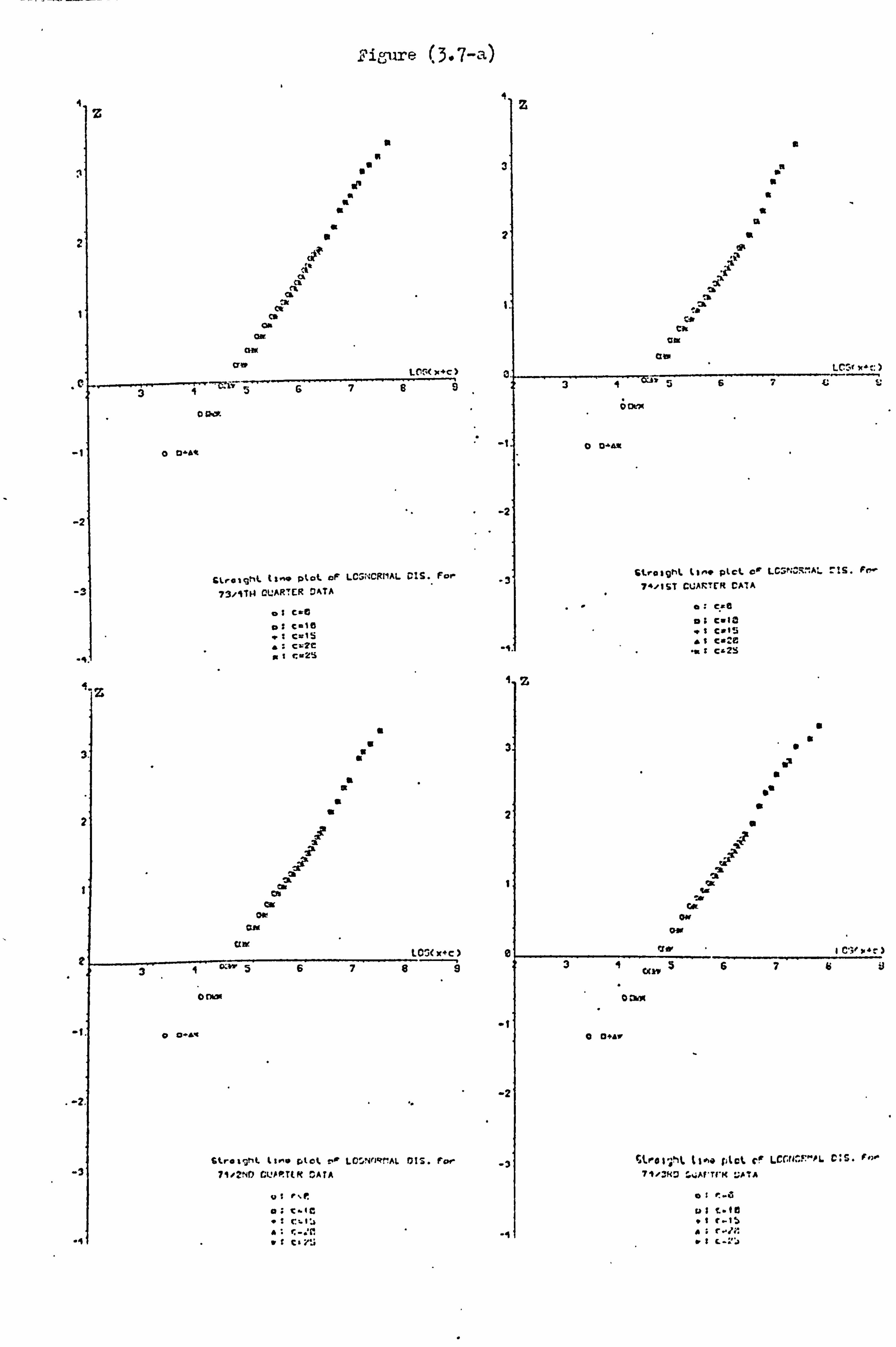
"i, ire (3.7-a)

. .

.

U' .

/

4ýý 3

Z C

I CIO rý:

6? 8 :i

a plct o! LCCfI:! '^IL C: S. i. >-

ii'K :; ATA

e-d DiL. 10 "t tý1S " "tc..

Ware (3-7-b)

Z

a a

3. a

a a

" 2.0

Q

I`1

l+l

R

Or cu

0*

Ctrl

0. LCU(, +c ) 34

CLAV bb789

C

a O. A.

Lt'ntght lt-o pct o- LCCNCM-AL DIS, foe

71d1TN CLARTER DATA

oZ C=0

o: C-13

f1 Ca1S

": c-23

4

I.?

0

ý r, a ý. " ý `_. ýý. ý C_

... _. ýeý

s: cr2 i

and (3.7-b). It can be seen that the directions of the curvatures for

c=0 and 10 are opposite to that for c= 25. For c= 15 and 20 the

points appear to lie more accurately on a straight line. Therefore,

we are satisfied that our samples are from 3-parameter lognormal distribu-

tions whose location parameters c have values between 10 to 20.

3.1.2 Estimation of the Parameters of the 3-Parameter Lognormal

Distribution

The existence of the unknown location parameter c, in addition to 2

and a, makes the estimation problem more difficult. Aitchison and

Brown (1957) do not deal with this problem for grouped data and only

examine the case when values of the individual observations in the

sample are given. They report methods of moments and quantiles where

three moments or quantiles, respectively, of the sample are put equal

to their corresponding population values. The method of maximum

likelihood is also considered which results in a non-linear equation in

c. They also report Kerrsley's (1952) method which consists of equating

the mean and two quantiles of the sample to their corresponding population

values. We can make assumptions, similar to the ones we made for the

two-parameter case, and modify the above methods for use with grouped

data (see section 3.7). However, as the analysis in the two-parameter

case showed, these methods would not provide very satisfactory results.

Their solutions may be of use, for example, in yielding initial values

for the parameters to be used in an iterative method of estimation.

Therefore, we will not consider these methods here.

Johnson and Kotz (1970) report the methods mentioned in Aitchison and

Brown (1957) and they do not consider estimation from grouped data. In

actuarial literature, Ferrara (1971) uses the method of quantiles to

87

bb,

determine c first and then finds u and c by least squares regression

(as in the 2-p ar=, eter case).

In this section, we will examine two methods which are directly

suitable for estimation from grouped data. The first one is the least

squares regression method. We will suggest a procedure for finding the

parameters which avoids solving non-linear equations. The second method

is the multinomial maximum likelihood which produced most satisfactory

results in the two-parameter case. This method will be modified and

used for the 3-parameter case. As-we mentioned in section 3.7.7, Tallis

and Young (1962) consider this method but they suggest equating the

partial derivatives of the loglikelihood function, with respect to the

parameters, to zero and solving iteratively the resulting set of non-

linear equations. This is more laborious than our proposed procedure.

3.12.1 The Method of Least Squares

Let us assume that a sample of grouped data as defined in section

3.7 is available. From section 3.4 we know that for the LN(x; - c, u, Q 2

)

distribution relationship (3.4-6), i. e.,

zq 1 log(xq + c) -Q

holds. If the random variable X (the claim amount) is assumed to be 2

distributed as LN(x; -c pa ), we can use the least squares regression

technique to find the estimates of the parameters. This consists of

minimizing SSD (the sum of the squares of deviations) simultaneously

with respect to c, u and a where, k-1

" SSD = [Zi -Q log(xi + c) + ý' l (3.12-1) i=1 c

One way to solve this problem would be to equate the partial derivatives

of SSD, with respect to c, p and a, to zero. Dut this will result in a

88

hlh. ý

system of non-linear equations in the parameters which has to be laboriously

solved by an iterative technique. We, however, suggest a different

method. Instead of searching for the set of parameters at which SSD

attains its minimum, we propose finding the minimum value of SSD and AAA

taking its corresponding estimates of the parameters (c , u, c ) as the

required solution. Let us explain this method in nore detail.

If our data is from a 3-parameter lognormal distribution, then

there exists ac at which SSD attains its minimum - see figure (*) below.

SSD

Figure (*) - The Graph of SSD with respect to c.

If we let c= co where co is some known value then the values of

log(xi'+ co), for all i, will be known and hence (3.12-1) becomes

similar to the SSD for the 2-parameter lognonnal distribution. Therefore,

the values of uo and vo corresponding to co can be found by the least

squares regression technique described in section 3.7.6. It will then

be possible to calculate the value of SSD, from (3.12-1), -corresponding

to (co' uo' ao). By choosing several different values for c and

calculating their corresponding SSDs we can find a range of values of c,

say (c1, c2), in which the SSD changes from a decreasing function to an

increasing function. The mininram of SSD lies in this range. By taking

89

C1 C C2 C

d, the required degree of accuracy for c, into consideration, we can

choose suitable values of c in (cl, c2) and hence reduce the range

gradually to (c ,c+ d) where SSD attains its minimum value at c 22

The set (c p, a) will be the required least squares estimates of

(c, ti, a) respectively. This technique can be programmed on the computer

and will then be much simpler and faster than solving a system of non-linear

equations.

Any prior knowledge about the maximum value of c should be utilized

in choosing the initial range of c: For example, in the case of our

accidental damage data we know that c, the voluntary excess, is at most

M. Therefore, to examine the behaviour of SSD, we should initially try

c=0,5,10,15,20,25 and 30.

3.12.2 The Multinomial Maximum Likelihood Method

This method was considered for the two-parameter lognormal

distribution in section 3.7.7. In this section we will present

the likelihood function for the 3-parameter case. Let us again assume

that a sanpie of grouped data as defined in section 3.7 is available. 2

If x is assumed to be distributed as LN(x; -cuo), by adopting the

notation of section 3.7.7,

22 pi = LN(xi; -c Ili Icy )- LN(xi-1; -c ,u ,Q)

log (x1 + c) -u log (xi-1 + c) -u pi 'N(a; 0,1) -N(Q1 001)

Therefore- the sample likelihood function will be proportional to L where,

L Pi i=1

and the loglikelihood function will be

90

k log L= nl log [ N(zi; 0,1) - N(zi-1,0,1) ) (3.12-2)

i=1

log(x1 + c) -u where zl =a

We will adopt the technique, described in section 3.7.7, of maximizing 2

log L with respect to (c, u, a ). To start the iteration process we can

use the least squares, or any other, estimates of the parameters. The

set of estimates (C, 11 $a ) which maximizes log L will be the required

multinomial maximum likelihood estimates.

3.13" Application of the 3-Parameter Lognormal Model to the AD Data

We wrote computer program P10 to use the least squares method to

estimate the parameters of a 3-parameter lognorml distribution

from a sample of grouped data. The program was run on an interactive

terminal which-made the task of estimation even simpler and faster. It

was used to estimate the parameters for our seven samples of accidental

damage data which were presented in tables (1.1) to (1.7). We explain

the procedure for a particular sample, say, 73/4th quarter. After the

sample data has been supplied to the program, it will require a value for

c along with an integer 'IPRINT' which is either 0 or 1. IPRINT =0

indicates that only the value of SSD is required. IPRINT =1 indicates

that a comprehensive table of results is also required. The results of

the computer rum to find the estimate of c for 73/4th quarter data are

presented in table (3.30). We started by c=0 and increased c in steps

of S. For each c its corresponding SSD was printed. We noticed that in

the range (c = 15, c= 25) SSD changed from a decreasing function to an

increasing one. Therefore, as a next step we tried c= 18 whose SSD

shoved that the optimum c is in the range (18,25). Because an

91

accuracy of 1 is acceptable in the estimate of c, we then tried c= 19

whose SSD indicated that the optimum c should be in the interval (20,25).

We then tried c= 21 whose SSD was less than that of c= 20. Therefore,

the optimum range was reduced to (21,25). As the next step we tried c= 22

whose SSD was greater than that of c= 21. Therefore, with our required

accuracy, c= 21 is the least squares estimate of c. This value was then

-supplied to the program, with IPRINT = 1, and the-estimates of u and a2

along with an extensive table of results were produced (see table (3.31)).

Similar tables were obtained for other samples and the results are

presented in tables (3.32) to (3.37). We can see that the value of c

for our data ranges from 13 to 25 which is reasonable. has generally

increased over time from 4.78 to 4.98 while v2 ranges from 0.67 to. 0.77.

The means and standard deviations of the fitted rndels are very close to

the means and standard deviations of the samples. The Chi-square statistics

are smaller than in the 2-parameter case but still indicate significant

differences between the fitted distributions and the actual sample values,

except in the case of 74/4th, 75/ist and 75/2nd quarters where the X2

values are not significant. The total expected loss statistics are very

small and are at most 2% of the total actual cost. This indicates an

overall agreement between the fitted models and the samples. It was

important to see how closely the actual sample points lie on the least

squares straight line. Therefore, we wrote computer program P11 to plot

the sample points (log(xi + c) , zi) and the least squares line

Z. log(x + c)

QQ

For the seven AD sau les the graphs are presente d in figures (3.8-a)

and (3.8-b). The points, for each sample, generally lie closely on the line.

92

FIGure (3.8-a)

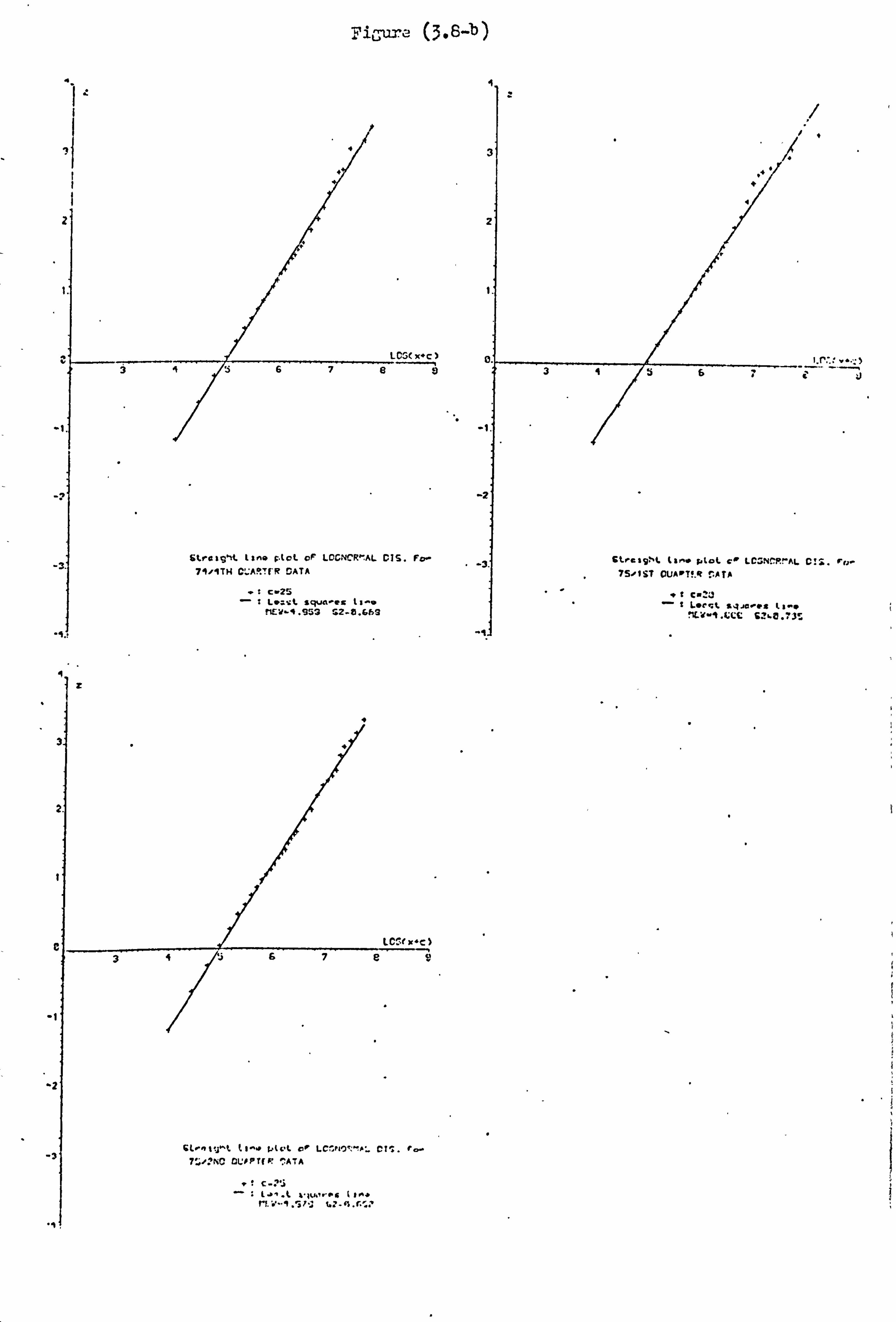
1 iere (;. Sb)

In the lower tails the fits are very good, unlike the large deviations

which were observed in the 2-parameter case. It is encouraging to see

that the introduction of parameter c into the model has produced more

satisfactory results.

-Computer program P12 was written to estimate the parameters by the

nethod of mul tinomrdal maximum likelihood. This program was used with the

samples of accidental damage data. z

estimates of (c, p, Q ) were supplied,

For each sample, the least squares

to the program, as the starting

values for the iteration process. The results for the seven samples are

presented in tables (3.38) to (3.44). In each case the estimates of the

parameters, the mean and the standard deviation of the fitted distribution

and an extensive table have been produced. The estimates of c range from A 10 to 21 with an average of about 15 which is reasonable. The values of u

generally show an increasing pattern and are in the 4.65 to 4.91 range.

a2 ranges from 0.71 to 0.86. We can observe that the Chi-square values

are smaller than their corresponding values for the least squares method.

They do not indicate significant differences, except for 74/1st and 74/3rd

quarters, between the fitted distributions and the sample values. For

74/1st and 74/3rd quarters the differences are, respectively, highly

significant and significant, but we should note that the major contribution

to the X2 values comes from just one cell in each case. The total

expected loss statistics are small and are at most 1.2% of the total actual

cost of claims. This indicates a very satisfactory general agreement

between the theoretical models and the samples values. Values of the

Kolmogorov-Srurnov statistics for all the samples were calculated, by

using the. (Actual-Expected) column in each table, and were compared with

the critical values of this statistic as given in table (2.2). Only for

74/1st quarter this statistic indicated almst significant differences

between the fitted distribution and the sample values. In all other cases

93

the differences were satisfactorily not significant.

The least squares method is very easy to use but, as in the case of

the 2-parameter lognormal, the multinomial maximum likelihood method has

produced better results in terms of the goodness-of-fit test statistics.

We, therefore, again recommend the use of this method in estimating the

parameters of the distribution from grouped data.

In order to see the agreement between the frequency curve of the

fitted distribution and the histogram of the sample values we plotted then,

for each of our seven AD samples, by using a modified version of program

P7 to suit the 3-parameter lognormal model. The resulting graphs are

presented in figures (3.9.1) to (3.9.7). For each sample, the rrultinomial

maximum likelihood parameters have been used to plot the frequency curve.

Each figure represents two graphs. One for claim amounts < £600 and the

other for claim amounts > £600. The agreement between the frequency curve

and the histogram is very satisfactory for all samples. The curve

portrays the mode of the histogram. The large deviations in the lower

tail between the curve and the histogram which were observed in the 2-

parameter case (see figures (3.5.1) to (3.5.7)) have now disappeared.

The long tail of the histogram has also been modelled very well by the

distribution. We are, therefore, satisfied that the 3-parameter

lognormal distribution offers a correct model for our accidental damage

claim arrounts. Hence, we shall next consider the problem of predicting

the distribution of claim amounts during a future period.

94

T!

l ýý; ure Y.,.

1

1

1

1

1

1

0J Itr, 7ZA5 it, G t)10 510 570 68(

X10-I 5. co

2

I

L'caý1 2t ýý .a2'0

:i

F

1

1

1

1

1

1

1

irr"gaN nCý)

pj ure (3.9.2)

HISIOGR. AM OF 71/IST QUART(R DATA AND 3-PAR.

LOC3N"0%MAL P. D. F. WITH Mt1LTN. UAXL. rArnrlr1C; ZG

C=1: ß. O MEW-4. G:; 0 SIGMA SA. -©. CUB

k ; ýC

Xf0-1 5.01

5 . 51

Jr ýý

3. aß

2.51

2xl

1. J(

I AS

o, 1ST CUARTER' DATA AND 3-FAR.

. WITH MULTN. MARL. PARAMETFF'S

. 650 SIGMA 50. -0. £: 58

?, h ý 6. ": f: '1 '1.2ýFJ 11C Pif..: fi

-

Fi. gare (3,9.3)

x

xla-1 s. ee

9.00.

2. `.; ©. '

2. oG9.

1. ýlOJ.

HISTOGRAM OF 71/2ND CUARTLR DATA AND 3-PAR.

LOGNORMAL P. D. F. WITH MULTN. MARL. PARAMETERS

C=15.0 MCW-i. 735 SIGMA So. =0.760

7 ( ^; "('i; ^, Ntf i 2C: ýZ~ . ^i;. ', 600 : Nl'tý 2200 bf)o flvo

2

1 t; 17

1

15

1'!

13

12

11

1iß

s 7

6 5 4 3

2 1

0

xnr1 5. Pý

1 . (fI

All

2. `. it

2.0c

1 . 0c

Figure (3.9.4)

t1STO5! <AN OF 71/380 CUART. E'R DATA ANI) 3-PAR.

_OSNCRMAL P. U. F. WITH MULTN. r11XL. PARAME1ERS

-16.0 11EW-1.021 SIGMA SO. -0.759

. "_I"1^

X

000

X13' s. c

I. I

I . eý

2.

2.:

2. C

1. J

i. C

OJE

ri,; i: re (3.9.5)

2.3 22

HISTOGRAP1 OF 7.1/"llli OUART(R f'ATA AND 3 "PAR. 20. L0 'N MAL P. D. r. WITH MULTN. 1V XL. rARAM -TE'R3 17

1E3 C-16.0 MCti'-9. $78 ;; IGMý Soll. -MGG

17.

15

1^.

13.

12.

11.

10.

F3

7.

9-

2.

e 30 60 SO 120 1;; 0_ 1&ßi_213 24©270 300 333_'G0_3°0 12LI 150 982 513

2 '-' 0 141.1. ) 1 W. U I'liv,

xie-t S. el

4.51

3.5c

3.

2. '

2.1

1 .:

t..

Fiuio (3.9.6)

ISTtGRA1 _CF 75/1ST QUART[: R DATA AND 3-PAR.

DCNCRNAL P. C. F. WITH MULTN. MAXL. PARAMETERS

-21.0 MEN'-1.915 SIGMA S0. =0.712

27(", r) : iýC f.! 1 Dili ý~ý `C'i4

C! V "Cid

cjcir IWO

I 2l f1

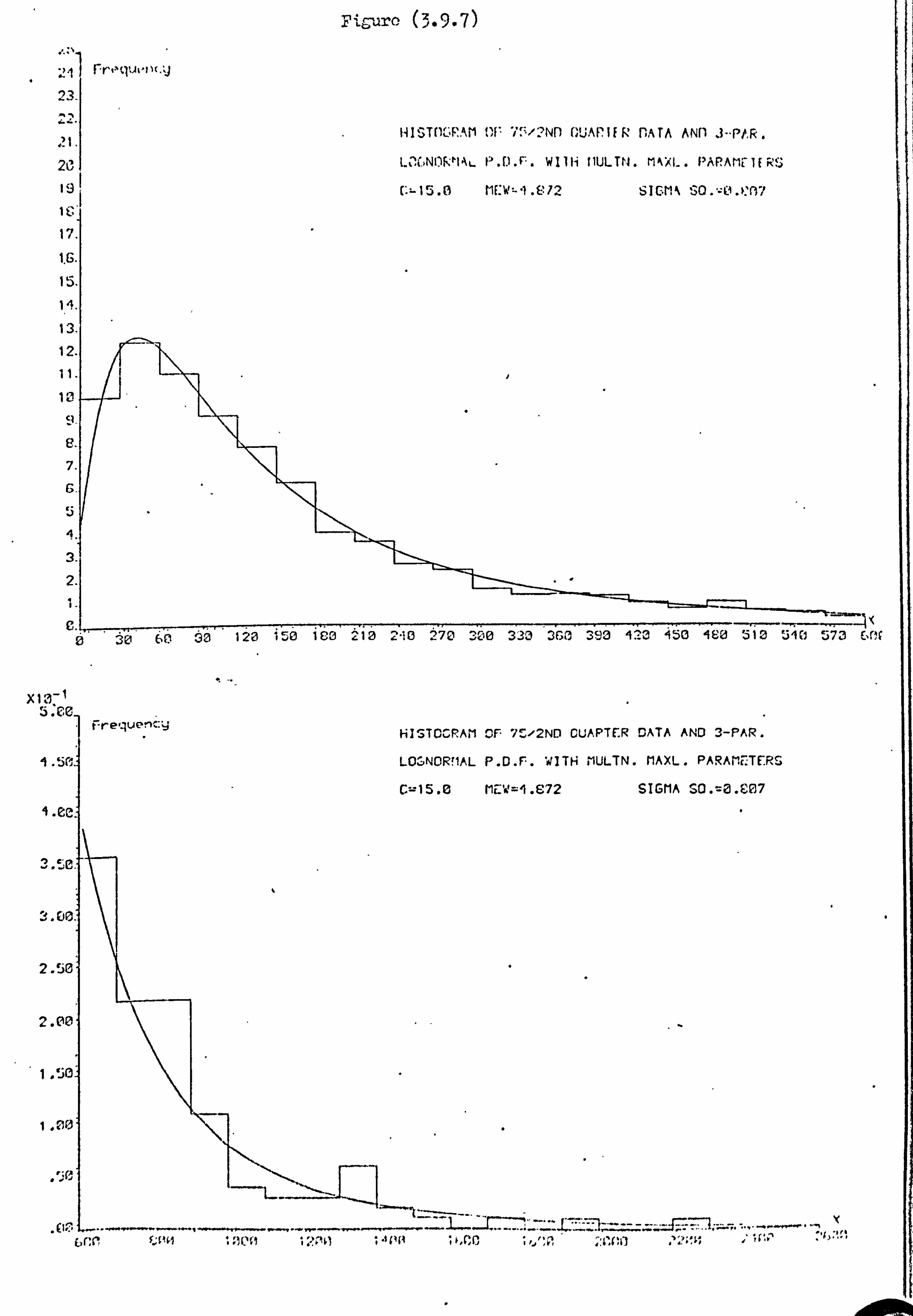
T.

7

i

i

2

1

1

1

1

1

1

1

Figure (3.9.7)

f"f

X1o-i 5. C

9 . 51

i. el

2.51

2.

1.

1.

CORAM OF 7'-'2ND CUAPTER DATA AND 3-PAR.

IORflAL P. D. F. WITH IULTN. MARL. PARAMETERS

;. e t1 W-4.072 SIGMA S0. =7. C7

ý'ýýýýi 1ýrrr ýrýr"Yr ý: i:

ý; {i : li'1, ; "; c; s., f; C; s"s+c1 . ; 'C'sý . ;: ßs1

3.14 Prediction of the Claim Amount Distribution :- The 3-Parameter

Lognormal Model

The importance of predicting the future cost of claims was mentioned

in 3.9 and here we will adopt techniques similar to those of that section

for predicting the future distribution of claim amounts. To save us

repeating some of the arguments of that section we suggest referring back

to it at this stage.

3.14.1 The Effects of Inflation on the Parameters of the Model

Let us again assume that the effect of inflation on a claim of amunt

X, during a period of time, is to increase it to U= X(1 + i) where i

is -the rate of inflation, according to some appropriate index, for that 2

period. If X is assumed to be distributed as LN(x; c, u, a ), then by a

transformation of variables we can show that U= X(1 + 1) will be

distributed as : 2

IN(u; rc, u+d, a) where r=1+i and d= log(1 + i)

Therefore, when the distribution of X is known, we can modify its parameters

to obtain the distribution of claim amounts in a future period. The

foregoing shows that inflation increases both c and I. in time but does not 2

affect a. This supports our intuition that the amount of voluntary

excess, c, should go up in time due to the inflation. For our accidental

damage data, the increase, over time, in the values of u is obvious from

tables (3.38) to (3.44). The values of c for the later samples are also

larger than for the earlier ones.

Based on the results for the two-parameter case, we suggest that the

technique of section 3.9.2 be used for predicting the distribution of

accidental damage claim anounts during a future period. The appropriate

index proved to be the General Index of Retail Prices and wo will use it

here again.

95

3.14.2 Prediction for the AD Data

To test the prediction technique on the accidental damage data,

we modified computer program P8 for use with the 3-parameter model. For tl

reasons presented in section 3.9.2, we used the parameters of the distri-

butions for 73/4th, 74/ist and 74/2nd quarters to predict the

distributions of claim amounts in 74/4th, 75/1st and 75/2nd quarters

respectively. The appropriate rate of inflation in each case was

calculated from the General Index of Retail Prices, as described in

section 3.9.2. The results, in the form of extensive tables which allow

comparisons between the actual and expected (predicted) distributions, are

presented in tables (3.45) to (3.47). In all three cases the Chi-square

statistics are relatively small, considering the amber of degrees of.

freedom, and do not indicate any significant differences between the

predicted distributions and the actual sample values. The total

expected loss statistics are small and show an over-prediction of the

total cost which is more satisfactory than an under-prediction. They

are a small proportion of the total actual cost in all cases. The

number of changes and non-changes of signs in the 'A - E' (i. e. , the

actual minus expected frequencies) column are roughly equal. The

Kolmogorov-Smirnov statistics were calculated from the results tables and

in each case were compared with the critical values given in table (2.1).

They showed that the differences between the actual and predicted

distributions were not significant for 74/4th and 75/1st quarters but

were almost significant for 75/2nd quarter.

These results show a great improvement over those given in tables

(3.27) to (3.29) for the 2-parameter model. The consistent satisfactory

outcomes of the goodness-of-fit tests indicate the success of the

prediction technique and the appropriateness of the General Index of Retail

96

prices for inflating accideiLal damage claim amounts. Various assumptions

about the future rate of inflation or values of the parameters can be

tested by this technique and the computer program associated with it. A

value for the future rate of inflation and a set of parameters can be

adopted as standard values and other rates and sets of parameters can then

be tested against them. The total expected loss statistic, T, in

each case will indicate, in terms of the easily understood amount of

coney, by how much the assumptions differ frone each other.

It may appear simpler just to increase the actual mean claim amount

in a particular period by the effective rate of inflation between that

period and a future one and to take the result as the mean claim ammunt

for the latter period. Using the total number of claims we can than

calculate the total expected cost of claims for the future period. But,

it can be shown that this method will result in a much larger over-

prediction of the total claims cost than by our distribution theory

approach. For example, the sample mean claim amount for the 73/4th

Quarter is £150.36 and the effective rate of inflation from this period

to 74/4th quarter is 18.2% which yields a mean claim amount of £177.7 for

the latter quarter. The number of claims for that quarter is 3064

and hence the total expected cost would be £544,551 which shows-an over-

prediction of £10,884, as compared with £4,093-by our approach. The

former discrepancy is 2.03% of the total actual cost while the distribution

theory resulted in a ratio of 0.77% only. Similar results can be observed

for the other two quarters we have considered. Therefore, one of the

merits of our distribution theory approach is that it results in accurate

but smaller reserves. This means that the insurance company will not

need to tie up funds in unnecessary reserves.

97

3.15 Conclusions

In this chapter the two and three parameter lognormal distributions

were studied as models for the distribution of claim amounts, in general

insurance and in particular for motor insurance accidental damage claims.

Simulation exercises showed that the graphical method is a good way of

testing for lognormality. In the 3-parameter case, this test also

provided a rough estimate of the location parameter c. It was observed

that, even in large sanpples of (size 2500) observations from an actual

lognormal population, the points (log x, z) deviate markedly from the

straight line for values of x in the upper tail of the distribution.

Therefore, in testing exercises, we should expect to find that the points

in-the upper tail deviate from the straight line which may fit the

rest of the distribution.

Several methods of estimation for the 2-parameter case were considered

and their efficiencies were calculated. It was observed that the

approximate maximum likelihood method was the most efficient amongst them.

It was mentioned that the most efficient mathod for-estimation from

grouped data is the multinomial maximum likelihood method. A teclmique

for estimating the parameters by this method was proposed and shown to

provide better estimates (in terms of a closer agreement between the

model and the actual data). For the 2-parameter case, the approximate

maximum likelihood and the multinormal maximum likelihood methods gave

approximately the same results and hence the use of the former method in

this case should be recormiended. In the 3-parameter case our proposed

technique for estimating the parameters by the least squares method was

shown to be very sinVle when programed on the computer. Ho4; ever, the

results produced by this method were not as satisfactory as those of the

multinormal maximum lir. eli. hcod method.

For the accidental damage data, it was found that the 3-parareter

J8

form of the distribution is the appropriate model. The inflation was

shown to be the main cause of the increase of the claim an, t over tim:..

We proposed a technique for predicting the distribution of the claim

amounts in a future period. This involved updating the parameters c and

j; with respect to an appropriate rate of inflation. The General Index

of Retail Prices was shottin to provide the appropriate rate of inflation

for accidental damage claims. We tested the prediction technique on

data from the past and it proved to be very successful.

The total expected loss statistic, T, was suggested in chapter 2 as. a

goodness-of-fit measure. In the present chapter it was put to use and

shown to-provide an easily understood measure (in monetary terns) of

overgraduation or undergraduation. Its use is particularly recommended

in prediction exercises where it indicates the extent to which a model

is overpredicting or underpredicting the actual total cost of the claims.

3.16 Tables

99

Cocfficicnts of skewness (gl) and excess kurtosis (g2)

and their standard errors for the distribution of log X, where X= claim amount

Table (3.1)

Accidental Damage Samples

Period of accident

gl Se(g1 ) g2 Se(g2)

73/4th quarter -0.107 0.044 -0.506 0.089

74/1st " -0.076 0.049 -0.503 0.099

74/2nd' -0.144 0.050 -0.464 0.100

74/3rd -0.179 0.046 -0.352 0.092

74/4th -0.199 0.044 -0.428 0.088

75/1st " -0.237 0.048 -0.394 0.096

75/2nd -0.184 0.049 -0.376 0.098

Table (3.2)

Simulated Samples

Sample g1 g2

1 -0.049 -0.328 2 0.105 -0.143 3 0.065 -0.167 4 0.122 -0.122 5 -0.007 -0.170 6 -0.013 -0.209 7 -0.037 -0.412 8 -0.039 -0.369 9 0.030 -0.223

10 0.067 -0.272 For all samples: Se(gl) = 0.049

Se(g2) = 0.098

100

Table (3.3)

Efficiencies of various methods of estimation for the

Two-Parameter Lognormal Distribution

Method of estimation Eff (ý) Eff (v2) Eff (a) Eff (ß)

Moments 0.044 0.095 4.145 17.710

Approx. Max. Likelihood 0.021 0.036 3.944 9.768

7& 93% quantiles 0.131 0.188 7.267 24.493

27 & 73% quartiles 0.026 0.050 4.634 12.186

Median & Coeff. of variation

0.026 0.095 7.525 24.561

Least squares regression

0.051. 0.104 4.363 18.999 1

101

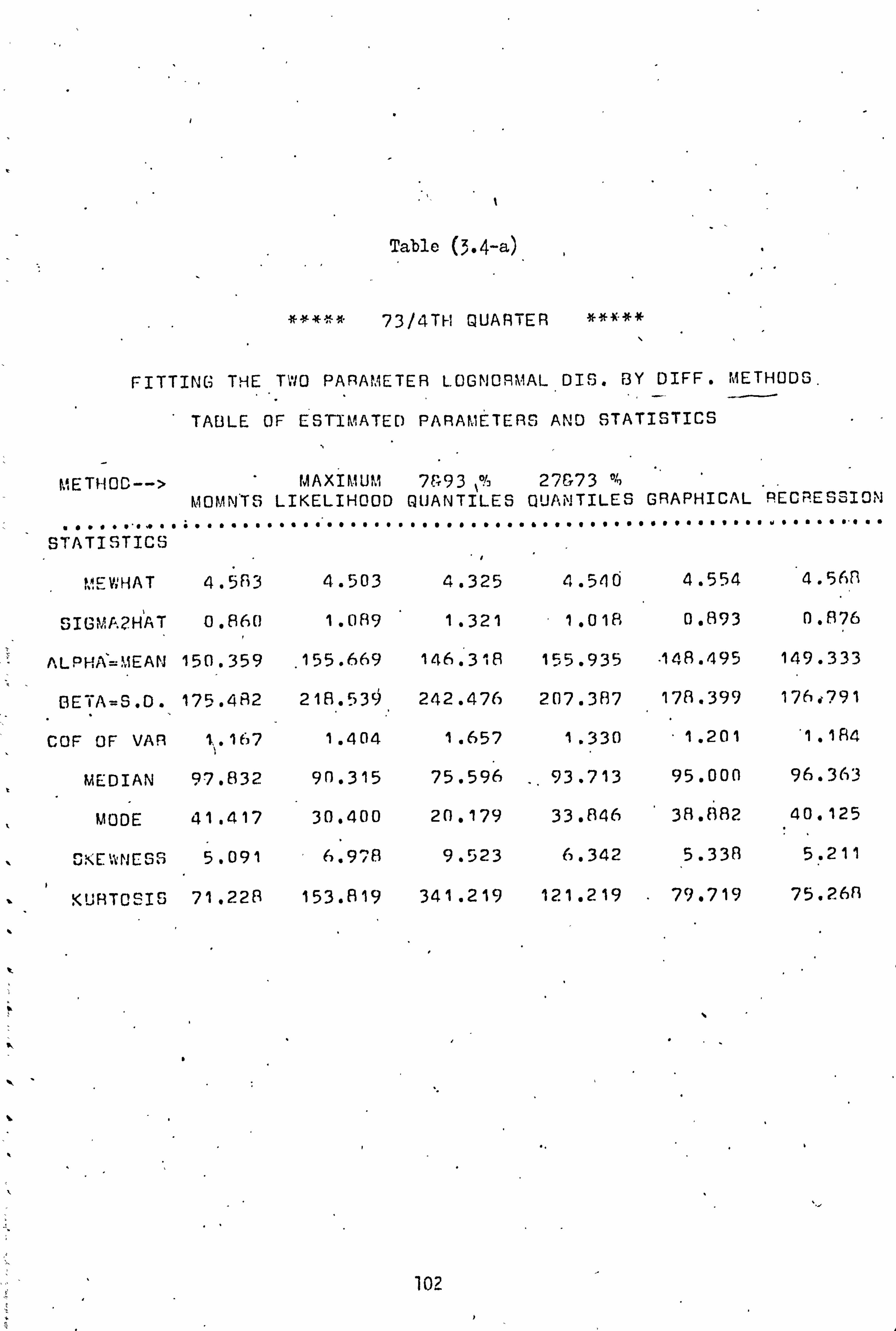
Table (3.4-a)

73 /4TH QUARTER ***#*

FITTING THE TWO PARAMET ER LOGNORMAL DIS. BY DIFF. METHODS.

TABLE OF ESTIMATED PARAMETERS AND STAT ISTICS

METHOD--> MAXIMUM 7&93 ý% 276,73 % MOMNTS LIKELIHOOD QUANTILES QUANTILES GRAPHICAL RECRESSION

STATISTICS

MEWHAT 4 . 583 4.503 4 "325 4 "5 10 4.554 4.568

SIGMA2H'AT 0.860 1.089 1.321 1.018 0.893 0 F176

ALPHA=MEAN 150.359 , 155.669 146.318 155.935 "148.495 149.333

BETA=S. D. 175.482 218.530 242.476 207.387 178.399 176,791

COF OF VAR 1.167 1.404 1.657 1.330 "1.201 1.184

MEDIAN 97.832 90.315 75.596 93.713 95.000 96.363

MODE 41.417 30.400 20.179 33.846 38.882 40.125

CKE -INESS 5.091 6.978 9.523 6.342 5.338 5 . 21 1

" KURTOSIS 71.228 153.819 341.219 121.219 79.719 75.2613

102

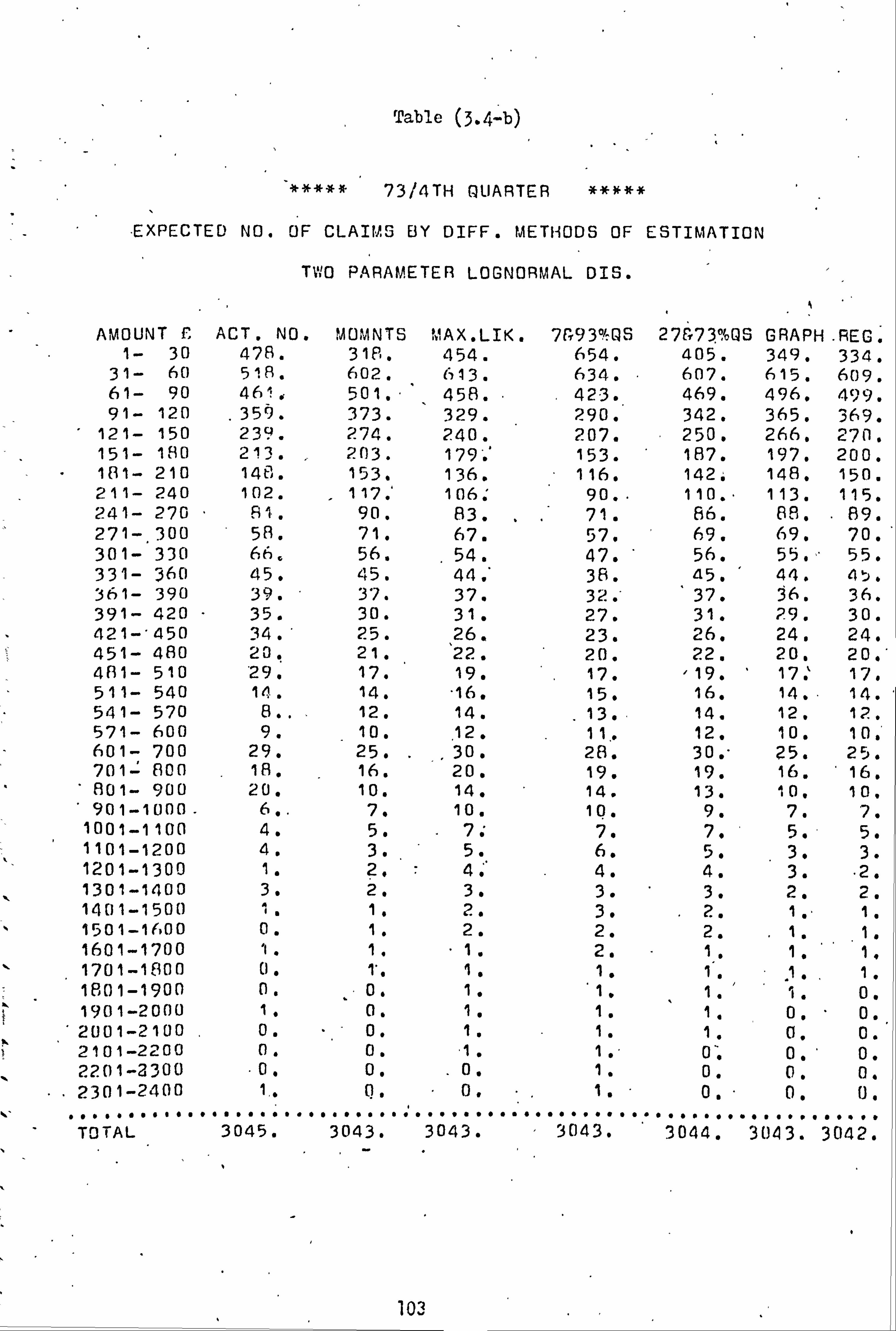
Table (3.4-b)

## 73/4TH QUARTER **##*

EXPECTED NO. OF CLAIMS BY DIFF. MET HODS OF ESTIMATI ON

T WO PARAM ETER LOGNORM AL DIS.

AMOUNT f ACT. NO. MOMNTS MAX. LIK. 7(93°JQS 27f*73%Q S GRAPH. REG. 1- 30 478. 318. 454. 654. 405. 349. 334.

31- 60 518. 602. 613. 634. 607. 615. 609. 61- 90 461. 501. - 458. 423. 469. 496. 499. 91- 120 .

359. 373. 329. 290. ' 342. 365. 369. 12 1- 150 239. 274. 240. 207. 250. 266. 270. 151- 180 213. 203. 179'. ' 153. 187. 197. 200.

" 151- 210 148. 153, 136. 116. 142. 148. 150. 211- 240 102.

- 117. ' 106. 90.. 110. " 113. 115.

241- 270 Al. 90. 83. 71. 86. ß?. . 89. 271-. 300 58. 71. 67. 57. 69. 69. 70. 301- 330 66. 56. 54. 47. 56. 55., - 55. 331- 360 45. 45. 44. " 35. a5. 44. 4t. 361- 390 39. 37. 37. 32. " 37. 36. 36. 391- 420 35. 30. 31. 27. 31. 29. 30. 421-"450 34. ' 25. 26. 23. 26. 24, 24. 451- 480 20. 21. 22. 20. 22. 20. 20, 451- 510 '29. 17. 19. 17. '19. 17, 17. 511- 540 1Q.. 14. "16. 15. 16. 14.. 14. 541- 570 8.. 12. 14.

_13.. 14. 12. 12.

571- 600 9. 10. 12. 11.. 12. 10. 10. 601- 700 29. 25.

. 30. 28. 30. " 25. 25.

701- 800 18. 16. 20. 19. 19. 16. 16. 801- 900 20. 10. 14. 14. 13. 10. 10, 901-1000- 6.. 7. 10. 10. 9. 7. 7.

1001-1100 4. 5. . 7: 7. 7. 5. 5. 1101-1200 4. 3. 5. 6. 5. 3. 3. 1201-1300 1. ?. 4. 4. 4. 3. . 2. 1301-1400 3. 2. 3. 3. 3. 2. 2. 1401-1500 1. 1. 2. 3. 2. 1. 1. 1501-1600 0. 1. 2. 2. 2. 1. 1. 1601-1700 1. 1. 1. 2. 1. 1. 1. 1701-1800 (1. T. 1. 1. 1. 1. 1. 1801-1900 0. 0. 1. 1. 1. 1. 0. 1901-2000 1. 0. 1. 1. 1. 0. " 0. 2001-2100 0. 0. 1. 1. 1. 0. 0. 2101-2200 0. 0. 1. 1. 0. 0. ' 0. 2201-2300 . 0. 0. "

0. 1. 0. 0. 0. 2301-2400 1.. Q. 0. 1. 0. 0. U.

TOTAL 3045. 3043. 3043. 3043. 3044. 3013. 3042.

103

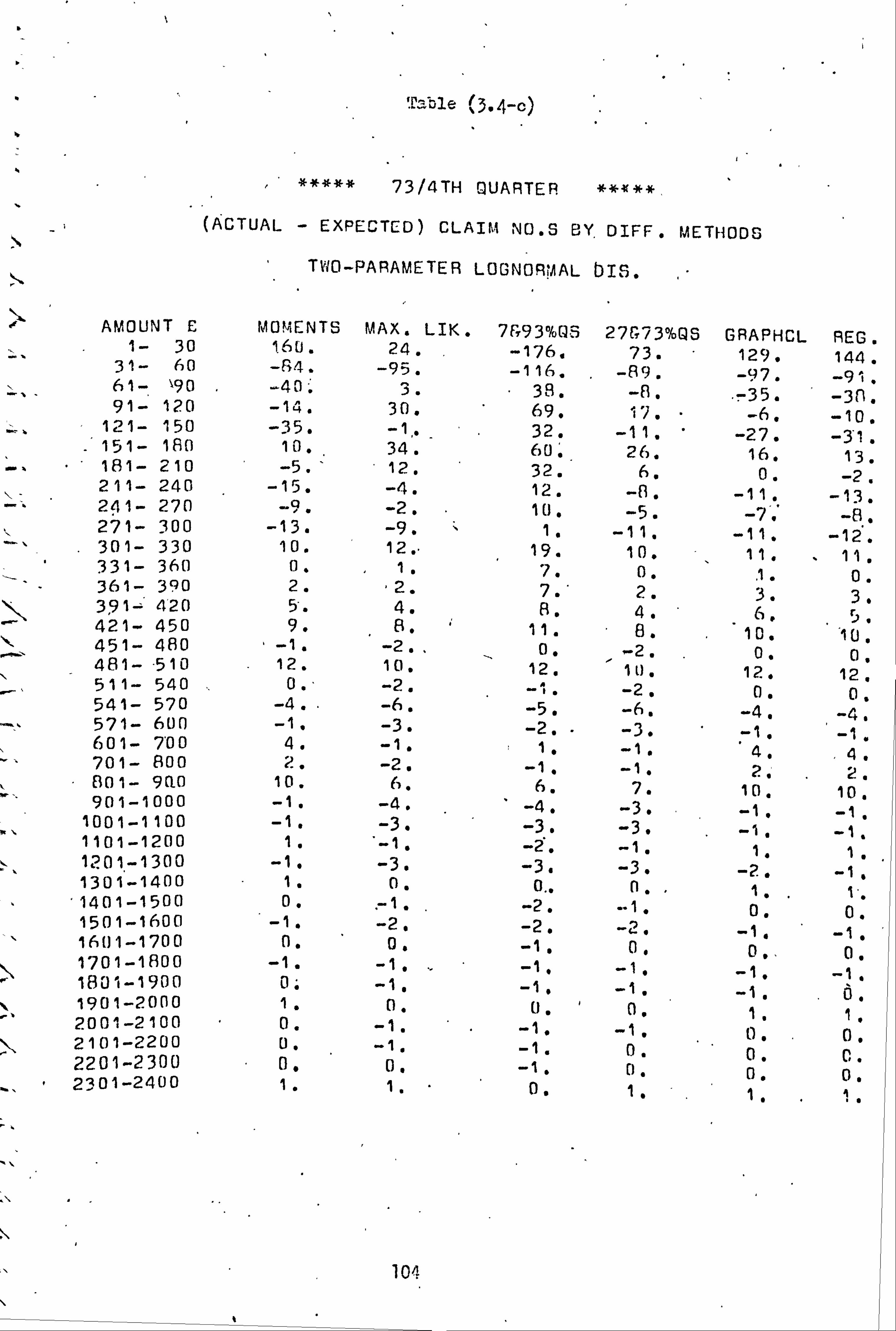
'. Cable (3-4-0

##### 73/4TH QUARTER ## #,

(ACTUAL - EXPECTED) CLAIM NO. S BY. DIFF. METHODS

TWO-PARAMETER LOGNOR! 'AAL bIS.

AMOUNT £ MOMENTS MAX. LIK. 7F, 93%QS 27G73%QS GRAPHCL AEG 1- 30 160. '

24. -176. 73. r 1 . 144 31- 60 -ý 4. -95. -116. -119. 97, -97.

. -91 61- '90 -40: 3. 38. -El. . -35.

. -3l. 91- 120 -14. 30. 69. 17. -6. -10. 121- 150 -35. -1,, 32. -1 1. -27. -31 151- 181) 10. 34. 60; 20. 16, ,

13. 181- 210 -5. ' 12. 32. 6. 0. -2. 211- 240 -15. -4. 12. -8, -11. -13. 241- 270 -9. -2. 10, -5. -7ý -8, 271- 300 -13. -9. 1. -11. -11. -12. 301- 330 10. 12. " 19. 10. 11. 11. 331- 360 0. 1. 7. 0. 3. 361- 390

' 2. 2. 7. ' 2. 3. 3. 3. 20 391= 4 5'. 4. B.

421- 450 9. H. 11. 8. 10. 'ý0 . -ý

451- 480 -1. -2. , 0. -2. 0. ' 0

\ \ 481- 510 12. 10. 12. 10. 12. . 12. 511- 540 .. 0.. -2. -1. -2. 0. 0. 541- 570 -4. -6, -5" -t, " -4. - 4.

... 571- 6001 -1. -3. -2. -3. -1, . -1 601- 700 4. -1. 1. -1. 4. . 4 701- 800 2. -2. -10 -10 2. . 2 801- 90-0 10. 6. 6. 7. 10. .

10. 901-1000 -1. -4. -4. -3. -1. -1 1001-1100 -1, -3. ' -3. -3.

. 1 101-1200 1, -1 . -2. --1 " 1, 1, 1201-1300 -1, -3. -3. -3. -2. -1, 1301-1400 1. 0, 0.. n. i. 1'

' 1401-1500 0. , -1 , -2. �1. 0. . 0

1501-1600 -1. -2. -2. -2. -1, .

. -1 16111-1700 0. 0, -1, 0. 0 0 1701-1800 -1. -1ý

' 1801-1900 0; -10 0 1901-2000 1. 0. 0 '

1 2001-2100 0. -1. -1, -1, 0, . 0 2101-2200 0. -1. -1. 0. 0 , C 2201-2300 0, 0. -1. 0. . 0. . 0 2301-2400 1. 1. 0, 1" 1. . 1.

10^

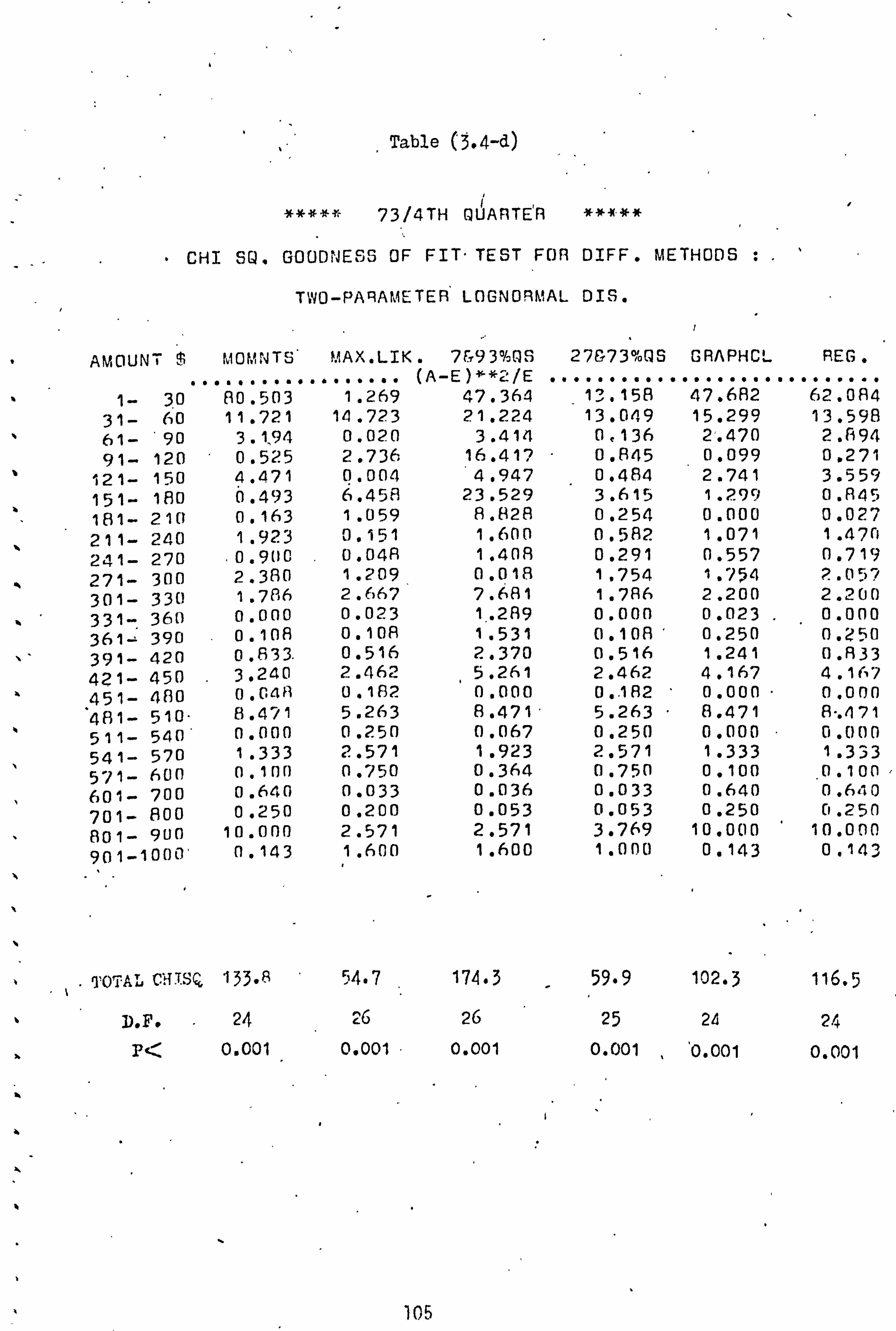
14

a

a

a

Table (3.4-d)

73/4TH QÜARTE'R ##x#*

" CHI SQ. GO ODNESS OF FI T- TEST FOR DIFF. ME THODS :.

T WO-PARAMETER LOGNORMAL DIS.

AMOUNT $ MOMNTS MAX. LIK. (A-

7ET93%QS E)**2/E

27&73%QS GRAPHCL REG.

1- ...

30 ....... 80.503

........ 1.2 9

.. 47.364

......... 13.158

........ 47.682

......... 62.014

31- 60 11.721 14.723 21.224 13.049 15.299 13.598 61- '90 3.1,94 0.020 3.414 0,136 2'. 470 2.894 91- 120 0.525 2.736 16.417 0.845 0.099 0,271

121- 150 4.471 0.004 4.947 0.484 2.741 3.559 151- 180 0.493 6.4513 23.529 3.615 1.299 0.845 181- 210 0.163 1.059 8.828 0,254 0.000 0.027 211- 240 1.923 0.151 1.600 0.582 1.071 1.470

241- 270 . 0.900 0.048 1.408 0.291 0.557 0.719

271- 300 2.380 1.209 0.018 1.754 1.754 2.057

301- 330 1.786 2.667 7.681 1.786 2.200 2.200

331- 360 0.000 0.023 1.. 289 0.000 0.023 0.000 361- 390 0.108 0.108 1.531 0.106 0.250 0.250 391- 420 0.833. 0.516 2.370 0.516 1.241 0.833 421- 450 .

3.240 2.462 5.261 2.462 4.167 4.167

451- 480 0. Cet A 0.1132 0.000 0.182 0.000 0.000

4131- 510. 8.4-/1 5.263 8.471 5.263 8.471 8". 4 71

511- 540 0.000 0.250 0.067 0.250 0.000 0.000

541- 570 1.333 2.571 1.923 2.571 1.333 1.333 571- 600 0.10r) 0.750 0.364 0.750 0.100 0.100 1 601- 700 0.640 0.033 0.036 0.033 0.640 0.6,10

701- 800 0.250 0.200 0.053 0.053 0.250 0.250

Sol- quo 10.000 2.571 2.571 3.769 10.000 10.000

901-1000' 0.143 1.600 1.600 1.000 0.143 0.143

DOTAL cxzsQ, 133.8 54.7 174.3 59.9 102.3 116.5

D. F. 24 26 26 25 24 24 P< 0.001 0.001 0.001 0.001

, 0.001 0.001

105

Table'(3.4-ej /

***-X* 73It1 TH QUA TER ## **

ACTUAL AND EXPECTED CLAIMS COST BY DIFF. METHODS

TWO PARAMETER LOGNORMAL DIS.

AMOUNT £ ACTUAL A40MNTS MAXLIK . 7&93%OS 27&730 QS GRAPHCL REG .' 1- 30 7409, 4.929. 7037. 1013?. 6277: 5409. 5177. 31- 60 23569. 27391. 27891. 28847. 27618. 27983. 27710. 61- 90- 3481)5. 37825'. 34579. 31936. 35410. 37448. 37674, 91- 120 37874. 39351. 34709. 30595. 36081. 38507, 38929,

121- 150 32384. 37127. 32520. 28040. ,

33875. 36043. 36585. 151- 180 35251. 33596. 29624. 25321. 30948, 32603. 33100, 181- 210 28934. 299.11. 2E5ß8. 22676. 27'761. ' 28934. 29325. 211- 240 23001. 26383. 23903. 20295. 24805. 25481, 25932. 241- 270 20695. 22995. 21206. 18140. 21973. 22464. 22740, 271- 300 16559. 20270. 19128. 16273. 19699. 19699. 19985, 301- 330 20823. 17668. 17037. 14829. 17668. 17352. 17352. 331- 360 15547. 15547. 15202. 13129. 1,5547, 15202. 15547. 361-'390 14644. 13893.

. 13893. 12016. 13893. 13518. 13518.

391- 420 14193. 12165. 12570. " 10948. 12570. 11759. 12165,. 421- 450 14807. 10887. -11323, 1.0016, 11323. 10452. 10452. 451- '180 93111.. 9775. 10241. 9310, 10241. 9310. 9310, 481- 511) 14369. 8423. 9414. 11423. 9414. 8423. 8423. 511- 540 7357. 7357. E408, 7882. 8408. 7357. 735 7. 541- 570 4444. 6666. 7777. 7222. 7777-. 6666. 6666, 57 1- 600 5269. . 5855.. 7026. 6440. 7026,

_ 5855. 5855.

601- 700 18864, 16262. 19515. 18214. 19515. 16262. 16262. 701- Bon 13509. 12008. 15010, 14259. 14259. 12008. 12009, 801--900 17010. 8505, 11907. 11907. 11056, 8505. 8505. 901-1000 5703. 6653. 9505. 9505. 6554. 6653. 6653,

1001-1100 4202. 5252. 7353. 7353. 7353. 5252: 5252. 1101-1200 4602. 3451. 5752. 6903. 5752. 3451. 3451. 1201-1300 1258. 2501. 5002. 5002. 5002. 3751. 2501 1301-1400 4051. 2701. 4051. 4051. 4051. 2701. .

" 270 1, 1401-1500 1450. 1450. 2901. 4351. 2901. 1450. 1450, 1501-1600 0. 1550, 3101.

. 3101, 3101. 1550. 1550, 1601-1700 1650. 1650. 1650. 3301. 165Q. 1650. 1650, 1701-1800 0, 1751. 1751. 1751. 1751. 1751, 1751, 1801-1900 0. 0. 1850. 1850. 1850. 1850, 0.

% 1901-2000 1950. 0, 1950. 1950. 1950. 0, 0. 2001-2100 0. 0. 2050. 2050. 2050. 0. 0. 2101-2200 0. 0. 2150. " 2150. 0. 0 0. 2201-2300 0. 0. '0. 22.50. 01 o, 0. 2301-2400 2350. 0. - 0. 2350. 0.

, o. 0.

....

TOTAL CL CAST ........

457843. ........

451757. ........

'165582. ........

43479;, .........

469117. ........

447327.

. ... ....

4.475'i 1, N

N

J

105

Table (3.4-i)

##* 73/4TH QUARTER ***+ý

EXPECTED LOSS BY DIFF . METHODS: (A-E)-(CLAIM AMOUNT)

' TWO-PARAMETER LOGNORMAL DIS.

AMOUNT £ MOMNTS MAX. LIK. 7&9301, -QS 27Ci73%QS - GRAPHCL REG,

1-- 30 240. 372. -2728. 1131. 1999. 2232. 31-" 60 -3822. -4322. -5278. -4049, -4413. . -4140. 61- 90 --3020. 227, 2869. -604. -2642. -2869 91- 120 -1477. 3165. 7279. 1793. -633-.

. -1055. 121- 150 -4742. -135. 4336. -1490, -3658, -4200. 151- 180 1655. 5627. 9930. 4303. 2648. 2151,

181- 210 -978. 2346. 6256. 1173. 0. -391. 211- 240 -3382. -902. 2706. . -1804. -2480. -2931, 241- 279, -2299. -511. 2555. -1277. -1788. -2044. 271- 300` -3711. -2569. 286. -3140. -3140. -3426. 301- 330 3155. 3786. 5994. 3155. " 3470. 3-1,70,

331- 360 0. 346. 2418. 0. 346, 0. 361- 390 751. 751. 2628. 751. 1126. - 1126. 391- 420 2027. 1622. 3244. 1622. 2433. 2027. 421- 450 3919-. 3484. 4790. 34134. 4355. 4355. 451- 480 -466. -931. . 0. -931. " 0. 0 481- 510 5946. - 4955. 5946. 4955. 5946, , 5946. 511- 540 %

0, -1051, -525. -1051, 0, 2 . 511- 570 -2222. -3333. -2777.. -3333. -2222. -2222. 571- 600 -585. -1756. -1171. . -1756, -585. -585, 601- 700 2602. -651.. 651.

. -651. 2602. 2602. " 701- 800 1501. -1501. -751. -751. 1501. ' 1501.

801- 900 8505. 5103. 5103. 5953. 8505. 8505, 901-1000 -951. -3802. -3802, -2851. -951. -951. 1001-1100 -1050. -3151. -3151. -3151, - -1050, -1050. 1101-1200 1150. -1150, -2301. -1150, 1150, 1150,

1201-1300 -1250. -3751. -3751. -3751. ' -2501. -1250 1301-1400 . 1350. . 0. 0. 0. 1350. ' . 1350.

1401-1500 0. -1450. "

-2901, -1450. 0. 0, 1501--16011 -1550. -3101. -3101. -3101. -1550.

. -1550. ` 1601-1700 0. 0, -1650. .

01 0. 0 1701-1800 -1751. -1751. ,. -1751. -1751, -1751. -1751. 1801-1900 0, . -1850. -1850,

-1850, -1850,. 0.

1901-2000 1950. 0. 0. 0. 1950. 1950 2001-2100- 0. -2050. -2050. -2050. 0, .

0 2101-2200 0. '-2150. -2150, 0. 0. 0. 2201-2300 0,, 0, -2250. 0. 01 p.

,. 2301-2400 2350. 2350. 0, 2350. 2350. 2350. .............

TOTAL .....

6(0,86, ..........

77739.

..................

2305.1. -11274. ........

10516, .......

10301. 1OTAL EXP. LOSS

--------------= 1.33% -"1.69'/1 5.03% -2.4f`ß, 1 2.30° 2.. 25^. 1'OTAL ACT. COST

I

107

Table (3.5)

ýti Kx 74 / 1: i T NtJAn'TER ** x**

FITTING 1 -HE TWO PARKMET ER L()GNE; HMAL 0: 16. BY DIFF. METHODS

"AHLE: [if: E5i :i MA TED PMHAIAE+ T EH S /AND SiAT : (ST': CS

METHOD--> FlAXINUM3 7i; c3 /1 27(, 73 ^l, MUPANIS l:: IKEI_: (H(l[l[) [-itlllý TILES ialýKýJ'i : it. Es GRAPHICAL. Fl(: GRESSICht

......... ........ ........ .... .......... .......... .......... ..

Sih TY. i. i?: CS

M"E1144 AT 4.5A9. 4.497 4.3112 4.51? 4.511 "4.581 "1

SX(zMA2HAT (1 . 942 1 . [IAA) 1.. 33A 0 97 3 0,975 (i . A53

ALPHA= FAN 149-F45-3 1 Eiu 599 15(I . (17f, 1110.995 140.125 1414.534

BETA=U. 1). 172 .l ()ä 216.901 251.666 191.132 1911-411 173.4 05

., - (: (JF OF VAR . 1.1a9 1.004 1.677 1.203 1.205 1.160

MEDIAN 98.371 09.707 76, A66' 91.603 91 . 1)00 97.620

MOUE 42.3Q 1 30 . 200 20.164 34 . 625 34 . 322 41.615

SKEWNESS , ý1f+5 6976 9.746 5.951. 5.977 5.042

KURTOSIS 67.1(15 153. x2 362.56() 104. ()21 104.779 64.626

7'C:, ".:. CH: SQ. 139.3 56.4 142.2 60.9 67o Q 128.2

D. ý'" 23 24- 24 23 23 23

p< 0.001 0.001 0.001 0.001 0.001 o. od1 T 3876 1197 20559 10161 11812 5391 T

," 1

0

108

Table (3,6)

7 4/2ND QUARTER . ##" x*

FITTING'THE TWO PARAME TER LOGNORMAL DIS. BY DIFF. ME THO'DS

TABLE OF ESTIMATE D'PARAMETERS AND STAT ISTICS

METHOD--> MAXIMUM 7', 93 °', 27F, 73 °% MOMNTS LIKELIHOOD QUANTILES QUANTILES GRAPHICAL REGRESSION

. """"""""""""""""" "a""""""""" """"""""""""""""r"""r """"""""" """""""""""

STATISTICS

1.1EWHA T 4.620 4.531 4.377 4.576 4.564 4.609

SIGMA2HAT" 0.801 1.057 1.306 0.9311 0.913 0.818

ALPHA=MEAN 151.574 --157.531 152.969 155.186" 151.505 151.201

BETA-S"'D. 167.980 215.867 250.932 193.447 1114.977 170.169

COF OF VAR 1.108 -1.370 1.640 1.247 1.221 1.125

MEDIAN 101.543 92.862 79.622 97.107 96.000` 100.430

MODE 45.572 32.269 21.572 38.023 38.544 44.308

SKEWNESS 4.686 6.684 9.335 5.677 5.48.3 4.802.

KURTOSIS 58.669 138.092 324.022 92.424 84.993 62.099

TOTAL (: N! SQ. 136.3 52.2 142"5 64.3 . 87.1 ' 119.3

-n" F. 25 24 25, 24 23 - 24

F< 0.001 0.001 0.001 0.001 0.001 0.001

T 3786 -4373 16604 -1293 4025 5616 T

Lý , ýC. '" CCST 1

'109

Table (3.7)

xk* 74/3P[) UUAP E! 1 *** .

"F7 º_NG YHE TWO OA' A ME TEH LOGNUHj! %[. [)): S. HY 01 FF . "A -f HUU

'IA(ILE OF ES"iXMAiE- [) PPRA, '4'r. 'iEH S H'f) 1; iAI 1h IC`i

}1E i H7i)__> ýMX: +: M1J 4 WI C19 7, 21 ; "):; *ýý Mtl'1N i.; LIKE: t. 1H1)(10 0U/tN ILE; ) GHAHH12AL r1E: G(? c.:;; 1!., '; '

ýfE:: HÄT a. 6U 4,622 llfiy 4 . 67/1

ii7; zMi 2HP T (I "R2 1.1162 1 , 253 0.020 fl, 71 t), ý; E, L+

1l6.1: aý1 6h 1f' 4,21?. 1E, A, (1: 44 1. '7fI. 6, i" 1'"5,, '1ý, n

i; E ýH=ci, iº. 9. f1.2 ? 3: '. )i, 11 ?q ; f03C)2 21,74 1U3.4 '7

(; [IF oof- VF. ý' 1.1 iý, 1, : i')5 1,5A 1 1 . 22'' I, 2P 1 1,1'72

! ";, )1F. CJ äi. 23'' 1(14. ` 1? 1(15. IV,?. 1K,

c' [! 7J ; i'+ ý? 2 4.22 n1 . 7ý, a r . 741; X15,133

týf. E ", i: E.:;;; tL"c'') h, 'ý? ý, ý. fýcý'I 5.1,40 P 5"12Fi

(4.2-,. i 14(1.2't 2h0"t, ý1 F'7,14: i 1cI: i. 51° 72.401

` TOTAL Cz, z: Q. 1117,3 69.4 171.3 34.1 " 76.5 111.6.

` D. F. 24 26 26 "24 2Q 2d

p< 0.001 0.001 0.001 0.001 0.001 0.001

T '35 6 -9106 19541 ý8? _A 5013 ; <1

T ; "r; o... rý-ýw, E-" d. 2; ß

110

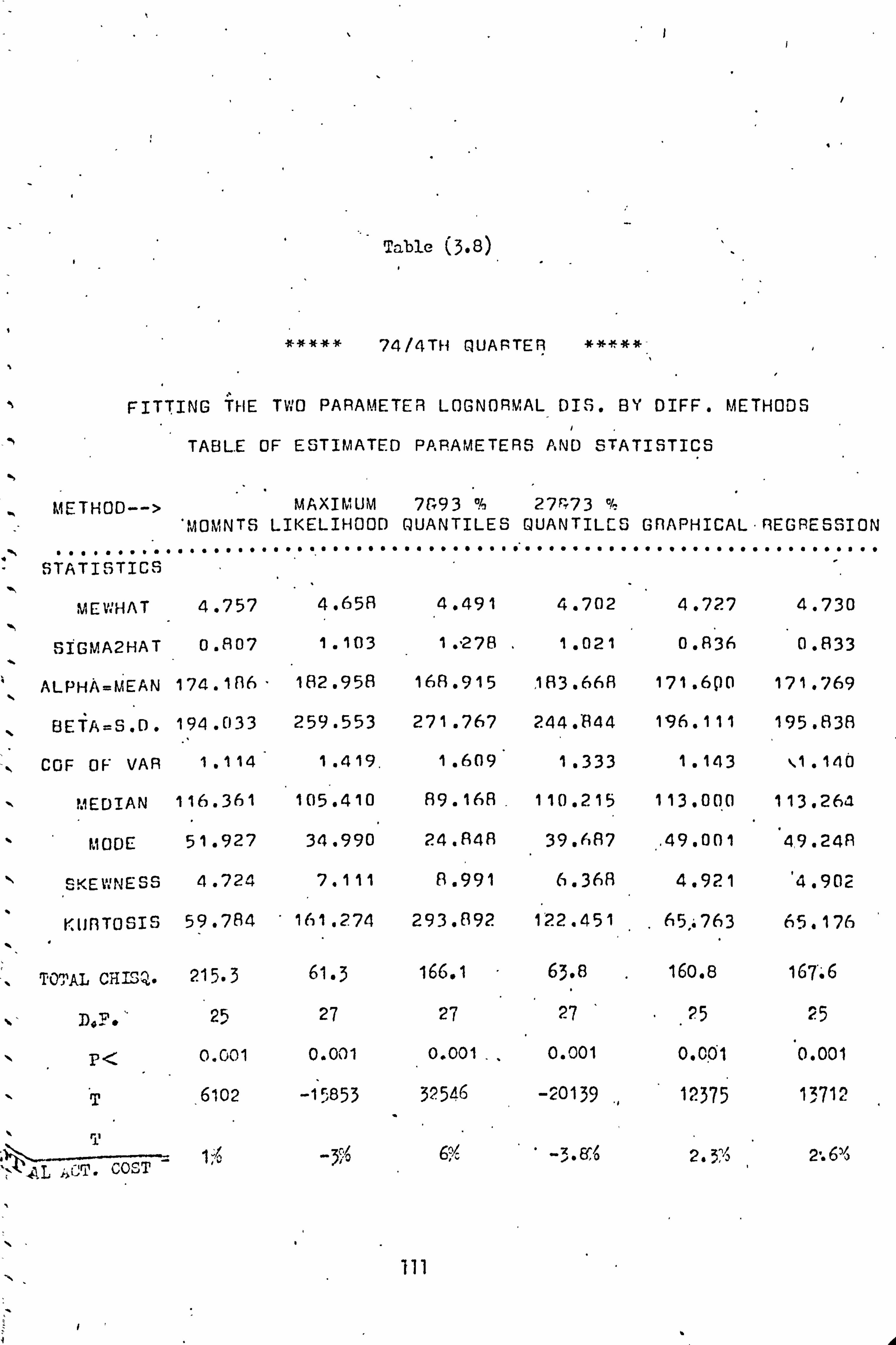
t

S

Table (3.8)

##** 74 /4TH QUARTER **ý`##

FITTING THE TWO PARAMET ER LOGNORM AL 025. BY DIFF. METHODS

TABL. E O F ESTIMATED PARAMETER S AND STAT ISTICS

METHOD--> MAXIMUM 7(, 93 % 27F', 73 01, 'MOMNTS LIKELIHOOD QUANTILES DUANTILES GRAPHICAL . REGRESSION

STATISTICS -.

MEWHAT 4.757 4.658 4.491 4.702 4.727 4.730

SIGMA2HAT 0.807 1.103 1. "278 1.021 0.836 0.833

ALPHA=MEAN 174.1116- 182.958 168.915 , 183.668 171.620 171.769

BETA=S. D. 194.033 259.553 271.767 244.844 196.111 195.838

COF OF VAR 1.114 1.419. 1.609 1.333 1.143 "1.140 i

MEDIAN 116.361 105.410 89.168. 110.215 113.000 113.26a

MODE 51.927 34.990 24.848 39,087 ..

49.001 49 . 24A

SKEWNESS 4.724 7.111 8.991 6.368 4.921 4.902

KIURTOSIS 59.784 161 , 2.74 293.892 122.451 65: 763 65.176

TOTAL CHISZ" 215.3 61.3 166.1 63.8 160.8 167.6

25 27 27 27 . 25 25

pC 0.001 0.001 0.001_, 0.001 0.001 0.001

T 6102 -15853 32546 -20139 12375 13712

ký " - 1 -3%' 6% -3. aö 2.3;; 2: 6'ý cosT

111

/r

F

Table (3.9) .

,

xý ,. xx 75 /1; 'i (1LfAfi'i Efi ý: * xx

F :[TYx. d; i 'i HE YW(1 P/ fil; r. 1E Y EH L(1GN(1RM Hl. [)I " HY C)FCFF " METHODS

A' CF E:: i'i : ý: "-; r; 'i E[i fýP, R MME'i E R1 1i AND S i, T xs'i IG-i

MET HO[)--> i4AX 3'MUJ'-" 27`*: 13 ý4C1(iIN- ; LXKEl_1H(1('C) : 4tiA; V Ty LE .ý' J! 1. .

Nýiý : L[- E f1 A I. 1TCHL f'HE i I(: id

""""". """"""""""" """""s"""""" """""""""" """""r""" """"""""""""""". ""w

^IEWHAT a""JaF, 4 1661u a"5() el a, 711 4,14'; d, 7(fi!

11: 1f C1; 'i (I " Fi1 z) 1. (l )6 1 "21 R 1 . '(1 12. C) "1 41i (I " R65,

ftl. i*i='kIEA N 173"((! 2 102.4`-, '' 16R"6R(1 1A4. _1R 175 . 6FA R 170,11°

5.3(1 2Ci: i"f fl 265"FO') 2 4.3.961 2(12 . c) 13 1UC'"306

Ct)i aF " V: \ f; 1.12 1 . 30f1' 1. '7C, 1.32'3 1.1 R5 r

1.172

:c (1 (fltiýJ 175.1?. R 9(Ih. 5'11 «(1.392 111.1'7 115"00 0 11f1"/11e1

M (1Cl(: 50 . 750 2ý, "04 14 [i (1 "[110 CIýJ, 273 4ý , 513

c: i . '1ý:: [i C"sýil(ý P ho R, h4(J h. 1Rf) 5; (IOfi ß) .

1?. 7

ý 1ýý: ýi ýw: i l: i ý'ý .J 71 1 CI'J

" i: iýi jrýý-

" (lýav i1 ýý

,!, h, 2 (

.4 L2 72 .

413

TOTAL 149.6 70.9 164.7 72.2 125.1 . 113.7

D. F. 24 27 27 21 244 ;4

P< 0.001. . 0.001' 0.001 0.001 0.001 0.001

T 3370 -14909 24317 21324 -368 14956

0.7 , _ 3.3; - 5.4': -4.7. '')' -0 1 zj

112

A

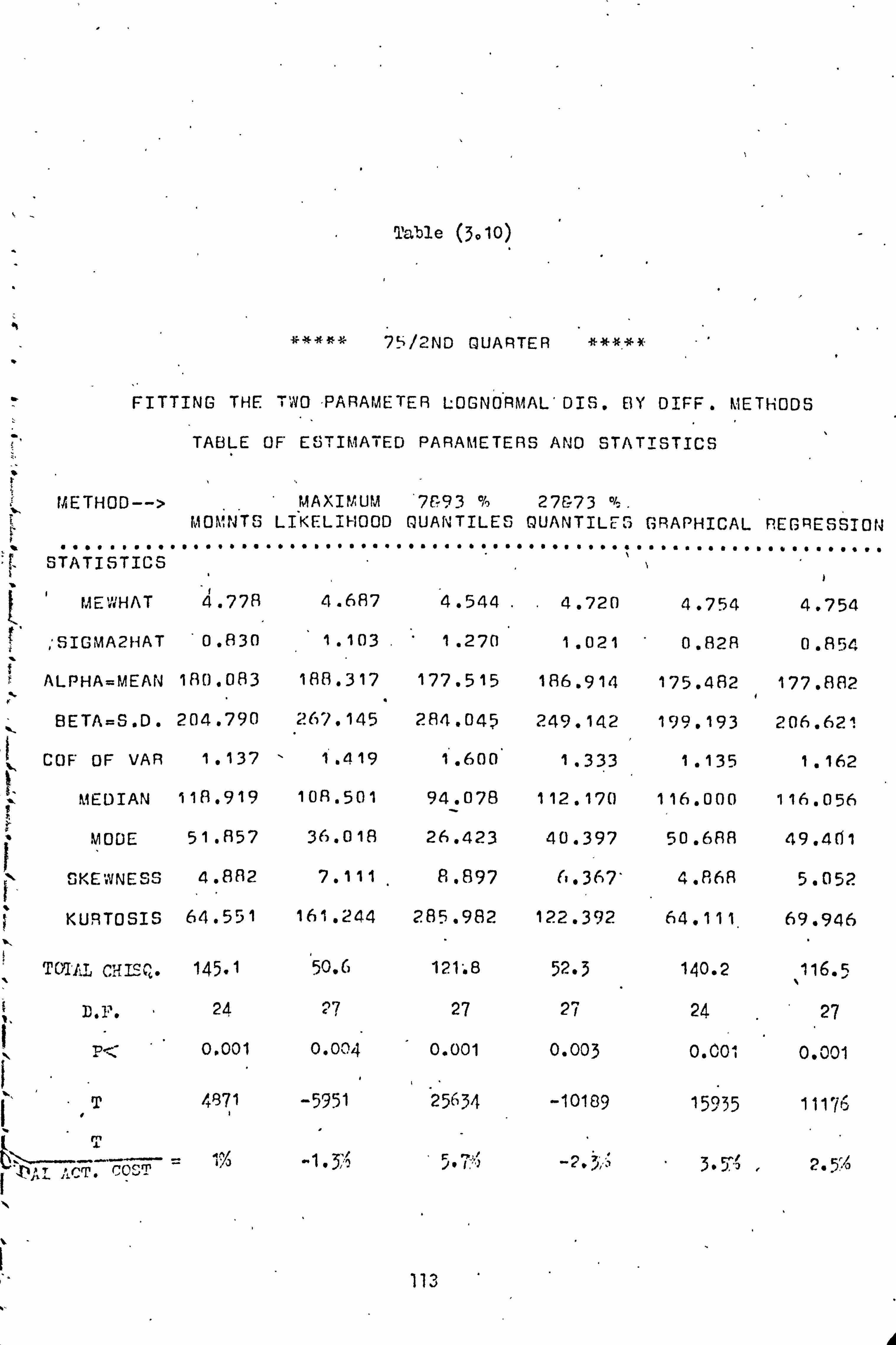
Table (3010)

* 75 /2ND QUARTER *# *-

FITTING THE TWO PARAMET ER LOGNORMAL"DIS" BY DIFF. METHODS

TABLE OF ESTIMATED PARAMETERS AND STAT ISTICS

' METHOD--> MAXIMUM 7e93 27E73 °ý . MOMNTS LIKELIHOOD QUANTILES QUANTILES GRAPHICAL REGRESSION

STATISTICS

ME1, '+HAT 4.778 4.687 4 "544. 4.720 4.754 4.754

9, IGMA2HAT 0.830 1.103 1.270 1.021 0.82A 0.854

ALPHA=MEAN 180.083 188.317 177.515 186.914 175.482 177.882

BETA=S"D. 204.790 267.145 284.045 249.142 199.193 206.621

COF OF VAR 1.137 1.419 1.600 1.333 1.135 1.162

MEDIAN 118.919 108.501 94.078 112.170 116.000 116.056

MODE 51.857 36.018 26.423 40.397 50.688 49.401

SKEWNESS 4.882 7.111 8.897 (1.367' 4.868 5.052

KURTOSIS 64.551 161.244 285.982 122.392 64.111, 69.946

T0T/L CHISQ" 145.1 50.6 121: 8 52.3 140.2 116.5

D. F. 24 27 27 27 24 27

p 01001 0.004 0.001 0.003 0.00. 0.001

T 4871

T COST t Till' T.

-5951 25634 -10189

ý1. ý`ä 5.?; '4)

15935 11176

3.51 , 2.5%

113

**l Y W0.4)AIIAr�CYFR L0GN0f1MAL [)I 3. x 73/4T; -+ QUARTER DATA

ESTIMATION EBY'MULTINOMIAL MAX. LIKELIHOOD METHOD : - MEW = 4.5163 " SIG%IA2=-. 1.0553

MEAN= 155.080 S. D. = 212.237

N

AMOUNT £ ACTUAL. EXPECTED ACTUAL- EXPECTED CL. NO. Cl.. NO. EXPECTED LOSS (A-E)**2/E

1- 30 47R. + 434. 44. 682. 4.1161 31- 6(}

, 518. 613. -95. -4322. 14.723

6,9C 461. 463. -2. -151. 0.009 91- 120 359. 335. 24. 2532. 1.719

121- 150 239. 245. -6. -813. 0.14i* 7 151- 160 213. 182. 31. 5130. 5.280 181- 210 "140. 139. 9. 1759.

. 0.: )83

211-- 240. ' 102. 107. -5. -1127. 0.234 24 1- 270 81. 84 . -- 3. -767. 0,10 7 271- 300 56. 67. -9, -2509, 11209 301-330 66. 55. 11. 347.0. 2.200

i- 361 45. 45. 0. 0. 0.000 361- 390 39. 37.

. 2. 7` 1. 0.108 391- 420' 35. 31. 4. 1622. " 0.516 421- 450 34, 26. 8. 3484. 2.462 451- 480 20'. 22. -2. -931. 0.182 491- 510 29. 19. 10 , 4955. '5 . 263 511- 540 14. 16. -10 r'

7'1 -

^2 -'; _1", ri n -, c

-651. u. 033 701- 800 '18. 19. -1. -"751. 0.053 601- 900 20. 13. 7. 5953. 3.769 901-1000 . 6. ' 9. -3. -2FI51. 1.000

9001-110: 1 4. 7. -3. -3151. 12E? f, 1101-12(10 4. 5. -1. -1150. 0.290" 1201-1300 1. 4. -3. -3751. 1301-1400 3. o... 0.

1401-1500 1. -1. -145(). 1.778 15; 11-16(10 0. 2. -2. -3101. 16(11-1700 1. 1. (, 0. 1 701-"'1ä0O 0. 1. -1 . -1751 . 19Q1-l900 0. 1, -1. -1650. 1901-2000 1. 1. (l. 0. 2001-2100 0. 1.. -1. -2050. 2101-2200 0. 0. 0, 0', 2201-2300 0. 0., . 0. 0. 23(11-24(1"

------- 1.

----------- (1k

----------- 1.

----------- 23 5(l.

---- - ' P. -ea6

---- TOTAL 3045. 3C; 4` .

-------- - -F,:,: ý "

----- 1----ý 53.375

e. - 25 " P ýý 1 < Q. ü TOTAL EXP, L. )ý; s .

TO AL AT /ý L/ A Y. l ll

5I 1ý. 0*1

pC. 114

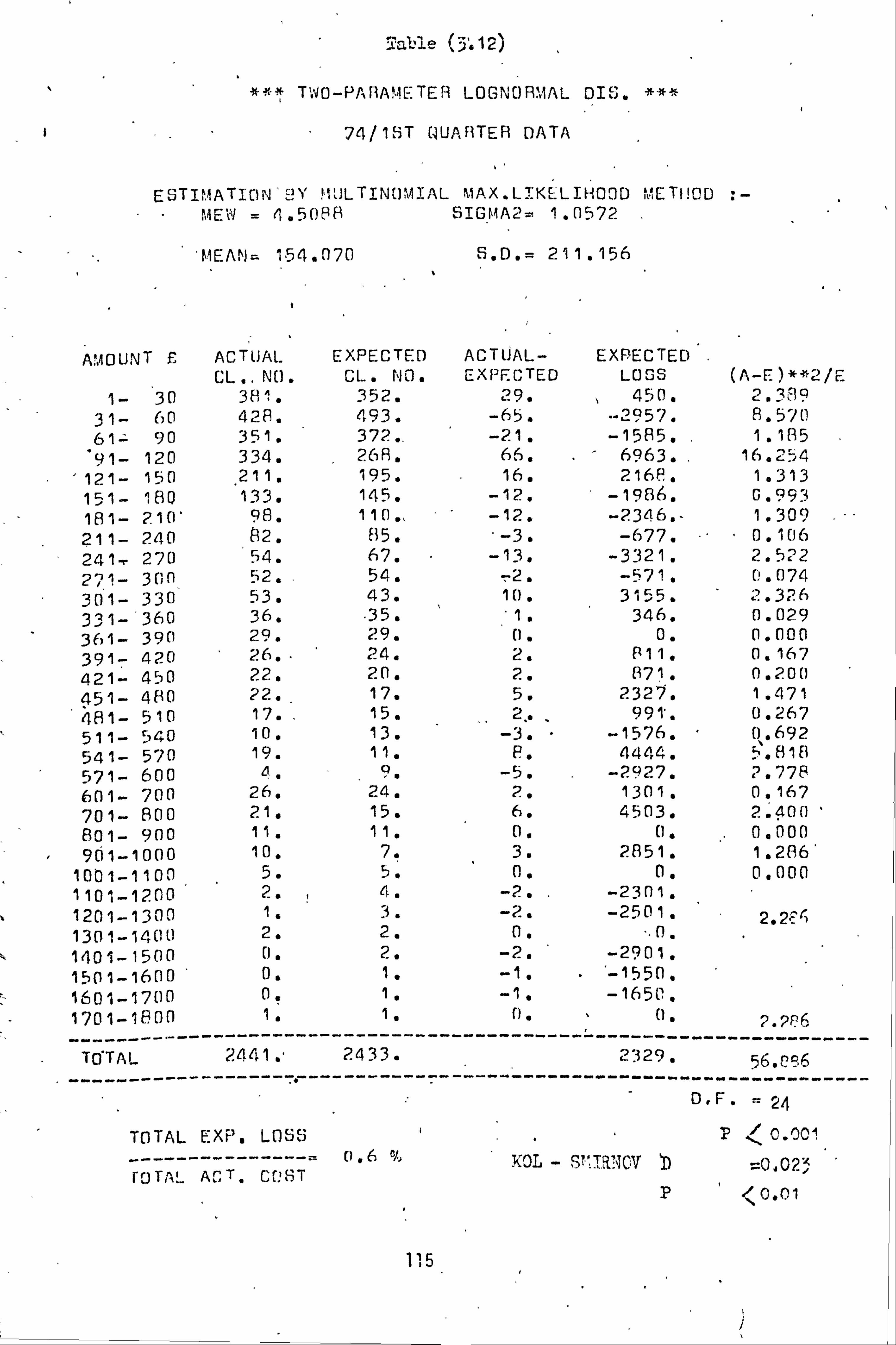
Table (3: 12)

T: UO-PARAMETER LOGNORMAL DIS.

74/18T (dUP. f1TER DATA I

ESTIMATION 'Y MULTINOJ"MAL MAX. LIKELIHOOD 'V, ETI! OD : - MEi'1 = 6.5098 SIGP4A2- 1.0572

MEAN^ 1,54.070 S. D. = 211.156

AMOUNT £ ACTUAL EXPECTED ACTUAL- EXPECTED CL.. NO. CL. NO. EXPECTE D LOSS (A-E)**"2/E

1- 30 381. 352. 29. 450. 2.389 31- 60 428. 493. -65. "-2957. 8.570 61= 90 351. 372.

- -21. -1585. 1.185 91- 120 334. 26A. 66. 6963. 16.254

121- 150 , 211. 195. 16. 2168ß 1.313

151- 180 133. 145. -12. -1986. 0.993 181- 210' 98. 110., -12. -2346. - 1.309 ý1 1- 240 82. 115. -3. -677. ' 0.106 241-, 270 54. 67. -13. -3321. 2.522 271- 3(1(1 52. -

54. -2. -571. 0.074 301- 330 53. 43. 1t1. 3155. 2.326 331- 360 36. -35. 1. 346. 0.029 3E61- 390 29. 29. 0. 0. 0.000 391- 420 26.. 24. 2. P11. 0.167 421- 450 22. 20. 2. 1371. 0.200

451- 480 22. 17. 5. 232'7. 1.471 481- 510 17. 15. 2. 9911. 0.267 511- 540 10. 13. -3. -1576. 0.692

541- 570 19. 11. P. 4444. 5.818 571- 600 4. 9. -5. -2927. 7.778 601- 700 26. 24. 2. 1301. 0.167 701- 800 21. 15. 6. 4503. 2.400- Sol- 900 11. 11. 0. 0. 0.000 901--1000 10. 7. 3. 2851. 1.286'

1001-1100 5. 5. 0. 0. 0.000 1101-1200 2. 4. -2. . -2301. 1201-1300 1. 3. -2. -2501. 2.2r<, 1301-1400 2. 2. 0. . D. 1401-1500 11. 2. -2. -2901. 1501-1600 0. 1. -1. -1550. 1601-1700 0. 1. -1. -16511. 1701-1600 is 1" 1)" 0. 2.2s? 6

TOTAL 2441 .' 2433. 2329. -

56.0-9.6 --

. ----------- --------. --- -------- -------- ------------ --------------- O. F. 24

TOTAL EX'r'. LOSS P `0.0c! 0.6 f1, KOL - S1 T, ft? JGV ý00? _; r0 Ti! AC: 7. C['S

P < 0.01

1'5

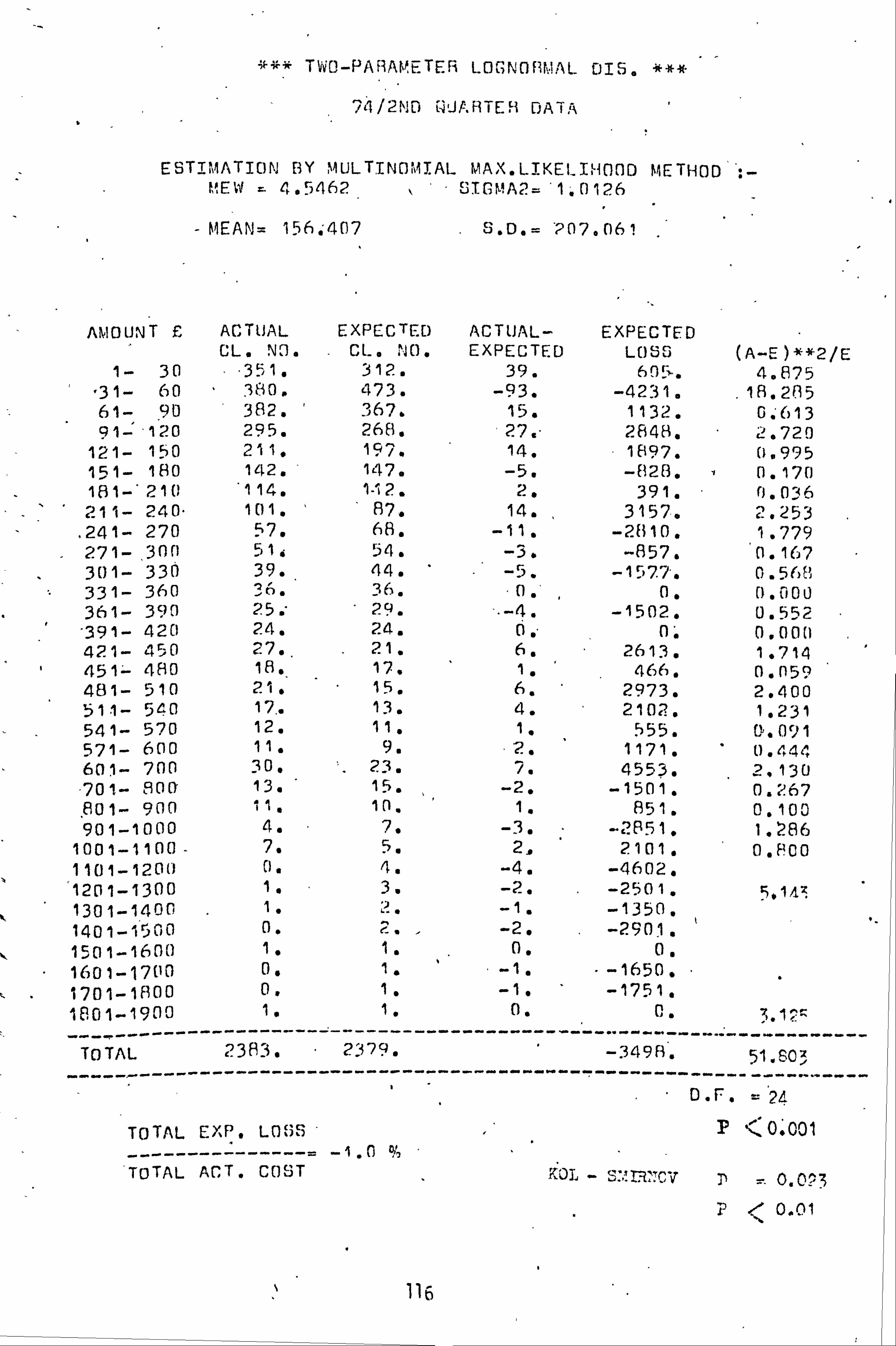
*#* TWO-PARAMETER LOGNORMAL DIE.

1/2ND [ JA. i1TEH DATA

ESTIMATION BY MULTINOMIAL MAX. LIKEi_IH000 METHOD MEW - 4.5462 SIGMA2= '1. n 126

MEAN= 156 : 407 S. D. = -207.061

AMOUNT £ ACTUAL EXPECTED ACTUAL- EXPECTED CL. NO. CL. NO. EXPECTED LOSS (A-E)**2/E

1- 30 -3`51. 312. 39. 60 . 4.875 "31- 60 380. 473. -93. -4231, .

18.205 61- 90 382. 367. 15. 1132. 0; 613 91- ' 120 295. 268. 27. " 2848. 2.720

121- 150 211. 1970 14. 1897. (). 995 151- 180 142. 147. -5. -828. 11.171) 181-" 2101 114. 112. 2. 391, f). 033 6 211- 240- 101. ' - 87. 14. 3157. 2.253

. 241- 270 57. 68. -11. -21110. 1.779 271-. 3n0 51: 54. -3. -857. '0.167 301- 330 39. 44. -5. -157.7. 0.5E, ß; 331- 360 30. 36. . n. ' 0, 0. CIO0 361- 390 25. 29. -. -4. -1502. 0.552

'391- 420 24. 24. 0, - 0. 0.000 421- 450 27.

" 21. 6. 2613. 1.714

451- 480 18. 17, 1. 466. 0. n59 481- 510 21, 15. 6. 2973. 2.400 311- 540 17.. 13. 4. 2102. 1.231 541- 570 12, 11. 1. 555. Ell. 091 571- 600 11. 9. 2. 1171. 0.444 601- 700 30. 23. 7. 4553. 2.130 -701- 800 13. 15. -2. -1501. 0,267 801- 900 11, in. 1. 851. 0.100 901-1000 4. 7. -3. -2851. 1.286

1001-1100- 7. 5. 2. 2101, 0.800 1101-120() 0. 4. -4. -4602, 1201-1300 1" 3. -2. -2501. 5), 142 1301-1400 1. 2. -1. -1350, 1401-º500 0. -2. . -2901, 1501-1600 1. 1. 0. 0. 1601-1700 0, 1. -1. "-1650.

" 1701-1800 0. 1. -1. -1751. 1E? 01-1900 1. 1. 0. 0. 3,12

TO TAL -------

-----------

----------

? 38i. ----------

-

2370,

----------- --------

_ -349Fi.

ý.. -

---- ------------

-Sý. rO;

-----

------------

TOTAL EXP. LOSS P \.. 0.001

------ ---------_ TOTAL ACT. COST KOI, - S: '. I "c7 T 0.0^3

P < 0.01

116

' #* TWO-PARAMETER LOG"yfRMAL DIS. *#*

"74/3RD QUARTER DATA

" ESTIMATION BY MULTINOMIAL MAX. LIKELIH00D METHOD -MEW = 4.6371 SIGMA2= 1.0112

MEAN= 171,1 9 S. D. = 226.355

I% AMOUNT £ ACTUAL EXPECTED ACTUAL- EXPECTED

CL. NO. CL. NO. EXPECTED LOSS (A-E)*"*2/E 1- 30 362. 315. 47. 726. 7.013

31- 60 427. 518. -91. -4140. . 15.986 61- 9T1 383. 421. -38. -2869. 3.430

. 91- 120 356. 317. 39. 4115. 4.798 121- 150 283". 238. 45. 6097, 8.508 151- 180 194. 181. 13. 2151. 0.934 181- 210 137. 140. -3. -587, 0.064 211- 240 97. 110. -13. -2931. 1,536 241- 270 86. 87. -1. -256. 0.011 271- 300' 71. 70. 1. 286, 0,014 301- 330 64. 57. 7. 2208. 0,860 331- 360 45. 47. -2. -691. 0. Q85 361- 390 44" 39. 5. 11377. 0.641 391- 420 25. 33. -8.1 -3244. 1.939 421- 450 26. 27. -1. -436. 0.037 451- 480 22, 23. -1. -466. 0.043 481- 510 25. 20. 5. ' 2477. 1.250 511-'540 14. 17. -3. "-1576. 0,529 541- 570 14. 15. -1, -555. 0.067 571- 600 17. 13. 4. . 2342. 1.231 601- 700 - 32. 32. 0., 0. ' 0.000 701- 800 34. 21. 13. 9756. 8.048. 801- 900 17. 15. 2. 1701. ' 0.267 901-1000 4. 10. -6. -5703. 3.600

1001-1100 9. 7. 2. 2101. 0.571 1101-1200 4. " 5. -1, -1150. ,

0.200 1201-1300 " 0. 4. -4. -5002. 1301-1400 1. 3. -2. -2701.

' 5.115

1401-1500 3. 2. 1. 1450, " . 1501-1600 Q. 2. -2. -3101. 1601-1700 1. 2. -1. . -1650. 0.667 1701-1800 0. 1. -1. -1751. 18o1-1900 0. 1. -1. -1850. 1901-2000 0.. 1, -1. -1950. ' 2001-2100'" 0. 1. -1. -2050, 2101-220.0 1. 1. 0. 0. 2201-2300 0. 0. 0.. 0. 2301-2400 . 0. 0. 0. 0. 2401-2500 0. 0. 0. 0. 2501-2600 1. 0. . 1 1. 2550. 1. COG

: E:::::: : EEEEI::: :: EE::::: ::::::::::::: EEI... '69,27A

1)- . _26

TOTAL EXP. LOSS P<0.001 ---------------- TOTAL ACT. COST X CL - 'D X0.029

i1T P<0.01

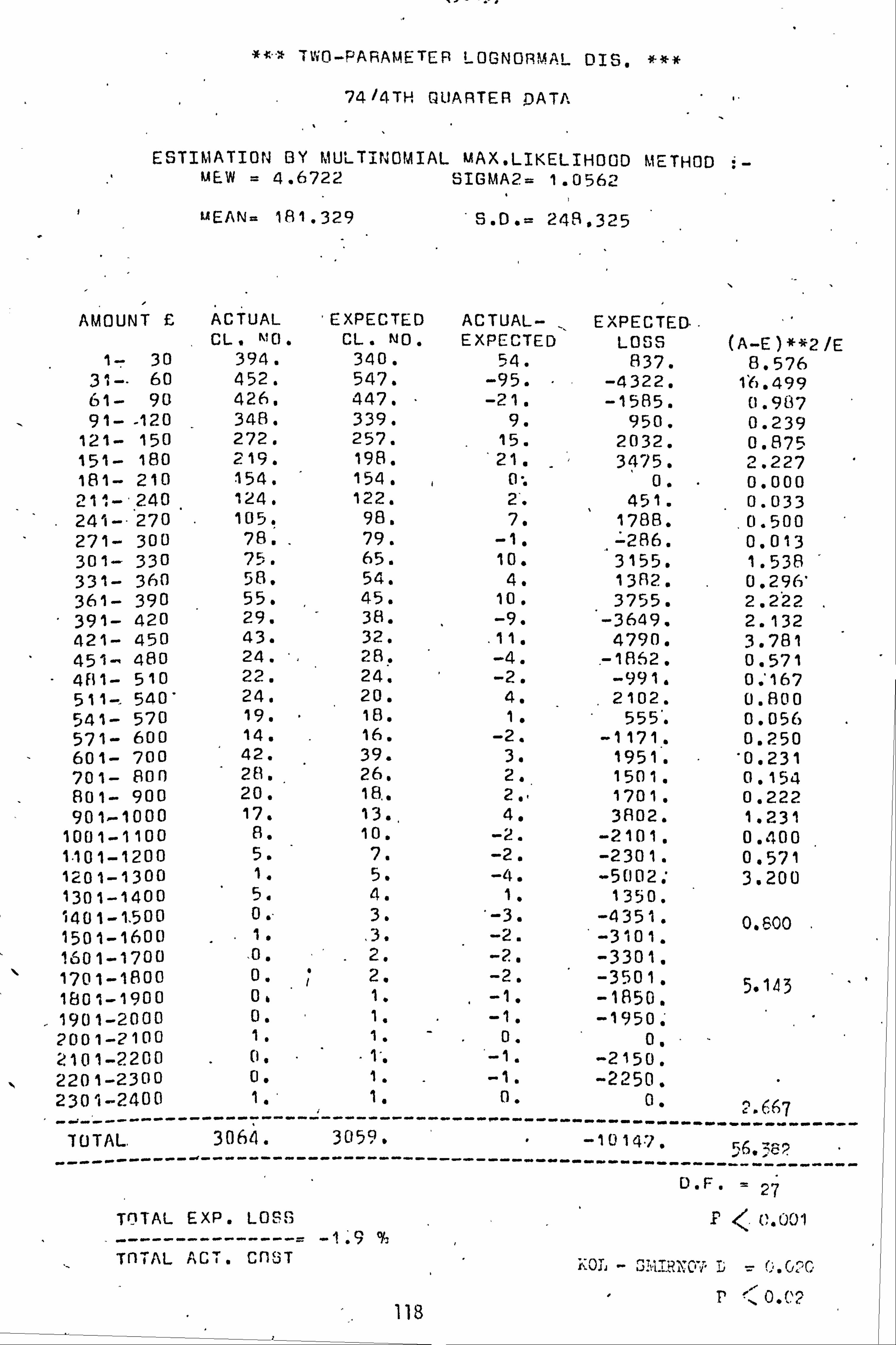
* TWO-PARAMETER LOGNORMAL DIS, ##*

74 /4TH QUARTER DATA.

ESTIMATION BY MULTINOMIAL MAX. LIKELIHOOD METHOD i MEW = 4.6722 SIGMA2= 1.0562

UUEAN- 181.329 S. D. = 248.325

'¼

AMOUNT £ ACTUAL 'EXPECTED ACTUAL- EXPECTED.. CL, X00. CL. NO. EXPECTED LOSS (A-E) **2 /E

1-- 30 394. 340. 54. 837. 8.576 31-- 60 452. 547. -95. -4322. 10.499 61- 90 426, 447. -21. -1585. 0.987 91--120 348. 339. 9. 950. 0.239

121- 150 272. 257. 15. 2032. 0.875 151- 180 219. 198. "21.

_ 3475. 2.227 181- 210 154. " 154. 0. 1 0. 0.000 211- 240 124. 122. 2. 451. 0.033 241--270 105. 98. 7. 1788.

"0.500 271- 300 78.. 79. -1. =286. 0.013 301- 330 75. 65. 10. 3155. 1.538 331- 360 58. 54. 4. 1382. 0.296' 361- 390 55. 45. 10. 3755. 2.222 391- 420 29. 38. -9. -3649. 2.132 421- 450 43. 32.

. 11. 4790. 3.781 451- 480 24. '. 28. -4. -1852. 0.571 4111- 510 22. 24. -2. -991. 0: 167 5 540' 24. 20. 4. 2102. 0.800 541- 570 19. 18. 1. 555'. 0.056 571- 600 14. 16. -2. -1171. 0.250 601- 700 42. 39. 3. 1951. 0.231 701- 800 211.. 26. 2. 1501. 0.154 801- 900 20. 18". 2., 1701. 0.222 901-1000 17. 13., 4. 3802. 1.231

1001-1100 8. 10. -2. -2101. 0.400 1.101-1200 5. 7. -2. -2301. 0.571 1201-1300 1. 5. -4. -5002; 3.200 1301-1400 5. 4. 1. 1350. 1401-1.500 0" 3. -3. -4351 . 0.600 1501-1600

.. 1. 3. -2. -3101.

1601-1700 "0. . 2. -2. -3301.

1701-1800 0. '

1 2. -2. -3501. Sýýa3 1801-1900 0b 1. -1. -1850. 1901-2000 0. -1. -1950. 2001-2100 1. 1. . 0. Q, .. 2101-2200 -2150. 2201-2300 0. 1. -1. -2250. 2301-2400 1. " 1. 0. 0. 2.667

--------------, ------------------. -------------------- ----------- TUTAL. ----------

3064. ----------

3059. ------------ -----------

-10147. ------------- ----- -------

D. F. = 27

TOTAL EXP. LOSS F <. C. 001

------- -------- TOTAL ACT. COST ,., Ko'

"F '; C. C2 . 118

Tab. 7f /1 STi QUARTER DATA

ESTIMATION By MULTINOMIAL M. AX. LIKELIHOOD METHOD : MEW - 4,6839 8IGMA2= 1.0241

MEAN= 180.540 S. D. = 241.173

AMOUNT £ ACTUAL EXPECTED ACTUAL- EXPECTED CL. NO. CL. NO. EXPECTED LOSS (A"-E) **2 /`

1- 30 324. - 275. 49. ' . 760. 8.731 31- 60

, 31-17. 463. -76. -3458. 12.475

"61- 90 345. 384. -39. -2944. 3.961 91- 120 289. 293. -4. -422. (1,055

121- 150 " 253. 223. 30. 4065. 4.036 151- 180 187. 171. 16. 2648.

. 1,497

181- 210 138. 133. 5. 978. 0.188 211- 240 114. 105. 9. 2029. 0.771 241- 270 93. 84, 9. . 2299. 0.964 271- 300 67. 68, -1. -286. 0.015 301- 330. 63. 56. 7. 2208. 0.875 331- 360 44, 46.. -2. -691. 0.087 361- 390 44. 39. 5. 1877. 0.641 391- 420 " 35. 32. 3. 1216. 0.281 421- 450 25.

. 28. -3. -1306. 0.321

451- 480 26. 23. 3. 1396. . 0.391

481- 510 18. ' 20. -2. -991. 0.200 511- 540 18. " 17. 1, 525. 0.059. 541- 570 22. 15. 7. 3888. 3.267 571- 600 '. 17. 13. 4. 2342. 1.231 601- 700 39.

. 33. 6. 3903. 1.091

701- 600 19. 22. -3. -2251. 0.409 801.900 18. - 15. 3. 2551. 0.600 901-1000 12. 11. 1. 951. 0.091

1001-1100 3. 8. -5. -5252. 3.125 1101=1200 1. 6. -5. -5752. 4.167 1201-1300 11 4" -3. ' -3751. 1301-1400 01 3. -3. -4051. Z 5.14Z 1401-150[) 1. 3. -2. -2901. 1501-1600 0. 2. -2. -3101.

. 1601-1700 1. 2. -1, -1650. z" "571 ý . 1701-1800 0. .1. -1 " -1751. 1801-1911. ) 0. 1. -1� -185,0

, 1901-2000 0+ 1. -1. -1950. 2001-2100 1. 1.4 01 0. 2101-"2200 1.

, 1. 0. 0,

2201-2300 0. _

1. -1. -2250. 2301-2400> 0. 01 01 2401-250'0 0. 0. 0. 01 2501-2600 0. 0. 0. 01 2601-2700 0. a. 01 01 2701-28[)0 0" 0" 0. 0' .e 2801-2900 0. 0. t). 0. 2901-3000 0. 0. 01 0. 3001-3100 0. 0. 0. 0, 3101-3200 0. 0. 09 00 3201-3300 0. 00. a. 0. 3301-34(10 0. 01 0, 0. 3401-3500 0. 0. C� 0 3,01-3600 1. 0. 1. - 3550.

Ti3S AL ------------

2607. ----------

2603. -------------

--__--_-

------

_- -ý- -9423.

--, ý;

_.. _ 50.7-

TO AL EXP LOSS ---- ------------ --------

T

- .

_ _-. - ---_- _ ý -2.. 1% 'Q. 01 p ý'>

... !

r0TAL A,;, T , COST

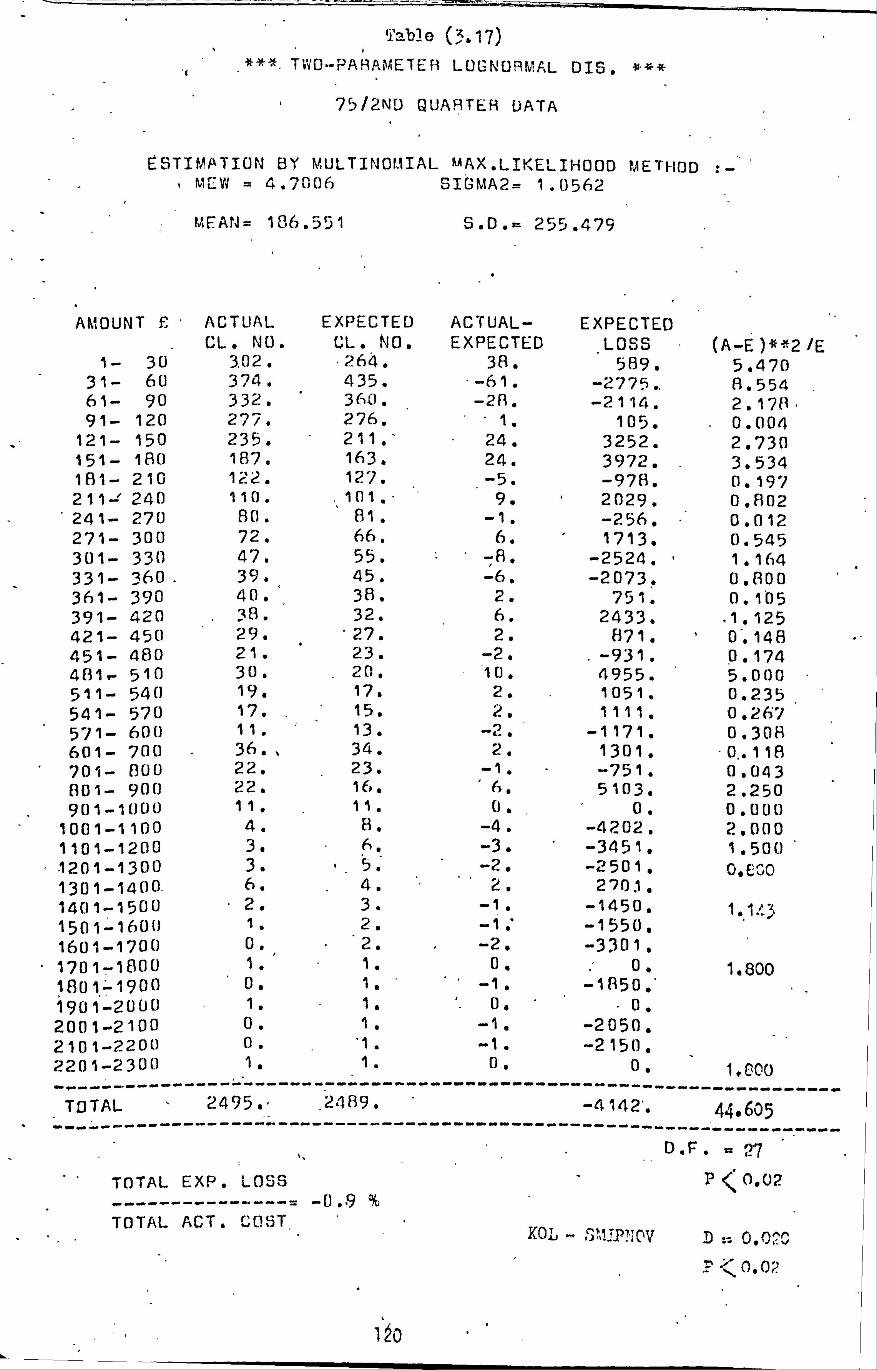
'Talb? e (31-17)

# TWO-PARAMETER LOGNORMAL DIS .##

75/2NU QUARTER DATA

ESTIMATION BY MULTINOt. 1IAL MAX. LIKELIHOOD METI-10D MEW = 4.7006 SIGMA2= 1.0562

MEAN= 186.551 S. D. = 255.479

AMOUNT F, ACTUAL EXPECTED ACTUAL- EXPECTED CL. NO. CL. No. EXPECTED LOSS (A-E )* '2 /E

1- 30 3.02. 264. 38. 589. 5.470 31- 60 374. 435. - -61 . -27751.. 8.554 61- 90 332. 360. -28. -2114. 2.178, 91- 120 277. 276. . 1. 105. . 0.004

121- 150 235. 211. ' 24. 3252. 2.730 151- 180 187. 163. 24. 3972.

. 3.534 181- 210 122. 127.

. -5. -978. 0.197 211- 240 110" . 101. 9. 2029. 0.802 241- 270 80. 81. -1. -256. 0.012 271- 300 72. 66. 6. 1713. 0.545 301- 330 47. 55. -8. -2524. 1.164 331- 360. 39. 45. -6. -2073. 0.800 361- 390 40. 38. 2. 751. 0.105 391- 420 38" 32. 6. 2433. . 1.125 421- 450 29. "27. 2. 871. 0.148 451- 480 21. 23. -2. . -931. 0.174 481 *- 510 30.

. 20. 10. 4955. 5.000

511- 540 19. 17. 2. 1051. 0.235 541- 570 17. 15. 2. 1111. 0.267 571- 600 11. 13. -2. -1171. 0.308 601- 700 - 36.. 34. 2. 1301. ' 0.. 1 1A 701- 800 22. 23. -1. -751. 0.043 801- 900 22. if,, 6. 5103. 2.250 901-1000 111 1 1. () . 0. 0.000

1001-1100 4. 8. -4. -4202. 2.000 1101-1200 3. 6.

' -3. -3451. 1.500'

-1201-1300 3.

. 51 -2. -2501. p. EO0

1301-1400. 6. -

4. ' 2. 201. 1401-1500 " 2. 3. -1 . -1450. 1 1 J3 1501-1600 1. 2. -1. -1550.

.

1601-1700 0., 2. -2. -3301. 1701--1800 1. 1" 0.

. 0" 1.800

1801-1900 0. 1. ' -1. -1850. ' 1901-2000 1. 1. '. 00 " 0. 2001-2100 0. 1. -1. -2050. 2101-2200 0. '1. -1. -2150. 2201-2300

---

1. -----

------

11 -----------

0. ----------

0. ............ -

11000 -

TOTAL

- -----------

2495. " ----------

. 2.489.

----------- -----------

----

-4142'. -----------

-------------

44.605

------------- D.

- F. a 27

TOTAL EXP. LOSS P<0.02

--------------- _ -O. 9 TOTAL ACT. COST YOL -. 3MIP OV D .. 0,020

1'o

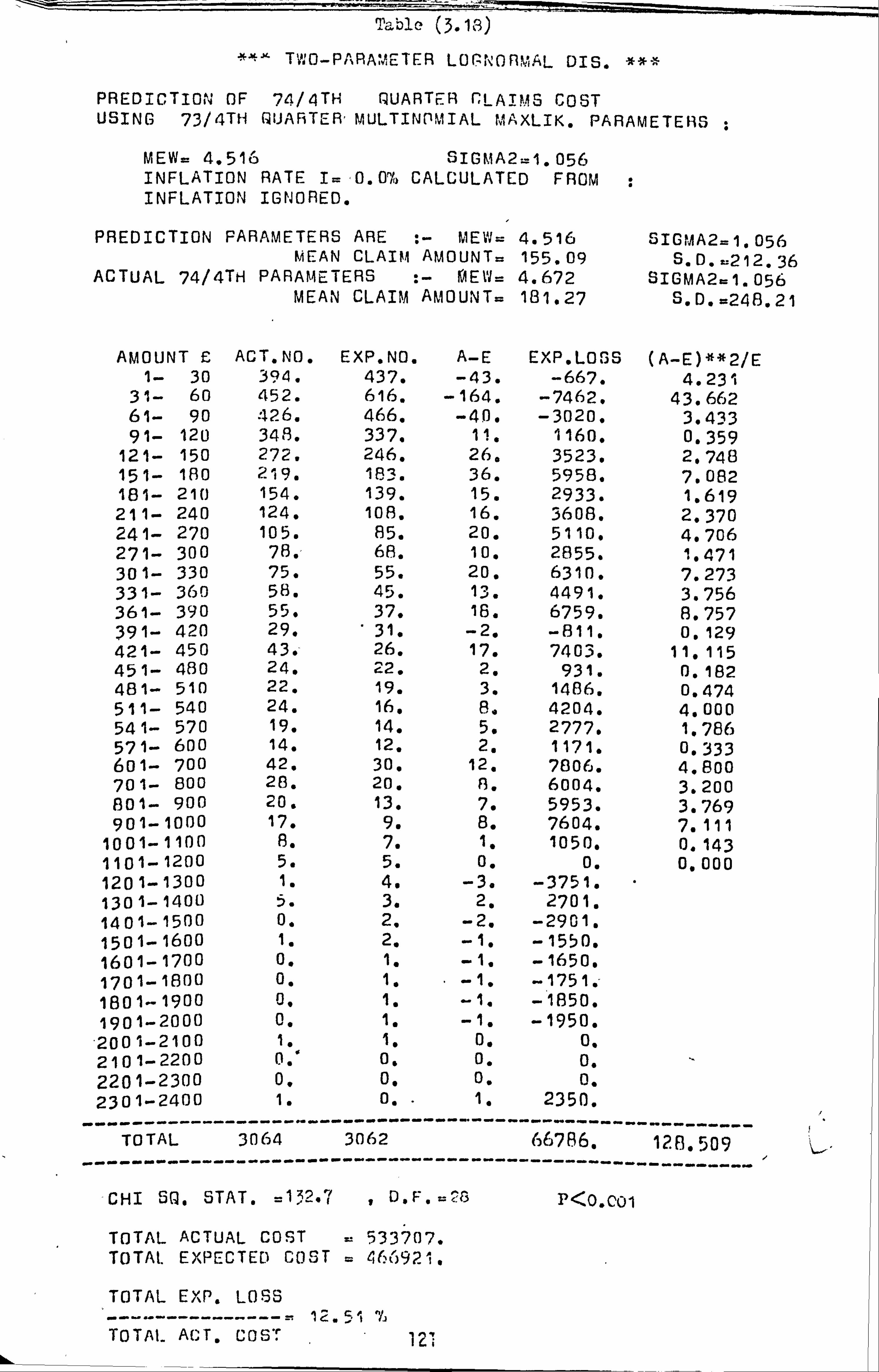
Table (3.18)

**' TWO-PARAMETER LOP NORMAL DIS. ***

PREDICTION OF 74/4TH QUARTER CLAIMS COST USING 73/4TH QUJARTER, MULTIN PMIAL MAXLIK. PARAMETERS

MEW= 4.516 SIGMA2_1.056 INFLATION RATE 1= 0.07* C ALCULATED FROM INFLATION IGNORED.

PREDICTION PAR AMETERS ARE : - MEW= 4.516 SIGMA2_1.056 MEAN CLAIM AMOUNT= 155.09 S. D. L212.36 ACTUAL 74/4TH PARAMETE RS : - MEW= 4.672 SIGMA2=1.056 MEAN CLAIM AMOUNT= 181.27 S. D. =248.21

AMOUNT £ AC T. NO. E XP. NO. A-E EXP. LOSS (A-E)**2/E 1- 30 394. 437. -43. -667. 4.231

31- 60 452. 616. -164. -7462. 43.662 61- 90 426. 466. -40. -3020. 3.433 91- 120 34.9. 337. l i. 1160. 0.359

121- 150 272. 246. 26. 3523. 2.748 151- 180 219. 183. 36. 5958. 7.082 181- 210 154. 139. 15. 2933. 1.619 211- 240 124. 108. 16. 3608. 2.370 241- 270 105. 85. 20. 5110. 4.706 271- 300 78. 68. 10. 2855. 1,471 301- 330 75. 55. 20. 6310. 7.273 331- 360 58. 45. 13. 4491. 3.756 361- 390 55. 37. 16. 6759. 8.757 391- 420 29. 31. -2. -811. 0.129 421- 450 43. 26. 17. 7403. 11.115 451- 480 24, c2. 2. 931. 0.182 481- 510 22. 19. 3. 1486. 0.474 511- 540 24. 16. 8. 4204. 4.000 541- 570 19. 14. 5. 2777. 1.786 571- 600 14. 12. 2. 1171. 0.333 601- 700 42. 30. 12. 7806. 4.800 701- 800 28. 20. A. 6004. 3.200 801- 900 20. 13. 7. 5953. 3.769 901- 1000 17. 9. 8. 7604. 7.111

1001-1100 8. 7. 1. 1050. 0.143 1101-1200 5. 5. 0. 0. 0.000 1201-1300 1. 4. -3. -3751. 1301-1400 5. 3. 2. 2701. 1401-1500 0. 2. -2. -2901. 1501-1600 1. 2. -1, -1550. 1601- 1700 0. 1. -1. -1650. 1701-1800 0. 1. -1. -1751. - 1801 1900 0, 1. -1. -1850. 1901-2000 0. 1. - 1. -1950. 2001-2100 1. 1. 0. 0. 2101-2200 0.4 0. 0. 0. 2201-2300 0. 0. 0. 0. 2301-2400 1. 0,

-- - 1.

-------- 2350.

- ------------------------- TOTAL 3064 3062

----------- 66786. ----------

128.509

CHI SQ. STAT. =13?.; , D. F .. ýO P<O. C01

TOTAL ACTUAL COST = 533707. TOTAL EXPECTED COST = 466921.

TOTAL EXP. LOSS

--------------- 12.51 ll, TßTAI_ ACT. COST 12

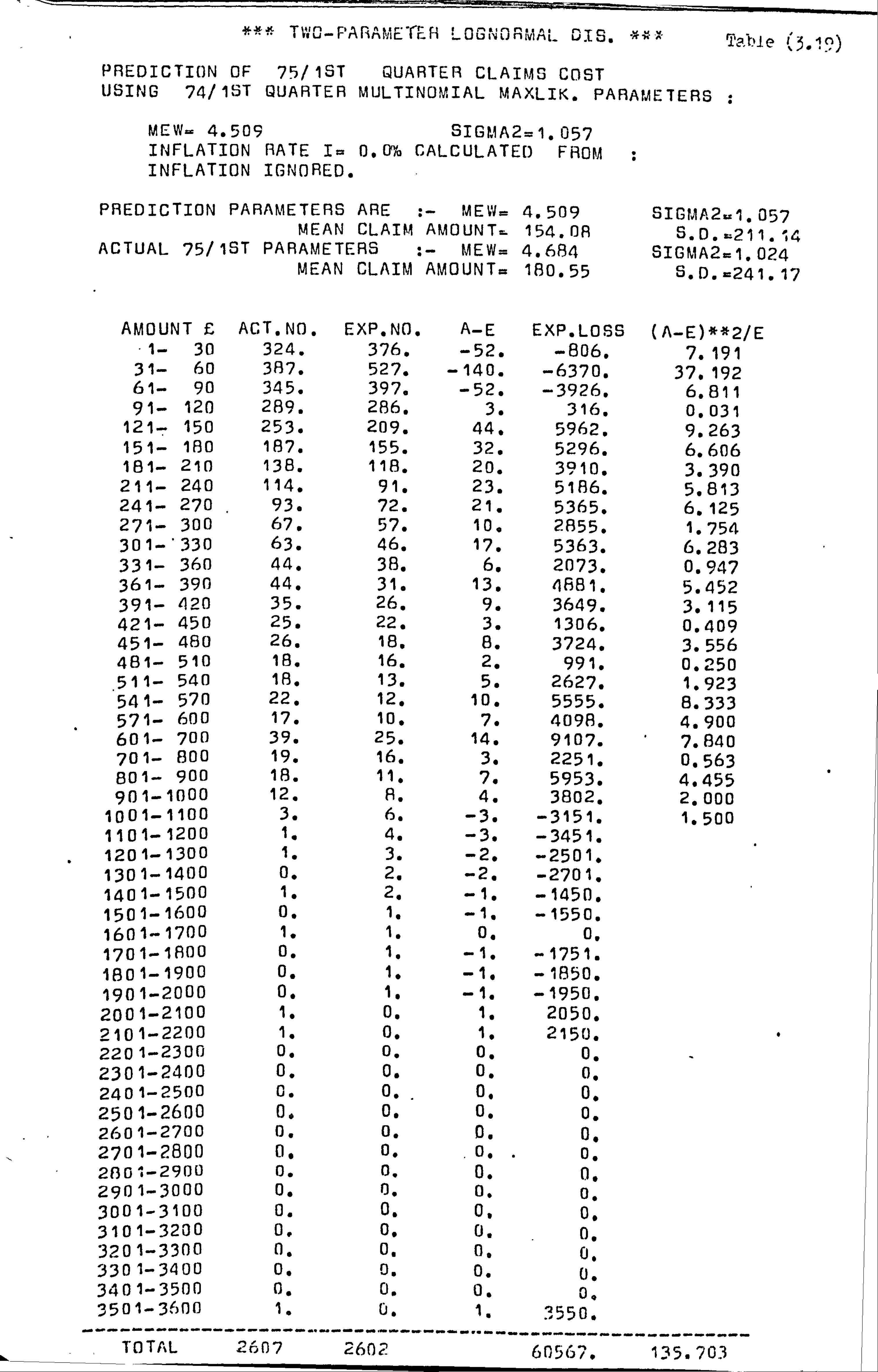
*** TV, Wun-F'ARnr. Mrc"" GNPiJntvS un.

nLnt_ nZ$. 1aý 1. ie } r_fi

Iý. üuýv %ýKý n` jýýý

PREDICTION OF 75/1ST QUARTER CLAIMS COST USING 74/1ST QUARTER MULTINOMIAL MAXLIK. PARA METERS

MEW- 4.509 SIGMA2=1.057 INFLATION RATE I= 0.0% CALCULATE[) FROM INFLATION IGNORED.

PREDICTION PARAMETERS ARE : - MEW= 4.509 SIGMA2.1.057 MEAN CLAIM AMOUNT= 154.08 S. D. -211. o4 ACTUAL 75/1ST PARAMETE RS : - MEW= 4.684 SIGMA2=1.024 MEAN CLAIM AMOUNT= 180.55 S. D. =241.17

AMOUNT £ ACT. NO. E XP. NO. A-E EXP. LOSS (A_E)**2/E 1- 30 324. 376. -52. -806. 7.191

31- 60 387. 527. -140. -6370. 37.192 61- 90 345. 397. -52. -3926. 6.811 91- 120 289. 286. 3. 316. 0.031

121- 150 253. 209. 44. 5962. 9.263 151- 180 187. 155. 32. 5296. 6.606 181- 210 138. 118. 20. 3910. 3.390 211- 240 114. 91. 23. 5186. 5.813 241- 270 93. 72. 21. 5365. 6.125 271- 300 67. 57. 10. 2855. 1.754 301-'330 63. 46. 17. 5363. 6.283 331- 360 44. 38. 6. 2073. 0.947 361- 390 44. 31. 13. 4881. 5.452 391- 420 35. 26. 9. 3649. 3.115 421- 450 25. 22. 3. 1306. 0.409 451- 480 26. 18. 8. 3724. 3.556 481- 510 18. 16. 2. 991. 0.250 511- 540 18. 13. 5. 2627. 1.923 541- 570 22. 12. 10. 5555. 8.333 571- 600 17. 10. 7. 4098. 4.900 601- 700 39. 25. 14. 9107. 7.840 701- 800 19. 16. 3. 2251. 0.563 801- 900 18. 11. 7. 5953. 4.455 901-1000 12. A. 4. 3802. 2.000

1001- 1100 3. 6. -3. -3151. 1.500 1101- 1200 1. 4. -3. -3451. 1201-1300 1. 3. -2. -2501. 1301-1400 0. 2. -2. -2701. 1401-1500 1. 2. -1. -1450. 150 1-1600 0. 1. -1. -1550. 1601- 1700 1. 1. 0. 0. 1701-1800 0. 1. -1. -1751. 180 1-1900 0. 1. -1, - 1850. 1901-2000 0. 1. - 1. -1950. 200 1-2100 1. 0. 1. 2050. 2101-2200 1. 0. 1. 2150. 2201-2300 0. 0, 0. 0. 2301-2400 0. 0. 0. 0. 2401-2500 0. 0. 0. 0. 2501-2600 0. 0. o. 0, 2601-2700 0. 0. 0. 0. 2701-2800 0. 0. o. 0. 2801-2900 0. 0. 0. 0. 2901-3000 0. 0. 0. 0. 3001-3100 0. 0. 0l 0, 3101-3200 0. 0. 0. 0. 3201-3300 0. 0. 0, 0. 3301-3400 0. 0. 0. 0. 3401-3500 0. 0. o. 0, 3501- 3600

----------- --

1.

---

0. 1. 3550. - - ------------

TOTAL 2 c607 2602 --------- ----------

60567. ---------- 135.703

Table (3.19) - continued

CHI SQ. STAT. =141.1 , D. F. _ 27 P<0.001

TOTAL ACTUAL COST = 452059. TOTAL EXPECTED COST _ 391491.

TOTAL EXP. LOSS

--------------- = 13.40 % TOTAL ACT. COST

0

123

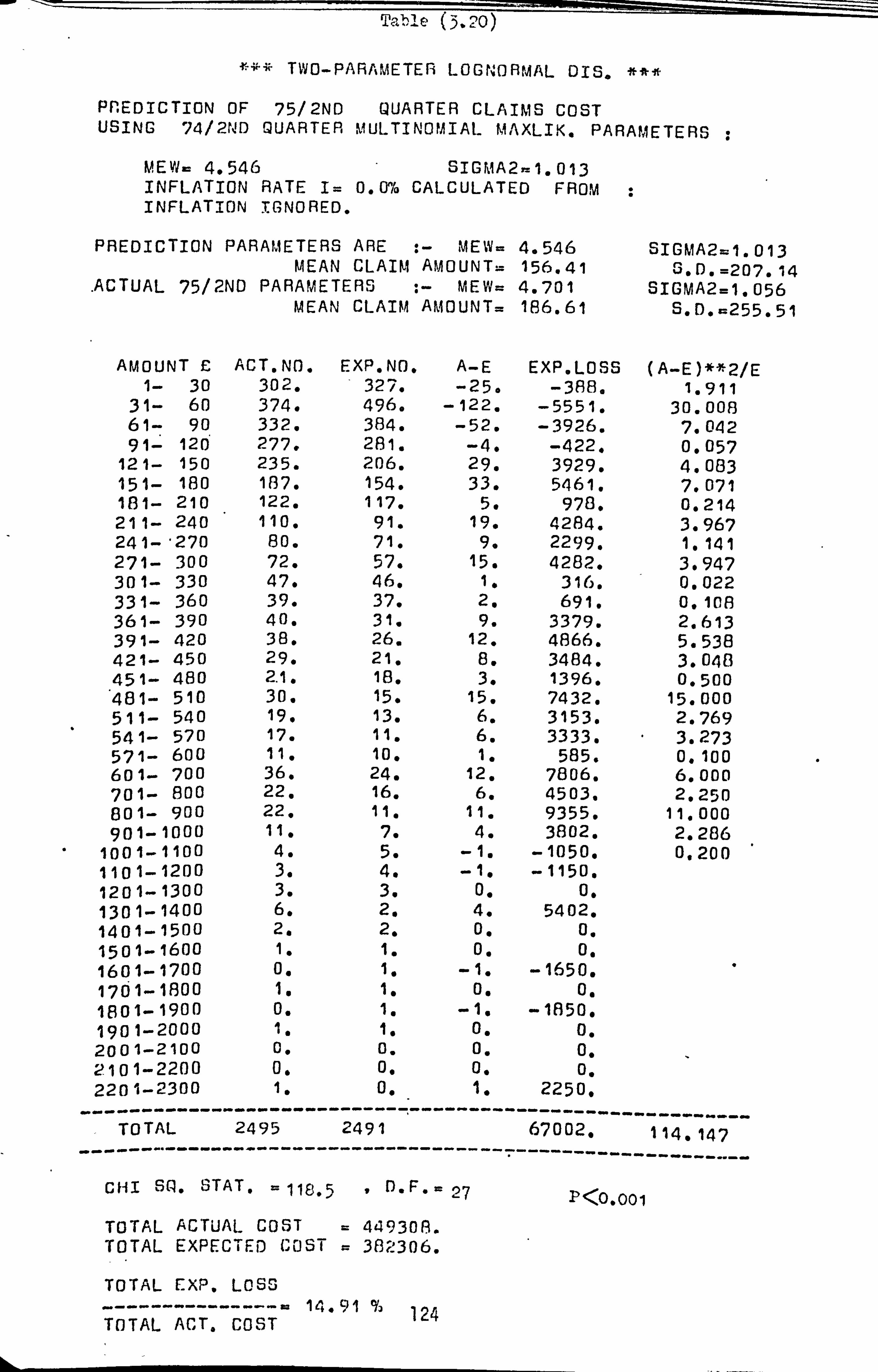
Table (3-20)

*x TWO-PARAMETER LOGNORMAL DIS. ***"

PREDICTION OF 75/2ND QUARTER CLAIMS COST USING 74/2ND QUARTER MULTINOMIAL MAXLIK. PARAMETERS ;

MEW= 4.546 SIGMA2r1.013 INFLATION RATE I= 0.0% CALCULATED FROM ; INFLATION IGNORED.

PREDICTION PARAMETERS ARE ; - MEW= 4.546 SIGMA2-1.013 MEAN CLAIM AMOUNT= 156.41 3. D. =207,14

. ACTUAL 75/2ND PARAMETE RS : - MEW= 4.701 SIGMA2=1.056

MEAN CLAIM AMOUNT= 186.61 S. D. =255.51

AMOUNT £ ACT. NO. E XP. NO. A-E EXP. LOSS (A-E)**2/E 1- 30 302. 327. -25. -388. 1.911

31- 60 374. 496. -122. -5551. 30.008 61- 90 332. 384. -52. -3926. 7.042 91- 120 277. 281. -4. -422. 0.057

121- 150 235. 206. 29. 3929. 4.083 151- 180 187. 154. 33. 5461. 7.071 181- 210 122. 117. 5. 978. 0.214 21 1- 240 110. 91. 19. 4284. 3.967 241- -270 80. 71. 9. 2299. 1.141 271- 300 72. 57. 15. 4282. 3.947 301- 330 47. 46. 1. 316. 0.022 331- 360 39. 37. 2. 691. 01108 361- 390 40. 31. 9. 3379. 2.613 391- 420 38. 26. 12. 4866. 5.538 421- 450 29. 21. 8. 3484. 3.048 451- 480 2.1. 18. 3. 1396. 0.500 481- 510 3o. 15. 15. 7432. 15.000 511- 540 19. 13. 6. 3153. 2.769 541- 570 17. 111 6. 3333. 3.273 571- 600 11. 10. 1. 585. 0.100 601- 700 36. 24. 12. 7806. 6.000 701- 800 22. 16. 6. 4503. 2.250 801- 900 22. 11. 111 9355. 11.000 901- 1000 111 7. 4. 3802. 2.286

1001-1100 4. 5. -1. -1050. 0.200 11(31-1200 3. 4. -1, -1150. 1201-1300 3. 3. 0. 01 1301-1400 6. 2. 4. 5402. 1401- 1500 2. 2. 0. 0. 1501-1600 1. 1. 0. 0. 1601- 1700 0. 1. -1. -1650. 1701-11300 1. 1. 0. 0. 1801- 1900 0. 1. -1. -1850. 1901-2000 1. 11 0. 0, 2001-2100 0. 0. 0. 0. 2101-2200 0. 0. 0. 0. 2201-2300 1.

-- 0.

------ 1. 2250.

--------------------- TOTAL 2495 2491

------------------------------ -------- 67002. -

----------- 114.147

----------

GIII SQ. STAT. = 118.5 " D. F .= 27 P<0,001

TOTAL ACTUAL COST = 44930 8. TOTAL EXPECTE D COST = 38230 6.

TOTAL EXP. LOSS

-w 14.91 124 TOTAL ACT, COST

. &able t5.21y---

-`* x TWO-PARAMETER LOGNORMAL DIS. ###

PREDICTION Ur 74/4TH QUARTER CLAIMS COST USING 73/4TH QUARTER MULTINOMIAL MAXI. TK. PARAMETERS ;

MEW= 4.516 SIGMA2=1.056 INFLATION RATE I=29.2' CALCULATED FROM INDEX OF MOTOR VEHICLES REPAIRS COST.

PREDICTION PARAMETERS ARE :- MEW= 4.772 SIGMA2=1.056 MEAN CLAIM AMOUNT= 200.38 S. D. =274.36 ACTUAL 74/4TH PARAMETERS :- MEW= 4.672 SIGMA2=1.056 MEAN CLAIM AMOUNT= 181.27 S. D. =248.21

t

AMOUNT £ ACT. NO. EXP. NO. A-E EXP. LOSS (A-E)**2/E 1- 30 394. 287. 107. 1658 39.892

31- 60 452. 501. -49. -2229. 4.792 61- 90 426. 430. -4. -302. 0.037 91- 120 348. 337. 11. 1160. 0.359

121-= 150 272. 262. 10. 1355. 0.382 151- 180 219. 205. 14. 2317. 0.956 181- 210 154. . 62. -8. -1564. 0.395 211- 240 124. 130. -6. -1353. 0.277 241- 270 105. 106. -1. -256. 01009 271- . 300 78. 137. -9. -2569. 0.931 301- 330 75. 72. 3. 947. 0.125 331- 360 58. 60. -2. -691. 0.067 361- 390 55. 51. 4. 1502. 0.314 391- 420 29. 43. -14. -5677. 4.558 421- 450 43. 37. 6. 2613. 0.973 451- 480 24. 32. -8. -3724. 2.000 481- 510 22. 27. -5. -2477. 0.926 511- 540 24. 24. 0. 0. 01000 541- 570 19. 21. -2. -1111. 0.190 571- 600 14. 18. -4. -2342. 0.889 601- 700 42. 47. -5. -3252. 0.532 701- 800 28. 32. -4. -3002. 0.500 801- 900 20. 22. -2. -1701. 0.182 901- 1000 17. M. 1. 951. 0.063

1001-1100 8. 12. -4. -4202. 1.333 1101-1200 5. 9. -4. -4602. 1.778 1201- 1300 1. 7. -6. -7503. 5.143 1301- 1400 5. 5. 0. 0. 0.000 1401-1500 0. 4. -4. -5802. 1501- 1600 1. 3. -2. -3101. 1601-1700 0. 3. -3. -4951. 1701- 1800 0. 2. -2. -3501. 1801- 1900 0. 2. -2. -3701. 1901-2000 0. 1. -1. -1950. 2001-2100 1. 1. 0. 0. 2101-2200 0. 1. -1. -2150. 220 1-2300 0. 1. - 1. -2250. 2301-2400 1. 1. 0. 0. 2401-2500 0, 1. - 1. -2450, 2501-2600 0. 1. -1. -2550. --

roTAL -

------------

3064 ---------

3063 ---------- -----

-68464,, - -

-----------

--67.603-y

---------- CHI SQ. ST AT. =53.2 , 0" F"= 31 p , 0000'!

TOTAL ACTUAL COST = 533707. TOTAL EXPECTED COST = 602172.

TOTAL EXP. LOSS

j2- ; {ETA ACT, COST

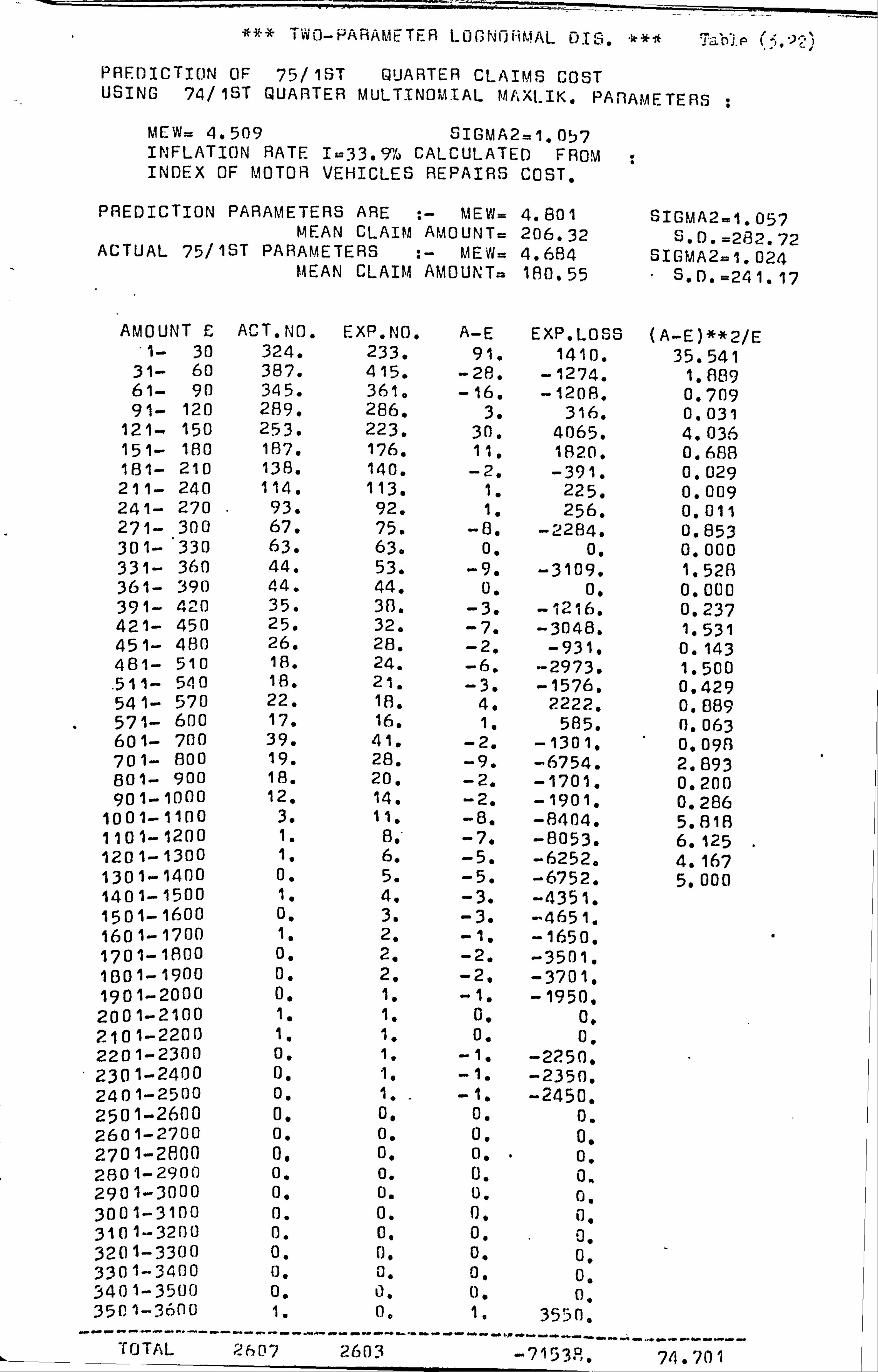
# '# TWO-PARAMETER LORNOHMAL 013.3t## Table i;; 4

PREDICTION OF 75/1ST QUARTER CLAIMS COST USING 74/ 1ST QUARTER MULTINOMIAL MAXI. IK. PARAMETERS

MEW= 4.509 SIGMA2=1.05'7 INFLATION RATE IL33.9"/o CALCULATED FROM INDEX OF MOTOR VEHICLES REPAIRS COST.

PREDICTION PARAMETERS ARE :- MEW= 4.801 SIGMA2=1.057 MEAN CLAIM AMOUNT. 206.32 S. D. =282.72 ACTUAL 75/1ST PARAMETERS :- MEW= 4.684 SIGMA2=1.024 MEAN CLAIM AMOUNT= 180.55 " S. D. =241.17

AMOUNT £ ACT. No. EXP. NO. A-E EXP. LOSS (A-E)**2/E . 1- 30 324. 233. 91. 1410. 35.541

31- 60 387. 415. -28. -1274. 1.889 61- 90 345. 361. -16. -1208. 0.709 91- 120 289. 286. 3. 316. 0.031

121-. 150 253. 223. 30, 4065. 4.03.5 151- 180 187. 176. 11. 1820, 0.688 181- 210 138. 140. -2. -391. 0.029 211- 240 114. 113. 1. 225. 0.009 241- 270 93. 92. 1. 256. 0.011 271- 300 67. 75. -8. -2284. 0.853 301- 330 63. 63. 0. 0. 0.000 331- 360 44. 53. -9. -3109. 1.528 361- 390 44. 44. 0. 01 0.000 391- 420 35. 38. -3. -1216. 0.237 421- 450 25. 32. -7. -3048. 1.531 451- 480 26. 28. -2. -931. 0.143 481- 510 18. 24. -6. -2973. 1.500 . 511- 540 18. 21. -3. -1576. 0.429 541- 570 22. 18. 4. 2222. 0.889 571- 600 17. 16. 1. 585. 0.063 601- 700 39. 41. -2. -1301. 01098 701- 800 19. 28. -9. -6754. 2.893 801- 900 18. 20. -2. -1701. 0.200 901-1000 12. 14. -2. - 1901. 0.286

1001- 1100 3. 11. -8. -8404. 5.818 1101-1200 1. Be- -7. -8053. 6.125 1201-1300 1. 6. -5. -6252. 4.167 1301-1400 0. 5. -5. -6752. 5.000 1401-1500 1. 4. -3. -4351. 1501- 1600 0. 3. -3. --4651. 1601-1700 1. 2. - 1. -1650. 1701-1800 0. 2. -2. -3501. 1801- 1900 0. 2. -2. -3701. 1901-2000 0. 1. - 1. -1950. 2001-2100 1. 1. 0. 0. 2_101-2200 1. 1. 0. 0. 220 1-2300 0. 1. - 1. -2250. 230 1-2400 0. 1. - 1. -2350. 2401-2500 0. 1,

. - 1. -2450. 2501-2600 0. 0. 0. 0. 2601-2700 0. 0. 0. 0. 2701-2800 0. 0. 0. 0. 2801-2900 0. 0. 0. 0. 2901-3000 0. 0. 0, 0. 3001-3100 0, 0. 0, 0, 3101-3200 0. 0. 0. "3ý 3201-3300 0. 0. 0. 0. 3301-3400 0. 0. 01 0. 3401-3500 0. 0. 0. n 3501-3600 1. 0. 1. 3550.

---------------------- ---------------- ----..... ----... -. .. -------- TOTAL 2607 2603 -7153. °,. 74.701

Table (3.22) - continued

CHI SQ. STAT. -£35.1 , D. F. = 30 P<0.001

TOTAL ACTUAL COST = 452059. TOTAL EXPECTED COST = 523597.

TOTAL EXP. LOSS

--------------- _- 15.82 % TOTAL ACT. COST

127

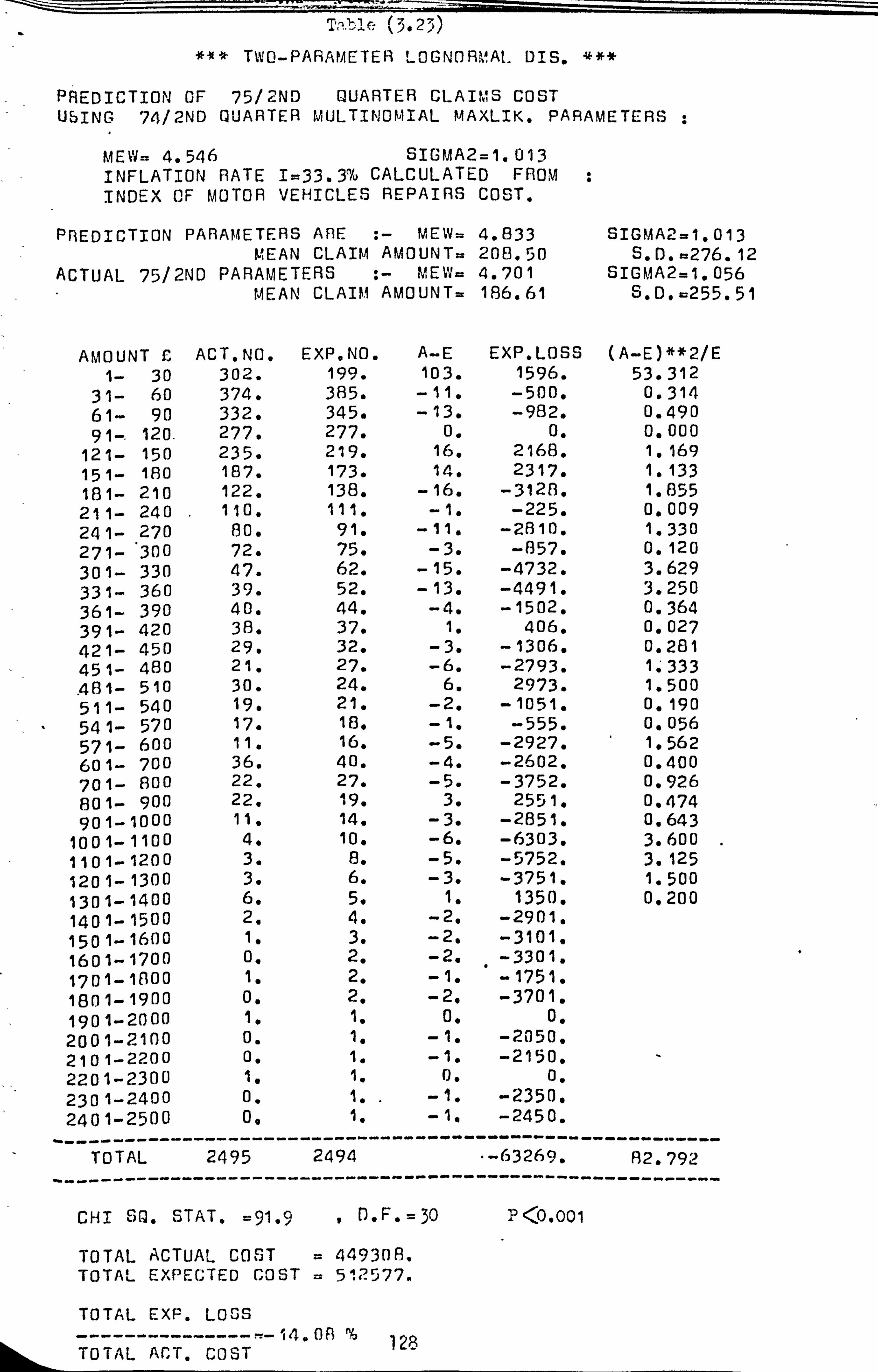
T'' if (3.23) *-x* TIWWO-PARAMETER LOGNORMAL DIS. ***

PREDICTION OF 75/2ND QUARTER CLAIMS COST USING 74/2ND QUARTER MULTINOMIAL MAXLIK. PARAMETERS ;

MEW= 4.546 SIGMA2=1.013 INFLATION RATE I=33.3% CALCULATED FROM ; INDEX OF MOTOR VEHICLES REPAIRS COST.

PREDICTION PARAMETERS ARE :- MEW= 4.833 SIGMA2=1.013 MEAN CLAIM AMOUNT= 208.50 S. D. =276.12

ACTUAL 75/2ND PARAMETERS :- MEW= 4.701 SIGMA2=1.056 MEAN CLAIM AMOUNT= 186.61 S. D. =255.51

AMOUNT £ ACT. NO. EXP. NO. A-E EXP. LOSS (A-E)**2/E 1- 30 302. 199. 103. 1596. 53.312

31- 60 374. 385. -11. -500. 0.314 61- 90 332. 345. -13. -982. 0.490 91-. 120. 277. 277. 0. 0. 0.000

121- 150 235. 219. 16. 2168. 1.169 151- 1130 187. 173. 14. 2317. 1.133 181- 210 122. 138. -16. -3128. 1.855 211- 240 .

110. 111. -1. -225. 0.009 241- 270 80. 91. - 11. -2810. 1.330 271- 300 72. 75. -3. -857. 0.120 301- 330 47. 62. -15. -4732. 3.629 331- 360 39. 52. -13. -4491. 3.250 361- 390 40. 44. -4. -1502. 0.364 391- 420 38. 37. 1. 406. 0.027 421- 450 29. 32. -3. -1306. 0.281 451- 480 21. 27. -6. -2793. 1: 333

. 481- 510 30. 24. 6. 2973. 1.500 51 1- 540 19. 21. -2. -1051. 0.190

54 1- 570 17. 18. -1. -555. 0.056 571- 600 11. 16. -5. -2927. 1.562 601- 700 36. 40. -4. -2602. 0.400 701- 800 22. 27. -5. -3752. 0.926 801- 900 22. 19. 3. 2551. 0.474 901- 1000 11. 14. - 3. -2851. 0.643

1001-1100 4. 10. -6. -6303. 3.600 1101-1200 3. 8. -5. -5752. 3.125 1201-1300 3. 6. -3. -3751. 1.500 1301- 1400 6. 5. 1. 1350. 0.200 1401-1500 2. 4. -2. -2901. 1501-1600 1. 3. -2. -3101. 1601-1700 0. 2. -2. . -3301. 1701-1800 1. 2. -1. -1751. 1801-1900 0. 2. -2. -3701. 1901-2000 1. 1. 0. 0. 2001-2100 0. 1. - 1. -2050. 2101-2200 0. 1. -1. -2150. - 2201-2300 1. 1. 0. 0.

230 1-2400 0. 1. -1. -2350. 240 1-2500 0. 1. - 1.

----- -2450.

-------- -----------

TOTAL -----------

---------

2495 ---------

----------

2494 ----------

-

------

--

"-63269. ----------

------------

82.792 -----------

CHI SO. STAT. =91.9 , D. F. = 30 P <o. ooi

TO TAL TOTAL

TOTAL

TOTAL

ACTUAL COST = 44930A. EXPECTED COST = 512577.

EXP. LOSS

- --14.0A % 128 ACT. COST

Table {. 2d)

## TWO-PARAMETER LOGNORMAL DIS. ###

129

PREDICTION OF 74/4TH QUARTER CLAIMS COST USING 73/4TH QUARTER MULTINOMIAL MAXLIK. PARAMETERS

MEW= 4.516 S; GMA2 =1.056 INFLATION RATE I= 23.5% CALCULATE D FROM INDEX OF'AVE. EAR NINGS, MISCELLA NEOUS SERVICES.

PREDICTION PARAMETERS ARE : - MEW= 4.727 SIGMA2=1.056 MEAN CLAIM AMOUNT= 191.54 S. D. =262.26 ACTUAL 74/4TH PARAMET ERS : - MEV9= 4.672 SIGMA2=1.056 MEAN CLAIM AMOUNT= 181.27 S. D. =248.21

AMOUNT £ AC T. NO. EXP. NO. A-E EXP. LOSS (A-E)**'2/E 1- 30 394. 310. 84. 1302. 22.761

31- 60 452. 522. -70. -3185. 9.387 61- 90 426. 438. -12. -906. 0.329 91- 120 348., 338. 10. 1055. 0.296

121- 150 272. 260. 12. 1626. 0.554 151- 180 219. 202. 17. 2813. 1.431 181- 210 154. 159. -5. -978. 0.157 211- 240 124. 127. -3. -677. 0.071 241- 270 105. 102. 3. 767. 0.088 271-"300 78. 83. -5. -1427. 0.301 301- 330 75. 69. 6. 1893. 0.522 331- 360 58. 57. 1. 346. 01018 361- 390 55. 48. 7. 2628. 1.021 391- 420 29. 41. -12. -4866. 3.512 421- 450 43. 35. 8. 3484. 1.829 451- 480 24. 30. -6. -2793. 1.200 481- 510 22. 26. -4. -1982. 0.615 511- 540 24. 22. 2. 1051. 0.182 541- 570 19. 19. 0. 0. 0.000 571- 600 14. 17. -3. -1756. 0.529 601- 700 42. 43. - 1. -651. 0.023 701- 800 28. 29. - 1. -751. 0.034 801- 900 20. 20. 0. 0. 0.000 901- 1000 17. 15. 2. 1901. 0.267

1001-1100 8. 11. -3. -3151. 0.818 1 10 1- 1200 5. 8. -3. -3451. 1.125 1201- 1300 1. 6. -5. -6252. 4.167 1301- 1400 5. 5. 0. 0. 0.000 1401-1500 0. 4. -4. -5802. 1501-1600 1. 3. -2. -3101. 1601- 1700 0. 2. -2. -3301. 1701- 1800 0. 2. -2. -3501. 1801- 1900 0. 2. -2. -3701. 1901-2000 0. 1. -1. -1950. 200 1-2100 1. 1. 0. 0. 21 01-2200 0. 1. -1. -2150. 2201-2300 0. 1. -1. -2250. 2301-2400 1. 1. 0. 0. 2401-2500 0. 1. . -1. -2450.

- TOTAL 3064

----------------------

3061

------- .

-------- -42168. ----------

51,237 - ---------

CHI SQ. STAT. =65.0 , D. F. = 30 P<o. 001

TOTAL ACTUAL COST = 533707. TOTAL EXPECTED COST - 575876.

TOTAL EXP. LOSS -- -----------= -7.90 %

TOTAL ACT. COST

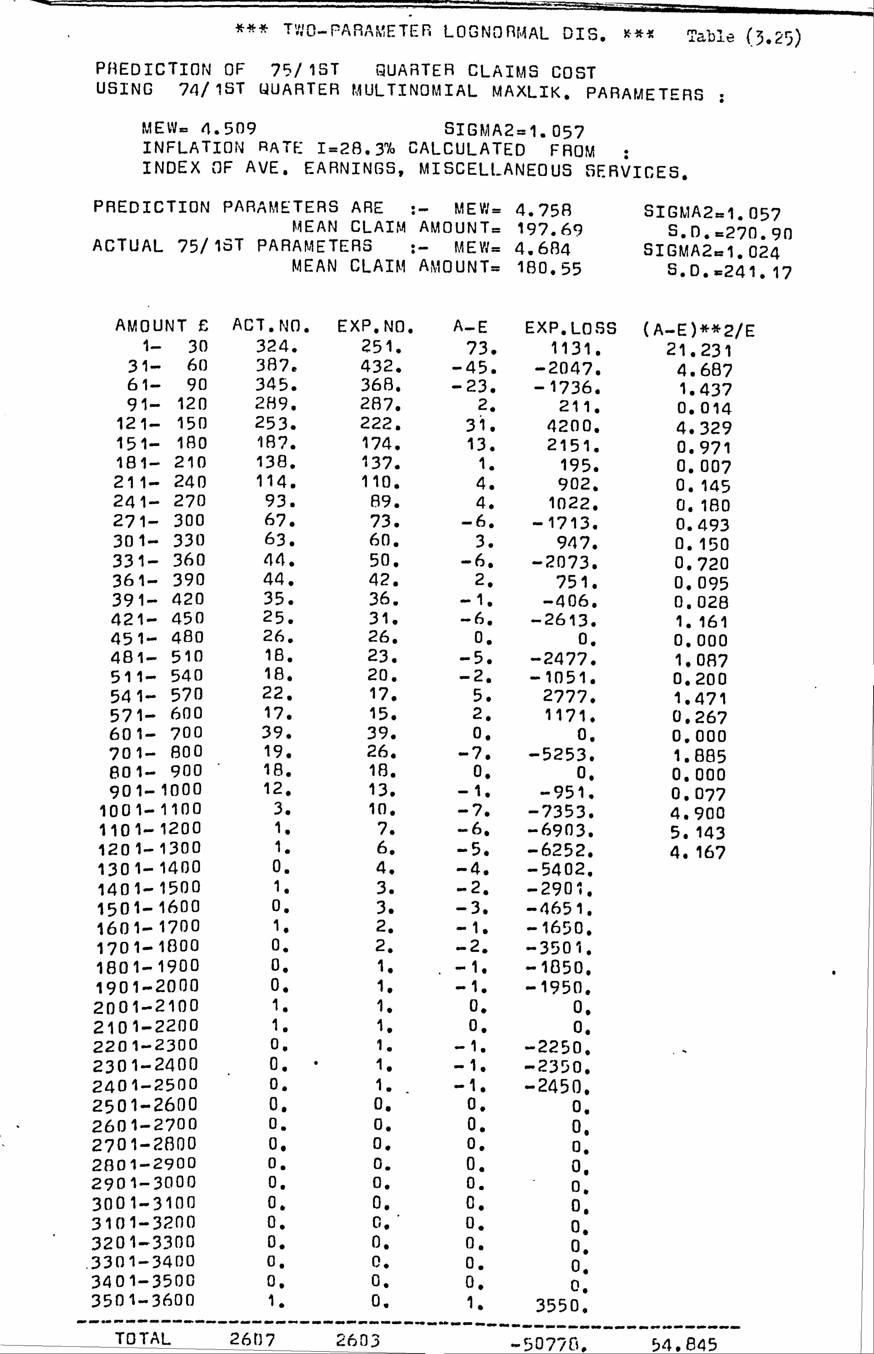
Týri0 -FAR ; METER LOGNORMAL DIS. Table (3.25)

PREDICTION OF 75/ 1ST QUARTER CLAIMS COST USING 74/1ST QUARTER MULTINOMIAL MAXLIK. PARAMETERS

MEW= 4.509 SIGMA2=1.057 INFLATION RATE I=28.3"/0 CALCULATED FROM INDEX OF AVE. EARNINGS, MISCELLANEOUS SERVICES.

PREDICTION PARAMETERS ARE :- MEW= 4.758 MEAN CLAIM AMOUNT= 197.69

ACTUAL 75/ 1ST PARAMETERS :- MEW= 4.6134 MEAN CLAIM AMOUNT= 180.55

AMOUNT £ 1- 30

31- 60 61- 90 91- 120

121- 150 151- 180 181- 210 211- 240 241- 270 271- 300 301- 330 331- 360 361- 390 391- 420 421- 450 451- 480 481- 510 511- 540 541- 570 571- 600 601- 700 701- 800 801- 900 901- 1000

1001- 1100 1101-1200 1201-1300 130 1- 1400 1401-1500 1501- 1600 1601-1700 1701-1800 1801-1900 1901-2000 2001-2100 2101-2200 2201-2300 2301-2400 2401-2500 2501-2600 2601-2700 2701-2800 2801-2900 2901-3000 3001-3100 3101-3200 3201-3300 3301-3400 3401-3500 3501-3600

SIGMA2.1.057 S. D. =270.90

SIGMA2=1.024 S. D. =241.17

(A-E)**2/E 21.231

4.687 1.437 0.014 4.329 0.971 0.007 0.145 0.180 0.493 0.150 0.720 0.095 0.028 1.161 0.000 1.087 0.200 1.471 0.267 0.000 1.885

0.000 0.077 4.900 5.143 4.167

2687 2611; ----------------------------------------------------------

TOTAL 5O77C+. 54.845

ACT. NO. 324. 387. 345. 289. 253. 187. 138. 114.

93. 67. 63. 44. 44. 35. 25. 26. 18. 18. 22. 17. 39. 19. 18. 12.

3. 1. 1. 0. 1. 0. 1. 0. 0. 0. 1. 1. 0. 0. 0. 0. 0. 0. 0. 0. 0.

0, 0. 0. 0. 1.

EXP. NO. 251. 432. 368. 287. 222. 174. 137. 110.

69. 73. 60. 50. 42. 36. 31. 26. 23. 20. 17. 15. 39. 26. 18. 13. 10. 7. 6. 4. 3. 3. 2. 2. 1. 1. 1. 1. 1. 1. 1.

_ 0. 0. 0. 0. 0. 0. 0. 0. 0. 0. 0.

A-E 73.

-45. -23.

2. 31. 13.

1. 4. 4.

-6. 3.

-6. 2.

-1. -6.

0.

-5. -2.

5. 2. 0.

-7. 0.

-1. -7. -6. -5. -4. -2. -3. -1. -2. -1. -1.

0. 0.

-1. -1. -1.

0. 0. 0. 0. 0. 0. 0. 0. 0. 0. 1.

EXP. LO SS 1131.

-2047. -1736.

211. 4200. 2151.

195. 902.

1022.

-1713. 947.

-2073. 751.

-406. -2613.

0. -2477. -1051.

2777. 1171.

0.

-5253. 0.

-951. -7353. -6903. -6252. -5402. -2901. -4651. -1650, -3501. -1850. -1950.

0. 0.

-2250. -2350. -2450.

0. 0, 0. 0, 0. 0, 0. 0, 0. 0.

3550.

Table (3.25) - continued

CHI SQ. STAT. = 68.0 . D. F. = 30 P <0.001

TOTAL ACTUAL COST = 452059. TOTAL EXPECTED COST = 502837.

TOTAL EXP. LOSS

---------------=-11.23 % TOTAL ACT. COST

0

131

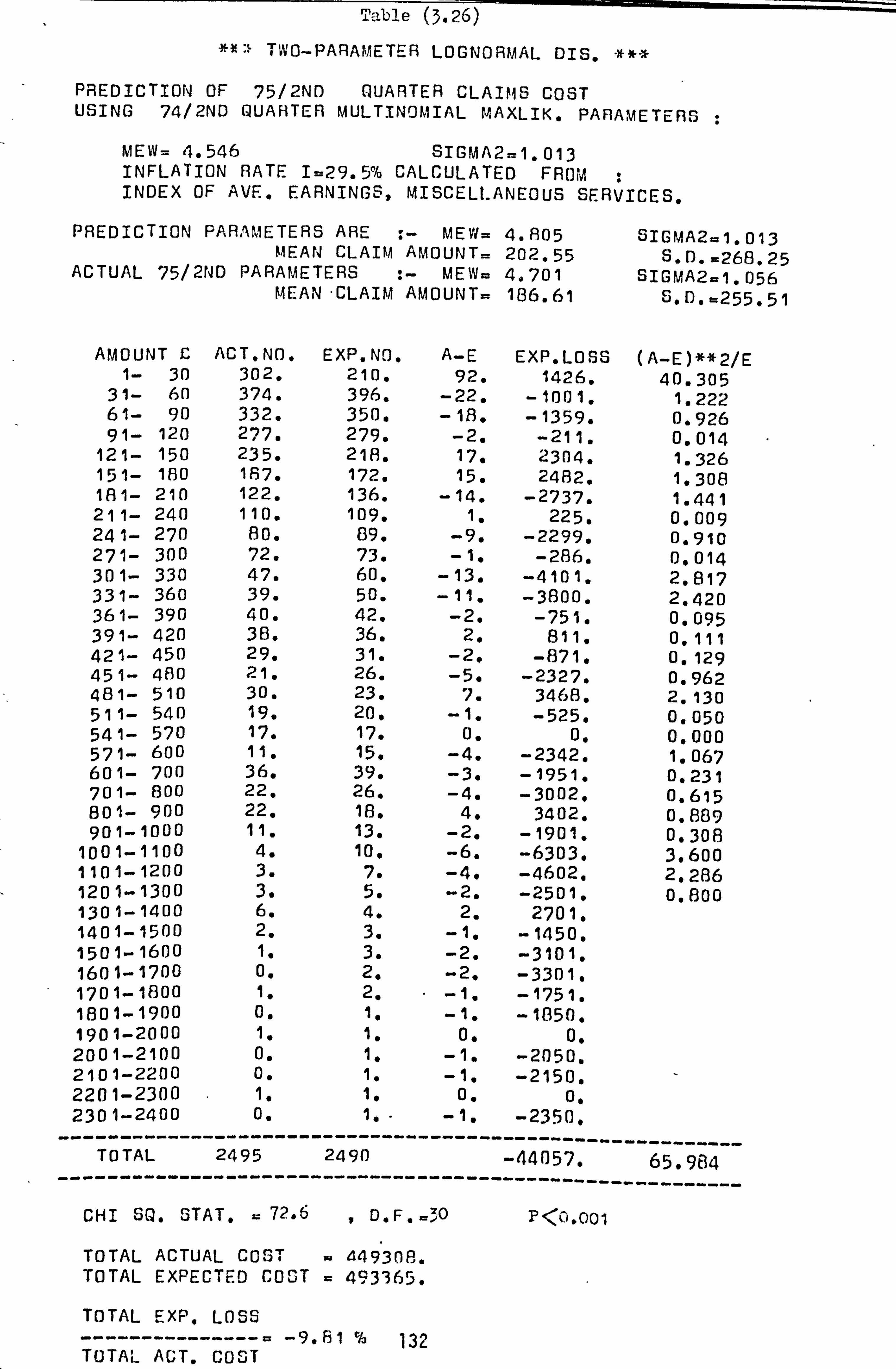
Table (3.26)

*" TWO-PARAMETER LOGNORMAL DIS.

PREDICTION OF 75/2ND QUARTER CLAIMS COST USING 74/2ND QUARTER MULTINOMIAL MAXLIK. PARAMETERS

MEW= 4.546 SIGMA2=1.013 INFLATION RATE I=29.5% CALCULATED FROM INDEX OF AVE. EARNINGS, MISCELLANEOUS SERVICES.

PREDICTION PARAMETERS ARE :- MEW= 4.805 SIGMA2a1.013 MEAN CLAIM AMOUNT= 202.55 S. D. =268.25 ACTUAL 75/2ND PARAMETERS :- MEW= 4.701 SIGMA2=1.056 MEAN -CLAIM AMOUNT= 186.61 S. D. =255.51

AMOUNT C ACT. NO. EXP. NO. A-E EXP. LOSS (A-E)**2/E 1- 30 302. 210. 92. 1426. 40.305

31- 60 374. 396. -22. -1001. 1.222 61- 90 332. 350. -18. -1359. 0.926 91- 120 277. 279. -2. -211. 0.014

121- 150 235. 218. 17. 2304. 1.326 151- 180 1887. 172. 15. 2482. 1.308 181- 210 122. 136. -14. -2737. 1.441 211- 240 110. 109. 1. 225, 0.009 241- 270 80. 89. -9. -2299. 0.910 271- 300 72. 73. -1, -286. 0.014 301- 330 47. 60. -13. -4101. 2.817 331- 360 39. 50. -11. -3800. 2,420 361- 390 40. 42. -2. -751. 0.095 391- 420 38. 36. 2. 811. 0.111 421- 450 29. 31. -2. -871. 0,129 451- 480 21. 26. -5. -2327. 0.962 481- 510 30. 23. 7. 3468. 2.130 51 1- 540 19. 20. -1. -525. 0.050 541- 570 17. 17. 0. 0, 0.000 571- 600 11. 15. -4. -2342. 1.067 601- 700 36. 39. -3. -1951. 0.231 701- 800 22. 26. -4. -3002. 0.615 801- 900 22. 18. 4. 3402. 0.889 901- 1000 11. 13. -2. -1901. 0o308

1001-1100 4. 10. -6. -6303. 3.600 1101-1200 3. 7. -4. -4602. 2.286 1201-1300 3. 5. -2. -2501. 0.800 1301-1400 6. 4. 2. 2701.

1401-1500 2. 3. -1. -1450. 1501-1600 1. 3. -2. -3101. 1601-1700 0. 2. -2. -3301. 1701-1800 11 2. " -1. -1751. 180 1-1900 0. 1, -1. - 1850. 1901-2000 1. 1, 0. 0, 2001-2100 0. 11 -1, -2050. 210 1-2200 0. 1. -1. -2150. 2201-2300 11 1. 0. 0, 230 1-2400

-

0.

-------

1, " --------

- 1,

- -2350.

---- ------- TOTAL

------------

-- 2495

---------

2490

--------

------

-------

----------- -44057.

-----------

---------- 65.984

----------

CHI SQ. ET AT. = 72.6 , D. F . -JO P<t'). 001

TOTAL ACTUAL COST = 44930A. TOTAL EXPECTED COST = 403365.

TOTAL EXP. LOSS --------------- _-9.81 % 132 TOTAL ACT. COST

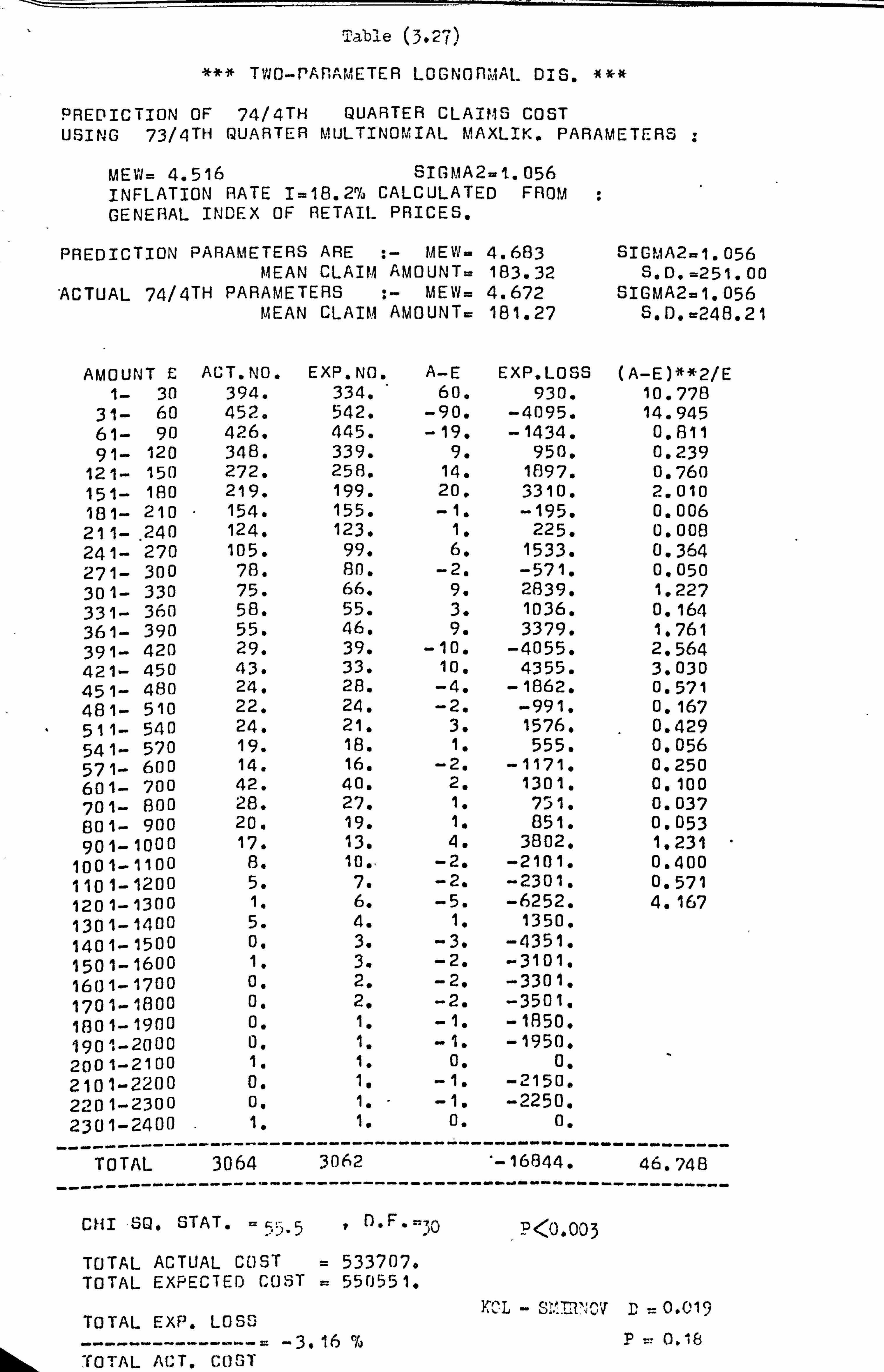
Table (3.27)

*** Two-rAnAMETER LOGNOfl MAL. DIS. ***

PREDICTION OF 74/4TH QUARTER CLAIMS COST USING 73/4TH QUARTER MULTINOf4IAL h"AXLIK. PARA METERS

MEW= 4.516 SIGMA2=1.. 056 INFLATION RATE I= 18.2% CALCULATED FROM GENERAL IN DEX OF RETAIL PRICES.

PREDICTION PAR AMETERS ARE : - MEW= 4.683 SIGMA2=1.056 MEAN CLAIM AMOUNT= 183.32 S. D. =251.00

"ACTUAL 74/4TH PARAMET ERS : - MEW= 4.672 SIGMA2=1.056 MEAN CLAIM AMOUNT= 181.27 S. D. =248.21

AMOUNT £ AC T. NO. EXP. NO. A-E EXP. LOSS (A-E)**"2/E 1- 30 394. 334. 60. 930. 10.778

31- 60 452. 542. -90. -4095. 14.945 61- 90 426. 445. -19. -1434. 0.811 91- 120 348. 339. 9. 950. 0.239

121- 150 272. 258. 14. 1897. 0.760 151- 180 219. 199. 20. 3310. 2.010 181- 210 154. 155. -1. -195. 0.006 21 1-

. 240 124. 123. 11 225. 0.008

241- 270 105. 99. 6. 1533. 0.364 271- 300 78. 80. -2. -571. 0.050 301- 330 75. 66. 9. 2839. 1.227 331- 360 58. 55. 3. 1036. 0.164 361- 390 55. 46. 9. 3379. 1.761 391- 420 29. 39. -10. -4055. 2.564 421- 450 43. 33. 10. 4355. 3.030 45 1- 480 24. 28. -4. -1862. 0.571 481- 510 22. 24. -2. -991. 0.167 511- 540 24. 21. 3. 1576. 0.429 541- 570 19. 18. 1. 555. 0.056 571- 600 14. 16. -2. -1171. 0.250 601- 700 42. 40. 2. 1301. 0.100

701- 800 28. 27. 1. 751. 0.037 801- 900 20. 19. 1. 851. 0.053

901- 100 0 17. 13. 4. 3802. 1.231 1()01-1100 8. 10.. -2. -2101. 0.400

1101-1200 5. 7. -2. -2301. 0.571 120 1-1300 1. 6. -5. -6252. 4.167 1301-1400 5. 4. 1. 1350.

1401-1500 0. 3. -3. -4351. 150 1- 1600 1. 3. -2. -3101. 1601- 1700 0. 2. -2. -3301. 1701-1800 0. 2. -2. -3501. 1801- 1900 0. 1. -1. - 1850. 190 1-2000 0. 1. - 1. -1950. 2001-2100 1. 1. 0. 0.

2101-2200 0. 1. -1. -2150. 220 1-2300 0. 1. - 1. -2250. 2301-2400 1.

- -

1.

------ ------

0.

------- ----- =-- 0.

--------- - ------------------- - ------------------- TOTAL 3064

---------------------

- - 3062

------- --------

- "-16844.

----------

--- -------- 46.748

-----------

CHI SQ. STAT. = 55.5 , D. F.:; Q

TOTAL ACTUAL COST = 533707. TOTAL EXPECTED COST = 550551.

TOTAL EXP. LOSS

"f0". AL ACT. COST

P<O. 003

J\CL - Jig: ;. +1NC D=0.01

9

pý: 0.18

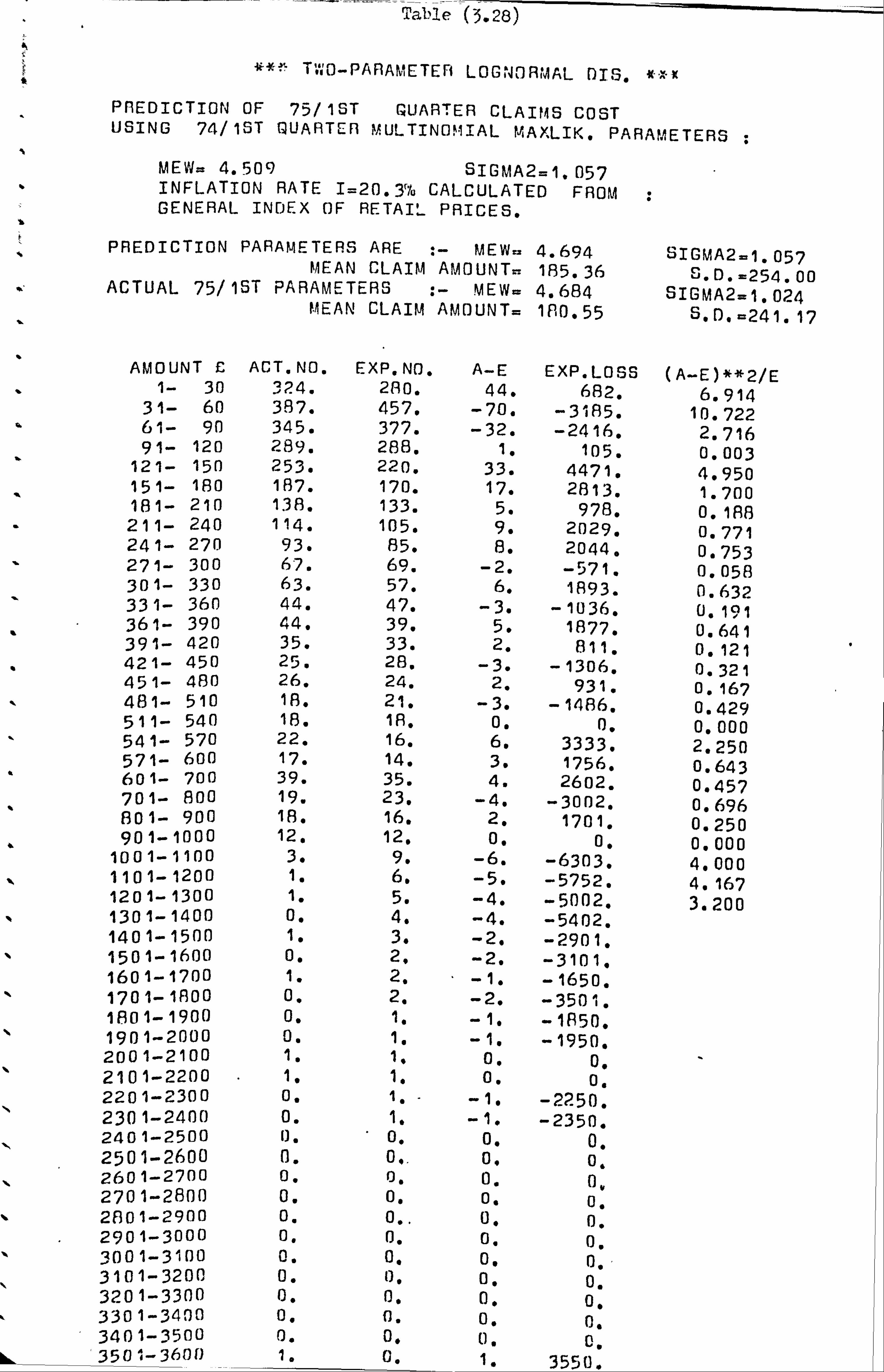
Table (3.28)

*** TýýO-PARAVETEFi LOGNORMAL DIS. *-. t

PREDICTION OF 75/1ST QUARTER CLAIMS COST USING 74/1ST QUARTER MULTINOMIAL MAXLIK. PARAMETERS

MEW= 4.509 SIGMA2=1.057 INFLATION RATE I= 20.3% CALCULATED FROM ; GENERAL INDEX OF RETAIL PRICES.

PREDICTION PARAMETERS ARE - MEW- 4.694 SIGMA2-1.057 MEAN CLAIM AMOUNT= 185.36 S. D. =254.00 ACTUAL 75/ 1ST PARAMETERS : - MEW= 4.684 SIGMA2-1.024 MEAN CLAIM AMOUNT= 180.55 S, D, =241.17

AMOUNT C ACT. NO. EXP. NO. A-E EXP. LOSS (A_E)**2/E 1- 30 324. 280. 44. 682. 6.914

31- 60 397. 457. -70. -3185. 10.722 ° 61- 90 345. 377. -32. -2416, 2.716

91- 120 289. 288. 1. 105, 0.003 121- 150 253. 220. 33. 4471. 4.950 15 1- 180 187. 170. 17. 2813. 1.700 181- 210 138. 133. 5. 978. 0.188 21 1- 240 114. 105. 9. 2029. 0.771 241- 270 93- 85. 8. 2044. 0.753 271- 300 67. 69. -2. -571. 0.058 301- 330 63. 57. 6. 1893. 0.632 331- 360 44. 47. -3. -1036. 0.191 361- 390 44. 39. 5. 1877. 0.641 391- 420 35. 33. 2. all. 0.121 421- 450 25. 28. -3. -1306. 0.321 451- 480 26. 24. 2. 931. 0.167 481- 510 18. 21. -3. -1486. 0.429 511- 540 18. in. 0. 0. 0.000 541- 570 22. 16. 6. 3333. 2.250 571- 600 17. 14. 3. 1756. 0.643 601- 700 39. 35. 4. 2602. 0.457 701- 800 19. 23. -4. -3002. 0.696 Sol- 900 18. 16. 2. 1701. 0.250

41 90 1- 1000 12. 12, 0. 0. 0.000

1001- 1100 3. 9. -6. -6303. 4.000 1101-1200 1. 6. -5. -5752. 4.167 1201- 1300 1. 5. -4. -5002, 3.200 130 1- 1400 0. 4. -4. -5402. 140 1- 1500 1. 3. -2. -2901.

% 150 1-1600 0. 2. -2. -3101. 160 1-1700 1. 2. -1, -1650. 170 1- 1800 0. 2. -2. -3501 . 180 1-1900 0. 1. - 1. -1850. 190 1-2000 0. 1. - 1. -1950. 2001-2100 1. 1. 0. 0, ' 2101-2200 1, 1. 0. 0. 2201-2300 0. 1, - - 1. -2250, 230 1-2400 0. 11 -1, -2350. 2401-2500 0. 0. o. 0 2501-2600 0. 00. 0. . 0. 2601-2700 0. 0. 0. 0. 2701-2800 0. 01 0, 0. 2801-2900 0. 0.. 0. 0. 2901-3000 0. 0. 0. 0. 3001-3100 0. 0, o, 00 3101-3200 0. 0. 0. 0 3201-3300 0. 0, 0. . 0. 3301-3400 0. 0. 0. 0. 3401-3500 0. 0, 0, 0, 350j-360f) I. 0. 1. 3550.

Table (3.28) - continued

---------------------------------------------------------

TOTAL 2607 2606 -23439.46.941 ---------------------------------------------------------

CHI SQ. STAT. = 57.7 ., D. F. = 29 P<o. 003

TOTAL ACTUAL COST = 452059. TOTAL EXPECTED COST = 475498.

TOTAL EXP. LOSS KOT - S: 1'IIRL; OV D= 0.022 --------------- - -5.19 % TOTAL. ACT. COST P=0.15

135

Table (3.29)

* TWO-PARAMETER LOGNORMAL DIS. ý***

PREDICTION OF 75/2ND QUARTER CLAIMS COST USING 74/2ND QUARTER MULTI NOMIAL MAXLIK. PARAMETERS

MEW= 4.546 SIGMA2=1.013 INFLATION RATE I= 24.3^ CALCULATED FROM GENERAL IN DEX OF RETAIL PRICES.

PREDICTION PAR AMETERS ARE ;- MEW= 4.764 SIGMA2=1.013 MEAN CLAIM AMOUNT= 194.42 S. D. -257.48

ACTUAL 75/2ND PARAMET ERS :- MEW= 4.701 SIGMA2=1.056 MEAN CLAIM AMOUNT= 186.61 S. D. =: 255.51

AMOUNT £ AC T. NO. EXP. NO . A-E EXP. LOSS (A-E)**2/E 1- 30 302. 226. 76. 1178. 25.558

31- 60 374. 412. -38. -1729. 3.505 61- 90 332. 357. -25. -1887. 1.751 91- 120 277. 280. -3. -316. 0.032

121- 150 235. 217. 18. 2439. 1.493 151- 180 187. 170. 17. 2813. 1.700 181- 210 122. 134. -12. -2346. 1.075 211- 240 110. 107. 3. 677. 0.084 241-

. 270 f30. 86. -6. -1533. 0.419

271- 300 72. 70. 2. 571. 0.057 301- 330 47. 58. -11. -3470. 2.086 331- 360 39. 48. -9. -3109. 1.687 361- 390 40. 41. - V. -376. 0.024 391- 420 38. 34. 4. 1622. 0.471 421- 450 29. 29. 0. 0. 0.000 451- 480 21. 25. -4. -18626 0.640

-481- 510 30. 21. 9. 4459. 3.857 51 1- 540 19. 19. 0. 0. 0.000 541- 570 17. 16. 1. 555. 0.063 571- 600 11. 14. -3. -1756. 0.643 601- 700 36. 36. 0. 0. 0.000 70 1- 800 22. 24. -2. -1501. 0.167 801- 900 22. W. 5. 4252. 1.471 901-1000 11. 12. -1. -951. 0.083

1001-1100 4. 9. -5. -5252. 2.778 110 1-1200 3. 7. -4. -4602. 2.286 1201-1300 3. 5. -2. -2501. 0.800 1301-1400 6. 4. 2. 2701. 1401-1500 2. 3. -1. -1450. 1501- 1600 1. 2. -1. -1550. 1601-1700 0. 2. -2. -3301. 170 1- 1800 1. 2. -1. -1751. 1801-1900 0. 1. " -1. -1850. 1901-2000 1. 1. 0. 0. 20 0 1-2100 0. 1. -1. -2050. 210 1-2200 0. 1. - 1. -2150. 2201-2300 1. 1. 0. 0.

---------------------- TOTAL 2495

----------------------

------ 2492 ------

--------

--------

----------- -26028.

-----------

---------- 52.728

----------

CHI SQ. STAT. =57.3 , D. F., -- 29 P<0.003

TOTAL ACTUAL COST - 44930R. TOTAL EXPECTED COST = 475336.

TOTAL EXP. LOSS

---. ----------_ - -. 5.79 'Y% TOTAL ACT. COST

<OL-sMPNOý! D=0.030

P -- 0.02

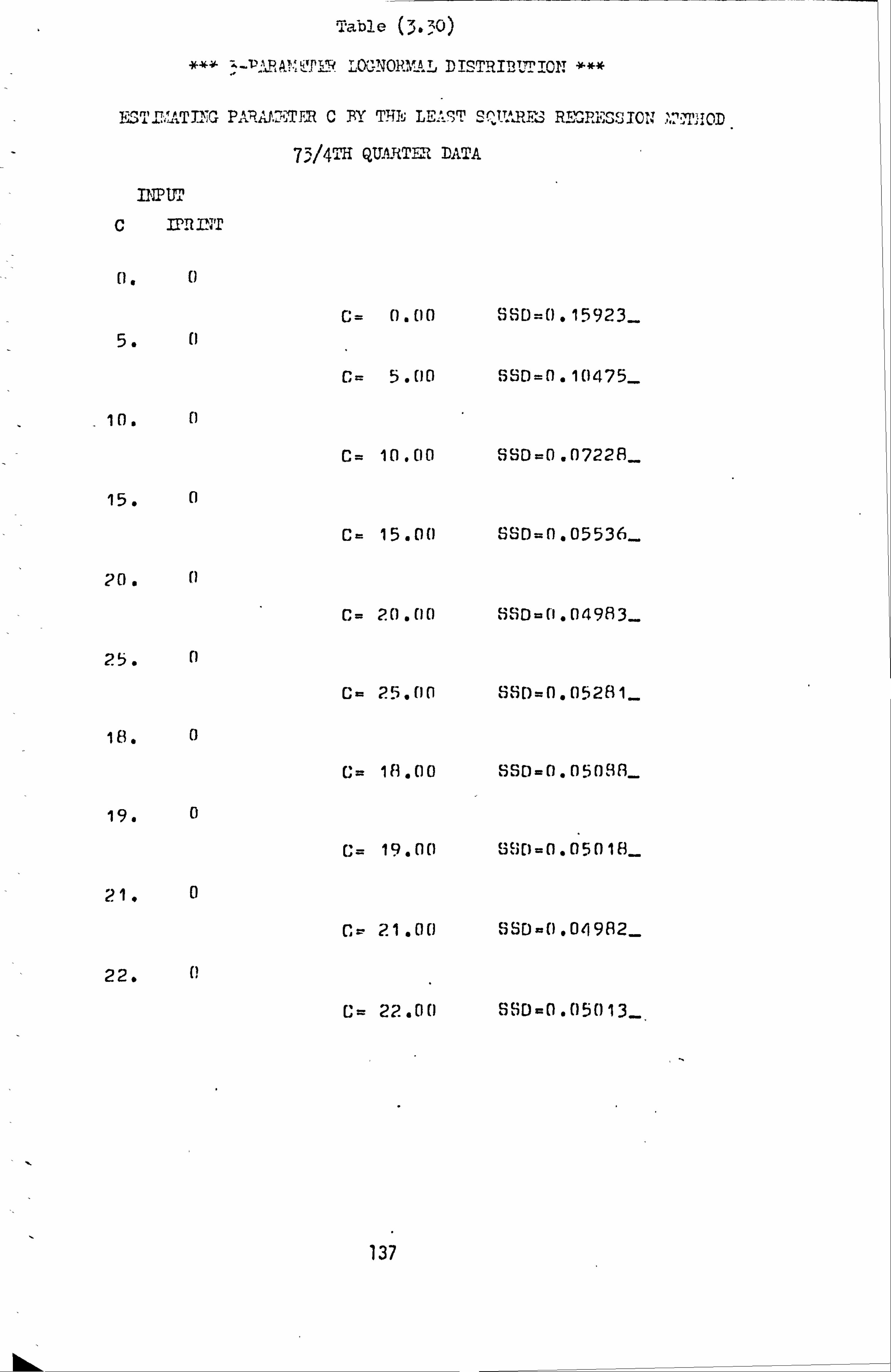
Table (3.: 0)

LOGNORMAL DISTRIBT. JTIOr: **

ESTIMATTY03 PAA-. APO, TER C BY THJ LEAST S rT ARE3 REGRESSION; I'JIOD

7314TH QUAHTM DATA

INPUT

c ]TIIBT

U. o C= 0.00 SSD=0.15923_

5.

C= 5.00 SSD=0.10475_

10. [1

15.0

20. ()

25. n

C= 10.00 SSO=0.0722E1_

C 15.00 SSD=0.05536_

C= 20.00 SSD=0.04983_

G- 25.00 SSD=n, o5281_

18. C)

C= 18.00 6Sa=0.050BA-

19.0

G= 19.00 Be Cl=0.05018__

21.0

Ov 21.00 ")SD-0,04982-

22.

C= 22.00 SSD=0.05013_

137

Table (3.31)

73/4TH (QUARTER DATA

C=01.00 PARAMETERS OF THE LOGNORMAL DIS. ESTIMATED OYL. S. REGRESSION : -

MEW = 4.778 SIGMA SO. = 0.730

MEAN= 150.219 S. 0. = 177.489

SSD=0.050

AMOUNT £ ACTUAL. EXPECTED ACTUAL- EXPECTED CL. NO. CL. NO. EXPECTED LOSS (A-E)**2/E

1- 30 478. 499, -21. -325. 0.834 31- 60 518. 504. 14.. 637. 0,389 61- 90 461. 429. 32. 2416. 2.387 91- 120 359, 337. 22. 2321. 1.436

121- 150 239. 260. -21.. -2845. 1.696 151- 180 213. 200. 13. 2151. 0.845 181- 210 148, 154, -6.. -1173. 0.234 211- 240 102. 121. -19. -4284. 2.983 241- 270 81, 95. - -14. -3577. 2.063 271- 300 58. 75.. -17.. -4853. 3,853 301- 330 66, 61. 5. 1577. 0.410 331- 360 45. 49. -4. -1382. 0.327 361- 390 39,. 40, -1, -376, 0.025. 391- 420 35.. 33. 2, all. 0.121 421*- 450 34. 27. 7. 3048. 1.815 451- 480 20. 23. -3. -1396. 0.391 . 481- 510 29, 19, 10, 4955. 5.263 511- 540 14, 16, -2. -1051. 0.250 541- 570 8. 13, -5. -2777. 1.923 571- 600 91 11, -2. -1171. 0.364 601- 700 29. 27. 2. 1301. 0.148 701- 800 18. 17. 1, 751. 0.059 801- 9(10 20, 11. 9. 7654. 7. °364 901-1000 6. 7. -1. -951. 0.143

1001-1100 4. 5. -1. -1050. 0,2C0 1101-1200 4. 3, 1. 1150. 1201-1300 1. 2. -1. -1250. 0.000 1301-1400 3. 2. 11 1350. 1401-1500 1. 1. 0. 0,

Al 1501-1600 0. 1, -1. -1550. 1601-1700 1. 1. 0. 0. 1701-1800 0. 1. -1. -1751. 11301-1900 0. 0. 0. 1901-2000 1. 0. 1. 1950. 2001-2100 0. 0. 0. 0. 2101-2200 0. 0. 0. 0. 2201-2300 0, 0, 0, 0. 2301-2400 1. 0. 1. 2350. ---------- ------------ ---------- ------------ -------- - ------ fl., 142

TOTAL ----------

3045. ------------

3044. ---------- -----------

2660. ----------

35. o/ý0

D. F. X23 TOTAL EXP. LOSS P_ 004

% ---------------= 0.6 % TOTAL ACT. COST

138

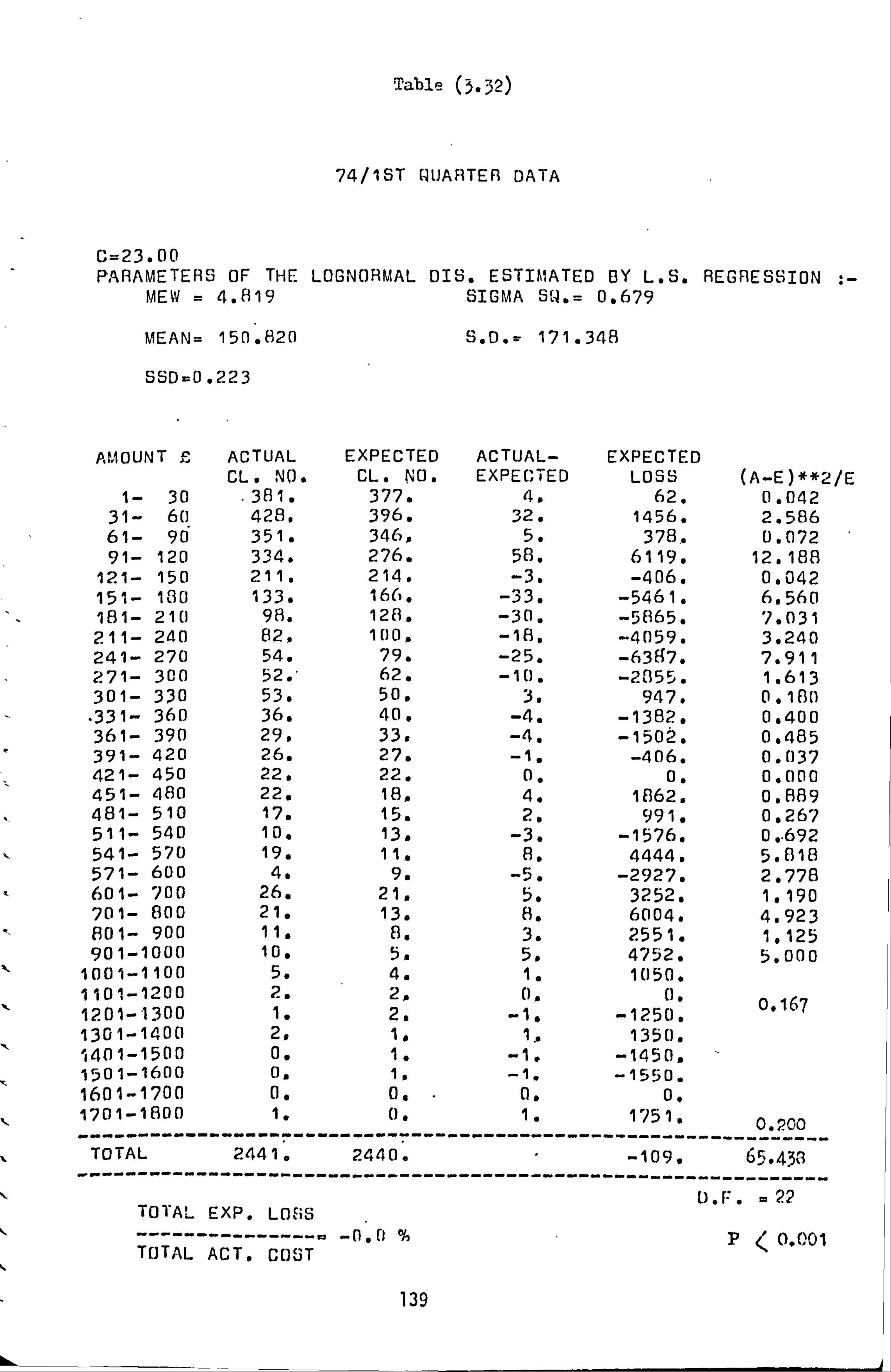
Table (3.32)

C=23.00 PARAMETERS OF THE

MEW = 4.819

MEAN= 150.820

SSD=D . 223

74/iST (QUARTER DATA

LOGNORMAL DIS. ESTIMATED ßY L. S. REGRESSION : - SIGMA S(. = 0.679

S. D. = 171.348

AMOUNT r ACTUAL EXPECTED ACTUAL- EXPECTED CL. NO. CL. NO. EXPECTED LOSS (A-E)**2/E

1- 30 . 381. 377. 4. 62. 0.042 31- 60 428. 396. 32. 1456. 2.586 61- 90 351. 346, 5. 378.. 0.072 91- 120 334. 276. 58. 6119. 12.188

121- 150 211. 214. -3. -406. 0.042 151- 180 133. 166. -33. -5461. 6.560 181- 210 98. 128. -30. -5865. 7.031 211- 240 82, 100, -18. -4059. 3.240 241- 270 54. 79. -25. -63E17. 7.911 271- 300 52. ' 62. -10. -2055. 1.613 301- 330 53. 50, 3. 947. 0.180

"331- 360 36. 40. -4. -1382. 0.400 361- 390 29. 33, -4. -1502. 0.485 391- 420 26. 27. -1. -406. 0.037 421- 450 22. 22. 0. 0. 0.000 451- 480 22. 18, 4. 1862. 0.889 481- 510 17. 15. 2. 991. 0.267 511- 540 10. 13, -3. -1576. 0. "692 541- 570 19. 111 8. 4444. 5.818 571- 600 4. 9. -5. -2927. 2.778 601- 700 26. 21, 5. 3252. 1.190 701- 800 21. 13. 8. 6004. 4.923 801- 900 11. 8. 3. 2551. 1.125 901-1000 10. 51 5. 4752. 5.000

1001-1100 5. 4. 1. 1050. 1101-1200 2. 2,. 0. 0'167 1201-1300 1. 2. -1. -1250. 1301-1400 2, 1, 1351). 1401-1500 0, 1. -1. -1450. 1501-1600 0, 1, -1. -1550. 1601-1700 0. 0. " 0. 0. 1701-1800 1. 0. 1.

- 1751.

--------- .? 00 .... -----0

TOTAL 2441. 2440.

----- ------- -109.

--- 65.438

------ ----------- U. F. e TOTAL EXP. LOSS

----- ---- ---- P 0.001 TOTAL ACT. COST

139

hk. ---

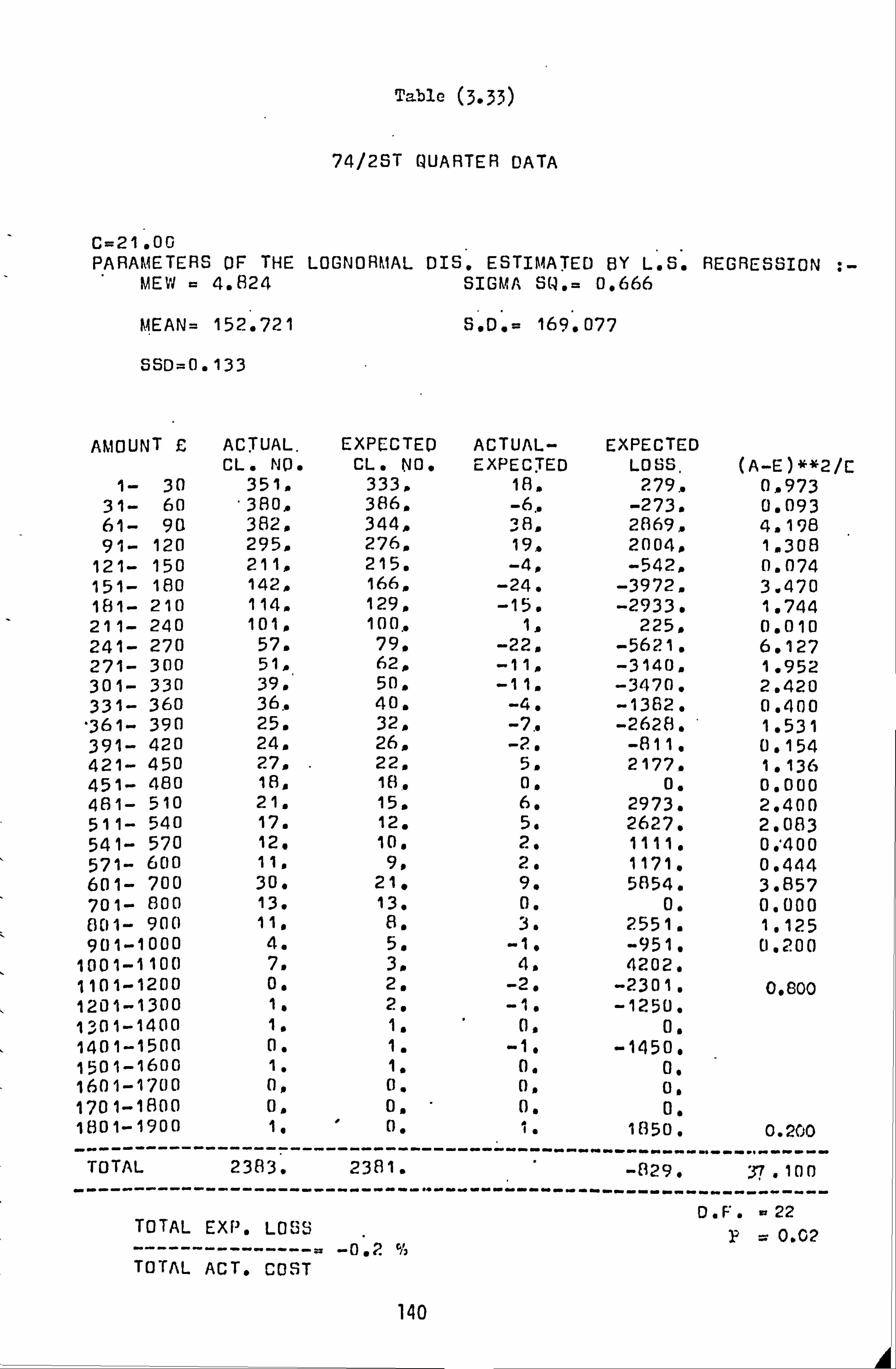
Table (3.33)

74/2ST QUARTER DATA

C=21.00 PARAMETERS OF THE LOGNORMAL DIS. ESTIMATED BY L. S. REGRESSION : -

MEW = 4.824 SIGMA S(.. = 0.666

MEAN= 152.721 S. O. = 169.077

SSD C. 133

AMOUNT £ ACTUAL. EXPECTED ACTUAL- EXPECTED CL. NO. CL. NO. EXPECTED LOSS, (A-E)**2/E

1- 30 351. 333, 18, 279.. 0,973 31- 60 -380, 386. -6,. -273. 0.093 61- 90 382. 344, 3A, 2869, 4,198 91- 120 295, 276. 19, 2004, 1,308

121- 150 211, 215. -4, -542, 0.074 151- 180 142, E 166, -24. -3972, 3.470 181- 210 114. 129, -15. -2933. 1.744 211- 240 101, 100,. 1, 225. 0.010 241- 270 57. 79. -22. -5621. 6.127 271- 300 51, 62, -11, -3140, 1.952 301- 330 39, 50. -11, -3470. 2.420 331- 360 36.. 40. -4. -1382. 0.400

"361- 390 25. 32. -7,. -2628. 1.531 391- 420 24, 26, -2. -811. 0.154 421- 450 27, 22, 5. 2177. 1.136 451- 480 18, 18. 0, o. 0.000 481- 510 21, 15. 6. 2973. 2.400 511- 540 17. 12. 5. 2627. 2.083 541- 570 12. 10. 2. 1111. 0.400 571- 600 11, 9. 2. 1171. 0.444 601- 700 30. 21. 9. 5854. 3.857 701- 000 13. 13. 0. 0. 0.000 001- 900 11, 8. 3. 2551. 1.125 901-1000 4. 5. -1, -951. 0.200

1001-1100 7. 3. 4. 4202. 1101-1200 0. 2. -2. -2301. 01800 1201-1300 1. 2. -1. -1250. 1301-1400 1, 1. 0, 0. 1401-1500 0. 1. -1. -1450. 1501-1600 1. 11 01 00 1601-1700 0, 0. 0, 1701-1800 0, 0. 0. 1801-1900 1. 0. 1. 1850. 0.260

TOTAL

---------- 2383.

----------- 2381.

------------

----

------------

---- -829.

---------

-" --- - 100

37

----------- D. F. x 22

TOTAL EXP, LOSS p: 0.02 ---------------= -0.2 % TOTAL ACT. COST

140

Table (3.34)

74/3RD QUARTER DATA

C=19.00 PARAMETERS OF THE LOGNORMAL DIS. ESTIMATED BY L. S. REGRESSION

MEW, = 4.857 SIGMA SO. = 0.731

MEAN= 166.520 S. D. = 192.635

SSD=0.103

AMOUNT £ ACTUAL EXPECTED ACTUAL- EXPECTED CL. NO. CL. NO. EXPECTED LOSS (A-E)**2/E

1- 30 362. 369. -7, -108, 0.133 31- 60 427. 433. -6. -273. 0.083 61- 90 383. 388, -5. -378. 0.064 91- 120 356. 315. 41. 4325. 5 . 337

121- 150 283. 248. 35. 4742. . 4.940 151- 18U 194. 195. -1. -165. 0.005 181- 210 137. 153. -16. -3128. 1.673 211- 240 97. 121. -24. -5412. 4.760 241- 270 86p. 97, -11.. -2810. 19247 271- 300 71. 78. -7. -1998. 0.628 301- 330 64. 63. 1. 316. 0.016 331- 360 45, 51. -6. -2073. 0.706 361- 390 44.. 42. 2. 751. 0.095 391- 420 25. 35. -10. -4055. 2.857 421- 450 26. 29. -3. -1306. 0.310 451- 480 22. 24. -2. -931. 0.167 481- 510 25. 21. 4. 1982. 0.762 511- 540 14. 17. -3. -1576, 0.529 541- 570 14. 15. -1. -555. 0.067 571- 600 17, 13. 4. 2342. 1.231 601- 700 32. 31. 1. 651. 0.032 701- 800 34, 19. 15. 11257. 11.842 801- 900 17. 12. 5. 4252. 2.083 901-1000 4. 80 -4. -3802. 2.000

1001-1100 9. 6. 3. 3151. 1.500 1101-1200 4. 4,. 0. 0. 0.000 1201-1300 01 3. -3. -3751. 1301-1400 1, 2. -1. -1350. 3.200 1401-1500 3. 2. 1. 1450,. 1501-1600 0. 11 -1. -1550. 1601-1700 1. 1.. 0, 0. 1701-1800 0. 1. -1. -1751. 1801-1900 01 1. -1. - 1850. 1901-2000 0. 0, 0. 0. 2001-2100 0. 0. 0. 0ý 2101-2200 1. 0,

, 1. 2150.

2201-2300 0, 0. 0, 0. 2301-2400 0. 0. 0. 0. 2401-2500 0. 0. 0. 0. 2501-2600 11 0. 1. 2550. 0,000

TOTAL 2799. - 2798. ---------- ----------

1095. --

--------- 46 .2 68

TOTAL EXP. LOSS ---------------

O. F. 24

------ -------- _ 0.2 % p 0.004 TOTAL ACT. COST 141

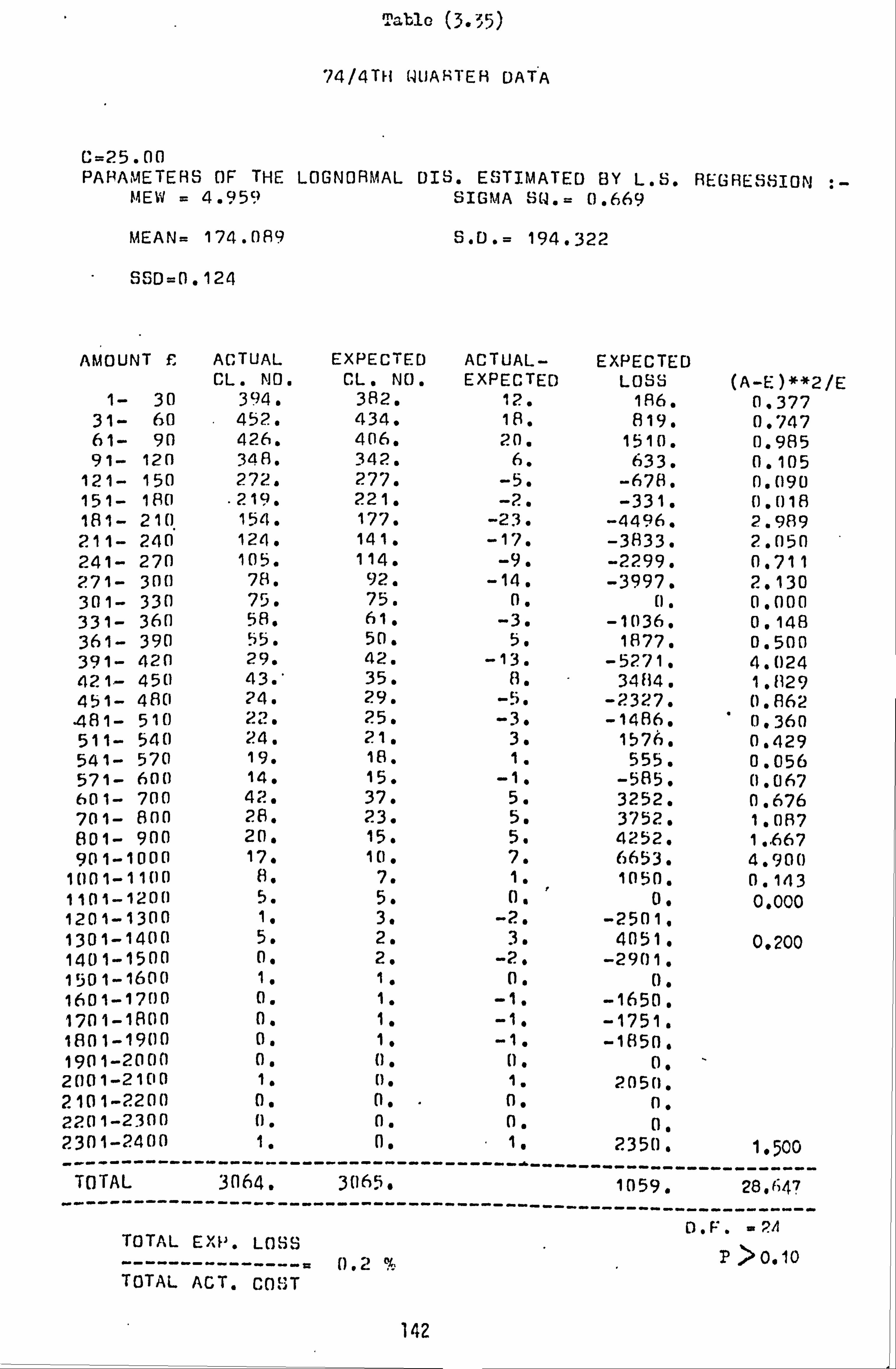
Table (3.35)

74/4TH NUAHTEF3 DATA

C=25.00 PARAMETERS OF THE LOGNORMAL DIS. ESTIMATED BY L. S. REGRES8ION : - MEW = 4.959 SIGMA SQ. = 0.669

MEAN= 174.089 S. D. = 194.322

SSD=D. 124

AMOUNT F ACTUAL EXPECTED ACTUAL- EXPECTED CL. NO. CL. NO. EXPECTED LOSS (A-E)**2/E

1- 30 394. 382. 12. 186. 0,377 31- 60 452. 434. 18. 819. 0.747 61- 90 426. 406. 20. 1510. 0.985 91- 120 348. 342. 6. 633. 0.105

121- 150 272. 277. -5. -678. 0.090 151- 180 . 219. 221. -2. -331. 0.018 181- 210 154. 177. -23. -4496. 2.989 211- 240 124. 141. -17. -3833. 2.050 241- 270 105. 114. -9. -2299. 0.711 271- 300 78. 92. -14. -3997. 2.130 301- 330 75. 75. 0. 0. 0.000 331- 360 58, 61. -3. -1036. 0.148 361- 390 55. 50. 5. 1877. 0.500 391- 420 29. 42. -13. -5271. 4.024 421- 450 43. ' 35. 8. 3484. 1. f129 451- 480 24. 29. -5. -2327. 0.862 481- 510 22. 25. -3. -1486. 0,360 511- 540 24. 21. 3. 157fß. 0.429 541- 570 19. 18. 1. 555. 0,056 571- 600 14. 15. -1. -585. 0.067 601- 700 42. 37. 5. 3252. 0.676 701- 800 28. 23. 5. 3752. 1.087 801- 900 20. 15. 5. 4252. 1., 667 901-1000 17. 10. 7. 6653. 4.900

1001-1100 H. 7. 1. 1050. 0.143 1101-1200 5. 5. 0. ' 0. 0.000 1201-1300 1. 3. -2. -2501. 1301-1400 5. 2. 3. 4051. 0.200 1401-1500 0. 2. -2, -2901. 1501-1600 1. 1. 0. 0. 1601-1700 0. 1. -1. -1650. 1701-1800 0. 1. -1. -1751. 1801-1900 0. 1. -1. -1850. 1901-2000 0. 0. 0. 09 2001-2100 1. 0. 1. 205(1. . 2101-2200 0. 0. . 0. 0 . 2201-2300 (l. 0. 0. 0 2301-2400 1. (1. - 1. 2350. 2350. 1.500 ------------------------------ ---------- -- - ---- ------- TOTAL ----------

3064. ------------

3065. ---------- -----------

1059. 28.647 ---------

D--. -- -------

TOTAL EX}'. LOSS P 1U 0

---------------- 0.2 . TOTAL ACT. COST

142

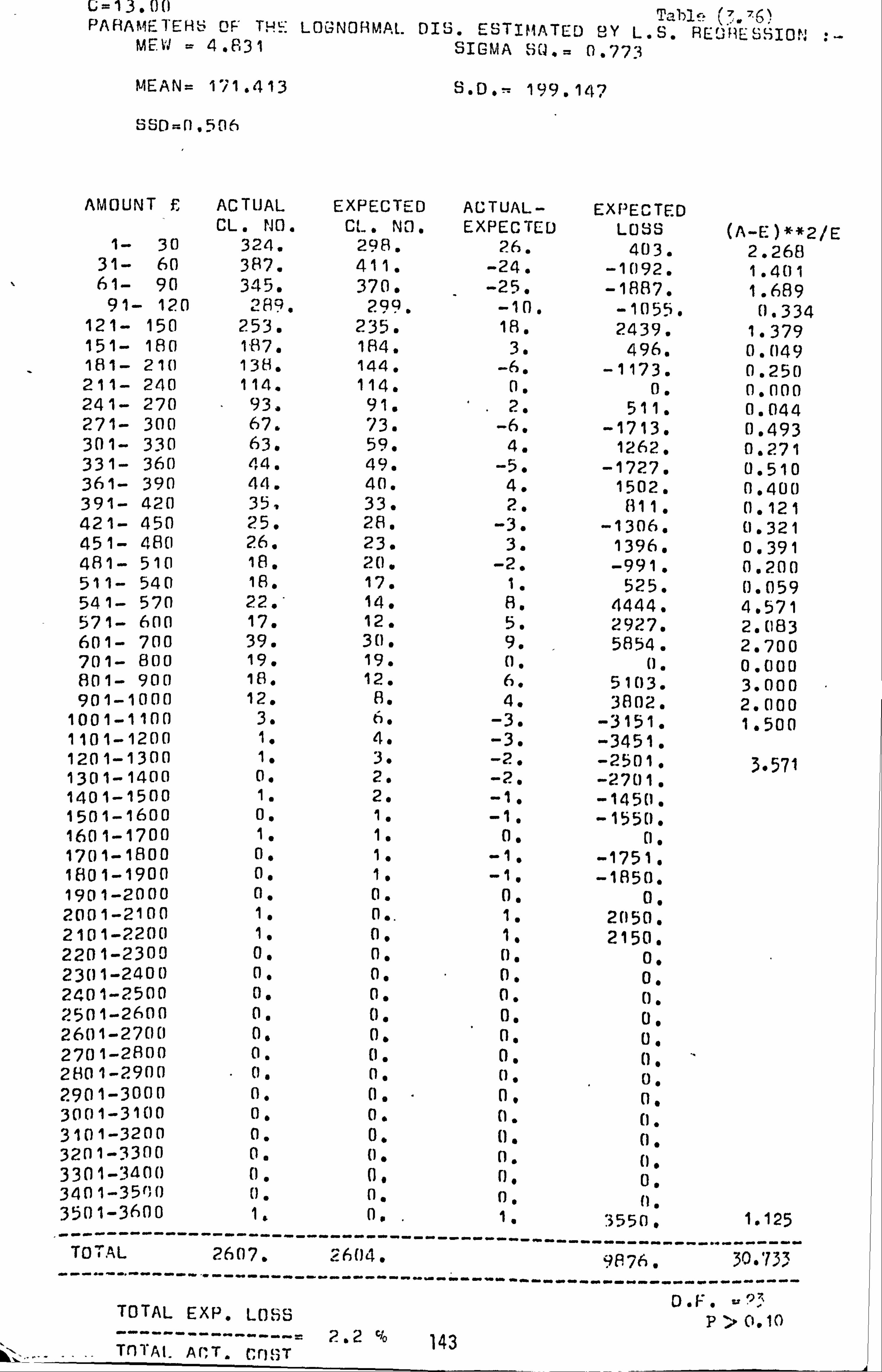
C; =13.00 1a. bZi! i

t7.75`

PAF1AMr TEHS OF THE LOGNORMAL. DIS. ESTIMATED By L. S. REJRESSION MEW = 4.831 SIGMA SO.. 0.773

MEAN= 171.413 S. D. - 199.14?

SSD=0.50f

kýý --

AMOUNT E ACTUAL EXPECTED ACTUAL- EXPECTED CL. NO. CL. NO. EXPECTED LOSS (A_E)**2/E

1- 30 324. 298. 26. 403. 2.268 31- 60 387. 411. -24. -1092. 1.401 61- 90 345. 370. -25. -1887. 1.689

91- 120 289. 299. -10. -1055. 0.334 121- 150 253. 235. 18. 2439. 1.379 151- 180 1.87. 184. 3. 496. 0.049 181- 210 138. 144. -6. -1173. 0.250 211- 240 114. 114. 0. 0. 0.000 241- 270 93. 91. 2. 511. 0.044 271- 300 67. 73. -6. -1713. 0.493 301- 330 63. 59. 4. 1262. 0.271 331- 360 44. 49. -5. -1727. 0.510 361- 390 44. 40. 4. 1502. 0.400 391- 420 35. 33. 2. 811. 0.121 421- 450 25. 211. -3. -1306. 0.321 451- 480 26. 23. 3. 1396. 0.391 481- 510 18. 20. -2. -991. 0.200 511- 540 18. 17. 1. 525. 0.059 541- 570 22. ' 14. 8. 4444. 4.571 571- 600 17. 12. 5. 2927. 2.083 601- 700 39. 30. 9. 5854. 2.700 701- 800 19. 19. 0. 0. 0.000 801- 900 18. 12. 6. 5103. 3.000 901-1000 12. 8. 4. 3802. 2.000

1001-1100 3. 6. -3. -3151. 1.500 1101-1200 1. 4. -3. -3451. 1201-1300 1. 3. -2. -2501. 3.571 1301-1400 0. 2. -2. -2701. 1401-1500 1. 2. -1. -145(1. 1501-1600 0. 1. -1. -1550. 160 1-1700 1. 11 0. (1 O 1701-1800 0. 1. -1. -1751. 1801-1900 0. 1. -1, -1850. 1901-2000 0. 0. 0. 0. 2001-2100 1. 0.. 1. 2050. 2101-2200 1. 01 1. 2150. 2201-2300 0. 0. o. 0. 2301-2400 0. 0. 0. 0. 2401-2500 0. 0. 0. 0. 2501-2600 0. 0. 0. 0 2601-2700 0. 0. 01 01 2701-2800 0. 0. 0. 0 2801-2900 . 0. 01 p. , 0. 2901-3000 0. 0, 0. 0. 3001-3100 0. 0. 0. 0. 3101-3200 0. 0. (1. 0. 3201-3300 0. 0. (1. 0, 3301-3400 (1. 0, n, 0. 3401-350, ) 0. 0. 0, tl 3501-3600 1. 0. 1. . 3550. 1.125

, ýL ToT 2607. ----------

2604. ------

-------------

----------

-------

--ýA7ýº. __-_- -30. '133-

TOTAL EXP. LOSS

--- ------------ D. F.

P

------- u23

> 0.10 ------

T --------- = 2.2 143 TOT AL. Al T. ensT

Table (3.37)

75/2ND QUARTER DATA

C=25.00 PARAMETERS pF THE LOGNORMAL DIS. ESTIMATED BY L. S. REGRESSION ; - MEW = 4.979 SIGMA SQ. = 0.692

MEAN= 180.416 S. p. = 205.254

SSD=0.086

AMOUNT £ ACTUAL, EXPECTED ACTUAL- EXPECTED CL. NO. CL. NO. EXPECTED LOSS. (A-E)**2/E

1- 30 302. 309, E -7. -108. 0,159 31- 60 374. 345, 29, 1319, 2,438 61- 90 332. 323,. 9, 680, 0.251 91- 120 "277, 273. 4, 422, 0.059

121- 15Q 235. 222, 13. 1761. 0.761 151- 180 187. 179, 8, 1324. 0.358 181- 210 122. 144, -22, -4301. 3.361 211- 240 110, 116, -6, -1353. 0.310 241- 270 80*, 94, -14, -3577. 2.085 271- 300 72, 76. -4, -1142, 0.211 301- 330 47, 63, -16, -5048, 4,063 331- 360 39, 52. -13, -4491. 3,250 361- 390 40. ' 43, -3,. -1126. 0.209 391- 420 38, 36, 2, 811, 0.111

. 421- 450 29, 30. -1. -436. 0,033 451- 480 21, 25, -4. -1862,. 0.640 481- 510 30, 21, 9, 4459, 3.857 511- 540 19. 18, 1, 525, 0,056 541- 570 17. 15, 2. 1111, 0.267 571- 600 11, 13. -2. -1171. 0.308 601- 700 36. 33, 3, 1951. 0. "273 701- 800 22. 21. 1, 751. 0.048 801- 900 22, 13, 9. 7654. 6.231 901-1000 11, 91 2. 1901, 0.444

1001-1100 4, 6.. -2.. -2101. 0.667 1101-1200 3. 4, -1. -1150. 1201-1300 3, 3. 0, 01 0.143 1301-1400 6, 2, 4. 5402, 1401-1500 2, 2, 0, 0, 1501-1600 11 11 0. 0. 1601-1700 0. 11 -1, -1650. 1701-1800 1. 1, 0, 00 1801-1900 0, 1, -1. -1850. 1901-2000 1, 0, 1, 1950. 2001-2100 0, 0. 0. 0, 2101-2200 0. 0, U, 2201-2300

-------

1,

------- -----

0.

---------- ----------.. 2250,

--------- 2.000

---------- --- TOTAL

----------

2495.

------------ 2494.

---------- ----------- 2905.

---------

- 32.501

----------- D. F. =23

TOTAL EXP. LOSS --------------- 0.6 % P =0,09 TOTAL ACT. COST

144

'Table (3.3£3 }

#** 3-PARAMETER LOGNORMAL DIS. ##*

73/4TH QUARTER DATA

ESTIMATION BY MULTINOMIAL MAX. LIK ELIHOOD METHOD t- C= 14.01 MEW= 4.700 SIGMA SQ. = 0.8 03

MEAN. 150.159 S. D. = 102.166

AMOUNT P ACTUAL EXPECTED ACTUAL- EXPECTED Cl.. NO. CL. NO. EXPECTED LOSS (A-E) **2 /E

1- 30 470. 477. 1. 15. 0.002 31- 60 51R. 535. -17. -774. 0.540 61- 90 461. 443. 18. 1359. 0.731 91- 120 359. " 340. IP. 2004. 1.062

121- 150 239. 257., -18. -2439. 1.261 151- 180 21'3. 196. 17. 2813. 1.474 101- 210 148. 150. -2. -391. 0.027 211- 240 102. 117. -15. -33P2. . 1.923 241- 270 Al. 92. -11. -2810. 1.315 271- 300 5A. 73. -15. -4202. 3.0 2. 301- 330 66. 50. A. 2524. 1.103 331- 360 45. 47. -2. -691. 0.005 361- 390 39. 39. n. 0. 0.000 391- 420 35.

. 32. 3. 1216. 0.281

421- 450 . 34. 26. H. 3404. 2.462

451-- 400 20. 22. -2. -931, 0.1 R2 401- 510 29. 1R. 11. 5450. 6.722 5.11- 540 14. M. -2. -1051. 0.250 541; - 570 8" 13. -5. -2777. 1.923 571- 600 9. 11. -2. -1171. 0.364 601- 700 29.

_ 27. 2. 1301. 0.148

701- 800 1R. 17". 1. 751. 0.059 801- 900 20. 11. 9. 7654. 7.364 901-1000 .

6. 7. -1. -951. 0.143 1001-1100 4. 5. - -1. -1050. 0.200 ' 1101-1200 4. 4, ' 0. 0. 1201- 1300 1. 3. -2. -250 1. 0457.1 1301-1400 3. 2.

. 1. 1390.

1401-1500 1. 1. ' n. 0. 1501-1600 0ti 1. -1. -1550. * 1601-1? 00 1. 1. 0. 0. 1701-1800 0. . 1. -. 1. -1751. 1001-1900 0. 0. 0. 0; 1901-2000 1" 0. 1. 1950. 2001-2100 0. 0. 0. 0. 2101-2200 0. 0. 0. 0. 2201-2300 0. 0. 0. n. 2301-? _400

---

1.

-----------

0. -- - -----

1. 2350. 0.167 -------

TOTAL 3045. - -- - ' 3042.

----------- -- ------------ 5721 "

-------

- -- - `, 3-4 ý1 "t

- --------------- -- --------- -----.. ------------------- - ----

D. F. P> TOTAL EXP. LOSS P > 0.07

TOTAL ACT. COST k; CL - S, Yov D ; ̂ 7

P >0. )n

ý' 145

Table (3,39)

*** 3-PARAMETER LOGNORMAL DIS. ***

74/1ST QUARTER DATA

ESTIMATION BY MULTINOMIAL MAX. LIKELIHOOD METHOD t- C= 10.40 MEW= 4.650 SIGMA S0. = 0.1) 58

MEAN- 150. 222 S. D. = 1R7.204'

AMOUNT f, ACTUAL EXPECTED ACTUAL- EXPECTED CL. NO. CL. NO. EXPECTED LOSS (A-E)**2/E

"1- 30 381. 379. 2. 31. 0.011 31-"" 60. 428. 444. -16. -72R. 0.577 61- 90 351. 359. -8. -6114. 0.178 91- 120 334. 271. " 63. 6646. 14.646

121- 150 211. 203. R. 1084. 0.315

. 151- 180 133. - 154. -21. -3475. 2.864 181- 210 98. 118. -20. -3910. 3.390 211- 240 82. 91. -9. -2029. " U. "890 241- 270 54. 72. -18. -4599. 4.500 271- 300 52. . 57. -5. 71427. . 0.439 301- 330 53. 46. 7. 2208. 1.085 331- 360 36. . 37. . -1. -346. 0.027 361- 390 .

29. 30. -1. -376. 0.033 391- 420 26. 25. 1. 406. 0.040 421-. 450 22. 21. 1. 436. 0.048 451- 481) 22. 17.. 5.. 2327. 1.471 4A 1- 510 17. 15. 2. 991. 0.267 511- 540 10. 12'. -2. -1051. 0.333 541-

. 570 19. 11. R. 4444. 5.818

571- 600 4. 9. - -5. -2927. 2.778 601- ? on 26. 22. 4. 2(, n2.. - 0.727 701- 800 21. 14. 7. 5253. 3.500 801- 900 11. 9. 2.

. 1701. 0.444 901-1000 10. 6. 4. 3802. 2.667

1001-11J0 5. 4. 1. 1050. 1101-1200 2. 3. -1. -1150. 000 0 1201-1300 1. 2. -1. -1250. . 130 1-1400 2. 2. 0. 0. 1401-1500

. 0. 1. -1. -1450. 1501-1600 0. 1. -1 .- 1550.

1601-1700. 0. j. -1. -1650. X701-1800 1. 1. 0. 0 '-_------- ----------- ----------- ---------

. -------------- -

2.000 - TOTAL 2441. "2437. 4457. 49 207 .

D. F. 22 TOTAL EXP. LOSS " --------------- 1.2 a DY <o . 001 TOTAL ACT. DOST ICO:, 0.020

P <0.03

14G

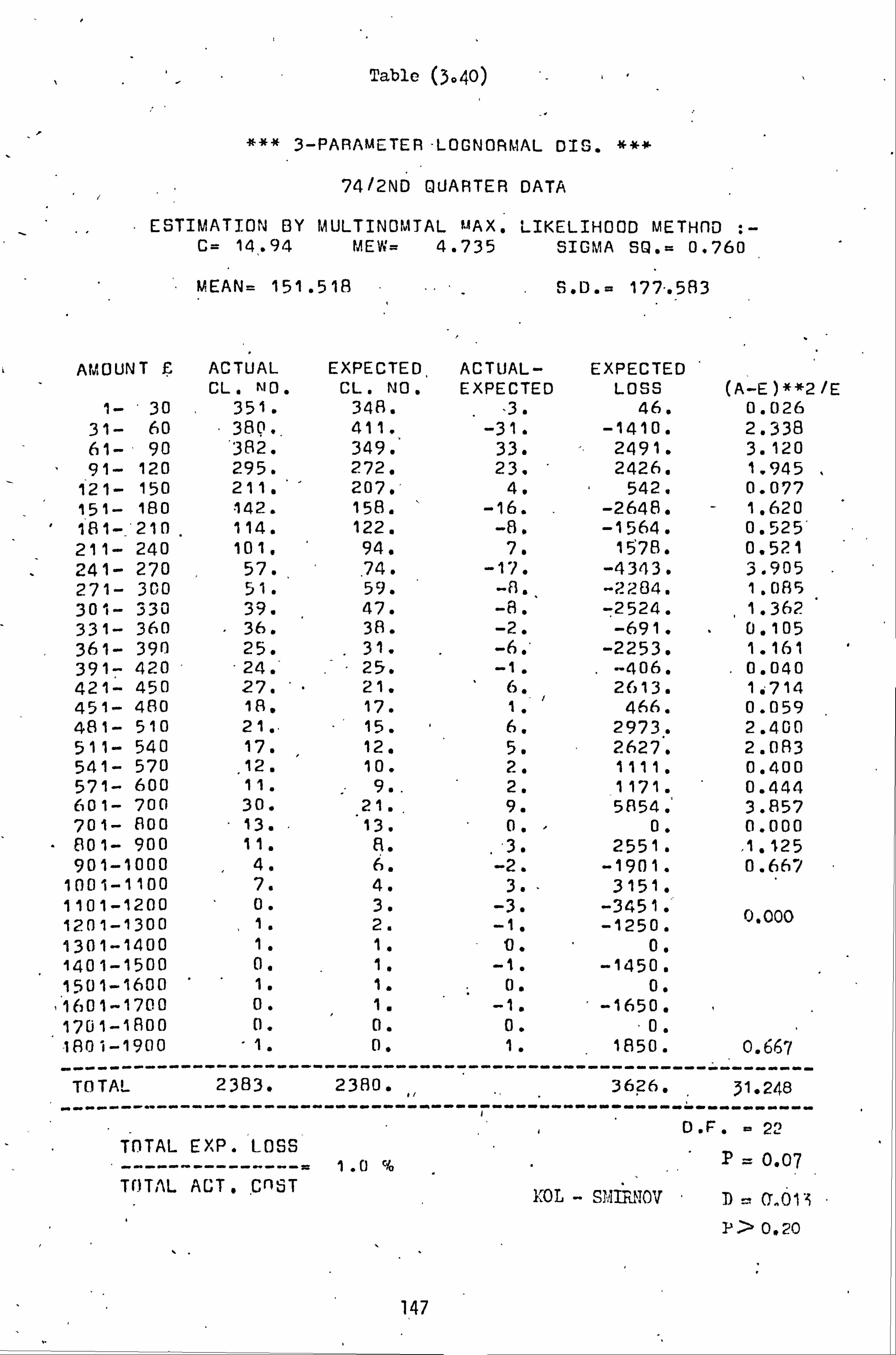
Table (3040 -

### 3-PARAMETER-LOGNORMAL DIG. ***

74/2ND QUARTER DATA

EST IMATION BY MULTINOMT AL MAX. LIKEL IHOOD METHfD : - C= 14,. 94 MEW= 4.735 SI GMA SQ. = 0.760

MEAN= 151.518 S. D. = 177-. 583

AMOUNT £ ACTUAL EXPECTED ,

ACTUAL- EXPECTED CL. NO. CL. NO. EXPECTED LOSS (A-E)**2/E

1- 30 351. 348. -3. 46. 0.026 31- 60 380.. 411. -31. -1410. 2.338 61- 90 382. 349. 33. 2491. 3.120 91- 120 295. 272. 23. 2426. 1.945 ,

121- 150 211. 207. 4. 542. 0.077 151- 180 142. 158. -16. -2648. - 1.620 181-_'210

" 114. 122. -8, -1564. 0.525

211- 240 101. 94. 7. 1578. 0.521 241- 270 57.

. 74. -17. -4343. 3.905

271- 300 51. 59. -a.. -2.284. 1.085 301- 330 39. 47. -8. -2524. 1.362 331- 360 36. 38. -2. -691. 0.105 361- 390 25.

. 31. -2253. 1.161

391- 420 '24. 25. -1. . -406. . 0.040 421- 450 27. 21. 6. 2013. 11714 451- 480 18. 17. 1. ' 466. 0.059 481- 510 21., 15. 6. 2973. 2.400 511- 540 17. 12. 5. 2627. 2.083 541- 570 12. 10. 2. 1111. 0.400 571- 600 11. 9.. 2. 1171. 0.444 601- 700 30. 21.. 9. 5854. ` 3.857 701- 800 . 13. . 13. 0. , 0. 0.000 801- 900 11. R. 3. 2551. 1.125 901-1000 4. 6.

-2. -1901. 0.667 1001-1100 7. 4. 3. - 3151. 1101-1200 0. 3. -3. -3451. " 1201-1300 ,

1. 2. -1. -1250. x"000

1301-1400 1. 1. 0. 0. 1401-1500 0. 1. -1. -1450. 1501-1600 " 1. 1. 0. 0.

, 1601-1700 0. 1. -1. -1650. 1701-1800 0. 0. 0. . 0.

-180 1-1900 " 1. 0. 1. _

1850. 0.667

---------- TOTAL

----------- 2383.

--------- 2380.

------------- ----------- 3626.

-------- 31.248

----------- ----------- --------- -----; D. F. 24

TOTAL EXP. LOSS . _-_-_ ---------- = 1.0 % ..

P 0.07 TOTAL ACT. CAST 1; OL - SP,, lI

. NOV D 0'. 01 i P>0�20

147

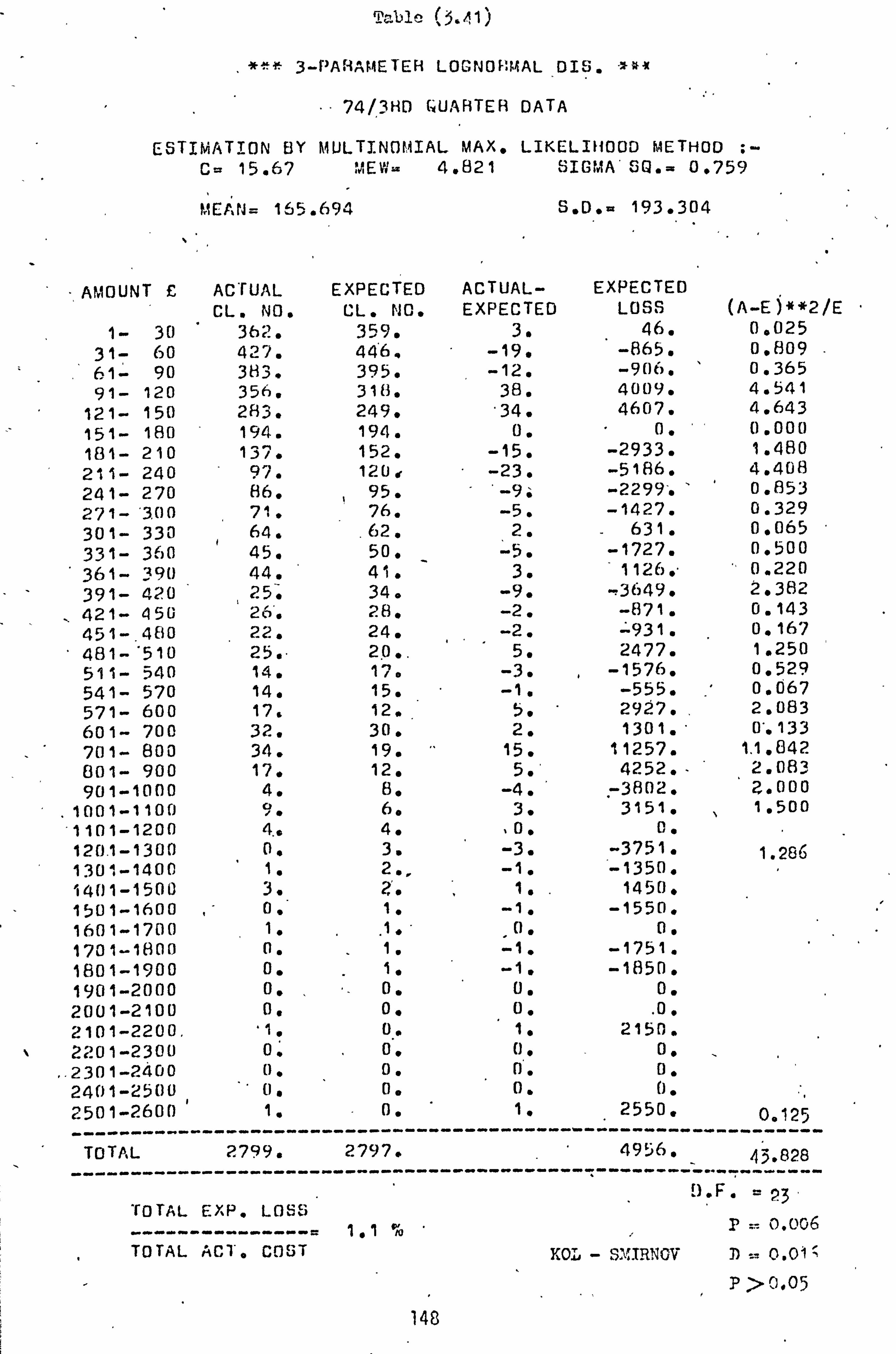
Table (3.4,1)

xý` 3-PAHAMETEH LOGNOF8 AL DIS.

74/3H0 ((UARTER DATA

ESTIMATION BY MULTINQMIAL MAX. LIKELIHOOD METHOD ; -- Cs 15.67 MEW- 4. ß21 SIGMA' 5Q. = 0.759

MEF, rd= 165.694 S. D. = 193.304

-AMOUNT £ ACTUAL EXPECTED ACTUAL- EXPECTED CL. NO. CL. NO, EXPECTED LOSS (A-Ej**2/E

1- 30 362. 359. 3. 46. 0.025 31- 60 427. 446. -19. -865. 0.809

61- 90 383. 395. -12, -906. 0.365 91- 120 356, 318. 38. 4009. 4.541

121- 150 283. 249. '34. 4607. 4.643 151- 180 194. 194. 0. 0. 0.000

181- 210 137. 152. -15. -2933. 1.480 211- 240 97. 120 -23. -5186. 4.408

241- 270 86. 95. -9: -2299-. 0.853 271- '3.00 71. 76. -5. -1427. 0.329 301- 330 64.

. 62. 2. 631. 0.065

331- 360 45. 50. -5. -1727. 0.500

361- 390 44. 41. 3. 1126. " 0.220 391- 420 25. 34. -9. -3649. 2,382 421- 450 20'. 28. -2. -871. 0.143 451-. 480 22. 24. -2. --931. 0.167 481- '510 25.. 20.. 5. 2477. 1.250 511- 540 14. 17. -3. -1576. 0.529 541- 570 14. 15. -1. -555. 0.067 571- 600 17. 12.. 5. 2927.. 2.083 601- 700 32. 30. 2. 1301. ' 0'. 133

701- Boo 34. 19. 15. 11257. 1.1.042 801- 900 17. 12. 5. ' 4252. - 2.083 901-1000 4. 8. -4. ' -3802. 2.000

. 1001-1100 9. 6. 3, 3151. 1.500 1101-1200 4.0 4. , 0. 0. 120.1-1300 0. 3. -3. -3751. 1.286 13011-1400 1. 2., -1. -1350. 1401-1500 3. 7, ". 1. . 1450. 1501-1600 0. 1. -1. -1550. 1601-1700 1.

. 1.. 0. 0.

1701-1800 0. 1. -1. -1751. 1801-1900 0. 1. -1. -1850. 1901-2000 0. 0. 0. 0. 2001-2100 0. 0. 0. . 0. 2101-2200, '1. U. 11 2150. 2201-2300 0. 00 0. 0.

.. 2301-2400 0. 0. 0. 0. 2401-2500 ' 0. 0. 0. 0.

2501-2600 ----

1. -----------

0. ----------

1. ------------

2550. -----------

0.125 -------- ------

TOTAL 2799. 2797. 4956. 43.828

D . F. ?3 TOTAL EXP. LOSS

---... -- ---------ý 1 .1 aro P 0.006

TOTAL ACT. COST Y0i - SMIRNOV D 0.01

P>0.05

148

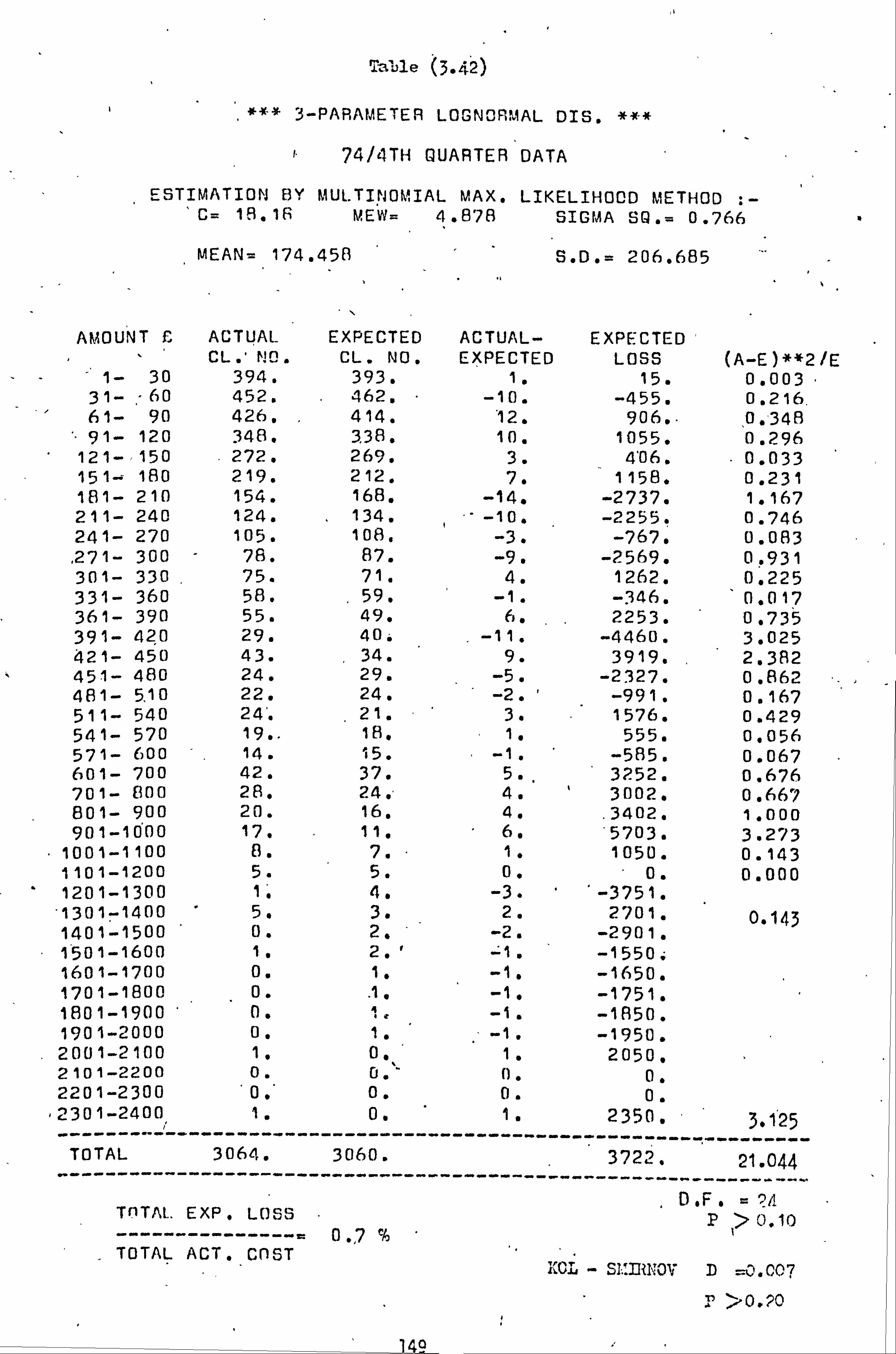
as ble 3.42)

3-PARAMETER LOGNOft

74/4TH QUARTER

ESTIMATION BY MULTINOMIAL MAX. C= 18.18 MEW= 4.878

MEAN= 174.458

L1AL DIS. * -*

DATA

LIKELIHOOD METHOD : - SIGMIA SQ. = 0.766

S. D. = 206.685

AMOUNT £ ACTUAL EXPECTED ACTUAL- EXPECTED' CL. NO. EXPECTED LOSS (A-E) **2 /E

1- 30 394. 393. 1. 15. 0.003. 31-, -60 452. 462. - -10. -455. 0.216. 61- 90 426. 414. 12. 906.. 0.34E 91- 120 348. 338. 10. 1055. 0.296

121--150 272. 269. 3. 4'06. 0.033 151- 180 219. 212. 7. 1158. 0.231 181- 210 154. 168. -14. -2737. 1.167 211- 240 124. 134. -10. -2255. 0.746 241- 270 105. 108. -3. -767' 0.083

, 271- 300 78. 87. -9. -2569. 0.931 301- 330 75. 71. 4. 1262. 0.225 331- 360 58. 59. -1. -346. 0.017 361- 390 55. 49. 6. 2253. 0.735 391- 420 29. 40.

. -Il. -4460. 3.025 421- 450 43. 34. 9. 3919. 2.382 451- 480 24. 29. -5. -2327. 0.862 481- 5.10 22. 24. -2. -991. 0.167 511- 540 24'. 21. 3. 1576. 0.429 541- 570 19.. 18. 1. 555. 0.056 571- 600 14. 15. -1. -585. 0.067 601- 700 42. 37. 5. 3252. 0.676 701- 800 28. 24. 4. 3002, 0.667 801- 900 20. 16. 4.

. 3402. 1.000

901-1000 17. 11. 6. 5703. 3.273 1001-1100 8. 7. 1. 1050. 0.143 1101-1200 5. 5. 0. . 0. 0.000 1201-1300 1, 4. -3. -3751. 1301-1400 5.

, 3.

, 2. 2701. 0.143

1401-1500 0. 2. , -2. -2901. 1501-1600 1. 2. ' =1. -1550. 1601-1700 0. 11 -1. -1650. , 1701-1800

_ 0.

. 1. -1. -1751. 1801-1900 0. 1. -1. -1850. 1901-2000 0. 1. -1. -1950. 2001-2100 1. 00 1. 2050. 2101-2200 0. 0. ` 0. 0. 2201-2300 ' 0.. 0. 0. 0. 2301-2400

11 -----------

1. -----------

0.

----------- 1.

------------ 2350. ",

------- 3,1'25

TOTAL ----------

3064. -----------

3060. ----------- ------------

-- 3722.

-- "

------------ 21.044

------- DF. . ' = 2/1 TOTAL. EXP. LOSS - P > 0.10

----- ----------- n ^7 ct i ----- -- u ", / rr

TOTAL ACT. CnST SI: MNOv D =0-C, (17

P >0.20

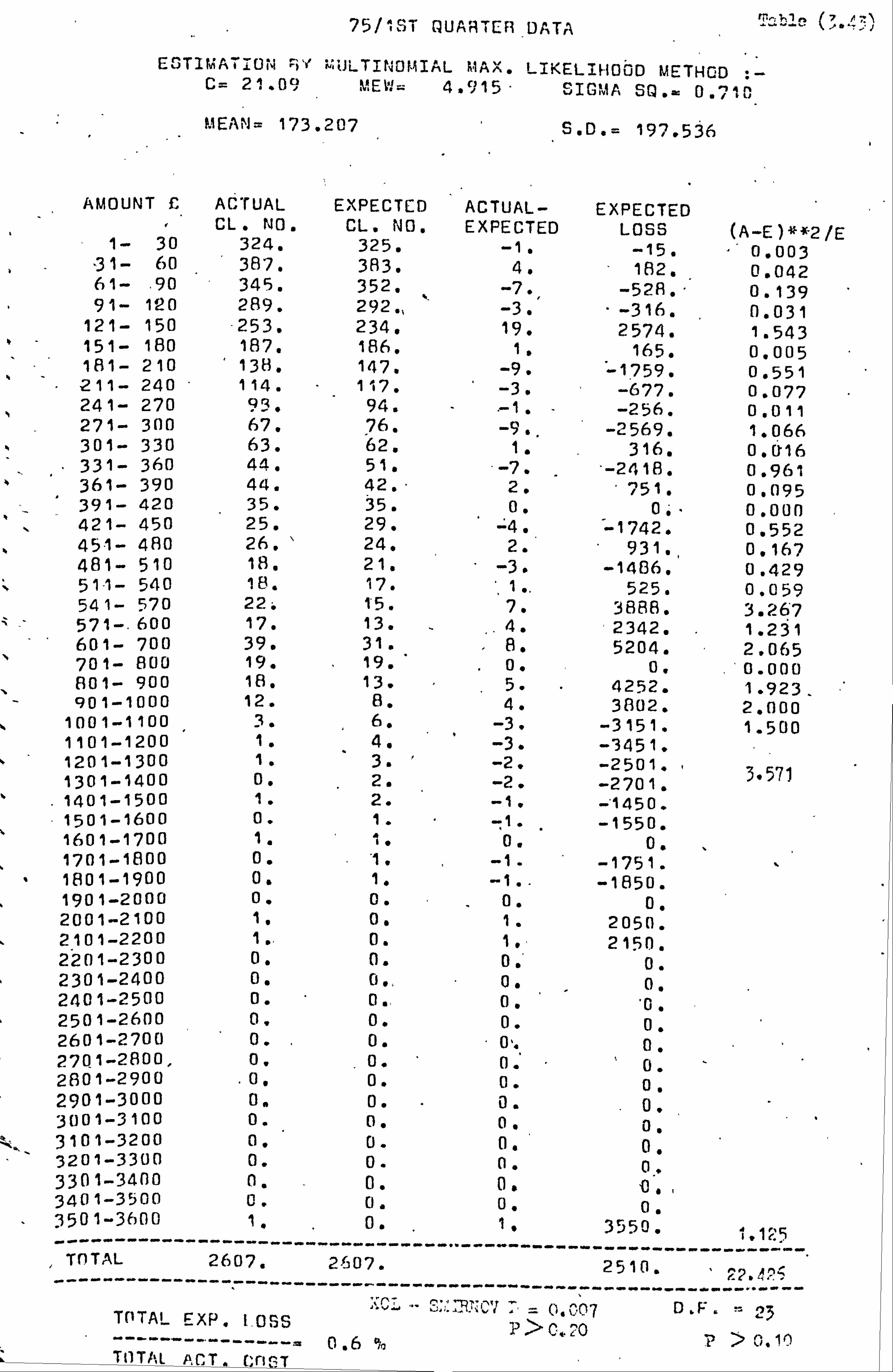
75/ *, S i QUAK i CR DATA Hin {7 A7, `

ESTIMATION i'v' MULTINOMRIAL MAX. LIKELIH0ü0 METHOD C= 21.00, N", EW 4.915 SIGMA SQ.. 0. -4n 1 ̂ ! MEAN= 173.207 S. D. = 197.536

AMOUNT C ACTUAL EXPECTED ACTUAL- EXPECTED CL. N0. CL. NO, EXPECTED LOSS (A_E)**"2/E

1- 30 324. 325. -1. -15. 0.003 "31- 60 387. 383. 4. 182. 0.042 61- . 90 345. 352. -7. ' -52R. 0.139 91- 120 289. 292., -3. -316. 0.031

121- 150 "253. 234. 19. 2574. 1.543 151- 180 187. 186. 1. 165. 0.005 181- 210 138. 147. -9. -1759. 0.551 211- 240 114. 117, -3. -677. 0.077 241- 270 93. 94. - -1. - -256. 0.011 271- 300 67. 76. -9.. -2569. 1.066 301- 330 63. 62. 1. 316. 0.016 331- 360 44. 51. -7. -2418. 0.961 361- 390 44. 42. 2. " 751. 0.095 391- 420 35. 35. 0. 0.. 0.000 421- 450 25. 29. -4. -1742. 0.552 45"1- 480 26. 24. 2. * 931. 0.167 481- 510 18. 21. -3. -1406. 0.429 511- 540 18. 17. 1.. 525. 0.059 541- 570 22. 1"5. 7. 31388. 3.267 571-. 600 17. 13. 4. 2342. 1.261 601- 700 39. 31. 8. 5204. 2.065 701- 800 19. 19. 0. 0. 0.000 801- 900 18, 13. 5. 4252. 1.923 901-1000 12. ß. 4. 3802. . 2.000

1001-1100 3. 6. -3. -3151. 1.500 1101-1200 1. 4. -3. -3451. 1201-1300 1. 3. -2. -2501. 3.571 1301-1400 0. 2. -2. -2701. 1401-1500 1. 2. -1. -1450. 1501-1600 0. 1. -1. -1550. 1601-1700 1. 1. 0. 0. 1701-1800 0. . 1. -1. -1751. ,. 1801-1900 0. 1. -1.. -1850. 1901-2000 0. 0. 2001-2100 1. 0. 1. 2050. 2101-2200 1.. 0. 1. 2150. 2201-2300 0. 0. 00. 0. 2301-2400 0. 0,, 01 0. 2401-2500 0. 0.. 0. 2501-2600 0. 0. 2601-2700 0.

. 0. . 0. 0ý 2701-2800, 0.

. 0. 0. 0.

2801-2900 . 0. 0. 0. 0. 2901-3000 0. 0. 0.

. 0. 3001-3100 0. 0. 01 3101 -3200 0. 0. 0. 0 3201-3300 0. 0. 0. .

0. 3301-3400 0. . 0. 0. 10», , 3401-3500 0. 0. 0. 3501-3600 1. 0. 1 3550 ..

---- ----------- ----------- .

-- TOTAL

__-.... ------ 2607.

----------- 2{07.

-----------

--

-----------

----------- 2510.

-----

----- -- -

TOTA! EXP 1 05S X4... ------

1?; C7 . (ß. v07 D .F. 23 ` p>G. '. 20 "----- ---------= 0 .6 % p C. 1ý TOTAL P. C [, r'iC, T

. 44) Table 0

---------- ---- TOTAL ACT. COSTr i: OL - ;; MU! "lo

151

" #'"` 3-PARAMETER LOGNORMAL DIS. ***

75/2N0 UUAP+ T ER DAT A

ESTIMATION BY MULTINOMIAL MAX,. LIK ELIHOOD METHOD ; - C- 15.16 MEW= 4.872 SIGMA SQ. = 0.8 07

MEAN- 180.409 S. D. = 217.852

AMOUNT £ ACTUAL EXPECTED ACTUAL- EXPECTED CL. NO. CL. NO. EXPECTED LOSS (A-E)**"2/E

1- 30 ; 302. 302. 0. 0. 0.000 31-. 60 374. 376. -2. -91. 0.011 61- 90 332-. 337.

.. -5. -378. 0.074 91- 120 277. 275. 2, 211. 0.015

121- 150 235. 218. 17. 2304. 1.326 151- 180 1137.

. 173. 14. 2317, 1.133

"181- 210 *

122. - 137. -15. -2933. - 1.642 240 2-11 110, 110. 0. o. 0.000

241- 270 f; 0, 89, -'-9. -2299. 0.910 271- 300 72. 72. 0.

, 0. 0.000 301- 330 47. 59. -12. --3786. 2.441

-331--, 360 39. 49. -10. -3455. 2.041 " 361- 390 40. 41. -1. . --376. 0.024

391- 420 38. 34. 4. . 1622. 0.471 421- 450 19. . 29. 0. 0. 01000 451- 480 219 '24" -3. " -1396. 0.375

. 481- 510 30. . 21* 9. 4459. 3.857 511- 540 19. 18. 1. 525. "0.056 541- 570 17. 15. 2. 1111. 0.267 571- 600 11. 13. -2. -11710 0.308 601- 700 36. 339 3. 1951. 0.273 701- 800 22. 21. "1. 751. 0.048 801- 900 22, 14. .

H. 6804. 4.571 901-1000 11. 10. 1. 951. 0.100

1001-1100. 4. 7. -3. -3151. 1.286 1101-1200 3. 5.

- -2. -2301. O. 11C

1201-1300 3. 4. -1. -1250. 1301-1400 6. 3. 3. 4051. 0.71 1401-1500 2. 2. 0, !1 1501-1600- 1. . - 2. -1. -1550. 1601-1700 0. 1. -1. -1650. 1701-1800 1. 1. 0. 0"40 "" 1801-1900 - (3. 1.. -1. -1850. 1901-2000 1. 1. - 0,

, 06

2001-2100 " 0. 0. 0� 0l 2101-2200 0. " 0. .O0 U 2201-2300 1. 0. 1. ." 2250.

0.1700 ------------ 0------------------- -------------------------

-------

TOTAL

-----------

2495.

---------- 24970

---------- ----------- 1669,

--------------- 23.897 --------

TOTAL ERP. LOSS 0, F.

p 24

.ý0.10

.ý

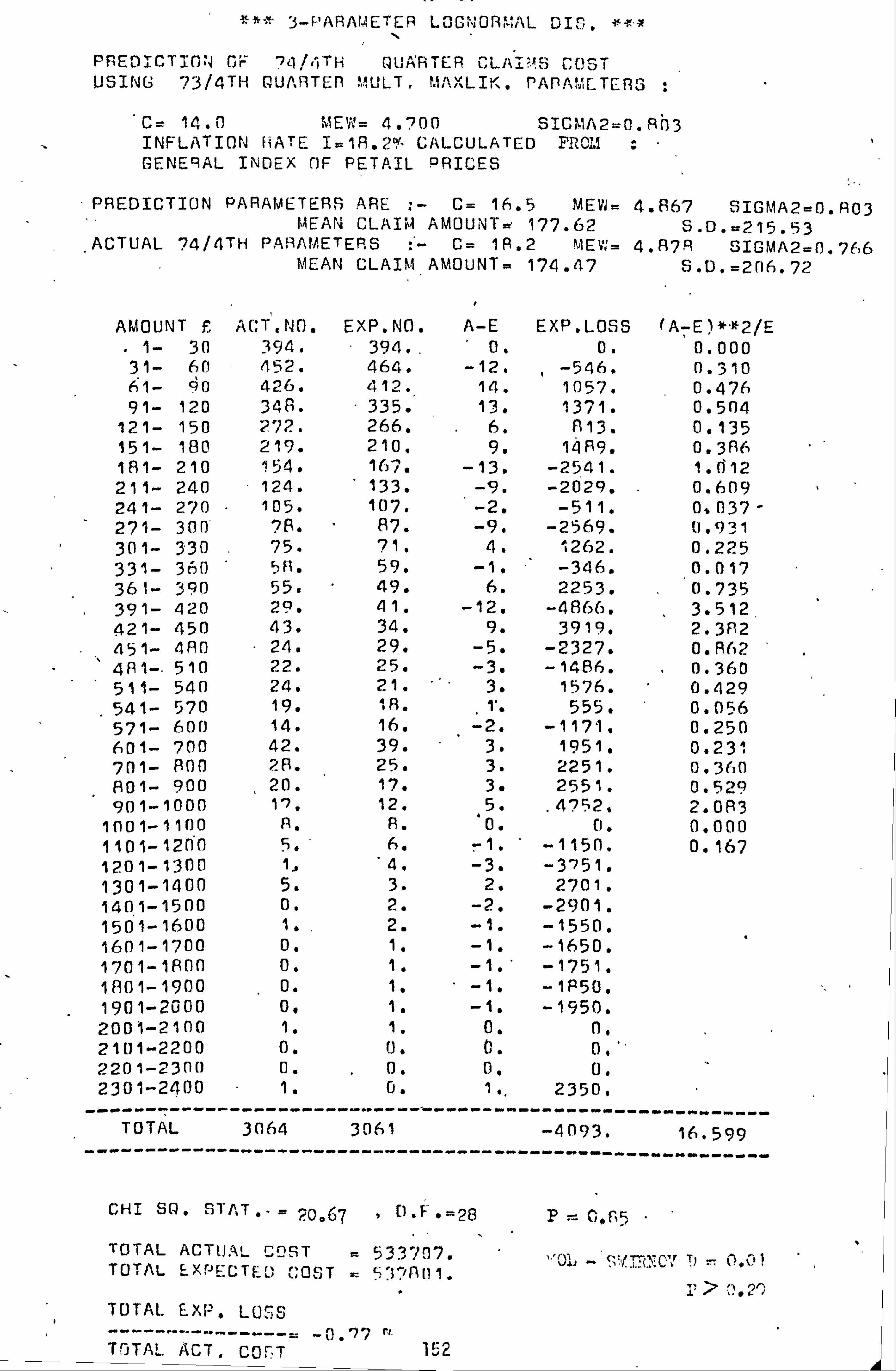
*** S-PARAMETER LOGNORMAL DIS. *x

PREDICTION OF 24/KITH QUARTER CLR1? MS COST USING 73/4TH QUARTER PArIAM TERS

C= 14. P MEW'= 4.700 SICMA2=C. Rh3

ti INFLATION HATE I=1R. 2°+ CALCULATED PROM GENERAL INDEX OF PETAIL PRICES

-PREDICTION PARAMETERS ARE .- C= 16.5 MEW- 4.867 SIGMA2=0. H03 MEAN CLAIM AMOUNT=e 177.62 S. D. =215.53

ACTUAL 74/4TH PARAMETERS :- C= I R. 2 MEW- 4.87R SIGMA2=0.7F, 6 MEAN CLAIM AMOUNT= 174.47 S. D. =2n6.72

AMOUNT £ ACT. NO. EXP. NO. A-E EXP. LOSS (A7E)*"*2/E

. 1- 30 394. 1 394.. 1 0. 0. 0.000 31- 61 452. 464. -12. -546. 0.310 fý1- 0 426. 412. 14. 1057. 0.476 91- 120 348. V335. 13. 1371. 0.504

121- 150 272. 266. 6. 813. 0.135 151- 180 219. 210. 9. 14 P9. 0.386 181- 210 154. 167. -13. -2541. 1.612 211- 240 124. 133. -9. -2029. 0.609 241- 270 105. 107. -2. -511. 01-037- 271- 300 ? S. 87. -9. -2569. 0.931 301- 330 75. 71. 4. 1262. 0,225 331- 360 `F8. 59. -1. -346. 0.017 361- 390 55. 49. 6. 2253. 0.735 391- 420 29. Al. -12. -4866. 3.512 421- 450 43. 34. 9. 3919. 2.382 451- 480 24. 29. -5. -2327. 0. R62 V 481- 510 22. 25. -3. -1486. 0.360 511- 540 24. 21. 3. 1576. 0.429

. 541- 570 19. 18.

. 1'" 555. V 0.056

571- 600 14. 16. -2. -1171. 0.250 601- 700 42. 39. V 3. 1951. 0.231 701- 800 2R. 25. 3. 2251. 0.360 801- 900 20. 17. 3. 2551. 0.529 901-1000 117. 12. 5.

. . 4752. 2.083

0 1001-110 A. R. 0. f1. 0.000 , 1101-1200 5. 6. -1. ' -1150. 0.167

1201-1300 1, 4. -3. -3 151 . 1301-1400 5. 3. 2. 2701. 1401-1500 0. 2. -2. -2901. 1501-1600 1.. 2. -1. -1550. 1601-1700 0. 1. -1. -1650. 1701-1800 0. 1. -1. ' -1751. 1801- 1900

, 0. 1. -10 -1 P50.

1901-2000 0. 1. -1. -1950. 2001-2100 1. 1. 0. 0. 2101-2200 0. U. C;. 0. 2201-2300 0. 0. 0. U. 2301-2400 V 1. 0. 1.. 2350.

------. ----- TOTAL

------------

-------- 3064

--------

---------- 3061

----------

-------

-------

---------- -4093.

----------

---------- 16.599

----------

CHI SO. STA, T ."= 20,67 > 0-F--28

TOTAL ACTUAL COST = 53? 707. TOTAL EXPECTED COST =

TOTAL EXP. LOSS

TOTAL ACT. COST 152

P=C;. FýS

t Ti 0.0 i' 7 ß'. 2O

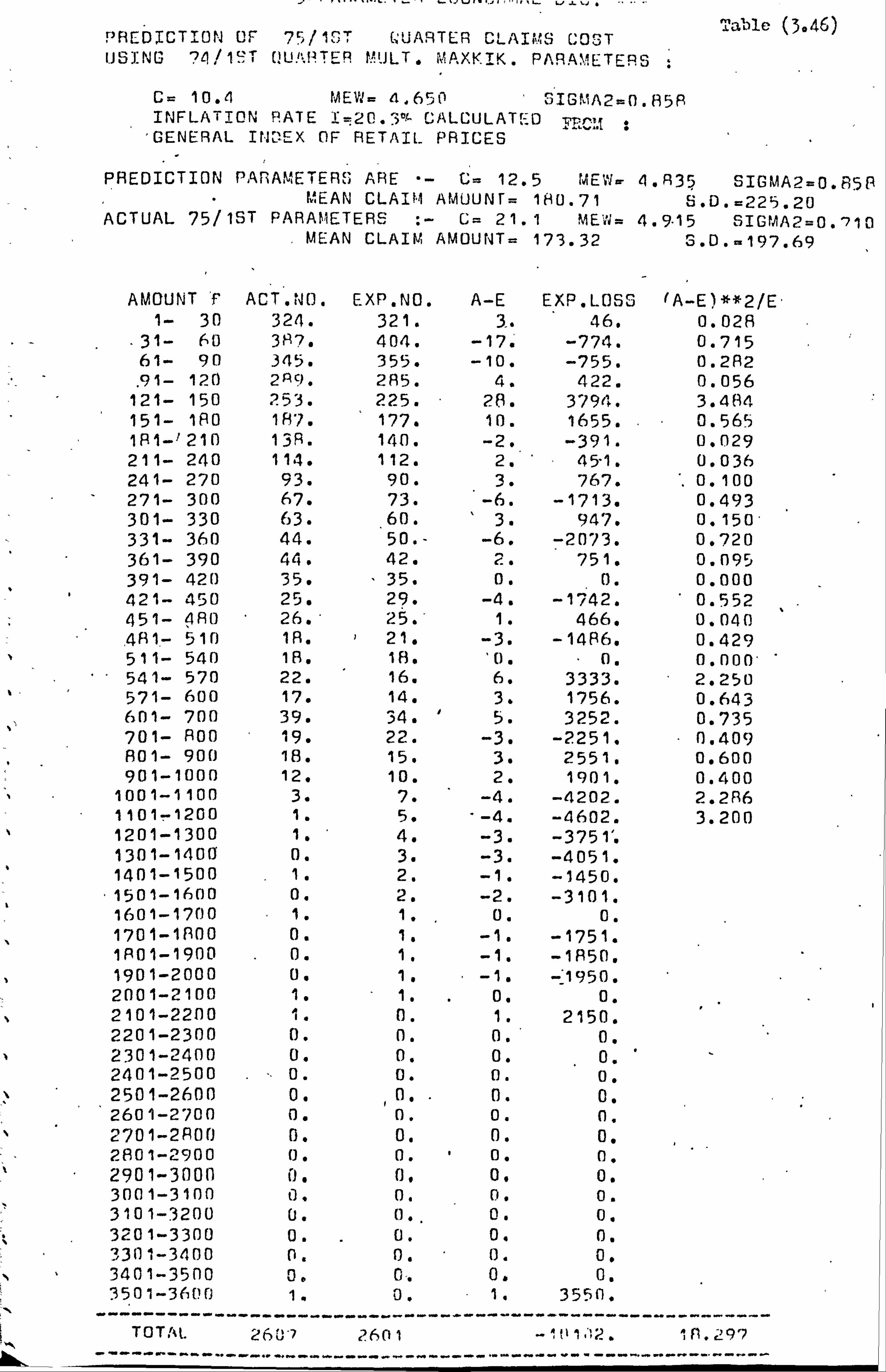
sable (3,46) PREDICTION OF 75, % 1ST (, MARTER CLAIMS COST USING ?L /1"- QL! RTER M JLT. PIiAXKIK. PARAMETERS ;

C= 10.4 MEVI= 4,650 SIGMA2=0.050 INFLATION PATE I_20.3°- CALCULATED C. pq

'GENERAL IN:? EX OF RETAIL PRICES

i

hhl-

PREDICTION PARAMETERS ARE "- L'- 12.5 MEW= 1,835 SIGMA2=0.85P " MEAN CLAIM AMUUNT= 18U. 71 S. D. =225.20

ACTUAL 75/1ST PARAMETERS C= 21.1 MEW= 4.9.15 SIGMA2=0. -710 MEAN CLAIM AMOUNT= 173.32 3. D. a197.69

AMOUNT 'f ACT. 140. EXP. NO. A-E EXP. LOSS (A-E)**2/E" 1- 30 324. 321. 3.. 46. 0.028

"31- 60 387. 404. -17. -774. 0.715 61- 90 345. 355. -10. -755. 0.282 . 91- 120 2A9. 285. 4. 422. 0.056

121- 150 253. 225. 28. 3794. 3.484 151- 190 1817. 177. 10. 1655. 0.565 1R1-'210 138. 140. -2. -391. 0.029 211- 240 114. 112. 2. 45-1. 0.036 241- 270 93. 90. 3. 767. . 0.100 271- 300 67. 73. -6. -1713. 0.493 301- 330 63. 60. 3. 947. 0.150' 331- 360 44. 50. - -6. -2073. 0.720 361- 390 44. 42. 2. 751. 0.095 391- 421) 35. " 35. 0. 0. 0.000 421- 450 25. 29. -4. -1742. 0.552 451- 4R0 26. ' 25. 1. 466. 0.040 481- 510 in. 21. -3. -1486. 0.429 511- 541) 18. 18. U. " 0. 0.000* - 541- 570 22. 16. 6. 3333. 2.250 571- 600 17. 14. 3. 1756. 0.643 601- 700 39. 34. ' 5. 3252. 0.735 701- 800 19. 22. -3. -2251. 0.409 801- 900 18. 15. 3. 2551. 0.600 901-1000 12. 10. 2. 1901. 0.400

1001-1100 3. 7. -4. -4202. 2.286 1101-1200 1. 5. -4. -4602. 3.200 1201-1300 1. 4. -3. -3751. 1301-1400 0. 3. -3. -4051. 1401-1500 1. 2. -1. -1450.

"1501-1600 0. 2. -2. -3101. 1601-1700 1. 1. 0. 0. 1701-11300 0. 1. -1. -1751. 1801-1900 0. 1. -1. -1850. 1901-2000 0. 1. -1. -1950. 2001-2100 1. 1. 0. 0. 2101-2200 1. 0. 1. 2150. 2201-2300 0. 0. 0.1 0. 2301-2400 0. 0. 0. 0. ` 2401-2500 0. 0. 0. 0. 2501-2600 0. 0. . 0. 0. 2601-2700 0. 0. 0. 0, 2701-2900 0. 0. 0. 0. 2801-2900 0. 0. 0. 0. 2901-30001 0. 01 01 0. 3001-3100 t3. 0. 0. 0. 3101-3200 U. 0.. 0. 0. 3201-3300 0. 0. 0. 0. 3301-3400 0. 0. 0. 0. 3401-3500 0. 0. 0. 0. 3501-3600

-

1. 0. 1. 3550. ---- -------

T0TAt. --------

26;; -7

-----------

2601

----- -----------

-I tý 1 . ", 2. ----------

1 f1.29'7

Table (3.46) - continued

CHI SO. STAT. = 25.76 , D. F. = 2E)

TOTAL ACTUAL COST = 452059-- TOTAL EXPECTED COST - 462161.

TOTAL EXP. LOSS

--------------- - -2.23 °c TOTAL ACT. COST

R

y

P>0.50

KOL - S"IIR? d0V I= 0.01

- P> 0.20

Ta! C ## j-PARAMEiE. I IA,

_ : 1ý::, **s.

1i

hkhl-

'Pi1E DICTION OF ? 5/2ND QUARTE9 CLAIMS COST. USING 74/2ND WUARTER MULT. MAXLIK. PARAMETERS

Ca 14.9 MEW= 4.735 RIGMA2so. 76n INFLATION RATE I=24.3% CALCULATED FROM : GENERAL INDEX dF RETAIL PRICES

PREDICTION PARAMETERS ARE :- C= 1R. 5 MEW- 4.953 SIGMA2 =. 760 MEAN CLAIM AMOUNT= 108.44 S. D. =220. x1"

ACTUAL 75/2 ND PARAMET ERS C= 15. 2 MEW= 4.072 SIGMA2=0. At)7 MEAN CLAIM AMOUNT= 180.29 S. 0. =217.79

AMOUNT f ACT. NO. EXP. NO. A-E EXP. LOSS (A-E)**2/E 1-

, 30 302. . 279. 23. 356. 1.896

31- 60 3? 4. 349. 25. 1137. 1.791 , (, )1- 90 332. 325. 7. 528. 0.151

91--120 277. 273. 4. 422. 0.059 121- 150 235. 222. 13. 1761. 0.761 151- 180 187. 170. 9. 1409. ' ' 0.45 5 181- 210 122. 143. -21. -4105. 3.0P4 211- 240 110. 116. -6. -1353. 0.310 241- 270 00.. 94. -14. -3577. 2.085 271- 300 72. 77. -5. -1427. 0.325 301- 330 47. 63. -16. -5040. 4.063 331- 36n 39. 52. -13. -4491. 3.250 361- 390 40. 44. - -4. -1502. 0.364 391- 420 30. 37. 1. 406. 0.027 421- 450

_29. 31. -2. -871. 0.129

451- 400 21. 26. -5. -2327. 0.962 481- 51Q 30. 22. A. 3964. 2.909 511- 540 19. 1q. 0. 0. , 0.000 541- 570 17. 16. 1.. 5550' . 0.063 571- 600 11. 14. -3. -1755. 0.643 601- 700 36. 35. 1. 651. 0.029 701- 900 22. 23. -10 -751. 0.043 001- 900 22. 15. 7. 5953. 3.267 90 1-1000 11. 10. 1. 951. 0.1(10 001-1100 4. 7. -3. -3151. 1.206

1101-1200 3. 5. -2. -2301. 0.300 1201-1300 3. 4. -1. -1250. 1301-1400 6. 3. 3. 405 1. 1401-1500 2.. 2. 0.. 0. 1501-1600 1. 2. -1. -1550. 1601-1700 0. 1. -. 1. -1650. 1701-1000 1. 1. 0, 0, 1001--1900 0. 1, 1901-2000 1. 1. 0. 2001-2100 . 0.. 0. 0. 0. 2101-2200 0. 0. n. 0. ," 2201-23(10 11 . 0. 1,

. 2250,

TOTAL . ------------

2495

----------

2490

------- ------- -14407.

.

----------

. _--20.05(_-

-------------

GHI ", Q. STAT. _ 29a9 , D. F. = ý",

T(. UT'A'L AGTUAL GQ; 3T TOTAL EXPECTED COST - 46379.

TO1AL EX! ". LD,: S

-3 TOTAL Ai; T_ý .? _?

"ý' 155 C. ST

p>o, o OL -P C' " C'

T_n. ý

CHAPTER 4

The Weibull Distribution

4.1 Introduction

The Weibull distribution is named after Waloddi Weibull, the

Swedish physicist, who in 1939 derived it empirically from practical

considerations of the size effect on failures in solids. He used this

distribution as a model for the breaking strength of materials.

The Weibull is a flexible distribution which is related to

the exponential family. For a suitable choice of parameters, it is

positively skewed with a tail longer than that of the exponential

distribution. Over the years, it has been used to represent the

distribution of random outcomes of various phenomena in science and

engineering. Weibull (1951) has fitted this distribution to data on

1- yield strength of Bofors steel ;

2- size distribution of fly ash ;

3- fibre strength of Indian cotton ;

4- statures for adult males, born in the British Isles ;

etc.

In recent years the Weibull distribution has become one of the most

widely used statistical distributions in the fields of reliability, life

and fatigue testing of engineering systems and their components. A

bibliography on this distribution and its applications appears in

Johnson and Kotz (1970).

156

The (negative) exponential distribution has been used in

general insurance, and in particular in fire insurance, as a model for

the distribution of claim armunts (see, for instance, Ramachandran (1970)).

It is important to see how the more flexible Weibull distribution

would perform in this respect. In addition, the fact that the Weibull

has successfully represented the distribution of positively skewed

random variables, in various fields, encourages us to consider its

application as the model for the distribution of claim amounts in

general insurance. Therefore, in this chapter, the Weibull distribution

will be initially defined and some of its properties will be mentioned.

Then a graphical procedure will be suggested for testing whether a

particular set of data may be regarded as a sample from a

Weibull population. The accidental damage data will then be tested

accordingly. In section 4.6 the least squares and multinomial maximum

likelihood methods of parameter estimation from grouped data will be

considered. These methods will then be used to fit the Weibull model

to the samples of accidental damage data. The effects of the inflation

on the parameters of the model will be studied in section 4.8. Finally,

the conclusions of this chapter will be discussed in section 4.9.

4.2' Definition

A random variable X is said to have a 3-parameter Weibull

distribution if its distribution function, denoted by

W(x ; C, A, B) is of the form .

157

P(X x) =1- exp [_ (x - ClB

;x>C (4.2-1) J

=0

for A>O, B>0, -oo <C<°

This distribution is related to the standard exponential distribution

via the transformation

Y= (X - C\B (4.2-2)

which leads to P(Y <, y) =1- e-y ,y>0

Hence Y has the standard exponential distribution (i. e. with mean = 1).

The. probability density function (p. d. f. ) of X, denoted by fw(x; C, A, B),

is

= B/x-CB-1 x-CB fW(x, C, A, B) A`A) exp -`Aj; x> C (4.2-3)

It is apparent that C is a location parameter below which the values of

X are not realized. C is often called the threshold parameter. A

and B are scale and shape parameters respectively. If in (4.2-1)

and (4.2-3) we put C=0 we will have the 2-parameter Weibull

distribution and probability density functions respectively.

4.3 Properties of the Weibull Distribution

In this section we will briefly report some properties of the 3-

parameter Weibull distribution. More details on this can be found in

Johnson and Kotz (1970), Bury (1975) or Mann et al. (1974). The

properties of the 2-parameter distribution will be obtained by putting C=0 in the following.

158

The Ii`eibull distribution can represent various shapes through

the parameter B. In particular, when B<1 the p. d. f. is monotone

decreasing, with a tail longer than that of the exponential distribution,

and there is no mode. For B=1 this distribution becomes equivalent

to an exponential distribution with C and A as location and scale

parameters respectively. For B>1 the p. d. f. of the Weibull

distribution is unimodal, with the node at

xC+A[ (B - 1)/B] 1/B

defined in (4.2-2), has the standard exponential distribution.

In this case the p. d. f. is positively skewed for B<3.6

(approx. ), and negatively skewed for B>3.6 (approx. ). For B=3.6

(approximately) the shape of the Weibull distribution will be similar

to that of a normal distribution.

To find the moments of X about zero we use the fact that Y, as

" Let Z=XAc therefore Y= ZB and X=C. + AZ.

The rth moment of Z about zero is

9 al

R A:

E (Zr) =E [(ZB)r/B

=E (Yr/B) =B th moment of Y about zero

hence from the theory of exponential distribution it follows that

(4.3-1)

E (Zr) =r(+ 1) 11 (4.3-2)

Therefore moments of Z and hence of X can be obtained. For r=1

we have E (Z) =r(,, + 1)

Therefore the mean of X. will be

E (X) =C+A r( + i) (4.3-3)

159

and by using r=2 in (4.3-2) we can derive the variance of X as

' var(X) -A {(2

+ 1) - [r (B

+ 1) ]2} (4.3-4)

The coefficients of skewness and kurtösis can be obtained as

complicated expressions involving the Gamma functions. These are

derived in Bury (1975).

The median of the distribution can easily be shown to be at

x=C+A (log 2)1/B (4.3-5)

The quantile of order q is at

xC +A log 1 1/B (4.3-6)

i-a

In many applications there is usually no explicit theoretical

justification for the use of the Weibull distribution as a model.

However, if a negative exponential model can be justified, or

shown to be reasonable, for a random phenomenon, then its replacement

by a Weibull distribution will. allow greater flexibility in the model.

It is with these remarks in mind, and the fact that the exponential

distribution has been used as a model for claim amounts, that we

study the Weibull distribution in this chapter.

4.4 The Graphical Test for the Weibull Distribution

We explain this test for the 3-parameter case. For the 2-

parameter Weibuil distribution the argument holds by putting C=0.

160

Let uS denote the cumulative distribution function

W(x; C, A, B) simply by W(x) where

11 (x) =1- exp -ACB]

Hence

1- W(x) = exp (xAC)B

A

by taking natural logarithm twice on both sides and simple manipulations

we can show that

log log 1 -1 «(x =B log (x - C) -B log A (4.4-1)

Therefore the locus of the points (

log(x - C), log log 1 -1W W(X7) is

a straight line. This provides us with a means of testing if a sample

of data is from a Weibull population. Let us assume that we are given

a sample of n independent observations on the random variable X. At

a particular value :: i we define the sample empirical distribution

" function F(xi), which is an estimate of ta(xi), as

F(xi) = the proportion of observations 4 xi (4.4-2)

Therefore if the value of C is knowm, for the 3-parameter case, and

the sample is from a Weibull population we would expect the points

(i. og(xj - C) , log log

1-l, Xi )

to lie approximately on a straight

line - say, line 1 in figure (4.1). The parameters A and B can be

estimated from the slope and intercept of this line. The use of a

special graph paper called the N'eibull probability paper makes the tasks

of calculations, for plotting the points, and of estimation of the

parameters easier. On this graph paper, one of the axes is scaled

161

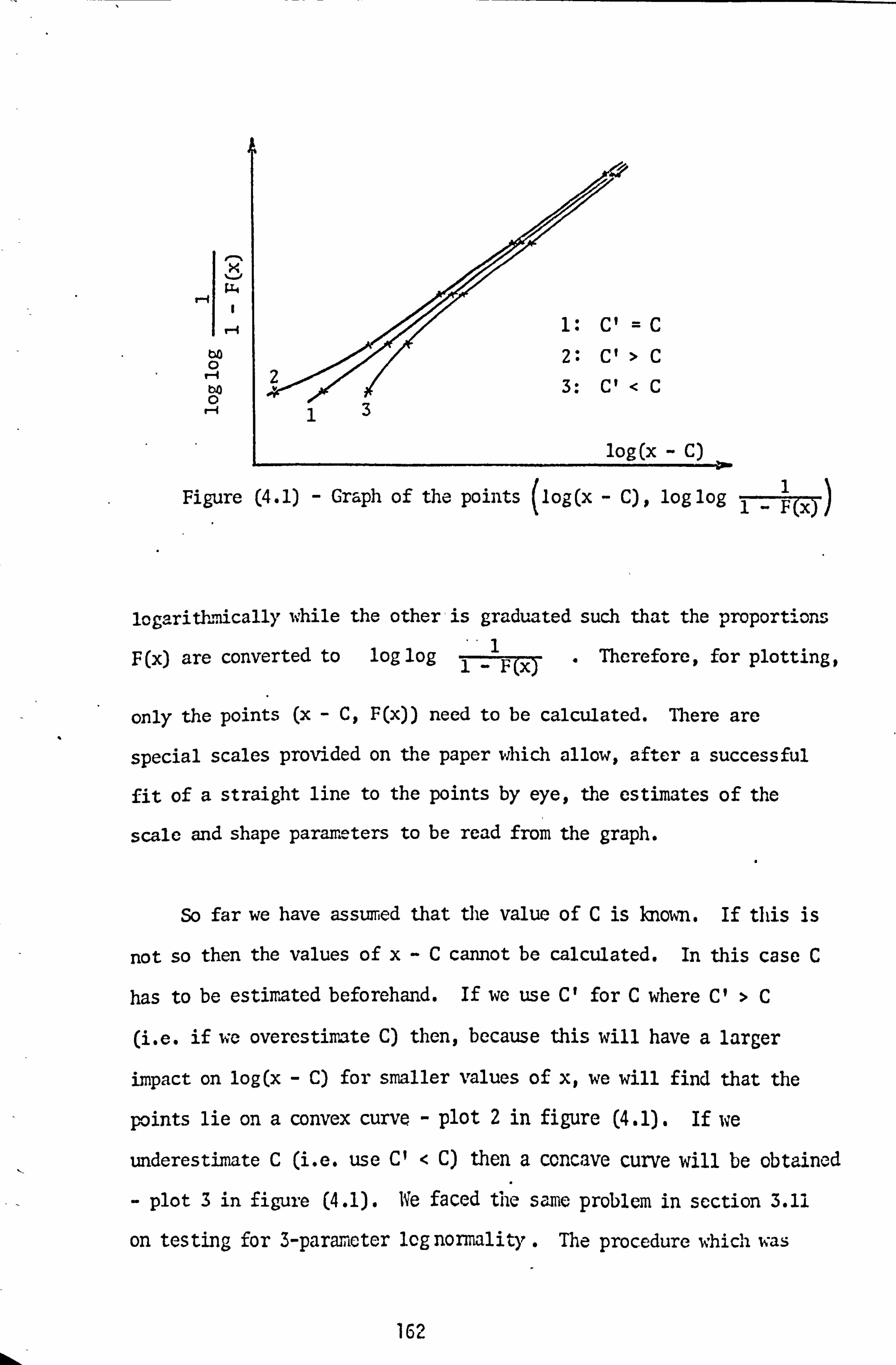
r4

bO 0 ho 0

r-i

=C

>C

<C

log (X - C)

Figure (4.1) - Graph of the points (log(x

- C), log log 1- F(x1)

logarithmically while the other is graduated such that the proportions

F(x) are converted to log log 1 _1F x. Therefore, for plotting,

only the points (x - C, F(x)) need to be calculated. There are

special scales provided on the paper which allow, after a successful

fit of a straight line to the points by eye, the estimates of the

scale and shape parameters to be read from the graph.

So far we have assumed that the value of C is known. If this is

not so then the values of x-C cannot be calculated. In this case C

has to be estimated beforehand. If we use Cl for C where Cl >C

(i. e. if we overestimate C) then, because this will have a larger

impact on log(x - C) for smaller values of x, we will find that the

points lie on a convex curve - plot 2 in figure (4.1). If we

underestimate C (i. e. use C' < C) then a concave curve will be obtained

plot 3 in figure (4.1). We faced the same problem in section 3.11

on testing for 3-parameter log normality The procedure which was

13

162

applied in that section can be adopted here. Therefore we try

various values of C and for each value plot the points

1 (log (x - C) , log log i_ `F;

X,. By observing the resulting

plots we decide on the best value of C which rectifies the points to

lie approximately on a straight line. If, in fact, such aC exists

then we can conclude that our sample is from a 3-parameter Weibull

population. If necessary, the parameters A and B can then be estimated,

as before, from the slope and intercept of the line.

The initial value of C to be tried always is C=0 which will

either indicate that the sample is from a 2-parameter Weibull population

or, alternatively, that by choosing C=0 we are underestimating or

overestimating C. If it indicates underestimation then the mdel will

involve a positive location parameter and its distribution function

can be expressed as

W(x; C, A, B) =1- exp L(XA C) B

(4.4-3)

If C=0 indicates overestimation then the model may involve a negative

location parameter. Hence, for the sake of avoiding the use of

negative values for parameter C, the model can be expressed as

W(x; -C, A, B) =1- exp [-( X+ C} BI

;C>0 (4.4-4) AJ

4.5 The Weibull Graphical 'Test ' on 'AD 'Data

We wrote the computer program P13 to use a sample of grouped

data, as input, and to plot the points (log(x

)-Cs log log g 1- x)

163

for various values of C. For each sarple of accidental dai-age data,

as presented in tables (1.1) to (1.7), values of C=0,10,15,20

and 25 were supplied to the program. For each C, the program then

calculated and plotted the resulting array of points. The graphs

for each of the seven samples of data are presented in figures

(4.2-a) and (4.2-b). It can be seen that for each sample, C=0

has produced a concave curve with a marked deviation from a straight

line in the lower values of x. Therefore C=0 has underestimated

the true value of C. On the other hand, for C= 25, for each sample,

a convex curve has been produced indicating an overestimation of C.

For each sample C= 10 also indicates an underestimation of C.

Therefore the true value of C, in each case, must lie between 10 to 25.

In fact it is apparent from the graphs that C= 15 or 20 are about the

best choice to make the array of points lie on a straight line.

There are slight deviations from the straight line in the upper tail

values for each sample. These are, as in the case of the lognormal

distribution, due to lack of sufficient observations in the long tail

of the sample histogram.

We feel justified that a 3-parameter Weibull model with a positive

location parameter C, in the range of 10 to 25, and cumulative

distribution function of the form (4.4-3) may be used to represent the

distribution of our accidental damage data.

We Imow that some policy holders do not claim for small amounts

because their no claim bonus is worth more than the amount they would

recover by a claim. Considering that our proposed Weibull model involves

terms of the form x-C we may interpret parameter C as the anount below which claims are not made.

164

Figure (4.2-a)

ps ,I lip ºfi

rr ri ID

RC jr,

RI. Y

X Il: C ºý

fY. vu

YNA RFC Ltý. ý. ýk-l') Q tr: "'Y-( 1 rj

31 Rrx: ) 67CI31 Ký 56 Eý ,"

KA"

R. I4D O

"OtOOR"fDO

.p -2.

Strotyht ta'a plot c. VUeULL Cis. : o- 5tra2 't LIAO plot CI' VEIS, L v.., io"

73.171, CCAPTFR CATA 71/IST CIA? "FR CA7A

0 c-ý o: Culp Cs'+t Ci t3

": cß[3 a. C-22

33 LOS( LO3(I . /C 1 . -FC x)))) LO3C LCCC I. /C 1 . -F(x))) )

ýn

ID

1ý

S S

i,

!L

mm LOS( x-c ) a 34 eise 5G789

Ioao

"1 as+o0

R"4DO -2 p

Str., p,. L, plot or Wr. IDLIL DIS. For 71,740 LUAPT(R DATA

C, Q

d: r... oil C IS

£: cýef Rý-....

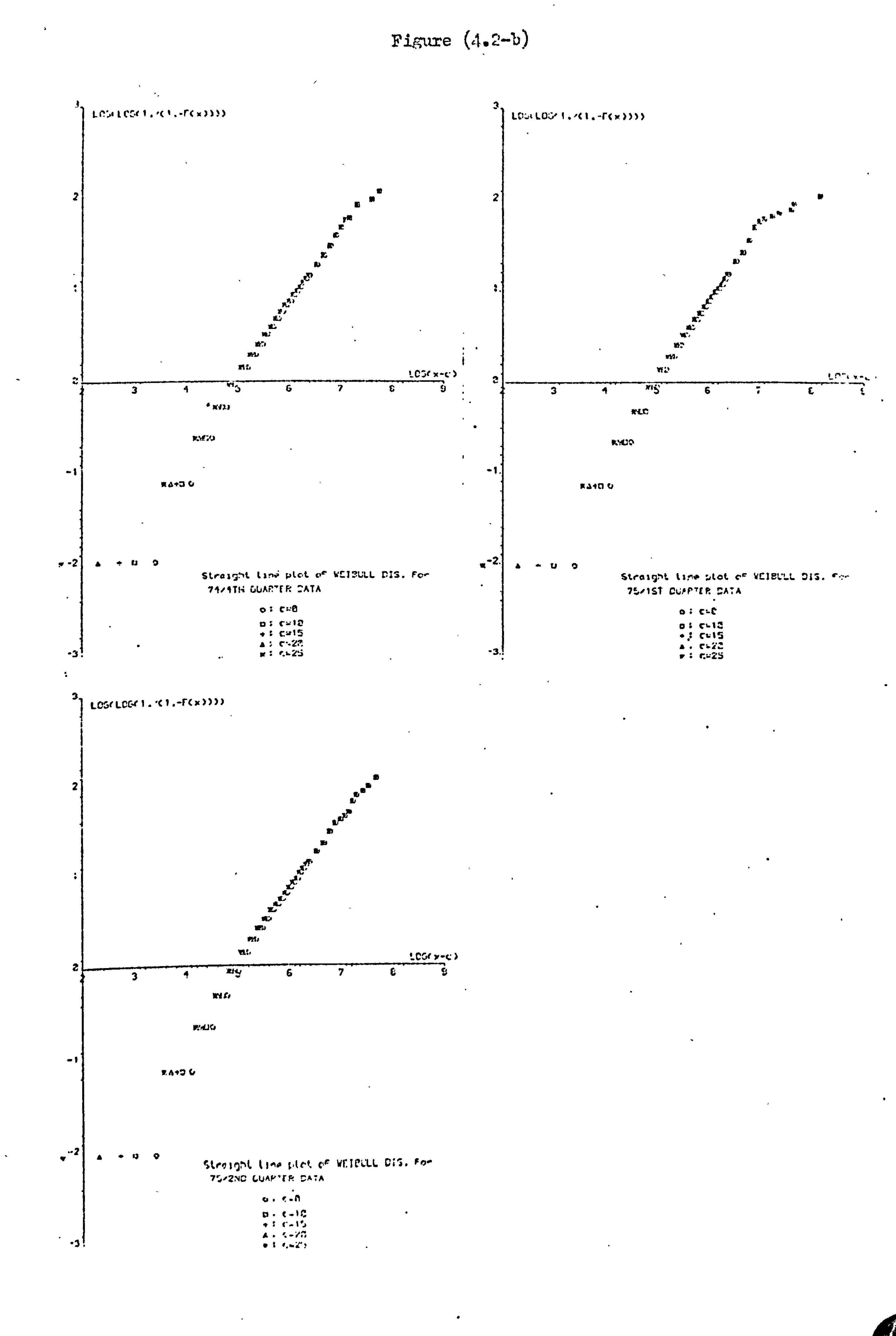
Figure (4.2-b)

3 1 L(, 'Lcs(I. "o. -r(., )

2e o 2

re e

c u

tiny

! C: i(x-c) 67C9;

Yin)

rxr: u

K d+0 4

3

. -2 "-ao SLravpt Land plot of YCI? ULL CIS. Fo-

74, ST14 LLAP FR _ATA

o: Cx"0 cwlo

": C+1S a: C "2?.

3

O 2

Oe v

O

F ti

X. 4

R7ý

R7i

d:.

2 Y+y 67C5 3ý

wit,

rdito

f. A+7 4

2f"UO

cit/91Qf+t t, Ae ;, tet C+S YC1PCLL Cs. fry'

7S' NC lUAF"FF: CATA

A "ý ""tß,. C7

wu 10

n

c c. W.

31 X's 6E,

ýrcr

MCI

Plain

"-su0 Straight tin. ;, tat c° vcleeu. 015.

7. OSi CiPP*ER pA; A

o: cle osc, %Z

c. s9

_3. a. c7. '. v C-25

4.6 Estimation of the Parameters of the leibull Distribution

The estimation problem for the Weibull distribution has been

dealt with by various authors. However, rast of the concentration

appears to have been on estimation from ungrouped data and for the 2-

parameter distribution. Kao (1956) considered the methods of least

squares and maximum likelihood for tmgrouped data when the scale

and shape parameters, A and B respectively, are unknown. In

addition, in Kao (1958) he dealt with estimation from grouped data, 2-

parameter case, by the methods of nnultinomial maximum likelihood

and minimum Chi-square.

The method of moments can be used which involves equating the firs:.

two (or three in the 3-parameter case) s Vle moments to their

corresponding population values and solving the resulting equations

for the unknown parameters. Dubey (1963) reports that he has found

" the asymptotic efficiencies for the roment estimators of the location

and scale parameters when the shape parameter is known. These, he

states, depend on the value of the shape parameter and are quite high

in some cases.

The method of quantiles may also be used for estimation. This

consists of equating two (or three in the 3-parameter case) sample

quantiles to their corresponding population values. Dubey (1967)

has applied this method for estimating parameters of the 2-parameter

distribution. He states that the 17 and 97% quantiles give an

estimate of the shape parameter which is asymptotically 66% efficient

when compared with the maximum likelihood estimator. The 40 and 82%

quantiles estimate the scale parameter with an asynptotic efficiency

of 82%.

165

A relatively quick and easy method of estimating the parameters

of the Weibull distribution is the graphical method which we explained

as part of the Weibull graphical test in section 4.4. This method

has been fully explored by Kao and we can, for example, rifer to

Kao (1959).

Haan and Beer (1967) deal with estimation from ungrouped data

by the ordinary maximum likelihood method for the 3-parameter Weibull.

In this case a system of equations involving powers of the unknown

parameters need to be solved iteratively.

When data only in grouped form is available the estimation problem

usually becomes more complicated. It is possible to assume that the

observations in every interval are concentrated at the mid-point of

that interval and hence use the estimation procedures for ungrouped

data. This assumption, cven when reasonably justified, results in

some loss of efficiency and may introduce certain biases in the

estimators. Therefore, as we showed in the 2-parameter lognormal

case, it is best to use methods which are directly suitable for

grouped data. Of these, the most efficient method is the multinomial

maximum likelihood. This, as we mentioned earlier, was considered

for the 2-parameter Weibull by Kao (1958). In the present work we

will extend this method to the case when all three parameters are

unknown. In addition, we will consider the method of least squares

and will propose a computing technique for estimating all three unknown

parameters.

Let us assume that we have a sample of grouped data where n inde-

pendent random observations on a random variable X (in cur case, the

claim amount) have been grouped according to their size into k mutually

exclusive intervals. Further, let ni be the number of obsertiaticns

166

(claims) in the class interval (xi_1 , xi) for i=1,2..., k such

that k

n= nl i=1

Also, let us assume that X has a 3-parameter Weibull distribution

with the cumulative distribution function of the form

W(x; C, A, B) =1- e{- (x

A C)B

x>C (4.6-1)

We define the sample empirical distribution function as

F(x) = the proportion of observations <x (4.6-2)

In. the following sections we shall use the above notation. Although

we will be considering the estimation problem of the 3-parameter

ti; Weibull distribution, the methods can be directly used for the 2-parameter

Weibull by putting C=0.

4.6.1 The Method of Least Squares

We showed in section 4.4 that if our sample is from a Weibull

population then the points (log (x1 - C), log log 1 -1F xi

)'

for i=1, ..., k-1 are expected to lie on the straight line

log log =B log(x - C) -B log A (4.6-3)

It should be noted that we cannot use xk because F(xk) =-1 and hence

will be ind3terninate.. To find the unknown parameters we 1-F (xk)

can use the least squares regression technique which consists of

167

(1

riinindsing SSD, the stur. of squares of deviations, where

k-1 SSD =

[log log 1 -F(x -B log(xi - C) +B log A (4.6-4)

i=1 i

simultaneously with respect to A, B and C. If we equate to zero the

partial derivatives of SSD, with respect to A, B and C, we will

produce a set of non-linear equations in the parameters which can be

solved, laboriously, by an iterative method. In addition, for this

purpose starting values for the parameters need to be obtained by

a-quick method of estimation, say, the graphical.

We instead suggest using the computing technique which we proposed for

the 3-parameter lognormal distribution in 3.12.1.

Let Vi = log log 1-F () and U1 = log (xi - C) . i

If C was known, or was fixed, to be equal to Co, say, then the points

(Ui, V1) would be coiapletely determined from the sample. Hence a

straight line, say

V= all +b (4.6-5)

could be fitted by the least squares regression technique with values

of a and b calculated from (3.7-24) and (3.7-25) of chapter 3. The

estimates, of the unknown parameters A and B would then be

B=a (4.6-6)

and � A= exp (- ä) (4.6-7)

Because the value of C is unknown our computing procedure,

described fully in section 3.12.1, is to find directly the minimum

value of SSD simultaneously with respect to C, A and B. For this

purpose we fix C, systematically, at different values and for each

168

value estimate A and B. according to the previous paragraph, and find

their corresponding value of SSD from equation (4.6-4). Hence we find

that value of C, with the required degree of accuracy, and its

corresponding parameters A and B which give the miniwarm value of

SSD. These values of A, B and C are the least squares estimates of

the Weibull parameters. Notice that for this procedure we do not

require anv starting values for the parameters. The procedure when

programmed on the computer is very fast (depending on the required

degree of accuracy) and easy to use on the interactive terminals.

4.6.2 Multinomial Maximum Likelihood Method

This method was previously considered for the lognormal distribution

in section 3.7.7. Here we will give the loglikelihood function for

the 3-parameter Weibull distribution. The computing technique to

find the estimates of the parameters, by maximizing the loglikelihood

is that described in section 3.7.7.

Let us assume that we have a sample of grouped data as defined in

section 4.6. Let pi be the probability that an observation (claim)

occurs in the interval (xi_1, xi). Adopting the notation of 4.6, we

have.

pi = W(xi; C, A, B) - W(xi_1; C, A, B)

for i=2,3, ... ,k

and

pl = W(xl; C, A, B) - {V(C; C, A, B)

Using (4.2--1) we have

cB xi_CB Pi. = exp -

(~l, -lA exp -) -A

for i. = 2,3, ... ,k 169

and xlC

B

p1 - 1-eýL A-

The likelihood function of the sample is proportional, to L where ,k ni

L=i pi

and the loglikelihood function, log L, is

k log L= nl log pi

i=1

xl -CB = nl {1 - exp

B x. -Ck C_e1 (4.6-8)

i=2 CA) ICCA )B1} i=2

The maximum likelihood estimates of the parameters are obtained by

simultaneously maximizing log L with respect to A, B and C. The

computing procedure of section 3.7.7. requires starting values for the

parameters. The least squares, or some other, estimates of A, B and C

may be used for this purpose.

4.7 Application of the Weibull Model to the AD Data

We wrote computer program P14 for estimating the parameters of the

Weibull distribution, by the least squares method, from a sample of

grouped data. This program mas run with samples of accidental damage

data as presented in tables (1.1) to (1.7). For each sample first

C=0 (i. e. the 2-parameter Weibull) was tried. The program provided

estimates of the parameters., A and B, as well as an extensive table of 2

results. The Chi-square statistic, X, was calculated by the program

170

as a measure of agreement between the fitted model and actual sample

values. A sui ry of the results is presented as part of table (4.1).

It is apparent that A has increased over time while B is, approximately 2

constant, about 0.9. Me X statistics are large for all the samples,

hence indicating a general disagreement between the model and actual

sample values. Examination of the components of the Chi-square

statistics showed that very large contributions are made by a. small

number of the intervals in the lower tail of the distribution.

For each sample, the 3-parameter distribution was then fitted by

finding the optimum value of C as described in section 4.6.1. The

results are summarized in table (4.2). It can be seen that estimates

of C, the anaunt below which claims are not made, is about 120. The

values of A and C have generally increased over time. Because the

mean and standard deviation of the Weibull distribution are functions

of all three parameters, they showed an increasing trend over time as

well. The Chi-square statistics are considerably smaller than in the

2-parameter case. However, they still indicate highly significant

differences between the model and actual sample values. Again the 2

major contributions to X values are from 2 or 3 of the intervals only.

The total expected loss statistics are relatively small as indicated

by R, the ratio of T to total actual cost of claims. Therefore, the

3-parameter Weibull distribution provides a better fit, in terms of 2

the X statistic, to the actual data.

To see how closely the least squares line fits the sample points

the computer program P15 was written to plot them. The graphs for

the accidental damage data arc presented in figures (4.3-a) and (4.3-b). 2

Despite the large values of the X statistic we observe that the

sample points lie very closely on the least squares line. This, of

171

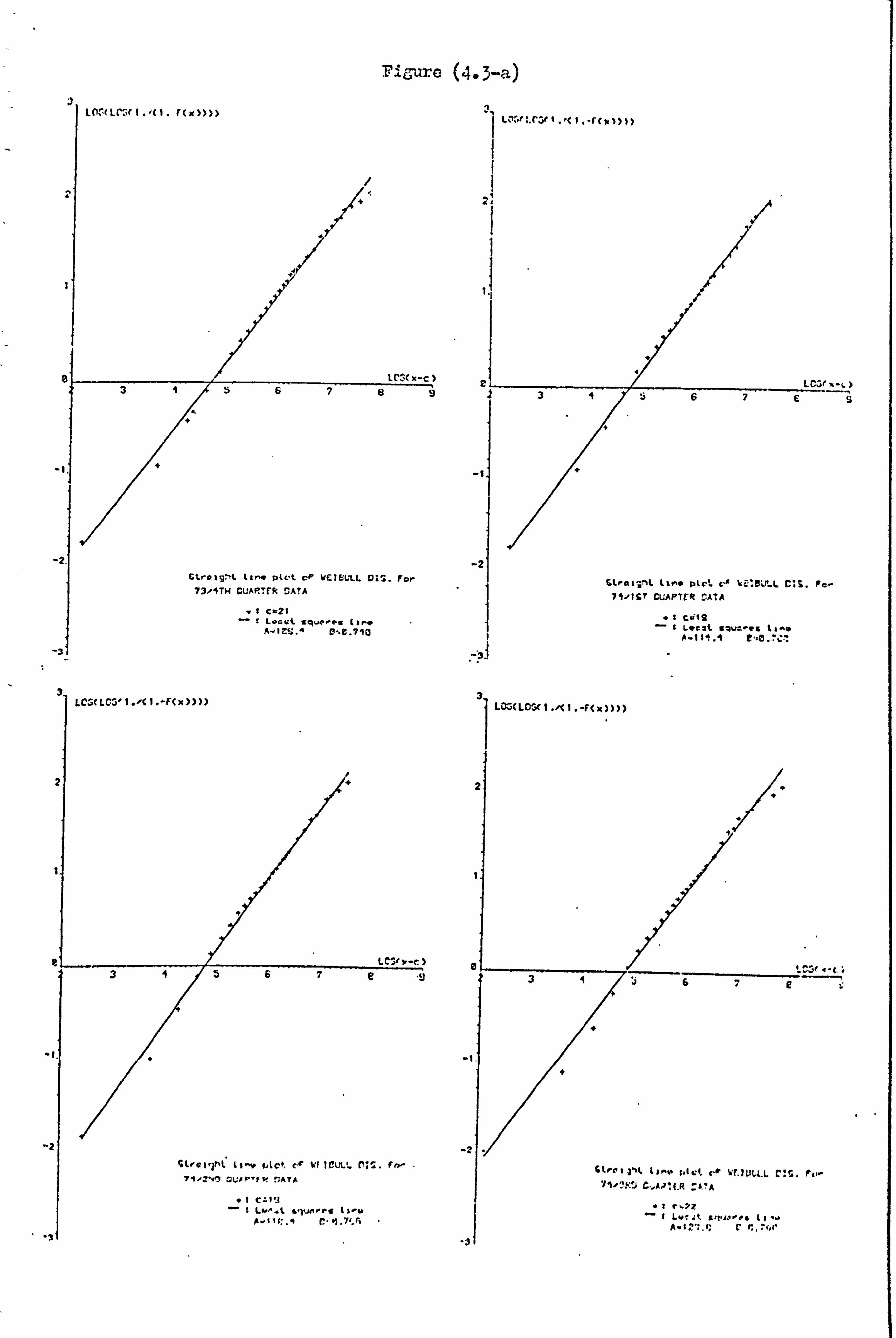
Figure (4.3-a)

LO: t LCS(I ., (I . ºt x»))>

i 1&iirc (4.3-b)

course, was expected from the graphical test which we carried out

previously.

We next wrote computer program P16 to estimate the parameters of

the 2-parameter Weibull distribution by multinomial maximum likelihood

(IiIL) method in order to see how the results compare with those of the

least squares method. For each of the accidental damage samples the

least squares estimates of A and B were used as starting values for

the iteration process. A summary of results is presented as part of

table (4.1). We can see that the estimates of A are very nearly the

same as their corresponding values by the least squares method but the

values of B are slightly larger. The Chi-square values, however, are

considerably smaller even when the slightly smaller degrees of freedom

are allowed for. The required pooling of the intervals, in the upper 2

tail of the distribution, for the calculation of the X statistics

were different from those of the least squares method. This resulted

in the difference in degrees of freedom. The ? C2 statistics, as

before, show significant differences between the model and actual

sample values. Based on the Chi-square goodness of fit test it is

observed that the 2-parameter Weibull distribution does not provide a

satisfactory model for the distribution of accidental damage claim

amounts. 0'

Computer program P17 was written to estimate the parameters of

the 3-parameter Veibull distribution by DfiIL method. For accidental

damage samples, the least squares estimates of the parameters A, B and

C, as given in table (4.2), were used as starting values for the iteration

process. For each sample the progr= prints estimates of the parameters,

the mean and the standard deviation of the fitted distribution of

172

claim amounts and also an extensive table which, for each interval,

provides the actual, the expected and the actual minus expected

number of claims as well as the expected loss and the contribution to

the Chi-square statistic (for those intervals where the expected

number is greater than 5). The results for the accidental damage

samples are presented in tables (4.3) to (4.9). The estimates of C

are about 15 and the estimates of A are smaller than their corresponding

values by the least squares method. The values of A, the estimates of 2

A, have generally increased over time. The X statistics are smaller

than their corresponding values by the least squares method. However,

they still indicate significant differences between the model and the

actual sample values. The major contribution to the Chi-square

statistic is from few intervals only. Otherwise the agreement in most

of the intervals is satisfactory. The total expected loss statistics

are small and in every case are less than It of the total actual cost.

The estimates of B are smaller than 1 for each of the sairples. This

means that the 1eibull frequency curve resembles the exponential

curve, but with a longer tail, and has no mode. Therefore, the model

ignores the distinct mode of the histograms of the accidental damage

data.

To see how closely the frequency curve of the 3-parameter Weibull

rmdel agrees with the histogram of the sample values we modified

computer program P7 to plot them. The graphs are presented in

figures (4.4.1) to (4.4.7). In each case the exponential shape of the

curve, with no mode, is observed and the tail of the curve is seen to

be shorter than the tail of the histogram. Large deviation between

the curve and the histogram can be observed at several intervals. This

could, of course, be expected. by looking at the large values of actual

173

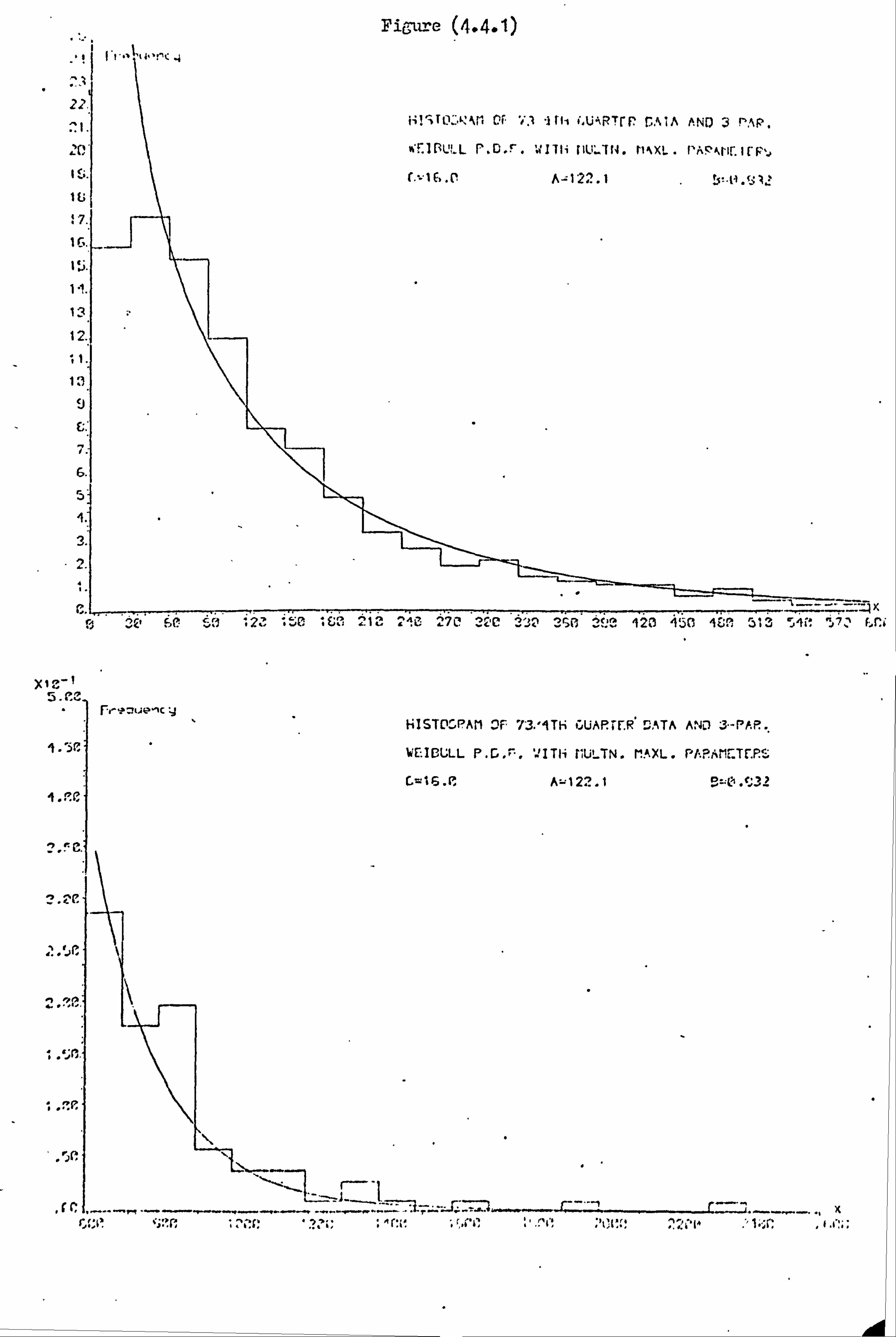
Firm e (4.4.1)

: ': ate. %l 2C'C ý30,2i13 3f: 2 I2ä1 450 iLý. 'ý : 1Sv

Xý4't

"ý, n(

i

7 7ý

i" Jý

r". Io

&TOGPAN OF 73. '9TH GUAPTr.. R DATA AND 3"-PAP.

[BULL J'ITH 11UL TN. rIAXL. P/. PAME P. E'

16. V A-122.1 $ý14A, '32

r-j

Nl;

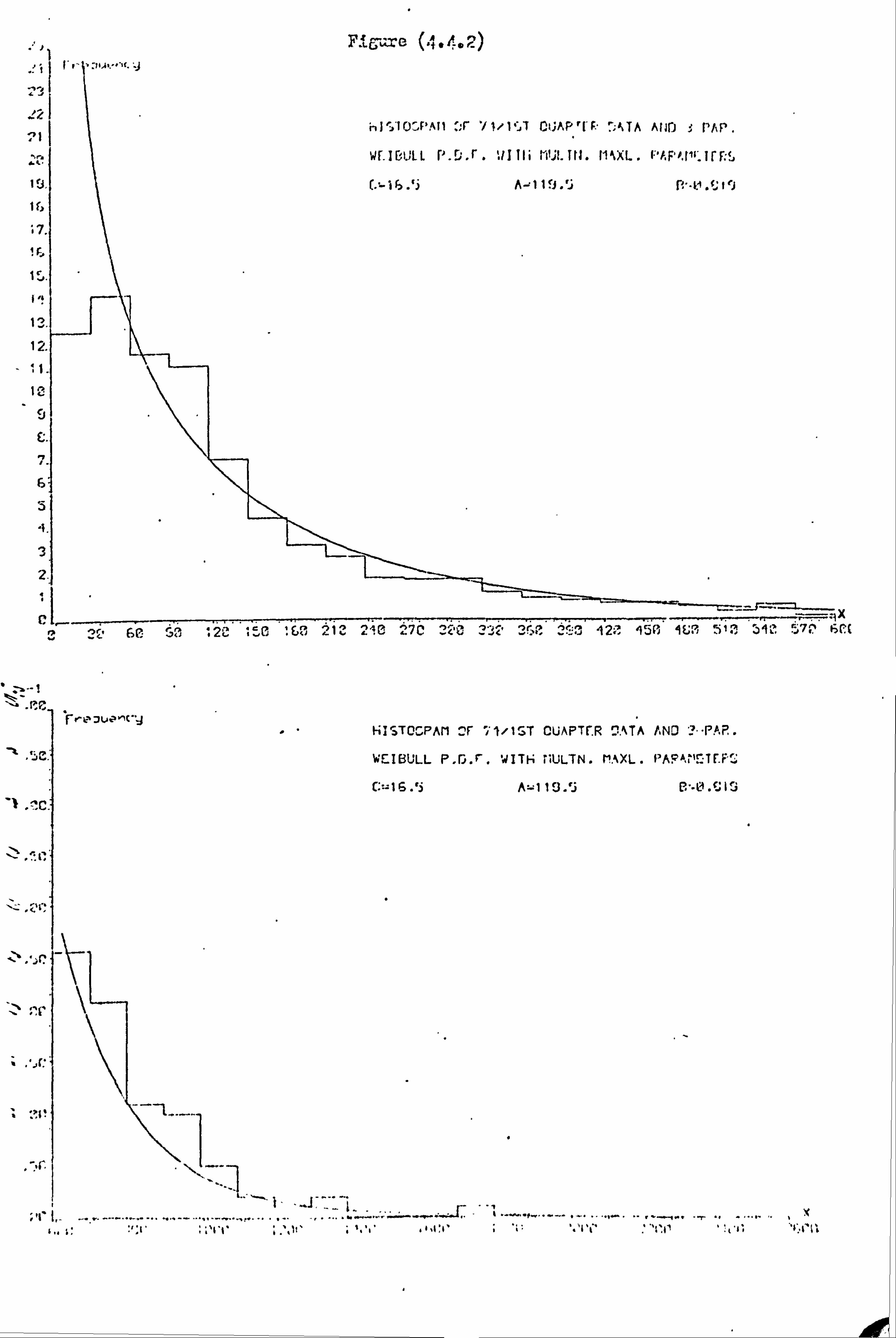
FI. g zre (+. A. 2)

v ýrý " .e.. C ". n°2' 2Z `"3' 2Cn 2SI r2 ýý

°C 6(? . ý<, 12 nC , 60,1. c ý. . "_. ý 92.. ýiJß 91; 5 59C 70 h('f

CJ IISTOGPAI1 OF i1/1ST CLAPTC. R PTA AND ? «PAR.

w. r. IBULL P. G. r. WITH TIULTN. f?. AXL. PAF-4-NE7F. Ks

C. - 16 . °i A-119. `3 E? '-0. tjIG

.. i: . 1' . 't'1'1ý

ý", ', lt' . ý. 'ý' . ý. taý .. i"

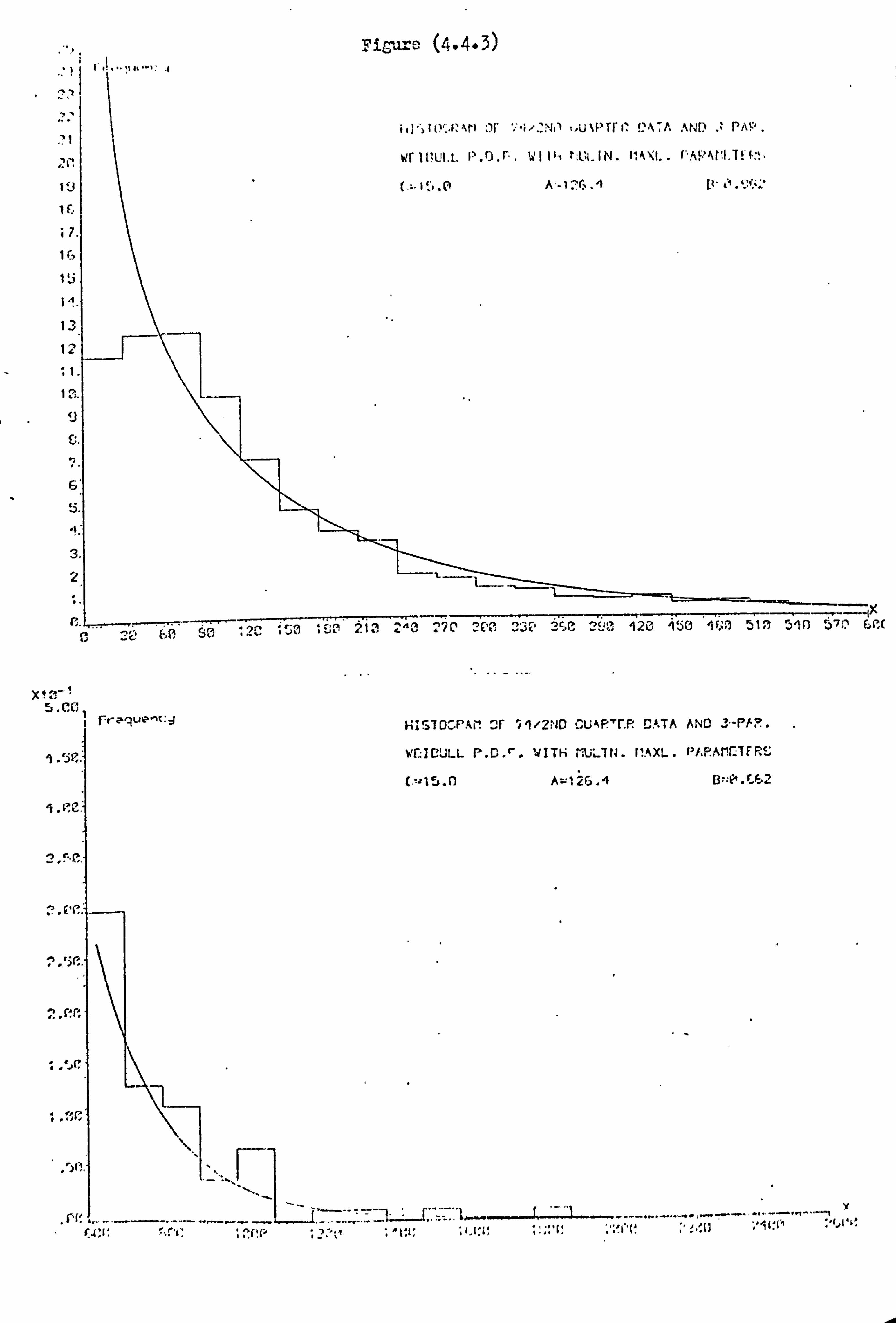
,^Z

7t

t:. 1

I £-

i7.

1r.

tj

t. 1

13

12

t?.

1

iý (4.4.3)

i. l ,io, - mo 7-i , -'Nt l :, U %fI Tr ' ! \A AN[) ., PAS' .

writ, uu. i. r) " r, WI 11-s rVt_ IN. I XI.. 1 . k4'Aftl-T ! J, ̀

iJi', i

i:. i ä? " Aý ý^

..

"'ýý. ve i27

s" f. nrJ r7n ;o

;? a, ý 2i3 . ýc _CIO sý , 120 150 'i ;I 51 10 Jfc

F. Uk, -j HISTOCF'AM or 112P4D CU NPTC. R DATA AND 3 -PFD .

W'GIDULL P. D. '. WITH MULTN. i'.. AXL. PP. P. Allf-M .:. '

A=12G. 4 B: CA . F. P, 2

i. Jr

1

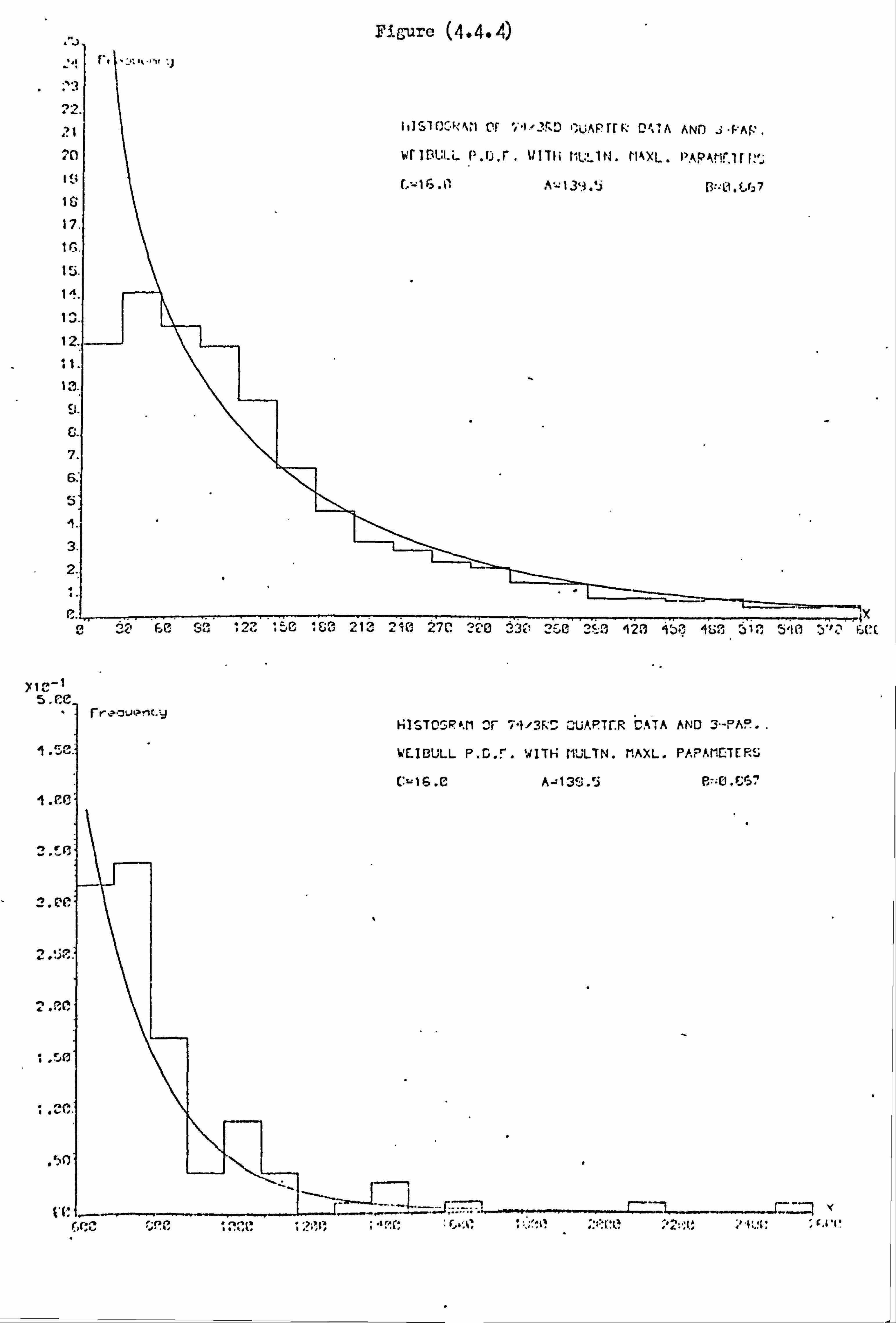
F1 ure (4.4.4)

:1 1ý151Cc i or , UAPrf 0'-'A AND j-PAP.

M WCISULL Pr . 111111 Mt2_1N, NkXL. PAPhrlr. 1rl';

13. I ß:: lß. ýºý7

17.

1r.

I; i.

1 '.

13.

12. 11.

C

7.

6.

5

3.

2.

.. ý'ý 6 (: SO .:.... 2Z ., 1.50 S£i3 .,.. 2121 2tCi 27C

ý '22c. © 33rC" ý C' `c e 0c.: '1 120 9)3 ISO ., "J. 5,10 1"

., _ 5''t Fj('(

X1c'1 5. ýI

2 . ß(

IX

. rIi

aK c. il' (rC. a. "ý" ý;

ý i. f. ý ?: 1, .. '.....

, ý: i 1. .

"a. l .c "'. l. r 4... 'l

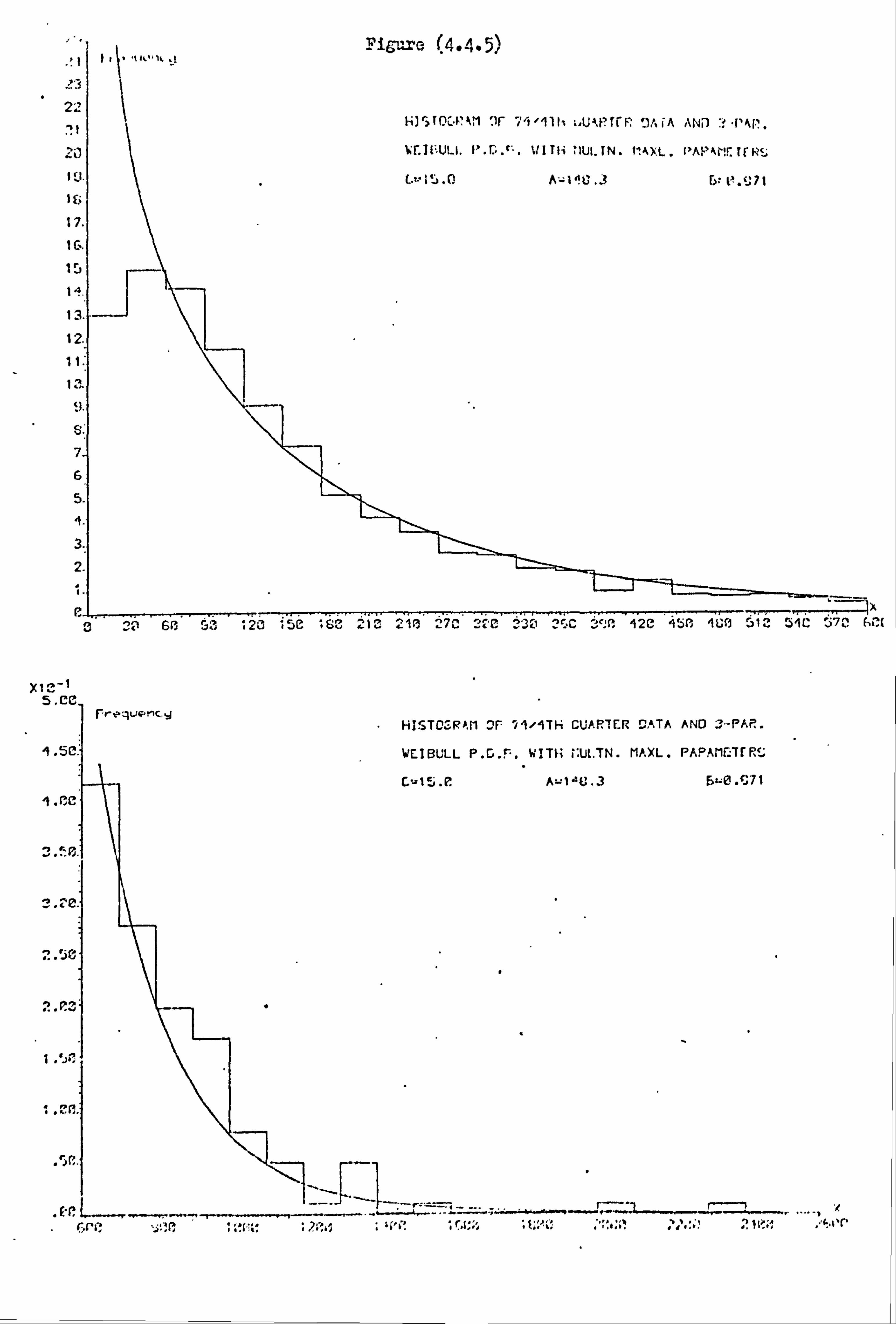
22 ý1

17.

! 6. 15

F 13.

12.

1 1:

: l.

7-

6

5.

2.

0 219 60

Fig=c- (P4.4.5)

F+3' T(XF'Ml 1(' 7, '11li :. U1'tri 'JAiA AND :' ('AP.

Kf. 1i'-"Ul. l. f'X. c'". WITH *, IUI. IN. T'. AXL. "APNP! L1fh! ý;

GL 1`:. Q A=; I! U. 3 G: l`. `,, 71

121ýi IJt+ Ip4 2%3 4113 27C 2M ? 30 2 SC ýý:

Jf 12C 1151! -10 512 54C 57C

HISTO R/. M VF li/9TH CUA. P. TER DATA AND 3--PAP.

WEIBULL P. G. r. WITH i-UI. TN. MAXL. PAPAMFTrR'C-15.

P. A-14U. 3 F y-O X71

; E:: '"i'r 2 }t? '; .. 'r .c., .,.. _.. _.,. r.. -

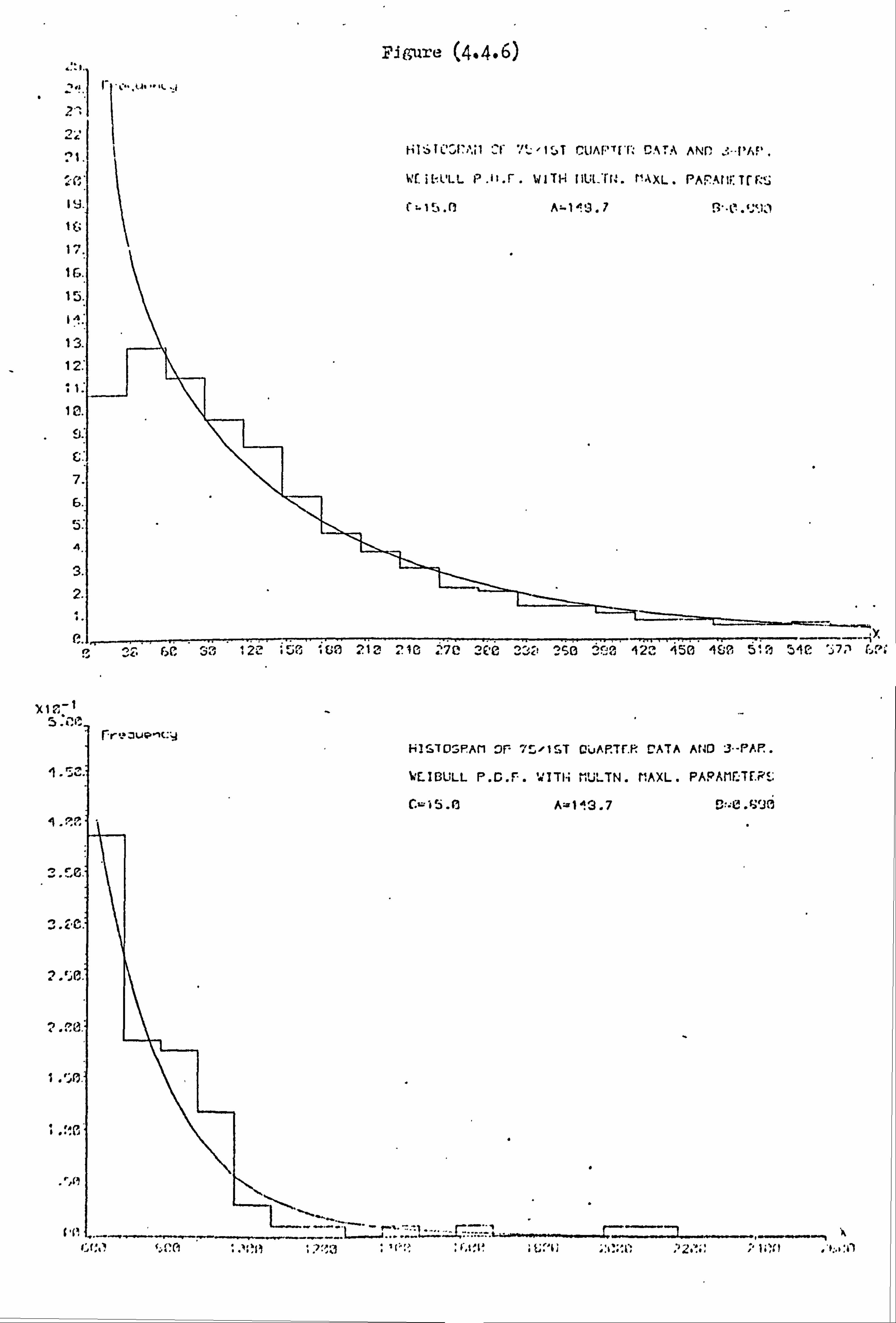
Figure (4.4.6)

HISIC317, 'al :f %L"It T CUAPT['I'. ' CA ANR . -I'AF'

WEUfULL PJ'. F. WITH 111JR-TI4. M"\XL. PArA[Ii: Tr&:;

A=1"9.7 3 "l'". '. `. il l f:

1 7.

16.

1 J.

1 ý.

13.

6.

7.

6.

5:

4.

3.

!, 2F" fiC 33 124 '5 , EUO 210 210 270 2CC 3. Z2 250 2C2 `12: 1i50 4C 5': 9 51CI ý7ý L-Pt

X1?, -1

F

i. ýý.

? ...

I . iii.

F4ISTD', FAft OP '., I1 ST C AP. Tf. F. L'ATA AND "3"-PAP..

%CIBULL P. G. F. '«ITI"i , ', j'-TN. f1AXL. PAPAMF. TE. F

C-15.93 A-113.7 Sl ýlLA . ý`Jfý

7k:: 'tl ;: ý:; a; : '2. '::: tt'tt . 'ý. ýal

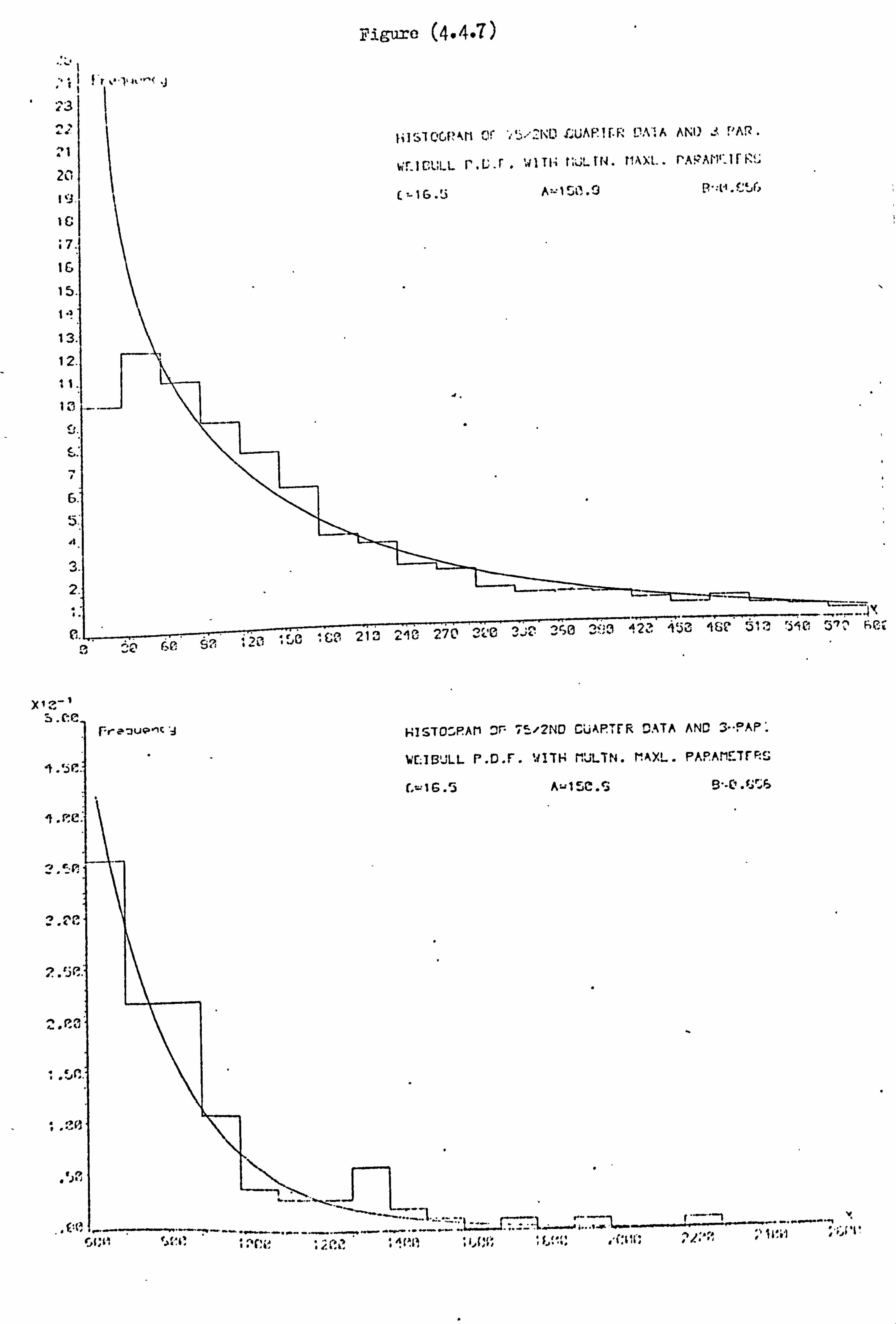
riguxe (4.4.7)

Y , C: r

r'{, H

CUAP. TFR DATA AND 3"-PAP:

MON. h'AY. L. PAPAt1;: TFFs

5C. 3 S"-Cl. t,: 6

i i: i {iýlý ý"iý{. '.

NT f

minus expected frequencies in the tables. It can be noticed that

the frequency curve fits the sample histogram rather well in the

middle but not at the tail values. The agreement between the frequency

curve of the model and the histogram of the data is not satisfactory

for any of the samples.

From the above analysis we can conclude that the Weibull

distribution does not provide an adequate mdel for the distribution

of the accidental damage claim amounts.

174

4.8 The Effects cif ' Iriflatiori *ft, * the Parameters of the Weibull. Model

Following the argument of chapter 3 about the effects of inflation

on the ; arameters of a model, it is considered important to study these

effects theoretically for the Weibull distribution. We will need to

allow for such effects when predicting the future distribution of

claim amounts for a class of general insurance business in which the

Weibull yodel has been found to represent the distribution of claim

amounts.

Let us again assume that the effect of inflation is to increase

a claim of amount X to X(1 + i) over a period where i is the effective

rate of inflation for that period. If X is distributed as a 2-

parameter Weibull with distribution function V, (x; A, B) then by a

transformation of variables we can show that Z= X(1 + i) is distributed

as a Weibull W(z; Ag, B) where g=1+i.

If X has a 3-parameter Weibull distribution, W(x; C, A, B), then again

by a transformation we can show that Z= X(1 + i) is distributed as

W(z; Cg, Ag, B). Therefore inflation increases the parameters C and

A but leaves the shape parameter B unchanged. The mean and the

standard deviation of the Weibull distribution are functions of all

three parameters and hence both increase over time due to inflation.

Although it has been found that the Weibull model is not completely

adequate for the distribution of accidental damage claim amounts,

nevertheless the increasing trends of C and A can be observed from the

tables of results.

Since the 11eibull is not a very satisfactory model for our data

we do not use it to predict the distribution of claim am is during

future periods.

175

4.9 Conclusions

The 2 and 3 parameter ý`'eibull distributions were studied in this

chapter as models for the distribution of claim amounts in general

insurance and in particular for the accidental damage claim amounts.

The Weibull distribution has been regarded as a more flexible model than

the exponential distribution and hence its use in various classes of

general insurance, where the latter has been successfully applied, is

recommended. An interpretation was offered for parameter C as the

amount below which claims were not made. The multinomial maximum

likelihood method is preferred to the least squares method for

estimating the parameters of the Weibull distribution since the former

method produced smaller Chi-square statistics and hence a better

agreement between the model and actual sample values. The 3-parameter

distribution represents our accidental damage data better than the

2-parameter distribution when judged by the Chi-square goodness-of-

fit test. i-bwever, even the 3-parameter model does not satisfactorily

represent the distribution of accidental damage claim amounts. This

was indicated by the significant differences between the nadel and the

actual sample values as judged by the values of X2. The value of the

shape parameter B was found to be less than 1 which indicates that

the model has an exponential-like shape with no mode. Hence the model

ignored the distinct mode which is observed in the histograms of our

sample values. It was observed that for each sample the frequency

curve of the model had a shorter tail than the histogram of the data.

The inflation was shown to affect the location and scale parameters,

C and A respectively, but to leave the shape pur, :, eter, B, unchanged. The effect of inflation in increasing C over time is plausible as it

is expected that with inflation the amount below which clams are not

made should be increased.

176

We may note down in conclusion that the 3-parameter Iveibull

nadel was riot found to be as adequate as the 3-parameter lognormal

model in -representing the distribution of our, accidental damage claim

antunts.

4.10 Tables

177

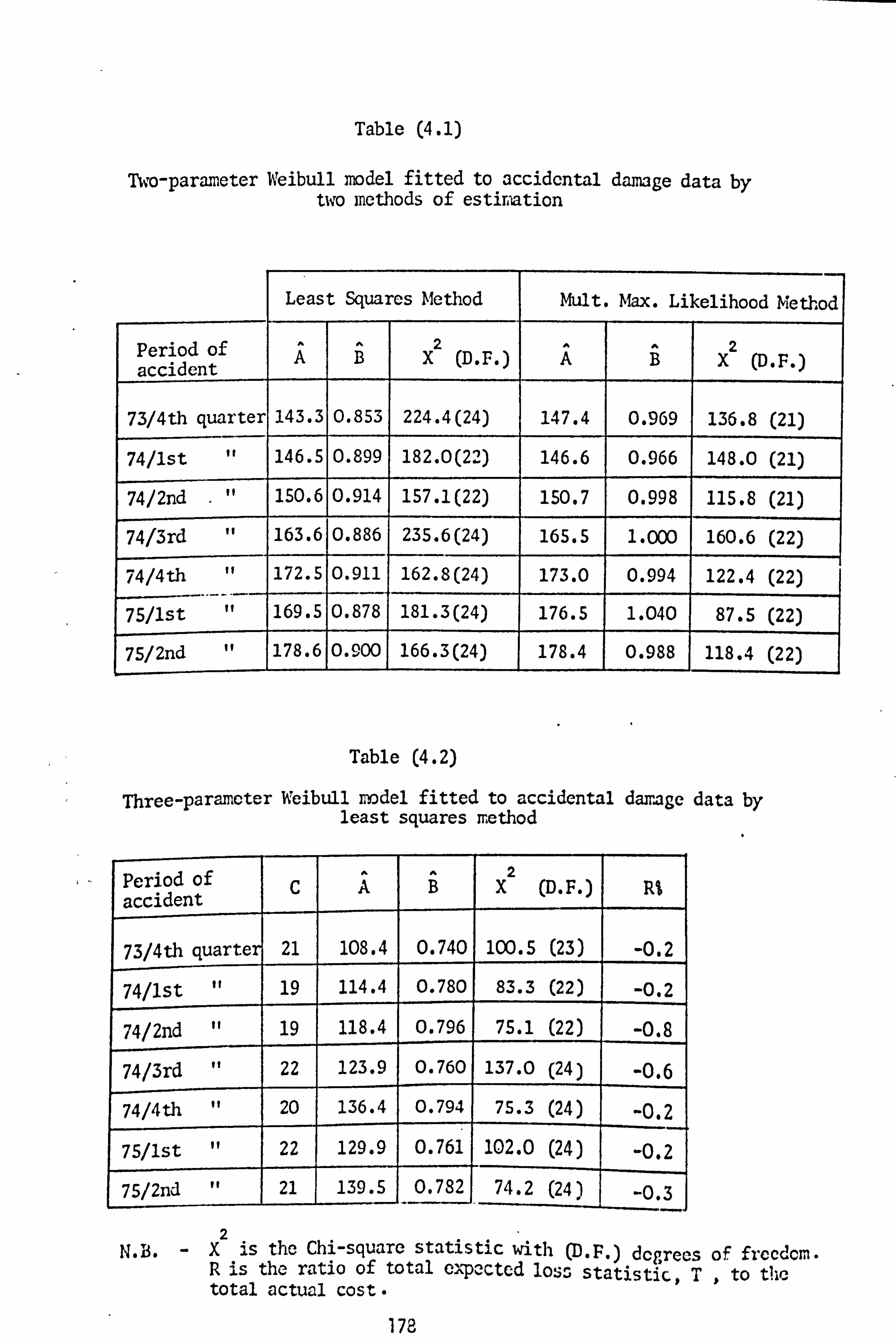
Table (4.1)

Two-parameter Weibull model fitted to accidental damage data by two methods of estivation

Least Squares Method Mult. Max. Likelihood Method

Period of accident

A B X2 (D. F. ) A B X2 (D. F. )

73/4th quarter 143.3 0.853 224.4(24) 147.4 0.969 136.8 (21)

74/1st 146.5 0.899 182.0(22) 146.6 0.966 148.0 (21)

74/2nd " 150.6 0.914 157.1(22) 150.7 0.998 115.8 (21)

74/3rd " 163.6 0.886 235.6(24) 165.5 1.000 160.6 (22)

74/4th " 172.5 0.911 162.8(24) 173.0 0.994 122.4 (22)

75/1st 169.5 0.878 181.3(24) 176.5 1.040 87.5 (22)

75/2nd " 178.6 0.900 166.3(24)_ 1 178.4 0.988 118.4 (22)

Table (4.2)

Three-parameter h'eibull m del fitted to accidental damage data by least squares method

Period of accident

C A B 2

X (D. F. ) R%

73/4th quarter 21 108.4 0.740 100.5 (23) -0.2

74/1st " 19 114.4 0.780 83.3 (22) -0.2

74/2nd " 19 118.4 0.796 75.1 (22) -0.8

74/3rd 22 123.9 0.760 137.0 (24)_ _-0.6

74/4th " 20 136.4 0.794 75.3 (24) -0.2

75/1st " 22 129.9 0.761 102.0 (24) -0.2

75/2nd 21 139.5 0.782 74.2 (24) -0,3

i N. B. -X is the Chi-square statistic with (D. P. ) degrees of frecdcm.

R is the ratio of total expected loss statistic, T, to the total actual cost.

178

Table (4-3.1).

1! ### 3-PARAMETER WEIBULL DIS.

73/4TH QUARTER DATA

ES TIMATION BY MULTINOMI AL &'AX. LIKELI HOOD METHOD ; - C= 15.73 A= 1 22.088 f3= 0.832

MEAN= 150,349 S. D .= 162,617

-AMOUNT £ ACTUAL EXPECTED ACTUAL- EXPECTED CL. NO. CL. NO. EXPECTED LOSS (A-E)**2/E

1- 30 478. "482", -4. -62. 0.033 31- 60 518. 590, -72. -3276. 8.786 61- 911 461. 407. 54. 4077. 7.165 91- 120. 359. 304. 55, 5802. 9.951

121- 150 239. 234. 678. 0.107 151- 180 213. 184. 29, 4799. 4.571 181- 210 148, 147, 195. 0.007'" 211"- 240

, 102. 119. -3833. 2.429

241- 270 .

81. 96. -15. -3832. 2.344 271- 300 58. 79. -21. -5995. 5.582

"301- 330 66. ,

65, 1. 316. 0.015 331- 360 45. 54. -9. -3109. 1,500 361- 390 39.. 45. -6. -2253. 0.800 391- 420 35. 37.. -2. -611. 0 108 421- 450 34. 31. '1306. .

0.290 451- 480 20. 2.6. -6. -2793. 1.385 481- 510 29. 22. 7. 3468, 2.227

_511- 540 14. . 18. -4. -2102. 0.889 541- 570 8. 15. -7. -3888. 3.267 571- 600 9. 13. -4. -2.342'. 1,231 601- 700 29. 31. -2. -1301. 0,129 701- E300

_ 18. 18' 0. 0, 01000

801- 900 20. 11. 9. 7654, 7.364 901-1000 6. 6. 0. 0. 0.000

1001-1100 4, 4. 0, 0l I 1101-1200 4. 2. 2. 2301. 0,000

. 1201-1300 1. 1. 0. 0. 1301-1400 3. 1. 2. 2701. 1401-1500 1. 1. 0, 0. 1501-i609 0. 0. 0. 0. 1601-1700 1. 0. 1, 1650.. 1701-1800. 0. 0. 0, 0. 1801-1900 0. 0. 0. 0. 1901-2000 1, 0. 1. 1950. 2001-2100 0. 0. 0. 0. 2101-2200 0. 0. . 0, 0. 2201-2300 o. . 0. 0. 0. 2301-2400 1. 0, 1. 2350.

---------- ------------ -------- -------------- ----------- . 9.600 TCOTAL. 3045. 3043. 3651. --- -

. D. F. =22 TOTAL EXP. LOSS Y < 0.001

--------------- =. 0ý8 ,o TOTAL ACT, CnST -

179

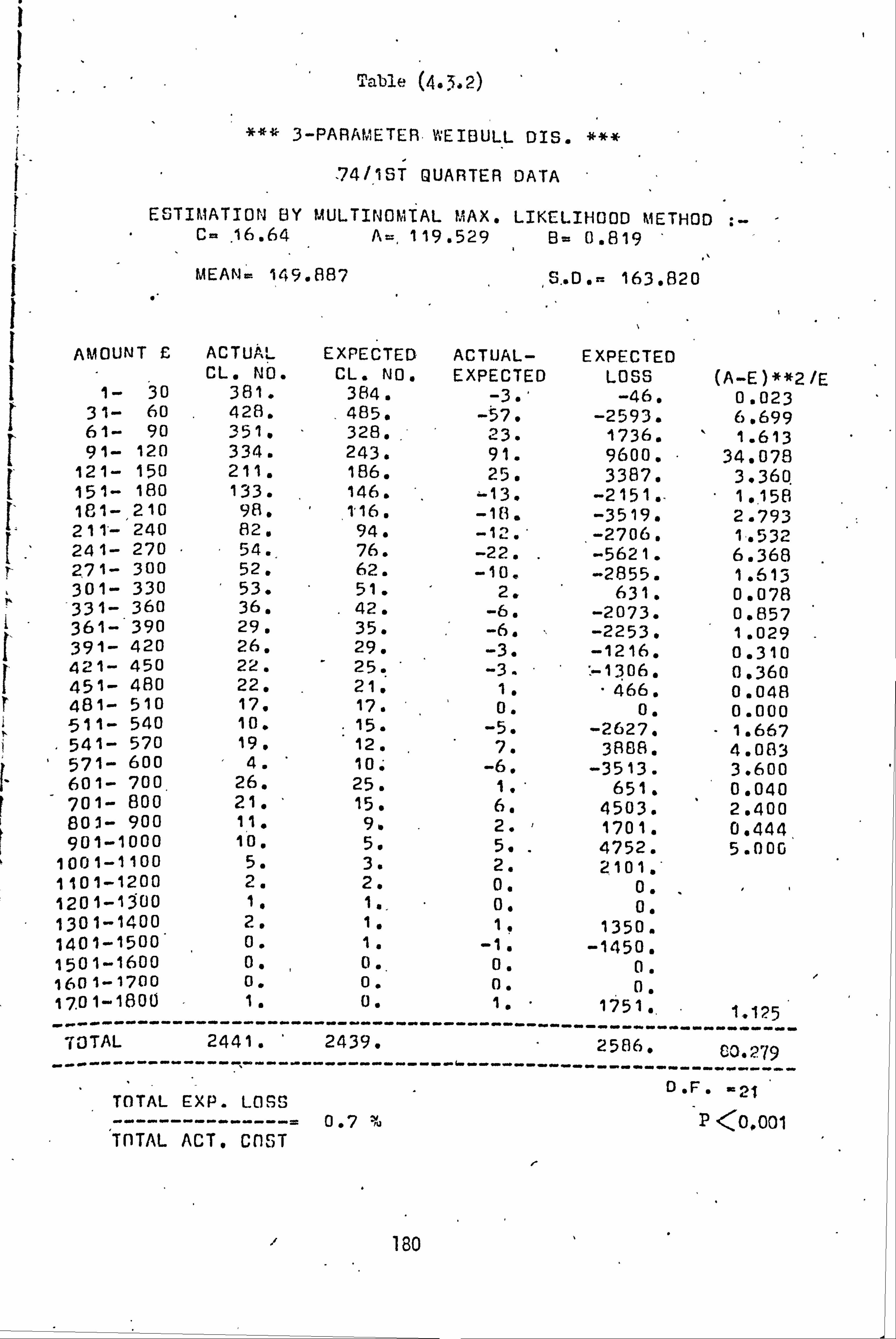
Table (4.5,2)

3-PARAMETER. WEI©ULL DIS. #**

14/16T QUARTER DATA

ESTIMATION BY MULTINOMIAL MAX. LIKELIHOOD METHOD t- C- . 16.64 A=, 119.529 B= 0.819

MEAN= 149.887 5.. D. - 163.820

AMOUNT £ ACTUAL EXPECTED ACTUAL- EXPECTED CL. NO. CL. NO. EXPECTED LOSS (A-E)**2/E

1- 30 381. 384. -3. ' -46. 0.023 31- 60 428.

. 485. -57. -2593. 6.699 61- 90 351. 328.. - 23. 1736. 1.613 91- 120 334. 243. 91. 9600. 34,078

121- 150 211. 186. 25. 3387. 3.360 151- 180 133. 146. '. -13. -2151.. 158 1. 181-, 210 98. 1.16. -18. -3519. , 2.793 211- 240 82. 94. -12. ' -2706. 1.532 241- 270 54. 76. -22. -5621. 6.368 2,71- 300 52. 62. -10. -2855. 1.613 301- 330 53. 51. 2. 631. 0.078 331- 360 36. 42. -6. -2073. 0.857 361- 390 29. 35. -6. -2253. 1.029 391- 420 26. 29. -3. -1216. 0.310 421- 450 22. 25. -3, '-1306. 0.360 451- 480 22. 21. 1. -466. 0.048 481- 510 17. 17. ' 0. 0. 0.000 , 511- 540 10. 15. -5. -2627. 1.667 541- 570 19. 12. 7. 3868. 4.083 571- 600 " 4. 10. -6. -3513. 3.600 601- 700, 26. 25. 1. ' 651. 0.040 701- 800 21. ' 15. 6. 4503. 2.400 801- 900 11. 9. 2. ' 1701. 0.444 901-1000 10, 5. 5. - 4752. 5.000'

1001-1100 5. 3. 2. 2101.. 1101-1200 2. 2. 0. 0. 120 1-1300 1. 1 ., 0l 0. 1301-1400 2. 1. 1. 1350. 1401-1500 o. 1. -1. -1450. 1501-1600 0. 0.. 0. 0. 160 1-1700 0. 0. 0. 0. 17.01-1600

----------

1.

-----------

0.

--.. _------ 1.

"'- 1751. . .

_- - -- 1.125

TOTAL 2441. ' 2439. _ 2586

-- OD. 279 O. P79

--------------- .. ---- -------------- -------------------- -- ' D. F. , ýL1 TOTAL EXP. LOSS

----- _-_-------= 0.7 "w P <0.001 TnTAL ACT. Cn ST

180

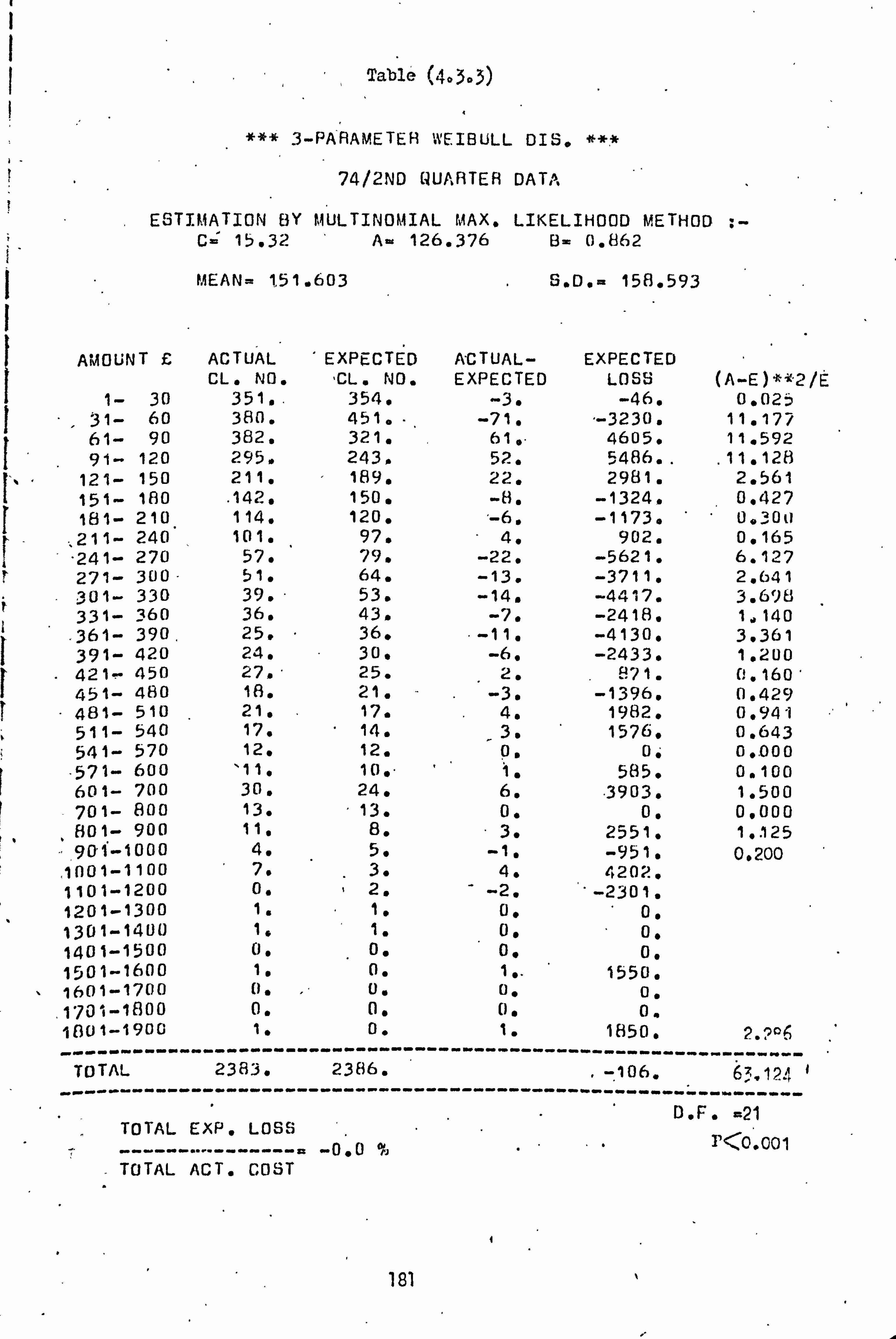
Table (403D3)

*** 3-PARAMETER WEIBI$LL DIS. ***

74/2ND NUARTER DATA

ESTIMATION BY MULTINOMIAL MAX. LIKELIHOOD METHOD : - C= 15.32 A- 126.376 E3 0.862

PAEAN= 151.603 S. D. - 158.593

AMOUNT £ ACTUAL EXPECTED ACTUAL- EXPECTED CL. NO. CL. NO. EXPECTED LOSS (A-E)"""2/E

1- 30 351.. 354. -3. -46. 0.025 31- 60 380. 451. -71. -3230. 11.177 61- 90 382. 321. 61, " 4605. 11.592 91- 120 295. 243. 52. 5486..

. 11.128 ` 121- 150 211. 189. 22. 2981. 2.561

151- 180 . 142, 150. -8. -1324. 0,427 181- 210 114. 120. -6. -1173. 0.30 1 211- 240 101. 97. 4. 902. 0.165

"241- 270 57. 79. -22. -5621. 6.127 271- 300- 51. 64. -13. -3711. 2.641 301- 330 39. " 53. -14. -4417. 3.698 331- 360 36. 43. -7. -2418. 1,140 361- 390" 25. " 36. . -11. -4130. 3.361 391- 420 24. 30. -6. -2433. 1.200 421-. 450 27. - 25.

. 2. 871. 11.160'

451- 480 18. 21. -3. -1396. 0.429 481- 510 21. . 17. 4. 1982. 0,941 511- 540 17. 14.

_3. 1576. 0.643

541- 570 12. 12. 0. 0. 0.. 000

"571- 600 '11. 100" 1. 585. 0.100 601- 700 30. 24. 6. . 3903. 1.500 701- 800 13. 13. 0. 0. 0.000 801- 900 11. Be 3. 2551. 1025 90-1-1000 4. 59 -1. -951. 0.200

'1001-1100 7. 3. 4. 4202.

1101-1200 0. 1 2. -2. " -2301. 1201-1300 1. 1. 0. 00 1301-1400 1.. 1. U. 01 1401-1500 0.

" 0. 0. 0f

1501-1600 1. 0. 11. 1550. 1601-1700 0. 0. 0. 0,

. 1'101-1800 0. 0. 0. 0. 11301-1900 1. 0. 1. 1850. 2.7°6 -------------------------------- --------------------------------

TOTAL -----------

2383. ----------

2386. ----- ------ - ----------

-106. -----------

63,124 -------- -

D. F. =21 TOTAL EXP. LOSS r

-----------------a -010 % , <0.001

TOTAL ACT. COST

4

181 %

Table ('1,3.4)

11 . .. *** 3-PARAUETER WETf3UL. L DIS, , ***

74/3RD QUARTER DATA I

ESTIMATION BY MULTINOMIAL MAX. LIKELIHOOD METHOD : - C- 16.07 A= 139.472 B= 0.867

MEAN= 166.012 S. D. = 173.566

AMOUNT £ ACTUAL EXPECTED ACTUAL- EXPECTED CL. NO. CL. NO. EXPECTED LOSS (A-E) **2 /E

1- 30 362. 366. -4. -62. 0.044 31- 60 427. 5.02. -75. -3412. 11.205 61- 90 383. 365. 18. 1359. 0.88A 91- 120 356. 281. 75". 7912. - 20.018

121- 150 283. 223. 60. 8130. 16.143 151, - 180 194. 1791. 15. 2482. 1.257 181- 210 137. 146. -9. --1759. 0.555 211- 240 97. 119. - -22. -4961. 4.067 241- 270 . 86. 981 -12. -3066. 1.469 271- 300 .

71. 82. -1.1, -3140. 1.476 301- 330 64. 68,, -4. -1262. 0.235 331- 360 45. 57. -12, -41.46. 2.526 361- 390 44. 48. -4. -1502. 0.333 391- 420 - 25. 40. " --15. -6082. 5�625 421- 450 26. 34. -80 -3484. 1,882 451- 480 22. 28. -6. -2793. . 1.286 481- 510 25. 24. 1., 496. 0.042 511-. 540 14. 20. -6. -3153. _ 1.800 541- 570 14. 17. ' -3. -1'666. 0.529 571- 600 17. 15.

. 2. 1171. 0,267 601- 700 32. 35. -3. -1951, 0.257 "701- 800 34. . 21. 13. -9756. 8.048 801- 900 17. 12. 5. 4252. 2.083 901-1000 4. 8. -4. -3802. 2.000

1001-1100 9. 5. 4. 4202. 3.200 1101-1200 4. 3. 1. 1150. 1201-1300 0. 2. -2. -2501. 1301-1400 1. ,

1. 0. 001 1401-1500 3. 1. 2. 2901. 1501-1600 0. 0. " 0. 0. 1601-1700 1'. 01 1. " 1650. 1701-1800 0". 0. 0, 0. 1801-1900 0. 0. 0. 0. 1901-2000 0. 0. 0. 01 2001-2100 0. 0. 0. 01 2101-2200 1. 0"

. 1" 2150.

2201-2300 0. 0. 0. 0. 2301-2400 0. 0. 0, 0. 2401-2500 0. 0. _

0, 0. . 2501-2600 -

. 1.

- 0. 1. 2550. 2: 286-

TOTAL

----------- 2799.

----------- 2800.

----------- ----------- 141gß'--

--------

-----__ý__ 92.722

----------- D. 'E. ^2

TOTAL EXP. LOSS --------- 0.3 ° P <0.001

TOTAL ACT. COST

182

Table `4-3-5)

*# 3-PARAMETER WEIBULL DIS. '***

74 /4TH QUARTER DATA

ES TIMATION BY MULTINOMIAL AJAX. LIKELIHOOD METHOD : - C= 15.15 A= 148 . 275 E= 0.871

" MEAN= 174.111 S. O. = 183.102

"AMOUNT £ ACTUAL EXPECTED ACTUAL- 'EXPECTED CL. NO. CL. NO, EXPECTED LOSS. (A-E)**2/E

1- 3.0 394. 397. -3. -46. 0.023 31- 60 452. 522. -70. -3185. 9.387 61- 90 426. 386. 40. 3020. 4.145 9.1-"120 348. 302; 46. 4853. , 7.007

121- 150 272. 241. 31. 4200. 3.988 151--'180 219. 196. 23. 3806. 2.699 181-210 154. 161. -7. -1368. 0.304 211- 240 124. 133. -9. -2029. 0.609 241.270

. 105. 111. -6. -1533. 0.324

271- 300 78. " 93. -15. -4282. 2.419 301- 330 75. 78. --3. ' -947. 0.115 331- 360 58. 65. -7. -2418. 0.754 361- 390 55. 55. 0. ' 0. 0.000 391--420 29. 47. -18. -7299. 6. x94 421-' 450 -43. 40. 3. 1306. 0.225 451 480 24. 34. -10. -4655. 2.941 48'1- 510 22. 29. -7. -3468. 1.690 511-"540 24. 25. -1. . -525. 0.040 541=- 570 19. 21. - -2.

-1111, 0.190 571='600 14. 1A. -4. -2342. 0.889 601- 700 42. 43. 1. -651. 0.023 701- 800 28. 26., 2. -" 1501. 0.154 801- 900 20. 16. 4. 3402. 1.. 000 901-1000 17. 10. 7. 6653. 4.900

1001=-1100 a. 6. -2. 2101. 0.667 1101-1200 5. 4. 1. 1150; F 0.290 1201-1300 1.

" 2. -1. -1250.

1301-1400 5. 2. 3. 4051. 1401-1500 0. 1. -1. -1450. 1501="1600 1. 1. - 0. 01 1601-1700 0. 0. 0. 0. 1701-1800 0. 0. 0. 0. 1801-1900 0" 0. 0. 0. 1901'-2000 0. 0. 0. 01 2001-2100 1.. 0. 1. 2050. 2101=2200' 0. 0. 0. 0. 2201-2300 0.

, 0. 0. 0.

2301-2400.

------------- ----------- ------------ 1.

-------- 2350�

--------- 1. . 500

TOTAL` 3064. _ 3065. ----- 1, ------- _ -------"--------------.. - ---» .. -------- , -----i--.. --------....

--- 5 L

-ý.. ý

--

ý

TOTAL EXP. LOSS D. F. s'

---------------= 0.4 % P Co. (, )al TOTAL ACT. COST

183

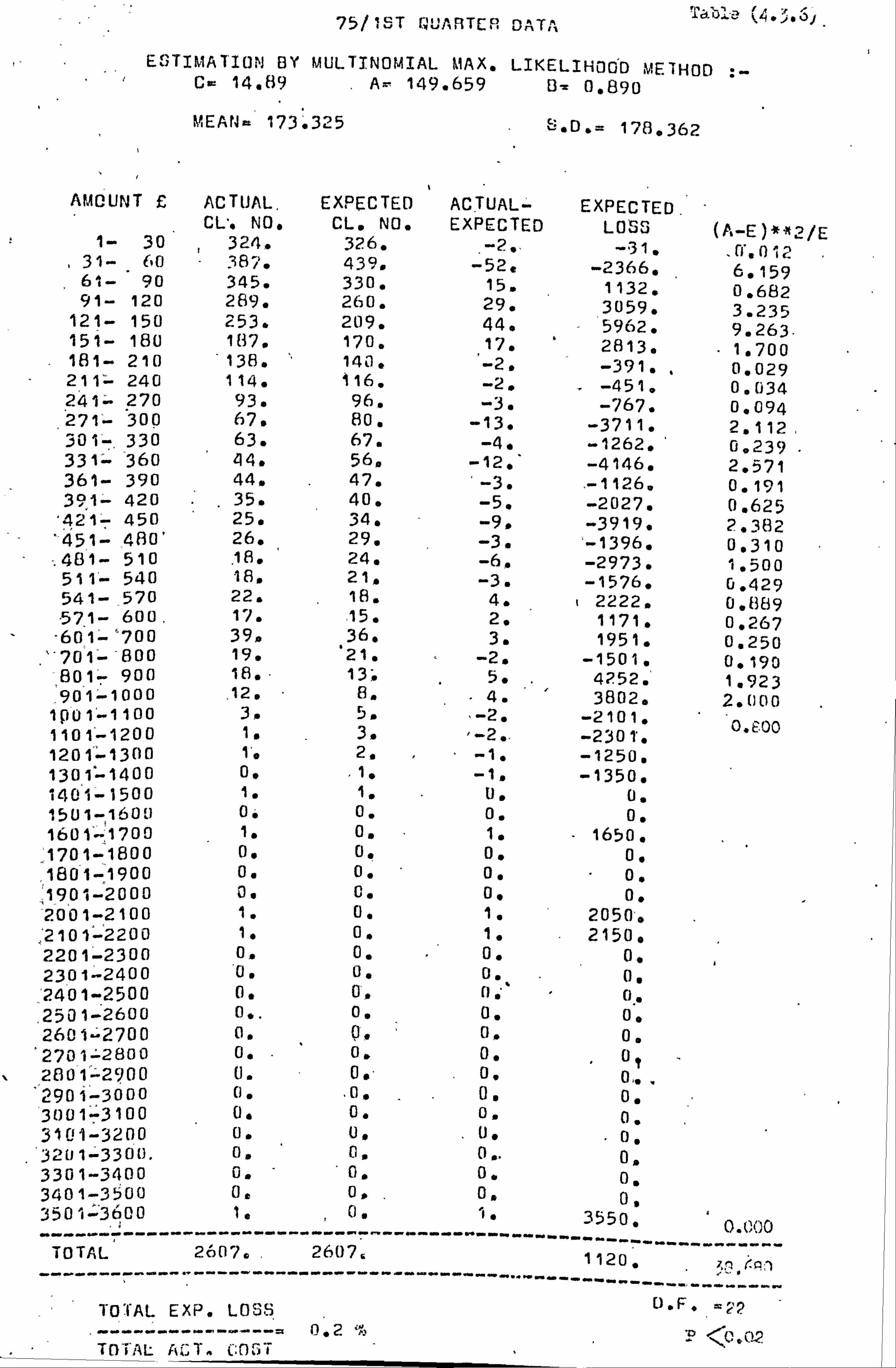
75/ 7ST N. "AfTE° L, "-, Y FM LI// a-ul-a. (4.3.6/

ESTIMATION BY MULTINOMIAL MAX. LIKELIHOOD METHOD ; C- 14.89 .

A= 149.659 E3= 0.890

MEAtJ= 173.325 ;. o. = 178.362

A(ACUNT £ ACTUAL. EXPECTED ACTUAL-- EXPECTED CL'. NO. CL. NO. EXPECTED LOSS (A-E)* 2/E 1- 30 324. 326. -2,. -31. f'i. 012 31- 60 387. 439. -52, -2366. 6.159 61- 90 345. 330. 15. 1132. 0.682 91- 120 289. 260. 29. 3059. 3.235 121- 150 253. 209. 44, - 5962, 9.263.

151- 180 1(i7. 170. 17. 2813. " 1,700

181- 210 138. 1461. -2, -391. , 0.029 211° 240 114. i16.

-2. -451. 0.034 2411 - 270 93. 96. -3. -767. 0.094 271- 300 67. 80. -13. -3711. 2.112

, 301-, 330 63. 67. -4. -1262. 0.239 331- 360 449 56, -12, * -4146. 2.571 361- 390 44. 47. -3. -1126. 0.191 391- 420 35. 40. -5. -2027. 0.625

'421- 450 25. 34. -9, -3919. 2,382 `451-. 4130' 26. 29. -3. ý-1396. 0.310 -. 481- 510

. 18. 24. -6, -2973. 1.500

511'- 540 18, 21. -3. -1576. 0.429 541-570 22, 18. 4. 2222. 01889 -57.1- 600. 17. 15. 2. 1171. 0.267

"601-'700 390 36. '

3. 1951. 0.250 701- -800 19. 21. -2. -1501. 0.190 801-- 900 18. 13:. 5. . 4252. ' 1.923 901-1000 12. . 8" 4. 3602, 2.000

1Q01-1100 3, 5. -2. -2101. 1101-1200 1. 3. -2.. -2301'.

aý 00 1201'-1300 1, 2. -1. -1250. 1301-1400 00 " 1. -1, -1350. 1401-1500 1. 1. U. U. 1501-160: ) 0" 0. 01 01 1601. -1700 1. 0. 1. . 1650.

:, 1701-1800 0. 0. 0. 00 1801-1900 0. 0. 01 0.

, 1901-2000 0. 0. 00 0. 2001-2100 1. 0. 1. 20501, 2101-2200 1. 0. 1. 2150. 2201-2300 o, 0. . 0. 00 2301--2400 01 0" 0.

% 00

2401-2500 0. 0, [): p. 2501-2600 0.. 0. 0. 00 2601-2700 0. p. a. 0. 2701-2800 0. . o. 0. 0 28012900 U. 0. * 01 0..

'2901-3000 0. . 09 0. 0. 3001-3100 0. 0. 01 0. 3101-3200 U. U. . U.

. p. 3201-3300. 0. 01 0.. 3301-3400 0. - 0. 01 0, 3401-3500 0, 0, 0, 0. 3501.3600 1, 01 1" 3550 ----- ----.. w _.. w-_--_-s_ ---w _. ýw-.. w -.. wM------- ----------- - _0.

c, ()G TOTAL 2607L. 2607, 1 120 . ,. n <p-)

,,, --------------------------------------------------

TOTAL EXP. LOSS D. F. G?.

---- .... _--_-_. -- 0,2 9 .°

4t, a 2

TOTAL ACT,. C: 0. )ß

(x.. 3.7)

'3-PARAMETER 1r+E'IBULL DIS.

75/2ND QUARTER DATA -

ES TIMATION BY MULTINOMIAL MAX. LIKELIHOOD METHOD ; - C= 16.52 A= 150 , 912 B= 0.856

MEAN= 179.934 "S. D. = 191.534

AMOUNT £ ACTUAL EXPECTED ACTUAL- EXPECTED CL. NO. CL. ' NO. EXPECTED LOSS (A-E) *2 /E

1- 30 302. 305. -3. ' -46. ' 0.030 31- 60 374. 428. -54. -2457. 6.813 61- 90 332. 312. 20. 1510. 1.. 282 91- 1.20 277. 243. 34. 3587. 4.757

121- 150 235. 195. 40. 5420. 8.205 151- 180 187. 159. 28. 4634. . 4.931 181= 210 122. 131. -9. -1759. 0.618 "

' 211- 240 1.10. 108, 2. 451. 0.037" 241- 270 80. 90. -10. -2555. 1.111 271- 300 72. 76. -4. -1142. 0.211 301- 330 47. 64. -17. -5363. 4.516 331- 360 39. 54. -15. -5182. 4.167 361- 390 40. 46. -6. " -2253. 0.783 391- 42.0 38. 39. -1. . -406. 0.026 421- 450 29. 33. -4. -1742. 0.485 451- 480. 21. 29. -8. -3724. 2.207 481- 510 30. 24. 6. 2973. 1.500 511- 540 19. 21. . -2. -1051. 0.190 541- 570 17. 18. -1. -555. 0.056 571- 600 11. 16. -5. -2927. 1.562 601- 700 36. 38.

. -2. -1301; 0.105 701- 800 22. 24. -2., -1501. 0.167 801- 900 22. 15. 7. 5953. 3.267 901-1000 11. 9. 2.

. 190,1. 0.444 1001-1100 4. 6. -2. " -2101. 0.667 1101-1200 3.

" 4. -1. --1150. " 0,250"

1201-1300 3. 2. 1. 1250. 1301-1400 6. 2. 4. 5402. 1401-1500 2. 1. 1. 1450. 1501-1600 1. 1. 0. . 0. 1601-1700 0. 0. 0.,

, 0. 1701-1800 1. 0. "" " 1.

.- 1751.

1801-1900 .

J. 0. 0. 0. 1901-2000 1. 0. 1. 1950. 2001-2100 0. 0. 0. 0. 2101-2200 0. , 0. 0.. 0. 2201-2300

------- --

1. -----------

0. ------------

1. ----- -

2250. 13.! ()0 --

TOTAL

----------- 2495.

----------- 2493.

------------

- ----

----------

---------- -"

3266. -------

61.065

- ----------- D. F,

------- =23 TOTAL EXP. LOSS

---------------- 0.7 % P<0.001

TOTAL ACT. COST

185

CHAPTER 5

The Liverse Gaussian Distribution

5.1 Introduction

This is a uninodal and positively skewed distribution which in

recent years has been shown to represent the distribution of random

outcomes of various phenomena. The name inverse Gaussian (or inverse

normal) was proposed by Tweedie (1947) who noticed the inverse

relationship between the cumulant generating function of this distribution

and that of the normal distribution. Tweedie (1957) investigated the

statistical properties of this distribution and indicated analogies

between its statistical analysis and that of the normal distribution.

In recent years this distribution has been studied by many authors.

Johnson and Kotz (]. 970) provide a bibliography, and Chhikara and Folks

(1978) give a review of the development since 1915 of the inverse

Gaussian distribution and of the statistical methods based upon it.

The frequency curve of the inverse Gaussian distribution is

similar in shape to that of the other skewed distributions like the

lognormal, the gamma or the Weibull. It is, therefore, important to

consider the application of this distribution in the fields where one,

or some, of the others have been successfully used as a model. Chhikara

and Folks (1978) give examples of sets of data equally well fitted by

the lognormal and inverse Gaussian distributions. They point out that

when more than one distribution fits a set of data equally well and

there is no evidence (based on the physical considerations of the

problem) in favour of a particular nadel then it is best to use that

which is more convenient to work with. An advantage of the inverse

Gaussian distribution over the lognormal is that its statistical

properties and inference procedures are well developed for small sample

situations.

If)t O

Applications of the inverse Gaussian distribution in various

fields have been reported by many authors. It has been successfully

used in life-testing and reliability studies by Chhikara and Folks

(1977). Hasofer (1964) considered it as a model for emptiness of a dari.

Lancaster (1972) used it as a model for the duration of strikes. We

have not cone across the use of this distribution in insurance, and

it is therefore considered important to study it as a model for the

distribution of claim amounts.

In the literature, only the 2-parameter inverse Gaussian distribution

his been considered. We will, however, introduce a location

parameter into the model and will name it the 3-parameter inverse

Gaussian distribution. Professor J. L. Folks, in a personal communication

with the author (1978), acknowledges that this is an original idea arcs

that this form of the distribution (i. e. the 3-parameter) has not been

previously considered. We will later show that the 3-parameter

distribution provides a better model for the accidental damage data.

In this chapter we will initially define the 2 and 3 parameter

inverse Gaussian distributions and will mention some of their

properties. The problem of estimation from grouped data is next

considered. In section 5.5 the inverse Gaussian models will be fitted

to our seven samples of accidental damage data and the results will

be discussed. The effect of inflation on the parameters of the model

will be studied in section 5.6 and, for the accidental damage data,

the distribution of claim amounts during a future period will be

derived and compared with the actual data. The findings of this

chapter will be sunrarized in section 5.7. The tables will be presented

in section 5.8.

5.2 Definition

A random variable X is said to have a (2-parameter) inverse

187

Gaussian distribution if its probability density function (p. d. f. ),

denoted by f IG (x; u , a) , is of the form

2 IG (x; tý ýxý _ (X/2'rx )

1/2 Pxp (_x(x_i) /2u2X) 'x>0

=0 otherwise

where }i and X are two independent and positive parameters. This

distribution is thus a member of the exponential family. A is a shape

parameter while p is only partially interpretable as a location

parameter.

Shuster (1968) has shown that the inverse Gaussian distribution function,

denoted by IG(x; u, a), can be expressed in terms of the standard

no-mal distribution function, N(z; 0,1), as :

IG(X; u, a) = N(zl; 0,1) + eta/u rß(72; 0,1) (5.2-2)

where Zl = .

(A/x): V2

(-1 + x/u)

z2 = -(x/x) (1 + x/u) I't

1e will show later in this chapter that the 2-parameter inverse

Gaussian distribution does not provide a satisfactory model for the

accidental damage claim amounts. This fact, together with the"concepts

of 3-para eter lognormal and SWleibull distributions, led us to consider

a 3-parameter inverse Gaussian distribution where one of the parameters

is a location (threshold) parameter below which the values of the

random variable X are not realized. Hence we introduce the unk noun

location parameter c into the nwdel and assume that X-c, rather

than X, is distributed as in (5.2-1).

We say that a random variable X has a 3-parameter inverse Gaussian

distribution if its p. d. f., denoted by fIG(x; c, u, X), is of the form

2

IG(x, [a/21r (x-C)3) exp[-x (x-c-u)` /2 i (x-C)] ;X>c =0U Lll--Il iSC

(J"2-�)

88 1

The transformation x- x-c is only a translation along he x-axis.

Therefore, the distribution function of X(i. e. the 3-parameter inverse

Gaussian random variable) is obtained from (5.2-2) by replacing x by

X-C.

In our research into the literature on the inverse Gaussian

distribution, we have not come across the 3-parameter distribution of

the form (5.2-3). In fact, as we mentioned earlier, Professor Folks

in a personal communication with the author confirms that the idea of

a 3-parameter inverse Gaussian distribution, with one of the parameters

being an unknown location parameter, has not been considered before.

This new form suggests, as an area for research, the study of th3

statistical properties and the estimation and inference problems for

the 3-parameter distribution. We shall deal with these problems in

this chapter as far as is relevant to the present work. It will be

shown that the 3-parameter distribution provides an adequate model for

our accidental damage claim amounts.

5.3 Properties of the inverse Gaussian Distribution

In this section, we first outline briefly sorge properties of

the 2-parameter distribution with p. d. f. of the form given by (5.2-1).

for more details and proofs reference should be made to Johnson and

Kotz (1970) or TNAreedie (1957).

Moments of all orders exist and in particular the rth positive

integral moment of X about 0 is given by Tweedie (1957) as :

1 I E (Xr) =r S=0

In particular E (X) 2

and E (X )

hence var(X)

r-l+s )s s! (r-1-s)! 2x

(5.3-2) 23 -1 +ua (5.3-3)

3 ä (5.3-4)

18

Also I: (X3) = 11 3+

311 x-1+ 31_a ` (5.3-5)

4 ý4 5 _1 6 -2 73 and E(X =p+ 611 X+ 1511 X+]. Su X (5.3-6)

Parameter p is, therefore, the population mean and is a measure of

location. This model, unlike for instance the lognormal model, possesses

the useful characteristic that one of its parameters is the population

mean. 2 The coefficient of variation for this distribution is ý-

2 where

4, >0 (5.3-7)

The coefficients of skewness and kurtosis, V-O1 and g2 respectively, are

(5.3-8)

02 =3+1=3+ 15q-i (5.3-9)

The shape of the distribution depends on + only and, since ý>0, its

frequency curve is skewed to the right and more peaked than the normal

frequency curve. The distribution becomes more and more nearly normal

when ý is increased.

The distribution has a single mode which is located at

or

r2y + )2 Xmode -u{ (1 _} (5.3-10)

` 4x 2

9z 31 + 44,2) 2ý (5.3-11) xirýode -u (1

The mode of the distribution is in general located to the left of

its mean because

Xnn de t u

but when ý is increased to infinity x, rode wiil converge to 11 . It is

possible to express the inverse Gaussian p. d. f. in terms of the pair

of parameters (u, ý) or (x, ý) , but the form give, by (5.2-1) is

T£0

generally considered as the standard form and is most usually used

in the literature. The one parameter form which is obtained by putting

p=1 in (S. 2-1) is knom as the standard Wald distribution.

The properties of th4 3-parameter inverse Gaussian distribution,

whose p. d. f. was given by (5.2-3), can be deduced from those of the

2-parameter. The transformation x -} x-c is one of translation along

the x-axis only and, therefore, the measures of location will be

increased by c while the measures of dispersion and the moments about

the mean will be unchanged. Hence, for the 3-parameter distribution

we will have :

E (X) =c+u (5.3-12)

var(X) = l' (5.3-13)

=r2 112 1

Xinode c+ u{ (1 + 9u2)

- 2ý } (5.3-14) tt 4ý JJ

3/2

and Coeff. of variation =u (5.3-15) [X(c )] 2

which is a function of all three parameters.

5.4 Estimation of the Parameters from Grouped Data

The problem of estimation from a sample of data containing the

values of individual observations has been dealt with by Schrodinger

and his maximum likelihood estimators are reported in Chikkara and

Folks (1978). Here we concentrate on the estimation from a sample

of grouped data. when all the parameters are assumed unknown.

Let us assume that we have a sample of grouped data where n independent

random observations on a random variable X (in our case the claim

amount) have been grouped according to their size into k nutually

exclusive intervals. Further, let n1 be the niunber of observations

(claims) in the class interval (xi_l, xi), for i=1,2, ... ,k,

191

and such that

k n= n1

i=1

Also let us assume that X has a 2-parameter inverse Gaussian

distribution of the form (5.2-1). The method of moments can be used

to estimate the parameters. This involves putting as many sample

moments as there are unknown parameters equal to their corresponding

population values and solving the resulting equations for the unknown

parameters. For the 2-parameter case the sample mean and coefficient

of variation may be used. The sample mean is the moment estimator of

and, when the values of individual observations are known, is

equal to its maximum likelihood estimator (see Johnson and kotz (1970)).

Therefore the sample mean is an unbiased and efficient estimator of u.

In calculating the sample moments from grouped data the usual assumption

about the concentration of all the observations in each interval at

the mid-point of that interval may be made. In the 3-parameter

case, as well as the sample mean and coefficient of variation, the

third central moment, which is independent of c, should be used to

yield sufficient equations in the unknown parameters.

It was observed in the previous chapters that the method of

multinomial maximum likelihood yielded the best fits of the models

to actual data. Here we consider this method for the 3-parameter

inverse Gaussian. The 2-parameter case can be similarly dealt with by

putting c=0 in the following exposition.

Let us assume that the have a sample of grouped data, as defined earlier,

and that random variable X has a 3-parameter inverse Gaussian distribution

with p. d. f. of the form (5.2-3) and distribution function given by :

(see section 5.2)

IG(x; c, u, X) ° N(: 1,0,1) + e2ý/u N(z2; 0,1) for x>c

=0 otherwise (5.4-1)

192

where zi = (a/ (x - c)) 2 (-1 + (x - c) /u )

and 1 z2 c))

/ (1 + (x - c)/

Let pi be the probability that an observation (claim, in our case)

occurs in the interval (xi-1, xi) , for i=1,2, a. ,k, where

Pi = IG(xi ; c, u, X) - IG(xi-1; c, p, X) (5.4-2)

which can be expressed in terms of the standard normal distribution

function by using (5.4-1). The likelihood of the s . ple will be

proportional to L where k

ni L=

i=1 pi

The loglikelihood equation, log L, can thus be expressed as

k

log L= nl log pi i=1

The rnaximun likelihood estimates are the set of parameter values

(c, u, Jý ) which maximizes log L. The iterative computing technique

which was described in section 3.7.7 of chapter 3 can be used to AA

maximize log L and yield the set (c, u, a). This technique requires

initial values for the parameters in order to start the iteration

procedure. The estimates of the parameters obtained by the method

of mments can be used for this purpose.

5.5-Application of the Inverse Gaussian Model to AD Data

We wrote computer program P18 to estimate the paraieters of the

2-parameter inverse Gaussian distribution by the multinormal maximum

likelihood , (ASS; [. ) , method. This program was run with the samples

of accidental danage data which were presented in tables (1.1) to (1.7).

193

For each sample the estimates of the parameters u and were found

by the method of moments. The statistics given at the bottom of each

of the tables (1.1) to (1.7) made the above task very easy. The

moment estimates were supplied to program P18 as starting values for

the iteration process. The program produced an extensive table of

results for each sample. These are summarized in table (5.1). The

estimate of u in each case is practically equal to the sample mean

(refer to tables (1.1) to (1.7)). The values of u and A show a generally

increasing trend over time. The ratio of the total expected loss

statistic, T, to the total actual cost is small in each case. This

indicates an overall agreement between the model and actual data. The

Chi-square statistics are, however, large and indicate significant

differences between the model and actual sample values. The examination

of the components of this statistic, for each sample, showed that 2

very large contributions are made to the value of X by only one or

two intervals. in the lower tail of the distribution. For example the 2

first and second intervals account for some 60% of the X values.

Therefore, the agreement between the nodel and actual sample values is

reasonable except in the lower tail. In terms of the Chi-square

statistic the 2-parameter lognormal model provided a better fit to the

actual sample values than the present model has.

The frequency curve of the inverse Gaussian distribution is very

similar to that of the lognormal distribution. To improve the fit of

the model to the actual data, we considered the idea of a 3-parameter

inverse Gaussian distribution similar to the idea of a 3-parameter log-

normal distribution. We, therefore, assumed that X+c, and not X, is

distributed as an inverse Gaussian distribution, with parameters u and

x, where c is an unk noun parameter which can be interpreted as the

voluntary excess on the policy. This assumption simply means that the

total amount of claim, X+c, (which consists of the amount X paid by

194

the insurance company and the amount c borne by the policy holder)

has an inverse Gaussian distribution.. The remarks we made about

parameter c of the lognormal model, in section 3.10, are valid here

as well and it is useful to refer back to then at this stage.

We, therefore, assume that c is fixed for all policies but that its

value is unknown, and proceed to estimate it, along with u and x from

the data. The computer program P19 estimates the 3 parameters from

a sample of grouped data and prints an extensive table of results.

For the accidental damage data of tables (1.1) to (1.7) the results are

presented in tables (5.2.1) to (5.2.7).

The estimates of c show an increase over time and are generally

greater than their corresponding values for the 3-parameter lognormal.

model. The mean claim amount of the model is, in each case, practically

equal to the sample mean. The standard deviations are also close to

their corresponding actual values and in each case are smaller than

those obtained by the 3-parameter lognormal model. The Chi-square

statistics are smaller than in the 2-parameter case. and (except in

two or three cases where large contributions from one or two cells 2

have resulted in large values for X) do not indicate any significant

differences between the model and the actual sample values. The Chi-

square statistics are practically equal to their corresponding values

for the 3-parameter lognormal model. The total expected loss statistics,

T, are also small and are at most 1% of the total actual cost. This

indicates a general agreement between the model and the sample values.

To see how closely the frequency curve of the model agrees with

the histogram of the sample, we wrote computer program P20 to plot

them. The ML estimates of c, u and X, given in tables (5.2.1) to

(5.2.7), were used to plot the frequency curve of the fitted model for

each sample. The graphs are presented in figures (5.1.1) to (5.1.7).

We observe an overall agreement be , Teen the curve and the histogram

for each sample. In particular, the cunfe has portrayed the distinct

195

.:, , aý frýýiluýýnr.; ý

? 3.

>-, rý >. s .v

. ýý{ý /1ýý llýTli

Figure (5.1.1)

M ^! " 73'iTH DUARTF. R DATA AND 3-PAR.

3S1AN P. G. F. WITH (1ULTU. MAX. PARAMMEf: s

MEW-1604.0 LAMDAL16ü. 5

v-r-77ý1 .

I'--- r. --,

-12.10 , (Alo

ICI ýTf1; C. ýM ^f' 73'ITIi QU\RT(R CATA /.! %1r)

I14V. GAU3$1A14 ('. r. F . {: 1 fli MULTN. M1XL. f Ai:, 1C1f: "f(fi5

I; v. o i ý, 01 wort 1 . 400

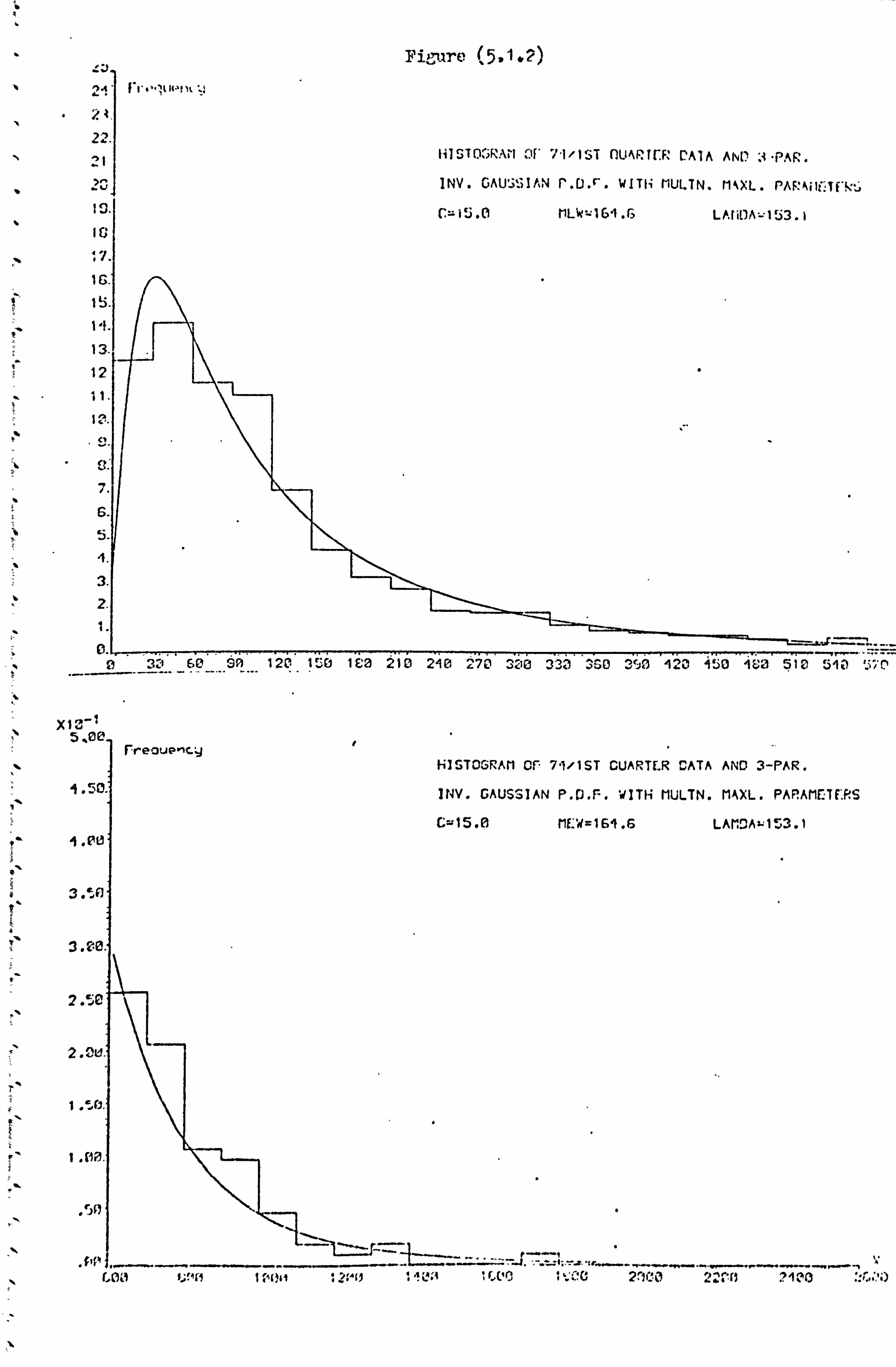
2d' I r. ` , u49 l

22.

2- 1J.

IC

'7.

16.

13.

12

11.

6

5.

` 3.

2.

CA- 3 30 6Eý 9sß 120 1

X12-1 5.00

ireouency

4.00

f3. Jul

2.5E

2. Oa.

Figure (5,1.2)

M OF. 7.1ilST CUARTE. R CATA AND 3-PAR.

ISSIAN P. U. F. WITZ; MULTN. MOL. PAPAME"TF: RS

ME. W=161.6 LAM')ALl 3.1

n^

2100 22. ̂ "( 29: 0

H1ST(X; RAM OF 7-l'lST OU'F T1: CA JA nay' ;ý "ý nR . INV. GAU3SIAN f . U. r. WITH MULTN. MNXL. ! 'AF: ^ili: TUk,

1.2.,. Ij It iv-i

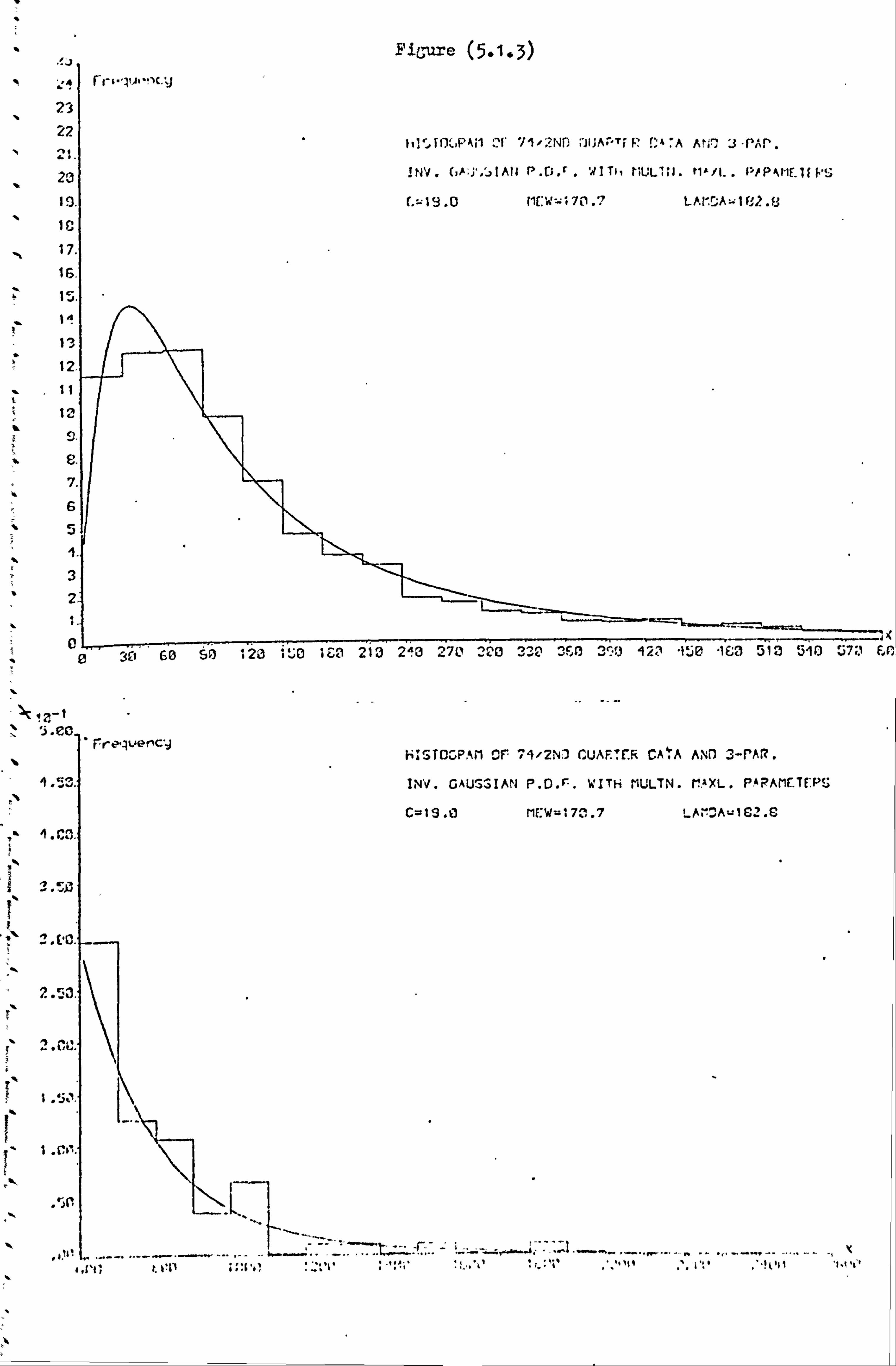
Fr 6

` 23

22 2t.

20

19. iG

17.

16.

13 12.

. tt 12

Figure 5.1.3)

{,:; rO., PAi1 (`f 71 ,? NP) , )I'Ar"TF P ! '. A At i-,, '3 "PAP.

! NV. I A, 1 P. CD. r . 'iIT', MUL'1Ii. tt"/I.. c%/P4M(. 1fPS i

Lu 19 .0 11(; w'zj; 70 .? LA! ': Aý 1 f; 2 . 81

act G© S%) 12L1' i: ý© ; E£1 213 2a© 27C' 200 33c 31'1 3ý0 92,1 lt O -IE; 510 510 57: 1 Eßt)

Frequency hISTD3PAT1 OF 74'2NO CUAF. TE'. R CAA Auf 3-PAR.

INV. GAUSSIAN P. D. r-. WITH MULTN. MaXL. PAPAMf_TE: PS

C=19.0 ME: W=27, .7 LA. -", Aw162. G

ii`li tl. iý_ý... i:: {'1ý . _.

ý1' r-ý: ýi

-. ý1ý ýr. ý41ý

.. 'ý1ý"

. `. i... 'llýll "Ltyr

t

t

E

ýý i

c

}

s a

r

a

t

4

X1.,. -1 5 . 'E+ý t

` 1.50

4. ee

3 .M

I 3. ý©

2.

2.

1.

1.

Figure (5.1.4

M DP 71/3RD DUARTE. k DATA AND 3""PAR.

JSSIAN P. D. F. WITI4 MULTN. M+1XL. PAiPAMOUPS

MEWs166.7 LAt1DA=193.9

. �-�-. _--_ --. -----. --------�

; tu' 2i'. 'l : 'it: (. f: PJ ü: 1i! irißi3

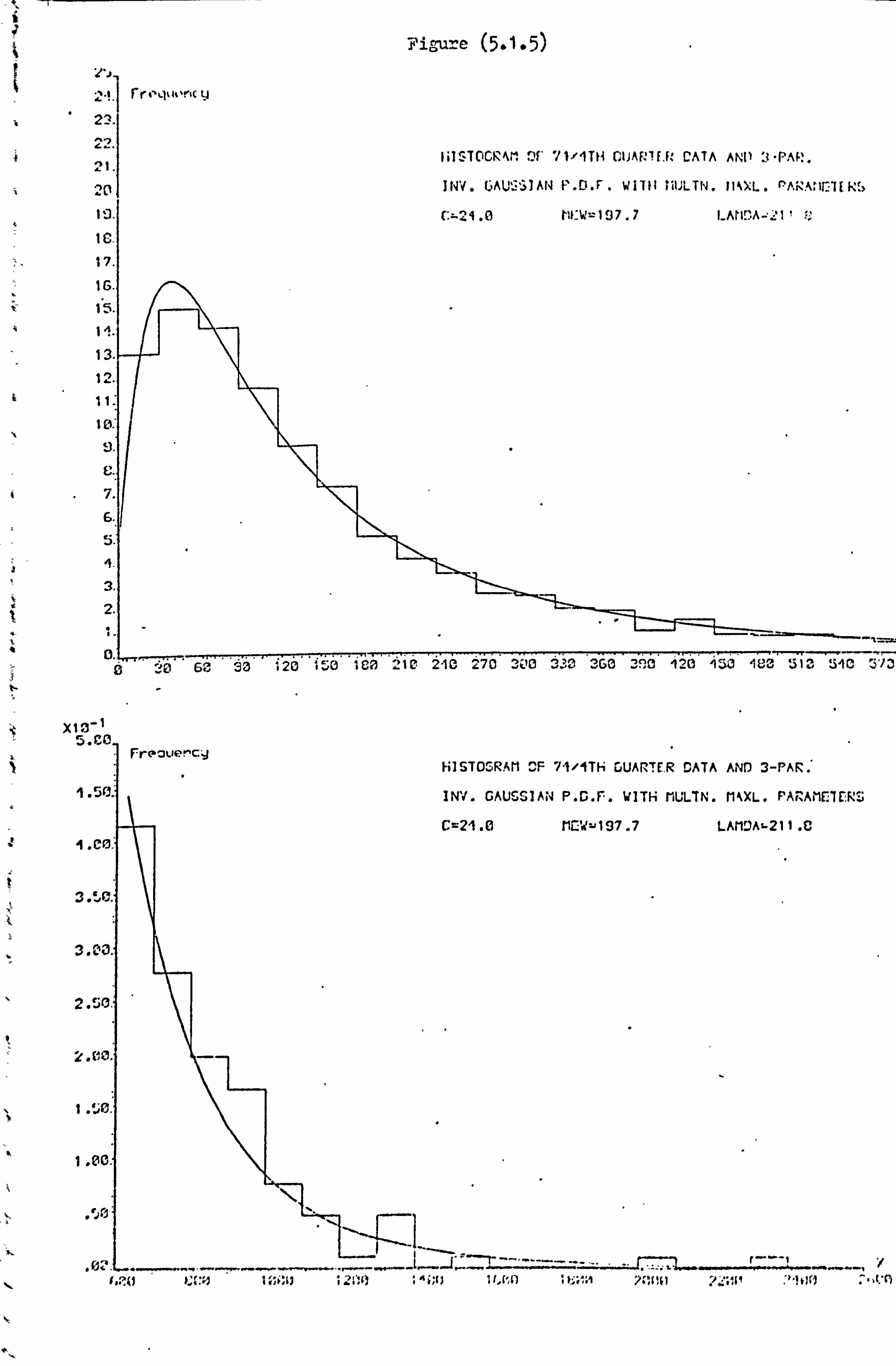
Fiore (5.1.5) 'l' .

x»-1 5. ri

3. ßs

2. J(

2. kߣ

1. ýk

1 . 0C

.1 rR

!ý {1 l:. a9 1üi3f7 i: {: ý i'ýF)t) Sfý(, t1 iY F"t1 ? (i(1F1 ?: i! Fý : r"iN(9

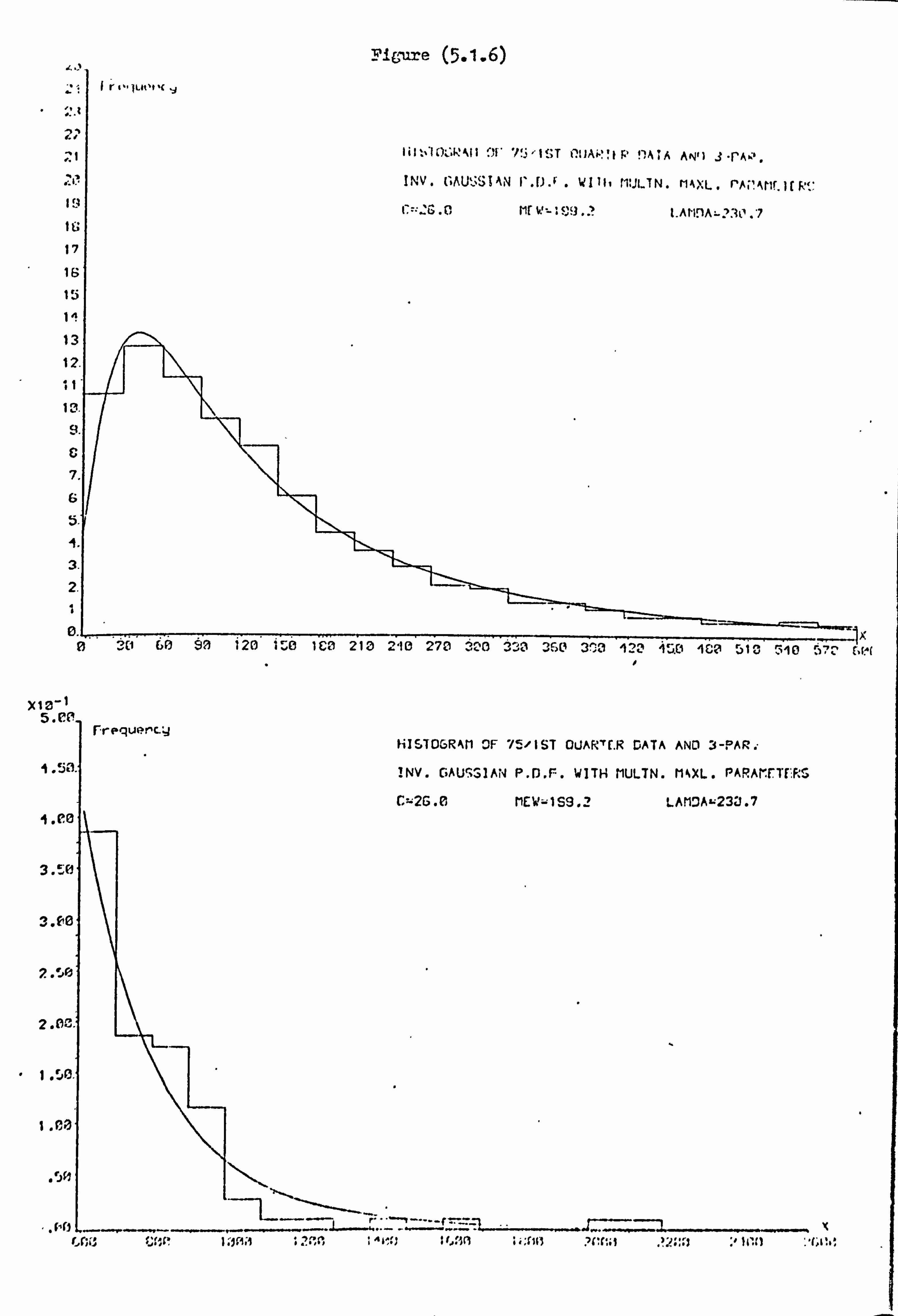
4 .'

2.

,. t

17

1S

1^

13

12.

111

a.

x12-1 5. ro.

F

i. 5a

1. ee

3. Eh

3. ý0

2. `M

2. (C.

" 1. Sß.

"Hfl - r c; C

Pirure (5.1.6)

HISTOGRAM OF 75/1ST QWRTC. R DATA AND 3-OAR.

1NV. GAU: SIAN P. D. F. WITH MULTN. MM. PARArr. TURS

Cu2G. 0 MEW-159.2 LAMOAL233.7

It'll NX. 7 COW I jfM 0 2. "fl,

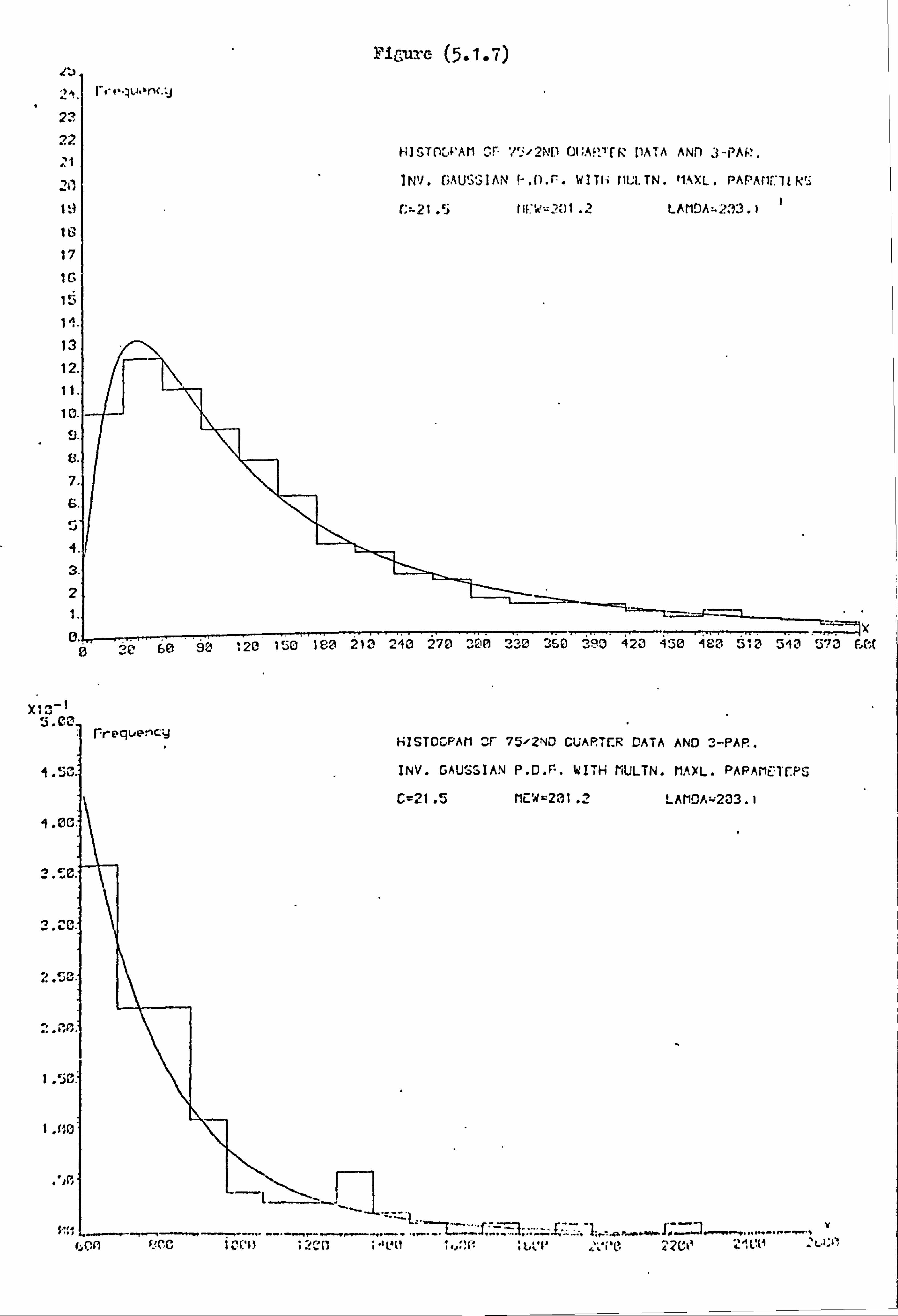
J', Flgure (5.1.7)

I

x13-ý s. ea

4

9 . CC.

:?. z. e.

2., ß.

IMO

ISTCCPAr OF 75-12ND CJARTtR DATA AND 3-PAP..

NV. GAUSSIAN P. D. F. WITH MULTN. MARL. PAPAMEUPS

=21.5 MEW=231.2 LAMDAL233.1

t. l. t NCO i: 4. Cl

mode and the long tail of the histogram very well. The curves look

remarkably similar to those for the 3-parameter lognormal distribution

given in figures (3.9.1) to (3.9.7). However, the latter curves have

a slightly fatter and longer tail.

The above analysis shows that the 3-parameter inverse Gaussian

distribution is an appropriate model for the accidental damage claim

amounts, This model produces results very similar to those of the

3-parameter lognormal distribution.

196

5.6 Prediction of the Claim amount Distribution

The importance of predicting; the future, cost of claims was

mentioned in section 3.9 (chapter 3). Here, we will adopt techniquez,

similar to those of that section for predicting the distribution of

claim amounts, during any future period, when the underlying model is

the inverse Gaussian distribution. To save us repeating some of the

arguments of that section, we suggest referring back to it at this stage.

5.6.1 The Effects of Inflation on the Parameters of the Model

Let us again assume that the effect of inflation on a claim of

amount X is to increase it, over a certain period, to U= X(i + i)

where i is the rate of inflation according to some appropriate index

for that period. If X is assumed to be distributed as the two-

parameter inverse Gaussian, IG(x; u, X) then, by a transformation of

variables, we can show that U= X(1 + i) will be distributed as

IG(u; ru, ra) where r=1+i. If X is assumed to have the 3-parameter

inverse Gaussian distribution IG(x; c, u, X) then similarly it can be

shown that is distributed as IG(u; rc, ru, rA). Therefore when

the distribution of X is known we can modify its parameters to obtain

the distribution of claim amounts in a future period. The foregoing

shows that inflation increases all the parameters of this model over

time. This is reflected in the estimates of the parameters from

different samples presented in table (5.1), for the 2-parameter

distribution, and in tables (5.2.1) to (5.2.7) for the 3-parameter case.

The data analysis of section 5.5 showed that the 2-parameter

inverse Gaussian distribution is not an adequate model for the accidental

damage claim amounts. Therefore, we will not consider this model for

prediction purposes. The 3-parameter distribution, however, was shown

to be a satisfactory model and hence we suggest using the technique

of section 3.9.2 for predicting the distribution of accidental damage

197

claim amounts during a future period. In chapter 3 it was shoi: rn tý. at

the appropriate index for calculating the rate of inflation for

accidental damage claims is the General Index of Retail Prices. We will

use the same index here again.

5.6.2 Prediction for the AD Data

To test the prediction technique on the Accidental Damage (AD)

data we wrote computer program P21 for the 3-parameter inverse Gaussian

model. For reasons presented in section 3.9.2 we used the I%HL estimates

of the parameters of the distributions for 73/4th, 74/1st and 74/2nd

quarters to predict the distributions of claim cmounts in 74/4th,

75/1st and 75/2nd quarters respectively. The rate of inflation in each

case was calculated from the General Index of Retail Prices as described

in section 3.9.2. The results for the AD data are presented in tables

(5.3.1) to (5.3.3). These are in the form of extensive tables which

allow comparisons between the actual and predicted distributions.

In all three cases the Chi-square statistics are relatively small,

considering the number of degrees of freedom, and do not indicate any

significant differences between the predicted distributions and the

actual sample values. The total expected loss statistics are small,

and show anover-prediction of the total cost, by at most 3.9%, which

is more acceptable than any under-prediction. The Kolmogorov-Smirnov

statistics were calculated from the tables and in each case were

compared with the significance points of table (2.1). They showed that

the differences between the actual and predicted distributions were

not significant for 74/4th and 75/ist quarters but were almost significant

for 75/2nd quarter.

Our prediction technique, therefore, provides a satisfactory mean:,

of predicting the future distribution of claim amoimts when the rnder"-

lying model is the 3-parameter inverse Caussien distribution. For the

198

AD data the values of the goodness-of-fit test statistics are verg

similar to those obtained from the 3-Parameter lognormal distributions

in tables (3.45) to (3.47). This is only to be expected since, as

we mentioned earlier, these two nodels are very similar to each other.

The lognomal model, however, resulted in smaller values for the total

expected loss statistics and hence overpredicted the total actual

cost by a smaller amount.

5.7 Conclusions

In this chapter the 2-parameter inverse Gaussian distribution was

initially defined and then modified to a three parameter distribution

by the introduction of a location parameter. The properties of these

distributions were considered and their problems of parameter estimation

from grouped data were dealt with. The multinomial maximum likelihood

method was suggested for these purposes. The two and three parameter

distributions. were next considered as models for the distribution of

accidental damage claim amounts. It was shown that the 2-parameter

distribution is not an adequate model, while our proposed 3-pararmeter

distribution provides a very satisfactory model which is as good as

the 3-parameter lognormal. The effects of inflation on the parameters

of the model were studied, and the future distribution of claim amounts

was predicted. It was shown that our prediction technique produces

satisfactory results when the underlying model is the 3-parameter inverse

Gaussian distribution.

The similar features of the 3-parameter inverse Gaussian and

lognormal models were pointed out at various stages. Although the latter

distribution has a slightly longer tail, and produced a Slightly better

fit to the data, either of the two models may be satisfactorily used.

The ATIL method can be used for estimation of parameters in both cases

with equal labour. The distribution functions of both yodels are

199

expressed in terns of the standard normal distribution function. It

is, however, possible to test if a given sample of data is from the

lognormal distribution, while similar tests do not exist for the

inverse Gaussian model. This is an advantage of the former model

since, if the test indicates that the sample is not very likely to be

from the distribution under consideration, then further analysis can

be avoided. The existence of a theoretical justification for the

emergence of the lognormal model as the distribution of claim amounts

is another strong point in favour of that model. On the question of

convenience in use, we believe that, with the wide availability of

computers,, either model is equally suitable.

5.8 Tables

-200

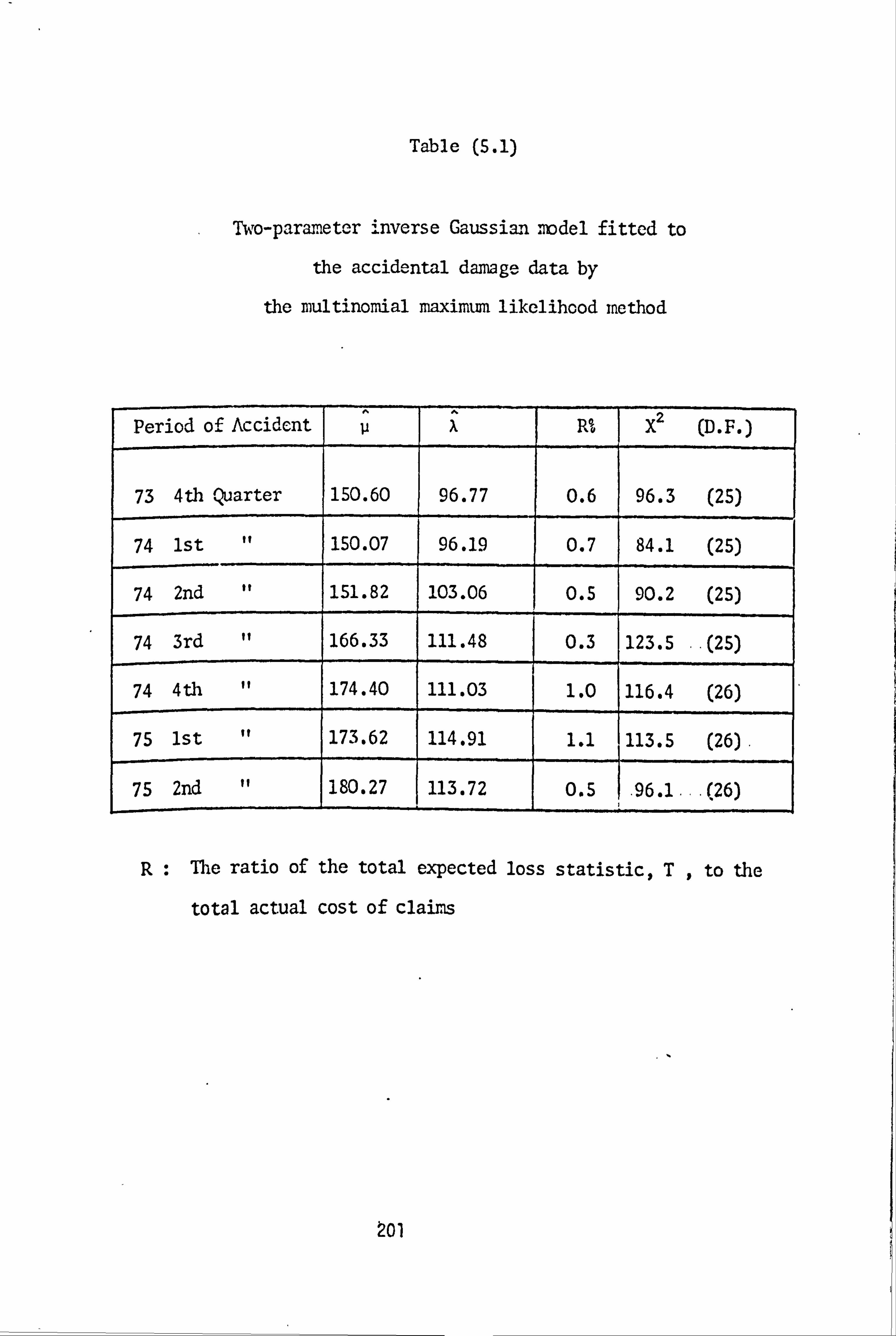
Table (5.1)

Two-parameter inverse Gaussian model fitted to

the accidental damage data by

the multinomial maximun likelihood method

Period of Accident u R% X2 (D. F. )

73 4th Quarter 150.60 96.77 0.6 96.3 (25)

74 1st it 150.07 96.19 0.7 84.1 (25)

74 2nd " 151.82 103.06 0.5 90.2 (25)

74 3rd " 166.33 111.48 0.3 123.5 . (25)

74 4th " 174.40 111.03 1.0 116.4 (26)

75 1st " 173.62 114.91 1.1 113.5 (26).

75 2nd " 180.27 113.72 0.5 . 96.1. .. (26)

R The ratio of the total expected loss statistic, T, to the

total actual cost of claims

201

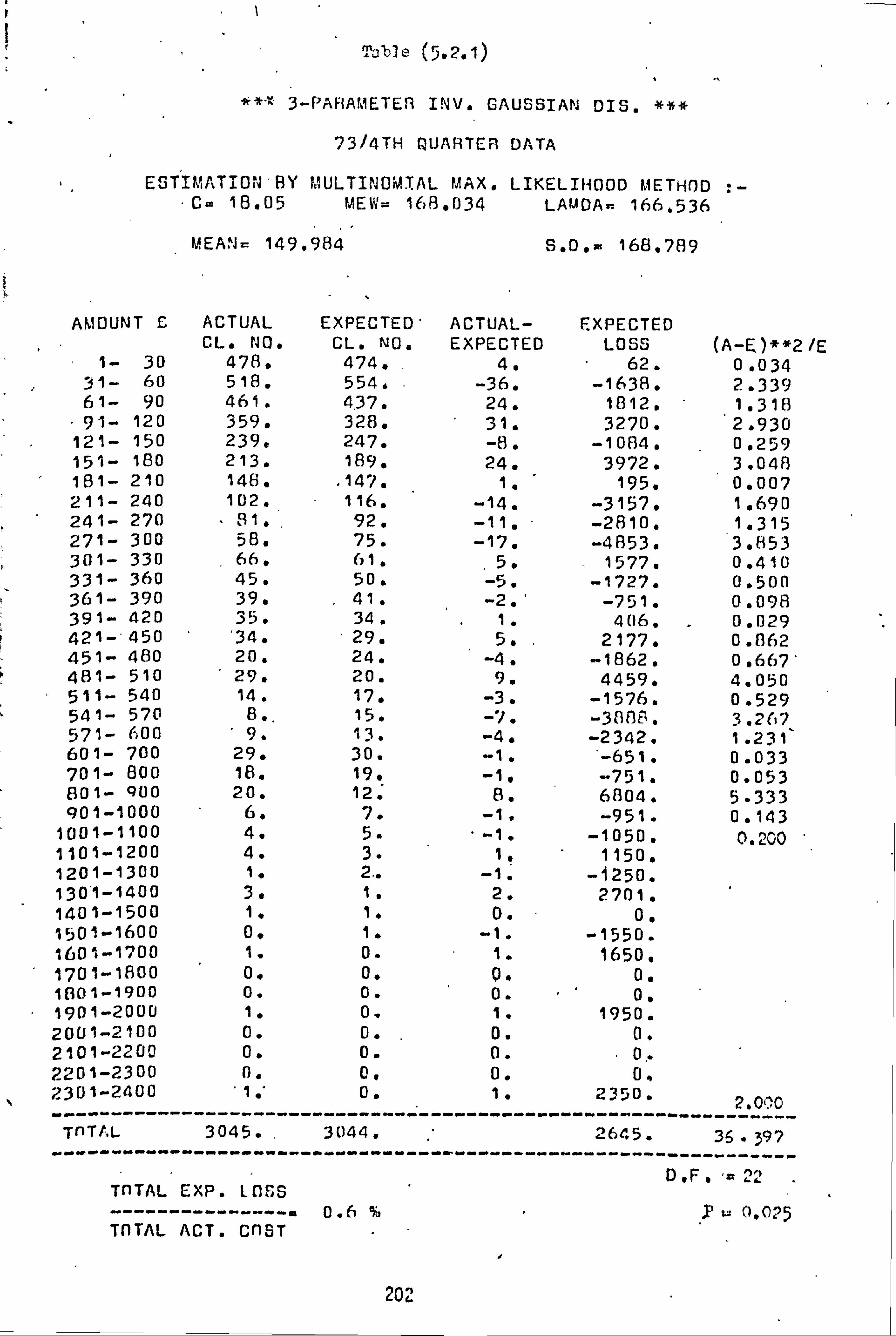
" Table tß. 2,1)

**- 3-PARAMETER INV. GAUSSIAN DIS, ***

73/4TH QUARTER DATA

E5TIMATi0 4' BY MULTINOMI AL MAX. LIKELI HOOD METHOD :- "C. 18.05 MEW= 1 68.034 LAM DA- 166.536

MEAN= 149.984 S. D .- 168.789

AMOUNT C ACTUAL EXPECTED ' ACTUAL- EXPECTED CL. NO. CL. NO. EXPECTED LOSS (A-E)**2/E

1- 30 478, 474. 4. 62. 0.034 31- 60 518. 554. -36. -1638. 2.339 61- 90 461. 437. 24. 1812. 1.318

"91- 120 359. 328. 31. 3270. 2.930 121- 150 239. 247. -8. -1084. 0.259 151- 180 213. 18qß 24. 3972. 3.048 181- 210 148. . 147. 1. 195. 0.007 211- 240 102.. 116. -14. -3157. 1.690 241- 270 91. 92. -11. -2810. 1.315 271- 300 58, 75. -17. -4853. 3.853 301- 330 66. 61.

. 5. 1577. 0.410

331- 360 45. 50. -5. -1727. 0.500 361- 390 39. 41. -2. ' -751. 0.098 391- 420 35. 34. 1. 406. 0.029 421- 450 '34. 29. 5. 2177. 0.862 451- 480 20. 24. -4. -1862. 0.667' 481- 510 29. 20. 9. 4459. 4.050 511- 540 14. 17. -3. -1576. 0.529 541- 570 8.. 15. -11. -3888. 3.267 571- 600 ' 9. 13. -4. -2342. 1.231` 601- 700 29. 30. -1. '-651. 0.033 701- 800 18. 19. -1. -751. 0.053 801- quo 20. 12. 8. 6804. 5.333 901-1000 6. 7. -1. -951. 0.143

1001-1100 4. 5. . -1. -1050. 0.200 1101-1200 4. 3. 11 1150. 1201-1300 1. 2.. -1, -1250. 1301-1400 3. 1. 2. 2701. 1401-1500 1. 1. 0. - 0. 1501-1600 0. 1. -1. -1550. 1601-1700 1. 0. 1. 1650.

1 1701-1800 0. 0. 0. 0, 1801-1900 0. 0. 0. " 01 1901-2000 1. 0. 1. 1950. 2001-2100 0. 0.

. 0. 0.

2101-2209 0. 0. 0. . 0. 2201-2300 0. 0. 0. 0, 2301-2400 ----------

1. ' -----------

0. -------- w..

1. -. r.. r. ýwr-------

2350. -----------

2.000 -------

TnTAL ----------

3045. .

----------- 3044.

---------- -------------- 2645.

----------- 35.397 -------

D. F. = 22 TOTAL EXP. L065

--------------- 0.6 % ii 0.025 TOTAL ACT. COST

202

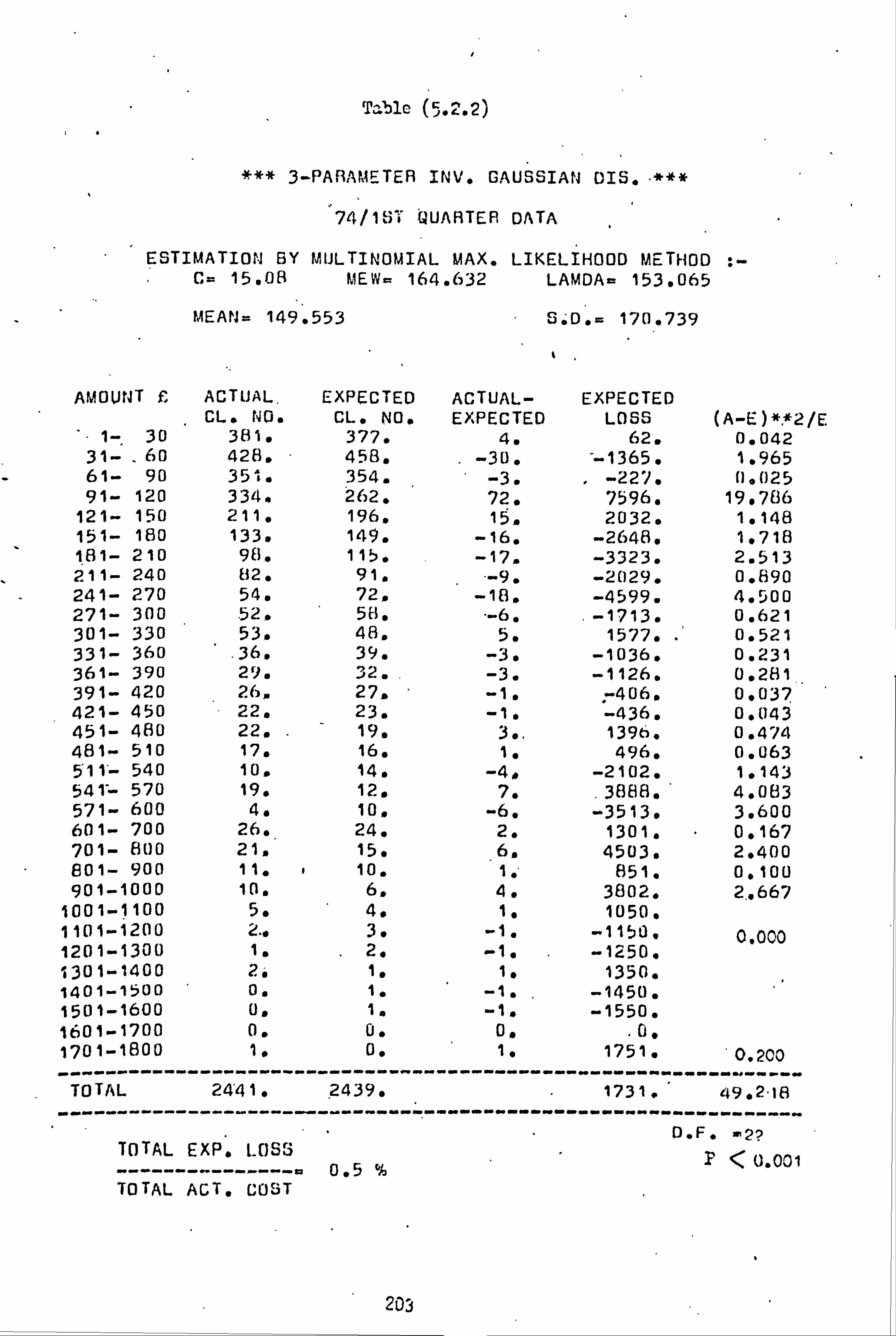
i

Table (5.2.2)

3-PARAMETER INV. GAUSSIAN DIS. "***

74/1S11' WUARTER DATA

ESTIMATION BY MULTINOMIAL MAX. LIKELIHOOD METHOD : - C= 15.08 MEW= 164.632 LAMDA- 153.065

MEAN= 149.553 0 6.0. = 170.739

AMOUNT £ ACTUAL. EXPECTED ACTUAL- EXPECTED CL, NO. CL, NO. EXPECTED LOSS (A-E)* *2/E

1-" 30 381, 377. 4, 62, 0,042 31- . 60 428, 458. -30. --1365. 1.965 61- 90 35 4. 354. -3. -227. 0,025 91- 120 334. 262, 72, 7596. 19.786

121- 150 211. 196, 15. 2032. 1.148 151- 180 133. 149. -16, -2648. 1.718 1"81- 210 98, 115. -17. -3323, 2.513 211- 240 82. 91, . -9, -2029. 00890 241- 270 54, 720 -18, -4599. 4.500 271- 300 . 52, 58. "-6. . -1713. 0.621 301- 330 53. 48, 5. 1577. 0.521 331- 360 . 36. 39. -3. -1036. 0.231 361- 390 29, 32. -3. -1126. 0,281 391- 420 26, 27, -1. -406, 0.037 421- 450 22. 23. -1. -436. 0.043 451- 480 22. 19. 3,. 1396. 0,474 481- 510 17, 16. 1. 496. 0.063 511"- 540 10, 14, -4" -2102. 1,143 541- 570 19. 12, 7.

. 3888. 4.083

571- 600 4. 10, -6. -3513. 3.600 601- 700 26, 24. 2, 1301. 0.167 701- 800 21, 15, 6. 4503. 2.400 801- 900 11,1 10. 1,, 851. 0.100 901-1000 10. 6. 4, 3802. 2.. 667

1001-1100 5. 4. 1. 1050. 1101-1200 2.. 3. -1. -1150, 0.000 1201-1300 11 . 2. -1. -1250. 1301-1400 2. 1. 1. 1350. 1401-1500 ' 0. 11 -16 . -1450. 1501-1600 0. 1" -10 -1550. 1601-1700 0. U, 06 . 0. 1701-1800 1, 0. 1. 1751. 0.200

------. - ------ .. ------------ ------ "---- .. --. ----------------------

TOTAL 24'41. 2439. 1731. ' 49.2.18 ---------------------"------- r--------------------- -------- -----

TOTAL EXP, LOSS - I' < t1,001 --------------- 0.5 % TOTAL ACT. COST

203

Table (5.2.3)

3-PARAMETER INV. "GAUSSIAN DIS. **

74/2ND QUARTER DATA

ESTIMATION BY MULTINOMIAL MAX. LIKELIHOOD METHOD : - C= 19.46 MEW 170.666 LAMDA= 1R2039

MEAN= . 151.20A S. D. = 164. SH7

0 AMOUNT F ACTUAL EXPECTED ACTUAL- EXPECTED

CL. NO., CL. NO. EXPECTED LOSS (A-E)**2/E 1- 30 351. 316. 5. 78. 0.072

31- 60 3A0. 424. -44. -2002. 4.566 61- 90 382. 345. 37. 2793. 3.968 91- 120 295. 263. 32. 3376. 3.894

121- 150 211. 200. 11. 1490. 0.605 151- 180 142. 153. -11. -1820. 0.791 181- 210 114. 119. -5. -978. 0.210 211- 240 101. 94. 7. 1578. 0.521 241- 270 57. 75. -18. -4599. 4.320 271- 300 51. 6n. -9. -2569. 1.350 301- 330 39. 49. -10. -3155. 2.041 331- 360 36. 40. -4. -1352. 0.400 361- 390 25. 33. -Fl. -3004. 1.939 391-" 420 24. ' 27.

. -3. -1216. 0.333 421- 450 27. 23. 4. 1742. 0.696 4'51- 480 18. 19. -10 -466. 0.053 4R1- 510 21. M. 5. 2477. 1.562 511- 540

"17. 14. 3. 1576. 0.643

541- 570 12. 11. 1. 555. 0.091 571- 600 11. 10. 1. 5F15. 0.100 601- 700 30. 23. 7. 4553. 2.430 701- 800 13. 14.

" -1. -751. 0.071 Sol- 900. 11. 9. 2. 170 1. 0.444 901-1000 4. 5. " -1. -951. 0.200"

1001-1100 7. .. 3. 4. 4202. 1101-, 1200 0. 2. -2. -2301. 1201-1300 1. 1. 0. 0. 1301-1400 1. 1. 0. " 01. 1401-1500 0. 1. -1. -1450. 1501-1600 1. 0. 1. 1550.

"1601-1700 0. 0. o. 0. 1701-1800 0. " 0. 0. 0. 1801-1900 ---- ----

1. ------------

0. ----------

1. -----------

1850. ----- -

1.125

TOTAL

--------- 2383.

------------ 2380.

---------- -----------

- - .

3466. -------

------------- 32.127

- -- "

------------ D. F. 21

TOTAL EXP. LOSS ----------------

y 0. (15 TOTAL ACT. COST

204

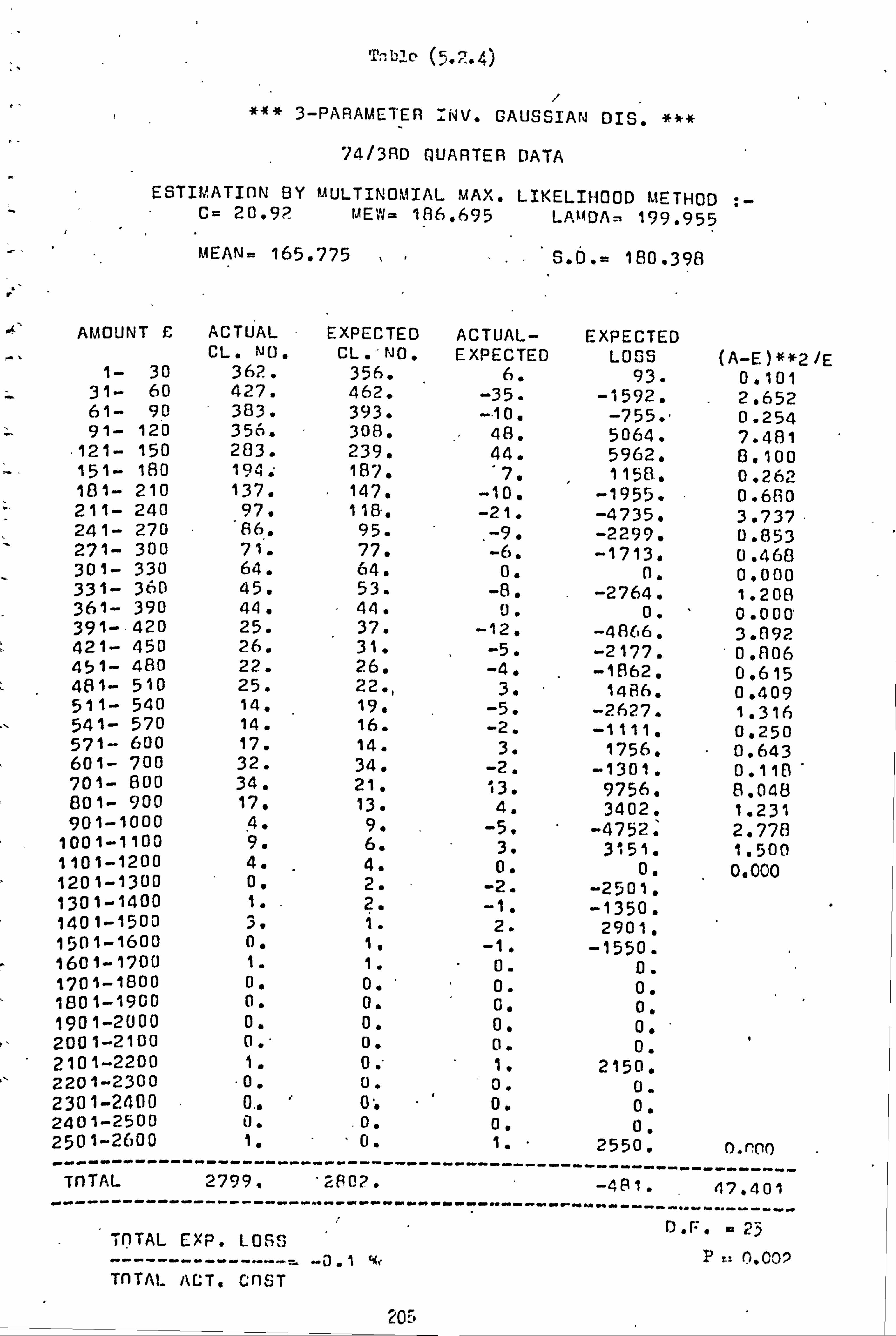
Týb1c (5. ". 4)

i *3 -PARAMETER ENV. GAUSSIAN DIS.

74/3RD QUARTER DATA

ES TIMATION BY MULTINOMIAL MAX. LIKELIHOOD METHOD ; - C= 20.92 MEW- 186.695 LAUUDA-, 199.955

MEAN= 165 . 775 S. D. = 180.398

AMOUNT £ ACTUAL EXPECTED ACTUAL- EXPECTED CL. NO. CL. 'N0. EXPECTED LOSS (A-E)**2/E

1- 30 362. 356. 6. 93. 0.101 31- 60 427. 462. -35. -1592. 2.652 61- 90 383. 393. -. 10. -755. " 0.254 91- 120 356. 308. 48. 5064. 7.481

. 121- 150 283. 239. 44. 5962. 8.100 151- 180 191. 187. '7. 115B. 0.262 181- 210 137. 147. -10. -1955. 0.660 211- 240 97. 118.1 -21. -4735. 3.737. 241- 270 66. 95. -9. -2299. 0.853 271- 300 71. 77. -6. -1713. 0.468 301- 330 64. 64. 0. 0. 0.000 331- 360 45. 53. -8. . -2764. 1.208 361- 390 44. - 44. U. 0. 0.000, 391- 420 25. 37. -12. -4806. 3.092 421- 450 26. 31. -5. -2177. 0.006 451- 480 22. 26. -4. -1862. 0.615 481- 510 25. 22., 3, . 1486. 0.409 511- 540 14. 19. -5. -2627. 1.316 541- 570 14. 16. -2. -1111. 0.250 571- 600 17. M. 3. 1756. 0.643

" 601- 700 32. 34. -2. -1301. 0.118" 701- 800 34. 21. 13. 9756. 8.048 801- 900 17. 13. 4. 3402. 1.231 901-1000 4. 9. -5. -4752. 2.778

1001-1 100 9. 6. 3. 31 51 . 1.500 1101-1200 4. 4. 0. 0. 0.000 1201-1300 0. 2. -2. -2501. 1301-1400 1. 2. -1. -1350. 140 1-1500 3. 1. 2. 2901. 1501-1600 0. 1, -1. -1550. 1601-1700 1. 1. 0. 0. 1701-1800 0. 0. 0. 0. 1801-1900 0. 0. 0. 0. 1901-2000 0. 0. 0. 00 2001-2100 0.. o. 0. 0. 2101-2200 1. 0. " 1. 2150.

11 2201-2300 "0. U. 0. 0. 2301-2400 0.. 0. 0. 2401-2500 0. 0. 0, 0. 2501-2600 -----------

1. -----------

. 0. ----------

1. " -----

2550. 0. roo

TnTAL

-----------

2799,

----------- ' 2802.

----------

-----

-----------

--------------------- -481.47.401

----------- "

----- D. f=.

------- a 23

TOTAL EXP. LOSS -----.. . -------- - -0 r1

Ci [, !ý f1/'ý/ L: 0.002

TOTAL ACT. nST

205

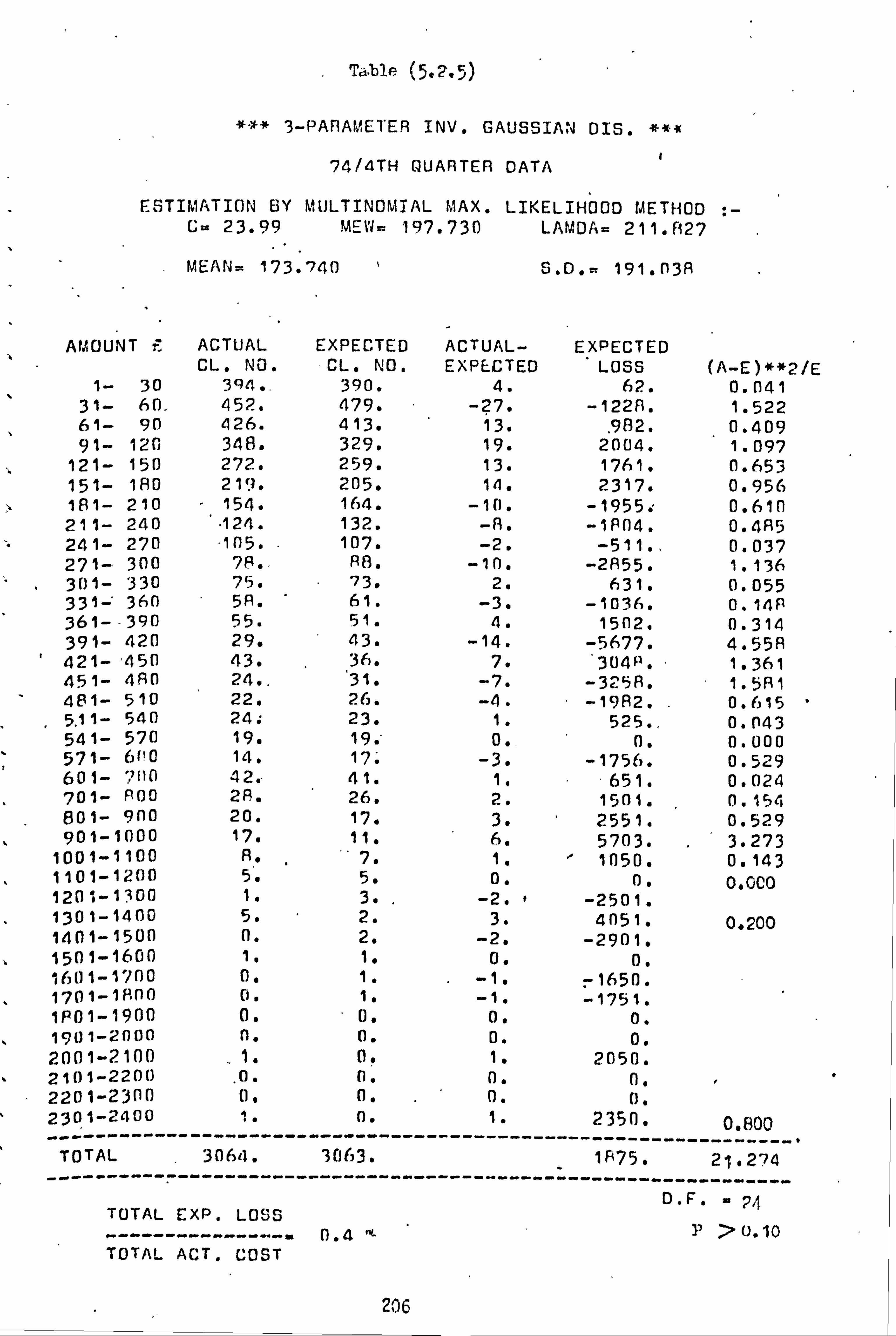
Table

*** 3-PARAMETER INV. GAUSSIAN DIS. *

74/4TH QUARTER DATA I

ESTIMATION BY MULTINOMIAL MAX. LIKELIHOOD METHOD t- c= 23.99 MEW= 197.730 LAMDA= 211.827

MEAN= 173,740 S . D. = 191.03A

AMOUNT r'. ACTUAL EXPECTED ACTUAL- EXPECTED CL. NO. CL. NO. EXPECTED LOSS (A-E)**2/E

1- 30 394.. 390. 4. 62. 0.041 31- 60. 452. 479. -? 7. -1228. 1.522 61- 90 426. 413. 13.

. 982. 0.409

91- 120 348. 329. 19. 2004. . 1.097 121- 150 272. 259. 13. 1761. 0.653 151- 180 219. 205. 1A. 2317. 0.956 181- 210 - 154. 164. -11). -1955. 0.610 21 1- 240 ' . 124. 132. -8. -1804. 0.485

" 241- 270 -105. 107. -2. -511.. 0.037 271- 300 78.. 88. -1n. -2855. 1.136 31)1- 330 75. 73. 2. 631. 0.055 331- 360 58. 61. -3. -1036. 0.14P 361--390 55. 51. 4. 15112. 0.314 391- 420 29. 43. -14. -5677. 4.558 421- '450 43. 30. 7. 3048. 1.361 451- 480 24.. 31. -7. -3258. 1.581 481- 510 22. 26. -4. -19A2. 0.615 5,11- 540 24. 23. 1. 525., 0.043 541- 570 19. 19.. 0.

_ 0. 0.000

571- 600 14. 17. -3. -1756. 0.529 601- 7110 42. - 41. 1. 651. 0.024 701- 800 28. 26. 2. 1501. 0.154 601- 900 20. 17. 3. 2551. 0.529 901-1000 17. 11. 6. 5703. 3.273

1001-1100 8. ,

7. 1. 1050. 0.143 1101-1200 5. 5. 0. a, 0.000 1201-1300 1. 3.

. -2. º -250 1. 1301-1400 5. 2. 3. 4051. 0.200 1401- 1500 0. 2. -2. -2901. 1501-1600 1. 1. 0. 0. 1601-1700 0. 1. -1. -1650. 1701-1800 0. 1. -1. -1751. 1P01-1900 0. 0. 0. 0. 1901-2000 n. 0. 0. 0. 2001-2100 1. 0. 1. 2050. 2101-2200 .

0. n. 0. n 2201-2300 0. 0. 0. () . 2301-2400 1. 0. 1. 2350. 0.800 ---------- ------------ ---------- -------------------------------

TOTAL 30611. 3063. 1875. 21.274

TOTAL EXP. LOSS

---------------- 0.4 y 7 0.10 TOTAL ACT. COST

206

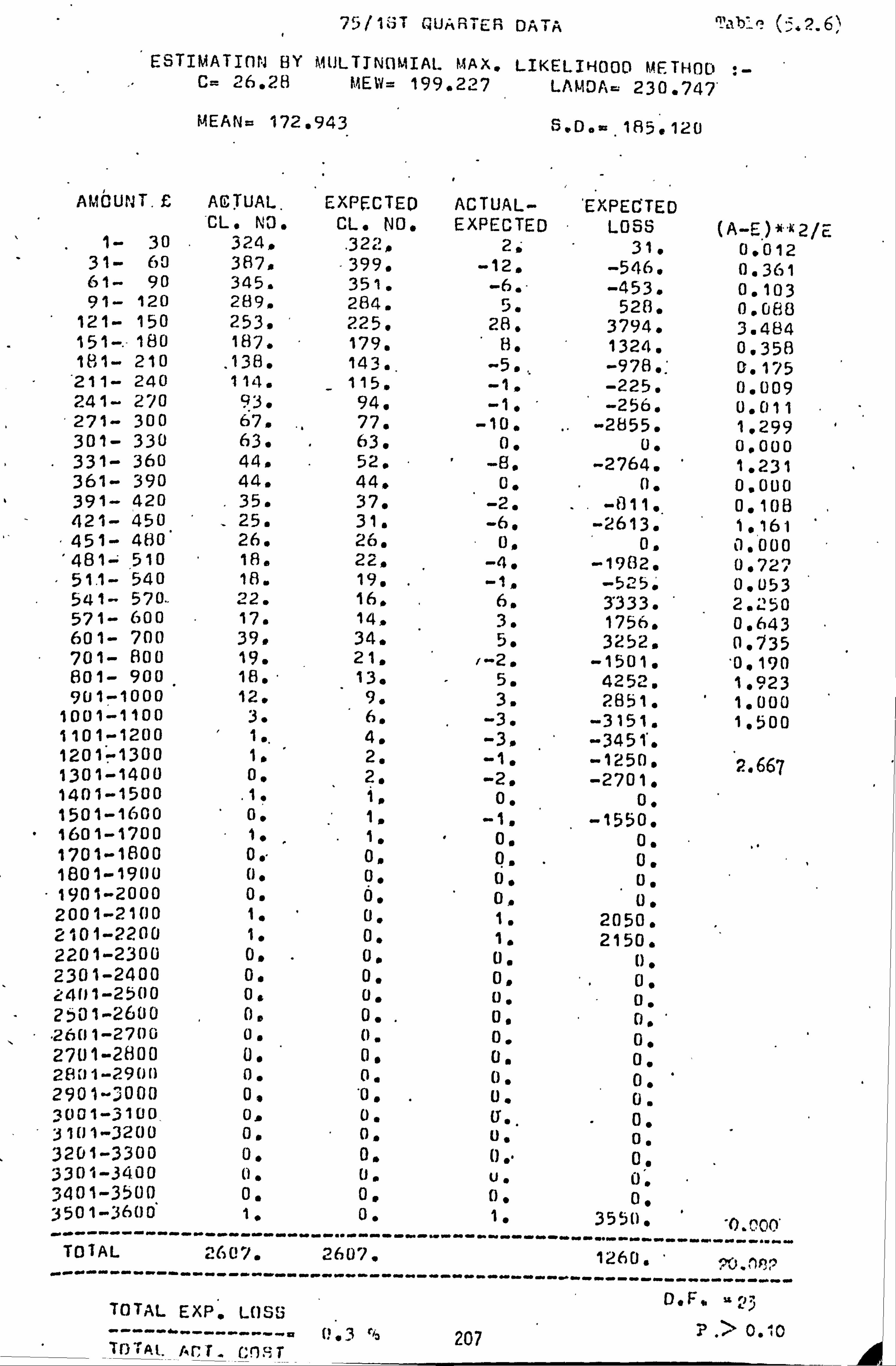
75%1$T QUARTER DATA Table (ßi2.6)

ESTIMATinN BY MULTINt1MIAL MAX. LIKELIHOOD METHOD ; - C= 26.28 MEW= 199.227 LAMM 230.747

MEAN= 172,943 S*Do-. 1A5.120

AMCUNNT. £ ACTUAL. EXPECTED ACTUAL- 'EXPECTED CL. NI O, CL. NO, EXPECTED LOSS (A-E 21G 1- 30 3249

. 322� 2; 31. 0.3 31- 60 387, -399. -12, -546. 1 0.361 61- 90 345. 351. -6. - -453. 0.103 91- 120 289. 284. 5. 528, 0.080

121- 150 253. 225, 28. 37949 3.484 151-. 180 187, 179, 86 1324. 0.358 181- 210

. 1389 143.. -5.,, -978.; 0.175

'211- 240 114. 115. -1, -225. 01009 241- 270 939 949 -1, ' -256. 0,011 271- 300 67. 77. -101 -2855. 1.299 301- 330 63. 63. 0. 00 0.000 331- 360 449 52. -8, -2764. 1.231 361- 390 44, 44,. 0, () . 0.000 391- 420 . 35. 37. -2, .. -811.. 0,108 421- 450 25. 31. -6. -2613. 1.161 451- 480 26. 269 0, 0.000

'481--; 510 18. 22, -4. -1982. 0,727 51.1- 540 18. 19. . -1, -525. 0,053 541- 570.. 22. 16, 6. 3'333. 2.2 50 571- 600 17. 14, 3. 1756, 0.643 601- 700 39. 34. 5, 3252. 0.735 701- 800 19. 21, /-2, -1501. 0.190 801- 900 18. " 13, - 5. 4252, 1,923 901-1000 12. 9. 3. 2851. 1.000

1001-1100 3. 6. -3. -3151. 11500 1101-1200 1.

" 4. -3, --3451'. 1201-1300 1. 2. -1, -1250. 2.667 1301-1400 2. -2. -2701, 1401-1500 . 1. 1, 0, 01

1501-1600 0. -1550.

" 1601-1700 01 00 1701-1800 0, " 0, 0. . 0 1801-1900 00 01 0. 01

'1901-2000 0. Ö. 01 0. 2001-2100 1, 0. 1. 2050. 2101-2200 1, 0, 11 2150, 2201-2300 011 0. 0. () 2301-2400 0. 0. 0, ,

01 2401-2500 04 0. 0, 0. 2501-2600 011 0. 01 0, ' . 26(11-2700 00 0. 0. 01 2701-2800 00 0, 0a 0, 28k') 1-2901) 01 0. 0. 0 2901.3000 08 '0, 0. 0. 3001-3100, 01 0. 0., 01 3101-3200 0. 0. 3201-3300 00 00 3301-3400 0. (1, u. U; 3401-3500 0. 01 00 0: 3501-3600

----------- 1,

----------- 011

------------ 1

---------- 355(), ,

- '0. cloo*

TO1AL -----------

2607. ---- ------ -

2607. ----------- -------~---

----------- 1260, '

----------

---------- 9ei f111) 8P

------mow--

TOTAL EXP. LOSS p>0.440

Treat. r, r, 7. (; ýýT

f Table (5.2.7)

3-PARAMETER- INV. GAUSSIAN CIS, ***

75/2ND QUARTER DATA

ESTIMATION BY MULTINOMIAL MAX. LIKELIHOOD METHOD ; - S 21.49 MEW- 201.211 LAMDA= 203.077

MEAN= 179.717 5. D. = 2009285

AMOUNT E ACTUAL. EXPECTED ACTUAL- EXPECTED CL. NO. CL. NO. EXPECTED LOSS (A-E)**2/E

1- 30 302. 299. 3. 46. 0.030 31- 60 374. 390. -16. -728, 0.656 61- 90 332. 336, E -4, -302. 0.048 91- 120 277. 267. 10. 1055. 0.375

121- 150 235. 210. - 25. 3387. 2.97e 151- 180 187. 166-. 21. 3475. 2.657 181- 210 122. 133. -11, -2150. " 0.910 211- 240 110. 108, 2. 451, 0.037 241- 270 80. 88. -8. -2044. 0.727 271- 300. 72. ,

72. 0. 0. 0.000 301- 330 47. 60. -13. -4101. 2,017 331- 360 39. 50, -11. _ -3800. 2.420 361-. 390 40. 42. -2. -751. 0.095 391- 420 38,, 36. 2. 811. 01111 421- 450 29, 30. -1, -436., 0,033 451- 480 21. 26.. -5. -2327, 0,9612 481- 510 30,

. 22. 8. 3964. 2.909

511- 540 19. 19. 0. 0. 0.000 541- 570 $7.. 17, 0. 0. 01000 571- 600 11. 14. --3. -1756. 0.643 " 601- 700 36. 36. 0. 0. 0.00'0 701- 800 22. 23. -1, -751. 0.043 801- 900 22. 15. 7: 5953. 3.267 901-1000 11. 10. 1. 951. 0.100

1001-1100 4. 7. -3. -3151. 1.286 1101-1200 3. 5. -2. -2301. 0.600 1201-1300 3. 3. 0, 0o , 1301-1400 6.

. 2. 4, 5402. 3.200

1401-1500 2,. 2. 0, 0, 1501-1600 1. " 1. 0. 00 1601-1700 0. 1. -11 -1650, 1701-1800' 1. 1. 0, 0l 1801-1900 00 0. 0. 0. 1901-20010 1. 0: 1, 1950. 2001-2100 0. 0. 0. 0. 2101-2200 " 0. "'0. 0,

. U.

2201-2300 -----------

1. ----------

0. - -----

1. ----

2250. 0 . Poo

TOTAL -----------

2495. ----------

2491. ' ------------ -----------

3447. ----------

'--23*101

---------- U. F. m 24

TOTAL EXP. LOSS

. ------ -------- = 0.8 °5 P>0.10 TOTAL ACT, COST

208

Table (5.3.1

*** 3-PARAMETER INV. GAUSSIAN DIG. ***

PREDICTION OF 74/4TH QUARTER CLAIMS Cn ,T USING 73/4TH QUARTER MULT. HAXLIK. PARAMETERS

C= 18.1 MEW= 168.034 LAt1DA= 166.536 INFLATION RATE I=18.2°: CALCULATED FRnt! GENERAL INDEX OF RETAIL PRICES

PREDICTION PARAMETERS ARE :v C=21.4 MEW=19f. 616 LAMDA=156.846 MEAI1 CLAIM AMOUNT= 177.22 S. D. =199.51

ACTUAL 74/4TH PARAtETERS :- C=24.0 MEY! =197.730 LAMDAm211.827 UEAN CLAIM AMOUNT= 173.73 S. D. -191.04

AMOUNT £ ACT. NO. EXP. NO. A-E EXP. LOSS (A_E)**2/E 1- 30 394. 386. A. 124. 0.166

31- 60 452. 486. -34. -1547. 2.379 61- 90 426. 413. 13. 982. 0.409 91- 120 348. 326. 22. 2321. 1.485

121- 150 272. 255. 17. 2304. 1.133 151- 180 219. 202. 17. 2813. 1.431 181- 210 154. 161. -7. -1368. 0.304 211- 240 124. 130. -6. -1353. 0.277 241- 270 105. 106. -1. -256. 0.009 271- 300 78. 87. -9. -2569. 0.931 301- 330 75. 72. 3. 947. 0.125 331- 360 58. 60. -2. -691. 0.067 361- 390 55. 51. 4. 1502. 0.314 391- 420 29. 43. -14. -5677. 4.558 421- 450 43. 37. 6. 2613. 0.973 451- 480 24. 31. -7. -3258. 1.581

, 481- 510 22. 27. -5. -2477. 0.926 511- 540 24. 23. 1. 525. 0.043 541- 570 19. 20. -1. -555. 0.050 571- 600 14. 17. -3. -1756. 0.529 601- 700 42. 43. -1. -651. 0.023 701--800 28. 28. 0. 0. 0.000 1101- 900 20, 18. 2. 1701. 0.222 901-1000 17. 12. 5. 475?. 2.0113

1001-1100 A. 8. 0. 0. 0.000 . 1101-1200 5. 6. -1. -1150. 0.167

1201-1300 1. 4. -3. -3751. 1301-1400 5. 3. 2. 2701. 1401-1500 0. 2. -2. -2901. 1501-1600 1. 1. 0. 0. 1601-1700 0. 1. -1. -1650. 1701-1800 0. 1. -1. -1751. 1801-1900 0. 1. -10 -1850. 1901-2000 0. 0. 0. 0. 2001-2100 1. 0. 11 2050. 2101-2200 0. 0, 0, 0. 2201-2300 0. 0. 0. 0. 2301-2400 1. 0.. 1. 2350.

------------ TOTAL ---------

3064 ----------

3061 ------ ---------- -7528.

---------- 20.185

------------------------------------- --------------------

CHI SQ. STAT. - 21.825 . D. E. = 27 F>0 10 , . TOTAL ACTUAL COST - 533707. TOTAL EXPECTED COST s 541234". i'OL - SI: T(NOV I= 0.015

1> 0.20 ý TOTAL EXP, LOSS ---------------- - 1.41 % TOTAL ACT, C05T 209

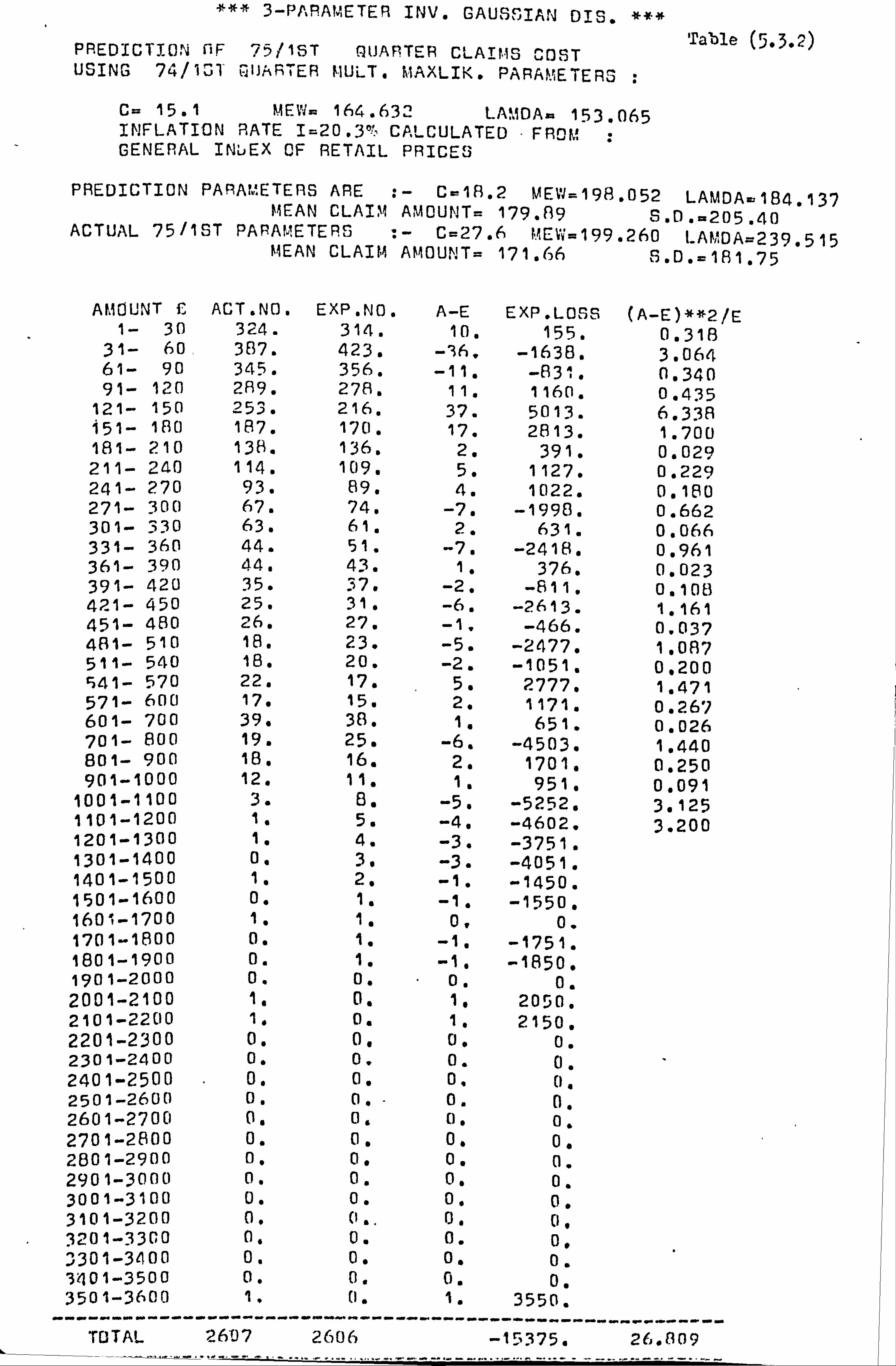
*** 3-PARAMETER INV. GAUSSIAN DIS. # "*

PREDICTION RF 75/13T QUARTER CLAIMS COST Table (5.3.2)

USING 74/13T t JARTER MULT. MAXLIK. PARAMETERS

C= 15.1 MEW- 164.632 LAMDA= 153-065 INFLATION RATE I=20.3°', CALCULATED - FROM

. GENERAL INbEX GF RETAIL PRICES

PREDICTION PARAMETERS ARE :- C-1A. 2 MEW=198.052 LAMDA=: 184.137 MEAN CLAIM AMOUNT= 17909 S. D. =205.40 ACTUAL 75/1ST PARAMETERS

.- C=27.6 MEW=199.260 LAMDA=239.515 MEAN CLAIM AMOUNT= 171.66 S. D. =181.75

AMOUNT C ACT. NO. EXP. NO. A-E EXP. LOSS (A-E)**2/E 1- 30 324. 314. 10. 155. 0.318

31- 60, 387. 423. -36. -1638. 3.064 61- 90 345. 356. -11. -E831. 0.340 91- 120 289. 278. 11. 1160. 0.435

121- 150 253. 216. 37. 5013. 6.3311 151- 180 187. 170. 17. 2813. 1.700 181- 210 138. 136. 2. 391. 0.029 211- 240 114. 109. 5. 1127. 0.229 241- 270 93. 89. 4. 1022. 0.160 271- 300 67. 74. -7. -1990. 0.662 301- 330 63. 61. 2. 631. 0.066 331- 360 44. 51. -7. -2418. 0.961 361- 390 44. 43. 1. 376. 0.023 391- 420 35. 37. -2. -811. 0.108 42_1- 450 25. 31. -6. -2613. 1.161 451- 480 26. 27. -1. -466. 0.037 481- 510 18. 23. -5. -2477. 1,087 511- 540 18. 20. -2. -1051. 0.200 541- 570 22. 17. 5. 2777. 1.471 571- 600 17. 15. 2. 1171. 0.267 601- 700 39. 38. 1, 651. 0.026 701- 800 19. 25. -6. -4503. 1.440 801- 900 18. 16. 2. 1701. 0.250 901-1000 12. 11. 1. 951. 0.091

1001-1100 3. 8. -5, -5252. 3,125 1101-1200 1. 5. -4. -4602. 3.200 1201-1300 1. 4. -3. -3751. 1301-1400 0. 3. -3. -4051. 1401-1500 1. 2. -1. -1450. 1501-1600 0. 1. -14b -1550. 1601-1700 1. 11 0, 0. 1701-1800 0. 1. -1. -1751. 1801-1900 0. 1. -1. -1850. 1901-2000 0. 0. 0. 0. 2001-2100 11 0. 1. 2050. 2101-2200 11 0. 1. 2150, 2201-2300 0. 0. 01 0. 2301-2400 0. 0. 0. 0. 2401-2500 0. 0. 0. 04 2501-2600 0. 0. 0. 0. 2601-2700 0. 0. 0. 0. 2701-2800 0. 0, 0. 0. 2801-2900 0. 01 0. 0. 2901-3000 0. 0. 0. 0. 3001-3100 0. 0. 0. 0. 3101-3200 0. 0.. 0. 0, 3201-3300 0. 0. 0. 01 3301-3400 0. 0. 0. 0. 3401-3500 0. 0. 0. 0. 3501-3600

-------------

1. --------

0. ----------

1.

------ 3550.

----------- --------- TOTAL 26t)7 2606 -15375.26.809

Table (5.3.2) - continued

CHI SQ. STAT. °32.619 , D. F. =27 9 P70. ß0

TOTAL ACTUAL COST = 452n59. TnTAL EXPECTED COST = 467433. KOL - SM. IRROV D=0.15

TOTAL-EXP. LOSS P> 0.20

---------------= -3.40 % TOTAL ACT. COST,

211

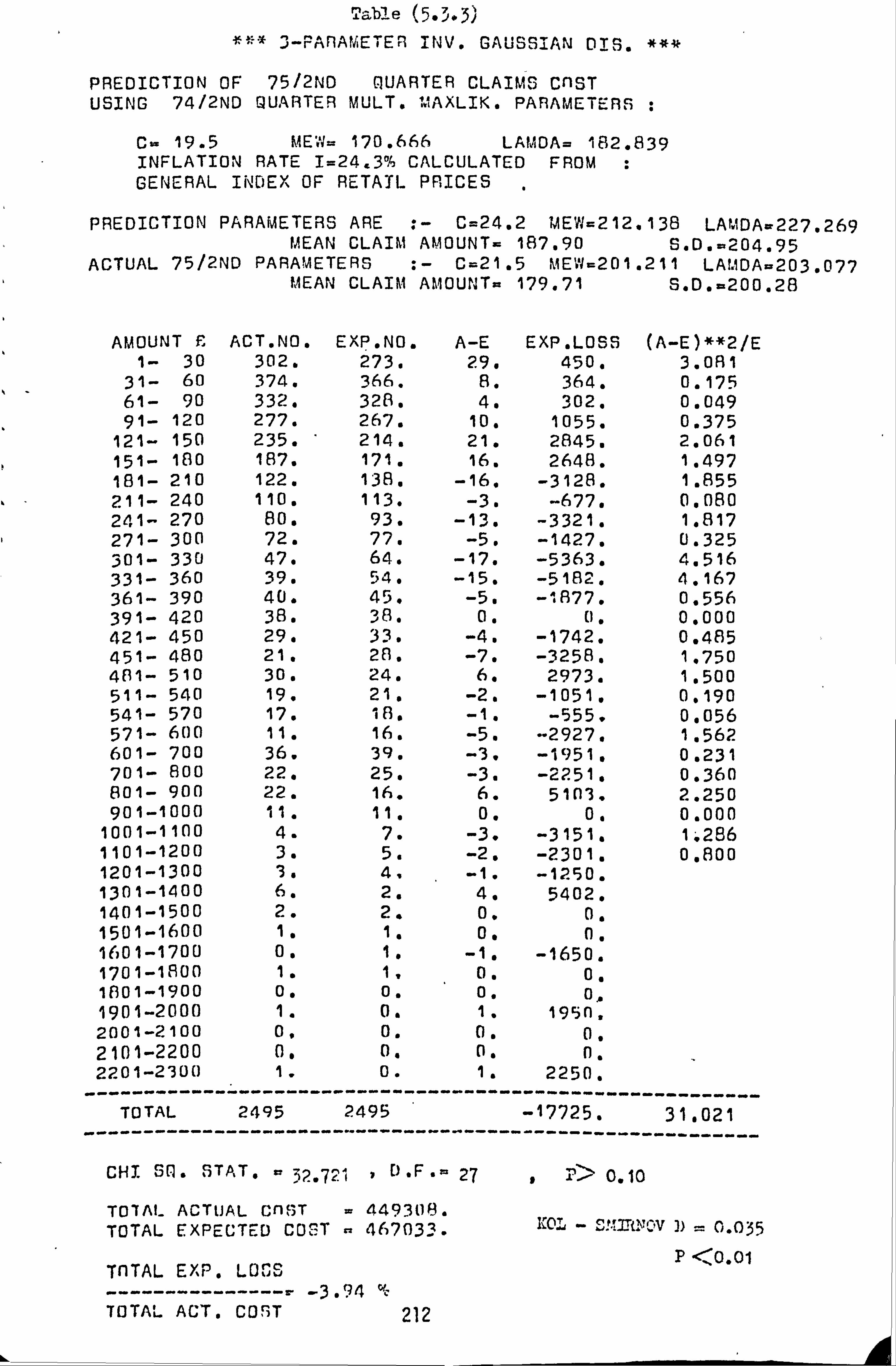
11 Table (5.3.3) 3-PAfAMETER INV. GAUSS-AN DIS.

PREDICTION OF 75/2ND QUARTER CLAIMS CnST USING 74/2ND QUARTER MULT. IMAXLIK. PARAMETERS

C= 19.5 MEW= 170.666 LAMDA= 182.839 INFLATION RATE I=24.3° CALCULATED FROM GENERAL INDEX OF RETAIL PRICES

PREDICTION PARAMETERS ARE :- C=24.2 UE'W=212.138 LAMDA=227.269 MEAN CLAIM AMOUNT= 187.90 S. D. -204.95

ACTUAL 75/2ND PARAMETERS :- C=21.5 MEW=201.211 LAMOAa203.077 MEAN CLAIM AMOUNT= 179.71 S. D. =200.28

AMOUNT F, ACT. NO. EXP. NO. A-E EXP. LOSS (A-E)**2/E 1- 30 302. 273. 29. 450. 3.081

31- 60 374. 366. 8. 364. 0.175 61- 90 332. 326. 4. 302. 0.049 91- 120 277. 267. 10. 1055. 0.375

121- 150 235. 214. 21. 2845. 2.061 151- 180 187. 171. 16. 2648. 1.497 181- 210 122. 138. -16. -3128. 1.855 211- 240 110. 113. -3. -677. 0.080 241- 270 80. 93. -13. -3321. 1.817 271- 300 72. 77. -5. -1427. 0.325 301- 330 47. 64. -17. -5363. 4.516 331- 360 39. 54. -15. -5182. 4.167 361- 390 40. 45. -5. -1877. 0.556 391- 420 38. 38. 0. 0. 0.000 421- 450 29. 33. -4. -1742. 0.485 451- 480 21. 28. -7. -3258. 1.750 481- 510 30. 24. 6. 2973. 1.500 511- 540 19. 21. -2. -1051. 0.190 541- 570 17. 18. -1. -555. 0.056 571- 600 11. 16. -5. "-2927. 1.562 601- 700 36. 39. -3. -1951. 0,231 701- 800 22. 25. -3. -2251. 0.360 801- 900 22. 16. 6. 51913. 2.250 901-1000 11. 11. 0. 0. 0.000

1001-1100 4. 7. -3. -3151. 1.286 1101-1200 3. 5. -2. -2301. 0,800 1201-1300 3. 4, -1. -1250. 1301-1400 6. 2. 4, 5402. 1401-1500 2. 2. 0. 0. 1501-1600 1. 1. 0. n. 1601-1700 0. 1. -1. -1650. 1701-1800 1. 1, 0. 01 11301-1900 0. 0. 0. 0» 1901-2000 1. 0. 1. 1950, 2001-2100 01 0. 0. 0. 2101-2200 0. 0. 01 n, 2201-2300

------ 1.

---------- 0.

---------- 1.

------ 2250.

--- ----- TOTAL

----------- 2495

--------- 2495

----------- ------

------- -17725.

----------

----------- 31.021

-----------

CHI SO. STAT. " 352.72 ,0F. ¢ 27 , r> 0. to TOTAL ACTUAL CnIT = 4493118. TOTAL EXPECTED COST - 467033. KOL - =r'ýý-ý'cv ýý 0.035

TnTAL EXP. LO; CS P <O. O1

---------------r -3 -94 % TOTAL ACT. CO 9T 212

CHAPTER 6

The Pareto Distribution

6.1 Introduction

The Iareto distribution, which is positively skewed and has a long

tail, was originally proposed by Vilfredo Pareto as a model for the

distribution of incomes over a population. It has also been successfully

used to model empirical distributions of claim amounts in general

insurance and, in particular, in fire insurance. Benckert and

Sternberg (1957), Anderson (1971) and Benckertand Jung (1974) have

used this distribution as a model for fire insurance claim amounts.

In this chapter we will study this model and will consider its

application to the accidental damage claim amounts. The Pareto

distributions of the first and second kind will be initially defined

and some of their properties will be studied. A graphical test will be

discussed for the purpose of determining whether a given sample is likely

to be from a Pareto population. We will then apply this test to our

accidental damage data and will, in the event, show that the Pareto

distribution is not a satisfactory rmdel. The estimation problem is

next dealt with and the effects of inflation on the parameters of the

model will be discussed.

6.2 Definition

A random variable X is said to have a Pareto distribution of the

first kind if its distribution function, denoted by P1(x; A, B), is of

the form A

P1(x; A.. B) =1- (i. ) A, B > O, x. B

This is a special form oE Pearson Type Vl distribution. The probability

density function (p. d. f. ) of X is

fi`A+1 fý, ý (x; A, B) =Bt Y) A, 13 > 0, B (G . 2-21

213

where A and B are the sham and scale parameters respectively.

A random variable X is said to have a Pare-to distribution of the second

kind if its distribution function, denoted by P2(x; C, A,. B), is of he

. bn

P2(x; C, A, B) =1- ()A A, B > 0, x >. B-C (6.2-3)

This is sometimes called the Lomax distribution and is also a Pearson

Type Vi. it differs fron Pl(x; A, ß) by having the location parameter

C which acts as a threshold below which the values of X are not

realized. The p. d. £. of X is given by

A+1 fß, 2 (x; C, A, B) =C iB -ff A, B > 0, x3B-C (6.2-4)

6.3 Properties of the Pareto Distribution

In this section we will mention some of the properties of the

Pareto distribution of the first kind. For more details reference should

be made to, for instance, Johnson and Kotz (1970).

For the distribution P1(x; A, B) it can be shown that the rth moment of

X about zero is

r E(XT) _

Tr (if A> r) (6.3-1)

Hence the mean of the distribution of X is

E(X) = AB (if A> 1) A-1 (6.3-2)

The variance of X can be shown to be 2

var(X) _ AB (if A, 2) (6.3-3)

(q-i) (A-2)

Therefore the mean and variance of tho distribution exist when A>1

and A>2 respectively.

The coefficient of variation of X is x where

214

1

2A=1 (if A- 2) A(A-2)

(6,3.4)

which is a function of A, the shape parameter, only. As the mean of

the distribution does not always exist, the single mode of the distribution

which is located at B may be used in its place.

The median of the distribution is at

Xmedian = B(2)i/A (6.3-5)

In general the quantile of order q is xq : where

X= B(1 - q) -'/A

O<a<1 (6.3-6) a

The properties of the Pareto distribution of the second kind can

be obtained from those of the first kind since the former distribution

is derived from the latter by the transformation x -" x+C. This is

a translation which leaves the shape of the frequency curve of P1(x; A , B)

unchanged and only shifts it by an amount -C along the x-axis. The

measures of central tendency are, therefore, decreased by C while

the moments about the mean and the measures of dispersion remain the

same as for the first kind.

6.4 The Graphical Test for the Pareto Distribution

It is possible to test graphically if a given sample is likely

to be from a Pareto population. For the distribution of the first

kind given by (6.2-1) we can show that

log(1-P1) = -A log x+A 1og B (6.4-1)

where P1 = P1 (x; A, B)

Therefore the locus of the points (logx , log(l - 11)) is a straight

line whose gradient and intercept are A and Alogl3 respectively. LCt

us assui e that we are giver. a samplo of n independent rundem

215

observations from n Pareto distribution. If we define the sample

empirical distribution function as

F(x) = the proportion of observations 6x (6.4-2)

then we can use F(x) as an estimate of Pl(x; A, B) at point x. Hence

if we plot the points (log x, log(1 - F(x))) on a rectangular system

of co-ordinate axes, or plot(x, l-F(x)) on logarithmic axes, we should

find that the points lie approximately on a straight line. If the

points do not appear to lie approximately on a straight line, we conclude

that the sample is not from a Pareto population of the first kind.

For the Pareto distribution of the second kind, equation (6.4-1)

becomes

log (1 - P2) = -A log (x + C) +A log B (6.4-3)

where P2 = P2(x; C, A, B)

Hence the locus of the points (109(x + Q, log (1 - P2)) is a straight

line. When C is unknown the first step is to assinne C=0 and to plot

the resulting points (as in the case of the 3-parameter lognormal and

Weibull distributions). If the sample is from a population with C not

equal to zero, judging by the curvature of the resulting curve, we

should choose another value for C such that the points are rectified

to lie approximately on a straight line. If such aC exists, we conclude

that the sample is from a Pareto population of the second kind and

riay use this value of C as a graphical estimate of the unknown parameter

C. This technique was described, in detail, in sections 3.11 and 4.4

for the 3-parameter lognormal and Weibull distributions respectively.

6.5 The Pareto Graphical Test on AD Dzta

To test if the Pareto distribution can be used as a model for the

accidental damage (AD) data we wrote coiputer program P22. From a

216

given saiiple of data, the program calculates the empirical distribution

function F(x) at each sample value x and then plots the points

(log x, log (l -F (x)) . For the seven samples of Al) data which were

given in tables (1.1) to (1.7) the graphs are presented in figures

(6.1-a) and (6.1-b). It is observed that for each sample the points

lie approximately on a curve which is far from a straight line. The

points in the upper tail of the sample values lie almost on a straight

line, but the curvature in the lower tail values is so marked that even

an addition of C to the values of x( and hence a Pareto distribution

of the second kind) does not seem likely to rectify the points enough

to lie on a straight line. We, therefore, conclude that the Pareto

distribution is not a possible model for the distribution of our AD

claim amounts. However, as indicated by the graphs, such a model may

very well fit the distribution of the larger claims in the sample.

217

Figure (6.1-a)

:,

10 1 "LOL" I.. r(*))

CIS. 0o-

el

s. "

-e

LOU w)

"1 4

LOG(x)

9

8

Str*oIght (3' plot oG PARETO DIS. For 7S/2ND QUARTER DATA

ICI -ttrcl. "r.. »

1j Ulraly'tl ltn+" plot oý 1'AI: CTC UI;.

7$'IST OUAFIIK MMA

LOUx)

6

3" "

s

f

3

i

2i

' *"

f f

f e

-; __-T"_---. 21C ei LI""f r)

171S67E Lx.. s>

6.6 Estimation of the Parameters of the Pareto Distribution

Although the results of the previous section were not encouraging,

for the sake of completeness of the present work, we deal with the

problem of estimation from grouped data. Several methods of estimation

such as the methods of moments, quantiles, graphical, least squares

and maximum likelihood have been studied by various authors and a

review is provided in Johnson and Kotz (1970). Some of these methods

are directly applicable for estimation from grouped data while others

(like the noments, quantiles and maximum likelihood) can be modified

for this purpose in the same way as we described for the 2-parameter

lognormal distribution. In this section, we explain briefly the method

of least squares and them concentrate on the multinomial maximum

likelihood (. &NL) method.

The least squares method is based on the relationship (6.4-1).

Instead of fitting a straight line to the points (log x, log(1-F(x)))by

eye, we use the least squares technique to find the unknown coefficients

of the line. For Pl(x; A, B) this is straightforward. For P2(x; ' C, A, B)

when C is unknown, in order to avoid solving a system of non-linear

equations in the parameters, we can use the computing technique which we

suggested for the 3-parameter lognormal and Weibull distributions in

sections 3.12.1 and 4.6.1 respectively.

The AML is a very suitable method of parameter estimation from

grouped data and it produces efficient estimators. Estimation of the

parameters of the Pareto distribution of the second kind, P2(x; C, A, B),

will be dealt with here but the same argent applies for Pl(x; A, B)

by putting C=0 in the following exposition.

Let us assune that we have a sample. of grouped data where n independent

random observations on a random variable X (in our case he claim

amount) have. been grouped according to t1heir size into k nni. tually exclusive

218

intervals. Iurther, let nl be the number of observations (claims) in

the class interval (x i-1 xi) for i=1,2, ... ,k, such that

k n= ni

i=i

If X is distributcd as P2(x; C, A, B), given by (6.2-3) , i. e.

P2 (X; C, A, B) =1- (X$` )A (6.6-1)

then let pi be the probability that an observation (claim) occurs

in the interval (xi_1, xi), i. e.

pi = P2(xi; C, A, B) - P2(xi-1; C, A, B) (6.6-2)

for i=1,2, ... ,k

from (6.6-1) it follows that

pi. = x1B + )A - (1

x+C )A (6.6-3)

therefore the sample likelihood function will be proportional to L where 1i yak r.. ". ... ý... ".. .ý

k L= pi

ni (6.6-4) i=1

and the loglikelihood function will be

k log L= nllog p1 (6.6-5)

i=1

from (6.6-3) it follows that

k log L + n1 log [(x±11+c)A

)A (6.6-6)

AA

The naxirzl likelihood cstioates, (C ,A, B), of the parameters are

obtained by maximizing logL sir: ultaneý, usly with respect to A, B and C.

To avoid solving; non-linear equations (which is a laborious task when k,

219

the number of intervals, is large) we suggest the computing tecxMique

described in section 3.7.7 for maximising log L with respect to A, B

and C. To start the iteration process we can use a set of estimates

found by one of the simpler, but less accurate, methods. For instr. nce,

the moments, quantiles or graphical estimates (or their combination)

may be used. The set (C, A, B) which ma irrizes log L will be the

required DINS, estimates.

The graphical tests showed earlier that the Pareto distribution does

not represent our AD data. Therefore, we will not attempt to fit

this model to the complete histogram of the data. However, figures

' (6.1-a) and (6.1-b) showed that the points corresponding to the upper

tail of the distribution of claim amunts lie approximately on a

straight line. In chapter 7 we will fit this model to the upper tail

of the AD histograms and will compare its fit with that of the truncated

lognonnal distribution.

6.7 The Effects of Inflation on the Parameters

Following the argument of chapter 3 abcut the effects of inflation

on the parameters of a model, it is considered important to study

these effects theoretically for the Pareto distribution. We will need

to allow for such effects when predicting the future distribution of

claim amounts for a class of general insurance business in which the

Pareto model has been found to represent the distribution of claim

amounts.

Let us again assume that the effect of inflation is to increase a

claim of amount X to U= X(1, + i) over a period where i is the effective

rate of inflation for that period. If Xis distributed as a Pareto

distribution of the second kind with p. d. f. fP2(x; C, A, B) then by a

simple trarsfoiration of variables we can show that U is distributed as

22.0

a Pareto distribution of the second kindwith p. d. f. fP2(u; rC, A, rB)

where r=1+i. Therefore inflation affects the parameters C and }3

but leaves the shape parameter A unaltered. The results for the

Pareto distribution of the first kind can be deduced from the above by

putting C=0.

6.8 Conclusions

The Pareto distribution was studied in this chapter as a model

for the distribution of claim amounts in general insurance and, in

particular, for the accidental damage claim amounts.

The Pareto distribution, as well as other positively skewed distributicns

like the lognormal, has been shown to represent empirical distributions

of many socio-economic and other naturally occurring quantities. In

section 6.1 reference was made to the uses of Pareto distribution in

fire insurance. A graphical procedure was described which may be used

to test if a sample is likely to be from a Pareto population. Our AD

data proved not to be from such a population. However, points

corresponding to the upper tails of the histograms appeared to lie

approximately on a straight line as shown in figures (6.1-a) and (6.1-b).

This indicates that the tail of the distribution of claim amounts may

well be modelled by the Pareto distribution. As a matter of fact, Johnsen

and Kotz (1970) mention that lognormal distribution fits well the

distribution of income over a large part of the income range but diverges

markedly at the extremities. On the other hand, it has been observed

that the fit of the Pareto curve is rather good at the extremities

of the income range but the fit over the whole range is often rather poor.

If we consider that income and claim amount are to some extent correlated

as represented by the sure at risk, ther.. the above conclusion from the

n aphical tests about the tail of the distribution of our AD claim amounts

becones plausible.

rI

I

z'ý

We proposed the NEC rretl-iod of parameter estimation from grouped data

but did not apply it to the AD data in this chapter. In chapter 7 this

method will be used to fit the Pareto model to the tails of our AD

samples.

The effects of inflation on the parameters were studied and it was

shown that both C and B are increased while A, the shape parameter, remains

unchanged.

222 hh,

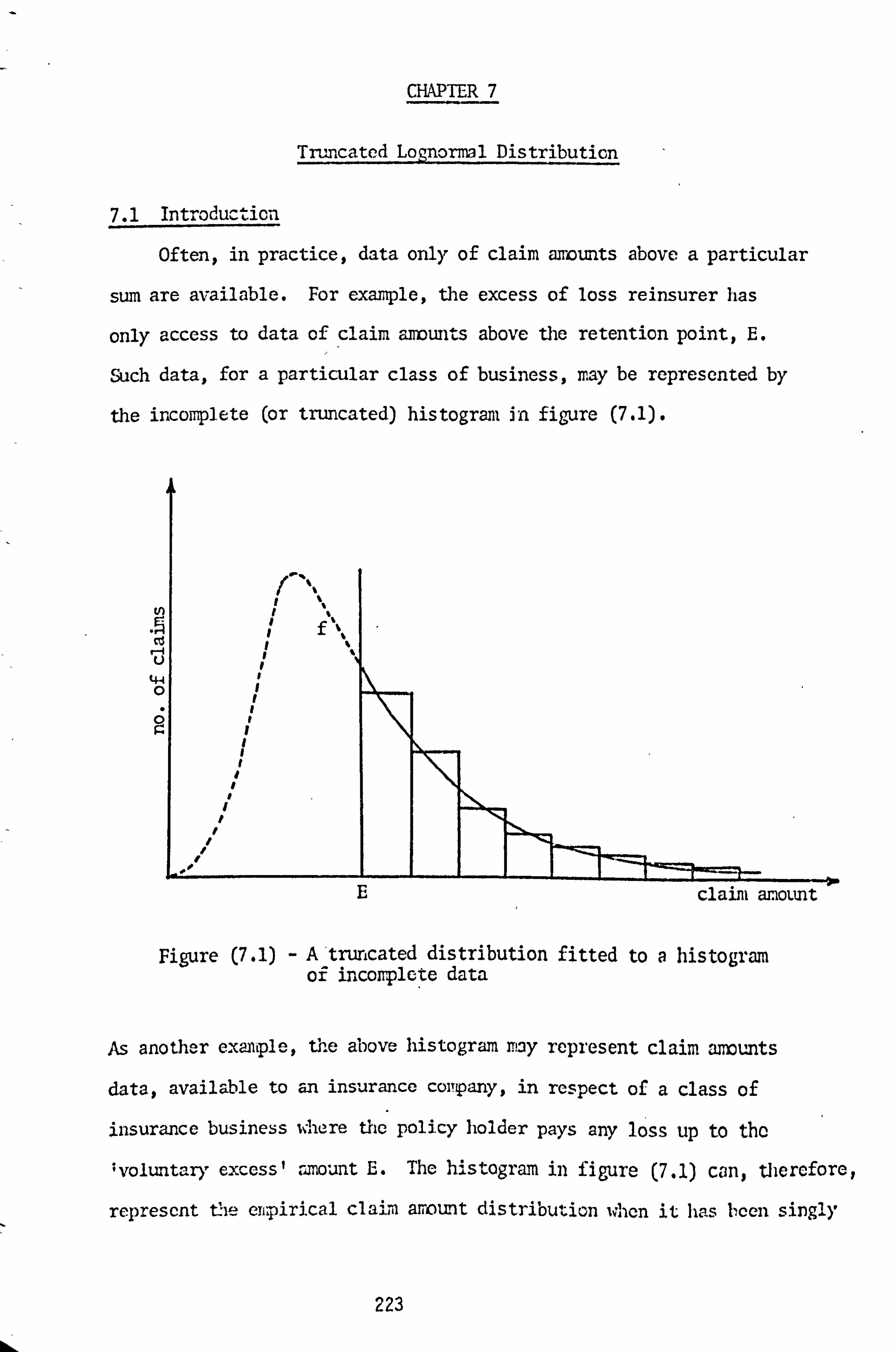
CHAPTER 7

Truncated Lognormal Distribution

7.1 Introduction

Often, in practice, data only of claim amounts above a particular

sum are available. For example, the excess of loss reinsurer has

only access to data of claim amounts above the retention point, E.

Such data, for a particular class of business, may be represented by

the incomplete (or truncated) histogram in figure (7.1).

N

c- U

44 0

Figure (7.1) - A"truncated distribution fitted to a histogram of inconiplete data

As another example, the above histogram may represent claim amounts

data, available to an insurance co1Tpany, in respect of a class of

insurance business where the policy holder pays any loss up to the

'voluntary excess' : mount E. The histogram in figure (7.1) can, therefore,

represent the empirical claim arrotmt distribution when it has been singly

223

Ii claim amount

truncated fron below at the 'point of truncation' E.

If we lclow that a particular statistical distribution represents the

complete distribution of claim amounts, then we may be able to fit a

truncated form of that statistical distribution to the incomplete data

as represented in figure (7.1). Essentially, we find a model with

probability density function f whose tail fits the incomplete empirical

distribution (see figure (7.1)). That part of the curve f which lies to

the right of the truncation point E is the frequency curve of the

truncated distribution. Barding (1968) considers the truncated lognormal

model for the distribution of excess of loss reinsurance claim amounts

of motor business.

The studies of the previous chapters of the present work showed that

the lognormal model represents the distribution of our accidental damage

(AD) claim amounts. The 2-parameter lognormal produced a 'better' fit

.n the sense of smaller Chi-square statistics) to the actual data than

the 2-parameter inverse Gaussian distribution. Therefore, in this chapter

we shall consider the truncated lognormal distribution. As we are only

interested in the tail of the distribution, only the 2-parameter model

will be dealt with. Initially, the truncated lognormal distribution will

be defined and some of its properties will be mentioned. Then the problem

of estimation of the parameters from grouped data will be considered

and the multinomial maximum likelihood method will be proposed. By

using this method, two problems' related to our AD data will then be

studied ; these are discussed below :-

1- In chapter 3 we noticed that the significant differences between

the 2-parameter lognoir. ýal distribution and the actual sample values were

caused by large contributions to the Chi-square statistic by one or two

of the intervals in the larger tail values. In that chapter we indicated

that the disagreement could-be due to the inaccuracies and incorpleteness

224

of the data in the lower tail intervals because in order to re, -, lain

entitled to their substantial no-claim discounts some policy holders

do not claim. small amounts. As the claims in the lower tail are

financially less important, it was suggested that the data should be

truncated at the upper boundary of these intervals to see if a more

exact fit to the rest of the data would be obtained. Therefore,, in

this chapter, we will fit the truncated lognormal distribution to samples

of our AD data, as presented in tables (1.1) to (1.7), but truncated

at 130 or £60 or £90. The results-for different points of truncation

will be examined and compared with those of chapter 3 for the complete

samples.

2- The larger claims form the tail of the claim amount distribution

and because of their financial importance a higher degree of agreement

between the model and the empirical distribution is required in this

region. Therefore, it is important to find out if a truncated distribution

fitted to the tail of the histogram of sample values produces a 'better'

fit. For our AD data we truncate the samples at 1600 and fit the

truncated lognormal model to the tail of the actual sample values. The

results will then be compared with the tails of the fitted lognormal

distributions in chapter 3 to see if, in fact, truncation does produce

a 'better' fit in this region.

The histograms of our AD samples in figures (3.5.1) to (3.5.7) indicate

that the Pareto distribution with its mode at 1600 Is likely to fit the

empirical distribution of claim amounts greater than 1600.. The graphical

tests of chapter 6 also implied a Pareto model for the tail of our AD

histograms. The Pareto distribution is much simpler to fit and develop

mathematically than the truncated lognormal distribution. Therefore, to

compare the performance of these two models we will, in this chapter, also

225

fit the Pareto distribution to samples of claim amounts greater than

£600.

As was mentioned previously, the excess of loss reinsurance claim 11

amounts data are available only in the truncated form and hence the treat-

ment of the present problem is applicable in that context.

The findings of this chapter will be summarized in the conclusion

section and the tables will be presented in section 7.6.

'7.2 Definiticn'and'Sdme Properties of'the'Truncated Lognormal Distribution

We say a random variable X has a truncated lognormal distribution 2

if its distribution function, denoted by TLN(x, E; u, o ) is of the form

222 TL1ý1(x, E; µ, ý)

I; N(x; i; d) -L (E; u, Q) for x>E (7.2-1) 1- LINE ;u, a)

=0.......................... otherwise

where E is the point of truncation and LN ("; u, o 2) is the distribution

function of a lognormal random variable, with parameters u and a2 , as

defined in chapter 3 by (3.2-4). Hence the probability density function

(p. d. f. ) of the truncated lognormal distribution, which we denote by

£TIN(X, E ; u, a ), is :

2

2 fLN (X; u"7 ) fTLN(x, E; u, a )= for x>E (7.2-2)

1-LN(E; u, a2)

where fLN ; 11,02 is the p. d. f. of a lognormal random variable, with 2

parameters u, a, as given by (3.2-3).

The rth moment of X about zero can be shown (see for instance,

Aitchison and Brown (1957)) to be

E(Xr) = exp(r u± ýr2a. )Z '- LN(x.; u+ ro?, a21 (7.2-3)

1- LNN(E u>o2)

L26

12 1-1 From (3.3-3) we lo ow that exp(ru +2ra) is the rth moment about zero

of the 2-parameter lognormal distribution. The remaining expression

on the right land side of (7.2-3) can be expressed in terms of the

standard normal distribution function by using relationship (3.2-4).

Hence Quensel (1945) expresses (7.2-3) as :

(rth moment if not truncated) 1- N(U -ra; 0,1) (7.2-4) 1-N(U; 0,1)

where U= log E and N( "; 0,1) is the standard normal

distribution function.

The mean of the distribution of X is, therefore,

E(X) exp (u+ 21 2) iu -Q; 0,1) (7 . 2-s) 1 -N(U ; 0,1)

and the variance of X can be shown to be

22 1 ^exp (u+ )2 Var(X) = exp(Q ) [1-N(U-2a; 0,1)] [1-N(U; 0,1)] - 1- N(U; 0,1)

21

(7.2-6)

7.3 Estimation of the Parameters

In this section we study the problem of estimating the parameters

ý, and c2 for a TL. N(x, E ; u, ß2) dist: ibuticn with the 1aown point of

truncation E. This problem has been dealt with by several authors.

Aitchison and Brown (1957) describe the maxiniun likelihood method when

values of the individual observations in the sarple are available. They

suggest using the tables given by Hald (1949) for carrying out the

inverse interpolation required in this method. Harding (1968) explains

this method for fitting the truncated lognormal modal to the third party

227

excess of loss reinsurance claim amounts of n for insurance business.

The quartile, and graphical methods are not applicable since an 2

estimate of LN(E ; u, Q ) (i. e., the area under the complete frequency 2

curve of 11\1(x ; 1,, a ) and to the left of the truncation point) is

required but there is no information on this.

The method of moments may be used which involves putting the first and

second sample moments equal to their corresponding theoretical values

given by (7.2-3). Ho' ever, there is no easy way of solving the resulting 2

equations for u and a except by trial and error. Grundy (1952) has

considered estimation, from grouped data, by the method of moments for

the truncated normal distribution. His method may be used for the

truncated lognormal distribution since log x is normally distributed. He

gives expressions for adjusting the first and second sample moments about

zero when they are calculated from grouped truncated data.

Tallis and Young (1962) have considered estimation from grouped data by

the nultinomial maximum likelihood, (. »L), method but their technique

involves solving iteratively a system of non. -linear equations in the

parameters.

We will adopt the AIINL method but will apply the computing technique,

described in section 3.7.7, of maximizing the loglikelihood function

iteratively with respect to the parameters.

Let us assume that we have a sample of grouped data where n

independent random observations-(clams) on a random variable X (claim

amount) have been grouped according to their size into k nutually

exclusive intervals. Further, let us assume that each claim is for an

arnount greater then E (the truncation point) and that ni is the number

of claims in the class interval (xi_1, xi) , for i=1,2, ... ,k

and with .: o = r, such that

2 L8

k n= ni

i=1 2

If X is distributed as a TLN(x, E ; ;,, Q ) distribution given by (7.2-1),

then let pi be the probability that the size of a random observation

(claim) will fall in the interval (xi-1, xi)' i. e.

22 pi = TLN(xi, E; u, Q )- TLN(xi-1' E'i, ) (7.3-1)

From (7.2-1) it follows that

LN(xi; u, Q2) - LN(xi-1 ; u, Q2) (7.3-2) pi -

1-LN(E; u, Q2)

Therefore, the sample likelihood function will be proportional to L

where k

_ TT n.

Lýj pi 1 (7.3-3) i=1

and the loglikelihood function will be

k log L ni log pi (7.3-4)

i=l

From (7.3-2) and remembering that from (3.2-4)

2 logx- u LN(x ; u, a )=N(Q; 0,1)

we can write (7.3-4) as :

+u logt =-n log(N ( Log E 0,1)) + 0

k log x. -ux. u + ni1og NC a; o, 1/ - N(log

of ; o'i/

(7.3-5)

2 The maxini^i likelihood estimates (p, o) of the parameters are obtained

by maximizing log L sinultaneously with respect to u and a2 . To avoid

solving non-linear equations in the parameters wo suggest the computing

technique described in section 3.7.7 for maximizing log L with respect to

229 kh.. -

2 u and a. To start the iteration process we can use the estimates of

2 u and a w1-ich we found for the complete samples in chapter 3. If such

a 1nowledge about the possible values of u and a2 is not available they.

the method of moments should be used to work out a set of ( u, a2 ) for

starting the iteration process. In any case, the penalty for choosing

a very inaccurate set of (11, Q2) as starting values is a few more iterations,

which is not really a problem when the computer is used.

7.4 Applications to the AD Data

Computer program P23 was written to estimate the parameters of the

truncated lognormal distribution by multinomial maximum likelihood, (MIL),

method. The complete samples of the AD data which were presented in

tables (1.1) to (1.7) are input to the program and a truncation point is

specified. in chapter 3 we showed that for our data the estimates of the

parameters of the complete 2-parameter lognormal distribution were A 4.5 and v2 1. These values are specified as initial values

of the parameters to start the iteration process.

We first dealt with problem 1 put forward in section 7.1, i. e.,

truncation in the lower tail sample values. Each sample of AD data was

truncated respectively at E= 30, E= 60 and E= 90, and the parameters

of the truncated model were estimated. In each case the computer program 2

gave the estimates of p and a and an extensive table of relevant statistics.

As an example, for the 73/4th quarter data the results of the computer

runs are given in tables (7.1), (7.2) and (7.3). The results for all

the samples have been summarized in tables (7.4) to (7.7). The correspon-

ding results for complete samples, which were given in tables (3.11) to

(3.17), are also reproduced for the sake of comparison. Table (7.4)

gives the estimates of p. We notice that truncation has given rise to

larger values of u compared with the corresponding values for complete

230

samples. Fora 2 we can see, from table (7.5), that truncation has

resulted in smaller values. Tables (7., I) to (7.3) show that the 2

contribution to the Chi-square statistic, X, by different intervals is 2

generally small. The values of X statistic for complete and truncated 2

samples are presented in table (7.6). For complete samples the X

values showed significant differences, at 0.05 level, between the 2

LN(x ; u, a ) model and actual sample values for every period of accident.

The values of these statistics for truncated samples are considerably

smaller and, except for 74/1st and 74/3rd quarters, do not show any

significant differences, at 0.05 level, between the actual sample values

and the truncated fitted models. Table (7.7) gives the ratio of the

total expected loss statistic, T, to the total actual cost of claims.

We observe that smaller values have been obtained for truncated samples

indicating a better overall agreement between the model and actual

sample values.. The above analysis shows that truncation in the lower

tail sample values of the AD data gives rise to a more exact fitting

statistical model compared with the 2-parameter lognormal distribution

for the complete sample. However, the fit does not seem to improve when

truncation is carried on beyond the first interval (E = 30). In terms

of the Chi-square goodness-of-fit test statistics, the results for the

truncated (E = 30) and 3-parameter lognormal (see tables (3.38) to (3.44))

distributions are very similar. The latter distribution is, however,

easier to work with and to develop mathematically. For the AD data, we,

therefore, recommend the use of the 3-parameter lognormal distribution.

The second problem we put forward in section 7.1 was the application

of the truncated lognormal as a model for the distribution of large AD

claim amounts. We, therefore, used progra'n P23 with our samples of AD

data. Each sample was truncated at f; 1600 and (u = 4.5, a' L 1) were

specified as starting values for the iteration process. rar each sample

231

the computer program produced the estimates of u and v2 as well as a

table of relevant statistics. The results are presented in tables

(7.8.1) to (7.8.7). We can see that u is larger than for complete samples

while a2 is considerably smaller. The actual means and standard deviations

of'the truncated samples are given in table (7.11). From tables (7.8.1)

to (7.8.7) we can see that the mean claim amounts of the fitted models

are approximately equal- to their corresponding sample values. The standard

deviations of the models are greater than their actual values but this

could be because we are fitting a curve with an infinite range to a sample

which has a finite range. From the tables of results it is apparent

that the contributions to the Z

statistic are generally small and that

the overall X2 statistics, except for 74/3rd quarter, do not indicate

any significant differences between the model and actual sample values.

The total expected loss statistics are small and are at most 5% of the

total actual cost of claims. This indicates an overall satisfactory fit

of the model to the sample values.

To see how the truncated lognormal model performs against the, mich

simpler to use, Pareto distribution, we wrote computer program P24 to

estimate, from a truncated sample, the parameters of the Pareto distribution

of the first kind. This program uses the MhL method of estimation.

The program was then modified to estimate the parameters of the Pareto

distribution of the second kind. In each case the estimates of the

parameters by the method of moments were input as starting values for

the iteration process. These programs were run with truncated samples

(at B= 600) of our AD data. For a particular sample, 73/4th quarter,

the results are given in tables (7.9) and (7.10). A summary of the results

for all samples are presented in tables (7.12) and (7.13). For the

Pareto distribution of the first kind the mean claim a, 'rnunt from each model

is approximately equal to its corresponding sample mean. The standard

232

deviations of the models are greater than their corresponding sample

values as we are fitting a curve with an infinite range to a sample 2

with a finite range. The X statistics show that, with the exception

of 74/3rd quarter, there are no significant differences, at 0.05 level,

between the model and actual sample values. The ratios of the total

expected loss statistics to the total actual. cost of claims are larger

than their corresponding values for the truncated lognormal distribution.

For the Pareto distribution of the second kind, P2 (x ; C, A, B),

parameter C can be interpreted as the 'voluntary excess' on the policy.

Estimates of C for each sample are given in table (7.13). They vary

considerably from each period of accident to the next. The mean claim

amounts are much closer to their corresponding sample values. The

standard deviations of the models are larger than their actual values but

are smaller than their corresponding values according to the Pareto

distribution of the first kind. The X2 statistics are smaller than

their corresponding values in table (7.12) and do*not indicate any

significant differences between the model and actual sample values. The

ratios of the total expected loss statistics to the total actual cost of

claims are generally smaller than those given for Pl (x ; A, B) in table

(7.12) but are larger than their respective values for the truncated

lognormal distribution. In terms of the X2 goodness-of-fit test

statistic, P2(x ; C, A, B) has provided a more exact fit to the AD data

than Pl (x ; A, B) distribution. In fact, the fit is almost as good as

that of the truncated lognormal distribution. One obvious reason for

this is that Pl(x ; A, B) has two parameters while P2 (x ; Cl A, B) and

TLN(x, E ;. u, Q 2)

each have three parameters. Therefore, given good

computer facilities, we would prefer the truncated lognormal model, for

the distribution of large AD claim amounts, though just as good a fit may

be obtained by P2(x ; C, A, B) or even P1 (x ; A, B) distributions.

233

7.5 Conclusions

In this chapter we considered the trancated lognormal distribution

as a model for the incompl;: te distribution of accidental damage claim

amounts. The method of M' was described for the estimation of parameters

from grouped data. The model was then fitted to samples of AD data

truncated at lower tail values. It was shown that by ignoring the first

claim a'nount interval this model would satisfactorily fit the AD samples.

In terms of the Chi-square goodness-of-fit statistic the fit was as

good as that of the complete 3-parameter lognormal distribution. Because

this latter distribution is relatively simpler to use and to develop

mathematically its application, in place of the truncated lognormal

distribution, was recommended.

Next, the trincated lognormal distribution was considered as a

model for the distribution of large claim amounts. Our AD samples were

truncated at 1600 and the model was fitted to the incomplete samples.

It was shown that a very satisfactory fit is provided by the truncated

lognormal distribution. For the sake of comparison, the Pareto

distributions of the first and second kind were also fitted to the same

truncated samples. The P2 (x ; C, A, B) provided a fit as good as the

truncated lognormal distribution. It was suggested that when computing

is not a problem the latter model should be used. Otherwise P2(x ; C, A, B)

or even the Pareto distribution of the first kind may be used as models

for large AD claim an unts.

The effects of inflation on the parameters of the truncated

distribution were not studied, but because of the relationship between

the complete and truncated lognormal distributions we can easily arrive

at these effects by following the exposition of section 3.9. It may, in

fact, be shown that inflation increases parameter u but leaves a2 unchanged.

7. E Tables

34 2

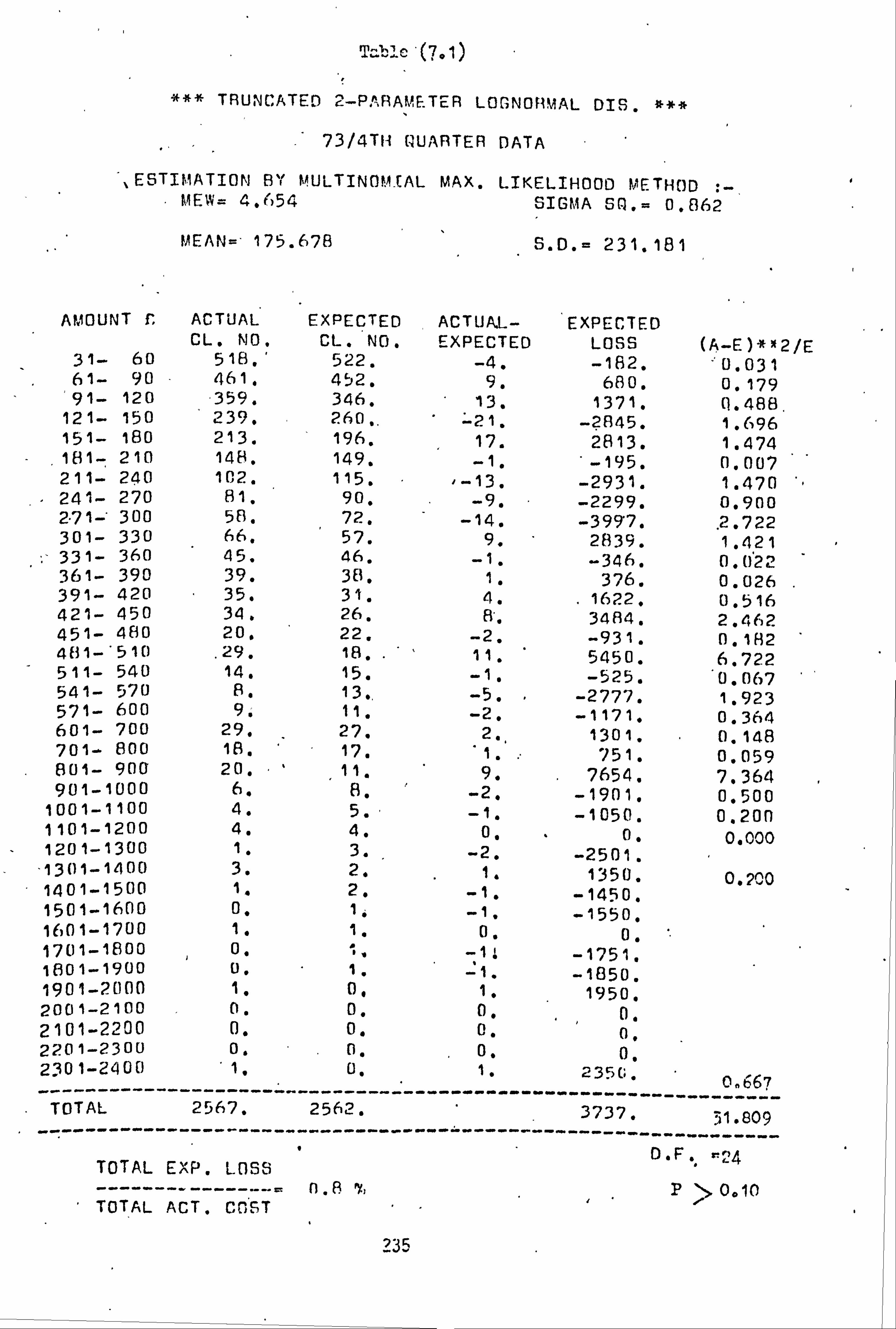
T ble '(7.1)

TRUNCATED 2-PARAMETER LOGNORMAL DIS. ***

73/4TH QUARTER DATA

, ESTIMATION BY MULTINOM_CAL MAX. LIKELIHOOD METHOD :-' MEW= 4.654 SIGMA SQ. = O. B62

MEAN=-175.678 S. D. = 231.181

AMOUNT C ACTUAL EXPECTED ACTUAL- EXPECTED CL. NO. CL. NO. EXPECTED LOSS (A-E)* 2/E

31- 60 518, ' 522. -4, -182. 0.031 61- 90 461. 452. 9. 680, 0.179 91- 120 359. 346. 13. 1371. (1,488,

121- 150 239. 260.. -21. -2A45. 1.696 151- 180 213. 196. 17. 2813. 1.474 181- 210 148. 149. -1. -195. 0.007 211- 240 102. 115, 1-13. -2931. 1.470 241- 270 81. 90 , -9. . -2299. 00900 2.71- 300 5E3, 72. -14. -3997. .

2.722 301- 330 66. 57. 9. 2839. 1,421 331- 360 45. 46. -1. -346. 0,0'22 361- 390 39, 38. 1. 376. 0.026 391- 420 35, 31. 4. 1622. 0,516 421- 450 34. 26. 8. 3484, 2,462 451- 480 20. 22. -2, -931. 0,182 481- 510 . 29. 18 ,. 11. 5450o 6.722 511- 540 14, 15. -10 -525. 0,067 541- 570 S. 13, -5, -2777. 1,923 571- 600 9. 11, -2, -1171, 0.364 601- 700 29. 27. 2., 1301, 0.148 701- 800 18, 17. 1. . 751, 0.059 801- 900" 20, 9. 7654, 7.364 901-1000 6, E3, -2, -1901. 00500

1001-1100 4, 5. ' -1. -1050. 0.200 1101-1200 4, 4. 0. 0. 0.000 1201-1300 3. -2. -2501.

-1301-1400 3. 2. 1. 1350. 01 0.2010 " 1401-1500 1. 2. -1. -1450. 1501-1600 0. 1. -1, -1550,

1601-1700 1. 0. 0ý . 1701-1800 0. -1: -1751. 1801-1900 0, 1. -1.

-1850. 1901-2000 1, 0. 1. 1950, 2001-2100 0. 0, 0, 0. 2101-2200 0. 0. 0. 0. 2201-2300 0, 0, 0, 0. 2301-2400 1, 0, 1, 235(; ---------- ------------- ------------- ----------

, ----------

0.667 TOTAL

---------

2567,

----------- 2562.

----------- -------------

--- 3737, ------------

------- 31.809

---- DEo

--- r`4 TOTAL EXP. LOSS '

-- = n. 8 P>0.10 TOTAL ACT. COST

? 35

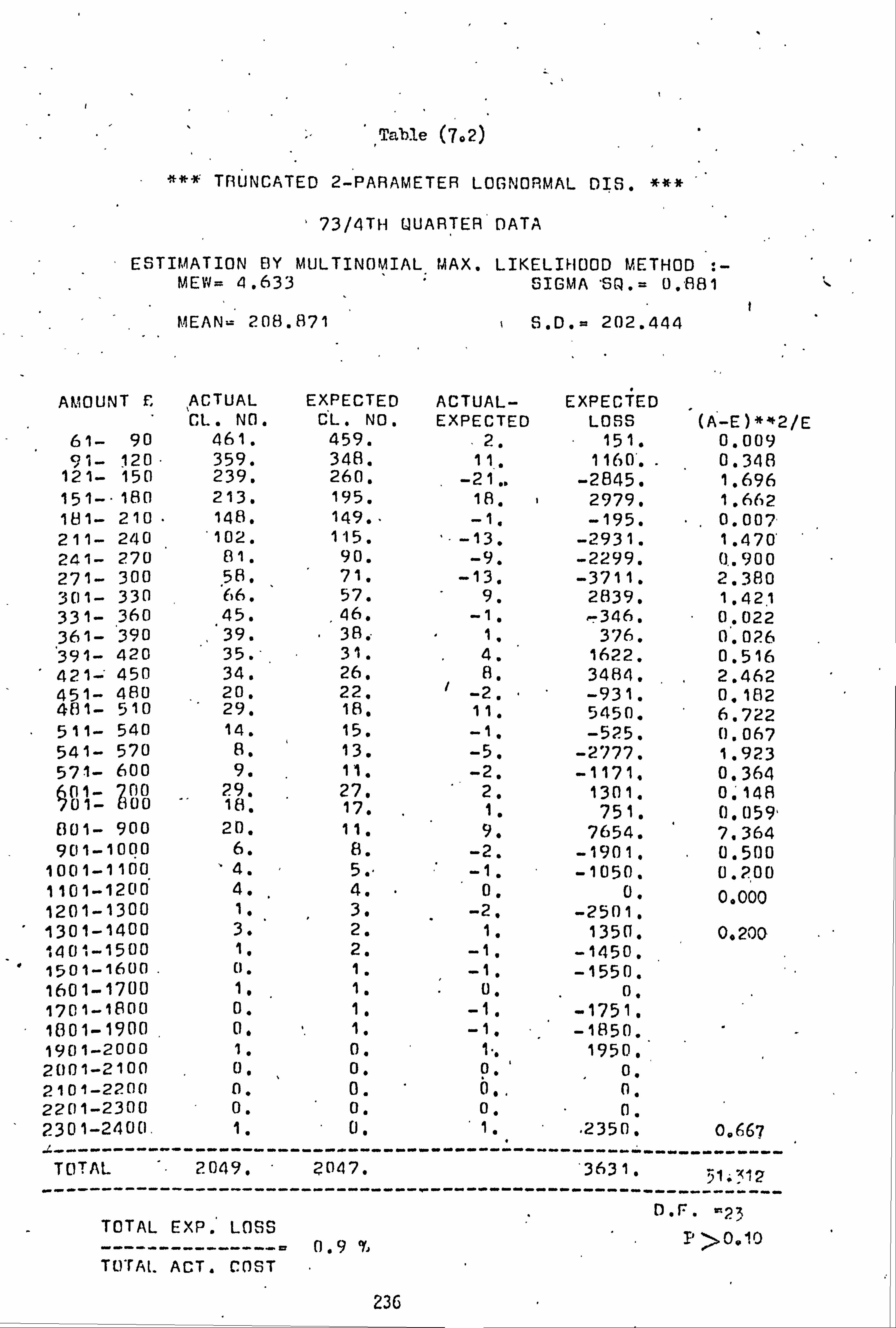
Table (702)

'ý# TRUNCATED 2-PARAMETER LOGNORMAL DIS. *##

' 73/4TH QUARTER DATA

ESTIMATION BY MULTINOMIAL MAX. LIKELIHOOD METHOD : - MEW= 4.633 SIGMA 'SCE .=0., 881

MEAN- 208.871 S. D. = 202.444

AMOUNT F. ACTUAL EXPECTED ACTUAL- EXPECTED CL. NO. CL. NO. EXPECTED LOSS (A-E)**2/E

61- 90 461. 459. 2. 151. 0.009 91- 120- 359. 348. 11. 1160.. 0.348

121- 150 239. 260. . -21,. -2845. 1.696

151-180 213. 195. 18, 2979. 1,662 181- 210. 148. 149. " -1. -195. 0.007 211- 240 102. 115. -13. -2931. 1,470' 241- 270 81. 90. -9. -2299. (1.900 271- 300 58. 71. -13. -3711. 2.380 301- 330 66. 57. 9. 2839. 1.421 331- 360 45. 46. -1, x-346, 0.022 361- 390 ,

39. 38; 1. 376. 0,026 391- 420 ' 35. ' 31. 4. 1622. 0,516 421= 450 34. 26. 8, 3484. 2.462 451- 480 20. 22. /

-2, -931. 0.182 481- 510 29. 18. 11. 5450. 6.722 51l- 540 14. 15. -1, -525. 0.067 541- 570 Be 13. -5, -2777. 1.923 571- 600 9. 11. -2. -1171. 0.364

zoo 00 01 9, 27. 2. 1301. 0,148 - 7 1 17. 1. 751. (1.059'

801- 900 20. 11. 9. 7654. 7.364 901-1000 6. 8. -2. -1901. 0.500

1001-1100 4. 5. " -1. -1050. 0.200 1101-1200 4. 4. " ' 0, 0. 0.000 1201-1300 1. 3. -2. -2501. 1301-1400 3. 2. 1, 1350. 0,200 1401-1500 1. 2. -1. -1450. , " 1501-1600. 0. 1. -1, -1550. 1601-1700 11

. 1. U. 0.

1701-1800 0. 11 -1. -1751. 1801-1900, 0.

. 1. -1. .. -1850.

1901-2000 1. 0. 1". 1950. 2001-2100 0. 0, 0. 0. 2101-2200 0. 0, ne. (0, 2201-2300 0. 0. 0. 0. 2301-24011.

------ ------- 0.

- . 1,

--------- . 2350. 0,667

' ---- TOTAL '.

-----------

---- 2049. '

-----------

--------- 2047.

----------

- -

-----------

---------- 3631.

-----------

---------- 51.17

--------- D. F. '23

TOTAL EXP. LOSS --------------- 0.9 9, P >0.10 TCOTAL ACT. CAST

236

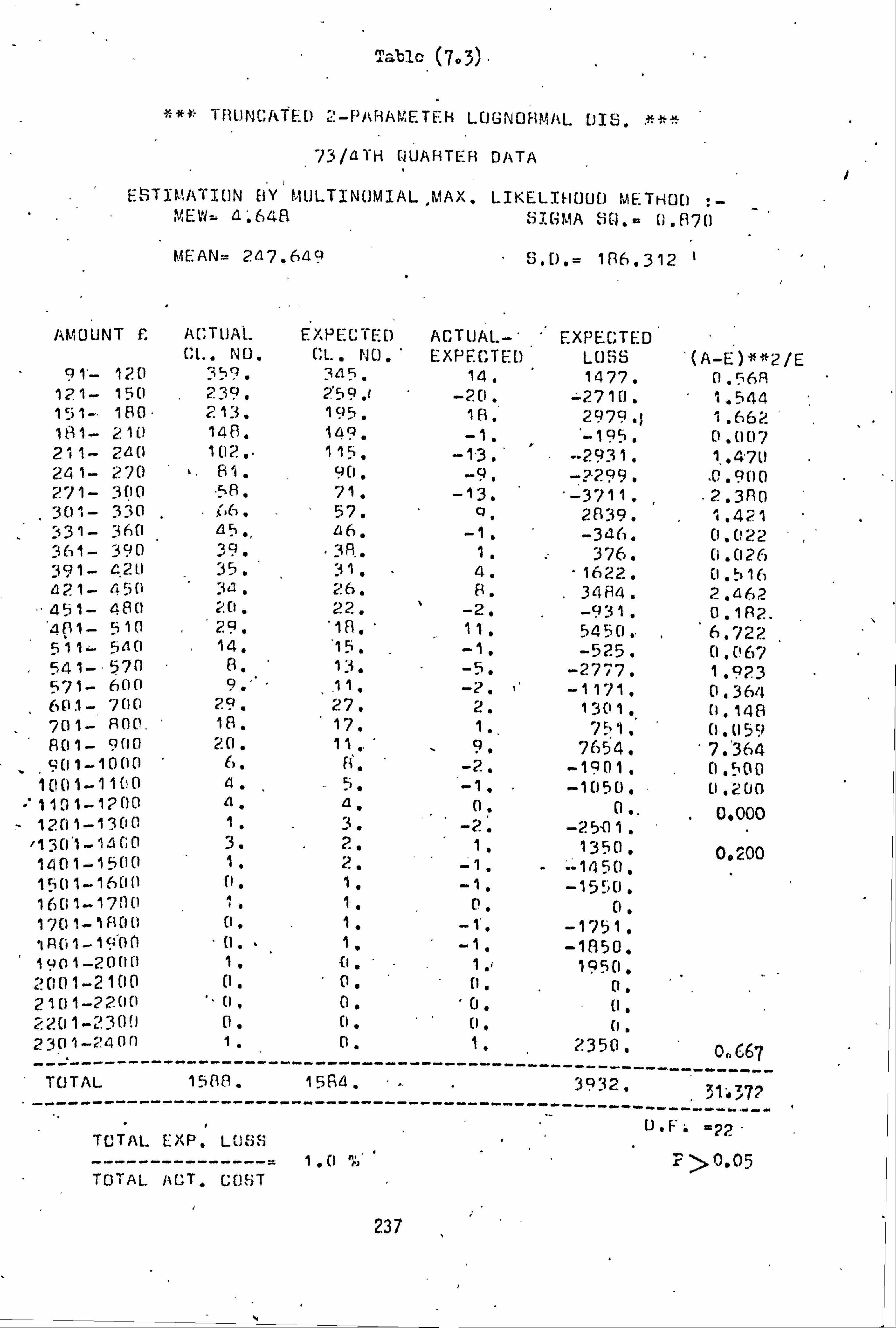
Table (703).

*#}- TRUNCATE: [? 2-PMAAMETEH LOGNORMAL DIS.

73 /a H (-WARTER DATA t

ESTIMATION BY MIJLTINUMIAL MAX. LIKELIHOOD METHOD MEW- G; 64B : iý. (iMA ; i[, 1. a (1 . E17(1 -

MEAN= 2[t7.6[tU S. U. = 1El6.312

AMOUNT £ ACTUAL. EXPECTED ACTUAL-' EXPECTED C[., NO. CL. NO, EXPECTED LOSS '(A-E)**2/E

91'- 120 359. 3a5. 14. 1477. 0,56- " 121- 150 239. 259,1 -2.11. -271[1. 1.544 151- 180' 2.13 . 195. 1S, 2979.1 1.662 181- 210 148. 149. -1. -195. (1.01)7 21 1- 240 102.. 115. -1.3, --2931. 1,. 47(1 24 1- 270 R1.

-? 299. [! . 900 271- 300 . 5R. 71, -13. -3711. .2 , 380 301- 330 57. 21139. 1.421

_ 331- 360 a5., 116. -1 -3a6. 0.0122 361- 90 39. 3R. 1 376. (1.026 391- 11,21) 35. i1. 4. 1622. (I 11 2 1121- 45(1 {c1. 26. 3484. . 2 . aF, 2 451-. 480 2.0. 22. -2. -931. 0,1 R2. 481- 510 29. 18. 11, 5450.. 6.722 511 560 14. 15.

. -1. -525. 0.067 541- 57() 8. 13. -5. -2777. 1 "923 571- 600 9, '

. 11, -2. ' -1171, 0.364

601- 7(1(1 29. 27. 2. 1301. (1.148 800. 1A. ' 17. 1.. 751. (1. (159

801- 9(10 20. 11 .. ' 90 7654. 7. '364 9(11-10(º(t 6. 8. -2. -1901 " 0.500

1(1 [t1-11(! 0 4. .. `_i" '-1. . -1050. 0.200

11(11-12(1(1 4. a" o" 0". 01000 1 eil 1-1 sui '. '. -7.. -25{11,

1tºCO 3. 2. 1. 135C1. Ooc00 1401-15(10 1. 2. 150 1-1161111 (1. 1, -1. -1550. 16(; 1-17O0 1. 1. 0. U. 1 1U 1-10U(1 0,

-1751. 10(11-190f1 (I. 1" -1 . -1A5o. 19o1-20(1(1 1,

21110 1-2100 2101-22.00 U. U. U. o. 2201-4 3011 0. 0. (i. U. 2301-24on

---------- I.

------------ 0.

---------- 1

---------- 2350.

--------- 0.667

TOTAL ------ ----

1500. ------------

1504,

---------- ----------

- 3932. ----------

----------- 3 ?. -

------- T

U. F. =22- TOTAL EXP, LOSS

------ --------- I. o > 0.05 TOTAL. ACT. COST

237

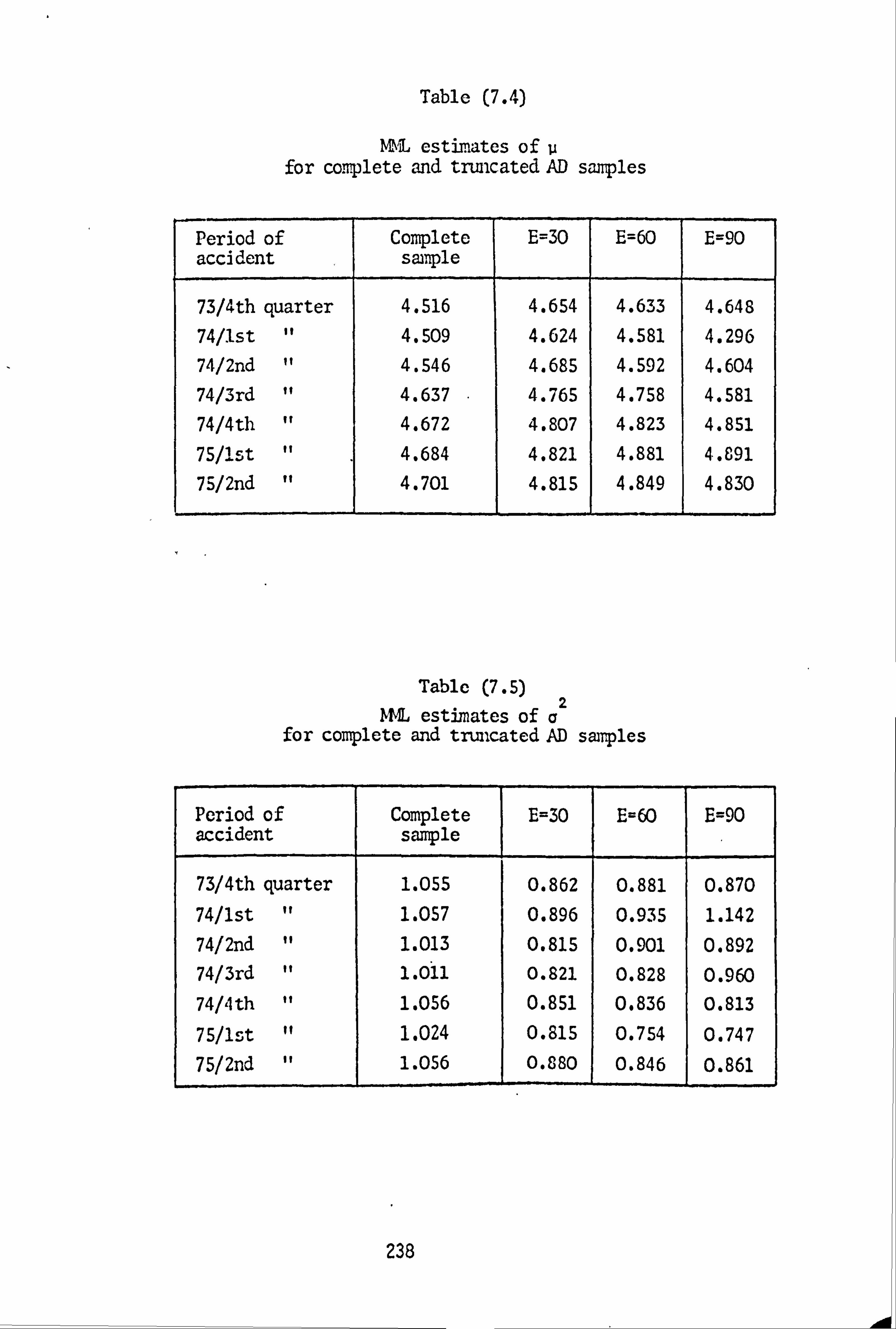
Table (7.4)

W, estimates of u for complete and truncated AD samples

Period of accident

Complete sample

E=30 E=60 E=90

73/4th quarter 4.516 4.654 4.633 4.648 74/1st " 4.509 4.624 4.581 4.296 74/2nd " 4.546 4.685 4.592 4.604 74/3rd " 4.637 4.765 4.758 4.581 74/4th " 4.672 4.807 4.823 4.851

75/1st " 4.684 4.821 4.881 4.891 75/2nd " 4.701 4.815 4.849 4.830

Table (7.5)

MNL estimates of a2 for complete and truncated AD samples

Period of accident

Complete sample

E=30 E=60 E=90

73/4th quarter 1.055 0.862 0.881 0.870 74/1st " 1.057 0.896 0.935 1.142 74/2nd " 1.013 0.815 0.901 0.892 74/3rd " 1.011 0.821 0.828 0.960

74/4th " 1.056 0.851 0.836 0.813 75/1st " 1.024 0.815 0.754 0.747 75/2nd " 1.056 0.880 0.846 0.861

238

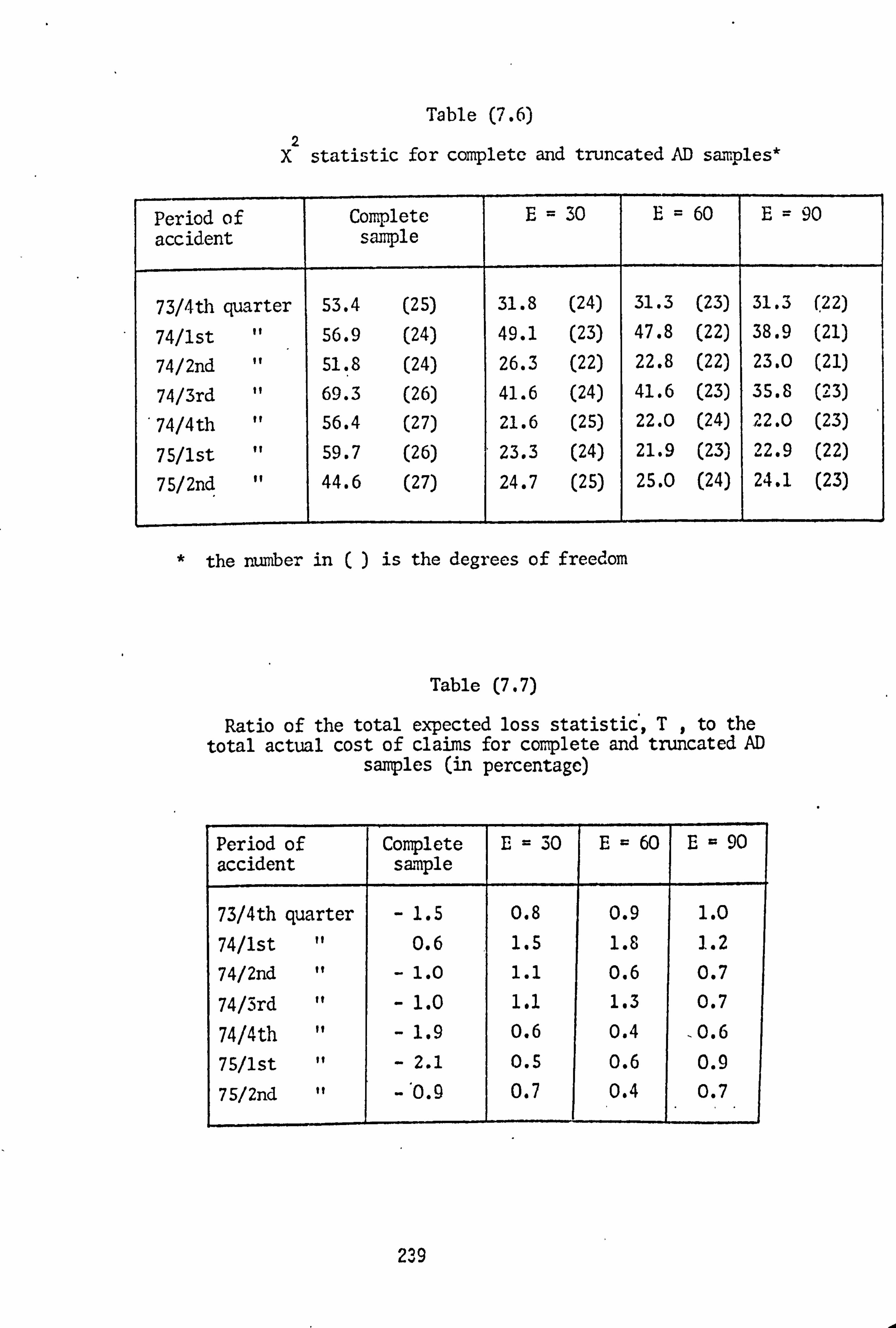
Table (7.6)

X2 statistic for complete and truncated AD samples*

Period of accident

Complete sample

E= 30 E= 60 E= 90

73/4th quarter 53.4 (25) 31.8 (24) 31.3 (23) 31.3 (22)

74/1st " 56.9 (24) 49.1 (23) 47.8 (22) 38.9 (21)

74/2nd 51.8 (24) 26.3 (22) 22.8 (22) 23.0 (21)

74/3rd 69.3 (26) 41.6 (24) 41.6 (23) 35.8 (23)

74/4th " 56.4 (27) 21.6 (25) 22.0 (24) 22.0 (23)

75/1st 59.7 (26) 23.3 (24) 21.9 (23) 22.9 (22)

75/2nd " 44.6 (27) 24.7 (25) 25.0 (24) 24.1 (23)

* the number in () is the degrees of freedom

Table (7.7)

Ratio of the total expected loss statistic, T, to the total actual cost of claims for complete and truncated AD

samples (in percentage)

Period of accident

Complete sample

E= 30 E= 60 E= 90

73/4th quarter - 1.5 0.8 0.9 1.0

74/1st " 0.6 1.5 1.8 1.2

74/2nd - 1.0 1.1 0.6 0.7

74/3rd " - 1.0 1.1 1.3 0.7

74/4th " - 1.9 0.6 0.4 . 0.6

75/1st " - 2.1 0.5 0.6 0.9

75/2nd -'0.9 0.7 0.4 0.7

239

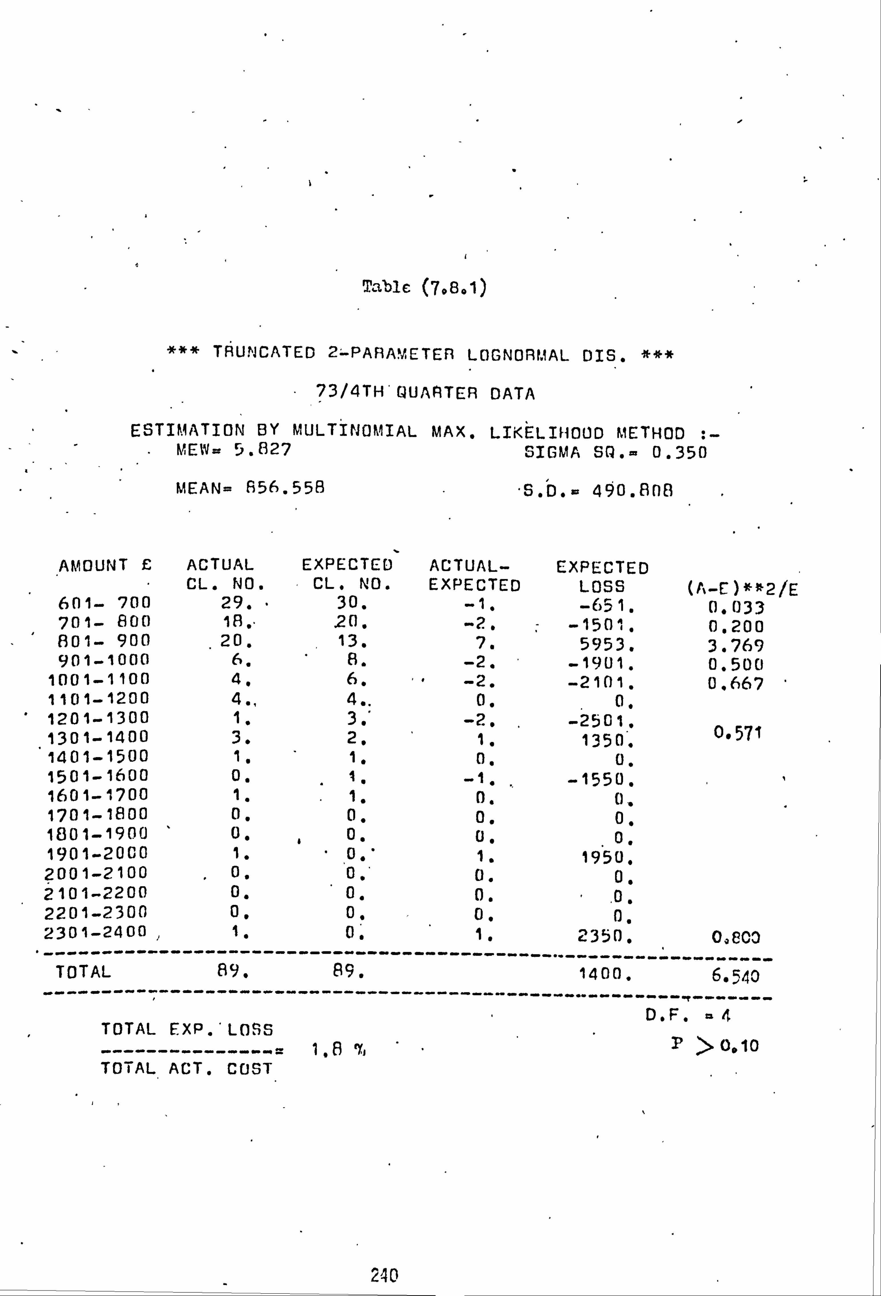
Table (7,8.1)

* TRUNCAT ED 2-PARAME TER LOGNOR MAL DIS.

73/4TH'UU ARTER DATA

ESTIMATION BY MULTINOMIAL MAX. LIKE LIHOOD METHOD : - MEW= 5.827 S IGMA SQ. - 0.3 50

MEAN= 856. 558 "s . D. - 490.8n8

AMOUNT £ ACTUAL EXPECTED ACTUAL- EXPECTED CL. NO. CL. NO. EXPECTED LOSS (A_E)**2/E

601- 700 29. " 30. -1. -651. 0.033 701- 800 18, " 20. -2. -1501. 0.200

" 801- 900 20. 13. 7. 5953. 3.769 901-1000 6. 8. -2. -1901. 0.500

1001-1100 4. 6. -2. -2101. 0.667 1 101-1200 4., 4.. 0. 0. 1201-1300 1. 3. -2. -2501. 1301-1400 3. 2. 1. 1350. 0.571

1401-1500 1. 1. 0. 0. 1501-1600 0. 1. -1. , -1550. 1 1601-1700 1. 1. 0. 0. 1701-1800 0. 0. 0. 0. 1801-1900 0. 0. 0. 0 1901-2000 1. 0. ' 1. 1950. 2001-2100 0. 0.. 0. 0. 2101-2200 0. 0. 0.

. 0.

2201-2300 0, 0. 0. 0. 2301-2400, 1. 0, 1. 2350. 0,8C0

TDTAL 89. A9. ------ --"------ 1400. --

ýý- 6.

---------, ----------- ------------ ------------------------r------- D. F. -4 TOTAL EXP. 'LOSS

----- ----------= 1.8 ry, P >0110

TOTAL ACT. COST

240

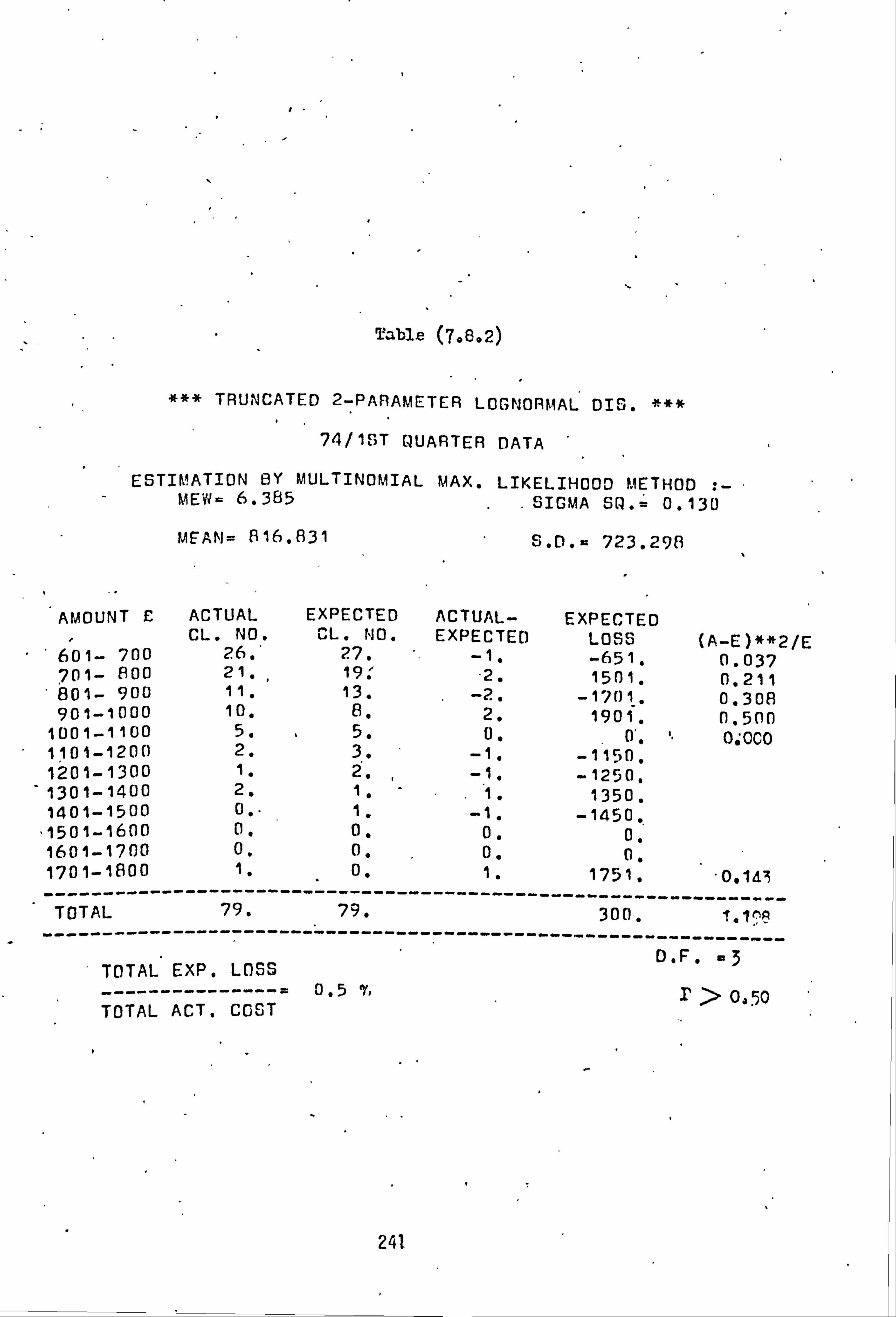
"1 ,

Table (708.2)

## TRUNCAT ED 2-PARAMETER LOGNORMAL DIS.

74/15T QUARTER DATA

ESTIMATION BY MULTINOMIAL MAX. LIK ELIHOOD ME THOD : - MEVr= 6.385 SIGMA SO. = D. 130

MEAN= 816. 831 S. D. - 723. 298

AMOUNT £ ACTUAL EXPECTED ACTUAL- EXPECTED CL. NO,

" CL. NO. EXPECTED LOSS (A-E)**2/E

601- 700 26. 27. -1. -651, 0.037 701- 800 21 ,, 19: -2. 1501. 0,21 1

'801- goo 11. 13. -2. -1701, 0.308 901-1000 10. 0, 2. 1901 , (1.500

1001-1 100 5. 5. 0. 01, 1" 0: 000 1101-1200 2. 3. -1. -1150, 1201-1300 1" 2.

-1 . -1250. 1301-1400 2. 1. 1. 1350. 1401-1500 0"" 1. -1. -1450.

11501-1600 0. 0. 0. 0, 1601-1700 0. 0. 0. 0, 1701-1000 1. 0. 1. 1751. "0,1.3 -----

TOTAL ----------

79"

------------ 79.

------------

---

--------

---------- 300.

-----------

------------ ?. tja

----------- D. F. =3 TOTAL EXP. LOSS

= 0.5 7, > 0' 50 TOTAL ACT. COST .

241

Table (7.8.3)

TRUNCATED 2-PARAMETER LOGNORMAL DIS. "#*

74/2ND QUARTER DATA

EST IMATION BY MULTINOMIAL MAX. LIKELIHOOD METHOD : - MEW- 5.265 SIGMA SQ. = 0 .41 9

MEAN- 804. 178 S. D. - 368.034

AMOUNT f 'ACTUAL EXPECTED ACTUAL- EXPECTED CL. NO. CL. NO. EXPECTED LOSS (A=E)**2/E

601- 700 30. 29. 1. - 651. 0.034 701- 800 13.. 16. -3. -2251. 0.563 "801-..

900 11. 9. 2. 1)11. 0.444 901-1000 4.. 5. -0 6, -951. 0.200

1001-1100' 7. 7. 3. 3. 4. 4202. 1101-1200 U. 2. -2. -2301. . 1201-1300 1. 1. 0. 0. 1301-1400 1. 1. 0. 0. 1401-1500 0. 1. -1. -1450. 1501-1600 1. 0. 1, 1550. 1601-1700 0. 0. a. 0. 1701-1800 0. 0. '"0. 0. 1801-1900

----- 1.

----------- 0.

---------- 1.

- 1850. 1.125

----- TOTAL 69. -- 67. ------- ---------------

3001. ------- 2.356

--" -------- ------------------------------ -----"----------------

D. F. 12 2 TOTAL EXP. LOSS

-- . 5.4 %" P =y 3Q

TOTAL ACT. COST

242

Table (70804)

*# TRUNCAT ED 2-PARAMETER LOGNOR MAL DIS.

74/3RD QUARTER DATA

ESTIMATION'SY MULTINOMIAL MAX. LIKE LIHOOD METHOD : - MEW- 5.596 S IGMA SQ. = 0.3 99

MEAN= 842. 542 S . D. - 42.1.929

AMOUNT C ACTUAL EXPECTED ACTUAL- EXPECTED CL. NO. CL. NO. EXPECTED LOSS (A-E)**2/E

601- 700 '

32. 39. -7. -4553. 1.256 701- 600. 34. 24. -' 10. 7505. 4.167 801- 900 17. 15. 2. 1701. 11.267 901-1000 4. 10. -6. ' -5703. 3.600

1001-1100 9. 6. '3. 3151. 1.500. 1101-1200 4. 4. 0. 0, 1201-1300 0, 3. -3. -3751. 1,286 1301-1400 1. 2. '-1. -1350. 1401-1500 3. 1.. 2. 2901. 0 1501-1600 0. 1 1. -1. -1550. 1601-1700 ' 1. 1. 0. 0. 1701-1800 0.1 0. 0. 0,, 1601-1900 0. 0. 0. 0. 1901-2000 0. 0. 0. 0. 2001-2100 0. 0. 0. 0. - 2101-2200 1. 0. 1. 2150. ' 2201-2300 0.

. 0. 0. 0. 2301-2400 0. 0. 0. " 0o' 2401-2500 0. 0. 0. 0. 2501-2600

---------- 1.

------------ 0.

------------ 1.

--------- 2550. 01800

TOTAL

---------- 107.

------------ 106.

----------- -

--------- -

------------- 3050,

------------- ------- 12.876 -------

TOTAL EXP. LOSS DF

-- TOTAL . COST

3.4 P = 001 v01

243

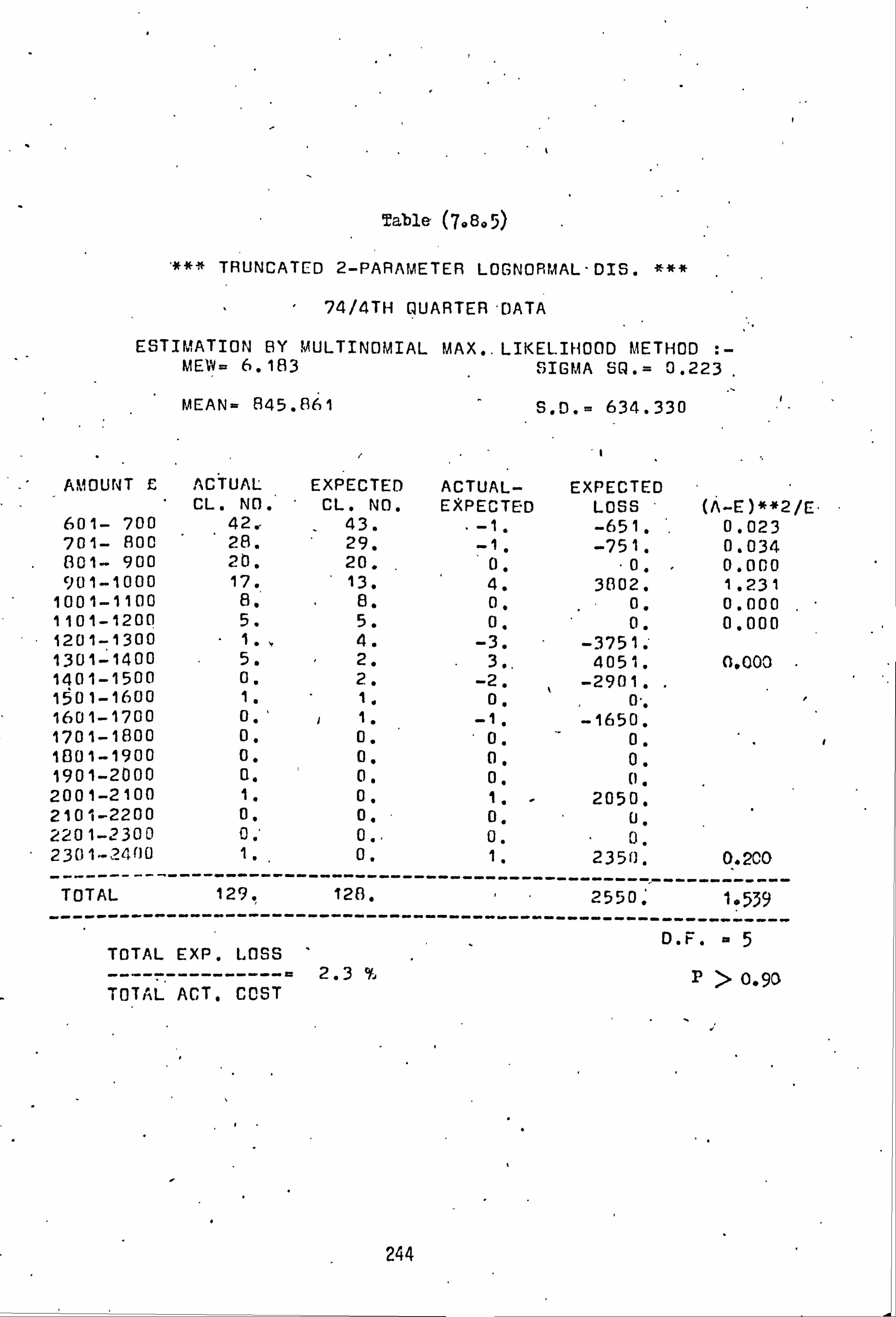
k

Table (7080 )

*# TRUNCATED 2-PARAMETER LOGNORMAL-DIS.

74/4TH QUARTER-DATA

ESTIMATION BY MULTINOMIAL MAX.. LIKELIHOOD METHOD MEW= 6.183 SIGMA SQ. = 0.223

MEAN- 845.861 S. D. = 634.330

AMOUNT £ ACTUAL EXPECTED ACTUAL- EXPECTED CL. NO. CL. NO, EXPECTED LOSS (A-E)**2/E. - 601- 700 42. - 43. -1. -651. .

0.023 701- Boo 28. 29. -1, -751. 0.034 801- 900 20. 20.

_ 1 0. . 0. , 0.000

901-1000 17. 13. 4. 3802. 1.231 1001-1100 8. 8. 0, 0. 0.000

. 1101-1200 5. 5. 0, 0. 0,000 1201-1300 " 1. t 4. -3. -3751. 1301-1400 5. 2. 3,. 4051. 01000 1401-1500 0. 2. -2. -2901. 1501_1600 1. 1, 0. 0", 1601-1700 00' 1, -1, -1650. 1701-1800 0. 0. 0. 0. 1001-1900 0. 0. 0. 0. 1901-2000 0. 0. 0, 0. 2001-2100 1. 0. 1. - 2050. 2101-2200 0. 04 0. 0. 2201-2300 0.1 0.. 0. 0. 2301-2400 1. 0. 1. 2350, 0.200

TOTAL

----------

129.

------------

128,

---------- ---------

- --2550. -

-----------

-----1,539

--- -------- D. r" =5 TOTAL EXP. LOSS

- ---= 2.3 %

r>0.90

TOTAL ACT, COST

244

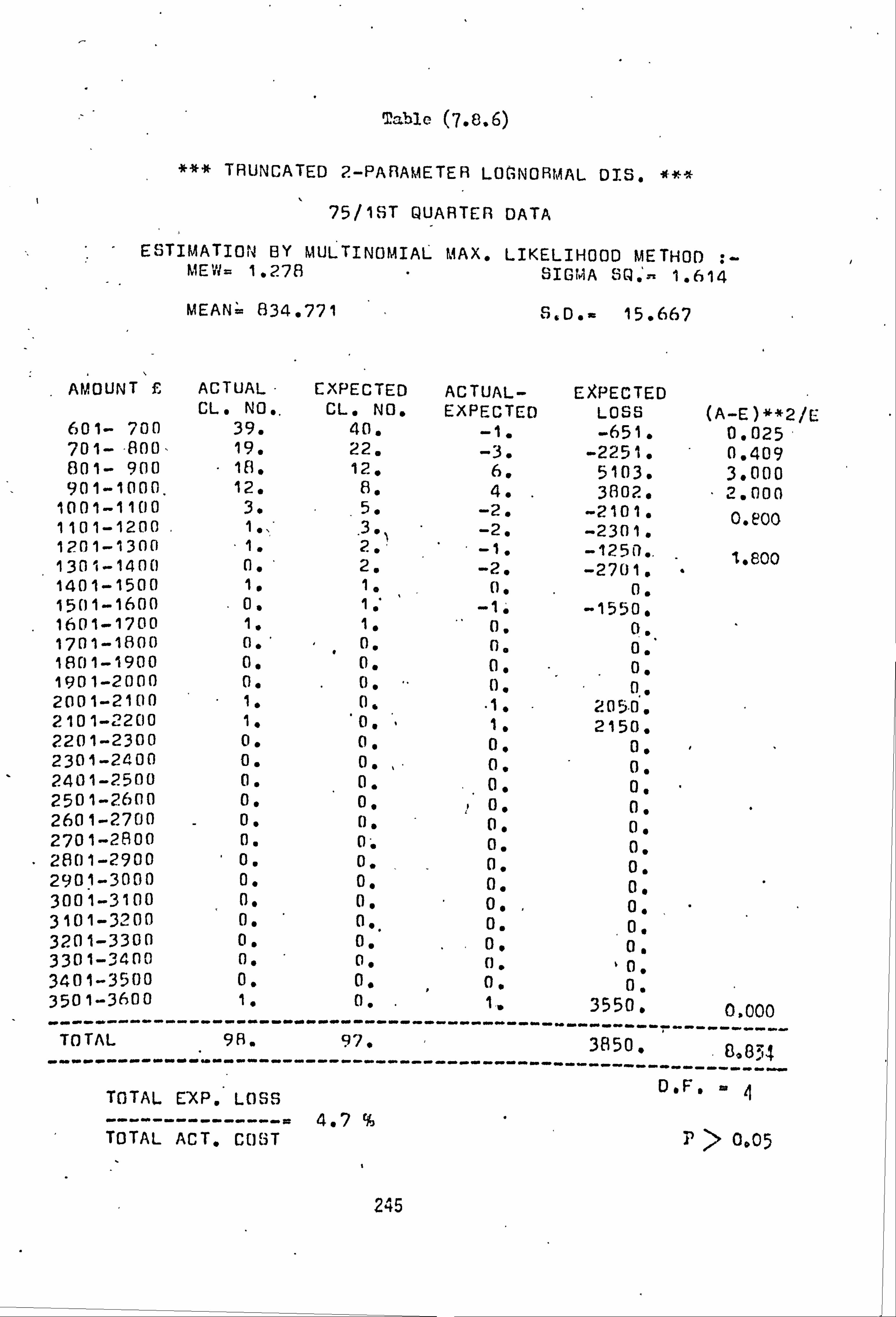
Table (7.8.6)

*# TRUNCATED 2-PAFIAMETER LOGNORMAL DIS. #**

75/1ST QUARTER DATA

ESTIMATION BY MULTINOMIAL MAX. LIKELIHOOD METHOD : - ME'W= 1.278 SIGMA SQ. - 1.614

MEAN= 834.771 S. D. = 15.667

AMOUNT E ACTUAL- EXPECTED ACTUAL- EXPECTED CL. NO.. CL. NO. EXPECTED LOSS (A-E)**2/E

601- 700 39. 40. -1. -651. 0,025 701- 800- 19. 22. -3. -2251. 0.409 a01- 900 " 18. 12. 6. 5103. 3.000 901-1000" 12. 8. 4. 3802. 2.000

1001-1100 3* ,

5. -2, -2101. 0. e00 1101-1200 1.1 , 3. -2. -2301.

1201-1300 1. 2. ' -1. -1250.. .ý ooo 1301-1400 0. 2. -2. -2701. . 1401-1500 1. 1. 0. 011 1501-1600 0.

-1550. 1601-1700 1. 1ý 0. 0ý 1701-1Ei00 0. ' 0. 0, 0. 1801-1900 0. 0. 01 0. 1901-2000 0. 0. 0, 01 2001-2100 1. 0.

"1. 205.0. 2101-2200 1. 0. , 1. 2150. 2201-2300 0. 0. 0, 0, 2301-2400 0. 0. 01 0. 2401-2500 0. 0. 01 0. 2501-2600 0. 0. 0. 01 2601-2700 _ 0. 0. 01 0. 2701-2600 0. 0; 01 0. 2801-2900 0. 0. 0. 0. 2901-3000 0. 0. 0. 00 3001-3100 01 01 o0

, o. 3101-3200 0. 0.

" 0. 01

3201-3300 0. 01 01 01 3301-3400 0. 0. n. 0 3401-3500 0. 0. 01 . 01 3501-3600 1. 0. " 1,. 3550. 0.000

TOTAL

-----------

98. ----------

97. ----------- -----------

3850. -------------

890; 4 -----

TfiTA1 r'XP I nqn D'F' m4

---------------= 4.7 TOTAL ACT. COST > 0D05

245

'Fable (7.8.7)

TRUNCAT ED 2-PARAMETER LOGNO RMAL DIS.

75/2ND QUARTER DAT A

ESTIMATION BY MULTINOMIAL MAX. LIK ELIHOOD METHOD : - "MEW= 5.982 SIGMA SQ. = 0.32 4

MEAN= 873.216 S. O. = 543.923

AMOUNT f. ACTUAL EXPECTED ACTUAL- EXPECTED CL. NO. CL. NO. EXPECTED LOSS ( A-E)**2/E

'. 601- 700 36. 36. 0.. 0. 0.000 701- 800 22. 24. -2. -1501. 0.167 801- 900 22. 16. 6. 5103. 2.250. 901-1000 11. 11. 0. 0. 1 0.000

1001-1100 4. A. -4. -4202. 2.000 1101-1200 3. 5., -2. -2301. 0., 800 120.1-1300 3. 4. -1. . -12511. 130,1-1400 6. 2. '4. 5402. 1,500 1401-1500

_ 2. 2. 0. 0.

1501-1600 1. 1. 0. 0. 1601-1700 0. 1. -1. -1650. 1701-1800" 1. 1. 0. 0. 1801-1900 0. 0. 0. 0. 1901-2000 1.; 0. 1. 1950. 2001-2100 0. 0. 0. 0. 2101-2200 0_0

. 0. 0. 0. 2201-2300

----------

1.

------------ 0.

----------- 1. "

---- 2250. 0,200

TOTAL 113. 111. ---- ---------------

3801. ------- 6. ß17

D. F. 5 EXP. LOSS

----- ---------- = 3.8 % P 0. -,, 3 TOTAL ACT. COST "

ti

J

246

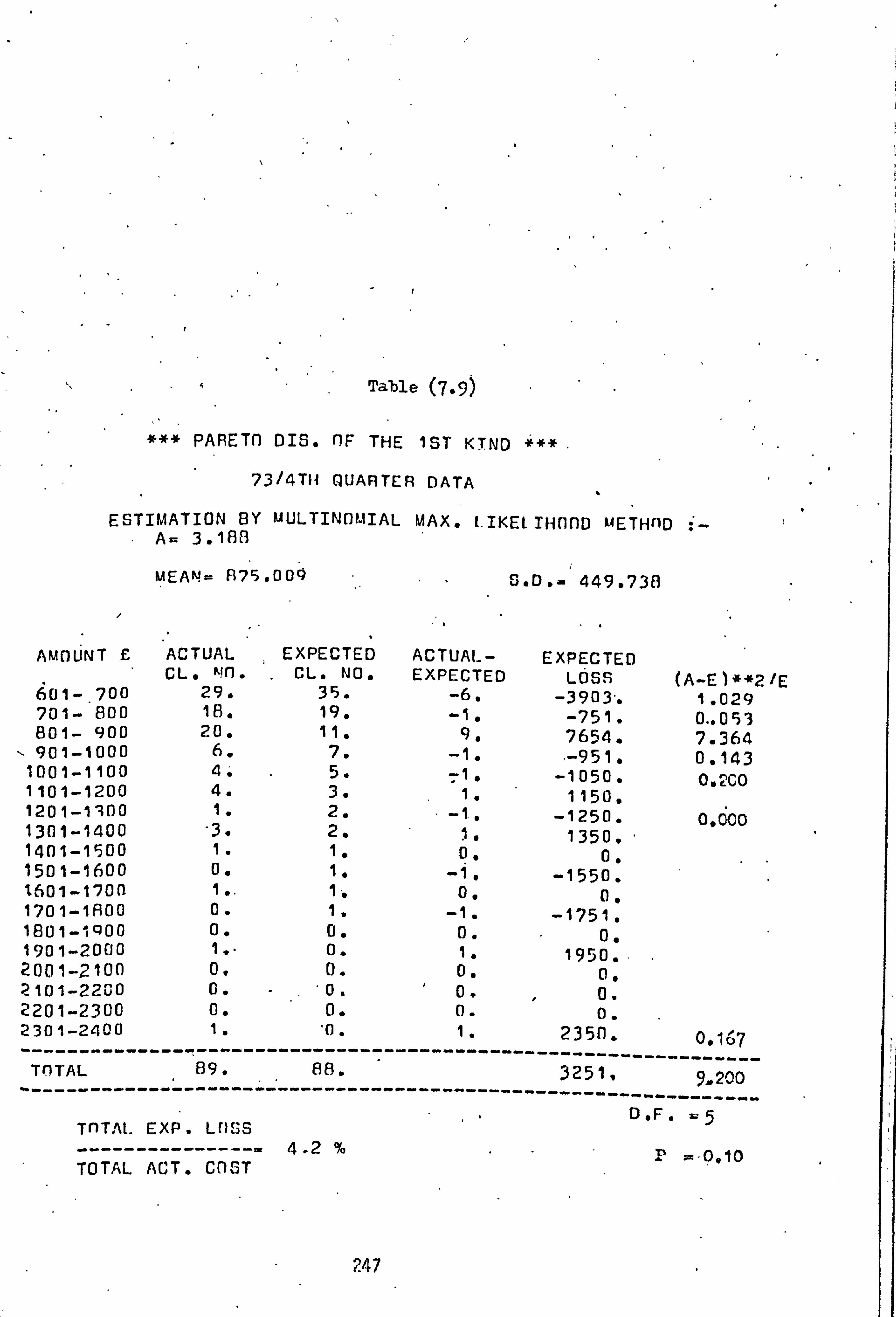
{ Table (7.9)

PARETO DIS. RF THE 1ST KTND *** .

734TH QUARTER DATA

ESTIMATION BY MULTINOMIAL MAX. t. IKE L THn(1D METHOD i- A= 3.188

MEAN= R75. 00(l S . D. = 449.738

AMOUNT £ ACTUAL EXPECTED ACTUAL- EXPECTED CL. NO.

. CL. NO. EXPECTED LOSS (A-E )**2 /E 601-. 700 29. 35. -6. -3903".

. 1.029 701- 800 18. 19. -1. -751. 0.. 053 801- 900 20. 11. 9. 7654. 7.364 901-1000 6. 7. -1. -951. 0.143

1001-1 100 4' 5. -1 . -1050. 0.2C0 1101-1200 4. 3. 1. 1150. 1201-1100 1. 2. -1. -1250. 0.600 1301-1400 -3. 2. 1. 1350. 1401-1500 1. 1. 0. 0. 1501-1600 0. 1. -1. -1550. 1601-17011 1.. 1", 0. 0. 1701-1800 0. 1. -1. -1751. 1801_1400 0. 0. 0. 0. 1901-2000 1.. 0. 1. 1950.1 2001-2100 0. 0. 0. o, 2101-2200 0. - 0. 0. 0. 2201-2300 0. 0. 0. o. 2301-2400 1.

------ 10.

------------ 1.

---------- 2350.

------- 0,167

TOTAL TOTAL ----------

89. ---------

88. ------------ ----------

- 3251,

-----

------------

------ -

- D. F.

------- -5 TOTAL EXP. Lf) 3S

-- 4.2 % P =0 10 TOTAL ACT. COST ,

247

w

Table (7,10)

- *** PARETO DIS. OF THE 2ND KTND

73 4TH QUARTER DATA

-EST IMATION BY MULTINOMTAI. _

MAX. I. TKELIHOOD METHOD : A- 3.493 C- 27.94

' iMEAN= 869. 306 S. D. - 368.417

AMOUNT £ ACTUAL EXPECTED ACTUAL- EXPECTED, CL. Mf. Cl_. * NO. EXPECTED LOSS (A-E)**2/E

601- 700 29. " 29. 0. 0. 0.000 701- 800 18. 23. -5. . -3752. 1.087 801-. 900 i 20. 13. 7. 5953. 3.769 901-1000 6. A. -2. -1901. 0-. 500

1001-1100 4. 5., -1 ." -1050. 0,2.00 1101-1200 4. .

3. 1. 1150; 1201-1300 1. 2. -1. -1250. 0.000 1301-1400 3. 1. 2. 2701. " 1401-1'500 1 .. 1. 0. ' 0. ' 1501-1600 0. 1, -1. . -1550. 1601-1700 1. 1. " 0. 0. 1701-1800 0.

. 0. 0. 0.

1801-1ßO0 0. "0. 0. "0. 1901-2000 1.. 0. 1. 1950. 2001-2100 0. 0. 0. 0. 2101-2200 0. 0. 0. 0. 2201-23(10 0. 0. 0. 0. 2301-2400

-------

1.

-----------

0.

------------ 1.

-------- 2350.

---------------- 2.7 0

------- --- TOTAL

--------

89.

------ -----

87.

------------ -------- 4601.

--------------- ß0ß6

---=---- -- D. F. /.

TOTAL EXP. LOSS 0010 ----- ---------- 6.0 % TOTAL ACT. COST

248

lag

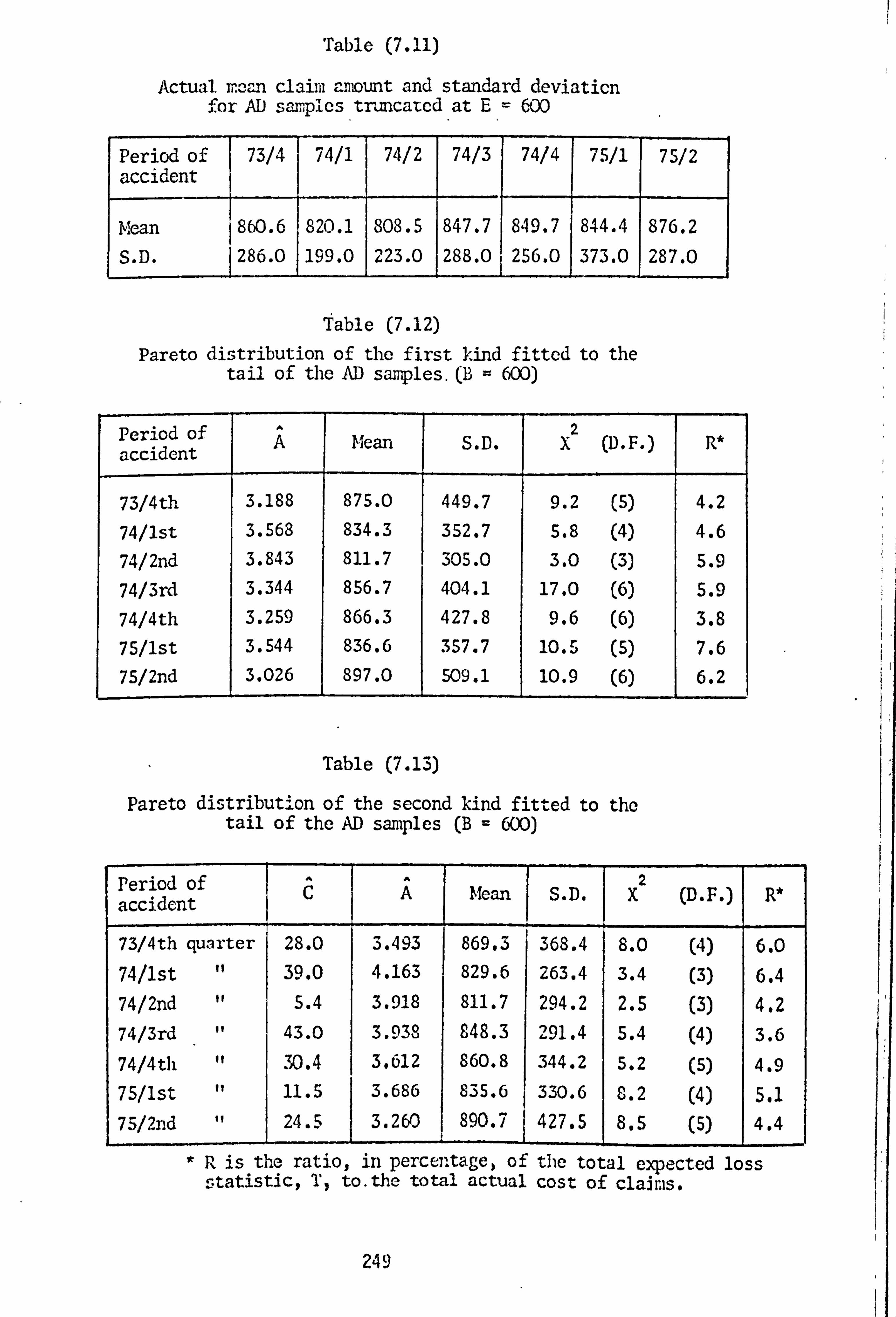
Table (7.11)

Actual. r: can claim amount and standard deviaticn for AD sa, Ics truncated at E= 600

Period of 73/4 74/1 74/2 74/3 74/4 75/1 75/2 accident

Mean 860.6 820.1 808.5 847.7 849.7 844.4 876.2

S. D. 286.0 199.0 223.0 288.0 256.0 373.0 287.0

Table (7.12)

Pareto distribution of the first kind fitted to the tail of the AD samples. (B = 600)

Period of accident

A Mean S. D. X2 (ll. F. ) R*

73/4th 3.188 875.0 449.7 9.2 (5) 4.2

74/1st 3.568 834.3 352.7 5.8 (4) 4.6

74/2nd 3.843 811.7 305.0 3.0 (3) 5.9

74/3rd 3.344 856.7 404.1 17.0 (6) 5.9

74/4th 3.259 866.3 427.8 9.6 (6) 3.8 75/1st 3.544 836.6 357.7 10.5 (5) 7.6

75/2nd 3.026 897.0 509.1 10.9 (6) 6.2

Table (7.13)

Pareto distribution of the second kind fitted to the tail of the AD samples (B = 600)

Period of accident

C A Mean S. D. 2

X (D. F. ) R*

73/4th quarter 28.0 3.493 869.3 368.4 8.0 (4) 6.0 74/1st tt 39.0 4.163 829.6 263.4 3.4 (3) 6.4

74/2nd " 5.4 3.918 811.7 294.2 2.5 (3) 4.2 74/3rd 43.0 3.938 848.3 291.4 5.4 (4) 3.6 74/4th " 30.4 3.612 860.8 344.2 5.2 (5) 4.9 75/1st " 11.5 3.686 835.6 330.6 8.2 (4) 5.1

75/2nd 24.5 3.260 890.7 427.5 8.5 (5) 4.4

*R is the ratio, in percentage, of the total expected loss statistic, ý', to. the total actual cost of claims.

249

CHAPTER 8

The Gaimu Distribution

8.1 Introduction

The gamma distribution is another positively skewed distribution

with a long tail which can assume a variety of shapes. It has,

therefore, been a most appropriate statistical model in applied science

work. Many sets of empirical data on positive valued random outcomes

of various random phenomena in science and engineering have been

represented by this distribution. Johnson and Kotz (1970) and Bury (1975)

give bibliographies on the applications of this model and the formers'

list includes references to the actuarial field as well.

Beard (1978) argues that "the amount of damage (physical) will

arise from impact and thus be related to the energy involved, that is,

to the square* of the velocity". If X is the amount of loss, and in and V

are the mass and the velocity of the car at the time of impact,

respectively, then the above statement means that

12 X is proportional to 2 mV

and hence Z=/ is proportional to V (8.1-2)

Beard (1978) then goes on to say that "velocity should have a reasonable

shape" and in Beard (1978, personal communication) suggests the gamma

distribution as a model for the distribution of velocity and hence of

the square root of the claim amount. Therefore, the problem we shall

consider in this chapter is- the application of the tti, -o-parameter gamma

distribution as a nadel for the square root of the claim amount. It

is immediately appreciated that data on the square root of the claim

amount, and not on the claim. amount itself, are required. Mien a

250

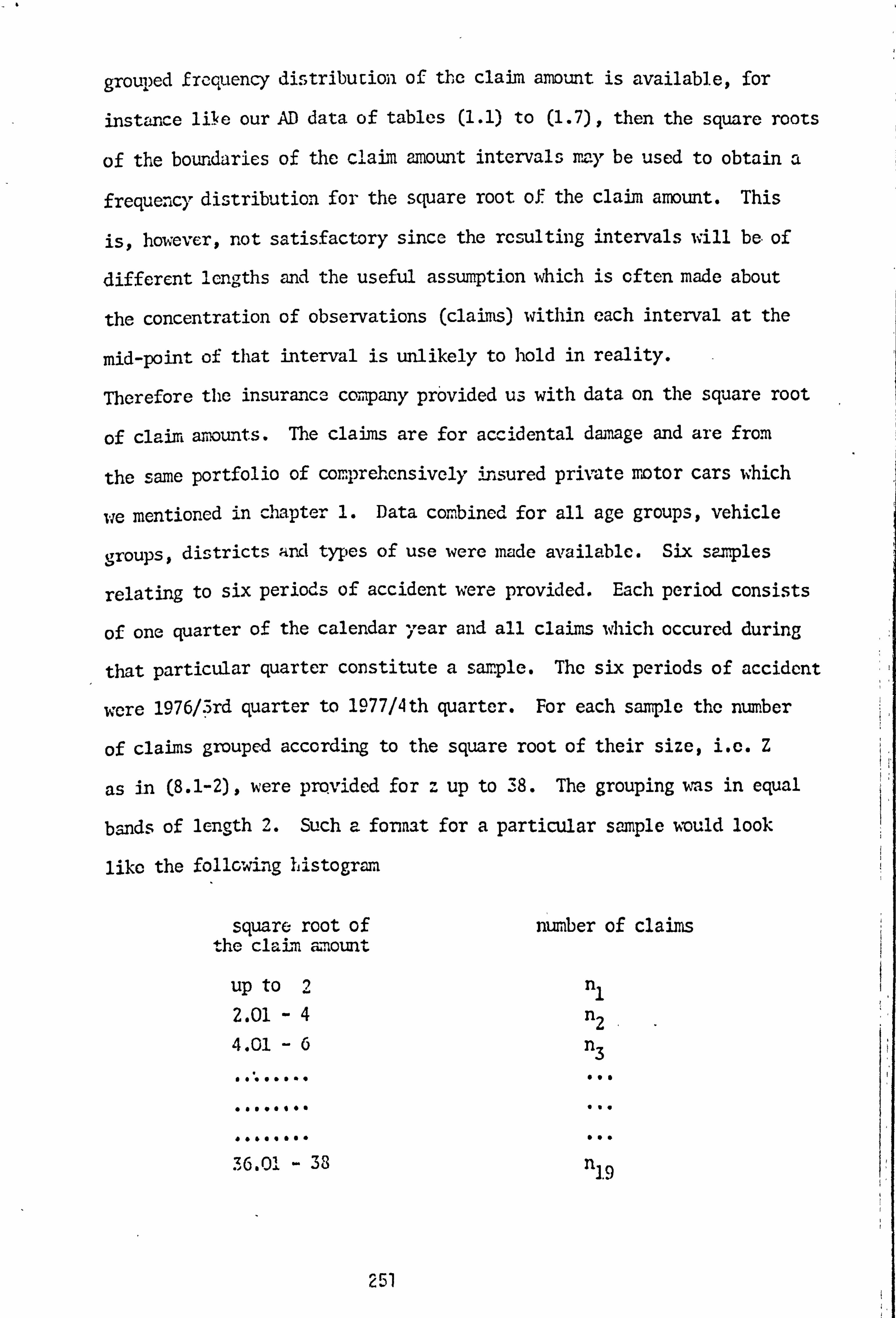
grouped frequency distribucion of the claim amount is available, for

instance like our AD data of tables (1.1) to (1.7), then the square roots

of the boundaries of the claim amount intervals may be used to obtain a

frequency distribution for the square root of the claim amount. This

is, howetier, not satisfactory since the resulting intervals will be-of

different lengths and the useful assumption which is cften made about

the concentration of observations (claims) within each interval at the

mid-point of that interval is unlikely to hold in reality. -

Therefore the insurance company provided us with data on the square root

of claim ar, unts. The claims are for accidental damage and are from

the same portfolio of corprehensively insured private rotor cars which

we mentioned in chapter 1. Data combined for all age groups, vehicle

groups, districts and types of use were made available. Six samples

relating to six periods of accident were provided. Each period consists

of one quarter of the calendar year and all claims which occured during

that particular quarter constitute a sample. The six periods of accident

were 1976/3rd quarter to 1977/4th quarter. For each sample the number

of claims grouped according to the square root of their size, i. e. Z

as in (8.1-2), were provided for z up to 38. The grouping was in equal

bands of length 2. Such a format for a particular sample would look

like the following histogram

square root of the claL, i amount

up to 2 2.01 -4 4.01 -6

number of claims

nl n2

n3

....... .

..... ...

36.01 - 33

..

n1.9

251

For larger claims details of individual claims were provided. We grouped

these into zurther bands of length 2 until the band containing the

largest claim (or claims) was reached. Because the square root of claim

amount is not readily understood in monetary terms we squared the boun-

daries of each interval for presentation of the data. The frequency

distributions of the six samples of AD data can, therefore, be seen

as the first two columns of tables (8.1.1) to (8.1.6). Both open and

settled claims have been included in each sa-nple. For 1976/3rd quarter

to 1977/2nd quarter the data were collected more than six months after

the end of each period of accident and hence no more, or only few,

claims are still to be reported. For 1977/3rd and 1977/4th quarters,

as we can see from tables (8.1.5) and (8.1.6), the total number of claims

are less than for other periods. This is because for these two periods

of accident the data were collected, respectively, three months after

the end and at the end of the periods. Therefore many more claims

are still expected to be reported to complete the histogram in each

case. We will not make any allowances for IBNR claims of these two

periods but will judge the results of the model fitting in the light of

the incompleteness of the data.

Initially, *in this chapter, we will define the gannna distribution

and will mention some of its properties. The estimation problem will

be discussed next and the method of multincnial naxinwn likelihood Gm)

will be described for estimation of the parameters from grouped data.

This method will then be used to fit the garmra distribution to the AD

square root data mentioned above. The results will be analysed and the

goodness-of-fit tests will indicate the adequacy o, f. this model. The

effects of inflation on the parameters of the model will be considered

in section 8.5. These will then be used to . redid the future distribution

of the square root of claim anuunts from past data. The actual and

252

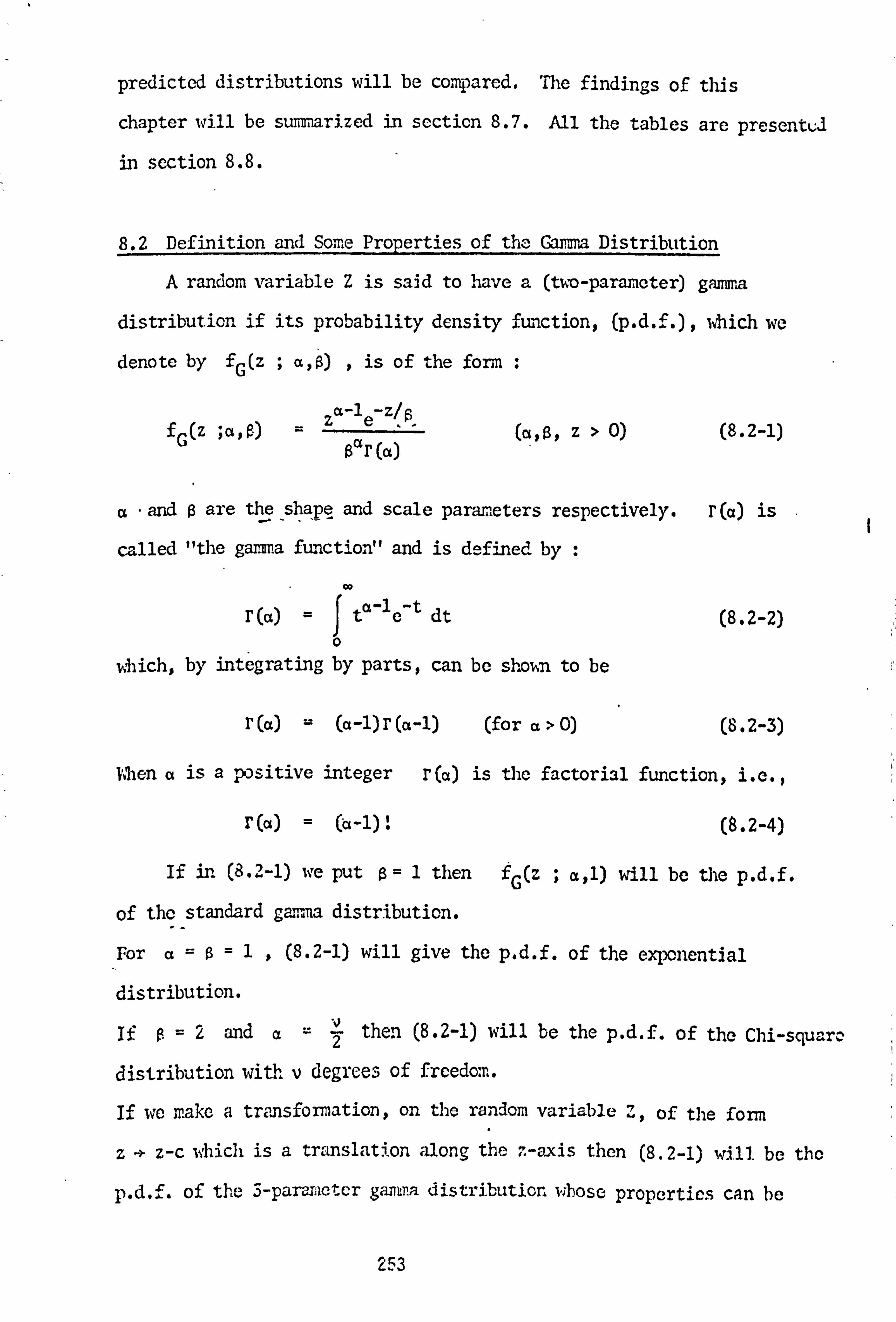
predicted distributions will be compared, The findings of this

chapter will be summarized in section 8.7. All the tables are presenteJ

in section 8.8.

8.2 Definition and Some Properties of the Ganmia Distribution

A random variable Z is said to have a (two-parameter) gamma

distribution if its probability density function, (p. d. f. ), which we

denote by fG(z ; a, $) , is of the form :

za-1e-z/O f (Z ; 0110 (8.2-1) G $aF (a)

a -and ß are the shape and scale parameters respectively. r(a) is

called "the gam a function" and is defined by

r(a) - Jt'c -t dt (8.2-2) 0

which, by integrating by parts, can be shokn to be

r (a) - (a-1) r (a-1) (for a> 0) (8.2-3)

V, hen a is a positive integer r (a) is the factorial function, i. e.,

T (a) = (a-1) (8.2-4)

If in (8.2-1) we put a= 1 then fG(z ; a, i) will be the p. d. f.

of the standard gamma distribution.

For a=B=1. (8.2-1) will give the p. d. f. of the exponential

distribution.

I£ 2 and a-2 then (8.2-1) will be the p. d. f. of the Chi-square

distribution with v degrees of freedom.

If we make a transformation, on the random variable Z, of the form

z ->. z-c which is a translation along the --axis then (8.2-I) will. be the

p. d. f. of the 3-parameter gam m distribution whose properties can be

253

easily derived from those of f0(z ; a, O). Therefore it will suffice

to consider only the 2-parameter ganmra distribution here. Further

reference can be made to Bury (1975) and Johnson and Kotz (1970).

We denote the distribution function of fG(z a, ß) by G(z

For the standard gamma distribution we have

z 1

G(z ; al1) =räJz lez dz

0

(8.2-5)

where the integral is called "the incomplete gamma function" and is

denoted by rZ (a) . Therefore

z(a) (8.2-6) G(z ; a, 1) r

r (a)

Since ß is a scale parameter we can show that

G(z ; a, $) = G(ß ; a, 1) (8.2-7)

hence the two parameter ganra distribution function is

rz/ß(°`) G (z ; a, ) = (8.2-8)

r (a)

Let x2 v(u) denote the distribution function of a Chi-square random

variable, U, with v degrees of freedom. As we mentioned earlier,

fG (z ; a, 2) is the p. d. £. of a Chi-square random variable with v= 2a

degrees of freedom. Hence the relationship between the gaim a and the

Chi-square distribution functions will be

2 G(z ; a, ß) = G( Zß

; a, 2) X2a (2ß ) (8.2-9)

Therefore tables of the Chi-square ctnnulative distribution function may

be used to calculate G(z ; a, ß). Pearson (1922) has, however, tabulated

G(z 1), to seven decimal places, for a=0(. OS)1(0.1)5(0.2)51.

more accurate tabulation. s, of G( z; a, l), to nine decimal places, have

2-54

been given by Harter (1564) fora = 0.5 (0.5) 75 (1)165. Pearson (1922)

has shown t; cat,

G(z ; ct, ß)=e O

ýY +J/, 4 («+J+1) l

J (8.2-10)

where y>0

For computing purposes, a good approximation to the value of G(z ; a, 0)

can be obtained by taking sufficient terms in the above series. We

shall use this formula in our estimation programs and other calculations

involving the gana cumulative distribution function. The values of

the complete gamra function r(. ) , as required in (8.2-10) are computed

by a special routine which exists in the NAG1 library of computer routines.

This routine is based on the Chebyshev expansion of the complete garra

function which is given in Abramowitz and Stegun (1968).

The rth moment of Z about zero can be directly obtained from (8.2-1)

and (3.2-2) as :

E (Zr) w ßr tr a+r (8.2-11)

hence the expected value of Z is

F(Z) = as (8.2-12)

and the variance of Z can be show i tu be 2

Var(Z) = aß

The coefficient of variation of Z is, therefore, equal to a-' which is

positive and depends en the shape parasieter only. The 3rd and 4th central

nornents of Z, denoted by a and 04 respectively, can be shown, by using

(8.2-11) , to be 3

63 = 2aa (8 2-14)

and 84 = 3aß 4

(rß+2) (5.2-15

1- Nottin harn Algorithmic Group L5

The coefficient of skewness, yl , is, therefore,

yl = 2a >0 (8.2-16)

hence all gamma models are positively skewed. The coefficient of

kurtosis is y2 where

y2 =3+ 6a-1 >3 (8.2-17)

which implies that all gamma densities are more peaked than normal

densities.

For large values of a, yl and y2*approach their normal values 0 and 3

respectively. Thus for large a the central portion of the corresponding

gamma p. d. f. should be well approximated by a normal p. d. f.

lVhhen a ,l the gamma distribution has a single mode which is located at

Zmode =ß (a-1) (8.2-18)

For values of a<1 the gamma p. d. f. has a singularity at the origin

and fG(z ; a, R) -} °° as z -'- 0.

The median, and in general the quintile of order q, of the gamma

distribution cannot be expressed in terms of its parameters but may be

obtained, by interpolation, from tables of the gamma distribution function.

As we mentioned in section 8.1 we intend to use the gamma distribution

as a model for the distribution of Z, the square root of claim amount X.

The mean and standard deviation of Z do not have any significance in

monetary terms. Therefore, it is important to obtain the mean and

standard deviation of X in terms of a and a, the parameters of the

gamma model. The expected value of X is

1)

E (X) = E(Z). since Z=

but from (8.2-11) and (8.2-3) it follows that

E (x) r (a+1) (r . 2-19)

256

The variance of X is by definition

2242

Var (X) = E(X) - (E "X)) z- E (Z )- (11(X) )

On using (8.2-11), (8.2-3) and (8.2-19), respectively, it follows that

42 6 ar(X) =ßa (4a + 10 +ä) (8.2-20) V

8.3 Estimation of the Parameters

Johnson and Kotz (1970) deal with the estimation problem when values

of individual observations in the sample are known. They consider the

usual methods of moments and maxi= likelihood. We are, however,

interested in estimation from grouped data. Therefore, in this section,

we will consider the method of multinormal maximum likelihood GM).

Let us assume that we have a sample of grouped data where n independent

random observations (claims) on a random variable Z (in our case, the

square root of the claim anwunt X) have been grouped according to their

size into k mutually exclusive intervals. Further, let ni be the number

of observations (claims) in the class interval (zi^1, zi), for

i=1,2, ... ,k, such that k

n= ni i=1

If Z has a gamma distribution given by G(z ; a, $) in (8.2-7), then let

pi be the probability that an observation (claim) occurs in the interval

(z. -. 1, zi), i. e.

ý pi = G(zi ; x, ý)

For i= is taking zo = 0,

pl = G(z1 ; a, a)

- G(zi-1 ' a, ß) (8.3-1)

for i=2,3, ... ,k

(8.3-2)

Therefore, the sariple 1.; kelihood function will be proportional to L

257

where 1. nl

" (8.3-3) I. = P1 i=1

and the loglikelihood function will be

k log L= nl log pi (8.3-4)

: i=1

where pi is as defined above. The values of G(zi ß) are calculated

from (8.2-10). AA

The maximum likelihood estimates of the parameters, (a, ß), are obtained

by maximizing log L simultaneously with respect to a and ß. To avoid

solving non-l: noar equations (which is a laborious task when k, the

rjwnber of intervals, is large) we suggest the confuting technique

described in section 3.7.7 for maximizing log L directly with respect

to the unl<no;, m parameters. To start the iteration process we can use

the moment estimates of a and ß. For grouped data the sample moments

can be calculated by assuming that in each interval (zi_1, zi), -all the

nl observations are concentrated at the mid-point of the interval, i. e.,

at (zi_1 + zi)/2. The sample first and second n ments when calculated

can be put equal to their corresponding population values to yield the

moment estimates of a and g.

8.4 Application of the Camera Distribution to the AD'Sguare'Rdot Data

To examine the adequacy of the garna distribution as a model for

the distribution of the square root of the AD claim amount we wrote

computer progr=, `P? for estimating parameters a and ß from a swrple 1

of grouped data. The hu". method described in section 8.3 was used.

The sw'nples of the square root. AD data, which were described in section

8.1, were input to the prograi<<. For each saiiple the program colrputed

and printed cut the N NI estimztes of a and 0, the shape and scale

2058

paraneters respectively , of the gamma distribution. The mean and

standard deviation of the claim amounts according to the fitted model

were also produced. The program also provided an extensive table of

results, giving in particular the values of the expected claim numbers,

the expected loss and the contribution to the total X statistic for W.

each claim amount interval. The results for the square root AD data

are presented in tables (8.1.1) to (8.1.6). The original grouping of

the data was in bands of length 2 but, for convenience in interpretation,

we have squared the boundaries of each interval and, therefore, the

grouping in the tables is in terms of the amount of claim and not its

square root. From these tables we can see that a is greater than 1

for all samples. Hence the model portrays the mode of the sample

histogram. The actual minus expected claim numbers are not small and

in few of the intervals the contributions to the X2 statistic are large.

The Xi statistics are significant, at 0.05 level, for all the samples.

These indicate significant differences between the model and actual

sample values.

The expected loss statistic for each interval was calculated by multiplying

the actual minus expected claim number by the square of the mid-point

of the original interval in terms of Z, the square root of the claim

amount. The values of this statistic show considerable disagreement, in

monetary terns, in the middle range of the claim account distribution.

Our analysis shows that the 2-parameter gamma distribution is not an

appropriate model for the distribution of the square root of AD claim

amounts. The fit of this model to the AD square root data is worse

than that of the 2-paramoter lognormal distribution to the AD data. Fence it

seers that collection of data on the square root of the claim amount is an

unnecessary task. To ponder on i: lry the fit. of the nedel should be so

259

poor we should examine the two assumptions which we made in section 8.1.

These were :

(i) - Z, the square root of the claim amount X, is proportional

to the velocity of the car at the time of impact (since X 2

is proportional to 7 mV , the kinetic energy of the car

at the time of impact).

(ii) - The velocity of the car at the time of impact has a gania

distribution

As regards assumption (i), it may be more reasonable to assume that

the claim amount X is proportional to mV, the momentum of the car at

the tijre of impact, and not to its kinetic energy. Hence, if assumption

(ii) holds, we should expect the claim amount X to have a gamma

distribution. To examine this on our AD data samples, presented in tables

(1.1) to (1.7), we used the method of moments to estimate the parameters

a and ß. -Th. - estimates of a were less than 1 for each sample, hence

indicating that the garnna model had no node to portray that of the

histogram of the sample values. The model also had a much shorter tail.

than the sample histogram. The values of the X2 statistic were

calculated from each sample and its corresponding gamma model.. These

were consistently large and indicated significant differences between

the model and actual sample values. Again the fit was considerably

poorer than that of the 2-parameter lognormal. This is not totally Un-

expected since the lognormal model has a mode and a longer tail than

the gaiima and is, therefore, more capable of representing the mode

and the long tail of the claim amount histogram.

There are no statistics available on the velocity of cars at the

time of impact to allow the examination of assumption (ii). Therefore,

even if assumption (i) or its revised form (X proportional to rr%o is

260

considered reasonable, there is no reason why Z, the square root of

claim wount X, (or X itself) should have a gamma distribution since it

is possible for V to have some other distribution.

8.5 The'Effects of Inflation on the Parameters of the Model

Although the gamma model proved not to be appropriate for the

distribution of the square root of the AD claim amounts, however, to

make this chapter complete, we consider the effects of inflation on

the parameters of the model. We follow the exposition of section 3.9

and investigate these effects theoretically. As was mentioned in that

section, we would need to allow for such effects when a prediction of

the future distribution of the square root of claim amounts is required.

Let us, therefore, again assume that the effect of inflation is to

increase a claim of amount X to U= X(1 + i) over a period of time where

i is the effective rate of inflation, according to some suitable index

of wages or prices, for that period. If Z- (Thas a gamma distribution

with p. d. f. fG(z ; a, a), as given by (8.2-1), then by a transformation

of variables it can be shown that

= rZ where r= (1 + i)

will have a gap-va distribution with parameters a and rß . Therefore

inflation affects ß and leaves a, the shape parameter, unchanged.

This means that when a gamma model is found appropriate for the distribution

of Z, the square root of the claim amount from a particular class of

insurance business, we can "update" the scale parameter ß, with

respect to inflation, and hence obtain the distribution of Z in a

future period.

8.6 Prediction for theAD Square Root Data

261

For the purpose of demonstrating our prediction technique for

the distribution of square roots of claim amounts ( despite the inadequacy

of the gonna model for the AD data) we wrote computer program P26. The

WL estü. ates a and for a particular period of accident and the rate

of inflation, calculated from the General Index of Retail Prices, are

input to the program. The parameters of the gamma model for the

future period are then calculated and the program prints out an extensive

table of results for comparing the actual and predicted distributions

of the square root of the claim amount. To see the result of predicting

one year ahead we used 1976/3rd and 1976/4th quarters to predict the

distributions for 1977/3rd and 1977/4th quarters respectively. The

results are presented in tables (8.2.1) and (8.2.2). The tables are

self-explanatory, and wire can see that the actual minus expected number

of claims is large for some intervals and that the Chi-square

statistics are very large and indicate highly significant differences

between the predicted and actual sample values. We did not expect to

obtain satisfactory results, since the fit of the model to the actual

data of 1976/3rd and 4th quarters was so poor in both cases.

8.7 Conclusicns

As we mentioned in the introduction to this chapter, encouraged

by _a

remark by Beard (1978), we studied the g an, ma distribution as a

model for the distribution of the square root of the claim =aunt. The

properties of the ¬aru a distribution were studied and the bM method

was considered for estimation of its parameters from grouped data. In

order to show the application of this mod. el in practice, we obtained

six samples of the square root of AD claim amounts. The model was fitted

to each sample by ML method and in each case it exhibited a sharper peal:

262

and a shorter tail than the histogram of the sample values. The Chi-

scviare goodness-of-fit test statistic indicated highly significant

differences between the model and actual sample values. Judged by

this statistic, the fit in each case was worse than that of the 2-

parameter lognormal model to the AD claim amounts as shown in chapter 3.

In section 8.4, based on the assumption that the amount of claim should

be proportional to the momentum of the car at the time of impact, we

examined the ganuna distribution as a model for the distribution of the

claim amount itself. Hence we fitted this model to the AD samples of

tables (1.1) to (1.7). The values of a, the shape parameter, were less

than 1 in each case. This indicated that the model ignored the distinct

mode of the actual distribution of claim amounts. The model also

exhibited a much shorter tail than the histograms of the samples. Judging

2 b) ,X statistic, a very poor fit was obtained. In each case, the fit

was worse than that of the 2-parameter lcgnonnal distribution as shown

in chapter 3. This was not surprising since the lognormal distribution

has a longer tail than the gamma and also always possesses a mode.

For the sake of a more complete study, the effects of inflation

on the parameters of the gamma model, when used for the distribution

of the square root of the claim amount, were considered. It was shown

that inflation increases ß, the scale parameter, but leaves a, the

shape parameter, unchanged. Predictions were made, using two samples

of our square root AD data and, as expected fr ., the poor fit of the

gamma model to the sample values, the predicted distributions were sho., n,

by the X2 statistic, to differ significantly from the actual ones.

Wo therefore ro j cct the gazitra distribution as ai cde1 for the

distribution of JD claim amounts or the square roots of clam vnounts.

For the latter, we b�lieve that the tasr, of collecting data on the square

263

root of claim amount is unnecessary when more adequate models, like

the lognor 1, exist for the distribution of claim. amount itself.

8.8 Tables

264

"2b1e i ß, 1.1i

* TWD-PARAMETER GAMMA DIS. *#*

76/3RD QUARTER DATA

ESTIMATION By MULTINOMIAL MAX. LIKELIH000 METHOD : - ALPHA - 3.474 BETA=. 3.866

MEAN=-232.223 S. D. = 262.746'

AMOUNT £ ACTUAL EXPECTED ACTUAL- EXPECTED CL. NO, CL. N0. EXPECTED LOSS,. (A-E)**2/E

UPTO 4 14. 13. 11 1, 0,077 4- 16 90, 116. 4, 36. 0,186

16- 36 147. 178. -31. -777. 5.399 36- 64 240. 243. -3. -147. (1,037 64- 100 297. 271. 26. 2108, 2.494

100- 144 , 290. 265. 25. 3028, 2,358

144- 196 260. 239. 21, 3552. 1,1345 196- 256 188. 204. -16. -3602. 1.255 256- 324 175. 166�'

' 19, 2603. 0.486

324- 400 119, 130 , -11, -3973. 0.931 400- 484 76. 99. -23. -10148. 5.343 484- 576 57. 74. -17, -8997. 3.905 576- 676' 49. 54. -5. -3126. 0.463 676- 784 45. 39. 6. 4376. 0,923' 7134- 900 28.. 28, . 0, 01 00000 900-1024 21, -20, 1,

. '961. 0,050

1024-1156 18. 1.4. 4. 4357, 1.143 1156-1296 17. 9, 8. 9803. 7.111 1296-1444 4. 6. -2. -2739. 0.667 1444-1600 2. 4, -2. -3043. 1600-1764 B. 3. " 5. 84017, . 1764-1936 1. 2. -1, -1949. 1936-2'116 1, 1. 0. 2116-2304 2. 11 1. 2209. 2304-2500 2. 1, 10 2401. 2500-2704 0. 0, 0. 01 2704-2916 01 0. 01 01 2916-3136 0. 0. 00 0. 3136-3364 0. 0, 0. 01 3364-3600 0. 01 01 0. 3600-3844 0. . 0. 0, 0. 3844-4096 01 0, 01 00 4096-4356 01 0. 0, 4356-4624 01 0.. 06 0. 4624-4900 01 0, . 0. 0. 4900-5114 0. 0. 0, 0. 51Rh1.. 5476 0. ' 01 0, 0, 5 76-6776 0 1. 5626. 0 ------------ -------- Y... - ----------- ----------- --------------- ---------

TOTAL .. ---------

2152, --- . -- +----

2150. ----------- -----------

11067, -----------

36.767 -- -----------

TOTAL EXP. LOSS 2.2 as J !ýa

TOTAL ACT. COST

26

Table (8.1.2)

# TWO-PARAMETER GAMMA DIS. *#*

76/4TH RUARTER DATA

ESTIMATION BY MULTINOMIAL MAX. LIKELIHOOD METHOD t- ALPHA = 3.733 BETA= 3.888

MEAN= 266.975 - S. D. - 290.604

AMOUNT f. ACTUAL -EXPECTED ACTUAL- EXPECTED CL. NO, CL. NO. EXPECTED LOSS (A-C)**-2/E

UPTO .4 11. 10. 1. 1. 01.100

4- 16 107. 82. 25. 226. 7.622 16- 36 145. 192. -47. ' -1177. 11.505

. 36- 64 266. 287. -2.1. -1030. 1.537

. 64- 1110 . 361. 342. 19, 1541. 1.056 100- 144 361. 354. 7. 8418.. n. 138 144- 196 -359. 334. 25. 4228. 1.871 196- 256 325. 296. 29. 6529. 2.841 256- 324 252. 249. 3. 868. 0.036 324 - 400 200. 202. -2. -722, 0.020 400- 484 137. 159. . -22. -9707. 3.044

X 484- 576 112. 122. -10. -X5292. 0.820 576- 676 80. 92. ' -- 12. 4503. 1 *565 676- 784 61. " 68. -7. -5'! 05. 0.721 784- 900 51. 49. 2. 1683.. 0.082

.. 900-1024 31. 35. -4. -3845. 0.457 1024-1156 28. 25. 3, . 3268. 0.360 1156-1296 24. 18. 6. 7352. 2.000 1296-1444' 13. " 12. 1. 1369. 0.083 1444-1600 8. 8. 00 0. 0.000 1600-1764 . 4. 6. -2. -3363. 0.667 1764-1936 9. . 4. 5. 9247. 1936-21 16 1; - 3. -2. -4051. 1.286 2116-2304 2. 2. 0. 0. 2304-2500 2. 1. 1. 2401.

. 2500-2704 1. 1. 0.. . 0,

2704-2916 0. 1. -1. -2810. 2916-3136 0. 0. 0. 0. 3136-3364 01. 0. 0. 0. 3364-3600 1. 0. 1. 3482. 3000-3844 . 1. 0. 1, 3722. 3844-4096 0. 0. 0. 0, 4096-4356 0. 4356-4624 ----------

1. ---- --- ----

0. --------- ! ----

1. -----------

4490. ----------

1.800 --

ToTAL - 2954-. 2954. 6648. ------------

39,610

Q. F. -70 TOTAL EXP. LOSS . 0.8 "

TOTAL ACT. COST

26G

Table (8.1,3)

-ý^# TEND-PARAMETER GAMMA DIS. -

$**

77 f 'i S'! ' QUARTER DATA

ESTIMATION 0Y. MULTINOMIAL MAX. LIKELIH00D METHOD '; - . ALPHA = 3.822 BETA= 3.790

MEAN= 264.715 S S. D. = 284-. 505

AMOUNT ACTUAL EXPECTED ACTUAL- EXPECTED CL. NO. CL. NO. EXPECTED LOSS (A_E)**2/E

UPTO 4 7. 7. . 0. 0. 0.000

4- 16 85. 62. 23. 208, 8.532 16-. 36 107. 151. -44. -1102. 12,821 36- 64

0 6 2069 280

22.9.. 2

-23. -1129. 2�310 4- - 10 . 75. 5. 405, 0.091

110- 144 328, 286. 42. 5087. 6.168 144 196 299. 271. 28. 4736. 2.893 196-. 256 262. 239. 23. 5178. 2.213 256- 324 196. 201. -5. -1446. 0.124 324- 400 151. 163, -12. -4334, 0,8113 400- 484 104. 127. -23. -10148. 4.165 484- 576 79. 97. -18. -9526. 3.340 -576- 676, 62. 73. -11. . -6878. 1.658 676- 784 50. 53. -3. -2188. 0.170 784=- 900 45. 138. 7. 5889. 1.269 900-1024 27. 27. 0. 0. 0.000

1024-1156 22. 19. 3. 3268. 0.474 1156-1296 8. 13. -5. -6127. 1,923 1296-1444 16, 9. 7.

. 9586. 5.444 1444-1600 8.

. 6. 2. 3043. 0.667

1600-1764 6. 4. 2. 3363. 1764-1936 4. 3. 1. 1849. 1.286 1936-2116 5. 2. 3. 6076. 2116-2304 2. 1. 1. 2209. 2304-2500 . 0. 1. -1. -2401. 2500-2704 0. 1. -1. -2602. 2704-2916 0. 0. 0, 0. 2916-3136 1. 0. 3026. 3136-3364 0. 0. 0. 0, 3364-3600 0, 0, 3600-3844 0. 00 - 0. 00 % 3844-4096 0. 0, 0. 0, 4096-4356 -

1. ----

" 0" ------------

11 ----- w_w»

4226. _- TOTAL L. 2361. 2358. 102fýH.

- ----- K,

------ ----------- - - ' 654 - - --------- --.. _---ww_ww--__ww.. -_w_ w - ------ TOTAL EXP. LOSS

D. F. '19 --- .. 1.6%

TOTAL ACT, COST

267

Table (8.1.4)

* TWO-PARAMETER GAMMA *** DIS,

77/2ND QUARTER DAT A

ESTIMATION BY r ULTINOMIAL MAX. LIKE LIHOOD METHOD ; - ALPHA = 3.746 BETA= 3.941

MEAN= 276.19A S. D. = 300.056

AMOUNT £ ACTUAL. EXPECTED ACTUAL- EXPECTED CL. NO. - CL. NO. EXPECTED LOSS (A-E)*-K-? /E

UPTO 4 5. 6. -1.. -1. 0.167 4- 16 68. 51. 17. . 154. 5.667.

16- 36 93. '

120. -27. -676. 6.075 36- 64 162. - '182. -20. -981. 2.198 64- 100' 236. 219, 17, 1379. 1.320

100- 144 237. 229. 8. 969. 0.279 114- 196 240. 218, 22. 3721. 2.220. 196- 256 209. 195.

, 14. 3152. 1.005

256- 324 153. ,

165, . -12. -3470. 0,1373

324- 400 137.. 135. " 2. 722. 0,030 4(101- 484 99. . 107. -8. -3530. ' 0.598 484- 576 71. 83. -129 -6351. 1.735 576- 676 58. - 63. -5. -3126, 0.397 6.76- 784 51. 47. 4. " 2917. 0.340 784- 900 31. 34. -3. -2524. 0.265 900-1024 22. 25. -3. --2884. 0.360

1024-1156 14, ' 18, -4. -4357. 0.889 1156-1296 15. 13. 2. 2451. 0.308 1296-1444 10. " 9. 1. 1369. 0., 111 1444-1600 10. 6. 4. 6086. 2.667 1600-1764 2. 4, -2. -3363 1764-1936 5. . 3. 2. . 3699. ý, CCO 1936-2116 5. 2.. 3. 6076. 2116-2304

, 0. 1. -1. -2209.

2304-2500 1. 1. 0. 0. 2500-2704 2.

. 1. . 1.

. 2602.

2704-2916 n. 0. 0. 2916-3136 1. 0. 1. 3026.

- 3,200

TOTAL

---------- '1937.

------------

1937.

------------ --------- 4848,

----

-------------- X0.702_

--

--------

TOTAL EXP. LOSS D. F. -- -

' --- 019 % P <0, ' TOTAL ACT. COST

263

Table (8,1.5)

## TWO-PARAMETER GAMMA OIS. ##*

77/3RD QUARTER DATA'

ESTIMATION By MULTINOMIAL MAX. LIKELIHOOD METHOD :- ALPHA = 3.331 BETA= 4.372

MEAN= 275.774 S. D. = 319.158

AMOUNT £ ACTUAL EXPECTED ACTUAL- EXPECTED CL. NO. CL. NO. EXPECTED LOSS (A-E)**2/E

UPTO 4 9. 10. -1. -1. 0.100 4- 16 96. 59. 37. 334. 23.203

16- 36 67. 122. -55. -1378. 24.795 36- 64 159. 169.,

_ -10. -491. 0.592 64- 100 191. 192. - -1. -81. 0.005

100- 144 189. 195. -6. -727. 0.1135 144- 196 210. 182. 28. 4736. 4.308' 196- 256 174. 161, 13. 2927. 1.050 256- 324 158. 136. 22. 6362. 3.559 324- 40G 107. 112. -5'. -1806. 0.223 400-484 86. 90. -4. -1765.. 0.178 484- 576 74. ' 70" 4. 2117. 0.229

' 576- 676 56. 54. 2. 1251. 0.074 676- 784 32. 41. -9. -6563. 1.976 784- 900 21. 31. -10. -8413. 3,226 900-1024 13. 23. -10. -9613. 4.348

1024-1156 13. 17. -4. -4357. 0.941 1156-1296 11. 12. -1; -1225. 0.083 1296-14,14 14. 9. 5. 6847. 2.778 1444-1600 5. 6. -1. -1521. 0.167 1600-1764 4. 4. ' 0. 0.. 00000 1764-1936 4" 3. 1. 18gq. 1936-2116 2. 2. 0. 0. 0,200 2116-2304 2. 2. 0. 0. 2304-2500 3. 1. 2. 4803. 2500-2704 1. 1. 0. 0. 2704-2916 0. 1. -1. -2810. 2916-3136 1. 0. "1. 3026. 33136-3364 0. 0. 0. 0" "3364-3600 0. 0. 0. U. 3600-3844 0. 0. 0. 0" 3844-4096 0. 0. 0, 0. - 4096-4356 0. 0. 0. 0. 4356-4624 2. 0. 2. 8979. 3.200

TOTAL

----------

1704.

----------- 17050

------------ ----------- 24I9.

µ- -

------- 75.4+0-----

----- D. F.

------------ _- ?0

TOTAL EXP. LOSS ----" ------ = 0 "5 oil v ý"! 1:

TOTAL ACT. COST

269

Table (8,, 1.6)

*** TWO-PARAMETER GAMMA DIS. ***

77/4TH QUARTE n DATA

ESTIMATION BY MULTINOwlI AL MIAX. LIKE LIH00D METHOD ; - ALPHA 2 . 690 BETA= 5.387

MEAN= 289 . 606 S. D. = 375.684

AMOUNT E ACTUAL EXP¬CTED ACTUAL- EXPECTED CL. NO. CL. NO. EXPECTED LOSS (A-E)**2/E

UPTO 4 3. 6. -3, -3. 1.500 4- 16 .

50. 25. 25. 226. 25.000 16- 36 19. 1 . 42. ' -23. -576. 12.591 36- 64 31. 51. -20. -981. 7.843 64- 100 57. 54. 3-. 243. 0.167

100- 144 54. - 52. 2. 242. 0.077 144- 196 '(7. 48. 19. 3213. 7.521 196- 256 42. 42. 0. 0. ' . 0.000 256- 324 53. 36. 17. 4916. B. 028 324- 400 24. 30. -6. -2167. 1.200 400- 484 17. 25. -8. -3530. 2.560 454-. 5.76 13. 20. -7. -3705. 2.450 576- 676 2?. 16. 6. 3752. 2.250 676- 704 10. 12. -2. -1459'. 0.333 784- 900 9. 10. -1. -641. 0.100 9O0-1024 13. 7. ; 6. 576E+. 5.143

1024-1156 0. 6. . -6. . -6536. 6.000

1156-1296 0. 4. -4. -4901. 1296-1444 ,

0. . 3. _. -3. -4108. ' 7.0Q0

1444-1600 3. 2. 1. 1521. 1600-1764 1. 2. -1. -1601. 01000 1764-1936 5. 1. 4. 7396. 1936-2116 2. 1. 1. . 2025. 211E-2304 3. 1. 2. 4419. 2304-2500 0. 1. -1. -2401. 2500-2704 . 1. 0.. 1. 2602,

' 2704-2916 1. 0. 1" 2810. 16.000

TOTAL.

----------- 500.

---------- 497.

---------- -----------

----------------------- 0244.105.767

------------- - D. F. - ---------

= 17 TOTAL EXP. LOSS

------ -----. ---- 4.3 P <001 TOTAL ACT. COST

270

Table (8.2.1)

*** - (WO-PARAMETER GAMMA DIS. ***

PREDICTION OF 7? /3RD (LJARTER CLAIMS CO ii USING 76/3RD (QUARTER PULT. MAXL. PARAMETERS

ALPHA= 3.474 BETA= 3. A66 INFLATION RATE I 1fß. 54 CALCULATED FROM GENERAL INDEX OF RETAIL PRICES.

PREDICTION P!, HAPMETEf1S ARE ALPHA= 3.474 BETA- 4.173 MEAN CLAIM AMOUNT= 2? 0.63 5. D. =306.19

ACTUAL 7? /3HU PARAMETE RS : - ALPHA = 3.331 BETA= 4.372 MEAN CLAIM hiAOLJNT= 275.75 S. D. =319. i5

AMOUNT f, ACT . NO. E XP. NO. A-E E XP. LOSS (A-E) **2/E UPTC) 4 9. A. ' 1. 1. 0.125

4- 16 96. 55. 41. 3? 0. 30.504 16- 36 67. 119. -52. -1303. 22.723 36- 64 159. 169. -10. -491. 0.592 64- 100 191. 195. -4. -324. 0.082

100- 144 189. 199. -10. -1211. 0.503 144- 196 210. 186. 24, 4059. 3.097 196- 256 174. 164. 10. 2252. n. 610 256- 324 158. 139. 19. 5494. 2.597 324- 400 107. 113. -6. -2167. 0.319 400- 484 86. 90. -4. -1765. 0.178 484- 5? ( 74. 70. 4. 2117. 0.229 576- 676 56. 53. 3. 1876. 0.170 676- 784 32. 40. -8. -5834. 1.600 784- 900 21. 29. -8. -6730. 2.207 900-1024 13. 22. -9. -8652. 3.682

1024-1 156 13. M. -3* -3268. n. 563 1156-1296 11. 11. n. n. 0.000 1296-1444 14. 8. 6. 8216. 4.500

144d-1600 5. 6. -1. -1521. 0.167 1600-1764 4. 4. n. n. 1764-1936 4. 3. 1. 1849. 1936-2116 2. 2. n. n. 2116-2304 2. 1. 1. 2209. 2304-2500 3. 1. 2. 4803. 2500-2704 1. 1. 0. 2704-2916 0. n, n, n. 2916-3136 1. 0. 1. 3026. 3136-3366 0. 0. 0. 0. 3364-3601) 0. 0. 0. 0. 3600-3844 n. 0. n. n. 3844-4096 n. n, n. n. 4096-4356 01 0. n. 0. 4356-4624 2. n. 2. [4979.

------------ TOTAL

-----------

----------- 1704

-----------

--------- 17114 ---------

-----

-----

--------- - 119V5,

-----------

----------- 711.504

-----------

CHI 5W. STMT. = 81. g 7 n. F. = 21 F <. 01

TOTAL. ACTUAL CURT = 47220fi. TOTAL. EXPECTED (; UET t 46(I223 .

TOTAL E: Yf. LOS`* ----------------- 2.54 TOTAL ACT. COST 271

Table (8.2.2)

*** TWO-PARAMETER GAMMA DI: i. ***

PREDICTION OF 7? /4TH QUARTER CLAIM(' COST USING 76/4TH QUARTER l4ULT. MAXL. PARAMETERS

ALPHA= 3.733 (SETA= 3.888 INFLATION RATE I=13. Cä CALCULATED FROM GENERAL INDEX OF RETAIL PRICES.

PREDICTION PARAMETERS ARE : - ALPHA= 3.733 BETA- 4.133 MEAN CLAIM AMOUNT- 31)1.80 5.0. -328.50

ACTUAL 77/4TH PARAMET ERS : - ALPHA- 2.648 BETA- 5.387 MEAN CLAIM AMOUNT.. 289.54 S. a. -3? 5.62

AMOUNT F ACT. NO. * EXP. NO. A-E EXP. LOSS (A-E)**2/E n- 4 3. 1. 2. 2. 4- 16 50. 12. 38. 343. 120.333

16- 36 19. 28. -9. -225. 2.893 36- 64 31. 43. -12. -589. 3.349

-64- 100 57. 53. 4. 324. 0.302 100- 144 54. 56. -2. -242. 0.071 144- 196 67. 55. 12. 2030. 2.618 196- 256 42. 5n. -A. -1801. 1.280 256- 324 53. 44. 9. 26n3. 1.841 324- 400 24. 36. -12. -4334. 4.000 400- 484 17. 29. -12. -5295. 4.966 484- 576 13. 23. -10. -5292. 4.348 576- 676 22. 1H. 4. 2501. 0.689 676- 784 10. 14. -4. -2917. 1.143A 784- 900 9. in. -1, -841. n. IIU) 900-1024 13. A. 5. 4807. 3.125

1024-1156 n. 6. -6. -6536. 6.000 1156-1296 0. 4. -4. -4901. 1296-1444 n. 3. -3. -4108. 1444-1600 3. 2. 1. 1521. 1600-1764 11 1. Q. n.

1764-1936 5. 1. 4. 7398. 1936-2116 2. 1. 11 2025. 21 16-2304 3. (31 3. 6628. 2304-250(1 0. 0. 0. n.

2500-2704 1. 0. 1. 2602. 2704-2916 1.

------ 0.

------- 1.

-------- 281 n,

----- ----------- TOTAL.

-----------

---- 500

---------

1198

------- --------

------ -14A9 .

-----------

---------- 157.258

----------

CHI : C'I. STAT. r 191,6 , D. F. r17 P <. 01

TOTAL ACTUAL COAT Q U15477. TOTAL EXPECTED COST = 146966.

TOTAL EXP. LOIF3S

--------------- TOTAL. ACT. CO,; T

272

CHAPTER 9

Summary of Conclusions

In this work several statistical distributions were examined

as models for the distribution of claim amounts in general insurance.

A chapter was devoted to the study of each. The results of examining

the applicability of different distributions were summarized in the

concluding sections of the various chapters. In those sections,

where applicable, recommendations were made as to procedures to be

adopted when testing whether a sample can be regarded as drawn from

a particular distribution. The preferred method (methods) of

parameter estimation for the model was also suggested and its

performance on the accidental damage (AD) data was reviewed. In

addition, the effects of inflation on the parameters of the

model were summarized and, with appropriate models, the

performance of the prediction technique on the AD data was reported.

To avoid unnecessary repitition we suggest that for a sunnzry of

the findings on each model reference should be made to the

relevant conclusions at the end of each chapter. The purpose of

this chapter is to summarize those aspects of the present work

which are common to all the models considered and which may be

useful in fitting distributions to general insurance data.

Mien fitting statistical models to empirical data we have to

deal with two problems. Firstly the estimation of the parameters

of the model from the sample and secondly the testing of the

agreement between the model and actual sample values. Due to the

large number of claims, general insurance claim aýx unts data are

I sually in grouped frequency format. ' Therefore the efficient

method of rultinomial rw. Lmun likelihood ON, ) is reco : ended

for. estimation from grouped data. Without the aid of computers

273

this method is not always practicable. However, as computers

are now commonly available the M method should present no

problems when our proposed computing technique is used to find

the estimates of the parameters. Applications of this method

were demonstrated on the AD data for various distributions.

With some models, like the 3-parameter lognormal or Weibull, it

is possible to use the least squares (LS) method of estimation

which is simpler than the NIML method but less efficient. In

such circumstances our LS computing technique is recommended

in place of solving a system of non-linear equations. When no

computer is at hand one of the other simpler but less efficient

methods of estimation may be adopted.

Due to the importance of testing the agreement between a fitted

model and actual sample values we devoted Chapter 2 to the study of

some goodness-of-fit tests. The Chi-square is the one test which

is widely used by actuaries and others. As it is not possible to

interpret the value of this statistic in monetary terms,, we

recommended supplementing it by our proposed total expected loss

statistic T. The T statistic is a measure of overall agreement in

monetary terms between the model and the actual sample values.

Another goodness-of-fit test which is usually more 'powerful'

than the chi-square is the Kolmogorov-Smirnov test. This test

does not appear to have been exploited in actuarial work. It is,

therefore, dealt with in Chapter 2 where the application procedure

for its use is also described. In practice, we recommend that,

when conditions allow (see Chapter 2), all three statistics be used since

in some cases they nay tell a slightly different story. In our

analysis of the AD data whenever possible we used all these statistics

for examining the goodness-of-fit of the models to the actual

sample values . 274

One of the purposes of model fitting is the prediction of the

future distribution of claim amounts and hence the future cost of

claims to the insurer. Inflation is believed to be the main

cause of increase in the claim amount over time. Therefore, its

effects on the parameters of each model were studied. A prediction

technique was proposed which consisted of updating the parameters

of the past model with respect to a given rate of inflation, as

calculated from a suitable index of wages or prices. These

updated parameters were then used in the model for the distribution

of future claim amounts. Mhenever a suitable model was found for

the AD claim amounts this technique was deomonstrated on the past

data and shown to perform very well (i. e. in terms of the goodness-

of-fit tests, no significant differences were observed between the

predicted and actual distributions). It was also shown that for

AD claim amounts he appropriate index, for the calculation of the

rate of inflation, is the General Index of Retail Prices. The

effectiveness of our proposed total expected loss statistic, T,

is clearly demonstrated when judging the agreement between the

predicted and actual distributions since in that case it shows-by

how much, in monetary terms, we have overpredicted or underpredicted

the total cost of claims. The advantage of using a statistical

model was made apparent in section 3.14.2 by the fact that it gave

a smaller over-prediction of the total cost of claims than the

simple method of updating the sample mean with respect to inflation.

Therefore, the distribution theory approach has the merit of

allowing the setting up of smaller, but accurate, reserves.

It is not possible to recomr-iend any one distribution as the

best model for the distribution of general. insurance claim amounts

since different models may fit data from different classes of business.

275

Care must be taken to adopt a model which represents the special

features of the data. For example, if the actual samples consistently

exhibit a mode near the origin, we must use a model like the

lognormal or the inverse Gaussian rather than the Weibull or the

gamma which have no'mode when the value of their shape parameter

is less than 1. If the histograms of the samples have very long

tails then the lognormal, or the inverse Gaussian, would be more

appropriate than the Weibull or the gamma since the former models

have a longer tail. If we are interested in the distribution of

large claims, the truncated lognormal or the Pareto distributions

should be found more suitable. If two models are found to fit

the same data equally well, then the one which has a thicker tail,

and which may overpredict the total cost of claims slightly more,

should be preferred. This is because it is wiser to overpredict

slightly rather than underpredict the total cost of claims. We

recommend the 3-parameter lognormal distribution as the model for

the distribution of the AD claim amounts. The location parameter,

c, of this model was interpreted as the amount of voluntary excess

on the policy. This distribution clearly exhibited the mode and

the long tail of the histograms of the samples. The agreements

between the model and the sample values and between the predicted

models and the sample values were satisfactory. Our proposed

3-parameter inverse Gaussian distribution also presented the above

features and gave almost as good a fit to the data. However, the

lognormal distribution seems more desirable because we have a

theoretical justification for it and because tests of lognormality

are available. In addition a slightly better fit to the ýT data

was provided by this distribution. For the distribution of ]arge

AD claim amounts we recommend the truncated lognormal on the basis

276

of its good fit to the data, but almost as good results may be

obtained by the simpler to use Pareto distribution.

We believe that with the wide availability of computers all

models are relatively easy to use. Therefore, it must be emphasised

that the particular features of the data rather than the ease of use

should be the criteria. in selecting a model.

277

APPFADI K

Computer Programs

pram Description pie

P1 Prints sample frequency and cumulative distribution 220 functions and a set of relevant sample statistics, (section 1.6)1.

P2 Generates, a sample of 2500 lognormal random 281 variates (u = 4.5, a2 = 1) and grcups them according to the format of AD samples. The sample frequency and cumulative distribution functions are printed; (section 3.6.4).

P3 Generates 100 samples of 2500 lognormal random 281 variates (u = 4.5, a2 = 1), (section 3.7.8).

p4 Measures the performance of various methods of 282 estimation on simulated lognomal samples, (section 3.7.8).

P; Estimates parametimrs p and 2, of the 2-parameter 284 e- lognormal distribution, by various methods of estimation, (section 3.8).

P6 Estimates parameters i and a2 , of the 2-parameter 286 i-- lognormal distribution by the AGIL method, (section 3.8).

P7 Plots the histogram of a given sample of AD data 287 and the frequency curve of 2-parameter logno renal model fitted to the actual data (section 3.8).

Performs the prediction of the future distribution 289 of claim amounts: - the 2-parameter lognonal model, (section 3.9.3).

P9 Plots the points (log(x+c), z) for various values 290 of c for the purpose of testing a given sample of data for 3-parameter lognorirality, (section 3.11.2).

,

Pio Estimates the parameters of the 3-parameter 291 logior,,. al distribution by the method of least squares, (section 3.13).

Pll plots the points (log (x+c) , z) , from the sample, 293 and the ]east squares line fitted to them , (section 3.13).

1- For each progr. ^*: the section r. tn: iber refers to the reievasrt section. in the text where the use of that parlAculaz combater prop. =1 i, mentioned for the first time.

? 73

profirar; Description Page

P12 Estimates th': parameters of the 3-parameter 294 lognormal distribution by the M4L method, (section 3.13).

P13 Performs the Weibull graphical test, 295 (section 4.5).

P14 Estimates the parameters of the 3-parameter 296 Weibull distribution by the method of least squares, (section 4.7).

P15 Plots the points (log (x-c) , log log 11x) 297 from the sample, and the least squares line fitted to them, (section 4.7).

P16 Estimates the parameters of the 2-parameter 298 Weibull distribution by the method of wL, (section 4.7).

P17 Estimates the parameters of the 3-parameter 299

. Weibull distribution by the IM method, (section 4.7).

P18 Estimates the parameters of the 2-parameter 301 inverse Gaussian distribution by the b\IL method, (section 5.5).

P19 Estimates the parameters of the 3-parameter 302 inverse Gaussian distribution by the M& method, (section 5.5).

P20 Plots the histogram of a given sample of AD 303 data and the frequency curve of the 3-parameter inverse Gaussian model fitted to the actual data (section S. 5).

P21 Performs the prediction of the future distribution 305 of claim amounts: - the 3-parameter inverse Gaussian model, (section 5.6.2).

P22 Performs the Pareto graphical test, 306 (section 6.5)

P23 Estimates the parameters of the truncated lognormal 307 distribution by the rDM method, (section 7.4)

P24 Estimates the parameter A, of the Pareto 309 distribution of the first kind, by the IMNI, method, (section 7.4).

P25 Estimates the parameters of the Gamii a model by 310 the TIC L method, (section 8.4).

P26 Perfowsthe prediction of the future distribution 312 of claim amounts :- the �a11"la i odel , (section W11.6).

279

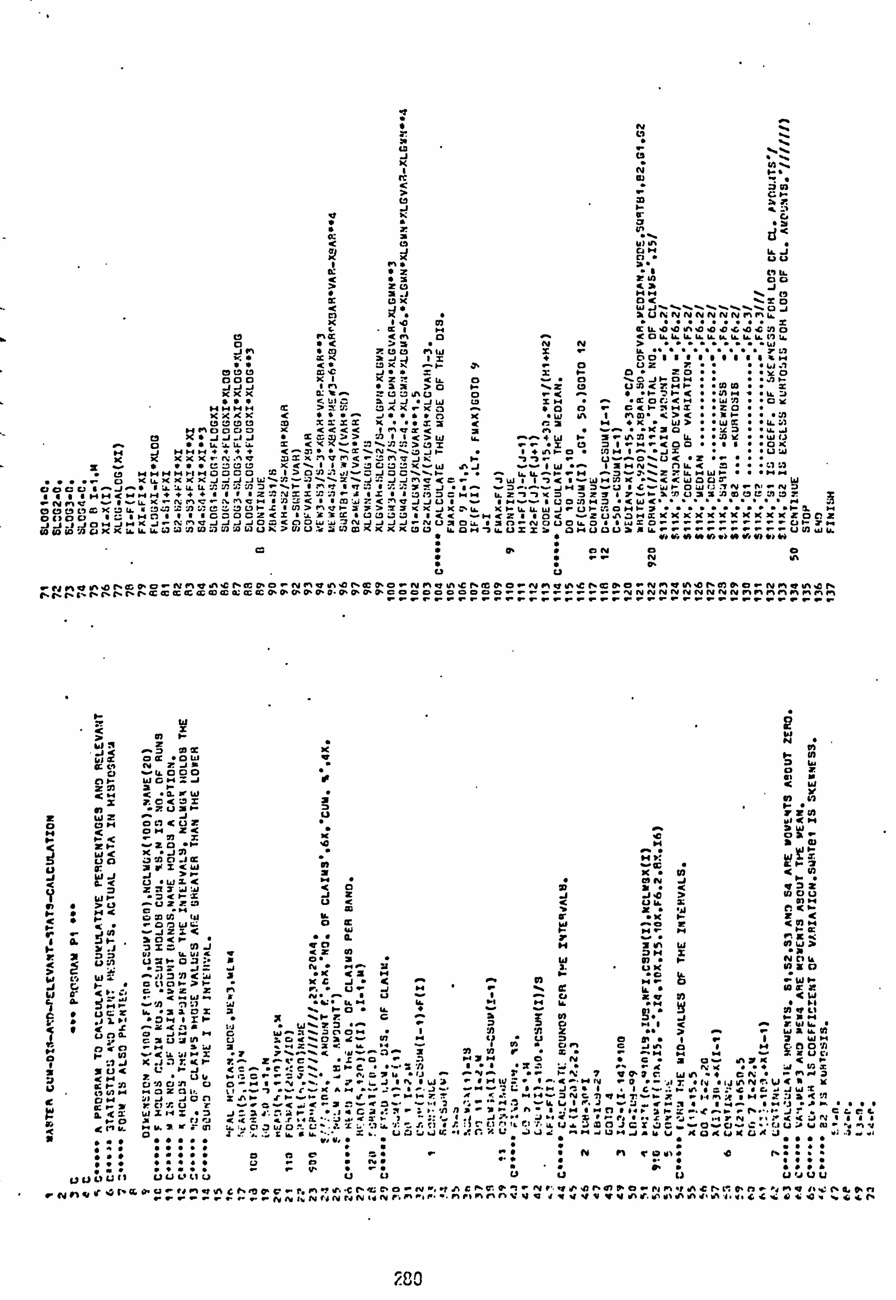
" N

K O y- c " t . w-

m CH

0 T J Fä

VX Q C. "w O " " T. tC i

Nd \

<0 Y) It" il [GH 4. J

cc I C-1 tL <"3 t U) OO

i to

= tJ" WJ\ \\ \\\\ \\ OJ

iU NNNNNNNFrSU. X 1ý S

g ft 1M Q LL'O'C V"ýO ýO ýD ýCi ýO dim O J O V _ OKKY. KKKKKKý lV

< " NN> t p 00 to '. -i 1 " " "

" aL K=J1 S "OO1 1/ 1 1" 1 / 1iM "" <" i. 1' K UXr.

F a ýC J" to

o UZ 27

.W v ý- O"O" I[ O "

000 KIXZ <Y_ 0 "O 10 JF ON " "J7F " S3 >0 1- 2 U' U: A<ZHF " "fA W". Y

xxx fibs """ tUs . ̂, S. _j -j . _j W +A X4"- "Q Of: <º1 " "WZ OY

HHHH tC >rU. :7 "[ X- XO .+ "OO C< FTMS "" Z0 " X KXX $"^ J" "t"OK " "U) "W Ifl 1 MCO" <> <" "*4- t9 t4 tD t9 ID ST S2 K" "" , "f: 3< /: iHfK" W> "W Q" "y, yl

M P'IOOUO X <46< 11a: < 7f " vr. " . K7 O" "Y O "u. J U' X"JJ

_I J"x 'r y> )) I1<>WY.

" YX. Z \J7 "" :AY""W f) ý"ý" 4W 1- 3 1f1 77 H U.

" + :7 : J: >: 7S < " ý. O""4: a. LL: ).

,, l HHHf ff4 <^:! 7"t\S\N\\ýJF " H,

v

"OX r"- "2 O71 -"-COO ""t/ 1f1flF0" 7H1^"J="="r

"""uW \ < K la>Z., 0: 7^. Xr

P. X"""tL.. ^. C7 t7 X 4\ I

77r (ý n0 U

ý1 ý+ CJ00\1F ." t, 9 MHNMHMOOCO '1. ' 1>0ý7- ^ LLLL^F M ^ýýT\ Z V. LL N WF "" "Hº" . lJSe<Or r ` Ä J 7W 1 1</vWH: /1K "\« WOOF W Z: <

/fir /q t \F J"/. + : fl7 :ý ddCU S ". J.. " t:

i : ýLLLL ... ) /, OW 5N'N J)N :7 "' ýi 1S1t ;7 f7 7CHM Nrr r/ 1c/ZJ; NS SC //// HH C N U3S 1J mV L^ :7 y' a KXO72S/7 2 32

I U_ I v/vfy K"'N n, -hmn-/nu< I d7' Z<rrJJU/ v U C. . O: AH7 "<W<"". """1 /" U , L

.. J' c7 F1c W> r Z f> :lSKXJK. Y. O f7 U'UdXf, Y. Y :7 +A +:: 17 L - OFOHF3" """ "FyM XF LL LLW Jý

£ CC " O 1100 /t HC /1//G ^OCZ <S t; t Y3 ft " UC7 :7:. 7 /t« ýH<Z // O< Z UJI .7 MS XX XXXXX KK xw OCI. `ý

ýJ , ). JOH JHK J"' N 1'"V J JJ JOu <00 W : al3N JJ JJ -UU. O: a 13 C] OUOY. O //W= Oý ýý^ýºý OF WU

d co to lJ axXY. K L6 W +7 ;n fA :. 7 OA Y7 UK7 UI U :ý5N (S1 XXXX GO Y. ON7Y. U IT OMUOU AWY.

" * VI

NNN Y) ") N Vi *1 *1 V)

"C" f)` "ONOO " "rN

rNM10M. 5rýcc V O=-M vm-z Cýcr PO cm in V In%01. cc ONO" NM'* kn c N(C O'Orfyr'vV C NCa0 rNmV U%%OPN OKOr Nn1 a v%z N nC, C, 91 n n('{1 r cc CC S, CC Cc m cc 0; ¢ cc PP O% PP O" PP a- a, o0r =0 oOarrr . -. -rrrNNNNNNNNNNnr P1

r1 - rrrrrrrrrrrrrrrrrrrrrrrrrrrrrr rý rrrrrr

...

.

uuüü(I . dnvrvc"aaoý-ýýnav\cf, mo cue. nou+"tna: e+o"rvý. ýr

n nanIr. o"-3 ; NI'VJ""A0%47P"Orin. r. 1%C ^. o- n oma ý.. C' . P. r,

... ."rý ." -- hh 8ý NNNNN 44 N f'. n r. . rr nnnvVaJ +1 VVVOV J1 N V\ 4% \ !. N '1. V. LiWG .Ovr44. C%

~ W Z 7

a 1" ,

-2 to "

Y1 CD (C w ° qr ¢ce JS lz

cl LLooo

w <"dXW

V C7M OH 7 <

1- 10 W<

ZJ71 X

wo M Z<W 0, E jow >r H

ei -w3. < Z z: l7 WW <

Li q- 7<rx J " 7L! -V2T'J' (. %

" N< r

p 37 to

~ tai fi.

" . OOW 0

1N -JZ i< "" p. JI- .

SO_<r " üi 4 a0 jj

un

s )

cýsroý_ v <z " o"

y a^ J i ["i W :: W - 11 ^ 3 K 3

*.. " > cl b C%Oh r 6 X "

r 'fl fl; i- W %,

" M

uG7 k71nx a " J1º1 "C1H 1 2r "R

,_ . +s 4: is id W\7 u Qd tl .JM G W^: 1\

\O ; . 7i U Jtfl U :. O a

: iJ KAZr"cr 7^ z"^c"a

0 1- /I JJ0 31 Srbt1.1- 0

11 <2 W ZI-tZ "2 . 0-0

<31 Y. i rJ rJ HK'" W -Q1

". < .CZaf ."ö. j ; ýcl ?u

fµ.

"w" """""

.ro f L1 tI 91 {. iLi t. 90 U

" 7 fll N

" iº 9W K p Oa

'C N >1 Q1

H A . ..

ý " C F" ?

a x" N < N m ty I.. <ö a i

s v 2z

m ý < f'. fC

tK F " ! <

OQ n0 ! IK W Nr M H fi "" C. 7 . `',

a0 H N 7 w MWi Q<Z ap ? S ?1 i O" 7 " w 1~ p " F N f, 4

_ N 1 NYh i "K <i - "C n

r. U-jv "r ^ " WC 7S

94 6 In .4 - r.. Y. G W^: s\ C. Ow "1 :A "1J Z "" > . ý. WA 1" M U i =ýi i a( It

I Y7 U? C pl " 1 "" 1WH

' . . r I 7 ýn m r"

i O "m

' J In M °' ° i

UU K 7. 7^ z^ 4t- C"jpr7 N7N ON "C

MM -K

CI

" ' - % º".: Gº'r J"n, GTI. "rJ "+ 4 r+ j "ý "- IF ": 7 V P7 C W, f GN "' O""rr " ýY ". "T º" ýJ " ti "Wý º' " NlV

' º "... tº. Nf4 ýp "ß. r "fV " WNNRW <O 1L

Lt . --3 "v rvK nM ." _^ "--, . i. -". - " º""(- J-: "I 1 C^. ".: r. Yl " .. "' i'. /C. .J W'[ S 11b t-. G If ýº"N T. - ="! º. Ný-ýNC'; 1 "lM T. ý"". 7. 1.4 " Nº" .? '! D "C'J) ý

rýCý<..: <"'7 ^. r K'ý. '. 1ý rte' MZ v4 frlr. J -3 a- a"" "y r. "w "f Jn, """" :1 1ý '"/ "" C7": f "" "f7

ö " O 7" ! ." .ý r""N" r+ E7 1Nºyr

r "» j

"r " x """ "f ý"

" rrh. " ". " JTCLCC Jr

. "". J '", ? < "i 'ar '"

qý tt si i ö '

I It r 'I r

Ct hi r, "cr y J " U " I, %`

"J - .q . O

rN.. r<<: 4 .0"/" : ""fJUJ um nv o . = Lz '`uaýI

.JY; ? zIpr 's

4L. "I .: n u

M2 UU .1.:

i , a'

ý " x 23 . (. "

O V3 O"0. " "" "'" "N m {' Y1 " d h" ".

UU U tJ Ij u "J fJ U

280

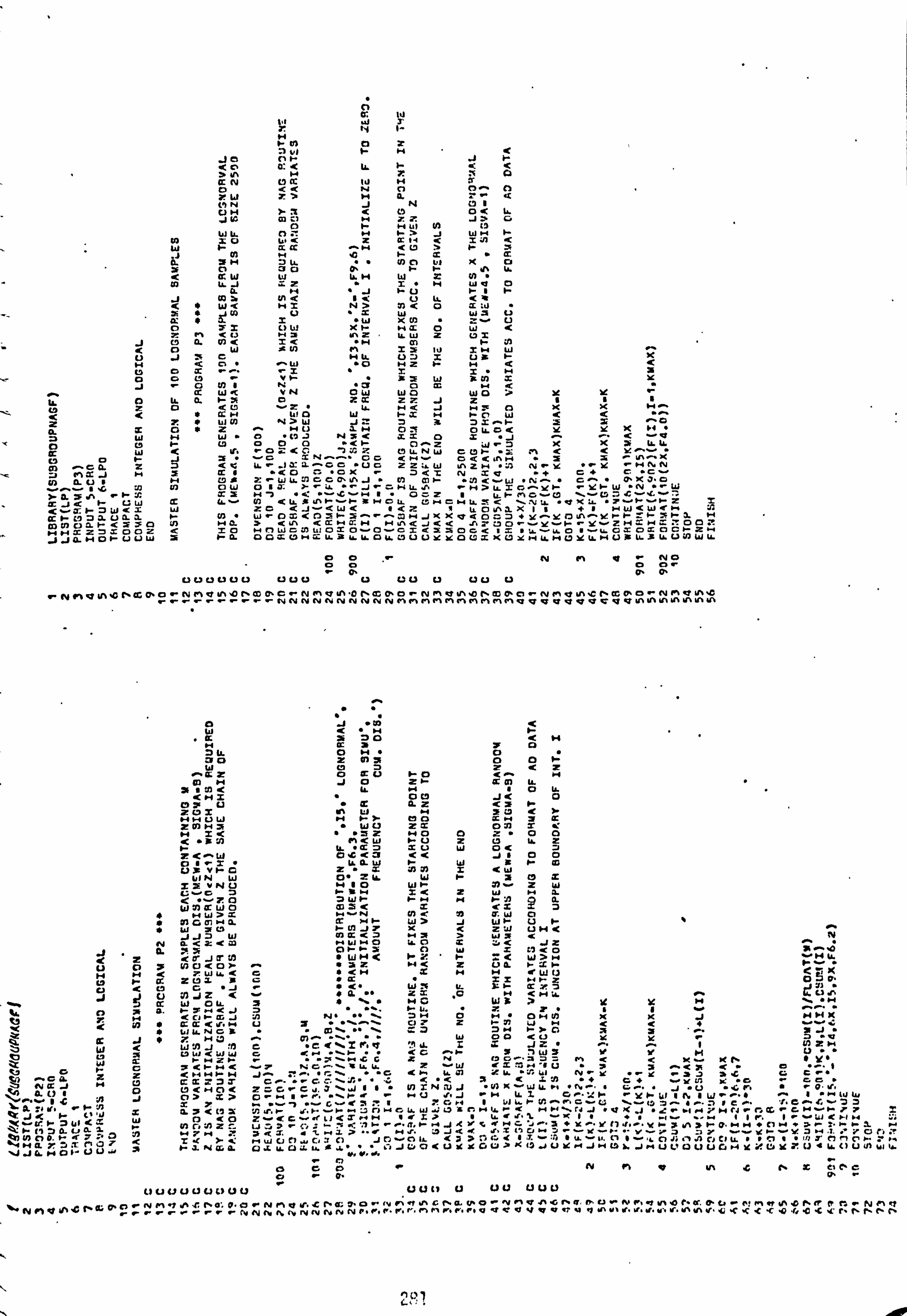
0 it. tu N

H CI O 2

- 4) º- H<

JO 0r J 1- K aH LL 2p

¢N O cc to H '. 1 O <<N C] O^ O

T IN IL < ON J N L9 1 OH -. T < 0 O< 11 -1 Le m H 3 C. Hü J

W LL C) I -

C) :H 1 lN

I- >JWH M" Cl SO 4t <2 ¢ li C5 /1 < Wr ¢¢ ^H < U" >ri J V3 HG I- T. ¢

11, vH " :3 tu H m4 1X iO OO O" 1""" iA N. < ¢W W Ii. H WZN W LLJ X. 2 " i- H WO 0

A H" J rUI. - Ir Jm N< 1C U LL ( C" W< N> HS 77< O TW

_ itW UT " WWVU a; " S"W XmU O 21 L) to Xr HS 0W< ZM CU Hi 1n2 " IL WZ UT

J CJ 0. mC S< "H al r £13 C OW tm M _ S `J IU SH W U Ji Cl H O. 0) Sur IC H <'" ^W O H<< HZ 6- M Cl ¢ S" S X. Hi O '0- Vr " ; 3i W km T IC ,J Om1 NC OmH<

r. ¢ to -C VN OW WO WO >YY 4 p LL 0. S-. 5 O Z¢ Z2Jz III

c 4c cc b-4

Z T. " too N> W J(V OX 7S^1- 2S ^G CL 2 OtZ HO1H Oý 0. O< YYKH

to _ 6-4 W Cl N<H 17 ¢ ZS j O cs e-- ( A 0 a XXi tI6 4 O^ W-

W < 1C. rOZ<C) (V Z . Z- in << 3C ̂ U" LLN WG C7 r N " X J " G "'. ^" O S <HV OC< iý . H^ sn CO QCA Z < <C a. ^ "U LL 1 .Y C 2Z"W in 2 1.4 :AN "' Y "-1 YoHNN ,- 110 H 3 i¢I -OX w<O . x C "C OR NSV "+ Gf

" N a" N 17 t ' ZWl, J% GGQ. 1fß J" - : O" X J" O Cl Qf r ": /1 <v W" N^ " G2 '

>~A SJý r A

r!!. )OW U

TS 0 1,3 }" "_ J "- G

1. H7 "4 "ý'. C HLL. " -N> LL Sa ^Yr "" W "N "" W .

002 1 l'ýGrC9 \vC' ¢""C,

s J< r L: W Q &L 5-5 i1 Nrvr 3s H U) < "S H2 C yr 2S L"HCHLL < \11LL "QX U. "

<""""T. r OW <I W < ZC < A-R W<1I HWC < <Z I O C) x11W <H +I HW< CC rU' 70. Ud1 r III " W- OS < Oir (^- """ U1^)Grr /- 4 -S H CA HJX XpG 7+ Y^YO -

40 M V)OZr < 230 m HQ c UN <¢Ho: H H 3 S ýn4 YU+ZHSHS 0 < n: r HH¢ZOS 00L < SO W 0 Otal02 O. O Z CS 52 I0. LI. O Iý40S OS OCr ZH <SOG< 1S s

JJa"HOr UU W 5 rd OO U. OOTCýHT LL3 LL1ý OIý OU i 0. CJU UY YOU T Xc N Hy, NOYLL HU 3t LL 3 LLUN W 1.

OO N Pl ONO o c3 Oo ""

O" P Cl C3 L) CI C]UU UUO U UO U L) L) 0

Nr1V If%, ndý rr rr rr 0 ýr r NN NNNNNNNN MI1 in C'%M 4141'lIn (4Q VVVVVCV Q1ý1lINU)hNN

O J "m < to 4c

.¢ 7O S <H a 0 0O

W l"+ " 00 Z Qf s OOH

C 14 m+0. Z

0WU rO

<^

Cl H J0 Zr¢ a) U. i LL O

<HS " OC) J< 0 i U "a AZ <i r

' U' x m If\ W H 30 <Y HHUW 14 r} Cl0 TH 2¢ =7)H 7F WO 2T 077 SC H S< ""iZ HOO Z" OO < "; ý ^Q LL 1 "" U.

7 TUW O<

2<^W 0003 CC J1OO O1x 4AW P- Wsr Cl U5 VI. - O ZT Jl 7) x <W

41N W O" 21 61 Wr3 tl S x 2i VNU H1O Wr 7).. 2W (, vv 7 rSH X< 2WHa. < T. O 7Wr rH HH I3 p? Wm¢WO mSC S <S S

f HW>T H.. N m<7! W. WO " 71031º+CL S NF' W> J WI- Ur "W 7t Cý I. - r -i %< ZW OH( ^

JJOW m¢< o N3>ýi< N N 0. < Y< Q3 HWHO ia" OS '" <J2 ^ 6 5, i Os-Ha OWi 0<0

I 2 <0-J¢i17 " WH< P. Zr < W>H U C) m0<Ot 2; " Z H< 2U IL F" :Lr ýýX H

H <? W Ir < C G" <H .2HH <W U 9 S

I- cc 20 . J G"¢ SS Hr Z 1

O" O " 13 a"

to .

% &L Jr. ^ HL O U Y J < CWJO

. 3S "

$4 G' W IL

> I

. H

0

,

m 4.

a. C W. N< J 3. "" " le x

r U. T. 11 Z ^

" H C1r a: J < U N""\^ý

" O7 2 5-33 OHM X Hýý

r `

iq " ¢il. H ¢ < Ui C4 << ry 0. - cl

d¢ " cil .4 D '! V L W7f

J ""A CC l\21'tQ 'LIN. ZS JZ "1 N 2H

N "C"3= " " W S

H R "", \MyG Z,

NG ý"\i 41, G Z m<< X5

C 2 UW C (V T: 3N /U " ^< C Y

O-1 Gr O

Z P4 C

<H5 H

<HHrH . "G J^ . ý' ", \ " "i "f

Q7 W14 'l. W N"' C )[ 1( ri) iy < Cl C" N Oa

H J U" CLQ Z3S " Gr. ýG ^. \l. " << S "< 3<S: A "f Cf J. V: "' N¢J Z/1 AU1 O U" <H Cl < " 2GG "' G v. J\ ,J11 "h ý" "G . ". " Vl 2NUJ"mXYW LL ºt yF

" ' " Q. v

1 J S> O> H1 r" .\r .r O G i H LL .-2 1"" " HV�. J" Y F- ýI 1h1W ý" 1 r Vi ^ "n G W

^I t""t to tu ! ý+ 7 'f

A "I Yr'. 17 " Z ZY d 3< C7 1

" ýr ^) "+. G .ý<11 'J7 . I'" r Y" 1"" ý+r «+ :Jr! º+

".. GHI U. vV\ t7 7^" ý" ý) IG ý" H LL I<H M\ CJ J" V<

.1"L "` º1 NYHN f7 G. G 4. W .w U'Zr .C^ .

GHr77S Jr C" a

4 W O (O Z-<C"+"CU<2HH "C i> 1 4<. r"1 """"<1 "f"a.. . -. r 1 1r. ' '

W (ýIH K tLr OW C ": r m C. J7 Z ", Z. J -- 3fY ý" V Cý J"-" Kr3 Y'1 3r O" H º1 + C1 O3 Ci - '- S .CA º" - ý. if, r ". j C Y% w i Hf} r ". rrS, y 1 I. 1 p A. U 0. y

"r "A O n H7H .. }RS "t7 ""4 x lýGº. r ý"[ r- -YýI7 7Y- CCS- H ý. UJ« r )" L t" J l . "- .. U' 0C. Y. 7H.

)ycio. r CO7 ti < Z< >i . . < u. . u. t ,r"O Ji , J1 UU LL "r !1 NW CO Ct wGYOJGv Cl IL < 7>

K "" wsnnnr. e, Hd7. >S

VJU. MONUU .r 7/ r "L N Cl U. O .L LL O "L Wt y" "lt w, r.. ".

JU 0< U 11 XGU? 49 JUY rfJ H0º, J rf U VV UUG .4YZU Y T. U4U. OU in ul k..

n r N *3 d vt t 1. S Cl C. G C

C. a. r

U UUUUUUC)U UC19) a aU UUV

, -N 7" d in "1 J) + ('0 "' N f"1 V If. "[; (�Cl 7. O "" N 4ýh J% G f% a. U. O "' N I1 V d" "0 IN Q. N+ CU .N *3 ") 1/1 "O 1- C. O. 4-P! In p V SC Ni? Rr "" NA "} %" NNV^, 4 P 6: P G rir

, . .-rrr ýº itr. .NNNHNNNNN P-1-r- V-1,11 11 I'll- O .ºV0VV tl r" qq to 41 �. Sr. V. "'" C. h Sri V" 4 "C "C < "C "O "I .0 "C 'c h f. (M1 Ph

GP .

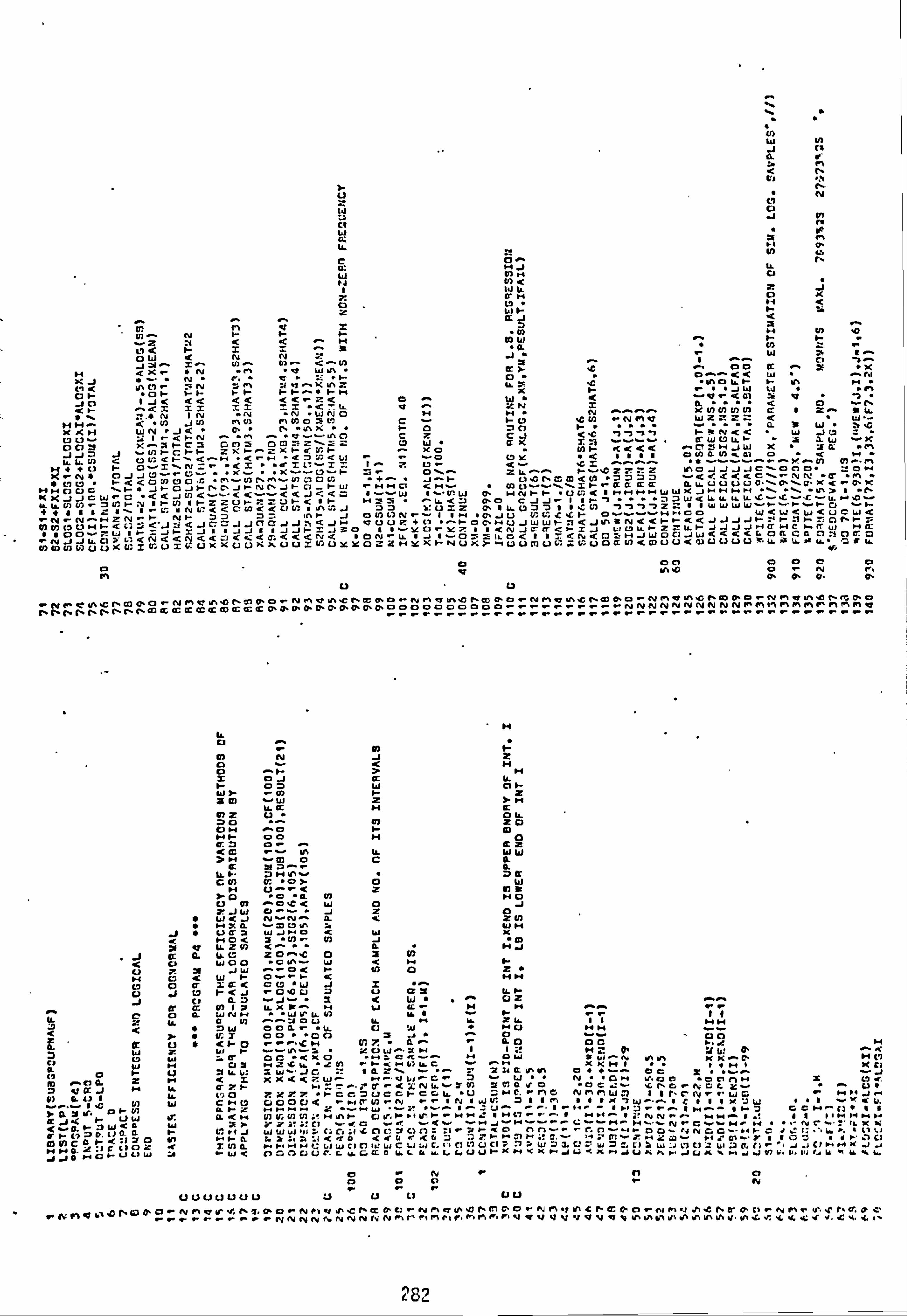
z

U) wN Jn a v' Z» rN tP

"N

V) L C 0- fN

U W O7 H G

'1 0) < 9-1 W J RN N

O ..

.O I-- 6- 1-

cc J N NN

.O

co z l1 4HSS^3 rw / ^ ---O0

C ME "X

N dx ."1. .

"O W

x -i ý.

t^1C N2 5N Y" 0 -C f LL Y IL I. - " JWWN -

NPl I- I- 01- r <-C.

- rN l Or al- ,j

- O KOm w

v" " < C

^4Y S22Z 22 .6 1i R^ ZN S K "N "N "W NO N 1N "ý "!. "

P' w MCI) -

C H"N ^^^

C7 IC N %NMO I)OINN atZ.

W .2: Z "'- L " 4

. 1 0 O

N J' N fý "N X. " r 70 !W " Y. 0

OUH WN'drN

""' ^

al ^ a. -"ýdn0 CZ z C,, 1 6C ')"')ýý I. - IN NK K "" W J19 O'w U' U 1- aw x

7C^Z rc3 Q) o©-"IZ\ý< 00= v07rCý'r z7Cr^z x rK 4)1-

C7 w" xo

aK NF- 4446 . 3

^C'T "'MJW X1f. ' . "Pl JJN

U.. WW Oi 6r 4^ "< W 2 ) º<f1lf .... i...

4Y ONQ 1A aGl^O .( .. -- r

N

C: `ý2 Q Nf FU F- OvS\N2ý .

K. =.. . . XvýC1ýý

1. + (C O\^ .. .OS

24^^ rvýpZTZ2 1f'OJJ JJC\On0y .Q C\. -N

yCH "1'1

1 ýd < ONC)Of. . 1'l " C1 C rW r l "f^ " J^1-

ýNý""I Cl <M. .6 f1 C; M< Of "O

as lvv\\Sr"'6Q ¢O: "N ' N "6<4K4

RLLUU UUO"\O. \O"X < ýOýK (C )\ J q NN(7UC 1-"f Jr OJ>-nC`Jr Nf

^. <4JN <v". ""<4ý`-'«Jd<ü C W( K - ) fývW I

C t 3V, a tMMNN TN Nrr W Wx JH N NN "\"\. Yl>

.G U 4 f "/ý

ý' _ KJJ Z'CU0K fr Otßr Yfr1rZ N U 'C Ný S"

. OHO C JJ- If rý """"

-7ý e -'1-f . u. W IC - =1I W4

yr U Zý ffwWW W"r ý-

N <C 4+*4i NO: «11: <4C/L7 f il1NJ iff f\ t "^L: f 7 OU "r J

IZ )IU 77 1 OOfON-z fº,

O' fw f "O. JU U: L:. C Oývvý. o< 1r oo W4w4W<U CW6

"'N N^NZN"'ý' Nr 7 <'J" 4 JC=: JJOCJJý <J CU U7 fU "^º o C" Jwwr :1 <JIn; « U M. q rº-«JJ JJr f, r [ (007 UUNr

Wi 14 ff OOv=  H Jr SJffJJttJ JI- J+O <1

1f -vo-V2.. O N- 4fJf-O

'N I tE Q Gr SJ SC]LL J .I G4 l1SK N< OHJW

R HC 0W

c Z' U. HJJJJ "ý O Cl JWa6 K< 4gQC6O .y

L H OQO

JJ LL OVL: << N< 4O6.: 403 6dK NUYY V- UXXUUXXUUZN O zL HYX º- NU

L C > La u7U L% O% UOaNm U U< WUUU U= 4 +Z U. I ýº 7dW

N O) N 4J UUX O% S O% L. l S

O 0ON 'C 0 O O Ol

0 l1 l P O" O" P

N1n r IA'C N 3PO ý-N P1Q Ný6 N Uf 0s 0; Ný, f W CN O'b N eý1 V u%'C NO

n

OHO rN1nQ1ný NO AO ýNMdýn ý. NOOrb rN I ýO N "C C. 0

-22r rrr rr r rr rrr rrr rr NN N f^1'11ý1ý P1 P1 ý^ r ýr r

rý P rýl1 n cl Co ¢¢¢¢Q Co ¢¢¢ 0' PeeP O' P TPOOO r xO2O2OO2. -

a aF Of NJ2 O KN O """ 1- >H

I- OW O1- w 21- a) 0- x 2m WZ >N

Y. QM IC 0)2 " OY. U 70 _ Q) 20 OM 'O Hm HH 00 MO ¢O a-.. C2

In WW U. H > >M rmOCU. C pt 7d

U. I. - MNr 7S CN CC "OT OW

M 1. 'C 2 fill, YO O "¢ O7 MO : U 41 " O .C<WOJ

" W<J NrN^ O. l' ZU) " MS U. ra CmU AWH

J * u 4r S W=HO<W L MOL SN- U) J0 21 LL Z N IL ~J

"J a O" Y. C 20O 2N < O WOO "C 1ý `-" W<MF U 7. 2 JW ý+ O< H 7) O z"

M 0 c WM C 1- KHM

J c) r<-0 a oa -) u as LL 0- O V 0.. ".! _ "1cW"^ OZ ....

Q' C N 11 I. IC R^+ HWCHM ý^ "'r O O. WNH "W IP U. N IL 1FrI1

2 U. Q U) ^^ JOUU. M Y. 2 4, 11 ~v < < " 7W COIL- 1L Ci w^ MO "M

2 } U

" "

Y: S <1-O

00"003 "ý "O .-' . CH N7 Qmm' v0 00

º-< ý

p , w z w r ý-" It ý"" M" i: Uw _" xH11;! NZ 0" 1WP HO W H co CW w

M C O3

OC "K ICO Hy C"Crte. W7 C7 N Y11f% X K-. C. HZ 'CW 1Nr I-t M6)1ýC r "^M XKM1 /f M1 IC CI

p º. U 7 U: Y. _ r"2 CL It. W, Offr.. OC. "r "+ W ý' JG.. t 0. i"\ J jp

I+O [L Z P'1 < i xX K< W^ H "". V 1.! ý' Gv '. U.. a öO CI f1 HS Cy f NQ

N H '

O VCC J 1"1 Y. 0.7.1- 72 ^ I[ O bC .4 -+ O" LN4 v rNC1 Yv H ^.. ^<

14 11O ^ 7a7.7"fCcVCc I- GG Y" "u=MC. IICNn r1 WO8 1 ('" C^ Nrr YI O h+ 1" J . "1 4) 41, N W c "o . 0000-c .M 0" N .-NrrtN IIJ V: 711 tr. 1tIx7W ^^ ICI11 Xý W"11r x< Y. r" p .

fLFZ HMHH 2 "vMW "r! "vr. InýUý. rý. IrHý" IflJrrn I5.4 1M7 GCMý[11 1I ýý

ý üW 3

If 4L<" O7 vNN:: HNI- 01f"I- "I U'"1' r MME t M67 rrý. I MH^ INN "'^ MM^ 1"I1 /IH HH11 vHrrrr LrrMr "

rQH>WKO W 3> M.. "v NrCvv MAN"". "Ntr.. ILKK %%i' Cl ý"O, O < r<r r NJ

' X

' ' < sº [ý o. uaa I- V. MJ M1 r7htO f1 t) w v" GOr .1 "- OO ý" NNGC a" HHCJ f.. . 1r +. I Cl WW Vl 1ý1 rüf. CI LOOJU [l

v º' M 11 M T f^ T H Ut G T tc7II º" 7 Cl " "' hO H< 17O C m 4 15 ' Y1 C

H 1- O. SNO

4" O4t .. 4 . :[ ý7 . MC. YI .. S .1 .+

.3 Z' D N U W7C GiLa Cl Cl 1I: WCWW C"t'1(jU CI C Ii WJ C12 W: 7 C J M ºU ir J cl ' w y C

. MO MO º' U t/ W :w . "-" W < r XMK a CM J KK V J U [7 UVCCOY. L4u. LLNUh.. ti r, h' J l'J Xa rl J tl1 u" 4.41 fr Y '" Y J 4 V C! C "L G '. ý

JJO

O-N f1 O OO C) N

ODUUUUU UU 'C1 VU

Dto 0% O'' O "" N Molf""I h? " OrN r%y VlC M1C 0. O "'NPI"1 dl"C h0' p. C) "" N I')r Y'.. C f" O: P. ' A Ic r, cc a, ift 01 P N el C C .0 IS C

hnQu ý ". r rr . "r.. º I A '. Ml el n VVV VVg0V V VNITYI VI NI[1 N 6/If. Nd".! '4. K 4: "[%0. 'c d. lý l +. N NN N r 44 N NN vN

282

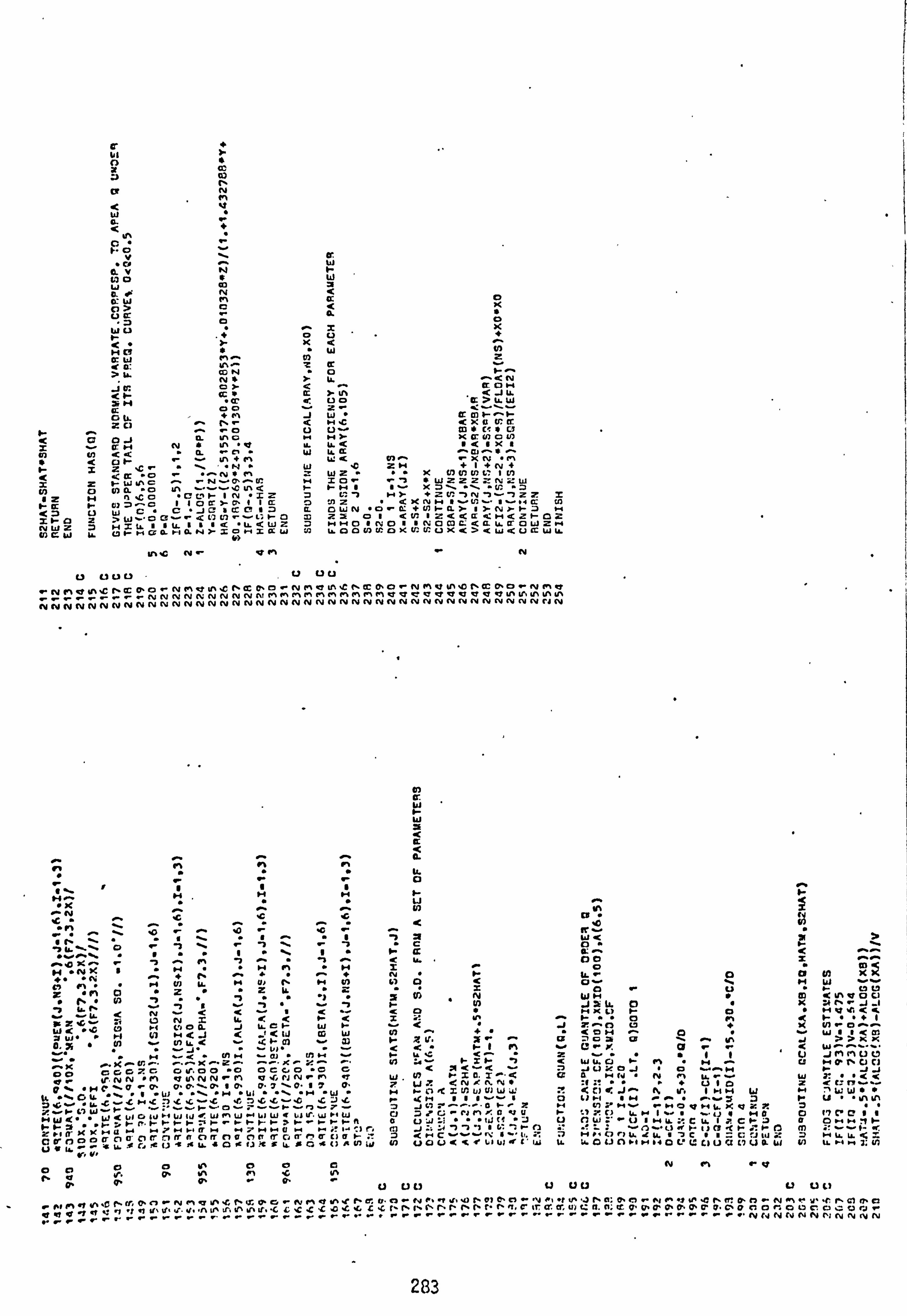
C + Y1 } n S

Z) to

R N

w

G

ný v P

to o m

aw C> Vj O W L)

MC! aw ý'+ ̂ ýa v+^ >In mN

N J W. O}

<r aM Q o0 Ö(1. M 20 1% :

I.. - -0 C j U. US O

= a "'O N o 113 44 n i 4 Or +

r Z z .c am -N cQo N in ^"

2 Z C rW "I ^rN N

N O & N ,cU u:

1 Z N ;CC C CI- 1N -7Z r ¢ I- W=)Ca 1 IOC >T11

S C JC 1 CC. t 'v t: =10 2 ?W OC r t] ýýQUJ N" - NWZ H2tn 11 jL 1116 t_<

GL NC W U. f. 7r H64 W H6NY Sý)HS

Y1 "(. N ý' O P1

a W

t- W ä 'C d "

0 ,. x x o U + X < N

" W M Z

Q 0 /' ^

Y U. ^<N < OH m >. Lr% -i LL

Uo ¢7 LL

J W" Q In I- < H. C LXu Q: 2 U Uw m" C, " U M HY X QN OU7

W 4¢ -a, -* ß. t4< N^ - XN "1ý

W "f) 2H +I +N 4 wz" X Ct, 0Nt: IN IO"' "' 7"W 2222N 2W

7 (J ') HY+Zm IV ý- "Izzx O :AZ

OWN .0 6 /C NH/- V7 -/- s4 6N

-a: +N7 - aY 1YN -P- H T. 230/ C U7 1 2<C ¢ 4H<2F- 02

MHO @N OI/ NOc: 3. <C U. SOW 2. "1 U2 In 0a N U: OK tr 7: UX<> <W <UCC W U.

N

U UUU -U UU

ý'_NMVeýC fý TONNMNN NC N t% cc

N0>o NIn Q LA %t lý cc ON O" NMQ Uß%0 t4 cr O> OrN1nO

NN NN NN NN �'NN Al NN Nn m Al MQ C' Q QQQ QQ QAl A' Al riAl

NNNNNNNNNN NNN NNNNNNNNNNNNNNNNNNNN Al N Al Al Al N Al N Al Al Al CJ Al

a. N

/f NN ^""

'C t

º"1 NK/NN 11 ^N 14 1:

r Fl" N Ol LL

" 2ý Lt (.

"N _^"Nv

-t

i

N<K

w a: "C º3

CNO CL J U. C I{- W 1<

ýW" "Hv º16J v t{tJ vw

"y wý"" f/1N ýC1"" NN v

OOOGG7. C Cl 1f. 0 OOOC0OCC

pr jr, NN" (n V 11\ NN M1 O W, NNNI Pt R

"04C ýO O" O. O"". O. 10" O"O"

*1 G4 "1 "t +W "" "N "W "\ .N .W 7ý.. ý 1`. C ... t C f. 7ýG ýG ý. 6 L 5. L

o U'" w ºý W 13

HW d" yl <WOWHW IJ eWWHWWw

', r .º yrmrrrr lr. rrrrýr. rrrn

º{ a- CXNUHNYHVITNH7NHUN M" 1- I C.

ca' o0 T0 IT CiT CI If if Cl ff C)O in C, sr OT nQ C7a P.

VW rr Yý

0O C) 0 in 0o 15

to cr. w W 3 <

91 t d

IA. O

H W N

') a " C

! U.

N L) G

N "N N O " <

- z Ir. ,, ^ < <" In I F" {" 'C <^

< 71<ý4 W N rSn. t ß'" 4 7 WZ NXNN H r-0 ZN U) to WW r . (M 11/"1 0 JL: +OF7 fJ . o ""/. 0"u O -a ) li U " "W C4 ;.

J .:: ß '7 'ý ") 1 L: ^. ºA 3 1! ) UOU ltl UIW lt' W

h a. .o

W O O: ^ 00

0 LLr O o ý" o. c) WH " J 11.0 " H L) h O

_ HO M tOM^Q

a ýf o3e t/1

z ra - w c " W I,. öº

w. J UXoJ O wem. H 6 QN fJ N 1'1

It .""f LL. - r' t. ) 1

4 ci s, ,J^ 1% tr" 1HHW O I. 1 º1 "H--" ^ý. 35 H NTHvH rJ tl = 1ý, N07.

")at) tLH 1ý ) 4 V0 2 CO - .7 H1, O ry4 6 U. "7C "" CCJW

4. U. 04.1171º"M640Vt; UUa C7 UaJ

N ""w "' V

r I-

0 M

m X

U CD

W 2 M I

b O

m

:p

N XX

WV I- O tC, V% v0 ci U :4 t`. ' J. 1

U, ""f1

Wi7KK

W^ JIINIUC7 "+ anuci FJJ r.. t<

yW"" u"" ýn In Ivc"a II

i-i4IL6S

0% U UU U 0U U L) cl

r Mýn"t r"O h fl. O. a' rN rt 4 f. 4 f""T. PG NM OI .f PC b, or NPI -t fl -4) C's P, v% '. 3 Pa; 0.4. - Ný tl. n RCPT. 0"! 7 -N %"ýL`"rt nc)Pa ý tin .. ýý ýýPPPP O" SON

(4 NNNN tY NNNN rrr rr r . -. rr..

283

NMv in .phUa VV

H 1fß ^hM1! ý 1f ßM U\ "i Y1 M r'1 M J\ 1'\ .

" l v v . v ý v v X Y r

i Kv ý! \ l+ K X \ Xß x ^ OKQMQvQMV"dMQM1 I" t

x^N F" 1- C v" Ifs ". w ý\ .. " .n" ýn . vý N 1

.1- O< º: SW vM r\ "CMu4OMhM CC OD OL

ry r4 nrM

in JiZN0M CO CO Y\ .G M" Mhm {L MhMXMh 01 hMn rr

' " ' O 1- rC 1"" F- M º" H 1- HC 'C 1- .

Y\ X V 7C <. " `F XC h ;

< `,

S S <

7 r. l "C N SN N<NW NON7 N ZN M SW .a <h <S ZS ST "\+ Z" N1NN "N "\N HN (H <S l3K "< «W <W "S

' r\tl; CC U\J1 H H- ! "N J'A r% 0 "ti "M "O I. r O """ t0 "0 J7 "< N"/% ^ - " "Ph" LA J1 1- " .X 1C HWNwJ-

O2f wý / ý" O ý" O HOO F" ". º 1 1,2

i". !< C

Z2 l

- H 0313 1- 31 -< 'N^ "M ^ "O WW <v'" (1ß f XCCU . c, - OZJ <"G-X 3 .. ý. . . v " "5 ý+ - - '

... COX 7: X^3 1- O Jai OSS" "" """" S3 y_ .. ý "ý v .J " :7W"xS W -C) - 1-ý ""/rý J"" r +; "- ºa CJ JJOr"lo J ý"OH Orr 7. Xý.. a KI-'C c" . 7F -H" -^ 1f t \ ^ 1"

7ý .. xc\ " Y"CC <ý <6 <N CU<": ! ý" e" < U1 Y < J: <H < < º XO : LLL O 1. U<:. 9

"f\S "' "< S" "<S: JC ý , G

1. + 2 U' +" `4 2^ """ -S. ý" " W N2 ý'J M+ +U "< 1- Oýx Xr"N1 H/ 0JJCgvý"J"ý" " "X"+ . "'C ... "..... º. . -.

wJl "O "1f\ "O r "G "IA Sý C\^ L^^ I- 1! \" O COC 01 fJ'U" "X^ 1- <<O : 70:: "M.. +. hm-; t7 C7 '2! 4 . t^ " U"Cih CC CCCOQ X "" XXNX n\X "\x CK ar

CPMJ"7 PMT TQPQ ý H JHºCH OOC / ýF" " Jº OJr hPJH Nh JI- cWOC SF-

^M % " 4 PXP "" HH3 a ri "+ " Uý"ý\ýS

O. NF"1- "Ký< C "ý "\ w\ "\ \\ "\ !" / " " << JJ1 4 X<4xX 1JCý++WýO "C<J: f: < <<ý`- . 3j rM2 00i-N U H J) "H Z2Uh 2ZC. H "ýCC /1- ""1 fý1

v tJ W /"" ý HS S" . -. y<7 TOO JJý 1/ ý"C `""'. C `ý`C `mot ý'G ý"`Cý`C `r `C "ýC

vH ýl+ý. "F""r b- ý r. F"+.. I+ l-". . :: . º/FIH +f/t/ vv2 t\/ "- J7 /N "1' < <J X< <U U LH //N: 1: º" NF" Z7 v<U, J'. H

. . "C ZYU22P/ U" // C'L"J]N- -1/H "PJ 05- 4 I- U<W <W <W 4W <W l' W<W Clý. i

ILx Xý"N"" n: ^º"F' ý"'12N / 0CD fA to '" c mz: º" <O 3 <JZ 6 J- ýJJ 3 JJ03 3º" <J 7H3 b"

..: LU2 +;, "J ". "". r-O PNJ W WH <JF' 24- 7H F" º" 31- '/- N '

HOO // 55O -ao2: J /2 Jr- J// JJ // JJ<-F- !S1 .. H J MS MS M1. C; ý_ /` iem Y2 // 4J"== CS JH1. ºýS n"ý. 0 N {m it y 3L K y SN N fL <tn xu2 4

I fAUY {ý<4N Co u3 U) U«UX W Z. o Ux i. IX x UUX XUUS LL S . , , . . . b4 UCo OL ZMYXº'N Ki

O 0 u% OO IA C\ 1R Cl M r 43 NNMM?

0' Ö"

O" P O. PP C'

N P1 {t Nlp Cýcc Pm M-0 N. O nmPOýN MIV NNo Pw PORN r1V N%o NCC 13N fkj P%af N4 PfO PO ýNNd Nýcrf I; PO rN V%at Nbn Qi 0%a

-::: -:: ; -ý"ýýNNNNNNNN NN tM1 nC, nn r%g, C (, f, ccQ IC Q4QQ cc CCc PPPTPPPPPwOC c ooc coo-

ý C7 1L O Cý J

4O

cs dW

0 R CL O In H

r&

3, - x im 0- lil Ns 41.7L1<2 y cg pace -a

ý jILMOý UU W CC 7 Z) C) ti x

N. %

º- o w - 0) o 0 ý a

0 ö

.Cü 2 I.. w W NN.. j = v"w<

-I- le U) oJl OZ \t-.

r Z O: w JW \M W wwWrO G U+WO "z W U. J7w ' Y, "W "7 Om U y M N H O ^O ^^ SO O OoOTUxw

w" 04 N Vrp 'O co :C WO ý

Z ý" Qf : 7[ 2

M m : )H ;7 H d23 w 7 3p O) U^wv X< y U W -. 0 ºi

0 < º- " r r \G

0 " W N" Ný "^CL \O

W d^ CPI c""oO \J N < < a W"

J 6 ý C Q "2W \ C 3

-C W _ -C 31 CL <

U W i. -vPOJ L z 0 cý X cýWýc<o

J a. w .JUIO.. O.

Q S W º"

K+,.... "" oa -" 7t r%

W i 79 CU SS \

21 1" \ cri W aa2. PEn 1-4w C<º-

W- ä w ä r us7 i u

o ac<c\., " 09 2272 YZF' OCO \1-

r C au OOUºa "' h "'ýº' z MP4 -1 2 "v L- Pl

ww om w 7Mi! 1 F. r. w {ý )2zzzo j<" H

U) I. WW 1W X17 ar. 7. ul mm=U= -C4-cr ! 2 N4NHNOWWC70CUC a º OOOOOUG x &. 0 u. -

0p ". n T

U0 00u U

" " cri "W

U) 1-4 U F" M 1"I Z º-P< "2 Nt1m ""O N4' 7"M

º- < "J) " t] º- W""2 W3 J. 7

M" IL O/H YZ"" << " 77

' =tau ""0 cc 11 . Wo ro 3

. WC Y2X "" t)

Q3J"W <r"W" x "3. *Y""p

HX O=J<"a !". \"Z

<XN2" Irr ^ýº 1C2U " .-H ýºý. "r Hr3H" O/ rr11 1- "C fl " '2 Iý LL 11 MH

<" w HH _ al W cc

Ax": - F Z -Z n r, i ý 0" r T

OIW": 7<"+ H 3WN A0 11 rf^01 _ 1"UrU.

WÖ "H ^^ S ZWin KxHI. ": V^

C" $. CC7. C "r' W^Cº 7"" _ N" "0 WCC! "OC QM

yý K "n Z" "vgy SMIC "COY- . CNO "'NCC ý. "ý ^

-C ~r 0 ý ~ 1 I ý U r 1 '1 A/ /r i 1 - u. N W

Sº 1

A3W^^ t. C

t1 1x La " "f 1

""_"< 'L "^1r. t1 ^+ .r / M^ ý". / HI 7ri. tM ^ý+ tH7OC 7t M^G CL "4. M IA P. HH . ". / "' ^/ 0.4 / 7. NN. ' NH^ 1 i. /" ti MI IN

i 77 Vý 7 º- <: f r1 ý""- �. "f" K"O " ý ºO OvMh" t1 O"-'N N ^. O vºi F. "` O tl l7 'll rýLL

wc ta7 Qº- X 1f-. "" \ "(o " . M1 m`ý ". T, r .. Z Q1`-"T i"7^C"a

W " r" o OD U KW O:. WW1 0. U "' NJ JU V) U "" U 11 W N CO. "" QC U. U a"t1 6- KA "c HJ U _ .j U >, R "+J CI XK J"ý OAý . 4f º+ J UNNN17 K ii Y. >:

Y/ W YI VI rl M,

O w

U C. ý Nr1VN. 01ýý7f 0. o rNAO M. U P67 0ý0 rNlýýf ýn . Onýbýn r Nýýý/NO Pa: Oný W f1 VYýO t`. M Oýn NMt} Y1. C h0: TO Nnvonen¢Pr"rý

r--- NNNNNf\: IVNýýNf1F. MMMP. P§P, r1MVOVgVýJdVYýTYJ1inin*IYýAV%w. bnc; c GC v. &&ý

284

0

1\

ö \

"" ° " I"+H i w

"p " ýn n[ a^ ca " "

^M " U S ý J " ^+ IX ýý0 º

"" fN "'< N LAý 7 2ý 1" W " . 7 N H

p "O " -. 1^ O" K 1- W

e 14 C, m IA. " LL . x

^ýX . "J. bU ýC I 0

"v L. U "" N^ " S N _

Z" X C "'C J < Q .rI KN ! Q " WN" rN ý O

ý I. - N. r1-w U. N w :b S "O r\ "" O 5 7

< "

W W W O " "" f X

M 4 ¢

^ r

r S

.' OU "LL ý..;

n. .. -. M<

<I- 10 CA . ....

_ O V O'HLL XX p, l X "! X f "X +J \S

:A+2 5 O NF- W ;Aý.

N y/ . O "+ \ :FO

r S"" N X . N5"\2 1- " orU U3 [7 :3 Wý

jN "ý " "O O ýd "^ý ` 51- < N WH a HI W WU1 atO0

' ry . J '7 2X. " ý" "" /- 2= ^W JS C) CJ NN " J -i aý (3 " "N W U: WIý1-N\O T< N 1- " ^FXLL O <JH

46

"OC\" "O O ". W º x UN JZ^U Uf KHZr O. -. r. X

J G J6 UJ\ NJ M" Nr " .f 0"O ý+H <1t Cm

d Y" J"" ""M

° N cJ WF-" W\X HW " ý1 f ^ . ýOCa '-' \ M dc LJ }

AM OlI <[, 1"

W `ý " ""W ýOý ".. \M <S^ f1 ^ 1ýºN r OrH . -. --- O MML S C'

y. ^w ^^ "" ^"- LL h-^\\ t- v 3. ý 33 "W A 11 f" MºN

Z, +1 "-

ýJ U U3 W hOO

ýi "CK. ` ^^ V1" UO\\ : ^

FI- I . WU. X U GJ O ^H :) J JJº

" MH N a. :: N.

Mr ct "X ä. n\^ ++ cxln O\G

A< < WW "'SZ^M

4<+ S ZN. L

J Sd ON NM LLr WWCL "« ý

" rC " X0 rK

O" "'X - 1i. " 3S "'N "J"'\ " NNv vý. W 32 "w+U[O .. < zs<n.. ä

NrM "13W "v: ". -ý .. W "\"<. \O H<OF-1Z: A W< S[L-f z<OH J-. N^it. IHH W ^" ^""S U

ºI <WW""2 'n " ".. ýry ý'n

ý; ý' , Cv "X '7 7 7.1; "ýý F-. O .. r F" JH 4N Xýýt J1 l M m

XXi" "

O: t: N"H J7 ? I-* 1H0 V HLL XCZZ """_ NLC% --Z-F-"

"I - ` U 1Z I Wd -WWWWWI m

"S DUZ "Y  X4 ""r[ H I- (A 70 LLH I -" .O[a. a )I- QN03OF I

<MK3W BHW `"C -

HW 6 - W< n J7(3P-Y'SN" F-5'Xd

" (L JW^^^W: f^^^^^^O O UaW U"H1t70LL IZbl- F- SOUHHS

yp. -1- º- Ha 7 a

º. :% -= 702": C " . HS \i00 m<s. NM " :n 010%Ic[x¢ p. 1-0 T_ ZZ

Si . +O. U<h UO<1- Zra IGz Z-vl- K II- O

" 13 ONOa ZO "X O O B JJOý: ONXýOvF"+ W UHvvvN "v... r. vvvWZ

J1 < OHHCI O U. 1. Y. "UO " [7UOWZ

OUGHMMGJU OU0 [3UI W 7NW J)16. H", %U) C1)Z W

[. <LL" MO W 4 OID W wUS lL U. N Ic. O« WW «««-W li4 "y .

° c

wa'1 UN o "1*) w

IIf1 öö NM-V 0

OC o L.

MV Y1 .L r ýo tl ' N elON. O d 0. O rNM V UN c 1, m [: "O rNMC Nb c%S PO rNMV U1. D N[C 0%O r NMV Y1. O(0Ti0% Or NMC V\ N

rrr N !

, rrNN N f\ NNNNNNNMMM to M tý1 QVOVs fO tf O a! W ßl1 "lý ßf1 N AG 10 `G lC `U '4 < 10 NNnnnNn (' C'

NNNNNNNNN NNNNN NNNNNNNNNNNNN NN Al NNNNNNNNNNNNNNNN N Al N Al NNNNNN (U NNNNNNNNNNNNNNNN NNNNNN Al NNNNNN

14

C; o M O .0 '0 \ A N 4. 1 "" "

< K .\ K < " LL

i A \" V cm "" X H

\H " , U)

" o

"

p fA <O " 00 "

" 0

t! 0

xS 4) " N

KW" '0 ""Nx 1C Nh Q" <Y W "" "1- y, NW V o LL "1 21; "0Ni"" K \ O` " !'

\ " It K0K .-" "" " .O \ 4" N" - ýw ý6 X

\4 N .C \N :" ". "

"" UN ~ ý n "-. 3\ F" K ^" 4 \>\ x "X \O^

\ J""

" ". X"

\s -3 N \O)\ < " " \tý

\ "

" r "O \ Z^ \ " X .

al " X " ý \H U) X W. O ) "\1_ \07) U)0 N. C \W r" ýf

\OM Y4 \ZM 1- W " "it \H N r vU. \p"

^ " " "X\0 Zx y"

> \ º" \

\" "

3 x � \y O "X ^"N74! ' h0 " M U)

\mJ zto .. rl .". " \º+J z Wrn \º1 h"" r+N \W H" f "c \c r of r \u J 710 " z

ý. i. fn S"x `"' c 7f "\JaaU VO \< ZW" ciF1

~ ' z c i " : U. ' ý "ox a: ý +ö c )x :"" -1º t, ^' v --C) " 11

< N S" "R \OJ x M \N2 " M " HFh"i-hh \J C:

L7U lt\ xx « \WO CD "v O:

X d

5.103 \W O Y)J " S \J (.

x TZ m: U

W" * \r J "\V O

0 7 , \YJ " U

. O NNNN NNN N \ V"

X I. - en T O)10 {!: to 10 nO º. cX 1' 10 \ "

r. J

N O ºa

\O 1 x

I-" 2 " U

MQ "º1 Z W O M 7. "" "N \y W

ý ^

`. O W . _ . "

.G\" 1- ý. ry

1ý ^" " -, -1 .. 1: ýýwör

< r" " W, CS /- c7" M.

a aS 7e 1-3

ayS3 w\ O7w7 10 1-F-H 3\ 32 tý

` ( / "" "'

3\ 7= f" "- 1 S '' \ x0 "

v1 ýHM

r"v""v... \W <"ý" N �'. O G. -"\J<""+ N 2-Ir. \7)S \

+ß O3 " 7\ 1 t " vý

r -1 cl G\F- y S CM " L

W.; ".,, �1" "G\d a «l5" C" "Ln\7 1 fý "

"0 "a: "

.( IA a: \ºý 0"N

r I . . 'O.

4' KWWW WWWJ. \:. ) Jý " O ýJ (+ OK "f7 Hhr

"L "O. xLL O iC "4J ` am 0 avä i0 U' I

) O. U

- 1'. ni

"4 ". 1 ci p

L) L) C, )

ci )a) . \S t V. a yc". xrL

" "�. Ht. rc

. c z W "� -" F" "

Wcý xc1""< ter G-c y . Gv L . 1. .r ýy^ t. r

�osayy º", C+GxxKxý"-"u. "r". ý . rr, ý . n". '... .. 1-rß ý " "W4?

.. r . G y<C

7.. r .r HW<4"

.. º N 14 I W '

.. r "W. [ I

W<" "W<, " JJ"- X C OW <L

1` ý< MW4 "

rs "c

r-n .x r" s.: .

. ̂"'t " .

"- n 1X "0 7: ý ý<. H

«r"z N

T jJJJ J ", )

J rl "2 xaM. T f R 1 pl it 77 t! Z z* S «I C 'K 1:

NM :L C` O V" MT

M : C 1maX

10 O 7' U 0 r p2U cqSON

fC O " s^\s"

n "- a ýc O/t,

. n7xo" 1ý T. C) I) s 1L ", sy^\1U. " . Gi1, It UIL\W 1L "" Li f ý"

U. VUUU

(d U V, W) 40) b, *1 ap

C U1 O O 4% O ä) Pc V 17. ýT

Vä &" 0' co

O" O" 0" O" P P o.

I- p) p "O

"U O " ä vx I o I. - I. 0 < OW cl, "N O N. j " " N< 0

K" "KU N l1. " MO "HN +" NI 1[ "" '"NN"

O X . 41 U + as. H \\ -"

\f < 03K I "J\ \< \ 5. co S O"' "L)\ \ý"

Uv "\\ \\ 1-. \ U) JN ^"J\\ "" r"+

\ \U " S "r 7 "O\ \C" r" \\ Uf C " 1"' \\I

.\ \#C v0 " "\ \WN - \r4 r "x5 \ao i

-C J J in in \n \VS m L) " U" "\ \ \i+ \Q Y- r X r lý ? j

. -\n oo "I. " U4 "5- 5-nß "\ " \WZ <" _ '. +\n \r0 " ýý ""\ a

U. \wo cý a " "n \ßc9

"\. ,wJ W in """\ýC -! \X \Z EG - Hý + f "U. \J

2 \C \WW 7' O : A\d \ 2 N 1 " "X \vW

W\ U UI Nom., " 0 J " M U) " "r 0 l5- II

. \S 4ý ý" ^w I\ W a. ... _j K -C 1' C 2 Z AYl "" 'n\U fß U"'. C\Ub\7 V ' N " wry\Wt1. .\ OG " It 0 C) " " 14 C.

.-. Q K T. 1r. I( C 5-. 1 "' " r a\ X a. a5- . . "

sr I- o. I- K M.. K <

ý- r < f"

w-ra ýA IN

"" r"+ r WIwW7 +l

"

b- 7 U) U1 M" HH " M Tt:. "H - _"xF 7hKt r )

xUI .4L U: [ L' \\Q' UN ax OC K0 "ýa. Oý. n Y

I YWM. "

O Ili Yý

O Jý O O0O 0A NN

ýn o0 ö ei �+ uu

N a: a.

ä=ýCý. O'

.ý Jy NNJNN�vNL Ji G "C "G 47 4GG fr (" 'Y

f- i`" ( '" =m CA; CC « f4 O. W-. IX 4: P O" PPO0.0. O" Pnl:. 00CC C- ..

-. ri f7 "ý+

ý ý. - ý ýV rV . -ý. - . ".. ý-" ý. -r" ri... . -hw - --- r" ------ .. NNNINNt NN r--,

285

a O V

1 40

z

c= Ui l k-- Jr

ýd h .: n

` a4ir- nn JKUrw ýc"-xcr. wx

OIL Mn. c». ti

H s° z=7 4C

". (. )N0;: C7w

"O O -Q Y- Y .. ^N '

w '0

º- 4W O

V c- T. 7

a '" a 7 0 x - " o. ä

E ý j r c º4 w t(. ̀ N > Iß

Y U" K H C)

cc " . "3 -. to W

cn c< zs N ao Ic r Hw a i w f- N "-, ti W V C =U UC 0i T.

" Hi z"G < W * 0 h

J a C< ý ^X zA S H z

aw < 11 CL m ýc a 0 cw 3)

w tc Z -_ 1 : "" 1--

~ a N T 7 ý S K > U) NY r /' " Cý M ¢

3 Q G O"" 1- a W" U)" "N "- a In z

7) a= {L " ;.; 1 z . 1"i " 'J7N Jx ." A1$ < O i ~p " Q - +

ý+ 2 w" c" O FiJ ^C OY3 f >v r U1 CC LL C ICY N3C Q" C ß/1 - 1ý

'ý ý" > t- a r1 2"d.. pN"1 C 73 ý"X aZ- z-"c Y^ "C^ " ý' z

z x 1"ý<c\P-Inc x "ý " "Ný" Qý L1 V" 22 " L`GG 9'\.. LL f- CC "' iX XS

CG GGY 3¢ ýN "*< ýC Ira ^^ "1 11 14 1- 2J NN 41 L'7 "' . ("vf .v N .m il C C^ Nr+= ", L

Z 2

2x äl7 äC1'. f `-'h .: 1fl h'

"-"6 WK ß-" 6 Md 1--N MhP1 ZY

4> IIa " *4 p< W 1T JC1:. S. F" >'" S- p GS " N^3O"^O$-0

< 7 x1 N .+c 02cwwC" Ww N Wn Ul oSN. ý" X> 0

' rN poU S aS :ý 3tý2 S LL W .L C¢u. _ºýx x;, 7 x ULL

P1 GGN G- N P1 rCO -

P- ULI000U U L1 tj U

w " "

7 w " J

. U to -K N"

K ýK

-1 z

Q `. : u ä 1 . l "J U

t m 0. t . ýf H" c1 .1 . x

c9 Wou " w xW t. J 7J7_ N {C 6 ºy Nt NJ< 71 < 0: 1- < HH 0: WnO

H" U. Z 7JWSNN < , ZN^H-. W U <S N 7 NWJ^\/- p "4r 1- Y JN. "\W J NI© V 0. < U. A< W 7. at

2 Cc ( a , cc-- « mit . v

W> V W\ 0 " H< I I Z "1- NW C O L7 ^ it -- "" 1-

U1 N Jä NN = W 1-. W N " " "H 7

O <k; " : Ot 3 ""43C4 I1 C OWa LL [9 "J W. W2

QH O 0: >0. C "4 it: "N 7F "h 1ýO: H 0 W C C W

)f\ "<Cl -" C, U . 0 7cýY Z X C C 07 < "WLL W<

\ 7LL LL 7 NF" i x WZZeh 11 ^K 4SX Jh\ýn"""IF C

^J NH NU :1 NH 7d" a. "' C, äa\ W . "W N CJ" H-. -"<XH< ýC XWW Z "\ i^

" xr

ýC 5-S. "ý wW =f" "c .: s". ^,

. tttHW<M`; n "Nýr t 7W'+1`C ýh " =H- ^^HJWF- " <W <t0. <'I. MW <N a; "W <

""). 2* X Y1-" HU 01wt2" 02 t «"' "Y X X1- 1 [ C IvYvý-'T fC 7. S<*-MSH. C .C H'l

-C 3- " C1S+LL "K }C U. LLCLL< LLLL0 7NH ui W HJ5 W'^ L N,. J. "4 O 02HY X} UM WLL UHLL 7F :n :73 {, <WOi kN"

61,

n _ U% N O O O 0' 0" p.

93 UU U

m -w Y1aPgo PCrN1'10 TCýN t, V on .Cf, tc O, Oý N In a UN 'o fýd TC NnK Yn-C PC TO NV%O in -Z F RP CNP10 ý0 lýS. OH Or rym rrrr rr rr e-N NIY NN cvN NN Nm V1 F%Mm P"r%m P1%rQ CQQ 4QOV Nr Y% ß LM 4A Y%If% h in W% V% Y. le ýG ýL7 ýG Ic IG ýc r, NC, f,

a- oo

U y '

ý 1- W 0 N ö

x T. + t

" O/O J C7

.C W tf%

<" G7 cl

VW " 41 O

Oo) X

CJi M ¢ Ov <

N

F1 W "N O Q

H. O= W CD '

Wi. OU _"

1=-ä "W N >

as v" Q .. 6 1n Z <CLL M I "

F" U N ! pX H

NN [f G. O d "OW

= M F" NW N

tot C. LL G N

. +" GO O N* o

%r a i ¢ cl i i^ W . <M Ox L3 U<

o ^" H O. SJW Z f

t1 cý

Nvv'A 4 " 9-1 f1^ 7Nd2 OiZ 1

f" H 7: 0 rNYWYiwv b- ui 4

12 cm *

M O ' Z J^G Y7 HC NF '! tL M l 00

r cGU" pa G'V

" "U) ýa N"X O "NNf AvV

W L']º" COOJ r'"O " YLL G c2 ^

fF1 fý

Wu^ "G üw! w X 3ýL iX L^ýS GJJNtI

^W I WUMw. UT.. _ C 7ZJ

. ". CD d V% CD

"C300 1 V p /. -. WX SC !1 "T G

º- I[: 7 r. [fl N: ý^ "C^

- .. I i -M to ".

Nt vý "p "4 . "c . L

KWW3xN ^rr ý

-X 2<0 1 "I14 . 12" "3 "l .. v l- 1 .+ "

Ixt "Nr. "" Ni <

3 . ý. f H2

1f1 "º+ý M3 S .rO "" Sr

[t. ýc " `.. ryin

ZZZ0 i 33 T =

HS3 """ ýi ..

H 14 '7 '7 W S^ """ wr 1 Mý Y. N W1. Rp

" ý" ýNvp ""f,

" N" UG F- W Hº1 "l i ý: '7ý

- +" . 1) _i " HýU" 17 JJM1^. '7 '7 "7 9vv i

4K4i 7 r. ýý"ý"vv". "h F" 2Z p,

C O 3. N3. GG

vv C 1f. < 1fl "Z U"h IN Si_ S

v Z; f; I "" VJ N0 Iv7'1/'7 .. 2

g --

" OL J'ýf""h ""j"ýLl 'J: 9'%7 ; ON . "S

ii n nclo h7 " " (J4 . "G

UW :! " 1 IOx>O (.

;y "J2 f3. t7 1* M C aT. NýG W d cl u

i n W<". "'0118 º M-WC OU f- ; IºIO x --t- AF-x/ T7"LIU""C'4 v- nn. "-Of f_:!

777%<x MQ OUG wj

' W

f iL : aý H" 1 MG

N! MIý

4 OWNUUWWU

J: JAL W Uw UU ) 'A0 14 Z4<HC7U . :a . W W ( y, L

t! N N"V fý1

U U UU U

n ý A "O hd O"n rNMHW .Ch O' O. O' ºý ýb Vý "

dh O7 O" C "" "y ! "ý dN .Q Pý TArMh l

rN f'1 a ý"p hGaur fy d O. O0

i1 7 p" p O" PGrC: CGP IC GCC "' º. ^

F M F r.

F IA IA ýP` PI Fin F'FI fJ ýý NN fv h Ný M F. n

A F% f11.1 MM fl%A Fm i N NNf! NNNNNNh "c r- f

ý . NN NNN w1 r, mmn . F. F", F, m'r%MnF. . . NN Y NN

a W. " CS C M`N

4o 7 !-" 'C N UZ W.. to alw NO Oº/N A 1!

M O< O^ <O ul 0 I-H

! tJO 21 MO º P- A. "( N -r% h. <

4. >JK y. v ; 11N2 W ca cc -j -1 "N WQ > CIQU ^N LL cc w o" LL w

J177C 5 n^ OW 3N N U M. pa0 lt G "

J la 4 f) CO tL 2 f O0

" U H)5WW N 3" Z R

<zz Xt; N"m " w w "AOO U wný 3 a N 7 t _ =Ir 10 o 1. - U LL N"O C^ XWWW K

w p Oa ncQ wr + S c " wwc xW^ N / U. " 7xU <'" 3A. 4

M Oc x aý S^ rJ (C cc cc ^W ^SLi C a .Q n U' 4.0.0 a^ JWQJ7 U'

J 2 A. 0702 tI NCI- 2a4 "C X O t C 1- LL vNN4>5 LL _ J

U O C) WC W +"" NZ tL X<N "- ^ K N Z 6 ">W> MEZ N ý"" 0 w^S\ 1i N L7 U' CL x2 T 46"Q f- NN " " A. " O a 'J' KU) ZS W- ZZQ "NW N N" N

40 tz .O O

LC CL

x, toN !-" 1- <

^ "4\ON CD JC/- ^ C^::. N U. N l- 4N^

^XN ^ ^'O "+

Yl

<Z0ý Z A. CO J nC "MLLO. Otf NCI- N "

N O'M O ¢ Hd r( K " NW Jt: , ON .: º- C%: $1. v --"IV>Y vPfN 1

" 1- cc LL >v U. L A. " N\ "ý X "

X Ifs

CL CL aw T " O4 A. " W<N7U= ""WK f "* L NO NIC "'

A. X X MO ^Ju. O" ZC "^ O^ >^M 2 Ic x

OOCI ca tr LLW U. CN J: Y\NW 3C <N C. Gý LN\ CN lJ 11""

ft f)' CL CA. W L^ X" nN "r O "6 Qf\ 2\ Mf "

-+ O> ^H -Li fA 7. n N

rXL -j to C3 1NNW NX ai A. . . A. Z \. -. \ tN fN >-+ rJ Oý sW "¢

OtA. m F" <NZ XN U- N W¢ Li ^RCCC ^ý+

" ' 3 ^ý+ W^GJ"J1NJJ [)

" G\F. , ý'. iº

M -" q -" q I'C N n CO SxC G C2 <N" <C< NNX x "NX Ix N "q Si 0. X <K "'

. - . - "

"YY N to

OOW d N. N . 1-0 2ZLLMU1-2. toc CPC "ý

- ^ -1vý. LC .G N 1"" 25 D v 3 w

"NU, T» .1 'i 1. - C :n

A. " CNN S3 J7

O J: \ J; "N" N" 1, C .-XW NNNW "" v (ý "v ýL v" t" r. 0

NX C1 N :7 NX1 Ll " QWX ý U. t t^. CZ1" "" F- 0110N F- NT

SIN yl v -j .G C1 J1 14Ns. ý7

Q ZIL J<O NW 1Z U. ON : rs zs CW CLiN N CN^N 2 N^N2 t NN111ý /Z ""d X W'J) 1M SMS ULNUý NU" 7 {` Kv A. cCN WT" W U" ui .. ZO J `-'! WG 1 rvN

1 rrNJ Y<JNNSZJ\HO I --C-j- 1 It  NI-(wx"- 1 "N

¢CSr.. L * U: L II 1- (gZNa "q ý.. r f0N WS SFOh X

N iqh-. GMOh JXN 1 ": (; MN ., o ý ' ý

O=Z::; J "'1 . +. b H T 1 E ýOTa X5 ~ NNZ 'CN<

fWON 2 Nri 1-Q <TF. 7. ýN CýZlý

1 O 1 N .Y7. NU7

O" ý+- " 02 11 NNN2mz 2 JN5 -C

O +rvOG / AC OO UOI>" N'J' WS 4fU X OXX

Ii C Li CC . al 0WOO O> LL W UI O X XN ZN V S -

01C W C7 ý"+ O (SZN N

JJJ0. wl"+Or- cý W -CU . . U 2 pZ UiN U ON p X UF J WU U. UY. :. JU

" O- NNM 'C n C. O +"

,

O0 Q-.

O -

P1 M

UL) 06)000L) UuUU V

01.2 in -43 nCCcy r Mei tlýY. n¢T IC n CO PONM tln CC NMI O. Or Ný1Vtf%. Z nm tH Or NMtt V)ýO PQ7 TOýNMaV1 .G nR, OHO N rr r. r rr N N "- rrN N NN NN Ft Ft F'. F'. i". Ft F'. F'. C". NN N F'. Qýt O Ov QvV Y1 Y1 Y1fýY1 Y1 Y1 JýY1 1A ý() V: .p .p .Q ý{: . (ý ý. Q n

Ix , I, ' Z Z Z j ý O ^ 1

" O m

ä CO

41 "\ 1 ' W H < \ 1 *Xý

4" p X ;O\ .. "\ "

" ýr: M 1c1\ "\ i ^ " .\ 1 X (00 U) c " P ý! U

Od OIC "t4. \ j W ý\ 1" 1 t W

"" " X x 1 tý 1\

p _ v H 1 Z. " H v O 1\ J

" ý z <1 1K" 1 "I\

1J ¢ in i I" u C)

< ULL ULL C. J Q ^" ". N1 1 Z H o G 1" 1 '-. t H" b ^1 1\

"^p K d O- i111

O" 1" U) m O)W

. XU.

a K4.

M N31"1I1

sý aO2 rw" W" O- .11 1ý" W i yW --W ^ "" "" 71" 1 1" \

sC ü P4 LJ 2'. 7 º N4. H1*. ""J 1 X"

: ', l 407 U' YO )V 4111 cl L"! p / U2N ^ "H "H 7ES 11Q

=ý J X Oß"7) Cý " WO J" `" cm w 1N

t ^"

7Q If. W HNC " 1 ) U)) U) at " 3*(. H V If. M p1 ý"" 0. T" 3v º" m" d" O. 1" O 1-

\ V 1,,, + X1KGJ v^ " r" C9 G O" JJ"

v . J" ý" d

JU 10 W .. 1 in t I ý". 1, "1ý. y! . ". + .r..! "7H

HF- 3 "F" v H ý .. . . >r " "y'. tl Y" 'ý"

. )f"H " .C" V x : I NZ1

- r, R. ". J VIN , ". 4p. C. "-C " " C. " "- Q R. J UN=

! ° O F" x JS 4 `-' C 0. > O1 "' "UW "G ""! O" X "' LG NO ax G O"" 1* X h "" - YI

C. .ý Fa R) "KX1 U- +"3 )4 I ."11I v" "7 ý "

"q U) _

W C. L.. ! s[ O

f. ý

G31 LV 4<i". W Wý l º" ZS ý""C ý. G. ". ý. 1 tv Cv 7 7N rvH 7 + " t`-"r 11"" 1 Jº'

W rp ,,, O yO1ýLA H; p1' "vvx Hf w- "

F" " Y NHýHHK t 4M nWW"1K

7" f" tj -A

" 1,,, �) " Jul "" """ ý"" "- , X '! ) Ar l' R :n (1 . ,Lo tr .AN : /I

n" º! 1v vv {y W W 7 1- rHX C7 X Y. 1v HSG "- "" V 7 "

fSQ. 1 F- "1

r Oýo 1- 46

+ alx G "",! " "rC I . 1.  xx. c: Iccc) .7 "" / "`" P Z ü0 G

14 7 1LOU

... n KKCI Q. 1 c- l- Z

CýlV ýýV ." CS 1 !vW WWf UJJ J <N R1 u. . "GGIýRi

7V ON JCS JJM X LL L7 O LL V Q i4 NW " VN N C, 0 N"s LL %: O U <W W ý,.

ýY. Y. KW tIF)

CGS to Pý O V

ry C. a No a P C" a

z w

M 3W

2 <H

r 00 Y. (c z LL aw H (1

Uo 7W m Y. 0

Am 00 ow xx HH

,u 3- 3e 111 0 4c HQ. O a J t9

YO H> Cd

.WHCHRH SS .O co to U)

2X (ý 1O .. LL ">t ýra -o^wC )c W

zr I- cs0 UWL. a1ºO "' (

JWý+> ý". 0 "C ß'"C0 (. C (1 "ºoHH "J

9K3. X . ̂ . uNO ( N.. NC W2KtX -_1 ]L Xý"K.. "" z WQ7.

It ý""X Y, R" "X YXU.

v u; .42. CL o

Y. U7 rlu. c Y" º ,, .0nOJ. rrs i "CC)clwi

Ji sir

YºH"[: aý r" n! ` 1 ý: -

to 4J1GU2 Zb 03 NOTf t]HNCJN 0770U4a. Wu

U LfC. IU

dJý"if hC Q"Cfr fýhK J'hý7: OG. rlMq JýLh?. PO r NrýJJti .CP, A. J=Oý' hrlq-f. 6 C% CL C.. O tlrN HJ. "Lh A^ wNP1? V1 C ý

i' ýý iý hC" Gr 6r . i. SMCU, 4C C LL O. 09 J" V" Q" O' J" O" 0AGLGC Gi f: C. -' f- .. "

---rrNN 1V %N fY lyN 14 eJ on N. r. ^

O, r. w\ 'Mr! 'T vQQ 11

287

n

u

4' ZW W

W O

JOO3

< 1- UwwN

cc 0

N

R O

4 7

CA

I- a zf p r. "

. i. _

LL "C o"" CO O U. rOC

sN". . t1i fz ;

Q . 1` a o Co "n

P'1 Ol PlN CvV.

<NO0 O}>> T h º- Mmmmm

.. > > >zzzz .O0OKKKH SS2JJJJz

M i. -1 JO, J OJ JJ JJ m

d cr 'c OU0J JJJJJI-z

y, DUC4Wz 0U L7 U L7 UUUUC. ) UZW

--Z- '

O 2PO. NO

haO"N i-NNO "N O "hý

""NN

-14 Inc -. NN 'Y. "OG

"- "ý1

{LO CNN fN Jýýf1 ChN "' "h

XN"N P1

X wýýý'1 ý': N 1

acouoxe0 wOODUSSN z waaunoaý F FXXXXX o6 a< a4 -C 402 O Jf SJJJJJJ -is m 6JJJJ -i -i

JI- S <4 4

C. W N ODUUUUU U= W

fy "' N

O, C C" C Ztýc "N

c

NN"a F "C O""a N1 ätfýlfý

"h ^h NN"Nt.

C" "C C-. O

N li M1 J\ CYO "1 l' :nV IIL "ý

arc W"-"

ncnc; I

ui 00VU::

XX U 2Wa .1J::!: C3 - M 2M NH HH H

F"X XX XXX U;

i

3JJJJJJJ7 :3SIj

.1<<<i -i <d (41 2

IA 0UUUU0U0TW

Mý"'N r'

OOCC^ 1! 1 Z

J_CN 'C

NrC" F" NC

1

JCG"- ao oc

O In (LCC4[7 "1C r ýA {f1 Ný "Q,

" o: v w to xWX

WGCUU wCL CL U,. no

MSM I- XX XXX XW HW

<Ct«<ýý

it JJJJJJJý <JJiJJ -i

D'

to OU UUU UU LX W

H N

l7 W

k. G

on

F- O WJ C1 G.

ww Y. x- 0-1-0

"N K7YC MD<

to C: Nd 1i xM

LOW "W

0 I- WO WH 7NH s 4. "º

_ O w 0 U } < 4r

Nth aJ W ýC 7N1 :7

OW< ! O 7 W

I- I- b ý> J

x ClN<o" )4 X ý " " T.

: J7 tL.: t"7 :0 41 = W C in W Wu: S .x C1 x Z r :7<X I . JZNJ NJ W WK<<O CJ O C] X xaza`r= ar. H N? XC " , TI

CY ul º Wi fi m : toxW Nu f XC7 O :U 1- 2OC W. w: JJK JJ m' k "O r' JJa JJ

tT 8 .[0 007 C7 4C Qu

N ß'1O

U C3 C3 U E3 L) U UU U UU U UUS7

-N In V, c Nd 0,0 NM V N, O t, d O1O2NM rIf%1C nm TOr Nnet UNIC NS 0,0 ¢ý

NMO Aa Pcc TO w: NIn V 0IC Ncc 01C zN P11i M%, c PQ 0.0

VQV sf' o Qvrrr rrr rrr rr rr r"r, "G BIS r, Ptýfýfýfýnfý{ýlýitC¢L¢¢aC¢¢ OfýT PPOýP OTNNNNNNG NNNN

In x d

n W x I-

r+ F-

cl °x

LL.

z Ili h: in Noz Pa " tt) ""Wh

ý+ Y1- XN= W It 4

1 A, I 21

Jfrrfr. >ah P1 ̂ NNYO . ". nN. Oi. ý N

C) yG(^ " LLQ. v

ý' .. �. " �-- O ww k. O. O" v ý" 1Z1,

.MNw C' N KUN 1 C. NGwNNP" Oi

vQU. NN3w ýZt K< 1 f^

_ :nYi1UWNDd. O> C) VW M') "'" "* O> "' VK w7 ff 1DXNr

^' . -< W . ): ý U.

rf ^^' .... f" OMG.

<: n D 7u. - /1 co " `-' N ruo º" m"� ws NUC" P-

>"

t Id 1 tvvWNr ýi.

>wQ1Wi "70">4< 4 HK 1 ">r NW : l: THfa: " "»n J7W ^v3rxa "Cý+> "9 3N CA 0

) .l r" M �T W. �. 7. cxcüfNzr. GM .i If CC Yr. G i'+ e- -P-.

nn a ºý '_ MWN

X� Iw N1 Nfv?

"ICUS SC XQ

"Y ". 3 iºý^^I 7. ONiýra4 f "NTT NN 1I. -ff fr. >ºT t LýSUUN. I CJ %IaNý""^%2^=xlr <0"C')

n LL q 0-4 P" 4 A-

Y Mr frN" ýC >w MM "w , 'i� i. % MN NNw K>"r QMM M

Nw. µy 0"ý^ t)t)JJ JJ JJJ J J> Jf1�"'J""�I JJ J" JuüJJ O"v�JF. > JJJ .i C1V> Jý"-'^'". t 1-. J

. 1Tly T "" AJ a'2 J7K I, JJJ f, JR t J. J I1 JTt 1 -)JJ J <.. " JJ t7 JTJ

sOW Oy 01ýNUv�CI )'- Z`ýn""m : )UC1UUUU CA

1 -4 0 's

I C7 V l) )ZUN

N CU OU Cj v. UO LIU U UV) r tJU 1r UU UU0,11

VHIU yVILN U Gmr S4UY

Cy w1 Ov� ý"

, -..

n In ýº U

of . . /; 1% "C. O' C1 hNM Qul 'C 1ý a) 0" Cf .N C% "1 ßf1 .6hmO. O "" N P1 rt J7 41 I` a1 OO

N 1^ "/ ý'1 ,0 CI 67 Q" O-N on U Y.. O N a) t% O-Nh "t J. 10 P. fY C. 0rNP, If M r" r, r, M r'+ n" nV

Q. 4. o" a" C iL wi Qw .cOPP -a a" OOPaU e's c- aGdC. eGO "' r" "- .-NNNNN ýi tv 'ý Nrr, P. rrrr. -r. -r rýi iýre"r r rýrr rý "r""rv"r. -r . ".. ."" . "w

238

IA LN W w1

W OJ . C) "H Z 0"< SU ". 0 . 1; 040W J Ö U UQ d

k WOO P- U O N P1 K M Cl S ZH "w N4 )N W G 0to)x-, r " x41 " "ý " ""n. " H8WH X 11 WZ"O tC " 1'1 x

z 7wn 11 Q wH na)H"X x

H YIt' ZOW UO "J cc I. - " C-4)N W

M CL La 4L dir Hx J EN NU

1- LL OW 4 4 " 4 N ! U. `ä W. ox X _ tL _ ? F C, l

J R 1.4 co In I, ft I, uj < OW HS "" H"O CC7 \Cl "lu "¢

13 I ¢ <C7 Q1Z W WO < U.

,X 0a ý- LL cc cm 1- a: L'i x S^ OH "U w\O "71x U" O HJ UF' 9H N ICW w" H H\ W7 ""71 I-

C3 <d" N rl C41'4OJ <HW 4 <e X {M tC O OX J f v -j V, G MM t'W 3\ ''160 "J " "t ZSW¢

' (c

" f

U - U "= X

OW l"/ n X.

C Cl- lJ GSO Q}GO H 1""1 Z

N. NV 1fß X4{O H N¢\ HN In 0 U.

º- It UU Z IL 11.1, U" Q )N: 7 W" \W HWH O^

,) W ß. C) H CZ2W ': <Z^ " U) W G\ J/- N" /- ef- <2

4 s "J S Hº/i WoGN " w 3N ""W -IJW º+ 3 U 4 S "7) ^yc "0) WI- N^W Z< 1\>Q<> US 1. ) G "" 4., l ¢ { HS 6J U) . t1. C+ "\ "30 > "\10S {< UN

7. ' C7 < K O< U 41 C U. ZcGH U' ^N S Z< /- 003 :7SS p S :ý S S7 00 OO 1- c0. - HG IC t\Z HO«dd " ý^ J I 0 W1 1- " W IJ C "ý "' 2{ U) " V. G O S\ L' :rxRW: Li ^ YI S

0 Q. ' ZN . 2JJ W ý1H -7. O Y. <J " :ý" ; r1 "\a" " 1ý "2WWZ /y O 7c A hO" ZO<: Z N\ LL LL H1 1 .) O .G'. J"w2"""IU. -

N " U2 1"" 0 to fS WYI : GZU) Z "^ d1 Hd "S\ ZK O "S. ^JH <X+V

<[ " :A I- 7S O"C I- HS H4N"^ " I

ß. d\Q C. C O. "I 1! N V1'iK >X " ?.

ß Z 7 O

" "

U"U' Z0 1".

>OW J. +0Zs

¢C I- W td"AN "F- LL <1- S d, L 3 "<

. 1- -1

wW "1' Utv" NC) < K\H'"

" a M 14Z 0M WSW HQ 0: 7 NS lJ O/- O47 C 01. \W F"<H\J\5 zr Sl" H V) US CCU º- LL HO > WJ) S WO \4}4J'7H X "N1 3 S "\SlL jam IC r% < C <l N 3W U G3 HS GC< 1- ¢ CL "< . JCO WW J3 H . " h\<GC. O W "_ "

!: v^ " f UO º- H SSv W H .TS U1 < C7 <`""'S 2< Z0 ^4\S Y. US Il1H J) J" . " G" ý

" "`-' W^C rt ßl r. C)ß, Z O 4O U. U U. H II CJ S-Q 7+3. a Q""+ a s\ QZ Ji Y" UY". Sý " "H 1 " "4 "Z " J dy JM W CU 9 WGO <J OC d\U iHSZX<S3 ý G W O\SO N C: c "" " r" O " "" XX ' ¢ C9 UiU 3. OJQ T C> SO /- uJ XwSX

' ' ., .O \1H1U" a D" 1""1 GG O^" h v N". U7 d O< OIC *U) . MUM ý "4JWý" . S. J , +SXul J O T d SO' O>S XN NSW 1N" "-

> 'J" ýc {I. e. N U) ¢H WW S" )v <t TC1. F- JWv -

1 C21 1ý1 " "" iOW lý ¢NX N\ 2 N. -1ý1- 'l S ý" C+ r'1 "' KM

¢ JC 1' OW ¢ bO : 172 55 W Wta_U J. <1^ 1 t- It QS <N 1-" . 'N

W 1ýa1-i-HT-s" \4S <\ : 13K "'1) N1 N>; O N \t\ Q vd `

4vT1-' W 4S W O Zn nap < c? ý- "<d Cu1S_J 3. <T 3 f' " .

"\. 1 WW <n iHp /M - WS, OG O lJ ^ 7NL^ N O

¢rcj ýatj aa I- ¢H W> JO '

O< 8J) 1.. 3 n 3-

. . <M tW QC O N "R {S J'N Ci Hvi J1 r"i! - H 1 C '

OIN c ß- ý4t sU N H¢ 3 ß! ¢ "W G4 1-1<W¢ J 7J /M H . ý !S"¢X {H ,H S 0: S C. U)4)<º1 WWCN Wv L/NL Wä

p"H¢ x 7CCÖO2 ö SW HO WWT. OOS I-

W Li >O W OK WLJ   . . . . : ]SAOf SNRCiU ) ýC i ý. 7 :, 7 r+J3 :n : 7MHHX r+ "i JX J `u " ; ""

�JJß. HUf UU W at º- ß. OU ¢.. 1-U. Z "U¢ <Y. O W Q<aa "1<W . . . Y. 4. N J) <Y.

0) ýYi /F ý fb " s Ys li)19 Kfý7ý

0 0"n 0 00

P C) UU ODU UUUUU UUU V

- MV Ln z 1`00.0 N 01 4 1! 1.0 IS c: 0. O"N N O. O"" N 1'1V In -Z lam IN 0 e" Non V V1 0(ý¢ a, 0 -N P1011%"O CýQ" O. 0 O. - Nm Rr In lC N r

: r" rý r" r. -ý r N F) NN NNN/'1 PMPl In l")1n /n 1'/ 1 P10 QV4 COO O OQU11f11l\ Y11(ß V\ 01f1 U"" W-C'r, -Z 'r, '0 W "G 4'a C C-

W Ir O 11.0

WW Q) A O 2 7) ýH

7: >a >O ¢ 11

U U Q

"O O 1I. W ¢W Z W t

< 2 ZZ

N C1 O

~ H O 0)

i2 0 H OX O vl W

O "y 2Z IA º- " H! " N

O N ä ö ý" G, pJ

^ In N F

c > U ^^ C

_ U O " *4 "<

w' O ZO "

i U.

O

C. <c º- Oa In <0 " .. r

8=W. HJ" GC

Ny NC h¢ C9 Z4 A UU NN " . 01 02 O¢

it, O 1"" <"h... " 4- < 2 ¢

WWZ IA NN N F-

W .C>> ¢ Q1 LW 1 1

0 . 9 7 L, U H Ö2"'C

S""OS i O 1-It "

L0Z "

H º` C« JJ2 S 72 30 4 fä U1 3: 0 7

' rl J) 1 41

' ''

"" 2

1Z

LL LL 17 J7 4: G J1 V

G G JJY JJJJ Ky

ý F U

1f S2 J1 a wCV

vy LL CU O'

'

. O *S. " " JJ: ) H

HO2 , N1JJ1JJNJJ

1" O yh I

yr F" HC 3 6<7UOJJ 1Z

Ci O 4<} U '

U. C '

O W t4. 9ODUQUÜC UUUU u Ntru

L : a/ U. K º" O. . C 2 J Y) 6

" "' N

V VOCE Cf 00

r M1M V ý! 1 OPCý' ý'

. C, Cf "fJ M. f 0. O Nfü 0"M e"1P

0%M 11% Cf1 r1 ty-: i of

on 0 .yv

NNE.

"W fV N NN NNN NN 'n V,

NN 04 C3 NNNNNNN fj NN fV NNNNNNNNNNNNN AV NNN lV NNNN

239E

N,

w 0, J 1- 13, UJs

M4< nU o 0+ U

...... 'ý ä c°

ciLD zaa

r+ .c< U' " coon>_ " aaa a' I" 7ý _f

oWx ccoo cc rc

acct r

U' a

00 p1 co Q1 ^U9ZZ »7atGH U'

ývý. N. _.

Q.. Y. N U7

j

>a Nº--- WQ QwJ<U

d{dC<F-7c1'r w a tC ¢ r- cD a7Un: I- in 43 cl ý, CL < v- ul NNHº4G' 07. CEOZ< JJJ -1 LL UH 0 F'UW 5

WvY Oj7

N U) O WUW

it J U. }

'C JO <

LL >w U. WN

H) OrZ Or vZO

HHt(! )

O4"U. x f1 r "C 40

6OHC ^OK ie U' HZO

c: V2_Z to W "O O0 JZ

^J JOVH<r

1( ZN2wo 'H

c<7rJ

C7 r .Cr{. 2ao O U) <tH

1 03,

- %. "H>0OO

s-- aomi+O+I

/0- W Ol aN

_Wt "W0Z

.iw CL 11) Z; to 0 L'i

OH1 0<" H U1 O :3H2 fa 5- O- a

O3 Jr QHZ C N" V7\y, 7 NHS'

1C 2 "Hýp oha s ^o + a: x¢. -<o C) N "H

a W-s w 2+

v<Icr+

cad z "c)oc CI. - "-oo-s ar -c. ý^S "HHQ ^s nMa.. w 0CYNýN "ý W1 LL^ "1W2/N 11 txwHU W* NWZ T>$ < G: WHW v= H" ý" G [9 H7/s"vN :J /< H "' WSS a2 N20ý(1 º-ýrH WNh NMMvZ1l: ýH -2yH. 17 X U2HS: -C3 2 O0 J

r2O-<W< M-< 1//H -O J) C: N .'//H/H WWs0 0= rP; O02 H^ O^ r03CZWO IA UU 2f^ F-^rJJJJJ HQ ax «4 H¢ < <2 IF-H2Z 7 =020 / Ivy YY2 H2 J_IJJJ 20HOWWOaOWOWO U- OvOHmom 11-4 60 N- Y. C, --C rte OUcc ataU. 200. U. HX U)XULL 000U) U. x02 ZH YXUCJO L, UUUL)UG)

OOOrN P1 a Ifl ýO 'roý

ýý N

60 Ný

-N-

.e Nw cor. O 1*1

C, O""N1r ". N

"NC 1IC. "1 O "u1 uý(ý[C" ""n

0-"N"NC MNO 1 Oý Oma. ` N1N

NNNN NM 47"C 4t <N Oý Y 1" ) OUL)LIa Ct CJ

I- CCC 6-4 0.4

CS O r- >Xr. 41$1-I> OMHNM XXK XXX 2, JJJJ d< 4<< 4-

J'J JJJJJJ -J

JJ .J JJJ .lJJJJ.. I J .JJ <U 4¢

U 14 U «

Cl UU UC. 1(1 Uý L) UUU C3

P UUUUUU UUUUU

C, 114 M 11 CY V% -7 Us ýo tý co 0, C* C-i mv UN 'r C, cr 0, C3 r Nhdlm -C. hOD OHO

rr dY1IL' hQ. ` OWN

NNNNNNNNNmmmm mMmmmQ OO QQQVQVVO Yl U1 Y1 Y1 Lr%Yno hn in Qý ,oOc4 ýG Zr ZO IC hh

lt 1 Cn O

1P1 \ - W

I- Z

Y 2 It. 1KN r

o O 6vO N 1" U sW

fý !ý K 1O N H Y. tý O

1 Cý "' W "1'i < K x 1 U. " \r U. > N N 1 " :, U D

" W 1' " W 0 0 1 0. 1 rU

1x I z h In ."W 1 HJ . 4 M 1' I

N .1 W ?F "X K 1. O< I x cc

Mn In

Nn a1

IK1P. V"O

1 1 ^

rO 2

0 0 OC "r I \ Z J" J" IA 1.. NO W W

N. U. 1J "K 1\ T< W" tJ " " 1" c 1\ SC

X Nn

2K H1,

_ W N\

1\ I-

H2 c<

3" s O/O I\ r <G <C 1 N " j

Va

. CC J W .ý

0. LL LL U2 1 ý ý. OUcO nx O C) " D. 2r N WN HK Hx X 1r " U: m 1 \\ " v 7. "N ýN WW "- CI MHW

� u. ý" lt. . a .l PU " 7J 1 " r n\ z . nz fNO0q

"Q mHra a) 0.4 c

mº+CL ) " U) 1 Z

H" IQC. Ir'r. r CIJ

o'. a7::. *-A HUQX7 " "K ""1Ju :r �J J" _ .V (5 7 11

JX[9 ;J H" H" W X1 W<Oýr, 21 /- K rXHWC: 1 l. " " R. Xz W f -'" " I :. IUUU 2 J ý "77 -. JaSN U

p" f f QU1 \ S" 6" " 4ü U1\I1 D. O O '1 w' Wý G W ,,, . WH f . 1J J" J"0. Z1"1r 'f.: f: "J t 2 G... L' C. 3e 1. " t "J, i CD "Z^ v'. .t (" ^ v' X ^11f CJ ý" "d

K 41 0. X "C W "C "" a,

" . ýý= 1 Cl" C: XrH "`H "

NH W O M" 111 QOC w11 UJa Cr

" Jr

R W

Lan /. .. K

l^ Cw W, r, gL üGJ "J 'd

. X 1a WP ýU ?X KU

J. WC C X'J)"'"

[y, L, Y .. + ." Hcr+W W "< "C 'G V'L "C%v'l. "'f, h " "Q `

:. P "¢, N I "S 1 I:. YI "\"f r< " = Q: 1

G Q"Z ' NYI ul Gf" G ý" "Wli/ Iy Z . +1 Ntntv/

`yý 7C - NZF C 1. ' / "J7 _R K f" 111 1" Lv

ý-r 1Ir". rr J O rJ

C O N

6) O r T. C9 fZ %04 J[ T

< _W "I X a"G IC Iw /j -n ý .' 1 we, Wo

Y `ýr

.11U "H4 o

. C: CW C)1-7 WC. 4Y)r H UUý' XvýC

º-rvHa+C. 1 C. 1< / N1 r H; f "r G 1

NY 1"i UCH .O K IDUO WW a UJ. 7H > t1. :1 ""' uti Y 2. . 11. - C1 x

Zm / Nu " UJ W4/C7 ryrtiý> JWIr Ir. / : 72 002 U+7 C) ZIT) rA 1'+J 1b: U: 2C CHH O Ha O15K1 WZN

G)ý wHd C7 C9 r1 Cý < .1w:! J rJ HN YJ fK CD a y, H C7

%< 6 ý' " f 1/" r ") N) L. NW V U .)UN V7 :JWNxWU. " HJ J YJ Y. Y)

n tl .C (ý in P- - C, 0% 43 N O N G O

D` T V. P U UUU U

L, M f nC gn Nn - V Nrd f. o) O. O r Nn NYý. O "O"P4 O. U. L[ 2G 4. It. P. "' [`1 M`/ PO a`P" Co To GG c: :: _ :!

290 4- 1

IL U) W ä

O U

td p

1. - Y U

(1 H y Yl

U. 2 W ! JY Cf c w !

5- p.

24 Cr H J t< sxm W

d U

.C O

" . r4 W2 In : ra¢ 0 J i

< a. Ww C cc X.

`Z W

! Z;

.Z xa .1Z d< N 1

c 0 . U) SO P1 C1( M

Uy Z Y P. QWa: U LL O

Z C3 < In w

u "

1- r" r" NO ¢ S F' Si .

'1" "

U. lA o-U FZ- O 7<

¢ OH Z HpO

S ` trS C7

IL o r vi ; W. I- IL M 14 :3a v: x y y r.

" <wG iirW ý^ < J

Q" U

J H w dOWr cN0 d

Sa > x MW 2a

ý4 cc rW rM w JWaH

CO W Si < W -J IN O- ^¢

4 cc 03 0 Ql a. W. O< "O O%

v Y. 1! 1 Nr I . -Of WrUH

y yJ :XU. "} H 2 2WrH^

<Y 00 ^W iOf ^ 4 r q7 ¢ OM MI- H x " QO*22"<""

. 0 O Cr ay WS UO C'1 WO HJ o C< O W. I- ^ Y0 0 01 CS M HHUCL^W C! 1 x0

HHC 1"'". X O O U. y U. <C "' Z HaO< M U%""' O7% H IA WW

OJ P M ": A K OU^ ¢c a. W Si

vY lA ZZ\O }r. f.

Cý "ni CC Z r. ". .

2JZ U Z -- P C77 U. ,. ¢ ,

" Jrri

2 In #H ^H rO . VUI7 0' XX 1rH <ä ^ OW^CL)TYO 3 < pp OU t r YS

S2 x H -C LL . -1 43

"^ . yaI Woc! ) 2z M-*X -x } "U N . '

2 == QHC In - SOW W

< M- Hý. + U" .O" LL Pr t "; al US ý: r)LJ 'n A US. N 1 LL^ "t1 ow tN ti U7 J 00 002

. 00) SJ H11 WW "_7H "v0 Oma-- 4. -I "-"- r " W

"C7 " X: AO II :

tN<O 21H v 7.0 M^O 4.4 Pl }. . } a. i

Jau tC w USUS Zi 1, " W¢Z OIf1rH Y11"ß iV ý1HPI- H'"""MMCr

H Y 0 M» t U2r UM 1 SZM.: ý"-P " ML .1

<AV.. "M IW

¢ <r .+v WS W :CZZO `ý. C -"'V I1 tv ry< ul W4J DO O 03H---00^O1- 3V !N O

G: J)N. -^ tH<Ot º" u O PUU T_ +Y- HOW "C "ý^M GS JS UU"'t]M JO

rCJy 7 ¢pJO;: a.

Z Ud h- d3OyHdS Si S<<< S< < CC 'HN 1- MNZjUC. 2

0 _ LL 0 ttYY2GM 2<=. 11)6 2ZJI

Ir .

-1 0 -C 0 HHOC OZ 7S OZ </

"1X iC C 9X

XU UOU: A ti ý ., OOÜS ¢Q LL ¢ O¢ t" 022MYXN

V ýH Or cc UF a IiHMO1G UL U'

. A. UH . , OI- UW Cr

t"NrO (A . ýi N1 r

0 0

0 13 0I000 UU U UU UVU U

NI. 1dIfl A %C .O Cbm TOýrr rrr¢P s N ý ý '

ý ¢ tl F% Ry &A le Cý CO ON 0 C%l r% V %Q (I CC ol C3 Y10 V%, C CCCCCC C

V '1 t"1 11" 1 " 11 '1 P1 NP1 wI "11 NN NN NN NN VV Ccf O< V"Ar% V . " " N YI U% &f1 U1

Q 0

M O "

yJ ¢ J - i :

13 r 91 i n

Qv ö tau v T V

" o z. O - . .0 J S i. J

U. OW " O > `ý

dc w U.

K Si <U J

Ö "w v > y W 1'1 1Ö ra to

""W y 2 Oo

" 1) r Y

0 p t4 0 1n "ý

cý z p In OOpop 1, "a v^ oz ý^ J

101 ^ 0t i^

iN u+ 1s V-. t C 2p co

[

""PYYY1Y O>

Q Örr ". " p 00 O .. pn »P V .y In dc..

M C-9 ý" 4 20 U

G) <d" WOO

J Cp J U. ^

U. O: NPJ "{'i GJV: 1fß J U1 W% JOJ4. U. It sJf QY C) O " ^ ^

""" C9 OGO U' O C9 G U' 1 """""* GH Orn ý` " .y "=O=

W O 30 O SC O SC pn SO O X00 "O "O "O "O X.; > O. +(, ^ (){P ^ -O

INO- co 6V .VCV Vr pr. aý r t7 º. pry.. gr " JO Jv1JO Jý. l x N" Nx

7. K. CL us Cl C yC) -.! ".

G L"r. -.. rýnýwralrr rZ. ý... ý.. W'J Ký O U

"V WY. N"I! "

JNJNJ NC NJN JN JNJN JN JfJ JNJN JNJh' 7b3! " 7I- 3º- mo }X"u ýO r

ylýl"1

OOn OO OCt O0OOU CcC. aC, ": In >5 u1 ;. V w ! - "

w<X YJ 'l ;

7. º" JO" "\ "N " Y /- z f" 2 . " ý :: 1- N Ti HZHa , F- z> ý" dr co l- hOfxf

> <T 3><? 7>< T : '" KyJ >"C+ > 4T_ <T_47_ dZ <Z<> .""< a ö.

M6O Y"' CW Cf H"Cr""

2 <<1 cl ^ -Z-- ^H > d7< < =O=O= O} OX O} OZ 0. - nx O> Ox O's . 'r. CU C"- OG W OzaJ. I 7 UU GA '

1- <M t.. "7 U >r O in - -, r N1t :f I3 iWaU

U U w U) 7 0Cr Ir- UU 93 Ut] UG a0 a ul >U =113 U3yTU CyY

MM (1 1T 'I

ý

JJJJJ JJJJJJJ JJJ JJJJJJJJJJJJJJJJ J JJ JJJJ4 JJJJJJ J O

O MQ ¢W II>". CSr J

PI rN T^O 1 OC N 1 Jf! t ýT 11 1OM It OW 29

' JJJ-I

J JJJJJJJJJJJJJJJJJJJJJJ.. IJJJ Cl >i i OZp. A 7nv. <yN rrU º. A a V UUJ UUUUUUUU UUUJU UUG^. W 1 000OK U4 ) O V

,U u UUUUUUUU W L) 000U W HUC M0. N 5: HZQW4. 4. U 41,

w V+"O N"an

V UV Cl 0(30

V aJO O uýV VG OC. OG ^ 0 'A -0 nm 45 rIO3 0, C5 nn -t P, fn N w r I

N nf, t, wm zw cr. cC 4: S. 6. m O" V 0"P PPP PP r ".

NN^ rº rr

N H ' NN ý'" nA rý+. """ S.

y "

291

W ri

X a; lilt

y0 (n o N

J 4 pu

X x MO r. : O

N H

ýr U)r

(A 1

H H. '

X L. X U. =S1 ý' W W 1 O`

ýC 0 yn U1

Oro . tea a 10 1 ý0 1

t7 -1 w vu.

"- W1 Cý> a >v a1

i" :" 'l: W$ 1 " 1 VJ 7) ,

vmý. mom. ýr 1

. -"In . -., r w-- cH º1 ý C

1 X 1114 D PX

" 0D` U

ý - 2 v

'C '-I- - >" F- m l- 0

. JWa O W WGH4 `H2 F- H5 Z0- HZ

39 L, 3m U. u 3, L6

r ö

C

U.

C.

0' U.

X O

11

"1-.

"1- Q1-.

1 xI C, I VA 1-

X"

1 VD 1`U

1N N OF'

1JU 1<

1 114J 1"1X< 1\1W 1- 1 P" O 1"J F- 2' 16 a" c

t-

1X 1/-0Wä C3 0

eý" . ýSW 40 Wý 49 40 0

U' _0 1- v

o m Ov ßt1 º- o t,

N Ow zW H> O cc T= f

Ou " A. "' to WO aw S N a O {L . U

N N N W

H F- H 0 O

H o a 2O

> } H ý

J< P1^ < In 3 40N

Ir cc N. ow OW G} Z 0. G .

" " O7 O0 Cr 4 aW - ^n O= "'O ä zr- inn 6

I CC Nt' "d

a . -o. LI w n p lL " \"N W2 -a ý. Nt PI 2 71f O Nv i- "G 1(1 11< U1 v

?. 60 N" "3C7h 1N "I zx cý -- o IIC, IC tIe rc w" "J^. 1 13%7 1pH

W WIC; CU CWW ýýt171- O2 HSu. 1 Ili 1I1Q "44WZH f: J QHOm H0. N1 = 0H2x w IL

H

C, N -o- Co PP

V &A -b

UUUU

N 10 C, 46 aoýN MV u. 10 nm To NmCN'o ncc Tom N ýQ UN Iz nm ýO

ý' n1 P1 O10 ýQ V V". výV ýýýýýýýýr"r. U1ýn ýG ý"Gr ýýýýýýr

.o z ) z ao ý" ° z I. - O U) W W^r

0i H H j 6 H " Z;

U) CL W%

to w < . - .O" 1- W Vr7J UI

V\I <U cc z I-- in w

NrU H Jw CL U

N N, "" p

A CL W .OW <so.

� H

W "

... r a- 0 LL 0 " /. L

-)J `ýº+ ~N W " "N W '2 W NN

39 H W O " Y)

O U) ICU) CD NV x7

sc - Ifl w " JJ

: ) <lýJ < N �

C) NWn " "Y 1 U9 1c f)

.c cc H LLO " < 8= -1.1 " W0) : to

U) "t J

YR /< 0OJ: N 1.4 3WUl2 Qº-1- O N C! O "7 v

ý. NWW3ý OZ JO N " ^ "C OH OM

Z ¢ "<Ü N I. HW2 " <N3

JtI " UO mw

NK

1-4 N O W< IN"

to <2 1HwwW

< O) W 0 Zy,

r. -. . WaZ UJ- JC 19 : U)" S¢ "\

Ö_J ^)

f-

a' <NvNH HU. i Or'^N H 11-0 " JN N HWN

" It "r'-"x 1... 0)r U) C" to S\ W"4: U"

- 0) frOH

C) W UJW X O "Z WO5N . U. GCº X"" "1W \ 3^>rNý

x OIýC fXS a1 "N "at "/C"' IC W 11 07 4CWS

t . 4L^ J1 LL : 1) dCt^U<NN:

n":. 1 f 1 % " C. 3 w WVSN r 1O

U "W L) " [7 N Sf YU Cc: " Or< zMa ". rC, "h "-Ui"

' .r t9 ]t04WN .J 1% 1">, ^NOU"

1- NýOC< 2WU' U) W 0L / r 2<" "

H IHSt K >

"" ""Y1 47NMMý"^ Ci. z

. l l. l .C tº

"" "

... aZ )Y C4 A cf ... r "y 7. ý0al YAM

" VO X1 K +ý ^ 0" H h4

. .r "". N WH U)3U

SL7ý 6Wý" " , ', d Jý'"N ^K K as

^ = . . GJ C1 UI^HWf "YN

J ý y . C h týor "OK A" ti NY) N: Kº <r\S / H1NNw w . rr? N SIC

i[ <U / CG ^^\U' WWI-"C1KW / C\UO! x. -:, -4- K^N JV3N " "P V" U hY177

" "N Uº'Wh PM . CPGN fý""P\ar KP\WV: <Y 3U "\a 0

r "ýl W. +yZý /rU "UW " cc r4 P " t

N>U43! P NY NS7'"\fý 0 ý"". ""V; C; UHd "\ SrC ý"" =WY "C 1" J" I

'S " r.. 0: / W HtL.

/S /^) CY " C: " ^ ^H O^^

º, IyHHN W PO O1' H NH. Lý"r rr- I "M. (' 0U W Cl J/ NK/I

UI UI K l W Y Z^d : 7HO^ C/ N U1 1+ß" Cl In ý4 U " ft -Mm

O tý L") N ". 7 P/ U. 1º 0t"X-r _J C J« t Q" W4 º" "" iJ K/ ) ' ) U) j .-- J"N. Hf H . r V7 Jr "" "/ rf N"r r1v x"

O 7 CJ 2. .4 "PJU0.. C .LW U V <t r S" drY to "Kr? a . . 1/1 NH lýl OCMNý

;

rn aaasr . V) N t) :7hrNKOKK W

Hr7O H Cj< lU WxJOTHUWJ "

41 ltl r "a (L'WKCHCK 9sa C' ` .. .. //QU/KK Jý OU " '" / F" /1

) Y7ZK H 0. r "/<NJrý c C 7c R d" OaOW r

W/" u [)º NrUJ O/ NW r , I 4 ý

º. 1 C) NHOW .7YY. OHd4XUO C) Sl

in tU // "H IU J

o f71 Ill ill Y< W Ol =" Y LL . ul 41 JJ l) 47 V) Op LL U Ca Q) U, 3dW O> 7yrNUW W< H< NaUGHJ lD jj

Vl W Y/ W l9 M" p, V iJ U l" +c YH L2 JUHW c d p ýp " 9) YJ Y' M

o N "' N o IS /C P4 r O r f? U Nr

P e" 0' P ~

ýý VVC) UU UU , U) N N U) O. O "" N r% V rwcrN f1 VN .Q1 r U, rr ~

Ol Q" CJ " N /'ý Vh 1.: G" aJ 6: P tC LU f" 1

¢ tý tr h cWU PO 0" U. N O. O. 0. OUUU rrr -

%N rr r " " NN N NN NNnN rb In rl r ýý ti Iw (. " rrr. rrr 4-4 rrr rrrrrrrr "" rrr ." "ý .. rrrr. rr

292

W HN J

"W rNt ý+ M

U .ý DC 4 CN^Xh

p L' ^ fJ M

" "Ill

to "O

". -1'

^"<

o a""... -.

cam N¢Jýn~týý h "ý CN. p.

. "y 'O PI aTJ

PI Nj """NC=CC"""1""J""

OG "C . NS . SAX ""cS G^ C "h "N U-1 S¢

ý(. q F: N hN Nhh+m J%4 «< JN Jh J CMG} T C: 7 :: "2 S OOOCO ^_

1"'ßq :i ; AH O. LS S. 1 a. SGG- I- 2H S

Q. «2Z2HNMNNF: 4QJ4 XXXXOSCI C= W ;=XGN "-H Xx

.TODU3JJJ J<<<<<¢ 2USC: 2U

JJJJJJJ. J JJJJJJJJJi*. i JJ

<4<<4<¢<<<¢<<K<44Q<< UC. ) UUUUUUuUUUUUUUUUUUUU

W z" Hi J"

CL 4 > >

r x n

W " M

WO nr 27

v .

<W \ w> aD N

U aC O N f" 92

c C9 W ý Z CC O N4 O T. J OK "

in J_ 1R ý+ WO ON i7 N"

Oq ¢" U1 ; cc

C C wa "

z - <4 a-c u. C 7 1-4 P- CL U, e

T 8; Na yý " c s ýc >4: U-%

2 c \ "N .. _ v M

z Nc x

r ý1 O.. + :A C M U. " t7

WN .. " ,C J+

i ! - U^c lS 'J7 S1CZC U W12 "J3IC. 2IM

J N< LL I. I.. % a"<" U. KW2M

It. 1-- W. an'C N "' Q in

UUUU

hfD 0. O N r% uO fwd gO2N m% 0 UN c(- 2 TC NcmQ LM C f, 6 0, O c-N cm O ßf1 0 rýcc 0h N ý"ýO NBC Pd ^CN rNP1O UN

ýý. G r(ý{ýNN NC. NN 91 W CG T rt Q Ct ZaC c: P OS P 01 O. TT OS 9101 CCCC CC CC ý' ý' N NNNNN rrrr r rrrr

Z- -- --- -rr eýýý-rrr

d

äää U. WQ C1 O U'

C C. W

yy}ii(. NU4

, C4;, -Zw h" ZW -.

R1 U)

TNC, x LA. /- t3A0

P- -3 2! H HNMý UMOº- UW

.JJJ .d

J"

.J" t 2 s C 0 0 J

W I I- m OM º- J tl zO MJ O Q OW U2 06-

V3 S

Of F- ý- M Zs H O tt 4Z

O WJ J< 4

U In 0

41 IJ r<

1- 2

hO OT_

JW 3i . car QW 01-0 GwWI SA fL it W ntr

a j 114

1 All

I- U) W_

_J "G "J

" SIR "- N

CCM C (C Y1 "" CC TNl`fý

_ýC ^ýL JýCNkýY

"Lf _"

"" N "C T C7 Cc C2 C "U'. "C Zuý`CGC

Z2 Z. Z! 01 - "Ir NrN X ýC K

NSC JNJ /Z Nh 'Ill JNT >Z ca. C0002CT000STCNa 2 >

>" S Mh Z SI- C to = Jul > G> S>Q Q> 2>> C> 4<6<4 -t > C2 CT CS SOHC2.: S Z SL, SUS.:: SU USJSUX UJ: 7: 7: -

JJJJJJUJJJJJJJJJJJi JJJJJJIJ J_ .. JJJJJJCC 4<< <<<U <K <<<d t «r- Z UUUUUUN0UUUUUUUUUU :AW

S

U C.

ö

0 J X

C

X

G

S

a

C

W }

z

U. Z 00

0) O W W

[7 .~ J=Z dc H >01

.JZ " o CA IW

J co "1 30. E

w cr. 1-

WI r<1) QI 7S M2W yJ

j 4W

UNS <

a N! N ('" "S =

02 U N ZUY ^ 1"

"- NO I- <Iw <C O P-s S, s^ o

jr

~

NC/

C'

.rU. U) co v N0 _ \w O U L N

in IL n WC* 1/1 ; 70W

^ ^ 0 H4J

(_ C 7 LL

"$

"" +1 "t 'W '^ h

0 i> Wº-. " º" r. 01 C7 '' O ß f' vX

7f N NJ. 704 "<v ý" G*

N " " f D "

SS O C º12 G . >. r. _

;r z- r =- 7Na

UW7 i . :Z

ý vL

W LJ " <C -Z"R" "N xA S f- v )[ rJvr. 6 b'" .: 07 Mtl 0

CU CC V" \ º. "" GC1A. " (J - 1ý "\ / "- I. -"1 W/ N/ )R

"NN7 r" 3" ""v M7W "' In "W7Uv1GGr U it <W

W Z. T. i ". rLvZN "vCl. N.. /r. v /S" of / CI". 7 ä" Li "" td F"ºý J JH N7A* Cr G"CK .fU N iM! t "J" rH Nom. v. hýý P1 7VMM;

:n fý "" f1 7N

Cy () I" JGG1 º"^ C. ^rxvTn W% L) t 1, r" r, rC r" U f" :f L5 "9 ;7 :ýJ f f"

. CA WW !! S NS! tX NI- N7: ) JUC . L: A C"1 'n "/ 1ý "

.r f / /v+CY Y T. NC: Y^ f/" . "1º "... v. Cl ! '"--J(3 " /r""Lt Nr 1! On 1U IJ2 h . C T J'7ZO ! OWCJV

/C UU0U 4) Y NX Q , U0 1Lx L) C'. 01- N 1- OO 0.1U U77 NYXU Q O: h U (L I {ºCL 02 LA. U' .

"N OCONh rC

0 Li t]ti Li t]Q t) UUU0 0

'. 4yr1V JA. 0 Q7(-4r%&. 0 0- Nr'. V Nd fwd: 0910 w Nn VO C11"I al. c - NMef W. G Ncl, 0-0 r Iy mw Y+. O NT 0, a rNr%V 4%ßt

rrrrrrrr ý' ý' NN ý' hNh fL NthN ý'. 911 P1 M r. r. 1'. P. f'. Pl VV tl VV qt v 'r Y

G

293

^ . 1i "m

"" "fa H

� NO J"

^ Nz W p 4" :f t0

JNJ < 4. I, "w OF al ""X<U K ^K Qf- .

H. O 1< NC NG

x 7W"X N" " in Cd) <<5 N1 OW [1 Q, O GO J Oj 3""47

IW" JLL JLL 1

K p<JK1U 11 . O ^V ^' 0

WWH"0. O H H1 cu (UF SNI xz w O s+O F1

"p " wo ZW\ C <"N W 4sz"

FS <H .WJ" Nw" N- "1 J CL LE rv ULL v Ni pl H HJ< J" < U. 4 Q. 3VXd 11

io _O -O "( IL W ' V "

+44 " Y

o ^1

H 4} v ^... .

d V) x CL - CL x L) C tC W KILL X U. JJ 31

(5 WZ "7 ^ z O S IW W O-1 P r+ C LL<

0 < O O ." _ _ 3 ( N "O" V: O 77 1 U 1 <

` ^ N

H .H ""G J

U. twU i H"' H 1 4W º +""P O "+P

L

C \p 1

J y I WO< Ü

< ". ON^ \ 3^ YN "ý F H11. -. 6 I

_ cu - 2XW S "

f^C O 3 N: S "t " M I«

" 4^U\r 0 7fß 1 UI WY Hr "11 . -. In p

"": pl"1 K

11,0 " CL^ t t X^ i " i" 4 6

3 S\"+ O. - ßi W\uJ St.

X ) 1

-0 WML^H^ 1 "i 1 in YJ OJ <U) /'t

GWH <2\" FW 4"" SN S<\ "<W

. C: ^r" 2 03 tnH m

1�1 " < z\xZ .p 2. r v

a ^ 3< " iC"i 1OJX v +" ^

J P N ^

J- ln

W

w U. . r <d 0. J^\h X :J WXK <1! ý\ý O

(0 NG. GF W

G "I^ HW SH W t H> N: M LH S" FF Jv LM H S¢ off

' " Jý

" 1n ^ 0 L) to 1 - r. /"t SWW LJ -S v" 5 ý" +C

- "PP ý"" ISI IV S CN P HO"X

! M O5K CO " " * -. W cr -C fv" O"\\O" P\

i " (J )" "X l,. ý"O. "" CJ " SX "K 3< xI ^fL" "S "+. -ý -

ýO W "^1 1 ý" "a7 "Q W= ""

ý ý C 0a wUr< "\a "\ ä^ v<MX"GýXJ "" S

" < C11C7<^W: J^HS S1- L "I "' I- OMG " º .i

Wv 4IfV F; FO J"nýl"" WWG " O "ýH O V'"Mlt Mý-ý" "

" ' " H-HH* H Z H F NH r' HH "ýF ýý+F 2f

"WW< iU <FCW< ý ýF w< 'C " 4<G. "' <X, IWNLLJ"(S1(

" 'S f <r . "YP9I- x 00. e

U) .NH " + " 1- D7 "vr ý+ t 1 l. r , a: ý+'fi H1 J oo J]W 9{ 110. M =A 1. '1N z Ntn F ýHX OX X 4. F 3' Or o. - .1X

S ZEHS F N>LL .rp; 1

a_ t7 's 'w

za 6F X "X zX W

H "100 `-' fXXX_ O^O. W "fz'/r" "vH: 1 O O< ZO 2 : f: "' OO LL "L O [D 7 tý. TOOT OfNW US W "' JJUN G7 "' y. p" HHWfHJ I- WSONJQ: SOH

""U () N" " + I. . UJ f is. UQ; Is. N J< W 0> 3u. zW UW W <H <t1J0 UONJ (3 JJ L60

HLLLL . NN S Uy <WC LL s . 46 19 49 /JH

V lý 6 O, ' NNI N 0' 0'

S S

0

I'

C

C zz

c;

P LL

If I 1N\

1 rf "\ 1\1-.

1"i\ t1\ 1"I\ 1 t. 1\ 1O1\

i"" 1\

1xI\ 1N1\ 1n1\

11X` 11CM 11.71 11. Ü

1tt! 1 1 1u7

1 O1- 1 JU 16

1"1 +c i

rii lWC.

1"1 Ji- 11 <" 1 {I. 11 "a 1K

(H CFU n" N v) a4nr, a

W

HN I. - 2 JW

t: W

. ca c. a. va 0 W 4.

Uor- KW

tl G

o,

Z. a ac

!N4U U.

UW2

N irr

JV WO 7 1'J NGIL

7fW OS

NF- rt7 N a S: ) G) MO

0V

(ID O, Or N In r Y%O f, dTON[nd N6 fe lt TO N r% V um C t, Co P Or NV NBC f- CC oý Or N r% a NCO n CC a O(VN 0% ra Gr NMO UN

ýýnnnnnn dd d(C y CE CC Co G; CGT .P cý P O> T O- P O, 2 00 G25C222" : "":

-- NNNN 2º NNNn 2M: 2 M'2

C, O ýö ä

-c 0 ý" fit. O o. !0 N

U 7 o V^ 7 O Z H

Z Y1 7) ä

O S In J . CI V

7 C: ^X W^ O" 7

2 ~ W 0. O^ cc < '

1 A

Y m

ýv "

mW^ r /1

"ý -W N

C U) W U.

=d x cc t SW U. ~

W W C O $ I- "N O <K U) U)

w _ IL A Ü " X CW Cc Z U)

^ N fy cr. 7 J W

U - < 0 c -I. - V

.1 =

p" d J., ̂ o v"1 31wW ä

u W 7 W ^0 º' 00W CH O) W

H 9 1- cC. c) (VU. o < trt r 7 C -H O"^ 47H 0) Ö t7 53 " o.. )1. c n¢ s w X ö iý w ac de n i

0X ^ "- X m> O 2 (1 r r O ltl "J "' /J 1fß 1. O ^

V. -K

T. 4c _j

t 1-c7 2">/ :K to _j

s. Q M " It

H r

O ^Ou2

H7"^r O" f O" 1- " lil " t9 ^MM -c

OO cr. 1-. is. N 41

U. s. W

2. W X N OON" J. W^ S! 2HuZ 1- ^ If) OO C) H> dH

O O U' O W s:: : l1 Yr HAG {! HV1M(M " 1 ýJ r+ M "" C) C 0. W Z U>" t] S KH. "= M" 1^ý+ C) -+ N 1 1 4) O W ýJ

ur Iý 2J r H 7 v"( J- ;e UZ', ^" "Oi+ " r. ' '

G :AOýr" u{

ON U/ 7 r < XXWX7 X-C fH^H N^ VOý. C" ""N l4 "

- J" U. CC= 1º 1) x

Or /1C H J Q x k, 7 .n" "M.. ý.. wý {car NGC ß

7".... <W G-c. GO c< O 0" " 7 C7 % 77. " . 1-" ECG "XX UOG. T\A C t.. 0"

' " " tJ NN >7" "o C t).

u"+u "N 'J) 7 O COOYJ ý/U. "/1/W "K ". " 1' / / l/ "' W wuUl H tltl i N

Y0. Zr.. CA S º"Hr" a v4_ 7M . vHO C. + N-O W% ""+LY% ' 1--r º . .N '

/r" " X}O Wº-O^"""""/N CI IG a JX U W ¢ 0. 9) 'J)'J7 2T 11 . N . f. . I-5 ( H nr H T. aH�

. "ý v ... ' sW Q 1^ MM7. _)- "' NK/

. M. " - 10 / JI' Wr

V! ý. ýcc {r 3 ar0aa

WT c) a

W I. - U)

l. G70 1 t l. 1 IJ 7c W

- <W n M JOO3 1- nn7 "' r" f) P. 3f rr ý" A G+ nr

^ '

. . i. .a c7º-....... 7 J"C >lf1Y. P_ 2UJJJ J" Ov .4UrJ "+

V, 07dº' t: l O 71 H 313N f 1-/Y! tT HC C< . (. T tAvMr. º. º"M. . L: [« I 1 O/ "1 w C7 t mo

tv ý.. v, 9); 0W OWF. / C'C , 1' J7 :ý C 0. a C) H ý- A1 K >" OL Hfl Cr ¢O < MH/. O st , K a C/ " WWWU7OW.. L.

V)¢UZt 7.1 s1 AMXKt"+K of VX ' / . . L6 / J '! _7 J r- I. "- LL "

KXKN MHM-UN UZH U4)N J Jy UH V I-- UW 7 r' OOOOW ý. ý a ZLL. M I. t.. W. 4.

fl övNrG'N t% w% 0 0

0 All - /au000 3v0 0U, tj

N1n 40.0 h 1L T o "" fJ r1 tl Vt' C t, a] TO - Nr7 'In1. Pc, t*"n- NneiA. 0Pa: 0-C"" N FtV d1.4 c-Ti PO - N"'1 V NI. 0 r. 1C O. O "` Nn at Yt 0P r " r" " ' "' - "' - "" M1N N NNN I"{ h (, Jj (V n F/ n F. F. Fl F. PI FI TI VVOOVQV .7V .1 Vn J, U' .1 10.4% Y. 4n W. Y5 %. aM i "0 rJ"M;

294

O

w '.

W

JUu 4 U)

yOWW 1". 'D Ja HC 1r,

U.

Kna: 0

W6 O0W LL ý1 2N to

F- H1x Mtn > 0. I-- W U. Ö<

" 2h O2a "H "OJ '0

0-1 V% Z) 0z $4

r- wm0sr Jw0. JH JOU Lf F- ik"40N0 JO0

WJ as tÖ iöcN">ä^ o<0 a'C º- zQo JH0i

40 Xöi 54 H 1W- 0

.. a uA xaI, cc + <ZU)

4<" tAw ."

LLp $ 13 YH 10 öo"" 'ON-

c, o za$. - "N frOi" "" O"Z"4On-2 P1 In IL CL CL cc

(o C9 OJrO

"GO W^ W 3. "r ^"

4' O0OM" "% O IC

70? 0 co J 0. W OHi O a+ <HOHR U) "a O/ºý n" N.

Uw 000

Co. WJG 3Jr<HZ ON- N" _ cc cc cz

V-O^Or.

rs MNO IC. L'i V, U. .., QJrOiwKXG. 2 ^"

>. ". "i Mn i :p .+xHnc vvv r-- --

.. >I ºy r U'CHN

NNNNNN M/O QO 2 "H^DO\W 3ý^O ." vv

YYY 707-/. C HH as X¢040\S rN " "H Q v; N i"fn "r WYLL " st6UH OY O m

NW

mN U3

x"1 ýO ONI> Ntn 1- M 33 CO W C. Q" "w U' O2 UC OOýýr. "/ ý 00. -+

1Wi

O"

/yN/U! ý+ Hý+HW O ^i

"=Wt-- 3OOYW Z2 ZZ "N O7 "ý

"rOW20ý><Q 72222H Q2 HW"

""ZI-I-H ""+OC HZ7J"-. /^v Iii " COJ /ýv<Z)3 W=T OH. HH'C

JCÜ ý

r' W O. H N'"Ouýr ý+r H fit- Ný1'ý. +ZUýHHi H: ) O XU ZY Hv(g4 2týi 6UC: "J JJ. /JZ = cr ¢ «z+ 6r 7 Wt- W 2O 44 U) "/H \O /H

¢a Q"r 0M Oa Ua r tau W 1002 ric Os Hý^O^rpsQ iL'7 NuU Z+ ^^r O"C "J^r JJJJJ JJJJJJ to U) Oidr CiO NH i2 <4a Ha Q 4aýHrHZZO DUO / /ýYY Y"ýL "" 4HZJJJ /J JJJJJJ

HHHHa O ZC 20 Z4 xLL HOW W OC OWOW C1ý- 0ý""'OH{J; OL7 /t ON'" la /vv0HO / m ir

/O <44 4K-CJJJJaUHUrUW3rOOU2Q4.3 1L 2OaU. HX L9 XUU. UDV L7 ýC OZ2HYX LL U U. Orr LL Ll UUUUU L1 OJUJU

N OOO-NMV in 'O

P UUUUUU U L3 UUU

/IQ UA"O 5 (C 0.0 rNIn V'Q<. ONO0.0 "'N1n O USSO NO P O" N P%U to C Na) 050 N P%U YA, C NO 0'0 "' N PSU 111, C (PLC C'0 r NPSU U1'G N rrr rr. rr rr NNNNN NNNN NI'% M1 ! '11+ýP11n 1'1 N11'1 P5UU VOVUUU to v1111"n in wN N0 in w%, C aCW "L 5C WC

'ö   U.

"X Iý 0) P1 N

Ol Z (0 WO 7HN Jr H «" >6 w1 YI

I JN

WH< x>"

IL W  x! 03 U.

WHrW 1- Oi HN a: I. - j itJ

7 pOU" n Z¢

W < Ö ( I - <"C

H JW WH " C " -

M<UH.

s0 urn r. U)   fS zöi v

17 WH U. UCZ

cN$ 1) 'z 4N "

y "H NMC

H f! -

W NC ZO aU U ZG C: U. º

. a

. r. . ý(1

^ co IN :! HU vW< ý h ^ 5"+2NN '

Ur pr V 0 4 IL 5U IU Ur L V . ZY 4, -. u zcozU$- aa

. a". r" "CL " Y ý. C -. ... r. C ý. Ca - . OH

-.: No Y-N-4, CUaC nM N

pýXvJY XvX-" PC W<C O-fN

_"i. ý" X U. <"X1. X4n Z 5. P" "UP" "O HL P Nf. 7ýSfM1rv ti'-^S. M W NYW

r""""6.4< -"  1 :J< J< . A r, HGr. a: """

y -, I ICI . f. -H OýCl(. > zZ Nom. t 7H W'n vt Ný"'r" Z2 , Yt4t4.4S. v p. t J `ý' Jv J -j O SZW Lr W d. "Z N

wfC. M 1J W 71 JU I I"ý. > ý HC 77 2 17r ") f ýf r- T! H

DH::.. N0"r Cr L 7t S< af [9 vIYvý. I ý. 177 IlIrC

ä " ' in N

IT rt "-r ¢ Ct ,rvoNWxm " C7 U try " 4.1 HUW" L/ H"O fr  "

VaNN C3 NOMNNUNGV 1º yW - L7 rOUR 1& V1 ! Y, 4 {L W Y. UVa

N äd

WI a L) uu

N M"0-0 r 0.0 rN mej, -e lý¢. O-O Cr) Oý. ý ýNna Mn 47%?: 41% 0 "'"C C" "tN rn nnn4" IU-vvv'v'7 ov a. o". rn f. y+ rn .n ý rn. n<. f. ( ý,

LOG

ý1 . NF

> W W (4) F h 0. W ^ &/1 tl)

41C CL. a. { p } .4W QO

2 Q U OFF y

0. Ot W 1º WZ

cm < xW W ^ <U) IC

W H W t M

C2 K W. W 0.

LL y, Q O N

HW V) cc x v X W O X 0. $-

* W WO U U2 O_ \KN

j W I- n.. N0 31 .W

"J ni O C>< F OOWU. J . - M I O

J 7 pp d

KN 0. W

v... s q -N U) F

FHU H7W

a: q Cl) b

W i dc U o J cc W (4) O is X CO K 5. C

NZ n Fw --OLL N H Q (L (7 w MQ cr. 4

"C "' 0 J d Cl U) ýW .. W . a. F W X XZ U' vF X O" Q tL FN < U< -0 LA 64 F

Ccy, "rUN U in

P 1 Zr "W H " M WH W

"U O ä HJ X. S K + +. HZ 0 FN j

a U) O F

^WS. 3O r"p 5º1 "q"

U. " 0

G: HA > O

W º .ý U) CC CZ W^F ^ - 4)0 1 ^ NF 0. (7 XO ( '! O( ý 1"" W 0) UtC <N Y1"" O OJ1 H" O) - NO ^XJ

OIL W d ý^ Ji 4 H0 N"1 "" 1O \WMO "HU. C` (CJ F .. ý' ýXT. WT_\ >^ "O. + ".. Z .. ^X +ý : I)ü 00"

i Ut= N C) XX O'K W ^6ý fH ^H 7 . C O"YQ HFNFd W^ 1 tý N M SN Y <S "N " "Nv O-+ W Z 1" J S 4^ r... " y1v0. PW "

F yý N ma Z2WOO C1--00 -tX XY . cj U^S "NN3 HZW "G^(S U0C7"C

V) NM W O DOTS-N t-1. ^ "t '"

ItW "N t3F r .. W ý7 WF"' "FOW 4. ýVJF 1 (W Fý ýJ. ZJ ý.. ý "vCG^ HH F "v H^J^ (^u trR" XU) =-C I --J7 ZO" <f9 M^7 HA1

1 Q Q U)J12 1lß/' H 1fýF /h 4)H N1vNZHH ^'Y : H7' (U ZJMV(ýq ZH Ut S-> H.. Jý "

I F7 W W 7_2C -< Fl -C I 1- '

(... .y. .. 7 UH W 9) \ H7 \O tH W"'< OC '

nacýa F Nm EO OSH^00^O5- f CZU0 WW 5OO F-J NUUZ 4 U"C "J^/-OJOS qUý U F OO r0. F dýO U) NN $Z X<C C 42vMMF NN 7.0 7UZC t5 .- )<2 J "'<H Z CCCS O=J

Uz 72.02 d -W HHO W WUW OW OU. ZO Z ON OU) .H( ON Y. t X.. ýU<O t tv0(i)<W CU. U. OJOKO0Z u)

UMOF- UW 3 F at OOUZ S 1.0.00... X XUXX UUOU: 1)U. Y W QZ ZH 5<XN000º-FNUQ M'0. LLHHGX UUIý

UU 93 UUU

N O-N 1'1

M

11

V

i- H N

J

ä O

M Af fa .n

u ý- a x. ý WN

.). a

0 0++ 1" .-U

-N Ut. r_ N:

"

oN 0- z1-

'J rOI

to N r-).

4. W WxN W

a. K Wlýl ? '.

C (30 -A4"4u

mNOO cli

u Jul X 7

MW4K U. azW: U

in -n J) 4 41 ti IT rx_ iR X)"

"I ö GJ W

*4 N 9: C7

h7 z

JfM O

u. x 93 t: u

uu uu c) L) L) v In lo ý6 OIC$ - IV MO"n. (i P GO PO- N nQ. f1b 1-m OHO ý ryr1Cvn onm TO- Nf, %QNCO lýQ7 POýNIn%, lr%ýO P CC 4ý Oz NhdýA ýO Pý70ýorNýVU1I

rr r rrr ý-rr r NNNN NN NN NNPl /n 1'1 V1 P1 P11'1 P1 P1 P'1QQQQ Q QQ QQQ N in in in in yY eil S, A UG ýC'r G ýc -4 K'i Z NG H: I. 0. Nhhn ff

a U J

tM w n Ac

r. :7

KO J

v . OI 0.

." r "rW

N ý, v2

O1Vr, """" V .-""""t "+ r"

NON OT"' Ifs ONOOOOO JO 67 ONN

" i" r. " JMI10 /n "

C, n vl Q

0 0 d

.n .. nn "n cr ... Pxxx >" x . -0 . . .J nf- +a tc ».! 01 «h Ri «"""" r". Nd J cO o .. a "I Ir y

.. Jc J J2 Nfý IýJt .L on Jan � " vJ lr If LL 4 (L " "/. ý'" 7"' .I1 ýJ ' .5 ý ^ ^

" ""... 77 " y/ . " " Lý C9 .

; '

4 (C .N O. 0 r0200"OO" OG O ,. 0 20SC "=O OOSO

i7 1 0 N "+ '" " ' 1 l JY 1. V "aý a "f J "' d Q^V. O0"V r yý r "" "ryý IlI 'X X X

a c., o Y GU K , a- -v a, N+tNX " Or. N I N- ý"Zýnýr frp1"""-- ryrra .GI ý"

r :,. ' a /' Z vN

1N -$N=' N J"V JN-IN 1N y)ý "[ý <NJ JN JN -ivy JN JN Jº' Z

UX (J {

>. a c rTYZ UOOQOOOOOO C7 OOO Cý U Cý CA Cr OGO 'J 2 C> 0>Q 000v C) L' O C)

N ' X Y J

4n W º" f- m F- Y `ý7r x-NýZ>N I717 t1 Y. QOf- ZH 1. ZI- <f-: 11 ." Lr Leh 1

ý( 1 /^ ' " - z X! . M " " ""

{ "y7dt{ .K .[ 0>3 %" t - r, w7 NHMNMi ;w 'r" i{ 7 "f Y1

tI aÖ ac mmý äd O . . 1ý

ý S O r Sw "' oz O f4KXxro C/iO OZo/"OYUr UZL: rp=[lr

A U l]U L9 U O Ü ' H. ..

mjUU 2U SN2 a U) :1U SNa u21 N2 L1 91 C. 1 U 0 "KK« <Ail2 N, MZM. 4N$ N

- JJJJJ -1 JJJJ .1 .JJJJJJ .1JJJJJJJJJJJJJJJJJJJJJ J". J JJ0.

C. 71 r ty tý ;7 "y I'l

IýJJJ J-1J-1 1 JJ. l J. J/J_ J "iJJIJJJ dJJJJJJJJJJJJJJWC.... a 31 or { [ "C K s {StS. S. S. S) 4I G) OJ0 f "ý "" f < C< < 4S ' , . (K ." {{ a, wwKK! (< f " .C K l . "ý .. t . 1 UwuUUUÜ UUU UL1 Ut1 U Y. u UUUUUUUWUULJULStju UU UUUU1

Wf . -1 1W GU 0x (i cl w

. y UUUUo U .

Rf 0. C NIn ýIN"0 Pto TA. ZN/+fýf0"O N Cf c-lrNP%-1W% ON tL O- OrN, ^ rl N"0 f% 0. Oý" N P%. 14%-A fN cD O+ A ý"N

ýp f, /+Ph hhh h l1 hnC. W S 4. W ¢a7 tC 2C. W. O"NýD"N U. U. O ýOý neýov o=r rr r rrr

v'rynýN

296

ýa

Ui= Mdat OD£ L7 0aL J U) aw

ýi. i. ¢x U. Vz ac

ar

CC H4t" a) CD0x 6Jsö IL IL CL O0OC

ca Ja OU w CC G

0S

0 0. Li j=_ U U)

y1 U6C. 2c4

Ol fl) fN G. uN W(O .n wý Z OF-

a E3 t- w cc 0 J<F7W4 Li 4G -x W

Q RQF)U x

». U1 H U: F- co co ai v) cs i- -c r: a ul HHHHZ 020" 02 I º, JJJJZ V" 0" UW i º- Y.

U QUO UV

N U

a 10 T

a "O

U) aJ

C

K

a N

t

M

C N

W

2

V. H

w< JO <w c+ } /- W W WNW

M ;c

S>L .

IL 4.4'1 d /C

° ý zn 1 L "r p2 O w 2 tr

N i- w

! to 11 U TM S Q a. SH O tam p CL.

4y H O<T ¢ sf W

W cc 1- 0.. ^CC ui SICtu 11: VN3 T. I- <4 "t H

(U O"N F- {1_WT N"

i O S a. m - F -

e z .s If1 r

Z<. r r" "> t] C"y GUW f" 0 O1 (9

_ i -6Hr. W* ow H

H O

tU\3 t zz ^ 0. G1 ^ 5- tM H N L" 3O!, N 1f1 CN to X Ifs in OO1 "

UWS Z\^" K y^ C ^ ýF ^Z 14 C. 1" OO NP. Z0. C\H ^Cýf 3 O 1M 1-O t1f ýY "G

"1y . "M WW 06-60\Q: D C ASU) 3fý+" v let, Uä HC GGO"\O "ýCCýf T "U^ "MMO ^Z " 1^f7X U" .. Ox (J:. 7Or.

ara. N". JI-1ý" " z 1W IN t3 rvýtu H7Wr. HU)S Uvtvr OOZS z. L 3. ... "('. zH """"'- c HOi+. ^v /3Y"r. V) 7. -""'-1^O Jý7ý Lý1-P- 1JM N6HW IA1 1.. 5-IW 1(ýHNP1 P1ý2 ýMM3 Kü ZM"J" ICMZ< O1 . 'ýK X UT M: 3--2 a-

-"'W P\"ýG 11 .

T. < K L l54 v7 " N "' : /1 :. ""M \O I=M" j JX" " ýº" O UI- O M OSH^O^º-3 37) O If%f.. 7UZf^^F'"C "J. U)P. 1KC31X1-U0OJJ

6 WJI t2 N5. L ICI . HI-N 7 OUC t "vYYY tNCZ 1t"At )1 JJ wxWZ WOT O WIa. OW Oma. -+p-p: ý Or) "t j ONýU. CY "ý"JO 1 . 'ýY5 NG Q 0. f- OOT lý i1 l. C 00M I. M X 0X U U0 UW Y U2ZMY X4. U0 -P. X UOT-NP. OUdd UU

rN OOO1 N P1 Q r1 "D S. Or

P

NP1V In()nIC TOr rr rrrr5N-O NNN N NN NN N P1 P1 P1 r% M en V% P1 Pl/nQO OVVQOVCv. n Y1 Y. h V% In In

aNN 'G 'O 'C W. 4'0 'G '0

M . j"

NA O W"

OY 0 w

p U) O1 " WI

Ur <U ^ X ^ W

Q" 7O w

d J 0) 0.

W " 01 N

"Q W Om OC

ýº ä O r ýý

O " c i K K WU I- HN""

-' A. O" ^v ^V O _

F <J 01 n\ KZ M M M Ifs i F S W p O `

JH H Q 'WWO y" "

" ý"- "' a (z ZH .C

1 J

M <O X"f J. ."U. U

ULL UIi. 71 Z Nt. . U GUO !" ,J "" ^" N M0] 1 N mrtO < ^

H ^O H

G H

ý1 OZWN C1 º= ... . . X . . ' . . R Mtn r1 16 Z<YN

:! 1 - C! U" <Z

W 0 X

0. º` X " OWH O w O

WH-wWUW W -

O Y r "

W " W O ý Zr 2X" ST "

" - _ J^ ^ NY .C ýO UN 1 W=sýr "

rý (7x\r L; " WÜ" H*

CH O^P ^P 1,0

i'y J ýN mu " "\I, X "" X^> N"' r H{i. My, ý"J > "ý� O H

NY Nrý ai. r<\C "n QXo" "N

F .ý TK W

pr "S h f"+O

O`+ U' >V >C

W f"

ýCýK70f "G " L' <fJ<N w zN 1 Co UZ Mr N ^H H ,: d O" /1Pl GS ý^ý^ C7 "OT"ý < Or

\"ý "N0. " ""r OU ""K r" /1 p CI "

rO" O" ý

vK mw 1 n~

Zr W" t7cc1 tJ NWJ" "" I- "0.

z . < U) UH0) "1

" l / N{! I LI pWZt

" .V = <K N

C: rN"-S"[X: J>F1W " " ý

ý" IflH t " F m G7" U"

y Wýº -SU" W NN3 4 Zu'. 7 5 "ý" ^

"G KW

" Si+ X1 OJK -- C1 W^HW " "XH

0+ JJ " " "r ul

^" Y%

10 La

W yi" X

SW<(Z, r FLL 4 (7 y r\ 2O4. ! lý i F" x ! V> hMHºv A> O T =a"" 1n H pM " If1

4pG <t[1! CC ^xm0 W«"1""G\<W " 0t7 ý" =`X IY3""-' f S" "l. J V1 X :: - " "P . O

% 1 {q c]rro C ý. \\mJ«<:; PZQ. r"<P\WN n ` ' "I +HK l XK"-. 42 N P MO' W

Wl Tv CO"

ý Ha, Nx7 \MI -"1 0a -r< " "S1i V. 14 . "1 <! W "

Z2 C". "K J" n tn r h G2WW O Hr ---CL t-. yvý Lv "G GGHH t"ý h >O - U: 1 .C "-

!" r1- H<" ýr WO J1 "' " OI HK 1 HLLYJHV... "x f . Z NH- HH K º. - rº. trH "t 1e0=¢vr "' kO J7 J. ] f

<r""W "I < .f" 2

" " F" Iý r "... " .. r "lf "ý. NI 'n N I N1 ý" ""ýr {y W W iY H < U 4 11WA W JI {. S" UtfT

"1 Il uJ V7 In 1 -MXOKKVFa C "KH.; ZOC :A IN ( "" 0 OFSr " .

h l- 3 'HÜ VI JHHH7O

HtC"-

T . . Y L: 41 Xrrwr ý1 <fH :tSW! ". WI:. 1 Kt-1c: WK ors) u. " OO 1"K4* OOO W!. v "r f "-""t ly, -i r

'' t- MI4

LL N LLLL 00 11 0OtrO001J4J. C. 7 1x 00 "!! ýNr 2 r<' TO" Cz0: O WNýUJO ! NW W WU7 JJUt, y

- IAUW <H < 23 'JU >I .LO

N L2J L/MM1! 417 0]«N p4 b LýC'l. C IA Aký to ZZ

A$ 4M, N

WW LL - W GH J: 3 Jnu. L2 i u. L1 3<W U 0.0%�

r) N nh ¢ Po n ; -1, %M ýý nppNrnNoo 421 :: QI l> lz,

iiu U vt7

o "... I U1ý O Ir

v .ý

"1`1

111

!1 d {i.

1

.C"1 r 0I

{"" iI 1r. 1ý

P1ý. 1J%1

"" 1 `n iS

11N "1 11n

i10 1- 1d c1

1It

.. x< 11 wr 1rC 1"1

. /rx IC a" c

,. ox x 1º-Jw

. gyn. r ,1 r) YWY Y/

0"Cl- N P1. t-AIc fýcc O"O- Nm ýA .C f"'li aC f's ý. f-. im -0'C Aa ly F% Y1ý I'+Q. O. O. "N M0 ^ rD 0. el 14 mT in C Nm A C. C3

.-N Q: QP .T O" 41 OP V` V V" 0G CI I% ý+ UOL ýJ L' NNNNNNNNN IV ý'1 ý'1 f1 I'1 ý1 M fl 1n .. I"... .Tyhb tl V V' V J'. n' h g& sr,

297

0 .. p o. vm tL1 W .O "

Y N\

U. on '.! U" N ; In m°

U U

X ä " m :M i

". m c, ̂ to x v to " X H k H r"C < F" S O m O'k ä sS c U V

ce . - "" J S X W M J2 1t A. "+ 1 C: W r wO

N ä" W

LL H

-CL CL " ; N U P-- HU

Q S ý. 3 C H 2U WU w WC <^ LL. \W < J Z G 316Z

" O " SS OO\Z m K H J7I. "1

'" O w W

LL S C "' \ C "+ G\ 7C

W S

T W

HWH ýt i<

7 m<

r7 "

o .c o ýG \p r r m 1. H: XI"IS U S J . U. """V 2 ft <^H^ W3 OY J r 0. mT taQ Y2 O W N U1"IJ^\

- 3< W"C

W W3 "X 2 <A 1"" (1 ft H. \ \

W "sm U s r ^" 4CW m O << C Z H < <Ui N 0. 6 W>LL WW KCý7 C7 J T SS CC < "J S W Z 1-: \ Sr

r ÖO

O 'f. C9 Hr rC r" <^ O N ,c HJ \ W i"

'J a r ý"ý < t>N U I H<c, ý"ý ý

0 iý"

4G > CC 0.

0 3- WID

O. + 0t OX " C9.

x W0

mC: VW OW "rN 1

4. O NP

«

z m JX LL t Z" Z "2 Ifs Q> 2HH "" U "" 1-4 t " X "^ C"HH < O W"5"

" Utrp

,Z 2 t OT C3tr" f LL W O Mmlai T

O "+ý " AO yS 0 t ZH N2" W* T <" A ""O r<^U OC r" W" W=" .

U; mw º"1 HO

_ Cý C W^S. <H I. - -L CC C 2LL0. C J<

"' V

M w HSC t- v <H ßl1 .' . C 1f1 LR OH m .

O N<<X" : a1 ` S c1

W J ""-"ý>r<Hý ; A1^ '

OvN "1 ý^ O "< ^WN C U. NH O+ "2CXS47. Ito 2J r Z S J v>< "p, 7. \ý "" -C Yý . Cr. t2 CNZý: al lºW

r 2 vß. "4 *? ^fýi f; ;` < " z C " H QO X>ZXHC\W^ "

' W5. C +H "^H \ 1-ZLLZH

K ýfj\ýO r W {L LL Z 1 Ca % r

CM I. - TO XT " Q =\ZNC S "e1 " . Hv W Qv " r+r. 7W" "7.

{ C<2 1 7. S - C\ý. C" ?S \ < fA OH 222 "U C.. Oý\r C la. r"" CC t X X Z S 1 HH m U. U G H\ t aS C"\\O

" <

T. W OW ' G CG l: ýh "\ . -h . . - U. -""+ " " r 1 W H ' .. J" c W H W " "C , Qý"p2 "\C r Id Srr J7 CC} HHH 111 "-.. C' Z "v ZH "... HC C^ ý Hvr 1^ XY.: ]r JC W :n Or Nrr< I<-< -: c

7" 4 S J<U r us x 1"

" to to N20rrvr HIA I. H 1(ßr vN P1H P1 ý^H Zx HH "" 2" It <W <r m NS mJ yr CJ ^^S Of

G"" t ' {+. Q <m WS W .Z ZZZ0 `-<W< ý6C "

s -C> 1 tv +

. vly rH rr. ^HJWS 4<W Nt t T_ <W NW " "G N<<"r" "' K ýý Sr LRy 70. U1 r m< WWW3 QOTr OC2

T T Ia O O? Hý+00^Gr a

:ný " If1Y Z YYr HUWJH S

- CL J " Y

aa"-: 7 "" SSWLSX HT KH 6N US3. r 4=O m ýC- H Z>3 S 44 << " HHr HHýzC 4< O

 YýýT<az J O :i

W ". H< N<< L C, .

MHTOZOSOZ < 1 º+ n'i ""a 0WWOSOWWO/ TT SQ GrJ

WCW " LL ýXC. -SOH . i OS J7 XX X

pHU. " X> C U. C U< V_ W UH - X

i. C.. Jý[ 9 <CK1NN Lo LoX > U3 U

JJZ UH Or UW S 1'" N U. LL 4 OOOU H L9X UJ. IG y, . UH W OZH"G {L Y ý"

8i

O fV O 0- N Vs UN . N 0 0 o u °, ° °"

UuUCJUU U cU Lj U U UU UL3 A. cC C, T "' ý Oý N1n Q1lýýC C ýN mv in Y) fpm TC ý N" O u`%c f%cc C "O Nw1V WNýc f'm TO NMO'N. c 1, cm TO-N m", OL Pý0. O NlR .T N1 fV 1

rr rr rrrr rNNNNN A. N NN N e"" C Mý mm of of m V% to r% ra %f vvOO a%Y1 Un in U% U'. N H1 WN 11% YG-C CCZ. 4 CCn! `C,

a s 0 J

41 " -3W

J " 4. KOw

"JW

"ý 0 ýi iä

__ .. m

"W ". N "vZr ""\Hm ""UJ<

Ob1 "" W

-NON CO 2-" O^_ O" "r JO 17

^, "ý "" -i JN I1 "'N

/ý/+1ý. IR .

r1 U" -ýýw i tf /'. I+ . /"` Imo. Iý a Y"

aa ä

"". n ni. "G"NO" C7 "Q""""U"" i".

hO """ OP

tit "NT. J IA O N- CO CO - CO N V1 CO O

ýOCP" O" ""7 "' J G: JSI .J

'I « r.

t"'Jt4vY

"T "O" "N " "N I "- "

"" IS

in0 "" "r"" """ "N' : ýý,

(ýLr :

c. 2 "2Gx. 1O0 Nil.

"C TIA4 0C0 r C., IS *r

N.. r11ý1NG 1 G"' Gý rN1 Ný. n r, ý v 2: . 0" Hý, r. .' Ný Hx KK

d HN NN NN N J1 ;nKK =N JN JN JNSNtNJ 1- NNN JN QSJY8

-C >. yYT0 0U ()S Z 00011.7. OGbU 2UU COX T OHY 11 N fll1-p O1 fQ M 0. CL 'r. tl/00ý 2 SI- 7h 1 T)h x "º- 71F 1'1" <: 1) J"d

J <417. .. Y/"HNH HN H> <S<s >> rJI . (? 2? <71 t4<S

41 ZY 1) HHNMC ýC KKx nC ý :"2 (7 7.0 SATi. i S- MO(SS .J QUUa JJJj <au ;bU. JiU3 UJL73 U USJS UU UUl : 90

,S

�1 JJJJJJJJJJJJJJJJJJJJJJJJJUJJJJJJJJJJJd

ºi J C3 -J J ýýj <

(4

Ci4C 4««<

Kwgt 4< VKiiU< K<{< t

VVVUUV00UUUUUU UU UUUUUUUUU0UUH IJUU . 000UUU. WW

N0- fy 0%y Nd 11m 0>O N -! re fI to 0, n-N! '1ý w. Z P0; Po- N IryO V%e I. W

.pg, r tf. ýP fin n týrc 6C 0: t04:. ä 3.: & 0 C. P O. O" P O. O e- e. O"uTO V r' -iQ =4-

298

J n

öl N

iI it L'1

r+ w o r y n: H N " F

¢ Cb !W H H J 4

- X 4-4 G co w a UN M K 1 H 5 W d U)J U. N y º. I. S UOO (C C1

< Q T. ý _ K W I O OW\

It

a wl o^_a ¢ ul h !n 441 e1 ýý O zW f .1

a Q t- W < 0. CC M" J o a^ u. 70 U. a

" O N 1- SX dº O ý ~ a N

O " W " . nWO C9 < S W o25 fn K> H

W . - 4 Z0 x "^LL

-3 2. y "r~

M dN N <G. 0. U W 2 F- ^Ov U. OW W UW W H Y < N Oc0 O Na O Qw C9 H ¢ W O .-HJ^J N O J C `- aZ <^ P1 < WN J x O W aX O1 >M "> 1

d ¢ x cu xM" . - Y. u. C3 Cl > o. r Ow^ r/- " cam /j In 00 º ." z

" "

cc) J .O HC. s z/ :ä xO 2M " O

N : n2

xJ O MM M

äQ H " .L1 ^O"+ >U " WY Q.. MM <""" º. WH "u. W > HH 00 U) . tn W^2 " <H "+Z P" ^ 1! 1 00 OhH

' dM

pO0 O LL W O- Nlp- W -L7 <f 4-v yMdH LM 011% WU U ^ er O. W z S --a,. UOr I2 N 1ýv v O 1. .

7N ý

p QJ º- H 2 v0. + r^ o ^^ -XJ "Z -

oN< 0 0

C3 NU/Z 1- <J . Li KXWX. 7W^v0 ^N W9^O -+H "

Q lý 11 10 " Lý L)

/. O H J Q3 X {y 1 IC 0\x N OO" S . U) . "Hv Rý 1 - U """

O py yl w U)I 12 " 1- 000. \HC U. 0' . 5.. m OC"X "`X O MM yJ

</ /"' OU< ' "N N

rarr ON S O

Qr o]1 - 000J N "\ ßp1"\ /may, ^^"/ It:

MMM dZ ""Cý+1 "r. Cý 2M "vy4OC: ^ 14^7 -ww ýý. 3 / /^ Xr7WC: ^^^IN

1 ýRR1 C/ /O "

6J dV 0. - W cc ya ( (3 U. Er 22 MU)H H M1fl l ZIA M Ugh ý+N l'1N 1+ýý"M 2 MM // 21 wN MX 1 v v

1J .u ZD W 2220Q "<WQ "4 W 60 1. % <» Y /ý-" "vM -

v vMr^^wh" Z ýyt"f JQ 71 = M J C

cýyny cis º' O" LUW W- W0021- :. CM1.2 "O OI r'M^00^O '

y Q U1! Z fY]LI- WJJ UM JM N 000U K HI

mmp : ara> :A HO 2'ý[=<K . MQ <<:. MO OQ <Q rr'HHI-H - ZO ML IQ /`- X5 2 W < MH F"º- in W8 L < l X O C

MM cc OZ .3S OZ d iM MMMOX W WOSO W:. IOG O" WO WOt ký770-: 1 / ,

.C r C " W L L W <X XXNMM S

JJy üHOF-UW = 1. -0 )X KL)x OOOU WQG: 4 3týQ2 U. 2 U. (pa JQ IA. NMX XG o=MYXrL) º" MVn U)

M 0oN Y1 o r" N M1 U)

OOO

L3 L) UCI UU 0" "- P

UU C7 VV

r NMtt - .C ! ̀m P Or NU) 1ý"GN a)C` O-NM Rt,. C C, cc P Oý N F% R U). C NO) 0, a NI4 UN. C r, wO`O"'NI'IR UN .O Na) 1), 0- NI"ýtl lfl ýC r rrrrrr rr NN NNNN NN NN U U) P11n U) In In m Pl m Ry RQwvQ RR QU" N UN 0 95 N 1I. ON 9% W% .0 'G. p -C .G .C .C

" .

Nm 1P\ <. wz LL ^ O

rW <1': jx ö C3 0-

V LL N P1 H 1O 1\ "

. ..... ý X MO y0 P"" aw O) Cl) " N

JI J4 : 1" -.

F \ 1

in U " W" r ^ 1 "Q : \ ol

4XZ ~ ~ 04 < ; - W . .. o . . I-

Q i 7 "' fOX I\

o

0 C . M . H .

1 1 1\ H

N 11 P- Z" O )W Kt. xU. up= 1"

1 iý

9j "C C) 2 ""W W O-1 -1 11

" ~%j \ ~%j N 1ºC Y. n U t! )1\111\ NW J il r O-o"

" ý"

<y 1" 1" \ c l .

V) Cl. qr jýC Ný " " g11 1" U W " yf `v J

txO "'"'J. J.

' ý"

" J" :! ) W1 vl

"d K

)^ ý" ^ U1 : "% HH: tr y "A. T7Icl Y. H

1 M'Cl'

"1 m"

yy1 U7 O "1 1" IOr

~ ""2 iX I XG 1 .. ^ O" J^ " J" 7

Jy 1\ 1. t. ) _ ý"º. X

`l h

G" Ir". w -" 1". W "TH / -. a- H P. /r7ý. "

" IF. S G. "" Y1 VH

1h VC H

P1 I< . .G1

W v1 .C G\L? %%S itv7v"*. VI """ . /17M1 OO -"C

OX Cl

X "G Cc IMJ

G a P\ w 10 G "\

XX e/ *X

I US 4/ "' "t) W

"" Ký "O. NOCM

: ý: /^ 111v"7 O"

"C 41 C u. I K< ""

C1"1Wr a G

ýý\"Jw " I ý. + .

- G3 t- W a" w w^. Ha '

:HGaG "' ^ SC L . h""""'

.C: = r+ "'ýr

- -C a-

1K 1 co 1 ". " r1s1

yr w r, C .a " 1%M   w. "ý"K H" HLL /, "r "n 71

C fY N" MM w NHý Iv ý"'ý"W W"ý ýH W ar. O< 1"1 <" W

"W< / 1 'i

.r . "r 7: "K "v / Wý+ dl "S N Z J: a. :km GnWC (ý w ."d6 C 'S rwHY. OXXr? 1N ."r Hr5 1G1 "- " p,

' >aC rx }+( O % .) /OOf 11XKX ýCO! 'J/ "

"7. ýý/r1 vHCCr H T. 'SO Q "

rHt t "IO V. C7 n [QU1S1r N n U Ui tn 1) JJ LL

.1 O" nWW

" Or U LL COC :74 "0G

ºl i U 0 IN O ý It

Z At W """ G ý4 V J) I NSW -f OJ :J : a. 2AUCWWHt, : 1ý 1 C, 7 C 64 J0JJ W

M" 4. o" hN ` �

V/ p r` V. O0 O C q fV N c .

0'" P P O.

Z Y1

OD

00 4. Q

7 {L OW MU ra UO

W

W cc

O 00

=i JDO WOO YW M ý" .JY U NY O

Y. O PI r" J

V 1

NO ý1 MG Q1

v n d z

i- p. X NO

lý "X K1 . ON " O\ N ! c -". r. P. º. It O WW6 m O" 0 2 ON 2Y "O CEO " C9 J J WvY " ý". O "O

4 " 4 dc Cf ... vº....

". º. U r. r. C4 X NO 1 4N t

W RR ý J >, C . " "H . "0

13. O1[ X" NPý""RNXN W

+ U. N ºNNX: Ri. '" I. X > 1 1 0 : 1707. Gl "N ++ R p.. X J.! . K . 7 ? 41 -Hýýý'". "º f [1N 1J ß't U ,n 24 a14 a. J N :IN CJ "1 Cº t o it. Cº IN "' Gjw1º. Y1 Y. 40) QH <dN0 Ji G º1 NGNGNGU it VW tº

U VuU

V% -Z {. a, ºr.. f NM hIC D. o. "N r1 V V% .C ha; 0. C. ºh 1ý V .nr N0 C. 2 - N.. F1q! N. O N. Or "Q NºN

1"ßq ft, G 0. PO +"w)rý of Y'1 IC h "C o. o ºN w'. -! .. s PN. t

!a fý fa tý r, y, U. [C .:. a n; CC W. v00, ?"o ný o q. P V. C. CGCGCG C- Crr ry NhNN ty fý ry (V N. P. +. wt rt I+. r. F. r'. "! VVLV "i "J 'ý at 7 r rrrr rr " rr-- rrrrr- ºrrrr rr rr rr "rr rrr irr rr. "r ."r. "r 7

299

2 U) f1- O W "' 1- U.

"w. w

-zC C') JW 'C ti N

'I

W

wwe .

OQ N

ti w 'C

N (1t 11ý

o- ¢ci äa

Qc > C00 LL OUWW

w 1-° < NHN

4OW

<NU O ("l LLWr 2Q 2

2 zO - Y' "1S

M O

U. °NJ F- H H~

vtUNU" ~O U 2H 2I UON27U zC :

aLM U. ^ UH

1ý U. äQ U) U. W iF

U l+JUO *"_"" r2

1 c2 CL z CJ UN =0

2WX N-

Na2Ö IO. 1 -N^

a>G. Z'°..

º °oßä 12

1-ý . '* .

N° º- wä -i¢-i UO:, H Zx-<W O-

^4 U" JW2UrO.

U. 6 CCU >O "'O>^> 12 >HU.. <^C. 010Nr10 1< 4O U1

w>j2X -CL JY^4 Z* W wo c cf

z Wý7 <"" a^^ Z x: 3 Z0.

HXWOX. X" NHNXNXNulm h- 00 HF Ir H r. i+i".. r u/r. 1 JvWv Wv Z 1-- N N'Q

Co Z"'Nin X1K1X1 7' 22) NQ CA.. l-'. 1- 2S

ON Co Z0`-'-""'X "K "X . >-NNNS OW <Z WSW ǼQ U)

S ONW 2 UUUý+"">M"r"-v"' +O1- 1Z ft W1- 71->NO H 32aSam 1y """""" Iv 1N1z4l'-mN SHW N0, . 1-OZ

Co Nf. Fyp 1 6/ 1- 1 OIL 1 r' 1N1r OUW2 Z CCrN¢ OIZ Of, 2º+

WW HOti U<f'J>ON OH>O>OCo OUI. CC WN; <031 U. äg Y. LLU. CC W 1i

NrO U) va o, o"

ODUUUUU

227 V 2702r- cin

22 OOÖ N9:

Z ult N CO 0

ýn uNim 2-t ,o2,4 Na) 00ý Nýý 'CC-CC ýL'n

2

f

r

"A J"

W1 I Y. H H C9

<" 'Q 3m 1 X

O U. rW tl: i -.

IR

" Ur

. 1 J ä Ve' M^ C1" 1r ..

CJX1 O XW Mc cri ý "..

H« OW f O). L9 1 rI N\ J WN. 7J WN 00 0c 1 IL 1 i

" W; 't j U. " \ JX " O Uw C "

w -C C, bc Li ; :; "K 1ý \ C ` rSN xz1 H" N1 W 1\ 1

1

1. - C

0.4 4"r' J 7w

- Q1 11 1\

N ý. ¢r XJ"

U" p

thr CJ Ia.

Vi w U4.

1 1\ 1.1\

H 00-3 1 JW " " yl 1" 1\

LL. fn 12 w in t rJ v

r r ^1

< r\

r ID l< < U 0. p . W* "CW a. <Z 7f W )C4, Xy v)N I 1x tf

U. r5a=ýa WX ^o^

z wW . W" c. v1 1 '

Ifß Iý 1\ I =X" O\" "\W J\ N 't O o . t1) C N

C79Xr" X WU" OH O^P ^ Cl \O 1 1" \ r O< 1.0 "fW ^N' rHL. HU. . "J 1 11 u"

PN w- N]i «w r "i. 1 Owr . 15 pv " v. rW1 I 1'. r 1 "

F a, _ \M \ ZXW< v%"^Om C9YSº ).. 4 .1 . tn "1 <C; \r 0\ ON 1 U3ýrfC ýjl4 ~ rK ý \

Q ý . ". .ý O C7 \ p7 C + n1 Cr< to to d"0Q O i 1I V I ^ ti z 00 1 WfW \vW rr K^tM OC7" J" J" (q W V 11 n ' 1 J <'"N3 f" )--

ý " C. 4" " ++ VI WH Cl) rl r. ++

... r" fl T ý" 03N ºr 1

I- ". "1

. tl7 to I O"1

111N" I o l. -

I, y <

Ui : 1. r fJ ."s<- 2 NMI<7. \X 2, "

U. "O O " . <e 4X 1 OJx "+ P j J

a, ,

" < ý,. +<. J, . -. \N r. )( W \; I^W- M Uzt "7M " " "U1 ^N . tl^ = < LL. W J U. U. Dý+U'. 1 O"C rN A .3T. "N 1n 'Ali " 11, H 3ým «t rr\"ýG 9 N\U 6]; J LT-A " "P P ^N " "in I"0. j

\f t PýC J" P\ W r1f rC. d! ".. O "V W wS. N O" wPX PK OP 1" IXK pp ^J " ui .7J0 C " IXK 1U ý"ý" $5 l4 1^ 1I "O

' "v W " J" 1\ 1 W"-

H" _ "" NrU V) "C `"'< HX "C ++X J<" 71H W^W W^M 4 Z^ < 7^A. ý^0. C S. .0S. `º+e r ýQv 1M1Q

^ ý. i"r iNtl%1""+rO 1N `. 'FýW 7O O1".. H. r : MlV WMv"... 1 KMf º

NHw HrlKvr r.... r .. 1ti1ý 1 "1 1hß 4r

NM ""11Z 6+1<N: a1 " Wd1 . M" +C) " "1-N XU" 111 IM Hr" 1 .. +ý. W W< W <H OW < 1m1 K" UAr .- .-N<1 ^` "Y I'" º" :t C) a. Q t%.. r f+. n. a. C7 v7 C7 .. .1 N nn

. .d 1+ rHX C) tr, . 1- 0-^ nr5 1 u. 1 º" ". HQý, 115 SSC H" Gd2 X -C 11 CO w1 Xx xOOOV 1

` 1z S" 1r11 114 tL c 5H

"' Z: H i. cC X 1"( Q t: ,y

/tHrN44AOJ cc [Y ONL. 1 IV W 4! WNJJU tL SA AUJf N " N(

OOt. Y) Ua :1 COt: a

] Q: C. O <¢ O 1K1 M- 4S ! - '

U X 'LON[)Co W wN" u, W. " .ý tII f LL" JWW4 +< .. t.. ý 7> 34. : O Ir JLýJ Jr sau, &2 it 4U Q. A "P ". " "' v W. H H Y).: IH to N 5*41*V Yl

ID O C! n cc O. 0 UN w e7 w 'J1 0 N NwN N t"\ w wl " a T C, P O"

C2 r CY V to Lh Cc 0. O ma' NM tl u, -O P co 1% rN to -7 in Kf r, CC Co orN to .t "''o fP' ` 0' ar 'V N1 0 'r, 'o n co POýNn .7 IM ýlJ P. T. 0' rN t7O M C. M 0, P O, ON 0% PPO ýý ooOrO O' rrrr.. r .. r"

rý FV tV NNINNNN t'ý . "ý ý' n n ý., n fý 1ý n fý fý fý fý fC C: 2SQ4. T. r rO r.. r r. -r. ý .ýr rr r. - r r. -ý"" .r..

300

w" x

1ý1 1º

N t

` U I w lr ^ 21 co "" `

NM N 1C (\ "\ 1" r\ "

O NC "\ 1 C' 1"

/ JLL J1a. "\ 1"

Iý " W" "" 'ý X X 1.1\ G r+% CI\

H" H" N1Jp 1" .-C vC I. ä 1" 1ý

äöxI. ýý U). C Cl).. "1 1- IP1. U LL U' \

Cl 1 I\ 1

H N" N" ^1 ý +. ý C r1 1\

NX d d 7- f' I\ L7 W KtLL XIt MN 1" I. O\

NL. C Cl. U7: I. 11 1\ vHW^ ". <T I" '

Ovi CH C-0' ^P \C 11 - \ X" ZE y x-N. + JI

a- º 1 4^ O "" yý p v C W 11 ., f fOO t!; G ^ >. V

IL H* -- c1 u IM 0 s

" 2 p"

v .` U XC

ms .C J" J" 17 W111N ; I- " . " C

E5 N r 0.2 Z C "

M OI1 I CI' ý.: 5^ XIXOJ ý^ P -- ß W I J<

C HIW+HW "ýH ; M1 I

M ^ 1 h r: ZHI- 3/ F- ý- 0 " 3 " 1fß

CQH "^ " " H * IC "

=Xý. _. fv Xý'ýJ'J%N "O ` O` " 'CHP'X '

C " OX

" C 1S 1AJ Cý X Cº

ý.... sa> o/º "U W SM1 O " " ^" "

Lt "" f r"XX / Uý'"f /S ý - C GW W/^1 11

C... +" O C- VC W1- C

º C-1X t ^WW^HMO. ' /> .. : OH . H "" :V ý 0

- 1- M 1ý M tYC H ZHLL Cl) N/ H? x - z Z NN N W4 1 W <N

" ` J CW41" ýtp " " L , N"^ /I I- La N4 W

Xx ra -e , 6

1C 11- 1 hýc t`výý a z:. r. mzN n z . -= IL r. KC ýl

H2)-H Z -" a- /I " . /- NS " CX O CO /  X XX OUOýW / v / .. 5 OCT OO C

C <2 O1 CL 1- F- Z 0 ý1Jr ONWWWN UJJ. +. ý: r% 4 ºOCLL CC

' 3LLI 73{ U 3; . "" rW 5 LL" tA ýWJ 07LLZýUCW WHtN i 7VONJL JJH 4 Hý Ii) ff) n

c C. 1C PO O "' U1r 'C N ."O NOr o

cr. P P

z ä

OW

Q7 00

r LL oW O MU

0V UO' ZW

LL. >.

O oO G1 W

H2 HN^ J7D^ W .70< YWO

UO J) Y_ J_

4JNt<

OU 30 OWO aWHO2: Z

a~~%" IV

C-O

{ý "XZC1 UJ; "W OCW r

º: X. z' r so

z ýIW

-ZY a ^ö ^^^L7

JW`-Q ýº'ýC 4> <Q

Xt ^XO tVX%6 W_ :C XJ_l1tXJY XX"

WGC `-' MS1O Y" UCsN. J '^

^N

ct1.2 ZU/2ýMZ Z} O1QNvNMY

= WS J. OtA} e MJT TI Z 1ý 3ZWZZtTvI !I

ONW fA

OW W-0. IA

O OH 0

N. no O US 7E JOLo

C. )

0- 0N 2>

NN < D ev =D < to

S J" Wm

w It H i Ul 1- .

O X\O

Xt¢

SG<" -C LL <i*"f2N

NJ ti "1N< ýJ "N6 N Y1

L1 2ßýähCL-Ný DOW I" *J--" N 22H2,2 2 a" r LL 2

n; NTJ2 r =\aeý xmcý1 ¢ C]! - 17U ý%X WT1 <> 7N

12I-OZ<<lIJIlh2F02 ýC UW ZD W"' Ii l'1-'NG HWiIti DUBS WIý. S ¢S¢»NN4 W4

C) 000U w

O. O r Ne+1Q tf1 D l%CC TOr NM V%IC N TO NMQ ß(1"C N TOrN1n Q1l1ýIndPO r NMQ hC fpm OHO ý"N In Q11ýýfýQ 0. OrN'%Qlfý"G PQf Q"O 11T CC

q" Qý{=Q{Iýý p"O"PPTQ"P PO' O'G GGGC Go CG CrrrN NNNN N IV fV N ýP1ýý+ý/"ýM ýý'ý Q'p' QQ VQ QO ýl W%

rrrrrrrrr-rrrrrrrrrrrrrrrrrrrrrrrrrrrrrrrrrrrr rr

o o . - ,ý "

" 19 N

W y"

º Z O

d Z z W

M1 O "

1 =

O LL } " U

ý"

t0 F O z DO D U. '- N z < -C . c~" (W < 0 z.. Cl W y. .1v O U) " in

. O O

" N"W 7X

> c co U_ i0 W S K «" 1<

z wO x

O J Q -C U. I cat

won WW

I u tL S to < a- m C1

ä3 VXW

UI ~ W O SH:: W

1 <J NW W J N U0 "" Ka

N Q. _ H \< 7 2 O z211W

w W ^ tt" \C < 0 Z X

Hº" 0" J

O " 2W OO \< - a w z H

~ W W ~pI, pr

" W I º "1 H NW

<to D

O U. Cv ýS 0- H H U

_ ZWJ<J Z

319 _ . z Cc 7tm

I 0.

m 14W J^\ "^7l " - K

W W "K

2 <Z Cl SJHý\ º "G UO 7<2J <cO J m< C\ <<

> isH \ s1H "\ U) O J

to HO rG 1<"" " :o O a 44M "G\ _ K OF" " JN W

J Si O º2 ý""' <f WN C) W <C-\ J[ :t <" tw V; 0.

S " 0J 1- W> V W\ WhY I

" ! O )" d WH *J Ox O N2

"H ZHN

91 HJt'HH 1 _ O3sH U.

W tj Oa W " z p) "7 JX kS<

>N o x Z 4c 0 5-< "S . -

iO ""

=n aJ

< r

i CJ f* ^O f U. O D¢ K S" Ill 5. . La ; a0CM O- <W

" "\ S 0 " Z< ý"" a Iii "" Wf Ci ^ <" "O "- OW"^1+ ý. J W% lit " 3: "

[" W H H0 CGv ÖW^wf

. ýH F^ . f1 '

00 '

0Sa1G J< «3 Y: iý " "H 0.

L7 ý" U. C W> <H Ze d" Hr <M Yt " " O ýI 1

w ºt 1. - >tKXWU. "

W < S. h <HZ i" S^ -_.. > C) N Q "" "1 "

. O "n2

0 V: N "<C) '" C

-" :C'. 1 "

O /- 1- ^º. _X W " O 0.

O: JH i 7 .1 v. > .{"}42\ n" S :: ^"

0^ )^ W 7ý""G "' N ^H

<W Wu HI- LLIa.

LL / r'l .C º- W ax ttt\\[f "

/Z Q H 1"

tS QW

KT 2K <Hý-. vC\< XJS "' <O\hhC " f"1 "" H'- OvW . ä" ý"" ý" OW"< ^1C\\ t') C\ C) V) S "aH "

cm to> _" tý T. ' " "UCGJ"\:: c h "CC .-sK ""X I "3 HH t1: t) I F" fA "C^: ý\V Ct [P \W!: 0. ýN w 02

. Ci nOY=J: "N "\ "" N 1.4+'"x" "/ 1"W t-

te W" ý" WH 7' VJ"H ^'. "" (: ""\<IWW"\SCC

^" ý" K \ _ r A M" H'. "r W UI ""r "C ý. Zr 7H.. HCG "+ .7 Hr

H 1 X> OC r"r ... 1-

' ."y"C ý" CH7iS JW

' : 7" s a N ::: ) I0O af. t... l- N If. 1" Jý Fv\ r1 MM /1 1Y "ýy n

HH// :efG. H Is a /- V7 ý. " "Y W ý" 1tt J" ý" I- WFC .. t7 " w ä ma W """"K < ýd Z. 0 t1 "ý at.. C) a

^ 1 wJwº" yaW

>> 41 ý a. D 4to ": u " F_ Sd0. ` l- W

OV t1 mt H N<d H C) < :) n}

G" (t O7fN ý". D ft

4.0 1.1 Il AJO f ý "t 61t ra ti 41 ý- HN 1ý H% l_ H U

l. 4YwY t" HU f) JHS tf .. ý" . ý"" º" :aV )- LJ /

CYKK "7O  "- H lý H a; 7 >". YXJ la C. 'L t7

h t' naöz H S16

. ti a . C/ .ta lJ WO HaHHOww<l "WO 41 f1 "4 ý' iC -: Ow " CN lt / ýC > fl LL C, <UOa OW t1l <! ý

r tl: ON J"S0

ýt 2UZ <

*4 N V7 VOZK . /) la KP!: 1KXU LL V lt LU Cl O0 tJ MTa. u "º U C) a. HY K> IJ HW4U º1 LL i . 011) St .Jy ý1 .i U" " \\ M 16

u cl . . .

C r` N O ""' NM Nt NO

-OU - f7 OP

' m a, P t] [) 0000 t0 V t] t3 UU Cl u

Pf+"" fJ Ma"tft "IIP Tfr C+"" N ON V LA "f. 1ý C 0%0"N 1nV u, %, c h. L" N" O nw Vt ,

,o f"A'. C"P"NMV utc Na: lwOýNMOI. ý. C Ptt?. T rf "'NMt+tN ' ýMVthJ h+n

ý.. . -r. "ý. """ ý""NN NNN IV NNNNr'1 MM rl M r% V. rl. 't rtV C 44 "V VV VV Yt dl Nttt\ MN 'N W% k WNo w(<. {, "", "ýy <. {: ý'1ý1ý/ "fýf"h

301

"

"

H 1'1

2 4. 1 v-" q " J" NM

"t N C. W

x 4" 4 ti O (C

c, cl " i-u cu

to " 43 W VM N 1 " XW"- X t110 _

Np 7 KSY, ow 47 " U,

r X. ' W Od Occ i

31 H "%

.je "- L)

J1& w

J{s. ý

H ~ ö. JXW

<ýM H"

41 " 0.0

X ^ý

K ýºO O1

yl W C7 1- YNC: X2 v v H " U 1) W O W O F"

z4 HLL" ~J cc W t- U I UL N W Q < " J U t I. N1

ri 4 II-- XI

3UW ä

ýº .o ^C 1 i. X H"M S O Z! N - I ^ L. Hq CI" i. . . . o 0 r nO LL O U " K K4 US 1 Yt vGX

" 4z Nw U.

"" W . " Oý I I O, W Kr 7rlL

- W <0Z

C W LLO uz I 3: J" G\. "\ O ^J^ N N.

-K : 13 1 ^ P \C j «X 5-" ý. WU* 4 v+-CN D P

fH C3 W\W LL OWO 4MM ^ h

J S^>N- i O"

. ýW 1

1.. .. N¢ OSN "Z J. V ). V 4

aCJHH< 4 ".. H cc 7K W CN I

3 to f^OO FI H 21

. -I cc JU\ Y" C. WUSN I- U)

V. L, - 3W\ 'J Z" 3\++ Yr "I C, U'"

` w"

1 J"

"1 tl: W m

0. N WS\ Y" 1 <" "

^If1 WHM^^ L " " " 0

.. <: v4ý

C z\ "W4

X3n o "d7.

OOS In `

"^+K1JX^ MO

" PJJ ^

" N

_ ý4WLLH 731- NS ^XW C H1W^'W4 "TH ^ M ZH F- 4W T'\ 04 C SCI-'

W. \ 1 vNN ZM31! -F ý " W%" Ti T ON

M "

"M "U tX ^ S\ \U J N U W

^S X 6v +x :rJ; n N r "

" "0% PýN " X P W V 012 4 ; 170\ \C"

" P"\W

C ""- + 0.0. }1 "-O -ow

"+r r3 NP NPX P. C

"" .'4 J" ß+""4U" "\

' cS 1C

X C " t: /XX to+U /s

CS W S-' S1vz % QW

'O O

v r p "NvJ N3. WI3K ý+ Z Yý X . - J C " ' '

/>^W W^HS 41 r. 4 \ý

ivr. G 1 7 HO^C^^ 5- 3: ý "

e IS

W 1,,, 4 p. S "-. vI3: 5 ,I ý" Y" C SI 1(1 1 "

. - Y W t

C N2H {L JI Nov/XN1 " "Y" lA ý U) '

H$4 K s- I-. 2N YI " 4

+ W 4H CC 21ý6S

IHYI `" r1 77 W`

a r/ 00 I I- 3 .:,! "ýG M

/  S H ! U)Y. Wr. W« M- 33C CtA NP'J7 Z IL 0.3: to U)U) Z NU')

NHr Iv "".. s =F-. YIX OX XW LLFWS Oh 31- MY-W S

,,, JTvT W CL S2SK NT X YI " 3: Xt1DO1XXX7 OOOvW " '

/Z v/ I- / /º"H3H HT 2 U-5- 3

C OT 1W KH ^T D X f-JIL TO W'r " UJON WWW U) JJULL 2I) "" 0to 'S 0

"- 00 LL DO m7 LL 2 OO2 OO V' ;

4G O CC R LL

V HLLF' W äLL U. ý J7. 1. " L. i {.. t 2N UWW <M6V7 o 4r

LL L) O UOM J L2 J JH 34 4a W, aw t ,

p ' o 0 1"- WPC. In 0 ;: U% Ö N N in N In

P P 0 . a, P W V

0 0

w LL

"1 \ W

OI

U 4

4ý

C X. \ yl "1Oý\ N

Oý r1\

"1\ <C 11\

1

ý

J 1ý \

2

HO 1\ H O1"1\ h1. 1 U U

X1 In l\

U W 11X p Y 1 01- " : º . "11 "N d

w1 \O V CI O

"1J. º- t1J" t) W 11UM y a

< LL. 1dJ

ld 1" 1 X< J: W 1"+ WFG =

ý O 1 1I ý

" am 0 . I- "a Iy C3

IOXOO © z 1K I- Oh8 :a m 1"ý "" "- NW

Y: IA Y)v) 40 o w

Uuu

hm PO; 'N P10 v% IC r. m T\O2 Nný U%. 0 fýCC TO; N Md%M 0 f. m Ch0 ý fV eia u% 0 hQ QUO r NH1 d 1R ý0 nLC OHO N 1'ßd UN DO hm OHO N Iýhhh Phhh tý Pý cz fL cc cc cc ý cc cc Q TOS OP 91 91 C, V> C> 000 oCCOCC 02::

2! 2ýe: ' .

l'C, "NN Ný N tn

-- ý- ý- -- e- --- -- r-- ------- y"

ry Ný v_ytV rNF -Mm r P1 r

O ^ z 7 v^ L H O " H 3O Z 0) W

1- ^r dY

V'

t up 'i O a

ä __ O " J . Yi 41 S < av ! = 1. 6, W .17 W

H $ L! OW C)

L < 1J1 X

d7\ d. H\ co I I- I^ X

n

U v {L a) M

vä oa C . O W"HI. l"1 *4 O or

<GOW ý H

" vZ ( U ! U) y I. - cc

W " p "O OOWt

H Ac W

O J 0 WW W

"+ " V

-c ; in 64 c "J^ 1"" C N

T Q

< N

" a

V) N

O7 +0 """ -C- 3 Z: W"<^NH!

OQ º. yJ <

W 7 yJ C CC UI " C) W^ a" Hu2 º' ^ U" OO UH .Z OU E7 O Gr MYº't Hi. G4"u 4N <H Nr Cub C1 W

W O 6. W Q 2 1ý ,a "" 7L1 ^u GvN"1iI () 0

ý C^ Aý+ "C^ ^ 7 \r^" 'J :

d^ NS it 0. J M

VIT. H º'

IP. tH

. .. . , KJ "X X KKW3C 'C H^"/0\H "N W3^O r fN ^N \4 If11A0 1"

n 'c H J Q )C 11 ia r' C\ "- NC G" 1" M""H ti Q rr "^nai """ O

y r, " L .. J U' " UCOO \G C" , rGd -0 K% 27.2 H

" /r , i". "". "tIt . Nº1 d "6CC

' "" O U) V1 VH U)

Y G,? rG p 7 OZ

I< y 0 \ W (7OUX Jft VJ rN "\<

HHH IW UU) C""ý M "-G" YN . -Im", --. º^ J r IJ ý+ -"1J1 t/" t- "C)J W^r^ IN C. //

/"" f- º" W v0. Q ßN . 1) U) AT. 733G. ýHýH J) U)HrH H U)H N MHMý"H 2

{WP vKW<G Mý+4Y 1 "v "v"y NM 1"t. l "" N MK t

vºarr... N/. ý. vuý1 /J LL

d JK ""< ß <º'JW'Y W W 22T. CQ

AV7 .-ioc al r ti 0n7f H^ [J ý^J ý" OH 11GVM Cl NV III J. w" yW HJJ iL" h' C/ C. 7 LL (J :L º" (n p) W ul W? WJJ

N .( C< QH1C -c <S UI .rNN I". NHZO 4 tn ' - . t """ 1C ýýTN (J OQW º' /K *Z "I

p) (7 `J LL h" 4a Ci U) TJ a7 º` .C v . i7 IL r. 1 t1 C) Q C) W VJ GJU/ 41 C7 Irl Cl " 4. J 13- 1 CJ 1 H x /� 1'9 .+1, )" CI Ul º` "' º' M G7 \YCR CI

NM IC C) !ýJ4 (] t t 4 H lr1 NV lb u) 2 Q¢ 11 V) 04 s( K CSK K UY <IL ILG 1+ LLa a mL , " 0z V l:! C: 6n la >i KN NH"AºýW

J6 C/HOº- VW 0-0 . " &. COOL) ,, "M OON 00% O a- N0 yl rCCCr P "' P

OODUQ C7 Cf u C) l7 V

1/! "O IýG P '% Or NM"r in t))fr C Oj e) rryM"1 Y%"G (SC PO r NMq rA J' PQ O7-C NMtl 11 "117-C ' abC r NM. p /ry y') hp7 (a c, r N /', 7 dý"(J V " N! rr rrr " r. " P1 M "% %QV4OYVO "f "rNNNNNNNNN IV Al .YMMMM1 q U' N r! 1 YI r1 �1 u an W. V %, C "C . C "C , t. "C V^

302

" ü O q ý) O o\ rr

< 'C 7O 1- 0: N-OJ 4: Cl [J io

H LL

HJ3 Oý+ <w o41. [H Oo a iln <iý < P1o Hr7

.! aJ ý"' r1 rW LL <OU U3 7r a U 13U. N ."N WUW

7 _ N ^ CL " Ö K -.

J J> W O + at. 4 OC O.

Q 7

7700 OH O

7- SZw7

x

41 <II U. rZ S< " "' re 40 UO " U. Ul Y- O

u s 31

S F

OO C, 04 W_ Ow N

W i

t)s * .Y SZC

�Cl .C 4ýr'H p-U)

.Sw WU^ ! I

U) cwW,. z W ^U) C C! 9 w N (9 (yQ V 2-

JWo _i K^ f J< 0. O O< 7 NC P- SW4"C 4 C9 F- H ý"NH 4r>S U.

> F- J XH-La-3 H 4H SCU . SHC ""J" ý. 2

"" 1 < <<

:yWT ý+ "m NNU. " [. 07 C L' U0 w

.H34 41%u: \ 1\2N K JH . J

O 0. r 1.1 U Ca7 'C 4r<H ^ ý"" kOw O ' .2Z

. 'F tý G w1 LL 4> HCr HH O" ! '\ "C W ^ << H4 t7W "W ýN)- U\C CG r NH^ ý"" 0ý 4OS

" 7" _ 7 * /- :Lr7

H W H\ . Y "-" UC

" XX 1fr

^ NC 4! 1C "+ < 1E SZ 0.4 O " Oiý W4 NZ "r "V W6

U TCU Z W47 <^

"+ Hr JWS C4 D h' Y C 'J' Q- +W O" . CF-T 4U)H;.: H'"' <N cr -"- 4N """- ". . ->4 S1

000 r GZ W tl Sr 7 IAH O rr C 4N Z\ F+rfOY ^Y rln F-! 7 lß C3 )

"N S¢ U' ý" SJ 1- 0 ' 2 1- r "1- X tt ý. LL 2 ý"+ . +H+H Y^ iJ U) C' 7" W

' C ' S

0 " YJ [ l O U  2 M-

411 4O XHU<rHW C^O 7 J NJ ' C^- 7"+v W ^C J f" 1 w" "' S^

'00 N ý; M y3 H

C 11W C co rro

4J "7 7 r4G < Z 7U ýUr cc <7c

NMK wMX IXN "4 S X171 """"ý r...... r "o cr yr S S. ýrý fv V" W

V347N [t .! \ " N 3) 7 OH rS . COX O- N"1\; Cr X  WN X  W" rr LLO WX (1371-J</ ýW'"Y! 7

YY Y0. t/'r . 733 2äN4 HH H W^T. . ý+: ^. º" "   ý+ I  ^7 C2  .v 4-  J  240H0' 1'\

r ßy1 1  CnS U Ný'1X

(C (C J4U 6 =1 ý. U. 77 V) 773 GW "rr -h- O H^H 7H^�7   NNH1r   2ry X Wr H"17"=JU40 1 " ^ 1 ft [ý t NI- Tx W 4"" Qr 7W « CC 7

Sl: 270 J v4 W4 

r ^ S J<f 4S rwH rvHJ TJ

JXr 1 º" JP3I" r M M4 0H . +^F" O r Q li cc º-U 0. ý0. U 2H

N 5 WW . r +Or N+O I N 1 OZ rC

<ar : 1vYLL  I 'P. 4 r H r X7S 'ß" NI r 1- MS H27U)S w ýýmCnO3 yrq 7f n 31) HO 4 4H« 4

0 ui HHT M2 4

00 w M- 4OU . XXU 1-

WOS4 F- UKMJzUUGH f1: OOUZO tL HH tL fi XOXXU UQNZ 1ý U fC ZJ

JJJ -1 ZUHOrUW2 º O

O "N Al \ ýc hQ O o 0 O

.". O r V C7t7000U U UUU C)

!: \ 1'00. Or' u\"C S0 O'O r NP1 V UN %C 11 IL` TOr NnwN. O5 Q) O. O-N P"100. O4-7 O. O; rN I5V IA"C C%w PO17 N 13011\"0 f% : Nn rrrr rr rrr N N NN NNN NNN 1'\1'\ r1 P1 P 1mmn P1 Pl V Qvvvv Vva OM if% U. NN N in UI N K"C .O .C "C `C V. `ý

4 y. O

< X

02 J

k O/ " 1ý WM MZN

ta C;

H7J "-

4c 7> W

54 HZ º" W y

O) s

u. W 7 C<J < 7UJ

do < ,t t

a 0 ^ U ZN^ 1^> O "6 C 36 NvJ Nm Hi O

c ^ J 4< 00 U"

< It < 7 0

44. <7 47 7

tj 0WO " IV HU ii ý.

: " 07 4. F. ' P 7 4 O VJ

J U n = ýU"i o Z 07.

tu 7 _

U U.

r a H

41 N ! Yt + W 0' LL H ä 03/

r" C'ý ̂ Üý[: Ov K ULrH

U. H^ 4WUF II. ý.

y tý. --. "tý cý "4. C ^> s

... o 71 0 4 3 x OXZ<Ur0.

.. 4 o z. 1. º-"" -)-0 r v47

. vv0J zS . 4l 0 it 9 LL s O 7^ ^ Q W U

ý �ý a Ci (477 < w U4 a WJr fa3 O 0.40 0

ýý 1+1XJ7 XX" 37 47" 1 N4 W NC Vf t

JV1 JV O 2 "O" O" <T t.

NYt7 H W J\ "

W -Uvý z . O > O

" C; 19 is 3. l.

.. "

7Ö ~

"" "7 " F sQ +a " 7a

. i r . lLv O.. a Co 1. - z} za-U " 7rM 7

v HH} N 7.7 r

7 H'" ; /- U) "7K K i[ t7t O 0 w4 1'47. W4W. ' Z f7 O `"'4-H

WS JU W IY"-HNtf. C. 'U r1 S W J43-W7 1 0.

t ii . T. 1_ O Q) 74 0  

25 WJ º"? r > f. 0M

HQ l7: [ H LL) M 4H

} 4Q f: 1 !Y"" IJ3 t a r Oy ." fV  r

7 1H O. O IJ Wr -)

O "" W "' N "- ýV H Ul 1'\ 1 I "L H .+ rJ I. 1'1 R tl fý 111 M

- C3 Wi IU "C UiJOW f7 º+ UPNO U 7r. QW fý W V W. S /L QT :s r4 ¢WN W 4HO0.11 Wü /º V3 IL W 1ý

pU6

N O Ill Vv O" O"

1'ýV n ' 77 it. rfl lh I'"NJ1MN. w"f. L. f. L "6.1.

CKCV .7

'C "04% fr Ph t- C' 6. Pfr

iq on w 1) :! _ ."

SC St 2 "-

V - -m ."7 r. rr """ý rr- "-r rr"" rr rrrwwrr iwrrý " r rr A

rr

303

n

36 -2

W Sw i<

"r _ O1^s

Y'rvWz

wWU3> F :3w

i~ . -. SZSO r"6.4

JI JJd JZJJOD J<SO

CO " <04 d. H L ONO, C: 000NW O

N

K O

J.

O

O

"Oo""GA G lý {ýoG

S 11 N . Ntz

1

ýI 6 U. m 0% en Z

-I Irv Q .NNN NN P: N

N1--FO-CE)y.

-> >>Z2ZZ

NvmKO 7E OM

j1-1N ýJJ JJ

3.1 IC

')JO JO JJJ JJ GIJýJº'JJJJJI"O S< OKOG4QQW2 O "Ut3 U0 UUU U Uý W

N oo%W

rNý

ZOO "N o I. oc.

N M- el C. O"N INN J""NN

1ý rr 1n NN "N

O

to W, UN NN "P X

x---PAN 1

0 :rXv KKKKC W000U S¢ ZX0.: n :A

4blU MiMIHb1MN /- F-X XXXXx W

U, «K<K<U2

CZ sJJJJJJJ mKJJJJJJJO

<4UKKKL :n ODU UU UUUG W

NýN

O'o c "'-. c zNO"N

NN"Q F "o O "cN

Pfý "N N U1 X11 ^N NN"

-%12 p"

LA O Y1 .ww

N lV 19 ": n UCVNNwN

ANN xw 1n

Do U 1fß c

LC C/=¢ Z zWS CL Ntl: 00ý+ H .L

NHM HNMN

m tax

KKY. Kx Y, IL

7K KK6OS x

; JJJ JJJ a4JJJJJ -i j 7¢4 K<! K< tW2 :n ODUU uu C3 3QW

occ- Yý

=, a-% 'o

JOO V dG " NP1

1'ý {V GGOG"1O

ºw a 7fýýN' .N ýV

X Wastes,:

W ooQs. r. v z WAAA2ooý W= NM MN N2J: I- 1-XXXX KX W

tt K< t< G2 TJJ.

IJJJJ. Sý

C7 < JJJ. IJJ JF- Q C SUS 4 4<<< WW :q OVVUV VV V. 1'W

tl (30 V 00 C) 0U (3 0u V

IR'O fpm PC2 r%V If% 10{, CC PO -N P1O kn %a fwd PORNmcf Ln c r, (c Po cyr%*A -M l. C PO - ry MV V%. 0 C, Cc PO P.

Mx'1 ? Y1. D Pm V. O

rrrrrrrrrr . ý- rr kA P ý" N ul rrrrr %Q rr%r r^ hPh f% f" rrrdd aG G dC SPPP P' rPrrN

an d

W

n I- O0 º- ýJ ^ oC nX Iý

HG^ F^ LL1

"" C MJ fý " WN ^P

r1- y" ,

N W" P1 ýrý Z N"" Y. K

M -l i "D HM4OY. "-1. _ "a ffi.. ". tC". C" U% "N )" o

4i 4hýA f""> dN P1 .. NInYC -- N VC - -^ N UV LLOPO .. v H. 1C . r.. ý ..... UvI

C Cv a. rC q-

= ^^

z. + 2ZZXK(f LC ý; 4 NNý+ N. (N 1""T. NNp. ."QL. N

"7 "4 f1 ý3 Y. H. - e "C S NW "' )CU. SU U41N O"C UY". UWr'1 :7 r'1 "4)O ±i", f -) .. "y 1.. 1 ^.. ' 1 ... f ý" tl a It :as 'If uY»m* <W -UvI-. a7 .

N S. a? u "" O 11ý

tlf. W1I. -. -U ý+Y Hft U13 " "L P"S "C6 <w(7">r NW nwfr " "; »r VI nd7rN« ". r. . ". ý /r. ^H5 X J. S CP. 00 1M :7 . `. C l"/L XX CI". "" O

Htß w

-3 O" 7t1, HN Jý'ý" 1Ni. + i ýC2M WSi .CR 7' Oý""f: 1 ý HN W

24 1" 1X YM r^Y^ZY /t C73 OU: 7 W K1ý3 "' 3M^^22R Sk K ? 'J' 1/ ý(7 M^^= LiNX Wf U' 1" NS T

ýl 7. fý ý'^ M" iHtNfY. YNMH2ý. PXYMN 1v hý +. " "" 1 iH N`"'ý p... f^tº"ý"UUJJ-I JJJJ-1 JH1Jº. . ZJ

jjij JJO ý"v, J l-ý"YJJJ Juu >J

HMrG LL K ""1 NMT. ZK "C JJJJJJJt .l4TJ71JJJOJiLRJKJIS J% 11J .l .JK f' 1J

tr1 f"IRr 0f OLL 10401ýN0ý' U av rý14LLta. K Kn KS "C "'r'O "" Irj s 

3U"[ 7 U4N4N $

U L' uu1UV 0C 00OuUU t) oZU.

UUUV In VJ >U ON4VpN7UXOWN

U< YOmY I< uS fJ L'7 UuoNUUU UU uYUOU L" uuJ

N wý EaM Eý

m fm M -4 t3

pr ti P1V�%1Of. CC 0,. O"Nra U1'O NCPOr NnO v% 'C t' 0: 0" n. ß NM It to YC PC fNC NM' 12 M. O c70"I0 .C '=NrIt 0'0 nr

, Olaf, r. r. nrnnt. h e( L, c6 a a. w OG a; ¢ 00. G, a" PPPP J" CPI c^caQcno"'^.. :::: : _r, rrrrrrr

'C-

Q 0,

"W "< c i M WM" ý O OJS Cl 2"t; l" O"< CI I

O> SM W C! K " It C) H IJ0. J .N 24 "" " - W :

O to. NWUX :) 1XX i {ý WU7 " M NN N OK

O " K< :. 1 ". " " UNXHU X 1- W(.. X\"-C. K 0

Ö. J HOWMWU OZ" N" " 1L N

Zw aW C)U. 0 aM 2< X"' ""st " O MO WY- ZU W 7. O HJ 0, S. U. r XW

C) a WH 4HW "< "\M " e NH

" M . til a CI 0. Y. - X" "5" 1- ". U X M <1UC1Up t, a ""# (C QCI 17 U. N" H < 2T_ L0. OZ X Hw \1-" 1.. 0 Um O

;r :4 tn LL 0 C., w N OH M4". 1- "0 K 7i <cl. I LL u in 21 M W -N a cr <a 1 4" " U" t u 0. ' 7 <N O2ulWU 4 U. U" <O" " O < 001- 11 " r6 " << " MD WS IXW

0.4 - L) v MCA Co 1-: MOo ¢Hw< « 7ar

" " < N H000 JSH 03 <1-K 6)< J-1 J K 7 " JW " Q"MMWW <\ JOOMJ <U " OW Q 2 " Uw XS W O! -0 Cl J00 DNOU "U .10 H Q WJ aw<a Cl M7 ¢\ J(/]7 07 < U.

r 4. W OU ¢J3< ^ WIl\S0'd4Q < Q G N O> ZZ U. 0. U. C. ) WV F 7"\f W- UW W W 5O^ "

J W 0. 2 ` HUZ2Wi<2 <" D\, -I6 /- S 1- H !. "N < ! - "H "{A O'HM2 C< " J UUI \We " 11" W" U1 < "W H O W 7 CC - -C WF- U N WT_ '7 ^ "4\tr<S" '% " :1 JH\O H S < ºd Q' 6S0. U. U. a. "\ZO 0 <0. My "<X < UI]N

CO < or 0< -< WUU. QCM < Of"`\<ý "'0N ' Q <" O ¢ (. 0 0. QJ cc oc I- "O 1- .- t0 <\O "<N " < 7" C7

< C W1 h ") WWOCC Z< "0Q. \ i<O UP Cl. -C r" CJ i

^ A. 4 S)'1 Co W v: /"" MNOU. J C WJ (7 \#U. " ' W C. W4 O U 1 0. " F- OG Z7 <OC O" \ LL S \D "(l 7 " SI CI.

. O 2 1't O U) "t4WWOt: Z \""\ä. 9>"O(. R " 1- <t < 036- O# O "aI. " GH O  4t\H<" "MLL < "7. v, rH

= aQ

2 C

" "

0 2(0

"W)OWQC U) ^S JMO2 "H U. "HC

' <

W< W f<\ "Mh " 2CJ\S"" 7C C.

' ""

X7< YNO O^

Ow H HZ C 7 W¢ WH 0C /"4C wo N

)r <D'"1\ W "C WMI J N. 3 U)I- " Cp W

º- U

IAH 0

oU<> W 6W O<\OS LL IQOH0.03 <r- 4 OOC "'<

40a Zý+S Cýh" U. . 6-O< O<^tO "- ^. <z JJ0 <WO

< \<N U + IR 1n a <l i N

r. p 1- H 7¢ "3H o_ aua. <\ ¢CO 3 fx C- --F ¢0 3 t- ^ J "o M - p aI ýp 0" T- O <O

" LLUQULL M M^<Q IL <2 W 4U " <fJ .: . L\ <7N a< U P" W^o r

NCt .JH W 0 U

' 5JW GO<JOC J\Za H

" U, J < U. "a Sr " "M 1

1 """ " " N vý ¢ U U a OJ<: JC<¢ M 1- 20 Cc- " 5 U: ." - :

"" Cl ^U T2\<M "O " X. "

"KK "-aa . " NZ U. 00 o ' .C (IS . .. % v+ rMN

a c< 2

L )= :iU t: 0< <S MWW 0¢ 1- a" -C==*

¢G6Q(: "7\ t. 1-" M (1111Lv1Jt H¢ X X

n ¢Wr "\X "v "" "oa "" 1 Ul

J( 1- OW "Q a0 (1727 QWW II. U U'" W Y- C. r 9¢ 3'" "OT SýKº. MMU<\N 0 <\ MUSI N0. H r. U, CC X

K" )r <. ý O: t S W<¢ W O 20 00.0<(0 5 Ct + Cl "

2 Z < W <2 <. -6Li " O" J\ " \ 0 1. X Ei " O\ ý< N

ý" C) WOCfM JN ) O 4H t9 Q. U 0. a º- t9 H W O JO 7

"J< U

2 ([ " "7 S J< "< 1 1- U Sf W" LL .: M

' " " N CMO O. C W

"1 <<CO J1 UOMý 4 0) t! 1 [l 0. F' 45 1D (n H= W H< ... 7 S«W 7ß: a17 W CM 7 (t "CX.. 4 M < xG

Y : l: C"W 4" " c 1"' a 4C F- Z 1ý 07 CU ¢

0 C3 = CL 3<

O" i 1, MoN aa

.O C 3 <WW . M

{r HwK ;J N MN N H X a44:: JJ

CL MOhUUW 3 U. U. .a OU . «4 <4 C4 U. U. U. 4 J MJ p r 6) VV Vi 464 ,

C C, O r" O O Or r a r

UUUC)Li C7 UUUUi. 1U La L) U

Y""L1ý¢O" '1 p 9% IC N CC 0' 0 N 0. < V NP rr r I V1 NNNNNNNNN N: ^ nn mnw inM r% VO OVOVCOV X O Lo in NN W% W Ifs in in N "G "C K "C

C. <. O

" N

: -0 o A O ¬30)- 9: W M2O

4 C1 W W

A 'c v 40

G YhC p, "2

a: 4c tC O C2

XOH CGW

-W ^

>Z

2Ü~ N

C Ö

O^ x 09!

tK6. h r 4c ry H WO 0 W

"WI1 MWW0 X

z^ 1-. l "v 00 1. - ww

0Ot "O" W

OF ýP Oa l- mN

C) -. J ^N ^iy ^N nih

F" G Ou

^^

K C. U"". f06. A o

C, NCC" -= YW :N )"0 U. 4 710

J TLL "

y zU -A

iTGMGCChGd Jý 0

SUC_r q UN C

id W 7" X /'ý KrXC ýc MXM vv vv K F

OM L4. + r" S OKS O r4 ýv

x oN JNJN CC NX NC: S

U' Z

zxK t*N N F- a W

C3U NN YY <

kl UU "- O. Cl XG 41 TihT .Nt - 6. - t N 6.. w O2 z

, y U LZ

H

z ><o N> ><G[. 1 . CGr(>C " (Z

' U IU U4 G Z

2 hY M F

i U U i< MN

HX r [l iV2

.7 M t1 T (" U= "

iU 4> U" 3[J 13U 1ýc U7 C, U7 M . : J) W) I1) 0"9" r7.

U T iLL LL JJ7

X11 J ýi NS ") ö

;

. h ý. pOrGOOS ZUli JJ J O /

1+

L

Vf 1Z$. -r. X

ºvlN. ýý

O 4U T 3. (l

31 jj .3 -"ýC1 Q -0 C"/ a al

" J11J1JJ JJ ' M: 4 c J-ý

ÜÜCW . .

CO 0u U0z W1' N pÜ V

ÜXUU'C Y UUYUU) U. 1, AOO xHZU W

0.

I- N

ýI NI1 V �1'G h Ti P p=AV M "ib -C/ýN " d%. cPO'O-el -N AOJ Q., f% Ir a. H-N W% e1 ý. Oh

h6 Un nG V C. rN NCh Nc! N NN N Nnn F, M Pl P. I. M n'f R O'a "'7 HV

toN(yNNNNNNNNfJNC4 N 94 NNNNNNNNNNNNNNNNNNNNN NN NNNNN NN

0 10

Oy W7

¢N <UN 6. "J

.. q c

W hM"1. rT NZ U) "Z w

ºOHOHW IC r .O tL S

J oN oH V"

UH .H

H"< ^O O ä"Nt

. CG =

qNHO UO ¢NZHU. - 0 19 0. "M O -C º'

{W7 a<

X< < to

oz<xow HHSW 13

"r <N2 ýJ

bJ 13 JOO". H ^U OO dtv JH¢SOX la " .. 7""

"HO"i. .. ". r. "d<0 4W O IL O 19 IC W" In v Ifs QO . "^^.. "O

ZHW "2 ""} ýº Mh "GGf.

`OIý ¢H<<<"NO^O"OfOz= 0- CL dC¢r"OSNI.

- " W" "0HH" ""-N= (C

OG 1- CCNwf 77WNJ7-HW 2" O1

OOO0 U' a6WH3 C<" H Ifs ON^NXrC^" C"O "' "N ¢ Q'Q Od W0 2¢ <H ZN" .'v\ ^ý Oq< "' MMNC 1L t9 O CI zJrr2W<UZ\ ^" <}0"c"2r ^_

Z^H CJ J v`-"`' `-' ý"" " ý' "'

W 'C 0' r< a^C -Hf^71H ý"O ý. C IL HN NNNN M1UI 6©C NU"=W <= 2W

7 77 N" "L 'H T ¢r W "' C0\

"N ""Q).. 3 . 4H

"v ý[ f, 7J V. 0) H}}O N N: O G.

U<CC

GP\0ý.. C " }- "U^ "HH7 ^7 O< OMR"J7M 'Z cr. m CZZ .NN4 OS OýN\1r 4^ "1W/NtS ýý+ý"'W Hý Wý HJ 1WTT? «1 HHHH1

}}}0.2rß CEO H2 "v. CvZN "... GC H7^"++v "ý[i " W7 "v<^7 NSW ý2CNHHMX ¢ ¢S J<U 1' W U. WH" P-51-:

50 r NMM-. 7 HHS H77 XUHH

I1 H7. LiLi LSV Z JJJJ< Zu.

«<ýQ <r7WS WW ýlMý+<11 7 WNN"'//H 1ý"H U Cl) JJ ¢¢¢rf. 7a 7S. US " WOOZGSH^O^Nr 2v. 3U 1fýUUZ "^^Z ^'J'r JJJ JJJJJ

co a) :rHMN OSZr<so 1-

HN Z<tSNS< <CvNr HZ7 : 1UC / "Y Y. Y "'H 07 J J. J JJJ JJJ JM H HHHH OZ 7T OZ< SN HW WOG OWOW 0Hx O71I ON"ý ¢ U. 1--00 4-JC <. (< «<< < JJJJd L)-Or UW3 1- D OX W. LL= w7: OZ tºNXU)K UUOUW Y02ZHY XIýUOr I6X UVVUVV VO V UUU U

00ö- C3

NM O UA K "- . -

P 0000013 OU C)

"^ on c (, co OýOrNM'C IA'0 NC C'C NMO N. [7 PC. Por N/101f". 0 PIZT0 "Q " NMO W. OPG TOr NP'10IA, O C Pd "C ý"'ý "' "' ý"' "'ý NN NNNNNNNNMMMMMMMMOIM V CCQ OVCVw NN41%9%M%in , U)'C'0

N to A1: W

C! n " co " Iý A

" " / 1ý T

< 7 p

^ KO 1º V

O O IO 0 H

n ^ Oö N P-4 -C 0 a JO

K X " \h 1I LL i "A N N

t U " v SK

1"W WO

. I IA I; .1 W P4 ". J 0.4 ý wý

N J I W 31 n -C 1 O x a- 7

07r M XI I - H0 In " Y: " 1vI"o 1a i 11 00 00 I I- 1v J J ! Yý " \

wO

Ar W) ct y. 1: U) 1f

N W zx

O 1

a CO MUZ>

Hn f N If ýK S" Ti O /O 1` LL

J

<O �CO N " u 91 A WJ "6 "\ Y: <

4L 'a %, c L so Ir U) 6n

LL i MN HK HX X 1I- UU) " f\ "7V W tl

WW \ O C) 9Wn r IC 4. LL zI ^mFN " N Z �CO z i

f CF) CI p pO NI-0. mH

O " al"CL

U) I 1" V UI "O rl" 1001. -Lý1_

to O\ I j> -C n

a  "$< rZ^ H OC7 lC " "X "11 JUN N " J" W"WX W\ ýºýo t

"S WJ0ýW H" M" W 1 WtOHC 71X /- X 1-11Im w7n ' ' " UaXZW r" ZI "17 J1?. 11N tq U= C1 N 7 r -< U QW "'

p In O Xm " C)" f UI\I 1\<U 0. C) O ^ WYOtiaS I> ý WI-aU, 1.1 J" -, "O i 1- I 1- L. U" J KU 2 aa1d< ')^ "M I-

O On "SP r %N< t/! "Y. ^N1 If"X ^1 I1I fl U7 "t W 4 lýi< 1\O "rt 4tl ' Y. 7 "" 10. OFw rH NM "J M. 1 1cl C, "wý

' H K W000 )^r"i Y111)>

' " y, lO U'G " ýW GJJ7 C) " CI 2 C "I IUJ0O/ Q C7 I 1<

J <U

W Z I f. C7" IN Wt1 ]t t Y) N "r H< w ýU "< Q. x J a" x in W Y" i.

I N&J "ft r< I > Y" ". WC J" NI

IC7 a ý+ ý . 'tl vt r0" h>Y " "o "IGw "6 11 OÖ y'

H%1W Ci f"rO^4"K"O. WN "C .ý 1'i "C " Ci CvI1"" 'C .r O O º"wr U) Of1 K

º' UH< v-- " tl Y1 " fT nW Y Y. G C N3I "º""u"aZ "ýºr ý""-6 r ý+1.1 / I1. " "`-"-J

11NO < J K

w F"

+P fa" la """ " O) O. r' Y - " ' to

/xJ"O1110 1" WMC. C7 ul H IQ W`

' Wtc 4 Wt W

" /' 1H '" 1"1R: " "HO U O K" Q C! L 1JJUa

." 1 .">1. a '] º. f WW> Ir, C) z :lN 1- 7C C) Cl "HC. XSO 11 Cy C' m S. rI L 7hiWC

" - )r

CI"I L1 "' wCO - K CI C: a z

W . "j ý IO >"/""" Y Ö {' !"G 7C !/ """ HzO/w 11 XvvC. 7 M tý HMth C7 J ý"' <" MO F" wS

,"O O "' AO1X1I r V "- - " "! wO fl r ry n. " Nrw "ý ox oW dw . CI .ý LJ i" W I. 4" Ci CI 4 .h<J 41 4" Y er L7 Cl QON Cl W, K4 0 NN tV a Y)W Si

. U": I V¢ aO: iIWIrV WWL W{" W Wr"/N a4L U L)KHJY. a .. Hm. Yl 11H4 c LLM U

N Y1h AY" . .

N I1 V"! i PNP' """ O

NNO " "

01.1 oO NO

P r O

V. PP U rlvu au

"' N r1? Y1-0nA Ph r NP1? N f"e60"hr NII. ºN. l. " h. f Ole) r NhQ yý . 0hä O" dr Nl"1 "/ Yý. f' C fPtl N1n o V% -A h<Q.

A aO S -0<n{ºloNN I' ýf"htýa! ¢a%W ¢a)wa¢60 PP PO"V"T C"TO"iý"O"\ýýGý

rý rr ýr"

rr.. ~NN^NN NN NN

306

OiG

"r W JO

<'Yy }U_" ^< U

Z NiA -- 2W

Q Ov Hw { 1- '/7 JYc

UO<U CWi Oh

" {L 0<Wy

o.. WC0 J1

vv yj0 HW

7ND: < 1- W' 1O < Cý 3CWOW

i N"X. ycWZS0. x2

WN <Z "20

Ö2. ^F- Z

<a4'O O' N U^ "O -C LL <W h U23 4/S ^Gý+ Om 00 J N7< S} COOZN<

1,1. - C 1- .. CI! co >

cc g2 0 1. - 0 mm -i"1 WIZ

^ tC CW C90. XX} v 0.0. "J t- LL l O00.1- " OW^}h 7 1- f <r ýzO

Ifs 0

V. z U. J :O "º4 "M">/MO 1.4

Z2* F+O XO 1-u) "i " U. O"

"" t0 IL

0h< h0 W

K0* 1- -=- 5<Ob . -W "2! ^h w I-I y, ) GGyF . GS Z WG i$ MM 1ý 1f1 00 UO

O00 1- W< C U) XH A"z"<" H<N U1r OW i"221.9 W

Q Od W<0 "U i O<NZ C0. ^O v N- 1r1"07^ vG }. + . G^ t^2 (C ON IL

V. -SJ h- 3 i^^. K JR O "y Z\ý.. <+ N ;ý G2

I. - 1-4

Z <O XX WI-

N U. 0 ^CG\F-^ "W S^Cr +M ^º"1 +h

^\ ¢ "'""O

H, <y "Z Z. ' C\NC 2 "ý'ý " "Nv Vv ,1Wa" "º <CO "O

w, 0. V. " .ýy OG Z 2Z "U OGC D"\ C. U. H rCC "XK1S W-H Q NM 0. " "G O

_ .N "y. WTG OOO Y J; J7 J1-1rN --w- N"r LL^ "/I/W N^WI- SZ 14 W `--w //rN

tCSI-r NO) J FiMM <wW<- . v. G "-"Z . -Z" " C. c. -. Ný. O /MO hH /- " X}7W-- /N rt

s J< U F' WCZX. 07 yz 2Z, O>< u1 H /- 1- u1 1. - º" U\ HN5Ml51.4 2 w. + Z f[ wNN // 2SrNK"$J

Qv0.6F'7W5 W0C ZZ20S 5Uv<W< v4 1', <1 /'+ /vN0 }H yv rN r. +. "'14 H''- ) CJ!

maUa- H<WWW WJOW202FSOO}O r"- O " y+HO ý '30,

a

KU+}z+xxh JJSOVNU ^"! K

my O>f' py M0. S är

<< -= <= MS E<C C <GýN""+M-HNZ G2 ZO I 7_

a: LL, w /vYý+v H Clow,

1.4 cc C, a Uº101"UW i hN OOÜWCSºýt-¢0ri LL¢¢U0¢ Oo ¢

L06"KX LOXX

ÜNOyÜýKXK OZº"YX}Üy XXyHº"N9 JJ

"OONO "' N P1 Q IA

rOO

L7 UUOVVU 13 UU Ui V (% 0

NlM1ONO P(D POrNA1 "f u1 ý0 ! ̀ ý. N NN

PS TG. NM O NZ Icy OHO rN FN00C r. CC (r. O r'. Cs (n Itt in "OC SI`ONr1I 11% ýOP NN r rr rr r. rr rNNNNNN hI'ý1 r% ON n V% Mm P% r% V QQ QO vv V hv 6A n v% v% in in N lr. to 14 c I'ýQ r

a 0 J S

U

" f" aO

J a

" XW

_j a N"{H

ON LL

~a

r It Nr0J

.p"< ýN1

c o' . .. "O "O S"

V1 " wG-10 J r"- CC

n" " :. 1 1,4 p =1 2ý YýIýrr

iXX SX "ZÖ

wrwNC to V1 r' l/1 h V1 <

yt<C <N ^N -i -j JN 7n

pU C) Q: 2 'J .. 0OO00 0C 3- z

O. NN Oct- X/- Xw" X1- <U) lJ

HHNH H% 6> 4 S<><( LU

XXXXXVX0X0XOSW. I. I

.,: 4«7U%Uäu=UUQ

jJJJJJJJJ JJJJJO. f!::

vÜU V VUVÜÜUUUUÜüN1yLL

a Y1 er ti 1>C3;: ruf-%" JKK1 na 0' o-

4.4w; 0& £r. rrr. rrP. t, rwW

'1 3V

I. un o Hf " OG

U. 1

_K1 H

am. I1

Z: C; I H^1 vp! IL 1W; 1

to SF 1 K LL 1 C;

C) ". si

ý. Q. ýO 1 -w

"H . =4 :: I

1

m" O"1 J" -1

i!

C5 H*U l'1

TK co' VW'

WdHOW4 rrHr2 HCC Z P. - H5

IV U C. ) cc .9U.

rar NMr

T

C

C U.

X M r

C

C

P U.

i

LL \

K. "\

1\

1\

1\ "1\

1_ 1\

oI\

n1\ Y: 1\

KIIX:

"1

c)- .1

I1 ýWJ

:. "C 11U "1 11 tC

11 cr 11JU 11Q 11

IL J 1"IX 1-1Wr 1a11 D 1"1 JI"

S1 4" 1LL 1r "4. 1.1OXOC 1X1rCrZ

MY " e- GA W

19 .ý W40 fa

xW Oz VN

"0 UO LS

LLLL

OU OO

zO 2W_

JU) O< Wm't3 Y7C!

ON" \_ < JO^Z

1CzWu QZY

S1x 21N^

OXNCO LL NXXWO"31 Ci "X ý_ N"CWN

P. Z+ ."OOZO WN9.1- z1

SZX W^ " 1^_ 1^

^C9 H J h-v . ZC ^C^CO O 6 U4.1 ^N "N "N "J 1 >" d I- ^N C' N- N- N<

U) N _N

4- .YN )c .X. Xv" WQ 2. ýXt. "1 XU. XLLXU. "" ZW OY3"-ems--0 ýavS ý^SNW L^ b- F-- I-I W O_ 0< 11-0 < =<'Jý <v7C

W O3 U10: 11 NN O JIMQ t 0i1Y ZJ Z U)i ýO 1 <J +J. J"" J"'>N<U) O<W 2 J" 2 <U "QN< U) O<'r<N. 1- 117 ZG ZK z<0 .'"O .-" F- . -. " ...   U) Z U) " 1- O N< N0WWH I- ZO LL / "' 01rI N" OtUW2 LLdOUS ME0 43 c3 O NNO CDN ON 92 NUNI. sw

U UUU

Nn it

O O O U. x -C MCI Jo Wo vw H -J)-. 9.2 co O JO

W w 1H r3

3 I. W 0x

N

LL

x n

N" 7<

J3 <H 9N

W

N

W() "0 JýH

-Co U U>MZ zrZ

O<U. UZ5 4dW

r U X17M CL zw "r.

ci ül

w" wm wo i"

H2HJ MC24w W 2< 2UF"

>ý"Zu dU^<

wwt FC

lw zx-0. N 1- 2O" bOMG

O fc-zw< zZEC (^,. MZZH2

l) 27 CL O in ali 0i LL

U ClUU

P. I'

2W cýa a

ý_ fH NO

NH WJ1 ºý

C7 U1-k 2. IL

NAN

0_to co Nv1-" 22 6W< "O N Z1- SJ1ý N [9N "U- QZ MQCCnW2N N3LL

40

W% cl CC PO-N IR 14 U% CLl CC TO -(IJ nO U% Y) PCC O, O-N eh 01n C Pd o'O Nin Q UN 0 f, c O. O- N r10 ýmOt. -cm

1+1 týý' Pl". P100Z 7QC vCV0 111 Y12 U, U2 ýn UN H1 u% ýA IC IC 10 IC C IC IG IC IC IL nrnnnn tý f. nn d' li¢ C. ¢Q. cr cc cc

UI j" Z " _

" 0) N_

U "J" Nm

<N cc <. ""O

W 31 m

Z ^ -1.

N" 1- W U. i s X "

i C, CU �" X 1. QXW N 1'ý

3 t0 z

J W

"O<" It. 0 za r% X W0

" J

11 0 W t N

OQ o4 7 11

< tJ J IJ

Ir 39 V' Ll .N \ \Q i"W" "X

I a. L) w Z C %

N N X\1 " CX N ^ O\ WN<W

N " " d 71 U \aF- W "3J

2

0 H 7 ý. J 2\S "U r N

J 31 N U 17ý N N " " t 21 X ý

60) Y. N W - \NC \ F". "n0] d

NO

UW ºýJ

" N\OZX\ UO" t- 1"ß

U) X U) W

CL k

Co W <z J ^<w o"0 < Ns\1-Ný wý z a W" "-

Z p &') a-\. O "\ La JN W "1

< -J"" - iNWN^

NU. 0 ý

. G\ 1 N a. L7 i M\U< 1a L) 4

(r' 4J W\W ý Ca . aN OH - \. N 1" " tH..

N i^Y N""+ to -"ä -It 0" n Hr. l- NQ

IX JN :< U'

N M tý t7 \ \N #\Z F" »

º" ^ ^ýW\1-N SX WO N1

O 7" \UN4 . CO ^ "

U: 'Q "N �" N NN. 0. WGG7

\< O'{ "\" O: /) O'<W \ USN(- vi it N 3)" "-"OU 113

V, dLL <s" N W . 4^tWw -

C" ZUG ^3 1WW\" "I \Y"J WSX

U: UO*

" i"1

t Z>p. :O JM- -

" <f

S º" <\i hJa" "" < N

Y It^r

"ý.: v. Q 1AN 1' W" t"7

"4 ^" LL IJ ý) 2% G^>ONG `""' STA L'7 Of

N^ " "^C :Jf1 .7J}: ß"a. Qý

r^1 r" i

.)" 4 (U 17. /" " <W ^\X\ Kw MC U' ""

\Gi C. L M- W C " il wf"aN". ^ Ili If H> N1.1 1+7 " I-h"" ýv

" a, Itl

f. 4 4 UYHM ^ W "

U) N> "> < L7N\Yý > 3) . ýS" r\ýtl0" N\UN1

. "" 2. -. ý"wý"(C". U JVIN ILL-. P 0' ýN

O<K " tf. a-N WNv

3"" d

\ ^^ v141I, 0. < J" \\< O"C`\WNh rh >t 4 ý' Q. SY" "" U" UW º"t Q: N PNT 7<

trUt jTVi J" `-^ d^ W )t W It w# 07 1. a.. 1). "\\ C. I `t w\ iOC ?tJW" " "" '

"" M ý". r. a fi K"-" J"3 4l " r" 1 f 1'"' a "". WIJ^NS G- I) _ Q , /`

1 ý" V C ý'"-ttC'- vp

"NýJZ "IW "O ýý

\N MC "C " vLl N [)lJ <W< <A "f- hß"7" W rC. - 1ý\ .

Mt < < . "ý'N Ow NhJl rývw" t3 "h "` NfN 34 a NN K-

H WI-«1  N rY

ý1- 1 "J t'13 4I RJ»IA "J "W<O tl " 4\ 4 r

. h U) J "' """ ""v ;n tf7 !"t. 7. " .)N º" r1 ý" vý W LI < . W hW y"r4.4

><<"3. Q2 F"

[) J1N

ul "1Nr :A1NN ?r "' \

Zr, Y. ". iYO C' N 4! f, K :n IL LL t1 3 'n ;n ; r) .. N V7 t7 M "" a. )t OxKL. I- AO <" > r

H t) t; "J tU

bi ! Q'". ". la t7t, % 16. ) <"+f"- "r 1 W>\NC'\NM "Na. \I"t: 10 "" "t J" N :) fl0 ; 'IV WA1"r1$I, rN t1. H CJ OO:. 7ý )rUJO "NW W w. 1 1 JU1 J3 c)O CO tI " O 1 Q . ýJ. U. to . m gS{"pS WNJ """"o""N51a U\

UJ): '!: 7 "(W US J {. ;tU1.4 W4 4º1 <W JU L)N j Na j 0.4 A L6 C9 Va < WN V U> VXI. 51 4ý d NIL NM La y LL H U. Un . , «" Y Yl Y)

n 13 1 n^ ¢ a, 4! A 0' ý,

N Q.

U N P

UU t) U

NM-4 �t"QNtC O. C) rN Plat U""i7 Nm Q"[s.. N to. "U0. U N0. f/ t) a" Ný1"t W"CN11 ß"cl "-Nw%U M''C hfl` R" t, wN "h. 1 41. C (%t) 0'O "" N v' ." ^'M '

r; N. VNNN. Iý h (, f`h^t, r. ca cc tC tL 10 C. 3) LüO"NO. O"fTJ"O. 4"Q"PCt: 73 oc: Ct3 r. 7 C. n

- .. " " " - JNNýPt P1 ON

" "" """. " " r. ý" . ývý. "- r. -.. r. " "-

308

"0 MW Ur cu xw

ta a ý: \OW

ý < W w W " 1 - O \" H i. U O \/ 2r IJ " _

\"Z (C XZ O \OMýW W . \2r

" U ýY: . a

_ <

LL 6 \r

s"4 OJ"

_ H

W ^\º

to " !A7 I- ".. W " n x X\

\ ZX " UU" 1 " NX r O W r" U)\2O. C X <Z G U) W

O V2ý r a. "" JN HWN i+

.` wll Wem' O \ý\ H1 ^v: Z^>"N"

Y i ^X\ "r "s rwO

ZK WJ -" "\U)N 7" U i. -. 07

MH US ' "t\H WO Ot' 1 UZHr'J7

3" O N . \O" U" Oº4 N a. OU

ý. z ý. 1 W\ "x I9 -0. K-U) Ot t ..

of 4 "ýä .O 4" ºI1

:. tHL: H.. az UX 4A ý"i4

H W NWK . "

" G: I ^HW + "2H ýLL 4 ! "v""+\T\

^XW C1

W i GNH L". " 1- F" 7. +

zH S W v 1fß\q\O" C. \V+ 1 ^1 "U +a. K tIJ77N

" \º-º\SCO N wU) P\ <OXP\W T, <

' "'r "Z 1} 1O "U W

J" W "2\tC2 ýL \1CC "4M ý" ?ýXx"-. 4ut2 "

Hy Z <rý"s NHº"t ý"XJ "" C2 IH Ir "W W^HS49. ^Q Cr .. "1ý. r'" "J\ý"HW Wo

".. ""-'M. r0HU. U)VV. +"XMf

"n ` 0 ' q - ZWW K" K W\ W< W

d OC V: U)l\'ý^Z 1b ZU)U7 J: ZN H Zv O r4 II- ýYF. r SO

"NS ZXtýUC W"x XX7000ýW" v5C" 2 K WXHS KfVH y, O" H 3L'"

" LL W U))J W O>3 i. S U)

WW< H4 U) WXÄ 34ýý"J

N Y. G 4 11, * +)* 4 *' :

H

1. t , w Ym

N 1'1 M i

O N O 1 C. " tl: YI " O¢ OG 1 J4 JI 1 W. W"

"K "K 1 -a "-o O1 M" N" N

rC rC 1- 1 S" 1" Q1 U) - - ¢1 U) - W "- "1 ULL L! I NI

rC "-C "1 M N ý1 rC rC "- 1

a. a- r+1 xli. xa ($ 5

ýw" w O s- 1 NL. C t. G UC. 1 6 ý/ 1

0-0 -a. \O1 HM . VY. -^J 1

L. $ 1 G) O YQ f

J" ý" NW1

"1 "1 to C. 1 r m" m" 01 3 O" J^ -. % W

Yt d C" " U1 M

W CM r V>

ra O" -^ N" P1 " " 01

N C' NPMTX Q" X C C" II" LiC

dr LMCý Z NN M/" HI Irº.

RAM- 1. `'W W W OW SHýMX O XIýI- OF- 7. M-Nh-3 /Z r/ f" 11vMS /ý MQ '+' FN5

OO LL '^ üSü LL SOOSC O< sU CýUOMJ: "+JJMitý: 7 ss 4. f-15 aZ +r

i

Lf%

O

O

Y.

C

O' U.

lip

ZZ

X" . C /.

1 ý1.

"iý

0 1. "iý K 1.

P 1. N1

ý1 'K"

I- Ü i

", 1 10 1 C1

11oF i -JU < 1

1"1Xd 1\1WF

1 ý"

1 .. 1 F- 1 Q. I <" 1ICXDC

1x se -z - " e. " Law 44 0 ww

IC

ow L& Z

oa N l7 Li

C _U U

U. 4

LL U. 93 r

U lJ 0 a xa. t aa 2 lý tj

ML

z wW

z . Js 7Jh 1i G

wW 7W il N /- F- N CN Cl N S0N mz 7M W U. F-

aF- ft: PF v% o. ýn N ýy NN ý'1 nn

PPPU UUU

6PO NMd v5lc flee TC wN MV N43 M1T ýa wN MON. DF"d` TO wN Md Lm c hC: PO w4 Mqýl1 O PQ ýO r N1-O UnIc h6 0%0 wNM

.4 'a nnn n^^ r. nnnQd cc ¢ cc cc tC d IL iG O, T C, O, G, v, o' TTPCGCCCCCCCGwwww ý" ^^" N N'om' NNNNNNN Fý MMM wwwwwwwwwwwwwwwwwwwwwwwwwwwww

ö

o aý 0

M Y 3 Y

... + 0. W

U) -C F: 2 1- oY- t0 M M

O: M< W Z Z U fi 0 JO `" ^O20 N

W im m 4A 2OS N Z i Q. N ¢ S " º F" JF " M C C3

" YN UO LO Z X Z U. Q) W hJWO O Ö ö ým H 3

4

C) <

J O^CO< S i M C W 1"" C º: O H F- W 0"

S N11 7-U) h Lp ! O Wh W MM M W º' C

S

-C U, ice`

U. w cc J CO

s =< b 4 H

CL * äz ä

OW ö< aH m 04

C O U. <

aw < ¢

O N O< -ZO O -. 1L U. 31 J 1, U. 1- .

. O" W <O CL

U O i ºW-N !d

^O- hW OW Ü<

x W f-

~ 2 -C -C H coo 7 N "

öV Lq

C 9 C i 'M Oä J C " W y

+ J S Yii OXX Ö

O LL4: b S 02

_ 0 I ~ ~ C" X WO a Wild- iNN i 1 WOH J 4. J

-K O

6ý 1,4 O Ni - NG C

H LLt < J

i Oý +0 O O 2"h O ") h WT cc x " Z (N NS

^C 3H > ^W "s". " GC 'J) " U. C tu m V" -hAC

. ý" V n1. W

OU' < i

W < IL C O""NKh" rr W3 HK " hr <H 1A "" '1fl CO WM 0 0

G O. W 1J h. tt ý". vu"1/ "-. OShN "' "OK ^ . '[ º"

ß 1 r

`. '"C . ". SJ 1- V, x

1- 3 <Z>

"XJ tt7.. "ý.. ý" Z. + >.. . c. " iio " XX Wh 707H""QCýW^C It) IJt^C 'fN-

:1^ iR 4C` IL FCO 4u

Od Lr COZ t ". GO. .J ZW " Kit. W4 C\=N Z wM " "Hv qý a ra " ý. º <7 "

: 10 C! K O tJ< ý

a yl "r o L72 W h -C CI" rt a[ H Ih :1 -'T WCC A\HG0

1 ow H. 'i )A MW " ^+ NM i1 {º ý"W " "" 7 C'7A t

"N "N ý' V S O Jr. .! , 4"0. t 1 OOCXJ T"N "-" " ^ :ý"VCh " '" C " '" "" )ý Jl ^ºN - C/ C

N SS "" . ""v . .H C HHH7h"... "ýt +r . M lýt wd :: Ný M H M "H

JJ "t '" <"" K" C JF" W1ý W fV

r~

' 'S" .i ii :" ý. Ylº-N . M M U): J74: 7 H . Ilh s"F- "11lt 1.

v >Ný. M r <1 "ý I I40 ý ' Z

. ",. ýH(- 1Ya IºC JaZ7 4 J <v. S H' Wt: W C)a t - T «20"C.

:7 Zý tW4100 ýK

O1 K yt> :tf T. M" E 07 M^Ol. ý"üM " /) 4~ 1VM 11) J 4hV HVNJH Rº. tad 70. t1d h

j d)IJ) MI-

GIWIJ1 WU i . l MT t4'C tI: i vHNh MMTG' C" tý+x ý" O3 1h+CH1 ý""ý I .. LWH J

ýy)tta dh[3O 2 . WLL

. `11SW OR O4J WOtIbW O4ý'3. O O"Of Ll th f^MY t MMC A t. IW u)Y h V) #U#&a 11

O HºfO. nZ OU

JJaUHO º" UW 2 (- } Cl 'T 1, ,

0OtWR IN # {w SSY, R .ýQY. HK AO KM C) WO :NU1: K02M 1( U L2 7C NM 01 M3N tt ºfýf)

r O ft N0wNMV N C, O -

UUUU()LJU _ P

UU UU LIU

DPtit0% 0 "- NMV Vl "li Ptn I 1%0 O' Or NmV Ill .ß Nrtf. C rf-NM"f N""C l' C, O11'ts Pl O. Cf ""NP1tl 1 1 V YI"H htt 0.0 ". t't V N. tl P"

"NI. 1V Yt 1 ". .. ". " "" r rNN tv N IV hNhN C\ M Pt MMM 1'1 M 1'1 1'1 V LS 0VVV%; YVYV. 1h wl 61 4 4 Cl Cl Yt UN Cl Y. W IC W "C ti 'C 'C 'D

309

ö

a' a Y45

F -.. j W Y OW 10

- .J IH Ü i

:30. Ic

_ W U Ö º - IJ C LL W 1- -0 1- a w 0-

"I ON WO H

S . ýX 14 N OfL a < NWOa

r a w 9, ý+w s " ý"" x'J fA m _ L \i C N <

" t

C U ~ T 2 t

CC W< IL x LL" a- Z< J W d U1 00 O <' \0. " 0. O I- C9 N O ý+ M- Z F- r

a X " N M < 2 1 1-- s ( I-- <Z M

U "C Z 1- I. I _t C1- Y 0 M 0. Q <S CON OH s to 1 X = cc. " "t zn u 0 N C MJ CJw C^ MX I J C /-Z "'O Sf "N t, n 1

S S AS F- " a Z U O O U. C OXX 1- " ^. - 0u 0

. V, Z y, JX MLL "W/" 1 T_ < z c< Cd .1 0t JN H 4

= z " LL S O " * CNxZWM t- ; <Z CO

tr L C to O l- 1ºH C.. Wrº-M0C .f lb IC 0.

c0. W d G ý-Sr OF <HZ L0. ^r C C C1O Q\ M^ C W M 5

N t: M a ý(1

F- SS (

X1iu x

hC U. P'1 " {i H^

SWS f�

Ham-- w MX v

N W - OO 0 CC !. C OCCYJCN f\ {ý r r. "1 LU 1- !l "Fý C' It c - MMH KW - "r "v Z1 H "^O

C Lc J6Uhw S 2. lI--3- ZGY1 1-. 7 'J7 F-ýn F. MWM ýNM 7. Y

vHW W S < zz C . - ZZZO v< W< -<- dC J ".

L[ F-L7101 U1 H 17< C WLW X GONh Ga O' " " G0. f'1 r^C F-O

yN 031 F-4 fO CO 1 H:. MC <<T KCC S V- 2SMäQ . tý ýH"-ý'ýZ a MM'S Ol Ox Oz < S( Hti1-I 'X W waT OWWCWaI WQO 1-Z'M OH I JJI UM01-U W a, (-N 0000WZ 2ta. 3" {ýZ+LL51ý: A 5: A C (UX X UU. Y

"'I CONC rk OO 0. r

ULIUUUU U t3 UU U

M N

O ýa

KU t2

w s z N "p p. " k«

" 95W o z yý -i IL S HmO

N<h J< Ia, HM :AH

ZZ N M< U LI M<" tL W.

Z7X 1/ W O M

w =a w - W 21

LIP < x cc I, - a, S OWn . z5 H " 4i{t

W -J W W. J .. O ! J` O U 2 h-l- NW

N 1- O"H6"I. - 0a M L, - Cs-I- W 0 T. t4. ' 8 1, Oh %D '1 MOJO to W M"M

S tII I- NJ "tt Cwt

1, "U-K W1, tU zZ L6 C3 ýe f.

MM C 4 y, U< C w --w t Sr P t4; O C SJ" t-I

" XY 701^^"N I-0. - C"" -ic "M4.1-0. 4 "" 2 ý' ýNXt M M O. t I WH I- w -C O

ýMfvvil vZ ý <Z

<C <W ZU. < f CJ<Z 6X tf in YZ +Y. Yý JJ: ý. U CHUHU W JMMX 2<

Icy ý+v 2 h" C "" Wh . I4AX7ZJ J OM1 /X YOWý1-1-' :A 0 .. U t Z Y : a. K a. CW <ý. ÖJ JW OZM x XP. UX X XW H M 0-4 M' HUPQ Uv M{6i -C CO

ö" L) U

CY "% r NP1 {f Y1ýO iýd a- 0r NInC 1fl , Ond!: fV NNNNNN NNN Mý P1 n Ol m of A r% mQOQQVQ {} QQV W% MH1 in Y1%n IA Yl V% 'C' ýC I71GQ tLON

%a 19 Iii

a C, 0

"y

0. ý

I

K

LL

K t

Ox N º: " MW ""N X N :3

J I5 Ä' j 1 WLW SN Xlü a

p7

.aLr""Fa C) "i rv 1 0" r" J ..

OV< WN LlA QNQN C) W (J W S. W

a J J v

ü

ti

H

1

0 3

0 QW W FH W: )

w W

t am

CL Cc 0) N

cc I-

O V0a 03

ww xU º- a cd z <z

0 2N nt-

Uw zH

w WS S º-

fr%

,o K

IA C U. .,

K

= VN LLM 1LM

WW J" WW2ýC4.

[ýH K IJ JdF-Z0'-

>Nau-... ¢ac' WAO za It.. c

MQ V J7vº. : JS r-MW MWW I- ? N7NY f'1-7"ýR O w<to 0lb Y.

W rj

U OH nt N V O'

sue. idýn N

m cl

ýýz x º- naw ºt ,ri. Oz

A U, ix t1i U.

eo v c'. o" u UcUciU

"/ ýn . 11 h tU fr O-N to V Nn %C P T. 1% %n ry n at 0% It N . t1 ON f1 IV M. Q

ýn S'wýýn rnn'S qVý? ' a1 VV=^! ". ̂Yý f5 ('. l J1�ý 1 1ý1 r.. -'

r .1C rrrrrrr rrr rý-r r rrrr r"rr

310

J

'ö "U

q2

Wm LL ß

G T' U ya

ºO p N

G º1"J Z ,, O O

XCxq

_j "C "<C UvrNjF

äärH Q> 22 QIEý.. [. ý>NH7T2 O

A_ß.. b- 1v. IzIhO0

c 007 OO0 GU L. WN

N "' C"1.

W

tO "" ONc

CL W LL W< =J

"I

2 t) J4 º-

> ui DWm 4> U_J

co b-

0N WJ

U. QJ H4 'C

Oti 0 U. Oa O U. i¢O

"ý

HH4 JU) FE WH t) jC T H: 0 m

. JM lb^

LO I2 O r' " F' J"2

" .4 LL "HO

U. H O

Oti - 0.

!AOr"IW wº+ rx. -I _^. F-^<W W-

<d -zu. - -f-

0. c WMO 0Q S2 ?"D ro

ýý1-".. M z V3 LL 1-" W<lJ<Q 20WWiFS7

I Is Is az a< oa42 LL QW

ao 2t W Q 0- W I-

Y1

<ü O

2Q CD

H 6.

UN Z > ZS iL U C7

w

0 H H U' 0"

N S "H U_

3D HO _ S t Uli ]L Z"'

C O+ CD < W H'f

ff 2º' 4 < v H

<W M 'Z N X U' I- = It

W O LL <0 < S ;. 13 2<r

< 1<a <ZO) (". 4'1 0. C 2<. fL CD G CJn W

WWCS. C CO -7 2 SS\> G HW + 1- Lj

F U) US 1 C\ a 2 < Jf F- x= U Z

W"XX<3 t+ i+C37H > Cß W "CCU 2> in -3 1- < 5- AS

H" 1ttt t .-O11 is. 1p C] W2H 1ý [76> U2 CD CD Q fnH Co. SW LL

o in oe PP

0 UUU U UUU UU

rnCO tý o; rino4m ýr Co 0% Nm t 0, (34 NIýenmao"NPN aLM Ic nm vao o 'oo o v, N ýý, 2,2N P, 2W, 2"-, ýtýtýnnnnnnnnn

VM12 Vý 2oo

i -

fl

W

" 67 C U 7

"" r. /n N /'1

W. 1 e" \

I ... 1 7.

ew t 3O CL ýQ

= 1 "" \

t rW Nlr <4 _

ý Z 3 t""

<U aX x - Ir

= \

1.1 -\ 00 4m

"" W <V1 N 1ý N " AK y ^ 2I.

ý " ". " O< O OS l'1 OW " ' 0 U) I4 I Imo.

\ NU 1- M" "nw _ (L co O2 1Itý R

LL. C<4U N" W L ix \ 7W 4H CL' W

" 11\ O1 4Y O X2

KtÖ " W"

V" V. 4 NJ1O 1\ m Q " UN < w O O C h1 1" 1\ <

I- 1" 1\ Cl ca N

p . " r. 9F " } <1 K 1\ OW V

U 1- WJ ^2SJ oo U -

C' V.

7r o- .10I (F 1h 1\ mx

< << WO" 31 O4 U 0II 1\ º1 N ""ý S wý 3wj Z)

C; w .

^o ^G 71 1 I\ 1\

I I. 11 Jý o W32 Z2w< 14 U" M" M r+ 111 ý" YW ºn . - 0-

ý m 0- U) .i ý < a "o t '

el I 111s. 1\ J 1"

J - (uc t i" o oý x " 2! r

a" L -4

h4111 I" ( 1\ ) ^ U' V%1"

° "H <2 <Y -1 'CWSO WO

W <C 7_

4 äö

+t4 ýw

3 LL W"

{ :! S 1ýý"1 "1 11 u off "

fm IH . \m rJ\ l<i c 4e (+ln 1\ 11 1ý U. C 14 "JNW NI W^ X"

R "" "" 4c tn. II

11 "\ "

U WHO 1- 3 C< st 41 U" 7

.- Sr 3 1. " mfJH

" 'C'1 W - It It

O- Q º" N 4

^ Q" H Y,

\ Ct l I ^J 1111 K" i I =r

"'1 ý f : i. oa «"". " U. <rr .. .. C1 r . . w11I1 "" rF ý+ < gJSr 1"ý" <w0 x an ý'o af ° .V = 1i i ö ." x o. l

^x . tno ." 7h 1 a ý , t I

"\ - IL " '. (U :

t<y "yO. C 1'1 O"' <W . JN 1 HHv9 U " 1A " z" 1 1 (J K G V] < "

m . .r '.

-ON w> 3'n.. O 1 ý. 1

SS S(7 1,2 C WW4 C " ä +( wW""<C "[ . ".. - S f7. a~

~ Rf " m" . U11"1C º"

T O º- ý. Y H .

"< " 1- " t<. -0 f11a 1 .4' , I U'. 'U J i ^ a. " j j. JtR 1I . I-1 > J%Ll

< I'

U , -X c iv jI - " 1 I "" 1- 1hG.

t. O" ' I

" $% VN hM I"1 "< " ('

4 } <a )( J tr W" t<\\OK 1 "'1 " )( VN 'H

�! 1ý L ^ .. Ný h""C

ý + " 1 CG IQ VI Cf X i. )ý w. '. -, czec\LJCS n

^+C CS<o \1.1 ; f. 1- cr RI... S O 9" J'- 4. h .U J

.. r ý"C tl>". -. C) 1r Cl L't " p. ". "ry " HC. .< C V-'<

p . cp. <` 14.1 `

Z W<!. " S >' ý

"" \ s, SJw "\:. G C. "1 U. -- f"i r ^ +

1.1 " w. ý ) 7"4v

"? "-'"1: Gr

" VW r ý "

W . . "" 1I h "

H 11 0 1( "( LI S. C ý"G H': $. Cý+ JW"r AW1.1 1 A 1. Q . ý" W ß". v4 M: $ "

ý H

.r . . "

º. ". N)t. ' " !1K1 C1

+ h F" M

. ('l "f

y"" ý'1' NJ" " ... 1. :. + F" ri "'ý'G 1f Ma N44] Nom] "ý. ý y

NI- J+. 11 Wem: /! "" ' ý ' .. N.. x"'41 r^ . aß-41 W< 8i L-8 tH

. -. i1f 1I Jº" q IJ a' 1"1 +" G LL A

00 0 /ý y, , f, S', <"W" "W C" "F-: 7 "

KX $- 3 .lC. : ll :7G " 1ý 1 ýC º , " C . "

C, (01 lS t1. ; Z. C^ Ji 61 ;h J) ;t=Y. ". r ,JK4 F" "" h º" 1" "a NM? 161M n 7

. 14 T f, - . j, ' MiP. 7w 1 i .ii ,i /$^h ý. " HJH

ý w 1' " .ýHS1" CS X +l .1 U) .. 1" lA

cr. N Cl fJ "- t" "ý

, (10. CN Jr'r' U ""U V] b) t ' a

ý :7hJ Ll 11 .ý ý/ J ... 0) :: L] 41 U<Y! WY UJY R. 7 fa a ]; ý2 GCI

IJ J 31 :º :]JJt il 12 It 6 L]

". d D /4: 1 e]h 7. Saw"l "" "- 7 t)

HIlIN C7 t9 C) I W Il. UXNA LL \" \\ L " . . " NI 4 .

Nö % Oh U Q ""'Ar ö

c O" N- Q. 111 C ""

w N Cý of P U U UUU

' "Nrla In . Ohe O. o. " N1%V U)))NO: Olt-1; ln"CI" R, CI O- Nl%e1 J1 "! f Q 0"UrN M, t; ý"T/w 3--:: 'n $u,. ll h tT+ (rr 1U I%

Win. t). h (% C" h IN h C" h 0' K Q' G: C. ru Cc 4 0. U- V" a. V' A3% P O" t... h V. n 0, uU' c) c. C, "

. ". iv rý NNN IV NN N N R. /1 .1 f"1 ,p h r'º

311

0 0 M ^

n n

""` LL K

n In

ö ä = " KI "" v"o " C, I xU N I- W X ý ;"

-0 1- zw S aw 'o º+ MM I-

N K X 1LL " ý5- f < N " C6 L) Uý

1 O C;

N

1: IW 1ý " J

ýý O

I' 1 1 ¢ -C < M 1" I/y

1 N kw

1 W I ON 7 K " : 1H

OJ u - n NK K 1.1 <

K " ( 1

M IM� Q " I 1

0 u0 > N9 N N C; 1_ 1O z OLL N 1\ S

N w. W' " . 19 M ..

JFl WX WX 01Ip 1ý NO

NH U

7 O H M OI10 1\ N < O S ij W

2 ýG SO 4" . FG

4" JIN 1 W1J1" F"

\ " "\

3 I. - Him

LL O

U M

( sn

Ta OL ý au: "Ir- 1 : nr I ow"" 1

o\ .

J 1o uz 1

:I cl. 2 G a

XI 1- 1L1 \\ -

- W WO N NN ^X ^X "

"-. -N

L 6 ZI 1^ CA 3W 13 f ^ H LLO LL O

: XUX W )) J. 1 1" ul \ {a < Yi

<{ 1.. U<

N 1? IIIIL rr " OOX

H O"

"I40 O "'X

H"1 1001- F ""11 JU: AHVI 11

O\ J"

1"'J O O'i x ^ O LL

N JU'W O1ýC J" J" W 1K 11WdGSO 2 t' K ZXý1" X Q

<U Qb i

4. < O dH

X W-"(0 I- 1- "1 .1Z J 1S 1 1: AJ: UUU "

"10 d

.. O GY<+ d" U' l'V O Kf

4tl1\ ^ý: 1 L O y"

" Q7" +

"d :] I\ 11 1\Q

1" 1 11-:!: :!: " 0

KU O Z WS "< 4 0. WG <S U' J w 1-2J% W

- " J

+ "+ J

X ^ z J ^1111 CO cn .. K< w G 1- <<3 < I1a 2S V)

"-. J; 1.. 1 f"" Z ^ " L

"M In

NMW /1" 11 1OOd 00 L

X UOS1 ü' nN C. <^ Q " I CS F-M rG

X Z " G1110 JO "-1- JH W W TZ ` O y GNU «JJ SG p.

iW "< "Q G o O"X

O OýXf U. K 11 1< W CT\U dU C. 7 JL^L7 WW m^C U) 7"

H* a Q Cr., "fNL, iH "- "z "yM "di111J1 "\<

111 . "tý f< z Xna: nl Z

O S\YO

M-<^1"' HWt F' U

I-< J

Gý "4O 1X /1 -I-'F.

C`-'nty" - / MH 1-: X2+4"

O. 0- 111Y-"v r

O HJ

0 H

WS X2 Ia/2 H U LL 41r " ý<2 1:

.C PNgC

"17 L'1G WML'7 W w d W<X u< < Wd 11 1 J: C W<<< "Q F- NQOJn cc I

1- U

CL N 'U I d\O ". W "X Y

< Ji hrSK Cl) <3. " 4F 4 Oý M c

Ob Mme' WK

O'" OZ EMI- 3'CH Z OF- +w " UOJ`-'4 ""+1-1 5 "- H5 1-H5 7

OF-S I. 1 00$-zh h M2 11 U^"ra O

"1-3. X000

U U2 7 W L; a.

a (0a 3F- O Y

. C i Co ý+ r W C4S Y Výll! - <1` f] 7 Y F. ýHH

v2N<JwLL LLS 002 OOS 0: 17 OO L OSO IX1W1S OI- Or-ý-Z

CO O HdG .K1 WZ

SW . ' 7 4

1 1 M"1. U' USJ1

""-O 1 1LL /OCýW 2M : nM7 U' 1ý W1ý 7{! 1 . C! (7Hf". 4X WMN: AM d {i03 y.:, 3 LL M 031 LL

UýWN t 4.

K ýý W IL JOU. O W A L . ý

C, p, o ýn NN : on a N O O

"'C P

o {T

NOP

U UUU U UUU UU

Y% tý cc PONM atA ý c P2 C %N mv v^, rýcc CNOr Nn od in c 0' or NnVVýýPQ3 0ý O rN nQVýýC f. 20,0"'fJn O Yý-O r, W Cl N r10

t"--t, l`1`/` 91 i, r% ¢ S¢ cc IL STM cc O. O, co c a, P47' a. 0 cr. 0,00\rrGGO G rrrrrrrrr rr

r NNNNN' NN rrnr nnýlrrr

J<" Wbm

Y O ly "MX S" OS¢CO Ca W 7OOOTX_ LL

QJ LLU

.. OA ý5 x"1`0.1

4 Hm=N0Z

2t <Dý 40

" rt0 D

HWW<OX I- MX"

-Z fa m zw Or O> WWm 1- O< XM1

yU cc

MWW ZSr O=CZZW tL "<"W "W cc AMWUZ "O Ma \< IX" X 0.

mZa<rH: O'er O': "JS, "t: "

º-r XL, z0 <3k LL J<a

2 OKOHWtL ^ 06 Z< rZ tNZN W

aT ZQSZ C} 7 .. i . 41-- tO

W O~ nJP I-

00 M" "k. 1N "Qy<3 ^<CC "V wi<U. "M 3 It. WWOr0M

< cc T. WXU. Jr4< Q< XXOO <J_03 "Q OTNW2J Z"" -TnN"1 "1 i"

xW 1W o" Ok"\OCU^S C< \3 Z HO Or "2 < CCO < Jr "\H\ Wr"«º"S d < �CO N HUZ "Jr

.S CC Y <WZX" ! r"

<Z ZX

\<CKmJ C" J" <> >W d"JSx1.4 wd CO "OXW ONO.. "CG^J <N " U"0 K"X1

0 "! W4 WrHC: H: v7r "<

"`<! \" LL3 tl:

<" t1.

U U. \rNOC "ý `C S "\ ý" "N x< S< WSO T< ýC -T < wNOS2 LL aJW=<UKOO"S S\ W" WW O^

Yy "ý D.: IJ C: 7U \" C< IV <" : JMWº1 Wº1

O<7: -3 "OHOP< Nw "k "r "O\O r 3<3r SS NS "m -i

a., LL Y: " \i 33.. C"ZXw< J<J UN

"J'<C O<P. UW LLr kXU, -< <º"" II. \'C. S. Z UX U"

QZ CC W.

X XZC. "DCL'C' " :v rý "º-. ºZ'7 "\ý "Oa

< "3^ J"MCk3 S< m<w! 1O -^. \Yazaz ty S

OU INC) 3 %" Wi.. W.: =7O kO C1SXZUIUi < *tk <" O2s º- SO xmr Ws :R\Jk. 0< 1< Z<ý 5:. \ C: "'C 'W'W)k ""

U. Ha O< Y: <r<rWOp "^ z .<zJ. J< " .\ CC 0i CC "j r .C1. sil- " .

7C «a"S"'\Q. ý "n "+" <. Z--J" C9 sr ýr O C7 tT"O3 "m> ws3Wk Wý"< J" 1- a .r

<\ W 1, Wr *" ""ý

2C" lýH ý")JH "?! r kr rr4 "W t"1 "W\r" "rUX" XD

wH"N 2< COW". L O M< SNWCX 33f d C"- C\W

L< M VI J4v fn W

J C9 r kMJ C <> ZO\. '. 1 =131 J'] -"".

". \w 4: " J. 7N<N <N UJ^i O OU "HýW: '<T CJ .: r t- xO "\"C " d\Oa. UKIºO C'

0^ C IW- Ur

ý" <r3,32. <t 2' a6"< ý" ?<9 """ (\ . )' - Y"", "" 4" C. " O. 7: \ :. Ua a" "C a .C"0.2 k"N1W Ifs NV Rby

, "JC fr WiUI1W

It O< J W\ tl "4

<WS"" UI J7 S I"I 1 ZU "k" kK wrcý r_ """M" AK ýR Ci ')1 " :7S

CCr U<S "ºCi U=-är W:. -1 .. -C:: t: <tl^ ". \. 7rH 3. K" YW 1.0 C"" . "-"CVý^

r 7) 3. lt M tJ : f1' r"".. 1N IJU l. ad"`. L'. i ý'"s U. )Y". l. " r" \ "' "r /1"" t7Lt yt

W to Qr r-4'<d 1C7 " /t7ý"" ""'º"Ha" \/ /\ M. IIr C7 ,. i. rN" ""ý 3

r OW CC ano N7.14P. LL " tr) r1 ý1 WI . i. 111 C1

U3Ja ý" 1 "[ 4r" :'fl �" :: «ti<< CI ""\ (\ !\ º' < t: .1 TýC. Ct C 41 v<O 1- ýW<T 3"

iL K"

t j, ) "~ NWO 1= t7

1f0JK [) AR++NC )4r R") ý.

W cl C. 4,

r9 MY7 O: C) l"W"1q4

a' OJTt tl CH :' t/ HW, v. " (ý º. < C7 FAHxDa<WS" W< JJ:, '

n "" J CL HnfüvwäHiCUV C"" IkH S<

W I-'. º" "Ol U 3. «< IC att.

ir {vL .ý

`)t k"

t k" "L kWWM Y) ºi'.

JJ ti 0. tN ii A

J Y" Yr Y) Y. w. U. Y. "1 N r, YI

C to ."C r" )J V V` O ".

r 0: "" UUUUUUU t)0t3CL) CCC C)

r% 1' r Nýýr art ""ý"tt 0` O' rrV i" i1r OT NNNNN

, in

NNNN V-N HWACf., m C. O Nr1V

v If% LNL. CS U"" NM OUI .CN at to t9 ""fy I' r'`'htt 0 C' C)

", ". 1'r 1+"t r1 6, n1 P'7 r, r% r1 r, r) r, ". ý vvvvvvV4v "ý1 rN "". Y". No º\ r\ ". '7 N L" V: V: K" "{. 11.4: ý: '. ̂ ý. h

312

LITFUNTCES,

AüR NDIVITZ, M. and SFEGUN, I. A. (1968) Handbook of Mathematical Fictions " Dover Publications.

AITClISýoN, J. and BROM, J. A. C. (1957) The Lognormal Distribution" Cambridge University Press, Cambridge.

ANDERSON, H. (1971) An analysis of the development of the fire losses in Northern Countries after the Second World War " The ASTIN Bulletin, Vol. 6, pp. 25-30.

B RTONT, D. B. and DENNIS, K. B. R. (1952) The conditions under which Gram-Charlier and Edgeworth curves are positive definite and Unimodal " Biometrika, Vol. 39, pp. 425-427.

BEARD, R. E. (1955) " Some statistical aspects of non-life insurance "

Journal of the Institute of Actuaries Students' Society, Vol. 13, part 3.

BEARD, R. E. (1957) Analytical expressions of the risks involved in general insurance Transactions of the 15th International Congress of Actuaries, New York.

BEARD, R. E. (1964) " Some statistical problems arising from the transaction

of motor insurance business " Journal of the Institute of Actuaries Shudents' Society, Vol. 17, part 4.

I333/J&D, R. E. (1974) IT Some historical, theoretical and practical aspects"

An article in (Claims Provisions for Non-Life Insurance Business); 'P he Institute of Mathematics and its Applications.

BEARD, R. R. (1978) Personal comianication with the author.

BEARD, R. E. (1978) " Claims inflation"

GIRO Bulletin, Nunber 17, pp. 7-10.

BUJCKEiRT, L-G. (1962) " The logomal made1 for the distribution of one claim "

The AMIN Eullctin, Vol. 2, part 1.

313

BENCKERT, L-G. and JUNG, J. (1974) Statistical models of claim distributions i

vn fire insurance 11 ASTIR? Bulletin, Vol. 8, pp. 1-25.

BE'ICKGRT, L -G. and STLRNBERG, I. (1957) " An attempt to find an expression for the distribution

of fire damage ariount " Trýrºsactio: s of the 15th International Congress of Actuaries

BENJAMIN, B. (1977) " General Insurance "

Iieinemann, London.

BENJAMIN, B. and HAYCOCKS, H. W. (1970) " The Analysis of Mortality and Other Actuarial Statistics "

Cambridge University Press, Cambridge.

BICKFRSTAFF, D. R. (1972) Automobile collision deductibles and repair cost groups: The lognormal model " Proceedings of the Casuality Actuarial Society, Vol. 59, pp. 68-102.

BIRN ', "1, Z. W. (1952) " Numerical tabulation of the distribution of Kolmogorov's

statistic for finite sample size'" Journal of the American Statistical Association, Vol. 47, pp. 425-441.

BURY, K. V. (1975) " Statistical Models in Applied Science "

John Wiley & Sons Inc., New York.

MHIKARA, R. S. and FOLKS, J. L. (1977) " The inverse Gaussian distribution as a lifetime model "

Technometrics, Vol. 19, pp. 461-468.

CFf-IIKARA, R. S. and FOLKS, J. L. (1978) " The inverse Gaussian distribution and its statistical.

application -a review " Journal of the Royal Statistical Society: series B, Vol. 40, pp. 263-239.

COCHRAN, 1. G. (1942) The Xý correction for continuity Iowa State College Journal of Science, Vol.. 16, pp. 421-436.

COCFI N, 1'r. G. (1952) " The x2 test of goodness of fit "

Annals of Mathematical Statistics, Vol. 23, pp, 315-345.

CPA ,rn, H. (i 46) Hathematieal Methods of Statistics Princeton University Pzers, Princeton, New Jorsey.

314

DAVID, F. N. (1947) 1' A x2 ' &mooth' test for goodness of fit"'

Biometrika, Vol. 34, pp. 299'310.

DUBEY, S. D. (1963) Asymptotic efficiencies of the moment estimators for the parameters of the Weibull laws"I kmals of Mathematical Statistics; Vol. 34, pp. 680-681.

DUBEY, S. D. (1967) " Some percentile estimators for Weibull parameters "

Technometrics, Vol. 9, pp. 119-129.

FERRARA, G. (1971) Distributions des sinistres incendie selon lour cout The ASTIN Bulletin, Vol. 6, pp. 31-41.

FINGER, R. J. (1976) "Estiiating pure premiums by layer- anapproach " Proceedings of the Casualty Actuarial Society, Vol. 63, pp. 34-52.

FISHER, R. A. (1924) The conditions under which Chi-square measures the discrepancy between observation and hypothesis " Journal of the Royal Statistical Society, Vol. 87, pp. 442-450.

FOLKS, J. L. (1978) Personal communication on the inverse Gaussian distribution

FRASER, D. A. S. (19950) " Note on the x smooth test'"

Bicmetrika, Vol. 37, pp. 447-448.

GEARY, R. C. and PE. 4RSON, E. S. (1938) Tests of Normality " Biometrika Office, University College London & Cambridge University Press.

GILL, P. E. and MURRAY, W. (1972) " Quasi-Newton methods for unconstrained optimization "

Journal of the Institute of Mathematics and its Applications, Vol. 9, pp. 91-108.

GJEDDEBAEK, N. F. (1949) Contributions to the study of grouped observations. Application of the method of maximum likelihood in case of normally distributed observations " Skandinavisk Aktua. rietidskrift, Vol.. 32, p. 135.

GIZIrI f, P. M. (1952) The fitting of grouped truncated and grouped censored none 1 distributions " Biornetrikn, Vol. 39, pp. 252-259.

GUMBEL, E. J. (1943) 2 On thýý reliability of the classical X test Annals of Mathematical Statistics, Vol. 14, pp. 253-263.

HARN, C. T. and BEER, C. D. (1967) Determination of niaxirnmi likelihood estimators for the tnree parameter Weibull distribution " Iowa State Journal of Science, Vol. 42, pp. 37-42.

BALD, A. (1949) Maxirum likelihood estimation of the parameters of a normal distribution which is truncated at a known point ". Skandinavisk Aktuarietidskrift, Vol. 32; p. 119.

flAr )ING, V. (1968) " The calculation of premivns

of motor business " for excess of loss reinsurances

Transactions of the 18th International Congress of Actuaries.

HARTER, H. L. (1964) " New Tables of the Incomplete Gamma Function Ratio and of

Percentage Points of the Chi-square and Beta Distributions U. S. Government Printing Office, Washington, D. C.

HASOFER, A. M. (1964) A dam with inverse Gaussian input " Proceedings of the Cambridge Philosophical Society, Vol. 60, pp. 931-933.

HASTINGS, C. (1955) Approximations For Digital Computers Princeton University Press.

HYDE, C. C. (1963) " On a property of the lognormal distribution

Journal of the Royal Statistical Society, Series B, Vol. 25, pp. 392-393.

JOHNSON, N. L. and KOTZ, S. (1970) Continuous Univariate Distributions -1" Houghton Mifflin Company, Boston.

KAO, J-11- K. (1956) A new life-quality measure for election tubes IRE Transactions on Reliability and Quality Control, PGRQC-7, pp. 1-11.

KAO, J. N. K. (1958) Computer methods for estimating jt'eibull parameters in reliability studies " IR Transactions on Reliability and Quality Control YGRCý. -13, pp. 15-2 2.

KAM, J. II. K. (f59) A gra; hi. cal estination of mixed 4lbibull parameters in life-testing of electron tubes " Techn nictric; s, Vol. 1, pp. 389-407.

316

YD- ISLEY, W. F. F. (1952) Body weight at different ages and heights Annals of Eugenics, London, Vol. 16, p. 316.

KENNDALL, M. G. and STUART, A. (1973) " The Advanced Theory of Statistics - Volume II "

Charles Griffin & Company Limited, London.

LANCASTER, A. (1972) A stochastic Model for the duration of a strike " Journal of the Royal Statistical Society, Series A, Vol. 135, pp. 257-271.

LAURENr, A. G. (1963) The lognormal distribution and the translation method: description and estimation problems " Journal of the Anerican Statistical Association, Vol. 58, pp. 231-235.

LILLIEFORS, H. W. (1967) On the Kolnogorov-Smirnov test for normality with mean and variance unimown " Journal of the American Statistical Association, Vol. 62, pp. 399-402.

LILLIEFORS, H. W. (1969) On the Kolmogorov-Smirnov test for the exponential distribution with mean wdaiown " Journal of the American Statistical Association, Vol. 64, pp. 387-389.

MANN, H. B. and WALD, A. (1942) On the choice of the number of class intervals in the application of the Chi square test ". Annals of Mathematical Statistics, Vol. 13, pp. 306-317.

MANN, N. R., SCHAFER, R. E. and SINGMIIALLA, N. D. (1974) " Methods for Statistical Analysis of Reliability

and Life Data " John Wiley, New York.

M'SSEY, F. J., Jr. (1950-a) A note on the stimation of a ctuculative distribution function by confidence intervals " Annals of Mathematical Statistics, Vol. 21, pp. 116-119.

MASSEY, F. J., Jr. (1950-b) "A note on the power of a non-parametric test "

Annals of Mathematical Statistics, Vol. 21, pp. 440-443.

MASSEY, F. J., Jr. (1951) The Kolnogorov-Sm irnov Journal of the. Arrnericin Vol. 46, pp. 68-718.

test for goodness of fit Statistical. Association,

31 7

PfA DN, K. (1922) Tables of the Incomplete r-Fun Lion Cambridge University Press, Cambridge.

QUENSEL, C--E. (1945) Studies of the logarithmic normal curve " Skandinavisk Aktuarietidskrift, Vol. 28, pp. 141-153.

RAMACHANDPJ\N, G. (1970) Some possible applications of the theory of extreme values for the analysis of fire loss data " Fire Research Note no. 837, Fire Research Station.

SAVAGE, I. R. (1953) Bibliography of non-parametric statistics and related topics " Journal of the American Statistical Association, Vol. 48, pp. 844-846.

SHUSTER, J. J. (1968) On the inverse Gaussian distribution function " Journal of the American Statistical Association, Vol. 63, pp. 1514-1516.

SHIRNOV, N. (1948) " Table for estimating the goodness of fit of empirical

distributions " Annals of Mathematical Statistics, Vol. 19, pp. 279-281.

TALLIS, G. M. and YOUNG, S. S. Y. (1962) " Maximum likelihood estimation of parameters of the

normal, the lognormal, truncated normal and bivariate normal distributions from grouped data The Australian Journal of Statistics, Vol. 4, pp. 49-54.

TWE; EDIE, M. C. K. (1947) it Functions of a statistical variate with given means,

with special reference to Laplacian distributions " Proceedings of the Cambridge Philosophical Society, Vol. 43, pp. 41-49.

TNIEEDIE, M. C. R. (1957) " Statistical properties of inverse Gaussian distributions, I"

Annals of Mathematical Statistics, Vol. 28, pp. 362-377.

WEIBULL, W. (1951) "A statistical distribution function of wide

applicability " Journal of Applied Mechanics, Vol. 18, pp. 293-297.

318