1886 IEEE Transactions on Power System, Vol. 9, No. 4, November 1994

CHOPIN, A HEURISTIC MODEL FOR LONG TERM TRANSMISSION ' EXPANSION PLANNING

Gerard0 Latorre-Rayona* Departamento de Ingenieria Elktrica y Electr6nica

' Universidad Industrial de Santander A.A. 678. Bucaramanga

COLOMBIA

Abstract - This paper describes the long term transmission expansion planning model CHOPIN. In CHOPIN, the network expansion is formulated as the static optimization problem of minimizing the global annual cost of electricity production, which is obtained as the sum of the annualized network investment cost, the operation cost and the reliability cost. The solution method takes advantage of the natural decomposition between the investment and operation submodels. The investment submodel is solved by a new heuristic procedure that in practice has invariably yielded the optimal plan. At the operation level CHOPIN optimizes over a multiplicity of scenarios which are characterized by the demand, the hydraulicity and the availability of components. The network is represented by any one out of four options: DC load flow (DCLF), transportation model and two hybrid models. Any of these models may consider the ohmic losses. The model is very efficient computationally; this fact was verified on test examples, as well as on the actual transmission expansion planning of the Spanish system.

K e y w o r d s - Power system expansion planning, Mathematical optimization.

1. Introduction The obiective of the ensemble

planning, Transmission programming, Heuristic

of transmission network planning fGctions is to determine the installation plans of new facilities (lines and other network equipment) so that the resulting bulk power system may be able to meet the forecasted demand at the lowest cost, while satisfying prescribed technical, financial and reliability criteria. This process is typically broken down into the two following stages: long term transmision expansion planning (L'ITEP, horizon of 15 to 30 years) and mid- term transmission expansion planning (MTTEP, horizon of up to 10 years, typically 5 to 10 years). There are a number of aspects

(*) This work is the outcome of his dactoral thesis while at the Universidad Pontificia Comillas on an extended leave of absence.

94 WM 226-1 PWRS by the IEEE Power System Engineering Committee of the IEEE Power Engineering Society for presentation at the IEEE/PES 1994 Winter Meeting, New York, New York, January 30 - February 3, 1994. Manuscript submitted July 28, 1993; made available for printing December 7, 1993.

A paper recommended and approved

Ipacio J. Ptkez-Arriaga, Member Instituto de Investigaci6n Tecnd6gica

Universidad Pontificia Comillas Albert0 Aguilera. 23

28015 Madrid, SPAIN

(e.g., those concerning transient stability limits, voltage violations, reactive power flows, short-circuit capacity, etc) which cannot be easily taken into account in the first stage, LTTEP. For this reason the definitive installation decisions are made at the MTTEP, where fully detailed models of the power system must be used, therefore allowing the consideration of the static and dynamic aspects mentioned above. In the LTTEP stage the objective is to cvaluate the global needs for network expansion so that thc basic guidelines for the future network structure are established. leaving the details for the MTTEP. The large number of possible expansion plans to be evaluated requires the utilization of simplified power system representations, which in general result in a large-scale mixed- integer optimization problem. This problem has been addresed either by heuristic models, most of them based on sensitivity analysis [5, 14, 15, 17, 201, or by mathematical optimization models [lo, 15, 21, 221. Only a few of these approaches have been tried on realistic power systems.

Presently, the most successful transmission expansion optimization models have used algorithms that are based on the generalized Benders decomposition technique [2, 91. This same approach was used in a collaborative research project between the Instituto de Investigacidn Tecnol6gica (IIT, Universidad Pontificia Comillas), and Red Elbctrica de Espaiia (REE). The outcome of this work was a model named PERLA (from Planificaci6n Estiitica de la Red a LArgo plazo) [ l l , 12, 131. However. several limitations were detected in PERLA:

i)

ii)

iii)

The nonconvexity of the DCLF version (the most detailed modelling option in PERLA) of the operation subproblem, with respect to the investment variables, rendered the application of the optimization algorithm an impossible task, despite the indications provided in [lo] and the use of several optimization packages [18, 19. 16, 81: sometimes the optimization process stopped at non-optimal solutions; other times the cost lower bound from the master problem happened to be larger than the cost upper bound from the subproblems, resulting in logical errors. Ohmic losses were represented in two alternative fashions: a) as a nonlinear term in the objective function; b) in the network model itself [3, 13, 231. therefore resulting in nonlinear constraints. In both cases the number of iterations of the optimization algorithm increased dramatically and convergence problems appeared frequently. Unreasonably large computation times were consistently needed when the investment variables were treated as discrete variables, regardless of the computer package being used: ZOOM [ 161 or BBMI [8].

An interesting attempt to cope with these limitations is presented in [24]. The idea basically consists of sequentially

0885-8950/94/$04.00 0 1994 IEEE

1887

using several optimization models with increasing accuracy in the network representation, in the expectation of getting close enough to the optimal solution of the DCLF model, so that the effects of nonconvexity in this last model may be bypassed and the optimal solution can be reached. This is essentially the same approach that, in a less structured fashion, is followed with the four modelling options of PERLA. as reported later in this paper. Unfortunately this experience was not successful with the real world models that were tested, since the continuous solutions provided by the less detailed models were only a rough estimate of the discrete solutions of the full DCLF model. Also, the lack of convexity of the DCLF model often resulted in aborted executions of the program, because of inconsistency problems in the Benders cuts.

This paper presents a heuristic model named CHOPIN (acronym from its Spanish name: C6digo Heuristic0 Orientado a la Planificaci6n INteractiva) that overcomes the limitations that have been detected with PERLA. CHOPIN takes also advantage of the natural decomposition between the investment and the operation submodels. While the operation submodels are optimized following well known techniques, the global investment problem is solved by a new heuristic procedure, that has proved to be very efficient (reductions of one to two orders of magnitude in computation time with respect to PERLA are routinely achieved). CHOPIN can easily accommodate electrical and economical constraints and has no limitations regarding the type of network model in the operation subproblems. CHOPIN is currently used by REE for long term expansion planning of the Spanish transmission network, what has allowed a thorough validation of its results.

2. Problem statement

2.1 Basic modelling options The basic input information for a LTTEP model consists of

the estimated forecasts for the load and the generation facilities for the considered horizon year. The objective function typically consists of the network investment costs. plus the operation costs and the unavailability costs, all of them for the considered year. This cost function is to be minimized, subject to technical operation limits, reliability constraints and investment restrictions. There is uncertainty associated to demand, hydraulic conditions and availability of equipment. A judicious choice has to be made among the many possible modelling approaches, looking for a good equilibrium between precision and computation requirements. CHOPIN allows the user to choose among several options. It follows the description of these models. Electric power system representation

The power system is represented by a number of aicas that are connected by transmission corridors. In general each area may represent either a single node or several nodes, with their total demand and their individual generating units. The transmission corridors may consists of either one or several lines in parallel, each one with its associated impedance and transmission capacity. The capacity limit of the corridors is represented as:

- - - f a l f s f b ( 1 1

where f is the active power flows vector. fa , fb are the vectors of maximum active flows, which are

allowed to be unequal in opposite directions. The transmission capacity of a corridor can be built up of

blocks, which represent the capacities of its individual lines. In this way it is easy to represent different availability states. The user can assign one or more of a predefined sct of types of transmission lines as expansion options for each corridor. Each

- -

expansion alternative is denoted by Xlkm where 1 is the corridor index, k is the type of line index and m is the line index within that corridor. All of the variables X l h are elements of the vector X. which is the vector of decision variables representing the expansion options. Demand and hydraulicity characterization

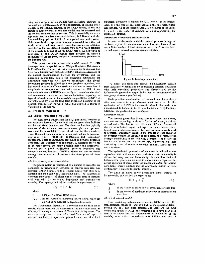
In order to adequately model the system operation throughout the horizon year, its load-duration curve has been broken down into a finite number of load situations, see figure 1. A load level for each area is defined for every demand situation.

Load t

h Time

Figure 1: Load representation.

The model also takes into account the uncertainty derived from hydraulicity conditions by considering different situations with their associated probability and characterized by the hydroelectric generation output limits. both for programmed and emergency situations (see below).

Each possible combination of demand and hydraulicity situations results in a production cost scenario. In the application of CHOPIN to the Spanish network, the model was dimensioned to handle up to 10 load blocks and 3 hydraulicity situations (30 production cost scenarios). Generation model

The thermal generation in any area is divided into blocks, each one corresponding to either a fraction of a unit, a unit or several units. The blocks can reflect the different features of thermal units (rated output, fuel type, heat rate characteristics, forced outage rate, maintenance plan) and can also be easily used to represent availability states. In the production cost scenarios the program derates the capacity of each block, to account for its average availability; in the reliability scenarios (see below) the blocks are either entirely on or off, depending on their availability state. Must run or technical minima constraints are not considered.

The hydroelectric generation of each area is reduced to one equivalent unit, with no variable production cost; its capacity is defined for every load and hydraulicity situation. Two limits of hydroelectric generation are used to approximately represent the actual operation of these units: the scheduled output for normal conditions (energy limited) and the emergency output for post- contingency situations (capacity limited).

The limits of active power generation, either thermal or hydroelectric, on each bus are expresed as:

O l g l g where

g g

is the vector of active power generation for each bus. is the vector of maximum active power generation for each bus.

-

Electrical network model Four modelling options are available: DCLF model [lo].

transportation model [ 6 ] and two hybrid transportation-DCLF models [4. 251. The most detailed and therefore the most interesting option is DCLF, the remaining ones have been used mostly to understand the implications of the nature of the models, to establish comparisons with PERLA and also to

1888

explore the advantages of having a reasonable starting solution for the optimization algorithms. It should be noted that the proposed heuristic algorithm can in principle be used regardless of the network model, even with a complete AC load flow.

In the DCLF model the per unit active power flow (which coincides with the per unit current intensity) in a line is given by the expression:

where

yi, Bi f;, xi, The following set of linear equations includes equation (3) for

each line of the complete network representation and also the first Kirchhoffs law (power balance equation) at each node:

is the simplified susceptance of line i-j. is the voltage angle on bus i. is the active power flow in line i-j. is the series reactance of line i-j.

-Sf + g = d ( 4 . a )

( 4 . b ) ~ - D S e = o T

where

8 D d is the demand vector. S T means transpose. The transportation model only accounts for the first

Kirchhoffs law. This amounts to greater flexibility in distributing the power flows in the network, since angle constraints do not exist and line capacities are the only limitation [6].

The hybrid models combine the:eharacteristics of the two preceding models. In hybrid model 1 the first Kirchhoff's law must be satisfied at each bus. but the second law has to be met only for the existing lines and not for the new investments [U]. Hybrid model 2 adds to hybrid model 1 the feature of also representing the second Kirchhoffs law for any new line in the same corridor as any existing line; however, the susceptance of the corridor must remain equal to the previous value for the existing lines [4].

is the vector of bus voltage angles. is a diagonal matrix of simplified line susceptances.

is the node-arc incidence matrix.

2.2 Investment model CHOPIN decides the installation of new transmission lines,

in order to reinforce existing corridors or to create new ones. Expansion costs include line costs as well as the associated installation expenses (i.e., the costs of new substations or ad- ditional positions at both ends of existing ones). The annualized value of these costs is considered (by means of a levelimd carry- ing charge), as well as the corresponding modifications because of escalation and actualization rates (so that these costs may be consistently compared with operation costs). The investment cost is expressed as:

K1 M l k

I € R k = l m = 1 c I ( x ) = a c h l k c X l k m ( 5 1

where

R

U

subset of branches (i.e.. corridors) where the user allows new investments. coefficient including the actualized levelized carrying charge and weighting factor of the investment cost in

the total cost function. total investment cost. investment cost of a line of type k in corridor 1. types of line that are allowed as expansion options in corridor 1. maximum number of new lines of type k that can be added to corridor 1.

The current model includes a number of investment constraints, namely: maximum total number of lines that can be installed in each corridor (6.a), maximum number of lines of a given type that can be installed in each corridor (this is intrinsic to the formulation), maximum total investment per corridor (6.b) or global for the network (6.c). All of these constraints are linear, although this is not a limitation imposed by CHOPIN:

K1 M l k

k = l m = l X l k m 5 L1 1 e Q ( 6 . a )

K1 M l k

k = l m = l h l k X l k m 11 1eR ( 6 . b )

K1 M l k 1 h l k 1 X l k m 7'1

I e R k = l Ill = 1

where

11 f.1

TI

maximum investment in corridor 1. maximum number of lines to be installed in corridor 1. maximum total investment in the network.

2.3 Operation model The operation of the power system is represented by two sets

of models: the production cost submodel and the reliability submodel. The production cost submodel considers the "normal" operation state of the system and it is focused on costs. On the other hand, the reliability submodel allows the user to impose reliability criteria on the planning process.

The production cost submodel is a properly weighted aggregation of the optimal economic dispatches (including the generation and the network representations) for each one of the production cost scenarios described previously. For every pro- duction cost scenario s the following objective function is minimized:

N E i N C E s = C C C i e S s , i e + C E N C r s , i ( 8 1

i = l e = l i = l where CE CEN cie

Ei ie

N

production cost. cost of unserved energy. variable production cost of generation block e in area i . total number of generation blocks in area i. power output of generation block e in area i. total number of areas. unserved power in area i.

Ohmic losses can be accounted for in the DCLF model, see [3. 231. by simply adding a fictitious load at both ends of each line, with every load being equal to one half of the total ohmic loss of the line [26]:

k i j = z c i j ( i - c o s ( e i - e j ) ) ( 9 ) where

1889

the production cost and the reliability subproblems. The projected augmented lagrangian algorithm (181 is employed for the nonlinear cases. This choice has practically eliminated the convergence difficulties reported with the approaches in [3] and Wl.

In both subproblems a dummy network with very high impedance and very low capacity [ 171 has been used in addition to the actual one, to avoid having to deal with islands in the network when the E L F model is used.

Ai, Gi, In the DCLF model, the minimization of the objective

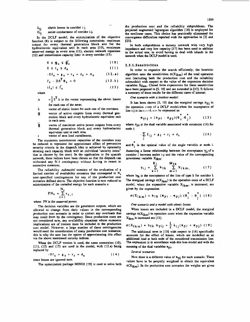
function (8) is subject to the following constraints: maximum output for every thermal generation block and for the hydroelectric equivalent unit in each area (lo), maximum unserved energy in every area (11). electric network equations (12) and transmission capacity limit in every corridor (13):

ohmic losses in corridor i-j. series conductance of corridor i-j.

0 I g s I rs 0 I r s I d,

where

A =$ST A is the vector representing the ohmic losses

for each one of the areas. vector of ohmic losses for each one of the corridors. vector of active outputs from every thermal gen- eration block and every hydroelectric equivalent unit in each area. vector of maximum active power outputs from every thermal generation block and every hydroelectric equivalent unit in each area. vector of area load curtailments.

A g

- g

r The maximum transmission capacities of the corridors may

be reduced to represent the approximate effect of preventive security criteria in the dispatch (this is achieved by optionally derating each capacity block with an individual "security index" that is chosen by the user). In the application to the Spanish network, these indices have been chosen so that the dispatch can withstand any N-1 contingency without having to resort to corrective measures.

The reliability submodel consists of the evaluation of a limited number of availability scenarios that correspond to N, user-specified contingencies for any of the production cost scenarios defined above. The objective function is now reduced to minimization of the curtailed energy for each scenario s:

N' P N s = C r s , i

i = l where PN is the unserved power.

The decision variables are the generation outputs, which are allowed to change from their values in the corresponding production cost scenario in order to correct any overloads that may result from by the contingency. Since production costs are not considered now, any availability situations whose economic implications are of interest must be included in the production cost model. However, a large number of these contingencies would need the consideration of many production cost scenarios; this is why the user has the option of approximating this effect via the above mentioned security indices.

When the DCLF version is used, the same constraints (10). (11). (12) and (13) are used in the model, with (12.a) being replaced by

- S f , + g , + r s = d, ( 1 4 ) since losses are ignored now.

The optimization package MINOS [19] is used to solve both

2 . 3 . l . S e n s t t i v l t i e s In order to organize the search efficiently, the heuristic

algorithm uses the sensitivities o(Xlkm) of the total operation cost (including both the production cost and the reliability submodels) with respect to the value of the expansion decision variables Xlkm. closed form expressions for these sensitivities have been proposed in [5, 101 and are extended in [13]. It follows a summary of these results for the different cases of interest:

One scenario with a Iosskss d e l : It has been shown [5 , 101 that the marginal savings v j in

the operation costs of a DCLF model,when the susceptance of line i-j is i n c r ~ ~ ~ w d , c m bc expressed as:

* * n y i j = ( n p i - n p j ) ( e i - e , ) ( 1 5 )

where npi is the dual variable associated with constraint (14) for node i:

* and O i is the optimal value of the angle variable at node i.

Asspming a linear relationship between the susceptance x j of a corridor 1 between nodes i-j and the value of the corresponding investment variable X l h :

K l M l k

k = l m = l Yi j = 2 b l k c X l k m , ( 1 7 )

where blk is the susceptance of the line of type k for corridor 1. The marginal savings o(Xlkm) in the operation costs of a DCLF model, when the expansion variable Xlkm, is increased, are given by the expression:

* * o ( X l k m ) = b l k ( n p i - n p j ) ( e i - e j

One scenario and a model with ohmic losses. When losses are included in a DCLF model, the marginal

savings o(X1km) in operation costs when the expansion variable X k m is increased are [13]:

1

( 1 8 )

o ( X l k m ) = b l k n y i j + l a i j ( " p i + n p j ) ( 1 9 )

The additional term in [19] with respect to [18] specifically accounts for the effect of losses, which are modelled as an additional load at both ends of the considered transmission line. The expression is m accordance with this loss model and with the meaning of the dual variables npi.

Several scenarios Now there is a different value of vj for each scenario. These

values have to be properly weighted to obtain the equivalent ~ ( X l h ) . In the production cost scenarios the weights are given

1890

by the duration of the demand conditions and the probability of the considered hydrologies. The weights for the reliability scnarios result fibm the probability pf and duration tf of each scenario. Finally:

D H F

where d, h and f are the indices for the different situations of demand, hydraulicity and reliability, respectively. Costtbenejit ratio of M investment option.

Knowledge of the sensitivities of the total cost of operation with respect to the zero-one investment variables X l d , makes it possible to compute marginal costbenefit ratios for each expansion option:

where hlk is the investment cost for the expansion option The value of A(Xlmk) is m general a good approximation to the actual costbenefit ratio for the complete inyeqtment. The search algorithm uses these indices to prioritize the level of interest of each expansion option Xlmk.

3. Solution method The global investment problem is solved by a new heuristic

procedure that starts from an user-provided initial expansion plan. Discrete investments are always considered, and the user also chooses the network model (only the transportation and DCLF models have been implemented in CHOPIN). The algorithm improves the initial plan by performing local searches, with the guidance of sensitivies, in a truncated subspace of the complete solution space of the investment variables X. Each one of the plans that are providcd by the heuristic search is evaluated by the corresponding subproblem modules in order to determine its investment. production and reliability costs. The modular structure of CHOPIN is shown in figure 2.

calculation

Figure 2 CHOPIN'S modular structure.

The heuristic search procedure in CHOPIN is guaranteed to avoid repetitions in the evaluation of the plans and, without truncation of the solution space, it yields exhaustive enumeration of the solutions. Unfortunately, truncation is unavoidable in network expansion problems of realistic size. However, there is no evidence that the truncated enumeration procedure in CHOPIN. when the model is used according to the simple rules that have been learned from experience, has ever failed to yield the optimal solution in each one of the numerous

cases that have been tested so far. The method is described in the next sections. 3.1. The search algorithm

The basic idea behind the algorithm is that a reasonable initial plan can be systematically improved by one-at-a-time modifications (i.e.. to include or to remove a line from the plan) that can be pictsd by easily computed msitivitks (see section 2.3.1) and some logical rules dr8t are obtained from experience with the algorithm itself. The search is organized in a tree format that prevents repetitions and facilitates the definition of meaningful truncations of the solution space, and a very efficient algorithm is obtained.

The algorithm basically uses a depth first logic when choosing the next modification to the current best plan, based on the information that is provided by the sensitivities. However, the algorithm also explores along directions where no improvement of the objective function takes place for one or more modifications of the plan (with the maximum number of "wrong steps" being prescribed by the user from the outset). These "wrong steps" (i.e.. local explorations with no improvement in the objective function) are meant to avoid getting trapped into local minima, by facilitating the addition (or removal) ( 1 1 lines whose installation is blocked by existing lines (or that 1w I' bciivr alternatives) in the current solution.

Together with the tlcfinition of the initial expansion plan, the user also optionally classifies the investment variables X into three mutually exclusive groups: questioned, frozen and attractive variables.

The questioned uuriaMes represent lines that are included in the initial plan: however the user conhiders that they may not belong to the optimal expansion plan.

The attrdctive variables represent lines that, although not included by the user in the initial expansion plan, may be part of the optimal plan.

The frozen variables must keep thgir initial values (that are fixed by the user from the outset: either,included in the plan, value of 1, or not included, value of 0) throughout the entire search. During the search the initial questioned and attractive variables gradually become frozen variables.

This classification of the variables is a first form of truncation of the solution space, and may be ignored in small networks, when the number of expansion options is small or when the user lacks enough information to make the choice. The classification is also used in the logic of the heuristic search (see below).

The search is organized in a pree format. In the search tree the nodes represent expansion plans, with the root of the tree being the user-provided initial plan. The branches represent the decisions (just one-change-at-a-time) that connect a node to a neighboring one. Each node in the tree contains a complete solution (i.e.. an expansion plan). where in general some of the options (i.e., the expansion variables) are still open (i.e.. the variable is not frozen yet) while some others are not. An open node does not have all the variables frozen and it can be expanded further, On the other hand, in a closed node all the decision variables are frozen, and it is not possible to continue the search. As the nodes correspond to complete solutions, and the best nodes are in general expanded first, the process may be interrupted at a y time and still provide a set of meaningful plans that improve over the initial one.

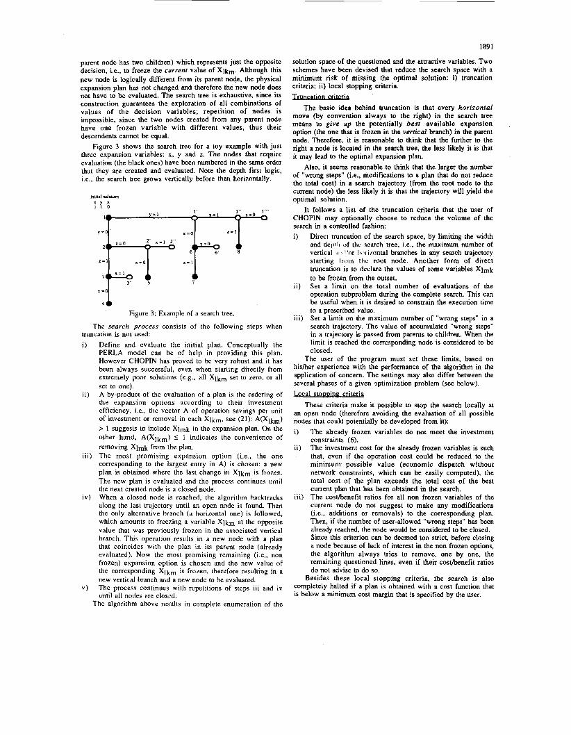
There are two types of branches (see fig.3). Vertical brunches represent a change in the value of a decision variable Xlkm. which becomes frozen from there on. The new node is different from its parent node and needs to be evaluated. To each vertical branch always corresponds one horizontal brunch, (i.e., each

1891

solution space of the questioned and the attractive variables. Two schemes have been devised that reduce the search space with a minimum risk of missing the optimal solution: i ) truncation criteria; ii) local stopping criteria.

The basic idea behind truncation is that every horizontal move (by convention always to the right) in the search tree means to give up the potentially best available expansion option (the one that is frozen in the vertical branch) in the parent node. Therefore, it is reasonable to think that the further to the right a node is located in the search tree, the less likely it is that it may lead to the optimal expansion plan.

Also, it seems reasonable to think that the larger the number of "wrong steps" (i.e., modifications to a plan that do not reduce the total cost) in a search trajectory (from the root node to the current node) the less likely it is that the trajectory will yield the optimal solution.

It follows a list of the truncation criteria that the user of CHOPIN may optionally choose to reduce the volume of the search in a controlled fashion:

y = o X = O .?=I

parent node has two children) which represents just the opposite decision, i.e., to freeze the current value of X]km. Although this new node is logically different from its parent node, the physical expansion plan has not changed and therefore the new node does not have to be evaluated. The search tree is exhaustive, since its construction guarantees the exploration of all combinations of values of the decision variables; repetition of nodes is impossible, since the two nodes created from any parent node have one frozen variable with different values, thus their descendents cannot be equal.

Figure 3 shows the search tree for a toy example with just three expansion variables: x, y and z. The nodes that require evaluation (the black ones) have been numbered in the same order that they are created and evaluated. Note the depth first logic, i.e., the search tree grows vertically before than horizontally.

24 1 Y 6'

1 = o z = 1 z = 1

a = O - 0 6' 8

Figure 3: Example of a search tree.

The search process consists of the following steps when truncation is not used:

i )

ii)

iii)

iv)

v)

Define and evaluate the initial plan. Conceptually the PERLA model can be of help in providing this plan. However CHOPIN has proved to be very robust and it has been always successful, even when starting directly from extremely poor solutions (e.g., all Xlkm set to zero. or all set to one). A by-product of the evaluation of a plan is the ordering of the expansion options according to their investment efficiency, i.e., the vector A of operation savings per unit of investment or removal in each Xlkm. see (21): A(Xlkm) > 1 suggests to include Xlmk in the expansion plan. On the other hand, A(Xlkm) 5 1 indicates the convenience of removing Xlmk from the plan. The most promising expansion option (i.e., the one corresponding to the largest entry in A) is chosen: a new plan is obtained where the last change in Xlkm is frozen. The new plan is evaluated and the process continues until the next created node is a closed node. When a closed node is reached, the algorithm backtracks along the last trajectory until an open node is found. Then the only alternative branch (a horizontal one) is followed, which amounts to freezing a variable Xlkm at the opposite value that was previously frozen in the associated vertical branch. This operation results in a new node with a plan that coincides with the plan in its parent node (already evaluated). Now the most promising remaining (i.e., non frozen) expansion option is chosen and the new value of the corresponding Xlkm is frozen. therefore resulting in a new vertical branch arLd a new node to be evaluated. The process continues with repetitions of steps iii and iv until all nodes are closed.

The algorithm above results in complete enumeration of the

i)

ii)

iii)

Direct truncation of the search space, by limiting the width and dcpili of the search tree, i.e.. the maximum number of vertical i ''or Ilalri/ontal branches in any search trajectory starting I r o m h e root node. Another form of direct truncation is to declare the values of some variables Xlmk to be frozen from the outset. Set a limit on the total number of evaluations of the operation subproblem during the complete search. This can be useful when it is desired to constrain the execution time to a prescribed value. Set a limit on the maximum number of "wrong steps" in a search trajectory. The value of accumulated "wrong steps" in a trajectory is passed from parents to children. When the limit is reached the corresponding node is considered to be closed.

The user of the program must set these limits, based on hisher experience with the performance of the algorithm in the application of concern. The settings may also differ between the several phases of a given optimization problem (see below). barn . . .

These criteria make it possible to stop the search locally at an open node (therefore avoiding the evaluation of all possible nodes that could potentially be developed from it):

i)

ii)

iii)

The already frozen variables do not meet the investment constraints (6). The investment cost for the already frozen variables is such that, even if the operation cost could be reduced to the minimum possible value (economic dispatch without network constraints, which can be easily computed), the total cost of the plan exceeds the total cost of the best current plan that has been obtained in the search. The costbenefit ratios for all non frozen variables of the current node do not suggest to make any modifications (i.e., additions or removals) to the corresponding plan. Then, if the number of user-allowed "wrong steps" has been already reached, the node would be considered to be closed. Since this criterion can be deemed too strict, before closing a node because of lack of interest in the non frozen options, the algorithm always tries to remove, one by one, the remaining questioned lines, even if their cost/benefit ratios do not advise to do so.

Besides these local stopping criteria, the search is also completely halted if a plan is obtained with a cost function that is below a minimum cost margin that is specified by the user.

1892

3.2. Utilization guidelines The utilization guidelines that follow are meant for the

toughest case wheie the user cannot provide a reasonable first guess of the optimal expansion plan. The rules for simpler cases can be easily derived in an ad hoc fashion. These guidelines hare been extracted from the exparience of trying different utilization schemes with a number of case examples, most partkuliuly with the actual expansion problm of the spanish network. The use of CHOPIN, with the prQpcwd utilization rules. has provided the optimal solution in all ewes, including one where the StarEing plan contained 011 posslbh expansion options, and another one which included none of thaan. '

The proposed utilization scheme consists of three phases: approach, local search aad verification. At the beginning of each phase all Xlkm variables are set to their original status of questioned, attractive or frozen, but the best solution from the preceding phase is adopted as the starting node.

The approach phose is a pure depth first search, where horizontal branching is not permitted -d there is no limit IO the number of "wrong steps". The process is repeated several timas (2 or 3 was adequate in the tested examples), always starting from the best previous solution.

In the local search phase the width of the search space (i.e. the maximum number of horizontal branches in a trajectory) is gradually increaMd to 1. 4 and finally 8 steps, while just one "wrong step" is permitted. The optimal solution has been always reached in this phase.

The verification phase allows the user to check rhat the best solution of the local search phase is actually the optimal one. Now the width of the search space may be of 4 steps and 2 "wrong steps" are permitted.

A graphical routine of the program can be used to plot the trajectories for the N best solutions in a compact representation of the search space, where the value of N is prescribed by the user. In this compact representation. the end nodes of two search trajectories with the s m e number of horizontal and vertical branches we aggregated in the same point of the plane. Simple closed form expressions give the number of plans contained in each p i n t of the plane, and the total number of plans in a search space of any size (i.e.. when the width and depth are specified), see [13]. These simple tools can be of much help to the planner in deciding about the most convenient settings of the program for a particular application.

4. Application to case examples Both PERLA and CMOPIN have been tested on a large number

of cases, which basically correspond to two network configurations. The simplest one is the very popular six areas network in [7]. The second one is a 46 areas reduced version of the spanish HV network, which is similar to om that was used (only with PERLA) by REE, in the expansion planning for the Spanish system. The data for the version reported here are not real, since they have been distorted in order to create scenarios with widely different expansion needs.

CHOPIN is currently being used by Red Elictrica dc Espafia in the network expansion, now with an extended network configuration (about 100 areas and 200 corridors) that fully represents the 400 kV spanish transmission network, see [l].

In the next two subsections the main results for the two case examples are summarized. Both PERLA and CHOPIN were used with the transportation and the hybrid network representations, and with continuous (only PERLA) and discrete variables; the same solutions were obtained with both models, although the execution times with CHOPIN were approximately two orders of

magnitude smaller than with PERLA. Only PERLA could be used for the cases where the expansion variables were assumed to be c o n b u s . In. most of the cases where PERLA was applied with the IXLF network madel, there were aborted executions because of convexity prablems or because the model converged to non optimal plans. No difficulties were detected with CHOPIN when the afarementioned utilization rules wme followed.

Two different versions of the expansion problem were considered. In version A, the expansion options are such that they may connect any pair of areas. thqe is only one type of line and up to 3 lines can be installed per corridor. This results in 75 expansion variables. In version B. see (lo]. only the corridors 2- 3. 2-6. 3-5 and 4-6 can be expanded, there is also only one type of line and up to two lines can be installed in corridors 2-6, 3-5 and 4-6. while only one can be added in corridor 2-3. Thus, in this version the number of expansion variables is just 7.

Both PERLA and CHOPIN (this one only with discrete variables) y S d the same optimal solution as [lo] with all modelling options (namely transportation, hybrid and DCLF network models; discrete or Wntinuous variables) for version A of the expansion problem.

With vcrs 'n R. DCLF network model and discrete investment v . 4 1 si-les, I'I:KLA obtains the same solution as [lo] for version A of the pr~hlcm. However, CHOPIN obtains a better solution, which appears LO be the optimal one.

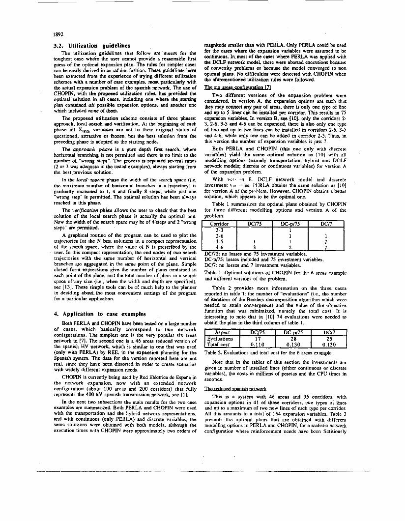
Table 1 summarizes the optimal plans obtained by CHOPIN for three different modelling options and version A of the problem.

Corridor 11 4-6

/75: no losses and 75 investment variables. DC-p/75: losses included and 15 investment variables. DCn: no losses and 7 investment variables. Table 1. Optimal solutions of CHOPIN for the 6 areas example and different versions of the problem.

Table 2 provides more information on the three cases reported in table 1: the number of "evaluations" (i.e., the number of iterations of the Benders decomposition algorithm which were needed to attain convergence) and the value of the objective function that was minimized, namely the total cost. It is interesting to note that in [lo] 74 evaluations were needed to obtain the plan in the third column of table 1.

Aspect I DC/75 I DC-p/75 I DC/7 1 Evaluations 17 28 25 Total cost' 0.110 0.130 0.130

Table 2. Evaluations and total cost for the 6 areas example.

Note that in the tables of this section the investments are given in number of installed lines (either continuous or discrete variables), the costs in millions of pesetas and the CPU times in seconds.

n e reduced S D ~ n e t w d This is a system with 46 areas and 95 corridors, with

expansion options in 41 of these corridors. two types of lines and up to a maximum of two new lines of each type per corridor. All this amounts to a total of 164 expansion variables. Table 3 presents the optimal plans that are obtained with different modelling options in PERLA and CHOPIN. for a realistic network configuration where reinforcement needs have been fictitiously

1893

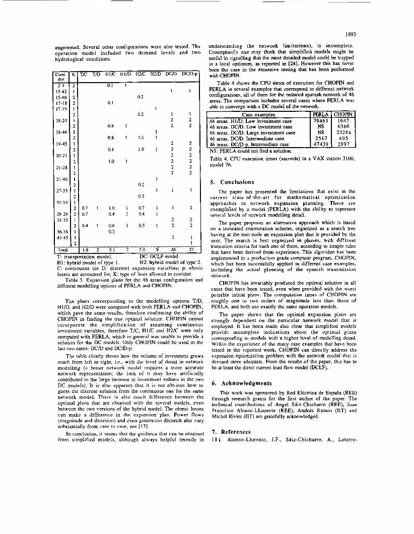
Case examples 46 areas. H1D. Low investment case 46 areas. D O . Low investment c m 46 areas. DCD. Large investment case 46 areas. DCD. Intermediate case

augmented. Several other configurations were also tested. The understanding the network limitations), is incomplete. operation model included two demand levels and two Conceptually one may think that simplified models might be

PERLA CHOPIN 79463 1047

NS 6360 NS 23284

2517 695

hidrological conditions.

- :Om dor 2-3

,5 -42 15-46

-

17-1 8 17-19

18-20

18-46

19-45

20-21

21-28

21-46

27-33

31-34

28-2'1 31-35

36-3t 43-45

Total - - T: trans1

- Z

z 1 2 2 1 2 1 2 1 2 1 2 1 2 1 2 1 2 1 2 1 2 2 1 2 1 1 2 - -

'/C T/D Hl/C HID H2/C H2/D K m K / D p

0.1 1

0.7 0.7

0.4

0.1

0.8

0.8

0.1

1.0

1.0 0.4

0.6 0.2

0.2

0.2

1.3

1 .o

0.2

0.5

0.7 0.4

0.5

1 1

1 I 2 2 2 2

2 2 2 2 2 2 2 2 2 2 2 2

1 1

1 2

2 2 2 2

2 1 1

1.8 2 5.1 7 5.0 9 26 27 tation model. DC: DCLF model.

H1: hybrid model of type 1. H2: hybrid model of type 2. C: continuous (or D: discrete) expansion variables; p: ohmic losses are accounted for; K: type of lines allowed in corridor.

Table 3. Expansion plans for the 46 areas configuration and different modelling options of PERLA and CHOPIN.

The plans corresponding to the modelling options T/D, Hl/D, and H2/D were computed with both PERLA and CHOPIN, which gave the same results, therefore confirming the ability of CHOPIN in finding the true optimal solution. CHOPIN cannot incorporate the simplification of assuming continuous investment variables, therefore T/C. Hl/C and H2/C were only computed with PERLA, which in general was unable to provide a solution for the DC models. Only CHOPIN could be used in the last two cases: DC/D and DCD-p.

The table clearly shows how the volume of investment grows much from left to right, i.e., with the level of detail in network modelling (a better network model requirps a more accurate network representation; the lack of it may have artificially contributed to the large increase in investment volume in the two DC models). It is also apparent that it is not obvious how to guess the discrete solution from the continuous one for the same network model. There is also much difference between the optimal plans that are obtained with the several models, even between the two versions of the hybrid model. The ohmic losses can make a difference in the expansion plan. Power flows (magnitude and direction) and even generation dispatch also vary substantially from case to case, see (131.

In conclusion, i t seems that the guidance that can he obtained from simplified models. although always helpful (mostly in

I 4 6 areas. DCD-p. Intermediate case I 4 7 4 3 9 I 2897 1 NS: PERLA could not find a solution. Table 4. CPU execution times (seconds) in a VAX station 3100, model 76.

5. Conclusions The paper has presented the limitations that exist in the

current state-of-the-art for mathematical optimization approaches to network expansion planning. These are exemplified by a model (PERLA) with the ability to represent several levels of network modelling detail.

The paper proposes an alternative approach which is based on a truncated enumeration scheme, organized as a search tree having at the root node an expansion plan that is provided by the user. The search is best organized in phases, with different truncation criteria for each one of them, according to simple rules that have been derived from experience. This algorithm has been implemented in a production grade computer program, CHOPIN, which has been successfully applied to different case examples, including the actual planning of the Spanish transmission network.

CHOPIN has invariably produced the optimal solution in all cases that have been tested, even when provided with the worst possible initial plans. The computation times of CHOPIN are roughly one to two orders of magnitude less than those of PERLA, and both use exactly the same operation models.

The paper shows that the optimal expansion plans are strongly dependent on the particular network model that is employed. It has been made also clear that simplified models provide incomplete indications about the optimal plans corresponding to models with a higher level of modelling detail. Within the experience of the many case examples that have been tested in the reported work, CHOPIN can directly address the expansion optimization problem with the network model that is deemed more adequate. From the results of the paper, this has to be at least the direct current load flow model (DCLF).

6. Acknowledgments This work was sponsored by Red ElCctrica de Espaiia (REE)

through research grants for the first author of the paper. The technical contributions of Angel Siiz-Chicharro (REE), Juan Francisco Alonso-LLorente (REE), Andrks Ramos (IIT) and Michel Rivier (IIT) are gratefully acknowledged.

7. References [ 1 ] Alonso-Llorente, J.F., Sbiz-Chicharro, A., Latorre-

Bayona, G., ?drez-Ar.riaga, I.J. Utilizacidn del nuevo c6digo CHOPIN en la planificacidn de la red de transporte espaiiola. 111 Jornadas Hispano-lusus de Ingenierla EUcrrica. BurceIona. Esparia, (Julio 1993). Benders, J.F. Partitioning Procedures for Solving Mixed- Variables Programming Problems. W u m e r i s c he Mathematik vo1.4 (1962), pp. 238-252. Berry. P:E. and Dunnett. R.M. Contingency Constrained Economic Dispatch Algorithm for Transmission Planning. IEE Proceedings Vol. 136, Pt. C, No. 4 (July

Cabrd, P.M. and Praca, J.C.O. An interactive software for Optimizing Transmission Network Expansion. 8th Power System Computation Conjerence. Ilelsinki, Finland (1 9- 14 August 1984). Dcchamus. C. and Jamoulle. E. Interactive ComDuter

1989), pp. 238-244.

P r o g r k 'for Planning the Expansion of Me-shed Transmission Networks. Electric Power and Energy Systems Vol.2, N0.2 (April 1980). pp.103-108. Eunson, E., Hautot, A. and Invemizzi, A. The use of the linear flow estimation in computing codes for long term power system planning: the practice of CEGR, EDF and ENEL. EDF Bulletin de la Direction Des Etudes Et Recherches - Serie B (1987), pp. 35-52. Carver, L.L. Transmission Network Estimation Using Linear Programming. IEEE Transactions on Power Apparaius Jnd Systems V o l . PAS-89, No. 7 (Sept./October 1970). pp. 1688-1696.

[ 2 1

[ 2 2

[ 161 Marsten, R., XLP Technical Reference Manual, XMP Software. Inc., Tucson (USA), 1989.

[ 171 Monticelli, A., Santos, A., Pereira. M.V.F., Cunha, S.H.F., Parker, B.J. and Praca. J.C.G. Interactive Transmission Network Planning Using Least-Effort Criterion. IEEE Trans. on Power Apparatus and Systems Vol. PAS-IOI. No. 10 (October 1982), pp. 3919-3925.

[ 181 Murtagh, B.A. and Saunders, M.A. A Projected Lagrangian Algorithm and Its Implementation for Sparse Nonlinear Constraints. Tech. Report SOL. Department of Operations Research. Stanford University., 1982.

[ 191 Murtagh, B.A. and Saunders, M.A., MINOS 5.1 USER'S G U I D E , SOL. Department of Operations Research, Stanford University. California 94305, 1987.

[ 2 0 ] Pereira, M.V.F. and Pinto, L.M.V.G. Application of Sensitivity Analysis of Load Supplying Capability to Interactive Transmission Expansion Planning. I E E E Transactions on Power Apparatus and Systems Vol. PAS- 104, No. 2 (February 1985), pp. 381-389. Pereira. M.V.F.. Pinto. M.V.G., Cun ha, S .H.F. and Oliveira. C.C. A Decomposition Approach to Automated Generation/Transmission Expansion Planning. YEEE Transactions on Power Apparatus and Systems Vol. PAS- 104. No. 11 (November 1985), pp. 3074-3083. Pinto, L.M.V.G. and Nunes, A. A Model for the Optimal Transmission Expansion Planning. Proceedings of the tenth Power Systems Computation Conference. IO PSCC. Graz, Austria 19-24 (August 1990). pp. 16-23.

Fuente. J.L. de la. Solucion de sistemas de ecuaciones, programacih lineal y entera. Universidad Politkcnica de Madrid. E.T.S. de lngenieros Industriales. Seccidn de publioaciones. Madrid, 1991. Geoffrion, A.M. Generalized Benders Decomposition. Journal of Optimization Theory and Applications vol . 10. NO. 4 { 1972), pp. 237-260.

12 31 Rivier, M., pkrez-~niga, j.1. and tuengo, G. J U ~ A C : A Model for Computation of Spot Prices in Interconnected Power Systems. Proceedings of the tenth Power Systems Computation Conference. I O PSCC, Graz. Austria 19-24 (August 1990).

[ 2 41 Romero, R., Monticelli, A. A hierarchical decomposition aDDroach for transmission network exuansion dannine.

[IO] Granville, S., Pereira, M.V.F., Dantzing, G.R., Avi- Itzhak. B.. Avriel, M.. Monticelli, A. and Pinto, L.M.V.G. Mathematical Decomposition Techniques for Power System Expansion Planning. Volume 2: Analysis of the Linearized Power Flow Model Using the Render Decomposition Technique. Tech. Report, Project 2473-6 EPRI EL-5299, Fcbruary. 1988.

[ 1 1 ] Latorre-Bayona, G., P6rez-Arriaga. J.I., Ramos. A., and Rom6i-i. J. Un modelo de planificaci6n estitico de la red de transporte a largo plazo. I Jornadas t l i spano-has de Ingenieria Elkctrica. Vigo. ESP&. (Julio 1990).

[ 121 Latorre-Rayona, G.. Ramos. A., PCre7-Arriaga. J.I., Alonso. J.F.. and Siiz, A. PERLA: Un modelo de planificacidn eststica a largo plazo de la red de transporte. Opciones de modelado y andisig de idoneidad. I / Jormdas Hispano-lusus de Ingenieria Eldctrica. Coimbra. Portugal. (Julio 1991).

1131 Latorre-Rayona, G. Modelos estaticos para la planificacibn a largo plazo de la red de transporte de energia eltctrica. Tesis doctoral. Universidad Pontificia Cornillas. Madrid (Espaiia). Marzo I993 ..

[ 1 4 ] Levi, V.A. and Calovic, M.S. A New Decomposition Based Method for Optimal Expansion Planning of Large Transmission Networks. IEEE Tramactions on Power Systems Vol. 6. No. 3 (August 1991), pp. 937-943.

[ 151 Limmer, H.D. Long-Range Transmission Expansion Models. Tech. Report TPS 79-728 EPRI EL1569, October, 1980.

IEEE PES I993 Winter Meeting, paper 93 W'M 192-3 PWRS.

[ 2 5 ] Villasana, R., Carver, L.L. and Salon, S.J. Transmission Network Planning Using Linear Programming. IEEE Transactions on Power Apparatus and Systems Vol. PAS- 104. No. 2 (February 1985), pp. 349-356.

[ 2 6 ] Wood, A.J. and Wollcnberg. B.F. Power Generation Operation, and Control, John Wiley & Sons (1984).

Gerardo Latorre-Ravona was born in Bucaramanga. Colombia, in 1958. He obtained the Ph.D. in Electrical Engineering from the Universidad Pontificia Comillas and the B.S. in Electrical Engineering from the Universidad Industrial de Santander (UIS). Bucaramanga, Colombia. He joined UIS in 1985 as assistant professor in the Department of Electrical and Electronic Engineering. His areas of intercst include reliability, operation. control and planning of electric power systems.

Imacio J. Pkrez-Arriaza was born in Madrid, Spain, in 1948. He obtained the Ph.D., and M.S. in Electrical Engineering from the Massachusetts Institute of Technology and the B.S. in Electrical Engineering from the Universidad Pontificia Comillas. He is the Director of the Instituto de Investigacibn Tecnoldgica and Professor in the Electrical Engineering School of the same University. His areas of interest include reliability. control, operation. planning and regulation of electric power systems.