Childhood circumstances and adult outcomes:

Evidence from World War II∗

Enkelejda HavariTor Vergata University

Franco PeracchiTor Vergata University and EIEF

October 2011This version: August 2012

Abstract

This paper studies the effects of episodes of stress, poor health, financial hardship and hungerearlier in life on education and health in later life. As a source of identification, we exploitthe huge temporal and regional variation of war events in Europe during the period from thebeginning of the Spanish Civil War in 1936 to the end of World War II in 1945. We concentrateon the cohorts born between 1930 and 1954 in 13 European countries, and combine the availablehistorical information with micro-level data from the Survey of Health Ageing and Retirementin Europe (SHARE), which provides detailed retrospective information on life histories fromchildhood to adulthood for people born before 1955. Using these data we find that hungerepisodes are more closely associated with war than any other hardship episode. Our instrumentalvariable estimates suggest that hunger in childhood or early adolescence has important negativelong-run effects on educational attainments and various measures of physical and mental healthpast age 50. They also suggest that suffering hunger for longer periods has stronger negativeeffects.

Key words: Socio-economic status; Health; Financial hardship; World War II; Europe;SHARE survey

JEL codes: I0, J13, J14, N34.

∗Corresponding author: Enkelejda Havari (enkelejda.havari@gmail.com). We thank the two Guest Editors andthree anonymous referees for valuable comments and constructive criticism, and Agar Brugiavini, Angus Deaton,Fabrizio Mazzonna, Cormac O Grada, Andrea Pozzi, Joachim Winter, and Jeff Wooldridge for helpful discussions.We also thank participants to the 2011 International SHARE User’s Conference (Tallinn, September 2011), theConference on Fetal Origins, Early Childhood Development, and Famine (Princeton, September 2011), the 2012SMYE Conference (Mannheim, April 2012), the 2012 ESI Spring Worshop (Jena, June 2012), and the 2012 ItalianSHARE User’s Conference (Venice, June 2012) for useful comments. This paper uses data from SHARELIFE release1, as of November 24, 2010, and from SHARE release 2.5.0, as of May 24, 2011. The SHARE data collection has beenprimarily funded by the European Commission. See www.share-project.org for the full list of funding instituions.

1 Introduction

World War II (WW2) was perhaps the deadliest conflict in history, with around 70 million casualties

(Beevor 2012). It directly affected most European countries, but at different times and with different

intensity. Though WW2 in Europe conventionally lasted from September 1, 1939, to May 8, 1945,

the period of “Europe at war” may actually be broadened to cover the period from the beginning of

the Spanish Civil War in 1936 to the descent of the Iron Courtain in 1949. In addition to the Spanish

Civil War (1936–39), this period includes the German occupation of Austria and Czechoslovakia

(1938), the aftermath of WW2 in the Axis countries and Eastern Europe (1945–48), and the Greek

Civil War (1946–1949).

Unlike World War I, WW2 was a war of movement rather than trenches, and a much greater

fraction of the civilian population was exposed to combat, bombing, stress and hunger. Children

and older people are likely to have suffered most. In particular, the war affected the childhood of

different cohorts of Europeans subjecting them to a variety of shocks. Many of those children are

still alive today and are able to recall these hardship episodes.

Our paper contributes to the recent literature on the long-run effects of wars and civil conflicts,

and the channels through which these effects operate (Ichino and Winter-Ebmer 2004, Bundervoet,

Verwimp and Akresh 2009, Akbulut-Juksel 2009, Jurges 2011, Kesternich et al. 2011, Akresh et

al. 2012, van den Berg, Pinger and Schoch 2012). Some of this literature focuses on the effects

of WW2 on the human capital and health of the survivors. In particular, Ichino and Winter-

Ebmer (2004) and Akbulut-Yuksel (2009) study the effects of disruption of the educational process,

while Jurges (2011), Kesternich et al. (2011) and van den Berg, Pinger and Schoch (2012) study

the effects of civilians being persecuted, dispossessed, exposed to hunger, food rationing or even

famine. Although they use different empirical strategies, most of these studies find negative effects

of experiencing war-related events (e.g. having lived in a heavily bombed city) on education, health

and earnings of the survivors.

Our paper is also related to the extensive literature on the long-run impact of childhood shocks

(Case, Fertig and Paxson 2005, Case and Paxson 2010, Currie 2009, 2011, Almond and Currie

2011) and the role of critical periods for investments in children (Cunha and Heckman 2007). A

general result from this literature is that childhood circumstances may affect outcomes at older

ages both directly and indirectly, through their effects on health and socio-economic status (SES)

at younger ages. Different channels may be at work. Case, Lubotsky and Paxson. (2002) show

that poor children in the U.S. tend to be in worse health at adult ages than wealthy children (SES

1

channel). On the other hand childhood health may affect adult SES directly through the health

channel or indirectly through it’s effect on human capital. Case and Paxson (2005, 2010) provide

a useful framework for thinking at the relationship between health and SES at different stages of

life. They distinguish between three periods–childhood, young adulthood and older adulthood–and

allow for both direct and indirect links between them. Estimating this kind of model puts stringent

requirements on the data, as critical information on health and SES at intermediate ages must

be available. In the absence of prospective studies, subjective data have been widely used (Elo

1998, Haas 2007, Smith 2009). For comprehensive reviews see Lumey, Stein and Susser (2010) and

Almond and Currie (2011).

Because identifying and estimating causal relationships is far from trivial, economists often rely

on the variation induced by extreme and sharp events, such as famines. Examples include the

Leningrad Siege (Sparen et al. 2004), the Greek hunger (Neelson and Stratmann 2011), the Dutch

“hunger winter” 1944–45 (Lumey, Stein and Susser 2010, Rooseboom, de Rooij and Painteret

2006, Ravelli, van der Meulen and Barker 1998), and China’s “great famine” (Gorgens, Meng

and Vaithianathan 2008, Meng and Qian 2009). Most of this literature is motivated by Barker’s

fetal origins hypothesis and focuses on nutritional shortages around birth, although attention has

recently also been devoted to hardship conditions after birth (Gluckman et al. 2005). Unlike

undernourishment or hunger, which can affect a person’s life for long time, famines have the feature

of being sharp events and finish in a relatively short time. However, famine is somewhat of a black

box, for it is not really clear what happens when it occurs and what mechanisms matter (lack of

food, disease, etc.). The main findings from this literature are that exposure to famine around

birth or in early childhood negatively influences educational attainments, health status, height,

and well-being. However, in this literature there are concerns in finding both appropriate control

groups for individuals affected by famine (especially while in utero) and accurate data on famine

intensity. Comparing the outcomes of exposed cohorts with those not exposed is not sufficient to net

out the effects of famine from other relevant changes over time. Further, when analyzing famines

one should be careful with selection issues arising from the high mortality rates that typically

characterize famines.

We explore the causal link between hardship episodes in childhood/early adolescence and adult

outcomes, exploiting the variation induced by major war operations on the individual probability of

suffering hardship episodes in childhood (ages 6–10) or early adolescence (ages 11–15). We choose

age 6 as our starting age to minimize issues of recall bias and because this an important “temporal

2

landmark”, as it represents the school-entry age in most countries considered. We initially consider

four types of hardship: stress, poor health, financial hardship and hunger. It turns out that, of

these hardships, hunger is by far the most relevant.

Unlike other papers that only exploit macro-level variation (e.g. Brakman, Garretsen and

Schramm 2004, Davis and Weinstein 2004, and Acemoglu, Hassan and Robinson 2010), we use

rich micro-level data from the Survey of Health, Ageing and Retirement in Europe (SHARE), a

multi-purpose and cross-national survey that provides detailed retrospective information on people

aged 50+ in 13 European countries. In particular, we take advantage of the life history data from

childhood to adulthood collected in the survey’s third wave, named SHARELIFE. Using SHARE-

LIFE offers several advantages. First, we can distinguish between cohorts born before, during, and

after WW2 in 13 different European countries. Second, the different cohorts were exposed to war

events at different ages, and the timing and intensity of the exposure was different both between

and within countries. SHARELIFE allows us to take into account the timing of these events, as

respondents are asked to recall the year in which specific hardship episodes occurred. Third, re-

call of hardship episodes can be combined with retrospective information on individual residence

history, thus allowing for substantial variation both between and within countries.

Since other researchers are recently investigating similar issues (Jurges 2011, Kesternich et al.

2011, van den Berg, Pinger and Schoch 2012), it is important to clarify the main differences between

our work and theirs. First, while Jurges (2011) focuses on Germany using data from the German

Socio-Economic Panel and van den Berg, Pinger and Schoch (2012) on Germany, Greece and the

Netherlands using SHARELIFE data, our paper has in common with Kesternich et al. (2011) the

focus on the full set of European countries in SHARELIFE. Second, unlike the other papers, we

jointly analyze episodes of stress, financial hardship, poor health and hunger. Third, our source

of quasi-experimental variation differs from van den Berg, Pinger and Schoch (2012), who use the

timing and duration of famine in the three countries that they consider. We use instead the spatial

and temporal information on major war operations. This allows us to cover both more countries

and more cohorts. Further, from the historical viewpoint, the periods of famine that some countries

experienced during WW2 (Greece, the Netherlands) were induced by war events.

The remainder of the paper is organized as follows. Section 2 describes our data. Section 3

presents some descriptive statistics. Section 4 presents the results of our regression analysis. Finally,

Section 5 concludes.

3

2 Data

We use data from two sources. The first is micro-level information from the second and third wave

of the Survey of Health, Ageing and Retirement in Europe (SHARE), a cross-national longitudinal

household survey whose main aim is to help understand patterns of ageing and how they affect

the welfare of individuals in the diverse cultural settings of Europe. In particular, we take advan-

tage of the life histories from childhood to adulthood collected in the survey’s third wave, called

SHARELIFE, which provides retrospective information on region of residence, various aspects of

the childhood environment, and the experience of hardship episodes.

The second is macro-level information on major war operations by region and year during the pe-

riod 1936–1945. We merged this information with the longitudinal information from SHARELIFE

on the region of residence, thus obtaining a panel data set with indicators of potential exposure to

war operations and experience of hardship episodes in each single year of age starting from birth.

2.1 SHARE and SHARELIFE

SHARE provides micro-data on health, socioeconomic status, family characteristics, etc., from

nationally representative samples of individuals born before 1955, speaking the official language

of the country and not living abroad or in an institution, plus their partners irrespective of age.

The survey is designed to be cross-nationally comparable and is harmonized with the English

Longitudinal Study of Ageing (ELSA) and the U.S. Health and Retirement Study (HRS). Three

waves of SHARE are currently available. The first two (2004–05 and 2006–07) mostly gather current

information on the respondents. The third, named SHARELIFE and conducted between fall 2008

and summer 2009, collects information on important areas of respondents’ life, namely events

related to partners and children, childhood health and family background characteristics, complete

employment transitions from the first job to retirement, information on past residences, health and

health care information from childhood to adulthood, income, and assessments of well-being and

happiness.

SHARELIFE was carried out in 13 European countries (Austria, Belgium, Czech Republic, Den-

mark, France, Germany, Greece, Italy, the Netherlands, Poland, Spain, Sweden and Switzerland)

and interviewed all people aged 50+ who participated in wave 2, plus their partners independently

of age. Our working sample consists of 20,473 individuals born between 1930 and 1954 who partic-

ipated in waves 2 and 3 of SHARE, which represents 76.2% of the total SHARE sample. Sample

sizes by country range between a minimum of 637 individuals in Austria and 957 in Switzerland,

4

to a maximum of 2,133 individuals in Belgium and 2,249 in Greece. Men represent 46.5% of our

working sample and women 53.5%.

2.1.1 Childhood environment and region of residence

In its Childhood SES (CS) section, SHARELIFE collects retrospective information on childhood

environment around age 10. This information includes household characteristics such as the occupa-

tion of the main breadwinner (white collar, blue collar, farmer, etc.), features of the accommodation

(presence of fixed bath, running water, inside toilet, or central heating), and the number of books

at home.

The Accommodation (AC) section of SHARELIFE also collects retrospective information on

each residence a person lived in for six months or more, starting from birth. This information

includes the year the person started and stopped living at that residence, whether its was private

or non-private and its type, and the country (at current boundaries), region and area of residence

(big city, suburbs or outskirts of a big city, large town, small town, rural area or village). This

allows us to construct a longitudinal data set with annual observations for each individual. The

level of regional disaggregation varies by country: it is at the coarser NUTS1 level for Belgium,

Denmark, France and the Netherlands, at the finer NUTS3 level for the Czech Republic, and at

the intermediate but not very detailed NUTS2 level for the other countries.

2.1.2 Hardship episodes

To the longitudinal information on the residence a person lived in, we add information from the

General Life (GL) section of SHARELIFE on the experience of hardship episodes.

This section first asks the following question: “Looking back on your life, was there a distinct

period during which you were under more stress compared to the rest of your life?”. If the answer

is yes, the following two questions are asked: “When did this period start?”, and “When did this

period stop?”. It then asks similar questions for poor health (“Looking back on your life, was there

a distinct period during which your health was poor compared to the rest of your life?”), financial

hardship (“Looking back on your life, was there a distinct period of financial hardship?”), and

hunger (“Looking back on your life, was there a distinct period during which you suffered from

hunger?”). The ordering of the questions is fixed: first stress, then poor health, financial hardship,

and finally hunger. Notice that respondents are asked to report only one episode for each type of

hardship, presumably the most salient. Further, the available information is rather coarse, as we

5

only have binary indicators for suffering hardship in a given year and we lack information on the

intensity of the various episodes.

Figure 1 shows the fraction of people reporting the various types of hardship in each single

year between 1930 and 1954, separately for six country groups: the German Reich (Germany and

Austria), Italy, the German occupied countries in Eastern Europe (Czech Republic and Poland)

and in Western Europe (Belgium, Denmark, France, Greece, and the Netherlands), Spain, and

the neutral countries (Sweden and Switzerland). During the period considered, financial hardship

and hunger are much more important than stress and poor health. Further, they are important

only for Spain and the countries involved in WW2, not for the neutral countries. While financial

hardship shows less of a time pattern, hunger is concentrated during the war and postwar periods,

where it appears to be much more important than financial hardship. In particular, for the German

Reich and Italy hunger is concentrated at the end of WW2 and in the postwar period, while for

the occupied countries in the East and the West it is important throughout the war. For Spain,

financial hardship and hunger rise steadily from 1931 to 1941, and decline afterwards but remain

at very high levels compared to most other countries. In fact, Spain is quite different from all other

countries, both because financial hardship and hunger were a problem even before the start of the

civil war and because they remain a problem also in the early 1950s.

Figure 2 looks at the relationship between hunger and financial hardship. It shows, for each

year and country group, the fraction of people reporting only hunger (top-left panel), only financial

hardship (top-right panel), and both hunger and financial hardship (bottom-left panel). It appears

that, for all country groups, hunger is most strongly associated with war.

To better understand the link between hunger and war, Figure 3 looks at people who report

suffering hunger in childhood and shows, for each country, the distribution of the year when hunger

started. Most hunger episodes start between 1939 and 1945. For Austria and Germany, they

mostly start in 1944 or 1945. For the Czech Republic, France and Poland, the distribution is

roughly bimodal, with peaks both at the beginning of the war in 1939 or 1940, and towards its end

in 1944 or 1945. Some evidence of bimodality is also found for Belgium, Greece and Italy, though

the first peak, in 1940, is much more pronounced than the second one, towards the end of the war.

while for the Netherlands, we observe a sharp peak in 1944, corresponding to the “Hunger Winter”.

For Spain, the majority of reported hunger episodes does not begin during the civil war but rather

after its end, with a peak in 1940. Finally, for the neutral countries, the few reported hunger

episodes start mostly during WW2. Overall, this evidence corresponds to the available historical

6

records.

The fact that, for many WW2 countries, hunger appears to start either with the war or with

the beginning of the German occupation raises the issue of what people really mean by a period

during which they suffered hunger. Specifically, people may not remember hunger episodes that

they actually suffered and may instead associate hunger with either the war in general or with the

country’s narrative based on collective memories rather than personal experience.

To address the first concern, Figure 4 looks at the distribution of hunger duration, computed

as the difference between the year when hunger is reported to end and the year when is reported

to start. A duration equal to zero means that hunger started and ended during the same year,

while a duration of 15 years also includes cases where hunger is reported to last more than 15

years (about 5% of the total). For the Netherlands hunger duration is typically short (zero or

one year), while for Austria and Germany the modal duration is three years. Thus, the evidence

from these three countries does not support the hypothesis that people just identify hunger with

WW2. For Belgium, France, Greece and Italy, the modal duration of hunger is five years, while for

Poland it is between five and six years. For four of these five countries (Italy being the exception),

the association between hunger and war may be stronger and more difficult to separate as they

experienced combat both at the beginning and towards the end of the war. Long durations (15

years or more) are also not uncommon, especially for Greece, Poland and Spain, which are also the

countries with the lowest levels of per capita income.

To address the second concern, Figures 5–7 show the fraction of people who report suffering

hunger, separately by age, birth year and country group: Figure 5 is for the German Reich and Italy,

Figure 6 is for the countries occupied by Germany in the East and the West, Figure 7 is for Spain

and the neutral countries. The downward sloping lines mark the combinations of age and birth

year corresponding to the calendar years 1939, 1945 and 1949. The figures show little evidence that

people respond on the basis of collective rather than personal memories, as the fraction reporting

suffering hunger below age 4 is always very small.

2.1.3 Data problems

We now briefly discuss the main problems we face when using the SHARE and SHARELIFE data.

The first problem is item nonresponse. In our data, this is an important problem for variables

such as income and wealth, but not for the hardship questions and the questions on childhood

environment (for example, nonresponse to the question on hunger episodes is less than 0.15%). A

7

potentially more serious problem is missing data on the region of residence during childhood and

early adolescence. In Section 4, we address this problem by adding an indicator that takes value

one if the region of residence is missing and value zero otherwise.

The second problem is survivorship bias due to selective mortality, as we focus on people who

survived until the SHARELIFE interview in 2008–09. A related problem is selective fertility, as

children born immediately before or during WW2 may be different in many unobservable dimensions

from those born after the war. To address these two problems, in Section 4 we distinguish between

different cohorts and include interactions between cohort and country fixed effects.

The third issue is the fact that information on the regions of residence during childhood is

rather coarse for some countries (most notably France). Thus, unlike Jurges (2011), we can only

establish a coarse link between the information in SHARELIFE and known war-related events.

The fourth problem is migration, as suffering combat, stress, hunger and financial hardship

may have triggered the decision to migrate, either between urban and rural areas within the same

region, or between regions within the same country, or between countries. We control for the first

type of migration using the information on the area of residence (rural vs. non-rural). The second

and third types of migration were especially important at the end of WW2 for people living in

the former German Reich (Germany and Austria), Poland and the Czech Republic (Fassmann and

Munz 1994). In Section 4.5 we check whether including or excluding these migrants changes our

results.

The last problem is the quality of recall data, as individuals may not remember events that

happened earlier in life, or may misreport them. An important advantage of SHARELIFE over

other surveys (HRS, PSID) is that it applies the life-history calendar method, which is based on

“temporal landmarks” (events that are striking or easier to remember) and should lead to better

accuracy (see the appendix). However, even if an event is a temporal landmark, one cannot rule

out coloring, namely the fact that individuals may answer questions about the distant past based

on their current status or on macro-events that are part of a country’s narrative. To reduce this

type of concern, we confine attention to events which occurred after 5 years of age.

2.2 Information on war operations

We use information from external sources to identify whether the region a person was living in

was subject to major war operations (combat operations or aerial bombings) during the period

between the beginning of the Spanish Civil War in 1936 and the end of WW2 in 1945. We refer

8

to these regions as “war regions”. It is worth stressing that we do not know whether a person in

SHARELIFE was directly exposed to war operations. Knowing that the person was living in a war

region only provides a measure of potential exposure. For the Spanish Civil War, the data on war

operation have been obtained from Thomas (2003), Preston (2006) and Wikipedia, while for WW2

they have been obtained from Ellis (1994) and Wikipedia.

Figure 8 shows our war regions. The Spanish Civil War began on July 17, 1936. In 1936 it

affected all of Spain, except Ceuta and Melilla and the Canary Islands. In 1937 it mostly affected

the Central, South-Eastern, Eastern and Northern regions of Spain. In 1938 and 1939 it mostly

affected the Central, South-Eastern and Eastern regions. The Spanish Civil War conventionally

ended on April 1, 1939.

Exactly five months later, on September 1, 1939, WW2 began with the German invasion of

Poland. Thus, in 1939, our war regions also include the whole of Poland and the border regions

between France and Germany. In 1940, they include Belgium, the Netherlands, and the Northern

and Eastern regions of France. In 1941, they include the whole of Greece, plus Bremen and

Hamburg in Germany that were subject to heavy aerial bombing. In 1942, no region considered

was affected by major combat operations, and our only war regions are some heavily bombed parts

of Germany. In 1943, combat was limited to the Southern Italian regions but aerial bombing

of Germany extended and intensified. In 1944, combat affected Central Italy, parts of Belgium,

France and the Netherlands, Eastern Poland and most of Greece, while large parts of Germany

were under heavy aerial bombing. In 1945, our war regions include most of Germany, Eastern

Austria, Northern Italy, parts of Belgium, Eastern France and the Netherlands, Western Poland,

and the Eastern and Central regions of the Czech Republic.

The shading in the map provides a measure of the length of potential exposure to war, and

becomes darker as the number of years with war operations increases. The darkest color, cor-

responding to three or more years, is for some regions of Belgium, the Netherlands and Eastern

France, the Berlin, Bremen, Hamburg and Ruhr regions in Germany, the region around Warsaw in

Poland, and Andalusia, Aragon, Castile La Mancha, Catalonia, Extremadura, and the Madrid and

Valencia regions in Spain. The Danish regions are never included among the war regions because,

although Denmark was occupied by German forces in April 1940, no major war operation took

place in this country.

9

3 Descriptive statistics

In this section we first ask whether living in a war region during childhood or early adolescence helps

predict adult outcomes (Section 3.1). We then ask whether it also helps predict the experience of

episodes of stress, poor health, financial hardship, or hunger (Section 3.2). Finally, in Section 3.3, we

try to identify the causal effect of hardship episodes on adult outcomes by exploiting the variation

induced by different potential exposure to war operations, both between and within countries.

3.1 War and adult outcomes

Most of the available micro-level literature on wars and civil conflicts is concerned with their long-

run effects on the education, health and well-being of individuals. This literature mainly focuses

on experiencing war and civil conflicts in childhood, both because this is a critical period in life

and because of its public policy implications. Different measures of intensity of war exposure have

been employed. Akbulut-Yuksel (2009) uses both an indicator for having lived during childhood

in a region affected by WW2 events and a variable measuring the amount of war destruction (tons

of bombs dropped by the Allies on a German city by the end of WW2). She finds that children

who grew up in these circumstances tend to be less educated and have worse health status and

lower earnings than children who lived in areas not exposed to war. Akresh et al. (2012) analyze

the effects of the Nigerian Civil War employing a difference-in-differences strategy and using a

measure of intensity of exposure given by the number of months an individual was living in an area

interested by war events. They find that several generations of Nigerian women carry the scars

of war exposure in terms of shorter adult stature, a latent stock measure of health. As for the

channels through which war affects adult outcomes, the paper stresses nutritional deficiency in late

childhood.

We find similar evidence in the SHARELIFE data. Table 1 presents, separately by country,

the mean value of various adult outcomes for people born in 1930–54 who lived in war regions in

childhood or early adolescence (Y1) and people who did not (Y0). For the WW2 countries it was

people born in 1930–39 who were exposed to war at ages 6–15, while for Spain it was people born

in 1924–33. Thus, for Spain, our sample selection criteria ignore the small fraction of people born

before 1930 who experienced the Spanish Civil War at ages 10–15 and survived until 2008. The

table also reports the value of the difference ∆Y = Y1 − Y0, along with the observed significance

level (p-value). For Denmark, Sweden and Switzerland, only Y0 is reported because no major war

operation took place in these countries.

10

The adult outcomes that we consider include measures of education, physical health and mental

health. As a measure of education we consider the age at which a person left schooling (AgeLeftEd).

As measures of physical health we consider self-rated health on the 1–5 scale (SRH), with 1 for

excellent health and 5 for poor health, the number of reported chronic conditions (Chronic), ranging

from 0 to 10, stature in centimeters (Height), and the body-mass index (BMI), namely the ratio

of weight in kilograms to squared height in meters. As a measure of mental health we consider an

overall index of depression on the 0–12 scale (Depression), with 0 for no depression and 12 for

very depressed.

The table shows that, for almost all countries affected by the war, people who lived in war

regions on average left education earlier, have more chronic conditions and worse self-rated health,

are more depressed, and have shorter stature. These differences are usually strongly statistically

significant and appear to be particularly strong for Greece. On the other hand, we observe no

statistically significant association between war exposure and BMI.

In Section 4, we extend this analysis by controlling for individual differences in SES, as children

of different SES may be affected differently by war.

3.2 War and hardship episodes

The channels through which exposure to war may influence adult outcomes are multiple. Some

of these channels may affect individuals indirectly, through destruction of physical capital and

infrastructures such as school or hospitals. Others, like physical injuries, nutritional deficiencies

or psychological stress, may affect them directly. SHARELIFE allows us to investigate the role of

four types of hardship episodes that directly affect individuals, namely stress, poor health, financial

hardship and hunger, and the time and duration of these individual experiences. In this section

we ask whether living in regions affected by major war operations makes individuals more likely to

experience this type of hardship.

Table 2 presents, separately by country, the fraction suffering hunger and financial hardship

among people born in 1930–54 who lived in war regions at ages 6–15 (H1) and people who did not

(H0). We ignore stress and poor health because they turn out to be low frequency events, at least

for the range of ages that we consider. They also turn out to be only weakly associated with war

exposure. The table also reports the value of the difference ∆H = H1 − H0 and the F statistic

for testing the hypothesis that the probability of experiencing hardship is the same for those who

lived in war regions and those who never did. For Denmark, Sweden and Switzerland, only H0 is

11

reported because no major war operation took place in these countries.

The table shows that, for all countries, experiencing hunger is much more frequent than expe-

riencing financial hardship. Further, while the association of war exposure with hunger is strongly

significant (F > 10) for all countries except Austria and the Czech Republic, its association with

financial hardship is weak, except for Greece, Italy and Poland. Thus, war exposure appears to be

a strong predictor only of hunger.

3.3 Wald estimates

The estimates in Sections 3.1 and 3.2 are the key ingredients when constructing Wald-type estimates

of the causal effect of hardship episodes on adult outcomes.

Consider for concreteness the population of individuals born in the same country between 1930

and 1954. Let Y be an adult outcome, for example a measure of educational attainments or health

status. Also let H be an indicator for suffering a hardship episode (e.g. hunger or financial hardship)

between 6 and 15 years of age. Our parameter of interest is β = E(Y | H = 1) − E(Y | H = 0),

the causal effect of suffering hardship at ages 6–15 on the adult outcome.

Given a sample of individuals randomly drawn from the population, the OLS estimator of β is

β = Y1 − Y0, where Y1 and Y0 respectively denote the sample average of Y for those who suffered

hardship at ages 6–15 and those who did not. This estimator is biased for β if the determinants of

Y also include unobservable variables that are correlated with H, such as the reaction of parents

to hardship episodes experienced by their children. Now suppose that, in addition to Y and H,

one has available a binary instrument W , that is, a binary variable that is correlated with H but

has no direct effect on Y . Then a Wald estimator of β is β = ∆Y /∆H, where ∆Y = Y1 − Y0 is

the mean difference in Y for people with W = 1 and W = 0, and ∆H = H1 − H0 is the difference

between the sample fractions of people with W = 1 and W = 0. If the unobservable determinants

of Y are mean independent of W , then plim ∆Y = β plim ∆H, so β is consistent for β provided

that H is relevant, that is, correlated with W , which implies that plim ∆H 6= 0.

In our case, a natural candidate instrument is the indicator for living in a war region between

6 and 15 years of age. A simple comparison of Figure 8 with Figures 9 and 10 suggests that, at

least for hunger, this variable is relevant because E(H | W = 1) 6= E(H | W = 0), that is, the

probability of suffering hunger is different for two randomly chosen individuals born in the same

country between 1930 and 1954, one ever living and one never living in a war region. The key

issue is whether this variable can also be regarded as exogenous, that is, uncorrelated with the

12

unobserved determinants of the adult outcome considered. Here, exogeneity means that living in a

war region during childhood has no direct effect on the adult outcome and its effect is only indirect,

through a higher probability of experiencing hardship. It means, in particular, that the postwar

experience of people of the same country and cohort is on average the same irrespective of whether

or not they lived in a region that witnessed major war operations.

Using this approach, we can only consider countries for which we have both regions affected

and regions not affected by major war operations. Thus, we cannot consider Denmark and neutral

countries (Sweden and Switzerland). Further, we can only include Axis and other WW2 countries

for the period 1939–1945, and Spain for the period 1936–39.

If the effect of hardship is heterogeneous in the relevant population, then the Wald estimator

is consistent for the local average treatment effect (LATE) of hardship among the “compliers”

(Imbens and Angrist 1994). In our case, the “compliers” are the members of the population who

suffered hardship because their region of residence was exposed to war operations. Notice that,

since our instrument is different from that used by van den Berg, Pinger and Schoch (2012), our

LATE parameter is also different from what they identify, namely the LATE for those who suffered

hunger because of exposure to a period of famine.

Table 3 reports, separately by country, the Wald estimates of the causal effect of hunger on

our adult outcomes. We ignore financial hardship because war exposure appears to be a weak

instrument for this variable. The numerator ∆Y of the Wald estimates is obtained directly from

Table 1, whereas the denominator ∆H is slightly different from the mean differences in Table 2

because we now exclude observations with missing values on the outcome of interest. Because

the denominator ∆H is always positive, that is, living in a war region is associated with a higher

probability of suffering hunger, the Wald estimates of β always have the same sign as the mean

differences in Table 1. In particular, the sign is negative for AgeLeftEd and Height, and positive

for Chronic, SRH, Depression and BMI. However, even when strongly statistically different from

zero, the denominator ∆H is sometimes much smaller in absolute value than the numerator ∆Y , so

the Wald estimates are sometimes “too large”. This mainly occurs for three countries: the Czech

Republic, where exposure to war does not help predict hunger France, where the sample sizes are

small, and Greece, where the association between adult outcomes and war exposure is very strong.

13

4 Regression analysis

A limitation of the estimates in Section 3 is that they only control for country of birth. Accounting

for the large number of personal characteristics available in SHARELIFE is important in order

to reduce potential biases due to omitted variables. This leads naturally to instrumental variable

(IV) regression. In this section we present the results of two alternative empirical strategies that

try to estimate the causal effect of hunger using as instruments a set of indicators for living in a

war region at various ages. We ignore financial hardship because, as argued in Section 3.3, war

exposure appears to be a weak instrument for this variable.

4.1 Empirical strategies

Let Yi be the value of an adult outcome for the ith sample unit, let Hia be an indicator for suffering

hunger at age a, let Wia be a binary indicator for living in a war region at age a, and let Xi be a

vector of observable time invariant characteristics of the person, such as gender, cohort and country

of birth, and indicators of the childhood environment.

The Wald estimates in Table 3 coincide with the estimated slope coefficients in separate country-

specific IV regressions of Yi on a constant and Hia using Wia as an instrument. So, a simple

extension of the approach in Section 3.3 is a set of age- and cell-specific IV regressions of the form

Yi = αa + βaHia + γaXi + Uia, (1)

where the slope coefficient βa represents the causal effect of suffering hunger at age a on the

adult outcome and the error term Uia may contain variables that are correlated with the hunger

indicator Hia but, hopefully, not with the instrument Wia and the variables in Xi. The model

is fitted separately by country group (German Reich, Italy, occupied Eastern countries, occupied

Western countries, and Spain) and age group (childhood and early adolescence). This allows us to

look for the existence of critical periods, namely periods in which the effect of exposure to hunger

is particularly severe.

In addition to country-group fixed effects, cohort fixed effects and their interactions, the vector

Xi includes an indicator for being a female (Female) and controls for household circumstances

and SES in childhood, namely indicators for ever living in a rural area or a small town (Rural),

having at least one shelf of books at home (Books), the main breadwinner being a white collar

(Wcollar) or a farmer (Farmer), parents drinking heavily (Pdrink), not living with the biological

mother (Nomother), and living in a bad accommodation (Badaccomm), that is, one without fixed

14

bath, running water, inside toilet, and central heating. Including them as additional regressors in

model (1) allows us to investigate whether suffering hunger in childhood or early adolescence has

an effect on adult outcomes separate from the SES channel. Table 4 shows the means of these

indicators, separately by country group and type of region (war vs. non-war).

Our second strategy imposes stronger parametric assumptions by estimating the “overall” model

Yi = α+∑a

βaH∗ia + γXi + Ui, (2)

where the H∗ia are mutually exclusive hunger-by-age indicators and the set of βa parameters measure

the causal effect of suffering hunger at different ages on adult outcomes after controlling for the

variables in Xi, which now also include a fully interacted set of country-group and cohort fixed

effects. These fixed effects are important because they capture a variety of factors that differentially

affect the various countries and cohorts, including differential survival and the different aggregate

effects of war on the various cohorts, the consequences of educational and health reforms in the

post-WW2 period, the different political developments in the Western and Eastern countries during

the post-war period, etc. Unlike model (1), which is fitted separately be cell, model (2) is fitted to

the full sample. It is much more parsimonious than model (1), but at the cost of forcing the βa

coefficients to be the same for all countries and cohorts.

Our set of hunger-by-age indicators includes dummies for experiencing hunger only during

childhood (6–10 (Hunger 6--10), only during early adolescence (Hunger 11--15), and during both

childhood and early adolescence (Hunger 6--15). This specification also allows us to take into

account the duration of hunger episodes. Our instruments consist instead of a set of mutually

exclusive indicators W ∗ia for living in a war region only during childhood (War 6--10), only during

early adolescence (War 11--15), and during both childhood and early adolescence (War 6--15),

plus an indicator for missing information on the region of residence (Regmis). Unlike model (1), we

now have one more instrument than parameters to be estimated, so we can test the over-identifying

restriction implied by the assumption of exogeneity of the instruments.

We estimate two different specifications of model (2). The first includes in Xi only a female

dummy, country-group and cohort fixed effects, and the interactions of country-group and cohort

fixed effects. The second adds our set of variables describing the childhood environment.

4.2 Reduced-form regressions

Panel A of Table 5 presents the reduced-form estimates of the effect of Wia in model (1), namely the

estimated coefficients on the instrument Wia in the regression of each adult outcome on a constant,

15

Wia and the variables in Xi, separately by country group and age group.

Table 6 instead presents the results from the set of reduced-form regressions for model (2),

namely the regressions of each adult outcome on a constant, the set of instruments W ∗ia and the

variables in Xi. Specification (a) omits the variables describing childhood conditions, while spec-

ification (b) includes them. Both specifications include country-group fixed effects, cohort fixed

effects and their interactions. Standard errors are robust to heteroskedasticity of unknown form.

We only report the coefficients on the indicators for experiencing war at different ages and on the

variables describing the childhood environment. We also report the sample size (N), the number

of regressors including the constant term (k), the adjusted R2, and the robust F test statistic for

the significance of the regression.

In general, the reduced-form regressions tend to have the expected sign and to be strongly

statistically significant. In particular, having lived in a war region tends to have a negative effect

on age when left schooling, self-rated health, and mean height, and a positive effect on the number

of chronic conditions, the depression index, and BMI. Interestingly, with the exception of the

depression index, living in a war region during early adolescence has a stronger effect on adult

outcomes than living in a war region during childhood, a result in line with the findings of Akresh

et al. (2012). These effects are somewhat weaker in specification (b), where we add the gender

indicator and variables describing the childhood environment.

On average, women have lower education, worse physical and mental health, shorter stature and

lower BMI. As for the variables describing the childhood environment, people living in rural areas

or in households where the main breadwinner is a farmer tend to have lower education, shorter

stature but less chronic conditions. People with higher SES status (more books at home or father

white collar) tend to have higher education, better physical and mental health, taller stature and

lower BMI, while people with lower SES status (parents drinking, no mother, bad accommodation)

tend to have lower education, worse physical and mental health, shorter stature and higher BMI.

4.3 First-stage regressions

Panel B of Table 5 presents the first-stage estimates of the effect of Wia in model (1), namely the

estimated coefficients on the instrument Wia in the regression of the hunger-by-age indicators Hia

on a constant, Wia and the variables in Xi, separately by country group and age group. The first-

stage estimates vary by outcome because the presence of missing values in the outcome considered

implies small differences in the sample used for IV estimation. The number in parentheses are the

16

robust F test statistics for the significance of Wia.

Table 7 instead presents the results from the set of first-stage regressions for model (2), namely

the regressions of each hunger-by-age indicator H∗ia on a constant, the set of instruments W ∗

ia and

the variables in Xi. Specification (a) omits the variables describing childhood conditions, while

specification (b) includes them. Both specifications include country-group fixed effects, cohort

fixed effects and their interactions. As before, we only report the coefficients on the indicators for

experiencing war at different ages and on the variables describing the childhood environment.

In general, these first-stage regressions tend to be strongly statistically significant and have the

expected positive sign, that is, people exposed to war operations at a given age tend to have higher

probability of suffering hunger at that age or at later ages relative to similar people who were not

exposed.

4.4 IV regressions

Panel C of Table 5 presents the IV estimates of βa in model (1), separately by country group and

age group. Like for the Wald estimates in Section 3.3, these IV estimates are ratios between the

reduced-form coefficients in panel A and the first-stage coefficients in panel B. Because the first-stage

coefficients are always positive, the IV estimates always have the same sign as the reduced-form

coefficients, namely negative for AgeLeftEd and Height, and positive for Chronic, SRH, Depression

and BMI. However, even when they are statistically different from zero, the first-stage coefficients

are sometimes much smaller in absolute value than the reduced-from coefficients so, again like the

Wald estimates in Section 3.3, our IV estimates are sometimes “too large”. This mainly occurs for

the Occupied East (which includes the Czech Republic) and the Occupied West (which includes

France and Greece).

Table 8 instead reports the IV estimates for two different specifications of model (2). Spec-

ification (a) omits the variables describing childhood conditions, while specification (b) includes

them. Both specifications also include country-group fixed effects, cohort fixed effects and their

interactions. As before, we only report the coefficients on the indicators for experiencing war at

different ages and on the variables describing the childhood environment. The table also reports the

Hansen-Sargan test statistic of the overidentifying restriction (J) implied by the model. The extra

instrument we have is an indicator for living in a region of residence which is missing. Based on

this test, we never reject the assumption of exogeneity of the instruments, especially for variables

such as chronic diseases, self-reported health, depression and height.

17

The results confirm our findings in Section 4.2 that hunger has a negative effect on education,

self-rated health, depression and stature, and that suffering hunger during both childhood and early

adolescence has stronger negative effects. On the other hand, we find no statistically significant

effect on the number of chronic conditions and BMI.

Women tend to have lower education, worse physical and mental health, shorter stature and

lower BMI. People living in rural areas or in households where the breadwinner is a farmer tend to

have lower education, less chronic conditions and shorter stature. People with higher SES status

(books at home, breadwinner white collar) tend to have higher education, better physical and

mental health, taller stature and lower BMI, while people with lower SES status (parents drank,

not living with the mother, living in a bad accommodation) tend to have lower education, worse

physical and mental health, shorter stature and higher BMI.

4.5 Robustness checks

Table 9 summarizes a number of checks that we carried out to assess the robustness of our results

to a number of modeling decisions. We report the IV estimates only.

Panel A excludes from our sample people who migrated between countries or between regions

of the same country during the period 1936–49. War and post-war developments, especially in

Germany and the occupied Eastern countries, led many people to leave their native country or

region (Figure 11). SHARELIFE allows us to identify these movers. Excluding them does not

change the results compared to Table 8.

Panel B excludes the countries considered by van den Berg, Pinger and Schoch (2012), namely

those that experienced episodes of famine during or immediately after WW2 (Germany, Greece

and the Netherlands). These episodes affected millions of people and were triggered by a reduction

in food supply caused by war operations, blockades or mismanagement by either the Axis or the

Allies. Country groups are redefined accordingly. The sample size is now lower but point estimates

do not change much, except for a higher and statistically more significant negative effect of hunger

on depression and height.

Panel C interacts hunger with a single measure of household SES constructed by applying

principal component analysis (PCA) to a set of four variables: the number of rooms per capita

after excluding common areas and indicators for having none or very few books at home, living in a

bad accommodation, and the main breadwinner being a blue collar. Our SES measure (SES) is the

first PCA component and explains 42% of the total variance. A higher value of this measure means

18

a lower level of household SES. To allow for nonlinearities, we interact our SES measure with the

hunger-by-age dummies. We find that higher SES has a “protective” role on adult outcomes and

the interaction terms have the expected negative sign but are not statistically significant.

Finally, following Poterba, Venti and Wise (2010), Panel D shows the results obtained using

as additional adult outcome a general health index constructed via PCA. The first two waves of

SHARE offer a large amount of information on health conditions. We apply PCA to 18 indicators

which refer to physical limitations (difficulties in walking, climbing stairs, etc.), difficulties with

daily life activities, the number of doctor visits or hospital stays, etc. Our health index is the first

PCA component and a higher value of this index means worse health. Again, results do not change

compared to Table 8.

5 Conclusions

WW2 affected the civilian population of Europe on an unprecedented scale. There was enough

variation–across regions, over time and between individuals–in the experience of war-related events

to hope to be able to identify the long-run effects of the war and some of the channels through

which they were produced.

To address these issues we use retrospective micro-data from the third wave of SHARE (SHARE-

LIFE) to construct a longitudinal data set with detailed information on residential location and the

occurrence of important episodes of stress, poor health, financial hardship and hunger in each year

of an individual’s life. Using these data we find that hunger episodes are more closely associated

with war than any other hardship episode.

To obtain estimates of the causal effect of hunger on adult outcomes, we exploit the temporal

and regional variation in potential exposure to major war operations. Our reduced-form estimates

show that exposure to war in childhood or early adolescence has strong negative effects on schooling

and various indicators of physical and mental health past age 50. Further, these negative effects do

not disappear after we control for other characteristics of the childhood environment, such as the

household SES.

Our first-stage regressions suggest that our instruments are relevant. They also show that

exposure to war at a given age increases the probability of suffering hunger at that age or at later

ages, and that living in a rural area or in a household with a higher SES has a protective effect.

Finally, our IV estimates are in line with the reduced-form estimates and show that hunger has

important negative long-run effects on educational attainments and various measures of physical

19

and mental health. They also suggest that suffering hunger for longer periods has stronger negative

effects.

20

References

Acemoglu D., Hassan T.A., and Robinson J.A. (2010), “Social structure and development: A legacy of theHolocaust in Russia,” NBER Working Paper 16083.

Akbulut-Yuksel M. (2009), “Children of war: The long-run effects of large-scale physical destruction andwarfare on children,” mimeo.

Akresh R., Bhalotra S., Leone M., and Osili U.O. (2012), “War and stature: Growing up during the NigerianCivil War,” American Economic Review Papers & Proceedings, 102: 273–277.

Almond D., and Currie J. (2011), “Killing me softly: The fetal origins hypothesis,” Journal of EconomicPerspectives, 25: 153-172.

Beevor A. (2012), The Second World War, Penguin, London.

Berney L., and Blane D. (1998), “Collecting retrospective data: Accuracy of recall after 50 years judgedagainst historical records,” Social Science and Medicine, 45: 1519–1525.

Brakman S., Garretsen H., and Schramm M. (2004), “The strategic bombing of German cities during WorldWar II and its impact on city growth,” Journal of Economic Geography, 4: 201–218.

Bundervoet T., Verwimp P., and Akresh R. (2009), “Health and Civil War in Rural Burundi,” Journal ofHuman Resources, 44: 536–563.

Case, A., and Paxson C. (2010), “Causes and consequences of early life health,” NBER Working Paper15637.

Case, A., Fertig A., and Paxson C. (2005), “The lasting impact of childhood health and circumstance,”Journal of Health Economics, 24: 365–389.

Case, A., Lubotsky A., and Paxson C. (2002), “Economic status and health in childhood: The origins ofthe gradient,” American Economic Review, 92: 1308–1334.

Currie J. (2009), “Helthy, wealthy, and wise: Socioeconomic status, poor health in childhood, and humancapital development,” Journal of Economic Literature, 47: 87-122.

Davis D.R, and Weinstein D.E. (2004), “Bones, bombs and breakpoints: The geography of economicactivity,” The American Economic Review, 92: 1269–1289.

Ellis J. (1994), World War II. A Statistical Survey, Aurum Press: London.

Fassmann H., and Munz R. (1994), “European East-Est migrations: 1945–1992”, International MigrationReview, 28: 520–538.

Garrouste C., and Paccagnella O. (2010), “Data Quality: Three examples of consistency across SHAREand SHARELIFE. SHARELIFE methodology,” mimeo.

Gluckman P.D., Hanson M.A., and Pinal C. (2005), “The developmental origins of adult disease,” Maternaland Child Nutrition 1: 130–141.

Gorgens T., Meng X., and Vaithianathan R. (2008), “Stunting and selection effects of famine: A case studyof the Great Chinese famine,” mimeo.

Haas S. (2007), “The long-term effects of poor childhood health: An assessment and application of retro-spective reports,” Demography, 44: 113-135.

Havari E., and Mazzonna F. (2011), “How much should we trust old people statements on their childhoodcircumstances? Evidence from SHARELIFE,” mimeo.

21

Ichino A., and Winter-Ebmer R. (2004), “The long-run educational cost of World War Two,” Journal ofLabor Economics, 22: 57–86.

Imbens G.W., and Angrist J.D. (1994), “Identification and estimation of local average treatment effects”,Econometrica, 62: 467–475.

Jurges H. (2011), “Collateral damage: Educational attainment and labor market outcomes among Germanwar and post-war cohorts,” mimeo.

Kesternich I., Siflinger B., Smith J.P., and Winter J.K. (2011), “The effects of World War II on economicand health outcomes across Europe,” mimeo.

Krall E.A., Valadian I., Dwyer J.T., and Gardner J. (1988), “Recall of childhood diseases,” Journal OfClinical Epidemiology, 41: 1059–1064.

Lumey L.H., Stein A.D., and Susser E. (2010), “Prenatal famine and adult health,” Annual Review ofPublic Health, 32: 237–262

Meng X., and Qian N. (2009), “The long term consequences of famine on survivors: Evidence from ChinasGreat Famine, 1959-61,” mimeo.

Neelsen S., and Stratmann T. (2011), “Effects of prenatal and early life malnutrition: Evidence from theGreek famine,” Journal of Health Economics, 30: 479–488.

Poterba, Venti and Wise (2010), “Family status transitions, latent health, and post-retirement evolution ofassets”, NBER Working Paper 15789.

Preston P. (2006), The Spanish Civil War: Reaction, Revolution, and Revenge, Norton: New York.

Ravelli A.C.J, van der Meulen J.H.P, and Barker D.J.P,(1998), “Glucose tolerance in adults after prenatalexposure to famine,” The Lancet, 351: 173–177.

Roseboom T., de Rooij S., and Painter R. (2006), “The Dutch famine and its long-term consequences foradult health,” Early Human Development, 82: 485–491.

Schroder M. (2011), “Retrospective data collection in the Survey of Health, Ageing and Retirement inEurope. SHARELIFE methodology,” mimeo.

Smith, J.P. (2009), “The impact of childhood health on adult labor market outcomes,” Review of Economicsand Statistics, 91: 478–489.

Smith J.P., and Thomas D. (2003), “Remembrances of things past: Test-retest reliability of retrospectivemigration histories,” mimeo.

Sparen P., Vagero D., Shestov D.B., et al. (2004), “Long-term mortality after severe starvation during thesiege of Leningrad: prospective cohort study,” British Medical Journal, 328: 11.

Thomas H. (2003), The Spanish Civil War, Penguin: London.

van den Berg G.J., and Lindeboom M. (2007), “Long-run longevity effects of a nutritional shock early inlife: The Dutch potato famine of 1846–1847,” mimeo.

van den Berg G.J., Pinger P.R., and Schoch J. (2012), “Instrumental variable estimation of the causal effectof hunger early in life on health later in life”, University of Mannheim, Department of Economics,Working Paper 12-2.

22

Table 1: Means of adult outcomes for people born in 1930–54 who lived in war regions at ages 6–15(Y1) and people who did not (Y0).

AgeLeftEd Chronic SRH

Country Y1 Y0 ∆Y Y1 Y0 ∆Y Y1 Y0 ∆Y

Austria 15.71 16.06 -.36 1.62 1.49 .13 3.35 3.19 .17Belgium 17.02 18.08 -1.06 *** 1.92 1.34 .59 *** 3.23 2.96 .27 ***Czech Republic 17.67 18.05 -.38 ** 2.17 1.66 .51 *** 3.72 3.38 .34 ***Denmark 19.31 1.59 2.81France 16.42 18.04 -1.62 *** 1.94 1.33 .61 *** 3.59 3.16 .43 ***Germany 18.45 18.92 -.47 * 1.77 1.32 .45 *** 3.50 3.27 .23 ***Greece 14.34 16.69 -2.35 *** 2.03 1.11 .91 *** 3.43 2.76 .67 ***Italy 12.85 14.58 -1.73 *** 2.49 1.60 .89 *** 3.61 3.26 .35 ***Netherlands 16.04 17.45 -1.41 *** 1.48 1.15 .33 *** 3.11 3.01 .10Poland 15.43 16.87 -1.44 *** 2.65 1.99 .66 *** 4.23 3.81 .42 ***Spain 13.60 14.60 -1.00 *** 2.19 1.71 .48 *** 3.85 3.54 .32 ***Sweden 20.36 1.46 2.87Switzerland 19.17 1.07 2.76

Depression Height BMI

Country Y1 Y0 ∆Y Y1 Y0 ∆Y1 Y1 Y0 ∆Y1

Austria 2.10 1.85 .24 167.77 168.51 -.74 27.55 27.55 -.00Belgium 2.22 2.28 -.06 166.93 168.57 -1.64 *** 26.84 26.54 .30Czech Republic 2.24 1.80 .44 *** 167.92 169.28 -1.37 ** 27.85 27.77 .09Denmark 1.71 .00 171.38 26.00France 2.52 2.58 -.06 165.09 166.74 -1.66 *** 26.33 26.26 .07Germany 1.79 1.88 -.09 169.73 170.34 -.61 27.03 26.85 .18Greece 1.84 1.48 .36 *** 165.49 168.03 -2.55 *** 27.43 27.18 .25Italy 3.01 2.42 .59 *** 165.49 165.41 .08 26.75 26.93 -.18Netherlands 1.76 1.83 -.07 171.23 172.20 -.97 * 26.20 26.30 -.10Poland 4.19 3.46 .72 *** 165.43 166.36 -.93 * 27.57 27.72 -.14Spain 3.17 2.64 .53 * 161.73 163.53 -1.80 ** 27.82 28.05 -.24Sweden 1.67 171.08 26.22Switzerland 1.73 168.95 25.34

Notes: Standard errors are robust to heteroskedasticity of unknown form.p-values: * < .10, ** < .05, *** < .01.

23

Table 2: Fraction suffering hardship episodes among people born in 1930–54 who lived in warregions at ages 6–15 (H1) and people who did not (H0).

Hunger Financial hardship

Country H1 H0 ∆H F H1 H0 ∆H F

Austria .162 .051 .111 5.9 .044 .028 .016 .4Belgium .091 .012 .079 44.0 .005 .007 -.002 .5Czech Rep .023 .008 .015 3.3 .015 .006 .008 1.5Denmark .005 .005France .143 .038 .105 29.9 .036 .012 .025 5.8Germany .278 .098 .180 53.6 .029 .022 .006 .4Greece .140 .024 .116 65.0 .111 .025 .086 43.5Italy .194 .046 .147 67.6 .082 .019 .063 25.6Netherlands .129 .026 .103 34.3 .000 .006 -.006 .0Poland .156 .033 .123 39.6 .043 .006 .037 11.5Spain .266 .094 .171 22.5 .082 .035 .048 4.5Sweden .014 .012Switzerland .025 .018

Notes: The F test statistic is robust to heteroskedasticity ofunknown form.

Table 3: Wald estimates of the causal effect of suffering hunger at ages 6–15 on adult outcomes forpeople born in 1930–54.

Country AgeLeftEd Chronic SRH Depression Height BMI

Austria -3.22 1.04 1.49 1.98 -6.16 -.02Belgium -13.45 *** 7.42 *** 3.40 *** -.78 -20.81 *** 3.79Czech Republic -23.94 31.85 * 21.98 * 27.41 -84.65 5.28France -15.99 *** 5.90 *** 4.09 *** -.63 -15.84 *** .68Germany -2.58 * 2.51 *** 1.27 *** -.48 -3.43 1.03Greece -26.31 *** 7.97 *** 5.79 *** 3.25 *** -21.34 *** 2.17Italy -11.95 *** 6.07 *** 2.38 *** 3.96 *** .56 -1.25Netherlands -13.59 *** 3.26 *** .94 -.65 -9.53 * -1.00Poland -12.26 *** 5.39 *** 3.40 *** 5.75 *** -7.54 * -1.16Spain -6.74 ** 3.22 *** 1.85 *** 3.46 * -11.33 ** -1.44

Notes: Standard errors are robust to heteroskedasticity of unknown form.p-values: * < .10, ** < .05, *** < .01.

Table 4: Means of the indicators describing household circumstances and SES status in childhood.

Country War region Rural Books Wcollar Farmer Pdrink Nomother Badaccom

German Reich 0 .687 .667 .325 .158 .094 .041 .2061 .677 .583 .307 .168 .056 .048 .241

Italy 0 .648 .528 .238 .318 .098 .031 .2411 .743 .196 .181 .319 .125 .040 .549

Occup. East 0 .553 .575 .282 .242 .080 .029 .1971 .611 .394 .206 .353 .070 .034 .354

Occup. West 0 .687 .658 .218 .293 .074 .029 .4261 .797 .477 .121 .423 .052 .027 .592

Spain 0 .618 .377 .185 .289 .081 .045 .4131 .722 .272 .178 .268 .096 .051 .589

Neutral 0 .585 .776 .350 .221 .090 .054 .091

24

Table 5: Estimates of model (1).

Country group Age group AgeLeftEd Chronic SRH Depression Height BMI

Panel A: Reduced-form estimates

German Reich 6–10 .215 .355 *** .118 ** .029 -.743 * .06011–15 .003 .385 *** .337 *** -.008 -.814 .056

Italy 6–10 -1.155 *** .651 *** .230 *** .515 *** -.696 * -.434 *11–15 -1.425 *** .709 *** .291 *** .571 *** .028 -.234

Occupied East 6–10 -.337 ** .519 *** .269 *** .520 *** -1.002 *** -.27911–15 -.599 *** .527 *** .316 *** .387 *** -1.126 *** -.398

Occupied West 6–10 -1.182 *** .512 *** .329 *** .077 -1.426 *** .11311–15 -1.264 *** .494 *** .373 *** .002 -2.027 *** -.007

Spain 6–10 -.779 ** .454 *** .273 *** .458 * -1.902 *** -.512

Panel B: First-stage estimates

German Reich 6–10 .145 (7.2) .151 (6.6) .144 (7.1) .150 (6.6) .147 (6.4) .148 (6.4)11–15 .255 (7.6) .263 (7.4) .255 (7.7) .263 (7.4) .264 (7.3) .266 (7.4)

Italy 6–10 .119 (8.8) .119 (8.7) .117 (8.8) .125 (8.9) .113 (8.4) .117 (8.5)11–15 .148 (6.4) .143 (6.1) .150 (6.9) .143 (6.2) .144 (6.3) .145 (6.1)

Occupied East 6–10 .060 (8.0) .063 (7.3) .062 (8.2) .064 (7.4) .063 (7.3) .064 (7.3)11–15 .068 (6.1) .065 (5.8) .071 (6.4) .066 (5.9) .066 (5.8) .067 (5.8)

Occupied West 6–10 .067 (15.7) .076 (16.5) .075 (18.7) .076 (16.2) .078 (17.1) .077 (16.6)11–15 .106 (12.4) .109 (11.5) .111 (13.8) .108 (11.2) .111 (11.9) .110 (11.4)

Spain 6–10 .153 (4.6) .132 (6.0) .160 (7.5) .139 (5.6) .140 (6.6) .140 (6.3)

Panel C: IV estimates

German Reich 6–10 1.481 2.359 *** .818 ** .193 -5.047 * .40811–15 .011 1.462 *** 1.324 *** -.031 -3.081 .209

Italy 6–10 -9.671 *** 5.465 *** 1.975 *** 4.130 *** -6.143 * -3.720 *11–15 -9.642 *** 4.960 *** 1.934 *** 3.980 *** .193 -1.611

Occupied East 6–10 -5.649 ** 8.225 *** 4.317 *** 8.147 *** -15.841 *** -4.37311–15 -8.792 *** 8.170 *** 4.427 *** 5.845 ** -17.098 ** -5.979

Occupied West 6–10 -17.598 *** 6.746 *** 4.375 *** 1.015 -18.312 *** 1.46811–15 -11.932 *** 4.553 *** 3.349 *** .019 -18.200 *** -.061

Spain 6–10 -5.081 * 3.446 ** 1.710 ** 3.306 -13.619 ** -3.669

Notes: Standard errors are robust to heteroskedasticity of unknown form.p-values: * < .10, ** < .05, *** < .01.The number in parentheses in panel B are the robust F test statistics for the significance of Wia

in the first-stage regressions.

25

Table 6: Reduced-form estimates of model (2).

AgeLeftEd Chronic SRH(a) (b) (a) (b) (a) (b)

War 6–10 -.511 *** -.294 ** .025 .027 .104 *** .087 ***War 11–15 -.782 *** -.694 *** .141 * .130 .230 *** .222 ***War 6–15 -1.007 *** -.565 *** .089 .063 .196 *** .151 ***Regmis -.047 .071 .109 .033 .180 *** .166 ***Female -1.044 *** -1.089 *** .273 *** .273 *** .117 *** .118 ***Rural -.276 *** -.062 *** .006Books 2.012 *** -.087 *** -.203 ***Wcollar 1.532 *** -.098 *** -.125 ***Farmer -.448 *** -.133 *** -.022Pdrink -.711 *** .271 *** .183 ***Nomother -.344 ** .184 *** .070 *Badaccomm -.736 *** .162 *** .083 ***

N 19889 19365 18178 17704 20455 19917k 29 36 29 36 29 36R2

a .146 .263 .092 .102 .101 .122F 116 225 65.7 56.1 86.8 84

Depression Height BMI(a) (b) (a) (b) (a) (b)

War 6–10 .239 *** .210 *** -.816 *** -.605 *** .384 *** .289 **War 11–15 .068 .031 -1.415 *** -1.152 *** .632 *** .531 **War 6–15 .300 *** .223 ** -1.449 *** -1.054 *** .253 .153Regmis .366 *** .292 ** -1.185 *** -1.118 *** .455 * .388Female .912 *** .911 *** -11.488 *** -11.506 *** -.232 *** -.227 ***Rural -.051 -.432 *** -.054Books -.349 *** 1.490 *** -.473 ***Wcollar -.078 ** .644 *** -.627 ***Farmer -.099 ** -.205 * -.046Pdrink .401 *** -.530 *** .315 **Nomother .163 * -.420 .097Badaccomm .233 *** -.836 *** .299 ***

N 17986 17516 18491 18014 17943 17476k 29 36 29 36 29 36R2

a .079 .093 .469 .486 .021 .032F 52.6 48.4 567 470 15 17.1

Notes: Both specifications include country-group fixed effect, cohort fixed effect and theirinteractions.Standard errors are robust to heteroskedasticity of unknown form.p-values: * < .10, ** < .05, *** < .01.

26

Table 7: First-stage estimates of model (2).

Hunger 6–10 Hunger 11-15 Hunger 6–15(a) (b) (a) (b) (a) (b)

War 6–10 .025 *** .022 *** .004 .004 .036 *** .035 ***War 11–15 -.048 *** -.048 *** .074 *** .075 *** .069 *** .071 ***War 6–15 -.020 *** -.023 *** .026 *** .025 *** .092 *** .090 ***Regmis .061 *** .046 *** .053 *** .058 *** .078 *** .081 ***Female -.004 ** -.004 ** -.003 *** -.003 *** -.005 ** -.005 **Rural -.005 ** -.001 -.009 ***Books -.006 *** .001 -.013 ***Wcollar -.005 ** .001 -.004Farmer -.010 *** -.001 -.001Pdrink .013 *** .003 .019 ***Nomother .009 * -.005 .012 *Badaccomm .005 ** .002 .014 ***

N 20461 19922 20461 19922 20461 19922k 29 36 29 36 29 36R2

a .043 .043 .050 .051 .048 .056F 33.5 26.7 39.3 31.8 38.0 34.7

Notes: Both specifications include country-group fixed effect, cohort fixed effect and theirinteractions.Standard errors are robust to heteroskedasticity of unknown form.p-values: * < .10, ** < .05, *** < .01.

27

Table 8: IV estimates of model (2).

AgeLeftEd Chronic SRH(a) (b) (a) (b) (a) (b)

Hunger 6–10 4.968 4.880 * -.120 -.451 .036 .116Hunger 11–15 8.024 2.663 1.319 .695 .981 1.335Hunger 6–15 -11.842 *** -5.305 * .573 .409 2.011 *** 1.460 **Female -1.068 *** -1.090 *** .281 *** .276 *** .130 *** .130 ***Rural -.296 *** -.061 ** .021Books 1.974 *** -.085 *** -.184 ***Wcollar 1.537 *** -.101 *** -.121 ***Farmer -.407 *** -.137 *** -.016Pdrink -.694 *** .266 *** .151 ***Nomother -.305 * .187 *** .058Badaccomm -.684 *** .157 *** .059 ***

N 19889 19365 18178 17704 20455 19917k 28 35 28 35 28 35R2

a . .215 .089 .098 .035 .084

J 4.144 4.520 .005 .401 1.925 2.178(.042) (.034) (.943) (.526) (.165) (.140)

Depression Height BMI(a) (b) (a) (b) (a) (b)

Hunger 6–10 1.529 1.701 -.924 -2.079 3.321 3.333Hunger 11–15 -3.310 -3.128 -1.241 -4.149 4.190 5.006Hunger 6–15 5.213 *** 4.394 ** -15.559 *** -11.093 ** 1.078 -.169Female .940 *** .935 *** -11.595 *** -11.599 *** -.199 *** -.199 ***Rural -.005 -.539 *** -.043Books -.275 *** 1.327 *** -.464 ***Wcollar -.045 .603 *** -.614 ***Farmer -.077 -.258 * .002Pdrink .307 *** -.271 .257 *Nomother .089 -.291 .085Badaccomm .171 *** -.657 *** .272 ***

N 17986 17516 18491 18014 17943 17476k 28 35 28 35 28 35R2

a .083 .096 .403 .451 .003 .010

J .001 .020 2.049 1.376 4.576 3.157(.969) (.887) (.152) (.240) (.032) (.076)

Notes: Both specifications include country-group fixed effect, cohort fixed effect and theirinteractions.Standard errors are robust to heteroskedasticity of unknown form.p-values: * < .10, ** < .05, *** < .01.

28

Table 9: IV estimates. Robustness checks

AgeLeftEd Chronic SRH Depression Height BMI

Panel A: Migrants excluded

Hunger 6–10 4.996 -.472 .273 2.050 -2.402 2.988Hunger 11–15 4.714 .591 1.730 -4.450 -5.071 5.896Hunger 6–15 -7.281 ** .521 1.509 ** 5.346 ** -11.724 ** -.492N 19365 17704 19917 17516 18014 17476k 34 34 34 34 34 34R2

a .186 .0972 .0774 .446 .00792J 5.325 .330 3.146 .0330 1.619 4.004

(.021) (.565) (.076) (.855) (.203) (.045)

Panel B: Germany, Greece and the Netherlands excluded

Hunger 6–10 .390 -.689 .283 3.206 -6.779 1.755Hunger 11–15 -3.043 -1.450 1.946 -10.306 8.281 6.096Hunger 6–15 -5.026 ** 1.139 1.036 6.935 ** -16.622 *** -1.829N 14182 13003 14553 12854 13168 12809k 35 35 35 35 35 35R2a .278 .076 .116 .408 .022J 1.968 .0554 1.146 .084 .775 1.391

(.160) (.814) (.284) (.772) (.379) (.238)

Panel C: SES interacted with hunger

Hunger 6–10 8.884 *** -1.180 -.439 1.400 -2.187 -1.721Hunger 11–15 5.113 .670 1.215 -3.318 -4.135 2.877Hunger 6–15 -6.723 ** -.074 1.826 ** 5.379 *** -13.396 ** 2.376SES 1.222 *** -.064 *** -.105 *** -.157 *** .847 *** -.354 ***SES*Hunger 6–10 1.710 -.669 -.464 -.407 .242 -3.967 **SES*Hunger 11–15 .367 -.053 -.053 .271 -3.565 -2.862SES*Hunger 6–15 -2.831 -.363 .631 1.319 -3.320 4.090 **N 19306 17644 19847 17461 17950 17417k 34 34 34 34 34 34R2

a .156 .082 .069 .447 .J 6.944 2.362 .563 .006 .746 4.824

(.008) (.124) (.453) (.936) (.388) (.028)Hunger1 8.427 *** -1.274 -0.510 1.375 -0.953 -2.841Hunger2 4.894 0.716 1.187 -3.344 -3.133 2.665Hunger12 -7.345 ** -0.064 1.843 ** 5.205 *** -14.762 *** 3.323SES 1.243 *** -0.053 *** -0.102 *** -.135 *** .823 *** -.365 ***H1ses 1.775 -0.952 -0.559 -0.453 1.371 -4.682 **H2ses 0.860 -0.169 -0.196 0.440 -2.499 -4.175 **H12ses -2.881 -0.296 0.633 0.942 -4.256 5.168 ***N 19306 17644 19847 17461 17950 17417k 33 33 33 33 33 33R2

a .168 .0754 .0658 . .442 .J 5.221 1.923 .658 .062 .508 4.039

(.022) (.165) (.417) (.804) (.475) (.044)

Panel D: Latent health index

Health indexHunger 6–10 -2.063Hunger 11–15 4.467Hunger 6–15 3.873 *N 15375k 35R2

a

J 4.116(.043)

Notes: All specifications include country-group fixed effect, cohort fixed effect, their interactions,and a set of proxies for family SES (books at home, breadwinner’s occupation, etc.).In Panel C we replace these proxies with an overall index of SES constructed via PCA.Standard errors are robust to heteroskedasticity of unknown form.p-values: * < .10, ** < .05, *** < .01.

29

Figure 1: Fraction suffering stress, poor health, financial hardship and hunger by year and countrygroup.

0.0

5.1

.15

0.0

5.1

.15

1930 1935 1940 1945 1950 1930 1935 1940 1945 1950 1930 1935 1940 1945 1950

AT, DE Italy BE, FR, GR, NL

CZ, PL Spain Non-WW2

Stress Poor health Financial hard. Hunger

Year

30

Figure 2: Fraction suffering hunger or financial hardship by year and country group.

0.0

5.1

.15

0.0

5.1

.15

1930 1935 1940 1945 1950

1930 1935 1940 1945 1950

Only hunger Only financial hardship

Both

AT,DE IT BE,FR,GR,NL CZ,PL ES CH,SE

Year

31

Figure 3: Distribution of start year of hunger by country.

0.2

.4.6

0.2

.4.6

0.2

.4.6

0.2

.4.6

1930 1935 1940 1945 1950 1930 1935 1940 1945 1950 1930 1935 1940 1945 1950 1930 1935 1940 1945 1950

1930 1935 1940 1945 1950 1930 1935 1940 1945 1950 1930 1935 1940 1945 1950 1930 1935 1940 1945 1950

1930 1935 1940 1945 1950 1930 1935 1940 1945 1950 1930 1935 1940 1945 1950 1930 1935 1940 1945 1950

1930 1935 1940 1945 1950

Austria Belgium Czech Rep Denmark

France Germany Greece Italy

Netherlands Poland Spain Sweden

Switzerland

Fra

ctio

n

Year

32

Figure 4: Distribution of hunger duration (number of years) by country.

0.5

0.5

0.5

0.5

0 5 10 15 0 5 10 15 0 5 10 15 0 5 10 15

0 5 10 15 0 5 10 15 0 5 10 15 0 5 10 15

0 5 10 15 0 5 10 15 0 5 10 15 0 5 10 15

0 5 10 15

Austria Belgium Czech Rep Denmark

France Germany Greece Italy

Netherlands Poland Spain Sweden

Switzerland

Fra

ctio

n

Duration

33

Figure 5: Exposure to hunger: German Reich (left), Italy (right).

05

1015

Age

1930 1935 1940 1945 1950Birth cohort

1939 1945 1949

0

2.5

5

7.5

10

15

20

25

30

35

Hun

ger

05

1015

Age

1930 1935 1940 1945 1950Birth cohort

1939 1945 1949

0

2.5

5

7.5

10

15

20

25

30

35

Hun

ger

34

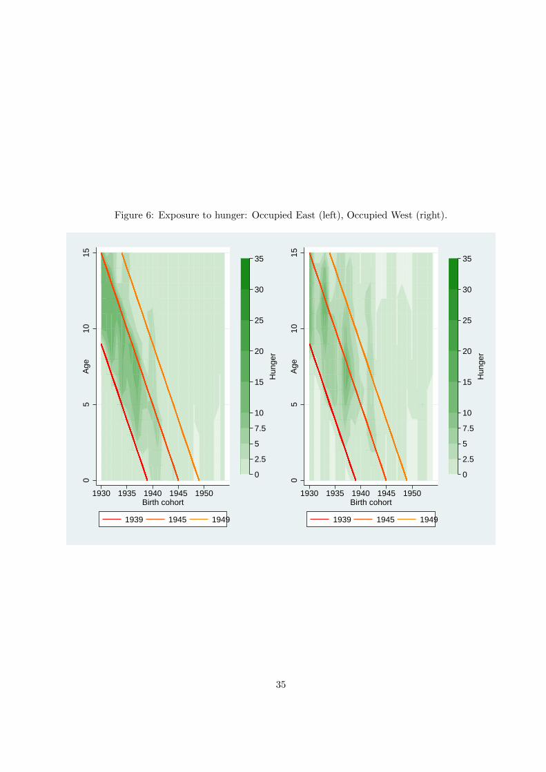
Figure 6: Exposure to hunger: Occupied East (left), Occupied West (right).

05

1015

Age

1930 1935 1940 1945 1950Birth cohort

1939 1945 1949

0

2.5

5

7.5

10

15

20

25

30

35

Hun

ger

05

1015

Age

1930 1935 1940 1945 1950Birth cohort

1939 1945 1949

0

2.5

5

7.5

10

15

20

25

30

35

Hun

ger

35

Figure 7: Exposure to hunger: Spain (left), Sweden and Switzerland (right).

05

1015

Age

1930 1935 1940 1945 1950Birth cohort

1939 1945 1949

0

2.5

5

7.5

10

15

20

25

30

35

Hun

ger

05

1015

Age

1930 1935 1940 1945 1950Birth cohort

1939 1945 1949

0

2.5

5

7.5

10

15

20

25

30

35

Hun

ger

36

Figure 8: Regions affected by major war operations in 1936–45 (number of years).

No war

1 year

2 years

3 years or more

No data

37

Figure 9: Fraction of people born in 1930–39 who report suffering hunger at ages 6–15 by region.

20.0 - 50.017.5 - 20.015.0 - 17.512.5 - 15.010.0 - 12.57.5 - 10.05.0 - 7.52.5 - 5.00.0 - 2.5No data

38

Figure 10: Fraction of people born in 1940–54 who report suffering hunger at ages 6–15 by region.

20.0 - 50.017.5 - 20.015.0 - 17.512.5 - 15.010.0 - 12.57.5 - 10.05.0 - 7.52.5 - 5.00.0 - 2.5No data

39

Figure 11: Fraction of individuals who migrated between countries or between regions of the samecountry during the period 1930–50.

0.0

2.0

4.0

60

.02

.04

.06

1930 1935 1940 1945 19501930 1935 1940 1945 19501930 1935 1940 1945 1950

German Reich Italy Occup. East

Occup. West Spain Neutral

Between countries Between regions

Year

40

Appendix: Quality of retrospective information in SHARELIFE

SHARELIFE asks individuals to remember events that may have occurred very early in life. Relying

on people’s recall is faster, less costly, and the risk of respondents dropping out is much smaller

than in prospective studies (Schroder 2010). However, there are important concerns about data

quality, due to the possibility of recall error and coloring. Recall error arises when individuals do

not remember precisely when and how an event took place in the past, whereas coloring is related

to the propensity of individuals to report information on their past based on their present.

Quality of recall generally depends on three main aspects: the socio-demographic characteristics

of the respondent (age, schooling, etc.), the features of the event (salience, timing, frequency, etc.),

and the survey instrument (Smith and Thomas 2003). Berney and Blane (1998) and Krall (1988)

show that simple socio-demographic information, such as father’s job, accommodation characteris-

tics and past illnesses, can be remembered with good precision after 50 years.

Two approaches are tipically followed when dealing with recall bias or coloring. The first

constructs ex-ante survey instruments to minimize recall bias. The second assesses the quality of

recall ex-post, by validating survey information with the use of external sources or by testing the

consistency of responses across waves of a survey (Haas 2007, Smith 2009, Havari and Mazzonna

2011).

SHARELIFE adopts the first approach by using the Life History Calendar (LHC) method. This

method, developed in psychology, tries to improve the accuracy of recall by using salient events,

such as marriage or the birth of a child, as anchors to recall more complicated or frequent events

(e.g. employment transitions). SHARELIFE uses a computerized version of the LHC that allows

respondents to see on a computer screen the calendar filled in as they answer to questions.

Evaluating ex-post the quality of retrospective information in SHARELIFE is not an easy task

because of the current lack of linkage to administrative records. Garrouste and Paccagnella (2010)

and Havari and Mazzonna (2011) look for evidence of recall bias by analyzing questions that are

repeated in all waves of SHARE, or by integrating SHARELIFE data with more objective historical

macro-data such as GDP growth rates, schooling level, etc.

41