CHILD FOSTERING IN RURAL ZIMBABWE

Bill Kinsey* and Renata Serra**

Work-in-progress Presentation

CSAE Conference on Micro-Opportunities in Africa

Oxford, St Catherine College

9-10 April 2000

Draft. Not for citation. For comments only

Please send comments to Renata Serra (renataserra99@yahoo.com)

* Faculty of Economic Sciences, Business Administration and Econometrics, Free University Amsterdam. ** Department of Statistics, University of Milano-Bicocca, and Centro Studi Luca d�Agliano, Milano.

1. Introduction: The research project

Child fostering involves the shift of some of the responsibilities connected with child rearing from natural parents to other people. Fostering is common in most Sub-Saharan African (SSA) societies, an element of the shared rights and duties among the extended family, and foster parents are mostly relatives. An important feature of fostering in SSA is that it occurs not only as a consequence of the break up of families (death of either parent, divorce) but also for a varied number of reasons in two-parent families. In the latter case it exhibits a temporary and reversible character, and children may be left with relatives for a period as short as few months up to several years. In fact there may be no discontinuity between what can be conceived as normal day sharing of child rearing responsibilities among kin and child fostering proper. Researchers need to adopt a convention based on the length of the period involved, in order to single out fostering cases.

The high incidence of fostering (up to 15-25% of children are commonly found to live with neither parent at any point in time) and its reversible character make this phenomenon a very interesting one from the point of view of understanding kin exchange systems. If fostering emerges out of choice, e.g. it is not just a forced outcome of a �crisis� situation, and kin themselves can decide on its length and features, then it can potentially respond to reciprocal needs for assistance, exchange over time, and economic support. This is more than a mere possibility and existing studies on fostering (mainly by anthropologists and demographers) point to the amenability of fostering arrangements to mothers� need to work and emigrate, to parents� inability to cope with large family sizes at some point in the life cycle, and to foster parents� willingness to keep an active link with other family members in view of future support.1

However, existing evidence is based mostly on qualitative data, or in any case on a single observation. Cross section data are most unsatisfactory to understand the nature of fostering arrangements, whose most important feature is intertemporal. The sending of children to relatives may be a tacitly acknowledged counterpart to a previous transfer of goods or services, or to an anticipated need for future support (Serra 1997). The child�s age and sex are also fundamental to understand whether fostering involves an immediate transfer of costs or benefits: a very young child certainly requires attention and resources whereas an older child, especially a girl, can be an asset to the foster family if she contributes household labour.

Our endeavour here is to analyse mainly the intertemporal dimension of fostering arrangements. It is based on a unique panel data set from rural Zimbabwe, for which detailed household level data have been collected since 1983 and annually since 1992. For the years 1997-99, and in some cases also for 1994-96, we have specific information on resident and non-resident children, and on their present or absent parents. This data will thus form the core data for our study. The children targeted for this more detailed data collection are aged seven years or less, but similar information also on older children 1 Ainsworth (1992); Blanc and Lloyd (1990); Bledsoe (1994); Etiènne (1979); Goody (1982); Isiugho-Abanihe (1985), Lallemand (1976).

will be available from the survey rounds 2000-01, providing a wider scope to the project in the future.

The objectives of this analysis are twofold. Firstly, to examine the extent to which fostering of young children (which can be interpreted unequivocally as a transfer of immediate costs) can represent a response to non-covariant past shocks to the households concerned. The hypothesis is that fostering serves an insurance purpose as an ex-post consumption mechanism. Both household-level exogenous income shocks and individual-level health shocks will be taken into account to assess the potential different role of fostering in these two instances.2 The importance of fostering as a risk insurance method will be assessed against other mechanisms (livestock, transfers and credit).

Households in poor agricultural settings resort to a variety of mechanisms in order to cope with the high risks (mainly weather related) affecting their incomes. These can be either income smoothing (ex-ante mechanisms) or consumption smoothing (ex-post) (Murdoch 1995). Among the former we have crop diversification, plot separation and differential occupations between family members; in the latter group, rural credit and saving markets, cattle, accumulation of other assets such as cereal stock or valuables, and informal kinship networks. Child fostering belongs to this very last category, the one for which we have the least knowledge in terms of its potential role in consumption smoothing. Evidence points to a limited ability of farmers in SSA to protect their consumption from negative shocks: for many poor farmers consumption fluctuations over time are not significantly smoother than income fluctuations (Deaton 1992, Udry 1994). However, existing studies are too few to reach a conclusion and more empirical research is needed into these issues.

A previous study has shown that cattle sales have represented a major response after drought for our sample of resettled Zimbabwean households (Kinsey, Burger and Gunning 1998). However, the extent to which consumption shortfalls have been protected by this means alone is not entirely clear. The contribution of alternative mechanisms thus need to be examined directly. This analysis partly fills this gap by focusing on kinship networks (which have been shown to play a fundamental consumption smoothing function in India, see Rosenzweig and Stark 1989). Child fostering is not only an important component of kinship networks, but is also one that enables us better to identify, and connect, the identity of the two parties (natural and foster parents) in a household survey, unlike other types of inter-household transfers, whose provenance is usually unknown.

The second objective of the larger project of which this analysis is part is to assess the consequences on foster children�s health of living with neither parent, controlling for household income and other characteristics. A few studies from other parts of the continent have warned against possible negative effects of fostering on child health (Castle 1995). Such effects may be a consequence not just of risks falling unevenly within the household, but also of household coping-mechanisms having different effects on

2 One could test, for instance, whether fostering responds more to individual shocks, especially of mothers, than to overall household shocks (see also Serra 2000).

individual family members. Although there may be compensating mechanisms, evidence so far shows that the household is far from representing the locus of full-risk sharing (Dercon and Krishnan 2000). Possibly, the particular type of response to risks that households choose is a function of the relative bargaining powers of individual members. The power of children less than seven years of age is the weakest (while older children have been reported to walk out of the foster house in some cases) and it is thus vital to examine what are, if anything, the mechanisms under which their welfare becomes most at risk.

One needs to consider that, underlying the notion of fostering as a risk insurance mechanism, there is the hypothesis that relatives know one another�s characteristics and can monitor each other�s behaviour to a significant extent, thus reducing adverse selection and moral hazard problems. This implies that natural parents should have not only a prior knowledge, but also a posterior understanding, of the child�s living condition in the foster home. Therefore, if fostering has detrimental effects on children, either reciprocal monitoring is not effective (because of geographical distance or other reasons) or natural parents accept the outcome as the price to pay for greater security, in the absence of alternative choices. Both possibilities should be examined.

This paper represents only the very first phase of this project.3 The rest of the presentation is organised as follows. Section 2 describes the data set and presents an overview of fostering in these communities over the period 1997-99. Section 3 exposes the theoretical analysis underlying the understanding of child fostering arrangements between relatives as an ex-post adjustment to exogenous income shocks. Section 4 presents preliminary estimation results of the cross-section analysis for the year 1997. However, a full understanding of the significance and role of fostering will be possible only with the analysis of the whole panel for the years 1994-2000.

2. Data description and main characteristics of in-fostering and out-fostering households

The data come from an 18-year panel study conducted by one of us (Kinsey). The initial sampling frame was all resettlement schemes established in 1980 and 1981--the first two years of Zimbabwe�s land reform programme. Households in the panel reside in schemes across three different agroclimatic zones and come from cultures with only minor differences in characteristics and practices. One scheme was selected randomly from each zone. One lies some 120km north of Harare in a high-potential zone. The second is situated 130km southeast of Harare in a zone of medium potential, while the third lies 300km southeast of Harare and in a zone of low and restricted potential. Random sampling was then used to select villages within schemes, and in each selected village an attempt was made to interview all households.

3 Due to the fact that the data on income and assets from the 1998 and 1999 survey rounds have not been fully cleaned and edited, we are able to present here only the first stage of our analysis.

These households were first interviewed during 1983 and 1984 and then were re-interviewed in the first quarter of 1987 and annually, during January to April, from 1992 to 2000. There has been remarkably little sample attrition. Approximately 85 percent of households interviewed in 1983/84 were re-interviewed in 1999. There is no systematic pattern to the few households that drop out. Some were inadvertently dropped during the re-surveys, some left the resettlement schemes for unknown reasons, a few disintegrated (such as those where all adults died) and a small number were evicted by government officials responsible for overseeing these schemes.

In addition, beginning in 1997, a second panel was constructed from among the communities of origin of those who resettled in the early 1980s. These communities lie in Zimbabwe�s so-designated Communal Areas (CAs). For each of the three resettlement areas (RAs), the two communities were selected, which had supplied the most households to the resettlement panel. In each of the resulting six communities, 25 households were randomly selected.

The data used in the paper thus come from two different panels: one of some 400 long-resettled families and the other of 150 families, which either chose not to relocate or were not selected to receive land. Prior to the period analysed in this paper, the households in the two panels differed in significant ways. Some of these differences persist while others have fallen away.

First, the families in any CA community will normally belong to the same lineage, a factor likely to facilitate local fostering. RA families, in contrast, were allocated their arable and residential plots by random draw, so that resettled villages are commonly inhabited by people who are unrelated and who were initially strangers. Prohibitions on transfers of plots in RAs have meant that villagers have been unable to rearrange themselves spatially.

Second, all households have been subject to factors that tend to induce increased mobility on the part of adults�either temporarily or permanently, thus raising the issue of what to do with young dependants. The sequence of droughts that occurred in the 1980s and 1990s stimulated searches for non-agricultural income-earning opportunities, either in the neighbourhood or through out-migration to more remote places.4 RA households, however, were prohibited from seeking off-farm employment throughout the 1980s, and this prohibition, which appears to have been strictly enforced, was only relaxed in the early 1990s. This latter period however also saw the introduction of Zimbabwe�s adjustment programme, which radically reduced the possibilities for securing formal sector employment in an urban area. Indeed, there is evidence in the panel data set that members of resettled households who once held urban-sector jobs have been returning home in ever greater numbers.

Third, all RA households command an identical amount of arable land, which is on average more than twice the area commanded by CA households and which is also generally of higher quality than land in the CAs. This fact means that resettled 4 See Kinsey, Burger and Gunning (1998) for a treatment of the strategies resettled households employed to cope with the droughts of 1992 and 1995.

households have a greater potential to earn a reasonable living from farming and thus have a stronger incentive to remain on their land. RA households however cannot legally subdivide their plots to provide land for their adult sons, and there is no further land in the RAs that can be allocated to those needing it. RA households therefore tend to be large and multigenerational, with married sons grudgingly farming as their fathers� unpaid labourers. When RA households do divide, the lack of land compels those who leave to move completely out of the area. In contrast, adult children tend to leave CA households, either when they secure a job or when the village headman allocates them their own plot of land in the same locale. And male household heads are more likely to be working elsewhere, resulting in a higher proportion of female-headed households.

As a combined result of these factors, the average total household income in all RAs in 1996/97 was 50 percent greater than in the CAs (Kinsey 1999). The components of the average income were strikingly different however. Crop and livestock income was more than six times higher among RA households than CA households, while income and transfers from all non-agricultural sources was more than twice as high in the communal areas as in resettlement areas.

Finally, rural-urban migration by males, together with temporary visits to rural areas, are an important mechanism by which HIV is passed from urban areas - where the disease is widespread - to rural areas. The prohibition on male household heads migrating for employment was in force until 1992, a factor which - combined with the relative isolation of many resettlement villages - makes us believe that the incidence of HIV/AIDS in the RAs under study here is lower than in many other parts of the country. If true, there may be a bias toward RAs fostering in children from other areas.

In this section we focus mainly on data for 1997-99, since useful information from the viewpoint of child fostering has been collected only recently. Households from the high potential area represent the majority (55%) of the sample with which we start the analysis, e.g. households with at least one resident child less than seven years of age. The rest is divided between households from the area with medium potential (24%) and those with low potential (21%).

Out-fosters

Information on out-fostering in this sample is less detailed than that on in-fostering. In fact, there is only a small section on changes in household size and composition, reporting whether household members have left during the previous year, for what reason and their new location. At this stage of the analysis, we can give only a cursory treatment of out-fostering.

Our sample contains 324 observations on children reported away at the time of the interview, in any of the surveys 1996-99. The majority of them were away with either parent, but 103 (32 percent) can be considered as out-fosters, e.g. children staying normally away with neither parent. Since the question was asked with whom the absent child was staying, four categories of carers other than natural parents can be identified: grandparents, aunt/uncle, sibling, and other relative. The first category is by far the most

important, given that two-thirds of out-fosters are found to stay with grandparents, whereas one-quarter stay with an aunt or uncle (see Table 1).

There are 77 households that have fostered out in total, and of these 8 have fostered out two children (none has fostered out more). An interesting aspect is the positive relationship between out-fostering and degree of potential of the area where the household is located. As mentioned before, there are two panels of households, those living in resettled (RA) and in communal areas (CA) respectively, and, in each, households have been selected from three areas with different agricultural potential: high, medium and low.

Regarding this latter distinction, we note that most of the households that have fostered out a child come from the high potential area (over 63%), a much lower percentage comes from the medium potential areas (25%) and even less from the low potential areas (12%) (Table 2). When weighting these values with the values from the distribution of observations in the original sample (respectively, 55.02%, 23.58% and 21.4%), we observe that high-potential-areas households foster out significantly more than their proportion in the sample would predict, medium-potential-areas households foster out just over their sample weight, but households in low potential areas are half as likely to foster out. Moreover, it is the households from the communal areas that foster out the least, especially if they reside in the medium and low potential areas. In conclusion, in this sample, out-fostering is mainly observed among the RA households of the high and medium potential areas.

In-fosters

The household questionnaire contains a section on the health and anthropometrics of each child less than seven years of age living in the households and of his/her parents, if present in the household. This section gives information on whether parents of each child are present and, if not, the reason for their absence and their current location. The identity code of each child is linked also to that of the full siblings, so that the identity of mother and father can be cross-checked. Our panel contains detailed information on one child of each full sibling group rather than on each child living in the household; this means that each observation refers to a �target� child and other children in the household of the same mother and father. This should be borne in mind throughout this paper, as we will not specify at all times that what we are really speaking about are �target� children within each sibling group.5

Putting together the RA and CA panels, we obtain a sample of 1027 children seven years of age or younger, observed at least once between 1997 and 1999. As can be seen from the top of Table 3 the panel is rather unbalanced, with just over a fifth of children observed for three consecutive years (one reason for this is certainly the fostering out of 5 These �target� children constitute a rolling cohort, which has been a particular focal group for assessing changes in welfare among panel households. Each year those children born in the previous year enter the cohort, while those who have passed their seventh birthday leave it. Far more detailed information is available for children in the cohort.

some children). These children belong to 458 households (there are 550 households in the panel for the Zimbabwe Rural Household Dynamics Study).

We have been able to identify with a certain degree of accuracy those children, whose parents do not live with them, either because they left the household where the child resides or because they have given the child to another household. All children whose parents live and work somewhere else are treated as in-fosters, even when their parents are considered to be household members by the respondent. The following describes how the subset of in-foster children has been obtained.

Initially, each child�s parent has been given a code to represent his/her resident status (called codeM and codeF respectively for mother and father). The identified categories are: 1, resident in the household; 2, living and working away but still household member;6 3, away and no more household member; 4, deceased; 5, divorced, never married, run away or married to another partner; 6, unknown (of fathers); 7, never been household member (Table 4).

Table 6 shows the distribution of children according to both parents� code, by year. It appears that, although the majority of children each year are found to live with both parents (between 56% and 62%), there is also quite a remarkable variety in child-parent living arrangements. The relatively high proportions of children living with just one or neither parent confirm findings from previous studies, in Zimbabwe and other countries in SSA (for a cross-country comparison see McDaniel and Zulu 1994).

We note two aspects here. One, if a child lives with just one parent, he/she is much more likely to stay with the mother than with the father. The proportion of children living with just the mother goes from 22% in 1997 to 26% in 1999, whereas the proportion of children living just with the father is around 2.40% in 1997 and rises to 3.40% in 1999. This is not surprising, since these children are very young and when parents separate, even in patrilineal societies such as these, a child is expected to stay with the mother until at least seven years old. The child may be sent to the father and its lineage only at a later stage, and in any case only if bridewealth (roora) has been paid in full to the mother�s lineage.

Two, there appears to be an increase of foster children over time, with the percentage of own children in the sample decreasing from 62% in 1997 to 56% in 1999. It will be shown further below that this is not simply due the unbalanced panel, which changes the number of children observed every year, but also to the fact that some of the children initially living in two-parent households are found living with no parents one period afterwards.

6 The existence of an ID No in the household roster is what determines whether a person is or ever has been considered a member of that household. It may happen that one year a parent is given an ID even if working away, while the next year he/she is no longer considered a household member: changes in residence take time to complete and to be so perceived by other household members. When a parent has an ID No and works somewhere else, but there is no specific information about residence, the conservative estimate has been adopted that a parent can be considered as mostly residing away from home if the work location is more than 100km distant.

From the code assigned to each parent, which summarises residence and marital status characteristics, we can identify different categories of children. The first distinction to make is between foster and non-foster children, the former identifiable by both parents having a code two or greater (e.g. not living normally in the household where the child resides).

Secondly, among non-foster children, we distinguish between those living with both parents and those living with just one parent, as the latter may be worse off and receive less care and resources. Living with just the father at a very young age implies that a child is de facto cared for by another woman, such as the father�s new wife, who is likely to give less care � both in quantitative and qualitative terms - than to her own children. This is also why several studies accept maternal non-residence as a proxy for fostering.7

Living just with the mother, however, also presents difficulties for the child, since women�s access to financial and other resources is usually more constrained. Evidence from different parts of the world shows that children have, ceteris paribus, better nutrition and health scores when they stay with the mother than when with the father, but this effect can be offset by the mother�s lower income and wealth. Moreover, a study on the same Zimbabwean data has shown that children living with their mother in her natal village suffer harsh competition for resources, because they are not considered to belong fully to the lineage (provided that some roora has been received) (Hoddinott and Kinsey 1998).

Thirdly, among children living with neither parent, the situation of fostering arising out of a family crisis is distinguished from the one where parents are likely to be together. Family crisis means that parents are divorced or one parent has run away, denied responsibility or died (in practice, this involves taking combinations of mother�s and father�s codes in the interval between 4 and 7, with the exceptions explained below, see Table 5). The other category instead includes cases where parents are reported as working and living elsewhere (mother�s or father�s code equal to 2 or 3). We include in the non-crisis fostering category also those cases where both parents are reported not being members of the household, as here survey responses do not refer to any particular family crisis (both mother and father are coded 7). We have instead excluded from either fostering category the instances where both parents are dead (8 cases overall) since these are clearly non-reversible situations, and here fostering is compulsory (they have been added to category 2 instead). Both categories 3 and 4, on the other hand, imply that at least one parent has chosen to leave a child with relatives, although this choice may be interpreted as more constrained for the instances in category 4, because of the difficulties associated with no marriage or subsequent marital break up.

Table 5 shows how an overall index (indexP) representing both parents� situation has been derived from combining the seven typologies previously identified for each parent.8

7 Page (1989) and, in general, many studies carried out on the basis of the WFS and DHS. 8 Some amount of information is thus lost when constructing indexP from codeM and codeF, but it has been thanks to the richness of information derived from codeM and codeF that the final categories for indexP could be confidently considered as the only relevant ones.

In-foster children in our sample are those associated with a parental code 3 or 4. Admittedly there is a certain degree of arbitrariness in the function mapping mother�s and father�s code into one parental code, but only as far as the distinction between category 3 and 4 is concerned. In any case, this is the best that can be done to draw some distinction between crisis and non-crisis fostering. Estimation results will not be biased by this distinction anyway, and in-foster children will be often treated as one category (e.g. 3 and 4 categories will be put together).

The panel described in the bottom half of Table 3 is the one which is the basis for our analysis of in-fostering behaviour. It contains observations on the 134 households that have at least one in-foster child, and 296 �target� children living in them. Not all of them are in-fosters, since own children also live in households where foster children are found. The great majority of households have only one foster child (88%) but a small percentage has two or three in-fosters.

Table 7 shows the distribution of children according to indexP and by year. The pattern identified from Table 6 is better discernible here, where it appears that the decline in the proportion of children living with both parents over the period 1997-99 is mainly due to an increase in the proportion of children living with just one parent (from 25% to 30%). As mentioned before, due to the unbalanced nature of the panel, we cannot tell whether the decline in the proportion of own children reflects real changes or is due to a lower number of own children �targeted� in our sample in one year with respect to previous years.

We calculated the transition probabilities associated with indexP, in order to track changes in child-parent residential status for those children for whom there are at least two observations in time (Table 8). The columns values indicate the starting state and the rows yield the final state. The first row shows that over 10% of children living with two parents are subsequently found to live with just one parent or neither parent, whereas movement back to state 1 (children living with two parents) is much less likely (see column 1). Fostering induced by parental crisis and family break up (state 4) is a frequent outcome; for instance, half of children living with just one parent in 1997 or 1998 move to state 4 the year after. Out of all child-parent arrangements, the one corresponding to living with just one parent is the least stable (the lowest value on the main diagonal), implying that when child rearing responsibilities fall on just one parent, the latter is likely to pass them on soon to other relatives. Overall, Table 8 points to an increasing variability in child-parent living arrangements over time and to a rising number of children living without either or both parents.

Considering now the households that foster in children, it is remarkable to note that 30% of all households with a young child foster at least once in 1997-99 (Table 9). This is indeed quite a high percentage, underlining the importance of the phenomenon of fostering in these households. As far as area is concerned, households from high potential areas foster in less than the average, those from low potential areas just about the average, and households from medium potential areas significantly more than the average (about 42% of these households have ever had an in-foster child). Moreover, whereas CA households are less likely to foster in children than RA households in all areas, the

contribution of in-fostering by CA households in the medium potential areas is remarkably high, and comparable to RA households.

Conditional on the probability of ever having fostered in, there is a negative relationship between the number of children fostered per household and an area�s potential: low-potential area households are relatively more likely to foster in two or three children than households from high-potential areas (Table 10).

In conclusion, in our sample, the higher is the potential of the area of residence the more likely is a household to foster out and the less likely to foster in. Moreover, RA households are more likely to both foster in and foster out. In order to understand what can drive this empirical fact, we need to spell out the set of relationships, which might determine whether a household fosters in or out. This is done in the model in the next section.

3. The model In the following, we model the situation in which there are only exogenous income shocks (to household and not individual income), thus assuming away health shocks. This is a simple setting where adult labour supply to household production is fixed, as there is neither a labour-leisure choice, nor the influence induced by nutrition and health variables. (Further elaboration will come at a later stage of the project, when data on health status and shocks are available.)

Each household is assumed to maximise an inter-temporal utility function, which is separable over time periods, and where instantaneous utility is a function of current consumption, taken to be a homogeneous good:9

( )∑=

−∂=T

tt

t cuUτ

τ [1]

The homogeneous consumption good is produced by the household according to a production function that uses as inputs the labour of the household members (assumed as fixed, e.g. there is no labour-leisure choice) and cattle. As is customary, the inputs to current income are indexed one period earlier, because of the delayed nature of the production process in agriculture. Each household is subject to a wealth constraint such as:

( ) ( )ttttttt NAcAlLYW

rW

α+−+=+ −−

+11

1 ;1

[2]

In this section we assume that the wealth consists only of livestock, so that (1+r) is the net return from livestock (e.g. the addition to the stock following the birth of a new calf). There is no price variability and everything is measured in terms of the homogeneous consumption good.

9 The model of this section is adapted from Serra (2000).

Let us now consider how the problem of utility maximisation is transformed when we take the more realistic scenario of a risky world. In an uncertain environment, the income of the household is subject to exogenous shocks, which affect either the inputs (health shocks reducing the labour supply of working household members or mortality affecting cattle), or the process by which inputs are translated into output, mainly weather risks. We focus here on the latter type of shocks and assume that the probability distribution of the weather income shocks is unchanging and that households know this distribution. This means they know the values that the stochastic variable can assume and the effects on next period production, but they cannot predict future values and will observe only income realisations ex-post.

Among the strategies that households in poor countries are found to put in place in order to protect consumption from income fluctuations, we consider two here: accumulation and sale of livestock and child fostering. After a negative shock, a household can thus either sell livestock or foster a child to another household. Livestock sales produce an immediate return, which needs to be set against the forgone income following lower livestock inputs into future production process. The fostering out of a child also releases resources immediately (the foregone cost of child consumption); future outlays are represented, as anthropological evidence shows, by transfers in services and goods that natural parents or the child itself make to the foster parents. Even if fostering is rarely accompanied by an agreement on compensation, it is intended that natural parents or their children will sooner or later show their gratitude to the carers, and the latter expect this (Bledsoe 1990, 1994). To simplify, it is assumed here that the transfer to the foster by the natural parents is known in advance, is fixed over time and across households, as if set by an implicit norm.

The intertemporal utility function under uncertainty, when S are the possible states of the world in each period, is:

( )∑∑==

−=S

s

st

sT

t

t cupU1τ

τδ [3]

The intertemporal constraint [2] becomes:

( ) ( ) 11; −− −+=−+ tttttttttt TfsPLlALYfNAc [4]

where 0<st<1 is the proportion of the cattle being sold in period t, at the fixed price P, and ft is the net number of children fostered out at time t. The variable ft assumes a negative or a positive value according to whether (more) children are fostered out or in.10 T represents the fixed compensation accruing to foster parents the period after a child has been fostered. If a child fostered in period t continues to stay in the foster household in period t+1, T is paid out not only in period t+1 but also in period t+2, and so on.

10 We consider here the possibility that households can foster in and out simultaneously, as evidence shows that this occurs often. In the case of older children, this may be due to a household fostering in for a labour-related reason and fostering out for educational/promotional purposes; also when parents care differently for their own and foster children (Serra 1997).

Note that we could have considered additions to this simple model, such as the fact that current benefits accrue from selling livestock products, but this would not have changed much the results. The equation governing the rate of growth of the livestock is the following:

( )( )rsLL ttt +−=+ 111 [5]

and the right-hand expression is what actually enters the production function the next period. Timing of events is therefore as follows: t harvest: realisation of Yt sales of livestock and fostering of children; consumption available inputs go into the production process to produce Yt+1 occurrence of weather shocks t+1 harvest: realisation of Yt+1 etc.

The household maximises utility function [3] subject to constraint [4] with respect to the choice variables st and ft. The two first order conditions are obtained:

0/

1111

=−+

∂∂∂∂−

−+∂∂=

∂∂

++++ ttt

tt

tttt

tt

tt fNALY

cU

fNALp

cu

sU [6]

( )( )

( )( )

02111

111

12 =

−+−+

∂∂−

−+−+

∂∂=

∂∂

+++

+++

+ ttt

ttt

tttt

tttt

tt fNAfNAT

cU

fNAfNAc

cu

fU

The conditions [6] above yield the equality between the intertemporal rates of return of, respectively, selling livestock and fostering out children, and the marginal rate of utility substitution between current and future consumption:

ttt

tt

t

t

cT

LpLY

uu

=∂∂

= +

+

/'' 1

1

[7]

The superscript s, for state of nature, has been omitted for simplicity but it is intended that the above equality should hold across states of nature. The case for households which experience a positive income shock is thus symmetric, with positive income shocks inducing households to �invest� in current resources in order to be better able to cope with future income downturns. One typical strategy is that of accumulating livestock, by purchasing them in the market. An alternative is to accept other people�s children in the household, not just out of kinship duty, but because this generates a �credit� towards the natural parents of these children. The hypothesis here is that this second strategy might have analogous effects in settings where fostering is widespread and highly reversible. Therefore, after either a negative or a positive income shock, the two strategies may be regarded as alternatives, with the adoption of one decreasing the extent of the other, other things being equal.

The above framework leads us to a formulation of the reduced form equation for the number of out-foster and in-foster children as the dependent variable:

( )( )DsLNBNTRfDsLNBNTRf

ttti

t

ttto

t

χϕδγσβαχϕδγσβα

−++++=

+−−−−=

−

−

****

****

1

1 [8]

It is better to estimate the equations for in- and out-fostering separately, to allow, if not for different independent variables, at least for different coefficients on these variables (Ainsworth 1991). Equations [8] predict fostering out (in) to be a function of previous negative (positive) income shocks (e.g. -σt-1 or +σt-1), other things being equal. In particular we control for substitution effects with other means of smoothing consumption, such as net transfers from family members (NTR), net borrowing (NB) and livestock sales/purchases (Ltst). The need for out-fostering should decrease when transfers or credit are received and when cattle are sold (hence the negative signs on coefficients for NTR, NB, and s). In-fostering instead should decrease if the household makes transfers, lends money out, or buys cattle (NTR, NB and s will in this case take negative values, hence the positive sign for the coefficients). Finally, we control for a number of exogenous demographic variables (D), such as the number of siblings, household size, either parent�s death and parents� age and marital status (in particular divorce or either parent�s death increase the probability that a child will live with neither parent). The coefficients on the demographic variables are of opposite sign for in-fostering and out-fostering.

4. Some preliminary empirical analysis

In this paper we cannot present the results from the empirical analysis for the panel 1997-99 because data for income, assets, livestock and other important variables are not yet ready for the years 1998-99. However, in order to give a flavour of the implications for empirical analysis of the model sketched in the previous section, we will present the result of the estimation using data from the 1997 cross section.

In 1997 just over 12% of all (target) children less than seven years of age were in-fosters (a percentage slightly lower than for 1998 and 1999). Our sample contains 316 households and 505 target children aged seven years or less.11

Equation [8] from last section predicts that the probability that a child is an in-foster should be positively related to previous positive income shocks experienced by the receiving household and negatively related to the latter�s purchase of livestock and other means of investing resources (making transfers to relatives or giving credit), controlling for demographic variables. 11 Since there is no information on income and assets for the CA sample before 1997, we have restricted analysis here to the RA sample. Out of the total 400 households in this sample we are left with 316 households, which have at least one child less than seven years of age and for which we have all relevant information.

In view of the exploratory nature of this analysis, we have constructed a (very rough) measure of income shocks, VarInc96-97, which measures the variation in real total income between 1996 and 1997, weighted by real income in 1996.12 The agricultural year 1994-95 was one of drought and consequently incomes were quite low in the following year; 1995-96 was instead a particularly good agricultural year and the incomes recorded in 1997 were among the highest in the last decade. This is reflected in the fact that the income variation between 1996 and 1997 is negative only for 40 of the 316 households. Income variation goes from a minimum value of �97% to a maximum of +9406%, and the mean value is +406%.

Table 11 shows the simple correlation coefficient between the probability of being an in-foster (value equal to 1 if a young child is an in-foster and equal to zero otherwise) and various sociodemographic variables. The probability of being in-foster is not significantly related to any of the economic variables of the first column, except for livestock market value, which is a good proxy for wealth in these communities. The observed negative relationship with per-capita total food expenditures would suggest that the latter decrease for households that foster in children; and the negative sign for both livestock sales and cereal stock would support the notion of substitutability between in-fostering children and these other means of investing surpluses. However, the coefficients are not significantly different from zero at conventional levels.

The second column shows that, whereas current and past income variables are insignificantly related to the probability of a child being an in-foster, the correlation with the variation of current to past income is highly significant. The third column of Table 11 shows that household size, number of total children and number of own children in the household are all significantly correlated with the probability of a child being an in-foster. The probability of being fostered is also positively related to area typology (ordered from high to low potential areas) confirming what was found in the previous section, e.g. that households from medium and low potential areas are more likely to foster in than households from high potential areas.

Table 12 shows the results of the probit analysis. The probability of a child being an in-foster appears to be positively related to a positive variation of current to past income and with area typology, and negatively related to household size and number of total children less than seven years of age. All coefficients are significant at conventional levels.

However, this result cannot be taken to confirm the hypothesis that child fostering serves an insurance function. Firstly, one should be able to show that both in-fostering and out-fostering respond to income shocks. Secondly, var9697 is not an appropriate measure of transitory income shocks. Thirdly, neither livestock sales nor remittances have any significant correlation with fostering, possibly questioning the insurance hypothesis.

12 This is a very imprecise measure of income shock, and the correct procedure would be that of measuring the impact of transitory rainfall variation on total crop income (or crop output) in order to identify a component of income that is both exogenous and transitory (see Fafchamps et al 1998). We will follow this procedure in the analysis of the panel data set.

What this preliminary exploratory analysis has established is that fostering responds to demographic, income and asset variable, and thus may have an important economic function. Full analysis of the panel data set in the second phase of our project should be able to establish whether this function is reciprocal risk-insurance or some other type.

Another aspect to follow closely is the result that in-fostering is higher in low potential areas (whereas out-fostering seems to be higher in high potential areas as seen in section 2). This is counterintuitive with respect to the hypothesis of risk-insurance, since households in high potential areas can be expected to be subject to less severe or less frequent negative shocks than the others, and be better equipped with alternative insurance mechanisms. It is still unclear at this stage why households from high potential areas should foster in less and foster out more. It is instead less surprising that RA households are more likely to foster in and out than CA households, as found in section 2. Movement by RA households has been limited by different factors (during the 1980s prohibition of leaving the assigned plot to take up non-farm jobs and more recently economic crisis in the urban job markets). Possibly, child mobility has taken place to a greater extent to compensate for lack of adult mobility.

REFERENCES Adepoju Aderanti and Oppong Christine (1994) Gender, Work and Population in Sub-Saharan Africa, London: James Currey.

Ainsworth Martha (1992) �Economic aspects of child fostering in Côte d'Ivoire� Living Standards Measurement Study Working Paper No. 92, The World Bank.

Blanc Ann K. and Lloyd Cynthia B. (1990) �Women�s childrearing strategies in relation to fertility and employment in Ghana� Population Council Research Division Working Papers No. 16.

Blanc Ann K. and Lloyd Cynthia B. (1994) �Balancing productive and reproductive roles� in: Adepoju and Oppong, eds.

Bledsoe Caroline (1990) �The politics of children: Fosterage and the social management of fertility among the Mende of Sierra Leone� in: W.P. Handwerker, Births and Power. Social Change and the Politics of Reproduction, Boulder, CO: Westview Press.

Bledsoe Caroline (1994) ��Children are like young bamboo trees�: Potentiality and reproduction in Sub-Saharan Africa� in: K. Lindahl-Kiessling and H. Landberg, (eds).

Castle Sarah E. (1995) �Child fostering and children�s nutritional outcomes in rural Mali: The role of female status in directing child transfers� Social Science and Medicine, 40 (5): 679-93.

Deaton Angus (1992) �Saving and income smoothing in Côte d�Ivoire� Journal of African Economies 1 (1): 1-24

Dercon Stefan and Krishnan Pramila (2000) �In sickness and in health: Risk-sharing within households in rural Ethiopia� Journal of Political Economy, august (forthcoming).

Etiènne Mona (1979) �The case for social maternity: Adoption of children by urban Baulé women� Dialectical Anthropology, 4, 237-242.

Fafchamps M, C. Udry and K. Czukas (1998) �Drought and saving in West Africa: Are livestock a buffer stock?� Journal of Development Economics 55:273-308.

Goody Esther (1982), Parenthood and Social Reproduction. Fostering and Occupational Roles in West Africa, Cambridge: Cambridge University Press.

Hoddinott John and Bill Kinsey (1998) �Child growth in the time of drought�, mimeo.

Isiugo-Abanihe Uche C. (1985), �Child Fosterage in West Africa� Population and Development Review, 11 (1), 53-73.

Kinsey, B. H. (1999) Report of the study on the Determinants of Rural Household Incomes and their Impact on Poverty and Food Security in the Resettlement and Communal Areas of Zimbabwe, Rome: Food and Agriculture Organization.

Kinsey, B. H., K. Burger and J. W. Gunning (1998) �Coping with drought in Zimbabwe: Survey evidence on responses of rural households to risk� World Development 26, 1.

Lallemand Suzanne (1976) �Génitrices et éducatrices Mossi� L'Homme 16 (1), 109-24.

Lesthaeghe Ron (1989) Reproduction and Social Organization in Sub-Saharan Africa, Berkeley: University of California Press.

McDaniel Antonio and Zulu Eliya (1994) Mothers, Fathers and Children: Regional Patterns in Child-Parent Residence in Sub-Saharan Africa, mimeo, Population Studies Center, University of Pennsylvania, Philadelphia.

Murdoch Jonathan (1995) �Income smoothing and consumption smoothing� Journal of Economic Perspectives 9 (3), 103-14.

Page Hilary (1989), �Child-bearing versus Child-rearing: Co-residence of mothers and children in Sub-Saharan Africa� in R. Lestaeghe (ed.).

Rosenzweig Mark R. and Stark Oded (1989) �Consumption smoothing, migration and marriage: Evidence from rural India� Journal of Political Economy, 97 (4), 905-26.

Serra Renata (1997) Fostering in Sub-Saharan Africa: An economic perspective, Centro Studi Luca d�Agliano and Queen Elizabeth House, Development Studies Working Papers, No. 110. October.

Serra (2000) �A framework to study child fostering arrangements and their interaction with household-level strategies in SSA� mimeo.

Udry Chris (1994) �Risk and insurance in a rural credit market: An empirical investigation in Northern Nigeria� Review of Economic Studies, 61 (3): 495-526.

Table 1. Out-foster children: distribution by type of carer

Observations Children

Carer N % N %

Grandparent 66 64.08 51 66.23

Aunt/uncle 26 25.24 21 27.27

Sibling 4 3.88 4 5.19

Other relative 7 6.8 5 6.49

Total 103 100 81 105.19

Table 2: Households that have fostered out at least one child: by area of residence

Households

Weight in the full sample

Area N % %

HIGH (TOT) 49 63.64 55.02 RA 40 51.95 46.07

CA 9 11.69 8.95

MEDIUM (TOT) 19 24.68 23.58 RA 16 20.78 16.59

CA 3 3.9 6.99

LOW (TOT) 9 11.69 21.4 RA 6 7.79 12.88

CA 3 3.9 8.52

TOTAL 77 100 100

Table 3. Panel on children seven years old or less

All children

Years covered

Observation per child

No of children N %

Number of observations

1997 1 228 22.20 228

1998 1 114 11.10 114

1999 1 168 16.36 168

1997 & 98 2 130 12.66 260

1998 & 99 2 106 10.32 212

1997 & 99 2 58 5.65 116

1997-99 3 223 21.71 669

TOTAL 1027 100.00 1767

Only children from households that have at least one in-foster

Years covered

Observation per child

No of children N %

Number of observations

1997 1 80 27.03 80

1998 1 50 16.89 50

1999 1 74 25.00 74

1997 & 98 2 27 9.12 54

1998 & 99 2 36 12.16 72

1997 & 99 2 7 2.36 14

1997-99 3 22 7.43 66

TOTAL 296 100.00 410

Table 4. Codes for either Mother or Father

CodeM or CodeF

Key

Code label

1 Resident: present or away but only temporarily

Resident

2 Work and live away, but is still considered a HH member

Workaway

3 Work and live away, but not HH member AwaynoID

4 Deceased Deceased

5 Divorced, run away, married elsewhere Divorced

6 Unknown (of fathers) Unknown

7 Never been a HH member NotHHM

Table 5. Child-parent living arrangements: Categories for parental code (IndexP)

CodeM CodeF* Key IndexP

1 1 Both parents live with the child

1 Two parents

1 2-7 4

2-7 1 4

Only one parent lives with the child or both are dead

2 One parent

2-3 7

2-3 7

In-foster: parents live together somewhere else

3 In-foster

2,3,4-7 5-7

5, 7 2-4, 5, 7

In-foster: parents are divorced or one is dead or ran away

4 In-foster crisis

*CodeF does not include value 6

Table 6. Distribution of children according to mother�s and father�s codes, by year (Percent values)

Year CodeF

CodeM Resident Workaway AwaynoID Deceased Divorced Unknown NotHHM Total

1997

Resident 61.66 3.91 5.32 4.07 5.16 0.47 3.44 84.04

Workaway 0.16 0.16 0.16 0.16 0.31 0.31 0.31 1.56

AwaynoID 0.16 0.16 2.35 0.31 0.16 0.16 0.16 3.44

Deceased 0.16 0.16 0.00 0.63 0.00 0.00 0.31 1.25

Divorced 1.72 0.16 0.31 0.31 0.94 0.16 0.63 4.23

NotHHM 0.16 0.00 0.00 0.00 0.16 0.00 5.16 5.48

Total 64.01 4.54 8.14 5.48 6.73 1.10 10.02 100.00

1998

Resident 57.42 6.28 3.84 5.58 4.71 0.17 4.71 82.72

Workaway 0.35 1.05 0.00 0.35 0.17 0.17 0.17 2.27

AwaynoID 0.00 0.00 1.05 0.35 0.35 0.00 0.35 2.09

Deceased 0.35 0.17 0.00 0.35 0.17 0.00 1.05 2.09

Divorced 1.75 0.00 0.87 0.17 2.27 0.17 1.22 6.46

NotHHM 0.00 0.00 0.00 0.35 0.00 0.00 4.01 4.36

Total 59.86 7.50 5.76 7.16 7.68 0.52 11.52 100.00

1999

Resident 56.40 5.23 5.95 5.23 3.06 1.98 5.05 82.88

Workaway 0.54 0.72 0.18 0.54 0.36 0.18 0.00 2.52

AwaynoID 1.26 0.90 0.18 0.00 0.00 0.00 0.00 2.34

Deceased 1.26 0.54 0.36 0.18 0.18 0.54 0.00 3.06

Divorced 0.72 0.54 0.36 0.36 1.80 0.36 0.00 4.14

NotHHM 0.90 0.18 0.18 0.90 0.00 0.00 2.88 5.05

Total 59.82 6.13 8.47 7.03 4.14 5.23 9.19 100.00

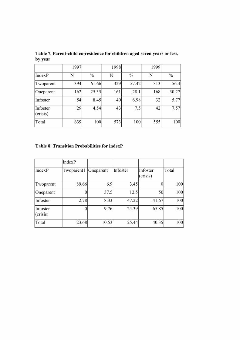
Table 7. Parent-child co-residence for children aged seven years or less, by year

1997 1998 1999

IndexP N % N % N %

Twoparent 394 61.66 329 57.42 313 56.4

Oneparent 162 25.35 161 28.1 168 30.27

Infoster 54 8.45 40 6.98 32 5.77

Infoster (crisis)

29 4.54 43 7.5 42 7.57

Total 639 100 573 100 555 100

Table 8. Transition Probabilities for indexP

IndexP

IndexP Twoparent1 Oneparent Infoster Infoster (crisis)

Total

Twoparent 89.66 6.9 3.45 0 100

Oneparent 0 37.5 12.5 50 100

Infoster 2.78 8.33 47.22 41.67 100

Infoster (crisis)

0 9.76 24.39 65.85 100

Total 23.68 10.53 25.44 40.35 100

Table 9. Distribution of all households, according to whether they foster in children and by area

High Potential Area Medium Potential Area Low Potential Area All Areas

RA CA RA+CA RA CA RA+CA RA CA RA+CA RA+CA

Non-Foster 75.83 80.49 76.59 56.58 62.50 58.33 59.32 84.62 69.39 70.74

(160) (33) (193) (43) (20) (63) (35) (33) (68) (324)

Foster 24.17 19.51 23.41 43.42 37.50 41.67 40.68 15.38 30.61 29.26

(51) (8) (59) (33) (12) (45) (24) (6) (30) (134)

% 83.73 16.27 100.00 70.37 29.63 100.00 60.20 39.80 100.00

N 211 41 252 76 32 108 59 39 98 (458)

Table 10. Households that foster in: (household-year) observations by number of children fostered and by area

Area

No. foster children

High Medium Low Total

1 91 59 39 189

2 6 10 6 22

3 1 2 3

Total 98 69 47 214

% 46.15 31.67 22.17 100.00

Table 11. Correlations between the probability of being an in-foster and some economic and demographic variables

Probfost Probfost Probfost

Tot food -0.0728 Real inc97 -0.0234 HH size -0.1025* expendit. (0.1025) (0.5984) (0.0204) Crop harvest -0.0573 Real inc96 -0.0055 Own childr. -0.4023* (0.1983) (0.9013) (0) Cereal -0.0378 Real inc95 -0.0376 Tot children -0.2116* stock (0.3972) (0.3959) (0) Livestock -0.014 Var Inc -0.002 Area 0.1852* sale reven. (0.7528) 95-96 (0.9638) (0) Livestock 0.1039* Var Inc 0.0917* value (0.0196) 96-97 (0.0393) * significant at 0.05 level

Table 12. Determinants of the probability that a child is an-infoster Probit Analysis

In-foster Coef. Std. Err. t P>|t|

VarInc96-97 0.007082* 0.004037 1.754 0.079

HH size -0.02679** 0.013382 -2.002 0.045

Area 0.394262** 0.095493 4.129 0

Children -1.058** 0.240087 -4.407 0

Constant -0.21764 0.357387 -0.609 0.543

* significant at 0.10 level

** significant at 0.05 level

N=505

Pseudo R2=0.1518

χ2(4)= 57.08 (significant at 0.00001 level)

Log Likelihod= -159.5266