Chaste: incorporating a novel multi–scale

spatial and temporal algorithm into a

large–scale open source library

By Miguel O Bernabeu1, Rafel Bordas1, Pras Pathmanathan1, JoePitt–Francis1, Jonathan Cooper1, Alan Garny2, David J Gavaghan1,

Blanca Rodriguez1, James A Southern1,3, Jonathan P Whiteley1†1Oxford University Computing Laboratory, Wolfson Building, University of

Oxford, Parks Road, Oxford OX1 3QD, UK2Department of Physiology, Anatomy and Genetics, Sherrington Building,

University of Oxford, Parks Road, Oxford OX1 3PT, UK3Fujitsu Laboratories of Europe Ltd, Hayes, Middlesex UB4 8FE, UK

Recent work (Pitt–Francis et al. Philosophical Transactions of the Royal SocietyA, vol. 366, pp. 3111–3136) has described the software engineering and computa-tional infrastructure that has been set up as part of the Chaste project. Chaste—Cancer Heart And Soft Tissue Environment—is an open source software packagethat currently has heart and cancer modelling functionality. This software has beenwritten using a programming paradigm imported from the commercial sector, andhas resulted in code that has been subject to a far more rigorous testing procedurethan is usual in this field. The exceptionally large number of tests written for eachsmall, individual subroutine of this code allows software development to be carriedout with confidence that new developments do not inadvertently degrade earlierfunctionality.

This software may be developed for two main purposes—either to add new phys-iological functionality, or to incorporate a different numerical algorithm for solvingthe governing equations which allows a given level of accuracy to be attained moreefficiently. In this paper, we will focus on the second of these purposes for the field ofcardiac electrophysiological modelling. Whiteley (Annals of Biomedical Engineer-ing, vol. 36, pp. 1398–1408) has developed a numerical algorithm for solving thebidomain equations that utilizes the multi–scale nature of the physiology modelledto enhance computational efficiency. When using this algorithm, only quantitiesthat vary on short time–scales or short length–scales are computed to a fine res-olution. Other more slowly varying quantities are computed at a lower resolution.Interpolation is then used to transfer information between different resolutions. Us-ing a simple geometry in two dimensions and a purpose–built code, this algorithmwas reported to give an increase in computational efficiency of over two orders ofmagnitude.

In this paper, we begin by reviewing numerical methods currently in use forsolving the bidomain equations, explaining how these methods may be developedto utilize the multi–scale algorithm discussed above. We then demonstrate the use ofthis algorithm within the Chaste framework for solving the monodomain and bido-

† Author for correspondence (jonathan.whiteley@comlab.ox.ac.uk)

Article submitted to Royal Society TEX Paper

2 M. O. Bernabeu and others

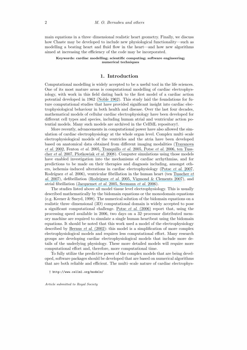
main equations in a three–dimensional realistic heart geometry. Finally, we discusshow Chaste may be developed to include new physiological functionality—such asmodelling a beating heart and fluid flow in the heart—and how new algorithmsaimed at increasing the efficiency of the code may be incorporated.

Keywords: cardiac modelling; scientific computing; software engineering;numerical techniques

1. Introduction

Computational modelling is widely accepted to be a useful tool in the life sciences.One of its most mature areas is computational modelling of cardiac electrophys-iology, with work in this field dating back to the first model of a cardiac actionpotential developed in 1962 (Noble 1962). This study laid the foundations for fu-ture computational studies that have provided significant insight into cardiac elec-trophysiological behaviour in both health and disease. Over the last four decades,mathematical models of cellular cardiac electrophysiology have been developed fordifferent cell types and species, including human atrial and ventricular action po-tential models. Many such models are archived in the CellML repository†.

More recently, advancements in computational power have also allowed the sim-ulation of cardiac electrophysiology at the whole organ level. Complex multi–scaleelectrophysiological models of the ventricles and the atria have been developedbased on anatomical data obtained from different imaging modalities (Trayanovaet al. 2002, Fenton et al. 2005, Tranquillo et al. 2005, Potse et al. 2006, ten Tuss-cher et al. 2007, Plotkowiak et al. 2008). Computer simulations using those modelshave enabled investigation into the mechanisms of cardiac arrhythmias, and forpredictions to be made on their therapies and diagnosis including, amongst oth-ers, ischemia–induced alterations in cardiac electrophysiology (Potse et al. 2007,Rodrıguez et al. 2006), ventricular fibrillation in the human heart (ten Tusscher etal. 2007), defibrillation (Rodrıguez et al. 2005, Vigmond & Clements 2007), andatrial fibrillation (Jacquemet et al. 2005, Seemann et al. 2006).

The studies listed above all model tissue level electrophysiology. This is usuallydescribed mathematically by the bidomain equations or the monodomain equations(e.g. Keener & Sneyd, 1998). The numerical solution of the bidomain equations on arealistic three–dimensional (3D) computational domain is widely accepted to posea significant computational challenge. Potse et al. (2006) report that, using theprocessing speed available in 2006, two days on a 32–processor distributed mem-ory machine are required to simulate a single human heartbeat using the bidomainequations. It should be noted that this work used a model of the electrophysiologydescribed by Bernus et al. (2002): this model is a simplification of more complexelectrophysiological models and requires less computational effort. Many researchgroups are developing cardiac electrophysiological models that include more de-tails of the underlying physiology. These more detailed models will require morecomputational effort and, therefore, more computational time.

To fully utilize the predictive power of the complex models that are being devel-oped, software packages should be developed that are based on numerical algorithmsthat are both reliable and efficient. The multi–scale nature of cardiac electrophys-

† http://www.cellml.org/models/

Article submitted to Royal Society

Chaste: incorporating a multi–scale numerical solver 3

iology results in the physical processes being described by stiff systems of differ-ential equations. The use of fully explicit time integration numerical methods areclearly an attractive option to anyone writing a cardiac simulation package, as thesetechniques do not require the solution of any non–linear systems. However, the per-formance of such explicit numerical methods is notoriously prone to degradationby stability issues when these methods are applied to stiff systems of differentialequations (Iserles et al. 1996). As a consequence, the timestep used by these solversis usually driven by stability issues and not by the time–scales of the physiologi-cal processes that are being modelled. An alternative choice is to use implicit timeintegration numerical methods. These methods are, however, more difficult to incor-porate into software as they require implementing methods for solving large systemsof non–linear equations. This presents a difficult decision for anyone writing cardiacsimulation software: the most appropriate numerical algorithm requires writing—and maintaining—code that describes complex mathematical algorithms. Even if acomplex numerical algorithm is successfully implemented, a future developer maystruggle to maintain the integrity of the software due to a lack of understanding ofthe algorithm implemented. Less complex code can be written, but at the cost ofusing algorithms whose performance is significantly lower than is possible.

A further complication that has recently arisen for writers of cardiac simula-tion software is the introduction into cardiac models of additional features such astissue deformation in response to the electrophysiology and the resulting flow offluid (e.g. Watanabe et al. 2004). The systems of partial differential equations thatmodel these coupled multi–physics problems are generally of mixed hyperbolic–elliptic–parabolic type and include constraints such as incompressibility of tissue.Simple numerical methods for discretizing these equations are often unconditionallyunstable—i.e. they will never converge no matter how small the timestep. Underthese conditions simple mathematical algorithms are not appropriate for computingthe numerical solutions of these equations, and more complex numerical algorithmsshould be used instead. This has been demonstrated when a simple model of tis-sue deformation has been coupled with electrophysiology (Whiteley et al. 2007,Niederer & Smith 2008). Software written for these simulations therefore requireswriting code for complex algorithms. As described above, such code is difficult towrite and maintain.

The two previous paragraphs have highlighted the need for reliable softwarepackages for cardiac simulations. This in turn requires reliable software engineeringmethods for writing this software. An attempt to initiate software engineering tech-niques borrowed from the commercial sector in this field has recently been madethrough the Chaste (Cancer, Heart And Soft Tissue Environment) software packagecurrently being developed within the Computational Biology Group at the Univer-sity of Oxford (Pitt–Francis et al. 2008). This package has been developed usingan agile programming technique (see, for example, Beck & Andres, 2004). One keyfeature of this software is the large number of focused tests included: these testseach cover a small portion of code (typically 5–10 lines), and each line of code iscovered by at least one test. When the code is modified all tests are run, and anyfailing test identifies very precisely the location of bugs in the software. This allowssoftware to be developed with the minimum of degradation of earlier functionality.A second key feature is that a decision has been made to distribute the code underan open source software license so that it can be downloaded, used and modified by

Article submitted to Royal Society

4 M. O. Bernabeu and others

other research groups. Any worker who suspects erroneous published results basedon Chaste is free to download the package themselves and search for the error and—if one is found—to alert the authors to allow the code and the associated researchto be corrected.

In this paper, we will describe how Chaste has been developed to combinethis rigorous software engineering approach with a recently published numericalalgorithm (Whiteley, 2008). In §2, we describe numerical algorithms that have beenused by other workers, justifying the choice of our numerical algorithm. In §3, webriefly summarize the software development process and tools that are used byChaste, explaining why this results in reliable software that may form the basis forthe next generation of cardiac modelling software. The accuracy and efficiency ofthe algorithm when implemented in this software is verified in §4. Finally, in §5, wediscuss future challenges for computational biologists in this area, and discuss howwe envisage developing the Chaste package to meet these challenges.

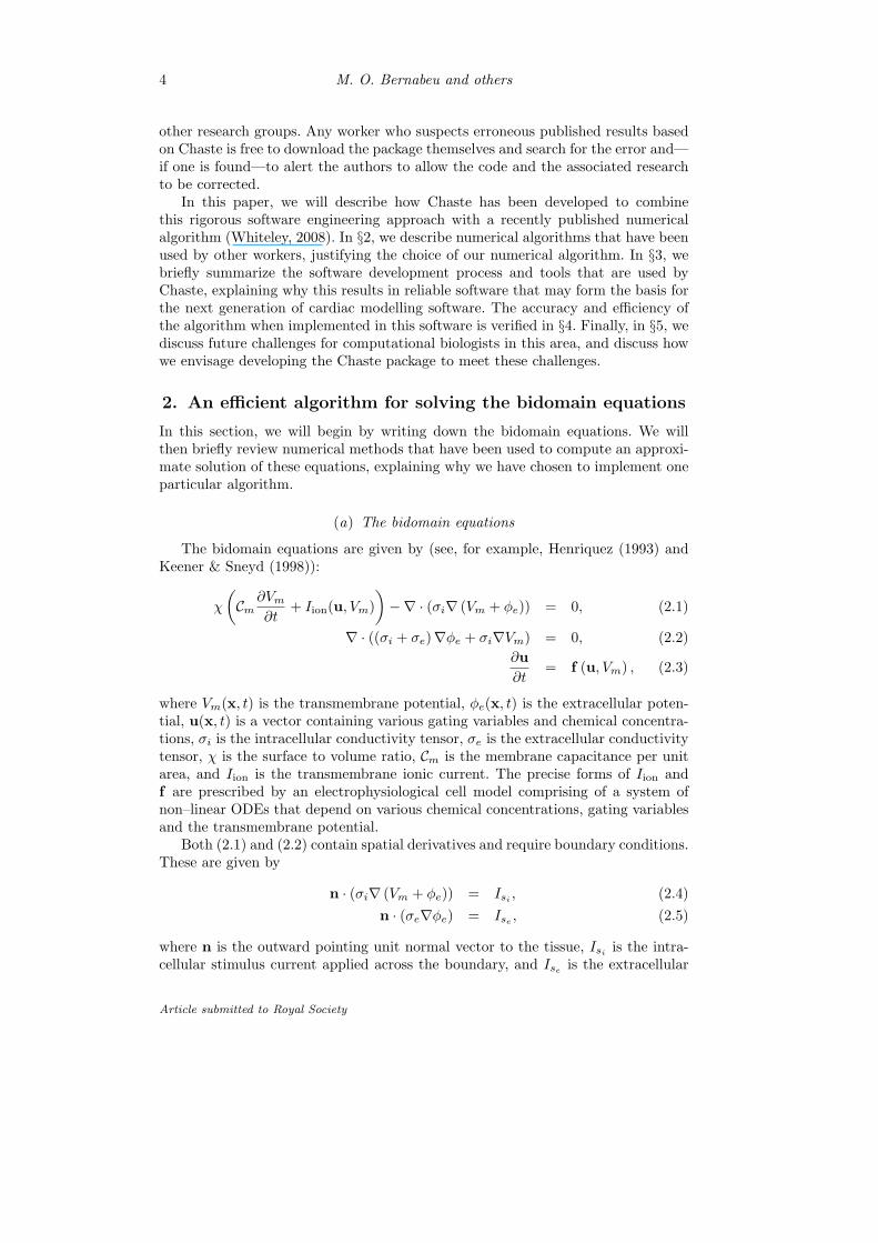
2. An efficient algorithm for solving the bidomain equations

In this section, we will begin by writing down the bidomain equations. We willthen briefly review numerical methods that have been used to compute an approxi-mate solution of these equations, explaining why we have chosen to implement oneparticular algorithm.

(a) The bidomain equations

The bidomain equations are given by (see, for example, Henriquez (1993) andKeener & Sneyd (1998)):

χ

(Cm

∂Vm

∂t+ Iion(u, Vm)

)−∇ · (σi∇ (Vm + φe)) = 0, (2.1)

∇ · ((σi + σe)∇φe + σi∇Vm) = 0, (2.2)∂u∂t

= f (u, Vm) , (2.3)

where Vm(x, t) is the transmembrane potential, φe(x, t) is the extracellular poten-tial, u(x, t) is a vector containing various gating variables and chemical concentra-tions, σi is the intracellular conductivity tensor, σe is the extracellular conductivitytensor, χ is the surface to volume ratio, Cm is the membrane capacitance per unitarea, and Iion is the transmembrane ionic current. The precise forms of Iion andf are prescribed by an electrophysiological cell model comprising of a system ofnon–linear ODEs that depend on various chemical concentrations, gating variablesand the transmembrane potential.

Both (2.1) and (2.2) contain spatial derivatives and require boundary conditions.These are given by

n · (σi∇ (Vm + φe)) = Isi , (2.4)n · (σe∇φe) = Ise , (2.5)

where n is the outward pointing unit normal vector to the tissue, Isi is the intra-cellular stimulus current applied across the boundary, and Ise

is the extracellular

Article submitted to Royal Society

Chaste: incorporating a multi–scale numerical solver 5

stimulus current applied across the boundary. The system is then solved by specify-ing initial conditions for Vm and u. As φe only appears in these equations throughspatial derivatives, this quantity is only defined up to an additive constant. Whena bath is modelled, it is treated as an extension of the interstitial fluid (Vigmondet al. 2008).

(b) Numerical methods for solving the bidomain equations

We now briefly describe some of the numerical methods that have been usedto solve the bidomain equations, highlighting the strength and weaknesses of eachapproach.

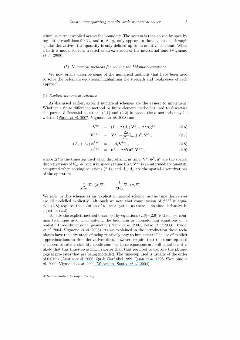
(i) Explicit numerical schemes

As discussed earlier, explicit numerical schemes are the easiest to implement.Whether a finite difference method or finite element method is used to discretizethe partial differential equations (2.1) and (2.2) in space, these methods may bewritten (Plank et al. 2007, Vigmond et al. 2008) as:

Vk∗ = (I + ∆tAi) Vk + ∆tAiφk, (2.6)

Vk+1 = Vk∗ − ∆tCm

Iion(uk,Vk∗), (2.7)

(Ai +Ae) φk+1 = −AiVk+1, (2.8)uk+1 = uk + ∆tf(uk,Vk∗), (2.9)

where ∆t is the timestep used when discretizing in time, Vk,φk,uk are the spatialdiscretizations of Vm, φe and u in space at time k∆t, Vk∗ is an intermediate quantitycomputed when solving equations (2.1), and Ai, Ae are the spatial discretizationsof the operators

1χCm

∇ · (σi∇) ,1

χCm∇ · (σe∇) .

We refer to this scheme as an ‘explicit numerical scheme’ as the time derivativesare all modelled explicitly—although we note that computation of φk+1 in equa-tion (2.8) requires the solution of a linear system as there is no time derivative inequation (2.2).

To date the explicit method described by equations (2.6)–(2.9) is the most com-mon technique used when solving the bidomain or monodomain equations on arealistic three–dimensional geometry (Plank et al. 2007, Potse et al. 2006, Trudelet al. 2004, Vigmond et al. 2008). As we explained in the introduction these tech-niques have the advantage of being relatively easy to implement. The use of explicitapproximations to time derivatives does, however, require that the timestep usedis chosen to satisfy stability conditions—as these equations are stiff equations it islikely that this timestep is much shorter than that required to capture the physio-logical processes that are being modelled. The timestep used is usually of the orderof 0.01ms (Austin et al. 2006, Qu & Garfinkel 1999, Quan et al. 1998, Skouibine etal. 2000, Vigmond et al. 2002, Weber dos Santos et al. 2004).

Article submitted to Royal Society

6 M. O. Bernabeu and others

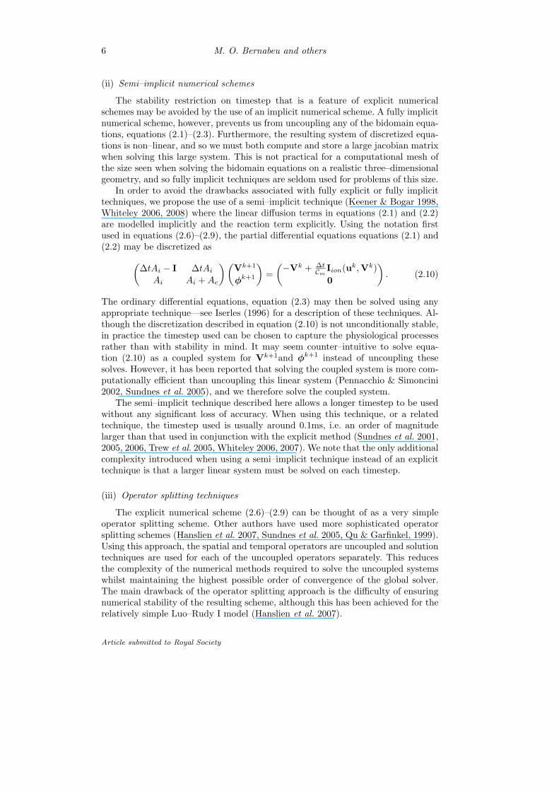
(ii) Semi–implicit numerical schemes

The stability restriction on timestep that is a feature of explicit numericalschemes may be avoided by the use of an implicit numerical scheme. A fully implicitnumerical scheme, however, prevents us from uncoupling any of the bidomain equa-tions, equations (2.1)–(2.3). Furthermore, the resulting system of discretized equa-tions is non–linear, and so we must both compute and store a large jacobian matrixwhen solving this large system. This is not practical for a computational mesh ofthe size seen when solving the bidomain equations on a realistic three–dimensionalgeometry, and so fully implicit techniques are seldom used for problems of this size.

In order to avoid the drawbacks associated with fully explicit or fully implicittechniques, we propose the use of a semi–implicit technique (Keener & Bogar 1998,Whiteley 2006, 2008) where the linear diffusion terms in equations (2.1) and (2.2)are modelled implicitly and the reaction term explicitly. Using the notation firstused in equations (2.6)–(2.9), the partial differential equations equations (2.1) and(2.2) may be discretized as(

∆tAi − I ∆tAi

Ai Ai +Ae

) (Vk+1

φk+1

)=

(−Vk + ∆t

CmIion(uk,Vk)0

). (2.10)

The ordinary differential equations, equation (2.3) may then be solved using anyappropriate technique—see Iserles (1996) for a description of these techniques. Al-though the discretization described in equation (2.10) is not unconditionally stable,in practice the timestep used can be chosen to capture the physiological processesrather than with stability in mind. It may seem counter–intuitive to solve equa-tion (2.10) as a coupled system for Vk+1and φk+1 instead of uncoupling thesesolves. However, it has been reported that solving the coupled system is more com-putationally efficient than uncoupling this linear system (Pennacchio & Simoncini2002, Sundnes et al. 2005), and we therefore solve the coupled system.

The semi–implicit technique described here allows a longer timestep to be usedwithout any significant loss of accuracy. When using this technique, or a relatedtechnique, the timestep used is usually around 0.1ms, i.e. an order of magnitudelarger than that used in conjunction with the explicit method (Sundnes et al. 2001,2005, 2006, Trew et al. 2005, Whiteley 2006, 2007). We note that the only additionalcomplexity introduced when using a semi–implicit technique instead of an explicittechnique is that a larger linear system must be solved on each timestep.

(iii) Operator splitting techniques

The explicit numerical scheme (2.6)–(2.9) can be thought of as a very simpleoperator splitting scheme. Other authors have used more sophisticated operatorsplitting schemes (Hanslien et al. 2007, Sundnes et al. 2005, Qu & Garfinkel, 1999).Using this approach, the spatial and temporal operators are uncoupled and solutiontechniques are used for each of the uncoupled operators separately. This reducesthe complexity of the numerical methods required to solve the uncoupled systemswhilst maintaining the highest possible order of convergence of the global solver.The main drawback of the operator splitting approach is the difficulty of ensuringnumerical stability of the resulting scheme, although this has been achieved for therelatively simple Luo–Rudy I model (Hanslien et al. 2007).

Article submitted to Royal Society

Chaste: incorporating a multi–scale numerical solver 7

(iv) Adaptive numerical schemes

There has recently been much interest in the numerical analysis communityin adaptive numerical schemes: see, for example, Estep et al. 1995, Gavaghan etal. 2006, Houston & Suli 2001. Rather than use a fixed computational mesh thesemethods allow a different mesh to be used on each timestep with a high density ofnodes being used only when the solution varies rapidly. These methods have theadvantage that computational effort is directed only towards regions of the compu-tational domain where it is required. Adaptive numerical methods have not beenparticularly popular in the field of electrophysiological modelling. This is proba-bly because: (i) significant computational effort is required to compute the meshrequired for each timestep; (ii) when the mesh is altered, the matrices Ai andAe used in equations (2.6), (2.8) and (2.10) must be re–computed, and this itselfrequires a large volume of computation; (iii) each node introduced at refinementrequires the generation of state from a cell model; and (iv) in modelling fibril-lation, the refinement is required to change rapidly. There is, however, a limitedselection of literature devoted to applying an adaptive numerical method to themonodomain or bidomain equations (see, for example, Cherry et al. 2003, ColliFranzone et al. 2006, Pennachio 2004, Whiteley 2007). None of these, however,have yet managed to demonstrate an increase in computational efficiency whenapplied to a realistic 3D computational domain.

(v) Multi–scale numerical schemes

A numerical method has recently been developed that utilizes the multi–scalenature of the problem (Whiteley 2008). This numerical algorithm uses the obser-vation that only a very small number of quantities vary on a short time–scale anda short length–scale, and computes only these quantities at a high resolution. Thekey to implementing this algorithm is the use of two meshes as shown in Figure 1.A fine mesh—represented by thin lines—has nodal spacing hfast, and rapidly vary-ing variables are approximated using this mesh. Other variables are computed on acoarser mesh—represented by thicker lines. Linear interpolation is used to transferthe slower variables onto the fine mesh when required.

hfast

hslow

Figure 1. The fine mesh (thin lines) and coarse mesh (thick lines)

Article submitted to Royal Society

8 M. O. Bernabeu and others

When using most electrophysiological models the rapidly varying variables arethose associated with the fast sodium current that causes the rapid action potentialupstroke, specifically the transmembrane potential Vm, the extracellular potentialφe, the sodium m–gate and the sodium h–gate. Approximating these quantities onthe fine mesh and all other quantities on the coarse mesh allows equation (2.10) tobe written (

∆tAi − I ∆tAi

Ai Ai +Ae

) (Vk+1

φk+1

)=

(Γ1 + Γ2

0

), (2.11)

where Γ1 is computed from variables approximated on the fine mesh, and Γ2 is de-pendent only on variables approximated on the coarse mesh. This system is solvedwith a timestep ∆tfast, although as the contributions to Γ2 vary on a slower time–scale this vector is updated less frequently on a time–scale ∆tslow. The terms in-cluded in Γ2 are generally the more computationally expensive terms—updatingthis quantity on a slower timestep should therefore give a significant computationalsaving.

Having computed Vm and φe using equation (2.11), we now turn our attentionto computing the solution of the ODEs given by equation (2.3). The equationsgoverning the sodium m–gate and the sodium h–gate must be computed at everynode of the fine mesh in order to calculate the contribution to Γ1 in equation (2.11).All other ODEs need only be solved at the nodes of the coarse mesh. As there areorders of magnitude fewer nodes on the coarse mesh as compared with the finemesh this also gives a substantial computational saving.

This algorithm has been implemented in a simple 2D geometry and, using theelectrophysiological cell model described by Noble et al. (1998) an increase in com-putational efficiency of around two orders of magnitude was achieved (Whiteley2008). Later in this paper, we will investigate how this algorithm performs whenapplied to a realistic 3D geometry.

(vi) Other methods for the numerical solution of the bidomain equations

In addition to the techniques described earlier in this section, other numer-ical analysis tools have been applied to the numerical solution of the bidomainequations. Skouibine et al. (2000) used a predictor–corrector scheme: an explicitnumerical method was used as a prediction of the solution at the next time level.This prediction was used as an initial guess to the solution of the non–linear sys-tem that arises from the implicit discretization of the bidomain equations. Domaindecomposition was used by Quan et al. (1998): this allowed different timesteps tobe used in different regions of the computational domain.

3. Writing reliable software

Writing reliable software has been a focus of the commercial sector for many years,resulting in a plethora of tools and techniques that may be used to aid softwaredevelopment. Some of these techniques have recently been imported into the com-putational biology domain through the Chaste project (Pitt–Francis et al. 2008).In this section, we begin by briefly reviewing the software engineering approach

Article submitted to Royal Society

Chaste: incorporating a multi–scale numerical solver 9

and computational infrastructure that has been used by Chaste in order to gener-ate high quality software. We then describe various tools included in Chaste for thepurpose of: (i) automating code generation from descriptions of electrophysiologicalmodels stored in the CellML format; and (ii) automating code optimization.

(a) The software engineering approach adopted by Chaste

In this section, we briefly describe the software engineering approach followedwhen developing Chaste (for more details, see Pitt–Francis et al. (2008)). Chaste iswritten in C++ using an agile programming technique known as ‘eXtreme program-ming’ (Beck & Andres 2004). Although the methodology used to develop Chasteincreases development time in the short term, it is anticipated that savings will bemade in the medium to long term when we reap the benefits of the features offeredthrough this software engineering approach. Specific features of this programmingmethodology that are relevant to the scientific computing domain are listed below.

(i) Test driven development

Before any new incremental functionality is added, code that tests this function-ality is written. The code is then developed to incorporate the new functionality.After this, all tests including the new test are run. Should any test fail then thecode is corrected before any subsequent development takes place. As a consequence,many tests are written that cover very specific parts of the code, and all lines ofcode are tested. Should a test fail then it is relatively easy to identify the locationof the problem.

(ii) Continuous integration

All developers integrate their separate strands of code into a central repositoryon a regular basis. When this is done, all the tests described above are run to ensureno incompatibilities or regressions have been introduced.

(iii) Pair programming and collective code ownership

Code is usually developed by a team of two programmers working on a singlecomputer. The composition of pairs is frequently rotated, allowing all developers tobecome acquainted with all aspects of the code, and all developers are familiar withthe whole of the code. This facilitates collective code ownership, where no singleperson is responsible for any section of the code. This prevents development fromstagnating due to a developer leaving the team or spending less time on developmentwork due to other responsibilities.

(iv) Refactoring

The large number of tests that cover small sections of the code allows any sectionof the code to be re–written, either to improve the quality or performance of thecode. After the code has been refactored all tests are run to prevent degradation ofquality due to the introduction of errors.

Article submitted to Royal Society

10 M. O. Bernabeu and others

(b) The computational infrastructure employed by Chaste

The latest version of the Chaste software is stored on a central server equippedwith the Subversion (http://subversion.tigris.org) version control system,and backed up to central university resources. Any development is carried out by apair of programmers “checking out” the latest version—i.e. copying the latest ver-sion onto their local machine. When incremental development has been successfullycarried out on the local machine, the code is then “checked in”—any alterationsmade on the local machine are duplicated on the latest version of Chaste storedon the central server. As more than one pair of developers may be working on thecode at a given time, checking in code may introduce incompatibilities in the lat-est version stored on the central server. These incompatibilities are eradicated byensuring all tests submitted pass before any more code may be checked in.

Many established tools and libraries are utilised by the Chaste project. Progresswith individual programming tasks are tracked using the Trac project manage-ment tool (http://trac.edgewall.org). Chaste developers use the Eclipse devel-opment environment (http://www.eclipse.org) for code development, CxxTest(http://cxxtest.sourceforge.net) for unit testing, and the SCons softwareconstruction tool (http://www.scons.org) for build automation. See Pitt–Franciset al. (2008) for more details.

Rather than develop our own mathematical libraries from scratch, we use estab-lished, maintained, libraries where possible. Large linear and non–linear systems aresolved using the PETSc parallel and sequential libraries (www.mcs.anl.gov/petsc).The boost C++ libraries (http://www.boost.org/) are used for the smaller vec-tors and matrices that arise from assembling the contribution to the global systemfrom a single element.

(c) Increasing the efficiency and reliability of software automatically

The complexity of the electrophysiology models that prescribe the Iion term inequation (2.1) and the size and complexity of the system of ODEs in equation (2.3)has grown substantially in models developed in recent years. In these recent mod-els, Iion typically consists of several separate currents, and is dependent on tensof quantities each modelled by a separate ODE. Furthermore, each of these ODEsincludes several constant parameters. When one research group develops a model ascomplex as this, it is clearly difficult for another group to use this model, as codingthis model without introducing errors in any of the constants is a near impossibletask. In order to facilitate sharing and re–use of these models the CellML mark–uplanguage was developed (Cuellar et al. 2003). CellML is an XML–based languagethat represents electrophysiological models (amongst others) as a structured docu-ment that may be read by both humans and computers. For details of the currentstate of CellML, see Garny et al. (2008).

Use of electrophysiological models stored in the CellML format should clearlybe an essential feature of any electrophysiological simulation software. Althoughdevelopment of CellML functionality is independent of the Chaste project, Chasteis fortunate in that some Chaste developers are also developers of a collection ofrelevant CellML tools. As a consequence, Chaste is fully able to utilise CellMLtools. We list below the CellML tools that we utilize in Chaste.

Article submitted to Royal Society

Chaste: incorporating a multi–scale numerical solver 11

(i) Automatic code generation

Tools exist to automatically generate C++ code from a CellML file representinga given model. Automatically generated code from the PyCml† tool is used inChaste to compute the Iion term in equation (2.1) and the right–hand side of ODEsin equation (2.3). This feature allows any electrophysiological model represented bya valid CellML file to be used in a Chaste simulation.

(ii) Look–up tables

Many expressions that are included in the Iion term and the system of ODEsin equation (2.3) are functions only of the transmembrane potential Vm, and con-tain exponential terms that are expensive to compute. These expressions may becomputed more efficiently by using look–up tables: the value of this expression ispre–computed at a number of points, and interpolation of these values is used toevaluate this expression during the course of the simulation. This technique hasbeen reported to give a substantial increase in computational efficiency whilst in-troducing only negligible error (Cooper et al. 2006, Victorri et al. 1985).

(iii) Partial evaluation

Many terms that are generated through the automatic code generation describedabove contain expressions that may be pre–computed at compilation time to avoidrepeated computation of an identical quantity. This may be achieved using partialevaluation. This technique gives a significant increase in computational efficiencyespecially when combined with look–up tables (Cooper et al. 2006).

(iv) Units checking

All of the variables and constants used in an electrophysiological cell model haveassociated units, for example a length may be quoted in the units millimetres. It iscrucial for an accurate simulation that compatible units are used for all quantities(we cannot add a length to an area, for instance), and that quantities are given inthe same units at either side of an interface between components of the simulator.Fortunately, this may be automatically verified through the use of a CellML tool,and more advanced tools (Cooper & McKeever 2008) are being developed allowingfor automatic conversion between compatible units.

4. Results

A number of basic simulations were carried out in Chaste, in order to assess thecomputational efficiency and accuracy of various approximations to the solution ofthe full cell ODE systems. The approximations were based on the semi-implicit dis-cretization in equation (2.10), but utilized different numerical schemes to update theODEs in the cell models. These numerical schemes range from an explicit solutionwith timestep size determined by stability requirements, to the linear interpolationscheme in the multi–scale algorithm described in Whiteley (2008). These simulationexperiments were designed to demonstrate the performance of the approximations

† https://chaste.ediamond.ox.ac.uk/cellml/

Article submitted to Royal Society

12 M. O. Bernabeu and others

when implemented in a generic high-performance computing code, and applied tomore realistic geometries.

(a) Description of simulations

In 2D, the computational meshes were chosen to be the same as those in White-ley (2008). The simulations were carried out on a square occupying the region0 < x, y < 20 mm in an isotropic medium. The electrophysiological model used wasthat described in Noble et al. (1998). A spatial nodal spacing of 0.1mm was usedin each of the x and y directions. In the multi–scale algorithm a node spacing ofhslow = 1.0 mm was used for the coarse mesh (with hfast = 0.1 mm). This resultedin 40,401 nodes on the fine mesh and 441 nodes on the coarse mesh. The nodesalong the x = 0 edge were stimulated for the first 0.5 ms, generating an actionpotential that propagated across the square. The simulation was run for 0.35 s,allowing the entire domain to be excited and to return to its resting state. For eachsimulation, the transmembrane potential was recorded at all nodes for the durationof the simulation at intervals of 0.1 ms. The traces from the points x = 10 mm,y = 10 mm (midpoint node) and x = 20 mm, y = 10 mm (furthest edge from thestimulus) were analysed. The conduction velocity between the points was calcu-lated. The action potential duration to 90% repolarization (APD90) and maximumupstroke velocity were calculated at the midpoint node.

In 3D, a cube mesh was chosen that generalized the mesh used in 2D and hada similar number of nodes. The mesh contained the region 0 < x, y, z < 3 mmin an isotropic medium. In common with the 2D simulations, hfast = 0.1 mm andhslow = 1.0 mm leading to 29,791 nodes on the fine mesh and 64 nodes on the coarsemesh. A stimulus was applied along the face x = 0 mm and the transmembranepotential was analysed at the midpoint (1.5, 1.5, 1.5) and on the x = 3 mm face at(3, 1.5, 1.5).

On a uniform grid in 3D, with a large number of nodes in each spatial direction,the choice of hfast and hslow used in these simulations would lead to the ratio of thenumber of coarse nodes to fine nodes being ∼1:1000. For the 2D simulations, thisratio would be ∼1:100. The ratio is closer to 1:500 for the uniform mesh used inthese simulations due to the relatively small number of nodes in each direction. Forour 2D simulation that uses a larger number of nodes in each spatial direction wesee that we are closer to the ratio of 1:100 expected on a grid with a large numberof nodes.

As a further indicator of how well these methods scale to realistic geometries,we also ran a bidomain simulation on a full ventricular mesh with 63,885 nodes.The multi–scale algorithm used a coarse mesh of 173 nodes which was producedfrom the original ventricular geometry via a decimation algorithm. The decimationscheme allows for the removal of surface nodes if the local change in volume is belowa threshold. This means that some of the nodes in the original fine mesh are outsidethe volume of the decimated coarse mesh. However, all nodes of the coarse mesh areguaranteed to be coincident with nodes on the fine mesh. The ratio of coarse to finenodes (∼1:400) is higher than that used on the regular 3D slab experiments, but wasselected because further decimation of the mesh was not possible without changingthe topology of the ventricular cavities. Unfortunately, there are some complicationswith the multi–scale algorithm on these meshes, since at the fine mesh nodes outside

Article submitted to Royal Society

Chaste: incorporating a multi–scale numerical solver 13

Parameter Value

Cm 0.01 µF/mm2

χ 140 /mm

σi 0.175 mS/mm

σe 0.7 mS/mm

Table 1. Physiological parameters used in all simulations

the volume of the coarse mesh interpolation becomes extrapolation or projection. Ifthe values of slow gating variables and ionic concentrations are extrapolated thereis potential for them to become unphysiological (small and negative). We are stillexploring a physiologically valid solution to this problem.

(i) The computational efficiency of the current code

It is worth noting that prior to these experiments the developers had beenprofiling and optimizing the code. Considerable effort had been put into resolvingcommon bottlenecks, particularly the assembly and solution of the linear systemfrom the diffusion PDE. Most of the steps in the solution method (ODE solution,mesh reading, output and assembly of the linear system) are linear in the numberof nodes; an exception is the solution of the linear system itself which usually runsin a time that is near quadratic in the number of nodes.

Since Chaste is designed to be scalable to meshes with large numbers of nodes(∼ 3×106), work focused on reducing the amount of time spent in the linear solver.It has been documented elsewhere (e.g. Plank et al. 2007) that the choice of linearsolver and pre-conditioner is critical in reducing the solution time of the bidomainequations. We have found empirically that a suitable selection is a (block) Jacobipre-conditioner with a symmetric LQ variant (SYMMLQ) of the conjugate gradientmethod. The SYMMLQ solver converges sufficiently rapidly that the tolerance ofthe solution may be varied by an order of magnitude with little change to the overallrun time. We found that the amount of time spent solving the bidomain systemwas 4 or 5 times that of solving the monodomain system, since the bidomain linearsystem has double the number of unknowns.

The other large computational bottleneck is in the assembly of the linear system.Some considerable time has been spent on profiling this code. During the course ofwriting code for these experiments we managed to optimise the assembly routinesso that they take no more time than ODE or linear solvers.

In all results presented in the paper, the physiological parameters used werethose tabulated in table 1. Conductivities σi and σe were isotropic (with no domi-nant fibre direction).

(ii) Types of simulation

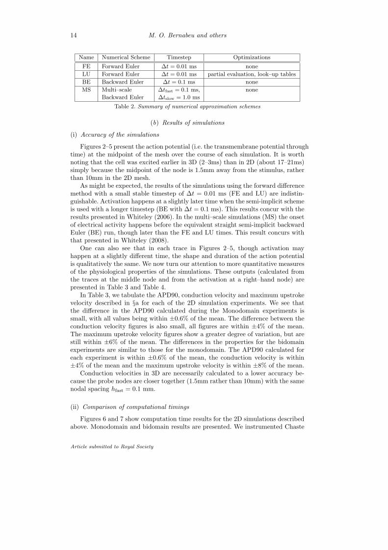
Throughout the following set of results, we refer to the four numerical schemesas in table 2. Note that ∆t refers to both the timestep used to update the cell modelODEs and to that used to solve the bidomain or monodomain PDEs. See §3 for abrief description of the optimizations (LU) and Whiteley (2006) for an explanationof the backward Euler scheme (BE).

Article submitted to Royal Society

14 M. O. Bernabeu and others

Name Numerical Scheme Timestep Optimizations

FE Forward Euler ∆t = 0.01 ms none

LU Forward Euler ∆t = 0.01 ms partial evaluation, look–up tables

BE Backward Euler ∆t = 0.1 ms none

MS Multi–scale ∆tfast = 0.1 ms, none

Backward Euler ∆tslow = 1.0 ms

Table 2. Summary of numerical approximation schemes

(b) Results of simulations

(i) Accuracy of the simulations

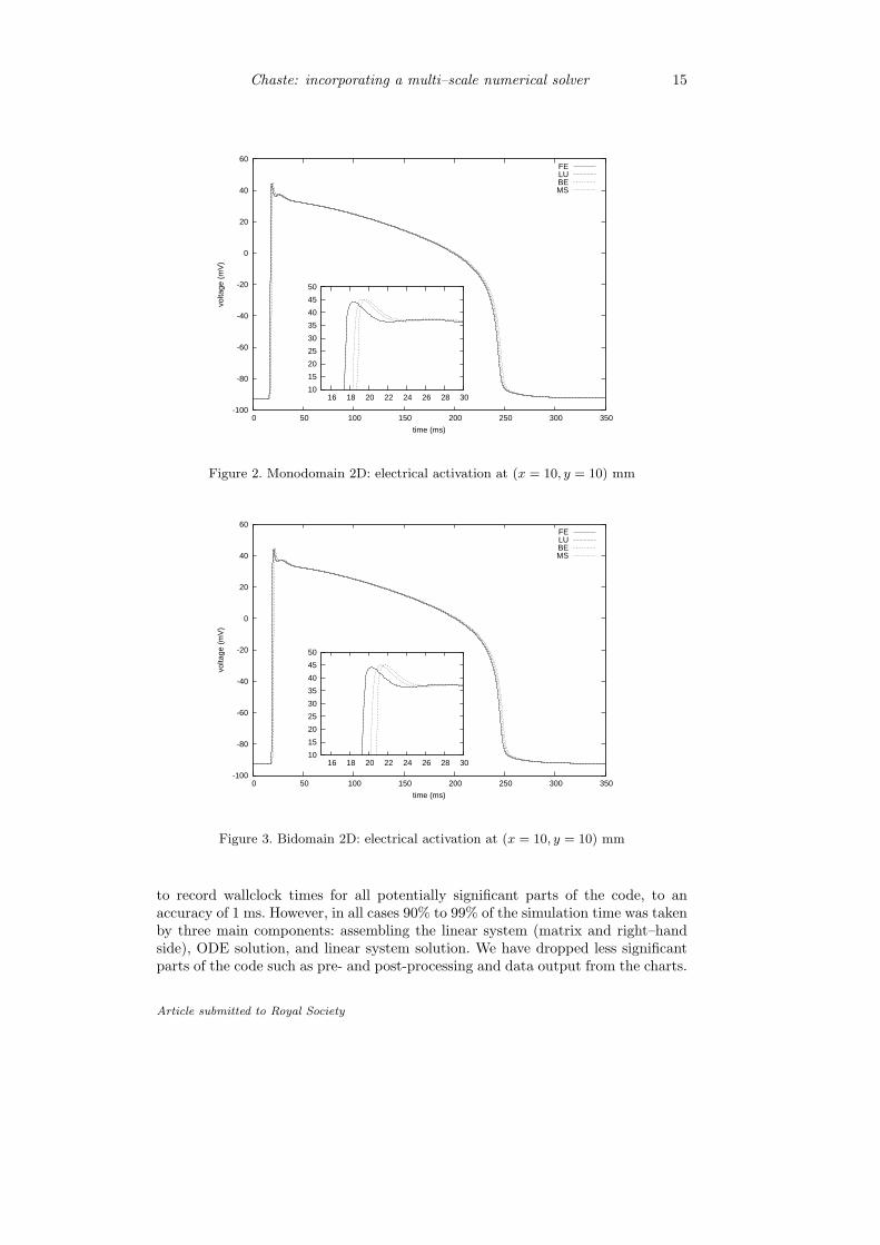
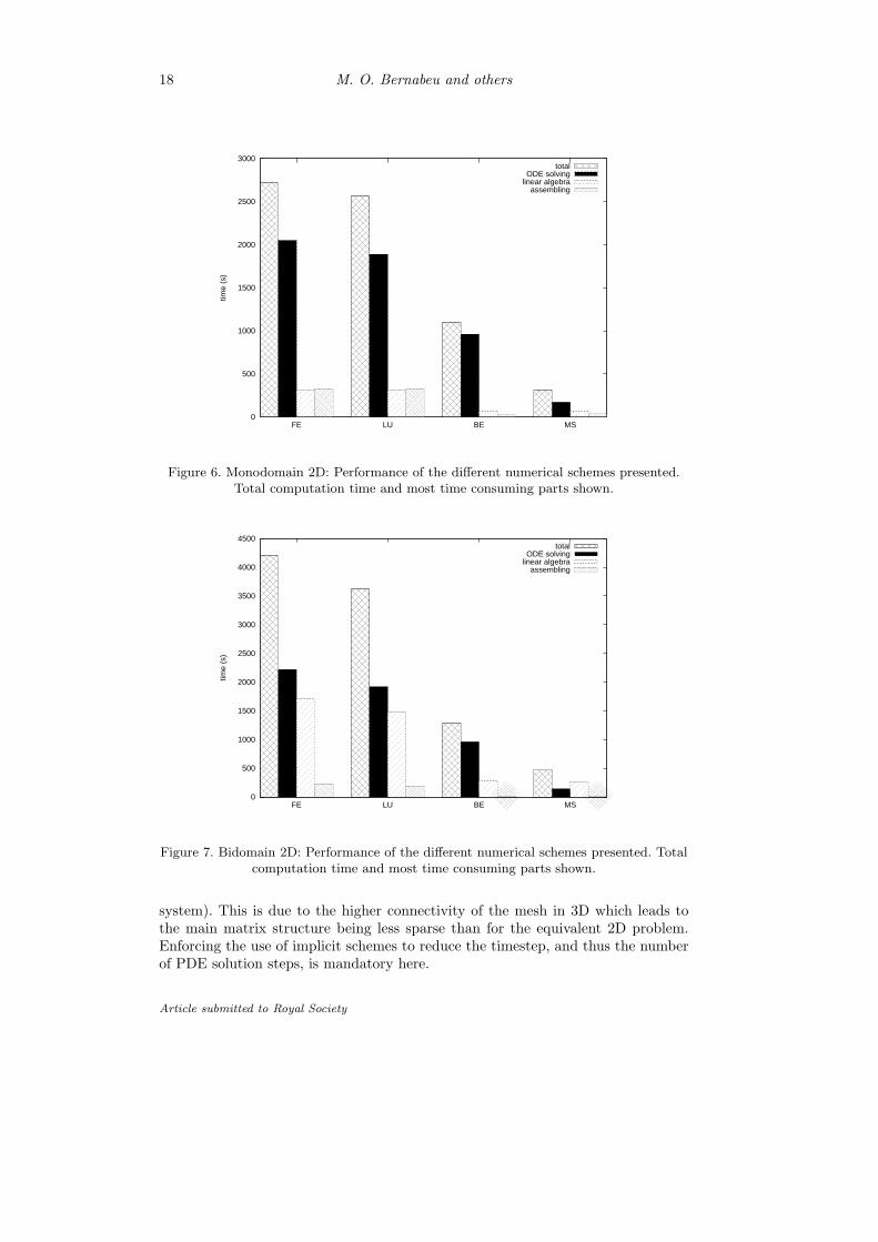
Figures 2–5 present the action potential (i.e. the transmembrane potential throughtime) at the midpoint of the mesh over the course of each simulation. It is worthnoting that the cell was excited earlier in 3D (2–3ms) than in 2D (about 17–21ms)simply because the midpoint of the node is 1.5mm away from the stimulus, ratherthan 10mm in the 2D mesh.

As might be expected, the results of the simulations using the forward differencemethod with a small stable timestep of ∆t = 0.01 ms (FE and LU) are indistin-guishable. Activation happens at a slightly later time when the semi-implicit schemeis used with a longer timestep (BE with ∆t = 0.1 ms). This results concur with theresults presented in Whiteley (2006). In the multi–scale simulations (MS) the onsetof electrical activity happens before the equivalent straight semi-implicit backwardEuler (BE) run, though later than the FE and LU times. This result concurs withthat presented in Whiteley (2008).

One can also see that in each trace in Figures 2–5, though activation mayhappen at a slightly different time, the shape and duration of the action potentialis qualitatively the same. We now turn our attention to more quantitative measuresof the physiological properties of the simulations. These outputs (calculated fromthe traces at the middle node and from the activation at a right–hand node) arepresented in Table 3 and Table 4.

In Table 3, we tabulate the APD90, conduction velocity and maximum upstrokevelocity described in §a for each of the 2D simulation experiments. We see thatthe difference in the APD90 calculated during the Monodomain experiments issmall, with all values being within ±0.6% of the mean. The difference between theconduction velocity figures is also small, all figures are within ±4% of the mean.The maximum upstroke velocity figures show a greater degree of variation, but arestill within ±6% of the mean. The differences in the properties for the bidomainexperiments are similar to those for the monodomain. The APD90 calculated foreach experiment is within ±0.6% of the mean, the conduction velocity is within±4% of the mean and the maximum upstroke velocity is within ±8% of the mean.

Conduction velocities in 3D are necessarily calculated to a lower accuracy be-cause the probe nodes are closer together (1.5mm rather than 10mm) with the samenodal spacing hfast = 0.1 mm.

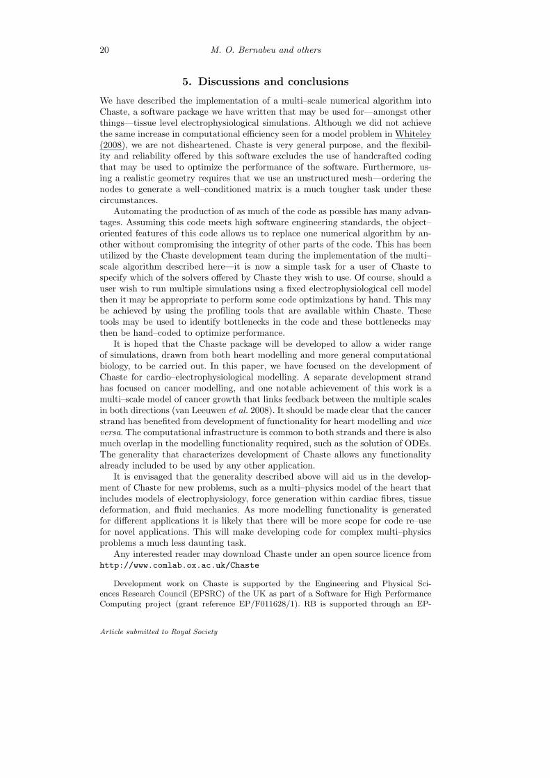
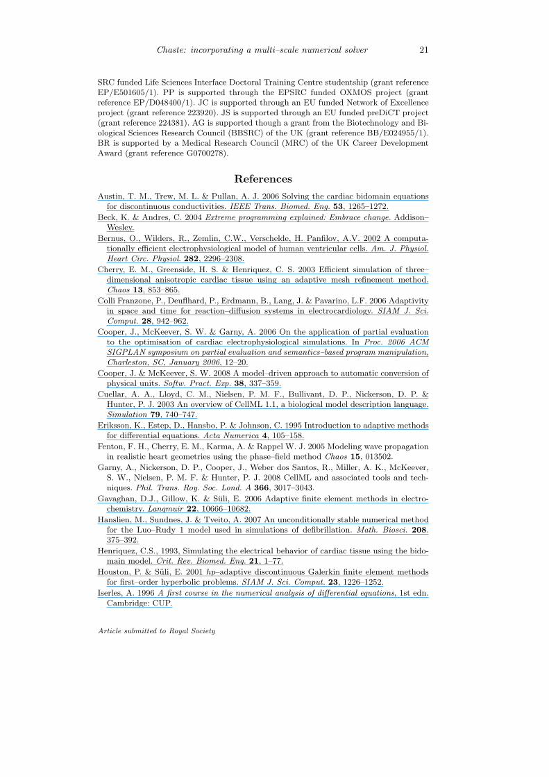
(ii) Comparison of computational timings

Figures 6 and 7 show computation time results for the 2D simulations describedabove. Monodomain and bidomain results are presented. We instrumented Chaste

Article submitted to Royal Society

Chaste: incorporating a multi–scale numerical solver 15

-100

-80

-60

-40

-20

0

20

40

60

0 50 100 150 200 250 300 350

volta

ge (

mV

)

time (ms)

FELUBEMS

10

15

20

25

30

35

40

45

50

16 18 20 22 24 26 28 30

Figure 2. Monodomain 2D: electrical activation at (x = 10, y = 10) mm

-100

-80

-60

-40

-20

0

20

40

60

0 50 100 150 200 250 300 350

volta

ge (

mV

)

time (ms)

FELUBEMS

10

15

20

25

30

35

40

45

50

16 18 20 22 24 26 28 30

Figure 3. Bidomain 2D: electrical activation at (x = 10, y = 10) mm

to record wallclock times for all potentially significant parts of the code, to anaccuracy of 1 ms. However, in all cases 90% to 99% of the simulation time was takenby three main components: assembling the linear system (matrix and right–handside), ODE solution, and linear system solution. We have dropped less significantparts of the code such as pre- and post-processing and data output from the charts.

Article submitted to Royal Society

16 M. O. Bernabeu and others

-100

-80

-60

-40

-20

0

20

40

60

0 50 100 150 200 250 300 350

volta

ge (

mV

)

time (ms)

FELUBEMS

10

15

20

25

30

35

40

45

50

0 2 4 6 8 10

Figure 4. Monodomain 3D: electrical activation at (x = 1.5, y = 1.5, z = 1.5) mm

-100

-80

-60

-40

-20

0

20

40

60

0 50 100 150 200 250 300 350

volta

ge (

mV

)

time (ms)

FELUBEMS

10

15

20

25

30

35

40

45

50

0 2 4 6 8 10

Figure 5. Bidomain 3D: electrical activation at (x = 1.5, y = 1.5, z = 1.5) mm

All times were recorded by running the code on a single core of a 64-bit Xeon 3GHzserver.

The performance improvement in ODE solving introduced by the use of partialevaluation and look-up tables can be observed by comparing the solid bar in FEand LU. These optimizations made the ODE solution around 10% faster yielding amore modest overall improvement of around 6%. Nevertheless its use in a numerical

Article submitted to Royal Society

Chaste: incorporating a multi–scale numerical solver 17

Simulation APD90 Conduction Velocity max dV /dt

(ms) (mm/ms) (mV/ms)

Monodomain FE 229.0 0.592 192.6

Monodomain LU 229.0 0.592 192.6

Monodomain BE 228.8 0.556 172.8

Monodomain MS 230.7 0.568 172.6

Bidomain FE 229.0 0.532 192.2

Bidomain LU 229.0 0.532 192.2

Bidomain BE 228.7 0.5 169.6

Bidomain MS 230.7 0.508 170.4

Table 3. Results of the 2D Simulations

Simulation APD90 Conduction Velocity max dV /dt

(ms) (mm/ms) (mV/ms)

Monodomain FE 229.4 0.652 195.8

Monodomain LU 229.4 0.652 195.8

Monodomain BE 229.2 0.6 171.4

Monodomain MS 231.0 0.652 178.5

Bidomain FE 229.3 0.6 193.6

Bidomain LU 229.3 0.6 193.6

Bidomain BE 229.2 0.56 173.0

Bidomain MS 231.0 0.58 179.7

Table 4. Results of the 3D Simulations

scheme like BE (not suffering from such a long assembling time) would lead to ahigher overall improvement.

Switching from an explicit (FE) to an implicit (BE) numerical scheme let uschoose a bigger ∆t without affecting stability. The assembly time is highly depen-dant on ∆t, as can be seen by comparing the second bar on both schemes. Thisis because the right–hand side of the linear system must be re-assembled on eachtimestep. The speed-up factor of 10 matches the ratio between ∆tFE and ∆tBE ,showing the assembly process to be a linear function of ∆t. The reduction in ODEsolving time (solid bar) comes straightforwardly from the fewer updates of the cellstate needed.

Compared to BE, our multi–scale algorithm reduces by a factor of 7 the timespent in ODE solving (corresponding to the ratio of 10 between ∆tslow and ∆tfast).Unfortunately, the complexity of other parts of the code grows due to the interpo-lation step needed. The overall improvement factor is around 3. The complete setof optimizations presented (from FE to MS) shows an order of magnitude speed-up. This speed-up was mainly due to switching to a more stable implicit solutiontechnique.

Figures 8 and 9 present computational timings for the 3D simulations. Most ofthe trends presented for the 2D simulations apply in 3D as well. The savings madein the ODE solution method from FE, through LU and BE, to MS are roughly thesame as those savings made in the 2D simulations. There is again a speed-up by afactor of 10 between LU and BE which corresponds to the difference in ∆t.

It must be noted that in the 3D simulation experiments the linear solver takesup to 60% of the overall time for bidomain LU (20% with the smaller monodomain

Article submitted to Royal Society

18 M. O. Bernabeu and others

0

500

1000

1500

2000

2500

3000

FE LU BE MS

time

(s)

totalODE solving

linear algebraassembling

Figure 6. Monodomain 2D: Performance of the different numerical schemes presented.Total computation time and most time consuming parts shown.

0

500

1000

1500

2000

2500

3000

3500

4000

4500

FE LU BE MS

time

(s)

totalODE solving

linear algebraassembling

Figure 7. Bidomain 2D: Performance of the different numerical schemes presented. Totalcomputation time and most time consuming parts shown.

system). This is due to the higher connectivity of the mesh in 3D which leads tothe main matrix structure being less sparse than for the equivalent 2D problem.Enforcing the use of implicit schemes to reduce the timestep, and thus the numberof PDE solution steps, is mandatory here.

Article submitted to Royal Society

Chaste: incorporating a multi–scale numerical solver 19

0

500

1000

1500

2000

2500

FE LU BE MS

time

(s)

totalODE solving

linear algebraassembling

Figure 8. Monodomain 3D: Performance of the different numerical schemes presented.Total computation time and most time consuming parts shown.

0

500

1000

1500

2000

2500

3000

3500

4000

4500

FE LU BE MS

time

(s)

totalODE solving

linear algebraassembling

Figure 9. Bidomain 3D: Performance of the different numerical schemes presented. Totalcomputation time and most time consuming parts shown.

The timing results from the test on the more realistic heart-based geometryare not presented here, but they show the same trend between the semi-implicitbackward Euler run (BE) and the multi–scale algorithm (MS). There was a eight-fold speed up in ODE solution which is similar to that obtained in 2D.

Article submitted to Royal Society

20 M. O. Bernabeu and others

5. Discussions and conclusions

We have described the implementation of a multi–scale numerical algorithm intoChaste, a software package we have written that may be used for—amongst otherthings—tissue level electrophysiological simulations. Although we did not achievethe same increase in computational efficiency seen for a model problem in Whiteley(2008), we are not disheartened. Chaste is very general purpose, and the flexibil-ity and reliability offered by this software excludes the use of handcrafted codingthat may be used to optimize the performance of the software. Furthermore, us-ing a realistic geometry requires that we use an unstructured mesh—ordering thenodes to generate a well–conditioned matrix is a much tougher task under thesecircumstances.

Automating the production of as much of the code as possible has many advan-tages. Assuming this code meets high software engineering standards, the object–oriented features of this code allows us to replace one numerical algorithm by an-other without compromising the integrity of other parts of the code. This has beenutilized by the Chaste development team during the implementation of the multi–scale algorithm described here—it is now a simple task for a user of Chaste tospecify which of the solvers offered by Chaste they wish to use. Of course, should auser wish to run multiple simulations using a fixed electrophysiological cell modelthen it may be appropriate to perform some code optimizations by hand. This maybe achieved by using the profiling tools that are available within Chaste. Thesetools may be used to identify bottlenecks in the code and these bottlenecks maythen be hand–coded to optimize performance.

It is hoped that the Chaste package will be developed to allow a wider rangeof simulations, drawn from both heart modelling and more general computationalbiology, to be carried out. In this paper, we have focused on the development ofChaste for cardio–electrophysiological modelling. A separate development strandhas focused on cancer modelling, and one notable achievement of this work is amulti–scale model of cancer growth that links feedback between the multiple scalesin both directions (van Leeuwen et al. 2008). It should be made clear that the cancerstrand has benefited from development of functionality for heart modelling and viceversa. The computational infrastructure is common to both strands and there is alsomuch overlap in the modelling functionality required, such as the solution of ODEs.The generality that characterizes development of Chaste allows any functionalityalready included to be used by any other application.

It is envisaged that the generality described above will aid us in the develop-ment of Chaste for new problems, such as a multi–physics model of the heart thatincludes models of electrophysiology, force generation within cardiac fibres, tissuedeformation, and fluid mechanics. As more modelling functionality is generatedfor different applications it is likely that there will be more scope for code re–usefor novel applications. This will make developing code for complex multi–physicsproblems a much less daunting task.

Any interested reader may download Chaste under an open source licence fromhttp://www.comlab.ox.ac.uk/Chaste

Development work on Chaste is supported by the Engineering and Physical Sci-ences Research Council (EPSRC) of the UK as part of a Software for High PerformanceComputing project (grant reference EP/F011628/1). RB is supported through an EP-

Article submitted to Royal Society

Chaste: incorporating a multi–scale numerical solver 21

SRC funded Life Sciences Interface Doctoral Training Centre studentship (grant referenceEP/E501605/1). PP is supported through the EPSRC funded OXMOS project (grantreference EP/D048400/1). JC is supported through an EU funded Network of Excellenceproject (grant reference 223920). JS is supported through an EU funded preDiCT project(grant reference 224381). AG is supported though a grant from the Biotechnology and Bi-ological Sciences Research Council (BBSRC) of the UK (grant reference BB/E024955/1).BR is supported by a Medical Research Council (MRC) of the UK Career DevelopmentAward (grant reference G0700278).

References

Austin, T. M., Trew, M. L. & Pullan, A. J. 2006 Solving the cardiac bidomain equationsfor discontinuous conductivities. IEEE Trans. Biomed. Eng. 53, 1265–1272.

Beck, K. & Andres, C. 2004 Extreme programming explained: Embrace change. Addison–Wesley.

Bernus, O., Wilders, R., Zemlin, C.W., Verschelde, H. Panfilov, A.V. 2002 A computa-tionally efficient electrophysiological model of human ventricular cells. Am. J. Physiol.Heart Circ. Physiol. 282, 2296–2308.

Cherry, E. M., Greenside, H. S. & Henriquez, C. S. 2003 Efficient simulation of three–dimensional anisotropic cardiac tissue using an adaptive mesh refinement method.Chaos 13, 853–865.

Colli Franzone, P., Deuflhard, P., Erdmann, B., Lang, J. & Pavarino, L.F. 2006 Adaptivityin space and time for reaction–diffusion systems in electrocardiology. SIAM J. Sci.Comput. 28, 942–962.

Cooper, J., McKeever, S. W. & Garny, A. 2006 On the application of partial evaluationto the optimisation of cardiac electrophysiological simulations. In Proc. 2006 ACMSIGPLAN symposium on partial evaluation and semantics–based program manipulation,Charleston, SC, January 2006, 12–20.

Cooper, J. & McKeever, S. W. 2008 A model–driven approach to automatic conversion ofphysical units. Softw. Pract. Exp. 38, 337–359.

Cuellar, A. A., Lloyd, C. M., Nielsen, P. M. F., Bullivant, D. P., Nickerson, D. P. &Hunter, P. J. 2003 An overview of CellML 1.1, a biological model description language.Simulation 79, 740–747.

Eriksson, K., Estep, D., Hansbo, P. & Johnson, C. 1995 Introduction to adaptive methodsfor differential equations. Acta Numerica 4, 105–158.

Fenton, F. H., Cherry, E. M., Karma, A. & Rappel W. J. 2005 Modeling wave propagationin realistic heart geometries using the phase–field method Chaos 15, 013502.

Garny, A., Nickerson, D. P., Cooper, J., Weber dos Santos, R., Miller, A. K., McKeever,S. W., Nielsen, P. M. F. & Hunter, P. J. 2008 CellML and associated tools and tech-niques. Phil. Trans. Roy. Soc. Lond. A 366, 3017–3043.

Gavaghan, D.J., Gillow, K. & Suli, E. 2006 Adaptive finite element methods in electro-chemistry. Langmuir 22, 10666–10682.

Hanslien, M., Sundnes, J. & Tveito, A. 2007 An unconditionally stable numerical methodfor the Luo–Rudy 1 model used in simulations of defibrillation. Math. Biosci. 208.375–392.

Henriquez, C.S., 1993, Simulating the electrical behavior of cardiac tissue using the bido-main model. Crit. Rev. Biomed. Eng. 21, 1–77.

Houston, P. & Suli, E. 2001 hp–adaptive discontinuous Galerkin finite element methodsfor first–order hyperbolic problems. SIAM J. Sci. Comput. 23, 1226–1252.

Iserles, A. 1996 A first course in the numerical analysis of differential equations, 1st edn.Cambridge: CUP.

Article submitted to Royal Society

22 M. O. Bernabeu and others

Jacquemet, V., Virag, N. & Kappenberger, L. 2005 Wavelength and vulnerability to atrialfibrillation: Insights from a computer model of human atria. Europace 7, S83–S92.

Keener, J. P & Bogar, K. 1998 A numerical method for the solution of the bidomainequations in cardiac tissue. Chaos 8, 234–241.

Keener, J. P. & Sneyd, J. 1998 Mathematical physiology, ch. 11. New York: Springer.

Luo, C. H. & Rudy, Y. 1991 A model of the ventricular cardiac action potential: depolar-ization, repolarization and their interaction. Circ. Res. 68, 1501–1526.

Niederer, S. A. & Smith, N. P. 2008 An improved numerical method for strong coupling ofexcitation and contraction models in the heart. Prog. Biophys. Molec. Biol. 96, 90–111.

Noble, D. 1962 A modification of the Hodgkin–Huxley equations applicable to Purkinjefibre action and pacemaker potentials. J. Physiol. 160, 317–352.

Noble, D., Varghese, A., Kohl, P. & Noble, P. J. 1998 Improved guinea–pig ventricular cellmodel incorporating a diadic space, IKr , and IKS , and length– and tension–dependentprocesses. Canadian Journal of Cardiology 14, 123–134.

Pennachio, M. & Simoncini, V. 2002 Efficient algebraic solution of reaction–diffusion sys-tems for the cardiac excitation process. J. Comput. Appl. Math. 145, 49–70.

Pennacchio, M. 2004 The mortar finite element method for the cardiac bidomain modelof extracellular potential. J. Sci. Comput. 20, 191–210.

Plank, G., Liebmann, M., Weber dos Santos, R., Vigmond, E. J. & Hasse, G. 2007 Alge-braic multigrid preconditioner for the cardiac bidomain model. IEEE Trans. Biomed.Eng. 54, 585–596.

Potse, M., Dube, B., Richer, J., Vinet, A. & Gulrajani, R. M. 2006 A comparison ofmonodomain and bidomain reaction-diffusion models for action potential propagationin the human heart. IEEE Trans. Biomed. Eng. 53, 2425–2435.

Potse, M., Coronel, R., Falcao, S., le Blanc, A. & Vinet, A. 2007 The effect of lesion sizeand tissue remodeling on ST deviation in partial–thickness ischemia. Heart Rhythm 4,200–206.

Pitt–Francis, J., Bernabeu, M. O., Cooper, J., Garny, A., Momtahan, L., Osborne, J. M.,Pathmanathan, P., Rodrıguez, B., Whiteley, J. P. & Gavaghan, D. J. 2008 Chaste: usingagile programming techniques to develop computational biology software. Phil. Trans.Roy. Soc. Lond. A 366, 3111-3136.

Plotkowiak, M., Rodrıguez, B., Plank, G., Schneider, J. E., Gavaghan, D. J., Kohl, P.& Grau, V. 2008 High performance computer simulations of cardiac electrical functionbased on high resolution MRI datasets. Lecture Notes in Computer Science 5101, 571–580.

Qu, Z. & Garfinkel, A. 1999 An advanced algorithm for solving partial differential equationin cardiac conduction. IEEE Trans. Biomed. Eng. 46, 1166–1168.

Quan, W., Evans, S. J. & Hastings, H. M. 1998 Efficient integration of a realistic two–dimensional cardiac tissue model by domain decomposition. IEEE Trans. Biomed. Eng.45, 372–385.

Rodrıguez, B., Li, L., Eason, J., Efimov, I. & Trayanova N. 2005 Differences between leftand right ventricular geometry affect cardiac vulnerability to electric shocks Circ. Res.97, 168–175.

Rodrıguez, B., Trayanova, N. & Noble, D. 2006 Modeling cardiac ischemia. Ann N Y AcadSci 1080, 395–414.

Seemann, G., Hoper, C., Sachse, F. B., Dossel, O., Holden, A. V., Zhang, H., 2006 Hetero-geneous three-dimensional anatomical and electrophysiological model of human atria.Transact A Math Phys Eng Sci. 364, 1465–1481.

Skouibine, K., Trayanova, N. A. & Moore, P. 2000 A numerically efficient model for sim-ulation of defibrilation in an active bidomain sheet of myocardium. Math. Biosci. 166,85–100.

Article submitted to Royal Society

Chaste: incorporating a multi–scale numerical solver 23

Sundnes, J., Lines, G. T. & Tveito, A. 2001 Efficient solution of ordinary differentialequations modeling electrical activity in cardiac cells. Math. Biosci. 172, 55–72.

Sundnes, J., Lines, G. T. & Tveito, A. 2005 An operator splitting method for solving thebidomain equations coupled to a volume conductor model for the torso. Math. Biosci.194, 233–248.

Sundnes, J., Nielsen, B. F., Mardal, K. A., Cai, X., Lines, T. L. & Tveito, A. 2006 On thecomputational complexity of the bidomain and monodomain models of electrophysiol-ogy. Ann. Biomed. Eng. 34, 1088–1097.

ten Tusscher, K. H., Hren R., & Panfilov A. V. 2007 Organization of ventricular fibrillationin the human heart. Circ. Res. 100, e87–101.

Tranquillo, J., Hlavacek, J., & Henriquez C. S. 2005 An integrative model of mouse cardiacelectrophysiology from cell to torso Europace 7, S56–S70.

Trayanova, N., Eason, J., & Aguel, A. 2002 Computer simulations of cardiac defibrillation:a look inside the heart. Comput. Visual Sci. 4, 259–270.

Trew, M. L., Smaill, B. H., Bullivant, D. P., Hunter, P. J. & Pullan, A. J. 2005 A generalizedfinite difference method for modeling cardiac electrical activation on arbitrary, irregularcomputational meshes. Math. Biosci. 198, 169–189.

Trudel, M-C., Dube, B., Potse, M., Gulrajani, R.M. & Leon, L.J. 2004 Simulation ofQRST integral maps with a membrane–based computer heart model employing parallelprocessing. IEEE Trans. Biomed. Eng. 51, 1319–1329.

van Leeuwen, I. M. M., Mirams, G. R., Walter, A., Fletcher, A., Murray, P., Osborne, J. M.,Varma, S., Young, S. J., Cooper, J., Pitt–Francis, J. M., Momtahan, L., Pathmanathan,P., Whiteley, J. P., Chapman, S. J., Gavaghan, D. J., Jensen, O. E., King, J. R., Maini,P. K., Waters, S. L. & Byrne, H. M. 2008 An integrative computational model forintestinal tissue renewal. Cell. Prolif. submitted.

Victorri, B. A., Vinet, F. A., Roberge, F. A. & Drouhard, J-P. 1985 Numerical integrationin the reconstruction of cardiac action potentials using Hodgkin–Huxley type models.Comput. Biomed. Res. 18, 10–23.

Vigmond, E. J., Aguel, F. & Trayanova, N. A. 2002 Computational techniques for solvingthe bidomain equations in three dimensions. IEEE Trans. Biomed. Eng. 49, 1260–1269.

Vigmond, E. J. & Clements, C. 2007 Construction of a computer model to investigatesawtooth effects in the Purkinje system. IEEE Trans. Biomed. Eng. 54, 389–399.

Vigmond, E. J., Weber dos Santos, R., Prassl, A. J., Deo, M. & Plank, G. 2008 Solversfor the cardiac bidomain equations. Prog. Biophys. Mol. Biol. 96, 3–18.

Watanabe, H., Sugiura, S., Kafuku, H. & Hisada, T. 2004 Multi–physics simulation ofleft ventricular filling dynamics using fluid–structure interaction finite element method.biophysics J. 87, 2074–2085.

Weber dos Santos, R., Plank, G., Bauer, S. & Vigmond, E. J. 2004 Parallel multigridpreconditioner for the cardiac bidomain model. IEEE Trans. Biomed. Eng. 51, 1960–1968.

Whiteley, J. P. 2006 An efficient numerical technique for the solution of the monodomainand bidomain equations. IEEE Trans. Biomed. Eng. 53, 2139–2147.

Whiteley, J. P, Bishop, M. J. & Gavaghan, D. J. 2007 Soft tissue modelling of cardiacfibres for use in coupled mechano–electric simulations. Bull. Math. Biol. 69, 2199-2225.

Whiteley, J. P. 2007 Physiology driven adaptivity for the numerical solution of the bido-main equations. Ann. Biomed. Eng. 35, 1510–1520.

Whiteley, J. P. 2008 An efficient technique for the numerical solution of the bidomainequations. Ann. Biomed. Eng. 36, 1398–1408.

Article submitted to Royal Society