Ecological Modelling 173 (2004) 271–281

Characterization of the variability of the daily course ofleaf water potential in the dominant shrub species

within Sahelian fallows in south-west Niger

Josiane Seghieria,∗, Francis Laloëba UMR 5126 Centre d’Etudes Spatiales de la Biosphère (UPS-CNRS-CNES-IRD),

18, Av. Edouard Belin bpi 2801, 31401 Toulouse Cedex 9, Franceb UMR C3ED (IRD-UVSQ), I.R.D. (ex-ORSTOM), Centre de Montpellier, BP 64501, 34394 Montpellier Cedex 5, France

Received 11 February 2003; received in revised form 5 August 2003; accepted 1 October 2003

Abstract

Around Niamey, in Niger, the shrubGuiera senegalensis dominates all of the fallows in almost totally monospecific stands.The species has a strong resprouting ability enabling it to survive cutting when clearing land for crops, whereas all otherspecies succumb to cutting. However, in this dry environment (560 mm of annual rainfall from June through September), thisremnant-increaser species has to cope with variations of available water in space and time. The daily course of its water status isan indicator of the variation of the intensity of water flux between the soil, vegetation and atmosphere, and it is often estimatedwith Soil Vegetation Atmosphere Transfer (SVAT) models.

We assessed the water status ofG. senegalensis through its daily cycle leaf water potential (Ψ ), using six populations repre-sentative of the local diversity by measuring three shrubs per population on two excised leaves per shrub for each measurement.We made our measurements over two vegetative cycles (from July 1994 to December 1995), fortnightly during the rainy season,and once a month during the dry season, until the sample shrubs lost their leaves in their deciduous cycle.

We used linear models to characterize the dailyΨ cycle of the shrubs, and of the populations during each season. For eachpopulation, three sources of variation were considered: the shrub number, the date and the hour in day. Date and hour in dayeffects are presented as trend surface models defined by the degrees of polynomials and the status of shrub effects. The status ofshrub effects characterizes the variability in accounting for environmental conditions.

The group of plant populations that explain the least variability in every model as well as the least total variance amongthe shrubs and between seasons were in locations with the best water supply. Two other groups were defined according to themedian and the highest explained variability ofΨ , respectively. For all stations, the most temporal variability is explained bymodels accounting for the interaction between shrubs and the temporal variation, with the least variability for models that donot account for the shrub effect at all. Models accounting only for the additive effect of shrubs explain intermediate values. Themodels used herein indicate the large range of variability inG. senegalensis water status, both for inter- and intra-populations.This high physiological plasticity must contribute to the strong species-dominance stability in its current distribution area.© 2003 Elsevier B.V. All rights reserved.

Keywords: Dry savanna;Guiera senegalensis; Linear model; Physiological heterogeneity; Water status

∗ Corresponding author. Tel.:+33-561-558-531; fax:+33-561-558-500.E-mail address: josiane.seghieri@cesbio.cnes.fr (J. Seghieri).

0304-3800/$ – see front matter © 2003 Elsevier B.V. All rights reserved.doi:10.1016/j.ecolmodel.2003.10.001

272 J. Seghieri, F. Laloë / Ecological Modelling 173 (2004) 271–281

1. Introduction

The savannas in Niger around Niamey are nowmainly composed of a patchwork of fallows varyingin age which are growing on sandy soils, classifiedas an arenosol using the FAO classification system(Gaze et al., 1998). Fallows are covered by an an-nual herbaceous stratum, and a species woody stra-tum comprised of Combretaceae,Guiera senegalen-sis J.L. Gmel. (Hutchinson and Dalziel, 1954–1972),which is an extremely dominant multi-stemmed andbasal-resprouting shrub. In this area,G. senegalensishas benefited for several decades by the eliminationof other native woody species due to the increasingintensity of repeated clearing for millet production(Delabre, 1998; Gaze et al., 1998). While the nativepreviously-in-place suite of Combretaceae (dominatedby Combretum micranthum G. Don,Hutchinson andDalziel, 1954–1972) has disappeared,G. senegalen-sis, with its high survival rates following cutting com-bined with its high resprouting ability, has filled thegaps. In the study area, the spatial variability of soilwater availability is due as much to soil aridificationafter over-exploitation of the pre-existing vegetationas to the topographic variation.G. senegalensis clearlyhas the capacity to deal with the spatial and temporalvariations in levels of available water across its areadistribution. It is of fundamental importance for theregional vegetation management to provide a betterunderstanding of the species ecophysiology. We con-tribute to this priority by analyzing the hour and spa-tial variabilities of the water status in six local popula-tions differing in fallow age, past intensity of exploita-tion, and topographic location. As a Sudano–Sahelianspecies, the study shrub is commonly dominant insandy Sahelian fallow lands from Senegal east to Su-dan (Aubreville, 1950, p. 90). It appears to be a typicalcase of a “human-mediated vegetation switch”sensuBarstow and McG King (1995), which is probablyamplified by recent droughts (1973, 1981, and 1984).Consequently our study is likely to be relevant to abroader area than only that of the study site.

During HAPEX-Sahel (Hydrological and Atmo-sphere Pilot Experiment in the Sahel, 1990–1992),several models of the flux of water, energy, and mat-ter in several fallows were supplied with inputs fromvery localized and hour limited data collections in aone-degree square (100 km×100 km) around Niamey

(Goutorbe et al., 1997). These types of results aredifficult to extrapolate up to the vegetation canopy asa whole, except through the use of more or less com-plex up-scaling models (Hanan and Prince, 1997).Another purpose of this analysis of large data sets ata local scale (six situations under the same climateconditions) is to provide regional investigators withbetter understanding of field heterogeneity. Our workassesses the actual magnitude of the water status vari-ability that the modellers need to take into accountwhen scaling up the vegetation physiological process.Leaf water potential following the soil water storagevariation combined with the atmospheric demand(Ritchie and Hinkley, 1975) is an indicator of thewater flux intensity between the vegetation and theatmosphere. However, in Soil Vegetation AtmosphereTransfer (SVAT), it is generally calculated throughthe presumed equality between the root extraction andthe transpiration (Braud et al., 1995; Lo Seen et al.,1997). We propose to model the direct measurementsof an estimator of the flux intensity frequently enoughto outline its daily course over two growing seasons.

In the Sahel, a dataset on the fine dynamics of vege-tation water status remains rare (Ullman, 1989; Bergeret al., 1996; Seghieri and Galle, 1999), and shouldconsiderably contribute to understanding this type ofcover functioning.

The study took place for fallows within the HAPEXone-degree square. We characterized the daily courseof the water status inG. senegalensis by monitoringthe leaf water potential (Ψ ) in six populations at theHAPEX-Sahel Central super-site during two succes-sive rainy seasons and the dry season between.

To quantify Ψ variability, we used linear models.They provided an overview of the inter- and intra-station variability of theΨ daily course accounting forshrub, date, and hour effects. Furthermore, linear trendsurface models also provide a visual “descriptive”analysis based on the shape of trend surfaces thatgives a lot of original 3-D information.

2. Material and methods

2.1. The study species and the study sites

G. senegalensis can grow up to 3 m in height. Beingsemi-evergreen, leaf shedding occurs as a drought-

J. Seghieri, F. Laloë / Ecological Modelling 173 (2004) 271–281 273

Table 1Characteristics of the stations studied

Stations Topographic situation Fallow age (afterDelabre, 1998)

Crop/fallow duration (%)(after Delabre, 1998)

1 Sandy field at middle-slope 3 422 Bottom-slope dune bulges 2 553 Hydrographic network 2 554 Very degraded at middle-slope 23 ≈05 Degraded at middle-slope 19 126 Hydrographic network 1 ≈100

avoiding strategy in the dry season in proportion toand during a period that varies with shrub location(Breman and Kessler, 1995, pp. 140–146;Seghieriand Simier, 2002). We monitored the daily course ofthe leaf water potential (Ψ ) in six fallow stands ofG. senegalensis considered as representative of thefallow diversity in the square degree around Niamey(Delabre, 1998). The fallows were selected around theBanizoumbou village in Southwest Niger (13◦32′Nand 2◦42′E), 75 km north-east of Niamey. In all ofthem, G. senegalensis was strongly dominant in thewoody cover, with an annual understorey and a fewother scattered woody shrubs (mainlyCombretummicranthum). Mean annual rainfall over the period1905–1989 was 560 mm (Le Barbé and Lebel, 1997).A single rainy season extends from June to Septem-ber. Long-term average potential evaporation exceedsrainfall in all months except August when it is simi-lar in magnitude (Peugeot et al., 1997). Mean annualETP is about 2300 mm (Gaze et al., 1998). The soil iscomposed of aeolian sandy deposits from ergs, whichare 15,000–50,000 years old (Delabre, 1998). It over-lies a weathered lateritic layer, below which lies asequence of Continental Terminal Miocene depositsof siltstones and mudstones (Gaze et al., 1998). Soilsare about 88% sand, 3% silt and 9% clay.

The six fallows studied differ in their disturbancehistories. We assessed each site in terms of time sincelast cutting (the fallow age) and the ratio of crop/fallowduration displayed inDelabre (1998). This ratio de-fined as “cumulated length of crop periods/cumulatedlength of fallow periods” indicates the intensity of ex-ploitation pressure the shrubs suffered. Fallows alsodiffer in their topographic situation. Their character-istics are displayed inTable 1. G. senegalensis standsin clumps of stems that could be several square me-ters in extent, according to their resprouting intensityafter cutting.

2.2. The data collection

A rectangular exclosure of around 10,000 m2 wasset up during 1993 in each site. Data were collectedwithin these exclosures (called “stations” below) fromJuly 1994 to December 1995, which included two suc-cessive rainy seasons and the intervening completedry season. There were three rainfall recorders: oneclose to the isolated station 1, another close to sta-tions 2 and 3, and the third close to stations 4, 5 and6. Rain recorders were provided and monitored by theEPSAT1 Program (which validates in the field rainfallassessment by remote sensing through a dense net-work of rain recorders).

In each station, the basal circumference of eachclump was measured. Three shrubs per station weresampled at random among the dominant classes of cir-cumference size, and among individuals in an appar-ent good state (taking account of parasite attack andplant diseases, etc.). A hydraulic press (HP, Objectif Kmodel, France) was used to measure the leaf water po-tential, because it was much stronger, more convenientand less dangerous than classic devices (using highlycompressed air such as a pressure chamber) to imple-ment in the field (stations were as far as 5 km apart).Calibration was not required for comparative analy-sis. In addition, rather good correlations were foundbetween the HP and pressure chamber (Jones andCarabaly, 1980; Hicks et al., 1986; Sojka et al., 1990).Data were collected fortnightly during the rainy sea-sons and once a month during the dry season.Ψ

was measured at each time interval for one smallpiece of each leaf, on two different leaves per sampledclump. Measurements were made every hour frompredawn until the daily maximum ofΨ was reached

1 Etablissement des Pluies par SATellite—Niger (ORSTOMproject).

274 J. Seghieri, F. Laloë / Ecological Modelling 173 (2004) 271–281

for the three sampled shrubs in a station. Cuts weretaken from mature leaves in well-lighted conditions ateye level (about 6 ft off the ground).

2.3. The data processing

During the study period, leaf water potential (Ψ )was measured on a set of 12,540 leaves (6270 twoleaf samples) taken from the 18 sampled shrubs inthe six fallows. For data analysis, we used the naturallogarithm ofΨ .

2.3.1. Reference modelWe sought to clearly show the magnitude of the

possible variability of the daily course ofΨ in thestudy species in Sahelian conditions at both the pop-ulation scale (intra-station differences) and betweenpopulations (inter-stations comparison). We first con-sidered those 6270 samples in an ANOVA with “sam-ple effect.” This reference model takes into accountthe two-leaf effect. When this reference model is ap-plied to each of the six stations, the residual meansquares are considered as indicators of the varianceof the distribution of theΨ logarithm among the “leafpopulation” of a given shrub at a given hour for agiven day.

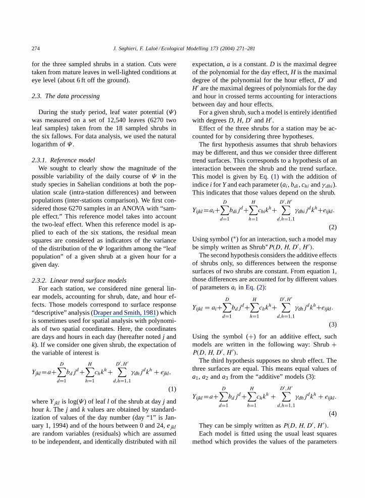
2.3.2. Linear trend surface modelsFor each station, we considered nine general lin-

ear models, accounting for shrub, date, and hour ef-fects. Those models correspond to surface response“descriptive” analysis (Draper and Smith, 1981) whichis sometimes used for spatial analysis with polynomi-als of two spatial coordinates. Here, the coordinatesare days and hours in each day (hereafter notedj andk). If we consider one given shrub, the expectation ofthe variable of interest is

Yjkl =a+D∑

d=1

bdjd +

H∑

h=1

chkh+

D′,H ′∑

d,h=1,1

γdhjdkh + ejkl,

(1)

whereYjkl is log(Ψ ) of leaf l of the shrub at dayj andhour k. The j andk values are obtained by standard-ization of values of the day number (day “1” is Jan-uary 1, 1994) and of the hours between 0 and 24,ejkl

are random variables (residuals) which are assumedto be independent, and identically distributed with nil

expectation,a is a constant.D is the maximal degreeof the polynomial for the day effect,H is the maximaldegree of the polynomial for the hour effect,D′ andH′ are the maximal degrees of polynomials for the dayand hour in crossed terms accounting for interactionsbetween day and hour effects.

For a given shrub, such a model is entirely identifiedwith degreesD, H, D′ andH′.

Effect of the three shrubs for a station may be ac-counted for by considering three hypotheses.

The first hypothesis assumes that shrub behaviorsmay be different, and thus we consider three differenttrend surfaces. This corresponds to a hypothesis of aninteraction between the shrub and the trend surface.This model is given byEq. (1) with the addition ofindicei for Y and each parameter (ai, bdi, chi andγdhi).This indicates that those values depend on the shrub.

Yijkl =ai+D∑

d=1

bdijd+

H∑

h=1

chikh+

D′,H ′∑

d,h=1,1

γdhijdkh+eijkl.

(2)

Using symbol (∗) for an interaction, such a model maybe simply written as Shrub∗P(D, H, D′, H ′).

The second hypothesis considers the additive effectsof shrubs only, so differences between the responsesurfaces of two shrubs are constant. From equation 1,those differences are accounted for by different valuesof parametersai in Eq. (2):

Yijkl = ai+D∑

d=1

bdjd+

H∑

h=1

chkh+

D′,H ′∑

d,h=1,1

γdhjdkh+eijkl.

(3)

Using the symbol (+) for an additive effect, suchmodels are written in the following way: Shrub+P(D, H, D′, H ′).

The third hypothesis supposes no shrub effect. Thethree surfaces are equal. This means equal values ofa1, a2 anda3 from the “additive” models (3):

Yijkl =a+D∑

d=1

bdjd +

H∑

h=1

chkh +

D′,H ′∑

d,h=1,1

γdhjdkh + eijkl.

(4)

They can be simply written asP(D, H, D′, H ′).Each model is fitted using the usual least squares

method which provides the values of the parameters

J. Seghieri, F. Laloë / Ecological Modelling 173 (2004) 271–281 275

(ai, bdi, chi and γdhi) for which the sum of squareddifferences between observed and fitted values (i.e.the residual sum of squares) is a minimum. The qual-ity of each fit and comparisons between them can bediscussed through standard statistical linear modelingtheory. It can also be discussed through examinationof the distribution of the residuals.

The nine models are classified into three groups,according to the status of shrub effect. Mod-els 2–4 [Shrub∗P(16, 5, 9, 4), Shrub∗P(9, 4, 9, 4),Shrub∗P(16, 5, 0, 0)] account for the interaction be-tween shrubs and the temporal variation. Models5–7 [Shrub+ P(16, 5, 9, 4), Shrub+ P(9, 4, 9, 4),Shrub + P(16, 5, 0, 0)] consider only an additiveeffect of the shrub, which means that the temporalpatterns are the same for each shrub with a constantdifference between them. The last three models 8–10,[P(16, 5, 9, 4), P(9, 4, 9, 4), P(16, 5, 0, 0)] assumeno shrub effect at all. For each group of models, thefirst one (2, 5, 8) considers the additive effects ofday and hour with degrees 16 and 5, and interactionslimited to degrees 9 and 4. The second models (3, 6,9) consider the additive effect and the interactions forwhich both of the polynomials are limited to degrees9 and 4. The third models (4, 7, 10) consider only theadditive effects of the day and hour (degrees 16 and 5).

We considered polynomials with rather high degrees(up to 16 for model 2). Such high degrees are neededto represent the observed variability. For example, foreach of the six stations, the usualF tests for the com-parison of models 2 and 3, the later having “lower”degrees (up to 9,Table 3), led to the rejection of model3 with an “α” risk level lower than 0.001.

2.3.3. Shape of the trend surfacesThe estimated values of the parameters are of no

great interest, since we are looking for the shape ofresponse surfaces which may be presented in a figure.As for non-parametric models, where the usual linearfunction of covariates is replaced with an unspecifiedfunction (Hastie and Tibshirani, 1990), may be pre-sented in a graphic. With the given values of the pa-rameters, we may compute the expected values of thevariable of interest for each shrub and for given val-ues of days and hours in a grid. This operation wasillustrated from the fit of model 2 for stations 1, 2and 6 considering day–shrub combinations for whichat least six observations were available. For each of

these day–shrub combinations, we estimated the ex-pectation ofY in half-hour time steps between 08:00and 17:00 LST.

2.3.4. Checking modelsThe quality of the models must be checked and

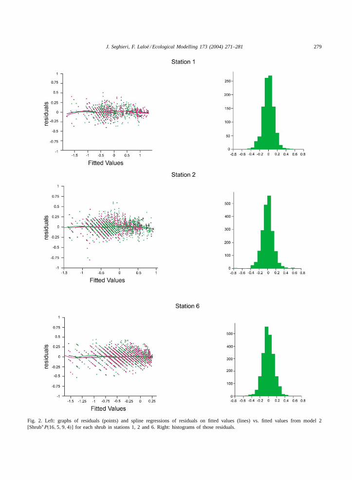
discussed through an examination of the distribu-tion of the residual differences between the observedand the fitted values (Draper and Smith, 1981; MacCullagh and Nelder, 1989). In Fig. 2, residuals areplotted versus fitted values (points) together withthe results (lines) of a spline regression (Hastie andTibshirani, 1990) for each shrub of those residuals onfitted values. Two main aspects are evident (i) if themodel is unbiased, those regressions are nil functionsand (ii) if the variance of the residuals does not de-pend on the expectation of the variable of interest, therange of residuals doesn’t depend on the fitted values.We also present histograms of the residuals (Fig. 2).

In theory, the closer the residual variance of a modelto the variance of the reference model, the more it ac-counts for shrub, date and hour effects. Such modelsonly exhibit regular events. For example, at each date,the maximum value ofΨ occurs around the “solarmidday,” i.e. when the sun is at its zenith. This typeof model doesn’t exhibit outcomes from casual lo-cal changes occurring in environmental conditions, asdoes the reference model. For instance, clouds cross-ing the sun temporarily decrease the luminosity andreduce the stomatal opening, which then causeΨ todecrease during a short time period. These sorts of ca-sual events are not what we want to describe, so evena model with a higher residual variance than that ofthe reference model would not necessarily be rejected.

3. Results

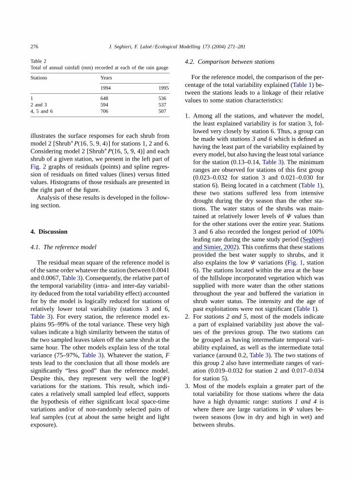
Total seasonal rainfall was higher and the durationof the rainy period was longer in 1994 than in 1995for each of the three rain gauge locations. Differencesin rainfall between the locations were smaller duringthe dryer year (1995,Table 2).

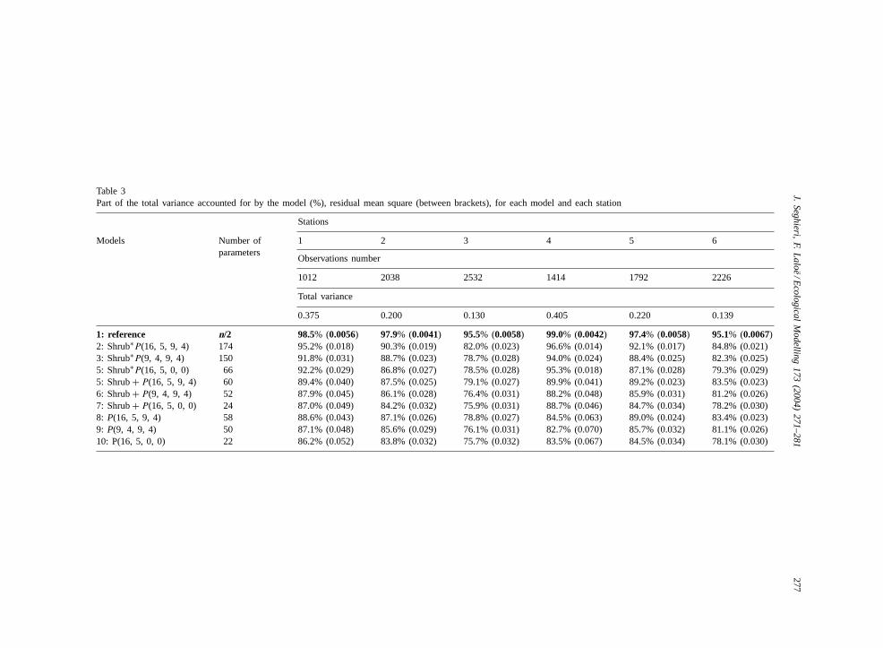
Results of the fit of the nine general linear modelsfor each of the six stations are summarized inTable 3.For each station and each model, the total variance,the percentage of total variance accounted for, and theresidual mean square are given in this table.Fig. 1

276 J. Seghieri, F. Laloë / Ecological Modelling 173 (2004) 271–281

Table 2Total of annual rainfall (mm) recorded at each of the rain gauge

Stations Years

1994 1995

1 648 5362 and 3 594 5374, 5 and 6 706 507

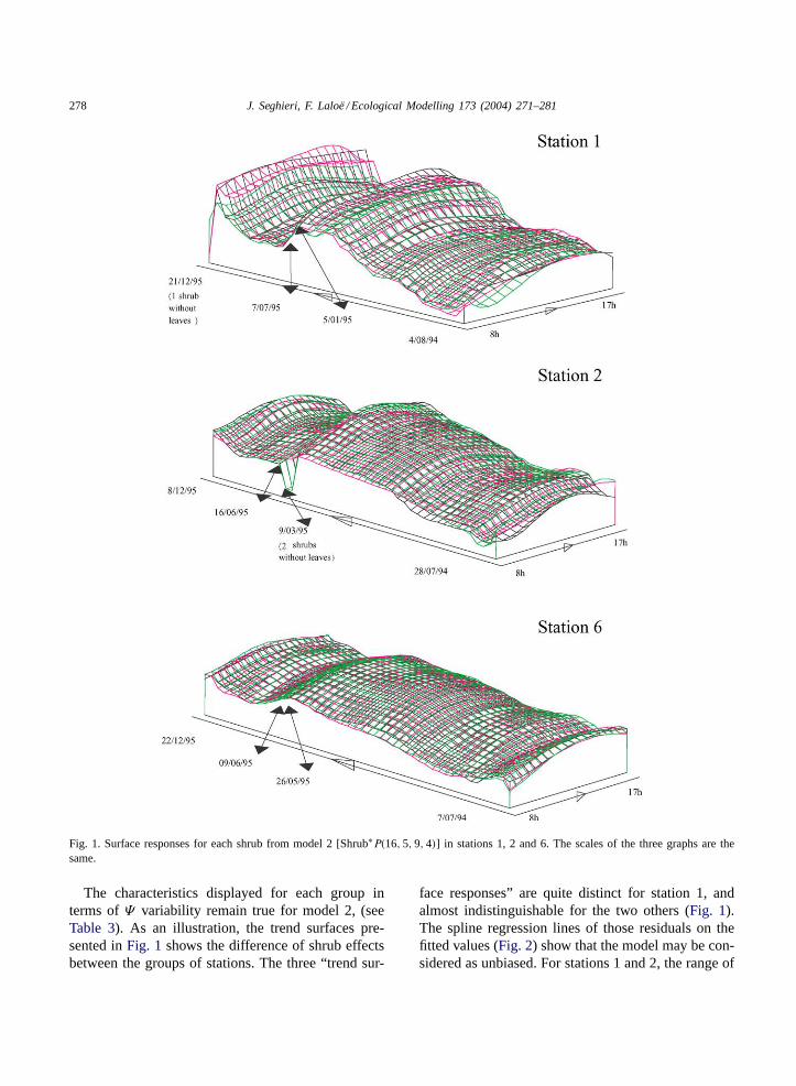
illustrates the surface responses for each shrub frommodel 2 [Shrub∗P(16, 5, 9, 4)] for stations 1, 2 and 6.Considering model 2 [Shrub∗P(16, 5, 9, 4)] and eachshrub of a given station, we present in the left part ofFig. 2 graphs of residuals (points) and spline regres-sion of residuals on fitted values (lines) versus fittedvalues. Histograms of those residuals are presented inthe right part of the figure.

Analysis of these results is developed in the follow-ing section.

4. Discussion

4.1. The reference model

The residual mean square of the reference model isof the same order whatever the station (between 0.0041and 0.0067,Table 3). Consequently, the relative part ofthe temporal variability (intra- and inter-day variabil-ity deduced from the total variability effect) accountedfor by the model is logically reduced for stations ofrelatively lower total variability (stations 3 and 6,Table 3). For every station, the reference model ex-plains 95–99% of the total variance. These very highvalues indicate a high similarity between the status ofthe two sampled leaves taken off the same shrub at thesame hour. The other models explain less of the totalvariance (75–97%,Table 3). Whatever the station,Ftests lead to the conclusion that all those models aresignificantly “less good” than the reference model.Despite this, they represent very well the log(Ψ )variations for the stations. This result, which indi-cates a relatively small sampled leaf effect, supportsthe hypothesis of either significant local space-timevariations and/or of non-randomly selected pairs ofleaf samples (cut at about the same height and lightexposure).

4.2. Comparison between stations

For the reference model, the comparison of the per-centage of the total variability explained (Table 1) be-tween the stations leads to a linkage of their relativevalues to some station characteristics:

1. Among all the stations, and whatever the model,the least explained variability is for station 3, fol-lowed very closely by station 6. Thus, a group canbe made withstations 3 and 6 which is defined ashaving the least part of the variability explained byevery model, but also having the least total variancefor the station (0.13–0.14,Table 3). The minimumranges are observed for stations of this first group(0.023–0.032 for station 3 and 0.021–0.030 forstation 6). Being located in a catchment (Table 1),these two stations suffered less from intensivedrought during the dry season than the other sta-tions. The water status of the shrubs was main-tained at relatively lower levels ofΨ values thanfor the other stations over the entire year. Stations3 and 6 also recorded the longest period of 100%leafing rate during the same study period (Seghieriand Simier, 2002). This confirms that these stationsprovided the best water supply to shrubs, and italso explains the lowΨ variations (Fig. 1, station6). The stations located within the area at the baseof the hillslope incorporated vegetation which wassupplied with more water than the other stationsthroughout the year and buffered the variation inshrub water status. The intensity and the age ofpast exploitations were not significant (Table 1).

2. For stations 2 and 5, most of the models indicatea part of explained variability just above the val-ues of the previous group. The two stations canbe grouped as having intermediate temporal vari-ability explained, as well as the intermediate totalvariance (around 0.2,Table 3). The two stations ofthis group 2 also have intermediate ranges of vari-ation (0.019–0.032 for station 2 and 0.017–0.034for station 5).

3. Most of the models explain a greater part of thetotal variability for those stations where the datahave a high dynamic range:stations 1 and 4 iswhere there are large variations inΨ values be-tween seasons (low in dry and high in wet) andbetween shrubs.

J.Seghieri,

F.L

aloë/E

cologicalM

odelling173

(2004)271–281

277

Table 3Part of the total variance accounted for by the model (%), residual mean square (between brackets), for each model and each station

Stations

Models Number ofparameters

1 2 3 4 5 6

Observations number

1012 2038 2532 1414 1792 2226

Total variance

0.375 0.200 0.130 0.405 0.220 0.139

1: reference n/2 98.5% (0.0056) 97.9% (0.0041) 95.5% (0.0058) 99.0% (0.0042) 97.4% (0.0058) 95.1% (0.0067)2: Shrub∗P(16, 5, 9, 4) 174 95.2% (0.018) 90.3% (0.019) 82.0% (0.023) 96.6% (0.014) 92.1% (0.017) 84.8% (0.021)3: Shrub∗P(9, 4, 9, 4) 150 91.8% (0.031) 88.7% (0.023) 78.7% (0.028) 94.0% (0.024) 88.4% (0.025) 82.3% (0.025)5: Shrub∗P(16, 5, 0, 0) 66 92.2% (0.029) 86.8% (0.027) 78.5% (0.028) 95.3% (0.018) 87.1% (0.028) 79.3% (0.029)5: Shrub+ P(16, 5, 9, 4) 60 89.4% (0.040) 87.5% (0.025) 79.1% (0.027) 89.9% (0.041) 89.2% (0.023) 83.5% (0.023)6: Shrub+ P(9, 4, 9, 4) 52 87.9% (0.045) 86.1% (0.028) 76.4% (0.031) 88.2% (0.048) 85.9% (0.031) 81.2% (0.026)7: Shrub+ P(16, 5, 0, 0) 24 87.0% (0.049) 84.2% (0.032) 75.9% (0.031) 88.7% (0.046) 84.7% (0.034) 78.2% (0.030)8: P(16, 5, 9, 4) 58 88.6% (0.043) 87.1% (0.026) 78.8% (0.027) 84.5% (0.063) 89.0% (0.024) 83.4% (0.023)9: P(9, 4, 9, 4) 50 87.1% (0.048) 85.6% (0.029) 76.1% (0.031) 82.7% (0.070) 85.7% (0.032) 81.1% (0.026)10: P(16, 5, 0, 0) 22 86.2% (0.052) 83.8% (0.032) 75.7% (0.032) 83.5% (0.067) 84.5% (0.034) 78.1% (0.030)

278 J. Seghieri, F. Laloë / Ecological Modelling 173 (2004) 271–281

Fig. 1. Surface responses for each shrub from model 2 [Shrub∗P(16, 5, 9, 4)] in stations 1, 2 and 6. The scales of the three graphs are thesame.

The characteristics displayed for each group interms ofΨ variability remain true for model 2, (seeTable 3). As an illustration, the trend surfaces pre-sented inFig. 1 shows the difference of shrub effectsbetween the groups of stations. The three “trend sur-

face responses” are quite distinct for station 1, andalmost indistinguishable for the two others (Fig. 1).The spline regression lines of those residuals on thefitted values (Fig. 2) show that the model may be con-sidered as unbiased. For stations 1 and 2, the range of

J. Seghieri, F. Laloë / Ecological Modelling 173 (2004) 271–281 279

Fig. 2. Left: graphs of residuals (points) and spline regressions of residuals on fitted values (lines) vs. fitted values from model 2[Shrub∗P(16, 5, 9, 4)] for each shrub in stations 1, 2 and 6. Right: histograms of those residuals.

280 J. Seghieri, F. Laloë / Ecological Modelling 173 (2004) 271–281

the residuals is slightly lower if the fitted values aregreater than 0.25. For station 6, for which fitted val-ues do not exceed 0.25, the range of the residuals isstable. This indicates a larger shrinkage effect of thelog transformation for the high values. Histograms ofthe residual indicate near normal distributions.

Again, for the group consisting of stations 2 and3, the intensity and the time since the last crop donot appear to be significant factors of physiologi-cal seasonal variation and intra-station heterogeneity(Table 1). However, this does not mean that the sec-ond group of stations (2 and 5), with intermediatevariability of Ψ , supply shrubs with higher soil mois-ture than the third group of stations (1 and 4) withthe highestΨ variation. Indeed, exceptions appear inthe relative rank of the accounted-for variability foreach model among these four stations (Table 3). Inaddition, phenology recorded at the population scaleby Seghieri and Simier (2002)was much more dis-turbed for stations 2 and 5 than for stations 1 and 4,which supports the hypothesis of adverse conditions.This confirms, first that the intensity of past exploita-tion per se is not a good indicator of the vegetationdisturbance when considered alone, and second thatthe relationships betweenG. senegalensis phenologyin dry and disturbed conditions and its water statusare more complex than what be shown by a simplecorrelation.

To go further in the analysis, we compared the linearmodels to each other.

4.3. Comparison between models

We recall that, as for the reference model, whena given model explains more variability for one sta-tion than another (Table 3), it does not mean that themodel fits the data better in absolute terms. As resid-ual mean squares are of the same order of magnitude(0.008–0.044,Table 3), a greater part of explainedvariation only means that there is more temporal vari-ability to be explained.

Linear models are made according to three groupsof shrub effects. For all stations, the range of theresidual mean square increases from the first (no. 2–4)to the third (no. 8–10) group of models (0.014–0.029to 0.026–0.067, respectively). But the magnitudeof this increase depends on the station group. It ismuch more important for the third group (stations

1 and 4) than for the other two. For station 1, weobserved an important effect of interactions involv-ing shrubs, with a low additive effect (residual meansquares are analogous for models groups 2 and 3).For station 4, the additive and interaction effects areimportant.

4.4. Conclusion

For sites where the water seems to be non-limiting,models of the dynamics of vegetation water statuscan be based on just a few field observations andcould be simplified regarding the shrub effect in-fluence. However, models or any other estimationmethod must take into account the inter-shrub vari-ability at the station scale. We clearly showed themagnitude of the possible variability at the popu-lation scale (intra-station differences), and the evenmore significant values at the meta-population scale(inter-stations comparison) of the leaf water potentialdaily course in the study species in Sahelian condi-tions. In terms of plasticity, the large range of waterstatus to whichG. senegalensis can survive shouldlargely contribute to the species sustainability in itsdominance area even after disturbances have stopped(Poupon, 1979; Devineau, 1999; Seghieri and Simier,2002).

This makes a natural regeneration of the otheroriginal native species doubtful. After a serious dis-turbance, there are a number of ecological nichesavailable for colonization, and plants with the mostplastic environmental requirements get a windowof opportunity that gives them a decisive competi-tive advantage.G. senegalensis behaves in this wayand our results have showed its physiological ad-vantages under the overall shifting hydrologic per-formance of the landscape. The value of the waterreserve globally alters with degradation (Casenaveand Valentin, 1992; Seghieri et al., 1994, 1995;Walker and Langridge, 1997), so that most of theecological niches of the original species could dis-appear. This is also probably why, when followinghuman transformation of ecosystems, plants frommore xeric habitats, since they are pre-adapted toa large range of conditions, tend to invade moremesic ones rather than the reverse (Blondel andAronson, 1999, pp. 38–39, 121,Seghieri and Simier,2002).

J. Seghieri, F. Laloë / Ecological Modelling 173 (2004) 271–281 281

Acknowledgements

This work was partially supported by “Jachère”project funds, EEC project “Reduction of the Fal-low Length, Biodiversity and Sustainable develop-ment in Central and West Africa” (TS3-CT93-0220,DG12 HSMU). We are grateful to D. Tongway(CSIRO-Wildlife and Ecology, Canberra) who helpus to fundamentally improve the first version. Wethank also A. Boone for his English review and thetwo anonymous referees.

References

Aubreville, A., 1950. Flore forestière Soudano-Guinéenne A.O.F.—Cameroun—A.E.F. Editions Maritime et Coloniales, Paris,523 pp.

Barstow, W., McG King, W., 1995. Human-mediated vegetationswitches as processes in landscape ecology. Landscape Ecol.10, 191–196.

Berger, A., Grouzis, M., Fournier, C., 1996. The water status ofsix woody species coexisting in the Sahel (Ferlo, Senegal). J.Trop. Ecol. 12, 607–627.

Blondel, J., Aronson, J., 1999. Biology and Wildlife of theMediterranean Region. Oxford University Press, Oxford, 328pp.

Braud, I., Dantas-Antonino, A.C., Vauclin, M., Thony, J.L.,Ruelle, P., 1995. A simple soil–plant–atmosphere transfer model(SiSPAT), development, field verification. J. Hydrol. 166, 231–260.

Breman, H., Kessler, J.J., 1995. Woody plants in agro-ecosystemsof semi-arid regions. In: Advanced Series in AgriculturalSciences, vol. 23. Springer-Verlag, Berlin, 340 pp.

Casenave, A., Valentin, C., 1992. A runoff capability classificationsystem based on surface features criteria in semi-arid areas ofWest Africa. J. Hydrol. 130, 231–249.

Delabre, E., 1998. Caractérisation et évolution d’écosystèmesanthropisés sahéliens: les milieux post-culturaux du sud-ouestnigérien. Doctoral thesis, University P. & M. Curie, Paris VI,251 pp.

Devineau, J.L., 1999. Seasonal rhythms and phenological plasticityof savanna woody species in a fallow farming system (south-west Burkina Faso). J. Trop. Ecol. 15, 497–513.

Draper, N., Smith, J., 1981. Applied Regression Analysis, 2nd ed.Wiley Series in Probability and Mathematical Statistics, 709 pp.

Gaze, S.R., Brouwer, J., Simmonds, L.P., Bromley, J., 1998. Dryseason water use patterns underGuiera senegalensis shrubs ina tropical savanna. J. Arid Environ. 40, 53–67.

Goutorbe, J.P., Dolman, A.J., Gash, J.H.C., Kerr, Y.H., Lebel, T.,Prince, S.D., Stricker, J.N.M., 1997. HAPEX-Sahel (Specialissues). J. Hydrol. 188/189, 1090.

Hanan, N.P., Prince, S.D., 1997. Stomatal conductance of west-central supersite vegetation in HAPEX-Sahel: measurementsand empirical models. J. Hydrol. 188/189, 536–562.

Hastie, T.J., Tibshirani, R.J., 1990. Generalized additive models.In: Monographs on Statistics and Applied Probabilities, vol.43. Chapman & Hall, 335 pp.

Hicks, S.K., Lascano, R.J., Wendt, C.W., Onken, A.B., 1986. Useof a hydraulic press for estimation of leaf water potential ingrain sorghum. Agron. J. 78, 749–751.

Hutchinson, J., Dalziel, J.M., 1954–1972. Flora of West TropicalAfrica. Crown Publishers, London.

Jones, C.A., Carabaly, A., 1980. Estimation of leaf water potentialin tropical grasses with the Campbell–Brewster hydraulic press.Trop. Agric. 57, 305–307.

Le Barbé, L., Lebel, T., 1997. Rainfall climatology of the centralSahel during the years 1950–1990. J. Hydrol. 188/189, 43–73.

Lo Seen, D., Chehbouni, A., Njoku, E., Saatchi, S., Mougin,E., Monteny, B., 1997. An approach to couple vegetationfunctionning and soil–vegetation–atmosphere-transfer modelsfor semi-arid grasslands during the HAPEX-Sahel experiment.Agric. Forest Meteorol. 83, 49–74.

Mac Cullagh, P., Nelder, J.A., 1989. Generalized linear models.Monographs on Statistics and Applied Probability, 2nd ed., vol.37. Chapman & Hall, 511 pp.

Peugeot, C., Estèves, M., Galle, S., Rajot, J.L., Vandervaere, J.P.,1997. Runoff generation process: results and analysis of fielddata collected at the East Central Supersite of HAPEX-Sahelexperiment. J. Hydrol. 188/189, 179–202.

Poupon, H., 1979. Etude de la phénologie de la strate ligneuseà Fété-Olé (Sénégal septentrional) de 1971 à 1977. Bull. del’IFAN, Série A 41, 44–85.

Ritchie, G.A., Hinkley, T.M., 1975. The pressure chamber as ainstrument for ecological research. Adv. Ecol. Res. 9, 165–254.

Seghieri, J., Floret, C., Pontanier, R., 1994. Development ofan herbaceous cover in a Sudano–Sahelian savanna in NorthCameroon in relation to available soil water. Vegetatio 114,175–184.

Seghieri, J., Floret, C., Pontanier, R., 1995. Plant phenology inrelation to water availability: herbaceous and woody species inthe savannas of northern Cameroon. J. Trop. Ecol. 11, 237–254.

Seghieri, J., Galle, S., 1999. Run-on contribution to a saheliantwo-phase mosaic system: soil water regime and vegetation lifecycle. Acta Oecol. 20, 209–218.

Seghieri, J., Simier, M., 2002. Variations in phenology of a residualinvasive shrub species in Sahelian fallow savannas, south-westNiger. J. Trop. Ecol. 18, 1–16.

Sojka, R.E., Sadler, E.J., Camp, C.R., Arnold, F.B., 1990.A comparison of pressure chamber, leaf-press and canopytemperature for four species under humid conditions. Environ.Exp. Bot. 30, 75–83.

Ullman, I., 1989. Stomatal conductance and transpiration ofAcaciaunder field conditions: similarities and differences betweenleaves and phyllodes. Trees Struct. Funct. 3, 45–56.

Walker, B., Langridge, J., 1997. Predicting savanna vegetationstructure on the basis of plant available moisture (PAM) andplant available nutrients (PAN): a case study from Australia. J.Biogeogr. 24, 813–825.