Characteristic-Based Schemes for Dispersive Waves I. The Method of Characteristics for Smooth Solutions Philip L. Roe and Mohit Arora The University of Michigan, Ann Arbor, Michigan 481 09-2140

Received 22 July 1992; revised manuscript received 21 December 1992

In order to embark on the development of numerical schemes for stiff problems, we have studied a model of relaxing heat flow. To isolate those errors unavoidably associated with discretization, a method of characteristics is developed, containing three free parameters depending on the stiffness ratio. It is shown that such “decoupled” schemes do not take into account the interaction between the wave families and hence result in incorrect wave speeds. We also demonstrate that schemes can differ by up to two orders of magnitude in their rms errors even while maintaining second- order accuracy. We show that n o method of characteristics solution can be better than second-order accurate. Next, we develop “coupled” schemes which account for the interactions, and here we obtain two additional free parameters, We demonstrate how coupling of the two wave families can be introduced in simple ways and how the results arc greatly enhanced by this coupling. Finally, numerical results for several decoupled and coupled schemes are presented, and we observe that dispersion relationships can be a very useful qualitative tool for analysis of numerical algorithms for dispersive waves. 0 1993 John Wiley & Sons, Inc.

1. INTRODUCTION

This paper is concerned with analyzing the method of characteristics for dispersive waves, represented here by a simple linear 2 X 2 system describing hyperbolic heat conduction. In this model, dispersive wave behavior is caused by a source term, which may be “stiff”. Our work is motivated by the fact that many problems of technical interest are stiff, i.e., the reaction or equilibration time of some nonequilibrium process is much smaller than the flow residence time. It is then highly inefficient to use for all the flow processes explicit time steps that are small enough to ensure stability of the reaction equations. One may use implicit schemes, which are also expensive (although the less expensive point-implicit schemes are often satisfactory [l]) or one may resort to split-operator methods [2], in which the hydrodynamic and reaction equations are solved alternately.

Neither alternative is wholly convincing. There have been many attempts to incorpo- rate “source terms” rationally into numerical procedures for the solution of simplified (sometimes scalar) flows. These have been based sometimes on physical arguments and

Numerical Methods for Partial Differential Equations, 9, 459-505 (1993) 0 1993 John Wiley & Sons, Inc. CCC 0749- 159X/93/050459-47

460 ROE AND ARORA

sometimes on mathematical analysis of model problems. We wished to study the simplest instance of this difficulty in this paper. The model of heat conduction that we study does not seem to have been considered previously in this context. We believe that it captures the true nature of the problem rather well. It exposes the key role of coupling between different wave families, a concept that could not be arrived at by analyzing any scalar problem.

The problem of hyperbolic heat conduction arises when Fourier’s law of heat flow proportional to temperature gradient is augmented by a term implying relaxation toward that condition [3,4]. This modification avoids the paradox of infinite propagation speed. It is also thought to be a more accurate representation of the real physics under certain conditions, such as thermal shock or very low temperatures (in liquid helium the waves are known as “second sound” [5] ) . Solutions of the hyperbolic heat equations have appeared in several places, usually obtained by Laplace-transform methods. Here, as underpinning for our numerical analysis, we present a solution of the Riemann problem for this system (two rods at different temperatures brought into sudden contact) and an integral solution for the general initial-value problem. These were found by exploiting an analogy with the hodograph method of compressible flow (Riemann’s equation). Since this connection seems to be new, a detailed analysis is given in Appendix A.

The main body of the paper has a fairly limited aim. We aim to develop a method of characteristics that will yield accurate solutions of the hyperbolic heat equations, even when the relaxation time 7 is much less than the time step A f . We are content to do this, for the present, for smooth solutions only. This turned out to be, by itself, a sufficiently difficult task, and the conclusions seem to be illuminating. Because the problem is linear, the method of characteristics would be exact if the source term were absent. Likewise, the problem would be trivial if only the source term were present (we then have a simple ordinary differential equation with an exponential solution). Any numerical difficulties that arise must then be due solely to the interaction between these two trivial problems. The fact that difficulties do arise confirms our feeling that the mechanism we uncover may have general significance.

Section I1 sets out the governing equations, and some of their more basic properties. A dispersion analysis reveals behavior typical of relaxation phenomena. High wave numbers propagate at a “frozen wave speed” and are strongly damped. Low wave numbers propagate at an “equilibrium wave speed” (equal to zero for this model problem) and contain both lightly and heavily damped modes. In later sections it turns out to be instructive to compare these with the dispersion relationships of the discretized equations, where we find them to be a good predictor of algorithm quality, and hence a useful qualitative tool to have at our disposal.

Section 111 briefly describes the Riemann problem that is employed to test our schemes. In Sec. IV we develop various discrete versions of the characteristic equations. In every

case, the stiffness factor

1 At 2 7

k = - -

appears in a natural manner. Two examples are studied in some detail. One is a straightforward discretization that corresponds in a sense to a point-implicit method. Inspection of the formulas inclines one to suppose that the results will not be good for k > 1. In fact, they were among the best we achieved for pure characteristic methods. We also examined a method derived from operator splitting. This looked better but performed worse.

CHARACTERISTIC-BASED SCHEMES FOR DISPERSIVE WAVES. 1.. . . 461

Section V gives a sketch of some of our attempts to design methods with desirable properties. The sketch is brief because although some of the properties were certainly relevant, they correlated very poorly with overall accuracy of the schemes, as illustrated by a choice that suggested itself quite strongly. This was a clear hint that the problem was not yet properly understood.

Section VI makes a fresh start, beginning with the general integral solution to the initial- value problem. We find, in fact, the exact solution for polynomial data consistent with the discrete values. This reveals that no method of characteristics solution is better than second- order accurate. The inclusion of an extra point in the stencil, however, raises the accuracy to third order and, perhaps even more significantly, enables greatly improved results to be obtained for large k. In fact, very acceptable results are obtained for time steps of around 100-fold greater than the relaxation time.

This success, however, relies on elaborate analysis that would not be feasible for general problems. In Sec. VII we aim to confirm the insight that coupling of the characteristics is the essential key. We incorporate the coupling by means of simple predictor-corrector schemes that rely on no special analysis of the governing equations. However, we do hold onto the concept of conservation. Analysis shows, and experiment confirms, that these schemes are indeed very close to optimal.

It. HYPERBOLIC HEAT EQUATIONS

We need a problem simple enough to permit detailed analysis, and carrying some physical meaning to help in understanding the results. The problem that has been chosen leads to a 2 X 2 system of equations. It has dispersive wave properties resembling those of a reactive flow, although no reaction is actually involved.

A. Derivation of Governing Equations

Consider the flow of heat in a uniform conducting bar. Conservation of energy can be stated as

1 k 6 , + -qx = 0

where 6 = temperature, q = heat flow per unit area, and k = heat capacity per unit volume.

Usually one now invokes Fourier’s law, that heat flow is proportional to the temperature gradient

q = - c o x , (2 .2)

to obtain the heat equation c

6, = -6 , . (2.3) k This is, of course, the prototype of all parabolic partial differential equations, in which information propagates with infinite speed. To avoid this unrealistic result, alternative

462 ROE AND ARORA

models are sometimes adopted [3,4,6] of which the simplest is to replace Eq. (2.2) with

rql + c6, = -4, (2.4)

where r is a relaxation time. The pair of equations (2.1) and (2.4) form a nonhomogeneous hyperbolic system for which the characteristic speeds are given by ( c / r k ) ” 2 . For simplicity, we will adopt units in which both c and k have the value 1.0, leading to the system

which we will call the hyperbolic heat equations. Maxwell introduced the concept of a relaxation time, and these equations are sometimes referred to in the literature as the Maxwell-Cattaneo equations. Several investigators have applied this concept to the problem of heat conduction (see [7] and its references) and there has been a resurgence of interest in these equations in the last five years (see [8,9] and references therein).

B. Dispersion Analysis

To see the dispersive character of Eqs. (2.5) and (2.6), consider solutions of the form

Substituting Eq. (2.7) into Eqs. (2.5) and (2.6) gives

i o T - i6Q = 0 ,

r i w Q - i [ T + Q = 0 ,

and these equations can be solved for T and Q only if

r w 2 - l2 = i w ,

which is the dispersion relationship for Eqs. (2.5) and (2.6). For an initial-value problem, 6 is a real wave number, and w may be written as

w = W R + iw l ,

where wR is a frequency and wI is a damping rate. Substituting Eq. (2.9) into Eq. (2.8) gives the pair of equations

(2.9)

wR(1 - 2 7 0 ~ ) = 0 ,

2 l2 - 0 1 wR - w; =

(2.10)

(2.1 1) r

If W R # 0, then from Eq. (2.10)

1 W I = -

27 (2.12)

CHARACTERISTIC-BASED SCHEMES FOR DISPERSIVE WAVES. I.. . . 463

and from Eq. (2.11)

(2.13)

The quantity ( w R / ( ) is a wave speed, which we call a ( ( ) . Then

(2.14)

For very high wave numbers (, the propagation speed is the characteristic speed , which could also be called the frozen wave speed. For lower wave numbers, the 7-112

propagation speed is reduced, becoming zero when ( = ; T - ” ~ . This could be interpreted as a vanishing equilibrium wave speed. For all wave numbers in the range [;r-”’,w], the waves are damped like e-t‘2T.

For wave numbers less than : T - “ ~ , we have wR = 0, and the waves do not propagate. After the typical time t = r , they are damped like e - w t T , with

(2.15)

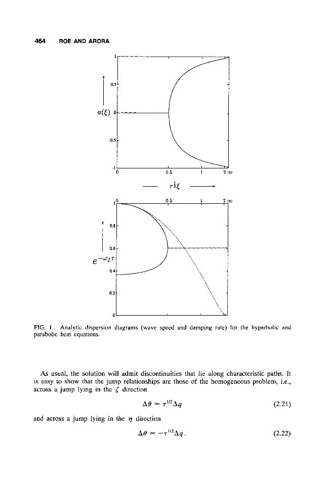
In Fig. 1 (upper), we plot the wave speed a ( ( ) against the nondimensional wave number r“’(, while in the lower, we plot the damping rate e-w‘T against the nondimensional wave number.

When ( = 0, the solution does not depend on x, and the problem reduces to 6, = 0, rqr + q = 0. Since these have solutions corresponding to W ~ T = 0, 1, respectively, both branches of Eq. (2.15) are relevant. The upper branch makes second-order contact with the dispersion relationship for the regular heat equation, which is

W I T = ( 2 7 , (2.16)

shown as a dotted line in Fig. 1 (lower).

C. Characteristic and Jump Relationships

Introduce characteristic coordinates f , 7 defined by

f = t + 7 l I 2 x ,

7 = t - 7 1 1 2 x .

Then Eqs. (2.5) and (2.6) transform to

(2.17)

(2.18)

(2.19)

(2.20)

which are the characteristic equations. Unfortunately, it is not possible to integrate these equations and obtain Riemann invariants, as can be done with linear homogeneous problems. Thus a numerical method of characteristics is no longer an exact method.

464 ROE AND ARORA

0 0.5 1

- T i ( .

FIG. 1. parabolic heat equations.

Analytic dispersion diagrams (wave speed and damping rate) for the hyperbolic and

As usual, the solution will admit discontinuities that lie along characteristic paths. It is easy to show that the jump relationships are those of the homogeneous problem, i.e., across a jump lying in the 5 direction

A 9 = r'I2Aq (2.21)

and across a jump lying in the q direction

A 9 = -r ' l2Aq, (2.22)

CHARACTERISTIC-BASED SCHEMES FOR DISPERSIVE WAVES. I.. . . 465

111. A RIEMANN PROBLEM FOR THE HYPERBOLIC HEAT EQUATIONS

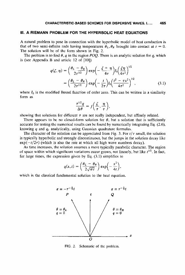
A natural problem to pose in connection with the hyperbolic model of heat conduction is that of two semi-infinite rods having temperatures O L , 6 ~ brought into contact at t = 0. The solution will be of the form shown in Fig. 2.

The problem is to find 6 , q in the region POQ. There is an analytic solution for q, which is (see Appendix B and article 12 of [lo])

where 10 is the modified Bessel function of order zero. This can be written in a similarity form as

showing that solutions for different r are not really independent, but affinely related. There appears to be no closed-form solution for 6 , but a solution that is sufficiently

accurate for testing the numerical results can be found by numerically integrating Eq. (2.6), knowing q and q, analytically, using Gaussian quadrature formulas.

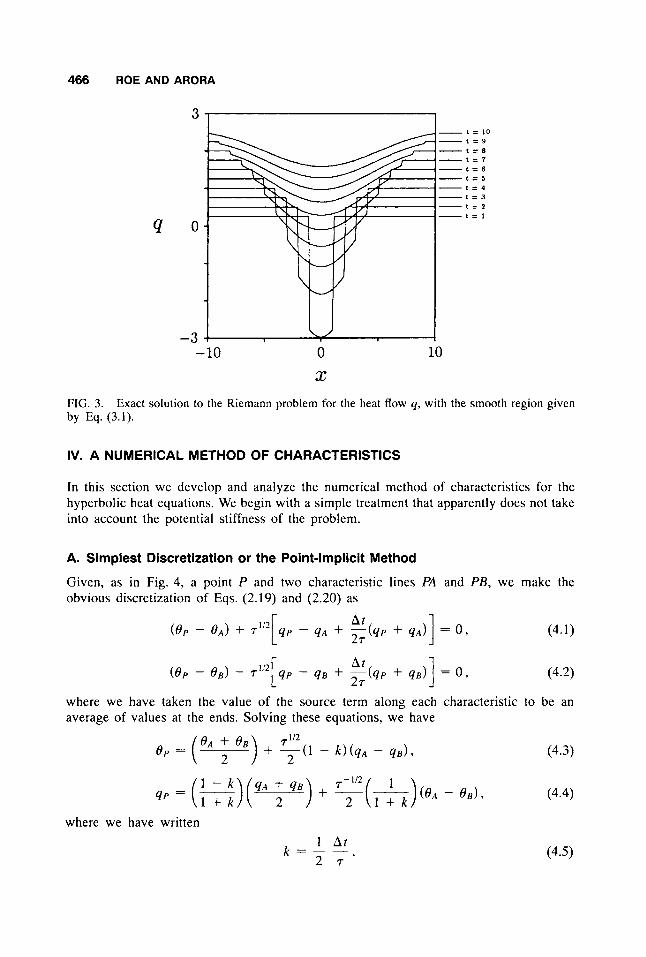
The character of the solution can be appreciated from Fig. 3. For t / r small, the solution is typically hyperbolic and strongly discontinuous, but the jumps in the solution decay like exp(-t/2r) (which is also the rate at which all high wave numbers decay).

As time increases, the solution assumes a more typically parabolic character. The region of space within which significant variations occur grows, not linearly, but like t”’. In fact, for large times, the expression given by Eq. (3.1) simplifies to

which is the classical fundamental solution to the heat equation.

t = --7-tt x = 7-41

P 2 Q t f

\ Lx 0

FIG. 2. Schematic of the problem.

466 ROE AND ARORA

t = 10 t = 9 t = 8 t = 7 t = 6 t = 5 t = 4 t = 3 t = P t = 1

X FIG. 3. by Eq. (3.1).

Exact solution to the Riemann problem for the heat flow q, with the smooth region given

IV. A NUMERICAL METHOD OF CHARACTERISTICS

In this section we develop and analyze the numerical method of characteristics for the hyperbolic heat equations. We begin with a simple treatment that apparently does not take into account the potential stiffness of the problem.

A. Simplest Discretization or the Point-Implicit Method

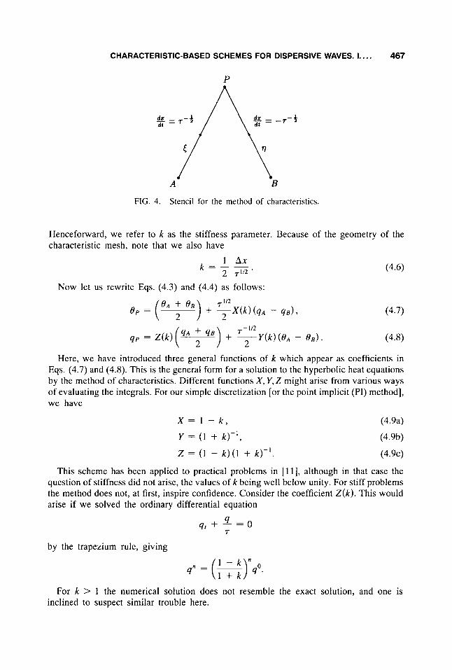
Given, as in Fig. 4, a point P and two characteristic lines PA and PB, we make the obvious discretization of Eqs. (2.19) and (2.20) as

where we have taken the value of the source term along each characteristic to be an average of values at the ends. Solving these equations, we have

where we have written 1 A t 2 r '

k = - - (4.5)

CHARACTERISTIC-BASED SCHEMES FOR DISPERSIVE WAVES. I . . . . 467

P

FIG. 4. Stencil for the method of characteristics.

Henceforward, we refer to k as the stiffness parameter. Because of the geometry of the characteristic mesh, note that we also have

Now let us rewrite Eqs. (4.3) and (4.4) as follows:

Here, we have introduced three general functions of k which appear as coefficients in Eqs. (4.7) and (4.8). This is the general form for a solution to the hyperbolic heat equations by the method of characteristics. Different functions X , Y , Z might arise from various ways of evaluating the integrals. For our simple discretization [or the point implicit (PI) method], we have

X z l - k ,

Y = ( 1 + k ) - ' ,

Z ~ ( 1 - k ) ( l + k ) - ' .

(4.9a)

(4.9b)

(4.9c)

This scheme has been applied to practical problems in [ll], although in that case the question of stiffness did not arise, the values of k being well below unity. For stiff problems the method does not, at first, inspire confidence. Consider the coefficient Z ( k ) . This would arise if we solved the ordinary differential equation

by the trapezium rule, giving

1 - k l + k

q" = (() 40.

For k > 1 the numerical solution does not resemble the exact solution, and one is inclined to suspect similar trouble here.

468 ROE AND ARORA

B. Operator Splitting

Stiff problems are in practice often broken into two parts. In one, we solve the ho- mogeneous problem

61 + q x = 0 , (4.10)

7qt + ex = 0 . (4.1 1)

In the other, we solve for the damping due to the source term as

(4.12) q:+' = q:e . Let us call the damping operation LI and the solution to the homogeneous problem by

the method of characteristics L2. To get second-order accuracy, we must use one of the sequence of operations L1L2L2L1 or L2L1L1L2 [2]. For the sequence LlL2L2L1,

At17

= 6 , ~ + 3 / 4 ,

= q:+3/4 e - k

In short, if we combine all the stages, we get Eqs. (4.7) and (4.8) with coefficients

~ ( k ) = e - k , (4.13a)

~ ( k ) = e - k , (4.13b)

~ ( k ) = e - 2 k . (4 .13~)

This looks more promising, because the coefficients seem to reflect appropriate decay rates. Indeed Z ( k ) = e-2k corresponds to the decay rate of the ordinary differential equation, and X ( k ) = Y ( k ) = K k corresponds to the decay rate of the characteristic discontinuities [see, for example, Eq. (B2)].

C. Some Numerical Results

We ran three groups of experiments for the Riemann problem described in Sec. 111. As boundary conditions we have supplied the analytical solution along both limiting characteristics. Thus we do not attempt to capture the discontinuities, and our tests relate purely to the smooth part of the solution. In the first group, our final time was tF, = 107, with time steps k = 0.5,0.25,0.125,0.0625, results being plotted at t / 7 = 3,6,10. Similarly, in the second and third groups, the final time fF2,1 = 1007, IOOOT, time steps k = [5,2.5,1.25,0.625] and [50,25,12.5,6.25], results being plotted at r /7 = [30,60,100] and [300,600, lOOO], respectively. All three are shown on the same picture, where we plot the L2 errors in q or 6 versus k on log-log scales. Each value of t / 7 plotted in our numerical

CHARACTERISTIC-BASED SCHEMES FOR DISPERSIVE WAVES. I.. . . 469

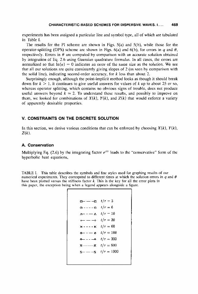
experiments has been assigned a particular line and symbol type, all of which are tabulated in Table I .

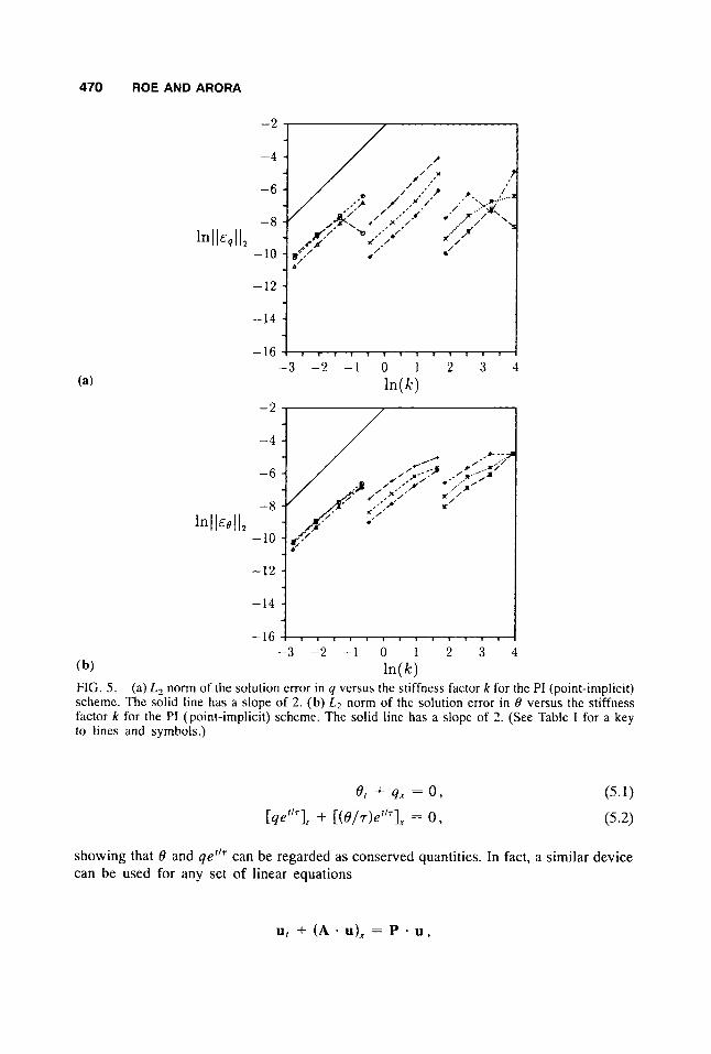
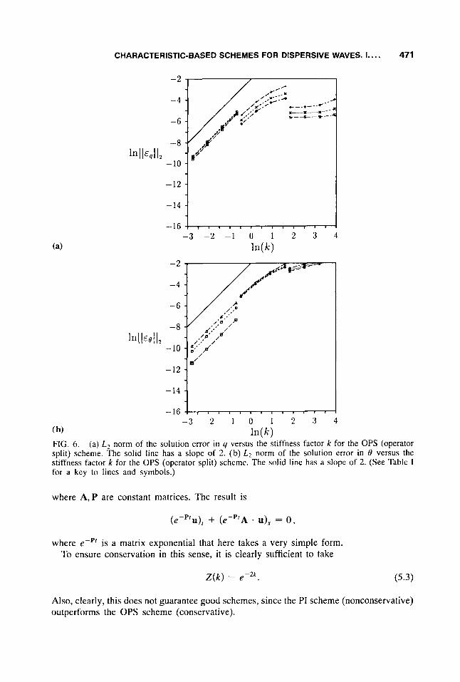
The results for the PI scheme are shown in Figs. 5(a) and 5(b), while those for the operator-splitting (OPS) scheme are shown in Figs. 6(a) and 6(b), for errors in q and 8, respectively. Errors in 8 are computed by comparison with an accurate solution obtained by integration of Eq. 2.6 using Gaussian quadrature formulas. In all cases, the errors are normalized so that In(&) = 0 indicates an error of the same size as the solution. We see that all our solutions are quite consistently giving slopes of 2 (as seen by comparison with the solid line), indicating second-order accuracy, for k less than about 2.

Surprisingly enough, although the point-implicit method looks as though it should break down for k > 1, it continues to give useful answers for values of k up to about 25 or so, whereas operator splitting, which contains no obvious signs of trouble, does not produce useful answers beyond k = 2. To understand these results, and possibly to improve on them, we looked for combinations of X ( k ) , Y ( k ) , and Z ( k ) that would enforce a variety of apparently desirable properties.

V. CONSTRAINTS ON THE DISCRETE SOLUTION

In this section, we derive various conditions that can be enforced by choosing X ( k ) , Y ( k ) , Z ( k ) .

A. Conservation

Multiplying Eq. (2.6) by the integrating factor e‘“ leads to the “conservative” form of the hyperbolic heat equations,

TABLE I. numerical experiments. They correspond to different times at which the solution errors in q and 6 have been plotted versus the stiffness factor k. This is the key for all the error plots in this paper, the exception being when a legend appears alongside a figure.

This table describes the symbols and line styles used for graphing results of our

I

t l s = 3

t/‘ = 10

t / s = 6

t / s = 30

t / s = 60

t / s = 100

t / s = 300

t / s = 600

t / s = 1000

470 ROE AND ARORA

In( k) -2

-4

-6

-8

- 10 In1 IEe I I,

-16 - 1 4 i - 3 - 2 - 1 0 1 2 3 4

( b) w> FIG. 5. (a) L, norm of the solution error in y versus the stiffness factor k for the PI (point-implicit) schemc. The solid line has a slope of 2. (b) L2 norm of the solution error in 0 versus the stiffness factor k for the PI (point-implicit) scheme. The solid line has a slope of 2. (See Table I for a key to lines and symbols.)

showing that 8 and qe‘’‘ can be regarded as conserved quantities. In fact, a similar device can be used for any set of linear equations

U; + (A * u), = P . U,

CHARACTERISTIC-BASED SCHEMES FOR DISPERSIVE WAVES. 1.. . . 471

-12 - -14 -

-2

-4

-6

-8

- 10

-12

-14

1nll412

-16

/ /

where A , P are constant matrices. The result is

(e-''u), + (e-"A . u), = 0 ,

where e-" is a matrix exponential that here takes a very simple form. To ensure conservation in this sense, it is clearly sufficient to take

Also, clearly, this does not guarantee good schemes, since the PI scheme (nonconservative) outperforms the OPS scheme (conservative).

472 ROE AND ARORA

B. Constraints from the Discrete Dispersion Relationship

Let us write Eq. (2.7) in discrete form as

(:); = %[ (i) exp[i(wnAt - AX)] (5.4)

Using this, we get from Eqs. (4.7) and (4.8) that

exp(iwAt) - cos([Ax) -irl”X(k) sin((Ax) detl -ir-”’Y(k) sin(6A.x) exp(ioAt) - Z ( k ) cos([Ax) / = 0

or

exp(2ioAt) - [ I + Z ( k ) ] exp(iwAt) cos([Ax) + Z ( k ) cos2((Ax) + X(k)Y(k) sin2([Ax) = 0

so that

exp(ioAt) =

2

and this is the discrete dispersion relationship for the method of characteristics. Note that we can only resolve wave numbers for which (Ax 5 zn-. The factor 2 arises

because the stencil for the method of characteristics decouples odd and even points. For this maximum frequency, we have

1 I

exp(iwAt) = %i[X(k)Y(k)]1’2

and hence, if XY is positive,

which gives the wave speed a( tmax) = +Ax/At = +r-’/’. If XY is negative we find

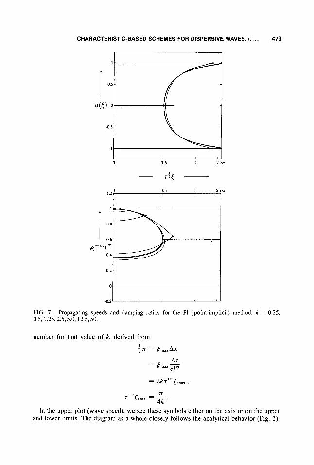
Thus, for any method of characteristics, the highest wave number observable on the mesh is either stationary or propagated at the frozen speed. This is a feature we cannot control. Figure 7 shows the discrete dispersion plots for the PI scheme for several values of k. Each plot is terminated at the right by a symbol located at the maximum wave

CHARACTERISTIC-BASED SCHEMES FOR DISPERSIVE WAVES. I.. . . 473

I

0 0.5 1 2co

-0.2' I

FIG. 7. 0.5,1.25,2.5,5.0, 12.5,50.

Propagating speeds and damping ratios for the PI (point-implicit) method. k = 0.25,

number for that value of k, derived from I in = S m a x A X

A t = [ - lnax 112

n 112 7 Smax = - 4k

In the upper plot (wave speed), we see these symbols either on the axis or on the upper and lower limits. The diagram as a whole closely follows the analytical behavior (Fig. 1).

474 ROE AND ARORA

In the lower plot (damping) there is only good agreement for the upper lobe at large k but moderate agreement everywhere else.

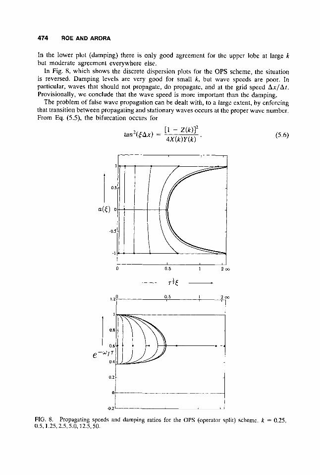
In Fig. 8, which shows the discrete dispersion plots for the OPS scheme, the situation is reversed. Damping levels are very good for small k, but wave speeds are poor. In particular, waves that should not propagate, do propagate, and at the grid speed Ax/At. Provisionally, we conclude that the wave speed is more important than the damping.

The problem of false wave propagation can be dealt with, to a large extent, by enforcing that transition between propagating and stationary waves occurs at the proper wave number. From Eq. ( 5 . 3 , the bifurcation occurs for

I ' I

I I I 0 0.5 1 2co

- 41

. . .. -

-0.2 O 2

FIG. 8. 0.5,1.25,2.5,5.0,12.5,50.

Propagating speeds and damping ratios for the OPS (operator split) scheme. k = 0.25,

CHARACTERISTIC-BASED SCHEMES FOR DISPERSIVE WAVES. I.. . . 475

Since bifurcation should actually take place at (Ax = ;T-”~AX = k (see Sec. ILB), we should enforce the condition

The actual wave numbers at which the schemes discussed so far bifurcate is plotted in Fig. 12.

There are a number of other conditions derivable from Eq. (5.5). For example,

ensures that the maximum wave number has the correct damping. Note that any condition deriving from Eq. (5.5) will only refer to the product XY, not X or Y individually.

In addition, we could stipulate that the scheme is derivable from some pair of characteristic equations, i.e., that Eqs. ( 4 . 7 ) and (4.8) can be combined to give an equation in which q A , 6 A (or qe,6B) do not appear. This condition is

Z ( k ) = X ( k ) Y ( k ) . (5.9)

I t also ensures that all propagating modes decay at the same rate. We attempted to design schemes by imposing some pair of constraints. For example, by imposing conservation [Eq. (5.3)J, and correct bifurcation [Eq. (5.6)J, we have the CB (conservative-bifurcative) scheme given by

Z ( k ) = e - 2 k , (5.10)

(1 - e-2k)2 X ( k ) Y ( k ) =

4 tan2 k ’ (5.11)

For this scheme, X ( k ) = Y ( k ) = [ X ( k ) . Y ( k ) ] * ’ 2 = (1 - e-2k ) / (2 tan k ) , and we set X ( k ) = Y ( k ) = 0 for k 2 7r/2.

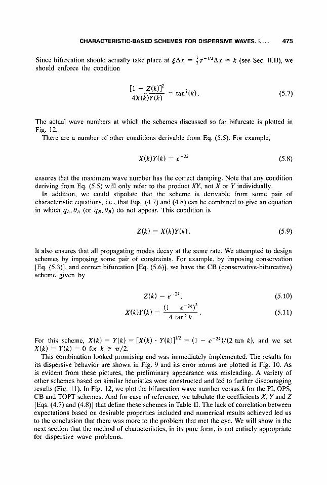
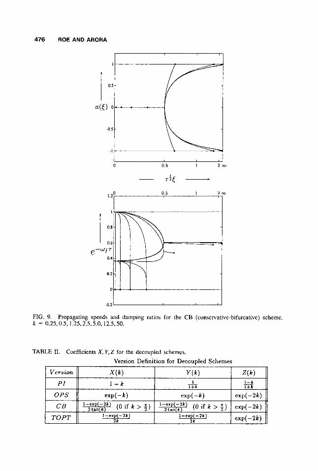
This combination looked promising and was immediately implemented. The results for its dispersive behavior are shown in Fig. 9 and its error norms are plotted in Fig. 10. As is evident from these pictures, the preliminary appearance was misleading. A variety of other schemes based on similar heuristics were constructed and led to further discouraging results (Fig. 11). In Fig. 12, we plot the bifurcation wave number versus k for the PI, OPS, CB and TOPT schemes. And for ease of reference, we tabulate the coefficients X, Y and 2 [Eqs. ( 4 . 7 ) and (4 .8)J that define these schemes in Table 11. The lack of correlation between expectations based on desirable properties included and numerical results achieved led us to the conclusion that there was more to the problem that met the eye. We will show in the next section that the method of characteristics, in its pure form, is not entirely appropriate for dispersive wave problems.

476 ROE AND ARORA

Version

PI OPS

CB TOPT

0 0.5 1 203

- T+( .

X ( k ) Y ( k ) Z ( k ) 1-1.

1+k 1+k - 1 - I - k

exP( - k) .XP(-k) exp( -2k)

exp(-2k)

exp( - 2 k )

(0 if k > 5 ) 1-ex -2k 1-ex -2k) 2taPn((k) ( O if ” 4 ) 2taPn((t)

l -exp(-Zk] 1 -exp( -2k) ‘IL “I.

FIG. 9. k = 0.25,0.5, 1.25,2.5,5.0, 12.5,50.

Propagating speeds and damping ratios for the CB (conservative-bifurcative) scheme.

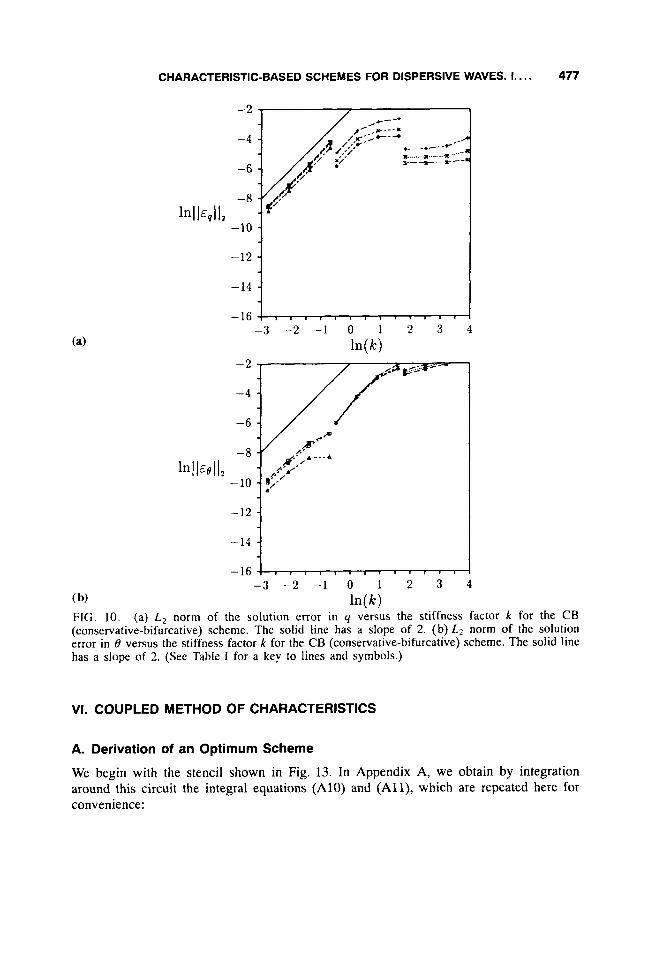
CHARACTERISTIC-BASED SCHEMES FOR DISPERSIVE WAVES. I . . . . 477

-2

-4

-6

-8

-10

-12

-14

lnllE*llz

-16 - 3 - 2 - 1 0 1 2 3 4

In(k)

VI. COUPLED METHOD OF CHARACTERISTICS

A. Derivation of an Optimum Scheme

We begin with the stencil shown in Fig. 13. In Appendix A, we obtain by integration around this circuit the integral equations (A10) and (All) , which are repeated here for convenience:

478 ROE AND ARORA

0

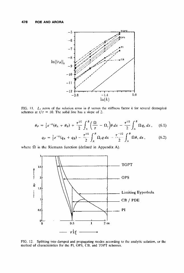
FIG. 1 1 . schemes at t / r = 10. The solid line has a slope of 2.

L2 norm of the solution error in 0 versus the stiffness factor k for several decoupled

q p = i e -k (qA + 9 s ) - (6.2)

where SZ is the Riemann function (defined in Appendix A).

TOPT

OPS

Limiting Hyperbola

CB / PDE

PI

FIG. 12. method of characteristics for the PI, OPS, CB, and TOPT schemes.

Splitting into damped and propagating modes according to the analytic solution, or the

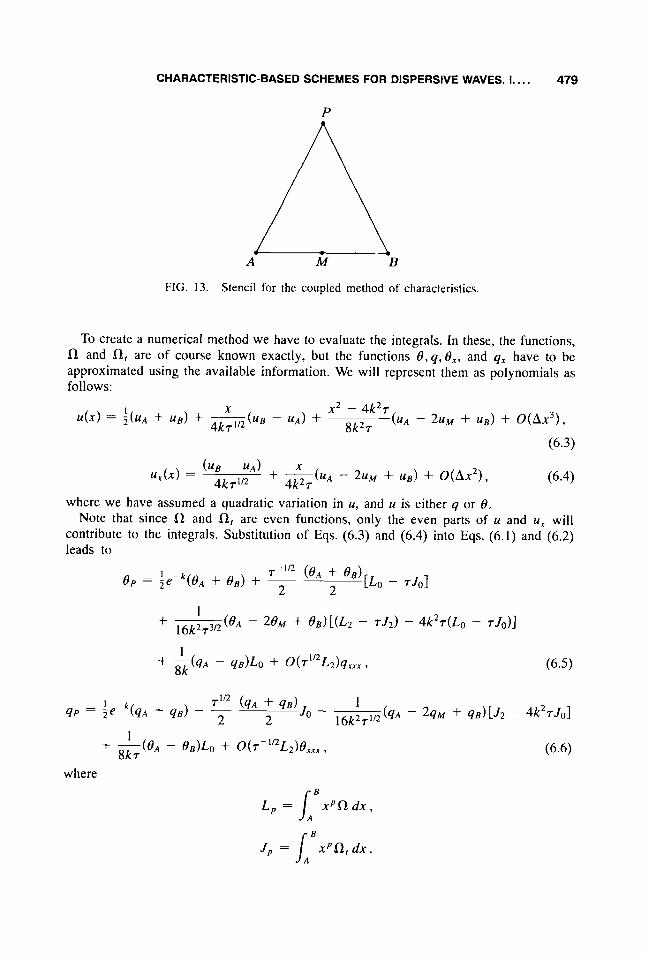
CHARACTERISTIC-BASED SCHEMES FOR DISPERSIVE WAVES. I . . . . 479

P

FIG. 13. Stencil for the coupled method of characteristics.

To create a numerical method we have to evaluate the integrals. In these, the functions, R and R, are of course known exactly, but the functions 8, q, 8,, and qx have to be approximated using the available information. We will represent them as polynomials as follows:

where we have assumed a quadratic variation in u, and u is either q or 8. Note that since R and R, are even functions, only the even parts of u and u, will

contribute to the integrals. Substitution of Eqs. (6.3) and (6.4) into Eqs. (6.1) and (6.2) leads to

where

L , = 1 xPRdx, A

J p = IA x P R , d x .

480 ROE AND ARORA

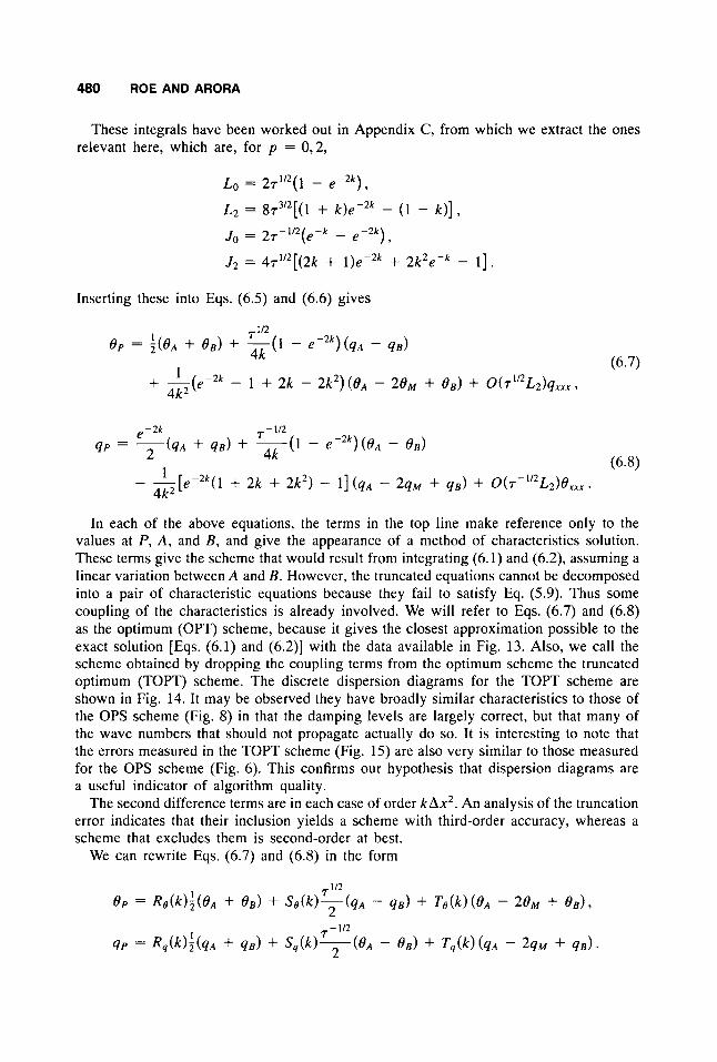
These integrals have been worked out in Appendix C, from which we extract the ones relevant here, which are, for p = 0 , 2 ,

LO = 2 ~ ' / ~ ( 1 - e - 2 k ) ,

L2 = 8r3l2[(1 + k)e -2k - ( 1 - k ) ] , Jo = 2r-1/2(e-k -

J2 = 4r1I2[ (2k + l )e-2k + 2k2e-k - 1 3 .

Inserting these into Eqs. (6.5) and (6.6) gives

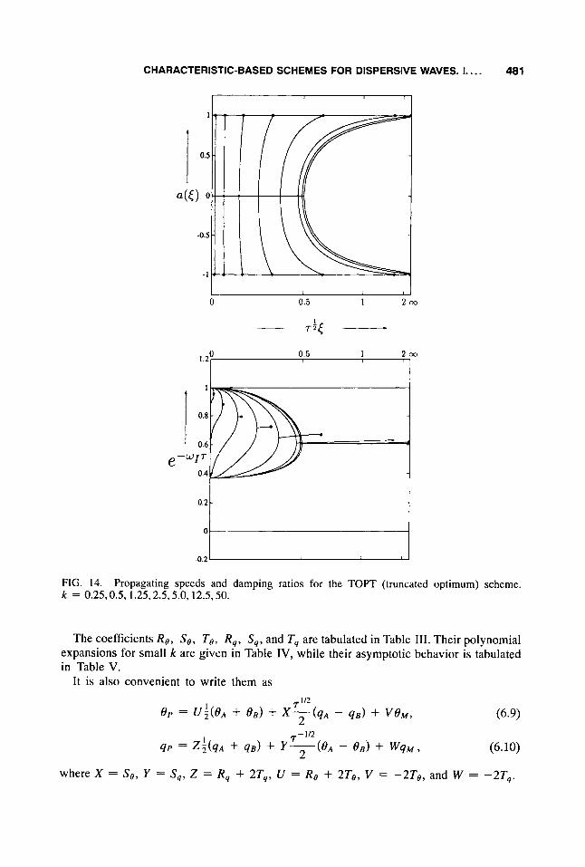
In each of the above equations, the terms in the top line make reference only to the values at P , A, and B, and give the appearance of a method of characteristics solution. These terms give the scheme that would result from integrating (6.1) and (6.2), assuming a linear variation between A and B. However, the truncated equations cannot be decomposed into a pair of characteristic equations because they fail to satisfy Eq. (5.9). Thus some coupling of the characteristics is already involved. We will refer to Eqs. (6.7) and (6.8) as the optimum (OPT) scheme, because it gives the closest approximation possible to the exact solution [Eqs. (6.1) and (6.2)] with the data available in Fig. 13. Also, we call the scheme obtained by dropping the coupling terms from the optimum scheme the truncated optimum (TOPT) scheme. The discrete dispersion diagrams for the TOPT scheme are shown in Fig. 14. It may be observed they have broadly similar characteristics to those of the OPS scheme (Fig. 8) in that the damping levels are largely correct, but that many of the wave numbers that should not propagate actually do so. It is interesting to note that the errors measured in the TOPT scheme (Fig. 15) are also very similar to those measured for the OPS scheme (Fig. 6). This confirms our hypothesis that dispersion diagrams are a useful indicator of algorithm quality.

The second difference terms are in each case of order k A x 2 . An analysis of the truncation error indicates that their inclusion yields a scheme with third-order accuracy, whereas a scheme that excludes them is second-order at best.

(6.7) and (6.8) in the form

CHARACTERISTIC-BASED SCHEMES FOR DISPERSIVE WAVES. I.. . . 481

-0.2 1 1

FIG. 14. k = 0.25,0.5,1.25,2.5,5.0,12.5,50.

Propagating speeds and damping ratios for the TOPT (truncated optimum) scheme.

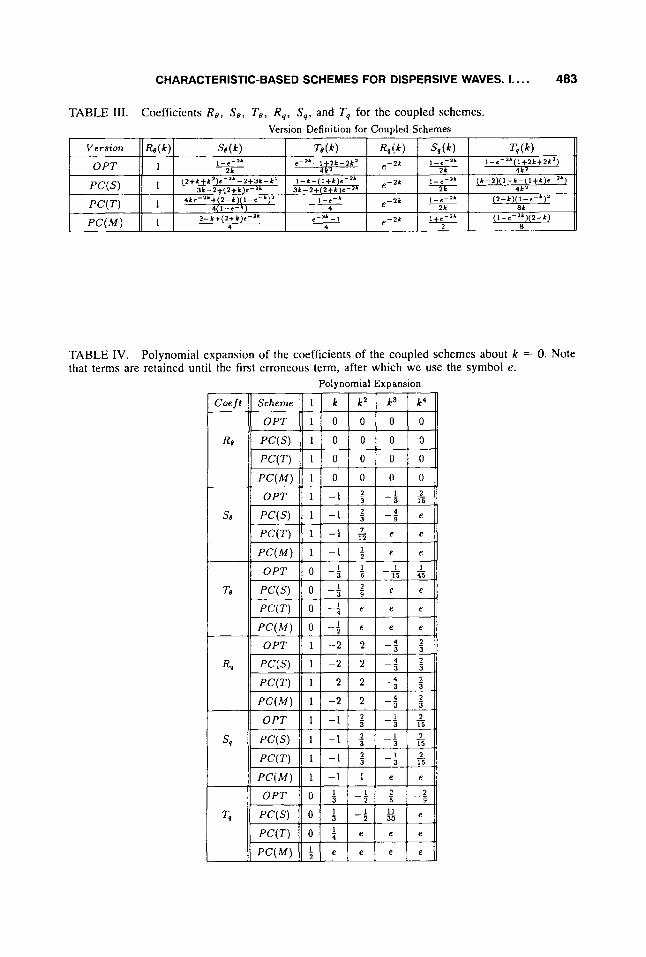
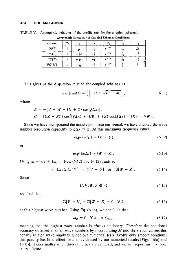
The coefficients Rg, S O , Tg, R,, S,, and T, are tabulated in Table 111. Their polynomial expansions for small k are given in Table IV, while their asymptotic behavior is tabulated in Table V.

It is also convenient to write them as

1

- 112

(6.10) 1

qf' = Z 2 ( q A + q B ) + Y-((BA - 6 B ) + WqM, 2 where X = S e , Y = S, , Z = R, + 2T,, U = Rg + 2T0, V = -2Tg, and W = -2T,.

482 ROE AND ARORA

-2

-4

-6

-8

-10

-12

- 14

lnll&(lllz

- 16

-2

-4

-6

-8

-10

-12

-14

In I I €8 I I

- 16 - 3 - 2 - 1 0 1 2 3 4

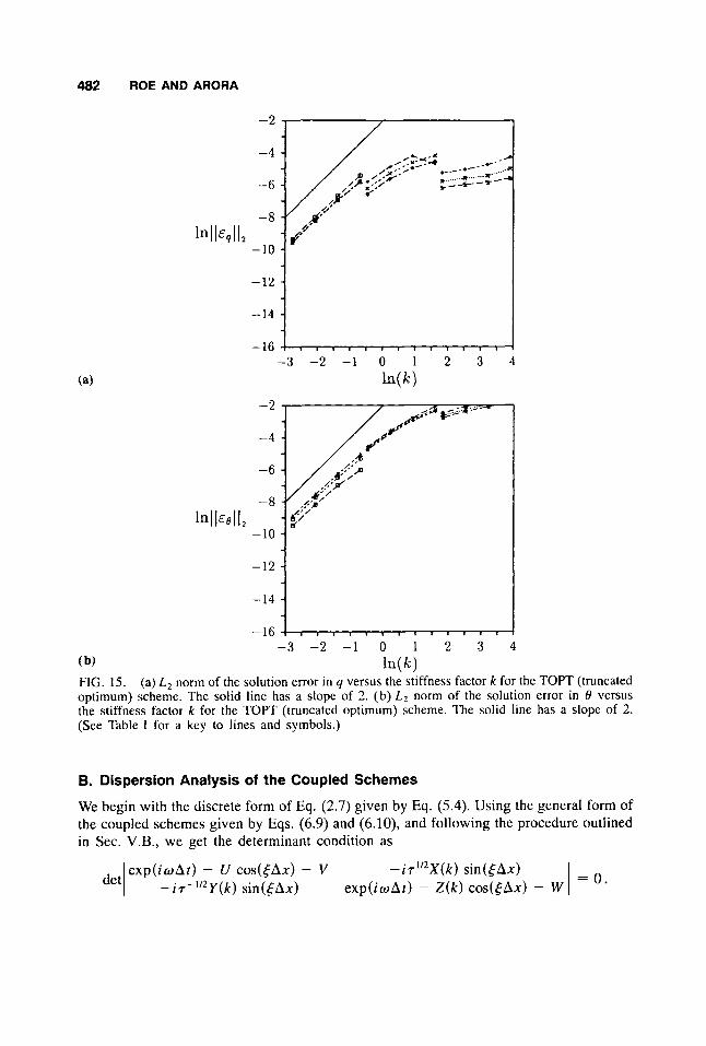
( b) In( k) FIG. 15. (a) L, norm of the solution error in q versus the stiffness factor k for the TOPT (truncated optimum) scheme. The solid line has a slope of 2. (b) L z norm of the solution error in 8 versus the stiffness factor k for the TOPT (truncatcd optimum) scheme. The solid line has a slope of 2. (See Table I for a key to lines and symbols.)

B. Dispersion Analysis of the Coupled Schemes

We begin with the discrete form of Eq. (2.7) given by Eq. (5.4). Using the general form of the coupled schemes given by Eqs. (6.9) and (6.10), and following the procedure outlined in Sec. V.B., we get the determinant condition as

1 = o . exp(iwAt) - U cos(5Ax) - V - iT112X(k) sin(5Ax) de t l -i7-11*Y(k) sin(5Ax) exp(iwAt) - Z ( k ) cos(5Ax) - W

CHARACTERISTIC-BASED SCHEMES FOR DISPERSIVE WAVES. I . . . . 483

TABLE 111. Coefficients Re, So, To, R, , S,, and T, for the coupled schemes. Version Definition for Coupled Schemes

TABLE IV. that terms are retained until the first erroneous term, after which we use the symbol e.

Polynomial expansion of the coefficients of the coupled schemes about k = 0. Note

Polynomial Expansion

484 ROE AND ARORA

TABLE V. Asymptotic behavior of the coefficients for the coupled schemes. Asymptotic Behaviour of Coupled Schemes Coefficients

This gives us the dispersion relation for coupled schemes as

exp(iwAt) = i [ - B 2 -1, (6.11)

where

B = - [V + W + (U + Z ) COS((AX)],

C = (UZ - X U ) COS*([AX) + (UW + V Z ) COS(~AX) + ( X Y + V W ) .

Since we have incorporated the middle point into our stencil, we have doubled the wave number resolution capability to [Ax 9 n-. At this maximum frequency either

exp(iwAht) = (V - U ) (6.12)

or

exp(iwAt) = (W - Z ) . (6.13)

Using w = O R + iw , in Eqs. (6.12) and (6.13) leads to

sin(wRAt)e-WfA' = S [ V - U ] or S [ W - Z ] . (6.14)

Since

u,v ,w , z E 8 (6.15)

we find that

S [ V - U ] = 3 [ W - Z ] = 0 V k (6.16)

at this highest wave number. Using Eq. (6.14), we conclude that

W R = 0 V k at emax. (6.17)

meaning that the highest wave number is always stationary. Therefore the additional accuracy obtained at small wave numbers by incorporating M into the stencil carries this penalty at high wave numbers. Since our numerical tests involve only smooth solutions, this penalty has little effect here, as evidenced by our numerical results [Figs. 16(a) and 16(b)]. It does matter when discontinuities are captured, and we will report on this topic in the future.

CHARACTERISTIC-BASED SCHEMES FOR DISPERSIVE WAVES. I.. . . 485

-2

-4

-6

-8 I I2

-10

-12

-14

- 16 - 3 - 2 - 1 0 1 2 3 4

ln(k) -2

- 4

-6

-8

- 10 In1 IEe I I ,

-12

-14

-16 - 3 - 2 - 1 0 1 2 3 4

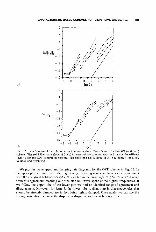
( b) w> FIG. 16. (a) L , norm of the solution error in q versus the stiffness factor k for the OPT (optimum) scheme. The solid line has a slope of 3. (b) L 2 norm of the solution error in 8 versus the stiffness factor k for the OPT (optimum) scheme. The solid line has a slope of 3. (See Table I for a key to lines and symbols.)

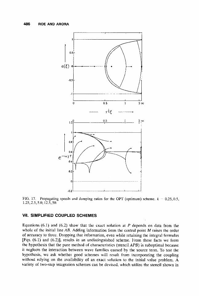
We plot the wave speed and damping rate diagrams for the OPT scheme in Fig. 17. In the upper plot we find that in the region of propagating waves we have a close agreement with the analytical behavior for [ A x 5 n-/2 but in the range n / 2 5 ( A x 5 n- we diverge from this agreement, reaching our predicted null wave speed at the highest frequencies. If we follow the upper lobe of the lower plot we find an identical range of agreement and disagreement. However, for large k, the lower lobe is disturbing in that frequencies that should be strongly damped are in fact being lightly damped. Once again, we can see the strong correlation between the dispersion diagrams and the solution errors.

486 ROE AND ARORA

I I r

-0.2' I

FIG. 17. 1.25,2.5,5.0, 12.5,50.

Propagating spccds and damping ratios for the OPT (optimum) scheme. k = 0.25,0.5,

VII. SIMPLIFIED COUPLED SCHEMES

Equations (6.1) and (6.2) show that the exact solution at P depends on data from the whole of the initial line AB. Adding information from the central point M raises the order of accuracy to three. Dropping that information, even while retaining the integral formulas [Eqs. (6.1) and (6 .2)] , results in an undistinguished scheme. From these facts we form the hypothesis that the pure method of characteristics (stencil APB) is suboptimal because it neglects the interaction between wave families caused by the source term. To test the hypothesis, we ask whether good schemes will result from incorporating the coupling without relying on the availability of an exact solution to the initial value problem. A variety of two-step integration schemes can be devised, which utilize the stencil shown in

CHARACTERISTIC-BASED SCHEMES FOR DISPERSIVE WAVES. I.. . . 487

P

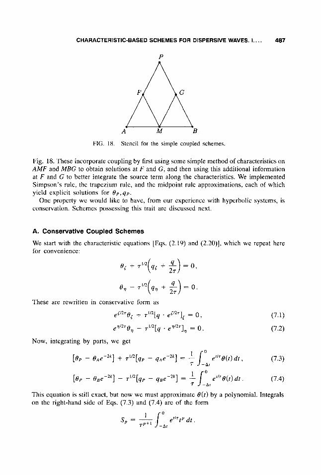
FIG. 18. Stencil for the simple coupled schemes.

Fig. 18. These incorporate coupling by first using some simple method of characteristics on AMF and MBG to obtain solutions at F and G, and then using this additional information at F and G to better integrate the source term along the characteristics. We implemented Simpson's rule, the trapezium rule, and the midpoint rule approximations, each of which yield explicit solutions for O p , qp .

One property we would like to have, from our experience with hyperbolic systems, is conservation. Schemes possessing this trait are discussed next.

A. Conservative Coupled Schemes

We start with the characteristic equations [Eqs. (2.19) and (2.20)], which we repeat here for convenience:

Now, integrating by parts, we get

This equation is still exact, but now we must approximate O ( t ) by a polynomial. Integrals on the right-hand side of Eqs. (7.3) and (7.4) are of the form

1 ' s, = - r p + I /-At er"tp dt .

488 ROE AND ARORA

Dividing this integral into two parts, we define

l o s p . 2 = - r p + I I-,,, e t i rrp d t .

These are easily evaluated as

-2k = e-' - e ,

S1.I = (1 + 2k)e-2k - (1 + k ) e - k ,

S2,1 = [2(1 + k ) + k2]e-' - 2[1 + 2k + 2k2]e-2k,

SO,^ = 1 - e - k ,

S 1 , 2 = (1 + k)e-k - 1,

S2,2 = 2 - [2(1 + k ) + k2]e-',

Letting 8 ( t ) vary quadratically along the characteristics, we get

along the t characteristic and

along the 7 characteristic. In terms of S p , 1 , S p , 2 , we get the right-hand side of Eqs. (7.3) and (7.4) to be

and

respectively, where, if the PI version of the method of characteristics is used to evaluate the solution at F and G,

CHARACTERISTIC-BASED SCHEMES FOR DISPERSIVE WAVES. 1.. . . 489

To facilitate comparison with other schemes, this can be rearranged as the rather cumbersome explicit, one-step formula

L

(6, - 26M + 6 B ) , 1 1 - k - (1 + k)eP2" 3k - 2 + ( 2 + k)e -2k

(7.5)

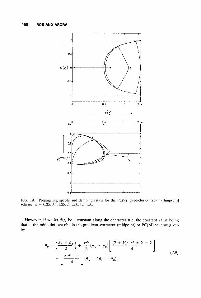
We shall call this the predictor-corrector (Simpson) or PC(S) scheme. For small k, the coefficients in the PC(Sj and OPT schemes agree to sufficient terms that the truncation error remains third order. There is very close agreement between the two, as can be seen from the dispersion (Fig. 19) and error (Fig. 20) plots.

A comment, however. is in order here. It was found that when the first step in the two-stage schemes was taken to be operator splitting, we got a much degraded result with respect to other coupled scheme solutions. Rephrased, we find that operator splitting is not good for large k, whether by itself, in conjunction with, or as part of another scheme.

Now, if we let 6( t> vary piecewise linearly along the characteristics, we get the right-hand side of Eqs. (7.3) and (7.4) as

which results in the predictor-corrector (trapezium) or PC(T) scheme, given by

L -1

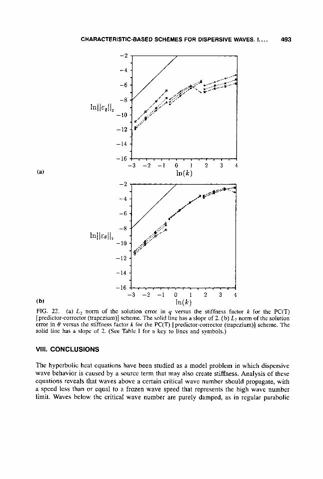
The results are plotted in Figs. 21 and 22. The dispersion characteristics are. very similar to those of the other coupled schemes (Fig. 21). The accuracy attained is second-order, as can be observed from Figs. 22(a) and 22(b). It appears to give satisfactory results up to fairly large k.

490 ROE AND ARORA

0 0.5 1 2 0 3

-0.2 x FIG. 19. schernc. k = 0.25,0.5,1.25,2.5,5.0, 12.5,50.

Propagating specds and damping ratios for the PC(S) [ predictor-corrector (Simpson)]

However, if we let 8( t ) be a constant along the characteristic, the constant value being that at the midpoint, we obtain the predictor-corrector (midpoint) or PC(M) scheme given by

CHARACTERISTIC-BASED SCHEMES FOR DISPERSIVE WAVES. 1.. . .

-2

-4

-6

-8

-10

-12

- 14

In I I€* I I 2

- 16 - 3 - 2 - 1 0 1 2 3 4

-2

-4

-6

-8

- 10

-12

-14

14 IEe I Iz

-16

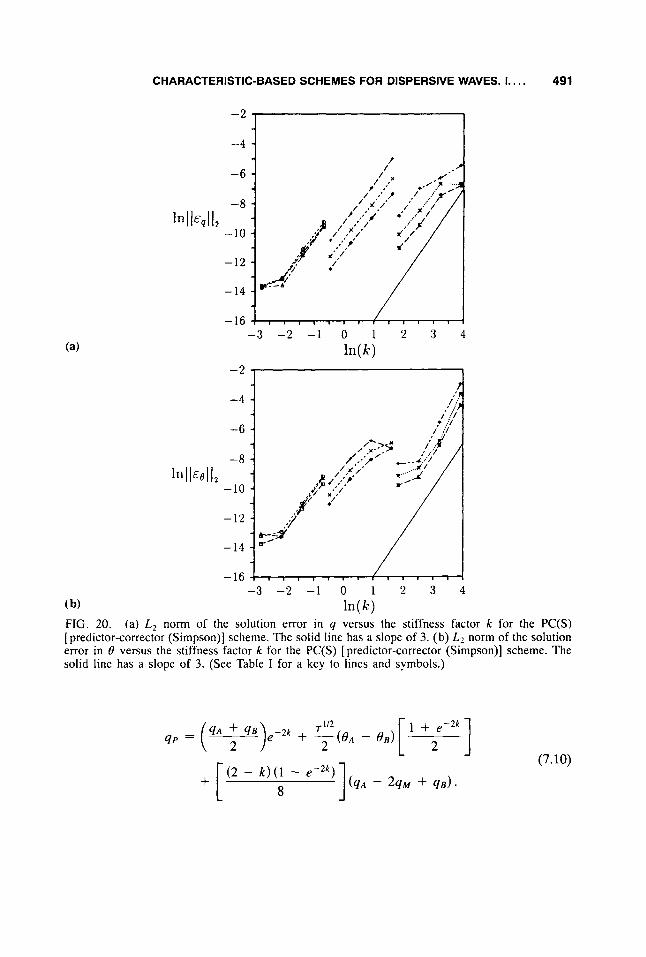
( b) FIG. 20. (a) L, norm o

- 3 - 2 - 1 0 1 2 3 4 In( k)

491

the solution error in q versus the stiffness factor k for the C(S) [ predictor-corrector (Simpson)] scheme. The solid line has a slope of 3. (b) L z norm of the solution error in t9 versus the stiffness factor k for the PC(S) [ predictor-corrector (Simpson)] scheme. The solid line has a slope of 3 . (See Table I for a key to lines and symbols.)

(7.10)

492 ROE AND ARORA

I I I I

e-

I 0 0.5 1 2m

__ T f C c

1

0.8

0.6

' W I 7

0.4

0.2

0 .- ..- .-

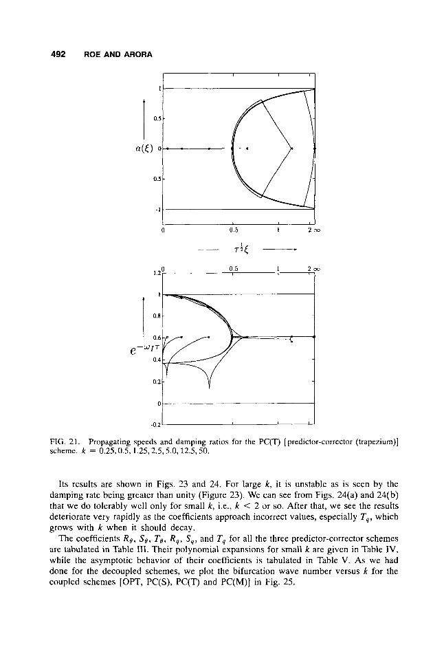
-0.2 L--i_' FIG. 21. scheme. k = 0.25,0.5,1.25,2.5,5.0,12.5,50.

Propagating speeds and damping ratios for the PC(T) [ predictor-corrector (trapezium)]

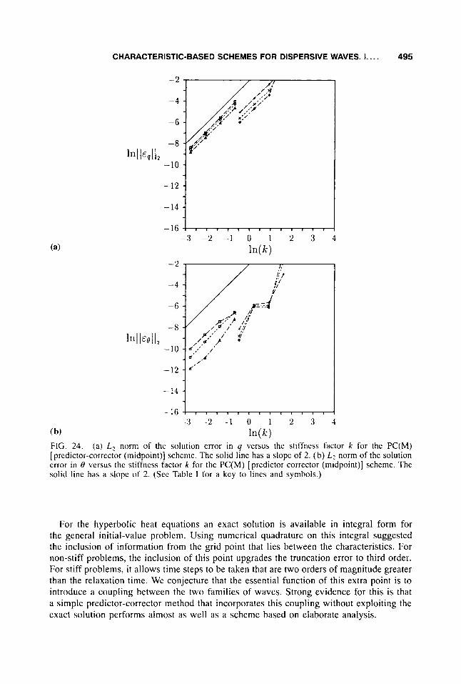
Its results are shown in Figs. 23 and 24. For large k , it is unstable as is seen by the damping rate being greater than unity (Figure 23). We can see from Figs. 24(a) and 24(b) that we do tolerably well only for small k, i.e., k < 2 or so. After that, we see the results deteriorate very rapidly as the coefficients approach incorrect values, especially T,, which grows with k when it should decay.

The coefficients Rg, S g , To, R,. S,, and T, for all the three predictor-corrector schemes are tabulated in Table Ill. Their polynomial expansions for small k are given in Table IV, while the asymptotic behavior of their coefficients is tabulated in Table V. As we had done for the decoupled schemes, we plot the bifurcation wave number versus k for the coupled schemes [OPT, PC(S), PC(T) and PC(M)] in Fig. 25.

CHARACTERISTIC-BASED SCHEMES FOR DISPERSIVE WAVES. I . . . . 493

In I 1% I I 2

-2

-4

-6

-8

- 10

-12

-14

- 16 - 3 - 2 - 1 0 1 2 3 4

ln(k) -2

-4

-6

-8

- 10

-12

lnll&ell,

-14 1 , , , , , , , , , , , , ,

- 16 - 3 - 2 - 1 0 1 2 3 4

( b) In@> FIG. (a) L , norm of the solution error in q versus the stiffness factor k for the PC(T) [ predictor-corrector (trapezium)] scheme. The solid line has a slope of 2. (b) L2 norm of the solution error in 0 versus the stiffness factor k for the PC(T) [ predictor-corrector (trapezium)] scheme. The solid line has a slope of 2. (See Table I for a key to lines and symbols.)

VIII. CONCLUSIONS

The hyperbolic heat equations have been studied as a model problem in which dispersive wave behavior is caused by a source term that may also create stiffness. Analysis of these equations reveals that waves above a certain critical wave number should propagate, with a speed less than or equal to a frozen wave speed that represents the high wave number limit. Waves below the critical wave number are purely damped, as in regular parabolic

494 ROE AND ARORA

0 0.5 1 2 0 0

O.* t 0.6 c L

I

-0.2

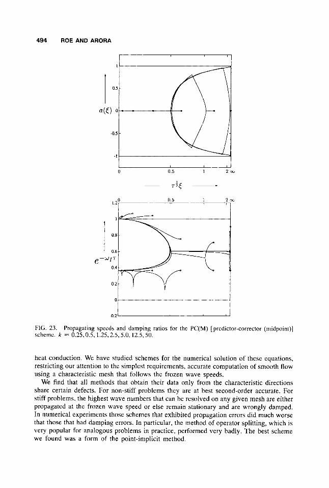
FIG. 23. scheme. k = 0.25,0.5,1.25,2.5,5.0: 12.5, SO.

Propagating speeds and damping ratios for the PC(M) [ predictor-corrector (midpoint)]

heat conduction. We have studied schemes for the numerical solution of these equations, restricting our attention to the simplest requirements, accurate computation of smooth flow using a characteristic mesh that follows the frozen wave speeds.

We find that all methods that obtain their data only from the characteristic directions share certain defects. For non-stiff problems they are at best second-order accurate. For stiff problems, the highest wave numbers that can be resolved on any given mesh are either propagated at the frozen wave speed or else remain stationary and are wrongly damped. In numerical experiments those schemes that exhibited propagation errors did much worse that those that had damping errors. In particular, the method of operator splitting, which is very popular for analogous problems in practice, performed very badly. The best scheme we found was a form of the point-implicit method.

CHARACTERISTIC-BASED SCHEMES FOR DISPERSIVE WAVES. I . . . . 495

-2

-4

-6

-8

-10

-12

1 4 lEel l 2

-2

-4

-6

-8

-10

-12

- 14

1 4 1% I I 2

-16 1 - 3 - 2 - 1 0 1 2 3 4

In(k)

For the hyperbolic heat equations an exact solution is available in integral form for the general initial-value problem. Using numerical quadrature on this integral suggested the inclusion of information from the grid point that lies between the characteristics. For non-stiff problems, the inclusion of this point upgrades the truncation error to third order. For stiff problems, it allows time steps to be taken that are two orders of magnitude greater than the relaxation time. We conjecture that the essential function of this extra point is to introduce a coupling between the two families of waves. Strong evidence for this is that a simple predictor-corrector method that incorporates this coupling without exploiting the exact solution performs almost as well as a scheme based on elaborate analysis.

4% ROE AND ARORA

k

Limiting Hyperbola

0 0.5 1 2 0 0

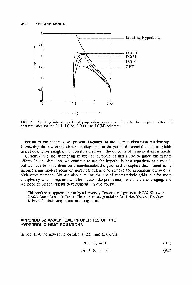
FIG. 25. characteristics for thc OPT, PC(S), PC(T), and PC(M) schemes.

Splitting into damped and propagating modes according to the coupled method of

For all of our schemes, we present diagrams for the discrete dispersion relationships. Compdring these with the dispersion diagrams for the partial differential equations yields useful qualitative insights that correlate well with the outcome of numerical experiments.

Currently, we are attempting to use the outcome of this study to guide our further efforts. In one direction, we continue to use the hyperbolic heat equations as a model, but we seek to solve them on a noncharacteristic grid, and to capture discontinuities by incorporating modern ideas on nonlinear filtering to remove the anomalous behavior at high wave numbers. We are also pursuing the use of characteristic grids, but for more complex systems of equations. In both cases, the preliminary results are encouraging, and we hope to present useful developments in due course.

This work was supported in part by a University Consortium Agreement (NCA2-521) with NASA Amcs Research Center. The authors are gratcful to Dr. Helen Yee and Dr. Steve Deiwert for their support and encouragement.

APPENDIX A: ANALYTICAL PROPERTIES OF THE HYPERBOLIC HEAT EQUATIONS

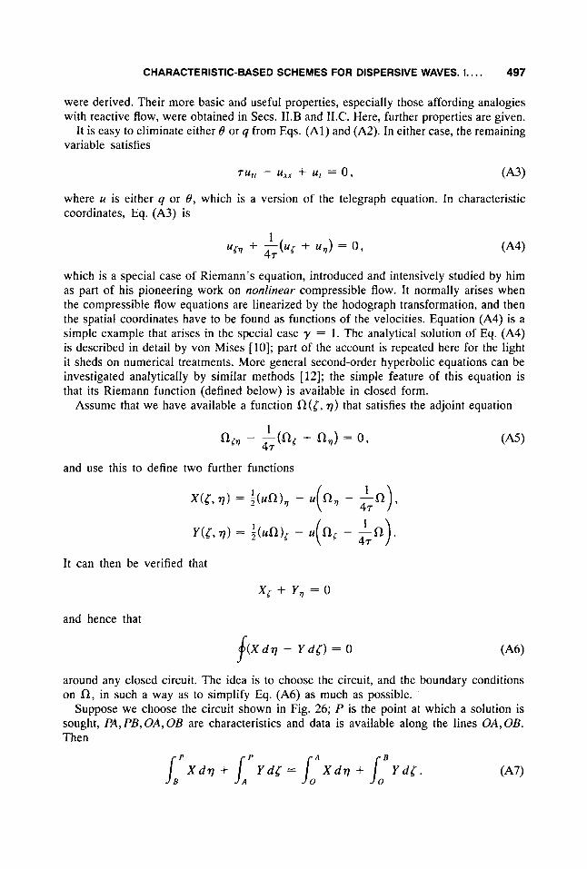
In Sec. 1I.A the governing equations (2.5) and (2.6). viz.,

8, + qx = 0 ,

Tq, + 8, = -9.

CHARACTERISTIC-BASED SCHEMES FOR DISPERSIVE WAVES. I . . . . 497

were derived. Their more basic and useful properties, especially those affording analogies with reactive flow, were obtained in Secs. 1I.B and 1I.C. Here, further properties are given.

It is easy to eliminate either 8 or q from Eqs. (Al) and (A2). In either case, the remaining variable satisfies

TU,, - u,, + u, = 0 ,

where u is either q or 8, which is a version of the telegraph equation. In characteristic coordinates, Eq. (A3) is

(A3)

1 47

U l T + -(u, + UT) = 0 ,

which is a special case of Riemann's equation, introduced and intensively studied by him as part of his pioneering work on nonlinear compressible flow. It normally arises when the compressible flow equations are linearized by the hodograph transformation, and then the spatial coordinates have to be found as functions of the velocities. Equation (A4) is a simple example that arises in the special case y = 1. The analytical solution of Eq. (A4) is described in detail by von Mises (101; part of the account is repeated here for the light it sheds on numerical treatments. More general second-order hyperbolic equations can be investigated analytically by similar methods [ 121; the simple feature of this equation is that its Riemann function (defined below) is available in closed form.

Assume that we have available a function n(l, 7) that satisfies the adjoint equation

1 47

a,, - -(a, + a,) = 0 ,

and use this to define two further functions

It can then be verified that

x, + Y , = 0

and hence that

{ ( X d v - Y d l ) = 0

In) 47 9

47 I n ) .

around any closed circuit. The idea is to choose the circuit, and the boundary conditions on a, in such a way as to simplify Eq. (A6) as much as possible.

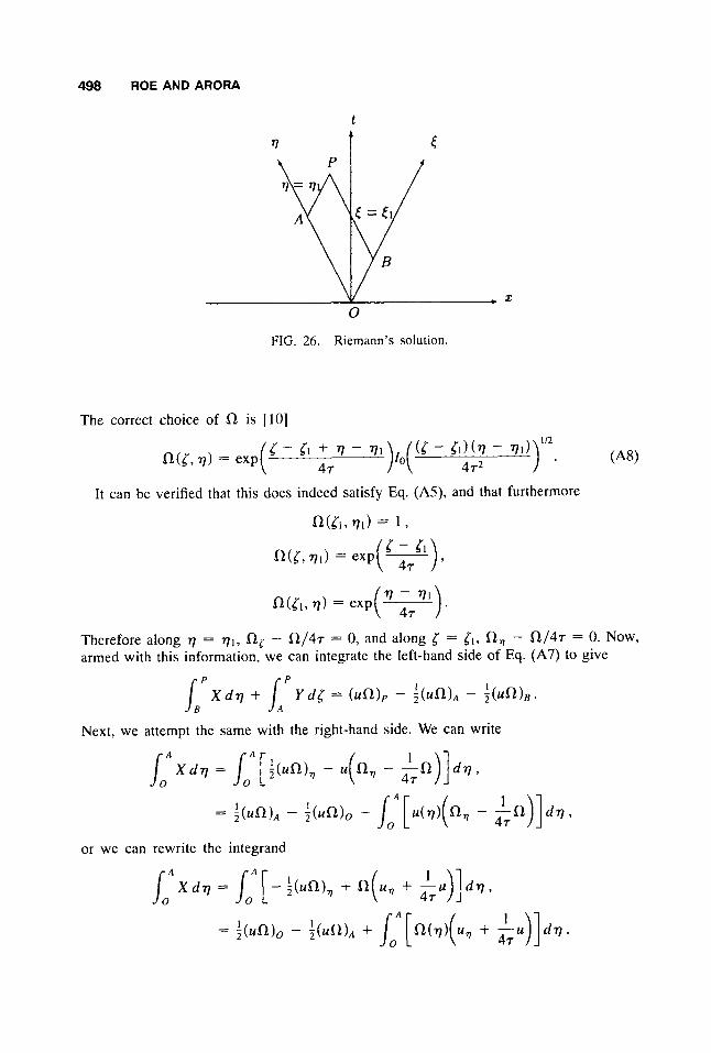
Suppose we choose the circuit shown in Fig. 26; P is the point at which a solution is sought, PA, PB, OA, OB are characteristics and data is available along the lines OA, OB. Then

L p X d 7 + l p Y d l = I O A X d 7 + I o B Y d l . (A7)

498 ROE AND ARORA

0

FIG. 26. Riemann's solution.

The correct choice of R is [lo]

I t can be verified that this does indeed satisfy Eq. (A5), and that furthermore

n(51,771) = 1 ,

5 - 51

Therefore along r ] = 71, R, - R/47 = 0, and along 5 = l1, R, - R/47 = 0. Now, armed with this information, we can integrate the left-hand side of Eq. (A7) to give

Next, we attempt the same with the right-hand side. We can write

or we can rewrite the integrand

CHARACTERISTIC-BASED SCHEMES FOR DISPERSIVE WAVES. 1.. . . 499

If u is chosen to satisfy u,, + u/(47) = 0 on OA [and u l + u/(47) = 0 on OBI, then the right-hand side gives

leading to

or

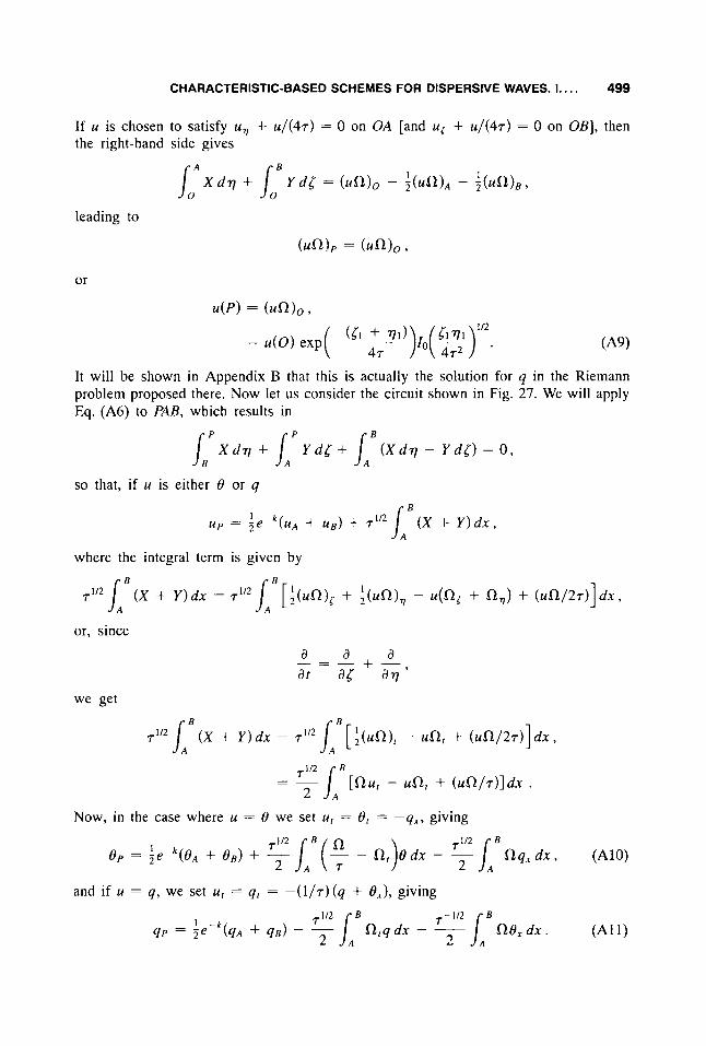
It will be shown in Appendix B that this is actually the solution for q in the Riemann problem proposed there. Now let us consider the circuit shown in Fig. 27. We will apply Eq. (A6) to PAB, which results in

[ B p X d v + / , p Y d l + / , B ( X d v - Y d l ) = O ,

so that, if u is either 0 or q

where the integral term is given by

or, since

a a a at a5 a 7 + - 3

- - _ -

we get

[nu, - uRr + ( u R / T ) ] ~ x

Now, in the case where u = 0 we set i f r = 8, = - q x , giving

dx .

and if u = q, we set u, = qr = - ( l / ~ ) (q + Ox), giving

500 ROE AND ARORA

P

FIG. 27. Stencil for the method of characteristics.

Up to this point, these integral equations are still exact.

II. APPENDIX B: EXACT RIEMANN SOLUTIONS FOR THE HYPERBOLIC HEAT EQUATIONS

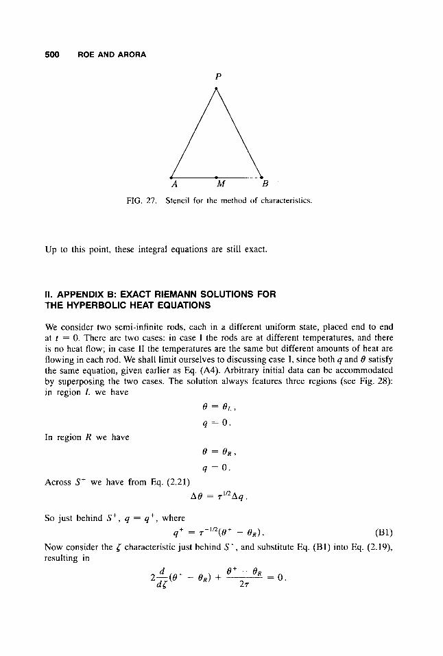
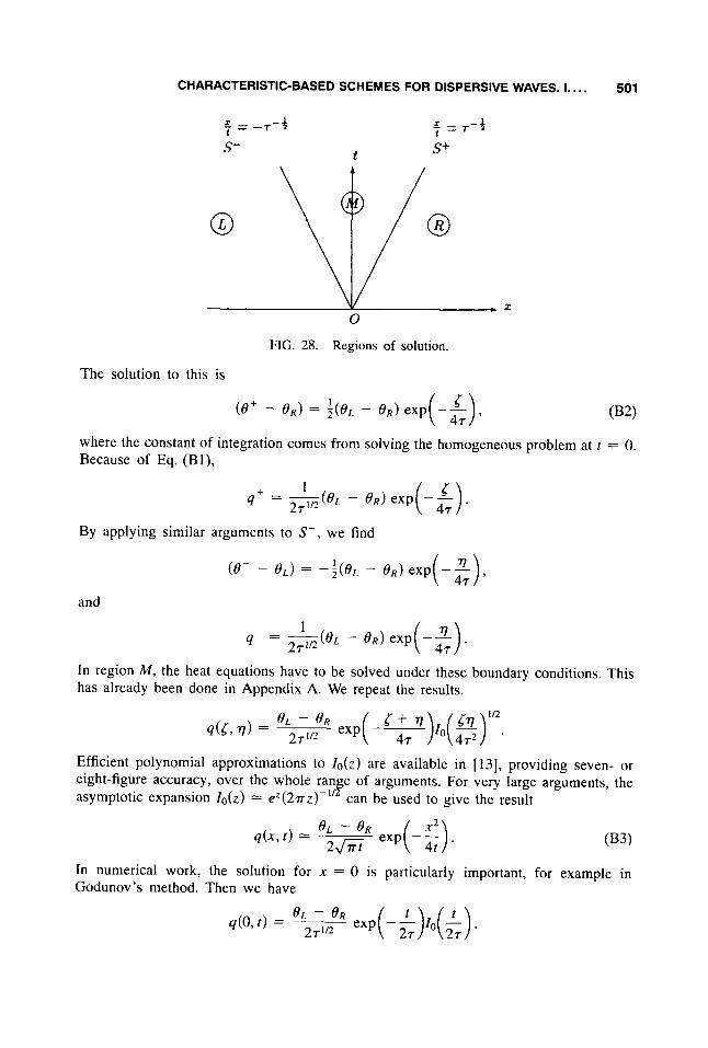
We consider two semi-infinite rods, each in a different uniform state, placed end to end at t = 0. There are two cases: in case I the rods are at different temperatures, and there is no heat flow; in case I1 the temperatures are the same but different amounts of heat are flowing in each rod. We shall limit ourselves to discussing case I, since both q and 8 satisfy the same equation, given earlier as Eiq. (A4). Arbitrary initial data can be accommodated by superposing the two cases. The solution always features three regions (see Fig. 28): in region L we have

8 = e L ,

In region R we have q = 0 .

8 = O R ,

q = 0 .

A 8 = P A q . Across S' we have from Eq. (2.21)

So just behind S', q = q', where 4' = 7-"*(8+ - O R ) . (B1)

Now consider the resulting in

characteristic just behind S+, and substitute Eq. (Bl) into Eq. (2.19),

CHARACTERISTIC-BASED SCHEMES FOR DISPERSIVE WAVES. I.. . . 501

- = - - r - f = = T - 4

S+ t - t

1 S-

O

FIG. 28. Regions of solution.

The solution to this is

where the constant of integration comes from solving the homogeneous problem at t = 0. Because of Eq. (Bl),

By applying similar arguments to S - , we find

and

In region M , the heat equations have to be solved under these boundary conditions. This has already been done in Appendix A. We repeat the results.

Efficient polynomial approximations to ZO(Z) are available in [ 131, providing seven- or eight-figure accuracy, over the whole ran e of arguments. For very large arguments, the asymptotic expansion lo(z) = eZ(27rz) - 118 can be used to give the result

In numerical work, the solution for x = 0 is particularly important, for example in Godunov's method. Then we have

502 ROE AND ARORA

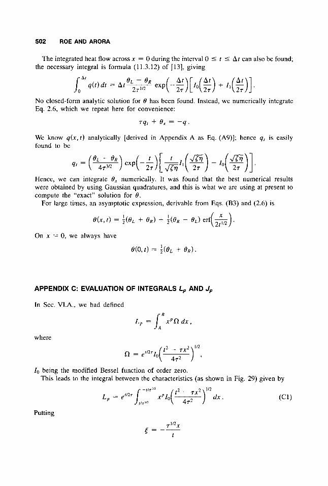
The integrated heat flow across x = 0 during the interval 0 I t I A t can also be found; the necessary integral is formula ( I 1.3.12) of [ 131, giving

No closed-form analytic solution for 8 has been found. Instead, we numerically integrate Eq. 2.6, which we repeat here for convenience:

7ql + ex = -4 .

We know q ( x , t ) analytically [derived in Appendix A as Eq. (A9)]; hence qr is easily found to be

Hence, we can integrate 8, numerically. It was found that the best numerical results were obtained by using Gaussian quadratures, and this is what we are using at present to compute the "exact" solution for 8 .

For large times, an asymptotic expression, derivable from Eqs. (B3) and (2.6) is

1 I 8 ( x , t ) = y(8, + 8,) + ? ( O R - 8,) erf

On x = 0, we always have

e(o,t) = : (eL + O R ) .

APPENDIX C: EVALUATION OF INTEGRALS L, AND J,

In Sec. VI.A., we had defined r B

L, = I x P R d x , A

where 2 112

= et12'L( t 2 - 7x ) , 4 7 2

I0 being the modified Bessel function of order zero. This leads to the integral between the characteristics (as shown in Fig. 29) given by

Putting

7 II2x ( = -- t

CHARACTERISTIC-BASED SCHEMES FOR DISPERSIVE WAVES. I . . . . 503

we get

L P = (- -&)p+1ef1279,(k) 7

where

= I-: t P 4 ( k / G ) d t

and still remains to be evaluated. Now, to integrate from A to B, we need to set t = - A t , which results in

L, = (2k7112)P+1e-k 9 , ( k ) . (C2)

Also, we had defined in Sec. V1.A

J , = x P R f d x , A

where

Thus

Now, if we differentiate Eq. ( C l ) with respect to time, we get

The left-hand side of Eq. (C4) can be obtained via the chain rule on Eq. (C2) as

Thus we get the second part of Eq. (C3) as

2 112

dIo(12 - 7 x ) d x 472 - f i 7 ' R I x p d t

ef127

1/71"

d9,(k) + [ 1 + (- I ) P ] , 1 - ( p + 1)9,(k) - k- dk

= (2k7112)Pe -k7- 112

504 ROE AND ARORA

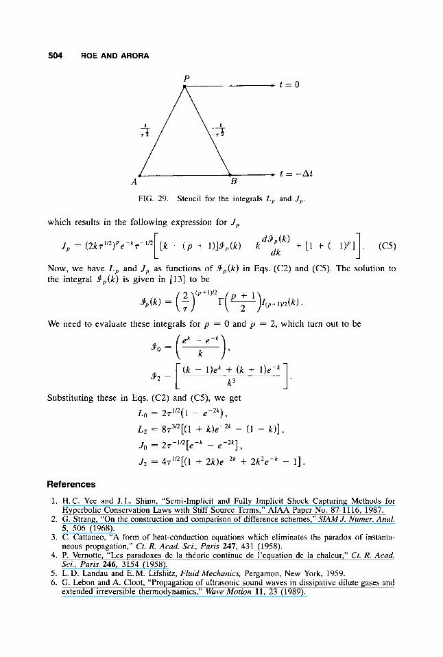
FIG. 29. Stencil for the integrals L , and J ,

which results in the following expression for .I,

d 9 p ( k ) + [ I + ( -1)PI . (C5) 1 J , = ( 2 k ~ * / ~ ) ~ e - ~ r - ” ~ [ k - ( p + 1)]9,,(k) - k - [ dk

Now, we have L, and J , as functions of 9 , ( k ) in Eqs. (C2) and ((25). The solution to the integral 9 , ( k ) is given in [13] to be

We need to evaluate these integrals for p = 0 and p = 2, which turn out to be

( k - I)ek + ( k + k 3 9 2 = [

Substituting these in Eqs. (C2) and (C5), we get

L~ = 27’”(1 - e - 2 k ) ,

L2 = 8r3I2[(1 + k ) C Z k - (1 - k ) ] , Jo = 2r-1/2[e-k - e - 2 k ]

52 = 4 ~ ’ ” [ ( 1 + 2k)e-2k + 2k2ePk - I ] .

References

1. H. C. Yee and J. L. Shinn, “Semi-Implicit and Fully Implicit Shock Capturing Methods for Hyperbolic Conservation Laws with Stiff Source Terms,” AIAA Paper No. 87-1 116, 1987.

2. G. Strang, “On the construction and comparison of difference schemes,” SIAM J . Numer. Anal. 5, 506 (1968).

3. C. Cattaneo, “A form of heat-conduction equations which eliminates the paradox of instanta- neous propagation,” Ct. R. Acad. Sci., Paris 247, 431 (1958).

4. P. Vernotte, “Les paradoxes de la thCorie continue de l’equation de la chaleur,” Ct. R. Acad. Sci., Paris 246, 3154 (1958).

5. L. D. Landau and E. M. Lifshitz, Fluid Mechanics, Pergamon, New York, 1959. 6. G. Lebon and A. Cloot, “Propagation of ultrasonic sound waves in dissipative dilute gases and

extended irreversible thermodynamics,” Wave Motion 11, 23 (1989).

CHARACTERISTIC-BASED SCHEMES FOR DISPERSIVE WAVES. 1.. . . 505

7. K. K. Tamma and S. B. Railkar, “Specially tailored transfinite-element formulations for hyper- bolic heat conduction involving non-Fourier effects,” Numer. Heat Transfer Part B, 15, 21 1 (1989).

8. N. V. Shemetov, “The Stefan problem for a hyperbolic heat equation,” in Numerical Methods for Free Boundary Problems, P. Neittaanmaki, Ed., Birkhauser Verlag, Boston, 1991, p. 365.

9. K. K. Tamma and R. R. Namburu, “Hyperbolic heat-conduction problems: Numerical simula- tions via explicit Lax-Wendroff-based finite element formulations,”J. Thermodyn. Heat Transfer 5, 232 (1991).

10. R. von Mises, Mathematical Theory of Compressible Fluid Flow, Academic, New York, 1958. 11. D. C. Wiggert, “Analysis of early-time transient heat conduction by method of characteristics,”

12. R. Courant and D. Hilbert, Methods of Mathematical Physics, Interscience, New York, 1963,

13. Handbook of Mathematical Functions, Nat. Bur. Stand. Appl. Math. Ser. No. 55, edited by M.

J . Heat Transfer 99, 35 (1977).

VOl. 11.

Abramowitz and LA. Stegun, U.S. GPO, Washington, D.C.. 1972.