Chapter 9 Dynamic stability analysis – III – Lateral motion ...

Flight dynamics –II Prof. E.G. Tulapurkara

Stability and control

Dept. of Aerospace Engg., IIT Madras 1

Chapter 9

Dynamic stability analysis – III – Lateral motion

(Lectures 33 and 34)

Keywords : Lateral dynamic stability - state variable form of equations,

characteristic equation and its roots ; motions indicated by roots - role

subsidence, spiral mode, Dutch roll ; stability diagram.

Topics

9.1 Introduction

9.2 State variable form of lateral dynamic stability equations

9.3 Roots of stability quartic for general aviation airplane Navion

9.3.1 Iterative solution for lateral stability quartic

9.4 Lateral dynamic stability analysis which includes angular displacement

in yaw (Δψ ) as a state variable

9.5 Response indicated by roots of characteristic equation of lateral

motion- change in flight direction, roll subsidence, spiral mode and

Dutch roll

9.6 Lateral-directional response of general aviation airplane (Navion)

9.7 Approximations to modes of lateral motion

9.8 Two parameter stability diagram for lateral motion

References

Exercises




Chapter 9

Dynamic stability analysis – III – Lateral motion - 1

Lecture 33

Topics

9.1 Introduction

9.2 State variable form of lateral dynamic stability equations

9.3 Roots of stability quartic for general aviation airplane Navion

Example 9.1

9.3.1 Iterative solution for lateral stability quartic


in yaw (Δψ ) as a state variable

9.5 Response indicated by roots of characteristic equation of lateral

motion- change in flight direction, roll subsidence, spiral mode and

Dutch roll

9.1 Introduction

In chapter 7 the small perturbation equations for the longitudinal and lateral

motions with controls fixed were derived. Expressions for the stability derivatives

were also obtained. The analysis of the longitudinal dynamic stability was dealt

with in Chapter 8. With this background, the lateral dynamic stability is briefly

discussed in this chapter. The distinguishing features of lateral dynamic stability

are highlighted.

9.2 State variable form of lateral dynamic stability equation

The equations of motion for the lateral case (Eqs.7.88, 7.89, 7.90) are

reproduced here for ready reference.

v 0 r 0 δr r

xzv p r

xx

d( -Y ) Δv - (u -Y )Δr - g cosθ Δφ = Y Δδ

dt

Id d-L' Δv + ( - L' )Δp - [ + L' ]Δr

dt I dt

(7.88)

δa a δr r= L' Δδ + L' Δδ (7.89)




xzv p r

zz

I d d- N Δv - ( + N ) Δp - [ - N ] Δr

I dt dt

δa a δr r= N Δδ +N Δδ (7.90)

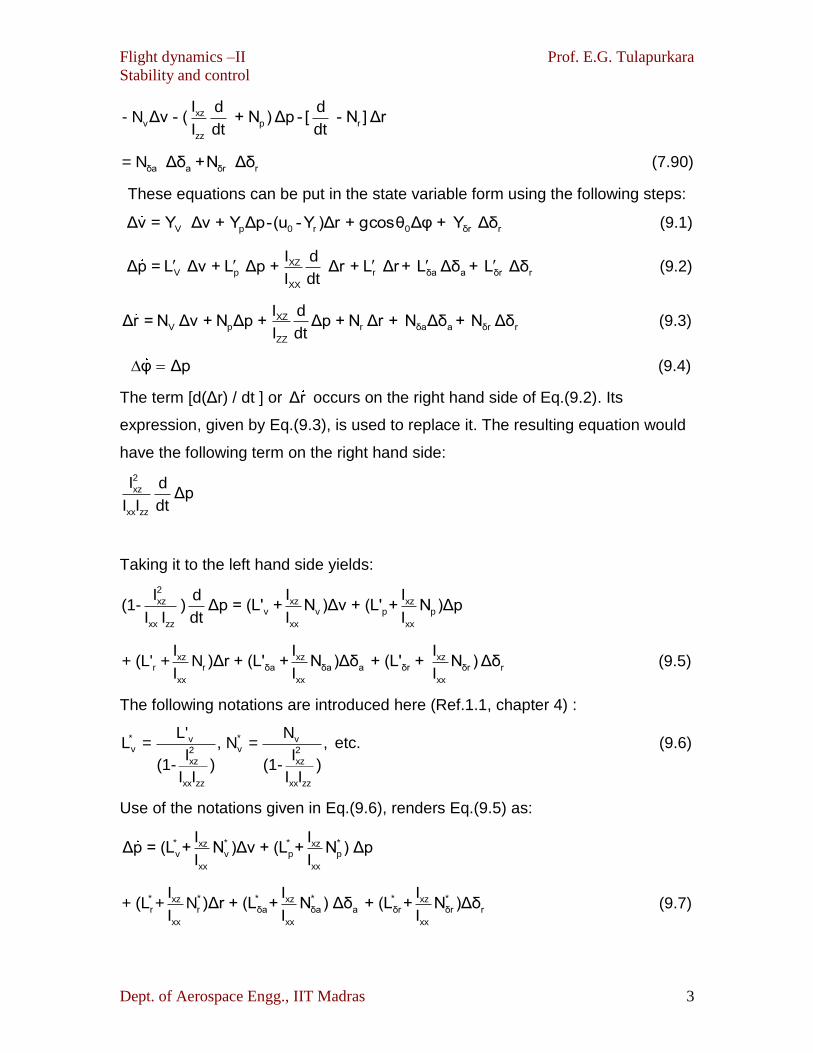
These equations can be put in the state variable form using the following steps:

V p 0 r 0 δr rΔv = Y Δv + Y Δp-(u -Y )Δr + gcosθ Δφ + Y Δδ (9.1)

XZV p r δa a δr r

XX

I dΔp = L Δv + L Δp + Δr + L Δr+ L Δδ + L Δδ

I dt (9.2)

XZV p r δa a δr r

ZZ

I dΔr = N Δv + N Δp + Δp + N Δr + N Δδ + N Δδ

I dt (9.3)

φ Δp (9.4)

The term [d(Δr) / dt ] or Δr occurs on the right hand side of Eq.(9.2). Its

expression, given by Eq.(9.3), is used to replace it. The resulting equation would

have the following term on the right hand side:

2

xz

xx zz

I dΔp

I I dt

Taking it to the left hand side yields:

2

xz xz xzv v p p

xx zz xx xx

I I Id(1- ) Δp = (L' + N )Δv + (L' + N )Δp

I I dt I I

xz xz xzr r δa δa a δr δr r

xx xx xx

I I I+ (L' + N )Δr + (L' + N )Δδ + (L' + N ) Δδ

I I I (9.5)

The following notations are introduced here (Ref.1.1, chapter 4) :

* *v vv v2 2

xz xz

xx zz xx zz

L' NL = , N = , etc.

I I(1- ) (1- )

I I I I

(9.6)

Use of the notations given in Eq.(9.6), renders Eq.(9.5) as:

* * * *xz xzv v p p

xx xx

I IΔp = (L + N )Δv + (L + N ) Δp

I I

* * * * * *xz xz xzr r δa δa a δr δr r

xx xx xx

I I I+ (L + N )Δr + (L + N ) Δδ + (L + N )Δδ

I I I (9.7)




Similarly, eliminating p from r.h.s of Eq. (9.3) and simplifying gives the following

expression for Δr :

* * * *xz xzv v p p

zz zz

I IΔ r = (N + L )Δv + (N + L ) Δp

I I

* * * * * *xz xz xzr r δa δa a δr δr r

zz zz zz

I I I+ (N + L )Δr + (N + L )Δδ + (N + L ) Δδ

I I I (9.8)

The final form of the equations for lateral motion in the state variable form is:

v p 0 r 0

* * * * * *xz xz xzv v p p r r

xx xx xx


zz zz zz

Y Y -u +Y gcosθΔv

ΔvI I IL + N L + N L + N 0

Δp ΔpI I I=

ΔrI I IΔr N + L N + L N + L 0

ΔI I IΔ 0 1 0 0

r

r

δ

a* * * *xz xzδa δa δr δ

rxx xx

* * * *xz xzδa δa δr δr

zz zz

0 Y

ΔδI I+ L + N L + N

ΔδI I

I IN + L N + L

I I

(9.9)

This can be put in the form:

X=A.X+B.η (9.10)

When the control deflections ( aδ and rδ in the present case) are fixed, η= 0 and

Eq.(9.10) reduces to:

X=A.X (9.11)

As pointed out in section 8.10, Eq(9.11) has the following solution.

r|λ | 0I A (9.12)

Where λ r’ s are the eigen values of matrix A.

Expanding Eq.(9.12), the following characteristic equation for the lateral motion is

obtained.




4 3 2

1 1 1 1 1A λ + B λ + C λ + D λ + E = 0 (9.13)

9.3 Roots of stability quartic for general aviation airplane (Navion)

This section illustrates the process of setting up matrix A and then

obtaining the eigen values.

Example 9.1

The general aviation airplane (Navion) discussed in example 8.1 has the

following lateral stability derivatives (Ref.2.4, section ‘X’).

Yv = - 0.2543 s-1,Yβ = -13.64 m s-2, Yp = 0, Yr = 0, L’v = -0.298 m-1 s-1,

L’β = -15.962 s-2, L’p = - 8.402 s-1, L’r = 2.193 s-1, Nv = 0.0838 m-1s-1,

Nβ = 4.495 s-2 , Np = - 0.3498 s-1, Nr = - 0.7605 s-1, Ixx = 1420.9 kg m2 ,

Izz = 4786. 0 kg m2, Ixz = 0.

The matrix A in Eqs.(9.9) and (9.10) in this case is

- 0.2543 0 - 53.64 - 9.80665 0

- 0.298 - 8.402 2.193 0 0

= 0.0838 - 0.3498 - 0.7608 0 0

0 1 0 0 0

0 0 1 0 0

A (9.14)

The eigen values of this matrix are the roots of the lateral stability quatric. Using

MATLAB software the roots are:

- 0.0089, - 8.4345, - 0.4867 ± i 2.3314

9.3.1 Iterative solution of lateral stability quartic

The characteristic equation (Eq. 9.13) is called lateral stability quartic.

Reference 1.5, part III chapter 2, contains an iterative method to solve it. The

case of Navion is considered to illustrate the procedure. Using the stability

derivatives in example 9.1, the following characteristic equation is obtained.

4 3 2λ + 9.4168λ +13.9662λ +47.9666λ+0.4258 = 0 (9.15)

As mentioned in section 8.5, the iterative technique, for obtaining roots of

a quartic, depends on the relative magnitudes of the coefficients of the terms in




the polynomial. For lateral stability quartic a technique different from that used in

section 8.5 is employed.

It is seen that the coefficient E1 is much smaller than D1. Hence, a small

root is expected. When the root is small, the terms with powers of λ would be

very small in Eq.(9.15) and the first approximation 1λ (1) can be written as:

(1)

1 1 1λ = - E / D = 0.4258 / 47.9666 = 0.00888

To get the second approximation to λ1, Eq.(9.15) is written as:

3 2(λ+0.00888) (λ +9.4079λ +13.8827λ+47.8433)+0.003651= 0

If 1λ (1) were the exact root, then the remainder should be zero. In this case it is

0.003651.

The second approximation is obtained as:

1λ (2) = - 0.4258 / 47.8433 = - 0.0089

Substituting in Eq.(9.15), gives:

3 2 -6(λ+0.0089)(λ +9.4079 λ +13.8825 λ+47.8430)+2.7 × 10 (9.16)

Since, the remainder is very small λ1 = - 0.0089 is taken as the first root.

To get the other three roots, the cubic part of Eq.(9.16) is now considered i.e.

3 2λ +9.4079λ +13.8825λ+47.843 = 0 (9.17)

To solve the Eq.(9.17), it is assumed that the second root ( λ 2) is large. Then, for

the first approximation ( λ 2(1)), the second and third terms in Eq.(9.17) can be

ignored i.e.

3 2 (1)

2λ +9.4079λ = 0 or λ = - 9.4079

To get the second approximation to λ2, Eq.(9.17) is divided by λ2 and λ 2

(1) is

substituted in the neglected terms. This gives :

(2)

2 2

13.8825 47.893λ = - 9.4079- - = - 9.4728

(-9.4079) (-9.4079)

In a similar fashion, (3) (4)

2 2λ = - 8.4358 and λ = - 8.4345 are obtained. The last two

values are fairly close to each other and 2λ = - 8.4345 is taken as the second

root.

Substituting for λ 1 and λ 2 in Eq.(9.15) leads to:




2(λ+0.0089)(λ+8.4345)(λ +0.9734 λ+5.6726) .

Hence, the four roots are: - 0.0089, - 8.4345, -0.4867 i 2.3315

which are almost the same as those obtained by using matrix ‘A’ and the

MATLAB Software.


in yaw (ΔΨ) as a state variable

In the analysis presented in section 9.2, the quantity Δφ is included as a

variable since, it is directly involved in Eq.(7.88). The angular displacement in

yaw ( ) can also be included. In this case the following additional governing

equation is obtained.

Δ = r (9.18)

Reference 1.12 (chapter 6) and Ref.1.5 (chapter 7 part II) follow this approach. In

this case Eq.(9.9) would get modified as:

v p 0 r 0


xx xx xx


zz zz zz

Y Y -u +Y gcosθ 0Δv

ΔvI I IL + N L + N L + N 0 0

Δp ΔpI I I

= ΔrI I IΔr N + L N + L N + L 0 0

ΔI I IΔ Δψ0 1 0 0 0Δψ 0 0 1 0

r

δr

a* * * *xz xzδa δa δ δr

rxx xx

* * * *xz xzδa δa δr δr

zz zz

0 Y

ΔδI I+ L + N L + N

ΔδI I

I IN + L N + L

I I

(9.19)

The characteristic equation corresponding to this set of equations would be :

5 4 3 2

1 1 1 1 1A λ + B λ + C λ + D λ + E λ = 0 (9.20)

This equation has λ = 0 as the fifth root in addition to the four roots discussed

earlier.




Note:

Similar result (i.e. a fifth degree polynomial as the characteristic equation), would

have been obtained, if Eqs.(7.88),(7.89) and (7.90) were solved assuming :

Δv = ρ1eλt, Δφ = ρ2e

λt, Δ = ρ3 eλt (9.21)

9.5. Response indicated by roots of characteristic equation of lateral

motion – change of flight direction, roll subsidence, spiral mode and

Dutch roll

The characteristic equation for the lateral motion (Eq.9.20) has five roots.

The motions indicated by these can be briefly described as follows.

I) λ equal to zero root:

From Eq.(9.21) it is observed that when, λ is zero the solution would be:

Δv = ρ1, Δφ = ρ2, Δ = ρ3. (9.22)

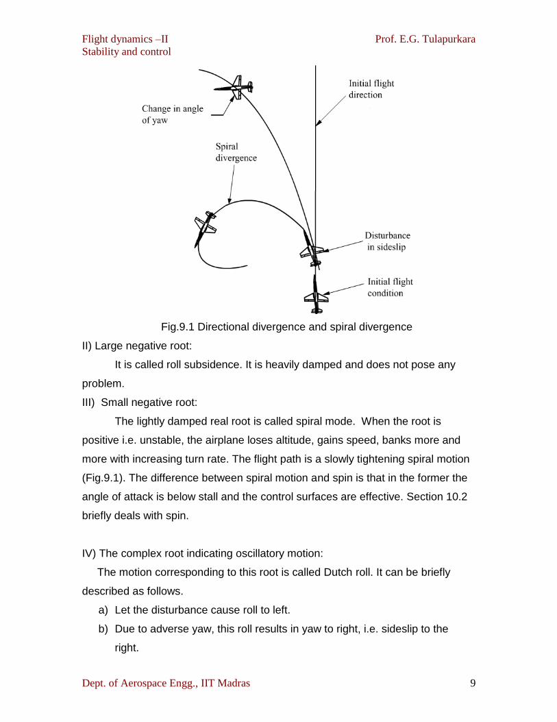
Substituting these in Eqs.(7.88),(7.89) and (7.90) shows that Δv equals 0 but Δφ

and ΔΨ need not be zero. Thus the zero root, which indicates neutral stability,

could lead to the airplane attaining a constant angle of bank (Δφ) and / or

yaw (ΔΨ). Figure 9.1 shows a change in flight direction as a result of the zero

root. This feature is discussed again, in section 9.6 , when the response of the

general aviation airplane to a lateral disturbance is considered . It may be pointed

out that appropriate control action is needed to correct the constant values of Δφ

and Δ .




Fig.9.1 Directional divergence and spiral divergence

II) Large negative root:

It is called roll subsidence. It is heavily damped and does not pose any

problem.

III) Small negative root:

The lightly damped real root is called spiral mode. When the root is

positive i.e. unstable, the airplane loses altitude, gains speed, banks more and

more with increasing turn rate. The flight path is a slowly tightening spiral motion

(Fig.9.1). The difference between spiral motion and spin is that in the former the

angle of attack is below stall and the control surfaces are effective. Section 10.2

briefly deals with spin.

IV) The complex root indicating oscillatory motion:

The motion corresponding to this root is called Dutch roll. It can be briefly

described as follows.

a) Let the disturbance cause roll to left.

b) Due to adverse yaw, this roll results in yaw to right, i.e. sideslip to the

right.




c) Because of the dihedral effect, the sideslip causes a restoring moment

causing roll to right.

d) Subsequently airplane yaws to left and rolls to left.

e) This sequence of events continues and when the real part of the root is

negative the amplitude of the oscillatory motion decreases with time.

f) During this oscillatory motion the airplane is all along moving forward

(Fig.9.2). The motion is similar to the weaving motion of an ice skater.

This mode is called Dutch roll.

According to Wikipedia, skating repetatively to the right and to the left is

referred to as Dutch roll. J.Hunsaker appears to be the first to refer the

aforesaid oscillatory motion of the airplane as Dutch roll.

Fig. 9.2 Dutch roll




Remark:

Dutch roll is an undesirable mode as it causes discomfort to the passengers

in civil airplanes and may result in missing the enemy targets in military

airplanes. It should have adequate damping.

Chapter 9 Dynamic stability analysis – III – Lateral motion ...

Documents

Transcript of Chapter 9 Dynamic stability analysis – III – Lateral motion ...