Chapter 4 – Design Calculations BIRMINGHAM POST ...
75
Chapter 4 – Design Calculations BIRMINGHAM POST-CONSTRUCTION STORM WATER MANUAL (ver. July 2018) 1
-
Upload
khangminh22 -
Category
Documents
-
view
1 -
download
0
Transcript of Chapter 4 – Design Calculations BIRMINGHAM POST ...

Chapter 4 – Design Calculations BIRMINGHAM POST-CONSTRUCTION STORM WATER MANUAL (ver. July 2018) 1

Chapter 4 – Design Calculations BIRMINGHAM POST-CONSTRUCTION STORM WATER MANUAL (ver. July 2018) 1
Table of Contents
Chapter 4 Design Calculations ............. Error! Bookmark not defined. 4.1 Design Principles .............................................................................. 4 4.2 Storm Water Quality Calculations .................................................. 6
4.2.1 Performance Standard Summary ..................................... 6 4.2.2 Eligibility for Rainfall Capture Reductions .................... 7 4.2.3 The Annual Runoff Reduction Method ......................... 8
4.2.3.1 Introduction ....................................................... 8 4.2.3.2 Process Summary .............................................. 8 4.2.3.3 Policies and Equations ...................................10 4.2.3.4 Special Case: GIPs in Series ..........................20
4.2.4 Sizing of Media-Based GIPs ..........................................20 4.2.5 Curve Number Adjustments ..........................................23 4.2.6 Multi-Benefit GIP Incentives.........................................24 4.2.7 Pollutant Removal............................................................28
4.2.7.1 Background ......................................................28 4.2.7.2 Accepted TSS Removal BMPs ......................28 4.2.7.3 Calculating TSS % Removal for BMPs in
Parallel ...............................................................29 4.2.7.4 BMPs in Series and in Flow through
Situations ..........................................................29 4.2.7.4 Calculating the TSS Treatment Volume
(TvTSS) ...............................................................30 4.2.8 Determining Land Cover Areas ....................................33
4.3 Hydrology .........................................................................................35 4.3.1 General Policies ................................................................35 4.3.2 Rainfall ...............................................................................35
4.3.2.1 Rainfall Distributions......................................35 4.3.2.2 Design Storms for Peak Flow
Calculations ......................................................38 4.3.3 Runoff ................................................................................39
4.3.3.1 Time of Concentration ...................................39 4.3.3.2 Peak Discharge (for Flood and Drainage
Designs) ............................................................39
4.3.3.3 Peak Discharge (for Storm Water Quality Design) ............................................................. 40
4.3.4 Discharge Hydrograph Generation .............................. 41 4.3.5 Off-site Analysis Policies ................................................ 42 4.3.6 Downstream Analysis (The 10% Rule) ........................ 44
4.4 Small Storm Extended Detention Design .................................. 46 4.4.1 Overview ........................................................................... 46 4.4.2 Estimation of the EDv ................................................... 46 4.4.3 The Design of EDv Outlets for Small Storm ED ..... 51
4.5 Storm Water Storage Practices ..................................................... 51 4.5.1 General .............................................................................. 51 4.5.2 Storage Practice Bottoms and Embankments ............ 52 4.5.3 Outlets and Outfalls ........................................................ 52
4.6 Storm Water Conveyance Design ................................................ 53 4.6.1 Purpose ............................................................................. 53 4.6.2 General Policies ............................................................... 53 4.6.3 Alignment and Placement Criteria ................................ 54
4.6.3.1 Placement in Existing Rights-of-Way and Easements ........................................................ 54
4.7 Inlets ................................................................................................. 55 4.7.1 Inlet Placement ................................................................ 55 4.7.2 Inlet Hydraulic Capacity ................................................. 56
4.7.2.1 Sump Condition .............................................. 57 4.7.2.2 Continuous Grade Condition ....................... 57
4.7.3 Gutter Flow ...................................................................... 65 4.8 Culverts ............................................................................................ 65
4.8.1 Purpose ............................................................................. 65 4.8.2 General Design Policies ................................................. 66 4.8.3 Structural Design Policies .............................................. 67 4.8.4 Inlet and Outlet Configuration ..................................... 67 4.8.5 Environmental Considerations ..................................... 67 4.8.6 Permitting ......................................................................... 68
4.9 Open Channels ............................................................................... 68 4.9.1 Channel Shape ................................................................. 69
4.9.1.1 V-Shaped Channels ........................................ 69

Chapter 4 – Design Calculations BIRMINGHAM POST-CONSTRUCTION STORM WATER MANUAL (ver. July 2018) 2
4.9.1.2 Dry Water Quality Swale/Enhanced Swale/Drainage Swales ..................................69
4.9.1.3 Trapezoidal Channels .....................................69 4.9.1.4 Composite Channel ........................................69
4.9.2 General Design .................................................................70 4.9.3 Side Slopes ........................................................................70 4.9.4 Bed Slope (Gradient) .......................................................70 4.9.5 Linings ...............................................................................70 4.9.6 Public Safety and Permitting ..........................................71 4.9.7 Hydraulic Design .............................................................71
4.9.7.1 Uniform Steady Flow Equations ..................71 4.9.7.2 Flow Regime ....................................................72
4.10 Energy Dissipation .........................................................................72 4.10.1 Riprap Aprons ..................................................................72 4.10.2 Riprap Basin ......................................................................73 4.10.3 Baffled Outlet ...................................................................73 4.10.4 Design Policies and Guidance .......................................73 4.10.5 Benefits and Limitations .................................................74
List of Tables
Table 4-1. Rainfall Capture Reductions and Amounts ........................... 7 Table 4-2. Land Cover Types for Use with the Annual Runoff
Reduction Method ...................................................................10 Table 4-3. Runoff Coefficients for Land Cover – HSG1
Combinations ...........................................................................11 Table 4-4. Land Cover Designation for Residential
Developments ..........................................................................11 Table 4-5. Runoff Reduction Credits for Intrinsic GIPs .....................13 Table 4-6. Land Use Applicability Policies for Intrinsic GIPs ............14 Table 4-7. Runoff Reduction Credits for Structural GIPs ...................16 Table 4-8. Land Use Applicability Policies for Structural GIPs .........17 Table 4-9. BMP Multipliers for Use in Equation 4-4 ...........................21 Table 4-10. Volume-Based Specifications for GIP Media .....................21 Table 4-11. Birmingham 24-Hour Rainfall Depths ................................23
Table 4-12. Multi-Benefit GIP Incentives & Eligibility Criteria ......... 25 Table 4-13 BMP Removal Rates for Total Suspended Solids
(TSS) .......................................................................................... 28 Table 4-14. GIP-TSS BMP Series Combinations ................................... 32 Table 4-15. Residential % Impervious Area Values by Lot Size .......... 34 Table 4-16. Intensity-Duration-Frequencies for the City of
Birmingham ............................................................................. 37 Table 4-17. Depth-Duration-Frequencies for the City of
Birmingham ............................................................................. 37 Table 4-18 Birmingham Design Storms for Peak Flow
Calculations .............................................................................. 38 Table 4-19. Initial Abstraction (Ia) for Runoff Curve Numbers .......... 42 Table 4-20. Policies for On-Site & Off-Site Storm Flow Analysis ...... 42 Table 4-21. Horizontal and Vertical Alignment Criteria........................ 54 Table 4-22. Allowable Use of Streets for 25-Year Storm Runoff ........ 55 Table 4-23. Allowable Use of Streets for 100-Year Storm Runoff ...... 56 Table 4-24. Open Channel Parameters ..................................................... 70 Table 4-25. Flow Regime Classification ................................................... 72
List of Figures
Figure 4-1. Dow Chemical Facility in Lake Jackson TX ........................... 5 Figure 4-2. Compliance Approach for Storm Water Quality
Protection ................................................................................... 6 Figure 4-3. Steps in the Annual Runoff Reduction Method .................... 9 Figure 4-4. Birmingham’s Railroad Park includes LID
Approaches .............................................................................. 11 Figure 4-5. Green Roof at Children’s Hospital, Birmingham AL ......... 14 Figure 4-6. PDS-based Intensity-Duration-Frequency (IDF)
Curves ....................................................................................... 36 Figure 4-7. Cumulative Distribution Curves for Different SCS
Rainfall Types (Source: Pitt, 2002) ......................................... 38 Figure 4-8. SCS Rainfall Distributions for Southeastern United
States ......................................................................................... 38

Chapter 4 – Design Calculations BIRMINGHAM POST-CONSTRUCTION STORM WATER MANUAL (ver. July 2018) 3
Figure 4-1. Unit Peak Discharge (qu) for NRCS (SCS) Type III Rainfall Distribution (Source: Soil Conservation Service, 1986) ..........................................................................................43
Figure 4-10. Potential Effect of On-Site Detention .................................44 Figure 4-11. Potential Effect of Cumulative Detention Basins ..............45 Figure 4-12. Downstream Analysis Example ............................................46 Figure 4-13. Unit Peak Discharge ...............................................................48 Figure 4-14. Detention Time vs. Discharge Ratios (Source:
Maryland Department of the Environment, 1998) .......................49 Figure 4-15. Approximate Detention Basin Routing for Rainfall
Types I, IA, II, and III (Source: USDA SCS TR-55, 1986) ..........................................................................................50
Figure 4-16. Illustration of Proper Extended Detention .........................51 Figure 4-17. Allowable Inlet Capacity for Green Space Areas –
Depression Conditions ...........................................................58 Figure 4-18. Allowable Inlet Capacity for Pavement Areas –
Depression Conditions ...........................................................59 Figure 4-19. Allowable Inlet Capacity Sag Condition– Curb &
Gutter for Neenah Foundry Castings ..................................60 Figure 4-20. Allowable Inlet Capacity Sag Condition – Curb &
Gutter for East Jordan Foundry Castings ...........................61 Figure 4-21. Allowable Inlet Capacity Continuous Grade
Condition – 2’ x 2’ Curb & Gutter Combination Casting .......................................................................................62
Figure 4-22. Allowable Inlet Capacity Continuous Grade Condition – 33” Round Curb & Gutter Combination Casting ..............................................................63
Figure 4-23. Allowable Inlet Capacity Continuous Grade Condition – 2’ x 3’ Curb & Gutter Combination Casting .......................................................................................64
Figure 4-24. Gutter Cross Section ...............................................................65 Figure 4-25. Riprap Apron with Typical Features ....................................73

Chapter 4 – Design Calculations BIRMINGHAM POST-CONSTRUCTION STORM WATER MANUAL (ver. July 2018) 4
4.1 Design Principles This chapter provides the calculation methods and associated equations
to support the requirements of Birmingham’s Storm Water Management
Ordinance and its supporting policies established in this manual.
The site design process presented in this chapter stems from several
general principles for storm water management design that have
become commonplace with the growth of LID and green infrastructure
techniques. Initially defined in the Georgia Stormwater Management Manual
(ARC, 2016), the principles align well with concepts defined in the
Alabama LID Handbook (ADEM, no date) and Birmingham’s objectives
for storm water management. These principals, presented below, guide
the requirements for on-site storm water management in Birmingham.
1. On-site storm water drainage system designs must address
drainage and water quantity control, water quality protection,
and in-stream channel erosion, ideally in an integrated
fashion.
This principle stems from the need to reduce negative storm water
impacts that Birmingham has experienced (see Chapter 1), mitigate
the potential for future impacts, and comply with state and federal
storm water requirements. The design process described in this
chapter facilitates implementation of comprehensive storm water
performance standards that can limit, and even eliminate, negative
impacts. Moreover, the process fully supports a flexible storm
water design method by including early steps that promote
consideration of cost-saving LID techniques and later steps for
careful consideration of a myriad of structural best management
practice options.
2. Storm water structural control practices must be appropriate
for the future land use and owner(s), thus establishing long-
term on-site storm water control that is effective and
manageable.
Maintenance and repair is critical to the long-term proper operation
of the onsite storm water system. These activities are regulated by
Birmingham, but ultimately are the responsibility of the property
owner. For this reason, the site designer must take into account
the appropriateness, maintenance need, and maintenance costs of
any green infrastructure practices (GIPs) and best management
practices (BMPs) being designed, in terms of both the proposed
land use and future property owner(s).
3. Site layout and on-site storm water management design
should strive to utilize the natural drainage system and
require as little maintenance as possible.
Almost all development sites contain natural features which can be
used to help manage and mitigate storm water from impervious
surfaces. Features on a development site might include natural
drainage patterns, depressions, permeable soils, wetlands,
floodplains, and undisturbed vegetated areas. These features can be
used to reduce storm water volume, provide infiltration and storm
water filtering of pollutants and sediment, recycle nutrients, and
maximize on-site storage of storm water. Natural systems typically
require low or no maintenance and will continue to function many
years into the future. Ideally, site designers should seek to improve
the effectiveness of natural systems rather than to ignore or replace
them. See Figure 4-1.
4. Structural storm water practices should be implemented on-
site only after all potential storm water LID techniques have
been examined and chosen.
Meeting the required storm water performance standards on a land
development will often be easier to do if the initial site layout of
buildings, pavement, and green space is established with storm
water in mind. Ideally, consideration of all LID options are
considered before the impervious surface layout is established.
Economically, operationally, and often aesthetically, the use of LID
techniques offers significant benefits to developers, site designers,

Chapter 4 – Design Calculations BIRMINGHAM POST-CONSTRUCTION STORM WATER MANUAL (ver. July 2018) 5
and post-construction property owners. Because LID techniques
reduce the amount of storm water generated on a land
development, materials and construction costs for land clearing,
pavement, and the storm water system can be similarly reduced.
After construction, a smaller storm water system and a more
natural site aesthetic can easily translate to less maintenance needs
and associated costs.
Figure 4-1. Dow Chemical Facility in Lake Jackson TX (Source: Asakura
Robinson LLC)
5. Multi-purpose structural storm water practices that integrate
well with the site’s land use, purpose, and/or aesthetic are
preferred over the use of single-purpose storm water
practices.
Structural storm water practices do not need to be an ugly nuisance
feature on a development site. Often, practices that only have a
storm water purpose can detract from the properties’ aesthetic, are
placed in locations that are difficult to access, and are less likely to
be maintained to serve its function. Considering the wide range of
storm water LID techniques, GIPs, and best management practices
(BMPs) that are available, site designers have the ability to
implement storm water management designs that serve multiple
purposes. For example, a bioretention area can be used for both
storm water management and site landscaping, pervious pavers can
be used for storm water management and parking stalls, and a
recreational field can be placed over an underground detention
BMP. With the proper site layout and design, multi-purposes
storm water practices can increase a site’s aesthetic and/or can
increase the functional value of on-site spaces.
6. “One size does not fit all” in terms of storm water
management solutions.
Although the potential impacts of storm water and the need for its
management are essentially the same for every land development,
each site (and sometimes the watershed in which it is located)
presents different challenges and opportunities when considering
storm water management. For instance, a redevelopment in
downtown Birmingham will likely require a much different set of
storm water management solutions than a residential subdivision
located on a previously undeveloped lot.
Site designers must take into account the characters of the property
and its unique storm water opportunities or limitations and plan
their site layout and storm water management designs accordingly.
Attempting to apply the same techniques and practices on every
site can result in storm water designs that don’t fit the site or
development vision, detract from the character from the area, and
This site layout was
planned around a local
stream and included a
buffer and substantial
amounts of natural space.

Chapter 4 – Design Calculations BIRMINGHAM POST-CONSTRUCTION STORM WATER MANUAL (ver. July 2018) 6
possibly cost more to achieve less. In contrast, thinking about each
unique site as a new design and unique design can yield significant
benefits. Implementation of this general design principle
combined with the use of the concepts and guidance provided in
this manual should result in unique, high-value storm water designs
that are compliant with local regulations and are economically and
aesthetically appealing.
4.2 Storm Water Quality Calculations
4.2.1 Performance Standard Summary
The calculation methods provided in this chapter are required by the
Birmingham Post-Construction Storm Water Ordinance. Figure 4-2 presents
the general approach that will be taken to achieve compliance with
Birmingham’s storm water quality protection standard. The
standard, established in Chapter 3 of this manual, is summarized below:
1. Obtain a weighted Rv ≤ 0.22 for the entire development or a
TSS Removal % of 80% or greater; and,
2. The storm water volume generated by the 1.1-inch rainfall
over the entire development (for new developments) or over
the new (added) impervious surfaces (for redevelopments)
must be managed to the Rv and/or TSS Removal
requirement above. (Note, a lessor rainfall is used if rainfall
capture reductions are applied, see Section 4.2.1.4).
3. Storm water shall not discharge from any applicable
impervious surface without being managed by a GIP, TSS
Removal BMP, or a combination thereof. (For a
redevelopment this equates to the amount of new impervious
surface added as part of the redevelopment project.)
If all of these conditions cannot be met, the project does not meet
Birmingham’s requirements for storm water quality.
Figure 4-2. Compliance Approach for Storm Water Quality Protection

Chapter 4 – Design Calculations BIRMINGHAM POST-CONSTRUCTION STORM WATER MANUAL (ver. July 2018) 7
4.2.2 Eligibility for Rainfall Capture Reductions Certain development types that inherently constitute a storm water LID
approach may be eligible for a reduction in the rainfall capture
requirement of 1.1-inches (item 2 in the policy summary above).
1. Eligibility criteria. Developments that conform to the criteria
below may receive a 10% reduction in the rainfall capture
requirement.
a. Brownfield Redevelopment, defined as a redevelopment of a
property where the presence of a hazardous substance,
pollutant, or contaminant is known or suspected. Note that
infiltration is prohibited where existing soil contamination is
present in areas that are, or could be, subject to contact with
infiltrated storm water.
b. Cluster Development, defined per Title 2-Zoning Ordinance
Chapter 3 District Area and Dimensional Regulations Article
II. Conservation Subdivision and Cottage Development. For
example, lots may be reduced in area the equivalent of one
smaller zone districts, except that no single-family lot shall be
less than 3,500 square feet.
c. Vertical Density Development, defined as a new
development or redevelopment that has a floor to area ratio of
at least 2 or at least 18 units per acre. Refer to Title 2-Zoning
Ordinance Chapter 1: Zoning Districts for vertical density
requirements. A parking garage is an example of a
development that could receive this credit.
The Director may deny use of a rainfall capture reduction for an
eligible development under any of the following circumstances:
a. The development discharges storm water, either directly or
through a public or private storm water drainage system, to a
stream that has an established Total Maximum Daily Load
(TMDL) or is subject to state or federal water quality
requirements or designations.
b. A storm water or watershed master plan or engineering study
indicates that controls are needed to limit the adverse impacts
of polluted storm water discharges from development.
c. The property has a history of hazardous substances, pollutants,
or contaminants that will, in the judgement of the Director, be
better managed with full storm water management controls.
2. Application. Reductions may be combined up to a maximum
rainfall capture reduction of 30%, as indicated in Table 4-1.
Table 4-1. Rainfall Capture Reductions and Amounts
Number of Eligible Criteria Met
% Rainfall Capture Reduction
Adjusted Rainfall Capture Amount
1 10% 1.0 inch
2 20% 0.9 inch
3 30% 0.8 inch
EXAMPLE 4-1: USING RAINFALL CAPTURE REDUCTIONS
An office park redevelopment is proposed for a 20-acre brownfield site. The site
designer uses LID techniques to minimize impervious surface area by increased
vertical density. This allows her to create an urban forest with walking trails,
ponds, and picnic areas as an amenity. Several multi-story office buildings that
meet the required floor to area ratio of 2 for a rainfall capture reduction are
planned. Question: What is the rainfall capture reduction amount?
This redevelopment is eligible to receive two rainfall capture reductions: a 10%
reduction for a brownfield development, and a 10% reduction for a vertical
density development. Table 4-1 indicates that a 20% combination results in a
reduced rainfall capture standard of 0.9.

Chapter 4 – Design Calculations BIRMINGHAM POST-CONSTRUCTION STORM WATER MANUAL (ver. July 2018) 8
4.2.3 The Annual Runoff Reduction Method This section is applicable to new developments and redevelopments.
4.2.3.1 Introduction The Annual Runoff Reduction Method (also called Annual Rv Method)
centers on achievement of a rainfall volume capture goal. Different
types of land cover are assigned ratings for rainfall volume capture
based on the analysis of land cover conditions combined with
Birmingham area rainfall and soil data. For example, if open space can
infiltrate all of the storm water from a single rainfall event, then it can
be credited for removing 100% of the pollutants within the storm water
volume. This allows the open space to be recognized as an effective
control. Even impervious surfaces capture a small amount of water
and therefore do not generate 100% storm water. Thus, site layout and
land cover decisions become critical aspects of storm water
management design, and understanding and calculating every aspect of
a site’s land and soil condition in relation to volume removal is
important.
In the Annual Runoff Reduction Method, a single metric is used for the
measurement of storm water and compliance with the Storm Water
Quality Performance Standard. This metric, called the volumetric
storm water coefficient or “Rv”, is the percentage of rainfall
precipitation that runs off a specific land use area. As such, Rv reflects
a development’s storm water volume for storm water of moderate
intensity. Continuous-simulation analysis of Birmingham rainfall
combined with standard land cover and soil conditions found that an
Rv of 0.22 generally indicates the capture of the first one inch of
rainfall on an average annual basis. Otherwise stated, Rv > 0.22 is an
indication that storm water runoff will be generated for a one-inch
rainfall. Alternatively, Rv < 0.22 indicates that no runoff will be
generated. Thus, Rv ≤ 0.22 is established as the Storm Water Quality
Performance Standard for applicable land developments in
Birmingham. Information on the derivation of Rv values for
Birmingham is provided in Appendix J.
Determining the Rv for a development is a straightforward area-
weighting calculation. Each land cover and hydrologic soil group
(HSG) combination within the development is assigned an appropriate
Rv, and then all of the Rv values are weighted by their areal coverage
(e.g., square feet or acres) to determine the weighted Rv for the
calculation area (i.e., the entire development for new developments,
new impervious area for redevelopments). If the weighted Rv for the
calculation area is 0.22 or less, then the development complies with the
Storm Water Quality Performance Standard.
4.2.3.2 Process Summary Conceptually, the Annual Runoff Reduction Method includes three
primary considerations: 1) developing the land cover (i.e., site) layout;
2) using green spaces for intrinsic storm water management; and, 3)
implementing structural green infrastructure practices (GIPs). The Rv
is reduced through application of LID and GIPs as th follwing steps
progress. This process is depicted graphically in Figure 4-3 and
described in more detail in the following paragraphs.
Step 1: Develop land cover layout. Step 1 focuses on basic land cover
types (e.g., forest, turf, impervious) and storm water-conscious decision
making for the site layout, as land cover, buildings, and pavement ideas
are being considered. While not required, the use of Low Impact
Development (LID) practices at this early stage of site planning can
lower the site’s weighted Rv value, thus decreasing the need for, or size
of, engineered practices to achieve Rv ≤ 0.22. See Chapter 5 for more
information on LID principles and approaches.
Step 1 should start when the site layout is first being conceptualized, so
that storm water management is considered early. Whether LID
practices are used or not, site designers are encouraged to determine
the area-weighted Rv for the development at this time, to give them an
early indication of the extent of storm water control needed to achieve
Rv ≤ 0.22. This step requires the assignment of Rv to every land
cover and Hydrologic Soil Group (HSG) combination and
determination of the area-weighted Rv for the development.

Chapter 4 – Design Calculations BIRMINGHAM POST-CONSTRUCTION STORM WATER MANUAL (ver. July 2018) 9
Figure 4-3. Steps in the Annual Runoff Reduction Method
Step 2: Apply Intrinsic GIPs. Step 2 focuses on implementing
Intrinsic GIPs, which are engineered practices that, with some
planning, can result from the land cover layout decisions made in Step
1. Intrinsic GIPs enhance the ability of pervious land cover to reduce
storm water volume through the planned and engineered use of such
practices as: downspout disconnection, sheet flow to pervious areas,
Urban Bioretention Areas, and grass channels. Each of these practices
is assigned an ability to reduce one inch of rainfall in a storm event of
moderate intensity; and this assignment is captured in the Runoff
Reduction Credit that is assigned to the area draining to/through the
BMP. The use of Intrinsic GIPs to reduce the development’s Rv is not
required but is strongly encouraged as a relatively “low-cost” approach
to storm water reduction. Design specifications for Intrinsic GIPs are
provided in Chapter 6.
Implementation of Intrinsic GIPs requires the assignment of Runoff
Reduction Credits followed by recalculation of the weighted Rv for the
development.
Step 3: Apply structural GIPs. If the Rv Standard has been achieved
through Steps 1 and 2, site designers can skip Step 3. However, this
will not be typical for most developments and some application of
structural (i.e., constructed) GIPs will usually be required. Structural
GIPs are controls that are designed and constructed to infiltrate,
evapotranspire, or harvest, and use rainfall and storm water. Examples
include infiltration trenches, bioretention, green roofs, permeable
pavement, and cisterns. Design and sizing specifications have been
created for each of these GIPs to account for the Runoff Reduction
Credit that can be assigned to the area draining to it. Design
specifications for GIPs are provided in Chapter 6.
The Rv calculation in Step 3 requires the assignment of Runoff
Reduction Credits and re-calculation of the weighted Rv for the
development. If an Rv ≤ 0.22 has not been achieved after Step 3, then
additional structural GIPs must be designed until the Rv standard is
met or exceeded. If additional GIPs are not possible, then the site
Step 1 – Land Cover Lay Out
Step 2 – Apply Intrinsic GIPs
Step 3 – Apply Structural GIPs
Complete Design
Rv ≤ 0.22?
Rv ≤ 0.22?
Rv ≤ 0.22?
Done
Done
Done

Chapter 4 – Design Calculations BIRMINGHAM POST-CONSTRUCTION STORM WATER MANUAL (ver. July 2018) 10
designer moves to the application of TSS Removal Best Management
Practices (BMPs) for the remainder of the rainfall that is not captured
using GIPs.
4.2.3.3 Policies and Equations
Step 1: Develop Land Cover Layout Step 1 begins with the creation of a site layout for the development or
for the portion of the property being redeveloped. Once the site layout
is established, the site designer must identify four basic land cover types
as defined in Table 4-2, and determine the area of each land cover and
hydrologic soil group (HSG) combination. A single Rv value will be
assigned to each land cover/HSG combination using Table 4-3. The
Rv values shown in the table were derived for Birmingham to estimate
storm water from storms of moderate intensity and meeting the
NPDES-MS4 permit’s design basis rainfall of 1.1 inches. Additional
information on the derivation of values provided in Table 4-3 is
provided in Appendix J.
An area-weighting calculation is used to determine the Rv for the
calculation area (the entire new development, or the new impervious
area on a redevelopment). Equation 4-1 is used for this purpose.
𝑾𝒆𝒊𝒈𝒉𝒕𝒆𝒅 𝑹𝒗
=(𝑹𝒗𝟏 × 𝑨𝟏) + (𝑹𝒗𝟐 × 𝑨𝟐) + ⋯ (𝑹𝒗𝐧 × 𝑨𝐧)
(𝑨𝟏 + 𝑨𝟐 + ⋯ 𝐀𝒏)
Eq. 4-1
Where:
Weighted Rv = the area-weighted Rv for the entire development Rvn = the Rv for a single land cover-HSG combination An = the area of a single land cover-HSG combination
Tip for Redevelopments! For redevelopments, storm water quality
standards are applicable only to the amount of new impervious surface
added as a result of redevelopment. Therefore, redevelopment projects
will always start with an Rv = 0.95, which is the Rv value for
impervious cover (see Table 4-2).
Table 4-2. Land Cover Types for Use with the Annual Runoff Reduction Method
Land Cover Type
Definition1
Forest2,3,4,5
Forests are green space areas that are undisturbed and unmaintained and meet the following minimum requirements:
a. At least 1 acre in size;
b. At least 120 feet wide;
c. At least 90% of the land area is covered during the summer months with the foliage of mature forest trees; and,
d. The ground surface is comprised of forest litter and naturally occurring understory vegetation and is undisturbed by another land use.
Urban Forest2,3,4,5
Urban forests are green space areas that may or may not be maintained and meet the following minimum requirements:
a. At least 1 acre in size;
b. At least 120 feet wide;
c. At least 70% of the land area is covered during the summer months with the foliage of mature forest trees; and,
d. The ground surface is comprised of turf, landscaped areas, understory forest litter or other vegetation (either managed or unmanaged).
Meadow/Turf
Meadow/Turf land cover are areas primarily covered by turf grasses and/or managed vegetation (including trees of any size, shrubs, ornamental grasses, etc.). Includes meadows, pastures, and recreational fields.
Impervious Cover
Hard surfaces that either prevent or significantly impede the entry of water into soil, as it entered under natural conditions as undisturbed property. Impervious cover causes water to run off the surface in greater quantities or at an increased rate of flow as compared to natural conditions. Examples include but are not limited to roofs, pavement, impermeable pavers, athletic courts, compacted gravel and “crusher” stone.
1 Land cover definitions apply to the land cover types for the POST-CONSTRUCTION condition for the proposed site.
2 Bullets a and b can be disregarded when considering land cover designations for a vegetated buffer along a water body.
3 Trees must be mature and already in existence at the site at the time the development is proposed. Runoff Reduction Credits for new tree plantings, (i.e., reforestation) are addressed later in this chapter.
4 Multiple non-contiguous areas of forest or urban forest vegetation that are, individually, less than 1 acre in area but are located on a single development site cannot be combined to meet this definition.
5 Forest and Urban Forest land cover types cannot be used for residential lots (see the discussion and Table 4-4 below).

Chapter 4 – Design Calculations BIRMINGHAM POST-CONSTRUCTION STORM WATER MANUAL (ver. July 2018) 11
Table 4-3. Runoff Coefficients for Land Cover – HSG1 Combinations
Land Cover Type Volumetric Runoff Coefficient (Rv)
HSG A HSG B HSG C HSG D Urban3
Forest2 0.02 0.04 0.05 0.06 0.06
Urban Forest 0.1 0.13 0.15 0.18 0.18
Meadow/Turf 0.15 0.20 0.22 0.26 0.26
Impervious 0.95 1 HSG is an acronym for Hydrologic Soil Group.
2 Forest Rv values can also be used for certain GIPs. See Table 4-5 for more
information.
3 Urban soils are defined as onsite soil having a non-agricultural, manmade surface
layer that has been produced by mixing, filling, compaction, or contamination of the
land surface in urban and suburban areas (adapted from Bockheim, 1974).
There are specific policies that must be applied when applying the land
cover types in Tables 4-1 and 4-2 to residential subdivision designs:
1. Forest and Urban Forest land cover cannot be used within the
boundaries of individual single family home lots for purposes of
calculating the weighted Rv. Pervious land cover on individual
single family home lots must be identified as Meadow/Turf,
regardless of the tree cover on the lot. The Forest and Urban
Forest land covers can still be used in the common and ROW areas
of residential developments. This policy, shown in tabular form in
Table 4-4, is applicable only to residential subdivisions for
individual, detached single family homes. It is not applicable to
duplexes, triplexes or multi-family housing development (e.g.,
apartments, townhomes, etc.).
2. Impervious land cover on individual residential lots shall be
determined using the policies and procedure identified in Section
4.2.5 of this chapter.
Example 4-1A shows how the Rv is determined for a new 10-acre
development that does not use any LID approaches. Example 4-1B
shows the Rv calculation for a 10-acre development with LID. In the
example, the use of the LID practice of tree preservation to create an
urban greenspace reduces the site-weighted Rv from 0.56 to 0.45.
Table 4-4. Land Cover Designation for Residential Developments
Land Cover Type
(Residential Developments) Land Cover Types Suitable for Rv Calculation
Single Family
Lots
Multi-Family
Lots
Common Areas
Right-Of-Way
Forest1 No Yes Yes Yes
Urban Forest No Yes Yes Yes
Meadow/Turf Yes1 Yes1 Yes Yes
Impervious Cover Yes2 Yes2 Yes Yes
1 The total area of meadow/turf land cover located on single or multi-family lots must be multiplied by 0.9 to account for potential future loss of land cover due to home renovations or additions, driveway expansions, shed or out-building construction, pool decking installations, etc.
2 The total area of impervious land cover located on single or multi-family lots must be multiplied by 1.1 to account for potential future increases in imperviousness due to home renovations or additions, driveway expansions, shed or out-building construction, pool decking installations, etc.
Figure 4-4. Birmingham’s Railroad Park includes LID Approaches (Source: Alabama ASLA)

Chapter 4 – Design Calculations BIRMINGHAM POST-CONSTRUCTION STORM WATER MANUAL (ver. July 2018) 12
EXAMPLE 4-1B: STEP 1 USING LOW IMPACT DEVELOPMENT Example B: The proposed site layout from the 10-acre development from Example A is rearranged in order to take advantage of the site’s natural storm water management properties using LID approaches. The figure below presents a comparison of the original layout (Example A) and revised layout (Example B).
In Example B, the site designer relocates the impervious cover to the area with the C soils, allowing the site’s pervious land covers to be located on the moderately well-draining B soils. Instead of using Turf, the site designer maximizes the Forest land cover by increasing its coverage area from 2 acres to 3 acres, and limits tree cutting in the remaining 2.75 acres to create a landscaped Urban Forest area with a managed understory area. This provides a natural, yet scenic landscape along the property’s street frontage. The site designer also reduces the parking area, which allows a decrease of the impervious cover by 0.75 acres. The Urban Forest land cover is used for this pervious area behind the office building, where it will serve as a shady picnic area for the office’s employees.
The resulting land cover distribution in the revised layout is 4.25 acres of Impervious cover over B soils and C soil (Rv = 0.95), 0.75 acres of Urban Forest over C soil (Rv = 0.15), 3 acres of Forest cover over B soil (Rv = 0.03), and 2 acres of Urban Forest over B soil (0.13). Determine the development’s weighted Rv using Table 4-3 and Eq. 4-1.
𝑾𝒆𝒊𝒈𝒉𝒕𝒆𝒅 𝑹𝒗 =(𝟎. 𝟗𝟓 × 𝟒. 𝟐𝟓 𝒂𝒄. ) + (𝟎. 𝟏𝟓 × 𝟎. 𝟕𝟓 𝒂𝒄. ) + (𝟎. 𝟎𝟑 × 𝟑 𝒂𝒄. ) + (𝟎. 𝟏𝟑 × 𝟐 𝒂𝒄. )
(𝟏𝟎 𝒂𝒄. ) = 𝟎. 𝟒𝟓
Thus, the developer’s decision to use Better Site Design principles results in a lower weighted Rv (0.45) for the site than that determined using a traditional site design (0.56). While the storm water quality performance standard of a weighted Rv ≤ 0.22 is not achieved, the extent of GIPs that must be designed and implemented to achieve the Standard will be smaller due to the natural capture that occurs as a result of the LID layout.
EXAMPLE 4-1A: STEP 1 FOR A TRADITIONALSITE LAYOUT Example A: A site layout is prepared for a proposed 10-acre business development. The site layout shows that the development’s land cover distribution is 5 acres of Impervious cover over B soils (Rv = 0.95), 2 acres of Forest cover over C soils (Rv = 0.05), and 3 acres of Turf grass over C soils (Rv = 0.22). Determine the development’s weighted Rv using Table 4-3 and Equation 4-1.
𝑾𝒆𝒊𝒈𝒉𝒕𝒆𝒅 𝑹𝒗 =(𝟎. 𝟗𝟓 × 𝟓 𝒂𝒄. ) + (𝟎. 𝟎𝟓 × 𝟐 𝒂𝒄. ) + (𝟎. 𝟐𝟐 × 𝟑 𝒂𝒄. )
(𝟏𝟎 𝒂𝒄. ) = 𝟎. 𝟓𝟓
The storm water quality performance standard of a weighted Rv ≤ 0.22 is not achieved, therefore Intrinsic and Green Infrastructure Practices must be considered.

Chapter 4 – Design Calculations BIRMINGHAM POST-CONSTRUCTION STORM WATER MANUAL (ver. July 2018) 13
Step 2: Apply Intrinsic GIPs Step 2 of the Annual Runoff Reduction Method involves the planning
and design of intrinsic GIPs, which are engineered practices that
enhance the ability of the pervious land cover established in Step 1 to
reduce storm water volume. Each intrinsic GIP is assigned a Runoff
Reduction Credit (RR Credit) that is applied to the Rv of the GIP’s
contributing drainage area, thus accounting for the ability of the GIP to
reduce storm water volume of the contributing drainage area.
Equation 4-2 is used to determine the Rv for a contributing drainage
area that flows through a storm water reduction GIP.
𝑹𝒗𝑪𝑫𝑨 = 𝑹𝒗𝑩𝒆𝒇𝒐𝒓𝒆 (𝟏 −𝑹𝑹 𝑪𝒓𝒆𝒅𝒊𝒕
𝟏𝟎𝟎) Eq. 4-2
Where:
RvCDA = the weighted value of Rv for contributing drainage area to the Intrinsic GIP after flow through the GIP
RvBefore = the weighted value of Rv for contributing drainage area to the Intrinsic GIP before flow through the GIP
RR Credit = the Runoff Reduction Credit from Table 4-5 (percent)
Note: RvCDA is the weighted Rv value for only the contributing
drainage area flowing into the GIP. If the area has multiple land cover
/ HSG combinations, then RvBefore will be a weighted value calculated
using Equation 4-1.
Table 4-5 lists the intrinsic GIPs and the credits for each. The two
levels refer to specific design requirements for each GIP, where GIPs
designed to Level 2 specifications will provide greater storm water
reduction capabilities than Level 1 designs. Level 1 and 2 design
specifications for intrinsic GIPs are provided in detail in Chapter 6.
Table 4-5. Runoff Reduction Credits for Intrinsic GIPs
Intrinsic GIP1
Runoff Reduction Credit2
(RR Credit)
Level 1 Level 2
Downspout Disconnection 17% 45%
Grass Channel
w/o compost amended soil
1% 20%
with compost amended soil
12% 30%
Green Roof 78% 89%
Sheet Flow
to pervious area 45% 72%
to filter strip 45%
(with compost amended soil)
50%
Reforestation3
Rv by Hydrologic Soil Group
D C B A
w/o compost amended soil
0.18 0.15 0.13 0.10
with compost amended soil
0.06 0.05 0.04 0.02
1 Level 1 GIPs can be assigned a Level 2 Runoff Reduction Credit value provided that compost soil amendments are performed to increase the infiltration rate to a value equivalent to that found in an A or B soil. Soil amendment information is provided in Appendix D.
2 RR Credit indicates the % rainfall volume captured by the GIP, and thus removed from surface runoff
3 The runoff reduction impact of the Reforestation GIP is not calculated using an RR Credit. It will be expressed as an Rv value for the reforested area, based on the area’s hydrologic soil group(s).

Chapter 4 – Design Calculations BIRMINGHAM POST-CONSTRUCTION STORM WATER MANUAL (ver. July 2018) 14
Table 4-6 provides the land use applicability policies for the Intrinsic
GIPs. These policies have been developed based on the suitability of
intrinsic GIPs for different types of land uses and any inherent
difficulties in tracking, inspecting, and maintaining the BMPs, especially
when located on individual residential lots.
Table 4-6. Land Use Applicability Policies for Intrinsic GIPs
Intrinsic GIP
Development Land Use Type
Residen-tial Lots
Residen-tial
Common Areas
Private Roadways
Public Roadways and ROW
All Other Land Use
Types
Downspout Disconnection
Grass Channel
Green Roof
Reforestation
Sheet Flow
Key: - The GIP is acceptable for the land use type. Site designs including this GIP may be
approved depending upon the GIP’s suitability for the specific development and whether the design is in accordance with all other local ordinances, codes, policies, and technical specifications.
- The GIP is not acceptable for the land use type.
- The GIP is allowed for the land use type, but it cannot be used to meet the Rv standard or included in storm water quality calculations.
As indicated by Table 4-6, the use of intrinsic GIPs on residential lots
and privately-owned roadways for purposes of compliance with the
Birmingham’s storm water quality protection requirement is limited.
As a result, designers of residential developments are encouraged to
consider these practices for common areas, where the long-term
operation and maintenance of these practices are better assured. In
addition, site designers should also consider the use of LID practices to
maximize the use of Forest and Urban Forest land cover types in
residential common areas. See Chapter 5 for more information on
LID.
Figure 4-5. Green Roof at Children’s Hospital, Birmingham AL (Source: Macknalley Land Design, Birmingham AL)

Chapter 4 – Design Calculations BIRMINGHAM POST-CONSTRUCTION STORM WATER MANUAL (ver. July 2018) 15
EXAMPLE 4-2: STEP 2 USING INTRINSIC GIPS
The LID site layout from Example 4-1B is proposed for a 10-acre office development. The layout is 4.25 acres of Impervious cover over B soils and C soils, 0.75 acres of Urban
Forest over C soil, 3 acres of Forest cover over B soils, and 2 acres of Urban Forest over B soils. After LID, the site-weighted Rv is 0.45. The site designer now considers the use
of Intrinsic GIPs. A portion (0.75 acre) of the development’s parking area can drain (using a level spreader) via a Level 2 sheet flow GIP to the urban forest area (B soil). As
well, approximately 0.75 acres of roof discharge can drain into the other urban forest area using Level 1 downspout disconnection GIP. Using Equation 4-2, determine two
RvCDA values for the sheet flow and downspout disconnection Intrinsic GIPs, and then determine the development’s weighted Rv after application of the Intrinsic GIPs.
First, the RvCDA is determined for the 0.75 acre parking area discharging via sheet flow (SF) over B soil area using Equation 4-2. From Table 4-3, RvBefore = 0.95, and the Runoff
Reduction Credit for a Level 2 sheet flow design is 50%, from Table 4-5.
𝐑𝐯𝐂𝐃𝐀(𝐒𝐅) = 𝟎. 𝟗𝟓 (𝟏 − 𝟎. 𝟓𝟎) = 𝟎. 𝟒𝟖
Thus, the Rv for the parking area that is managed via sheet flow is reduced from 0.95 to 0.48. A similar calculation is performed to determine the Rv for the roof contributing
drainage area to the Level 1 downspout disconnection to C soil design (RvCDA(DS)). RvBefore = 0.95 and the Runoff Reduction Credit = 17%.
𝐑𝐯𝐂𝐃𝐀(𝐃𝐃) = 𝟎. 𝟗𝟓 (𝟏 − 𝟎. 𝟏𝟕) = 𝟎. 𝟕𝟗
Now the development’s new weighted Rv can be determined with the consideration of the runoff reduction provided by the Intrinsic GIPs. With the GIPs in place, the site
layout is as follows:
0.75 acres of parking area discharged to a Level 2 Sheet Flow GIP, RvCDA = 0.48;
0.75 acres of rooftop discharged to a Level 1 Downspout Disconnection GIP, RvCDA = 0.79;
2.75 acres of impervious area (remaining rooftop, parking and driveway), Rv = 0.95;
3 acres of Forest cover over B soil; and, Rv = 0.03;
0.75 acres of Urban Forest cover over C soil, Rv = 0.15;
2 acres of Urban Forest cover over B soil, Rv = 0.13
𝐖𝐞𝐢𝐠𝐡𝐭𝐞𝐝 𝐑𝐯 =(𝟎. 𝟒𝟖 × 𝟎. 𝟕𝟓𝐚𝐜) + (𝟎. 𝟕𝟗 × 𝟎. 𝟕𝟓𝐚𝐜) + (𝟎. 𝟗𝟓 × 𝟐. 𝟕𝟓𝐚𝐜) + (𝟎. 𝟎𝟑 × 𝟑𝐚𝐜) + (𝟎. 𝟏𝟓 × 𝟎. 𝟕𝟓𝐚𝐜) + (𝟎. 𝟏𝟑 × 𝟐𝐚𝐜)
(𝟏𝟎 𝐚𝐜)
𝐖𝐞𝐢𝐠𝐡𝐭𝐞𝐝 𝐑𝐯 = 𝟎. 𝟒𝟎
The application of Intrinsic GIPs uses the natural runoff reduction characteristics of the site to decrease the weighted Rv from 0.45 to 0.40. Through the use of relatively low
cost and low maintenance Intrinsic GIPs, progress has been made toward meeting the storm water quality performance standard of a weighted Rv ≤ 0.22. However, the
performance standard still has not been achieved. Structural GIPs must be designed to further reduce the weighted Rv.

Chapter 4 – Design Calculations BIRMINGHAM POST-CONSTRUCTION STORM WATER MANUAL (ver. July 2018) 16
Step 3: Apply Structural GIPs Step 3 of the Annual Runoff Reduction Method involves the planning
and design of structural GIPs, which are practices designed and
constructed to enhance storm water reduction through infiltration,
harvest and use, or evapotranspiration. The determination of a
development’s weighted Rv after application of structural GIPs is
exactly the same as that used for intrinsic GIPs. Each GIP is assigned
a RR Credit that is applied to the contributing drainage area of the
BMP. The RR Credit is applied using Equation 4-2, which is provided
again below.
𝑹𝒗𝑪𝑫𝑨 = 𝑹𝒗𝑩𝒆𝒇𝒐𝒓𝒆 (𝟏 −𝑹𝑹 𝑪𝒓𝒆𝒅𝒊𝒕
𝟏𝟎𝟎) Eq. 4-2
Where:
RvCDA = the weighted value of Rv for contributing drainage area to the Intrinsic GIP after flow through the GIP
RvBefore = the weighted value of Rv for contributing drainage area to the Intrinsic GIP before flow through the GIP
RR Credit = the Runoff Reduction Credit from Table 4-7 (percent)
Note again that RvCDA is the weighted Rv value for only the
contributing drainage area flowing into the GIP. If the area has
multiple land cover / HSG combinations, then RvBefore will be a
weighted value calculated using Equation 4-1.
Table 4-7 lists the GIPs and the assigned credits for each. The two
levels represent a baseline design (Level 1) and a more complex design
(Level 2) that can achieve a greater degree of runoff reduction, and
hence, pollution removal. This distinction is important because
performance can vary greatly depending on sizing and design features.
The site designer can choose which design level is most appropriate to
the development’s needs. Level 1 and Level 2 design specifications are
provided Chapter 6.
Table 4-7. Runoff Reduction Credits for Structural GIPs
Structural GIP
Runoff Reduction Credit (RR Credit))
Level 1 Level 2
Bioretention1 56% 78%
Urban Bioretention1 56% Not Applicable
Permeable Pavement 39% 72%
Infiltration Trench1 45% 89%
Water Quality Swale1 34% 56%
Cisterns Design Dependent – See Chapter 6
Detention (ED or standard)2 6% Not Applicable
1 These structural GIPs typically occupy a portion of the land area within the development and have the ability to infiltrate (and in some cases evapotranspirate) the rain that falls on them. For this reason, the land area occupied by these GIPs can be assigned the Forest cover Rv value (from Table 4-3) for their underlying Hydrologic Soil Group.
2 Detention ponds, whether in a standard or extended detention (ED) configuration, are
popular BMPs for the multiple primary purposes of TSS Removal and flood protection. Thus, detention ponds are not typically protected or managed to preserve infiltration, and therefore should not be considered as a first choice practice for runoff reduction purposes. However, it is recognized that detention ponds can provide some limited infiltration, as indicated in the table. The design specifications for detention ponds are provided in the TSS Removal BMP Design Specification sheets, which are provided in Chapter 6.

Chapter 4 – Design Calculations BIRMINGHAM POST-CONSTRUCTION STORM WATER MANUAL (ver. July 2018) 17
Photo: Example of GIPs used
in series. The bioretention
area is located within a
pervious concrete parking
area.
Courtesy: City of
Chattanooga TN
Table 4-8 provides the land use applicability policies for the structural
GIPs included in Chapter 6. These policies have been developed based
on the suitability of intrinsic GIPs for different types of land uses and
any inherent difficulties in tracking, inspecting, and maintaining the
GIPs, especially when located on individual residential lots.
Table 4-8. Land Use Applicability Policies for Structural GIPs
Structural GIP
Land Use Type
Residen-tial Lots
Residen-tial
Common Areas
Private Roadways
Public Roadways and ROW
All Other Land Use
Types
Cistern
Urban Bioretention
Permeable Pavement
Dry Water Quality Swale
Infiltration Trench
Bioretention
Extended Detention
Key: - The GIP is generally allowed for the land use type. Site designs including this GIP may be approved depending upon the GIP’s suitability for the specific development and whether the design is in accordance with all other local ordinances, codes, policies and technical specifications.
- The GIP is not allowed for the land use type.
- The GIP is allowed for the land use type, but it cannot be used to meet the Rv standard or included in storm water quality calculations.
As indicated by Table 4-8, the use of GIPs on residential lots for
purposes of compliance with the Rv Standard is generally not allowed.
However, site designers of residential developments are encouraged to
consider these practices for common areas where their long-term
operation and maintenance is better assured. The use of LID practices
to maximize the use of Forest and Urban Forest land cover types in
residential common areas is also recommended. Chapter 5 has
information on LID.
Site Design Tip Mixing GIPs to Maximize Effectiveness GIPs are often most effective when they are designed as multiple, small,
decentralized facilities that are located in a number of locations within a
development. When using multiple GIPs, site designers can often save time
and money by mixing BMP design levels to meet the needs of the
performance standard. Level 1 GIPs may be sufficient in developments with
relatively low imperviousness, while Level 2 GIPs might be necessary to
meet the performance standard in a highly impervious site. Regardless, a
site’s need for Level 1 or Level 2 GIPs can easily be “tested” prior to full-scale
GIP sizing and design by performing trial calculations using Equations 4-1
and 4-2 and the appropriate RR Credits from Tables 4-5 and 4-7.

Chapter 4 – Design Calculations BIRMINGHAM POST-CONSTRUCTION STORM WATER MANUAL (ver. July 2018) 18
EXAMPLE 4-3: STEP 3 – USING GREEN INFRASTRUCTURE PRACTICES
This expands on Example 4-2 and presents calculations for Structural GIPs to finish the design. Continuing with Example 4-2, the LID site layout with Intrinsic GIPs for a 10-
acre business development results in a weighted Rv = 0.40. To meet the storm water quality performance standard, the weighted Rv for the development must be less than
or equal to 0.22. Apply structural GIPs and to reduce weighted Rv to achieve the performance standard.
The site designer decides to use permeable pavers for the driveway, a portion of the parking area, and side alley, resulting in 1.3 acres of permeable paver area. The permeable
paver area does not receive drainage from any other areas of the site. Several bioretention GIPs will be used to manage the runoff from the remaining impervious area
(connected rooftop, parking in front of the building, and the rear alley). These facilities will be located on C soils around the end of the building. The total surface area of the
bioretention will amount to 0.35 acres and these areas will control runoff from 1.1 acres of impervious surface. The new site layout with both the intrinsic and structural GIPs
is shown in the graphic below.
First, the designer attempts to meet the storm water quality performance standard using Level 1 GIP designs. The RR Credit calculation for the bioretention area is first. For
the 1.1 acre area discharging to the Level 1 bioretention areas: RvBefore = 0.95 and the RR Credit = 56%, from Table 4-7.
𝐑𝐯𝐂𝐃𝐀(𝐁𝐢𝐨) = 𝟎. 𝟗𝟓 (𝟏 − 𝟎. 𝟓𝟔) = 𝟎. 𝟒𝟐
Second, Table 4-7 (footnote 1) indicates that the 0.35 acres of bioretention can be assigned an Rv for Forest on C soil, Rv = 0.05.
Now the development’s new weighted Rv can be determined with the consideration of the runoff reduction provided by the Structural RRPs.
This example is continued on the next page.

Chapter 4 – Design Calculations BIRMINGHAM POST-CONSTRUCTION STORM WATER MANUAL (ver. July 2018) 19
EXAMPLE 4-3: CONTINUED
For the 1.3 acre area of the Level 1 permeable pavers, RvBefore = 0.95 and the RR Credit = 39%, from Table 4-7. Applying Equation 4-2:
𝐑𝐯𝐂𝐃𝐀(𝐏𝐏) = 𝟎. 𝟗𝟓 (𝟏 − 𝟎. 𝟑𝟗) = 𝟎. 𝟓𝟕
Now the development’s new weighted Rv can be determined with the consideration of the runoff reduction provided by the GIPs.
The site layout is now as follows:
1.1 acres of impervious surface discharged to a Level 1 Bioretention GIP, RvCDA(Bio) = 0.42;
0.35 acres of Bioretention area over C soil, Rv = 0.05
1.3 acres of Level 1 Permeable Pavement GIP, RvCDA(PP) = 0.57;
0.75 acres of parking area discharged to a Level 2 Sheet Flow GIP, RvCDA = 0.48;
0.75 acres of rooftop discharged to a Level 1 Downspout Disconnection GIP, RvCDA = 0.79;
3 acres of Forest cover over B soil; and, Rv = 0.03;
0.75 acres of Urban Forest cover over C soil, Rv = 0.15;
2 acres of Urban Forest cover over B soil, Rv = 0.13
Weighted Rv =(0.42 × 1.1𝑎𝑐) + (0.05 × 0.35𝑎𝑐) + (0.57 × 1.3𝑎𝑐) + (0.48 × 0.75𝑎𝑐) + (0.79 × 0.75𝑎𝑐) + (0.03 × 3𝑎𝑐) + (0.15 × 0.75𝑎𝑐) + (0.13 × 2𝑎𝑐)
(10 ac)
𝐖𝐞𝐢𝐠𝐡𝐭𝐞𝐝 𝐑𝐯 = 𝟎. 𝟐𝟔
With a weighted Rv = 0.26, the application of Level 1 Structural GIPs allows the runoff reduction characteristics of the site to decrease, but not sufficiently to meet the storm
water quality performance standard of a weighted Rv ≤ 0.22. Next, the site designer tests the use of a Level 2 design for the bioretention and permeable pavement GIPs,
Level 2 RR Credit of 78% and 72% respectively from Table 4-7. Again applying Equation 4-2:
𝐑𝐯𝐂𝐃𝐀(𝐁𝐢𝐨) = 𝟎. 𝟗𝟓 (𝟏 − 𝟎. 𝟕𝟖) = 𝟎. 𝟐𝟏 𝐑𝐯𝐂𝐃𝐀(𝐏𝐏) = 𝟎. 𝟗𝟓 (𝟏 − 𝟎. 𝟕𝟐) = 𝟎. 𝟐𝟕
Reapplying Equation 4-1,
Weighted Rv =(0.21 × 1.1𝑎𝑐) + (0.05 × 0.35𝑎𝑐) + (0.27 × 1.3𝑎𝑐) + (0.48 × 0.75𝑎𝑐) + (0.79 × 0.75𝑎𝑐) + (0.03 × 3𝑎𝑐) + (0.15 × 0.75𝑎𝑐) + (0.13 × 2𝑎𝑐)
(10 ac)
𝐖𝐞𝐢𝐠𝐡𝐭𝐞𝐝 𝐑𝐯 = 𝟎. 𝟐𝟎
Using Level 2 bioretention and permeable pavement GIPs will allow the site to have a weighted Rv = 0.20, which is less than the required performance standard. The site
designer checks again that all impervious areas are managed using storm water quality protection using GIPs and that required treatment volumes can be captured by the
GIPs (not shown in this example). Upon positive confirmation of these checks, the designer can be confident that his/her design will meet the storm water quality performance
standard in Birmingham.

Chapter 4 – Design Calculations BIRMINGHAM POST-CONSTRUCTION STORM WATER MANUAL (ver. July 2018) 20
4.2.3.4 Special Case: GIPs in Series Using GIPs in series can provide the site designer with tremendous
flexibility in evaluating the most effective approach to apply the Annual
Runoff Reduction Method. However, the calculation of the volume
removal percentage for controls in series can be complex and it is
dependent upon the type of GIP being considered. When GIPs are
placed in series, the upstream control has the advantage of initially
handling runoff from the many small storms, while the downstream
GIP must be able to handle the overflow from the first GIP (i.e., a set
of fewer, but larger storms). Therefore the ability to capture immediate
volumes and store them for later removal is critical for the downstream
BMP. When placing GIPs in series, any GIP can be used as the
upstream control, but downstream GIPs are limited to:
Bioretention Water Quality Swale
Urban Bioretention Areas Detention
Permeable Pavement Cisterns
Infiltration Trench
Equation 4-3 must be used to calculate the Rv for the contributing
drainage area to GIPs placed in series. Note that credit will be given
for no more than two controls used in series.
𝑹𝒗𝑪𝑫𝑨 𝑺 = 𝑹𝒗𝑪𝑫𝑨 [(𝟏 − 𝑹𝑹 𝑪𝒓𝒆𝒅𝒊𝒕𝟏) × (𝟏 − 𝑹𝑹 𝑪𝒓𝒆𝒅𝒊𝒕𝟐)] Eq. 4-3
Where:
RvCDA S = the weighted Rv for contributing drainage
area(s) to the GIPs placed in series after flow
through the GIPs
RvCDA = the weighted Rv for the CDA(s) to the
upstream GIP before flow through the GIP
RR Credit1 = the Runoff Reduction percentage for the
upstream GIP, defined from Table 4-5 or
Table 4-7
RR Credit2 = the Runoff Reduction Credit percentage for the
downstream GIP, defined in Table 4-7
Example calculations for GIPs in series are provided after the next
section in Example 4-5.
4.2.4 Sizing of Media-Based GIPs
This section presents the method that must be used to determine the
treatment volume for media-based GIPs, and thus size the GIPs.
Treatment volume calculation for non-media-based GIPs is provided in
the design specifications for the GIPs, provided in Chapter 6. Note
that the “treatment volume” discussed herein is the volume of storm
water that will be managed by the GIP for the contributing drainage
area (CDA) that discharges to that GIP.
Equations 4-4 and 4-5 are the general equations that must be used to
determine the GIP treatment volume (TvGIP). Example 4-5 indicates
how these two equations are used.
𝑻𝒗𝑮𝑰𝑷 = 𝑴𝒖𝒍𝒕. [(𝑷(𝑹𝒗) (𝑪𝑫𝑨) ) (𝟒𝟑, 𝟓𝟔𝟎 𝒇𝒕𝟐
𝟏 𝒂𝒄) (
𝟏 𝒇𝒕)
𝟏𝟐 𝒊𝒏)] Eq. 4-4
𝑻𝒗𝑮𝑰𝑷 = 𝒏(𝑫)(𝑺𝑨) Eq. 4-5
Where:
TvGIP = the GIP treatment volume (in ft3)
Mult. = the multiplier for the GIP from Table 4-9
P = 1.1 inch

Chapter 4 – Design Calculations BIRMINGHAM POST-CONSTRUCTION STORM WATER MANUAL (ver. July 2018) 21
Rv = the weighted Rv for the contributing drainage area to the GIP without consideration of GIPs located within the CDA1
CDA = the contributing drainage area to the GIP (in acres)
n = porosity of the media
D = media depth of the GIP (in feet)
SA = surface area of the GIP (in square feet)
n(D) = the equivalent storage depth (DE) for multi-media GIPs
Equation 4-4 includes a multiplier (Mult.), which is required for the
design of some GIPs, especially Level 2 designs. BMP multipliers are
provided in Table 4-9 and in the design specifications in Chapter 6.
Table 4-9. BMP Multipliers for Use in Equation 4-4
GIP Multiplier
Level 1 Level 2
Bioretention 1 1.25
Urban Bioretention 1 not applicable
Permeable Pavement 1 1.1
Infiltration Trench 1 1.1
Water Quality Swale 1 1.1
Detention 1.25 not applicable
1 Note: TvGIP must be calculated for the volume of runoff from one inch of rainfall that will be
discharged to the GIP from its’ contributing drainage area. Therefore, when using Equation 4-4 to calculate TvGIP for a solitary BMP, Runoff Reduction Credits (from Table 4-7) cannot be applied in the calculation of the weighted Rv. When using the equation to calculate TvGIP for
Equation 4-6 must be used to find the equivalent storage depth (DE)
for media-based BMPs with multiple layers of media, which is used in
calculation of TvGIP.
𝑫𝑬 = 𝒏𝟏(𝑫𝟏) + 𝒏𝟐(𝑫𝟐) + ⋯ Eq. 4-6
Where:
DE = the equivalent storage depth
nx = the porosity the 1st layer, 2nd layer, etc. (see Table 4-11)
Dx = the depth of media in the 1st layer, 2nd layer, etc.
Table 4-10 provides basic specifications for porosity and field capacity
for the standard recommended soil-based media and gravel for GIPs.
Additional GIP design specifications are provided in Chapter 6.
Table 4-10. Volume-Based Specifications for GIP Media
Parameter Value
Porosity Field Capacity
Soil-Based Media1 0.40 0.25
Gravel2 0.40 0.04
Ponding 1.0 not applicable
1. For soil-based media in bioretention, water quality swales and tree planter boxes. 2. For gravel-based media in bioretention and urban bioretention areas, water quality
swales, permeable pavement and infiltration trenches.
BMPs in series, the weighted Rv can include consideration of the Runoff Reduction Credit that is provided by the upstream BMP. The resulting TvGIP is then applicable to the treatment volume that will be required for the downstream BMP.

Chapter 4 – Design Calculations BIRMINGHAM POST-CONSTRUCTION STORM WATER MANUAL (ver. July 2018) 22
EXAMPLE 4-5: GIPS IN SERIES, GIP SIZING
RvCDA(SF) = 0.22(1 − 0.72) = 0.06 RvCDA(SF,Bio) = 0.06(1 − 0.78) = 0.01
Finally, the weighted Rv for the entire area (after flow through the bioretention GIP) is found using Equation 4-1.
𝐖𝐞𝐢𝐠𝐡𝐭𝐞𝐝 𝐑𝐯 =(𝟎. 𝟎𝟔 × 𝟎. 𝟓 𝐚𝐜) + (𝟎. 𝟎𝟏 × 𝟎. 𝟐𝟓 𝐚𝐜) + (𝟎. 𝟎𝟓 × 𝟎. 𝟎𝟔 𝐚𝐜)
(𝟎. 𝟖𝟏 𝐚𝐜)= 𝟎. 𝟎𝟒
To size the bioretention GIP, first calculate the weighted Rv for the bioretention GIP’s contributing drainage area (excluding the GIP itself) using Equation 4-1.
Weighted Rv𝐶𝐷𝐴 =(0.95 × 0.5 ac) + (0.06 × 0.25 ac)
(0.75 ac)= 0.65
After applying a Level 2 bioretention GIP (RP Credit =78%), the resulting RvCDA = 0.14. To size the GIP, consult Table 4.9 and the design specification for the bioretention GIP
in Chapter 6. The multiplier for a Level 2 bioretention BMP design volume (TvGIP) is 1.25, the media depth (D) must be no less than 36-inches (3 ft), and the maximum ponding
depth is 6-inches (0.5 ft). Using Table 4-11, the porosity (n) for soil-based media is 0.4 and for ponding is 1.0. Use Equation 4-6 to calculate the Equivalent Storage Depth (DE).
𝐃𝐄 = 𝟎. 𝟒 (𝟑 𝐟𝐭) + 𝟏. 𝟎 (𝟎. 𝟓 𝐟𝐭) = 𝟏. 𝟕 ft
The Surface Area (SA) can be determined by application of Equations 4-4 and 4-5 and solving for SA. Note that the equivalent depth, (DE) is substituted for n(D) and rainfall
depth of 1.1 inches (for Birmingham). TvGIP = 1.25 (1.1 in)(0.75ac)(0.65)(43560 ft2
1 ac)(
1 ft
12 in) = n(D)(SA)
𝐓𝐯𝐆𝐈𝐏 = 𝟐, 𝟒𝟑𝟑 𝐟𝐭𝟑 = 𝐃𝐄(𝐒𝐀)
𝟐, 𝟒𝟑𝟑 𝐟𝐭𝟑
𝟏. 𝟕 𝐟𝐭= 𝟏, 𝟒𝟑𝟏 𝐟𝐭𝟐 = 𝐒𝐀
A site designer will be using a mix of Intrinsic GIPs and GIPs to manage storm water discharges from a
0.5-acre impervious area (Rv = 0.95). The impervious area is first disconnected via Sheet Flow (an Intrinsic
GIP, Level 2), through a 0.25-acre turf area on C soil (Rv = 0.22). The sheet flow area has a Runoff
Reduction Credit of 72%. Storm water from the sheet flow area will then discharge to a 0.06 acre
bioretention facility constructed in C soil (Rv = 0.22). The bioretention facility will have a Level 2 design,
and therefore has a Runoff Reduction Credit of 78%. The figure provides a basic schematic of the
situation. Note that the only the runoff generated by the impervious area (denoted by the blue line
labeled “1”) is being managed by GIPs placed in series. Determine the Rv for each of the three areas,
and the weighted Rv for the total area, then determine the surface area of the bioretention GIP.
The Rv for the Impervious Area after flow through both GIPs is calculated using Equation 4-3.
RvCDA(Imp) = 0.95 [(1 − 0.72)(1 − 0.78)] = 0.06
Thus, the effective Rv of the GIPs in series becomes 0.06. Now calculate the weighted Rv value for the
entire site. The Rv for the bioretention GIP is 0.05 (Forest Cover on C soil per footnote 1 of Table 4-7).
The Rv for the Sheet Flow area after flow through the bioretention GIP is calculated using Equation 4-2.

Chapter 4 – Design Calculations BIRMINGHAM POST-CONSTRUCTION STORM WATER MANUAL (ver. July 2018) 23
4.2.5 Curve Number Adjustments The capture of storm water by structural GIPs changes the runoff
depth entering downstream detention structures that are designed for
peak discharge and flood control. As a result, the lower depth can be
considered when sizing detention structures on developments that
implement GIPs. This is done by adjusting the curve number for the
development. The adjusted curve number can be used for all return
period events required for detention sizing.
Note: the reduction of detention requirements can be considered only
if structural GIPs will be used at a development. This reduction does
not apply to sites that employ only LID or Intrinsic GIPs to address
runoff reduction. The impact of LID and pervious areas associated
with Intrinsic GIPs on peak discharge calculations is already inherently
included in the determination of a curve number (CN).
An approximate approach to account for the impact of the GIPs on
runoff volumes is to adjust the CN for the post-developed conditions
off site. The adjusted curve number (CNadj) can then be used in
hydrologic calculations and in routing. The standard SCS rainfall-runoff
equation in Equations 4-7a and 7b below provides a way to calculate a
total runoff. Table 4-11 is used for the precipitation parameter (P).
𝑸 =(𝑷 − 𝟎. 𝟐𝑺)𝟐
(𝑷 + 𝟎. 𝟖𝑺) 𝑺 =
𝟏𝟎𝟎𝟎
𝑪𝑵− 𝟏𝟎
Eqs. 4-7a and 4-7b
Where:
Q = the accumulated direct runoff (inches), for P greater than Ia = 0.2S.
P = the accumulated rainfall depth (inches) for the 24-hr design storm (see Table 4-11)
S = the potential maximum soil retention (inches)
CN = the SCS Curve Number
The adjusted total runoff in depth entering the flood control facility
downstream of a GIP is calculated by taking the difference in the
original total runoff in depth and the depth captured by the BMP
(TvGIP) from Equations 4-4 and 4-5) expressed in watershed inches.
Table 4-11. Birmingham 24-Hour Rainfall Depths
Return Period (Years) Rainfall Depth (inches)
1 3.63
10 5.83
25 7.14
100 9.49
Equation 4-8 is used to make the initial adjustment by determining the
adjusted total Runoff (Qadj).
𝑸𝒂𝒅𝒋 = 𝑸 −𝟏𝟐(𝑻𝒗𝑮𝑰𝑷)
𝟒𝟑𝟓𝟔𝟎(𝑪𝑫𝑨) Eq. 4-8
Where:
Qadj = the accumulated direct runoff adjusted for the volume
removed by GIPs (inches)
Q = the accumulated direct runoff from Equation 4-7a
(inches)
TvGIP = the GIP design volume (cubic feet)
CDA = the contributing drainage area (acres)
Equation 4-9 then calculates the modified curve number (CNadj) based
on Qadj.
𝑪𝑵𝒂𝒅𝒋 = 𝟏𝟎𝟎𝟎
𝟏𝟎 + 𝟓𝑷 + 𝟏𝟎(𝑸𝒂𝒅𝒋) − 𝟏𝟎(𝑸𝒂𝒅𝒋𝟐 + 𝟏. 𝟐𝟓𝑸𝒂𝒅𝒋𝑷)
𝟏𝟐
Eq. 4-9

Chapter 4 – Design Calculations BIRMINGHAM POST-CONSTRUCTION STORM WATER MANUAL (ver. July 2018) 24
Where:
CNadj = the adjusted curve number for the development
Qadj = the accumulated direct runoff adjusted for the volume
removed by GIPs
P = the accumulated rainfall depth (inches) for the 24-hr
design storm (see Table 4-11)
4.2.6 Multi-Benefit GIP Incentives This section identifies how the incentives available with Multi-Benefit
GIPs are used and provides policies for their application during the
design of a development. The incentives are applied in the design
calculations for the Annual Runoff Reduction Method. Further
discussion the rationale behind Multi-Benefit GIPs is provided in
Chapter 3.
Table 4-12 lists the incentives and states the eligibility requirements.
EXAMPLE 4-6: ADJUSTING THE CURVE NUMBER
A proposed site design includes a 1.5-acre parking lot that will drain into the
site’s detention pond. The detention pond must be designed for the 25-year,
24-hour storm event. A bioretention GIP is used at the downstream end of the
parking lot. Before designing the detention pond, the site designer wishes
adjust the curve number (CN) to account for the volume captured by the GIP.
Determine CNadj for the site. Note: Prior to adjustment, the SCS CN for the
parking lot is 98.
Step 1. Calculate the Total Runoff (Q): From Table 4-11, P is 7.14 inches (25-
year storm). Use Equations 4-7a, 7b.
𝑆 =1000
98− 10 = 0.2 𝑡ℎ𝑒𝑛, 𝑄 =
(7.14 − 0.2(0.2))2
(7.14 + 0.8(0.2))= 6.90 𝑖𝑛.
Step 2. Calculate bioretention design volume (TvGIP): Use Equation 4-4 to
determine TvGIP. Rv = 0.95 (Table 4-2), Mult. = 1.25 (Table 4-11), P = 1.1 inches
and CDA = 1.5 acres.
TvGIP = (1.25)1.1 in(1.5ac)(0.95)43,560 ft2
1ac(
1 ft
12 in) = 7,113 ft3
Step 3. Calculate the adjusted total runoff (Qadj): Use Equation 4-8 to
determine Qadj.
𝑸𝒂𝒅𝒋 = 𝟔. 𝟗𝟎 𝒊𝒏 −𝟏𝟐(𝟕, 𝟏𝟏𝟑𝒇𝒕𝟑)
(𝟒𝟑, 𝟓𝟔𝟎)(𝟏. 𝟓𝒂𝒄)= 𝟓. 𝟓𝟗 𝒊𝒏
Step 4. Calculate the adjusted curve number (CNadj): Use Equation 4-9 to
determine CNadj. P = 7.14 inches
EXAMPLE 4-6: CONTINUED
𝐶𝑁𝑎𝑑𝑗 = 1000
10 + 5(7.14) + 10(5.59) − 10(5.592 + 1.25(5.59)7.14)1
2⁄
𝐶𝑁𝑎𝑑𝑗 = 86.7
The site designer can perform a check by substituting CNadj into Equation 4-7(b)
to obtain S, and then using Equation 4-7(a) to calculate Qcheck. Note that P in
Equation 4-7(a) is the 24-hour design storm used (7.14 inches in this case).
𝑆 =1000
86.7− 10 = 1.53 𝑡ℎ𝑒𝑛, 𝑄𝑐ℎ𝑒𝑐𝑘 =
(7.14 − 0.2(1.53))2
(7.14 + 0.8(1.53))= 5.59 𝑖𝑛.
Qcheck = Qadj ; therefore the adjusted curve number is correct.

Chapter 4 – Design Calculations BIRMINGHAM POST-CONSTRUCTION STORM WATER MANUAL (ver. July 2018) 25
Table 4-12. Multi-Benefit GIP Incentives & Eligibility Criteria
GIP Incentive Eligibility Criteria Application Criteria
Use of the Site Reforestation GIP or Stream Buffer Preservation GIP
Site reforestation refers to the planting of trees, shrubs, and other native vegetation in previously disturbed areas to permanently restore them to a forest land cover.
Eligibility requires the permanent preservation and protection of the reforestation area, such that vegetation will not be disturbed or removed in the future. The GIP shall be designed and installed in accordance with this manual.
This incentive may not be combined with the Soil Restoration GIP incentive defined in this table for the same area.
Rv criterion: Subtract 50% of any permanently protected reforested areas from the total site area when calculating the GIP treatment volume (TvGIP) for the development. If soil restoration is performed in the reforested areas, then the 100% of the reforested areas can be subtracted.
TSS Removal criterion: Subtract 50% of any permanently protected reforested areas from the total site area when calculating the TSS treatment volume (TvTSS) for the development. 100% of the reforested areas can be subtracted if soil restoration is performed in the reforested areas.
Qp criterion: The post-development hydrologic condition of any permanently protected reforested areas are equivalent to those of a similar cover type (e.g., meadow, brush, woods) in FAIR condition. If soil restoration is performed in the reforested areas, then the post-development hydrologic condition of the reforested areas are equivalent to those of a similar cover type in GOOD condition.
Use of the Soil Restoration GIP
Soil restoration is the process of tilling and adding compost and other amendments to previously compacted or disturbed soils or fill to restore infiltration and percolation to that of a well-drained soil.
Eligibility requires the permanent protection of the soil restoration area to maintain well-draining properties. The GIP shall be designed and installed in accordance with this manual.
This incentive may not be combined with the Site Restoration GIP incentive defined in this table for the same area.
Rv or TSS Removal criterion: Subtract 50% of any permanently protected soil restoration areas from the total site area when calculating the GIP or TSS treatment volume (TvGIP or TvTSS, respectively) for the development.
Qp criterion: The post-development hydrologic condition of any permanently protected soil restoration areas are equivalent to those of a similar cover type (e.g., meadow, brush, woods) in FAIR condition.

Chapter 4 – Design Calculations BIRMINGHAM POST-CONSTRUCTION STORM WATER MANUAL (ver. July 2018) 26
Table 4-12 continued
GIP Incentive Eligibility Criteria Application Criteria
Use of the Stream Buffer Preservation GIP
A stream buffer is a permanent, mature forest or reforested, natural conservation area along a stream that physically separates the stream from development. Buffers provide storm and stream water quality benefits such as protection, infiltration, evapotranspiration, filtration, shade, and habitat.
Eligibility requires a minimum average stream buffer width of 50 feet across one side of the stream and permanent preservation and protection of a mature forest or reforested stream buffer. Pervious trails, walkways, and other passive recreation areas may be present. There are no impervious areas, except those associated with utilities or roadway/pedestrian crossings. The GIP shall be designed and installed in accordance with this manual.
A mature forest buffer is defined as an undisturbed stream buffer where at least 90% of its area is covered during the summer months with the foliage of mature forest trees. The ground surface is comprised of forest litter and naturally occurring understory vegetation and is undisturbed by another land use.
A reforested buffer area is defined as an undisturbed stream buffer that requires reforestation (i.e., the planting of immature trees) to adequately establish a forested buffer.
Rv criterion and TSS Removal Criterion: Subtract a percentage of any permanently protected stream buffer area from the total site area when calculating the GIP or TSS treatment volume (TvGIP or TvTSS, respectively) for the development. The percentage is determined using the table below.
Average Buffer Width
% Reduction of Stream Buffer Area used to determine Tv
Mature Forest Reforested
0 to 49 feet No incentive No incentive
50 to 100 feet 50 to 100% Divide average
width by 2
> 100 feet 100% 50%
Example 1: A mature forest buffer having an average width of 36 feet is preserved. No reduction in Tv is allowed.
Example 2: A mature forest buffer having an average width of 64 feet is preserved. A 64% reduction in Tv is allowed.
Example 3: A reforested buffer having an average width of 64 feet is preserved. Tv reduction = 64/2 = 32%.
Qp criterion: The post-development hydrologic condition of any permanently protected buffers are as follows:
Reforested buffer: Woods-grass combo – FAIR condition*
Mature forest buffer: Woods – GOOD condition*
* See TR-55 Table 2-2c (Runoff curve numbers for other agricultural lands)

Chapter 4 – Design Calculations BIRMINGHAM POST-CONSTRUCTION STORM WATER MANUAL (ver. July 2018) 27
Table 4-12 continued
GIP Incentive Eligibility Criteria Application Criteria
Use of Green Roof or Permeable Pavement GIPs
Green roof and permeable pavement GIPs reduces of amount of storm water generated on a development through evapotranspiration or infiltration. A green roof GIPs may also be used to capture water for a cistern.
Eligibility requires the permanent protection of the GIP area. The GIP shall be designed and installed in accordance with this manual.
Rv or TSS Removal criterion: Subtract 50% of any areas covered by a green roof or permeable pavement from the total site area when calculating the GIP or TSS treatment volume (Tv) for the development.
Green roofs and permeable/porous paver systems do not provide flood protection, so an incentive is not provided for the calculation of Qp.
The remainder of this page intentionally left blank.

Chapter 4 – Design Calculations BIRMINGHAM POST-CONSTRUCTION STORM WATER MANUAL (ver. July 2018) 28
4.2.7 Pollutant Removal 4.2.7.1 Background The combined methodology provided in this section has been
developed to satisfy the Storm Water Quality Performance Standard for
developments that have limitations that preclude full achievement of
the Rv Standard. In these situations, the site design must achieve the
TSS Standard of 80% TSS Removal using TSS Removal BMPs such as
extended detention ponds, sand filters, and wet ponds. It is important
to keep in mind that compliance with the TSS Standard is a three-
pronged requirement.
1. 80% TSS Removal must be achieved for the remainder of the
treatment volume; and,
2. all impervious surfaces must be managed by a GIP or TSS
Removal BMPs (note that for a new development this includes all
impervious surfaces, while for a redevelopment this includes only
impervious surfaces that have been added as part of the
redevelopment), and,
3. there must be sufficient storage volume in the proposed
GIP(s) and/or TSS Removal BMPs to capture the treatment
volume from the required 1.1 inch of rain (set forth by the
NPDES-MS4 permit).
If these conditions cannot be met, the TSS Standard has not been
achieved. Ideally, TSS Removal BMPs will only be applied when the
site design cannot support full achievement of the Rv Standard due to
limitations in the application of GIPs (see limitations in Chapter 3).
TSS Removal BMPs are applied only to the volume of the 1.1-inch
rainfall that is not managed using the Annual Runoff Reduction
Method. Therefore, all site designs will start with application of the
Method to calculate a weighted Rv for the site, even if LID and GIPs
are not used. However, there are design benefits that result from the
use of LID and GIPs, regardless of whether Rv Standard is attained.
These benefits include:
The curve number used for peak flow calculations can be adjusted
to recognize the storm water captured by GIPs.
The volume of storm water that must be managed by TSS Removal
BMPs will be reduced based on the Rv achieved using LID and
GIPs.
This section provides the policies, tables and equations that will be used
to calculate compliance with the TSS Standard. Design specifications
for TSS Removal BMPs are provided in Chapter 6 of this manual.
4.2.7.2 Accepted TSS Removal BMPs Table 4-13 provides Birmingham’s-accepted TSS Removal BMPs and
the TSS removal percentage (%) used to calculate compliance with the
TSS Standard (ARC, 2016). The values reflect expected average annual
TSS loads in typical urban post-development storm water when the
structural BMP is sized, designed, constructed and maintained in
accordance with Chapter 6 specifications.
Table 4-13 BMP Removal Rates for Total Suspended Solids (TSS)
TSS Removal BMP TSS Removal Value (%)
Dry Detention Pond 60%
Dry Extended Detention Pond 60%
Water Quality Swale/Enhanced Swale 80%
Gravity (oil-grit) Separator 40%
Manufactured Treatment Device See Chapter 6
Open Channel1 50%
Sand Filters (Surface & Perimeter) 80%
Storm Water Wetland/Submerged Gravel Wetland
80%
Storm Water Wet Ponds 80%
Underground Detention See Chapter 6 1 Refers to open channel practice designed for hydraulic control.

Chapter 4 – Design Calculations BIRMINGHAM POST-CONSTRUCTION STORM WATER MANUAL (ver. July 2018) 29
4.2.7.3 Calculating TSS % Removal for BMPs in Parallel The percent TSS removal (% TSS) that is achieved on a site can be
calculated using Equation 4-10, which is an area-weighted TSS
reduction equation that accounts for the TSS reduction that is
contributed from BMPs that area treating separate areas and not being
used in series.
𝒘𝒆𝒊𝒈𝒉𝒕𝒆𝒅 𝑻𝑺𝑺% =∑ (𝑻𝑺𝑺𝟏𝑨𝟏 + 𝑻𝑺𝑺𝟐𝑨𝟐 + … + 𝑻𝑺𝑺𝒏𝑨𝒏)𝒏
𝟏
∑ (𝑨𝟏 + 𝑨𝟐 + ⋯ + 𝑨𝒏)𝒏𝟏
Eq. 4-10
Where:
weighted TSS%
= weighted TSS Removal % for the area treated by
the TSS Removal BMPs
TSSn = TSS Removal % for an individual BMP from
Table 4-13
An = the area draining to an individual BMP (acres)
4.2.7.4 BMPs in Series and in Flow through Situations BMPs in Series: The case of two or more TSS Removal BMPs in
series, where storm water is treated in one BMP and discharged into
another BMP for further treatment, is called a treatment train.
Equation 4-11 is used to calculate the total % TSS removal for a
treatment train comprised of two or more TSS Removal BMPs.
𝑻𝑺𝑺𝒕𝒓𝒂𝒊𝒏 = 𝑻𝑺𝑺𝒖𝒑 + 𝑻𝑺𝑺𝒅𝒐𝒘𝒏 − (𝑻𝑺𝑺𝒖𝒑 𝒙 𝑻𝑺𝑺𝒅𝒐𝒘𝒏)
𝟏𝟎𝟎 Eq. 4-11
Where:
TSStrain = TSS Removal % for treatment train (%)
TSSup = TSS Removal % - upstream BMP (Table 4-13)
TSSdown = TSS Removal % - downstream BMP (Table 4-13)
Flow-Through Condition: TSS Removal BMPs within a treatment
train may sometimes be separated by a contributing drainage area. For
purposes of this manual, this is called a “flow-through” condition. In
this case, Equation 4-12 is used since some of the flow entering the
downstream BMP has not been treated by the upstream BMP.
𝑻𝑺𝑺𝒕𝒓𝒂𝒊𝒏 =𝑻𝑺𝑺𝒖𝒑𝑪𝑫𝑨𝒖𝒑 + 𝑻𝑺𝑺𝒅𝒐𝒘𝒏𝑪𝑫𝑨𝒅𝒐𝒘𝒏 +
𝑻𝑺𝑺𝒅𝒐𝒘𝒏𝑪𝑫𝑨𝒖𝒑 (𝟏𝟎𝟎 − 𝑻𝑺𝑺𝒖𝒑)𝟏𝟎𝟎
𝑪𝑫𝑨𝒖𝒑 + 𝑪𝑫𝑨𝒅𝒐𝒘𝒏
Eq. 4-12
Where:
TSStrain = TSS Removal % for treatment train (%)
TSSup = TSS Removal % - upstream BMP (Table 4-13)
TSSdown = TSS Removal % - downstream BMP (Table 4-13)
CDAup = Contributing drainage area - upstream BMP (acres)
CDAdown = Contributing drainage area - downstream BMP (acres)
Several situations for TSS Removal BMPs in series and flow through
conditions are possible. Calculation policies for each situation are listed
below.
A. For development sites where the treatment train provides the only
storm water treatment on the site, it is required that TSStrain ≥ 80%
to meet the TSS Standard.
B. For development sites that have other TSS Removal BMPs for
storm water treatment that are not included in the treatment train,
TSStrain must be included in Equation 4-10 in the calculation of the
overall % TSS removal for the site.
C. Equation 4-12 is not used when the TSS Removal BMP is placed in
series with an upstream GIP. The TSS Standard is applied only to
the volume that is not managed using GIPs. Therefore, the storage
volume of the GIP is not a part of this remaining volume and the
GIP is not included in the calculation of % TSS removal.

Chapter 4 – Design Calculations BIRMINGHAM POST-CONSTRUCTION STORM WATER MANUAL (ver. July 2018) 30
4.2.7.4 Calculating the TSS Treatment Volume (TvTSS) There are two basic scenarios for the application of TSS Removal
BMPs on a development site, depending on the extent to which the
Annual Runoff Reduction Method is applied at the development and
whether the site designer wishes to use a GIP in series with a TSS
Removal BMP. The various circumstances that could occur when
using TSS Removal BMPs and the calculations required to determine
compliance with the TSS Standard are described in the following
sections.
BMPs Alone or in Parallel This situation can occur as a result of two design conditions: 1) the
development is severely runoff reduction limited and the Annual
Runoff Reduction Method cannot be applied at all; or 2) one or more
GIPs are designed, but will have completely different contributing
drainage areas than the TSS Removal BMP(s). In this situation, the
TSS Removal BMP is sized for the storm water volume that is not
captured by GIPs. In the case of design condition 1 described above,
the TSS Removal (BMPs) must treat the volume resulting from the
entire 1-inch of rainfall.
The volume that must be treated by the TSS Removal BMP (TvTSS) is
determined using Equation 4-13.
𝑻𝒗𝑻𝑺𝑺 = 𝑻𝒗𝒕𝒐𝒕𝒂𝒍 − 𝑻𝒗𝑮𝑰𝑷𝒔 Eq. 4-13
TvTSS = the volume of runoff that must be treated by TSS
Removal BMPs to comply with the TSS Standard
TvGIPs = the total capture volume of all structural GIPs
proposed for the development. If no GIPs are
designed for the site, then TvGIPs = 0.
Tvtotal = the capture volume from the 1.1-inch rainfall over
the entire development (Equation 4-4 (no
multiplier))
EXAMPLE 4-8: %TSS REMOVAL (FLOW THRU CONDITION)
A storm water management system located on a 9-acre development site
consists of a dry extended detention pond and a bioretention cell. Five (5) acres
drain to an open channel which then drains to an underground pipe system. The
pipe system receives discharge from an additional 4 acres that have not been
treated for water quality. The pipe system discharges to a dry extended
detention (ED) pond which is used for final treatment. Determine the % TSS
removal for the site.
The % TSS removal value for each BMP located on the site is determined from
Table 4-13: For the channel, TSSup = 50% and for the ED pond, TSSdown = 60%.
Use Equation 4-12 to calculate TSStrain, which in this situation represents the
%TSS Removal for the entire site.
TSStrain =50%(5ac) + 60%(4𝑎𝑐) +
60%(5𝑎𝑐) (100 − 30)100
5𝑎𝑐 + 4𝑎𝑐
TSStrain = 77.8%
The % TSS removal for the site is 66.7%, which is below the Pollutant Removal
Performance Standard of 80% TSS Removal. Converting the open channel to a
wet water quality swale would allow the upstream BMP to have a higher TSS
removal ability and help the site meet the standard.
EXAMPLE 4-9: CALCULATING TvTSS (BMPs IN PARALLEL)
A site designer is sizing a micropool extended detention (ED) pond (a TSS
Removal BMP) for a 10-acre runoff reduction limited development. Three (3)
acres of parking lot development discharges to a Level 2 bioretention. In a
separate drainage area, the remaining 7 acres of the development (4.5 acres
impervious cover and 2.5 acres meadow/turf on B soil) will discharge to the
micropool ED pond. Determine the treatment volume for the bioretention BMP
and the micropool ED pond.
This example is continued on the next page.

Chapter 4 – Design Calculations BIRMINGHAM POST-CONSTRUCTION STORM WATER MANUAL (ver. July 2018) 31
BMPs in Series with a GIP When using a GIP and TSS Removal BMP in series, the equation(s)
used to determine TvTSS will depend on the compliance situation with
the Rv Standard.
In short, the site design has not met the Rv Standard because it does
not meet one or both of the following conditions.
1. A weighted Rv ≤ 0.22 for the entire development
2. Sufficient storage volume in the proposed GIP(s) to capture
the entire treatment volume from the required 1.1 inch of rain
Equations 4-14, 4-15 and 4-16 will be used to calculate the TSS
Treatment Volume (TvTSS) when a TSS Removal BMP is used in
combination with an upstream GIP.
𝑻𝒗𝑻𝑺𝑺 = 𝑨 + 𝑩 Eq. 4-14
Where:
TvTSS = the volume of runoff that must be treated by TSS
Removal BMPs to comply with the Pollutant Removal
Performance Standard
A = TSS treatment volume if GIPs do not provide sufficient
storage for the entire treatment volume (TvGIP). If GIPs
capture the entire 1.1-inch rainfall, then A = 0. See
Equation 4-15 to calculate A.
B = TSS treatment volume if the weighted Rv > 0.22 after
application of the Annual Runoff Reduction Method. If
weighted Rv ≤ 0.22, then B = 0. See Equation 4-16 to
calculate B.
The application of Equation 4-14 is explained in tabular form in Table
4-14, which lists the combinations and the form of the equation that is
used for each combination.
EXAMPLE 4-9 continued
TvGIP is calculated using Equation 4-4 (see below). It is determined by the site
designer that the bioretention area can be sufficiently sized to capture this
volume, thus a downstream BMP is not needed.
𝑇𝑣𝐺𝐼𝑃 = (1.25)(1.1 in)(0.95)(3ac) (43560 ft2
1 ac) (
1 ft
12 in) = 14,225 ft3
When the Level 2 bioretention RR Credit (78%) is applied to the 3 acre drainage
area, the Rv is reduced to 0.21, which is less than the target of Rv ≤ 0.22. Thus,
the storm water quality performance standard is met in the CDA for the
bioretention area.
The micropool ED pond is sized using Equation 4-13. First, find Tvtotal using
Equation 4-4 without the multipler, which initially requires calculation of the
weighted Rv for entire development without consideration of GIPs (use
Equation 4-1): Rv (parking lot) = 0.95; Rv (meadow/turf on B soil) = 0.20.)
Weighted Rv (for development) =(0.95 × 7.5 ac) + (0.20 × 2.5 ac)
(10 ac)= 0.76
𝑇𝑣𝑡𝑜𝑡𝑎𝑙 = [(1.1 in)(0.76)(10ac) (43560 ft2
1 ac) (
1 ft
12 in)] = 30,347 ft3
Applying Equation 4-13:
𝑇𝑣𝑇𝑆𝑆 = 𝑇𝑣𝑡𝑜𝑡𝑎𝑙 − 𝑇𝑣𝐺𝐼𝑃
TvTSS = 30,347 ft3 − 14,225 ft3 = 16,122 ft3
Note that the % TSS Removal for the micropool ED pond = 80%, so a properly
sized pond will be sufficient to meet the TSS Removal standard of 80% TSS
Removal.

Chapter 4 – Design Calculations BIRMINGHAM POST-CONSTRUCTION STORM WATER MANUAL (ver. July 2018) 32
Table 4-14. GIP-TSS BMP Series Combinations
GIP-TSS BMP Combination
Rv Standard Compliance Situation
Form of Equation 4-14
used to calculate TvTSS
Is Rv ≤ 0.22?
Do GIPs capture the entire TvGIP?
GIP-BMP Combination 1
No Yes 𝑻𝒗𝑻𝑺𝑺 = 𝑩
GIP-BMP Combination 2
Yes No 𝑻𝒗𝑻𝑺𝑺 = 𝑨
GIP-BMP Combination 3
No No 𝑻𝒗𝑻𝑺𝑺 = 𝑨 + 𝑩
Equations 4-15 and 4-16 are provided below.
𝑨 =𝑴𝒖𝒍𝒕. (𝑷 𝒙 𝑹𝒗 𝒙 𝑨 𝒙
𝟒𝟑𝟓𝟔𝟎𝟏𝟐 ) − 𝑻𝒗𝒂𝒄𝒕𝒖𝒂𝒍
𝑴𝒖𝒍𝒕. Eq. 4-15
𝑩 = 𝑷 𝒙 𝑹𝒗(𝟏 − 𝑹𝑹 𝑪𝒓𝒆𝒅𝒊𝒕) 𝐱 𝑨 𝒙 𝟒𝟑𝟓𝟔𝟎
𝟏𝟐 Eq. 4-16
Where:
Mult. = multiplier for the GIP from Table 4-9
P = rainfall depth, 1.1 inches
Rv = weighted Rv of the contributing drainage area to the
GIP. (E.g., if the entire contributing drainage area to
the GIP is impervious, then Rv = 0.95.)
A = contributing drainage area to the GIP (acres)
Tvactual = treatment volume that will be captured by the GIP
RR Credit
runoff reduction credit for the GIP, from Table 4-5
or 4-7
The examples that follow show how these equations are applied.
EXAMPLE 4-10: CALCULATING TvTSS (COMBINATION 1)
A site designer is performing water quality calculations for a 3-acre commercial
parking lot development. A Level 1 infiltration trench on C soil (RR Credit = 45%)
manages the TvGIP for the 2.5 acre parking lot, but does not lower the weighted
Rv for the site sufficiently to achieve Rv ≤ 0.22. Other GIPs are not feasible so
the designer plans for a micropool ED pond (i.e., wet ED pond) downstream of
the infiltration trench to meet the TSS Standard. The area of the infiltration
trench is 0.2 acres and it has a Rv = 0.05 (Forest on C soil). Determine the
treatment volume for the micropool ED pond.
The Rv for the contributing drainage area to the infiltration trench is determined using Equations 4-1 and 4-2.
Weighted Rv =(0.95 × 2.5 ac) + (0.05 × 0.2 ac)
(2.7 ac)= 0.88
The treatment volume of the micropool ED pond is calculated using Equation 4-
14 (and Equation 4-16), where A = 0 because the parking lot has sufficient
storage volume to manage TvGIP. So, Equation 4-14 becomes:
TvTSS = P x Rv(1 − RR Credit) x A x 43560
12
= 1.1 (0.88)(1 − 0.45)(2.7𝑎𝑐)43560
12= 5,218 ft3
Note that the % TSS Removal for the micropool ED pond = 80%, so a properly
sized pond will be sufficient to meet the TSS Standard of 80% TSS Removal.

Chapter 4 – Design Calculations BIRMINGHAM POST-CONSTRUCTION STORM WATER MANUAL (ver. July 2018) 33
4.2.8 Determining Land Cover Areas The determination of the area of impervious surfaces nad/or the other
types of land cover is critical to storm water quality protection
calculations. The policies, guidance, and equations for the measurement
of land cover areas are provided in this section.
1. Land cover area determination for single lot developments.
For planned unit developments and other single lot developments
where the pervious land cover designations and impervious cover
footprints are part of the proposed design plans, land cover areas
shall be determined by measuring the areas of the proposed
boundaries for all pervious land cover designations (see Table 4-2)
and impervious surfaces.
2. Land cover area determination for residential subdivisions.
The coverage area of impervious surfaces will often not be well-
understood for proposed residential subdivisions at the time the
development is being submitted to the local jurisdiction for
approval. The person(s) responsible for establishing the
subdivision lot layout, streets, common area, and infrastructure
often sells lots to subsequent property owners who will establish
the site layout on each individual lot. Therefore, the impervious
area can usually only be measured for streets and common areas,
but must be estimated on individual lots. Pervious land cover areas
and common-use impervious areas (roadways, common areas, etc.)
can then be determined using measurements.
Equation 4-17 and Table 4-15 are used for impervious area
estimation on individual lots. Example 4-12 illustrates land cover
determination for residential subdivisions.
𝑰𝑨𝒕𝒐𝒕𝒂𝒍 = 𝟏. 𝟏(%𝑰𝒍𝒐𝒕𝒔𝑨𝒍𝒐𝒕𝒔) + 𝑰𝑨𝒄𝒐𝒎𝒎𝒐𝒏 Eq. 4-17
EXAMPLE 4-11: CALCULATING TvTSS (COMBINATION 2)
A site designer is performing water quality calculations for a 5-acre
development. The site’s weighted Rv is less than 0.22 due to the use of a Level
2 bioretention GIP, but it does not have sufficient storage volume available to
capture the entire volume from the 1.1 inch rainfall. The land cover is as follows:
4 acres of impervious surface (Rv = 0.95) and 1 acre of meadow/turf on B soil
(Rv = 0.20). The entire development discharges to the Level 2 bioretention BMP,
which can capture no more than 8,500 ft3 (determined using Equation 4-4).
Overflow from the GIP discharges to a micropool ED pond. Determine the
treatment volume for the micropool ED pond.
The weighted Rv for the development (without RR credits) is determined using
Equation 4-1.
Weighted Rv =(0.95 × 4 ac) + (0.20 × 1 ac)
(5 ac)= 0.80
The required treatment volume for the development is calculated using
Equation 4-14 (and Equation 4-15), where B = 0 because Rv was less than 0.22.
So, Equation 4-14 becomes:
TvTSS = Mult. (P x Rv x A x
4356012
) − Tvactual
Mult.
= [1.25 ((1.1)(0.80)(5ac) (
4356012
) ) − 8,500 ft3
1.25]
TvTSS =19,965ft3
− 8,500ft3
1.25= 9,172 ft3
Note that the % TSS Removal for the micropool ED pond = 80%, so a properly
sized pond will be sufficient to meet the TSS Removal standard of 80% TSS
Removal.

Chapter 4 – Design Calculations BIRMINGHAM POST-CONSTRUCTION STORM WATER MANUAL (ver. July 2018) 34
Where:
IAtotal = the impervious area of the entire site or the
contributing drainage area
1.1 = ten percent increase factor to account for future
changes in residential impervious cover that can
happen as a result of property owner renovations.
%Ilots = the percent (%) impervious value for only the
residential lots, including streets but excluding
common areas. This value is determined using Table
4-15.
Alots = the total area of the residential lots used to determine
%Ilots, including streets but excluding common areas.
IAcommon the area of impervious cover in common areas,
excluding streets, as measured from the subdivision’s
concept plan or site plan.
Table 4-15. Residential % Impervious Area Values by Lot Size
Residential Lot Size1 % Impervious2
Less than 1/4 acre 65 1/4 acre 38 1/3 acre 30 1/2 acre 25 3/4 acre 22.53
1 acre 20
2 acres or greater 15 1 - Where the average lot size falls between the categories shown, interpolate between
the ranges to determine the % impervious value. 2 - % impervious values include lots streets. Common areas must be measured separately. 3 – The % impervious value is interpolated from SCS data.
EXAMPLE 4-12: RESIDENTIAL IMPERVIOUS AREA CALCS.
A development of upscale residential cottages is being designed. The
subdivision has a total area of 10 acres, and will include 22 residential lots, each
having an area close to ¼ acre for a total of 5.5 acres of land located on
residential home lots. Of the remaining 4.5 acres, 2 acres will be used as green
space amenity area within the center of the property, with a wood chip
pedestrian path and several park benches. The area will meet the criteria for
the urban forest land cover designation. The remaining 2.5 acres will be utilized
for a neighborhood pool area comprised of the pool and surrounding deck, a
pool house and bathrooms, a small parking area and surrounding turf with some
small landscaped areas. The development has two distinct contributing
drainage areas (CDA). CDA A is 4 acres in size and is comprised solely of
residential lots (including roadways). CDA B is 6 acres in size and includes the
remainder of the lots (1.5 acres) and the common areas. Determine the land
cover areas within each CDA.
The impervious area of CDA A is easily estimated because the land use is
homogeneous (all 1/4 acre lots). Using Table 4-15, the impervious area of CDA
A is:
IA𝐴 = 1.1(0.38 X 4 𝑎𝑐. ) = 1.67 𝑎𝑐.
From Table 4-2, the pervious areas on residential lots will have a turf land cover.
Turf𝐴 = 4.0 𝑎𝑐. −1.67 𝑎𝑐. = 2.33 𝑎𝑐.
The impervious area and associated turf area of the residential lots in CDA B is
estimated using the same approach.
𝐼𝐴𝑙𝑜𝑡𝑠 𝐵 = 1.1(0.38 x 1.5 𝑎𝑐. ) = 0.63 𝑎𝑐.
𝑇𝑢𝑟𝑓𝑙𝑜𝑡𝑠 𝐵 = 1.5 𝑎𝑐. − 0.63 𝑎𝑐. = 0.87 𝑎𝑐.
The remaining impervious cover and pervious land cover areas for the urban
forest amenity and the pool area in CDA B can be measured directly from the
site plan. By measurement it is determined that the pool area has 2.13 acres of
impervious cover and 0.37 acres of turf and landscaping. Although some trees
are present in the landscape, the area does not meet the criteria for urban forest
land cover designation.
The example is continued on the next page.

Chapter 4 – Design Calculations BIRMINGHAM POST-CONSTRUCTION STORM WATER MANUAL (ver. July 2018) 35
4.3 Hydrology
4.3.1 General Policies This section provides design policies which shall be used to perform
hydrologic analyses. General policies are as follows.
1. Pre-development condition defined. The pre-developed
condition is the existing condition of the new development or
redevelopment at the time the application for a storm water post-
construction permit is submitted and prior to any grubbing,
grading, demolition, or other disturbance that may have already
been performed as a result of the proposed new development or
redevelopment. For purposes of the runoff curve number, the
pre-development condition will be an undeveloped condition in
new developments. For redevelopment, the pre-development
condition will be an improved condition. Consult the Birmingham
Post-Construction Storm Water Ordinance for provisions
regarding the pre-development condition.
2. Post-development condition defined. The post-development
condition shall be the improved condition shown in the proposed
fully developed land use plan. Changes in flow patterns (from the
pre-development condition) caused by the proposed development
shall be considered during all hydrologic and hydraulic calculations,
and the proposed lot grading shall be used to calculate the time of
concentration or the runoff calculation parameters.
4.3.2 Rainfall The most recent precipitation data is kept by the National Oceanic and
Atmospheric Administration (NOAA), and is located at the website
listed below. Select station BIRMINGHAM WSFO (0.-0829).
https://hdsc.nws.noaa.gov/hdsc/pfds/pfds_map_cont.html?bkmrk=al
The probability that a storm event of a certain magnitude will occur in
any given year is expressed in terms of event frequency and return
period. The frequency, or exceedance probability, is a measure of how
often a specific rainfall event will be equaled or exceeded. For specific
storm durations, a rainfall intensity exists that corresponds to a given
frequency. The intensity-duration-frequency (IDF) curve provided in
Figure 4-6 illustrates the average rainfall intensities in Birmingham
corresponding to a particular storm for various storm durations.
Tables 4-16 and 4-17 contain frequency and duration of events based
on rainfall intensity and rainfall depth, respectively.
4.3.2.1 Rainfall Distributions Figures 4-7 and 4-8 refer to the SCS rain distribution types that are
commonly used in urban drainage design. The cumulative rain
distribution in Figure 4-7 shows how the rain intensities vary
throughout this hypothetical event. The slope of this curve, averaged
over the time of concentration (described later) is the rain intensity that
corresponds to the value on the IDF curve. Figure 4-8 shows which of
these rain types are applicable for different southeastern US areas. Most
of the US uses type II rains, but the gulf coast and eastern seaboard use
type III rains. Type I and IA are used in some parts of the western
states (Pitt, 2002).
The SCS Type III rainfall shall be used for hydrologic
calculations in Birmingham, unless otherwise specified.
EXAMPLE 4-12 continued
All land cover areas are shown in the table below.
Land Cover CDA A (4 acres) CDA B (6 acres)
Forest 0 ac. 0 ac.
Urban Forest 0 ac. 2.0 ac.
Turf 2.33 ac. 0.87 + 0.37 = 1.24 ac.
Impervious Cover 1.67 ac. 0.63 + 2.13 = 2.76 ac.
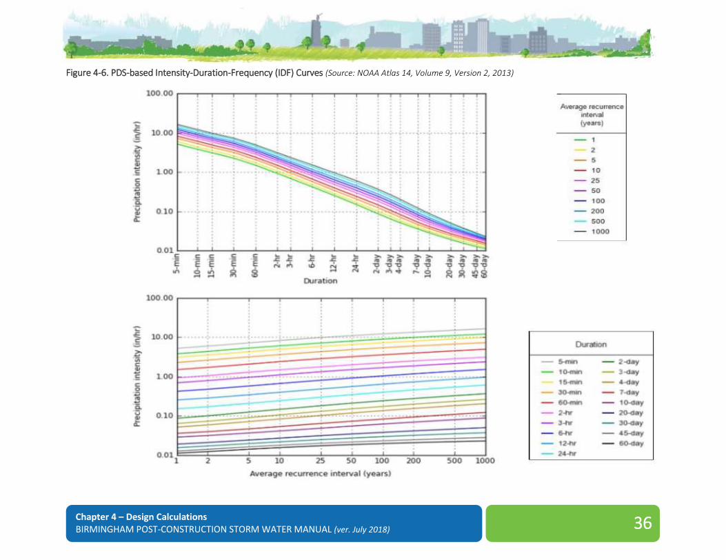
Chapter 4 – Design Calculations BIRMINGHAM POST-CONSTRUCTION STORM WATER MANUAL (ver. July 2018) 36
Figure 4-6. PDS-based Intensity-Duration-Frequency (IDF) Curves (Source: NOAA Atlas 14, Volume 9, Version 2, 2013)

Chapter 4 – Design Calculations BIRMINGHAM POST-CONSTRUCTION STORM WATER MANUAL (ver. July 2018) 37
Table 4-16. Intensity-Duration-Frequencies for the City of Birmingham
Hours Minutes Return Frequency - Rainfall Intensity (in/hr)
1-Yr 2-Yr 5-Yr 10-Yr 25-Yr 50-Yr 100-Yr
0.08 5 5.2 5.95 7.2 8.27 9.77 11 12.2
0.17 10 3.8 4.36 5.27 6.05 7.15 8.02 8.91
0.25 15 3.09 3.54 4.28 4.92 5.82 6.52 7.24
0.5 30 2.27 2.6 3.16 3.63 4.3 4.83 5.38
1 60 1.49 1.71 2.08 2.39 2.84 3.2 3.58
2 120 0.925 1.06 1.29 1.48 1.77 2 2.23
3 180 0.69 0.788 0.957 1.11 1.32 1.5 1.68
6 360 0.421 0.476 0.575 0.666 0.802 0.917 1.04
12 720 0.254 0.285 0.343 0.398 0.483 0.558 0.639
24 1440 0.151 0.171 0.208 0.243 0.298 0.346 0.398
*Minimum time of concentration (Tc)
Table 4-17. Depth-Duration-Frequencies for the City of Birmingham
Hours Minutes Return Frequency - Rainfall Depth (in)
1-Yr 2-Yr 5-Yr 10-Yr 25-Yr 50-Yr 100-Yr
0.08 5 0.433 0.496 0.6 0.689 0.814 0.913 1.01
0.17 10 0.634 0.726 0.879 1.01 1.19 1.34 1.49
0.25 15 0.773 0.885 1.07 1.23 1.45 1.63 1.81
0.5 30 1.14 1.3 1.58 1.82 2.15 2.42 2.69
1 60 1.49 1.71 2.08 2.39 2.84 3.2 3.58
2 120 1.85 2.12 2.57 2.97 3.54 3.99 4.47
3 180 2.07 2.37 2.87 3.32 3.97 4.5 5.05
6 360 2.52 2.85 3.45 3.99 4.81 5.49 6.23
12 720 3.06 3.43 4.13 4.79 5.83 6.72 7.7
24 1440 3.63 4.1 4.99 5.83 7.15 8.3 9.56
*Minimum time of concentration (Tc)

Chapter 4 – Design Calculations BIRMINGHAM POST-CONSTRUCTION STORM WATER MANUAL (ver. July 2018) 38
Figure 4-7. Cumulative Distribution Curves for Different SCS Rainfall Types (Source: Pitt, 2002)
4.3.2.2 Design Storms for Peak Flow Calculations The design storm frequency is the basis for hydrologic computations
and varies depending on the design element. Table 4-18 summarizes
the design storms for peak flow calculations in Birmingham. Where no
duration is indicated, the Engineer shall run the appropriate return
frequency storm(s) for the full range of durations (5 minute through 24
hours).
Figure 4-8. SCS Rainfall Distributions for Southeastern United States (Source: NRCS 2002b)
Table 4-18 Birmingham Design Storms for Peak Flow Calculations
Performance Standard
Summary Description
Flood Protection
1. Extended detention of the 1-year, 24-hour storm event volume; and,
2. Qppost ≤ Qppre for the 10- and 25-year, 24-hour storm events; and,
3. Safely pass the Qp100 from the property.
Downstream Channel Analysis
Qppost ≤ Qppre for the 2-year, 10-year, and 25-year 24-hour storm events to a prescribed 10% point downstream
Drainage System Design
Design box culverts & pipes for the 25-year storm event

Chapter 4 – Design Calculations BIRMINGHAM POST-CONSTRUCTION STORM WATER MANUAL (ver. July 2018) 39
4.3.3 Runoff Proper calculation of runoff is critical to proper planning and sizing of
storm drainage facilities. This section identifies the methodology to be
used for determining the storm runoff design peaks and hydrograph
generation for preparation of storm drainage studies, plans, and facility
designs.
4.3.3.1 Time of Concentration Time of Concentration (Tc) is the amount of time it takes for the most
hydraulically distant point in the watershed to contribute flow. Tc
influences the shape of the runoff hydrograph and has two
components:
1. The time for overland flow to occur from a point on the perimeter
to a natural or artificial drainage conduit or channel.
2. The travel time in the conduit or channel to the outflow point of the catchment.
The minimum time of concentration for all computations shall be 5
minutes. Chapter 3 in Technical Release 55 (TR-55, June 1986)
provides the procedure for calculating Tc.
4.3.3.2 Peak Discharge (for Flood and Drainage Designs) Peak discharge calculations represent the first level of runoff analysis.
This analysis is used to determine the maximum flow rate at a given
point resulting from a storm event. Peak discharge analysis is sufficient
to design storm water conveyances and culverts whose purpose is only
to convey runoff. The Rational Method and the National Resource
Conservation Service (NRSC) Graphical Peak Discharge Methods are
approved peak discharge calculation methods for use in Birmingham.
Both methods are described further below.
The Rational Method The Rational Method can be used to compute peak flows only for
stormwater conveyance drainage systems in watershed areas less than
20 acres. It cannot be used for sizing detention ponds, regardless of
watershed size.
The Rational Method assumes that all rainfall abstractions are
represented by a single runoff coefficient, C. Where distinctive land use
features are known, use of an area weighted C factor is required.
The Rational Method equation is presented in Equation 4-18.
𝑸 = 𝑪𝑰𝑨 Eq. 4-18
Where:
Q = runoff (cfs)
C = runoff coefficient (see Technical Release 55, TR-55,
June 1986)
I = rainfall intensity (in/hr, see Table 4-16)
A = area (acres)
The Rational Method assumes:
The rainfall intensity is uniform over the entire watershed during
the entire storm duration.
The storm duration is equal to Tc.
The Tc is the time required for the runoff from the most remote
part of the watershed to reach the point under design.
The NRCS Graphical Peak Discharge Method In general, the use of the NRCS (formerly Soil Conservation Service, or
SCS) Graphical Peak Discharge Method to calculate peak discharges is
preferred for the design most onsite drainage system components. The
unit hydrograph method (also called the hydrologic method) requires
basic data similar to the Rational Method: drainage area, a runoff factor,
time of concentration, and rainfall. The NRCS approach, however, is
more sophisticated in that it also considers the time distribution of the

Chapter 4 – Design Calculations BIRMINGHAM POST-CONSTRUCTION STORM WATER MANUAL (ver. July 2018) 40
rainfall, the initial rainfall losses to interception and depression storage,
and an infiltration rate that decreases during the course of a storm. The
method is summarized below. Further detail can be found in the
NRCS National Engineering Handbook, Part 630, Hydrology, or in
Technical Release 55 (TR-55).
The Graphical Peak Discharge Method can be used to compute peak
flows for watersheds of any size. This method uses the runoff curve
number (CN), where CN > 40. This number is a function of soil type
and land use.
This method is implemented by first applying the Equations 4-19a
and 4-19b to calculate the runoff depth:
𝑸 =(𝑷 − 𝟎. 𝟐𝑺)𝟐
(𝑷 + 𝟎. 𝟖𝑺) 𝑺 =
𝟏𝟎𝟎𝟎
𝑪𝑵− 𝟏𝟎
Eqs. 4-19a and 4-19b
Where:
Q = the accumulated direct runoff (inches), for P greater than Ia = 0.2S.
P = the accumulated rainfall depth (inches) for the 24-hr design storm (see Table 4-17)
S = the potential maximum soil retention (inches)
CN = the SCS Curve Number
Peak discharge is estimated using Equation 4-20.
𝒒𝒑 = 𝒒𝒖 ∗ 𝑨 ∗ 𝑸 ∗ 𝑭𝒑 Eq. 4-20
Where:
qp = peak discharge rate (cfs)
qu = unit peak flow rate (cfs/mi2 per inch of runoff, refer to TR-55)
A = drainage area (mi2)
Q = runoff depth calculated from Equation 4-17a
Fp = pond and swamp adjustment factor, Fp = 1 if there are no ponds or swamps.
4.3.3.3 Peak Discharge (for Storm Water Quality Design) The peak rate of discharge for the water quality design storm (Qwq),
also called the water quality peak discharge, is sometimes needed to size
storm water quality controls that are located off-line, such as sand
filters and infiltration trenches. More traditional peak discharge
calculation methods are not appropriate for this application for a
variety of reasons. First, the use of more traditional methods, such as
the Rational Method would require the choosing of an arbitrary design
storm event that will differ from the rainfall event that must be treated
for water quality. Further, conventional SCS methods have been found
to underestimate the volume and rate of runoff for rainfall events of
less than two inches. This discrepancy in estimating runoff and
discharge rates can lead to situations where a significant amount of
runoff bypasses the storm water quality control due to an inadequately
sized diversion structure and leads to the design of undersized bypass
channels.
The method employed to calculate the water quality peak discharge
uses the runoff coefficient to find the depth of runoff for the water
quality storm of 1.1 inches. The SCS method is then used to find a unit
peak discharge that is combined with the runoff depth to find a peak
runoff rate.
The following procedure can be used to calculate Qwq. This procedure
relies on the Rv and the simplified peak discharge calculation:
1. Utilize Equation 4-21 to calculate Dwq.
𝑫𝒘𝒒 = 𝟏. 𝟎𝟒𝑹𝒄 Eq. 4-21
Where:
Dwq = water quality runoff depth (inches)

Chapter 4 – Design Calculations BIRMINGHAM POST-CONSTRUCTION STORM WATER MANUAL (ver. July 2018) 41
Rc = Runoff coefficient [Rc = 0.015 + 0.0092(I)] where I is the % impervious area of the contributing drainage basin to the storm water quality control
2. A runoff curve number (CN) can be estimated using the standard
SCS Runoff Curve Number estimation technique, or can be
computed utilizing Equation 4-22 (Pitt, 1994).
𝑪𝑵 =𝟏𝟎𝟎𝟎
𝟏𝟎 + 𝟓𝐏 + 𝟏𝟎𝑫𝒘𝒒 − 𝟏𝟎(𝑫𝒘𝒒𝟐 + 𝟏. 𝟐𝟓𝑫𝒘𝒒𝑷)
𝟏𝟐⁄
Eq. 4-22
Where:
CN = runoff curve number
P = 1.1 inches (or the adjusted rainfall capture amount, see Section 4.2.2)
Dwq = water quality runoff depth (inches) from Equation 4-21
3. Determine the initial abstraction (Ia) from Table 4-19, and the
ratio Ia/P is then computed (P = 1.1 inches or the adjusted rainfall
capture amount, see Section 4.2.2).
4. Compute the drainage area time of concentration (tc) for the post-
development land use with standard SCS methods.
5. The time of concentration is used with the ratio Ia/P to obtain the
unit peak discharge, qu, from Figure 4-9 for the Type III rainfall
distribution. If the ratio Ia/P lies outside the range shown in the
figure, use the limiting values.
6. The water quality peak discharge (Qwq) is computed using
Equation 4-23.
𝑸𝒘𝒒 = 𝒒𝒖𝑨𝑫𝒘𝒒 Eq. 4-23
Where:
Qwq = the water quality peak discharge (cfs)
qu = unit peak flow rate (cfs/mi2 per inch of runoff, refer to TR-55)
A = contributing drainage area (mi2)
Dwq = water quality runoff depth (inches) from Equation 4-21
4.3.4 Discharge Hydrograph Generation A hydrograph represents runoff flow as it varies over time at a
particular location. The area under the hydrograph represents the total
volume of runoff. As opposed to peak rate of runoff, the hydrograph
accounts for the variation in volume and flow rate over the duration of
the of the storm event. Hydrographs are necessary to assess the effects
of storm water detention/retention facilities. Hydrographs are also
necessary for assessing the effects of combining runoff from two or
more sub-catchments discharging to a common location in complex
drainage areas with multiple sub-catchments.
Most standard hydrologic modeling software that use the hydrograph
generation and routing techniques included in this manual will be
acceptable for use in Birmingham. These include, but are not limited to
TR-55, TR-20, HEC-HMS, and various SWMM models. Engineers are
responsible for understanding the limitations and correct application of
modeling software used for hydrograph generation. For details on the
Tabular Hydrograph Method refer to TR-55, June 1986. In some
cases, detailed hydrologic studies may have been completed for the area
of interest and can be used with approval from the Director.
The hydrologic technique used must be appropriate for the design
approach. For example, peak flow methods, such as the Rational
Method, is not acceptable for volume required designs.

Chapter 4 – Design Calculations BIRMINGHAM POST-CONSTRUCTION STORM WATER MANUAL (ver. July 2018) 42
Table 4-19. Initial Abstraction (Ia) for Runoff Curve Numbers (Source: SCS, TR-55, Second Edition, June 1986)
Curve
Number Ia (in)
Curve
Number Ia (in)
40 3.000 70 0.857
41 2.878 71 0.817
42 2.762 72 0.778
43 2.651 73 0.740
44 2.545 74 0.703
45 2.444 75 0.667
6 2.348 76 0.632
47 2.255 77 0.597
48 2.167 78 0.564
49 2.082 79 0.532
50 2.000 80 0.500
51 1.922 81 0.469
52 1.846 82 0.439
53 1.774 83 0.410
54 1.704 84 0.381
55 1.636 85 0.353
56 1.571 86 0.326
57 1.509 87 0.299
58 1.448 88 0.273
59 1.390 89 0.247
60 1.333 90 0.222
61 1.279 91 0.198
62 1.226 92 0.174
63 1.175 93 0.151
64 1.125 94 0.128
Curve
Number Ia (in)
Curve
Number Ia (in)
65 1.077 95 0.105
66 1.030 96 0.083
67 0.985 97 0.062
68 0.941 98 0.041
69 0.899 - -
4.3.5 Off-site Analysis Policies The design of storm water facilities shall consider and accommodate
any discharges to them from areas upstream as stated in Table 4-20.
Table 4-20. Policies for On-Site & Off-Site Storm Flow Analysis
Analysis
Type Requirements for Use in Birmingham
Onsite
Analysis
The post-construction condition shall be used to determine runoff coefficients.
Changes in flow patterns (from preconstruction conditions) caused by the proposed development shall be considered.
The proposed grading shall be used to calculate the time of concentration and other runoff parameters.
Offsite
Analysis Upstream drainage areas shall be considered
developed for analysis of onsite storm water facilities.
Where the offsite area is fully or partially undeveloped, the runoff shall be calculated assuming the basin is fully developed. Storm water parameters (i.e. C and CN) shall be based on current zoning.
Downstream analysis of the impacts of drainage improvements shall be completed in accordance with the 10% rule defined in this Manual (Section 4.3.6).

Chapter 4 – Design Calculations BIRMINGHAM POST-CONSTRUCTION STORM WATER MANUAL (ver. July 2018) 43
Figure 4-1. Unit Peak Discharge (qu) for NRCS (SCS) Type III Rainfall Distribution (Source: Soil Conservation Service, 1986)

Chapter 4 – Design Calculations BIRMINGHAM POST-CONSTRUCTION STORM WATER MANUAL (ver. July 2018) 44
4.3.6 Downstream Analysis (The 10% Rule) Birmingham’s storm water design criteria may require the design to
control peak discharges at the outlet of a site, such that the post-
development peak discharge does not exceed the pre-development
peak discharge. Typically, this peak discharge control is achieved
through construction of one or more on-site detention facilities. Peak
discharge control does not always provide effective water quantity
control from the site, and may actually exacerbate flooding problems
downstream of the site. Moreover, master plans have shown that a
development site’s location within a watershed may preclude the
requirement for overbank flood control from a particular site.
A major reason for negative impacts due to storm water detention
facilities involves the timing of the peak discharge from the site in
relation to the peak discharges in the receiving stream and/or its
tributaries. If detention structures are indiscriminately placed in a
watershed without consideration of the relative timing of downstream
peak discharges, the structural control may actually increase the peak
discharge downstream. An example of this situation is presented in
Figure 4-10, which shows a comparison of the total downstream flow
on a receiving stream (after development) with and without detention
controls. In the figure, the smaller dashed-dot and solid lines denote
the runoff hydrograph for a development site with and without
detention, respectively. These runoff hydrographs will combine with a
larger runoff hydrograph of the receiving stream (not shown). The
combined discharges from the site and receiving stream are shown in
the larger solid and dashed lines.
Poor peak discharge timing can have an even greater impact when one
considers all the developments located in a watershed and the
cumulative effects of increases in runoff volume and the duration of
high volume runoff in the channel, as well as peak discharge timing.
Even if peak discharges are handled effectively at the site level and
immediately downstream, the longer duration of higher flows due to
the increased volume from many developments located on or near a
stream may combine with downstream tributaries and receiving streams
to dramatically increase the downstream peak flows.
Figure 4-10. Potential Effect of On-Site Detention
Figure 4-11 illustrates this concept. The figure shows the pre- and
post-development hydrographs at the confluence of two tributaries.
Development occurs, meets the local flood protection criteria (i.e., the
post-development peak flow is equal to the pre-development peak flow
at the outlet from the site), and discharges to Tributary 1. When the
post-development detained flow from Tributary 1 combines with the
first downstream tributary (Tributary 2), it causes a peak flow increase
when compared to the pre-development combined flow. This is due to
the increased volume and timing of runoff from Tributary 1, relative to
the peak flow and timing in Tributary 2. In this case, the detention
volumes on Tributary 1 would have to have been increased to account
for the downstream timing of the combined hydrographs to mitigate
the impact of the increased runoff volume.

Chapter 4 – Design Calculations BIRMINGHAM POST-CONSTRUCTION STORM WATER MANUAL (ver. July 2018) 45
Figure 4-11. Potential Effect of Cumulative Detention Basins
Potential problems such as those described above are quite common,
but can be avoided through the use of a storm water master plan
and/or downstream analysis of the effects of a planned development.
Studies have shown that if a developer is required to assess the impacts
of a development downstream to the point where the developed
property is 10% of the total drainage area, and there are no adverse
impacts (i.e., stream peak discharge increases), then there is assurance
that there will not be significant increases in flooding problems further
downstream. For example, for a 10-acre site, the assessment would
have to take place down to a point where the total accumulated
drainage area is 100 acres. Policies for the downstream analysis are
provided in Chapter 3.
While this assessment does require some additional labor on the part of
the design engineer, it allows smart storm water management within a
watershed. The assessment provides the developer, the City, and
downstream property owners with a better understanding (and
corresponding documentation) of the potential downstream impacts of
development. In turn, this information identifies those developments
for which waivers or reductions in the flood protection requirements
may prove beneficial. Typical steps in the application of this analysis
are as follows.
1. Using a topographic map determine the lower limit of the “zone of
influence” (i.e., the 10% point), and determine all downstream
analysis comparison points (at the outlet of the proposed land
development, all downstream tributary junctions, and all public or
major private bridges or culverts, ending at the next tributary
junction beyond the 10% point).
2. Using an accepted hydrologic model, determine the pre-
construction peak discharges for the 2-year, 10-year, and 25-year,
24-hour storm events and the timing of those peaks at each
comparison point.
3. Change the site land use to post-construction conditions and
determine the post-construction peak discharges and timing for the
same storms at the same comparison points. Compare results.
4. If post-construction conditions increase the peak flow at any of the
comparison points, on-site flood protection BMPs must be
redesigned (or conveyance improvements/flow easements may be
allowed by the Director until all post-construction peak discharges
from the site for all storm events do not exceed the pre-
construction peak discharges at all comparison points.)
EXAMPLE 4-13: DOWNSTREAM ANALYSIS EXAMPLE
Figure 4-12 illustrates the concept of the downstream analysis for two sites in a
watershed. Site A is a development of 10 acres, all draining to a wet ED storm
water pond. Looking downstream at each tributary in turn, it is determined that
the analysis should end at the tributary marked “120 acres.” The 100-acre (10%)
point is in between the 80-acre and 120-acre tributary junction points.
The designer constructs a simple HEC-1 (HEC-HMS) model of the 120-acre areas
using single existing condition sub-watersheds for each tributary. Key detention
structures existing in other tributaries must be modeled. An approximate curve
number is used since the actual peak flow is not the key for initial analysis, only
the increase or decrease is important. The accuracy in curve number
determination is not as significant as an accurate estimate of the time of
concentration. Since flooding is an issue downstream, the pond is designed
(through several iterations) until the peak flow does not increase at junction
points downstream to the 120-acre point.

Chapter 4 – Design Calculations BIRMINGHAM POST-CONSTRUCTION STORM WATER MANUAL (ver. July 2018) 46
Figure 4-12. Downstream Analysis Example
10 acres
40 acres 80 acres
120 acres
190 acres
Site A
Site B
4.4 Small Storm Extended Detention Design
4.4.1 Overview The Birmingham Post-Construction Storm Water Ordinance requires
adherence to the Small Storm Extended Detention Standard which
requires extended detention of the small storm extended detention
volume (EDv). The EDv is determined for the 1-year frequency, 24-
hour storm over the entire site and must be discharged over no less
than a 24-hour period.
4.4.2 Estimation of the EDv The Simplified SCS Peak Runoff Rate Calculation approach can be
used for estimation of EDv prior to storage facility design, but must be
modified to determine the volume for a 1-year frequency, 24-hour
duration design storm event. The calculation procedure is as follows.
Step 1: The 1-year, 24-hour rainfall depth (P) for Birmingham is 3.63
inches.
Step 2: A runoff curve number (CN) is then estimated using standard
CN Runoff Curve Number estimation techniques.
Step 3: The CN is used to determine the initial abstraction (Ia) from
Figure 4-13 and the ratio Ia/P is computed.
Step 4: The accumulated runoff (Qd, inches) can then be calculated
using the SCS method provided previously in Equations 4-19a and 4-
19b, where initial abstraction (Ia) = 0.2S.
Step 5: Compute the drainage area time of concentration (tc) for the
post-development land use using standard SCS methods.
Step 6: Use tc with the ratio Ia/P to obtain the unit peak discharge, qu,
from Figure 4-9 for the Type III rainfall distribution. If the ratio Ia/P
lies outside the range shown in the figure, either use the limiting values
or use another peak discharge method.
EXAMPLE 4-13 (continued)
Site B is located downstream at the point where the total drainage area is 190
acres. The site itself is only 6 acres. The first tributary junction downstream
from the 10% point is the junction of the site outlet with the stream. The total
190 acres is modeled as one basin with care taken to estimate the time of
concentration for input into the hydrologic model of the watershed. The model
shows that a detention facility, in this case, will actually increase the peak flow
in the stream.

Chapter 4 – Design Calculations BIRMINGHAM POST-CONSTRUCTION STORM WATER MANUAL (ver. July 2018) 47
Step 7: Knowing qu and T (extended detention time, minimum of 24
hours and maximum of 72 hours); the qo/qi ratio (peak outflow
discharge/peak inflow discharge) can be estimated from Figure 4-14.
Step 8: Vs/Vr is then determined using the SCS detention basin routing
formula of Equation 4-24 or using Figure 4-15. The equation is
suspect when the expression qo/qi approaches the limits of 0.1 and 0.8.
𝑽𝒔
𝑽𝒓
= 𝟎. 𝟔𝟖𝟐 − 𝟏. 𝟒𝟑 (𝒒𝒐
𝒒𝒊
) + 𝟏. 𝟔𝟒 (𝒒𝒐
𝒒𝒊
)𝟐
− 𝟎. 𝟖𝟎𝟒 (𝒒𝒐
𝒒𝒊
)𝟑
Eq. 4-24
Where:
Vs = required storage volume (acre-feet)
Vr = runoff volume (acre-feet)
qo = peak outflow discharge (cfs)
qi = Peak inflow discharge (cfs)
Step 9: The required storage volume (EDv) can then be calculated
using Equation 4-25. To check the EDv estimate, the volume must be
incorporated into a BMP design and the 1-year 24-hour storm routed
through the BMP. The EDv is adequate when the 1-year, 24-hour
design storm is detained for 24 hours, and measured from the centroid
of the inflow hydrograph to the centroid of the outflow hydrograph.
𝑬𝑫𝒗 =(
𝑽𝒔
𝑽𝒓) 𝑸𝒅𝑨
𝟏𝟐
Eq. 4-25
Where:
Qd = the runoff depth for the design storm (inches)
A = Total drainage area (acres)
EXAMPLE 4-14: ESTIMATION OF EDv
Estimate the EDv necessary for a 50-acre wooded watershed, which will be
developed as follows:
1) Forest land - good cover (hydrologic soil group B) = 10 ac
2) Forest land - good cover (hydrologic soil group C) = 10 ac
3) Residential with 1/3 acre lots (hydrologic soil group B) = 20 ac
4) Industrial development (hydrological soil group C) = 10 ac
5) Total impervious area = 18 acres
6) % of pond and swamp area = 0
Step 1. The 1-year 24-hour design storm for Birmingham is 3.63 inches (Table 4-12).
Step 2. The Curve Number (CN) is determined to be 72, using SCS Methods (see Section 4.2.5 of this chapter).
Step 3. Calculate Ia/P for CN= 72: Ia = 0.778, Ia/P = (0.778/3.63) = 0.21
Step 4. Qd for 1-year, 24-hour storm is determined to be 1.21 inches, using Equations 4-7a and b.
Step 5. The time of concentration (Tc) is determined to be = 0.35 hrs, using SCS Methods.
Step 6. The unit discharge is determined from Figure 4-13 using Tc and Ia/P
from previous steps. qu (1-year) = 135 csm/in
Step 7. EDv = VS. Knowing qu from Step 6 and T (extended detention time of
24 hours), find qo/qi from Figure 4-3, qo/qi = 0.120
Step 8. Estimate storage/runoff using Equation 4-21 (can check using
Figure 4-14):
𝑽𝒔
𝑽𝒓= 𝟎. 𝟔𝟖𝟐 − 𝟏. 𝟒𝟑 (𝟎. 𝟏𝟐𝟎) + 𝟏. 𝟔𝟒 (𝟎. 𝟏𝟐𝟎)𝟐 − 𝟎. 𝟖𝟎𝟒 (𝟎. 𝟏𝟐𝟎)𝟑
= 𝟎. 𝟓𝟑
Step 9. The necessary detention volume is calculated using Equation 4-22:
𝑽𝒔 ≈ (𝑽𝒔
𝑽𝒓) 𝑸𝒅
𝑨
𝟏𝟐= 𝟎. 𝟓𝟑 (𝟏. 𝟐𝟏) (
𝟓𝟎
𝟏𝟐) ≈ 𝟐. 𝟔𝟖 𝒂𝒄𝒓𝒆 𝒇𝒆𝒆𝒕

Chapter 4 – Design Calculations BIRMINGHAM POST-CONSTRUCTION STORM WATER MANUAL (ver. July 2018) 48
Figure 4-13. Unit Peak Discharge (Source: USDA SCS TR-55, 1986)

Chapter 4 – Design Calculations BIRMINGHAM POST-CONSTRUCTION STORM WATER MANUAL (ver. July 2018) 49
Figure 4-14. Detention Time vs. Discharge Ratios (Source: Maryland Department of the Environment, 1998)

Chapter 4 – Design Calculations BIRMINGHAM POST-CONSTRUCTION STORM WATER MANUAL (ver. July 2018) 50
Figure 4-15. Approximate Detention Basin Routing for Rainfall Types I, IA, II, and III (Source: USDA SCS TR-55, 1986)
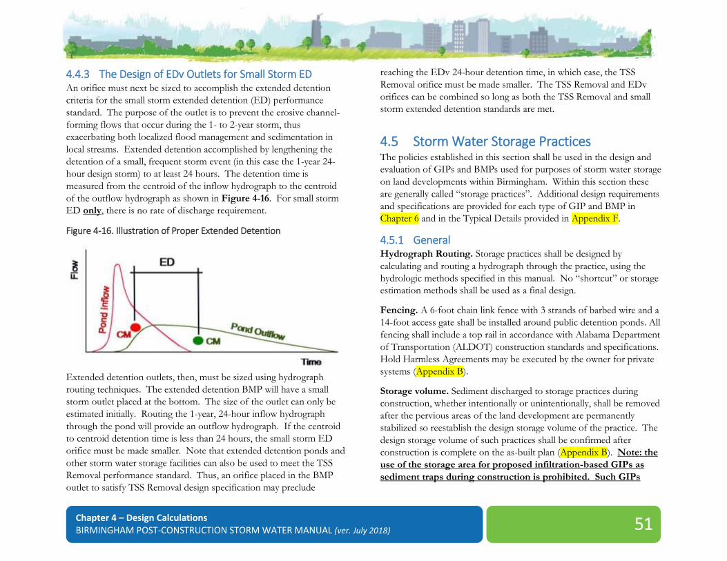
Chapter 4 – Design Calculations BIRMINGHAM POST-CONSTRUCTION STORM WATER MANUAL (ver. July 2018) 51
4.4.3 The Design of EDv Outlets for Small Storm ED An orifice must next be sized to accomplish the extended detention
criteria for the small storm extended detention (ED) performance
standard. The purpose of the outlet is to prevent the erosive channel-
forming flows that occur during the 1- to 2-year storm, thus
exacerbating both localized flood management and sedimentation in
local streams. Extended detention accomplished by lengthening the
detention of a small, frequent storm event (in this case the 1-year 24-
hour design storm) to at least 24 hours. The detention time is
measured from the centroid of the inflow hydrograph to the centroid
of the outflow hydrograph as shown in Figure 4-16. For small storm
ED only, there is no rate of discharge requirement.
Figure 4-16. Illustration of Proper Extended Detention
Extended detention outlets, then, must be sized using hydrograph
routing techniques. The extended detention BMP will have a small
storm outlet placed at the bottom. The size of the outlet can only be
estimated initially. Routing the 1-year, 24-hour inflow hydrograph
through the pond will provide an outflow hydrograph. If the centroid
to centroid detention time is less than 24 hours, the small storm ED
orifice must be made smaller. Note that extended detention ponds and
other storm water storage facilities can also be used to meet the TSS
Removal performance standard. Thus, an orifice placed in the BMP
outlet to satisfy TSS Removal design specification may preclude
reaching the EDv 24-hour detention time, in which case, the TSS
Removal orifice must be made smaller. The TSS Removal and EDv
orifices can be combined so long as both the TSS Removal and small
storm extended detention standards are met.
4.5 Storm Water Storage Practices The policies established in this section shall be used in the design and
evaluation of GIPs and BMPs used for purposes of storm water storage
on land developments within Birmingham. Within this section these
are generally called “storage practices”. Additional design requirements
and specifications are provided for each type of GIP and BMP in
Chapter 6 and in the Typical Details provided in Appendix F.
4.5.1 General Hydrograph Routing. Storage practices shall be designed by
calculating and routing a hydrograph through the practice, using the
hydrologic methods specified in this manual. No “shortcut” or storage
estimation methods shall be used as a final design.
Fencing. A 6-foot chain link fence with 3 strands of barbed wire and a
14-foot access gate shall be installed around public detention ponds. All
fencing shall include a top rail in accordance with Alabama Department
of Transportation (ALDOT) construction standards and specifications.
Hold Harmless Agreements may be executed by the owner for private
systems (Appendix B).
Storage volume. Sediment discharged to storage practices during
construction, whether intentionally or unintentionally, shall be removed
after the pervious areas of the land development are permanently
stabilized so reestablish the design storage volume of the practice. The
design storage volume of such practices shall be confirmed after
construction is complete on the as-built plan (Appendix B). Note: the
use of the storage area for proposed infiltration-based GIPs as
sediment traps during construction is prohibited. Such GIPs

Chapter 4 – Design Calculations BIRMINGHAM POST-CONSTRUCTION STORM WATER MANUAL (ver. July 2018) 52
include bioretention areas, urban bioretention areas, infiltration
trenches, and water quality channels.
Large storage facilities. Certification of dam embankment design
and stability, by an Alabama-registered Professional Engineer, shall be
provided for storage practices that will be designed to detain volumes
in excess of 100 acre-feet or earthen embankments higher than 25 feet.
Floodplain policies. The following conditions shall be provided in
accordance with the City of Birmingham Floodplain Ordinance,
adopted in October 1995.
a. Existing and future floodplains shall be preserved to the extent
possible.
b. Storage facilities shall not be located within the 100-year floodplain.
4.5.2 Storage Practice Bottoms and Embankments 1. The bottom of the storage practice shall be sloped towards the
outlet to prevent standing water. Other methods to achieve full discharge of storm water from the facility may be used, with written approval from the Director.
2. Control measures shall be installed within the storage practice to prevent transport of sediment and settled materials resulting from detained storm water into the outlet structure and downstream receiving waters.
3. Slopes of earthen embankments shall be constructed with two to one (2:1) horizontal to vertical dimensions or flatter.
4. Soil in all areas of storage practice shall be permanently stabilized with a dense stand of grass or other appropriate vegetation or by other means to eliminate bare soil exposure to rainfall, prevent erosion, and control sediment discharges. Failure to establish permanent stabilization of the practice may result in withholding approval of the as-built plan.
5. Sheet flow over the side banks of storage practices is discouraged; off-site flow shall be routed to common locations and conveyed into the practices utilizing structural controls to minimize erosion.
4.5.3 Outlets and Outfalls 1. Storage practices, including the principal spillway or outlet
structure, shall be designed in keeping with the design storm events identified by the flood protection performance standard.
2. In general, the outfall from a storage practice should be located to discharge to the nearest natural drainage feature or nearest storm water drainage system with adequate capacity to convey discharges from the storage facility.
3. Outlet structures for storage practices shall be designed to provide release of low flow volume to prevent standing water, yet still remain in keeping with performance standards for storm water quality protection and small storm extended detention.
4. An emergency overflow or spillways shall be provided for all detention and retention ponds, capable of passing the 100-year frequency, 24-hour duration storm event without catastrophic damage to the facility or downstream areas, unless the 100-year storm is accommodated through the principal spillway/outlet. Overflows or spillways may or may not be located near the principal outlet structure for the practice, depending on the capacity of the downstream receiving water or storm water drainage system, and the potential impact to downstream properties.
5. Trash racks and safety gates will be required for all outlet structures and pipes greater than or equal to eighteen (18) inches.
6. The outlet pipe for storage practices that will be dedicated to the City shall be constructed with O-ring reinforced concrete pipe (RCP) for the entire length of pipes penetrating the embankment or dam; justifiable exceptions to this requirement may be accepted by the Director.

Chapter 4 – Design Calculations BIRMINGHAM POST-CONSTRUCTION STORM WATER MANUAL (ver. July 2018) 53
7. Energy dissipation structures shall be provided at storage practice outfalls to control discharged storm water to non-erosive velocities.
4.6 Storm Water Conveyance Design
4.6.1 Purpose This section establishes the minimum standards and technical design
criteria for all storm water conveyances in Birmingham, in regard to
hydrology, size, and alignment. The primary function of storm water
conveyances is to collect excess storm water from street gutters, convey
the excess storm water through storm water conveyances and along the
street right-of-way, and discharge it into a GIP or BMP, or the nearest
receiving water body (FHWA 1996). The design of storm water
conveyances presented in this section relies on fundamental hydrologic
and hydraulic design concepts. Designers should refer to other
sections in this chapter for additional design methodology for
hydrologic, inlets, culverts, and open channels.
4.6.2 General Policies Minimum design storm. In keeping with the drainage system design
policies established in Chapter 3 of this manual, the minimum return
period to be used in the design of storm water drainage conveyance
systems is the 25-year return frequency, 24-hour duration storm event,
unless otherwise specified by the Director.
Required hydrologic methods. System components shall be designed
by calculating peak discharges using the hydrologic methods specified
in this manual.
Conveyance sizing. In each case, storm water conveyances shall be
sized to carry the portion of the runoff that cannot be conveyed on the
surface, as dictated by the available capacity in streets and swales during
these design event. Designers shall ensure that storms in excess of pipe
design flows can be safely conveyed through a land development
without damaging structures or flooding major roadways.
Minimum diameter. The minimum diameter for a storm drainage
pipe is 18 inches.
Pipe material. Storm sewer pipe shall be a minimum of Class 3
reinforced concrete if the storm sewer:
a. is to be transferred to the City of Birmingham for maintenance;
b. is located in a recorded easement; and/or,
c. conveys offsite storm water runoff through a site.
Pipe materials other than reinforced concrete may be used on systems
that do not meet the above criteria.
Inlet spacing. Inlets shall be spaced in street gutter lines to prevent
flow from entering public road intersections and to allow one lane
(based on lane width of the road) of traffic to remain open for local
streets. Arterial and collector streets must have one travel lane in each
direction open to traffic.
Hydraulic grade line (HGL). The HGL shall not exceed the crown
of the pipe by more than five percent (5%) of the diameter of the pipe
for the design storm.
Sizing for the 100-year design storm. The storm water conveyances
shall be sized to convey the 100-year storm event if any of the
following conditions are met:
a. The street capacity for the 100-year storm event is exceeded;
especially where the grade slopes down behind the curb and the
100-year storm capacity is limited to the height of the curb.
b. The 100-year storm flows split off in an undesired direction (e.g.
flow splits at intersections).
c. The storm water conveyance is accepting flow from an upstream
storm water conveyance system or branch that is designed for the
100-year storm.

Chapter 4 – Design Calculations BIRMINGHAM POST-CONSTRUCTION STORM WATER MANUAL (ver. July 2018) 54
d. Regional storm water conveyances are designed for the 100-year
storm.
e. The storm water conveyances must convey un-detained flows to a
regional detention basin if an over-land flow path to the basin is
not available.
4.6.3 Alignment and Placement Criteria Straight alignment required. All storm water conveyances shall be
constructed with a straight alignment between manholes. Table 4-21
provides the minimum horizontal and vertical alignment criteria.
Distances shall be measured from outside edge of pipe to outside edge
of pipe.
Table 4-21. Horizontal and Vertical Alignment Criteria
Alignment of
Conveyance
Relative to:
Alignment
Comment Minimum
Vertical
Clearance
Minimum
Horizontal
Clearance
Water Main 18 inches 10 feet
The distance shall be measured edge to edge. Approval from Birmingham
Water Works will be required for lesser clearances.
Building
Structure or
Foundation
--
10 feet (@
depth <
10 feet)
15 feet (@
depth >
10 feet)
No comment.
Cover 3 feet --
Minimum cover depends on the pipe size, type, and class, and the soil
bedding condition. The storm sewer grade shall maintain a minimum cover to withstand AASHTO HS-20 loading on
the pipe in vehicular traffic areas (existing or potential) and HS-15
loading in all other areas.
Minimum distance from water lines. In instances where it is not
possible to maintain the minimum horizontal alignment specified in
Table 4-21, the Director may allow deviation on a case-by-case basis.
This deviation may allow installation of the storm water conveyance
closer to the water main, provided that the water main is in a separate
trench or on an undisturbed earth shelf located on one side of the
sewer and at an elevation so the bottom of the water main is at least
18” above the top of the storm water conveyance.
Minimum distance from additional utilities. The location of the
utilities shall be derived from the best information available. Each
utility company shall receive a set of plans prior to final submittal on
which they may note changes or additions to utility information. The
adequacy of the separation of the storm water conveyance and other
utilities shall be determined by both the appropriate utility company
and the design engineer. Any necessary relocation shall be closely
coordinated with the respective utility company.
4.6.3.1 Placement in Existing Rights-of-Way and Easements Conveyance location. Existing rights-of-way and easements shall be
utilized for storm water conveyances if possible. Otherwise, sound
engineering judgment shall be utilized when determining locations for
storm water conveyances. Service needs of both the present service
area and future service areas should be considered when locating storm
water conveyances.
Concrete pavement. In areas of concrete pavement, consideration
shall be given to placing the storm water conveyance in a location such
that when saw-cut, an edge of the pavement to be removed would
coincide with an existing construction joint resulting in the need to only
saw-cut one side of the pavement. Manhole structures shall be either
completely outside the pavement or completely inside the pavement.
The existence of curbs or proposals of future curb and gutter shall be
taken into account when evaluating the benefit of reducing the number
of manholes in curved streets.

Chapter 4 – Design Calculations BIRMINGHAM POST-CONSTRUCTION STORM WATER MANUAL (ver. July 2018) 55
4.7 Inlets The purpose of this Section is to establish a basis for the design of
inlets to storm water conveyance systems. Storm water inlets are a vital
component of the urban storm water collection and conveyance
system. Inlets intercept excess storm water from streets and developed
areas and transition surface flow into storm water conveyances. Proper
inlet design includes both the proper inlet hydraulic capacity and
appropriate inlet placement. If too few inlets are provided, if inlets are
placed in the wrong location, or if inlets do not have adequate hydraulic
capacity, then even amply sized pipes in the storm water conveyance
system will not function as intended.
There are three general types of inlets acceptable for use in
Birmingham including curb opening (designated Type “HF Inlet”),
valley (designated “Yard Inlet”), and combination inlets (designated
Type “AF Inlet”). Typical installation settings include:
Street curb and gutter
Pavement depression
Drainage swale or channel
Greenspace or undeveloped area
Inlet components can be manufactured using cast-iron, steel, cast in
place concrete, and/or pre-cast concrete. For inlets placed in the right-
of-way, see also the City of Birmingham’s Standard Specifications for the
Construction of Public Works Projects.
4.7.1 Inlet Placement Inlets must be placed at each location where surface runoff flow should
be interrupted and transitioned into storm water conveyance system
pipe flow. Inlets can be placed in roadside ditches, grass or lined
swales, parking or pavement area depressions, and in roadway or
parking area curbs and gutters. The following location requirements
must be considered during the design of inlets.
a. Inlets shall be placed in all streets and roadway sags. For the 25-
year design storm, the depth of ponded water at the inlet shall not
exceed the values shown in Table 4-22. For the 100-year design
storm, the depth of ponded water at the inlet shall not exceed the
values shown in Table 4-23.
b. In developed areas, inlets shall be located in all pavement and green
space depression areas where surface runoff collects and transitions
to storm water conveyance pipe flow.
c. Inlets shall be placed in grass or lined swales and open channels
where concentrated flow transitions to storm water conveyance
pipe flow.
Table 4-22. Allowable Use of Streets for 25-Year Storm Runoff
Street Type
Maximum Street Encroachment
Street Width Face of Curb to
Face of Curb (ft)
Maximum Top Width
from Gutter Tmax (ft)
Maximum Depth in Gutter
Flow, d (ft)
Local No curb overtopping. Flow may spread to
crown of street.
28 15 0.30
32 16 0.32
36 18 0.36
Collector
No curb overtopping. Flow spread must leave at least one lane free of water with 5 ft on either
side of street crown.
36 13 0.26
40 15 0.30
44 17 0.34
Arterial
No curb overtopping. Flow spread must
leave at least two 10 ft lanes free of water
with 10 ft on each side of street crown.
Coordinate allowable use with the agency having jurisdictional authority of the
roadway.

Chapter 4 – Design Calculations BIRMINGHAM POST-CONSTRUCTION STORM WATER MANUAL (ver. July 2018) 56
Table 4-23. Allowable Use of Streets for 100-Year Storm Runoff
Street Type Maximum Depth and Inundated Area
Local and Collector
The Maximum Depth of Water:
Shall not exceed 12-inches above the gutter flowline and,
Shall not reduce the localized Flood Protection Grade to less than 12-inches.
(Whichever is more restrictive)
Arterial
The Maximum Depth of Water:
Shall not exceed 12-inches above the gutter flowline,
Shall not reduce the localized Flood Protection grade to less than 12-inches and,
Shall not exceed the street crown (to allow for emergency vehicles)
(Whichever is most restrictive)
d. Inlet grate capacities shall be designed to adequately pass the storm
water conveyance pipe design storm event flow with 50% of the
inlet grate free open areas clogged.
e. An emergency overland flow path shall be included at street and
roadway sags in the event that the inlet or storm water conveyance
is not functioning. The depth of ponded water at the inlet shall not
exceed twelve inches (12”).
f. Depth of ponded water shall not exceed eight inches (8”) in private
development parking areas, except in areas used as detention.
g. Depth of ponded water shall not exceed twenty-four inches (24”)
in green space areas, except in areas used as detention.
h. In streets and roadways, inlets shall be placed immediately
upstream of intersections, pedestrian walkways, and handicap
ramps. Required inlets shall be placed not closer than two feet (2')
from the upstream edge of walkways and handicap ramps.
i. In streets or roadways where opposing lanes are separated by a
grass median or concrete center curb, inlets shall be placed
upstream of a crossover.
j. On continuous roadway or street grades, inlet spacing is
determined by limiting maximum width of gutter flow (Tmax).
Inlets shall be spaced to collect a minimum of 75 percent (75%) of
the watershed design flow. Bypass flow, flow not intercepted by an
individual inlet, shall not exceed 25 percent (25%). Bypass flow
shall be considered when determining the location of the next
downstream inlet. General inlet spacing on continuous grades is
300 feet to 600 feet (300' to 600') provided the Tmax criteria is not
exceeded. Exact spacing shall be computed by the designer. See
the Section 4.7.3 - Gutter Flow for more information on Tmax
design.
k. Uniform inlet and casting types should be used on individual street
and roadway projects. Uniformity limits confusion and
misplacement of proper inlet types during construction.
4.7.2 Inlet Hydraulic Capacity All storm water runoff that enters a sump or gutter must pass through
an inlet to enter the storm water conveyance system. In most situations
storm water is laden with debris and the inlet will be susceptible to
clogging. Therefore, the capacity of inlets must account for this
clogging potential.
Design of inlet hydraulic capacity is separated into either a sump or
continuous grade situation. The following sections include design
considerations and figures for inlet capacity for these two situations:
sump condition and continuous grade condition.

Chapter 4 – Design Calculations BIRMINGHAM POST-CONSTRUCTION STORM WATER MANUAL (ver. July 2018) 57
4.7.2.1 Sump Condition Inlets in depressions or sumps function like weirs for shallow flow, but
as the depth of storm water increases, inlets begin to function like an
orifice. Figures 4-17 through 4-20 provide the allowable inlet
capacities in sump conditions. Assumptions made for the figures are
listed below.
Weir flow assumed for water depths below 2”.
Weir Equation 4.26:
𝑸𝟏 = 𝟑. 𝟑𝟎 ∗ 𝑷 ∗ 𝒅𝟏.𝟓 Eq. 4-26
Where:
Q1 = rate of flow into the inlet (cfs)
P = perimeter of grate (ft)
d = depth of water surface above inlet (ft)
Orifice flow assumed for water depths above 4”.
Orifice Equation 4.27:
𝑸𝟏 = 𝟒. 𝟖𝟏 ∗ 𝑨 ∗ 𝒅𝟎.𝟓 Eq. 4-27
Where:
Q1 = rate of flow into the inlet (cfs)
A = net open area of grate (ft)
d = depth of water surface above inlet (ft)
Transition flows assumed between 2” and 4” water depth.
Clogging reduces weir length by 50%.
Clogging reduces free open area by 50%.
4.7.2.2 Continuous Grade Condition Inlet hydraulic capacity on a continuous grade is designed as a function
of depth of water flow in the street gutter and the inlet grate constant.
The grate constant is determined empirically by the inlet manufacturer.
Note that inlets shall be spaced so that allowable inlet capacity
intercepts at least 75% of the gutter flow during the 25-year rainfall
event.
Figures 4-21 through 4-23 provide the allowable inlet capacities in
continuous grade conditions: assumptions for the figures are listed
below.
Inlet capacity on a continuous grade Equation 4.28:
𝑸𝒊 = 𝑲 ∗ 𝒅𝟓 𝟑⁄ Eq. 4-28
Where:
Qi = rate of flow into the inlet (cfs)
K = Inlet grate constant based on grade geometry and
longitudinal and transverse slopes (provided by
manufacturer) (Neenah inlet constants are utilized
for comparable East Jordan grates)
d = maximum depth of water surface above inlet (ft)
Casting capacity reduced by 50% for clogging.
Continuous grade capacity curves only apply when street flow
is at the maximum allowable depth. For lower gutter depths,
the inlet interception rate will decrease.

Chapter 4 – Design Calculations BIRMINGHAM POST-CONSTRUCTION STORM WATER MANUAL (ver. July 2018) 58
Figure 4-17. Allowable Inlet Capacity for Green Space Areas – Depression Conditions (Source: Fort Wayne IN Design Standards Manual)

Chapter 4 – Design Calculations BIRMINGHAM POST-CONSTRUCTION STORM WATER MANUAL (ver. July 2018) 59
Figure 4-18. Allowable Inlet Capacity for Pavement Areas – Depression Conditions (Source: Fort Wayne IN Design Standards Manual)

Chapter 4 – Design Calculations BIRMINGHAM POST-CONSTRUCTION STORM WATER MANUAL (ver. July 2018) 60
Figure 4-19. Allowable Inlet Capacity Sag Condition– Curb & Gutter for Neenah Foundry Castings (Source: Fort Wayne IN Design Standards Manual)

Chapter 4 – Design Calculations BIRMINGHAM POST-CONSTRUCTION STORM WATER MANUAL (ver. July 2018) 61
Figure 4-20. Allowable Inlet Capacity Sag Condition – Curb & Gutter for East Jordan Foundry Castings (Source: Fort Wayne IN Design Standards Manual)

Chapter 4 – Design Calculations BIRMINGHAM POST-CONSTRUCTION STORM WATER MANUAL (ver. July 2018) 62
Figure 4-21. Allowable Inlet Capacity Continuous Grade Condition – 2’ x 2’ Curb & Gutter Combination Casting (Source: Fort Wayne IN Design Standards
Manual)

Chapter 4 – Design Calculations BIRMINGHAM POST-CONSTRUCTION STORM WATER MANUAL (ver. July 2018) 63
Figure 4-22. Allowable Inlet Capacity Continuous Grade Condition – 33” Round Curb & Gutter Combination Casting (Source: Fort Wayne IN Design
Standards Manual)

Chapter 4 – Design Calculations BIRMINGHAM POST-CONSTRUCTION STORM WATER MANUAL (ver. July 2018) 64
Figure 4-23. Allowable Inlet Capacity Continuous Grade Condition – 2’ x 3’ Curb & Gutter Combination Casting (Source: Fort Wayne IN Design Standards
Manual)

Chapter 4 – Design Calculations BIRMINGHAM POST-CONSTRUCTION STORM WATER MANUAL (ver. July 2018) 65
4.7.3 Gutter Flow The capacity of gutter flow in curbed pavement helps determine proper
inlet casting and inlet spacing designs. Many factors affect the flow
capacity of gutters. These factors work together to provide a safe limit
on storm water encroachment into driving lanes and parking areas.
Policies for gutter flow are as follows.
Allowable use of streets for storm water flows. Use Tables 4-22 and
4-23 to determine the allowable encroachment into driving lanes for
various street types and widths, for the 25-year and 100-year events,
respectively.
Gutter flow capacity. Use Equation 4-29 to determine the gutter
flow capacity. Note the assumptions below the equation. Note also
that the equations refers to the gutter cross-section in Figure 4-24.
𝑸 =𝟎. 𝟓𝟔(𝑺𝑿
𝟏.𝟔𝟕𝑺𝑳𝟎.𝟓𝟎𝑻𝟐.𝟔𝟕)
𝒏 Eq. 4-29
Where:
Q = flow (cfs)
SX = pavement cross slope, (ft/ft)
SL = average longitudinal slope of gutter, (ft/ft) T = top width of flow extending from face of curb to
street, (ft) n = Manning’s roughness coefficient
Equation assumptions:
Sx = 2.0% or 0.020 ft/ft
n = 0.016
A minimum of 75% of design flow shall be intercepted by the inlet
Total gutter width = 1.5 feet (consists of a 6 inch wide curb
and 12 inch wide gutter section, typically cast-in-place
concrete.)
Maximum curb height = 6 inches
Maximum allowable gutter flow for the 25-year event is 10 cfs.
SX is equivalent across both the pavement and gutter.
Figure 4-24. Gutter Cross Section
4.8 Culverts
4.8.1 Purpose A culvert is defined as a conduit for the conveyance of water under a
roadway, railroad, or other embankment. In addition to serving
hydraulic functions, culverts must also carry overhead loads from
traffic and other activities, thereby serving a structural function. Proper
culvert design is essential because culverts often significantly influence
upstream and downstream flood risks, floodplain management, and
public safety.
A culvert, as distinguished from a bridge, is usually covered with
embankment and is composed of structural material around the entire
perimeter although it can be supported on spread footings with the
streambed serving as the bottom.
A bridge is a structure having an opening measured along the centerline
of a roadway of more than 20 feet between faces of abutments or
spring lines of arches. Multiple barrel box culverts or multiple pipe
culverts having an opening of more than 20 feet between the limits of
the extreme openings are sometimes classed as bridges.

Chapter 4 – Design Calculations BIRMINGHAM POST-CONSTRUCTION STORM WATER MANUAL (ver. July 2018) 66
4.8.2 General Design Policies The criteria presented in this section shall be used in the design of
culverts.
Design storms for public culverts. Publicly owned culverts crossing a
roadway shall be designed to convey the peak flow resulting from a
100-year event. Driveway culverts within right-of-way shall convey the
peak flow resulting from a 50-year event.
Design storms for private culverts. Privately owned culverts located
outside right-of-way and serving areas which do not require detention
shall be designed to convey the peak flow resulting from a 50-year
event and provisions shall be made to contain the runoff from a 100-
year event. Lesser capacities may be considered provided that proper
accommodations are provided for on- site storage of the 100-year
event.
Required design specifications. The design of culverts shall conform
to the methodology described in the Hydraulic Design of Highway
Culverts published by the U.S. Department of Transportation’s Federal
Highway Administration’s Publication No. FHWA-HIF-12-026, April
2012 (or current edition), unless otherwise specified herein or by the
Director. This design publication is available online at:
https://www.fhwa.dot.gov/engineering/hydraulics/pubs/12026/hif12
026.pdf.
Required design program. The HY-8 program is the computerized implementation of FHWA culvert hydraulic approaches and protocols and shall be used for culvert design. Available online at http://www.fhwa.dot.gov/engineering/hydraulics/software/hy8/.
Use of Alabama Department of Transportation (ADOT) guidance encouraged. The ADOT 2014 Standard and Special Drawings for Highway Construction (or current edition) provides valuable culvert design information. The document is available online at: http://alletting.dot.state.al.us/Docs/Standard_Drawings/StdSpecialDrawingsEnglish2014.htm.
Required Manning’s coefficient. A Manning’s roughness coefficient of 0.013 shall be used to size concrete pipe and box culverts.
Culvert length. Culvert length design shall consider embankment width, installation depth, and embankment slopes.
Culvert material. Culverts shall be a minimum of Class 3 reinforced
concrete if the storm sewer:
a. is to be transferred to the City of Birmingham for
maintenance;
b. is located in a recorded easement; and/or,
c. conveys offsite storm water runoff through a site.
Culvert materials other than reinforced concrete may be used on systems that do not meet the above criteria.
Box culvert loading. Box culverts shall be designed for AASHTO HS-20 loading in vehicular traffic areas (existing or potential) and HS-15 loading in all other areas.
Backwater. Culverts shall not increase backwater elevations on upstream properties. Backwater shall be contained within existing banks of the upstream open channel.
Overland flow routes. Emergency overland flow routes shall be checked to assure that backwater resulting from a potentially blocked culvert or intense storm does not flood or damage property. If an emergency overland flow route is not available, culvert flow capacity shall be increased. Sound engineering judgment shall be applied in determining the potential extent of backwater damage and the necessary increase in culvert flow capacity.
Minimum diameter. The minimum diameter for culverts crossing a
public roadway shall be 18 inches (18”). The minimum diameter for
private driveway culverts within right-of-way shall be 12 inches (12”).

Chapter 4 – Design Calculations BIRMINGHAM POST-CONSTRUCTION STORM WATER MANUAL (ver. July 2018) 67
Flow velocity. Both minimum and maximum flow velocities should be considered when designing a culvert.
a. A minimum velocity of 3.0 feet/second when the culvert is flowing
partially full is recommended to ensure a self- cleaning condition
during partial depth flow.
b. The maximum velocity should not exceed culvert manufacturer
recommendations. The maximum velocity should be consistent
with channel stability requirements at the culvert outlet.
c. The maximum allowable outlet velocity of culverts, which
discharge to an earthen channel, shall be 6 feet/second.
d. As outlet velocities increase, the need for channel stabilization at
the culvert outlet increases. If velocities exceed permissible
velocities for the various types of nonstructural outlet lining
material available, the installation of structural energy dissipaters
are required.
Sumped culverts. Circular and elliptical pipes shall be installed with
pipe inverts lower than adjacent channel flowline for sumped culverts.
Sound engineering judgment shall be applied to determine the depth of
sumping. Sumping increases the base flow capacity of circular and
elliptical pipes, accommodates the future lowering of the channel, may
increase the depth of pipe cover, and in environmentally sensitive areas
allows for a natural stream bottom in the pipes.
4.8.3 Structural Design Policies Loading. All culverts crossing a roadway shall be designed to
withstand a minimum HS-20-44 loading as defined by the American
Association of State Highway and Transportation Officials (AASHTO).
Culverts crossing a railroad shall be designed to withstand an E-80
loading.
Installation depth. Refer to manufacturer specifications or
recommendations for installation depth requirements.
Bedding and backfill. Backfill classifications, materials, and methods
of compaction shall be in accordance with Birmingham Water Works
standards for projects inside of the City limits unless special
circumstances warrant otherwise.
Floatation and anchoring. Pipe floatation can occur when the uplift
(buoyancy) forces outside the pipe are greater than the downward
weight forces on the pipe. This uplift force can be great enough to
cause the pipe to bend and dislodge from the embankment. Large
diameter, flexible material culverts are more vulnerable to floatation.
Anchoring may be achieved using concrete end sections, ties to a
concrete footer, or other similar means.
4.8.4 Inlet and Outlet Configuration General. All culverts, public and private, shall have end treatments
such as prefabricated end sections, wing walls and aprons, or headwalls
at the inlet and the outlet. The design of end treatments shall consider
public safety and erosion control.
Roadside safety. Roadside ditch culverts for commercial and
residential drives shall have sloped prefabricated end sections.
Headwalls and wing walls are not permitted.
Trash racks. Trash racks should be considered for inlet culvert end
treatment where inlet clogging or downstream trash pollution is
anticipated due to upstream land use activities. In general, trash racks
shall not be used on culvert outlets. However, trash racks may be
warranted on outlets in areas where public safety is a concern.
Erosion control. Channel stabilization and erosion control measures
shall be utilized at the inlet and outlet of a culvert.
4.8.5 Environmental Considerations Migrating fish. In channels with a base flow or normal pool,
migration of aquatic species should be considered. Culverts should be
sumped to maintain a base flow depth through the culvert equal to or

Chapter 4 – Design Calculations BIRMINGHAM POST-CONSTRUCTION STORM WATER MANUAL (ver. July 2018) 68
greater than the adjacent channel base flow depth. Bottomless culverts
may be considered to maintain a natural stream bottom. Where fish
migration is a concern, contact the Alabama Department of
Conservation and Natural Resources (ADCNR), Wildlife and
Freshwater Fisheries Division for culvert design assistance.
4.8.6 Permitting Culvert installation may require approval and/or permitting from
federal, state, or other local agencies. It is the responsibility of the
applicant to understand and obtain all required permits. Early
coordination regarding permitting and approval is recommended. Each
public agency may have design criteria which must be complied with
for permitting.
The public agencies who may require approval for culvert design or
installation include the following.
City of Birmingham Department of Planning, Engineering and Permits for work within city street or road right-of-way or within floodplains or floodways.
Alabama Department of Transportation, District 31 for work within state, federal, or interstate highway rights-of-way.
Jefferson County Highway Department for work within county road right-of-way.
Birmingham Park and Recreation Department for work affecting the Greenway, trails, and bicycle system.
Jefferson County Surveyor’s Office for work affecting Jefferson County regulated drains or mutual drains.
Alabama Department of Conservation and Natural resources (ADCNR) for:
o Early coordination for projects affecting stream channels or wetlands.
o Stream crossings.
o Work within a floodway or flood plain.
o All culverts and bridges, public or private, with a drainage area equal to or greater than 1 square mile.
Alabama Department of Environmental Management (ADEM) for Early Coordination for projects affecting stream channels including regulated drains.
United States Army Corps of Engineers (USACE) for Early Coordination for projects affecting wetlands or stream channels including regulated drains.
4.9 Open Channels By definition, an open channel is a conduit for the conveyance of
liquids. Flow in an open channel is open to the atmosphere and driven
by gravity.
Open channels for the conveyance of storm water can be natural or
constructed. Natural channels include rivers, streams, and natural
intermittent drainage courses. Investigation and analysis of the capacity
of existing natural channels using the USACE Hydrologic Engineering
Center River Analysis System (HEC-RAS) is complex and time
consuming. Alteration of a natural channel is also regulated and can
require permits from the USACE, ADCNR, and ADEM.
Constructed channels include drainage ditches, roadside ditches,
swales, bio-swales, and water quality treatment channels. New
constructed channels can be excavated or existing constructed channels
can be reconstructed as part of a new or altered storm drainage system.
Alteration of existing constructed channels might require permits from
the City of Birmingham Department of Planning, Engineering and
Permitting, USACOE, ADCNR or ADEM. This section provides
information for the design of constructed channels for the conveyance
of storm water in Birmingham.

Chapter 4 – Design Calculations BIRMINGHAM POST-CONSTRUCTION STORM WATER MANUAL (ver. July 2018) 69
Grass channels. Historically, design criteria for channels considered
minimum flow velocity to prevent sedimentation within the channel.
However, maintaining a minimum flow velocity may not always be
desirable. Grass channels are GIPs or BMPs for storm water quality,
depending on their design. In these cases, low velocity and high
infiltration is encouraged within the channel. Site designers who plan
to design and construct a water quality channel or a grassed swale for
purposes of storm water quality shall refer to the appropriate design
specification in Chapter 6.
4.9.1 Channel Shape The site designer shall determine the appropriate shape for a
constructed channel using engineering judgement and the following
guidance.
4.9.1.1 V-Shaped Channels V-shaped open channels are used for roadside ditches or swales. These
types of channels are not efficient for conveyance of high flows and are
generally designed for collection of intermittent surface sheet flow.
4.9.1.2 Dry Water Quality Swale/Enhanced Swale/Drainage Swales
Swales are shallow channels with relatively flat side slopes frequently
used in maintained yard areas or fields. Flow in swales is generally
intermittent, collecting runoff during and immediately following rainfall
events. Swales can also be used as overland flow routes for protection
of property if storm water conveyance or detention facilities fail or
overflow.
Swales are not necessarily V-shaped channels. Swales can have uniform
or variable width bottoms.
4.9.1.3 Trapezoidal Channels A trapezoid is defined as a quadrilateral figure with two parallel sides.
In the case of an open channel, the channel bottom and top of water
are regarded as parallel. Channels with rounded bottoms shall be
treated as trapezoidal. The sides of an excavated trapezoidal channel
are sloped to provide stability; channel slopes generally do not exceed
1.5 horizontal to 1 vertical (1.5:1). Three to one (3:1) slopes are
recommended for grass lined channels.
Trapezoidal channels can have uniform or variable bottom widths and
side slopes. In developed or agricultural areas where land is premium,
storm drainage channels are generally designed to be uniform and
functional with minimum use of land.
Two-stage open channels are designed with a low flow channel and at a
higher elevation a wider second stage channel. Two-stage channels
provide in channel storage and reduce flow velocity at higher flow
rates.
4.9.1.4 Composite Channel Composite channels are designed with a low flow channel in
combination with additional natural channel features. Composite
channels can be utilized as storm water quality best management
practices, detention facilities, wildlife habitat, attractive landscape
feature, or a combination of the above.
Composite channels may incorporate a low flow, meandering, variable
width channel through constructed wetlands, or open pools. The low
flow channel may meander through a wider valley which can flood
during higher flows. Composite channels can be used with a water
control structure or multiple control structures which reduce flow
velocity and provide storage during periods of high flow.
Low flow channel and valley side slopes and bottom widths may vary
to provide the appearance of a natural topography. Riparian vegetation
may be planted for water quality treatment and to provide a naturally
appearing landscape. Upland slopes can be planted with prairie grass
mixes and native woody species.

Chapter 4 – Design Calculations BIRMINGHAM POST-CONSTRUCTION STORM WATER MANUAL (ver. July 2018) 70
4.9.2 General Design Hydraulic design requirements. Open channels serving storm water conveyances and tributary flows from upstream watersheds shall be designed to convey runoff from a 100-year storm event. Hydraulic design shall be in accordance with Section 4.9.7 that follows.
Freeboard required. Open channels shall convey the 100-year event with two (2) feet of freeboard to the top of the channel bank.
Channel lining design. Channel lining shall be incorporated into the
design to prevent scour and erosion and to assure stability of the
channel. At minimum, the peak flow from a 25-year design storm shall
be used to design channel linings criteria for determining required
channel lining type and design criteria are set forth in Table 4-24.
Table 4-24. Open Channel Parameters
Channel Lining
Maximum Channel Gradient Maximum Flow Velocity
(ft/sec)
Maximum Side Slope (Hor:Vert) Percent ft/ft
Grass 3.0 0.0 5.0 2:1
Riprap 10.0 0.1 - 2:1
Concrete - - - 1.5:1*
Manufactured Lining
** ** ** **
* The concrete lining shall be designed as a structural retaining wall. ** Per manufacturer’s specifications
4.9.3 Side Slopes Channel side slope design is dependent on several factors including soil
stability, available land area for top of bank width, ease of maintenance,
and safety. Policies are as follows.
Grass lined channels. Side slopes in grass lined channels shall not
exceed 2 feet horizontal to 1 foot vertical (3:1).
Yard swales. Side slopes in swales used to convey storm water through
or between residential yards shall not exceed 4:1 for ease of
maintenance.
Lining required. Channel side slopes between 1.5:1 and 2:1 shall be
riprap lined. Where side slopes are steeper than 1.5:1, the channel
slopes shall have a concrete lining, and the concrete lining shall be
designed as a structural retaining wall.
4.9.4 Bed Slope (Gradient) Channel bed slope is the channel bottom gradient or profile grade
defined as the ratio of elevation change over length. The channel bed
slope is expressed as a percentage or a decimal. Channel bed slopes
vary due to existing topography and the design requirements of each
storm drainage system. Policies are as follows.
Minimum bed slope. The desirable minimum slope for open channels is 0.5% (.005 ft/ft). This is not always possible to achieve in areas of flat topography. Swales with a gradient less than 1.0% shall be served by an underdrain.
Yard swales. The desirable minimum slope for swales used to convey storm water through or between residential yards is 1.0 percent. Yard swales with slopes less than 1.0 percent should be constructed with subsurface drains.
Armoring required. Riprap or rock armor lining is required where channel bottom slope exceeds 3.0% or flow velocity exceeds 5 feet per second. Concrete lining shall be used where channel bottom slope exceeds 10% or flow velocity exceeds 15 feet per second.
4.9.5 Linings Open channel bottoms and side slopes require stabilization measures to
prevent scour and erosion. Grass is the most common method of
channel stabilization in areas of flat topography. Other acceptable
methods include riparian vegetation, riprap or rock, concrete, or

Chapter 4 – Design Calculations BIRMINGHAM POST-CONSTRUCTION STORM WATER MANUAL (ver. July 2018) 71
manufactured linings. Policies and guidance related to channel linings
are provided below.
Required flow rate. At minimum the peak flow rate from a 25-year
storm shall be used to design armored linings for all channels.
Hard armoring required. Riprap or rock lined channels are required
where flow velocity might result in bottom or side slope erosion.
Grass lined channels. Grass or vegetation lining is permitted in
channel bottoms with slopes not exceeding 3.0 percent or flows not
exceeding 5 feet per second. Grass is permitted on channel side slopes
not exceeding 3:1. Armor such as rip rap or rock might be required in
areas of grass lined channels where scour or erosion might occur.
Areas which might require armor include storm water conveyance
outlets, changes in bottom slope grade, bends in channel alignment, or
areas where gullies might be formed in side slopes by concentrated flow
entering a channel over the bank.
Riprap or rock lined channels. Riprap shall comply with the latest
version of the ALDOT Standard Specifications for Highway
Construction, Section 610. ALDOT Class 1 or class 2 riprap may be
used for energy dissipaters. The maximum slope for riprap lined
channels shall not exceed 10.0 percent.
Concrete lined channels. Due to the maintenance required, concrete
lined channels are permitted only in areas where limited space due to
existing development prohibits the construction of grass or riprap lined
channels, or where the bed slope or side slopes require concrete lining.
Additional policies are as follows.
o Concrete channel lining shall be steel reinforced ALDOT Class A concrete with a minimum thickness of 5 inches.
o Concrete channel lining shall be designed with lugs where bottom slope exceeds 3%.
Manufactured linings. Manufactured channel linings include
concrete revetment, gabions and Reno mattresses, or turf
reinforcement mats. Manufactured linings shall be designed and
constructed according to the manufacturer’s specifications.
4.9.6 Public Safety and Permitting Public safety. Public safety shall be considered where an open channel
presents a potentially dangerous situation to pedestrians or vehicular
traffic. Guardrail or fencing may be required for the protection of the
public.
Permitting. Open channels are frequently constructed through low
lying areas which may contain wetlands. Permitting may be required if
wetlands are affected by construction.
4.9.7 Hydraulic Design
4.9.7.1 Uniform Steady Flow Equations For the purposes of open channel design, flow is usually considered
steady and uniform. Given steady uniform flow or a reasonable
approximate condition, Equation 4-30 (Manning’s equation) shall be
used to calculate the capacity of a channel. Using this equation for
gradually varied or rapidly varied flow will result in errors.
𝑸 = (𝟏. 𝟒𝟗𝒏⁄ )𝐀𝑹𝒉
𝟐 𝟑⁄ 𝑺𝒇𝟏 𝟐⁄ Eq. 4-30
Where:
Q = flow rate (cfs)
n = Manning’s roughness coefficient
A = flow area (ft2) Rh = hydraulic radius (ft), defined as flow area, A, in ft2
divided by the wetted perimeter, Pw, in feet Sf = Friction slope (equal to storm water conveyance
slope for uniform flow), ft/ft

Chapter 4 – Design Calculations BIRMINGHAM POST-CONSTRUCTION STORM WATER MANUAL (ver. July 2018) 72
4.9.7.2 Flow Regime A more detailed analysis of an open channel design might be required
by the Director if there is concern regarding the flow regime. Flow
regime describes the state of flow in an open channel. Critical flow
represents the minimum specific energy for a given discharge. The
flow depth at critical flow is considered critical depth. Designers must
calculate critical depth to classify design flows in the open channel as
supercritical or subcritical. To distinguish supercritical and subcritical
flow, the Froude number (FR), which represents the ratio of inertial
forces to gravitational forces, is defined by Equation 4-31.
𝑭𝑹 = = 𝒗
(𝒈 ∗ 𝑨
𝑻)
𝟎.𝟓
Eq. 4-31
Where:
FR = Froude number
v = mean velocity (ft/s)
g = acceleration of gravity (32.2 ft/s2) A = cross-sectional area of flow (ft2) T = top width of flow (ft)
For flows near critical depth (Fr=1), small disturbances can cause
changes in flow state and unexpected hydraulic jumps. Flow with a
Froude number between 0.8 and 1.2 are unstable and must be avoided.
Designers should seek to create open channels with subcritical flow.
When flow in open channels is subcritical it is relatively easier to handle
through bends and flow transitions. Supercritical flow has higher
erosive power and hydraulic losses. Due to erosion potential, curves in
an open channel with supercritical flow are not practical. A description
of each flow regime is provided in Table 4-25.
Table 4-25. Flow Regime Classification
Flow Regime Characteristics
Fr > 1 (Supercritical Flow)
Flow depth controlled by upstream influence, usually critical depth. Flow characterized as shallow with high
velocities and steeper slopes. Higher potential for erosion.
Fr < 1 (Subcritical Flow)
Flow depth controlled by downstream influence, usually a ponded area or larger downstream channel. Flow
characterized as deep with lower velocities and mild slopes. This flow regime produces most stable open
channels.
Fr = 1 (Critical Flow)
Minimum specific energy for a given discharge.
4.10 Energy Dissipation Energy dissipaters are devices or practices designed to reduce the
velocity, energy, and turbulence of flow. Energy dissipaters are
required when highly erosive velocities are encountered at the end of
culverts or at the bottom of steep slopes. Energy dissipaters include,
but are not limited to, riprap aprons, riprap basins, and baffled outlets.
Energy dissipaters are commonly used as an inlet control for
bioretention basins, ponds, and wet basins. Depending on the site
layout and storm water conveyance design, they may be applicable to
media filters. They can be used downstream of other inlet controls that
concentrate storm water flow, as well as on steeper slopes, to reduce
erosion potential.
In addition to the policies and guidance below, more information on
energy dissipation is provided in Chapter 6.
4.10.1 Riprap Aprons Riprap aprons are commonly used for energy dissipation due to their
relatively low cost and ease of installation. A flat riprap apron can be
used to prevent erosion at the transition from a pipe or box culvert
outlet to a natural channel. Riprap aprons will provide adequate
protection against erosive flows provided there is sufficient length and

Chapter 4 – Design Calculations BIRMINGHAM POST-CONSTRUCTION STORM WATER MANUAL (ver. July 2018) 73
flare to dissipate energy by expanding the flow. An example is
provided in Figure 4-25.
Figure 4-25. Riprap Apron with Typical Features (Source: Fort Wayne IN
Design Standards Manual)
4.10.2 Riprap Basin A riprap outlet basin is a pre-shaped scour hole lined with riprap that
functions as an energy dissipater. Like a riprap apron, a riprap basin can
be used to prevent erosion at the transition from a pipe or box culvert
outlet to an earthen channel.
4.10.3 Baffled Outlet Baffled outlets are concrete or fiberglass boxes containing an
alternating series of baffles and chambers. In addition to reducing flow
velocity and energy, baffled outlets can effectively remove sediment,
suspended particles, and associated pollutants from storm water.
4.10.4 Design Policies and Guidance 1. Energy dissipaters shall be designed and sized in accordance with
the design procedures in the latest edition of the USACE Hydraulic
Engineering Center Circular 14 (HEC-14). HEC-14 includes
design information for alternate types of energy dissipaters, such as
drop structures and stilling basins.
2. The energy dissipater type selected for the application shall be
appropriate for the intended use and for the characteristics of the
site such as slope, available area, and landscape aesthetics.
3. A key design issue for energy dissipater is the interface between the
end of the dissipater and the adjacent downstream area, which is
typically vegetated. The site designer shall indicate the ground
cover at this location on the post-construction storm water plan
and as-built plan. If this interface area is to be vegetated, the
vegetation shall consist of a dense stand of grass (or other ground
cover) that is/can be well-established and will withstand periods of
flowing water. Turf reinforcement matting may be used at this
interface to provide additional structure for vegetation.
4. Vegetation/plantings can be used to obscure views of energy
dissipation structures if aesthetics are a concern.

Chapter 4 – Design Calculations BIRMINGHAM POST-CONSTRUCTION STORM WATER MANUAL (ver. July 2018) 74
4.10.5 Benefits and Limitations When designed and installed appropriately, energy dissipaters have the
following benefits.
Reduce velocities of concentrated storm water runoff.
Reduce erosion potential and allow for more efficient sediment
removal efforts, reducing overall maintenance costs and improving
GIP/BMP performance.
Prevent scour that may undermine the structure discharging
concentrated storm water runoff.
Prevent downslope erosion that may create gullies and scour holes.
Poor application, design, or installation will limit the effectiveness of
energy dissipaters and potentially cause larger problems resulting in
added maintenance. Potential problems include the following.
X Increased erosion in the GIP, BMP, or downstream channel that
potentially leads to sedimentation, clogging, or vegetation damage,
and poor storm water quality
X Installation difficulties on steep slopes or highly constrained sites.
References
Alabama Department of Transportation, 2012. Standard Specifications for Highway Construction. Alabama Department of Transportation (ALDOT).
Atlanta Regional Commission. Georgia Stormwater Management Manual.
2016.
Bockheim, J.G. 1974. Nature and Properties of Highly Disturbed Urban Soils. Philadelphia, Pennsylvania. Paper presented before Div. S-5, Soil Science Society of America, Chicago, Illinois.
Pitt, R. July 10, 2001. http://rpitt.eng.ua.edu/Workshop/WSErorionControl/Module4/Module4.htm.
City of Birmingham, Department of Planning, Engineering and Permits, 2005. Standard Specifications for the Construction of Public Works Projects.
City of Birmingham, Alabama. 2012 City of Birmingham Comprehensive
Plan, 2012.
City of Fort Wayne. June 2015. City Utilities Design Standards Manual.
NOAA. 2013. Atlas 14, Volume 9, Version 2. National Oceanic and Atmospheric Administration (NOAA).
U.S. Department of Agriculture, Natural Resource Conservation Service, Engineering Division. 1986. Urban Hydrology for Small Watersheds. Technical Release 55 (TR-55). Natural Resource Conservation Service (NRCS).
U.S. Department of Agriculture, Natural Resource Conservation Service, Engineering Division. 2004. NRCS National Engineering Handbook 630. Natural Resource Conservation Service (NRCS).
U.S. Department of Transportation, Federal Highway Administration. 1984. Hydrology. Hydraulic Engineering Circular No. 19.
U.S. Department of Transportation, Federal Highway Administration. 2012. Hydraulic Design of Highway Culverts. Third Edition.