TABLE OF CONTENTS CHAPTER THIRTY....................................................................................................................... 4 30-1.0 INTRODUCTION.............................................................................................................. 4

30-1.01 Definitions .................................................................................................................... 4 30-1.02 Significance .................................................................................................................. 5 30-1.03 Design........................................................................................................................... 5 30-1.04 Purpose ......................................................................................................................... 5 30-1.05 Symbols ........................................................................................................................ 5

30-2.0 POLICY.............................................................................................................................. 6 30-2.01 General.......................................................................................................................... 6 30-2.02 Federal Policy............................................................................................................... 6 30-2.03 INDOT Policy............................................................................................................... 6

30-3.0 DESIGN CRITERIA .......................................................................................................... 7 30-3.01 General.......................................................................................................................... 7 30-3.02 Stream Channels ........................................................................................................... 7 30-3.03 Roadside Channels (Side Ditches) ............................................................................... 8

30-3.03(01) General............................................................................................................... 8 30-3.03(02) Channel Linings ................................................................................................. 9

30-3.04 Drainage Ditches ........................................................................................................ 10 30-3.05 Other Criteria.............................................................................................................. 11

30-4.0 OPEN CHANNEL FLOW ............................................................................................... 11 30-4.01 General........................................................................................................................ 11 30-4.02 Definitions .................................................................................................................. 12 30-4.03 Flow Classification ..................................................................................................... 14

30-5.0 HYDRAULIC ANALYSIS.............................................................................................. 17 30-5.01 General........................................................................................................................ 17 30-5.02 Cross Sections............................................................................................................. 17

30-5.02(01) Manning’s n Value Selection........................................................................... 18 30-5.02(02) Calibration........................................................................................................ 18 30-5.02(03) Switchback Phenomenon ................................................................................. 19

30-5.03 Single-Section Analysis.............................................................................................. 19 30-5.04 Step-Backwater Analysis............................................................................................ 21

30-5.04(01) Step-Backwater Models ................................................................................... 21 30-5.04(02) Step-Backwater Methodology ......................................................................... 22 30-5.04(03) Profile Computation......................................................................................... 24

30-5.05 Water and Sediment Routing...................................................................................... 27 30-6.0 DESIGN PROCEDURE................................................................................................... 28

30-6.01 General........................................................................................................................ 28 30-6.02 Stream Channels ......................................................................................................... 28 30-6.03 Roadside Channels ..................................................................................................... 31

30-6.03(01) Step-By-Step Procedure................................................................................... 31 30-6.03(02) Design Considerations ..................................................................................... 34

30-7.0 STREAM MORPHOLOGY............................................................................................. 35 30-7.01 Introduction ................................................................................................................ 35 30-7.02 Levels of Assessment ................................................................................................. 36 30-7.03 Factors That Affect Stream Stability .......................................................................... 37 30-7.04 Stream Response To Change...................................................................................... 38 30-7.05 Countermeasures ........................................................................................................ 39

30-7.05(01) Meander Migration .......................................................................................... 40 30-7.05(02) Channel Braiding ............................................................................................. 40 30-7.05(03) Degradation...................................................................................................... 40 30-7.05(04) Aggradation...................................................................................................... 41

30-8.0 EXAMPLE PROBLEMS ................................................................................................. 41 30-9.0 REFERENCES .................................................................................................................. 47 LIST OF FIGURES Figure Title

30-1A Symbols for Open Channels 30-3A Maximum Velocities in Drainage Ditches 30-3B Lug Intervals 30-4A Specific Energy and Discharge Diagram for Rectangular Channels 30-4B Uniform Flow (Values of Manning’s n) 30-4C Terms in the Energy Equation 30-5A Hypothetical Cross Section Showing Reaches, Segments and Subsections Used in Assigning n Values 30-5A.1 Switchback 30-5B Trapezoidal Channel Capacity Chart 30-5C Nomograph for Normal Depth 30-5D Profile Convergence Pattern Backwater Computations 30-5E Profile Study Limits 30-5F Editable Water Surface Profile Form 30-6A Sample Roadside Channel 30-6B Classification of Vegetal Covers as to Degrees of Retardancy 30-6C Summary of Permissible Shear Stress for Variable Protection Measures 30-6D Manning’s Roughness Coefficients and Roughness Element Height, kS

30-6E Manning’s n Versus Relative Roughness for Selected Lining Types (HEC 15) 30-6F Manning’s n Versus Hydraulic Radius, R, for Class A Vegetation (HEC 15) 30-6G Manning’s n Versus Hydraulic Radius, R, for Class B Vegetation (HEC 15) 30-6H Manning’s n Versus Hydraulic Radius, R, for Class C Vegetation (HEC 15) 30-6 I Manning’s n Versus Hydraulic Radius, R, for Class D Vegetation (HEC 15) 30-6J Manning’s n Versus Hydraulic Radius, R, for Class E Vegetation (HEC 15) 30-7A Geomorphic Factors That Affect Stream Stability 30-7B Channel Classification and Relative Stability as Hydraulic Factors Are Varied 30-7C Sinuosity Versus Slope with Constant Discharge 30-7D Slope-Discharge for Braiding or Meandering Bed Streams 30-8.1 Site Data For Example 30-8.1 30-8.2 Stream Cross Section “A” For Example 30-8.1 30-8A Channel Computation Form 30-8B Example Stage-Discharge Curve 30-8C WSPRO Input Data File 30-8D WSPRO Results 30-8E Water Surface Profiles for Q - 10000 ft3/s and Variable Tailwater (TW) Elevations 30-8F Design of Straight-Wall Contractions in Supercritical Flow Example 30-8.6 30-8G Contraction Ratio τ and Depth Ratio y3/y1 for Supercritical Flow in Contraction of Angle θ

CHAPTER THIRTY

CHANNELS 30-1.0 INTRODUCTION

30-1.01 Definitions Open channels are a natural or constructed conveyance for water in which: 1. the water surface is exposed to the atmosphere, and 2. the gravity force component in the direction of motion is the driving force. There are various types of open channels related to transportation facilities. 1. stream channels, 2. roadside channels or ditches, 3. interceptor ditches, and 4. drainage ditches. The principles of open channel flow hydraulics are applicable to all drainage facilities including culverts and storm drains. Stream channels are usually the following: 1. natural channels with their size and shape determined by natural forces, 2. compound in cross section with a main channel for conveying low flows and a flood

plain to transport flood flows, and 3. shaped geomorphologically by the long term history of sediment load and water dis-

charge which they experience. Artificial channels include roadside channels, interceptor ditches and drainage ditches which are the following: 1. constructed channels with regular geometric cross sections; and 2. unlined or lined with artificial or natural material to protect against erosion.

Although the principles of open channel flow are the same regardless of the channel type, stream channels and artificial channels (primarily roadside channels) will be treated separately in this Chapter as needed.

30-1.02 Significance Channel analysis is necessary for the design of transportation drainage systems to assess the following: 1. potential flooding caused by changes in water surface profiles, 2. disturbance of the river system upstream or downstream of the highway right-of-way, 3. changes in lateral flow distributions, 4. changes in velocity or direction of flow, 5. need for conveyance and disposal of excess runoff, and 6. need for channel lining to prevent erosion.

30-1.03 Design Hydraulic design associated with natural channels and side ditches is a process which selects and evaluates alternatives according to established criteria. These criteria are the standards established by INDOT to ensure that a highway facility meets its intended purpose without endangering the structural integrity of the facility itself and without undue adverse effects on the environment or the public welfare.

30-1.04 Purpose The purpose of this Chapter is as follows: 1. establish INDOT policy, 2. specify design criteria, 3. review design philosophy, 4. outline channel design procedures, and 5. demonstrate design techniques by example problems.

30-1.05 Symbols

To provide consistency within this Chapter and throughout this Manual, see Figure 30-1A, Symbols for Open Channels. 30-2.0 POLICY

30-2.01 General Policy is a set of goals that establish a definite course or method of action and that are selected to guide and determine present and future decisions. Policy is implemented through design criteria established as standards for making decisions. See Section 30-3.0.

30-2.02 Federal Policy The following Federal policies apply. 1. Channel designs and/or designs of highway facilities that impact channels shall satisfy

the policies of the Federal Highway Administration applicable to flood plain management if Federal funding is involved.

2. Federal Emergency Management Agency floodway regulations and Corps of Engineers’

wetland restrictions for permits shall be satisfied.

30-2.03 INDOT Policy The following INDOT policies apply. 1. Coordination with other Federal, State and local agencies concerned with water resources

planning shall have high priority in the planning of highway facilities. 2. The safety of the general public shall be an important consideration in selection of the

cross- sectional geometry of artificial drainage channels. 3. The design of artificial drainage channels or other facilities shall consider the frequency

and type of maintenance expected and make allowance for the access of maintenance equipment.

4. A stable channel is the goal for all channels that are located on highway right-of-way or

that impact highway facilities.

5. The environmental impacts of channel modifications, including disturbance of fish

habitat, wetlands and channel stability, shall be assessed. 6. The range of design channel discharges shall be selected and approved by the designer

based on functional class of roadway, the consequences of traffic interruption, flood hazard risks, economics and local site conditions.

30-3.0 DESIGN CRITERIA

30-3.01 General Design criteria establishes the standards by which a policy is placed into action. They form the basis for the selection of the final design configuration. Listed below are examples of design criteria which shall be considered for channel design.

30-3.02 Stream Channels The following criteria apply to natural channels. 1. The hydraulic effects of flood plain encroachments shall normally be evaluated over a

full range of frequency-based peak discharges from the mean annual or bank full flood through the 500-year flood on any major highway facility as deemed necessary by the designer.

2. If relocation of a stream channel is unavoidable, the cross-sectional shape, meander,

pattern, roughness, sediment transport and slope shall conform to the existing conditions insofar as practical. Some means of energy dissipation may be necessary where existing conditions cannot be duplicated. See Chapter Thirty-four.

3. Streambank stabilization shall be provided, where appropriate, as a result of any stream

disturbance such as encroachment and shall include both upstream and downstream banks and the local site.

4. Incorporate provisions into the design and construction for access by maintenance

personnel and equipment to maintain features such as dikes and levees. 5. Realignment or changes to natural channels should be minimized. The following

examples illustrate conditions that warrant channel changes:

a. the natural channel crosses the roadway at an extreme skew,

b. the embankment encroaches on the channel,

c. the natural channel has inadequate capacity, or

d. the location of the natural channel endangers the highway embankment or

adjacent property.

The most important factor in channel design is the effects of scour and siltation.

30-3.03 Roadside Channels (Side Ditches) Roadside channels are those channels (side ditches) adjacent to the roadway which intercept runoff and ground water within the right-of-way and transport this flow to drainage structures or to natural waterways.

** PRACTICE POINTER **

If a property owner has a pipe instead of an open ditch on the

property, an equivalent new pipe should be provided instead of an open ditch.

30-3.03(01) General The following general criteria apply to roadside channels. 1. Safety. Clear zone requirements should be met (see Chapter Forty-nine). Channel side

slopes shall not exceed the angle of repose of the soil and/or lining and shall be 2H:1V or flatter for rock riprap lining. See Chapter Forty-five for more information on the cross section of roadside channels.

2. Design Discharge. The design discharge for permanent roadside channel lining shall

have a 10-year frequency, although temporary linings shall be designed for the 2-year frequency flow.

3. Freeboard. If an inadequate freeboard is provided, the depth of flow may exceed dmax

and, thereby, increase the potential for scour in the channel. In addition, freeboard provides a margin of safety against channel overtopping and its consequences. In general, channel freeboard should be 6 in. to 12 in. or two velocity heads, whichever is greater, measured vertically. This should be adequate for small drainage channels; however, in some cases, more freeboard is appropriate and, in some cases, no freeboard is necessary.

30-3.03(02) Channel Linings The selection of a roadside channel lining must reflect both initial costs and long-term maintenance costs. INDOT policy is that the channel lining should be selected based on the method of allowable tractive force. This is discussed in detail in Section 30-6.03. The following presents typical INDOT practices for roadside channel linings; however, the use of these criteria should be confirmed by the lining selection methodology in Section 30-6.03: 1. Seeded Channels (G < 1%). Seeded channels are protected from erosion by the flat

grades (less than 1%) and fast-growing permanent seeding. This type of channel has the advantage of being low in initial cost and maintenance, aesthetically pleasing and compatible with the natural environment. The use of an erosion control mat (e.g., straw, coconut fiber) is encouraged to help establish seed growth.

2. Sod-Lined Channels (1% ≤ G < 3%). Sod-lined channels are protected from erosion by a

sod cover. They are used for roadside channels with grades generally from 1% to 2.99%, in medians and at channel changes of small watercourses. They may also be used on steeper grades where ditch flow is a minimum. A sodded channel has the advantage of being low in initial cost, aesthetically pleasing and compatible with the natural environment. This type of channel should be selected for use wherever practical. In general, all sodded channels should be sodded to a point 1 foot above the flow line.

3. Paved Channels (G > 3%). A paved ditch (typically concrete) is extremely resistant to

erosion. Its principal disadvantages are its high maintenance and initial costs, susceptibility to failure if undermined by scour, and the tendency for scour to occur downstream due to an acceleration of flow.

The INDOT Standard Drawings illustrate the various paved channels used by the Department. Types A through H are used where the toe of the ditch is outside of the clear zone. Types J through M are used where the toe of the ditch is inside the clear zone. For Types J through M, place the 6H:1V side slope nearest to the roadway. The

INDOT Standard Drawings also indicate the type of paved channel that should be used based on the diameter of the pipe at the outlet and inlet.

4. Riprap-Lined Channels (3% ≤ G ≤ 10%). Riprap linings are effective on mild slopes,

generally from 3% to 10% depending on the design flow of the channel. However, riprap should be used on slopes steeper than 10% at bridge cones. It is also appropriate to use riprap in a ditch where the grade is flatter than 3%. For example, if there is a hill in the ditch watershed, riprap should be placed to dissipate energy and minimize ditch erosion. Mild slopes are constructed by dumping riprap into a prepared channel lined with geotextile filter cloth and grading to the desired shape. The advantages are low construction and maintenance costs and self-healing characteristics. Riprap has limited application on steep slopes where the flow will tend to displace the lining material.

5. Non-Erodible Channels (3% ≤ G ≤ 15%). A non-erodible channel has a lining of soil

erosion matting that is highly resistant to erosion on grades up to 15%. This type of channel is moderately expensive to construct and, if properly designed, should have a very low maintenance cost.

In general, most lining materials should extend to the top of the channel or to at least 500 ft above the design water level measured vertically.

30-3.04 Drainage Ditches Drainage ditches are those special channels not immediately adjacent to the roadway but which are part of the roadway facility’s overall drainage system. They include, for example, interceptor ditches, which are located in the natural ground near the top edge of a cut slope or down the backslope in a cut section from a small natural drainage course from outside the right-of-way. The criteria for roadside channels are more stringent than those for drainage ditches; therefore, they are listed separately. This is especially true for ditches that may be located off highway right-of-way. The following criteria apply to drainage ditches. 1. Unlined drainage ditches are generally considered erodible and should have a capacity

equal to, or greater than, the 10-year frequency design flow with a velocity equal to or less than the maximum allowable velocity as shown in Figure 30-3A, Maximum Velocities in Drainage Ditches.

2. A bend in an erodible drainage ditch should have a minimum radius to the center of the ditch of three times the bottom width. This will tend to minimize the scouring effect at the bend.

3. Erodible drainage ditches may need scour protection where they are located adjacent to

highway embankments, especially at bends in the ditch. Riprap or other suitable protection should be provided where necessary.

30-3.05 Other Criteria The following applies to both roadside channels and other drainage ditches. 1. Transitions. Paved side ditch transitions are required at intersections with earth ditches

and pipe culverts. 2. Cut-Off Walls. Cut-off walls are required at the beginning and end of all paved side

ditches. 3. Lugs. Lugs have been proven to prevent sliding on steep slopes. Lugs should be

provided at the following locations. a. 10 ft downslope from a grade change, b. 10 ft downslope from the intersection of different types of paved side ditches, c. at the downslope end of a transition between different types of paved side ditches,

and d. as shown in Figure 30-3B, Lug Intervals.

30-4.0 OPEN CHANNEL FLOW

30-4.01 General Design analysis of both natural and artificial channels proceeds according to the basic principles of open channel flow (see Chow, 1970; Henderson, 1966). The basic principles of fluid mechanics continuity, momentum and energy can be applied to open channel flow with the additional complication that the position of the free surface is usually one of the unknown variables. The determination of this unknown is one of the principal problems of open channel flow analysis and it depends on quantification of the flow resistance. Natural channels display a much wider range of roughness values than artificial channels.

30-4.02 Definitions 1. Specific Energy. Specific energy, E, is defined as the energy head relative to the channel

bottom. If the channel is not too steep (slope less than 10 percent) and the streamlines are nearly straight and parallel (so that the hydrostatic assumption holds), the specific energy E becomes the sum of the depth and velocity head.

E = y + α (V2/2g) (Equation 30-4.1)

Where: y = depth, ft

α = velocity distribution coefficient (see Equation 30-4.2) V = mean velocity, ft/s g = gravitational acceleration, 32.2 ft/s2

The velocity distribution coefficient is taken to have a value of one for turbulent flow in prismatic channels but may be significantly different than one in natural channels.

2. Velocity Distribution Coefficient. Due to the presence of a free surface and also due to

friction along the channel boundary, the velocities in a channel are not uniformly distributed in the channel section. As a result of nonuniform distribution of velocities in a channel section, the velocity head of an open channel is usually greater than the average velocity head computed as (Q/At)/2g. A weighted average value of the velocity head is obtained by multiplying the average velocity head, above, by a velocity distribution coefficient, α, defined as follows:

∑=

⎟⎟⎠

⎞⎜⎜⎝

⎛⎟⎟⎠

⎞⎜⎜⎝

⎛=

n

i t

t

i

i

AK

AK

12

3

2

3

α (Equation 30-4.2)

Where: Ki = conveyance in subsection (see Equation 30-4.8) ft3/s Kt = total conveyance in section (see Equation 30-4.8) ft3/s Ai = cross-sectional area of subsection, ft2

At = total cross-sectional area of section, ft2

n = number of subsections 3. Total Energy Head. The total energy head is the specific energy head plus the elevation

of the channel bottom with respect to some datum. The locus of the energy head from one cross section to the next defines the energy grade line. See Figure 30-4A, Specific Energy and Discharge Diagram for Rectangular Channels.

4. Steady and Unsteady Flow. A steady flow is one in which the discharge passing a given

cross section is constant with respect to time. The maintenance of steady flow in any

reach requires that the rates of inflow and outflow be constant and equal. When the discharge varies with time, the flow is unsteady.

5. Uniform Flow and Nonuniform Flow. A nonuniform flow is one in which the velocity

and depth vary in the direction of motion while they remain constant in uniform flow. Uniform flow can only occur in a prismatic channel, which is a channel of constant cross section, roughness and slope in the flow direction; however, nonuniform flow can occur either in a prismatic channel or in a natural channel with variable properties.

6. Gradually Varied and Rapidly Varied. A nonuniform flow, in which the depth and

velocity change gradually enough in the flow direction that vertical accelerations can be neglected, is referred to as a gradually varied flow; otherwise, it is considered to be rapidly varied.

7. Froude Number. The Froude number, Fr , is an important dimensionless parameter in

open channel flow. It represents the ratio of inertial forces to gravitational forces and is defined by the following:

Fr = V/[(gd)0.5/α] (Equation 30-4.3)

Where: α = velocity distribution coefficient

V = mean velocity = Q/A, ft/s g = acceleration of gravity, 32.2 ft/s2

d = hydraulic depth = A/T, ft A = cross-sectional area of flow, ft2

T = channel topwidth at the water surface, ft Q = total discharge, ft3/s

This expression for Froude number applies to any single section channel. For rectangular channels the hydraulic depth is equal to the flow depth.

8. Critical Flow. Critical flow occurs when the specific energy is a minimum. The

variation of specific energy with depth at a constant discharge shows a minimum in the specific energy at a depth called critical depth at which the Froude number has a value of one. Critical depth is also the depth of maximum discharge when the specific energy is held constant. These relationships are illustrated in Figure 30-4A, Specific Energy and Discharge Diagram for Rectangular Channels. During critical flow, the velocity head is equal to half the hydraulic depth. The general expression for flow at critical depth is as follows:

αQ2/g = A3/T (Equation 30-4.4)

Where: α = velocity distribution coefficient Q = total discharge, ft3/s g = gravitational acceleration, 32.2 ft/s2

A = cross-sectional area of flow, ft2

T = channel topwidth at the water surface, ft

When flow is at critical depth, Equation 30-4.4 must be satisfied, regardless of the shape of the channel.

9. Subcritical Flow. Depths greater than critical occur in subcritical flow and the Froude

number is less than one. In this state of flow, small water surface disturbances can travel both upstream and downstream, and the control is always located downstream.

10. Supercritical Flow. Depths less than critical depth occur in supercritical flow and the

Froude number is greater than one. Small water surface disturbances are always swept downstream in supercritical flow, and the location of the flow control is always upstream.

11. Hydraulic Jump. A hydraulic jump occurs as an abrupt transition from supercritical to

subcritical flow in the flow direction. There are significant changes in depth and velocity in the jump, and energy is dissipated. For this reason, the hydraulic jump is often employed to dissipate energy and control erosion at highway drainage structures.

30-4.03 Flow Classification The classification of open channel flow can be summarized as follows: 1. Steady Flow a. Uniform Flow b. Nonuniform Flow

(1) Gradually Varied Flow (2) Rapidly Varied Flow

2. Unsteady Flow a. Unsteady Uniform Flow (rare) b. Unsteady Nonuniform Flow

(1) Gradually Varied Unsteady Flow (2) Rapidly Varied Unsteady Flow

The steady uniform flow case and the steady nonuniform flow case are the most fundamental types of flow treated in highway engineering hydraulics. 30-4.04 Equations The following equations are those most commonly used to analyze open channel flow. The use of these equations in analyzing open channel hydraulics is discussed in Section 30-5.0. 1. Continuity Equation. The continuity equation is the statement of conservation of mass in

fluid mechanics. For the special case of one-dimensional, steady flow of an incompressible fluid, it assumes the simple form as follows:

Q = A1V1 = A2V2 (Equation 30-4.5)

Where: Q = discharge, ft3/s

A = cross-sectional area of flow, ft2

V = mean cross-sectional velocity, ft/s (which is perpendicular to the cross section)

The subscripts “1” and “2” refer to successive cross sections along the flow path. 2. Manning’s Equation. For a given depth of flow in an open channel with a steady,

uniform flow, the mean velocity, V, can be computed with Manning’s equation:

V = (1.486/n)R2/3S1/2 (Equation 30-4.6) Where: V = velocity, ft/s

n = Manning’s roughness coefficient R = hydraulic radius = A/P, ft P = wetted perimeter, ft S = slope of the energy gradeline, ft/ft (Note: For steady uniform flow, S

= channel slope, ft/ft) A = cross-sectional area of flow, ft2

The selection of Manning’s n is generally based on observation; however, considerable experience is essential in selecting appropriate n values. The selection of Manning’s n is discussed in Section 30-5.02(01). The range of n values for various types of channels and floodplains is given in Figure 30-4B, Uniform Flow (Values of Manning’s n).

The continuity equation can be combined with Manning’s equation to obtain the steady, uniform flow discharge as follows:

Q = [(1.486/n)AR2/3S1/2] (Equation 30-4.7)

For a given channel geometry, slope and roughness, and a specified value of discharge Q, a unique value of depth occurs in steady, uniform flow. It is called normal depth and is computed from Equation 30-4.7 by expressing the area and hydraulic radius in terms of depth. The resulting equation may require a trial-and-error solution. See Section 30-5.03 for a more detailed discussion of the computation of normal depth.

If the normal depth is greater than critical depth, the slope is classified as a mild slope; on a steep slope, the normal depth is less than critical depth. Thus, uniform flow is subcritical on a mild slope and supercritical on a steep slope.

3. Conveyance. In channel analysis, it is often convenient to group the channel properties in

a single term called the channel conveyance K.

K = (1.486/n)AR2/3 (Equation 30-4.8) and then Equation 30-4.7 can be written as follows:

Q = KS1/2 (Equation 30-4.9)

The conveyance represents the carrying capacity of a stream cross section based upon its geometry and roughness characteristics alone and is independent of the streambed slope.

The concept of channel conveyance is useful when computing the distribution of overbank flood flows in the stream cross section and the flow distribution through the opening in a proposed stream crossing. It is also used to determine the velocity distribution coefficient, ά (see Equation 30-4.2).

4. Energy Equation. The energy equation expresses conservation of energy in open channel

flow stated as energy per unit weight of fluid which has dimensions of length and is therefore called energy head. The energy head is composed of potential energy head (elevation head), pressure head and kinetic energy head (velocity head). These energy heads are scalar quantities which give the total energy head at any cross section when added. Written between an upstream open channel cross section designated 1 and a downstream cross section designated 2, the energy equation is as follows:

h1 + α1(V1

2/2g) = h2 + α2(V22/2g) + hL (Equation 30-4.10)

Where: h1 and h2 = the upstream and downstream stages, respectively, ft

α = velocity distribution coefficient

V = mean velocity, ft/s hL = head loss due to local cross-sectional changes (minor loss) and

boundary resistance, ft

The stage h is the sum of the elevation head z at the channel bottom and the pressure head, or depth of flow y; i.e., h = z + y. See Figure 30-4C, Terms in the Energy Equation. The energy equation states that the total energy head at an upstream cross section is equal to the energy head at a downstream section plus the intervening energy head loss. The energy equation can only be applied between two cross sections at which the streamlines are nearly straight and parallel so that vertical accelerations can be ne-glected.

30-5.0 HYDRAULIC ANALYSIS

30-5.01 General The hydraulic analysis of a channel determines the depth and velocity at which a given discharge will flow in a channel of known geometry, roughness and slope. The depth and velocity of flow are necessary for the design or analysis of channel linings and highway drainage structures. Two methods are commonly used in hydraulic analysis of open channels. The single-section method is a simple application of Manning’s equation to determine tailwater rating curves for culverts or to analyze other situations in which uniform or nearly uniform flow conditions exist. Manning’s equation can be used to estimate highwater elevations for bridges that do not constrict the flow. The step-backwater method is used to compute the complete water surface profile in a stream reach to evaluate the unrestricted water surface elevations for bridge hydraulic design or to analyze other gradually varied flow problems in streams. The single-section method will generally yield less reliable results because it requires more judgment and assumptions than the step-backwater method. In many situations, however, the single-section method is all that is justified (e.g., a standard roadway ditch, culverts, storm drain outfalls).

30-5.02 Cross Sections Cross-sectional geometry of streams is defined by coordinates of lateral distance and ground elevation which locate individual ground points. The cross section is taken normal to the flow direction along a single straight line where possible but, in wide floodplains or bends, it may be

necessary to use a section along intersecting straight lines; i.e., a “dog-leg” section. It is especially important to plot the cross section to reveal any inconsistencies or errors. Cross sections should be located to be representative of the subreaches between them. Stream locations with major breaks in bed profile, abrupt changes in roughness or shape, control sections such as free overfalls, bends and contractions, or other abrupt changes in channel slope or conveyance will require cross sections taken at shorter intervals to better model the change in conveyance. Cross sections should be subdivided with vertical boundaries where there are abrupt lateral changes in geometry and/or roughness as in the case of overbank flows. The conveyances of each subsection are computed separately to determine the flow distribution and ά and are then added to determine the total flow conveyance. The subsection divisions must be chosen carefully so that the distribution of flow or conveyance is nearly uniform in each subsection (Davidian, 1984). Selection of cross sections and vertical subdivision of a cross section are shown in Figure 30-5A, Hypothetical Cross Section Showing Reaches, Segments and Subsections Used in Assigning n Values.

30-5.02(01) Manning’s n Value Selection Manning’s n is affected by many factors and its selection in natural channels depends heavily on engineering experience. Pictures of channels and floodplains for which the discharge has been measured and Manning’s n has been calculated are very useful (see Arcement and Schneider, 1984; Barnes, 1978). For situations lying outside the engineer's experience, a more regimented approach is presented in Arcement and Schneider, 1984. Once the Manning’s n values have been selected, it is highly recommended that they be verified or calibrated with historical highwater marks and/or gaged streamflow data. Manning’s n values for artificial channels are more easily defined than for natural stream chan-nels. See Figure 30-4B, Uniform Flow (Values of Manning’s n), for typical n values of both artificial channels and natural stream channels.

30-5.02(02) Calibration The equations should be calibrated with historical highwater marks and/or gaged streamflow data to ensure that they accurately represent local channel conditions. The following parameters, in order of preference, should be used for calibrations: Manning’s n, slope, discharge and cross section. Proper calibration is essential if accurate results are to be obtained.

30-5.02(03) Switchback Phenomenon If the cross section is improperly subdivided, the mathematics of Manning’s equation causes a switchback. A switchback results when the calculated discharge decreases with an associated increase in elevation. This occurs where, with a minor increase in water depth, there is a large increase of wetted perimeter. Simultaneously, there is a corresponding small increase in cross-sectional area which causes a net decrease in the hydraulic radius from the value it had for a lesser water depth. With the combination of the lower hydraulic radius and the slightly larger cross-sectional area, a discharge is computed which is lower than the discharge based upon the lower water depth. More subdivisions within such cross sections should be used to avoid the switchback. See Figure 30-5A.1 for switchback This phenomenon can occur in any type of conveyance computation, including the step-backwater method. Computer logic can be seriously confused if a switchback were to occur in any cross section being used in a step-backwater program. For this reason, the cross section should always be subdivided with respect to both vegetation and geometric changes. Note that the actual n-value itself may be the same in adjacent subsections.

30-5.03 Single-Section Analysis The single-section analysis method (slope-area method) is simply a solution of Manning’s equa-tion for the normal depth of flow given the discharge and cross section properties including geometry, slope and roughness. It implicitly assumes the existence of steady, uniform flow; however, uniform flow rarely exists in either artificial or natural stream channels. Nevertheless, the single-section method is often used to design artificial channels for uniform flow as a first approximation and to develop a stage-discharge rating curve in a stream channel for tailwater determination at a culvert or storm drain outlet. A stage-discharge curve is a graphical relationship of streamflow depth or elevation to discharge at a specific point on a stream. This relationship should cover a range of discharges up to at least the base 100-year flood. The stage-discharge curve can be determined as follows. 1. Select the typical cross section at or near the location where the stage-discharge curve is

needed.

2. Subdivide the cross section and assign n-values to subsections as described in Section 30-5.02(01).

3. Estimate water-surface slope. Because uniform flow is assumed, the average slope of the

streambed can usually be used. 4. Apply a range of incremental water surface elevations to the cross section. 5. Calculate the discharge using Manning’s equation for each incremental elevation. Total

discharge at each elevation is the sum of the discharges from each subsection at that elevation. In determining hydraulic radius, the wetted perimeter should be measured only along the solid boundary of the cross section and not along the vertical water interface between subsections.

6. After the discharge has been calculated at several incremental elevations, a plot of stage versus discharge should be made. This plot is the stage-discharge curve, and it can be used to determine the water-surface elevation corresponding to the design discharge or other discharges of interest.

An example application of the stage-discharge curve procedure is presented in Section 30-8.0. Alternatively, a graphical technique such as that given in Figure 30-5B, Trapezoidal Channel Capacity Chart, or a nomograph as in Figure 30-5C, Nomograph for Normal Depth, can be used for trapezoidal and prismatic channels. The best approach, especially in the case of stream channels, is to use a computer program such as WSPRO, HEC-RAS or HEC-2 to obtain the normal depth. In stream channels the transverse variation of velocity in any cross section is a function of sub-section geometry and roughness and may vary considerably from one stage and discharge to another. It is important to know this variation for purposes of designing erosion control measures and locating relief openings in highway fills, for example. The best method of establishing transverse velocity variations is by current foot measurements. If this is not possible, the single-section method can be used by dividing the cross section into subsections relatively uniform roughness and geometry. It is assumed that the energy grade line slope is the same across the cross section so that the total conveyance Kt of the cross section is the sum of the subsection conveyances. The total discharge is then KtS1/2 and the discharge in each subsection is proportional to its conveyance. The velocity in each subsection is obtained from the continuity equation, V = Q/A. Alluvial channels present a more difficult problem in establishing stage-discharge relations by the single-section method because the bed itself is deformable and may generate bed forms such as ripples and dunes in lower regime flows. These bed forms are highly variable with the addition of form resistance, and selection of a value of Manning’s n is not straightforward. In-

stead, several methods outlined in Vanoni, 1977 have been developed for this case (Einstein-Bar-barossa; Kennedy-Alam-Lovera; and Engelund) and should be followed unless it is possible to obtain a measured stage-discharge relation. There may be locations where a stage-discharge relationship has already been measured in a channel. These usually exist at gaging stations on streams monitored by the USGS. Measured stage-discharge curves will generally yield more accurate estimates of water surface elevation and should take precedence over the analytical methods described above.

30-5.04 Step-Backwater Analysis Step-backwater analysis is useful for determining unrestricted water surface profiles where a highway crossing is planned and for analyzing how far upstream the water surface elevations are affected by a culvert or bridge. Because the calculations involved in this analysis are tedious and repetitive, it is recommended that a computer program such as the FHWA/USGS program WSPRO or Corps of Engineers HEC-2 be used.

30-5.04(01) Step-Backwater Models The WSPRO program has been designed to provide a water surface profile for six major types of open channel flow situations. 1. unconstricted flow, 2. single opening bridge, 3. bridge opening(s) with spur dikes, 4. single opening embankment overflow, 5. multiple alternatives for a single site, and 6. multiple openings. The HEC-2 or HEC-RAS programs developed by the Corps of Engineers are widely used for calculating water surface profiles for steady gradually varied flow in a natural or constructed channel. Both subcritical and supercritical flow profiles can be calculated. The effects of bridges, culverts, weirs and structures in the floodplain may be also considered in the computations. This program is also designed for application in floodplain management and flood insurance studies.

30-5.04(02) Step-Backwater Methodology The computation of water surface profiles by WSPRO, HEC-RAS and HEC-2 is based on the standard step method in which the stream reach of interest is divided into a number of subreaches by cross sections spaced such that the flow is gradually varied in each subreach. The energy equation is then solved in a step-wise fashion for the stage at one cross section based on the stage at the previous cross section. The method requires definition of the geometry and roughness of each cross section as discussed in Section 30-5.01. Manning’s n values can vary both horizontally and vertically across the section. Expansion and contraction head loss coefficients, variable main channel and overbank flow lengths, and the method of averaging the slope of the energy grade line can all be specified. To amplify on the methodology, the energy equation is repeated from Section 30-4.04: h1 + α1(V1

2/2g) = h2 + α2(V22/2g) + hL (Equation 30-5.1)

Where: h1 and h2 = the upstream and downstream stages, respectively, ft

α = velocity distribution coefficient V = mean velocity, ft/s hL = head loss due to local cross-sectional changes (minor loss) and boundary

resistance, ft The stage h is the sum of the elevation head z at the channel bottom and the pressure head, or depth of flow y; i.e., h = z + y. The energy equation is solved between successive stream reaches with nearly uniform roughness, slope and cross-sectional properties. The total head loss is calculated as follows: hL = Km[(α1V1

2/2g) - (α2V22/2g)] + S fL (Equation 30-5.2)

Where: Km = expansion or contraction loss coefficient

S f = the mean slope of the energy grade line evaluated from Manning’s equation and a selected averaging technique, ft/ft

L = discharge-weighted or conveyance-weighted reach length, ft These equations are solved numerically in a step-by-step procedure called the Standard Step Method from one cross section to the next. The default values of the minor loss coefficient Km are zero and 0.1 for contractions and 0.5 and 0.3 for expansions in WSPRO and HEC-2, respectively. HEC-RAS requires that the user input

values for Km. The range of these coefficients, from ideal transitions to abrupt changes, is 0.0 to 1.0 for expansions and 0.0 to 0.5 for contractions. WSPRO calculates a conveyance-weighted reach length, L, as follows: L = [(LlobKlob + LchKch + LrobKrob)/(Klob +Kch + Krob)] (Equation 30-5.3) Where: Llob, Lch, Lrob = flow distance between cross sections in the left overbank, main

channel and right overbank, respectively, ft

Klob, Kch, Krob = conveyance in the left overbank, main channel and right overbank, respectively, of the cross section with the unknown water surface elevation

HEC-2 or HEC-RAS calculates a discharge-weighted reach length, L, as follows: L = [(Llob Q lob + Lch Q ch + Lrob Q rob)/(Q lob + Q ch + Q rob)] (Equation 30-5.4) Where: Llob, Lch, Lrob = flow distance between cross sections in the left overbank,

main channel and right overbank, respectively, ft

Q lob, Q ch, Q rob = arithmetic average of flows between cross sections for the left overbank, main channel and right overbank, respectively, ft3/s

WSPRO, HEC-RAS and HEC-2 allow the user the following options for determining the friction slope, S f: 1. Average conveyance equation:

S f = [(Qu + Qd)/(Ku + Kd)]2 (Equation 30-5.5) 2. Average friction slope equation:

S f = (Sfu + Sfd)/2 (Equation 30-5.6) 3. Geometric mean friction slope equation:

S f = (SfuSfd)1/2 (Equation 30-5.7) 4. Harmonic mean friction slope equation:

S f = (2SfuSfd)/(Sfu + Sfd) (Equation 30-5.8)

Where: Qu, Qd = discharge at the upstream and downstream cross sections, respectively,

ft3/s

Ku, Kd = conveyance at the upstream and downstream cross sections, respectively

Sfu, Sfd = friction slope at the upstream and downstream cross sections,

respectively, ft/ft The default option is the geometric mean friction slope equation in WSPRO and the average conveyance equation in HEC-2 and HEC-RAS.

30-5.04(03) Profile Computation Water surface profile computation requires a beginning value of elevation or depth (boundary condition) and proceeds upstream for subcritical flow and downstream for supercritical flow. In the case of supercritical flow, critical depth is often the boundary condition at the control section but, in subcritical flow, uniform flow and normal depth may be the boundary condition. The starting depth in this case can either be found by the single-section method (slope-area method) or by computing the water surface profile upstream to the desired location for several starting depths and the same discharge. These profiles should converge toward the desired normal depth at the control section to establish one point on the stage-discharge relation. If the several profiles do not converge, then the stream reach may need to be extended downstream, or a shorter cross section interval should be used, or the range of starting water-surface elevations should be adjusted. In any case, a plot of the convergence profiles can be a very useful tool in such an analysis (see Figure 30-5D, Profile Convergence Pattern Backwater Computations). Given a long enough stream reach, the water surface profile computed by step-backwater will converge to normal depth at some point upstream for subcritical flow. Establishment of the upstream and downstream boundaries of the stream reach is required to define limits of data collection and subsequent analysis. Calculations must begin sufficiently far downstream to assure accurate results at the structure site, and continued a sufficient distance upstream to accurately determine the impact of the structure on upstream water surface profiles (see Figure 30-5E, Profile Study Limits). The Corps of Engineers (UASCOE, 1986) developed equations for determining upstream and downstream reach lengths as follows: Ldn = 8000 (HD0.8/S) (Equation 30-5.9)

Lu = 10000 [(HD0.6)(HL0.5)]/S (Equation 30-5.10) Where: Ldn = downstream study length (along main channel), ft (for normal depth starting

conditions) Lu = estimated upstream study length (along main channel), ft (required for

convergence of the modified profile to within 0.1 ft of the base profile) HD = average hydraulic depth (1-percent chance event flow area divided by the

top width), ft S = average reach slope, ft/ft HL = head loss ranging between 0.50 ft and 5.0 ft at the channel crossing structure

for the 1-percent chance flood, ft References (Davidian, 1984 and USCE, 1986) are very valuable sources of additional guidance on the practical application of the step-backwater method to highway drainage problems involving open channels. These references contain more specific guidance on cross section determination, location and spacing and stream reach determination. Reference (USCE, 1986) investigates the accuracy and reliability of water surface profiles related to n-value determination and the survey or mapping technology used to determine the cross section coordinate geometry. Computation Procedure: A sample procedure is taken from Hydrologic Engineering Methods For Water Resources Development - Volume 6, Water Surface Profiles, The Hydrologic Engineering Center, Corps of Engineers, U.S. Army, Davis, California. A convenient form for use in calculating water surface profiles is shown in Figure 30-5F. An editable version of this form may also be found on the Department’s website at www.in.gov/dot/div/contracts/design/dmforms/ In summary, Columns 2 and 4 through 12 are devoted to solving Manning’s equation to obtain the energy loss due to friction; Columns 13 and 14 contain calculations for the velocity distribution across the section; Columns 15 through 17 contain the average kinetic energy; Column 18 contains calculations for “other losses” (expansion and contraction losses due to interchanges between kinetic and potential energies as the water flows); and Column 19 contains the computed change in water surface elevation. Con-servation of energy is accounted for by proceeding from section to section down the computation form.

Column 1 - CROSS SECTION NO. is the cross section identification number. Miles upstream from the mouth are recommended.

Column 2 - ASSUMED is the assumed water surface elevation which must agree with the

resulting computed water surface elevation within + 0.05 ft, or some allowable tolerance, for trial calculations to be successful.

Column 3 - COMPUTED is the rating curve value for the first section but, thereafter, is the

value calculated by adding WS to the computed water surface elevation for the previous cross section.

Column 4 - A is the cross section area. If the section is complex and has been subdivided into

several parts (e.g., left overbank, channel and right overbank) use one line of the form for each sub-section and sum to get At, the total area of cross section.

Column 5 - R is the hydraulic radius. Use the same procedure as for Column 4 if section is

complex, but do not sum subsection values. Column 6 - R2/3 is 2/3 power of hydraulic radius. Column 7 - n is Manning roughness coefficient. Column 8 - K is conveyance and is defined as (CmAR2/3/n) where Cm is 1.486. If the cross sec-

tion is complex, sum subsection K values to get Kt. Column 9 - K t is average conveyance for the reach and is calculated by 0.5(Ktd + Ktu) where

subscripts d and u refer to downstream and upstream ends of the reach, respectively. Column 10 - S f is the average slope through the reach determined by (Q/ K t)2. Column 11 - L is the discharge-weighted or conveyance-weighted reach length. Column 12 - hf is energy loss due to friction through the reach and is calculated by hf = (Q/ K t)2L

= S fL. Column 13 - Σ(K3/A2) is part of the expression relating distributed flow velocity to an average

value. If the section is complex, calculate one of these values for each subsection and sum all subsection values to get a total. If one subsection is used, Column 13 is not needed and Column 14 equals one.

Column 14 - α is the velocity distribution coefficient and is calculated by Σ(K3/A2)/(Kt3/At

2) where the numerator is the sum of values in Column 13 and the denominator is calculated from Kt and At.

Column 15 - V is the average velocity and is calculated by Q/At. Column 16 - αV2/2g is the average velocity head corrected for flow distribution. Column 17 - α(αV2/2g) is the difference between velocity heads at the downstream and upstream

sections. A positive value indicates velocity is increasing; therefore, use a con-traction coefficient for “other losses.” A negative value indicates the expansion coefficient should be used in calculating “other losses.”

Column 18 - ho is “other losses,” and is calculated by multiplying either the expansion or

contraction coefficient, Km, times the absolute value of Column 17. Column 19 - αWS is the change in water surface elevation from the previous cross section. It is

the algebraic sum of Columns 12, 17 and 18.

30-5.05 Water and Sediment Routing The BRI-STARS (Bridge Stream Tube Model for Sediment Routing Alluvial River Simulation) Model was developed by the National Cooperative Highway Research Program and FHWA. It is based on utilizing the stream tube method of calculation which allows the lateral and longitudinal variation of hydraulic conditions and sediment activity at various cross sections along the study reach. Both energy and momentum functions are used in the BRI-STARS model so the water surface profile computation can be carried out through combinations of subcritical and supercritical flows without interruption. The stream tube concept is used for hydraulic computations in a semi-two-dimensional way. Once the hydraulic parameters in each stream tube are computed, the scour or deposition in each stream tube determined by sediment routing will give the variation of channel geometry in the vertical direction. The BRI-STARS model contains a rule-based expert system program for classifying streams by size, bed and bank material stability, planform geometry, and other hydrologic and morphological features. Due to the complexities of a single classification system that utilizes all parameters, no universally acceptable stream classification method presently exists. Consequent-ly this model does not contain a single methodology for classifying all streams. Instead, methodologies were first classified according to the channel sediment sizes they were derived for then, within each size group, one or more classification schemes have been included to cover a

wider range of environments. The stream classification information can be used to assist in the selection of model parameters and algorithms. Applications of the BRI-STARS can be summarized as follows: 1. Fixed bed model to compute water surface profiles for subcritical, supercritical or the

combination of both flow conditions involving hydraulic jumps. 2. Movable bed model to route water and sediment through alluvial channels. 3. Use of stream tubes to allow the model to compute the variation of hydraulic conditions

and sediment activity in the longitudinal and the lateral directions. 4. The armoring option allows simulation of longer term riverbed changes. 5. The minimization procedure option allows the model to simulate channel widening and

narrowing processes. 6. The local bridge scour option allows the computation of pier and abutment scour. 7. The bridge routines for fixed geometry mode from WSPRO are available as an option in

the program. 30-6.0 DESIGN PROCEDURE

30-6.01 General The design procedure for all types of channels has some common elements and some substantial differences. This Section will outline a process for assessing a natural stream channel and a more specific design procedure for roadside channels.

30-6.02 Stream Channels The analysis of a stream channel in most cases is in conjunction with the design of a highway hydraulic structure such as a culvert or bridge. In general, the objective is to convey the water along or under the highway such that it will not cause damage to the highway, stream or adjacent property. An assessment of the existing channel is usually necessary to determine the potential for problems that might result from a proposed action. The detail of studies necessary should be commensurate with the risk associated with the action and with the environmental sensitivity of

the stream and adjoining flood plain. Additional information on stream morphology and factors that affect stream stability is available in Section 30-7.0. Although the following step-by-step procedure may not be appropriate for all possible applica-tions, it does outline a process which will usually apply. 1. Step 1: Assemble Site Data and Project File.

a. Data Collection (1) Topographic, site and location maps (2) Roadway profile (3) Photographs (4) Field reviews (5) Design data at nearby structures (6) Gaging records

(7) Historic flood data and local knowledge (8) pH readings b. Studies by Other Agencies

(1) Flood insurance studies (2) Floodplain studies (3) Watershed studies

c. Environmental Constraints (1) Floodplain encroachment (2) Floodway designation (3) Fish and wildlife habitat (4) Commitments in review documents

d. Design Criteria. See Section 30-3.0. 2. Step 2: Determine the Project Scope.

a. Determine Level of Assessment (1) Stability of existing channel (2) Potential for damage (3) Sensitivity of the stream

b. Determine Type of Hydraulic Analysis (1) Qualitative Assessment (2) Single-section Analysis (3) Step-backwater Analysis

c. Determine Additional Survey Information (1) Extent of streambed profiles (2) Locations of cross sections (3) Elevations of flood-prone property

(4) Details of existing structures (5) Properties of bed and bank materials

3. Step 3: Evaluate Hydrologic Variables.

a. Compute Discharges for Selected Frequencies b. Consult Chapter Twenty-nine “Hydrology”

4. Step 4: Perform Hydraulic Analysis.

a. Single-section Analysis (Section 30-5.03) (1) Select representative cross section (Section 30-5.02) (2) Select appropriate n values (Figure 30-4B, Uniform Flow (Values of

Manning’s n)) (3) Compute stage-discharge relationship

b. Step-backwater Analysis (Section 30-5.04) c. Calibrate with Known High Water

5. Step 5: Perform Stability Analysis.

a. Geomorphic Factors b. Hydraulic Factors c. Stream Response to Change

6. Step 6: Design Countermeasures.

a. Criteria for Selection (1) Erosion mechanism (2) Stream characteristics (3) Construction and maintenance requirements (4) Vandalism considerations (5) Cost

b. Types of Countermeasures (1) Meander migration countermeasures (2) Bank stabilization (Chapter Thirty-eight) (3) Bend control countermeasures (4) Channel braiding countermeasures (5) Degradation countermeasures (6) Aggradation countermeasures

c. For Additional Information (1) HEC 20 Stream Stability (2) Highways in the River Environment

(3) See Reference List 7. Step 7: Documentation.

a. Prepare Report and File with Background Information b. See Chapter Twenty-eight

30-6.03 Roadside Channels A roadside channel is defined as an open channel usually paralleling the highway embankment and within the limits of the highway right-of-way. It is normally trapezoidal or V-shaped in cross section and lined with grass or a special protective lining. The primary function of roadside channels is to collect surface runoff from the highway pavement and areas which drain to the right-of-way and convey the accumulated runoff to acceptable outlet points. A secondary function of a roadside channel is to drain subsurface water from the base of the roadway to prevent saturation and loss of support for the pavement or to provide a positive outlet for subsurface drainage systems such as pipe underdrains. The alignment, cross section and grade of roadside channels are usually constrained largely by the geometric and safety criteria applicable to the project. These channels should accommodate the design runoff in a manner which assures the safety of motorists and minimizes future mainte-nance, damage to adjacent properties, and adverse environmental or aesthetic effects. The procedure below will assist the designer in stable channel design and in determining the type of lining if necessary. Section 30-6.03(02) presents information on the computer program HYCHL which may be helpful.

30-6.03(01) Step-By-Step Procedure Each project is unique, but the following six basic design steps are normally applicable. 1. Step 1: Establish a Roadside Plan.

a. Collect available site data.

b. Obtain or prepare existing and proposed plan-profile layout including highway, culverts, bridges, etc.

c. Determine and plot on the plan the locations of natural basin divides and roadside channel outlets. An example of a roadside channel plan/profile is shown in Figure 30-6A, Sample Roadside Channel.

d. Perform the layout of the proposed roadside channels to minimize diversion flow lengths.

2. Step 2: Obtain or Establish Cross Section Data.

a. Provide channel depth adequate to drain the subbase and minimize freeze-thaw effects.

b. Choose channel side slopes based on geometric design criteria including safety, economics, soil, aesthetics and access.

c. Establish bottom width of trapezoidal channel. d. Identify features which may restrict cross section design:

(1) right-of-way limits, (2) trees or environmentally sensitive areas, (3) utilities, and (4) existing drainage facilities.

3. Step 3: Determine Initial Channel Grades.

a. Plot initial grades on plan-profile layout. (Slopes in roadside ditches in cuts are usually controlled by highway grades.)

b. Provide minimum grade of 0.3% to minimize ponding and sediment accumulation.

c. Consider influence of type of lining on grade. d. Where possible, avoid features which may influence or restrict grade, such as

utility locations. 4. Step 4: Check Flow Capacities and Adjust As Necessary.

a. Compute the design discharge at the downstream end of a channel segment (see Chapter Twenty-nine).

b. Set preliminary values of channel size, roughness coefficient and slope. c. Determine maximum allowable depth of channel including freeboard. d. Check flow capacity using Manning’s equation and single section analysis. e. If capacity is inadequate, possible adjustments are as follows:

(1) increase bottom width, (2) make channel side slopes flatter, (3) make channel slope steeper,

(4) provide smoother channel lining, and/or (5) install drop inlets and a parallel storm drain pipe beneath the channel to

supplement channel capacity. f. Provide smooth transitions at changes in channel cross sections. g. Provide extra channel storage where needed to replace floodplain storage and/or

to reduce peak discharge. 5. Step 5: Determine Channel Lining/Protection Needed (HEC 15). a. Select a lining and determine the permissible shear stress τp in lb/ft2 from Figure

30-6B, Classification of Vegetal Covers as to Degrees of Retardancy and/or Figure 30-6C, Summary of Permissible Shear Stress for Variable Protection Measures.

b. Estimate the flow depth and choose an initial Manning’s n value from Figure 30-6D, Manning’s Roughness Coefficients and Roughness Element Height, kS, or from the figures as follows:

30-6E Manning’s n Versus Relative Roughness for Selected Lining Types (HEC 15) 30-6F Manning’s n Versus Hydraulic Radius, R, for Class A Vegetation (HEC 15) 30-6G Manning’s n Versus Hydraulic Radius, R, for Class B Vegetation (HEC 15) 30-6H Manning’s n Versus Hydraulic Radius, R, for Class C Vegetation (HEC 15) 30-6 I Manning’s n Versus Hydraulic Radius, R, for Class D Vegetation (HEC 15) 30-6J Manning’s n Versus Hydraulic Radius, R, for Class E Vegetation (HEC 15)

c. Calculate normal flow depth yo (ft) at design discharge using Manning’s equation and compare with the estimated depth. If they do not agree, repeat Steps 5B and 5C.

d. Compute maximum shear stress at normal depth as follows:

τd (lb/ft2) = 2990 yo S, where S = channel slope, ft/ft

e. If τd < τp then lining is acceptable. Otherwise, consider the following options. (1) choose a more resistant lining; (2) use concrete, gabions or other more rigid lining either as full lining or

composite; (3) decrease channel slope; (4) decrease slope in combination with drop structures; and/or (5) increase channel width and/or flatten side slopes.

6. Step 6: Analyze outlet points and downstream effects.

a. Identify any adverse impacts such as increased flooding or erosion to downstream properties which may result from one of the following at the channel outlet. (1) increase or decrease in discharge, (2) increase in velocity of flow, (3) concentration of sheet flow, (4) change in outlet water quality, or (5) diversion of flow from another watershed.

b. Mitigate any adverse impacts identified in Step 6A. Possibilities include:

(1) enlarge outlet channel and/or install control structures to provide detention of increased runoff in channel,

(2) install velocity control structures (energy dissipators), (3) increase capacity and/or improve lining of downstream channel, (4) install sedimentation/infiltration basins, (5) install sophisticated weirs or other outlet devices to redistribute con-

centrated channel flow, and (6) eliminate diversions which result in downstream damage and which

cannot be mitigated in a less expensive fashion.

30-6.03(02) Design Considerations To obtain the optimum roadside channel system design, it may be necessary to conduct several trials of the previous procedure before a final design is achieved. More details on channel lining design may be found in HEC 15 including consideration of channel bends, steep slopes and composite linings. The riprap design procedures covered in HEC 15 are for channels having a design discharge of 50 ft3/s or less. Where the design discharge exceeds 50 ft3/s, the design procedure presented in Chapter Thirty-eight on bank protection should be followed. Stable channel design can be accomplished with the assistance of the HYCHL computer program. HYCHL is a module of the integrated system HYDRAIN. The basis for program algorithms are the FHWA publications HEC-11 and HEC-15. Although both documents address the analysis of lining stability, each document addresses different classes of problems. HEC 15 focuses on linings in roadside channels which are characterized by relatively uniform cross sections on a constant slope. Alternatively, HEC 11 addresses natural channels with irregular cross sections, varying bottom slopes and generally carrying larger flows. HEC 11 focuses on

the design of riprap lining in such cases. Together, HEC 15 and HEC 11 provide a series of analysis and design tools that are present in HYCHL. HYCHL allows the use of either English or SI (metric) units of measurement. The computational elements of the program are all based in English units because these are the common units for all of the reference materials. When metric units are preferred, HYCHL performs the necessary input and output conversions. HEC 15 outlines procedures for analyzing channel linings based on tractive force theory. The procedure involves comparing an estimated shear stress resulting from flow in a channel to the maximum permissible shear stress determined for a given lining type. If the shear from flowing water increases to where it is greater than the permissible shear of the lining, failure may occur. This concept allows for calculation of the maximum discharge a channel can convey, when the calculated shear is assumed to equal permissible shear. The analysis of rigid, vegetative, gabion and temporary linings in HYCHL is applicable to channels of uniform cross section and constant bottom slope. Roadside channels typically exhibit such characteristics. HYCHL offers a variety of design and analysis options including the following: 1. rigid or flexible linings, 2. temporary or permanent linings, 3. single or composite linings, 4. straight or bend channel sections, 5. alternative regular channel shapes, and 6. constant or variable channel flow. HEC 15 and HEC 11 both outline procedures for analyzing riprap-lined channels. These procedures are based on the tractive force theory but include additional considerations not necessary for analyzing rigid, vegetative, gabion and temporary lining types. A channel lined with riprap can be analyzed for stability given the riprap size, or the riprap size can be determined based on a user-supplied stability factor. Composite channels which have riprap for the low-flow lining and another lining type for the high-flow channel can be analyzed. HYCHL can also analyze irregular channel shapes which are lined with riprap only. 30-7.0 STREAM MORPHOLOGY

30-7.01 Introduction

The form assumed by a natural stream, which includes its cross-sectional shape and its plan--form, is a function of many variables for which cause-and-effect relationships are difficult to establish. The stream may be graded or in equilibrium with respect to long time periods, which means that on average it discharges the same amount of sediment that it receives although there may be short-term adjustments in its bedforms in response to flood flows. On the other hand, the stream reach of interest may be aggrading or degrading as a result of deposition or scour in the reach, respectively. The planform of the stream may be straight, braided or meandering. These complexities of stream morphology can be assessed by inspecting aerial photographs and topographic maps for changes in slope, width, depth, meander form and bank erosion with time. A qualitative assessment of the river response to proposed highway facilities is possible through a thorough knowledge of river mechanics and the accumulation of engineering experience. Equilibrium sediment load calculations can be made by a variety of techniques and compared from reach to reach to detect an imbalance in sediment inflow and outflow and thus identify an aggradation/degradation problem. The BRI-STARS model (see Section 30-5.0) is recommended as a tool to quantify the expected scour and/or sedimentation of potential problem locations. References (FHWA, 1990 and Molinas, 1994) should be consulted to evaluate the problem and propose mitigation measures, and the proposed methodology should be approved by the Hydraulic Engineer. The natural stream channel will assume a geomorphological form which will be compatible with the sediment load and discharge history which it has experienced. To the extent that a highway structure disturbs this delicate balance by encroaching on the natural channel, the consequences of flooding, erosion and deposition can be significant and widespread. The hydraulic analysis of a proposed highway structure should include a consideration of the extent of these consequences.

30-7.02 Levels of Assessment The analysis and design of a stream channel will usually require an assessment of the existing channel and the potential for problems as a result of the proposed action. The necessary detail of studies should be commensurate with the risk associated with the action and with the environmental sensitivity of the stream. Observation is the best means of identifying potential locations for channel bank erosion and subsequent channel stabilization. Analytical methods for the evaluation of channel stability can be classified as either hydraulic or geomorphic, and it is important to recognize that these analytical tools should only be used to substantiate the erosion potential indicated through observation. A brief description of the three levels of assessment are as follows:

1. Level 1. Qualitative assessment involving the application of geomorphic concepts to identify potential problems and alternative solutions. Data needed may include historic information, current site conditions, aerial photographs, old maps and survey notes, bridge design files, maintenance records and interviews with long-time residents.

2. Level 2. Quantitative analysis combined with a more detailed qualitative assessment of

geomorphic factors. Generally includes water surface profile and scour calculations. This level of analysis will be adequate for most locations if the problems are resolved and relationships between different factors affecting stability are adequately explained. Data needed will include Level 1 data in addition to the information needed to establish the hydrology and hydraulics of the stream.

3. Level 3. Complex quantitative analysis based on detailed mathematical modeling and

possibly physical hydraulic modeling. Necessary only for high risk locations, extraordinarily complex problems and possibly after-the-fact analysis where losses and liability costs are high. This level of analysis may require professionals experienced with mathematical modeling techniques for sediment routing (see Section 30-5.0) and/or physical modeling. Data needed will require Levels 1 and 2 data and field data on bed load and suspended load transport rates and properties of bed and bank materials such as size, shape, gradation, fall velocity, cohesion, density and angle of repose.

30-7.03 Factors That Affect Stream Stability Factors that affect stream stability and, potentially, bridge and highway stability at stream cross-ings can be classified as geomorphic factors and hydraulic factors. 1. Geomorphic Factors. a. Stream size b. Flow variability c. Valley setting d. Floodplains e. Natural levees f. Apparent incision g. Sinuosity h. Channel boundaries i. Width variability j. Degree of braiding k. Bar development l. Degree of anabranching

Figure 30-7A, Geomorphic Factors That Affect Stream Stability, depicts examples of the various geomorphic factors.

2. Hydraulic Factors. a. Magnitude, frequency and duration of floods b. Bed configuration c. Resistance to flow d. Water surface profiles

Figure 30-7B, Channel Classification and Relative Stability as Hydraulic Factors Are Varied, depicts the changes in channel classification and relative stability as related to hy-draulic factors.

Rapid and unexpected changes may occur in streams in response to man’s activities in the water-shed such as alteration of vegetative cover. Changes in perviousness can alter the hydrology of a stream, sediment yield and channel geometry. Channelization, stream channel straightening, stream levees and dikes, bridges and culverts, reservoirs and changes in land use can have major effects on stream flow, sediment transport and channel geometry and location. Knowing that man’s activities can influence stream stability can help the designer anticipate some of the problems that can occur. Natural disturbances such as floods, drought, earthquakes, landslides, volcanoes and forest fires can also cause large changes in sediment load and thus major changes in the stream channel. Although difficult to plan for such disturbances, it is important to recognize that, when natural disturbances do occur, it is likely that changes will also occur to the stream channel.

30-7.04 Stream Response To Change The major complicating factors in river mechanics are the large number of interrelated variables that can simultaneously respond to natural or imposed changes in a stream system; and the continual evolution of stream channel patterns, channel geometry, bars and forms of bed roughness with changing water and sediment discharge. To better understand the responses of a stream to the actions of man and nature, a few simple hydraulic and geomorphic concepts are presented herein. The dependence of stream form on slope, which may be imposed independently of other stream characteristics, is illustrated schematically in Figure 30-7C, Sinuosity Versus Slope with Constant Discharge.

Any natural or artificial change which alters channel slope can result in modifications to the existing stream pattern. For example, a cutoff of a meander loop decreases channel sinuosity and increases channel slope. Referring to Figure 30-7C, this shift in the plotting position to the right could result in a shift from a relatively tranquil, meandering pattern toward a braided pattern that varies rapidly with time, has high velocities, is subdivided by sandbars and carries relatively large quantities of sediment. Conversely, it is possible that a slight decrease in slope could change an unstable braided stream into a meandering one. The different channel dimensions, shapes and patterns associated with different quantities of discharge and amounts of sediment load indicate that, as these independent variables change, major adjustments of channel morphology can be anticipated. Further, a change in hydrology may cause changes in stream sinuosity, meander wave length, and channel width and depth. A long period of channel instability with considerable bank erosion and lateral shifting of the channel may be required for the stream to compensate for the hydrologic change. Figure 30-7D, Slope-Discharge for Braiding or Meandering Bed Streams, illustrates the dependence of river form on channel slope and discharge, showing when SQ0.25 ≤ 0.00070 in a sandbed channel, the stream will meander. Similarly, when SQ0.25 ≥ 0.0041, the stream is braid-ed. In these equations, S is the channel slope in feet per foot and Q is the mean discharge in cubic feet per second. Between these values of SQ0.25 is the transitional range. Many U.S. rivers plot in this zone between the limiting curves defining meandering and braided streams. If a stream is meandering but its discharge and slope border on a boundary of the transitional zone, a relatively small increase in channel slope may cause it to change, in time, to a transitional or braided stream.

30-7.05 Countermeasures A countermeasure is defined as a measure incorporated into a highway crossing of a stream to control, inhibit, change, delay or minimize stream and bridge stability problems. They may be installed at the time of highway construction or retrofitted to resolve stability problems at existing crossings. Retrofitting is good economics and good engineering practice in many locations because the magnitude, location and nature of potential stability problems are not always discernible at the design stage and, indeed, may take a period of several years to develop.

The selection of an appropriate countermeasure for a specific bank erosion problem is dependent on factors such as the erosion mechanism, stream characteristics, construction and maintenance requirements, potential for vandalism and costs. Below is a brief discussion of possible countermeasures for some common river stability prob-lems. Note: The reader is encouraged to consult with the references listed at the end of this Chapter

for detailed information on the design and construction of the countermeasures.

30-7.05(01) Meander Migration The best countermeasure against meander migration is a crossing location on a relatively straight reach of stream between bends. Other countermeasures include the protection of an existing bank line, the establishment of a new flow line or alignment, and the control and constriction of channel flow. Countermeasures identified for bank stabilization and bend control are bank revetments, spurs, retardance structures, longitudinal dikes, vane dikes, bulkheads and channel relocations. Measures may be used individually or a combination of two or more measures may be used to combat meander migration at a site (FHWA, 1990; HEC-20, 1991).

30-7.05(02) Channel Braiding Countermeasures used at braided streams are usually intended to confine the multiple channels to one channel. This tends to increase sediment transport capacity in the principal channel and encourage deposition in secondary channels. The measures usually consist of dikes constructed from the limits of the multiple channels to the channel over which the bridge is constructed. Spur dikes at bridge ends used in combination with revetment on highway fill slopes, riprap on highway fill slopes only, and spurs arranged in the stream channels to constrict flow to one channel have also been used successfully.

30-7.05(03) Degradation Degradation in streams can cause the loss of bridge piers in stream channels, piers and abutments in caving banks. A check dam, which is a low dam or weir constructed across a channel, is one of the most successful techniques for halting degradation on small to medium streams. Longitudinal stone dikes placed at the toe of channel banks can be effective countermeasures for bank caving in degrading streams. Precautions to prevent outflanking, such as tiebacks to the

banks, may be necessary where installations are limited to the vicinity of the highway stream crossing. In general, channel lining alone is not a successful countermeasure against degradation problems (HEC-20).

30-7.05(04) Aggradation Current measures in use to alleviate aggradation problems at highways include channelization, bridge modification, continued maintenance or combinations of these. Channelization may include excavating and cleaning channels, constructing cutoffs to increase the local slope, constructing flow control structures to reduce and control the local channel width, and constructing relief channels to improve flow capacity at the crossing. Except for relief channels, these measures are intended to increase the sediment transport capacity of the channel, thus reducing or eliminating problems with aggradation. Another technique which shows promise is the submerged vane technique developed by the University of Iowa. The studies suggest that the submerged vane structure may be an effective, economic, low-maintenance and environmentally acceptable sediment-control structure with a wide range of applications (HEC-20, Odgaard and others, 1986). 30-8.0 EXAMPLE PROBLEMS Problem 30-8.1 Given: The 25-year and 100-year peak discharges equal Q25 = 175 ft3/s and Q100 = 220 ft3/s.

Cross-section information is given in the following table of surveyed data points for a typical cross section.

Table Of Cross-Section Data (Section “A” -- Sta. 1 + 36)

Distance Elevation n-value

0.00 745.23 0.06 8.13 742.90 0.06 40.63 742.50 0.035 45.73 738.63 0.035 50.80 738.63 0.035 53.83 742.30 0.05 23.77 741.07 0.05 79.23 742.70 0.05 109.73 745.73 0.05

Subsection 1 consists of an overbank area with light brush and trees. Subsection 2 is in the main channel of this stream and comprises a clean, straight stream with a few weeds and rocks. Subsection 3 is in the right floodplain and includes some scattered brush with considerable weediness.

See Figure 30-8.1 for site data. Find: Use the single-section method to develop a stage-discharge curve for the channel

cross-section at Station 4 + 53 which is located downstream from a highway culvert. Determine the tailwater elevation at the outlet of the culvert (assume a channel station of 1 + 00 for this location) for the 25-year and 100-year floods.

See Figure 30-8.2 for stream cross section “A.” Solution: The slope of the stream can be determined by examining the reach from stream

Station -3 + 03 to our typical section at Station 4 + 53. The flow line differential for this reach is 2 ft (in 757 ft of stream reach). Therefore, the slope (S) is 0.0027 ft/ft.

Figure 30-8A can be used to assist in the development of a stage-discharge curve for this typical section. Assuming water surface elevations beginning at 739.63, calculate pairs of water surface elevation/discharge for plotting on a stage-discharge curve. Illustrative calculations in which arbitrary increments of water surface elevation of 1 ft were used are shown in Figure 30-8A, Channel Computation Form. A plotted stage-discharge curve is shown in Figure 30-8B. The water elevation for Q25 (175 ft3/s) is 742.60 and for Q100 (220 ft3/s) is 742.80.

Because the calculation section for the stream is downstream of the culvert site, it will be necessary to project the water surface elevation as determined from the typical section at stream 4 + 53 to represent the tailwater elevation at stream Station 1 + 00. Therefore, the projected tailwater levels are calculated as follows:

TW25 = 742.60 + (453 - 100) (0.0027) = 743.55 ft

TW100 = 742.80 + 0.953 = 743.75 ft

Example 30-8.2 Given: A series of five cross sections are available for a creek flowing at a discharge of

10000 ft3/s. The ground data points (GR), roughness (n), and subsection data (SA) are given in the WSPRO data input shown in Figure 30-8C, WSPRO Input Data File, for cross sections A, B, C, D and E.

Find: For tailwater elevations of 607.57 ft, 608.60 ft and 609.60 ft at cross section A, compute the water surface profiles using the FHWA/USGS program WSPRO.

Solution: The computer results for tailwater (TW) values of 607.75 ft, 608.60 ft and 609.60 ft

are shown in Figure 30-8D, WSPRO Results. The message no. 135 is ignored because the ratio of conveyances of cross sections A and B is only slightly outside the recommended limit of 1.4. If this ratio becomes too large (>1.4) or too small (< 0.6), additional cross sections may be required. The water surface profiles are shown in Figure 30-8E, Water Surface Profiles for Q - 10000 ft3/s and Variable Tailwater (TW) Elevations. The critical water surface elevations (CRWS) at each cross section are shown to emphasize that these profiles are all subcritical. The profiles tend to converge in the upstream direction, but the distance required for convergence at the desired cross section should be determined as discussed in Section 30-5.04(03).

Example 30-8.3 Given: A roadside drainage channel is trapezoidal with a bottom width of 4 ft and 3H:1V

side slopes. The bed slope is 0.005 ft/ft and the design flow rate is 21 ft3/s. Find: Calculate the required diameter (D50) of a gravel riprap that is to be used as a

permanent channel lining and the design depth of flow. Solution: The solution follows the procedure outlined in HEC 15 which is based on the tractive

force method.

1. Choose a rounded gravel with D50 = 1 in.

Then τp = 0.40 lb/ft2 (Figure 30-6C, Summary of Permissible Shear Stress for Variable Protection Measures)

2. Estimate n=0.033 from Figure 30-6D, Manning’s Roughness Coefficients and

Roughness Element Height, kS, for d = 0.5 - 2 ft

3. Calculate y from Manning’s equation (Figure 30-5B, Trapezoidal Channel Capacity Chart):

(nQ)/(b8/3)(S1/2) = (0.033)(21) / (4.08/3)(0.0051/2) = 0.242 Then from Figure 30-5B with Z = 3: y/b = 0.28 and y = (4.0)(0.28) = 1.12 ft

4. Check n value:

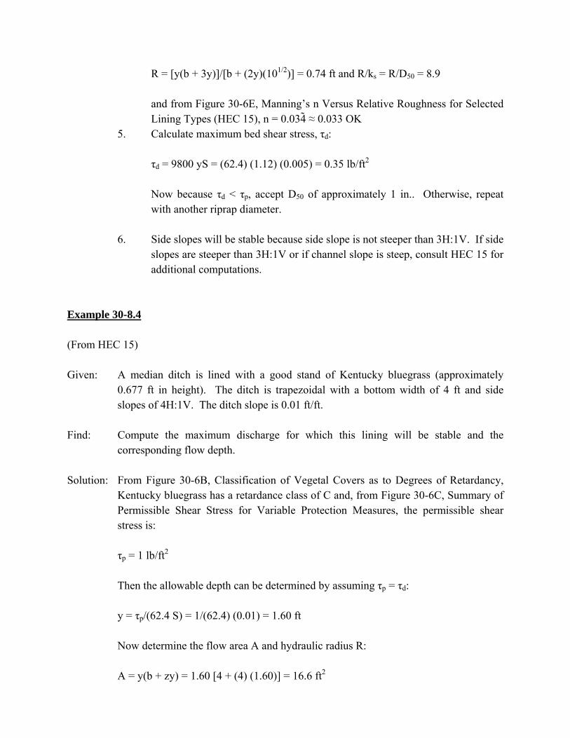
R = [y(b + 3y)]/[b + (2y)(101/2)] = 0.74 ft and R/ks = R/D50 = 8.9

and from Figure 30-6E, Manning’s n Versus Relative Roughness for Selected Lining Types (HEC 15), n = 0.034 ≈ 0.033 OK

5. Calculate maximum bed shear stress, τd:

τd = 9800 yS = (62.4) (1.12) (0.005) = 0.35 lb/ft2

Now because τd < τp, accept D50 of approximately 1 in.. Otherwise, repeat with another riprap diameter.

6. Side slopes will be stable because side slope is not steeper than 3H:1V. If side

slopes are steeper than 3H:1V or if channel slope is steep, consult HEC 15 for additional computations.

Example 30-8.4 (From HEC 15) Given: A median ditch is lined with a good stand of Kentucky bluegrass (approximately

0.677 ft in height). The ditch is trapezoidal with a bottom width of 4 ft and side slopes of 4H:1V. The ditch slope is 0.01 ft/ft.

Find: Compute the maximum discharge for which this lining will be stable and the

corresponding flow depth. Solution: From Figure 30-6B, Classification of Vegetal Covers as to Degrees of Retardancy,

Kentucky bluegrass has a retardance class of C and, from Figure 30-6C, Summary of Permissible Shear Stress for Variable Protection Measures, the permissible shear stress is:

τp = 1 lb/ft2

Then the allowable depth can be determined by assuming τp = τd:

y = τp/(62.4 S) = 1/(62.4) (0.01) = 1.60 ft

Now determine the flow area A and hydraulic radius R:

A = y(b + zy) = 1.60 [4 + (4) (1.60)] = 16.6 ft2

P = b + 2y(1 + z2)1/2 = 4 + (2) (1.60)(1 + 16)1/2 = 17.19 ft

R = A/P = 16.6/17.19 = 0.97 ft

Finally, determine the Manning’s n value from Figure 30-6H, Manning’s n Versus Hydraulic Radius, R, for Class C Vegetation (HEC 15), and solve for Q from Manning’s equation.

From Figure 30-6H, n = 0.072 and

Q = (1.486/n) A R2/3 S1/2

Q = (1.486/0.072)(16.6)(0.97)2/3 (0.01)1/2 = 33.6 ft3/s

(This method is called the maximum discharge method and is useful for determining the stable channel capacity for a variety of different linings for purposes of comparison.)

Example 30-8.5 Given: A rectangular channel on a slope of 0.001 with a width of 6 ft expands to a width of

10 ft in a straight walled transition, Z = 0. The design discharge is 300 ft3/s and Manning’s n = 0.02.

Find: Calculate the depth of flow in the upstream 6 ft wide channel if normal depth is the

downstream control. Solution: 1. Compute the downstream normal depth y2:

nQ/(b8/3)(S1/2) = (0.02)(300)/(108/3)(0.0011/2) = 0.41

Then from Figure 30-5B, Trapezoidal Channel Capacity Chart, with z = 0: y2/b = 0.65 and y2 = 6.50 ft, and for a rectangular channel, yc=[(Q/b)2/g]1/3 = 3.0 ft SUBCRITICAL

2. The specific energy downstream is:

E2 = y2 + Q2/(2gA2

2) = 6.5 + (300)2/(2)(32.2)[(10)(6.5)]2 = 6.83 ft

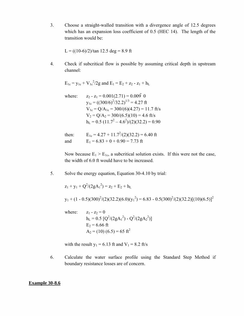
3. Choose a straight-walled transition with a divergence angle of 12.5 degrees which has an expansion loss coefficient of 0.5 (HEC 14). The length of the transition would be:

L = ((10-6)/2)/tan 12.5 deg = 8.9 ft

4. Check if subcritical flow is possible by assuming critical depth in upstream

channel:

E1c = y1c + V1c2/2g and E1 = E2 + z2 - z1 + hL

where: z2 - z1 = 0.001(2.71) = 0.009 0

y1c = ((300/6)2/32.2)1/3 = 4.27 ft V1c = Q/A1c = 300/(6)(4.27) = 11.7 ft/s V2 = Q/A2 = 300/(6.5)(10) = 4.6 ft/s hL = 0.5 (11.72 – 4.62)/(2)(32.2) = 0.90

then: E1c = 4.27 + 11.72/(2)(32.2) = 6.40 ft and E1 = 6.83 + 0 + 0.90 = 7.73 ft

Now because E1 > E1c, a subcritical solution exists. If this were not the case, the width of 6.0 ft would have to be increased.

5. Solve the energy equation, Equation 30-4.10 by trial:

z1 + y1 + Q2/(2gA1

2) = z2 + E2 + hL

y1 + (1 - 0.5)(300)2/(2)(32.2)(6.0)(y1

2) = 6.83 - 0.5(300)2/(2)(32.2)[(10)(6.5)]2

where: z1 - z2 = 0

hL = 0.5 [Q2/(2gA12) - Q2/(2gA2

2)] E2 = 6.66 ft A2 = (10) (6.5) = 65 ft2

with the result y1 = 6.13 ft and V1 = 8.2 ft/s

6. Calculate the water surface profile using the Standard Step Method if

boundary resistance losses are of concern. Example 30-8.6

Given: A rectangular transition contracts from a width of 10 ft to a width of 5 ft. The approach flow rate is 300 ft3/s with a depth of 1 ft.

Find: Calculate the depth in the contracted section and the angle and length of the

contraction so that the transmission of standing waves downstream is minimized. Solution: 1. Calculate the approach Froude number for a rectangular channel: F = V/(gd)1/2 = (300/(10)(1))/[(32.2)(1)]1/2 = 5.3 SUPERCRITICAL 2. Determine the contraction ratio: τ = b3/b1 = 5.0/10.0 = 0.5 3. Use Figures 30-8F and 30-8G: θ = 5 deg and y3/y1 = 2.1 or y3 = 2.1 ft F3/F1 = τ-1 (y3/y1)-3/2 = 0.66 or F3 = 3.6 L = ((b3 - b1)/2)/tan 5 deg = 28.6 ft 4. This design satisfies the criterion F3 > 2 and also is just to the left of curve A

which means choking is not possible. For the complete equations, see HEC 14 and Sturm, 1985. 30-9.0 REFERENCES The references shown are recommended additions to the designer’s library of references. 1. AASHTO, Highway Drainage Guidelines, Volume VI, “Hydraulic Analysis and Design

of Open Channels,” AASHTO Task Force on Hydrology and Hydraulics, 1982. 2. AASHTO, Model Drainage Manual, AASHTO Task Force on Hydrology and

Hydraulics. 3. American Society of Civil Engineers, High Velocity Flow in Open Channels: A

Symposium, “Design of Channel Curves for Supercritical Flow,” Transactions, Vol. 116, 1951.

4. Arcement, G.J., Jr., and Schneider, V.R., Guide for Selecting Manning’s Roughness Coefficients for Natural Channels and Flood Plains, Report No. FHWA-TS-84-204, Federal Highway Administration, 1984.

5. Barnes, Harry H., Jr., “Roughness Characteristics of Natural Channels,” U.S. Geological

Survey, Water Supply Paper 1849, U.S. Government Printing Office, Washington, D.C., 1978.

6. Behlke, C.E., “The Design of Supercritical Flow Channel Junctions,” Highway Research

Record No. 123, Transportation Research Board, 1966. 7. Blodgett, J.C., “Rock Riprap Design for Protection of Stream Channels Near Highway

Structures,” Vol. 1, Water Resources Investigations Report 86-4127, U.S. Geological Survey, prepared in Cooperation with Federal Highway Administration, 1986.

8. Blalock, M.E., and Sturm, T. W., “Minimum Specific Energy in Compound Open

Channel,” Journal of Hydraulics Division, ASCE, Vol. 107, No. HY6, pp. 699-717, June 1981.

9. Blodgett, J.C., and McConaughy, C.E., “Rock Riprap Design for Protection of Stream

Channels Near Highway Structures,” Vol. 2, Water Resources Investigations Report 86-4127, U.S. Geological Survey, prepared in Cooperation with Federal Highway Administration, 1986.

10. Brice, J.C., and J.C. Blodgett, Countermeasures for Hydraulic Problems at Bridges, Vol.

1, Analysis and Assessment, FHWA-RD-78-162, Federal Highway Administration, Washington, D.C., 1978.

11. Brown, S.A., Streambank Stabilization Measures for Stream Crossings - Executive Summary, FHWA/RD-84/099, FHWA, Washington, D.C., 1985.

12. Brown, S.A., Design of Spur-Type Streambank Stabilization Structures, FHWA/RD-

84/101, FHWA, Washington, D.C., 1985. 13. Brown, S.A., Streambank Stabilization Measures for Highway Engineers, FHWA/RD-

84/100, FHWA, Washington, D.C., 1985. 14. Chow, V.T., Open Channel Hydraulics, McGraw-Hill, 1970. 15. Clopper, Paul E., Hydraulic Stability of Articulated Concrete Block Revetment Systems

During Overtopping Flow, FHWA-RD-89-199, FHWA, Washington, D.C., November 1989.

16. Davidian, Jacob, “Computation of Water Surface Profiles in Open Channels,” Techniques of Water Resources Investigation, Book 3, Chapter A15, U.S. Geological Survey, 1984.

17. Federal Highway Administration, Highways in the River Environment, Training and

Design Manual, 1990. 18. Federal Highway Administration, Hydraulic Design of Energy Dissipators for Culverts

and Channels, Hydraulic Engineering Circular No. 14, FHWA-EPD-86-110, FHWA, Washington, D.C., 1983.

19. Federal Highway Administration, Design of Roadside Channels with Flexible Linings,

Hydraulic Engineering Circular No. 15, U.S. DOT, U.S. Government Printing Office, Washington, D.C., 1988.

20. Federal Highway Administration, Design Of Riprap Revetments, Hydraulic Engineering

Circular No. 11, FHWA-IP-89-016, FHWA, Washington, D.C., 1989. 21. Federal Highway Administration, Stream Stability at Highway Structures, Hydraulic

Engineering Circular No. 20, FHWA-IP-90-014, FHWA, Washington, D.C., 1991. 22. Henderson, F.M., Open Channel Flow, Macmillan, 1966. 23. Lane, E.W., “A Study of the Shape of Channels Formed by Natural Stream Flowing in

Erodible Material,” M.R.D. Sediment Series No. 9, U.S. Army Engineers Division, Missouri River, Corps of Engineers, Omaha, Nebraska, 1957.

24. Molinas, Albert, Users Manual For BRI-STARS, NCHRP Project HR 15-11A, 1994. 25. Odgaard, A. Jacob, and Spoljaric, Anita, “Sediment Control by Submerged Vanes,”

Journal of Hydraulic Engineering, ASCE, Vol. 112, No. 12, Dec., 1986. 26. Odgaard, A. Jacob, and Mosconi, Carlos E., “Streambank Protection by Submerged

Vanes,” Journal of Hydraulic Engineering, ASCE, Vol. 113, No. 4, April, 1987. 27. Richardson, E.V., D.B. Simons and P.Y. Julien, “Highways in the River Environment,”

prepared for the Federal Highway Administration, Washington, D.C. by the Department of Civil Engineering, Colorado State University, Fort Collins, Colorado, June 1990.

28. Rouse, Hunter, ed., Engineering Hydraulics, John Wiley & Sons, Inc., 1950. 29. Shearman, J.O., WSPRO User's Instructions, FHWA IP-89-27, 1990.

30. Shen, H.W., S.A. Schumm, J.D. Nelson, D.O. Doehring and M.M. Skinner, Methods for Assessment of Stream-Related Hazards to Highways and Bridges, FHWA/RD-80/160, Federal Highway Administration, Washington, D.C., 1981.

31. Sturm, T.W., “Simplified Design of Contractions in Supercritical Flow,” Journal of

Hydraulic Engineering, ASCE, Vol. 11, No. 5, May, 1985. 32. U.S. Army Corps of Engineers, Accuracy of Computed Water Surface Profiles, The

Hydrologic Engineering Center, Davis, California, December 1986. 33. U.S. Army Corps of Engineers, HEC-2 Water Surface Profiles, User’s Manual, The

Hydrologic Engineering Center, Davis, CA, CPD-2A, 1990 (Revised 1991). 34. U.S. Army Corps of Engineers, HEC-RAS, River Analysis System Hydraulic Reference

Manual, The Hydrologic Engineering Center, Davis, CA., Version 1.0, July 1995. 35. U.S. Army Corps of Engineers, HEC-RAS, River Analysis System, User’s Manual, The

Hydrologic Engineering Center, Davis, CA., Version 1.0, July 1995. 36. Vanoni, Vito A., ed., Sedimentation Engineering, ASCE Manual No. 54, ASCE, 345 East

47th St., New York, NY, 1977.