TRANSIENT RESPONSE SPECIFICATIONS

The actual output behaviour according to the various time response specifications refferering to figure below :

MAR 2011

1) Delay Time, Td It is the time required for the response to reach 50 % of the final value in the first attempt

2) Rise Time, TrIt is the time required for the response to rise from 10 % to 90 % of the final value for overdamped system and 0 % to 100 % of the final value for underdamped second order system

MAR 2011

3) Peak Time, TpIt is the time required for the response to reach its peak value

4) Peak Overshoot, MpIt is the largest error between reference input and output during the transient period

5) Settling Time, TsTime required for the response to decrease and stay within specified percentage of its final value (within tolerance band : 2 % or 5 % is used as the percentage of final value)

MAR 2011

SECOND ORDER SYSTEM AND TRANSIENT RESPONSE SPECIFICATIONS

EXAMPLE 1

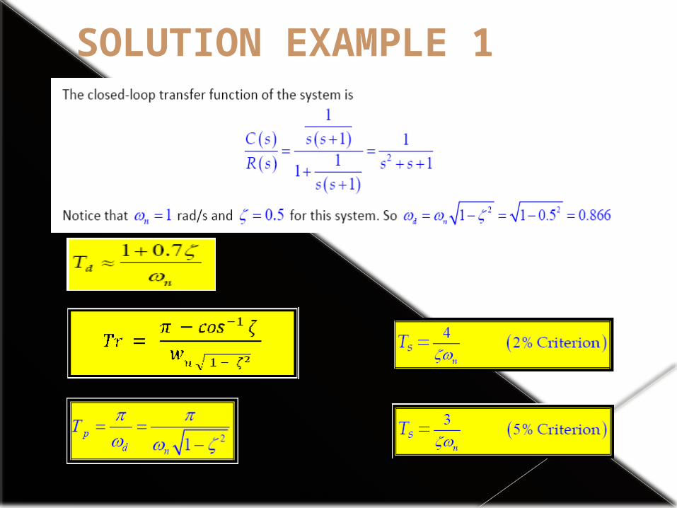
SOLUTION EXAMPLE 1

MAR 2011

EXERCISE1. The transfer function of the

closed loop position control system is given below :

Determine :- i) Peak time, Tp

ii) Rise time, Triii) % maximum overshoot, %Mpiv) Settling time, Ts

Steady State Error Definition : It is the difference between the actual a/p and the desired o/p

Mathematically it is defined in Laplace domain as,

and systemsfeedback unity non for H(s), C(s) - R(s) E(s) e(t) L

systemsfeedback unity for C(s), - R(s) E(s) e(t) L

Derivation of Steady State Error

Consider a simple closed loop system using –ve f/back as shown in the fig :

Where E (s) = Error signal B (s) = Feedback signal

Now, E (s) = R(s) – B(s)But B (s) = C(s) H(s)

E (s) = R (s) – C (s) H (s)And C (s) = E (s) G (s)

E (s) = R (s) – E (s) G (s) H (s)

Therefore E(s) + E (s) G (s) H (s) = R (s)

This E (s) is the error in Laplace domain and is expression in ‘s’

In time domain, corresponding error will be e(t); remain the steady state of the system as t so:

fedbackunity for )(1)()(

fedbacknonunity for )()(1)()(

sGsRsE

sHsGsRsE

t e(t) Lim e error, stateSteady ss

Relate the Laplace domain by using final value theorem which states that,

where F (s) = L { f(t) }

Therefore, where E (s) is L { e(t) }

Substituting E (s) from the expression derived, so :

For –ve f/back system use +ve sign in denominator For +ve f/back system use –ve sign in denominator

0s tsf(s) Lim f(t) Lim

0s tsE(s) Lim e(t) Lim ess

0s G(s)H(s)1sR(s) Lim e ss

Conclusion Steady state error, ess depends on,

i) R (s) i.e reference i/p, its type and magnitude

ii) G (s) H (s) i.e open loop t.f.

Effect of Input (Type and Magnitude) on Steady State Error

Static Error Coefficient Method

Consider a system having open loop T.F G(s) H(s) and excited by reference i/p is step of magnitude A

Reference input is step of magnitude A

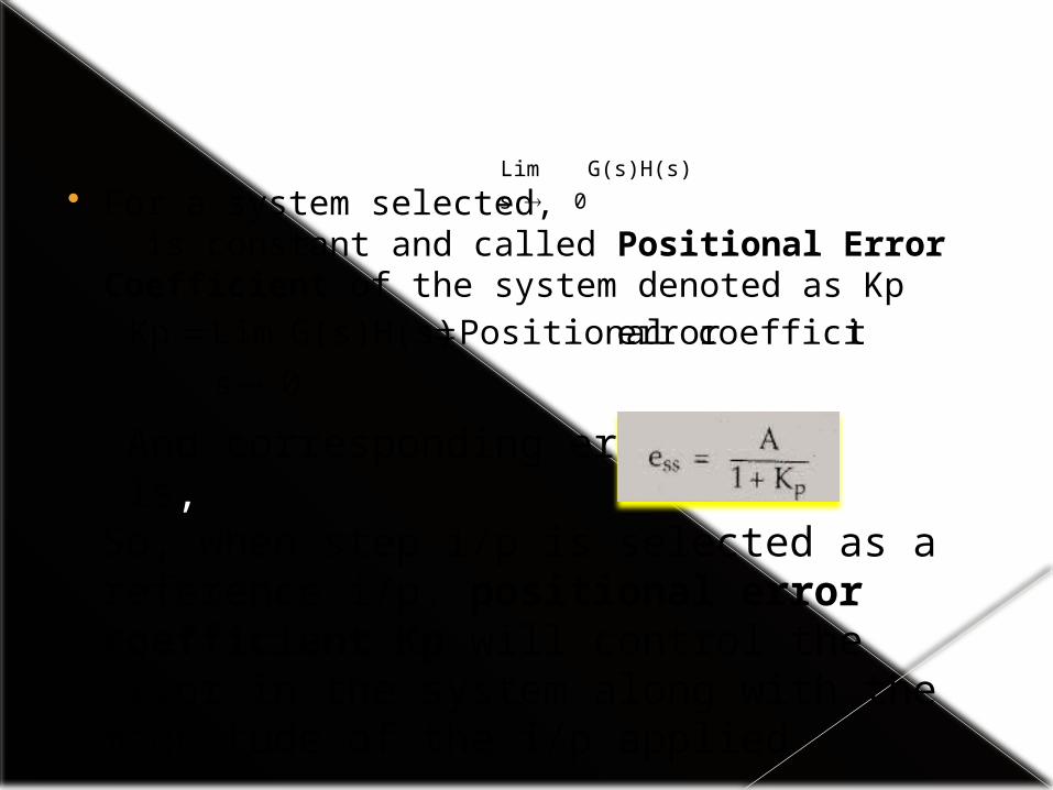
For a system selected, is constant and called Positional Error Coefficient of the system denoted as Kp

0sG(s)H(s) Lim

And corresponding error is,

So, when step i/p is selected as a reference i/p, positional error coefficient Kp will control the error in the system along with the magnitude of the i/p applied

0s tcoefficienerror Positional G(s)H(s) Lim Kp

Reference input is ramp of magnitude 'A'

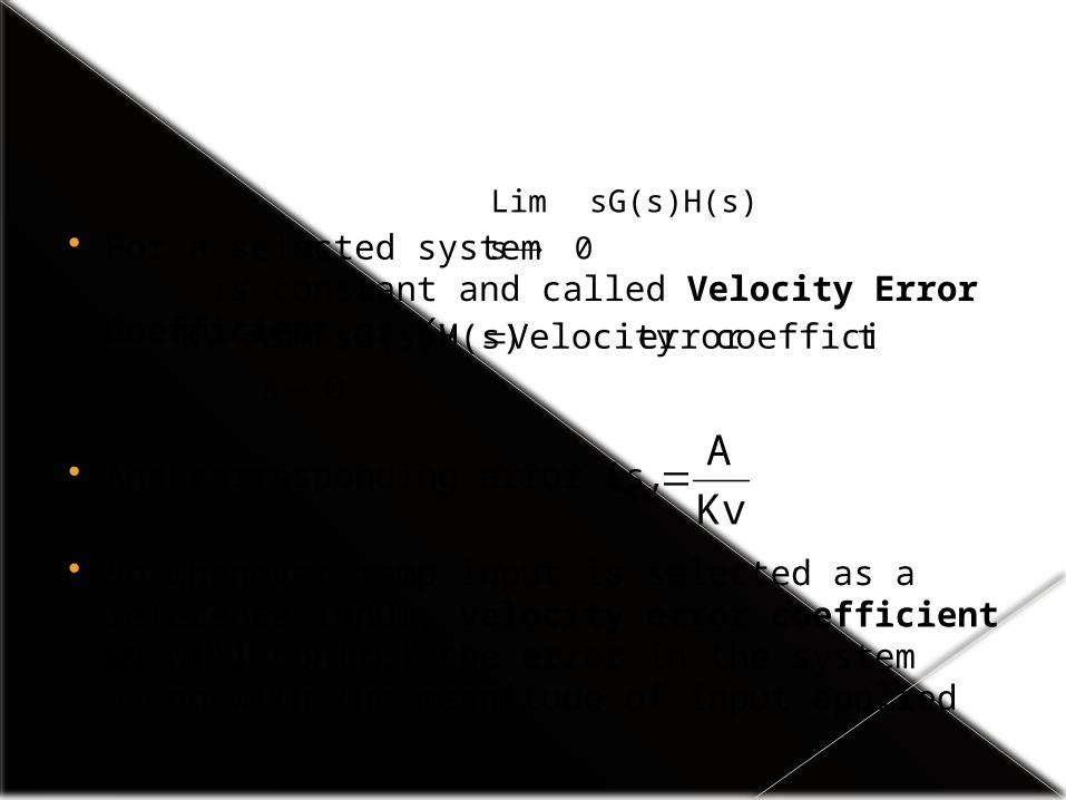
For a selected system is constant and called Velocity Error Coefficient as Kv

And corresponding error is,

So whenever ramp input is selected as a reference input, velocity error coefficient Kv will control the error in the system along with the magnitude of input applied

0ssG(s)H(s) Lim

0s tcoefficienerror Velocity sG(s)H(s) Lim Kv

KvAess

Reference input is parabolic of magnitude A

So for a selected system is constant and called Acceleration Error Coefficient as Ka

And corresponding error is,

So whenever parabolic input is selected as a reference input, acceleration error coefficient Ka will control the error in the system along with magnitude of input applied

0sG(s)H(s)s Lim 2

0s tcoefficienerror on Accelerati G(s)H(s)s Lim Ka 2

KaAess

Table for Static Error Coefficients