CHAPTER 1 FUNDAMENTAL CONCEPTS

Database: collection of interrelated date which represents some aspects of the UoD, is logically coherent and

has an intended group of users and applications

Database Management System (DBMS): a collection of programs that enables us to create and maintain a

database. General purpose software system that facilitates the process of defining, constructing and

manipulating databases for various applications

Database system: combination of a DBMS and a database

FILE BASED APPROACH TO DATAMANGEMENT

Duplicate storage waste of memory space

Redundant data

Inconsistent data (data changes in only one data source)

Dependency between applications and data (changes in data definitions changes in all apps)

Difficult to integrate with various applications (EAI)

DATABASE-ORIENTED APPROACH TO DATA MANAGEMENT

Self-describing nature of the DB system (catalog)

Insulation between programs and data, data independence

Support for multiple views of the data

Sharing data and multi-user transaction processing ( concurrency control to prevent inconsistencies)

ELEMENTS OF A DATABASE SYSTEM

Data model

o Collection of concepts that can be used to describe the structure of a DB (data types,

relationships, constraints, …)

o Conceptual data model (high-level concepts, EER and UML)

o Implementation data model (relational model

o Physical data model (low-level concepts that describe data storage details, query’s)

Schemas and instances

o Database schema: description of a DB, which is specified during DB design and is not

expected to change too frequently = model

o Database state: the data in the DB at a particular moment, current set of instances

Data dictionary (catalog)

o Contains definitions of: conceptual schema, external views, physical schema

DBMS languages

o DDL: used by DBA to define DB’s conceptual, internal and external schemas

o DML: used to retrieve, insert, delete and modify data; can be entered interactively

(terminal) or embedded (general-purpose programming language)

o Relational DBS: SQL is DDL & DML and interactive SQL & embedded SQL

ADVANTAGES OF USING THE DBMS APPROACH

Data and functional independence

DB modeling

o Should provide a formal and perfect mapping of the real world (e.g. EER, relational, etc.)

Managing data redundancy

o Compared to file base approach

o Data redundancy may be desired (performance)

o DBMS guarantees synchronization and consistency of redundant data

Specifying integrity rules

o Determine syntactical (not numeric) and semantical (not unique) correctness of data

o Specified as part of the conceptual schema (in catalog)

o Integrity rules are checked during data loading and data manipulation

o Also concurrency control

Data security

o Read/write access

o User accounts and passwords

o Account authorizations are stored in catalog

o E-business and CRM stress the importance of data security

Backup and recovery facilities

o Backups perform full or incremental backups

o Recovery facilities allow to restore data after loss or damage

Performance utilities

o Part of the job of the DBA

o Examples: optimizing buffer management, index tuning to optimize indices and queries,

detecting and solving I/O problems, etc.

WHEN NOT TO USE A DMBS

There are situations in which a DBMS may involve unnecessary overhead costs that would not be incurred in

traditional file processing

High initial investment in hardware, software and training

The generality that a DBMS provides for defining and processing data

Overhead for providing security, concurrency control, recovery and integrity functions

It may be more desirable to use regular files under the following circumstances:

Simple, well-defined DB applications that are not expected to change at all

Stringent, real-time requirements for some application programs that may not be met because of

DBMS overhead

Embedded systems with limited storage capacity, where a general-purpose DBMS would not fit

No multiple-user access to data

THREE-SCHEMA ARCHITECTURE

Goal: separate the user applications from the physical DB.

1) The internal level has an internal schema

describes physical storage of the DB, details of data

storage and access paths

2) The conceptual level has a conceptual schema

describes the structure of the whole DB, hides the

details of physical storage structures and concentrates on

describing entities, data types, relationships, user operations

and constraints

3) The external view level has external schemas / views

describes part of the DB that a user is interested in and hides

the rest of the DB

The 3 schemas are only descriptions of data; the stored data that actually exists is at the physical level only.

DATA INDEPENDENCE

The capacity to change the schema at one level of a DB without having to change the schema at the next higher

level.

Logical data independence: capacity to change the conceptual schema without having to change external

schemas or application programs. After the conceptual schema undergoes a logical reorganization, application

programs that reference the external schema must work as before.

Physical data independence: capacity to change the internal schema without having to change the conceptual

schema and thus neither the external schema.

Generally, physical data independence exist is most DBs and file environments. Logical data independence is

harder to achieve because it allows structural and constraint changes without affecting application programs, a

much stricter environment.

The three-schema architecture can make it easier to achieve true data independence, both physical and logical.

But the 2 levels of mappings can create an overhead during compilation or execution of a query or program,

leading to inefficiencies in the DBMS few DBMSs have implemented the full three-architecture schema arch.

Functional independence: implementation (method) can change without impact on software applications

E.g. calculate salary changes in the method won’t affect other programs.

CHAPTER 2 ARCHITECTURE AND CLASSIFICATION OF DBMSS

INTERNAL ARCHITECTURE OF A DBMS

DDL compiler

o Ideally 3 DDLs

o Only 1 with 3 independent set

of instructions

o Translates DDL definitions, checks

syntax, generates errors and when

successful register data definitions

as meta data in the catalog

o Loading utility: data in user DB

DML compiler

o Sublanguage needed to access and

manipulate the dada (eg embedded SQL)

o DB programs are offered 1st to DML

precompiler

o DML precompiler extract DML statements

and gives them to DML compiler to compile them to objectcode

o Catalog is inspected to see whether data are available in the DB

o Data is retrieved depending on type of DML

o Procedural DML: record-at-a-time DML, DML statements specify how to navigate in DB to

locate and find the data

o Declarative DML: set-at-a-time DML (eg SQL), DML statements determine which data

should be retrieved and DBMS autonomically determines access path and navigational

strategy itself

Query processor

o Query language is high-abstraction DML to interactively consult data

o Checks if data are available in DB via catalog, rearranges and optimizes query, consults

the catalog for data statistics and indices, determines the “best” access path to data

which will be offered as executable code to the runtime DB processor

Runtime DB processor

o Receives DB assignments and supervised their execution

o Guarantees data integrity

o Coordinates communication of results to users and applications, generate error message

Stored data manager

o Controls access to data in catalog and user DB

o Communicates with transaction manager, buffer manager and recovery manager

DB system utilities

o Loading utility, Back-up and recovery utilities, transaction manager, reorganization

utilities, performance monitoring, sorting, user monitoring, data compression

Impedance mismatch: data structures of DBMS and data sublanguage may be different than data structures of

host language eg relations DBMS vs OO host language solution: OODMBS (persistent language) or object

relational mapping frameworks (middleware)

CLASSIFICATION BASED ON DATA MODEL

Hierarchical DBMS

o Procedural DML (record-at-a-time)

o Definitions of conceptual and physical schema intertwined

o IMS (IBM)

Network DBMS

o Network data model, CODASYL DBMS

o Procedural DML (record-at-a-time)

o Definitions of conceptual and physical schema intertwined

o CA-IDMS (Computer Associates)

Relational DBMS

o Relational data model, usually based on SQL (DDL +DML)

o Declarative DML (set-at-a-time)

o Data independence (logical and physical)

o Universal DB2 v10 (IBM), Oracle 11g r2 (Oracle), SQLServer 2008 r2 (MS)

Object oriented DBMS

o Object oriented data model, objects with states and behavior

o No separate Object Manipulation Language (operations are imbedded in object)

o No impedance mismatch

o ODMG defined standard OO model with ODL, OQL and bindings

o Difficult to use, not so popular

o Gemstone (Gemstone Corporation)

Object relational DBMS

o Extended relational model with OO concepts

o SQL3 (SQL 99)

o User-defined types and functions, collections, inheritance, behavior, etc.

Mainframe DB computing

o Host based computing, all processing (UI, applications, DB) occurs on mainframe

o Terminals receive data from end-users and show results

o Monolithic architecture, no architecturally separate components but all interwoven

PC/Fileserver DB computing

o DBMS is installed on PC, all processing on PC (UI, applications, DB)

o DB is stored on a fileserver

o High network load, many replications, high maintenance and possible low performance

Client/Server DB computing

o Clients are active and request services, servers are passive and respond to client requests

o Multiple clients per server

o Fat-client variant: UI logic and application logic is stored on client, DB logic and DBMS is

stored on server transparent communication using middleware

o Fat-server variant: application logic, DB logic and DBMS stored on server, usage of stored

procedures

o Hybrid variants

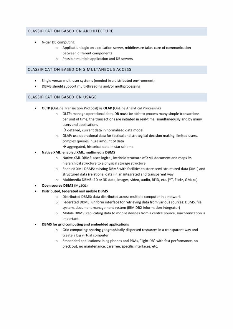
CLASSIFICATION BASED ON ARCHITECTURE

N-tier DB computing

o Application logic on application server, middleware takes care of communication

between different components

o Possible multiple application and DB servers

CLASSIFICATION BASED ON SIMULTANEOUS ACCESS

Single versus multi user systems (needed in a distributed environment)

DBMS should support multi-threading and/or multiprocessing

CLASSIFICATION BASED ON USAGE

OLTP (OnLine Transaction Protocal) vs OLAP (OnLine Analytical Processing)

o OLTP: manage operational data, DB must be able to process many simple transactions

per unit of time, the transactions are initiated in real-time, simultaneously and by many

users and applications

detailed, current data in normalized data model

o OLAP: use operational data for tactical and strategical decision making, limited users,

complex queries, huge amount of data

aggregated, historical data in star schema

Native XML, enabled XML, multimedia DBMS

o Native XML DBMS: uses logical, intrinsic structure of XML document and maps its

hierarchical structure to a physical storage structure

o Enabled XML DBMS: existing DBMS with facilities to store semi-structured data (XML) and

structured data (relational data) in an integrated and transparent way

o Multimedia DBMS: 2D or 3D data, images, video, audio, RFID, etc. (YT, Flickr, GMaps)

Open source DBMS (MySQL)

Distributed, federated and mobile DBMS

o Distributed DBMS: data distributed across multiple computer in a network

o Federated DBMS: uniform interface for retrieving data from various sources: DBMS, file

system, document management system (IBM DB2 Information Integrator)

o Mobile DBMS: replicating data to mobile devices from a central source, synchronization is

important

DBMS for grid computing and embedded applications

o Grid computing: sharing geographically dispersed resources in a transparent way and

create a big virtual computer

o Embedded applications: in eg phones and PDAs, “light DB” with fast performance, no

black out, no maintenance, carefree, specific interfaces, etc.

CHAPTER 3 DATA MODELS

Concepts of data modeling:

Conceptual schema to capture the specifications

of the data and constraints that have to be

represented in the DB

Conceptual data modeling: capture the semantics

of the UoD as accurately as possible

requires a high-level model that is not

implantation specific (eg EER)

THE HIERARCHICAL MODEL

Parent record type and child record type

Relationship type can only be 1:N (i.e. 1…1 to 0…N)

Parents can be multiple parents

A child only has 1 parent

A child can be also be a parent ( hierarchy)

Structural limitations:

Procedural DML: record data needs to be retrieved by navigating from the rood node

No straightforward way to model N:M and 1:1 relationships

Only relationships of degree 2, recursive relationships (=degree 1) are created via VCs

Maximum and minimum cardinality from child to parent is 1 cascading effect upon deletion

Modeling N:M relationships:

Transforms a network structure to tree structure

Creates redundancy

Puts relationship type attributes in child record

Alternative: create 2 hierarchical structure and connect them with a VC

no more redundancy and relationship attributes are in VC

THE RELATIONAL MODEL

FUNCTIONAL DEPENDENCY X Y

For any two tuples t1 and t2 in r that have t1[X] = t2[X], we must also have t1[Y] = t2[Y]

The values of the Y components of a tuple in r depend on and are determined by the values of the X

component

The values of the X component of a tuple uniquely (or functionally) determine the values of the Y

component

If X Y, this does not mean that Y X

If X is a candidate key of R this implies that X Y for any subset of attributes Y in R

Example: SSN ENAME

o ENAME SSN does not hold since multiple employees can have the same name

Example: PNUMBER {PNAME, PLOCATION}

Example: {SSN, PNUMBER} HOURS

Full functional dependency: removal of any attribute from X means that dependency does not hold anymore

SSN, PNUMBER HOURS

Partial dependency: attributes of X can be removed and the dependency still holds

SSN, PNUMBER PNAME

Transitive dependency: there is a set of attributes (Z) that is neither a candidate key nor a subset of any key and

bot X Z and Z Y holds

SSN, ENAME, DNUMBER, DNAME, DMGRSSN: SSN DNUMBER and DNUMBER DNAME, DMGRSSN

THE NORMALISATION PROCESS

Process of analysing the given relation schemas based on their FDs and candidate keys to achieve the

desirable properties of

o (1) minimising redundancy

o (2) minimising the insertion, deletion and update anomalies

Relation schemas are decomposed into smaller relation schemas

Sometimes controlled denormalisation is acceptable for performance purposes

FIRST NORMAL FORM (1NF)

Attributes must be

o Atomic (no composite)

o Single-value (no multi-values)

Remove multi-value attributes and place it in a separate relation together with the primary key of the

original relation, the primary key of the new relation is the combination of the attribute and primary

key of the original relation

Remove nested, composite relation attributes into a new relation and propagate the primary key into

it, the primary key of the new relation is the combination of the partial key of the nested relation with

the primary key of the original relation

(DNUMBER, DLOCATION, DMGRSSN) (DNUMBER, DMGRSSN) and (DNUMBER, DLOCATION)

(SSN, ENAME, DNUMBER, DNAME, PROJECT(PNUMBER, PNAME, HOURS)

(SSN, ENAME, DNUMBER, DNAME) and (SSN, PNUMBER, PNAME, HOURS)

SECOND NORMAL FORM (2NF)

Satisfies 1NF and every nonprime attribute A in R is fully functional dependent on any key of R

Decompose and set up a new relation for each partial key with its dependent attribute(s)

(SSN, PNUMBER, PNAME, HOURS) (SSN, PNUMBER, HOURS) and (PNUMBER, PNAME)

THIRD NORMAL FORM (3NF)

Satisfies 2NF and no nonprime attribute of R is transitively dependent on the primary key

Decompose and set up a relation that includes the nonprime attribute(s) that functionally determines

other nonprime attributes

(SSN, ENAME, DNUMBER, DNAME, DMGRSSN)

(SSN, ENAME, DNUMBER) and (DNUMBER, DNAME, DMGRSSN)

BOYCE-CODD NORMAL FORM (BCNF)

Stricter than 3NF (every BCNF is 3NF but not every 3NF is BCNF)

Trivial functional dependency: X Y and Y is a subset of X

For every non-trivial functional dependency X Y, X is a superkey

Supplier (SNR, SNAME, PRODNR, QUANTITY)

- superkey {SNR, PRODNR}: SNR SNAME

(SNR, SNAME) and (SNR, PRODNR, QUANTITY)

- superkey {SNAME, PRODNR}: SNAME SNR

(SNAME, SNR) and (SNAME,PRODNR, QUANTITY)

FOURTH NORMAL FORM (4NF)

Multi-valued dependency: XY if each X value exactly determines a set of Y values, independently

of the other attributes

Satisfies BCNF and for every one of its non-trivial multivalued dependencies XY, X is a superkey

(COURSE, INSTRUCTOR, TEXTBOOK) (COURSE, TEXTBOOK) and

(COURSE, INSTRUCTOR)

CHAPTER 4 DATABASE DESIGN

Conceptual design: (E)ER or object-oriented modelling (UML)

Logical design:

o Mapping (E)ER conceptual scheme to a CODASYL or relational DB scheme

o Mapping object-oriented conceptual scheme (UML) to a relational DB scheme

o Mapping object-oriented conceptual scheme to an object-oriented DB scheme

Physical design: actual implementation

EER TO CODASYL

Create record type for every entity type (composite and multivalued attributes supported)

Create separate record for weak entity types as a member record of the owner record on which it is

existence dependent

Create a set type for every 1:N binary relationship type

Create a set type for every 1:1 binary relationship type

o Owner and member defined arbitrarily or via ED

o Cannot enforce maximum cardinality of 1 loss of semantics application code

Create dummy record type for every binary N:M relationship type

o Dummy record type defined as member in 2 set types

o Dummy record type contains attributes of relationship type

Create dummy record type for every recursive relationship type

o Dummy record type becomes member in 3 set types

Superclass/subclass relationship difficult

o Create record type for superclass as owner in set types with subclasses as members

Cannot guarantee that each set contains exactly 1 member

Cannot indicate type of specialization (partial/complete, overlap/disjoint)

o One record type that contains data from superclass and all the subclasses

Lots of empty data fields

ER TO RELATIONAL

Example in slides (heel duidelijk)

CHAPTER 5 DATA LANGUAGES IN A RELATIONAL ENVIRONMENT

RELATIONAL DATABASE SYSTEMS

RDBMSs are databases which implement the relational model

SQL is used for both data definition, data retrieval and data updating (DDL + DML)

o SQL is set-oriented: retrieve many records at a time

o SQL is declarative: only needs to specify which data to retrieve

procedural: declare how to retrieve the data (access paths)

SQL versions

o SQL 1 (1986, “ANS! SQL”)

o SQL 2 (1992)

o SQL 3 (1999, object-relational extensions)

Use of SQL

o Standalone interactive SQL (Access)

o Embedded in a host language embedded SQL (JAVA)

SQL as DDL

o Logical schema: “create table”

o Physical schema: “create database”, “create tablespace” and “create index”

o External schema: “create view”

SQL as DML

o Select … from … where …

o Insert … into …

o Update … where …

o Delete where …

SQL can also be used to specify security etc.

CREATING DATABASE OBJECTS: SQL DATA DEFINITION STATEMENTS

Creating schemas, tables, views, indexes

Dropping schemas and tables, altering tables

Referential triggered action clauses

SQL SCHEMA

= a grouping of tables and other constructs (constraints, views, …) that logically belong together

Identified by a schema name and includes an authorization identifier to indicate the user or account

who owns the schema (full access, add, modify, …)

CREATE SCHEMA COMPANY AUTHORIZATION JSMITH;

TABLE

CREATE TABLE EMPLOYEE … or CREATE TABLE COMPANY.EMPLOYEE…

Data types:

o Numeric: INT, SMALLINT, FLOAT, REAL

o Character-string: CHAR(n), VARCHAR(n)

o DATE (format: YYYY-MM-DD), TIME (format: HH:MM:SS)

Constraints:

o NOT NULL

o DEFAULT <value>

o PRIMARY KEY

o UNIQUE

o FOREIGN KEY

o CHECK

Primary key by default unique

DROP SCHEMA AND DROP TABLE COMMANDS

DROP SCHEMA COMPANY CASCADE

automatically drop objects (tables, functions, etc.) that are contained in the schema

DROP SCHEMA COMPANY RESTRICT

refuse to drop the schema if it contains any objects this is the default

DROP TABLE EMPLOYEE CASCADE

automatically drop objects that depend on the table (such as views, other tables)

DROP TABLE EMPLOYEE RESTRICT

refuse to drop the table if any objects depend on it this is the default

ALTER TABLE COMMAND

Purpose: adding or dropping a column, changing a column definition or adding/dropping table constraints

ALTER TABLE EMPLOYEE ADD JOB VARCHAR(12)

ALTER TABLE EMPLOYEE DROP ADRESS CASCADE

ALTER TABLE DEPARTMENT ALTER MGRSSN DROP DEFAULT

ALTER TABLE DEPARTMENT ALTER MGRSSN SET DEFAULT “333444555”

ALTER TABLE EMPLOYEE DROP CONSTRAINT EMPSUPERFK CASCADE

REFERENTIAL TRIGGERED ACTION CLAUSES

Attaching referential triggered action clause (set null, cascade, set default, restrict) to a foreign key constraint:

Specifies actions to be taken if a referential integrity constraint is violated upon deletion of a referenced

tuple (on delete) or upon modification of a referenced primary key value (on update)

ON UPDATE CASCADE: changes in the primary key of DEPARTMENT will automatically change the foreign key

ON UPDATE DELETE: if DEPARTMENT is deleted all employees working there will also be deleted

CONSULTING AND UPDATING DAT WITH SQL: INTERACTIVE SQL

SELECT-FROM-WHERE syntax, joined tables, prefixing and aliasing

DISTINCT keyword Set operations: UNION, EXCEPT, INTERSECT

Substring comparison, arithmetic operators ORDER BY clause

Nested queries IN, ANY, ALL operators

EXISTS and NOT EXISTS functions Checking for NULL values

Aggregate functions GROUP BY clause

HAVING clause INSERT, DELETE and UPDATE statements

Sample schema that will be used for explaining these concepts:

THE SELECT-FROM-WHERE STRUCTURE

SELECT <attribute list>

FROM <table list>

WHERE <condition>;

Retrieve the birthdate and address of the employee whose name is “John B. Smith”.

SELECT BDATE, ADDRESS

FROM EMPLOYEE

WHERE FNAME = 'John'

AND MINIT = 'B'

AND LNAME = 'Smith';

Retrieve the name and address of all employees who work for the “Research” department

SELECT FNAME, LNAME, ADDRESS SELECT FNAME, LNAME, ADDRESS

FROM EMPLOYEE, DEPARTMENT FROM (EMPLOYEE JOIN DEPARTMENT ON DNUMBER = DNO)

WHERE DNAME = ‘Research' WHERE DNAME = 'Research';

AND DNUMBER = DNO;

Retrieve every project located in “Stafford”, list project number, department number and manager’s last name,

address and birthdate 2 join conditions

SELECT PNUMBER, DNUM, LNAME, ADDRESS, BDATE

FROM PROJECT, DEPARTMENT, EMPLOYEE

WHERE DNUM = DNUMBER

AND MGRSSN = SSN

AND PLOCATION = 'Stafford';

Prefixing and aliasing (avoids ambiguity)

SELECT FNAME, EMPLOYEE.NAME, ADDRESS

FROM EMPLOYEE, DEPARTMENT

WHERE DEPARTMENT.NAME = 'Research'

AND DEPARTMENT.DNUMBER = EMPLOYEE.DNUMBER;

SELECT E.FNAME, E.NAME, E.ADDRESS

FROM EMPLOYEE E, DEPARTMENT D

WHERE D.NAME = 'Research' AND D.DNUMBER = E.DNUMBER;

SELECT E.FNAME, E.LNAME, S.FNAME, S.LNAME

FROM EMPLOYEE E, EMPLOYEE S

WHERE E.SUPERSSN = S.SSN;

SELECT E.LNAME AS EMPLOYEE_NAME, S.LNAME AS SUPERVISOR_NAME

FROM EMPLOYEE AS E, EMPLOYEE AS S

WHERE E.SUPERSSN = S.SSN;

Unspecified WHERE-clause

SELECT SSN SELECT SSN, NAME

FROM EMPLOYEE FROM EMPLOYEE, DEPARTMENT

retrieves all of employees SSN selects all combinations EMPLOYEE SSN & DEPARTMENT DNAME

Use of asterisk (*)

SELECT * SELECT *

FROM EMPLOYEE FROM EMPLOYEE, DEPARTMENT

WHERE DNO = 5; WHERE DNAME = ‘Research’ AND DNO = DNUMBER;

selects all attributes of employees with dno=5 selects all attributes of emps and dep of research dep

THE DISTINCT KEYWORD

SQL usually treats tables as a multiset rather than as a set

SQL doesn’t automatically eliminate duplicate tuples tuples can appear more than once in a query result

Duplicate elimination is an expensive operation

The user may want to see duplicate tuples in a query result

If we use aggregate functions (eg AVG, MAX, MIN) we usually do not want to eliminate duplicates

eliminate duplicates by using the DISTINCT keyword in the SELECT-clause

SELECT SALARY VS SELECT DISTINCT SALARY

FROM EMPLOYEE FROM EMPLOYEE;

SET OPERATIONS: UNION (OR), EXCEPT, INTERSECT (AND)

Set operations only aply to union-compatible relations: same attributes in the same order!

Make a list of project numbers for projects that involve an employee whose last name is “Smith”, either as a

worker or as a manager of the department that controls the project

(SELECT DISTINCT PNUMBER

FROM PROJECT, DEPARTMENT, EMPLOYEE

WHERE DNUM = DNUMBER

AND MGRSSN = SSN

AND LNAME = 'Smith')

UNION

(SELECT DISTINCT PNUMBER

FROM PROJECT, WORKS_ON, EMPLOYEE

WHERE PNUMBER = PNO

AND ESSN = SSN

AND LNAME = 'Smith');

Notice that duplicates in the union are possible (from the 1st and the 2nd part)

SUBSTRING COMPARISON AND ARITHMETIC OPERATORS

Retrieve all employees whose address in in Houston, Texas

SELECT FNAME, LNAME

FROM EMPLOYEE

WHERE ADRESS LIKE ‘%HOUSTON,TX%’

Retrieve all employees who were born during the 1950s

SELECT FNAME, LNAME Note: ‘AB\_CD\%EF’ ESCAPE ‘\’

FROM EMPLOYEE literal string of ‘AB_CD%EF’

WHERE BDATE LIKE ‘195 _ - _ _ - _ _’ using ’ in a string: ’’

Arithmetic operators in queries:

+, -, *, /, BETWEEN, <, >, <=, >=, =, <>

ORDER BY-CLAUSE

The default order is in ascending (ASC) order of values

Retrieve list of employees and the projects they are working on, ordered by department name and within each

department ordered by last name, first name

SELECT DNAME, LNAME, FNAME, PNAME

FROM DEPARTMENT, EMPLOYEE, WORKS_ON, PROJECT

WHERE DNUMBER = DNO

AND SSN = ESSN

AND PNO = PNUMBER

ORDER BY DNAME DESC, LNAME ASC, FNAME ASC;

NESTED QUERIES

SCALAR SUBQUERY

Retrieve the first name and last name of all employees working in the department “Research”

SELECT FNAME, LNAME

FROM EMPLOYEE

WHERE DNO =

(SELECT DNUMBER

FROM DEPARTMENT

WHERE DNAME = 'Research')

IN OPERATOR

Retrieve project numbers of the projects where either Smith is involved as manager or as worker

SELECT DISTINCT PNUMBER

FROM PROJECT

WHERE PNUMBER IN

(SELECT PNUMBER

FROM PROJECT, DEPARTMENT, EMPLOYEE

WHERE DNUM = DNUMBER

AND MGRSSN = SSN

AND LNAME = 'Smith')

OR PNUMBER IN

(SELECT PNO

FROM WORKS_ON, EMPLOYEE

WHERE ESSN = SSN

AND LNAME = 'Smith');

Select SSNs of all employees who work the same (project, hours) combination on some project that employee

John Smith (SSN = 123456789) work on

SELECT DISTINCT ESSN

FROM WORKS_ON

WHERE (PNO, HOURS) IN

(SELECT PNO, HOURS

FROM WORKS_ON

WHERE ESSN = '123456789');

Retrieve SSNs of all employees who work on project numbers 1, 2 or 3

SELECT DISTINCT ESSN

FROM WORKS_ON

WHERE PNO IN (1, 2, 3);

ANY AND ALL OPERATORS (COMBINED WITH <, <=, >, >=, <>)

Give the names of employees whose salary is greater than the salary of all employees in department 5

SELECT LNAME, FNAME

FROM EMPLOYEE

WHERE SALARY > ALL (SELECT SALARY

FROM EMPLOYEE

WHERE DNO = 5);

CORRELATED NESTED QUERIES

a condition in the WHERE-clause of a nested query references some attribute of a relation declared in the

outer query the inner query is evaluated once for each tuple or combination of tuples in the outer query

Retrieve first name and last name of all employees with a higher wage than the manager of their department

SELECT E1.FNAME, E1.LNAME

FROM EMPLOYEE E1

WHERE E1.SALARY >=

(SELECT E2.SALARY

FROM EMPLOYEE E2, DEPARTMENT D

WHERE E1.DNO = D.DNUMBER

AND D.MGRSSN = E2.SSN)

Note: no E1 in the second query for each tuple in E1 the inner query will be executed correlated query

EXISTS AND NOT EXISTS FUNCTIONS

Retrieve name of each employee who has a dependent with the same first name and sex as the employee

SELECT E.FNAME, E.LNAME SELECT FNAME, LNAME

FROM EMPLOYEE E FROM EMPLOYEE

WHERE EXISTS (SELECT * WHERE NOT EXISTS (SELECT *

FROM DEPENDENT FROM DEPENDENT

WHERE E.SSN = ESSN WHERE SSN = ESSN) ;

AND E.SEX = SEX Employee names with no dependents

AND E.FNAME = DEPENDENT_NAME);

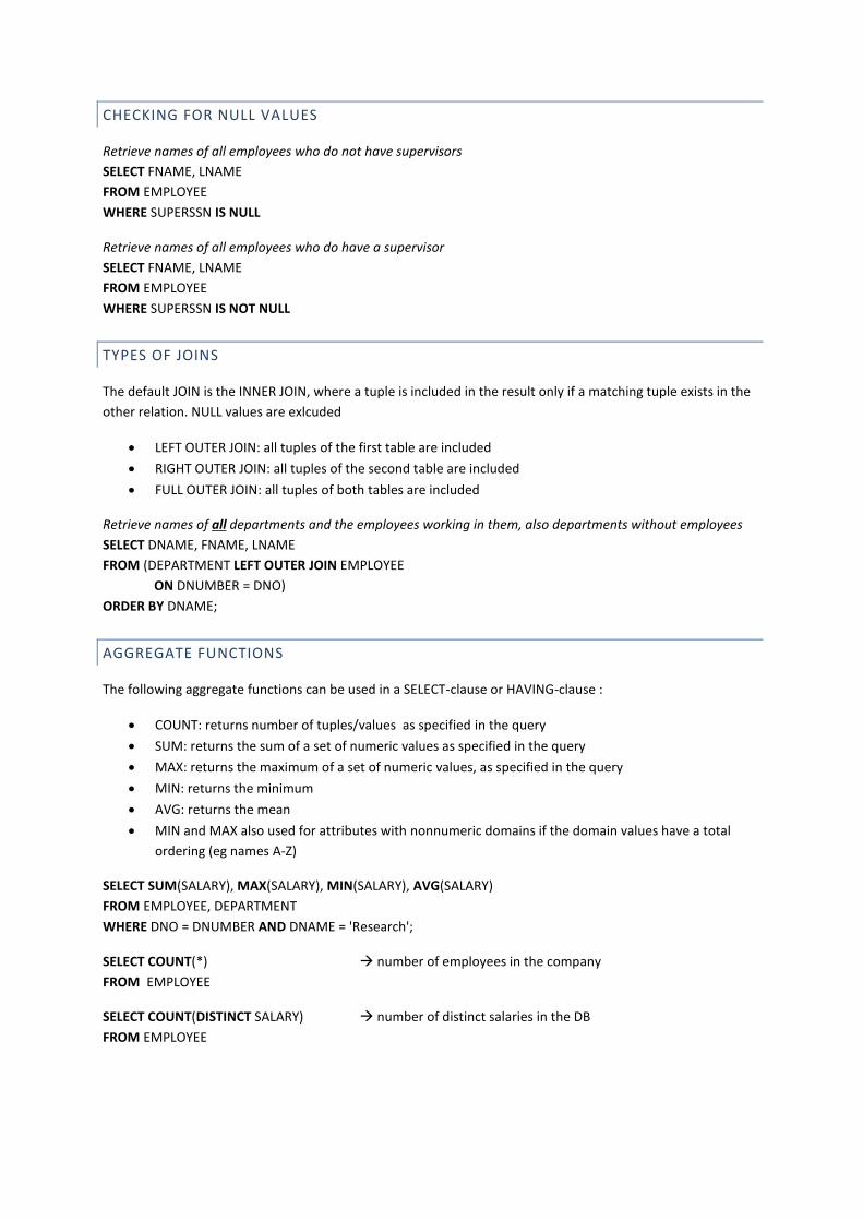
CHECKING FOR NULL VALUES

Retrieve names of all employees who do not have supervisors

SELECT FNAME, LNAME

FROM EMPLOYEE

WHERE SUPERSSN IS NULL

Retrieve names of all employees who do have a supervisor

SELECT FNAME, LNAME

FROM EMPLOYEE

WHERE SUPERSSN IS NOT NULL

TYPES OF JOINS

The default JOIN is the INNER JOIN, where a tuple is included in the result only if a matching tuple exists in the

other relation. NULL values are exlcuded

LEFT OUTER JOIN: all tuples of the first table are included

RIGHT OUTER JOIN: all tuples of the second table are included

FULL OUTER JOIN: all tuples of both tables are included

Retrieve names of all departments and the employees working in them, also departments without employees

SELECT DNAME, FNAME, LNAME

FROM (DEPARTMENT LEFT OUTER JOIN EMPLOYEE

ON DNUMBER = DNO)

ORDER BY DNAME;

AGGREGATE FUNCTIONS

The following aggregate functions can be used in a SELECT-clause or HAVING-clause :

COUNT: returns number of tuples/values as specified in the query

SUM: returns the sum of a set of numeric values as specified in the query

MAX: returns the maximum of a set of numeric values, as specified in the query

MIN: returns the minimum

AVG: returns the mean

MIN and MAX also used for attributes with nonnumeric domains if the domain values have a total

ordering (eg names A-Z)

SELECT SUM(SALARY), MAX(SALARY), MIN(SALARY), AVG(SALARY)

FROM EMPLOYEE, DEPARTMENT

WHERE DNO = DNUMBER AND DNAME = 'Research';

SELECT COUNT(*) number of employees in the company

FROM EMPLOYEE

SELECT COUNT(DISTINCT SALARY) number of distinct salaries in the DB

FROM EMPLOYEE

AGGREGATE FUNCTIONS IN THE WHERE-CLAUSE

Retrieve names of all employees who have two or more dependents

SELECT LNAME, FNAME

FROM EMPLOYEE

WHERE (SELECT COUNT(*)

FROM DEPENDENT

WHERE SSN = ESSN) >= 2;

THE GROUP BY-CLAUSE

Allows to apply aggregate functions to subgroups of tuples in a relation, based on some attribute

grouping attribute

The function is applied to each group independently

The grouping attributes have to appear in the SELECT-clause

GROUP BY has nothing to do with ORDER BY

For each employee, retrieve the department number, the number of employees in the department and their

average salary

SELECT DNO, COUNT(*), AVG(SALARY) these 3 are reported separately

FROM EMPLOYEE

GROUP BY DNO ;

COMBINATION OF A JOIN AND THE GROUP BY-CLAUSE

For each project, retrieve the project number, the project name and the #employees working on that project

SELECT PNUMBER, PNAME, COUNT(*)

FROM PROJECT, WORKS_ON

WHERE PNUMBER = PNO

GROUP BY PNUMBER, PNAME;

THE HAVING-CLAUSE

When GROUP BY-clause is used, the HAVING-clause allows to select only groups that satisfy certain conditions

On each project on which more than two employees work, retrieve the project number, project name and the

number of employees working on that project

SELECT PNUMBER, PNAME, COUNT(*)

FROM PROJECT, WORKS_ON

WHERE PNUMBER = PNO

GROUP BY PNUMBER, PNAME

HAVING COUNT(*) > 2;

SUMMARY OF THE SQL SELECT SYNTAX

SELECT <attribute and function list> attributes or functions to be retrieved

FROM <table list> all tables needed + joined relations but not those in nested queries

[WHERE <condition>] conditions for selection of tuples, including join conditions

[GROUP BY <grouping attribute(s)>] grouping attributes

[HAVING <group by condition>] conditions on the groups being selected

[ORDER BY <attribute list>]; order in which to display the query result

Select project numbers of projects that have “Smith” involved as manager

SELECT DISTINCT PNUMBER FROM PROJECT

FROM PROJECT, DEPARTMENT, EMPLOYEE WHERE EXISTS

WHERE DNUM = DNUMBER (SELECT *

AND MGRSSN = SSN FROM DEPARTMENT, EMPLOYEE

AND LNAME = 'Smith'; WHERE DNUM = DNUMBER

join AND MGRSSN = SSN

AND LNAME = 'Smith');

exists operator

SELECT DISTINCT PNUMBER

FROM PROJECT

WHERE PNUMBER IN

(SELECT PNUMBER

FROM PROJECT, DEPARTMENT, EMPLOYEE

WHERE DNUM = DNUMBER

AND MGRSSN = SSN

AND LNAME = 'Smith');

nested query

INSERT, DELETE AND UPDATE STATEMENTS IN SQL

INSERT INTO EMPLOYEE(FNAME, LNAME, DNO, SSN) null value for other attributes

VALUES (‘Richard’, ‘Marini’, 4, ‘111222333’) ;

DELETE FROM EMPLOYEE

WHERE SSN = ‘111222333’ WHERE SALARY > 4000;

UPDATE PROJECT

SET PLOCATION = ‘Bellaire’, DNUM = 5

WHERE PNUMBER = 10

OTHER SQL ISSUES

VIEWS

= virtual tables, without physical tuples

= a formula that determines which attributes from the base tables are to be shown upon invocation

the view’s content is generated upon this invocation

Advantages of views:

Ease of use: can represent complex queries (eg joinviews)

Data protection (you don’t have to give all data)

(Logical) data independence

Can be materiaslised: temporary physical table is created when the view is 1st queried

speed up and duplication

DBMS must implement an efficient strategy for automatically updating view table

CREATING AND DROPPING VIEWS

CREATE VIEW WORKS_ON1

AS SELECT FNAME, LNAME, PNAME, HOURS

FROM EMPLOYEE, PROJECT, WORKS_ON

WHERE SSN = ESSN

AND PNO = PNUMBER;

CREATE VIEW DEPT_INFO (DEPT_NAME, NO_OF_EMPS, TOTAL_SAL)

AS SELECT DNAME, COUNT(*), SUM(SALARY)

FROM DEPARTMENT, EMPLOYEE

WHERE DNUMBER = DNO

GROUP BY DNAME;

DROP VIEW WORKS_ON1 RESTRICT;

DROP VIEW DEPT_INFO CASCADE;

SQL SELECT QUERIES ON VIEWS

SELECT FNAME, LNAME

FROM WORKS_ON1

WHERE PNAME = ‘ProjectX’ ;

UPDATABLE VIEWS

Some views can be updated view serves as a ‘window’ through wich updates are propagated to base tables

Updatable views require that INSERT, UPDATE and DELETE on a view can be mapped unambiguously to INSERT,

UPDATE and DELETE on the base tables otherwise : the view is read only

Requirements for views to be updatable :

no DISTINCT option in the SELECT-clause

no aggregate functions in the SELECT-clause

only one table name in the FROM-clause ( no joins)

no correlated subqueries in the WHERE-clause

no GROUP BY in the WHERE-clause

no UNION, INTERSECT or EXCEPT in the WHERE-clause

THE WITH CHECK OPTION

If rows are inserted or updated through an updatable view, there is the chance that such row does not satsify

the view definition after the update, i.e. the row cannot be retrieved through the view.

WITH CHECK option allows to avoid such ‘unexpected’ effects : UPDATE and INSERT statements are checked

for conformity with the view definition

If changes are made to tuples of a view, the tuple must still be part of the view, otherwise change rejected

CREATE VIEW LOW_SALARY_EMPLOYEES

AS SELECT FNAME, LNAME, SSN, SALARY

FROM EMPLOYEE

WHERE SALARY < 30000

WITH CHECK OPTION;

UPDATE LOW_SALARY_EMPLOYEES

SET SALARY = 45000

WHERE SSN = 453453453;

Update is rejected by the DBMS

UPDATE LOW_SALARY_EMPLOYEES

SET SALARY = 29000

WHERE SSN = 453453453;

Update is accepted by the DBMS

INDEXES

Belong in the physical DB schema

they were specified in the initial SQL standard but removed in SQL2 because not conceptual

Can be defined over one or more columns

They don’t influence the data but allow for faster retrieval

Their implementation (and syntax) is DBMS specific, although a few basic concepts are fairly common

CREATE INDEX EMPLOYEE_NAME_INDEX

ON EMPLOYEE(FNAME ASC, LNAME ASC);

CREATE INDEX EMPLOYEE_SALARY_INDEX

ON EMPLOYEE(SALARY DESC);

DROP INDEX EMPLOYEE_SALARY_INDEX;

CREATE UNIQUE INDEX EMPLOYEE_UNIQUE_NAME_INDEX

ON EMPLOYEE(FNAME ASC, LNAME ASC, MINIT ASC);

CREATE INDEX EMPLOYEE_NAME_CLUSTERING_INDEX

ON EMPLOYEE(FNAME ASC, LNAME ASC) CLUSTER;

PRIVILEGES

SQL has a language construct for specifying the granting and revoking of privileges to users

Authorisation identifier: refers to user accounts or groups of user accounts

DBMS provides selective access to each relation in the DB, based on accounts

Each relation is assigned an owner and either the owner or DBA can grant privileges to use an SQL

statement (eg SELECT, INSERT, DELETE, UPDATE) to access the relation

The DBA can grant privileges to create schemas, tables or views to user accounts

Privileges are granted on account level and on table level

Retrieval privilege: SELECT privilege, MODIFY privilege (update,insert,delete), REFERENCES privilege: for

referential integrity constraints, GRANT OPTION: propagation of privileges

to create a view, the account must have SELECT privilege on all relations involved in the view definition

DBA: CREATE SCHEMA EXAMPLE AUTHORIZATION A1;

A1: CREATE TABLE EMPLOYEE (NAME, SSN, BDATE, ADDRESS, SEX, SALARY, DNO);

A1: CREATE TABLE DEPARTMENT (DNUMBER, DNAME, MGRSSN);

A1: GRANT INSERT, DELETE ON EMPLOYEE, DEPARTMENT TO A2;

A1: GRANT SELECT ON EMPLOYEE, DEPARTMENT TO A3 WITH GRANT OPTION;

A3: GRANT SELECT ON EMPLOYEE TO A4;

A1: REVOKE SELECT ON EMPLOYEE FROM A3;

A1: CREATE VIEW A3EMPLOYEE AS

SELECT NAME, BDATE, ADDRESS FROM EMPLOYEE WHERE DNO = 5;

A1: GRANT SELECT ON A3EMPLOYEE TO A3 WITH GRANT OPTION;

A1: GRANT UPDATE ON EMPLOYEE (SALARY) TO A4;

TRANSACTION

= atomic unit of work that is either completed in its entirety or not done at all

For recovery purposes the system needs to keep track of when transaction starts, terminates and

commits or aborts

o BEGIN_TRANSACTION : marks beginning of transaction execution

o Read from / write to the DB

o END_TRANSACTION : read and write operations have ended

o COMMIT_TRANSACTION : sucessful end of the transaction

o ROLLBACK (or ABORT) : unsucessful end of the transaction

Desired properties of transaction : ACID

o Atomicity

o Consistency : transaction execution brings the DB from one consistent state to another

o Isolation : parallel still possible

o Durability : updates in buffer that are committed must be moved to HD

SQL does not specify an explicit BEGIN_TRANSACTION statement.

But, every transaction must have an explicit end statement : COMMIT or ROLLBACK

CONSULTING AND UPDATING DATA WITH SQL : EMBEDDED SQL

Many RDBMS users are never confronted directly with SQL language constructs

interactions is with applications (often with GUI)

hides complexity of SQL

These applications are written in general-purpose programming languages (C, COBOL, Java) combined

with SQL statements for DB access

Two broad options for using SQL statements in general-purpose programming languages:

o Call level interface (CLI): SQL statements as parameters to procedure calls

o Embedded SQL: SQL statements are embedded in a host language

Embedded SQL resembles interactive SQL but specifies additional language constructs for the

interaction between SQL statements and host language

EXECUTION OF EMBEDDED SQL STATEMENTS

Compiling: translates text to executable code

SPECIFIC LANGUAGE CONSTRUCTS FOR EMBEDDED SQL

SQL DELIMITERS

Seperate the SQL instructions (to be processed by the precompiler) from the native host language instructions

Java: #SQL {<sql instructions>};

HOST LANGUAGE VARIABLES

A variable that is declared in the host language

can be accessed in embedded SQL instructions to pass data from SQL to host language & vice versa

Output host variable: pass DB data to app; input host variable: value in app is used in SQL statement

Embedded SQL allows host variable in any position whereas interactive SQL would allow for a constant

Preceded by “:” in embedded SQL differentiate from eg column names

C and COBOL require host variables to be explicitly declared (SQL DECLARE SECTION), Java does not

SELECT STATEMENT FOR A SINGLE TUPLE (SINGLETON SELECT)

If only a single tuple is expected as the query result (singleton select), this result can be read directly “into” the

host variable.

<begin delimiter > entering SQL mode

SELECT BDATE, ADDRESS

INTO :BIRTHDATE, :ADDRESS output host language

FROM EMPLOYEE

WHERE FNAME = :FIRSTNAME input host language

AND LNAME = :LASTNAME input host language

< end delimiter > exiting SQL mode and entering host language mode

Note: when precompiling there will be a “type check” eg BDATE vs :BIRTHDATE (check for same format)

CURSORS

Way of scrolling/running through your SQL result one by one

SQL is set oriented generally result = many multiple tuples

Host language (C, COBOL, Java) is record oriented cannot handle more than 1 record/tuple at a time

impedance mismatch

Solution: cursor mechanism tuples from SQL query are presented to the application code 1 by 1

A cursor has to be declared, i.e. associated with a query

Cursors can be used in embedded SQL SELECT instructions and (positioned) UPDATE and DELETE instr.

< begin delimiter >

DECLARE MYEMPLOYEES CURSOR FOR “MYEMPLOYEES” = name cursor

SELECT FNAME, LNAME

FROM EMPLOYEE

WHERE DEPNO = :MYDEPARTMENT input host variable

< end delimiter >

< begin delimiter >

OPEN MYEMPLOYEES CURSOR

< end delimiter >

< begin delimiter >

FETCH MYEMPLOYEES INTO :FIRSTNAME, :LASTNAME the 1st row is fetched (only 1 at a time!)

while <no more rows condition = false> FETCH default = the next row

display :FIRSTNAME, :LASTNAME

FETCH MYEMPLOYEES INTO :FIRSTNAME, :LASTNAME scrolling through result

endwhile

< end delimiter >

< begin delimiter >

CLOSE CURSOR MYEMPLOYEES

< end delimiter >

POSITIONED UPDATE AND POSITIONED DELETE

Positioned UPDATE instruction: affects the current tuple in the cursor

contains a CURRENT OF <cursor name> statement (instead of WHERE-clause)

Positioned DELETE instruction: deletes the cursor’s current tuple from the corresponding table

contains a CURRENT OF <cursor name> statement

POSITIONED UPDATE: EXAMPLE

< begin delimiter >

DECLARE MYEMPLOYEES2 CURSOR FOR

SELECT SSN, FNAME, LNAME, SALARY

FROM EMPLOYEE

WHERE DEPNO = :MYDEPARTMENT

< end delimiter >

< begin delimiter >

OPEN MYEMPLOYEES2 CURSOR

< end delimiter >

< begin delimiter >

FETCH MYEMPLOYEES2 INTO :SSN, :FIRSTNAME, :LASTNAME, :SALARY

while <no more rows condition = false> < application program code determines the salary raise of current employee. This value is attributed to the input host

variable SALARY_RAISE.> outside delimiter : this is host language

UPDATE EMPLOYEE

SET SALARY = SALARY * :SALARY_RAISE WHERE CURRENT OF MYEMPLOYEES2

FETCH MYEMPLOYEES2 INTO :SSN, :FIRSTNAME, :LASTNAME, :SALARY

endwhile

< end delimiter >

< begin delimiter >

CLOSE CURSOR MYEMPLOYEES2

< end delimiter >

SEARCHED UPDATE AND SEARCHED DELETE

< begin delimiter >

UPDATE EMPLOYEE

SET SALARY = SALARY * :SALARY_RAISE

WHERE SSN = :SSN

< end delimiter >

< begin delimiter >

DELETE FROM EMPLOYEE

WHERE SALARY > 40000

< end delimiter >

THE INSERT STATEMENT

A positioned INSERT statement would not make sense: it is useless to insert a tuple at a given cursor postion

the rows in a table are not logically ordered

< begin delimiter >

INSERT INTO EMPLOYEE(FNAME, LNAME, DNO, SSN)

VALUES ('Richard', 'Marini', :DEPNUMBER, '653298653');

< end delimiter >

CHAPTER 6 UNIVERSAL INTERFACES TO RELATIONAL DATABASE SYSTEMS

EMBEDDED DB API VERSUS CALL-LEVEL DB API

Client/Server interaction 2 tiers versus 3 tiers

DATABASE API

Acts as a mediator between application and DB, the application “talks” to DB through the API

Call-level API: provides methods that can be called to perform the desired DB operations

Establishing a DB connection, buffering and executing SQL instructions, processing query results

and returning status information

Embedded API: the SQL instructions are embedded in a host language

The SQL code is processed separately during precompilation phase

SQL BINDING TIME (COMPILATION TIME)

Conversion of SQL code to an internal format that can

be executed by the DB engine

o validation table & column names

o authorisation checks

o generation, optimisation access path

o generation machine code

o binding access path to DB

Static SQL: early binding (cannot be changed at execution time)

Dynamic SQL: late binding (binding happens at runtime)

SQL BINDING TIME AND API TYPE

STORED PROCEDURES

Piece of precompiled executable code (may consist of SQL and program language instructions) which

is stored in the DBMSs catalog

Code is activated by an explicit call from an application program

Advantages: store behavioural specifications into DB, grouping of logically related operations, host

language independence and increased data independence

OPEN DATABASE CONNECTIVITY CALL-LEVEL API (ODBC)

Developed by Microsoft

Open standard to provide applications with a uniform

interface to relational DBMSs

The ODBC API hides underlying DBMS specific API

Components

o ODBC API: call-level interface, early and late binding

DB independent API

o Database drivers: routine libraries made to interact with

a particular DBMS

o ODBC Driver Manager: selects appropriate driver to access

a particular DBMS type

o Service Provider Interface: interface between the driver

manager and the DB drivers

ODBC FUNCTIONS

Connect to a data source, close the connection

“Prepare” (i.e. bind) an SQL statement

Execute an SQL statement, close a statement

Call a stored procedure

Retrieve query results and status

Retrieve information from the catalog

Retrieve information about a driver or data source

JAVA DATABASE CONNECTIVITY CALL-LEVEL API (JDBC)

Implements a call-level DB API that is independent of the underlying DBMS

Java based and exclusively targeted at providing DB access to Java applications

Features typical Java advantages: OO constructs, platform independence

dynamic code loading, etc.

myConnection.setTransactionIsolation(

Connection.TRANSACTION_SERIALIZABLE);

myConnection.setAutoCommit(false);

Statement myStatement1 = myConnection.createStatement();

Statement myStatement2 = myConnection.createStatement();

Statement myStatement3 = myConnection.createStatement();

Statement myStatement4 = myConnection.createStatement();

myStatement1.executeUpdate(myQuery1);

myStatement2.executeUpdate(myQuery2);

Savepoint mySavepoint = myConnection.setSavepoint();

myStatement3.executeUpdate(myQuery3);

myConnection.rollback(mySavepoint);

myStatement4.executeUpdate(myQuery4);

myConnection.commit();

JDBC OVERVIEW

DriverManager interface: provides uniform interface to establish a DB connection

o Register an appropriate driver for the DB system

o Call the getConnection method

DB identified by URL and possibly uname and pw

Driver interface: mediates between DriverManager and DB

a driver object is never accessed directly by an application

o Driver to access DBMC through its native interface

o DBMS-neutral “net protocol” driver

o JDBC-ODBC “bridge” driver

Connection interface: a connection object represents an individual DB session

o Maintains the DB connection

o Generates statements to execute SQL queries

o Transaction control: defines commit and rollback methods and supports locking

Statement interface: a statement object is the Java abstraction of an SQL query

o Generates ResultSet object that will contain the query result

o Methods for executing SELECT and UPDATE queries and stored procedures

o PreparedStatement: separates binding and execution in a query

o CallableStatement: calls a stored procedure

ResultSet interface: a ResultSet object contains the results of a SELECT query that was executed

through a Statement query

o Structured as rows and columns

o A cursor indicates the current row of the result calling next() method moves the cursor

o getXXX() method reads the current row in the result XXX = data type desired column

o Possible to inquire for metadata (e.g. data types and column names of the ResultSet)

Other classes and interfaces

o ResultSetMetaData interface: used to retrieve metadata regarding query result

o DataBaseMetaData interface: used to retrieve metadata regarding the DB

o SQLException class: used for error handling

Transaction management in JDBC (SLIDES!!)

SQLJ EMBEDDED API

Implements embedded SQL standards for Java

only static SQL (because dynamic SQL was already established with JDBC)

The static code is precompiled into standard Java instructions, which access the DB through an

underlying call-level interface (e.g. JDBC), the Java code is then compiled in its entirety

At compilation time, the SQL code can be check for syntactical correctness, type computability and

conformance to the corresponding DB schema

SQL CONCEPTS

SQLJ-clauses: delimit the SQLJ code (i.e. code that is to be subject

to precompilation

Each SQLJ clause defines a connection-context, like with JDBC

Host variables: Java objects can be used as parameters in SQLJ

instructions pass information between Java and SQL

Iterator: object that contains the result rows of an SQL query

which can be accessed one by one (cursor)

CALL statement: used to invoke a stored procedure

CHAPTER 7 TRANSACTIONS, RECOVERY AND CONCURRENCY CONTROL

TRANSACTION

Series of DB operations that are to be executed as one, undividable whole

o Users should never be able to see inconsistent data

o It should be impossible to complete a set of operations in such a way that the DB is left in

an inconsistent state

Series of DB operations that are guaranteed to bring the DB from one consistent state to another

Beginning of a transaction

o Implicit or through BEGIN TRANSACTION instruction

o The transaction is fed to a transaction manager and put into a schedule

o The transaction is started

End of a transaction

o Implicit or through END TRANSACTION instruction

o Successful end COMMIT

o No successful end ABORT or ROLLBACK

Example: see picture of transaction management in JDBC previous chapter

RECOVERY

Several kind of errors or calamities may occur during the execution of a transaction

Activity of ensuring that data can always be recuperated

Coordinated by recovery manager: only effects of successful transactions are persisted into the DB and

all (partial) effects of unsuccessful transactions are undone

CONCURRENCY CONTROL

Multiuser environment transaction interfere unwanted side effects

Activity of coordinating the operations of simultaneous transactions which the affect same data

Data cannot become inconsistent

Schedule should be serialisable it produces the same output as a serial schedule

Locking

o Lock = access privilege that can be granted over an object

o Locking protocol specifies rules that determine when transactions obtain/release locks

TRANSACTIONS AND TRANSACTION MANAGEMENT

REGISTRATIONS ON THE LOGFILE

File with redundant information that is necessary to recuperate or restore the data

Logrecords: contain data about individual transactions

o Transaction ID (shows beginning transaction & type of transaction: read-only write-only)

o Record ID of the records that are used

o Operation ID of operations that execute on the records (select, update, insert, delete)

o Before images: undo part of the logfile

o After images: redo part of the logfile

o The current state of the transaction: active, committed or aborted

o Checkpoint records: synchronization points to allow rollback (JDBC: savepoint)

Write ahead log strategy: updates on the logfile always precede the corresponding updates in the DB

Transaction only executed if before images are registered on logfile

Transaction only committed if after images of corresponding data are registered on the logfile

Force writing the logfile strategy: the logfile should be written to disk before a transaction can be

committed

Transaction table: contains one row for each active transaction, the row contains:

o Transaction identifier

o Current state of the transaction

o Log sequence number of the most recent log record for this transaction

TRANSACTION PROPERTIES (“ACID” PROPERTIES)

Atomicity: a transaction is atomic whole everything or nothing (recovery & transaction manager)

Consistency: states before and after a transaction have to be consistent (programmer)

Isolation: to avoid interference (locking & recovery manager)

Durability: when transaction commit persistent in data (recovery manager)

RECOVERY TECHNIQUES

TYPES OF FAILURE

Transaction failure: a transaction “aborts” by application or DB system system recovery

System failure: the content of the main memory is lost, content DB buffer lost system recovery

Medium failure: some data in the DB and/or logfile are damaged or destroyed medium recovery

MEDIUM RECOVERY

Solution: redundancy

o Disk mirroring: data written in real-team to two or more disks

o Archiving: the DB (and logfile) are duplicated periodically

if log is not damaged: committed transactions are reconstructed by rollforward utility

that used the REDO part of the logfile, uncommitted transactions have disappeared

SYSTEM RECOVERY

DB buffer is lost

Transaction that have written data to this buffer belong to either of two categories:

o reached committed state at the moment of the fault REDI

o were still active at the moment of the fault UNDO

Assumption: the recovery manager periodically commands buffer manager to write the DB buffer to

disk checkpoint denotes which transaction were finished and which ones were active

CONCURRENCY CONTROL TECHNIQUES

When multiple transactions are executed simultaneously, and no preventive measures are taken, problems

may occur because of interference between the transactions’ actions

LOST UPDATE PROBLEM

UNCOMMITTED DEPENDENCY PROBLEM (“DIRTY READ PROBLEM”)

INCONSISTENT ANALYSIS PROBLEM

SERIAL SCHEDULES

A schedule S is a sequential ordering of the operations of n transactions in such a way that for each

transaction T in S the following holds:

“if operation I precedes operation j in T, then operation I precedes operation j in S”

Ordering of operations within a transaction should always be respected, ordering of operations

between transactions can be scheduled randomly

each alternative ordering results in a different schedule

Serial schedule: all operations of each transaction in the schedule are processed consecutively

n! different schedules

puts a heavy burden on throughput

Assumption: a transaction is correct if it executed in isolation and transaction are independent

serial schedule is always correct

SERIALISABLE SCHEDULES

Are the equivalent of serial schedules in terms of output

Check for serialisability precedence graph

Schedule is serialisable if the precedence graph has no cycles

Arrow T1 T2 if:

o T2 reads a value that was last written by T1

o T2 writes a value after it was read by T1

You can put constraints on schedules to ensure there are no cycles

Checking every schedule for serialisability causes overhead

o Optimistic protocols: assumes conflicts between simultaneously transactions occur rarely;

at the moment a transaction is completed and is about to be committed, the scheduler

checks if conflict occurred rollback too optimistic throughput is worse

o Pessimistic protocols: assumes conflict is likely; operations are delayed until the scheduler

overviews the situation and enforces a schedule that minimizes risk for conflict

extreme case: serial scheduler

LOCKING AND LOCKING PROTOCOLS

Conflicting transactions: two operations from different transactions conflict if

o they are to be executed on the same DB object

o (at least) one of them is “write” operation

Locking protocol: a set of rules enforcing that if two conflicting operations try to access the same

object, the access to this object is granted to only a single operation at a time

Lock: a variable associated with a DB object, for which the value determines which operations are

allowed (at this time) on the object

Locking manager: grants/releases locks on the basis of a “lock table” and a locking protocol

Exclusive lock: write lock, exclusive right to access an object no other transaction can read or write

to this object until the lock is released (write operation)

Shared lock: read lock, guarantee that no other transaction can write to that object (read operation)

Exclusive lock released: any of the waiting transactions is a

candidate to acquire a lock scheduling strategy

Shared lock released: it is possible other shared locks remain, the lock manager

has to use a priority schema to determine whether

o New shared locks are granted

o The shared locks are gradually removed for an exclusive lock

Unfair priority schemas may result in “livelocks” (transaction in an endless waiting state)

THE TWO-PHASE LOCKING PROTOCOL (2PL-PROTOCOL)

(1) When a transaction wants to “read” resp. “write” from/to an object, it will first have to request and

acquire a read lock resp. write lock with the lock manager

(2) Lock manager determines (based on compatibility matrix) whether some operations are conflicting

or not and grants the lock right away or determines to postpone it

(3) Requesting and releasing lock occurs in two phases:

o A growth phase: transactions acquire new locks without releasing any locks

o A shrink phase: transaction release locks without acquiring new locks

A transaction satisfies rule (3) when all its locking instructions proceed the first unlock instruction

2PL-protocol is the solution to the lost update and uncommitted dependency problem

But: risk of deadlocks (two transactions keep waiting on each other

Deadlock prevention: static 2PL if a transaction fails in acquiring all necessary lock at the start time,

it is put in a wait state possible decrease of throughput

Better to not take measures to avoid deadlocks but to detect and resolve them

Deadlock detection: wait-for-graph each transaction is a node and arrows indicate a lock

deadlock = cycle in wait-for-graph

o Deadlock detection algorithm that investigates wait-for-graph periodically

o Interval too short much overhead

o Interval too long detections takes a while

Deadlock resolving: victim selecting and aborting and rollback avoid aborting transaction that made

a lot of changes to the DB

CASCADING ROLLBACK

Rollback of a transaction may cause a cascade of rollbacks of transactions that used the data that were

updated by the initial transaction that was rolled back

Avoid: transaction holds all its lock until it commits dynamic 2PL

VARIATION POINTS

CHAPTER 8 WEB-DB CONNECTIVITY AND DB SYSTEMS IN AN N-TIER ENVIRONMENT

HTML: HyperText Markup Language

o Specifies the document format used to write web documents

o Features limited constructs for user input (eg buttons, checkboxes, etc.) in so-called

HTML forms

URL: Uniform Resource Locator

o Uniquely and unambiguously identifies Web documents

HTTP: HyperText Transfer Protocol

o High-level protocol for requesting/fetching Web documents, given their URL

o Build upon underlying TCP/IP network protocol stack

THE WEB AS CLIENT/SERVER MEDIUM

Architecture where end users (with a web browser) can transparently access DB data

No attention to underlying connection details and no need for installing specific client software

Thin client principle, all core business logic is implemented server-side

Shortcomings:

o HTML are static text pages, no execution

o Limited GUI capabilities of HTML

o HTTP protocol is not connection oriented and stateless

EXECUTABLE CODE IN A WEB ENVIRONMENT

COMMON GATEWAY INTERFACE (CGI)

First technology in WWW with executable code

API that allows for executable code (stored at webserver) to be activated from

a web browser

Request is similar to a call to a static HML page

Mechanism to pass parameter values by means of a HTML form to the application

Application queries the DB, results are packaged as a HTML page

Problems:

o Complex parameter binding

o Each request = new server process (a new instance of CGI program)

o Bad performance and no difficult scalability

o Security issues (easy hackable)

JAVA

OO programming language and a real computing platform

Portability: write once, run anywhere where JVM is installed

Mobility: dynamic code loading

Security: untrusted code in run in a “sandbox” shield resources from executable code

DB access: JDBC, SQLJ

Web integration: applets, servlets

Distributed object computing and components: RMI and EJB (Enterprise JavaBeans)

Worldwide deployment: JVM exists in any web browser, webserver, DB server or application server

JAVA APPLETS

Pieces of Java code that can be downloaded and executed in JVM of a web browser (client side)

Applet invocations are embedded in code HTML page applet runs in HTML page

Applets can use Java GUI objects

It is possible to directly access DBMS from applets

o Goes against think client principle

o Interaction/Connection with DB is not available locally for security reasons

Applets can improve client functionality:

o Better GUI features than HTML forms

o Receive and validate user input

o Cutting short web server communicate with server side applications via non-HTTP

based interaction mechanism

JAVA SERVLETS

Special Java application that run on a webserver with a servlet engine

Platform independent server-side programs, accessible through universal API

Interaction mechanism resembles CGI based approach

Remain active after handling a request, able to contain session info stateless

Multiple requests can be dealt with by same servlet instance in separate threads

Performance and security improvements in comparison to CGI programs

CLIENT-SIDE AND SERVER-SIDE SCRIPTING

Scripting code = code that is interpret rather than compiled

Can be embedded in a static HTML page dynamic features for HTML page

Server-side scripts: pieces of code that are executed when the document is accessed on the server

Comparable to servlet (behavioral)

Client-side script: executed when the document is received by the web browser

o Certain degree of dynamism at client side

o Comparable to applets (behavioral)

o Mainly used for UI enhancements

Server-side scripting technologies:

o JSP (Java Server Pages): server side system Java, compiled into servlet for performance

o ASP (Active Server Pages): server side system MS, embedded in HTML or separate file

More recent: ASP.NET (for MS .NET framework)

o PHP (PHP HyperText Preprocessor): strong integration with open source technologies

DISTRIBUTED OBJECT ARCHITECTURES

Support method based interaction between objects on

different hosts

Objects interact by remotely calling one another’s methods

Not necessarily web based

Java environment: RMI

o Part of Java EE

o Interaction between Java components (enterprise beans)

MS environment

o DCOM (Distributed Common Object Model): earlier pre-web approach

o WCF (Windows Communication Foundation): more recent, part of .NET framework

CLIENT/SERVER INTERACTION ON THE WEB

Only executable code on server:

o Interaction through HTTP and servlets

o Interaction through HTTP and server-side scripts

Executable code on server and in the web browser:

o Interaction through TCP/IP and socket-to-socket communication

o Interaction through distributed objects (e.g. RMI)

CLIENT/SERVER INTERACTION THROUGH SERVLETS

Servlet invoked like a static page

DB access and query results in generated static HTML page

Interaction is entirely HTTP based

Client requirements minimal only web browser

No client-side intelligence, input validation server-side

GUI is entirely HTML based

Very simple, no firewall problems

CLIENT/SERVER INTERACTION THROUGH SERVER-SIDE SCRIPTS

Similar to servlet-based interaction

Communication between browser and script HTTP based

Server-side code consists of a script, embedded in HTML page

Script calls upon DO that implement actual business logic

DO executes queries and result is incorporated in HTML page by the script

Advantage: separation of business logic and HTML layout servlets

CLIENT/SERVER INTERACTION THROUGH SOCKET-TO-SOCKET COMMUNICATION

Sockets define low-level TCP/IP connections

Client-side and server-side code interact through sockets

Webserver downloads initial HTML page with an applet browser can’t “talk” TCP/IP

Applet directly interacts with server-side application no webserver as intermediary

o Applet validates input variables

o TCP/IP communicates input and query results, no need to package in HTML

o Business logic in server-side application

Server-side application executes queries

Interaction by means of variables instead of entire HTML pages

Much faster than HTTP and it is session based

Very low-level considerate amount of “plumbing” code required

Possible firewall problems don’t approve the TCP/IP connection

CLIENT/SERVER INTERACTION THROUGH DISTRIBUTED OBJECT ARCHITECTURE

Objects in applets and on application server interact by remotely calling one another’s method (RMI)

Webserver downloads initial HTML page with an applet

Applet directly interacts with server-side application no webserver as intermediary

o Applet validates input variables

o Much higher-level and less “plumbing” than socket-to-socket communication

RMI is used as high-level protocol instead of HTTP

RMI is a layer above TCP/IP and is more programmer friendly

Possible firewall problems with RMI only suitable on an intranet

Security enhancement:

Intranet: distributed object architecture

Extranet: server side scripts

A GLOBAL ARCHITECTURE FOR WEB-BASED DATABASE ACCESS

JAVA EE: OVERVIEW

Java applic = applet, standalone client

JSP: server side script

Straight from JSP to DMBS through JDBC when no business

logic is needed

RMI: firewall difficulties HTTP

Actual business logic: components of Java (beans)

The applet provides better performance + UI

There are possibilities to enhance UI in browser

MICROSOFT .NET: OVERVIEW

Browser UI enhancements possible through web forms

Windows forms only works on Windows

(not that much used)

FROM THIN CLIENTS TOWARDS RICH INTERNET APPLICATIONS

RIA: web based applications with “rich” look and feel, similar to desktop applications

Two lines of technologies:

o Browser-based (AJAX, Asynchronous JavaScript and XML)

GUI functionality is split over browser and web server

No refresh of entire HTML page but rather individual page fragments

Client side scripting combined with server side technology

XML based data exchange

Often used by GUI technologies that allow for handling GUI event server side

(JavaServer Faces, Microsoft Web Forms)

o Plugin based

Executable code downloaded and run in web browser

Rich, non-HTML based GUI objects

Communication with server side business logic

Flash, Java applets, Microsoft Silverlight

CONCLUSIONS

Access DB data through web browser without installation of client-side software

Download of plugins into browser thin client, only UI and performance improvements

Different technologies with different distribution of GUI functionality over browser and server: not all

thin clients are equally thin

Business logic remains server-side different technologies for server side executable code

Importance of separating page layout and GUI design from developing business logic

CHAPTER 9 DATA WAREHOUSING

Business intelligence: process of collecting, processing, communicating and interpreting information in

order to support an organization’s tactical and strategical decision making

Business intelligence systems often rely on data warehouses to support these activities

DATA WAREHOUSE

Subject-oriented, integrated, time-variant and non-volatile collection of data

Subject-oriented: organized around the major subjects (customer) of an enterprise rather than the

major application areas (customer invoicing)

Integrated: integrates application-oriented data from different sources (Transaction processing

systems, legacy systems or external sources)

o Data may be stored in different formats

o Same entity with different identifiers

o Web extraction (external source): can be part of competitive intelligence

Time-variant: all data in warehouse is associated with time series of historical snapshots

Non-volatile: new data is always added as supplement rather than as replacement

Data mart: designed to support decision-making of particular user group; subset of company data that

is relevant for this user group

ADVANTAGES OF SEPARATE DATA WAREHOUSE

Performance

o Off-load complex analytical processing from the OLTP

o Concurrency control and recovery modes of OLTP are not compatible with OLAP analysis

not so much an issue when you’re only consulting data

Function

o Integrated with company-wide view of high-quality data

o Tailored to meet information needs of decision making

o Management of historic data resources

DATA WAREHOUSE DESIGN

Method: star schema (or snowflake)

Relation design with a fact table

o Data that describes transactions or events from a business process

o Attributes (eg customerID, sales, etc.)

o Contains numeric measures that can ben aggregated over attributes of dimension tables

o Design decisions (granularity and surrogate keys)

1. And dimension tables

o Determine dimensions along which analyses will occur

o Attributes (also key that relates dimension to fact table)

o Design decisions (denormalise snowflake)

2. Fact constellations: multiple fact tables share dimension tables

PHASES IN DATA WAREHOUSE DESIGN

1. Global data warehouse design

o Develop knowledge strategy and identify processes that generate knowledge

o Decisions about fact tables (granularity, meaning of 1 row, identify attributes

o Decisions about dimension tables (determined by fact tables, attributes)

2. Designing data marts

o Determine scope and time frame of data mart

o Determine development priorities

o Detailed logical design + adapt for physical implementation

Denormalise

Identify mini dimensions and use surrogate keys

Generate aggregated data

o Physical design

Cluster tables

Apply special index types and other storage methods

Partitioning and parallelism

3. Building an enterprise data warehouse: integration of data marts into global data warehouse

CHOOSING THE GRAIN

Grain of a fact table = the meaning of one fact table row

Determines the maximum level of detail of the warehouse

Finer-grained fact tables are more expensive and have more rows

Trade-off between performance and expressiveness

o Rule of thumb: err in favor of expressiveness

o Pre-computed aggregates can solve performance problems

TRACKING SLOWLY CHANGING DIMENSIONS

Overwrite records in dimensions tables (loss of historic information)

Introduce validity range (use surrogate keys)

Use minidimensions

Validity range Minidimensions

THE ETL PROCESS

Extract data from source systems

(operational, legacy, external)

o Full copy or only “changed data capture”

o Latency (daily/weekly/monthly)

trend analysis: longer is ok

corporate performance management: 0

Transform data

o Can be done on source or target system

o Format cleanse aggregate & merge

enrich

Load data into target system (DW, DM)

o Fill fact and dimension table, generate

key values, etc

Post-processing

o Derived data, aggregated tables, etc.

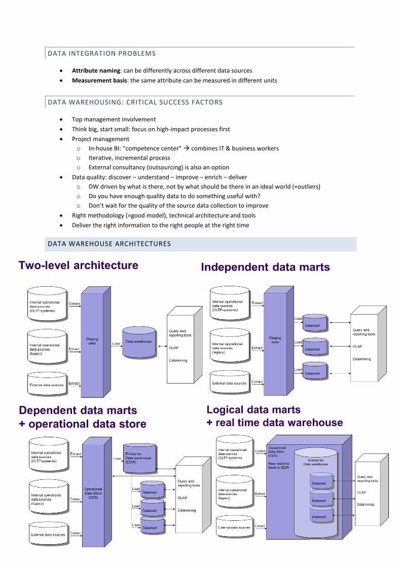
DATA INTEGRATION PROBLEMS

Attribute naming: can be differently across different data sources

Measurement basis: the same attribute can be measured in different units

DATA WAREHOUSING: CRITICAL SUCCESS FACTORS

Top management involvement

Think big, start small: focus on high-impact processes first

Project management

o In-house BI: “competence center” combines IT & business workers

o Iterative, incremental process

o External consultancy (outsourcing) is also an option

Data quality: discover – understand – improve – enrich – deliver

o DW driven by what is there, not by what should be there in an ideal world (+outliers)

o Do you have enough quality data to do something useful with?

o Don’t wait for the quality of the source data collection to improve

Right methodology (=good model), technical architecture and tools

Deliver the right information to the right people at the right time

DATA WAREHOUSE ARCHITECTURES

FEDERATED DBS

= alternative to data warehouses

DW: create a copy of all the data; execute queries against the copy

FDB: pull data from source systems as needed to answer queries

WH VS FDB

Advantages FDBs:

o No redundant copying of data

o Queries see real-time view of evolving data

o More flexible security policy

Disadvantages FDBs:

o Analysis queries place extra load on transactional systems

o Query optimization is hard to do well

o Historical data may not be available

o Complex “wrappers” needed to mediate between analysis server and source systems

DWs are much more common in practice:

o Better performance

o Lower complexity

o Slightly out-of-date data is acceptable

OLAP AND DATA MINING

Verification based analysis techniques: testing of hypotheses as formulated by user

SQL based querying and reporting

On-Line Analytical Processing (OLAP)

Discovery based analysis techniques: generation of new hypotheses

Data mining and text mining

OLAP

Interactive analysis of large chunks of multidimensional data from a DW or DM

Advanced graphical representation of the data

Rollup: aggregate data along one or more dimensions (daily to monthly)

Drill-down: disaggregate data along one or more dimensions

Slicing and dicing: analyze data from different angles

Basic way of doing OLAP: pivot tables

interactively re-arrange and manipulate aggregated

data using a two dimensional table

KNOWLEDGE DISOVERY IN DATA (KDD)

= “the non-trivial process of identifying valid, novel, potentially useful and ultimately understandable

patterns in data”

Iterative and multi-disciplinary process

Retail (response modelling, retention modelling), Credit card+Ebay+Phone company (fraud detection),

Amazon (customized recemmendations), Email (spam detection), Financial institutions (credit risk

prediction), etc.

DATA MINING

= discovery of new patterns in a collection of structured data

o descriptive analysis: discover patterns in past events (association, sequencing, clustering)

o predictive analysis: discover patterns to predict future events (classification, regression)

Text mining: identify new patterns in a collection of unstructured data

CLASSIFICATION (PREDICTIVE ANALYSIS)

The target variable is discrete. Used in financials (credit scoring), marketing (response model, churn) and

counter-terrorism.

REGRESSION (DESCRIPTIVE ANALYSIS)

The target variable is continuous (forecasting loss, stock prices, customer lifetime value, etc.)

ASSOCIATIONS (DESCRIPTIVE ANALYSIS

Detects frequently occurring patterns between items and are represented as association rules.

Eg: market basket analysis which products are bought together?

SEQUENCES (DESCRIPTIVE ANALYSIS)

These are associations with a time aspect and they detect temporal patterns between items.

Eg: web mining if web page A then webpage B and then webpage C

Eg: medical if operation X then 30% chance of infection in 1 week

CLUSTERING (DESCRIPTIVE ANALYSIS)

Divides data in groups: maximal similarity within group, maximal dissimilarity between groups

Eg: segmentation innovators, early adopters, …, late majority often pre-processing to other techniques