Chaos in periodically perturbed planar Hamiltonian systems using linked twist maps

J. Differential Equations 249 (2010) 3233–3257

Contents lists available at ScienceDirect

Journal of Differential Equations

www.elsevier.com/locate/jde

Chaos in periodically perturbed planar Hamiltonian systemsusing linked twist maps

Alessandro Margheri a,∗,1, Carlota Rebelo a,1, Fabio Zanolin b,2

a Fac. Ciências de Lisboa e Centro de Matemática e Aplicações Fundamentais, Av. Prof. Gama Pinto 2, 1649-003 Lisboa, Portugalb University of Udine, Department of Mathematics and Computer Science, via delle Scienze 206, 33100 Udine, Italy

a r t i c l e i n f o a b s t r a c t

Article history:Received 6 May 2009Revised 7 May 2010Available online 17 September 2010

MSC:34C2534C2854H20

Keywords:Periodic pointsChaotic dynamicsTopological horseshoesLinked twist mapsHamiltonian systems

We present a simple topological approach for the search of fixedpoints and the detection of chaotic dynamics for two-dimensionalmaps satisfying a twist condition on linked annuli. Applications toplanar Hamiltonian systems are given.

© 2010 Elsevier Inc. All rights reserved.

1. Introduction

In this paper we describe a general setting for detecting periodic solutions and complex dynamicsin perturbed planar Hamiltonian systems via linked twist maps (LTM). Generally speaking, by a linkedtwist map we mean the composition of two twist maps defined on two annuli that cross each otheralong a topological rectangle. The dynamic properties of such maps have been already investigatedby several authors, both from the theoretical point of view [4,7,23,24] and also for their interest in

* Corresponding author.E-mail addresses: [email protected] (A. Margheri), [email protected] (C. Rebelo), [email protected]

(F. Zanolin).1 Supported by Fundação para a Ciência e a Tecnologia, Financiamento Base 2008 - ISFL/1/209.2 Supported by the PRIN project “Ordinary Differential Equations and Applications”. The author also thanks the CMAF of

Lisbon for the hospitality.

0022-0396/$ – see front matter © 2010 Elsevier Inc. All rights reserved.doi:10.1016/j.jde.2010.08.021

http://dx.doi.org/10.1016/j.jde.2010.08.021

http://www.ScienceDirect.com/

http://www.elsevier.com/locate/jde

mailto:[email protected]



http://dx.doi.org/10.1016/j.jde.2010.08.021

3234 A. Margheri et al. / J. Differential Equations 249 (2010) 3233–3257

the applications to different areas like celestial mechanics [1, pp. 231–237], [17, pp. 90–94] and fluidmixing [27,30,31]. As mentioned by Devaney in [7], LTMs also occur in some problems concerningthe motion of charged particles in magnetic fields and in the study of diffeomorphisms of surfaces.Some results in this area have been obtained using as a main tool the celebrated Smale’s horseshoe(see [17,25]) or its consequences. As is well known, in order to apply the classical horseshoe theoryone has to check some hyperbolicity conditions which, roughly speaking, require that the map funder consideration is a diffeomorphism such that both df and df −1 are contractive along somecomplementary directions. These conditions, when translated to the setting of LTM usually impose(besides other technical assumptions) the smoothness of the maps as well as the monotonicity of thetwists.

In recent years a great deal of research has been devoted to the study of the so-called topological(or geometric) horseshoes. With this term one often refers to the adaptations of Smale’s theory to amore topological setting. More precisely, one tries to develop some methods in which the hyperbol-icity assumptions are replaced by weaker conditions of topological crossing, keeping some essentialfeatures of Smale’s construction. Some approaches in this direction can be found in [3,12,15,26,32,33](just to quote a few different points of view).

In the present paper we apply an elementary topological approach (introduced by Papini andthe third author in [18]) to study a generalized case of LTMs. Indeed, in our setting we deal withtopological planar annuli which are linked only by the fact that their intersection has a compo-nent homeomorphic to the unit square (we call such a set a topological rectangle). For the mapsacting on the two annuli we only assume the continuity and a twist condition on the boundarylike in the Poincaré–Birkhoff fixed point theorem. In particular, for our maps we do not requireneither area-preserving properties, nor the monotonicity of the twist. Our main abstract results areTheorem 3.1 and Theorem 3.2 of Section 3. In the first theorem we prove the existence of fixedpoints as well as chaotic dynamics (including periodic points of any period) under a minimal set ofassumptions, but with the requirement of the invariance of the boundaries of the annuli. Accord-ingly, our result may be viewed as an extension of the classical version of the Poincaré–Birkhofftheorem to the case of linked twist maps. In our second theorem we weaken the assumptionof boundary invariance at the expense of a stronger twist condition. Also for this aspect we fol-low an analogous line as for the Poincaré–Birkhoff theorem (see [6] and [13] and the referencestherein for a recent discussion of this topic). We also mention the fact that, in our opinion, thegeneral theorems obtained in this section allow a simplified approach (and, consequently, a moretransparent proof) compared to some results previously achieved in some particular cases of planarODEs [21].

The abstract theorems of Section 3 are applied in Section 4 to a class of periodically perturbedplanar Hamiltonian systems. Theorem 3.1 finds its application in Theorem 4.1 where the forcingterm is assumed to be a square-wave. The particular shape of the forcing simplifies the analysis;however, such kind of periodic perturbations may have their own interest from the point of viewof the applications, as pointed out in [5]. Next, in Theorem 4.2 (which is a consequence of The-orem 3.2) we consider the case of more general perturbations. In particular we allow also forcingterms which do not preserve the Hamiltonian structure of the equation, like, for instance, some(small) dissipative terms. Finally, in Section 5 we analyze in detail the dynamics of a forced asym-metric oscillator recently considered in [34] with respect to the problem of boundedness of thesolutions.

In order to keep as self-contained as possible this work we have collected in Section 2 all the basicpreliminaries about the “stretching along the paths” technique which are needed for the proofs of themain results in Section 3.

2. Basic setting

We recall, for the reader’s convenience, the topological tools and the concept of chaos which areused in this paper.

A. Margheri et al. / J. Differential Equations 249 (2010) 3233–3257 3235

Definition 2.1. Let X be a metric space, let φ : Dφ(⊆ X) → X be a map and D ⊆ Dφ a nonempty set.Assume also that p � 2 is an integer. We say that φ induces chaotic dynamics on p symbols in the set Dif there exist p nonempty pairwise disjoint compact sets

K1, K2, . . . , K p ⊆ D

such that, for each two-sided sequence of p symbols

(si)i∈Z ∈ Σp := {1, . . . , p}Z,

there exists a corresponding sequence (wi)i∈Z ∈ DZ with

wi ∈ Ksi and wi+1 = φ(wi), ∀i ∈ Z (1)

and, whenever (si)i∈Z is a k-periodic sequence (that is, si+k = si , ∀i ∈ Z) for some k � 1, there existsa k-periodic sequence (wi)i∈Z ∈ DZ satisfying (1).

Observe that, according to Definition 2.1, for each i ∈ {1, . . . , p} there is at least one fixed point ofφ in Ki . We also notice that if the map φ fulfills Definition 2.1 and is also continuous and injective on

K :=p⋃

i=1

Ki ⊆ D

(like in the case of our applications of Section 4 where φ is the Poincaré map associated to a planarsystem), then there exists a nonempty compact set

Λ ⊆ K

which is invariant for φ (i.e., φ(Λ) = Λ) and such that φ|Λ is semiconjugate to the two-sided Bernoullishift σ on p symbols

σ : Σp → Σp, σ((si)i∈Z

) = (si+1)i∈Z,

according to the commutative diagram

Λφ

g

Λ

g

Σpσ

Σp

where g is a continuous and surjective function.3 In our setting, it is also possible to have an invariantset Λ which contains as a dense subset the periodic points of φ and such that the counterimage (bythe semiconjugacy g) of any periodic sequence (si)i in Σp contains a periodic point of φ having thesame period of (si)i (see [20] for the details).

3 We recall that Σp is a compact metric space with the usual distance d(s′, s′′) := ∑+∞i=−∞

|s′i−s′′i |p|i| , for s′ = (s′

i)i∈Z and s′′ =(s′′

i )i∈Z (or with an equivalent metric [29]).


We recall that the semiconjugation to the Bernoulli shift (even without reference to the periodicpoints) is one of the typical requirements for chaotic dynamics as it implies a positive topologicalentropy for the map φ|Λ (see [28]). Actually, the occurrence of such a situation for a map φ (or forone of its iterates) has been considered as a possible definition of chaotic dynamics by some authors(see the concept of horseshoe factor according to Burns and Weiss [3] or that of chaos in the sense ofBlock and Coppel as in [2]).

Now we are ready to present the abstract setting for our method. Borrowing notation and termi-nology from [20], we start with the following definitions. By path γ in a metric space X we mean acontinuous mapping γ : [t0, t1] → X and we set γ := γ ([t0, t1]). Without loss of generality we willusually take [t0, t1] = [0,1]. By a sub-path σ of γ we mean just the restriction of γ to a compactsubinterval of its domain. An arc is the homeomorphic image of the compact interval [0,1]. We de-fine an oriented rectangle in X, as a pair

R := (R, R−)

,

where R ⊆ X is homeomorphic to the unit square [0,1]2 (in this case we call R a topological rectan-gle) and

R− := R−left ∪ R−

right

is the disjoint union of two disjoint compact arcs R−left, R−

right ⊆ ∂R (which are called the “com-

ponents” or “sides” of R−).4 We also denote by R+ the closure of ∂R \ (R−left ∪ R−

right) which is

the union of two compact arcs R+down and R+

up. Given an oriented rectangle (R, R−) it is always

possible to find a homeomorphism h : [0,1]2 → R = h([0,1]2) ⊆ X such that h({0} × [0,1]) = R−left,

h({1} × [0,1]) = R−right, h([0,1] × {0}) = R+

down and h([0,1] × {1}) = R+up . This can be proved using

some classical results from plane topology like the Schönflies theorem [16].Next we introduce the concept of “stretching along the paths” which plays a central role in our

approach.Suppose that X is a metric space and that φ : Dφ(⊆ X) → X is a map defined on a set Dφ . Let

M := (M, M−) and N := (N , N −) be oriented rectangles in X .

Definition 2.2. Let H ⊆ M ∩ Dφ be a compact set. We say that (H, φ) stretches M to N along the pathsand write

(H, φ) : M �−→ N ,

if the following conditions hold:

• φ is continuous on H;• for every path γ : [a,b] → M such that γ (a) ∈ M−

left and γ (b) ∈ M−right (or γ (a) ∈ M−

right and

γ (b) ∈ M−left), there exists a subinterval [t′, t′′] ⊆ [a,b] such that

γ (t) ∈ H, φ(γ (t)

) ∈ N , ∀t ∈ [t′, t′′]

and, moreover, φ(γ (t′)) and φ(γ (t′′)) belong to different components of N −.

4 We warn the reader that, in order to simplify the presentation, we have allowed some ambiguity in the use of the sym-bol ∂R. In our setting ∂R denotes the image of the boundary of the unit square [0,1]2 under the homeomorphism whichdefines R. However, no ambiguity occurs in the applications. Indeed, for X = R

2, ∂R is the topological boundary of R.


In the special case in which H = M, we simply write

φ : M �−→ N .

Roughly speaking, (H, φ) : M �−→ N means that there is a subset of H which is mapped by φ

across N from N −left to N −

right. The verification of this crossing property is made by means of the paths

in M connecting M−left to M−

right. Such paths are “intercepted” by H and then expanded across N .

The [·]−-sets are thus reminiscent of the exit sets in the Conley–Wazewski theory, as they represent(although in a rather generalized sense) an expansive direction for the map φ. Complex dynamics forφ arise when (Hi, φ) : M �−→ M for at least p � 2 nonempty pairwise sets H1, . . . , H p (see [20,Theorems 2.2–2.3]).

In this framework, and when φ splits as the composition of two maps, we have the followingtheorem which is adapted to our context from [20].

Theorem 2.1. Let X be a metric space, let ϕ : Dϕ(⊆ X) → X and ψ : Dψ(⊆ X) → X be continuous mapsand let P := (P , P −), Q := (Q, Q−) be oriented rectangles in X . Suppose that the following conditions aresatisfied:

(Hϕ) there exist m � 1 pairwise disjoint compact sets H1, . . . , Hm ⊆ P ∩ Dϕ such that (Hi,ϕ) : P �−→ Q,

for i = 1, . . . ,m;(Hψ) there exist � 1 pairwise disjoint compact sets K1, . . . , K ⊆ Q ∩ Dψ such that (Ki,ψ) : Q �−→ P ,

for i = 1, . . . , .

Then we have:

• If m = = 1, then the map φ := ψ ◦ ϕ has at least a fixed point z ∈ H := H1 such that ϕ(z) ∈ K := K1.

• If at least one between m and is greater or equal than 2, then the map φ := ψ ◦ ϕ induces chaoticdynamics on m × symbols in the set

H∗ :=⋃

i=1,...,mj=1,...,

H′i, j with H′

i, j := Hi ∩ ϕ−1(K j).5

Moreover, for each sequence of m × symbols

s = (sn)n = (pn,qn)n ∈ {1, . . . ,m}N × {1, . . . , }N,

there exists a compact connected set Cs ⊆ H′p0,q0

, with

Cs ∩ P +down �= ∅, Cs ∩ P +

up �= ∅

and such that, for every w ∈ Cs , there exists a sequence (yn)n with y0 = w and

yn ∈ H′pn,qn

, φ(yn) = yn+1, ∀n � 0.

5 The result about periodic points for φ = ψ ◦ ϕ which comes from Definition 2.1 reads now as follows: for each k-periodicsequence of m × symbols s = (sn)n = (pn,qn)n ∈ {1, . . . ,m}N × {1, . . . , }N, there exists a k-periodic sequence (wn)n∈Z such thatwn+1 = φ(wn) and wn ∈ H′

pn ,qn. In particular, there is a fixed point for φ in each of the H′

i, j -sets.


We note that when m � 2 (or � 2) the assumptions (Hϕ) and (Hψ) are related to the concept of“crossing number” considered by Kennedy and Yorke in [12].

Theorem 2.1 will be applied in the next section to a case of Linked Twist Maps. In order to stressone of the main differences between our approach and other results dealing with standard circularannuli, we observe that two topological annular regions which cross each other do not necessarilyintersect in exactly two rectangular domains (like in [7]).6 Indeed, the range of different possibilitiesfor which two topological annuli can be linked together by means of rectangular sets is wide. InSection 3 we restrict ourselves to the “minimal” situation in which at least one topological rectangleR results as a component of the intersection of two annuli A1 and A2. The oriented rectanglesP and Q on which we will apply Theorem 2.1 will consist just of the set R oriented in differentmanners. Clearly, the theory can be easily generalized to the case of more complicated configurations.Moreover, we observe that the topological tools we presented in this section for the two-dimensionalframework can be developed also for R

n with n � 3. In this case one has to consider the higherdimensional analogue of a topological rectangle, that is a topological cylinder (a subset of R

n whichis homeomorphic to the cartesian product of a compact interval with a closed (n − 1)-dimensionaldisk). The interested reader is referred to [19] and [22]. For the application we consider in this paperthe planar setting will suffice.

3. Main results

Let, for i = 1,2, Ai ⊆ R2 be a closed planar topological annulus surrounding a point Pi .

To each of the Ai we associate a covering projection

Πi = Πi(θ,α) : Ai := R × [ai,bi] → Ai .

The maps Πi should be thought as a generalization to our topological setting of the standard polarcoordinates in the plane, and we use them to induce a coordinate system on Ai . Accordingly, theyhave to satisfy a periodicity condition

Πi(θ + 1,α) = Πi(θ,α), ∀θ ∈ R, ∀α ∈ [ai,bi]and the following properties:

• For each β ∈ [ai,bi], the set Ci(β) := {Πi(s, β): s ∈ R} is a Jordan curve around Pi . Moreover,Ci(ai) and Ci(bi) are, respectively, the inner and outer boundaries of Ai .

• For each s ∈ R, the set Li(s) := {Πi(s, β): β ∈ [ai,bi]} is an arc contained in Ai and joining theinner and the outer boundaries of Ai .

From the theory of covering spaces [9], it follows that Ci(α) is contained in the interior of the regionbounded by Ci(β), for ai � α < β � bi . Moreover, Li(s′) and Li(s′′) either coincide or are disjoint,according to the fact that s′′ − s′ ∈ Z or s′′ − s′ /∈ Z. We also have that⋃

β∈[ai ,bi ]Ci(β) = Ai =

⋃s∈[r,r+1[

Li(s) (for r ∈ R)

and that Πi is a homeomorphism of the rectangle [s′, s′′] × [ai,bi] onto its image contained in Ai ifs′′ − s′ < 1. More generally, if B ⊆ R × [ai,bi] is a compact set such that Πi is injective on B, thenΠi |B : B → Πi(B) is a homeomorphism. To have the injectivity satisfied, it is sufficient to assume thatwhenever (s′, β), (s′′, β) ∈ B, then s′′ − s′ /∈ Z.

6 For instance, the energy level lines of x′′ + Ax3 = 0 and x′′ + Bx3 = 0, with 0 < A < B , may determine annuli which intersectin four rectangular sets.


Fig. 1. As a comment to Definition 3.1, we show an example of two annuli which are linked only through one topologicalrectangle (the darker region).

The following definition plays a crucial role in our theory.

Definition 3.1. Let R ⊆ A1 ∩ A2, be a topological rectangle. We say that A1 and A2 are linkedthrough R if the boundary of R is the union of four consecutive arcs σ 1

int , σ 2int , σ 1

out and σ 2out , con-

tained, respectively, in the inner boundary of A1, in the inner boundary of A2, in the outer boundaryof A1 and in the outer boundary of A2 (see Fig. 1).

If A1 and A2 are linked through a topological rectangle R, then, for each i = 1,2, we have

Π−1i (R) =

⋃k∈Z

((k,0) + Ri

),

where Ri ⊆ Ai is a topological rectangle. The map Πi is a homeomorphism of Ri onto its imageΠi(Ri) = R.

The boundary of R1 can be split into four consecutive arcs ω11, ω2

1, ω31 and ω4

1, such that

Π1(ω1

1

) = σ 1int ⊆ C1(a1), Π1

(ω3

1

) = σ 1out ⊆ C1(b1),

while

Π1(ω2

1 ∪ ω41

) = σ 2int ∪ σ 2

out.

More precisely, there exist s′1, s′′

1 as well as t′1, t′′

1 with

s′1 < s′′

1 < s′1 + 1, t′

1 < t′′1 < t′

1 + 1

such that

ω11 = [

s′1, s′′

1

] × {a1}, ω31 = [

t′1, t′′

1

] × {b1}.

For the sequel, it will be useful also to define the lengths of these intervals, by setting

L1int := s′′

1 − s′1, L1

out := t′′1 − t′

1.


Fig. 2. Illustration of our geometrical setting. The bolder arcs represent σ 1int and, for i = 1,2, its inverse image in Ri through

the covering projection Πi .

Similarly, the boundary of R2 can be split into four consecutive arcs ω12, ω2

2, ω32 and ω4

2, such that

Π2(ω1

2

) = σ 2int ⊆ C2(a2), Π2

(ω3

2

) = σ 2out ⊆ C2(b2),

while

Π2(ω2

2 ∪ ω42

) = σ 1int ∪ σ 1

out.

As above, there exist s′2, s′′

2 as well as t′2, t′′

2 with

s′2 < s′′

2 < s′2 + 1, t′

2 < t′′2 < t′

2 + 1

such that

ω12 = [

s′2, s′′

2

] × {a2}, ω32 = [

t′2, t′′

2

] × {b2}.

The corresponding interval lengths are now defined by

L2int := s′′

2 − s′2, L2

out := t′′2 − t′

2.


After having described our geometrical setting (see Fig. 2), we consider now the dynamical part byintroducing continuous maps acting on the annuli. For each i = 1,2, let φi : Ai → Ai be a continuousmap which admits a lifting

φi : Ai → Ai, Πi ◦ φi = φi ◦ Πi,

φi : (θ,α) �→ (Gi(θ,α), Ri(θ,α)

) = (θ + gi(θ,α), Ri(θ,α)

),

with gi, Ri : Ai → R continuous functions such that

gi(θ + 1,α) = gi(θ,α), Ri(θ + 1,α) = Ri(θ,α), ∀(θ,α) ∈ R × [ai,bi].

As in the classical version of the Poincaré–Birkhoff fixed point theorem, we assume:

(BI) Boundary Invariance. Ri(θ,ai) = ai , Ri(θ,bi) = bi , ∀θ ∈ R.

(TC) Twist Condition. For each i = 1,2, one of the following holds: there exist integers ki and ji suchthat either

maxθ∈[s′i ,s′′i ]

gi(θ,ai) � −Liint + ki and min

θ∈[t′i ,t′′i ]gi(θ,bi) � Li

out + ji, with ki � ji

or

minθ∈[s′i ,s′′i ]

gi(θ,ai) � Liint + ki and max

θ∈[t′i ,t′′i ]gi(θ,bi) � −Li

out + ji, with ki � ji .

Under these assumptions, the following result holds.

Theorem 3.1. Suppose that A1 and A2 are linked through R and assume (BI) and (TC). Then, φ2 ◦ φ1, aswell as φ1 ◦ φ2, have a fixed point in R. Moreover if ji �= ki for i = 1 or i = 2 then φ2 ◦ φ1, as well as φ1 ◦ φ2,

induce chaotic dynamics on (| j1 − k1| + 1)(| j2 − k2| + 1) symbols according to Definition 2.1.

Proof. We prove the theorem only for the composite map φ := φ2 ◦ φ1 (the other case being analo-gous) and apply Theorem 2.1 with X = R

2, ϕ := φ1 and ψ := φ2. To this end, as a first step, we definethe oriented rectangles P and Q as follows:

P := R, P −left := σ 1

int, P −right := σ 1

out.

Q := R, Q−left := σ 2

int, Q−right := σ 2

out.

Since the twist condition (TC) allows four different combinations, in order to fix the ideas, we assume(without loss of generality) the first alternative for φ1 and the second one for φ2. Therefore, thanks tothe properties of the lifting (i.e., possibly replacing g1 with g1 − k1 and g2 with g2 − j2), we suppose

maxθ∈[s′1,s′′1]

g1(θ,a1) � −L1int, min

θ∈[t′1,t′′1 ]g1(θ,b1) � L1

out + m1 (2)

and

minθ∈[s′ ,s′′]

g2(θ,a2) � L2int + m2, max

θ∈[t′ ,t′′]g2(θ,b2) � −L2

out, (3)
2 2 2 2


with

m1 := | j1 − k1| = j1 − k1 and m2 := | j2 − k2| = k2 − j2.

To get our result, we prove (Hϕ) and (Hψ) for

m := m1 + 1, := m2 + 1.

In order to prove that (Hϕ) of Theorem 2.1 is satisfied, we work in the covering space A1 =R × [a1,b1] where we define the sets

H j := {(θ,α) ∈ R1 : φ1(θ,α) ∈ R1 + ( j − 1,0)

}, j = 1, . . . ,m.

From the H j ’s through the homeomorphism Π1|R1we obtain m pairwise disjoint compact sets

H j := Π1(H j) ⊆ R = P, j = 1, . . . ,m.

We prove now that the H j ’s are nonempty and

(H j, φ1) : P �−→ Q, ∀ j = 1, . . . ,m.

Let γ : [0,1] → R be a continuous curve such that

γ (0) ∈ σ 1int, γ (1) ∈ σ 1

out.

We denote by

γ := (Π1|R1)−1 ◦ γ : [0,1] → R1

the lifting of γ to R1. Note that γ (0) ∈ ω11 and γ (1) ∈ ω3

1 and that by (2) we have

g1(γ (0)

)� −L1

int and g1(γ (1)

)� L1

out + m1.

Therefore φ1(γ (0)) = (G1(γ (0)),a1) with G1(γ (0)) � s′1 and φ1(γ (1)) = (G1(γ (1)),b1) with

G1(γ (1)) � t′′1 + m1. As φ1(γ ([0,1])) is connected we conclude that there exist m disjoint sub-

intervals [ξ ′j, ξ

′′j ] ⊆ [0,1] such that, for each j = 1, . . . ,m, φ1(γ ([ξ ′

j, ξ′′j ])) ⊆ R1 + ( j − 1,0) and

φ1(γ (ξ ′j)) and φ1(γ (ξ ′′

j )) belong to different components of (ω21 ∪ ω4

1) + ( j − 1,0). Actually, we canalways take ξ ′

1 and ξ ′′1 such that

φ1(γ

(ξ ′

j

)) ∈ ω41 + ( j − 1,0), φ1

(γ

(ξ ′′

j

)) ∈ ω21 + ( j − 1,0). (4)

Hence we conclude that the sets H j are nonempty which implies that the sets H j are nonempty.Let now j ∈ {1, . . . ,m} be fixed and consider γ (t) with t ∈ [ξ ′

j, ξ′′j ]. By the above construction we

know that γ (t) ∈ H j and, moreover,

φ1(γ (t)

) ∈ R1 + ( j − 1,0),


which, in turn implies that

Π1(φ1

(γ (t)

)) = (Π1 ◦ φ1 ◦ (Π1|R1

)−1)(γ (t)) = φ1

(γ (t)

) ∈ Π1(

R1 + ( j − 1,0)) = R = Q.

On the other hand, from (4) we also have that

φ1(γ

(ξ ′

j

)) ∈ σ 2out, φ1

(γ

(ξ ′′

j

)) ∈ σ 2int.

Therefore, by the definition of Q = (Q, Q−) at the beginning of the proof, we conclude that

(H j, φ1) : P �−→ Q

and thus the stretching property for (H j, φ1) is verified. This proves (Hϕ). Using a similar argumentwe can prove (Hψ). Then the thesis follows from Theorem 2.1. �

Our next goal is to show how the condition of boundary invariance can be relaxed. Similarly towhat happens in the classical case of the Poincaré–Birkhoff theorem the possibility of weakening thehypothesis on the invariance of the boundary leads to results which are more suitable for applica-tions to non-autonomous ODEs. Here we present a result (Theorem 3.2 below) which shows thatour method is stable under small continuous perturbations of the maps. This fact will allow us toapply our technique to some non-autonomous equations which are small perturbations of piecewiseautonomous planar systems.

We would like to observe that in formulating the setting and assumptions we make below, wehave kept in mind the geometric configurations which arise from the applications. For example, theannuli Ui ⊆ Ai defined below are usually obtained as the union of closed orbits of an unperturbedplanar autonomous Hamiltonian system. Although more general results could be interesting from thetopological point of view, we think that the framework we consider presents a good balance betweensimplicity and generality, allowing to deal with many applications.

Keeping the setting introduced above, with A1 and A2 two closed topological annuli linkedthrough R, we define two new annular sub-regions in the following manner.

Let, for i = 1,2, λ−i , λ+

i : R → R be two continuous functions such that

ai � λ−i (θ) < λ+

i (θ) � bi, λ±i (θ + 1) = λ±

i (θ), ∀θ ∈ R.

Through these functions we define the strips

Ui := {(θ,α) ∈ Ai : λ−

i (θ) � α � λ+i (θ)

}, i = 1,2

and the annuli

Ui := Πi(Ui) ⊆ Ai, i = 1,2.

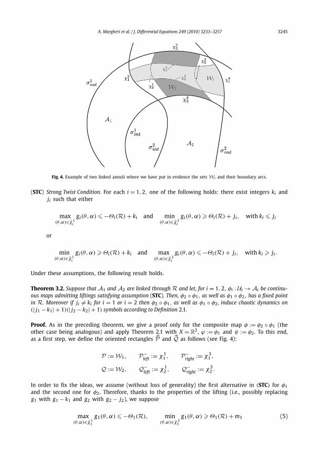
As a technical condition we assume that there exist topological rectangles

W1 ⊆ U1 ∩ R and W2 ⊆ U2 ∩ R

satisfying the following properties (see Fig. 4): we suppose that the boundary of W1 is the unionof four consecutive arcs χ1

1 ⊆ Π1(λ−1 ([0,1])), χ2

1 ⊆ σ 2int , χ3

1 ⊆ Π1(λ+1 ([0,1])) and χ4

1 ⊆ σ 2out . In

the same manner, we assume that the boundary of W2 is the union of four consecutive arcs


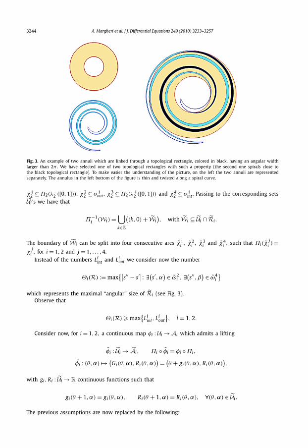
Fig. 3. An example of two annuli which are linked through a topological rectangle, colored in black, having an angular widthlarger than 2π . We have selected one of two topological rectangles with such a property (the second one spirals close tothe black topological rectangle). To make easier the understanding of the picture, on the left the two annuli are representedseparately. The annulus in the left bottom of the figure is thin and twisted along a spiral curve.

χ12 ⊆ Π2(λ

−2 ([0,1])), χ2

2 ⊆ σ 1out , χ3

2 ⊆ Π2(λ+2 ([0,1])) and χ4

2 ⊆ σ 1int . Passing to the corresponding sets

Ui ’s we have that

Π−1i (Wi) =

⋃k∈Z

((k,0) + Wi

), with Wi ⊆ Ui ∩ Ri .

The boundary of Wi can be split into four consecutive arcs χ1i , χ2

i , χ3i and χ4

i , such that Πi(χj

i ) =χ

ji , for i = 1,2 and j = 1, . . . ,4.

Instead of the numbers Liint and Li

out we consider now the number

Θi(R) := max{∣∣s′′ − s′∣∣: ∃(

s′,α) ∈ ω2

i , ∃(s′′, β

) ∈ ω4i

}which represents the maximal “angular” size of Ri (see Fig. 3).

Observe that

Θi(R) � max{

Liint, Li

out

}, i = 1,2.

Consider now, for i = 1,2, a continuous map φi : Ui → Ai which admits a lifting

φi : Ui → Ai, Πi ◦ φi = φi ◦ Πi,

φi : (θ,α) �→ (Gi(θ,α), Ri(θ,α)

) = (θ + gi(θ,α), Ri(θ,α)

),

with gi, Ri : Ui → R continuous functions such that

gi(θ + 1,α) = gi(θ,α), Ri(θ + 1,α) = Ri(θ,α), ∀(θ,α) ∈ Ui .

The previous assumptions are now replaced by the following:


Fig. 4. Example of two linked annuli where we have put in evidence the sets Wi and their boundary arcs.

(STC) Strong Twist Condition. For each i = 1,2, one of the following holds: there exist integers ki andji such that either

max(θ,α)∈χ1

i

gi(θ,α) � −Θi(R) + ki and min(θ,α)∈χ3

i

gi(θ,α) � Θi(R) + ji, with ki � ji

or

min(θ,α)∈χ1

i

gi(θ,α) � Θi(R) + ki and max(θ,α)∈χ3

i

gi(θ,α) � −Θi(R) + ji, with ki � ji .

Under these assumptions, the following result holds.

Theorem 3.2. Suppose that A1 and A2 are linked through R and let, for i = 1,2, φi : Ui → Ai be continu-ous maps admitting liftings satisfying assumption (STC). Then, φ2 ◦ φ1, as well as φ1 ◦ φ2, has a fixed pointin R. Moreover if ji �= ki for i = 1 or i = 2 then φ2 ◦ φ1, as well as φ1 ◦ φ2 , induce chaotic dynamics on(| j1 − k1| + 1)(| j2 − k2| + 1) symbols according to Definition 2.1.

Proof. As in the preceding theorem, we give a proof only for the composite map φ := φ2 ◦ φ1 (theother case being analogous) and apply Theorem 2.1 with X = R

2, ϕ := φ1 and ψ := φ2. To this end,as a first step, we define the oriented rectangles P and Q as follows (see Fig. 4):

P := W1, P −left := χ1

1 , P −right := χ3

1 ,

Q := W2, Q−left := χ1

2 , Q−right := χ3

2 .

In order to fix the ideas, we assume (without loss of generality) the first alternative in (STC) for φ1and the second one for φ2. Therefore, thanks to the properties of the lifting (i.e., possibly replacingg1 with g1 − k1 and g2 with g2 − j2), we suppose

max(θ,α)∈χ1

g1(θ,α) � −Θ1(R), min(θ,α)∈χ3

g1(θ,α) � Θ1(R) + m1 (5)
1 1


and

min(θ,α)∈χ1

2

g2(θ,α) � Θ2(R) + m2, max(θ,α)∈χ3

3

g2(θ,α) � −Θ2(R), (6)

with

m1 := | j1 − k1| = j1 − k1 and m2 := | j2 − k2| = k2 − j2.

To get our result, we prove (Hϕ) and (Hψ) for

m := m1 + 1, := m2 + 1.

In order to prove that (Hϕ) is satisfied, we work in the covering space A1 = R × [a1,b1] where wedefine the sets

H j := {(θ,α) ∈ W1: φ1(θ,α) ∈ Π−1

1 (W2) ∩ R1 + ( j − 1,0)}, j = 1, . . . ,m.

From the H j ’s through the homeomorphism Π1|W1 we obtain m pairwise disjoint compact sets

H j := Π1(H j) ⊆ W1 = P, j = 1, . . . ,m.

We prove now that the H j ’s are nonempty and

(H j, φ1) : P �−→ Q, ∀ j = 1, . . . ,m.

Let γ : [0,1] → R be a continuous curve such that

γ (0) ∈ P −left = χ1

1 , γ (1) ∈ P −right = χ3

1 .

We denote by

γ := (Π |W1)−1 ◦ γ : [0,1] → W1

the lifting of γ to W1. Note that γ (0) ∈ χ11 and γ (1) ∈ χ3

1 and that by (5) we have

g1(γ (0)

)� −Θ1(R) and g1

(γ (1)

)� Θ1(R) + m1.

Therefore φ1(γ (0)) = (G1(γ (0)), R1(γ (0))) with G1(γ (0)) � s′ and φ1(γ (1)) = (G1(γ (1)), R1(γ (1)))

with G1(γ (1)) � s′′ + m1 where s′ = min{s: ∃(s,α) ∈ ω21} and s′′ = max{s: ∃(s,α) ∈ ω4

1}. Asφ1(γ ([0,1])) ⊂ A1 is connected we conclude that there exist m disjoint sub-intervals [ξ ′

j, ξ′′j ] ⊆ [0,1]

such that, for each j = 1, . . . ,m, φ1(γ ([ξ ′j, ξ

′′j ])) ⊆ Π−1

1 (W2) ∩ R1 + ( j − 1,0) and φ1(γ (ξ ′j)) and

φ1(γ (ξ ′′j )) belong to different components of Π−1

1 (χ12 ∪χ3

2 )∩ R1 + ( j − 1,0). Hence we conclude that

the sets H j are nonempty which implies that the sets H j are nonempty.Let now j ∈ {1, . . . ,m} be fixed and consider γ (t) with t ∈ [ξ ′

j, ξ′′j ]. By the above construction we

know that γ (t) ∈ H j and, moreover,

φ1(γ (t)

) ∈ Π−11 (W2) ∩ R1 + ( j − 1,0),


which, in turn implies that

Π1(φ1

(γ (t)

)) = (Π1 ◦ φ1 ◦ (Π1|W1

)−1)(γ (t))

= φ1(γ (t)

) ∈ Π1(Π−1

1 (W2) ∩ R1 + ( j − 1,0))

= W2 = Q.

On the other hand, we also have that φ1(γ (ξ ′j)) and φ1(γ (ξ ′′

j )) belong to different components of

χ12 ∪ χ3

2 . Therefore, by the definition of Q = (Q, Q−) at the beginning of the proof, we conclude that

(H j, φ1) : P �−→ Q

and thus the stretching property for (H j, φ1) is verified. This proves (Hϕ). Using a similar argumentwe can prove (Hψ). Then the thesis follows from Theorem 2.1. �4. Applications to planar Hamiltonian systems

In this section we provide a general framework for the application of the results of Section 3 tosome classes of periodically forced planar Hamiltonian systems.

We start building up our setting by introducing the class of Hamiltonian systems we will be con-cerned with. Namely, we will consider periodically forced and piecewise autonomous planar Hamilto-nian systems of the form:

(H)1,2 z′ = J∇H(z) + e1,2(t), z = (x, y)

where H : R2 → R is a continuously differentiable function, J =

[0 −11 0

]is the symplectic matrix in R

2,

and e1,2 : R → R2 is a piecewise constant T -periodic forcing term defined on [0, T [ by:

e1,2(t) ={

p, t ∈ [0, τ1[,q, t ∈ [τ1, τ1 + τ2[, (7)

with

τ1, τ2 > 0, τ1 + τ2 = T

and p := (p1, p2),q := (q1,q2) ∈ R2 are constant vectors with p �= q.

By definition, system (H)1,2 leaps periodically between the two different autonomous Hamiltoniansystems

(H)1 z′ = J∇H1(z) := J∇H(z) + p

and

(H)2 z′ = J∇H2(z) := J∇H(z) + q

with (H)1,2 = (H)1 when t mod(T ) ∈ [0, τ1[ and (H)1,2 = (H)2 when t mod(T ) ∈ [τ1, τ1 + τ2[.Consistently with the above notation, we have that

H1(x, y) := H(x, y) + xp2 − yp1, H2(x, y) := H(x, y) + xq2 − yq1.


The autonomous equations (H)i (i = 1,2) induce local dynamical systems in the plane. We denotetheir respective flows by φt

i .

To complete our setting we make the following assumption:

(LC) Link Condition. For i = 1,2 there exists a topological annulus Ai filled with non-trivial periodicorbits of system (H)i . Moreover, A1 and A2 are linked through a topological rectangle R.

In many applications (see for example the one we present in Section 5 or the ones in [20,21])one deals with two systems of the form (H)i , i = 1,2, each one possessing a center Ci , i = 1,2, withC1 �= C2. Then, condition (LC) is satisfied if a closed orbit O1 of system (H)1 intersects transversally aclosed orbit O2 of system (H)2 at a point z0 = (x0, y0). In fact, in this case the vectors J∇H(z0) + pand J∇H(z0) + q, are linearly independent and it is possible to construct a small topological rectan-gle R around z0 as follows. By the linear independence of the two vectors it follows that the map(x, y) → (u, v) defined by u := H1(x, y) − H1(x0, y0), v := H2(x, y) − H2(x0, y0) defines a local dif-feomorphism between a neighbourhood of (x0, y0) and a neighbourhood of (0,0) in the (u, v) plane.Then, we can obtain R as the inverse image of a small closed rectangle around (0,0) with sides par-allel to the axis u and v. Finally, for each i = 1,2, the closed orbits of (H)i which intersect R definean annulus Ai and A1, and A2 are linked through R.

Since (H)1,2 is a periodically perturbed differential system we investigate the behaviour of itssolutions by studying the dynamics of the associated Poincaré map φ. We recall that φ : Dφ(⊆ R

2) →R

2 associates to a point z0 ∈ R2 the point φ(z0) := z(T ; z0), where z(·; z0) is the solution of system

(H)1,2 satisfying the initial condition z(0) = z0. From the fundamental theory of ODEs it is known thatthe domain Dφ of φ is open and φ is a homeomorphism of Dφ onto its image. Due to the particularchoice of the forcing term e1,2 it turns out that φ may be split as

φ := φ2 ◦ φ1

where φi is the Poincaré map associated to (H)i at the time τi, that is

φi := φτii , i = 1,2. (8)

We note that, for each i = 1,2 the level lines of the Hamiltonian function Hi are invariant sets forthe flow φt

i induced by the corresponding Hamiltonian vector field (see [10], Chapter 5). In particularthe topological annulus Ai filled by closed level lines of Hi is a compact invariant set on which thePoincaré map φi is globally defined. It follows that the maps φ1 and φ2 are defined on R.

By condition (LC), it is well known that for each i = 1,2, there exists a covering projection

Πi : R × [ai,bi] → Ai

which is obtained by introducing suitable action-angle variables. In fact, one can prove (see for exam-ple [11]) the existence of continuous functions ηi : [ai,bi] → R

2, i = 1,2, such that

Hi(ηi(α)

) = α, ∀α ∈ [ai,bi].Then, denoting by Ti(α) the minimal period of the solution of (H)i starting for t = 0 from ηi(α) ∈ Ai,

one can define Πi as follows:

Πi(θ,α) := φθTi(α)

i

(ηi(α)

). (9)

The meaning of the coordinates α and θ is as follows. The variable α ∈ [ai,bi] corresponds tothe energy levels of the Hamiltonian function Hi and its values are in one to one correspondence,through the function ηi, with the closed orbits of (H)i . The variable θ may be thought as an angular


coordinate which measures the progress of a solution of (H)i along the corresponding closed orbit insuch a way that one full turn on such orbit corresponds to a variation of one unit in θ.

We are now ready to apply the general results of the previous section for the study of chaoticdynamics of system (H)1,2.

In our first result, which we describe here informally, we assume that, for each i = 1,2 the periodsof the two closed orbits of system (H)i which define the boundary of Ai are different (see condition(10) below). This implies that the motion on one boundary is slower than on the other one. As aconsequence, the flow of (H)i gives rise to a twist of the annulus Ai . If τi is large, the periodic orbitwith lower period will be traversed more times than the other one, and the twist will grow larger.Actually, the twist will tend to +∞ when τi → +∞. It follows that, for each i = 1,2, by choosingτi sufficiently large, we can guarantee that the stretching along the path property will hold for thesuitable paths and orientations of R (which will depend on i) and, moreover, the image of a paththrough φi will cross R in the right way as many times as we want. Therefore, we can obtain chaoticdynamics on any number of symbols for system (H)1,2 by choosing τ1 and τ2 sufficiently large.

The precise statement of our result is the following.

Theorem 4.1. In the above setting, suppose that assumption (LC) is satisfied and

T1(a1) �= T1(b1) and T2(a2) �= T2(b2). (10)

Then, for any integer N � 2 there exist τ ∗1 > 0 and τ ∗

2 > 0 such that if

τi > τ ∗i for i = 1,2,

then the Poincaré map of system (H)1,2 induces chaotic dynamics on N symbols on R.

Proof. Our goal is to enter in the setting of Theorem 3.1 with φ1 and φ2 defined as in (8). First of allwe observe that φi : Ai → Ai for i = 1,2. Moreover, if we denote by φi : Ai → Ai the correspondinglifting, we find that

φi(θ,α) = (θ + gi(θ,α), Ri(θ,α)

),

with

Ri(θ,α) = α, ∀θ ∈ R, α ∈ [ai,bi].

Hence the boundary invariance condition (BI) is satisfied.Concerning the first component of φi, we recall that

Πi(φi(θ,α)

) = φi(Πi(θ,α)

) = φτii

(Πi(θ,α)

) = φτi+si

(ηi(α)

)for

s = θTi(α).

On the other hand,

Πi(φi(θ,α)

) = Πi(θ + gi(θ,α),α

) = φti

(ηi(α)

)


where, by (9) it follows that

t := (θ + gi(θ,α)

)Ti(α).

We thus conclude that

gi(θ,α) = τi

T i(α), for i = 1,2. (11)

We suppose that (10) is satisfied with

T1(a1) > T1(b1) and T2(a2) > T2(b2). (12)

The other three possibilities can be treated in a similar way and the corresponding discussion isomitted.

By (11) and (12) we have

maxθ∈[s′i ,s′′i ]

gi(θ,ai) = τi

T i(ai)<

τi

T i(bi)= min

θ∈[t′i ,t′′i ]gi(θ,bi).

Given the integer N � 2 we decompose it as a product

N = N1 × N2, Ni � 1, max{N1, N2} � 2.

One can easily check that for

τ ∗i := (Ni + 1 + Li

int + Liout)Ti(ai)Ti(bi)

Ti(ai) − Ti(bi), i = 1,2,

the twist condition (TC) is satisfied and Theorem 3.1 can be applied with

j1 − k1 = N1 − 1 and j2 − k2 = N2 − 1.

The proof is complete. �Next we present an application of Theorem 3.2 to the perturbed Hamiltonian system

(H∗)1,2 z′ = J∇H(z) + e1,2(t) + u(t, z), z = (x, y)

where e1,2(t) is as in (7), and u : R × R2 → R

2 is a function which is T -periodic in the first variableand satisfies the following Carathéodory assumptions:

(i) t → u(t, z) is measurable for all z;(ii) z → u(t, z) is continuous for almost every t;

(iii) for each compact set K ⊂ R2 there exists a real valued function t → gK (t) which belongs to

L1[0, T ] and such that |u(t, z)| � gK (t) for any z ∈ K and a.e. t ∈ [0, T ]

(see [10], p. 28). Under these assumptions, for any (t0, z0) ∈ R×R2 there exists a generalized solution

t → z(t) of (H∗)1,2 such that z(t0) = z0. We recall that a generalized solution of (H∗)1,2 is an abso-lutely continuous function defined on a non-degenerate interval and which satisfies the differentialsystem almost everywhere in this interval.


Due to the fact that to apply our method we need to follow the evolution of suitable curves ofinitial points under the flow of the differential equation, we assume the uniqueness of the solutions.7

We stress that under the previous assumptions the Poincaré map of (H∗)1,2, which we denote byψ : Dψ(⊆ R

2) → R2, is well defined and, moreover, it is a homeomorphism between Dψ and ψ(Dψ).

This fact is all we need to make possible the application of our theory.Our aim is to prove an extension of Theorem 4.1 to the above system by assuming that u is a

sufficiently small perturbation. In particular, this hypothesis will allow to define a subset of Dψ inwhich we can carry out our constructions.

Besides this smallness assumption, we do not require other specific conditions on u. In particularwe do not assume that our perturbation is Hamiltonian and thus we can allow also the presenceof (small) dissipative terms. This makes our results applicable to systems which do not possess avariational structure.

Theorem 4.2. In the above setting, suppose that assumption (LC) and (10) are satisfied. Then, for any integerN � 2 there exist τ#

1 > 0 and τ#2 > 0 for which the following holds: for every (τ1, τ2) with

τi > τ#i for i = 1,2,

there exists ε = ε(τ1, τ2) > 0 such that the Poincaré map of system (H∗)1,2 induces chaotic dynamics on Nsymbols on R provided that

‖u‖∞ := essup{∥∥u(t, z)

∥∥: t ∈ [0, T ], z ∈ A1 ∪ A2}

< ε. (13)

Proof. In order to enter the setting of Theorem 3.2, first of all we split the Poincaré map ψ of (H∗)1,2as

ψ = ψ2 ◦ ψ1

where ψ1 and ψ2 are both Poincaré maps for (H∗)1,2; the first one associates to an initial point fort = 0 the point along the trajectory at time t = τ1 while the second one associates to an initial pointfor t = τ1 the point along the trajectory at time t = T = τ1 + τ2. To get our result we will use the factthat, when u is small, the maps ψ1 and ψ2 are close, respectively, to the maps φ1 and φ2 definedin (8). Hence, we use the estimates for φ1 and φ2 obtained in the proof of Theorem 4.1 to verify thetwist conditions for ψ1 and ψ2.

We start now to make more precise the strategy of proof outlined above. In particular, below wewill define the domains of the maps ψi , i = 1,2, and, as a consequence, it will be identified a subsetof the domain of ψ = ψ2 ◦ ψ1 in which all our constructions take place.

As in the preceding proof, given the integer N � 2 we decompose it as a product

N = N1 × N2, Ni � 1, max{N1, N2} � 2.

We also assume that (10) holds in the form of (12). Then we fix constants a′i , b′

i with

ai < a′i < b′

i < bi, for i = 1,2

such that

7 A standard assumption that guarantees the uniqueness of solutions is the following: for each compact subset K ⊂ R2 there

exists a real valued function t → hK (t) which belongs to L1[0, T ] and such that |u(t, v) − u(t, w)| � hK (t)|v − w|, for anyv, w ∈ K and a.e. t ∈ [0, T ].


T1(a′

1

)> T1

(b′

1

)and T2

(a′

2

)> T2

(b′

2

)(14)

and define

τ#i := (Ni + 1 + 2Θi(R))Ti(b′

i)Ti(a′i)

Ti(a′i) − Ti(b′

i), i = 1,2.

Using the constants a′i,b′

i we define the strips

Ui := {(θ,α) ∈ Ai: α ∈ [

a′i,b′

i

]}, i = 1,2

and the annuli

Ui := Πi(Ui) ⊆ Ai, i = 1,2.

The construction of the topological rectangles

Wi ⊆ Ui ∩ R

requires a few steps. We give the details only for W1 by showing how to define its boundary. Theconstruction of W2 is similar and therefore is omitted.

For α = a′1, we consider the continuous and 1-periodic map

h : θ �→ Π1(θ,α) = φθT1(α)1

(η1(α)

)and take a minimal interval [θ ′

1, θ′′1 ] such that h(θ ′

1),h(θ ′′1 ) ∈ ∂R and h(θ) ∈ R for all θ ∈ [θ ′

1, θ′′1 ]. Since

h is defined through an orbit of a dynamical system the set χ11 := h([θ ′

1, θ′′1 ]) is an arc. Similarly, we

define χ31 for α = b′

1. The arc χ21 is the sub-arc of σ 2

int , joining χ11 to χ3

1 and χ41 is the sub-arc of

σ 2out , joining χ3

1 to χ11 . From these arcs, we easily obtain the corresponding liftings χ1

1 , χ21 , χ3

1 andχ4

1 , which determine the boundary of W1.As a last step, we fix the times

τ1 > τ#1 , τ2 > τ#

2 , T = τ1 + τ2

and check that for ε sufficiently small the strong twist condition (STC) is satisfied.By the theorem about the continuous dependence of the solutions of ordinary differential equa-

tions on the initial data and the vector field (see [10], Lemma 3.1) we find a ε0 such that

ψi : Ui → Ai, i = 1,2

provided that ‖u‖∞ < ε0.As a consequence, we note that the Poincaré maps ψi are well defined on U1 ∩ U2 ⊆ R. Since only

the restrictions of ψi to this set are involved in our constructions, they are meaningful.If we denote by ψi : Ui → Ai the corresponding lifting, taking into account that (H∗)1,2 is a per-

turbation of (H)1,2 and recalling (11) and (12), we obtain that

ψi(θ,α) =(

θ + τi

T (α)+ ξi(θ,α),α + ρi(θ,α)

)
i


where

ξi,ρi : Ui → R, i = 1,2

are continuous functions which are 1-periodic in the θ -variable and such that ξi,ρi → 0 uniformly as‖u‖∞ → 0.

Looking at the first components of ψi and at the definitions of τ#i it is immediate to verify that

(STC) holds provided that sup(θ,α)∈Ui|ξi(θ,α)| are sufficiently small. Hence the thesis follows by tak-

ing ‖u‖∞ < ε for ε � ε0 sufficiently small. �Remark 4.1. From the above proof and the theorem on continuous dependence of the solutions forCarathéodory systems [10] it is clear that the same result holds if the smallness of the perturbingterm is assumed in L1 instead of L∞ . More precisely, we could replace condition (13) with

∥∥u(t, z)∥∥ � ε(t), ∀z ∈ A1 ∪ A2 and for a.e. t ∈ [0, T ], with

∥∥ε(·)∥∥1 < ε.

In particular, for

u = u(t) := e(t) − e1,2(t),

we get a result of chaotic dynamics for

z′ = J∇H(z) + e(t) (15)

provided that ‖e − e1,2‖1 is sufficiently small. Note that in (15) the forcing term e(t), although closeto a stepwise function, can be as smooth as we like.

Theorem 4.1 and Theorem 4.2 provide a general framework for detecting the presence of chaotic-like dynamics also for periodically forced second order scalar equations as

x′′ + f (x) = e(t).

For instance, the results in [21] for f (x) = bx+ −ax− (a piecewise linear map) can be revisited andextended to other kind of nonlinearities f (x) in the light of the above theorems.

Remark 4.2. In condition (LC) we have assumed that the closed annuli A1 and A2 are completelyfilled by the periodic orbits of the corresponding Hamiltonian systems. We can relax this part of the(LC) hypothesis, by assuming that closed orbits fill the Ai ’s except for the inner or for the outerboundary. In such a case we can allow the presence of equilibrium points on one (and only one) ofthe two boundaries for one annulus (or for both annuli). For instance, this situation may occur whenone of the two boundaries of Ai contains a rest point with its homoclinic orbit or more equilibriumpoints with their heteroclinic connections. With this proposed variant of condition (LC), the abstractresults of Section 3 can be still applied provided that the τi ’s are sufficiently large (like in Theorem 4.1and Theorem 4.2). In this setting, the assumption (10) is no more required for the annulus whichcontains an equilibrium point in its inner or outer boundary. In other terms, we can think (10) asautomatically satisfied for an index i ∈ {1,2} such that Ti(ai) = +∞ and Ti(bi) ∈ R (or vice versa).

Chaotic solutions in slowly varying perturbations of planar Hamiltonian systems have been previouslyobtained in [8] using topological techniques of the Conley index theory.


5. Example of an asymmetric oscillator

In [34] the following planar Hamiltonian system which generalizes the forced asymmetric oscillatoris considered: {

x′ = a+ y+ − a− y− + f (t),

y′ = −b+x+ + b−x− + g(t),(16)

where a±,b± are positive constants and f , g ∈ L∞[0,2π ]. In [34] some sufficient conditions for theexistence of unbounded solutions of (16) are given. System (16) generalizes the case of periodicallyforced piecewise-linear oscillators

x′′ + b+x+ − b−x− = e(t)

which have been widely studied in the past thirty years (see [14] for a recent survey on this topic).Here we are interested in entering the setting of the theory developed in Section 4 in order to

prove the existence of chaotic dynamics for system (16). Therefore, we assume that the T -periodicforcing term is piecewise constant and of the form (7). As a consequence, system (16) takes the form(H)1,2 and splits into two autonomous systems, namely the systems

(H)i

{x′ = a+ y+ − a− y− + p1

i ,

y′ = −b+x+ + b−x− + p2i ,

i = 1,2,

with (H)1,2 = (H)1 when t mod(T ) ∈ [0, τ1] and (H)1,2 = (H)2 when t mod(T ) ∈ [τ1, τ1 + τ2].We note that for each i = 1,2, the phase plane of system (H)i corresponds to a global center Ci ,

and we will be first concerned with the study of the period function associated to Ci, i = 1,2.In order to avoid cumbersome expressions, in what follows we will consider p1 = (0, p), p2 =

(0,−q), p,q > 0.

We start our computations with system (H)1.For this system the global center is C1 = (

pb+ ,0) and all the cycles are level lines of the Hamilto-

nian function

H1(x, y) = a+

2

(y+)2 + a−

2

(y−)2 + b+

2

(x+)2 + b−

2

(x−)2 − px.

As there is a bijection between the level lines of H1 and the points of the form (α,0) for α ∈(−∞,

pb+ ] we can parametrize with α the orbits of system (H)1, through the equality

H1(x, y) = H1(α,0).

In what follows, for α ∈ (−∞,p

b+ [, we denote with Oα the cycle of (H)1 parametrized by α and byT1(α) its period.

We note that if α ∈ [0,p

b+ [, then Oα is contained in the first and fourth closed quadrants, whereasif α ∈ (−∞,0[ then Oα passes through the interior of all the four quadrants.

We consider first α ∈ [0,p

b+ [. In this case, note that for y � 0 system (H)1 reduces to{x′ = a+ y,

y′ = −b+x + p,(17)

which is the system corresponding to a linear oscillator with center in (p

b+ ,0) and with frequency√a+b+ . Hence, the time of travel along an arc of solution of (H)1 with y > 0 corresponds to the


semiperiod of system (17), which is π√a+b+ . In a similar way we obtain that the time of travel along

an arc of solution of (H)1 with y < 0 is π√a−b+ . We conclude that for α ∈ [0,

pb+ [, T1(α) is constant

and equal to π√a+b+ + π√

a−b+ .

In the remaining case, α ∈ (−∞,0[, we denote by σi(α) the time it takes to the solution of system(H)1 which corresponds to α to cross the i-th quadrant. In order to compute σ1(α) we denote byx+(α) the intersection of the orbit with the positive x semiaxis. Then, by the law of conservation ofthe energy, we have that

b+

2x2+ − px+ = b−

2α2 − pα (18)

and, moreover, the arc of the orbit contained in the first quadrant can be written in the form

x′ = a+ y = √2a+g(x), (19)

with

g(x) :=((√

b+2

x+ − p√2b+

)2

−(√

b+2

x − p√2b+

)2) 12

(20)

for 0 � x � x+ . From (19), using (18), it follows that

σ1(α) = 1√2a+

x+∫0

dx

g(x)= 1√

a+b+(π − h+(α)

),

where we have set

h+(α) := arctan

√b+b−α2 − 2b+αp

p.

Analogously, we can compute σ j(α), j = 2,3,4, and summing up the results we obtain T1(α)

when α ∈ (−∞,0[.In this way we get the following expression for the period function of system (H)1:

T1(α) =⎧⎨⎩ ( 1√

a+ + 1√a− )( 1√

b+ (π − h+(α)) + 1√b− h−(α)), α ∈ (−∞,0[,

π( 1√a+b+ + 1√

a−b+ ), α ∈ [0,p

b+ [,

where we have set

h−(α) := arctan

√(b−α)2 − 2b−αp

p.

Hence, it follows immediately that

T ′1(α) =

{(b−−b+)

D (p(p − b−α)√

b−α2 − 2αp ), α ∈ (−∞,0[,0, α ∈ [0,

p+ [,
b


where

D := (p − b−α

)2(p2 − 2b+αp + b+b−α2) > 0.

We conclude that for α ∈ (−∞,0[,

sign(T ′

1(α)) = sign

(b− − b+)

.

We turn now to system (H)2 in order to compute the period function T2(α) which corresponds tothe center C2 = (− q

b− ,0). We observe that the change of variables x → −x, t → −t transforms (H)2

in a system which can be obtained by (H)1 interchanging b+ and b− and substituting p with q andα with −α. Hence, we see that T2(α) may be obtained by T1(α) making the same substitutions. Asa consequence, for α ∈]0,+∞), we get

sign(T ′

2(α)) = sign

(b+ − b−)

.

At this point both Theorem 4.1 and Theorem 4.2 can be applied to any geometric configurationpossessing the following features: we take any closed orbit Γ1 with negative α of system (H)1 and anyclosed orbit Γ2 with positive α of system (H)2 which cross each other in (exactly) two points, say P1 and P2 .We claim that in every neighbourhood of P i (for i = 1 as well as for i = 2) the Poincaré map of system (H)1,2induces chaotic dynamics provided that the times τ1 and τ2 (and therefore the period T ) are sufficiently large.Indeed, if Ni is any neighbourhood of Pi we can construct inside Ni a topological rectangle Ri whichis the intersection of two thin closed annuli A1 ⊇ Γ1 and A2 ⊇ Γ2 made by closed orbits of (H)1 and(H)2, respectively. The fact that A1 and A2 are linked through Ri follows by the simple geometry ofthe level lines of the two Hamiltonians. Thus (LC) holds true. Condition (10) follows by the fact thatthe Ti(·)’s are strictly monotone functions near the α’s defining Γ1 and Γ2.

The example that we have proposed here could be tackled also by different methods. In fact, insuch a special case, we have the strict monotonicity of the twist maps. However, we think that suchan example shows how our method can be easily applied (with a minimum of computations). In anycase we stress the fact that of our general theorems (Theorem 4.1 and Theorem 4.2) do not requireany monotonicity condition for the twists.In conclusion, our approach may be also seen as an elementary way to check the presence of complexdynamics in planar systems, by assuming a minimal set of easily verifiable hypotheses. Of course,nothing prevents the possibility of trying to perform a deeper analysis in the frame of the classicalSmale’s horseshoe theory (at the expense of more specialized assumptions and a more difficult proof)once that some form of chaos (semiconjugacy to the Bernoulli shift) is detected by our method.

Acknowledgments

We would like to thank the referee for his comments, which helped to improve the presentationof the manuscript.

References

[1] V.I. Arnold, V.V. Kozlov, A.I. Neishtadt, Mathematical Aspects of Classical and Celestial Mechanics. Dynamical Systems III,Encyclopaedia Math. Sci., vol. 3, Springer-Verlag, Berlin, 1993.

[2] B. Aulbach, B. Kieninger, On three definitions of chaos, Nonlinear Dyn. Syst. Theory 1 (2001) 23–37.[3] K. Burns, H. Weiss, A geometric criterion for positive topological entropy, Comm. Math. Phys. 172 (1995) 95–118.[4] R. Burton, R.W. Easton, Ergodicity of linked twist maps, in: Global Theory of Dynamical Systems, Proc. Internat. Conf.,

Northwestern Univ., Evanston, Ill., 1979, in: Lecture Notes in Math., vol. 819, Springer-Verlag, Berlin, 1980, pp. 35–49.[5] E.I. Butikov, Square-wave excitation of a linear oscillator, Amer. J. Phys. 72 (2004) 469–476.[6] J. Campos, A. Margheri, R. Martins, C. Rebelo, A note on a modified version of the Poincaré–Birkhoff theorem, J. Differential

Equations 203 (2004) 55–63.[7] R.L. Devaney, Subshifts of finite type in linked twist mappings, Proc. Amer. Math. Soc. 71 (1978) 334–338.


[8] M. Gameiro, T. Gedeon, W. Kalies, H. Kokubu, K. Mischaikow, H. Oka, Topological horseshoes of travelling waves for afast–slow predator–prey system, J. Dynam. Differential Equations 19 (2007) 623–654.

[9] M.J. Greenberg, Lectures on Algebraic, 3rd ed., Topology, Benjamin, Reading, MA, 1973.[10] J.K. Hale, Ordinary Differential Equations, R.E. Krieger, Huntington, New York, 1980.[11] M. Henrard, F. Zanolin, Bifurcation from a periodic orbit in perturbed planar Hamiltonian systems, J. Math. Anal. Appl. 277

(2003) 79–103.[12] J. Kennedy, J.A. Yorke, Topological horseshoes, Trans. Amer. Math. Soc. 353 (2001) 2513–2530.[13] R. Martins, A. Ureña, The star-shaped condition on Ding’s version of the Poincaré–Birkhoff theorem, Bull. Lond. Math.

Soc. 39 (2007) 803–810.[14] J. Mawhin, Resonance and nonlinearity: a survey, Ukrainian Math. J. 59 (2007) 197–214.[15] K. Mischaikow, M. Mrozek, Isolating neighborhoods and chaos, Japan J. Indust. Appl. Math. 12 (1995) 205–236.[16] E.E. Moise, Geometric Topology in Dimensions 2 and 3, Grad. Texts in Math., vol. 47, Springer-Verlag, New York, 1977.[17] J. Moser, Stable and Random Motions in Dynamical Systems, Princeton University Press, Princeton, NJ, 1973, With spe-

cial emphasis on celestial mechanics, Hermann Weyl Lectures, Ann. of Math. Stud., vol. 77, Institute for Advanced Study,Princeton, NJ.

[18] D. Papini, F. Zanolin, Fixed points, periodic points, and coin-tossing sequences for mappings defined on two-dimensionalcells, Fixed Point Theory Appl. 2 (2004) 113–134.

[19] D. Papini, F. Zanolin, Some results on periodic points and chaotic dynamics arising from the study of the nonlinear Hillequations, Rend. Semin. Mat. Univ. Politec. Torino 65 (1) (2007) 115–157.

[20] A. Pascoletti, M. Pireddu, F. Zanolin, Multiple periodic solutions and complex dynamics for second order ODEs via linkedtwist maps, in: Proceedings of the 8th Colloquium on the Qualitative Theory of Differential Equations, Szeged, 2007, in:Electron. J. Qual. Theory Differ. Equ. (Szeged), vol. 14, 2008, pp. 1–32.

[21] A. Pascoletti, F. Zanolin, Chaotic dynamics in periodically forced asymmetric ordinary differential equations, J. Math. Anal.Appl. 352 (2009) 890–906.

[22] M. Pireddu, F. Zanolin, Cutting surfaces and applications to periodic points and chaotic-like dynamics, Topol. MethodsNonlinear Anal. 30 (2) (2007) 279–319, Topol. Methods Nonlinear Anal. 33 (2) (2009) 395, erratum.

[23] F. Przytycki, Ergodicity of toral linked twist mappings, Ann. Sci. École Norm. Sup. 16 (1983) 345–354.[24] F. Przytycki, Periodic points of linked twist mappings, Studia Math. 83 (1986) 1–18.[25] S. Smale, Differentiable dynamical systems, Bull. Amer. Math. Soc. 73 (1967) 747–817.[26] R. Srzednicki, A generalization of the Lefschetz fixed point theorem and detection of chaos, Proc. Amer. Math. Soc. 128

(2000) 1231–1239.[27] R. Sturman, J.M. Ottino, S. Wiggins, The Mathematical Foundations of Mixing. The Linked Twist Map as a Paradigm in

Applications: Micro to Macro, Fluids to Solids, Cambridge Monogr. Appl. Comput. Math., vol. 22, Cambridge UniversityPress, Cambridge, 2006.

[28] P. Walters, An Introduction to Ergodic Theory, Grad. Texts in Math., vol. 79, Springer-Verlag, New York, 1982.[29] S. Wiggins, Global Bifurcations and Chaos. Analytical Methods, Appl. Math. Sci., vol. 73, Springer-Verlag, New York, 1988.[30] S. Wiggins, Chaos in the dynamics generated by sequences of maps, with applications to chaotic advection in flows with

aperiodic time dependence, Z. Angew. Math. Phys. 50 (1999) 585–616.[31] S. Wiggins, J.M. Ottino, Foundations of chaotic mixing, Philos. Trans. R. Soc. Lond. Ser. A Math. Phys. Eng. Sci. 362 (2004)

937–970.[32] K. Wójcik, P. Zgliczynski, Isolating segments, fixed point index, and symbolic dynamics, J. Differential Equations 161 (2000)

245–288.[33] P. Zgliczynski, M. Gidea, Covering relations for multidimensional dynamical systems, J. Differential Equations 202 (2004)

32–58.[34] X. Yang, Unbounded solutions of a class of planar systems, J. Math. Anal. Appl. 296 (2004) 708–718.

Chaos in periodically perturbed planar Hamiltonian systems using linked twist maps

Documents

Transcript of Chaos in periodically perturbed planar Hamiltonian systems using linked twist maps