Changes in the welfare caseload and the health of low-educated mothers

NBER WORKING PAPER SERIES

CHANGES IN THE WELFARE CASELOAD AND THEHEALTH OF LOW-EDUCATED MOTHERS

Robert KaestnerElizabeth Tarlov

Working Paper 10034http://www.nber.org/papers/w10034

NATIONAL BUREAU OF ECONOMIC RESEARCH1050 Massachusetts Avenue

Cambridge, MA 02138October 2003

The authors thank Rachel Gordon, Chris Ruhm and seminar participants from the University of Illinois atChicago Sociology Department for their helpful comments. The views expressed herein are those of theauthors and not necessarily those of the National Bureau of Economic Research.

©2003 by Robert Kaestner and Elizabeth Tarlov. All rights reserved. Short sections of text, not to exceedtwo paragraphs, may be quoted without explicit permission provided that full credit, including © notice, isgiven to the source.

Changes in the Welfare Caseload and the Health of Low-educated MothersRobert Kaestner and Elizabeth TarlovNBER Working Paper No. 10034October 2003JEL No. I12, I13, I38

ABSTRACT

Declines in the welfare caseload in the late 1990s brought significant change to the lives of many

low-educated, single mothers. Many single mothers left welfare and entered the labor market and

others re-arranged their lives in order to avoid going on public assistance. These changes may have

affected the health and health behaviors of these women. To date, there has been no study of this

issue. In this paper, we obtained estimates of the association between the welfare caseload and

welfare policies, and three health behaviors – smoking, drinking, and exercise – and two self-

reported measures of health – days in poor mental health, and overall health status. The results of

our study reveal that changes in the caseload had little effect on measures of health status, but were

significantly associated with two health behaviors: binge drinking and regular exercise. The fall in

the welfare caseload was associated with a decrease in binge drinking and an increase in regular and

sustained physical activity.

Robert KaestnerInstitute of Government and Public AffairsUniversity of Illinois at Chicago815 W. Van Buren Street, Suite 525Chicago, IL 60607and [email protected]

Elizabeth TarlovDepartment of Health Policy and AdministrationUniversity of Illinois at Chicago815 W. Van Buren Street, Suite 525Chicago, IL 60607

2

Introduction To many observers, welfare reform has been an unqualified success. During the period of reform,

welfare caseloads decreased markedly; single mothers began working in unprecedented numbers; and

poverty rates did not increase (Haskins 2001; Blank 2002). But a broader evaluation of the effects of

welfare reform suggests a more tempered assessment of its success. For example, there is little evidence

that welfare reform decreased nonmarital births, or increased marriage rates (Grogger et al. 2002; Joyce et

al. 2003). Thus, welfare reform had little effect on the two most important behaviors that create the need

for public assistance. In addition, welfare reform may have had some unintended negative consequences.

There is evidence that welfare reform has adversely affected adolescent development and academic

achievement (Duncan and Chase-Lansdale 2001). And several studies have shown that approximately 40

percent of women who left welfare did not have health insurance in the year following their exit from

public assistance (Guyer 2000; Garrett and Holahan 2000; Garrett and Hudman 2002).

Another area where welfare reform may have unintended effects is women’s health (O’Campo

and Rojas-Smith 1998). Obviously, if welfare reform resulted in a loss of health insurance coverage, then

it may have adversely affected women’s health, but welfare reform may have affected women’s health in

other ways. Between 1994 and 2000, changes in welfare policy and a strong economy caused

approximately one-fifth of all low-educated, single mothers to transition from welfare-to-work.1 The

switch from subsidized household work (welfare) to paid employment may affect financial resources,

time constraints, and the amount and kind of physical activity, all of which may affect women’s health

and health behaviors.2 For example, single mothers who leave welfare and go to work face greater time

pressures and a new set of responsibilities (e.g., arranging for child care) that may increase their

psychological distress, which may in turn lead to adoption of coping mechanisms that adversely affect

1 Between 1994 and 2000, the welfare caseload decreased by approximately 60 percent resulting in a 23 percentage-point decrease in the proportion of low-educated single mothers receiving public assistance. During the same period, there was a 17 percentage-point increase in the proportion of low-educated single mothers who were employed. The figures cited are from the authors’ calculation using a sample of women ages 18 to 44 drawn from the Current Population Survey. See also Lerman (2001) for similar figures on employment. 2 Below, we elaborate on the different types of transitions that comprise the change in welfare caseload.

3

health such as greater alcohol and tobacco use. On the other hand, employment may result in improved

feelings of self worth (self efficacy), increased earnings, and greater access to quality health care through

employer-sponsored insurance, and these changes may improve women’s health.3

To date, there has been no research on the effect of changes in the welfare caseload and welfare

reform on women’s health. This is unfortunate since health is an essential component of wellbeing and

arguably as important as material wellbeing, which has been widely studied vis-à-vis welfare reform.

Moreover, evidence as to the effect of welfare reform on women’s health would undoubtedly influence

the ongoing debate over the reauthorization of current welfare policy. In this paper, we address this

shortfall of knowledge. We use data from the 1993 to 2001 Behavioral Risk Factor Surveillance System,

and a quasi-experimental research design, to obtain estimates of the associations between changes in the

welfare caseload and changes in welfare policy, and the health and health behaviors of low-educated,

single mothers.

Changes in the Welfare Caseload and Women’s Health

Declines in the welfare caseload are mechanically determined by a lower rate of entrance to, and

a higher rate of exit from, the public assistance program. It is widely believed that changes in the rate of

entry and exit and the decline in the welfare caseload during the late 1990s were largely caused by

changes in welfare policy and an improving economy (Blank 2002). A higher rate of exit is caused by an

increase in two types of transitions off of public assistance: from government paid household work (i.e.,

welfare) to employment, or what we will refer to as welfare-to-work, and from government paid

household work to unpaid household work, or what we will refer to as welfare-to-home.4 A lower rate of

entry is caused by an increase in three types of transitions: from unpaid household work to employment

3 Hamilton (2002) suggests that one reason why program group members participating in the National Evaluation of Welfare-to-Work Strategies experienced a decrease in the incidence of physical abuse was because their employment resulted in improved self efficacy and self esteem. 4 Approximately 30 to 35 percent of single mothers who exit welfare are in the welfare-to-home category (Acs et al. 2001; Zedlewski and Loprest 2001). But over half of this group is receiving disability benefits, or has worked recently, or has a working spouse (Zedlewski and Loprest 2001). The remaining portion must have some other source of income (Edin and Lein 1997).

4

instead of from household work to welfare (home-to-work); from a continuation of unpaid household

work (home-to-home) instead of from unpaid household work to welfare; and from a continuation of

employment (work-to-work) instead of from employment to welfare. While it may seem incorrect to

refer to the continuation of paid work (work-to-work) and the continuation of unpaid household work

(home-to-home) as transitions, these states represent transitions vis-à-vis the counterfactual outcomes that

involve entering welfare from either paid employment or unpaid household work.

The five types of transitions described above may affect women’s health in several ways. As

noted earlier, several studies have found that a significant portion—approximately 40 percent—of women

who go from welfare-to-work and welfare-to-home are without health insurance in the year following

their exit from public assistance (Guyer 2000; Garrett and Holahan 2000; Garrett and Hudman 2002).

The decline in insurance coverage is most likely attributable to administrative hurdles associated with

enrollment for transitional Medicaid benefits and because many jobs that former welfare recipients obtain

do not provide health insurance. However, a more complete analysis of the issue, which includes the

experiences of women in all five transition groups, including those that were deterred from entering

public assistance, finds much smaller changes in health insurance coverage. Estimates in Kaestner and

Kaushal (2003) suggest that only between 5 and 20 percent of low-educated women (mothers) who in the

absence of changes in the caseload would have been on welfare and enrolled in Medicaid are without

health insurance. While smaller than the estimates from “leaver” studies, these estimates still suggest a

possible adverse effect of changes in the welfare caseload on women’s health.

It is important to note that policy changes were responsible for only a portion of the decline in the

welfare caseload. Therefore, only part of the decline in health insurance associated with a decline in the

welfare caseload is due to changes in policy. Estimates from the literature suggest that between 10 to 50

percent of the decline in the welfare caseload is due to policy (Blank 2002). This implies that only 10 to

50 percent of the change in health insurance associated with the decline in the welfare caseload is due to

policy. However, it is possible that the consequences of the caseload decline differ by whether the change

in the caseload was caused by policy or caused by other factors such as the strong economy. For

5

example, those induced to leave welfare because of a policy change may make more use of transitional

Medicaid benefits than those who leave for other reasons. Kaestner and Kaushal (2003) find evidence

that changes in the caseload due to policy had relatively little effect on health insurance coverage of low-

educated single mothers while changes in the caseload due to other causes had a more adverse effect. In

general, the effect of welfare reform per se on women’s health is expected to be smaller than the effect of

broader changes in the welfare caseload on women’s health. In the empirical analysis below, we separate

these two effects.

The transitions associated with declines in the welfare caseload can affect women’s health in

other ways than through changes in health insurance. Consider those who go from welfare-to-work. The

major change in these women’s lives is the replacement of government subsidized household work (i.e.,

welfare) with paid employment. This may change the level of what we will refer to as employment stress,

which includes both physical and psychological components. Clearly, the activities and working

conditions (e.g., autonomy) differ between household work, which includes a significant amount of child

care, and paid employment. Paid employment may entail more or less physical labor than household

work, and there may also be differences in the amount of psychological distress between the two types of

labor (Haw 1982; Rosenfield 1989; Lennon and Rosenfield 1992; Lennon 1994; Pugliesi 1995; Ali and

Avison 1997). Therefore, the transition from welfare-to-work may affect low-educated, mothers’

physical and mental health, although it is not clear in which direction (O’Campo and Rojas-Smith 1998).

There are only two studies that explicitly examined the effect of welfare receipt and employment on

health. Elliot (1996) found that a woman’s self esteem is higher when employed, and lower when on

welfare, than it is when she is engaged in unpaid and unsubsidized household work. Similarly,

Ensminger (1996) found that welfare recipients had greater levels of psychological distress than similar

women not on welfare.5

5 These studies are purely descriptive and do not address the question as to whether the transition off of welfare caused a change in health.

6

Those who go from welfare-to-work may also experience a change in what we will refer to as

organizational stress. The transition from welfare-to-work significantly changes the daily routine of

mothers. For example, it requires that single mothers arrange for child care, and transportation to and

from work and child care. It may also reduce leisure (non-work) time since employment increases the

amount of organizing activities, and the reduced leisure may adversely affect health, for example, by

reducing the amount of time available for exercise and preparation of nutritious meals (Ruhm 2003).

More generally, the transition from welfare-to-work entails a different schedule and different set of

responsibilities for carrying out the daily tasks of life than household work, and as a result may affect the

amount of psychological distress of women. Previous authors have referred to this as role overload and

role conflict, and have investigated the effect of such conditions on women’s mental health (Thoits 1986;

Reskin and Coverman 1985; Coverman 1989; Lennon 1994; Barnett and Marshall 1992; Ali and Avison

1997).

Changes in employment stress and organization stress may also cause changes in coping

strategies that adversely affect health. There is considerable research that greater psychological distress

causes people to increase use of alcohol and tobacco (Sayette 1999; Frone 1999; Cooper et al. 1992;

Frone et al. 1993; Kassel et al. 2003). In addition, there is evidence that greater psychological distress

causes changes in dietary habits (e.g., overeating) that may adversely affect health (Greeno and Wing

1994; Wardle et al. 2000; Oliver and Wardle 1999; Weinstein et al. 1997; Mitchel and Perkins 1998).

Again, it is unclear whether the transition from welfare-to-work will positively or negatively affect

psychological distress and consequently, whether health behaviors such as smoking and drinking will be

adversely affected.

The transition from welfare-to-work may also affect family income and access to government

benefits, or what we will refer to as financial stress. And given the well documented positive relationship

between income and health, transitions from welfare-to-work may affect women’s health through changes

in material wellbeing (Smith 1999). Changes in financial stress may also affect mental health and coping

mechanisms that adversely affect health (Pearlin and Radabaugh 1976; Peirce et al. 1994; Fenwick and

7

Taussig 1994; Ross and Huber 1985; Ruhm 2003). Evidence suggests that there has been little change—

if anything a slight improvement—in the material wellbeing of women who have left welfare, and poverty

rates have not increased among low-income women in general (Acs et al. 2001; Haskins 2001).

Therefore, it is unlikely that on average women’s health has been significantly affected by changes in

material wellbeing related to changes in the welfare caseload. But for some women, changes in material

wellbeing may have affected health, and even if material wellbeing is unchanged, changes in

psychological stress caused by new financial arrangements or financial uncertainty may affect health and

health behaviors.

In sum, we have identified three broad pathways, which we refer to as employment stress,

organizational stress, and financial stress, by which transitions from welfare-to-work may affect the

health and health behaviors of low-educated, single mothers. These pathways are also relevant for the

other four types of transitions that comprise the change in the welfare caseload. Each transition

represents a potential change in daily activities, working conditions, responsibilities, and financial

circumstances that may affect health and health behaviors. This includes transitions that are a

continuation of paid employment (work-to-work) and a continuation of unpaid household work (home-to-

home). For example, it may be that women who lose a job and who would otherwise enter welfare are

induced by policy to find an alternative position that has worse working conditions and lower pay. This

may increase employment and financial stress. Similarly, women engaged in household work and who

live independently may decide to change living arrangements by taking on a partner or moving back in

with parents, and this may affect physical and mental health.6

In this paper, we investigate the effect of changes in the welfare caseload on women’s health and

health behaviors. Notably, we allow the effect of changes in the welfare caseload on women’s health and

health behaviors to differ depending on whether changes in the caseload were associated with changes in

policy or changes in other factors. We focus on low-educated single mothers because they are the group

6 There is considerable evidence that married persons are healthier than unmarried (Lillard and PAnis 1996; Murray 2000). So changes in living arrangements are a potentially important factor affecting health.

8

most likely affected by changes in the welfare caseload and changes in welfare policy. It is important to

recognize that the population affected by changes in the welfare caseload is all women at risk of using

public assistance, and not just current or former program participants. Changes in the welfare caseload

are caused by changes in entry rates as well as changes in exit rates. Therefore, it is necessary to identify

a sample of women at risk of welfare receipt, and low-educated, single mothers are traditionally at the

highest risk.

Research Design and Methods

The objective of this study is to obtain estimates of the association between changes in the

welfare caseload and changes in low-educated, single mothers’ health and health behaviors. To

accomplish this goal we use multivariate regression methods and several years of data from the

Behavioral Risk Factor Surveillance System (BRFSS). The BRFSS provides information on women’s

health and health behaviors, as well as demographic characteristics, socioeconomic status, and state of

residence. To this data, we merge information about the size of the welfare caseload, Medicaid eligibility

rules, and macroeconomic conditions in a woman’s state of residence. Estimates of the association

between changes in the welfare caseload and women’s health are obtained using ordinary least squares.7,8

Ideally, we would like to obtain estimates that can plausibly be considered “causal”. Since

changes in the welfare caseload were largely caused by changes in policy and changes in economic

conditions, events that are beyond the control of individuals and in this sense exogenous, we use a quasi-

experimental research design—a pre- and post-test with comparison group—in conjunction with the

multivariate regression methods to obtain estimates. Under certain conditions, which we describe below,

7 Sample weights are included in the regression model (i.e., are used as an covariate). This strategy improves the efficiency of the estimates vis-à-vis weighted least squares while simultaneously controlling for any potential bias due to sampling design (Korn and Graubard 1995). 8 Most of the dependent variables are dichotomous, and therefore, it may be preferable to use maximum likelihood Logit or Probit regression methods. To see whether estimates were sensitive to the method used, we re-estimated some models using the Logit regression procedure. The results from this model were very similar to those presented in the text. Therefore, we chose to present ordinary least squares estimates because of the straightforward interpretation of estimates.

9

the pre- and post-test with a comparison group research design will yield “causal” estimates. The starting

point of this empirical approach is the regression model that links changes in health outcomes to changes

in the welfare caseload. This model is specified as follows:

(1)

)years(2001,...,1994t(states) 51,...,1j(persons)N,...,1i

uXZCaseload)*(H ijtijtjtjttjjijt

===

+Γ+Φ++++= γδββα

In equation (1), health ( ijtH ) of woman i in state j and year t is a function of the welfare caseload in state

j and year t; time-varying state characteristics ( jtZ ) such as the Medicaid income eligibility threshold,

the unemployment rate, and per-capita income; individual characteristics ( ijtX ) such as age, race and

family composition; state fixed effects ( jβ ); and state-specific time trends ( tj *δβ ).9 It is important

that we control for economic conditions because changes in the economy may affect health in ways

besides through changes in the welfare caseload.

One disadvantage of equation (1) is that it does not differentiate between the effect of changes in

the welfare caseload due to policy and the effect of changes in the welfare caseload due to other factors

such as a strong economy. Evidence suggests that most of the change in the caseload was not due to

policy, particularly prior to the implementation of Personal Responsibility and Work Opportunity

Reconciliation Act (PRWORA) in 1996 (Blank 2002). Therefore, estimates of the association between

the welfare caseload and health in equation (1) represent upper bound estimates of the effect of welfare

reform. For example, if welfare reform was responsible for one-third of the decline in the caseload, then

estimates from equation (1) may be divided by three to derive the effect of welfare reform. However, it is

possible that those who leave welfare because of government policy may have different experiences than

those who leave for other reasons such as robust economic growth. If so, then it is not appropriate to

simply apportion the effect of the caseload to estimate the effect of welfare reform.

9 In the empirical analysis, we use a quadratic specification for the time trend.

10

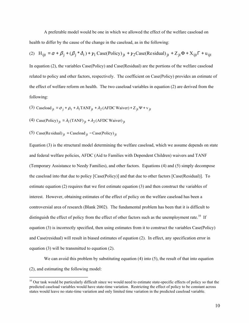
A preferable model would be one in which we allowed the effect of the welfare caseload on

health to differ by the cause of the change in the caseload, as in the following:

(2) ijtijtjtjt2jt1tjjijt uXZ)sidual(ReCase)Policy(Case)*(H +Γ+Φ+++++= γγδββα

In equation (2), the variables Case(Policy) and Case(Residual) are the portions of the welfare caseload

related to policy and other factors, respectively. The coefficient on Case(Policy) provides an estimate of

the effect of welfare reform on health. The two caseload variables in equation (2) are derived from the

following:

(3) jtjt2jt1tjjt vZ)WaiverAFDC(TANFCaseload +Ψ++++= λλρσ

(4) jt2jt1jt )WaiverAFDC()TANF()Policy(Case λλ +=

(5) jtjtjt )Policy(CaseCaseload)sidual(ReCase −=

Equation (3) is the structural model determining the welfare caseload, which we assume depends on state

and federal welfare policies, AFDC (Aid to Families with Dependent Children) waivers and TANF

(Temporary Assistance to Needy Families), and other factors. Equations (4) and (5) simply decompose

the caseload into that due to policy [Case(Policy)] and that due to other factors [Case(Residual)]. To

estimate equation (2) requires that we first estimate equation (3) and then construct the variables of

interest. However, obtaining estimates of the effect of policy on the welfare caseload has been a

controversial area of research (Blank 2002). The fundamental problem has been that it is difficult to

distinguish the effect of policy from the effect of other factors such as the unemployment rate.10 If

equation (3) is incorrectly specified, then using estimates from it to construct the variables Case(Policy)

and Case(residual) will result in biased estimates of equation (2). In effect, any specification error in

equation (3) will be transmitted to equation (2).

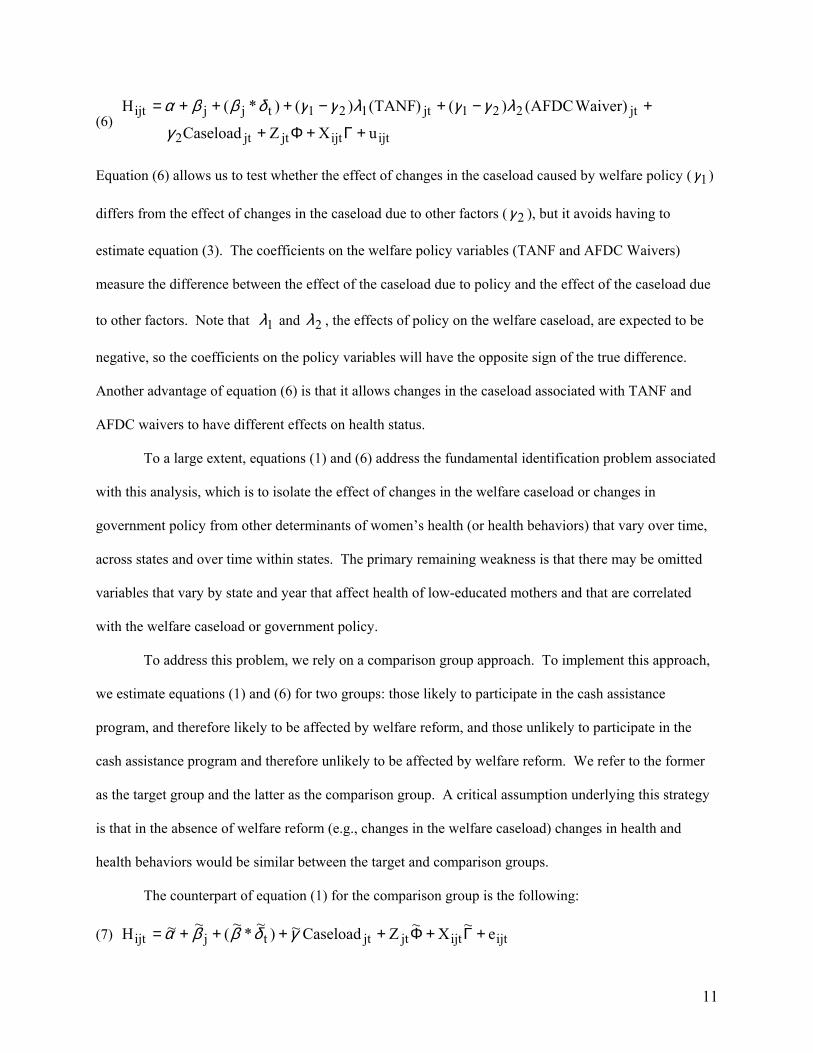
We can avoid this problem by substituting equation (4) into (5), the result of that into equation

(2), and estimating the following model:

10 Our task would be particularly difficult since we would need to estimate state-specific effects of policy so that the predicted caseload variables would have state-time variation. Restricting the effect of policy to be constant across states would leave no state-time variation and only limited time variation in the predicted caseload variable.

11

(6) ijtijtjtjt2

jt221jt121tjjijt

uXZCaseload

)WaiverAFDC()()TANF()()*(H

+Γ+Φ+

+−+−+++=

γλγγλγγδββα

Equation (6) allows us to test whether the effect of changes in the caseload caused by welfare policy ( 1γ )

differs from the effect of changes in the caseload due to other factors ( 2γ ), but it avoids having to

estimate equation (3). The coefficients on the welfare policy variables (TANF and AFDC Waivers)

measure the difference between the effect of the caseload due to policy and the effect of the caseload due

to other factors. Note that 1λ and 2λ , the effects of policy on the welfare caseload, are expected to be

negative, so the coefficients on the policy variables will have the opposite sign of the true difference.

Another advantage of equation (6) is that it allows changes in the caseload associated with TANF and

AFDC waivers to have different effects on health status.

To a large extent, equations (1) and (6) address the fundamental identification problem associated

with this analysis, which is to isolate the effect of changes in the welfare caseload or changes in

government policy from other determinants of women’s health (or health behaviors) that vary over time,

across states and over time within states. The primary remaining weakness is that there may be omitted

variables that vary by state and year that affect health of low-educated mothers and that are correlated

with the welfare caseload or government policy.

To address this problem, we rely on a comparison group approach. To implement this approach,

we estimate equations (1) and (6) for two groups: those likely to participate in the cash assistance

program, and therefore likely to be affected by welfare reform, and those unlikely to participate in the

cash assistance program and therefore unlikely to be affected by welfare reform. We refer to the former

as the target group and the latter as the comparison group. A critical assumption underlying this strategy

is that in the absence of welfare reform (e.g., changes in the welfare caseload) changes in health and

health behaviors would be similar between the target and comparison groups.

The counterpart of equation (1) for the comparison group is the following:

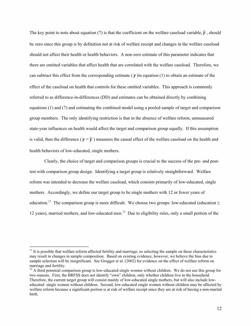
(7) ijtijtjtjttjijt e~X~ZCaseload~)~*~(~~H +Γ+Φ++++= γδββα

12

The key point to note about equation (7) is that the coefficient on the welfare caseload variable,γ~ , should

be zero since this group is by definition not at risk of welfare receipt and changes in the welfare caseload

should not affect their health or health behaviors. A non-zero estimate of this parameter indicates that

there are omitted variables that affect health that are correlated with the welfare caseload. Therefore, we

can subtract this effect from the corresponding estimate (γ )in equation (1) to obtain an estimate of the

effect of the caseload on health that controls for these omitted variables. This approach is commonly

referred to as difference-in-differences (DD) and estimates can be obtained directly by combining

equations (1) and (7) and estimating the combined model using a pooled sample of target and comparison

group members. The only identifying restriction is that in the absence of welfare reform, unmeasured

state-year influences on health would affect the target and comparison group equally. If this assumption

is valid, then the difference ( γγ ~− ) measures the causal effect of the welfare caseload on the health and

health behaviors of low-educated, single mothers.

Clearly, the choice of target and comparison groups is crucial to the success of the pre- and post-

test with comparison group design. Identifying a target group is relatively straightforward. Welfare

reform was intended to decrease the welfare caseload, which consists primarily of low-educated, single

mothers. Accordingly, we define our target group to be single mothers with 12 or fewer years of

education.11 The comparison group is more difficult. We choose two groups: low-educated (education ≤

12 years), married mothers, and low-educated men.12 Due to eligibility rules, only a small portion of the

11 It is possible that welfare reform affected fertility and marriage, so selecting the sample on these characteristics may result in changes in sample composition. Based on existing evidence, however, we believe the bias due to sample selection will be insignificant. See Grogger et al. (2002) for evidence on the effect of welfare reform on marriage and fertility. 12 A third potential comparison group is low-educated single women without children. We do not use this group for two reasons. First, the BRFSS does not identify “own” children, only whether children live in the household. Therefore, the current target group will consist mainly of low-educated single mothers, but will also include low-educated single women without children. Second, low-educated single women without children may be affected by welfare reform because a significant portion is at risk of welfare receipt since they are at risk of having a non-marital birth.

13

comparison groups are at risk of welfare receipt, and for the most part persons in these two groups are

unaffected by changes in the welfare caseload.13

A cursory way to assess the adequacy of the comparison groups is to compare them to the target

group. Ideally, we would like the mean characteristics of the comparison groups to be quite similar to the

mean characteristics of the target group. These figures are shown in Table 1.14 We focus on the initial

years of our analysis, 1993-94, which predated most welfare reform legislation. Figures in Table 1

indicate that the target and comparison groups are approximately the same age and have similar levels of

education, which is not that surprising since age and education were used to select the samples. However,

the target group has a larger proportion of Black, non-Hispanic persons. As would be expected, the target

group and comparison groups differ by family structure, and employment status. Low-educated men

(comparison) have fewer children than low-educated mothers (target), and married mothers (comparison)

have more adults in the household than unmarried mothers (target). Interestingly, the employment rates

of married and unmarried mothers are approximately the same, but low-educated men have somewhat

higher employment rates. In regard to the dependent variables, which we describe in more detail below,

the target and comparison groups are relatively similar except for binge drinking behavior and mental

health. Low-educated men are more likely to binge drink then either married or unmarried mothers, and

married mothers are slightly less likely to binge drink than unmarried mothers. In regard to mental

health, women report a greater incidence of poor mental health days than men, but married and unmarried

mothers have similar means. In general, the target and comparison groups have relatively similar means,

and based on this limited criterion, the comparison groups appear to be adequate.

Data

Our primary data source is the Behavioral Risk Factor Surveillance System (BRFSS) which

provides information on current health behaviors and health status. The BRFSS is an ongoing data

13 Because a portion of the comparison group may be affected and portion of the target group may be unaffected by changes in the welfare caseload, estimates of the “treatment” effect will be biased toward zero. 14 Appendix Table 1 presents means calculated from all available years of data.

14

collection program designed to monitor behavioral risk factors in non-institutionalized adults in the

United States (CDC). Designed to collect state-level data, surveys are fielded by the states through

telephone interviews using a probability sampling design.15 In our multivariate regressions, we use

weights developed by the BRFSS to make the data representative of state populations. We use data from

survey years 1993 through 2001, a period that spans welfare reform. These data were collected by all 50

states and the District of Columbia, with the exception that Wyoming did not participate in 1993.

We focus on low-educated women because this is the target group of welfare reform.

Specifically, we define the target group to be unmarried mothers between the ages of 19 and 39 who have

12 or fewer years of education. As previously noted, we use two comparison groups in the analysis: low-

educated (education ≤ 12 years), married mothers and low-educated (education ≤ 12 years) men,

regardless of marital and parental status. Both comparison groups are restricted to individuals between

the ages of 19 and 39.

The BRFSS contains most of the data necessary to complete our analysis. We focus on three

health behaviors, cigarette smoking, alcohol intake, and exercise and on two self-assessed health status

measures, mental health and general health.16 More specifically, the outcomes we study are daily

smoking, binge drinking, engaging in regular and sustained physical activity, mental health reported as

being “not good” for one or more days in the last month, and reporting fair or poor health (rather than

good, very good, or excellent health).

Due to changes in tobacco-related questions in the BRFSS during the study years, the daily

smoking variable was constructed slightly differently in the three survey years 1993 – 1995, than it was in

the remaining six years. From 1996 on, respondents were specifically asked whether they smoke every

day. For 1993, we coded respondents as daily smokers if they reported current smoking and did not

respond “Don’t smoke regularly” to a question asking number of cigarettes currently smoked per day.

15 Sampling designs have varied somewhat across survey years and states. All 50 states and the District of Columbia whose data are included in this study used a disproportionate stratified sample design in 2001 Samples are identified through telephone-based methods (CDC, 2001). 16 We often used two different measures of each health behavior, and we report on these findings below. For example, we use a dichotomous indicator of binge drinking and the number of binge drinking occasions.

15

For 1994 and 1995, current smokers were coded as daily smokers if they indicated that they smoked on

30 of the last 30 days.

Survey questions on alcohol use and exercise are included on a rotating basis in the core

questionnaire required of all participating states. For this reason, we use data on those behaviors only

from the odd years, in the case of alcohol, and the even years, in the case of exercise. The binge drinking

variable was constructed as a dichotomous variable from responses to a question asking number of times

in the last month that the respondent had 5 or more drinks on an occasion. Anyone giving an answer of

one time or more to this question was coded as “1” on binge drinking. Nondrinkers and those who

answered zero were coded as “0”. The dichotomous variable indicating regular and sustained exercise is

constructed by the BRFSS from responses to several questions regarding physical activity habits. Criteria

for coding has varied slightly over the survey years but generally indicates engaging in physical activity

for 30 or more minutes 5 or more times per week, regardless of how vigorous is the activity.17

The reliability of BRFSS data has been investigated in several test-retest studies (e.g., Shea, et al.,

1991; Stein, et al., 1995). Some degree of misreporting of behaviors perceived to be socially undesirable,

like smoking and heavy drinking, is known to occur. However, studies comparing self-reported to

biochemical measures have generally found a high degree of sensitivity and specificity of the self-report

measures (Patrick, et al., 1994; Poikolainen et al., 2002; Wagenknecht, et al., 1992). Heavy drinkers

underestimate their alcohol intake more than light drinkers (Poikolainen, Podkletnov, and Alho). Our

measure of binge drinking, because it is a simple dichotomous measure indicating zero, versus one or

more binge drinking occurrences, does not rely on reporting accuracy along increasing levels of intake.

Also, there is no obvious reason to think that reporting accuracy within any of the three groups we have

identified should have varied over time or with changes in welfare caseload and so, for these reasons,

should not affect our results.

17 BRFSS documentation on the calculated physical activity variable contains the following note: “See article ‘Description of the Scoring System for the Physical Activity Questions of the Behavioral Risk Factor Surveillance System’ written by Carl Caspersen, PhD (770-488-5513) for computation of the scoring system (activity levels)” (CDC, 2000).

16

The BRFSS also contains basic demographic information that can be used to construct control

variables. As noted, we define our target and comparison groups on the basis of education and marital

status. Other personal characteristics included in the model include: household size (number of children

and number of adults), age, race, and high school graduation or GED.

A limitation of BRFSS data is that it does not specifically identify parents. Rather, questions

related to children inquire about children in the household. For the purposes of this analysis we assume

that anybody indicating children in the household was a parent. This would not have affected the second

group, men, because that group included all low-educated men, aged 19-39. However, since we use these

data to identify single and married mothers, this will have resulted in an unknown degree of

misspecification of the target and first comparison groups. To investigate its likely impact on our results,

we identified a subgroup of women who, by virtue of their indicating that only one adult lived in that

household, we felt certain were true single mothers. We estimated regression models identical to those

we report on below using this group. The results from this analysis were substantively comparable, as

when we used the whole sample of single women with children in the household.

Finally, the BRFSS provides respondents’ state of residence, which allows us to append state-

level information. We use the following: state and federal welfare policy; monthly state welfare caseload;

Medicaid income eligibility threshold; current unemployment rate and one-year lag; and real per-capita

income.18 State Medicaid eligibility variables are defined on the basis of Medicaid eligibility of pregnant

women; we use the following categories: 0 to 133 percent of federal poverty line, 134 to 199 percent of

federal poverty line, and above 200 percent of the federal poverty line.

The monthly welfare caseload data is taken from the Administration for Children and Families.

We measure the caseload as the natural logarithm of the caseload. It is matched to the month prior to the

BRFSS interview. To best reflect employment conditions affecting survey respondents, those

18 Unemployment statistics are from the U.S. Department of Labor, Bureau of Labor Statistics, http://www.bls.gov/data/home.htm/. State Medicaid eligibility were provided by Aaron Yellowitz and updated with data from the National Governor’s Association, in their annual Maternal and Child Health (MCH) Update reports, http://www.nga.org/center/divisions/1,1188,C_ISSUE_BRIEF^D_5114,00.html/.

17

interviewed in the first half of the year were assigned the employment rate for the prior year while those

interviewed in the last six months of the year were assigned the rate for that year. The data on welfare

policies is drawn from Assistant Secretary for Planning and Evaluation of the Department of Health and

Human Services, as well as from the Urban Institute

(www.urban.org/content/Research/NewFederalism/Data/StateDatabase/StateDatabase.htm) and the State

Documentation Project of the Center on Budget and Policy Priorities (www.cbpp.org).

We follow the earlier literature on the effects of welfare reform and use dummy variables for

whether a state had implemented an AFDC waiver or TANF at the time (month) of the BRFSS interview.

We set the waiver variable to zero when TANF is implemented. However, we also use a more detailed

specification of welfare policy; specifically, we create three dummy variables that indicate whether a state

had implemented time-limited benefits, had an exemption from work requirements only for women with

children under six-months of age, and had full financial sanctions for non-compliance.

Results

Tables 2 through 6 present ordinary least squares regression estimates of the parameters of

equations (1) and (6) for the target and comparison groups. We also present difference-in-differences

(DD) estimates. We estimate two versions of equation (6). One that characterizes welfare reform using

dummy variables indicating that a state has implemented an AFDC waivers or TANF, and another that

characterizes welfare reform using dummy variables indicating that a state has implemented different

aspects of reform: time-limited benefits, strict work exemption policy, and a strict sanction for

noncompliance policy. Standard errors have been constructed under the assumption that observations

within states may not be independent (Bertrand et al. 2002). We also include the sampling weight as an

independent variable to account for sampling design.

We begin by examining the relationship between the welfare caseload and three health behaviors:

smoking, drinking, and exercise. Table 2 presents estimates of the association between the welfare

caseload and welfare policies and the probability of daily smoking. Panel one contains estimates of

18

equation (1). These estimates indicate that the association between the natural logarithm of the welfare

caseload and the probability of daily smoking is not statistically significant for any of the samples.

Further the magnitudes of the estimates are quite small. For example, according to data from the

Administration for Children and Families (http://www.acf.dhhs.gov/news/tables.htm) between January

1996 and June 2000, the welfare caseload declined by 0.74 log points (52 percent). A decline of this

magnitude is associated with a 1.6 percentage point, or four percent, decline in daily smoking among low-

educated, unmarried mothers (target group). Other estimates in panel one imply similarly small

associations. Difference-in-difference estimates are also not statistically significant and small.

In panels two and three of Table 2, we present estimates of equation (6). The addition of the

welfare policy variables makes little difference. The estimates of the association between the welfare

caseload and daily smoking are not statistically significant and remain small in magnitude. Estimates

associated with the policy variables are mostly not statistically significant. The exception is the indicator

for a strict financial sanction policy. The estimate is positive, which indicates that changes in the

caseload due to sanction policy had a less positive association with daily smoking than did changes in the

caseload due to other reasons. In fact, the algebraic relations embedded in equation (6) suggest that

changes in the caseload due to sanction policy were negatively associated with daily smoking; a decrease

in the caseload due to sanction policy is associated with an increase in daily smoking. To see how we

reached this conclusion, note that the coefficient on the sanction variable is 0.027 and is equal to the

following: 121 )( λγγ − (from equation 6). 1γ is the association between changes in the caseload due to

sanctions and daily smoking, and 2γ is the association between changes in the caseload due to other

factors and daily smoking. Estimates of equation (6) provide an estimate of 2γ , which is equal to 0.036

(Table 2). 1λ is the change in the (log) caseload due to sanction policy. If we assume that it is equal to -

0.2, which is in the range reported by Blank (2002) and which implies that sanctions were responsible for

approximately 20 percent of the change in caseload, then 1γ is equal to -0.099. Thus, a 0.74 log point, or

52 percent, decrease in the welfare caseload as a result of financial sanctions would increase daily

19

smoking by 7.3 percentage points, or 19 percent. We note, however, that the estimate associated with

sanctions is also statistically significant for married mothers and that the difference-in-differences

estimate is virtually zero. Thus, we conclude that changes in the welfare caseload, whether because of

policy or for other reasons are not associated with daily smoking of low-educated single mothers.

The next health behavior we examine is binge drinking. Table 3 presents the estimates of the

association between the welfare caseload and the probability of binge drinking in the last month.

Estimates in panel one show that changes in the welfare caseload are positively associated with binge

drinking for single mothers. A 0.74 log point decline in the welfare caseload is associated with a 4.2

percentage point, or 30 percent, decrease in the probability of binge drinking. Moreover, the welfare

caseload is not associated with the binge drinking of low-educated, married mothers or low-educated

men. The difference-in-difference estimates are positive and significant and of the same approximate

magnitude as the estimate associated with the target group. This provides evidence that the significant

association between changes in the welfare caseload and binge drinking is not general, but specific to the

low-educated single mothers—the group most likely to be affected by changes in the caseload. If the

identifying assumption of the difference-in-difference analysis holds, this association can be considered

causal. Decreases in the welfare caseload caused low-educated mothers to decrease their binge drinking

by a significant amount.

The estimates in panels two and three of Table 3 reveal that the coefficients associated with the

policy variables are not statistically significant. Moreover, the addition of these variables had relatively

little effect on the estimate of the effect of the welfare caseload. This implies that the association between

changes in the caseload and binge drinking does not differ by the underlying cause of the caseload

change. The binge drinking behavior of low-educated single mothers who changed welfare status

because of policy is the same as the binge drinking behavior of low-educated mothers who changed

welfare status for other reasons. We also estimated models in which the dependent variable was the

number of binge drinking occasions in the last month. The results form this analysis were qualitatively

the same as those reported except that estimates were not as precise and the p-values were higher.

20

Table 4 presents estimates of the association between changes in the welfare caseload and the

probability of engaging in regular and sustained physical activity. In this case, estimates in panel one

indicate that changes in the caseload are negatively associated with being regularly physically active

among single mothers. For the comparison groups, changes in the caseload are positively related to

physical activity. Accordingly, the DD estimates are negative, and when men are used as a comparison

group, statistically significant. However, the DD estimates associated with both comparison groups are of

the same magnitude. DD estimates indicate that the decline in the welfare caseload between January

1996 and June 2000 (52 percent or 0.74 log points) is associated with approximately a four percentage

point, or 27 percent, increase in the probability of engaging in regular and sustained physical activity. We

also obtained estimates of the association between welfare caseload and the probability of engaging in

any leisure-time physical activity. In this case, the caseload was negatively associated with physical

activity among single mothers, but not statistically significant. DD estimates related to this outcome were

close to zero.

Estimates in panel two and three suggest similar effects, although DD estimates associated with

some of the policy variables are relatively large. For example, the coefficient on time limits is 0.039 and

statistically significant and the estimate of the effect of the caseload is much smaller than in panel one.

The coefficient on time limits implies that changes in the welfare caseload due to time-limited benefits are

negatively associated with regular physical activity. The implied estimate is -0.22, which is much larger

than the estimate associated with the caseload itself.19 Thus changes in the welfare caseload due to time-

limited benefits have a larger (more negative) effect on physical activity than changes in the caseload due

to other factors.20 A similar result pertains to the coefficient on AFDC waivers. The positive coefficient,

which approaches statistical significance, suggests that changes in the caseload due to AFDC waivers had

a larger (more negative) effect on physical activity than changes in the caseload due to other reasons.

19 The estimate was obtained using equation (6) and similar assumptions as those described in the text. 20 We recognize that the estimate, -0.22, may be implausibly large, but we also recognize that the calculations used to obtain the estimate are somewhat crude and subject to significant sample variation.

21

We now turn to an examination of the association between the welfare caseload and health status,

which we measure in two ways: the probability of reporting a non-zero number of days in poor mental

health in the last month; and the probability of reporting fair or poor health.21 Table 5 presents estimates

of the association between changes in the welfare caseload and the probability of having poor mental

health. None of the estimates associated with the welfare caseload are statistically significant, and all are

small in magnitude. The same is true in Table 6; all estimates of the association between the welfare

caseload and poor health status are not significant and small in magnitude. Overall, estimates in Tables 5

and 6 indicate that changes in the welfare caseload are not associated with self-reported mental health or

self-reported general health.

Conclusions

Declines in the welfare caseload in the late 1990s brought significant change to the lives of many

low-educated single mothers. Many single mothers left welfare and entered the labor market and others

re-arranged their lives in new ways in order to avoid going on public assistance.22 These changes may

have affected the health and health behaviors of these women. Switching from unpaid household work to

paid employment may affect the amount of physical activity and psychological stress, and it may alter

financial circumstances, all of which may affect health and health behaviors. Similarly, other strategies to

avoid public assistance such as cohabitation with a partner or family member may affect physical and

mental health, and health behaviors. Moreover, because welfare is an important entry point for Medicaid,

changes in the welfare caseload may have affected health insurance coverage, which may affect health.

To date, there has been no study of this issue, which is surprising because of the central role that

health plays in personal wellbeing. In contrast, there has been an outpouring of research on the effects of

21 We also examined the effect of welfare reform on the probability of being overweight. Results from this analysis were similar to those reported below—estimates of the association were not statistically significant and small in magnitude. 22 One way to avoid public assistance is to alter living arrangements including cohabitating with a partner, or co-residing with parents and other family members. However, there is little evidence as to the effect of welfare reform on living arrangements (Bitler et al. 2002; Grogger et al. 2002).

22

changes in the welfare caseload and welfare reform on material wellbeing. In this paper, we addressed

this shortfall of research. We obtained estimates of the association between the welfare caseload and

welfare policies, and three health behaviors—smoking, drinking, and exercise—and two self-reported

measures of health—days in poor mental health, and overall health status. Importantly, we allowed the

association between changes in the caseload and these outcomes to differ by whether the change in the

caseload was due to policy or other factors such as a strong economy. In addition, we employed a

research design that under certain assumptions yields causal estimates of the association between the

welfare caseload and health. Our attempt to obtain causal estimates is important because policy

development and evaluation requires knowledge of causal pathways. This makes our study relevant to the

current Congressional debate over the renewal of the Personal Responsibility and Work Opportunity

Reconciliation Act (PRWORA).

The results of our study reveal that changes in the caseload had little effect on measures of health

status, but were significantly associated with two health behaviors: binge drinking and regular exercise.

Changes in the welfare caseload were positively and significantly related to binge drinking. Decreases in

the welfare caseload such as those that occurred between January 1996 and June 2000 were associated

with a 3.7 percentage point, or 27 percent, decrease in the probability of binge drinking in the past month

among low-educated single mothers. Similar results were also found when we studied the number of

binge drinking occasions in the past month instead of the incidence of binge drinking. Further, estimates

suggested that the association between changes in the welfare caseload and binge drinking did not differ

by the underlying cause of the caseload change. Changes due to policy had similar effects as changes due

to other factors such as the economy.

Interestingly, the relationship between changes in the welfare caseload and binge drinking was

virtually unchanged when we added employment status to the regression model. The transition from

welfare to paid employment, which includes what we have referred to as welfare-to-work and work-to-

work transitions, was responsible for a significant portion of the decline in the caseload. Therefore, we

hypothesized that the inclusion of employment status in the model would greatly reduce the association

23

between welfare caseload and binge drinking since much of the change in the caseload is associated with

an increase in paid employment. The fact that it did not suggests that the association between changes in

the welfare caseload and binge drinking is not a consequence of greater employment. In fact,

employment status (i.e., employed) was positively and significantly related to binge drinking for low-

educated, single mothers (estimates not shown). This is inconsistent with the positive association

between the welfare caseload and binge drinking. If much of the decline in the caseload was employment

related, and employment is positively related to binge drinking, then decreases in the caseload should

increase binge drinking, which is not what we found.23 The inconsistency is most likely due to the fact

that employment status is not exogenous; employed persons differ from unemployed persons in

unobserved ways. Therefore, the relationship between employment status and binge drinking is likely

confounded by omitted factors. In contrast, declines in the welfare caseload are much more likely to be

associated with exogenous changes in employment since most of the decline was due to policy changes

and a strong economy—two exogenous factors. The fact that the association between binge drinking and

the welfare caseload was not diminished by the inclusion of employment status implies that the decrease

in binge drinking associated with the decline in the caseload occurred equally among those whose

transitions ended in employment and those whose transitions did not end in employment.

We hypothesized that changes in the caseload would affect alcohol use primarily because of

changes in psychological distress. If this hypothesis is correct, the findings suggest that declines in the

caseload were associated with less distress. However, we did not find an improvement in mental health,

as currently measured. We also did not observe any change in the effect of the caseload when we

included the mental health indicator in the regression. An alternative explanation is that changes in the

caseload may have affected coping skills that resulted in less binge drinking. It is clear from this

discussion, that further study is required to identify the underlying reason for the association between

changes in the welfare caseload and changes in binge drinking.

23 The positive effect of employment on binge drinking is consistent with evidence in Ruhm (1995) that alcohol sales are procyclical—increase when employment increases.

24

Changes in the welfare caseload were also significantly associated with the probability of

engaging in regular and sustained physical activity. Decreases in the caseload were associated with

increases in physical activity. In this case, there was some evidence that changes in the caseload due to

policy had larger (more negative) effects than changes in the caseload due to other reasons. However, the

coefficients on the policy variables in these models did not have consistent signs and most were not

statistically significant. Therefore, we view this evidence as at best suggestive. Here too, the association

between changes in the caseload and physical activity was unaffected by the addition of employment

status to the model, but in this case, the estimate associated with employment status was not statistically

significant.24 So again, the association between changes in the caseload and physical activity occurred

equally among women whose transition ended in employment and women whose transition did not end in

employment.

Intuition suggests that decreases in the caseload would be associated with less exercise, as time

constraints become more burdensome because of the greater labor market commitment. We find the

opposite. But we also do not find that the increase in physical activity is a consequence of greater

employment. So those who transition to employment are not the only women who increased their

physical activity. Again, our analysis is unable to identify the underlying reasons and we can only

conjecture about the possible mechanisms. More study is needed to uncover the mechanisms and to

validate our findings.

Overall, our results suggest that the recent declines in the caseload have lead to healthier lifestyles

among low-educated single mothers. Decreases in the caseload are associated with less binge drinking

and greater exercise. Notably, the improvements in lifestyle associated with the decrease in the welfare

caseload were not due to greater employment. This suggests that lifestyle improvements were

experienced by women in all of the five transition groups described above, and not just those that made

the transition to paid employment. We also explored whether changes in the caseload due to welfare

24 Ruhm (2000) showed that a decrease in unemployment rate (greater employment) is associated with a decrease in exercise. So we expected to find that employment was negatively related to regular physical exercise. We did not.

25

reform policies had a differential effect on health and health behaviors than changes in the caseload due to

other factors. On this point the results were mixed. In the case of binge drinking, there did not appear to

be any difference between the broad categories of “welfare leavers”. But for physical activity, there was

some evidence that those who left the caseload because of policy (e.g., time-limited benefits) were more

likely to increase their physical activity than those who left the caseload for other reasons. The evidence

on this point was not robust and therefore suggests that this conclusion remain tentative.

In sum, the results of this analysis suggest that welfare reform and the decrease in the welfare

caseload have not adversely affected the health of low-educated, single mothers. This finding is

consistent with research by Kaestner and Kaushal (2003) who find that welfare reform had modest

adverse effects on the health insurance coverage of this group. These findings should prove useful in the

current debate over the merits of the 1996 federal welfare reform law and whether it should be renewed.

26

References

Acs, Gregory, Pamela Loprest, and Tracey Roberts. 2001. “Final Synthesis Report of Findings from ASPE ‘Leavers’ Grants.” Washington, D.C.: Urban Institute Press. Available at http://aspe.hhs.gov/search/hsp/leavers99/synthesis02/index.htm

Ali, Jennifer, and William R. Avison. 1997. “Employment Transitions and Psychological Distress: The

Contrasting Experiences of Single and Married Mothers.” Journal of Health and Social Behavior 38:345-362.

Barnett, Rosalind C., and Nancy L. Marshall. 1992. “Worker and Mother Roles, Spillover Effects, and

Psychological Distress.” Women and Health 18:9-40. Bertrand, M., Duflo, E., and Mullainathan, S. 2002. “How Much Should We Trust Difference-in-

Differences Estimates?” NBER WP 8841. Cambridge, MA: National Bureau of Economic Research.

Bitler, Marianne, Jonah Gelbach, and Hillary Hoynes. 2002. “The Impact of Welfare Refom on Living

Arrangements.” NBER Working Paper #8784, National Bureau of Economic Research, Cambridge, MA.

Blank, R. 2002. “Evaluating welfare reform in the United States.” Journal of Economic Literature

40(4):1-43. Centers for Disease Control and Prevention (CDC). Behavioral Risk Factor Surveillance System Survey

Data. Atlanta, Georgia: U.S. Department of Health and Human Services, Centers for Disease Control and Prevention, 1993-2001.

Centers for Disease Control and Prevention. 2001. “Overview: BRFSS 2001.”

http://www.cdc.gov/brfss/ti-surveydata2001.htm. Centers for Disease Control and Prevention. 2000. “Calculated Variables in Data Files.”

http://www.cdc.gov/brfss/ti-surveydata2000.htm. Cooper, M. Lynne, Marcia Russell, Jeremy B. Skinner, Michael R. Frone, and Pamela Mudar. 1992.

“Stress and Alcohol Use: Moderating Effects of Gender, Coping, and Alcohol Expectancis.” Journal of Abnormal Psychology 101:139-152.

Coverman, Shelley. 1989. “Role Overload, Role Conflict, and Stress: Addressing Consequences of

Multiple Role Demands.” Social Forces 67:965-982. Duncan, Greg J., P. and Lindsay Chase-Lansdale. 2001. “Welfare Reform and Children’s Well-being.” In

The New World of Welfare, edited by Blank, Rebecca M. and Ron Haskins. Washington, D.C.: Brookings Institution Press. 391-412.

Elliott, Marta. 1996. “Impact of Work, Family, and Welfare Receipt on Women’s Self-Esteem in Young

Adulthood.” Social Psychology Quarterly 59:80-95. Edin, Kathryn and Laura Lein. 1997. “Making Ends Meet: How Single Mothers Survive Welfare And

Low-Wage Work.” New York: Russell Sage Foundation.

27

Ensminger, Margaret. 1996. “Welfare and Psychological Distress: A Longitudinal Study of Afircan American Urban Mothers.” Journal of Health and Social Behavior 36(4):246-359.

Fenwick, Rudy, and Mark Tausing. 1994. “The Macroeconomic Context of Job Stress.” Journal of

Health and Social Behavior 35:266-282. Frone, Michael R., Marcia Russell, and M. Lynne Cooper. 1993. “Relationship of Work-Family

Conflict, Gender, and Alcohol Expectancies to Alcohol Use/Abuse.” Journal of Organizational Behavior 14:545-558.

Frone, Michael R. 1999. “Work Stress and Alcohol Use.” Alcohol Research and Health 23:284-291. Garrett, Bowen and John Holohan. 2000. “Health Insurance Coverage After Welfare.” Health Affairs.

19:175-184. Garrett, Bowen and Julie Hudman. 2002. “Women Who Left Welfare: Health Care Coverage, Access and

Use of Health Services.” The Kaiser Commission on Medicaid and the Uninsured, Washington, DC.

Greeno, Catherine G., and Rena R. Wing. 1994. “Stress-Induced Eating.” Psychological Bulletin

115:444-464. Grogger, Jeff, Lynn Karoly, and Jacob Klerman. 2002. “Consequences of Welfare Reform: A Research

Synthesis.” DRU-2676-Depatment of Health and Human Services. Guyer, Jocelyn. 2000. “Health Care After Welfare: An Update of the Findings from State-Level Leaver

Studies.” Washington, DC: Center on Budget and Policy Priorities. Hamilton, Gayle. 2002. “Moving People from Welfare to Work: Lessons from the National Evaluation of

Welfare-to-Work Strategies.” http://aspe.hhs.gov/hsp/NEWWS/synthesis02/ Haskins, Ron. 2001. “Effects of Welfare Reform on Family Income and Poverty.” In The New World of

Welfare, eds. Rebecca Blank and Ron Haskins. Washington, DC: The Brookings Institution. Haw, Mary Ann. 1982. “Women, Work and Stress: A Review and Agenda for the Future.” Journal of

Health and Social Behavior 23:132-144. Joyce, Theodore, Robert Kaestner, and Sanders Korenman. 2003. “Welfare Reform and Non-marital

Fertility in the 1990s: Evidence From Birth Records” Chicago: University of Illinois at Chicago. Unpublished manuscript.

Kaestner, Robert, and Neeraj Kaushal. In press. “Welfare Reform and Health Insurance Coverage of

Low-income Families.” Journal of Health Economics. Kassel, Jon D., Carol A. Paronis, and Laura R. Stroud. 2003. “Smoking, Stress, and Negative Affect:

Correlation, Causation, and Context Across Stages of Smoking.” Psychological Bulletin 129:270-304.

Korn, Edward L. and Barry I. Graubard. 1995. “Analysis of Large Health Surveys: Accounting for the

Sampling Design.” Journal of the Royal Statistical Society: Series A. 158:263-295.

28

Lennon, Mary Clare. 1994. “Women, Work, and Well-Being: The Importance of Work Conditions.” Journal of Health and Social Behavior 35:235-247.

Lennon, Mary Clare, and Sarah Rosenfield. 1992. “Women and Mental Health: The Interaction of Job

and Family Conditions.” Journal of Health and Social Behavior 33:316-327. Lerman, Robert. 2001. “Less Educated Single Mothers Achieved High Wage and Employment Gains in

the mid 1990s.” Single Parents’ Earnings Monitor October 26, 2001, Urban Institute. Lillard, L.A. and C.W.A. Panis. 1996. "Marital Status and Mortality: The Role of Health." Demography

33:313-27. Mitchell, Shari L., and Kenneth A. Perkins. 1998. “Interaction of Stress, Smoking, and Dietary Restraint

in Women.” Physiology and Behavior 64:103-109. Murray, John E. 2000. “Marital Protection and Marital Selection: Evidence from a Historical-Prospective

Sample of American Men” Demography 37(4):511-521. O’Campo, Patricia, and Lucia Rojas-Smith. 1998. “Welfare Reform and Women’s Health: Review of the

Literature and Implications for State Policy.” Journal of Public Health Policy 19(4):420-446. Oliver, Georgina, and Jane Wardle. 1999. “Perceived Effects of Stress on Food Choice.” Physiology

and Behavior 66:511-515. Patrick, Donald L., Allen Cheadle, Diane C. Thompson, Paula Diehr, Thomas Koepsell, and Susan Kinne.

1994. “The Validity of Self-reported Smoking: A Review and Meta-analysis.” American Journal of Public Health 84: 1086-1093.

Pearling, Leonard I., and Clarice W. Radabaugh. 1976. “Economic Strains and the Coping Function of

Alcohol.” American Journal of Sociology 82:652-663. Peirce, Robert S., Michael R. Frone, Marcia Russell, and M. Lynn Cooper. 1994. “Relationship of

financial Strain and Psychosocial Resources to Alcohol Use and Abuse: The Mediating Role of Negative Affect and Drinking Motives.” Journal of Health and Social Behavior 35:291-308.

Poikolainen, Kari, Irina Podkletnov, and Hannu Alho. 2002. “Accuracy of Quantity-Frequency and

Graduated Frequency Questionnaires in Measuring Alcohol Intake: Comparison with Daily Diary and Commonly Used Laboratory Markers.” Alcohol and Alcoholism 36:573-576.

Pugliesi, Karen. 1995. “Work and well-being: Gender Differences in the Psychological Consequences of

Employment.” Journal of Health and Social Behavior 36:57-71. Reskin, Barbara F., and Shelley Coverman. 1985. “Sex and Race in the Determinants of Psychophysical

Distress: A Reappraisal of the Sex-Role Hypothesis.” Social Forces 63:1038-1059. Rosenfield, Sarah. 1989. “The Effects of Women’s Employment: Personal Control and Sex Differences

in Mental Health.” Journal of Health and Social Behavior 30:77-91. Ross, Catherine E., and Joan Huber. 1985. “Hardship and Depression.” Journal of Health and Social

Behavior 26:312-327.

29

Ruhm, Christopher J. 1995. “Economic Conditions and Alcohol Problems.” Journal of Health Economics 14:583-603.

Ruhm, Christopher J. 2000. “Are Recessions Good for Your Health?” Quarterly Journal of Economics

115(2):617-650. Ruhm, Christopher J. 2003. “Healthy Living in Hard Times.” NBER Working Paper 9468. National

Bureau of Economic Research, Cambridge, MA. Sayette, Michael A. 1999. “Does Drinking Reduce Stress?” Alcohol Research and Health 23:250-255. Shea, Steven, Aryeh D. Stein, Rafael R. Lantigua, and Charles E. Basch. 1991. “Reliability of the

Behavioral Risk Factor Survey in a Triethnic Population.” American Journal of Epidemiology 133:489-500.

Smith, James P. 1999. “Healthy Bodies and Thick Wallets: The Dual Relation Between Health and

Economic Status.” Journal of Economic Perspectives. 13:145-166. Stein, Aryeh D., Jeanne M. Courval, Ruth I. Lederman, and Steven Shea. 1995. “Reproducibility of

REsponses to Telephone Interviews: Demographic Predictors of Discordance in Risk Factor Status.” American Journal of Epidemiology 141: 1097-1105.

Thoits, Peggy A. 1986. “Multiple Identities: Examining Gender and Marital Status Differences in

Distress.” American Sociological Review 51:259-272. Wagenknecht, Lynne E., Gregory L. Burke, Laura L. Perkins, Nancy J. Haley, Gary D. Friedman. 1992.

“Misclassification of Smoking Status in the CARDIA Study: A Comparison of Self-report with Serum Cotinine Levels.” American Journal of Public health 82:33-36.

Wardle, Jane, Anderw Steptoe, Georgina Oliver, and Zara Lipsey. 2000. “Stress, Dietary Restraint and

Food Intake.” Journal of Psychosomatic Research 48:195-202. Weinstein, Suzanne E., David J. Shide, and Barbara J. Rolls. 1997. “Changes in Food Intake in

Response to Stress in Men and Women: Psychological Factors.” Appetite 28:7-18. Zedlewski, Sheila R. and Pamela Loprest. 2001. “Will TANF Work for the Most Disadvantaged

Families?” In The New World of Welfare, edited by Blank, Rebecca M. and Ron Haskins. Washington, D.C.: Brookings Institution Press. 311-328.

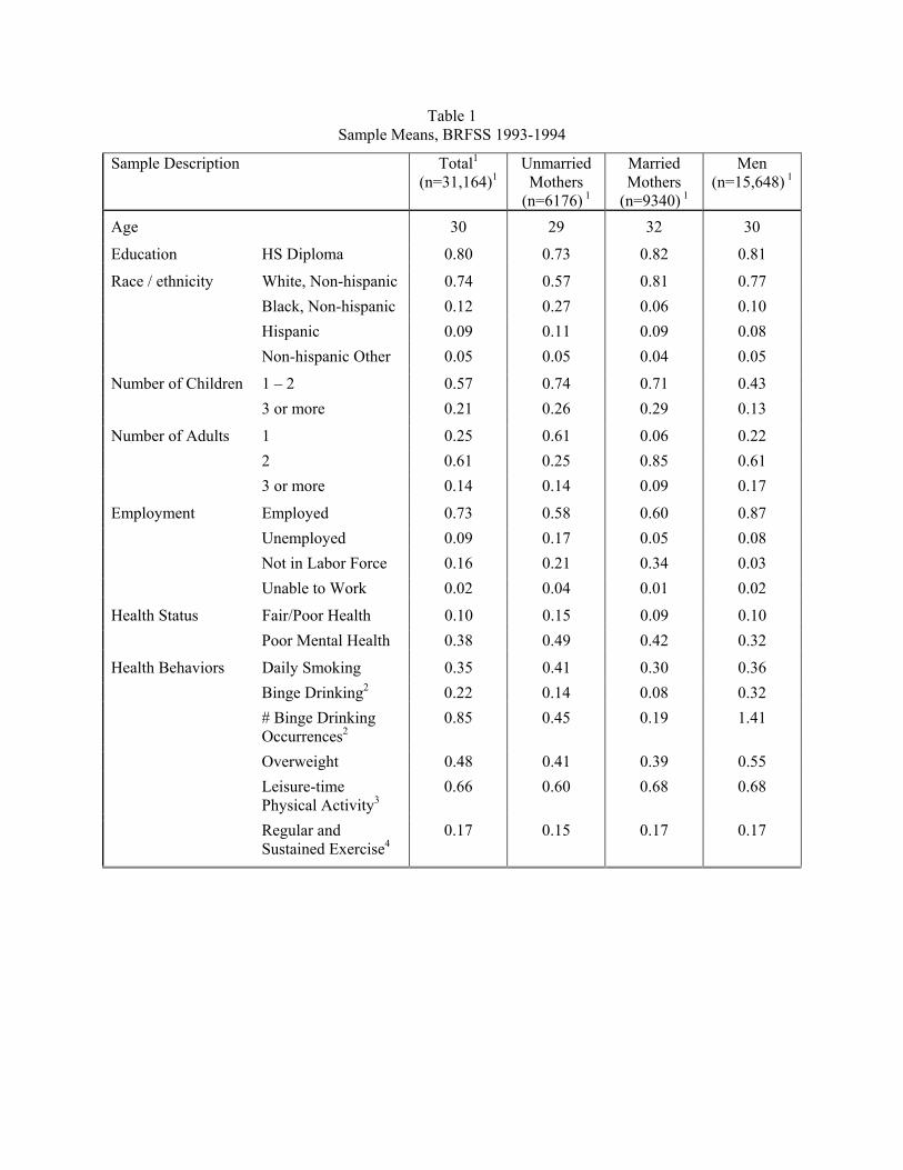
Table 1 Sample Means, BRFSS 1993-1994

Sample Description Total1 (n=31,164)1

Unmarried Mothers

(n=6176) 1

Married Mothers

(n=9340) 1

Men (n=15,648) 1

Age 30 29 32 30

Education HS Diploma 0.80 0.73 0.82 0.81

Race / ethnicity White, Non-hispanic 0.74 0.57 0.81 0.77 Black, Non-hispanic 0.12 0.27 0.06 0.10 Hispanic 0.09 0.11 0.09 0.08 Non-hispanic Other 0.05 0.05 0.04 0.05

Number of Children 1 – 2 0.57 0.74 0.71 0.43 3 or more 0.21 0.26 0.29 0.13

Number of Adults 1 0.25 0.61 0.06 0.22 2 0.61 0.25 0.85 0.61 3 or more 0.14 0.14 0.09 0.17

Employment Employed 0.73 0.58 0.60 0.87 Unemployed 0.09 0.17 0.05 0.08 Not in Labor Force 0.16 0.21 0.34 0.03 Unable to Work 0.02 0.04 0.01 0.02

Health Status Fair/Poor Health 0.10 0.15 0.09 0.10 Poor Mental Health 0.38 0.49 0.42 0.32

Health Behaviors Daily Smoking 0.35 0.41 0.30 0.36 Binge Drinking2 0.22 0.14 0.08 0.32 # Binge Drinking

Occurrences2 0.85 0.45 0.19 1.41

Overweight 0.48 0.41 0.39 0.55 Leisure-time

Physical Activity3 0.66 0.60 0.68 0.68

Regular and Sustained Exercise4

0.17 0.15 0.17 0.17

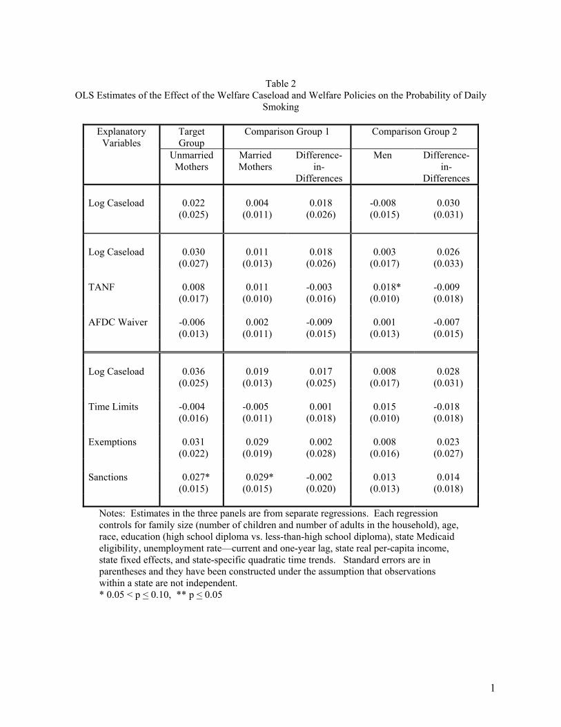
1

Table 2

OLS Estimates of the Effect of the Welfare Caseload and Welfare Policies on the Probability of Daily Smoking

Target Group

Comparison Group 1 Comparison Group 2 Explanatory Variables

Unmarried Mothers

Married Mothers

Difference-in-

Differences

Men Difference-in-

Differences Log Caseload 0.022

(0.025) 0.004

(0.011) 0.018

(0.026) -0.008 (0.015)

0.030 (0.031)

Log Caseload 0.030

(0.027) 0.011

(0.013) 0.018

(0.026) 0.003

(0.017) 0.026

(0.033) TANF 0.008

(0.017) 0.011

(0.010) -0.003 (0.016)

0.018* (0.010)

-0.009 (0.018)

AFDC Waiver -0.006

(0.013) 0.002

(0.011) -0.009 (0.015)

0.001 (0.013)

-0.007 (0.015)

Log Caseload 0.036

(0.025) 0.019

(0.013) 0.017

(0.025) 0.008

(0.017) 0.028

(0.031) Time Limits -0.004

(0.016) -0.005 (0.011)

0.001 (0.018)

0.015 (0.010)

-0.018 (0.018)

Exemptions 0.031

(0.022) 0.029

(0.019) 0.002

(0.028) 0.008

(0.016) 0.023

(0.027) Sanctions 0.027*

(0.015) 0.029*

(0.015) -0.002 (0.020)

0.013 (0.013)

0.014 (0.018)

Notes: Estimates in the three panels are from separate regressions. Each regression controls for family size (number of children and number of adults in the household), age, race, education (high school diploma vs. less-than-high school diploma), state Medicaid eligibility, unemployment rate—current and one-year lag, state real per-capita income, state fixed effects, and state-specific quadratic time trends. Standard errors are in parentheses and they have been constructed under the assumption that observations within a state are not independent. * 0.05 < p < 0.10, ** p < 0.05

2

Table 3 OLS Estimates of the Effect of the Welfare Caseload and Welfare Policies on the Probability of Binge

Drinking1

Target Group


Unmarried Mothers

Married Mothers

Difference-in-

Differences

Men Difference-in-

Differences Log Caseload 0.051**

(0.022) 0.001

(0.010) 0.051*

(0.025) -0.017 (0.014)

0.069** (0.025)

Log Caseload 0.050**

(0.023) -0.005 (0.010)

0.056** (0.026)

-0.022 (0.017)

0.072** (0.026)

TANF -0.008

(0.018) -0.012* (0.007)

0.004 (0.019)

-0.011 (0.019)

0.003 (0.023)

AFDC Waiver -0.024

(0.018) -0.002 (0.012)

-0.022 (0.020)

-0.008 (0.019)

-0.017 (0.028)

Log Caseload 0.057**

(0.023) -0.001 (0.010)

0.058** (0.026)

-0.018 (0.017)

0.075** (0.026)

Time Limits -0.003

(0.020) -0.008 (0.010)

0.005 (0.022)

-0.000 (0.023)

-0.003 (0.025)

Exemptions 0.005

(0.023) 0.026*

(0.013) -0.021 (0.028)

-0.007 (0.030)

0.012 (0.034)

Sanctions 0.022

(0.021) -0.003 (0.014)

0.024 (0.024)

0.001 (0.026)

0.021 (0.032)


1 Greater than or equal to 5 drinks on at least one occasion in the last month. Data are from odd years, 1993 – 2001.

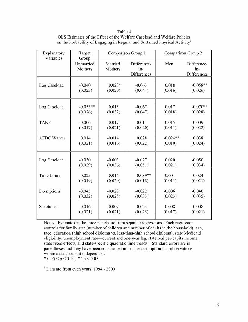
3

Table 4 OLS Estimates of the Effect of the Welfare Caseload and Welfare Policies on the Probability of Engaging in Regular and Sustained Physical Activity1

Target Group


Unmarried Mothers

Married Mothers

Difference-in-

Differences

Men Difference-in-

Differences Log Caseload -0.040

(0.025) 0.023*

(0.029) -0.063 (0.044)

0.018 (0.016)

-0.058** (0.026)

Log Caseload -0.053**

(0.026) 0.015

(0.032) -0.067 (0.047)

0.017 (0.018)

-0.070** (0.028)

TANF -0.006

(0.017) -0.017 (0.021)

0.011 (0.020)

-0.015 (0.011)

0.009 (0.022)

AFDC Waiver 0.014

(0.021) -0.014 (0.016)

0.028 (0.022)

-0.024** (0.010)

0.038 (0.024)

Log Caseload -0.030

(0.029) -0.003 (0.036)

-0.027 (0.051)

0.020 (0.021)

-0.050 (0.034)

Time Limits 0.025

(0.019) -0.014 (0.020)

0.039** (0.018)

0.001 (0.011)

0.024 (0.021)

Exemptions -0.045

(0.032) -0.023 (0.025)

-0.022 (0.033)

-0.006 (0.023)

-0.040 (0.035)

Sanctions 0.016

(0.021) -0.007 (0.021)

0.023 (0.025)

0.008 (0.017)

0.008 (0.021)


1 Data are from even years, 1994 - 2000

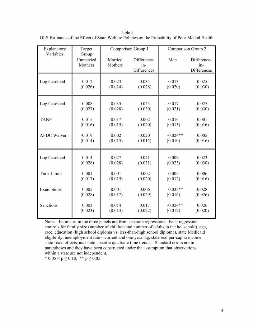
4

Table 5 OLS Estimates of the Effect of State Welfare Policies on the Probability of Poor Mental Health

Target Group


Unmarried Mothers

Married Mothers

Difference-in-

Differences

Men Difference-in-

Differences Log Caseload 0.012

(0.026) -0.023 (0.024)

0.035 (0.028)

-0.013 (0.020)

0.025 (0.030)

Log Caseload 0.008

(0.027) -0.035 (0.028)

0.043 (0.030)

-0.017 (0.021)

0.025 (0.030)

TANF -0.015

(0.016) -0.017 (0.015)

0.002 (0.020)

-0.016 (0.013)

0.001 (0.016)

AFDC Waiver -0.019

(0.014) 0.002

(0.013) -0.020 (0.015)

-0.024** (0.010)

0.005 (0.016)

Log Caseload 0.014

(0.028) -0.027 (0.028)

0.041 (0.031)

-0.009 (0.023)

0.023 (0.030)

Time Limits -0.001

(0.017) 0.001

(0.015) -0.002 (0.020)

0.005 (0.012)

-0.006 (0.016)

Exemptions 0.005

(0.028) -0.001 (0.017)

0.006 (0.029)

0.033** (0.016)

-0.028 (0.026)

Sanctions 0.003

(0.023) -0.014 (0.013)

0.017 (0.022)

-0.024** (0.012)

0.026 (0.020)


5

Table 6 OLS Estimates of the Effect of State Welfare Policies on the Probability of Fair or Poor Health

Target Group


Unmarried Mothers

Married Mothers

Difference-in-

Differences

Men Difference-in-

Differences Log Caseload -0.016

(0.014) 0.006

(0.008) -0.022 (0.016)

-0.006 (0.009)

-0.011 (0.015)

Log Caseload -0.004

(0.015) 0.004

(0.009) -0.008 (0.018)

-0.007 (0.009)

0.002 (0.017)

TANF 0.018

(0.011) -0.005 (0.007)

0.023* (0.013)

-0.002 (0.005)

0.020 (0.013)

AFDC Waiver 0.000

(0.009) -0.007 (0.007)

0.007 (0.010)

-0.001 (0.005)

0.002 (0.010)

Log Caseload -0.000

(0.016) 0.005

(0.009) -0.005 (0.018)

-0.001 (0.009)

0.001 (0.016)

Time Limits 0.024

(0.010) -0.001 (0.007)

0.025* (0.014)

0.002 (0.005)

0.022* (0.012)

Exemptions -0.005

(0.016) -0.006 (0.011)

0.001 (0.016)

0.000 (0.011)

-0.005 (0.016)

Sanctions 0.004

(0.011) 0.003

(0.009) 0.000

(0.014) 0.007

(0.008) -0.004 (0.012)


6

Appendix Table 1 Sample Means, BRFSS 1993-2001

Sample Description Total1 (n = 67,698)

Unmarried Mothers

(n = 36,274)

Married Mothers

(n = 48,199)

Men (n = 83,225)

Age 30 29 32 30

Education HS Diploma 0.79 0.74 0.81 0.80

Race / ethnicity White, Non-hispanic 0.71 0.55 0.77 0.74 Black, Non-hispanic 0.12 0.25 0.06 0.09 Hispanic 0.13 0.15 0.13 0.12 Non-hispanic Other 0.05 0.05 0.04 0.05

Number of Children 1 – 2 0.56 0.72 0.69 0.42 3 or more 0.22 0.28 0.31 0.14

Number of Adults 1 0.25 0.59 0.06 0.22 2 0.60 0.28 0.84 0.60 3 or more 0.15 0.13 0.10 0.18

Employment Employed 0.75 0.64 0.61 0.88 Unemployed 0.08 0.14 0.05 0.07 Not in Labor Force 0.14 0.17 0.32 0.02 Unable to Work 0.03 0.05 0.02 0.03

Health Status Fair/Poor Health 0.11 0.15 0.10 0.10 Poor Mental Health 0.38 0.49 0.41 0.32

Health Behaviors Daily Smoking 0.33 0.38 0.28 0.33 Binge Drinking2 0.22 0.14 0.08 0.33 # Binge Drinking

Occurrences2 0.91 0.43 0.20 1.54

Overweight 0.53 0.47 0.45 0.59 Leisure-time

Physical Activity3 0.67 0.60 0.66 0.70

Regular and Sustained Exercise4

0.14 0.13 0.14 0.15

Notes: 1 Unless otherwise indicated, sample sizes pertain to the combined total for years 1993-2001

2 Data are from odd years only, 1993–2001. Sample sizes are: 91,911 (total); 19,715 (Unmarried Mothers); 26,609 (Married Mothers); 5,587 (Men) 3 Data are from 1994, 1996, 1998, 2000, and 2001. Sample sizes are: 97,376 (total); 21,727 (Unmarried Mothers); 27,549 (Married Mothers); 48,100 (Men) 4 Data are from 1994, 1996, 1998, and 2000. Sample sizes are: 70,357 (total); 15,528 (Unmarried Mothers); 20,213 (Married Mothers); 34,616 (Men)

Changes in the welfare caseload and the health of low-educated mothers

Documents

Transcript of Changes in the welfare caseload and the health of low-educated mothers