Chang*, S.-K. and T.-L. Yuan. 2014. Deriving high-resolution spatiotemporal fishing effort of large-scale longline fishery from vessel monitoring system (VMS) data and validated by observer data. Canadian Journal of Fisheries and Aquatic Sciences (Accepted on 18 May 2014, Published online 22 May 2014) doi:10.1139/cjfas-2013-0552 http://www.nrcresearchpress.com/journal/cjfas (This is personal manuscript for the purpose of exchange of academic idea only.)

Deriving high-resolution spatiotemporal fishing effort of large-scale longline fishery from vessel monitoring system (VMS) data and validated by observer data Shui-Kai Chang* and Tzu-Lun Yuan

Shui-Kai Chang Institute of Marine Affairs, National Sun Yat-sen University 70, Lien-hai Road, Kaohsiung 80424, Taiwan skchang@faculty.nsysu.edu.tw Tzu-Lun Yuan Institute of Marine Affairs, National Sun Yat-sen University 70, Lien-hai Road, Kaohsiung 80424, Taiwan ken1234582@hotmail.com Corresponding author Shui-Kai Chang 70, Lien-hai Road, Kaohsiung 80424, Taiwan +886-7-5250050 (phone & fax) skchang@faculty.nsysu.edu.tw

1

Abstract Estimating geo-referenced fishing effort is vital to develop advice for effective fisheries management. Many studies in recent decades have attempted to obtain complete, high-resolution effort data from vessel monitoring system (VMS). The main challenge in this regard is to develop a classification method for differentiating fishing activities (e.g., fishing days) from non-fishing activities in VMS data. This study developed a simple, novel classification criterion for a large-scale tuna longline (LTLL) fishery which has not been studied before. LTLL operations were first explored using observer data. Three approaches were designed for developing fishing-day classification criteria, using maximizing sum of sensitivity and specificity (SS) as the major performance measure and minimizing difference of SS as a reference. At least one VMS report with speed in the range of 2–5 kn detected during the time-of-day period of 14:00–23:00 hrs, was recommended as the criterion for defining a fishing day. Possible explanations for the differences between the estimated fishing days from VMS data and those reported on logbooks were discussed; most causes were related to specific features of the fishery. Keywords Vessel monitoring system (VMS), fishing day classification, VMS speed, tuna longline

2

Introduction Estimating fishing effort is crucial to fisheries scientists, because it can provide information for calculating catch per unit effort (CPUE) to index stock abundance. While utilizing the effort data, its spatial component deserves proper attention for the reasons that, the spatial distributions of fleets may change over time, causing bias in CPUE interpretation, and non-randomly distributed fishing efforts may falsely lead to hyperstability or hyperdepletion in abundance indices (Rose and Kulka 1999; Bordalo-Machado 2006; Ellis and Wang 2007). Geo-referenced effort data are traditionally compiled from commercial logbooks, which are often unreliable because they are incomplete and prone to error (e.g., missing or inaccurate positions) (Mullowney and Dawe 2009; Lee et al. 2010), or too coarse in resolution to identify resource concentration areas (Marrs et al. 2002; Bordalo-Machado 2006). Although nominal efforts are usually standardized to remove the effects of a number of influencing factors (Maunder and Punt 2004; Chang et al. 2011), those deficiencies can hardly be compensated for using this process. Thus, since the 2000s, many scientists have attempted to obtain complete, high-resolution effort data from vessel monitoring systems (VMSs) or coastal surveillance radar systems (see summary Table 1 of Lee et al. 2010; Chang 2014). The main challenge in this regard is the development of a classification method to differentiate fishing activities from non-fishing activities in the data. Understanding the operation pattern of a fishery is crucial for developing proper classification methods, because no single method is applicable to all fisheries (Lee et al. 2010; Bez et al. 2011). Previous studies on estimating fishing effort from VMS data have dealt mostly with different types of trawl or dredge fisheries (Lee et al. 2010, Table 1; Lambert et al. 2012), and more recently, with purse seine fisheries (Bez et al. 2011; Joo et al. 2011). Compared to towed or fish-surrounding gears, pelagic longline is a passive gear, and differs in operation from the abovementioned active gears. No study has yet developed classification methods for the pelagic longline fisheries. Previous classification methods were developed based on knowledge of the operation patterns of fisheries, and can be grouped into two types: (a) simple classification criteria (or rules), developed according to vessel speed (kn) deduced from VMS data (e.g., Lee et al. 2010; Gerritsen and Lordan 2011; Jennings and Lee 2012) or concurrently referencing the vessel heading (the directional movement of the vessel) (e.g., Mills et al. 2007; Hintzen et al. 2010); and (b) sophisticated classification methods such as state-space models and artificial neural networks (e.g., Bez et al. 2011; Joo et al. 2011). Vessel speed has been used in all proposed classification methods, and simple speed-related criteria have been applied more widely and frequently than any other criteria. The vessel heading has also been used in many methods, although it was considered to be less informative (Lee et al. 2010; Gerritsen and Lordan 2011). In recent decades, many tuna and billfish resources have experienced continued excessive fishing pressure by multinational fisheries worldwide; these stocks have been mainly exploited by longline and purse seine fisheries (Williams and Terawasi 2011). Taiwan accounts for the second largest catch in the world, after Japan (Chang et al. 2010), and has the largest spatial coverage of fishing effort by large-scale tuna

3

longliners (LTLLs) (≥ 24 m in length overall). VMSs have been installed in all Taiwanese LTLL vessels since 2004 (Chang et al. 2010). Over the last decade, other fishing nations have also implemented VMSs on their LTLL vessels in response to regulations of the regional fisheries management organizations specifically for managing tuna and tuna-like species (the tuna-RFMOs), to enhance monitoring and enforcement on the fisheries (Aranda et al. 2010). VMS data do not provide the information necessary to derive the number of hooks deployed for LTLL fishery. However, one LTLL operation set lasts one day and so fishing days could be used to represent fishing effort. The purpose of this study was to develop a simple criterion for classifying days into fishing or non-fishing, for estimating high-resolution spatiotemporal efforts, using the VMS data of Taiwanese LTLL fishery. To develop the criterion, three approaches that considered either one of the following information were used: (a) the appearance of VMS report within a specific speed range during a specific time range (referred as the optimal-speed-time-ranges approach), (b) the moving distances between two consecutive days (the between-days distance approach), and (c) the distance within a day (the within-day distance approach). The classification performance was evaluated using observer data and the optimal criterion was determined from the evaluations. The criterion was then applied to derive VMS-based fishing days which were used to compare with regular logbook-based fishing days and to reveal the high-resolution spatial distribution of LTLL fishing efforts. The results of this study can be applied to future spatial studies involving evaluating the dynamics of fishing fleets with insufficient logbook coverage, and determining the relationship between longline fishing effort concentration and environmental parameters. Materials and methods Data Fishery observer data, VMS data, and commercial logbook data from the Taiwanese LTLL fishery in the Pacific Ocean were provided by the Overseas Fisheries Development Council of the Republic of China. The fishery observer program has been implemented since 2002 (Chang et al. 2011). The format of the observer log sheet has changed several times to balance the needs of more information to be collected and the ability of observers to reliably record these data. Observer data from 2008 and 2009 were presented in an interim format that contained more complete information regarding operational details (the date, time, and location of the start and end of hook deployment and retrieval operations) both during fishing and at other times (including information regarding activity on non-fishing days); these data were used in this study. There were 13 LTLL vessels (1 460 observation days) in the 2008 data, and 21 LTLL vessels (1 486 observation days) in the 2009 data. Two types of automatic location communicators (ALCs) integrated with Global Positioning Systems (GPS) were used in Taiwanese LTLL vessels: the ARGOS and Inmarsat systems. The former transmits locations per hour or in shorter time periods, and the latter generally transmits locations every six hours, subject to the regulations of tuna-RFMOs (Chang et al. 2010). Unprocessed VMS data from Pacific LTLL

4

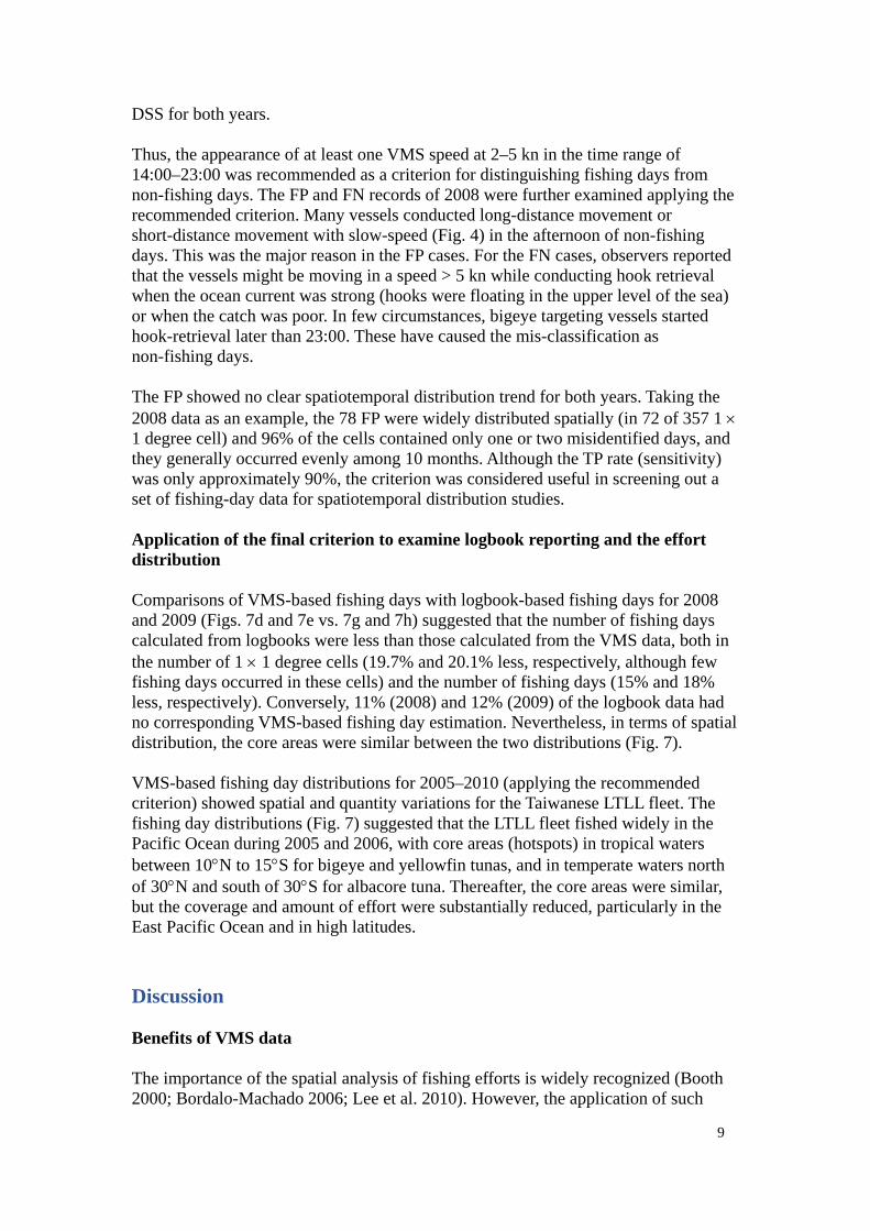
vessels, from 2005–2010, were used in this study. This period covers a time in which the fleet size was substantially reduced (FA and OFDC 2010) and for which observer data were available. The data included vessel identification, date and time (UTC), location (in seconds), speed (the speed at the moment of the VMS acquisition, in kn), and heading (in degrees). The data were pre-processed by removing duplicate records and records close to ports (approximately at less than 5.5 nautical miles) (Deng et al. 2005; Lee et al. 2010). Standardizing the VMS records to local time was necessary to characterize the diurnal operation of the fishing activity. Adjusting the coordinated universal time (UTC) recorded in the VMS data to the local time of the observer data was a crucial task for cross-referencing the VMS and observer data. Additional efforts were undertaken to verify dates presented in observer records when the vessels were operating in the vicinity of the International Date Line. Commercial logbooks submitted by Taiwanese LTLL fishing vessels provided records of fishing days (not including transit days, which vessels were not required to report). The logbooks contained date, noontime position, hooks deployed, and catch by species information. Data for 2008 and 2009 were compared with fishing days obtained from the application of the final recommended fishing-day classification criterion to the VMS data. There were 15 512 and 14 848 fishing records in the 2008 and 2009 logbook data, respectively. Criteria for identifying fishing days A longline fishing set typically involves a fast hook deployment operation in the morning and a slower retrieval operation (including processing of the fish caught) in the afternoon (till midnight or dawn). This operation pattern composes two key elements in a fishing day: the time (in the morning or afternoon) and the speed (fast-speed or slow-speed), both are available from VMS data. VMS data also provide information on the vessel heading. However, only 4–6 VMS reports per day are required by tuna-RFMOs and so a clear vessel track can hardly be constructed from these data. In this regard, heading data provide insufficient information for identifying fishing activities and were not used in this study. The first step for the optimal-speed-time-ranges classification approach was to define the optimal range of time (the time range) for identifying a fishing-day. A recursive partitioning method, Classification and Regression Trees (CART) (Lewis 2000; Loh 2011), was applied on the combined observer and VMS data using the rpart package in R (R-Development Core Team 2009), with observer data as the learning dataset. The typical longline fishing pattern suggests that a fishing set may have two different operational speed ranges in two time ranges. Therefore, this study considered two scenarios for simulating all possible time ranges: one-time-range-scenario (one-TRS, only one time range in a day) and two-time-range-scenario (two-TRS, two time ranges in a day). In the one-TRS, the time range was simulated as any possible combinations of x:00 to y:00 in 1-hourly units, where both x and y are from 0 to 23 and y ≥ x in each simulated time range, such as, 0:00–0:00 (within the hour of 0 o’clock), 0:00–1:00 (within the hours of 0 and 1 o’clock), ..., 0:00–23:00 (i.e., any time in the day), 1:00–1:00, 1:00–2:00, ..., 1:00–23:00, and so on. For the two-TRS, the first time range was identical to that of the one-TRS and the second time range

5

covered the remaining time intervals. A total of 300 simulations were designed for the one-TRS and 276 for the two-TRS. CART analysis was conducted for each simulation. The fishing or non-fishing information from the observer data were the categorical dependent variables. The median speed of the VMS speeds within each time range was the predictor (independent) variable. The optimal time range was identified out of all the CART results based on the performance measures that will be described later. The second step of this approach was to define the optimal speed range by examining the performance measure at various minimum and maximum speed combinations, for the optimal time range selected from the first step. A fishing day was identified when there was at least one VMS report with speed in the optimal speed range during the optimal time range. The second and the third approaches considered the between-days distance and within-day distance, respectively. Because the vessel speed is reduced during fishing, the moving distance between two consecutive days or in a day could be used to index the fishing days. The distance (d) was calculated using the haversine formula (Sinnott 1984) at two positions P1 = (φ1, λ1) and P2 = (φ2, λ2), where φ and λ represent their latitude and longitude, respectively,

−+

−= )

2(sin)cos()cos()

2(sinarcsin2 122

21122 λλφφφφrd

In the between-days distance approach, the P1 and P2 are the first VMS positions within the optimal time range (determined from the first approach) of day one and day two, respectively, of the consecutive two days. Day one was defined as a fishing day when d < k where k was a defined distance threshold. The distance between two consecutive fishing days was 151 ± 364 km (mean ± standard deviation) when calculated from observer data. Accordingly, five options of k, from 100 to 500 km at 100-km intervals, were examined to identify the optimal distance. The last day of the data examined was automatically considered as a non-fishing day. For the within-day distance approach, P1 and P2 are the first and the last VMS positions in the same day. The day was considered as a fishing day when d < k; and five options of k, from 30 to 150 km at 30-km intervals, were examined according to the observer data (58 ± 67 km). Performance of the criteria The performance of the fishing day classification criterion was assessed based on the ability to maximize agreement between the predicted fishing-day/non-fishing-day distribution from the VMS data and the observed distribution from the observer data. Elements of the confusion matrix were denoted as true positive (TP), false negative (FN), false positive (FP), and true negative (TN). The sensitivity of the criterion (or the true positive rate) was measured as the ability to accurately predict fishing days, using the formula TP/(TP + FN). The specificity (or the true negative rate) was measured as the ability to accurately predict non-fishing days, using the formula TN/(TN + FP) (Fawcett 2006; Fukuda et al. 2011). Performance measures used in this study took into account both the sensitivity and the specificity (SS). Criterion that maximized the “sum of SS” (SSS) was considered optimal (Liu et al. 2005;

6

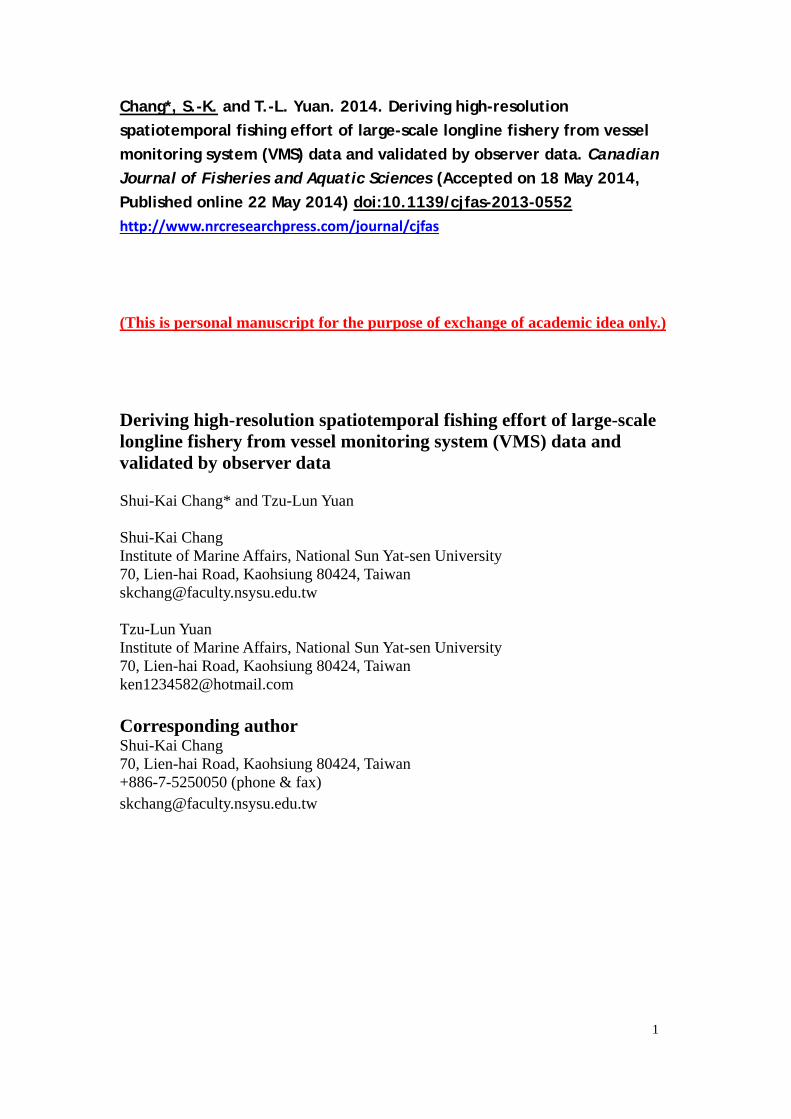
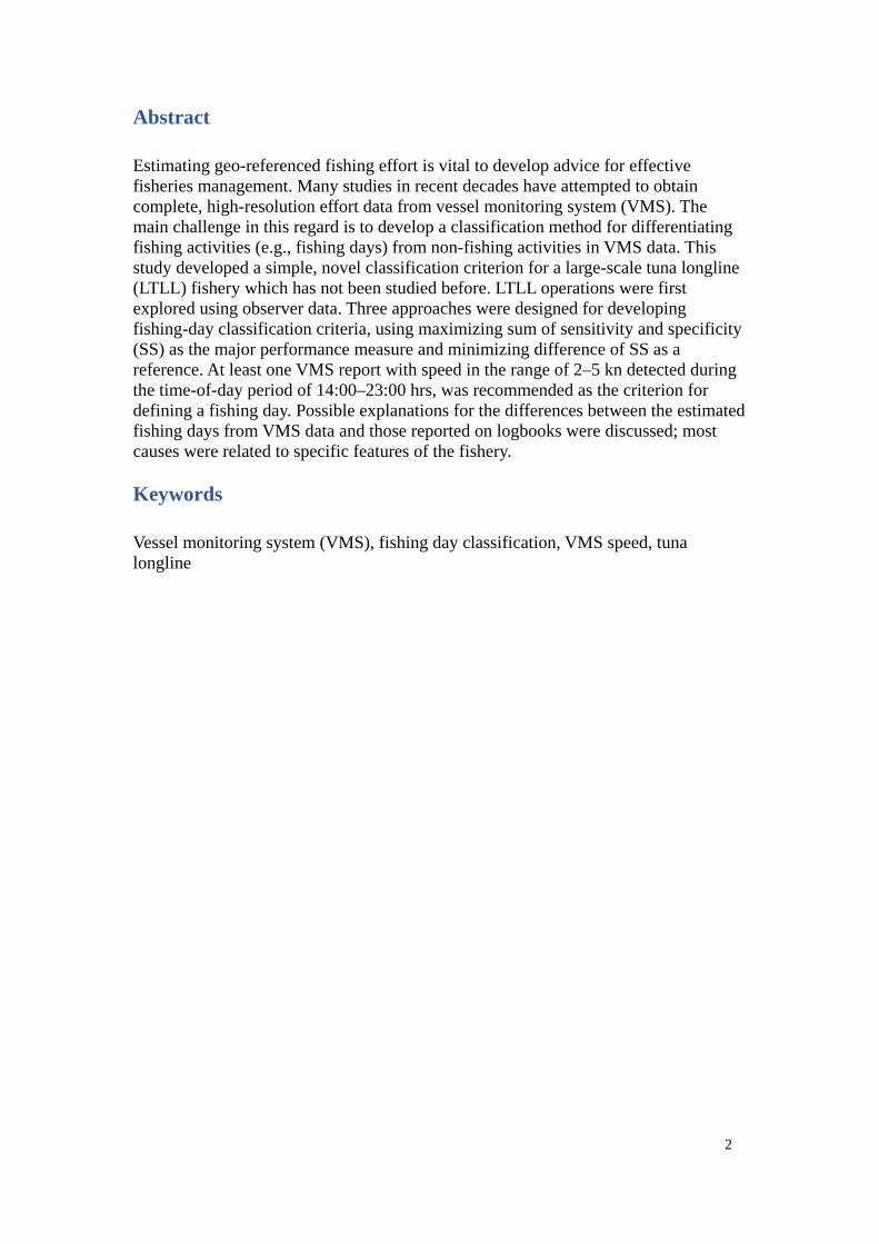
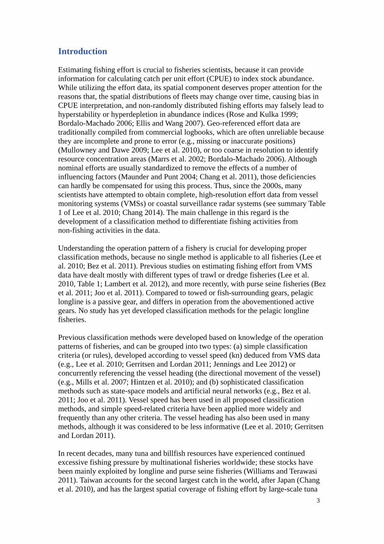
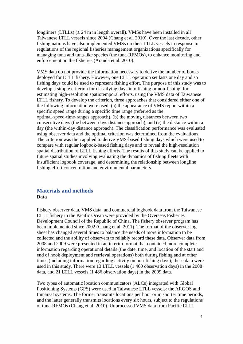
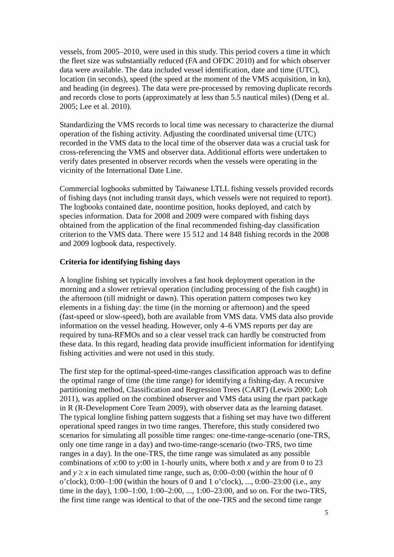
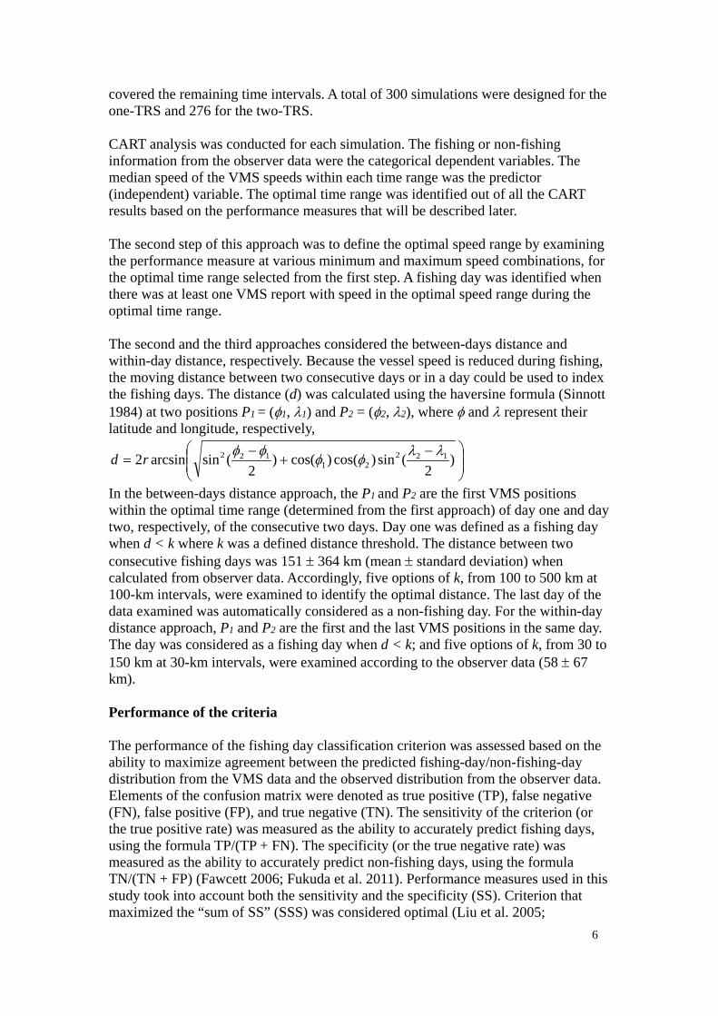
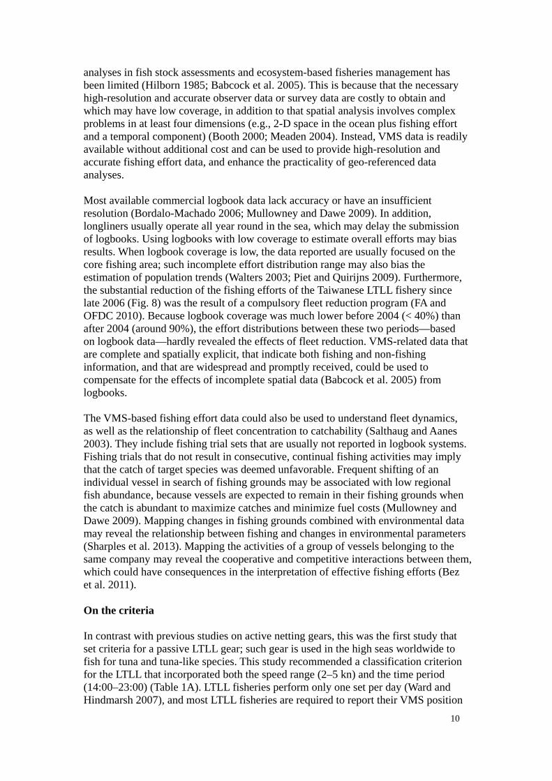
Jiménez-Valverde and Lobo 2007). When the SSS values of some criteria were similar, the criterion with the lowest value of the “absolute difference of the SS” (DSS) was selected. LTLL vessels operating in the Pacific Ocean are requested to report VMS data at six-hour intervals; therefore, while conducting the first step of the optimal-speed-time-ranges approach, certain records (days) might not have any VMS reporting in the simulated time range (for example, the short time range of 0:00–2:00). These records were not qualified and thus were excluded from the CART runs because no VMS median speed could be calculated for the time range. For such cases, the active data ratio (the ratio of qualified data records) was low, nevertheless the SSS might be falsely high. To account for this, the sensitivity and specificity were adjusted by replacing the denominators of the formula with the true fishing days and true non-fishing days from observer data, respectively. Application of the final criterion to examine logbook reporting and effort distribution The recommended final criterion was applied to (a) VMS data from 2008 and 2009 to construct VMS-based fishing effort distributions for comparison with those from the logbook data of the same years. (b) VMS data from 2005–2010 to determine the overall distribution of fishing days, and to briefly discuss changes in distribution during this period. Results LTLL operation pattern Fishing situations The basic LTLL operation pattern was explored by analyzing the start and end times of the deployment and the retrieval operations recorded in the observer data, which denoted fishing days. Generally, deployment starts from 4:00–6:00 (in hour unit), and ends at 10:00–12:00 (Fig. 1a and 1b); after one to two hours of soaking, the retrieval operation starts from 11:00–13:00, and ends at 1:00–5:00 of the next day (Fig. 1c and 1d). There are generally two ranges of vessel speed on a fishing day (Fig. 2): fast-speed in the morning (> 5 kn during 4:00–10:00), and slow-speed in the afternoon till midnight (≤ 5 kn during 13:00–23:00). Plots of the types of operation (i.e., deployment and retrieval) on the VMS speed data (Fig. 3) suggested that the vessels were primarily conducting deployment operations in the fast-speed periods, whereas they were conducting retrieval operations in the slow-speed periods. The large speed ranges observed during the transition periods (e.g., at 2:00 or 11:00, Fig. 2) were mainly produced by the two operations that had different starting and ending time for all the vessels examined (Fig. 1). The two figures indicated that the retrieval operation, conducted from the afternoon until midnight, involved a lower variation in vessel speed than did the morning deployment operation, and had a consistent median after 14:00. This operation pattern suggested that for longline fisheries, unlike trawl or dredge

7

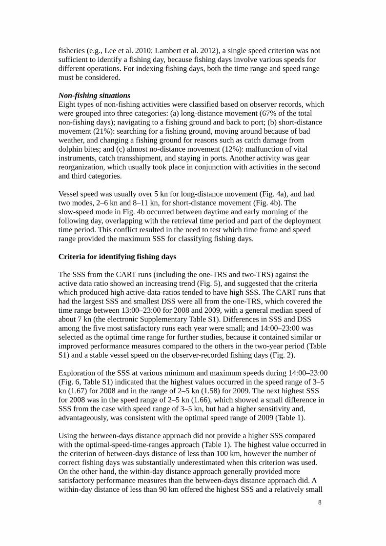
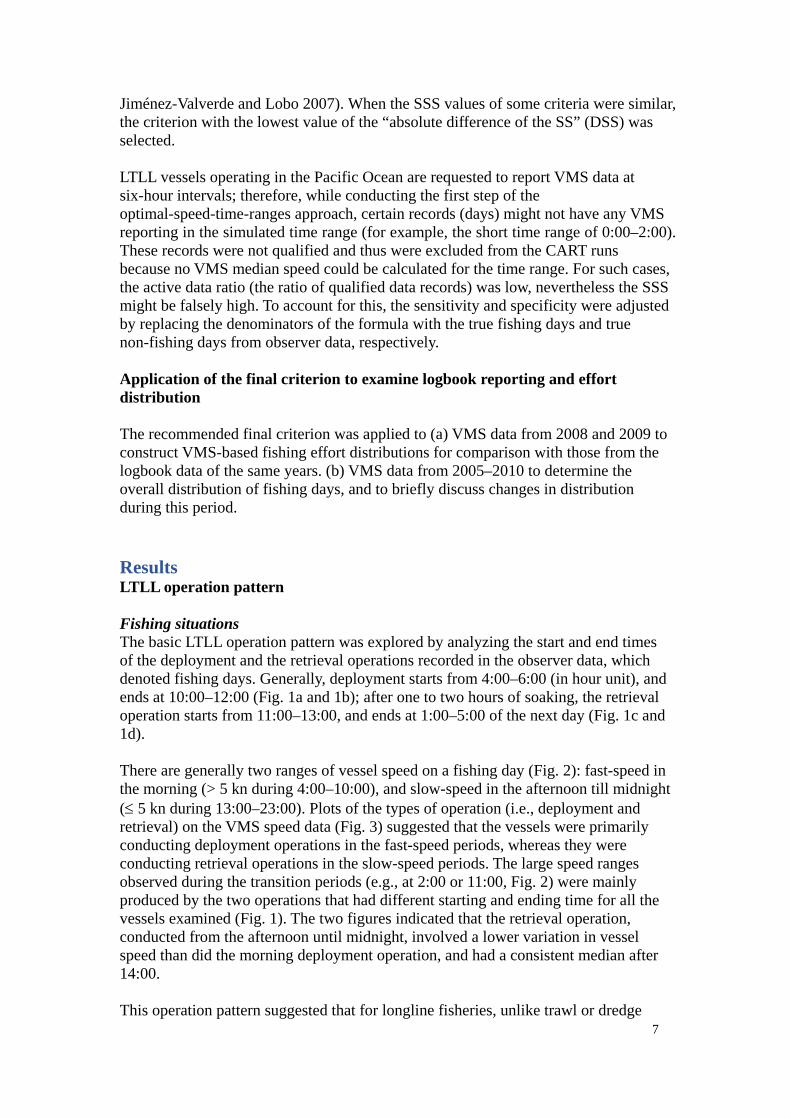
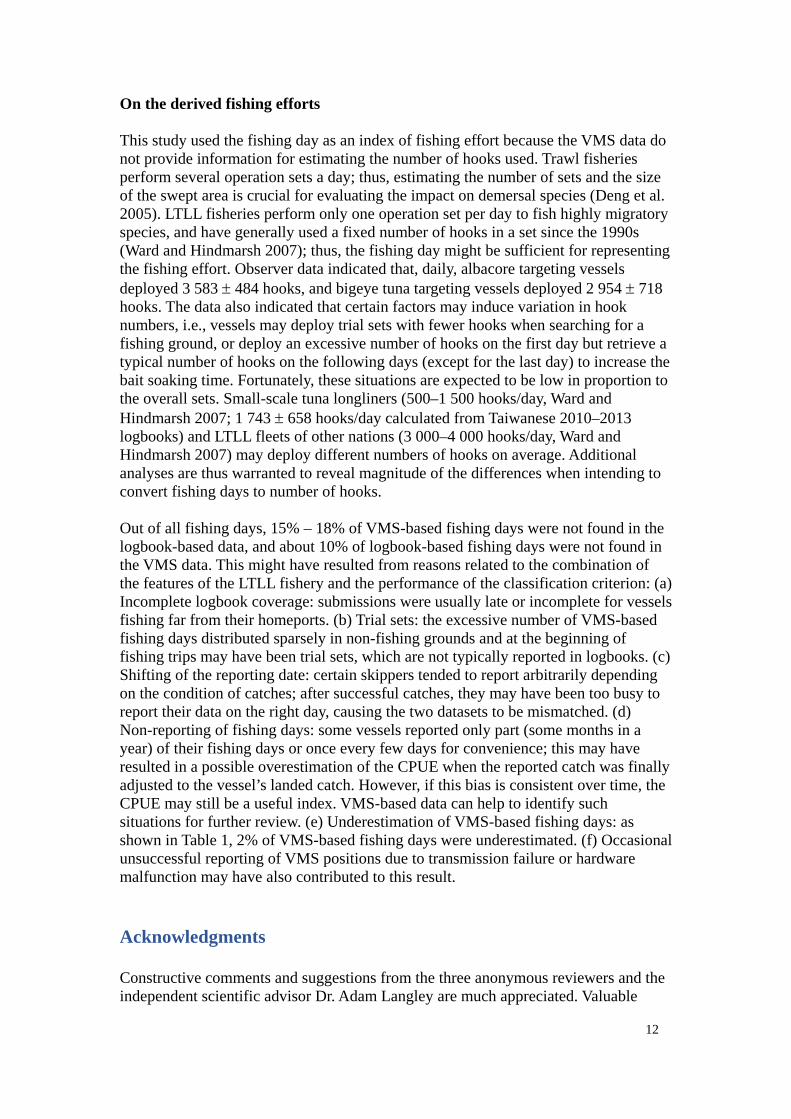
fisheries (e.g., Lee et al. 2010; Lambert et al. 2012), a single speed criterion was not sufficient to identify a fishing day, because fishing days involve various speeds for different operations. For indexing fishing days, both the time range and speed range must be considered. Non-fishing situations Eight types of non-fishing activities were classified based on observer records, which were grouped into three categories: (a) long-distance movement (67% of the total non-fishing days); navigating to a fishing ground and back to port; (b) short-distance movement (21%): searching for a fishing ground, moving around because of bad weather, and changing a fishing ground for reasons such as catch damage from dolphin bites; and (c) almost no-distance movement (12%): malfunction of vital instruments, catch transshipment, and staying in ports. Another activity was gear reorganization, which usually took place in conjunction with activities in the second and third categories. Vessel speed was usually over 5 kn for long-distance movement (Fig. 4a), and had two modes, 2–6 kn and 8–11 kn, for short-distance movement (Fig. 4b). The slow-speed mode in Fig. 4b occurred between daytime and early morning of the following day, overlapping with the retrieval time period and part of the deployment time period. This conflict resulted in the need to test which time frame and speed range provided the maximum SSS for classifying fishing days. Criteria for identifying fishing days The SSS from the CART runs (including the one-TRS and two-TRS) against the active data ratio showed an increasing trend (Fig. 5), and suggested that the criteria which produced high active-data-ratios tended to have high SSS. The CART runs that had the largest SSS and smallest DSS were all from the one-TRS, which covered the time range between 13:00–23:00 for 2008 and 2009, with a general median speed of about 7 kn (the electronic Supplementary Table S1). Differences in SSS and DSS among the five most satisfactory runs each year were small; and 14:00–23:00 was selected as the optimal time range for further studies, because it contained similar or improved performance measures compared to the others in the two-year period (Table S1) and a stable vessel speed on the observer-recorded fishing days (Fig. 2). Exploration of the SSS at various minimum and maximum speeds during 14:00–23:00 (Fig. 6, Table S1) indicated that the highest values occurred in the speed range of 3–5 kn (1.67) for 2008 and in the range of 2–5 kn (1.58) for 2009. The next highest SSS for 2008 was in the speed range of 2–5 kn (1.66), which showed a small difference in SSS from the case with speed range of 3–5 kn, but had a higher sensitivity and, advantageously, was consistent with the optimal speed range of 2009 (Table 1). Using the between-days distance approach did not provide a higher SSS compared with the optimal-speed-time-ranges approach (Table 1). The highest value occurred in the criterion of between-days distance of less than 100 km, however the number of correct fishing days was substantially underestimated when this criterion was used. On the other hand, the within-day distance approach generally provided more satisfactory performance measures than the between-days distance approach did. A within-day distance of less than 90 km offered the highest SSS and a relatively small

8

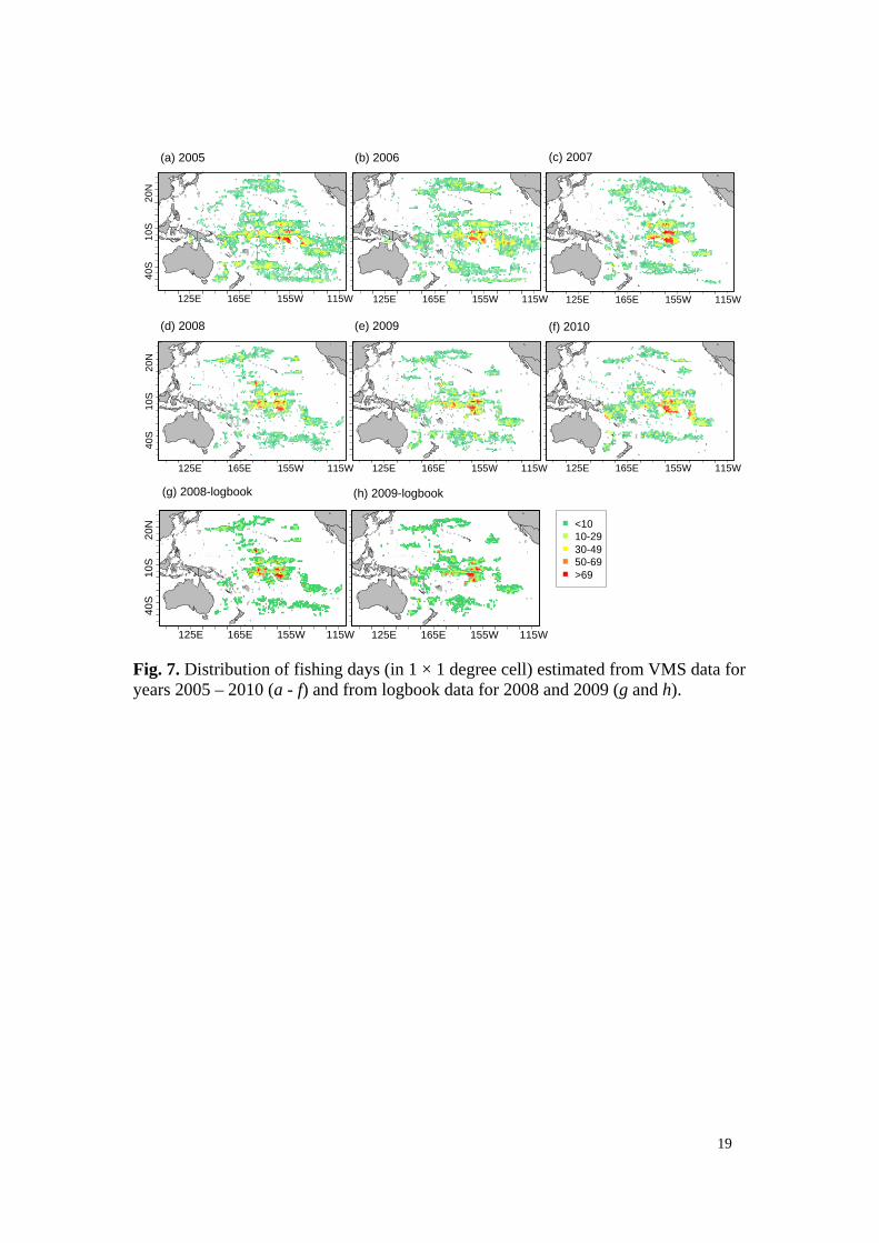
DSS for both years. Thus, the appearance of at least one VMS speed at 2–5 kn in the time range of 14:00–23:00 was recommended as a criterion for distinguishing fishing days from non-fishing days. The FP and FN records of 2008 were further examined applying the recommended criterion. Many vessels conducted long-distance movement or short-distance movement with slow-speed (Fig. 4) in the afternoon of non-fishing days. This was the major reason in the FP cases. For the FN cases, observers reported that the vessels might be moving in a speed > 5 kn while conducting hook retrieval when the ocean current was strong (hooks were floating in the upper level of the sea) or when the catch was poor. In few circumstances, bigeye targeting vessels started hook-retrieval later than 23:00. These have caused the mis-classification as non-fishing days. The FP showed no clear spatiotemporal distribution trend for both years. Taking the 2008 data as an example, the 78 FP were widely distributed spatially (in 72 of 357 1 × 1 degree cell) and 96% of the cells contained only one or two misidentified days, and they generally occurred evenly among 10 months. Although the TP rate (sensitivity) was only approximately 90%, the criterion was considered useful in screening out a set of fishing-day data for spatiotemporal distribution studies. Application of the final criterion to examine logbook reporting and the effort distribution Comparisons of VMS-based fishing days with logbook-based fishing days for 2008 and 2009 (Figs. 7d and 7e vs. 7g and 7h) suggested that the number of fishing days calculated from logbooks were less than those calculated from the VMS data, both in the number of 1 × 1 degree cells (19.7% and 20.1% less, respectively, although few fishing days occurred in these cells) and the number of fishing days (15% and 18% less, respectively). Conversely, 11% (2008) and 12% (2009) of the logbook data had no corresponding VMS-based fishing day estimation. Nevertheless, in terms of spatial distribution, the core areas were similar between the two distributions (Fig. 7). VMS-based fishing day distributions for 2005–2010 (applying the recommended criterion) showed spatial and quantity variations for the Taiwanese LTLL fleet. The fishing day distributions (Fig. 7) suggested that the LTLL fleet fished widely in the Pacific Ocean during 2005 and 2006, with core areas (hotspots) in tropical waters between 10°N to 15°S for bigeye and yellowfin tunas, and in temperate waters north of 30°N and south of 30°S for albacore tuna. Thereafter, the core areas were similar, but the coverage and amount of effort were substantially reduced, particularly in the East Pacific Ocean and in high latitudes. Discussion Benefits of VMS data The importance of the spatial analysis of fishing efforts is widely recognized (Booth 2000; Bordalo-Machado 2006; Lee et al. 2010). However, the application of such

9

analyses in fish stock assessments and ecosystem-based fisheries management has been limited (Hilborn 1985; Babcock et al. 2005). This is because that the necessary high-resolution and accurate observer data or survey data are costly to obtain and which may have low coverage, in addition to that spatial analysis involves complex problems in at least four dimensions (e.g., 2-D space in the ocean plus fishing effort and a temporal component) (Booth 2000; Meaden 2004). Instead, VMS data is readily available without additional cost and can be used to provide high-resolution and accurate fishing effort data, and enhance the practicality of geo-referenced data analyses. Most available commercial logbook data lack accuracy or have an insufficient resolution (Bordalo-Machado 2006; Mullowney and Dawe 2009). In addition, longliners usually operate all year round in the sea, which may delay the submission of logbooks. Using logbooks with low coverage to estimate overall efforts may bias results. When logbook coverage is low, the data reported are usually focused on the core fishing area; such incomplete effort distribution range may also bias the estimation of population trends (Walters 2003; Piet and Quirijns 2009). Furthermore, the substantial reduction of the fishing efforts of the Taiwanese LTLL fishery since late 2006 (Fig. 8) was the result of a compulsory fleet reduction program (FA and OFDC 2010). Because logbook coverage was much lower before 2004 (< 40%) than after 2004 (around 90%), the effort distributions between these two periods—based on logbook data—hardly revealed the effects of fleet reduction. VMS-related data that are complete and spatially explicit, that indicate both fishing and non-fishing information, and that are widespread and promptly received, could be used to compensate for the effects of incomplete spatial data (Babcock et al. 2005) from logbooks. The VMS-based fishing effort data could also be used to understand fleet dynamics, as well as the relationship of fleet concentration to catchability (Salthaug and Aanes 2003). They include fishing trial sets that are usually not reported in logbook systems. Fishing trials that do not result in consecutive, continual fishing activities may imply that the catch of target species was deemed unfavorable. Frequent shifting of an individual vessel in search of fishing grounds may be associated with low regional fish abundance, because vessels are expected to remain in their fishing grounds when the catch is abundant to maximize catches and minimize fuel costs (Mullowney and Dawe 2009). Mapping changes in fishing grounds combined with environmental data may reveal the relationship between fishing and changes in environmental parameters (Sharples et al. 2013). Mapping the activities of a group of vessels belonging to the same company may reveal the cooperative and competitive interactions between them, which could have consequences in the interpretation of effective fishing efforts (Bez et al. 2011). On the criteria In contrast with previous studies on active netting gears, this was the first study that set criteria for a passive LTLL gear; such gear is used in the high seas worldwide to fish for tuna and tuna-like species. This study recommended a classification criterion for the LTLL that incorporated both the speed range (2–5 kn) and the time period (14:00–23:00) (Table 1A). LTLL fisheries perform only one set per day (Ward and Hindmarsh 2007), and most LTLL fisheries are required to report their VMS position

10

only every 4–6 hours. Thus, requiring one VMS report in the specified speed and time ranges in the criterion was considered sufficient, although this may risk increasing the number of FP classifications when more non-fishing activities are conducted at low speeds. Alternatively, distance within a day was as conceptually simple and straightforward as the cut-off speed threshold used in other fisheries to define a fishing day. The criterion of within-day distance < 90 km offered the most satisfactory performance for both years (Table 1C). Combining these two criteria (Table 1D) increased the true negative rate (specificity) but decreased the true positive rate (sensitivities), and produced very similar SSS (but larger for 2008 and smaller for 2009), compared to the statistics of the recommended criterion (Table 1A). This suggests that incorporating additional criterion with the recommended one will not necessarily improve the accuracy in fishing-day classification much. The recommended criterion that showed the most satisfactory performance was acquired from the one-TRS. This was counter-intuitive, because it was expected that the two-TRS would include more information. However, for the two-TRS, the requirements of two time ranges had to be met simultaneously to classify a fishing day. This reduced the number of records for the fishing-day classification because on some days (four VMS reports a day) there were not at least one VMS report for each of the two time ranges simultaneously, and thus were excluded (for example, 17% records less for two-TRS comparing to one-TRS in 2008). Furthermore, speeds in the morning deployment operation varied substantially (Fig. 2); adding this requirement to the criterion has caused reduction of the chance for a true fishing day to be recognized as a fishing day. The between-days distance has been applied to provide a rough estimate of the fishing days for an Atlantic longline fleet to resolve the problem of catch underreporting (Chang 2011). Criterion of “< 500 km” was used based on estimation from observers, and the resulted fishing-day estimates were multiplied by CPUE in weight of bigeye catch per day to estimate the annual total catch and the annual underreported catch. This study showed that the criterion produced the lowest SSS and the highest FP among the five tests (Table S1) and overestimated the number of fishing days by 19% (2008) and 14% (2009). Simple criteria are powerful, easy to understand and thus generally be more transparent than sophisticated methods are (Jennings and Lee 2012; Jones et al. 2012). Simple speed criteria therefore have been applied widely (e.g., Mullowney and Dawe 2009; Votier et al. 2010; Lambert et al. 2012). LTLL fleets operate in a specific diurnal pattern regardless of vessel size (Sakagawa et al. 1987; Ward and Hindmarsh 2007). Many Pacific LTLL fleets, including those of China and many island countries, operate similarly to the Taiwanese fleet. Therefore, the simple criterion obtained from this study is easily applicable to a number of LTLL fleets for deriving high-quality fishing efforts from VMS data. The collective results could facilitate analyzing and understanding the effects of LTLL fisheries on fish stocks and ecosystems in a global scale. LTLL fleets with different target species or in different development stages, from different nations (e.g., Japan), and at different scales may vary in operation times and speeds (Yamaguchi 1989; Ward and Hindmarsh 2007). For these cases, the approaches used in this study are also applicable as a basis for the development of other suitable criteria.

11

On the derived fishing efforts This study used the fishing day as an index of fishing effort because the VMS data do not provide information for estimating the number of hooks used. Trawl fisheries perform several operation sets a day; thus, estimating the number of sets and the size of the swept area is crucial for evaluating the impact on demersal species (Deng et al. 2005). LTLL fisheries perform only one operation set per day to fish highly migratory species, and have generally used a fixed number of hooks in a set since the 1990s (Ward and Hindmarsh 2007); thus, the fishing day might be sufficient for representing the fishing effort. Observer data indicated that, daily, albacore targeting vessels deployed 3 583 ± 484 hooks, and bigeye tuna targeting vessels deployed 2 954 ± 718 hooks. The data also indicated that certain factors may induce variation in hook numbers, i.e., vessels may deploy trial sets with fewer hooks when searching for a fishing ground, or deploy an excessive number of hooks on the first day but retrieve a typical number of hooks on the following days (except for the last day) to increase the bait soaking time. Fortunately, these situations are expected to be low in proportion to the overall sets. Small-scale tuna longliners (500–1 500 hooks/day, Ward and Hindmarsh 2007; 1 743 ± 658 hooks/day calculated from Taiwanese 2010–2013 logbooks) and LTLL fleets of other nations (3 000–4 000 hooks/day, Ward and Hindmarsh 2007) may deploy different numbers of hooks on average. Additional analyses are thus warranted to reveal magnitude of the differences when intending to convert fishing days to number of hooks. Out of all fishing days, 15% – 18% of VMS-based fishing days were not found in the logbook-based data, and about 10% of logbook-based fishing days were not found in the VMS data. This might have resulted from reasons related to the combination of the features of the LTLL fishery and the performance of the classification criterion: (a) Incomplete logbook coverage: submissions were usually late or incomplete for vessels fishing far from their homeports. (b) Trial sets: the excessive number of VMS-based fishing days distributed sparsely in non-fishing grounds and at the beginning of fishing trips may have been trial sets, which are not typically reported in logbooks. (c) Shifting of the reporting date: certain skippers tended to report arbitrarily depending on the condition of catches; after successful catches, they may have been too busy to report their data on the right day, causing the two datasets to be mismatched. (d) Non-reporting of fishing days: some vessels reported only part (some months in a year) of their fishing days or once every few days for convenience; this may have resulted in a possible overestimation of the CPUE when the reported catch was finally adjusted to the vessel’s landed catch. However, if this bias is consistent over time, the CPUE may still be a useful index. VMS-based data can help to identify such situations for further review. (e) Underestimation of VMS-based fishing days: as shown in Table 1, 2% of VMS-based fishing days were underestimated. (f) Occasional unsuccessful reporting of VMS positions due to transmission failure or hardware malfunction may have also contributed to this result. Acknowledgments Constructive comments and suggestions from the three anonymous reviewers and the independent scientific advisor Dr. Adam Langley are much appreciated. Valuable

12

comments from Dr. Nicolas Bez on the first manuscript, suggestions from Dr. Trevor Branch on the working version, efforts from Drs. Rong-Chung Hsu and Sam McKechnie in reviewing the final draft, and data provisions of the Fisheries Agency and the Overseas Fisheries Development Council of the ROC are deeply acknowledged and appreciated. Financial support for this research was provided by the Fisheries Agency of the ROC (100AS-4.1.1-STa3), and by the Asia-Pacific Ocean Research Center, National Sun Yat-sen University. References Aranda, M., de Bruyn, P., and Murua, H. 2010. A report review of the tuna RFMOs:

CCSBT, IATTC, IOTC, ICCAT and WCPFC. EU FP7 project nº212188, Technical Experts Overseeing Third Country Expertise, Deliverable 2.2. AZTI Tecnalia, Pasaia, Spain.

Babcock, E.A., Pikitch, E.K., McAllister, M.K., Apostolaki, P., and Santora, C. 2005. A perspective on the use of spatialized indicators for ecosystem-based fishery management through spatial zoning. ICES J. Mar. Sci. 62(3): 469-476. doi:10.1016/j.icesjms.2005.01.010.

Bez, N., Walker, E., Gaertner, D., Rivoirard, J., and Gaspar, P. 2011. Fishing activity of tuna purse seiners estimated from vessel monitoring system (VMS) data. Can. J. Fish. Aquat. Sci. 68(11): 1998-2010. doi:10.1139/f2011-114.

Booth, A.J. 2000. Incorporating the spatial component of fisheries data into stock assessment models. ICES J. Mar. Sci. 57(4): 858-865. doi:10.1006/jmsc.2000.0816.

Bordalo-Machado, P. 2006. Fishing effort analysis and its potential to evaluate stock size. Rev. Fish. Sci. 14(4): 369-393. doi:10.1080/10641260600893766.

Chang, S.-K. 2011. Application of a vessel monitoring system to advance sustainable fisheries management--Benefits received in Taiwan. Mar. Policy 35(2): 116-121. doi:10.1016/j.marpol.2010.08.009.

Chang, S.-K. 2014. Constructing logbook-like statistics for coastal fisheries using coastal surveillance radar and fish market data. Mar. Policy 43(0): 338-346. doi:10.1016/j.marpol.2013.07.003.

Chang, S.-K., Hoyle, S., and Liu, H.-I. 2011. Catch rate standardization for yellowfin tuna (Thunnus albacares) in Taiwan's distant-water longline fishery in the Western and Central Pacific Ocean, with consideration of target change. Fish. Res. 107(1-3): 210-220. doi:10.1016/j.fishres.2010.11.004.

Chang, S.-K., Liu, K.-Y., and Song, Y.-H. 2010. Distant water fisheries development and vessel monitoring system implementation in Taiwan - History and driving forces. Mar. Policy 34(3): 541-548. doi:10.1016/j.marpol.2009.11.001.

Deng, R., Dichmont, C., Milton, D., Haywood, M., Vance, D., Hall, N., and Die, D. 2005. Can vessel monitoring system data also be used to study trawling intensity and population depletion? The example of Australia's northern prawn fishery. Can. J. Fish. Aquat. Sci. 62: 611-622. doi:10.1139/f04-219.

Ellis, N., and Wang, Y.-G. 2007. Effects of fish density distribution and effort distribution on catchability. ICES J. Mar. Sci. 64(1): 178-191. doi:10.1093/icesjms/fsl015.

FA, and OFDC. 2010. Tuna fisheries status report of Chinese Taipei in the Western and Central Pacific region. In 6th Regular Session of the Scientific Committee, WCPFC, Nukualofa, Tonga, 10 - 19 August 2010. WCPFC-SC6-AR/CCM-22. Available from http://www.wcpfc.int/doc/ar-ccm-22/chinese-taipei-0 [accessed

13

12 May 2012]. Fawcett, T. 2006. An introduction to ROC analysis. Pattern Recog. Lett. 27(8):

861-874. doi:10.1016/j.patrec.2005.10.010. Fukuda, S., De Baets, B., Mouton, A.M., Waegeman, W., Nakajima, J., Mukai, T.,

Hiramatsu, K., and Onikura, N. 2011. Effect of model formulation on the optimization of a genetic Takagi–Sugeno fuzzy system for fish habitat suitability evaluation. Ecol. Model. 222(8): 1401-1413. doi:10.1016/j.ecolmodel.2011.01.023.

Gerritsen, H., and Lordan, C. 2011. Integrating vessel monitoring systems (VMS) data with daily catch data from logbooks to explore the spatial distribution of catch and effort at high resolution. ICES J. Mar. Sci. 68(1): 245-252. doi:10.1093/icesjms/fsq137.

Hilborn, R. 1985. Fleet dynamics and individual variation: why some people catch more fish than others. Can. J. Fish. Aquat. Sci. 42(1): 2-13. doi:10.1139/f85-001.

Hintzen, N.T., Piet, G.J., and Brunel, T. 2010. Improved estimation of trawling tracks using cubic Hermite spline interpolation of position registration data. Fish. Res. 101(1–2): 108-115. doi:10.1016/j.fishres.2009.09.014.

Jennings, S., and Lee, J. 2012. Defining fishing grounds with vessel monitoring system data. ICES J. Mar. Sci. 69(1): 51-63. doi:10.1093/icesjms/fsr173.

Jiménez-Valverde, A., and Lobo, J.M. 2007. Threshold criteria for conversion of probability of species presence to either–or presence–absence. Acta Oecol. 31(3): 361-369. doi:10.1016/j.actao.2007.02.001.

Jones, M.C., Dye, S.R., Pinnegar, J.K., Warren, R., and Cheung, W.W.L. 2012. Modelling commercial fish distributions: Prediction and assessment using different approaches. Ecol. Model. 225(0): 133-145. doi:10.1016/j.ecolmodel.2011.11.003.

Joo, R., Bertrand, S., Chaigneau, A., and Ñiquen, M. 2011. Optimization of an artificial neural network for identifying fishing set positions from VMS data: An example from the Peruvian anchovy purse seine fishery. Ecol. Model. 222(4): 1048-1059. doi:10.1016/j.ecolmodel.2010.08.039.

Lambert, G.I., Jennings, S., Hiddink, J.G., Hintzen, N.T., Hinz, H., Kaiser, M.J., and Murray, L.G. 2012. Implications of using alternative methods of vessel monitoring system (VMS) data analysis to describe fishing activities and impacts. ICES J. Mar. Sci. 69(4): 682-693. doi:10.1093/icesjms/fss018.

Lee, J., South, A.B., and Jennings, S. 2010. Developing reliable, repeatable, and accessible methods to provide high-resolution estimates of fishing-effort distributions from vessel monitoring system (VMS) data. ICES J. Mar. Sci. 67(6): 1260-1271. doi:10.1093/icesjms/fsq010.

Lewis, R. 2000. An introduction to classification and regression tree (CART) analysis. In Annual Meeting of the Society for Academic Emergency Medicine, San Francisco, CA. p. 14.

Liu, C., Berry, P.M., Dawson, T.P., and Pearson, R.G. 2005. Selecting thresholds of occurrence in the prediction of species distributions. Ecography 28(3): 385-393. doi:10.1111/j.0906-7590.2005.03957.x.

Loh, W.-Y. 2011. Classification and regression trees. Wiley Interdisciplinary Reviews: Data Mining and Knowledge Discovery 1(1): 14-23. doi:10.1002/widm.8.

Marrs, S.J., Tuck, I.D., Atkinson, R.J.A., Stevenson, T.D.I., and Hall, C. 2002. Position data loggers and logbooks as tools in fisheries research: results of a pilot study and some recommendations. Fish. Res. 58(1): 109-117.

14

doi:10.1016/S0165-7836(01)00362-9. Maunder, M.N., and Punt, A.E. 2004. Standardizing catch and effort data: a review of

recent approaches. Fish. Res. 70(2-3): 141-159. doi:10.1016/j.fishres.2004.08.002.

Meaden, G.J. 2004. Challenges to using geographic information systems in aquatic environments. In Geographic Information Systems in Fisheries. Edited by W.L. Fisher and F.J. Rahel. American Fishery Socity, Bethesda, Maryland. pp. 13-48.

Mills, C.M., Townsend, S.E., Jennings, S., Eastwood, P.D., and Houghton, C.A. 2007. Estimating high resolution trawl fishing effort from satellite-based vessel monitoring system data. ICES J. Mar. Sci. 64(2): 248-255. doi:10.1093/icesjms/fsl026.

Mullowney, D.R., and Dawe, E.G. 2009. Development of performance indices for the Newfoundland and Labrador snow crab (Chionoecetes opilio) fishery using data from a vessel monitoring system. Fish. Res. 100(3): 248-254. doi:10.1016/j.fishres.2009.08.006.

Piet, G.J., and Quirijns, F.J. 2009. The importance of scale for fishing impact estimations. Can. J. Fish. Aquat. Sci. 66(5): 829-835. doi:10.1139/f09-042.

R-Development Core Team. 2009. R: a language and environment for statistical computing. R Foundation for Statistical Computing, Vienna, Austria.

Rose, G.A., and Kulka, D.W. 1999. Hyperaggregation of fish and fisheries: how catch-per-unit-effort increased as the northern cod (Gadus morhua) declined. Can. J. Fish. Aquat. Sci. 56(S1): 118-127. doi:10.1139/f99-207.

Sakagawa, G.T., Coan, A.L., and Bartoo, N.W. 1987. Patterns in longline fishery data and catches of bigeye tuna, Thunnus obesus. Mar. Fish. Rev. 49(4): 57-66.

Salthaug, A., and Aanes, S. 2003. Catchability and the spatial distribution of fishing vessels. Can. J. Fish. Aquat. Sci. 60(3): 259-268. doi:10.1139/f03-018.

Sharples, J., Ellis, J.R., Nolan, G., and Scott, B.E. 2013. Fishing and the oceanography of a stratified shelf sea. Prog. Oceanogr. 117(0): 130-139. doi:10.1016/j.pocean.2013.06.014.

Sinnott, R.W. 1984. Virtues of the haversine. Sky & Tel. 68(2): 159. Votier, S.C., Bearhop, S., Witt, M.J., Inger, R., Thompson, D., and Newton, J. 2010.

Individual responses of seabirds to commercial fisheries revealed using GPS tracking, stable isotopes and vessel monitoring systems. J. Appl. Ecol. 47(2): 487-497. doi:10.1111/j.1365-2664.2010.01790.x.

Walters, C. 2003. Folly and fantasy in the analysis of spatial catch rate data. Can. J. Fish. Aquat. Sci. 60(12): 1433-1436. doi:10.1139/f03-152.

Ward, P., and Hindmarsh, S. 2007. An overview of historical changes in the fishing gear and practices of pelagic longliners, with particular reference to Japan’s Pacific fleet. Rev. Fish Biol. Fish. 17(4): 501-516. doi:10.1007/s11160-007-9051-0.

Williams, P., and Terawasi, P. 2011. Overview of tuna fisheries in the Western and Central Pacific Ocean, including economic conditions – 2010. In 7th Regular Session of the Scientific Committee, WCPFC, Pohnpei, Federated States of Micronesia, 9 - 17 August 2011. WCPFC-SC7-2011/GN WP-1. Available from http://www.wcpfc.int/node/2810 [accessed 12 May 2012].

Yamaguchi, Y. 1989. Tuna long‐line fishing II: Fishing gear and methods. Mar. Behav. Physiol. 15(1): 13-35. doi:10.1080/10236248909378715.

15

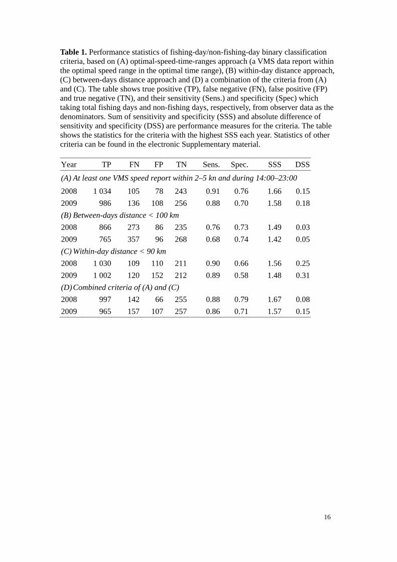
Table 1. Performance statistics of fishing-day/non-fishing-day binary classification criteria, based on (A) optimal-speed-time-ranges approach (a VMS data report within the optimal speed range in the optimal time range), (B) within-day distance approach, (C) between-days distance approach and (D) a combination of the criteria from (A) and (C). The table shows true positive (TP), false negative (FN), false positive (FP) and true negative (TN), and their sensitivity (Sens.) and specificity (Spec) which taking total fishing days and non-fishing days, respectively, from observer data as the denominators. Sum of sensitivity and specificity (SSS) and absolute difference of sensitivity and specificity (DSS) are performance measures for the criteria. The table shows the statistics for the criteria with the highest SSS each year. Statistics of other criteria can be found in the electronic Supplementary material. Year TP FN FP TN Sens. Spec. SSS DSS

(A) At least one VMS speed report within 2–5 kn and during 14:00–23:00 2008 1 034 105 78 243 0.91 0.76 1.66 0.15 2009 986 136 108 256 0.88 0.70 1.58 0.18 (B) Between-days distance < 100 km 2008 866 273 86 235 0.76 0.73 1.49 0.03 2009 765 357 96 268 0.68 0.74 1.42 0.05 (C) Within-day distance < 90 km 2008 1 030 109 110 211 0.90 0.66 1.56 0.25 2009 1 002 120 152 212 0.89 0.58 1.48 0.31 (D) Combined criteria of (A) and (C) 2008 997 142 66 255 0.88 0.79 1.67 0.08 2009 965 157 107 257 0.86 0.71 1.57 0.15

16

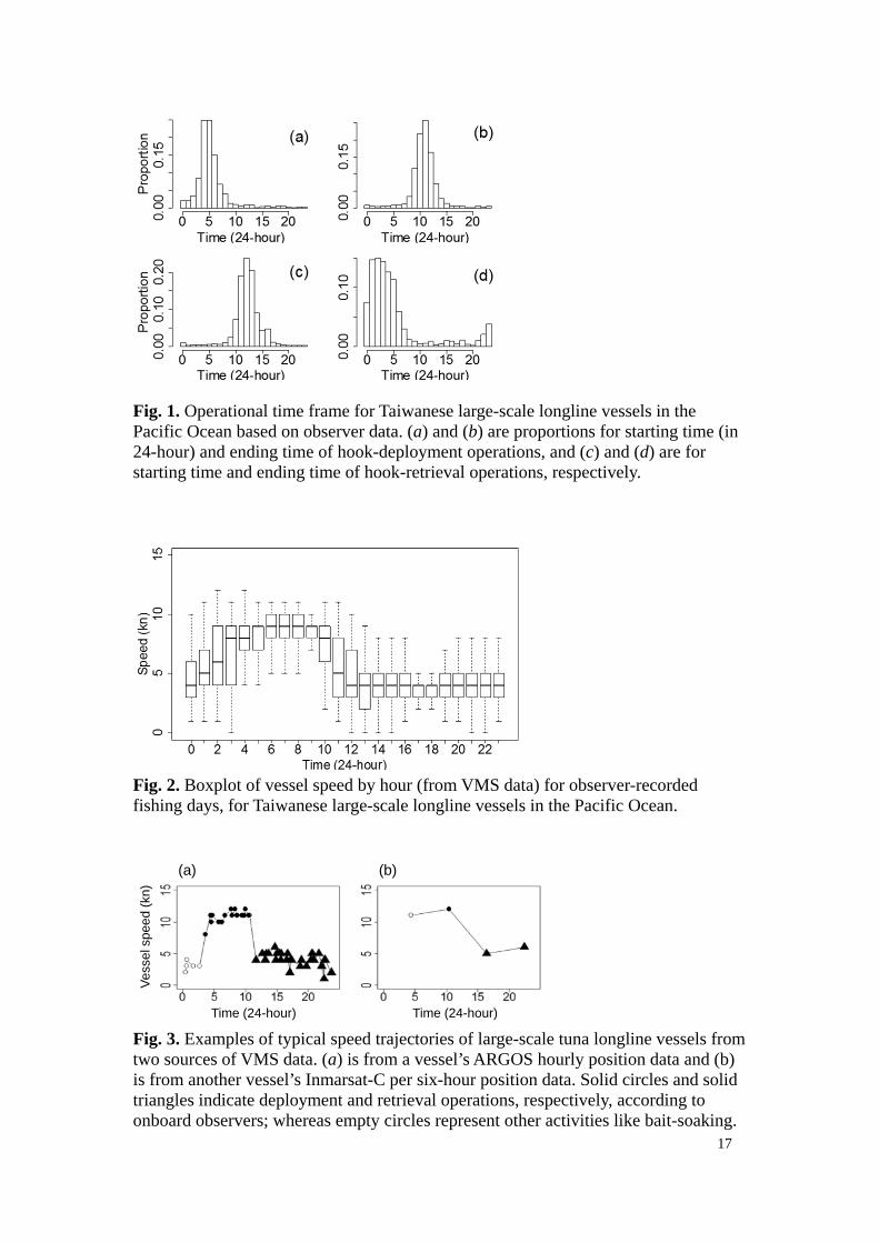
Fig. 1. Operational time frame for Taiwanese large-scale longline vessels in the Pacific Ocean based on observer data. (a) and (b) are proportions for starting time (in 24-hour) and ending time of hook-deployment operations, and (c) and (d) are for starting time and ending time of hook-retrieval operations, respectively.

Fig. 2. Boxplot of vessel speed by hour (from VMS data) for observer-recorded fishing days, for Taiwanese large-scale longline vessels in the Pacific Ocean.

(a) (b)

Time (24-hour) Time (24-hour)

Vess

el s

peed

(kn)

Fig. 3. Examples of typical speed trajectories of large-scale tuna longline vessels from two sources of VMS data. (a) is from a vessel’s ARGOS hourly position data and (b) is from another vessel’s Inmarsat-C per six-hour position data. Solid circles and solid triangles indicate deployment and retrieval operations, respectively, according to onboard observers; whereas empty circles represent other activities like bait-soaking.

17

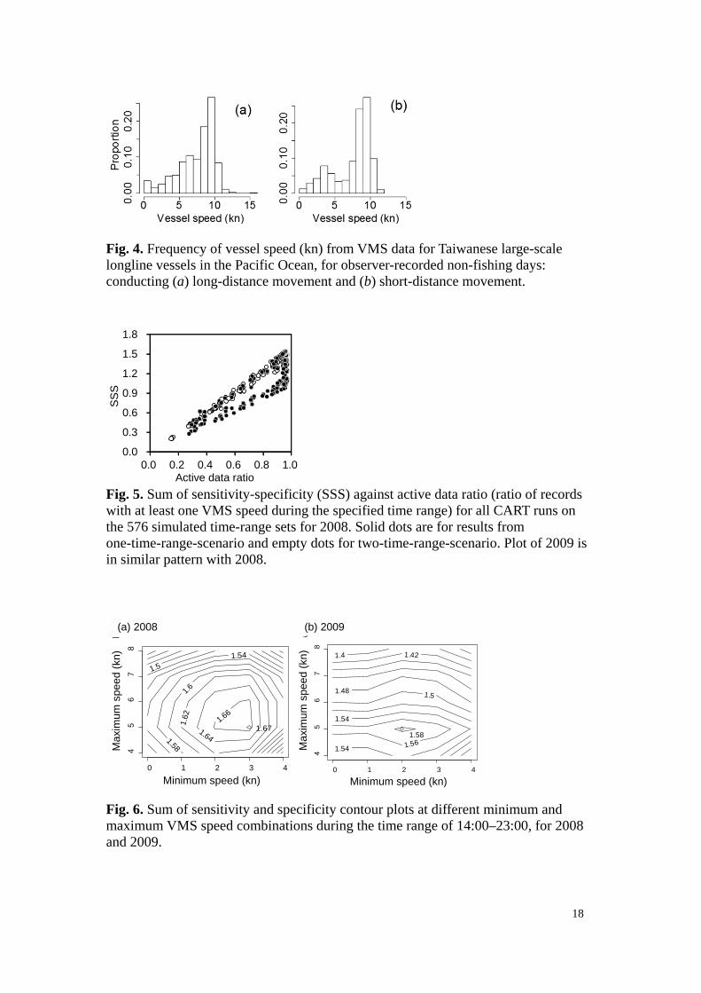
Fig. 4. Frequency of vessel speed (kn) from VMS data for Taiwanese large-scale longline vessels in the Pacific Ocean, for observer-recorded non-fishing days: conducting (a) long-distance movement and (b) short-distance movement.

0.0

0.3

0.6

0.9

1.2

1.5

1.8

0.0 0.2 0.4 0.6 0.8 1.0

SSS

Active data ratio Fig. 5. Sum of sensitivity-specificity (SSS) against active data ratio (ratio of records with at least one VMS speed during the specified time range) for all CART runs on the 576 simulated time-range sets for 2008. Solid dots are for results from one-time-range-scenario and empty dots for two-time-range-scenario. Plot of 2009 is in similar pattern with 2008.

Max

imum

spe

ed (k

n)

(a) 2008

Minimum speed (kn) Minimum speed (kn)

(b) 2009

Max

imum

spe

ed (k

n)

Minimum speed (kn)

Max

imum

spe

ed (k

n)

1.4 1.42

1.48 1.5

1.54

1.54

1.56

0 1 2 3 4

45

67

8

1.58

Minimum speed (kn)

Max

imum

spe

ed (k

n)

1.5 1.54

1.58

1.6

1.6

2

1.64

1.66

0 1 2 3 4

45

67

8

1.67

Max

imum

spe

ed (k

n)

(a) 2008

Minimum speed (kn) Minimum speed (kn)

(b) 2009

Max

imum

spe

ed (k

n)

Fig. 6. Sum of sensitivity and specificity contour plots at different minimum and maximum VMS speed combinations during the time range of 14:00–23:00, for 2008 and 2009.

18

40S

10S

20N

125E 165E 155W 115W

40S

10S

20N

125E 165E 155W 115W

40S

10S

20N

125E 165E 155W 115W

(a) 2005 (c) 2007(b) 2006

(d) 2008 (e) 2009 (f) 2010

(g) 2008-logbook (h) 2009-logbook

40S

10S

20N

125E 165E 155W 115W

<1010-2930-4950-69>69

40S

10S

20N

125E 165E 155W 115W

40S

10S

20N

125E 165E 155W 115W

40S

10S

20N

125E 165E 155W 115W

40S

10S

20N

125E 165E 155W 115W

Fig. 7. Distribution of fishing days (in 1 × 1 degree cell) estimated from VMS data for years 2005 – 2010 (a - f) and from logbook data for 2008 and 2009 (g and h).

19