
Central Bank Frameworks: Evolution or Revolution?
286
Central Bank Frameworks: Evolution or Revolution? 2018
-
Upload
khangminh22 -
Category
Documents
-
view
0 -
download
0
Transcript of Central Bank Frameworks: Evolution or Revolution?

SP
INE
SP
INE
Proceedings of a Conference 2018Central Bank Fram
eworks: Evolution or Revolution?
Central Bank Frameworks: Evolution or Revolution?
2018

Proceedings of a Conference
Held in Sydney on 12–13 April 2018
Editors: John Simon
Maxwell Sutton
Central Bank Frameworks:
Evolution or Revolution?

The publication of these Conference papers is aimed at making results of research undertaken in the Bank, and elsewhere, available to a wider audience. The views expressed are those of the authors and discussants and not necessarily those of the Reserve Bank of Australia. References to the results and views presented should clearly attribute them to the authors, not to the Bank. Responsibility for any errors rests with the authors.
Figures in this publication were generated using Mathematica.
The content of this publication shall not be reproduced, sold or distributed without the prior consent of the Reserve Bank of Australia.
Website: www.rba.gov.au
Cover Design Reserve Bank of Australia
Printed in Australia by Reserve Bank of Australia 65 Martin Place Sydney NSW 2000 Tel: +61 2 9551 8111 Fax: +61 2 9551 8000
ISBN 978-0-6480470-5-6 (Print) ISBN 978-0-6480470-6-3 (Online) Sydney, December 2018

IntroductionJohn Simon 1
Session One: Twenty-something Years of Inflation Targeting – What Has Worked? What Has Changed?
Inflation Targeting in New Zealand: An Experience in EvolutionJohn McDermott and Rebecca Williams 7
Credibility, Flexibility and Renewal: The Evolution of Inflation Targeting in CanadaThomas J Carter, Rhys Mendes and Lawrence L Schembri 25
Twenty-five Years of Inflation Targeting in AustraliaGuy Debelle 53
General Discussion 69
Session Two: The Changing Environment
The Transmission of Monetary Policy through Banks’ Balance SheetsAnthony Brassil, Jon Cheshire and Joseph Muscatello 73Discussant Aarti Singh 123
A Factor Model Analysis of the Effects of Inflation Targeting on the Australian EconomyLuke Hartigan and James Morley 127Discussant Marcelle Chauvet 161
Session Three: Framework Alternatives
Twenty-five Years of Inflation Targeting in Australia: Are There Better Alternatives for the Next Twenty-five Years?Warwick J McKibbin and Augustus J Panton 173Discussant Stephen Grenville 199
Monetary and Macroprudential Policies: The Case for a Separation of PowersBen Broadbent 209Discussant Sally Auld 227
Contents

Robust Design Principles for Monetary Policy CommitteesDavid Archer and Andrew T Levin 233Discussant Bruce Preston 252
Session Four: Review of Papers and Discussions
Wrap-up Panel DiscussionJessica Irvine, Philip Lowe, Adam Posen and Sayuri Shirai 259
Biographies of Contributors 265
List of Conference Participants 277
Other Volumes in this Series 279
1CO N F E R E N C E V O L U M E | 2 018
John Simon
Twenty-five years ago the Governor of the Reserve Bank of Australia (RBA), Bernie Fraser, gave a speech declaring that ‘My own view is that if the rate of inflation in underlying terms could be held to an average of 2 to 3 per cent over a period of years, that would be a good outcome’ (Fraser 1993, p 2). While this did not mark the formal adoption of inflation targeting in Australia – that would take a few more years – it is as good a point as any to mark the de facto beginning of inflation targeting in Australia.
In the 25 years since, many things have changed. Where recession, high inflation and high unemployment were once common, there has not been a recession in Australia since the start of inflation targeting, inflation has fallen from around 8 per cent to an average of 2–3 per cent and unemployment has fallen from over 10 per cent to average closer to 5 per cent. But, despite these significant macroeconomic improvements, the global financial crisis (GFC) has challenged the practice of central banking.
Around the world, questions are being asked about whether the flexible inflation-targeting framework used by many central banks is the most appropriate framework given the experience of the crisis. Thus, it is a good time to consider whether the inflation-targeting framework that has served Australia so well over the past 25 years is well adapted to the next 25 years.
Reflecting this context, the title of this conference, ‘Central Bank Frameworks: Evolution or Revolution?’, implicitly asks whether the current framework needs to change and, if so, how dramatically. However, while many people think about evolution as a slow process that proceeds gradually and revolution as one that proceeds quickly, the rate of evolutionary change is not necessarily always constant or slow. Within the field of evolutionary biology there are two broad characterisations of the process of evolution: phyletic gradualism, which is most similar to the popular view of evolution as a slow and gradual process, and punctuated equilibria that emphasises the alternation of periods of rapid change with long periods of stasis. The distinction with revolution is not so much the speed of change as the fact that what emerges from evolution is still recognisably similar, while revolution leads to something distinctly different from that which went before.
When thinking about the practice of central banking it seems, at a distance at least, to be characterised by both revolution and punctuated equilibria. There are typically long periods of stability interspersed with relatively rapid change. For example, the gold standard and Bretton Woods systems prevailed for long periods of time before being replaced by very
Introduction

2 R E S E R V E B A N K O F A U S T R A L I A
J O H N S I M O N
different arrangements. Furthermore, just as evolutionary change is a response to external pressures, so we can also think about the evolution of central bank frameworks. The external pressures on central banking have ebbed and flowed over the years. When those pressures are large, such as around the late 1960s and early 1970s, the frameworks have evolved rapidly. When those pressures are more benign, such as during the Great Moderation, evolution has been slower.
A question this conference is particularly focused on is whether the pressures on inflation targeting over recent years are such that rapid evolution of, or even a revolution in, the monetary policy framework is necessary or whether the current framework is well adapted to the current post-GFC environment.
To answer these questions, the conference was organised in three sections. The first looked at the experiences of New Zealand, Canada and Australia. An important focus of this section was how the various regimes had evolved over the course of the twenty-something years they had been in operation. By understanding what has happened so far, we should be better placed to think about the way things might change in the future. The second section looked at changes in financial markets and the macroeconomy since the introduction of inflation targeting in Australia. By establishing what changes have occurred in the economy, it also provides pointers to ways the inflation-targeting regime might have to adapt. The third section then considered alternatives to the current arrangements. If the framework was going to change, how should it change? The conference concluded with a panel discussion that synthesised the various papers and reflected on what had been learnt over the course of the two days.
The three papers in the first session, looking at the experiences of New Zealand, Canada and Australia, highlight both how inflation targeting has evolved since it was first adopted by New Zealand in 1990 and the differences between the three inflation-targeting regimes. Inflation targeting is not an unchanging framework exactly replicated across countries, but rather a framework that has been adapted to the various country-specific institutional environments it has been used in. An example, perhaps, of niche evolution. For example, while initial formulations of inflation targeting were relatively strict, the dominant form today is ‘flexible inflation targeting’ that places greater emphasis on unemployment or output stabilisation.
The paper on New Zealand by John McDermott and Rebecca Williams highlights that New Zealand’s initial choice of a relatively strict inflation-targeting regime grew out of the need to establish the Reserve Bank of New Zealand’s (RBNZ’s) institutional credibility. It also seems likely that, as the first central bank to adopt inflation targeting, there may have been a broader need to establish the credibility of the regime itself. The framework was designed with four pillars, or stakes, chosen to support the growth of the newly planted regime: operational independence; transparency; a single objective; and a single decision-maker. They note that there have been some changes to the single objective. From a relatively strict objective it has evolved into a more flexible objective and the particular numerical target has also changed over time. In particular, they note that the government of the day has

3CO N F E R E N C E V O LU M E | 2018
I N T R O D U C T I O N
frequently led these changes. That is also true about the most recently announced changes to the RBNZ’s framework – replacing the single objective with a dual mandate, adding unemployment to the inflation mandate, and replacing the single decision-maker with a monetary policy committee. Notwithstanding the evolution of the regime, it has delivered low and stable inflation in New Zealand.
The paper on Canada by Thomas J Carter, Rhys Mendes and Lawrence L Schembri emphasises three factors that are seen as central to the success of the Canadian regime: a simple, readily understood specification of the inflation target; the recognition that the government shares the duty of achieving the target and should set non-monetary policies in a way that is coherent with the achievement of the target; and, finally, the regular review of the regime, which has occurred every five years since 2001. As with New Zealand, the regime delivered low and stable inflation. The authors also note that the strength of the regime was demonstrated throughout the GFC. In particular, they emphasise the importance of the joint responsibility for macroeconomic outcomes shared by the central bank and the government – supportive macroprudential policies freed the central bank to focus on macroeconomic risks.
Finally, in the first session, Guy Debelle reflects on Australia’s experience. He emphasises the relative stability of the regime and evolutionary nature of Australia’s experience. In particular, the Reserve Bank of Australia’s mandate has been unchanged since it was first enacted in 1959. The evolution has occurred through the broader policy framework and the way that the mandate has been interpreted and operationalised. Of note, the inflation-targeting regime has been a flexible inflation-targeting regime from the start, in part reflecting the mandate of the RBA, which includes the maintenance of full employment, the stability of the currency, and the welfare of the people of Australia. Debelle also emphasises the fact that, as the regime has evolved, the communication of the RBA has had to evolve along with it. He notes that communication has played an increasingly important role in the operation of the regime given the centrality of inflation expectations to a flexible inflation-targeting regime.
The second session of the conference contained two papers that served as a bridge between the primarily backward-looking first session and the forward-looking third session. The first, by Anthony Brassil, Jon Cheshire and Joseph Muscatello, looked at the transmission of monetary policy through bank balance sheets and how that might have changed during the inflation-targeting period. The second, by Luke Hartigan and James Morley, looked at how the transmission of monetary policy through the macroeconomy might have changed as a result of the adoption of inflation targeting. These papers draw out the way the economic environment has changed since the introduction of inflation targeting. As such, they offer some pointers to ways the inflation-targeting framework might have to evolve.
Brassil, Cheshire and Muscatello consider the way the RBA’s policy rate is transmitted to the interest rates Australians pay on their mortgages and receive on their deposits. They document a number of interesting findings, including the fact that, following a reduction in the cash rate, the increase in the relative cost of deposit funding is broadly offset by a reduction in expected loan losses. Their main finding is that, while cash rate changes between 2003 and 2012 were fully passed through to the major banks’ lending and deposit

4 R E S E R V E B A N K O F A U S T R A L I A
J O H N S I M O N
rates (in aggregate), pass-through since 2012 has fallen to around 90 per cent as the major banks’ return on equity has not fallen with the cash rate. They further highlight the increasing importance of low- or no-interest deposits in bank balance sheets – as interest rates fall these accounts become relatively more expensive, and their share of banks’ funding increases at low rates. This points to the possibility that the ‘zero lower bound’ may be a more important consideration for monetary policy frameworks than was the case when inflation targeting was first being developed.
Hartigan and Morley use a factor model of the Australian economy to capture information from a wide range of economic indicators and distil it into a useable form. Having done this, they find that inflation targeting has been associated with a substantial reduction in the common components of economic volatility with little change in the idiosyncratic elements. This finding is highly suggestive that inflation targeting has been particularly successful at stabilising the economy. Importantly, they find that this stabilisation applies not only to nominal aspects of the economy, that one might expect to have been most affected by inflation targeting, but also the real aspects. A second implication of their results, however, is that it is much harder to measure the common component of economic activity (because the idiosyncratic elements are now relatively larger) and so policymakers need to look at a much wider range of indicators in order to correctly judge the state of the economy. A corollary seems to be that communication will be more difficult in this environment because there may be no single indicator policymakers can point to when explaining the reasons for their actions.
The third section of the conference contained three papers. The first, by Warwick J McKibbin and Augustus J Panton, considers whether there might be better frameworks than inflation targeting and proposes nominal income targeting as a superior framework. The second, by Ben Broadbent, considers the relationship between monetary policy and macroprudential policy and whether the experience of the GFC argues for a closer relationship between the regulators. The final paper, by David Archer and Andrew T Levin, considers the appropriate decision-making body for a central bank and, in particular, how a monetary policy committee should be structured.
McKibbin and Panton review a range of alternative monetary policy regimes and compare them with key criteria for a monetary regime. They ask such questions as: How well does the regime handle shocks? Can the target be credibly measured and understood? How transparent is the regime when exceptions are needed? Are prices expectations anchored by the regime? After considering how well each of the alternatives do on these criteria, they suggest that nominal income targeting would be a good regime and one that is superior to the current flexible inflation-targeting framework. An important reason for their conclusion is that, while inflation targeting deals with demand shocks well, it is less well suited to dealing with supply shocks; nominal income targeting, on the other hand, can handle supply shocks better.
Ben Broadbent considers whether macroprudential policy should be conducted jointly with monetary policy, and whether it should be done within the same institution, or

5CO N F E R E N C E V O LU M E | 2018
I N T R O D U C T I O N
separately. He makes the argument that full integration of the two policies could compromise accountability. In particular, he notes that the nature of the objectives of monetary policy and macroprudential policy are quite different. While monetary objectives are clear and verifiable, macroprudential objectives are multiple, opaque and hard to verify. If both these kinds of objectives are merged, there will be an inevitable problem as the clear and verifiable objectives crowd out the opaque objectives. He also notes that the benefits from formal coordination are overstated and, at least in open economies with floating exchange rates, financial stability depends much more on prudential policy than on monetary policy.
Archer and Levin focus on developing a set of robust design principles for monetary policy committees that mitigate the risk of political interference and groupthink. They argue that independence from political interference rests not on statutory independence but on public confidence and the legitimacy of the institution. As such, transparency and public accountability are important to the extent that they support the legitimacy and, thus, independence of the institution. To guard against groupthink they argue that the monetary policy committee should be made up of a diverse group of experts who are individually accountable for their policy decisions.
The conference closed with a panel discussion moderated by Jessica Irvine. The panellists were Philip Lowe, Adam Posen and Sayuri Shirai. The discussion served to draw the various threads of the conference together. In summarising the areas of agreement at the conference, one panellist suggested that participants generally agreed that: regimes matter, flexibility is important, transparency is important, committees bring benefits to the decision-making process and inflation-targeting regimes have enjoyed wide political support. In thinking about Australia’s experience, it was felt that Australia’s inflation-targeting framework had worked well for the past 25 years and an important part of that was the flexibility it had built in from the start. Looking forward, the discussion considered whether the shocks Australia is likely to face in the future might be different to the shocks it has faced in the past and, if so, there was a possibility that the inflation-targeting regime might have to evolve further. Nonetheless, while it was generally agreed that it was good to consider alternatives to the current regime, and to do so from a position of strength before problems emerged, there was no obvious need for change.
This conference volume collects together the papers presented at the conference, the discussants’ comments and a summary of the general discussion that followed each presentation. As the conference is run under the Chatham House Rule, individual participants are not identified in the general discussions.
ReferenceFraser BW (1993), ‘Some Aspects of Monetary Policy’, RBA Bulletin, April, pp 1–7.

6 R E S E R V E B A N K O F A U S T R A L I A

7CO N F E R E N C E V O L U M E | 2 018
John McDermott and Rebecca Williams
1. IntroductionIt is a pleasure to discuss an issue that is especially pertinent to the Reserve Bank of New Zealand (RBNZ) at present – the evolution of central bank frameworks. As many of you will be aware, the New Zealand Government is in the process of changing our monetary policy framework to add employment to our existing mandate of price stability and formalise a decision-making structure based on a committee. This would bring us closer to a framework like the one here in Australia and in the United States.
This paper is in a session titled ‘Twenty-something Years of Inflation Targeting’, but in New Zealand it has actually been closer to thirty. The Reserve Bank of New Zealand Act 1989 (RBNZ Act) came into effect in February 1990, making New Zealand the first country to formally adopt inflation targeting as we now know it.
New Zealand’s experience has been one of evolution. As the RBNZ established its credibility – by which I mean it became clear that we could and would meet our price stability objective – we were able to develop a more flexible approach to inflation targeting, consistent with the literature and with developments in other inflation-targeting countries.
We are about to enter the next stage of that evolution. I believe this next step is indeed an evolution, which builds on the flexible approach we have been taking for some time, rather than a revolution. That said, it is still too early to determine precisely what effect the new framework will have on the implementation of monetary policy. The New Zealand framework has changed significantly over 30 years, reflecting lessons learned and the changing economic and political environment. And it is likely to continue to evolve as we are faced with new developments.
You may be very familiar with our tale and want me to cut to the chase – our move towards a dual mandate and formalised committee – but before I touch on where we are going, I want to provide you with some context: where we started, and where we have been.
Inflation Targeting in New Zealand: An Experience in Evolution

8 R E S E R V E B A N K O F A U S T R A L I A
J O H N M C D E R M O T T A N D R E B E CC A W I L L I A M S
2. The Origins of Inflation Targeting: A Need for CredibilityAs I have noted, inflation targeting as we now know it was pioneered in New Zealand.1,2 Other countries had been pursuing disinflationary monetary policy since the late 1970s and, by the early 1980s, most Organisation for Economic Co-operation and Development (OECD) countries were announcing some form of money or credit target in an attempt to convince the public and markets that they were taking the challenge of controlling inflation seriously (Reddell 1999). But the focus internationally was on these ‘intermediate’ targets – the quantity of money or credit – rather than inflation itself. Intermediate targets were thought to be informative for monetary policy as they were susceptible to a degree of central bank control. The extent to which intermediate targets were connected to the objective of price stability was, however, subject to debate (e.g. Friedman 1984, 1990).
In the 1970s and 1980s, New Zealand had a very poor track record of price stability. Annual consumer price index (CPI) inflation had been around 10 to 15 per cent since the early 1970s (Figure 1), and was considerably higher than inflation in our main trading partners. A key driver of high inflation in New Zealand over this period was government spending, accommodated by generally loose monetary policy (Grimes 1996). There had been episodes of tight monetary policy over this period. But successive governments had been unwilling to face the short-term costs to output and employment that disinflation brought with it, and had quickly reversed course and loosened policy.3
Bringing high inflation under control was a key priority for the Labour Government that came into power in New Zealand in July 1984.4 In 1986, the then Minister of Finance, Roger Douglas, invited officials to explore options for reforming the monetary policy framework, aiming to reduce the scope for political influence that had seen past attempts to control inflation fail so badly.
1 Bernanke et al (1999) provide a widely cited definition of inflation targeting.
2 Italy, Greece and Portugal all published single-year targets for inflation at times during the early 1980s, and Sweden briefly operated a form of price level targeting in the 1930s. However, none of these provided a complete, sustained structure for inflation targeting of the kind now understood by the term. In the 1970s and 1980s, West Germany conducted monetary policy in a framework that closely resembled inflation targeting, although it was officially designated as money targeting (Bernanke and Mihov 1997). In addition, in 1995 the Bundesbank itself drew a distinction between its approach and inflation targeting, arguing at the time that inflation targeting was the inferior approach.
3 Nelson (2005) provides detailed discussion of another factor that contributed to New Zealand’s poor inflation performance before 1984, namely that there remained a view at the government level that high inflation was predominantly generated by cost-push factors (such as wage bargaining) rather than monetary or demand factors. This belief eventually led the Muldoon Government to impose a wage price freeze in 1982 in an attempt to control inflation directly.
4 Then RBNZ Governor Spencer Russell (1984) discussed the new government’s commitment to bring inflation under control:
We have had periods of tight monetary policy in the past. But by backing off at the eleventh hour, money and credit growth rates have been allowed to expand excessively again and the benefits from the temporary period of tightness have been lost. The Government has made it clear this will not be the case again.

9CO N F E R E N C E V O LU M E | 2018
I N F L AT I O N TA R G E T I N G I N N E W Z E A L A N D : A N E X P E R I E N C E I N E V O L U T I O N
Figure 1: Annual CPI InflationTarget range shaded
2006199419821970 2018-5
0
5
10
15
%
-5
0
5
10
15
%
Reserve Bank of New Zealand Act 1989
Wage and price freeze
Oil priceshocks
GST introduced
GST increased Targetmidpoint
Source: Statistics New Zealand
The framework that evolved over the next four years was the culmination of various strands of economic thought and the principles that were underpinning the wider reform of New Zealand’s public sector at the time.5,6 At its core, the framework that emerged provided the RBNZ with a means to credibly commit to bringing inflation down and keeping it there.
And why does credibility matter? If policymakers are able to convince firms and workers that they will set policy to achieve the inflation target, this anchoring of inflation expectations makes it more likely that prices and wages will be set in a manner consistent with the target, even in the face of shocks to the economy. This naturally makes the target itself easier to achieve.
Picture the New Zealand inflation-targeting framework as a newly planted tree. In the 1970s and 1980s, several seedlings of low inflation had been planted, but none took hold. The ground conditions – a highly regulated financial market and economy – were not conducive to growth, and the winds of politics kept blowing the seeds of low inflation away before they had a chance to flourish.
By the mid 1980s, ground conditions were much improved. New Zealand had gone through a dramatic period of financial market reform in the nine months between July 1984 and March 1985. The float of the New Zealand dollar and the commitment of the government to fund the fiscal deficit via issuance of public debt to the private sector freed up the RBNZ to pursue domestic monetary policy (Kamber, Karagedikli and Smith 2015). To ensure that
5 Reddell (1999) contains a detailed discussion of the origins and early development of the inflation target; Grimes (1996) provides a comprehensive summary of monetary policy developments within the wider reform environment; Singleton et al (2006) provides a history of the RBNZ between 1973 and 2002; Grimes (2014) also discusses the origins and evolution of inflation targeting in New Zealand.
6 Don Brash, who was the first Governor of the inflation-targeting era, once said of the origins of inflation targeting in New Zealand ‘I will simply note that history can be surprisingly confusing, even for those who were there’ (Brash 1998, p 222).

1 0 R E S E R V E B A N K O F A U S T R A L I A
J O H N M C D E R M O T T A N D R E B E CC A W I L L I A M S
inflation targeting could establish credibility and take hold, four highly related aspects of the framework were provided as stakes in the ground to support the new sapling.7 These stakes were: operational independence; transparency; the single objective of price stability; and the Governor as sole decision-maker, which I will now discuss in turn.
2.1 Operational independence (RBNZ Act, Section 13)The RBNZ Act provided the RBNZ with its operational independence and its monetary policy objective.8 It was heavily influenced by the literature on the time inconsistency of monetary policy and the experience during the 1970s and 1980s, in which successive governments had been unwilling to endure the short-term effects of disinflation for the longer-term gains of price stability.9 The specific monetary policy target of the RBNZ Act was to be publicly agreed upon in a Policy Targets Agreement (PTA) between the Minister of Finance and the Governor of the RBNZ. Prior to the late 1980s, RBNZ independence had been non-existent: the 1973 Amendment to the 1964 RBNZ Act had stated that the RBNZ was to ‘give effect to the monetary policy of the Government’.10 The RBNZ Act contributed to the RBNZ’s credibility by making it clear that its objective was no longer subject to concerns or incentives related to the electoral cycle.
2.2 Transparency (RBNZ Act, Section 15)Monetary policy operates with significant lags and in an inherently uncertain environment. It, therefore, naturally requires a great deal of judgement and discretion. To ensure that operational independence was used appropriately, the RBNZ Act also specified a high degree of transparency in how the RBNZ formulated policy. The RBNZ Act requires the RBNZ to publish regular statements on its monetary policy decisions and for these to be laid before Parliament. The Governor’s deliberations were also to be monitored and assessed by a board consisting of members appointed by the Minister of Finance.
2.3 Single objective (RBNZ Act, Section 8)Providing the RBNZ with one objective, rather than a list of objectives – production, trade, full employment and price stability – as had been the case previously, made it more likely that the RBNZ could actually achieve its mandate and, thus, contributed to the credibility
7 It is worth noting that the RBNZ Act does not specify that there must be targets for inflation itself. The RBNZ Act specifies only ‘policy targets for the carrying out by the Bank of its [price stability objective]’, which leaves open the possibility of specifying targets such as nominal gross domestic product consistent with medium-term price stability.
8 Except as otherwise provided for in the RBNZ Act, Section 12 allows for the Bank to be directed by the Governor-General to implement policy for a different economic objective than the one in Section 8, by Order in Council on the advice of the Minister. This section was included primarily for use in times of emergency (such as wartime) and has never been used. Any temporary redirection of policy would be well publicised since Orders in Council must be published in the New Zealand Gazette. The RBNZ Act can be accessed at <http://www.legislation.govt.nz/act/public/1989/0157/latest/DLM199364.html>.
9 The time-inconsistency problem is that authorities have an incentive to promise low inflation in the future, but then renege in order to boost activity (to obtain more votes, for example). As firms and households begin to anticipate this behaviour, their expectations of inflation increase and so they set prices and demand wages accordingly. The economy then ends up in a worse position with higher inflation and (potentially) higher unemployment (e.g. Barro and Gordon 1983).
10 Graham and Smith (2012) provide a history of RBNZ independence.

1 1CO N F E R E N C E V O LU M E | 2018
I N F L AT I O N TA R G E T I N G I N N E W Z E A L A N D : A N E X P E R I E N C E I N E V O L U T I O N
of that objective. The RBNZ Act states ‘The primary function of the [RBNZ] is to formulate and implement monetary policy directed to the economic objective of achieving and maintaining stability in the general level of prices’. It acknowledged that price stability was the greatest contribution monetary policy could make to New Zealand’s economic wellbeing. It recognised the limitations of monetary policy over the medium term, and provided the RBNZ, financial markets and wider public with a clear objective for policy. Moreover, the initial PTA clearly defined price stability with a numerical target band of 0 to 2 per cent. This clear numerical target provided a transparent measure against which the Governor’s performance could be assessed and around which inflation expectations could converge.
2.4 Single decision-maker (RBNZ Act, Section 9)The final stake in the ground was the assignment of authority and responsibility to an individual – the Governor. This ‘single decision-maker’ model was highly influenced by the principles underpinning the reform of the wider public sector at the time that gave individual public sector managers the authority to manage, but made them directly accountable for outputs (Reddell 1999; Sherwin 1999). The employment contract between the Minister of Finance and the Governor evolved into the PTA. The legislation made it clear that the Governor could lose his or her job for ‘inadequate performance’ in meeting these objectives.11
2.5 SummaryIn summary, the inflation-targeting framework established in the late 1980s was planted under conditions that increased its likelihood of success. The four stakes of operational independence, transparency, the single objective of price stability, and the single decision-maker model provided essential support to a new framework, and encouraged it to take root and establish its credibility. All well and good, but why have I taken you through this history lesson? To provide you with some context on the New Zealand framework, and to introduce some aspects of the framework that remain as critical today as they were in 1989, and some that are about to change. But I will come back to that shortly.
3. The Evolution of Inflation Targeting: Increasingly FlexibleSince being planted in the late 1980s, New Zealand’s framework has evolved significantly. As we were pioneers, it was always unlikely that we could introduce a framework that got everything ‘right’ from the start, especially given that the environment in which policy operates has itself developed a lot over the years (Sherwin 1999).
The evolution of the inflation-targeting framework in New Zealand can be characterised as one of increasing flexibility, consistent with the academic literature and with developments
11 Donald Brash (2002) recalls the response of the Minister responsible for the RBNZ legislation when he expressed initial surprise that the PTA would be between the Government and Governor, rather than the Government and the Bank: ‘We can’t fire the whole Bank. Realistically, we can’t even fire the whole Board. But we sure as hell can fire you!’

1 2 R E S E R V E B A N K O F A U S T R A L I A
J O H N M C D E R M O T T A N D R E B E CC A W I L L I A M S
in other advanced economies.12 As our tree grew taller and its roots grew deeper – as we gained credibility by actually meeting our target, and anchored inflation expectations – we could be more confident that our tree could bend in the wind, without being uprooted.
What exactly do I mean by flexibility? Over the past three decades, monetary policymakers and academics have learned that there is a trade-off, not between inflation and output, but between the volatility of inflation and output. Monetary policy that is set to offset short-term movements in inflation away from target – referred to as ‘strict’ inflation targeting – will result in more volatility in output and other economic variables such as employment and the exchange rate (e.g. Svensson 1997). As the RBNZ established its credibility in achieving its inflation target, we could allow some volatility in realised inflation in order to offset some volatility elsewhere in the economy. In practice, this meant that interest rates were generally adjusted more slowly. And in this sense, the RBNZ has increasingly paid regard to the wider economy despite having a consistent overall objective of price stability specified in the RBNZ Act. This increasingly flexible approach has been reflected in the evolving content of successive PTAs over the past 30 years.
The PTA – which you will remember provides the RBNZ with its specific target in meeting its overall objective – must be renegotiated with the Minister of Finance each time a Governor is appointed or reappointed, and has also tended to be updated on the formation of a new government. This process naturally lends itself to incremental adjustments, influenced by the economic and political environment at the time. Since 1990, there have been 13 PTAs, with some alterations more significant than others. The RBNZ has seen more changes to its target than most other inflation-targeting central banks, and the process of renegotiation also provides more opportunity for government direction than is the case in some other countries (Wadsworth 2017).
In some ways, the large number of changes has been less than ideal, as it has the potential to undermine the public’s faith in the policy target. But since these changes have formalised things that we have learned in the process of operating policy, and reflected the underlying preferences of the public via the political process, they have been entirely appropriate.
There are several highly related dimensions of flexibility, and I will now take you through some key developments in New Zealand’s inflation-targeting framework across these dimensions, which are summarised in Table 1 below.
12 There was an early preference within the RBNZ for a flexible approach to inflation targeting. While an internal questionnaire to selected RBNZ staff in 1987 found seven respondents in favour and five against the use of ‘an explicitly-stated desired inflation time path [for either in-Bank or public use]’, the same survey also found nine in favour of the proposition that ‘short-run effects of monetary policy on real output [should] be included in any assessment of monetary policy’ (see Silverstone (2014)).

1 3CO N F E R E N C E V O LU M E | 2018
I N F L AT I O N TA R G E T I N G I N N E W Z E A L A N D : A N E X P E R I E N C E I N E V O L U T I O N
Table 1: Evolution of Flexible Inflation Targeting in New Zealand1990–2017
Dimension Early to mid 1990s Late 1990s and 2000s 2010sTime to target Initially, target to be
achieved by a set date
Dec 1990: annual inflation to remain inside the target band; RBNZ to calculate and explain deviations due to shocks outside the RBNZ’s control (explicit ‘caveats’)
Time to target implicitly lengthened; RBNZ to respond to general inflationary pressure
List of shocks that could result in deviation from target became illustrative, rather than exhaustive
2002: medium-term focus made explicit
Explicit medium-term focus has remained
Secondary considerations
1999: RBNZ shall seek to avoid unnecessary instability in output, interest rates and the exchange rate
2012: RBNZ to have regard to the efficiency and soundness of the financial system; RBNZ to monitor asset prices
Other secondary considerations (stability of output, interest rates and the exchange rate) have remained
Target definition
Initially: 0–2 per cent
1996: 0–3 per cent
2002: 1–3 per cent 2012: 1–3 per cent, with a focus on the 2 per cent target midpoint
3.1 Early to mid 1990sThe initial inflation target of 0–2 per cent originated primarily as a communications device – a way for Minister Roger Douglas to refocus expectations and convince the public that the anti-inflation drive would continue (Reddell 1999).13 Inflation was within the target by 1991, and stayed there until June 1995 when adverse weather pushed up the prices of fruit and vegetables and saw inflation increase to 2.2 per cent.
13 During a televised interview broadcast on 1 April 1988, Roger Douglas said that policy was to be directed to reducing inflation to ‘around zero to one per cent’ over the following couple of years. By the June 1988 RBNZ Bulletin, the Bank felt confident enough to describe the ultimate goal as being ‘price stability by the 1990s’ and that ‘[i]n terms of the CPI, this objective is likely to be consistent with a small positive measured inflation rate, in the order of 0–2 per cent, as a result of several problems in the construction of the index’ (Reddell 1988).

1 4 R E S E R V E B A N K O F A U S T R A L I A
J O H N M C D E R M O T T A N D R E B E CC A W I L L I A M S
Over the next few years, inflation remained at the top of, or marginally above, the target range. With hindsight, the RBNZ was slow to recognise the pace of acceleration of the economy in 1992–93, and relied on the transmission of policy via the exchange rate to a greater extent than was ideal given the structural changes we later learned were underway (RBNZ 2000b). The RBNZ learned that keeping inflation within such a narrow range could likely only be achieved at the cost of undesirably high volatility in the real economy, and began talking about the target as something that we would constantly aim for rather than something we could – or should – deliver every quarter (Brash 2002).
Since December 1990, PTAs had contained some allowance for actual inflation to deviate from target. These were in the form of explicit ‘caveats’ or ‘principal shocks’ recognised as being outside the RBNZ’s control. We were required to calculate and publish the direct effect these had on inflation outcomes. In practice, we found it increasingly difficult to determine which items to include or exclude, and were exposed to (although never received much) criticism that we could manipulate the calculation in order to meet our objective.
In 1996, the target was widened to 0–3 per cent, reflecting the new National/New Zealand First Coalition Government’s preferences (RBNZ 2000a). The RBNZ was comfortable with this widening as we felt it was unlikely to materially affect monetary policy credibility or adversely affect inflation expectations.14 By allowing slightly more inflation variability it enabled policy to offset volatility in the real economy to a greater extent. The 1996 PTA also modified the explanation of the RBNZ’s overall objective to be more explicit that price stability was the best contribution that monetary policy could make to economic growth and employment, rather than simply being an end in and of itself (RBNZ 2000a).
3.2 Late 1990s and 2000sAs the RBNZ learned more about the transmission of monetary policy in the New Zealand economy during the 1990s, we put increasing weight on real economy channels and less on direct exchange rate effects (Brash 1998). Specifically, we found that the pass-through of nominal exchange rate changes into local prices had become more muted over the 1990s. This meant that the slower part of the monetary policy transmission mechanism – via the real economy – was given even greater prominence in meeting our objective (RBNZ 2000b). This change in emphasis effectively lengthened the horizon over which policy was formulated, which, in itself, encouraged less variability in interest rates, the exchange rate and output.
In 1999, the incoming Labour/Alliance Coalition Government initiated the modification of the PTA to state that ‘[i]n pursuing its price stability objective, the [RBNZ] … shall seek to avoid unnecessary instability in output, interest rates and the exchange rate’. The RBNZ viewed these changes as largely confirming the flexible approach we had been taking for most of the inflation-targeting period (RBNZ 2000a). It reflected the fact that several policy paths could be chosen to meet our inflation target, and the effect of these paths on the real economy and other variables was influential in determining which path was ultimately selected (RBNZ 2000c).
14 Recent research by the RBNZ has found that the widening of the target did result in an increase in long-term inflation expectations, but that this increase was not statistically significant (Lewis and McDermott 2016).

1 5CO N F E R E N C E V O LU M E | 2018
I N F L AT I O N TA R G E T I N G I N N E W Z E A L A N D : A N E X P E R I E N C E I N E V O L U T I O N
The changes were also a reflection of economic developments. The RBNZ initially underestimated the combined effect of the Asian crisis and the droughts that affected rural New Zealand in the summers of 1997–98 and 1998–99, which led to recession in New Zealand. We operate in an uncertain world, and monetary policy would never have been able to completely offset the effect of these shocks. Yet the way we implemented monetary policy over this period – via the Monetary Conditions Index (MCI), which was introduced in mid 1997 – shaped the response in a way that probably contributed to the fall in output and added unnecessary interest rate volatility (RBNZ 2000b).15 The RBNZ recognised this, and we replaced the MCI with the Official Cash Rate (OCR) as the instrument of monetary policy in March 1999. The MCI was a branch that we lopped off fairly quickly.
In May 2000, the Minister of Finance invited Professor Lars Svensson to review the operation of monetary policy in New Zealand. He found the framework to be ‘entirely consistent with the best international practice of flexible inflation targeting, with a medium-term inflation target that avoids unnecessary variability in output, interest rates and the exchange rate’ (Svensson 2001, p 2). He did recommend a move from the single decision-maker to committee model, but the government chose not to support this recommendation at this time (see Cullen (2001)).
During the early 2000s, however, concern continued to grow among politicians, industry representatives, commentators and the wider public that the economy’s trend growth rate had been unnecessarily constrained by the performance of monetary policy (RBNZ 2002). Those expressing concern suggested that this constraint resulted from a target that was too low and policy that was too aggressive. It was argued that these factors had resulted in interest rates that were too high on average, and in interest rates and the exchange rate being too volatile.
The RBNZ noted the long-held and internationally accepted view that monetary policy was unlikely to have a large influence on the long-run performance of the economy, and that there was no evidence that policy in New Zealand was more aggressive than elsewhere. But we also had not found any clear evidence that trend inflation of 2 per cent would produce better or worse outcomes for trend growth than trend inflation of 1.5 per cent. In the end, the target (and therefore midpoint) was changed to 1–3 per cent in the 2002 PTA. Recent RBNZ research has found that this change was accompanied by an immediate increase in long-run inflation expectations (Lewis and McDermott 2016).
The 2002 PTA also made the medium-term focus of monetary policy explicit, and firmly embedded the flexible approach (e.g. Hunt 2004). It changed the target from ‘12-monthly increases’ to ‘future CPI inflation outcomes … on average over the medium term’. This medium-term focus has been an enduring feature of PTAs to this day. The RBNZ has interpreted this target to mean that it should set policy in order for inflation to remain or settle comfortably within the target band in the latter half of a three-year horizon (Bollard and Ng 2008).
15 The MCI was a weighted summation of the exchange rate and short-term interest rate, with weights reflecting each variable’s medium-term effect on aggregate demand and thus inflation. The MCI was used to identify the overall stance of monetary policy and to communicate the likely direction and extent of change in stance in the future.

1 6 R E S E R V E B A N K O F A U S T R A L I A
J O H N M C D E R M O T T A N D R E B E CC A W I L L I A M S
During the mid 2000s, economic developments reignited concern about the monetary policy framework. Although New Zealand had been one of the faster-growing OECD economies since the early 1990s, this growth had been accompanied by the emergence of macroeconomic imbalances: a relatively large current account deficit, high house price inflation and household indebtedness, and a real exchange rate that had risen to levels sometimes regarded as unjustified by medium-term fundamentals (RBNZ 2007b). In early 2007, the government requested another inquiry into the monetary policy framework.
The RBNZ reiterated that there was no compelling evidence to suggest that these features had arisen from the design of the monetary policy framework. We recognised that, with the benefit of hindsight, we had been slow to fully recognise the strength of demand and housing market pressure on inflation over the cycle. However, this was a feature of having to operate policy under uncertainty (RBNZ 2007a; Chetwin and Reddell 2012). We noted that solutions to New Zealand’s imbalances were likely to lie in other policy domains, and suggested several ‘supplementary stabilisation instruments’.16 Following the review, the government decided not to make any changes to the RBNZ Act or the PTA, nor introduce any of the suggested instruments (see FEC (2008) for the full report).17
Monetary policy during the global financial crisis (GFC) of 2008–09 demonstrated the flexibility of the inflation-targeting framework. Despite CPI inflation being driven well above the target band by higher oil prices over 2008, the RBNZ reduced the OCR by 575 basis points between June 2008 and June 2009. Our tree remained firmly planted, anchored by its roots of credibility, despite the largest global storm since the Great Depression. Longer-term inflation expectations remained within the target range, and the reduction in the OCR helped support the New Zealand economy at a time of global distress (e.g. Chetwin 2012).
3.3 2010sThe GFC led many central banks to focus more heavily on how financial system developments should be treated by monetary policy. The RBNZ had always monitored asset prices and taken them into account in both monetary and prudential policy (see Bollard (2004)), and the RBNZ Act had long contained a requirement for the RBNZ to have regard for financial stability when setting monetary policy. Nonetheless, the 2012 PTA made this explicit by adding asset prices to the list of prices the RBNZ was directed to monitor, and including the requirement that the RBNZ ‘have regard to the efficiency and soundness of the financial system’ (see Kendall and Ng (2013)).
The RBNZ is unusual internationally, although not unique, in having both monetary policy and prudential responsibilities. In October 2013, the RBNZ introduced restrictions on high loan-to-value ratio (LVR) mortgage lending (e.g. Rogers 2013; Dunstan 2014). While these
16 These included cyclical variations in migrant approvals, increasing the responsiveness of housing supply, measures to limit procyclicality in fiscal policy, and consideration of various aspects of the tax regime (RBNZ 2007a, 2007b).
17 The FEC (2008, p 16) report stated that
Continuity is an important part of this framework, providing the public with confidence in the framework’s commitment to low and stable inflation. In view of the broad success of the framework, we do not recommend any change to the framework.
1 7CO N F E R E N C E V O LU M E | 2018
I N F L AT I O N TA R G E T I N G I N N E W Z E A L A N D : A N E X P E R I E N C E I N E V O L U T I O N
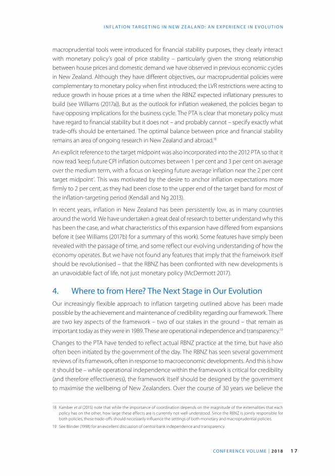
macroprudential tools were introduced for financial stability purposes, they clearly interact with monetary policy’s goal of price stability – particularly given the strong relationship between house prices and domestic demand we have observed in previous economic cycles in New Zealand. Although they have different objectives, our macroprudential policies were complementary to monetary policy when first introduced; the LVR restrictions were acting to reduce growth in house prices at a time when the RBNZ expected inflationary pressures to build (see Williams (2017a)). But as the outlook for inflation weakened, the policies began to have opposing implications for the business cycle. The PTA is clear that monetary policy must have regard to financial stability but it does not – and probably cannot – specify exactly what trade-offs should be entertained. The optimal balance between price and financial stability remains an area of ongoing research in New Zealand and abroad.18
An explicit reference to the target midpoint was also incorporated into the 2012 PTA so that it now read ‘keep future CPI inflation outcomes between 1 per cent and 3 per cent on average over the medium term, with a focus on keeping future average inflation near the 2 per cent target midpoint’. This was motivated by the desire to anchor inflation expectations more firmly to 2 per cent, as they had been close to the upper end of the target band for most of the inflation-targeting period (Kendall and Ng 2013).
In recent years, inflation in New Zealand has been persistently low, as in many countries around the world. We have undertaken a great deal of research to better understand why this has been the case, and what characteristics of this expansion have differed from expansions before it (see Williams (2017b) for a summary of this work). Some features have simply been revealed with the passage of time, and some reflect our evolving understanding of how the economy operates. But we have not found any features that imply that the framework itself should be revolutionised – that the RBNZ has been confronted with new developments is an unavoidable fact of life, not just monetary policy (McDermott 2017).
4. Where to from Here? The Next Stage in Our EvolutionOur increasingly flexible approach to inflation targeting outlined above has been made possible by the achievement and maintenance of credibility regarding our framework. There are two key aspects of the framework – two of our stakes in the ground – that remain as important today as they were in 1989. These are operational independence and transparency.19
Changes to the PTA have tended to reflect actual RBNZ practice at the time, but have also often been initiated by the government of the day. The RBNZ has seen several government reviews of its framework, often in response to macroeconomic developments. And this is how it should be – while operational independence within the framework is critical for credibility (and therefore effectiveness), the framework itself should be designed by the government to maximise the wellbeing of New Zealanders. Over the course of 30 years we believe the
18 Kamber et al (2015) note that while the importance of coordination depends on the magnitude of the externalities that each policy has on the other, how large these effects are is currently not well understood. Since the RBNZ is jointly responsible for both policies, these trade-offs should necessarily influence the settings of both monetary and macroprudential policies.
19 See Blinder (1998) for an excellent discussion of central bank independence and transparency.
1 8 R E S E R V E B A N K O F A U S T R A L I A
J O H N M C D E R M O T T A N D R E B E CC A W I L L I A M S
framework has served New Zealanders well – most of the graduates we have hired in recent years have never known anything other than low and stable inflation.
Transparency also remains a critical aspect of the framework. Being transparent about our assessment of the economy and our plan to meet our objective has an influence on expectations, and helps us achieve our objective. The RBNZ was the first central bank to publish its interest rate forecast, starting in 1997.20 And crucially, transparency aids in the assessment of our actions, and allows us to be held to account.21
But what of the other supports, the single decision-maker and single objective?
As I noted at the very start, these are the two aspects of the framework that the New Zealand Government is in the process of changing, to formalise a committee structure and add employment to our mandate. We agree that the single decision-maker model has become less relevant over time. In reality, RBNZ Governors have a long history of utilising advisory committees (Bollard and Karagedikli 2006). And in 2013, we established the Governing Committee, that at the time consisted of the Governor (as Chair), two Deputy Governors and myself (as Assistant Governor). While the Governor retains the right of veto on decisions, and continues to have statutory responsibility for policy, the committee members work together to test ideas and build consensus around the monetary policy decision (Wheeler 2013; Richardson 2016). The flexibility of our approach to inflation targeting requires a great deal of judgement, and the use of a committee maximises the knowledge and experience of members individually and as a collective.
The government will formalise a monetary policy committee (MPC) in the RBNZ Act, and add members from outside the RBNZ, ‘externals’, onto the committee. The RBNZ Act will allow the MPC to have between five and seven members, but there will be seven initially, and there will always be more internal than external members. All members will be nominated by the RBNZ Board, and appointed by the Minister of Finance. There will also be a non-voting observer from the New Zealand Treasury. Figure 2 illustrates the structure of the committee to be established in the RBNZ Act.
The MPC and Minister of Finance will agree on a Charter setting out the approach to issues defined in the RBNZ Act, including the approach to communications. Details of the first Charter are yet to be determined, but the Minister intends for the MPC to aim to reach decisions by consensus, and for non-attributed votes to be published where there is not consensus. The Minister also intends for non-attributed records of meetings to be published that reflect any differences of view among the MPC. We will no doubt explain these and other changes – and their potential implications for the setting and communicating of policy – as they are finalised.
20 Dincer and Eichengreen (2014) found that New Zealand was one of the most transparent central banks in the world (third behind Sweden and the Czech Republic in 2014), although by their estimates we rank much lower on central bank independence. The authors base the transparency indices on public reports and communications by each central bank, and the independence indices on central bank law in each country. Updated estimates can be found at <https://eml.berkeley.edu/~eichengr/data.shtml>.
21 See Ford, Kendall and Richardson (2015) for more on the evaluation of monetary policy.

1 9CO N F E R E N C E V O LU M E | 2018
I N F L AT I O N TA R G E T I N G I N N E W Z E A L A N D : A N E X P E R I E N C E I N E V O L U T I O N
Figure 2: Monetary Policy Committee to be Established in the RBNZ Act
Source: New Zealand Government
Internal members (majority)
Governor and Deputy Chief Executive ex-officio members, Governor as Chair, casting vote if required
Five-year terms (staggered)Maximum two terms in one roleFull-time
External members (minority)
Non-RBNZ staff with relevant knowledge and experience
Four-year terms (staggered)Maximum two termsPart-time
Non-voting Treasury observer
Of course, the creation of a formal (or indeed informal) committee does not guarantee superior outcomes. How the MPC will operate in practice is also extremely important. Committees are more successful when they have processes in place that aim to minimise various human biases, such as the pressure to conform, confirmation bias, and a tendency to rely on the most recent events to a greater extent than is sometimes warranted. The RBNZ will continue to ensure our internal processes aim to maximise the benefits that committees can provide.
And what of the move to a ‘dual mandate’? The RBNZ has always had regard to developments in the labour market, and this has been encouraged by our increasingly flexible approach. We have a long history of meeting with businesses and organisations across the country, and we regularly assess the available labour market data and are committed to discussing labour market developments. So my current sense is that, to a large extent, the changes are a way of ensuring that the flexibility in our approach endures.
The exact wording of the full employment objective in the RBNZ Act is yet to be determined. However, the PTA that Adrian Orr signed on 26 March 2018 reflected the upcoming changes to the RBNZ Act, and does not provide the RBNZ with a numerical target for full employment

2 0 R E S E R V E B A N K O F A U S T R A L I A
J O H N M C D E R M O T T A N D R E B E CC A W I L L I A M S
as it has with price stability. This is helpful, as ‘maximum sustainable employment’ cannot be fully captured by a single indicator.
Focusing too narrowly on one indicator, such as the unemployment rate, can be misleading. For example, a fall in the unemployment rate could be the result of an increased demand for labour – typically reflecting a strong economy – or the result of people dropping out of the labour force altogether because they are unable to find a job and have become discouraged. These different causes have very different implications for how the labour market is evolving and would therefore have very different implications for monetary policy. Specifying a numerical target for inflation but leaving the employment target as a qualitative objective is consistent with the practice here in Australia and in the United States too. The RBNZ will continue to consider a wide range of labour market indicators when formulating policy, although we will communicate our assessment of, and outlook for, the labour market in more detail than we have in the past. And just as with inflation, our understanding of the labour market can always be improved as we are faced with new data, new developments, and as new research methods become available.
That said, there are widely recognised limits to what monetary policy can do over the long run. We have some influence over the degree to which the unemployment rate, as just one example, deviates from its underlying trend. But ultimately, that underlying trend is determined by factors outside of our influence that rely, instead, upon the age and skills of the population, the efficiency with which jobs are matched to available workers, and the nature of employment regulation.
5. ConclusionI would like to conclude by reiterating that New Zealand’s experience with inflation targeting has been one of evolution. The RBNZ Act provided the supports that enabled us to establish the credibility of our intent to meet our price stability objective. As we lowered inflation, and anchored expectations within the target range, we could implement an increasingly flexible approach to monetary policy that has been reflected in successive PTAs. This flexible approach means that we have long had regard to the real economy, including employment.
That the RBNZ has operational independence and is transparent in meeting our objective is as important for credibility today as it was in 1989. But the framework and the specific targets that we operate within and towards are for the public to determine via the political process. The government is currently in the process of changing the framework, to assign monetary policy responsibility to a committee with external members and add employment to the RBNZ’s current mandate of price stability.
I see the inclusion of (maximum sustainable) employment into our mandate as reinforcing the flexibility of inflation targeting. That said, it is still too early to determine what effect these changes will have on the conduct and communication of monetary policy. I expect that in 5 or 10 years’ time someone from the RBNZ will be back at a similar conference, to explain how it all went.

2 1CO N F E R E N C E V O LU M E | 2018
I N F L AT I O N TA R G E T I N G I N N E W Z E A L A N D : A N E X P E R I E N C E I N E V O L U T I O N
ReferencesBarro RJ and DB Gordon (1983), ‘Rules, Discretion and Reputation in a Model of Monetary Policy’, Journal of Monetary Economics, 12(1), pp 101–121.
Bernanke BS, T Laubach, FS Mishkin and AS Posen (1999), Inflation Targeting: Lessons from the International Experience, Princeton University Press, Princeton.
Bernanke BS and I Mihov (1997), ‘What Does the Bundesbank Target?’, European Economic Review, 41(6), pp 1025–1053.
Blinder AS (1998), Central Banking in Theory and Practice, The Lionel Robbins Lectures, The MIT Press, Cambridge.
Bollard A (2004), ‘Asset Prices and Monetary Policy’, Reserve Bank of New Zealand Bulletin, 67(1), pp 27–34.
Bollard A and Ö Karagedikli (2006), ‘Inflation Targeting: The New Zealand Experience and Some Lessons’, Paper presented at the ‘Inflation Targeting Performance and Challenges’ Conference held by the Central Bank of the Republic of Turkey, Istanbul, 19–20 January.
Bollard A and T Ng (2008), ‘Flexibility and the Limits to Inflation Targeting’, Reserve Bank of New Zealand Bulletin, 71(3), pp 5–13.
Brash D (1998), ‘Inflation Targeting in New Zealand: Experience and Practice’, Reserve Bank of New Zealand Bulletin, 61(3), pp 221–227.
Brash D (2002), ‘Inflation Targeting 14 Years on’, Speech given at the American Economic Association Annual Meeting, Atlanta, 4–6 January.
Chetwin W (2012), ‘Business Cycle Review, 1998-2011’, Reserve Bank of New Zealand Bulletin, 75(1), pp 14–27.
Chetwin W and M Reddell (2012), ‘Monetary Policy in the Last Business Cycle: Some Perspectives’, Reserve Bank of New Zealand Bulletin, 75(2), pp 3–14.
Cullen M (2001), ‘Govt’s Response to Monetary Policy Review’, Minister of Finance Media Statement, 30 May.
Dincer NN and B Eichengreen (2014), ‘Central Bank Transparency and Independence: Updates and New Measures’, International Journal of Central Banking, 10(1), pp 189–253.
Dunstan A (2014), ‘The Interaction between Monetary and Macro-Prudential Policy’, Reserve Bank of New Zealand Bulletin, 77(2), pp 15–25.
FEC (Finance and Expenditure Committee) (2008), ‘Inquiry into the Future Monetary Policy Framework’, (C Chauvel, Chair), Report of the Finance and Expenditure Committee, September.
Ford D, E Kendall and A Richardson (2015), ‘Evaluating Monetary Policy’, Reserve Bank of New Zealand Bulletin, 78(7), pp 3–21.
Friedman BM (1984), ‘The Value of Intermediate Targets in Implementing Monetary Policy’, NBER Working Paper No 1487.
Friedman BM (1990), ‘Targets and Instruments of Monetary Policy’, in BM Friedman and FH Hahn (eds), Handbook of Monetary Economics: Volume II, Handbooks in Economics 8, Elsevier Science B.V., Amsterdam, pp 1185–1230.
2 2 R E S E R V E B A N K O F A U S T R A L I A
J O H N M C D E R M O T T A N D R E B E CC A W I L L I A M S
Graham J and C Smith (2012), ‘A Brief History of Monetary Policy Objectives and Independence in New Zealand’, Reserve Bank of New Zealand Bulletin, 75(1), pp 28–37.
Grimes A (1996), ‘Monetary Policy’, in B Silverstone, A Bollard and R Lattimore (eds), A Study of Economic Reform: The Case of New Zealand, Contributions to Economic Analysis 236, Elsevier Science, Amsterdam, pp 247–278.
Grimes A (2014), ‘Inflation Targeting: 25 Years’ Experience of the Pioneer’, in ‘Four Lectures on Central Banking’, Motu Economic and Public Policy Research, Motu Working Paper 14-02, pp 4–37.
Hunt C (2004), ‘Interpreting Clause 4(b) of the Policy Targets Agreement: Avoiding Unnecessary Instability in Output, Interest Rates and the Exchange Rate’, Reserve Bank of New Zealand Bulletin, 67(2), pp 5–20.
Kamber G, Ö Karagedikli and C Smith (2015), ‘Applying an Inflation-Targeting Lens to Macroprudential Policy “Institutions”’, International Journal of Central Banking, 11(Supplement 1), pp 395–429.
Kendall R and T Ng (2013), ‘The 2012 Policy Targets Agreement: An Evolution in Flexible Inflation Targeting in New Zealand’, Reserve Bank of New Zealand Bulletin, 76(4), pp 3–12.
Lewis M and CJ McDermott (2016), ‘New Zealand’s Experience with Changing Its Inflation Target and the Impact on Inflation Expectations’, New Zealand Economic Papers, 50(3), pp 343–361.
McDermott J (2017), ‘The Value of Forecasting in an Uncertain World’, Speech given at the New Zealand Manufacturers and Exporters Association (NZMEA) Leaders’ Network event, Christchurch, 15 May.
Nelson E (2005), ‘Monetary Policy Neglect and the Great Inflation in Canada, Australia, and New Zealand’, International Journal of Central Banking, 1(1), pp 133–179.
RBNZ (Reserve Bank of New Zealand) (2000a), ‘The Evolution of Policy Targets Agreements’, Supporting paper to the Submission by the Reserve Bank of New Zealand to the Independent Review of the Operation of Monetary Policy, September.
RBNZ (2000b), ‘Independent Review of the Operation of Monetary Policy’, Submission by the Reserve Bank of New Zealand to the Independent Review of the Operation of Monetary Policy, September.
RBNZ (2000c), ‘Inflation Targeting in Principle and in Practice’, Supporting paper to the Submission by the Reserve Bank of New Zealand to the Independent Review of the Operation of Monetary Policy, September.
RBNZ (2002), ‘The Policy Targets Agreement: A Briefing Note’, Policy Targets Agreement: Reserve Bank Briefing Note and Related Papers, September, Reserve Bank of New Zealand, Wellington, pp 5–21.
RBNZ (2007a), ‘Main Submission by the Reserve Bank of New Zealand’, Select Committee Submission, Submission to the Finance and Expenditure Select Committee Inquiry into the Future Monetary Policy Framework, July, Reserve Bank of New Zealand, Wellington, pp 3–23.
RBNZ (2007b), ‘Supporting Paper A6: Supplementary Stabilisation Instruments Project and the Macroeconomic Policy Forum’, Select Committee Submission, Submission to the Finance and Expenditure Select Committee Inquiry into the Future Monetary Policy Framework, July, Reserve Bank of New Zealand, Wellington, pp 84–86.
Reddell M (1988), ‘Inflation and the Monetary Policy Strategy’, Reserve Bank of New Zealand Bulletin, 51(2), pp 81–84.

2 3CO N F E R E N C E V O LU M E | 2018
I N F L AT I O N TA R G E T I N G I N N E W Z E A L A N D : A N E X P E R I E N C E I N E V O L U T I O N
Reddell M (1999), ‘Origins and Early Development of the Inflation Target’, Reserve Bank of New Zealand Bulletin, 62(3), pp 63–71.
Richardson A (2016), ‘Behind the Scenes of an OCR Decision in New Zealand’, Reserve Bank of New Zealand Bulletin, 79(11), pp 3–15.
Rogers L (2013), ‘A New Approach to Macro-Prudential Policy for New Zealand’, Reserve Bank of New Zealand Bulletin, 76(3), pp 12–22.
Russell S (1984), ‘Monetary Policy since the Change in Government’, Reserve Bank of New Zealand Bulletin, 47(9), pp 467–468.
Sherwin M (1999), ‘Inflation Targeting: 10 Years on’, Reserve Bank of New Zealand Bulletin, 62(3), pp 72–80.
Silverstone B (2014), ‘Inflation Targeting in New Zealand: The 1987 Reserve Bank Survey Questionnaire and Related Documents’, University of Waikato Working Paper in Economics 11/14.
Singleton J, A Grimes, G Hawke and F Holmes (2006), Innovation and Independence: The Reserve Bank of New Zealand 1973–2002, Auckland University Press, Auckland.
Svensson LEO (1997), ‘Inflation Targeting in an Open Economy: Strict or Flexible Inflation Targeting?’, Reserve Bank of New Zealand Discussion Paper G97/8.
Svensson LEO (2001), ‘Independent Review of the Operation of Monetary Policy in New Zealand: Report to the Minister of Finance’, February.
Wadsworth A (2017), ‘An International Comparison of Inflation-Targeting Frameworks’, Reserve Bank of New Zealand Bulletin, 80(8), pp 3–34.
Wheeler G (2013), ‘Decision Making in the Reserve Bank of New Zealand’, Speech given at the University of Auckland Business School, Auckland, 7 March.
Williams R (2017a), ‘Business Cycle Review: 2008 to Present Day’, Reserve Bank of New Zealand Bulletin, 80(2), pp 3–22.
Williams R (2017b), ‘Characterising the Current Economic Expansion: 2009 to Present Day’, Reserve Bank of New Zealand Bulletin, 80(3), pp 3–22.

2 4 R E S E R V E B A N K O F A U S T R A L I A

2 5CO N F E R E N C E V O L U M E | 2 018
Thomas J Carter, Rhys Mendes and Lawrence L Schembri*
1. IntroductionIn February 1991, Canada became the second country, after New Zealand, to adopt an inflation target as a central pillar of its monetary policy framework, along with a flexible exchange rate.1,2 Its main purpose was to achieve price stability in the form of low, stable and predictable inflation. At the time, price stability was seen as the main contribution that monetary policy could make to achieving the Bank of Canada’s (BoC) mandate ‘to promote the economic and financial welfare of Canada’, a view which experience has since only strengthened.3
The inflation-targeting regime proved much more successful than expected in achieving price stability. In contrast to the high inflation witnessed in the 1970s and 1980s, inflation has averaged just below 2 per cent since its adoption. Because of this success, inflation expectations have become very well anchored at the BoC’s 2 per cent target, and this credibility has increased the effectiveness of monetary policy as a countercyclical tool. The resulting monetary policy framework has allowed Canada to chart a course for monetary policy independent of that of the United States and to adjust to various shocks more smoothly, including the sizeable commodity price movements that took place over this period. Overall economic performance has improved, with lower and less volatile interest rates and steadier employment and output growth.
The purpose of this paper is to review the Canadian experience with inflation targeting, then distil and analyse some key observations and lessons learned, especially those that are unique to Canada. Based on these findings and important trends in the global economy, the paper also examines the issues likely to shape the future of inflation targeting, monetary policy frameworks and central banking more generally.
The success of the inflation-targeting regime in Canada owes much to three important factors that have underpinned its credibility from the outset. The first is the simple, readily understood and consistently applied specification of the inflation target, which, since
1 Formally, the inflation target is described as an ‘inflation-control target’ (italics added) in joint agreements between the Bank of Canada and the government, but in common usage, the word ‘control’ has largely disappeared.
2 Canada has operated under a flexible exchange rate since mid 1970 and had previously done so over the years 1950–62.
3 Bank of Canada Act 2017 at <https://laws-lois.justice.gc.ca/eng/acts/B-2/>.
* We thank Robin Brace, Vivian Chu, Katerina Gribbin, Laura Murphy, Zhi (Renée) Pang and Pujan Thakrar for superb research assistance. We also thank Bob Amano, José Dorich and John Murray for some very helpful input. In addition, we note that Section 2 of this paper draws on ongoing work by Amano, Carter and Schembri examining the processes through which central banks in Canada and other countries review and renew their respective monetary policy frameworks.
Credibility, Flexibility and Renewal: The Evolution of Inflation Targeting in Canada

2 6 R E S E R V E B A N K O F A U S T R A L I A
T H O M A S J C A R T E R , R H Y S M E N D E S A N D L AW R E N C E L S C H E M B R I
adoption, has taken the form of a point target for annual consumer price index (CPI) inflation, with a surrounding symmetric control range reflecting the normal volatility of inflation. In particular, the target has been specified as the 2 per cent midpoint of a 1–3 per cent control range since 1995. The 2 per cent midpoint has thus served as an important focal point to coordinate and anchor inflation expectations throughout the economy. The specification of the target has also allowed the BoC to better communicate its goals and explain its conduct, thereby enhancing transparency and accountability.
Another factor contributing to the success of the inflation-targeting regime relates to its governance. From its inception, the regime has been based on an agreement between the BoC and the Government of Canada that grants the BoC de facto operational independence while emphasising that inflation control ultimately remains a joint duty of both parties. In other words, non-monetary policies, primarily fiscal policy, but also including financial regulation and supervision, must be coherent with the achievement and maintenance of the inflation target. This governance framework is an important theme of the paper because it has contributed to the success of the regime by enhancing the political legitimacy and credibility of the target.
The third and final key factor is that the regime is regularly subject to a formal and transparent review-and-renewal process. These renewals, which started in earnest in 2001 and have since occurred every five years, have led to continual improvement on the basis of accumulated experience and understanding, especially with respect to the operational aspects of the regime’s implementation. They have also provided the BoC and government with regular opportunities to affirm the specification of the target and their joint commitment to it.
These three factors have helped to anchor inflation expectations around a credible target, and this anchoring has in turn made it easier for monetary policy to stay on target, setting a powerful virtuous cycle into motion. An additional benefit is that well-anchored inflation expectations leave monetary policy with greater flexibility to take account of its impacts on output and employment variability, as well as financial stability. In Canada, this flexibility has been operationalised as flexibility over the horizon at which monetary policy aims to return inflation to target. This proved essential in facilitating the BoC’s response to the global financial crisis (GFC) and other large shocks.
While monetary policy was not the root cause of the GFC, which stemmed instead from massive regulatory and supervisory failures in core economies, the crisis nonetheless brought central banks and their monetary frameworks under increased public scrutiny. The depth and length of the ensuing Great Recession only intensified this scrutiny, and important economic developments – primarily lower equilibrium real interest rates and relatively high debt burdens in certain sectors – now present monetary policy with significant challenges.4 While inflation-targeting frameworks have generally fared well over the past two decades, confronting these and other challenges will not be straightforward. To remain successful, inflation-targeting central banks should, among other things, give careful thought to steps
4 See Schembri (2018) for more detail on the implications of these and other notable economic developments for the Canadian monetary policy framework.

2 7CO N F E R E N C E V O LU M E | 2018
CR ED I B I L I T Y, FL E X I B I L I T Y A N D R EN E WA L : T H E E VO LU T I O N O F I N FL AT I O N TA R G E T I N G I N C A N A DA
that can be taken to refine and strengthen their policy frameworks, widen their toolkits and best ensure complementarity with other macrofinancial policies.
The remainder of the paper is organised as follows. Section 2 provides a chronological review of the Canadian inflation-targeting experience, focusing on key themes that we feel are unique to this experience. We also elaborate on the factors that led to the framework’s establishment and the details of its governance. Section 3 highlights key lessons learned from the Canadian experience to date, which we illustrate using ToTEM III, the most recent iteration of the BoC’s main structural model. Specifically, we use a series of policy simulations to illustrate the importance of credibility for the overall effectiveness of monetary policy and the practical usefulness of flexibility in the horizon at which policymakers aim to return to target, among other key themes. Section 4 then considers the future of the Canadian monetary framework, with emphasis on the policy options available to best ensure macroeconomic resilience in the face of the challenges posed by the developments emphasised above. The final section offers some brief concluding remarks.
2. Evolution of the Inflation-targeting Framework and the Renewal Process
2.1 Historical contextThe history of inflation targeting in Canada can be traced back to June 1970, when Canada left the Bretton Woods system to allow the exchange rate to adjust to inflationary pressures then building abroad.5 This departure left the BoC in need of a target that could replace the exchange rate as a nominal anchor for monetary policy. The first such target with which the BoC experimented was the M1 money stock, beginning in 1975. Though the BoC was generally successful in achieving its money growth targets, the intended pass-through to inflation proved elusive: total CPI inflation averaged nearly 8 per cent from 1975 through to the targeting framework’s abandonment in 1982 (Figure 1); and expectations of high inflation became so entrenched that the decline in inflation witnessed soon after could only be achieved at the cost of a sharp tightening of monetary policy and a consequent deep recession.
Several factors contributed to this relatively poor record, not least a series of financial sector innovations that severed a previously stable link between M1 and aggregate demand.6 Other contributing factors included lax fiscal policy at the federal and provincial levels, along with oil price shocks. To be clear, these factors were not unique to Canada. In fact, after the collapse of Bretton Woods in the early 1970s, many advanced economies underwent similarly disappointing experiments with money growth targeting and, thus, found themselves similarly situated in the 1980s, searching for new targets around which
5 Similar concerns motivated an earlier departure in 1950 in response to rising commodity prices and capital inflows. Canada then returned to Bretton Woods 12 years later, in 1962. See Bordo, Dib and Schembri (2010) for details.
6 As then Governor Gerald Bouey famously put it in testimony to Parliament: ‘We did not abandon M1, M1 abandoned us.’ (Bouey, as cited in Thiessen (2000)). See also Thiessen (1983).

2 8 R E S E R V E B A N K O F A U S T R A L I A
T H O M A S J C A R T E R , R H Y S M E N D E S A N D L AW R E N C E L S C H E M B R I
their respective monetary policies could be organised. In Canada, this search touched on a wide range of potential replacement targets, including broader money aggregates and antecedents to what is now known as nominal gross domestic product (GDP) and price level targeting. Unfortunately, none of these candidates were ultimately assessed to be up to the task at hand (Longworth and Poloz 1986; Caramazza, Hostland and Poloz 1990; Duguay and Longworth 1998).
Figure 1: CPI InflationYear-ended
20092001199319851977 2017-3
0
3
6
9
12
%
-3
0
3
6
9
12
%
Inflation target
Notes: Dashed vertical lines show agreement dates; shaded area shows the inflation-control rangeSources: Bank of Canada; Statistics Canada
In 1988, then Governor John Crow used the occasion of his Hanson Memorial Lecture at the University of Alberta to argue for directly targeting price stability itself (Crow 1988). Crow opted not to provide a quantitative definition of ‘price stability’, nor a view on how a target of this sort might be operationalised – indeed, economic theory was far from the point where these issues could be tackled with much confidence, and the BoC could not yet look to any of its peer institutions around the world for practical examples in action. The Hanson Lecture thus served as a signal of the BoC’s intentions to rein in inflation, then running over 4 per cent, though the contours of the framework that would ultimately implement those intentions had yet to be specified.
2.2 The 1991 agreementThe situation changed in 1991 when Canada became the second country to adopt a formal inflation-targeting regime, following a precedent set by New Zealand one year earlier. The new regime was established in a short, non-legislative agreement between the BoC and the Government of Canada, the latter represented by the Department of Finance. Under

2 9CO N F E R E N C E V O LU M E | 2018
CR ED I B I L I T Y, FL E X I B I L I T Y A N D R EN E WA L : T H E E VO LU T I O N O F I N FL AT I O N TA R G E T I N G I N C A N A DA
the target path, year-over-year CPI inflation, then exceeding 6 per cent, would gradually fall to 2 per cent by the end of 1995, with a control band of plus or minus 1 percentage point around each of the path’s milestones.
That the inflation-targeting framework was presented as a joint agreement between the BoC and government distinguished it from the money growth-targeting regime discussed above, which the BoC had announced independently. In fact, inflation targeting was first introduced to the public as part of that year’s federal budget speech. Moreover, a press release issued after the speech acknowledged that a ‘range of public policies besides monetary policy can make a significant contribution [to achieving the target path]’ (Bank of Canada 1991b).7 These signals that the target enjoyed a high degree of government endorsement likely contributed to the success with which the BoC subsequently disinflated since the task of reducing inflation is easier when firms and households understand the target path, perceive it as credible and adjust their expectations accordingly. A high degree of credibility would have been difficult to achieve absent some form of political agreement, especially in light of the large deficits that the government was running at the time.8
Though the agreement provided no targets for the post-1995 period, the aforementioned press release noted that ‘the objective would be further reductions … until price stability is achieved’.9 In addition, a background document released at the time of the announcement outlined the broad case for price stability as a long-run goal (Bank of Canada 1991a), arguing that ‘inflation creates uncertainty, requires households and businesses to divert resources away from productive endeavours and is socially unjust’. In contrast, price stability would allow the economy to ‘operate more fairly and more productively’.
2.3 The 1993 extensionThe longer-run questions that the 1991 agreement tabled for later consideration came back to the fore in late 1993. This owed to a confluence of two events: an election saw the government that had signed the agreement replaced only months before Governor Crow’s term was due to expire in January 1994.10 Crow and the new Minister of Finance disagreed on the inflation rate that should be targeted post 1995, with Crow viewing the goal as a rate ‘clearly below 2 per cent’, while the Minister preferred that the 2 per cent target for 1995 be extended.
7 This point was reinforced in November of the same year, when a parliamentary subcommittee began exploring issues related to the inflation-targeting framework. One of the subcommittee’s main conclusions was to recognise price stability as a key objective for monetary policy while maintaining that it should remain a joint duty of the BoC and government: ‘[m]onetary policy should continue to be formulated and conducted by the Bank of Canada, with ultimate responsibility resting with the federal government’ (Canada, House of Commons 1992, p xvii). In particular, they argued against an earlier proposal that price stability be enshrined as the BoC’s sole legislative mandate, in part on the grounds that ‘fiscal authorities at all levels of government would soon interpret this as a licence to shun any responsibility for inflation control’ (p 22).
8 In addition, a 1967 amendment to the Bank of Canada Act gave the Minister of Finance the ability to issue the Governor a binding written directive if the two encountered irreconcilable differences concerning monetary policy. However, this power has not been exercised to date and entails large political costs to the extent that the directive must be made public in the Canada Gazette and would likely trigger the Governor’s resignation.
9 It also noted that research to that point favoured an operational definition of price stability that was ‘clearly below 2 per cent’.
10 Though the inflation-targeting framework had not itself been a major issue on the campaign trail, the leading opposition party had expressed regular criticism of the BoC for pursuing what they characterised as overly tight policies.

3 0 R E S E R V E B A N K O F A U S T R A L I A
T H O M A S J C A R T E R , R H Y S M E N D E S A N D L AW R E N C E L S C H E M B R I
This impasse ultimately precluded Crow’s reappointment and instead saw Gordon Thiessen appointed as the BoC’s sixth Governor. In a joint statement released at the time of the appointment, the government and BoC announced a new agreement which extended the 2 per cent target through to 1998 while deferring a decision on the appropriate ‘long-run monetary policy goal’ (Bank of Canada 1993).
2.4 The 1998 renewal and important operational reformsLanguage very similar to that in the 1993 extension appeared in the next agreement, which took place in 1998 and extended the 2 per cent target through to 2001, further postponing a determination of ‘the appropriate long-run target’ (Bank of Canada 1998). The decision to allow the status quo to continue owed largely to the strong track record that the framework had then accumulated: since passing the first target milestone in late 1992, CPI inflation had averaged 1.5 per cent up to the time of the 1998 agreement, spending nearly 70 per cent of that interval inside the control band. An aggressive fiscal retrenchment initiated at the federal level in 1995 also served to enhance the credibility of the target over this period.
The combination of an increasingly credible inflation target and stronger fiscal situation helped to bolster the economy’s resilience during this period. On this point, an instructive example can be gleaned from a brief comparison between Canada’s experiences during the 1994 Tequila crisis on one hand and the 1997 Asian financial crisis and 1998 Russian debt crisis on the other. The global flight to safety associated with the 1994 Tequila crisis proved punishing for the Canadian dollar as foreign investors seized on unflattering parallels between the Canadian and Mexican fiscal situations.11 In fact, the above-noted fiscal retrenchment was largely motivated by a need to assuage external concerns about fiscal sustainability, which up till then had weighed on the credibility of monetary policy. In contrast, the downward pressure that the 1997–98 crises brought to bear on the Canadian dollar was largely judged to stem from fundamental forces, namely declines in global commodity demand and prices, rather than portfolio shifts driven by concerns about fiscal sustainability. The relatively orderly depreciation that ensued thus helped to insulate the economy from these forces, consistent with the textbook ‘shock absorber’ role of a flexible exchange rate. The growing credibility of monetary policy, owing in part to the fiscal consolidation, also played a role in enabling the stimulative policies that the BoC pursued in the mid 1990s, when Canadian interest rates fell well below their American analogues, a previously unthinkable occurrence. In contrast, attempts at stimulus earlier in the decade often ran a risk of being interpreted as a sign of weakness in the BoC’s inflation-fighting resolve, if not the first step toward some form of subordination to fiscal priorities.12
11 An editorial in The Wall Street Journal (‘Bankrupt Canada?’, 12 January 1995, p A14) went so far as to declare Canada ‘an honorary member of the Third World’, and Moody’s downgraded Canada’s credit rating twice over the 1994–95 period. In some circles, the Canadian dollar was described as the ‘Northern peso’.
12 See in Laidler and Robson (1993, pp 101–104) for an example from 1990. Freedman (2001, p 13) provides an insider’s perspective on the constraints that this issue placed on Canadian monetary policy in the early 1990s:
On a number of occasions, especially in the first half of the 1990s, the [BoC] would have preferred easier monetary conditions (or at least wished to avoid the tighter monetary conditions that emerged), but financial market outcomes were inconsistent with the [BoC]’s desired track … efforts to aggressively lower very short-term interest rates would have risked undermining confidence in Canadian dollar-denominated assets and causing interest rates further out the yield curve to increase—a counterproductive outcome.

3 1CO N F E R E N C E V O LU M E | 2018
CR ED I B I L I T Y, FL E X I B I L I T Y A N D R EN E WA L : T H E E VO LU T I O N O F I N FL AT I O N TA R G E T I N G I N C A N A DA
In many ways, the 1998 renewal marked the end of the first phase of inflation targeting in Canada. The framework had performed better than expected despite sizeable shocks, and the economy was enjoying a period of strong growth. The accumulating years of experience also afforded an opportunity to reflect on the framework’s strengths and weaknesses. One important realisation was that the target’s clarity and simplicity made it easier for the BoC to communicate its decision-making to the public, which then helped to enhance the target’s credibility and the general effectiveness of monetary policy. At the same time, an explicit target made it easier for the public to hold the BoC accountable for its performance and this increased accountability necessitated more transparency and effective communication from the BoC. In short, the public’s demand for transparency was rising at precisely a time when the BoC found it advantageous to increase supply.
For these reasons, the years leading up to the 1998 renewal saw a series of changes in the operational aspects of the framework, many of them oriented toward better exploiting communication as a tool of monetary policy.13 For example, 1995 saw the BoC issue its first Monetary Policy Report, a publication that aims to explain the BoC’s economic outlook and policy decisions.14 The transparency and simplicity of the policy-setting process also improved, starting with a phase-out of statutory reserve requirements over the 1992–94 period, followed by a 1994 decision to begin communicating monetary policy in terms of an explicit operating band for the overnight rate.15 The latter policy was then bolstered by a 1996 decision that changes in the band should always be accompanied by explanatory press releases. A further step in this general direction would later occur in 2000, when the BoC established a set of fixed announcement dates for policy rate decisions, in contrast to the more ad hoc approach pursued earlier. In addition to making policy more predictable, this had the benefit of better enabling the BoC to chart a course for Canadian monetary policy independent of that in the United States, while the previous system had sometimes produced episodes when rate decisions immediately followed those of the Federal Reserve. 16
2.5 The 2001 renewal and supporting research programOver the mid and late 1990s, the academic literature on inflation targeting matured considerably. Among its themes were two factors that potentially favoured a target higher than 2 per cent, namely downward nominal wage rigidity (DNWR) and the effective lower bound on nominal rates (ELB).17 BoC staff initiated research projects aiming to explore these
13 Indeed, Bernanke et al (1999) identify the strong emphasis on transparency and clear communication during this period as one of the BoC’s main distinguishing features when compared against other early inflation targeters.
14 The Report was initially published biannually, then it switched to its current quarterly schedule in early 2000.
15 From 1980 through 1996, the so-called ‘Bank rate’, meaning the minimum rate at which financial institutions could borrow overnight from the BoC, was set 25 basis points above the average yield set in weekly auctions of 3-month Treasury bills. When the BoC first began emphasising the operating band for the overnight rate in mid 1994, the two approaches briefly coexisted until February 1996 saw the Bank rate directly equated with the top of the operating band, thus allowing 3-month rates to become more responsive to market conditions.
16 Indeed, Champagne and Sekkel (2017) compare the periods 1974–91 and 1992–2015 and find that Canadian monetary policy in the latter period was much less responsive to changes in the federal funds rate and USD/CAD exchange rate. The improvements in transparency described in the main text are also consistent with their observation that the latter period generally witnessed smaller monetary policy shocks.
17 See Summers (1991), Akerlof, Dickens and Perry (1996), Fischer (1996) and Krugman (1996, 1998).

3 2 R E S E R V E B A N K O F A U S T R A L I A
T H O M A S J C A R T E R , R H Y S M E N D E S A N D L AW R E N C E L S C H E M B R I
topics in greater detail. Though most of these projects were still works in progress at the time of the 1998 agreement, a series of articles and working papers were released leading up to the 2001 renewal. The findings of this research pointed toward modest costs of DNWR and the ELB. When the BoC and the government ultimately agreed to extend the 2 per cent target through to 2006, the decision was partly based on these results, coupled with the BoC’s view that the wider literature supported similar conclusions.
For this renewal, the BoC organised and conducted an extensive research program to systematically address key framework questions. In contrast to previous extensions, the 2001 agreement was circulated along with a series of background documents in which the BoC explained its reasoning at some length (Bank of Canada 2001a, 2001b, 2001c). The background documents also provided a substantial amount of operational information, including an announcement of a change in the BoC’s preferred measure of core inflation, along with a clarification that policymakers placed emphasis on hitting the midpoint of the symmetric control range, stressing that the band was not a ‘zone of indifference’.18
These are not the only important respects in which the 2001 agreement differed from previous rounds. Another distinguishing feature was its longer five-year term through to the next renewal in 2006. The 2001 agreement was also the first to avoid any specific reference to ‘price stability’, re-interpreting the objective as ‘low, stable and predictable inflation’ (Department of Finance Canada 2001). Gone as well was the suggestion that the longer-run form of the targeting framework was a question that would be decisively settled at some point, rather than one that could be revisited on an ongoing basis. In general, the 2001 agreement stands out as a departure from the relatively ad hoc renewals of the 1990s in favour of the more transparent, deliberate and research-oriented approach that has since been pursued.
2.6 The 2006 renewal and emerging emphasis on horizon flexibility
Following on the precedents set by the 2001 renewal, the remainder of the early 2000s saw the BoC identify three issues that warranted research in advance of the next agreement: (i) the horizon at which policymakers should aim to return inflation to target; (ii) the extent to which monetary policy should respond to asset price movements; and (iii) the usefulness of core inflation as a guide for monetary policy. The level of the target was, thus, not a major theme of the 2006 renewal, which ultimately extended the 2 per cent target through to 2011. Nonetheless, the conclusions reached regarding all three of these issues had strong bearing on the shape of the targeting framework.
For example, the first and second of these issues proved to be linked in important ways. While a background document (Bank of Canada 2006) reaffirmed a view expressed in earlier rounds that the lags associated with monetary transmission generally favoured a six- to eight-quarter
18 The new measure of core inflation was called CPIX and excluded the eight most volatile components of the CPI, namely fruits, vegetables, gasoline, fuel oil, natural gas, mortgage interest, intercity transportation and tobacco products. It also excluded the effect of indirect taxes on all other components.

3 3CO N F E R E N C E V O LU M E | 2018
CR ED I B I L I T Y, FL E X I B I L I T Y A N D R EN E WA L : T H E E VO LU T I O N O F I N FL AT I O N TA R G E T I N G I N C A N A DA
target horizon, it now added a caveat that some shocks, crucially including large asset price movements, may ‘have more long-lived effects … and might, therefore, require a longer time horizon’.19 Indeed, the renewal’s broader take on asset prices was that they generally warranted attention only to the extent that they provided information about future output and inflation, though large asset price shocks might require ‘sacrificing something in terms of inflation performance over the usual horizon’ in return for ‘greater financial, economic, and inflation stability over a somewhat longer horizon’.
This willingness to introduce more flexibility into the policy framework, operationalised as adjustments in the target horizon, owed in no small part to the fact that the early and mid 2000s witnessed a firm anchoring of inflation expectations despite a variety of shocks (Figure 2). These shocks included 9/11 and the US dot.com recession, along with a steady and significant rise in commodity prices beginning around the time of China’s 2002 entry into the World Trade Organization (Figure 3). Much as during the 1997–98 crises described earlier, the firm anchoring of inflation expectations around an increasingly credible target made it possible for the flexible exchange rate to adjust smoothly to higher commodity prices, effectively facilitating the necessary economic adjustments.
Figure 2: Inflation ExpectationsYear-ended
20132009200520011997 20171.4
1.6
1.8
2.0
2.2
%
1.4
1.6
1.8
2.0
2.2
%
Consensus Economics(a)
Department of FinanceSurvey of Private Sector Forecasters(b)
Notes: (a) Average of the annual inflation forecasts for two and three years out in each quarter (b) Average of the surveyed private sector forecasts for two years out in each quarterSources: Consensus Economics; Department of Finance Canada
19 For this reason, inflation targeting as practised in Canada bears many similarities to inflation forecast targeting à la Svensson (1997).

3 4 R E S E R V E B A N K O F A U S T R A L I A
T H O M A S J C A R T E R , R H Y S M E N D E S A N D L AW R E N C E L S C H E M B R I
Figure 3: Commodity Prices and Real Exchange RateJanuary 1991 = 100
20122007200219971992 201750
100
150
200
250
300
index
60
70
80
90
100
110
index
Real effective exchange rate(RHS)
Commodity price index (LHS)
Sources: Authors’ calculations; Bank of Canada; IMF
2.7 The global financial crisis and 2011 renewalThe next renewal was heavily influenced by the GFC and its aftermath. While Canadian financial institutions weathered the crisis relatively unscathed, thanks in part to the strength of the regulatory and supervisory framework, the wider fallout quickly triggered a collapse in global trade and commodity prices. This ultimately led to Canada’s first recession in nearly 20 years, one whose depth necessitated an extraordinary response from policymakers.
On the monetary side, this response involved maximal conventional stimulus and a year-long experiment with conditional forward guidance. The BoC enacted more than 4 percentage points’ worth of conventional easing between December 2007 and April 2009, when the overnight rate reached the ELB, then assessed at 25 basis points. At that point, the BoC issued a commitment to maintain the overnight rate at this level through to the end of June 2010, conditional on the outlook for inflation.20 Medium- and long-term inflation expectations crucially remained anchored throughout the episode, and fiscal policy also provided strong stimulus at the federal and provincial levels. By the time of the 2011 renewal, Canada was the only G7 country to have recovered all the output and jobs that it lost during the global downturn, and policymakers began to implement a series of G20 financial sector reforms that further enhanced the resilience of the Canadian financial system. This reduced the likelihood
20 A Monetary Policy Report (Bank of Canada 2009) issued soon thereafter outlined other unconventional policies with which the BoC would consider supplementing the conditional commitment, though these ultimately did not prove necessary. See Bank of Canada (2015) for an update on the BoC’s framework for conducting monetary policy at low interest rates.

3 5CO N F E R E N C E V O LU M E | 2018
CR ED I B I L I T Y, FL E X I B I L I T Y A N D R EN E WA L : T H E E VO LU T I O N O F I N FL AT I O N TA R G E T I N G I N C A N A DA
and impact of future crises, along with the frequency of ELB episodes to the extent that these episodes are often triggered by financial crises.21
While the 2006 renewal had already specified issues to be explored leading up to 2011, the experiences described above naturally prompted changes in the research agenda. The relationship between monetary policy and financial stability was added as a new research theme. Meanwhile, the two issues identified in 2006, namely the merits of a lower target or a switch to price level targeting (PLT), both took on new colour as policymakers revisited their assessments of the frequency and cost of ELB episodes.
BoC research indicated that a lower inflation target would likely lead to superior economic outcomes during periods when the ELB was not binding, but at the same time it would increase the likelihood of hitting the ELB. Consequently, the net benefit of a lower target was uncertain. Considerable uncertainty also surrounded the potential benefits of PLT. Its theoretical stabilising effects proved dependent on strong assumptions regarding the rationality of private sector expectations and credibility of the new framework – credibility which could, in practice, prove more difficult to secure than had been the case for the inflation-targeting framework. Moreover, the bar for change on both fronts was high, given the established regime’s own credibility and success in anchoring inflation expectations. The BoC and the government thus opted to extend the 2 per cent inflation target through to 2016. However, a background document (Bank of Canada 2011) acknowledged that the benefits and costs surrounding these issues might change in the future as policymakers accumulated more experience with non-conventional monetary policies and the above-noted financial sector reforms.
As for the relationship between monetary policy and financial stability, the background document began by recognising that the crisis emerged from financial imbalances that had accumulated during the relatively quiescent years of the early and mid 2000s. This experience suggested that ‘macroeconomic stability … does not guarantee financial stability’. Moreover, the asset price movements that were a focus of the 2006 renewal did not represent the only form that financial vulnerabilities might take. On the contrary, ‘experience has underlined the importance of focusing on indebtedness [i.e. leverage] … as a defining feature of dangerous financial imbalances’. While micro and macroprudential tools are best suited to mitigating these vulnerabilities, the BoC acknowledged that the vulnerabilities might occasionally necessitate monetary responses above and beyond those dictated by their direct implications for output and inflation over the usual target horizon, especially in cases ‘where imbalances pose an economy-wide threat and/or where the imbalances themselves are being encouraged by a low interest rate environment’. In addition, if an exceptional response was warranted, then the horizon flexibility emphasised in the 2006 renewal would play a key role in enabling it.
21 For details, see Schembri (2013).

3 6 R E S E R V E B A N K O F A U S T R A L I A
T H O M A S J C A R T E R , R H Y S M E N D E S A N D L AW R E N C E L S C H E M B R I
2.8 The 2016 renewalThe 2016 renewal tackled three questions: (i) whether the inflation target should be raised to a level somewhat higher than 2 per cent; (ii) to what extent monetary policy should be used to address financial stability concerns; and (iii) how best to measure core inflation for the purpose of monetary policy.
The first question was largely motivated by mounting evidence that neutral policy rates had fallen substantially in many advanced economies, implying a higher likelihood of hitting the ELB, all else being equal. Additional motivation for the adoption of a higher target arose from concerns about the use of unconventional monetary policies in the post-GFC period, typically when policy rates were at or close to the ELB. While empirical evidence suggested that unconventional policies had indeed proven reasonably effective in easing monetary conditions, especially as central banks became more experienced with their use, they nonetheless attracted criticism for distorting financial markets and asset prices, unduly expanding the central banks’ balance sheets and blurring the distinction between monetary and fiscal policy.
Estimates of the ELB were also revised down over this period as several central banks began experimenting with negative policy rates as a source of additional stimulus. Overall, the experience with unconventional policy at or near the ELB was judged sufficiently positive to conclude that the additional benefits that a higher inflation target had to offer would likely not outweigh the associated costs. A higher target would likely entail a greater distortion of relative price signals, along with possible adverse distributional effects and the risk that a higher target might prove less credible.22
At the same time, renewed interest in the question of whether monetary policy should address financial vulnerabilities stemmed from post-crisis experience that financial vulnerabilities had increased in an environment characterised by ‘low for long’ interest rates. While borrowing, risk-taking and higher asset prices were intended consequences of monetary stimulus, concerns arose regarding whether these vulnerabilities had become excessive.
On this front, some analysis indicated that the role that monetary policy had to play in ensuring financial stability had likely diminished since the time of the 2011 renewal. This was due to a comprehensive set of G20- and Financial Stability Board-sponsored reforms that had increased the overall resilience of the global financial system, coupled with a series of macroprudential measures with which the Canadian government had aimed to lower household debt and mitigate various housing market vulnerabilities. Moreover, research at the BoC and elsewhere suggested that the inherently blunt nature of monetary policy implied that it could likely only deliver a marginal impact on financial vulnerabilities at the cost of extreme variability in output and inflation (e.g. Svensson 2016). While the balance of the evidence thus militated against active use of monetary policy to address financial
22 With regard to distributional effects, we note that higher inflation could prove socially unjust to the extent that households with lower or fixed incomes may have trouble adequately hedging their finances against inflation or securing the higher nominal wages needed to maintain real purchasing power. For example, Fung, Huynh and Stuber (2015) show that lower-income households in Canada tend to rely more heavily on cash for their transactions. Distributional effects would also likely arise during the transition between targets, given that nominal assets and liabilities are not evenly distributed in the economy (Amano, Carter and Terajima 2017).

3 7CO N F E R E N C E V O LU M E | 2018
CR ED I B I L I T Y, FL E X I B I L I T Y A N D R EN E WA L : T H E E VO LU T I O N O F I N FL AT I O N TA R G E T I N G I N C A N A DA
stability considerations, the renewal nonetheless noted that central banks should be mindful of the impact of monetary policy on financial vulnerabilities, especially in an environment of persistently weak demand where interest rates are likely to be low for prolonged periods. More specifically, central banks should be flexible about the horizon over which they aim to return inflation to target to avoid unduly increasing vulnerabilities or triggering instability through a sudden hike in interest rates.
As for the final question regarding the measurement of core inflation, the BoC did extensive research on several candidate measures and ultimately found that three dominated in terms of performance against key criteria, namely CPI-common, CPI-trim and CPI-median. The BoC thus decided to adopt all three measures to better reflect the uncertainty associated with measuring underlying inflation. If anything, any spread between these measures would provide a useful gauge of this uncertainty.
3. Lessons LearnedIt is no exaggeration to say that the inflation-targeting framework has performed much better than initially expected, despite large external shocks and pronounced cycles in commodity prices. Total CPI inflation has averaged 1.9 per cent since the framework was first adopted, and both inflation and inflation expectations have generally held close to target since the late 1990s, apart from discrete episodes associated with the GFC and its aftermath, along with the 2014–15 collapse in commodity prices.23
In this section, we highlight three aspects of the targeting framework that have played key roles in enabling this record:
1. A clear and simple 2 per cent target that was readily understood by the public and served as a Schelling (1960)-style focal point to coordinate economic decision-making while improving the reliability of price signals.24,25
2. A joint agreement with the government that:
i. endowed the target with political legitimacy, thus enhancing its credibility;
ii. provided the BoC with operational independence to direct its tools toward achieving the target; and
iii. served as a mechanism for promoting coherence between monetary policy, including exchange rate policy, and the other parts of the overall policy mix.26
3. A regular review-and-renewal process that led to continual improvement in our understanding of the framework and its specification and operation.
23 While other advanced economies also experienced moderations in the level and volatility of inflation over the period in question, Beaudry and Ruge-Murcia (2017) provide evidence that the Canadian experience compares favourably with that of Australia, New Zealand and Sweden, along with the United States and United Kingdom.
24 Indeed, an overwhelming majority of participants in the ‘Canadian Survey of Consumer Expectations’ report that they understand the concept of inflation. See Gosselin and Khan (2015) for details.
25 Prices are more likely to convey information about real fundamentals when the target is consistently achieved and understood by the public, ultimately leading to a more productive allocation of resources. Similar mechanisms operate in, for example, Hellwig (2005), Mendes (2008, ch 3) and Lorenzoni (2010).
26 See Poloz (2016) for details on the need for coherence between monetary and fiscal policy in particular, along with a view that the inflation-targeting agreement served as an implicit mechanism for fostering this coherence.

3 8 R E S E R V E B A N K O F A U S T R A L I A
T H O M A S J C A R T E R , R H Y S M E N D E S A N D L AW R E N C E L S C H E M B R I
Together, these ingredients have helped to anchor inflation expectations around an increasingly credible target. To the extent that this anchoring then made it easier for the BoC to stay on target going forward, they also set in motion a virtuous cycle of the sort depicted in Figure 4.
Figure 4: Anchored Expectations and the Success of Inflation Targeting
Credibility: anchored
expectations
Inflation on target
Monetary policy
effectiveness
Clear and simple target
• Legitimacy• Tools• Coherence
Continual improvement
via renewal process
We stress that these ingredients have not delivered low, stable inflation at the cost of a deterioration in real economic outcomes. On the contrary, Figure 5 compares the economy’s experience under inflation targeting against that of the preceding two decades and indicates that output growth and short-term interest rates have both become less volatile, while BoC estimates associate most of the relatively modest decline in average output growth

3 9CO N F E R E N C E V O LU M E | 2018
CR ED I B I L I T Y, FL E X I B I L I T Y A N D R EN E WA L : T H E E VO LU T I O N O F I N FL AT I O N TA R G E T I N G I N C A N A DA
with changes in potential. One factor contributing to the framework’s relatively strong performance on the real side is that well-anchored inflation expectations leave monetary policy with more scope and flexibility to stimulate the real economy when necessary. For example, the BoC could likely not have supplied the unprecedented amount of stimulus that it marshalled in response to the GFC had Canadians entered that juncture with less confidence in policymakers’ commitment to the 2 per cent target. In addition, this and other rounds of stimulus were likely more effective to the extent that well-anchored inflation expectations enabled a given reduction in nominal rates to translate more directly into lower real rates.
Figure 5: Macroeconomic Outcomes before and after 1991
Average
CPIinflation(a)
RealGDPgrowth
3-monthinterestrate(b)
0
2
4
6
8
10
% Standard deviation
CPIinflation(a)
RealGDPgrowth
3-monthinterestrate(b)
0
2
4
6
8
10
%
1975:M1–1991:M1 1991:M2–2018:M1Notes: (a) Year-ended (b) Refers to the 3-month prime corporate rateSources: Bank of Canada; Statistics Canada
3.1 Illustrative simulations using ToTEM IIIWe use the remainder of this section to illustrate some of these points in the context of ToTEM III, the current version of the BoC’s main structural model. ToTEM III is an open economy New Keynesian model whose main distinguishing feature relative to previous iterations is that it includes elaborated housing and collateralised household debt markets, allowing it to capture a range of interactions between household balance sheets and macroeconomic

4 0 R E S E R V E B A N K O F A U S T R A L I A
T H O M A S J C A R T E R , R H Y S M E N D E S A N D L AW R E N C E L S C H E M B R I
outcomes.27 We focus on the model’s solution when the central bank sets the policy rate under full commitment, subject to one of three ad hoc loss functions. The first two take the form
απ πt−π( )2+αy yt− yt( )2+αΔi it−it−1( )2 (1)
where πt and π respectively denote inflation and its target value; yt and yt respectively denote (the logarithms of) actual and potential output; and it denotes the policy rate. We specifically consider weights απ ,αy ,αΔi( )= 1.5,0.5,0.5( ) and απ ,αy ,αΔi( )= 1.0,1.0,0.5( ). In addition, we consider a loss function that departs from the latter, more balanced weights by attaching some small value to stabilising household debt:
1.0−0.5ε( ) πt−π( )2+ 1.0−0.5ε( ) yt− yt( )2+0.5 it−it−1( )2+ε dt−d( )2 (2)
where ε is a small number, while dt denotes (the logarithm of) household debt, with steady-state value d . Table 1 reports key moments under these loss functions and various versions of the model. We also report mean and median target horizons, computed using the method in Coletti, Selody and Wilkins (2006), which involves making repeated draws from the joint distribution of shocks, then calculating the number of quarters needed to return to within 10 basis points of target, assuming that no further shocks arrive. The interquartile range of the resulting distribution of target horizons has been included as well.
Panel A in the table focuses on a baseline version of the model. It crucially assumes that agents always perceive the inflation target as credible, leaving long-run inflation expectations well anchored. In contrast, Panel B considers an illustrative counterfactual under which negative (positive) supply shocks lead a certain portion of price and wage setters to temporarily perceive a target somewhat higher (lower) than that actually pursued by policymakers.28 The counterfactual thus aims to capture one – though certainly not all – of the channels via which low credibility and weakly anchored expectations might hamper monetary policy. As shown in the table, this channel leads to a sizeable increase in macroeconomic volatility, along with a widening of the target horizon.
27 For details, see the appendix in Bank of Canada (2017).
28 Formally, we allow rule-of-thumb price setters, who normally behave in a manner similar to that in Galí and Gertler (1999), to perceive a target πt
p that sometimes differs from the actual target π , with the gap πtp−π assumed to follow an AR(1) process
with innovations proportional to a convex combination of the underlying innovations in the model’s supply shocks. The model also features rule-of-thumb wage setters, whom we treat analogously.

4 1CO N F E R E N C E V O LU M E | 2018
CR ED I B I L I T Y, FL E X I B I L I T Y A N D R EN E WA L : T H E E VO LU T I O N O F I N FL AT I O N TA R G E T I N G I N C A N A DA
Table 1: Moments and Target Horizons under Various Loss Functions
Loss function #1απ ,αy ,αΔi( )= 1.5,0.5,0.5( )
απ ,αy ,αΔi( )= 1.5,0.5,0.5( )in Equation (1)
Loss function #2απ ,αy ,αΔi( )= 1.0,1.0,0.5( )
απ ,αy ,αΔi( )= 1.0,1.0,0.5( )in Equation (1)
Loss function #3ε = 0.015
in Equation (2)
Panel A: Baseline scenario
std dev (πt) – ppt pa 0.77 0.83 0.92
std dev yt− yt( ) – ppt 1.00 0.81 0.83
std dev (it – it – 1) – ppt pa 0.80 0.92 0.92std dev (dt) – % of steady state 20.8 20.8 20.1Mean horizon – quarters 5.6 7.1 7.8Median horizon – quarters 6 6 7Interquartile range – quarters 3–7 4–9 4–9Panel B: Low credibility scenario
std dev (πt) – ppt pa 0.83 0.97 1.04
std dev yt− yt( ) – ppt 1.17 0.88 0.90
std dev (it – it – 1) – ppt pa 0.80 0.92 0.93std dev (dt) – % of steady state 20.9 20.8 20.1Mean horizon – quarters 7.5 11.8 12.7Median horizon – quarters 7 9 9Interquartile range – quarters 4–10 5–17 5–18Panel C: High debt scenario
std dev (πt) – ppt pa 0.78 0.85 0.97
std dev yt− yt( ) – ppt 1.13 0.95 1.00
std dev (it – it – 1) – ppt pa 0.83 0.96 0.99std dev (dt) – % of steady state 25.6 25.5 24.6Mean horizon – quarters 5.7 7.3 10.4Median horizon – quarters 6 7 7Interquartile range – quarters 3–8 4–9 4–12
As we emphasised earlier, one of the advantages of having expectations anchored on a credible target is that monetary policy then enjoys greater flexibility to stimulate real activity when necessary or to take financial stability considerations into account. Indeed, the mean and median target horizons reported in Table 1 consistently suggest that policymakers should be prepared to tolerate longer deviations from target when they place more weight on stabilising the output gap or household debt. Perhaps more importantly, the breadth of the reported interquartile ranges implies a need to do this in a relatively shock-specific way. For example, consistent with the theory emerging from simpler New Keynesian models, we find that target horizons in the upper part of the distribution are often associated with large supply shocks. Large shocks to the exchange rate have a similar property, as do shocks with a differential effect on household balance sheets in the case where debt enters the loss function directly. See Figures 6 to 8 for some illustrative impulse responses.

4 2 R E S E R V E B A N K O F A U S T R A L I A
T H O M A S J C A R T E R , R H Y S M E N D E S A N D L AW R E N C E L S C H E M B R I
Figure 6: Negative Mark-up ShockDeviations from steady state
— Loss function #1 — Loss function #2 — Loss function #3Quarters since shock
ppt pa
% % %
-0.18
-0.12
-0.06
0.00
0.06
0 5 10 15 20
Household debt
-0.14
-0.07
0.00
0.07
0.14
0 5 10 15 20-0.32
-0.24
-0.16
-0.08
0.00
0 5 10 15 20
-0.10
-0.05
0.00
0.05
0.10
0 5 10 15 20-0.8
-0.4
0.0
0.4
0.8
0 5 10 15 200.0
0.4
0.8
1.2
1.6
0 5 10 15 20
Nominal policyrate
Real policy rate CPI inflation
Output gap Exchange rate(a)
ppt pa ppt pa
Note: (a) C$ per unit foreign currency
Figure 7: Positive Commodity Price ShockDeviations from steady state
— Loss function #1 — Loss function #2 — Loss function #3Quarters since shock
ppt pa
% % %
-0.06
0.00
0.06
0.12
0.18
0 5 10 15 20
Household debt
-0.07
0.00
0.07
0.14
0.21
0 5 10 15 20-0.24
-0.16
-0.08
0.00
0.08
0 5 10 15 20
-0.05
0.00
0.05
0.10
0.15
0 5 10 15 20-1.6
-1.2
-0.8
-0.4
0.0
0 5 10 15 200.0
0.4
0.8
1.2
1.6
0 5 10 15 20
Nominal policyrate
Real policyrate
CPI inflation
Output gap Exchange rate(a)
ppt pa ppt pa
Note: (a) C$ per unit foreign currency

4 3CO N F E R E N C E V O LU M E | 2018
CR ED I B I L I T Y, FL E X I B I L I T Y A N D R EN E WA L : T H E E VO LU T I O N O F I N FL AT I O N TA R G E T I N G I N C A N A DA
Figure 8: Positive Shock to Investment in Residential StructuresDeviations from steady state
— Loss function #1 — Loss function #2 — Loss function #3Quarters since shock
ppt pa
% % %
-0.06
0.00
0.06
0.12
0.18
0 5 10 15 20
Household debt
-0.07
0.00
0.07
0.14
0.21
0 5 10 15 20-0.24
-0.16
-0.08
0.00
0.08
0 5 10 15 20
-0.10
-0.05
0.00
0.05
0.10
0 5 10 15 20-1.2
-0.8
-0.4
0.0
0.4
0 5 10 15 200.0
0.4
0.8
1.2
1.6
0 5 10 15 20
Nominal policyrate
Real policyrate
CPI inflation
Output gap Exchange rate(a)
ppt pa ppt pa
Note: (a) C$ per unit foreign currency
While the foregoing analysis illustrates the importance of flexibility, credibility and strong anchoring of inflation expectations, Panel C of Table 1 can be interpreted as speaking to the need for coherence between monetary policy and other parts of the broader macrofinancial policy framework. In contrast to the baseline parameterisation in Panel A, which aims to capture historical levels of household debt, the parameterisation in Panel C aims to capture the higher current levels of household debt (Figure 9). We see that this rise in indebtedness leads to an increase in volatility, especially for the output gap, along with longer-lived deviations of inflation from target. This reflects the fact that household expenditure, including consumption and residential investment, is more dependent on debt financing, which then tends to amplify the feedback loop between household borrowing and house prices. These findings therefore serve as an example of complementarity between monetary and macroprudential policies to the extent that the latter can help to rein in household leverage before it becomes excessive. More generally speaking, they raise important questions about the overall policy mix that would best ensure the economy’s resilience. We elaborate further on this issue in the next section, which shifts attention to the future of the Canadian monetary policy framework.

4 4 R E S E R V E B A N K O F A U S T R A L I A
T H O M A S J C A R T E R , R H Y S M E N D E S A N D L AW R E N C E L S C H E M B R I
Figure 9: Aggregate Household DebtPer cent of GDP
20122007200219971992 201750
60
70
80
90
100
%
50
60
70
80
90
100
%
Canada
G7 excluding Canada(PPP GDP-weighted)
Sources: Authors’ calculations; BIS; IMF
4. Looking AheadThe BoC’s next renewal will take place in 2021. Though formal research topics have not yet been selected, many of the candidates are motivated by the low neutral rates currently being estimated for Canada and many other advanced economies. For example, while BoC estimates placed the Canadian real neutral rate around 3 per cent in the mid 2000s, current estimates centre around a midpoint of 1 per cent (Dorich, Reza and Sarker 2017). This downward shift is likely to persist for an extended period, given the largely secular nature of its underlying drivers, including slower growth in potential output, higher global savings, lower capital intensity of production, greater demand for safe assets and demographic trends.
As mentioned earlier, the main policy challenge associated with a lower neutral rate is that it increases the likelihood and expected duration of ELB episodes, all else being equal. For example, if one assumes an ELB of 25 basis points, as the BoC did in the aftermath of the GFC, then Dorich et al (2018) estimate that the unconditional probability of a binding ELB has risen from 3 per cent in the mid 2000s to nearly 14 per cent at present. Even after accounting for policymakers’ growing openness to modestly negative interest rates, which has shifted the BoC’s assessed ELB to –50 basis points (Witmer and Yang 2016), the latter figure still stands near 8 per cent, more than double the mid 2000s estimate.
Apart from a low neutral rate and elevated ELB risk, large debts in the household and public sectors also stand out as important features of the medium- to long-term economic environment (Figures 9 and 10). As explained in Poloz (2016), these are largely a consequence of the extraordinarily stimulative monetary and fiscal policies needed to support aggregate
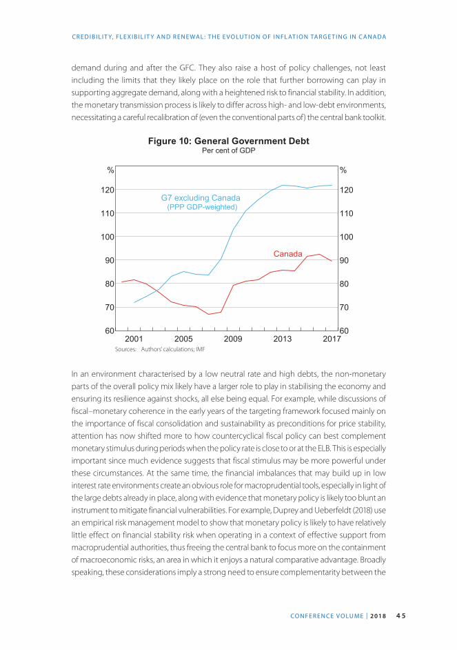
4 5CO N F E R E N C E V O LU M E | 2018
CR ED I B I L I T Y, FL E X I B I L I T Y A N D R EN E WA L : T H E E VO LU T I O N O F I N FL AT I O N TA R G E T I N G I N C A N A DA
demand during and after the GFC. They also raise a host of policy challenges, not least including the limits that they likely place on the role that further borrowing can play in supporting aggregate demand, along with a heightened risk to financial stability. In addition, the monetary transmission process is likely to differ across high- and low-debt environments, necessitating a careful recalibration of (even the conventional parts of) the central bank toolkit.
Figure 10: General Government DebtPer cent of GDP
2013200920052001 201760
70
80
90
100
110
120
%
60
70
80
90
100
110
120
%
Canada
G7 excluding Canada(PPP GDP-weighted)
Sources: Authors’ calculations; IMF
In an environment characterised by a low neutral rate and high debts, the non-monetary parts of the overall policy mix likely have a larger role to play in stabilising the economy and ensuring its resilience against shocks, all else being equal. For example, while discussions of fiscal–monetary coherence in the early years of the targeting framework focused mainly on the importance of fiscal consolidation and sustainability as preconditions for price stability, attention has now shifted more to how countercyclical fiscal policy can best complement monetary stimulus during periods when the policy rate is close to or at the ELB. This is especially important since much evidence suggests that fiscal stimulus may be more powerful under these circumstances. At the same time, the financial imbalances that may build up in low interest rate environments create an obvious role for macroprudential tools, especially in light of the large debts already in place, along with evidence that monetary policy is likely too blunt an instrument to mitigate financial vulnerabilities. For example, Duprey and Ueberfeldt (2018) use an empirical risk management model to show that monetary policy is likely to have relatively little effect on financial stability risk when operating in a context of effective support from macroprudential authorities, thus freeing the central bank to focus more on the containment of macroeconomic risks, an area in which it enjoys a natural comparative advantage. Broadly speaking, these considerations imply a strong need to ensure complementarity between the

4 6 R E S E R V E B A N K O F A U S T R A L I A
T H O M A S J C A R T E R , R H Y S M E N D E S A N D L AW R E N C E L S C H E M B R I
monetary, fiscal and macroprudential policy frameworks while respecting and preserving the operational independence on which central bank credibility depends. In the Canadian case, we stress that special aspects of the institutional framework already help to encourage complementarity of this sort, not least including the highly centralised nature of federal fiscal policy, a long tradition of cooperation among macrofinancial authorities, and the above-noted fact that inflation control is a joint duty of the BoC and government.
Heightened ELB risk also enhances the role of unconventional monetary policies. These include forward guidance, a tool with which the BoC already has direct experience, along with several tools, like large-scale asset purchases, funding for credit and negative interest rates, with which other central banks experimented during and after the GFC and European debt crisis. Despite the body of experience thus accumulated, many open questions remain regarding the use of these tools, especially concerning their optimal coordination and relative strengths and weaknesses. Another important question is the extent to which unconventional monetary policies can substitute for the non-monetary measures discussed above. While this issue was less important in Canada due to the fact that Canadian rates had already escaped the ELB at the time that the government began withdrawing the fiscal stimulus marshalled in the aftermath of the GFC, it proved highly relevant in other jurisdictions, where central banks’ interest in unconventional monetary policy derived partly from a perceived need to provide stimulus independent of fiscal authorities, especially as fiscal policy in many advanced economies began tightening around the time of the G20’s 2010 Toronto Declaration.
While the unconventional policies just discussed can be incorporated into an inflation targeter’s toolkit without necessitating some change in the overall inflation-targeting framework, the literature has also identified alternative frameworks that may deliver superior outcomes when nominal rates are at or near the ELB. These include the average inflation-targeting (AIT) framework proposed by Nessén and Vestin (2005), which aims to stabilise average inflation over a multi-year window and, thus, represents an intermediate case between pure inflation targeting and PLT. Another possibility would be the regime-switching frameworks analysed by Mendes and Murchison (2014) and Bernanke (2017), which involve switching to PLT at the onset of ELB episodes, then committing to not raise rates until prices have reached the target path.
The essential feature of these alternative frameworks is that they introduce history dependence into monetary policy, in contrast to the fully forward-looking nature of inflation targeting, which makes no attempt to correct for past deviations from target. Going back to seminal work by Krugman (1998) and Eggertsson and Woodford (2003), it is well known that optimal monetary policy generally entails some degree of history dependence during and after ELB episodes – in particular, policymakers should be prepared to respond to ELB episodes by committing to keep rates lower for longer than a purely forward-looking analysis would imply, since expectations of an extended period of high inflation and low nominal rates would then help to stimulate demand through their effect on long-term real rates. A commitment of this sort can be approximated under AIT and temporary PLT frameworks, both of which have the property that low levels of inflation in the early phases of an ELB episode mechanically extend the period over which agents can expect lax monetary conditions.

4 7CO N F E R E N C E V O LU M E | 2018
CR ED I B I L I T Y, FL E X I B I L I T Y A N D R EN E WA L : T H E E VO LU T I O N O F I N FL AT I O N TA R G E T I N G I N C A N A DA
Of course, a permanent shift to PLT was contemplated as part of the 2011 renewal and was ultimately rejected due to concerns about its credibility and heavy reliance on expectational mechanisms, among other issues. However, these concerns are somewhat mitigated in the case of AIT and temporary PLT. For example, an oft-cited challenge to the credibility of full PLT in small open economies is that extended periods of tight monetary policy would sometimes be needed to unwind the price impact of large terms of trade shocks, and episodes of this sort could prove prohibitively unpopular. Fortunately, this issue would be less of a concern under AIT (since the offending shocks would eventually pass out of the averaging window) and would remain entirely moot under temporary PLT due to that framework’s asymmetric nature. The asymmetries inherent in temporary PLT also have other advantages. For example, if credibility or expectational issues prevented temporary PLT from exerting its intended effects on long-term real rates, then the costs associated with the periods of overly expansionary policy that the framework would then entail would nonetheless be mitigated to the extent that the efficient level of output is likely to exceed potential in practice.29
That said, a more radical set of recent policy proposals aims to respond to heightened ELB risk by circumventing the ELB entirely. Though all such proposals remain highly speculative, we briefly highlight two leading examples, namely the frameworks advocated by Agrawal and Kimball (2015) and Goodfriend (2016), which involve introducing a time-varying exchange rate between paper currency and some form of e-money (e.g. deposits at the central bank). More specifically, Agrawal and Kimball (2015) argue for a time-varying fee on deposits at the central bank’s cash window, while Goodfriend (2016) proposes fixing the quantity of paper currency and then allowing an endogenous determination of the exchange rate.
In principle, approaches like these could deliver negative interest rates on e-money so long as the public expects an offsetting depreciation of paper currency. However, they would also entail a host of challenges. For example, commercial banks may be hesitant to pass negative rates on to their retail depositors. Negative interest rates would also leave firms and households with incentives to delay the deposit of e-money cheques or prepay e-money liabilities, potentially including taxes. In addition, the magnitudes of the required depreciations might trigger disruptions in the e-money-to-paper market not unlike those sometimes witnessed in real-world foreign exchange markets. Large depreciations would also raise distributional issues to the extent that e-money and paper currency are not evenly distributed in the economy.
To be clear, most of the policy measures discussed in this section are not mutually exclusive. If anything, many would likely prove complementary. For example, if AIT or temporary PLT were ultimately adopted, then the need for strong macroprudential policy would likely be enhanced to the extent that these frameworks enable monetary policy to set rates lower for longer than would otherwise be the case.
In summary, the foregoing discussion has identified at least four topics that warrant further study, either in the context of the 2021 renewal or as part of the BoC’s broader research agenda, namely: (i) complementarities in the monetary, fiscal, and macroprudential policy
29 Distortions such as taxes and market power likely cause the level of potential output to be inefficiently low. Hence, a temporary period of excess demand may be less costly than commonly assumed in analyses of monetary policy frameworks.

4 8 R E S E R V E B A N K O F A U S T R A L I A
T H O M A S J C A R T E R , R H Y S M E N D E S A N D L AW R E N C E L S C H E M B R I
frameworks; (ii) the costs, benefits, and optimal use of forward guidance, large-scale asset purchases, credit for funding, and negative interest rates as additions to the central bank toolkit; (iii) the merits of AIT, temporary PLT, and other potential strategies for introducing greater history dependence into the conduct of monetary policy; and (iv) the long-term prospects for circumventing the ELB.
5. Concluding RemarksLooking back over Canada’s more than quarter-century experience with an inflation-targeting-based monetary policy framework, the framework has proven much more successful than initially expected. In hindsight, we underestimated how quickly credibility could be achieved and how effectively well-anchored inflation expectations would help to keep inflation close to target.
The consistent application of a clear and simple 2 per cent inflation target within a symmetric control range has proven to be a tremendous strength of the framework. The 2 per cent target, which is now firmly ingrained in the Canadian mindset, has served as a Schelling (1960)-style focal point for the coordination of economic decisions while improving the reliability of price signals. In turn, the anchoring of inflation expectations has enhanced the flexibility and general effectiveness of monetary policy, thus making the target easier to achieve and improving overall macrofinancial outcomes.
The governance of the inflation target has played an important role in ensuring its credibility. In particular, the underlying joint agreement committed the federal government to the target while granting the BoC the operational independence needed to achieve it. In addition, the agreement has served as an implicit mechanism for promoting coherence between the monetary and non-monetary parts of the overall policy mix, including fiscal policy and financial regulation and supervision.
At the same time, a regular and highly deliberate renewal process has provided multiple opportunities to review the framework, conduct in-depth research on its structure and implementation, and examine our growing experience and related theoretical work. While the structure of the framework has largely remained intact, its operation has continually improved as our understanding has deepened, especially regarding the importance of clear and effective communication.
Looking ahead to the next renewal in 2021, a few ongoing economic developments pose important challenges to inflation-targeting-based monetary policy frameworks, most notably low neutral rates, heightened ELB risk, and high debt burdens in the household and public sectors. The goal of the 2021 renewal will be to strengthen the Canadian framework in the face of these developments to maintain the economy’s resilience to adverse shocks.
The academic and policy literatures have put forward several proposals for dealing with the above-noted developments, including alternative monetary frameworks (e.g. PLT, AIT, nominal GDP targeting) and various additions to the central bank toolkit (e.g. conditional forward guidance, large-scale asset purchases, negative interest rates). The need to ensure a

4 9CO N F E R E N C E V O LU M E | 2018
CR ED I B I L I T Y, FL E X I B I L I T Y A N D R EN E WA L : T H E E VO LU T I O N O F I N FL AT I O N TA R G E T I N G I N C A N A DA
complementary mix of monetary, fiscal, and macroprudential policy has also received growing attention. Clearly, there is some degree of substitutability among these three policy choice sets: framework, toolkit, and policy mix. Moreover, a sufficiently coherent and resilience-enhancing policy mix would imply less need to consider more radical changes to the framework or toolkit. At the same time, some of these options, including large purchases of government debt or substantial changes in the policy mix, raise important concerns about central bank independence. Such concerns will also need to be examined as these options are considered going forward.

5 0 R E S E R V E B A N K O F A U S T R A L I A
T H O M A S J C A R T E R , R H Y S M E N D E S A N D L AW R E N C E L S C H E M B R I
ReferencesAgrawal R and M Kimball (2015), ‘Breaking through the Zero Lower Bound’, IMF Working Paper No WP/15/224.
Akerlof GA, WT Dickens and GL Perry (1996), ‘The Macroeconomics of Low Inflation’, Brookings Papers on Economic Activity, 27(1), pp 1–59, 74–76.
Amano R, T Carter and Y Terajima (2017), ‘Redistributive Effects of a Change in the Inflation Target’, Bank of Canada Staff Analytical Note 2017-13.
Bank of Canada (1991a), ‘Background Note on the Targets’, Background information released 26 February, in Bank of Canada Review, March, pp 9–15.
Bank of Canada (1991b), ‘Press Release: Targets for Reducing Inflation’, 26 February, in Bank of Canada Review, March, pp 5–6.
Bank of Canada (1993), ‘Statement of the Government of Canada and the Bank of Canada on Monetary Policy Objectives’, Press Release, 22 December.
Bank of Canada (1998), ‘Inflation-Control Targets Extended’, Joint Statement of the Government of Canada and the Bank of Canada, 24 February.
Bank of Canada (2001a), Renewal of the Inflation-Control Target: Background Information, May, Bank of Canada, Ottawa.
Bank of Canada (2001b), ‘Technical Background Document 1: A Brief Review of the Literature on whether a Low-Inflation Regime Leads to Economic Difficulties’, 18 May.
Bank of Canada (2001c), ‘Technical Background Document 2: Lower Rates of Inflation and Improved Economic Outcomes’, 18 May.
Bank of Canada (2006), Renewal of the Inflation-Control Target: Background Information, November, Bank of Canada, Ottawa.
Bank of Canada (2009), Monetary Policy Report, April.
Bank of Canada (2011), ‘Renewal of the Inflation-Control Target: Background Information—November 2011’.
Bank of Canada (2015), ‘Framework for Conducting Monetary Policy at Low Interest Rates’, December.
Bank of Canada (2017), Monetary Policy Report, October.
Beaudry P and F Ruge-Murcia (2017), ‘Canadian Inflation Targeting’, Canadian Journal of Economics, 50(5), pp 1556–1572.
Bernanke BS (2017), ‘Monetary Policy in a New Era’, Paper presented at the Peterson Institute for International Economics Conference ‘Rethinking Macroeconomic Policy’, Washington DC, 12–13 October.
Bernanke BS, T Laubach, FS Mishkin and AS Posen (1999), Inflation Targeting: Lessons from the International Experience, Princeton University Press, Princeton.
Bordo M, A Dib and L Schembri (2010), ‘Canada’s Pioneering Experience with a Flexible Exchange Rate in the 1950s: (Hard) Lessons Learned for Monetary Policy in a Small Open Economy’, International Journal of Central Banking, 6(3), pp 51–99.

5 1CO N F E R E N C E V O LU M E | 2018
CR ED I B I L I T Y, FL E X I B I L I T Y A N D R EN E WA L : T H E E VO LU T I O N O F I N FL AT I O N TA R G E T I N G I N C A N A DA
Canada, House of Commons (1992), ‘The Mandate and Governance of the Bank of Canada’, (JP Manley, Chair), First Report of the Sub-committee on the Bank of Canada, Eighth Report of the Standing Committee on Finance, Minutes of Proceedings and Evidence of the Standing Committee on Finance, House of Commons, Issue No 34, February.
Caramazza F, D Hostland and SS Poloz (1990), ‘The Demand for Money and the Monetary Policy Process in Canada’, Journal of Policy Modeling, 12(2), pp 387–426.
Champagne J and R Sekkel (2017), ‘Changes in Monetary Regimes and the Identification of Monetary Policy Shocks: Narrative Evidence from Canada’, Bank of Canada Staff Working Paper 2017-39.
Coletti D, J Selody and C Wilkins (2006), ‘Another Look at the Inflation-Target Horizon’, Bank of Canada Review, Summer, pp 31–37.
Crow JW (1988), ‘The Work of Canadian Monetary Policy’, Bank of Canada Review, February, pp 3–17.
Department of Finance Canada (2001), ‘Joint Statement of the Government of Canada and the Bank of Canada on the Renewal of the Inflation-Control Target’, News Release 2001-050, 17 May.
Dorich J, N Labelle St-Pierre, V Lepetyuk and RR Mendes (2018), ‘Could a Higher Inflation Target Enhance Macroeconomic Stability?’, Canadian Journal of Economics, 51(3), pp 1029–1055.
Dorich J, A Reza and S Sarker (2017), ‘An Update on the Neutral Rate of Interest’, Bank of Canada Review, Autumn, pp 27–41.
Duguay P and D Longworth (1998), ‘Macroeconomic Models and Policymaking at the Bank of Canada’, Economic Modelling, 15(3), pp 357–375.
Duprey T and A Ueberfeldt (2018), ‘How to Manage Macroeconomic and Financial Stability Risks: A New Framework’, Bank of Canada Staff Analytical Note 2018-11.
Eggertsson GB and M Woodford (2003), ‘The Zero Bound on Interest Rates and Optimal Monetary Policy’, Brookings Papers on Economic Activity, 2003(1), pp 139–211, 203–233.
Fischer S (1996), ‘Why are Central Banks Pursuing Long-Run Price Stability?’, in Achieving Price Stability, A Symposium sponsored by the Federal Reserve Bank of Kansas City, Kansas City, pp 7–34.
Freedman C (2001), ‘Inflation Targeting and the Economy: Lessons from Canada’s First Decade’, Contemporary Economic Policy, 19(1), pp 2–19.
Fung B, KP Huynh and G Stuber (2015), ‘The Use of Cash in Canada’, Bank of Canada Review, Spring, pp 45–56.
Galí J and M Gertler (1999), ‘Inflation Dynamics: A Structural Econometric Analysis’, Journal of Monetary Economics, 44(2), pp 195–222.
Goodfriend M (2016), ‘The Case for Unencumbering Interest Rate Policy at the Zero Bound’, in Designing Resilient Monetary Policy Frameworks for the Future, A Symposium sponsored by the Federal Reserve Bank of Kansas City, Kansas City, pp 127–160.
Gosselin M-A and M Khan (2015), ‘A Survey of Consumer Expectations for Canada’, Bank of Canada Review, Autumn, pp 14–23.
Hellwig C (2005), ‘Heterogeneous Information and the Welfare Effects of Public Information Disclosures’, Unpublished manuscript, UCLA Department of Economics, October. Available at <http://www.econ.ucla.edu/people/papers/Hellwig/Hellwig283.pdf>.

5 2 R E S E R V E B A N K O F A U S T R A L I A
T H O M A S J C A R T E R , R H Y S M E N D E S A N D L AW R E N C E L S C H E M B R I
Krugman PR (1996), ‘Stable Prices and Fast Growth: Just Say No’, The Economist, 31 August–6 September, pp 15–18.
Krugman PR (1998), ‘It’s Baaack: Japan’s Slump and the Return of the Liquidity Trap’, Brookings Papers on Economic Activity, 29(2), pp 137–187, 204–205.
Laidler DEW and WBP Robson (1993), The Great Canadian Disinflation: The Economics and Politics of Monetary Policy in Canada, 1988–93, Policy Study 19, C.D. Howe Institute, Toronto.
Longworth D and SS Poloz (1986), ‘A Comparison of Alternative Monetary Policy Regimes in a Small Dynamic Open-Economy Simulation Model’, Bank of Canada Technical Report No 42.
Lorenzoni G (2010), ‘Optimal Monetary Policy with Uncertain Fundamentals and Dispersed Information’, The Review of Economic Studies, 77(1), pp 305–338.
Mendes R (2008), ‘Information, Central Bank Communication, and Aggregate Fluctuations’, PhD thesis, University of Toronto.
Mendes R and S Murchison (2014), ‘Should Forward Guidance be Backward-Looking?’, Bank of Canada Review, Autumn, pp 12–22.
Nessén M and D Vestin (2005), ‘Average Inflation Targeting’, Journal of Money, Credit and Banking, 37(5), pp 837–863.
Poloz SS (2016), ‘The Doug Purvis Memorial Lecture—Monetary/Fiscal Policy Mix and Financial Stability: The Medium Term Is Still the Message’, Canadian Public Policy, 42(3), pp 225–236.
Schelling TC (1960), The Strategy of Conflict, Harvard University Press, Cambridge.
Schembri L (2013), ‘Born of Necessity and Built to Succeed: Why Canada and the World Need the Financial Stability Board’, Remarks to the CFA Society (Ottawa), Ottawa, 24 September.
Schembri L (2018), ‘Anchoring Expectations: Canada’s Approach to Price Stability’, Remarks to Manitoba Association for Business Economists, Winnipeg, 15 February.
Summers L (1991), ‘Panel Discussion: Price Stability: How Should Long-Term Monetary Policy be Determined?’, Journal of Money, Credit and Banking, 23(3, Part 2), pp 625–631.
Svensson LEO (1997), ‘Inflation Forecast Targeting: Implementing and Monitoring Inflation Targets’, European Economic Review, 41(6), pp 1111–1146.
Svensson LEO (2016), ‘Cost-Benefit Analysis of Leaning against the Wind’, NBER Working Paper No 21902, rev May 2017.
Thiessen GG (1983), ‘The Canadian Experience with Monetary Targeting’, in P Meek (ed), Central Bank Views on Monetary Targeting, Federal Reserve Bank of New York, New York, pp 100–104.
Thiessen GG (2000), ‘Can a Bank Change? The Evolution of Monetary Policy at the Bank of Canada 1935–2000’, Lecture given at the Faculty of Social Science, University of Western Ontario, London, 17 October.
Witmer J and J Yang (2016), ‘Estimating Canada’s Effective Lower Bound’, Bank of Canada Review, Spring, pp 3–14.

5 3CO N F E R E N C E V O L U M E | 2 018
Guy Debelle*
1. IntroductionIt has been 25 years since Australia adopted an inflation-targeting regime as the framework for monetary policy. At the time of adoption, inflation targeting was in its infancy. New Zealand had announced its inflation target in 1989, followed by Canada and Sweden. The inflation-targeting framework was untested and there was little in the way of academic analysis to provide guidance about the general design and operational principles. Practice was very much ahead of theory.
Now 25 years later, inflation targeting is widely used as the framework for monetary policy. While there are differences in some of the features across countries, the similarities are more pervasive than the differences. And generally, the features of inflation-targeting frameworks have tended to converge over time.
It is interesting to firstly examine how the inflation-targeting framework in Australia has evolved over the past 25 years. Secondly, it is also timely to reassess the appropriateness of the regime. The first is the main task of my paper, the second is the task of the conference collectively.
In terms of the first, the main point I will make is that the Australian framework has not changed much over the past 25 years. The flexible nature of the framework, which was there at its inception, has proven to be resilient to the quite substantial changes in the macroeconomic environment that have taken place since. This is in contrast to some other countries that have moved from an initially rigid definition (which may well have been appropriate at their framework's inception) towards something more flexible. The framework in Australia was adaptable from the start, which caused some issues in convincing some people of the seriousness of the Reserve Bank of Australia’s (RBA’s) commitment to that framework.
While the specification of the regime has not materially changed, one thing that has changed is the degree of confidence that the regime might actually work. Australia, like other countries, came to inflation targeting after trying a number of alternative approaches to monetary policy. These approaches had not delivered either the desired price stability or acceptable macroeconomic outcomes. Inflation targeting was the next attempt to try to better achieve these outcomes. There was no guarantee of success. Now, after 25 years, there is considerably greater confidence that the regime can contribute to sound macroeconomic outcomes in terms of both inflation and growth. The proof of the pudding has been in the eating. There
* Deputy Governor, Reserve Bank of Australia. This draws on a number of pieces I have written on inflation targeting over the past two decades, both at the RBA and the International Monetary Fund. Thanks to Claudia Seibold for her assistance with the data.
Twenty-five Years of Inflation Targeting in Australia

5 4 R E S E R V E B A N K O F A U S T R A L I A
G U Y D E B E L L E
is greater confidence and understanding about the framework from the public, from the political process, from financial markets and from the policymakers themselves.
There is also now a large academic literature supporting inflation targeting, and examining and advising on various questions about the appropriate design and operation of the framework. That has validated many of the decisions taken by policymakers in setting up their inflation-targeting frameworks, but has also questioned some features of the framework.
One noteworthy change in the inflation-targeting framework in Australia (and elsewhere) is communication. The content and scope of our communication has increased considerably over 25 years. I will spend some time outlining these changes and the motivation for them.
As I said, the second question about the appropriateness of the regime is very much the theme of this conference. What, if any, changes to the framework might be worth considering? In a later section I will raise some questions that will be considered by other speakers at the conference and provide some brief observations on these issues.
When Glenn Stevens and I wrote in 1995 about the motivations for the (then) new inflation-targeting framework in Australia, we said, ‘If, some years hence, we can look back and observe that the average rate of inflation has a “2” in front of the decimal place, that will be regarded as a success.’ (Stevens and Debelle 1995, pp 82–83) We are now quite some years hence and we can look back and observe that the average rate of inflation has a ‘2’ in front of the decimal place.
2. How Did the Regime Come About?Unlike a number of inflation-targeting countries, the adoption of an inflation-targeting framework in Australia was evolutionary rather than revolutionary.1 It was not accompanied by a change to the central bank’s legislation as was the case in New Zealand. Nor did it result from a rapid departure from an exchange rate regime as in the United Kingdom and Sweden. But, like those other cases, it reflected the recognition that previous monetary frameworks had not been successful in delivering either price stability, in the form of low inflation, or desirable macroeconomic outcomes in terms of sustainable full employment.
The inflation target in Australia was outlined in a number of speeches by the then RBA Governor, Bernie Fraser, in 1993 and 1994 (Fraser 1993, 1994). It was a low-key launch, in part reflecting the political climate of the time. As Steve Grenville and Ian Macfarlane noted, it was in the context of locking in the low inflation that had occurred in the aftermath of the early 1990s recession.
The target was the operational interpretation of the goals of monetary policy set out in the RBA’s founding legislation in 1959, namely:
1. the stability of the currency of Australia
2. the maintenance of full employment in Australia; and
3. the economic prosperity and welfare of the people of Australia.
1 For detailed accounts of the conception of inflation targeting in Australia, those present at its birth are the best source: see Grenville (1997), Macfarlane (1998) and Stevens (2003).

5 5CO N F E R E N C E V O LU M E | 2018
T W E N T Y- F I V E Y E A R S O F I N F L AT I O N TA R G E T I N G I N A U S T R A L I A
The stability of the currency goal reflects the fact that the legislation was written when fixed exchange rates were the norm. It has been interpreted as preserving the purchasing power of the currency and hence is consistent with the maintenance of low and stable inflation.
As noted, the inflation target was first adopted by the RBA in 1993. It was verbally endorsed by the government of the day. But it was not formally endorsed by the government until 1996, when the first Statement on the Conduct of Monetary Policy (the Statement) was signed jointly by the incoming government and the new RBA Governor, Ian Macfarlane. The political support for the inflation target has been bipartisan. The Statement has been renewed at the start of the term of each of the subsequent two Governors. It has also been endorsed with each change of government.
The Reserve Bank Act 1959 states that monetary policy has both nominal and real objectives. Consistent with that, the Statement makes it clear that the inflation-targeting framework recognises both nominal and real objectives. The flexibility of the target in terms of specifying that the inflation goal will be achieved over the cycle (subsequently adjusted to be ‘on average, over time’) is the feature that recognises the dual mandate. To maintain full employment requires that the economy be on a sustainable path. Thus, the trajectory of economic growth matters, as does the presence of low inflation and financial stability.
In the case of demand shocks, there is not a material conflict between the real and nominal objectives, as the appropriate monetary response is effectively the same. That said, the flexibility of the target potentially allows for greater inflation variability to achieve lower variability in the real economy. However, the experience of other inflation-targeting central banks suggests that this difference is not substantial in practice.
In the case of supply shocks, where the appropriate monetary responses to achieve the real and nominal objectives are likely to be in conflict in the short term, the medium-term horizon of the inflation target in Australia allows for a greater weight to be placed on output stabilisation and a more gradual return of the inflation rate to target than with a strict inflation target. Again, the practice of most central banks over the past two decades has tended to evolve towards the sort of flexibility explicitly recognised in the Australian target, notwithstanding the lexicographic ranking of inflation and output objectives in the specification of some other inflation targets.2
The Statement has not undergone much change since 1996. The current formulation is: ‘an appropriate goal is to keep consumer price inflation between 2 and 3 per cent, on average, over time’. Beyond some drafting changes that simply reflect the passage of time, the most substantive change has been the articulation of the financial stability objective of the RBA, which I will return to later. In terms of the description of the inflation target itself, the only change has been the objective, from keeping ‘underlying inflation between 2 and 3 per cent, on average, over the cycle’ to keeping ‘consumer price inflation between 2 and 3 per cent, on
2 For example, the Bank of England Act 1998 states that the objectives of the Bank of England shall be (a) to maintain price stability, and (b) subject to that, to support the economic policy of Her Majesty’s Government, including its objectives for growth and employment (Kuttner 2004).

5 6 R E S E R V E B A N K O F A U S T R A L I A
G U Y D E B E L L E
average, over time’. I regard this as purely a presentational change without any operational consequences.3
As I noted in a speech at the Bank of England last year, inflation targeting and central bank independence are sometimes conflated given their similar birth dates in a number of countries (Debelle 2017). In large part, this is because both were a response to the inflation experience of the 1970s and 1980s. In Australia, just as the inflation target was evolutionary rather than revolutionary, so too, greater central bank independence also evolved through time rather than there being a distinct break from past practice. As Ian Macfarlane (1998) stated:
... the Reserve Bank, by virtue of its Act in 1959, was always given a high degree of general independence as an institution. The fact that it had been unable to exercise this independence in monetary policy for much of the post-war period was due to a practical impediment – it did not possess the instruments of monetary policy.
As these impediments were removed, the RBA was able to become more independent in its setting of monetary policy. Thus, while the formal recognition of this independence was not completely visible until the first Statement in 1996, the practical independence had been there some time before that.
3. The Inflation Target in PracticeHow has the inflation target in Australia actually delivered in practice?
Figure 1 shows the outcomes for inflation and unemployment and Table 1 summarises the macroeconomic outcomes since the early 1970s. It updates a similar table in Stevens (2016). The table shows that the average headline inflation rate over the inflation-targeting period has been 2.5 per cent, as measured by the consumer price index (CPI). So the inflation target has been achieved over its period of operation.
The inflation target can be thought of as a ‘thick point’ (Stevens and Debelle 1995). This doesn’t mean that inflation with a ‘2’ in front of it implies a zone of policy inaction. It simply acknowledges that inflation will obviously vary through time and that there is probably not much to be gained from being too precise about the appropriate inflation rate, while also recognising that the specification of the inflation target plays an important role in anchoring inflation expectations. It would appear that the latter goal has been achieved because the inflation expectations of the public have generally been consistent with the target.
3 The change from underlying inflation in large part reflected the change in the measurement of the consumer price index to exclude mortgage interest rates.

5 7CO N F E R E N C E V O LU M E | 2018
T W E N T Y- F I V E Y E A R S O F I N F L AT I O N TA R G E T I N G I N A U S T R A L I A
Figure 1: Australian Inflation and Unemployment in the Long Run
2005199319811969 2017-5
0
5
10
15
%
-5
0
5
10
15
%
CPI(a)
CPI(b)
Unemployment rate
Notes: (a) Year-ended; excludes interest charges prior to the September quarter 1998; adjusted for the tax changes of 1999–2000
(b) Year-endedSources: ABS; RBA
Table 1: Selected Australian IndicatorsPer cent
Real GDP growth
Unemployment rate
Headline CPI inflation
Underlying inflation
Annual average
Standard deviation
Annual average
Standard deviation
Annual average
Standard deviation
Annual average
Standard deviation
1973:Q1–1993:Q1 2.8 1.2 6.9 2.2 8.8 1.2 8.4 1.1
1993:Q2–2017:Q4 3.2 0.6 6.3 1.6 2.5 0.4 2.6 0.2
2007:Q1–2017:Q4 2.5 0.4 5.4 0.6 2.3 0.4 2.5 0.2
Notes: Both price measures exclude interest charges prior to the September quarter 1998 and are adjusted for the tax changes in 1999–2000; underlying inflation is calculated using the Treasury underlying rate of inflation in the 1973–93 period and trimmed mean inflation for subsequent periods; standard deviations are calculated from quarterly growth rates for the GDP and price series, and from the quarter-average unemployment rate; geometric averages are presented for annual average GDP growth and inflation rates
Sources: ABS; RBA
At times, the inflation rate has been above the band; at times it has been below the band (though none of these deviations have been that persistent). This also illustrates the flexibility of the framework, which I will discuss in more detail in the next section. Of note, as is apparent in Figure 1, the inflation outcomes in the past decade have been at the lower end of the distribution of outcomes over the period. That is, as in other countries, inflation in Australia has been lower in the post-crisis period than in the decade preceding it. I will return to this point later in discussing some of the current challenges.

5 8 R E S E R V E B A N K O F A U S T R A L I A
G U Y D E B E L L E
While the average inflation rate has been consistent with the target, the real economic outcomes have also been good. The average unemployment rate in the most recent decade is lower than the one in the decade preceding it, which in turn was lower than the one before that.
Clearly, these outcomes are also a function of the macroeconomic environment, and cannot be solely attributable to the inflation target. Part of the first period of inflation targeting was the NICE (non-inflationary continuous expansion) decade and macroeconomic outcomes in the late 1990s and early 2000s were better in many countries, regardless of whether they had a (formal) inflation target or not. That said, many of the early adopters of inflation targets had experienced sub-par economic outcomes in the 1980s, particularly in terms of high inflation, when other countries had been able to achieve successful disinflations.
But it is important to note that the period for which the inflation-targeting framework has been in place has not been that benign. Most obviously, it has included the Asian crisis and the global financial crisis, as well as one of the largest rises (and falls) in the terms of trade in Australia’s economic history – an event that has been the undoing of the Australian economy a number of times in its history. Moreover, to paraphrase some words from Glenn Stevens in his final speech as Governor: ‘Had anyone, [in 1993], accurately forecast all the international events and simultaneously predicted that things would turn out in Australia as they have, they would not have been believed. But here we are’ (Stevens 2016).
The variability in global output has been higher over the past decade, but in Australia it has been lower. At the same time, the table shows that the variability of inflation has been lower in the inflation-targeting period than in the period before that.
When inflation targeting was in its infancy, there was a lot of research in central banks examining the trade-off between output and inflation variability, and assessing the ability of different policy rules to achieve different points on that trade-off.4 This work followed on from that of John Taylor, along with Dale Henderson and Warwick McKibbin. The inflation target has been associated with the inflation/output variability curve in Australia shifting in, notwithstanding the volatility of the world more generally. As Glenn noted, one significant contributor to the lower output volatility in Australia has been the avoidance of a large downturn. But the avoidance of a large downturn is in part a function of the avoidance of an inflation breakout, which I would argue can be attributed, to a reasonable extent, to the operation of monetary policy under the inflation target.
Hence, when we look back over the past 25 years: the inflation target has been achieved; real growth has been robust; average unemployment has declined through time; and nominal and real variability has been lower. So I think it is reasonable to argue that the inflation-targeting framework in Australia does seem to have played some part in contributing to the improved outcomes.
4 Stevens and Debelle (1995) is an example of this. See also de Brouwer and O'Regan (1997).

5 9CO N F E R E N C E V O LU M E | 2018
T W E N T Y- F I V E Y E A R S O F I N F L AT I O N TA R G E T I N G I N A U S T R A L I A
4. Flexibility in PracticeI will use four episodes over the past 25 years to illustrate some different features of the operation of the inflation target in Australia, in particular illustrating the flexibility of the target in practice, as well as its forward-looking nature.5 The first episode is the first tightening cycle under the inflation-targeting framework in 1994/95; the second, the response to the Asian crisis a few years later. The third episode is the introduction of the goods and services tax (GST) in 2000, when the price level was boosted by 3 per cent overnight. The fourth episode is the period around the onset of the global financial crisis in 2007–08.
4.1 1994/95By the middle of 1994, inflation pressures were building as economic growth was accelerating. The unemployment rate had declined by 3 percentage points in two years and wage pressures were evident.
There were doubts about whether the Australian inflation-targeting regime was sufficiently serious enough to be able to curtail these burgeoning inflation pressures. Indeed there were doubts about whether we even really had an inflation-targeting framework. One manifestation of this was that the Bank of England was organising a conference on the nascent area of inflation targeting and wasn’t sure whether Australia should be invited or not. Graciously they did end up including us and invited Glenn Stevens and me to talk about the Australian model alongside the stricter frameworks of New Zealand and Canada.6
The flexible specification of the inflation target in Australia was seen as a vulnerability. It didn’t have the electric fence of the more hard-edged inflation targets in some other countries. The ‘over the cycle’ language was too ‘fuzzy’. Reflecting such concerns, bond yields had risen quite significantly in 1994 in anticipation of a material increase in inflation.
But inflation was still at its post-recession lows of 2 per cent when the RBA increased the cash rate by 275 basis points in three moves over the second half of 1994. This pre-emptive tightening was assessed to be necessary to curtail the RBA’s forecast that inflation would rise. It is noteworthy that the tightening occurred with inflation still only at 2 per cent. Financial markets had anticipated that significantly more tightening would be required, reflecting their lack of faith in the new framework. Subsequently, inflation did actually rise to slightly above 3 per cent. The flexibility of the target allowed the avoidance of an unnecessary cost to the real economy of trying to cap the rise in inflation to below 3 per cent, consistent with the dual mandate.
In 1996, as demand pressures were easing, the RBA’s forecast was for inflation to decline. The stance of policy was eased, even though inflation was still above 3 per cent. The flexibility of the target, and its forward-looking focus, allowed the assessment of whether the inflation target was at risk in the medium term to determine the appropriate policy response.
5 See Debelle (2009) for a previous summary.
6 See Haldane (1995).

6 0 R E S E R V E B A N K O F A U S T R A L I A
G U Y D E B E L L E
That episode went a long way to enhancing the credibility of the framework with wage and price setters as well as with financial markets. It also increased confidence within the RBA that the inflation-targeting framework would be successful in achieving the RBA’s legislated goals.
4.2 The Asian crisis and exchange rate shocksAt the onset of the Asian crisis, the Australian economy was growing at around trend rates, with domestic demand beginning to accelerate, and underlying inflation at 1.6 per cent. Monetary policy had been eased over the prior year or so in anticipation of the decline in inflation that subsequently occurred. Thus, the Asian crisis hit the Australian economy at a time when it was in reasonable shape with the stance of monetary policy already relatively expansionary.
Exports to east Asia accounted for around one-third of Australia's exports at the time. In the year following the onset of the crisis, Australia’s exports to the region declined by nearly 20 per cent, directly subtracting around 1 percentage point from aggregate growth. Thus, the decline in output in the east Asian region represented a significant negative demand shock to the Australian economy. Australia's terms of trade also fell sharply as commodity prices declined, further exacerbating the decline in export demand.
In the event, inflation in Australia rose by less than was forecast, in part because of a decline in the pass-through of the exchange rate depreciation, as well as a greater-than-expected disinflationary impulse from the Asian region that put downward pressure on import prices.
If policy had been set to ensure that inflation did not rise above 3 per cent, the necessary rise in interest rates would have exacerbated the contractionary shock to foreign demand. With the benefit of hindsight, given the lower-than-expected inflation outcomes, this would have resulted in a significant undershooting of the inflation target.
The flexible inflation target served as a useful framework to think about the Asian crisis. Strong consideration was given to the goal of output stabilisation because the inflation target in the medium term was not felt to be in jeopardy. In addition, the policy credibility that had built up since the adoption of the inflation-targeting regime also allowed the RBA greater flexibility in its policy response.
4.3 GST 2000On 1 July 2000, a 10 per cent GST was introduced. As a result, the price level as measured by the CPI increased by 3 per cent overnight (Figure 2). Hence inflation as measured by the CPI was boosted, in a year-ended sense, by 3 percentage points for the next 12 months. The increase in the price level was fully anticipated by the public and financial markets.

6 1CO N F E R E N C E V O LU M E | 2018
T W E N T Y- F I V E Y E A R S O F I N F L AT I O N TA R G E T I N G I N A U S T R A L I A
Figure 2: Inflation and Monetary Policy
2012200720021997 20170
1
2
3
4
5
6
7
%
0
1
2
3
4
5
6
7
%
Inflation(a)
Cash rateIntroduction of the GST
Note: (a) Treasury underlying inflation prior to the September quarter 1998; thereafter, year-ended CPI inflation
Sources: ABS; RBA
The RBA did not seek to offset the effect of the GST on the price level. Its assumption was that the boost to the price level would be a once-off, and that the (by now well-enhanced) credibility of the inflation target would ensure that medium-term inflation expectations would remain well anchored. The RBA communicated that this was its assessment well in advance of the introduction of the GST to help condition expectations.
Again, the specification of the regime allowed the RBA the flexibility to look through the increase in the price level. It is worth noting that such flexibility would be more problematic under a price level-targeting regime, or even a nominal income target. With a strict price level target, the effect of the GST in boosting the price level would have to be unwound over some period of time, notwithstanding that households were compensated for the change by income tax cuts.
In the event, the credibility of the target and the RBA’s strategy was demonstrated. Inflation expectations remained anchored. Nearly all of the public discussion at the time focused on the inflation rate net of the GST effect. While policy was tightened around that time, it reflected standard sources of price pressure, such as strong growth, a rise in oil prices and a depreciating exchange rate, not the effect of the price level shock.
While the mid-1990s episode went a long way to building the credibility of the framework, the GST episode confirmed that the framework was well entrenched in wage- and price-setting behaviour in the Australian economy.

6 2 R E S E R V E B A N K O F A U S T R A L I A
G U Y D E B E L L E
4.4 2007–08From around 2006, it became clear that inflation pressures were again growing in the Australian economy. The RBA’s forecasts for inflation were revised upwards in late 2007 and into 2008. Monetary policy was tightened to contain the rise in inflation as the Australian economy was overheating. Inflation reached as high as 5 per cent.
But as the global economy turned south sharply, the RBA was able to change the settings of monetary policy quickly, even with inflation still high. As the facts changed and the outlook changed, in this case quite dramatically, the RBA changed its assessment about the appropriate setting of policy. The fact that inflation was still high as these events unfolded did not constrain the decision to reduce the cash rate. Again, the flexibility and forward-looking nature of the framework together with its recognition of the real, as well as the nominal, goals of monetary policy provided the necessary scope for action.7
4.5 SummarySo throughout its 25 years, the specification of the framework has allowed the RBA to focus on the medium-term outlook for inflation and not be unnecessarily constrained by any current level of the inflation rate. That seems obviously appropriate behaviour now, and reflects the decision-making process in all inflation-targeting frameworks today. But it was not obvious that this was the appropriate approach to monetary policy back at the inception of inflation targeting. While the confidence in being able to use the flexibility in the framework has undoubtedly increased, the willingness to use it has always been there. You will note that I have not included the current cycle of monetary policy in this assessment. That is still to play out and I will leave it to a later iteration of this conference to conduct a post-mortem.
5. CommunicationWhile the flexible operational approach to inflation targeting has been present throughout, the communication by the RBA has changed quite substantially.
Before the introduction of the inflation target, the principal vehicle for the RBA’s economic commentary was the Annual Report and the Bulletin. This commentary often ran to no more than a few pages. There were also speeches on macroeconomic issues by the Governor and Deputy Governor. Changes in the stance of monetary policy had been announced since 1990 (which was quite innovative at the time), but were generally a one-line statement announcing the decision to change the cash rate. That was the extent of the public communication. There was not much information to understand the central bank’s general approach to monetary policy or the central bank’s reaction function. Financial markets had to employ large teams of analysts to divine the central bank’s intentions.
The advent of the inflation-targeting framework saw communication increase, though it should be noted that this was a worldwide phenomenon and not confined to inflation-
7 In this instance, most central banks responded in a similarly flexible way. In large part, I would argue this reflects the convergence to more flexible frameworks by this time.
6 3CO N F E R E N C E V O LU M E | 2018
T W E N T Y- F I V E Y E A R S O F I N F L AT I O N TA R G E T I N G I N A U S T R A L I A
targeting central banks. Why was there such an increase in communication? One reason that I have stated before is that the inflation-targeting central banks did not have a good track record of monetary policymaking. So there was a need to build that track record. A track record requires a track and inflation targeting provided that track. But then you also need to make it clear to people how you are progressing along that track and that is where the communication is important.
Given the relatively poor starting point, a high level of communication and transparency was necessary to build credibility as quickly as possible, to enhance the effectiveness of monetary policy and to help anchor inflation expectations. Mervyn King described this in his 1997 paper (King 1997) as ‘trust building by talk’. That was very much the goal of communication when inflation targeting was in its infancy.
Similarly, communication was a mechanism to deliver accountability. As I noted earlier, inflation targeting often went hand in hand with greater central bank independence. The quid pro quo for greater independence was greater accountability. In Australia’s case, the need for accountability, and communication as one mechanism to deliver that accountability, was reflected in the first Statement on the Conduct of Monetary Policy, which stated that ‘it is important that the Bank report on how it sees developments in the economy, currently and in prospect, affecting expected inflation outcomes’. It noted that this would include the Statement on Monetary Policy (SMP), public addresses and required semiannual appearances of the Governor before the Parliament.
Today, the extent and nature of communication have increased still further. The SMP is a comprehensive document detailing the assessment of the current conjuncture, the RBA’s outlook for the economy, the risks and uncertainties around that outlook, and an explanation of the Board’s assessment of the monetary policy settings. The scope and content of the SMP has grown materially over the past 25 years.
All monetary policy decisions are accompanied by a statement explaining the basis of the decision (whether the stance is changed or not). Minutes of the Board’s decision-making meeting are published two weeks later.8 The number and frequency of speeches by the Governor and Deputy Governor, as well as other senior RBA staff, have increased. The Financial Stability Review is published twice each year providing the RBA’s assessment of those issues. There is a website which makes this material, as well as other material describing the monetary policy framework, readily available to the public. There is also an extensive business liaison program and recently an increased focus on public education about the RBA’s role. So the volume of communication and overall transparency have increased materially.
In considering the changed nature of the communication, it is important to ask two questions: what is the objective of the communication? and to whom are we communicating?
8 The RBA’s accountability is collective rather than individual so the minutes represent the collective view of the Board rather than conveying any individual’s views. The Board as a whole is accountable, in large part reflecting its composition where the majority of members are business people rather than practising economists. Individual accountability in the RBA’s case may compromise the ability of the business members of the Board to take decisions in the national interest rather than their sectoral interest (Stevens 2007).

6 4 R E S E R V E B A N K O F A U S T R A L I A
G U Y D E B E L L E
One of the critical roles of communication is a vehicle for accountability. That communication is directed to the parliament and the public, to whom the RBA is accountable. It is also important that the public and parliament have a good understanding of the inflation-targeting framework to enhance understanding as to why policy decisions are being taken. They may not always agree with them, but it is important that they can understand the rationale behind them.
Communication can help anchor inflation expectations, which in turn helps enhance the effectiveness of the regime. There is strong evidence that anchoring of inflation expectations has been enhanced over the past 25 years.9
It is also important the central bank’s reaction function is understood. That is helpful for the effective and timely transmission of monetary policy. It helps to ensure that inadvertent monetary policy surprises don’t occur, which serves to enhance the overall credibility of the regime. This communication is important for businesses and households in their decision-making. On the basis of their outlook for the economy, they can have confidence in how the central bank is likely to react and what that would imply for their borrowing costs. An understanding of the reaction function is also important for financial markets participants in setting financial markets prices that form an important part of the transmission mechanism of monetary policy actions.
The effectiveness of communication or transparency is sometimes measured by interest rate surprises. While this might be appropriate in some cases, sometimes the surprise happens through a previous signal by the central bank. In my view, the surprise should be primarily confined to data or event surprises. That is, with a well-understood reaction function, the vast bulk of surprises should come from unexpected developments, not unexpected actions by the central bank.
The amount and content of communication has been one of the most substantive changes over the past 25 years. That has, in my opinion, been clearly beneficial for the accountability of the RBA, as well as the effective functioning of the inflation-targeting framework. That said, it is always worth checking that the increased communication is delivering signal rather than noise. That is, the quality of the message is more important than the quantity.
6. Open IssuesI have argued that the inflation target has delivered macroeconomic outcomes that have been beneficial for the Australian economy. I think a strong case can be made that it has contributed materially to better economic outcomes than the monetary frameworks that preceded it. I have also noted that the framework in Australia has not changed much over the 25 years of its operation, with the notable exception of communication.
So does that mean that the current configuration of the inflation target is the most appropriate or even that inflation targeting is the most appropriate framework for monetary policy? What changes could be contemplated? Those questions are going to be addressed in other papers
9 This is very evident in consensus forecasts and surveys of union inflation expectations, inter alia.

6 5CO N F E R E N C E V O LU M E | 2018
T W E N T Y- F I V E Y E A R S O F I N F L AT I O N TA R G E T I N G I N A U S T R A L I A
at this conference. But let me raise some here and discuss issues worth considering around each of them.
The first is the role of financial stability in an inflation-targeting framework. The RBA research conference last year considered this issue at some length (Hambur and Simon 2017). As I said earlier, financial stability is now articulated in the Statement. I talked about this issue at the Bank of England last year (Debelle 2017) and Ben Broadbent is addressing it at this conference. One question that arises is how the financial stability goal interacts with the inflation target. Is it a separate goal that sets up potential trade-offs or is it aligned with the inflation-targeting goal? In the latter case, a potential reconciliation is the time horizon. When it materialises, financial instability is likely to be detrimental to inflation, unemployment and output: the global recession of 2008 and the subsequent slow recovery in a number of economies bears testament to the potential costs of financial instability (although here in Australia we didn’t experience this to as great an extent). So over some time horizon, potentially quite long, the inflation target and financial stability are aligned. But translating this into monetary policy implications over a shorter time horizon is a large challenge, which still seems to me to be far from resolved.
What about alternative regimes? Price level targeting is one that has been considered in some countries, including Canada, and has been proposed in the academic literature (Ball, Mankiw and Reis 2005). One argument for a price level target is that it delivers predictability of the price level over a long horizon. It is not clear to me that this is something that is much valued by society. By revealed preference, the absence of long-term indexed contracts suggests that the benefits are not perceived to be high. I struggle to think of what contracts require such a degree of certainty. To me the benefits mostly derive from having inflation at a sufficiently low level that it doesn’t affect decisions. That supports an inflation target rather than a price level target. One important difference is that an inflation target allows bygones to be bygones, whereas a price level target does not. In a world where there are costs to disinflation (and particularly deflation), the likely small gains from the full predictability of the price level that comes with a price level target are not likely to offset the costs of occasional disinflations following positive price level shocks. Another challenge is how fast the price level should be returned to its target level. This presents both a communication and an operational challenge as the speed is likely to vary with the size of the deviation.
While the argument at the moment is that a price level target allows the central bank to let the economy grow more strongly after a period of unexpectedly low inflation, I do not think that practically this will deliver better outcomes than a flexible inflation target. That is an empirical question in the end that is worth testing.
The appropriate level of the inflation target is currently being debated in some parts of the world, including the United States. The argument for a higher target rate of inflation is that it might reduce the risk of hitting the zero lower bound because a higher inflation rate would result in a higher nominal interest rate structure. In thinking about this, we should ask the question as to whether what we have seen is the realisation of a tail event in the historical distribution of interest rates (for a given level of the real interest rate). While this event has now lasted quite a long time, if you thought it was a tail event, then you would expect the

6 6 R E S E R V E B A N K O F A U S T R A L I A
G U Y D E B E L L E
nominal rate structure to revert back to its historical mean at some point. If it is a tail event, and the world has just been unlucky enough to have experienced a realisation of that tail event, then there would not obviously be a need to raise the inflation target. We also need to question whether the real interest rate structure has shifted lower permanently, because of permanently lower trend growth say, which would also shift down the nominal rate structure and increase the likelihood of hitting the zero lower bound.
Also, as with price level targeting, in thinking about this question, it needs to be taken into account that it is highly beneficial to have the inflation target at a level where it doesn’t materially enter into economic decision-making: 2–3 per cent seems to achieve that. We know that some number higher than 2–3 per cent will materially enter decision-making, because we have had plenty of experience of higher rates of inflation that demonstrate that. How much higher though, we don’t really exactly know.
Another consideration in answering the question of whether the inflation target is at the right level is the range of policy instruments in the toolkit. Over the past decade, this toolkit has expanded at a number of central banks. For example, we now know that the zero lower bound is not at zero. Asset purchase programs have been utilised and the assets purchased have included sovereign paper and also assets issued by the private sector. An assessment of the effectiveness of these instruments is still a work in progress. We also need to think about whether they are part of the standard monetary policy toolkit or whether they should only be broken out in case of emergency.
Nominal income targeting is another alternative regime to inflation targeting. I am not convinced that flexible inflation targeting of the sort practised in Australia is significantly different from nominal income targeting in most states of the world. I also think that there are some quite significant communication challenges with nominal income targeting. Firstly, nominal income is probably more difficult to explain to people than inflation. Secondly, as a very practical matter, nominal income is subject to quite substantial revisions, which poses difficulties both operationally and, again, in communicating with the public.
Finally, one criticism of inflation targeting more generally is that central banks are fighting the last war. The fact that, for a number of years now, inflation globally has been stubbornly low is not obviously the signal to declare victory over inflation and move on. Indeed, the declaration of victory may well be the signal that hostilities are about to resume and that inflation will shift up again. Moreover, even if victory can be declared that doesn’t mean you should go off to fight another war in another place without securing the peace. Inflation targeting can help secure the peace.
7. ConclusionToday, inflation targeting is now the default framework for monetary policy. This is in stark contrast to the situation 25 years ago, when inflation targeting was greeted with a large degree of scepticism. At its heart, inflation targeting is a simply expressed acknowledgement of what monetary policy can achieve and what it can’t. The flexible version of inflation targeting

6 7CO N F E R E N C E V O LU M E | 2018
T W E N T Y- F I V E Y E A R S O F I N F L AT I O N TA R G E T I N G I N A U S T R A L I A
that has been present in Australia since its inception was once regarded as an outlier, but over time we have seen most other regimes evolve in that direction, either through explicit changes to the regime or in practice. The dual mandate of the RBA is embodied in the flexible expression of the target.
Over the past 25 years, there have not really been material changes in the specification of the inflation target in Australia. The extent and content of our communication has increased, in line with the general trend across all central banks. This has helped to enhance the understanding of the public of what the RBA is aiming to achieve and, thereby, increased the effectiveness of monetary policy.
The inflation target has made a material contribution to the very satisfactory macroeconomic outcomes that the Australian economy has enjoyed over the past 25 years. Inflation has been consistent with target. The unemployment rate, on average, has been lower and less variable than in earlier periods. This has gone a long way to fulfilling the mandate of the RBA of contributing to the welfare and prosperity of the Australian people.
But it is important to continue to question whether the framework remains the right framework going forward and whether there are enhancements that could be made to it. There is now a much greater community to draw on to help answer those questions, both from central banks and from academia, in contrast to the situation 25 years ago when inflation targeting was a new frontier.

6 8 R E S E R V E B A N K O F A U S T R A L I A
G U Y D E B E L L E
ReferencesBall L, NG Mankiw and R Reis (2005), ‘Monetary Policy for Inattentive Economies’, Journal of Monetary Economics, 52(4), pp 703–725.
de Brouwer G and J O'Regan (1997), ‘Evaluating Simple Monetary-Policy Rules for Australia’, in P Lowe (ed), Monetary Policy and Inflation Targeting, Proceedings of a Conference, Reserve Bank of Australia, Sydney, pp 244–276.
Debelle G (2009), ‘The Australian Experience with Inflation Targeting’, Paper presented at the XI Annual Inflation Targeting Seminar of Banco Central do Brasil, Rio de Janeiro, 14–15 May.
Debelle G (2017), ‘Central Bank Independence in Retrospect’, Address given at Bank of England ‘Independence: 20 Years On’ Conference, London, 28–29 September.
Fraser BW (1993), ‘Some Aspects of Monetary Policy’, RBA Bulletin, April, pp 1–7.
Fraser BW (1994), ‘Managing the Recovery’, RBA Bulletin, April, pp 20–28.
Grenville S (1997), ‘The Evolution of Monetary Policy: From Money Targets to Inflation Targets’, in P Lowe (ed), Monetary Policy and Inflation Targeting, Proceedings of a Conference, Reserve Bank of Australia, Sydney, pp 125–158.
Haldane AG (ed) (1995), Targeting Inflation: A Conference of Central Banks on the Use of Inflation Targets Organised by the Bank of England, Bank of England, London.
Hambur J and J Simon (eds) (2017), Monetary Policy and Financial Stability in a World of Low Interest Rates, Proceedings of a Conference, Reserve Bank of Australia, Sydney.
King M (1997), ‘Changes in UK Monetary Policy: Rules and Discretion in Practice’, Journal of Monetary Economics, 39(1), pp 81–97.
Kuttner KN (2004), ‘A Snapshot of Inflation Targeting in its Adolescence’, in C Kent and S Guttmann (eds), The Future of Inflation Targeting, Proceedings of a Conference, Reserve Bank of Australia, Sydney, pp 6–42.
Macfarlane I (1998), ‘Australian Monetary Policy in the Last Quarter of the Twentieth Century’, Shann Memorial Lecture, Perth, 15 September.
Stevens G (2003), ‘Inflation Targeting: A Decade of Australian Experience’, Address given to South Australian Centre for Economic Studies April 2003 Economic Briefing , Adelaide, 10 April.
Stevens G (2007), ‘Central Bank Communication’, Address given to The Sydney Institute, Sydney, 11 December.
Stevens G (2016), ‘An Accounting’, Address given to the Anika Foundation Luncheon, Sydney, 10 August.
Stevens G and G Debelle (1995), ‘Monetary Policy Goals for Inflation in Australia’, in AG Haldane (ed), Targeting Inflation: A Conference of Central Banks on the Use of Inflation Targets Organised by the Bank of England, Bank of England, London, pp 81–100.

6 9CO N F E R E N C E V O L U M E | 2 018
General Discussion
The presentation of the experiences of the three countries back to back made it clear that, while the inflation-targeting frameworks each country operated were broadly similar, the political and economic contexts in which they developed had important differences. These differences have had, in turn, important effects on the way the regimes have evolved over the past 25 or so years. The general discussion considered a number of the most notable differences between the regimes, which are summarised in turn below.
Discussion began on whether the inflation-targeting regime should use a range or a target. One participant asked if the introduction of a range in Australia, Canada and New Zealand had provided a better anchor for inflation expectations than might have been the case with a point target. Participants broadly agreed that a range was chosen initially because they believed that central banks only had so much control over inflation. Inflation wasn’t expected to remain within the target ranges nearly as much as it actually did and central banks were concerned that a point target would imply a higher degree of control than they had, which would lead to a loss of credibility. Many participants stated that a point target may help focus expectations, but with the benefit of experience, they did not see much practical difference between a point or a range target.
Participants then considered whether small differences in the level of the target were important. One participant raised the concern that if the Phillips curve is very flat, a 0.5 per cent difference in inflation can have a large effect on the economy. Another participant agreed; they stated that 25 years ago central banks were working out whether they could get 2 per cent rather than 10 per cent inflation, but small distinctions may matter now. This prompted a discussion of the optimal degree of flexibility for monetary policy. One participant stated that there was a tension between revealing the central bank’s reaction function and discretion for flexible inflation targeting. Another participant responded, saying that it’s impossible to pin down exact policy responses, but central banks need to explain deviations.
The discussion also highlighted that the degree of public understanding plays an important role. Many participants noted that the public often doesn’t know details about the inflation target or the current level of inflation. This is apparent even after 25 years of increased communication, transparent policies and repeated statements. Some participants suggested that this may be because of rational inattention: inflation has been low and stable for a long time so the public doesn’t need to pay attention to the actions of the central bank. However, one participant stressed the need for communication with the public if there were any changes to the framework.
Participants also discussed the risks from changing the inflation target. One participant noted that many central banks were reviewing whether inflation targets were too low. Another participant said they were surprised at how little change in targets had taken place over the

7 0 R E S E R V E B A N K O F A U S T R A L I A
G E N E R A L D I S C U S S I O N
past 25 years. There was agreement that this was likely because of the large fixed costs to changing the regime. One participant stated that these costs arose because expectations were so strongly anchored and this had been embedded into asset prices. Any changes to the target could cause significant redistributions of wealth. Another participant likened the situation to a fixed exchange rate regime and quoted Rudi Dornbusch: ‘the frequency of change is an imminent predictor of a regime’s demise’. However, that participant also acknowledged the apparent low costs of the incremental changes that have been made to New Zealand’s regime since its inception.
A number of participants discussed the process of evolution among inflation-targeting regimes. One participant suggested that the smaller central banks that pioneered inflation targeting (Australia, Canada and New Zealand) were more likely to pursue modifications than large central banks who had only recently adopted inflation targeting. Another participant pointed out that this appeared to be part of a convergence process over the past 25 years. Another participant posed the question: should the force for change be internal, through central bank renewals and reviews, or external, through a push by politicians?
The lack of public engagement with inflation targeting was a concern of participants. One participant wondered whether we needed more public debate about inflation targeting. Public consultations and reviews are important for building and maintaining the credibility of the framework with the public. But many participants were troubled by the lack of political concern in recent years as the public viewed the issues as ‘settled’. They thought that renewed engagement with politicians and informed debates about the monetary policy framework would be beneficial. However, participants were cautious of politicising the framework, especially around election cycles.
Another participant wondered whether the process of regular research and ‘renewals’ of inflation-targeting regimes could have unintended costs. A potential pitfall to the consultation and renewal process is that the central bank may not change their framework and this may make the process look like a formality. A second pitfall is that constant discussion about changes to the target may weaken the anchoring of inflation expectations and the credibility of the framework. Participants suggested that small, incremental changes within existing frameworks may be a way to address these concerns.
A range of questions focused on central banks having multiple mandates, such as price stability and unemployment. Some participants questioned whether each mandate should be given equal weight, or whether price stability should be a primary objective. One participant asked how employment mandates should be interpreted: one suggestion was that it should mean avoiding long-lasting downturns and the resulting hysteresis. Another participant noted that increasing the number of goals of a central bank required careful communication to ensure credibility is maintained. Participants also discussed how central banks in small open economies should respond to the exchange rate. One participant noted that the volatility of the exchange rate should be a secondary concern as smaller economies have less control over the level of the exchange rate.

7 1CO N F E R E N C E V O L U M E | 2 018
G E N E R A L D I S C U S S I O N
A number of participants asked questions about the role of financial stability considerations in an inflation-targeting framework. Some participants thought that the potential trade-offs, such as the effects of unconventional monetary policy, were not discussed enough. The focus on financial stability by many central banks has tended to be on the housing sector and household debt, because that’s where the vulnerabilities are.
One participant asked whether central banks’ approaches to financial stability had changed since the early 2000s, when there were also asset booms in many countries. Participants noted that macroprudential actions had been taken in recent years. Participants concluded that it was unclear whether the monetary policy reaction functions had changed over the period in question or whether the economic and financial circumstances, including the structure of balance sheets, were different. One participant noted that the global financial crisis had also raised general awareness of financial stability concerns.
Some participants discussed monetary policy committee arrangements. One participant stated that committees do not imply better decisions, but it is important to ensure that diverse views are considered and committees can enable this. Another participant agreed, saying that while committees may increase the quality of the decision-making process, it is not obvious that they would result in material changes in decisions. One participant suggested moving towards individual accountability of members of monetary policy committees, as this can play an important part of the public process that sustains public confidence in those institutions.
Overall, participants thought that inflation targeting had performed better than they had expected when it was introduced. However, central banks should engage more with their governments and the broader public about the future evolution of their monetary policy frameworks.

7 2 R E S E R V E B A N K O F A U S T R A L I A

7 3CO N F E R E N C E V O L U M E | 2 018
Anthony Brassil, Jon Cheshire and Joseph Muscatello*
1. IntroductionThe Reserve Bank of Australia’s (RBA’s) policy rate (known as the ‘cash rate’) is not directly linked to the interest rates Australians pay on their mortgages, nor the rates they receive on their deposits.1 These rates are mostly determined by the banking system.2 However, the cash rate does have a strong indirect effect on these rates through its effect on banks’ cost of funding (the interest rates banks pay on their liabilities and the banks’ cost of equity). The question we seek to address is ‘how much does the cash rate influence banks’ lending and deposit rates?’
This is an important question for the RBA – understanding how cash rate changes are passed through to banks’ lending and deposit rates ensures the RBA can set its cash rate target appropriately to achieve its goals. Knowledge of how pass-through is influenced by the level of the cash rate is also important for ascertaining any limits on pass-through.
While there are a number of monetary policy transmission channels (see Atkin and La Cava (2017) for an exposition), from the perspective of Australian households, the transmission through banks’ lending and deposit rates is the most explicit; almost one-quarter of working-age Australians currently have a bank loan, while almost all have a deposit account (World Bank 2017). Therefore, correcting any mistaken perceptions about pass-through is important for households’ decision-making. For example, if households erroneously believe the link between the cash rate and lending rates has weakened, they may underestimate the effect future cash rate increases will have on their mortgage rates, potentially leading to mortgage stress when these increases occur. On the other hand, erroneously believing future cash rate reductions will not be passed through would dampen the effect monetary policy has via households’ forward-looking decision-making (e.g. the consumption versus saving decision).
Unfortunately, determining how much the cash rate influences banks’ lending and deposit rates is not straightforward. This is because banks’ lending and deposit rates are influenced by many factors other than the cash rate (and expectations of future cash rates), and it is difficult to distinguish the influence of the cash rate from these other factors.
1 The RBA implements monetary policy via a target for the average interest rate banks charge each other for unsecured overnight loans – the ‘cash rate’. See Baker and Jacobs (2010) for information on how the RBA operates in markets to achieve this target.
2 In addition to banks, loans can be made by non-bank authorised deposit-taking institutions (non-bank ADIs) and non ADIs. However, the non-bank share of the market is currently small. For example, non-bank ADIs account for less than 3 per cent of outstanding residential mortgages (APRA 2018), while non ADIs account for less than 5 per cent (Gishkariany, Norman and Rosewall 2017).
* The authors are from Economic Research Department (Brassil) and Domestic Markets Department (Cheshire and Muscatello) of the Reserve Bank of Australia. Views expressed in this paper are those of the authors and not necessarily those of the Reserve Bank of Australia.
The Transmission of Monetary Policy through Banks’ Balance Sheets

7 4 R E S E R V E B A N K O F A U S T R A L I A
A N T H O N Y B R A S S I L , J O N C H E S H I R E A N D J O S E P H M U S C AT E L LO
Included in these other factors are the various risks that banks take into account when setting interest rates. These include the risk of the borrower not repaying the loan (credit risk), the risk to the bank of not having the money available for withdrawal requests (liquidity risk), and the risk that future short-term interest rates will not turn out as expected (interest rate risk). Banks’ rates are further influenced by banking regulations, competition, and conditions in banks’ various funding markets (including offshore markets).
By focusing on the cash rate we do not mean to suggest that these other factors are unimportant. During the late 1980s and 1990s, increased competition following the deregulation of the financial system caused a large reduction in the major banks’ net interest margins (RBA 2014b). More recently, the global financial crisis prompted disruptions to banks’ funding markets, changes in risk perception, and regulatory changes (e.g. Davies, Naughtin and Wong 2009; RBA 2014b).3
Rather, these other factors are not the focus of this paper (they are, however, examined in regular RBA analyses – see, for example, annual RBA Bulletin articles on banks’ funding from Davies et al (2009) to McKinnon (2018)). As the focus of this paper is the influence of the cash rate on banks’ lending and deposit rates, it is important to abstract from changes in these other factors to determine the influence of the cash rate.
To show why it is important to abstract from these other factors, Table 1 provides pass-through estimates from regressions that do not control for changes in any other factors that influence banks’ interest rates. In the 1986–94 subset, the deviations of these estimates from unity partly reflected regulations, competition, and changes in risk (Lowe 1995). In the two post-2007 subsets, the pass-through estimates differ markedly from the estimates in this paper that properly control for the other factors.
Table 1: Simple Linear Relationships of Bank Rates with the Cash Rate
1986–94(a) 1997–2006 2007–11 2012–17Housing (variable) 0.56 1.00 0.75 0.80Large business (variable) 0.83 0.72 0.75 1.24Credit card (variable) 0.36 0.81 0.08 –0.06Term deposit (1 month) 0.75 0.71 0.27 0.57Term deposit (12 months) 0.78 1.07 0.59 1.12Notes: Each number is the ordinary least squares estimate of the slope coefficient in a simple linear regression of
the bank interest rate on the cash rate (a) Lowe (1995)Sources: Authors’ calculations; Lowe (1995); RBA
Since properly abstracting from the other influences on banks’ rates is difficult, Table 1 likely reflects people’s perceptions of monetary policy pass-through. For the decade from 1997, people were used to seeing variable home loan rates move one-for-one with the cash rate. The fall in the simple pass-through estimates since the onset of the financial crisis may have
3 The RBA Board has accounted for financial market and regulatory developments when setting the cash rate target (e.g. Debelle 2012; Lowe 2012).

7 5CO N F E R E N C E V O LU M E | 2018
T H E T R A N S M I S S I O N O F M O N E TA R Y P O L I C Y T H R O U G H B A N K S’ B A L A N C E S H E E T S
caused people to think the potency of monetary policy has diminished. This paper seeks to provide a more accurate estimate of monetary policy pass-through.
1.1 Summary of our approach and resultsA common approach to estimating monetary policy pass-through is to directly analyse the effect of cash rate changes on various lending and deposit rates. This approach (discussed in Section 2) presents some significant challenges for separately identifying pass-through from the aforementioned ‘other factors’ that influence banks’ rates. Instead, we create a novel framework for indirectly measuring the pass-through of monetary policy that overcomes many of these challenges. Specifically, we:
• construct a detailed model of banks’ balance sheets, incomes, and expenses;
• calibrate this model using data the major banks report to the Australian Prudential Regulation Authority (APRA) and interest rate data held by the RBA (accuracy is assessed by comparing other more aggregated data to the equivalent aggregates produced by our model);
• determine the effect of the cash rate (and expectations of future cash rates) on what we define as the ‘non-discretionary’ components of the banks’ balance sheets (Table 2);
º the non-discretionary components are those where the banks have little control over pricing, either because they are price takers in the respective markets (e.g. wholesale debt funding and securities held as assets), the price is fixed by virtue of the product (e.g. non-interest bearing deposits), or because of regulations defining how the price must be set (e.g. provisions for expected losses);
• determine the effect of the cash rate on return on equity (ROE); and
• use the balance sheet identity to equate this ‘intermediate pass-through’ to the non-discretionary components and ROE with the pass-through to discretionary lending and deposit rates.4
Table 2: Stylised Balance Sheet
Assets FundingNon-discretionary Cash and liquid assets
SecuritiesProvisions(a)
No-/low-interest depositsWholesale debt(b)
Wholesale deposits(c)
Discretionary Loans At-call high-interest depositsTerm depositsEquity
Notes: (a) Provisions subtract from the value of assets (b) Examples include bonds, certificates of deposit, bank bills, asset-backed securities, and hybrid securities (c) Deposits of corporations, pension funds, and governments
4 By ‘discretionary’ we mean that the price is a choice variable of the bank. Importantly, we are not claiming that this choice is unconstrained (e.g. competition and regulations constrain banks’ choices), only that it is not exogenously determined.

7 6 R E S E R V E B A N K O F A U S T R A L I A
A N T H O N Y B R A S S I L , J O N C H E S H I R E A N D J O S E P H M U S C AT E L LO
This approach has several advantages over existing approaches. By looking at each part of the balance sheet separately, we are able to model each component in the way most appropriate for that component (so we can more accurately control for the other factors mentioned above). And by focusing our analysis on the non-discretionary components of the banks’ balance sheets, our analysis is not influenced by unobserved changes in banks’ pricing decisions (e.g. due to changes in demand for particular funding sources).
Moreover, we are able to determine whether the intermediate pass-through to some components offsets the intermediate pass-through to others; this is important as these components may change in size in the future. We can evaluate whether the speed of intermediate pass-through differs between components, and can identify any differing nonlinearities. And for components with long maturities or interest rate hedges, we can determine when the peak effect of any cash rate change will occur.
We document several interesting findings:
• The major banks’ assets and liabilities have similar repricing structures, and almost all of the remaining interest rate risk is hedged. Therefore, changes in the cash rate do not have the mechanical effect on net interest spreads that they would if assets and liabilities repriced at different speeds. This differs from other banking systems where repricing mismatch is a more important component of policy transmission.
• We estimate that the major banks source around 9 per cent of their debt funding from deposits that pay either no interest or a low fixed rate of interest (henceforth, no-/low-interest deposits). Cash rate reductions increase the relative cost of these deposits, but the banks smooth this adjustment through hedging. Our model can estimate both the relative cost increase and the timing of these smoothed cost increases. These deposits have directly contributed 23 basis points to the major banks’ relative cost of debt funding since January 2007 (relative to current and expected cash rates); they are now among the largest contributors to the increase in the majors’ relative debt funding costs since 2007. Due to the smoothing, we estimate that the direct contribution of these deposits will peak at 31 basis points around the end of 2020.
• Recently, the low level of the cash rate may have caused depositors to shift away from higher interest deposits into no-/low-interest deposits; this would partially offset the above direct effect (by a maximum of 8 basis points).
• We find that the major banks’ provisions for potential future losses have a positive relationship with the cash rate (new provisions effect profitability and may therefore influence pass-through). This is expected; after controlling for changes in macroeconomic conditions (and forecasts of these conditions), lower interest rates reduce both the probability of borrower default (due to lower required repayments) and the expected loss given default (due to higher asset prices).
º Cutting the cash rate from 7.25 per cent to 1.5 per cent is estimated to have reduced annual provisioning rates by 41 basis points.

7 7CO N F E R E N C E V O LU M E | 2018
T H E T R A N S M I S S I O N O F M O N E TA R Y P O L I C Y T H R O U G H B A N K S’ B A L A N C E S H E E T S
• The major banks’ cash and liquid assets spread has a negative relationship with the cash rate, consistent with several of the assets within this category not paying interest. However, this asset category makes up just 3 per cent of the major banks’ balance sheets, so we estimate that these assets increase the major banks’ relative return on assets by 2 basis points per 100 basis point reduction in the cash rate.5
• While the timing of the effects have differed, the features identified above have been partially offsetting and have had a small aggregate effect. In aggregate, intermediate pass-through has been slightly amplified by these non-discretionary components. On average since 2003, intermediate pass-through to these non-discretionary components has been 103 to 109 basis points per 100 basis point cash rate change.
• Our estimates suggest that, between 2003 and 2012, the major banks’ ROE moved to offset the non-discretionary amplification, such that aggregate pass-through to lending and deposit rates was broadly one-for-one. Conversely, from mid 2012, ROE has moved to offset changes in provisioning rates, but has not moved with either the cash rate or the remaining non-discretionary components. This has more than offset the amplification coming from the non-discretionary components, such that aggregate pass-through to lending and deposit rates has been less than one-for-one since mid 2012.
º That said, with equity comprising around 8 per cent of the majors’ funding, the aggregate effect is small. If this intermediate pass-through were spread evenly across the majors’ discretionary lending and deposit rates, the deviation from one-for-one pass-through would be around 11 basis points for every 100 basis point change in the cash rate since mid 2012. In other words, aggregate pass-through has been around 90 per cent since mid 2012. So this channel of monetary policy transmission is still very effective (in contrast to the estimates in Table 1).
Importantly, further substitutions into no-/low-interest deposits will increase the direct funding cost impact of any further cash rate reductions (assuming these deposit rates remain fixed). While the process of substituting to these no-/low-interest deposits will offset the direct effect in the near term, there is a limit to how much this can offset the increasing direct impact. Therefore, there is a point beyond which we would expect the pass-through from cash rate reductions to be much lower than what we have estimated in this paper.6
To the extent that shareholders value an ROE that does not move with the cash rate, increasing the correlation between ROE and the cash rate may increase the future cost of equity, thereby increasing future average prices for the banks’ customers. Evaluating the size of this trade-off, and whether the banks’ customers would prefer lower average prices or greater pass-through, is beyond the scope of this paper.
5 The cash and liquid assets referred to here are those in the ‘cash and liquid assets’ category reported to APRA. Importantly, ‘trading securities’ and ‘investment securities’ are in separate categories, even though they may be liquid.
6 This assumes that no-/low-interest deposit rates cannot go below zero. There are policy suggestions that could allow deposit rates to move below zero; see Rogoff (2017), for example.

7 8 R E S E R V E B A N K O F A U S T R A L I A
A N T H O N Y B R A S S I L , J O N C H E S H I R E A N D J O S E P H M U S C AT E L LO
2. Literature Review and Our ApproachThe pass-through of monetary policy to banks’ lending and deposit rates has been well researched internationally. In recent years this has included analysis of the effects of zero or negative interest rates amid concerns about whether banks would pass through interest rate decreases, and what impact this would have on both their profitability and financial stability more broadly (e.g. Cœuré 2012; Bech and Malkhozov 2016).
Importantly, bank profitability and interest rate pass-through are two sides of the same coin; any change to a bank’s non-discretionary funding costs requires a change in its ROE and/or a change in lending/deposit rates. So the literature estimating pass-through is connected to the literature estimating the impact of low interest rates on banks’ profitability.
Theoretically, there are several reasons why monetary policy changes may not be fully passed through to lending and deposit rates. There is the traditional view of banks as institutions that lend at long maturities and borrow at short maturities. If these lending rates reprice infrequently, unexpected changes in monetary policy will take time to flow through to the real economy. There are several general and partial equilibrium models that incorporate this maturity mismatch (either explicitly or implicitly via repricing frictions) and find that monetary policy shocks are attenuated by the banking system (e.g. Gerali et al 2010; Andreasen, Ferman and Zabczyk 2013; Alessandri and Nelson 2015).
Monetary policy may not fully pass through if changes in the policy rate affect banks’ profitability. Brunnermeier and Koby (2017) argue that policy rate reductions beyond a certain level will be contractionary. This occurs because policy rate reductions shrink banks’ net interest margins (after the short-term benefit of liabilities repricing faster than assets subsides), reducing profitability. Beyond some point, profitability is sufficiently inhibited to cause banks to shift away from risky lending (due to regulatory constraints requiring more capital to be held against these loans); the more the policy rate falls, the more this constraint binds, and the more contractionary the policy becomes.
Monetary policy may not fully pass through if there are bounds on some interest rates. Eggertsson, Juelsrud and Getz Wold (2017) build a New Keynesian dynamic stochastic general equilibrium model in which deposit rates have a floor because people have the ability to switch into cash. In their model, this floor means policy rate reductions below the floor have no effect on banks’ funding costs, and therefore do not pass through to lending rates.
Ultimately, whether monetary policy fully passes through to lending and deposit rates is an empirical question. There are three common approaches in the literature: stationary time series models, the analysis of long-run relationships, and panel models.
Stationary time series models, such as univariate regressions and vector autoregressions, use the co-movement between monetary policy rates and bank rates over time to identify how much monetary policy is passed through to bank rates. Some studies, such as Angeloni and Ehrmann (2003) and de Bondt (2005), use a small number of variables in their analysis (such as bank rates, money market rates, and the policy rate); implicitly assuming that monetary policy is not correlated with any of the excluded variables that would influence bank rates.

7 9CO N F E R E N C E V O LU M E | 2018
T H E T R A N S M I S S I O N O F M O N E TA R Y P O L I C Y T H R O U G H B A N K S’ B A L A N C E S H E E T S
This assumption is problematic. We know that banks account for changes in both their cost of funding and the risk of their loan portfolio when pricing their loans. We also know that increases in perceived risk often occur at the same time as central banks cut their policy rates to stabilise their economies (e.g. when there is an increase in the probability of a recession).
Including more controls can help identify the true relationship between monetary policy and bank rates. von Borstel, Eickmeier and Krippner (2016) use a factor modelling approach that allows them to parsimoniously include a much larger set of controls. However, even these large studies typically do not include controls for the risk of the loan portfolio. They typically assume the relationships are linear and that there are no structural changes, such as changes in portfolio composition, competition or regulation. They also implicitly assume that the balance sheet components they have not included, such as expected loan losses and profitability, are not correlated with the monetary policy variable, which theoretically need not be the case (e.g. Van den Heuvel 2007).
Another issue with stationary time series models is that they implicitly assume the timing and magnitude of pass-through to bank rates is constant over time. This assumption will be violated if banks have some discretion over when they change their bank rates, or if the bank rates are long-term rates, in which case the model would need to control for expected future policy rate changes. To overcome these issues, and the abovementioned issues with using only a small number of variables, a very common approach is to analyse long-run relationships between monetary policy and bank rates. Examples include, Lowe (1995), Borio and Fritz (1995), Aristei and Gallo (2014), Darracq Paries et al (2014), Horvath, Kotlebova and Siranova (2018), and Cook and Steenkamp (2018).
If the monetary policy rate and bank rates have a unit root and are cointegrated, then, with a sufficiently large sample, the long-run relationship between these variables can be identified without needing to control for any stationary variables (this is the super-consistency property of cointegrated variables, see Maddala and Kim (1998)). However, monetary policy rates in inflation-targeting economies can only have a unit root if the neutral real rate has a unit root.7 Moreover, there is evidence that interest rates were mean-reverting before inflation targeting (see Figure 2 in Simon (2015)).
Studies that analyse long-run relationships typically test for the presence of unit roots, but while these tests have nice asymptotic properties, they are known to have poor finite sample properties (Andries and Billon 2016). Moreover, even if these variables were cointegrated, accurately estimating the cointegrating relationship requires a time series sufficiently long that the variance of the common stochastic trend dominates the variances of the stationary variables; this is unlikely to be the case when estimating recent pass-through, especially when one considers how much risk spreads changed during the global financial crisis. As
7 In the long run, monetary policy rates equal the neutral real interest rate plus inflation, with the neutral real rate being the real interest rate that equates saving and investment in the long run, and inflation being determined by the inflation target (McCririck and Rees 2017). There is disagreement as to whether global neutral real rates have a unit root or whether they exhibit structural breaks and/or nonlinear mean reversion (Neely and Rapach 2008).

8 0 R E S E R V E B A N K O F A U S T R A L I A
A N T H O N Y B R A S S I L , J O N C H E S H I R E A N D J O S E P H M U S C AT E L LO
a result, these long-run analyses are likely subject to the same biases as the stationary time series models.8
The final common method is to use panel data; that is, instead of using aggregate data, one uses data on many individual banks over time. One advantage of panel data is that it allows the researcher to control for the various features of individual banks that may change over time and confound aggregate estimates of pass-through. That said, the panel models still require the researcher to have properly controlled for variables correlated with both monetary policy and bank rates. One way to do this is to include time fixed effects and to interact the policy rate with some of the time-varying bank-specific features. But then the researcher is only able to identify the features that cause pass-through to differ across banks, rather than the aggregate pass-through.
Because panel models ideally have a large cross-section, they are best used in jurisdictions with a large number of different banks (e.g. the euro area or the United States). Examples of papers with panel models include Gambacorta (2008) and Hristov, Hülsewig and Wollmershäuser (2014). The profitability literature referred to above also typically uses panel models. Examples of these papers include Borio, Gambacorta and Hofmann (2015), Claessens, Coleman and Donnelly (2017), and Altavilla, Boucinha and Peydró (2017).
Unfortunately, panel data is unlikely to sufficiently aid pass-through estimation in Australia. Australia has a small and highly concentrated banking system with little variation among the balance sheets of the major banks.9 And while there is more variation among the smaller Australian-owned and foreign-owned banks, extrapolating this information to the major banks would require the brave assumption that we had completely controlled for everything that would cause the major banks to respond differently to the other banks.
In Australia, Lowe (1995) finds that between 1986 and 1994, banks’ lending and deposit rates moved far less than one-for-one with the cash rate (some of these results are reported in Table 1). Apergis and Cooray (2015) report evidence of asymmetric pass-through, but do not report the level of pass-through. However, their paper falls into the category of the long-run analyses discussed above, and their finding of asymmetric pass-through could just be proxying for changes in pass-through over time (the cash rate was rising in the first part of their sample, then falling in the second).
2.1 Our approachInstead of using regression techniques that estimate pass-through by trying to directly control for the various other influences on banks’ lending and deposit rates (i.e. the approaches above), we construct a detailed model of banks’ balance sheets. We then use data that the major banks report to APRA and interest rate data held by the RBA to calibrate
8 To get an idea of the potential problem, the regressions in Table 1 are typical of the long-run analysis literature, with these pass-through estimates differing markedly from the results of our analysis.
9 There are 86 banks in Australia (of which 44 are branches of foreign banks), with the 4 major banks accounting for around 80 per cent of domestic banking assets. In contrast, the US and European banking systems consist of thousands of banks, and are far less concentrated than the Australian banking system (based on the Herfindahl-Hirschman indices reported in Wheelock (2011) and Deloitte Access Economics (2014)).

8 1CO N F E R E N C E V O LU M E | 2018
T H E T R A N S M I S S I O N O F M O N E TA R Y P O L I C Y T H R O U G H B A N K S’ B A L A N C E S H E E T S
the components of this model. Having a model of the banks’ balance sheets allows us to determine the effect of the cash rate on each balance sheet component separately, thereby allowing us to account for differing amounts of intermediate pass-through, different controls (to abstract from the various other influences on banks’ lending and deposit rates), and different intermediate pass-through speeds. It also allows us to account for differences in maturity structure between assets and liabilities, account for any hedging, and identify the source of any incomplete pass-through. While calibration may be less accurate than an unbiased estimator and a large sample, given all the estimation issues discussed above, we believe that calibration is likely to provide more accurate parameter values.
We split the banks’ balance sheet into discretionary and non-discretionary components. The non-discretionary components are those where the banks have little control over pricing; this is either because they are price takers in the respective markets (e.g. wholesale debt funding and securities held as assets), the price is fixed by virtue of the product (e.g. non-interest bearing deposits), or because of regulations defining how the price must be set (e.g. provisions for expected losses). Since these components are non-discretionary, we can analyse the effect of the cash rate on them without needing to control for unobserved changes in banks’ pricing decisions that may occur at the same time as the cash rate changes.
Once we determine the effect of the cash rate (and cash rate expectations) on banks’ non-discretionary components, due to the balance sheet identity this must equal the effect of the cash rate on the discretionary components. The banks’ discretionary components are the loans and deposits over which they have some pricing power, non-interest incomes and expenses, and their ROE. Therefore, the pass-through to lending and deposit rates equals a combination of the relationships between the cash rate and the non-discretionary components, net non-interest income, and ROE (i.e. the balance sheet identity means ‘pass-through’ equals ‘intermediate pass-through’); this is explained in detail in Section 3.
That said, this approach does have some disadvantages. First, the model is not behavioural; so we can’t say whether the banks will respond to future cash rate changes in the same way as they have responded to past cash rate changes. While this is a critique of empirical models in general, it is particularly important for this research because the banks likely have some flexibility in how they respond to cash rate changes.
Second, we do not attempt to determine the extent of pass-through to individual lending and deposit rates, only the aggregate pass-through. This is because – without information on how the banks price their products, changes to competitive pressures, changes to regulations, or any other unobservable changes to the decision-making of banks – estimates of individual pass-through based on historical relationships are likely to be fraught with error and are unlikely to accurately estimate future pass-through. In any case, aggregate pass-through is what most concerns a central bank. While the marginal propensities to consume of net borrowers differ from net savers (La Cava, Hughson and Kaplan 2016), these differences are of second-order importance to the aggregate pass-through effect.

8 2 R E S E R V E B A N K O F A U S T R A L I A
A N T H O N Y B R A S S I L , J O N C H E S H I R E A N D J O S E P H M U S C AT E L LO
Third, we do not look at the effect of cash rate changes on lending volumes, which means we are not capturing every part of the transmission of monetary policy through the banking system. Nevertheless, the transmission through volumes acts on the flow of loans, whereas the transmission through rates acts on both the stock and flow of loans and deposits. The latter is likely to be the more important of the two mechanisms, especially in Australia, where 80 per cent of the major banks’ assets have interest rates that can be repriced in under three months.
3. Model of Banks’ Incomes and ExpensesAs with most research that incorporates a theoretical model of banks’ incomes and expenses (e.g. Lowe 1995; Borio et al 2015), we start with a stylised balance sheet identity:
Ai ≡ Lj+Ej∑
i∑
where Ai is the current value of asset i, Lj is the current value of liability j, and E is the current book value of equity. From this balance sheet identity, we construct a relationship between the bank’s ROE (rE) and its incomes and expenses:
1+ rE( )E= 1−pi( ) 1+ rA ,i( )Ai− 1+ rL , j( )Lj+ f−c( ) Aii∑
j∑
i∑ (1)
where rA,i is the interest income from asset i, rL,j is the interest cost of liability j, f is the non-interest income gained per unit of assets (e.g. fees), c is the non-interest expense per unit of assets (e.g. staffing costs).
We assume that the bank never defaults (so rL,j is always paid in full), but that some borrowers will not repay their loans. pi 1+ rA ,i( )Ai is the unconditional expected loss from asset Ai; it is an unconditional expectation as it incorporates both the probability of default and the expected loss given default. Therefore, element i in the first sum on the right-hand side of Equation (1) is the expected gross interest income from asset i.
In this model, banks’ ROE (rE) is the actual ROE, not the expected ROE. It is a function of expected losses Σi pi 1+ rA ,i( )Ai( ), rather than actual losses, because Australian banks are required to ‘provision’ for losses when they become likely (not only after they occur) and account for new provisions in current expenses. Provisions include likely losses on individual loans and an expense to cover ‘currently unidentified’ losses, with this expense based on historical loss experience and prevailing economic conditions (RBA 2009a).
Dividing both sides of Equation (1) by the total current value of assets (ΣiAi) and subtracting the cash rate (rC) from both sides of the equation gives:
rE−rC( ) 1− α jj∑( )= rA ,i−rC( )βi− rL , j−rC( )α j+ f−c( )− pi 1+ rA ,i( )βii∑
j∑
i∑ (2)
where α j ≡LjΣi Ai
and βi ≡AiΣi Ai
. Equation (2) is the framework that will be used in the rest
of this paper.
Equation (2) expresses the interest rates as spreads to the cash rate. If any of these assets or liabilities have interest rates that are fixed for some period, changes in the cash rate will mechanically change these spreads. For example, banks that borrow at short maturities and

8 3CO N F E R E N C E V O LU M E | 2018
T H E T R A N S M I S S I O N O F M O N E TA R Y P O L I C Y T H R O U G H B A N K S’ B A L A N C E S H E E T S
lend at long maturities (with fixed interest rates) would see their ROE spread fall as the cash rate increased (ceteris paribus). In practice, banks may reduce their exposure to interest rate risk by lending for long maturities with interest rates that can be repriced frequently or by using derivatives to hedge the interest rate risk from repricing mismatches.
To hedge interest rate risk, a bank will enter into derivatives that ‘swap’ a stream of interest payments with one repricing term for a stream of interest payments with a different repricing term. These derivatives must be incorporated into Equation (2). Appendix A shows that these derivatives can be incorporated into Equation (2) simply by replacing the ‘spreads to cash rate’ of the hedged assets and liabilities with ‘spreads to the relevant reference rates’.10 Moreover, any additional margin can be added to these spreads without affecting Equation (2); we add the BBSW–OIS spread so that the spreads we analyse are hedged spreads to current/expected cash rates.11
Over the past decade, the majority of the major banks’ assets and liabilities had interest rates that repriced in less than three months (Figure 1). Furthermore, the remaining repricing mismatch between assets and liabilities was hedged (Figure 2). This has two main implications for our analysis. First, changes in the cash rate do not affect the major banks’ ROE via repricing mismatches; this differs from several other banking systems, see Gambacorta (2008) and Alessandri and Nelson (2015), for example.12 And second, we can use the spreads to reference rates in place of the spreads to cash rate for the assets and liabilities in Equation (2).
The benefit of converting the interest rates on banks’ assets and liabilities into spreads to reference rates is that we do not need to separately control for the repricing structure of each asset and liability class, or for changes in expected future cash rates (e.g. a 5-year interest rate that does not fully adjust because expected future cash rates do not change does not indicate incomplete monetary policy pass-through). Any regression that does not fully control for these features would be biased. If the spreads we analyse are all independent of (current and expected) changes in the cash rate, monetary policy would pass through one-for-one to banks’ lending and deposit rates (as the reference rates are market determined and assumed to fully incorporate current and expected cash rate changes).
10 The reference rates for assets/liabilities with terms longer than one year are the rates at which the market is willing to swap a stream of fixed interest payments for a stream of variable-rate payments (each term will have a different reference rate). The reference rates for shorter-term assets/liabilities are the variable interest rates typically used in these swaps, known as bank bill swap (BBSW) rates (Gizycki and Gray 1994).
Importantly, we are not saying that the derivative instruments used for hedging do not influence profits; banks can still gain or lose money on these derivatives if future short-term rates do not turn out as expected. All we are saying is that, if these derivatives offset other positions on a bank’s balance sheet, then any gain/loss on the derivatives will be offset by a loss/gain on the balance sheet (i.e. their interest rate risk is hedged).
For assets and liabilities with the same repricing term, the spreads to cash rate in Equation (2) can trivially be replaced by spreads to the relevant reference rates; any change in reference rates are offsetting by virtue of the assets and liabilities having the same repricing term.
11 Overnight index swaps (OIS) are ‘derivatives in which one party agrees to pay the other party a fixed interest rate in exchange for receiving the average cash rate recorded over the term of the swap’ (Finlay and Chambers 2008, p 11).
12 Hoffmann et al (2017) find that euro area banks use derivatives to reduce interest rate risk by only 25 per cent, while Begenau, Piazzesi and Schneider (2015) finds that US banks use derivatives to increase interest rate risk.

8 4 R E S E R V E B A N K O F A U S T R A L I A
A N T H O N Y B R A S S I L , J O N C H E S H I R E A N D J O S E P H M U S C AT E L LO
Figure 1: Major Banks’ Interest Rate RiskGross positions, by repricing term
Assets(a)
201320090
20
40
60
80
%
0–3 months
1–5 years
Liabilities(b)
20132009 20170
20
40
60
80
%
>5 years
3–12 months
Notes: Gross positions include $A and foreign currency assets and liabilities; per cent of total (a) Includes loans, cash and liquid assets, investment securities, and acceptances (b) Includes deposits, borrowings, and acceptancesSources: APRA; Authors’ calculations
Figure 2: Major Banks’ Interest Rate RiskNet positions, by repricing term
20132009-10
-5
0
5
10
15
%
0–3 months
3–12 months
20132009 2017-10
-5
0
5
10
15
%
>12 months
Pre-hedging Post-hedging(a)
Notes: Net positions are assets minus liabilities (both $A and foreign currency); assets include loans, cash and liquid assets, investment securities, and acceptances; liabilities include deposits, borrowings, and acceptances; per cent of assets
(a) Includes swaps, options, futures, forward rate agreements, and foreign exchange derivativesSources: APRA; Authors’ calculations

8 5CO N F E R E N C E V O LU M E | 2018
T H E T R A N S M I S S I O N O F M O N E TA R Y P O L I C Y T H R O U G H B A N K S’ B A L A N C E S H E E T S
Since this paper is not concerned with the effect of the cash rate on loan volumes, Equation (2) normalises the size of the balance sheet to one (the βi and αj are the balance sheet shares of each asset and liability class, respectively). We then assume that banks are profit-maximising and therefore choose the cheapest funding mix given their constraints (constraints include the supply of each funding source, liquidity considerations, and regulatory requirements). This means we can focus our analysis on changes in spreads.13
The remainder of the paper will evaluate the effect cash rate changes have on each part of Equation (2): provisioning (Section 4.1); debt funding spreads (Section 4.2); non-loan asset spreads (Section 4.3); non-interest income and expenses (Section 4.4); and ROE (Section 5). These components will then be aggregated to determine the aggregate pass-through of monetary policy to the major banks’ discretionary lending and deposit rates (Section 5).
4. The Relationship between the Cash Rate and the Model Components
4.1 New provisionsIn this section, we model banks’ net new provisions for expected loan losses (also known as their ‘charge for bad and doubtful debts’). We model these new provisions (relative to assets in the previous quarter, henceforth the provisioning rate) as a linear function of the cash rate, long-term interest rates, and economic variables.14
Loan losses are determined by two variables, whether a borrower defaults on their loan, and the amount the bank is able to recover from the borrower after they have defaulted (including through asset sales). Therefore, expected losses are determined by both the probability of default and the expected loss given default.
Theoretically, the cash rate will affect both components. By reducing the interest burden, an unexpected reduction in either current or future cash rates should reduce borrowers’ probability of default. By increasing asset values, an unexpected reduction in current or future cash rates should reduce the expected loss given default.
Expected losses will also be affected by the prevailing economic conditions. For example, an unexpected increase in either current or future unemployment will increase borrowers’ probability of default. While an unexpected downgrade in GDP forecasts, for example, will increase expected losses given default. Therefore, when determining the relationship between the cash rate and provisioning rates, it is important to control for current and expected macroeconomic conditions.
As a key component of profits, the international literature evaluating the effect of interest rate changes on bank profitability typically evaluates the effect on banks’ provisioning rates.
13 From the Envelope Theorem, changes in the cash rate influence funding costs through any direct effects on spreads and through changes in any binding constraints (to a first-order approximation, see Appendix C for explanation).
14 We regress provisioning rates on the levels of these variables, rather than the changes, because of the way provisions are constructed. Individual provisions require a loan to be identified as being ‘impaired’, while provisions for ‘currently unidentified’ losses incorporate both the prevailing economic conditions and historical loss experience (RBA 2009a); the latter meaning provisions do not all occur the moment conditions deteriorate.
8 6 R E S E R V E B A N K O F A U S T R A L I A
A N T H O N Y B R A S S I L , J O N C H E S H I R E A N D J O S E P H M U S C AT E L LO
Two recent international studies (Altavilla et al 2017; Borio et al 2015) both found a positive and statistically significant relationship between short-term interest rates and provisioning rates, as expected. Importantly, Altavilla et al (2017) found that controlling for macroeconomic forecasts is important for determining the relationship between interest rates and provisioning rates. Rodgers (2015) conducted a comprehensive analysis of Australian banks’ credit losses between 1980 and 2013 and found a positive relationship between interest rates and losses. However, unlike the above studies and our analysis, Rodgers analysed ‘current losses’, a less forward-looking measure than provisioning rates. So our results are not directly comparable.
We have quarterly data on net new provisions between 2002 and 2017, but the similarity between the major banks means we cannot utilise the panel aspect of our data; so we analyse the aggregate provisions of the major banks divided by the value of their assets in the previous quarter, that is, a concept consistent with Equation (2). This gives us 61 observations.
We want to control for the prevailing and expected economic conditions as best as possible, so we have 14 macroeconomic variables and forecasts we would like to include (see Table B1 for a list). However, the small number of observations means including this many variables would make our analysis prone to overfitting. To overcome this problem, we use a common dimensionality reduction technique known as principal component analysis (PCA). We find that the first two principal components contain 57 per cent of the variation contained within our collection of macroeconomic variables (see Appendix B for further explanation and details about the make-up of the principal components).
We regress quarterly provisioning rates on the cash rate, the slope of the yield curve (to control for expectations of future cash rates), and our two principal components. As expected, both the cash rate and yield curve variables have a positive and statistically significant effect on provisioning rates, while an economic deterioration causes provisioning rates to rise. Our explanatory variables are able to explain 55 per cent of the variation in provisioning rates.15
Figure 3 decomposes quarterly provisioning rates into the contribution of each explanatory variable. The impact of the economic deterioration during the crisis (including the deteriorating forecasts) is obvious, as is the counteracting effect of the large reduction in the cash rate during this period. While a lot of the identification comes from the crisis period, the subsequent period of falling provisioning rates in line with further cash rate reductions is also evident.
Based on these estimates, a 100 basis point cut in the cash rate is expected to reduce annual provisioning rates by 7 basis points (with a 2 standard deviation confidence interval of 5–10 basis points). This may not seem like much, but the cut in the cash rate from 7.25 per cent to 1.50 per cent means annual provisioning rates are 41 basis points lower. Compared with an average annual provisioning rate of 23 basis points (during 2002–17), this is a big effect.
15 Our residuals exhibit serial correlation (Figure 3). To remove the serial correlation we estimated a version of the model including the first lag of the dependent variable and regressors. These lags increased the explained variation to 79 per cent. However, this model exhibited features symptomatic of overfitting, which is why it is not our preferred model. For example, with cash rate changes typically being small except for December quarter 2008, the model uses the large change in this quarter to ‘explain’ the large positive residual (Figure 3), even though the large change was a fall in the cash rate (so it should not have caused an increase in provisioning rates). In any case, even with the likely overfitting, the conclusion that the cash rate level has a positive relationship with provisioning rates remained.

8 7CO N F E R E N C E V O LU M E | 2018
T H E T R A N S M I S S I O N O F M O N E TA R Y P O L I C Y T H R O U G H B A N K S’ B A L A N C E S H E E T S
Figure 3: Decomposition of Quarterly Provisioning RatesMajor banks, ratio to assets, demeaned
201320092005 2017-0.10
-0.05
0.00
0.05
0.10
%
-0.10
-0.05
0.00
0.05
0.10
%
Total
Unexplained
Yield curve(b)
Macro variables(a)
Cashrate
Notes: (a) First two principal components of macro variables (GDP growth, inflation, unemployment, RBA forecasts, credit growth, house price growth, business profits, household disposable income, terms of trade, ASX VIX)
(b) 3-year Australian Government securities minus 3-month OISSources: ABS; APRA; Authors’ calculations; RBA; Thomson Reuters
The effect of the cash rate on provisioning rates may diminish at low interest rates. Provisioning rates can only be negative if previously provisioned losses are no longer in danger of being realised. Therefore, the benefit of lower interest rates is likely to weaken as provisioning rates approach zero.
4.2 Debt funding spreads
4.2.1 Construction of funding spreads and shares
In this section, we outline the key assumptions and data used to construct the funding side of our model.16 The shares of each funding component – the αj parameters in Equation (2) – are calibrated using APRA data reported by the major banks (Figure 4) and other balance sheet data obtained by the RBA.17 The spreads are estimated from major bank interest rate data collected by the RBA and data reported to APRA (see Appendix E for more detail):
• Long-term debt spreads equal the value-weighted average spreads at issuance of the major banks’ outstanding bonds. The spreads at issuance equal the estimated foreign currency-hedged yield at issuance minus the swap rate of similar maturity. We then add the BBSW–OIS spread (as discussed in Section 3).
16 Our assumptions in this section are similar to the assumptions used in previous RBA work. See Davies et al (2009) and Berkelmans and Duong (2014), for example.
17 See APRA (2006) for a breakdown of what banks report to APRA.

8 8 R E S E R V E B A N K O F A U S T R A L I A
A N T H O N Y B R A S S I L , J O N C H E S H I R E A N D J O S E P H M U S C AT E L LO
• Short-term debt spreads equal value-weighted spreads between market-based estimates of the major banks’ foreign currency-hedged short-term debt funding costs (e.g. for foreign currency debt we use BBSW rate plus the cross-currency basis) and maturity-matched OIS rates.
• Term deposit spreads are weighted averages of the maturity-matched spreads (to OIS) at issuance of term deposits assumed to remain outstanding. The weights depend on the proportion choosing each term, the length of each term, and the volume of term deposits issued at each point in time. The proportion choosing each term depends on the advertised ‘special’ rates at each point in time, and a mapping from the distribution of remaining terms to maturity (for which we have data) to the historical original-maturity distributions.
• High-interest deposits include at-call high-interest accounts (such as online savings accounts, bonus saver accounts, and cash management accounts) and the accounts of corporations, pension funds, and governments.
º At-call high-interest account spreads are weighted average spreads between the rates on these accounts and the cash rate, with weights depending on the volumes in the various account types.
º For corporations, pension funds and governments, we assume their remaining deposit accounts pay interest rates that move with rates in the domestic markets for short-term bank debt securities (these are converted into spreads to OIS); these securities are plausible substitutes for many of these institutions.
• No-/low-interest deposits include non-interest-bearing deposits (excluding balances in home loan offset accounts) and the accounts of households and unincorporated enterprises not classified as at-call high interest (these are assumed to pay a non-zero but low fixed rate). We assume banks hedge these deposits into a variable interest rate exposure by entering into 3-year fixed-for-floating swaps (this is known as a ‘replicating portfolio’ hedge); this variable rate is converted into a spread to OIS.18
18 If the cash rate cycle is shorter than the length of the hedge, then the amplitude of the cycle in no-/low-interest spreads will be smaller after hedging, but the amplitude will not be zero (so this is only a partial hedge).

8 9CO N F E R E N C E V O LU M E | 2018
T H E T R A N S M I S S I O N O F M O N E TA R Y P O L I C Y T H R O U G H B A N K S’ B A L A N C E S H E E T S
Figure 4: Major Banks’ Funding CompositionDomestic books, share of liabilities and equity
201320092005 20170
5
10
15
20
25
%
0
5
10
15
20
25
%
Equity
Term deposits
High-interest deposits
Short-term debt(b)
Long-term debt(a)
No-/low-interest deposits(c)
Notes: (a) Issued domestically and offshore (b) Issued domestically and offshore; includes deposits and intragroup funding from non-
residents (c) Excludes home loan offset accountsSources: APRA; Authors’ calculations; RBA
4.2.2 Accuracy of the debt funding part of the model
This section evaluates how well the funding part of our model lines up with more aggregated data reported to APRA. This is important as our model calibration requires multiple assumptions about the maturity structure of the major banks’ debt and that our interest rate data accurately reflect their costs of funding.
While the reported data may be more accurate than our model estimates, they likely also contain measurement error and do not provide a sufficiently rich breakdown for our purposes. For example, we need to know the share of no-/low-interest-bearing deposits relative to other types of deposit accounts. None of the data used for comparison in this section was used to calibrate our model, so this is a true external validation exercise.
Figure 5 compares quarterly average outstanding non-term and term deposit interest rates estimated from our model (the parts of our model requiring the most assumptions) to quarterly average interest rates reported to APRA by the banks. Our model provides a close approximation to the reported rates. Moreover, it is not just the broad trends that are matched, but the shape of the interest rate curves. These results give us confidence in the accuracy of our assumptions and calibration.

9 0 R E S E R V E B A N K O F A U S T R A L I A
A N T H O N Y B R A S S I L , J O N C H E S H I R E A N D J O S E P H M U S C AT E L LO
While the quarterly average rates reported by APRA provide the best comparison, we only have data from 2009. For a longer time series, we approximate quarterly average interest rates from the major banks’ quarterly interest expense data reported to APRA.19
The APRA data in Figures 6 and 7 are constructed on a ‘licensed authorised deposit-taking institution (ADI)’ basis, while our model and the APRA data in Figure 5 are based on Australian dollar deposits on the ‘domestic book of the licensed ADI’. So we do not expect our model to align as closely in Figures 6 and 7 as they do in Figure 5. That said, our model closely approximates these licensed ADI estimates over the entire sample, providing further validation of our assumptions and calibration.20
Figure 5: Average Outstanding Deposit RatesQuarter average
Non-term(a)
1
2
3
%
1
2
3
%
APRA dataModel estimate(b)
Term
2015201320112009 20172
3
4
5
%
2
3
4
5
%
Notes: (a) Model estimate includes no-/low-interest deposits and high-interest accounts; home loan offset accounts are given an interest rate of zero
(b) UnhedgedSources; APRA; Authors’ calculations; RBA
19 The APRA data in Figure 6 is constructed by taking the quarterly deposit expense, dividing it by the average deposit balance during the quarter, and annualising. Figure 7 is similarly constructed – dividing total interest expense by average interest-bearing liabilities during the quarter.
20 Even after extracting the cash rate, there is still a high correlation between the model estimates and the APRA data in Figures 6 and 7 (over 80 per cent).

9 1CO N F E R E N C E V O LU M E | 2018
T H E T R A N S M I S S I O N O F M O N E TA R Y P O L I C Y T H R O U G H B A N K S’ B A L A N C E S H E E T S
Figure 6: Deposit Interest CostUnhedged, quarter average
2014201120082005 20170
2
4
6
%
0
2
4
6
%
Model estimate(a)
APRA data(b)
Notes: (a) Home loan offset accounts are given an interest rate of zero (b) Licensed ADI; from ARF 330.1.LSources: APRA; Authors’ calculations; RBA
Figure 7: Total Debt Funding CostHedged, quarter average
2014201120082005 20170
2
4
6
%
0
2
4
6
%
Model estimate(a)
APRA data(b)
Notes: (a) Home loan offset accounts are given an interest rate of zero (b) Licensed ADI; from ARF 330.1.LSources: APRA; Authors’ calculations; RBA

9 2 R E S E R V E B A N K O F A U S T R A L I A
A N T H O N Y B R A S S I L , J O N C H E S H I R E A N D J O S E P H M U S C AT E L LO
4.2.3 Wholesale funding assumptions
We assume the major banks’ are price takers in offshore wholesale debt markets.21 This means that they are not sufficiently large issuers of debt that changes in their wholesale debt volumes change the price of debt in these markets (i.e. the debt supply curve faced by the banks is flat, so offshore debt is a non-discretionary source of funding).22 The small share of outstanding offshore debt that was issued by the major banks gives credence to this assumption; the major banks’ outstanding offshore debt comprised less than 1 per cent of total global financial-corporation debt at the end of June 2017 (BIS 2017).
Since the major banks are able to tap both offshore and domestic markets, hedged spreads in offshore debt markets provide an approximate upper bound for domestic market spreads. However, in normal times, the spreads in both markets are very close and the major banks issue in both markets. Therefore, the price-taker assumption in offshore markets typically means the banks’ issuance volumes do not influence spreads in either domestic or offshore markets.
That said, there have been periods during which offshore spreads diverged from domestic spreads; the height of the global financial crisis is an example (Black, Brassil and Hack 2010). During these periods, the volume of banks’ debt issuance may have influenced domestic spreads. For example, the lower issuance by banks during the financial crisis may have caused domestic spreads to be lower than they would have been had banks continued to issue the same amount. As long as the change in issuance is not caused by a change in current or expected cash rates, the resulting change in spreads is not important for our analysis of monetary policy pass-through.
We further assume that the spreads between the major banks’ debt and the risk-free rates in the various domestic and offshore markets do not depend on the levels of the risk-free rates. Instead, changes in these spreads are determined by changes in perceptions of risk (such as credit risk or liquidity risk). This assumption is consistent with numerous RBA publications that analyse the changes in these spreads and mention changes in risk as causal factors, not changes in the level of the risk-free rate (e.g. Davies et al 2009; Black et al 2010; Berkelmans and Duong 2014).
While changes in historical spreads may not be caused by changes in global risk-free rates, this need not always be the case. The ‘search for yield’ argument suggests that demand for riskier assets may cause spreads to shrink as risk-free rates fall. That said, as long as this search for yield behaviour relates to global risk-free rates rather than the cash rate, the search for yield behaviour is not important for our analysis.
Combined, these assumptions mean changes in monetary policy transmit one-for-one to the cost of the major banks’ wholesale debt funding.
21 Wholesale debt markets include the markets for bank bills, certificates of deposits, bonds, asset-backed securities, and hybrid securities.
22 This is an assumption about being able to move the market. This assumption does not cover a change in debt volumes sufficiently large to change the risk characteristics of the issuing bank.

9 3CO N F E R E N C E V O LU M E | 2018
T H E T R A N S M I S S I O N O F M O N E TA R Y P O L I C Y T H R O U G H B A N K S’ B A L A N C E S H E E T S
4.2.4 Direct effect of the cash rate on no-/low-interest deposits
By paying a fixed interest rate in our model (this is why it is a non-discretionary source of funding), the spreads on no-/low-interest deposits increase one-for-one as the cash rate falls. But these spread increases are assumed to be smoothed via a replicating portfolio hedge.
The large cash rate reductions following the onset of the financial crisis initially had only a small effect on the major banks’ no-/low-interest spreads (due to the replicating portfolio), especially relative to their other sources of debt funding (Figure 8). Since then, the historically low levels of the cash rate and the length of time it has remained at these low levels have increased the cost of these deposits relative to other sources of funding. The change in the no-/low-interest spread now contributes a similar amount to the increase in the major banks’ debt funding spreads as wholesale funding (Figure 8), despite being a much lower share of funding (Figure 4); contributing 23 basis points to the major banks’ debt funding spreads since 2007.
Figure 8: Changes in Major Banks’ Debt Funding SpreadsChange from January 2007, contributions to total
201320092005 2017-0.3
0.0
0.3
0.6
0.9
%
-0.3
0.0
0.3
0.6
0.9
%Total
No-/low-interestdeposit spread
Term depositspread
Other depositspreads
Wholesalespreads
Fundingmix
Note: Excludes home loan offset accountsSources: APRA; ASX; Authors’ calculations; Bloomberg; Canstar; RBA; Tullett Prebon (Australia) Pty Ltd;
UBS AG, Australia Branch
Since we model both the share of these deposits and the replicating portfolio hedge, we can use expectations of future cash rates to forecast how these no-/low-interest deposit spreads will develop in the future. Using estimates of market-expected future cash rates, and assuming these deposits remain at their current share of debt funding, we estimate that the contribution of no-/low-interest spreads will peak at 31 basis points in late 2020. The ability to model the timing of changes in funding costs, and to project how these changes will evolve, is an advantage of our framework over the existing research methodologies.

9 4 R E S E R V E B A N K O F A U S T R A L I A
A N T H O N Y B R A S S I L , J O N C H E S H I R E A N D J O S E P H M U S C AT E L LO
While no-/low-interest deposits currently make up a similar share of major banks’ deposits as they did at the beginning of the inflation-targeting period, they accounted for over half of their deposits in 1980 (Lowe 1995). As a result, changes in the cash rate would have had a larger impact on the major banks’ funding spreads prior to the inflation-targeting period.
4.2.5 Indirect effect of the cash rate on no-/low-interest deposits
If cash rate reductions also cause a substitution of depositors into these no-/low-interest deposits, this indirect effect may partially offset the direct effect estimated in the previous section. The indirect effect may include both an increase in the share of no-/low-interest deposits (which reduces funding costs) and an increase in the spreads on substitute deposits (e.g. term and high-interest deposits).23 Under some mild assumptions, the indirect effect will be cost-reducing in total (see Appendix C for a detailed explanation). So even though we are not able to provide a point estimate of the size of this indirect effect, we can show that the upper bound of the indirect effect is likely small.
There is no evidence of substitution occurring between 2007 and 2013; the share of no-/low-interest deposits was broadly stable despite a large fall in the cash rate (and therefore increase no-/low-interest deposit spread). Conversely, the share of no-/low-interest deposits is estimated to have increased from 5 per cent to 8 per cent recently (Figure 4). To estimate an upper bound, we assume this increased share was completely due to the cash rate fall.
We then produce an upper bound by running a counterfactual exercise in which all the spreads move as they do in the data, but the share of no-/low-interest deposits remains around 5 per cent (Appendix C explains this exercise in detail).24 In this exercise, the funding mix component of the change in the major banks’ debt funding spreads since 2007 would currently be –5 basis points (as opposed to the –13 basis points in Figure 8). So an upper bound for the offsetting indirect effect is 8 basis points.
The broadly constant share of no-/low-interest deposits between 2007 and 2013, but increasing share recently, is consistent with a nonlinear supply curve for no-/low-interest deposits.25 Identifying a nonlinear supply curve is important for evaluating the total effect of any future cash rate reductions. As the share of no-/low-interest deposits increases, cash rate reductions have a larger direct effect. However, if the supply curve flattens, the indirect offset will also be larger. But this can only occur up to the point where most of the potential substitution has already occurred, after which the indirect offset would wane while the direct effect would be large. Unfortunately, it is not possible to know either the size of the indirect effects from any future cash rate reductions, nor the point at which these indirect effects will wane.
23 When there is substitution, an exogenous increase in the no-/low-interest deposit spread is expected to reduce the supply of substitute deposits (as depositors switch to the no-/low-interest deposits), thereby increasing the spread on these deposits and reducing their shares.
24 For the counterfactual exercise, we retain the reduction in the share of term deposits, but reallocate the increase in no-/low-interest deposits to high-interest deposit accounts.
25 It is possible that the usual difference between no-/low-interest spreads and spreads on other deposits is typically too large for small changes in these spreads to affect the supply of no-/low-interest deposits (i.e. the supply curve of the no-/low-interest share is typically vertical), but also that depositors are more willing to keep funds in these accounts when the spread differential reaches a sufficiently low level.

9 5CO N F E R E N C E V O LU M E | 2018
T H E T R A N S M I S S I O N O F M O N E TA R Y P O L I C Y T H R O U G H B A N K S’ B A L A N C E S H E E T S
4.2.6 Effect of the cash rate on term deposit and at-call high-interest deposit spreads
The interest rates of term deposits and at-call high-interest deposits are set by the banks. While banks will be constrained in their choice of rate – by competition and the supply of these deposits, for example – the fact that they are set by the banks makes them discretionary sources of funding. We assume that banks set these spreads to maximise their profits given any constraints. This means that the cash rate will only affect these spreads via its effect on any non-discretionary substitute spreads or its effect on any constraints (see Appendix C).
In our model, term deposit spreads and spreads on at-call high-interest deposits have contributed to the increase in the major banks’ funding costs since 2007 (Figure 8). In contrast to no-/low-interest accounts, changes in the cash rate are unlikely to be an important determinant of changes in term deposit and high-interest spreads. Wholesale funding spreads and demand-side factors unrelated to the cash rate are the important determinants.
Before the crisis, spreads on these deposit accounts were broadly constant, despite an increasing cash rate (Figure 9). Once the crisis hit, spreads on new term deposits increased due to intense competition between banks for this source of funding (Davies et al 2009). As spreads on substitute sources of funding increased (i.e. wholesale spreads), banks vied for the cheaper sources of funding, pushing these spreads higher. Moreover, banks were likely to have reassessed the virtues of short-term wholesale debt as a stable source of funding, adding to the pressure on deposit spreads. Competition initially focused more on term deposits due to these being a reasonably stable source of funding that allow banks to offer higher interest rates without immediately repricing their existing deposits (Brown et al 2010).
While not as stable as term deposits, at-call high-interest accounts often have minimum monthly deposits or withdrawal limitations that make them a partial substitute, leading to increased competition for these deposits before 2016 (Berkelmans and Duong 2014). The release of APRA’s net stable funding ratio proposal (in 2016) – classifying term deposits as a more stable source of funding than at-call high-interest deposits – led to renewed competition for term deposits relative to at-call high-interest accounts (Cheung 2017).
While the level of the cash rate is not typically cited as an explanatory factor for changes in these deposit spreads, it is still possible that changes in the cash rate have had a small effect (e.g. see Section 4.2.5). Crucially though, as discretionary components, for the cash rate to have affected these spreads they must have affected either non-discretionary substitute spreads or the constraints. We do not see the cash rate as affecting any of the demand-side constraints on term and high-interest deposits (risk considerations and regulations, for example). Therefore, any effect of the cash rate on term and high-interest deposits can only occur indirectly via changes in other spreads.

9 6 R E S E R V E B A N K O F A U S T R A L I A
A N T H O N Y B R A S S I L , J O N C H E S H I R E A N D J O S E P H M U S C AT E L LO
Figure 9: Major Banks’ SpreadsEnd of month
0
100
bps
0
100
bpsTerm deposits(a)
At-call high-interest deposits(b)
Wholesale(c)
Cash rate
2014201120082005 20170
3
6
%
0
3
6
%
Notes: (a) Weighted average of spreads between current special-offer rates and equivalent maturity OIS
(b) Spread to cash rate; new and existing customers (c) Weighted average of short-term and new long-term debt spreads; weighted by balance
sheet sharesSources: APRA; ASX; Authors’ calculations; Bloomberg; Canstar; RBA; Tullett Prebon (Australia) Pty Ltd;
UBS AG, Australia Branch
4.3 Non-loan assetsAs with the banks’ wholesale debt funding, the trading and investment securities that banks hold likely have spreads that depend on changes in risk perception (e.g. credit and liquidity risks) rather than changes in the level of the cash rate. Therefore, it is not surprising that the estimated spreads do not appear to be correlated with the cash rate, but instead have spreads exhibiting a similar pattern to wholesale debt funding spreads (Figure 10).
Conversely, several of the asset classes included in cash and liquid assets pay no interest. These include notes and coins, gold, and some receivables due from financial institutions. As a result, the interest spread on these assets rises as the cash rate falls.
Since 2009, a negative relationship between the cash and liquid asset spread and the cash rate is evident in our estimates (Figure 10), but it is not evident beforehand. This post-2009 relationship suggests a 100 basis point reduction in the cash rate causes a 73 basis point increase in the spread.26 At around 3 per cent of the major banks’ assets, this translates to a 2 basis point increase in the major banks’ interest spread per 100 basis point reduction in the cash rate.
26 Despite the increasing spread, there is no evidence of the major banks shifting their asset mix towards these cash and liquid assets. Regressing the share of these assets on the cash rate produces an R2 of just 5 per cent.

9 7CO N F E R E N C E V O LU M E | 2018
T H E T R A N S M I S S I O N O F M O N E TA R Y P O L I C Y T H R O U G H B A N K S’ B A L A N C E S H E E T S
Figure 10: Major Banks’ Non-loan Interest SpreadsQuarter average
Spread to cash rate(a)
-2
0
2
%
-2
0
2
%
Trading and investmentsecurities
Cash andliquid assets
Cash rate
201320092005 20170
2
4
6
%
0
2
4
6
%
Note: (a) Interest rates constructed from ARF 330 quarterly income and average balances of the licensed ADI
Sources: APRA; Authors’ calculations; RBA
4.4 Non-interest income and expensesBanks gain non-interest income through, for example, trading securities, foreign exchange transactions, and by charging their customers fees and commissions for various activities. They also have non-interest expenses such as personnel, occupancy, equipment, information technology, and tax. These non-interest incomes and expenses are, at least partially, discretionary and enter Equation (2) via the (f – c) component.
As a share of assets, the major banks’ net non-interest income, while volatile, has had a broadly stable average since 2004 (Figure 11). Underlying this has been a downward trend in both the ratio of banks’ fees to assets (Fitzpatrick and White 2017) and improvements in operational efficiencies (RBA 2014a).
During our sample, there is no evidence of a relationship between the cash rate and the major banks’ net non-interest income. Therefore, we focus only on the major banks’ interest income and interest expenses in the remainder of this paper.

9 8 R E S E R V E B A N K O F A U S T R A L I A
A N T H O N Y B R A S S I L , J O N C H E S H I R E A N D J O S E P H M U S C AT E L LO
Figure 11: Major Banks’ Net Non-interest IncomeRatio to banking assets, quarter average
2014201120082005 2017-1.50
-1.25
-1.00
-0.75
-0.50
%
-1.50
-1.25
-1.00
-0.75
-0.50
%
Notes: Non-interest income minus non-interest expenses, goodwill amortisation, income tax and minority interests, from both continuing and discontinued operations; consolidated group; from APRA’s Quarterly ADI Performance Statistics
Sources: APRA; Authors’ calculations
4.5 Summary of non-discretionary intermediate pass-throughTo summarise our results so far, we find:
• The spread on no-/low-interest deposits has a negative one-for-one relationship with the cash rate (excluding the effects of the replicating portfolio hedge). Via this channel, we estimate the major banks’ unhedged funding spread to increase by around 6 basis points per 100 basis point cash rate reduction (based on the average funding share of no-/low-interest deposits since 2003). This estimate represents an upper bound on the full effect, because both hedging and the possible indirect effects discussed in Section 4.2.5 would reduce the estimate.
• Provisions for potential future losses have a positive relationship with the cash rate. We estimate that a 100 basis point reduction in the cash rate reduces provisioning rates by 7 basis points.
• The cash and liquid assets spread has a negative relationship with the cash rate, consistent with several of the assets within this category not paying interest. However, this asset category makes up just 3 per cent of the major banks’ balance sheets. So we estimate that, via this channel, the major banks’ income spread increases by 2 basis points per 100 basis point reduction in the cash rate.
• With respect to Equation (2), these effects have been partially offsetting, such that changes in the cash rate have been slightly amplified by the non-discretionary balance sheet components. While the size of the amplification depends on the balance sheet

9 9CO N F E R E N C E V O LU M E | 2018
T H E T R A N S M I S S I O N O F M O N E TA R Y P O L I C Y T H R O U G H B A N K S’ B A L A N C E S H E E T S
shares of the aforementioned components, the average amplification since 2003 amounted to 3–9 basis points per 100 basis point cash rate change.27
5. Return on Equity and Aggregate Pass-throughIn this section, we assess intermediate pass-through to the major banks’ ROE. Since we find a slight amplification in intermediate pass-through to the non-discretionary components, one-for-one pass-through to discretionary lending and deposit rates requires ROE to have an offsetting relationship with the cash rate.
Importantly, we make no claim as to whether banks’ ROE should move in this manner. What we evaluate here is an identity: if ROE does not move to exactly offset the amplification, then pass-through to discretionary lending and deposit rates will not be one-for-one.
Assessing the level of ROE is also beyond the scope of this paper. There are many other factors that influence the level of ROE (see Lowe (1995) and ACCC (2018) for discussions); all we seek to determine is how ROE moves with the cash rate over time.
Changes in these other factors can mask how ROE moves with the cash rate. We proceed by excluding some components in a way that improves the accuracy of our analysis (see Appendix F for further discussion). First, we exclude net non-interest income, as it is volatile and does not move with the cash rate (Section 4.4). We call the resulting variable return on equity from net interest income (ROE–NII).28 Importantly, while the level of ROE–NII will differ from the level of ROE, due to the lack of correlation between net non-interest income and the cash rate any correlation between the cash rate and ROE must also be present in the correlation between the cash rate and ROE–NII.
Second, we exclude provisioning. Excluding provisioning is more contentious than the first exclusion because it has the potential to bias our analysis. This bias may occur if banks do not absorb changes in provisioning rates into their ROE but instead pass these changes through to discretionary lending and deposit rates (see Appendix F for further discussion). By excluding provisioning, we are therefore assuming that the major banks absorb changes in provisioning rates into their ROE. The large reduction in the variance of ROE–NII after excluding provisioning (henceforth ROE–EP) is evidence in favour of this assumption (Figure 12).
Figure 12 also includes a line that shows how ROE–EP would need to have changed to result in one-for-one pass-through of cash rate changes to discretionary lending and deposit rates (see Appendix F for a derivation). Up to 2012, ROE–EP broadly tracked the ‘one-for-one pass-through’ ROE–EP, suggesting that aggregate pass-through was indistinguishable from one-for-one. However, from mid 2012 ROE–EP deviated from one-for-one pass-through ROE–EP. Our analysis suggests that, not only was aggregate pass-through less than one-for-one during this period, but that ROE–EP had no discernible relationship with the cash rate.
27 The 3–9 basis point range accounts for the no-/low-interest deposit number being an upper bound.
28 The ROE–NII constructed here is based on the domestic books of the licensed ADI (as opposed to the global operations of the consolidated group). Our model-based measure of ROE–NII is defined as ‘interest income’ minus ‘provisioning’ minus ‘interest expenses’, all divided by equity. Constructing this measure requires us to calibrate the shares and spreads of the loan assets in our model. See Appendix D for details about our calibration and for an assessment of model accuracy.

1 0 0 R E S E R V E B A N K O F A U S T R A L I A
A N T H O N Y B R A S S I L , J O N C H E S H I R E A N D J O S E P H M U S C AT E L LO
Figure 12: Return on Equity from Net Interest IncomeRelative to pre-crisis (2003–07) average
201320092005 2017-8
-6
-4
-2
0
2
ppt
-8
-6
-4
-2
0
2
ppt
Actual Excluding provisioning(one-for-one pass-through)(b)
Excluding provisioning(a)
Notes: Interest income (loan and non-loan assets) minus provisioning and interest expenses, all divided by equity
(a) Actual plus ‘provisioning rate divided by equity share’ (b) Required for one-for-one pass-through to discretionary rates; derived from changes in non-
discretionary components (excluding provisioning) caused by cash rate changesSources: APRA; ASX; Authors’ calculations; Bloomberg; Canstar; RBA; Tullett Prebon (Australia) Pty Ltd;
UBS AG, Australia Branch
We cannot determine how this deviation from one-for-one pass-through was distributed across the banks’ lending and deposit rates. But we can use our model to provide some scenarios. Denoting the set of discretionary lending and deposit rates as D, then from Equation (2), when ROE–EP does not move with the cash rate the change in these discretionary rates must satisfy the following equality:
βid rA ,i−rC( )
drC+ α j −
d rL , j−rC( )drC
⎛
⎝
⎜⎜⎜⎜⎜
⎞
⎠
⎟⎟⎟⎟⎟=− 1− α jj∑( )−0.04
j∈D∑
i∈D∑ (3)
where the –0.04 on the right-hand side is the combination of the deviations from one-for-one intermediate pass-through since mid 2012 coming from no-/low-interest deposits and cash and liquid assets.
If the deviation from one-for-one pass-through were spread evenly across the banks’ discretionary lending and deposit rates, the absolute value of the derivatives in Equation (3) would all be equal. Then, using the 2017 calibrations for αj and βi, for every 100 basis point reduction in the cash rate lending rates would be 11 basis points higher than one-for-one pass-through and discretionary deposit rates would be 11 basis points lower.
If the deviation were spread across lending rates alone, lending rates would be 16 basis points higher than one-for-one pass-through (per 100 basis point cash rate reduction). If the deviation were spread across discretionary deposits alone, these deposit rates would be

1 0 1CO N F E R E N C E V O LU M E | 2018
T H E T R A N S M I S S I O N O F M O N E TA R Y P O L I C Y T H R O U G H B A N K S’ B A L A N C E S H E E T S
32 basis points lower than one-for-one pass-through. These figures would be larger if the deviation were spread across only a subset of loans or deposits.
The small variation in ROE–EP from mid 2012 suggests the major banks may have a preference for maintaining a specific level of ROE–EP, and is consistent with some banks historically maintaining ROE-level targets that have not varied with the cash rate (see Fabbro and Hack (2011), RBA (2016a, 2016b), and Norman (2017) for further discussion of banks’ ROE targets).29
The question remains as to why the major banks may have this preference. From the dividend discount model (e.g. Norman 2017), a constant ROE reduces the correlation between a bank’s share price and the cash rate.30 To the extent that equity investors desire this reduced correlation, increasing intermediate pass-through to ROE may increase this bank’s future cost of equity (by increasing the equity premium), thereby increasing future average prices for the bank’s customers. Determining whether bank customers would prefer lower average prices or more complete pass-through is beyond the scope of this paper.
6. Conclusions and Policy ImplicationsIn this paper, we have constructed a detailed model of banks’ balance sheets and have used the model to determine the pass-through of monetary policy to the major banks’ lending and deposit rates. This method of determining pass-through is a novel approach in the literature, and is preferred over existing approaches, because our approach:
• can more credibly identify the true response to changes in monetary policy (e.g. we more effectively control for changes in banks’ funding markets, properly account for changes in cash rate expectations, and our analysis will not be influenced by unobserved changes in banks’ pricing decisions);
• does not make the problematic assumption that interest rates are non-stationary and cointegrated; and
• does not rely on panel models that would require the brave assumption that we had completely controlled for the differences between the major banks and other banks.
Moreover, our novel approach allows each balance sheet component to be separately modelled, thereby permitting identification of any offsetting intermediate effects, differing speeds, and nonlinearities.
While we find that the major banks’ intermediate pass-through differs across non-discretionary components, the components’ deviations from full intermediate pass-through have been partially offsetting. This is mostly due to the positive relationship between the cash rate and
29 Regulatory changes to investor and interest-only loans, and the fall in net non-interest income during 2016 (Figure 11), may have contributed to the increase in ROE–EP since 2016 (see ACCC (2018) for a discussion of banks’ price-setting behaviour during this period).
30 This is a theoretical argument about how changes in the relationship between ROE and the cash rate affect the correlation between banks’ share prices and the cash rate. Importantly, increases in equity premia, even if they occur at the same time as cash rate reductions, need not prevent ROE from moving with the cash rate, as the share price would move to compensate. Davis (2012) provides an in-depth discussion of the relationship between banks’ cost of equity, return on equity, and share price.

1 0 2 R E S E R V E B A N K O F A U S T R A L I A
A N T H O N Y B R A S S I L , J O N C H E S H I R E A N D J O S E P H M U S C AT E L LO
provisioning being partially offset by the negative relationship between the cash rate and the no-/low-interest deposit spread. In aggregate, intermediate pass-through has been slightly amplified by the non-discretionary components.
Between 2003 and 2012, this amplification was offset by ROE, such that aggregate pass-through to the major banks’ lending and deposit rates was broadly one-for-one. Since mid 2012, aggregate pass-through has been less than 100 per cent as the correlation between ROE and the cash rate has been lower than during 2003–12. Nevertheless, because the share of equity in banks’ funding is small, aggregate pass-through remains high (around 90 per cent). So this channel of monetary policy transmission remains very effective (in contrast to the estimates in Table 1).
We also identify multiple nonlinearities that may have affected recent pass-through and may become more important if the cash rate were to be reduced further:
• At low interest rates, the difference between the rate on no-/low-interest deposits and the rate on other deposits may be sufficiently small that cash rate reductions entice people to substitute into no-/low-interest deposits, offsetting the effect of the increasing no-/low-interest deposit spread. But this substitution has a limit, beyond which any cash rate reductions will have a bigger impact on funding costs due to the larger share of no-/low-interest deposits.
• Provisioning rates can only be negative if previously provisioned losses are no longer in danger of being realised. Therefore, the benefit of lower interest rates is likely to weaken as provisioning rates approach zero.
In addition to most of the cash rate changes since 2003 being passed through to lending and deposit rates, they have passed through quickly, with over 80 per cent of the major banks’ assets repricing in less than three months. This differs from other banking systems, such as the United States (where three-quarters of housing loans are at long-term fixed rates), the United Kingdom (where around half of housing loans are at rates fixed for one to five years), and Canada (where three-quarters of housing loans are at fixed rates, mostly for five years) (RBA 2009b). As a result, the cash flow channel of monetary policy likely works more quickly in Australia than in jurisdictions with slower pass-through.
However, this means that borrowers and depositors in Australia are more exposed to movements in interest rates than those in other countries.31 If the low level of long-term fixed-rate loans is demand driven (e.g. because the borrowers are sufficiently less averse to bearing interest rate risk than banks’ shareholders), then the Australian system may be welfare maximising. However, if the low level of long-term fixed-rate loans is due to market frictions preventing the efficient pricing of the risk (i.e. supply-side factors), then the Australian system may not be welfare maximising. An assessment of these welfare implications is beyond the scope of this paper.
31 While interest rate risk is not diversifiable, heterogeneity in individuals’ ability to manage this shock creates an idiosyncratic default risk that can be diversified away. Increasing the prevalence of fixed rate loans may therefore improve welfare.

1 0 3CO N F E R E N C E V O LU M E | 2018
T H E T R A N S M I S S I O N O F M O N E TA R Y P O L I C Y T H R O U G H B A N K S’ B A L A N C E S H E E T S
The features of the Australian banking system may have implications for financial stability. For example, the Australian major banks are not subject to the same countercyclical profitability as banks that assume more interest rate risk (i.e. short-term profits don’t fall as interest rates rise due to the repricing mismatch between assets and liabilities). This potentially makes the credit provision of Australian banks more stable across the cycle.
On the other hand, maintaining ROE-level targets as the cash rate falls could increase banks’ desire for risk. This incentive has been shown theoretically (e.g. Dell’Ariccia, Laeven and Marquez 2014), and has been highlighted as a potential concern (RBA 2016a; Norman 2017). Over the period we’ve assessed, the amplified intermediate pass-through to non-discretionary components would have moderated any incentive for banks to ‘search for yield’. However, the nonlinearities mentioned above could reduce the size of the amplification associated with any further cash rate reductions.

1 0 4 R E S E R V E B A N K O F A U S T R A L I A
A N T H O N Y B R A S S I L , J O N C H E S H I R E A N D J O S E P H M U S C AT E L LO
Appendix A: The Impact of Hedging on the ModelThis appendix explains why, for any hedged interest rate risk or for assets and liabilities with the same repricing term, the ‘spreads to cash rate’ can be replaced with ‘spreads to the relevant reference rates’ and the Equation (2) equality will still hold.
Reproducing Equation (2) without the non-interest incomes/expenses or provisioning rates (as these are not hedged), gives:
rE−rC( ) 1− α jj∑( )= rA ,i−rC( )βi− rL , j−rC( )α jj∑
i∑
Now suppose we group the assets and liabilities into their various repricing terms (where St is the set of assets and liabilities with pre-hedging repricing term t) and rewrite the right-hand side as spreads of the bank interest rates to the reference rates for each repricing term (rt):
rE−rC( ) 1− α jj∑( )=rA ,i−rt( )βi− rL , j−rt( )α j
j∈St
∑i∈St
∑+ rt−rC( )βi− rt−rC( )α j
j∈St
∑i∈St
∑
⎧
⎨
⎪⎪⎪⎪
⎩⎪⎪⎪⎪
⎫
⎬
⎪⎪⎪⎪
⎭⎪⎪⎪⎪
t∑ (A1)
Now suppose the bank enters into derivative contracts for some assets and liabilities such that their interest rates are hedged to some other term (term s). For each of these assets in Equation (A1), we need to add a derivative that pays rt and receives rs ; and for each of these liabilities, we need to add a derivative that pays rs and receives rt. Let the subset of each St that is hedged into term s be St,s (assets and liabilities that are not hedged belong to the subset St,t), then with the derivatives Equation (A1) becomes:
rE−rC( ) 1− α jj∑( )=rA ,i−rt( )βi− rL , j−rt( )α j+ rt−rC( )βi
i∈St
∑j∈St
∑i∈St
∑− rt−rC( )α j
j∈St
∑ + rs−rt( )βi+ rt−rs( )α jj∈St ,s
∑s∑
i∈St ,s
∑s∑
⎧
⎨
⎪⎪⎪⎪
⎩⎪⎪⎪⎪
⎫
⎬
⎪⎪⎪⎪
⎭⎪⎪⎪⎪
t∑
The above equation can be simplified by regrouping the last four sums into their post-hedging terms:
rE−rC( ) 1− α jj∑( )=rA ,i−rt( )βi− rL , j−rt( )α j
j∈St
∑i∈St
∑
+ rt−rC( ) βi− α jj∈Ss ,t
∑i∈Ss ,t
∑⎧⎨⎪⎪
⎩⎪⎪
⎫⎬⎪⎪
⎭⎪⎪s∑
⎧
⎨
⎪⎪⎪⎪⎪⎪
⎩
⎪⎪⎪⎪⎪⎪
⎫
⎬
⎪⎪⎪⎪⎪⎪
⎭
⎪⎪⎪⎪⎪⎪
t∑ (A2)
Equation (A2) produces our results. Assets and liabilities with the same post-hedging repricing
term (t) will belong to one of the Ss,t subsets. Therefore, the sum βi− α jj∈Ss ,t∑i∈Ss ,t∑{ }s∑measures the extent of hedging. If interest rate risk for repricing term t is completely hedged (i.e. the value of assets with post-hedging repricing term of t equals the value of liabilities with
the same post-hedging repricing term), then βii∈Ss ,t∑ − α jj∈Ss ,t∑{ }=0s∑ .
Therefore, for hedged assets and liabilities, the spreads to cash rate can be replaced with spreads to the relevant reference rates and the Equation (2) equality will still hold.

1 0 5CO N F E R E N C E V O LU M E | 2018
T H E T R A N S M I S S I O N O F M O N E TA R Y P O L I C Y T H R O U G H B A N K S’ B A L A N C E S H E E T S
Since the value of assets is greater than the value of liabilities, there will be some assets with post-hedging repricing terms that are not offset by liabilities. Therefore, even if all liabilities are hedged (as is shown in Figure 2), replacing the spreads to cash of all assets and liabilities in Equation (2) with spreads to reference rates will introduce a new term into Equation (2). This new term will equal:
rt−rC( ) βii∈Ss ,t
∑ − α jj∈Ss ,t
∑⎧⎨⎪⎪
⎩⎪⎪
⎫⎬⎪⎪
⎭⎪⎪s∑
⎧⎨⎪⎪⎪
⎩⎪⎪⎪
⎫⎬⎪⎪⎪
⎭⎪⎪⎪t
∑
With all liabilities hedged, βii∈Ss ,t∑ − α jj∈Ss ,t∑{ }>0s∑ for all t. Moreover,
βi−i∈Ss ,t∑ α jj∈Ss ,t∑{ }=1− α jj∑s∑t∑ . So, if we divide this new term by 1− α jj∑( ),it becomes a weighted average of spreads between reference rates (rt ) and the cash rate (rC ), with weights equal to the post-hedging net position of each term. If we let the proportional post-hedging net position of each repricing term be represented by
Vt ≡βii∈Ss ,t∑ − α jj∈Ss ,t∑{ }s∑
1− α jj∑, then Equation (2) becomes (we have excluded non-interest
incomes/expenses and provisions for simplicity):
rE− rtVtt∑( ) 1− α jj∑( )= rA ,i−rt( )i∈St
∑ βi− rL , j−rt( )α jj∈St
∑⎧⎨⎪⎪
⎩⎪⎪
⎫⎬⎪⎪
⎭⎪⎪t∑
Therefore, our analysis of the ROE spread should not look at the spread to cash, but should look at the ROE spread to a weighted average of reference rates (with the weights determined by the post-hedging repricing term structure of the major banks’ balance sheets). This replacement is not necessary in this paper since we add an additional margin to all spreads to convert them into hedged spreads to current/expected cash rates, and we only evaluate the long-run relationship between the ROE and the cash rate (so different repricing terms do not matter).

1 0 6 R E S E R V E B A N K O F A U S T R A L I A
A N T H O N Y B R A S S I L , J O N C H E S H I R E A N D J O S E P H M U S C AT E L LO
Appendix B: Principal Component Analysis
Table B1: Principal Component Variable List and SourcesVariable Detail SourceReal GDP Annual,
year-ended growthRBA statistical table H1 Gross Domestic Product and Income
Real GDP forecast One-year-ahead, annual, year-ended growth
RBA forecast
CPI inflation Year-ended RBA statistical table G1 Consumer Price Inflation
CPI inflation forecast One-year-ahead, year-ended
RBA forecast
Unemployment rate End of quarter RBA statistical table H5 Labour Force
Unemployment rate forecast
One-year-ahead RBA forecast
Business credit Nominal, year-ended growth
RBA statistical table D1 Growth in Selected Financial Aggregates
Housing credit Nominal, year-ended growth
RBA statistical table D1
Personal credit Nominal, year-ended growth
RBA statistical table D1
Business profits(a) Nominal, year-ended growth
ABS
Household disposable income(b)
Real, annual, year-ended growth
ABS/RBA
Established house price index
Year-ended growth ABS
Terms of trade Year-ended growth RBA statistical table H1ASX 200 option-implied volatility(c)
Quarter average Thomson Reuters
Notes: (a) Gross operating surplus and gross mixed income (b) Excluding unincorporated businesses, after tax and before deductions for interest payments (c) Implied volatility from at-the-money ASX SPI call options used before 2008, ASX VIX data used after 2008
To parsimoniously incorporate information from a large number of variables, we use a common dimensionality reduction technique known as principal component analysis. In short, out of all possible linear combinations of the variables, the first principal component (PC) is the linear combination with the largest variance.32 The second PC then has the largest variance conditional on the linear combination being orthogonal to the first linear combination. And so on. Ideally, as a result of this process we can construct a small number
32 More accurately, our method normalises each variable by its standard deviation before conducting the PCA. So the first PC maximises the normalised variance.

1 0 7CO N F E R E N C E V O LU M E | 2018
T H E T R A N S M I S S I O N O F M O N E TA R Y P O L I C Y T H R O U G H B A N K S’ B A L A N C E S H E E T S
of variables that contain the majority of the explanatory power contained within the array of original variables. We find that the first two PCs contain 57 per cent of the variation contained within our collection of variables.
Figure B1 shows the time series of the first two PCs (also known as the ‘scores’). From our regression results, after controlling for the cash rate and the yield curve, both PCs have a negative relationship with provisioning rates. Figure B2 shows each underlying variable’s ‘loading’ with respect to each PC (to construct each principal component, each underlying variable is multiplied by a loading, these products are then summed). In this figure, the scores are normalised such that the loadings are the correlations between the underlying variables and each PC.
Figure B1: Provisions and Principal ComponentsMajor banks, demeaned
Net new provisionsRatio to assets
0.00
0.05
0.10
0.15%
0.00
0.05
0.10
0.15%
Principal components(a)
201320092005 2017-6
-3
0
3
index
-6
-3
0
3
index
First PC (34.5%)
Second PC (22.2%)
Note: (a) First two PCs of macro variables (GDP growth, inflation, unemployment, RBA forecasts, credit growth, house price growth, business profits, household disposable income, terms of trade, ASX VIX); constructed from correlation matrix of macro variables and with loadings normalised to have unit length; numbers in parentheses are the proportions of variation explained by each PC
Sources: ABS; APRA; Authors’ calculations; RBA
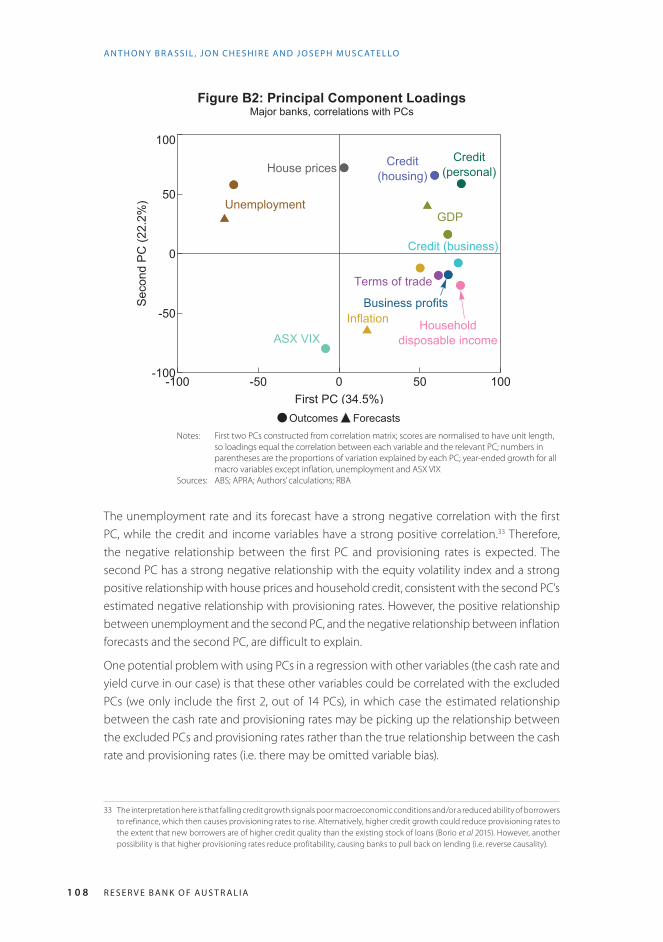
1 0 8 R E S E R V E B A N K O F A U S T R A L I A
A N T H O N Y B R A S S I L , J O N C H E S H I R E A N D J O S E P H M U S C AT E L LO
Figure B2: Principal Component LoadingsMajor banks, correlations with PCs
-100 -50 0 50 100-100
-50
0
50
100
First PC (34.5%)
SecondPC
(22.2%)
ASX VIXInflation
GDP
Credit (business)
Unemployment
House pricesCredit
(personal)Credit
(housing)
Householddisposable income
Business profits
Terms of trade
Outcomes ForecastsNotes: First two PCs constructed from correlation matrix; scores are normalised to have unit length,
so loadings equal the correlation between each variable and the relevant PC; numbers in parentheses are the proportions of variation explained by each PC; year-ended growth for all macro variables except inflation, unemployment and ASX VIX
Sources: ABS; APRA; Authors’ calculations; RBA
The unemployment rate and its forecast have a strong negative correlation with the first PC, while the credit and income variables have a strong positive correlation.33 Therefore, the negative relationship between the first PC and provisioning rates is expected. The second PC has a strong negative relationship with the equity volatility index and a strong positive relationship with house prices and household credit, consistent with the second PC’s estimated negative relationship with provisioning rates. However, the positive relationship between unemployment and the second PC, and the negative relationship between inflation forecasts and the second PC, are difficult to explain.
One potential problem with using PCs in a regression with other variables (the cash rate and yield curve in our case) is that these other variables could be correlated with the excluded PCs (we only include the first 2, out of 14 PCs), in which case the estimated relationship between the cash rate and provisioning rates may be picking up the relationship between the excluded PCs and provisioning rates rather than the true relationship between the cash rate and provisioning rates (i.e. there may be omitted variable bias).
33 The interpretation here is that falling credit growth signals poor macroeconomic conditions and/or a reduced ability of borrowers to refinance, which then causes provisioning rates to rise. Alternatively, higher credit growth could reduce provisioning rates to the extent that new borrowers are of higher credit quality than the existing stock of loans (Borio et al 2015). However, another possibility is that higher provisioning rates reduce profitability, causing banks to pull back on lending (i.e. reverse causality).

1 0 9CO N F E R E N C E V O LU M E | 2018
T H E T R A N S M I S S I O N O F M O N E TA R Y P O L I C Y T H R O U G H B A N K S’ B A L A N C E S H E E T S
To evaluate the potential extent of this problem, we regress the cash rate on all excluded PCs. By construction, no other linear combination could reduce the unexplained portion of the cash rate (i.e. the squared residuals are minimised). Therefore, the R2 from this regression can be interpreted as the maximum possible (squared) correlation between the cash rate and the information omitted by only using the first two PCs. We find an R2 of 0.16 and that it is insignificantly different from zero. So we conclude that the estimated relationship between the cash rate and provisioning rates is not just picking up the relationship between provisioning rates and the omitted macro variables.

1 1 0 R E S E R V E B A N K O F A U S T R A L I A
A N T H O N Y B R A S S I L , J O N C H E S H I R E A N D J O S E P H M U S C AT E L LO
Appendix C: The Envelope Theorem as It Relates to Cost of Funding
Suppose each bank is subject to a cost function f(x,a), where the vector x contains the bank’s discretionary variables and the vector a contains the bank’s non-discretionary variables. And that each bank, as a profit maximiser, wants to minimise this cost function subject to a vector of constraints g(x,a) ≥ 0.
Let the constrained optimum values of x be x*(a) (i.e. the optimum values are a function of the non-discretionary variables), and let the Lagrange multipliers at the optimum point be λ*(a). And suppose we put these optimum values back into the cost function to get the constrained optimum value of the cost function: f(x*(a),a).
The Envelope Theorem states that, assuming the cost function and constraints are continuously differentiable, then the total derivative of the optimised cost function with respect to the non-discretionary variables, a, is equal to the partial derivatives of the Lagrangian with respect to a. In other words, to a first-order approximation, we can ignore the effect changes in a have on x*(a) and λ*(a), and just evaluate the effect the change has on the cost function and any binding constraints.
The intuition behind this result is as follows. From the chain rule, the total derivative of the
optimised Lagrangian with respect to a will include ∂L∂x⋅dx∗ a( )da
terms and ∂L∂λ⋅dλ∗ a( )da
terms.34 However, at the optimum, the derivative of the Lagrangian with respect to the components of x and the Lagrange multipliers must be zero (i.e. the first-order conditions), so all these terms will equal zero. All that remains of the total derivative are the partial
derivatives of the cost function with respect to a (i.e. ∂f x ,a( )∂a
), and the partial derivatives of
the constraints with respect to a multiplied by the Lagrange multipliers (i.e. λ∗ a( )⋅∂g x ,a( )∂a
).
So what does this mean for our analysis? Take the following simplified summary of a bank’s cost minimisation problem:
minrH ,x ,y
rD x+ rH y+ rW 1− x− y( )+D y( ){ }
Subject to:
x= sx rH ,rD ,rW( )y= sy rH ,rD ,rW( )
where rD is the spread on no-/low-interest deposits, x is the share of no-/low-interest deposits, rH is the discretionary spread on the bank’s other deposit accounts (e.g. high-interest and term deposits) and y is the share of these deposits, and rW is the cost of wholesale funding and equity. D(y) is some demand function for discretionary deposits (e.g. demand for stable funding).
34 The complementary slackness condition from the Karush–Kuhn–Tucker theorem means that f(x*(a),a) and the Lagrangian at x*(a) and λ*(a) are identical.

1 1 1CO N F E R E N C E V O LU M E | 2018
T H E T R A N S M I S S I O N O F M O N E TA R Y P O L I C Y T H R O U G H B A N K S’ B A L A N C E S H E E T S
The two constraints are the supply functions of no-/low-interest deposits and other deposits, respectively; they are a non-negative function of their own spread and a non-positive function of the spreads on substitutes. There is no supply curve for wholesale funding as the bank is assumed to be a price taker in the wholesale market.
When minimising the cost function subject to the constraints, the Lagrange multipliers associated with the no-/low-interest deposit supply curve and the other deposit supply curve are, respectively, λx = rD−rW and λy = rH−rW + ′D y( ); these are the shadow prices of the constraints.
From the first-order condition for rH:
y+ rD−rW( )∂sx∂rH+ rH−rW + ′D y( )⎡⎣ ⎤⎦
∂sy∂rH=0
Assuming rD < rW and that ∂sy∂rH>0 (both realistic assumptions from the data), the above
equality requires rH−rW + ′D y( )<0 . That is, both shadow prices are negative.
Then, from the Envelope Theorem, the change in the cost function following an exogenous increase in rD (i.e. a decrease in the cash rate) equals:
x+ rD−rW( )∂sx∂rD+ rH−rW + ′D y( )⎡⎣ ⎤⎦
∂sy∂rD
⎡
⎣⎢⎢
⎤
⎦⎥⎥drD
Suppose we further assume that: rH < rD (a realistic assumption from the data); ∂sx∂rD≥−∂sy∂rD
(i.e. a change in rD cannot have a bigger effect (in absolute value) on the supply of substitute deposits than it has on no-/low-interest deposits); and the demand for discretionary deposits is not so inelastic that it causes an increase in rH so large that it completely offsets the cost reduction from substituting into the cheaper deposits. Then:
rD−rW( )∂sx∂rD+ rH−rW( )
∂sy∂rD+ ′D y( )
∂sy∂rD<0 (C1)
The first two terms in Equation (C1) are captured in the ‘funding mix’ part of Figure 8, the third term could be partially captured in the funding mix part and would cause an endogenous increase in rH. Since we know the change in rH will be ≥ 0, the funding mix component must be negative. Moreover, it must be larger in absolute value than any endogenous increase in rH. Therefore, the absolute value of the funding mix component is an upper bound on the total size of the combined indirect effects from changes in the constraints. The counterfactual exercise we run in Section 4.2.5 estimates the size of this upper bound.
Importantly, if the supply curve for no-/low-interest deposits was vertical, both sx and sy would not directly be affected by rD. Therefore, the total change in funding costs resulting from an increase in rD would be the direct effect (xdrD).

1 1 2 R E S E R V E B A N K O F A U S T R A L I A
A N T H O N Y B R A S S I L , J O N C H E S H I R E A N D J O S E P H M U S C AT E L LO
Appendix D: Accuracy of the Lending Spreads Part of the ModelThe shares of each asset component – the βi parameters in Equation (2) – are calibrated using APRA data reported by the major banks and other balance sheet data obtained by the RBA. The spreads are estimated from major bank interest rate data collected by the RBA.
The loan asset classes are: housing loans (split into the various combinations of owner-occupier/investor, principal and interest/interest only, variable/fixed), home equity loans, unsecured personal loans (variable/fixed), credit cards, margin loans, and business loans (small/large, variable/bank bills/fixed). The RBA collects interest rate data on each of these asset classes (including average discounts on the advertised rates offered by the major banks), and we use information on the repricing maturity of these loans to convert these interest rates into spreads to reference rates. The offset accounts of home loans are assigned an interest rate of zero.
This appendix evaluates how well the loan assets part of our model lines up with more aggregated data reported to APRA. While the reported data may be more accurate than our model estimates, they likely also contain measurement error and do not provide a sufficiently rich breakdown for our purposes. For example, we need to know the repricing terms of the various loan types, the shares of each loan type, and the spreads to reference rates of the loans. None of the data used for comparison in this section was used to calibrate our model, so this is a true external validation exercise.
Figure D1 compares quarterly average outstanding loan rates estimated from our model, to quarterly average lending rates reported to APRA by the banks. Our model provides a close approximation to the reported rates. Moreover, it is not just the broad trends that are matched, but the shape of the interest rate curves. These results give us confidence in the accuracy of our assumptions and calibration.
While the quarterly average rates reported by APRA provide the best comparison, we only have data from 2009. For a longer time series, we approximate quarterly average lending rates from the major banks’ quarterly interest income data reported to APRA. The APRA data in Figure D2 are constructed by taking the quarterly loan interest income, dividing it by the average loan balance during the quarter, and annualising.
The APRA data in Figure D2 are constructed on a ‘licensed authorised deposit-taking institution (ADI)’ basis, while our model and the APRA data in Figure D1 are based on the ‘domestic book of the licensed ADI’. So we do not expect our model to align as closely in Figure D2 as it does in Figure D1. That said, our model closely approximates these licensed ADI estimates over the entire sample, providing further validation of our assumptions and calibration.

1 1 3CO N F E R E N C E V O LU M E | 2018
T H E T R A N S M I S S I O N O F M O N E TA R Y P O L I C Y T H R O U G H B A N K S’ B A L A N C E S H E E T S
Figure D1: Average Outstanding Lending RatesQuarter average
2015201320112009 20174
5
6
7
%
4
5
6
7
%
APRA data
Model estimate(a)
Note: (a) Hedged; home loan offset accounts are given an interest rate of zeroSources: APRA; Authors’ calculations; RBA
Figure D2: Average Outstanding Lending RatesHedged, quarter average
2014201120082005 20174
5
6
7
8
9
%
4
5
6
7
8
9
%
APRA data(b)
Model estimate(a)
Notes: (a) Home loan offset accounts are given an interest rate of zero (b) Licensed ADI; from ARF 330.1.LSources: APRA; Authors’ calculations; RBA

1 1 4 R E S E R V E B A N K O F A U S T R A L I A
A N T H O N Y B R A S S I L , J O N C H E S H I R E A N D J O S E P H M U S C AT E L LO
Appendix E: Further Details about the Construction of Debt Funding Spreads
This appendix outlines the construction of debt funding spreads and funding shares in more detail.
Wholesale debt
The long-term debt spreads at issuance are estimated from a combination of primary and secondary market data.
We use BBSW rates as the measure of domestic short-term funding costs. For foreign currency debt, we add the cost of foreign currency hedging to get an estimate of the hedged foreign currency cost.
Term deposits
We estimate the weighted-average outstanding term deposit spread from a daily time series of advertised term deposit ‘special’ rates on new (and rolled-over) deposits, monthly APRA data on the total outstanding volume of term deposits, quarterly APRA data on the remaining time to maturity of outstanding term deposits, and an ad hoc query of the banks’ actual average cost of term deposits.
The interest rate data is collected for monthly maturities up to 12 months, plus 24-, 36-, and 60-month maturities; at each point in time, only a subset of maturities will have a ‘special’ rate. We begin by assigning these maturities into short, medium, and long buckets X ∈ S ,M ,L{ }( ). For each maturity (m), let Tm be the length of that maturity in days. And use rm,t,i to denote the spread to equivalent-maturity OIS of a new m-month special term deposit issued on day t – i. We compute the weighted-average outstanding term deposit spread as:
rt =dX ,m ,t ,i rm ,t ,ii=0
Tm−1∑m∈X∑X∑dX ,m ,t ,ii=0
Tm−1∑m∈X∑X∑+q
dX ,m ,t ,i =βX ,t−iIm ,t−i /Tm
I j ,t−i /Tjj∈X∑⎡
⎣
⎢⎢⎢
⎤
⎦
⎥⎥⎥Vt−i
where:
• Vt – i is the outstanding volume of term deposits at time t – i. This is intended to proxy for the relative volume of new and rolled-over deposits. Since the level of V doesn’t matter, this will be a good proxy as long as the portion of outstanding term deposits that are new or rolled does not change much over time.
•• βX,t – i is the share of new term deposits at time t – i with a maturity in bucket X. We use a time series on the ‘remaining time to maturity’ structure to recursively estimate the β parameters. We aggregate maturities into buckets because not every maturity will have a special rate on every day, and because our remaining time to maturity data is not available at a monthly disaggregation.

1 1 5CO N F E R E N C E V O LU M E | 2018
T H E T R A N S M I S S I O N O F M O N E TA R Y P O L I C Y T H R O U G H B A N K S’ B A L A N C E S H E E T S
º Specifically, we assume the longest remaining time to maturity category are all new term deposits (i.e. we assume the banks do not offer longer-maturity deposits). For the next longest category, we take the residual maturity data and remove the deposits in the longest maturity category that were issued in the previous period (as these would still be outstanding); this gives an estimate of the new term deposits issued with this maturity. This process continues until we reach the shortest maturity category.
• Im,t – i is an index function equal to one if at least one of the major banks offered a ‘special’ rate on a term deposit of maturity m on day t – i; it is equal to zero otherwise. We are implicitly assuming that no-one chooses a term deposit of this maturity if there is not a special rate. We divide this index by Tm to account for the fact that depositors with a preference for longer maturities will roll their term deposits less frequently; all else being equal, this means a given depositor is more likely to choose a shorter-term deposit. The sum is included in the denominator to ensure the share of new deposits at time t – i with a maturity in bucket X equals βX,t – i.
• q is a constant derived from the ad hoc bank query (only our most recent query asked about term deposits); its value ensures the rt we compute for 30 June 2017 equals the average value provided by the major banks through the query for this day. This constant is designed to account for any unadvertised special rates provided to some customers. We compute a value of q equal to 16 basis points.
• The average must include spreads on all term deposits still outstanding. We assume term deposits remain outstanding until their original maturity date has been reached. This is accounted for in the Σi=0
Tm−1 sum.
At-call high-interest deposits
We use data from the ad hoc queries of the major banks to determine the total volume of the major banks’ at-call high-interest accounts (such as online savings accounts, bonus saver accounts, and cash management accounts); we interpolate the data between queries.35 We then use interest rate data collected by the RBA to determine the advertised spread to the cash rate on these deposits at each point in time. We add a constant to account for any difference between the advertised and actual rates given to some customers; we compute an average difference of 15 basis points (based on the difference between our advertised weighted average rate and the rates reported in the ad hoc queries).
Wholesale deposits
For corporations, pension funds, and governments, we assume their remaining deposit accounts pay interest rates that move with rates in the domestic markets for short-term bank debt securities (these are converted into spreads to OIS); these securities are plausible substitutes for many of these institutions. From the ad hoc queries, we found that the average difference between these deposit rates and the rates on short-term debt securities was
35 These ad hoc queries occur on an approximately annual basis.

1 1 6 R E S E R V E B A N K O F A U S T R A L I A
A N T H O N Y B R A S S I L , J O N C H E S H I R E A N D J O S E P H M U S C AT E L LO
–71 basis points; so we add this constant to the short-term debt spreads to get our estimate of wholesale deposit spreads.
The volume of these deposits are computed as a residual – the total volume of deposits minus the deposits assigned to other categories.
No-/low-interest deposits
The volumes of non-interest bearing deposits, and low but fixed-rate deposits of households and unincorporated enterprises, are computed from the ad hoc queries of the major banks; we interpolate the data between queries. We estimate the low fixed rate using the average rate on these deposits reported in the queries (1.01 per cent). We assume banks hedge these no-/low-interest deposits into a variable interest rate exposure by entering into 3-year fixed-for-floating swaps (this is known as a ‘replicating portfolio’ hedge); this variable rate is converted into a spread to OIS.

1 1 7CO N F E R E N C E V O LU M E | 2018
T H E T R A N S M I S S I O N O F M O N E TA R Y P O L I C Y T H R O U G H B A N K S’ B A L A N C E S H E E T S
Appendix F: Excluding Components from Return on Equity (ROE)From Equation (2), we have the following relationship between the ROE and the various components that must sum to equal the ROE:
rE ,t−rC ,t( ) 1− α j ,tj∑( )= rA ,i ,t−rC ,t( )i∈D∑ βi ,t− rL , j ,t−rC ,t( )α j ,t
j∈D∑ + ft−ct( )
+ rA ,i ,t−rC ,t( )i∉D∑ βi ,t− rL , j ,t−rC ,t( )α j ,t
j∉D∑ − pi ,t
i∑ 1+ rA ,i ,t( )βi ,t
(F1)
where we have split out the discretionary and non-discretionary components (D is the set of discretionary lending and deposit components), and we have added a time subscript (t).
Equation (F1) is not a causal equation. That is, banks have discretion over their discretionary lending and deposit rates (by definition), and therefore have discretion over their ROE. So this equation is not enough for us to determine the level of ROE for a given level of the non-discretionary components. To characterise the behaviour of the banks, we define the following general behavioural function that determines a bank’s ROE:
rE ,t = ft Xt ,rC ,t( )+εt (F2)
where ft ⋅( ) is some (potentially time-varying) function that determines the systematic response of the bank’s ROE to some set of variables (Xt and rC,t), and εt is some mean-zero independent random component (that would have a variance of zero if ROE is completely deterministic given Xt and rC,t). This equation is sufficiently general to cover all possible behavioural response functions, but it is not very helpful in its current form. To get something more useful, we require more assumptions.
Splitting ft(Xt,rC,t) into f2,t(Xt,rC,t) and a part of the function that is orthogonal to rC,t (call it f1,t(Xt)) is innocuous because we can recover ft(Xt,rC,t) by setting f1,t(Xt) ≡ 0. So we rewrite Equation (F2) as:
rE ,t = f1,t Xt( )+ f2,t Xt ,rC ,t( )+εt
From Equation (F1), for any change in the non-discretionary components that results from a cash rate change, there exists some f2,t(Xt,rC,t) such that the aggregate pass-through to discretionary lending and deposit rates is one-for-one. From Equation (F1), this function (call it f2,t
∗ Xt ,rC ,t( )) must satisfy:
df2,t∗
drC ,t=1+
11− α j ,tj∑⎛
⎝
⎜⎜⎜⎜⎜
⎞
⎠
⎟⎟⎟⎟⎟⎟
dNt
drC ,t
where Nt ≡ rA ,i ,t−rC ,t( )βi ,ti∉D∑ − rL , j ,t−rC ,t( )α j ,tj∉D∑ − pi ,ti∑ 1+ rA ,i ,t( )βi ,t are the non-discretionary components, and we have assumed the equity share does not change with the cash rate.
To determine whether aggregate pass-through to discretionary lending and deposit rates is
one-for-one, we need to determine whether df2,tdrC ,t=
df2,t∗
drC ,t. With some assumptions, this can
be done by looking at the co-movement of drE ,tdt
and df2,t∗
drC ,t⋅drC ,tdt
over time.

1 1 8 R E S E R V E B A N K O F A U S T R A L I A
A N T H O N Y B R A S S I L , J O N C H E S H I R E A N D J O S E P H M U S C AT E L LO
First, we assume the changes in rE,t not caused by changes in the cash rate are also not correlated with changes in the cash rate. For changes in f1,t(Xt) and εt, this is true by construction. For
f2,t(Xt,rC,t), this requires df2,tdXt
⋅dXt
dt and ∂f2,t
∂t to not be correlated with df2,t
drC ,t⋅drC ,tdt
. If this assumption
holds, then with a sufficiently large sample we would be able to statistically determine whether the pattern in drE ,t
dt is significantly different from df2,t
∗
drC ,t⋅drC ,tdt
plus uncorrelated noise.
For a given sample size, the accuracy of this statistical analysis decreases as the variance of the uncorrelated noise increases. So, when constructing rE,t from the components of our model, we can increase the accuracy of our analysis by excluding components of the uncorrelated noise.
From Section 4.4, net non-interest income is volatile and is not correlated with the cash rate. Therefore, if net non-interest income is part of the majors’ ROE behavioural function, it would be in the uncorrelated noise (specifically, it would be in f1,t(Xt)), and excluding it would increase the accuracy of our analysis. So we exclude net non-interest income from ROE.36
Second, we exclude provisioning. From Section 4.1, changes in the provisioning rate can be caused by both changes in the cash rate and changes in other factors. Since these other factors can be large, excluding provisioning and adjusting df2,t
∗
drC ,t accordingly may improve
the accuracy of our analysis. Unfortunately, with provisioning rates being correlated with the cash rate, if provisioning is not part of f2,t(Xt,rC,t) then excluding it from ROE will introduce a bias into our analysis (because the erroneously excluded component will go into εt and will be correlated with the cash rate). Therefore, by excluding provisioning from ROE we are implicitly assuming that all provisioning is captured in f2,t(Xt,rC,t). The large reduction in the variance of ROE–NII after excluding provisioning is evidence in favour of this assumption.
At each point in time (T), the ‘one-for-one pass-through’ line in Figure 12 is defined as:
Δf2,t
∗∗
ΔrC ,tΔrC ,t−µ= 1+
Δ rCLA ,t−rC ,t( )ΔrC ,t
βCLA ,t1− α j ,tj∑⎛
⎝
⎜⎜⎜⎜⎜
⎞
⎠
⎟⎟⎟⎟⎟⎟−Δ rND ,t−rC ,t( )ΔrC ,t
αND ,t1− α j ,tj∑⎛
⎝
⎜⎜⎜⎜⎜
⎞
⎠
⎟⎟⎟⎟⎟⎟
⎡
⎣
⎢⎢⎢
⎤
⎦
⎥⎥⎥t=1
T
∑ ΔrC ,t−µt=1
T
∑
where f2,t∗∗ is f2,t
∗ excluding the ROE response to provisioning, CLA denotes ‘cash and liquid assets’, ND denotes no-/low-interest deposits, μ is the adjustment required for the 2003–07 average to equal zero, and Δ(rND,t – rC,t) accounts for the replicating portfolio hedge.
36 If net non-interest income is not part of the majors’ ROE behavioural function, then excluding it from ROE would add a component to εt. This would increase the variance of the uncorrelated noise and reduce the accuracy of our analysis, but it would not introduce a bias (because net non-interest income is uncorrelated with the cash rate). The smaller variance of ROE–NII relative to ROE suggests that net non-interest income is part of the majors’ ROE behavioural function.

1 1 9CO N F E R E N C E V O LU M E | 2018
T H E T R A N S M I S S I O N O F M O N E TA R Y P O L I C Y T H R O U G H B A N K S’ B A L A N C E S H E E T S
ReferencesACCC (Australian Competition and Consumer Commission) (2018), ‘Residential Mortgage Price Inquiry: Interim Report’, March.
Alessandri P and BD Nelson (2015), ‘Simple Banking: Profitability and the Yield Curve’, Journal of Money, Credit and Banking, 47(1), pp 143–175.
Altavilla C, M Boucinha and J-L Peydró (2017), ‘Monetary Policy and Bank Profitability in a Low Interest Rate Environment’, ECB Working Paper No 2105.
Andreasen MM, M Ferman and P Zabczyk (2013), ‘The Business Cycle Implications of Banks’ Maturity Transformation’, Review of Economic Dynamics, 16(4), pp 581–600.
Andries N and S Billon (2016), ‘Retail Bank Interest Rate Pass-Through in the Euro Area: An Empirical Survey’, Economic Systems, 40(1), pp 170–194.
Angeloni I and M Ehrmann (2003), ‘Monetary Transmission in the Euro Area: Early Evidence’, Economic Policy, 18(37), pp 469–501.
Apergis N and A Cooray (2015), ‘Asymmetric Interest Rate Pass-Through in the U.S., the U.K. and Australia: New Evidence from Selected Individual Banks’, Journal of Macroeconomics, 45, pp 155–172.
APRA (Australian Prudential Regulation Authority) (2006), ‘ARF_320_0: Statement of Financial Position (Domestic Books)’, Plain English Taxonomy form, rev 10 April 2017, viewed 17 March 2018. Available at <http://webarchive.nla.gov.au/gov/20171113042437/http://www.apra.gov.au/sbr-pet/ARF/ARF_320_0-D2A2.html>.
APRA (2018), ‘Quarterly ADI Property Exposures December 2017’, Statistical publication, accessed 17 March 2018. Available at <https://www.apra.gov.au/publications/quarterly-authorised-deposit-taking-institution-property-exposures>.
Aristei D and M Gallo (2014), ‘Interest Rate Pass-Through in the Euro Area during the Financial Crisis: A Multivariate Regime-Switching Approach’, Journal of Policy Modeling, 36(2), pp 273–295.
Atkin T and G La Cava (2017), ‘The Transmission of Monetary Policy: How Does It Work?’, RBA Bulletin, September, pp 1–8.
Baker A and D Jacobs (2010), ‘Domestic Market Operations and Liquidity Forecasting’, RBA Bulletin, December, pp 37–43.
Bech M and A Malkhozov (2016), ‘How Have Central Banks Implemented Negative Policy Rates?’, BIS Quarterly Review, March, pp 31–44.
Begenau J, M Piazzesi and M Schneider (2015), ‘Banks’ Risk Exposures’, NBER Working Paper No 21334.
Berkelmans L and A Duong (2014), ‘Developments in Banks’ Funding Costs and Lending Rates’, RBA Bulletin, March, pp 69–75.
BIS (Bank for International Settlements) (2017), ‘Debt Securities Statistics’, accessed 17 March 2018. Available at <https://www.bis.org/statistics/secstats.htm>.
Black S, A Brassil and M Hack (2010), ‘Recent Trends in Australian Banks’ Bond Issuance’, RBA Bulletin, March, pp 27–33.
Borio C and W Fritz (1995), ‘The Response of Short-Term Bank Lending Rates to Policy Rates: A Cross-Country Perspective’, BIS Working Paper No 27.

1 2 0 R E S E R V E B A N K O F A U S T R A L I A
A N T H O N Y B R A S S I L , J O N C H E S H I R E A N D J O S E P H M U S C AT E L LO
Borio C, L Gambacorta and B Hofmann (2015), ‘The Influence of Monetary Policy on Bank Profitability’, BIS Working Paper No 514.
Brown A, M Davies, D Fabbro and T Hanrick (2010), ‘Recent Developments in Banks’ Funding Costs and Lending Rates’, RBA Bulletin, March, pp 35–44.
Brunnermeier MK and Y Koby (2017), ‘The “Reversal Interest Rate”: An Effective Lower Bound on Monetary Policy’, Unpublished manuscript, Princeton University, 10 July.
Cheung B (2017), ‘Developments in Banks’ Funding Costs and Lending Rates’, RBA Bulletin, March, pp 45–50.
Claessens S, N Coleman and M Donnelly (2017), ‘“Low-For-Long” Interest Rates and Banks’ Interest Margins and Profitability: Cross-Country Evidence’, Board of Governors of the Federal Reserve System International Finance Discussion Papers No 1197.
Cœuré B (2012), ‘Central Banks and the Challenges of the Zero Lower Bound’, Speech given at the ‘Meeting on the Financial Crisis’, hosted by the Initiative on Global Markets, at the University of Chicago Booth School of Business, Miami, 19 February.
Cook B and D Steenkamp (2018), ‘Funding Cost Pass-Through to Mortgage Rates’, Reserve Bank of New Zealand Analytical Note AN2018/02.
Darracq Paries M, DN Moccero, E Krylova and C Marchini (2014), ‘The Retail Bank Interest Rate Pass-Through: The Case of the Euro Area during the Financial and Sovereign Debt Crisis’, ECB Occasional Paper Series No 155.
Davies M, C Naughtin and A Wong (2009), ‘The Impact of the Capital Market Turbulence on Banks’ Funding Markets’, RBA Bulletin, June, pp 1–13.
Davis K (2012), ‘Banking Profitability, Bank Capital and Competition’, Australian Centre for Financial Studies Financial Regulation Discussion Paper FRDP 2012 - 1.
de Bondt GJ (2005), ‘Interest Rate Pass-Through: Empirical Results for the Euro Area’, German Economic Review, 6(1), pp 37–78.
Debelle G (2012), ‘Bank Funding’, Opening Keynote Address given to the 2012 KangaNews DCM Summit, Sydney, 22 March.
Dell’Ariccia G, L Laeven and R Marquez (2014), ‘Real Interest Rates, Leverage, and Bank Risk-Taking’, Journal of Economic Theory, 149, pp 65–99.
Deloitte Access Economics (2014), ‘Competition in Retail Banking’, Report commissioned by the Australian Bankers’ Association, March. Available at <https://www2.deloitte.com/content/dam/Deloitte/au/Documents/Economics/deloitte-au-economics-retail-banking-competition-010314.pdf>.
Eggertsson GB, RE Juelsrud and E Getz Wold (2017), ‘Are Negative Nominal Interest Rates Expansionary?’, NBER Working Paper No 24039.
Fabbro D and M Hack (2011), ‘The Effects of Funding Costs and Risk on Banks’ Lending Rates’, RBA Bulletin, March, pp 35–41.
Finlay R and M Chambers (2008), ‘A Term Structure Decomposition of the Australian Yield Curve’, RBA Research Discussion Paper No 2008-09.
Fitzpatrick R and G White (2017), ‘Banking Fees in Australia’, RBA Bulletin, June, pp 35–39.
Gambacorta L (2008), ‘How Do Banks Set Interest Rates?’, European Economic Review, 52(5), pp 792–819.

1 2 1CO N F E R E N C E V O LU M E | 2018
T H E T R A N S M I S S I O N O F M O N E TA R Y P O L I C Y T H R O U G H B A N K S’ B A L A N C E S H E E T S
Gerali A, S Neri, L Sessa and FM Signoretti (2010), ‘Credit and Banking in a DSGE Model of the Euro Area’, Journal of Money, Credit and Banking, 42(s1), pp 107–141.
Gishkariany M, D Norman and T Rosewall (2017), ‘Shadow Bank Lending to the Residential Property Market’, RBA Bulletin, September, pp 45–52.
Gizycki M and B Gray (1994), ‘Default Risk and Derivatives: An Empirical Analysis of Bilateral Netting’, RBA Research Discussion Paper No 9409.
Hoffmann P, S Langfield, F Pierobon and G Vuillemey (2017), ‘Who Bears Interest Rate Risk?’, Unpublished manuscript, October.
Horvath R, J Kotlebova and M Siranova (2018), ‘Interest Rate Pass-Through in the Euro Area: Financial Fragmentation, Balance Sheet Policies and Negative Rates’, Journal of Financial Stability, 36, pp 12–21.
Hristov N, O Hülsewig and T Wollmershäuser (2014), ‘The Interest Rate Pass-Through in the Euro Area during the Global Financial Crisis’, Journal of Banking & Finance, 48, pp 104–119.
La Cava G, H Hughson and G Kaplan (2016), ‘The Household Cash Flow Channel of Monetary Policy’, RBA Research Discussion Paper No 2016-12.
Lowe P (1995), ‘The Link between the Cash Rate and Market Interest Rates’, RBA Research Discussion Paper No 9504.
Lowe P (2012), ‘Bank Regulation and the Future of Banking’, Remarks to the 41st Australian Conference of Economists ‘The Future of Economics: Research, Policy and Relevance’, Melbourne, 11 July.
Maddala GS and I-M Kim (1998), Unit Roots, Cointegration, and Structural Change, Themes in Modern Econometrics, Cambridge University Press, Cambridge.
McCririck R and D Rees (2017), ‘The Neutral Interest Rate’, RBA Bulletin, September, pp 9–18.
McKinnon T (2018), ‘Developments in Banks’ Funding Costs and Lending Rates’, RBA Bulletin, March, viewed 3 May 2018. Available at <https://www.rba.gov.au/publications/bulletin/2018/mar/developments-in-banks-funding-costs-and-lending-rates.html>.
Neely CJ and DE Rapach (2008), ‘Real Interest Rate Persistence: Evidence and Implications’, Federal Reserve Bank of St. Louis Working Paper 2008-018A.
Norman D (2017), ‘Return on Equity, Cost of Equity and the Implications for Banks’, RBA Bulletin, March, pp 51–58.
RBA (Reserve Bank of Australia) (2009a), ‘Box A: Banks’ Provisioning’, Financial Stability Review, September, pp 39–41.
RBA (2009b), ‘Box B: An International Comparison of Pass-Through of Policy Rate Changes to Housing Loan Rates’, Statement on Monetary Policy, February, pp 57–58.
RBA (2014a), ‘Box B: Australian Major Banks’ Cost-to-Income Ratios’, Financial Stability Review, September, pp 35–38.
RBA (2014b), Submission to the Financial System Inquiry, Reserve Bank of Australia, Sydney, March.
RBA (2016a), ‘Box C: Recent Developments in Australian Banks’ Capital Position and Return on Equity’, Financial Stability Review, October, pp 40–43.
RBA (2016b), Financial Stability Review, April.

1 2 2 R E S E R V E B A N K O F A U S T R A L I A
A N T H O N Y B R A S S I L , J O N C H E S H I R E A N D J O S E P H M U S C AT E L LO
Rodgers D (2015), ‘Credit Losses at Australian Banks: 1980–2013’, RBA Research Discussion Paper No 2015-06.
Rogoff K (2017), ‘Dealing with Monetary Paralysis at the Zero Bound’, Journal of Economic Perspectives, 31(3), pp 47–66.
Simon J (2015), ‘Low Interest Rate Environments and Risk’, Address given to the Paul Woolley Centre for the Study of Capital Market Dysfunctionality Conference ‘Are Financial Markets in the Eye of the Storm?’, Sydney, 8 October.
Van den Heuvel SJ (2007), ‘The Bank Capital Channel of Monetary Policy’, Unpublished manuscript, The Wharton School, University of Pennsylvania, June.
von Borstel J, S Eickmeier and L Krippner (2016), ‘The Interest Rate Pass-Through in the Euro Area during the Sovereign Debt Crisis’, Journal of International Money and Finance, 68, pp 386–402.
Wheelock DC (2011), ‘Banking Industry Consolidation and Market Structure: Impact of the Financial Crisis and Recession’, Federal Reserve Bank of St. Louis Review, 93(6), pp 419–430.
World Bank (2017), ‘Global Financial Development Database’, accessed 23 February 2018. Available at <http://www.worldbank.org/en/publication/gfdr/data/global-financial-development-database>.

1 2 3CO N F E R E N C E V O L U M E | 2 018
Discussion
1. Aarti SinghI would like to thank the organisers for giving me this opportunity to discuss this paper by Anthony Brassil, Jon Cheshire and Joseph Muscatello on the transmission of monetary policy. In my discussion I will first briefly describe some of their results that I find really interesting. And then I will attempt to relate their findings about monetary policy transmission with the modelling assumptions of dynamic stochastic general equilibrium (DSGE) models with financial intermediation. Finally, given that they have this very detailed dataset about banks’ balance sheets from the Australian Prudential Regulation Authority, my suggestion to the authors would be to extend the analysis in the paper to comment on the competitiveness of the banking sector in Australia.
Let me begin by first saying that the authors are working on a very interesting topic. Both academics and policymakers are always interested in understanding which factors affect the transmission of monetary policy. Monetary policy in Australia affects not only the cash rate (or the policy rate) but numerous other interest rates in the economy, and these interest rates in turn affect the aggregate economy. While some researchers directly examine the effect of monetary policy shocks on the aggregate economy, using either aggregate- or disaggregate-level data; the authors of this paper carefully examine, albeit indirectly, how changes in the cash rate affect two key interest rates set within the banking sector: banks’ lending rates and deposit rates. The approach adopted by the authors is innovative and flexible. They first construct a detailed model of the banks’ balance sheets, then they estimate the monetary policy pass-through on non-discretionary components of the banks’ balance sheets and on equity, which is discretionary. Using the balance sheet identity they indirectly determine the pass-through to discretionary components of the banks’ balance sheets, such as the lending and the deposit rates. On average, they find that, between 2003 and 2012, the aggregate pass-through to lending and deposit rates was broadly one-for-one, however, since mid 2012, it has been incomplete, only about 90 per cent.
To understand their methodology, consider the following equation where the expected net return from borrowing and lending is the return from equity. The balance sheet identity is therefore given by
Ai ≡ Lj+Ej∑
i∑ (1)
Using this identity, the authors derive a relationship between the bank’s return on equity, rE; and its lending rate rL and deposit rate rA
1+ rE( )E= 1−pi( ) 1+ rA ,i( )i∑ Ai− 1+ rL , j( )Lj+ f−c( )
j∑ Ai
i∑ (2)

1 2 4 R E S E R V E B A N K O F A U S T R A L I A
D I S C U S S I O N
The authors then rewrite this equation by expressing each interest rate as a spread to the cash rate.
The first finding, which I find really interesting, is that, for a majority of the banks in Australia, interest rates on assets and liabilities are repriced within three months. What this means is that if the cash rate changes, the banks are able to change their interest rates such that the spreads are not affected and the banks can hedge the interest rate risk. This leads me to my first comment. Looking back, some of the earlier papers on financial intermediation, for example Bernanke, Gertler and Gilchrist (1999), focused on the demand side of credit. In these models when there was a negative shock to the net worth of a borrower, their ability to borrow was inhibited and capital fell subsequently, generating the well-known financial accelerator effect. In these models the financial intermediation sector was perfectly competitive. More recently, Gerali et al (2010) have incorporated the supply side of credit (competition and interest rate-setting strategies), and in these models the banking sector has imperfect competition. The banks in these models face a repricing friction where banks have short-term deposits but lend long term. Therefore, this maturity mismatch of the banking sector dampens the impact of the monetary policy shock. However, the results of this paper by Brassil, Cheshire and Muscatello suggest that, in Australia’s case, banks are able to hedge interest rate risk. This is unlike other banking systems where repricing mismatch plays an important role in the transmission of monetary policy, which is also discussed by the authors in their paper. Does that mean that monetary policy shocks are not attenuated by the Australian banking sector? I would suggest that the authors discuss their findings and what their results imply for the DSGE models of the Australian economy with an imperfectly competitive banking sector.
I now briefly mention some of the other findings in the paper on the non-discretionary items on the balance sheet. In the case of provisions, the rate of provisions is typically increasing in the cash rate. This is because, for example, when interest rates fall, the chances of people defaulting on their loans also falls. The authors find evidence of incomplete pass-through and their estimates suggest that a 100 basis point cut in the cash rate is expected to reduce annual provisioning rates by 7 basis points. In wholesale debt markets, the banks are price takers and the cost of borrowing from these markets sees a full pass-through of cash rate changes. For the no-/low-interest rate deposits, by construction, spreads on these deposits have a one-for-one negative relationship with the cash rate. Overall, the authors find that, based on Equation (2), written in terms of spreads with respect to the cash rate, changes in the cash rate pass on to the non-discretionary components of the banks’ balance sheets almost one-for-one.
Looking at the discretionary components, the authors find that the return to equity, the left-hand side of Equation (2), has not moved with the cash rate since 2007. So this would then suggest that there is incomplete pass-through to discretionary components of the balance sheet. Finally, the authors conclude that, if the lack of return on equity pass-through were spread evenly across both discretionary lending and deposit rates, the deviation from full pass-through would be around 11 basis points for every 100 basis point change in the

1 2 5CO N F E R E N C E V O L U M E | 2 018
D I S C U S S I O N
cash rate since 2007. And if, instead, the pass-through was offset by lending rates alone, then lending rates would be 16 basis points higher than full pass-through.
The analysis is extremely rigorous and I would encourage the authors to construct a simple example to illustrate the implications on savings. For example, what are the implications if the pass-through is 11 basis points versus 16 basis points to one of the lending rates faced by Australian households, such as the loan rate on mortgages.
More broadly, what do the results of this paper suggest about the competitiveness of the banking sector in Australia? Based on the estimates of pass-though, are banks in Australia very competitive? If not, and the banking sector is imperfectly competitive, banks in Australia are likely to charge interest rates on their loans (deposits) at a mark-up (mark-down) over their marginal cost. In a study of banks in the United Kingdom, Alessandri and Nelson (2015) calibrate the mark-down of deposit rates below the interbank rate as 0.6 and the mark-up on their lending rates as 1.47, such that the deposit and loan rates implied by the model are 1.8 per cent and 6.25 per cent. My suggestion to the authors would be to determine the mark-ups and mark-downs in the key deposit and loan markets and discuss whether their conclusion of incomplete monetary policy transmission is consistent with these simple calculations. In the end I want to briefly mention the findings on a paper by Claessens and Laeven (2004) on competition in the banking sector using a panel of 50 countries for the period 1994–2001. Their evidence (in Table 2 of their paper) suggests that the level of competition in the banking sector in Australia is comparable to other developed countries such as the United States and the United Kingdom. Understanding the dynamics of banking competition would be another interesting way to understand the transmission of monetary policy in Australia in future research.
Finally, I enjoyed reading the paper and it was very competently executed.
Thank you.
ReferencesAlessandri P and BD Nelson (2015), ‘Simple Banking: Profitability and the Yield Curve’, Journal of Money, Credit and Banking, 47(1), pp 143–175.
Bernanke BS, M Gertler and S Gilchrist (1999), ‘The Financial Accelerator in a Quantitative Business Cycle Framework’, in JB Taylor and M Woodford (eds), Handbook of Macroeconomics: Volume 1C, Handbooks in Economics 15, Elsevier Science, Amsterdam, pp 1341–1393.
Claessens S and L Laeven (2004), ‘What Drives Bank Competition? Some International Evidence’, Journal of Money, Credit, and Banking, 36(3, Part 2), pp 563–583.
Gerali A, S Neri, L Sessa and FM Signoretti (2010), ‘Credit and Banking in a DSGE Model of the Euro Area’, Journal of Money, Credit and Banking, 42(s1), pp 107–141.

1 2 6 R E S E R V E B A N K O F A U S T R A L I A
D I S C U S S I O N
2. General DiscussionDiscussion initially focused on the structure of the residential mortgage market in Australia. Participants highlighted that variable-rate loans accounted for a significant share of Australia’s residential mortgage market. This means that the cash flow channel of monetary policy is more potent in Australia than in other countries where fixed-rate mortgages are more prevalent. There was some discussion as to whether this feature of the Australian market was desirable. One participant noted that the widespread use of variable-rate lending in Australia had led to greater public focus on monetary policy decisions, and had allowed Australian banks to move mortgage rates in line with their funding costs during the global financial crisis. On the other hand, this meant that cash rate changes could induce larger balance sheet responses than in other markets through changes in the volume of lending.
The high share of variable-rate mortgages in Australia means that households are more exposed to interest rate risk than banks. Participants discussed whether this was optimal. Some participants thought it was preferable for some interest rate risk to remain with households. One reason given was that banks may have incentives to take ‘directional bets’ on interest rate movements if they bore a greater share of this risk. Other participants considered that it would be reasonable for Australian banks to take on a greater share of interest rate risk, given they had the ability to diversify over their entire portfolio (which is not an option available to households). Others observed that the Australian market had developed its own hedging products (e.g. fixed-rate mortgages and offset accounts) and institutional features (e.g. a focus on lending standards and financial literacy) in response to the dominant pricing conventions. However, these products are not available to all households.
Focusing on the analysis, one participant asked whether interest rate pass-through differed in magnitude, timing or symmetry with respect to the direction of cash rate movements. Anthony Brassil noted that pass-through to variable-rate mortgages tended to occur within a few weeks of cash rate movements because around 80 per cent of mortgages have variable rates. He acknowledged that it was difficult to assess asymmetries because the cash rate had mainly moved in one direction over the sample used in the paper. The authors noted that the analysis intentionally abstracted from volume effects and, instead, examined pass-through to banks’ existing assets. Future analysis could examine changes in credit provision over time to gain broader insights into the bank lending channel.

1 2 7CO N F E R E N C E V O L U M E | 2 018
Luke Hartigan and James Morley*
1. IntroductionA quick look at the data in Figure 1 makes it clear that the introduction of inflation targeting corresponded to a stabilisation of the level of consumer price index (CPI) inflation in Australia around the numerical target range of 2–3 per cent introduced by the Reserve Bank of Australia (RBA) in 1993 (Stevens 1999). An important question is whether inflation targeting had other effects on the Australian economy, such as changing common movements in macroeconomic variables, including those related to the transmission of monetary policy shocks. Factor modelling provides a powerful and flexible way to investigate this empirical question in a data-rich environment.1
Figure 1: CPI InflationYear-ended
2005199319811969 2017-5
0
5
10
15
%
-5
0
5
10
15
%
Notes: Excludes interest charges prior to the September quarter 1998 and adjusted for the tax changes of 1999–2000; shaded region indicates the RBA’s inflation target range
Sources: ABS; RBA
1 See Stock and Watson’s (2016) survey of factor modelling and its use in examining the effects of structural shocks.
* Luke Hartigan is from the Economic Research Department of the Reserve Bank of Australia (RBA) and James Morley is from the University of Sydney. The views expressed in this paper are those of the authors and not necessarily those of the RBA.
A Factor Model Analysis of the Effects of Inflation Targeting on the Australian Economy

1 2 8 R E S E R V E B A N K O F A U S T R A L I A
L U K E H A R T I G A N A N D J A M E S M O R L E Y
We compile a large panel of macroeconomic data for the Australian economy and conduct factor model analysis to investigate the effects of inflation targeting. Our analysis suggests that a sizeable portion of macroeconomic fluctuations for Australia can be captured by two common factors. This result is the same as was found for the US economy by Stock and Watson (2005) and many others. Standard selection criteria suggest the need for two to four common factors, with recursive estimates generally suggesting a possible decline in the number of common factors following the introduction of inflation targeting. This possible decline stands in contrast to findings for the US economy by Bai and Ng (2007) of a possible increase. A change in the number of factors is indicative of a change in the factor structure, with a decline implying a different type of structural change than an increase. We explore the particular nature of changes in the factor structure of the Australian economy in detail.
Based on the standard selection criteria, we estimate an approximate dynamic factor model of the Australian economy with three common factors. The estimation is based on quasi-maximum likelihood, as in Doz, Giannone and Reichlin (2011, 2012). Our estimates suggest that only two common factors explain a sizeable portion of macroeconomic fluctuations and they have clear ‘real’ and ‘nominal’ interpretations based on their factor loadings. We apply a recent test developed by Han and Inoue (2015) for a structural break in factor loadings and find a significant break, with the test statistics for two versions of the test maximised just before and after the introduction of inflation targeting in mid 1993 (Stevens 1999, 2003). Notably, both versions of the test would still be significant if the break were in 1993:Q1, corresponding to the introduction of inflation targeting in the next quarter, with 1993:Q1 close to the earliest date at which both test statistics are significant. Meanwhile, there is no evidence for additional structural breaks once accounting for the break at the estimated dates or in 1993:Q1.
Looking at the cross-sectional variation in the common and idiosyncratic components of macroeconomic variables before and after the introduction of inflation targeting, it is clear that there was a much larger reduction in the volatility of common components than idiosyncratic components. That is, inflation targeting has not just stabilised the level of inflation, but it also appears to have stabilised the common components of macroeconomic variables. This reduction in common volatility is broad based, applying to both real and nominal variables. Meanwhile, the fact that idiosyncratic components have remained relatively volatile suggests that signal-to-noise ratios for common and idiosyncratic movements in variables such as CPI inflation have declined, making the benefit of using factors rather than noisy individual variables even greater during the inflation-targeting era. Interestingly, recursive estimates of factor loadings for real gross domestic product (GDP) growth, CPI inflation, and the overnight cash rate (OCR) suggest a stabilisation rather than an abrupt change with the introduction of inflation targeting. This argues against a ‘Type 1’ break, in the terminology of Han and Inoue (2015), in which there is a change in cross-correlations related to common factors or, equivalently, an increase in the number of relevant factors. Instead, it is consistent with a change in the volatility of factors or, equivalently, a decrease in the number of relevant factors, consistent with our recursive estimates of the number of factors.

1 2 9CO N F E R E N C E V O LU M E | 2018
A FA C T O R M O D E L A N A LY S I S O F T H E E F F E C T S O F I N F L AT I O N TA R G E T I N G O N T H E A U S T R A L I A N E CO N O M Y
The results for the approximate dynamic factor model motivate us to consider a factor augmented vector autoregression (FAVAR) model in order to investigate possible changes in the transmission of monetary policy shocks following the introduction of inflation targeting. Even if cross-correlations of variables related to factors are relatively stable, shock identification will still be affected given changes in relative variances. For identification of monetary policy shocks, we follow Bernanke, Boivin and Eliasz (2005) and use estimated loadings to relate the full panel to a three-variable structural vector autoregressive (VAR) model that includes the ‘real’ and ‘nominal’ factors from our approximate dynamic factor model and the policy interest rate. Importantly, the two common factors are re-estimated from a subset of the panel that corresponds only to ‘slow-moving’ variables that should only respond with a lag to a monetary policy shock. We find that a contractionary monetary policy shock temporarily lowers real activity and inflation, with the ‘price puzzle’ almost completely resolved, as was found by Bernanke et al (2005) for the US data.2 The CPI stabilises at a lower level, making it clear that the RBA targets inflation, not the price level (i.e. it lets ‘bygones be bygones’, as argued by Stevens (1999)). Structural break tests based on Qu and Perron (2007) suggest possible changes in VAR parameters around the introduction of inflation targeting and the global financial crisis (GFC). Sub-sample estimates suggest a resolution of the price puzzle and a flattening of the Phillips curve since the mid 2000s.
Our findings have important implications for monetary policy. First and foremost, they suggest that the benefits of inflation targeting are more than just in terms of stabilising the level of inflation, but also appear to involve reducing the common volatility of macroeconomic variables. This link in timing of a reduction in macroeconomic volatility with inflation targeting would be obscured somewhat by looking at real GDP growth on its own, but is clearer from the factor analysis. Relatedly, because idiosyncratic volatility has not reduced by as much as common volatility, our results suggest benefits to measuring real activity and price pressures using a factor modelling approach. The mitigation of a price puzzle for our FAVAR model provides an example of such a benefit. Despite apparent changes in the transmission of monetary policy, the factor modelling approach also allows for relatively precise estimation of the effects of a monetary policy shock in a data-rich environment and the possibility to relate the effects of policy to any variable in the panel, as well as any other variable that may only be available more recently due to data limitations, but for which we can estimate factor loadings. One clear implication of our FAVAR estimates is that the RBA currently pursues inflation targeting in line with its mandate, rather than price level targeting. Another clear implication is that, consistent with a flattening of the Phillips curve, the implied sacrifice ratio appears to have increased since the mid 2000s, suggesting caution against a shift to price level targeting.
The rest of this paper is organised as follows. Section 2 discusses the panel dataset, investigates the relevant number of common factors, presents estimates for an approximate dynamic factor model, and conducts break tests for the factor structure of the Australian economy. Section 3 examines the effects of inflation targeting on the factor structure of the Australian economy and draws some implications for monetary policy. Section 4 directly investigates possible changes in the transmission of monetary policy shocks by estimating a FAVAR model and also
2 See Bishop and Tulip (2017) on the challenges in removing the price puzzle for Australian structural VARs.

1 3 0 R E S E R V E B A N K O F A U S T R A L I A
L U K E H A R T I G A N A N D J A M E S M O R L E Y
considers changes with the introduction of inflation targeting and during the inflation-targeting era, again drawing implications for monetary policy. Section 5 concludes. Full details of the dataset and estimation methods are provided in the appendices.
2. A Factor Model of the Australian Economy
2.1 An Australian macroeconomic panel datasetWe expand the panel datasets in Gillitzer, Kearns and Richards (2005) and Gillitzer and Kearns (2007) to cover 104 time series variables for the Australian economy from 1976:Q4 to 2017:Q2.3 Due to data availability issues, the broader coverage of variables necessitates a later starting point for the sample than in Gillitzer et al (2005) and Gillitzer and Kearns (2007). However, the sample still includes 15 years before the introduction of inflation targeting in mid 1993 and nearly 25 years since its introduction.
Because many of the raw data series are non-stationary, we transform variables by taking logs and first differences as appropriate. As part of the transformation, we allow for a structural break in the mean levels of the price growth series in 1993:Q1, corresponding to the introduction of inflation targeting. This renders all of these series stationary without needing to take second differences. Once transformed to be stationary, we standardise all series by subtracting any remaining sample mean and dividing by the sample standard deviation. This implicitly gives each variable equal weight in the factor model.
In terms of broad categories, 42 per cent of the panel corresponds to real activity variables, 19 per cent to price variables, and 15 per cent to financial variables. Table 1 provides a more detailed breakdown into categories that we will refer to when looking at panel R2s for factors. Meanwhile, a list of all variables and their corresponding data transformations is provided in Appendix A.
3 Gillitzer et al (2005) and Gillitzer and Kearns (2007) focus on smaller panels and extracting a single coincident business cycle index for the Australian economy rather than looking at the effect of inflation targeting on the factor structure of the economy. Similarly, Sheen, Trück and Wang (2015) construct a daily coincident index using mixed frequency modelling of a smaller-scale dynamic factor model.

1 3 1CO N F E R E N C E V O LU M E | 2018
A FA C T O R M O D E L A N A LY S I S O F T H E E F F E C T S O F I N F L AT I O N TA R G E T I N G O N T H E A U S T R A L I A N E CO N O M Y
Table 1: Number of Variables by Category
Category NumberExpenditure 20Income 5Production 19Employment 8Surveys 5Building & capital expenditure (capex) 5Overseas transactions 5Prices 20Money & credit 6Interest rates 8Miscellaneous 3Total 104Note: ‘Miscellaneous’ includes ‘Share price index’, ‘Real trade-weighted exchange rate index’, and the ‘Southern
Oscillation Index’Sources: ABS; RBA
2.2 How many common factors?Figure 2 displays the ‘scree plot’ for the Australian macroeconomic panel dataset based on principle components analysis (PCA).4 It provides a simple diagnostic for a likely number of relevant common factors. The largest two eigenvalues from PCA explain much more variation than all of the remaining eigenvalues. This is suggestive of two relevant common factors that capture about 13 per cent and 9 per cent of the joint variation in the macroeconomic variables, with the remaining ‘scree’ likely corresponding to much less important common factors or even idiosyncratic movements in some of the individual variables. This finding of two dominant common factors is consistent with findings for datasets for other countries, including for the US economy by Stock and Watson (2005).
Table 2 reports formal selection criteria results for the number of common factors. As can be seen from the cumulative explained variation in Figure 2, the next eight largest eigenvalues from PCA more than double the total variation explained. Thus, it is unclear whether two common factors are actually sufficient for the dataset. Starting with Bai and Ng (2002), formal selection criteria have been developed to determine the number of relevant common factors in a given dataset. The results in Table 2 capture this uncertainty about the number of common factors. While a majority of criteria select two common factors, there could be as many as seven relevant common factors.
4 The typical shape of a scree plot – a steep drop off in explained variation after the first few eigenvalues and then a more shallow long tail for the remaining eigenvalues – is thought to be visually reminiscent of the side of a mountain after an avalanche, with the flattened-out rubble at the base of the mountain corresponding to the ‘scree’.

1 3 2 R E S E R V E B A N K O F A U S T R A L I A
L U K E H A R T I G A N A N D J A M E S M O R L E Y
Figure 2: Scree PlotAustralian macroeconomic dataset
Cumulative explained variation
20
40
%
20
40
%
Explained variation
1 2 3 4 5 6 7 8 9 100
5
10
%
0
5
10
%
Eigenvalues
Table 2: Number of Common Factors
NumberBai and Ng (2002)PCP2 4ICP2 2Ahn and Horenstein (2013)Eigenvalue ratio (ER) 2Growth ratio (GR) 2Onatski (2010)Edge distribution (ED) 7Note: The upper bound on the maximum number of factors used with each method was 10
For our approximate factor model, we consider three common factors. We do so as a compromise between the 2–4 common factors suggested by the two Bai and Ng (2002) criteria. As will be seen with our estimates, two common factors appear to be sufficient to capture the main common variation in the dataset, but allowing for three common factors in the model makes this clear. Meanwhile, any evidence of more than three common factors, such as suggested by the Onatski (2010) criterion, could reflect changes in the factor structure, which we will also investigate in full detail.

1 3 3CO N F E R E N C E V O LU M E | 2018
A FA C T O R M O D E L A N A LY S I S O F T H E E F F E C T S O F I N F L AT I O N TA R G E T I N G O N T H E A U S T R A L I A N E CO N O M Y
As a first step in looking at possible changes in the factor structure, Figure 3 reports recursive (expanding window) estimates of the number of common factors.5 The end-of-sample estimates are the same as those reported in Table 2. What is notable, however, about the recursive estimates is that, among the criteria that suggest a larger number of common factors, there is a decline in the suggested number of factors since 1993:Q1. It is consistent with a particular type of structural change in which the factor structure simplifies over time due to an elimination of common variation and, thus, corresponds to a reduction in volatility rather than a change in cross-correlations explained by common factors. Notably, this decline contrasts with findings by Bai and Ng (2007) for the US economy of an increase in the suggested number of factors in recent years. Again, we will investigate this possibility in full detail.
Figure 3: Number of FactorsRecursive estimates
201120051999199319871981 20170
2
4
6
8
10
no
0
2
4
6
8
10
no
ED
GRER
2PCP
ICP2
Notes: Maximum number of factors set to 10; initial window set to 20 quarters; dashed vertical line indicates the start of inflation targeting
2.3 Estimates for an approximate dynamic factor modelBased on the Bai and Ng (2002) selection criteria, we estimate an approximate dynamic factor model with three common factors:
Yt =ΛFt−1+εt (1)
where Yt is the data, Λ are the factor loadings, Ft are the factors and εt is the idiosyncratic component. Yt and εt are N × 1, Λ is N × 3, Ft and ηt are 3 × 1. The factors are assumed to follow
5 We prefer recursive to rolling-window estimates because they better illustrate possible permanent changes in the structure, while rolling windows could capture possible recurring changes, but are sensitive to the window size. For recurring changes, the sensitivity to window size makes it preferable to formally test and model the changes via a regime-switching factor model. We leave such analysis for future research.

1 3 4 R E S E R V E B A N K O F A U S T R A L I A
L U K E H A R T I G A N A N D J A M E S M O R L E Y
a VAR(1), Ft = Φ(L)Ft – 1 + ηt, while Φ(L) is a 3 × 3 conformable lag polynomial. An approximate dynamic factor model allows the elements of εt to be weakly dependent across series and time, but they are uncorrelated with the common factors, E εt ′ηt⎡⎣ ⎤⎦=0,∀k .6
We conduct initial ‘static’ estimation using PCA, following Stock and Watson (2005).7 Then, using these static estimates, we calculate dynamic factor estimates using quasi-maximum likelihood estimation (QMLE) for a VAR of the factors with one lag based on Schwarz information criterion (SIC) and Kalman filter/smoother recursions via the expectation maximisation (EM) algorithm, following Doz et al (2011, 2012). See Appendix B for more details.
Figure 4 displays the static and dynamic estimates of the three common factors.8 There is a strong coherence between the estimates for the first two factors, which display considerable persistence. There is less evidence of a link between the estimates of the third factor, which also appears to be far less persistent. An explanation could be that the static estimates of the third factor capture some lagged dynamics of the first two factors, but it is mostly noise when considering dynamic factor estimation with a VAR(1) structure. Meanwhile, the dynamic estimates of the third factor turn out to explain very little variation of the panel dataset.
Figure 4: Common FactorsQMLE versus PCA factor estimates
Factor 1(a)
-202%
-202%
Factor 2
-202%
-202%
QMLEFactor 3
20102003199619891982 2017-4-202%
-4-202%
PCA
Note: (a) Renormalised to change sign
6 Labelling this model as ‘dynamic’ follows Doz et al (2011, 2012) and reflects the fact that the estimation explicitly accounts for the dynamic VAR structure for the factors, rather than an alternative notion of a dynamic factor model having non-zero loadings for variables on lags of factors. Of course, the model we consider could allow for lagged relationships between variables and factors by including any lagged dynamic factors as additional ‘stacked’ factors in Ft.
7 Stock and Watson (2002), Bai and Ng (2002), and Bai (2003) prove consistency of PCA estimation for approximate factor models.
8 We renormalise the sign of the first factor such that real GDP growth has a positive loading for ease of interpretation as a real activity factor.

1 3 5CO N F E R E N C E V O LU M E | 2018
A FA C T O R M O D E L A N A LY S I S O F T H E E F F E C T S O F I N F L AT I O N TA R G E T I N G O N T H E A U S T R A L I A N E CO N O M Y
Figure 5 reports the variation of data in different categories explained by the common dynamic factors based on panel R2s that capture the fraction of the variance of a series explained by a given common factor. The fact that these are all reasonably low suggests that variables in each category are subject to considerable idiosyncratic variation. It is also clear based on the categories that the first factor corresponds more to ‘real’ variables such as measures of expenditure, employment, and activity surveys, while the second factor corresponds more to ‘nominal’ variables, such as prices, money, credit, and interest rates. Notably, we find that interest rate spreads in particular load on both factors, which likely reflects their information content about both real activity and inflation. As mentioned above, the third factor explains very little variation of the panel, with the highest R2s corresponding to activity surveys and interest rates. Thus, it may capture something about expectations of future real activity or ‘sentiment’, but it is possibly just noise that can be dropped from the model.
Figure 5: Explained VariationCoefficient of determination by category, 1976:Q4–2017:Q2
Factor 1
0.2
0.4R2
0.2
0.4R2
Factor 2
0.1
0.2R2
0.1
0.2R2
Factor 3
Expenditure
Production
Income
Employment
Surveys
Building&capex
O/stransactions
Prices
Money&credit
Interestrates
Misc0.0
0.1
0.2R2
0.0
0.1
0.2R2

1 3 6 R E S E R V E B A N K O F A U S T R A L I A
L U K E H A R T I G A N A N D J A M E S M O R L E Y
2.4 Breaks in the factor structure?As noted above, one reason why some selection criteria might suggest more than two factors could be due to changes in the factor structure. We formally test for structural breaks using an approach recently proposed by Han and Inoue (2015).9 The null hypothesis of their test is that all factor loadings are constant over time against the alternative that a non-negligible fraction of factor loadings have changed. The test makes use of the fact that the presence of a structural break in factor loadings implies changes in the second moments of the factors. Han and Inoue (2015) note that a change in the volatility of factors or in factor loadings would not be separately identified, so a rejection could reflect either or both. The idea of a change in dynamic factor loadings in the sense of being equivalent to additional factors in a PCA setting corresponds to a ‘Type 1’ break, where the change in the factor structure reflects a change in cross-correlations between variables related to common factors. By contrast, the idea of a change in the volatility of factors corresponds to a ‘Type 2’ break, where the change in the factor structure reflects a change in the volatility of variables related to common factors, but with the same cross-correlations between variables related to common factors. Our earlier finding of a reduction in the number of factors implied by some of the criteria in Figure 3 is more consistent with a Type 2 break than a Type 1 break, but we will examine issue this directly.
Figure 6 plots the Han and Inoue (2015), LM and Wald test statistics for a structural break in factor loadings. In both cases, we can reject the null of no break, with the LM test statistic maximised in 1991:Q4 and the Wald test statistic maximised in 1998:Q3. Notably, however, both test statistics are still significant if the break occurred in 1993:Q1 with the introduction of inflation targeting, which is close to the earliest date at which both test statistics are significant. Thus, the results for Han and Inoue’s (2015) test are consistent with the idea that the introduction of inflation targeting led to a change in the factor structure of the Australian economy. Furthermore, we note that the there is no support for an additional break, whether the first break is set to have occurred at the estimated dates or in 1993:Q1. Given a break in the factor structure around the time of the introduction of inflation targeting, we turn next to an investigation of what effects it had on the Australian economy.
9 Breitung and Eickmeier (2011) and Chen, Dolado and Gonzalo (2014) also propose tests for structural instability in factor models. However, both of these alternative tests have drawbacks. For example, Breitung and Eickmeier’s (2011) joint test appears to be oversized when idiosyncratic errors contain serial correlation and a heteroskedasticity autocorrelation consistent (HAC)-based covariance matrix estimator is used. Meanwhile, the Lagrange multiplier (LM) version of Chen et al’s (2014) test is not consistent in some settings. Importantly, Monte Carlo analysis in Han and Inoue (2015) suggests that their test has better finite sample performance compared with Chen et al (2014).

1 3 7CO N F E R E N C E V O LU M E | 2018
A FA C T O R M O D E L A N A LY S I S O F T H E E F F E C T S O F I N F L AT I O N TA R G E T I N G O N T H E A U S T R A L I A N E CO N O M Y
Figure 6: Factor Loadings Structural Break Test
LM
5
10
15
5
10
15
Wald
20062001199619911986 20110
5
10
15
0
5
10
155% critical value
Notes: Test statistic is for an unknown break date with 15 per cent trimming; dashed vertical lines indicate the start of inflation targeting; solid vertical lines indicate the maximal test statistic for each test
3. Effects of Inflation Targeting
3.1 Decline in common shocksWe find that the introduction of inflation targeting corresponded to a much larger reduction in the volatility of common components of macroeconomic time series than idiosyncratic components. To see this, we calculate the cross-sectional variance of common components, which reflects the variability of common factors, and of idiosyncratic components, which reflects the residual variability of the data, at each point in time. Figure 7 plots measures of common and idiosyncratic volatility over the whole sample for: (i) all of the variables, (ii) just real variables, (iii) just nominal variables, and (iv) just price variables. The pattern is consistent in all of the cases. Although there are still peaks in the volatility measures after 1993 that seem to be related to events such as the introduction of the goods and services tax in 2000 (idiosyncratic volatility) and the GFC in 2007–09 (both common and idiosyncratic volatility), there is clearly lower average common volatility since the introduction of inflation targeting. The absence of a recession in Australia since 1993 could help explain the relative lack of peaks in common volatility that occurred with the recessions in the early 1980s and 1990s. However, the common volatility is still generally lower after the introduction of inflation targeting than it was even during expansions prior to inflation targeting. Furthermore, contrary to recessions being the primary driver of volatility, the idiosyncratic volatility looks only slightly lower on average since 1993, and this is not even clear for the price variables. Meanwhile, because the reduction of idiosyncratic volatility is not as large as the reduction of common volatility, signal-to-noise ratios for individual variables that proxy for the common factors have clearly dropped since the introduction of inflation targeting.

1 3 8 R E S E R V E B A N K O F A U S T R A L I A
L U K E H A R T I G A N A N D J A M E S M O R L E Y
Figure 7: Australian Macroeconomic Volatility
All
0.5
1.0
1.5
%
Common
Real(a)
0.5
1.0
1.5
%Idiosyncratic
Nominal(b)
200219870.0
0.5
1.0
1.5
% Prices
20021987 20170.0
0.5
1.0
1.5
%
Notes: Volatility is defined as the cross-sectional standard deviation for each component; dashed vertical lines indicate the start of inflation targeting
(a) Includes expenditure, production, income, employment, surveys, building & capital expenditure and overseas transactions
(b) Includes prices, money & credit and interest rates
Figure 8 illustrates the decline in the signal-to-noise ratio by plotting the common and idiosyncratic components of (adjusted and standardised) CPI inflation. The variation in both components seems to have lessened somewhat, but much more so for the common component. Thus, a higher proportion of the quarterly fluctuations in CPI inflation reflect noise since the introduction of inflation targeting. A direct implication for monetary policy is that it makes sense to ‘look through’ some of the high frequency movements in CPI inflation. Such movements are more likely to be reflecting noise rather than a persistent change in underlying inflationary pressures. Furthermore, the dynamic factor model provides a way to extract a signal about underlying inflationary pressures from a noisy series such as CPI inflation.

1 3 9CO N F E R E N C E V O LU M E | 2018
A FA C T O R M O D E L A N A LY S I S O F T H E E F F E C T S O F I N F L AT I O N TA R G E T I N G O N T H E A U S T R A L I A N E CO N O M Y
Figure 8: Signal and NoiseCPI inflation
20102003199619891982 2017-4
-2
0
2
%
-4
-2
0
2
%
Idiosyncraticcomponent
Commoncomponent
Notes: Excludes interest charges prior to the September quarter 1998 and adjusted for the tax changes of 1999–2000; series mean adjusted for the introduction of inflation targeting in June quarter 1993; dashed vertical line indicates the start of inflation targeting
3.2 Stabilised factor loadingsTo further investigate the nature of the change in the factor structure, we calculate recursive estimates of factor loadings for real GDP growth, CPI inflation and the OCR on the estimated factors.10 Figure 9 plots these recursive estimates along with 95 per cent confidence bands.11 Real GDP growth loads significantly on all three factors, CPI inflation only loads significantly on the second factor, and the OCR loads significantly on the first two factors. The estimated loadings for all three variables on the first factor are positive (although, again, insignificant for CPI inflation). This suggests that the first factor could reflect demand pressures in the economy. The estimated loadings for the second factor are negative on real GDP growth and positive for CPI inflation and the OCR, suggesting the factor could reflect supply-side inflationary pressures. The estimated loadings for the third factor are positive for real GDP growth and effectively zero for CPI inflation and the OCR, suggesting that factor could reflect high frequency real activity movements that do not spill over into inflation or affect monetary policy. Meanwhile, it is quite notable that the recursive estimates of the factor loadings seem to stabilise rather than jump with the introduction of inflation targeting. This is consistent with a Type 2 break.
10 Again, we focus on recursive rather than rolling-window estimates in order to better understand possible permanent changes rather than possible temporary changes, and to avoid making an arbitrary choice about the window size.
11 Confidence bands are based on inverted t tests using the alternative HAC standard errors proposed in Hartigan (2018).

1 4 0 R E S E R V E B A N K O F A U S T R A L I A
L U K E H A R T I G A N A N D J A M E S M O R L E Y
Figure 9: Factor LoadingsRecursive estimates
GDP
0.700.720.74
CPI
Loading 1
OCR
-101
-0.48-0.46-0.44
Loading 2012
200219870.420.440.460.48
20021987 20021987 2017-2-101
Loading 3
Notes: The first 10 per cent of observations were dropped in estimation; bands represent 95 per cent confidence intervals; dashed vertical lines indicate the start of inflation targeting; GDP refers to the LHS, CPI and OCR refer to the RHS
3.3 Interpretation and implicationsThe structural break analysis suggests that inflation targeting has done more than just stabilise the level of inflation in Australia. It has also reduced the volatility of common movements in macroeconomic variables and possibly reduced the number of common factors in the economy. This reduction in volatility is not just in price growth and other nominal variables but is broad based. One possibility is that it could be driven by an elimination of ‘sunspot’ shocks following the introduction of inflation targeting due to its provision of a clear nominal anchor for inflation expectations.12 Notably, the estimated timing of the reduction in macroeconomic volatility that is linked to the introduction of inflation targeting is different than that implied by looking at real GDP growth on its own (Figure 10).13 This suggests that there is a clear benefit from using factor analysis in this case. The timing is also different than that of the volatility reduction in US output growth and inflation (the mid 1980s) found in numerous studies (e.g. Stock and Watson 2003), which suggests it is not due to any changes in global factors at the same time as the introduction of inflation targeting in Australia.
12 See Lubik and Schorfheide (2004) and Lubik and Surico (2010) on the interaction between monetary policy and sunspot shocks.
13 The break date estimates are 1984:Q1 and 1998:Q4 using the Bai and Perron (1998) sequential test procedures for squared demeaned real GDP growth regressed on a constant and allowing for HAC standard errors. Without HAC standard errors, the evidence is only for one break in 1984:Q1, corresponding to the so-called ‘Great Moderation’ that has been argued to have occurred in Australia around the same time as in the United States (Summers 2005). Interestingly, if we use the Qu and Perron (2007) sequential test procedures for structural breaks in mean and/or variance of real GDP growth, we only find evidence of one break in variance in 1998:Q4, with or without HAC standard errors, closely corresponding to the estimated timing for the Wald test statistic of a break in factor loadings in Figure 6. However, if we estimate two breaks in variance, the estimated break dates are 1984:Q1 and 1998:Q4, as was found with the Bai and Perron (1998) procedures. Furthermore, reflecting the presence of idiosyncratic noise, a change in volatility in real GDP growth in 1998:Q4 is far less visually evident in Figure 10 than the common volatility changes with the introduction of inflation targeting in Figure 7.

1 4 1CO N F E R E N C E V O LU M E | 2018
A FA C T O R M O D E L A N A LY S I S O F T H E E F F E C T S O F I N F L AT I O N TA R G E T I N G O N T H E A U S T R A L I A N E CO N O M Y
Figure 10: Real GDP Growth
2005199319811969 2017-1
0
1
%
-1
0
1
%
Notes: Computed as log differences on quarterly observations; dashed vertical line indicates the start of inflation targeting; solid vertical lines indicate estimated break dates using the Bai and Perron (1998) sequential test procedures for squared demeaned real GDP growth regressed on a constant and allowing for HAC standard errors
Sources: ABS; Authors’ calculations
In addition, the larger drop in the volatility of common components relative to idiosyncratic components implies an increased benefit of looking at common factors to eliminate noise in individual observed variables. Notably, price measures, including CPI inflation, have particularly large idiosyncratic components, while our factor model estimates suggest that the RBA can ‘look through’ most quarterly fluctuations in these measures and focus on underlying measures such as the common component of price growth variables provided by our approximate dynamic factor model.
The stability of the factor loadings is reassuring for the use of a factor model to capture real and nominal fluctuations in the Australian economy. However, even with stable loadings, changes in relative variances of shocks in the economy can result in changes in the dynamic interactions of variables. For example, the transmission of monetary policy shocks may have changed with the introduction of inflation targeting. We turn to this issue next.
4. Transmission of Monetary PolicyBased on the apparent factor structure of the Australian economy, we develop a FAVAR model to examine the transmission of monetary policy shocks, including possible changes due to the introduction of inflation targeting.

1 4 2 R E S E R V E B A N K O F A U S T R A L I A
L U K E H A R T I G A N A N D J A M E S M O R L E Y
4.1 FAVAR modelFollowing Bernanke et al (2005), we estimate a FAVAR model based on their preferred specification of using the policy interest rate as an observed factor. The model uses factor loadings to relate the full panel of data to a three-variable VAR that includes the first two common factors corresponding to real and nominal fluctuations and the OCR. We extract the first two factors from a subset of the panel that corresponds only to ‘slow-moving’ variables. It excludes, for example, survey measures, oil prices, commodity prices, financial variables and the exchange rate. The full list is given in Table A1. Crucially, the panel excludes the OCR and the factors are rotated to remove any residual effects of the policy rate. Despite these changes, the extracted factors are very similar to the original factors estimated from the full panel (Figure 11). Then, monetary policy shocks are identified by assuming they are contemporaneously uncorrelated with other shocks that drive the factors.14 See Appendix C for full details.
Figure 11: Common FactorsOriginal versus rotated factor estimates
Factor 1(a)
-2
0
2
%
-2
0
2
%
QMLEFactor 2
20102003199619891982 2017-4
-2
0
2
%
-4
-2
0
2
%
Rotated(b)
Notes: (a) Renormalised to change sign (b) Rotated to remove any residual effects of monetary policy
4.2 Full sample estimatesBefore considering structural change, we start by estimating a FAVAR with two lags (based on the SIC) for the full sample of 1976:Q4–2017:Q2 to provide benchmark results. Given FAVAR parameter estimates, we calculate impulse response functions (IRFs) for a surprise 25 basis point increase in the OCR, with reported 95 per cent confidence bands based on 500 bootstrap replications.
14 In practice, this identification involves ordering the OCR last in the VAR and using a Cholesky factorisation of the forecast error variance-covariance matrix to identify monetary policy shocks. However, due to the construction of factors and their rotation, the correlation between the forecast errors for the VAR is very low, so ordering has very little effect on the identified shocks.

1 4 3CO N F E R E N C E V O LU M E | 2018
A FA C T O R M O D E L A N A LY S I S O F T H E E F F E C T S O F I N F L AT I O N TA R G E T I N G O N T H E A U S T R A L I A N E CO N O M Y
Figure 12 plots IRFs for the OCR and the two factors. The OCR increases 25 basis points on impact, by construction, and then it gradually reverts back to its initial level, while both factors contract significantly at business cycle horizons. Given the loadings for these factors (positive for real GDP growth on the first factor and positive for CPI inflation on the second factor), these results are consistent with the interpretation of the identified monetary policy shock as being contractionary.
Figure 12: Impulse Response Functions1976:Q4–2017:Q2
OCR
0.0
0.2
0.4
%
0.0
0.2
0.4
%
Factor 1
-0.1
0.0
0.1
%
-0.1
0.0
0.1
%
Factor 2
0 6 12 18 24 30 36 42 48-0.2
-0.1
0.0
0.1
%
-0.2
-0.1
0.0
0.1
%
Quarters after shockNotes: Response to a 25 basis point contractionary monetary policy shock; bands represent 95 per
cent confidence intervals computed by bootstrap from 500 replications
Figure 13 directly examines the implied IRFs for real GDP growth and CPI inflation. The point estimates still show contractionary effects, although the response of real GDP growth is no longer significant, reflecting the fact that real GDP growth also loads negatively on the second factor in addition to loading positively on the first factor. The response of CPI inflation is very similar to the response of the second factor, reflecting an insignificant loading of CPI inflation on the first factor. Accumulated responses are also reported to show the implied effects of a monetary policy shock on the log levels of real GDP and the CPI. Consistent with long-run monetary neutrality, there is no significant long-run effect on log real GDP. Meanwhile, log CPI is permanently lower following the contractionary monetary policy shock. This reflects the dynamics of the OCR in response to the policy shock, with the RBA gradually

1 4 4 R E S E R V E B A N K O F A U S T R A L I A
L U K E H A R T I G A N A N D J A M E S M O R L E Y
returning the policy rate back to its original level, but not overshooting in order to reverse the initial effects of the shock on the price level. That is, the IRFs are consistent with the RBA targeting the inflation rate, not the price level, and letting ‘bygones be bygones’.
Figure 13: Impulse Response Functions1976:Q4–2017:Q2
Real GDP growth
-0.1
0.0
0.1
% CPI inflation
-0.1
0.0
0.1
%
Log real GDP
0 12 24 36-3
-2
-1
0
1% Log CPI
12 24 36 48-3
-2
-1
0
1%
Quarters after shockNotes: Response to a 25 basis point contractionary monetary policy shock; bands represent 95 per
cent confidence intervals computed by bootstrap from 500 replications
The point estimate for the response of CPI inflation to a contractionary monetary policy shock is slightly positive at the one quarter horizon. However, it is insignificant and the point estimates are negative and often significantly so at subsequent horizons. Thus, these IRFs largely resolve the so-called ‘price puzzle’, as Bernanke et al (2005) did with their FAVAR for the US economy.15 The price puzzle has been particularly challenging to solve for Australian SVARs, as discussed in Bishop and Tulip (2017). So our result is particularly encouraging for using a FAVAR to estimate the effects of monetary policy shocks on the Australian economy.
A benefit of the FAVAR model is that it allows us to examine the effects of a monetary policy shock on any variable in the panel (and even variables not in the panel, as long as we can determine relevant loadings on the factors). Figure 14 plots the IRFs for a selection of other variables that reflect different aspects of the Australian economy. The variables are private gross fixed capital formation (GFCF), the domestic final demand (DFD) price deflator, housing commencements, the unemployment rate, housing prices, a survey of expected output, total employment growth, an index of commodity prices (ICP), and a consumer sentiment index
15 The price puzzle is the tendency for estimated IRFs to initially show a positive response of inflation to a contractionary monetary policy shock. It is often seen as a failure to completely identify the true monetary policy shock by partially reflecting an endogenous response of the policy rate to other shocks, although it could reflect a genuine economic response in the case where inflation expectations are not anchored (see Lubik and Schorfheide (2003)).

1 4 5CO N F E R E N C E V O LU M E | 2018
A FA C T O R M O D E L A N A LY S I S O F T H E E F F E C T S O F I N F L AT I O N TA R G E T I N G O N T H E A U S T R A L I A N E CO N O M Y
(CSI). The series are transformed to be stationary where appropriate and as noted in the figure. The IRFs behave as expected given a contractionary monetary policy shock. For example, DFD price deflator inflation behaves very similarly to CPI inflation, the unemployment rate increases significantly at business cycle horizons, and consumer sentiment falls significantly at business cycle horizons.
Figure 14: Impulse Response Functions – Other Macroeconomic Variables
1976:Q4–2017:Q2
Private GFCF
-0.10.00.1% DFD price deflator Commencements
-0.10.00.1%
Unemployment(a)
-0.20.00.2% Housing prices Expected output(b)
-0.20.00.2%
Employment
0 12 24 36-0.4
-0.2
0.0
% ICP
12 24 36
CSI(b)
12 24 36 48-0.4
-0.2
0.0
%
Quarters after shockNotes: Response to a 25 basis point contractionary monetary policy shock; bands represent 95 per
cent confidence intervals computed by bootstrap from 500 replications; responses for each series mapped using estimated factor loadings; all series are growth rates besides those indicated otherwise
(a) First difference (b) Level
4.3 Breaks in the FAVAR?Given the benchmark full sample results, we now consider whether the introduction of inflation targeting changed the FAVAR parameters or whether they changed at any other point of the sample. To test for structural breaks in the FAVAR, we apply the Qu and Perron (2007) procedures. In principle, the methods in Qu and Perron can be applied to a linear system of regression equations with multiple structural breaks in mean or variance. However, given the large number of parameters for the FAVAR model, we need to apply tests for structural breaks equation by equation. Tables 3 and 4 report the results of Qu and Perron’s (2007) supLR tests and sequential tests for each equation of the VAR portion of the model allowing for breaks in conditional mean and variance. Given a VAR set-up, we assume no residual serial correlation. We consider a maximum of three breaks with 15 per cent trimming from sample end points and between breaks.

1 4 6 R E S E R V E B A N K O F A U S T R A L I A
L U K E H A R T I G A N A N D J A M E S M O R L E Y
The results support the existence of structural change in all three dynamic equations of the FAVAR, with the sequential tests providing some insight into the number and timing of the breaks. For the first factor, there appear to be two breaks, estimated to have occurred in 1990:Q1 and 2010:Q2. For the second factor, there appears to have been one break in 2011:Q1. For the OCR, there appear to be two breaks, estimated to have occurred in 1990:Q3 and 2011:Q1.
Table 3: Qu and Perron (2007) SupLR Test
Number Test statistic Critical value (5 per cent)Factor 1 Factor 2 OCR
1 43.31 45.77 197.80 24.212 78.91 69.89 268.87 40.093 99.33 91.23 290.40 55.00Notes: Test is for a break in the conditional mean and variance; number of breaks tested for is three; trimming
parameter is set to 0.15; total number of parameters in each equation is eight
Table 4: Qu and Perron (2007) Seq( + 1| ) Test
Seq( + 1|) Factor 1 Factor 2 OCR Critical value
(5 per cent)Test
statisticH0
dateTest
statisticH0
dateTest
statisticH0
date
Seq(2|1) 35.60 1990:Q1 24.12 2011:Q1 71.07 1990:Q3 26.58Seq(3|2) 22.93 2010:Q2 na na 26.49 2011:Q1 27.58Notes: Test is for a break in the conditional mean and variance; number of breaks tested for is three; trimming
parameter is set to 0.15; total number of parameters in each equation is eight
Figure 15 reports 95 per cent confidence sets for the structural break dates.16 The confidence sets vary considerably in their precision for the different variables. However, the results broadly suggest that we should account for two breaks in the FAVAR, with the first break around the introduction of inflation targeting and the second break around the GFC. Technically, the apparent timing of the first break for the first factor and the OCR based on the 95 per cent confidence sets occurred just after the introduction of inflation targeting (the data are not informative at all about the timing of a break for the second factor). However, for simplicity of interpretation and because it can be shown that 1993:Q1 is within the 99 per cent confidence sets, we consider our first sub-sample for the FAVAR to be up to the introduction of inflation targeting, although our FAVAR estimates would be similar if we used either of the earlier estimated break dates in 1990. For the second break, we find the FAVAR estimates are highly imprecise using only data after the GFC, which is likely due to few surprise changes in the OCR during this period. If we extend the sub-sample back to begin in the mid 2000s, which is consistent with 95 per cent confidence sets for the two factors and what can be shown to be the 99 per cent confidence set for the OCR, the FAVAR estimates are relatively more precise. Thus, we consider the last sub-sample for our FAVAR to begin in 2005:Q1, which is consistent
16 Confidence sets are based on inverted likelihood ratio tests proposed in Eo and Morley (2015).

1 4 7CO N F E R E N C E V O LU M E | 2018
A FA C T O R M O D E L A N A LY S I S O F T H E E F F E C T S O F I N F L AT I O N TA R G E T I N G O N T H E A U S T R A L I A N E CO N O M Y
with the earliest second break for the first factor in the 95 per cent confidence set. The results would be similar, but increasingly less precise, if we moved the start of the last sub-sample to later in the 2000s.
Figure 15: FAVAR Structural Break Test
Factor 1(a)
-303%
-303%
Factor 2
-202%
-202%
OCR
20102003199619891982 2017-4-202%
-4-202%
Notes: Series standardised to have zero mean and unit variance; test is for a break in the conditional mean and variance; number of breaks tested for in each equation is three; dashed vertical lines indicate the start of inflation targeting; solid vertical lines indicate estimated break dates; shaded regions are 95 per cent confidence sets, difference in shading represents separate breaks
(a) Renormalised to change sign
4.4 Sub-sample estimatesBased on the structural break test results, we split the sample into three regimes: pre-inflation targeting, 1976:Q4–1993:Q1; early inflation targeting, 1993:Q2–2004:Q4; and late inflation targeting, 2005:Q1–2017:Q2. The apparent changes in the VAR parameters motivate our consideration of this sub-sample analysis. In particular, a change in any of the reduced-form slope coefficients or cross-correlations for the forecast errors should lead to different identified structural shocks for the FAVAR and, therefore, different estimated IRFs.
Looking at the top row of Figure 16, the dynamics of the OCR following a contractionary shock have changed considerably over the full sample of 1976:Q4–2017:Q2. In the pre-inflation-targeting period, the RBA appeared to quickly bring the OCR back to its previous level and even significantly lowered it for a while afterwards. In the early inflation-targeting period, the RBA appears to have introduced a bit more persistence into the OCR and seems to have deliberately avoided any expansionary overshooting following a contractionary shock. In the late inflation-targeting period, the RBA further increased the persistence of the OCR, but may have allowed some expansionary offset at long horizons, although it is not significant.

1 4 8 R E S E R V E B A N K O F A U S T R A L I A
L U K E H A R T I G A N A N D J A M E S M O R L E Y
Figure 16: Impulse Response FunctionsBy inflation-targeting period
Pre
-0.40.00.4%
OCR
Early Late
-0.40.00.4%
-0.60.00.6%
Real GDP growth -0.60.00.6%
0 12 24 36-1.0-0.50.00.5%
CPI inflation
12 24 36 12 24 36 48-1.0-0.50.00.5%
Quarters after shockNotes: Response to a 25 basis point contractionary monetary policy shock; bands represent 95 per
cent confidence intervals computed by bootstrap from 500 replications; inflation-targeting periods are: 1976:Q4–1993:Q1 for ‘Pre’, 1993:Q2–2004:Q4 for ‘Early’ and 2005:Q1–2017:Q2 for ‘Late’
In terms of the effects of a contractionary monetary policy, the second and third rows of Figure 16 display the sub-sample responses of real GDP growth and CPI inflation, respectively. In the pre-inflation-targeting period, the contractionary shock always decreases real GDP growth at short horizons, but the lower OCR at longer horizons seems to have stimulatory effects. In the early inflation-targeting period, the estimated response of real GDP is quite volatile, perhaps reflecting a less successful identification of a policy shock for this sub-sample, as evidenced by a return of a price puzzle in the response of CPI inflation. The strong estimated rebound of real GDP growth could then reflect too quick of a decrease in the policy rate back to zero in the face of an underlying inflationary shock that leads to a policy contraction.17 In the late inflation-targeting period with the policy framework well established, the more persistent contraction of monetary policy has stronger effects on real GDP growth and CPI inflation, without a price puzzle.
Using the estimated impulse responses for a monetary policy shock, we examine implied sacrifice ratios for the Australian economy by calculating the accumulated response of real GDP relative to the response of CPI inflation. Figure 17 plots these ratios at the one- to two-year
17 The Bernanke et al (2005) approach to monetary policy shock identification for the FAVAR always risks including contemporaneous shocks to the economy that the RBA immediately responds to in the identified monetary policy shock. In particular, the identified shock is effectively the forecast error for the policy rate from the VAR with the policy rate and the two rotated factors (see Appendix C for details). To the extent that most of the forecast error reflects a surprise exogenous change in the policy rate, this approach works well. However, it may be that there were some relatively large endogenous surprise changes in the policy rate during the early inflation-targeting period that led to a return of the price puzzle. We will consider this in future research that will allow for more observed factors in the FAVAR, but will continue to order the OCR last.
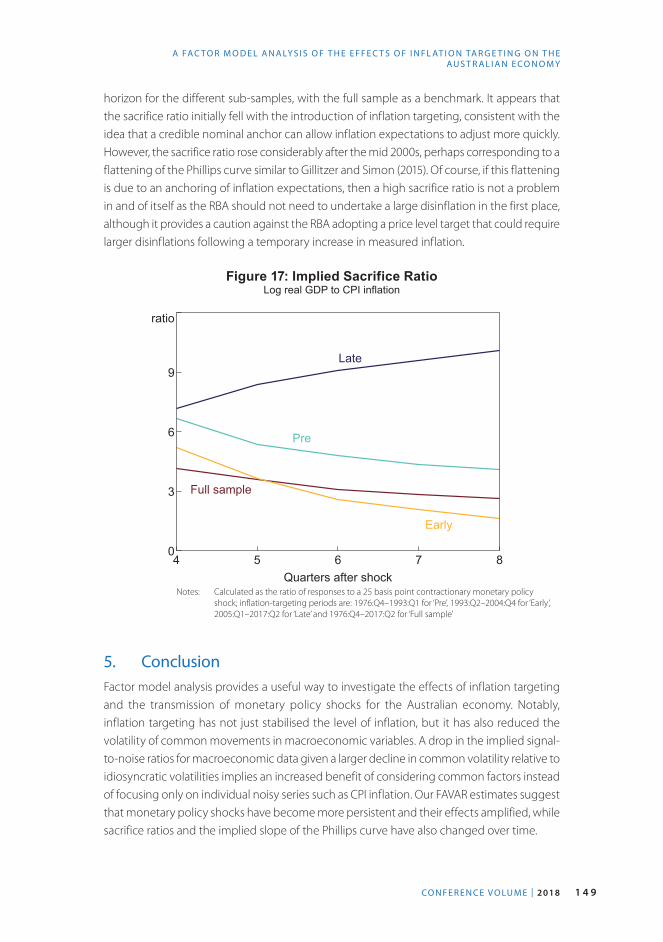
1 4 9CO N F E R E N C E V O LU M E | 2018
A FA C T O R M O D E L A N A LY S I S O F T H E E F F E C T S O F I N F L AT I O N TA R G E T I N G O N T H E A U S T R A L I A N E CO N O M Y
horizon for the different sub-samples, with the full sample as a benchmark. It appears that the sacrifice ratio initially fell with the introduction of inflation targeting, consistent with the idea that a credible nominal anchor can allow inflation expectations to adjust more quickly. However, the sacrifice ratio rose considerably after the mid 2000s, perhaps corresponding to a flattening of the Phillips curve similar to Gillitzer and Simon (2015). Of course, if this flattening is due to an anchoring of inflation expectations, then a high sacrifice ratio is not a problem in and of itself as the RBA should not need to undertake a large disinflation in the first place, although it provides a caution against the RBA adopting a price level target that could require larger disinflations following a temporary increase in measured inflation.
Figure 17: Implied Sacrifice RatioLog real GDP to CPI inflation
4 5 6 7 80
3
6
9
ratio
Quarters after shock
Pre
Full sample
Early
Late
Notes: Calculated as the ratio of responses to a 25 basis point contractionary monetary policy shock; inflation-targeting periods are: 1976:Q4–1993:Q1 for ‘Pre’, 1993:Q2–2004:Q4 for ‘Early’, 2005:Q1–2017:Q2 for ‘Late’ and 1976:Q4–2017:Q2 for ‘Full sample’
5. ConclusionFactor model analysis provides a useful way to investigate the effects of inflation targeting and the transmission of monetary policy shocks for the Australian economy. Notably, inflation targeting has not just stabilised the level of inflation, but it has also reduced the volatility of common movements in macroeconomic variables. A drop in the implied signal-to-noise ratios for macroeconomic data given a larger decline in common volatility relative to idiosyncratic volatilities implies an increased benefit of considering common factors instead of focusing only on individual noisy series such as CPI inflation. Our FAVAR estimates suggest that monetary policy shocks have become more persistent and their effects amplified, while sacrifice ratios and the implied slope of the Phillips curve have also changed over time.

1 5 0 R E S E R V E B A N K O F A U S T R A L I A
L U K E H A R T I G A N A N D J A M E S M O R L E Y
The flexibility of factor modelling allows us to propose a number of possible extensions to our analysis. We plan to consider alternative models of structural change in the future, such as: a Markov-switching dynamic factor model used by Diebold and Rudebusch (1996), Chauvet (1998), Kim and Nelson (1998) and Camacho, Perez-Quiros and Poncela (2015); or a time-varying parameter dynamic factor model used in Korobilis (2013). These alternative models will allow us to determine if there is any recurring dependence in the effects of monetary policy shocks or other identified shocks (e.g. foreign shocks) on the state of the business cycle, or if there are other slower moving changes. We also plan to utilise methods recently developed by Koopman, Mesters and Schwaab (2018) for jointly estimating level and volatility factors and their interaction. This will allow us to examine the role of uncertainty in driving the Australian economic conditions in a data-rich environment. Also, we plan to consider more observed factors, such as commodity prices, US real GDP growth, US CPI inflation, the federal funds rate and government spending, in the FAVAR in order to consider the dynamic effects of different types of structural shocks and to possibly better identify monetary policy shocks.

1 5 1CO N F E R E N C E V O LU M E | 2018
A FA C T O R M O D E L A N A LY S I S O F T H E E F F E C T S O F I N F L AT I O N TA R G E T I N G O N T H E A U S T R A L I A N E CO N O M Y
Appendix A: Australian Macroeconomic Dataset
Table A1: Full List of Variables(continued next page)
Variable Category Transformation Slow variable
Gross domestic product (GDP) Expenditure Δlog xt( ) YesNon-farm GDP Expenditure Δlog xt( ) YesGDP per capita Expenditure Δlog xt( ) YesPublic final demand Expenditure Δlog xt( ) YesPrivate final demand Expenditure Δlog xt( ) YesPrivate gross fixed capital formation (GFCF)
Expenditure Δlog xt( ) Yes
Household consumption (HC) Expenditure Δlog xt( ) YesHC: Cigarettes and tobacco Expenditure Δlog xt( ) YesHC: Alcoholic beverages Expenditure Δlog xt( ) YesHC: Clothing and footwear Expenditure Δlog xt( ) YesHC: Food Expenditure Δlog xt( ) YesHC: Household equipment Expenditure Δlog xt( ) YesHC: Purchase of vehicles Expenditure Δlog xt( ) YesHC: Rent and other dwelling services Expenditure Δlog xt( ) YesHC: Hotels, cafes and restaurants Expenditure Δlog xt( ) YesHC: Transport services Expenditure Δlog xt( ) YesPrivate GFCF: Dwellings: Alterations and additions Expenditure Δlog xt( ) YesPrivate GFCF: Dwellings: New and used Expenditure Δlog xt( ) YesPrivate non-farm inventories to total sales
Expenditure Δxt Yes
Changes in inventories Expenditure xt YesGross domestic income Income Δlog xt( ) YesGross operating surplus: Financial corporations
Income Δlog xt( ) Yes
Gross operating surplus: Private non-financial
Income Δlog xt( ) Yes
Gross operating surplus: Public non-financial
Income Δlog xt( ) Yes
Household disposable income Income Δlog xt( ) YesAgriculture, forestry and fishing Production Δlog xt( ) YesMining and exploration Production Δlog xt( ) YesManufacturing Production Δlog xt( ) YesElectricity, gas and water services Production Δlog xt( ) YesConstruction Production Δlog xt( ) Yes

1 5 2 R E S E R V E B A N K O F A U S T R A L I A
L U K E H A R T I G A N A N D J A M E S M O R L E Y
Variable Category Transformation Slow variable
Wholesale trade Production Δlog xt( ) YesRetail trade Production Δlog xt( ) Yes
Accommodation and food services Production Δlog xt( ) Yes
Transportation Production Δlog xt( ) YesInformation media and telecommunications
Production Δlog xt( ) Yes
Financial and insurance services Production Δlog xt( ) YesRental hiring and real estate services Production Δlog xt( ) YesProfessional, scientific and technical services
Production Δlog xt( ) Yes
Administration and support services Production Δlog xt( ) YesPublic administration and safety Production Δlog xt( ) YesEducation and training Production Δlog xt( ) YesHealthcare and social assistance Production Δlog xt( ) YesArts and recreation services Production Δlog xt( ) YesOther services Production Δlog xt( ) YesFull-time employment Employment Δlog xt( ) YesPart-time employment Employment Δlog xt( ) YesTotal employment Employment Δlog xt( ) YesUnemployment rate Employment Δxt Yes
Labour productivity Employment Δlog xt( ) YesReal unit labour costs Employment Δlog xt( ) YesAverage weekly earnings Employment Δlog xt( ) YesAverage weekly hours worked Employment Δlog xt( ) YesCapacity utilisation (net balance) Surveys xt NoGeneral business situation (next 6 months net balance)
Surveys xt No
Output actual (change in past 3 months net balance)
Surveys xt No
Output expected (change in next 3 months net balance)
Surveys xt No
Consumer sentiment index Surveys xt NoCommencements: Total new houses and flats excl conversion
Building & capex Δlog xt( ) No
Completed: Total new houses and flats excl conversion
Building & capex Δlog xt( ) Yes
Approvals: Private new houses and flats
Building & capex Δlog xt( ) No
Table A1: Full List of Variables(continued next page)

1 5 3CO N F E R E N C E V O LU M E | 2018
A FA C T O R M O D E L A N A LY S I S O F T H E E F F E C T S O F I N F L AT I O N TA R G E T I N G O N T H E A U S T R A L I A N E CO N O M Y
Variable Category Transformation Slow variable
Approvals: Government new houses and flats
Building & capex Δlog xt( ) No
Approvals: Total new houses and flats Building & capex Δlog xt( ) NoCurrent account (per cent of GDP) Overseas
transactionsΔxt Yes
Services imports Overseas transactions
Δlog xt( ) Yes
Services exports Overseas transactions
Δlog xt( ) Yes
Goods debits Overseas transactions
Δlog xt( ) Yes
Goods credits Overseas transactions
Δlog xt( ) Yes
Consumer price index (CPI) : All groups Prices Δlog xt( ) YesCPI: Food and non-alcoholic beverages Prices Δlog xt( ) YesCPI: Alcohol and tobacco Prices Δlog xt( ) YesCPI: Clothing and footwear Prices Δlog xt( ) YesCPI: Housing Prices Δlog xt( ) YesCPI: Household equipment and services Prices Δlog xt( ) YesCPI: Transportation Prices Δlog xt( ) YesCPI: Communication Prices Δlog xt( ) YesCPI: Goods component Prices Δlog xt( ) YesCPI: Services component Prices Δlog xt( ) YesEstablished house prices Prices Δlog xt( ) YesOil prices Prices Δlog xt( ) NoGDP price deflator Prices Δlog xt( ) YesHousehold final consumption expenditure price deflator
Prices Δlog xt( ) Yes
Private GFCF price deflator Prices Δlog xt( ) YesDomestic final demand (DFD) price deflator
Prices Δlog xt( ) Yes
Export price index: Goods and services credits
Prices Δlog xt( ) Yes
Import price index: Goods and services debits
Prices Δlog xt( ) Yes
Terms of trade Prices Δlog xt( ) YesIndex of commodity prices (ICP) Prices Δlog xt( ) No
Table A1: Full List of Variables(continued next page)

1 5 4 R E S E R V E B A N K O F A U S T R A L I A
L U K E H A R T I G A N A N D J A M E S M O R L E Y
Variable Category Transformation Slow variable
Money: M1 Money & credit Δlog xt( ) NoMoney: M3 Money & credit Δlog xt( ) NoMoney: Broad money Money & credit Δlog xt( ) NoCredit: Total Money & credit Δlog xt( ) NoCredit: Other personal Money & credit Δlog xt( ) NoCredit: Business Money & credit Δlog xt( ) No
Overnight cash rate (OCR) Interest rates Δxt No
Real OCR Interest rates Δxt No
3-month bank bill Interest rates Δxt No5-year Australian Government security (AGS)
Interest rates Δxt No
10-year AGS Interest rates Δxt No3-month bank bill spread to OCR Interest rates xt No5-year AGS spread to OCR Interest rates xt No10-year AGS spread to OCR Interest rates xt NoShare price index Miscellaneous Δlog xt( ) NoReal trade-weighted exchange rate index (TWI)
Miscellaneous Δlog xt( ) No
Southern Oscillation Index (SOI) Miscellaneous xt NoNotes: Seasonally adjusted data are used when available; monthly series are converted to quarterly by taking the three-
month average; ‘Slow variable’ refers to whether the respective series is used to extract ‘slow-moving’ factors as part of the procedure when estimating the FAVAR model; the ‘Money & credit’ series are break adjusted
Sources: ABS; Bureau of Meteorology; RBA
Table A1: Full List of Variables(continued)
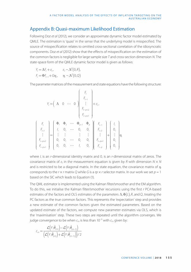
1 5 5CO N F E R E N C E V O LU M E | 2018
A FA C T O R M O D E L A N A LY S I S O F T H E E F F E C T S O F I N F L AT I O N TA R G E T I N G O N T H E A U S T R A L I A N E CO N O M Y
Appendix B: Quasi-maximum Likelihood EstimationFollowing Doz et al (2012), we consider an approximate dynamic factor model estimated by QMLE. The estimation is ‘quasi’ in the sense that the underlying model is misspecified. The source of misspecification relates to omitted cross-sectional correlation of the idiosyncratic components. Doz et al (2012) show that the effects of misspecification on the estimation of the common factors is negligible for large sample size T and cross-section dimension N. The state-space form of the QMLE dynamic factor model is given as follows:
Yt =ΛFt+εt , εt ~N 0,R( ),Ft =ΦFt−1+Gηt , ηt ~N 0,Q( )
The parameter matrices of the measurement and state equations have the following structure:
Yt = Λ 0 ! 0( )
FtFt−1!
Ft−p+2Ft−p+1
⎛
⎝
⎜⎜⎜⎜⎜⎜⎜⎜⎜⎜⎜⎜⎜⎜⎜⎜⎜
⎞
⎠
⎟⎟⎟⎟⎟⎟⎟⎟⎟⎟⎟⎟⎟⎟⎟⎟⎟⎟⎟⎟
+εt ,
FtFt−1!
Ft−p+2Ft−p+1
⎛
⎝
⎜⎜⎜⎜⎜⎜⎜⎜⎜⎜⎜⎜⎜⎜⎜⎜⎜
⎞
⎠
⎟⎟⎟⎟⎟⎟⎟⎟⎟⎟⎟⎟⎟⎟⎟⎟⎟⎟⎟⎟
=
Φ1 Φ2 ! Φp−1 Φp
Ir 0r ! 0r 0r
" " " "0r 0r ! 0r 0r
0r 0r ! Ir 0r
⎛
⎝
⎜⎜⎜⎜⎜⎜⎜⎜⎜⎜⎜⎜⎜⎜⎜⎜⎜
⎞
⎠
⎟⎟⎟⎟⎟⎟⎟⎟⎟⎟⎟⎟⎟⎟⎟⎟⎟⎟⎟⎟
Ft−1Ft−2!
Ft−p+1Ft−p
⎛
⎝
⎜⎜⎜⎜⎜⎜⎜⎜⎜⎜⎜⎜⎜⎜⎜⎜⎜
⎞
⎠
⎟⎟⎟⎟⎟⎟⎟⎟⎟⎟⎟⎟⎟⎟⎟⎟⎟⎟⎟⎟
+
Ir0r
!0r
0r
⎛
⎝
⎜⎜⎜⎜⎜⎜⎜⎜⎜⎜⎜⎜⎜⎜⎜⎜⎜
⎞
⎠
⎟⎟⎟⎟⎟⎟⎟⎟⎟⎟⎟⎟⎟⎟⎟⎟⎟⎟⎟⎟
ηt
where Ir is an r-dimensional identity matrix and 0r is an r-dimensional matrix of zeros. The covariance matrix of εt in the measurement equation is given by R with dimension N × N and is restricted to be a diagonal matrix. In the state equation, the covariance matrix of ηt corresponds to the r × r matrix Q while G is a rp × r selector matrix. In our work we set p = 1 based on the SIC which leads to Equation (1).
The QML estimator is implemented using the Kalman filter/smoother and the EM algorithm. To do this, we initialise the Kalman filter/smoother recursions using the first r PCA-based estimates of the factors and OLS estimates of the parameters Λ,Φ L( ),R, andQ , treating the PC factors as the true common factors. This represents the ‘expectation’ step and provides a new estimate of the common factors given the estimated parameters. Based on the updated estimate of the factors, we compute new parameter estimates via OLS, which is the ‘maximisation’ step. These two steps are repeated until the algorithm converges. We judge convergence to be when cm is less than 10–6 with cm given by:
cm=L Y ;θ(m )( )−L Y ;θ m−1( )( )L Y ;θ m( )( )+L Y ;θ m−1( )( )( )/ 2

1 5 6 R E S E R V E B A N K O F A U S T R A L I A
L U K E H A R T I G A N A N D J A M E S M O R L E Y
where θ is a vector of the model parameters and m=1,…,M is the number of evaluations needed to achieve convergence up to a maximum M set by the researcher. We set M = 1 000 but the number of evaluations needed in all cases we considered was much less than 100. L Y ;θ( ) is the log-likelihood function given as:
L Y ;θ( )=− 12Yt−ΛFt[ ]′ R−1 Yt−ΛFt[ ]
⎛⎝⎜⎜⎜
⎞⎠⎟⎟⎟−
T2log R
t=1
T
∑
−12Ft−ΦFt−1[ ]′Q−1 Ft−ΦFt−1[ ]
⎛⎝⎜⎜⎜
⎞⎠⎟⎟⎟−
T−12
logQt=2
T
∑
−12F1−F0[ ]′P0
−1 F1−F0[ ]− 12log P0 −
T p+ r( )2
log 2π( )
with the initial state F0 = 0rp and initial state variance vec P0( )= Irp2−Φ⊗Φ( )−1vec Q( ). See
Ghahramani and Hinton (1996) for more details.
A convenient feature of this specification is that the computational complexity of the Kalman filter/smoother depends only on the number of states, which in our case corresponds to the number of factors r, and is independent of the size of the cross-section N.
Note, while the EM algorithm will converge, it is not guaranteed to find the global maximum and can converge to a local maximum. However, the chance of this occurring can be offset by starting the algorithm, as we do, with the PCA estimates which are consistent for large cross-sections.
The main reason we use this estimation method relates to its potential to improve efficiency of the estimates of the common factors. This comes from explicitly accounting for factor dynamics. Doz et al (2012) show the efficiency improvements are relevant when there are more common factors to estimate. Other desirable features of this method (which we do not explore in our work) relate to structural analysis by allowing the researcher to impose restrictions on the factor loadings to extract shocks. Furthermore, the method is capable of handling either missing or mixed frequency data.

1 5 7CO N F E R E N C E V O LU M E | 2018
A FA C T O R M O D E L A N A LY S I S O F T H E E F F E C T S O F I N F L AT I O N TA R G E T I N G O N T H E A U S T R A L I A N E CO N O M Y
Appendix C: FAVAR EstimationHere we describe the FAVAR model estimation in detail. Let Rt be the official cash rate. Suppose that additional economic information can be summarised by a k × 1 vector of unobserved factors Ft, where k is small and is not necessarily equal to r as determined via some formal selection criteria. We can think of the unobserved factors as possibly capturing variation in economic activity or price pressures that may not be readily proxied by any particular individual observed variable, but are important in a wide range of economic data series. Assume the joint dynamics of Ft, and Rt are given by the following equation:
FtRt
⎛
⎝
⎜⎜⎜⎜⎜
⎞
⎠
⎟⎟⎟⎟⎟⎟=Φ L( )
Ft−1Rt−1
⎛
⎝
⎜⎜⎜⎜⎜
⎞
⎠
⎟⎟⎟⎟⎟⎟+εt
where Φ(L) is a conformable lag polynomial of finite order p. We set p = 2 in our case based on SIC. We then assume that what Bernanke et al (2005) call ‘informational’ time series Yt are related to the unobserved factors Ft and observed Rt by the equation:
Yt =ΛFFt+ΛRRt+et
where ΛF is an N × k matrix of common factor loadings, ΛR is an N × 1 vector of Rt loadings and et is an N × 1 vector of error terms with mean zero that are assumed to display a small amount of cross-correlation.
We consider only one approach to estimating the FAVAR (Bernanke et al (2005) consider two, one via PCA and the other via Bayesian estimation). We use their two-step method based on the PCA estimator, but we replace this with the QML estimates of the factors. This is not new as Bernanke and Boivin (2003) did something similar using a mixed frequency panel for the US economy. Denote the estimated common factors of Yt by C Ft ,Rt( ). Because C Ft ,Rt( ) corresponds to an arbitrary linear combination of its arguments, obtaining Ft involves determining the part of C Ft ,Rt( ) that is not spanned by Rt.
Because Rt is not explicitly imposed as a common component in the first estimation step, any of the linear combinations underlying C Ft ,Rt( ) could involve Rt. Bernanke et al (2005) argue that it would not be valid to simply estimate a VAR based on C Ft ,Rt( ) and identify the policy shock recursively. Instead, they argue that the direct dependence of the common factors of Yt on Rt must be removed first.
If linear combinations implicit in C Ft ,Rt( ) were known, this would involve subtracting Rt times the associated coefficient from each of the elements of C Ft ,Rt( ) . However, because they are unknown, Bernanke et al propose to estimate the coefficients through a multiple regression of the form:
C Ft ,Rt( )=βC*C * Ft( )+βRRt+νt
where C * Ft( ) is an estimate of all the common components other than Rt. Bernanke et al (2005) suggest one way to obtain C * Ft( ) is to extract factors from a subset of slow-moving variables,

1 5 8 R E S E R V E B A N K O F A U S T R A L I A
L U K E H A R T I G A N A N D J A M E S M O R L E Y
which by assumption are not affected contemporaneously by Rt. Then Ft is constructed as C Ft( )−βRRt and a VAR in Ft and Rt is estimated using ordinary least squares and identified recursively.
Note that the key assumption is that most of the forecast error for Rt reflects monetary policy shocks, not an endogenous response to economic conditions. Finally, because this second step involves the presence of generated regressors, we use the bootstrap and 500 replications to compute confidence bands for the impulse response functions displayed in Section 4.

1 5 9CO N F E R E N C E V O LU M E | 2018
A FA C T O R M O D E L A N A LY S I S O F T H E E F F E C T S O F I N F L AT I O N TA R G E T I N G O N T H E A U S T R A L I A N E CO N O M Y
ReferencesAhn SC and AR Horenstein (2013), 'Eigenvalue Ratio Test for the Number of Factors', Econometrica, 81(3), pp 1203–1227.
Bai J (2003), ‘Inferential Theory for Factor Models of Large Dimensions’, Econometrica, 71(1), pp 135–172.
Bai J and S Ng (2002), ‘Determining the Number of Factors in Approximate Factor Models’, Econometrica, 70(1), pp 191–221.
Bai J and S Ng (2007), ‘Determining the Number of Primitive Shocks in Factor Models’, Journal of Business & Economic Statistics, 25(1), pp 52–60.
Bai J and P Perron (1998), ‘Estimating and Testing Linear Models with Multiple Structural Changes’, Econometrica, 66(1), pp 47–78.
Bernanke BS and J Boivin (2003), ‘Monetary Policy in a Data-Rich Environment’, Journal of Monetary Economics, 50(3), pp 525–546.
Bernanke BS, J Boivin and P Eliasz (2005), ‘Measuring the Effects of Monetary Policy: A Factor-Augmented Vector Autoregressive (FAVAR) Approach’, The Quarterly Journal of Economics, 120(1), pp 387–422.
Bishop J and P Tulip (2017), ‘Anticipatory Monetary Policy and the “Price Puzzle”‘, RBA Research Discussion Paper No 2017-02.
Breitung J and S Eickmeier (2011), ‘Testing for Structural Breaks in Dynamic Factor Models’, Journal of Econometrics, 163(1), pp 71–84.
Camacho M, G Perez-Quiros and P Poncela (2015), ‘Extracting Nonlinear Signals from Several Economic Indicators’, Journal of Applied Econometrics, 30(7), pp 1073–1089.
Chauvet M (1998), ‘An Econometric Characterization of Business Cycle Dynamics with Factor Structure and Regime Switches’, International Economic Review, 39(4), pp 969–996.
Chen L, JJ Dolado and J Gonzalo (2014), ‘Detecting Big Structural Breaks in Large Factor Models’, Journal of Econometrics, 180(1), pp 30–48.
Diebold FX and GD Rudebusch (1996), ‘Measuring Business Cycles: A Modern Perspective’, The Review of Economics and Statistics, 78(1), pp 67–77.
Doz C, D Giannone and L Reichlin (2011), ‘A Two-Step Estimator for Large Approximate Dynamic Factor Models Based on Kalman Filtering’, Journal of Econometrics, 164(1), pp 188–205.
Doz C, D Giannone and L Reichlin (2012), ‘A Quasi-Maximum Likelihood Approach for Large, Approximate Dynamic Factor Models’, The Review of Economics and Statistics, 94(4), pp 1014–1024.
Eo Y and J Morley (2015), ‘Likelihood-Ratio-Based Confidence Sets for the Timing of Structural Breaks’, Quantitative Economics, 6(2), pp 463–497.
Ghahramani Z and GE Hinton (1996), ‘Parameter Estimation for Linear Dynamical Systems’, Department of Computer Science, University of Toronto Technical Report CRG-TR-96-2.
Gillitzer C and J Kearns (2007), ‘Forecasting with Factors: The Accuracy of Timeliness’, RBA Research Discussion Paper No 2007-03.
Gillitzer C, J Kearns, and A Richards (2005), ‘The Australian Business Cycle: A Coincident Indicator Approach’, in C Kent and D Norman (eds), The Changing Nature of the Business Cycle, Proceedings of a Conference, Reserve Bank of Australia, Sydney, pp 262–307.

1 6 0 R E S E R V E B A N K O F A U S T R A L I A
L U K E H A R T I G A N A N D J A M E S M O R L E Y
Gillitzer C and J Simon (2015), ‘Inflation Targeting: A Victim of its Own Success’, International Journal of Central Banking, 11(Supplement 1), pp 259–287.
Han X and A Inoue (2015), ‘Tests for Parameter Instability in Dynamic Factor Models’, Econometric Theory, 31(5), pp 1117–1152.
Hartigan L (2018), ‘Alternative HAC Covariance Matrix Estimators with Improved Finite Sample Properties’, Computational Statistics & Data Analysis, 119, pp 55–73.
Kim C-J and CR Nelson (1998), ‘Business Cycle Turning Points, a New Coincident Index, and Tests of Duration Dependence Based on a Dynamic Factor Model with Regime Switching’, The Review of Economics and Statistics, 80(2), pp 188–201.
Koopman SJ, G Mesters and B Schwaab (2018), ‘Nonlinear Dynamic Factor Models with Interacting Level and Volatility’, Paper presented at the 26th Symposium of the Society of Nonlinear Dynamics and Econometrics, Tokyo, 19–20 March.
Korobilis D (2013), ‘Assessing the Transmission of Monetary Policy Using Time-Varying Parameter Dynamic Factor Models’, Oxford Bulletin of Economics and Statistics, 75(2), pp 157–179.
Lubik TA and F Schorfheide (2003), ‘Computing Sunspot Equilibria in Linear Rational Expectations Models’, Journal of Economic Dynamics & Control, 28(2), pp 273–285.
Lubik TA and F Schorfheide (2004), ‘Testing for Indeterminacy: An Application to U.S. Monetary Policy’, The American Economic Review, 94(1), pp 190–217.
Lubik TA and P Surico (2010), ‘The Lucas Critique and the Stability of Empirical Models’, Journal of Applied Econometrics, 25(1), pp 177–194.
Onatski A (2010), ‘Determining the Number of Factors from Empirical Distribution of Eigenvalues’, The Review of Economics and Statistics, 92(4), pp 1004–1016.
Qu Z and P Perron (2007), ‘Estimating and Testing Structural Changes in Multivariate Regressions’, Econometrica, 75(2), pp 459–502.
Sheen J, S Trück and BZ Wang (2015), ‘Daily Business and External Condition Indices for the Australian Economy’, Economic Record, 91(S1), pp 38–53.
Stevens G (1999), ‘Six Years of Inflation Targeting’, RBA Bulletin, May, pp 46–61.
Stevens G (2003), ‘Inflation Targeting: A Decade of Australian Experience’, Address to South Australian Centre for Economic Studies April 2003 Economic Briefing, Adelaide, 10 April.
Stock JH and MW Watson (2002), ‘Forecasting Using Principal Components from a Large Number of Predictors’, Journal of the American Statistical Association, 97(460), pp 1167–1179.
Stock JH and MW Watson (2003), ‘Has the Business Cycle Changed and Why?’ in M Gertler and K Rogoff (eds), NBER Macroeconomics Annual 2002, 17, The MIT Press, Cambridge, pp 159–218.
Stock JH and MW Watson (2005), ‘Implications of Dynamic Factor Models for VAR Analysis’, NBER Working Paper No 11467.
Stock JH and MW Watson (2016), ‘Dynamic Factor Models, Factor-Augmented Vector Autoregressions, and Structural Vector Autoregressions in Macroeconomics’, in JB Taylor and H Uhlig (eds), Handbook of Macroeconomics: Volume 2A, Handbooks in Economics, Elsevier, Amsterdam, pp 415–525.
Summers PM (2005), ‘What Caused the Great Moderation? Some Cross-Country Evidence’, Federal Reserve Bank of Kansas City Economic Review, Third Quarter, pp 5–32.

1 6 1CO N F E R E N C E V O L U M E | 2 018
Discussion
1. Marcelle Chauvet*
OverviewThe paper by Luke Hartigan and James Morley examines how the dynamics of the macroeconomy in Australia have changed since the inception of the inflation-targeting regime in the second quarter of 1993. It focuses on changes in the common components of real and nominal variables, and whether there is evidence of changes in the transmission of monetary policy shocks. The paper implements an analysis using factor models on a large panel of real and nominal variables (104 variables, 1976:Q4–2017:Q2), and explores the dynamics of the factor structure in detail. It takes into account several measures of potential change such as structural breaks, changes in volatility, changes in cross-correlations and changes in the transmission of monetary shocks. The paper uses three methods: i) exploratory principal components analysis to obtain the number of factors; ii) approximate dynamic factor models to estimate the factors and to test for potential breaks and stability of the factor loadings; and iii) factor augmented vector autoregressions (FAVAR) to examine potential changes in the transmission of monetary shocks.
The paper finds that Australian macroeconomic fluctuations are mostly captured by two common factors representing ‘real’ economic activity and the ‘nominal’ sector. Recursive estimation indicates a decline in the number of factors over time, which could be related to changes in cross-correlation or volatility in the factor structure associated with the inflation-targeting regime. In order to examine this further, the Han and Inoue (2015) structural break test is used to evaluate potential changes. The Lagrange multiplier (LM) statistic indicates a break in 1991:Q4, the Wald test in 1998:Q3. The paper notes that both tests are significant if the break occurred in 1993:Q1, around the time inflation targeting was implemented. The evidence points to changes in volatility rather than in the cross-correlation between variables.
The paper further investigates this possibility by studying the cross-section standard deviation of the common components and of the idiosyncratic components for the real and nominal sectors for: (i) all variables, (ii) for prices, and (iii) also for consumer price index (CPI) inflation. It finds a large reduction in the volatility of common components, including for CPI inflation, but not in the volatility of the noisy idiosyncratic components over time. This is particularly the case since the introduction of inflation targeting. This result suggests that monetary policy should target more persistent quarter-to-quarter changes rather than noisy oscillations, which can be separated out using the factor structure. The paper recursively estimates loadings of real gross domestic product (GDP), CPI inflation, and the overnight cash rate (OCR) on the factors, and finds that they stabilise over time rather than display sudden
* Marcelle Chauvet is a professor of economics at the University of California, Riverside and a Director of the International Association for Applied Econometrics

1 6 2 R E S E R V E B A N K O F A U S T R A L I A
D I S C U S S I O N
jumps. This result is, once again, consistent with changes in the volatility of the factors rather than with changes in cross-correlations related to the factor structure.
Finally, the paper uses FAVAR to examine the effects of inflation targeting on the transmission of monetary policy shocks, using the (rotated) first two factors and the interest rate represented by the OCR. For the full sample, contractionary monetary policy leads to a fall in the ‘real’ factor, the ‘nominal’ factor and, as expected, also in GDP growth and CPI inflation. In order to investigate potential changes in the transmission of monetary shocks, the Qu and Perron (2007) break test is applied to each equation of the FAVAR. The results indicate changes in the parameters in 1990 and around 2010–11, which coincides with the European debt crisis. Impulse response functions are then obtained for three sub-samples: before the inflation-targeting regime (1976:Q4–1993:Q1), during the first part of the regime (1993:Q2–2004:Q4), and for the latest part of the sample (2005:Q1–2017:Q2). The results show a small negative response of GDP growth and inflation to contractionary policy in the first part of the sample, a larger but shorter-lived positive response after the introduction of inflation targeting, and a medium-sized negative response of longer duration in the last part of the sample. This suggests that the introduction of inflation targeting has led to a noticeable change in the effect of monetary policy on inflation, with a stronger response in the first decade of the regime. On the other hand, the results show the importance of the inflation-targeting regime in curbing inflation: before the introduction of inflation targeting, contractionary monetary policy had a small effect on inflation and over time the effect became stronger and longer lasting.
Dynamics of Australian economic activity and inflationAs can be observed in Figure 1, Australian real GDP growth and CPI inflation display substantial changes in their dynamics over time. Both the level and volatility of inflation have been decreasing, and GDP growth shows tamer oscillations. This has been the case since the mid 1990s, and it was more accentuated in the last decade. Features that stand out are that the stabilisation has both smooth and sudden changes in GDP growth and inflation. The challenge is how to account for these dynamics. Hartigan and Morley go beyond this question, aiming to investigate the potential effect of the inflation-targeting regime not only on inflation or GDP growth, but on a large panel of real and nominal economic variables using factor analysis.
The paper shows that there is overwhelming evidence of a broad stabilisation in the real and nominal sectors of Australia, particularly since the inception of the inflation-targeting regime (Figure 2). There is evidence of multiple breaks in the factors and in the monetary transmission mechanism estimated through the proposed FAVAR. This has important consequences for the effect of monetary shocks on real economic activity and inflation, as shown in the paper and discussed below. The findings in the paper also raise several interesting research questions that can be explored further in the future.

1 6 3CO N F E R E N C E V O L U M E | 2 018
D I S C U S S I O N
Figure 1: Dynamics of Australian Economic Activity and Inflation
Real GDP growth
-2
0
2
4%
-2
0
2
4%
CPI inflation
2006199419821970 2018-5
0
5
10
15%
-5
0
5
10
15%
Notes: Shaded regions indicate economic recessions; vertical lines indicate the start of the Reserve Bank of Australia’s (RBA’s) inflation-targeting regime; inflation excludes interest charges prior to the September quarter 1998 and adjusted for the tax changes of 1999–2000
Sources: Author’s calculations; Federal Reserve Bank of St Louis; RBA
Figure 2: Interbank Overnight Cash Rate
20102002199419861978 20180
5
10
15
%
0
5
10
15
%
Notes: Shaded regions indicate economic recessions; vertical line indicates the start of the RBA’s inflation-targeting regime
Sources: Author’s calculations; RBA

1 6 4 R E S E R V E B A N K O F A U S T R A L I A
D I S C U S S I O N
Comments and suggestions
Summary
Hartigan and Morley implement a careful analysis, using a sequence of methods to provide insights about the economic and nominal stabilisation in Australia since the implementation of inflation targeting. The paper undertakes an extensive and meticulous analysis of structural breaks in both principal components and FAVAR methods and obtains interesting and thoughtful insights regarding changes in volatility and changes in the transmission mechanism of monetary policy.
I find the paper interesting and well executed with important new findings. Below, I give some comments and suggestions regarding the empirical application and modelling of the transmission of monetary shocks, which I think can improve the analysis in this and future papers.
I discuss the data transformation, the relationship between the real factor and production, and the possible existence of outliers and pulse (temporary) breaks that can bias the structural break tests. Additionally, throughout the sections in the paper, there seem to be multiple breaks in the real and nominal sectors. The evidence points to increased stabilisation more so than breaks in the level. I suggest recursive tests that have more power for multiple breaks, which would reduce the uncertainty regarding the location of the breakpoints. Further, I suggest that the tests for breaks in level and variance should be undertaken separately, as it could be the case that the breaks in these moments took place at different dates. A more extensive sub-sample analysis should be implemented based on the results of these tests.
Overall, the results seem to indicate that the decrease in volatility is not a one-time event, but it is a continuous process, with increased stabilisation over time and very minor oscillations in the last decade. It could be the case that the changes are recurrent or that the changes have taken place gradually. The paper implements an extensive analysis assuming that inflation targeting engendered structural breaks in the economy. Instead of studying the effect of exogenous breakpoints through sub-sample analysis, the paper could integrate potential breaks into the FAVAR model. For example, the FAVAR could be estimated with Markov switching in the mean and variance, which would allow analysis of recurrent changes, or of permanent structural breaks. Another possibility is to estimate the FAVAR with Markov switching in the mean parameters and allow for stochastic volatility.
Finally, I discuss the interpretation of the results regarding changes in the impulse response functions, sacrifice ratio and Phillips curve, compared with changes in monetary policy in the United States.
Data transformation
Comments. The series on price growth are a priori adjusted for a structural break in mean in 1993:Q1, corresponding to the beginning of inflation targeting. The goal is to make the series stationary without needing to take second differences. However, demeaning the series

1 6 5CO N F E R E N C E V O L U M E | 2 018
D I S C U S S I O N
with an a priori breakpoint can engender problems in the subsequent analysis. First, as found throughout the paper, break locations are subject to uncertainty – the potential break in mean may have occurred before or after 1993. Second, even if there is a break in the series, it should remain in the data studied since it would be part of the evidence that there has been a structural change in inflation since the inception of inflation targeting. Demeaning and standardising the series around the break may reduce the evidence of a break in 1993 in the subsequent analysis. Finally, the Qu and Perron (2007) test indicates that there is a breakpoint in price growth in 1990:Q1 instead of 1993:Q1. This is consistent with the findings in the paper for the factor structure in Section 4.3.
Additionally, if there is a break in variance around the same time, in the early 1990s, the equalisation of the intensity of oscillations before and after inflation targeting with the data transformation might mask abrupt changes in volatility. It may also make smaller fluctuations in the latter part of the sample more important than warranted, compared with the 1970s and 1980s.
As an illustration, the left-hand panel of Figure 3 plots CPI in log growth rates and in differences, with the solid vertical line indicating a breakpoint in 1990:Q1 (as found in Qu and Perron’s test) and the dashed line indicating a breakpoint in 1993:Q1 (as assumed in the paper).1 The right-hand panel shows these series demeaned and standardised assuming a break in 1993:Q1 as in the paper. As seen, demeaning the series around 1993:Q1 masks the major change (break in mean and/or variance) in the dynamics of inflation between 1990 and 1993. This can show up in the factor analysis of the original data later on, which indicates higher macroeconomic stability since the beginning of inflation targeting.
Suggestions. One of the main methods used in the paper to examine the effect of inflation targeting on the Australian macroeconomy is analysis of potential structural breaks in the factor models. The whole analysis is performed on the premise that there are breaks in the structure of the economy. Thus, the a priori data transformation might be hindering a more precise detection of breaks in the factor analysis. My suggestion is that either the price growth series are used without any transformation, or that they be used in second differences if necessary to obtain stationarity instead of transformed by assuming a break in 1993:Q1.
1 Note that although CPI growth is corrected for the tax changes of 1999–2000 and the interest charges prior to 1998, the other price series used in the paper are not. Thus, the effects of the goods and services tax may still show in the factors as discussed in the next section of this discussion.

1 6 6 R E S E R V E B A N K O F A U S T R A L I A
D I S C U S S I O N
Figure 3: The Effects of Transformations and Standardisation on CPI Inflation
Original
200419901976-3
0
3
6
9
12
15 Standardised
20041990 2018-4.5
-3.0
-1.5
0.0
1.5
3.0
4.5
Log first difference First differenceNote: Vertical lines indicate breakpointsSources: Author’s calculations; Federal Reserve Bank of St Louis
Estimation and interpretation of factors
Comments. The results indicate that two factors capture most of the joint variation in the data. Interestingly, the variables with the highest correlations with the ‘real’ factor (Factor 1) are the surveys, which are expectation measures. Their correlation with the real factor is twice as large as with the next groups of variables (employment, expenditure and money and credit). On the other hand, the series measuring production have a low correlation with the real factor. Given the importance of the production sector in determining prices, a higher correlation between production and the real factor is desirable in the analysis of the channel of inflation targeting through the real sector.
Suggestions. There is a possibility that the real factor is out of phase with production – the real factor could be a leading indicator of the production sector (given that it is most correlated with survey series). This should be investigated. If this is the case, production variables should be added into the baseline FAVAR, as this would give a better assessment of the effect of monetary policy on and through the supply side of the economy.
Breaks in the factor structure
Comments. The paper tests for structural breaks in factor loadings using Han and Inoue’s (2015) test. The LM test statistic is maximised in 1991:Q4 and the Wald test statistic in 1998:Q3. The paper finds that both tests are significant in 1993:Q1, around the time inflation targeting was implemented.

1 6 7CO N F E R E N C E V O L U M E | 2 018
D I S C U S S I O N
However, as seen in Figure 6 of the paper, the LM test is significant for an interval starting in 1990, roughly from 1990 to 2001 (with the exception of 1997), and the Wald test from 1993 to 2002. Thus, both tests are significant between 1993 and 2001 (not only in 1993). This implies that, at a minimum, there is uncertainty regarding the date of the structural break. This may also be an indication that perhaps there are multiple breaks, the changes are recurrent or have taken place gradually over time. Non-identification of further breaks does not imply that they are not present in the data as this could just reflect the power of the test.
Suggestions. The alternative hypothesis in the Han and Inoue (2015) test is that a fraction of or all factor loadings have a single break at a common date. This raises two issues. First, there might be more than one structural break and this would reduce the power of the test. Second, the break in different factor loadings might take place at different dates. If any of these possibilities is present in the factor structure for the Australian economy, the location and significance of the breaks might be uncertain. My suggestion is that the Han and Inoue (2015) test be implemented recursively and once a break is found, to restart the recursive test from then on to find other breaks.2 Alternatively, the Yamamoto and Tanaka (2015) test can be used for multiple structural changes in factor loadings. The goal in both exercises is to find the breakpoint dates more precisely. However, these tests should be applied keeping in mind that there seems to be some pulse (temporary) breaks in the Australian economy. As seen in Figure 4 of the paper, the ‘nominal’ factor (Factor 2) has spikes in 1997 and 2000, and the real factor also in 2000, possibly related to the introduction of the goods and services tax.3 Thus, the tests should also take these pulse breaks or outliers into account when recursively implemented.
In addition, given the uncertainty regarding the break dates, it might be the case that changes in the mean or volatility of the Australian macroeconomy occurred gradually over time, rather than at one or another point in time. The implementation of inflation targeting in 1993 may have affected expectations and uncertainty regarding the actions of the RBA more immediately, but the effects of monetary policy on the volatility of the economy may also have happened over time. For example, the volatility of inflation itself is smaller in the 2000s than in the 1990s. Modelling recurrent or gradual changes is further discussed below.
Decline in the volatility of common shocks
Comments. The paper finds that the volatility of common components reduced substantially over time. This is the case for the real and nominal variables, and also for the common component of CPI inflation. On the other hand, the idiosyncratic volatility for all sectors has not shown a reduction. In addition, the factor loadings display stabilisation coinciding with the implementation of inflation targeting.
Suggestions. First, the evidence is mostly from looking at the volatilities in Figure 7 rather than statistical tests. Tables with statistics of the volatilities across sub-samples should be
2 Note that although the power of the Han and Inoue (2015) test increases for longer samples, it also decreases in the presence of multiple breaks.
3 GDP growth also displays a spike in 1997, as observed in Figure 1.

1 6 8 R E S E R V E B A N K O F A U S T R A L I A
D I S C U S S I O N
provided, possibly for more sub-samples as determined by the several breaks found in the paper, for example, before 1990:Q1, before 1993:Q1, between 1990:Q1 and 2007:Q4, between 1993:Q2 and 2007:Q4, covering the global financial crisis and European debt crisis between 2008:Q1 and 2012:Q4, and from 2013:Q1 to the end of the sample.
Second, the evidence from the Han and Inoue (2015) test, recursive factor loadings and cross-correlation volatility indicate that the major change in the Australian economy since the inception of inflation targeting has been an increased stabilisation in both the real and nominal sectors. Increased stabilisation (in addition to a reduction in the inflation level) has important positive implications for welfare, for planning, for the structure of the economy, as well as for the transmission of monetary policy shocks. Specific tests for changes in volatility should be implemented. Further, the implications and linkages of the lower volatility and effect of monetary policy in the real and nominal sectors could be more thoroughly explored in the paper, as discussed below.
Transmission of monetary policy shocks – FAVAR model and break tests
Comments. The proposed FAVAR is estimated for the full sample and for three sub-samples. The model yields sensible and insightful results. The break test by Qu and Perron (2007) is appropriate as it tests for breaks in the mean and/or variance. The test is applied recursively, allowing for multiple breaks. However, there are some problems in the test and sub-sample analysis. First, the test assumes that breaks in mean and volatility happen at the same time. The paper does not consider the possibility that there could be breaks in the regression coefficients and in the variance at different times. Breaks in volatility can contaminate the results of breaks in the persistent parameters and it can affect the impulse response functions.
Suggestions. Andrews and Ploberger’s (1994) test can be recursively applied separately for breaks in mean and for breaks in variance. This will allow direct evaluation of changes in volatility over time and since the implementation of inflation targeting. It will also allow analysis of changes in impulse response functions over time. Since the breaks were a rough guideline to choose the sub-samples used in the paper, and the impulse response functions are different across periods, the break dates are important and could be re-examined to study potential changes in the transmission of monetary policy shocks.4
Alternatively, instead of studying the impact of exogenous breakpoints through sub-sample analysis, the paper could integrate potential breaks into the FAVAR model. For example, the FAVAR could be estimated with Markov switching in the mean and variance. This model approach would allow analysis of recurrent changes or of permanent structural breaks by modelling the transition probability with an absorbing state. Another option is to estimate the FAVAR with Markov switching in the mean parameters and allow for stochastic volatility. One of the main findings of the paper is increased stabilisation over time. Thus, allowing for a FAVAR with some sort of dynamics in the variance is important to capture this feature.
4 The paper finds breaks in 1990:Q1 and 2010:Q2 for the real factor equation, a break in 2011:Q1 for the nominal factor equation, and breaks in 1990:Q3 and 2011:Q1 for the OCR equation. The sub-samples chosen are 1976:Q4–1993:Q1, 1993:Q2–2004:Q4 and 2005:Q1–2017:Q2. Regarding the sub-samples used, the paper should part them according to the breaks found. Here, again, I would suggest before 1990:Q1, before 1993:Q1, 1990:Q1–2007:Q4, 1993:Q2–2007:Q4, 2008:Q1–2012:Q4 and 2013:Q1–2017:Q2.

1 6 9CO N F E R E N C E V O L U M E | 2 018
D I S C U S S I O N
In all cases, as in the previous analysis, the model should be estimated taking into account potential pulse breaks in 1997 and 2000 as discussed earlier.
Changes in impulse response functions over time and the price puzzle
Comments. In order to illustrate the importance of changes in the monetary transmission of shocks over time, Chauvet and Tierney (2018) estimate a structural vector autoregression (SVAR) of US real-time GDP growth, inflation, unemployment and interest rates. The model is recursively estimated over increasing samples, yielding time series of the coefficients, variances and impulse response functions resulting from each recursive estimation. These are shown in Figure 4, which plots the impulse response functions of output and inflation to an unexpected increase in the federal funds rate in 1975:Q1, 1980:Q4 to 1981:Q3, 1996:Q1 and 2006:Q4. These dates are selected to reflect different economic conditions and to represent the governance of Burns, Volcker, Greenspan and Bernanke. The paper finds a reduction in the effect of monetary policy shocks, especially with respect to the response of inflation.
Figure 4: Real-time Response to Shocks to Interest Rates on Different Dates
Output
-1
0
1
%
-1
0
1
%
Inflation
1 2 3 4 5 6 7 8 9 10-1.0
-0.5
0.0
0.5
%
-1.0
-0.5
0.0
0.5
%
Quarters from shock1975:Q1 1980:Q3 1980:Q4 1981:Q11981:Q2(a) 1996:Q1 2006:Q4
Note: (a) 1981:Q3 for inflation

1 7 0 R E S E R V E B A N K O F A U S T R A L I A
D I S C U S S I O N
Monetary policy shocks have a strong and lasting negative effect on output during the Volcker period, especially between 1980:Q3 and 1981:Q3, and have the weakest effect in the later dates of 1996:Q1 and in 2006:Q4. The response of inflation to monetary policy shocks shows an even greater time variation. The largest negative response occurs in 1975:Q1, in the Burns period, followed by milder, but still negative, effects in the Greenspan and the Bernanke periods (1996:Q1 and 2006:Q4, respectively). On the other hand, inflation shows a positive response in the Volcker period between 1980:Q4 and 1981:Q3, even though the SVAR considered includes commodity price inflation to minimise the price puzzle. Notice that the price puzzle does not appear in other periods.
Suggestions. Hartigan and Morley find the price puzzle for the nominal factor and for CPI inflation for the full sample, and for the period between 1993:Q2 and 2004:Q4, but not for the other sub-samples. This might be a consequence of the disinflation that took place between 1993:Q2 and 2004:Q4, similar to the one observed in the United States in the early 1980s. It could also be due to the existence of breaks (non-stationarities) around the period between 1990 and 1993, which can lead to very different impulse responses quarter by quarter, as illustrated in Chauvet and Tierney (2018). The paper could further explore this possibility by separating and estimating the model using several sub-samples around this period. It could also add commodity price variables to the FAVAR, which is known to reduce the price puzzle. Finally, adding the production variables may reduce the price puzzle as well, since the real factor is mostly associated with surveys of expected output rather than with production per se, as discussed earlier.
Sacrifice ratio and the Phillips curve
Comments. The paper examines the sacrifice ratio for Australia using the accumulated response of real GDP relative to the response of CPI inflation. The authors find that it dropped with the introduction of inflation targeting, but it has increased since the mid 2000s. The paper relates this to a possible flattening of the Phillips curve. However, the sacrifice ratio could have increased because the inflation level is low enough during this more recent period that changes in interest rates do not change inflation as much, since it is not warranted. This can be seen in the impulse response function in the later part of the sample – inflation does not fall as much as a response to a shock in monetary policy compared with the earlier phase of the inflation-targeting period. This might indicate that the sacrifice ratio is higher not because of the response of output compared with earlier periods, but because inflation is responding less than output since the mid 2000s – which is also found in the United States. This is an expected result in an environment with low inflation, as found also in Chauvet and Tierney (2018) for the United States.
Suggestions. If the paper wants to further study the Phillips curve or the RBA reaction function, it can use the results from the FAVAR to estimate these equations as, for example, in Cogley and Sargent (2005), and draw more definite conclusions regarding changes in the Phillips curve. More interestingly, the paper should further explore the implications of (lower) levels and volatility of inflation on inflation’s response to monetary policy shocks.

1 7 1CO N F E R E N C E V O L U M E | 2 018
D I S C U S S I O N
ReferencesAndrews DWK and W Ploberger (1994), ‘Optimal Tests When a Nuisance Parameter is Present Only under the Alternative’, Econometrica, 62(6), pp 1383–1414.
Chauvet M and HLR Tierney (2018), ‘Real Time Changes in Monetary Policy’, Unpublished manuscript, University of California, Riverside.
Cogley T and TJ Sargent (2005), ‘Drifts and Volatilities: Monetary Policies and Outcomes in the Post WWII US’, Review of Economic Dynamics, 8(2), pp 262–302.
Han X and A Inoue (2015), ‘Tests For Parameter Instability in Dynamic Factor Models’, Econometric Theory, 31(5), pp 1117–1152.
Qu Z and P Perron (2007), ‘Estimating and Testing Structural Changes in Multivariate Regressions’, Econometrica, 75(2), pp 459–502.
Yamamoto Y and S Tanaka (2015), ‘Testing for Factor Loading Structural Change under Common Breaks’, Journal of Econometrics, 189(1), pp 187–206.
2. General DiscussionMuch of the discussion was focused on identification and causality, with participants noting that macroeconomic volatility had fallen globally over the sample period. A number of participants suggested that causality from the introduction of inflation targeting to lower macroeconomic volatility in Australia was hard to determine because other structural factors may have had significant effects around the same time.
One participant noted that empirical work for small open economies such as Australia should be easier than similar analysis for the United States. This is because variables such as global commodity prices, global gross domestic product and global interest rates can be treated as exogenous when examining small economies. Another participant agreed and stated this would help identify whether the low global inflation had caused lower inflation in Australia.
Participants also discussed alternative reasons for why macroeconomic volatility may have fallen in Australia in the early 1990s. Alternatives raised included the Great Moderation, tariff reductions, structural changes in the regulation of product markets, the increased use of information technology and the deregulation of the labour market. Another reason raised was the decentralisation of wage determination, which occurred through the late 1980s and early 1990s. This reduced the propagation of commodity price shocks to other sectors that likely contributed to the fall in macroeconomic volatility. One participant suggested that relaxing the assumption of a single break date could reveal something about the timing. All of these factors, as well as inflation targeting, occurred over time and this may be why the break dates in Luke Hartigan and James Morley’s analysis were inconclusive.
However, participants also referred to the sharp decline in common volatility and in the volatility of the main categories of ‘real’ and ‘nominal’ variables around the introduction of
1 7 2 R E S E R V E B A N K O F A U S T R A L I A
D I S C U S S I O N
inflation targeting. While there was uncertainty in the confidence intervals of the break tests, the abrupt change in volatility in 1993 suggested that the introduction of inflation targeting did contribute to the fall in macroeconomic volatility.
Another major area of discussion was focused more on the implications of inflation targeting for identification. One participant noted inflation targeting is about more than just establishing a nominal anchor – it’s also about moving towards a more transparent and systematic policy framework. In an ideal world, central banks should be moving interest rates endogenously to stabilise the economy. Participants agreed that this would not provide monetary policy shocks for identifying the effect of monetary policy on macroeconomic variables. It seems that the last decade has had less variation in monetary policy than previous years, which makes identification harder.
One participant stated that solving the inference problem is getting harder because all movements are being dominated by idiosyncratic volatility. Central banks are now looking at a wider group of variables, which makes communication trickier because the economic narratives must be more nuanced. The participant noted that, the more successful inflation targeting is, the more the central bank needs to rely on communication. Another participant agreed and said that, the more relative noise there is, the more the central bank needs to communicate about why it is looking through it. However, they also noted that inflation targeting has been successful because it targeted a single variable and targeting a factor would not be beneficial as it would be much more difficult to communicate to the public.

1 7 3CO N F E R E N C E V O L U M E | 2 018
Warwick J McKibbin and Augustus J Panton*
1. IntroductionThis paper surveys alternative monetary frameworks and evaluates whether the current inflation-targeting framework, followed by the Reserve Bank of Australia (RBA) for the past 25 years, is likely to be the most appropriate framework for the next 25 years. While flexible inflation targeting has appeared to work well in Australia in the past decades, the nature of future shocks suggests that some form of nominal income targeting is worth considering as an evolutionary change to Australia’s framework for monetary policy.
The core mandates of the RBA are promoting price stability, employment and the economic prosperity and welfare of the Australian people. However, the way in which monetary policy has been conducted, in order to achieve these goals, has undergone evolutionary changes over the past 35 years. Most notable was the switching from money targeting that prevailed throughout the 1980s, to a ‘checklist’ approach and finally to inflation targeting beginning around 1993. Under the inflation-targeting framework, the RBA’s price stability objective is defined as achieving a medium-term average inflation rate of 2 to 3 per cent over the cycle for consumer price inflation (CPI) – which allows some policy space for short-run considerations of output and employment fluctuations. While the introduction of inflation targeting has witnessed a substantial containment in inflationary pressure, with year-ended inflation averaging under 3 per cent since 1993 (Figure 1), the theoretical debate about the desirability of inflation targeting as an optimal monetary policy regime remains active. The debate has been less focused on whether inflation targeting has tamed inflation, and more on whether its side effects (e.g. sacrificing output stability for price stability, weak anchoring of expectations, etc) are more pronounced compared to outcomes under alternative monetary policy regimes.
* Warwick McKibbin is from the Centre for Applied Macroeconomic Analysis, Crawford School of Public Policy, Australian National University (ANU) and The Brookings Institution, Washington DC. Augustus Panton is a Doctoral Student Research Associate at the Centre for Applied Macroeconomic Analysis, Crawford School of Public Policy, ANU. The views expressed in the paper are those of the authors and should not be interpreted as reflecting the views of any of the above institutions with which the authors are affiliated including the trustees, officers or other staff of the ANU or The Brookings Institution.
Twenty-five Years of Inflation Targeting in Australia: Are There Better Alternatives for the Next Twenty-five Years?

1 7 4 R E S E R V E B A N K O F A U S T R A L I A
WA R W I C K J M C K I B B I N A N D A U G U S T U S J PA N T O N
Figure 1. Evolution of CPI Inflation
2004199119781965 2017-4
0
4
8
12
16
%
-4
0
4
8
12
16
%
Target introduced
Note: Excludes interest charges prior to September quarter 1998 and adjusted for the tax changes of 1999–2000
Sources: ABS; RBA
In discussing the possible future role for inflation targeting in Australia, this paper begins with a summary of the alternative monetary frameworks that have been proposed in the economics literature over many decades. Section 3 addresses the major issues that are important for the relevance of each monetary framework with a particular focus on the Australian context. Section 4 explores the nature of historical shocks experienced during the inflation-targeting period in Australia and then conjectures the likely nature of future shocks in the domestic and global economies over the coming decades. A summary and policy implications are outlined in Section 5.
2. Alternative Monetary FrameworksStanley Fischer (1995) observed that the search for an optimal monetary policy framework is an unending one. This is reflected in the RBA’s monetary policy framework undergoing evolutionary changes over the years. From the failure of money targeting in the 1980s to the introduction of inflation targeting in the early 1990s, changes to the conduct of monetary policy have been mostly dictated by the prevailing macroeconomic fundamentals. In this section, we place the current inflation-targeting regime in the broader context of alternative monetary regimes in the literature. The goal is to provide a summary analysis on how changing macroeconomic fundamentals can require rethinking the monetary policy framework over time.

1 7 5CO N F E R E N C E V O LU M E | 2018
T W E N T Y- F I V E Y E A R S O F I N F L AT I O N TA R G E T I N G I N A U S T R A L I A : A R E T H E R E B E T T E R A LT E R N AT I V E S F O R T H E N E X T T W E N T Y- F I V E Y E A R S ?
2.1 Inflation targetingIn its strictest form, an inflation-targeting regime is concerned with achieving and maintaining low and stable inflation, with a base drift, without consideration of controlling deviations in the output level. That is, all shocks that affect price stability – whether temporarily or permanently – are accommodated by changes to the policy rates as summarised by Equation (1):
it = it−1+α πt ,t+n−π( ) (1)
where the nominal interest rate i set in period t is a function of the rate in period t – 1 and α measures how the central bank responds to shocks that cause forecast inflation (πt,t + n ) to deviate from the inflation target (π).
However, in practice, as per the mandate of most central banks, some considerations are given to output stabilisation, under what is termed flexible inflation targeting. Under such a regime, the central bank has an objective function given in Equation (2):
Lt =12πt−π( )2+λyt
2⎡⎣⎢
⎤⎦⎥
(2)
where πt is inflation in period t, π is the central bank’s inflation target and λ≥0 is the weight given to output gap (yt) stabilisation. That is, instead of responding to all shocks that affect inflation, a flexible inflation-targeting central bank distinguishes between temporary and permanent shocks in balancing the price stabilisation objective with the output stabilisation goal (Fischer 1995; King 1997; Bernanke 2015).
Equations (1) and (2) imply that the accuracy of the forecasts of inflation and potential output are critical in achieving optimal monetary policy outcomes – in the form of strongly anchored expectations and policy credibility. Indeed, most central bank inflation forecasting models include an estimate of the output gap as a critical element in the forecast of future inflation. However, there is strong evidence that central banks’ forecasts, particularly in measuring the output gap, are subject to large errors. The less well central banks can forecast the output gap, the more policy credibility is undermined (Orphanides 2001; Beckworth and Hendrickson 2018). A variant of the flexible inflation-targeting regime is the set of rules proposed by Henderson and McKibbin (1993) and applied to the US Federal Reserve policy behaviour by Taylor (1993). As indicated by Equation (3), the monetary policy reaction function under a Henderson-McKibbin-Taylor (HMT)-type rule is expressed as:
it = it−1+α πt−π( )+γ Yt−Yt( ) (3)
where α and γ•represent the respective weights on price or inflation stability and output stability and Yt is output.1 Under the assumption of sticky nominal wages, these parameters can be derived, as was the case in Taylor (1993) for the US Federal Reserve covering the period 1984–1992. In addition to price and output stability, other macroeconomic indicators such as exchange rates can be included in HMT-type rules using a general equilibrium modelling framework. An example is the approach in the G-Cubed model (McKibbin and Wilcoxen 2013).
1 The output term can also be written in terms of output growth relative to target. This alternative is the specification used in the G-Cubed model because average trend output growth is easier to measure than the level of potential output at each point in the future (McKibbin and Wilcoxen 2013).

1 7 6 R E S E R V E B A N K O F A U S T R A L I A
WA R W I C K J M C K I B B I N A N D A U G U S T U S J PA N T O N
2.2 Price level targetingThe foremost objective of monetary policy, achieving and maintaining price stability, is usually interpreted as maintaining a low and stable rate of inflation (Svensson 1999). For the RBA, ‘low and stable’ is defined as maintaining an average CPI inflation rate of 2 to 3 per cent over the cycle. But it could also mean maintaining a stable price level, instead of its rate of increase – the inflation rate.
Under price level targeting, the goal of monetary policy is to maintain stability in the price level, with the price level maintained along a desired path by compensating lower past inflation with higher current inflation and vice versa. That is, under price level targeting, bygones are not bygones, making it an effective regime in anchoring expectations. However, the effectiveness of a price level target as a monetary policy anchor is crucially dependent upon whether economic agents are rational – that is, whether they fully understand the history-dependent nature of a central bank’s policy response (Amano, Engle-Warnick and Shukayev 2011). Notwithstanding this, recent findings by Woodford (2013) and Honkapohja and Mitra (2018) show that under the assumption that agents are not fully rational or have imperfect knowledge about the history-dependent nature of policy, price level targeting is still superior to inflation targeting.
As illustrated in Figure 2, the core CPI inflation rate has largely averaged below 2.5 per cent – the midpoint of the RBA’s 2 to 3 per cent target range – since the introduction of inflation targeting in 1993. As periods of below-target inflation are not offset by above-target inflation under inflation targeting, the core price level remains slightly lower during most of the inflation-targeting era than it would have been had inflation been targeted at 2.5 per cent per annum with no bygones being bygones.
Figure 2. Quarterly CPI and CPI InflationExcluding volatiles
2012200720021997 201780
100
120
140
160
180
index
0
1
2
3
4
5
%
Price level (LHS) (RHS)
(LHS)2.5% target price level
CPI inflation
Notes: The 2.5 % target price level is the price level had inflation (excluding volatiles) been targeted at exactly 2.5 % throughout the entire period; levels are indexed at March 1993 = 100
Sources: ABS; Authors’ calculations; RBA

1 7 7CO N F E R E N C E V O LU M E | 2018
T W E N T Y- F I V E Y E A R S O F I N F L AT I O N TA R G E T I N G I N A U S T R A L I A : A R E T H E R E B E T T E R A LT E R N AT I V E S F O R T H E N E X T T W E N T Y- F I V E Y E A R S ?
By letting bygones be bygones – as is the case under inflation targeting – the price level becomes non-trend stationary with a base drift, potentially increasing the variance of output indefinitely. As Svensson (1999) has shown, assuming agents are rational, and that the central bank has perfect control over inflation, then the monetary policy loss function under price level targeting can be written as:
Lt =12
Pt−Pt∗( )2+λ Yt−Yt
∗( )2⎡⎣⎢
⎤⎦⎥
(4)
where Pt and Pt∗ are the price level and socially optimal price level, respectively, while Yt and
Yt∗ are output and potential output and λ≥0 is the weight placed on output stabilisation.
Contrary to the argument that a price level-targeting regime creates high output variability by not letting some (temporary) bygones be bygones, the strong anchoring of expectations and promotion of policy credibility cannot be overemphasised. Similar to arguments by Evans (2012) and Williams (2017), Bernanke (2017) points out that, with the strong anchoring of expectations that can be achieved under price level targeting, monetary policy can be effective under a binding zero lower bound (ZLB) on interest rates by introducing a temporary price level target.
According to the temporary price level-target argument, instead of creating policy space by increasing the inflation target – which is inefficient (Eggertsson and Woodford 2003) – or making a complete regime change to price level targeting – which could create high policy uncertainty – the optimal approach is the introduction of a temporary price level target invoked during periods when the ZLB is binding and communicated with clear Odyssean-type forward guidance.
2.3 Nominal income targetingNominal income targeting has long been advanced in the literature as a suitable policy rule.2 Indeed, before the widespread adoption of inflation targeting by central banks in the 1990s, various forms of nominal income targeting were seen to be a better alternative than inflation targeting under a range of assumptions. Unlike flexible inflation targeting (or price level targeting), that addresses the symptoms of output volatility (price volatility), the objective of monetary policy under nominal income targeting is the stabilisation of some measure of total nominal income. A policy rule targeting a specific level of nominal income can be expressed as:
it = it−1+α PYt ,t+n−PY t+n( ) (5)
with PYt,t + n representing the nominal income level in period t + n, forecast in period t, and PY t+n the targeted level. McCallum (2015) argues that, in order to overcome the time-inconsistency problem, nominal income targeting should be based on the growth rate of nominal income (gt), instead of its level, as expressed in Equation (6):
it = it−1+α gt ,t+n−gt+n( ) (6)
Apart from the fact that there need not be a divine coincidence to simultaneously achieve price and output stability (Blanchard and Galí 2007) under nominal income targeting, a central bank following the nominal income-targeting regime does not need to have real-time knowledge
2 See Henderson and McKibbin (1993), Woodford (2012), Sumner (2014) and Beckworth and Hendrickson (2018).

1 7 8 R E S E R V E B A N K O F A U S T R A L I A
WA R W I C K J M C K I B B I N A N D A U G U S T U S J PA N T O N
of potential output – a source of serious policy errors under inflation targeting. A nominal income target can be achieved with a range of outcomes for inflation and real output. For example, inflation could be above that desired by Equation (3) and real output growth below that desired in Equation (3) but the nominal income target could still be achieved ex post.
A second advantage of nominal income targeting is that productivity shocks that create divergent paths for price and output need not be accommodated by sacrificing output stability for price stability (Rogoff 1985; Henderson and McKibbin 1993). Third, in an extreme crisis when real interest rates may need to fall sharply to stabilise falling output, a nominal income target automatically allows expected inflation to rise well above the long-run inflation goal. The sharper the fall in expected output, the larger the capacity for the central bank to drive higher expected inflation without abandoning the nominal income target. With falling real output, the inflation upper bound is automatically relaxed. In a very transparent way, the extent to which inflation can rise is restricted to a band that is determined by the amount real gross domestic product (GDP) changes for a given shock. Thus, there is still a credible band for expected inflation but the upper and lower inflation rates vary with the extent of economic shocks. This can be interpreted as a transparent rule that implements the idea of ‘inflation targeting over the cycle’. This can be contrasted with a central bank following an inflation target. With a hard upper bound of 3 per cent, a well-anchored expected inflation rate is unlikely to rise above 3 per cent unless a central bank announces a special circumstance. In the case of extreme negative supply shocks, nominal income targeting enables the real interest rate to fall more quickly (if expected inflation can rise) and further than under a flexible inflation target.
A further consideration is that in a time of large private and public debts, a key part of financial stability is to ensure nominal GDP grows at a reasonable rate. Sustainable growth of nominal GDP is more important than low inflation in a highly leveraged world.
There are a number of additional considerations regarding the form of nominal income rules. Apart from level versus growth rate issues, a key question is whether a nominal GDP rather than a nominal gross national product (GNP) rule is more appropriate. In a closed economy the two would be the same. However, in an open economy, GDP is a measure of production location whereas GNP is a measure of what income is generated. In countries with large swings in the terms of trade, GNP varies far more than GDP over time.
2.4 Financial stabilityIn addition to the conventional goals of promoting price stability and output stability as required by the mandates of most central banks, there has been an active debate on whether central banks should also worry about financial stability. An early contribution to this was Borio and Lowe (2002) and the global financial crisis (GFC) accentuated the debate. By 2010 it was a key issue in the debate about the role of monetary policy in Australia.3 Evidence in the literature remains mixed on which policy rule can optimally incorporate financial stability
3 This was a major focus in the paper by Cagliarini, Kent and Stevens (2010) on 50 years of monetary policy.

1 7 9CO N F E R E N C E V O LU M E | 2018
T W E N T Y- F I V E Y E A R S O F I N F L AT I O N TA R G E T I N G I N A U S T R A L I A : A R E T H E R E B E T T E R A LT E R N AT I V E S F O R T H E N E X T T W E N T Y- F I V E Y E A R S ?
as an objective of monetary policy, with Woodford (2012) arguing for a Taylor-type rule and Sheedy (2014) recommending a nominal income rule.
Using the weighted sum of asset prices and household debt in relation to an equilibrium level as a proxy for financial stability risks (see Disyatat (2010); Woodford (2012)), an additional mandate incorporating financial stability can be described by a loss function of the form:4
Lt =12E0 β t πt
2+λy yt2+λΩΩt
2⎡⎣⎢
⎤⎦⎥
t
∞
∑ (7)
where λy ≥0 and λΩ ≥0 are the weights on output stability and financial stability, Ωt is a measure of financial risks and 0 < β < 1 is a discount factor. In this ternary framework, flexible inflation targeting is still the standard rule with an invariant long-run price level but addressing financial stability risks is included as a mandate of monetary policy, not one to be only tackled through regulatory policies.
2.5 Other monetary regimesIn addition to the above policy rules, there are a number of alternative proposals for monetary regimes. A fixed exchange rate regime is popular in countries with central banks that don’t have sufficient credibility to follow independent monetary policies. The fixed exchange rate regime effectively imposes on the domestic central bank the monetary regime of the country to which the exchange rate is pegged. Other variations include pegging the commodity price index or other definitions of the inflation or price level targets. These have been comprehensively evaluated by Frankel (2011) in the context of the specific problems faced by emerging economies, and economies subject to large variations in their terms of trade due to commodity price fluctuations.
In the Australian context, with the apparent success of inflation targeting over the past 25 years, the debate in 2018 is between the continuation of flexible inflation targeting or switching to a more clearly identified nominal income target. The key issues to be carefully considered in making such a switch are analysed in the next section.
3. Key Issues in the Choice of the Monetary RegimeIn the debate regarding the appropriate monetary regime for Australia, there are a number of critical issues that need to be considered. Included are questions such as:
1. How well does each monetary regime handle shocks?
2. Can the target of monetary policy be credibly measured and clearly understood?
3. How forecastable are the different targets?
4. Are price expectations anchored by the monetary regime?
Each of these issues are considered in turn below.
4 In the monetary literature this is referred to as a ‘ternary’ mandate.

1 8 0 R E S E R V E B A N K O F A U S T R A L I A
WA R W I C K J M C K I B B I N A N D A U G U S T U S J PA N T O N
3.1 How well does each monetary regime handle shocks?One of the more important issues in the choice of a monetary regime is how well each regime handles different types of shocks. This question goes back to the work of Poole (1970) on money demand versus goods demand shocks and supply shocks and extended by Henderson and McKibbin (1993) to consider: money demand shocks; aggregate demand shocks; supply shocks; and changes in country risk.
The standard result in the theoretical literature and the large modelling literature (summarised in Bryant, Hooper and Mann (1993)) is that inflation targeting and nominal income targeting handle money demand shocks well because both would neutralise the monetary shocks before they emanate from the money market. Both regimes handle demand shocks equally well, since a rise in demand implies a rise in inflation as well as a rise in nominal income. Under both regimes, a rise in the interest rate would automatically dampen the effects of demand shocks on output and inflation.
The exact extent of policy change, and therefore the trade-off between output and inflation, would be different under each regime and which regime performs best depends on the parameters of the particular model. Thus, in practice, the relative performance is an empirical question. Because of the constantly changing nature of money velocity, a fixed money rule does not handle demand shocks well, causing many countries to abandon monetary targeting during the 1970s.
The type of shocks that are not handled well by strict inflation targeting are aggregate supply shocks, such as a surprise fall in productivity or the occurrence of an earthquake. In the face of a negative supply shock, an inflation-targeting central bank would see prices rising and output falling. In response to rising prices, monetary policy would be tightened and therefore the output fall would be accentuated. A flexible inflation-targeting central bank, if it knew the nature of the supply shock, could argue that policy did not need to be tightened and therefore the response would be tempered. A nominal income-targeting central bank would see prices rising and output falling and nominal income approximately unchanged (the outcome would depend on output and price elasticities).
To the extent that some supply shocks are unobserved, there is an advantage of nominal income targeting over inflation targeting, and even over flexible inflation targeting in the form of weakened policy credibility. While a flexible inflation-targeting central bank may have to signal special circumstances under which certain supply shocks would not be accommodated (if they are considered temporary), a nominal income-targeting central bank on the other hand does not have to make such a distinction. To the extent that the distinction between shocks that can be accommodated and those that cannot be accommodated is not correctly made due to the lack of real-time knowledge by the central bank, a nominal income target can be argued to promote stronger policy credibility than a flexible inflation target.

1 8 1CO N F E R E N C E V O LU M E | 2018
T W E N T Y- F I V E Y E A R S O F I N F L AT I O N TA R G E T I N G I N A U S T R A L I A : A R E T H E R E B E T T E R A LT E R N AT I V E S F O R T H E N E X T T W E N T Y- F I V E Y E A R S ?
3.2 Can the target of monetary policy be credibly measured and clearly understood?
Whatever target a central bank adopts as the anchor for monetary policy, effective communication is crucial for the formation of expectations by private agents. Crucial to such communication are two key issues. First, can the selected target be credibly measured by the central bank? Second, is the target clearly understood by economic agents?
3.2.1 Measurement
For all monetary policy rules, the question of how credibly the central bank can measure the target is a key concern, particularly for indicators whose measurement in real time cannot be done with precision. There is strong empirical evidence that there is unlikely to be divine coincidences in the conduct of monetary policy, especially when there are real wage rigidities (Blanchard and Galí 2007) or supply shocks (Kim 2016).5
That is, when there are divergent paths for price and output, central banks that aim to achieve both price and output stability – via flexible inflation targeting or price level targeting – are faced with a strong trade-off. A key input into such flexible monetary policy reaction or loss functions is an estimate of the output gap. However, as the economy’s potential output is not observed in real time, the use of preliminary estimates of the output gap is the norm. Apart from the lack of uniformity in measurement and large ex post revisions of preliminary estimates, the unreliability of output gap data for policy purposes is largely underpinned by the constant changes in the end-point of trend output as the true nature of the economy changes with hindsight (Orphanides and van Norden 2002). The lack of a reliable output gap measure is the ‘Achilles heel’ of inflation targeting as currently practised.
As no publicly available historical output gap series is available for Australia, most empirical analyses on the issue follow an econometric approach (see Gruen, Robinson and Stone (2002)). For nominal income targeting, such real-time knowledge burden from output gap measurement is not placed on the central bank. That is, for a monetary policy regime based on a nominal income target (as opposed to an inflation or a price level target), the real-time knowledge problem faced by the central bank is of forecasting nominal income, instead of the output gap.
Another issue relating to measurement is the extent of revision of data over time. Compared with inflation statistics, nominal GDP statistics are published with long time lags and are subject to revisions over time. However, as there is evidence that errors from nominal income growth forecasts are stationary, the effect of growth data revisions on target credibility may not be a major concern compared with errors in measuring the output gap. Furthermore, it may be feasible, by using big data, to generate daily information on a large part of nominal expenditure. Whether good proxies for nominal income growth in real time may be developed is an area where future research could focus.
5 Achievement and maintenance of price stability does not guarantee output stability, with a strong trade-off in achieving both objectives.

1 8 2 R E S E R V E B A N K O F A U S T R A L I A
WA R W I C K J M C K I B B I N A N D A U G U S T U S J PA N T O N
3.2.2 Understanding
Monetary policy is considered credible if the expectations of economic agents are firmly anchored. But such anchoring of expectations depends on how clearly and easily the policy or target can be understood. A nominal income target outperforms other policy rules on this count. First, unlike a flexible inflation target for which both price stability and output stability goals are communicated, only a nominal growth target is communicated for a nominal income-targeting regime (McCallum 2011; Sumner 2011).6 Second, with volatile items, particularly oil and food prices, excluded from underlying inflation – the measure of inflation accommodated by most inflation-targeting central banks, including the RBA – the persistent disconnect between headline and underlying inflation may weaken policy credibility, particularly in an environment characterised by persistent supply shocks that drive a wedge between underlying and headline inflation. No such distinction between underlying and headline inflation needs to be made under nominal income targeting.
3.3 How forecastable are the different targetsFigure 3 shows the forecast errors made by the Organisation for Economic Co-operation and Development (OECD) in forecasting annual nominal GDP growth, real GDP growth and CPI inflation for Australia from 1993 until 2014. The forecast errors are stationary when tested for a unit root. They also appear to be of a similar magnitude. The results are similar for errors made by the Australian Treasury in forecasting nominal GDP and inflation over the decade 2007/08–2016/17 (Table 1). For the period 2007/08–2011/12, the errors made in the May forecasts for one-year-ahead nominal GDP and CPI inflation are of similar magnitude as measured by the root mean squared error (RMSE). For the succeeding period (2012/13–2016/17), the RMSE for the May one-year-ahead nominal GDP forecast is almost twice that of inflation for the same period, although the December one-year-ahead forecast for nominal GDP performance is better than the inflation forecast performance. However, over the entire ten-year period, there appears to be little difference between the Treasury’s forecast performance for both CPI inflation and nominal GDP.
6 Nothing prevents the central bank from announcing the underlying inflation and real growth goals – indeed this would enhance understanding of the policy.

1 8 3CO N F E R E N C E V O LU M E | 2018
T W E N T Y- F I V E Y E A R S O F I N F L AT I O N TA R G E T I N G I N A U S T R A L I A : A R E T H E R E B E T T E R A LT E R N AT I V E S F O R T H E N E X T T W E N T Y- F I V E Y E A R S ?
Figure 3: OECD Forecast Errors
20102006200219981994 2014-3
-2
-1
0
1
%
-3
-2
-1
0
1
%
Real GDP growth
CPI inflation
Nominal GDP growth
Sources: Authors’ calculations; OECD
Table 1: Root Mean Squared Errors of Australian Treasury’s Forecasts of Nominal GDP and CPI Inflation
Forecast for next financial year
Period Nominal GDP CPI inflationMay December May December
2007/08–2011/12 1.38 0.89 1.18 1.102012/13–2016/17 1.52 0.74 0.87 0.702007/08–2016/17 1.45 0.82 1.04 0.92Notes: The RMSE is calculated by squaring the forecast errors, averaging them over the indicated periods and
taking the square root of the result; the forecast error at each horizon is computed as actual (out-turn) less forecast
Sources: Australian Treasury; Authors’ calculations
3.4 Are price expectations anchored by the monetary regime?It is often argued that a focus on inflation by central banks is the best way to anchor inflation expectations. It is worth exploring if this is correct. The key measure of how credibly a central bank has performed under inflation targeting is to test for any decoupling between the inflation expectations of private agents and the central bank’s inflation target or forecast (King 2005). The best explanation of this concept is the statement by Blinder (2000, p 1422) that ‘[a] central bank is credible if people believe it will do what it says’. Under a credible flexible inflation-targeting regime, short-term deviations from the target are allowed without fear of weakening policy credibility, provided economic agents are confident that the target will be achieved over the cycle.

1 8 4 R E S E R V E B A N K O F A U S T R A L I A
WA R W I C K J M C K I B B I N A N D A U G U S T U S J PA N T O N
That is, while the goal is the firm anchoring of long-term inflation expectations, short- and medium-term expectations can be anchored through forward guidance – more likely so if the forward guidance is ‘Odyssean’, rather than ‘Delphic’, in nature (see Bernanke (2017)). However, as wage- and price-setting behaviours are more contingent on short- and medium-term expectations than longer-term ones, persistent flexibility in postponing target achievement may drive a de-anchoring of inflation expectations.
We explore several aspects of the anchoring of inflation expectations in Australia. We follow the work by Demertzis, Marcellino and Viegi (2008) on the US economy and Łyziak and Paloviita (2016) on the inflation expectations in the euro area. First, we test how long-term expectations are influenced by actual inflation. Second, we examine the dependence of long-term expectations on short-term expectations. We base these inflation expectations on a mix of financial market data and different surveys of expectations. An alternative approach using survey data is proposed by Carvalho et al (2017), using data for a range of countries but not including Australia. Further work could use this approach to test the conclusion from our analysis.
An inflation-targeting central bank minimises the following loss function (8) subject to the Lucas supply function (9):
Lt =12E πt−π( )2+λyt
2⎡⎣⎢
⎤⎦⎥
(8)
yt =πt−πte+ξt (9)
where ξt is a zero-mean and constant variance supply shock. The optimisation of Equation (8) can be written as:
πt ξt =12π+πe−ξt⎡⎣⎢
⎤⎦⎥ (10)
where πt is the inflation outcome in period t, which is conditional on ξt and πte is private
agents’ expectations. Under a credible monetary policy regime, private agents’ expectations are firmly anchored ( π = πe). This means that from Equation (10):
πt ξt =π−12ξt (11)
E π( )=π (12)
Assuming that long-run inflation expectations, πte, at any given time is a function of the
weighted average of the inflation target ( π ) and one-period lagged inflation rate (πt – 1) as in Equation (13):
πte =ρtπ+ 1−ρt( )πt−1 (13)
Then, ρt ∈ 0,1[ ]( ) denotes how firmly inflation expectations are anchored. Therefore, at one extreme is full credibility (ρt = 1) where expectations are exactly anchored at target. At the other extreme is the case of no policy credibility (ρt = 0) with complete de-anchoring of expectations. Therefore, if the argument that inflation targeting has successfully tamed inflation in a credible manner is true, then there must be a disconnect between inflation and inflation expectations in the historical data.

1 8 5CO N F E R E N C E V O LU M E | 2018
T W E N T Y- F I V E Y E A R S O F I N F L AT I O N TA R G E T I N G I N A U S T R A L I A : A R E T H E R E B E T T E R A LT E R N AT I V E S F O R T H E N E X T T W E N T Y- F I V E Y E A R S ?
To test this hypothesis, we follow the approach by Demertzis et al (2008) as summarised by the vector autoregressive (VAR) model below:
πtπt
e
⎛
⎝
⎜⎜⎜⎜⎜⎜
⎞
⎠
⎟⎟⎟⎟⎟⎟=
c1c2
⎛
⎝
⎜⎜⎜⎜⎜
⎞
⎠
⎟⎟⎟⎟⎟⎟+
a L( ) b L( )c L( ) d L( )
⎛
⎝
⎜⎜⎜⎜⎜⎜
⎞
⎠
⎟⎟⎟⎟⎟⎟⎟
πt−1πt−1
e
⎛
⎝
⎜⎜⎜⎜⎜⎜
⎞
⎠
⎟⎟⎟⎟⎟⎟+ε1tε2t
⎛
⎝
⎜⎜⎜⎜⎜
⎞
⎠
⎟⎟⎟⎟⎟⎟ (14)
ε1tε2t
⎛
⎝
⎜⎜⎜⎜⎜
⎞
⎠
⎟⎟⎟⎟⎟⎟~ iid 0
0
⎛
⎝⎜⎜⎜⎜
⎞
⎠⎟⎟⎟⎟⎟,σ11 σ21σ12 σ22
⎛
⎝
⎜⎜⎜⎜⎜
⎞
⎠
⎟⎟⎟⎟⎟⎟
⎛
⎝
⎜⎜⎜⎜⎜⎜
⎞
⎠
⎟⎟⎟⎟⎟⎟⎟
where πt and πt – 1 are the actual CPI inflation and one-quarter lagged CPI inflation rates, respectively, and πt
e is medium- or long-term inflation expectations. Under the conditions that actual lagged inflation has no effect on inflation expectations (medium- and long-term) and vice versa, as well the lack of any contemporaneous shock transmission from actual inflation to expected inflation (and vice versa), then impulse response functions (IRFs) generated from Equation (14) must show no reaction dynamics. Similar to Gillitzer and Simon (2015), we split the sample into two regimes with different inflation dynamics: the era before inflation targeting (1986:Q3–1993:Q4) and the inflation-targeting era (1994:Q1–2017:Q4).
Inflation expectations data are those based on the RBA’s statistical tables. Short-term expectations are represented by the business inflation expectations 3-months ahead data series (1989:Q3–2017:Q4), while medium-term expectations are represented by the union officials’ 2-year ahead data series (1997:Q2–2017:Q4). We use the break-even 10-year inflation rate as a proxy for longer-term inflation expectations (1989:Q3–2017:Q4).
3.4.1 Pre-inflation-targeting era: was monetary policy credibility low?
The primary goal of adopting inflation targeting was to improve the credibility of monetary policy. As shown in Figure 4, both CPI inflation and long-term inflation expectations have been on a downward trend throughout the decades leading to inflation targeting.
To test monetary policy credibility during the pre-inflation-targeting era, we examine the sensitivity of long-term inflation expectations to actual inflation dynamics (lagged one quarter) using the VAR model in Equation (14) with two lags (determined by information criteria). Empirical diagnostic checks show, among other things, that the model was correctly specified, with serially uncorrelated and homoskedastic errors. The impulse responses are provided in Figure 5. The results show that the formation of long-term expectations was sensitive to actual inflation dynamics during the period, indicating weak anchoring and poor credibility.

1 8 6 R E S E R V E B A N K O F A U S T R A L I A
WA R W I C K J M C K I B B I N A N D A U G U S T U S J PA N T O N
Figure 4: Inflation and Long-term Inflation Expectations
2012200720021997 2017-1
0
1
2
3
4
5
6
%
-1
0
1
2
3
4
5
6
%
Long-term inflation expectations
Lagged CPI inflation
Note: Long-term inflation expectations are represented by the average annual inflation rate implied by the difference between the 10-year nominal bond yield and the 10-year inflation-indexed bond yield, as compiled by the RBA
Sources: RBA; Yieldbroker
Figure 5: IRFs – CPI and Long-term Inflation Expectations1986:Q3–1993:Q4
0.0
0.5
1.0
1.5%
Lagged
CPI
Lagged CPI shock
0.0
0.5
1.0
1.5%
Long-term inflationexpectations shock
1 2 3 4 5 6 7 8 9 10-0.4
0.0
0.4
0.8
1.2%
Horizon
Long-te
rminflation
expectations
1 2 3 4 5 6 7 8 9 10-0.4
0.0
0.4
0.8
1.2%
HorizonNote: Response to Cholesky one standard deviation (degrees of freedom adjusted) innovations
with ±2 standard errorsSources: Authors’ calculations; RBA

1 8 7CO N F E R E N C E V O LU M E | 2018
T W E N T Y- F I V E Y E A R S O F I N F L AT I O N TA R G E T I N G I N A U S T R A L I A : A R E T H E R E B E T T E R A LT E R N AT I V E S F O R T H E N E X T T W E N T Y- F I V E Y E A R S ?
3.4.2 Inflation-targeting era: have expectations been credibly anchored?
Figure 6 shows inflation and expectations dynamics during the inflation-targeting era. As more data on expectations are available for the inflation-targeting era, we examine not just how actual inflation affects long-term inflation and vice versa, but also how long-term expectations are influenced by short-term expectations. Under strong anchoring, both actual inflation and short-term inflation expectations should not influence long-term expectations and vice versa.7
Figure 6: Inflation and Inflation Expectations
2012200720021997 2017-1
0
1
2
3
4
5
6
%
-1
0
1
2
3
4
5
6
%
Short-term inflation expectations Medium-term inflation expectationsLong-term inflation expectations Lagged CPI inflationNotes: Short-term inflation expectations are represented by business inflation expectations – 3-months
ahead as compiled by the National Australia Bank (NAB); medium-term inflation expectations are represented by union officials’ inflation expectations – 2-years ahead; long-term inflation expectations, see notes to Figure 4
Sources: ABS; Australian Council of Trade Unions; Employment Research Australia; NAB; RBA; Workplace Research Centre; Yieldbroker
As shown in Figure 7, actual inflation and long-term inflation expectations exhibit strong contemporaneous responses to shocks emanating from either direction, indicative of incomplete anchoring of expectations. However, there is a return of inflation expectations to baseline after eight quarters which indicates stronger anchoring over time. Figure 8 also shows similar dynamics between CPI inflation and medium-term expectations.
7 We use Quarterly Business Survey inflation expectations – 3-months ahead as compiled by the National Australia Bank as a measure of short-term inflation expectations.

1 8 8 R E S E R V E B A N K O F A U S T R A L I A
WA R W I C K J M C K I B B I N A N D A U G U S T U S J PA N T O N
Figure 7: IRFs – CPI and Long-term Inflation Expectations1994:Q1–2017:Q4
0.0
0.4
0.8
%
Lagged
CPI
Lagged CPI shock
0.0
0.4
0.8
%
Long-term inflationexpectations shock
1 2 3 4 5 6 7 8 9 10-0.4
-0.2
0.0
0.2
%
Horizon
Long-te
rminflation
expectations
1 2 3 4 5 6 7 8 9 10-0.4
-0.2
0.0
0.2
%
HorizonNote: Response to Cholesky one standard deviation (degrees of freedom adjusted) innovations
with ±2 standard errorsSources: Authors’ calculations; RBA
Figure 8: IRFs – CPI and Medium-term Inflation Expectations1994:Q1–2017:Q4
0.0
0.4
0.8
%
Lagged
CPI
Lagged CPI shock
0.0
0.4
0.8
%
Medium-term inflationexpectations shock
1 2 3 4 5 6 7 8 9 10-0.4
-0.2
0.0
0.2
%
Horizon
Medium-te
rminflation
expectations
1 2 3 4 5 6 7 8 9 10-0.4
-0.2
0.0
0.2
%
HorizonNote: Response to Cholesky one standard deviation (degrees of freedom adjusted) innovations
with ±2 standard errorsSources: Authors’ calculations; RBA

1 8 9CO N F E R E N C E V O LU M E | 2018
T W E N T Y- F I V E Y E A R S O F I N F L AT I O N TA R G E T I N G I N A U S T R A L I A : A R E T H E R E B E T T E R A LT E R N AT I V E S F O R T H E N E X T T W E N T Y- F I V E Y E A R S ?
3.4.3 Did the GFC affect the anchoring of expectations in Australia?
To account for the possibility of changes in de-anchoring risks over time during the GFC, we split the sample into two: before the GFC (data available for 1989:Q3 to 2008:Q2) and after the GFC (2008:Q3 to 2017:Q4), using a crisis dummy, dGFC, which equals 0 for the period before the GFC and 1 otherwise. Following Ehrmann (2015) and Łyziak and Paloviita (2016), we estimate the following equation:
πt t+ne = 1−dGFC( ) φpre-GFC+ψpre-GFCπt−1⎡
⎣⎤⎦+dGFC φpost-GFC+ψpost-GFCπt−1⎡
⎣⎤⎦+εt (15)
where πt t+ne denotes the average medium-term or long-term inflation expectations. πt – 1 is
one-quarter lagged inflation rate and εt is white noise. From the results provided in Table 2, there is further evidence that inflation expectations are not strongly anchored in the short term, with the GFC having no real noticeable effects on such dynamics. While both pre-GFC and post-GFC coefficients are statistically significant, the pre-GFC coefficients are slightly larger.
Table 2: Pre-GFC and Post-GFC Inflation and Expectations Dynamics
Dependent variable ψpre-GFC ψpost-GFC Adjusted R2
Dependence of medium expectations on πt – 1
Medium-term expectations 0.364***(7.22)
0.240***(4.70)
0.657
Dependence of long and medium expectations on short-term expectationsLong-term expectations 1.164***
(3.61)1.037***(2.64)
0.562
Medium-term expectations 0.566***(5.23)
0.424***(3.31)
0.365
Notes: πt – 1 refers to actual CPI inflation rate lagged one quarter; estimation done using ordinary least squares with Newey-West heteroskedasticity autocorrelation consistent standard errors; *** indicates statistical significance at 99 per cent level; t-statistics are indicated in parentheses
Sources: Authors’ calculations; RBA
4. Empirical Evidence on Shocks
4.1 The nature of historical shocksAs outlined in Section 3, the various monetary regimes handle shocks to the economy in different ways. Faced with demand shocks, an inflation-targeting central bank can appropriately tighten the monetary policy stance, simultaneously containing inflationary pressure and slowing down output growth. Therefore, with demand shocks, there can be a divine coincidence, such that an inflation-targeting central bank faces no trade-off between achieving the price and output stability objectives.8 However, in the case of supply shocks that create divergent paths for price and output, such divine coincidence disappears, creating
8 Divine coincidence occurs when the stabilisation of both inflation and output can be achieved with a single monetary instrument.

1 9 0 R E S E R V E B A N K O F A U S T R A L I A
WA R W I C K J M C K I B B I N A N D A U G U S T U S J PA N T O N
a stark trade-off between achieving price stability and output stability (see Blanchard and Galí (2007) and Kim (2016)). There are a number of studies of the Australian economy that have attempted to evaluate whether shocks historically have been demand or supply shocks. A brief overview of empirical evidence on the nature of shocks (demand versus supply) that characterised Australia’s business cycle over the years is provided below.
Empirical evidence on the nature of shocks (demand versus supply) underpinning Australia’s business cycle is mixed. Using a structural VAR model developed for the Australian economy covering the period 1980–98, Dungey and Pagan (2000) provide evidence that demand shocks are the dominant driver of business cycle activities over the period, with limited influence from monetary policy. Buncic and Melecky (2008) reach similar conclusions. According to their findings, domestic demand shocks were the key driver of variations in Australia’s potential output during the period 1981–2005, with limited influence from supply shocks. But the opposite is true for inflation, with aggregate supply shocks being the major determining factor. In a study analysing key features of Australia’s business cycles covering the period 1959–2000, Cashin and Ouliaris (2001) find strong empirical evidence demonstrating a persistent countercyclical relationship between output and prices over the entire period, indicative of the dominance of supply shocks in explaining fluctuations in output.
Similar findings, that supply shocks were the dominant drivers of Australia’s macroeconomic fluctuations, were reached by Backus and Kehoe (1992) covering different periods spanning 1861–1985 and Fisher, Otto and Voss (1996) for the period 1959–95. Recent evidence also remains mixed, although demand shocks are largely believed to be the major driver of the fluctuations in output relative to supply shocks. Using quarterly data covering 1992 to 2013, Rees, Smith and Hall (2015) find that, while demand shocks (consumption preferences and expenditures) are relatively more pronounced in influencing output fluctuations and particularly strong in driving variations in consumption, aggregate supply shocks (mark-up shocks in the non-traded, non-resource and import sectors) are the major driver of the fluctuations in inflation.
4.2 Likely future shocksWhile the debate on the performance of monetary policy regimes usually focuses on how regimes would have performed historically, it is also useful to be forward thinking about the likely nature of future shocks to the global and Australian economies.9 There are three main areas where future shocks can be anticipated. The first is climate change and climate policy responses. The second is the emergence of a fourth industrial revolution or a new Renaissance due to the rapid adoption of new technologies such as artificial intelligence. The third is the growth of larger emerging economies into the world economy following the experience of China.
9 Such a historical review of performance was the basis of the Brookings model comparison project (see Bryant et al (1993)).

1 9 1CO N F E R E N C E V O LU M E | 2018
T W E N T Y- F I V E Y E A R S O F I N F L AT I O N TA R G E T I N G I N A U S T R A L I A : A R E T H E R E B E T T E R A LT E R N AT I V E S F O R T H E N E X T T W E N T Y- F I V E Y E A R S ?
4.2.1 Climate change and policy responses
In a recent paper, McKibbin et al (2017) explored the interdependence between the choice of climate policy regimes and the choice of monetary regimes. They argue that, while climate policy and monetary policy have been considered and pursued separately as two distinct policy regimes, the joint interaction of both policies in influencing macroeconomic fluctuations must be the concern for future macroeconomic stabilisation policy. That is, while optimal monetary policy outcomes can be achieved when the traditional goals (price stability and output stability) are met, the climate policy objective of promoting low carbon emissions cannot be achieved without consequences for price and output stability under alternative monetary policy and climate policy regimes.
There are several issues raised by McKibbin et al. The first is that increasing climate shocks will likely imply greater output volatility from supply side shocks due to climate-related disruption. This greater volatility in the real economy also implies that estimating the output gap is likely to become increasingly difficult. Thus, an inflation-targeting regime based on output gap forecasting is likely to be more difficult to implement. As mentioned above, a nominal income-targeting regime does not rely on output gap estimation and may be better at anchoring inflation expectations within a band.
The second problem is related to the nature of the likely climate policy response. A cap-and-trade carbon emissions trading framework targets the level of emissions over time through a market-determined carbon price that stabilises or reduces emissions. The more ambitious the carbon target, the higher and more volatile the carbon price will be. The carbon price feeds directly into the price of energy and therefore into the inflation rate. Over time, the carbon price is likely to have a trend increase given the nature of the carbon reduction targets adopted by countries, including Australia, under the Paris Agreement. Thus, an inflation-targeting regime would need to adjust for both a change in trend inflation due to the carbon price as well as volatility in inflation due to volatility in carbon prices. The second effect is less problematic if the climate policy is implemented as a carbon tax because the carbon price (equal to the tax) is known. There would, however, still be a trend change in the underlying inflation rate which needs to be considered in the monetary regime.
The extent to which the issues raised by climate change are important will depend on a number of highly uncertain events: the nature of future climate disruption; the extent to which Australia takes on a deep cut in its emissions target; and the nature of the actual climate policy that is eventually implemented in Australia. McKibbin et al (2017) conclude that considering climate change should be thought of as an increasing importance of supply side shocks, which are better handled by nominal income targeting than inflation targeting.

1 9 2 R E S E R V E B A N K O F A U S T R A L I A
WA R W I C K J M C K I B B I N A N D A U G U S T U S J PA N T O N
4.2.2 The rise of artificial intelligence
There is a large and growing literature on the impact of artificial intelligence on economic activity.10 While some analysts and policymakers are more optimistic about the potential benefits from artificial intelligence, ranging from enhanced real-time forecasting capabilities, spotting bubbles, and uncovering complex macrofinancial links (Lagarde 2017), some are more concerned about how such changes to the nature of the economy could make real-time forecasting and understanding of macroeconomic fundamentals more complicated than ever before. Saniee et al (2017) suggest that the world could be on the verge of a fourth industrial revolution underpinned by the rapid advancement in technology. This would make forecasts of potential growth and the output gap highly uncertain. Currently, there is a huge mismatch between low growth and productivity statistics on one hand and high expectations of improvement in productivity due to rapid advancement in technology on another.
The real problem could be due to two issues. Either there is a problem with how the effects of new technologies on economic growth and productivity are measured by economists (Feldstein 2017), or we are yet to clearly understand the lag from the introduction of new technologies to the realisation of their impacts on output and productivity (Brynjolfsson, Rock and Syverson 2017). In either case, as new technologies make the structure of the economy more complex, measuring the underlying fundamentals, particularly concepts like ‘potential output’ will become even more challenging. An alternative view is offered by Gordon (2016) who argues that productivity growth will remain weak for many years. Such uncertainty over productivity growth will make projection of potential growth very difficult.
In such an environment where central banks cannot account for surprise increases in productivity, then inflation would be surprisingly low for long periods. The credibility and effectiveness of monetary policy in such an environment will be contingent upon the nature of the monetary policy framework in place. Suppose productivity growth rises more sharply than expected. Inflation-targeting central banks would continue to see inflation below their inflation target because monetary policy would be too tight relative to that possible in a strongly growing economy. They would need to continually relax monetary policy to attempt to raise inflation to the target. Over time, failure to achieve this would undermine the credibility of the inflation target.
Under a nominal income target, suppose the target of the RBA is 6 per cent per year calculated assuming 3 per cent potential growth and 3 per cent inflation. If growth was surprisingly strong because of higher-than-expected productivity growth, output growth may turn out to be 4 per cent with inflation at 2 per cent. The nominal income target can still be met without affecting the credibility of the central bank. The difference would be that inflation would be lower than desired. If this is sustained then the central bank could announce a higher future nominal income target, adjusting to the new reality of higher real growth.
10 For example, see Bostrom (2014), Brynjolfsson and McAfee (2014), Benzell et al (2015), Acemoglu and Restrepo (2016), Kavuri and McKibbin (2017) and Kavuri (2018).

1 9 3CO N F E R E N C E V O LU M E | 2018
T W E N T Y- F I V E Y E A R S O F I N F L AT I O N TA R G E T I N G I N A U S T R A L I A : A R E T H E R E B E T T E R A LT E R N AT I V E S F O R T H E N E X T T W E N T Y- F I V E Y E A R S ?
4.2.3 Continued emergence of developing economies into the global economy
The accession to the World Trade Organization in 2000 and the implementation of structural reforms by Chinese authorities since then have positioned China as a major economy, transforming the global economy through millions of workers, producers and consumers entering global production and consumption networks. The importance of the China boom for the Australian economy from 2001 to 2016 is explored in Dungey, Fry-McKibbin and Linehan (2014) and Dungey et al (2017).
An emerging country boom would affect Australia in a similar way to the China boom of the 2000s – strong external demand, high Australian nominal income growth and an appreciating exchange rate, which would lower import prices. It might also lead to a lowering of Australian country risk, as investment in Australia is seen as a high return activity given Australia’s production structure and trade links into emerging economies. This would raise domestic prices but reduce import prices. It would also increase asset prices in Australia. An inflation-targeting central bank would face what the RBA faced from 2000. Thus, a flexible inflation target and a nominal income growth target would both perform well as long as the shock was clearly understood and enunciated within the inflation-targeting framework.
5. Summary and ImplicationsThe past 25 years of inflation targeting has coincided with an impressive performance of the Australian economy. The flexible inflation-targeting regime followed by the RBA has clearly outperformed the alternative monetary frameworks (fixed exchange rates; a fixed monetary rule; a checklist of intermediate targets) that had been implemented in earlier decades. However, as Australia positions itself as a competitive economy in a rapidly changing global economy, it is worth asking whether there is likely to be a better approach for monetary policy in the future.
There has certainly been a long and rigorous debate that other monetary regimes can outperform inflation targeting in theory. Both flexible inflation targeting and the normal income targeting have appealing characteristics in theory. Flexible inflation targeting has worked well, although it could be argued that this is mostly because of the nature of the shocks in the Australian economy, which have largely been domestic and foreign demand shocks. The key issue is what will be the nature of future shocks hitting the Australian economy. In recent years, productivity shocks have become more important globally. This has seen central banks, including the RBA, become less successful at forecasting inflation and achieving the inflation target. We show in this paper that inflationary expectations appear not to be as well anchored in the Australian economy, as would be expected given the existence of the inflation-targeting framework.
Looking to the future, the importance of supply shocks being driven by climate policy, climate shocks and other productivity shocks generated by technological disruption as well as a structural transformation of the global economy appear likely to be increasingly important. This suggests an important evolution of the monetary framework may be to shift from the current flexible inflation-targeting regime to a more explicit nominal income growth-

1 9 4 R E S E R V E B A N K O F A U S T R A L I A
WA R W I C K J M C K I B B I N A N D A U G U S T U S J PA N T O N
targeting framework. The key research questions that need further analysis are: (1) how forecastable is nominal income growth relative to inflation? and (2) what precise definition of nominal income is most appropriate given the ultimate objectives of policy (e.g. nominal GDP, nominal GNP, domestic demand netting out terms of trade shocks – or some other measure that is available at high frequency)? Also, whether the target should be specified in growth rates or levels is an open research question analogous to the choice between inflation targeting and price level targeting.
It would be a mistake to argue that there is no need to change the monetary policy regime because the existing monetary policy regime in Australia has been successful. Monetary regimes have evolved for centuries and when they have changed it has usually been because of a crisis – the collapse of Bretton Woods or the recession that Australia didn’t need to have in 1991. It is better to have a policy regime change in an evolutionary way backed by theoretical and empirical research (as has been the case with flexible inflation targeting in Australia since 1993) than to wait for a breakdown in the existing regime. The difference between inflation targeting over the cycle and a nominal growth target is an incremental move from a less transparent to a more transparent policy rule that has a number of attractive features, particularly under the type of supply side shocks that are likely over coming decades.

1 9 5CO N F E R E N C E V O LU M E | 2018
T W E N T Y- F I V E Y E A R S O F I N F L AT I O N TA R G E T I N G I N A U S T R A L I A : A R E T H E R E B E T T E R A LT E R N AT I V E S F O R T H E N E X T T W E N T Y- F I V E Y E A R S ?
ReferencesAcemoglu D and P Restrepo (2016), ‘The Race between Man and Machine: Implications of Technology for Growth, Factor Shares and Employment’, NBER Working Paper No 22252, rev June 2017.
Amano R, J Engle-Warnick and M Shukayev (2011), ‘Price-Level Targeting and Inflation Expectations: Experimental Evidence’, Bank of Canada Working Paper 2011-18.
Backus DK and PJ Kehoe (1992), ‘International Evidence on the Historical Properties of Business Cycles’, The American Economic Review, 82(4), pp 864–888.
Beckworth D and JR Hendrickson (2018), ‘Nominal GDP Targeting and the Taylor Rule on an Even Playing Field’, AIER Sound Money Project Working Paper No 2018–10, January.
Benzell SG, LJ Kotlikoff, G LaGarda and JD Sachs (2015), ‘Robots are Us: Some Economics of Human Replacement’, NBER Working Paper No 20941.
Bernanke BS (2015), ‘The Taylor Rule: A Benchmark for Monetary Policy?’, Brookings Institution blog post, 28 April, viewed 22 February 2018. Available at <https://www.brookings.edu/blog/ ben-bernanke/2015/04/28/the-taylor-rule-a-benchmark-for-monetary-policy/>.
Bernanke BS (2017), ‘Monetary Policy in a New Era’, Paper presented at the Peterson Institute for International Economics Conference ‘Rethinking Macroeconomic Policy’, Washington DC, 12–13 October.
Blanchard O and J Galí (2007), ‘Real Wage Rigidities and the New Keynesian Model’, Journal of Money, Credit and Banking, 39(s1), pp 35–65.
Blinder AS (2000), ‘Central-Bank Credibility: Why Do We Care? How Do We Build It?’, The American Economic Review, 90(5), pp 1421–1431.
Borio C and P Lowe (2002), ‘Asset Prices, Financial and Monetary Stability: Exploring the Nexus’, BIS Working Paper No 114.
Bostrom N (2014), Superintelligence: Paths, Dangers, Strategies, Oxford University Press, Oxford.
Bryant RC, P Hooper and CL Mann (eds) (1993), Evaluating Policy Regimes: New Research in Empirical Macroeconomics, The Brookings Institution, Washington DC.
Brynjolfsson E and A McAfee (2014), The Second Machine Age: Work, Progress, and Prosperity in a Time of Brilliant Technologies, W.W. Norton & Company, New York.
Brynjolfsson E, D Rock and C Syverson (2017), ‘Artificial Intelligence and the Modern Productivity Paradox: A Clash of Expectations and Statistics’, NBER Working Paper No 24001.
Buncic D and M Melecky (2008), ‘An Estimated New Keynesian Policy Model for Australia’, The Economic Record, 84(264), pp 1–16.
Cagliarini A, C Kent and G Stevens (2010), ‘Fifty Years of Monetary Policy: What Have We Learned?’, in C Kent and M Robson (eds), Reserve Bank of Australia 50th Anniversary Symposium, Proceedings of a Conference, Reserve Bank of Australia, Sydney, pp 9–37.
Carvalho C, S Eusepi, E Moench and B Preston (2017), ‘Anchored Inflation Expectations’, Unpublished manuscript, 15 August. Available at <https://papers.ssrn.com/sol3/papers.cfm?abstract_id=3018198>.
Cashin P and S Ouliaris (2001), ‘Key Features of Australian Business Cycles’, IMF Working Paper No WP/01/171.

1 9 6 R E S E R V E B A N K O F A U S T R A L I A
WA R W I C K J M C K I B B I N A N D A U G U S T U S J PA N T O N
Demertzis M, M Marcellino and N Viegi (2008), ‘A Measure for Credibility: Tracking US Monetary Developments’, De Nederlandsche Bank Working Paper No 187
Disyatat P (2010), ‘Inflation Targeting, Asset Prices, and Financial Imbalances: Contextualizing the Debate’, Journal of Financial Stability, 6(3), pp 145–155.
Dungey M, R Fry-McKibbin and V Linehan (2014), ‘Chinese Resource Demand and the Natural Resource Supplier’, Applied Economics, 46(2), pp 167–178.
Dungey M, R Fry-McKibbin, V Todoroski and V Volkov (2017), ‘Recovery from Dutch Disease’, Australian National University, Crawford School of Public Policy, Centre for Applied Macroeconomic Analysis, CAMA Working Paper 69/2017.
Dungey M and A Pagan (2000), ‘A Structural VAR Model of the Australian Economy’, Economic Record, 76(235), pp 321–342
Eggertsson GB and M Woodford (2003), ‘The Zero Bound on Interest Rates and Optimal Monetary Policy’, Brookings Papers on Economic Activity, 2003(1), pp 139–211, 230–233.
Ehrmann M (2015), ‘Targeting Inflation from below: How Do Inflation Expectations Behave?’, International Journal of Central Banking, 11 (Supplement 1), pp 213–249.
Evans CL (2012), ‘Monetary Policy in a Low-Inflation Environment: Developing a State-Contingent Price-Level Target’, Journal of Money, Credit and Banking, 44(s1), pp 147–155.
Feldstein M (2017), ‘Understanding the Real Growth of GDP, Personal Income, and Productivity’, Journal of Economic Perspectives, 31(2), pp 145–164.
Fischer S (1995), ‘The Unending Search for Monetary Salvation’, in BS Bernanke and JJ Rotemberg (eds), NBER Macroeconomics Annual 1995, 10, The MIT Press, Cambridge, pp 275–286.
Fisher LA, G Otto and GM Voss (1996), ‘Australian Business Cycle Facts’, Australian Economic Papers, 35(67), pp 300–320.
Frankel JA (2011), ‘A Comparison of Product Price Targeting and Other Monetary Anchor Options for Commodity Exporters in Latin America’, Economia, 12(1), pp 1–57, 66–70.
Gillitzer C and J Simon (2015), ‘Inflation Targeting: A Victim of Its Own Success’, International Journal of Central Banking, 11(Supplement 1), pp 259–287.
Gordon RJ (2016), The Rise and Fall of American Growth: The U.S. Standard of Living since the Civil War, The Princeton Economic History of the Western World, Princeton University Press, Princeton.
Gruen D, T Robinson and A Stone (2002), ‘Output Gaps in Real Time: Are They Reliable Enough to Use for Monetary Policy’, RBA Research Discussion Paper No 2002-06.
Henderson DW and WJ McKibbin (1993), ‘A Comparison of Some Basic Monetary Policy Regimes for Open Economies: Implications of Different Degrees of Instrument Adjustment and Wage Persistence’, Board of Governors of the Federal Reserve System International Finance Discussion Paper No 458.
Honkapohja S and K Mitra (2018), ‘Price Level Targeting with Evolving Credibility’, Bank of Finland Research Discussion Paper 5/2018.
Kavuri AS (2018), ‘Technology, Leisure, Growth’, PhD dissertation, Australian National University.
Kavuri AS and WJ McKibbin (2017), ‘Technology and Leisure: Macro Economic Implications’, Australian National University, Crawford School of Public Policy, Centre for Applied Macroeconomic Analysis, CAMA Working Paper 43/2017.

1 9 7CO N F E R E N C E V O LU M E | 2018
T W E N T Y- F I V E Y E A R S O F I N F L AT I O N TA R G E T I N G I N A U S T R A L I A : A R E T H E R E B E T T E R A LT E R N AT I V E S F O R T H E N E X T T W E N T Y- F I V E Y E A R S ?
Kim B-G (2016), ‘Supply Shocks and the Divine Coincidence’, Economics Letters, 145, pp 210–213.
King M (1997), ‘Changes in UK Monetary Policy: Rules and Discretion in Practice’, Journal of Monetary Economics, 39(1), pp 81–97.
King M (2005), ‘Monetary Policy: Practice ahead of Theory’, Mais Lecture 2005 delivered at the Cass Business School, City University London, London, 17 May.
Lagarde C (2017), ‘Central Banking and Fintech—A Brave New World?’, Address given at the Bank of England ‘Independence: 20 Years On’ Conference, London, 28–29 September.
Łyziak T and M Paloviita (2016), ‘Anchoring of Inflation Expectations in the Euro Area: Recent Evidence Based on Survey Data’, European Central Bank Working Paper Series No 1945.
McCallum B (2011), ‘Nominal GDP Targeting’, Shadow Open Market Committee Position Paper, 21 October.
McCallum B (2015), ‘Nominal GDP Targeting: Pollicy Rule or Discretionary Splurge?’, Journal of Financial Stability, 17, pp 76–80.
McKibbin WJ, AC Morris, PJ Wilcoxen and AJ Panton (2017), ‘Climate Change and Monetary Policy: Dealing with Disruption’, Brookings Climate and Energy Economics Discussion Paper, 30 November.
McKibbin WJ and PJ Wilcoxen (2013), ‘A Global Approach to Energy and the Environment: The G-Cubed Model’, in PB Dixon and DW Jorgenson (eds), Handbook of Computable General Equilibrium Modeling: Volume 1B, Handbooks in Economics, Elsevier, Amsterdam, pp 995–1063.
Orphanides A (2001), ‘Monetary Policy Rules Based on Real-Time Data’, The American Economic Review, 91(4), pp 964–985.
Orphanides A and S van Norden (2002), ‘The Unreliability of Output-Gap Estimates in Real Time’, The Review of Economics and Statistics, 84(4), pp 569–583.
Poole W (1970), ‘Optimal Choice of Monetary Policy Instruments in a Simple Stochastic Macro Model’, The Quarterly Journal of Economics, 84(2), pp 197–216.
Rees D, P Smith and J Hall (2015), ‘A Multi-Sector Model of the Australian Economy’, RBA Research Discussion Paper No 2015-07.
Rogoff K (1985), ‘The Optimal Degree of Commitment to an Intermediate Monetary Target’, The Quarterly Journal of Economics, 100(4), pp 1169–1189.
Saniee I, S Kamat, S Prakash and M Weldon (2017), ‘Will Productivity Growth Return in the New Digital Era? An Analysis of the Potential Impact on Productivity of the Fourth Industrial Revolution’, Bell Labs Technical Journal, 22.
Sheedy KD (2014), Debts and Incomplete Financial Markets: A Case for Nominal GDP Targeting’, Brookings Papers on Economic Activity, Spring, pp 301–361.
Sumner S (2011), The Case for NGDP Targeting: Lessons from the Great Recession, Adam Smith Institute, London.
Sumner S (2014), ‘Nominal GDP Targeting: A Simple Rule to Improve Fed Performance’, Cato Journal, 34(2), pp 315–337.
Svensson LEO (1999), ‘Price-Level Targeting versus Inflation Targeting: A Free Lunch?’, Journal of Money, Credit and Banking, 31(3, Part 1), pp 277–295.

1 9 8 R E S E R V E B A N K O F A U S T R A L I A
WA R W I C K J M C K I B B I N A N D A U G U S T U S J PA N T O N
Taylor JB (1993), ‘Discretion versus Policy Rules in Practice’, Carnegie-Rochester Series on Public Policy, 39, pp 195–214.
Williams JC (2017), ‘Preparing for the Next Storm: Reassessing Frameworks and Strategies in a Low R-Star World’, FRBSF Economic Letter, No 2017-13.
Woodford M (2012), ‘Inflation Targeting and Financial Stability’, NBER Working Paper No 17967.
Woodford M (2013), ‘Macroeconomic Analysis without the Rational Expectations Hypothesis’, Annual Review of Economics, 5, pp 303–346.

1 9 9CO N F E R E N C E V O L U M E | 2 018
Discussion
1. Stephen Grenville*If the task is to see what alternatives there are to the current flexible inflation-targeting (FIT) regime, the starting point is to examine what’s gone wrong. In Australia and elsewhere, FIT has served us well in delivering fairly consistent, low inflation in the 1990s and in the first half of the 2000s – Mervyn King’s non-inflationary continuous expansion (NICE), aka ‘the Great Moderation’. FIT shouldn’t take too much of the blame for the global financial crisis (GFC) as this was mainly a failure of prudential supervision. The only charge that could be made against FIT is that it might have made central banks too complacent and a bit blinkered so that they overlooked finance. But FIT did its job as advertised: it delivered price stability.
The period after 2008, however, revealed some deeper concerns. If we are now asking what alternatives there are to FIT, then the focus should be on how such alternatives might better address these newly recognised inadequacies while, at the same time, retaining the well-proven advantages of FIT.
Two problems can be identified – the first more easily addressed than the second.
The first is that the simple and unambiguous policy guidance that FIT provided doesn’t seem simple any longer. We used to think that if we focused just on inflation (or, more precisely, the forecast of inflation), that would be enough to tell us when to raise or lower interest rates. The 2007–08 experience in the United States and Europe has shown that inflation didn’t fall as much as might be expected, given the rise in unemployment. Since 2008, the US experience has demonstrated that some version of ‘full employment’ could be attained (or perhaps even exceeded) without this showing up clearly in wages or inflation. FIT policy guidance depended on the ‘divine coincidence’ of full capacity and inflation and on a fairly clearly defined Phillips curve, and neither seems reliable.1
The second (more serious) problem is that interest rates didn’t work as well as we had hoped in addressing the macro problems of the past decade. There are two aspects of this ‘not working well’ problem. Even with the policy interest rates at historically low levels for a substantial period, the universal experience has been that this didn’t seem to have much effect in stimulating output. Economies usually experience fast recoveries after deep recessions, but the post-2008 recovery was pathetically slow just about everywhere. Pushing harder on the instrument (lower interest rates) ran into the effective lower bound (ELB). The textbook problem of the ELB became a problem in practice.
The second aspect of this ‘not working well’ problem was that the low policy rates did seem to have quite an impact on financial markets – this is not a central part of the FIT mindset
1 The lower trend trajectory also suggests hysteresis and a disconnect between output and inflation (Blanchard, Cerutti and Summers 2015).
* Non-resident visiting fellow, Lowy Institute, Sydney. Thanks to Leon Berkelmans for useful discussions.

2 0 0 R E S E R V E B A N K O F A U S T R A L I A
D I S C U S S I O N
(Borio et al 2018). Lower interest rates stimulated asset prices, which must have helped output to some degree, but at a cost. This cost is just one manifestation of a broader concern. Monetary policy works by distorting short-term interest rates – one of the key prices in financial markets.2 Specifically, stimulatory policy works by putting the policy interest rate below the neutral (Wicksellian) interest rate, which distorts financial decisions, expectations, budgets, balance sheets and incentives to invest and to save. Asset prices can be the most obvious manifestation, but not the only one. Borrowing is cheaper, so there is a lending boom which entices households into borrowings which may well prove excessive when normality returns. A bubble in asset prices combined with excessive lending may even put financial stability at risk. Zombie companies stay alive with below-normal interest rates. Exchange rates are distorted, leading to accusations of ‘beggar thy neighbour’. Balance sheets of pension and insurance funds are at risk, with their assets no longer matching their long-term liabilities. Self-funded pensioners find their retirement plans in disarray.
In normal circumstances, these distortions are acceptable, even desirable: they are, after all, the channels through which monetary policy operates. But if the policy interest rate is set below the neutral rate by a large margin and for an extended period of time, these distortions provide a less acceptable trade-off. Policymakers are in an uncomfortable bind. Their instrument hasn’t delivered the expected (and desired) effect on the main objective of encouraging activity (and getting inflation back to target), but has had these ongoing detrimental effects on the financial sector and elsewhere. The result is a policy tension. Central banks just about everywhere feel the urge to get their policy rates back to ‘normality’ as quickly as possible. But their FIT target constrains them (and even delivers the opposite policy guidance), and the combination of asset booms and overleveraged borrowers threatens an uncomfortable period when interest rates return to normality.
Having identified these problems, we can now turn to the various suggestions for either alternatives to FIT or additions. Let’s not spend any time on money targets or exchange rate targets. No country is going there, although some developing countries will want to keep one eye on exchange rates because of the volatility of foreign capital flows.
What about the favoured alternative in the paper by Warwick McKibbin and Augustus Panton – targeting nominal income growth instead of inflation? If anyone was using a pure version of inflation targeting rigorously focused just on inflation, the case for this alternative is easy to understand. Gross domestic product (GDP) targeting shows itself to be superior in some contexts, especially in responding to supply shocks. But for a FIT regime that has some ability to take account of output, the question is whether combining both inflation and output together in a single target is superior to being able to look at them separately. (It’s worth noting that the Taylor rule doesn’t usually have the same coefficients on output and inflation.) It is also worth noting that nominal income growth is much more variable than inflation, especially in Australia where export price volatility is important. The variance may well be unbiased, as the paper shows, but when the central bank has to explain its policy changes, big variations in the recent figures will be inconvenient, to say the least. And there
2 For two different views on ‘distortions’, see Bernanke (2017) and Blanchard (2018).

2 0 1CO N F E R E N C E V O L U M E | 2 018
D I S C U S S I O N
are the old problems of delays and revisions to data. In short, it seems doubtful that the alternative of GDP targeting would have done any better than FIT, either during the GFC or in the recovery period. At the same time, it would have taken the focus off inflation, thus weakening the expectations-anchoring function.
The post-GFC decade has seen innovations (some proposed, some implemented) to modify and supplement FIT overseas (but not in Australia): quantitative easing; forward guidance; price level targeting; helicopter money; and measures to address the ELB (a higher target or negative interest rates).3 In addition, there are options that address financial sector stability issues more directly: the ‘lean-or-clean’ debate; and the new panacea of macroprudential policy.
This isn’t the place to evaluate quantitative easing (QE) at length. It might be enough just to note that there is a growing consensus that its effect is specific to the time and circumstance. It was clearly very effective in getting frozen mortgage markets working again, but it looks like the third round of QE in the United States didn’t have much effect. Its use as a signalling device can be done better by other signalling methods. And as for its portfolio effects, analysis seems to neglect the portfolio effect of the banking sector being forced to hold substantial excess reserves. I’m a sceptic on its reliability as a policy instrument. It’s also worth noting that long-term interest rates play a smaller role in countries like Australia, where floating rates are the norm for much borrowing.
I find the usual discussion of forward guidance unhelpful. The FIT system already embodies a very clear and explicit description of how the policymakers will react to unfolding circumstances. If financial markets have a very different view of how output and inflation will develop over time, there might be some point in the central bank striving to make its own forecasts of these two variables more convincing.4 But if the central bank goes further (‘Odyssean’), and essentially overrides the policy response built into the FIT process (by, for example, setting a specific unemployment target or a commitment not to change the policy rate for a specific period), then this is undermining the beautiful simplicity of the FIT framework.5
I put Bernanke’s (2017) idea of setting a temporary price level target when the central bank wants to signal a long period of low policy rates in much the same category – as a substantial override on the well-understood FIT framework. Desperate times might justify desperate responses, but are we that desperate?
We can dismiss helicopter money quickly. It is fiscal policy (funded from the central bank balance sheet), not monetary policy, and should have the same governance procedures which surround fiscal policy. It is not something that the central bank should decide to do on its own initiative. More fiscal expansion (or at least less contractions) certainly would have been a good idea during the feeble recovery in 2011–13, but this was not (and is not) part of the central bank’s remit.
3 For good discussions on these possibilities, see Bernanke (2017), Blanchard and Summers (2017), and Cecchetti and Schoenholtz (2017).
4 This might be what ‘Delphic’ means, where there is no commitment, for example, the US ‘dot-plot’ forecasts or the Reserve Bank of New Zealand policy forecast. See Tarullo (2017) for insights into how Fed Board members view the US forecasts.
5 Both the Bank of England and the Sveriges Riksbank got themselves into trouble with Odyssean promises that they overrode later.

2 0 2 R E S E R V E B A N K O F A U S T R A L I A
D I S C U S S I O N
Trying to get more impact out of interest rate movements suggests two policy possibilities: raising the inflation target or breaking through the ELB. Both possibilities are driven by the realisation that countries might begin the next downturn with the policy interest rate still quite low, with limited room to lower it further. It is common to measure this challenge in terms of past peak-to-trough falls in the policy rate (e.g. Cecchetti and Schoenholtz 2017). This seems to me to be the wrong measure – the better measure is how far the policy rate can be shifted below the nominal neutral rate. This is the best measure of the stimulatory power of the policy setting, not how far the policy rate fell over the course of a cycle.
Setting a higher target seems to be giving away a lot, abandoning not only the Greenspan criterion of ‘a rate of inflation which does not affect decisions much’, but also abandoning the painful process that has gone into establishing something around 2 per cent as a sensible number for inflation.6 Exploring below-zero settings when required may be slightly more acceptable: certainly there is no magic about the ‘zero’ number, as we have all experienced below-zero real rates without the sky falling in. My guess is that it’s quite hard to get far below zero nominal rates: even if you got rid of cash, the financial markets would develop alternative deposits which would be beyond the ability of policy to influence.7 Negative interest rates don’t seem like a longer-run solution. Paul Samuelson reminded us long ago that there is something abnormal about zero interest long-run borrowing costs: it would be profitable to flatten to Rockies. If the nominal policy rate needs to be at zero (and negative in real terms) for an extended period of time, it would be better to ask what has gone wrong with the economy to require this setting.
But the powerful argument against either of these policies is that the effort to get more room to manoeuver for the policy instrument is a false objective. The argument made above is that stimulatory policy settings below the neutral rate have a trade-off between benefit and harm, and a substantial and sustained margin can do more harm than good.
Judgements on this depend heavily on what the Wicksellian neutral rate is. A common view (especially in the United States) is that the neutral rate has fallen substantially and permanently (Laubach and Williams 2015).8 The counterargument is that profits have been quite high since 2008, so if we think of the neutral rate as the marginal product of capital (rather than the rate at which current monetary policy would be neutral), then there would be some hope that we will find the neutral rate hasn’t fallen much. Maybe the risk premium on investment is high for specific and temporary reasons and in time this will revert. If so, the case for this kind of disruptive regime change (especially raising the FIT target) is weak: at the very least we shouldn’t be rushing to change.
One lesson from the experience of the GFC is that the financial sector should have a larger role in policy thinking. This is not an entirely new view. It’s not that financial stability was
6 This level was chosen as it was close to effective price stability while allowing for unrecorded quality improvements.
7 The tentative experience so far suggests that negative interest rates mainly work through the exchange rate, which some would see as ‘beggar thy neighbour’ policy.
8 The econometric work which comes up with very low (even negative) neutral rates seems to be influenced by the long period of post-2007 abnormally low rates (especially when compared with the high real rates after the Volcker shock).

2 0 3CO N F E R E N C E V O L U M E | 2 018
D I S C U S S I O N
ignored (as the universality of financial stability reports demonstrates), it’s just that it was intentionally separated from monetary policy and handed over to the prudential supervisors. Even well before 2007, some were trying to link what was happening in the financial sector with monetary policy: running in the background during the FIT regime was a concern about finance, expressed most cogently at the Bank for International Settlements (Borio and Lowe 2002). This was not so much an alternative to FIT, but an additional objective. ‘Lean-or-clean’ was part of the pre-2007 debate, but has had more attention since. It reflects the not very satisfactory role of asset prices and credit in monetary policy.9 Clearly asset prices are much more volatile than inflation and, if they became a specific target for monetary policy, there would be seriously conflicting policy guidance.
Even if the lean-or-clean debate is unresolved, one policy instrument has emerged from the post-GFC debates, which is both a response to the previous neglect of financial sector stability and a panacea: macroprudential policy. Why is this relevant to the question of alternative monetary targets? Macroprudential policy has the capacity to address not only financial stability issues, but also to reinforce and correct the apparent weakness of the monetary policy instrument. If higher interest rates aren’t reining in excessive demand, then direct limits on borrowing will do the job. If, as I argued above, the GFC was largely caused by prudential failures, this is reason enough to give macroprudential policy a bigger role. Of course, every policy has its caveats and constraints. This is not the place to give chapter and verse on macroprudential policy. I have just two observations. The first is that macroprudential policy is ‘back to the future’: this is what we did before financial deregulation and we abandoned it (or it abandoned us) because of the great ability of the financial sector to evolve in order to evade direct controls. Second is that whatever macroprudential policy might be able to do to support monetary policy and make it more powerful, this benefit won’t exactly correspond with the objective of using macroprudential policy to ensure financial sector stability. During the cyclical upswing when monetary policy might be calling for restraint, bank profits are high and the prudential supervisor has few worries about bank health, so little reason to act. In the downturn, the prudential supervisor is looking for banks to conserve capital by reining in lending, at the very moment when monetary policy would prefer stimulation of the weakening economy. We can only hope for well-coordinated efforts.
How can we draw this wide-ranging discussion together? Monetary policy regimes, like sovereign regimes, don’t change when they are working acceptably well: they change when they fail. So has FIT failed?
For me, the answer is a clear ‘no’. The two great advantages of FIT framework are:
1. it insulates the central bank from political pressure; and
2. it directly anchors inflation expectations.
Success in maintaining these two advantages depends on FIT’s simplicity and clarity: one prime objective and one instrument. To have anything other than inflation as the prime target (e.g. GDP growth) threatens the directness of the anchoring function. Changing the
9 Hence the persistent effort by Claudio Borio to get these two variables added into the policy guidance regime.

2 0 4 R E S E R V E B A N K O F A U S T R A L I A
D I S C U S S I O N
inflation number raises the same issue, now that the 2 per cent-ish target is well established. To add other objectives (a full employment target number; temporary price level) increases the complexity of the policy debate and makes decisions harder to explain simply and thus threatens political support. To use other instruments (e.g. QE) has the same problem of putting the beautiful simplicity of FIT at risk.
Instead of abandoning FIT when it doesn’t seem to be working perfectly, the better answer is to acknowledge that monetary policy is an imperfect and often weak instrument, overwhelmed by ‘headwinds’ such as fiscal austerity or balance sheet constraints.10 When central banks hit the ELB, they should explain that their policy is still working strongly (the policy rate is below the natural rate), it’s ‘pedal to the metal’ and other policy instruments (notably fiscal policy) should be brought to bear. This is the primary lesson of the feeble post-2008 recovery experience, with the recovery undermined by fiscal austerity.
What about the first problem: the absence of a clearly defined Phillips curve?11 I said that I regard this as a lesser problem, because I think that what has happened can be well explained in terms of the expectations-augmented Phillips curve combined with flat short-run curves, thanks to the success of FIT. Why should we fret if this is allowing the US economy to operate with low unemployment, perhaps slowly reversing some of the post-2008 labour market hysteresis? The right response is to cautiously explore just how far this can be pushed (keeping a weather eye particularly on output and labour market indices) without triggering an adverse response in price expectations. This might give a larger role to output than in the early versions of inflation targeting, but this greater flexibility is now more feasible, with inflation expectations more firmly anchored than when FIT was new.
Meanwhile, the main challenge for central banks is elsewhere. Before 2007, monetary policy seemed to be largely separable from the finance sector. Financial markets, balance sheets and asset prices, which were in the distant background in the FIT framework, have been brought centre stage by the GFC. Where the prudential supervisor is not the central bank, this raises sensitive territorial issues. Where there is overlap (e.g. in the lean-or-clean debate), this has to be finessed, hopefully with a well-coordinated and collegiate relationship between the central bank and the prudential supervisor.
ReferencesBernanke BS (2017), ‘Monetary Policy in a New Era’, Paper presented at the Peterson Institute for International Economics Conference ‘Rethinking Macroeconomic Policy’, Washington DC, 12–13 October.
Blanchard O (2017), ‘Should We Reject the Natural Rate Hypothesis?’, Peterson Institute for International Economics Working Paper 17–14.
Blanchard O (2018), ‘Distortions in Macroeconomics’, in M Eichenbaum and JA Parker (eds), NBER Macroeconomics Annual 2017, 32, University of Chicago Press, Chicago, pp 547–554.
10 For a different view on the power of monetary policy, see Romer and Romer (2013).
11 See Blanchard (2017) for a discussion of this.

2 0 5CO N F E R E N C E V O L U M E | 2 018
D I S C U S S I O N
Blanchard O, E Cerutti and L Summers (2015), ‘Inflation and Activity – Two Explorations and Their Monetary Policy Implications’, in Inflation and Unemployment in Europe: Conference Proceedings, ECB Forum on Central Banking, European Central Bank, Frankfurt am Main, pp 25–46.
Blanchard O and L Summers (2017), ‘Rethinking Stabilization Policy. Back to the Future’, Paper presented at the Peterson Institute for International Economics Conference ‘Rethinking Macroeconomic Policy’, Washington DC, 12–13 October.
Borio C, P Disyatat, M Juselius and P Rungcharoenkitkul (2018), ‘Monetary Policy in the Grip of a Pincer Movement’, BIS Working Paper No 706.
Borio C and P Lowe (2002), ‘Asset Prices, Financial and Monetary Stability: Exploring the Nexus’, BIS Working Paper No 114.
Cecchetti SG and KL Schoenholtz (2017), ‘A Monetary Policy Framework for the Next Recession’, MoneyandBanking.com commentary, 11 December, viewed March 2018. Available at <https://www.moneyandbanking.com/commentary/2017/12/10/a-monetary-policy-framework-for-the-next-recession>.
Laubach T and JC Williams (2015), ‘Measuring the Natural Rate of Interest Redux’, Hutchins Center on Fiscal & Monetary Policy at Brookings, Hutchins Center Working Paper No 15.
Romer CD and DH Romer (2013), ‘The Most Dangerous Idea in Federal Reserve History: Monetary Policy Doesn’t Matter’, The American Economic Review, 103(3), pp 55–60.
Tarullo DK (2017), ‘Monetary Policy without a Working Theory of Inflation’, Hutchins Center on Fiscal & Monetary Policy at Brookings, Hutchins Center Working Paper No 33.
2. General DiscussionParticipants initially reflected on why previous monetary policy regimes had changed. In the 1980s, financial evolution meant that there were fundamental shifts in the way that money worked. This meant that central banks couldn’t control their monetary instruments or targets and so the regime had to be abandoned. In Australia, this money-targeting regime was followed by the ‘checklist’ approach, which involved looking at a wide range of variables including the current account. This regime broke down because of a vicious cycle between an increasing current account deficit, rising interest rates and an appreciating exchange rate – which suggested that the regime itself was not completely stable.
Reflecting on this, and others’ experiences, a participant recommended that central banks should avoid switching policy regimes during crises. This is because it is the hardest time to change regime and mistakes are more likely to be made. They stated that the best approach is to try to improve a working regime – to make it more resilient to future shocks – before it comes under stress. In that light, it was noted by a number of participants that, although the existing inflation-targeting regime was reasonably flexible and had improved transparency, it did have some issues. As such, it was appropriate to consider improvements now.

2 0 6 R E S E R V E B A N K O F A U S T R A L I A
D I S C U S S I O N
One issue raised was that, in the most recent crisis, central banks couldn’t move real interest rates enough because inflation expectations were so firmly anchored by inflation targets. This limited the amount of support that monetary policy could provide to the recovery. Another issue mentioned was that the inflation-targeting central bank community had got into trouble because of false precision. Central banks had fine-tuned interest rates so that their forecasts always hit the numerical target, but this misled the public about the degree of control central banks really had over inflation.
Participants then discussed what other current influences might drive changes to the monetary policy regime. One participant raised potential changes to the payments system as an influence, through the growth of peer-to-peer lending and digital cash. These changes would affect the transmission mechanism of monetary policy and require a change in the operating system of central banks more broadly. Another challenge identified was the low level of interest rates, which might not leave enough breathing room for central banks to respond to serious negative shocks.
Another reason for change that was noted was the rising levels of government debt globally. In order to pay these debts down, either governments will have to raise taxes or inflation will have to be higher to deflate the debt. Because of this, it was suggested that an inflation target is harder to maintain when the debt-to-GDP ratio keeps rising. A participant stated that monetary policy and fiscal policy ultimately have to be consistent. The participant suggested that a nominal income target could be a suitable alternative in those circumstances.
A major part of the discussion centred on nominal income targeting and the challenges central banks would face in implementing it. One participant referred to transcripts in which Janet Yellen had identified significant practical challenges to targeting nominal GDP. One of those challenges was that the measures of actual GDP and potential GDP are subject to revision, while the consumer price index (CPI) is not. The participant noted that there are two possible approaches to dealing with revisions, both with issues. The first is to stick to the nominal GDP target, even if the data is revised. But this may mean that inflation is higher than otherwise, which will be unpopular. The second approach is to make changes to the target when potential GDP changes. But changing the target will erode credibility and hinder the formation and anchoring of expectations. Another participant stated that revisions to nominal GDP are not only large, they are biased – the revisions always seem to be upward as the statisticians find more GDP. The participant questioned whether the central bank would target nominal GDP as first reported, or target whatever nominal GDP would be after it had been revised. One participant noted that the revision issue is deceptive – CPI is not revised because of legal issues on contract indexation rather than because our measurement of it is exact.
Another challenge for nominal income targeting discussed by participants was that nominal GDP is very volatile. A participant relayed their experience that forecasting the level and growth of nominal GDP was much harder than for real GDP. Multiple participants stated that this was because nominal GDP includes terms of trade shocks, which have been quite large for Australia over the phases of the mining boom. One participant suggested that

2 0 7CO N F E R E N C E V O L U M E | 2 018
D I S C U S S I O N
nominal GDP may be appropriate for other countries, but not for Australia. However, another participant stated that Warwick McKibbin and Augustus Panton’s paper showed that the OECD forecast errors were similar for nominal GDP and CPI. They also suggested that nominal income targeting should have a longer horizon than CPI, perhaps something closer to five years. If this longer horizon were adopted, a set of indicators would need to be developed to see how well the central bank was achieving its target in the short term. This would also address a concern raised about the timeliness of GDP data.
Alternative monetary policy frameworks were also discussed. One participant brought up the idea of targeting nominal wage growth, which was described as comparable to nominal trimmed mean GDP, and robust to supply shocks. Another participant argued that nominal GDP or price level targets were oversold as a means of dealing with the issue of the zero lower bound, and that implementing digital cash would be a better policy for removing the constraint currently posed by the zero lower bound.
The discussion was summarised by one participant: no regime works perfectly and the question of which framework is the best depends on the relative strengths of each regime. Participants called for further research to assess empirically which framework will be more robust to future shocks.

2 0 8 R E S E R V E B A N K O F A U S T R A L I A

2 0 9CO N F E R E N C E V O L U M E | 2 018
Ben Broadbent*
Periodically, public services in Britain are criticised for what is described as a ‘target culture’. The charge is that, because they’re asked by politicians to concentrate on the more prominent and observable objectives of the job, public services can pay too little attention to their less visible requirements, even when those are equally important. If you ask doctors to prioritise a reduction in waiting lists, they might then spend too little time with individual patients. If schools are judged only by exam results, there’s a risk that they ‘teach to the test’ and neglect the broader aspects of education.
What these jobs have in common is that they involve multiple objectives, some of which are more easily measured than others. Many jobs are like this and economists have suggested that this can explain why, in the real world, performance-based pay contracts are much less prevalent than one would expect. In general, and certainly if someone’s performance can be easily verified, it helps to offer incentives of this sort (Fernie and Metcalf 1999; Groves et al 1994). But if oversimplified targets sufficiently distort an employee’s incentives, because they ignore the less verifiable aspects of a job, it can be better simply to pay a flat wage.1
The same analysis can also be used to think about how multiple tasks should be allocated in the first place. In some cases the various aspects of a job are inextricably linked – they can only be done by one person. Those broader parts of a child’s education have to be provided by the same institution – a school – that teaches what’s needed to pass exams. But in other cases, the allocation may be a matter of choice. When it is, it turns out that it makes sense – all else equal – to group the more visible objectives together, in one job, and the less verifiable tasks in another. This limits the risk that one dominates the other.
I think this insight has some bearing on how central banks, whose responsibilities have been expanded since the global financial crisis (GFC), should be organised. Specifically, it’s relevant when deciding whether the newly created ‘macroprudential’ policies should be conducted separately or jointly with monetary policy.
Some have argued that, because there are significant interactions between the two, monetary and macroprudential policy should be housed not just in the same institution, but in the same policymaking committee within the central bank. The distinct Monetary Policy Committee (MPC) and Financial Policy Committee (FPC) should become a single ‘FMPC’.
1 The key reference in the economics literature is Holmstrom and Milgrom (1991).
* I have benefited from helpful comments from my colleagues at the Bank of England. I would particularly like to thank Mette E Nielsen, Richard Harrison, Lien Laureys, Roland Meeks, Ambrogio Cesa-Bianchi and Matthew Corder for their valuable research assistance. The views expressed are my own and do not necessarily reflect those of the Bank of England or other members of the Monetary Policy Committee.
Monetary and Macroprudential Policies: The Case for a Separation of Powers

2 1 0 R E S E R V E B A N K O F A U S T R A L I A
B E N B R O A D B E N T
My purpose today is to put the case for continued separation, albeit within the single Bank of England (BoE). I think the interactions between the two policies are often overstated, particularly in small open economies like the United Kingdom. Domestic interest rates have a smaller effect on financial stability, and financial policy a less significant impact on demand and inflation, than sometimes suggested. And whatever the benefits of formal coordination, a full merger could compromise accountability. The risk is that a single committee would pay too much attention to its more verifiable objectives – the cyclical stabilisation of inflation and growth, currently allocated in the main to the monetary policymaker – and too little to financial stability.
I should say before I start that nothing I say here is very novel. Others, including my predecessor Charlie Bean and the economist Lars Svensson, have made similar points about the interaction of monetary and macroprudential policy (Bean et al 2010; Svensson 2015). I discovered when writing this paper that my former colleague Paul Tucker made very similar arguments regarding accountability back in 2011 (Tucker 2011). FPC external member Donald Kohn (2017) gave a talk on this topic only a few months ago. There is, more generally, a substantial and growing literature on the governance of macroprudential policy and its interaction with monetary policy.
But the case for a merger is still being made – one still hears the argument that the two policymaking committees should be collapsed into one – and, if the arguments against are worthwhile, they probably bear the odd repetition.
Here, at any rate, is the plan for this paper: I’ll begin with a very brief account of the development of macroprudential policy frameworks since the GFC; I’ll then explain why I think interaction with monetary policy, and therefore the gains from formal coordination of the two, are often overstated, particularly in more open economies with floating exchange rates. (One relevant observation here is that some countries had a much worse experience than others during the GFC – the United Kingdom versus Australia is an example – despite having somewhat lower inflation. This suggests that, at least in open economies, financial stability depends much more on prudential policy than on monetary policy.) Hoping you’ll forgive the clumsy word, I’ll then make some remarks about the difference in the ‘measurability’ of the performance of the two policies. There’s a short concluding section at the end.
1. Macroprudential Policy, Monetary Policy and the Limited Costs of Separation
The GFC prompted a radical overhaul of financial regulation. Much of this involved the rules for individual institutions, most obviously minimum levels of capital for banks. In the United Kingdom, banks’ equity is now around 5 per cent of their unweighted assets, around 14½ per cent on a risk-weighted basis. These ratios are many times what they were prior to the GFC (Figure 1).

2 1 1CO N F E R E N C E V O LU M E | 2018
M O N E TA R Y A N D M A C R O P R U D E N T I A L P O L I C I E S : T H E C A S E F O R A S E PA R AT I O N O F P O W E R S
Figure 1: UK Banks Now Much Better Capitalised
2013200920052001 20170
2
4
6
8
10
12
14
%
0
2
4
6
8
10
12
14
%
Basel II core Tier 1(a)
Basel III common equity Tier 1(b)
Notes: Weighted by risk-weighted assets; dashed lines show BoE estimates (a) Major banks’ core Tier 1 capital as a percentage of their risk-weighted assets; major banks
include: Banco Santander, Bank of Ireland, Barclays, Co-operative Banking Group, HSBC, Lloyds Banking Group, National Australia Bank, Nationwide, RBS and Northern Rock (until 2007); from 2008, shows core Tier 1 ratios as published by banks, excluding hybrid capital instruments and preference shares, and making deductions from capital based on Financial Services Authority (FSA) definitions; prior to 2008 that measure was not typically disclosed
(b) Peer group includes: Barclays, Co-operative Banking Group, HSBC, Lloyds Banking Group, Nationwide, RBS and Santander UK; from 2012, calculated as common equity Tier 1 capital over risk-weighted assets, according to the Capital Requirements Directive IV definition as implemented in the United Kingdom
Sources: Bank of England; Banks’ published accounts; Prudential Regulation Authority regulatory returns
Recognising the feedback mechanisms that so amplified the severity of the GFC, there were also reforms designed to ensure the stability of the financial system as a whole. Extra capital is now required for institutions judged to be systemically important. Trading in many derivatives has been shifted to central clearing houses, and the associated collateral requirements tightened. And in several countries, new authorities have been created to identify and mitigate system-wide risks, using what is known as macroprudential policy. In the United Kingdom, macroprudential policy is conducted by the FPC, housed within the BoE. Mirroring the set-up for the BoE’s MPC, the FPC’s remit is set by the UK Government but it is operationally independent of the executive and accountable directly to parliament.
There are many instruments that might fall under the heading of macroprudential policy, some of which – quantitative restrictions on lending, for example – have, in one form or another, been around for a long time (Elliott, Feldberg and Lehnert 2013; Goodhart 2015). Others, such as the countercyclical capital buffer, are newer. But a distinctive feature of the policy is that it should be responsive to economic and financial conditions. The primary aim is to ensure that the financial system should be sufficiently robust that it doesn’t act to amplify economic cycles by increasing the supply of credit in good times and curtailing it in bad times. And, if it’s to react in this way, macroprudential policy needs to be flexible over time.

2 1 2 R E S E R V E B A N K O F A U S T R A L I A
B E N B R O A D B E N T
This raises the question of its interaction with monetary policy. In moderating financial risks, macroprudential policy could, in principle, affect activity and inflation, for which the MPC is held responsible. Conversely, if changes in interest rates affect asset prices and credit markets, they may have an impact on financial stability. And, if both policies affect both objectives, how should they then be used? Is it right that official interest rates should be set only with inflation in mind, leaving financial stability to prudential policy alone – or should the burden be shared in some way, in which case decisions might better be set by a single committee or somehow coordinated across the two?
1.1 When policy coordination mattersThere are many examples of these issues in the economics literature. While the details are often case specific, there are basically two sets of conditions that tend to favour coordination.
One is that there are material cross-policy spillovers: A’s actions have to have a significant effect on B’s objectives (or vice versa). Without these, it makes no difference whether two policies are set jointly or separately.
The other is that the objectives themselves are at odds with each other, or at least sufficiently distinct – and that there are economic events or shocks that can drive a wedge between them. This can create ‘push-me pull-you’ conflicts in which the two policies appear at odds with each other.2,3
In some well-known instances in the economics literature, these policy conflicts are built in from the start. One involves so-called ‘currency wars’. Suppose the world as a whole is in an economic downturn and that the domestic channels of monetary policy are somehow impaired. In that case, an easing in policy works mainly by depressing the domestic exchange rate. This necessarily means stronger exchange rates, and weaker output, in other countries. A more cooperative approach, in which countries with surpluses instead eased fiscal policy and allowed their exchange rates to appreciate, would lead to better outcomes all round. But
2 The economists Howard Davies and Sushil Wadhwani have both made arguments for a merged committee. Speaking in 2010, Wadhwani put it like this: suppose that we have a house price bubble and the FPC increases capital requirements. This slows the economy and leads the MPC to lower the policy rate. Can we be confident that this does not keep the house price boom going? (Wadhwani 2010).
3 It’s worth emphasising here that the mere fact that policies might move in opposite directions – that at any one time macroprudential policy might (say) be ‘tight’ and monetary policy ‘loose’ – doesn’t in and of itself mean there’s a coordination problem. Facing an economy with low inflation and rapid credit growth, a single policymaker might well choose such a policy setting. It’s generally the case that, as long as there are at least as many objectives as policy instruments, and when there can be independent shocks to those objectives, the policy instruments will occasionally move contrariwise, whatever the arrangements for setting them. For example, the same would be true in an economy with a weak economy but an undesirably high public sector deficit – the right reaction, even for a single decision-maker, could well be to set tight fiscal policy but loose monetary policy (see Kohn (2017) on this point).
2 1 3CO N F E R E N C E V O LU M E | 2018
M O N E TA R Y A N D M A C R O P R U D E N T I A L P O L I C I E S : T H E C A S E F O R A S E PA R AT I O N O F P O W E R S
that’s hard to achieve when countries act individually, because they don’t take into account the effect of their actions on others.4
I don’t see that, in either respect – whether it’s the frequency of conflicting shocks or the extent of cross-policy spillovers – the situation is as serious for the monetary/macroprudential interaction.
Regarding the first, my guess is that outright conflicts between the two sets of objectives are unlikely to occur that frequently. Indeed, I suspect that, given the sorts of shocks that tend to hit the economy, the two policies will more often be complementary. Conventional aggregate demand shocks would tend to push inflation and credit growth in the same direction. The same goes for independent shocks to the supply of domestic credit: expansions in lending are more likely to occur alongside periods of relatively strong economic growth and rising inflationary pressure than are economic downturns. In that case, and to the extent there really are cross-policy spillovers, the two policies will tend to help rather than hinder each other.
1.2 The UK experienceBroadly speaking, I think this is exactly what’s happened over the past few years. In the United Kingdom one sometimes hears that the historically low interest rates after the GFC have been fuelling ‘unsustainable booms’ in asset prices and in lending. If that’s been true at all over the past couple of decades, it’s a much more accurate description of the pre-GFC economy, when interest rates were significantly higher, than of the years since.
Currently, house prices, equity prices and mortgage lending are all still materially lower, when measured in real terms, than they were a decade ago (Figure 2). In fact, this has been the first ten-year period since the Second World War in which the real stock of mortgage lending has declined in the United Kingdom. So, if there had been a macroprudential authority throughout the past twenty years, its policies would presumably have been a lot tighter in the period before the GFC than after (Meeks 2017). And the same is true of the actual level of UK Bank Rate. Unsurprisingly, given the importance of movements in credit supply in driving the economy, first up and then down, the two instruments would’ve moved in the same direction.
4 Differences in objectives also drive many results concerning fiscal and monetary policy coordination. The literature is significant and diverse. But one strand (e.g. Sargent and Wallace 1981; Leeper 1991; Bianchi and Melosi 2018) examines the implications for monetary policy of an exogenous and unsustainable path for fiscal policy; another (e.g. Dixit and Lambertini 2003) considers the strategic interaction between the two when the monetary authority has more conservative objectives for output and inflation than the fiscal authority. There may, of course, be gains to coordination even if both authorities recognise the same social welfare function but are assigned different parts of it, particularly when commitment is not possible for either, but the most severe problems nonetheless result from explicit disagreements.
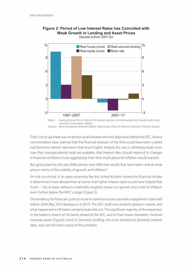
2 1 4 R E S E R V E B A N K O F A U S T R A L I A
B E N B R O A D B E N T
Figure 2: Period of Low Interest Rates has Coincided with Weak Growth in Lending and Asset Prices
Decade to/from 2007:Q3
Real house prices Real equity prices
Real secured lendingBank rate
1997–2007 2007–17-3
0
3
6
9
%
-3
0
3
6
9
%
Notes: Equity prices are for an index of UK-focused equities; nominal variables are transformed to real using the consumption deflator
Sources: Bank of England; Halifax/IHS Markit; Nationwide; Office for National Statistics; Thomson Reuters
That’s not to say there was no tension at all between the two objectives before the GFC. Several commentators have claimed that the financial excesses of the time could have been curbed had domestic interest rates been that much higher. Indeed, the case is still being made, even now that macroprudential tools are available, that interest rates should respond to changes in financial conditions more aggressively than their implications for inflation would warrant.
But going back to the pre-2008 period, how effective would that have been, and at what price in terms of the stability of growth and inflation?
I’m not convinced, in an open economy like the United Kindom where the financial climate is determined more abroad than at home, that higher interest rates would have helped that much – not, at least, without a materially negative impact on growth and a rate of inflation even further below the MPC’s target (Figure 3).
The tendency for financial cycles to move in common across countries is apparent in data well before 2008 (Rey 2013; Baskaya et al 2017). The GFC itself was certainly global in nature, and what happened to UK banks certainly bears this out. The significant majority of the expansion in the balance sheets of UK banks ahead of the GFC, and of their losses thereafter, involved overseas assets (Figures 4 and 5). Domestic lending, the most sensitive to domestic interest rates, was not the main source of the problem.

2 1 5CO N F E R E N C E V O LU M E | 2018
M O N E TA R Y A N D M A C R O P R U D E N T I A L P O L I C I E S : T H E C A S E F O R A S E PA R AT I O N O F P O W E R S
Figure 3: UK Inflation was Relatively Low in the Pre-crisis Period
2004200220001998 20060.5
1.0
1.5
2.0
2.5
3.0
%
0.0
0.5
1.0
1.5
2.0
2.5
%
CPI
RPIX
Target(a)
(LHS)
(RHS)
Note: (a) In December 2003, the Bank of England's inflation target changed: from 2.5 per cent for the 12-month increase in the RPIX to 2 per cent for the 12-month increase in the CPI
Source: Office for National Statistics
Figure 4: Pre-crisis Growth in UK Banks Driven by Overseas AssetsPer cent of GDP
Non-UK exposuresOther UK exposuresLoans to UK privatenon-financial sector
2013200920052001 20170
100
200
300
%
0
100
200
300
%
Sources: Bank of England; Office for National Statistics

2 1 6 R E S E R V E B A N K O F A U S T R A L I A
B E N B R O A D B E N T
Figure 5: Losses Predominantly Global2008:H2–2011:H1
Write-off Impairment Trading book and goodwill losses
UK Non-UK UK Non-UK UK Non-UK UK Non-UK0
10
20
30
40
£b
0
10
20
30
40
£b
Secured Unsecured Secured Unsecured Otherhouseholds households corporates corporates
Notes: Goodwill losses are calculated on a pro forma basis and may be subject to error; impairments and write-offs are taken from FSA regulatory returns; due to sampling and definitional differences, these may not match those disclosed in published accounts or in the BoE’s Bankstats
Sources: Bank of England; Banks’ published accounts; FSA regulatory returns
No financial crisis is exactly like another – it is now a cliché to compare them to Tolstoy’s unhappy families – and I’m certainly not suggesting that domestic lending is unimportant or that the risks involved are entirely immune from domestic interest rates. But I do think that the effect is less marked the more financially open an economy is, and that the spillover effect of monetary policy – its impact on financial stability relative to that on inflation – may not be that large. If so, you’d have to pay quite a high price, in terms of output and inflation, for interest rates to be of any material help in containing independent swings in financial risks.
More careful studies bear this out. In 2010, my predecessor Charlie Bean estimated that, even had UK Bank Rate been 100 basis points higher from 2005, this would’ve reduced banks’ balance sheets by only 3 per cent by 2008. The cost would have been 3½ per cent in foregone output and a rate of inflation more than a percentage point further below target.
In a more recent study, Aikman et al (2018) come to similar conclusions. They find not only that monetary policy has relatively weak effects on financial stability, at least in the United Kingdom, but also the converse – that, partly because they’re directed more at mitigating tail risks rather than affecting the most likely path of the economy, macroprudential policies do not have very large effects on demand and inflation. Figure 6 is a summary of their results when comparing the effects of changes in policy rates and changes in the countercyclical capital buffer (CCyB). The impacts of the two policies on growth and inflation are on the left-hand

2 1 7CO N F E R E N C E V O LU M E | 2018
M O N E TA R Y A N D M A C R O P R U D E N T I A L P O L I C I E S : T H E C A S E F O R A S E PA R AT I O N O F P O W E R S
side, with the effects on measures of financial stability on the right. It’s very clear in this paper, at least, that the comparative advantage of monetary policy is in stabilising growth and inflation with financial stability best left to macroprudential policy.5
Figure 6: The Impact of Monetary and Macroprudential Tools100 basis point increase
Output Inflation Creditspreads
Crisisprobability
-0.8
-0.6
-0.4
-0.2
0.0
0.2
ppt
-0.8
-0.6
-0.4
-0.2
0.0
0.2
ppt
Macroeconomic Financial stabilityoutcomes outcomes
In policy rate
In CCyB
Source: Aikman et al (2018)
So, rather than increasing the burden on monetary policy and depressing inflation still further, what, to my mind, would have helped far more ahead of the GFC was an effective prudential policy – in particular, higher capital requirements for banks. And if that’s more obvious after the event than before, let me offer one other pre-GFC comparison, this one between the United Kingdom and two countries whose experiences of the GFC were far less severe than ours, namely Canada and Australia.
These countries had significantly smaller and less international banking systems than the United Kingdom’s. But policy – and specifically prudential policy – probably mattered too. Even as a share of what turned out to be much less risky assets, Canadian and Australian banks had more loss-absorbing capital (Figure 7), enough to avoid any risk of insolvency. Meanwhile, real short-term interest rates were generally lower than those in the United Kingdom (Figure 8). So monetary policy was if anything looser yet, thanks in part to better prudential policy, the GFC was far less severe.
5 See also Ferrero, Harrison and Nelson 2018.

2 1 8 R E S E R V E B A N K O F A U S T R A L I A
B E N B R O A D B E N T
Figure 7: Canadian and Australian Banks Better Capitalised than UK’s in 20052005 and 2006 average
0 1 2 3 4
Australia
Canada
UK
Tangible common equity as a share of total unweighted assets – %Source: Bush, Guimarães and Stremmel (2015)
Figure 8: Real Short-term Interest Rates Were Generally Lower in Canada and Australia
200320011999 2005-1
0
1
2
3
4
5
%
-1
0
1
2
3
4
5
%
Australia
Canada
UK
Sources: Bank of England; Thomson Reuters

2 1 9CO N F E R E N C E V O LU M E | 2018
M O N E TA R Y A N D M A C R O P R U D E N T I A L P O L I C I E S : T H E C A S E F O R A S E PA R AT I O N O F P O W E R S
2. Some Simple MitigantsIf this is right, the gains from formal coordination might not be that significant. Even a single, ‘joined-up’ committee would generally find itself reaching for macroprudential tools to control financial risk and using interest rates to moderate cyclical swings in demand and inflation.
Shortly, in the next section, I’ll offer a more positive reason to keep some distance between the two policies. Before that, I should point out that, even in instances where there may be gains from policy coordination, there are things you can do within the existing framework.
One involves the appropriate choice of secondary objectives. As I’ve tried to explain, the case for cooperation is stronger the more severe and frequent any conflicts between the respective objectives are. There’s a very general result that puts the same point the other way around: if you give the two committees exactly the same objectives there is no coordination problem. The outcomes are the same whether their policies are set separately or jointly.
To many of you that might seem obvious (less immediately to me, I must confess). And if there’s any reason at all to keep the two functions apart, it would rather defeat the purpose simply to give them the same, overarching remit. If the MPC and FPC were both made responsible for inflation control, stabilising demand and financial stability, that’s a merger by default.
But the result does provide some intuition as to why you can get closer to the full coordination outcome – and in some cases replicate it exactly – by a judicious mapping of the overall objectives across the two committees. If, for example, you thought that some macroprudential measures had important spillover effects on aggregate demand, then you can get closer to the cooperative outcome simply by supplementing the remit of the macroprudential authority with the equivalent secondary objective. You ask the FPC to think not just about financial stability but also to take into account the effects of its policies on economic activity. The spillovers are then internalised and, under some circumstances, you can mimic precisely the full coordination regime. As I say, I do not believe these effects are, in fact, that powerful or, therefore, that the secondary objective will come into play very often. But it’s worth pointing out that the FPC’s remit was expanded in exactly this way when the Committee was put on formal statutory footing in 2012.
I think the set-up in the UK, with both committees living in the same central bank, also allows for more formal coordination in the extreme cases when the need is clear. I’ve explained that the gains are larger the greater the scale of cross-policy spillovers. This is a relative point: what matters is whether A’s policy has a significant impact on B’s objectives compared with B’s own policy. In Figure 6, it’s the fact that the orange bars are much bigger than the dark green on the left-hand side, and conversely on the right, that weakens the case for coordination. But, conceivably at least, there could be instances when this isn’t the case – most obviously if B comes to doubt the effectiveness of its main policy instrument. Suppose, for example, that inflation is much too low but the monetary policymaker believes the zero lower bound on nominal interest rates has reduced the room for further easing. Or maybe the macroprudential authority is concerned that, in the midst of a boom, the financial system might be finding ways round its conventional tools, something that only higher interest rates

2 2 0 R E S E R V E B A N K O F A U S T R A L I A
B E N B R O A D B E N T
could address. In these cases there would be clear gains from a more cooperative approach, in which the burden is more evenly shared.
If only conditionally, this is exactly what was proposed in the MPC’s guidance about interest rates back in 2013. The MPC set out a necessary condition for UK Bank Rate to rise: that unemployment fall below 7 per cent. It also added various ‘knock-outs’ that, if breached, would automatically bring the guidance to an end. One of those involved financial stability: the guidance would become obsolete if, among other things, the FPC judged ‘that the stance of monetary policy poses a significant threat to financial stability that cannot be contained by the substantial range of mitigating [macroprudential] policy actions available …’ (Bank of England 2013, p 7).
So there has already been an episode where one policy committee accepted the possibility, however remote, that it might be asked to take into account the other’s objective. I can see no reason why, if the circumstances warrant it, this shouldn’t happen again.
3. The Positive Case for SeparationAll I’ve done so far is to make the case that the separation of monetary and macroprudential policies has limited costs on average and that, if and when those costs are ever material, there are other ways, short of full integration, to deal with those situations.
Whether or not my arguments are persuasive, that doesn’t mean there’s no conceivable cost. In the coordination literature, in its various guises, there’s always some price to pay for a separation of powers: it’s inevitable, given the way things are modelled, that the ‘first-best’ answer is that policy tools should be set jointly, taking into account all the collective objectives at once. The only question is how large the costs of decentralised decision-making are and what might be done to mitigate them.
In fact, the more one reads of this stuff, the more puzzling it becomes that policies aren’t more often coordinated. Economics is a positive as well as a normative science. Much of it seeks to explain why things are as they are. And if there’s only upside to policy coordination, why isn’t there much more of it? Why, indeed, isn’t there just one, all-powerful decision-maker in charge of everything?
In the case of international coordination, perhaps the answer is obvious: only countries are wholly sovereign. That hasn’t prevented all sorts of other mechanisms for joint decision-making, whether in trade, defence or environmental policy, to name a few. But, in some areas, there are limits to the extent to which national sovereignty can be compromised and, as the current debates in the euro area illustrate, fiscal policy may be one of them.
When it comes to decisions about fiscal and monetary policy, we know there’s a positive reason for separation. It’s harder for governments to commit to a fixed nominal objective. Because the gains from commitment are significant, it makes sense to delegate monetary policy to an independent body. (Though it happened later than in many other countries, I would argue strongly that its separation from the government – first via the introduction of inflation targeting in 1992 and then thanks to the creation of an operationally independent MPC in 1997 – has led to much improved monetary policy in the United Kingdom.)

2 2 1CO N F E R E N C E V O LU M E | 2018
M O N E TA R Y A N D M A C R O P R U D E N T I A L P O L I C I E S : T H E C A S E F O R A S E PA R AT I O N O F P O W E R S
I also think there’s an additional justification for separation in many of these cases, and for monetary and macroprudential policies in particular. It’s essentially a matter of accountability.6
I think there’s little doubt that, over any limited period of time, monetary stability is more easily measured than financial stability. The MPC’s primary target is inflation, as measured by the rate of change of the Consumer Prices Index (CPI). We get to see the CPI every month, it’s never revised, and it’s therefore reasonably clear over time whether the target has been reached.
Judging the MPC’s performance is, in reality, a little more complex than this. Policy takes time to work, so it’s inevitable that intervening shocks will prevent inflation from being exactly at the 2 per cent target all the time, even if that were the sole objective of policy. In addition, the MPC’s remit involves a secondary objective, subject to the primary inflation target, to stabilise the real economy. If they occur, the MPC is asked to identify trade-offs between the two. However, when that has happened – for example, following the sharp fall in sterling that accompanied the result of the UK’s European Union membership referendum – I don’t think it’s been insuperably difficult to explain the policy approach. People can then monitor how the economy is performing, relative to our earlier projections. We on the MPC, for our part, can use surveys and market prices to gauge very regularly, in ‘real time’, what’s happening to inflation expectations. Judging the performance of monetary policy isn’t an exact science, but we can, over time, distinguish what works from what doesn’t.
Things are rather different for macroprudential policy. Financial stability is harder to define – there’s no monthly ‘financial stability index’. And, while we know all too well what financial instability looks like and what its costs can be, it’s more difficult to demonstrate a reduction in that risk, simply because serious problems in the financial system aren’t that common to begin with.
One can make the point, albeit with an absurdly extreme example, by imagining that the only thing a sceptical outside observer can see is whether or not there has actually been such a problem. We’re interested in how long it would take, possessing only this information, to conclude that the likelihood of such an event had changed.
The precise answer depends on what one means by ‘conclude’ and how sure the observer is of her prior belief.7 But imagine, for illustration, that after a relatively long period with several such episodes, our observer’s best guess is that the per annum chances of a serious problem in the financial system are 8 per cent – she expects it to happen only once every 12½ years, on average (I’m thinking of something less severe and less infrequent than the ‘once-in-a-century’ financial crisis of 2008).
What she doesn’t know is that, thanks to some beneficial piece of prudential legislation, the likelihood has actually fallen to 4 per cent a year. Figure 9 shows how her estimate of the
6 By that I do not mean we necessarily need better oversight of policy. We would all have a sense, I think, of the virtue of the separation of powers as a check on their possible abuse. ‘[I]n all the subordinate distributions of power, where the constant aim is to divide and arrange the several offices in such a manner as that each may be a check on the other’, is how James Madison (1788) put it. That’s not the issue here: a second committee wasn’t created so it could keep an eye on the first and there are plenty of robust mechanisms – our public communications and press conferences and, more formally, the direct accountability to (and regular interrogations by) parliament – that already hold the various parts of the central bank to public account.
7 The observer updates her distribution over the probability using Bayes’ law. Figure 9 is the mean of that updated distribution as a function of the number of years of data that the agent has observed.

2 2 2 R E S E R V E B A N K O F A U S T R A L I A
B E N B R O A D B E N T
probability is likely to evolve over time. Because these events are rare, this happens only very slowly. Even if she’s not that sure of her initial 8 per cent estimate – the diffuse prior line illustrates the case where the standard deviation around her prior is 2 percentage points – it’s still likely to take more than 100 years for the observer’s central estimate to fall even half way to the truth (i.e. to 6 per cent). If the observer’s wrong but confident (the more certain prior line illustrates the case with a 1 percentage point standard deviation around the initial 8 per cent prior), one would expect it to take well over half a millennium to get to 6 per cent. King John and the barons might have tightened prudential regulation in the Magna Carta and her acknowledgement of its benefits would even now be somewhat grudging.
Figure 9: Learning about Rare Events Takes a Long Time
0 100 200 300 400 500 600 7003
4
5
6
7
8
9
Years
Valueofeventprobaility–%
More certain prior
Diffuse prior
(std dev = 1 ppt)
(std dev = 2 ppt)
Note: Expected value of event probability (initial prior = 8%, true number = 4%)Source: Bank of England
This is, as I say, a wholly unrealistic experiment because we get to see far more than the simple occurrence (or non-occurrence) of a financial crisis. Our sceptical observer would presumably be aware of the prudential legislation and, more importantly, its effects on things that relate to financial risk (e.g. asset valuations and banks’ capital ratios). That information would allow a much faster updating of estimated risk than in Figure 9. In the real world, the information set available to the FPC, and by which its performance can be judged, is richer still. Having seen several such events, in many countries, we know quite a bit about what typically precedes them. Stress-testing gives us an extremely useful and powerful way to expand our knowledge about the impacts of ‘tail events’. Armed with the whole array of price and quantity indicators of risk, we – and others – can make informed judgements about the right level of loss-absorbing capital in the banking system and about the appropriateness of more targeted policy tools.

2 2 3CO N F E R E N C E V O LU M E | 2018
M O N E TA R Y A N D M A C R O P R U D E N T I A L P O L I C I E S : T H E C A S E F O R A S E PA R AT I O N O F P O W E R S
And if it takes time to demonstrate decisively a reduction in system-wide risk, there are some policies whose effects are more immediately obvious. In 2014, responding to concerns about growth in riskier mortgages, the FPC introduced limits on the share of banks’ mortgage lending at high (> 4.5) loan-to-income ratios. Recently, the FPC noted that there’s since been quite a bit of ‘bunching’ in new loans just below this limit. I’m not so sure this is a problem: for my part, I see it mainly as clear and timely evidence that the policy has had an impact.
The point remains, however, that the FPC’s objective is inevitably less precise, and its success less immediately measurable, than that of the MPC. Recalling the results of the analysis I discussed at the start of the paper on the appropriate allocation of tasks, this suggests that there might well be a cost if you asked a single body – an ‘FMPC’ – to meet all these objectives at once. Yes, there could occasionally be instances when policies would be better coordinated (although these are rarer and less grievous than many suppose). But there’s also a risk that a single committee might be incentivised to pay more attention to the more verifiable elements of its remit – the cyclical stability of growth and inflation – than to the less obvious achievement of financial stability.
4. ConclusionIn public debate, politicians often extol the virtues of ‘joined-up’ policymaking. Policies set by one body might affect another’s objectives and people should be aware of such interactions. In some instances, where the interactions are sufficiently strong, it can be desirable to merge the two bodies into one.
But if you try pushing that argument to its logical limit – to ensure we internalise all possible spillovers let’s just have one body determining every aspect of public policy – I think we’d all have misgivings with the outcome. Apart from anything else, the policymaking process would be far too complicated to hold any one bit of it to account and the all-powerful policymaker would naturally tend to focus on the more verifiable tasks. A bit like the man who loses his keys in the park but looks for them under the streetlamp ‘because that’s where the light is’, the attention of policy would be directed to the most observable objectives. Perhaps we collectively fell foul of this trap, in some ways, ahead of the GFC. The risk of a rare event is not an easy thing to judge and, having gone so long without a serious problem in the financial system, our attention was distracted by the more easily monitored task of stabilising the economic cycle. Maybe people were too beguiled by the ‘Great Stability’, if only because data confirming it arrived with such regularity, to notice what was going on within the financial system.
One obvious lesson has been that the stability of inflation is no guarantee of financial stability – hence the (re-)creation of macroprudential policymaking. I think another lesson is that it’s better to grant these powers to a single, accountable body, ring-fenced from the other functions of the central bank.
I don’t want to overstate the case and I’m certainly not suggesting any sort of ‘Chinese wall’ between the two functions. There are clear advantages in having them housed in the same

2 2 4 R E S E R V E B A N K O F A U S T R A L I A
B E N B R O A D B E N T
institution. Many economic issues are relevant for both and, in the BoE, the MPC and FPC regularly receive joint briefings on such matters. Even if the two hands act separately, it is important that the one should know what the other is doing and, in that respect, it helps that some people sit on both committees. And if and when there were a serious coordination challenge – for example, if one body became concerned about its ability to meet its primary objective, without enlisting the assistance of the other – then I think the current system in the United Kingdom would allow that to happen.
Equally, there are also clear advantages in a degree of separation. One – something I haven’t gone into today but which still matters a great deal – concerns specialised skills. The two committees at the BoE profit greatly from having external members steeped in particular experience, whether that’s monetary experts on the MPC or financial experts on the FPC. Another, the topic of this talk, is a matter of accountability and focus. I think there would be risks in asking the central bank to meet a wide range of objectives with no distinctive accounting for the use of its various tools.
Thank you.

2 2 5CO N F E R E N C E V O LU M E | 2018
M O N E TA R Y A N D M A C R O P R U D E N T I A L P O L I C I E S : T H E C A S E F O R A S E PA R AT I O N O F P O W E R S
ReferencesAikman D, J Giese, S Kapadia and M McLeay (2018), ‘Targeting Financial Stability: Macroprudential or Monetary Policy?’, Bank of England Staff Working Paper 734.
Bank of England (2013), Inflation Report, August.
Baskaya YS, J di Giovanni, Ş Kalemli-Özcan, J-L Peydro and MF Ulu (2017), ‘Capital Flows and the International Credit Channel’, Journal of International Economics, 108(Supplement 1), pp S15–S22.
Bean C, M Paustian, A Penalver and T Taylor (2010), ‘Monetary Policy after the Fall’, Paper presented at the Federal Reserve Bank of Kansas City Economic Policy Symposium on ‘Macroeconomic Challenges: The Decade Ahead’, Jackson Hole, 26–28 August.
Bianchi F and L Melosi (2018), ‘Constrained Discretion and Central Bank Transparency’, The Review of Economics and Statistics, 100(1), pp 187–202.
Bush O, R Guimarães and H Stremmel (2015), ‘Beyond the Credit Gap: Quantity and Price of Risk Indicators for Macroprudential Policy’, Unpublished manuscript, Bank of England.
Dixit A and L Lambertini (2003), ‘Interactions of Commitment and Discretion in Monetary and Fiscal Policies’, The American Economic Review, 93(5), pp 1522–1542.
Elliott DJ, G Feldberg and A Lehnert (2013), ‘The History of Cyclical Macroprudential Policy in the United States’, Board of Governors of the Federal Reserve System Finance and Economics Discussion Series No 2013-29.
Fernie S and D Metcalf (1999), ‘It’s Not What You Pay It’s the Way that You Pay It and that’s What Gets Results: Jockeys’ Pay and Performance’, Labour: Review of Labour Economics and Industrial Relations, 13(2), pp 385–411.
Ferrero A, R Harrison and B Nelson (2018), ‘Concerted Efforts? Monetary Policy and Macro-Prudential Tools’, Bank of England Staff Working Paper No 727.
Goodhart CAE (2015), ‘Linkages between Macro-Prudential and Micro-Prudential Supervision’, Butterworths Journal of International Banking and Financial Law, 30(10), pp 607–609.
Groves T, Y Hong, J McMillan and B Naughton (1994), ‘Autonomy and Incentives in Chinese State Enterprises’, The Quarterly Journal of Economics, 109(1), pp 183–209.
Holmstrom B and P Milgrom (1991), ‘Multitask Principal–Agent Analyses: Incentive Contracts, Asset Ownership, and Job Design’, Journal of Law, Economics & Organization, 7(Special Issue), pp 24–52.
Kohn D (2017), ‘Cooperation and Coordination across Policy Domains’, Keynote speech given at the Financial Stability Institute Conference ‘Supervisory Policy Implementation in the Current Macro-Financial Environment – “A Cross-Sectoral Journey”’, Basel, 18–19 September.
Leeper EM (1991), ‘Equilibria under “Active” and “Passive” Monetary and Fiscal Policies’, Journal of Monetary Economics, 27(1), pp 129–147.
Madison J (1788), ‘The Structure of the Government Must Furnish the Proper Checks and Balances between the Different Departments’, Federalist Papers No 51. Available at <https://billofrightsinstitute.org/founding-documents/primary-source-documents/the-federalist-papers/federalist-papers-no-51/>.
Meeks R (2017), ‘Capital Regulation and the Macroeconomy: Empirical Evidence and Macroprudential Policy’, European Economic Review, 95, pp 125–141.

2 2 6 R E S E R V E B A N K O F A U S T R A L I A
B E N B R O A D B E N T
Rey H (2013), ‘Dilemma not Trilemma: The Global Financial Cycle and Monetary Policy Independence’, in Global Dimensions of Unconventional Monetary Policy, A Symposium Sponsored by the Federal Reserve Bank of Kansas City, Kansas City, pp 285–333.
Sargent TJ and N Wallace (1981), ‘Some Unpleasant Monetarist Arithmetic’, Federal Reserve Bank of Minneapolis Quarterly Review, 5(3), pp 1–17.
Svensson LEO (2015), ‘Monetary Policy and Macroprudential Policy: Different and Separate’, Paper presented at the Federal Reserve Bank of Boston’s 59th Economic Conference ‘Macroprudential Monetary Policy’, Boston, 2–3 October.
Tucker P (2011), ‘Macroprudential Policy: Building Financial Stability Institutions’, Speech given at the 20th Annual Hyman P Minsky Conference ‘Financial Reform and the Real Economy’, New York, 13–15 April.
Wadhwani SB (2010), ‘What Mix of Monetary Policy and Regulation is Best for Stabilising the Economy?’, in The Future of Finance: The LSE Report, London School of Economics and Political Science, London, pp 145–163.

2 2 7CO N F E R E N C E V O L U M E | 2 018
Discussion
1. Sally Auld
IntroductionGood afternoon. Let me begin by thanking the conference organisers for the opportunity to participate in today’s session. I have to admit that when I read in the newspaper earlier this week that the Bank of England’s (BoE’s) Chief Economist had organised for Billy Bragg to come and speak to BoE officials, I was a little worried that Ben’s paper might have taken a radical turn! But, as he notes at the beginning, his paper is sympathetic with the prevailing orthodoxy on the topic, and so our session is defined more by evolution than revolution.
The paper argues the case for the continued separation of monetary and macroeconomic policies. On one level, the case for separation of these powers relies on an assumption that spillover effects are small.
Another argument for separation rests on the quantification of objectives. It’s easy to assess the performance of an inflation-targeting central bank relative to its policy objective, as both the target and the target variable can be easily and credibly observed. Macroprudential objectives, in contrast, are harder to define and harder to measure. The theory around incentive design suggests that it might be optimal to separate jobs relating to easily measured objectives from those that relate to more opaque objectives.
In discussing Ben’s paper, it’s only fair that I state from the outset that I am not an expert in the academic literature on this topic. So I thought I would frame my comments with reference to the local experience, given that the topic is particularly pertinent in both Australia and New Zealand. I want to add a couple of additional arguments to the case for separation, and then will talk a little about what might happen when tension arises between monetary and macroprudential policy objectives.
Some more thoughts on separation of macroeconomic and macroprudentialThe first argument for separation that I want to address starts with something called Maslow’s hammer, which states that if you only have a hammer, then every problem looks like a nail. For the topic at hand, this is just saying that interest rates are not necessarily the right tool to deal with financial stability issues. This concept of the right tool for the job was espoused by Ben Bernanke in a speech back in 2002 (Bernanke 2002). Bernanke doesn’t really argue one way or the other for separating responsibility for economic and financial stability objectives; rather, he simply argues that interest rates are not the right tool for dealing with financial stability problems.

2 2 8 R E S E R V E B A N K O F A U S T R A L I A
D I S C U S S I O N
I think his argument can be extended in favour of the case for separation. Effectively, it comes down to taking a view on what it is appropriate – or even sensible – for a central bank to do.
It goes without saying that central banks pay close attention to financial markets when thinking about the economy’s trajectory and the optimal path of interest rates.
But this is a very different proposition to thinking about whether macroprudential tools should be deployed for dealing with financial stability issues. For a start, this would require the central bank to take a view on the valuation of an asset class, whether it be stocks, houses, or something else. Moreover, it also probably relies on an assumption that the central bank is better, on average, than the market at valuing assets, meaning it can identify a bubble in an asset class before others. In my experience, central bankers generally tend to shy away from such pronouncements, and for good reason.
Central bank officials have sometimes bemoaned the overanalysis of their comments on the economy and outlook for monetary policy. If the market was also trying to second guess the central bank’s view on a particular asset class, then this would probably be highly detrimental to achieving an optimal allocation of capital across asset markets.
If the experience in New Zealand in recent years is any guide, market participants also become unnecessarily obsessed with the trade-off between policies, trying to gauge what any particular tweak to macroprudential policy is worth in terms of interest rates. This seems almost reminiscent of the days of monetary conditions indices.
To be fair, some might argue that the benefits of coordination outweigh potential communication difficulties, especially given that acute financial stability issues are relatively rare. But as Guy Debelle noted in his paper at this conference, the communication demands on central banks have increased over the past decade or so, and so, in light of this, I think there’s a compelling practical case for keeping it simple.
Another benefit of separation derives from the fact that we cannot rely on a stable relationship between macroprudential and monetary policy. Over time, the relationship between these policies and the associated spillover effects will essentially depend on: the extent to which the business and credit cycles are synchronised; structural factors that determine the extent to which lending occurs outside of the regulated sector; and global influences on domestic interest rate and currency settings.
We don’t have to look too far to find examples where inflation has been lower than desired but the credit cycle robust, thanks to a globally induced regime of low rates and a strong currency. One might argue that policymakers in both Australia and New Zealand have found themselves facing this mix of outcomes in recent years. In both jurisdictions, the credit and inflation cycles have de-coupled, allowing the possibility that macroprudential policy and interest rate policy might be in conflict. In such circumstances, monetary policy settings would be aimed at generating above-trend growth, in order to return inflation to target. In contrast, macroprudential settings would be trying to restrain or slow credit growth. Macroprudential policies could therefore potentially thwart the objective of monetary policy, if slower credit growth became a headwind to gross domestic product (GDP) growth.

2 2 9CO N F E R E N C E V O L U M E | 2 018
D I S C U S S I O N
If so, it might make sense from a communications perspective if the policies were owned by separate entities. It is relatively simple to explain policy actions in terms of the deviation of inflation or output from desired levels. But how does a central bank explain the trade-off between pursuing macroeconomic and macroprudential objectives? In the event that there is tension between the two policies, this might invite questioning of who sets the parameters around the trade-off, and could, in some circumstances, unsettle otherwise well-anchored inflation expectations.
And, at a time when the two objectives were complementary to one another, the distributional impact of using one policy in preference to the other might be quite different. In such circumstances it might be quite uncomfortable for a central bank to defend its actions.
The local experienceHere in Australia, financial stability is now explicitly mentioned in the Statement on the Conduct of Monetary Policy. This is not problematic when monetary policy is set such that it is sympathetic with achieving both macroprudential and macroeconomic objectives. But policymakers should be aware that this is not always the case. As I have alluded to, the current environment is a case in point.
In the short run, good (inflation) target design can help minimise trade-offs. For example, it’s no secret that the inherent flexibility in our inflation-targeting regime has provided policymakers here in Australia with the timely opportunity to focus on financial stability concerns in the last 18 months, particularly as they relate to household balance sheets and the types of mortgage lending.
The Reserve Bank of Australia (RBA) has been quite explicit about this, and has explained that a period in which inflation is a little below target and growth a little below trend is an appropriate cost to wear in order to ameliorate risks around household balance sheets. Were the inflation target less flexible then, arguably, the RBA could have been forced to pursue policy outcomes that exacerbated financial stability issues.
However, it is also important to remember that this flexibility is not infinite – that is, inflation outcomes eventually have to be consistent with the target. After all, one of the stated objectives of the inflation-targeting regime is the anchoring of inflation expectations.
Locally, I don’t think it’s too hard to see how this scenario could become somewhat uncomfortable for policymakers. In Australia at present, macroprudential policy is working effectively to tighten credit to mortgage borrowers – particularly to investors – and has delivered both a slowing in credit growth and house price growth. To be sure, these are desired outcomes.
But to the extent they could also compromise household consumption outcomes over the next little while, and thus see the economy sustain a period of below-trend GDP growth for longer, they might also delay the return to trend growth and target-consistent inflation outcomes. This outcome is acceptable for a while, but not for a long time. As noted above, the inflation target is not infinitely flexible.

2 3 0 R E S E R V E B A N K O F A U S T R A L I A
D I S C U S S I O N
A priori, it’s not clear which path policymakers should take in such circumstances. Does the inflation target, by virtue of its importance to the anchoring of inflation expectations, eventually take primacy over macroprudential considerations? Or alternatively, as Ben suggests in his paper, is the body tasked with macroprudential objectives asked to internalise its spillovers (as was the case in the United Kingdom in 2013)?
Clearly the circumstances matter, as does the policy at hand. Some macroprudential policies are potentially complex in their application, and hence their effect on the overall economy is subtle and takes longer to occur. In contrast, policies aimed at restricting growth in a particular type of lending, or to a specific borrower, can be more effective over a shorter time period.
Perhaps the right view is the long view. In the long run, failure to deal with financial stability issues will ultimately mean failure on the inflation target and, potentially, as we have seen in the global economy in the past decade, legitimate fears around the ability of central banks to anchor inflation expectations. In this context, if the cost of dealing with financial stability issues is low (but not too low) inflation, then that’s probably an acceptable price to pay. Again, it might just come down to communication – if a credible central bank can communicate a sense that it knows flexibility in the inflation target isn’t infinite, then it can buy itself a lot of time and minimise the cost of any tension between macroprudential and macroeconomic objectives.
In summary, I think the case for the separation of macroeconomic and macroprudential objectives makes a lot of sense. But even with separation, it’s not clear what happens when the policy objectives are in conflict. Target flexibility, credibility and strong communication all help. In Australia, we are lucky enough to have all three, and hopefully this will be just enough to buy us the time to deliver success on both our macroeconomic and macroprudential objectives.
ReferenceBernanke BS (2002), ‘Asset-Price “Bubbles” and Monetary Policy’, Address given to the New York Chapter of the National Association for Business Economics, New York, 15 October.
2. General DiscussionOne of the major topics of the discussion was the accountability of the macroprudential authority. Following Ben Broadbent’s presentation advocating separation of monetary and financial stability powers, a participant asked whether the responsibility for the two policies should be in two different institutions. The discussion covered several points in favour of having both committees remain at the same institution: the ease of coordinating policy, overlapping areas of interests, the ability to have joint briefings and economies of scale in monitoring the same developments. Participants preferred this arrangement to a diffuse

2 3 1CO N F E R E N C E V O L U M E | 2 018
D I S C U S S I O N
system of multiple agencies looking at various parts of the system, as is the case in the United States. The dedication of a group of people to the issues of financial stability was said to be more important than whether that group of people is within the central bank or outside of it. The separation of powers enhances accountability by giving monetary and macroprudential issues different forums.
One participant questioned why there wasn’t greater demand for some quantitative measures of financial stability. Governments generally provide the target of monetary policy, but no central bank has been given a target or even definition of financial stability. Another participant agreed, preferring a situation where the central bank does not have discretion over the definition of a target or the instrument used to achieve the target. The participant did suggest that practice should create, de facto, a commonly used target and instrument.
This led to some discussion on transparency and communication. A participant noted that these had previously been agreed as two key pillars of an effective inflation-targeting regime, and that they should be similarly important, or even more important, for financial stability policy. Macroprudential policy requires central banks to sustain policy arguments over a longer time and the policy effects may be higher on households – for example, macroprudential policies in the United Kingdom have prevented some people from getting mortgages. Good, clear communication was said to be necessary when explaining why financial stability policy is acting to address a risk that some event may occur in the future, perhaps many years ahead. Participants also commented that the public and the media have more experience and understanding of monetary policy and that may be why macroprudential issues receive less coverage.
The other major topic covered by the discussion was the trade-off between price stability and financial stability. This discussion opened with a question regarding whether the zero lower bound makes this trade-off more acute. The effective lower bound may cause interest rates to be ‘stuck’ at a very low level for an extended period of time, which could make monetary policy very ‘predictable’ and also lead to financial imbalances. There was agreement that the zero lower bound could complicate the task of policy coordination in the case, for example, where inflation was weak, interest rates were low and yet there was very strong credit growth. In such a case, a tightening response by the macroprudential authority may be uncomfortable for the monetary authority. Participants also noted that there is a small range for interest rates, close to the zero lower bound, where the goals of financial stability and monetary stability could be said to be in conflict. In this range, institutions that have a lending book with thin spreads over the bank rate would face depressed earnings and possible insolvency if the policy rate was lowered beyond the effective lower bound.
Participants discussed the implications of this trade-off for the organisation and actions of the monetary and macroprudential authorities. One participant, citing the example from Broadbent’s paper, stated that the conflicts raised are not sufficient reason to merge the two policy committees into one because they can coordinate instead. In 2013, the Bank of England issued formal monetary policy guidance that interest rates would not rise until the unemployment rate fell below a certain level. However, they qualified the guidance by noting

2 3 2 R E S E R V E B A N K O F A U S T R A L I A
D I S C U S S I O N
that it would not hold if the macroprudential authority judged that low interest rates posed risks to financial stability that could not be mitigated. Another participant shared the view that the overall policy package implemented in the euro area had counterbalancing effects with respect to bank profitability, and that the implementation of non-standard measures was said to improve the overall macroeconomic outlook for the economy. While negative policy rates were said to reduce net interest income for banks, this was offset by lower loan provisions and the asset purchases program led to a capital gain for banks. These circumstances highlighted that coordination was possible while retaining the benefits of separate bodies discussed earlier.
The discussion also covered the role of money as a unit of account and how the trade-off between price and financial stability might evolve with possible changes to the means of payments. A participant suggested that these changes to payments may result in a currency with a constant real value and that the central bank would not consider adjusting the real value of money to address financial stability. While there was some sympathy for the view that a constant real value of the currency could help people make good decisions, it was noted that this is not so different from a world with a successful inflation-targeting regime. Participants reflected on the period of the classical gold standard, which showed that a relatively stable real value of money is no guarantee of financial stability. One participant stated that financial stability can be better dealt with by other tools and there was little support to use the ‘hard-won’ credibility of monetary policy to adjust domestic credit supply.
Lastly, the point was made that the role of fiscal policy and the fiscal position of the government should play a larger role in the debate regarding financial stability policy. This reflects the recent experience when financial stability policy actions relied on the balance sheet of the public sector in the form of quantitative easing and government bailouts of banks. Participants agreed that the three-way interaction between fiscal policy, monetary policy and macroprudential policy could be rather complicated but that research tends to show that commitment and the separation of policy assignments can assist operationally.

2 3 3CO N F E R E N C E V O L U M E | 2 018
David Archer and Andrew T Levin*
1. IntroductionDuring the 1980s and 1990s, economists reached a broad consensus about the rationale for central bank independence. Generally speaking, that consensus emphasised the role of statutory provisions to insulate monetary policymaking from fiscal pressures and from political interference aimed at short-term electoral outcomes. Such provisions included various aspects of the central bank’s governance (e.g. staggered terms of office), clarification of the monetary policy objectives in its legal mandate, and removal of constraints on its ability to adjust its policy instruments in order to achieve those objectives.
In the light of subsequent experience, however, it has become increasingly evident that the institutional design of monetary policymaking needs to be revisited.
• Statutory provisions are not sufficient to protect the central bank from political interference aimed at short-term electoral outcomes. One obvious pitfall is that such statutes can be weakened or removed by subsequent governments. In the absence of mechanisms for the orderly involvement of elected officials in periodic strategic choices, politicians may opt for disruptive legal changes or seek to exert pressure via informal channels. Better governance mechanisms can help alleviate such risks, but ultimately the operational independence of the central bank can only be sustained over time by fostering broad public support for its mission.
• The objectives of monetary policy need to be transparent but cannot be adequately encapsulated and enshrined in a static legal mandate. Analytical studies have often represented the monetary policy committee’s (MPC’s) goals in terms of a quadratic loss function, but such a formulation assumes that the optimal monetary policy is completely invariant to uncertainty about the economic outlook. By contrast, the experience of the past decade has underscored the importance of risk management in determining the appropriate policy strategy.
• Expert judgement is required at all levels of the monetary policy process. There is evidently no single ‘correct’ model or analytical approach for setting the course of monetary policy. Thus, the role of judgemental input is not merely a matter of using anecdotal information
* David Archer is the head of the Central Banking Studies section at the Bank for International Settlements (BIS). Andrew Levin is a professor of economics at Dartmouth College. We appreciate helpful comments from Andrew Berg, Danny Blanchflower, Michael Bordo, Claudio Borio, Alina Carare, Chris Erceg, Peter Fisher, Jinill Kim, John Murray, Hyun Shin, Masaaki Shirakawa, Lars Svensson, Harald Uhlig, Tsutomu Watanabe and Tack Yun. The views expressed here are solely those of the authors and should not be interpreted as representing the views of the BIS or any other person or institution.
Robust Design Principles for Monetary Policy Committees

2 3 4 R E S E R V E B A N K O F A U S T R A L I A
DAV I D A R C H E R A N D A N D R E W T L E V I N
to gauge current economic and financial conditions. Rather, good judgement is essential in characterising the dynamic behaviour of the economy, identifying material risks to the economic outlook, and formulating contingency plans to address such risks.
• Excessive insularity and groupthink can hinder the effectiveness of monetary policymaking. Risk management necessarily involves questioning standard assumptions and encouraging outside-the-box thinking. Thus, even a committee of experts can be susceptible to groupthink if its members have similar educational and professional backgrounds and hence naturally tend to share a common perspective. Groupthink can also emerge from a policy process that emphasises consensus rather than individual accountability.
In this paper, we formulate a set of robust design principles for MPCs, that is, the decision-making body within the central bank that is responsible for setting the course of monetary policy. This set of principles is intended to strengthen the MPC’s transparency and accountability while mitigating the risk of severe policy errors resulting from political interference or groupthink. Thus, these principles encompass the MPC’s governance as well as the procedures for determining its policy strategy.
The governance principles can be summarised as follows. The MPC should be a fully public institution. Its size and voting procedures should foster genuine engagement and diminish the influence of any single member. Each member should serve a staggered non-renewable term that lasts longer than the political cycle. The procedures for selecting MPC members should foster a diverse set of perspectives and forms of expertise. Each member should be individually accountable to elected officials and the public. And the MPC should undergo periodic external reviews of its strategy, procedures and operations.
The procedures for determining the MPC’s policy strategy should facilitate its democratic legitimacy and accountability while protecting the MPC’s operational independence. Therefore, this determination should involve a multilayered approach as follows:1
1. The MPC’s legal mandate should establish its goals and authority in fairly broad terms, so that this statute can remain in place over a time frame of multiple decades.
2. The law should require the MPC to specify its targets and instruments in a policy framework document that is approved or endorsed by elected officials, and this framework should be revisited regularly every five years.
3. Given those targets and instruments, the MPC should formulate a systematic and transparent strategy that guides its policy decisions, and the MPC should reconsider its strategy on an annual basis.
4. The MPC should publish regular reports explaining its specific policy decisions in terms of its framework and strategy; these reports should also convey the diversity of views of MPC members.
1 In terms more familiar to academic macroeconomists, the overarching objective function should be determined in layer 1; selection of the policy framework in layer 2; selection of a policy reaction function in layer 3; and tactical choices on instrument settings in layer 4.

2 3 5CO N F E R E N C E V O LU M E | 2018
R O B U S T D E S I G N P R I N C I P L E S F O R M O N E TA R Y P O L I C Y CO M M I T T E E S
Over the past couple of decades, academics and government officials have collaborated with the World Bank to produce a ‘body of knowledge’ about the institutional design of regulatory agencies overseeing utilities in the energy, transportation and telecommunications sectors.2 That work has emphasised the importance of operational independence and accountability, thereby ensuring that the regulator promotes the general welfare rather than catering to politicians or special interests. Moreover, a recurring theme is the crucial role of legitimacy because an agency’s operational independence rests on sustaining public confidence in the integrity and effectiveness of its decisions.
While the practical challenges of monetary policymaking are distinct from those of utility regulation, many of the underlying institutional issues are remarkably similar. For example, electricity producers and end users make forward-looking decisions that hinge on the rate structure and its expected path. Hence the regulatory framework needs to be systematic and transparent. Moreover, a given rate structure cannot be set in stone because regulators face substantial uncertainty about technical innovation and other structural factors that may warrant adjustments to the regulatory framework.
As emphasised by Tucker (2018), issues of public legitimacy and operational independence are also crucial for the design of financial regulatory agencies. Indeed, the onset of the global financial crisis (GFC) underscored the complex and subtle linkages between monetary policy and financial stability. Many central banks now have responsibility for monitoring the financial system and identifying emerging risks, and some central banks have direct oversight of commercial banks and other systemically important financial institutions. However, a detailed consideration of such arrangements is beyond the scope of our analysis.
The remainder of this paper is organised as follows. Section 2 considers the key pitfalls that can induce severe monetary policy errors. Section 3 identifies design principles for governance and transparency. Section 4 concludes.
2. Basic RisksUnlike stylised academic models, the actual conduct of monetary policymaking inevitably involves some degree of judgement – at least in economies where the foreign exchange value of the currency is not permanently fixed. In effect, such judgements may be open to question in ‘real time’ (at the time when a given decision is made) and often remain so for many years afterwards. The quality of such judgements can certainly be enhanced through quantitative research and conjunctural analysis. But the future remains unknowable, and the dynamics shaping lingering responses to past events remain extraordinarily complex. Predicting future paths will likely always confront pervasive uncertainty; policy choices will rarely be black or white in nature. The crucial task in designing an effective governance structure is thus to mitigate the risk of severe policy errors.
Effective monetary policymaking cannot be achieved through the mechanical application of fixed rules; rather, careful judgement is an intrinsic necessity. Against that background,
2 See <http://regulationbodyofknowledge.org/regulatory-process/institutional-design/>.

2 3 6 R E S E R V E B A N K O F A U S T R A L I A
DAV I D A R C H E R A N D A N D R E W T L E V I N
the experiences of many central banks over recent decades highlight two basic types of risk exposure in monetary policymaking: (1) electoral politics are allowed to affect tactical monetary policy decisions, and (2) excessive insularity and groupthink fosters complacency about tacit assumptions, lack of attention to material risks, and failure to prepare contingency plans for adverse scenarios. A comprehensive historical and global review of such experiences is beyond the scope of this paper. Our analysis here focuses on selected case studies that illustrate salient characteristics of these pitfalls.
2.1 Political interferenceThe collapse of the Bretton Woods system was associated with burgeoning inflation in many advanced and emerging market economies. Monetisation of fiscal deficits was not a significant impetus for most of those episodes. Analytical misconceptions of the causes of inflation certainly contributed to these inflation outcomes (Meltzer 2010a, 2010b; DiCecio and Nelson 2013). The truly endemic problem was short-term political pressures, which induced excessively accommodative monetary policies, especially in the lead-up to elections, and kept policy from tightening enough to avoid or reverse the inflationary consequences of earlier mistakes.
Over subsequent decades, many countries around the globe succeeded in fostering low and stable inflation. However, it is essential to recognise that legislative reforms were neither necessary nor sufficient for achieving that outcome. Rather, the fundamental challenge is to develop and sustain the transparency and legitimacy of the monetary policy framework, because those characteristics can effectively curtail politicians’ ability to interfere with the monetary policymaking process. To illustrate these points, we consider two specific case studies: the roots of the US Great Inflation of 1965–79, and the Venezuelan banking crisis of 1994.
2.1.1 The roots of the US Great Inflation
The Federal Reserve System was established in 1913 but its governance structure was overhauled during the Great Depression in the mid 1930s. In particular, the Banking Act of 1933 established the Federal Open Market Committee (FOMC) as the monetary policymaking body. The voting members of the FOMC include the seven members of the Board of Governors, the president of the Federal Reserve Bank of New York, and four of the presidents from the other eleven regional Federal Reserve Banks who cast votes on a rotating basis.
From a legal standpoint, the FOMC’s structure might have seemed sufficient to insulate its policy decisions from political interference. After all, the members of the Board of Governors – who are nominated by the US President and confirmed by the Senate – have staggered 14-year terms of office and can only be removed by the US President ‘for cause’ (e.g. serious misconduct or malfeasance). Moreover, the president of each regional Federal Reserve Bank is appointed by its board of directors and can only be removed ‘for cause’ by the Board of Governors, but not by the US President or Congress.

2 3 7CO N F E R E N C E V O LU M E | 2018
R O B U S T D E S I G N P R I N C I P L E S F O R M O N E TA R Y P O L I C Y CO M M I T T E E S
Nonetheless, the FOMC remained subservient to the executive branch for nearly two decades.3 That relationship finally changed in 1951, when the Federal Reserve and the Treasury Department issued a joint accord that distinguished the responsibilities of monetary policy and debt management, and enunciated a commitment to ‘minimize monetization of the public debt’ (Treasury and FOMC 1951). In effect, the FOMC acquired a large degree of operational independence without the enactment of any legislation at all. Over the subsequent decade and a half, the Federal Reserve was remarkably successful in fostering price stability (Romer and Romer 2002; Meltzer 2010a). As shown in Figure 1, actual inflation exhibited significant fluctuations but inflation expectations remained relatively stable until the mid 1960s.
Figure 1: US Consumer Price Inflation
19781972196619601954 1984-5
0
5
10
%
-5
0
5
10
%
Actual inflation
Expected inflation
Fed–Treasury Accord(March 1951)
Notes: Actual inflation is measured by the twelve-month change in the consumer price index (CPI); expected inflation is measured by the Livingston Survey of one-year-ahead CPI projections
Sources: Bureau of Labor Statistics; Federal Reserve Bank of Philadelphia
Political interference in FOMC decisions re-emerged during the mid-to-late 1960s and 1970s (Mayer 1999; Meltzer 2010a, 2010b; Levin and Taylor 2013). One stark example is the occasion in which President Johnson took Federal Reserve Chair Martin ‘out to the woodshed’ in 1965 following a hike in the Federal Reserve’s discount rate. Transcripts of President Nixon’s office recordings revealed the behind-the-scenes pressures faced by Chairman Burns in the early 1970s. Federal Reserve officials were also subject to intense political pressures during the early years of the Carter Administration. Consequently, inflation expectations drifted upwards along with actual inflation, indicating that forecasters no longer anticipated that upswings in actual inflation would be purely transitory. By the late 1970s, inflation reached double-digit levels and became known as the Great Inflation (Bordo and Orphanides 2013).
3 During World War II, the Federal Reserve held the short-term Treasury bill rate close to zero and capped the yield on long-term Treasury bonds. After the war ended, the Truman Administration pushed the FOMC to keep providing the Treasury with cheap financing that induced recurring bouts of double-digit inflation (Romero 2013).

2 3 8 R E S E R V E B A N K O F A U S T R A L I A
DAV I D A R C H E R A N D A N D R E W T L E V I N
At the end of the 1970s, the FOMC finally acted to bring inflation down to low single digits, and since then the conduct of US monetary policy has remained fairly well insulated from political pressures. Several distinct factors are responsible for that outcome: (1) legislative reforms enacted in 1977–78 strengthened the Federal Reserve’s transparency and accountability and required presidential appointees for Federal Reserve chair and vice-chair to be confirmed by the US Senate; (2) President Reagan consistently supported the Fed’s operational independence, and subsequent administrations have generally refrained from commenting on specific FOMC decisions; (3) during the 1970s, the US public became acutely aware of the costs of elevated inflation as well as the macroeconomic instability induced by stop-start monetary policies.
Over subsequent decades, the public became increasingly cognisant that the Federal Reserve is an independent agency, not a cabinet office reporting to the President.
2.1.2 The Venezuelan banking crisis of 1994
In the wake of the US Great Inflation, as well as inflationary episodes in numerous other economies, a burgeoning number of studies analysed and documented the merits of insulating monetary policy from short-term political pressures.4 In light of that research, central bank independence became a key element of the so-called ‘Washington Consensus’ advocated by the International Monetary Fund (IMF) and other organisations during the late 1980s and early 1990s (Williamson 1990). Soon thereafter, however, events in Venezuela demonstrated that legislation alone cannot insulate monetary policymakers from political interference.
In late 1992, the government of Venezuela granted statutory independence to the central bank in a reform bill that was seen as a paragon of the Washington Consensus. Under that legislation, the central bank would be governed by board members serving staggered six-year terms who could only be dismissed for grave malfeasance.5 The central bank was prohibited from lending directly to the government and could only transfer net realised gains. Its board was given full control of its own budget and the central bank would publish semi-annual reports explaining its monetary policy decisions.
However, these reforms were enacted in the midst of severe political turmoil, including mass riots and repeated coup attempts.6 During 1993, the incumbent president was impeached on corruption charges and removed from office, and the next presidential administration was elected on a platform that promised a rapid return to populist policies. If the Venezuelan economy had remained quiescent, perhaps the central bank might still have been able to retain its operational independence. But in January 1994, a major commercial bank ran out of funds and triggered a fully-fledged banking crisis.
4 Following the seminal work of Kydland and Prescott (1977), subsequent contributions include Barro and Gordon (1983), Rogoff (1985), Alesina (1988), Rogoff and Sibert (1988), Cukierman (1992), Alesina and Summers (1993), and Persson and Tabellini (1993). For a contrarian view, see Posen (1993).
5 As noted by de Krivoy (2000), one of the seven members of the central bank board was designated as representing the government, but all board members were prohibited from engaging in political activities.
6 In 1989, Carlos Andrés Pérez was elected president on a populist platform but quickly reversed course and accepted an IMF assistance package that included sharp price increases for gasoline and public transport, which in turn generated an intense public backlash. A similar case of abrupt policy reversal can be seen in the 2015 film Our Brand Is Crisis.

2 3 9CO N F E R E N C E V O LU M E | 2018
R O B U S T D E S I G N P R I N C I P L E S F O R M O N E TA R Y P O L I C Y CO M M I T T E E S
The central bank had no role in supervision or regulation and hence could not be blamed for the crisis, but it faced intense pressures to monetise the bank bailout. In particular, the central bank extended large amounts of short-term funding to the deposit insurance agency (equivalent to about 4 per cent of Venezuelan gross domestic product (GDP)). That financing was extended on the understanding that the fiscal authorities would refinance those funds in the open market, thereby enabling the central bank to restore its balance sheet and resume its focus on fostering price stability (de Krivoy 2000, pp 137–144). By spring 1994, however, the administration indicated that it expected the central bank to cover the full costs of the banking crisis by drawing down its foreign exchange reserves and expanding the monetary base. Consequently, the central bank chief and two other board members resigned from office and were replaced by officials who were willing to carry out the administration’s new policies.7
2.2 GroupthinkMany decades ago sociologists identified ‘groupthink’ as a key form of organisational dysfunction.8 In particular, groupthink is characterised by excessive insularity and consensus-oriented decisions that foster complacency and leave an organisation susceptible to catastrophic failure. This phenomenon has been studied extensively by political scientists and business management analysts but has been largely ignored in monetary economics and central banking, apart from the path-breaking study of Sibert (2006).9
Prior to the GFC, the dearth of concerns about groupthink among monetary economists likely stemmed from a widespread perception of monetary policymaking as an essentially objective technical task that could be carried out by experts using state-of-the-art analytical tools (Mishkin 2007; Blanchard 2008). By the 1990s and early 2000s, it had become fairly standard for monetary policy decisions to be made by a committee, but that arrangement was mostly viewed as a means of aggregating diverse sources of information about the current state of the economy. There was a broad consensus about the monetary transmission mechanism, as embedded in dynamic stochastic general equilibrium (DSGE) models. And adjustments to the stance of policy were generally framed in terms of the inflation outlook over the medium run: that is, ‘flexible inflation targeting’.
In retrospect, however, it is evident that groupthink was a pervasive problem in monetary policymaking as well as in financial supervision and regulation during the run-up to the GFC. For example, in a retrospective evaluation of the IMF performance, its Independent Evaluation Office stated that, ‘The IMF’s ability to correctly identify the mounting risks was hindered by a high degree of groupthink, intellectual capture, a general mindset that a major financial crisis in large advanced economies was unlikely, and inadequate analytical approaches’ (IMF Independent Evaluation Office 2011, p 1). In the remainder of this section, we highlight some generic elements of the prevailing groupthink and then consider case studies of decision-making during 2007–08 at the FOMC and at the Bank of England.
7 For a vivid recounting of that impasse, see de Krivoy (2000, pp 148–152).
8 See the seminal work of Asch (1951), Whyte (1956), and Janis (1971). For discussion of organisational management issues, see Mellahi and Wilkinson (2004) and Campbell, Whitehead and Finkelstein (2009).
9 See also Buiter (2007, pp 76–80) and Warsh (2016).

2 4 0 R E S E R V E B A N K O F A U S T R A L I A
DAV I D A R C H E R A N D A N D R E W T L E V I N
2.2.1 Generic elements
Analytical tools. In conducting macroeconometric analysis and forecasting, central banks predominantly relied on linear methods using DSGE models and vector autoregressions (VARs). For example, even though the generic structure of a DSGE model is nonlinear, the standard methodology utilised log-linear approximations around the model’s deterministic steady state. Those methods were quite effective in encapsulating the typical macroeconomic dynamics of the ‘Great Moderation’ era – modest economic disturbances and fairly rapid mean reversion – but proved completely inadequate for assessing nonlinear feedback loops that transpire rapidly during the onset of a crisis.
Core assumptions. A widely held tenet among academic economists and monetary policymakers was that macroeconomic analysis could be de-linked from the analysis of credit markets and institutions. There were a few notable exceptions, including the seminal work of Bernanke, Gertler and Gilchrist (1999) and Christiano, Motto and Rostagno (2003). Moreover, BIS officials repeatedly drew attention to empirical evidence regarding the links between credit and macroeconomic boom-bust cycles (Borio and Lowe 2002; Borio and Drehmann 2009; Drehmann, Borio and Tsatsaronis 2011). But such linkages remained largely absent from the workhorse models of central banks as well as the discussions of most MPCs.
Uncertainty and risks. Prior to the GFC, the mainstream approach in monetary economics characterised the central bank’s goals in terms of a quadratic objective function, usually specified in terms of output gaps and inflation gaps (Clarida, Galí and Gertler 1999; Woodford 2003). This formulation, in conjunction with linear macroeconomic dynamics and additive disturbances, implied that the optimal monetary policy could be expressed as a linear targeting rule with the property of certainty equivalence: policy could be formulated based solely on the modal outlook without reference to the balance of risks. In practice, many inflation-targeting central banks regularly published fan charts to convey the uncertainty surrounding their benchmark outlook but paid little attention to identifying any specific material risks to that outlook.
Central bank culture. Some former central bankers have occasionally suggested that no-one could have possibly foreseen the onset of the GFC. Nonetheless, as Shiller (2008) noted in an incisive commentary, numerous warnings were indeed raised well in advance of the crisis but were largely ignored by policymakers. For example, in the second edition of his book on irrational exuberance, Shiller (2005) clearly stated that a catastrophic collapse of the housing boom could induce a worldwide recession. Similarly, in a presentation at a major central banking conference, Rajan (2005) flagged the dangers of growing financial imbalances but was harshly criticised by other attendees (see Lahart (2009)). Unfortunately, such reactions were symptomatic of an excessively insular and complacent central banking culture.
2.2.2 Case Study #1: The September 2008 FOMC meeting
From September 2007 to April 2008, the FOMC slashed the target federal funds rate by a total of 3 percentage points to a level that was still a percentage point higher than the trough reached in the previous (and relatively mild) recession a half-decade earlier. At its

2 4 1CO N F E R E N C E V O LU M E | 2018
R O B U S T D E S I G N P R I N C I P L E S F O R M O N E TA R Y P O L I C Y CO M M I T T E E S
meeting in mid June 2008, the FOMC decided to retain that policy setting, stating that the downside risks to economic growth had diminished and that upside risks to the inflation outlook had increased. At the subsequent meeting in early August, the FOMC stated that, ‘Although downside risks to growth remain, the upside risks to inflation are also of significant concern to the Committee’ (FOMC 2008a).
The next FOMC meeting was held on 16 September 2008, just one day after the failure of Lehman Brothers. Lehman Brothers was the fourth largest US investment bank and key counterparty to a huge array of outstanding financial transactions. At that juncture, one might reasonably have expected the FOMC to take decisive action while issuing a sober but reassuring press release. But in fact the FOMC took no action at all, and its statement was very sanguine, noting that financial strains had ‘increased significantly’ and that ‘[t]ight credit conditions, the ongoing housing contraction, and some slowing in export growth are likely to weigh on economic growth over the next few quarters’, concluding that ‘[t]he downside risks to growth and the upside risks to inflation are both of significant concern to the Committee’ (FOMC 2008b). Perhaps most remarkably, this was a unanimous FOMC decision, with a recorded vote of 10 ayes and 0 dissents.
Of course, a public display of unanimity may simply serve as a veneer in instances where the actual debate behind closed doors was highly contentious. In this case, that notion is utterly dispelled by the FOMC meeting transcripts, which are regularly released to the public after a five-year time lag.
The discussion at this particular FOMC meeting was calm, relaxed and light-hearted, with 22 outbursts of laughter that were specifically noted in the transcript (FOMC 2008c). Although the National Bureau of Economic Research subsequently determined that the downturn in US economic activity began in December 2007, the participants at the September 2008 FOMC meeting never referred to the possibility of a ‘downturn’ and the words ‘contraction’ and ‘recession’ were only used a couple of times in reference to credit aggregates. The lone exception was Chairman Bernanke, who refrained from expressing his own views until the end of the discussion and then noted the likelihood that a mild recession was already underway.
Moreover, the views of FOMC participants were broadly in line with the analysis provided by the staff. The staff outlook – referred to as the Greenbook – had been circulated a few days earlier. The chief domestic economist provided an update at the FOMC meeting and characterised the macroeconomic outlook as follows:
... certainly the story behind our forecast is very similar to the one that we had last time, which is that we’re still expecting a very gradual pickup in GDP growth over the next year and a little more rapid pickup in 2010 (FOMC 2008c, p 20).
Further insight into the staff outlook can be garnered from the Tealbook itself, which is also released to the public after a five-year lag. In particular, Figure 2 reproduces the unemployment outlook that was presented in the September 2008 outlook compared with the actual trajectory of the unemployment rate.

2 4 2 R E S E R V E B A N K O F A U S T R A L I A
DAV I D A R C H E R A N D A N D R E W T L E V I N
Figure 2: The Evolution of the US Unemployment Rate
September 2008 Greenbook
2010 20133
5
7
9
% Actual unemployment
2010 20133
5
7
9
%
Actual
Greenbook baselineCostly reallocationFinancial rebound
Stronger aggregate supplyMore persistant headwindsUnanchored inflation
Typical recession
Note: The 70 per cent and 95 per cent confidence intervals generated by the FRB/US model for the Greenbook baseline are denoted by the dark and light shaded areas, respectively
Sources: Board of Governors of the Federal Reserve System; Bureau of Labor Statistics
While the Federal Reserve Board (FRB) staff benchmark outlook was constructed via a judgemental process, the FRB/US model was used to quantify the degree of forecast uncertainty and to simulate alternative scenarios. The basic specification of the FRB/US model is broadly similar to the DSGE models in use at many other central banks, and its dynamic properties are quite close to those of a VAR fitted to recent decades of US macroeconomic data.10
The left panel of the figure reproduces the fan chart and alternative scenarios for the US unemployment rate that were shown in the September 2008 Greenbook. The shaded areas denote the 70 and 95 per cent confidence intervals for the benchmark forecast; these confidence intervals were obtained via stochastic simulations using shocks drawn from the estimated distribution of model residuals from 1987 to 2007 (the Great Moderation era). Given the approximate linearity of the model and symmetry of the shocks, these confidence bands imply a very low probability (odds of roughly 50:1) that the unemployment rate would exceed 7 per cent at the end of 2009. The six alternative scenarios illustrated various sources of risks to the outlook, including benign developments (such as a financial rebound) as well as adverse developments (such as persistent headwinds or a typical recession).
Nonetheless, as shown in the right panel, this analysis was grossly deficient in gauging the true magnitude of risks to the US economic outlook. The generic elements noted above are evident in this deficiency:
10 See Brayton et al (1997). For the current FRB/US model, see <https://www.federalreserve.gov/econres/us-models-about.htm>.

2 4 3CO N F E R E N C E V O LU M E | 2018
R O B U S T D E S I G N P R I N C I P L E S F O R M O N E TA R Y P O L I C Y CO M M I T T E E S
1. The dynamics of the FRB/US model are essentially linear and cannot capture adverse feedback loops.
2. FRB/US does not explicitly model the banking sector or credit market frictions, which are assumed to be purely exogenous.
3. The confidence bands were generated under sanguine assumptions about the distribution of shocks.
4. The set of alternative scenarios was routinely determined in order to illustrate a range of macroeconomic outcomes that would be broadly consistent with the model-based confidence intervals.
2.2.3 Case Study #2: Voting patterns at the Bank of England in 2007–08
Of course, the Federal Reserve was not the only central bank that was hindered by groupthink during the period leading up to the GFC. For example, this pitfall was also apparent at the Bank of England (BoE). Such an outcome might seem rather surprising, because the design of the BoE’s MPC – which had been created just a decade earlier – was specifically intended to foster diverse views and individual accountability. Each policy decision was determined by a simple majority vote, and the tally was recorded in the meeting minutes that were published shortly thereafter. The MPC comprised five ‘internal’ members (the governor, two deputy governors, and two other senior BoE officials) and four ‘external’ members who were not full-time employees of the BoE. All MPC members were accountable for explaining their individual views to the BoE’s oversight body, whose title (‘Court of Directors’) reflected its historical roots in the era when the BoE had been a government-chartered private institution.
During late 2007 and early 2008, the MPC remained sanguine about domestic and international economic developments. As noted above, the FOMC had slashed the target federal funds rate by 3 percentage points over that timeframe, whereas the MPC cut its policy rate by a modest 0.75 points. Through the spring and summer of 2008, the MPC’s predominant concern was the upside risks to inflation. In fact, one member even cast consecutive votes in favour of rate hikes.
Nonetheless, one lone member of the MPC, David Blanchflower, was a consistent advocate for more aggressive monetary easing, which is evident in Figure 3. His remarks to the Royal Society in April 2008 proved remarkably prescient:
For some time now I have been gloomy about prospects in the United States, which now seems clearly to be in recession
…
Developments in the UK are starting to look eerily similar
…
My biggest concern right now is that the credit crisis will trigger a rapid downward spiral in activity. Now it is time to get ahead of the curve (Blanchflower 2008, pp 16, 21, 23).

2 4 4 R E S E R V E B A N K O F A U S T R A L I A
DAV I D A R C H E R A N D A N D R E W T L E V I N
Figure 3: Voting Patterns at the Bank of England’s MPC Meetings
Cut 0.25% Cut 0.50% Raise 0.25%
O N D J F M A M J J A S O2007 2008
0
2
4
6
8
votecount
0
2
4
6
8
votecount
Notes: Each bar indicates the number of MPC members who voted in favour of a rate cut of 0.25 per cent, a rate cut of 0.5 per cent, or a rate increase of 0.25 per cent; all other MPC members voted in favour of an unchanged policy rate (not shown)
Source: Bank of England
Blanchflower’s remarks were not mere handwaving: he was a highly distinguished empirical economist, and the comprehensive details of his analysis were issued in a companion paper. The speech itself was published soon thereafter in the BoE’s quarterly bulletin. Unfortunately, his analysis was never discussed internally by the BoE’s Court of Directors, and none of the other MPC members made any public comments endorsing or refuting it (Pilkington 2008; Papdopoullos 2015).
The MPC took no further policy actions until December quarter 2008, when the financial crisis had become truly global and utterly catastrophic. The MPC finally agreed to reduce the policy rate by 0.5 per cent in October and by a further 1.5 per cent in November, thereby slashing the policy rate to its lowest level since the mid 1950s.
Parliament’s Treasury Select Committee subsequently investigated the MPC’s decision-making processes during the lead-up to the financial crisis, and the Committee chair concluded that ‘The Bank appears to have been a very hierarchical organisation, with clear signs of “groupthink” among its leadership’ (as quoted in Papadopoullos (2015)). In particular, all of the generic factors noted in Section 2.2.1 were evidently at work in fostering the prevailing degree of groupthink at the BoE:
• The staff’s macroeconomic analysis was conducted using BEQM, a log-linearised macroeconometric model that was essentially similar to the FRB/US model and to the DSGE models in use at many other central banks.

2 4 5CO N F E R E N C E V O LU M E | 2018
R O B U S T D E S I G N P R I N C I P L E S F O R M O N E TA R Y P O L I C Y CO M M I T T E E S
• The BoE’s economic outlook and policy decisions were strongly influenced by the core assumption that macroeconomic analysis could be conducted without referring to commercial banks or credit markets.
• The forecasting process was largely focused on refining the details of the benchmark outlook, while uncertainty was conveyed by fan charts that were generated by stochastic simulations of BEQM using the estimated disturbances from the Great Moderation era.
• The culture of the BoE’s staff was highly conservative and hierarchical, with no tolerance for questioning of conventional wisdom or outside-the-box thinking.11
Beyond those generic patterns, it became clear that the extent of groupthink was magnified by specific shortcomings in the BoE’s governance:
• The MPC’s structure was intended to foster diversity of views, but, in fact, its decision-making process remained highly autocratic. One of the deputy governors, Sir John Gieve, stated that ‘It is a monarchy and always has been – sometimes constitutional, other times autocratic’. Kate Barker, who served as an external member from 2001 to 2010, subsequently indicated that ‘My overriding feeling was how old-fashioned and hierarchical the Bank was’. A former head of division noted, ‘If the governor has the inclination, he can decide anything’.12 Blanchflower (2012) gave an essentially similar but more colourful characterisation, stating that the governor ‘controlled the Bank with an iron fist, slaying any dissenters in his path’.
• The Court of Directors was intended to oversee the BoE’s strategic direction and processes, but in practice its role was constrained by lack of information, formality, and deference to the governor's views. Indeed, Sir John Gieve acknowledged that ‘Court was largely out of the loop’ (Giles 2012) and the chair of the parliamentary committee stated, ‘The Court was almost entirely reactive: there is hardly any sign of its non-executives coming forward with suggestions or constructive challenges to the assumptions of the executive’ (Giles 2015).
• Parliament’s oversight of the BoE was deficient for similar reasons. Rachel Lomax, deputy governor between 2003 and 2008, subsequently emphasised that ‘... the Select Committee should expect to hear from the deputies as well as the governor, and if there are differences of view, they should be aired, even though the governor will normally have the last word’ (as quoted in Giles (2012)).
3. Robust Design PrinciplesTaking lessons learned from these case studies, we have formulated a set of design principles for MPCs to strengthen their governance and transparency.
11 As reported by Giles (2012), one former BoE official stated that ‘As a member of staff, there is no incentive to rock the boat’ and another indicated that ‘Within the Bank of England hierarchy, the staff dance to the governor’s tune’.
12 All three quotations are taken from Giles (2012).

2 4 6 R E S E R V E B A N K O F A U S T R A L I A
DAV I D A R C H E R A N D A N D R E W T L E V I N
3.1 Governance principlesPrinciple #1: The MPC should be a fully public institution whose members are accountable to elected officials and the general public.
Among the other advanced economies, the Sveriges Riskbank is the oldest central bank and has been fully public since its inception in 1768. The Bank of England was originally chartered as a private corporation but became public in 1946. The Bank of Canada was established in 1934 as a private corporation but was converted into a public institution just a few years later. The Bank of Japan has outstanding shares of stock, but a majority of those shares are held by the national government and private shareholders have no role in its governance. Likewise, a majority of the outstanding shares of the Swiss National Bank are held by Swiss public institutions.13
The European Central Bank has been a public institution since its inception in the 1990s, and 16 of the 19 national central banks (NCBs) in the euro area are fully public. (The most recent ownership transition occurred at the Oesterreichische Nationalbank, which became a public institution in 2010.) The National Bank of Belgium has outstanding shares but a majority are held by public institutions. Thus, the central banks of Greece and Italy are now the only remaining NCBs that are majority-owned by private shareholders.
In nearly all of the emerging market economies, the central bank is a fully public institution. The two exceptions are the Central Bank of the Republic of Turkey and the South African Reserve Bank.14 In both cases, private shareholders have no role in selecting central bank executives or in the monetary policymaking process.
Finally, the US Federal Reserve System has a complex governance structure involving both public and private elements. The Federal Reserve Board of Governors is an agency of the federal government. By contrast, each regional Federal Reserve Bank is owned by commercial banks which select two-thirds of its directors – half of whom are involved in selecting its president, who sits at the FOMC and votes regularly on monetary policy.
Principle #2: The selection of MPC members should ensure diverse perspectives and expertise.
Earlier studies of MPCs were mostly focused on heterogeneous preferences (hawks/doves) or the heterogeneity of anecdotal information. In contrast, this principle combats groupthink by appointing experts with diverse educational backgrounds and professional experiences. In large countries and federated systems, geographical diversity may also be important for fostering and maintaining public legitimacy. As discussed below, diversity may be enhanced significantly by having a substantial portion of members of the MPC who are not full-time employees of the central bank.
13 The paid-in capital of the Bank of Japan has a nominal value of 100 million yen (roughly US$1 million), and 55 per cent of those shares are held by the Japanese government. The paid-in capital of the Swiss National Bank has a nominal value of 25 million Swiss francs (roughly US$25 million), and about two-thirds of those shares are held by Swiss public institutions.
14 The South African Reserve Bank (SARB) has 2 million shares with a nominal value of 1 rand per share and a dividend rate of 10 per cent, so that the total annual dividend payout is 200 000 rands (about US$15 000). In December 2017, the African National Congress approved a resolution to make the SARB fully public, and its executive committee has recently initiated a process of preparing draft legislation to implement that resolution.

2 4 7CO N F E R E N C E V O LU M E | 2018
R O B U S T D E S I G N P R I N C I P L E S F O R M O N E TA R Y P O L I C Y CO M M I T T E E S
Principle #3: The process of selecting MPC members should be systematic, transparent, and consistent with democratic legitimacy.
The process should have ‘checks and balances’: multiple steps involving different sets of decision-makers. Transparency mitigates the risk of undue influence by special interests. The process should foster public confidence in the integrity of the institution.
Principle #4: The MPC’s size and voting rules should foster genuine engagement among members and diminish the influence of any single individual.
This principle mitigates the risks of autocracy, which has pitfalls like those of groupthink. Previous analysis generally prescribed a fairly small size as optimal for engagement (e.g. five members), but a somewhat larger size may be needed to encompass sufficiently diverse perspectives.
Principle #5: Terms of office of MPC officials should be staggered, non-renewable, and last longer than the political cycle, with removal only in cases of malfeasance or grossly inadequate performance.
Staggered terms are fairly conventional but only effective if members serve out a full term. Foreclosing the possibility of reappointment mitigates risks of political interference and avoids the entrenchment of power bases. The heads of many MPCs serve terms of 7–10 years, whereas the Federal Reserve’s chair and vice chairs have renewable 4-year terms.
Principle #6: Each MPC member should be individually accountable to elected officials and the public.
Individual accountability is crucial for mitigating the risk of groupthink. Such accountability should occur through MPC communications, speeches and interviews, and hearings before elected officials. MPC communications should diminish the risk of cacophony by elucidating the range of individual views of MPC members.
Principle #7: The MPC should be subject to periodic external reviews of its strategy and operations, but not its specific policy decisions.
External reviews can be invaluable in identifying and mitigating groupthink. Such reviews should occur on a regular schedule rather than triggered by political motives or idiosyncratic factors. These reviews should focus on assessing past and prospective performance, not on evaluating individual policy decisions.
3.2 Transparency principlesPrinciple #8: The MPC should have a legal mandate that sets forth its governance, goals, and tools.
Some previous analysts have advocated that the MPC’s objectives and priorities should be clarified in its statutory mandate. With pervasive and persistent model uncertainty, the appropriate specification of those goals and priorities may be complex and time-varying.

2 4 8 R E S E R V E B A N K O F A U S T R A L I A
DAV I D A R C H E R A N D A N D R E W T L E V I N
Thus, the mandate should set forth the MPC’s responsibilities and tools in fairly broad terms to minimise the need to amend that statute.
Principle #9: The MPC’s medium-term policy framework should be approved or endorsed by elected officials roughly once every five years.
This framework should provide a quantitative description of the MPC’s goals, priorities, intermediate targets, and main operating methods. The approval or endorsement of elected officials is crucial for the legitimacy and credibility of the policy framework.
Principle #10: The MPC should formulate a systematic and transparent strategy that guides its specific policy decisions over the coming year or so.
This near-term strategy effectively clarifies the MPC’s ‘policy reaction function’. The strategy may be characterised using model-based forecasts, simple rules, scenario analysis or contingency plans. The MPC should have operational independence in determining its near-term strategy, but should be held accountable for that decision.
Principle #11: The MPC should regularly publish reports explaining the rationale for its specific decisions in terms of its policy framework and strategy.
The MPC should generally meet on a regular schedule with meeting dates that are determined and communicated well in advance. The MPC should promptly announce each policy decision. Its reports should be published on a fixed schedule, roughly once per quarter. These reports should explain the rationale for the majority’s decision along with concurring and dissenting opinions that convey the range of views of individual MPC members.
4. ConclusionThe MPC has responsibility for a critically important task. The institutional design of the MPC is crucial for mitigating the risk of severe policy errors due to political interference or groupthink. The principles formulated here are framed with that purpose, but the specific application necessarily depends on the particular context of any given central bank. Finally, it should be reiterated that a number of other key governance issues remain beyond the scope of this paper, including: (i) governance arrangements to ensure appropriate consultation or coordination between monetary policy and macroprudential regulation; (ii) the terms of office and responsibilities of external MPC members; and (iii) appointment processes for senior central bank officials who serve major public policy roles (such as the chief legal counsellor).

2 4 9CO N F E R E N C E V O LU M E | 2018
R O B U S T D E S I G N P R I N C I P L E S F O R M O N E TA R Y P O L I C Y CO M M I T T E E S
ReferencesAlesina A (1988), ‘Macroeconomics and Politics’, in S Fischer (ed), NBER Macroeconomics Annual 1988,3, The MIT Press, Cambridge, pp 13–52.
Alesina A and LH Summers (1993), ‘Central Bank Independence and Macroeconomic Performance: Some Comparative Evidence’, Journal of Money, Credit and Banking, 25(2), pp 151–162.
Asch SE (1951), ‘Effects of Group Pressure upon the Modification and Distortion of Judgments’, in H Guetzkow (ed), Groups, Leadership and Men: Research in Human Relations, Carnegie Press, Pittsburgh, pp 177–190.
Barro RJ and DB Gordon (1983), ‘Rules, Discretion and Reputation in a Model of Monetary Policy’, Journal of Monetary Economics, 12(1), pp 101–121.
Bernanke BS, M Gertler and S Gilchrist (1999), ‘The Financial Accelerator in a Quantitative Business Cycle Framework’, in JB Taylor and M Woodford (eds), Handbook of Macroeconomics: Volume 1C, Handbooks in Economics 15, Elsevier Science, Amsterdam, pp 1341–1393.
Blanchard OJ (2008), ‘The State of Macro’, NBER Working Paper No 12459.
Blanchflower D (2008), ‘Inflation, Expectations and Monetary Policy’, Speech given to the Royal Society, Edinburgh, 29 April.
Blanchflower D (2012), ‘Mervyn King is a Tyrant, but Who Will Succeed Him at the Bank?’, New Statesman online, 18 April, viewed February 2018. Available at <https://www.newstatesman.com/politics/2012/04/mervyn-king-tyrant-who-will-succeed-him-bank>.
Bordo MD and A Orphanides (eds) (2013), The Great Inflation: The Rebirth of Modern Central Banking, National Bureau of Economic Research Conference Report, University of Chicago Press, Chicago.
Borio C and M Drehmann (2009), ‘Assessing the Risk of Banking Crises – Revisited’, BIS Quarterly Review, March, pp 29–46.
Borio C and P Lowe (2002), ‘Asset Prices, Financial and Monetary Stability: Exploring the Nexus’, BIS Working Paper No 114.
Brayton F, A Levin, R Tryon and JC Williams (1997), ‘The Evolution of Macro Models at the Federal Reserve Board’, Carnegie-Rochester Conference Series on Public Policy, 47, pp 43–81.
Buiter WH (2007), ‘How Robust is the New Conventional Wisdom in Monetary Policy? The Surprising Fragility of the Theoretical Foundations of Inflation Targeting and Central Bank Independence’, Paper presented at the Bank of England Chief Economists’ Workshop ‘Policy Challenges to Monetary Theory’, London, 16–18 April. Available at <https://www.willembuiter.com/konstanz.pdf>.
Campbell A, J Whitehead, and S Finkelstein (2009), ‘Why Good Leaders Make Bad Decisions’, Harvard Business Review, February, pp 60–66.
Christiano L, R Motto and M Rostagno (2003), ‘The Great Depression and the Friedman–Schwartz Hypothesis’, Journal of Money, Credit, and Banking, 35(6, Part 2), pp 1119–1197.
Clarida R, J Galí and M Gertler (1999), ‘The Science of Monetary Policy: A New Keynesian Perspective’, Journal of Economic Literature, 37(4), pp 1661–1707.
Cukierman A (1992), Central Bank Strategy, Credibility, and Independence: Theory and Evidence, The MIT Press, Cambridge.

2 5 0 R E S E R V E B A N K O F A U S T R A L I A
DAV I D A R C H E R A N D A N D R E W T L E V I N
de Krivoy R (2000), Collapse: The Venezuelan Banking Crisis of 1994, The Group of Thirty, Washington DC.
DiCecio R and E Nelson (2013), ‘The Great Inflation in the United States and the United Kingdom: Reconciling Policy Decisions and Data Outcomes’, in M Bordo and A Orphanides (eds), The Great Inflation: The Rebirth of Modern Central Banking, National Bureau of Economic Research Conference Report, University of Chicago Press, Chicago, pp 393–438.
Drehmann M, C Borio and K Tsatsaronis (2011), ‘Anchoring Countercyclical Capital Buffers: The Role of Credit Aggregates’, International Journal of Central Banking, 7(4), pp 189–240.
FOMC (Federal Open Market Committee) (2008a), ‘FOMC Statement’, Press release, 5 August.
FOMC (2008b), ‘FOMC Statement’, Press release, 16 September.
FOMC (2008c), ‘Meeting of the Federal Open Market Committee on September 16, 2008’, Transcript.
Giles C (2012), ‘The Court of King Mervyn’, FT.com, 5 March, viewed February 2018. Available at <https://www.ft.com/content/f853d068-94b7-11e1-bb0d-00144feab49a>.
Giles C (2015), ‘BoE Governing Body Kept in Dark during Crisis’, FT.com, 7 January, viewed February 2018. Available at <https://www.ft.com/content/849be4dc-95c0-11e4-a390-00144feabdc0>.
IMF Independent Evaluation Office (Independent Evaluation Office of the International Monetary Fund) (2011), ‘IMF Performance in the Run-Up to the Financial and Economic Crisis: IMF Surveillance in 2004–07’, Evaluation report.
Janis IL (1971), ‘Groupthink’, Psychology Today, 5(6), pp 43–46, 74–76.
Kydland FE and EC Prescott (1977), ‘Rules Rather Than Discretion: The Inconsistency of Optimal Plans’, Journal of Political Economy, 85(3), pp 473–492.
Lahart J (2009), ‘Mr. Rajan Was Unpopular (but Prescient) at Greenspan Party’, The Wall Street Journal online, 2 January, viewed February 2018. Available at <https://www.wsj.com/articles/SB123086154114948151>.
Levin A and JB Taylor (2013), ‘Falling behind the Curve: A Positive Analysis of Stop-Start Policies and the Great Inflation’, in M Bordo and A Orphanides (eds), The Great Inflation: The Rebirth of Modern Central Banking, National Bureau of Economic Research Conference Report, University of Chicago Press, Chicago, pp 217–244.
Mayer T (1999), Monetary Policy and the Great Inflation in the United States: The Federal Reserve and the Failure of Macroeconomic Policy, 1965–79, Edward Elgar Press, Cheltenham.
Mellahi K and A Wilkinson (2004), ‘Organizational Failure: A Critique of Recent Research and a Proposed Integrative Framework’, International Journal of Management Reviews, 5–6(1), pp 21–41.
Meltzer AH (2010a), A History of the Federal Reserve: Volume 2, Book 1, 1951–1969, University of Chicago Press, Chicago.
Meltzer AH (2010b), A History of the Federal Reserve: Volume 2, Book 2, 1970–1986, University of Chicago Press, Chicago.
Mishkin FS (2007), ‘Will Monetary Policy Become More of a Science?’, Board of Governors of the Federal Reserve System Finance and Economics Discussion Series No 2007-44.
Papadopoullos C (2015), ‘Bank of England Minutes: New Documents Reveal Flaws in Financial Crisis Response’, CityAM.com, 7 January, viewed February 2018. Available at <http://www.cityam.com/206590/new-documents-reveal-flaws-crisis-response>.

2 5 1CO N F E R E N C E V O LU M E | 2018
R O B U S T D E S I G N P R I N C I P L E S F O R M O N E TA R Y P O L I C Y CO M M I T T E E S
Persson T and G Tabellini (1993), ‘Designing Institutions for Monetary Stability’, Carnegie-Rochester Conference Series on Public Policy, 39, pp 53–84.
Pilkington E (2008), ‘”They Called Me Bonkers”’, The Guardian online, 27 November, viewed February 2018. Available at <https://www.theguardian.com/business/2008/nov/27/economics-interestrates>.
Posen AS (1993), ‘Why Central Bank Independence Does Not Cause Low Inflation: There is No Institutional Fix for Politics’, in R O’Brien (ed), Finance and the International Economy: 7, The Amex Bank Review Prize Essays: In Memory of Robert Marjolin, Oxford University Press, Oxford, pp 40–65.
Rajan RG (2005), ‘Has Financial Development Made the World Riskier?’, The Greenspan Era: Lessons for the Future, A Symposium sponsored by the Federal Reserve Bank of Kansas City, Kansas City, pp 313–369.
Rogoff K (1985), ‘The Optimal Degree of Commitment to an Intermediate Monetary Target’, The Quarterly Journal of Economics, 100(4), pp 1169–1189.
Rogoff K and A Sibert (1988), ‘Elections and Macroeconomic Policy Cycles’, The Review of Economic Studies, 55(1), pp 1–16.
Romer CD and DH Romer (2002), ‘A Rehabilitation of Monetary Policy in the 1950’s’, The American Economic Review, 92(2), pp 121–127.
Romero J (2013), ‘Treasury-Fed Accord: March 1951’, Federal Reserve History, 22 November, viewed February 2018. Available at <https://www.federalreservehistory.org/essays/treasury_fed_accord>.
Shiller RJ (2005), Irrational Exuberance, 2nd edn, Princeton University Press, Princeton.
Shiller RJ (2008), ‘Challenging the Crowd in Whispers, Not Shouts’, The New York Times, 1 November, p BU5.
Sibert A (2006), ‘Central Banking by Committee’, International Finance, 9(2), pp 145–168.
Treasury and FOMC (Secretary of the Treasury and the Chairman of the Board of Governors and the Federal Open Market Committee) (1951), ‘Joint Announcement by the Secretary of the Treasury and the Chairman of the Board of Governors, and of the Federal Open Market Committee, of the Federal Reserve System’, Release Morning Newspapers S-2614, 4 March. Available at <https://www.richmondfed.org/-/media/richmondfedorg/publications/research/special_reports/treasury_fed_accord/historical_documents/pdf/accord_announcement_03_04_1951.pdf>.
Tucker P (2018), Unelected Power: The Quest for Legitimacy in Central Banking and the Regulatory State, Princeton University Press, Princeton.
Warsh KM (2016), ‘Institutional Design: Deliberations, Decisions, and Committee Dynamics’, in JH Cochrane and JB Taylor (eds), Central Bank Governance and Oversight Reform, Hoover Institution Press Publication No 666, Hoover Institution Press, Stanford, pp 173–199, 219–220.
Whyte WH, Jr (1956), The Organization Man, Simon & Schuster., New York.
Williamson J (1990), ‘What Washington Means by Policy Reform’, in J Williamson (ed), Latin American Adjustment: How Much Has Happened?, Institute for International Economics, Washington DC, pp 5–20.
Woodford M (2003), Interest and Prices: Foundations of a Theory of Monetary Policy, Princeton University Press, Princeton.

2 5 2 R E S E R V E B A N K O F A U S T R A L I A
Discussion
1. Bruce PrestonIt is a pleasure to discuss the paper ‘Robust Design Principles for Monetary Policy Committees’ by David Archer and Andrew Levin. The authors’ task is to identify a set of principles to apply to the design and conduct of monetary policy committees. Motivated by monetary history over the past 100 years or so in the United States, and recent case studies from several countries, they propose 11 principles – 7 relating to governance and 4 to transparency – that they argue will minimise the risk of serious errors in monetary policy. This is an ambitious topic and certainly a useful contribution to a conference marking 25 years of inflation targeting in Australia.
Given the nature of the paper, and the breadth of ideas canvassed, I will restrict my comments to the four transparency principles. While they are, for the most part, what would be expected by students of modern monetary economics, I think it is useful to review the theoretical foundations of the stated principles. With these preparatory insights established, I will then provide some reflections on what these principles might mean for the future of central bank communications policy in Australia.
Elements of policy designTo give content to the proposals of Archer and Levin, recall some basics of policy design. Do this in the simplest formal model to be precise about ideas. Nothing hinges on the choice of model, or indeed the formal statement of a model – the same points can be made using verbal argument and description, and the use of a model doesn’t imply judgement is unimportant in actual policymaking. Consider a central bank that adopts inflation targeting to implement monetary policy and specifies the numerical objective
πt =π (1)
where π is the legislated target rate.1 By itself, this policy rule represents an incomplete policy framework. The central bank must also specify a theory of the transmission mechanism to determine how its instrument of policy – in Australia, the overnight cash rate – affects inflation.
For the purposes of this discussion, take the standard New Keynesian model as the true model of the economy. Aggregate demand and supply are given by the equations:
xt = Et xt+1−σ it−Etπt+1−rtn( ) (2)
πt =κxt+βEtπt+1 (3)
1 Objectives consistent with the Reserve Bank of Australia’s, which acknowledge nominal and real concerns, leave the following discussion unchanged.

2 5 3CO N F E R E N C E V O L U M E | 2 018
D I S C U S S I O N
where σ, κ > 0 and 0 < β < 1 are model parameters, xt the output gap, it the nominal interest rate, rtn the exogenously determined natural rate of interest, and Et the mathematical expectation
conditional on information observed in period t. To determine the current interest rate setting, it, the central bank must solve the system (1)–(3) which requires computing projections of the macroeconomic variables
iT ,πT , xT{ }T=tT=∞
(4)
into the indefinite future. The need to compute these projections is a consequence of the forward-looking behaviour of household spending and firm price-setting decisions in Equations (2) and (3).
To see this property of rational expectations equilibrium models clearly, in any bounded equilibrium aggregate demand and supply must satisfy
xt =−σEt iT −πT+1−rTn( )
T=t
∞
∑
πt =κEt βT−1xTT=t
∞
∑
This equivalent representation underscores the centrality of the conditional expectations of interest rates, inflation and the output gap for policy design. In particular, it is not only the current interest rate that matters for aggregate demand, but rather the entire future sequence of one-period interest rates. That long-term interest rates matter – an example of the expectations hypothesis of the term structure – highlights why communication about the future conduct of monetary policy can influence current demand conditions, and why such policy may be effective even when policy is temporarily constrained by the zero lower bound on nominal interest rates.
For a central bank with a mandate to minimise the variability of inflation and the output gap, an immediate implication is that optimal policy has π=0. The central bank can completely stabilise prices and the output gap by choosing
it = Etπt+1+ rtn (5)
in each period. Anticipation of this policy conduct is consistent with xt = 0 and, therefore, πt = 0. While it would be tempting to conclude that the central bank’s job is done at this point, in general, it will be insufficient for the central bank to communicate only the projections in Equation (4) that are consistent with the interest rate rule in Equation (5). There are two difficulties with such an approach. The first is that households and firms may hold different views about future macroeconomic outcomes, which are nonetheless consistent with the announced interest rate projections – an example of indeterminacy of rational expectations equilibria. Announcement of the profile of interest rates implied by Equation (5) does not permit agents to infer how alternative projections will change the future conduct of policy. The second difficulty is that purely forward-looking decision procedures of the kind described will not always be the best policy.

2 5 4 R E S E R V E B A N K O F A U S T R A L I A
D I S C U S S I O N
One simple example of when a purely forward-looking decision procedure for monetary policy is not the best policy arises when aggregate supply is affected by cost-push shocks (that is, inefficient variations in firm’s cost structures). In this case, optimal monetary policy will be history dependent, taking the form
πt =−λxκ
xt− xt−1( ) (6)
where λx > 0 is the weight on output gap stabilisation in the central bank’s loss function. History dependence is captured by the lagged output gap in the target criterion. This term arises because the central bank internalises the effects of its policy conduct on inflation expectations. Commitment to this target criterion ensures determinacy of the equilibrium and is the optimal policy in response to both natural rate and cost-push disturbances.
Adding a cost-push shock, ut, to the aggregate supply curve modifies the system (2), (3) and (6) such that the interest rate rule becomes
it =1σEt xt+1−
λxλx+κ
2 xt−1+βκλx+κ
2 +σ⎛
⎝⎜⎜⎜⎜
⎞
⎠⎟⎟⎟⎟Etπt+1+
κλx+κ
2 ut+ rtn
⎡
⎣⎢⎢⎢
⎤
⎦⎥⎥⎥ (7)
This central bank reaction function demonstrates how interest rates will be adjusted in response to past outcomes, to changing economic disturbances, and to shifting expectations. To assist economic decision-making, which depends on future interest rate decisions, households and firms need to know, or be able to infer, this reaction function. Knowing the reaction function permits agents to contemplate alternative paths for the future evaluation of inflation and the output gap, and their implications for the conduct of policy. To do this, it is not enough that a central bank announces the target criterion in Equation (6) as the goal of policy along with the projections this policy implies when solved with Equations (2) and (3) – agents must also have information about the model the central bank uses to inform its choice of the interest rate. This idea is central to good communications policy.
This simple theory highlights the importance of Archer and Levin’s transparency principles. The principles, in large part, represent an attempt to codify properties of what theory considers good policy – properties which permit the public to evaluate a central bank’s execution of its mandated duty. How does the Reserve Bank of Australia (RBA) fare on their proposed design principles?
Current practice in AustraliaA core document in the RBA’s communication strategy is the Statement on Monetary Policy. This document is produced quarterly and provides an assessment of the current state of the economy, a set of projections on inflation and the real economy, and some risk assessments to these projections. While this document is an evolving project, the above discussion underscores some dimensions for possible development. First, providing projections each quarter (without a clear statement of the supporting intellectual framework) is an example of a purely forward-looking decision procedure which will be subject to indeterminacy of equilibrium and be sub-optimal. While the projections may well be consistent with the goals

2 5 5CO N F E R E N C E V O L U M E | 2 018
D I S C U S S I O N
of policy, they may be equally consistent with many other economic outcomes. The difficulty arises not solely because projections are based on market expectations. It would remain a problem even if the RBA provided its own interest rate projections because necessary information about the modelling framework used to construct them would still be absent. Either approach represents a description of future policy which fails to clarify the reaction function, knowledge of which permits agents to contemplate how policy would change in response to different economic conditions. And because such forward-looking interest rate decision procedures lack history dependence, they cannot be the best possible policy.
Second, there is very little information about the policy framework. It is hard to discern the reaction function, and what perceived trade-offs are relevant for the conduct of policy. The absence of this information limits credibility as households and firms cannot distinguish poor policy from developments that are beyond the control of the central bank. For example, in the simple model above, knowledge of the optimal policy rule in Equation (7) permits evaluating policy ex post: if interest rates turn out to be different than announced, one can infer whether this is because there were unanticipated disturbances to the economy (events beyond the control of the central bank which require changes in the stance of policy) or because the central bank did not fulfil announced promises (poor policy). Evaluations of this kind give content to credibility. Without them, credibility has no content.
Third, while outlines of various risks to the projections are welcome, this discussion is largely executed without any reference to a central bank reaction function. While this may not matter when taking any one risk to the projections in isolation (because the implications for policy are thought to be obvious – though this begs the question of why they aren’t then stated), the absence of information becomes problematic when two or more risks are material to the near-term evolution of the economy. For market participants to evaluate the implications of different risks for the future conduct of policy, they need to understand how these risks are weighed against each other, as they may imply qualitatively different adjustments to the policy rate. Again, information of this kind is directly encoded in the central bank’s model of the economy and resulting reaction function.
Going forwardProposals for communications policy reform are invariably met with scepticism. Common objections, at least in the Australian context, are: that the RBA already has credibility; that providing additional detail about the RBA’s policy framework would represent false precision and undermine existing credibility; and that businesses simply don’t care for clarification about the near-term evolution of interest rates.
Discussions of RBA credibility typically focus on the narrow criterion that past inflation rates have been consistent with the formal objectives of policy – see Debelle (in this volume) and Stevens (2016). But arguing that the inflation rate has averaged ‘two point something per cent over the business cycle’ ignores the fact that there are many ways such an outcome could be obtained and that, without further information, it is impossible to determine whether this is because a set of policy mistakes have simply averaged out, or whether it was truly the

2 5 6 R E S E R V E B A N K O F A U S T R A L I A
D I S C U S S I O N
result of good policy. Similarly, the idea that businesses currently don’t think clarification of the near-term conduct of interest rate policy is useful for investment and hiring decisions, doesn’t mean there would not be circumstances in which it would be helpful for the RBA to have them hold certain views about the future conduct of policy – indeed, one need only look abroad for countless examples. And failure to spell out what different risks mean for the conduct of policy may be interpreted as an act of plausible deniability (e.g. ‘we never said we wouldn’t change policy if China collapsed – we just didn’t say how we would change’), which can damage credibility.
This brings me to a fundamental point about communication policy and the value of credibility: consider a situation in which the central bank misses the inflation target for a sustained period (as had been the case in many advanced countries after the global financial crisis). The central bank will want to claim that this is for reasons beyond its control – but how would we know? Communication and credibility go hand in hand. Without communication, credibility has no content. And without credibility, a central bank will find its ability to defend its policy framework limited in certain circumstances.
The RBA has much to be proud of. Establishing a low-inflation environment and the legitimacy of the inflation-targeting regime is an important achievement, one rightly commemorated by this conference. But this doesn’t imply the framework can’t or shouldn’t evolve, or that future events wouldn’t challenge its legitimacy. Australia is in the fortunate position of being able to have a discussion about the policy framework outside of a financial crisis, and to integrate some of the policy lessons which emerge from recent international experience. The financial crisis underscores some limitations of inflation targeting as practised, with a number of high-profile central banks experimenting with new communications policies to provide stimulus when conventional interest rate policy was constrained by the zero lower bound. As such, it seems worth developing a framework that has the flexibility to respond to developments of this kind. Archer and Levin’s principles provide a useful template for critical review and potential reform.
ReferenceStevens G (2016), ‘An Accounting’, Address given to the Anika Foundation Luncheon, Sydney, 10 August.
2. General DiscussionDiscussion initially focused on central bank communication. A participant suggested that economists have focused primarily on the behaviour of those sending information, while the clarity of the message to those receiving the information is just as important. Another participant highlighted that central banks had been scared of press conferences because they might say the wrong thing, but there’s a risk to saying nothing. There was some concern that some measures designed to increase transparency had caused problems.

2 5 7CO N F E R E N C E V O L U M E | 2 018
D I S C U S S I O N
Participants discussed the value of the US Federal Reserve’s practice of publishing long-run projections and dot plots. Dot plots were designed to show diversity of opinion on the future path of interest rates. The long-run projections were introduced to provide the public with information about where Federal Open Market Committee (FOMC) members wanted inflation to end up, which was useful before the introduction of the Federal Reserve’s inflation target. Projections of long-run gross domestic product (GDP) growth and employment were supposed to indicate the views of FOMC members on potential GDP growth and the non-accelerating inflation rate of unemployment (NAIRU). However, the volatility of these projections caused market participants to focus on the effect of data releases on changes in the decimal points of forecasts, rather than the long-term outlook for the economy. This communication also failed to reveal the reasons for differences in opinions and the risks to the modal forecast.
Participants were also concerned that too much of the focus of central bank communication has been on market participants, without much attention to explaining to the general public what the central bank is trying to do and why. This has meant that there was too much communication, and the information was too technical. In this context, participants debated central banks’ near-term strategies. Some participants felt that reaction functions should be made explicit to improve transparency and help the public make economic decisions. However, other participants felt that this would be too technical for the broader public. There was agreement that publishing forecasts of alternative scenarios was an appropriate solution. Scenarios can communicate how the central bank would react to future events, while also providing a diversity of views and highlighting uncertainty in forecasts.
The second major theme of the discussion was the importance of a diversity of views. Participants reflected on the experiences over the past decade and stated that groupthink had been apparent and had persisted through the global financial crisis. A lack of diversity in backgrounds and experience was identified as one of the reasons for this groupthink. One participant noted that following the Asian financial crisis, many Asian countries followed a very formulaic and ‘cookie-cutter’ approach on issues such as the structure of monetary policy committees and communication. Another participant said that making a central bank’s near-term strategy explicit could conflict with encouraging a diversity of opinion. This is because having a near-term strategy implies a high degree of consensus. One solution proposed to increase the diversity of views considered was for economists to look to other disciplines because they could provide beneficial insights.
The discussion then turned to how monetary policy committees should be designed to minimise groupthink and take into account a diversity of views. The mix of expert and non-expert members was central to this debate. Participants desired experts on monetary policy committees to allow thorough economic analysis of the state of the economy. Participants felt that the role of the committee is to provide a quality review on the decision-making process. This role can be filled by non-experts just as well as experts, because this quality review should cover aspects such as whether there was enough diversity of views coming through and the number of different scenarios being considered. Non-experts also

2 5 8 R E S E R V E B A N K O F A U S T R A L I A
D I S C U S S I O N
contribute to the diversity of experience and opinions and provide insightful conclusions, which can combat a single person dominating the monetary policy discussion.
Participants then turned to how the dissent of committee members should be communicated to the public. One participant suggested that central banks should follow the model used by the US Supreme Court, which allows for differing levels of agreement: majority opinions, concurring opinions and dissenting opinions. The dissenting views can pave the way for change and they do not need to come from experts. However, some participants were concerned that attributing dissenting opinions could limit the free expression of non-experts’ perspectives.
One participant noted that a diversity of backgrounds and opinions of central bank staff is also necessary. Central bank staff are important in informing the monetary policy committee of economic developments and shaping the decisions made. Participants agreed that the central bank board should foster a ‘culture of curiosity’ and welcome staff challenges to its thinking. This diversity of staff opinion should also be communicated to the committee to encourage a discussion of perspectives, because committee members may be discouraged from dissenting if they are presented with a consolidated view that is said to represent all central bank staff.
Overall, participants felt that there was a need to ask deep questions about the way central banks operate and the way monetary policy committees are structured. Every step of the decision-making process should be examined for improvements and central banks should seek external reviews of their monetary policy committees because, as insiders, central bankers may be too close to the process to see some of the problems.

2 5 9CO N F E R E N C E V O L U M E | 2 018
The final part of the conference was a panel discussion focused on central bank frameworks and reflecting on 25 years of flexible inflation targeting. The discussion was moderated by Jessica Irvine, senior economics journalist at The Sydney Morning Herald and The Age, and included the following panellists:
• Philip Lowe, Governor of the Reserve Bank of Australia (RBA)
• Adam Posen, President of the Peterson Institute for International Economics
• Sayuri Shirai, Professor of Economics at Keio University
Conference participants also joined the discussion at various points. As the conference and panel were conducted under the Chatham House Rule, no individuals’ comments are attributed.
1. IntroductionThe session opened with a brief discussion where it was noted that it had been interesting to reflect on how the inflation-targeting framework had evolved over the past 25 years and to consider what the challenges over the next 25 years may be. It was agreed that it was useful to consider alternatives to the current framework, although participants did not seem to be suggesting any changes to the framework in practice. The moderator opened the discussion by asking panellists what lessons they drew from the conference overall. Panellists then discussed the features of the current Australian framework and what had worked well, before the discussion turned to how that framework had evolved and how it may continue to evolve in the future in response to potential challenges and risks.
2. Areas of Broad AgreementOne panellist noted that, despite some disagreement, there was quite a lot of agreement throughout the conference about the current framework – flexible inflation targeting. The panellist identified five areas of agreement in particular.
1. Monetary policy regimes matter. A view repeated many times during the conference was that the shift to inflation targeting appears to have been associated with low and stable inflation, less macroeconomic variability, well-anchored inflation expectations and a greater public understanding of the way monetary policy operates. This has delivered substantial benefits to the public, especially when compared with earlier monetary policy regimes.
2. Flexibility in the framework is beneficial. The conference discussions highlighted a clear preference among participants and countries, through their choice of regimes, for flexible rather than strict inflation targeting. When inflation targeting was first introduced, some
Wrap-up Panel Discussion

2 6 0 R E S E R V E B A N K O F A U S T R A L I A
W R A P - U P PA N E L D I S C U S S I O N
countries required strict adherence to the target in an attempt to build credibility. Flexible inflation targeting has, however, built the same credibility through results rather than design. As such, flexible inflation targeting appears to have delivered better outcomes in terms of output variability and financial stability without, perhaps surprisingly, any decline in the control of inflation.
3. Political systems in most countries support flexible inflation targeting. There is broad acceptance at a high level in countries around the world that flexible inflation targeting is the right monetary policy framework.
4. Transparency is important. Transparency is important for accountability and it makes the monetary policy transmission mechanism work better. The panellist noted that central banks correctly place a higher priority on communication now. However, central banks may currently focus too much on communicating with the market and this probably causes the communication to become too technical. Simpler communication is better when speaking to the community because it improves understanding and transparency.
5. Committees bring benefits to decision-making. Monetary policy decisions should be made by committees rather than an individual decision-maker. Diversity on boards is important to bring in a mix of perspectives and people with business backgrounds bring experience in making decisions under uncertainty.
3. The Current Framework in AustraliaDiscussion then turned to a review of the past 25 years and, in particular, the features of the current Australian system that had contributed to its success. One panellist noted that there has been relatively little change in the inflation-targeting framework in Australia since it was introduced 25 years ago. This is in contrast to a reasonable amount of change in central bank frameworks in other countries. There was a discussion about the effect of change on outcomes. It was noted that some minor changes, such as between a point or a band target or changes in the size of the band, appear to have been relatively easy to implement and created few difficulties in other countries. Notwithstanding this, there was a concern that changing too frequently could undermine the independence of the central bank given an increasingly politicised environment.
The stability in the RBA’s mandates was also remarked upon. The Reserve Bank Act was enacted in 1959 with a triple mandate of stability of the currency (low and stable inflation), full employment and the welfare of the people. It was noted that even dual mandates were unfashionable in the 1990s because it wasn’t ‘serious inflation targeting’. The RBA’s third mandate, the welfare of the people, was then discussed. Panellists noted that the third mandate changes the focus of policymakers and holds them accountable to the people of Australia, rather than the financial sector, academics or other central banks. Panellists noted that the RBA’s communication with the public in 2017 to explain why interest rates were not being lowered made reference to this leg of the mandate. It was noted that the third mandate allows a considerable degree of flexibility to address broader macroeconomic concerns than even a dual mandate. While the current concern in Australia and other countries is financial stability, the factors that could weigh on social welfare may change over time.

2 6 1CO N F E R E N C E V O LU M E | 2018
W R A P - U P PA N E L D I S C U S S I O N
Multiple participants noted that anchoring inflation expectations has been an important aspect of flexible inflation targeting. A panellist observed that this has turned out to be easier than expected for Australia, and contrasts with the Japanese experience where it has been difficult to raise inflation expectations towards the Bank of Japan’s 2 per cent target. The panellist also noted that inflation expectations have turned out to be sticky because inflation targeting works, leading to rational inattention by the public about the current inflation rate. However, another participant, also citing the Japanese experience, noted that households continue to expect price rises despite effectively zero inflation and, therefore, haven’t put off purchases despite deflationary periods. In such an environment, public communication was required to explain why inflation needed to be raised. The participant concluded that central banks must pay attention to the mindset of households.
The question from Guy Debelle’s paper over whether central banks are fighting the last war or defending security with regards to high inflation was noted. A panellist opined that while central banks should be cautious about losing gains, high-inflation periods might be an anomaly and inflation expectations have proven to be very sticky recently. Another panellist stated that we do not know enough about the formation of inflation expectations, so we should not assume they will remain anchored if the regime is changed.
4. Evolution in a Changing EnvironmentWhile it was agreed that the Australian framework had been comparatively stable, the environment it operated in has not. A panellist observed that the currently accepted framework of inflation targeting was a product of evolution, with no single overwhelming pressure having led to any revolutions in the framework. This evolution has been in the context of many other changes in the policy and economic environment, with panellists noting factors such as changes to central bank independence, a decline in bond yields, an acceleration in productivity growth in the 1990s, US debt consolidation, and China and eastern Europe joining the world market. A panellist noted that Australia, Canada and New Zealand had adopted inflation targeting to lock in low inflation. However, it is difficult to assess the effectiveness of the inflation-targeting framework as these environmental factors may have contributed to the positive macroeconomic outcomes.
A panellist opined that Australia’s inflation-targeting framework has been a case of niche evolution. In particular, the liberality of government in Australia and the development of the Pacific and China, which was said to have benefited the labour market, have ultimately worked well for Australia and thus the inflation-targeting regime. However, the panellist noted that Australia has an open economy and may therefore be more susceptible to future changes in the economic environment, which may require adaptations in the monetary policy framework. In addition, the RBA was identified as more independent than most central banks but not immune to peer pressure and market pressures that have led to some changes in frameworks overseas.
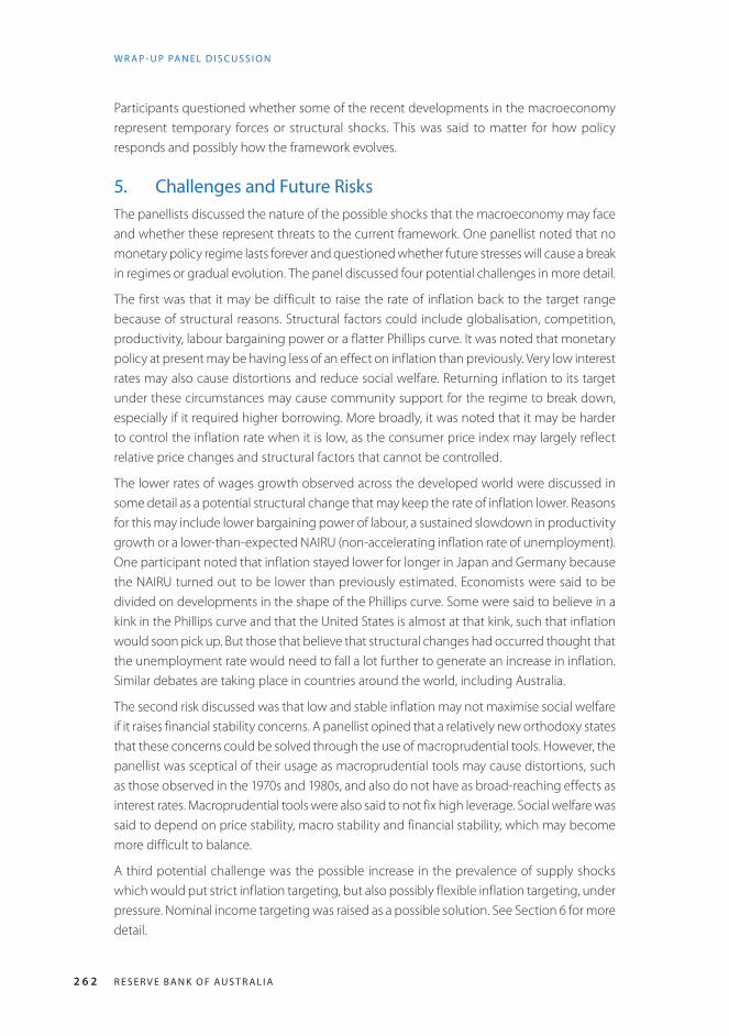
2 6 2 R E S E R V E B A N K O F A U S T R A L I A
W R A P - U P PA N E L D I S C U S S I O N
Participants questioned whether some of the recent developments in the macroeconomy represent temporary forces or structural shocks. This was said to matter for how policy responds and possibly how the framework evolves.
5. Challenges and Future RisksThe panellists discussed the nature of the possible shocks that the macroeconomy may face and whether these represent threats to the current framework. One panellist noted that no monetary policy regime lasts forever and questioned whether future stresses will cause a break in regimes or gradual evolution. The panel discussed four potential challenges in more detail.
The first was that it may be difficult to raise the rate of inflation back to the target range because of structural reasons. Structural factors could include globalisation, competition, productivity, labour bargaining power or a flatter Phillips curve. It was noted that monetary policy at present may be having less of an effect on inflation than previously. Very low interest rates may also cause distortions and reduce social welfare. Returning inflation to its target under these circumstances may cause community support for the regime to break down, especially if it required higher borrowing. More broadly, it was noted that it may be harder to control the inflation rate when it is low, as the consumer price index may largely reflect relative price changes and structural factors that cannot be controlled.
The lower rates of wages growth observed across the developed world were discussed in some detail as a potential structural change that may keep the rate of inflation lower. Reasons for this may include lower bargaining power of labour, a sustained slowdown in productivity growth or a lower-than-expected NAIRU (non-accelerating inflation rate of unemployment). One participant noted that inflation stayed lower for longer in Japan and Germany because the NAIRU turned out to be lower than previously estimated. Economists were said to be divided on developments in the shape of the Phillips curve. Some were said to believe in a kink in the Phillips curve and that the United States is almost at that kink, such that inflation would soon pick up. But those that believe that structural changes had occurred thought that the unemployment rate would need to fall a lot further to generate an increase in inflation. Similar debates are taking place in countries around the world, including Australia.
The second risk discussed was that low and stable inflation may not maximise social welfare if it raises financial stability concerns. A panellist opined that a relatively new orthodoxy states that these concerns could be solved through the use of macroprudential tools. However, the panellist was sceptical of their usage as macroprudential tools may cause distortions, such as those observed in the 1970s and 1980s, and also do not have as broad-reaching effects as interest rates. Macroprudential tools were also said to not fix high leverage. Social welfare was said to depend on price stability, macro stability and financial stability, which may become more difficult to balance.
A third potential challenge was the possible increase in the prevalence of supply shocks which would put strict inflation targeting, but also possibly flexible inflation targeting, under pressure. Nominal income targeting was raised as a possible solution. See Section 6 for more detail.

2 6 3CO N F E R E N C E V O LU M E | 2018
W R A P - U P PA N E L D I S C U S S I O N
Finally, a participant raised the risk that the national currency may be replaced with other means of payment, such as electronic tokens. This was identified as a very unlikely but plausible scenario. Nonetheless, if it occurred central banks would need to rethink how monetary policy operated and its effects.
Many of these issues were said to raise the question of how much flexibility should be built into the framework. One participant opined that the answer to this question is ‘quite a lot’ and that inflation should be allowed to remain below the target for a while, provided that it returns to target eventually. A couple of participants asked ‘what is so wrong with inflation a bit below 2 per cent?’ when balanced against risks on the financial side. Another participant asked whether this would damage credibility. One panellist argued that it would not, provided that progress was being made and that the public saw that progress was being made.
6. Alternative FrameworksMultiple participants noted that what the public care about is rising income, and that it is easier to talk to people about income than inflation. This may lend itself to a nominal income target. Several issues were raised. First, nominal income can be difficult to measure and forecast, and a nominal income target may instead be approximated by flexible inflation targeting. Second, finding a mechanism to deliver stronger income growth was noted to be difficult and generated much discussion. In Australia, many politicians and businesses have started to talk about wages growth, but it is not happening due to coordination failure, which nominal income targeting is unlikely to fix. It is possible that recent lower income growth globally may have been structural, making it difficult for monetary policy to address.
A panellist stated that it was constructive and brave to rethink the framework from a position of strength, which is consistent with the mindset of practical flexibility displayed in Australia’s current framework. Participants reflected on the session discussing alternative frameworks, concluding that while inflation targeting may have some issues, so do the alternatives. In considering nominal income targeting, a participant noted that flexible inflation targeting can approximate the nominal income targeting's policy responses without the accompanying issues and while retaining the benefits of inflation targeting.

2 6 4 R E S E R V E B A N K O F A U S T R A L I A

2 6 5CO N F E R E N C E V O L U M E | 2 017
David ArcherDavid Archer is the Head of the Central Banking Studies unit at the Bank for International Settlements (BIS). He is also the Secretary to the Central Bank Governance Group, a group of Governors that meets regularly in Basel to consider issues relating to the organisation and governance of central banks.
Prior to joining the BIS, Mr Archer was Assistant Governor at the Reserve Bank of New Zealand (RBNZ). For the last five years of his time with the RBNZ he was responsible for monetary policy analysis and advice, forecasting, and research. For the five years before that he was responsible for the RBNZ’s financial market activities, including foreign reserve management. He was a member of the RBNZ’s Governor’s Committee (the peak executive committee), Monetary Policy Committee, Financial System Oversight Committee, and Risk Management Committee.
During his time at the RBNZ, the focus, governance, organisation and management of the institution was comprehensively reshaped, with a number of innovative legislative and operational features being introduced. For a number of years in the late 1980s, Mr Archer was seconded to the International Monetary Fund, where he was a desk economist in the European Department.
Sally AuldSally Auld joined JP Morgan in September 2008 and is Chief Economist and the Head of Fixed Income and Foreign Exchange Strategy for Australia and New Zealand. Sally is responsible for views on the antipodean economic and policy outlook, as well as strategic and tactical trade recommendations in antipodean interest rate and foreign exchange markets. Her research is targeted at a variety of institutional clients, both domestic and offshore.
Previously, Sally was Co-head of Economics and Interest Rate Strategy at ANZ. Sally initially started her career as an interest rate strategist at Credit Suisse in January 2001. In 2007, Sally was a recipient of the inaugural Women’s College Young Alumna Award, given to a woman 35 years or under for her contribution to professional life or the community. Currently, Sally is a member of the Council of The Women’s College, within the University of Sydney. She also sits on the Scholarships Selection Committee for The Pinnacle Foundation.
Sally holds a Bachelor of Economics with First Class Honours and the University Medal from the University of Sydney and a DPhil in Economics from Oxford University.
Biographies of Contributors

2 6 6 R E S E R V E B A N K O F A U S T R A L I A
B I O G R A P H I E S O F CO N T R I B U T O R S
Anthony BrassilAnthony Brassil is currently a Senior Research Economist in the Economic Research Department of the Reserve Bank of Australia (RBA). During 2006–10, Anthony held several positions within the RBA’s Financial Markets Group, including a position that saw him develop the first iteration of the RBA’s bank funding cost model and a secondment to the Australian Treasury to assist the financial markets team within their International Economy Division.
Anthony’s research interests include time series econometrics, financial markets, and network analyses.
After completing a Bachelor of Economics (First Class Honours and University Medal) at the University of Sydney, Anthony joined the RBA in 2006. During 2010–12, Anthony read for an MPhil in Economics at the University of Oxford, which he completed with Distinction. He was then awarded a Clarendon Scholarship to continue at Oxford and read for a DPhil in Economics, which he completed in 2015.
Ben BroadbentDr Ben Broadbent became Deputy Governor of the Bank of England (BoE) on 1 July 2014. Prior to that, he was an external member of the Monetary Policy Committee from 1 June 2011. In addition to his membership of the Monetary Policy Committee (MPC), Financial Policy Committee and Prudential Regulation Committee, he has specific responsibility within the BoE for monetary policy, including monetary analysis and notes and shared responsibility for the BoE’s international macroeconomic analysis, strategy and engagement.
He was formerly an Economic Adviser at HM Treasury, and Assistant Professor of Economics at Columbia University from 1997 to 2000. For the decade prior to his appointment to the MPC, Dr Broadbent was Senior European Economist at Goldman Sachs, during which time he researched and wrote widely on the UK economy and monetary policy.
Ben graduated with a BA in Economics from Cambridge University in 1988, and in 1997 completed a PhD in Economics at Harvard University, where he was a Fulbright Scholar.
Thomas J CarterThomas J Carter is a principal economist in the Canadian Economic Analysis Department at the Bank of Canada. He works in the Model Development division, which is responsible for building and maintaining a suite of macroeconomic models that are used to analyse policy and prepare economic projections for Canada. His research has focused on a variety of topics in monetary and financial economics.
Born in Unionville, Ontario, Mr Carter holds a PhD in Economics from Princeton University.

2 6 7CO N F E R E N C E V O LU M E | 2018
B I O G R A P H I E S O F CO N T R I B U T O R S
Marcelle ChauvetMarcelle Chauvet is a Professor of Economics at the University of California, Riverside. Prior to that she worked at the Ministry of Industry in Brazil, where she served as a research economist and policy adviser. She has also worked as a senior economist and associate policy adviser for the Research Division at the Federal Reserve Bank of Atlanta. She has served as a consultant and visiting scholar for several international institutions and corporations, including the Central Bank of Brazil and the International Monetary Fund. Marcelle has been one of the seven members of Economic Cycle Dating Committee in Brazil since 2005. Marcelle is also the director of the Center for Research on Economic and Financial Cycles.
Marcelle Chauvet’s research focuses on macroeconomics and econometrics, and she is particularly interested in measuring and predicting business cycles and financial markets, and in modelling and predicting the interactions between monetary policy, financial markets, and the real economy. Marcelle has an extensive list of publications in major academic journals and is serving or has served on the editorial board of several journals. She has recently been appointed as one of the Fellows of the International Association for Applied Econometrics, and serves as one of its directors.
Marcelle received her BSc in Economics and MSc in Economic Policy from the University of Brasilia, and an MA and PhD in Economics from the University of Pennsylvania.
Jon CheshireJon Cheshire is currently a senior manager working for the Reserve Bank of Australia's (RBA’s) Payments Policy Department, overseeing a team that supervises the operations of clearing and settlement facilities such as LCH (European-based clearing house) and CME (Chicago Mercantile Exchange). Prior to this, he worked in the RBA’s Financial Markets Group, undertaking operational roles that involved the deployment of RBA reserves through events such as the Asian financial crisis (1997), US dollar bubble (2000), global financial crisis (2007–09) and European crises (2009–14). He prepared a review of the RBA’s Reserve Management Framework in 2010, which forms the basis of the current operations. Whilst in Financial Markets Group he undertook regular work in assessing financial conditions in currency, securities and intermediated markets. More recently the focus of this work has been on the impact of global post-crisis reforms and other policy changes on financial markets and banks, and competition in the banking system.
Jon graduated with a BA in Economics and Econometrics (First Class Honours) from the Australian National University.

2 6 8 R E S E R V E B A N K O F A U S T R A L I A
B I O G R A P H I E S O F CO N T R I B U T O R S
Guy DebelleGuy Debelle commenced as Deputy Governor of the Reserve Bank of Australia (RBA) on 18 September 2016. He is Deputy Chair of the Reserve Bank Board and Chair of the RBA's Risk Management Committee. Guy is a former chair of the Australian Foreign Exchange Committee and also chaired the BIS Foreign Exchange Working Group responsible for the development of the Global Code of Conduct for the Foreign Exchange Market.
Prior to his current role, Guy was the Assistant Governor, Financial Markets.
Guy also worked at the International Monetary Fund, Bank for International Settlements, Australian Treasury and as a visiting professor in economics at the Massachusetts Institute of Technology (MIT).
He graduated from the University of Adelaide with an honours degree in economics and gained his PhD in Economics at MIT under Stanley Fischer and Rudi Dornbusch.
Guy is a signatory to The Banking and Finance Oath.
Stephen Grenville AODr Grenville is a Non-resident Fellow at the Lowy Institute. He works as a consultant on financial sector issues in East Asia. Between 1982 and 2001 he worked at the Reserve Bank of Australia, for the last five years as Deputy Governor and as a member of the Reserve Bank Board. Before that, Dr Grenville was with the Organisation for Economic Co-operation and Development in Paris, the International Monetary Fund in Jakarta, the Australian National University and the Department of Foreign Affairs.
Dr Grenville received his PhD from the Australian National University.
Luke HartiganLuke Hartigan is a Research Economist in the Economic Research Department at the Reserve Bank of Australia (RBA). Before joining the RBA, Luke worked in financial markets in the private sector as an economist and analyst at HSBC and the Commonwealth Bank of Australia.
His research interests focus on time series econometrics, specifically in relation to methods for understanding and describing business cycle dynamics. Luke has published research articles on long-run covariance matrix estimation as well as on topics related to real asset markets.
He holds a Bachelor of Economics (Hons) from Macquarie University and a PhD in Economics from the University of New South Wales.
Jessica IrvineJessica Irvine is one of Australia’s leading economic commentators, notable for her ability to explain complex economic ideas in an easy to understand and often amusing way.
She has an honours degree in Economics (Social Sciences) from the University of Sydney and began her career working at the Australian Competition and Consumer Commission.

2 6 9CO N F E R E N C E V O LU M E | 2018
B I O G R A P H I E S O F CO N T R I B U T O R S
Today, she is a senior economics writer for The Sydney Morning Herald and The Age newspapers, which she joined in 2005. In 2006, she was appointed the papers’ Economics Correspondent in the federal press gallery in Canberra, before returning to Sydney as a senior editorial writer and columnist.
Jessica has also worked for News Corp Australia, where for two years she was National Economics Editor of all metropolitan mastheads, including Sydney’s The Daily Telegraph and Melbourne’s The Herald Sun.
She is a regular commentator on television and radio and the author of two books, Zombies, Bananas and Why There Are No Economists in Heaven and The Bottom Line Diet.
Andrew T LevinAndrew Levin is a Professor of Economics at Dartmouth College. He worked as an economist at the Federal Reserve Board for two decades, including two years as a Special Adviser to then Chairman Ben Bernanke and then Vice Chair Janet Yellen on monetary policy strategy and communications (2010–12). Dr Levin subsequently served as an Adviser in the Research Department at the International Monetary Fund, and he joined the Dartmouth faculty in July 2015. Dr Levin has had extensive interactions with many other central banks across the globe: He served as a consultant to the European Central Bank’s Inflation Persistence Network and to the Bank of Canada’s external review of research, as a co-editor of the International Journal of Central Banking, he has been a Visiting Scholar at the Bank of Japan and De Nederlandsche Bank, and he has provided technical assistance to the national banks of Albania and Macedonia, and most recently, the Bank of Ghana.
His research has been published in leading economic journals, including The American Economic Review, the Journal of the European Economic Association, the Journal of Monetary Economics, and the Journal of Econometrics.
Dr Levin received his PhD in Economics from Stanford University in 1989.
Philip LowePhilip Lowe is an Australian economist who is the current Governor of the Reserve Bank of Australia (RBA), having succeeded Glenn Stevens on 18 September 2016. He was previously Deputy Governor from February 2012 to September 2016.
Philip attended St Michael's High School and Trinity Senior High School in Wagga Wagga, New South Wales. He later moved to Sydney and was hired by the RBA straight out of high school. He was initially employed as a clerical worker in 1980, while completing his undergraduate commerce degree at the University of New South Wales by attending night classes. He was awarded first-class honours and the University Medal on his graduation in 1985. He later completed a doctorate at the Massachusetts Institute of Technology (MIT), with Paul Krugman as his adviser.

2 7 0 R E S E R V E B A N K O F A U S T R A L I A
B I O G R A P H I E S O F CO N T R I B U T O R S
In 1997, Philip was appointed Head of the Economic Research Department. He later headed the RBA’s Financial Stability Department (from 1999 to 2000), the Domestic Markets Department (from 2002 to 2003), and the Economic Analysis Department (from 2003 to 2004). From 2000 to 2002, he worked at the Bank for International Settlements in Switzerland, as Head of the Financial Institutions and Infrastructure Division. He was made Assistant Governor (Financial System) at the RBA in 2004 and Assistant Governor (Economic) in 2009, eventually becoming Deputy Governor in 2012. In May 2016, the Hon Scott Morrison MP (then Australian Treasurer) announced that he would succeed Glenn Stevens as the Governor of the RBA at the end of his term in September 2016.
Philip is Chair of the Reserve Bank Board, the Payments System Board and the Council of Financial Regulators, and a member of the Financial Stability Board. He is Chair of the Financial Markets Foundation for Children and a Director of The Anika Foundation, and a signatory to The Banking and Finance Oath. He is also Chair of the Committee on the Global Financial System of the Bank for International Settlements.
John McDermottJohn McDermott is the Assistant Governor and Head of Economics at the Reserve Bank of New Zealand. He is responsible for advising the Governor on the economic outlook and the management of monetary policy. His current research interests include business cycles and commodity prices.
John has held posts at Victoria University of Wellington, the National Bank of New Zealand and the International Monetary Fund, where he was also a visiting scholar, and taught at the World Bank Institute.
He gained a BSc and MCom from the University of Auckland and a PhD in Economics from Yale University.
Warwick J McKibbin AOProfessor Warwick McKibbin, AO is Professor of Public Policy and Director of the Centre for Applied Macroeconomic Analysis (CAMA) in the Crawford School of Public Policy at the Australian National University (ANU). He is also an ANU Public Policy Fellow; a Fellow of the Australian Academy of Social Sciences; a Distinguished Fellow of the Asia and Pacific Policy Society; a non-resident Senior Fellow at the Brookings Institution in Washington DC (where he is co-director of the Climate and Energy Economics Project) and President of McKibbin Software Group Inc. Professor McKibbin was foundation Director of the ANU Centre for Applied Macroeconomic Analysis and foundation Director of the ANU Research School of Economics. He was also a Professorial Fellow at the Lowy Institute for International Policy for a decade from 2003 where he was involved in its design and development. Professor McKibbin served for a decade on the Board of the Reserve Bank of Australia until July 2011. He has also served as a member of the Australian Prime Minister’s Science, Engineering and Innovation

2 7 1CO N F E R E N C E V O LU M E | 2018
B I O G R A P H I E S O F CO N T R I B U T O R S
Council, and on the Australian Prime Minister’s Taskforce on Uranium Mining Processing and Nuclear Energy in Australia.
Professor McKibbin is internationally renowned for his contributions to global economic modelling. Professor McKibbin has published more than 200 academic papers as well as being a regular commentator in the popular press. He has authored/edited five books including Climate Change Policy after Kyoto: A Blueprint for a Realistic Approach with Professor Peter Wilcoxen of Syracuse University. He has been a consultant for many international agencies and a range of governments on issues of macroeconomic policy, international trade and finance, greenhouse policy issues, global demographic change and the economic cost of pandemics. His research project entitled ‘Macroeconomics: Climate Change & Energy’ focuses on rapid global economic growth, particularly in China and India, and its important implications for global energy use, as well as causing a rapid rise in greenhouse gas emissions with implication for climate change. This program focuses on the importance of energy use and climate change, as well as the associated policy responses on the macroeconomy.
Professor McKibbin received his BCom (First Class Honours) and University Medal from University of NSW (1980) and his AM (1984) and a PhD (1986) from Harvard University. He was awarded the Centenary medal in 2003 ‘For Service to Australian Society through Economic Policy and Tertiary Education’ and made an Officer of the Order of Australia in 2016.
Rhys MendesRhys Mendes was appointed Managing Director of the International Economic Analysis Department (INT) at the Bank of Canada (BoC), effective 1 November 2017. In this capacity, he is responsible for the management and strategic direction of the department, which includes providing rigorous and timely analysis of global economic conditions, as well as advice on the conduct of monetary policy and international policy issues.
Mr Mendes joined the BoC in 2004. Four years later, he was appointed Assistant Chief of the Canadian Economic Analysis Department (CEA) where he led the team responsible for the development of ToTEM II, an updated version of the BoC’s main macroeconomic model. In 2011, he became Director of Policy Analysis in INT, where he represented Canada at G20 meetings and other international forums. He was then appointed Deputy Chief of CEA in 2013. Prior to his current role, Mr Mendes was Managing Director of Economic and Financial Research, working with the analytic departments to develop and execute a leading-edge research work plan to support all of the BoC’s policy functions.
Throughout his career, Mr Mendes has contributed to the BoC’s research on the monetary policy framework and is regularly consulted by foreign central banks on framework design issues. In March 2006, Mr Mendes was seconded to the International Monetary Fund as an advisor to the Indonesian central bank.
Born in Richmond Hill, Ontario, Mr Mendes holds a PhD in economics from the University of Toronto.

2 7 2 R E S E R V E B A N K O F A U S T R A L I A
B I O G R A P H I E S O F CO N T R I B U T O R S
James MorleyJames Morley was appointed as Professor of Macroeconomics at the University of Sydney in 2017. He previously held positions at Washington University in St Louis and the University of NSW, most recently as Associate Dean (Research) of the UNSW Business School from 2014 to 2017. His research focuses on the empirical analysis of business cycles, stabilisation policy, and sources of persistent changes in macroeconomic and financial conditions.
He is an Academic Fellow of the Reserve Bank of New Zealand and has been a Visiting Scholar at various policy institutions worldwide, including the Bank of Canada, Bank Negara Malaysia, and the Bank for International Settlements. He is a former President of the Society for Nonlinear Dynamics and Econometrics and is currently co-editor of The Economic Record.
He received his PhD from the University of Washington in 1999.
Joseph MuscatelloJoseph Muscatello is an analyst in the Risk and Compliance Department at the Reserve Bank of Australia. Prior to this, he was an analyst in the Domestic Markets Department.
He holds a Bachelor of Commerce (Hons) from the University of Melbourne.
Augustus J PantonAugustus is a PhD scholar (economics) in the Crawford School of Public Policy at the Australian National University (ANU) under the supervision of Warwick McKibbin. He is a Research Assistant at the ANU Centre for Applied Macroeconomic Analysis (CAMA), a Teaching Assistant at the ANU Research School of Economics and a Doctoral Research Fellow with the ARC Centre of Excellence in Population Ageing Research (CEPAR). His PhD research is focused on the monetary policy implications of climate change and climate policy. Prior to joining the ANU, Augustus worked as an economist in the Research, Policy & Planning Department at the Central Bank of Liberia. Before then, he worked with the Ministry of Commerce & Industry (Liberia) as Economist and as Principal Risk Management Officer at the Ministry of Finance (Liberia). He has provided consulting services, at various times, for the International Finance Corporation/World Bank, the Brookings Institution and the ECOWAS (Economic Community of West African States) Commission.
Augustus holds an Honours degree in Accounting and Economics (summa cum laude/University Medal) from the University of Liberia and a Masters in International Economics from the University of Queensland.
Adam PosenAdam Posen has been President of the Peterson Institute for International Economics since January 2013, after first joining in July 1997. Over his career, he has written about the financial and economic challenges faced by the European Union following the adoption of the euro, the lasting impact of Japan's economic crisis of the 1990s, and monetary and fiscal policies in the G7. While at the Federal Reserve Bank of New York (1994–97), he co-authored

2 7 3CO N F E R E N C E V O LU M E | 2018
B I O G R A P H I E S O F CO N T R I B U T O R S
Inflation Targeting: Lessons from the International Experience with Ben Bernanke and others. He was one of the first scholars to seriously address the political foundations of central bank independence.
In September 2009, Dr Posen was appointed by the UK Chancellor of the Exchequer to serve a three-year term as an External Voting Member of the Bank of England's rate-setting Monetary Policy Committee (MPC). Leading up to the successful London G20 summit of 2009 during the global financial crisis, he consulted for the UK Cabinet Office. In addition to his leadership at the Institute, Dr Posen advises the US Congressional Budget Office, and he has been a visiting scholar at a number of G20 central banks, as well as a consultant to the International Monetary Fund and numerous US government departments.
Dr Posen has been the recipient of major grants and research fellowships from the American Academy in Berlin, the Bank of England, the Brookings Institution, the European Commission, the Ford Foundation, the Sloan Foundation, and the US National Science Foundation. He received his BA and PhD from Harvard University.
Bruce PrestonBruce Preston, Professor of Economics, University Of Melbourne, is one of Australia’s most outstanding macroeconomists. He held the Richard Snape Chair in Business and Economics at Monash University; is an Australian Research Council Future Fellow; Senior Research Adviser to the Reserve Bank of Australia and former faculty member at Columbia University.
His main interests concern monetary policy and the formation of expectations. A specific focus of his research explores empirical evidence supporting different theories of belief formation and also how ‘near-rational expectations’ potentially constrain what can be achieved by macroeconomic policy.
His recent work has been published in prestigious journals such as The American Economic Review, Journal of Monetary Economics, the Journal of International Economics, the Journal of the European Economics Association, and the Journal of Econometrics.
Bruce holds a PhD in Economics from Princeton University.
Lawrence L SchembriLawrence L Schembri was appointed Deputy Governor of the Bank of Canada (BoC) in 2013, serving as one of two deputy governors responsible for overseeing the BoC’s analysis and activities to promote a stable and efficient financial system. In 2016, he became responsible for overseeing the BoC’s analysis of domestic economic developments. As a member of the BoC’s Governing Council, he shares responsibility for decisions with respect to monetary policy and financial system stability, and for setting the strategic direction of the BoC.
Mr Schembri joined the BoC in 1997 as a visiting Research Advisor in what is now the International Economic Analysis Department. In 2001, he was appointed Research Director in the same department and became Chief of the department in 2005. In 2010, he was

2 7 4 R E S E R V E B A N K O F A U S T R A L I A
B I O G R A P H I E S O F CO N T R I B U T O R S
appointed Advisor to the Governor, with responsibilities for financial stability analysis and co-ordinating the BoC’s contribution to the Financial Stability Board. His published research has focused on exchange rate and monetary theory and policy in open economies, the international monetary system and financial stability.
Born in Toronto, Ontario, Mr Schembri received a Bachelor of Commerce degree from the University of Toronto in 1979, an MSc in Economics from the London School of Economics and Political Science in 1980, and a PhD in Economics from the Massachusetts Institute of Technology in 1985. After completing his PhD, Mr Schembri was an assistant professor and, later, associate professor of economics at Carleton University until 2001.
Sayuri ShiraiDr Sayuri Shirai is currently a Professor of Keio University and also a Visiting Scholar at the Asian Development Bank Institute. She was a Member of the Policy Board of the Bank of Japan (BOJ) from April 2011 to March 2016, responsible for making policy decisions. She supported the BOJ’s quantitative and qualitative monetary easing (QQE) in 2013 and QQE expansion in 2014, but voted against the negative interest rate policy in January 2016. During this term, she made 22 official speeches at various central banks (including the Federal Reserve Board (FRB), European Central Bank (ECB), and Bank of England) and had extensive discussions with many central bankers. Speeches were also delivered at the International Monetary Fund (IMF), European Commission, Bruegel, and academic conferences.
She worked as Professor of Economics at Keio University before becoming a Board Member at BOJ. She also taught at Science-Po in France in 2007–08. She was formerly an economist at the IMF (1993–98). She is the author of numerous articles in professional journals and has published many books on China’s exchange rate system, Japan’s macroeconomic policy, IMF policy, European debt crisis, etc. The most recent book (in Japanese) published in August 2016 was about the monetary policies of BOJ, ECB, and FRB (translated title: Unwinding Super-Easy Monetary Policy). She published an e-book entitled Mission Incomplete – Reflating Japan’s Economy in English in February 2017.
She provides commentaries for Reuters, CNBC, Bloomberg, BBC, and many Japanese TV programs and newspapers on Japanese economy and monetary policy.
She graduated from Keio University and holds a PhD in Economics from Columbia University.
John SimonJohn Simon is Head of Economic Research Department at the Reserve Bank of Australia (RBA). Before this he undertook a three-year secondment to the International Monetary Fund, where he worked on the World Economic Outlook. He was previously the Chief Manager in the Payments Policy Department of the RBA. He has published numerous articles on macroeconomics, including on the ‘Great Moderation’, monetary policy and payments policy.
John holds a Bachelor of Economics (Hons) and a Bachelor of Science from the Australian National University and a PhD from the Massachusetts Institute of Technology.

2 7 5CO N F E R E N C E V O LU M E | 2018
B I O G R A P H I E S O F CO N T R I B U T O R S
Aarti SinghAarti Singh is a senior lecturer at the University of Sydney and joined the School of Economics in 2008 after completing her PhD in Economics from Washington University in St Louis. Her main research interests are in macroeconomics and monetary economics. Aarti has published her research in journals such as the Journal of Monetary Economics, International Economic Review, Journal of Money, Credit and Banking among others.
Maxwell SuttonMaxwell Sutton is a Research Economist in the Economic Research Department at the Reserve Bank of Australia. Prior to this, he was an analyst in Payments Policy Department. His research has focused on topics including monetary economics and time series econometrics.
He holds a Bachelor of Commerce (Hons) with the University Medal and a Bachelor of Science from the University of Sydney.
Rebecca WilliamsRebecca Williams is the manager of the Policy Analysis team in the Economics department of the Reserve Bank of New Zealand (RBNZ). Since joining the RBNZ in 2010, she has also spent time in the Research and Forecasting teams, including a period operating the RBNZ’s core forecasting model. Her recent research interests include business cycles, neutral interest rates, and the global dairy market.
Rebecca holds a BCom (Hons) in Economics and a BA in History from the University of Canterbury.

2 7 6 R E S E R V E B A N K O F A U S T R A L I A

2 7 7CO N F E R E N C E V O L U M E | 2 018
List of Conference Participants
Ivailo Arsov Reserve Bank of Australia
Sally Auld JP Morgan Australia
Benjamin Beckers Reserve Bank of Australia
Michelle Bergmann Reserve Bank of Australia
Leon Berkelmans Reserve Bank of Australia
Paul Bloxham HSBC Bank Australia
Anthony Brassil Reserve Bank of Australia
Ben Broadbent Bank of England
Sean Carmody Australian Prudential Regulation Authority
Mark Caputo Reserve Bank of Australia
Mary Cavar Productivity Commission
Mark Chambers Reserve Bank of Australia
Iris Chan Reserve Bank of Australia
Marcelle Chauvet University of California, Riverside
Jon Cheshire Reserve Bank of Australia
Selwyn Cornish Reserve Bank of Australia
Mark Crosby Monash University
John Daley Grattan Institute
Guy Debelle Reserve Bank of Australia
Piti Disyatat Bank of Thailand
Corrine Dobson Reserve Bank of Australia
Simon Duggan Department of Prime Minister and Cabinet
Luci Ellis Reserve Bank of Australia
Kathryn Fagg Reserve Bank of Australia
Renee Fry-McKibbin Australian National University
Nick Garvin Reserve Bank of Australia
Christopher Gibbs University of New South Wales
Stephen Grenville Lowy Institute
Luke Hartigan Reserve Bank of Australia
Timo Henkel Australian National University
Keene Ho Reserve Bank of Australia
John Hutchinson European Central Bank
Jessica Irvine Sydney Morning Herald
Jarkko Jääskelä Reserve Bank of Australia

2 7 8 R E S E R V E B A N K O F A U S T R A L I A
L I S T O F CO N F E R E N C E PA R T I C I PA N T S
David Jacobs Reserve Bank of Australia
Bradley Jones Reserve Bank of Australia
Jonathan Kearns Reserve Bank of Australia
Mariano Kulish University of Sydney
David Lancaster Reserve Bank of Australia
Andrew Levin Dartmouth College
Guay Lim University of Melbourne
Philip Lowe Reserve Bank of Australia
Warwick McKibbin Australian National University
Rhys Mendes Bank of Canada
James Morley University of Sydney
Gabriela Nodari Reserve Bank of Australia
David Orsmond Reserve Bank of Australia
Augustus Panton Australian National University
Lara Pendle Reserve Bank of Australia
Michael Plumb Reserve Bank of Australia
Adam Posen Peterson Institute for International Economics
Bruce Preston University of Melbourne
Ewan Rankin Reserve Bank of Australia
Nigel Ray Australian Treasury
Øistein Røisland Norges Bank
Tom Rosewall Reserve Bank of Australia
Jeffrey Sheen Macquarie University
Sayuri Shirai Keio University
Shigenori Shiratsuka Bank of Japan
John Simon Reserve Bank of Australia
Aarti Singh University of Sydney
Maxwell Sutton Reserve Bank of Australia
Dmitry Titkov Reserve Bank of Australia
Christian Vallence Reserve Bank of Australia
Rebecca Williams Reserve Bank of New Zealand
Calvin Yap Reserve Bank of Australia
James Yetman Bank for International Settlements
AcknowledgementThe editors are grateful to Michelle Bergmann, Alexandra Brown, Mark Caputo, Blair Chapman, Corrine Dobson, Paula Drew, Katie Fitzpatrick, Phillipa Kelly, David Lancaster, Christian Maruthiah, Tams Pretty, Russell Thomson and the staff of Secretary’s Department for much help in organising the conference and producing this volume.

2 7 9CO N F E R E N C E V O L U M E | 2 018
Other Volumes in this Series
2017 Monetary Policy and Financial Stability in a World of Low Interest Rates
2016 Structural Change in China: Implications for Australia and the World
2015 Small Business Conditions and Finance
2014 Financial Flows and Infrastructure Financing
2013 Liquidity and Funding Markets
2012 Property Markets and Financial Stability
2011 The Australian Economy in the 2000s
2010 Reserve Bank of Australia 50th Anniversary Symposium
2009 Inflation in an Era of Relative Price Shocks
2008 Lessons from the Financial Turmoil of 2007 and 2008
2007 The Structure and Resilience of the Financial System
2006 Demography and Financial Markets
2005 The Changing Nature of the Business Cycle
2004 The Future of Inflation Targeting
2003 Asset Prices and Monetary Policy
2002 Globalisation, Living Standards and Inequality
2001 Future Directions for Monetary Policies in East Asia
2000 The Australian Economy in the 1990s
1999 Capital Flows and the International Financial System
1998 Unemployment and the Australian Labour Market
1997 Monetary Policy and Inflation Targeting
1996 The Future of the Financial System
1995 Productivity and Growth
1994 International Integration of the Australian Economy
1993 The Exchange Rate, International Trade and the Balance of Payments
1992 Inflation Disinflation and Monetary Policy
1991 The Deregulation of Financial Intermediaries
1990 The Australian Macro-Economy in the 1980s
1989 Studies in Money and Credit

2 8 0 R E S E R V E B A N K O F A U S T R A L I A

SP
INE
SP
INE
Proceedings of a Conference 2018Central Bank Fram
eworks: Evolution or Revolution?
Central Bank Frameworks: Evolution or Revolution?
2018