Working Paper 95-15 Departamento de Economía Economics Series 10 Universidad Carlos 111 de Madrid April 1995 Calle Madrid, 126

28903 Getafe (Spain) Fax (341) 624-9875

CAPACITY UTILIZATION DYNAMICS AND MARKET POWER

Jean-Fran~ois Fagnart, Omar Licandro and Henri Sneessens'"

Abstract _

In an intertemporal general equilibrium model with imperfect competition, we settle a relationship between factor utilization and markups, via the eifect of capacity utilization rate changes on firms' market power when the demand for goods is uncertain. When competition is imperfect, the existence of capacity constraints introduces a distinction between demand and sales price elasticities. At given demand price elasticity, the price elasticity of sales will be smaller the larger the aggregate capacity utilization rateo In such a framework, capacity utilization aifects the propagation mechanism of exogenous disturbances in two ways. The first eifect is similar to the eifect that bottlenecks and stockouts would have in a perfectly competitive setup; the second eifect is related to imperfect competition and works through market power and optimal markup changes. We study these interactions and their implications for the dynamic behavior of sorne key macro variables in response to various "structural" changes. We show that the same shock can have quite diiferent short run eifects depending on the characteristics of the initial stationary state (low or high capacity utilization rate).

Key Words Business Cycles, Capacity Utilization, Market Power, Markup Rate

'" Jean-Fran<;ois Fagnart and Henri Sneessens, Université Catholique de Louvain, Bel­gium. Ornar Licandro, FEDEA and Universidad Carlos 111 de Madrid. This paper is a revised version of "Capacity utilization Dynamics in an Intertemporal General Equi­librium Model" presented at the First International Conference on Economic Theory at Universidad Carlos III de Madrid, July 4-9 1994. We thank Raouf Boucekkine for his most helpful advice on the numerical analysis of the model and Franck Portier for his comments on an earlier version. Financial support of the Ministerio de Educación y Ciencia (CE92­0017) and the "Projet d'action concertée" 93/98-162 of the Ministery of the Scientific Research of the Belgian French Speaking Community is gratefully acknowledged.

¡

11-­

1

1. Introduction

The analysis of the determinants of factor utilization and markup rate variations is currently at hart of several research programs in macroeconomics. It is now recognized that factor utilization and markup rate variations may playa crucial role in explaining business cycle fiuctuations, either by contributing to generate endogenous fiuctuations 1

or by complexifying the economic mechanisms that propagate through the economy the effects of exogenous shocks. Our contribution is based on this latter point of view. The literature on propagation mechanisms has usually discussed the effects of factor uti­lization and of markup rate changes separately. Factor utilization rate changes have received much attention in purely competitive real business cycle models, where they contaminate the so-called Solow residual and make it an inadequate measure of ex­ogenous technological shocks2. Business cycle models with imperfect competition have instead emphasized the effects of markup rate variations, especially counter-cyclical variations generated by exogenous demand shocks3. We emphasize in this paper the relationship between the two phenomena (factor utilization and markups), via the ef­fect of capacity utilization rate changes on firms'market power when the demand for goods is uncertain.

In most existing intratemporal models with variable capacity utilization, the uti­lization rate variable is introduced in the firm's intertemporal decision problem via its impact on capital depreciation4

• In this setup, the equilibrium capacity utilization rate is such that the marginal revenue that could be obtained from a more intensive capac­ity utilization and additional sales is exactly compensated by the marginal cost coming from faster capital depreciation. Although there may be such' a link between capital utilization intensity and physical depreciation, we believe that the latter is unlikely to be the main driving force ~ehind actual capacity utilization rate fiuctuations, as reported in business surveys. For this reason, we chose to rely on a different represen­tation, wherein capacity utilization rate changes follow from microeconomic demand uncertainty and (temporary) technological rigidities (which imply that firms prefer capacity underutilization to costly capital-Iabour ratio changes). Firms may then be either sales- or capacity-constrained, the proportion of firms in each case infiuencing the aggregate capacity utilization rateo In an imperfectly competitive setup, capacity constraints introduce a distinction between dema:nd and sales price elasticities and for this reason infiuences optimal markup values. At given demand price elasticity, the price elasticity of sales will be smaller the larger the aggregate capacity utilization rateo In other words, the fact that sorne firms are producing at full capacity and unable to serve any extra demand increases the market power of firms with spare productive ca­pacities. In such a setup, capacity constraints affect the propagation mechanism in two

lSee for instance the model developped in d'Aspremont, Dos Santos, Gerard-Varet (1994a), where the variability of markup rates leads to the possibility of endogenous business cycles. In de la Croix­Licandro (1994), factor underutilization may be a source of endogenous fluctuations.

20n labour hoarding, see e.g. Burnside, Eichenbaum and Rebelo, (1993)). On capacity utilization, see e.g. Greenwood, Hercovitz and Huffman (1988), Burnside and Eichenbaum (1994)) or Cooley, Hansen and Prescott (1994))·

3See a.o. Rotemberg-Woodford (1991), (1992) and (1993), Gali (1994)· 4 An exception is Cooley et alii (1994) who propose a modelisation clase to ours.

2

ways. The first effect is similar to the effect that bottlenecks and stockouts would have in a perfectly competitive setup: the second effect is related to imperfect competition and works through market power and optimal markup changes.

Constructing a model with such features in an intertemporal setup raises different difficulties. First, we do want a model wherein the diversity of situations across firms is recognized and wherein the underutilization of capital at the macro level does not imply identical utilization rates at the micro leve!. Second, if capacity constraints can be binding, we must specify a rationing scheme. obtain effective demands and supplies and take into account spillover effects. It is of course impossible to tack1e all these issues at once within a full-fledged stochastic model. Our primary objective is to build a model which remains tractable and at the same time flexible enough to be later extended. Our formulation is based on earlier work on macroeconomic models with capacity constraints and imperfeclty competitive price setting (see Sneessens (1987), and subsequent work by a.o. Licandro (1992), de la Croix and Fagnart (1993))5.

The key elements of our stylized intertemporal model can be briefly surnmarized as follows. The model relies on a particular market organisation with two sectors. the intermediate and the final goods sectors respectively. In the intermediate goods sector, the firm uses the primary inputs to produce the intermediate goods. These intermediate goods are then sold to firms in the final goods sectoL which combine them to produce a final good that can be either consumed or invested6

. We assume perfect competition on the final goods market, and monopolistic competition on the intermediate goods one where product differentiation gives sorne monopoly power to the individual firmo The latter announces her selling price on the basis of (rational) expectations, before knowing the exact value of the demand for her production. This structure implies that an intermediate goods firm can be either sales- or capacity-constrained; it also allows different firms to face different quantity constraints. At the aggregate level, the productive capacity of the economy will be systematically underutilised. It is worth noting that the price pre-setting assumption is not necessary for aggregate capacity underutilization. As we will show, in an imperfect competion setup, it suffices that the productive capacity be pre-determined. However, the price pre-setting assumption is not unrealistic and has the advantage of giving us a symmetric equilibrium in prices.

The rest of the paper is organized as follows. Section 2 is devoted to the descrip­tion of individual behaviours. Section 3 characterizes the general equilibrium of this economy and analyzes the properties of its stationary state. Section 4 illustrates the dynamic properties of the model with numerical examples. Section 5 concludes.

5These models have been used extensively to study the causes of unemployrnent persistence in Europe (see a.o. Sneessens-Dreze (1986) and Drez~Bean (1990)). Our objective in this paper is to show that they also provide an interesting framework for a better understanding of the determinants of business cycle fluctuations.

6AE, in Romer (1987), we interpret an aggregator index a la "Dixit-Stiglitz" as the production function used by the firms in the final sector. In the present model, it may also be interesting to consider the final good producing firms as a distribution network that makes the (differentiated) goods available to final consumers under the form of a basket of goods, the precise composition -and price- of which may depend on the availability of the basic ingredients. As a consequence, consumers do not feel quantity constrained since the distribution firms keep on proposing a basket of goods which satisfies their needs.

. ir.--.-·..-.----------------------------------­

3

2. Behaviours

2.1 Consumers

We suppose an infinitely lived consumer whose intertemporal preferences with respect to consumption and labour are represented by a time separable utility function. The optimal time profiles of consumptions {Ct}{t=l.... ,oo} and labour supplies {Lt}{t=I,...,oo}

are given by the solution of the following problem:

max L00

[3t U (Ct,Lt) {Cc,Lt} t=1

subject to the wealth constraint

At = At- 1 (1 + Tt) + WtLt - Ct - Tt \f t. (1)

where /3 is a constant subjective discount rate; At and Tt denote respectively the real financial wealth -with the price of consumption as numeraire- and a lump-sum tax. Function U is strictly increasing in Ct , decreasing in L t , twice differentiable and concave. There is no aggregate uncertainty in the model and the sequence of equilibrium real wages and rates of return {Wtl Td{t=l.. ..,oo} is perfectly forecast by the consumero Aa is given.

Optimal consumption demand and labour supply profiles must satisfy the following two first-order conditions at any time t = 1. ... , oc

U1(Ct, Lt) - U1(CH1 ' Lt+¡) /3 (1 + Tt+l) (2)

Wt -U2 (Ct , L t )

U1(Ct , L t )' (3)

The transversality condition on wealth must also be satisfied:

lim [3t U1 (Ct, Lt) At t-oo

= O

The interpretation of these standard conditions is fairly straightforward.

2.2 Product firms

The homogeneous final good is produced by the so-called product firms. It is sold on a competitive market, and can be used either as a consumption or an investment good. All firms use the same production technology. There is no fixed input, which implies that the optimization programme of firms remains purely static. We have however to take into account the effect of input supply quantity constraints.

The production technology of each product firm is represented by a constant return to scale CES production function defined over a continuum of variable inputs, each one denoted by y and indexed by j, with j belonging to the interval [0,1]. More formally, the representative product firm's output (denoted Y) is obtained from the following production function:

[1 .1 .6-1 ] ~ ~ = [ Jo v{~ '!It -rdj with () > 1 (4)

4

Each parameter v1 2:: O is drawn from an i.i.d. stochastic process with unit mean and distribution function F(v). The total supply of input j is limited to an amount bt ki-l (see below), equal to the predetermined productive capacity of the corresponding input supplying firm, i.e., the available capital stock times its (here non stochastic) productivity. H we asswne a uniform non-stochastic rationing scheme and use the final good as nwneraire, we can write the optimization programme of the representative firm as:

max ~ - rol pf yf dj {yn Jo

subject to the supply constraints

yf ::s bt ~-l 'Vj,

\\iith ~ defined in (4). It is well-known1 that with deterministic quantity constraints and a uniform rationing scheme. effective demands are not well-defined, although re­alized transactions are. The latter can easily be shown to be

, {(Pl) -6 ~ v{ if v{::s v{ yf= (5)

bt ~-l if v{ > vl where the critical value of the productivity parameter, vi, is such that the demand for input j at price Pl is equal to the productive capacity of supplier j, Le.,

_j bt ~-l 'V j. (6)Vt = (Pl) -6 ~'

For notational convenience, let us define d{ as follows:

di = (pO -6 ~ v{

that is, di represents the demand for input j that would be expressed to firm j if there were no shortage of that input8

.

Because all the product firms are identical and face the same technological and quan­tity constraints, we shall in the sequel use the same symbol Y to represent both the individual and the aggregate production of final goods. The aggregate production of final goods can be obtained by substituting (5) into (4). Note that the marginal pro­ductivity of a supply-constrained input remains larger than its marginal costo With constant returns to scale, this implies positive profits despite the perfect competition assumption9

.

7See for instance Green (1980), Svensson (1980). 8The variable di actually corresponds to the so-called Benassy (1975) effective demand concept,

as opposed to the Dreze (1975) effective demand concepto The choice between the two concepts is in our case unconsequential. It has no impact whatsoever on the determination of input prices nor of any other variable,

9Indeed, by using Euler theorem, one obtains y; = 101 ~ y1 dj > 101 p1 Y!. dj.

5�

2.3 Input firms

2.3.1 Individual Firm's Problem

Each input j is produced by a single finn (henceforth input finn). In order to obtain a simple productive capacity concept, we assume that the production of each interme­diate good combines labour and capital through a Leontief technology with technical coefficients equal to at and bt respectively. The input firm's productive capacity is predetermined and equal to the capital stock IG-l times its productivity bt . Labour is supposed to be a purely variable input. It is bought on a competitive market and can be adjusted instantaneously to its optimallevel. From equation (5), the latter is given by

, y¡ 1 {' '}ti = - = - min di, btJc:-l at at

In other words, as long as the productive capacity is not fully utilised, the firm adjusts her production plan to her customers' orders.

We assume that the price decision has to be taken before the realized values of the stochastic terms vl are known. The exact position of the demand function is thus not known with certainty and the price and investment decisions have to be taken with respect to expected sales, which are given by

-j

E(yl) = E(dl) l Vtv dF(v) + bt kLll~ dF(v) (7)

where E(dl) = (pO -8 ~

The expression E(Xt ) denotes the expected value of the variable X t before observing the value of the parameter v/.. The ex ante optimization problem can then be written as:

subject to kl = (1 - 6) IG-l + i1,

where Rt is a real discount factor:

t 1Rt = I1 (1 +Tit , 'V t > O.

i=l

6 is the depreciation rate of capital and v!. represents that particular value of the input demand shock which makes demand equal to productive capacity (see (6)) with ko given.

6�

In every period t, the optimality condition for price10 can be written as

J. fJ ~t Wt Pt - (8)

fJ 7r~t - 1 at

where the variable 7r~ is defined as

_� E(d{) r1v dF(v) (9)E(yf) Jo

and can be interpreted the weighted probability of a demand constraint. The optimality condition for investment is at each period t

(10)

The following transversality condition must also hold:

lim R t kt = O t--oo

The presence of 7r~t in equations (8) and (10) makes their interpretation slighty unusual. The optimal pricing rule (8) implies a markup over marginal costs, which is negatively related to the (absolute value of the) price elasticity of expected sales. The latter is equal to the elasticity of expected sales to expected demand (denoted 7r~t) times the price elasticity of expected demand (fJ)ll. In other words, when the probability of a sales constraint is large, the firm's actual market power is reduced (Le., the price elasticity of sales is higher), whi~h implies a smaller markup rate, and conversely when the probability of a sales constraint is small. 7r~t is of course endogenous and depends on the firm's price decision (as well as on other variables). The higher the price, the larger the probability of a sales constraint ceteris paribus. It is easily seen from (8) that the profit margin can be written as ~. - wf /at = Pi/(fJ7r~t).

The optimal invesment decision (10) imposes that investment in every period be such that the marginal revenue expected from an additional unit of capital (left-hand side) be equal to its marginal cost (right-hand side). The expected marginal revenue is equal to the productivity of capital bt times the profit margin per unit of output, times the probability of using this extra unit of capital.

10The derivation of this condition supposes that each monopolistic firm only considers the direct effect of her price decision on demand and neglects aH the indirect effects (e.g. the effect through yt). This approximation is certainly perfectly reasonable in a framework where there is a continuum of firrns. For a thourough analysis of this question, see d'Aspremont, Dos Santos Ferreira and Gérard­Varet (1994b) who compare this approximation with the solution obtained when aH the indirect effects are taken into account.

11 As prices are pre-set, the equilibrium wage rate has not been observed yet at the time prices have to be announced. Since there is no aggregate uncertaínty in the marlel, the equílíbrium wage rate can however be perfectly anticipated. See the labour market equilibrium condition below.

7�

2.3.2 Symmetric Equilibrium and Aggregation

At the time they have to take their investment and price decisions, all the input firms j have the same infonnation about individual demand and face exactly the same un­certainty. At a syrnmetric equilibrium, they will thus all choose the same capital stock and price level:

TI j E [O, 1], kt = kt and pt = Pt < 1

Note that p is always lower than 1. Because the marginal productivity of the con­strained inputs is larger than their price, Pt is always lower than the price of final output Pt (nonnalized to 1) which is also the shadow price index for intennediate inputs l2 .

With all prices identical , aggregate employment, denoted Lt , is equal (up to a scaling factor) to individual expected employrnent levels. It is determined by:

Lt = -!.. {(pt)-8 yt rv t

v dF(v) + btKt- 1 ~oo dF(v)} (11)at Jo JVt

where K t - l stands for the aggregate capital stock installed at time t - 1 and available at time t, and

bt Kt - l Vt - (pt)-8 yt (12)

represents the ratio of productive capacity to expected demand for intermediate inputs l3 .

3. General Equilibrium

3.1 Intertemporal Equilibrium

For each period t, we may characterize the equilibriwn as follows.

12Indeed, the shadow price index for intermediate inputs must be computed by using the marginal productivities of inputs in the production of final output. Without binding supply constraints, marginal productivities are equal to the observed prices at equilibrium. In this model, the marginal productivity of each supply constrained inputs remains larger than its price. At a symmetric equilib­rium in prices, the shadow price index is therefore

r1 (ay.) 1-9 ] 6 [ t ]6 1 = Pe = [Jo aJ v1 dj > Jo {Pe)1-9 v1 dj = Pe

The difference between shadow and market prices expl~ why the term p-9(> 1) remains in the un­constrained demand function for input j (d~ = p;-9 'Ye vf) even though the equilibrium is symmetric in prices. This term measures in fact the spillover effects coming from the constraints on the interme­diate inputs produced by the input firms that are at full capacity. Obviously, the larger the number of constrained inputs, the more pe departs from its upper bound 1 and the larger the spillover effect p-9 . In the limit case where all input firms would underuse their productive capacity at equi~ibrium

(Pe = Pe = 1), there would be no spillover effect. At a symmetric equilibrium in prices, each d~ would then be equal to rí vi·

13The definition of ti gives us another opportunity to outline the effect of binding capacity con­straints. Each firm that underuses its productive capacity satisfies a demand increased by the spillover effect p-B. It is obvious that the critical value ti aboye which firms use fully their capacity has to take such an effect into account.

8�

a) The labour market equilibriurn is characterized by equations (3) for supply and (11) and (12) for demando

b) The intermediate 'input market equilibriurn is, from equation (8), characterized by lfhrdt Wt 9 X iit

Pt = fj 1 - with 1rdt = P- -L v dF(v) (13)1rdt - at at t o

The aggregate value of 1rdt is a weighted measure of the proportion of firms for which demand is smaller than the productive capacityl4.

c) Theproduct market equilibriurn is characterized by:

(14)

where public consumption Gt is exogenous and non-stochastic. The optimal consump­tion level is derived from equation (2); the optimal investment rule is, from equation (10), given by

Pt+I lOO ()Tt+I + 8 = () bt+I _ dF v . (15) 1rdt+I t.'t+l

By substituting (5) into (4) and taking into account the equality of all input prices, the aggregate production of final goods can be written as:

9

9}~ = { [ (pt)-9 X]!jl [lVtVt dF(V)] + (bt J(t-d 9 1 [l~ (Vt)i dF(v) ] }-n=I (16)

d) Financial markets Product and input firms are owned by consumers. Both types of firms make positive profits at equilibrium; the corresponding shares have thus positive market values. At equilibrium, these shares prices .must satisfy the arbitrage condition (expected rates of return equal to the riskIess market interest rate). Because share prices do not appear in the previous expressions, the financial market equilibriurn conditions will not be presented here and are presented in appendix 1.

e) A dynamic general equilibrium for this economy is a sequence ofprices {Pt, Wt, Tth

and quantities {Ct , Lt , X, Kth such that the aboye equilibrium conditions are satisfied at each time period t (t = 1, ... ,00), with Ko given.

f) Capacity utilization and markup

As Vt > O, the aggregate productive capacity is underutilized at equilibrium. Let Dt

be the capacity utilization rate at the aggregate economy level:

XDt = -- < 1.bt Kt -

The underutilization of productive capacities at the aggregate level cumulates two effects, Le., the underutilization of capital in sorne input firms and the productive

14 At equilibrium, F(Vt) represents the proportion of firms that underuse their productive capacities (Le., those for which v{ E [O,VtD. The variable 7Tdt weights F(Vt) by the relative importance of the production of the latter firms in total production,

9�

inefficiency in product firms (the marginal productivity of supply-constrained inputs� remains larger than their price15 ).�

For a given distribution function of F(v), there exists of course a decreasing relation­�ship between the capacity utilization rate Dt and the weighted propotion 1T'dt, which� determines the markup rateo Indeed, the aggregate capacity utilization rate is linked� directly to the proportion of firms which produce at full capacity. As the latter pro­�portion is equal to (1 - 1T'dt), the larger Dt , the lower 1T'dt. At given price elasticity� of demand, this implies a positive relationship between the capacity utilization and� markup rates.�

It is also worth stressing that the underutilization of the productive capacity de­pends more crucially on the assumption of a predetermined capacity and uncertainty than on the assumption of pre-set prices. lf prices were set ex-post, each firm's optimal capacity would still imply a positive probability of underutilization. When the demand for its good turns out to be too low, the input firm would never reduce its markup rate below ()I (() - 1); it would instead prefer underutilize its productive capacity. There would however be no input demand rationing and the equilibrium in prices would no longer be symmetric in prices. The crucial assumption is uncertainty. Without un­certainty~ the installed productive capacity would always perfectly match the demand for intermediate inputs. With constant returns to scale, all p! would then again be identical.

3.2 Stationary State Equilibrium

At the stationary state, equation (2) determines the stationary interest rate as a func­tion of the subjective time discount rate:

1- ,Br=p' (17)

Let us denote by X the following ratio:

aL X= bK'

We can next rearrange the three equations (11), (15) and (16) (without time subscripts) as follows:

x = ~ [1V

v dF(V)] + [J:co dF(v)] (18)

() (r + 8) ti- 1 f~ v dF(v)x - (19)b P fvco dF(v)

P = {[1V

v dF(v)] + (ti)!j1 [lCO vidF(v)] }J:!:r < 1 (20)

Equation (19) is obtained from the optimal investment rule (15), after eliminating 1T'd

with (13). From (20), it is easy to show that P is increasing in ti. The larger the number

15Without quantity rationing, the latter inefficiency would vanish.

10�

oí constrained inputs (Le. the lower ti), the more p departs from its upper bound 1 (see also íootnote 11).�

With the solutions X, ti and p oí this system, the capacity utilizationrate D and the� proportion 7rd are determined easi1y by using equations (12) and the definition oí 7rdt in� equation (13). From the equation oí prices (13), the stationary wage level w becomes:�

w = p (1 - _1_) a (21) 07rd

The stationary real wage rate is thus lower than the marginal productivity oí labour a. The gap between the two is increasing in the proportion oí firms working at íull capacity. If aH the firms underused their productive capacity, 7rd and p would be equal to 1 and the real wage rate would be simply equal to (1 - l/O) a.

Note that, because oí the constant return to scale assumption, the stationary state values oí the variables ti, D, 7rd, W do not depend on the consumer's intratemporal preíerences U. Defining the latter next allows the computation oí the stationary levels oí output Y, employment L, consumption e, the capital stock K. Oí course, the íact that the stationary values oí D, X, 'ird, P and w do not depend on the intratemporal preferences does not prevent the specification oí U to have substantial effects on the dynamics of these variables.

In appendix 2. atable details the effects oí the parameters oí the model on the stationary values of D, 'ird, P and w.

4. Transitional Dynamics and Local 8tability

This section has two objectives. The first one is simply to check the local stability oí the modeP6. The second one is to illustrate the interactions between capacity utilization and markup rate changes by analysing numerically the dynamic behavior oí sorne key macro variables in response to various structural changes in the environment oí firms. This will allow us to show that a same shock can have quite different short run effects depending on the characteristics oí the initial steady state ("low" or "high" capacity utilization rate).

For this numerical part, we consider two economies which are identical except íor the variance 0"; oí the idyosynchratic shocks -uf, Because oí that, the main difference between the stationary equilibria oí these two economies is the value oí the equilibrium capacity utilisation rate, which is higher the lower17 the variance 0";. F(v) is assumed a lognormal distribution function with a variance 0"; equal to 0.01 in the first economy (called hereafter the High D economy) and equal to 0.25 in the second one (called hereafter the Low D economy).

16To solve this nonlinear model, we use a a Newton-Raphson relaxation method proposed by Laffar­gue (1990) and further developed by Boucekkine (1994). As Boucekkine shows, Laffargue's algorithm allows ones to check very easily the existence of a unique stable saddle-point solution. Indeed, when the latter algorithm is used, non saddlepoint models are ill-conditioned and induce an explosive behavior of the algorithm.

1ilndeed, the larger O'~, the larger the mismatch between demands and supplies, and consequently the lower D t at any productive capacity level (see also appendix 2).

11�

For the set of the other pararneters of the modeL we choose the following calibration. We assume a utility function of the eRRA variety like

.cl--r Ll+T

U(Ct,Lt) = -- --- (22)1-"1 1+7

and choose the following values for the other parameters of the model: a = b = 1, f) = 7 (which implies a mark-up rate of about 40% if 1rd is about 0.5), /3 = 0.971 (so that the real interest rate is 3%), G = O, Ó = 0.07, 'Y = 1.5 and 7 = 1.

The values of the most important variables at the stationary state in these two economies are given in the following table:

yD w p c

High D economy (u: = 0.01) 0.952 57.5% 0.748 0.995 0.932 0.86 Low D economy (u: = 0.25) 0.795 52.6% 0.708 0.972 0.919 0.84

Before presenting the numerical exercices, we propose a diagrammatical represen­tation of the labour market equilibrium at given capital stock and at the stationary state. This diagrarnmatical apparatus will provide good intuitions on the interactions between capacity utilization and markup variations in the short runo It will thus be very usefull to understand why the short run effects of a same shock depends crucially on the value of the capacity utilisation rate when the shock occurS. It will also provide a better understanding of the role played by the parameters 'Y and 7 of the utility function.

Figure 1: Instantaneous and stationary equilibria in the labour market

Wt Equilibrium at Given K t -

w Stationary State 1� 8-1�-d-ar----­

L

4.1 A Representation of the Labour Market Equilibrium

In the two panels of figure 1, the upward-sloping curve represents the labour supply curve (see equation (3) with U given by (22)). The other curve (sloping downwards in figure La. horizontal in figure 1.b) represents the macroeconomic labour demand curve

12�

given by equation (11) (combined of course with equations (12), (13), (16)). In the previous section, the s.tationary state wage level has been shown to be independent of the employrnent level. so that the long-term labour demand curve is horizontal (figure l.b). In the very short run, Le. at given capital stock, the labour demand curve is sloping downwards and intersects the two axes. It necessarily intersects the horizontal axis because, even at zero wage, the short run demand for labour is bounded aboye by the number of available work-stations corresponding to the full employrnent of installed capacities (Le., from equation (11) in that case, Lt = btKt-datJ). As labour and capital are complementary, higher employrnent levels imply a higher capacity utilization rateo The capacity utilization rate and other related variables (the proportion 1T'clt, markups) thus vary along the labour demand curve. Conversely, when L goes to zero, all firms underutilise their productive capacity and 1T'clt = 1. The input price p is then equal to 1 and the feasible real wage is equal to (1 - l/e) a (see (21)). Along the short run labour demand curve, there is thus a negative relationship between the demand elasticity of sales (1T'dt) and employment: a downwards shift along the short run labour demand curve corresponds to an increase in the proportion of firms that produce at full capacity and therefore to an increase in the markup rateo

4.2 Transitional Dynamics: Numerical Simulations

In this section. we analyse successively the effects of four structural changes: an increase in governement spendings G, a labour and capital augmenting technical progress (in­crease in the productivity coefficients a and b), a labour augmenting technical progress (increase in a), an increase in the elasticity of substitution between goods e. In each case. we first present a qualitative analysis of the instantaneous and long run impacts on the basis of the diagrammatical apparatus presented in the previous section. For the two economies (High ¡j and Low D), we next report the time profiles of the capacity utilization rate (fig. 2-3-4.a), the markup rate (fig. 2-3-4.c), the proportion of firms facing a sales constraint (fig. 2-3-4.e), the real wage rate (fig 2-3-4.b), the employment (fig. 2-3-4.d) and output (fig. 2-3-4.f) levels. In each case, the vertical axis measures the gap (in %) between the value of the variable at time t and its value at the initial stationary state. The size of the four shocks has been calibrated so as to produce a 1% increase in final output Y at the new stationary state.

a) Permanent Increase in Government Purchases

i) Qualitative Analysis (figure a in Appendix [])� A (permanent) increase in G leaves the labour demand curves unaffected and only shifts� the labour supply curve to the right (negative wealth effect). Both the instantaneous� and the steady state effect on output are unambiguously positive.�

The instantaneous output increase is achieved thanks to a more intensive use of ex­�isting capacities (downwards move along the short run labour demand curve). The instantaneous effect thus depends crucially on the capacity utilization rate at the time of the public spending increase. For instance. if the economy lies in the fiat part of the labour demand curve (low utilization .rates), firms will respond to the increase in

13�

G by raising production with little change in markup and prices. H, to the contrary, the utilization rate is .high when the change occurs (in the steeper part of the curve), firms will raise their markup and there will be littIe output effect in the short runo

ii) Numerical Simulation (see figure ·2)

As expected, the short ron effects of the gouvernement spending increase are much more expansionary in the Low D economy than in the High Done. The instantaneous output change in the former is even twice larger than in the latter where firms have initialIy more market power and raise much more their markup.

FolIowing the initial increase in the capacity utilization rate (with a drop in 7T"d), the transitional dynamics are mainly driven by iIlcreased investments. During this phase, the output increase is smaller than the capacity extensions; there is thus a progressive falI in the capacity utilization and in the markup rates. The correlation between output and D t (and thus between output and markups) is thus negative during this phase.

b) Labour and Capital Augmenting Technical Change

\Ve consider here an increase in the average productivities a and b with a/b constant.�

i) Qualitative Analysis (figure b in Appendíx 3)�

On the left-hand part of figure 1, the productivity gain shifts the labour demand curve� upwards (as labour is more productive, any level of employment is now compatible with a higher real wage). However. the maximum employrnent level is unchanged since, at given capital stock, the simultaneous increase in the productivity of both factors has not changed the number of available work-stations in the economy. The labour supply curve shifts upwards. As a result of these two shifts, the instantaneous effect of the global productivity increase on ~he capacity utilization rate and the employment level is ambiguous, although final output is clearly stimulated. The net effect on employment can be positive or negative, depending on the value of the intertemporal elasticity of substitution. There are two counteracting forces at work: the increase in productive capacities produced by the change in b (at given Kt-d and the positive wealth effect on the supply of labour. Note however that, in the short run, the expansionary effects of the productivity gain is likely to be larger when there are initialIy few idle capacities (equilibrium in the steeper part of the curve) than when capital is widely in excess.

In the right-hand part of figure 1, both the long run feasible wage and labour supply curves shift upwards. ConsequentIy, the effects on L and K are again ambiguous even though the stationary level of output is increased. As the increase in b reduces the cost of capital per unit of output, the input firm can choose a more "risky" investment policy, i.e., a policy with a lower expected capacity utilization rateo D is thus slightly lower at the new stationary state.

ii) Numerical Simulation (see figure 3)

With our calibration. we need a productivity gain of more than 1% to produce a 1% increase in the stationary level of final output. This means a lower level of employment and capital at the new stationary equilibrium. In the present case, the capacity utilization variable seems finally to play líttle role in the transmission of the global productivity gain. In fact, D t falIs. This is because the productivity gain affects

14�

installed capital as well as labour, and increases the productive capacity of firms at once. Hence, the fact that the output increase is initially larger than 1% does not follow from a more intensive use of installed capital but from a reduction in market power associated to a lower capacity utilisation rateo As expected, this effect is larger in the High D economy than in the Low Done.

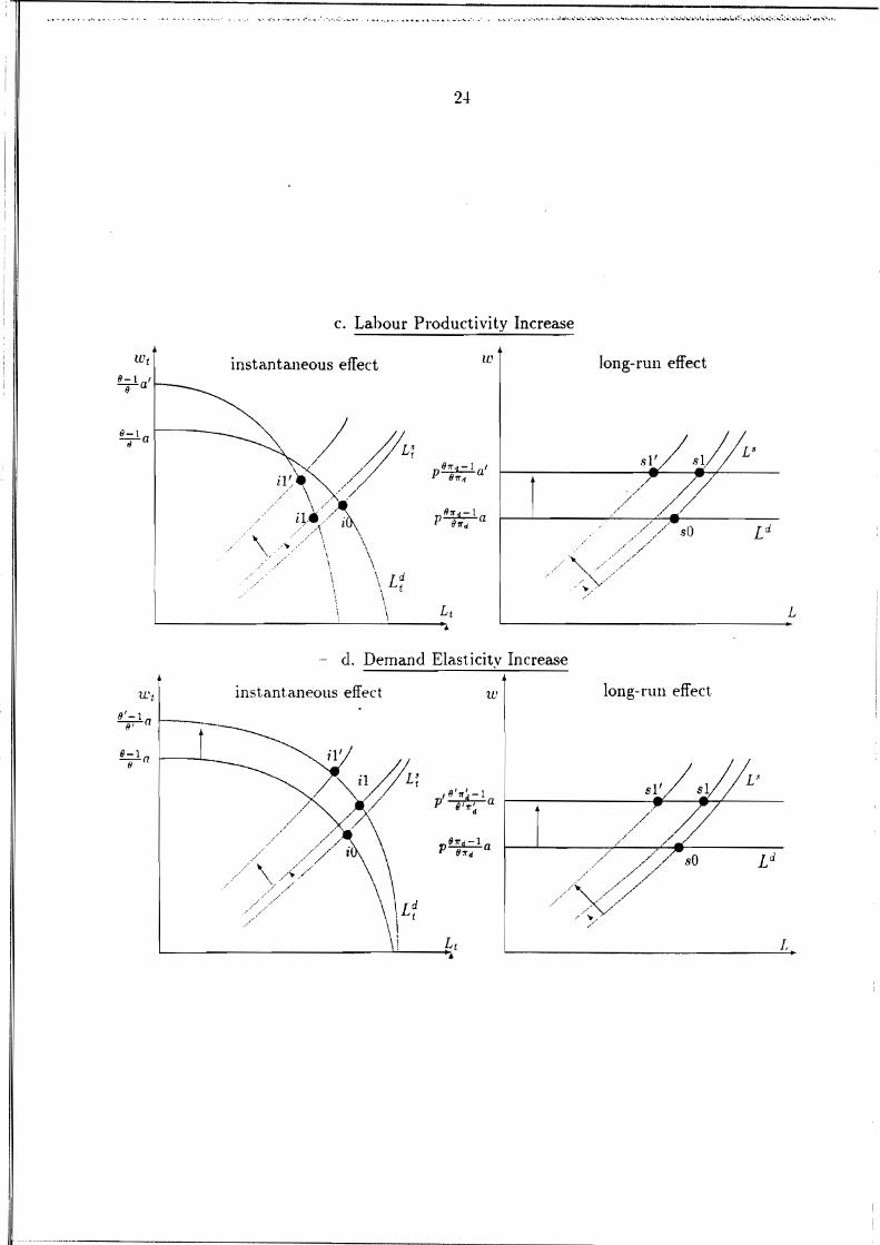
e) Labour Augmenting Technical Progress a.

We now consider an increase in the productivity of labour, at unchanged capital pro­�ductivity.�

i) Qualitative Analysis (figure e in Appendix 3)�

In the short run, the increase in the productivity of labour reduces the maximum employment level (less workers are now necessary for a given productive capacity) but increases the maximum wage leve!. The short run labour demand curve thus moves upwards at low levels of employment and inwards near the maximum employment leve!. As in b), the labour supply curve shifts upwards. The instantaneous effects of the productivity gain depend crucially on whether the initial employment level is to the left or to the right of the intersection point between the old and the new demand curves. i.e .. on whether the initial equilibrium capacity utilization rate is small (flat part of the labour demand curve) or large (steep part of the labour demand curve). In the first case, the productivity gain induces an instantaneous rise in real wages while the effect on employrnent remains ambiguous and depends on the labour supply behavior. In the second case, whatever U, the instantaneous effect on employrnent is negative; the size of the employment contraction determines whether the short run real wage falls increases.

The stationary levels of output and capital are higher; the stationary effect on employ­�ment remains ambiguous.�

ii) Numerical Simulation (see figure 3)�

The two numerical exercices illustrate the "second" case referred aboye. The short run employrnent level falls below its new stationary value in both economies. At given capital productivity, the labour productivity gain leacls in the short ron to an increase in capacity utilization and in markup rates. But the increase in D t is larger in the Low D economy than in the High Done whereas markups increase more in the latter than in the former. The employment contraction is thus much larger in the High D economy than in the Low Done. In the short run, the equilibrium real wage has to decrease in the former but can increase irnmediately in the latter.

It is also worth stressing that a labour productivi ty gain generates strikingly differ­ent dynamic paths and short run effects than a global (labour and capital) productivity gain, although the long run effects are similar. As it appears clearly in figure 3, the instantaneous effects on the capacity utilization rate, the proportion 7rdt, the markup rate and the real wage go in opposite directions and the time profiles of output and employment are very different.

1;')

Fignre 2: Government Spending Increase

2.a capacity utilisation rale 0.9 r---...,.-----r---,....--~-____,

0.8 LowD ­

0./ High D -o.n 0.5 0.'1 (U 0.2 0.1 oL.-_L---=t:::::==~~ ....--i

1 .) / 9 11

2.c Illark-up 2.:> .----.,..----.----,----..----,

2

1.5

1

0.5

3 ;) / 9 11

3.e firms facing a sales constraint o

-1

-2

-3

-4

-5

-6 1 :l 5 / 9 11

o

-0.5

-1

-1..5

-2

.) ~ I -~.;)

1.1

1

0.9

0.8

0./

0.6

O.,')

0.4 1

1.1�

1�

0.9

0.8�

0./�

0.6

0.5

0.'1 1

2.b real wage

j :1 :> "j 9 11

3.d employment

3 5 / 9 11

3,[ final output

:l 5 / 9 11

16�

Figure 3: Productivity Increases

2.a capacity utilisation rate lr------.------r----r---,....----, 2

2.1"> real wage

0.8

0.6

0.4

0.2

Low D:

High D :

a n&b­

a as:' b-­

1.5

0.5

O r---=:::::;:3~~~=~ O

-0.2 L­__------------~ -0.5

3 3 'i 9 11 -O.-l '------'----'-----'------''-----'

1 -1

1 :3 5 'i 9 11

2.c mark-up 2.5� ,....----,..---,---....,----,....----, -0.1

2 -0.2

1.5� -0.3

-0.4

0.3� -O .:J

O ~:::;;;;;;;:::::;:======~ -o.n -0.5� -0.7

-1 L-_---l.__--L__-'--__l....-__ -0.8

3.d employm~JJt

1 3 5 7 9 11 1 3 [) 'i 9 11

2 3.e firms facing a sales constraint

1.1 3.f final output

1 1 O 0.9

-1 -2

-3 -4

0.8

0.7

0.6

-5 0.5

-6 1 :3 )) 7 9 11

0.'1 1 :l 5 7 9 11

17

d) Increase in the Elasticity of Substitution 8

i) Qualitative Analysis (figure d in Appendix 3)

Although the price elasticity of demand is constant in this model, it ~ould not be too difficult to endogenize it I8 • Here, we simply assume an exogenous change in 8. This wil! allow us to assess qualitatively the combined effects of changes in the price elasticity of demand 8 and in the demand elasticity of sales 7T'd, which determine together the markup rateo Changes in the latter simply corresponds to movements along the short run labour demand curve; changes in 8 shift the labour demand curve itself. The increase in 8 leads the intermediate firms to lower their margins. Both the short run and the long run labour demand curve now shift upwards, and the real wage comes closer to the marginal productivity of labour a. A positive wealth effect shifts the labour supply schedule upwards. These two shifts are responsible for the same ambiguities as in the global productivity change. Although output is stimulated, the net effect on employment can be positive or negative, depending on the value of the intertemporal elasticity of substitution. ii) Numerical Simulation (see figure 4)

In both economies, the effect on employment and capital is positive. The increase in the price elasticity of demand has two immediate and opposite effects on markups. The first effect (linked directly to the elasticity change) dominates clearly the second one (linked to the higher capacity utilisation rate I9 ). The markup thus falls below its initial value.

However. when comparing the time profiles of the variables in the two economies, it appears clearly that the increase inDt interacts with the change in 8. It implies that the initial reduction in market power is lower in the High D economy than in the Low Done. The initial output increase is thus much larger in the latter. In both economies. however, the correlation between markup and output is negative during the adjustment phase.

5. Conclusions

Our objective was to develop a dynamic intertemporal model with imperfect compe­tition, wherein the combined effects of capacity utilization and markup rate changes could be discussed. By introducing microeconomic demand uncertainty and aggregat­ing over firms, we have been able to obtain a model wherein capacity underutilization is a macroeconomic equilibrium feature. In this setup, capacity utilization and markup rate changes are related via the effect of the former on the firm's actual market power. We studied these interactions and their implications for the dynamic behavior of sorne key macro variables in response to various "structural" shocks. Capacity constraints introduce potentially important non-linearities in the dynamic adjustment path. The same shock can have quite different effects depending on the characteristics of the ini­

18The easiest solution would be to introduce a relationship between the price elasticity of demand and the composition of aggregate demand (see e.g. d'Aspremont et alii (op citum), Gali (op citum).

19At any capacity level, the increase in degree of substituability between goods eases the spillover effects between firms. There are thus less firms facing a sales constraint than before.

18

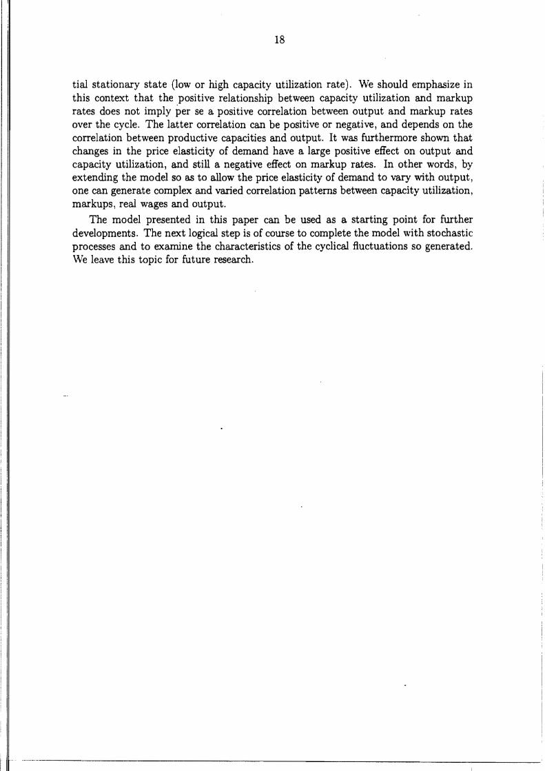
tial stationary state (low or high capacity utilization rate). We should emphasize in this context that the positive relationship between capacity utilization and markup rates does not imply per se a positive correlation between output and markup rates over the cycle. The latter correlation can be positive or negative, and depends on the correlation between productive capacities and output. It was furthermore shown that changes in the priee elasticity of demand have a large positive efi'ect on output and capacity utilization, and still a negative efi'ect on markup rates. In other words, by extending the model so as to allow the price elasticity of demand to vary with output, one can generate complex and varied correlation patterns between capacity utilization, markups, real wages and output.

The model presented in this paper can be used as a starting point for further developments. The next logical step is of course to complete the model with stochastic processes and to examine the characteristics of the cyclical f1.uctuations so generated. We leave this topie for future research.

1 1

19�

Figure 4: Elasticity of Substitution Increase

2.a capacity utilisatioll rate 2.b real wage 2 4,-----,.--......----,-..--,---_--,

1.8 LowD ­

1.6 3.5 High D­1.4

31 .,... 1 2.5

0.8 20.6

0.-1 1.5 ~_---l.. __-'-__...l...-__l...-_---1

1 .)3 7 9 11 1 1) 7 11

2.r mark-up 3.d employnwnt-lA ,------,---.,.----,---..,......---, l.l r-----,...---.---,------,-_--, - J.() 1.05 -1.8

1-2 -2.2 0.95 -2..! O.!) -2.6 0.85 -¿.S

0.8-:3 -:3.2 0.75 -3.4 L-_---L-__...L-_--JL.-_--L_--' 0.7 L-_--l.__.....L__....L..__.L.-_---J

1 3 5 7 9 11 1 3 5 7 9 11

3.e firms facing a sales constraint 3.f final output -2 ·1.15

1.1-3 1.05

-4 1

-5 0.95 0.9-6

0.85-7

0.8� -8 0.7:)� -u 0.7�

1 :l 5 7 9 II 1 :3 5 7 9 1J

11

20�

References

[1]� d'Aspremont C.,' L-A. Gerard-Varet, R. Dos Santos Ferreira (1994a), "Market Power, Coordination Failures and Endogeneous Fluctuations", CORE Discussion Paper nO 9468.

[2]� d'Aspremont C., L-A. Gerard-Varet, R. Dos Santos Ferreira (1994b), "On the Dixit-Stiglitz Model oí Monopolistic Competition", CORE Discussion Paper nO 9467.

[3]� Benassy J-P. (1975), "Neo-Keynesian Disequilibrium Theory in a Monetary Econ­omy", Review 01 Economic Studies, XLII, 503-524.

[4]� Boucekkine R. (1994), "An Alternative Methodology íor Solving Nonlinear Forward-Looking Models", íorthcoming in The Journal 01 Economic Dynamics and Control.

[5]� Burnside C., M.Eichenbaum and S.Rebelo (1993), "Labor Hoarding and the Busi­ness Cycle", Journal 01 Political Economy, Vol. 101, (April), 245-273.

[6]� Burnside C. and M.Eichenbaum (1994), "Factor Hoarding and the Propagation oí Business Cycle Shocks", NBER \Vorking Paper N° 4675.

[7]� Cooley, G. Hansen and E. Presscott (1994), "Equilibrium Business Cycles with Idle Resources and Variable Capacity Utilization", Federal Reserve Bank oí Min­neapolis, WP 535.

[8]� de la Croix D. and J-F.Fagnart (1993), "Underemployrnent oí Production Factors in a Forward-looking Model", mimeo CEPREMAP n° 9315, íorthcoming in Labour Economics, 58(1995)'

[9]� de la Croix D. and O.Licandro (1994), "Irreversibility, Uncertainty and Underem­ployment Equilibria", mimeo IRES, Université Catholique de Louvain n° 9428.

[10]� Dixit A. and J.Stiglitz (1977), "Monopolistic competition and Product Diversity", American Economic Review, 67(3), 297-308.

[11]� Dreze J.H. (1975), "Existence oí an Equilibrium under Price Rigidity and Quantity Rationing", International Economic Review; 16, 301-320.

[12]� Dreze J.H. and C. Bean (1990), " European Unemployment: Lessons from a Multicountry Econometric Study", Scandinavian Journal 01 Economics, 92(2), 135-165.

[13]� Fagnart J-F, O.Licandro and H.R.Sneessens (1994), "Capacity utilization Dy­namics in a General Equilibrium ModeP', mimeo presented at presented at the First International Coníerence on Economic Theory at Universidad Carlos III de Madrid, july 4-9 1994.

[14]� Gali J. (1994), "Monopolistic Competition, Business Cycle and the Composition oí Aggregate Demand", Journal 01 Economic Theory

[15]� Green J. (1980), "On the Theory oí Effective Demands", The Economic Journal, 90, 341-353.

21

[16]� Greenwood J., Z.Hercowitz and G. Huffman (1988) "Investment, Capacity Utiliza­tion and the Real Business Cycle", American Economic Review, Vol. 78, (June) 402-417. '

[17]� Laffargue J-P. (1990), "Résolution d'un modele macroéconomique aanticipations rationnelles", Annales d'Economie et de Statistique, 17, 97-119.

[18]� Licandro O. (1992), "A Non-Walrasian General Equilibrium Model with Mo­nopolistic Competition and Wage Bargaining", mimeo forthcorning in Annales d 'Economie et de Statistique, z1995.

[19]� Lucas R. and M. Woodford (1993), "Real Effects of Monetary Shocks in an Econ­omy with Sequential Purchases", NBER Working Papero

[20]� Romer P. (1987), "Growth Based on Increasing Returns Due to Specialization", American Economic Review, 77(2), 56-62.

[21]� Rotemberg J. and M. Woodford (1991), "Markups and the Business Cycle", NBER lvfacroeconomics Annual, O.J. Blanchard and S. Fisher eds., Cambridgge, MA: MIT Press, 63-128. .

[22]� Rotemberg J. and M. Woodford (1992), "Olígopolistic Pricing and the Effects of Aggregate Demand on Economic Activity", Journal 01 Political Economy, 1992, 100. 1153-1207.

[23]� Rotemberg J. and M. Woodford (1993), "Dynamic General Equilibrium Models with Imperfectly Competitive Product Markets", mimeo MIT and University of Chicago.

[24]� Sneessens H.R. (1987), "Investment and the Inflation-Unemployment Tradeoff in a Macroeconomic Rationing Model with Monopolistic Competition", European Economic Review, 31:781-815.

[25]� Sneessens H.R. and J.H. Dreze (1986), "A Discussion of Belgian Unemployment Combining Traditional Concepts and Disequilibrium Econometrics", Economica, 53, S89-S119.

[26]� Svensson L.E. (1980), "Effective Demands and Stochastic Rationing", Review 01 Economic Studies, XLVII, 339-355.

Appendix 1: Financial markets equilibrium

Although there is uncertainty at the individual firm level (in the intermediate good� sector), there is no aggregate uncertainty. At a symmetric equilibrium, all the inter­�mediate good (input) firm have the same expected rate of profit at a given point in� time. Consumers thus choose to diversify and eliminate risk by holding shares of all� the intermediate good firms. The number of shares is assumed to be fixed and invest­�ment in fixed capital is entirely financed by borrowing at the market rate of interest.� Because risk can be eliminated by diversification, bonds and (the market portfolio of)� shares must, by arbitrage, bear the same sure rate of return.� Let q{ and q~ represent the market value of final good firms and of intermediate good�

I

22

firms respectively. The corresponding share prices must satisfy for aH t ~ 1 the foHow­ing dynamic relationships:

with

q{+l + II{+1 - (1 + Tt+d q{ with II{+1 = Yi+l - Pt+l Yi+l

where II{+1 and II~+1 represent the aggregate profit levels of the two types of firms. In every period t, the demand for assets by households is then given by:

iqt� [1At =� [ 1+ qt + (1 + Tt) K t - 1] + IIt + IIi

t + WtLt - Ct

The financial markets equilibrium condition requires:

At = qt 1 + qt

i + Kt .

Appendix 2: Influences of Parameters on the Stationary Equilibrium

The table below gives the signs of the partial derivatives (at the stationary equilibrium) of the capacity utilization rate, D, the proportion Íld, (8Íld)-1 (Le., the markup in percentage points), the spillover effect p-o and the real wage W with respect to the parameters 0';,8, b, a, /3 and G.

a and b a 8 /3 G

D� o + O +� O + O

O + O O + O

+� + + + O

In the case of the global productivity increase, the increase in b reduces the cost of capital per unit of output. The input firms can choose a more "risky" investment policy, i.e., a policy with a lower expected degree of capacity utilization. At macroe­conomic equilibriwn, D is thus lower. In the case of a labour productivity increase at unchanged capital productivity, the real cost of capital remains unaffected, hence the capacity utilization rate and the proportion Íld are unchanged. A mean-preserving spread of the distribution of the parameters v reduces both D and Íld. The larger O'~, the larger the mismatch between demands and supplies. A mean­preserving spread thus reduces the capacity utilization rate at any capacity leve!. In order to compensate the resulting 1055 of profitability, firms increase their markup rate (lower Íld).

The larger 8, the lower margin and the higher the relative cost of overcapacity (equip­ments are less profitable). Firms thus restore their profitability by decreasing the probability of a sale shortage, thereby choosing to increase their average capacity uti­lization rateo An increase in /3 reduces the real capital cost ando at given F(v), allows the firms to reduce their optimal capacity utilization rate.­

• !

Appendix 3: Short- and Long-runs Effects of Structural Changes

a. Gouvernment Purchase Increase

wWt instantaneolls effect long mn effect

8-1-I/-a

~L'

~l V /;// /,/ \1 / h 1 -1 a./ ,/ P 9':r1 . \ ...

/~/ iO / \

\ Ld .. t \.

b. Productiyity Increase (bot h fartors)� 4�

tet ti'

8 - 1 .'1----: _ -e-(11

' 1/-1 ¡1 . / / L' ".1 I

-e-a 11//

I e.r:'-I I ~---r------__- __+--­P e,,:, a,(./,A\ ,./ ,/

). \ \\ /'., ..'..../..>/ sO ..... \. /"./~/ /\,\L1

I , L t • L_

L..--------.L---o¡ LI

.......__...._---------------------------­

L

24�

c. Labour Productivity Increase

Wt

8-1 ,-e-a instantalleous effect W long-run effect

8-1 -~-a

\ ...,. ./

.•......

, \. \

\ \ \, Ld

'; t \ \

fA L

U't

8' -1-8-,-n t""-­__

d. Demand Elasticity Increase

instantéllleous effect w long-run effect

8-1-&-n

, e'''"4- 1 p 8/"4 a

\/

.......... __.-----_._-------------------------­