Can we curb retail sales volatility through marketing mix actions

Working Paper 11-24 (07) Departamento de Economía de la Empresa Business Economics Series Universidad Carlos III de Madrid November 2011 Calle Madrid, 126 28903 Getafe (Spain) Fax (34-91) 6249607

CAN WE CURB RETAIL SALES VOLATILITY THROUGH MARKETING MIX ACTIONS?

Mercedes Esteban-Bravo1, Gökhan Yildirim2, and José M. Vidal-Sanz 3

Abstract

Sales uncertainty is a central problem for marketing management. Marketers tend to focus on expected sales, rather than short-term time-varying oscillations. With long supply-chain streams, the Bullwhip effect can turn retail sales volatility into a major problem for upstream companies. While it has been recognized that conditional expected sales change through time (for a review see Dekimpe and Hanssens, 2000), marketers have not yet started to modeling explicitly time variation of sales' conditional variances. In this paper we focus on this issue, modeling and forecasting time-varying retail sales and marketing mix volatility and their crossed effects within brand, and between competitive brands. We analyze up to 6 product categories sold by Dominick's Finer Foods, finding volatility and co-volatilities in all of them. We discuss managerial implications for brand management and competitive strategy. Keywords: Sales, Volatility, Bullwhip effect, Marketing mix.

Research funded by two research projects, by the Comunidad de Madrid and the Spanish Government. 1 Mercedes Esteban-Bravo, Department of Business Administration, University Carlos III de Madrid, C/ Madrid 126, 28903 Getafe (Madrid), Spain; tel: +34 91 624 8921; fax: +34 91 624 8921; e-mail: [email protected] 2 Gökhan Yildirim, Department of Business Administration, University Carlos III de Madrid, C/ Madrid 126, 28903 Getafe (Madrid), Spain; tel: +34 91 624 8921; fax: +34 91 624 8921; e-mail: [email protected] 3 Jose M. Vidal-Sanz, Department of Business Administration, University Carlos III de Madrid, C/ Madrid 126, 28903 Getafe (Madrid), Spain; tel: +34 91 624 8642; fax: +34 91 624 9607; e-mail: [email protected]

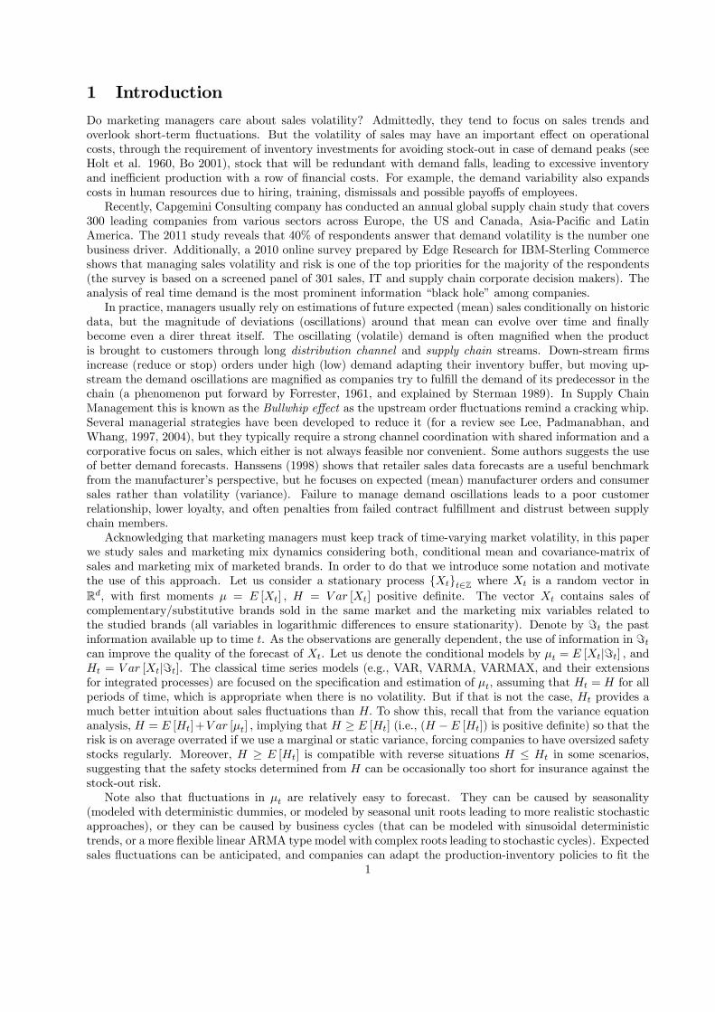
1 Introduction

Do marketing managers care about sales volatility? Admittedly, they tend to focus on sales trends and

overlook short-term fluctuations. But the volatility of sales may have an important effect on operational

costs, through the requirement of inventory investments for avoiding stock-out in case of demand peaks (see

Holt et al. 1960, Bo 2001), stock that will be redundant with demand falls, leading to excessive inventory

and inefficient production with a row of financial costs. For example, the demand variability also expands

costs in human resources due to hiring, training, dismissals and possible payoffs of employees.

Recently, Capgemini Consulting company has conducted an annual global supply chain study that covers

300 leading companies from various sectors across Europe, the US and Canada, Asia-Pacific and Latin

America. The 2011 study reveals that 40% of respondents answer that demand volatility is the number one

business driver. Additionally, a 2010 online survey prepared by Edge Research for IBM-Sterling Commerce

shows that managing sales volatility and risk is one of the top priorities for the majority of the respondents

(the survey is based on a screened panel of 301 sales, IT and supply chain corporate decision makers). The

analysis of real time demand is the most prominent information “black hole” among companies.

In practice, managers usually rely on estimations of future expected (mean) sales conditionally on historic

data, but the magnitude of deviations (oscillations) around that mean can evolve over time and finally

become even a direr threat itself. The oscillating (volatile) demand is often magnified when the product

is brought to customers through long distribution channel and supply chain streams. Down-stream firms

increase (reduce or stop) orders under high (low) demand adapting their inventory buffer, but moving up-

stream the demand oscillations are magnified as companies try to fulfill the demand of its predecessor in the

chain (a phenomenon put forward by Forrester, 1961, and explained by Sterman 1989). In Supply Chain

Management this is known as the Bullwhip effect as the upstream order fluctuations remind a cracking whip.

Several managerial strategies have been developed to reduce it (for a review see Lee, Padmanabhan, and

Whang, 1997, 2004), but they typically require a strong channel coordination with shared information and a

corporative focus on sales, which either is not always feasible nor convenient. Some authors suggests the use

of better demand forecasts. Hanssens (1998) shows that retailer sales data forecasts are a useful benchmark

from the manufacturer’s perspective, but he focuses on expected (mean) manufacturer orders and consumer

sales rather than volatility (variance). Failure to manage demand oscillations leads to a poor customer

relationship, lower loyalty, and often penalties from failed contract fulfillment and distrust between supply

chain members.

Acknowledging that marketing managers must keep track of time-varying market volatility, in this paper

we study sales and marketing mix dynamics considering both, conditional mean and covariance-matrix of

sales and marketing mix of marketed brands. In order to do that we introduce some notation and motivate

the use of this approach. Let us consider a stationary process {}∈Z where is a random vector in

R, with first moments = [] = [] positive definite. The vector contains sales of

complementary/substitutive brands sold in the same market and the marketing mix variables related to

the studied brands (all variables in logarithmic differences to ensure stationarity). Denote by = the pastinformation available up to time . As the observations are generally dependent, the use of information in =can improve the quality of the forecast of . Let us denote the conditional models by = [|=] and = [|=]. The classical time series models (e.g., VAR, VARMA, VARMAX, and their extensionsfor integrated processes) are focused on the specification and estimation of assuming that = for all

periods of time, which is appropriate when there is no volatility. But if that is not the case, provides a

much better intuition about sales fluctuations than To show this, recall that from the variance equation

analysis, = []+ [] implying that ≥ [] (i.e., ( − []) is positive definite) so that the

risk is on average overrated if we use a marginal or static variance, forcing companies to have oversized safety

stocks regularly. Moreover, ≥ [] is compatible with reverse situations ≤ in some scenarios,

suggesting that the safety stocks determined from can be occasionally too short for insurance against the

stock-out risk.

Note also that fluctuations in are relatively easy to forecast. They can be caused by seasonality

(modeled with deterministic dummies, or modeled by seasonal unit roots leading to more realistic stochastic

approaches), or they can be caused by business cycles (that can be modeled with sinusoidal deterministic

trends, or a more flexible linear ARMA type model with complex roots leading to stochastic cycles). Expected

sales fluctuations can be anticipated, and companies can adapt the production-inventory policies to fit the

1

forecast. The actual risk is caused by deviations ( − ) that cannot be anticipated previously, but

which average magnitude is measured by on the whole, and by for each specific period of time. Our

central objective is the study of As the vector includes sales and marketing mix variables for several

competitors in the same market, estimating we study the crossed co-volatilities of marketing-mix on retail

sales. The results show that the marketing mix can be used to curb volatility whilst increasing expected

levels in . We also analyze crossed effects among competitors, via mean and variance, and how this can

be used as a competitive advantage.

We organize this article as follows: after presenting the models that we will consider for the empirical

problem at hand, we discuss the market panel-data which we use to estimate each firm’s volatility dynamics.

We then elaborate on our modelling approach for fitting the model to the data. Next we provide the analysis

of the market for several categories, with a managerial discussion of marketing mix impact on sales volatility,

and competitive effects between brands. We end up with a discussion of our contributions and managerial

implications.

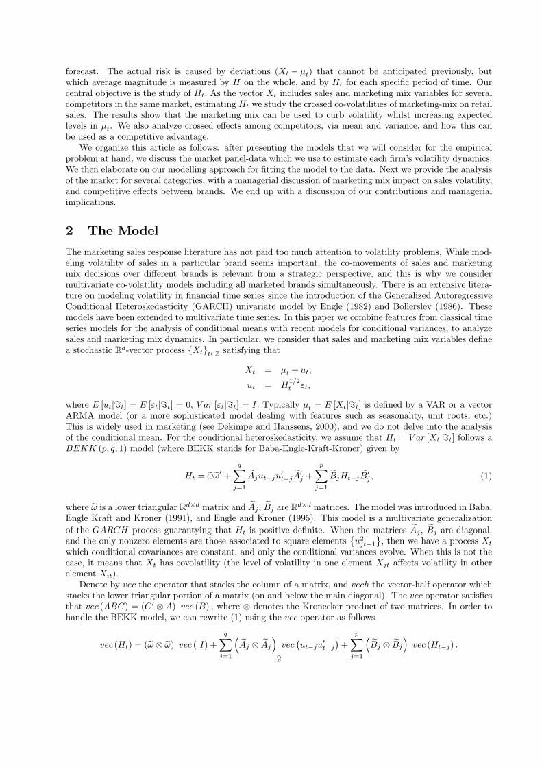
2 The Model

The marketing sales response literature has not paid too much attention to volatility problems. While mod-

eling volatility of sales in a particular brand seems important, the co-movements of sales and marketing

mix decisions over different brands is relevant from a strategic perspective, and this is why we consider

multivariate co-volatility models including all marketed brands simultaneously. There is an extensive litera-

ture on modeling volatility in financial time series since the introduction of the Generalized Autoregressive

Conditional Heteroskedasticity (GARCH) univariate model by Engle (1982) and Bollerslev (1986). These

models have been extended to multivariate time series. In this paper we combine features from classical time

series models for the analysis of conditional means with recent models for conditional variances, to analyze

sales and marketing mix dynamics. In particular, we consider that sales and marketing mix variables define

a stochastic R-vector process {}∈Z satisfying that

= +

= 12

where [|=] = [|=] = 0 [|=] = Typically = [|=] is defined by a VAR or a vectorARMA model (or a more sophisticated model dealing with features such as seasonality, unit roots, etc.)

This is widely used in marketing (see Dekimpe and Hanssens, 2000), and we do not delve into the analysis

of the conditional mean. For the conditional heteroskedasticity, we assume that = [|=] follows a ( 1) model (where BEKK stands for Baba-Engle-Kraft-Kroner) given by

= ee0 + X=1

e−0− e0 + X=1

e− e0 (1)

where e is a lower triangular R× matrix and e e are R× matrices. The model was introduced in Baba,Engle Kraft and Kroner (1991), and Engle and Kroner (1995). This model is a multivariate generalization

of the process guarantying that is positive definite. When the matrices e e are diagonal,

and the only nonzero elements are those associated to square elements©2−1

ª, then we have a process

which conditional covariances are constant, and only the conditional variances evolve. When this is not the

case, it means that has covolatility (the level of volatility in one element affects volatility in other

element ).

Denote by the operator that stacks the column of a matrix, and the vector-half operator which

stacks the lower triangular portion of a matrix (on and below the main diagonal). The operator satisfies

that () = ( 0 ⊗) () where ⊗ denotes the Kronecker product of two matrices. In order tohandle the BEKK model, we can rewrite (1) using the operator as follows

() = (e ⊗ e) ( ) +

X=1

³ e ⊗ e

´

¡−0−

¢+

X=1

³ e ⊗ e

´ (−)

2

The dimension of () is 2 Since the matrices involved in this representation are symmetric, we can

reduce the dimension. Using the vector-half operator we rewrite (1) as

= +

X=1

¡−0−

¢+

X=1

−

= + () (0) + () (2)

where = () has dimension (+ 1) 2 and we have used the matrices = + (e ⊗ e) ( )

= +

³ e ⊗ e

´, = +

³ e ⊗ e

´ with the

2 × (+ 1) 2 duplication matrix defined

by the property () = () for any symmetric × matrix (i.e., contains some columns

from the identity matrix 2×2 extracting elements in () coming from the lower triangle of ) and +

denotes its Moore Penrose inverse. For the last equation (2) we have used a compact notation with matrix

polynomials () =P

=1 and () =

P=1

in the lag operator .

3 Data Description

We use store-level scanner data made available by the James M. Kilts Center, University of Chicago, from

Dominick’s Finer Foods, the largest grocery retailer in the Chicago market. The database includes all weekly

sales, shelf price, possible presence of sales promotions (coupons, bulk buy, or a special sale), retail margin,

and daily store traffic, by individual item (referenced by UPC) for more than 25 product categories, and

collected for 96 stores operated in the Chicago area over a period of more than seven years from 1989 to

1997. For the analysis, we aggregate the weekly sales data across stores, computing also the average price.

We also compute a continuos promotion variable defined as the percentage of stores implementing any sales

promotion. We perform our empirical analysis using six different ‘fast moving consumer product categories’

(products are sold quickly and at relatively low cost): cheese, refrigerated juice, laundry detergent, toilet

tissue, paper towel and toothpaste. As can be seen in Table 1, for cheese and refrigerated juice categories,

we consider two brands with the highest market share, forming 80% and 82% of the total category volume

respectively whereas for laundry detergent, toilet tissue, paper towel and toothpaste categories we focus on

the top three selling brands constituting 70%, 66%, 60% and 73% of the market, respectively.

Table1. Description of six categories used in the application

Category

Number of analyzed brands

Total number of brands in the

category

Market Share of the analyzed

brands

Cheese 2 12 80%

Refrigerated juice 2 7 82%

LaundryDetergent 3 14 70%

Toilet tissue 3 10 66%

Paper towel 3 13 60%

Toothpaste 3 13 73%

Table 2 provides more details on the analyzed brands in each category. In the cheese category, the two

competing brands Dominick’s and Kraft do not differ much since their average prices, promotions and sales3

are very close to each other. Also, the standard deviations of those variables show very small difference.

In the refrigerated juice category, the two brands, Minute Maid and Tropicana, are similar in terms of

average prices. The prices of those brands do not vary too much, i.e. the standard deviations are very

close to each other. However, the sales of Tropicana almost doubles that of Minute Maid. For the laundry

detergent we observe that brand’s promotion intensity, are close to each other on average as well as their

variabilities. The prices differ across the three brands. This difference may be perceived as signals of quality.

This difference may make the brands differentiate them from the competitors. Similarly, in the toilet tissue

category, brands’ average promotions as well as the variability of the brand’s promotions do not differ much,

but prices are different and have different volatilities. Regarding the paper towel category, the average

prices differ across the brands Bounty, Scott and Dominick’s. Scott does more promotion on average, but we

see almost no difference in the promotions variability. In the toothpaste category, the average prices of the

three brands are very close to each other. Aquafresh has the highest price variability and the lowest average

sales, while Crest has the moderate price variability, but the highest average sales. The average promotion

differs across brands, but the level of the promotion is low.

4

Table 2. Descriptive statistics of the analyzed brands

Category Variable Mean Median Maximum Minimum Std. Dev.

Observations

Cheese

Sales Dominick's 104123.20 101624.00 264441.00 53745.00 26753.70 392

Price Dominick's 2.10 2.11 2.71 1.26 0.21 392

Prom Dominick's 92.24 97.67 100.00 0.00 20.09 392

Sales Kraft 138445.50 122791.00 543061.00 83550.00 53543.57 392

Price Kraft 1.99 1.95 4.10 0.90 0.28 392

Prom Kraft 93.81 97.67 100.00 0.00 15.31 392

Refrigerated

Juice

Sales Minute Maid 38690.04 23664.00 263612.00 13651.00 35673.52 396

Price Minute Maid 2.14 2.17 3.49 1.06 0.35 396

Prom Minute Maid 69.93 94.12 100.00 0.00 40.51 396

Sales Tropicana 65726.83 48877.50 271965.00 26883.00 40931.44 396

Price Tropicana 2.47 2.55 3.44 1.21 0.35 396

Prom Tropicana 82.64 97.42 100.00 0.00 31.10 396

Laundry

detergent

Sales Wisk 7339.28 4841.50 52357.00 1967.00 7061.49 396

Price Wisk 5.31 5.24 8.88 2.81 0.87 396

Prom Wisk 65.11 92.96 100.00 0.00 42.59 396

Sales All 8332.82 5368.50 133703.00 2265.00 12171.34 396

Price All 4.51 4.55 7.05 2.48 0.56 396

Prom All 67.96 94.12 100.00 0.00 40.92 396

Sales Tide 26318.69 20320.50 135839.00 10586.00 19925.67 396

Price Tide 6.20 6.29 9.22 3.43 0.85 396

Prom Tide 68.04 94.12 100.00 0.00 41.12 396

Toilet Tissue

Sales Scott 86464.14 56745.50 2062849.00 26163.00 155969.67 384

Price Scott 0.70 0.66 1.88 0.25 0.20 384

Prom Scott 47.67 56.89 100.00 0.00 44.17 384

Sales Charmin 37143.97 19470.50 478101.00 9436.00 58301.06 384

Price Charmin 2.11 2.13 3.14 0.70 0.51 384

Prom Charmin 40.30 4.22 100.00 0.00 44.37 384

Sales Northern 31854.61 18358.00 314957.00 10125.00 38232.68 384

Price Northern 1.71 1.67 3.45 0.82 0.39 384

Prom Northern 49.55 61.76 100.00 0.00 46.12 384

Paper Towel

Sales Bounty 34452.86 29840.50 163198.00 17202.00 17121.08 388

Price Bounty 1.42 1.44 2.68 0.75 0.24 388

Prom Bounty 39.72 2.33 100.00 0.00 44.20 388

Sales Scott 22764.20 20314.00 112534.00 6115.00 15312.97 388

Price Scott 1.35 1.28 2.28 0.76 0.30 388

Prom Scott 61.15 86.04 100.00 0.00 42.96 388

Sales Dominick's 23822.99 18030.50 208968.00 1346.00 24810.48 388

Price Dominick's 0.76 0.71 2.31 0.34 0.21 388

Prom Dominick's 40.29 35.92 100.00 0.00 40.49 388

Toothpaste

Sales Aquafresh 3746.22 3159.00 20727.00 1642.00 2171.50 398

Price Aquafresh 2.24 2.31 3.24 1.05 0.50 398

Prom Aquafresh 36.43 1.18 100.00 0.00 43.25 398

Sales Colgate 9082.61 8297.00 25196.00 4926.00 3383.23 398

Price Colgate 2.21 2.25 2.60 1.56 0.24 398

Prom Colgate 49.72 48.54 100.00 0.00 44.31 398

Sales Crest 12176.40 11528.00 49820.00 6769.00 4144.69 398

Price Crest 2.30 2.37 2.80 1.18 0.32 398

Prom Crest 43.10 29.48 100.00 0.00 43.99 398

5

4 Empirical analysis

Our model building approach consists of six main steps: In step 1, we perform preliminary analysis that

includes exploratory data analysis, and the analysis of the time series’ levels. In step 2, we estimate con-

sistently a model for the conditional mean (typically a VAR model parameters by OLS). Then, in step 3,

we explore the existence of volatility in the data, specifying and estimating a BEKK model for the resid-

uals using a Maximum Likelihood Estimation (MLE). In step 4 we compute preliminary estimations for

the parameters of the BEKK model. Finally, in step 5, we improve the efficiency of the estimators. We

simultaneously estimate the VAR and BEKK parameters by full Gaussian Maximum Likelihood, using the

consistent estimates from step 2 and 4 as initial values for the Newton Method (this choice is crucial given

the high dimension of the problem). In Step 6 we analyze the estimation output and perform specific tests

of independence and Granger Causality.

Step 1: Preliminary Analysis: We perform the standard exploratory data analysis. Then, we

study the usual properties such as stationarity and cointegration, involving inspection of data graphs, Auto

Correlation Functions (ACF), crossed, and partial autocorrelations. We determine to take natural logarithm

for all variables. For most of the brands in all categories, we observe that the ACFs decay very slowly

which is typical of a nonstationary time series. This conclusion is also consistent with the results of the

Augmented Dickey-Fuller, Phillips-Perron and Kwiatkowski—Phillips—Schmidt—Shin (KPSS) unit root tests.

Given the evidence, we opt for taking one difference of all variables in logarithms, which can be interpreted

as growth ratios of the original series from period to period. Next, we conduct Johansen’s cointegration

test to study whether the integrated variables are cointegrated (i.e., if they have a long-run equilibrium

in levels). Cointegration would imply the specification of a Vector Error Correction (VEC) model instead

of a VAR model for variables in differences. For all categories, we accept the null hypothesis that the

variables are not cointegrated. Note that in general these tests (unit root and cointegration tests) do not

take into account conditional heteroskedasticity, and the output is somewhat exploratory, but it confirms the

graphic analysis suggestions. Therefore, we proceed to estimate a VAR model for variables in logarithmic

first differences. More complex models could be used if the inspection of the data shows evidence of other

alternative specifications such as VARMA or VECM.

Step 2: Conditional mean analysis: Let us denote the vector of log-differenced variables. Here

we focus on the analysis of = [|=] We model the dynamic interactions among the variables througha VAR model (including all variables as endogenous). We choose the optimal lag length of the VAR model

to be 1 based on the visual inspection of the ACFs of the first differenced log series. We also compute the

information criteria (commonly used in the marketing literature, see Dekimpe and Hanssens, 1999; Pauwels

et al. 2004). Schwarz information criterion (SIC) suggests one lag for all categories. As a result, we specify

a VAR(1) model = Π−1. We estimate bΠ by OLS, minimizing (Π) =

(X=2

( −Π−1)0( −Π−1)

)(3)

where denotes the trace. The solution is bΠ0 = ³P=2

0−1−1

´−1P=2

0−1 We also obtain the

residuals b = − bΠ−1 to be used as a preliminary tool for volatility analysis.Step 3: Volatility Modeling: Before carrying out our volatility model estimation, we explore the

presence of volatility in our data. We first study the volatility of the residual series independently (univariate

analysis), and then study the appropriate multivariate BEKK model:

(i) visual inspection of the sales plots: As an example, Figure 1 shows the first differenced logarithm of

one brand for each category. The plots show that in general the volatility is higher at some periods of time

than others, indicating that the conditional variance is not constant over time.

6

Figure 1. First Differenced Logged Sales for some brands

0 50 100 150 200 250 300 350 400-2

-1

0

1

21st Diff. Log Kraft Sales (Cheese Category)

Time

1st

Diff

. Lo

g S

ale

s0 50 100 150 200 250 300 350 400

-4

-2

0

2

41st Diff. Log Minute Maid Sales (Refrigerated Juice Category)

Time

1st

Diff

. Lo

g S

ale

s

0 50 100 150 200 250 300 350 400-4

-2

0

2

41st Diff. Log All Sales (Laundry Detergent Category)

Time

1st

Diff

. Lo

g S

ale

s

0 50 100 150 200 250 300 350 400-4

-2

0

2

41st Diff. Log Charmin Sales (Toilet Tissue Category)

Time

1st

Diff

. Lo

g S

ale

s0 50 100 150 200 250 300 350 400

-2

-1

0

1

21st Diff. Log Bounty Sales (Paper Towel Category)

Time

1st D

iff.

Log

Sa

les

0 50 100 150 200 250 300 350 400-2

-1

0

1

21st Diff. Log Crest Sales (Toothpaste Category)

Time

1st D

iff.

Log

Sa

les

(ii) ACFs of the squared OLS residuals from the VAR(1) model: We find substantial evidence of Au-

toregressive Conditional Heteroscedasticity (ARCH) effects as judged by the autocorrelations of the squared

residuals. As can be seen from Figure 2, even though the magnitude of the autocorrelations sometimes are

small after lag 1 or 2, the ACF plots of the squared residuals of sales variables show the presence of autocorre-

lation patterns. This suggests the existence of (Generalized) Auto Regressive Conditional Heteroskedasticity

(ARCH/GARCH models).

7

Figure 2. ACFs of the squared residuals of sales for some brands

1 5 10 15-0.2

0

0.2ACF of the squared residuals of Kraft Sales (Cheese)

Lag length1 5 10 15

-0.2

0

0.2

ACF of the squared residuals of Minute Maid Sales (Juice)

Lag length

1 5 10 15-0.2

0

0.2

0.4

0.6ACF of the squared residuals of All Sales (Laundry Detergent)

Lag length1 5 10 15

-0.2

0

0.2ACF of the squared residuals of Charmin Sales (Toilet Tissue)

Lag length

1 5 10 15-0.2

0

0.2ACF of the squared residuals of Bounty Sales (Paper Towel)

Lag length1 5 10 15

-0.2

0

0.2

ACF of the squared residuals of Crest Sales (Toothpaste)

Lag length

(iii) ARCH test: We tested formally the hypothesis of conditional heteroskedasticity applying Engle’s

(1982) ARCH test. The null hypothesis is that there is no autocorrelation in the squared residuals (and

therefore no ARCH effect). For all brands (with two exceptions: brand Wisk in the laundry detergent

category and brand Colgate in the toothpaste category), we reject the no-ARCH hypotheses, supporting our

findings in (i) and (ii).

Finally, we study multivariate co-volatility relationships and specify a full BEKK model. In order to

decide how many lags to be included, we use the ACFs and partial ACFs of the squared residuals. If we

define = (0)− then we can write model (2) as a ( ) with = max ( ) given by

(0) = + ( () + ()) (

0)− () +

where are martingale differences, and if has four order moments [0] = [ (

0)]− [0]

The model is covariance stationary if and only the roots of | () + ()| = 1 lie outside the unit circle,

which usually occurs when ( (1) + (1)) has eigenvalues with modulus smaller than one. We also assume

that are as small as possible given that the matrices and have full rank, and the polynomials

( − ( () + ())) and ( − ()) have neither unit roots nor common left factors other than unimodular

ones. The ( ) representation shows that we can identify with the classical tools. If we

estimate with standard time series methods (i.e. without taking care of the heteroskedasticity), and we

can use the residuals b = ( − b) to estimate autocorrelation functions for (bb0) which can be usedto determine an appropriate orders. In our case, inspection of sample autocorrelations for (bb0),subsequent estimation of the identified models, and implementation of a diagnosis process, leaded us to

accept that a BEKK(1,1,1) model is an appropriate choice for all product categories.

Step 4: Preliminary BEKK model estimation: The estimation of the volatility model, similar to

that of a univariate GARCH. We denote by the parameter vector of the model, the matrices = ()

= () = () are functions of (in practice the components of are precisely the entries in these

matrices). The parameters can be estimated by conditional pseudo maximum likelihood, i.e. minimizing

−2 · () =X=1

³ln ||+ ( − )

0−1 ( − )

´

8

Results for the asymptotic properties of the estimator have been studied by Jeantheau (1998) and Comte

and Lieberman (2003). In order to simplify its computation, once we have estimated using (3), we replace

by b in the likelihood function. This estimation is consistent, but inefficient as it is based on inefficientOLS estimations for the VAR model.

Step 5: Simultaneous estimation of the VAR and BEKK parameters to improve efficiency.

We consider the estimated parameters from VAR(1) and BEKK(1,1) models as initial values, and use them

in the full likelihood function to estimate all parameters together in order to achieve asymptotic efficiency.

Therefore, including the parameters in in the vector we minimize

−2 · () =X=1

³ln ||+

¡ −

¢0−1

¡ −

¢´

using the Newton-Raphson method from the preliminary estimators. Using Step 2 and 4 estimations as initial

point is crucial for ensuring convergence given the high computational effort caused by the large dimension

of the parameters.

Step 6: Inference analysis

We applied the analysis described above to the full vector of sales and marketing mix actions (price,

promotion) for all the selected leader brands on each of the six categories. In all the cases, the estimations

are globally significant, and their signs and magnitudes are as expected.

The dimension of the tables with the estimators is too large, and we do not report them in detail (they

can be provided from the authors upon request). The dynamic structure of the volatility can be visualized

using appropriate impulse response functions. Notice that we can expand (2) as

= ( − (1))−1

+Ψ () (0)

where

Ψ () = ( − ())−1( ()) =

∞X=1

Ψ

the coefficients {Ψ} can easily computed, they can be interpreted as an impulse-response function explainingthe effect of previous unexpected changes of (

0) over current covolatility levels . In the particular

case of a BEKK(1,1,1) we have

= ( −1)−1

+Ψ11 () (0)

Ψ11 () = ( −1)−1

1 =

⎛⎝ ∞X=0

1

⎞⎠1 =

∞X=0

11

+1

so that

Ψ0 = 0Ψ1 = 1 Ψ2 = 11

Ψ = −11 1 = 1Ψ−1 ≥ 2

Inversion of the operator leads to an infinite BEKK expansion. Figures depicting coefficients in the

matrices Ψ provide a visual description of the volatility (or covolatility) transmission of random shocks.

Some of these graphs are shown in the main results section.

Furthermore, we can obtain much more insightful features from the conditional maximum likelihood

estimations by testing conditional independence and Granger causality hypotheses. Consider a partition of

two groups of variables 1 and 2 then we can study the crossed effects between the different parts.

In particular, we study the exogeneity and the independence of marketing mix (price and promotions) and

sales within the context of a brand. A similar analysis is carried out for several competitors (e.g. the

crossed relationship between sales of a brand and marketing mix of a competitor). From the VAR model,

= Π−1 + we partition in two blocks:µ1

2

¶=

µΠ11 Π12Π21 Π22

¶µ1−12−1

¶

If we only consider mean-dependence, it is sufficient to test some of the following hypotheses:9

• If Π12 = 0 holds (i.e., Π is block-triangular) with Π21 significant, then there is Granger causality from1 to 2

• If Π12 = 0 Π21 = 0 holds, (i.e., Π is block-diagonal), then 1 and 2 are independent conditionally

on the past.

In order to test 0 : Π12 = 0, (e.g. to test Granger causality of the marketing mix of a brand on the

sales of the same/other brand) one can consider a Wald test

· (bΠ12) h ((bΠ12))i−1 (bΠ12)→ 2

where ((bΠ12)) is the block- component (1,2) of the Maximum Likelihood Estimator covariance matrix(we estimate this matrix using a standard HAC estimator), and is the number of tested parameters in Π12.

Tests for conditional independence are analogous, using estimators for Π12 and Π21 and it can be applied

for example to test independence between brands. The standard causality tests, including the presented

Wald test consider just in-mean effects. Note that with conditional heteroskedasticity, the standard Granger

causality tests cannot be used as the concept involves causality in both mean (VAR) and variance (BEKK)

equations.

Note that any test based on the parameters of Π ignores the conditional variance dependences. Under

volatility patterns, we should also pay attention to the conditional covariance model, testing if the appropriate

parameters in e and e in (1) are zero. Consider, for example, the matrix e1. If the sub-matrix e12 = 0the conditional variance of 1 does not depend on 2 which is a requeriment for exogeneity. This is obvious

computing the symmetric matrixÃ e11 0e21 e22!µ

1−12−1

¶µ1−12−1

¶0Ã e11 0e21 e22!0

and noticing that the element e111−101−1 e011 does not depend on 2 and analogously for the coefficients

in the matrices e . Therefore, an exogeneity Wald test in this context is given by,

µ(bΠ12) (be12) (be12)

¶0 ∙

µ(bΠ12) (be12) (be12)

¶¸−1µ(bΠ12) (be12) (be12)

¶

If both e12 and e21 are zero there is block independence between the conditional variance of 1 and 2

Therefore, for testing full conditional independence the Wald test is a quadratic form including the estimatorsµ(bΠ12) (bΠ21) (be12) (be21) (be12) (

be21)

¶

If we are not interested in mean effects, but just in co-volatility, we would compute a Wald test with the

estimators

µ(

be12) (be21) (be12) (be21)

¶

Summarizing, we consider total independence (exogeneity) test for all the parameters, amean-independence

(exogeneity) test using the VAR parameters, and a variance-independence (exogeneity) test using the BEKK

parameters.

5 Main Results

Upon our conditional maximum likelihood estimation for the complete model with conditional mean (VAR

model) and variance (BEKK model), we compute the Wald tests, and discuss the results of Granger exogene-

ity1 for the marketing mix, and the independence2 tests of marketing mix variables and sales (all measured as

1Exogeneity test example: we test if marketing mix of brand A is independent of its sales (in our context conditional mean

and variance do not depend on sales), and not viceversa. Put it differently, causality is one-directional that goes from marketing

mix to sales.2 Independence test example: we test the block independence between marketing mix and sales of brand A. In other words,

neither of them affects the other, through expectations nor variances.10

logarithmic growth rates). First, we discuss the results of the exogeneity and independence tests of marketing

mix variables and sales for each brand separately, and then across brands. Note that given the observed

volatility, all standard parametric inferences based on VAR model would be erroneous, as their usual tests

do not account for conditional heteroskedasticity.

5.1 Within-Brand Analysis

For each brand, we particularly test the exogeneity of the marketing mix of the brand from its sales, and

the independence between the sales and the marketing mix of the same brand. The results show that, for

all brands in all categories (laundry detergent, toilet tissue, toothpaste, paper towel, cheese and refrigerated

juice), we do reject the exogeneity of marketing mix hypotheses and we do also reject the strongest

conditional independence hypotheses with a 95% of confidence (meaning that for each brand, the empirical

evidence supports that sales means and variances depend on previous sales and marketing mix actions, and

vice versa marketing mix actions are set based on previous sales and marketing actions). Table 3 contains a

summary of these tests.

Table 3. Within-Brands Wald tests analysis

Category Brand Null hypothesis Wald Test d.f. Chi‐square Critical Value at 5%

Cheese Dominicks

Marketing mix exogeneity 565,0 6 12,59

Conditional independence 3992,7 12 21,03

Kraft

Marketing mix exogeneity 441,0 6 12,59


Refrigerated juice Minute Maid Marketing mix exogeneity 7383,7 6 12,59


Tropicana Marketing mix exogeneity 7556,7 6 12,59


Laundry Detergent Wisk Marketing mix exogeneity 1096,0 6 12,59


All Marketing mix exogeneity 1088,0 6 12,59


Tide Marketing mix exogeneity 3064,9 6 12,59


Toilet Tissue Scott Marketing mix exogeneity 513,1 6 12,59


Charmin Marketing mix exogeneity 90,0 6 12,59


Northern Marketing mix exogeneity 262,0 6 12,59


Paper Towel Bounty Marketing mix exogeneity 1316,7 6 12,59


Scott Marketing mix exogeneity 2456,4 6 12,59


Dominicks Marketing mix exogeneity 593,3 6 12,59


Toothpaste Aquafresh Marketing mix exogeneity 8689,0 6 12,59


Colgate Marketing mix exogeneity 885,1 6 12,59


Crest Marketing mix exogeneity 965,5 6 12,59


We have also performed a narrowed version of the analysis, testing for conditional independence and

exogeneity particularized for the conditional mean or for the conditional variance separately. In this setting,

all but one null independence hypotheses are rejected when they are carried our just for VAR and for BEKK11

parameters, in line with the joint tests reported in Table 3, with just an exception: when we focus just on

the VAR parameters, we accept the mean-independence between the marketing mix and sales of Northern in

the Toilet Tissue category [48 (0308)]3 , nevertheless focusing on the BEKK parameters the null hypotheses

of volatility independence of Northern’s sales and marketing mix is rejected.

In order to display estimation results and to show the impact of a unit shock to a marketing mix element

on sales volatility over time, we use the impulse-response analysis. Because of the space limitation we do

not provide all of them. As an example, Figure 3 shows the volatility impulse-response function (VIRF)

plots for cheese, refrigerated juice and paper towel categories. Notice that for Kraft brand in the Cheese

category, increasing price and promotion growth rate have a positive impact on the sales growth volatility

although the effect decays in few periods. For Minute Maid brand juices, the effect is longer for prices than

for promotions, whereas for Scott Paper Towel promotions have a longer effect. Recall that all variables are

in logarithmic differences, meaning that for the in-levels series the impact is permanent.

Figure 3. Within-brands volatility Impulse Response Functions

0 5 10 150

2

4

6x 10

-3 Response of Kraft sales volatil ty to ts own price (Cheese)

Time

Re

spo

nse

0 5 10 150

0.1

0.2

0.3

0.4Response of Kraft sales volatility to its own promotion (Cheese)

Time

Re

spo

nse

0 5 10 150

2

4

6

8x 10

- Resp. of Minute Maid sales vol. to its own price (Juice)

Time

Re

spo

nse

0 5 10 150

0.005

0.0

0.015

0.02Resp. of Minute Maid sales vol. to its own promotion (Juice)

Time

Re

spo

nse

0 5 10 150

0.5

1

1.5

2

2.5x 10

-3 Resp. of Scott sales vol. to its own price (Paper Towel)

Time

Re

spo

nse

0 5 10 150

0.02

0.04

0.06

0.08

0.1Resp. of Scott sales vol. to its own promotion (Paper Towel)

Time

Re

spo

nse

5.2 Between-Brand Analysis

For all categories, we test the exogeneity of the focal brand’s marketing mix from the competitors’ sales,

the independence between the focal brand’s marketing mix and the competitors’ sales, the exogeneity of

the focal brand’s marketing mix from the competitors’ marketing mix, the independence between the focal

brand’s marketing mix and the competitor’s marketing mix, the exogeneity of the focal brand’s sales from

the competitors’ sales, and the independence between the focal brand’ sales and the competitors’ sales.

When we consider jointly the VAR and BEKK model parameters in the Wald test, we find significant

crossed effects for all brands in the all categories. We rejected conditional independence between the sales

of all competitors, and we also rejected block conditional dependence between sales and marketing mix for

all pairs of competitors, see Table 4. If we consider just exogeneity (unidirectional effects), the results are

analogous with a few exceptions. For example, in the Cheese category we accept that Dominick’s sales are

independent from Kraft’s sales [42 (02407)], but the opposite effect is rejected suggesting that Dominick’s

is a leader and Kraft is a follower in this market, regardless of the fact that Kraft average sales are slightly

3The first value is the Wald test statistic and the second value in parenthesis is the corresponding p-value. From now on,

we will show the results of the rejected hypotheses in this this format.12

larger (see Table 2). Both use their marketing mix as a competitive tool, since the block-independence

between their marketing mix is rejected [60553 (00001)], also the exogeneity is rejected for any of them.

Similar conclusions can be drawn for other product categories.

We have also narrowed the analysis to just mean or just variance dependence. Most conditional indepen-

dence and exogeneity tests for volatility are rejected in all categories with few exceptions. Reciprocally, if we

only focus on the conditional mean parameters, most conditional independence and exogeneity tests are also

rejected, which is well established in the sales response models literature. The volatitlity analysis can shed

some additional insights. For example, in the Cheese category (in spite the fact that we rejected that the

sales of brand Kraft are independent from Dominick’s sales), if we focus just on the volatility parameters we

accept it [22 (03329)] (we reject for mean [204 (00001)]), indicating that the leadership of Dominick’s mat-

ters in terms of volatility rather than average patters. Summarizing, the competitive effects are transmitted

either through mean or variance, but usually both effects are relevant.

We can depict some Between-Brands effect using volatility impulse-response functions. For example,

Figure 4 shows VIRF plots for laundry detergent category. Notice that a unit shock to the promotion change

of the brand Wisk leads to increase in the sales growth volatility of the brand All, and a unit shock to brand

Tide’s price growth rate generates an increment on the sales growth volatility of All. Since all variables

are in logarithmic differences, for the in-levels series the impact is permanent. An emergent conclusion is

that promotional actions can be used to increase sales volatility of a competitor, which eventually can lead

to a cost increment, and therefore to a competitive advantage but aware competitors could apply a similar

strategy. This suggests that some commercial wars could be triggered by co-volatilities, rather than by the

effects on average sales.

Figure 4. Between-brands co-volatility Impulse Response Functions

0 5 10 150

0.0

0.02

0.03

0.04

0.05Resp. of All sales vol. to Wisk promotion (Laundry Detergent)

Time

Re

spo

nse

0 5 10 150

1

2

x 10- Resp. of All sales vol. to Tide Price (Laundry Detergent)

Time

Res

pon

se

13

Table 4. Between-Brands Wald tests analysisCategory Null hypothesis (Block conditional independence) Wald Test d.f. Chi‐square

Critical Value at 5%

Cheese Between Dominicks marketing mix and Kraft sales 4004,7 12 21,03

Between Dominicks marketing mix and Kraft marketing mix 6055,3 24 36,42

Between Dominicks sales and Kraft sales 591,6 6 12,59

Between Dominicks sales and Kraft marketing mix 2297,7 12 21,03

Refrigerated juice

Between Minute Maid marketing mix and Tropicana sales 7117,9 12 21,03

Between Minute Maid marketing mix and Tropicana marketing mix 37997,0 24 36,42

Between Minute Maid sales and Tropicana sales 626,6 6 12,59

Between Minute Maid sales and Tropicana marketing mix 19314,0 12 21,03

Laundry Detergent

Between Wisk marketing mix and competitors (All and Tide) sales 30939,0 24 36,42

Between Wisk marketing mix and competitors (All and Tide) marketing mix 88156,0 48 65,17

Between Wisk sales and competitors (All and Tide) sales 12564,0 12 21,03

Between Wisk sales and competitors (All and Tide) marketing mix 20854,0 24 36,42

Between All marketing mix and competitors (Wisk and Tide) sales 610400,0 24 36,42

Between All marketing mix and competitors (Wisk and Tide) marketing mix 270940,0 48 65,17

Between All sales and competitors (Wisk and Tide) sales 13794,0 12 21,03

Between All sales and competitors (Wisk and Tide) marketing mix 31793,0 24 36,42

Between Tide marketing mix and competitors (Wisk and All) sales 34891,0 24 36,42

Between Tide marketing mix and competitors (Wisk and All) marketing mix 254000,0 48 65,17

Between Tide sales and competitors (Wisk and All) sales 6978,8 12 21,03

Between Tide sales and competitors (Wisk and All) marketing mix 65035,0 24 36,42

Toilet Tissue Between Scott marketing mix and competitors (Charmin and Northern) sales 14614,0 24 36,42

Between Scott marketing mix and competitors (Charmin and Northern) marketing mix 100470,0 48 65,17

Between Scott sales and competitors (Charmin and Northern)sales 3729,0 12 21,03

Between Scott sales and competitors (Charmin and Northern) marketing mix 14181,0 24 36,42

Between Charmin marketing mix and competitors (Scott and Northern) sales 533520,0 24 36,42

Between Charmin marketing mix and competitors (Scott and Northern) marketing mix 88358,0 48 65,17

Between Charmin sales and competitors (Scott and Northern) sales 2947,3 12 21,03

Between Charmin sales and competitors (Scott and Northern) marketing mix 15391,0 24 36,42

Between Northern marketing mix and competitors (Scott and Charmin) sales 12160,0 24 36,42

Between Northern marketing mix and competitors (Scott and Charmin) marketing mix 119460,0 48 65,17

Between Northern sales and competitors (Scott and Charmin) sales 918,7 12 21,03

Between Northern sales and competitors (Scott and Charmin) marketing mix 21128,0 24 36,42

Paper Towel Between Bounty marketing mix and competitors (Scott and Dominicks) sales 19483,0 24 36,42

Between Bounty marketing mix and competitors (Scott and Dominicks) marketing mix 104160,0 48 65,17

Between Bounty sales and competitors (Scott and Dominicks) sales 2310,5 12 21,03

Between Bounty sales and competitors (Scott and Dominicks) marketing mix 27106,0 24 36,42

Between Scott marketing mix and competitors (Bounty and Dominicks) sales 33632,0 24 36,42

Between Scott marketing mix and competitors (Bounty and Dominicks) marketing mix 142900,0 48 65,17

Between Scott sales and competitors (Bounty and Dominicks) sales 5243,2 12 21,03

Between Scott sales and competitors (Bounty and Dominicks) marketing mix 15374,0 24 36,42

Between Dominicks marketing mix and competitors (Bounty and Scott) sales 39155,0 24 36,42

Between Dominicks marketing mix and competitors (Bounty and Scott) marketing mix 97228,0 48 65,17

Between Dominicks sales and competitors (Bounty and Scott) sales 4168,0 12 21,03

Between Dominicks sales and competitors (Bounty and Scott) marketing mix 16443,0 24 36,42

Tooth Paste Between Aquafresh marketing mix and competitors (Colgate and Crest) sales 10639,0 24 36,42

Between Aquafresh marketing mix and competitors (Colgate and Crest) marketing mix 42411,0 48 65,17

Between Aquafresh sales and competitors (Colgate and Crest) sales 5946,1 12 21,03

Between Aquafresh sales and competitors (Colgate and Crest) marketing mix 34889,0 24 36,42

Between Colgate marketing mix and competitors (Aquafresh and Crest) sales 135270,0 24 36,42

Between Colgate marketing mix and competitors (Aquafresh and Crest) marketing mix 56618,0 48 65,17

Between Colgate sales and competitors (Aquafresh and Crest) sales 3864,9 12 21,03

Between Colgate sales and competitors (Aquafresh and Crest) marketing mix 9563,3 24 36,42

Between Crest marketing mix and competitors (Colgate and Aquafresh) sales 20942,0 24 36,42

Between Crest marketing mix and competitors (Colgate and Aquafresh) marketing mix 72844,0 48 65,17

Between Crest sales and competitors (Colgate and Aquafresh) sales 5374,4 12 21,03

Between Crest sales and competitors (Colgate and Aquafresh) marketing mix 18314,0 24 36,42

14

6 Conclusions

Sales data often have a high level or temporal aggregation which disguises their volatility. The use of

relatively short time aggregation windows, such as weekly, daily, and even hourly for internet sales, allows

marketers to capture short term fluctuations impacting production and stock management. In turbulent

markets, it is possible to find volatility even with data aggregated over larger time windows, such as monthly

and quarterly sales. A closer analysis of sales volatility may lead to better management of distribution and

supply chain relationships, creating long-term competitive advantages for marketers.

In this paper we analyzed the presence of volatility in weekly retail sales and marketing mix data. We

build a VAR model for the conditional mean and a BEKK model for the conditional variance, and use

the estimated parameters to study conditional independence and exogeneity using Wald tests. We observe

significant dependence in all categories for most brands, either in mean, variance or both. The volatility

impulse response analysis shows the impact of marketing mix changes (price or promotions) over sales growth

volatility, either for own marketing mix or a rival’s action. One possibility to alleviate the sales growth

variability could be to lower the rate of change in promotional intensity. Also, the retailer may choose more

stable price policy because price fluctuations may result in stockpiling behavior of the customers which in

turn leads to sales volatility (Lee et al., 1997).

A managerial implication of this research is the fact that marketing mix (at least, price and promotional

actions) can be a useful tool for product and brand managers to curb volatility for smoothing out eventually

the Bullwhip effect at the retail source level. Lower price and promotional growth rates lead to less volatility

in sales growth. Managers should balance the positive effects on expected sales, and the negative effects

on volatility. The article complements the work by Hanssens (1998) in which better expected sales data

forecasts is proposed as an instrument to handle Bullwhip effects.

7 References

Baba, Yoshi, Robert F. Engle, Dennis F. Kraft, and Kenneth F. Kroner (1991), “Multivariate Simultaneous

generalized ARCH,” University of California, San Diego: Department of Economics, Discussion Paper No.

8957.

Bo, Hong (2001), “Volatility of sales, expectation errors, and inventory investment: Firm level evidence,”

Int. J. Production Economics, 72, 273-283.

Bollerslev, Tim (1986). “Generalized autoregressive conditional heteroskedasticity,” Journal of Econo-

metrics, 31, 307-327.

Capgemini Consulting (2011), “The 2011 Global Supply Chain Agenda: Market and demand volatility

drives the need for supply chain visibility,”

http://storage.vuzit.com/public/2larq/The_2011_Global_Supply_Chain_Agenda.pdf; accessed Octo-

ber 5th, 2011.

Comte, F., Lieberman, O. (2003). Asymptotic theory for multivariate GARCH processes,” Journal of

Multivariate Analysis, 84, 61-84.

Dekimpe, Marnik G. and Dominique M. Hanssens (1999). “Sustained spending and persistent response:

a new look at long-term marketing profitability,” Journal of Marketing Research 36, 397-412.

Dekimpe, Marnik G. and Dominique M. Hanssens (2000), “Time-series models in marketing: Past, present

and future,” Intern. J. of Research in Marketing 17, 183—193.

Edge Research Inc. (2010), “Manufacturing & Logistics Industry Survey: Supply Chain Volatility,"

http://www.sterlingcommerce.com/PDF/Sterling_Commerce_Report.pdf; accessed October 4th, 2011.

Engle, Robert F. and Kenneth F. Kroner (1995), “Multivariate Simultaneous generalised ARCH,” Econo-

metric Theory, 11, 122-150.

Engle, Robert F. (1982). “Autoregressive conditional heteroscedasticity with estimates of the variance

of the United Kingdom inflations,” Econometrica, 50, 987-1007.

Forrester, Jay Wright (1961). Industrial Dynamics. MIT Press.

Hanssens, Dominique M. (1998), "Order forecasts, retail sales, and the marketing mix for consumer

durables," Journal of Forecasting , Vol: 17, 327—346.

Holt, Charles C., Franco Modigliani, John F. Muth, and Herbert A. Simon (1960), Planning Production,

Inventories, and the Work Force. Prentice-Hall, New Jersey.15

Jeantheau, Thierry (1998), Strong consistency of estimators for multivariate ARCH models. Econometric

Theory, 14, 70-86.

Lee, Hau L., V. Padmanabhan and Seungjin Whang (1997). “Information distortion in a supply chain:

the bullwhip effect”, Management Science, 43 (4), 546-558.

Lee, Hau L., V. Padmanabhan and Seungjin Whang (2004), “Ten Most Influential Titles of "Manage-

ment Science’s" First Fifty Years”, Management Science, Vol. 50, No. 12 (Dec.), 1875-1886. See also the

Comments on pp. 1887-1893.

Pauwels, Koen, Jorge Silva-Risso, Shuba Srinivasan, and Dominique M. Hanssens (2004), “New Products,

Sales Promotions, and Firm Value: The Case of the Automobile Industry,” Journal of Marketing, 68(4), 142-

156.

Sterman, John D. (1989), “Modeling managerial behavior: Misperceptions of feedback in a dynamic

decision making experiment,” Management Science, 35 (3), 321-339.

16

Can we curb retail sales volatility through marketing mix actions

Documents

Transcript of Can we curb retail sales volatility through marketing mix actions