CAMELS-GB: Hydrometeorological time series and

landscape attributes for 671 catchments in Great Britain

Gemma Coxon1,2, Nans Addor3,4, John P. Bloomfield5, Jim Freer1,2, Matt Fry6, Jamie Hannaford6,7,

Nicholas J. K. Howden2,8, Rosanna Lane1, Melinda Lewis5, Emma L. Robinson6, Thorsten 5

Wagener2,8, Ross Woods2,8

1 Geographical Sciences, University of Bristol, Bristol, United Kingdom 2 Cabot Institute, University of Bristol, Bristol, United Kingdom 3 Climatic Research Unit, School of Environmental Sciences, University of East Anglia, Norwich, UK 10 4 Department of Geography, College of Environmental and Life Sciences, University of Exeter, UK 5 British Geological Survey, Wallingford, Oxfordshire, United Kingdom 6 UK Centre for Ecology & Hydrology, Maclean Building, Crowmarsh Gifford, Wallingford, United Kingdom 7 Irish Climate and Research Unit, Maynooth University, Ireland 8 Department of Civil Engineering, University of Bristol, Bristol, United Kingdom 15

Correspondence to: Gemma Coxon (gemma.coxon@bristol.ac.uk)

Abstract

We present the first large-sample catchment hydrology dataset for Great Britain, CAMELS-GB 20

(Catchment Attributes and MEteorology for Large-sample Studies). CAMELS-GB collates river

flows, catchment attributes and catchment boundaries from the UK National River Flow Archive

together with a suite of new meteorological timeseries and catchment attributes. These data are

provided for 671 catchments that cover a wide range of climatic, hydrological, landscape and human

management characteristics across Great Britain. Daily timeseries covering 1970-2015 (a period 25

including several hydrological extreme episodes) are provided for a range of hydro-meteorological

variables including rainfall, potential evapotranspiration, temperature, radiation, humidity, and river

flow. A comprehensive set of catchment attributes are quantified including topography, climate,

hydrology, land cover, soils, and hydrogeology. Importantly, we also derive human management

attributes (including attributes summarising abstractions, returns and reservoir capacity in each 30

catchment), as well as attributes describing the quality of the flow data including the first set of

discharge uncertainty estimates (provided at multiple flow quantiles) for Great Britain. CAMELS-GB

(Coxon et al, 2020; available at https://doi.org/10.5285/8344e4f3-d2ea-44f5-8afa-86d2987543a9) is

intended for the community as a publicly available, easily accessible dataset to use in a wide range of

environmental and modelling analyses. 35

1 Introduction

Data underpin our knowledge of the hydrological system. They advance our understanding of water

dynamics over a wide range of spatial and temporal scales and are the foundation for water resource

planning and regulation. With the emergence of new digital technologies and increased monitoring of

the earth system via satellites and sensors, we now have greater access to data than ever before. This 40

proliferation of data has been reflected in recent projects where there has been a focus on sharing data

and collaborative research (SWITCH-ON; Ceola et al., 2015), collecting new datasets through the

creation of terrestrial environmental observatories (TERENO; Zacharias et al., 2011) or the Critical

Zone Observatories (CZO; Brantley et al., 2017), and cloud based resources for modelling and

visualising large datasets such as the Environmental Virtual Observatory (EVO; Emmett et al., 2014) 45

and the CUASHI hydrodesktop (Ames et al., 2012).

To synthesize hydrologically relevant data and learn from differences between catchments, several

large-sample hydrological datasets have been produced over the last decades. These datasets rely on

complementary data sources to provide the community with hydrometeorological time series and

landscape attributes enabling the characterisation of dozens to thousands of catchments (see Addor et 50

al., 2019 for a review). Many studies have demonstrated the importance of large sample catchment

datasets for understanding regional variability in model performance (Coxon et al., 2019; Kollat et al.,

2012; Lane et al., 2019; Newman et al., 2015; Perrin et al., 2003), testing model behaviour and

robustness under changing climate conditions (Coron et al., 2012; Fowler et al., 2016; Werkhoven et

al., 2008), understanding variability in catchment behaviour including hydrologic signatures and 55

classification (Sawicz et al., 2011; Yadav et al., 2007), assessing trends in hydro-climatic extremes

(Berghuijs et al., 2017; Blöschl et al., 2017; Gudmundsson et al., 2019; Hannaford and Buys, 2012;

Stahl et al., 2010), exploring model and data uncertainty (Coxon et al., 2014; Westerberg et al., 2016)

and regionalising model structures and parameters (Lee et al., 2005; Merz and Blöschl, 2004;

Mizukami et al., 2017; Parajka et al., 2005; Pool et al., 2019; Singh et al., 2014). 60

However, while the number of studies involving data from large samples of catchments is rapidly

increasing, publicly available large sample catchment datasets are still rare. Researchers spend

considerable time and effort compiling large sample catchment datasets, yet these datasets are rarely

made available to the community due to data licensing restrictions, strict access policies or because of

the time required to make these datasets readily usable (Addor et al., 2019; Hannah et al., 2011; 65

Hutton et al., 2016; Nelson, 2009; Viglione et al., 2010). Notable exceptions of open-source, large-

sample, catchment datasets include the MOPEX dataset that includes hydro-meteorological timeseries

and catchment attributes for 438 US catchments (Duan et al., 2006), the CAMELS dataset that covers

671 US catchments (Catchment Attributes and MEteorology for Large-Sample studies, Addor et al.,

2017; Newman et al., 2015), the CAMELS-CL dataset that contains data for 516 catchments across 70

Chile (Alvarez-Garreton et al., 2018) and the Canadian model parameter experiment (CANOPEX)

database (Arsenault et al., 2016). Daily streamflow records often are not allowed to be redistributed,

thus researchers have computed streamflow indices (hydrological signatures) and made them publicly

available together with catchment attributes. This is the approach taken for the Global Streamflow

Indices and Metadata Archive (Do et al., 2018; Gudmundsson et al., 2018), which includes >35,000 75

catchments globally, and the dataset produced by Kuentz et al., (2017) which includes data for

>30,000 catchments across Europe. Overall, datasets for large samples of catchments are vital to

advance knowledge on hydrological processes (Falkenmark and Chapman, 1989; Gupta et al., 2014;

McDonnell et al., 2007; Wagener et al., 2010), to underpin common frameworks for model evaluation

across complex domains (Ceola et al., 2015) and ensure hydrological research is reusable and 80

reproducible through the use of common datasets and code (Buytaert et al., 2008; Hutton et al., 2016).

In Great Britain, there is a wide availability of gridded, open source datasets and free access to

quality-controlled river flow data via the UK National River Flow Archive (NRFA). While this is a

large resource of open data by international standards, these datasets have not yet been combined and

processed over a consistent set of catchments and made publicly available in a single location. 85

Further these are dynamic datasets subject to change which cannot support consistent repeatable

analysis. Finally, the range of variables and catchment attributes is more limited than other large-

sample datasets such as CAMELS.

To address this data gap, we produced the CAMELS-GB dataset (Coxon et al., 2020). CAMELS-GB

collates river flows, catchment attributes and catchment boundaries from the NRFA together with a 90

suite of new meteorological timeseries and catchment attributes for 671 catchments across Great

Britain. In the following sections we describe the key objectives behind CAMELS-GB and how they

have shaped the content of the dataset. We also provide a comprehensive description of all data

contained within CAMELS-GB including 1) its source data, 2) how the timeseries and attributes were

produced and 3) a discussion of the associated limitations. 95

2 Objectives

CAMELS (Catchment Attributes and MEteorology for Large-sample Studies) began as an initiative to

provide hydro-meteorological timeseries (Newman et al., 2015) and catchment attributes covering

climatic indices, hydrologic signatures, land cover, soil and geology (Addor et al., 2017) for the

contiguous United States. Since then, the dataset has been used widely in other studies (e.g. Addor et 100

al., 2018; Gnann et al., 2019; Pool et al., 2019; Tyralis et al., 2019) and has provided the framework

for the production of similar datasets. CAMELS for Chile (CAMELS-CL, Alvarez-Garreton et al.,

2018) was released and CAMELS datasets for other countries are in production (Brazil and Australia).

While each CAMELS dataset has unique features (for example CAMELS-CL provides snow water

equivalent estimates and CAMELS-GB characterises uncertainties in streamflow timeseries), all the 105

CAMELS datasets consistently apply the same core objective; make hydrometeorological time series

and landscape attributes for a large-sample of catchments publicly available. They strive to use the

same open-source code, variable names and datasets in order to increase the comparability and

reproducibility of hydrological studies. In creating the CAMELS-GB dataset, we wanted to build on

the successful CAMELS blueprint to provide a large-sample catchment dataset for Great Britain based 110

on four core objectives.

Firstly, we wanted to build on the wealth of data already available for GB catchments but synthesize

the diverse range of data into a single, consistent, up-to-date dataset. The UK has a rich history of

leading research in catchment hydrology and integrating large samples of data for many catchments.

For example, the Flood Studies Report (NERC, 1975) extracted high rainfall events, peak flows and 115

catchment characteristics for 138 catchments to support flood estimation using catchment

characteristics. The UK NRFA contains a wealth of data (including flow timeseries, catchment

attributes, catchment masks) for the UK gauging station network which contains approximately 1,500

gauging stations as summarised in the UK Hydrometric Register (Marsh and Hannaford, 2008).

Where possible, we have made use of the existing data available on the NRFA in CAMELS-GB to 120

ensure consistency and to avoid duplicating efforts. We also build on these existing datasets by

providing new catchment attributes and timeseries that are currently not available on the NRFA (e.g.

potential-evapotranspiration, temperature, soils, and human impacts).

Secondly, we wanted to provide a large-sample catchment dataset for Great Britain based on

information that i) are sufficiently detailed to enable the exploration of hydrological processes at the 125

catchment scale, ii) are well documented (ideally in open-access peer-reviewed journals), iii) rely on

state-of-the-art methods and iv) include recent observations. Consequently, some catchment attributes

currently available on the NRFA have been re-calculated for CAMELS-GB as better quality or higher

spatial resolution datasets are now available (e.g. to derive land cover and hydrogeological attributes).

This also means that we have primarily used the best available national datasets for the derivation of 130

the catchment timeseries and attributes. These timeseries and attributes can be compared at a later

stage to estimates derived from global datasets.

Thirdly, we wanted to provide qualitative and quantitative estimates of the limitations/uncertainties of

the data provided in CAMELS-GB. Characterising data uncertainties is crucial as different data

collection techniques or quality standards can bias comparisons between catchments. By providing 135

quantitative estimates of uncertainty (including the first set of national discharge uncertainty

estimates), we hope to raise awareness and encourage users of the dataset to consider these

uncertainties in their analyses.

Finally, where possible, we have ensured that the underlying datasets (such as gridded geophysical

and meteorological data) are publicly available to allow reproducibility and reusability. 140

3 Catchments

The catchments included in the CAMELS-GB dataset were selected from the UK NRFA Service

Level Agreement (SLA) Network. Approximately half of the NRFA gauging stations are designated

as SLA stations in collaboration with measuring authorities (as described in Dixon et al., 2013;

Hannaford, 2004), embracing catchments which are considered to contribute most to the overall 145

strategic utility of the gauging network. Selection criteria include hydrometric performance,

representativeness of the catchment, length of record and degree of artificial disturbance to the natural

flow regime. The flow records for these SLA stations are subject to an additional level of validation

on the NRFA and are also used to calculate performance metrics that quantify completeness and

quality (see the methods and metrics outlined in Dixon et al., 2013 and Muchan and Dixon, 2014). 150

This process focuses on the credibility of flows in the extreme ranges and the need to maintain

sensibly complete time series, thus providing good quality and long time series for CAMELS-GB. All

gauges from the UK SLA network are included in CAMELS-GB except catchments from Northern

Ireland (due to a lack of consistent meteorological datasets across the UK) and two gauges where no

suitable surface area catchment could be derived (e.g. a groundwater spring for which surface 155

catchment area is not hydrologically relevant). This results in a total of 671 catchments (includes

nested catchments – see Supplement Fig S1) covering a wide range of climatic and hydrologic

diversity across GB that is representative of the wider gauging network (see Supplement Fig S2 and

S3 for a comparison of key attributes for the CAMELS-GB catchments and all GB gauged

catchments). 160

In keeping with the CAMELS-CL dataset (Alvarez-Garreton et al., 2018), we chose to include both

non-impacted and human impacted catchments in the dataset complemented with catchment attributes

on the size and type of human impacts these catchments experience. Human impacted catchments are

provided to support the current IAHS Panta Rhei decade which is focused on how the water cycle is

impacted by human activities (McMillan et al., 2016; Montanari et al., 2013) and also enable national 165

scale hydrological modelling and analyses across catchments that are impacted by reservoirs,

abstractions and land use change.

4 Catchment Masks

Catchment masks are provided in the dataset to allow other users to create their own catchment hydro-

meteorological timeseries and attributes from gridded datasets not used in this study. The catchment 170

masks were derived from the UK Centre for Ecology & Hydrology (CEH) 50m Integrated

Hydrological Digital Terrain Model (IHDTM; Morris and Flavin, 1990) and a set of 50m flow

direction grids. The flow direction grids are based on a Digital Elevation Model and contours from

the UK Ordnance Survey Land-Form Panorama dataset (now withdrawn and superseded by OS

Terrain 50) and hydrologically corrected by “burning in” rivers using CEH’s 1:50K digital river 175

network (Moore et al., 2000). The catchment boundaries were created using bespoke code for

identifying all IHDTM cells upstream of the most appropriate grid cell to represent the gauging

station location and generating a meaningful “real-world” boundary around these cells. In a few cases,

where the topographical data makes automated definition difficult, catchment masks were manually

derived. Catchment masks are provided as shapefiles in the OSGB 1936 co-ordinate system (British 180

National Grid).

ASCII files were generated from the shapefiles by converting the shapefile onto a 50m raster grid and

then exporting the rasters to individual ascii files. These files are used to calculate all catchment

averaged time series and attributes in CAMELS-GB. To calculate the catchment average

timeseries/attribute for each dataset, the 50m grid cells in each catchment mask were assigned a value 185

from the respective dataset grid cell (determined by which dataset grid cell the lower left hand corner

of the mask grid cell lay within) and an arithmetic mean of these values were calculated (unless

specified otherwise). This ensures a weighted average is calculated that accounts for the differences in

grid cell sizes between the catchment mask (on a 50m grid) and any other datasets (often on a 1km

grid). This is particularly important for smaller catchments in areas of highly variable data. 190

It is important for users to note that as the topographical boundaries are used throughout the study to

quantify the hydrometeorological timeseries and attributes, this could mean significant errors where

the catchment area is poorly defined.

5 Time Series Data

Daily meteorological and hydrological time series data are provided for the 671 CAMELS-GB 195

catchments including flow, rainfall, potential evapotranspiration, temperature, short-wave radiation,

long-wave radiation, specific humidity and wind speed (summarised in Table 1). These datasets were

chosen for inclusion in CAMELS-GB to cover the common forcing and evaluation data needed for

catchment hydrological modelling, to allow users to derive different estimates of potential

evapotranspiration and to provide the key hydro-meteorological data for catchment characterisation. 200

Hydro-meteorological timeseries data for the 671 catchments were obtained from a number of

datasets for a 45 year time period from the 1st October 1970 – 30th September 2015. These long time

series enable the dataset’s use in trend-analysis, provide a valuable dataset for model forcing and

evaluation and ensures the robust calculation of hydro-climatic signatures. These long time series

also cover a wide range of nationally important climatic events such as the 1976 drought and 2007 205

floods (see summaries of UK drought and flood episodes for a more extensive review including

Folland et al., 2015; Marsh et al., 2007; Stevens et al., 2016). From previous analyses, it is important

to note that there are key known non-stationarities over this period in hydro-meteorological data and

human activity (see for example Hannaford and Marsh, 2006) for GB. For example, seasonal changes

in precipitation have been well documented (Jenkins et al., 2009) and linked to changes in river flow 210

(Hannaford and Buys, 2012; Harrigan et al., 2018).

5.1 Meteorological Timeseries

Meteorological timeseries were derived from high-quality national gridded products chosen for their

high spatial resolution (1km2), long time series availability and basis on UK observational networks.

For each of the meteorological datasets, daily time series of catchment areal averages were calculated 215

using the catchment masks and methods described in Section 3. These timeseries are available for all

CAMELS-GB catchments with no missing data.

Daily rainfall timeseries were derived from the CEH Gridded Estimates of Areal Rainfall dataset

(CEH-GEAR) (Keller et al., 2015; Tanguy et al., 2016). This dataset consists of 1km2 gridded

estimates of daily rainfall for Great Britain and Northern Ireland from 1st January 1961 – 31st 220

December 2015. The daily rainfall grids are derived using natural neighbour interpolation of a

national database of quality-controlled, observed precipitations from the Met Office UK rain gauge

network. It should be noted that the rainfall timeseries available in CAMELS-GB use the same

underlying data but are not identical to catchment average rainfall series available from the NRFA

which are derived using only 1km grid cells with >50% of their area within the catchment boundary. 225

Daily meteorological timeseries were derived from the Climate Hydrology and Ecology research

Support System meteorology dataset (CHESS-met; Robinson et al., 2017a). The CHESS-met dataset

consists of daily 1km2 gridded estimates for Great Britain from 1st January 1961 – 31st December

2015 and includes several meteorological variables derived from observational data (see Table 1).

CHESS-met was derived from the observation-based MORECS, which is a 40 km resolution gridded 230

dataset, derived by interpolating daily station data (Hough and Jones, 1997; Thompson et al., 1981).

The CHESS-met variables are obtained by downscaling MORECS variables to 1 km resolution and

adjusting for local topography using lapse rates, modelled wind speeds and empirical relationships.

CHESS-met air temperature and wind speed were directly downscaled from MORECS, specific

humidity was calculated from MORECS vapour pressure, downward short-wave radiation was 235

calculated from MORECS sunshine hours while long-wave radiation was calculated from the

downscaled temperature, vapour pressure and sunshine hours (see Robinson et al 2017b for details).

Daily potential evapotranspiration timeseries were derived from the Climate Hydrology and Ecology

research Support System Potential Evapotranspiration dataset (CHESS-PE; Robinson et al., 2016).

The CHESS-PE dataset consists of daily 1km2 gridded estimates of potential-evapotranspiration for 240

Great Britain from 1st January 1961 – 31st December 2015. Potential evapotranspiration is calculated

using the Penman-Monteith equation and CHESS-met datasets (see Robinson et al., 2017b). In

recognition of the uncertainty in PET estimates, we provide two estimates of potential

evapotranspiration available from CHESS-PE. The first estimate (PET) is calculated using the

Penman-Monteith equation for FAO-defined well-watered grass (Allen et al., 1998) and is used to 245

calculate all subsequent PET catchment attributes provided in CAMELS-GB. This estimate only

accounts for transpiration and doesn’t allow for canopy interception. The second estimate (PETI) uses

the same meteorological data and the Penman-Monteith equation for well-watered grass but a

correction is added for interception on days where rainfall has occurred (Robinson et al., 2017b). The

seasonal differences between these two data products can be seen in Figure S12b (supplementary 250

information). Generally, the PETI estimate with the interception correction is higher because

interception is a more effective flux than transpiration under the same meteorological conditions.

CHESS PETI can be between 5%-25% higher than CHESS PET at the grid-box level, whereas at a

regional level, CHESS PETI is 7% higher than PET in England and 11% higher than PET in Scotland

overall (Robinson et al., 2017b). In comparison to other PET products commonly used in GB, the 255

CHESS PETI estimate is similar to grass-only MORECS (the United Kingdom Meteorological Office

rainfall and evaporation calculation system; Hough and Jones, 1997) which has its own interception

correction. It is important to note that the effect of seasonal land cover is not accounted for in the

CHESS-PE products, this means that for arable agriculture which may have bare soil for part of the

year, or deciduous trees which lose leaves and thus reduce both transpiration and interception, the 260

potential evapotranspiration could be lower during winter than is estimated here. This leads to a

varying difference between the PET and PETI of grass and other land cover types throughout the year

(Beven, 1979).

5.2 Hydrological Timeseries

Daily streamflow data for the 671 gauges were obtained from the UK NRFA on the 27th March 2019 265

using the NRFA API (https://nrfaapps.ceh.ac.uk/nrfa/nrfa-api.html, last access 11 December 2019).

This data is collected by measuring authorities including the Environment Agency (EA), Natural

Resources Wales (NRW) and Scottish Environmental Protection Agency (SEPA) and then quality

controlled, on an ongoing annual cycle, before being uploaded to the NRFA site. It is important to

note that, on occasion, these flow timeseries are reprocessed when a rating curve is revised (for 270

example) and so there may be differences between the flow timeseries on the NRFA website and

contained in CAMELS-GB. If users wish to extend the timeseries beyond that available in CAMELS-

GB, we suggest downloading and using the extended flow timeseries available from the NRFA

website and re-calculating the hydrological signatures using the code we have archived. Data are

provided in m3 s-1 and mm day-1, and calculated using catchment areas derived from the catchment 275

boundaries described in Section 4.

Figure 1a shows the flow data availability for all gauges contained in the CAMELS-GB dataset

covering different time periods. Over the 45 year time period (1970 – 2015), 60% (401) of the gauges

have 5% missing flow data or less and 81% (542) of the gauges have 20% missing flow data or less.

Figure 1b shows the number of years of available flow data for each CAMELS-GB gauge across 280

Great Britain. 97% (654) of the gauges have at least 20 years of data and 70% (468) of the gauges

have at least 40 years of data. Overall there is good spatial coverage of long flow timeseries across

Great Britain, with slightly shorter timeseries concentrated in Scotland and in central GB.

6 Catchment Attributes

6.1 Location, Area and Topographic Data 285

Catchment attributes describing the location and topography were extracted for each catchment from

the NRFA (see Table 2). Catchment areas are calculated from the catchment masks described in

Section 4. Catchment elevation is extracted from CEH’s 50m Integrated Hydrological Digital Terrain

Model and the minimum and, maximum catchment elevation within the catchment mask is provided

alongside different percentiles (10th, 50th and 90th). On occasion minimum elevation may differ 290

slightly from the gauge elevation attribute. The latter are as reported to the NRFA by the measuring

authorities and derived in a variety of ways with different levels of accuracy. Furthermore some may

refer to the bank top, the gauge minimum, or a local datum. The minimum elevation attribute provides

a more consistent metric (though itself limited in accuracy due to the 50m grid representation). Mean

elevation and mean drainage path slope are also provided from pre-computed grids developed for the 295

Flood Estimation Handbook (Bayliss, 1999). The mean drainage path slopeprovides an index of

overall catchment steepness by calculating the mean of all inter-nodal slopes from the IHDTM for the

catchment. For two catchments (18011 and 26006) where automatic derivation of the catchment

boundary from the IHDTM for the gauge location was not possible and catchment masks were

manually derived, no appropriate pre-computed values for the mean elevation or mean drainage path 300

slope was available.

6.2 Climatic Indices

Climatic indices were derived using the catchment daily rainfall, potential evapotranspiration and

temperature time series described in section 5.1 (see Table 2). The Penman-Monteith formulation

without correction for interception is used to calculate all PET catchment attributes provided in 305

CAMELS-GB as it has more consistency with other global and national PET products. To provide

consistency with previous CAMELS datasets, we compute the same climatic indices for all

catchments in CAMELS-GB. However, it is important to note that in CAMELS-GB climatic indices

are calculated for the full meteorological timeseries available in CAMELS-GB (water years from 1st

Oct 1970 to 30th Sept 2015), whereas CAMELS and CAMELS-CL both use the water years from 310

1990 to 2009. The meteorological timeseries and code (https://github.com/naddor/camels, last access:

11 December 2019) are provided for users to calculate indices over different time periods if required.

6.3 Hydrologic Signatures

Hydrologic signatures were derived using the catchment daily discharge and rainfall time series

described in section 5.1 and 5.2 (see Table 2). To provide consistency with the previous CAMELS 315

datasets, we compute the same hydrologic signatures for all catchments in CAMELS-GB but add an

additional formulation of baseflow index developed by the UK Centre for Ecology & Hydrology and

commonly used in Great Britain (Gustard et al., 1992; see Appendix A and Figure S10a). Hydrologic

signatures are calculated for the flow timeseries available during water years from 1st Oct 1970 to

30th Sept 2015 (previous CAMELS datasets calculated these metrics during water years from 1990 to 320

2009) using code available on github (https://github.com/naddor/camels, last access: 11 December

2019). We advise users to take the length of the flow timeseries and percentage of missing data

(available in the hydrometry catchment attributes – see section 6.7) into account when comparing

hydrologic signatures across catchments.

6.4 Land Cover Attributes 325

Land cover attributes for each catchment were derived from the UK Land Cover Map 2015

(LCM2015) produced by CEH (Rowland et al., 2017). While other land cover maps are available

from CEH for 1990, 2000 and 2007, attributes are only provided for LCM2015 as different methods

have been used to derive each of the land cover maps preventing straightforward analysis of changes

in land cover over time. LCM2015 was chosen as it contains the most up-to-date data and 330

methodology used to derive the land cover. LCM2015 uses a random forest classification of Landsat-

8 satellite images based on the Joint Nature Conservation Committee (JNCC) Broad Habitats,

encompassing the range of UK habitats.

In this study, the 1km percentage target class is used from the LCM2015 products, consisting of a

1km raster with 21 bands relating to the percentage cover value of different target classes that 335

represent Broad Habitats. This is a significant number of land cover classes and so the 21 target

classes were mapped to eight land cover classes; deciduous woodland, evergreen woodland, grass and

pasture, shrubs, crops, suburban and urban, inland water, bare soil and rocks (see Appendix B). These

are the same as the eight land cover classes used when running the JULES model with the CHESS

meteorological driving data, and so provide consistency with other national scale efforts across Great 340

Britain (Best et al., 2011; Blyth et al., 2019; Clark et al., 2011). For each catchment, the percentage of

the catchment covered by each of the eight land cover types was calculated and is provided in

CAMELS-GB, alongside the most dominant land cover type (see Table 2).

Key limitations of this dataset are that the land cover attributes reflect a snapshot of the land cover in

time and are subject to uncertainties in the Landsat-8 satellite images and the random forest 345

classification. It is important to note that the land cover attributes provided in CAMELS-GB are

different to those provided on the NRFA website which use LCM2000 and different land use

groupings.

6.5 Soil Attributes

Soil attributes for each catchment were derived from the European Soil Database Derived Data 350

product (Hiederer, 2013a, 2013b), and the Pelletier et al., (2016) modelled depth to bedrock global

product. The European Soil Database (ESDB; European Commission Joint Research Centre, 2003) is

the most detailed and comprehensive soils dataset available for Europe. It was selected for

CAMELS-GB as no national soils datasets exist for GB that are both freely available and cover the

same comprehensive range of soil descriptors. 355

As this dataset only characterises the top soil layers (up to 1.3m), we also used the Pelletier et al.,

(2016) modelled soil depth dataset to give an indication of the depth to unweathered bedrock

extending up to 50m depth. Soil attributes for depth available to roots, percentage sand, silt and clay

content, organic carbon content, bulk density and total available water content were calculated from

the ESDB. We additionally estimated the saturated hydraulic conductivity and porosity (saturated 360

volumetric water content) using two pedo-transfer functions, with the aim of providing one estimate

consistent with CAMELS and a best estimate for European soil types. These were, (1) the widely-

applied regressions based on sand and clay fractions first proposed by Cosby et al., (1984) based on

soil samples across the United States, and (2) the HYPRES continuous pedotransfer functions using

silt and clay fractions, bulk density and organic matter content developed using a large database of 365

European soils (Wösten et al., 1999, 2001; Wösten, 2000) (see Appendix C for equations).

To estimate average values of all soil properties with depth, we calculated a weighted mean of the

topsoil and subsoil data for each 1km grid cell. Weights were assigned based on the topsoil/subsoil

proportion of the overall soil depth for that cell. Catchment average soil properties were calculated by

taking the arithmetic mean (or harmonic mean for saturated hydraulic conductivity as advised in 370

Samaniego et al., 2010) of all 1km grid cells that fell within the catchment boundaries. To give an

indication of the distribution of soil properties across the catchment, the 5th, 50th and 95th percentile

values of all grid cell values falling within the catchment boundaries was also calculated for all soil

attributes apart from percentage sand, silt and clay. There were some grid cells where no soil data was

available. Rather than set default values for these grid cells, we chose to exclude them from the 375

calculations of catchment-average properties and provide the percentage of no-data cells within a

catchment as an indication of the data availability of the catchment-average properties.

There are some key limitations associated with these datasets. Firstly, the soils information given on

a 1km grid is only representative of the dominant soil typological class within that area. This means

that much of the soil information is not represented in the soil maps, and the variation of soil 380

properties within the 1km grid is lost. The high spatial heterogeneity of soils data means that

correlations between soil property values given in the soil product and ground soil measurements are

likely to be low (Hiederer, 2013a, 2013b). Secondly, as can be seen from Figure S12c-d in the

supplement, there are large uncertainties relating to the choice of pedotransfer function. Care should

be taken when interpreting results for saturated hydraulic conductivity, as the HYPRES equation is 385

relatively inaccurate with a low R2 value of 0.19, and application of a single continuous pedotransfer

function may result in poor results for some soil types (Wösten et al., 2001). Finally, it is important to

be aware that measured soils data were unavailable for some urban areas including London, and these

areas had been gap-filled (Hiederer, 2013a, 2013b).

6.6 Hydrogeological Attributes 390

Hydrogeological attributes for each catchment were derived from the UK bedrock hydrogeological

map (BGS, 2019) and a new superficial deposits productivity map, both developed by the British

Geological Survey. The UK bedrock hydrogeological map is an open source dataset that provides

detailed information (at 1:625,000 scale) on the aquifer potential based on an attribution of lithology

with seven classes of primary and secondary permeability and productivity (see Appendix D). The 395

superficial deposits productivity map is a new dataset of similarly attributed superficial deposits

aquifer potential across Great Britain (at 1:625,000 scale). These two datasets were chosen as they are

the only two spatially continuous, consistently attributed hydrogeological maps of the bedrock and

superficial deposits at the national scale for GB.

These two datasets were combined by superimposing the superficial deposits layer on top of the 400

bedrock layer to provide catchment attributes for CAMELS-GB that characterise the uppermost

geological layer (i.e. superficial deposits where present and bedrock where superficial deposits are

absent). Combining the two datasets gave a total of nine hydrogeological productivity classes (see

Appendix D). For each catchment, the percentage of the nine hydrogeological classes was calculated

and is provided in CAMELS-GB (see Table 2). These nine classes indicate the influence of 405

hydrogeology on river flow behaviour and describe the proportion of the catchment covered by

deposits of high, moderate or low productivity and whether this is predominantly via fracture or

intergranular flow (see Table 2). Such classifications have previously been used to enable

correlations between catchment hydrogeology and measures of baseflow (Bloomfield et al., 2009).

Users should be aware that the aquifer productivity dataset is heuristic, based on hydrogeological 410

inference that are based on mapped lithologies rather than on statistical analysis of borehole yields. It

can be used for comparison between catchments at the regional to national scales. It should not be

used at the sub-catchment scale where more refined hydrogeological information would be required to

understand groundwater-surface water interactions. The hydrogeological attributes provided in

CAMELS-GB will differ to those available on the NRFA website as CAMELS-GB uses the latest 415

geological data.

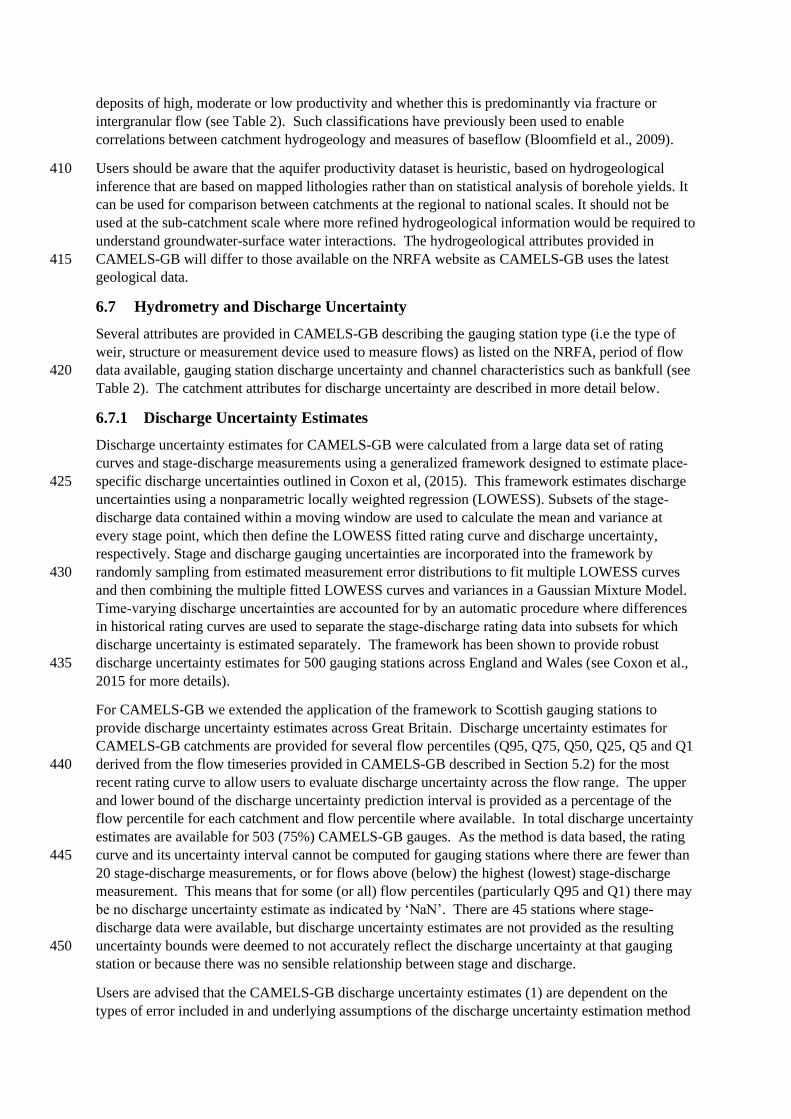
6.7 Hydrometry and Discharge Uncertainty

Several attributes are provided in CAMELS-GB describing the gauging station type (i.e the type of

weir, structure or measurement device used to measure flows) as listed on the NRFA, period of flow

data available, gauging station discharge uncertainty and channel characteristics such as bankfull (see 420

Table 2). The catchment attributes for discharge uncertainty are described in more detail below.

6.7.1 Discharge Uncertainty Estimates

Discharge uncertainty estimates for CAMELS-GB were calculated from a large data set of rating

curves and stage-discharge measurements using a generalized framework designed to estimate place‐

specific discharge uncertainties outlined in Coxon et al, (2015). This framework estimates discharge 425

uncertainties using a nonparametric locally weighted regression (LOWESS). Subsets of the stage‐

discharge data contained within a moving window are used to calculate the mean and variance at

every stage point, which then define the LOWESS fitted rating curve and discharge uncertainty,

respectively. Stage and discharge gauging uncertainties are incorporated into the framework by

randomly sampling from estimated measurement error distributions to fit multiple LOWESS curves 430

and then combining the multiple fitted LOWESS curves and variances in a Gaussian Mixture Model.

Time‐varying discharge uncertainties are accounted for by an automatic procedure where differences

in historical rating curves are used to separate the stage‐discharge rating data into subsets for which

discharge uncertainty is estimated separately. The framework has been shown to provide robust

discharge uncertainty estimates for 500 gauging stations across England and Wales (see Coxon et al., 435

2015 for more details).

For CAMELS-GB we extended the application of the framework to Scottish gauging stations to

provide discharge uncertainty estimates across Great Britain. Discharge uncertainty estimates for

CAMELS-GB catchments are provided for several flow percentiles (Q95, Q75, Q50, Q25, Q5 and Q1

derived from the flow timeseries provided in CAMELS-GB described in Section 5.2) for the most 440

recent rating curve to allow users to evaluate discharge uncertainty across the flow range. The upper

and lower bound of the discharge uncertainty prediction interval is provided as a percentage of the

flow percentile for each catchment and flow percentile where available. In total discharge uncertainty

estimates are available for 503 (75%) CAMELS-GB gauges. As the method is data based, the rating

curve and its uncertainty interval cannot be computed for gauging stations where there are fewer than 445

20 stage-discharge measurements, or for flows above (below) the highest (lowest) stage-discharge

measurement. This means that for some (or all) flow percentiles (particularly Q95 and Q1) there may

be no discharge uncertainty estimate as indicated by ‘NaN’. There are 45 stations where stage-

discharge data were available, but discharge uncertainty estimates are not provided as the resulting

uncertainty bounds were deemed to not accurately reflect the discharge uncertainty at that gauging 450

station or because there was no sensible relationship between stage and discharge.

Users are advised that the CAMELS-GB discharge uncertainty estimates (1) are dependent on the

types of error included in and underlying assumptions of the discharge uncertainty estimation method

(see Kiang et al., 2018 for a comparison of seven discharge uncertainty estimation methods) and (2)

may not be applicable to the whole flow timeseries (as they cover the most recent rating curve) or for 455

stations where flow is measured directly (i.e. at ultrasonic or electromagnetic stations).

6.8 Human Influences

Providing information on the impact of humans in each catchment is a vital part of CAMELS-GB. To

account for the degree of human intervention in each catchment we compiled data on reservoirs,

abstraction and discharge returns provided by national agencies. We focused on providing quantitative 460

data of human impacts in CAMELS-GB, however it is important to note that additional datasets are

available that qualitatively characterise human impacts in GB including the Factors Affecting Runoff

(FAR) codes available from the National River Flow Archive.

6.8.1 Benchmark Catchments

The UK Benchmark Network consists of 146 gauging stations that have been identified by the NRFA 465

as suitable for the identification and interpretation of long-term hydrological variability and change

against several criteria including length of record, quality of flow data, known impacts within the

catchment and expert consultation (for a full description see Harrigan et al, 2018). Consequently,

these gauging stations can be treated as relatively ‘near-natural’ and indicate that the influence of

humans on the flow regimes of these catchments is modest. It is important to note that some impacts 470

were tolerated where they were deemed to have a modest overall influence on flows and known to be

stable over time. This was to ensure coverage in regions such as the heavily impacted south and east

of GB. These data are available for all the CAMELS-GB catchments on whether it is part of the UK

Benchmark Network or not.

6.8.2 Abstraction and Discharges 475

The abstraction data consists of monthly abstraction data from January 1999 – December 2014 that

are reported by abstraction licence holders to the Environment Agency. These data are the actual

abstraction returns and represent the total volume of water removed by the licence holder for each

month over the time period. A mean daily abstraction rate for all English catchments is provided in

CAMELS-GB for groundwater and surface water sources. The monthly returns for each abstraction 480

licence in the database were averaged to provide a mean monthly abstraction from 1999 – 2014. All

abstraction licences that fell within each catchment boundary (using the catchment masks outlined in

section 4) were then summed for surface water and groundwater abstractions respectively and

converted into mm day-1 using catchment area. The mean daily abstraction rate is provided alongside

attributes describing the use of the abstracted water (agriculture, amenities, environmental, industrial, 485

energy or for water supply). The discharge data consists of daily discharges into water courses from

water companies and other discharge permit holders reported to the Environment Agency from 1st

January 2005 – 31st December 2015. To calculate a mean daily discharge rate for each catchment,

the daily discharge data for each discharge record was averaged and then all discharge records that

fell within the catchment boundary were summed and then converted into mm day-1 using catchment 490

area.

There are several important caveats associated with these data. Firstly, these data are only available

for England. Consequently, there are many catchments where no data are available (identified by

‘NaN’) and only a proportion of the abstractions may have been accounted for catchments which lie

on the border of England/Wales or England/Scotland. Furthermore, not all licence types/holders are 495

required to submit records to the Environment Agency, therefore this is not the full picture of human

intervention within each catchment. Secondly, the abstractions and discharges data cover different

time periods. Thirdly, the topographical catchment mask was used to define which abstraction returns

were included in each catchment. Groundwater abstractions that lie within the topographical

catchment may not have a direct impact on the catchment streamflow and instead may impact a 500

neighbouring catchment that shares the same aquifer. Conversely, groundwater abstractions that lie

outside the catchment could have an impact on the catchment streamflow. Fourthly, there is a large

inter-annual and intra annual variation in the abstraction and discharges data and their impacts will be

different across the flow regime. Consequently, it is important that the mean abstraction totals are

used as a guide to the degree of human intervention in each catchment rather than absolute totals of 505

the abstraction for any given month. Finally, although ‘abstractions’ represent removed from surface

water or groundwater sources, some of this water will be returned to catchment storages. The

discharge data provided accounts just for treated water from sewage treatment works and does not

provide information on other water returns that may be fed back into catchment storages. The mean

totals for abstractions and discharges are a very broad guide that point to the possible influence of 510

abstractions but do not quantify the net influence of these impacts on the actual flow regime. Other

(less widely available) metrics have been applied in the UK which use modelling approaches to assess

the net impact of abstractions/discharges across the whole flow regime (for example the Low Flows

Enterprise methodology; see also Hannaford et al. 2013).

6.8.3 Reservoirs 515

Reservoir attributes are derived from an open source UK reservoir inventory (Durant and Counsell,

2018) supplemented with information from SEPA’s publicly available controlled reservoirs register.

The UK reservoir inventory includes reservoirs above 1,600 megalitre (ML) capacity, covering

approximately 90% of the total reservoir storage in the UK. This dataset was collected from the

Environment Agency through a Freedom of Information request, the UK Lakes Portal (CEH) and 520

subsequent internet searches. It includes information on the location of the reservoir, its capacity, use

and year the reservoir was built. To check the accuracy of this dataset, we cross-referenced the

reservoirs in the UK reservoir inventory with reservoirs in the Global Reservoir and Dam (GRanD

v1.3) database (Lehner et al., 2011). While many of the reservoirs and their capacity data was

consistent for reservoirs for England and Wales, many Scottish reservoirs contained in the GRanD 525

database were not present in the UK reservoir inventory or reported very different storage capacities.

This is likely due to the estimation of storage capacities of Scottish reservoirs in the UK reservoir

inventories (see Hughes et al., 2004) rather than actual storage capacities. Consequently, for

reservoirs in Scotland, we used information from SEPA’s publicly available controlled reservoirs

register (http://map.sepa.org.uk/reservoirsfloodmap/Map.htm, last access: 11 December, 2019) 530

including the reservoir name, location and storage capacity, and then supplemented this information

with the year the reservoir was built and reservoir use by cross-referencing data from the UK reservoir

inventory (users should be aware that reservoir use and the year the reservoir was built were not

available for every reservoir).

For CAMELS-GB several reservoir attributes are derived for each catchment by determining the 535

reservoirs that lie within the catchment mask from the reservoir locations and then calculating (1) the

number of reservoirs in each catchment, (2) their combined capacity, (3) the fraction of that capacity

that is used for hydroelectricity, navigation, drainage, water supply, flood storage and environmental

purposes, and (4) the year when the first and last reservoir in the catchment was built.

6.9 Regional Variability in Catchment Characteristics 540

Figure 2 highlights some of the key catchment variables and in this section we discuss their regional

variability (according to the regions in Figure 2a). Spatial maps of all catchment attributes can be

found in the supplementary information (Figures S4-S11).

There are distinct regional differences in climate across GB (Figure 2b). Precipitation is typically

higher in the west and north of GB corresponding with the areas of high elevation and prevailing 545

winds from the west that bring significant rainfall. The wettest areas of the UK are in mountainous

regions with a maximum of 9.6 mm day-1 (annual average of 3500 mm year-1) in the north-west.

Snow fractions are generally very low across Great Britain (median snow fraction of 0.01) except for

catchments in the Cairngorm mountains in north-east Scotland where the fraction of precipitation

falling as snow can reach 0.17 (see supplementary information, Figure S5e). Precipitation is lowest in 550

the south and east of GB with a minimum of 1.5 mm day-1 in the east. In contrast, potential

evapotranspiration (PET) is much less variable across GB with mean daily totals ranging from 1 to

1.5mm day-1. PET is highest in the south (where temperatures are highest) and lowest in the north.

Mean flow varies from 10 to 0.09 mm day-1 and is typically higher in the north and west, reflecting

the regional variability in precipitation and PET. This is also reflected in Figure 2c, where catchments 555

in the north and west of GB tend to be wetter with higher runoff coefficients and catchments in the

south and east are much drier with lower runoff coefficients. Figure 2c also shows that annual

precipitation totals exceed annual PET totals; the aridity index is below 1 for all catchments reflecting

the temperate and humid climate of GB. It is important to note that these estimates are dependent on

the underlying data. For example, there can be significant variability in the calculation of PET, 560

depending on the methods and assumptions used (e.g. Tanguy et al., 2018) and here we have used a

PET estimate where canopy interception is not accounted for. Interception is an important component

of the water cycle in GB, which experiences a large amount of low to moderate rainfall intensities

(Blyth et al., 2019), thus using the CHESS PETI estimate instead would increase the aridity index

above one in some locations. 565

There is also regional variability in baseflow index (the ratio of mean daily baseflow to daily

discharge), which is typically higher in the south and east of GB and lower in the north-west. Some

of these differences can be attributed to regional aquifers that have high/moderate productivity which

are more prevalent in the south-east, east and north-east (see Figure 2b).

From Figure 2c, it is notable that runoff deficits significantly exceed total potential evapotranspiration 570

for many of the CAMELS-GB catchments in the south-east – this could be due to water loss to

regional aquifers, the issue of catchment areas not mapping onto the contributing area and/or due to

the choice of PET used (see above). There are also seven catchments where the runoff exceeds total

rainfall – this could be due to water gains from regional aquifers, catchment areas not mapping onto

the contributing area, inter-basin transfers, uncertainties in the rainfall and/or under-estimation of 575

rainfall. Many of the widely-used hydrological models and analysis techniques will not be able to

reproduce catchment water balances which are outside the water and energy limitations shown in Fig

2c, unless the models or analysis techniques are explicitly adapted to consider the sources of

uncertainty, potential unmeasured groundwater flow pathways and/or human influences that we have

noted. We encourage users of the data to consider whether the assumptions of their methods are 580

consistent with the uncertainties we have documented.

Land cover and human modifications can also impact river flows. Crops and grassland tend to be the

dominant land cover for GB catchments, with crops typically the dominant land cover for catchments

in the east and grassland for catchments in the west (Figure 2d). There is also a higher percentage of

catchments in the east which are dominated by urban land cover. Large reservoir capacity is 585

concentrated in the more mountainous northern and western regions of GB, particularly in Western

Scotland (Figure 2e).

7 Data Availability

The CAMELS-GB dataset (Coxon et al., 2020) detailed in this paper is freely available via the UK

Centre for Ecology & Hydrology Environmental Information Data Centre 590

(https://doi.org/10.5285/8344e4f3-d2ea-44f5-8afa-86d2987543a9). The data contain catchment

masks, catchment time series and catchment attributes as described above. A full description of the

data format is provided in the supporting documentation available on the Environmental Information

Data Centre.

8 Conclusions 595

This study introduces the first large sample, open-source catchment dataset for Great Britain,

CAMELS-GB (Catchment Attributes and MEteorology for Large-sample Studies), consisting of

hydro-meteorological catchment timeseries, catchment attributes and catchment boundaries for 671

catchments. A comprehensive set of catchment attributes are quantified describing a range of

catchment characteristics including topography, climate, hydrology, land cover, soils and 600

hydrogeology. Importantly, we also derive attributes describing the level of human influence in each

catchment and the first set of national discharge uncertainty estimates that quantify discharge

uncertainty across the flow range.

The dataset provides new opportunities to explore how different catchment characteristics control

river flow behaviour, develop common frameworks for model evaluation and benchmarking at 605

regional-national scales and analyse hydrologic variability across the UK. To ensure the

reproducibility of the dataset, many of the codes and datasets are made available to users.

While a wealth of data is provided in CAMELS-GB, there are many opportunities to expand the

dataset that were outside the scope of this study. Currently there are no plans to regularly update

CAMELS-GB, however, future work will concentrate on 1) expanding the dataset to include higher 610

resolution data (such as hourly rainfall e.g. Lewis et al., 2018, and flow timeseries) and datasets for

the analysis of trends (such as changes in land cover over time), and 2) refining the characterisation of

uncertainties in catchment attributes and forcing (particularly for rainfall data). We are also striving to

increase the consistency among the CAMELS datasets (in terms of time series, catchment attributes,

naming conventions and data format, see Addor et al., 2019), and to create a dataset that is globally 615

consistent. We anticipate that this will happen as part of a second phase, which will build upon the

current first phase that is focussed on the release of national products, such as CAMELS-GB.

Appendices

Appendix A Base flow index

The baseflow separation followed the Manual on Low-flow Estimation and Prediction of the World 620

Meteorological Organization (2008). It relies on identifying local minima in daily streamflow series

and producing a continuous baseflow hydrograph by linear interpolation between the identified local

streamflow minima. The baseflow separation was performed using the R package lfstat (Koffler et al.,

2016). The streamflow minima were identified using non-overlapping periods of N = 5 (block size)

consecutive days and f = 0.9 as turning point parameter value. 625

Appendix B Land cover classes

We used the following classification to map the 21 land cover classes contained in the UK Land

Cover Map 2015 to the eight land cover classes used in CAMELS-GB.

Table A1 Band ID and name from Land Cover Map (LCM) 2015 and corresponding land cover

classes used in CAMELS-GB 630

Band LCM2015 Band Name CAMELS-GB Land Cover Classes

1 Broad-leaved Woodland Deciduous woodland

2 Coniferous Woodland Evergreen woodland

3 Arable and Horticulture Crops

4 Improved Grassland Grass and pasture

5 Neutral Grassland Grass and pasture

6 Calcareous Grassland Grass and pasture

7 Acid Grassland Grass and pasture

8 Fen, marsh and swamp Grass and pasture

9 Heather Medium scale vegetation (shrubs)

10 Heather Grassland Medium scale vegetation (shrubs)

11 Bog Medium scale vegetation (shrubs)

12 Inland Rock Bare soil and rocks

13 Saltwater Not classified

14 Freshwater Inland water

15 Supra-littoral Rock Bare soil and rocks

16 Supra-littoral Sediment Bare soil and rocks

17 Littoral Rock Not classified

18 Littoral Sediment Not classified

19 Saltmarsh Inland water

20 Urban Urban and suburban

21 Suburban Urban and suburban

Appendix C Soil pedo-transfer functions

We estimated the saturated hydraulic conductivity and porosity (also referred to as maximum water

content, saturated water content, satiated water content) using two pedo-transfer functions.

The first was the widely-applied regressions based on sand and clay fractions first proposed by Cosby 635

et al., (1984):

𝐾𝑠 = 2.54 ∗ 10−0.6+0.012𝑆𝑎−0.0064𝐶𝑙

𝜃𝑠 = 50.5 − 0.142𝑆𝑎 − 0.037𝐶𝑙

Where 𝐾𝑠 is saturated hydraulic conductivity in cm hour-1 and 𝜃𝑠 is porosity in percent (m3m-3).

Predictor variables are Sand (𝑆𝑎) and Clay (𝐶𝑙). 640

The second, was the HYPRES continuous pedotransfer functions using silt and clay fractions, bulk

density and organic matter content (Wösten et al., 1999; Wösten, 2000):

𝐾𝑠 = 0.04167 𝑒

(7.755+0.0352𝑆𝑖+0.93𝑇𝑝−0.967𝐷𝑏2−0.000484𝐶𝑙2−0.000322𝑆𝑖2+

0.001𝑆𝑖−1−0.0748𝑂𝑚−1−0.643 ln(𝑆𝑖)−0.01398𝐷𝑏𝐶𝑙−0.1673𝐷𝑏𝑂𝑚+0.02986𝑇𝑝𝐶𝑙−0.03305𝑇𝑝𝑆𝑖)

𝜃𝑠 = 0.7919 + 0.001691𝐶𝑙 − 0.29619𝐷𝑏 − 0.000001491𝑆𝑖2 + 0.0000821𝑂𝑚2 + 0.02427𝐶𝑙−1

+ 0.01113𝑆𝑖−1 + 0.01472 ln(𝑆𝑖) − 0.0000733𝑂𝑚𝐶𝑙 − 0.000619𝐷𝑏𝐶𝑙645

− 0.001183𝐷𝑏𝑂𝑚 − 0.0001664𝑇𝑝𝑆𝑖

Where 𝐾𝑠 is saturated hydraulic conductivity in cm hour-1 and 𝜃𝑠 is porosity (m3m-3). Predictor

variables are Sand (𝑆𝑎) and Clay (𝐶𝑙). Predictor variables are Percentage Silt (𝑆𝑖), Percentage Clay

(𝐶𝑙), Percentage Organic Matter (𝑂𝑚), Bulk density (𝐷𝑏), and a binary variable for topsoil (𝑇𝑝).

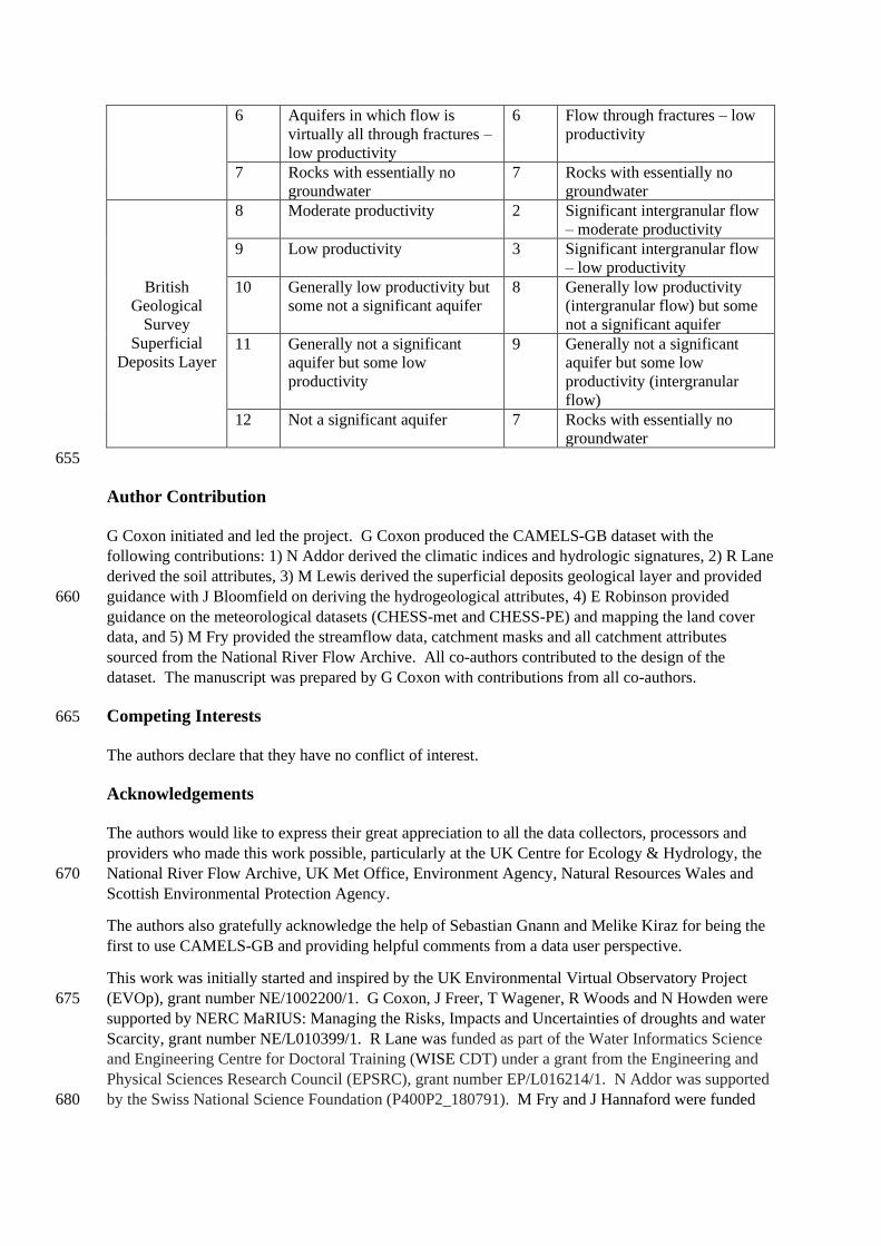
Appendix D Hydrogeological classes 650

For CAMELS-GB, we combined the BGS Hydrogeology map and superficial deposits layer. The

table below provides a summary of the different classes in each dataset and how these were

amalgamated to form the nine classes used in CAMELS-GB.

Table A2 Data source, class and description of the hydrogeological datasets

Original Data CAMELS-GB

Data Source Class

ID Description

Class

ID Description

British

Geological

Survey

Hydrogeology

Map (BGS,

2019)

1 Aquifers with significant

intergranular flow – highly

productive

1 Significant intergranular flow

– high productivity

2 Aquifers with significant

intergranular flow – moderately

productive

2 Significant intergranular flow

– moderate productivity

3 Aquifers with significant

intergranular flow – low

productivity

3 Significant intergranular flow

– low productivity

4 Aquifers in which flow is

virtually all through fractures –

highly productive

4 Flow through fractures – high

productivity

5 Aquifers in which flow is

virtually all through fractures –

moderately productive

5 Flow through fractures –

moderate productivity

6 Aquifers in which flow is

virtually all through fractures –

low productivity

6 Flow through fractures – low

productivity

7 Rocks with essentially no

groundwater

7 Rocks with essentially no

groundwater

British

Geological

Survey

Superficial

Deposits Layer

8 Moderate productivity 2 Significant intergranular flow

– moderate productivity

9 Low productivity 3 Significant intergranular flow

– low productivity

10 Generally low productivity but

some not a significant aquifer

8 Generally low productivity

(intergranular flow) but some

not a significant aquifer

11 Generally not a significant

aquifer but some low

productivity

9 Generally not a significant

aquifer but some low

productivity (intergranular

flow)

12 Not a significant aquifer 7 Rocks with essentially no

groundwater

655

Author Contribution

G Coxon initiated and led the project. G Coxon produced the CAMELS-GB dataset with the

following contributions: 1) N Addor derived the climatic indices and hydrologic signatures, 2) R Lane

derived the soil attributes, 3) M Lewis derived the superficial deposits geological layer and provided

guidance with J Bloomfield on deriving the hydrogeological attributes, 4) E Robinson provided 660

guidance on the meteorological datasets (CHESS-met and CHESS-PE) and mapping the land cover

data, and 5) M Fry provided the streamflow data, catchment masks and all catchment attributes

sourced from the National River Flow Archive. All co-authors contributed to the design of the

dataset. The manuscript was prepared by G Coxon with contributions from all co-authors.

Competing Interests 665

The authors declare that they have no conflict of interest.

Acknowledgements

The authors would like to express their great appreciation to all the data collectors, processors and

providers who made this work possible, particularly at the UK Centre for Ecology & Hydrology, the

National River Flow Archive, UK Met Office, Environment Agency, Natural Resources Wales and 670

Scottish Environmental Protection Agency.

The authors also gratefully acknowledge the help of Sebastian Gnann and Melike Kiraz for being the

first to use CAMELS-GB and providing helpful comments from a data user perspective.

This work was initially started and inspired by the UK Environmental Virtual Observatory Project

(EVOp), grant number NE/1002200/1. G Coxon, J Freer, T Wagener, R Woods and N Howden were 675

supported by NERC MaRIUS: Managing the Risks, Impacts and Uncertainties of droughts and water

Scarcity, grant number NE/L010399/1. R Lane was funded as part of the Water Informatics Science

and Engineering Centre for Doctoral Training (WISE CDT) under a grant from the Engineering and

Physical Sciences Research Council (EPSRC), grant number EP/L016214/1. N Addor was supported

by the Swiss National Science Foundation (P400P2_180791). M Fry and J Hannaford were funded 680

by National Environment Research Council as part of the National Capability programmes Hydro-

JULES (award number NE/S017380/1) and UKSCAPE (NE/R016429/1)

J Bloomfield and M Lewis publish with permission of the Executive Director, British Geological

Survey (NERC/UKRI)

References 685

Addor, N., Newman, A. J., Mizukami, N. and Clark, M. P.: The CAMELS data set: catchment

attributes and meteorology for large-sample studies, Hydrol Earth Syst Sci, 21(10), 5293–5313,

doi:10.5194/hess-21-5293-2017, 2017.

Addor, N., Nearing, G., Prieto, C., Newman, A. J., Le Vine, N. and Clark, M. P.: A Ranking of

Hydrological Signatures Based on Their Predictability in Space, Water Resour. Res., 54(11), 8792–690

8812, doi:10.1029/2018WR022606, 2018.

Addor, N., Do, H. X., Alvarez-Garreton, C., Coxon, G., Fowler, K. and Mendoza, P. A.: Large-

sample hydrology: recent progress, guidelines for new datasets and grand challenges, Hydrol. Sci. J.,

0(0), 1–14, doi:10.1080/02626667.2019.1683182, 2019.

Allen, R. G., Pereira, L. S., Raes, D. and Smith, M.: Crop evapotranspiration - Guidelines for 695

computing crop water requirements, Food and Agriculture Organization of the United Nations.,

Rome. [online] Available from: http://www.fao.org/3/X0490E/X0490E00.htm (Accessed 7 October

2019), 1998.

Alvarez-Garreton, C., Mendoza, P. A., Boisier, J. P., Addor, N., Galleguillos, M., Zambrano-

Bigiarini, M., Lara, A., Puelma, C., Cortes, G., Garreaud, R., McPhee, J. and Ayala, A.: The 700

CAMELS-CL dataset: catchment attributes and meteorology for large sample studies – Chile dataset,

Hydrol. Earth Syst. Sci., 22(11), 5817–5846, doi:https://doi.org/10.5194/hess-22-5817-2018, 2018.

Ames, D. P., Horsburgh, J. S., Cao, Y., Kadlec, J., Whiteaker, T. and Valentine, D.: HydroDesktop:

Web services-based software for hydrologic data discovery, download, visualization, and analysis,

Environ. Model. Softw., 37, 146–156, doi:10.1016/j.envsoft.2012.03.013, 2012. 705

Arsenault, R., Bazile, R., Dallaire, C. O. and Brissette, F.: CANOPEX: A Canadian

hydrometeorological watershed database, Hydrol. Process., 30(15), 2734–2736,

doi:10.1002/hyp.10880, 2016.

Bayliss, A.: Flood estimation handbook: Catchment descriptors, Institute of Hydrology., 1999.

Berghuijs, W. R., Aalbers, E. E., Larsen, J. R., Trancoso, R. and Woods, R. A.: Recent changes in 710

extreme floods across multiple continents, Env. Res Lett, 8, 2017.

Best, M. J., Pryor, M., Clark, D. B., Rooney, G. G., Essery, R. L. H., Ménard, C. B., Edwards, J. M.,

Hendry, M. A., Porson, A., Gedney, N., Mercado, L. M., Sitch, S., Blyth, E., Boucher, O., Cox, P. M.,

Grimmond, C. S. B. and Harding, R. J.: The Joint UK Land Environment Simulator (JULES), model

description – Part 1: Energy and water fluxes, Geosci. Model Dev., 4(3), 677–699, 715

doi:https://doi.org/10.5194/gmd-4-677-2011, 2011.

Beven, K.: A sensitivity analysis of the Penman-Monteith actual evapotranspiration estimates, J.

Hydrol., 44(3), 169–190, doi:10.1016/0022-1694(79)90130-6, 1979.

BGS: BGS hydrogeology 625k, [online] Available from:

https://www.bgs.ac.uk/products/hydrogeology/maps.html (Accessed 8 October 2019), 2019. 720

Bloomfield, J. P., Allen, D. J. and Griffiths, K. J.: Examining geological controls on baseflow index

(BFI) using regression analysis: An illustration from the Thames Basin, UK, J. Hydrol., 373(1), 164–

176, doi:10.1016/j.jhydrol.2009.04.025, 2009.

Blöschl, G., Hall, J., Parajka, J., Perdigão, R. A. P., Merz, B., Arheimer, B., Aronica, G. T., Bilibashi,

A., Bonacci, O., Borga, M., Čanjevac, I., Castellarin, A., Chirico, G. B., Claps, P., Fiala, K., Frolova, 725

N., Gorbachova, L., Gül, A., Hannaford, J., Harrigan, S., Kireeva, M., Kiss, A., Kjeldsen, T. R.,

Kohnová, S., Koskela, J. J., Ledvinka, O., Macdonald, N., Mavrova-Guirguinova, M., Mediero, L.,

Merz, R., Molnar, P., Montanari, A., Murphy, C., Osuch, M., Ovcharuk, V., Radevski, I., Rogger, M.,

Salinas, J. L., Sauquet, E., Šraj, M., Szolgay, J., Viglione, A., Volpi, E., Wilson, D., Zaimi, K. and

Živković, N.: Changing climate shifts timing of European floods, Science, 357(6351), 588–590, 730

doi:10.1126/science.aan2506, 2017.

Blyth, E. M., Martínez-de la Torre, A. and Robinson, E. L.: Trends in evapotranspiration and its

drivers in Great Britain: 1961 to 2015, Prog. Phys. Geogr. Earth Environ., 43(5), 666–693,

doi:10.1177/0309133319841891, 2019.

Brantley, S. L., McDowell, W. H., Dietrich, W. E., White, T. S., Kumar, P., Anderson, S. P., 735

Chorover, J., Lohse, K. A., Bales, R. C., Richter, D. D., Grant, G. and Gaillardet, J.: Designing a

network of critical zone observatories to explore the living skin of the terrestrial Earth, Earth Surf.

Dyn., 5(4), 841–860, doi:https://doi.org/10.5194/esurf-5-841-2017, 2017.

Buytaert, W., Reusser, D., Krause, S. and Renaud, J.-P.: Why can’t we do better than Topmodel?,

Hydrol. Process., 22(20), 4175–4179, doi:10.1002/hyp.7125, 2008. 740

Ceola, S., Arheimer, B., Baratti, E., Blöschl, G., Capell, R., Castellarin, A., Freer, J., Han, D.,

Hrachowitz, M., Hundecha, Y., Hutton, C., Lindström, G., Montanari, A., Nijzink, R., Parajka, J.,

Toth, E., Viglione, A. and Wagener, T.: Virtual laboratories: new opportunities for collaborative

water science, Hydrol Earth Syst Sci, 19(4), 2101–2117, doi:10.5194/hess-19-2101-2015, 2015.

Clark, D. B., Mercado, L. M., Sitch, S., Jones, C. D., Gedney, N., Best, M. J., Pryor, M., Rooney, G. 745

G., Essery, R. L. H., Blyth, E., Boucher, O., Harding, R. J., Huntingford, C. and Cox, P. M.: The Joint

UK Land Environment Simulator (JULES), model description – Part 2: Carbon fluxes and vegetation

dynamics, Geosci. Model Dev., 4(3), 701–722, doi:https://doi.org/10.5194/gmd-4-701-2011, 2011.

Clausen, B. and Biggs, B. J. F.: Flow variables for ecological studies in temperate streams: groupings

based on covariance, J. Hydrol., 237, 184–197, doi:10.1016/S0022-1694(00)00306-1, 2000. 750

Coron, L., Andréassian, V., Perrin, C., Lerat, J., Vaze, J., Bourqui, M. and Hendrickx, F.: Crash

testing hydrological models in contrasted climate conditions: An experiment on 216 Australian

catchments, Water Resour. Res., 48(5), doi:10.1029/2011WR011721, 2012.

Cosby, B. J., Hornberger, G. M., Clapp, R. B. and Ginn, T. R.: A Statistical Exploration of the

Relationships of Soil Moisture Characteristics to the Physical Properties of Soils, Water Resour. Res., 755

20(6), 682–690, doi:10.1029/WR020i006p00682, 1984.

Coxon, G., Freer, J., Wagener, T., Odoni, N. A. and Clark, M.: Diagnostic evaluation of multiple

hypotheses of hydrological behaviour in a limits-of-acceptability framework for 24 UK catchments,

Hydrol. Process., 28(25), 6135–6150, doi:10.1002/hyp.10096, 2014.

Coxon, G., Freer, J., Westerberg, I. K., Wagener, T., Woods, R. and Smith, P. J.: A novel framework 760

for discharge uncertainty quantification applied to 500 UK gauging stations, Water Resour. Res.,

51(7), 5531–5546, doi:10.1002/2014WR016532, 2015.

Coxon, G., Freer, J., Lane, R., Dunne, T., Knoben, W. J. M., Howden, N. J. K., Quinn, N., Wagener,

T. and Woods, R.: DECIPHeR v1: Dynamic fluxEs and ConnectIvity for Predictions of HydRology,

Geosci. Model Dev., 12(6), 2285–2306, doi:https://doi.org/10.5194/gmd-12-2285-2019, 2019. 765

Coxon, G., Addor, N., Bloomfield, J. P., Freer, J. E., Fry, M., Hannaford, J., Howden, N. J. K., Lane,

R., Lewis, M., Robinson, E. L., Wagener, T. and Woods, R.: Catchment attributes and hydro-

meteorological timeseries for 671 catchments across Great Britain (CAMELS-GB), NERC Environ.

Inf. Data Cent., doi:https://doi.org/10.5285/8344e4f3-d2ea-44f5-8afa-86d2987543a9, 2020.

Dixon, H., Hannaford, J. and Fry, M. J.: The effective management of national hydrometric data: 770

experiences from the United Kingdom, Hydrol. Sci. J., 58(7), 1383–1399,

doi:10.1080/02626667.2013.787486, 2013.

Do, H. X., Gudmundsson, L., Leonard, M. and Westra, S.: The Global Streamflow Indices and

Metadata Archive (GSIM) – Part 1: The production of a daily streamflow archive and metadata, Earth

Syst. Sci. Data, 10(2), 765–785, doi:https://doi.org/10.5194/essd-10-765-2018, 2018. 775

Duan, Q., Schaake, J., Andréassian, V., Franks, S., Goteti, G., Gupta, H. V., Gusev, Y. M., Habets, F.,

Hall, A., Hay, L., Hogue, T., Huang, M., Leavesley, G., Liang, X., Nasonova, O. N., Noilhan, J.,

Oudin, L., Sorooshian, S., Wagener, T. and Wood, E. F.: Model Parameter Estimation Experiment

(MOPEX): An overview of science strategy and major results from the second and third workshops, J.

Hydrol., 320(1), 3–17, doi:10.1016/j.jhydrol.2005.07.031, 2006. 780

Durant, M. J. and Counsell, C. J.: Inventory of reservoirs amounting to 90% of total UK storage,

NERC Environ. Inf. Data Cent., doi:https://doi.org/10.5285/f5a7d56c-cea0-4f00-b159-c3788a3b2b38,

2018.

Emmett, B., Gurney, R., McDonald, A., Blair, G., Buytaert, W., Freer, J. E., Haygarth, P., Johnes, P.

J., Rees, G., Tetzlaff, D., E, A., Ball, L., Beven, K., M, B., J, B., Brewer, P., J, D., Elkhatib, Y., Field, 785

D., A, G., Greene, S., Huntingford, C., Mackay, E. H., Macklin, M., MacLeod, K., Marshall, K. E.,

Odoni, N., Percy, B., Quinn, P., Reaney, S., M, S., B, S., Thomas, N., C, V., Williams, B., Wilkinson,

M. and P, Z.: Environmental Virtual Observatory: Final Report, [online] Available from:

https://research-information.bris.ac.uk/en/publications/environmental-virtual-observatory(32e19260-

0aae-44fb-a6be-7eeecc497aaa)/export.html (Accessed 12 December 2019), 2014. 790

Falkenmark, M. and Chapman, T. G.: Comparative Hydrology: An Ecological Approach to Land and

Water Resources, Unesco., 1989.

Folland, C. K., Hannaford, J., Bloomfield, J. P., Kendon, M., Svensson, C., Marchant, B. P., Prior, J.

and Wallace, E.: Multi-annual droughts in the English Lowlands: a review of their characteristics and

climate drivers in the winter half-year, Hydrol. Earth Syst. Sci., 19(5), 2353–2375, 795

doi:https://doi.org/10.5194/hess-19-2353-2015, 2015.

Fowler, K. J. A., Peel, M. C., Western, A. W., Zhang, L. and Peterson, T. J.: Simulating runoff under

changing climatic conditions: Revisiting an apparent deficiency of conceptual rainfall-runoff models,

Water Resour. Res., 52(3), 1820–1846, doi:10.1002/2015WR018068, 2016.

Gnann, S. J., Woods, R. A. and Howden, N. J. K.: Is There a Baseflow Budyko Curve?, Water 800

Resour. Res., 55(4), 2838–2855, doi:10.1029/2018WR024464, 2019.

Gudmundsson, L., Do, H. X., Leonard, M. and Westra, S.: The Global Streamflow Indices and

Metadata Archive (GSIM) – Part 2: Quality control, time-series indices and homogeneity assessment,

Earth Syst. Sci. Data, 10(2), 787–804, doi:https://doi.org/10.5194/essd-10-787-2018, 2018.

Gudmundsson, L., Leonard, M., Do, H. X., Westra, S. and Seneviratne, S. I.: Observed Trends in 805

Global Indicators of Mean and Extreme Streamflow, Geophys. Res. Lett., 46(2), 756–766,

doi:10.1029/2018GL079725, 2019.

Gupta, H. V., Perrin, C., Blöschl, G., Montanari, A., Kumar, R., Clark, M. and Andréassian, V.:

Large-sample hydrology: a need to balance depth with breadth, Hydrol. Earth Syst. Sci., 18(2), 463–

477, doi:https://doi.org/10.5194/hess-18-463-2014, 2014. 810

Gustard, A., Bullock, A. and Dixon, J. M.: Low flow estimation in the United Kingdom, [online]

Available from: http://nora.nerc.ac.uk/id/eprint/6050/ (Accessed 12 December 2019), 1992.

Hannaford, J.: Development of a strategic data management system for a national hydrological

database, the uk national river flow archive, in Hydroinformatics, pp. 637–644, World Scientific

Publishing Company., 2004. 815

Hannaford, J. and Buys, G.: Trends in seasonal river flow regimes in the UK, J. Hydrol., 475, 158–

174, doi:10.1016/j.jhydrol.2012.09.044, 2012.

Hannaford, J. and Marsh, T.: An assessment of trends in UK runoff and low flows using a network of

undisturbed catchments, Int. J. Climatol., 26(9), 1237–1253, doi:10.1002/joc.1303, 2006.

Hannah, D. M., Demuth, S., Lanen, H. A. J. van, Looser, U., Prudhomme, C., Rees, G., Stahl, K. and 820

Tallaksen, L. M.: Large-scale river flow archives: importance, current status and future needs, Hydrol.

Process., 25(7), 1191–1200, doi:10.1002/hyp.7794, 2011.

Harrigan, S., Hannaford, J., Muchan, K. and Marsh, T. J.: Designation and trend analysis of the

updated UK Benchmark Network of river flow stations: the UKBN2 dataset, Hydrol. Res., 49(2),

552–567, doi:10.2166/nh.2017.058, 2018. 825

Hiederer, R.: Mapping Soil Properties for Europe- Spatial Representation of Soil Database Attributes,

Luxembourg., 2013a.

Hiederer, R.: Mapping soil typologies: spatial decision support applied to the European Soil

Database., Publications Office, Luxembourg. [online] Available from:

http://dx.publications.europa.eu/10.2788/87286 (Accessed 20 June 2019b), 2013. 830

Hough, M. N. and Jones, R. J. A.: The United Kingdom Meteorological Office rainfall and

evaporation calculation system: MORECS version 2.0-an overview, Hydrol. Earth Syst. Sci., 1(2),

227–239, doi:https://doi.org/10.5194/hess-1-227-1997, 1997.

Hughes, M., Hornby, D. D., Bennion, H., Kernan, M., Hilton, J., Phillips, G. and Thomas, R.: The

Development of a GIS-based Inventory of Standing Waters in Great Britain together with a Risk-835

based Prioritisation Protocol, Water Air Soil Pollut. Focus, 4(2), 73–84,

doi:10.1023/B:WAFO.0000028346.27904.83, 2004.

Hutton, C., Wagener, T., Freer, J., Han, D., Duffy, C. and Arheimer, B.: Most computational

hydrology is not reproducible, so is it really science?, Water Resour. Res., 52(10), 7548–7555,

doi:10.1002/2016WR019285, 2016. 840

Jenkins, G. J., Perry, M., Prior, J., UKCIP09 and UK Climate Impacts Programme: The climate of the

United Kingdom and recent trends, Met Office Hadley Centre, Exeter. [online] Available from:

http://www.ukcip.org.uk/images/stories/08_pdfs/Trends.pdf (Accessed 12 December 2019), 2009.

Keller, V. D. J., Tanguy, M., Prosdocimi, I., Terry, J. A., Hitt, O., Cole, S. J., Fry, M., Morris, D. G.

and Dixon, H.: CEH-GEAR: 1 km resolution daily and monthly areal rainfall estimates for the UK for 845

hydrological and other applications, Earth Syst. Sci. Data, 7(1), 143–155,

doi:https://doi.org/10.5194/essd-7-143-2015, 2015.

Kiang, J. E., Gazoorian, C., McMillan, H., Coxon, G., Le Coz, J., Westerberg, I. K., Belleville, A.,

Sevrez, D., Sikorska, A. E., Petersen-Øverleir, A., Reitan, T., Freer, J., Renard, B., Mansanarez, V.

and Mason, R.: A Comparison of Methods for Streamflow Uncertainty Estimation, Water Resour. 850

Res., 54(10), 7149–7176, doi:10.1029/2018WR022708, 2018.

Koffler, D., Gauster, T. and Laaha, G.: lfstat: Calculation of Low Flow Statistics for Daily Stream

Flow Data version 0.9.8 from R-Forge. [online] Available from: https://rdrr.io/rforge/lfstat/ (Accessed

7 October 2019), 2016.

Kollat, J. B., Reed, P. M. and Wagener, T.: When are multiobjective calibration trade-offs in 855

hydrologic models meaningful?, Water Resour. Res., 48(3), doi:10.1029/2011WR011534, 2012.

Kuentz, A., Arheimer, B., Hundecha, Y. and Wagener, T.: Understanding hydrologic variability

across Europe through catchment classification, Hydrol. Earth Syst. Sci., 21(6), 2863–2879,

doi:https://doi.org/10.5194/hess-21-2863-2017, 2017.

Ladson, A. R., Brown, R., Neal, B. and Nathan, R.: A Standard Approach to Baseflow Separation 860

Using The Lyne and Hollick Filter, Australas. J. Water Resour., 17(1), 25–34,

doi:10.7158/13241583.2013.11465417, 2013.

Lane, R. A., Coxon, G., Freer, J. E., Wagener, T., Johnes, P. J., Bloomfield, J. P., Greene, S.,

Macleod, C. J. A. and Reaney, S. M.: Benchmarking the predictive capability of hydrological models

for river flow and flood peak predictions across over 1000 catchments in Great Britain, Hydrol. Earth 865

Syst. Sci., 23(10), 4011–4032, doi:https://doi.org/10.5194/hess-23-4011-2019, 2019.

Lee, H., McIntyre, N., Wheater, H. and Young, A.: Selection of conceptual models for regionalisation

of the rainfall-runoff relationship, J. Hydrol., 312(1), 125–147, doi:10.1016/j.jhydrol.2005.02.016,

2005.

Lehner, B., Liermann, C. R., Revenga, C., Vörösmarty, C., Fekete, B., Crouzet, P., Döll, P., Endejan, 870

M., Frenken, K., Magome, J., Nilsson, C., Robertson, J. C., Rödel, R., Sindorf, N. and Wisser, D.:

High-resolution mapping of the world’s reservoirs and dams for sustainable river-flow management,

Front. Ecol. Environ., 9(9), 494–502, doi:10.1890/100125, 2011.

Lewis, E., Quinn, N., Blenkinsop, S., Fowler, H. J., Freer, J., Tanguy, M., Hitt, O., Coxon, G., Bates,

P. and Woods, R.: A rule based quality control method for hourly rainfall data and a 1 km resolution 875

gridded hourly rainfall dataset for Great Britain: CEH-GEAR1hr, J. Hydrol., 564, 930–943,

doi:10.1016/j.jhydrol.2018.07.034, 2018.

Marsh, T. and Hannaford, J.: UK hydrometric register. A catalogue of river flow gauging stations and

observation wells and boreholes in the United Kingdom together with summary hydrometric and

spatial statistics, edited by T. Marsh and J. Hannaford, Centre for Ecology & Hydrology, Wallingford. 880

[online] Available from: http://nora.nerc.ac.uk/id/eprint/3093/ (Accessed 16 July 2019), 2008.

Marsh, T., Cole, G. and Wilby, R.: Major droughts in England and Wales, 1800–2006, Weather,

62(4), 87–93, doi:10.1002/wea.67, 2007.

McDonnell, J. J., Sivapalan, M., Vaché, K., Dunn, S., Grant, G., Haggerty, R., Hinz, C., Hooper, R.,

Kirchner, J., Roderick, M. L., Selker, J. and Weiler, M.: Moving beyond heterogeneity and process 885

complexity: A new vision for watershed hydrology, Water Resour. Res., 43(7),

doi:10.1029/2006WR005467, 2007.

McMillan, H., Montanari, A., Cudennec, C., Savenije, H., Kreibich, H., Krueger, T., Liu, J., Mejia,

A., Loon, A. V., Aksoy, H., Baldassarre, G. D., Huang, Y., Mazvimavi, D., Rogger, M., Sivakumar,

B., Bibikova, T., Castellarin, A., Chen, Y., Finger, D., Gelfan, A., Hannah, D. M., Hoekstra, A. Y., Li, 890

H., Maskey, S., Mathevet, T., Mijic, A., Acuña, A. P., Polo, M. J., Rosales, V., Smith, P., Viglione,

A., Srinivasan, V., Toth, E., Nooyen, R. van and Xia, J.: Panta Rhei 2013–2015: global perspectives

on hydrology, society and change, Hydrol. Sci. J., 61(7), 1174–1191,

doi:10.1080/02626667.2016.1159308, 2016.

Merz, R. and Blöschl, G.: Regionalisation of catchment model parameters, J. Hydrol., 287(1–4), 95–895

123, doi:10.1016/j.jhydrol.2003.09.028, 2004.

Mizukami, N., Clark, M. P., Newman, A. J., Wood, A. W., Gutmann, E. D., Nijssen, B., Rakovec, O.

and Samaniego, L.: Towards seamless large-domain parameter estimation for hydrologic models,

Water Resour. Res., 53(9), 8020–8040, doi:10.1002/2017WR020401, 2017.

Montanari, A., Young, G., Savenije, H. H. G., Hughes, D., Wagener, T., Ren, L. L., Koutsoyiannis, 900

D., Cudennec, C., Toth, E., Grimaldi, S., Blöschl, G., Sivapalan, M., Beven, K., Gupta, H., Hipsey,

M., Schaefli, B., Arheimer, B., Boegh, E., Schymanski, S. J., Baldassarre, G. D., Yu, B., Hubert, P.,

Huang, Y., Schumann, A., Post, D. A., Srinivasan, V., Harman, C., Thompson, S., Rogger, M.,

Viglione, A., McMillan, H., Characklis, G., Pang, Z. and Belyaev, V.: “Panta Rhei—Everything

Flows”: Change in hydrology and society—The IAHS Scientific Decade 2013–2022, Hydrol. Sci. J., 905

58(6), 1256–1275, doi:10.1080/02626667.2013.809088, 2013.

Moore, R. V., Morris, D. G. and Flavin, R. W.: CEH digital river network of Great Britain (1:50,000),

EIDC [online] Available from: https://catalogue.ceh.ac.uk/id/7d5e42b6-7729-46c8-99e9-

f9e4efddde1d (Accessed 2 November 2019), 2000.

Morris, D. G. and Flavin, R. W.: A digital terrain model for hydrology, in Proc 4th International 910

Symposium on Spatial Data Handling, vol. 1, pp. 250–262, Zürich., 1990.

Muchan, K. and Dixon, H.: Ensuring hydrometric data are fit-for-purpose through a national Service

Level Agreement, , 7, 2014.

Nelson, B.: Data sharing: Empty archives, Nature, 461(7261), 160–163, doi:10.1038/461160a, 2009.

NERC: Flood Studies Report, London., 1975. 915

Newman, A. J., Clark, M. P., Sampson, K., Wood, A., Hay, L. E., Bock, A., Viger, R. J., Blodgett, D.,

Brekke, L., Arnold, J. R., Hopson, T. and Duan, Q.: Development of a large-sample watershed-scale

hydrometeorological data set for the contiguous USA: data set characteristics and assessment of

regional variability in hydrologic model performance, Hydrol Earth Syst Sci, 19(1), 209–223,

doi:10.5194/hess-19-209-2015, 2015. 920

Parajka, J., Merz, R. and Blöschl, G.: A comparison of regionalisation methods for catchment model

parameters, Hydrol. Earth Syst. Sci., 9(3), 157–171, doi:https://doi.org/10.5194/hess-9-157-2005,

2005.

Pelletier, J. D., Broxton, P. D., Hazenberg, P., Zeng, X., Troch, P. A., Niu, G., Williams, Z., Brunke,

M. A. and Gochis, D.: A gridded global data set of soil, intact regolith, and sedimentary deposit 925

thicknesses for regional and global land surface modeling, J. Adv. Model. Earth Syst., 8(1), 41–65,

doi:10.1002/2015MS000526, 2016a.

Pelletier, J. D., Broxton, P. D., Hazenberg, P., Zeng, X., Troch, P. A., Niu, G., Williams, Z. C.,

Brunke, M. A. and Gochis, D.: Global 1-km Gridded Thickness of Soil, Regolith, and Sedimentary

Deposit Layers, ORNL DAAC, doi:https://doi.org/10.3334/ORNLDAAC/1304, 2016b. 930

Perrin, C., Michel, C. and Andréassian, V.: Improvement of a parsimonious model for streamflow

simulation, J. Hydrol., 279(1), 275–289, doi:10.1016/S0022-1694(03)00225-7, 2003.

Pool, S., Viviroli, D. and Seibert, J.: Value of a Limited Number of Discharge Observations for

Improving Regionalization: A Large-Sample Study Across the United States, Water Resour. Res.,

55(1), 363–377, doi:10.1029/2018WR023855, 2019. 935

Robinson, E. L., Blyth, E., Clark, D. B., Comyn-Platt, E., Finch, J. and Rudd, A. C.: Climate

hydrology and ecology research support system potential evapotranspiration dataset for Great Britain

(1961-2015) [CHESS-PE], NERC Environ. Inf. Data Cent., doi:https://doi.org/10.5285/8baf805d-

39ce-4dac-b224-c926ada353b7, 2016.

Robinson, E. L., Blyth, E., Clark, D. B., Comyn-Platt, E., Finch, J. and Rudd, A. C.: Climate 940

hydrology and ecology research support system meteorology dataset for Great Britain (1961-2015)

[CHESS-met] v1.2, NERC Environ. Inf. Data Cent., doi:https://doi.org/10.5285/b745e7b1-626c-4ccc-

ac27-56582e77b900, 2017a.

Robinson, E. L., Blyth, E. M., Clark, D. B., Finch, J. and Rudd, A. C.: Trends in atmospheric

evaporative demand in Great Britain using high-resolution meteorological data, Hydrol. Earth Syst. 945

Sci., 21(2), 1189–1224, doi:https://doi.org/10.5194/hess-21-1189-2017, 2017b.

Rowland, C. S., Morton, R. D., Carrasco, L., McShane, G., O’Neil, A. W. and Wood, C. M.: Land

Cover Map 2015 (1km percentage target class, GB), NERC Environ. Inf. Data Cent.,

doi:https://doi.org/10.5285/505d1e0c-ab60-4a60-b448-68c5bbae403e, 2017.

Samaniego, L., Kumar, R. and Attinger, S.: Multiscale parameter regionalization of a grid-based 950

hydrologic model at the mesoscale, Water Resour. Res., 46(5), doi:10.1029/2008WR007327, 2010.

Sankarasubramanian, A., Vogel, R. M. and Limbrunner, J. F.: Climate elasticity of streamflow in the

United States, Water Resour. Res., 37(6), 1771–1781, doi:10.1029/2000WR900330, 2001.

Sawicz, K., Wagener, T., Sivapalan, M., Troch, P. A. and Carrillo, G.: Catchment classification:

empirical analysis of hydrologic similarity based on catchment function in the eastern USA, Hydrol. 955

Earth Syst. Sci., 15(9), 2895–2911, doi:https://doi.org/10.5194/hess-15-2895-2011, 2011.

Singh, R., Werkhoven, K. van and Wagener, T.: Hydrological impacts of climate change in gauged

and ungauged watersheds of the Olifants basin: a trading-space-for-time approach, Hydrol. Sci. J.,

59(1), 29–55, doi:10.1080/02626667.2013.819431, 2014.

Stahl, K., Hisdal, H., Hannaford, J., Tallaksen, L. M., Lanen, H. A. J. van, Sauquet, E., Demuth, S., 960

Fendekova, M. and Jódar, J.: Streamflow trends in Europe: evidence from a dataset of near-natural

catchments, Hydrol. Earth Syst. Sci., 14(12), 2367–2382, doi:https://doi.org/10.5194/hess-14-2367-

2010, 2010.

Stevens, A. J., Clarke, D. and Nicholls, R. J.: Trends in reported flooding in the UK: 1884–2013,

Hydrol. Sci. J., 61(1), 50–63, doi:10.1080/02626667.2014.950581, 2016. 965

Tanguy, M., Dixon, H., Prosdocimi, I., Morris, D. G. and Keller, V. D. J.: Gridded estimates of daily

and monthly areal rainfall for the United Kingdom (1890-2015) [CEH-GEAR], NERC Environ. Inf.

Data Cent., doi:https://doi.org/10.5285/33604ea0-c238-4488-813d-0ad9ab7c51ca, 2016.

Tanguy, M., Prudhomme, C., Smith, K. and Hannaford, J.: Historical gridded reconstruction of

potential evapotranspiration for the UK, Earth Syst. Sci. Data, 10(2), 951–968, 970

doi:https://doi.org/10.5194/essd-10-951-2018, 2018.

Thompson, N., Barrie, I. A. and Ayles, M.: The Meteorological Office rainfall and evaporation

calculation system: MORECS, Meteorol. Off. Bracknell, 1981.

Tyralis, H., Papacharalampous, G. and Tantanee, S.: How to explain and predict the shape parameter

of the generalized extreme value distribution of streamflow extremes using a big dataset, J. Hydrol., 975

574, 628–645, doi:10.1016/j.jhydrol.2019.04.070, 2019.

Viglione, A., Borga, M., Balabanis, P. and Blöschl, G.: Barriers to the exchange of

hydrometeorological data in Europe: Results from a survey and implications for data policy, J.

Hydrol., 394(1), 63–77, doi:10.1016/j.jhydrol.2010.03.023, 2010.

Wagener, T., Sivapalan, M., Troch, P. A., McGlynn, B. L., Harman, C. J., Gupta, H. V., Kumar, P., 980

Rao, P. S. C., Basu, N. B. and Wilson, J. S.: The future of hydrology: An evolving science for a

changing world, Water Resour. Res., 46(5), doi:10.1029/2009WR008906, 2010.

Werkhoven, K. van, Wagener, T., Reed, P. and Tang, Y.: Characterization of watershed model

behavior across a hydroclimatic gradient, Water Resour. Res., 44(1), doi:10.1029/2007WR006271,

2008. 985

Westerberg, I. K. and McMillan, H. K.: Uncertainty in hydrological signatures, Hydrol. Earth Syst.

Sci., 19(9), 3951–3968, doi:10.5194/hess-19-3951-2015, 2015.

Westerberg, I. K., Wagener, T., Coxon, G., McMillan, H. K., Castellarin, A., Montanari, A. and Freer,

J.: Uncertainty in hydrological signatures for gauged and ungauged catchments, Water Resour. Res.,

52(3), 1847–1865, doi:10.1002/2015WR017635, 2016. 990

Woods, R. A.: Analytical model of seasonal climate impacts on snow hydrology: Continuous

snowpacks, Adv. Water Resour., 32(10), 1465–1481, doi:10.1016/j.advwatres.2009.06.011, 2009.

World Meteorological Organization (Geneva): Manual on low-flow estimation and prediction, WMO,

Geneva., 2008.

Wösten, J. H. M., Lilly, A., Nemes, A. and Le Bas, C.: Development and use of a database of 995

hydraulic properties of European soils, Geoderma, 90(3), 169–185, doi:10.1016/S0016-

7061(98)00132-3, 1999.

Wösten, J. H. M., Pachepsky, Ya. A. and Rawls, W. J.: Pedotransfer functions: bridging the gap

between available basic soil data and missing soil hydraulic characteristics, J. Hydrol., 251(3), 123–

150, doi:10.1016/S0022-1694(01)00464-4, 2001. 1000

Wösten, J. J. H.: The HYPRES database of hydraulic properties of European soils, in Subsoil

compaction; distribution, processes and consequences, edited by R. Horn, J. J. H. van den Akker, and

J. Arvidsson, pp. 135–143., 2000.

Yadav, M., Wagener, T. and Gupta, H.: Regionalization of constraints on expected watershed

response behavior for improved predictions in ungauged basins, Adv. Water Resour., 30(8), 1756–1005

1774, doi:10.1016/j.advwatres.2007.01.005, 2007.

Zacharias, S., Bogena, H., Samaniego, L., Mauder, M., Fuß, R., Pütz, T., Frenzel, M., Schwank, M.,

Baessler, C., Butterbach-Bahl, K., Bens, O., Borg, E., Brauer, A., Dietrich, P., Hajnsek, I., Helle, G.,

Kiese, R., Kunstmann, H., Klotz, S., Munch, J. C., Papen, H., Priesack, E., Schmid, H. P.,

Steinbrecher, R., Rosenbaum, U., Teutsch, G. and Vereecken, H.: A Network of Terrestrial 1010

Environmental Observatories in Germany, Vadose Zone J., 10(3), 955, doi:10.2136/vzj2010.0139,

2011.

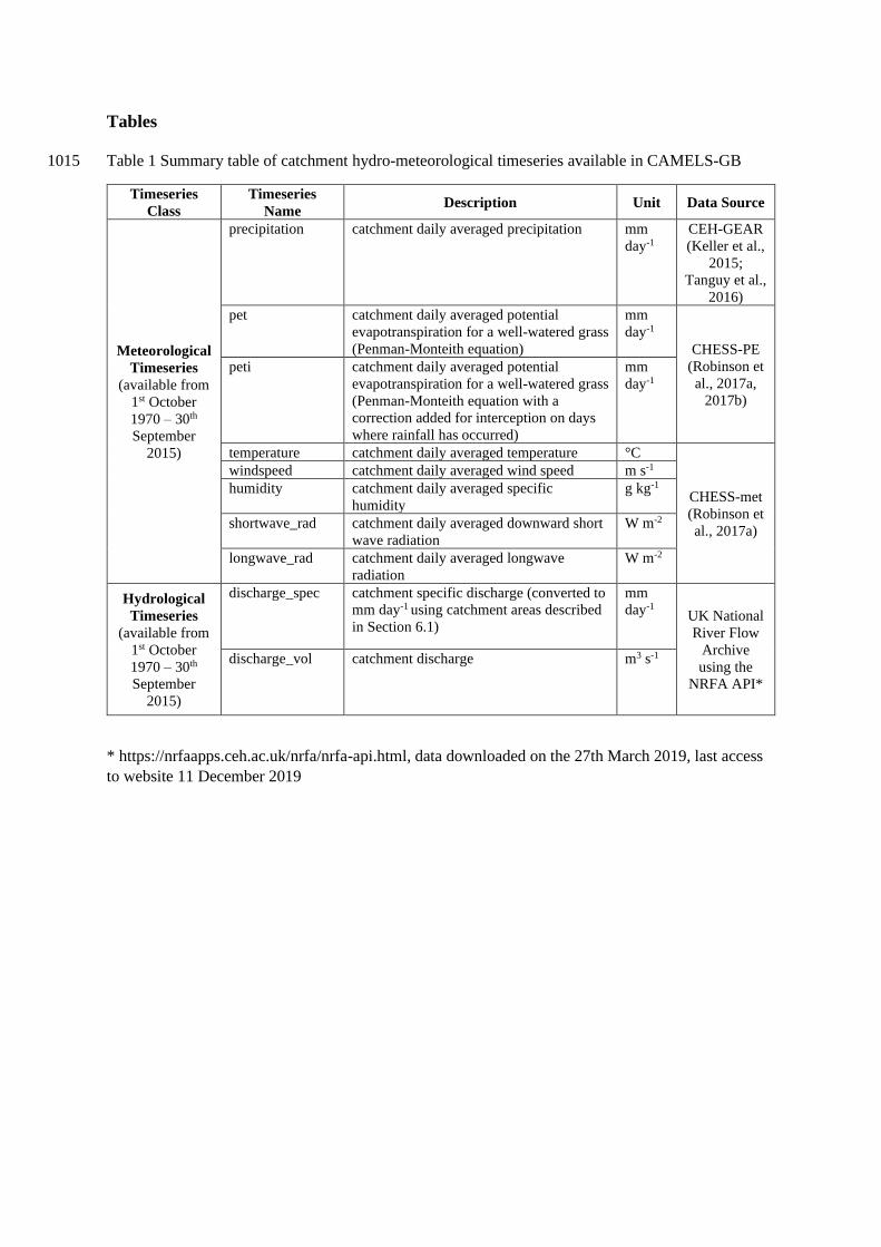
Tables

Table 1 Summary table of catchment hydro-meteorological timeseries available in CAMELS-GB 1015

Timeseries

Class

Timeseries

Name Description Unit Data Source

Meteorological

Timeseries

(available from

1st October

1970 – 30th

September

2015)

precipitation catchment daily averaged precipitation mm

day-1

CEH-GEAR

(Keller et al.,

2015;

Tanguy et al.,

2016)

pet catchment daily averaged potential

evapotranspiration for a well-watered grass

(Penman-Monteith equation)

mm

day-1

CHESS-PE

(Robinson et

al., 2017a,

2017b)

peti catchment daily averaged potential

evapotranspiration for a well-watered grass

(Penman-Monteith equation with a

correction added for interception on days

where rainfall has occurred)

mm

day-1

temperature catchment daily averaged temperature °C

CHESS-met

(Robinson et

al., 2017a)

windspeed catchment daily averaged wind speed m s-1

humidity catchment daily averaged specific

humidity

g kg-1

shortwave_rad catchment daily averaged downward short

wave radiation

W m-2

longwave_rad catchment daily averaged longwave

radiation

W m-2

Hydrological

Timeseries

(available from

1st October

1970 – 30th

September

2015)

discharge_spec catchment specific discharge (converted to

mm day-1 using catchment areas described

in Section 6.1)

mm

day-1 UK National

River Flow

Archive

using the

NRFA API*

discharge_vol catchment discharge m3 s-1

* https://nrfaapps.ceh.ac.uk/nrfa/nrfa-api.html, data downloaded on the 27th March 2019, last access

to website 11 December 2019

Table 2. Summary table of catchment attributes available in CAMELS-GB

Attribute Class Attribute Name Description Unit Data Source

Location and

Topography

gauge_id catchment identifier (corresponds to

the gauging station ID provided by

the NRFA)

-

UK National

River Flow

Archive

using the

NRFA API

gauge_name gauge name (river name followed

by gauging station name)

-

gauge_lat gauge latitude °

gauge_lon gauge longitude °

gauge_easting gauge easting m

gauge_northing gauge northing m

gauge_elev gauge elevation m.a.s.l

area catchment area km2 CEH’s

Integrated

Hydrological

Digital

Terrain

Model

(Morris and

Flavin,

1990)

dpsbar catchment mean drainage path

slope

m km-1

elev_mean catchment mean elevation m.a.s.l

elev_min catchment minimum elevation m.a.s.l

elev_10 catchment 10th percentile elevation m.a.s.l

elev_50 catchment median elevation m.a.s.l

elev_90 catchment 90th percentile elevation m.a.s.l

elev_max catchment maximum elevation m.a.s.l

Climatic

Indices

(computed for

1st Oct 1970 to

30th Sept 2015)

p_mean mean daily precipitation mm day-1

Catchment

timeseries of

precipitation

, potential

evapotranspi

ration and

temperature

described in

Section 5.1

and Table 1

pet_mean mean daily PET (Penman-Monteith

equation without interception

correction)

mm day-1

aridity aridity, calculated as the ratio of

mean daily potential

evapotranspiration to mean daily

precipitation

-

p_seasonality seasonality and timing of

precipitation (estimated using sine

curves to represent the annual

temperature and precipitation

cycles; positive (negative) values

indicate that precipitation peaks in

summer (winter) and values close

to zero indicate uniform

precipitation throughout the year).

See equation 14 in (Woods, 2009)

-

frac_snow fraction of precipitation falling as

snow (for days colder than 0°C)

-

high_prec_freq frequency of high precipitation days

(≥ 5 times mean daily precipitation)

days yr-1

high_prec_dur average duration of high

precipitation events (number of

consecutive days ≥ 5 times mean

daily precipitation)

days

high_prec_timing season during which most high

precipitation days (≥ 5 times mean

daily precipitation) occur. If two

seasons register the same number of

events, a value of NaN is given.

season

low_prec_freq frequency of dry days (< 1mm day-

1)

days yr-1

low_prec_dur average duration of dry periods

(number of consecutive days <

1mm day-1)

days

low_prec_timing season during which most dry days

(< 1mm day-1) occur. If two seasons

register the same number of events,

a value of NaN is given.

season

Hydrologic

Signatures

(computed for

1st Oct 1970 to

30th Sept 2015)

q_mean mean daily discharge mm day-1

Catchment

timeseries of

streamflow

and

precipitation

described in

Sections 5.2

and 5.1

respectively,

and Table 1

Thresholds

for high/low

flow

frequency

and duration

were

obtained

from

(Clausen and

Biggs, 2000;

Westerberg

and

McMillan,

2015)

runoff_ratio runoff ratio, calculated as the ratio

of mean daily discharge to mean

daily precipitation

-

stream_elas streamflow precipitation elasticity

(sensitivity of streamflow to

changes in precipitation at the

annual timescale, using the mean

daily discharge as reference). See

equation 7 in (Sankarasubramanian

et al., 2001), with the last element

being �̅��̅�⁄ not

�̅��̅�

⁄

-

slope_fdc slope of the flow duration curve

(between the log-transformed 33rd

and 66th streamflow percentiles)

(Yadav et al., 2007). There can be

NAs in this metric when over a

third of the flow time series are

zeros (see zero_q_freq)

-

baseflow_index baseflow index (ratio of mean daily

baseflow to daily discharge,

hydrograph separation performed

using the Ladson et al., 2013 digital

filter)

-

baseflow_index_ceh baseflow index (ratio of mean daily

baseflow to daily discharge,

hydrograph separation performed

using the Gustard et al., 1992

method described in Appendix A)

-

hfd_mean mean half-flow date (date on which

the cumulative discharge since 1

October reaches half of the annual

discharge)

days

since 1st

October

Q5 5% flow quantile (low flow) mm day-1

Q95 95% flow quantile (high flow) mm day-1

high_q_freq frequency of high-flow days (> 9

times the median daily flow)

days yr-1

high_q_dur average duration of high flow

events (number of consecutive days

>9 times the median daily flow)

days

low_q_freq frequency of low flow days (< 0.2

times the mean daily flow)

days yr-1

low_q_dur average duration of low flow events

(number of consecutive days < 0.2

times the mean daily flow)

days

zero_q_freq fraction of days with Q = 0 -

Land Cover

Attributes

dwood_perc percentage cover of deciduous

woodland

% 1km

percentage

target class,

Land Cover

Map 2015

(Rowland et

al., 2017)

ewood_perc percentage cover of evergreen

woodland

%

grass_perc percentage cover of grass and

pasture

%

shrub_perc percentage cover of medium scale

vegetation (shrubs)

%

crop_perc percentage cover of crops %

urban_perc percentage cover of suburban and

urban

%

inwater_perc percentage cover of inland water %

bares_perc percentage cover of bare soil and

rocks

%

dom_land_cover dominant land cover (the land cover

class that has the highest percentage

cover in each catchment)

-

Soil Attributes

Each soil

attribute (apart

from percentage

sand, silt, clay

and organic

content) is

accompanied by

the 5th, 50th

and 95th

percentile of

that attribute

across the

catchment and

the percentage

missing

sand_perc percentage sand %

European

Soil

Database

Derived

Data product

(Hiederer,

2013a,

2013b), and

the modelled

depth to

bedrock

global

product

(Pelletier et

al., 2016b)

silt_perc percentage silt %

clay_perc percentage clay %

organic_perc percentage organic content %

bulkdens bulk density g cm-3

tawc total available water content

(calculated over the soil depth

available for roots)

mm

porosity_cosby volumetric porosity (saturated

water content estimated using a

pedotransfer function based on sand

and clay fractions)

-

porosity_hypres volumetric porosity (saturated

water content estimated using a

pedotransfer function based on silt,

clay and organic fractions, bulk

density and topsoil)

-

conductivity_cosby saturated hydraulic conductivity

(estimated using a pedotransfer

function based on sand and clay

fractions)

cm h-1

conductivity_hypres saturated hydraulic conductivity

(estimated using a pedotransfer

function based on silt, clay and

organic fractions, bulk density and

topsoil)

cm h-1

root_depth depth available for roots m

soil_depth_pelletier depth to bedrock (maximum 50m) m

Hydrogeology

Attributes

inter_high_perc significant intergranular flow – high

productivity

%

British

Geological

Survey

hydrogeolog

y map (BGS,

2019) and

superficial

deposits map

inter_mod_perc significant intergranular flow –

moderate productivity

%

inter_low_perc significant intergranular flow – low

productivity

%

frac_high_perc flow through fractures – high

productivity

%

frac_mod_perc flow through fractures – moderate

productivity

%

frac_low_perc flow through fractures – low

productivity

%

no_gw_perc rocks with essentially no

groundwater

%

low_nsig_perc generally low productivity

(intergranular flow) but some not

significant aquifer

%

nsig_low_perc generally not significant aquifer but

some low productivity

(intergranular flow)

%

Hydrometry station_type gauging station type denoted by the

following abbreviations (B Broad-

- UK National

River Flow

crested weir; C Crump profile

single-crest weir; CB Compound

broad-crested weir; CC Compound

Crump weir; EM Electromagnetic

gauging station; EW Essex weir;

FL Flume; FV Flat V triangular

profile weir; MIS Miscellaneous;

TP Rectangular thin-plate weir; US

Ultrasonic gauging station; VA

Velocity-area gauging station; VN

Triangular (V notch) thin-plate

weir). Two abbreviations may be

applied to each station relating to

the measurement of low or high

flows.

Archive

using the

NRFA API

flow_period_start first date that daily flow time series

provided in CAMELS-GB is

available for this gauging station

-

Catchment

timeseries of

streamflow

described in

Section 5.2

flow_period_end end date that daily flow time series

provided in CAMELS-GB are

available for this gauging station

-

flow_perc_complete percentage of days with flow time

series available from 1st October

1970 – 31st September 2015

%

bankfull_flow flow at which the river begins to

overlap the banks at a gauging

station (obtained from stage-

discharge relationships so may be

derived by extrapolation)

m3 s-1

UK National

River Flow

Archive

using the

NRFA API

structurefull_flow flow at which the river begins to the

wingwalls of a structure at a

gauging

station (obtained from stage-

discharge relationships so may be

derived by extrapolation)

m3 s-1

qXX_uncert_upper upper bound of the discharge

uncertainty interval for the XX

percentile flow given as a

percentage of the XX percentile

flow – estimates for XX values of

5, 25, 50, 75, 95, 99 are provided

%

Derived

from Coxon

et al (2015)

qXX_uncert_lower lower bound of the discharge

uncertainty interval for the XX

percentile flow given as a

percentage of the XX percentile

flow – estimates for XX values of

5, 25, 50, 75, 95, 99 are provided

%

quncert_meta metadata describing the reasons

why discharge uncertainty

estimates are (not) provided;

Calculated discharge

uncertainties; No stage-discharge

measurements available; Less

than 20 stage-discharge

measurements available for most

recent rating; Discharge

uncertainty estimates not

provided as the estimated

uncertainty bounds were deemed to

not accurately reflect the discharge

-

uncertainty or because there was no

sensible relationship between stage

and discharge.

Human

Influence

Attributes

benchmark_catch benchmark catchment (Y indicates

the catchment is part of the UK

Benchmark Network, while N

indicates that it is not)

Y/N UK National

River Flow

Archive;

Harrigan et

al., (2018)

surfacewater_abs mean surface water abstraction mm day-1

Abstractions

and

discharges

sourced

from the

Environment

Agency

groundwater_abs mean groundwater abstraction mm day-1

discharges mean discharges (daily discharges

into water courses from water

companies and other discharge

permit holders reported to the

Environment Agency)

mm day-1

abs_agriculture_perc percentage of total (groundwater

and surface water) abstractions in

catchment for agriculture

%

abs_amenities_perc percentage of total (groundwater

and surface water) abstractions in

catchment for amenities

%

abs_energy_perc percentage of total (groundwater

and surface water) abstractions in

catchment for energy production

%

abs_environmental_per

c

percentage of total (groundwater

and surface water) abstractions in

catchment for environmental

purposes

%

abs_industry_perc percentage of total (groundwater

and surface water) abstractions in

catchment for industrial,

commercial and public services

%

abs_watersupply_perc percentage of total (groundwater

and surface water) abstractions in

catchment for water supply

%

num_reservoir number of reservoirs in the

catchment

-

UK

Reservoir

Inventory

(Durant and

Counsell,

2018) and

SEPA’s

publicly

available

controlled

reservoirs

register

(http://map.s

epa.org.uk/re

servoirsflood

map/Map.ht

m, last

access: 11

December,

2019)

reservoir_cap total storage capacity of reservoirs

in the catchment in megalitres

ML

reservoir_he percentage of total reservoir storage

in catchment used for

hydroelectricty

%

reservoir_nav percentage of total reservoir storage

in catchment used for navigation

%

reservoir_drain percentage of total reservoir storage

in catchment used for drainage

%

reservoir_wr percentage of total reservoir storage

in catchment used for water

resources

%

reservoir_fs percentage of total reservoir storage

in catchment used for flood storage

%

reservoir_env percentage of total reservoir storage

in catchment used for

environmental

%

reservoir_nousedata percentage of total reservoir storage

in catchment where no use data

were available

%

reservoir_year_first year the first reservoir in the

catchment was built

-

reservoir_year_last year the last reservoir in the

catchment was built

-

Figures

Figure 1. a) Number of stations with percentage of available streamflow data for different periods, b) Length of

the flow time series for each gauge

a) b)

Fig

ure

2.

Key

cat

chm

ent

var

iab

les

a) M

ap o

f G

reat

Bri

tain

riv

er b

asin

reg

ion

s b

ased

on

the

UK

CP

09

riv

er b

asin

s ag

gre

gat

ed f

rom

21

riv

er b

asin

dis

tric

ts t

o 8

reg

ion

s, b

)

bo

xp

lots

sh

ow

ing

th

e ra

ng

e o

f k

ey c

lim

atic

, hy

dro

log

y a

nd

hy

dro

geo

log

ic (

def

ined

by

th

e p

ropo

rtio

n o

f th

e ca

tch

men

t un

der

lain

by

hig

h o

r m

od

erat

e p

rodu

ctiv

ity

aq

uif

ers)

catc

hm

ent

attr

ibu

tes

for

each

reg

ion

, c)

bud

yko

-ty

pe

curv

e re

lati

ng

ru

no

ff c

oef

fici

ent

to a

rid

ity

in

dex

, p

oin

ts a

re c

olo

ure

d b

y r

egio

n a

nd

th

e y

-ax

is i

s li

mit

ed t

o 1

.5 w

hic

h

mea

ns

two

gau

ges

(2

600

6 a

nd 2

70

38

) ar

e n

ot

sho

wn

th

at h

ave

a ru

no

ff c

oef

fici

ent

of

3,

d)

the

per

cen

tag

e o

f ca

tch

men

ts i

n e

ach

reg

ion

wit

h a

do

min

ant

lan

d c

ov

er o

f ei

ther

wo

od

lan

d (

ever

gre

en a

nd

dec

idu

ou

s), g

rass

, sh

rub

, cr

op

or

urb

an,

e) t

he t

ota

l re

serv

oir

cap

acit

y i

n t

he

catc

hm

ents

in

eac

h r

egio

n

a)

b)

c)

d)

e)