CAMEL(S) AND BANKS PERFORMANCE

Electronic copy available at: http://ssrn.com/abstract=1150968

1

CAMEL(S) AND BANKS PERFORMANCE EVALUATION: THE WAY FORWARD.

BY

WIRNKAR A.D. AND TANKO M.


2

ABSTRACT

Despite the continuous use of financial ratios analysis on banks performance evaluation

by banks’ regulators, opposition to it skill thrive with opponents coming up with new

tools capable of flagging the over-all performance ( efficiency) of a bank. This research

paper was carried out; to find the adequacy of CAMEL in capturing the overall

performance of a bank; to find the relative weights of importance in all the factors in

CAMEL; and lastly to inform on the best ratios to always adopt by banks regulators in

evaluating banks’ efficiency. The data for the research work is secondary and was

collected from the annual reports of eleven commercial banks in Nigeria over a period of

nine years (1997 – 2005). The purposive sampling technique was used. The presentation

of data was in tables and analyzed via the Efficiency Measurement System (EMS) 1.30

software of Holger School and independent T-test equation. The findings revealed the

inability of each factor in CAMEL to capture the wholistic performance of a bank. Also

revealed, was the relative weight of importance of the factors in CAMEL which resulted

to a call for a change in the acronym of CAMEL to CLEAM. In addition, the best ratios

in each of the factors in CAMEL were identified. For example, the best ratio for Capital

Adequacy was found to be the ratio of total shareholders’ fund to total risk weighted

assets. The paper concluded that no one factor in CAMEL suffices to depict the overall

performance of a bank. Among other recommendations, banks’ regulators are called upon

to revert to the best identified ratios in CAMEL when evaluating banks performance.


3

Introduction

It is usual to measure the performance of banks using financial ratios. Often, a

number of criteria such as profits, liquidity, asset quality, attitude towards risk, and

management strategies must be considered. In the early 1970s, federal regulators

in USA developed the CAMEL rating system to help structure the bank

examination process. In 1979, the Uniform Financial Institutions Rating System

was adopted to provide federal bank regulatory agencies with a framework for

rating financial condition and performance of individual banks (Siems and Barr;

1998). Since then, the use of the CAMEL factors in evaluating a bank’s financial

health has become widespread among regulators. Piyu (1992) notes “currently,

financial ratios are often used to measure the overall financial soundness of a bank

and the quality of it management. Bank regulators, for example, use financial

ratios to help evaluate a bank’s performance as part of the CAMEL system”. The

evaluation factors are as follows;

C → Capital adequacy

A → Asset quality

M → Management quality

E → Earnings ability

L → Liquidity.

Each of the five factors is scored from one to five, with one being the strongest

rating. An overall composite CAMEL rating, also ranging from one to five, is then

developed from this evaluation. As a whole, the CAMEL rating, which is

determined after an on-site examination, provides a means to categorize banks

based on their overall health, financial status, and management. The Commercial

Bank Examination Manual produced by the Board of Governors of the Federal

Reserve System in U.S describes the five composite rating levels as follows

(Siems and Barr, 1998).

CAMEL = 1 an institution that is basically sound in every respect.

4

CAMEL = 2 an institution that is fundamentally sound but has modest

weaknesses.

CAMEL = 3 an institution with financial, operational, or compliance

weaknesses that give cause for supervisory concern.

CAMEL = 4 an institution with serious financial weaknesses that could

impair future viability.

CAMEL = 5 an institution with critical financial weaknesses that render

the probability of failure extremely high in the near term.

In Nigeria, commercial banks are examined annually for safety and

soundness by the Banking Supervision Department of the Central Bank of Nigeria

(CBN).

Statement of the Problem

Bank’s performance or rather solvency or insolvency has been given much

attention both at the local and international level. Financial ratios are often used to

measure the overall financial soundness of a bank and the quality of its

management. Banks’ regulators, for example, use financial ratios to help evaluate

a bank’s performance as part of the CAMEL system (YUE, 1992). Despite

continuous use of ratios analysis in banks performance appraisal by regulators, opponents

to it still thrive. Financial ratios are somewhat limited in scope, that is, simple gap

analysis are one dimensional views of a service, product, or process that ignore

any interactions, substitutions or trade-offs between key variables (Siems and

Barr, 1998).

According to David A. and Vlad M. (2002), “Studies on productivity growth in

the banking sector usually base their analysis on cost ratio comparisons. There are

several cost ratios to be used and each one of them refers to a particular aspect of

bank activity. Since the banking industry uses multiple inputs to produce multiple

5

outputs, a consistent aggregation may be problematic. Some attempts have been

made to estimate average practice cost functions. While these approaches were

successful in identifying the average practice productivity growth, they failed to

take into account the productivity of the best practice banks. These problems

associated with the classical approach to productivity led to the emergence of

other approaches which incorporate multiple inputs/outputs and take into account

the relative performance of banks”.

Hypotheses

HO1: There is no significant difference between banks’ efficiency and capital adequacy.

HO2: There is no significant difference between banks’ efficiency and asset quality.

HO3: There is no significant difference between bank’s efficiency and management

quality.

HO4: There is no significant difference between bank’s efficiency and earnings ability.

HO5: There is no significant difference between bank’s efficiency and liquidity.

Literature Review

Bank’s performance or rather solvency or insolvency has been given much

attention both at the local and international level. Financial ratios are often used to

measure the overall financial soundness of a bank and the quality of its

management. Banks’ regulators, for example, use financial ratios to help evaluate

a bank’s performance as part of the CAMEL system (YUE, 1992). Empirical

evidence on the use of ratios for banks’ performance appraisal include; Beaver

(1966), Altman (1968), Maishanu (2004), Mous (2005).

Beaver (1966) was the first person to use financial ratios for predicting bankruptcy

his study was limited to looking at only one ratio at a time. Altman (1968)

changed this by using a multiple discriminant analysis (MDA). His analysis

6

combined the information from several financial ratios in a single prediction

model. Altman’s z- score model was the result of this multiple discriminant

analysis and has been popular for a number of decades as it was easy to use and

highly accurate. But there was critique on the MDA model. Altman treated

businesses from different sectors as the same, ignoring the fact that there should be

different values for a healthy indication by the financial ratios of the different

kinds of businesses.

Maishanu (2004) identified eight financial ratios that could serve in

informing financial analysts on the financial state of a bank. As such, he put forth

a univariate model for predicting failure in commercial banks.

In comparing two bankruptcy predicting models using financial ratios,

(Mous, 2005) found that the decision tree approach performed better than the

multiple discriminant analysis (MDA) with decision tree correctly classifying 89%

of bankrupt banks within two years while multiple discriminant analysis (MDA)

got 81%. The financial ratios used had variables; profitability, liquidity, leverage,

turnover and total assets.

The changing nature of the banking industry has made such evaluations

even more difficult, gingering the need for more flexible alternative forms of

financial analysis. These are the parametric methods of; the stochastic frontier

approach (SFA), the thick frontier approach (TFA) and the distribution freehall

approach (DFA); and the non parametric method of data envelopment analysis

(DEA).

The empirical evidence of the parametric approaches are; Asaftei (2003),

Limam (2002) while the empirical evidence of the non parametric of data

envelopment analysis (DEA) are; Cinca and Molinero (2001), Cinca et al (2002),

Sathye (2001), Yue (1992), Grigorian and Manole (2002), Su (2004) and Tanko

(2006), Wirnkar ( 2007), Wirnkar and Tanko (2007).

7

In selecting DEA specifications and ranking units via PCA, Cinca and

Molinero (2000) were able to identify and rank the 18 Chinese cities in terms of

efficiency in utilizing inputs to produce outputs. Maverick cities were also

identified that could ignite any directed economic reform by the Chinese

government.

In evaluating the performance of 60 Missouri Commercial Banks between

(1984 – 1990) using DEA with an intermediary approach of inputs (interest

expenses, non-interest expenses, transaction deposits, and non-transaction

deposits) with outputs (interest income, non-interest income and total loans), Yue

(1992) found that while five of the Missouri banks were technologically efficient,

they were not operating at the most efficient scale of operation.

Measuring Inputs and Outputs of Banks

In the banking literature, there has been some disagreement on the

definition of banks’ inputs and outputs and how they could be measured. Su

(2004), Mlima and Hjalmarsson (2002), Sathye (2001). These terms from the

quantum of services banks provide as well as the different views regarding the

treatment of such services as inputs and/or outputs. Banks mostly provide

customers with low risk assets, credit and payment services, and play an important

role as intermediaries in directing funds from savers to borrowers. They also

perform non-monetary services such as protection of valuables, accounting

services and running of investment portfolios (Colwell and Davis, 1992) in

(Mlima and Hjalmarrson; 2002).

Ahmed (1999) identifies these services to include the following:

1) Deposit collection through savings account, current account and fixed deposit

account.

2) Provision of credit to customers in form of loans, overdraft, advance, bill

discounting, leasing, acceptance of bills, bonds and guarantees.

8

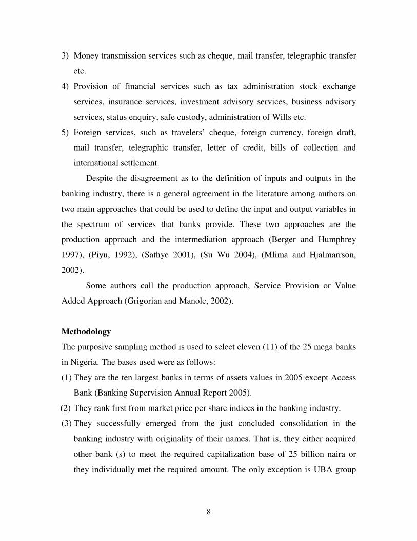
3) Money transmission services such as cheque, mail transfer, telegraphic transfer

etc.

4) Provision of financial services such as tax administration stock exchange

services, insurance services, investment advisory services, business advisory

services, status enquiry, safe custody, administration of Wills etc.

5) Foreign services, such as travelers’ cheque, foreign currency, foreign draft,

mail transfer, telegraphic transfer, letter of credit, bills of collection and

international settlement.

Despite the disagreement as to the definition of inputs and outputs in the

banking industry, there is a general agreement in the literature among authors on

two main approaches that could be used to define the input and output variables in

the spectrum of services that banks provide. These two approaches are the

production approach and the intermediation approach (Berger and Humphrey

1997), (Piyu, 1992), (Sathye 2001), (Su Wu 2004), (Mlima and Hjalmarrson,

2002).

Some authors call the production approach, Service Provision or Value

Added Approach (Grigorian and Manole, 2002).

Methodology

The purposive sampling method is used to select eleven (11) of the 25 mega banks

in Nigeria. The bases used were as follows:

(1) They are the ten largest banks in terms of assets values in 2005 except Access

Bank (Banking Supervision Annual Report 2005).

(2) They rank first from market price per share indices in the banking industry.

(3) They successfully emerged from the just concluded consolidation in the

banking industry with originality of their names. That is, they either acquired

other bank (s) to meet the required capitalization base of 25 billion naira or

they individually met the required amount. The only exception is UBA group

9

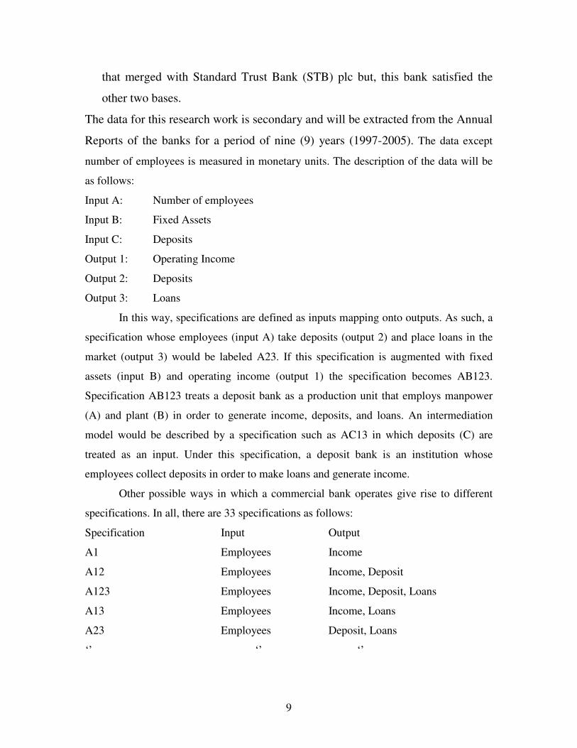
that merged with Standard Trust Bank (STB) plc but, this bank satisfied the

other two bases.

The data for this research work is secondary and will be extracted from the Annual

Reports of the banks for a period of nine (9) years (1997-2005). The data except

number of employees is measured in monetary units. The description of the data will be

as follows:

Input A: Number of employees

Input B: Fixed Assets

Input C: Deposits

Output 1: Operating Income

Output 2: Deposits

Output 3: Loans

In this way, specifications are defined as inputs mapping onto outputs. As such, a

specification whose employees (input A) take deposits (output 2) and place loans in the

market (output 3) would be labeled A23. If this specification is augmented with fixed

assets (input B) and operating income (output 1) the specification becomes AB123.

Specification AB123 treats a deposit bank as a production unit that employs manpower

(A) and plant (B) in order to generate income, deposits, and loans. An intermediation

model would be described by a specification such as AC13 in which deposits (C) are

treated as an input. Under this specification, a deposit bank is an institution whose

employees collect deposits in order to make loans and generate income.

Other possible ways in which a commercial bank operates give rise to different

specifications. In all, there are 33 specifications as follows:

Specification Input Output

A1 Employees Income

A12 Employees Income, Deposit

A123 Employees Income, Deposit, Loans

A13 Employees Income, Loans

A23 Employees Deposit, Loans

‘’ ‘’ ‘’

10

‘’ ‘’ ‘’

‘’ ‘’ ‘’

ABC Employees Loans

This is followed by the calculation of the efficiency scores using DEA for all

specifications. Efficiency scores are on a scale of 0% to 100% for all commercial banks

for the period under constant return to scale at maximum average with the Efficiency

Measurement System (EMS) 1.30 of Holger Scheel. See www.wiso.uni-

dortmund.de/lsfg/or/scheel/ems/.

Next is followed by the calculation of average Capital Adequacy ratios and

average Sub-Capital Adequacy ratios for the test of the main hypothesis and Sub-

hypotheses under Capital Adequacy. Then the calculation of the of average Asset Quality

ratios and average Sub-Asset Quality ratios for the test of the main hypothesis and Sub-

hypotheses under Asset Quality up until the calculation of average liquidity ratios and

average sub-liquidity ratios for the test of the last (5th

) hypothesis and Sub-hypotheses.

The various CAMEL ratios are as follows:

CAPADR 1 – A ratio of total assets to total shareholders’ funds. It shows the

extent to which total assets are supported by shareholders’ funds. The lower the

value of this ratio, the better the financial health of a bank.

CAPADR 2 – A ratio of total shareholders’ funds to total assets. It shows the

proportion of a unit naira of equity to a unit naira of asset. The higher the value of

this ratio, the better the financial health of a bank.

CAPADR 3 A ratio of total shareholders’ funds to total net loans. It shows the

proportion of shareholders funds in granting loans. The higher the value of this

ratio, the better the financial health of a bank.

CAPADR 4 – A ratio of total shareholders’ funds to total deposits. It shows the

capacity of shareholders’ funds to withstand sudden withdrawals. The higher the

value of this ratio, the better the financial health of the company.

11

CAPADR 5 – A ratio of shareholders’ funds to contingency liabilities. This

measures the extent to which a bank carries off-balance sheet risks. The higher the

value of this ratio, the better the financial health of a bank.

CAPADR 6 – A ratio of total shareholders’ funds to total risk weighted assets (non

performing loans). It measures the ability of a bank in absorbing losses arising

from risk assets. The higher the value of this ratio, the better the financial health of

a bank.

The Asset Quality ratios are divided into two. The mean of these ratios will

be used.

ASSETQR 1 – A ratio of loan loss provision to total net loans. This ratio shows

the ability of a bank to meet further losses on total net loans. The higher the value

of this ratio, the worsening the financial health of a bank.

ASSETQR2 – A ratio of loan loss provision to gross loans. It measures the ability

of a bank to meet further losses on gross loans. The higher the value of this ratio,

the worsening the financial health of a bank.

The management quality ratio is defined from the perspective of risk in

Asset portfolio (mix). The only ratio here is a ratio of total of risk weighted assets

to total assets. The higher the value of this ratio, the worsening the financial health

of a bank.

The Earnings Ability ratios are two. The average of these ratios will be

used. These are:

EargAR1 (ROA) – A ratio of net profit after tax to total assets. It measures a unit

yield of profit to a unit value of assets. The higher the value of this ratio, the better

the financial health of a bank.

EargAR2 (ROE) – A ratio of net profit after tax to total shareholders’ funds. It

measures a unit yield of profit to a unit value of total shareholders’ funds. The

higher the value of this ratio, the better the financial health of a bank.

The Liquidity ratios are three. The average of these ratios will be used.

12

Liq R1 – A ratio of total net loans to total deposits. It shows how far a bank has

tied up its deposits in less liquid assets. The higher the value of this ratio, the

weaker the financial health of a bank.

Liq R2 – A ratio of demand liabilities to total deposits. This shows the portion of

total deposits that is in the risk of sudden withdrawals.

Liq R3 – A ratio of gross loans to total deposit. It shows how a bank has tied its

deposit in less liquid assets. The higher the value of this ratio, the weaker the

financial health of a bank.

From the above breakdown of CAMEL ratios, we shall have altogether

fourteen hypotheses (five main hypotheses and thirteen sub-hypotheses).

The main hypotheses will inform on the relative weight of each factor in

CAMEL to capture the wholistic efficiency of a bank.

The Sub-hypotheses will inform us on the best ratios to be used for each of

the factors in CAMEL.

All the hypotheses will be tested using the Independent T-test equation for

testing the difference between means (x).see Chambers and Crawshaw, (1990)

/ Z / = (x1 – x2) – (µ1 – µ2)

+

n1 n2

Where / Z / = magnitude of

(1) Capital adequacy

(2) Asset quality

(3) Management quality

(4) Earning ability

(5) Liquidity

X1 = mean of:


(7) Asset quality

δ12 δ2

2

13


(9) Earnings ability

(10) Liquidity

X2 = mean of gross efficiency scores (performance).

µ1 = µ2 = mean of Population (number of banks)

= Variance of;


(2) Asset quality



(5) Liquidity

= Variance of gross efficiency scores (performance)

n1 = numerical number of;


(2) Asset quality



(5) Liquidity

n2 = numerical number of gross efficiency scores (performance)

Decision rule:

The Null hypothesis is accepted if the magnitude / Z / falls within / Z /> 1.96 that

is

-1.96 <Z< +1.96 at 5% level of significance otherwise the Alternative hypothesis

is accepted. The two tailed test will be used.

This will be followed by the interpretation of the findings, conclusion,

recommendations, bibliography and lastly appendices.

δ12

δ22

14

The Data Envelopment Analysis (DEA)

DEA is a multi-factor productivity analysis model for measuring the relative efficiencies

of a homogenous set of decision making units (DMUs). Talluri (2000) states that the

efficiency score in the presence of multiple input and output factors is defined as:

Efficiency = Weighted sum of outputs

Weighed sum of inputs

The procedure for finding the efficiency scores of decision making units (DMU)

is formulated as a linear programming problem. Assuming that there are n DMUs, each

with M inputs and S outputs, the relative efficiency score of a test DMU p is obtained by

solving the following model proposed by Charnes et al (1978).

max

s.t

Where

k = l to s,

j = l to m,

I = l to n,

Yki = amount of output K produced by DMUi,

k = 1

s

Vk Ykp

j = 1

m

Uj Xjp

k = 1

s

Vk Ykp

j = 1

m

Uj Xjp

< 1 i

Vk, Uj > 0 k, j,

15

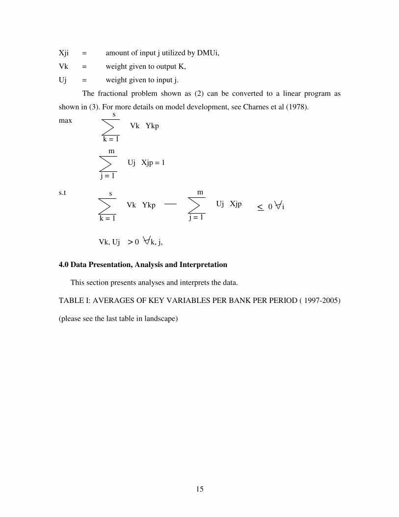
Xji = amount of input j utilized by DMUi,

Vk = weight given to output K,

Uj = weight given to input j.

The fractional problem shown as (2) can be converted to a linear program as

shown in (3). For more details on model development, see Charnes et al (1978).

max

s.t

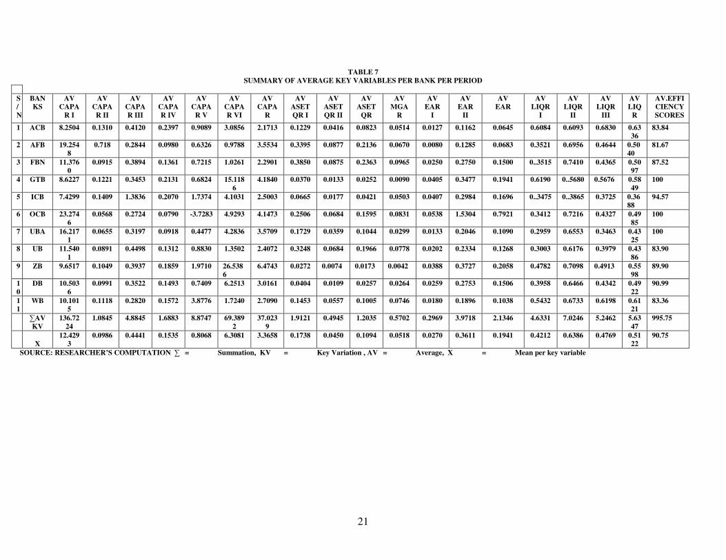
4.0 Data Presentation, Analysis and Interpretation

This section presents analyses and interprets the data.

TABLE I: AVERAGES OF KEY VARIABLES PER BANK PER PERIOD ( 1997-2005)

(please see the last table in landscape)

k = 1

s

Vk Ykp

j = 1

m

Uj Xjp = 1

k = 1

s

Vk Ykp < 0 i

Vk, Uj > 0 k, j,

j = 1

m

Uj Xjp

16

TABLE II: RESULTS OF THE TEST OF HYPOTHESES CAMEL RATIOS CAMEL

RATIOS EFFICIENCY

SCORES (X) /Z/ DECISION

RULE SUB CAMEL

RANkING CAMEL

RANKING AV CAPAR 3.3658 90.52 -12.5620 Reject Ho 1

st

AV CAPAR 1 12.4293 90.52 -9.3464 Reject Ho 2nd

AV CAPAR 2 0.09866 90.52 -13.2321 Reject Ho 6

th

AV CAPAR 3 0.4441 90.52 -13.1688 Reject Ho 4th


th

AV CAPAR 5 0.8068 90.52 -12.7329 Reject Ho 3rd


st

AV ASSET QR 0.1094 90.52 -13.2297 Reject Ho 4th

AV ASSET QR 1 0.1738 90.52 -13.2189 Reject Ho 1

st

AV ASSET QR 2 0.0450 90.52 -13.2399 Reject Ho 2nd

AV MGQR 9.0518 90.52 -13.2389 Reject Ho 5

th

AV EARGAR 0.1941 90.52 -13.2129 Reject Ho 3rd

AV EARGAR 1 0.0270 90.52 -13.2427 Reject Ho 2

nd

AV EARGAR 2 0.3611 90.52 -13.1736 Reject Ho 1st

AV LI QR 0.5122 90.52 -13.1708 Reject Ho 2nd

AV LI QR 1 0.4212 90.52 -13.1831 Reject Ho 3

rd

AV LI QR 2 0.638690.5

2 90.52 -13.1519 Reject Ho 1

st

AV LI QR 3 0.4769 90.52 -13.1753 Reject Ho 2nd

SOURCE: AUTHOR’S COMPUTATION. SEE APPENDIX F

From the above table, the following findings are unveiled:

That no factor in CAMEL is able to capture the wholistic efficiency of a bank. This is

evidenced by the rejection of the null hypotheses in all the main and sub-hypotheses. The

proximal weights or ability of each factor in CAMEL to capture the wholistic

performance of a bank are ascertained. This yielded an order in ranking the factors in

CAMEL to CLEAM. As such, giving us a new acronym for CAMEL as CLEAM to

reflect the ability of each of the factors to capture a wholistic performance of a bank.

In consideration of sub-hypotheses under capital adequacy, the best ratio is CAPAR 6

which is a ratio of total shareholders fund to total risk weighted assets. The other five

capital adequacy ratios are rated accordingly. In consideration of the asset quality ratios,

Asset quality ratio1 comes first. This is a ratio of Loan Loss provision to total net loans.

And lastly, Assets Quality ratio 2.

17

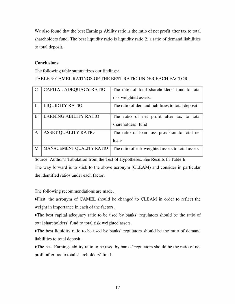
We also found that the best Earnings Ability ratio is the ratio of net profit after tax to total

shareholders fund. The best liquidity ratio is liquidity ratio 2, a ratio of demand liabilities

to total deposit.

Conclusions

The following table summarizes our findings:

TABLE 3: CAMEL RATINGS OF THE BEST RATIO UNDER EACH FACTOR

C CAPITAL ADEQUACY RATIO The ratio of total shareholders’ fund to total

risk weighted assets.

L LIQUIDITY RATIO The ratio of demand liabilities to total deposit

E EARNING ABILITY RATIO The ratio of net profit after tax to total

shareholders’ fund

A ASSET QUALITY RATIO The ratio of loan loss provision to total net

loans

M MANAGEMENT QUALITY RATIO The ratio of risk weighted assets to total assets

Source: Author’s Tabulation from the Test of Hypotheses. See Results In Table Ii

The way forward is to stick to the above acronym (CLEAM) and consider in particular

the identified ratios under each factor.

The following recommendations are made.

♦First, the acronym of CAMEL should be changed to CLEAM in order to reflect the

weight in importance in each of the factors.

♦The best capital adequacy ratio to be used by banks’ regulators should be the ratio of

total shareholders’ fund to total risk weighted assets.

♦The best liquidity ratio to be used by banks’ regulators should be the ratio of demand

liabilities to total deposit.

♦The best Earnings ability ratio to be used by banks’ regulators should be the ratio of net

profit after tax to total shareholders’ fund.

18

♦More so, the best Asset Quality ratio is the ratio of Loan Loss Provision to total net

loans.

♦And lastly, the best management quality ratio is the ratio of risk weighted assets to total

assets.

♦It is also recommended that more research be conducted in this area of banks’

performance evaluation. Other versions of DEA such as the DEA solver pro, Frontier

Analyst, Onfront, Warwick DEA, DEA Excel Solver, DEAP and Pioneer should be

explored in application in the banking industry.

Bibliography

Altman I. Edward (1968) : Financial Ratios, Discriminant Analysis and Prediction

of Corporate Bankruptcy in Journal of Finance,

September, 1968, New York University.

Annual Reports and Accounts of the banks (1997-2006)

Berger A.N, and Humphrey, D.B., (1997): Efficiency of financial

Institutions: International Survey and Directions for

Future research, European Journal of Operational

Research, University of Pennsylvania

Cinca et al (2002): Behind DEA Efficiency in Financial Institutions:

Discussion Paper in Accounting and Finance, Number

AFO2-7, School of Management, University of

Southampton

Crawshaw J.and Chambers J. (1984): A Concise Course in A-Level Statistics,

Second Edition, Bath Press, Avon, Britain.

David A. Grigorian and Vlad Monola (2002:5&6) Determinants of Commercial

Bank

Performance in Transition: An Application of Data

Envelopment Analysis, World Bank Policy Research

Working Paper 2850, June 2002.

19

Efficiency Measurement System (EMS) 130 of Holger Scheel at www.wiso.uni-

dortmund.de/lsfg/or/scheel/ems/

Gabriel Asaftei (1995) and Kumbhakar(1995) @ www.fma-

org/siena/papers/720495.pdf Regulation and

Efficiency of banking in a transition

economy,Department of Economics, University of

Richmond, VA, 23179, USA.

Imed Limam (2002): Measuring Technical Efficiency of Kuwaiti Banks:

Arab Planning Institute, Kuwait.

Kuru Lawan Ahmed (1999):The Marketing of Banking Services in the Current

Competitive Environment: A Case Study of Habib

Nigeria Bank Ltd

Lonneke Mous (2005): Predicting bankruptcy with discriminant analysis and

decision tree using financial ratios, University of

Rotterdam.

Malami M. Maishanu (2004:76): “ A univariate Approach to Predicting failure in

the Commercial Banking Sub-Sector” in Nigerian

Journal of Accounting Research, Volume 1, Number 1,

Department of Accounting, Ahmadu Bello University,

Zaria.

Milind Sathye (2001): Efficiency of Banks in a Developing Economy: School

of Accounting and Finance, University of Canberra.

Mlima and Hjalmarrsom (2002): Measurement of Inputs and Outputs in Banking

Industry: Tanzanet Journal (2002), Volume 3(1),

University of Gothenburg.

Muhammad Tanko (2004): “A Data Envelopment Analysis of Banks Performance

in Nigeria.” In Nigerian Journal of Accounting

20

Research, Volume 1, Number 4, Department of

Accounting, Ahmadu Bello University, Zaria

Piyu Yue (1992:31): Data Envelopment Analysis and Commercial Bank

Performance: A Primer with Applications to Missouri

Banks, IC2

Institute, University of Texas at Austin.

Serrono C. et al (2001): Selecting DEA Specifications and Ranking Units via

PCA: Discussion Papers in Management, Number

MO1-3, and University of Southampton.

Thomas F. Siems and Richard S. Barr (1998): Benchmarking the Productive

Efficiency of U.S. Banks: Financial Industry Studies,

Federal Reserve Bank of Dallas.

Wirnkar A.D. and Tanko M (2007): “A post consolidation Appraisal of Commercial

Banks Efficiency in Nigeria”. In Nigerian Journal of

Accounting Research, Volume , Number , Department

of Accounting, Ahmadu Bello University, Zaria

21

TABLE 7

SUMMARY OF AVERAGE KEY VARIABLES PER BANK PER PERIOD

S

/

N

BAN

KS

AV

CAPA

R I

AV

CAPA

R II

AV

CAPA

R III

AV

CAPA

R IV

AV

CAPA

R V

AV

CAPA

R VI

AV

CAPA

R

AV

ASET

QR I

AV

ASET

QR II

AV

ASET

QR

AV

MGA

R

AV

EAR

I

AV

EAR

II

AV

EAR

AV

LIQR

I

AV

LIQR

II

AV

LIQR

III

AV

LIQ

R

AV.EFFI

CIENCY

SCORES

1 ACB 8.2504 0.1310 0.4120 0.2397 0.9089 3.0856 2.1713 0.1229 0.0416 0.0823 0.0514 0.0127 0.1162 0.0645 0.6084 0.6093 0.6830 0.63

36

83.84

2 AFB 19.254

8

0.718 0.2844 0.0980 0.6326 0.9788 3.5534 0.3395 0.0877 0.2136 0.0670 0.0080 0.1285 0.0683 0.3521 0.6956 0.4644 0.50

40

81.67

3 FBN 11.376

0

0.0915 0.3894 0.1361 0.7215 1.0261 2.2901 0.3850 0.0875 0.2363 0.0965 0.0250 0.2750 0.1500 0..3515 0.7410 0.4365 0.50

97

87.52

4 GTB 8.6227 0.1221 0.3453 0.2131 0.6824 15.118

6

4.1840 0.0370 0.0133 0.0252 0.0090 0.0405 0.3477 0.1941 0.6190 0..5680 0.5676 0.58

49

100

5 ICB 7.4299 0.1409 1.3836 0.2070 1.7374 4.1031 2.5003 0.0665 0.0177 0.0421 0.0503 0.0407 0.2984 0.1696 0..3475 0..3865 0.3725 0.36

88

94.57

6 OCB 23.274

6

0.0568 0.2724 0.0790 -3.7283 4.9293 4.1473 0.2506 0.0684 0.1595 0.0831 0.0538 1.5304 0.7921 0.3412 0.7216 0.4327 0.49

85

100

7 UBA 16.217

1

0.0655 0.3197 0.0918 0.4477 4.2836 3.5709 0.1729 0.0359 0.1044 0.0299 0.0133 0.2046 0.1090 0.2959 0.6553 0.3463 0.43

25

100

8 UB 11.540

1

0.0891 0.4498 0.1312 0.8830 1.3502 2.4072 0.3248 0.0684 0.1966 0.0778 0.0202 0.2334 0.1268 0.3003 0.6176 0.3979 0.43

86

83.90

9 ZB 9.6517 0.1049 0.3937 0.1859 1.9710 26.538

6

6.4743 0.0272 0.0074 0.0173 0.0042 0.0388 0.3727 0.2058 0.4782 0.7098 0.4913 0.55

98

89.90

1

0

DB 10.503

6

0.0991 0.3522 0.1493 0.7409 6.2513 3.0161 0.0404 0.0109 0.0257 0.0264 0.0259 0.2753 0.1506 0.3958 0.6466 0.4342 0.49

22

90.99

1

1

WB 10.101

5

0.1118 0.2820 0.1572 3.8776 1.7240 2.7090 0.1453 0.0557 0.1005 0.0746 0.0180 0.1896 0.1038 0.5432 0.6733 0.6198 0.61

21

83.36

∑AV

KV

136.72

24

1.0845 4.8845 1.6883 8.8747 69.389

2

37.023

9

1.9121 0.4945 1.2035 0.5702 0.2969 3.9718 2.1346 4.6331 7.0246 5.2462 5.63

47

995.75

X

12.429

3

0.0986 0.4441 0.1535 0.8068 6.3081 3.3658 0.1738 0.0450 0.1094 0.0518 0.0270 0.3611 0.1941 0.4212 0.6386 0.4769 0.51

22

90.75

SOURCE: RESEARCHER’S COMPUTATION ∑ = Summation, KV = Key Variation , AV = Average, X = Mean per key variable

CAMEL(S) AND BANKS PERFORMANCE

Documents

Transcript of CAMEL(S) AND BANKS PERFORMANCE