CALIFORNIA STATE UNIVERSITY, NORTHRIDGE

IMPATT DIODE POWER ACCUMULATOR

A thesis submitted in partial satisfaction of the requirements for the degree of Master of Science in

Engineering

by

Steven Eugene ~amilton /

June, 1979

The Thesis of Steven Eugene Hamilton is approved:

Steven D. Gavazza

Edmond S. Gillespie~

California State University, Northridge

ii

TO MY LOVING WIFE

AND CHILDREN

iii

TABLE OF CONTENTS

ABSTRACT

Section I INTRODUCTION

Section II ACTIVE CIRCUIT DESIGN

Section III SINGLE DIODE WAVEGUIDE OSCILLATOR

Section IV HI-PAC DESIGN

Section V POWER COMBINER PERFORMANCE

Section VI CONCLUSIONS

REFERENCES

APPENDIX A DIODE CHARACTERIZATION

LIST OF TABLES

LIST OF FIGURES

iv

Page ix

1

3

14

20

46

57

59

62

v

vi

f '

LIST OF TABLES

. TABLE p4~e 1 Power and Efficiency Versus Rc

2 Power and Efficiency Results 52

Al Varian Diode VSX9251 AD 99

A2 Diode Comparison 100

v

Figure 1

2

·3

4

5

6

7

8

9

10

11

12

13

14

LIST OF FIGURES

IMPATT Diode (a) Structure {b) Field Profile (c) Electron Energy (d) Voltage Wave Form (e) Injected and External Current

Equivalent Circuit of Diode and Load (a) Diode Chip and Load (b) Packaged Diode and Load

Coaxial Oscillator (a) Structure {b) Equivalent Circuit

Design Curves for a Single Step Transformer

Single Diode Waveguide Oscillator (a) Side View (b) End View

Equivalent Circuit of Single Diode Waveguide Oscillator

Kurokawa Waveguide Oscillator End View

Kurokawa Waveguide Oscillator Top View

24 Diode HiPac

Module Configuration (a) Kurokawa Module (b) HiPac Module

Cross-Sectional View of Diode

Module Spacing for HiPac

Waveguide TE011 Mode Cavity

Power Versus Current for Different Circuit Load

vi

Page 5

8

10

12

15

17

21

22

24

26

27

29

31

36

Figure 15

16

17

18

19

20

21

22

23

24

25

26

Al

A2

A3

A4

AS

A6

A7

Equivalent Circuit of HiPac

Power and Efficiency Versus Current for Rc < Ropt

Power and Efficiency Versus Current for Rc = Ropt

Power and Efficiency Versus Current for Rc > Ropt

IMPATT Oscillator Test Set-up

Assembled End View of HiPac

Disassembled View of HiPac

Power and Efficiency Versus Current 8 Diodes in HiPac

Comparison of HiPac Performance to Eight Times Single Diode Data

Power and Efficiency Versus Current 4 Diodes in HiPac

Power and Efficiency Versus Current 2 Diodes in HiPac

Mechanical Tuning Bandwidth of HiPac

Low-High-Low Diode (a) Doping Profile (b) Electric Field

Hie;h-Low Diode (a) Doping Profile (b) Electric Field

Cross Section of High-Low Diode

High-Low Diode (a) Layer Definition (b) Electric Field

Mean Life to Failure

Cross-Sectional View of Diode

Doping Profile of High-Low Diode

vii

pjge

40

41

42

45

47

48

49

so

53

54

56

64

65

66

67

76

78

82

Figure AB A9

AlO

C-V Plot of High-Low Diode

Equivalent Circuit of Packaged Diode

Equivalent Circuit of the Packaged Diode and Load Reactance

viii

PB~e

90

92

ABSTRACT

IMPATT DIODE POWER ACCUMULATOR

by

Steven Eugene Hamilton

Master of Science in Engineering

This thesis presents the development of a new type of

I~ATT diode power accumulator. The design has twice the

capacity of similar accumulators of the same size. The

circuit offers high combining efficiency, reduced thermal

interaction and broad tuning bandwidth.

The basic concepts of IMPATT oscillators are dis­

cussed. A single diode version of the power accumulator is

presented in detail along with an equivalent circuit. A

technique to optimize IMPATT oscillators is covered with

experimental verification.

The power combiner performance is demonstrated

utilizing 2, 4 and 8 diodes. The broad tuning bandwidth of

the combiner is presented for the eight diode configuration

only.

The optimum performance of a power combiner is

attained when all the diodes, to be combined, have similar

characteristics. To achieve the optimum condition, a

ix

technique is presented which determines if the diodes are

suitable for combiner application.

X

SECTION I

INTRODUCTION

The development of solid state microwave sources has

experienced tremendous growth over the past ten years.

Their high reliability, low cost and small volume are

characteristics which attract many designers. Solid state

sources have been developed for communications, space and

radar systems to replace low and medium power tube type

transmitters.

The principal devices responsible for solid state

growth have been FETs and IMPATTs*. These devices have all

served as the fundamental building blocks in the new solid

state components. Within the past six years the IMPATT

diode has clearly set the pace for solid state technology

by replacing several tube type transmitters. This has been

accomplished by the development of many new devices and

power combining circuits.

Recently, improvements in combiner power level have

been attained only through the development of higher power

diodes. This presents a problem to the solid state design­

er in that future requirements will exceed the capability

* FET is an acronym for Field Effect Transistor. IMPATT is an acronym for Impact and Transit Time Device.

1

~'·

of present combining techniques. To maintain their growth,

solid state designers have resorted to utilizing circuits

which can potentially meet future requirements by combining

larger numbers of diodes; unfortunately, the new circuits

operate at reduced efficiency, require increased fabrica­

tion cost and exhibit reduced reliability. The aforemen­

tioned characteristics reduce the advantages that solid

state sources have over other transmitter technologies.

It is the object of this thesis to reclaim some of the

desirable characteristics of solid state sources and, in

addition, to satisfy future power requirements. To accom­

plish this task, a new combining technique has been

developed which is capable of summing more devices than was

previously attainable. This technique offers high combin­

ing efficiency and greater reliability than other designs.

In order to demonstrate the new combiner circuit,

three oscillators were designed and fabricated. The design

utilizes a waveguide cavity with a plurality of coaxial

modules located along the cavity walls. IMPATT diodes are

located at one end of a coaxial transmission line with a

bias filter at the other end. The test results are

presented both in tabular and graphical form to illustrate

the circuits capability and to compare its performance

against previously developed technology. A simple model

will be presented to discuss the various characteristics of

the new circuits, hereafter referred to as HiPac.

2

A. Introduction

SECTION II

ACTIVE CIRCUIT DESIGN

~··

The design of an active circuit utilizing negative

resistance devices is a complicated process. The param­

eters which must be considered involve areas of semi­

conductor physics and standard microwave circuit technol­

ogy. Unfortunately, the non-linearity of the device, which

makes it useful, also prevents closed form solutions in

large signal analysis. In addition, as one strives for

high power sources, devices are typically combined in

complex microwave circuits. These circuits usually have

mutual coupling interactions which are as equally difficult

to analyze as the active device. In this section, several

aspects of the design will be presented, although only

those subjects pertinent to the design process will be

discussed. Approximations and limits will be presented as

required, and more detailed studies will be referenced.

B. IMPATT Diode

The type of device used in this study is a gallium

arsenide IMPATT [1] [2]. The GaAs IMPATT is the highest

efficiency device in the IMPATT family [3] [4]. Silicon

3

and indium phosphide materials are also used in construct­

ing IMPATT diodes; but they operate at half the efficiency

of GaAs.

As previously stated, the IMPATT diode is a negative

resistance device. The negative resistance occurs as a

result of a 180° phase difference which is developed be­

tween the ac current and voltage within the device. The

diode is essentially composed of two constituents: (1) the

avalanche zone and (2) the drift zone (also known as

depletion zone). Consider the simple P+N N+ diode shown in

Figure la, with reverse bias applied as indicated. Within

the diode, an electric field profile, as shown in Figure

lb, is developed. The high field, which exists between x1 and x2 , establishes the avalanche zone. In this region

avalanche breakdown occurs which generates hole electron

pairs. The region between x2 and x3 is called the drift

zone, where the field is high enough to maintain constant

drift velocity but not high enough for avalanche to occur.

Figure lc shows the energy band diagram under breakdown

conditions. The holes generated in the avalanche zone go

into the p+ region while the electrons are injected into

the N region, drift zone. If an ac voltage, as shown in

Figure ld, is applied to the diode, via noise or some other

stimulus, the electric field will change periodically with

time around some average value. The rate of impact

ionization will follow the change in field almost

4

-1 ELECTRIC FIELD

ELECTRON ENERGY

AC VOLTAGE

CURRENT

p+

p+

5

14--- DRIFTZONE ~

I i N

I

N+ ~+ ~~-- AVALANCHE

ZONE

(a) Structure

~ I N N+

I I

X x 1 x 2 x3

DISTANCE

(b) Field Profile

DISTANCE

(c) Electron Energy

8 = Wt

(d) Voltage Wave Form

T 2T

(e) Injected and External Currents

Figure 1. lmpatt Diode

instantaneously. However, the carrier density does not

follow the field change in unison because the generation of

carriers depends on the number already generated. So when

the field is maximum, carrier generation is still increas­

ing and does not peak until after the field has decreased

by some amount. Thus we have the carrier density peak

lagging the ac voltage by about 90° (see Figure ld and le).

The injected electrons then enter the drift zone where,

because of the field, they travel at a saturated or

scattering-limited velocity. Figures ld and le show that

the remaining phase shift is provided by the drift zone

where the drifting carriers become 180° out of phase with

the ac voltage. The length of the drift zone is designed

to be about one-half cycle of the desired operating fre­

quency, and the induced external current is as illustrated

in Figure le.

This explanation is extremely elementary and was used

to give physical insight into IMPATT operation. To com­

plete this description, one would have to study the effects

of ionization rates, doping profile, saturated velocity,

etc. Papers covering these topics have been presented in

great detail and thus will not be covered here [5] [6] [7].

Appendix A will present further information on the doping

profile and internal dimensions of the diode used in this

study. The appendix is presented in order to explain how

the tolerances on doping and internal dimensions affect

6

microwave performance.

C. Condition for Oscillation

The condition for oscillation, for a negative resist­

ance device, has been described by several authors [8] [9]

[10] and is given by

Z' + Z' = 0 d c (1)

where Zd is the impedance of the diode at a reference plane

and Z~ is the impedance of the circuit at the same refer­

ence plane. The impedances Zd and Z~ are presented as

zd Z' c

= Rd - jXd = R' + ·x• c J c·

Figure 2a shows an equivalent circuit of the diode chip

connected to a matched load impedance. Figure 2b is an

equivalent representation of the packaged diode with

mounting parasitics connected to the matched load. It is

important to recognize that the package and mount para­

sitics contribute to the impedance at port B which is

normally the actual diode/circuit interface. The exact

model of the package and mount parasitics will not be con­

sidered here but have been presented in many papers [11]

7

8

A

I

I A

(a) Diode Chip and Load

A B

I I Lp

CpT -;x, T ... _--<0>--------...&.---0>------T..... -ixc

I I A B

(b) Packaged Diode and Load

Figure 2. Equivalent Circuit of Diode and Load

[12]. The important concept here is that Zd, at port A, is

transformed via 1p and Cp to an impedance Zd at port B.

Where zd is given by

(2)

Since Zd has changed form, Zc must also be modified in

order for Equation (1) to be satisfied. The circuit imped­

ance Z~ can now be represented as

(3)

Where Zc is the new circuit impedance which matches Zd.

D. Oscillator Design

To develop an understanding of oscillator design, let

us consider the simple coaxial oscillator illustrated in

Figure 3a. In this circuit, the 50 ohm transmission line

is the circuit load impedance. A transmission line of

impedance ZT transforms the circuit load impedance to one

that satisfies Equation (1) at port B. Usually informa­

tion is provided by the diode manufacturer in which Zd is

given; for our diode, Zd = -1.0 + j5.0. From Equation (1)

the impedance presented at port B by the load impedance

must be Zc = 1.0 - j5.0. To obtain Zc, a line transformer

9

B

DIODE TRANSFORMER

(a) Structure

TRANSMISSION LINE

B C

TRANSFORMER TRANSMISSION ZT LINE

(b) Equivalent Circuit

Figure 3. Coaxial Oscillator

10

of impedance ZT and length L is used to transform the load

impedance to Zc· To determine ZT, one may use the trans­

mission line equation or, more simply, the graph provided

by the Hewlett-Packard Company, which is shown in Figure 4.

The real and imaginary components of Zc are located on the

graph, and the intersection of these lines defines ZT and

L. The graph was developed for a load impedance of 50

ohms. In operation, the oscillator will probably not

operate in accordance with the design requirements.

Toierances on diode package parameters and various fring­

ing effects usually degrade the performance from ideal.

If the manufacturer does not provide data which gives

Zd, then one will have to measure this impedance. Active

diode impedance measurement requires a large complex

measuring system and a computer. The measurement system

and associated computer programs have been described by

many papers [13] [14] [15] [16] and will not be presented.

A simpler de technique can be employed to determine an

approximation of Zd; this method requires only the use of a

capacitance bridge and a de power supply. Initially the

capacitance Cb of the packaged diode is measured at or near

the breakdown voltage. The value of diode reactance at a

specific frequency, f, can then be calculated by

(4)

11

a u

a:

30 ZT 22.3

20

15.81

10 9 8 7 6

5

4

3

2

1.or------;-------+~~~~-7~-+~~*-~~~=r~~~~;-----~ 0.9 0.8 0.7~-----4-------+~~~~~~~~~~~~~~~~~~~----~

0.6

0.5 1-------+----:

0.4

0.05 0.1 0.15 0.2

1.1'1\

0.25 0.3

Figure 4. Design Curves for a Single Step Transformer

0.35 0.4

12

The value of Rd does not vary extensively from one diode

type to another. Typically, Rd has a range between -1.0

and -2.0 ohms; with this fact, one arbitrarily selects Rd.

Since changes in the original design are frequently

required, this technique is both expedient and economical.

13

SECTION III

SINGLE DIODE WAVEGUIDE OSCILLATOR

A. Introduction

The fundamental theory used in development of HiPac is

based on the design of a popular single diode waveguide

oscillator (SDWO). The SDWO was conceived by Harkless [17]

and was developed by Magalhaes and Kurokawa [18] [19]. The

SDWO has been used in the development of stable low-noise

oscillators because of the controls over stability afforded

to the designer. The SDWO basically operates like HiPac

but with fewer diodes and in a much simpler form. Thus it

will be useful to understand the SDWO before presenting the

design of the HiPac.

B. SDWO Description

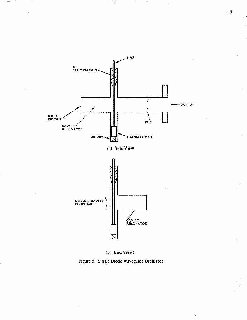
The SDWO, shown in Figure 5, essentially consists of a

coaxial line, hereafter denoted as module, and a high Q

cavity resonator. The cavity length is determined by the

distance between the short circuit and the inductive iris.

The module contains a diode and transformer at one end, a

coupling section in the center, and an RF termination at

the other end. Basically, the power is coupled from the

14

RF TERMINATION

~~A0c"u~T ~/-CAVITY/ RESONATOR

DIODE

MODULE-CAVITY { COUPLING

BIAS

n \

IRIS

ANSFORMER

(a) Side View

LTY RESONATOR

(b) End View)

D

Figure 5. Single Diode Waveguide Oscillator

15

--oUTPUT

module to the cavity and coupled from the cavity to the

load, through the iris. The frequency of oscillation is

determined by the length of the transformer and the posi­

tion of the short circuit. The impedance required to

satisfy Equation (1) is obtained in the following manner:

The load impedance, which is the characteristic impedance

of the waveguide, is transformed by the iris to the cavity­

module interface. The impedance at the cavity-module

interface is transformed to the diode, thus satisfying

Equation (1).

C. Equivalent Circuit

Near the resonant frequency of the cavity, the SDWO

may be represented by the equivalent circuit shown in

Figure 6. Port C is the diode-transformer interface, port

A is the cavity-module interface at mid-height of the wave­

guide, and port B is the connection to the load. The

impedance ZT represents the transformer, z1 is the RF

termination, and ZL is the load. M1 is the module-cavity

coupling, M0 is the cavity-load coupling, and R-L-C repre­

sents the cavity.

It can be shown [20] [21] that, at the resonant fre­

quency, the coupling factors can be represented as

(5)

16

........ -.....)

1-

'

where ~l is the module-cavity coupling, and ~2 is the

cavity-load coupling. By simple manipulation of the

equivalent circuit, it is seen that

Rc = [<1 + ~2 ) I (1 + 2~ + ~2 >] <zi 1 z1)

~ = (2~1 ~2) I [<1 + 2~1 + ~2> <1 + ~2>J

(6)

(7)

(8)

where Rc is defined by (3) and ~ is the efficiency of the

circuit. The circuit efficiency is defined as the ratio of

power delivered to ZL relative to the power available at

port A.

D. SDWO Optimization

The parameter ~l is mainly determined by the position

of the module within the cavity and the geometry at that

interface. It is important to note that a standing wave

exists in the module; therefore, for maximum value of ~1 ,

the diode should be located at the position N Xl4 from mid

height of the cavity where N is an odd integer. Because ~l

is defined by the position of the module within the cavity,

~2 is usually the variable adjusted to maximize the effi­

ciency. The adjustment of ~2 affects both the efficiency

and the value of Rc· To maintain the required value of Rc,

18

as ~2 is adjusted for maximum efficiency, it may be neces­

sary to adjust ZT, see Equation (7). An important condi­

tion to be considered is when ZT is less than 8 ohms. At

that point, ZT may be physically unrealizable, and the

efficiency will be less than that predicted by (8).

Ideally the value of Rc is adjusted to maximize the

power produced by the diode; however, ~l and ~2 are found

to be interdependent. Therefore, the design usually has to

be iterated several times before maximum power and maximum

circuit efficiency are attained. A measurement technique

described by Tjassens [22] can be used to determine Pl and

~2 . A more rigorous analytical approach has been described

by Davydova and Danyushevskiy [23]. When the circuit is

employed as a stable oscillator, ~2 is made small. This

increases the external Q of the circuit and hence stabil­

ity. For stable operation, the efficiency of the circuit

is essentially traded for stability. HiPac will differ in

this respect, because it will be adjusted for maximum

efficiency and then injection-locked for stability.

19

A. Introduction

SECTION IV

HI-PAC DESIGN

HiPac is an extension of a multiple diode oscillator

developed by Kurokawa [24] [25]. Both designs incorporate

the basic technology of the SDWO, namely, the magnetic

coupling of a module to a cavity resonator. Kurokawa

located a module on each side of a waveguide across the

narrow dimension as shown in Figure 7. In addition, he

positioned other modules in similar planes spaced by Ag/2,

as illustrated in Figure 8. As shown in Figure 8, Kurokawa

was able to combine twelve modules in this fashion. The

combining efficiency he attained was approximately 77% at a

power level of 10.5 watts CW in X-band. This oscillator

was the first of its type produced in this country and only

preceded by Tager [26] [27] of the U. S. S. R.

While Kurokawa's circuit is useful, it is also large

and cannot compete with the newer cylindrical combiners. A

cylindrical combiner at mid X-band can sum the power from '

18 modules within a 1.0-inch diameter cavity. The high

density packing of modules, though, does lead to thermal

interaction between modules, which typically dissipate

20

21

Figure 7. Kurokawa Waveguide Oscillator End View

\ IRIS

WAVEGUIDE FLANGE

MODULE

Figure 8. Kurokawa Waveguide Oscillator Top View

SHORT CIRCUIT

22

30-40 watts each.

If one wanted to combine 18 or more diodes, the simple

cylindrical combiner, which is operated in the TMQ10 mode,

is limited by its diameter and the size of the diode. To

overcome this problem, radial line combiners have been

designed which have larger diameters and can combine more

modules. Unfortunately, these combiners require mode sup­

pression, since several modes which do not couple to the

output are generated. In addition, these combiners are

marginally stable and operate at reduced efficiency. To

overcome the stability, thermal and combining limitations

of the previous circuits, HiPac was developed.

B. HiPac Configuration

HiPac essentially doubles the diode capacity of Kuro­

kawa's circuit by positioning two modules on each sidewall

of the waveguide cavity rather than one as shown in Figure

9. In the HiPac configuration, each diode has only one

close neighbor; thus, a thermal advantage is realized over

cylindrical combiners. The stability of the HiPac circuit

is not affected by the use of two closely spaced modules,

since no higher order degenerate modes are propagated. The

combining limits combined to other circuits is greater, be­

cause one can simply make the circuit longer to combine

more modules.

23

t WAVEGUIDE FLANGE

t IRIS TWIN

MODULES

Figure 9. 24 Diode Hi Pac

-sHORT CIRCUIT

"" ~

The differences between Kurokawa's circuit and HiPac

are confined to module position, diode location, and RF

termination. In Kurokawa's circuit, the module is posi­

tioned along the sidewall of the cavity where the magnetic

field is maximum. In addition the diode is located 3/4A

from the mid-height of the waveguide, as shown in Figure

lOa. The HiPac design positions the modules on either side

of the maximum magnetic field with the diodes located A/4

from mid-height of the waveguide (Figure lOb). Kurokawa

terminates his module with a matched load, and HiPac uses a

mismatched load as shown in Figure 10.

C. Design

In the following paragraph, an X-band design example

will be provided to describe the basic structure of HiPac.

The modules in HiPac are 0.125 inches in diameter and are

separated by 0.150 inches center to center. The diameter

of the module is determined by the physical size of the

diode. The diode used in the design is a Microwave

Associates type 46072 IMPATT, shown in Figure 11. The

separation between the modules is determined by compromise

between physical and electrical constraints. It is desir­

able to have the modules as close as possible for the

electrical constraint but separated for the physical

requirement. In this design, the separation between a

25

3/4>.

.,.,..~

/ -/---

/

WAVEGUIDE CAVITY

MAGNETIC FIELD AMPLITUDE DISTRIBUTION

__.TRANSFORMER

(a) Kurokawa Module

WAVEGUIDE CAVIT\ t

DIODE

(b) HiPac Module

Figure 10. Module Configuration

26

HEAT SINK

0.100

METAL CAP

WIRE MESH

DIODE CHIP

CERAMIC RING

----3-48 UNG-2A

Figure 11. Cross-Sectional View of Diode

27

module pair is 0.025 inches. If this spacing is reduced,

tighter dimensional tolerances will be required.

The module pairs are separated by Ag/2 as shown in

Figure 9. The design frequency is 9.25 GHz. The waveguide

cavity width is 0.9 inches, and the height of the cavity is

0.4 inches. With the given parameters, the value of Ag can

be determined by

(9) Ag =

The parameter A is the free space wavelength, which equals

c/f, where c is the velocity of light and f is the design

frequency. The parameter 'a' is the width of the wave­

guide. For the given conditions, Ag = 1.809 inches and

Ag/2 is 0.905 inches. Figure 12 illustrates the module

design which is repeated along the length and on both sides

of the waveguide cavity.

Since the modules are located off the peak of the mag­

netic field, it is necessary to determine how this affects

performance.

The waveguide cavity operates in the TE0rn mode.

Since the field is periodic, it is only necessary to

examine the complex field representation of a TE011 mode

cavity. The field components for the TE011 mode are given

by [28]

28 f' '

CENTER LINE: --7 WAVEGUIDE CAVITY

0.905

Figure 12. Module Spacing for Hi Pac

CAVITY SIDEWALL

"' \0 ·~

Ex = Eo sin , y cos 1T z (10)

a c

Hy = Ja Eo sin , y cos , z (11)

77[b2 + c2]~ a c

Hz = -Jc Eo cos , y sin 1T z (12)

7} [ b2 + c 2]~ b c

Figure 13 illustrates the geometry of the TE011 cavity. To

examine the reduction in coupling by the placement of

modules off of the maximum magnetic field point, let y = 0

in Equations (10), (11), and (12). The only field term re­

maining is Hz. If Equation (12) is normalized to remove

the constants, Hz becomes

(13)

c A g •

At Z = Ag/4 maximum coupling is realized, but in our case

z = A.g/4 + ~' (14)

where ~is one-half the module spacing in wavelengths.

Since the reduction in coupling will be the same on either

side A_&, only one side needs to be considered. For the 4

30

31

> >. ..... -~ u ~

'"0

-< 0 ::2:

-0 tJ.: ~ ~

'"0

-~ ~

~ :::: M

X

~ e

CD

= -~ u..

N

given design .1 = 0.041 .\g, so that Z = .!.....& + 0.041 ,\g which 4

results in Hz= 0.967. The maximum coupling then, to a

given module, can be considered to be reduced by the reduc­

tion in Hz. In this example, Hz is reduced 3.3% from the

maximum case, Hz = 1.0. As a worse case, one might expect

the maximum efficiency to also be reduced by this amount.

From Equation {8), it is found that a reduction of 3.3% in

$ 1 results in an efficiency reduction of less than 0.3%.

To design the module transformer, one must first

approximate the impedance presented at the module-cavity

interface. Initially one-half the characteristic impedance

of the waveguide is selected. The impedance is given by

120 ;;b (15)

For our case, A= 1.276, a = 0.900, and b = 0.400, there­

fore, Z = 237.55 ohms. Then, by assuming that ZT is a me quarter wave line transformer, the impedance is given by

{16)

where Zc = 1.0, from {3), this results in ZT = 15.41 ohms.

To determine the physical dimensions of ZT, the following

equation, which defines the impedance of a coaxial line, is

used

32

Z _ 60 .fn b - --r

f ~ a r . (17)

In Equation (17), 'b' is the module diameter and 'a' is the

diameter of the coaxial center conductor. The parameter fr

is the dielectric constant of the material used between the

center conductor and module diameter. In this example,

a = 0.083 inches, b = 0.125 inches, and fr = 2.53 (rexo­

lite} from which Z = 15.41 ohms.

The RF termination used in this design was made from

Eccosorb MF - 124, a high-loss dielectric (175 dB/inch).

The impedance of this load is established by the desired

stability and efficiency of the circuit. For maximum effi­

ciency, the impedance should be zero, but then the circuit

would be unstable. If the load is matched to the 50 ob~s

transmission line, the circuit would be stable. The module

efficiency is given by

"~me = (18)

where Z is the impedance at the module-cavity interface me and z1 is the termination impedance. For example, if

Zmc = 237.55 ohms and z1 =50 ohms, then "~me= 82.6%. For

the design example, a termination impedance of 25 ohms was

used; therefore, "~me = 90.5%. Since the RF termination

33

does not match the coaxial line impedance, its position is

critical. The location is typically set to be A/2 from the

face of the termination to mid-height of the cavity. The

length of the termination is determined by the desired

amount of attenuation of the RF energy incident at the load

face. In the example, the length was 0.350 inches which

results in 61.3dB of attenuation.

The cavity short circuit is positioned Ag/4 from the

last module pair. The position of the short circuit deter­

mines the resonant frequency of the cavity. In addition,

it indirectly establishes the coupling of the modules to

the cavity. The coupling is altered by the position of the

short because the short circuit establishes an electro­

magnetic boundary. The location of the electric and mag­

netic fields in the cavity are set by the short circuit

position. By moving the short, one also moves the fields;

but with the module location fixed within the cavity, the

coupling of the module to the cavity is affected. The

exact effect was described earlier when the module-cavity

coupling was discussed.

The output coupling is determined by the iris, shown

in Figure 9. In this example, an inductive iris was used.

The width of the iris opening determines the amount of

coupling between the oscillator cavity and load. For this

example, a width of 0.385 inches was used. The adjustment

of the iris affects both the impedance, which is

34

transformed to the diode, and the combining efficiency. A

discussion on how to determine the correct width of the

iris will be presented later.

D. Optimization

The procedure for setting the coupling and optimum

transformer is as follows: For a given module transformer,

adjust the iris and short position for maximum power, then

check the diode threshold current. The threshold current

is the current amplitude where the combiner initially

oscillates. For each diode type, there is an optimum

threshold current and maximum operating current for maximum

power, as shown in Figure 14. If the threshold current is

too low, as Ithl' the resulting power saturates before !max

is achieved. Correspondingly, if the threshold is too

high, as shown by Ith3 , Pmax is not obtained. The Ithl

condition is obtained by underloading the diode, and Ith3

is caused by overloading the diode. Plots of power versus

current are very useful for the optimization of the design.

This is because optimum diode loading can be obtained for

reduced circuit efficiencies.

The tolerance, surface conditions and flatness of

mating parts must follow good microwave practice. Losses

due to poor short circuits or cavity roughness all reduce

Q0 of the resonator and hence the combining efficiency.

! ' ' l

35

POWER (WATTS)

Figure 14.

36

Iop (AMPS)

Power Versus Current for Different Circuit Load

E. Equivalent Circuit

The HiPac circuit has the same characteristics as

Kurokawa's circuit; therefore, they will have the same

equivalent circuit. The equivalent circuit of HiPac is

shown in Figure 15. Where M1 , ---, Mn represents the

module-to-cavity coupling of the individual modules to the

cavity. Since the analysis of this circuit has been done

by Kurokawa and Davydova [19] [23], it will not be pre­

sented. The principal difference between Kurokawa's cir­

cuit and HiPac is the required coupling of the output load,

~2· Let the impedance at the module cavity interface be

~c' for one diode in the oscillator, and the required

loading by the output be RL. Then, for "N" modules, each

of which requires an impedance ~c' a much larger value of

RL will be required which is equal to N~. The larger

value of RL is obtained by increasing the output coupling,

~2·

F. Diode

All of the tests conducted with HiPac used a Microwave

Associates diode, MA - 46072. This diode is a single­

drift, low-high-low GaAs-pulsed IMPATT. Typically this

device produces 9.0 watts of peak power at 1/3 duty factor.

The dc-to-RF efficiency of the diode is approximately

15.5%. The efficiency and power characteristics of the

37

....JXd

L A c

~------------_j Mo ~

Ml

....JXd

Figure 15. Equivalent Circuit of Hi Pac

ZLOAO

w 00

diodes are a function of the circuit loading. The optimum

performance is attained when Re {zc} equals Ropt' where

Ropt is the optimum loading on the device. Figures 16, 17

and 18 depict the type of performance one would attain with

Rc < Ropt' Rc = Ropt and Rc > Ropt·

Once a diode has been characterized in a test circuit

to determine Ropt' the information can then be used to

determine what load is present on the device in any other

circuit. This is accomplished by observing Ith' where Ith

is the threshold current at which oscillations begin.

Table 1 summarizes the diode performance from Figures 16,

17 and 18. As shown in Table 1, the performance varies

considerably with Rc. It is also noticed that Ith is pro­

portional to Rc. Thus, if one uses the diodes in another

circuit and sets the Ith = 270ma, by varying Rc, optimum

performance can be obtained.

There are two cases in which the optimum setting of Rc

will not yield optimum performance: 1) if the circuit

causes parasitic oscillation, and 2) if the diode jumps to

a new operating point as the current is increased. Both of

the exceptions are easily recognizable. The first case is

distinguished by subharmonic and/or tone pair oscillations

which can be observed on a spectrum analyzer. The second

case can be identified by plotting the power-versus-current

curve and observing any definite changes in slope. If the

diode jumps to a new operating point, the power curve will

39

00'· IT:''·

40

3.0 ....-------------------------.,

2.5

14

2.0 -- 12 --..,;

,.-"' /

10 / de- RF / PRF

EFFICIENCY~/ 'r/ (%)

(AVE 1.5 / 8 WATTS) /

/ / 6

1.0 4

0.2 0.4 0.6 0.8 1.0

laP (AMPS)

Figure 16. Power and Efficiency Versus Current for Rc < RoPT

41

3,0 ..--------------------------.

2.5 16

14

/ 2.0 / 12

/ / de- RF

/ 10 fJ (%)

PRF EFFICIENCY / (AVE 1.5 ~/ B

WATTS) /

/ 6

/ 1,0 4

0,5

0.2 0.4 0.6 0.8 1.0

laP (AMPS)

Figure 17. Power and Efficiency Versus Current for Rc = RoPT

42

3.0 .---------------------------,

2.5

14

2.0 12

....-:: / 10 /

EFFICIENCY '-y/ / PRF de- RF (AVE 1.5 8 17

_WATTS) / (%)

/ / 6

/ /

1.0 / 4 /

/

2

0.5

0.2 0.4 0.6 0.8 1.0

lQp (AMPS)

Figure 18. Power and Efficiency Versus Current for Rc > RoPT

Table 1. Power and Efficiency Versus Rc

AVE DC-RF loP 1TH POWER EFFICIENCY

(WATTS) '1(%) (AMPS) (AMPS)

2.30 12.6 1.0 0.22

2.80 16.6 1.0 0.27

2.40 12.4 1.0 0.31

Rc (OHMS)

< ROPT

"ROPT

> RoPT

+="' VJ

noticeably change; this is usually accompanied by a fre­

quency jump as well.

The power and efficiency characteristics were obtained

by placing the diodes in a coaxial oscillator circuit.

Figures 16, 17 and 18 represent the average values for the

eight diodes used during this study. The block diagram of

the test setup used is shown in Figure 19. This type of

measuring system is typically required when working with

IMPATT devices.

44

PULSE GENERATOR

DC POWER SUPPLY 1--

PULSE MODULATOR

IMPATT OSCILLATOR

OSCILLOSCOPE

CURRENT PROBE

VOLTAGE PROBE

POWER METER

BAND PASS

FILTER

XX 40dB

COUPLER

~ X><C

40dB COUPLER

Figure 19. IMPA TI Oscillator Test Set-Up

SPECTRUM ANALYZER

HIGH POWER LOAD

45

~'·

SECTION V

POWER COMBINER PERFORMANCE

A. Introduction

To demonstrate the combining performance of HiPac, an

eight diode version was fabricated. (See Figures 20 and

21). The unit was tested as a free-running oscillator in

three different configurations. Measurements were con­

ducted using two, four and eight diodes in the combiner.

Data is presented which gives a comparison of the circuit

performance of the eight diode combiner with that of eight

times the single diode performance. This data will be used

to determine the combining efficiency of HiPac.

B. HiPac Performance

The HiPac combiner was optimized and characterized

with the use of the setup shown in Figure 19. It was

operated at 1/3 duty factor with a pulse repetition fre­

quency of 250kHz. The combiner was initially optimized

with eight diodes; the power and efficiency characteristic

is shown in Figure 22.

The power and efficiency characteristic of HiPac com­

bining eight diodes is compared in Figure 23 to Figures 17

46

47

Figure 20. Assembled End View of HiPac

48

Figure 21. Disassembled View of HiPac

PRF (AVE

WATTS)

24

22

20

18

16

14

12

10

8

6

4

2

0 0.2

/ /

0.4

~··

11~_,.. /

/ /

/

0.6 0.8

lop (AMPS)

1.0 1.2

Figure 22. Power and Efficiency Versus Current 8 Diodes in Hi Pac

49

12

10

de- RF 8 11

(%)

6

4

I ·----

50

and 18. Figure 17 is referenced since it represents the

optimum condition for the diodes. Figure 18 is used be­

cause it has a similar threshold level as the HiPac com-

biner with eight diodes. In Figure 23 it is shown that the

loading on HiPac is greater than Ropt' since the power

curve of HiPac follows that of eight times Figure 18. A

summary of the HiPac performance is given in Table 2. The

only area which needs explanation is the determination of

the combining efficiency, ~c' which is defined as

~HiPac (19)

where ~ HiPac is the dc-to-RF efficiency of HiPac, and sd

is the dc-to-RF efficiency of a diode. If ~sd of the

optimized diode is used for the evaluation of (19), then

~c = 76%. If ~sd for the case where Rc is greater than

Ropt is used, then ~c = 94%. Figure 23 indicates that the

diodes in HiPac were not optimally loaded. This condition

can be corrected by lowering the impedance of the diode

transformer in accordance with Equation (17).

Figures 24 and 25 show the performance of HiPac when

4 and 2 diodes are combined. The performance was optimized

for each case by adjusting the output coupling. The fre­

quency, transformers and short position were all main­

tained, at the same values as used during the eight diode

51

Table 2. Power and Efficiency Results

NUMBER NUMBER AVE OF OF

s'OP VOP Poe PRF TWIN DIODES MODULES COMBINED. (AMPS) (VOLTS) (WATTS) (WATTS)

1 2 1.0 58.0 38.7 3.4

2 4 1.0 58.0 77.3 8.8

4 8 1.0 58.1 157.3 18.4

- - ----- --

• SEE TEXT FOR DEFINITIONS

DC-RF EFFICIENCY

"7%

8.8

11.1

11.7

COMBINING EFFICIENCY

• '7C (%)"

58/71.0

72190

76/94

I !

VI N

:!

PRF (AVE

WATTS)

12

11

10

9

8

7

6

5

4

3

2

/ /

/

/

/ /

/

//.

0~----'-~--------~--------~--------~------~--~ 0.2 0.4 0.6 0.8 1.0 1.2

loP (AMPS)

Figure 24. Power and Efficiency Versus Current 4 Diodes in Hi Pac

53

12

10

8 de- RF

77 (%)

6

4

2

6r-------------------------------------------------,

5

4

PRF (AVE 3

WATTS)

2

0~----~~--------~------~--------~------~~~ 0.2 0.4 0.6 0.8 1.0 1.2

loP (AMPS)

Figure 25. Power and Efficiency Versus Current 2 Diodes in Hi Pac

12

10

8 de- RF 1'/ (%)

6

4

2

54

operation, for each case tested. The results of the four

diodes case are similar to that of the eight diode case,

but the two diode configuration is very different. The

reason for this difference is found in Equation (8) and the

output coupling factor. As the output coupling, ~2 , is

reduced, for a fixed value of ~1 , the combining efficiency

is reduced. Since the coupling, ~2 , is proportional to the

number of diodes combined, as fewer diodes are combined in

this circuit, with a fixed ~1 , rye is reduced.

The final characteristic measured on HiPac was the

mechanical tuning bandwidth. The short position, which is

the principal frequency-determining element, was varied in

order to determine the RF power as a function of frequency

as shown in Figure 26. This test was conducted using the

eight diode configuration. No adjustments other than the

short circuit position were made. The results indicate a

relatively flat power band of 240rnHz and a full band per­

formance of 360mHz. The broad band nature of this circuit

suggests that a varactor might be included in the design,

so that the circuit may be used as a voltage-controlled

oscillator.

~··

55 ,, .

2no.---------------------------------------------------------------------------------------,

18.0

16.0

iii ~ 12.0

~ w ~ 10.0

u. a:

Q. 8.0

I~

360 MHz 1.38 dB POWER VARIATION

240 MHz 0.5dB POWER VARIATION

OL-----------------------~-----------------------L------------------------~------------~ 8.665 8.765 8.865

FREQUENCY IGHz)

Figure 26. Mechanical Tuning Bandwidth of Hi Pac

8.965 9.025

V1 0\

SECTION VI

CONCLUSIONS

A new type of power combiner has been developed. The

diode capacity has been doubled over previously developed

circuits without a noticeable reduction in efficiency. The

waveguide cavity is a low-loss circuit capable of handling

high power levels. The physical separation of the module

pairs reduces thermal interaction, thus, the power dissi­

pation per unit area of heat sink is reduced, when compared

to a cylindrical combiner. The tunable bandwidth of HiPac

is greater and exhibits less power variation than similar

power level combiners. This suggests that the HiPac could

be used as a high power voltage tunable oscillator.

The design of the unit is relatively simple, but good

microwave construction techniques must be utilized. The

use of usual microwave tolerances on the mechanical parts

will ensure repeatable performance. The optimization of

HiPac is easily accomplished by using the procedure out­

lined in Section IV.

The performance of HiPac is dependent on the consist­

ency of the diodes. A diode selection technique should be

used to ensure that all diodes operate the same in a given

circuit. A theoretical analysis of GaAs IMPATT diodes is

57

presented in Appendix A. The analysis presents a technique

which can predict the RF performance of the aforementioned

diodes through the use of easily obtainable de parameters.

58

REFERENCES

1. Read, W. T., "A Proposed High-Frequency Negative Resistance Diode," Bell System Tech. J., val. 37, pp. 401-446, March 1958.

2. Irvin, J. C., "GaAs Avalanche Microwave Oscillators," IEEE Trans. on Elec. Dev., ED-13, pp. 208-210, Jan. 1966.

3. Armstrong, L., "High Efficiency X-band GaAs IMPATT Diodes," IEEE Trans. on Elec. Dev., ED-15, p. 938, Nov. 1968.

4. Salmer, G., et al., "Theoretical and Experimental Study of GaAs IMPATT Oscillator Efficiency," Jour. of App. Phy., vol. 44, No. 1, pp. 314-324, Jan. 1973.

5. Haddad, G. I., et al., "Basic Principles and Proper­ties of Avalanche Transit-Time Devices," IEEE Trans. on MTT, val. MTT-18, No. 11, pp. 752-772, Nov. 1970.

6. Misawa, T., "Negative Resistance in P-N Junctions Under Avalanche Breakdown Conditions, Pts. I and II," IEEE Trans. on Elec. Dev., val. ED-13, pp. 137-151, Jan. 1966.

7. Scharfetter, D. L. and H. K. Gummel, "Large-Signal Analysis of a Silicon Read Diode Oscillator," IEEE Trans. on Elec. Dev., ED-16, No. 1, pp. 64-77, Jan. 1969.

8. Kurokawa, K., An Introduction to the Theory of Micro­wave Circuits, Chap. 9, Academic Press, New York, 1969.

9. Gibbons, G., Avalanche-Diode Microwave Oscillators, Clarendon Press, Oxford, 1973.

10. Howes, M. J. and D. V. Morgan, Microwave Devices, Chap. 5, John Wiley and Sons, New York, 1976.

11. Eisenhart, R. L., "Take the Trouble Out of Diode Mounting," Microwaves, pp. 78-81, Nov. 1974.

59

12.

13.

14.

15.

16.

17.

18.

19.

20.

21.

22.

23.

24.

Teraoka, A. E., "TMPATT Oscillator Design," Master's Thesis, Cal. State Univ., Northridge, June 1978.

Iperen, B. B. and H. Tjassens, "Measurement of Large­Signal Impedance, Optimum AC Voltage and Efficiency of Si pun+, Ge npp+ and GaAs Schotty-Barrier Avalanche Transit-Time Diodes," Proc. of Eighth Int. Conf. on Microwaves and Optical Generation and Amplification, Amsterdam, pp. 7-27 - 7-32, Sept. 1970.

Kramer, N. B., "Characterization and Modeling of IMPATT Oscillators," IEEE Trans. on Elec. Dev., ED-15, No. 11, pp. 838-846, Nov. 1968.

Dunn, C. N. and J. E. Dalley, "Computer-Aided Small­Signal Characterization of IMPATT Diodes," IEEE Trans. on MTT, vol. MTT-17, pp. 691-695, 1969.

Gewartowski, J. W. and J. E. Morris, "Active IMPATT Diode Parameters Obtained from Computer Reduction of Experimental Data," IEEE Trans. on MTT, vol. MTT-18, pp. 157-161, 1970.

Harkless, E. T., U. S. Patent 3534293, Oct. 13, 1970.

Magalhaes, F. M. and K. Kurokawa, "A Single-Tuned Oscillator for IMPATT Characterizations~" Proc. of the IEEE, pp. 831-832, May 1970. -

Kurokawa, K. "The Single-Cavity Multiple-Device Oscillators,~ IEEE Trans. on MTT, vol. MTT-19, No. 10, Oct. 1971.

Montgomery, C. G., et al., Principles of Microwave Circuits, Chap. 7, McGraw Hill, New York, 1948.

Ginzton, E. L., Microwave Measurements, Chap. 9, McGraw Hill, New York, 1957.

Tjassens, H., "Circuit Analysis of a Stable and Low Noise IMPATT-Diode Oscillator for X-Band," ACTA Electronics, 17, 2, pp. 181-185, 1974.

Davydova, N. S. and Y. Z. Danyushevskiy, "Design of the Electro-Magnetic System of a Multidiode Microwave Amplifier," Telecommunications and Radio Engineering, vol. 31, pp. 96-103, May 1976.

Kurokawa, K., "The Single-Cavity Multiple-Device Oscillator," IEEE Trans. on MTT, vol. MTT-19, No. 10, pp. 793-801, Oct. 1971.

60

25. Kurokawa, K. and F. Magalhaes, U. S. Patent 3628171, Dec . 14, 19 71.

26. Tager, A. S. and A. D. Khodnevich, Russian Patent 192252, 1967.

27. Tager, A. S. and A. D. Khodnevich, "IMPATT Diode Oscillators with Electrical Frequency Tuning and Multidiode Oscillators," Radio Engr. and Elec. Physics, vol. 14, No. 3, 1969.

28. Harrington, R. F., Time-Harmonic Electromagnetic Fields, McGraw Hill, New York, 1961.

29. Sze, S. M. and R. M. Ryder, "Microwave Avalanche Diodes," Proceedings of the IEEE, vol. 59, No. 8, pp. 1140-1154, Aug. 1971.

30. Miller, G. L., "A Feedback Method for Investigating Carrier Distributions in Semi Conductors," IEEE Trans. on Elec. Dev., vol. ED-19, No. 10, Oct. 1972.

31. Johnson, W. C. and P. T. Panousis, "The Influence of Debye Lenftth on the C-V Measurement of Doping Profiles,' IEEE Trans. on Elec. Dev., ED-18, No. 10, Oct. 1971.

32. Gordon, B. J., H. L. Stover, and R. S. Harp, "A New Impurity Profile Plotter for Epitaxy and Device," Proceedings of 1970 ASTM Symposium on Silicon Device Processing, June 1970.

61

A. Introduction

APPENDIX A

DIODE CHARACTERIZATION

The characterization of IMPATT diodes has, in the

past, been a goal for many designers. The efficient opera­

tion of power combiner circuits requires that every diode

used in the circuit have the same RF characteristics. Most

combiner circuits present the same impedance to each diode;

thus, if the diodes are different from each other, the

overall performance will be suboptimum. Once a power com­

biner design has been established for production, it is

desirable for the production diodes to operate similar to

those used in the initial design. There have been many

investigations [13] [16] in the past on the characteriza­

tion of diodes, but these have resulted in slow and expen­

sive measurement techniques. It is the purpose of this

appendix to present a simple de measurement technique which

can be used to select diodes. This technique will deter­

mine whether the diodes will combine efficiently and have

repeatable RF performance. At present, this technique is

limited to GaAs single-drift diodes with high-low or low­

high-low profiles.

62

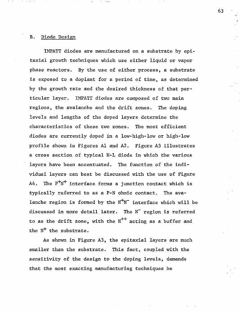
B. Diode Design

IMPATT diodes are manufactured on a substrate by epi­

taxial growth techniques which use either liquid or vapor

phase reactors. By the use of either process, a substrate

is exposed to a dopiant for a period of time, as determined

by the growth rate and the desired thickness of that par­

ticular layer. IMPATT diodes are composed of two main

regions, the avalanche and the drift zones. The doping

levels and lengths of the doped layers determine the

characteristics of these two zones. The most efficient

diodes are currently doped in a low-high-low or high-low

profile shown in Figures Al and A2. Figure A3 illustrates

a cross section of typical H-L diode in which the various

layers have been accentuated. The function of the indi­

vidual layers can best be discussed with the use of Figure

A4. The p~+ interface forms a junction contact which is

typically referred to as a P-N ohmic contact. The ava­

lanche region is formed by the N+N- interface which will be

discussed in more detail later. The N- region is referred

to as the drift zone, with the N++ acting as a buffer and

the ~ the substrate.

As shown in Figure A3, the epitaxial layers are much

smaller than the substrate. This fact, coupled with the

sensitivity of the design to the doping levels, demands

that the most exacting manufacturing techniques be

63

64

EPITAXIAL LAYER ------4 .. ~1 SUBSTRATE

X

(a) Doping Proflle

X r- Wa _..,.,. .... , .. ____ Wd

(b) Electric Field

Figure Al. Low-High-Low Diode

E1

~--------------------------------------~X

EPITAXIAL LAYER -----t•~l SUBSTRATE

(a) Doping ProfJ.le

j~.----------------------------~ .. ~~------~x w

8--t• ... j ..... .,_ ____ · wd - ·

(b) Electric Field

Fiplre A2. lfilh-Low Diode

65

GOLD CONTACT HEAT SINK 301J.M

l - GOLO CONTACT

SUBSTRATE

1 ~>nnmm>mm>>>>>>11111>1~~~::::A::::::.::JjM p+ REGION 1.0 IJ.M

Figure A3. Crossection of High-Low Diode

0\ 0'1

GOLD CONTACT

E FIELD V/CM

\

N++ SUBSTRATE

I I

(a) Layer Defmition

(b) Electric Field

Figure A4. High-Low Diode

.....-- GOLD CONTACT

67

utilized. As a basic review of the parameters that affect

IMPATT performance, let us consider the two zones. In

order for avalanche to occur, the field must reach a par­

ticular value which is realized with a high level of doping

in the N+ region. For efficiency, the length of this zone

must be very narrow in order to keep the voltage (Va)

across this region small. The efficiency is given by

(Al)

where Vd is the voltage across the drift zone. The doping

of the N- layer keeps the field high enough to maintain the

scattering limited velocity. This level must not be so

large that the field extends into the buffer and substrate

layers, a condition known as punch through. Operation of

an IMPATT in punch through will cause the diode to fail.

In addition, the N- layer must be designed for a particu­

lar frequency as given by

where W is the length of the N- region, and Vs is the

scattering limited velocity (for GaAs Vs = 9.0 x 106

em/sec). A long N- layer leaves undepleted material

(A2)

68

~··-

during operation which causes there to be a series resist­

ance and a corresponding reduction in efficiency. The

buffer layer serves to provide a pure high doped region

which is used to compensate for some of the defects found

in the substrate material. The epitaxial growth process is

not currently used to manufacture substrate material be­

cause of the substrate's size and the fact that epitaxial

growth is slow.

The frequency and efficiency characteristics of a

diode have been shown to be affected by the internal

dimensions of the device; now it will be shown how the

power level is established. The optimum profile is based

on the diode operating at a particular current density, J0

,

typically 1000 Amps cm-2 • For a desired power level, P0 ,

one must adjust the area of the diode to yield

(A3)

where "A" is the area of the diode, and V0 P is the operat­

ing voltage of the diode which is given by

(A4)

where Vb is the breakdown voltage. The parameter V'is the

volt-temperature characteristic of the material. The fac­

tor ~T is the operating temperature of the diode minus the

69

ambient temperature at which Vbr is measured. The param­

eter I0

p is the operating current and Rsc is the space

change resistance. Thus, for high power levels, the area

must be large; but there are limits to be imposed on the

area and maximum P0

•

It is known that the area of the diode is inversely

proportional to the impedance of the device, so that large

areas result in low values of Zd. Consequently, Zd could

reach a limiting value below which it cannot be properly

matched by the circuit impedance Zc. The condition for

oscillation states that

Zd + Zc = 0. (AS)

Consider a circular diode with radius 'r' and represent Zd

as

(A6)

It can be shown [1] [29] that

w 1 - cos ( v;) (A7)

70

•

and

2 -1 -JXd = (1rr w C)

where

and

c = l

W depletion width (em)

A area of diode (cm2)

l dielectric permittivity (Farads/em)

w operating frequency (radians/sec)

"'r avalanche resonant frequency (radians/sec)

Vs scattering limited velocity {em/sec).

At a particular frequency, w0

, Equations (A7) and (A8)

reduce to

WK.

-JXd = (A "'o C) -1

{A8)

(A9)

(AlO)

(All)

where K is constant at w0

• It can be shown that K is

approximated by -1/2. The negative sign occurs because w0

71

is greater than wr. The device only has negative resist­

ance at frequencies greater than wr, so that

-w (Al2)

2 At w0

•

If the operating frequency is near the designed frequency

of the diode, w0

can be expressed as w0

= (" Vs)/W. From

Equation (AS), Rc = -Rd and JXc = JXd and, upon substitu­

tion of JXc and Rc into (All) and (Al2) respectively, one

obtains

-w (Al3) Rc =

2 At w0

-1 XC = (A w

0 C) (Al4)

If A = "r2 and w0 = (" Vs)/W is substituted into (Al3) and

(Al4), the new equations are in terms of the diode radius

'r' given by

(Al5)

and

72

w (Al6)

If Equation (A9) is substituted into (Al6}, it becomes

(Al7)

From Equation (Al5), r 2 is given by

w2 r2 =-----

(Al8}

2" 2 £ V s Rc

By use of Equation (Al7), one finds that r 2 is also given

by

Since r 2 must be the

they can be equated,

2 2

1r £ V X s c

same for Equations (A18) and

i.e.,

w2 4 w2 =

f vs Rc 1T f v s XC

(Al9}

(Al9},

(A20}

73

or

1 4 (A21) ---=-

thus

(A22)

In actual circuits, obtaining a value for Rc that is prac­

tical becomes the limiting factor. This fact is demon­

strated through the use of the transformer equation

(A23)

If Zo = SOn, Rc = 0.50, then ZT = sn which is difficult to

achieve. If Rc = O.Sn is substituted into Equation (Al8),

one obtains the maximum value of 'r' in terms of W, given

by

r = 103.1 W. (A24)

For an X-band diode, W is usually 4~m, so r = 412.2~m. In addition to the limitation on output power due to

the impedance of the device, there is also a limitation due

74

to thermal properties of the device. The factor ~T occur­

ring in Equation (A4) is the rise in temperature of the

diode junction above ambient temperature. The reliability

of the device is determined by the junction temperature Tj,

as shown in Figure AS, and thus must be considered in the

design. Manufacturers recommend that T. be maintained less J

than 270°c; and, therefore, they design diodes for a Tj =

200°c. This provides a mean failure time greater than 106

hours. Tj is defined as

(A25)

where ~T arises from the device efficiency, input de power

and the thermal resistance (et) of the device. Equation

{A25) can be rewritten as

(A26)

(A27)

Typical values of 8t for high power GaAs devices, mounted

on copper heat sinks, range from 8.5 - 11.0. If it is

assumed that 8t = 10° c/watt, P de = 23 watts, 7J = 24% and

Tamb = 25° c, then one finds that Tj = 200° c. To deter­

mine the maximum RF power that can be produced at the upper

temperature limit, one can solve Equation (A26) for P0

,

75

76 ' '

300~----------------------------------------~

MEAN LIFE (HOURS)

Figure AS. Mean Life to Failure

where

p = 7J (T; - Tamb)

(1 - 7]) (Jt

Substitution of the values 7J = 24%, Tamb = 25° c,

(A28)

Tj = 270° c and et = 10° c/w, into Equation (A26), one

finds that P0

= 6.13 watts. If one computes the power

based on Equation (A3) and uses the largest diode radius

attainable, with V0 P = 40 volts, it is found that P0 =

213.0 watts. In comparing the two power levels, it is

seen that there is a thermal limitation on the amount of

power that can be produced.

C. dc-to-RF Correlation

With the previous discussion, the development of the

relationships between the RF performance and de character­

istics can begin. The doping levels and layer thicknesses

have been shown to be the most important parameters. The

doping profiles shown in Figures Al and A2 provide this

information, under the assumption that the diode diameter

is known. Typically, a circuit designer only works with

the packaged device, shown in Figure A6. Upon testing the

commercially available diodes, a designer may notice

performance differences between the diodes and slight to

77

HEAT SINK

0.100

r- 0.060 __.,

:-~---~ 1_--r-- METALCAP

I WIREMESH

I DIODECHIP

L---+' -"t'-- CERAMIC 1 - J. RING

--~~----~-----4-

T

----3-48 UNc-2A

Figure A6. Cross-Sectional View of Diode

78

major tuning may be required. The frequency may differ by

as much as 500mHz or the efficiency can vary as much as 5%.

All of the above differences may occur while meeting or

exceeding a required specification provided by the manu­

facturer. On the other hand, if the parameters of the test

circuit are fixed and the diodes are retested, one would

observe larger performance variations. Most likely, some

diodes would not meet the manufacturer's specification when

tested in this condition.

It is the intent of this section to present a method

of predetermining a diode's RF performance based on simple

de measurements. It will be assumed that a diode type has

been selected and optimized in a given circuit. Further,

it will be required that the predicted performance of the

diodes be restricted to the aforementioned circuit. The

idea is that power combiner circuits present the same

impedance to each diode. Therefore, in trying to attain

repeatable optimum performance, the diodes are required to

have the same RF characteristics.

The doping profile, diode junction diameter and cur­

rent density define the RF characteristics of a device. We

will assume that the diode is always operated at the proper

current density, and that the junction diameter is easily

attainable from the manufacturer. Next, the doping profile

must be defined. Several papers [30] [31] [32] have been

written describing the measurement of the profile. All of

79

~··

these techniques require a knowledge of the junction area

and a measurement of the capacitance-versus-voltage (C-V)

characteristic of the device. Typically a microprosser

is used in conjunction with a capacitance meter to generate

the doping profile. For the typical circuit designer, most

of the information provided by the doping profile is

unfamiliar and, without a knowledge of solid state physics,

it is useless. Nevertheless, it is important that a

designer be capable of specifying the parameters of the

diode, so that its RF performance will be reproducible.

Specifications such as minimum power and efficiency are not

adequate to guarantee repeatable performance. To

accomplish this task, the capacitance of the device will be

examined, since this is a quantity that most designers

understand and can easily measure. The basic idea will be

to develop relationships between operating characteristics,

profile and capacitance.

The depletion-layer capacitance of a diode is given by

A ( (A29) c =

w '

which is the standard capacitance equation for two parallel

plates of area 'A' and separation 'W' • With a diode, the

equivalent plate separation 'W' varies as the voltage is

changed. So the diode capacitance is given by

80

where

q

(

v w

A

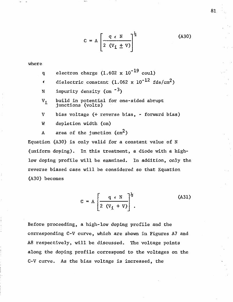
c =A [z ~

q ( N 12 (Vi + V) J

electron charge (1.602 x lo- 19 coul)

dielectric constant (1.062 x lo-12 fds/cm2)

impurity density (em -3)

build in potential for one-sided abrupt junctions (volts)

(A30)

bias voltage (+ reverse bias, - forward bias)

depletion width (em)

area of the junction (cm2)

Equation (A30) is only valid for a constant value of N

(uniform doping). In this treatment, a diode with a high­

low doping profile will be examined. In addition, only the

reverse biased case will be considered so that Equation

(A30) becomes

c = A [z q ( N l~ (Vi + V) J

(A31)

Before proceeding, a high-low doping profile and the

corresponding C-V curve, which are shown in Figures A7 and

AB respectively, will be discussed. The voltage points

along the doping profile correspond to the voltages on the

C-V curve. As the bias voltage is increased, the

81

82

1017

8

6

4 -

7.0

2

r> I

:E 1016 ~ Cl 8 z ii: 0 0 6

4

2

1015~------~~------~----~--~--~--------~------~----~--~~ 0.1 1.0 10.0

DEPTH CMICRONSI

Figure A 7 Doping Profile of High-Low Diode

83

II) '0 0 .... 0

~ ~ 0 ~

I .s:: 00 ....

:I: ~

c,... 0

...1 ... 0 0 > -=-

>. u 00

< II) .... . ~ ~

ICJVYV::I OOid

1 capacitance decreases in a manner proportional to v-~ until

it reaches the end of the uniformly doped high region. The

region between the high and low doped layers is called the

abrupt junction. The capacitance then changes as v-l/3 ;

i.e. ,

C =A a rl qa€2] 12 (Vi + V)

1/3 (A32)

where 'a' is the doping gradient between the regions. As

the bias is further increased, the diode is depleted into

the low doped material and the capacitance once again is

proportional to V -~. The important points to consider are

the levels of doping and the length of the doped layers.

To define the high doping level (NH), let us consider

Equation {A30) with V = o. The capacitance for this condi-

tion will be defined as co and is given by

[q , Na r (A33) co = A

2 vi .

If Equation (A33) is rewritten to determine NH, one obtains

2 V· ~

q (

(A34)

84

Since c0 can be measured, and all the other parameters are

known, thus NH is determined. To obtain the low doping

level (NL), let V = Vb, in Equation (A30), and define this

capacitance as Cb, which is given by

(A35)

The parameter Vb is the breakdown voltage of the diode. If

Equation (A35) is solved for NL, one obtains

(A36)

q l

With the measurement of ~ and, since all the other param­

eters are known, NL is obtained. Since the doping level is

independent of the area of the diode, the parameter 'A' can

be factored out by taking the ratio NH/NL, which is given

by

(A37)

For a GaAs diode, Vi = 1.2 volts. Equation (A37) repre­

sents the ratio of the doping levels determined directly

from the capacitance and voltage characteristic.

85

To develop the relationship between the RF character-

istics and capacitance values, let us consider the

device efficiency which is given by

(A38)

in which Va equals the de voltage across the avalanche

region and Vd is the equivalent de voltage across the drift

region. The voltages expressed in terms of the electric

field and respective layer length are

(A39)

(A40)

where Ea and Ed are the average electric fields in ava­

lanche and drift regions respectively. For the avalanche

region

(A41)

and for the drift region

86

(A42)

q NH La where W = La + Ld, Emax = 1.5 Ea, Ea = l Upon sub-

stitution of Equations (A41) and (A42) into (A39) and (A40)

one obtains

or

and

q NH La 2 Va = ~ --==-~

l

The efficiency can then be defined with the use of

Equations (A43) and (A44) as

(A43)

(A44)

(A45)

87

where La is the length of the avalanche region and is

expressed as

A( {A46)

The parameter Cs is the point shown in Figure A8; it is the

capacitance at the beginning of the abrupt region. The

drift length, Ld, is given by

(A47)

where W is the total depletion length determined by

(A48) w =-

The substitution of Equations (A46) and (A48} into (A47)

yields

(A49)

Upon substitution of Equations (A37) and (A46) and (A49}

into (A45), one obtains

88

(ASO)

1 .,., =-

7T

~ v. ~

2 cb - (Cs - cb) + ___ v...;;;i;:...._c..;;;.o ___ _

(Vi + Vb) (Cs - ~)

The diode efficiency is now in terms of easily measured

quantities.

Since the efficiency of the device has been derived,

it is now possible to determine the maximum RF power. This

is achieved by use of Equation (A28) and, since the diode

power is thermally limited,

(A28)

To determine the power, one only requires the efficiency

(T'/), thermal resistance (Ot), and the maximum operating

temperature (Tj).

The next dc-to-RF correlation to be derived is the

relative frequency difference. Let us consider Figure A9

as the equivalent circuit of the packaged diode. In

Figure A9(a), the diode chip represented by Rand C, where

~ and Cp are the package parameters. For the purpose of

simplifying the analysis, let R = 0, since it is typically

less than -1.0 . By eliminating R, the circuit now has

89

90

R c, I CT 0

I (a) A

A 4 I

J I 'VYV" 0

1 c,I 0

I (b) A

A

4 I

C+~l 'V'V'Y"' 0

1 0

I (c) A

.figure A9 Equivalent Circuit of Packaged Diode

the form shown in Figure A9(b) which, in turn, reduces to

Figure A9(c). The resulting L-C circuit, in Figure A9(c),

must resonate at a desired frequency with the load circuit

reactance to satisfy the condition for oscillation. If the

load is capacitive and is represented by Cc, as shown in

Figure AlO, one can solve for the resonant frequency, f 0 .

Since the reactive elements of the circuit, in Figure 10,

must sum to zero at the resonant frequency, one obtains

-j j (A51) ------ + J 2" fo ~- ---- = o. 2 "fo (c + cP) 2" fo cc

The resonant frequency of the circuit, if found to be

1 {A52)

The value of Cc can be determined by measuring the circuit

reactance {Xc} and substituting it into

1 (A53}

The parameter {C + CP) is determined by measuring the

capacitance of the diode at the breakdown voltage, thus

91

c•c,ll~----------~o~--]1- cc I A

Figure AIO Equivalent Circuit of The Packaged Diode and Load Reactance

92

(AS4)

The substitution of Equation (AS4) into (AS2) yields

(ASS)

Equation (ASS) describes the operating frequency of a diode

in terms of its package inductance, breakdown capacitance,

and the load circuit capacitance. Diodes to be used in

power combiner circuits will all have the same load capaci-

tance, Cc. Thus, variation in operating frequency can only

be caused by variations in the package inductance and/or

breakdown capacitance. Typically the package inductance

does not change from diode to diode. Therefore, only

changes in Cb will affect the operating frequency. To

determine the sensitivity of fo to variations in ~, it is

necessary to define a reference diode. The reference diode

will operate at frequency fr with a breakdown capacitance

cbr" The frequency difference between the reference diode

and any other diode, that operates at some frequency f 0

with breakdown capacitance ~' is obtained by simple manip­

ulation of Equation (ASS) and yields

{AS6) f - fo = f r r

93

Equation (A56) represents the change in frequency one can

expect to measure between diodes of the same type tested in

the same circuit but with different values of breakdown

capacitance.

The final diode characteristic to simplify, in terms

of measured quantities, is the real part of its impedance,

R. The small-signal expression is given by

1 (A57) R---

where the transit angle is defined as

(} = (ASS)

and Vs is the scattering-limited velocity. The two right­

hand factors in Equation (A57) can be approximated by

-1/2.

With this approximation, Equation (A57) reduces to

94

-1 R=---

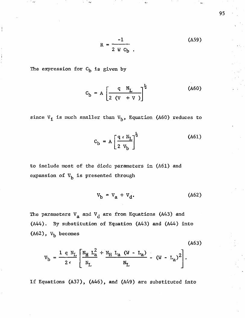
2.WCb.

The expression for cb is given by

[-_q_N.;;;;;,L_)J~ cb = A 2 {V + V

(A59)

{A60)

since Vi is much smaller than Vb, Equation (A60) reduces to

to include most of the diode parameters in (A61) and

expansion of vb is presented through

vb = va + vd.

(A61)

{A62)

The parameters Va and Vd are from Equations (A43) and

(A44). By substitution of Equation (A43) and (A44) into

{A62), Vb becomes

(A63)

1 q NL [NH L~ + NH La (W - La)

2 ( NL NL

If Equations (A37), (A46), and (A49) are substituted into

95

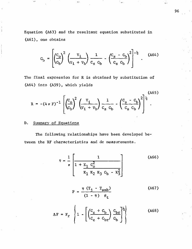
Equation (A63) and the resultant equation substituted in

(A61), one obtains

= [(~:Y (vi V· ) 1 (s ~)l~ (A64) cb +~Vb .

Cs cb Cs cb

The final expression for R is obtained by substitution of

(A64) into (A59), which yields

D. Summary of Equations

The following relationships have been developed be-

tween the RF characteristics and de measurements .

., = 1 ----....,2_1 ____ 1 " 1 + K1 C0 J -K=-

1-K-.:

2;__K_

3_c_b ___ K-:=-~

p = 7J (Tj - Tamb)

(l-7J) ot

(A66)

(A67)

(A68)

96 I '

(A69)

4rrF

where

The above equations can be used by the circuit

designer to determine a specification for a given diode.

Once a diode with desirable RF characteristics has been

selected, the designer can measure the values of C0

, Cb,

cs, vb, cc and the operating frequency. The diode param­

eters can then be varied until a range of reasonable

tolerances are determined.

A tolerance analysis was conducted on a GaAs single­

drift, high-low diode. The result of this exercise is

described as follows:

1. Tolerance on Cb determines AF;

2. Ratio of C0 /Cb mainly determines ~' PRF, and R;

97

3. Tolerance on Cs affects R, ~, and PRF' effect is

greater for low ratios of C0

/Cb;

4. Tolerance on Vb greatly affects R with reduced

effects on ~ and PRF.

In determining a specification, it is suggested that

the tolerances be established in the following manner:

1. Set vb to restrict R variation;

2. ,Set Co/Cb for max/min~;

3. Set cb for allowable frequency differences;

4. Set cs for R variation.

For the aforementioned diode, the parameters and toler­

ances, listed in Table Al, were successfully implemented.

It should be recognized that ~' P0 , ~F and R are

approximations to the actual values. The results of the

tolerance study indicate the equations do predict trends

quite accurately. All tolerances described in Table Al

were verified by measuring good and bad diodes. The veri­

fication is clearly demonstrated by the data presented in

Table A2. The correlation between the theoretical and

measured values shown in Table A2 are typical and were

taken from a sample of over 200 diodes.

98

Table Al. Varian Diode VSX9251 AD

PARAMETER VALVE

vb 33.0 ± 1.5 VOLTS

Co/Cb 18.6 ± 2.0

cb 3.85 ± 0.25 Pfd

cs 27.5 ± 2.0 Pfd

"' 22.0 ± 2.0%

PRF 5.1 ± 0.33 WATTS

AF 186.0 MHz

R -3.0 ± 0.4 OHMS

\0 \0

DIODE PARAMETERS

Co cb cs vb CASE (Pfd) (Pfd) (Pfd) (VOLTS)

1 72.5 3.9 25.5 31

2 77.0 3.6 26.5 39

3 56.5 4.0 20.0 34

4 74.5 5.1 30.0 38

Table A2. Diode Comparison

THEORETICAL VALUES

"' t.F PRF R (%) (MHz) WATTS

23.8 0 5.0 -2.99

24.6 -20 5.2 -3.24

19.8 +35 3.9 -2.50

17.5 +338 3.4 -1.77

EXPERIMENTAL VALUES

"' AF PRF % (MHz) (WATTS)

23.1 0 4.9

25.0 -30 5.5

18.7 +40 3.8

15.2 +300 2.75

R (OHMS)

-2.9

-3.2

-2.7

-2.7

1-' 0 0