Calibration of the Root Zone Water Quality Model for Simulating Tile Drainage and Leached Nitrate in...

Rep

rodu

ced

from

Agr

onom

y Jo

urna

l. P

ublis

hed

by A

mer

ican

Soc

iety

of A

gron

omy.

All

copy

right

s re

serv

ed.

Calibration of the Root Zone Water Quality Model for Simulating Tile Drainage andLeached Nitrate in the Georgia Piedmont

D. A. Abrahamson,* D. E. Radcliffe, J. L. Steiner, M. L. Cabrera, J. D. Hanson, K. W. Rojas,H. H. Schomberg, D. S. Fisher, L. Schwartz, and G. Hoogenboom

ABSTRACT and texture, and known parameter values. This processserves to verify whether the model functions properlyCalibration procedures and data used to parameterize a model,during execution or simulates values that are outside theincluding model components that may or may not have been ad-range of reasonably acceptable estimates or measure-dressed, are generally not well documented in modeling studies. A

comprehensive description of the process and parameters used for ments. It also reveals important information pertainingcalibrating the Root Zone Water Quality Model, v. 1.3.2004.213, is pre- to model processes and sensitive parameters that may besented in this article. The model was calibrated to simulate tile drain- overlooked when using soils, climate, and managementage and leached nitrate under conventional tillage management prac- practices different from those under which the model wastices for maize (Zea mays L.) production followed by a rye (Secale developed (Mulla and Addiscott, 1999; Gijsman et al.,cereale L.) cover crop in Cecil soils (kaolinitic, thermic, Typic Kanhap- 2002). The calibration process allows refinement of pa-ludults), and for cotton (Gossypium hirsutum L.) development in the

rameters and reveals sensitive parameters that can re-Georgia Piedmont. Tile drainage and nitrate leaching were simulatedveal a model’s ability to accurately reflect different sce-within 15% of the observed values in the calibrated maize scenariosnarios of interest (Hanson, 2000).with and without the soil macroporosity option. Simulated and ob-

Calibration of a model includes parameterization basedserved tile drainage and leached nitrate were not significantly differ-ent, and the simulated values were not significantly different with and on direct measurements, pedotransfer functions, or di-without the macroporosity option. Simulated cotton biomass and leaf rect or indirect fitting of the model to measured data.area index were well correlated with observed biomass and leaf area Pedotransfer functions (PTFs) provide estimates of pa-index until the last 21 d of the reproductive stage. Simulated and rameters such as soil hydraulic properties that are oftenobserved cotton water use were different by �1 mm d�1 based on � difficult and time-consuming to measure but accuratesoil water in a 60-cm profile during the critical peak bloom period. enough for many applications (Pachepsky and Rawls,A detailed analysis of the calibration procedure and parameters used

2005). However, Vereecken et al. (1992) showed thatin this study will aid subsequent users of the model as well as aid in�90% of the variability in simulations of a soil mapa subsequent evaluation of the model’s performance for simulationsunit was due to the variability in the estimated hydraulicof tile drainage and nitrate leaching in Georgia Piedmont cottonparameters using PTFs.production systems.

Recently, some modeling studies have begun to pro-vide more details on the calibration approach or proce-dure that was used (Abrahamson et al., 1999; CornelisThe soil–plant–atmosphere system is highly com-et al., 2004; Zhang, 2004; FAO, 2004). This is due inplex and difficult to characterize in terms of effec-part to the recognition of the need for standardizationtive parameters. For complex systems such as this, modelof calibration procedures, and subsequent guidelinescalibration and testing may be the only way to estimatethat have been developed (Clarke et al., 1994; Hansonthose parameters that cannot be easily measured or de-et al., 1999; Dubus et al., 2002; Saseendran et al., 2003;termined (Hanson, 2000). Calibration of a model is anBouman and van Laar, 2004). Though the modelingessential step in the basic protocol for hydrologic model-process can be defined procedurally, processes such asing, regardless of the scale of the problem (Mulla andcalibration and validation are completely subjective andAddiscott, 1999). Before simulated values can be expectedopen to best professional judgment, and modelers haveto accurately represent a system within an acceptable er-no obligation to meet a standardized set of criteria (Cor-ror range, a calibration data set should be used to examinewin et al., 1999). A lack of emphasis on the process usedthe model under simple sets of initial and boundary con-for calibration may have resulted in assumptions or con-ditions, such as upper and lower soil moisture limitsclusions by readers and subsequent users of a modelthat may or may not be accurate. It may not be clear

D.A. Abrahamson, H.H. Schomberg, and D.S. Fisher, USDA-ARS- in the reported documentation if parameters were basedJPCNRCC, Watkinsville, GA 30677; D.E. Radcliffe and M.L. Ca- on measured data, if parameters were adjusted duringbrera, Dep. of Crop and Soil Sci., Univ. of Georgia, Athens, GA

calibration, if all major processes in the model were30602-7274; J.L. Steiner, USDA-ARS-GRL, El Reno, OK 73036; J.D.parameterized, or if sensitivity analyses were performed.Hanson, USDA-ARS-NGPRL, Mandan, ND 58554; K.W. Rojas,

USDA-NRCS-ITC, Fort Collins, CO 80526-8121; L. Schwartz, Dupont The lack of reporting of the calibration process may leaveResearch, Wilmington, DE 19898; and G. Hoogenboom, Biol. and a reader with limited information to discern the model’sAgric. Eng. Dep., Univ. of Georgia, Griffin, GA 30223-1797. Received ability to comprehensively address the system tested. Ad-15 June 2004. *Corresponding author ([email protected]).

Abbreviations: CI, confidence interval; CT, conventional tillage; EF,Published in Agron. J. 97:1584–1602 (2005).Modeling tile drain express fraction; LAB, sorptivity factor for lateral infiltra-

tion; MSEA, management system evaluation areas; NT, no tillage;doi:10.2134/agronj2004.0160© American Society of Agronomy PTFs, pedotransfer functions; RRMSE, relative root mean square error;

TDR, time domain reflectometry; WT, wetting thickness.677 S. Segoe Rd., Madison, WI 53711 USA

1584

Published online November 17, 2005

Rep

rodu

ced

from

Agr

onom

y Jo

urna

l. P

ublis

hed

by A

mer

ican

Soc

iety

of A

gron

omy.

All

copy

right

s re

serv

ed.

ABRAHAMSON ET AL.: CALIBRATION OF ROOT ZONE WATER QUALITY MODEL 1585

justments made to parameters during calibration may Plains and Midwest regions of the USA. This paper re-ports results of the calibration of the most recent versionimpact other processes in the model that do not concern

the current modeler, but may not be suitable under dif- of the RZWQM (v. 1.3.2004.213) for simulations of tiledrainage and nitrate leaching in maize and cotton pro-ferent conditions that would be of interest to another

modeler. duction with a winter rye cover crop as well an analysisof the effect of macroporosity on tile drainage and ni-This modeling study is based on a current water qual-

ity field experiment initiated in 1991 at the USDA-ARS trate leaching under conventional tillage managementpractices in the southeastern USA.J. Phil Campbell, Sr. Natural Resources Conservation

Center in Watkinsville, GA. Objectives of the study in- The main objective of this study was to calibrate theRZWQM for its ability to simulate tile drainage andcluded the water quality impacts of maize production

based on the effects of conventional tillage (CT) or no nitrate leaching in a Cecil soil in maize and cotton pro-duction with a winter rye cover under conventional till-tillage (NT), cover crop, and nutrient source. A model

that could accurately simulate the sensitivity of drainage age management practices in the Georgia Piedmont re-gion. A second objective was to evaluate the model’sand nitrate leaching to these management practices

would provide a valuable tool for testing and evaluating sensitivity to soil macroporosity in relation to tile drain-age since regions of preferential flow are found in Cecildifferent agricultural production scenarios in Cecil and

associated series soils which occupy approximately two- soils of the Piedmont region (Gupte et al., 1996). Finally,we aimed to provide a detailed explanation of our cali-thirds of the cultivated land in the southern Piedmont

region (Hendrickson et al., 1963). bration procedures for other modelers and user groupswho are interested in the process of calibration thatUsing this same study, Johnson et al. (1999) tested the

LEACHN model (Hutson and Wagenet, 1992) for maize might be useful before model evaluation. Clarificationof calibration procedures provides a better understand-production for its ability to simulate soil NO3–N and

NH4–N content, and drainage and leached nitrate under ing of the parameterization process, and the sensitiveparameter adjustments that are discovered during theCT or NT management with and without a winter rye

cover crop. Using modifications based on laboratory process. It may have implications for potential users ofthe model if any specific parameters or parameter ad-estimates for input parameters, LEACHN generally

underestimated soil NH4–N and NO3–N during the win- justments have significantly influenced test results. Inaddition, this study contributes toward the standardi-ter and overestimated soil NH4–N during the summer.

The model also overestimated cumulative drainage and zation of the calibration phase of modeling. A standardcalibration protocol supplements the current protocol ofleached nitrate during both seasons (Johnson et al.,

1999). The overestimation of leached nitrate in a wetter parameterization, calibration, and testing with an inde-pendent data set, with guidelines that for now are leftthan normal year was attributed to the absence of a soil

macropore–matrix exchange component in the model. somewhat arbitrarily up to the modeler (Dubus et al.,2002).We chose to evaluate The Root Zone Water Quality

Model (RZWQM) because it includes a macropore com-ponent as well as an exchange component between the MATERIALS AND METHODSsoil matrix and macropore walls. Visible macropores and

Field Experimentspreferential flow patterns are found in Cecil soils (Gupteet al., 1996), and we expected that the RZWQM might The study site is located in northeastern Georgia in thebe able to better simulate drainage and leached nitrate Piedmont region that extends from Virginia to Alabama. Thebased on the results of the Johnson et al. (1999) study. water quality study is located at the USDA-ARS J. Phil Camp-

bell, Sr. Natural Resources Conservation Center in Watkins-In addition, the RZWQM includes an option for tileville, GA, USA (33�54� N lat; 83�24� W long; 229 m elev.).drainage, an important consideration when tile drainsThe study was undertaken to evaluate the effects of tillage andhave been used in the field due to changes in the soilwinter cover cropping on nitrate leaching from maize produc-water dynamics caused by artificial drainage systemstion (McCracken et al., 1995). Tillage treatments included CT(Skaggs, 1978; Ritzema, 1994).and NT, and cover cropping treatments consisted of winter ryeThe hydrology, pesticide, and nitrate movement, crop or fallow conditions. To meet our objectives for the modeling

growth, and several agricultural management practices objective of this study, and to simplify the complexity andin the original version of the RZWQM model published scope of the calibration for later evaluation of the model, wein 1992 have been tested nationally and internationally chose to calibrate the model using only the CT treatment plotswith data collected from 1972 to 1996 (Ahuja et al., in winter rye cover. In addition, the fallow treatment plots

were discontinued in 1992 and all plots were planted with a2000). Tillage effects on hydraulic properties, manurewinter rye cover so that continuous complete data sets formanagement, crop yield response to water stress, andone treatment were not available for this modeling study. Thetile drainage are just some of the refinements presentNT treatment will be tested in the evaluation study later.in the version of the model used in our study (USDA-

The treatment plots were 10 by 30 m and instrumentedARS-GPSR RZWQM development team, personal com-with 10 cm i.d. PVC drain tiles installed 2.5 m apart at 75- tomunication, 2004). Conclusions drawn from some of the 100-cm depths on a 1% slope. The plots were hydrologically

early applications in the literature may not be strictly isolated from each other with polyethylene sheets extendingvalid, and may not represent typical behavior of the cur- from the soil surface to a depth of 1 m and with plastic bordersrent model (Ma et al., 2001). In addition, soils and cli- 10 cm deep. The volume of water drained from a plot was mea-

sured by tipping bucket gauges and digitally recorded by auto-mate in the Southeast are very different from the Great

Rep

rodu

ced

from

Agr

onom

y Jo

urna

l. P

ublis

hed

by A

mer

ican

Soc

iety

of A

gron

omy.

All

copy

right

s re

serv

ed.

1586 AGRONOMY JOURNAL, VOL. 97, NOVEMBER–DECEMBER 2005

mated dataloggers. The tipping bucket gauges had a sampling tilizer was applied after cotton planting at a rate of 67 kg Nha�1, and winter rye was fertilized after planting with 54 kgslot that subsampled drainage and routed it to a beaker. For

every 2 mm of cumulative drainage, a sample was pumped N ha�1. Cotton biomass and leaf area samples were collectedseven times during the growing season beginning on 16 Julyfrom the beaker into a polyethylene bottle inside a refrigerated

sequential waste water sampler (Isco Model 3700 FR, Lincoln, 1997 through 23 Sep. 1997. Plant height and populations werealso estimated at each sampling date (Schomberg and En-NE). An aliquot of this effluent was stored frozen in polyethyl-

ene vials and later analyzed for nitrate using the Griess-Ilosvay dale, 2004).method (Keeney and Nelson, 1982). The samples were filteredthrough a 0.45-�m filter before analysis (McCracken et al., Model Input and Parameters1995; Johnson et al., 1999).

The soil was a Cecil sandy loam. The pH normally ranged The RZWQM model uses a Windows interface and caninitially be set up with a minimum dataset using readily avail-from 5.5 to 5.8 as measured at the study site; therefore, lime

was applied approximately every 3 yr to maintain a pH of 6.0 able data. The required soil properties are texture and bulkdensity. Parameters for soil crusting, macroporosity, tile drain-to 6.3 in the surface horizon to avail plant nutrients and prevent

aluminum toxicity. Since these soils are variably charged, posi- age, and various soil hydraulic properties can be supplied bythe user or, where data are limited or unknown, the modeltively charged soil particles can attract anions such as nitrate

that can be weakly held in the soil matrix. Nitrate may bypass will use default values based on known research documentedin an extensive user help utility. The model has been appliedthe soil matrix via soil macropores. However, Gupte et al.

(1996) found regions of preferential flow in dye-stained soil to simulate best management practices for the ManagementSystems Evaluation Areas (MSEA) research project for maize,cores from the study site that were not necessarily associated

with distinct open macropores observed from the mean cross- soybean, and wheat (Ahuja et al., 2000). The calibrated maize,soybean, and wheat crop parameters in the model can be ad-sectional areas of the soil columns.

In April 1991, the plots were plowed, disked, and planted justed during the calibration procedure to simulate crop growthfor the area of interest to the modeler. Other crops may beto maize. In October 1991, maize was harvested, and six plots

were no-till planted to rye and six plots left fallow through added to the generic plant growth submodel and parameter-ized by the user. Daily weather data can be generated withthe winter. In April 1992, three plots from each of the rye

cover and fallow treatments were placed under either CT the CLIGEN stochastic model (USDA-ARS, 2003) based onnearby historic weather station parameters when measuredor NT management. The CT plots were mowed, moldboard

plowed, and disked. On 24 Apr. 1992, plots were planted to data is not available. However, we used measured rainfall andweather data from the Georgia Environmental Monitoringmaize in 76-cm rows at the rate of 60 000 seeds ha�1. Ammo-

nium nitrate fertilizer was applied at a rate of 168 kg N ha�1 Network for Watkinsville located approximately 15 m fromthe study site (Hoogenboom, 2003).on 26 Apr. 1992. Maize was harvested on 7 Oct. 1992 and rye

was planted on 30 Oct. 1992. Rye was sampled and killed with We parameterized the physical properties of the soil in theRZWQM model from measurements made near the study siteparaquat (1,1�-dimethyl-4,4�-bipyridinium ion) on 12 Apr. 1993,

CT plots were plowed and disked on 13 April, and maize was by Bruce et al. (1983) and Gupte et al. (1996). Seven distinctlayers to a depth of 1.25 m were parameterized based onagain planted on 14 Apr. 1993. Maize was harvested on 14 Sep.

1993 and rye was planted on 29 Sep. 1993. Maize and rye measured properties of each layer. The initial soil water con-tent at the beginning of the simulation period on 1 Jan. 1991yields and N uptake were measured from biomass samples

before each field harvest (McCracken et al., 1995). The same was set to the measured field capacity for each layer (Table 1).The van Genuchten (1980) equation parameters, � and n wereprocedure of planting maize followed by winter rye was used

until Nov. 1994 when winter wheat was planted as the cover fitted using PROC NLIN (SAS Institute, 2000) based on mea-sured soil water content and pressure head for each depthcrop followed by the first cotton crop in May 1995.

To calibrate the RZWQM for cotton growth, and its ability where residual � was estimated as that of the wilting point ath �15 000 cm. The parameters were then converted to theto simulate tile drainage and leached nitrate from cotton pro-

duction during the period when the water quality study was Brooks-Corey parameters, S2 and A2, the bubbling pressureand pore size distribution index, respectively, based on theplanted to cotton, we used parameters from a field experiment

in cotton production in 1997 adjacent to the water quality study. RZWQM documentation (Ahuja et al., 2000). We included asoil crusting option with a crust hydraulic conductivity rateThe calibration study site was planted on 16 May 1997 on a

1.3-ha watershed using a no-till drill. A winter rye cover crop set to 0.68 cm h�1 based on measurements of a Cecil sandyloam crust under simulated rainfall conditions (Chiang et al.,was planted in late October following cotton harvest. Soil

moisture was measured in 15-cm increments to a soil depth of 1993). The initial soil NO3–N and NH4–N concentrations usedare described in Johnson et al. (1999) from soil data collected90 cm using time domain reflectometry (TDR) (Moisture

Point, ESI, Victoria, BC, Canada). Ammonium nitrate fer- from the study site in November 1991. We used 1 Mg ha�1 as

Table 1. Physical properties of Cecil sandy clay loam soil used in model. Data for soil cores and horizons compiled from Bruce et al.(1983). Macroporosity and pore radius are average measured values of all pores 0.2 cm diameter for soil column depths fromGupte et al. (1996).

Model Measured Core Core Soilsoil Model core Core particle bulk Horizon column Porelayer no. depths depths Ks density density Horizon depths Sand Silt Clay depths radius Macroporosity

cm cm h�1 g cm�3 cm % cm %1 1–5 1–7 18 2.64 1.34 Ap 0–21 78 15 7 0.35 0.0142 5–15 6–12 20 2.65 1.56 78 15 7 0–20 0.35 0.0203 15–25 17–23 8 2.72 1.69 BA 21–26 43 20 37 0.35 0.0204 25–35 27–33 18 2.72 1.43 30 20 50 30–45 0.35 0.0205 35–65 57–63 10 2.65 1.37 Bt1 26–102 30 20 50 0.35 0.0256 65–95 87–93 2.6 2.65 1.51 30 20 50 45–60 0.35 0.0257 95–125 127–133 0.2 2.65 1.55 Bt2 102–131 34 25 41 0.10 0.025

Rep

rodu

ced

from

Agr

onom

y Jo

urna

l. P

ublis

hed

by A

mer

ican

Soc

iety

of A

gron

omy.

All

copy

right

s re

serv

ed.


the amount of initial surface residue based on fallow condi- 2000). If the user does not select the macroporosity option,then drainage occurs through the soil matrix only.tions and on one season of maize production before the first

winter rye cover crop in October 1991. The fraction of surface Water can only enter the macropores at the surface, andthe model allows preferential flow through macropores to goresidue mass that would be incorporated by natural means

was set to 2% based on model references. The field area used directly to the tile drain when the water table resides abovethe tile drains. Macropore flow may also exchange the soil so-was 0.03 ha based on the size of a plot, and the slope was 2%.

Input data and initial parameter values used are listed in lution with the soil matrix by miscible displacement throughmacropore walls. The water solution in the macropore is sub-the Appendix.ject to lateral absorption into the drier soil matrix, and thechemicals in solution are also subject to adsorption or desorp-Model Processes tion from the macropore walls. Maximum flow-rate capacityof macropores is calculated using Poiseuille’s law assumingThe RZWQM is an integrated physical, biological, and chem-gravity flow. Lateral absorption into the macropore walls is sim-ical process model that simulates plant growth, movement ofulated using Green-Ampt equations (Green and Ampt, 1911;water, nutrients, and pesticides into the soil and through theChilds and Bybordi, 1969; Hachum and Alfaro, 1980). Theroot zone at a representative point in an agricultural croppinguser may also adjust the fraction of microporosity in each soilsystem. The model is one-dimensional, and designed to simu-layer though to not less than 1% of total porosity.late conditions on a unit area basis. It was originally developed

Other than measured values of macroporosity includingto provide a comprehensive simulation of the root zone pro-macropore size and number, the adjustable parameters in thecesses that affect water quality, and to respond to a wide rangemodel that can affect macropore flow are the sorptivity factorof agricultural management practices and surface processesfor lateral infiltration, the effective lateral infiltration wetting(Ahuja et al., 2000). It was designed with interactive feedbackthickness, and the tile drain express fraction. To account for thebetween soil water, available N, and plant development (Han-effect that compaction or lining of macropore walls may haveson et al., 1999). The RZWQM includes several detailed pro-in reducing the ability of a soil to absorb water and chemicals,cesses and user options that can affect the simulation results.the calculated Green-Ampt radial (lateral) infiltration rate orDescriptions of some of the processes that affect tile drainagesorptivity rate will be multiplied by a user-specified sorptivityand nitrate leaching are described below for the purpose offactor ranging from 0 to 1. The lateral infiltration wetting thick-aiding the reader in discernment of model processes that mayness into a macropore wall can be adjusted to a value betweenhave affected the outcome of the calibration performed in this0 and 2 cm. The tile drain express fraction can be adjusted tostudy. Complete descriptions of the processes, equations, anda value between 0 and 0.1 to vary the percentage of macroporeinteractions of processes can be found in the model documen-flow that follows the path into the tile drains and is not subjecttation (Ahuja et al., 2000).to absorption into the soil matrix.

Soil HydraulicsTile Drainage

The soil profile can have up to 12 distinct horizons. TheIf the user chooses to simulate tile drainage in the model,profile can be parameterized based on distinct horizons or as

flux out of the drains will occur when the water table in thedistinct layers within horizons. Three grids are then created—soil profile is above the depth of the drains. The depth of theone for defining hydraulic properties, a second nonuniformwater table is defined as the depth at which the pressure headlayering system for redistribution of water and nutrients, andfirst becomes negative, and all heads below that depth are non-a third 1-cm grid that only functions during infiltration. Hy-negative. When tile drainage is selected, the system will auto-draulic properties in the model are defined by the soil watermatically set the bottom boundary condition for the Richardscontent–matric suction relationship and the unsaturated hy-equation to a constant flux condition described by the Buck-draulic conductivity–matric suction relationship described byingham-Darcy equation (Buckingham, 1907) where the totalBrooks and Corey (1964) with slight modifications. The modelhead is the sum of the matric potential and gravitational heads,estimates soil hydraulic properties from soil texture, bulk dens-h � z, in the form:ity, and soil water content at a suction of 33 or 10 kPa when

measured data for Brooks-Corey parameters are not available. vw �K (h)(� h/� z � 1)If soil water content at a suction of 33 or 10 kPa is unknown,the parameters for the hydraulic function properties are taken for z zw; t � 0; where vw water table leakage rate (groundfrom Rawls et al. (1982) based on the soil texture class and water leakage rate) in cm h�1, �K(h) unsaturated hydraulicthen adjusted based on bulk density. The user has the option conductivity as a function of matric pressure head in cm h�1,of using a minimum description of these properties or a full and z the lower boundary of the soil profile at time (t)Brooks-Corey description to account for the effects of trapped greater than zero. The ground water leakage rate can be ad-air in the soil, which can reduce Ks by as much as 50% during justed during calibration. The Buckingham-Darcy equation isinfiltration (Bouwer, 1969). The field saturated Ks is divided also used as the surface boundary condition set to the evapora-by a viscous resistance correction factor of 2.0 so that the tive flux rate until the surface pressure head falls below ainfiltration rate at any given time is a function of this reduced minimum value (set to �20 000 cm), at which time a constantKs in the Green-Ampt infiltration equation (Green and Ampt, head condition h h(z) is used.1911). Between rainfall events, soil water is redistributed using Lateral flow to tile drains can introduce error in the mea-the Richards equation minus a sink term for root water uptake surement of unsaturated zone parameters. However, Radcliffeand tile drainage flux. These terms are described in more et al. (1996) found that tile drain breakthrough curves can bedetail in other sections of the paper. used in Cecil soils to determine field-scale unsaturated zone

The model includes an option to define soil macroporosity transport parameters if a model accounts for two-dimensionalin terms of size and number of macropores present in the soil. flow in the saturated zone. The drainage rate to the tile drainsThe user supplies the macropore number and size (radius) for in the RZWQM is calculated according to the Hooghoudt equa-each soil layer. If data on macroporosity are unavailable, it is tion as applied by Skaggs (1978) to correct for the two-dimen-

sional flux to the drains. The RZWQM adds the flux to rootbest to run RZWQM assuming no macropores (Ahuja et al.,

https://www.researchgate.net/publication/240488743_The_Vertical_Movement_Water_in_Stratified_Porous_Material_1_Infiltration?el=1_x_8&enrichId=rgreq-5aae1acf-f3c9-4b28-b2b9-a280fb96555c&enrichSource=Y292ZXJQYWdlOzQzMjU3MDU2O0FTOjEwMzgyNTcyMTUyODMyNEAxNDAxNzY1Mzg5MzAx

Rep

rodu

ced

from

Agr

onom

y Jo

urna

l. P

ublis

hed

by A

mer

ican

Soc

iety

of A

gron

omy.

All

copy

right

s re

serv

ed.


Soil Nutrient Cycling

The submodel for Organic Matter and Nitrogen cycling(OMNI) is linked to other related submodels in the RZWQMsuch as soil chemistry, solute transport, and plant growth.Significant use of concepts and principles found in nutrientmodels such as NTRM (Shaffer and Larson, 1987), Phoenix(Juma and McGill, 1986), CENTURY (Parton et al., 1983),and Frissel’s N model (Frissel and van Veen, 1981) were alsoused (Shaffer et al., 2000). Organic Matter and Nitrogen cy-cling (OMNI) accounts for all N and C processes and pools,with a subset of these processes modeled independently byrate equations. The remaining processes are modeled as func-tions of specified zero-order and first-order rate equations.The user may adjust many of these rates; however, the modeldocumentation recommends against adjustments of these rateswithout carefully considering the complexity of the processas implemented in the RZWQM (Shaffer et al., 2000).

The initial dry mass of surface crop residue is user-specified.The model determines the mass incorporated into the surfacesoil residue pools for initializing the nutrient chemistry model.Initialization of microbial and humus pools will determinehow most C and N cycling processes function during the firstseveral years of a simulation. During the simulation, flat sur-face residue is made available for decomposition after incorpo-

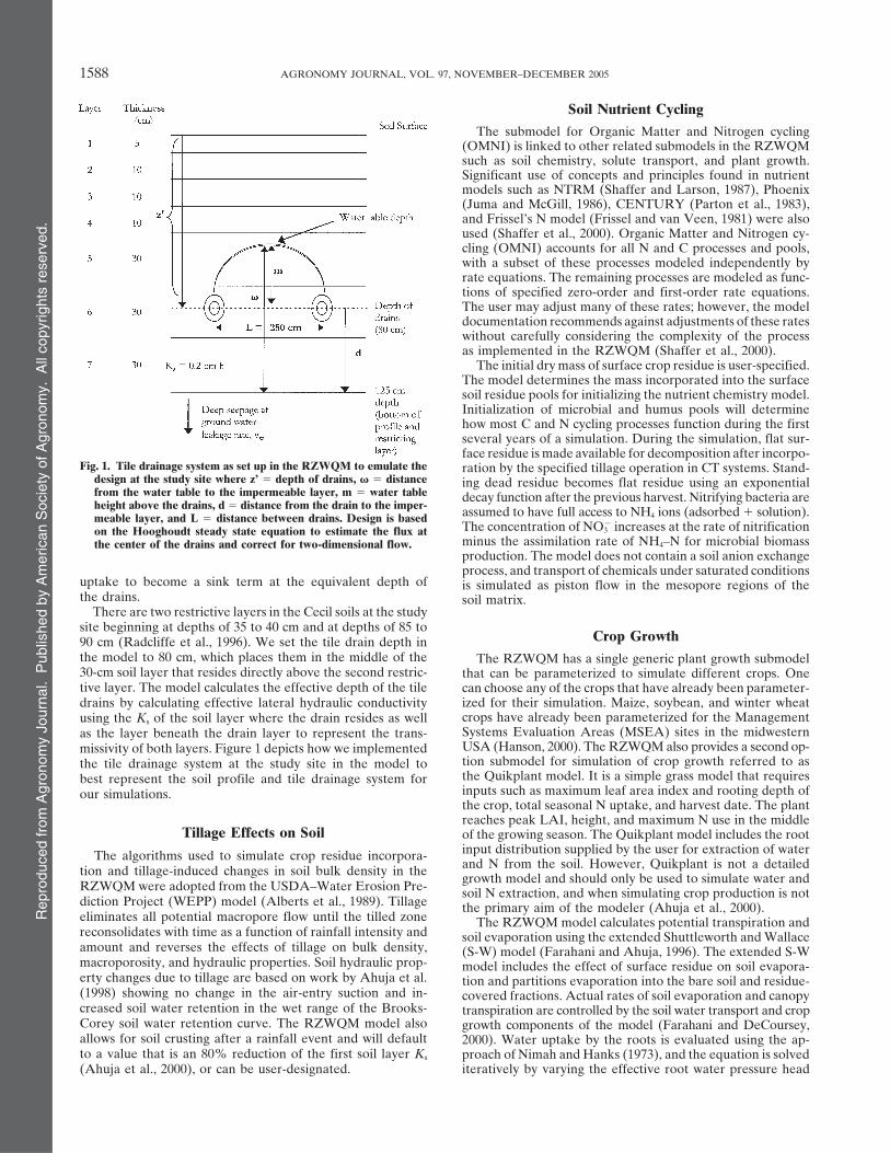
Fig. 1. Tile drainage system as set up in the RZWQM to emulate the ration by the specified tillage operation in CT systems. Stand-design at the study site where z’ depth of drains, � distance ing dead residue becomes flat residue using an exponentialfrom the water table to the impermeable layer, m water table decay function after the previous harvest. Nitrifying bacteria areheight above the drains, d distance from the drain to the imper- assumed to have full access to NH4 ions (adsorbed � solution).meable layer, and L distance between drains. Design is based

The concentration of NO3� increases at the rate of nitrificationon the Hooghoudt steady state equation to estimate the flux at

minus the assimilation rate of NH4–N for microbial biomassthe center of the drains and correct for two-dimensional flow.production. The model does not contain a soil anion exchangeprocess, and transport of chemicals under saturated conditions

uptake to become a sink term at the equivalent depth of is simulated as piston flow in the mesopore regions of thethe drains. soil matrix.

There are two restrictive layers in the Cecil soils at the studysite beginning at depths of 35 to 40 cm and at depths of 85 to

Crop Growth90 cm (Radcliffe et al., 1996). We set the tile drain depth inthe model to 80 cm, which places them in the middle of the The RZWQM has a single generic plant growth submodel30-cm soil layer that resides directly above the second restric- that can be parameterized to simulate different crops. Onetive layer. The model calculates the effective depth of the tile can choose any of the crops that have already been parameter-

ized for their simulation. Maize, soybean, and winter wheatdrains by calculating effective lateral hydraulic conductivitycrops have already been parameterized for the Managementusing the Ks of the soil layer where the drain resides as wellSystems Evaluation Areas (MSEA) sites in the midwesternas the layer beneath the drain layer to represent the trans-USA (Hanson, 2000). The RZWQM also provides a second op-missivity of both layers. Figure 1 depicts how we implementedtion submodel for simulation of crop growth referred to asthe tile drainage system at the study site in the model tothe Quikplant model. It is a simple grass model that requiresbest represent the soil profile and tile drainage system forinputs such as maximum leaf area index and rooting depth ofour simulations.the crop, total seasonal N uptake, and harvest date. The plantreaches peak LAI, height, and maximum N use in the middle

Tillage Effects on Soil of the growing season. The Quikplant model includes the rootinput distribution supplied by the user for extraction of waterThe algorithms used to simulate crop residue incorpora-and N from the soil. However, Quikplant is not a detailedtion and tillage-induced changes in soil bulk density in the growth model and should only be used to simulate water and

RZWQM were adopted from the USDA–Water Erosion Pre- soil N extraction, and when simulating crop production is notdiction Project (WEPP) model (Alberts et al., 1989). Tillage the primary aim of the modeler (Ahuja et al., 2000).eliminates all potential macropore flow until the tilled zone The RZWQM model calculates potential transpiration andreconsolidates with time as a function of rainfall intensity and soil evaporation using the extended Shuttleworth and Wallaceamount and reverses the effects of tillage on bulk density, (S-W) model (Farahani and Ahuja, 1996). The extended S-Wmacroporosity, and hydraulic properties. Soil hydraulic prop- model includes the effect of surface residue on soil evapora-erty changes due to tillage are based on work by Ahuja et al. tion and partitions evaporation into the bare soil and residue-(1998) showing no change in the air-entry suction and in- covered fractions. Actual rates of soil evaporation and canopycreased soil water retention in the wet range of the Brooks- transpiration are controlled by the soil water transport and cropCorey soil water retention curve. The RZWQM model also growth components of the model (Farahani and DeCoursey,allows for soil crusting after a rainfall event and will default 2000). Water uptake by the roots is evaluated using the ap-to a value that is an 80% reduction of the first soil layer Ks proach of Nimah and Hanks (1973), and the equation is solved

iteratively by varying the effective root water pressure head(Ahuja et al., 2000), or can be user-designated.

Rep

rodu

ced

from

Agr

onom

y Jo

urna

l. P

ublis

hed

by A

mer

ican

Soc

iety

of A

gron

omy.

All

copy

right

s re

serv

ed.


Table 2. Initial soil nitrogen on 1 Jan. 1991, and the observeduntil the potential transpiration demand is met based on theand simulated N balance using the calibrated vw value beforeability of the soil to supply the demand. The sum of the sinkand after adjusting the sensitive plant parameter, Ap, for theterm cannot exceed the potential transpiration demand. TheN balance simulation period, November 1991 to April 1993.pressure head reaches a minimum value where it is held steady, No macroporosity model.

and the sum of the sink term for root water uptake from allInitial soil NO3–N, kg ha�1 36.5soil layers then resides below potential demand. The sink termInitial soil NH4–N, kg ha�1 6.25for the Richards equation consists of both the distributed sink

due to root uptake, and a point sink arising from tile drainage. N balance(Day 6 Nov. 1991–13 Apr. 1993) SimulatedNitrogen is passively taken up by the plant in proportion

to plant transpiration and in quantities necessary to satisfy the N component, kg ha�1 Observed Unadjusted Adjustedpresent N demand. The amount of N that passively enters the

Initial soil NO3–N 82 65 65plant is determined by the concentration of N in soil water Initial soil NH4–N 14 0 0extracted by the root system from each soil layer. If inadequate Fertilizer (NH4NO3) 168 168 168

Final soil NO3–N 17 1 1N is brought into the plant via transpiration, active N uptakeFinal soil NH4–N 29 0 0occurs in a manner similar to the Michaelis-Menten substrateDifference total soil mineral N 50 64 64

model. The total amount of additional N available to the plant Leached NO3 (tile drains) 63 38 62through uptake is the sum of passive and active uptake. Avail- Leached NO3 (below drains) – �4 �3

Biomass N 205 227 235able N is hierarchically allocated to roots and then to the otherNet N mineralized 50 34 66plant organs. Any N remaining after plant demands are met

is placed into a storage pool and subtracted from plant Ndemand the following day (Hanson, 2000). out macroporosity (Fig. 2). We ran the simulations from 1 Jan.

1991 through April 1993 based on the availability of mea-sured data for comparison to simulated values of tile drainage,Model Calibration leached nitrate, plant production, and soil N. Model simu-lations from November 1991 through April 1993 were used toGeneral Procedureevaluate and adjust the N balance by comparing simulatedAfter entering all of the model inputs and parameters, weand observed values for soil N, nitrate leaching, and tile drain-ran the model for a period of 12 yr (3 yr of climate and rainfallage. The period from November 1992 through April 1993 wasdata repeated four times) to initialize the organic N poolsused to test the sensitivity of tile drainage to the ground water(rapid, medium, and slow decomposition pools) as suggestedleakage rate, and as the final evaluation period for tile drainagein the model documentation. This step is performed beforeand leached nitrate after adjustments to the N balance. Theactual calibration begins. The only parameters that we ad-reason for this was twofold. The tile drains were installed injusted after the initialization procedure were the soil nitrateone of the three conventional till plots that we used for calibra-and soil ammonium nitrate values for each soil layer beginningtion in 1981 and in the other two conventional till plots usedon 1 Jan. 1991, the first day of the period for simulating tilefor calibration in 1990. Since a winter rye cover crop was firstdrainage and leached nitrate for the analysis period (Table 2).introduced to the study in October 1991, the period fromThe reason for this was that after the initialization procedure,November 1992 through April 1993 allowed the simulation ofthe model greatly over- or underestimated these values al-conventional tillage maize production with winter rye coverthough we had used a value of 1 Mg ha�1 and a wheat coverafter winter rye had been planted for at least one season. Thisfactor type based on model references and conventional tillalso allowed additional time for the soil around the drains tomanagement practices during parameterization before run-settle from disturbance due to the installation of tile drainsning the initialization procedure. The measured mineral soilin two of the plots 2 yr earlier.N data had been collected immediately after winter rye was

Field measurement errors are typically �10%; therefore,planted for the first time as a cover crop at the study site init is unrealistic to match the observed data any more closelythe fall of 1991 (Johnson et al., 1999; McCracken et al., 1995);(Hanson et al., 1999). Our target error rate for the responsetherefore, the measurements reflected the previous 2 yr ofvariables in all periods was �15% or less of measured valueswinter and spring fallow conditions followed by a maize cropbased on the goodness-of-fit test or the percentage differencein the summer of 1991. Including a winter rye cover crop as partrecommended in the model documentation calculated as:of the management practices during the 12-yr initialization

procedure created more residue for simulated decomposition %D [(P � O)/O] 100and, therefore, more mineralized soil N than that measuredin the Fall of 1991. However, the simulation period for calibra- where P is the predicted value and O is the observed value.

We first calibrated the model without the macroporositytion that began after initialization of the model (1 Jan. 1991–14 Apr. 1993) included conventional till and winter rye cover option, and then with macroporosity because measurements

of macroporosity were available from the study site (Guptecrop management practices. Resetting the initial values of soilmineral N to their measured values after the initialization et al., 1996). We ran the model with the macroporosity op-

tion to determine whether or not the model could simulateprocedure before we began the simulations of tile drainage andleached nitrate on 1 Jan. 1991 reflected the soil N conditions at tile drainage more accurately with macropores since work by

Gupte et al. (1996) showed preferential flow in Cecil andthe study site just before the introduction of the winter ryecover crop in the fall of 1991. related soils of the Piedmont that was not necessarily associ-

ated with distinct open macropores but also occurred by wayFor the calibration simulations, we used the general proce-dure recommended in the model documentation by calibrating of infilled macropores. We followed the same general proce-

dure for calibration with and without the macroporosity op-the water balance, then the nutrient balance, and finally, cropproduction (Hanson, 2000) with additional details to meet our tion, and compared the results of simulated tile drainage and

leached nitrate with and without macroporosity.objectives for tile drainage and nitrate leaching with and with-

Rep

rodu

ced

from

Agr

onom

y Jo

urna

l. P

ublis

hed

by A

mer

ican

Soc

iety

of A

gron

omy.

All

copy

right

s re

serv

ed.


Fig. 2. Flow chart of procedure used to calibrate and evaluate the Root Zone Water Quality Model.

adjustable macroporosity parameters in the model. The pa-Water Balance Calibration for Tile Drainagerameters for adjusting the amount of macropore flow that

No Macroporosity occurs in the soil include the wetting thickness or effective lat-eral infiltration into the macropore wall (WT), the tile drainTo calibrate the water balance, we chose to adjust the groundexpress fraction (EF), or the proportion of macropore waterwater leakage rate (water table leakage rate), vw, or the waterthat flows to the tile drains, and the sorptivity factor for lateralthat will flow out of the bottom of the user-designated soilinfiltration (LAB), an adjustment to the calculated Green-profile. We used this parameter for calibration because thereAmpt lateral infiltration rate. These parameters were chosenwere no available measurements of it from the study area.because there was no measured data available for predetermi-We chose a parameter that had not been measured becausenation of possible values, and preliminary runs of the modelone of the strengths of our study was the number of field mea-that showed tile drainage was sensitive to them.surements that were available. According to Corwin et al.

(1999), the definition of calibration is a test of a model with One of the most common forms of sensitivity analysis is toknown input and output information that is used to adjust or vary model parameters around their base values by some fixedestimate parameters for which there is no measured data. We percentage (Silberbush and Barber, 1983; Ma et al., 2000).increased the ground water leakage rate beginning with a We chose values of each of the three macroporosity param-value of 0 cm h�1 until total simulated tile drainage was within eters based on the range of values allowed by the model andthe prescribed 15% range of total observed tile drainage. Dur- created a matrix parameter set varying each parameter by ap-ing this step, we also observed the effect this adjustment had proximately 50%. In the case of EF and LAB, initial and finalon leached nitrate since chemicals in the soil move with the soil values were increased or decreased from the 50% target valuesolution. In addition, this assured that simulation of leached to avoid unreasonable combinations of parameter values. Fornitrate stayed within our target error range of �15% of mean example, a wetting thickness of zero and an absorption ratemeasured leached nitrate. The measurement period used for of zero with an express fraction of 0.09 would result in 9% ofcomparison after this adjustment was November 1992 through macropore water flowing into the tile drains. However, thereApril 1993, after all conventionally tilled plots were in winter would be no absorption into the macropore wall. The param-rye cover for 1 yr and all of the drain tiles had been installed eter set that we used consisted of values of WT ranging fromfor at least 2 yr. 0.5 cm to 2.0 cm by 0.5 cm; EF values of 0.01, 0.05, and 0.09;

and LAB values of 0.1, 0.5, and 1.0, which would reduce lateralWith Macroporosity absorption calculated with Green-Ampt by either 10, 50, or

0%, respectively, for a total of 36 simulations. The results ofAfter we calibrated the model without macroporosity, wecalibrated the model with macroporosity by first testing three each parameter set on total simulated tile drainage and leached

Rep

rodu

ced

from

Agr

onom

y Jo

urna

l. P

ublis

hed

by A

mer

ican

Soc

iety

of A

gron

omy.

All

copy

right

s re

serv

ed.


nitrate were compared to find the best combination for reduc- same sensitive parameters as well as changes to some of thephysiological and phenological parameters described belowing errors between simulated and measured tile drainage andand used in the plant production input file. The calibrationleached nitrate. Our target error rate of �15% or less was usedfor each crop then proceeded by varying each of the sensitivefor differences between total simulated and total measuredparameters until total biomass and yield were within the 15%tile drainage and total simulated and total measured leachedrange of measured values. During adjustment of these param-nitrate. We tested each macroporosity parameter and param-eters to improve yield simulations to reflect the observed values,eter combination set for its sum of squares contribution towe also checked the effect on simulated tile drainage andthe model sum of squares, described below in the model evalu-leached nitrate. This process was used iteratively as depictedation section, to determine if parameter values needed to bein Fig. 2 until simulated tile drainage, leached nitrate, andadjusted to a more narrow range of values. Final adjustmentsmaize yield were within, or as close as possible, to the desiredof these parameters to best simulate tile drainage for our15% error range of observed values.study in conjunction with crop development provided a better

The parameters for the Quikplant model to simulate theunderstanding of how macroporosity functions and influenceswinter rye cover crop were obtained from local crop measure-drainage in Cecil soils under conditions modeled, e.g., con-ments or estimates based on measurements of rye crops (Univ.ventional tillage in maize or cotton production.of Georgia College of Agric. and Environ. Sciences, 1998; Blountet al., 2000). The parameters included total seasonal N uptake,Leached Nitrate Calibrationlength of growing season (days), maximum crop height, leaf

After total simulated and measured drainage were within area index, rooting depth, stover after harvest, the C/N ratiothe 15% error range, we adjusted the sensitive plant param- of fodder material, and winter dormancy recovery day of yeareters in an attempt to bring the simulated aboveground bio- (Appendix A).mass N of the maize crop within, or as close as possible to, After the model was calibrated for tile drainage and leached15% of the measured value. We then evaluated the simulated nitrate in maize and winter rye production, we held all param-N balance relative to N mineralization to begin refining the eters constant and added cotton to the generic plant growth

submodel. Parameters were obtained from the cotton field studycalibration for leached nitrate in drainage if needed. In plotsconducted adjacent to the water quality site (Schomberg andwith tile drains, Groffman (1984) found that tile drainage inEndale, 2004), and from literature values (Carns and Mauney,Cecil soils increased aeration and thereby increased mineral-1968; Miley and Oosterhuis, 1990; Univ. of Georgia Collegeization while decreasing gaseous N losses, resulting in a greaterof Agric. and Environ. Sciences, 2000; Nyakatawa and Reddy,supply of nitrate in the drains. Based on available measured2000; Nyakatawa et al., 2000; Reddy et al., 2004). The cottondata, we evaluated simulated net mineralization for the periodcalibration simulation period was 1 Jan. 1997 through 31 Dec.from 6 Nov. 1991 through 13 Apr. 1993 as follows:1997. The parameters adjusted for cotton in the generic plant

Nnet (Soil Nfinal � Crop Nuptake � Nleached) � growth input file included the physical dimensions of the plant;the maximum, minimum and optimum temperature for growth;(Soil Ninit � Nfert)maximum leaf area index; and the minimum number of days

where Nnet net mineralization; Soil Nfinal final soil mineral the plant required to transect each physiological growth stageN on 13 Apr. 1993; Crop Nuptake aboveground biomass N; (Appendix A7). Through iterative adjustments of these pa-Nleached leached N in tile drains; Soil Ninit initial soil mineral rameters, we compared simulated and observed cotton totalN on 6 Nov. 1991; and Nfert fertilizer N applied. If the model biomass until simulated values were within 15% of observedover- or under-predicted a N component in the system, we values. Since we did not have measures of tile drainage orfirst adjusted the plant parameters to improve the simulation leached nitrate from the study used to calibrate for cotton,of N uptake, which in turn would affect the other N com- we compared simulated and calculated PET and water use toponents. If simulated Nnet could not be achieved within �15% ensure that the model could simulate both reasonably well asof observed Nnet, or the system was producing too much or a basis for later evaluating simulated tile drainage in the watertoo little nitrate, we adjusted the nitrification and denitrifica- quality study. Calculated PET was based on the Priestley-tion rates to bring Soil Nfinal, Crop Nuptake, and Nleached to within Taylor equation (Priestley and Taylor, 1972) from the weather�15% of, or as close as possible, to observed values. We station near the water quality study site, approximately 100 mreevaluated the N balance after each adjustment. Iterative ad- from the cotton calibration study site (Hoogenboom, 2003).justments to sensitive plant parameters and the nitrification We calculated observed and simulated water use for cotton as:and denitrification rates were made until Nleached and Crop

Water use Nuptake were as close as possible to their measured values.Rainfall � Observed or simulated � Soil Water

Crop Growth Calibration where Rainfall measured rainfall at the weather stationadjacent to the water quality study site, � Soil Water SoilSince plant production was part of the N balance and tightlywateri�1 � Soil wateri , where soil water was measured or sim-coupled to the other processes, we followed the procedureulated in a 60-cm profile, and i day of year. Observed soilfor calibrating plant growth recommended for the model bymoisture in cotton showed little or no change below 60 cm inHanson (2000) when using the generic plant growth submodel.the field study used for calibration (Schomberg and Endale,This procedure is based on adjustments to five sensitive plant2004). The rooting depth for cotton is shallow in acid soils be-parameters including active N uptake rate (�1), daily respira-cause it is one of the most sensitive crops to aluminum toxicity,tion as a function of photosynthesis (�), the biomass to leafwhich frequently occurs in acid subsoils such as those in Geor-area conversion coefficient (CLA), and the age effect for plantsgia (Mitchell et al., 1991; Sumner, 1994; Gascho and Parker,during the propagule stage and the seed development stage2001).(Ap and As). We used the generic plant growth submodel for

both the maize and cotton calibrations, and based adjustments Evaluation of Simulation Resultsof these parameters for maize within the range of values usedfor calibration of the MSEA sites (Hanson, 2000). The calibra- For the analysis of the macroporosity parameters, we tested

for the main effects and interactions of the three parameterstion for cotton development included adjustments of these

Rep

rodu

ced

from

Agr

onom

y Jo

urna

l. P

ublis

hed

by A

mer

ican

Soc

iety

of A

gron

omy.

All

copy

right

s re

serv

ed.


for macroporosity and selected the most significant effects basedon the Type I sum of squares each contributed to the modelsum of squares (SAS Institute, 2000). Based on this informa-tion, we identified the parameter or combination of param-eters with the highest correlations and highest probabilitiesfor simulated and observed tile drainage. We determined atthis point whether further testing was needed within a morenarrow range of parameters. Since one of our objectives wasto try to simulate how macropore flow may affect drainage inCecil soils, we chose to refine the range of the parameters asmuch as possible to improve our understanding by way of thesimulation process.

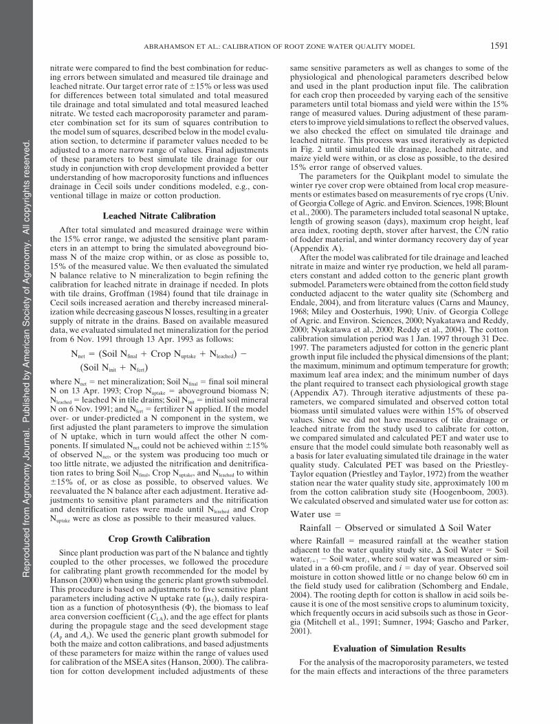
For the analysis of simulated and observed values of tiledrainage and of nitrate leaching, we regressed the final ob-served values on simulated values using linear regression anal-ysis (SAS Institute, 2000), to compare r 2 values, slopes, andintercepts. We calculated the relative root mean square error Fig. 3. Simulations using values of ground water leakage rate, vw, for(RRMSE), standard error of the mean difference (Addiscott sensitivity analysis of simulated tile drainage and leached nitrate.and Whitmore, 1987), maximum error, average and standarddeviation of measured and simulated values to characterize

the lower layer into ground water to warrant calibrationsystematic over- or under-prediction, and used graphical dis-of the ground water leakage rate when the model is usedplays to show trends and distribution patterns (Loague and

Green, 1991). The RRMSE, which is the RMSE relative to to simulate tile drainage. In a study of tile drain break-the mean of the observed values, is calculated as follows: through curves on two plots adjacent to the water quality

study in 1991, Radcliffe et al. (1996) found that seepage��N

j1

(sj � oj)/N�0.5

(100/O) through the two layers below the tile drains accountedfor approximately 10% of irrigation water applied. Mea-

where N number of observations; oj observed value j ; sured values of Ks in these two layers were 0.2 andsj simulated value j ; and O mean of the observed values. 0.035 cm h�1, respectively, at a site near the water qualityThe RRMSE standardizes the RMSE, and is expressed as a study without tile drains (Bruce et al., 1983). The bottompercentage that represents the standard variation of the esti- of the first layer in that study (133-cm depth) corre-mator. The RRMSE assigns equal weight to any overestima- sponds to the bottom layer of the soil profile (125-cmtion or underestimation of the statistic (S.P. Weschsler, www.

depth) in our study. The difference in the Ks of the layercsulb.edu/~wechsler; verified 18 Aug. 2005).below 133 cm and our calibrated ground water leakageFor the cotton water use analyses, we compared observedrate (0.035 cm h�1 vs. 0.0039 cm h�1) could be due toand simulated water use for the period of peak water use inthe mechanical compaction of the soil around the drainscotton from first square to first bloom and from first bloom

to peak bloom. Our criteria for the acceptable differences that was performed after installation in the water qualitybetween daily simulated and observed water use was �15% study. The compaction of the soil below the installationor less based on a minimum daily value of 6.4 mm of water depth during the process could have decreased the rateuse for cotton during these periods, a total of approximately of soil water movement below the measured value of55 d in July and August (NCSU-CES, 2004). 0.035 cm h�1 as well.

Though we chose the ground water leakage rate thatbest simulated total tile drainage when compared withRESULTS AND DISCUSSIONtotal observed drainage, simulated leached nitrate was

Calibration: No Macroporosity not within �15% of observed leached nitrate for theperiod used to evaluate the N balance from NovemberIncreasing the ground water leakage rate from 0 to1991 through April 1993. Simulated leached nitrate was0.004 cm h�1 decreased simulated tile drainage linearly.25 kg ha�1 less than observed leached nitrate and simu-The final ground water leakage rate used for calibrat-lated aboveground biomass N for maize was 30 kg ha�1ing the model for tile drainage and leached nitrate wasgreater than observed aboveground biomass N, and both0.0039 cm h�1 because simulated values were in goodwere outside the �15% error range. Simulated soil min-agreement with observed values compared with the othereral N was 45 kg ha�1 less than observed but withinrates that were tested (Fig. 3). A higher Ks for a soil�15% of observed soil mineral N, and simulated maizelayer above a layer with lower Ks as depicted in Fig. 2yield was within �15% of observed yield. Since leachedfor the two bottom layers of the profile could create un-nitrate was underpredicted and aboveground biomasssaturated conditions in the lower layer due to negativeN was overpredicted by almost the same amount, we de-pressure at the interface of the two layers. This wouldcreased the Ap parameter (propagule age effect). A de-result in very slow soil water movement from the uppercrease in this parameter will reduce yield in relation tolayer into the lower layer over time and create a perchedtotal biomass and therefore reduce the crop N demand.water table. However, though the ground water leakageThis is due to the fact that propagule N demand is metrate turned out to be very small, simulated tile drainagefirst when the plants are in the reproductive stage inwas sensitive to very small changes in the ground waterthe hierarchical scheme for N allocation in the genericleakage rate. Our analysis indicates that adequate flow

occurred in the RZWQM simulation of drainage through plant growth submodel (Hanson, 2000). In addition, our

Rep

rodu

ced

from

Agr

onom

y Jo

urna

l. P

ublis

hed

by A

mer

ican

Soc

iety

of A

gron

omy.

All

copy

right

s re

serv

ed.


Fig. 5. Measured and simulated event tile drainage (top) and leachednitrate (bottom) for the simulation period from November 1992

Fig. 4. Cumulative observed and simulated tile drainage (top) and through April 1993 with and without the macroporosity option forleached nitrate (bottom) with and without macroporosity for the maize. Observed drainage events shown with 95% C.I. bars.simulation period November 1992 through April 1993 for maize.

ference between simulated and observed values for tiledrainage, leached nitrate and maize yield of 15% or lesstarget error range for yield was large (5716–7734 kg ha�1)

so that a slight reduction in yield would be acceptable. for the final analysis period, we considered the calibra-tion acceptable as the final calibrated scenario for maizeOur previous experience of adjusting the sensitive plant

parameters by trial and error showed that the model production with a winter rye cover crop without macro-porosity.would allocate the N balance components differently

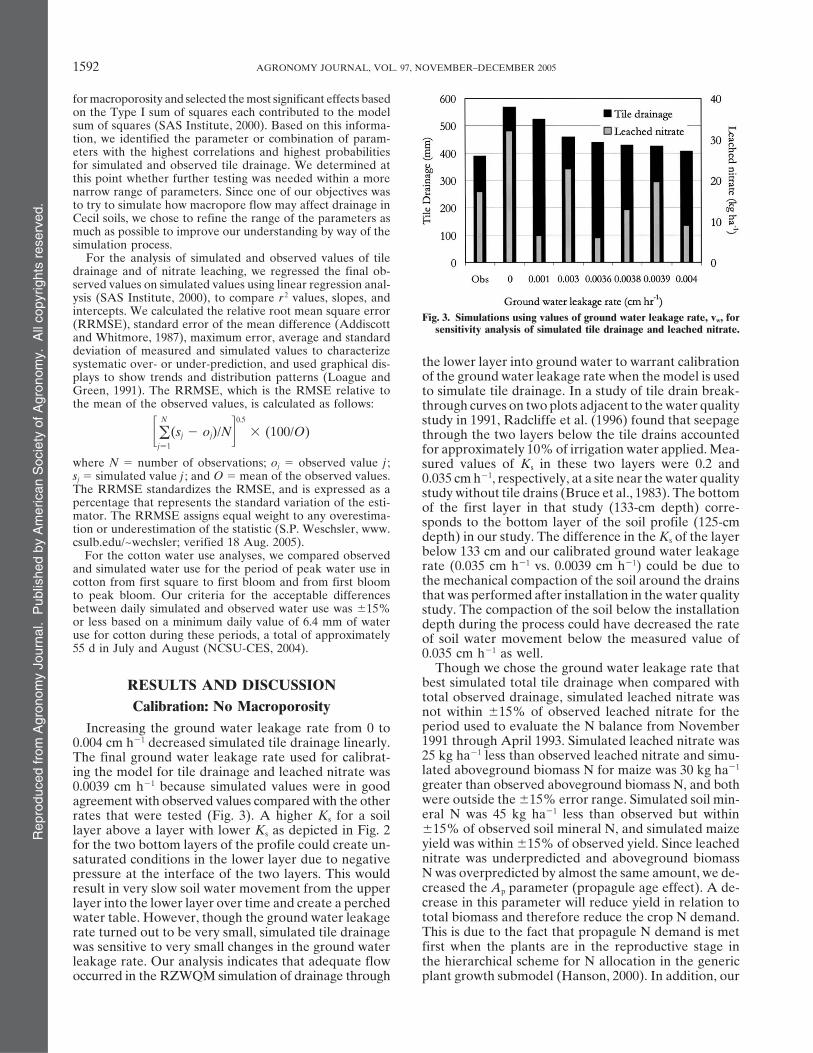
with this adjustment. The adjusted Ap parameter increased The analysis of simulated tile drainage and leachednitrate for the calibrated scenario revealed that cumu-simulated leached nitrate to within �1% of observed

leached nitrate while simulated maize yield remained lative simulated tile drainage followed the pattern of cu-mulative observed tile drainage (Fig. 4). However, 7 ofwithin 15% of observed yield, though it decreased slightly.

The remaining sensitive crop parameters for maize were 12 simulated drainage events were outside of the 95%CI of observed tile drainage events (Fig. 5). Simulatedleft unadjusted from their original values. Total simu-

lated N uptake was slightly higher in the adjusted model leached nitrate increased at the same rate as observedleached nitrate during the first five drainage events andthan in the unadjusted model. However, total simulated

aboveground biomass N for all three crops (winter rye then leveled out at or near zero for the remaining sevenevents while observed leached nitrate continued to in-1992, maize 1992, and winter rye 1993) was within 15%

of total observed aboveground biomass N for all three crease slightly (Fig. 4). Six out of 12 simulated leachednitrate events were outside the 95% CI of observedcrops (Table 2).

The analysis of simulated and observed soil mineral leached nitrate (Fig. 5). The RRMSE showed a largepercentage deviation from the mean observed values,N for each day of 12 field-measured values from Novem-

ber 1991 through April 1993 revealed that 3 of the 12 reflecting the fact that the majority of simulated eventsfor tile drainage and half of the events for leached nitratesimulated soil mineral N predictions were outside the

95% confidence interval (CI) of observed soil mineral were outside of the 95% CI (Table 3). Linear regressionanalysis of total observed tile drainage on total simu-N. Total simulated tile drainage and leached nitrate for

the final analysis period of November 1992 through lated tile drainage revealed that simulated tile drainageexplained 37% of the variation in observed tile drainage.April 1993 were 6 and 5% of total observed values, re-

spectively. Since we met our objective of obtaining a dif- Analysis of total observed leached nitrate on total simu-

Rep

rodu

ced

from

Agr

onom

y Jo

urna

l. P

ublis

hed

by A

mer

ican

Soc

iety

of A

gron

omy.

All

copy

right

s re

serv

ed.


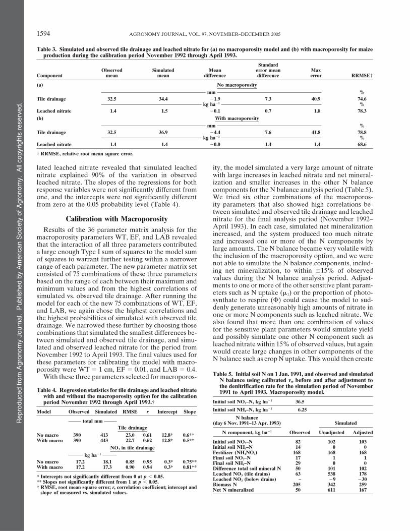
Table 3. Simulated and observed tile drainage and leached nitrate for (a) no macroporosity model and (b) with macroporosity for maizeproduction during the calibration period November 1992 through April 1993.

StandardObserved Simulated Mean error mean Max

Component mean mean difference difference error RRMSE†

(a) No macroporositymm %

Tile drainage 32.5 34.4 �1.9 7.3 40.9 74.6kg ha�1 %

Leached nitrate 1.4 1.5 �0.1 0.7 1.8 78.3(b) With macroporosity

mm %Tile drainage 32.5 36.9 �4.4 7.6 41.8 78.8

kg ha�1 %Leached nitrate 1.4 1.4 �0.0 1.4 1.4 68.6

† RRMSE, relative root mean square error.

lated leached nitrate revealed that simulated leached ity, the model simulated a very large amount of nitratewith large increases in leached nitrate and net mineral-nitrate explained 90% of the variation in observed

leached nitrate. The slopes of the regressions for both ization and smaller increases in the other N balancecomponents for the N balance analysis period (Table 5).response variables were not significantly different from

one, and the intercepts were not significantly different We tried six other combinations of the macroporos-ity parameters that also showed high correlations be-from zero at the 0.05 probability level (Table 4).tween simulated and observed tile drainage and leachednitrate for the final analysis period (November 1992–Calibration with MacroporosityApril 1993). In each case, simulated net mineralizationResults of the 36 parameter matrix analysis for theincreased, and the system produced too much nitratemacroporosity parameters WT, EF, and LAB revealedand increased one or more of the N components bythat the interaction of all three parameters contributedlarge amounts. The N balance became very volatile witha large enough Type I sum of squares to the model sumthe inclusion of the macroporosity option, and we wereof squares to warrant further testing within a narrowernot able to simulate the N balance components, includ-range of each parameter. The new parameter matrix seting net mineralization, to within �15% of observedconsisted of 75 combinations of these three parametersvalues during the N balance analysis period. Adjust-based on the range of each between their maximum andments to one or more of the other sensitive plant param-minimum values and from the highest correlations ofeters such as N uptake (�1) or the proportion of photo-simulated vs. observed tile drainage. After running thesynthate to respire (�) could cause the model to sud-model for each of the new 75 combinations of WT, EF,denly generate unreasonably high amounts of nitrate inand LAB, we again chose the highest correlations andone or more N components such as leached nitrate. Wethe highest probabilities of simulated with observed tilealso found that more than one combination of valuesdrainage. We narrowed these further by choosing thosefor the sensitive plant parameters would simulate yieldcombinations that simulated the smallest differences be-and possibly simulate one other N component such astween simulated and observed tile drainage, and simu-leached nitrate within 15% of observed values, but againlated and observed leached nitrate for the period fromwould create large changes in other components of theNovember 1992 to April 1993. The final values used forN balance such as crop N uptake. This would then createthese parameters for calibrating the model with macro-

porosity were WT 1 cm, EF 0.01, and LAB 0.4.Table 5. Initial soil N on 1 Jan. 1991, and observed and simulatedWith these three parameters selected for macroporos- N balance using calibrated vw before and after adjustment to

the denitrification rate for the simulation period of NovemberTable 4. Regression statistics for tile drainage and leached nitrate 1991 to April 1993. Macroporosity model.

with and without the macroporosity option for the calibrationInitial soil NO3–N, kg ha�1 36.5period November 1992 through April 1993.†Initial soil NH4–N, kg ha�1 6.25Model Observed Simulated RMSE r Intercept Slope

N balancetotal mm (day 6 Nov. 1991–13 Apr. 1993) Simulated

Tile drainageN component, kg ha�1 Observed Unadjusted AdjustedNo macro 390 413 23.0 0.61 12.8* 0.6**

With macro 390 443 22.7 0.62 12.8* 0.5** Initial soil NO3–N 82 102 103Initial soil NH4–N 14 0 0NO3 in tile drainageFertilizer (NH4NO3) 168 168 168kg ha�1Final soil NO3–N 17 1 1

No macro 17.2 18.1 0.85 0.95 0.3* 0.75** Final soil NH4–N 29 0 0With macro 17.2 17.3 0.90 0.94 0.3* 0.81** Difference total soil mineral N 50 101 102

Leached NO3 (tile drains) 63 538 178* Intercepts not significantly different from 0 at p � 0.05. Leached NO3 (below drains) – �9 �30** Slopes not significantly different from 1 at p � 0.05. Biomass N 205 342 259† RMSE, root mean square error; r, correlation coefficient; intercept and Net N mineralized 50 611 167slope of measured vs. simulated values.

Rep

rodu

ced

from

Agr

onom

y Jo

urna

l. P

ublis

hed

by A

mer

ican

Soc

iety

of A

gron

omy.

All

copy

right

s re

serv

ed.


a situation that required an endless number of iterative nitrate with macroporosity for the calibrated scenario re-vealed that cumulative simulated tile drainage followedadjustments to bring simulate leached nitrate, tile drain-

age, and yield back to within a reasonable range of ob- the pattern of cumulative observed tile drainage (Fig. 4)with 8 of 12 simulated drainage events outside the 95%served values. After several attempts to adjust the

macroporosity components and the sensitive plant pa- CI of observed tile drainage events (Fig. 5). There wereno significant differences in the means or the variancesrameters to simulate leached nitrate and net mineraliza-

tion within our 15% target error range without success, between tile drainage simulated with or without macro-porosity. Simulated leached nitrate increased at thewe set both the nitrification and denitrification rates to

zero to allow the model to produce mineral N by way same rate as observed leached nitrate during the first 5 of12 drainage events following the same pattern as simu-of organic matter decay and microbial biomass N miner-

alization and decay (Shaffer et al., 2000). Under these lated leached nitrate without macroporosity (Fig. 4). Sixof the 12 simulated leached nitrate events were outsideconditions, the OMNI submodel will test for sufficient

NH4� and NO3

� in the system and shut down the decay the 95% CI of observed leached nitrate, as was the casewith no macroporosity (Fig. 5). The RRMSE showedprocess if net immobilization is occurring, limiting the

amount of NH4� that can be released by the microbial a large percentage deviation from the mean observed

values, reflecting the fact that the majority of simulatedbiomass decay process. In contrast, nitrifying autotro-phic bacteria have full access to NH4

� in the model in events for tile drainage and half of the simulated leachednitrate events were outside of the 95% CI of measuredboth adsorbed and solution phases so that as long as

mineralization is occurring, NH4� will be nitrified. Set- events (Table 3). Linear regression analysis of total ob-

served tile drainage on total simulated tile drainage,ting the nitrification and denitrification rates to zerodecreased soil nitrate N and increased soil ammonium and total observed leached nitrate on total simulated

leached nitrate revealed nearly the same relationship asN. This also reduced leached nitrate, although it wasstill 48 kg ha�1 greater than observed leached nitrate, the regressions without macroporosity. The slopes were

not significantly different from one, and the interceptsand N uptake by the second winter rye crop increased17 kg ha�1. Finally, we set the nitrification and denitrifi- were not significantly different from zero at the 0.05

probability level (Table 4). There were no significant dif-cation values back to the model default values, and in-creased the denitrification rate incrementally to decrease ferences between the means or the variances with and

without macroporosity for simulated leached nitrate.the amount of nitrate in the system (Table 5). Using aLatin Hypercube Sampling technique to determine the Though it was more difficult to calibrate the model

with macroporosity than without macroporosity due tosensitivity of crop N uptake, silage yield, and nitrateleaching below the root zone in the RZWQM, Ma et al. the volatile nature of the N balance with macroporosity,

the differences between simulated tile drainage and(2000) found that all of the responses were negativelyrelated to the denitrification constant. In addition, the leached nitrate relative to macroporosity indicated that

macroporosity did not have a significant influence onauthors found that a combination of mean irrigationand manure application rates simulated leached nitrate the amount of tile drainage that occurred in these soils.

In a study of intact dye-stained soil cores from the studyconcentrations from 0 to 755 kg N ha�1. They describedthe outcome of combining irrigation and manure rates area in conventional tillage, Gupte et al. (1996) found

little evidence of preferential flow in the upper 45 cmas the worst scenario for simulating their response vari-ables. By using the model default nitrification rate and of the cores. Preferential flow often occurred in regions

of soil and in-filled macropores at depths between 45increasing the denitrification rate, we were able to stabi-lize the N balance components, and to simulate leached and 60 cm rather than through open macropores. In ad-

dition, the presence of tile drains below 60 cm in ournitrate, tile drainage, and maize yield more accuratelyfor the final analysis period of November 1992 through study would influence the way drainage occurs both in

the field and in model simulations due to the differenceApril 1993. However, we were not able to simulate anyof the response variables to within �15% of observed in the flow patterns created when tile drains are present

(Skaggs, 1980; Ritzema, 1994). Any preferential flow thatvalues during the N balance analysis period (Table 5).The analysis of simulated soil nitrate and 12 measured occurs due to the presence of macropores near the depth

of the tile drains would be difficult to quantify separatelyvalues of soil nitrate revealed that 3 of 12 simulatedvalues were outside the 95% CI of measured values as from the impact of tile drains on soil water flow.

The contribution of macropore flow to simulationswas the case for the calibration without macroporosity.However, leached nitrate and biomass N for all three of nitrate leaching was also difficult to quantify because

the amount of nitrate leached was greatly affected bycrops were still overpredicted for the period from No-vember 1991 to April 1993 initially used to test the N changes to other parameters such as the plant param-

eters, the nitrification and denitrification rates, and thebalance (Table 5), but simulated tile drainage and leachednitrate were within 15% of observed values for the final macroporosity parameters. This was in spite of the fact

that we narrowed the combination of adjustable param-analysis period. Due to the volatile nature of the N bal-ance with macroporosity after numerous attempts to eters for macroporosity to those that best simulated our

response variables before adjustments to any of theimprove the N balance, we accepted the scenario asthe final calibration of the model in maize production plant parameters. A sensitivity analysis using all of the

combined parameters that appeared to affect nitratewith macroporosity.The analysis of simulated tile drainage and leached leaching with the macroporosity option might be effec-

Rep

rodu

ced

from

Agr

onom

y Jo

urna

l. P

ublis

hed

by A

mer

ican

Soc

iety

of A

gron

omy.

All

copy

right

s re

serv

ed.


Table 6. Final adjusted values used for the sensitive parameters for cotton calibration of the RZWQM.

Parameter Definition Value Units

�1 maximum active N uptake 3.5 g plant�1 d�1

� daily respiration as a function of photosynthesis 0.005 d�1

CLA biomass to leaf area conversion coefficient 12 g leaf area�1

Ap age effect for plants in propagule development stage 0.97 –As age effect for plants in seed development stage 0.97 –– minimum leaf stomatal resistance 50 s m�1

– maximum rooting depth 1.0 m– N sufficiency index (trigger for timed application of fertilizer) 0.9 –– luxurious N uptake factor (increases or reduces uptake) 1 –

tive in the case of calibration for nitrate leaching for one entered the reproductive stage followed by leaf senes-cence. The optimum balance for the number of days inscenario or one study. However, based on our experi-

ence in this study, it is likely the model will not perform each of the vegetative and reproductive growth stagesto achieve a simulated pattern of development thatconsistently if the conditions tested are different than

those under which the model was calibrated due to the matched observed development for cotton resulted ina period of 115 d for the vegetative stage and 40 d for thevolatile nature of the N balance once macroporosity is

introduced. Ma et al. (2000) concluded that the inter- reproductive stage. This allowed the model to simulatecotton biomass accumulation and leaf area similarly todependency of various parameters can introduce high

variability in response variables that are tested with the observed biomass and leaf area during the majority ofthe growing season by slowing biomass accumulationRZWQM, but that model output responses can be much

less sensitive to variations in one parameter than in the until the last 21 d of observed cotton boll developmentwhen simulated biomass began to decline (Fig. 6).other. A closer examination of this variability is needed

where the model produces large amounts of nitrate with Simulated biomass developed according to observedminor changes to crop parameters or N rates before the biomass based on the days that biomass was measuredmodel can be expected to perform in a reliable manner until Day 246 through the final measurement on Dayin subsequent simulations of nitrate leaching with the 266 when total observed biomass was 21 100 kg ha�1,macroporosity option. and total simulated biomass was 8148 kg ha�1 without

macroporosity and 8180 kg ha�1 with macroporosity.The maximum simulated leaf area index for the cottonCotton Calibrationgrowth period was 3.9 cm3 cm�3 without macroporosityAfter cotton was included in the generic plant growthand 3.4 cm3 cm�3 with macroporosity, and occurred 21 dsubmodel, the sensitive parameters, �1, Ap, As, �, andbefore the maximum observed value of 4.83 cm3 cm�3

CLA, and leaf stomatal resistance were iteratively ad-on Day 266. Simulated cotton yield was 2559 kg ha�1

justed as well as the minimum number of days requiredwithout macroporosity, 3448 kg ha�1 with macroporos-for the vegetative and reproductive growth stages toity, and observed seed lint yield was 1205 kg ha�1. Thesimulate cotton biomass development as closely as pos-final observed weights for the cotton bolls were 55% ofsible to observed development (Table 6). We also ad-the final observed total biomass, and simulated cot-justed the albedo of a mature plant to 0.2 based onton yields were 31% of total simulated biomass with-model references to bring total simulated PET at theout macroporosity and 42% of total simulated bio-end of the cotton growth period as close as possible tomass with macroporosity.total calculated PET from the weather station near the

The mean difference between observed and simulatedstudy site (Hoogenboom, 2003). The result of this ad-biomass for the seven measurement days in 1997 wasjustment was a difference of �3 mm between total simu-1250 kg ha�1 without macroporosity and 1538 kg ha�1

lated and total calculated PET for the cotton growthperiod. Adjustments to the minimum number of days foreach of the vegetative and reproductive growth phaseswere particularly sensitive in our efforts to achieve agrowth pattern and values for simulated cotton biomassand leaf area index that matched observed values onmeasurement days. It was not possible to simulate totalbiomass to within 15% of total observed biomass despitenumerous iterative adjustments and combinations ofthe phenology parameters. This was because the modelcould not produce the large increase in observed bio-mass between Day 245 and Day 266 without adjustingthe plant parameters to rapidly increase total biomassearly in the season (before the first bloom period forcotton) (Fig. 6). When we adjusted the parameters torapidly accumulate biomass early in the season, aftersimulated vegetative growth peaked, biomass accumu- Fig. 6. Observed and simulated cotton biomass development with and

without the macroporosity option in the model.lation would begin to decline as the simulated plant

Rep

rodu

ced

from

Agr

onom

y Jo

urna

l. P

ublis

hed

by A

mer

ican

Soc

iety

of A

gron

omy.

All

copy

right

s re

serv

ed.


with macroporosity. The mean observed water use for measured soil moisture depletion were nearly equalfrom Day 211 until 223 when rainfall began, and simu-the entire period was 3.1 mm d�1 and the mean simu-

lated water use was 3.2 mm d�1 without macroporosity lated and observed biomass accumulation for the periodwere different by only 25 kg ha�1, although total simu-and 3.1 mm d�1 with macroporosity. Simulated water

use was positively correlated with observed water use. lated biomass on Day 225 was 5522 kg ha�1 and observedbiomass was 3717 kg ha�1.For the period from first square to first bloom in cotton

development (Day 188–197), observed water use was From Day 223 through 231, total rainfall was 38 mmand simulated ET with and without the macroporosity3.0 mm d�1 and simulated water use was 2.5 mm d�1

without macroporosity and 3.3 mm d�1 with macropo- option was 36 mm. A dry period followed from Day 232through the end of the cotton growing season on Dayrosity (Fig. 7). Greater soil water depletion in a 60-cm

profile with macroporosity from Day 180 through 190 265, during which time measured soil moisture showedgreater depletion than simulated soil moisture with andwas a result of simulated tile drainage during the period

of rainfall from Day 150 through 190 after the soil be- without macroporosity. Total measured biomass accu-mulation was 14 900 kg ha�1, and simulated biomasscame saturated. Tile drainage from Day 150 through

190 was 70 mm without macroporosity and 94 mm with accumulation was 2010 kg ha�1 without macroporosityand 2600 kg ha�1 with macroporosity during this period,macroporosity. Simulated ET without macroporosity

was 7 mm greater than with macroporosity for the same and explained the lower values of simulated soil waterdepletion compared with measured depletion.period with an average of 2.7 mm d�1 and 2.5 mm d�1,

respectively. During the period of greatest cotton water During the critical period just before peak bloom,cotton requires approximately 7 to 8 mm of water peruse and when temperatures were the warmest during

the growing season (mid to end of July, Day 197–210), day to reach potential yield (Bednarz et al., 2003). Dur-ing the critical peak bloom period in 1997 (Day 197–111 mm of rainfall recharged the profile. Simulated ET

for this period was 4.4 mm d�1 with and without macro- 228), mean observed water use was 5.8 mm d�1 and meansimulated water use was 5.6 mm d�1 without macro-porosity, reflecting no difference in simulated cotton

water use. However, simulated tile drainage without porosity and 5.1 mm d�1 with macroporosity. Total simu-lated PET was 149 mm and calculated PET was 145 mmmacroporosity was 33 mm greater than simulated tile

drainage with macroporosity due to greater antecedent or 4.5 and 4.4 mm d�1, respectively, indicating that bothcalculated and simulated water use could be somewhatsoil moisture without macroporosity before rainfall be-

gan on Day 197. Daily average temperatures were nor- high for this period. Lower values of calculated andsimulated PET relative to calculated and simulated soilmal for this period (Hoogenboom, 2003), and total simu-

lated and calculated PET for the period were each water use would mean that the roots did not extract allof the soil water in the 60 cm soil profile. Low values66 mm. Cotton water use normally ranges from 2.5 to

6.4 mm d�1 during this time from first square to first of actual cotton water use compared with the potentialwater use might be due to the effect that temperaturesbloom in the development period (NCSU-CES, 2004).

However, on Day 197 measured biomass was 831 kg had on cotton development for this period in contrastto the period from first square to first bloom. Duringha�1, and simulated biomass was 1480 kg ha�1 without

macroporosity and 1466 kg ha�1 with macroporosity. the 1997 growing season, temperatures ranged from 0.3to 2.6�C below the long-term monthly means for theAlthough calculated and simulated PET values were

the same, large differences in observed and simulated area (Schomberg and Endale, 2004). The authors attrib-uted the low cotton seed lint yield on Day 265 to thebiomass accumulation during the period revealed that

the model was not accurately simulating water use effi- lower-than-average daily temperatures for the cottongrowing season. The optimum mean maximum tempera-ciency, or the number of units of water required to pro-

duce a relative number of units of cotton biomass at ture for cotton growth is approximately 32�C (Nyaka-tawa et al., 2000). The mean maximum daily tempera-this stage of development. In addition, simulated andture during the entire period of critical peak bloom was28�C based on measurements at the weather station nextto the study site (Hoogenboom, 2003).

Simulated cotton biomass accumulated more rapidlythan measured biomass during the peak bloom periodfrom Day 197 until 231 (Fig. 6). On Day 231, simulatedand observed cotton biomass values were nearly equal.The average difference between observed and simulatedbiomass on Day 231 and 246 was 841 kg ha�1 withoutmacroporosity and 1428 kg ha�1 with macroporosity.The average observed water use was 2.5 mm d�1 fromDay 231 to 246, and the average simulated water use was1.6 mm d�1 without macroporosity and 1.9 mm d�1 withmacroporosity, indicating the difference between ob-served and simulated biomass accumulation and waterFig. 7. Observed soil moisture and rainfall and simulated soil moistureuse during the period. Calculated PET was 72 mm for thewith and without macroporosity for the cotton growing season

in 1997. period or 4.8 mm d�1, and simulated PET was 74 mm

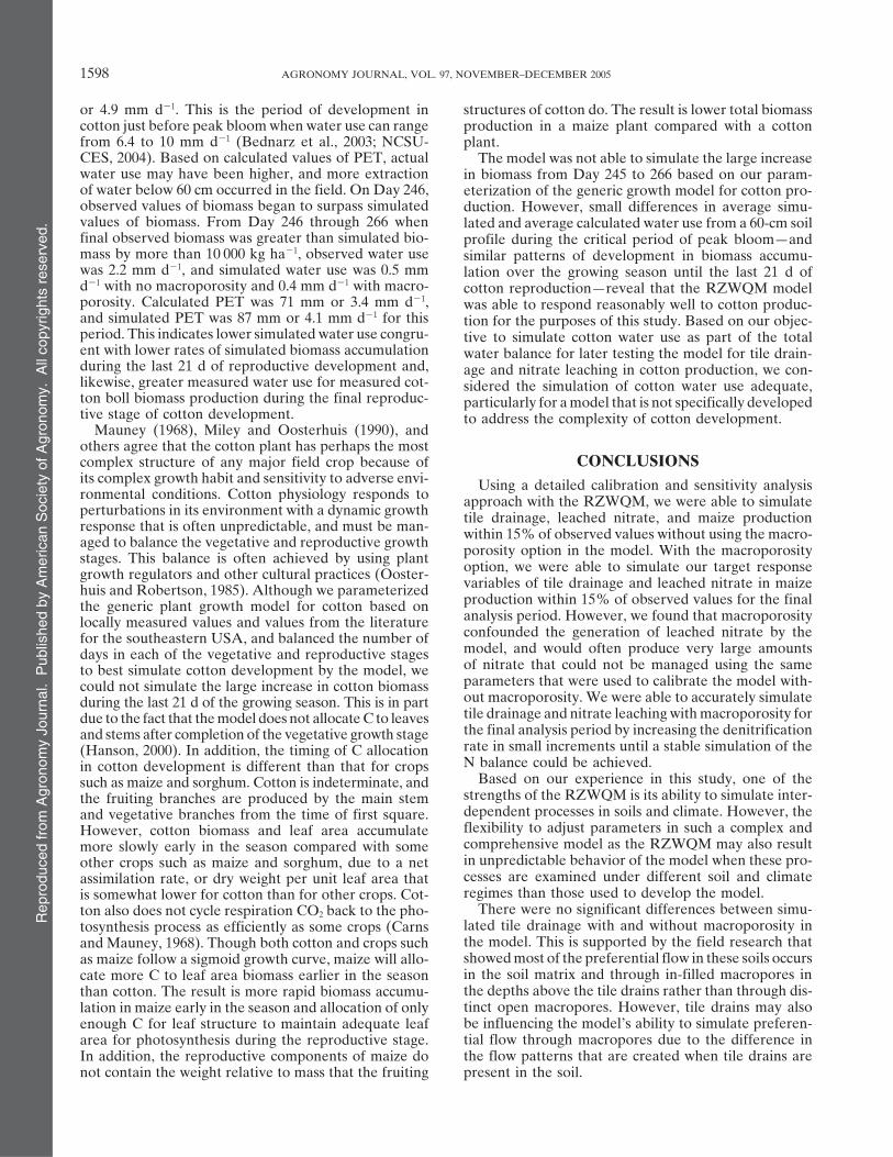
Rep

rodu

ced

from

Agr

onom

y Jo

urna

l. P

ublis

hed

by A

mer

ican

Soc

iety

of A

gron

omy.

All

copy

right

s re

serv

ed.


or 4.9 mm d�1. This is the period of development in structures of cotton do. The result is lower total biomasscotton just before peak bloom when water use can range production in a maize plant compared with a cottonfrom 6.4 to 10 mm d�1 (Bednarz et al., 2003; NCSU- plant.CES, 2004). Based on calculated values of PET, actual The model was not able to simulate the large increasewater use may have been higher, and more extraction in biomass from Day 245 to 266 based on our param-of water below 60 cm occurred in the field. On Day 246, eterization of the generic growth model for cotton pro-observed values of biomass began to surpass simulated duction. However, small differences in average simu-values of biomass. From Day 246 through 266 when lated and average calculated water use from a 60-cm soilfinal observed biomass was greater than simulated bio- profile during the critical period of peak bloom—andmass by more than 10 000 kg ha�1, observed water use similar patterns of development in biomass accumu-was 2.2 mm d�1, and simulated water use was 0.5 mm lation over the growing season until the last 21 d ofd�1 with no macroporosity and 0.4 mm d�1 with macro- cotton reproduction—reveal that the RZWQM modelporosity. Calculated PET was 71 mm or 3.4 mm d�1, was able to respond reasonably well to cotton produc-and simulated PET was 87 mm or 4.1 mm d�1 for this tion for the purposes of this study. Based on our objec-period. This indicates lower simulated water use congru- tive to simulate cotton water use as part of the totalent with lower rates of simulated biomass accumulation water balance for later testing the model for tile drain-during the last 21 d of reproductive development and, age and nitrate leaching in cotton production, we con-likewise, greater measured water use for measured cot- sidered the simulation of cotton water use adequate,ton boll biomass production during the final reproduc- particularly for a model that is not specifically developedtive stage of cotton development. to address the complexity of cotton development.

Mauney (1968), Miley and Oosterhuis (1990), andothers agree that the cotton plant has perhaps the most

CONCLUSIONScomplex structure of any major field crop because ofits complex growth habit and sensitivity to adverse envi- Using a detailed calibration and sensitivity analysisronmental conditions. Cotton physiology responds to approach with the RZWQM, we were able to simulateperturbations in its environment with a dynamic growth tile drainage, leached nitrate, and maize productionresponse that is often unpredictable, and must be man- within 15% of observed values without using the macro-aged to balance the vegetative and reproductive growth porosity option in the model. With the macroporositystages. This balance is often achieved by using plant option, we were able to simulate our target responsegrowth regulators and other cultural practices (Ooster-

variables of tile drainage and leached nitrate in maizehuis and Robertson, 1985). Although we parameterizedproduction within 15% of observed values for the finalthe generic plant growth model for cotton based onanalysis period. However, we found that macroporositylocally measured values and values from the literatureconfounded the generation of leached nitrate by thefor the southeastern USA, and balanced the number ofmodel, and would often produce very large amountsdays in each of the vegetative and reproductive stagesof nitrate that could not be managed using the sameto best simulate cotton development by the model, weparameters that were used to calibrate the model with-could not simulate the large increase in cotton biomassout macroporosity. We were able to accurately simulateduring the last 21 d of the growing season. This is in parttile drainage and nitrate leaching with macroporosity fordue to the fact that the model does not allocate C to leavesthe final analysis period by increasing the denitrificationand stems after completion of the vegetative growth stagerate in small increments until a stable simulation of the(Hanson, 2000). In addition, the timing of C allocationN balance could be achieved.in cotton development is different than that for crops

Based on our experience in this study, one of thesuch as maize and sorghum. Cotton is indeterminate, andstrengths of the RZWQM is its ability to simulate inter-the fruiting branches are produced by the main stemdependent processes in soils and climate. However, theand vegetative branches from the time of first square.flexibility to adjust parameters in such a complex andHowever, cotton biomass and leaf area accumulatecomprehensive model as the RZWQM may also resultmore slowly early in the season compared with somein unpredictable behavior of the model when these pro-other crops such as maize and sorghum, due to a netcesses are examined under different soil and climateassimilation rate, or dry weight per unit leaf area thatregimes than those used to develop the model.is somewhat lower for cotton than for other crops. Cot-

There were no significant differences between simu-ton also does not cycle respiration CO2 back to the pho-lated tile drainage with and without macroporosity intosynthesis process as efficiently as some crops (Carnsthe model. This is supported by the field research thatand Mauney, 1968). Though both cotton and crops suchshowed most of the preferential flow in these soils occursas maize follow a sigmoid growth curve, maize will allo-in the soil matrix and through in-filled macropores incate more C to leaf area biomass earlier in the seasonthe depths above the tile drains rather than through dis-than cotton. The result is more rapid biomass accumu-tinct open macropores. However, tile drains may alsolation in maize early in the season and allocation of onlybe influencing the model’s ability to simulate preferen-enough C for leaf structure to maintain adequate leaftial flow through macropores due to the difference inarea for photosynthesis during the reproductive stage.the flow patterns that are created when tile drains areIn addition, the reproductive components of maize do

not contain the weight relative to mass that the fruiting present in the soil.

Rep

rodu

ced

from

Agr

onom

y Jo

urna

l. P

ublis

hed

by A

mer

ican

Soc

iety

of A

gron

omy.

All

copy

right

s re

serv

ed.


The model was able to simulate the pattern of biomass simulate biomass accumulation as well as daily wateruse for indeterminate crops such as cotton.accumulation and leaf area of cotton development rela-

tive to the observed pattern with and without macropo- By carefully outlining our calibration procedurealong with relevant details often absent in modelingrosity until the last 21 d of reproduction. This appears

to be due to the inability of the model to simulate vegeta- studies that test a model or that may only describe asensitivity analysis, we hope to have contributed to thetive growth after the crop enters the reproductive stage.

It may also be due to the method by which the model understanding of how a calibration may proceed, par-ticularly for such a complex and comprehensive modelpartitions C during the various stages of crop develop-

ment that cannot be adjusted except by way of the mini- as the RZWQM. Guidelines or standard protocols usedfor calibrating a model may also be addressed with moremum number of days required to complete each growth

stage. We were able to simulate average daily cotton interest because of our efforts in this study. We willtest the model under conventional as well as no tillagewater use to within less than 1 mm of average observed

daily water use during the period of peak critical bloom management practices in cotton production in a follow-up study to this paper that we hope will lend furtherwith and without the macroporosity option. An option

to adjust C allocation to the different plant components insight into our ability to simulate tile drainage andnitrate leaching for cotton and other crops in Piedmontas well as allow vegetative growth to continue into the

reproductive stage may improve the model’s ability to soils and climate.

APPENDIX

Table A1. Soil hydraulic properties used in model. Soil water content from Bruce et al. (1983), with Brooks-Corey ha (air-entry pressure)and � (pore size distribution index) derived from soil water characteristic fit with van Genuchten parameters and converted to Brooks-Corey parameters.

Soil water content, cm3 cm�3 at pressure in kPa Brooks-Corey parametersSoillayer no. Depth Saturation 10 30 100 1500 Ks ha � fraction

cm cm h�1 kPa1 5 0.49 0.21 0.16 0.11 0.05 18 1.61 0.492 15 0.41 0.16 0.13 0.10 0.05 20 0.68 0.413 25 0.38 0.25 0.22 0.20 0.14 8 0.45 0.184 35 0.47 0.35 0.32 0.30 0.24 18 0.45 0.445 65 0.48 0.40 0.37 0.35 0.27 10 0.77 0.266 95 0.43 0.40 0.38 0.36 0.27 2.6 9.62 0.407 125 0.43 0.41 0.39 0.36 0.27 0.2 9.90 0.54

Table A2. Initial soil temperatures and field capacity volumetricwater content on 1 Jan. 1991 used for model calibration.

Soil layer no. Depth Soil temp. Water content

cm �C cm3 cm�3

1 5 6 0.222 15 6 0.163 25 6 0.254 35 10 0.265 65 10 0.296 95 10 0.387 125 10 0.41

Table A3. Soil nutrient parameters with units per kilogram of soil as used in model. Data compiled from Franzluebbers (personalcommunication, 2001) and Johnson et al. (1999).

HumusSoil Total Fast Aerobic Anaerobiclayer no. Depth organic C residue Fast Transition Stable heterotrophs Autotrophs heterotrophs NO3–N NH4–N

cm mg kg�1 mg C kg�1 no. organisms kg�1 106† mg N kg�1

1 5 6960 1044 1044 2088 2784 1083 285 285 2.85 1.582 15 5800 725 725 2030 2320 632.7 161.5 161.5 2.85 1.583 25 4060 406 406 1624 1624 383.8 76 76 2.85 1.584 35 3480 261 261 1218 1740 273.6 57 57 2.50 1.115 65 2900 145 145 870 1740 228 47.5 47.5 2.50 1.006 95 2320 116 116 696 1392 182.4 38 38 3.22 1.387 125 2320 116 116 696 1392 146.3 28.5 28.5 3.22 1.38

† Multiply value in table by 106 for actual value.

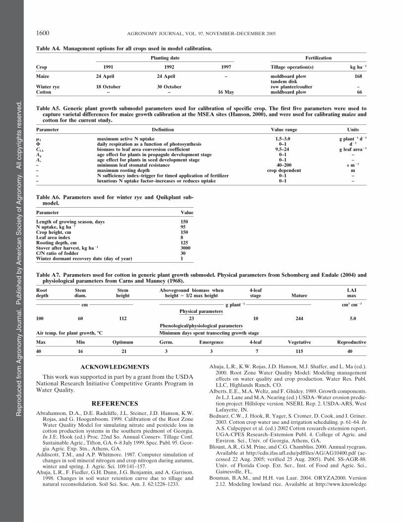
Rep

rodu

ced

from

Agr

onom

y Jo

urna

l. P

ublis

hed

by A

mer

ican

Soc

iety

of A

gron

omy.

All

copy

right

s re

serv

ed.


Table A4. Management options for all crops used in model calibration.

Planting date Fertilization

Crop 1991 1992 1997 Tillage operation(s) kg ha�1

Maize 24 April 24 April – moldboard plow 168tandem disk

Winter rye 18 October 30 October row planter/coulter –Cotton – – 16 May moldboard plow 66

Table A5. Generic plant growth submodel parameters used for calibration of specific crop. The first five parameters were used tocapture varietal differences for maize growth calibration at the MSEA sites (Hanson, 2000), and were used for calibrating maize andcotton for the current study.

Parameter Definition Value range Units

�1 maximum active N uptake 1.5–3.0 g plant�1 d�1

� daily respiration as a function of photosynthesis 0–1 d�1

CLA biomass to leaf area conversion coefficient 9.5–24 g leaf area�1

Ap age effect for plants in propagule development stage 0–1 –As age effect for plants in seed development stage 0–1 –– minimum leaf stomatal resistance 40–200 s m�1

– maximum rooting depth crop dependent m– N sufficiency index–trigger for timed application of fertilizer 0–1 –– luxurious N uptake factor–increases or reduces uptake 0–1 –

Table A6. Parameters used for winter rye and Quikplant sub-model.

Parameter Value

Length of growing season, days 150N uptake, kg ha�1 95Crop height, cm 150Leaf area index 8Rooting depth, cm 125Stover after harvest, kg ha�1 3000C/N ratio of fodder 30Winter dormant recovery date (day of year) 1

Table A7. Parameters used for cotton in generic plant growth submodel. Physical parameters from Schomberg and Endale (2004) andphysiological parameters from Carns and Mauney (1968).

Root Stem Stem Aboveground biomass when 4-leaf LAIdepth diam. height height 1/2 max height stage Mature max

cm g plant�1 cm3 cm�3

Physical parameters100 60 112 23 10 244 5.0

Phenological/physiological parametersAir temp. for plant growth, �C Minimum days spent transecting growth stage

Max Min Optimum Germ. Emergence 4-leaf Vegetative Reproductive

40 16 21 3 3 7 115 40

Ahuja, L.R., K.W. Rojas, J.D. Hanson, M.J. Shaffer, and L. Ma (ed.).ACKNOWLEDGMENTS2000. Root Zone Water Quality Model: Modeling management

This work was supported in part by a grant from the USDA effects on water quality and crop production. Water Res. Publ.National Research Initiative Competitive Grants Program in LLC, Highlands Ranch, CO.Water Quality. Alberts, E.E., M.A. Weltz, and F. Ghidey. 1989. Growth components.

In L.J. Lane and M.A. Nearing (ed.) USDA–Water erosion predic-tion project: Hillslope version. NSERL Rep. 2. USDA-ARS, WestREFERENCESLafayette, IN.

Abrahamson, D.A., D.E. Radcliffe, J.L. Steiner, J.D. Hanson, K.W. Bednarz, C.W., J. Hook, R. Yager, S. Cromer, D. Cook, and I. Griner.Rojas, and G. Hoogenboom. 1999. Calibration of the Root Zone 2003. Cotton crop water use and irrigation scheduling. p. 61–64. InWater Quality Model for simulating nitrate and pesticide loss in

A.S. Culpepper et al. (ed.) 2002 Cotton research-extension report.cotton production systems in the southern piedmont of Georgia.UGA-CPES Research–Extension Publ. 4. College of Agric. andIn J.E. Hook (ed.) Proc. 22nd So. Annual Conserv. Tillage Conf.Environ. Sci., Univ. of Georgia, Athens, GA.Sustainable Agric., Tifton, GA. 6–8 July 1999. Spec. Publ. 95. Geor-

Blount, A.R., G.M. Prine, and C.G. Chambliss. 2000. Annual ryegrass.gia Agric. Exp. Stn., Athens, GA.Available at http://edis.ifas.ufl.edu/pdffiles/AG/AG10400.pdf (ac-Addiscott, T.M., and A.P. Whitmore. 1987. Computer simulation ofcessed 22 Aug. 2005; verified 25 Aug. 2005). Publ. SS-AGR-88.changes in soil mineral nitrogen and crop nitrogen during autumn,Univ. of Florida Coop. Ext. Ser., Inst. of Food and Agric. Sci.,winter and spring. J. Agric. Sci. 109:141–157.Gainesville, FL.Ahuja, L.R., F. Fiedler, G.H. Dunn, J.G. Benjamin, and A. Garrison.

Bouman, B.A.M., and H.H. van Laar. 2004. ORYZA2000. Version1998. Changes in soil water retention curve due to tillage andnatural reconsolidation. Soil Sci. Soc. Am. J. 62:1228–1233. 2.12. Modeling lowland rice. Available at http://www.knowledge

Rep

rodu

ced

from

Agr

onom

y Jo

urna

l. P

ublis

hed

by A

mer

ican

Soc

iety

of A

gron

omy.

All

copy

right

s re

serv

ed.


bank.irri.org/oryza2000/ (accessed 9 Dec. 2004; verified 25 Aug. Hanson, J.D., K.W. Rojas, and M.J. Shaffer. 1999. Calibrating theRoot Zone Water Quality Model. Agron. J. 91:171–177.2005). IRRI, Manila, Philippines.

Bouwer, H. 1969. Infiltration of water into a nonuniform soil. J. Irrig. Hendrickson, B.H., A.P. Barnett, J.R. Carreker, and W.E. Adams.1963. Runoff and erosion control studies on Cecil soil in the south-Drain. Div., Am. Soc. Civ. Eng. 95:451–462.

Brooks, R.H., and A.T. Corey. 1964. Hydraulic properties of porous ern piedmont. USDA-ARS Tech. Bull. 1281. U.S. Gov. Print. Of-fice, Washington, DC.media. Hydrology Pap. 3. Colorado State Univ., Fort Collins, CO.

Bruce, R.R., J.H. Dane, V.L. Quisenberry, N.L. Powell, and A.W. Hoogenboom, G. 2003. Georgia Automated Environmental Moni-toring Network. Available at www.georgiaweather.net (accessedThomas. 1983. Physical characteristics of soils in the southern re-

gion: Cecil. S. Coop. Ser. Bull. 267. Georgia Agric. Exp. Stn. and 2 Dec. 2004; verified 18 Aug. 2005). Univ. of Georgia, Griffin, GA.Hutson, J.L., and R.J. Wagenet. 1992. LEACHM: Leaching estimationUniv. of Georgia, Athens, GA.

Buckingham, E. 1907. Studies on the movement of soil moisture. and chemistry model: A process-based model of water and solutemovement, transformations, plant uptake and chemical reactionsUSDA Bur. Soils Bull. 38. U.S. Gov. Print. Office, Washington, DC.

Carns, H.R., and J.R. Mauney. 1968. Physiology of the cotton plant. in the unsaturated zone. Res. Ser. 92-3. Cornell Univ., Ithaca, NY.Johnson, A.D., M.L. Cabrera, D.V. Mccracken, and D.E. Radcliffe.p. 43–73. In F.C. Elliot et al. (ed.) Advances in production and

utilization of quality cotton: Principles and practices. Iowa State 1999. LEACHN simulations of nitrogen dynamics and water drain-age in an Ultisol. Agron. J. 91:597–606.Univ. Press, Ames, IA.

Chiang, S.C., D.E. Radcliffe, and W.P. Miller. 1993. Hydraulic proper- Juma, N.G., and W.B. McGill. 1986. Decomposition and nutrientcycling in agroecosystems. p. 74–136. In M.J. Mitchell and J.P.ties of surface seals in Georgia soils. Soil Sci. Soc. Am. J. 57:

1418–1426. Nakas (ed.) Microfloral and faunal interactions in natural and agro-ecosystems. Dordrecht, Boston, MA.Childs, E.C., and M. Bybordi. 1969. The vertical movement of water

in a stratified porous material: I. Water Resour. Res. 5:446–459. Keeney, D.R., and D.W. Nelson. 1982. Nitrogen—inorganic forms.p. 643–689. In A.L. Page et al. (ed.) Methods of soil analysis. Part 2.Clarke, K.C., S. Hoppen, and L.J. Gaydos. 1994. Methods and tech-

niques for rigorous calibration of a cellular automation model of 2nd ed. Agron. Monogr. 9. ASA and SSSA, Madison, WI.Loague, K., and R.E. Green. 1991. Statistical and graphical methodsurban growth. Available at www.ncgia.ucsb.edu/conf/SANTA_FE_

CD-ROM/sf_papers/clarke_keith/clarkeetal.html (accessed 2 Aug. for evaluating solute transport models: Overview and applications.J. Contam. Hydrol. 7:51–73.2005; verified 18 Aug. 2005). National Center for Geographic Infor-

mation and Analysis, Santa Barbara, CA. Ma, L., L.R. Ahuja, M.J. Shaffer, K.W. Rojas, R.W. Malone, and M.R.Cameira. 2001. Integrating system modeling with field research inCornelis, W.M., D. Gabriels, and R. Hartmann. 2004. A conceptual

model to predict the deflation threshold shear velocity as affected agriculture: Applications of the Root Zone Water Quality Model(RZWQM). Adv. Agron. 71:233–292.by near-surface soil water: II. Calibration and verification. Soil Sci.

Soc. Am. J. 68:1162–1168. Ma, L., J.C. Ascough, II, L.R. Ahuja, M.J. Shaffer, J.D. Hanson, andK.W. Rojas. 2000. Root Zone Water Quality Model sensitivityCorwin, D.L., J. Letey, Jr., and M.L.K. Carrillo. 1999. Modeling non-

point source pollutants in the vadose zone: Back to the basics. analysis using Monte Carlo simulation. Trans. ASAE 43:883–895.Mauney, J.R. 1968. Morphology of the cotton plant. In F.C. Elliotp. 323–342. In D.L. Corwin et al. (ed.) Assessment of non-point

source pollution in the vadose zone. Am. Geophys. Union, Wash- et al. (ed.) Advances in production and utilization of quality cotton:Principles and practices. Iowa State Univ. Press, Ames, IA.ington, DC.

Dubus, I.G., S. Beulke, and C.D. Brown. 2002. Calibration of pesticide McCracken, D.V., J.E. Box, Jr., W.L. Hargrove, M.L. Cabrera, J.W.Johnson, P.L. Raymer, A.D. Johnson, and G.W. Harbers. 1995.leaching models: Critical review and guidance for reporting. Pest

Manage. Sci. 58:745–758. Tillage and cover crop effects on nitrate leaching in the southernpiedmont. In C. Heatwole (ed.) Proc. Clean Water, Clean Environ-FAO. 2004. Water resources and irrigation in Africa. Available at

www.fao.org/ag/agl/aglw/aquastat/watresafrica/index6.stm (accessed ment, 21st Century: Team Agriculture, Working to Protect WaterResources, Kansas City, MO. 5–8 Mar. 1995. ASAE, St. Joseph, MI.9 Dec. 2004; verified 18 Aug. 2005). FAO, Rome, Italy.

Farahani, H.J., and L.R. Ahuja. 1996. Evapotranspiration modeling of Miley, W.N., and D.M. Oosterhuis (ed.). 1990. Proc. 1st Annual Work-shop for Practicing Agronomists: Nitrogen Nutrition of Cotton:partial canopy/residue covered fields. Trans. ASAE 39:2051–2064.

Farahani, H.J., and D.G. DeCoursey. 2000. Potential evaporation and Practical Issues, North Little Rock, AR. 7 Feb. 1990. ASA, Madi-son, WI.transpiration processes in the soil–residue–canopy system. p. 51–80.

In L.R. Ahuja et al (ed.) Root Zone Water Quality Model: Model- Mitchell, C.C., C.H. Burmester, and K.L. Edmisten. 1991. Cotton fer-tilization management in Alabama. ANR-0619. Available at www.ling management effects on water quality and crop production.

Water Res. Publ. LLC, Highlands Ranch, CO. aces.edu/pubs/docs/A/ANR-0619/ (accessed 10 Dec. 2004; verified18 Aug. 2005). Alabama Coop. Ext. System.Frissel, M.J., and J.A. van Veen. 1981. Simulation model for nitro-

gen immobilization and mineralization. p. 359–381. In I.K. Iskan- Mulla, D.J., and T.M. Addiscott. 1999. Validation approaches forfield-, basin-, and regional-scale water quality models. p. 63–78. Indar (ed.) Modeling wastewater renovation. Land treatment. John

Wiley & Sons, New York. D.L. Corwin et al. (ed.) Assessment of non-point source pollutionin the vadose zone. Am. Geophysical Union, Washington, DC.Gascho, G.J., and M.B. Parker. 2001. Long-term liming effects on

coastal plains soils and crops. Agron. J. 93:1305–1315. NCSU-CES. 2004. North Carolina State Univ. Coop. Ext. Service.Available at www.ces.ncsu.edu/ (accessed 2 Dec. 2004; verified 18Gijsman, A.J., G. Hoogenboom, W.J. Parton, and P.C. Kerridge. 2002.

Modifying DSSAT crop models for low-input agricultural systems Aug. 2005). North Carolina State Univ., Raleigh, NC.Nimah, M., and R.J. Hanks. 1973. Model for estimating soil–water–using a soil organic matter–residue module from CENTURY.

Agron. J. 94:462–474. plant–atmospheric interrelation: I. Description and sensitivity. SoilSci. Soc. Am. Proc. 37:522–527.Green, W.H., and G.A. Ampt. 1911. Studies on soil physics: I. Flow

of air and water through soils. J. Agric. Sci. 4:1–24. Nyakatawa, E.Z., and K.C. Reddy. 2000. Tillage, cover cropping, andpoultry litter effects on cotton: I. germination and seedling growth.Groffman, P.M. 1984. Nitrification and denitrification in conventional

and no-tillage soils. Soil Sci. Soc. Am. J. 49:329–334. Agron. J. 92:992–999.Nyakatawa, E.Z., K.C. Reddy, and D.A. Mays. 2000. Tillage, coverGupte, S.M., D.E. Radcliffe, D.H. Franklin, L.T. West, E.W. Tollner,

and P.F. Hendrix. 1996. Anion transport in a piedmont ultisol: II. cropping, and poultry litter effects on cotton: II. growth and yieldparameters. Agron. J. 92:1000–1007.Local-scale parameters. Soil Sci. Soc. Am. J. 60:762–770.

Hachum, A.Y., and J.F. Alfaro. 1980. Rain infiltration into layered Oosterhuis, D.M., and W.C. Robertson. 1985. The use of plant growthregulators and other additives in cotton production. Spec. Rep. Univ.soils: Simulation. J. Irrig. Drain. Div., Am. Soc. Civ. Eng. 106:

311–321. of Arkansas Agric. Ext. Service. Available at www.uark.edu/depts/agripub/Publications/specialreports/198ms5.pdf (accessed 2 Dec.Hanson, J.D. 2000. Generic crop production. p. 81–118. In L.R. Ahuja

et al (ed.) Root Zone Water Quality Model: Modelling manage- 2004; verified 18 Aug. 2005). Univ. of Arkansas Agric. Ext. Service.Pachepsky, Y.A., and W.J. Rawls. 2005. Status of pedotransfer func-ment effects on water quality and crop production. Water Res.

Publ. LLC, Highlands Ranch, CO. tions. p. 7–16. In Y.A. Pachepsky and W.J. Rawls (ed.) Develop-

Rep

rodu

ced

from

Agr

onom

y Jo

urna

l. P

ublis

hed

by A

mer

ican

Soc

iety

of A

gron

omy.

All

copy

right

s re

serv

ed.


ment of pedotransfer functions in soil hydrology. Developments et al. (ed.) Root Zone Water Quality Model: Modelling manage-ment effects on water quality and crop production. Water Res.in soil science 30. Elsevier Press, New York.

Parton, W.J., D.W. Anderson, C.V. Cole, and J.W.B. Stewart. 1983. Publ. LLC, Highlands Ranch, CO.Silberbush, M., and S.A. Barber. 1983. Sensitivity analysis of param-Simulation of soil organic matter formations and mineralization in

semiarid ecosystems. p. 359–381. In Lowrance et al. (ed.) Nutrient eters used in simulating K uptake with a mechanistic mathematicalmodel. Agron. J. 75:851–854.cycling in agricultural ecosystems. Spec. Publ. 23. Univ. of Georgia,

Athens, GA. Skaggs, R.W. 1978. A water management model for shallow watertable soils. Tech. Rep. 134. Water Resour. Res. Inst., North Caro-Priestley, C.H.B., and R.J. Taylor. 1972. On the assessment of sur-

face heat flux and evaporation using large-scale parameters. Mon. lina State Univ., Raleigh, NC.Skaggs, R.W. 1980. DRAINMOD reference report. Methods for de-Weather Rev. 100:81–82.

Radcliffe, D.E., P.M. Tillotson, P.F. Hendrix, L.T. West, J.E. Box, sign and evaluation of drainage-water management systems forsoils with high water tables. USDA-SCS, SNTC, Ft. Worth, TX.and E.W. Tollner. 1996. Anion transport in a piedmont ultisol: I.

Field-scale parameters. Soil Sci. Soc. Am. J. 60:755–761. Sumner, M.E. 1994. Amelioration of subsoil acidity with minimumdisturbance. p. 147–185. In N.S. Jayawardane and B.A. StewardRawls, W.J., D.L. Brakensiek, and K.E. Saxton. 1982. Estimation of

soil water properties. Trans. ASAE 25:1316–1320, 1328. (ed.) Advances in soil science. Lewis Publ., Boca Raton, FL.University of Georgia College of Agricultural and EnvironmentalReddy, K.R., S. Koti, G.H. Davidonis, and V.R. Reddy. 2004. Inter-

active effects of carbon dioxide and nitrogen nutrition on cot- Sciences. 1998. Statewide variety testing program. Available at www.griffin.uga.edu/swvt/ (accessed 11 Nov. 2004; verified 18 Aug. 2005).ton growth, development, yield, and fiber quality. Agron. J. 96:

1148–1157. Univ. of Georgia, Griffin, GA.University of Georgia College of Agricultural and EnvironmentalRitzema, H.P. 1994. Subsurface flow to drains. In H.P. Ritzema (ed.)

Drainage principles and applications. 2nd ed. Publ. 16. Int. Inst. for Sciences. 2000. Cotton production guide. Available at www.griffin.uga.edu/caes/cotton/ (accessed 2 Dec. 2004; verified 18 Aug. 2005).Land Reclam. and Improve (ILRI), Wageningen, the Netherlands.

SAS Institute. 2000. The SAS system for Windows. Release 7.0. SAS Univ. of Georgia, Griffin, GA.USDA-ARS and USDA–Forest Service. 2003. CLIGEN weather gen-Inst., Cary, NC.

Saseendran, S.A., D.C. Nielsen, L. Ma, L.R. Ahuja, and A.D. Halvor- erator, expanded and improved by USDA Agricultural ResearchService and U.S. Forest Service. Available at http://horizon.nserl.son. 2003. Modeling nitrogen management effects on winter wheat

production using RZWQM and CERES-WHEAT. Agron. J. 96: purdue.edu/Cligen/ (accessed 5 May 2005; verified 18 Aug. 2005).USDA-ARS, NSERL, West Lafayette, IN.615–630.

Schomberg, H.H., and D.M. Endale. 2004. Cover crop effects on van Genuchten, M.Th. 1980. A closed form equation for predicting thehydraulic conductivity of unsaturated soils. Soil Sci. Soc. Am. J.nitrogen mineralization and availability in conservation tillage sys-

tems. Biol. Fertil. Soils 40:398–405. 44:892–898.Vereecken, H., J. Diels, J. Van Orshoven, J. Feyen, and J. Bouman. 1992.Shaffer, M.J., and W.E. Larson. 1987. NTRM, a soil–crop simulation

model for nitrogen, tillage, and crop-residue management. Con- Functional evaluation of pedotransfer functions for the estimation ofsoil hydraulic properties. Soil Sci. Soc. Am. J. 56:1371–1378.serv. Res. Rep. 34-1. USDA-ARS Tech. Inf. Service. U.S. Gov.

Print. Office, Washington, DC. Zhang, X.J. 2004. Calibration, refinement, and application of theWEPP model for simulating climatic impact on wheat production.Shaffer, M.J., K.W. Rojas, D.G. Decoursey, and C.S. Hebson. 2000.

Nutrient chemistry processes: OMNI. p. 119–144. In L.R. Ahuja Trans. ASAE 47:1075–1085.

Calibration of the Root Zone Water Quality Model for Simulating Tile Drainage and Leached Nitrate in...

Documents

Transcript of Calibration of the Root Zone Water Quality Model for Simulating Tile Drainage and Leached Nitrate in...