Calcium imaging of adult-born neurons in freely moving mice

llOPEN ACCESS

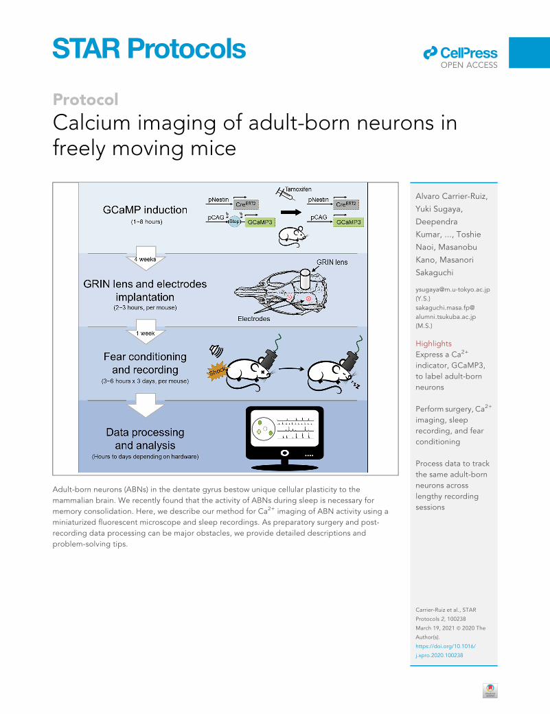
Protocol

Calcium imaging of adult-born neurons infreely moving mice

Alvaro Carrier-Ruiz,

Yuki Sugaya,

Deependra

Kumar, ..., Toshie

Naoi, Masanobu

Kano, Masanori

Sakaguchi

[email protected]

(Y.S.)

sakaguchi.masa.fp@

alumni.tsukuba.ac.jp

(M.S.)

Highlights

Express a Ca2+

indicator, GCaMP3,

to label adult-born

neurons

Perform surgery, Ca2+

imaging, sleep

recording, and fear

conditioning

Process data to track

the same adult-born

neurons across

lengthy recording

sessions

Adult-born neurons (ABNs) in the dentate gyrus bestow unique cellular plasticity to the

mammalian brain. We recently found that the activity of ABNs during sleep is necessary for

memory consolidation. Here, we describe our method for Ca2+ imaging of ABN activity using a

miniaturized fluorescent microscope and sleep recordings. As preparatory surgery and post-

recording data processing can be major obstacles, we provide detailed descriptions and

problem-solving tips.

Carrier-Ruiz et al., STAR

Protocols 2, 100238

March 19, 2021 ª 2020 The

Author(s).

https://doi.org/10.1016/

j.xpro.2020.100238

mailto:[email protected]



https://doi.org/10.1016/j.xpro.2020.100238


http://crossmark.crossref.org/dialog/?doi=10.1016/j.xpro.2020.100238&domain=pdf

Protocol

Calcium imaging of adult-born neurons in freely movingmice

Alvaro Carrier-Ruiz,1,2,4 Yuki Sugaya,1,2,5,* Deependra Kumar,3 Pablo Vergara,3 Iyo Koyanagi,3

Sakthivel Srinivasan,3 Toshie Naoi,3 Masanobu Kano,1,2 and Masanori Sakaguchi3,6,*

1Department of Neurophysiology, Graduate School of Medicine, The University of Tokyo, Tokyo 113-0033, Japan

2International Research Center for Neurointelligence (WPI-IRCN), The University of Tokyo Institutes for Advanced Study(UTIAS), Tokyo 113-0033, Japan

3International Institute for Integrative Sleep Medicine (WPI-IIIS), University of Tsukuba, Tsukuba, Ibaraki 305-0006, Japan

4Department of Neuroscience, Karolinska Institute, Stockholm 17165, Sweden

5Technical contact

6Lead contact

*Correspondence: [email protected] (Y.S.), [email protected] (M.S.)https://doi.org/10.1016/j.xpro.2020.100238

Summary

Adult-born neurons (ABNs) in the dentate gyrus bestow unique cellular plasticityto themammalian brain. We recently found that the activity of ABNs during sleepis necessary for memory consolidation. Here, we describe our method for Ca2+

imaging of ABN activity using a miniaturized fluorescent microscope and sleeprecordings. As preparatory surgery and post-recording data processing can bemajor obstacles, we provide detailed descriptions and problem-solving tips.For complete details on the use and execution of this protocol, please refer toKumar et al. (2020).

Before you begin

All experiments were performed in accordance with the Science Council of Japan’s Guidelines for

Proper Conduct of Animal Experiments. Experimental protocols were approved by the Institutional

Animal Care and Use Committee at the University of Tsukuba. C57BL/6 mice (Jackson Laboratory)

were bred in our colony at the University of Tsukuba andmaintained on a 12-h light/dark cycle (lights

on 9 am to 9 pm) with ad libitum access to food and water. All mice were group-housed with 2–5

mice/cage, and only male mice were used in the experiments. To induce transgene expression in

ABNs, mice were treated with tamoxifen at 7 weeks of age. At �9–12 weeks of age, mice were anes-

thetized with isoflurane and fixed in a stereotaxic frame for the surgery demonstrated in the videos.

Generate transgenic mice

Timing: 3–4 months

1. Obtain at least two transgenic mouse lines: one that expresses tamoxifen-inducible Cre recom-

binase in neural stem/progenitor cells, and one that expresses a fluorescent calcium (Ca2+) indi-

cator protein after exposure to Cre recombinase.

Alternatives: We successfully used Nestin-CreERT2 transgenic mice from The Jackson Lab-

oratory (stock #016261), in which Cre recombinase is expressed in Nestin-positive cells in

the adult brain by tamoxifen induction. Alternatively, Ascl1-CreERT2 mice (The Jackson

STAR Protocols 2, 100238, March 19, 2021 ª 2020 The Author(s).This is an open access article under the CC BY license (http://creativecommons.org/licenses/by/4.0/).

1

llOPEN ACCESS




http://crossmark.crossref.org/dialog/?doi=10.1016/j.xpro.2020.100238&domain=pdf

http://creativecommons.org/licenses/by/4.0/

Laboratory, stock #012882) could be used to specifically target transient amplifying progen-

itors (Kim et al., 2007, Yang et al., 2015), although we do not have experience using this line.

Note:We recommend using the GCaMP3mouse line Ai38 (RCL-GCaMP3) to express the fluo-

rescent Ca2+ indicator in adult-born neurons (ABNs). Although next-generation indicators,

such as GCaMP6f and GCaMP6s, are usually preferable, their mouse lines (Madisen et al.,

2015) show very low or absent expression of Cre-inducible transgene when expressed in

ABNs after crossing with Nestin-CreERT2 mice. For example, crossing Nestin-CreERT2

mice with Ai96 (RCL-GCaMP6s) or Ai94 (TRE-LSL-GCaMP6s)/RCL-tTA mice (The Jackson Lab-

oratory, stock #008600) does not induce expression of GCaMP6 (unpublished results). We

speculate that expression of recently developed GCaMP sensors in early neural progenitors

interferes with Ca2+ signaling mechanisms essential for immature ABN survival.

Note: Instead of using mouse transgenic lines, induction of Ca2+ indicators and/or Cre re-

combinase could be achieved by viral transduction. However, most adeno-associated vi-

ruses (AAVs) are not suitable for infecting neural stem/progenitor cells due to their low

infection rate (Kotterman et al., 2015) and potential cytotoxicity (Johnston et al., 2020).

Although AAV-mediated expression of GCaMP6 was reported in combination with two

AAVs (Danielson et al., 2016), this previous study did not confirm expression of GCaMP6

in progenitor cells.

2. Cross transgenic lines, in accordance with their corresponding guidelines, to generate mice in

which expression of GCaMP3 is initiated by tamoxifen-inducible Cre recombinase (i.e., CreERT2)

in adult neural stem/progenitor cells (i.e., nestin:GCaMP3 mice).

Key resources table

REAGENT or RESOURCE SOURCE IDENTIFIER

Chemicals, peptides, and recombinant proteins

Tamoxifen Merck T5648-1G

Isoflurane inhalation solution Pfizer n/a

Ibuprofen Wako, Japan 094-02643

Xylocaine injection 1% with epinephrine (lidocaine) Aspen Japan n/a

OCT mounting medium Sakura Finetek 4583

Vectashield Vector H-1000

4% paraformaldehyde phosphate buffer solution Nacalai Tesque 09154-85

Sucrose Nacalai Tesque 30404-45

Sunflower oil Sigma 1642347

Corn oil Sigma C8267

Flunixin meglumine Fujita FLUNIXIN INJ. 10%

Antibiotics (sulfadiazine/trimethoprim) Kyoritsu Seiyaku Tribrissen injection

Tarivid ophthalmic ointment 0.3% (Ofloxacin) Santen Pharmaceutical 1319722M1056

Experimental models: organisms/strains

Mice: C57BL/6-Tg(Nes-cre/ERT2)KEisc/J The Jackson Laboratory 016261

Mice: Ai38(RCL-GCaMP3) The Jackson Laboratory 029043

Software and algorithms

nVista HD Inscopix n/a

Inscopix image decompressor Inscopix n/a

EEG and EMG recording and analysis software KISSEI COMTEC Vital Recorder and Sleep Sign

Mosaic Inscopix n/a

MATLAB MathWorks 2016b

IgorPro 8 WaveMetrics n/a

(Continued on next page)

llOPEN ACCESS

2 STAR Protocols 2, 100238, March 19, 2021

Protocol

Step-by-step method details

Induction of Ca2+ sensor expression in ABNs

Timing: 1–8 h

Express GCaMP3 via tamoxifen-inducible Cre recombinase in adult neural stem/progenitor cells.

1. Prepare 20 mg/mL tamoxifen solution.

a. Heat corn oil to 42�C for 30 min.

b. Dissolve tamoxifen in corn oil at a concentration of 20 mg/mL in an ultrasonic bath (generic

consumer glassware is sufficient) or with continuous shaking at 37�C. Store the prepared so-

lution at 4�C.

Continued

REAGENT or RESOURCE SOURCE IDENTIFIER

Other

*GRIN lens probe, 1.0-mm diameter, ~4.0-mm length Inscopix 1050-004595

*Rectangular metal frame Narishige CF-10

*Baseplate Inscopix 1050-004638

*Miniscope Inscopix nVista(2.0)

*Baseplate cover Inscopix 1050-004639

*Miniscope gripper Inscopix 1050-002199

*Dummy miniscope Inscopix 1050-003762

**Electrodes for EEG recording Yamazaki f1.0 3 2.0

**Electrodes for EMG recording Cooner Wire AS633

**Flat cable for EEG/EMG signal transfer Hitachi Cable 20528-ST LF

**EEG/EMG signal amplifier Kyoto Biotex n/a

**Analog-to-digital convertor for EEG/EMG signal Contec AD16-16U(PCIEV)

**4-pin header for EEG/EMG socket Hirose A3B-4PA-2DSA(71)

Fear conditioning setup Med Associates n/a

Isoflurane vaporizer Shinano Seisakusyo SN-487-OT

Stereotaxic frame Narishige SR-6M

Drill Minitor Minimo

Vacuum pump Iwaki VPUMP-140

Surgical microscope Leica Leica GZ6

Dental cement liquid Shofu PROVINICE 204310644

Dental cement powder Shofu PROVINICE 096017656

Loctite cyanoacrylate adhesive Loctite Loctite 454

Super glue Konishi Alon Alfa A

Silicone Shofu DENTSILICONE-V

Head-fixing support Narfishige MAG-1

Perista perfusion pump ATTO AC2110

Cryostat Leica Microsystems Leica CM 1850

Confocal fluorescent microscope Olympus FV1200

Glass electrodes Harvard Apparatus GC150F-7.5

Ultrasonic bath SND US-101

Glass electrode puller Narishige PC-10

Deposited data

Data and code underlying the results describedin this manuscript

https://github.com/vergaloy/ABNs-Calcium-extraction

n/a

Raw data from the related article (Kumar et al., 2020) https://data.mendeley.com/datasets/gfbdv5kfrz/1

n/a

*Materials only for imaging surgery.

**Materials only for EEG/EMG surgery.

llOPEN ACCESS

STAR Protocols 2, 100238, March 19, 2021 3

Protocol

CRITICAL: As tamoxifen is sensitive to light, it must be made and stored away from light in

an amber or foil-wrapped tube.

Note: Tamoxifen may take 1–7 h to completely dissolve depending on the dissolution

method.

2. Inject tamoxifen into nestin:GCaMP3 mice.

a. Select an appropriate number of adult nestin:GCaMP3 mice.

Note: The definition of ‘‘adult’’ is usually determined by sexual maturity, which is commonly

accepted to be�6 weeks of age for mice. Older or younger mice can be used if needed. How-

ever, older mice have lower levels of adult neurogenesis, which decreases the success rate of

imaging, whereas younger mice might be too delicate to survive the necessary surgical

procedures.

b. Administer tamoxifen (120 mg/kg) into the intraperitoneal cavity five times at 1- or 2-day in-

tervals. Store the solution at 4�C until the next injection.

CRITICAL: Avoid using tamoxifen that has been stored for more than 1 week. The

efficiency of tamoxifen-induced recombination is severely impaired when using old or

light-exposed tamoxifen.

Note: The duration of the injection period is correlated with the degree of developmental varia-

tion of labeled ABNs. That is, the longer the injection period, the higher the chance of recording

ABNs with different properties resulting from differences in their maturational stages.

Maturation of labeled ABNs

Timing: dependent on experimental design

Allow ABNs to mature after tamoxifen injection.

3. Wait a pre-determined period of time to allow GCaMP3-labeled ABNs to mature.

Note: The length of the waiting period depends on the target age of ABNs at the time of Ca2+

imaging. Keep in mind that 1–2 weeks is needed to prepare for imaging. For example, if the

target age of ABNs is 6 weeks, wait 4 weeks after tamoxifen injection to move on to the next

step. If the target age of ABNs is 1 week or less, consider performing lens implantation before

tamoxifen injection. So far, we have successfully performed Ca2+ imaging of ABNs as early as

3 days after the last tamoxifen injection.

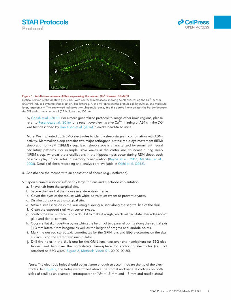
Note: GCaMP3 expression can be verified by examining brain sections from a tamoxifen-in-

jected mouse using a fluorescence microscope (Figure 1) before the next step.

GRIN lens and EEG/EMG electrode implantation

Timing: 2–3 h per mouse

Surgically implant a gradient-index (GRIN) lens and electroencephalogram (EEG)/electromyogram

(EMG) electrodes into the brains of tamoxifen-injected mice.

Note: We describe a specific protocol for imaging ABNs in the dentate gyrus (DG) in freely

moving mice. The original miniscope technology used in this protocol was first developed

llOPEN ACCESS


Protocol

by Ghosh et al., (2011). For a more generalized protocol to image other brain regions, please

refer to Resendez et al. (2016) for a recent overview. In vivo Ca2+ imaging of ABNs in the DG

was first described by Danielson et al. (2016) in awake head-fixed mice.

Note:We implanted EEG/EMG electrodes to identify sleep stages in combination with ABNs

activity. Mammalian sleep contains two major orthogonal states: rapid eye movement (REM)

sleep and non-REM (NREM) sleep. Each sleep stage is characterized by prominent neural

oscillatory patterns. For example, slow waves in the cortex are abundant during deep

NREM sleep, whereas theta oscillations in the hippocampus occur during REM sleep, both

of which play critical roles in memory consolidation (Boyce et al., 2016; Marshall et al.,

2006). Details of sleep recording and analysis are available in Oishi et al. (2016).

4. Anesthetize the mouse with an anesthetic of choice (e.g., isoflurane).

5. Open a cranial window sufficiently large for lens and electrode implantation.

a. Shave hair from the surgical site.

b. Secure the head of the mouse in a stereotaxic frame.

c. Cover the eyes of the mouse with white petrolatum cream to prevent dryness.

d. Disinfect the skin at the surgical site.

e. Make a small incision in the skin using a spring scissor along the sagittal line of the skull.

f. Clean the exposed skull with cotton swabs.

g. Scratch the skull surface using a drill bit to make it rough, which will facilitate later adhesion of

glue and dental cement.

h. Obtain a flat skull position by matching the height of two parallel points along the sagittal axis

(G3 mm lateral from bregma) as well as the height of bregma and lambda points.

i. Mark the desired stereotaxic coordinates for the GRIN lens and EEG electrodes on the skull

surface using the stereotaxic manipulator.

j. Drill five holes in the skull: one for the GRIN lens, two over one hemisphere for EEG elec-

trodes, and two over the contralateral hemisphere for anchoring electrodes (i.e., not

attached to EEG wires; Figure 2, Methods Video S1, 00:00–00:30).

Note: The electrode holes should be just large enough to accommodate the tip of the elec-

trodes. In Figure 2, the holes were drilled above the frontal and parietal cortices on both

sides of skull as an example: anteroposterior (AP) +1.5 mm and �3 mm and mediolateral

Figure 1. Adult-born neurons (ABNs) expressing the calcium (Ca2+) sensor GCaMP3

Optical section of the dentate gyrus (DG) with confocal microscopy showing ABNs expressing the Ca2+ sensor

GCaMP3 induced by tamoxifen injection. The letters g, h, and ml represent the granule cell layer, hilus, and molecular

layer, respectively. The arrowhead indicates the subgranular zone, and the dotted line indicates the border between

the DG and cornu ammonis 1 (CA1). Scale bar, 100 mm.

llOPEN ACCESS


Protocol

(ML) G1.5 mm and G1.7 mm, respectively. The anchoring electrodes prevent the implant

from becoming detached at later points in the experimental protocol.

k. Make a cranial window for GRIN lens implantation using a drill (Methods Video S1, 00:30–

00:41).

Note: The cranial window should be just large enough to accommodate the GRIN lens

implant. We recommend using an Inscopix GRIN lens 1 mm in diameter and 4 mm in length

to record ABNs in the dorsal DG. In this case, a 1.2-mm2 cranial window centered at AP

�2 mm and ML +0.7 mm works well.

6. Implant the EEG electrodes, anchoring screws, and GRIN lens.

a. Insert the EEG electrodes and anchoring screws epidurally (i.e., not completely penetrating

the skull; Figure 2, Methods Video S1, 00:42–01:31).

b. For the lens hole, aspirate cortical tissue above the region of interest using a glass pipette

connected to a vacuum pump in circular movements from the center to the periphery of the

cranial window (Methods Video S2, 00:00–00:36). While aspirating the cortex, the brain tis-

sue will first have a homogeneous appearance. Stop aspiration when white matter tracts

of the corpus callosum and alveus hippocampus are visible as identified by striations

(Figure 3).

Note: From this point onward, some bleeding is normal during the procedure. Continuously

irrigate the exposed brain tissue with sterile saline while aspirating the cortex (Methods

Video S2, 00:13–00:23).

CRITICAL: A surgical microscope is needed to observe distinctions in brain structure

during surgery. In our experience, damaging the CA1 by aspiration usually destroys

the structural organization of the DG.

c. After reaching the corpus callosum fibers, keep the exposed brain tissue irrigated with sterile

saline while aspirating any blood present in the region to maintain visibility (Methods Video

S2, 00:37–00:53).

d. Attach a GRIN lens to a stereotaxic manipulator using a clip holder (Figure 4) and align it above

the center of the cranial window (Methods Video S3, 00:00–00:15).

Figure 2. Positions of the four screws and hole for the gradient-index (GRIN) lens

The blue arrow indicates the GRIN lens position. The green arrowhead indicates bregma.

llOPEN ACCESS


Protocol

Note: We made a lens holder by gluing a generic spring clip holder to the base of a manip-

ulator bar. We recommend holding the GRIN lens at the tip (�0.5-mm length) of the clip

holder and keeping the lens straight (Methods Video S3, 00:00–00:09).

Methods Video S3. Implanting the GRIN lens, refer to step 6d–h

e. Carefully lower the lens using 0.1-mm dorso-ventral steps into the hippocampus. The final co-

ordinate of the objective surface of the GRIN lens is 1.3 mm lower than the top of the skull

(Methods Video S3, 00:16–00:34).

Note: We lower the lens at a rate of �500 mm/min. Tissue swelling and relaxation affect the

quality of subsequent recordings. We do not recommend using a smaller diameter lens

because the resulting reduction in field of view makes it substantially more difficult to

observe a population of ABNs that is sparse in both number and activity.

f. Fix the GRIN lens to the skull and all four screws with a thin layer of cyanoacrylate adhesive

(Loctite 454, referred to henceforth as Loctite glue) and allow it to cure for �5–10 min

(Methods Video S3, 00:35–00:53).

Note: We find that adding dental cement liquid on top of Loctite glue rapidly solidifies the

adhesive and reduces this step to a few minutes.

g. Release the lens from the stereotaxic manipulator (Methods Video S3, 00:54–01:00).

h. Cover the skull using a layer of Loctite glue and dental cement liquid around the insertion point

(Methods Video S3, 01:00–01:23) and allow it to completely cure.

i. Attach the EEG/EMG socket to the skull using Loctite glue, add a drop of dental cement liquid,

and allow it to completely cure (Methods Video S4, 00:00–00:11).

CRITICAL: The EEG/EMG socket should be fixed far enough from the lens to avoid later

collision between the socket and microscope.

Figure 3. White matter tracts with white striations exposed during aspiration of cortical tissue

The area of white matter tracts is surrounded by the light blue dotted line. The cranial window (blue dotted line) is

larger than the exposed area. Scale bar, 1 mm.

llOPEN ACCESS


Protocol

j. Insert two wires into the cervical portion of the trapezoid muscles for EMG recording (Methods

Video S4, 00:12–00:33).

k. Apply carbon black powder-mixed dental cement (liquid + powder) to any exposed area of the

skull as well as to the area where the Loctite gluemeets the GRIN lens and EEG/EMGwires and

let it solidify for �10 min (Methods Video S4, 00:34–00:49).

CRITICAL: Completely cover the EEG/EMG wires with Loctite glue to prevent damage

when the mouse scratches its head (Figure 5).

l. Apply Loctite glue to the outer border of the dental cement to connect it to the surrounding

skin and wait until it completely cures (Methods Video S4, 00:50–01:00).

7. Cover the GRIN lens and surrounding area with silicone to protect it from damage resulting from

mouse activity in the home cage (Figure 6, Methods Video S4, 01:01–01:12).

Optional: Attach a rectangular metal frame (123 193 1 mm) to the skull using dental cement

and let it solidify for 5 min. This frame will prevent the mouse from scratching the lens and aid

in manipulating the awake mouse when attaching the miniaturized fluorescent microscope

(miniscope) and EEG/EMG cables before recording.

8. Finish the surgical procedure.

a. Stop anesthesia.

b. Remove the mouse from the stereotaxic holder.

c. Administer postoperative 5% glucose solution and ibuprofen (30 mg/kg).

d. Place the mouse in a clean cage partially covering a heating pad to prevent hypothermia and

allow it to recover.

9. House the operated mouse individually to avoid damage to the implant.

Note: To prepare ibuprofen (30 mg/kg) solution, dissolve 30 mg ibuprofen powder in 100 mL

of 100% ethanol, add 1 mL sunflower oil, and evaporate the ethanol by centrifuging.

Postoperative recovery

Timing: at least 1 week

Allow operated mice to rest for at least 1 week with minimal manipulation.

Figure 4. Setup for GRIN lens insertion

A GRIN lens (blue arrow) is held by a clip holder (green arrow) and inserted into the hippocampus.

llOPEN ACCESS


Protocol

Note:We recommend keeping mice in the sleeping chamber/room during recovery to habit-

uate them to the environment.

Note: Manipulation of mice during this period may cause detachment of the lens and elec-

trodes, as some degree of inflammation might still be present, making the implant more

vulnerable to detachment from the skull.

Miniscope baseplate attachment

Timing: 30 min per mouse

Attach a magnetic baseplate for the miniscope to lens-implanted mice.

10. Anesthetize the mouse with an anesthetic of choice (e.g., isoflurane).

11. Secure the head of the mouse in the stereotaxic frame.

12. Prepare the miniscope.

a. Attach the magnetic baseplate to the miniscope.

b. Secure the miniscope to its gripper tool and attach it to a micromanipulator.

c. Connect the recording hardware to the computer.

d. Position the miniscope above the head of the mouse.

e. Start the image acquisition software.

13. Attach the magnetic baseplate.

a. Remove the silicone protection from the skull of the mouse.

b. Adjust the position of the miniscope using the micromanipulator, centering it above the im-

planted lens.

Figure 5. Electrodes and GRIN lens fixed with dental cement

The skull and electroencephalogram (EEG)/electromyogram (EMG) wires are completely covered with black dental

cement. Note that the EEG/EMG socket (green arrow) and GRIN lens (blue arrow) are not covered.

llOPEN ACCESS


Protocol

c. Turn on the LED light of the miniscope and lower it until the top surface of the lens becomes

visible through the camera.

d. Carefully continue lowering the miniscope until the DG becomes visible.

Note: The DG will be recognizable by its abundant vasculature. Due to GCaMP3 expression in

ABNs and our implantation method, this will be the first focusable structure.

e. From this point, to adjust the imaging focus to the granular/subgranular layer, lower the min-

iscope�50 mm. The vasculature should become slightly out of focus at this point (Figure 7A).

Optional: When the outlines of GCaMP3-expressing ABNs can be visualized, we recommend

switching to the nVista software DF/F function to confirm the presence of dynamic changes in

fluorescence corresponding to Ca2+ transients (Figure 7B).

Note: Due to the low signal-to-noise ratio of GCaMP3 and the small number of ABNs labeled

using our protocol, the fluorescence signal from ABNs may be undetectable at this point. It

may still be possible to observe ABN activity with post-recording processing of the images.

The success rate is �50%.

f. After choosing the optimal focal plane, secure the baseplate to the skull using dental cement

(liquid + power) and allow it to completely cure (Figure 8, Methods Video S5).

CRITICAL: When fixing the baseplate, there are three points at which dental cement

should not be directly applied: the surface of the implanted lens, the screw for the mag-

netic baseplate, and the miniscope.

Note: Fixing the baseplate without gaps will prevent dust and ambient illumination from inter-

fering with the field of view during imaging.

Note: Generic dental cement may shrink to a small degree when it becomes solid. If the po-

sition of the baseplate changes significantly, setting the baseplate 5–10 mmabove the optimal

focal plane before applying dental cement or using C&B Metabond as recommended by In-

scopix may be helpful. In addition, the focal plane can be adjusted at the time of recording by

turning the microscope as instructed by Inscopix.

14. Finish the imaging preparation.

a. After the dental cement has solidified completely, release the miniscope from the gripper

tool.

Figure 6. GRIN lens and the surrounding area covered with silicone

The silicone is indicated by dotted line.

llOPEN ACCESS


Protocol

b. Detach the miniscope from the magnetic baseplate, which should remain attached to the

skull.

c. Attach the baseplate cover to prevent dust on the lens.

d. Release the mouse and return it to its home cage.

Note: At this point, mice are in principle ready for recording.

Habituation for EEG/EMG recording and Ca2+ imaging during sleep

Timing: �6 h per day for at least 3 days per mouse

Habituate mice to the miniscope and EEG/EMG cables.

15. Attach the dummy miniscope and dummy EEG/EMG cables to the mouse.

a. Hold the mouse head on both sides of the implant (Methods Video S6, 00:00–00:23).

CRITICAL: The mouse will stop moving if its eyes are covered (Methods Video S6). Avoid

applying too much force to the implant, which could cause its detachment later.

b. Remove the baseplate cover and attach the dummyminiscope and dummy EEG/EMG cables

(Figure 9, Methods Video S6, 00:24–01:39).

Note: Mice might initially show difficulties moving around with the miniscope and EEG/EMG

cables. We find that a minimum of 9 days of habituation is necessary for mice to freely move.

As the goal is only to habituate mice, it is not necessary to use the real recording system at this

point.

16. Place the mouse inside the sleeping chamber for �6 h (Methods Video S6, 01:40–02:02).

Note: Periodically visually confirm whether the mouse sleeping. Mice should be able to fall

asleep more quickly after each habituation session.

17. Finish the habituation protocol.

a. Remove the mouse from the sleeping chamber.

b. Detach the dummy materials and attach the baseplate cover.

c. Return the mouse to its home cage.

18. Repeat the habituation protocol on the following day until the mouse is able to sleep and freely

move around inside the sleeping chamber.

Figure 7. Fluorescent signals from the DG observed through the GRIN lens

The DG is shown (A) without or (B) with DF/F processing. Red arrows indicate vasculature, and the blue arrowhead

indicates a Ca2+ transient in an ABN. Scale bar, 100 mm.

llOPEN ACCESS


Protocol

EEG/EMG recording and Ca2+ imaging during sleep: day 1, baseline recording

Timing: 3–6 h per mouse depending on desired imaging period

Note: For illustrative purposes, we present a protocol for cued fear conditioning as previously

described (Kumar et al., 2020).

Record EEG/EMG and Ca2+ transients during sleep.

19. Prepare the mouse for EEG/EMG recording and Ca2+ imaging.

a. Start the acquisition software and set the imaging parameters.

Note: For consistency, use the same imaging settings/parameters for all mice. For lengthy im-

aging sessions, we recommend setting the acquisition rate at�5 Hz to reduce the file size. For

5 Hz recordings, we find that an LED intensity of 10%–30% of its maximum power for 4 h does

not oversaturate any detected pixel. We usually do not observe cell death resulting from

phototoxicity during lengthy imaging sessions, but a small degree of photobleaching is inev-

itable. As the signal-to-noise ratio of GCaMP3 is not as good as that for newer-generation

Ca2+ sensors, we recommend leaving gain at 1 to reduce imaging noise.

b. Secure the miniscope and EEG/EMG cables above the recording chamber.

CRITICAL: To avoid damage to the cables, ensure that they do not hang close to the

mouse, which can bite and damage them. At the same time, there should be sufficient

slack on the cables to avoid movement-induced cable twisting and strain.

Note:We placed the EEG/EMG and miniscope cable close to each other so that their rotation

axes are similar. During our recording period (maximum�4 h), we did not experience substan-

tial tangling of the EEG/EMG andminiscope cables, presumably because we typically perform

experiments during the early half of daytime, when mice are often sleeping. If tangling occurs,

we recommend using a slip ring for the miniscope with a hole to accommodate the EEG/EMG

cable passing through it (or vice versa).

c. Remove the baseplate cover and attach the miniscope and EEG/EMG cables.

20. Start EEG/EMG recording and Ca2+ imaging simultaneously.

CRITICAL: Periodically monitor the state of the mouse and cables to ensure that that

mouse is behaving naturally and there is no twisting of the cables.

Figure 8. Black baseplate secured above the GRIN lens using black dental cement

(A) Top view.

(B) Rear view. Note that the screw (blue arrows) and the surface of the baseplate are not covered by dental cement.

llOPEN ACCESS


Protocol

Note: We recommend closely monitoring for signs of sleep apnea. This can generally be

achieved by monitoring for fragmented sleep during an NREM sleep episode.

21. Finish the recordings.

a. Stop the recordings.

b. Detach both the miniscope and EEG/EMG cables and reattach the dummy miniscope and

EEG cable.

EEG/EMG recording and Ca2+ imaging during sleep: day 2, fear conditioning

Timing: 3–6 h per mouse depending on the research aim

Fear condition mice with tones and foot shocks.

22. Prepare the mouse for the fear conditioning chamber.

a. Remove the baseplate cover and attach the miniscope.

b. Start the Ca2+ imaging acquisition software and set the imaging parameters.

c. Arrange the cables above the conditioning chamber by taking the same precautions as those

used for the sleeping chamber.

Note: Use the dummy miniscope if the actual recoding equipment is not needed during

conditioning.

23. Fear condition the mouse.

a. Place the mouse inside the conditioning chamber.

b. Perform Ca2+ imaging for 10 min during the pre-conditioning period (i.e., pre-shock

recording).

c. Stop the imaging and quickly detach the miniscope and reattach the dummy miniscope

(<1 min) to avoid a change in either the shock condition or the field of view (due to hitting

the miniscope against the wall during shock).

d. Perform cued fear conditioning (Methods Video S7).

Methods Video S7. Fear conditioning with the miniscope attached to the head, refer to step

23d

e. Quickly reattach the miniscope and perform 5 min of Ca2+ imaging (i.e., post-shock

recording).

f. Finish the recording and return the mouse to the sleeping chamber.

Figure 9. Dummy miniscope and dummy EEG/EMG cables attached to the mouse

The dummy miniscope and the dummy EEG/EMG cables are indicated by a blue and a green arrow, respectively.

llOPEN ACCESS


Protocol

g. Connect the EEG/EMG cable and start EEG/EMG recording and Ca2+ imaging simulta-

neously.

24. Record EEG/EMG activity and Ca2+ transients.

a. Transfer the sleeping chamber to the sleep recording room.

Note: If necessary, it is possible to record the activity of neurons during the foot shocks of fear

conditioning (Grewe et al. 2017). In this case, we recommend covering the interior walls of the

conditioning chamber with a shock-absorbing material to prevent damage to the miniscope if

the mouse hits the walls when reacting to the foot shocks.

Note: Avoid detaching the miniscope and cables from the head of the mouse when transfer-

ring it to the sleeping chamber to avoid a change in the field of view. If necessary, disconnect

the cables from the computer port and reconnect them after transferring the mouse.

Note: If the mouse is not properly habituated to the experimental manipulation, it is possible

that some procedures (e.g., plugging and unplugging the cables/miniscope) could stress the

mouse and affect its freezing response. Therefore, we suggest confirming whether freezing is

specifically observed in the shocked context. For a no-learning control group, a no shock or

immediate shock protocol can be considered.

b. Start the EEG/EMG recording and Ca2+ imaging simultaneously.

25. Finish the recording as done on the previous day.

EEG/EMG recording and Ca2+ imaging: day 3, fear conditioning test

Timing: 5–10 min per mouse

Confirm the establishment of a fear memory.

26. Prepare the mouse for the fear conditioning chamber as done on the previous day.

Note: Use the dummy miniscope if the actual recoding equipment is not needed during

conditioning.

27. Confirm the establishment of a fear memory.

a. Start EEG/EMG recording and Ca2+ imaging software.

b. Place the mouse inside the conditioning chamber.

c. Start the EEG/EMG recording and Ca2+ imaging simultaneously.

d. Leave the mouse inside the chamber for 5–10 min.

Note: Attaching the miniscope during the test tends to reduce the overall amount of freezing

(Kumar et al., 2020). To avoid confounding effects, we habituated mice to the weight of the

miniscope using a dummy miniscope and cables. A similar approach is widely adopted in

tetrode experiments. We found that although mice tend to show low freezing behavior

when the miniscope is attached, they freeze only in the learning context (Kumar et al.,

2020). If the freezing duration is still too short, longer habituation with the dummymicroscope

or counterbalancing the microscope should be considered. Alternatively, a slip ring could be

used.

28. Finish the recording as done on the previous day.

llOPEN ACCESS


Protocol

Anatomical confirmation of the recorded signals

Timing: dependent on the desired histological method

Verify the position of the implanted GRIN lens post-mortem.

29. Obtain a brain sample

a. Euthanize the mouse according to institutional guidelines.

b. Transcardially perfuse the mouse with cold 4% paraformaldehyde (PFA).

c. Remove the brain and place it inside a tube with 4% PFA at 4�C for 24 h.

Pause point: The brain can be stored at 4�C for several days. In this case, exchange the PFA

for phosphate-buffered saline (PBS) after 24 h and protect the tube from light, but expect a

natural decay of the fluorescence signal over time. Long exposure to PFA may interfere

with immunohistochemical detection of antigens, some of which are critical for adult neuro-

genesis research, such as doublecortin (Moreno-Jimenez et al., 2019).

Optional: A peristaltic pump can be used for perfusion. Replace the 4% PFA with 20%–30%

sucrose solution if a cryostat will be used to slice the brain. After the brain sinks, remove it

from the tube and cryopreserve it in an OCT mounting medium block at �80�C.

30. Slice the brain.

a. Slice the brain using a cryostat or vibratome at 50 mm thickness and collect the slices in plastic

wells or dishes with desired buffer.

Note: We use 60% glycerol/PBS solution for long-term storage of brain slices in a freezer. In

case slices must be kept at 4�C, we recommend adding 0.1% sodium azide to the buffer to

prevent bacterial contamination.

31. Confirm the location of the implanted lens and GCaMP3 fluorescence signal.

a. Mount the brain slices on microscope slides using fluorescence-preserving medium.

b. Image the slides with a fluorescence microscope (Figure 10).

Note: GCaMP3 fluorescence is usually sufficiently bright to be detected without immunohis-

tochemical staining. If it is not possible to observe the fluorescence signal due to a particular

reason (e.g., acetone pretreatment), a simple antibody stain targeting the GFP molecule is

sufficient to confirm GCaMP3 expression. We found that using Malinol mounting medium is

an economical option for rapid confirmation of the signal.

Expected outcomes

Successful completion of this method allows the detection of ABN Ca2+ transients in freely moving

mice. A recording session configured with the parameters described here will produce a raw

recording file with a size of �1,327 kb/frame. A representative recording video of Ca2+ transients

is provided in our previous article (Kumar et al., 2020).

Quantification and statistical analysis

Here, we present steps for processing raw video files into Ca2+ fluorescence time series. We

use Mosaic software for preprocessing and motion correction and the MATLAB implementation

of the constrained non-negative matrix factorization (CNMF)-E algorithm (Zhou et al., 2018) and

custom scripts to optimize extraction of ABN Ca2+ transients (available through the GitHub link

below).

llOPEN ACCESS


Protocol

Note: We recommend the following system requirements: R128 GB RAM; MATLAB 2020 or

above; most recent Intel Core i7 processor; 1 TB SSD.

1. Decompress the raw files using the Inscopix image decompressor.

Note:We recommend downsampling the video by a factor of 4 during decompression to save

disc space and reduce loading times. Decompressing video files into .hdf5 format substan-

tially improves loading times in Mosaic and MATLAB.

2. Preprocess the video file according to the standard Mosaic workflow (Methods Video S8, 00:00–

00:22).

a. Import the video file into Mosaic software.

b. Preprocess the file in Mosaic. Select ‘‘fix defective pixels’’ and ‘‘fix isolated dropped frames.’’

Methods Video S8. Analyzing Ca2+ imaging data, refer to quantification and statistical analysis

steps 2–5

Note: Spatial downsampling is not necessary if already done during decompression.

3. Perform motion correction according to the standard Mosaic workflow (Methods Video S8,

00:22–01:25).

a. Save the file in ‘‘.h5’’ format.

Note: Preprocessing and motion correction can be performed using any version of Inscopix

Data Processing Software (https://www.youtube.com/watch?v=YF4IlcotTrM&feature=emb_

logo). Motion correction can be performed using CaImAn (Giovannucci et al., 2019) or any

Figure 10. Histological confirmation of GRIN lens position and GCaMP3 signal

The letters g, h, and ml indicate the granule cell layer, hilus, and molecular layer of the DG, respectively. The white line

indicates the position of the lens, and the white dotted line indicates the border between the DG and stratum

lacunosum moleculare. The expression of GCaMP3 is shown in green. Scale bar, 100 mm.

llOPEN ACCESS


Protocol

https://www.youtube.com/watch?v=YF4IlcotTrM&feature=emb_logo

https://www.youtube.com/watch?v=YF4IlcotTrM&feature=emb_logo

other software while considering the specific characteristics of ABN activity as described

below.

Note: Ideally, perform optimal motion correction by choosing a reference point in the field of

view where most ABNs are located with clear spatial markers (i.e., blood vessels). This is

important because movements of the brain occur in three dimensions andmight be non-rigid.

Thus, perfect motion correction in the entire field of view is not possible in most cases. Instead,

choose reference regions that minimize motion in the region where ABNs are located and

consider cropping out unnecessary portions of the video, which will reduce the number of

false positives and decrease processing time. Moreover, some regions in the field of view

may move asynchronously. This can occur when tissue or blood clots get stuck between the

lens and focal plane, which creates different planes of movement in the image. Try to avoid

analyzing regions that contain desynchronized movement.

Note: Detecting ABN activity by the naked eye can be challenging. This is because ABNs are

low in number (�5–25 ABNs per field of view) and very sparsely active (�1 transient/min).

Moreover, the GCaMP3 signal is weaker than newer-generation GCaMPs. To improve the

identification of regions with active ABNs, adjust the contrast to between 40%–95% of the

maximum observed signal. An estimation of neuronal location can be obtained in the motion

correction panel when you check ‘‘subtract spatial mean,’’ ‘‘invert image,’’ and ‘‘apply spatial

mean,’’ which makes ABNs visible as black circular shapes in the field of view.

CRITICAL: After performing motion correction, check that no major signs of motion are

visually detected. A single run of the motion correction algorithm is usually not sufficient

to solve all problems. Instead, try using different combinations of reference region and

motion correction type (e.g., translation, rotation). We recommend first using ‘‘transla-

tion only’’ as the motion correction type. If there is still motion that was not corrected,

check whether this is due to rotations or expansions in the field of view and change the

motion correction type accordingly.

Note: For information on how to perform motion correction when tracking the same ABNs

through different recording sessions, see the ‘‘tracking the same neurons’’ section in our pre-

vious article (Kumar et al., 2020).

4. Extract Ca2+ transients in MATLAB using CNMF-E (Methods Video S8, 1:25–6:25).

a. Set up a folder with the ‘‘.h5’’ video files to analyze.

b. Add the folder with the CNMF-E scripts provided in this article to the MATLAB path.

c. Open the file ‘‘ABNs_PV.m.’’

d. Input the path of the folder with the video files in line 2.

e. Input the frame rate in line 46.

f. Run the code.

Note: For short video sessions, run ‘‘demo_large_data_1p.m’’ instead of ‘‘ABNs_PV.m.’’

5. Perform the following quality controls:

a. Run ‘‘neuron.viewNeurons([], neuron.C_raw);’’ to visually inspect each neuron.

Note: Delete extracted components with temporal traces or spatial shapes that do not corre-

spond to real neurons. If you must delete too many neurons, consider repeating the analysis

with higher peak-to-noise ratio (PNR) or local correlation (CORR) thresholds.

b. Run ‘‘neuron.show_contours(0.6, [], neuron.PNR.*neuron.Cn, 1)’’ to see the contours of the ex-

tracted components over the PNR image multiplied by the CORR image.

llOPEN ACCESS


Protocol

Note: Enlarged non-circular regions usually reflect motion artifacts. If contours are not drawn

over several neuron-like regions, this suggests that the PNR or CORR threshold were set too

high. If contours are drawn over several non-neuron-like regions, this suggests that the PNR or

CORR threshold were set too low.

c. Run ‘‘implay(cat(2,mat2gray(neuron.PNR_all),mat2gray(neuron.Cn_all)),5);’’ to see the PNR

and CORR images from consecutive temporal segments of 1,000 frames.

d. Check for signs of motion artifacts and the presence of a visual representation of the mean ac-

tivity of ABNs across different times.

e. Run stackedplot(neuron.C_raw); to see several Ca2+ transients at the same time.

Note:Correlated ensemble activity is common in ABNs; however, perfectly overlapping rising

dynamics with square-like shapes may indicate motion artifacts. Check the video in the

specific frames to corroborate whether this is real ensemble activity (example in Methods

Video S8).

Pause point: To extract Ca2+ transients, we use CNMF-E (Zhou et al., 2018) with some mod-

ifications. We recommend first reading the original CNMF-E article to understand the main

concepts behind the algorithm. We choose CNMF-E because it is particularly good at extract-

ing noisy signals, and the code is easily adapted to a wide range of experimental needs. We

made someminor modifications to the original code that are necessary for lengthy recordings

(>10 min), which is available in GitHub link below. For shorter recordings, we recommend us-

ing the original code.

The parameters that mainly affect CNMF-E results are theminimum local correlation of a pixel and its

neighbors (Figure 11A, left; noted as ‘‘min_corr’’) and the minimum PNR of a pixel (Figure 11A, right;

noted as ‘‘min_pnr’’). These parameters are thresholds used to obtain the first estimation of the

spatial and temporal components that will be used to initialize the CNMF algorithm. For sparse

data, such as that from ABNs, total video length may affect the estimation of CORR. This happens

because in one-photon imaging, pixels associated with a neuron are highly correlated only when

that neuron is active. Given that ABNs are usually inactive, increasing the video length may be trans-

lated into a poor CORR, especially for files that are several hours long.

To solve this problem, we segment the video in short overlapping batches of 1,000 frames, which allows

us to estimate the spatial component of ABNs from discrete temporal windows in which they are highly

active. This is depicted in Figure 11B, in which the CORR and Ca2+ transients of three close ABNs are

shown for three consecutive batches. Note that ABNs display prominent Ca2+ transients that translate

into a higher CORR, particularly in the third batch. Because the spatial component of each neuron is

shared across batches, only this batch is necessary to initialize those ABNs, even if other batches have

CORR comparable to the background level. Having obtained a good initial estimation of spatial compo-

nents, the CNMF algorithm can extract temporal traces from other batches, even if its CORR or PNR is

below the defined threshold. An overlapping batch approach produces a cleaner estimation of CORR,

in contrast to the analysis of the entire video sequence (Figure 11C).

The multi-batch algorithm is implemented in the original CNMF-E article (Zhou et al., 2018); howev-

er, we find that in some cases, artifacts are introduced in the concatenation point between batches.

Thus, we implement a multi-batch algorithm using overlapping batches. We also include some utility

functions to correct for variations in baseline noise between batches and some minor bugs produc-

ing empty matrices given the sparse activity of ABNs. Our code contains optimized parameters that

can extract Ca2+ transients from ABNs in most cases. To illustrate the differences between the over-

lapping batches (OB) method and the conventional CNMF-E (CC) method (i.e., running CNMF-E on

the whole video sequence), we compared the spatial and temporal components extracted by both

methods (Figure 11D). True-positive neurons are expected to display circular shapes and Ca2+ tran-

sients distinguishable from noise. Neurons extracted by the OB method display higher circularity

llOPEN ACCESS


Protocol

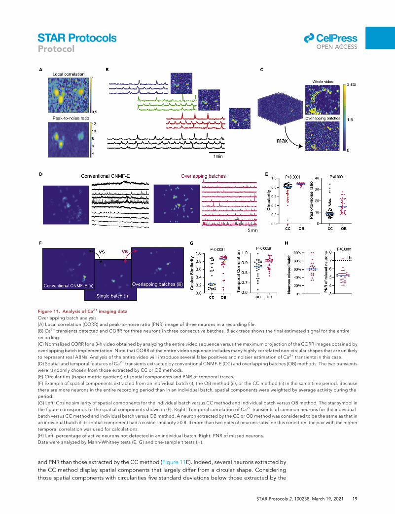
and PNR than those extracted by the CCmethod (Figure 11E). Indeed, several neurons extracted by

the CC method display spatial components that largely differ from a circular shape. Considering

those spatial components with circularities five standard deviations below those extracted by the

Figure 11. Analysis of Ca2+ imaging data

Overlapping batch analysis.

(A) Local correlation (CORR) and peak-to-noise ratio (PNR) image of three neurons in a recording file.

(B) Ca2+ transients detected and CORR for three neurons in three consecutive batches. Black trace shows the final estimated signal for the entire

recording.

(C) Normalized CORR for a 3-h video obtained by analyzing the entire video sequence versus the maximum projection of the CORR images obtained by

overlapping batch implementation. Note that CORR of the entire video sequence includes many highly correlated non-circular shapes that are unlikely

to represent real ABNs. Analysis of the entire video will introduce several false positives and noisier estimation of Ca2+ transients in this case.

(D) Spatial and temporal features of Ca2+ transients extracted by conventional CNMF-E (CC) and overlapping batches (OB) methods. The two transients

were randomly chosen from those extracted by CC or OB methods.

(E) Circularities (isoperimetric quotient) of spatial components and PNR of temporal traces.

(F) Example of spatial components extracted from an individual batch (i), the OB method (ii), or the CC method (ii) in the same time period. Because

there are more neurons in the entire recording period than in an individual batch, spatial components were weighted by average activity during the

period.

(G) Left: Cosine similarity of spatial components for the individual batch versus CC method and individual batch versus OB method. The star symbol in

the figure corresponds to the spatial components shown in (F). Right: Temporal correlation of Ca2+ transients of common neurons for the individual

batch versus CC method and individual batch versus OB method. A neuron extracted by the CC or OB method was considered to be the same as that in

an individual batch if its spatial component had a cosine similarity >0.8. If more than two pairs of neurons satisfied this condition, the pair with the higher

temporal correlation was used for calculations.

(H) Left: percentage of active neurons not detected in an individual batch. Right: PNR of missed neurons.

Data were analyzed by Mann-Whitney tests (E, G) and one-sample t tests (H).

llOPEN ACCESS


Protocol

OB method, we estimated that 34% of components extracted by the CC method are false positives

(Figure 11E, left, red dots). Next, we examined how the final temporal and spatial components of the

transients extracted by theOB or CCmethod (analysis of >30,000 frames) differ from those extracted

from the analysis of an individual batch (analysis of �1,000 frames) (Figure 11F). Components ex-

tracted by the OB method were spatially and temporally more similar to those extracted from an in-

dividual batch (Figure 11G). We estimate that, on average, 61% of neurons remain undetected in in-

dividual batch analysis compared with the OB method (Figure 11H, left) because they display PNR

significantly below the detection threshold. These results indicate that theOBmethodminimizes the

number of false positives without compromising true-positive detection.

6. To track ABNs across different sessions, motion correct each session as previously described

(Ghandour et al., 2019). In Mosaic software, this is done as follows:

a. Motion correct each session independently.

b. Extract one frame from one session to use as a reference for other sessions.

c. Motion correct each session relative to the extracted frame.

Note: Sometimes using different reference frames from different sessions provides better re-

sults. Consider the points mentioned in ‘‘Quantification and statistical analysis: step 3.’’

d. Concatenate the recording sessions, ensuring that sessions are correctly aligned.

Pause point: Tracing ABNs across several days using tracking algorithms (Sheintuch et al.,

2017) may not be possible given the small number of ABNs. However, we were able to track

ABNs across different recording sessions within the same day by concatenating different ses-

sions into one file. Spatial markers, such as blood vessels or ABNs with persistent activity, can

be used to align different sessions.

Analyzing sessions independently and then identifying the same ABNs based on their footprints

assumes that all ABNs can be detected in each recording session. However, this is not always the

case, especially considering the sparse activity of ABNs and the low signal-to-noise ratio of

GCaMP3. This issue is illustrated in Figure 11B; note that in the first batch, three ABNs are

active with CORR comparable to the background local correlation. If lower CORR and PNR

thresholds are used to detect these ABNs, many false-positive neurons would be included in the

analysis, further hindering the tracking of ABNs. Instead, we initialize these ABNs in a specific period

in which they show high activity (e.g., third batch in Figure 11B). The CNMF algorithm is then used to

extract Ca2+ transients from other batches with a lower signal-to-noise ratio. This is particularly

important when tracking the same ABNs because some may be more active in some recording ses-

sions than in others and, hence, be wrongly labeled as inactive if these sessions are analyzed

independently.

7. After extracting the raster plot of ABN activity, we further analyzed data for each sleep stage in

10-s bins using Sleep Sign software (example raw data are available in Kumar et al., 2020). Alter-

natively, several other types of software are available for sleep analysis (e.g., Sleep, Combrisson

et al., 2017). More details of sleep recording and analysis are available in Oishi et al. (2016).

Limitations

Although GCaMP imaging and miniscope technologies fuel new discoveries of how neuron activity

generates specific behaviors in freely moving animals, their limitations are well known.

One limitation is related to the resolution of the z-axis. Theminiscope used in our study (Kumar et al.,

2020) excites fluorescence molecules without focusing or scanning the light; it does not have a

pinhole. Therefore, all fluorescence molecule hundreds of micrometers below the miniscope can

be excited and detected at the same time. This can allow researchers to obtain a larger number

llOPEN ACCESS


Protocol

of ABN signals. However, it is possible that a detected Ca2+ transient can stem from two ABNs

aligned in the z-axis.

Another limitation is that the experimental preparation for DG imaging in freely moving mice results

in a partial lesion of the ipsilateral CA1 area when implanting the GRIN lens. Less invasive techniques

could be used in the future to prevent possible circuit reorganization induced by surgery, as previ-

ously recommended (Hainmueller and Bartos, 2018; Kirschen et al., 2017; Pilz et al., 2016).

Finally, the developing nature of ABNs imposes a time constraint on the experimental schedule. As

the activity and behavioral significance of ABNs change as they transition from immature to mature

granule cells (e.g., Kumar et al., 2020), it can be challenging to use the same mice in multiple behav-

ioral tasks and ensure that the recorded ABNs have the same physiological properties across the task

periods.

A final limitation is the overall cost of the necessary equipment. Using the described hardware makes

the experiment faster and easier to perform, but it costs more than $150,000 USD in total. Fortu-

nately, more budget-friendly options are available. A similar miniscope can be built by a researcher

using the open-source miniscope platform (UCLA Miniscope). In addition, simpler over-the-counter

computers can be used for the experiments, but this would likely increase the data processing time.

Troubleshooting

Problem 1

GCaMP3-labeled cells are rare or absent (steps 1, 2, and 31).

Potential solution

The presence of a small number of GCaMP3-labeled neurons can be due to inefficient Cre induction/

recombination by tamoxifen administration. The dose-dependency of GCaMP3 expression should

be confirmed in each experimental setting. Always prepare fresh tamoxifen solution, protecting it

from light. Ensure that tamoxifen is completely dissolved to achieve a sufficient dose. Also, when in-

jecting, leave the needle tip in the intraperitoneal space for a few seconds to avoid reflux of tamox-

ifen. The injected dose can be systematically increased to determine whether this solves the

problem.

When using different versions of GCaMP, confirm immunohistologically that Cre recombinase is ex-

pressed and that there is no cell death induced by cytotoxicity of Ca2+ sensors in ABNs.

Problem 2

The lens is incorrectly positioned (steps 4–9).

Potential solution

This problem can occur due to variations in different stereotaxic equipment or unintended changes

in lens position during implantation. Confirm that the lens is oriented precisely within the hole and

re-evaluate the coordinates for each experimental setting.

Implanting the lens into the CA1 generates resistance, which can force the lens out of the brain. Only

release the lens from the stereotaxic micromanipulator after the glue/dental cement cures; other-

wise, the position of the lens may shift when released from the grip.

Problem 3

The implant detaches from the mouse (steps 6–28).

llOPEN ACCESS


Protocol

Potential solution

Implant detachment can occur when it is not well secured to the skull. When applying several layers

of different adhesives, ensure that each layer completely cures before applying the next one, as mix-

ing them could compromise their stability. In some cases, standard black cement may compromise

the longevity of the implant. One possibility for this case is to use regular light dental cement and

cover it with black paint or nail polish to prevent ambient light-derived artifacts. Infection and tissue

inflammation can also decrease the adhesive strength of the glue/dental cement; ensure adequate

prophylactic practices during surgery and postoperative recovery to prevent this problem. In addi-

tion, do not immobilize mice by holding the baseplate, as physical stress at the implant can cause its

detachment.

Problem 4

Excessive motion artifacts are present during data acquisition (steps 12–14, 19, 24, and 27).

Potential solution

Ensure that the baseplate is fixed properly on the skull and that theminiscope is correctly attached to

the baseplate and tightly secured in place by its screw. Also, low frame rates may increase the

amount of motion blur, which can impair performance of the motion correction algorithm.

Problem 5

Fluorescence signals do not show dynamic changes in intensity (steps 13, 20, 24, 27).

Potential solution

‘‘False’’ fluorescence signals are usually derived from autofluorescent materials (e.g., damaged tis-

sue or blood cells below the lens) and not from GCaMP3. To prevent these, ensure that the cortex

above the target coordinates is completely aspirated and that there is no residual bleeding before

implanting the lens. As lowering the lens too quickly into the brain can damage the tissue, ensure

that the lens is implanted slowly and allow the tissue to settle after each 150-mm step. If necessary,

retract the lens G25 mm before each step to further alleviate pressure and prevent unnecessary

damage.

Problem 6

Data processing is extremely slow or impossible (Quantification and statistical analysis steps).

Potential solution

As sleep recordings can be >3 h long, the final compressed file can be >200 GB. To be processed,

the file will need to be decompressed and spatially down-sampled (43), resulting in a �216 kb/

frame file. However, because some MATLAB scripts require double precision, we recommend

that the PC has at least four times more RAM than the down-sampled file size. When it is not possible

to reduce the size of the data file by temporal and/or spatial binning, the full-length recording can be

split into two shorter files. The initial processing steps can be performed separately for each file,

which can later be concatenated before detecting active ABNs using batch implementation and

disabling parallel computing (although this can take several hours).

Problem 7

Few or no ABNs are present in the imaging file (Quantification and statistical analysis step 4).

Potential solution

If there are no problems with GCaMP3 expression or lens implantation coordinates, this problem can

be solved by changing parameters in the CNMF-E script. Start by modifying the minimumCORR and

PNR thresholds. In this case, visual inspection of cell shape and temporal dynamics of Ca2+ transients

become more important, as the rate of false cell detection increases with less stringent parameters.

llOPEN ACCESS


Protocol

Problem 8

MATLAB code crashes during analysis (Quantification and statistical analysis steps 4–6).

Potential solution

The code (original or provided) is not bug-proof. In case of an error, read the error message in the

MATLAB command window. If no ABN is detected, the code will crash. Visually confirm whether you

can detect Ca2+ activity. If active ABNs can be visually detected in the raw file, consider using a lower

PNR or CORR threshold. Also, monitor your RAM usage when running the code. Consider upgrading

your hardware or reducing the recording duration.

Resource availability

Lead contact

Further information and requests for resources and reagents should be directed to and will be ful-

filled by the Lead Contact, Masanori Sakaguchi ([email protected]).

Materials availability

We did not generate any unique/stable reagents in this study.

Data and code availability

Data and code underlying the results described in this manuscript are available at:


Also, the raw data from the related article (Kumar et al., 2020) are available at:

https://data.mendeley.com/datasets/gfbdv5kfrz/1

Supplemental information

Supplemental information can be found online at https://doi.org/10.1016/j.xpro.2020.100238.

Acknowledgments

We thank Dr. K.G. Akers for comments on the manuscript. This work was partially supported by

grants from the World Premier International Research Center Initiative fromMEXT, JST CREST grant

no. JPMJCR1655, JSPS KAKENHI grant nos. 16K18359, 15F15408, 15H01276, 15K18332,

26115502, 25116530, JP16H06280, and 20H03552, Takeda Science Foundation, Shimadzu Science

Foundation, Kanae Foundation, Research Foundation for Opto-Science and Technology, Ichiro Ka-

nehara Foundation, Kato Memorial Bioscience Foundation, Japan Foundation for Applied Enzy-

mology, Senshin Medical Research Foundation, Life Science Foundation of Japan, The Uehara Me-

morial Foundation, Brain Science Foundation, Kowa Life Science Foundation, Inamori Research

Grants Program, and GSK Japan to M.S.; JSPS KAKENHI grant nos. 25000015 and 18H04012 to

M.K.; Tokyo Biochemical Research Foundation and JSPS FPD to S.SR.; JSPS FPD to D.K.

Author contributions

Conceptualization, Y.S., M.K., and M.S.; Methodology, A.C.-R., Y.S., D.K., I.K., P.V., S.S., and M.S.;

Investigation, A.C.-R., D.K., Y.S., I.K., S.S., and T.N.; Validation, A.C.-R, Y.S., D.K., and P.V.; Formal

Analysis, Y.S., A.C.-R., and P.V.; Data Curation, A.C.-R., Y.S., P.V., and M.S.; Writing – Original Draft,

A.C.-R and Y.S.; Writing – Review & Editing, Y.S., D.K., A.C.-R, P.V., and M.S.; Funding Acquisition,

M.S., M.K., and Y.S.; Resources, M.K., M.S., and T.S.; Supervision, M.K. and M.S.; Project Adminis-

tration, Y.S., M.K., and M.S. All authors discussed and approved the manuscript.

Declaration of interests

The authors declare no competing interests.

llOPEN ACCESS


Protocol



https://data.mendeley.com/datasets/gfbdv5kfrz/1


References

Boyce, R., Glasgow, S.D., Williams, S., andAdamantidis, A. (2016). Causal evidence for therole of REM sleep theta rhythm in contextualmemory consolidation. Science 352, 812–816.

Combrisson, E., Vallat, R., Eichenlaub, J.B.,O’Reilly, C., Lajnef, T., Guillot, A., Ruby, P.M., andJerbi, K. (2017). Sleep: an open-source pythonsoftware for visualization, analysis, and staging ofsleep data. Front. Neuroinform. 11, 60.

Danielson, N.B.B., Kaifosh, P., Zaremba, J.D.D.,Lovett-Barron, M., Tsai, J., Denny, C.A.A., Balough,E.M.M., Goldberg, A.R.R., Drew, L.J.J., Hen, R.,et al. (2016). Distinct contribution of adult-bornhippocampal granule cells to context encoding.Neuron 90, 101–112.

Ghandour, K., Ohkawa, N., Fung, C.C.A.C.A., Asai,H., Saitoh, Y., Takekawa, T., Okubo-Suzuki, R.,Soya, S., Nishizono, H., Matsuo, M., et al. (2019).Orchestrated ensemble activities constitute ahippocampal memory engram. Nat. Commun. 10,2637.

Ghosh, K.K., Burns, L.D., Cocker, E.D.,Nimmerjahn, A., Ziv, Y., Gamal, A.E., and Schnitzer,M.J. (2011). Miniaturized integration of afluorescence microscope. Nat. Methods 8,871–878.

Giovannucci, A., Friedrich, J., Gunn, P., Kalfon, J.,Brown, B.L., Koay, S.A., Taxidis, J., Najafi, F.,Gauthier, J.L., Zhou, P., Khakh, B.S., Tank, D.W.,Chklovskii, D.B., and Pnevmatikakis, E.A. (2019).CaImAn an open-source tool for scalable calciumimaging data analysis. eLife 8, e38173.

Grewe, B.F., Grundemann, J., Kitch, L.J., Lecoq,J.A., Parker, J.G., Marshall, J.D., Larkin, M.C.,Jercog, P.E., Grenier, F., Li, J.Z., Luthi, A., andSchnitzer, M.J. (2017). Neural ensemble dynamicsunderlying a long-term associative memory.Nature 543, 670–675.

Hainmueller, T., and Bartos, M. (2018). Parallelemergence of stable and dynamic memoryengrams in the hippocampus. Nature 558,292–296.

Johnston, S.T., Parylak, S.L., Kim, S., Mac, N., Lim,C.K., Gallina, I.S., Bloyd, C.W., Newberry, A.,Saavedra, C.D., Novak, O., et al. (2020). AAVablates neurogenesis in the adult murinehippocampus. bioRxiv. https://doi.org/10.1101/2020.01.18.911362.

Kim, E.J., Leung, C.T., Reed, R.R., and Johnson, J.E.(2007). In vivo analysis of Ascl1 defined progenitorsreveals distinct developmental dynamics duringadult neurogenesis and gliogenesis. J. Neurosci.27, 12764–12774.

Kirschen, G.W.W., Shen, J., Tian, M., Schroeder, B.,Wang, J., Man, G., Wu, S., and Ge, S. (2017). Activedentate granule cells encode experience topromote the addition of adult-born hippocampalneurons. J. Neurosci. 37, 4661–4678.

Kotterman, M.A., Vazin, T., and Schaffer, D.V.(2015). Enhanced selective gene delivery to neuralstem cells in vivo by an adeno-associated viralvariant. Development 142, 1885–1892.

Kumar, D., Koyanagi, I., Carrier-Ruiz, A., Vergara,P., Srinivasan, S., Sugaya, Y., Kasuya, M., Yu, T.S.,Vogt, K.E., Muratani, M., et al. (2020). sparse activityof hippocampal adult-born neurons during REMsleep is necessary for memory consolidation.Neuron 107, 552–565.

Madisen, L., Garner, A.R., Shimaoka, D., Chuong,A.S., Klapoetke, N.C., Li, L., van der Bourg, A.,Niino, Y., Egolf, L., Monetti, C., et al. (2015).Transgenic mice for intersectional targeting ofneural sensors and effectors with high specificityand performance. Neuron 85, 942–958.

Marshall, L., Helgadottir, H., Molle, M., and Born, J.(2006). Boosting slow oscillations during sleeppotentiates memory. Nature 444, 610–613.

Moreno-Jimenez, E.P., Flor-Garcia, M., Terreros-Roncal, J., Rabano, A., Cafini, F., Pallas-Bazarra, N.,Avila, J., Llorens-Martin, M., Moreno-Jimenez, E.P.,Flor-Garcıa, M., et al. (2019). Adult hippocampalneurogenesis is abundant in neurologically healthysubjects and drops sharply in patients withAlzheimer’s disease. Nat. Med. 25, 554–560.

Oishi, Y., Takata, Y., Taguchi, Y., Kohtoh, S., Urade,Y., and Lazarus, M. (2016). Polygraphic recordingprocedure for measuring sleep in mice. J. Vis. Exp.e53678.

Pilz, G.A.A., Carta, S., Stauble, A., Ayaz, A.,Jessberger, S., Helmchen, F., Stauble, A., Ayaz, A.,Jessberger, S., and Helmchen, F. (2016). Functionalimaging of dentate granule cells in the adult mousehippocampus. J. Neurosci. 36, 7407–7414.

Resendez, S.L., Jennings, J.H., Ung, R.L.,Namboodiri, V.M., Zhou, Z.C., Otis, J.M., Nomura,H., McHenry, J.A., Kosyk, O., and Stuber, G.D.(2016). Visualization of cortical, subcortical anddeep brain neural circuit dynamics duringnaturalistic mammalian behavior with head-mounted microscopes and chronically implantedlenses. Nat. Protoc. 11, 566–597.

Sheintuch, L., Rubin, A., Brande-Eilat, N., Geva, N.,Sadeh, N., Pinchasof, O., and Ziv, Y. (2017).Tracking the same neurons across multiple days inCa2+ imaging data. Cell Rep. 21, 1102–1115.

Yang, S.M., Alvarez, D.D., and Schinder, A.F. (2015).Reliable Genetic Labeling of Adult-Born DentateGranule Cells Using Ascl1 CreERT2 and GlastCreERT2 Murine Lines. J. Neurosci. 35, 15379–15390.

Zhou, P., Resendez, S.L.L., Rodriguez-Romaguera,J., Jimenez, J.C.C., Neufeld, S.Q.Q., Stuber,G.D.D., Hen, R., Kheirbek, M.A.A., Sabatini, B.L.L.,Kass, R.E.E., et al. (2018). Efficient and accurateextraction of in vivo calcium signals frommicroendoscopic video data. eLife 7, 1–37.

llOPEN ACCESS


Protocol

http://refhub.elsevier.com/S2666-1667(20)30225-2/sref1










































https://doi.org/10.1101/2020.01.18.911362

https://doi.org/10.1101/2020.01.18.911362






































































Calcium imaging of adult-born neurons in freely moving mice

Documents

Transcript of Calcium imaging of adult-born neurons in freely moving mice