
B.tech ME ,6th, Heat Transfer.pdf - IITM Group Of Institution
162
INTERNATIONAL INSTITUTE OF TECHNOLOGY & MANAGEMENT, MURTHAL SONEPAT E-NOTES , Subject : HEAT TRANSFER, Subject Code: ME 306 B Course: B. TECH. , Branch : Mechanical Engineering , Sem-6 th Prepared By: Mr. ishank , Assistant Professor , MED) H.T HEAT TRANSFER UNIT CONTENT PAGE NO NO 1 CONDUCTION 1.1 GENERAL HEAT CONDUCTION IN CARTESIAN 5 COORDINATES ,POLAR 1.2 DERIVATION ON PLANE WALL 8 1.3 DERIVATION ON COMPOSITE SYSTEMS 11 1.4 CONDUCTION WITH INTERNAL HEAT 15 1.5 EXTENDED SURFACES 17 1.6 UNSTEADY STATE HEAT TRANSFER 20 1.7 LUMPED HEAT ANALYSIS 23 1.8 SEMI INFINITE SOLIDS 27 2 CONVECTION 2.1 FREE AND FORCED CONVECTION 30 2.2 FORMATION OF THERMAL AND HYDRODYNAMIC LAYER 32 2.3 FREE AND FORCED CONVECTION OVER PLATES 34 37 2.4 FLOW OVER CYLINDERS 2.5 INTERNAL FLOW THROUGH TUBES 44 3 PHASE CHANGE HEAT TRANSFER AND HEAT EXCHANGERS 3.1. NUSSELT S THEORY OF CONDENSATION 67 72 3.2 REGIMES OF POOL BOILING
-
Upload
khangminh22 -
Category
Documents
-
view
0 -
download
0
Transcript of B.tech ME ,6th, Heat Transfer.pdf - IITM Group Of Institution

INTERNATIONAL INSTITUTE OF TECHNOLOGY & MANAGEMENT, MURTHAL SONEPATE-NOTES , Subject : HEAT TRANSFER, Subject Code: ME 306 B Course: B.TECH. , Branch : Mechanical Engineering , Sem-6th Prepared By: Mr. ishank ,
Assistant Professor , MED)
H.T HEAT TRANSFER
UNIT CONTENT PAGENO NO
1 CONDUCTION
1.1 GENERAL HEAT CONDUCTION IN CARTESIAN 5COORDINATES ,POLAR
1.2 DERIVATION ON PLANE WALL 8
1.3 DERIVATION ON COMPOSITE SYSTEMS 11
1.4 CONDUCTION WITH INTERNAL HEAT 15
1.5 EXTENDED SURFACES 17
1.6 UNSTEADY STATE HEAT TRANSFER 20
1.7 LUMPED HEAT ANALYSIS 23
1.8 SEMI INFINITE SOLIDS 27
2 CONVECTION
2.1 FREE AND FORCED CONVECTION 30
2.2 FORMATION OF THERMAL AND HYDRODYNAMIC LAYER 32
2.3 FREE AND FORCED CONVECTION OVER PLATES 34
372.4 FLOW OVER CYLINDERS
2.5 INTERNAL FLOW THROUGH TUBES 44
3 PHASE CHANGE HEAT TRANSFER AND HEAT EXCHANGERS
3.1. NUSSELT S THEORY OF CONDENSATION 67
723.2 REGIMES OF POOL BOILING

INTERNATIONAL INSTITUTE OF TECHNOLOGY & MANAGEMENT, MURTHAL SONEPATE-NOTES , Subject : HEAT TRANSFER, Subject Code: ME 306 B Course: B.TECH. , Branch : Mechanical Engineering , Sem-6th Prepared By: Mr. ishank ,
Assistant Professor , MED)
4 H.T

INTERNATIONAL INSTITUTE OF TECHNOLOGY & MANAGEMENT, MURTHAL SONEPATE-NOTES , Subject : HEAT TRANSFER, Subject Code: ME 306 B Course: B.TECH. , Branch : Mechanical Engineering , Sem-6th Prepared By: Mr. ishank ,
Assistant Professor , MED)
H.T HEAT TRANSFER
753.3 CORRELATIONS IN BOILING AND CONDENSATION
763.4 HEAT EXCHANGER TYPES
3.5 FOULING FACTORS AND NTU METHOD 82
4 RADIATION
4.1 BLACK BODY AND GREY BODY RADIATION 105
4.2 SHAPE FACTOR 106
4.3 RADIATION SHIELDS 109
4.4 RADIATION THROUGH GASES 114
5 MASS TRANSFER
5.1 BASIC CONCEPTS 136
1375.2 STEADY STATE MOLECULAR DIFFUSION
1375.3 CONVECTIVE MASS TRANSFER
5.4 HEAT TRANSFER ANALOGY 140
1435.5 CONVECTIVE MASS TRANSFER

INTERNATIONAL INSTITUTE OF TECHNOLOGY & MANAGEMENT, MURTHAL SONEPATE-NOTES , Subject : HEAT TRANSFER, Subject Code: ME 306 B Course: B.TECH. , Branch : Mechanical Engineering , Sem-6th Prepared By: Mr. ishank ,
Assistant Professor , MED)
5
INTERNATIONAL INSTITUTE OF TECHNOLOGY & MANAGEMENT, MURTHAL SONEPATE-NOTES , Subject : HEAT TRANSFER, Subject Code: ME 306 B Course: B. TECH. ,
Branch : Mechanical Engineering , Sem-6th Prepared By: Mr. ishank , AssistantProfessor , MED)
H.T HEAT TRANSFER
CHAPTER 1: CONDUCTION
GENERAL DIFFERENTIAL EQUATION OF HEAT CONDUCTION
1.1The General Heat Conduction Equation in Cartesian coordinates and Polar coordinates
;
Any physical phenomenon is generally accompanied by a change in space and time of its
physical properties. The heat transfer by conduction in solids can only take place when there is a
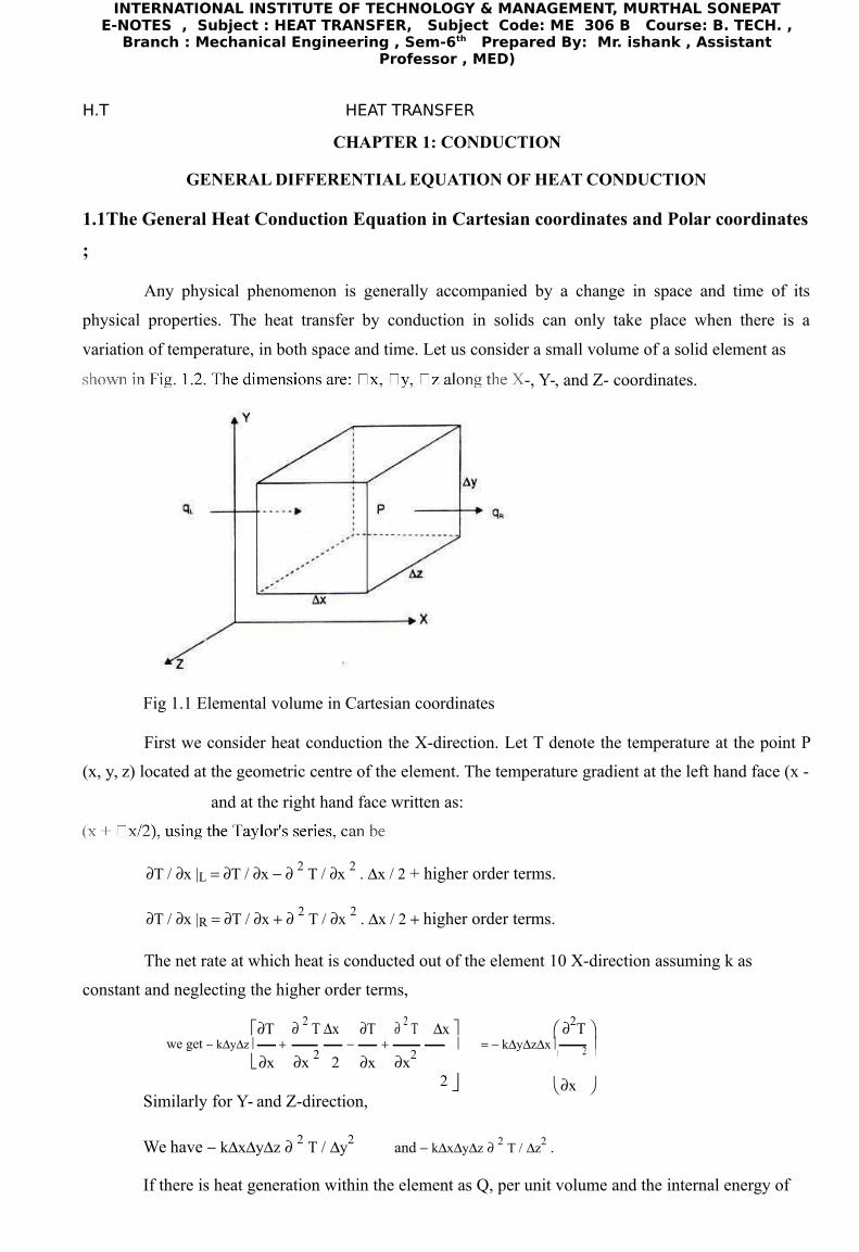
variation of temperature, in both space and time. Let us consider a small volume of a solid element as
-, Y-, and Z- coordinates.
Fig 1.1 Elemental volume in Cartesian coordinates
First we consider heat conduction the X-direction. Let T denote the temperature at the point P
(x, y, z) located at the geometric centre of the element. The temperature gradient at the left hand face (x -
and at the right hand face written as:
T / x |L T / x 2 T / x
2 . x / 2 + higher order terms.
T / x |R T / x 2 T / x
2 . x / 2 higher order terms.
The net rate at which heat is conducted out of the element 10 X-direction assuming k as
constant and neglecting the higher order terms,
T 2 T x T
2 T
we get kyz x x
2 2 x x
2
Similarly for Y- and Z-direction,
x 2T kyzx 2
2
x
We have kxyz 2 T / y2
and kxyz 2 T / z2 .
If there is heat generation within the element as Q, per unit volume and the internal energy of

INTERNATIONAL INSTITUTE OF TECHNOLOGY & MANAGEMENT, MURTHAL SONEPATE-NOTES , Subject : HEAT TRANSFER, Subject Code: ME 306 B Course: B. TECH. ,
Branch : Mechanical Engineering , Sem-6th Prepared By: Mr. ishank , AssistantProfessor , MED)
6
H.T HEAT TRANSFER
the element changes with time, by making an energy balance, we write
Heat generated within Heat conducted away Rate of change of internal
the element from the element energy within with the element
or, Q v xyz k xyz 2 T / x 2 2 T / y 2 2 T / z2
c xyz T / t
Upon simplification, 2 T / x 2 2 T / y 2 2 T / z 2 Q v / k
kc T / t or, 2 T Q v / k 1/ T / t
where k / . c , is called the thermal diffusivity and is seen to be a physical property of the
material of which the solid is composed.
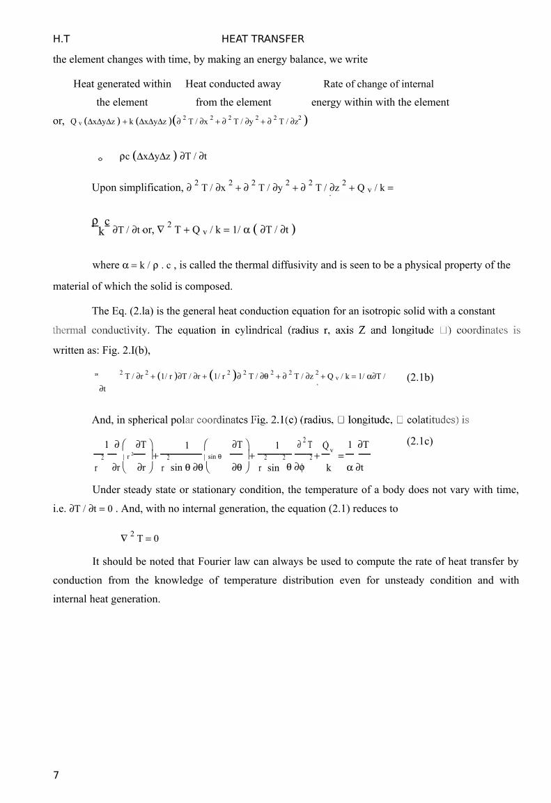
The Eq. (2.la) is the general heat conduction equation for an isotropic solid with a constant
written as: Fig. 2.I(b),
2 T / r 2 1/ r T / r 1/ r 2 2 T / 2 2 T / z 2 Q v / k 1/ T /
t
And, in spherical pol
1 T 1 T 1 2 T Q v1 T
r 2 sin
r2
r2
r2
sin2
2
tr r sin k
(2.1b)
(2.1c)
Under steady state or stationary condition, the temperature of a body does not vary with time,
i.e. T / t 0 . And, with no internal generation, the equation (2.1) reduces to
2 T 0
It should be noted that Fourier law can always be used to compute the rate of heat transfer by
conduction from the knowledge of temperature distribution even for unsteady condition and with
internal heat generation.
7
H.T HEAT TRANSFER
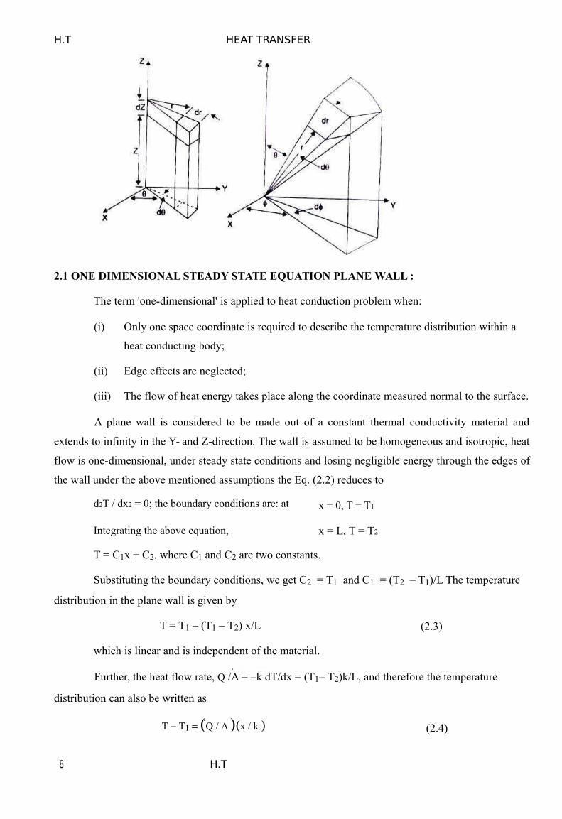
2.1 ONE DIMENSIONAL STEADY STATE EQUATION PLANE WALL :
The term 'one-dimensional' is applied to heat conduction problem when:
(i) Only one space coordinate is required to describe the temperature distribution within a
heat conducting body;
(ii) Edge effects are neglected;
(iii) The flow of heat energy takes place along the coordinate measured normal to the surface.
A plane wall is considered to be made out of a constant thermal conductivity material and
extends to infinity in the Y- and Z-direction. The wall is assumed to be homogeneous and isotropic, heat
flow is one-dimensional, under steady state conditions and losing negligible energy through the edges of
the wall under the above mentioned assumptions the Eq. (2.2) reduces to
d2T / dx2 = 0; the boundary conditions are: at x = 0, T = T1
Integrating the above equation, x = L, T = T2
T = C1x + C2, where C1 and C2 are two constants.
Substituting the boundary conditions, we get C2 = T1 and C1 = (T2 – T1)/L The temperature
distribution in the plane wall is given by
T = T1 – (T1 – T2) x/L (2.3)
which is linear and is independent of the material.
Further, the heat flow rate, Q /A = –k dT/dx = (T1– T2)k/L, and therefore the temperature
distribution can also be written as
T T1 Q / A x / k (2.4)
8 H.T

H.T HEAT TRANSFER
i.e., “the temperature drop within the wall will increase with greater heat flow rate or when k is
small for the same heat flow rate,"
2.2 A Cylindrical Shell-Expression for Temperature Distribution
In the cylindrical system, when the temperature is a function of radial distance only and is
independent of azimuth angle or axial distance, the differential equation (2.2) would be, (Fig. 1.4)
d2T /dr2 +(1/r) dT/dr = 0
with boundary conditions: at r = rl, T = T1 and at r = r2, T = T2.
The differential equation can be written as:
1r dr
d r dT / dr 0 , or, dr
d r dT / dr 0
upon integration, T = C1 ln (r) + C2, where C1 and C2 are the arbitrary constants.
Fig 1.3: A Cylindrical shell
By applying the boundary conditions,
C1 T2 T1 / ln r2 / r1
and C2 T1 ln r1 . T2 T1 / ln r2 / r1
The temperature distribution is given by
T T1 T2 T1 . ln r / r1 / ln r2 / r1 and
Q / L kA dT / dr 2kT1T2/ lnr2/ r1(2.5)
From Eq (2.5) It can be seen that the temperature varies 10gantJunically through the cylinder wall In
contrast with the linear variation in the plane wall .
If we write Eq. (2.5) as Q kA m T1 T2 / r2 r1 , where
A m 2 r2 r1 L / ln r2 / r1 A2A1/ lnA2/ A1
9
H.T HEAT TRANSFER
where A2 and A1 are the outside and inside surface areas respectively. The term Am is called
‘Logarithmic Mean Area' and the expression for the heat flow through a cylindrical wall has the same
form as that for a plane wall.
3.1ONE DIMENSIONAL STEADY STATE HEATCONDUCTION COMPOSITE SYSTEMS:
3.2Composite Surfaces
There are many practical situations where different materials are placed m layers to form
composite surfaces, such as the wall of a building, cylindrical pipes or spherical shells having different
layers of insulation. Composite surfaces may involve any number of series and parallel thermal circuits.
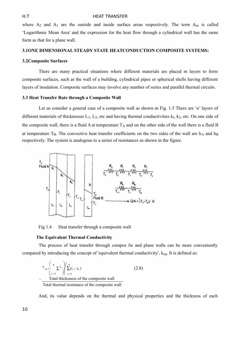
3.3 Heat Transfer Rate through a Composite Wall
Let us consider a general case of a composite wall as shown m Fig. 1.5 There are ‘n’ layers of
different materials of thicknesses L1, L2, etc and having thermal conductivities kl, k2, etc. On one side of
the composite wall, there is a fluid A at temperature TA and on the other side of the wall there is a fluid B
at temperature TB. The convective heat transfer coefficients on the two sides of the wall are hA and hB
respectively. The system is analogous to a series of resistances as shown in the figure.
Fig 1.4 Heat transfer through a composite wall
The Equivalent Thermal Conductivity
The process of heat transfer through compos lie and plane walls can be more conveniently
compared by introducing the concept of 'equivalent thermal conductivity', keq. It is defined as:
n nk
eq L
i L i / ki (2.8) i 1 i 1
= Total thickeness of the composite wall
Total thermal resistance of the composite wall
And, its value depends on the thermal and physical properties and the thickness of each
10
H.T HEAT TRANSFER
constituent of the composite structure.
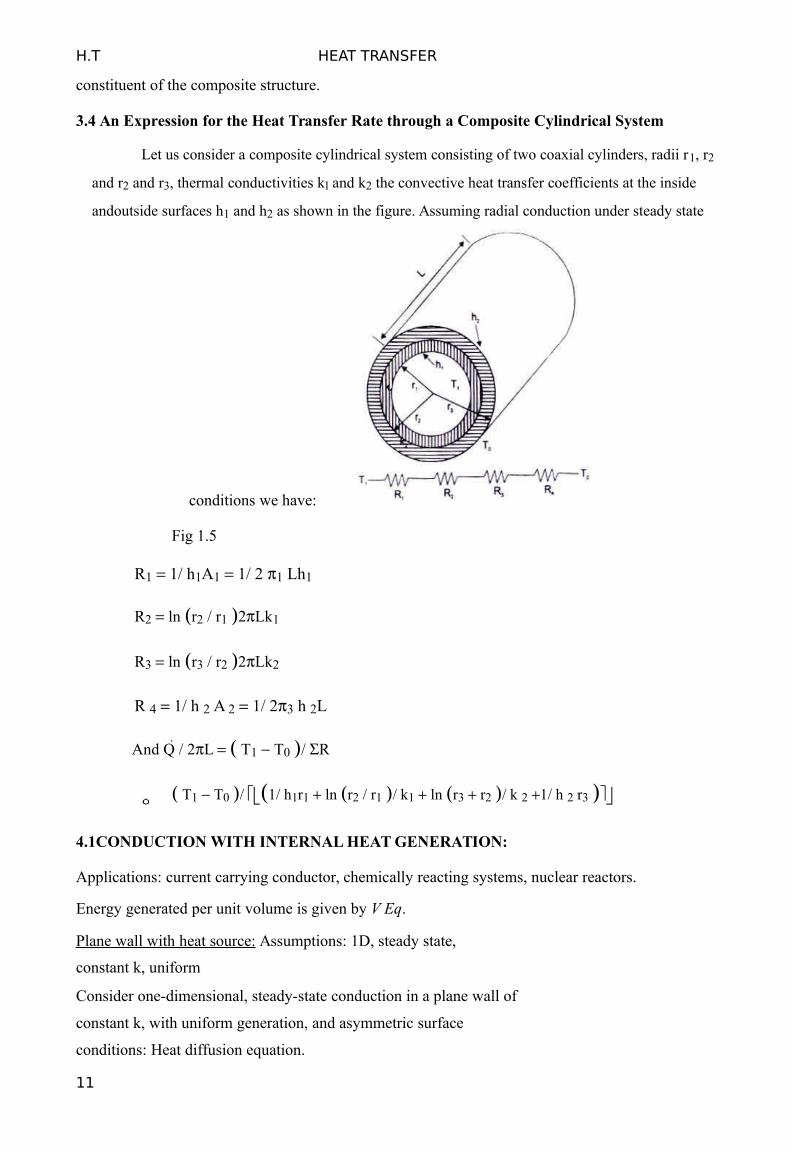
3.4 An Expression for the Heat Transfer Rate through a Composite Cylindrical System
Let us consider a composite cylindrical system consisting of two coaxial cylinders, radii r1, r2
and r2 and r3, thermal conductivities kl and k2 the convective heat transfer coefficients at the inside
andoutside surfaces h1 and h2 as shown in the figure. Assuming radial conduction under steady state
conditions we have:
Fig 1.5
R1 1/ h1A1 1/ 2 1 Lh1
R2 ln r2 / r1 2Lk1
R3 ln r3 / r2 2Lk2
R 4 1/ h 2 A 2 1/ 23 h 2L
And Q / 2L T1 T0 / R
T1 T0 / 1/ h1r1 ln r2 / r1 / k1 ln r3 r2 / k 2 1/ h 2 r3
4.1CONDUCTION WITH INTERNAL HEAT GENERATION:
Applications: current carrying conductor, chemically reacting systems, nuclear reactors.
Energy generated per unit volume is given by V Eq.
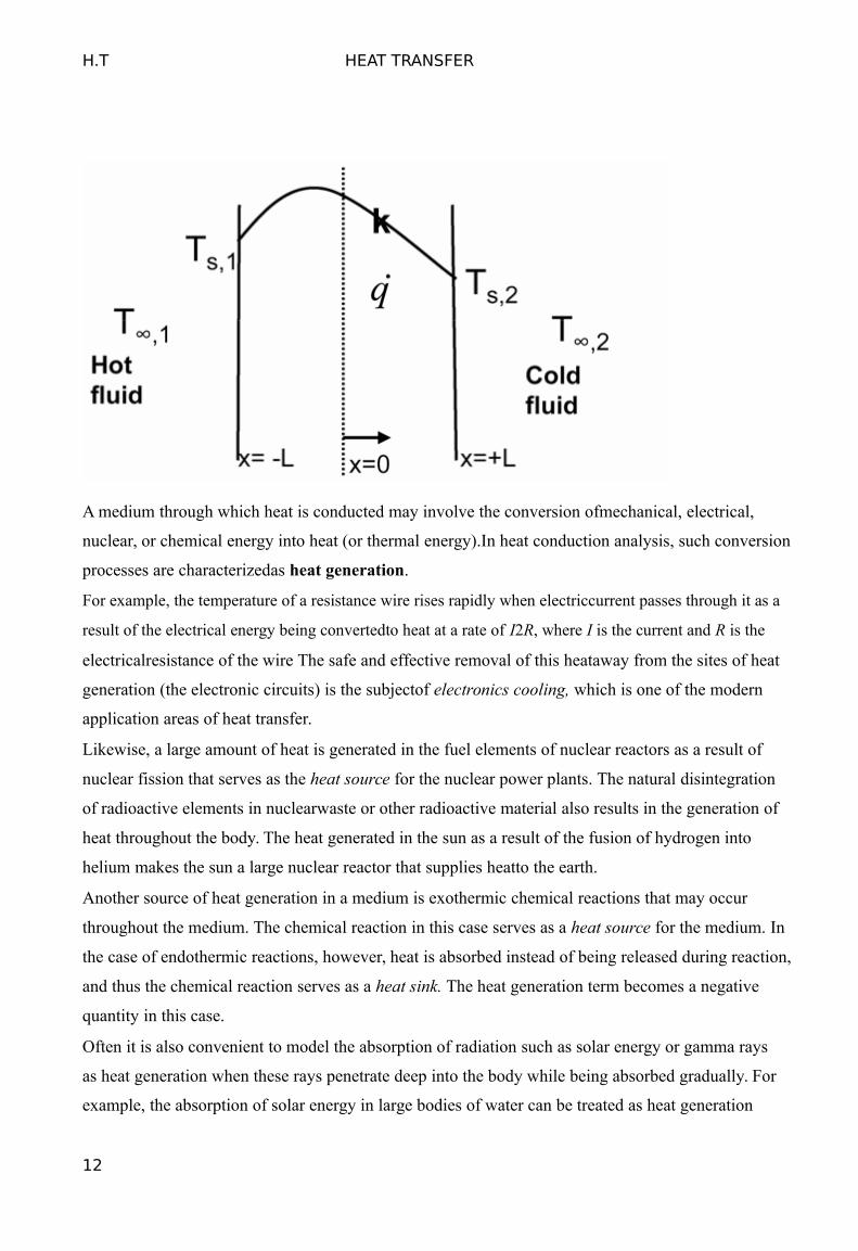
Plane wall with heat source: Assumptions: 1D, steady state,
constant k, uniform
Consider one-dimensional, steady-state conduction in a plane wall of
constant k, with uniform generation, and asymmetric surface
conditions: Heat diffusion equation.
11
H.T HEAT TRANSFER
A medium through which heat is conducted may involve the conversion ofmechanical, electrical,
nuclear, or chemical energy into heat (or thermal energy).In heat conduction analysis, such conversion
processes are characterizedas heat generation.
For example, the temperature of a resistance wire rises rapidly when electriccurrent passes through it as a
result of the electrical energy being convertedto heat at a rate of I2R, where I is the current and R is the
electricalresistance of the wire The safe and effective removal of this heataway from the sites of heat
generation (the electronic circuits) is the subjectof electronics cooling, which is one of the modern
application areas of heat transfer.
Likewise, a large amount of heat is generated in the fuel elements of nuclear reactors as a result of
nuclear fission that serves as the heat source for the nuclear power plants. The natural disintegration
of radioactive elements in nuclearwaste or other radioactive material also results in the generation of
heat throughout the body. The heat generated in the sun as a result of the fusion of hydrogen into
helium makes the sun a large nuclear reactor that supplies heatto the earth.
Another source of heat generation in a medium is exothermic chemical reactions that may occur
throughout the medium. The chemical reaction in this case serves as a heat source for the medium. In
the case of endothermic reactions, however, heat is absorbed instead of being released during reaction,
and thus the chemical reaction serves as a heat sink. The heat generation term becomes a negative
quantity in this case.
Often it is also convenient to model the absorption of radiation such as solar energy or gamma rays
as heat generation when these rays penetrate deep into the body while being absorbed gradually. For
example, the absorption of solar energy in large bodies of water can be treated as heat generation
12

H.T HEAT TRANSFER
throughout the water at a rate equal to the rate of absorption, which varies with depth. But the
absorption of solar energy by an opaque body occurs within a few microns of the surface, and the solar
energy that penetrates into the medium in this case can be treated as specified heat flux on the surface.
Note that heat generation is a volumetric phenomenon. That is, it occurs throughout the body of a
medium. Therefore, the rate of heat generation in a medium is usually specified per unit volume.
The rate of heat generation in a medium may vary with time as well as position within the medium.
When the variation of heat generation with position is known, the total rate of heat generation in a
medium of volume V can be determined from In the special case of uniform heat generation, as in
the case of electric resistance heating throughout a homogeneous material, the relation in
reduces to E ·gen _ e · genV, where Egen is the constant rate of heat generation
per unit volume.
5.1 EXTENDED SURFACES :
Convection: Heat transfer between a solid surface and a moving fluid is governed by the
Newton’s cooling law: q = hA(Ts -
one can Increase the temperature difference (Ts - the fluid.
Increase the convection coefficient h. This can be accomplished by increasing the fluid flow over the
surface since h is a function of the flow velocity and the higher the velocity, the higher the h. Example: a
cooling fan.
Increase the contact surface area A. Example: a heat sink with fin.
Ac : the fin cross-sectional area.
P: the fin perimeter.
Many times, when the first option is not in our control and the second option (i.e. increasing h) is already
stretched to its limit, we are left with the only alternative of increasing the effective surface area by using
fins or extended surfaces. Fins are protrusions from the base surface into the cooling fluid, so that the extra
surface of the protrusions is also in contact with the fluid. Most of you have encountered cooling fins on air-
cooled engines (motorcycles, portable generators, etc.), electronic equipment (CPUs), automobile radiators,
air conditioning equipment (condensers) and elsewhere.
The fin efficiency is defined as the ratio of the energy transferred through a real fin to that transferred
through an ideal fin. An ideal fin is thought to be one made of a perfect or infinite conductor material. A
perfect conductor has an infinite thermal conductivity so that the entire fin is at the base material
temperature.
6.1 UNSTEADY HEAT CONDUCTION :
6. 1 Transient State Systems-Defined
13
H.T HEAT TRANSFER
The process of heat transfer by conduction where the temperature varies with time and with
space coordinates, is called 'unsteady or transient'. All transient state systems may be broadly classified
into two categories:
(a) Non-periodic Heat Flow System - the temperature at any point within the system changes as
a non-linear function of time.
(b) Periodic Heat Flow System - the temperature within the system undergoes periodic changes
which may be regular or irregular but definitely cyclic.
There are numerous problems where changes in conditions result in transient temperature
distributions and they are quite significant. Such conditions are encountered in - manufacture of
ceramics, bricks, glass and heat flow to boiler tubes, metal forming, heat treatment, etc.
6.2. Biot and Fourier Modulus-Definition and Significance
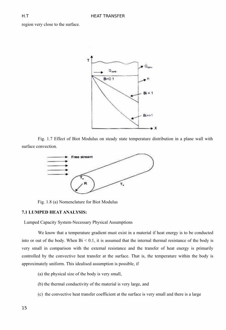
Let us consider an initially heated long cylinder (L >> R) placed in a moving stream of fluid at
T Ts , as shown In Fig. 3.1(a). The convective heat transfer coefficient at the surface is h, where,
Q = hA ( Ts T )
This energy must be conducted to the surface, and therefore,
Q = -kA(dT / dr) r = R
or, h( Ts T ) = -k(dT/dr)r=R -k(Tc-Ts)/R
where Tc is the temperature at the axis of the cylinder
By rearranging,(Ts - Tc) / ( Ts T ) h/Rk (3.1)
The term, hR/k, IS called the 'BlOT MODULUS'. It is a dimensionless number and is the ratio
of internal heat flow resistance to external heat flow resistance and plays a fundamental role in transient
conduction problems involving surface convection effects. I t provides a measure 0 f the temperature
drop in the solid relative to the temperature difference between the surface and the fluid.
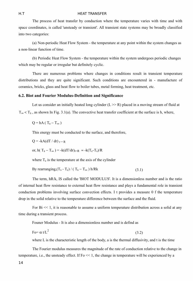
For Bi << 1, it is reasonable to assume a uniform temperature distribution across a solid at any
time during a transient process.
Founer Modulus - It is also a dimensionless number and is defind as
Fo= t/L2(3.2)
where L is the characteristic length of the body, a is the thermal diffusivity, and t is the time
The Fourier modulus measures the magnitude of the rate of conduction relative to the change in
temperature, i.e., the unsteady effect. If Fo << 1, the change in temperature will be experienced by a
14
H.T HEAT TRANSFER
region very close to the surface.
Fig. 1.7 Effect of Biot Modulus on steady state temperature distribution in a plane wall with
surface convection.
Fig. 1.8 (a) Nomenclature for Biot Modulus
7.1 LUMPED HEAT ANALYSIS:
Lumped Capacity System-Necessary Physical Assumptions
We know that a temperature gradient must exist in a material if heat energy is to be conducted
into or out of the body. When Bi < 0.1, it is assumed that the internal thermal resistance of the body is
very small in comparison with the external resistance and the transfer of heat energy is primarily
controlled by the convective heat transfer at the surface. That is, the temperature within the body is
approximately uniform. This idealised assumption is possible, if
(a) the physical size of the body is very small,
(b) the thermal conductivity of the material is very large, and
(c) the convective heat transfer coefficient at the surface is very small and there is a large
15
H.T HEAT TRANSFER
temperature difference across the fluid layer at the interface.
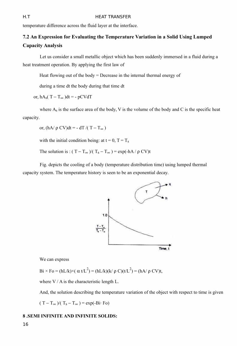
7.2 An Expression for Evaluating the Temperature Variation in a Solid Using Lumped
Capacity Analysis
Let us consider a small metallic object which has been suddenly immersed in a fluid during a
heat treatment operation. By applying the first law of
Heat flowing out of the body = Decrease in the internal thermal energy of
during a time dt the body during that time dt
or, hAs( T T )dt = - pCVdT
where As is the surface area of the body, V is the volume of the body and C is the specific heat
capacity.
or, (hA/ CV)dt = - dT /( T T )
with the initial condition being: at t = 0, T = Ts
The solution is : ( T T )/( Ts T ) = exp(-hA / CV)t
Fig. depicts the cooling of a body (temperature distribution time) using lumped thermal
capacity system. The temperature history is seen to be an exponential decay.
We can express
Bi × Fo = (hL/k)×( t/L2) = (hL/k)(k/ C)(t/L2) = (hA/ CV)t,
where V / A is the characteristic length L.
And, the solution describing the temperature variation of the object with respect to time is given
( T T )/( Ts T ) = exp(-Bi· Fo)
8 .SEMI INFINITE AND INFINITE SOLIDS:
16

H.T HEAT TRANSFER
A semi-infinite solid is an idealized body that has a single plane surface and extends to infinity in all
directions, as shown in .This idealized body is used to indicate that the temperature change in the part of
the body in which we are interested (the region close to the surface) is due to the thermal conditions on a
single surface. The earth, for example, can be considered to be a semi-infinite medium in determining
the variation of temperature near its surface. Also, a thick wall can be modeled as a semi-infinite
medium if all we are interested in is the variation of temperature in the region near one of the surfaces,
and the other surface is too far to have any impact on the region of interest during the time of
observation. The temperature in the core region of the wall remains unchanged in this case.
For short periods of time, most bodies can be modeled as semi-infinite solids since heat does not have
sufficient time to penetrate deep into the body,and the thickness of the body does not enter into the heat
transfer analysis. A steel piece of any shape, for example, can be treated as a semi-infinite solid when it
is quenched rapidly to harden its surface. A body whose surface is heated by a laser pulse can be treated
the same way.
Consider a semi-infinite solid with constant thermo physical properties ,no internal heat
generation,uniform thermal conditions on its exposed surface, and initially a uniform temperature of Ti
throughout. Heat transfer in this case occurs only in the direction normal to the surface (the x direction),
and thus it is one-dimensional. Differential equations are independent of the boundary or initial
conditions, and thus for one-dimensional transient conduction in Cartesian coordinates applies. The
depth of the solid is large (x → _) compared to the depth that heat can penetrate, and these phenomena
can be expressed mathematically as a boundary condition as T(x →_, t) _ Ti.
Heat conduction in a semi-infinite solid is governed by the thermal condition simposed on the exposed
surface, and thus the solution depends strongly on the boundary condition at x _ 0. Below we present a
detailed analytical solution for the case of constant temperature Ts on the surface, and give the results for
other more complicated boundary conditions. When the surface temperature is changed to Ts at t _ 0 and
held constant at that value at all times, the formulation of the problem The separation of variables
technique does not work in this case since the medium is infinite. But another clever approach that
converts the partial differential equation into an ordinary differential equation by combining the two
independent variables x and t into a single variable h, called the similarity variable, works well. For
transient conduction in a semi-infinite medium, it is defined as Similarity variable.
9.USE OF HEISLER CHARTS :
There are three charts, associated with different geometries. For a plate/wall
(Cartesian geometry) the Heisler chart
The first chart is to determine the temperature at the center 0 T at a given time.
By having the temperatureat the center 0 T at a given time, the second chart is to determine
the temperature at other locations at the same time in terms of 0 T .
17

H.T HEAT TRANSFER
The third chart is to determine the total amount of heat transfer up to the time.
18
H.T HEAT TRANSFER III/II MECHANICAL
PART A1. Define Heat Transfer. (AU 2010)
Heat transfer can be defined as transmission of energy from one region to another region due to temperature difference.
2. What are the modes of heat transfer?
Conduction,
Convection,Radiation.
3.State Fourier law of conduction. (AU2014)The rate of heat conduction is proportional to the area measured normal to the direction of heatflow and to the temperature gradient in that direction.
Q kAdT / dx
4. Define Thermal Conductivity. (AU2013)
Thermal conductivity is defined as the ability of a substance to conduct heat.
5. Write down the three dimensional heat conduction equations in cylindrical coordinates.
The general three dimensional heat conduction equation in cylindrical coordinates
T/ +1/r / +1/ T/ + T/ +q/k = 1/ .
6. List down the three types of boundary conditions. (AU 2011)
1. Prescribed temperature.
2. Prescribed heat flux.
3. Convection boundary conditions.
7. State Newtons law of cooling. (AU2010)
Heat transfer by convection is given by Newtons law of cooling
Q= h A ( - )
Where A- Area exposed to heat transfer in
h- Heat transfer coefficient in W/ K
T- Temperature of the surface and fluid in K.
19 -

H.T HEAT TRANSFER III/II MECHANICAL
8. What is meant by lumped heat analysis? (AU 2013)
In a Newtonian heating or cooling process the temperature throughout the solid is considered to be uniform at a given time. Such an analysis is called lumped heat capacity analysis.
9.Define fin efficiency and fin effectiveness. (AU 2012)
The efficiency of a fin is defined as the ratio of actual heat transfer to the maximum possible heattransferred by the fin.
fin = Q fin / Q max.Ƞ
Fin effectiveness is the ratio of heat transfer with fin to that without fin.
Fin effectiveness = Q with fin/ Q without fin.
10. What is critical radius ofinsulation?( AU 2010)
Addition of insulating material on a surface does not reduce the amount of heat transfer rate always .in fact under certain circumstances it actually increases the heat loss up to certain thickness of insulation. The radius of insulation for which the heat transfer is maximum is calledcritical radius of insulation.
11.Write the Poisson’s equation for heat conduction.
When the temperature is not varying with respect to time, then the conduction is called as steady state condition.
/ = 0.
12.What is heat generation in solids? Give examples.
The rate of energy generation per unit volume is known as internal heat generation in solids.
Examples: 1.Electric coils 2. Resistanceheater3. Nuclearreactor.
13. A 3 mm wire of thermal conductivity 19 W / m K at a steady heat generation of 500
MW/. Determine the centre temperature is maintained at 25 . (AU 2013)
Solution;
Critical / Centre temperature,
T c= T + /4K
= 298 + 500×X(0.015 2
=298+14.8
20 -

H.T HEAT TRANSFER III/IIMECHANICAL
Tc = 312.8 K.
14. What are the factors affecting the thermal conductivity?
Moisture,
Density of material,
Pressure,
Temperatures.
15. What are Heislercharts ? (AU 2009)
In Heisler chart, the solutions for temperature distributions and heat flow in plane walls, long cylinders and spheres with finite internal and surface resistance are presented. Heisler chart nothing but a analytical solution in the form of graphs.
Part B
ANSWER THE FOLLOWING:
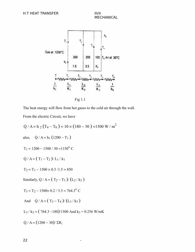
1. A composite wall consists of three layers of thicknesses 300 mm, 200mm and100mm with
thermal conductivities 1.5, 3.5 and is W/m K respectively. The inside surface is exposed to
gases at 1200°C with convection heat transfer coefficient as 30W/m2K. The temperature of
air on the other side of the wall is 30°C with convective heat transfer coefficient 10 Wm2K.
If the temperature at the outside surface of the wall is 180°C, calculate the temperature at
other surface of the wall, the rate of heat transfer and the overall heat transfer coefficient.
Solution: The composite wall and its equivalent thermal circuits is shown in the figure.
21 -
H.T HEAT TRANSFER III/IIMECHANICAL
Fig 1.1
The heat energy will flow from hot gases to the cold air through the wall.
From the electric Circuit, we have
Q / A h 2 T4 T0 10 180 30 1500 W / m2
also, Q / A h1 1200 T1
T1 1200 1500 / 30 1150o C
Q / A T1 T2 / L1 / k1
T2 T1 1500 0.3 /1.5 850
Similarly, Q / A T2 T3 / L2 / k2
T3 T2 1500 0.2 / 3.5 764.3o C
And Q / A T3 T4 / L3 / k3
L3 / k3 764.3 180/1500 And k3 = 0.256 W/mK
Q / A 1200 30/ R;
22 -
H.T HEAT TRANSFER III/IIMECHANICAL
Where R 1/ h1 L1 / k1 L 2 / k 2 L3 / k 3 1/ h2
R 1/ 30 0.3/1.5 0.2 / 3.5 0.1/ 0.256 1/10 0.75
And Q / A 1170 / 0.78 1500 W / m2
The overall heat transfer coefficient, U 1/ R 1/ 0.78 1.282 W / m 2K
Since the gas temperature is very high, we should consider the effects of radiation also.
Assuming the heat transfer coefficient due to radiation = 3.0 W/m2K the electric circuit would
be:
The combined resistance due to convection and radiation would be
1 1 1 1 1 h h 60W / m 2oCc r
R R 1 R 21 1
h c hr
Q / A 1500 60T T1 601200 T1
T1 1200 1500
60 1175o C
Again, Q / A T1 T2 / L1 / k1 T2 T1 1500 0.3 /1.5 875o C
And T T 1500 0.2 / 3.5 789.3o C3 2
L3 / k3 789.3 180/1500; k3 0.246 W / mK
R 1 0.3 0.2 0.2 0.1 1 0.781.5 3.5 0.24660 1.5 10
And U 1/ R 1.282 W / m 2K .
2.Derivethe General Heat Conduction Equation for an Isotropic Solid with Constant
Thermal Conductivity in Cartesian coordinates. (AU 2014,2013)
Any physical phenomenon is generally accompanied by a change in space and time of
its physical properties. The heat transfer by conduction in solids can only take place when there
is a variation of temperature, in both space and time. Let us consider a small volume of a solid
23 -
H.T HEAT TRANSFER III/II MECHANICAL
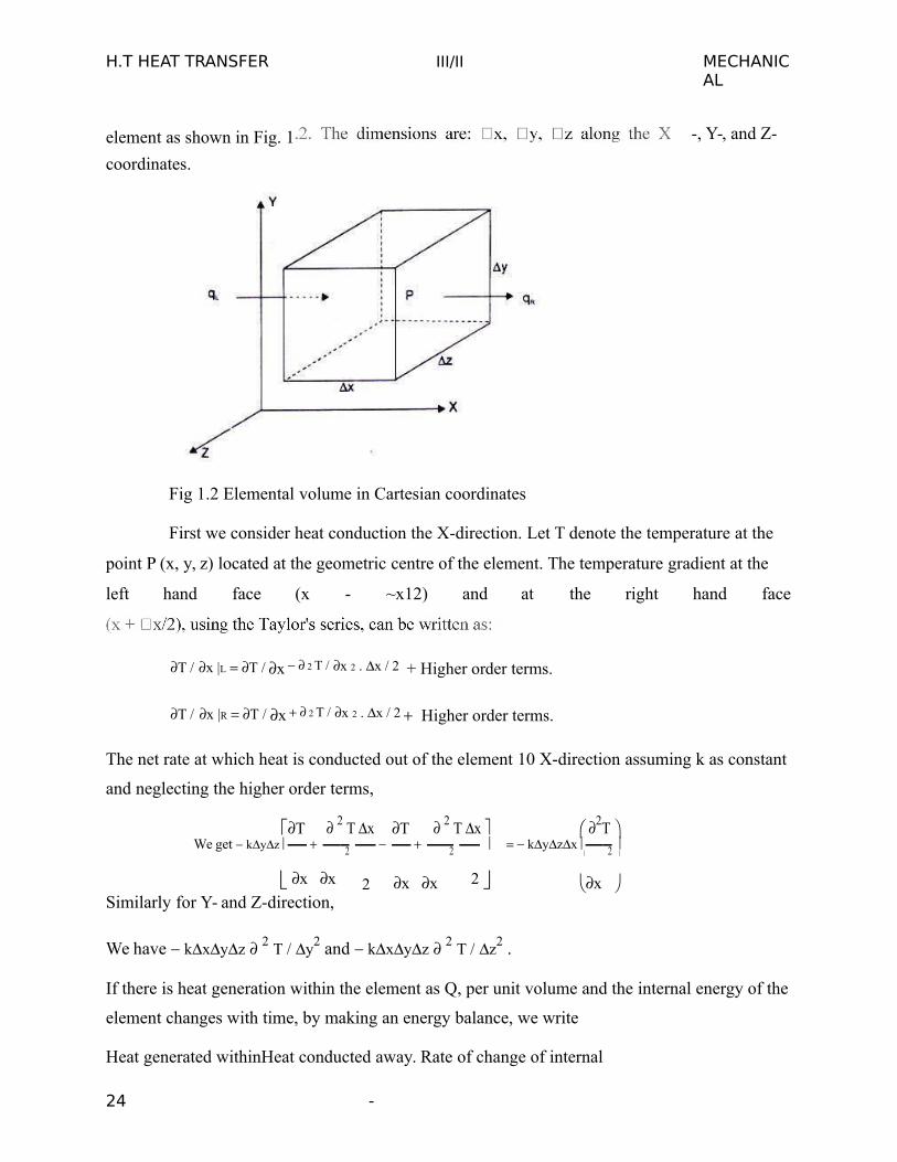
element as shown in Fig. 1
coordinates.
-, Y-, and Z-
Fig 1.2 Elemental volume in Cartesian coordinates
First we consider heat conduction the X-direction. Let T denote the temperature at the
point P (x, y, z) located at the geometric centre of the element. The temperature gradient at the
left hand face (x - ~x12) and at the right hand face
T / x |L T / x 2 T / x 2 . x / 2 + Higher order terms.
T / x |R T / x 2 T / x 2 . x / 2 Higher order terms.
The net rate at which heat is conducted out of the element 10 X-direction assuming k as constant
and neglecting the higher order terms,
T 2 T x T 2 T x 2T We get kyz kyzx 2 2 2
x x 2 x x 2
x
Similarly for Y- and Z-direction,
We have kxyz 2 T / y2 and kxyz 2 T / z2 .
If there is heat generation within the element as Q, per unit volume and the internal energy of the
element changes with time, by making an energy balance, we write
Heat generated withinHeat conducted away. Rate of change of internal
24 -

H.T HEAT TRANSFER III/IIMECHANICAL
The element from the elementenergy within with the element
Or, Q v xyz k xyz 2 T / x 2 2 T / y 2 2 T / z2
c xyz T / t
Upon simplification, 2 T / x 2 2 T / y 2 2 T / z 2 Q v / k
kc T / t
Or, 2TQv/ k1/T /t
Where k / . c , is called the thermal diffusivity and is seen to be a physical property of the
material of which the solid is composed.
The Eq. (2.la) is the general heat conduction equation for an isotropic solid with a constant
thermal conductivity. The equation rdinates
is written as:
2 T / r 2 1/ r T / r 1/ r 2 2 T / 2 2 T / z 2 Q v/ k
1 T 1 T 1 2 T Q v r
2 sin r
2
r2
r2
sin2
2
kr r sin
1/ T / t
1 T t
(2.1b)
(2.1c)
Under steady state or stationary condition, the temperature of a body does not vary with time, i.e.
T / t 0 . And, with no internal generation, the equation (2.1) reduces to
2 T 0
It should be noted that Fourier law can always be used to compute the rate of heat transfer by
conduction from the knowledge of temperature distribution even for unsteady condition and with
internal heat generation.
3. A 20 cm thick slab of aluminums (k = 230 W/mK) is placed in contact with a 15 cm thickstainless steel plate (k = 15 W/mK). Due to roughness, 40 percent of the area is in directcontact and the gap (0.0002 m) is filled with air (k = 0.032 W/mK). The difference intemperature between the two outside surfaces of the plate is 200°C Estimate (i) the heatflow rate, (ii) the contact resistance, and (iii) the drop in temperature at the interface.
25 -

H.T HEAT TRANSFER III/IIMECHANICAL
(AU 2010)
Solution: Let us assume that out of 40% area m direct contact, half the surface area is occupied
by steel and half is occupied by aluminums.
The physical system and its analogous electric circuits is shown in Fig. 1.3.
R 0.2 0.00087 , R 0.0002 4.348 106
12301
2230 0.2
R 0.0002 1.04 102 , R 0.0002 6.667 10
5
3 0.64
0.032 15 0.2
And R 0.15 0.015 151
Again 1/ R 2,3, 4 1/ R 2 1/ R 3 1/ R4
2.3 105 96.15 1.5 104 24.5 104
Therefore, R 2, 3, 4 4.08 106
Fig 1.3
Total resistance, R R1 R 2,3, 4 R5
870 106 4.08 10
6 1000 10 6 1.0874 10
2
Heat flow rate, Q = 200/1.087 × 10–2 = 18.392 kW per unit depth of the plate.
Contact resistance, R R 2, 3, 4 4.08 106 mK / W
26 -

H.T HEAT TRANSFER III/IIMECHANICAL
–6 × 18392 = 0.075oC
4. A steel pipe. Inside diameter 100 mm, outside diameter 120 mm (k 50 W/m K) ISInsulated with a40mm thick hightemperature Insulation(k = 0.09 W/m K) and anotherInsulation 60 mm thick (k = 0.07 W/m K). The ambient temperature IS 25°C. Theheattransfer coefficient for the inside and outside surfaces are 550 and 15 W/m2Krespectively. The pipe carries steam at 300oC. Calculate (1) the rate of heat loss by steamper unit length of the pipe (11) the temperature of the outside surface .
Solution: A cross-section of the pipe with two layers of insulation is shown Fig. 1.4with its
analogous electrical circuit.
Fig1.4A crosssection through an insulated cylinder, thermal resistances in series.
For L = 1.0 m. we have
R1–3) = 0.00579
R2, the resistance of steel pipe = ln(r2/rl
= ln(60/50
R3, resistance of high temperature Insulation
ln(r3/r2
R4 = 1n(r4/r3
R5–3) = 0.0663
27 -

H.T HEAT TRANSFER III/IIMECHANICAL
The total resistance = 2.04367
And Q T / R = (300 – 25) / 204367 = 134.56 W per meter length of pipe.
Temperatureat the outside surface. T4 = 25 + R5, Q = 25 + 134.56 × 0.0663 = 33.92o C
When the better insulating material (k = 0.07, thickness 60 mm) is placed first on the steel pipe,
the new value of R3 would be
R3 = 4 will be
R4
The total resistance = 2.15737 and Q = 275/2.15737 = 127.47 W per m length (Thus the better
insulating material be applied first to reduce the heat loss.) The overall heat transfer coefficient,
U, is obtained as U = Q / A T
–3 × 1 = 1.0054
And U = 134.56/(275 × 1.0054) = 0.487 W/m2 K.
5. Steel balls 10 mm in diameter (k = 48 W/mK), (C = 600 J/kgK) are cooled in air attemperature 35°C from an initial temperature of 750°C. Calculate the time required for thetemperature to drop to 150°C when h = 25 W/m2K and density p = 7800 kg/m3. (AU 2012).
Solution: Characteristic length, L = VIA = 4/3 r3/4 r2 = r/3 = 5 × 10-
3/3m Bi = hL/k = 25 × 5 × 10-3/ (3 × 48) = 8.68 × 10⁻⁴<< 0.1,
Since the internal resistance is negligible, we make use of lumped capacity analysis: Eq. (3.4),
( T T ) / ( Ts T )=exp(-Bi Fo) ; (150 35) / (750 35) = 0.16084
Bi × Fo = 1827; Fo = 1.827/ (8. 68 × 10-4) 2.1× 10³ Or,
t/ L2 = k/ ( CL2)t = 2100 and t = 568 = 0.158 hour
We can also compute the change in the internal energy of the object as:
U 0 U t 01 CVdT 0
1CV Ts T hA / CV exp t hAt / CV dt
s = CV T T exp hAt / CV 1 (3.5)
28 -
H.T HEAT TRANSFER III/IIMECHANICAL
= -7800 × 600 × (4/3) (5 × 10⁻³)3 (750-35) (0.16084 - 1)
= 1.47 × 10³ J = 1.47 kJ.
If we allow the time't' to go to infinity, we would have a situation that corresponds to steady state in
the new environment. The change in internal energy will be U0 - U = [ CV( Ts T ) exp(-
)- 1] = [ CV( Ts T ].
We can also compute the instantaneous heal transfer rate at any time.
Or. Q = - VCdT/dt = - VCd/dt[ T + ( Ts T )exp(-hAt/
CV) ] = hA( Ts T )[exp(-hAt/ CV)) and for t = 60s,
Q = 25 × 4 × 3.142 (5 × 10⁻³)2(750 35) [exp( -25 × 3 × 60/5 × 10-3 × 7800 ×
600)] = 4.63 W.
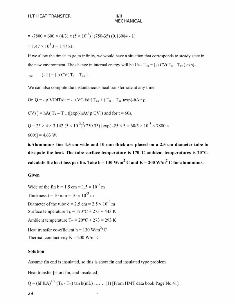
6.Aluminums fins 1.5 cm wide and 10 mm thick are placed on a 2.5 cm diameter tube to
dissipate the heat. The tube surface temperature is 170C ambient temperatures is 20C.
calculate the heat loss per fin. Take h = 130 W/m2 C and K = 200 W/m2 C for aluminums.
Given
Wide of the fin b = 1.5 cm = 1.5 10-2 m
Thickness t = 10 mm = 10 10-3 m
Diameter of the tube d = 2.5 cm = 2.5 10-2 m
Surface temperature Tb = 170C + 273 = 443 K
Ambient temperature T = 20C + 273 = 293 K
Heat transfer co-efficient h = 130 W/m2C
Thermal conductivity K = 200 W/mC
Solution
Assume fin end is insulated, so this is short fin end insulated type problem.
Heat transfer [short fin, end insulated]
Q = (hPKA)1/2 (Tb - T) tan h(mL) ……..(1) [From HMT data book Page No.41]
29 -
H.T HEAT TRANSFER III/IIMECHANICAL
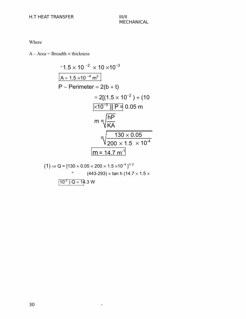
Where
A – Area = Breadth thickness
1.5 10 2 10 103
A 1.5 10 4 m2
P Perimeter 2(b t)
= 2[(1.5 102 ) (10
103 )] P = 0.05 m
m =hPKA
= 130 0.05
200 1.5 10-4
m = 14.7 m-1
(1) Q = [130 0.05 200 1.5 104 ]1/ 2
(443-293) tan h (14.7 1.5
10-2 ) Q 14.3 W
30 -

H.T HEAT TRANSFER III/IIMECHANICAL
UNIT 2
CONVECTION
2.1 Convection Heat Transfer-Requirements
The heat transfer by convection requires a solid-fluid interface, a temperature difference
between the solid surface and the surrounding fluid and a motion of the fluid. The process of heat
transfer by convection would occur when there is a movement of macro-particles of the fluid in
space from a region of higher temperature to lower temperature.
2.2. Convection Heat Transfer Mechanism
Let us imagine a heated solid surface, say a plane wall at a temperature Tw placed in an
atmosphere at temperature T , Fig. 2.1 Since all real fluids are viscous, the fluid particles
adjacent to the solid surface will stick to the surface. The fluid particle at A, which is at a lower
temperature, will receive heat energy from the plate by conduction. The internal energy of the
particle would Increase and when the particle moves away from the solid surface (wall or plate)
and collides with another fluid particle at B which is at the ambient temperature, it will transfer a
part of its stored energy to B. And, the temperature of the fluid particle at B would increase. This
way the heat energy is transferred from the heated plate to the surrounding fluid. Therefore the
process of heat transfer by convection involves a combined action of heat conduction, energy
storage and transfer of energy by mixing motion of fluid particles.
Fig. 2.1 Principle of heat transfer by convection
2.3. Free and Forced Convection
When the mixing motion of the fluid particles is the result of the density difference
31 -

H.T HEAT TRANSFER III/IIMECHANICAL
caused by a temperature gradient, the process of heat transfer is called natural or free convection.
When the mixing motion is created by an artificial means (by some external agent), the process
of heat transfer is called forced convection Since the effectiveness of heat transfer by convection
depends largely on the mixing motion of the fluid particles, it is essential to have a knowledge of
the characteristics of fluid flow.
2.4. Basic Difference between Laminar and Turbulent Flow
In laminar or streamline flow, the fluid particles move in layers such that each fluid p
article follows a smooth and continuous path. There is no macroscopic mixing of fluid particles
between successive layers, and the order is maintained even when there is a turn around a comer
or an obstacle is to be crossed. If a lime dependent fluctuating motion is observed indirections
which are parallel and transverse to t he main flow, i.e., there is a radom macroscopic mixing of
fluid particles across successive layers of fluid flow, the motion of the fluid is called' turbulent
flow'. The path of a fluid particle would then be zigzag and irregular, but on a statistical basis,
the overall motion of the macroparticles would be regular and predictable.
2.5. Formation of a Boundary Layer
When a fluid flow, over a surface, irrespective of whether the flow is laminar or
turbulent, the fluid particles adjacent to the solid surface will always stick to it and their velocity
at the solid surface will be zero, because of the viscosity of the fluid. Due to the shearing action
of one fluid layer over the adjacent layer moving at the faster rate, there would be a velocity
gradient in a direction normal to the flow.
Fig 2.2: sketch of a boundary layer on a wall
32 -
H.T HEAT TRANSFER III/IIMECHANICAL
Let us consider a two-dimensional flow of a real fluid about a solid (slender in cross-
section) as shown in Fig. 2.2. Detailed investigations have revealed that the velocity of the fluid
particles at the surface of the solid is zero. The transition from zero velocity at the surface of the
solid to the free stream velocity at some distance away from the solid surface in the V-direction
(normal to the direction of flow) takes place in a very thin layer called 'momentum or
hydrodynamic boundary layer'. The flow field can thus be divided in two regions:
( i) A very thin layer in t he vicinity 0 f t he body w here a velocity gradient normal to
the direction of flow exists, the velocity gradient du/dy being large. In this thin region, even a
very small Viscosity of the fluid exerts a substantial Influence and the shearing stress
du/dy may assume large values. The thickness of the boundary layer is very small and decreases
with decreasing viscosity.
(ii) In the remaining region, no such large velocity gradients exist and the Influence of
viscosity is unimportant. The flow can be considered frictionless and potential.
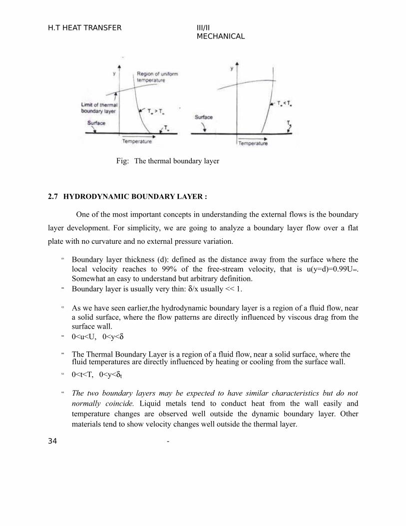
2.6. Thermal Boundary Layer
Since the heat transfer by convection involves the motion of fluid particles, we must
superimpose the temperature field on the physical motion of fluid and the two fields are bound to
interact. It is intuitively evident that the temperature distribution around a hot body in a fluid
stream will often have the same character as the velocity distribution in the boundary layer flow.
When a heated solid body IS placed In a fluid stream, the temperature of the fluid stream will
also vary within a thin layer In the immediate neighbourhood of the solid body. The variation in
temperature of the fluid stream also takes place in a thin layer in the neighbourhood of the body
and is termed 'thermal boundary layer'. Fig. shows the temperature profiles inside a thermal
boundary layer.
33 -
H.T HEAT TRANSFER III/IIMECHANICAL
Fig: The thermal boundary layer
2.7 HYDRODYNAMIC BOUNDARY LAYER :
One of the most important concepts in understanding the external flows is the boundary
layer development. For simplicity, we are going to analyze a boundary layer flow over a flat
plate with no curvature and no external pressure variation.
Boundary layer thickness (d): defined as the distance away from the surface where thelocal velocity reaches to 99% of the free-stream velocity, that is u(y=d)=0.99U.Somewhat an easy to understand but arbitrary definition.
Boundary layer is usually very thin: /x usually << 1.
As we have seen earlier,the hydrodynamic boundary layer is a region of a fluid flow, neara solid surface, where the flow patterns are directly influenced by viscous drag from thesurface wall.
0<u<U, 0<y<
The Thermal Boundary Layer is a region of a fluid flow, near a solid surface, where the fluid temperatures are directly influenced by heating or cooling from the surface wall.
0<t<T, 0<y<t
The two boundary layers may be expected to have similar characteristics but do notnormally coincide. Liquid metals tend to conduct heat from the wall easily andtemperature changes are observed well outside the dynamic boundary layer. Othermaterials tend to show velocity changes well outside the thermal layer.
34 -
H.T HEAT TRANSFER III/IIMECHANICAL
2.8 FREE AND FORCED CONVECTION DURING EXTERNAL FLOW OVER
PLATES :
Dimensionless Parameters and their Significance
The following dimensionless parameters are significent in evaluating the convection
heat transfer coefficient:
(a) The Nusselt Number (Nu)-It is a dimensionless quantity defined as hL/ k, where h =
convective heat transfer coefficient, L is the characteristic length and k is the thermal
conductivity of the fluid The Nusselt number could be interpreted physically as the ratio of the
temperature gradient in the fluid immediately in contact with the surface to a reference temperature
gradient (Ts - T ) /L. The convective heat transfer coefficient can easily be obtained
if the Nusselt number, the thermal conductivity of the fluid in that temperature range and the
characteristic dimension of the object is known.
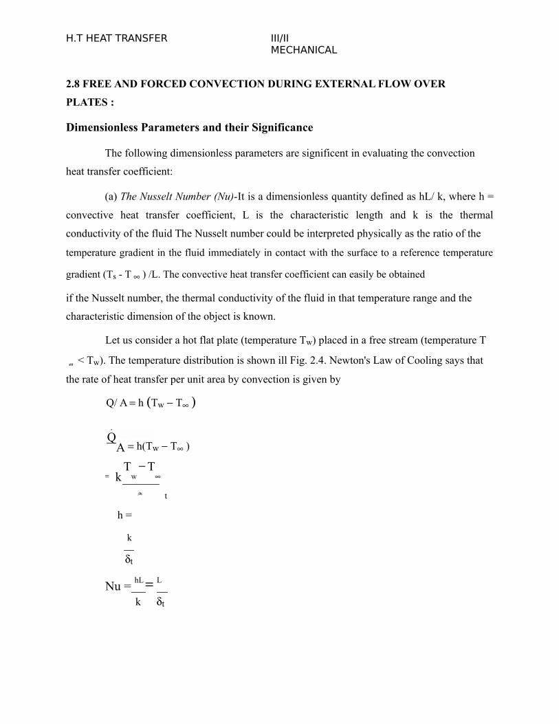
Let us consider a hot flat plate (temperature Tw) placed in a free stream (temperature T
< Tw). The temperature distribution is shown ill Fig. 2.4. Newton's Law of Cooling says that
the rate of heat transfer per unit area by convection is given by
Q/ A h Tw T
QA h(Tw T )
= k T
w
T
t
h =
k
t
Nu =hL L
k t

35 -
H.T HEAT TRANSFER III/IIMECHANICAL
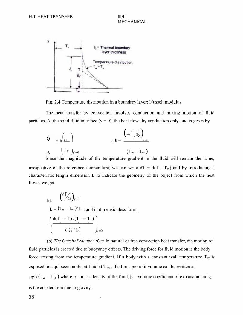
Fig. 2.4 Temperature distribution in a boundary layer: Nusselt modulus
The heat transfer by convection involves conduction and mixing motion of fluid
particles. At the solid fluid interface (y = 0), the heat flows by conduction only, and is given by
Q kdT dy
k dT h = y 0
Tw T A dy Y 0
Since the magnitude of the temperature gradient in the fluid will remain the same,
irrespective of the reference temperature, we can write dT = d(T - Tw) and by introducing a
characteristic length dimension L to indicate the geometry of the object from which the heat
flows, we get
hL
dT dyy 0
, and in dimensionless form,k Tw T / L
d(T T) /(T T ) = w w
d y / L
y 0
(b) The Grashof Number (Gr)-In natural or free convection heat transfer, die motion of
fluid particles is created due to buoyancy effects. The driving force for fluid motion is the body
force arising from the temperature gradient. If a body with a constant wall temperature Tw is
exposed to a qui scent ambient fluid at T , the force per unit volume can be written as
g tw T where = mass density of the fluid, = volume coefficient of expansion and g
is the acceleration due to gravity.
36 -
H.T HEAT TRANSFER III/IIMECHANICAL
The ratio of inertia force × Buoyancy force/(viscous force)2 can be written as
Gr V2 L2 g Tw T L3
VL2
=
2
g
T
w 2
T
L3 g L3 Tw T / 2
The magnitude of Grashof number indicates whether the flow is laminar or turbulent. If
the Grashof number is greater than 109, the flow is turbulent and for Grashof number less than
108, the flow is laminar. For 108 < Gr < 109, It is the transition range.
The Prandtl Number (Pr) - It is a dimensionless parameter defined
as Pr = Cp / k /
where is the dynamic viscosity of the fluid, v = kinematic viscosity and = thermal
diffusivity.
This number assumes significance when both momentum and energy are propagated
through the system. It is a physical parameter depending upon the properties of the medium It is
a measure of the relative magnitudes of momentum and thermal diffusion in the fluid: That is, for
Pr = I, the r ate of diffusion of momentum and energy are equal which means that t he calculated
temperature and velocity fields will be Similar, the thickness of the momentum and thermal
boundary layers will be equal. For Pr <<I (in case of liquid metals), the thickness of the thermal
boundary layer will be much more than the thickness of the momentum boundary layer and vice
versa. The product of Grashof and Prandtl number is called Rayleigh number. Or, Ra = Gr × Pr.
2.9 Evaluation of Convective Heat Transfer Coefficient
The convective heat transfer coefficient in free or natural convection can be evaluated
by two methods:
(a) Dimensional Analysis combined with experimental investigations
(b) Analytical solution of momentum and energy equations 10 the boundary layer.
Dimensional Analysis and Its Limitations
37 -
H.T HEAT TRANSFER III/IIMECHANICAL
Since the evaluation of convective heat transfer coefficient is quite complex, it is based
on a combination of physical analysis and experimental studies. Experimental observations
become necessary to study the influence of pertinent variables on the physical phenomena.
Dimensional analysis is a mathematical technique used in reducing the number of
experiments to a minimum by determining an empirical relation connecting the relevant
variables and in grouping the variables together in terms of dimensionless numbers. And, the
method can only be applied after the pertinent variables controlling t he phenomenon are
Identified and expressed In terms of the primary dimensions. (Table 1.1)
In natural convection heat transfer, the pertinent variables are: h, , k, , Cp, L, ( T),
and g. Buckingham 's method provides a systematic technique for arranging the variables in
dimensionless numbers. It states that the number of dimensionless groups, ’s, required to
describe a phenomenon involving 'n' variables is equal to the number of variables minus the
number of primary dimensions 'm' in the problem.
In SI system of units, the number of primary dimensions are 4 and the number of
variables for free convection heat transfer phenomenon are 9 and therefore, we should expect (9 -
4) = 5 dimensionless numbers. Since the dimension of the coefficient of volume expansion, , is
1 , one dimensionless number is obviously ( T). The remaining variables are written in a
functional form:
h, , k, , C p , L, g= 0.
Since the number of primary dimensions are 4, we arbitrarily choose 4 independent
variables as primary variables such that all the four dimensions are represented. The selected
primary variables are: ,g, k. L Thus the dimensionless group,
1 a g b k c Ld h ML3 a LT
2 b . MLT 31 M 0 L0 T0 0
Equating the powers of M, L, T, on both sides, we have

38 -
H.T HEAT TRANSFER III/IIMECHANICAL
M : a + c + 1 = 0 } Upon solving them,
L : -3a + b + c + d = 0
T : -2b -3c -3 = 0Up on solving them,
: -c - 1 = 0
c = 1, b = a = 0 and d = 1.
and 1 = hL/k, the Nusselt number.
The other dimensionless number
2= pagbkcLdCp = (ML-3)a (LT-2)b(MLT-3 -1)c(L)d(MT-1 1
) = M0L0T0 0 Equating
the powers of M,L,T and and upon solving, we get
3= 2 / 2 g L3
By combining 2 and 3 , we write 4 2 3 1/ 2
= 2 gL3C 2 / k 2 2 / gL3 1/ 2
= Cp (the Prandtl number) p k
By combining
3 with T, we have
5= T* 1
3
2 gL3
= T g T L3 / 2 (the Grashof number)2
Therefore, the functional relationship is expressed as:
Nu, Pr, Gr 0;Or, Nu 1 Gr Pr Const Gr Pr m(2.1)
and values of the constant and 'm' are determined experimentally.
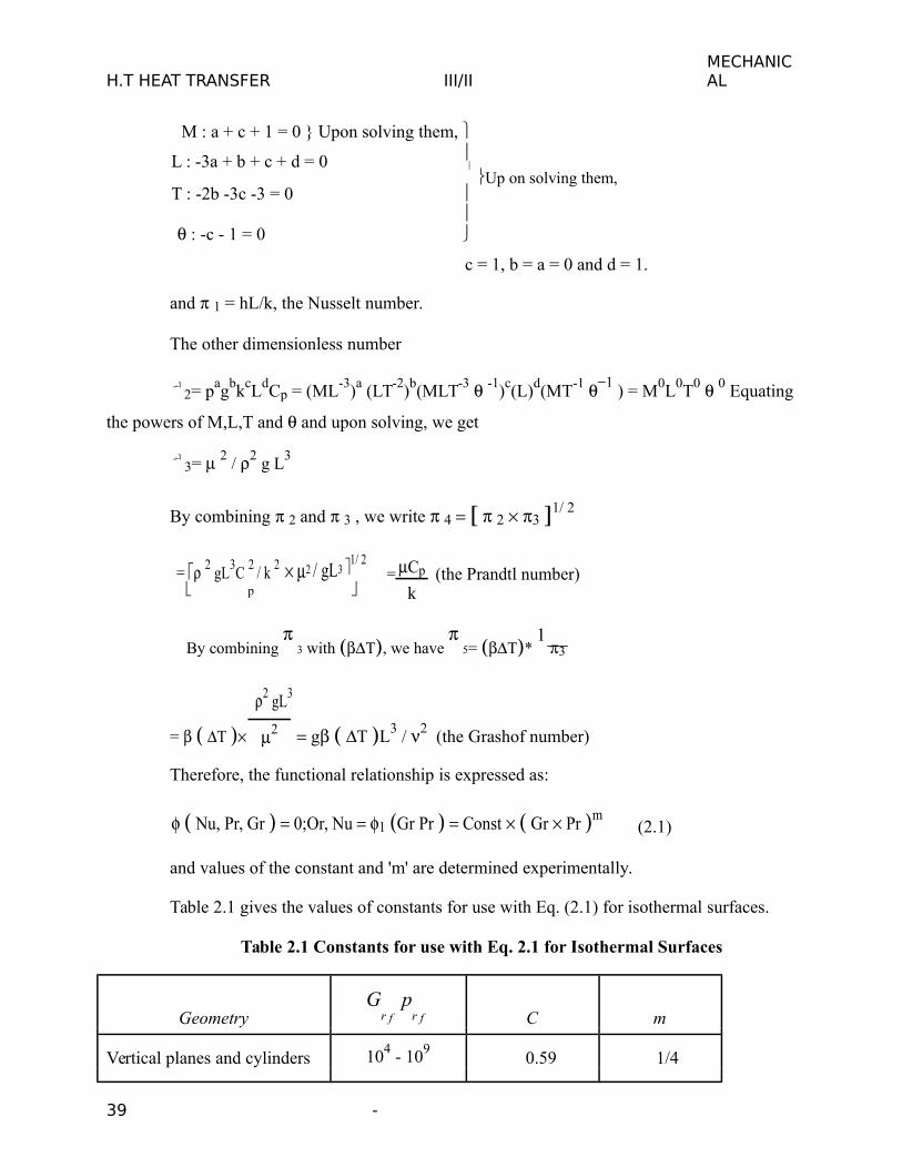
Table 2.1 gives the values of constants for use with Eq. (2.1) for isothermal surfaces.
Table 2.1 Constants for use with Eq. 2.1 for Isothermal Surfaces
GeometryG
r f p
r f C m
Vertical planes and cylinders 104 - 1090.59 1/4
39 -

H.T HEAT TRANSFER III/IIMECHANICAL
Horizontal cylinders
Upper surface of heated
plates or lower surface of
cooled plates
- do -
Lower surface of heated
plates or upper surface of
cooled plates
Vertical cylinder height =
diameter characteristic length
= diameter
Irregular solids, characteristic
length = distance the fluid
particle travels in boundary
layer
109 - 10130.021 2/5
109 - 10130.10 1/3
0 - 10-50.4 0
104 - 1090.53 1/4
109 - 10120.13 1/3
1010 - 10-20.675 0.058
10-2 - 1021.02 0.148
102 - 1040.85 0.188
104 - 1070.48 1/4
107 - 10120.125 1/3
8 × 10⁶ - 10110.15 1/3
2 × 10⁴ - 8 × 1060.54 1/4
105 - 10110.27 1/4
104 - 1060.775 0.21
104 - 1090.52 1/4
Analytical Solution-Flow over a Heated Vertical Plate in Air
40 -
H.T HEAT TRANSFER III/IIMECHANICAL
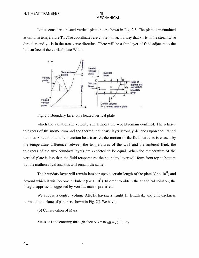
Let us consider a heated vertical plate in air, shown in Fig. 2.5. The plate is maintained
at uniform temperature Tw .The coordinates are chosen in such a way that x - is in the streamwise
direction and y - is in the transverse direction. There will be a thin layer of fluid adjacent to the
hot surface of the vertical plate Within
Fig. 2.5 Boundary layer on a heated vertical plate
which the variations in velocity and temperature would remain confined. The relative
thickness of the momentum and the thermal boundary layer strongly depends upon the Prandtl
number. Since in natural convection heat transfer, the motion of the fluid particles is caused by
the temperature difference between the temperatures of the wall and the ambient fluid, the
thickness of the two boundary layers are expected to be equal. When the temperature of the
vertical plate is less than the fluid temperature, the boundary layer will form from top to bottom
but the mathematical analysis will remain the same.
The boundary layer will remain laminar upto a certain length of the plate (Gr < 108) and
beyond which it will become turbulent (Gr > 109). In order to obtain the analytical solution, the
integral approach, suggested by von-Karman is preferred.
We choose a control volume ABCD, having a height H, length dx and unit thickness
normal to the plane of paper, as shown in Fig. 25. We have:
(b) Conservation of Mass:
Mass of fluid entering through face AB = m AB 0H udy
41 -

H.T HEAT TRANSFER III/IIMECHANICAL
Mass of fluid leaving face CD = m CD 0H udy dx
d 0
H udy dx
Mass of fluid entering the face DA = dxd
0
H udy
dx
(ii) Conservation of Momentum :
Momentum entering face AB = 0H u 2dy
Momentum leaving face CD = 0H u 2 dy dx
d 0
H u 2dy dx
Net efflux of momentum in the + x-direction = dxd
0
H u
2dy
dx
The external forces acting on the control volume are:
(a) Viscous force = du dx acting in the –ve x-directiondy y 0
(b) Buoyant force approximated as 0
H g T T dy dx
From Newton’s law, the equation of motion can be written as:
d u 2dy
du gT T dy (2.2)0 0
dx dy y 0
because the value of the integrand between and H would be zero.
(iii) Conservation of Energy:
QAB ,convection + QAD ,convection + QBC ,conduction = QCD convection
H d H dTor, 0 uCTdy CT 0 udy dx k dx
dx dy y 0
= 0H uCTdy dx
d 0
H uTCdy dx

42 -
H.T HEAT TRANSFER
d
u T T dy
k dT
or 0dx C dy
The boundary conditions are:
or,
(2.3)
Velocity profile
u = 0 at y = 0
u = 0 at y =
du/dy = 0 at y =
III/II MECHANICAL
dT
(2.3)y 0 dy y 0
Temperature profile
T = Tw at y = 0
T = T at y = 1
dT/dy 0 at y = 1
Since the equations (2.2) and (2.3) are coupled equations, it is essential that the
functional form of both the velocity and temperature distribution are known in order to arrive at a
solution.
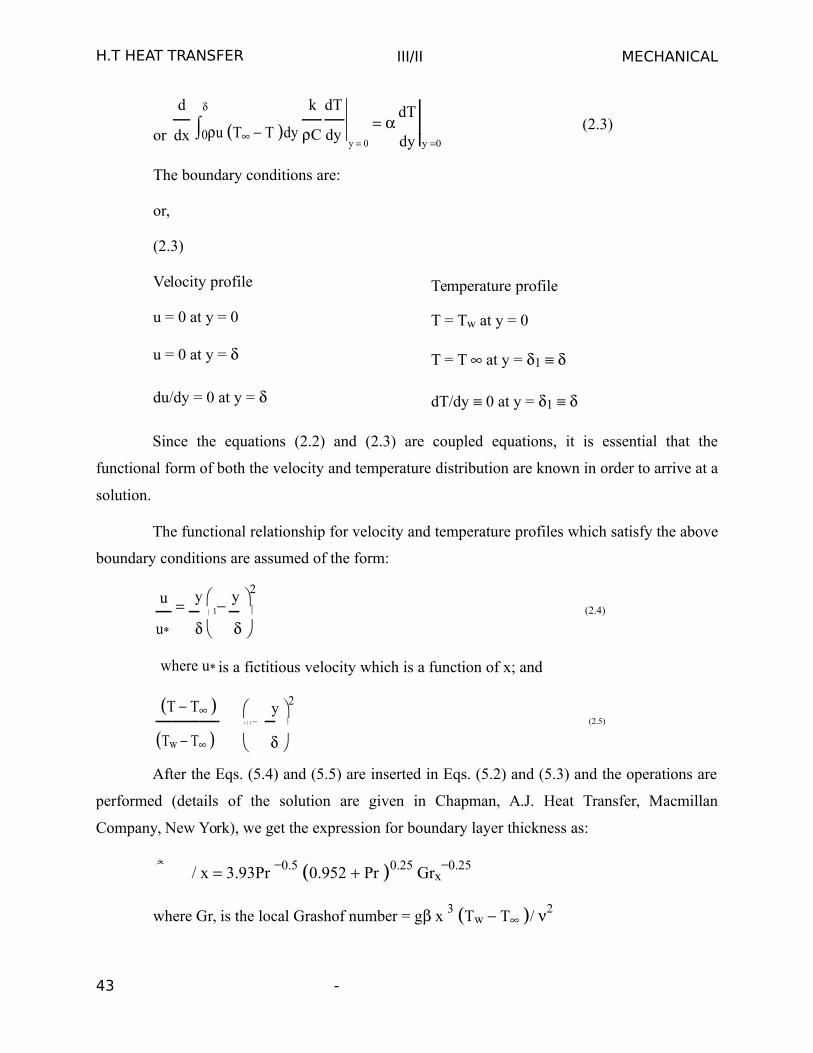
The functional relationship for velocity and temperature profiles which satisfy the above
boundary conditions are assumed of the form:
u y y 2
1 (2.4)
u*
where u* is a fictitious velocity which is a function of x; and
T T y 2
1 (2.5)
Tw T
After the Eqs. (5.4) and (5.5) are inserted in Eqs. (5.2) and (5.3) and the operations are
performed (details of the solution are given in Chapman, A.J. Heat Transfer, Macmillan
Company, New York), we get the expression for boundary layer thickness as:
/ x 3.93Pr 0.5 0.952 Pr 0.25 Grx
0.25
where Gr, is the local Grashof number = g x 3 Tw T / 2
43 -
H.T HEAT TRANSFER III/IIMECHANICAL
The heat transfer coefficient can be evaluated from:
q w k dT h Tw T dy y 0
Using Eq. (5.5) which gives the temperature distribution, we have
h = 2k/ or, hx/k = Nux= 2x/
The non-dimensional equation for the heat transfer coefficient is
Nux= 0.508 Pr0.5 (0.952 + Pr)-0.25 Grx0.25
(2.7)
The average heat transfer coefficient, h L1
0L h x dx 4 / 3hx L
NuL= 0.677 Pr0.5 (0.952 + Pr)-0.25 Gr0.25
(2.8)
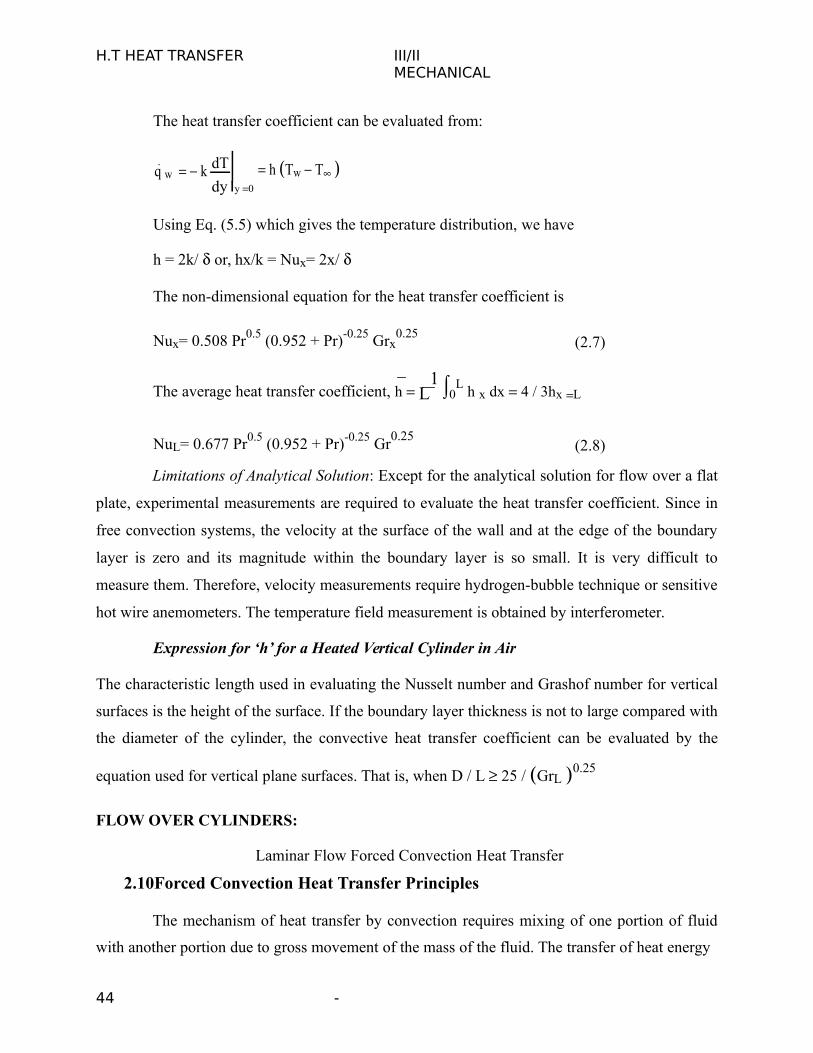
Limitations of Analytical Solution: Except for the analytical solution for flow over a flat
plate, experimental measurements are required to evaluate the heat transfer coefficient. Since in
free convection systems, the velocity at the surface of the wall and at the edge of the boundary
layer is zero and its magnitude within the boundary layer is so small. It is very difficult to
measure them. Therefore, velocity measurements require hydrogen-bubble technique or sensitive
hot wire anemometers. The temperature field measurement is obtained by interferometer.
Expression for ‘h’ for a Heated Vertical Cylinder in Air
The characteristic length used in evaluating the Nusselt number and Grashof number for vertical
surfaces is the height of the surface. If the boundary layer thickness is not to large compared with
the diameter of the cylinder, the convective heat transfer coefficient can be evaluated by the
equation used for vertical plane surfaces. That is, when D / L 25 / GrL 0.25
FLOW OVER CYLINDERS:
Laminar Flow Forced Convection Heat Transfer
2.10Forced Convection Heat Transfer Principles
The mechanism of heat transfer by convection requires mixing of one portion of fluid
with another portion due to gross movement of the mass of the fluid. The transfer of heat energy
44 -

H.T HEAT TRANSFER III/IIMECHANICAL
from one fluid particle or a molecule to another one is still by conduction but the energy is
transported from one point in space to another by the displacement of fluid.
When the motion of fluid is created by the imposition of external forces in the form of
pressure differences, the process of heat transfer is called ‘forced convection’. And, the motion of
fluid particles may be either laminar or turbulent and that depends upon the relative magnitude of
inertia and viscous forces, determined by the dimensionless parameter Reynolds number. In free
convection, the velocity of fluid particle is very small in comparison with the velocity of fluid
particles in forced convection, whether laminar or turbulent. In forced convection heat transfer,
Gr/Re2<< 1, in free convection heat transfer, GrRe2>>1 and we have combined free and forced
convection when Gr/Re2 1.
Methods for Determining Heat Transfer Coefficient
The convective heat transfer coefficient in forced flow can be evaluated by:
Dimensional Analysis combined with experiments;
(a)
(b) Reynolds Analogy – an analogy between heat and momentum transfer;
Analytical Methods – exact and approximate analyses of boundary layer
(c)
equations.
2.11 Method of Dimensional Analysis
As pointed out in Chapter 5, dimensional analysis does not yield equations which can be
solved. It simply combines the pertinent variables into non-dimensional numbers which facilitate
the interpretation and extend the range of application of experimental data. The relevant
variables for forced convection heat transfer phenomenon whether laminar or turbulent, are
(b) the properties of the fluid – density p, specific heat capacity Cp, dynamic or
absolute viscosity , thermal conductivity k.
(ii) the properties of flow – flow velocity Y, and the characteristic dimension of the
system L.
k) = 0
As such, the convective heat transfer coefficient, h, is written as h = f ( , V, L,
(5.14)
, Cp,
Since there are seven variables and four primary dimensions, we would expect three
45 -
H.T HEAT TRANSFER III/IIMECHANICAL
dimensionless numbers. As before, we choose four independent or core variables as ,V, L, k,
and calculate the dimensionless numbers by applying Buckingham ’s method:
1 = a V b Lc K d h ML
3 a LT
1 b L c MLT
3 1 d MT
3
1 = M o Lo To o
M : a + d + 1 = O
L : - 3a + b + c + d = 0
T : - b – 3d – 3 = 0
: - d – 1= 0.
By solving them, we have
D = -1, a = 0, b = 0, c = 1.
Therefore, 1 = hL/k is the Nusselt number.
2 = a V b Lc K d ML
3 a LT
1 b L c MLT
31 d ML
1T
1
= M o Lo To o
: - d = 0.
By solving them, d = 0, b = - 1, a = - 1, c = - 1
and /VL;or,1
VL
2 3 2
(Reynolds number is a flow parameter of greatest significance. It is the ratio of inertia
forces to viscous forces and is of prime importance to ascertain the conditions under which a
flow is laminar or turbulent. It also compares one flow with another provided the corresponding
length and velocities are comparable in two flows. There would be a similarity in flow between
46 -
H.T HEAT TRANSFER III/IIMECHANICAL
two flows when the Reynolds numbers are equal and the geometrical similarities are taken into
consideration.)
4 a V b Lc k d C p ML3 a LT
1 b L c MLT 31 d L2 T
2 1
M o Lo To o
Equating the powers of M, L, T, on both Sides, we get
M : a + d = 0; L : - 3a + b + c + d + 2 = 0
T : - b – 3d – 2 = 0; : - d – 1 = 0
By solving them,
d =- 1,a = l, b = l, c = l,
VL C ; 4 4 2k p 5
VLC
=Cp
pk VL k
5 is Prandtl number.
Therefore, the functional relationship is expressed as:
Nu = f (Re, Pr); or Nu = C Rem Prn(5.15)
where the values of c, m and n are determined experimentally.
2.12 Principles of Reynolds Analogy
Reynolds was the first person to observe that there exists a similarity between the
exchange of momentum and the exchange of heat energy in laminar motion and for that reason it
has been termed ‘Reynolds analogy’. Let us consider the motion of a fluid where the fluid is
flowing over a plane wall. The X-coordinate is measured parallel to the surface and the V-
coordinate is measured normal to it. Since all fluids are real and viscous, there would be a thin
layer, called momentum boundary layer, in the vicinity of the wall where a velocity gradient
normal to the direction of flow exists. When the temperature of the surface of the wall is
different than the temperature of the fluid stream, there would also be a thin layer, called thermal
47 -
H.T HEAT TRANSFER III/IIMECHANICAL
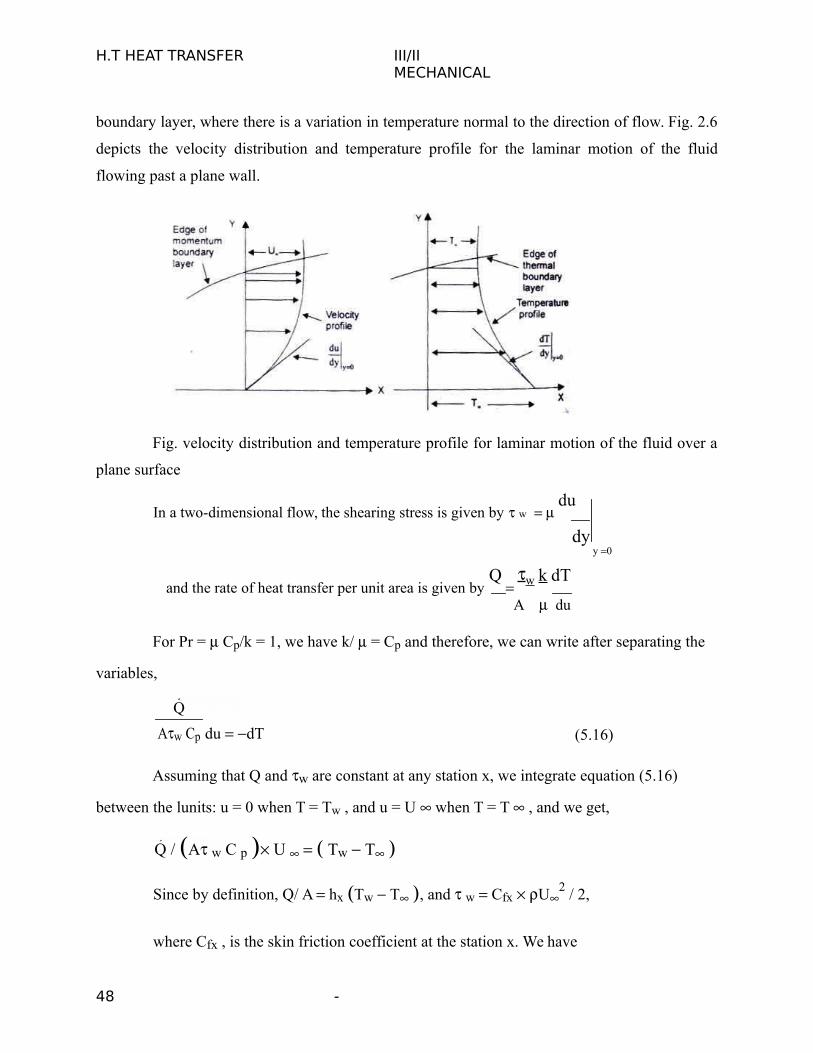
boundary layer, where there is a variation in temperature normal to the direction of flow. Fig. 2.6
depicts the velocity distribution and temperature profile for the laminar motion of the fluid
flowing past a plane wall.
Fig. velocity distribution and temperature profile for laminar motion of the fluid over a
plane surface
In a two-dimensional flow, the shearing stress is given by w du
dy y 0
and the rate of heat transfer per unit area is given by Q
w
k dT
A du
For Pr = Cp/k = 1, we have k/ = Cp and therefore, we can write after separating the
variables,
Q
du dT (5.16)Aw Cp
Assuming that Q and w are constant at any station x, we integrate equation (5.16)
between the lunits: u = 0 when T = Tw , and u = U when T = T , and we get,
Q / A w C p U Tw T
Since by definition, Q/ A hx Tw T , and w Cfx U2 / 2,
where Cfx , is the skin friction coefficient at the station x. We have
48 -

H.T HEAT TRANSFER III/II MECHANICAL
Cfx /2 = hx/ (Cp U ) (5.17)
Since h x / CpU h x. x / k / U k / .C p Nu x / Re.Pr ,
Nu x / Re.Pr Cfx / 2 Stan tonnumer,St. (5.18)
Equation (5.18) is satisfactory for gases in which Pr is approximately equal to unity.
Colburn has shown that Eq. (5.18) can also be used for fluids having Prandtl numbers ranging
from 0.6 to about 50 if it is modified in accordance with experirnental results.
Or, Nux .Pr 2 / 3 Stx
Pr 2 / 3 Cfx
/ 2 (5.19)
Re x Pr
Eq. (5.19) expresses the relation between fluid friction and heat transfer for laminar
flow over a plane wall. The heat transfer coefficient could thus be determined by making
measurements of the frictional drag on a plate under conditions in which no heat transfer is
involved.
2.13 Analytical Evaluation of ‘h’ for Laminar Flow over a Flat Plat – Assumptions
As pointed out earlier, when the motion of the fluid is caused by the imposition of
external forces, such as pressure differences, and the fluid flows over a solid surface, at a
temperature different from the temperature of the fluid, the mechanism of heat transfer is called
‘forced convection’. Therefore, any analytical approach to determine the convective heat transfer
coefficient would require the temperature distribution in the flow field surrounding the body.
That is, the theoretical analysis would require the use of the equation of motion of the viscous
fluid flowing over the body along with the application of the principles of conservation of mass
and energy in order to relate the heat energy that is convected away by the fluid from the solid
surface.
For the sake of simplicity, we will consider the motion of the fluid in 2 space dimension, and a
steady flow. Further, the fluid properties like viscosity, density, specific heat, etc are constant in
the flow field, the viscous shear forces m the Y –direction is negligible and there are no
variations in pressure also in the Y –direction.
49 -

H.T HEAT TRANSFER III/IIMECHANICAL
2.14 Derivation of the Equation of Continuity–Conservation of Mass
We choose a control volume within the laminar boundary layer as shown in Fig. 6.2. The mass
will enter the control volume from the left and bottom face and will leave the control volume
from the right and top face. As such, for unit depth in the Z-direction, u
m udy ; m u .dx dy;
mAB vdx ; mCD v
dy
u .dy
dx;
For steady flow conditions, the net efflux of mass from the control volume is zero, therefore,
50 -

H.T HEAT TRANSFER III/IIMECHANICAL
Fig. 2.7 a differential control volume within the boundary layer for laminar flow over a plane
wall
udy xdx udy u dxdy vdx v .dxdyxx
or, u / x v y 0, the equation of continuity. (2.20)
2.15 Concept of Critical Thickness of Insulation
The addition of insulation at the outside surface of small pipes may not reduce the rate of heat
transfer. When an insulation is added on the outer surface of a bare pipe, its outer radius, r0
increases and this increases the thermal resistance due to conduction logarithmically whereas t he
thermal resistance to heat flow due to fluid film on the outer surface decreases linearly with
increasing radius, r0. Since the total thermal resistance is proportional to the sum of these two
resistances, the rate of heat flow may not decrease as insulation is added to the bare pipe.
Fig. 2.7 shows a plot of heat loss against the insulation radius for two different cases.
For small pipes or wires, the radius rl may be less than re and in that case, addition of insulation
to the bare pipe will increase the heat loss until the critical radius is reached. Further addition of
insulation will decrease the heat loss rate from this peak value. The insulation thickness (r* – rl)
must be added to reduce the heat loss below the uninsulated rate. If the outer pipe radius r l is
greater than the critical radius re any insulation added will decrease the heat loss.
51 -

H.T HEAT TRANSFER III/IIMECHANICAL
2.16 Expression for Critical Thickness of Insulation for a Cylindrical Pipe
Let us consider a pipe, outer radius rl as shown in Fig. 2.18. An insulation is added such that the
outermost radius is r a variable and the insulation thickness is (r – rI). We assume that the thermal
conductivity, k, for the insulating material is very small in comparison with the thermal
conductivity of the pipe material and as such the temperature T1, at the inside surface of the
insulation is constant. It is further assumed that both h and k are constant. The rate of heat flow,
per unit length of pipe, through the insulation is then,
Q / L 2 T1 T / ln r / r1 / k 1/ hr , where T is the ambient temperature.
Fig 2.8 Critical thickness for pipe insulation
52 -
H.T HEAT TRANSFER III/IIMECHANICAL
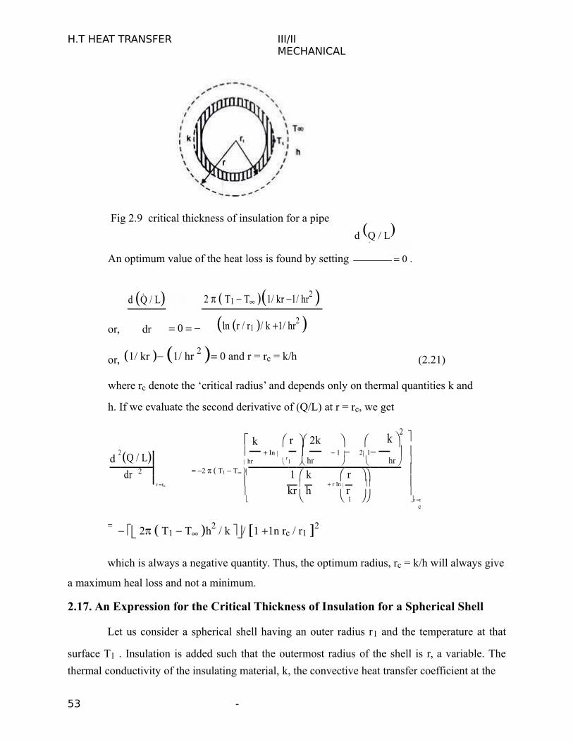
Fig 2.9 critical thickness of insulation for a pipe
d Q / L
An optimum value of the heat loss is found by setting 0.
or,
d Q / L 0
2 T1 T 1/ kr 1/ hr2 dr ln r / r1 / k 1/ hr2
or, 1/ kr 1/ hr 2 0 and r = rc = k/h (2.21)
where rc denote the ‘critical radius’ and depends only on thermal quantities k and
h. If we evaluate the second derivative of (Q/L) at r = rc, we get
k r 2k k 2
d2Q / L In 1 2 1
hr r1 hr hr
2 T1 T dr 2 1 k r r rc r In kr h r
1 r r
c
= 2 T1 T h2 / k / 1 1n rc / r1 2
which is always a negative quantity. Thus, the optimum radius, rc = k/h will always give
a maximum heal loss and not a minimum.
2.17. An Expression for the Critical Thickness of Insulation for a Spherical Shell
Let us consider a spherical shell having an outer radius r1 and the temperature at that
surface T1 . Insulation is added such that the outermost radius of the shell is r, a variable. The
thermal conductivity of the insulating material, k, the convective heat transfer coefficient at the
53 -
H.T HEAT TRANSFER III/IIMECHANICAL
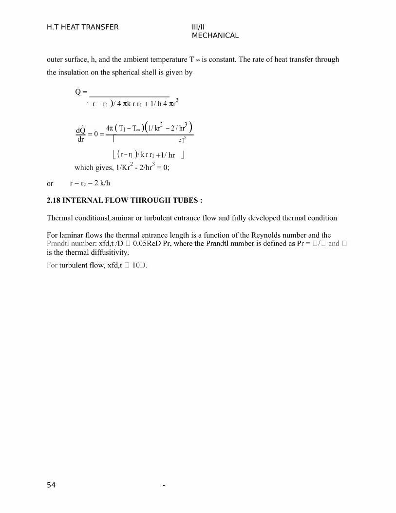
outer surface, h, and the ambient temperature T is constant. The rate of heat transfer through
the insulation on the spherical shell is given by
Q r r1 / 4 k r r1 1/ h 4 r2
dQ 0 4 T1 T 1/ kr2 2 / hr3
dr
/ k r r1 1/ hr
2 2
r r1 which gives, 1/Kr2 - 2/hr3 = 0;
or r = rc = 2 k/h
2.18 INTERNAL FLOW THROUGH TUBES :
Thermal conditionsLaminar or turbulent entrance flow and fully developed thermal condition
For laminar flows the thermal entrance length is a function of the Reynolds number and the
is the thermal diffusitivity.
54 -
H.T HEAT TRANSFER III/IIMECHANICAL
PART A
TWO MARK QUESTIONS:
1. Define convection. (AU2013)
Convection is a process of heat transfer that will occur between a solid surface and a fluid medium when they are at different temperatures.
2. What is meant by free or natural convection? (AU 2011)
If the fluid motion is produced due to change in density resulting from temperature gradients, themode of heat transfer is said to be free or natural convection.
3. What is forced convection? (AU 2010)
If the fluid motion is artificially created by means of an external force like a blower or fan, that type of heat transfer is known as forced convection.
4. What are the dimensionless parameters used in forced convection?
1. Reynolds number (Re)2. Nusselt number (Nu)3. Prandtl number (Pr)
5. Define boundary layer thickness. (AU2014)
The thickness of the boundary layer has been defined as the distance from the surface at whichthe local velocity or temperature reaches 99% of the external velocity or temperature.
6. What is meant by laminar flow and turbulent flow? (AU 2012)
Laminar flow: Laminar flow is sometimes called stream line flow. In this type of flow, the fluidmoves in layers and each fluid particle follows a smooth continuous path. The fluid particles ineach layer remain in an orderly sequence without mixing with each other.
Turbulent flow: In addition to the laminar type of flow, a distinct irregular flow is frequencyobserved in nature. This type of flow is called turbulent flow. The path of any individual particleis zig– zag and irregular. Fig. shows the instantaneous velocity in laminar and turbulent flow.
7. What is hydrodynamic boundary layer? (AU2012)
In hydrodynamic boundary layer, velocity of the fluid is less than 99% of free stream velocity.
8. What is thermal boundary layer? (AU 2012)
55 -

H.T HEAT TRANSFER III/IIMECHANICAL
In thermal boundary layer, temperature of the fluid is less than 99% of free stream velocity.
9. Define Grashof number (Gr). (AU 2009)
It is defined as the ratio of product of inertia force and buoyancy force to the square of viscousforce.
Gr Inertia force Buyoyancy force
(Viscous force)2
10. Define Reynolds number (Re). (AU2010)
It is defined as the ratio of inertia force to viscous force.
Re Inertia force
Viscous force
11. Define prandtl number (Pr).
It is the ratio of the momentum diffusivity of the thermal diffusivity.
Pr Momentum diffusivity
Thermal diffusivity
12.Whichmode heattransfer is the convection heat transfer coefficient usually
higher,natural or forced convection ? why ?
Convection heat transfer coefficient is usually higher in forced convection than in naturalconvection, because it mainly depends upon the factors such as fluid density, velocity andviscosity.
PART B
ANSWER THE FOLLOWING:
1. Air at 20C at atmospheric pressure flows over a flat plate at a velocity of 3 m/s. if the
plate is 1 m wide and 80C, calculate the following at x = 300 mm. (AU2010)
1. Hydrodynamic boundary layer thickness,
2. Thermal boundary layer thickness,
3. Local friction coefficient,
4. Average friction coefficient,
56 -

H.T HEAT TRANSFER III/IIMECHANICAL
5. Local heat transfer coefficient
6. Average heat transfer coefficient,
7. Heat transfer.
Given: Fluid temperature T = 20C , Velocity U = 3 m/s
Wide W = 1 m
Surface temperature Tw = 80C
Distance x = 300 mm = 0.3 m
Solution: We know
Film temperature Tf Tw
T
2 80 20
2Tf 50CProperties of air at 50C
Density = 1.093 kg/m3
Kinematic viscosity v = 17.95 10-6m2 / s
Pr andtl number Pr =0.698
Thermal conductivity K = 28.26 10-3W / mK
We know,
Reynolds number Re = UL
v 3 0.3
17.95 106
Re 5.01 10 4 5 105
Since Re < 5 105, flow is laminar
For Flat plate, laminar flow,
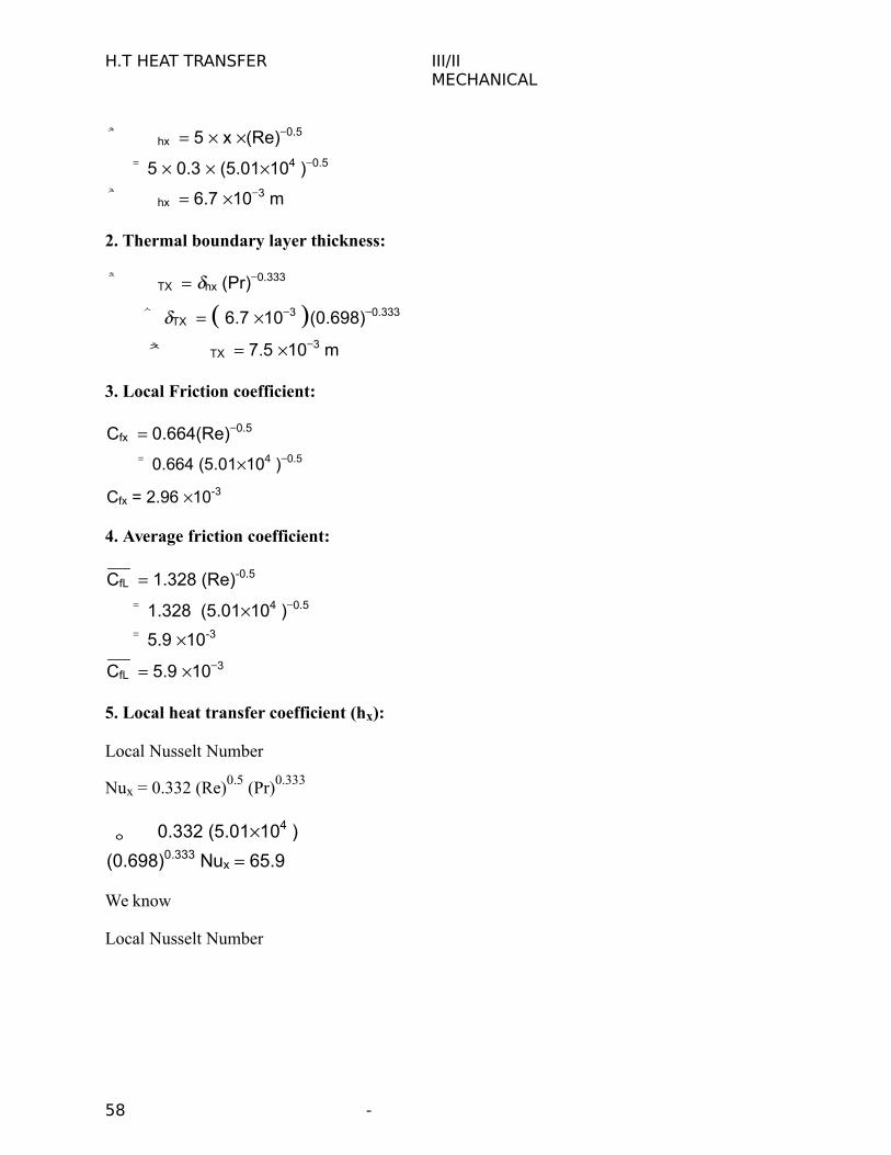
1. Hydrodynamic boundary layer thickness:
57 -
H.T HEAT TRANSFER III/IIMECHANICAL
hx 5 x (Re)0.5
= 5 0.3 (5.01104 )0.5
hx 6.7 103 m
2. Thermal boundary layer thickness:
TX hx (Pr)0.333
TX 6.7 103 (0.698)0.333
TX 7.5 103 m
3. Local Friction coefficient:
Cfx 0.664(Re)0.5
= 0.664 (5.01104 )0.5
Cfx = 2.96 10-3
4. Average friction coefficient:
CfL 1.328 (Re)-0.5
= 1.328 (5.01104 )0.5
= 5.9 10-3
CfL 5.9 103
5. Local heat transfer coefficient (hx):
Local Nusselt Number
Nux = 0.332 (Re)0.5 (Pr)0.333
0.332 (5.01104 )
(0.698)0.333 Nux 65.9
We know
Local Nusselt Number
58 -

H.T HEAT TRANSFER III/IIMECHANICAL
Nu hxL
x K
65.9 h
x
0.3
x = L = 0.3m 3
hx 6.20 W/m2K
Local heat transfer coefficient hx 6.20 W / m2K
6. Average heat transfer coefficient (h):
h 2 hx
2 6.20
h 12.41 W / m2K
7. Heat transfer:
We know that,
Q h A(Tw T )
= 12.41 (1 0.3) (80-20)
Q = 23.38 Watts
2. Air at 40C is flows over a flat plate of 0.9 m at a velocity of 3 m/s. Calculate the
following: (AU 2012)
1. Overall drag coefficient2. Average shear stress,3. Compare the average shear stress with local shear stress (shear stress at the trailing
edge)Given:
Fluid temperature T = 40C
Length L = 0.9 m
Velocity U = 3 m/s.
Solution:
Properties of air at 40C:
1.128 Kg/m3
= 16.96 10-6
m2 / s Pr 0.699
K 26.56 10-3 W/mK
59 -
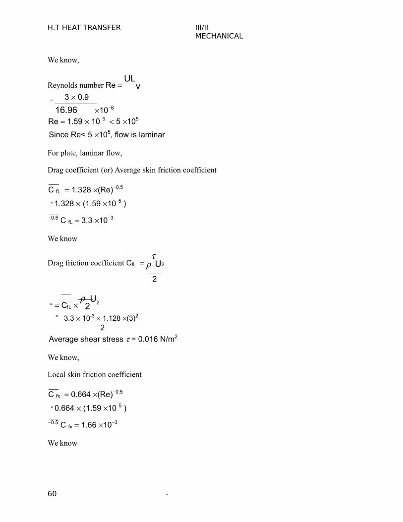
H.T HEAT TRANSFER III/IIMECHANICAL
We know,
Reynolds number Re UL
v 3 0.9
16.96 106
Re 1.59 10 5 5 105
Since Re< 5 105, flow is laminar
For plate, laminar flow,
Drag coefficient (or) Average skin friction coefficient
C fL 1.328 (Re)0.5
1.328 (1.59 10 5 )
0.5 C fL 3.3 103
We know
Drag friction coefficient CfL U2
2
CfL 2U2
= 3.3 10-3 1.128 (3)2
2
Average shear stress = 0.016 N/m2
We know,
Local skin friction coefficient
C fx 0.664 (Re)0.5
0.664 (1.59 10 5 )
0.5 C fx 1.66 103
We know
60 -
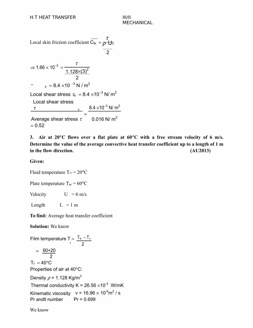
H.T HEAT TRANSFER III/IIMECHANICAL
Local skin friction coefficient Cfx U2
2
1.66 103
1.128(3)2
2
x 8.4 10 3 N / m2
Local shear stress x 8.4 103 N/ m2
Local shear stress x
8.4 103 N/ m2
Average shear stress 0.016 N/ m2
0.52
3. Air at 20C flows over a flat plate at 60C with a free stream velocity of 6 m/s.Determine the value of the average convective heat transfer coefficient up to a length of 1 min the flow direction. (AU2013)
Given:
Fluid temperature T = 20C
Plate temperature Tw = 60C
Velocity U = 6 m/s
Length L = 1 m
To find: Average heat transfer coefficient
Solution: We know
Film temperature T Tw Tf 2
60+202
Tf 40CProperties of air at 40C:
Density = 1.128 Kg/m3
Thermal conductivity K = 26.56 10-3 W/mK
Kinematic viscosity v = 16.96 10-6m2 / sPr andtl number Pr = 0.699
We know

61 -

H.T HEAT TRANSFER III/IIMECHANICAL
Reynolds number Re = UL
v 6 1
16.96 106
Re 3.53 105 5 105
Since Re < 5 105, flow is laminar
For flat plate, laminar flow
Local nusselt number} Nux = 0.332 (Re)0.5 (Pr)0.333
= 0.332 (3.53 105)0.5 (0.699)0.333
NUx = 175.27
We know,
LocalNusselt number} NUx h
x L
K
175.27 hx 1
26.56 103
2 4.65
h 9.31 W/m2K
4. Engine oil flows through a 50 mm diameter tube at an average temperature of 147C.The flow velocity is 80 cm/s. Calculate the average heat transfer coefficient if the tube wall
is maintained at a temperature of 200C and it is 2 m long.
Given:
Diameter D = 50 mm = 0.050 m
Average temperature Tm= 147C
Velocity U= 80 cm/s = 0.80 m/s
Tube wall temperature Tw= 200C
Length L= 2m
62 -
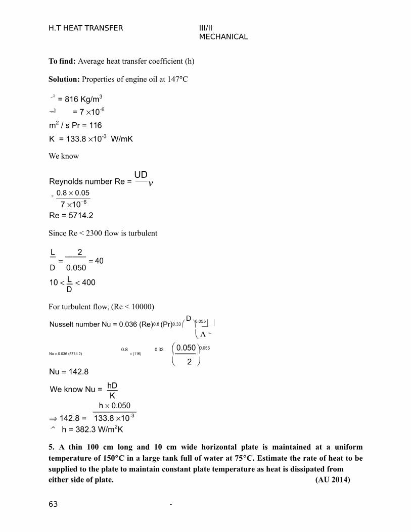
H.T HEAT TRANSFER III/IIMECHANICAL
To find: Average heat transfer coefficient (h)
Solution: Properties of engine oil at 147C
= 816 Kg/m3
= 7 10-6
m2 / s Pr = 116
K = 133.8 10-3 W/mK
We know
Reynolds number Re = UD
0.8 0.05
7 106
Re = 5714.2
Since Re < 2300 flow is turbulent
L
2 40
D 0.050
10 L 400D
For turbulent flow, (Re < 10000)
Nusselt number Nu = 0.036 (Re)0.8 (Pr)0.33 D
0.055
0.8 0.33 0.0500.055Nu 0.036 (5714.2) (116)
2 Nu 142.8
We know Nu = hDK
142.8 =
h 0.050
133.8 10-3
h = 382.3 W/m2K
5. A thin 100 cm long and 10 cm wide horizontal plate is maintained at a uniformtemperature of 150C in a large tank full of water at 75C. Estimate the rate of heat to besupplied to the plate to maintain constant plate temperature as heat is dissipated fromeither side of plate. (AU 2014)
63 -

H.T HEAT TRANSFER III/II MECHANICAL
Given:
Length of horizontal plate L = 100 cm = 1m
Wide W = 10 cm = 0.10 m
Plate temperature Tw = 150C
Fluid temperature T = 75C
To find: Heat loss (Q) from either side of plate
Solution:
1 1
Coefficient of thermal expansion} = Tfin K 112.5 273 2.59 10 3 K1
Grashof Number Gr = g
L3
T
v2
For horizontal plate,W 0.10
L c = 0.05 m
(1) Gr = 9.81 2.59 10-3 (0.05)3 (150 75)
(0.264 106 )2
Gr = 3.41109
Gr Pr = 3.41 109 1.55
Gr Pr = 5.29 109
Gr Pr value is in between 8 106 and 1011
i.e., 8 106< G r Pr < 1011
For horizontal plate, upper surface heated:
Nusselt number Nu = 0.15 (Gr Pr)0.333
Nu = 0.15 [5.29 109 ]0.333
Nu = 259.41
We know that,
64 -
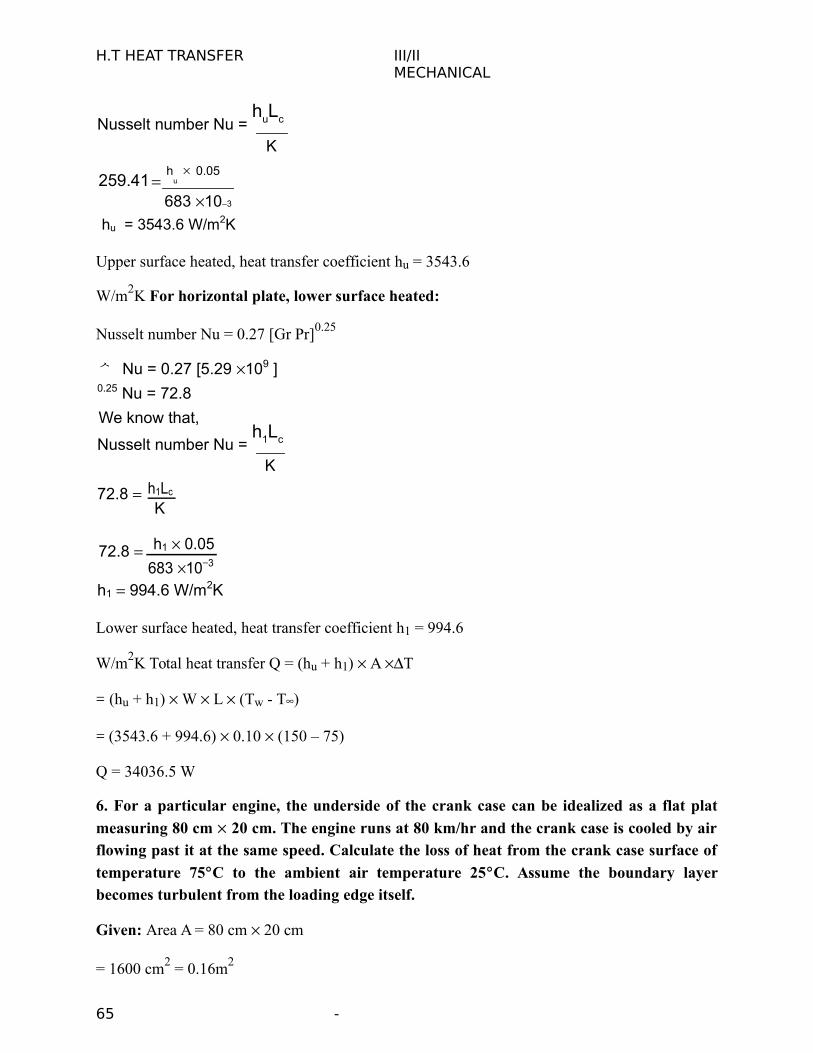
H.T HEAT TRANSFER III/IIMECHANICAL
Nusselt number Nu = huLc
K
259.41 h
u 0.05
683 103
hu = 3543.6 W/m2K
Upper surface heated, heat transfer coefficient hu = 3543.6
W/m2K For horizontal plate, lower surface heated:
Nusselt number Nu = 0.27 [Gr Pr]0.25
Nu = 0.27 [5.29 109 ]0.25 Nu = 72.8
We know that,
Nusselt number Nu = h1Lc
K
72.8 h1Lc
K
72.8 h1 0.05
683 103
h1 994.6 W/m2K
Lower surface heated, heat transfer coefficient h1 = 994.6
W/m2K Total heat transfer Q = (hu + h1) A T
= (hu + h1) W L (Tw - T)
= (3543.6 + 994.6) 0.10 (150 – 75)
Q = 34036.5 W
6. For a particular engine, the underside of the crank case can be idealized as a flat plat
measuring 80 cm 20 cm. The engine runs at 80 km/hr and the crank case is cooled by airflowing past it at the same speed. Calculate the loss of heat from the crank case surface of
temperature 75C to the ambient air temperature 25C. Assume the boundary layerbecomes turbulent from the loading edge itself.
Given: Area A = 80 cm 20 cm
= 1600 cm2 = 0.16m2
65 -
H.T HEAT TRANSFER III/IIMECHANICAL
Velocity U = 80 Km/hr
80 10 3 m3600s
22.22 m/s
Surface temperature Tw 75CAmbient air temperature T 25C
Flow is turbulent from the leading edge, flow is fully turbulent.
To find:
1. Heat loss
Film temperature Tf T
w
T
75
25
2 2Tf 50CProperties of air at 50C: = 1.093 Kg/m3
= 17.95 10-6
m2 / s Pr 0.698
K 28.26 103 W/mK
Re ynolds number Re = ULv
22.22 0.8 [ L = 0.8m]17.95 106
Re = 9 105
Re 9 105 5 105
Since Re>5 105, Flow is turbulent
For flat plate, turbulent flow,
[Fully turbulent from leading edge – given]
Local Nusselt number} NUx = 0.0296 (Re)0.8
(Pt)0.333 = 0.0296 [9 105]0.8 (0.698)0.33
NUx = 1524.6
66 -
H.T HEAT TRANSFER III/IIMECHANICAL
We know that, NU h xLx K
1524.6 h x 0.8
[ L = 0.8m]28.26 103
hx 53.85 W/m2K
Local heat transfer coefficient} hx = 53.85
W/m2K For turbulent flow, flat plate
Average heat transfer coefficient} h = 1.24 hx
h = 1.24 53.85
h = 66.78 W/m2K
We know,
= 66.78 0.16 (75 –
25) Q = 534.2 watts.
67 -
H.T HEAT TRANSFER III/IIMECHANICAL
UNIT 3 PHASE CHANGE HEAT TRANSFER AND HEAT EXCHANGERS :
NUSSELT THEORY OF CONDENSATION :
Condensation is a rather complicated process. It was Wilhelm Nusselt's idea to reduce the
complexity of the real process to a rather simple model,namely that the only resistance for the
removal of the heat released duringcondensation occurs in the condensate film. The following
gives anexplanation of the Nusselt theory at the example of condensation on avertical wall.
Condensation occurs if a vapor is cooled below its (pressure dependent) saturation temperature.
The heat of evaporation which is released duringcondensation must be removed by heat transfer,
e.g. at a cooled wall. Figure shows how saturated vapor at temperature Ts is condensing on a
vertical wall whose temperature Tw is constant and lower than the saturation temperature.
3.1. Condensation and Boiling
Heat energy is being converted into electrical energy with the help of water as a
working fluid. Water is first converted into steam when heated in a heat exchanger and then the
exhaust steam coming out of the steam turbine/engine is condensed in a condenser so that the
condensate (water) is recycled again for power generation. Therefore, the condensation and
boiling processes involve heat transfer with change of phase. When a fluid changes its phase, the
magnitude of its properties like density, viscosity, thermal conductivity, specific heat capacity,
etc., change appreciably and the processes taking place are greatly influenced by them. Thus, the
condensation and boiling processes must be well understood for an effective design of different
types of heat exchangers being used in thermal and nuclear power plants, and in process cooling
and heating systems.
3.2 Condensation-Filmwise and Dropwise
Condensation is the process of transition from a vapour to the liquid or solid state. The
process is accompanied by liberation of heat energy due to the change 10 phase. When a vapour
comes 10 contact with a surface maintained at a temperature lower than the saturation
temperature of the vapour corresponding to the pressure at which it exists, the vapour condenses
on the surface and the heat energy thus released has to be removed. The efficiency of the
condensing unit is determined by the mode of condensation that takes place:
68 -

H.T HEAT TRANSFER III/IIMECHANICAL
Filmwise - the condensing vapour forms a continuous film covering the entire surface,
Dropwise - the vapour condenses into small liquid droplets of various sizes. The
dropwise condensation has a much higher rate of heat transfer than filmwise condensation
because the condensate in dropwise condensation gets removed at a faster rate leading to better
heat transfer between the vapour and the bare surface. .
It is therefore desirable to maintain a condition of dropwise condensation 1D
commercial application. Dropwise condensation can only occur either on highly polished
surfaces or on surfaces contaminated with certain chemicals. Filmwise condensation is expected
to occur in most instances because the formation of dropwise condensation IS greatly influenced
by the presence of non-condensable gases, the nature and composition of surfaces and the
velocity of vapour past the surface.
Filmwise Condensation Mechanism on a Vertical Plane Surface--
Assumption
Let us consider a plane vertical surface at a constant temperature, Ts on which a pure
vapour at saturation temperature, Tg (Tg > Ts) is condensing. The coordinates are: X-axis along
the plane surface wit~ its origin at the top edge and Y-axis is normal to the plane surface as
shown in Fig. 11.1. The condensing liquid would wet the solid surface, spread out and form a
continuous film over the entire condensing surface. It is further assumed that
(i) the continuous film of liquid will flow downward (positive X-axis) under the action
of gravity and its thickness would increase as more and more vapour condenses at the liquid -
vapour interface,
69 -
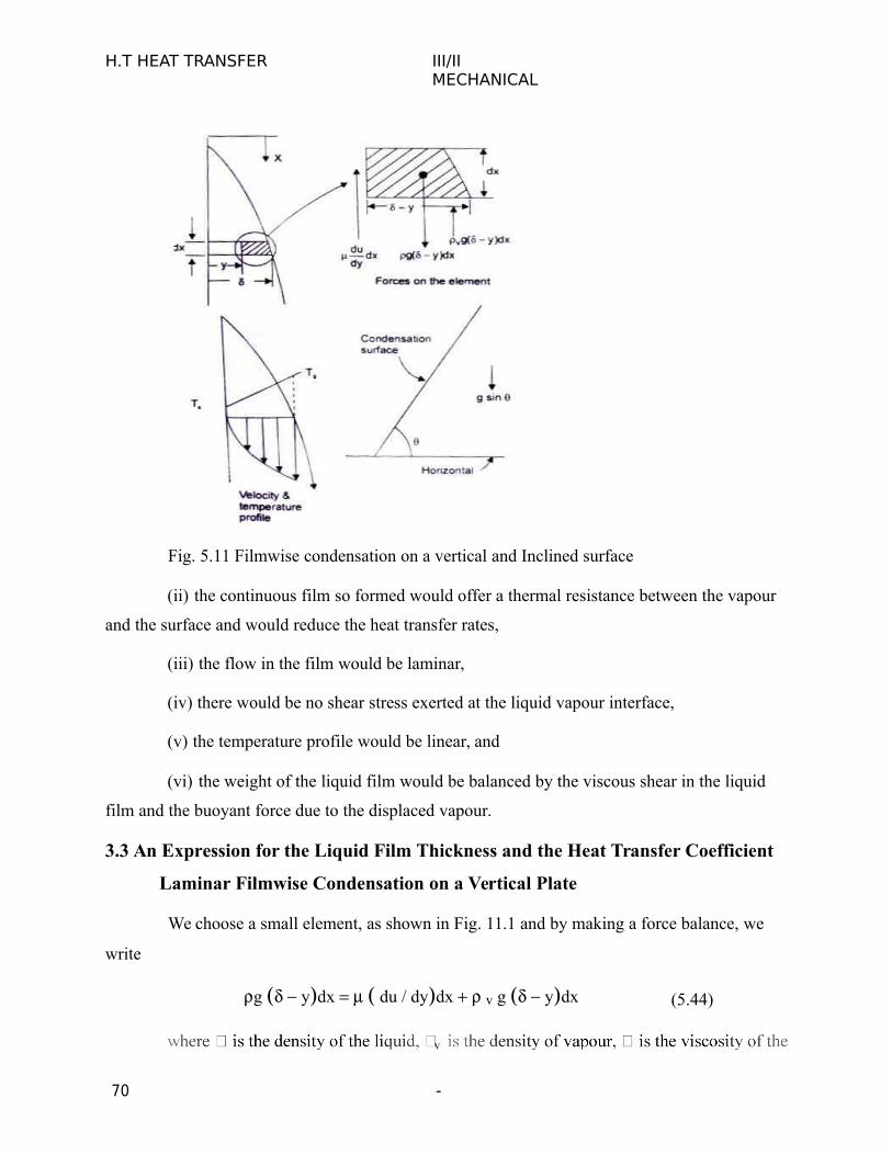
H.T HEAT TRANSFER III/IIMECHANICAL
Fig. 5.11 Filmwise condensation on a vertical and Inclined surface
(ii) the continuous film so formed would offer a thermal resistance between the vapour
and the surface and would reduce the heat transfer rates,
(iii) the flow in the film would be laminar,
(iv) there would be no shear stress exerted at the liquid vapour interface,
(v) the temperature profile would be linear, and
(vi) the weight of the liquid film would be balanced by the viscous shear in the liquid
film and the buoyant force due to the displaced vapour.
3.3 An Expression for the Liquid Film Thickness and the Heat Transfer Coefficient
Laminar Filmwise Condensation on a Vertical Plate
We choose a small element, as shown in Fig. 11.1 and by making a force balance, we
write
g ydx du / dydx v g ydx (5.44)
v
70 -
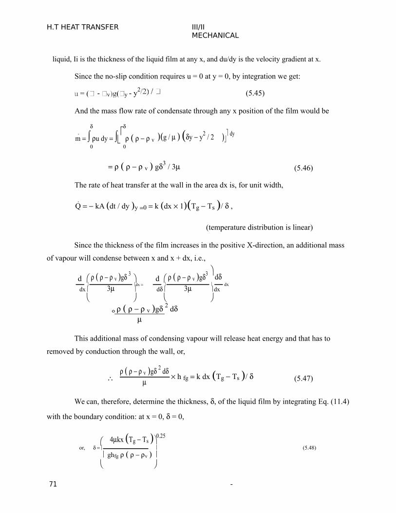
H.T HEAT TRANSFER III/IIMECHANICAL
liquid, Ii is the thickness of the liquid film at any x, and du/dy is the velocity gradient at x.
Since the no-slip condition requires u = 0 at y = 0, by integration we get:
- v y - y2 (5.45)
And the mass flow rate of condensate through any x position of the film would be
g / y y2 / 2 dy
m u dy v
0 0
v g3 / 3 (5.46)
The rate of heat transfer at the wall in the area dx is, for unit width,
Q kA dt / dy y 0 k dx 1Tg Ts / ,
(temperature distribution is linear)
Since the thickness of the film increases in the positive X-direction, an additional mass
of vapour will condense between x and x + dx, i.e.,
d v g 3 d v g3 d
dx dx3 3dx d dx
v g 2 d
This additional mass of condensing vapour will release heat energy and that has to
removed by conduction through the wall, or,
v g 2 d
h fg k dx Tg Ts / (5.47)
We can, therefore, determine the thickness, , of the liquid film by integrating Eq. (11.4)
with the boundary condition: at x = 0, = 0,
4kx Tg Ts 0.25
or, (5.48) ghfg v
71 -
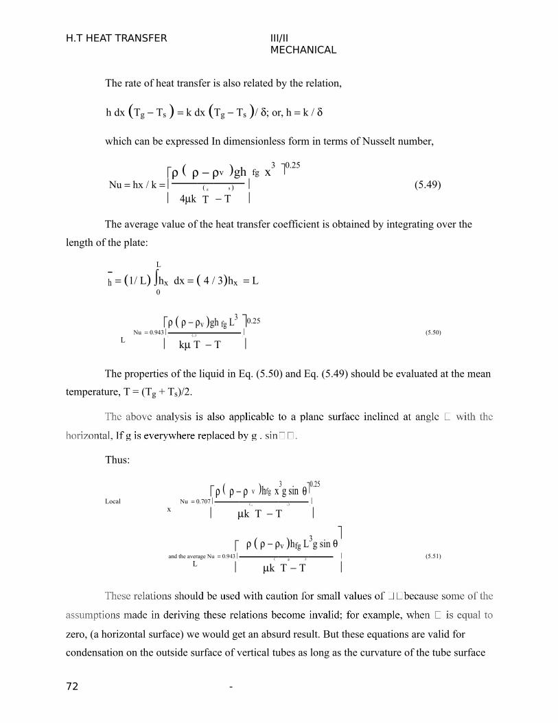
H.T HEAT TRANSFER III/IIMECHANICAL
The rate of heat transfer is also related by the relation,
h dx Tg Ts k dx Tg Ts / ; or, h k /
which can be expressed In dimensionless form in terms of Nusselt number,
vghfgx30.25
Nu hx / k (5.49)4k
g s
T T
The average value of the heat transfer coefficient is obtained by integrating over the
length of the plate:
L
1/ L hx dx 4 / 3hx Lh0
v gh fg L3 0.25
Nu 0.943 (5.50) gs
L
k T T
The properties of the liquid in Eq. (5.50) and Eq. (5.49) should be evaluated at the mean
temperature, T = (Tg + Ts)/2.
Thus:
vhfgx3g sin0.25
Local Nu 0.707 g s
x
k T T
v hfg L3g sin
and the average Nu 0.943 (5.51) g s
L
k T T
zero, (a horizontal surface) we would get an absurd result. But these equations are valid for
condensation on the outside surface of vertical tubes as long as the curvature of the tube surface
72 -
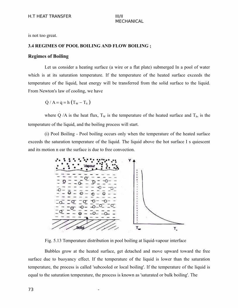
H.T HEAT TRANSFER III/IIMECHANICAL
is not too great.
3.4 REGIMES OF POOL BOILING AND FLOW BOILING ;
Regimes of Boiling
Let us consider a heating surface (a wire or a flat plate) submerged In a pool of water
which is at its saturation temperature. If the temperature of the heated surface exceeds the
temperature of the liquid, heat energy will be transferred from the solid surface to the liquid.
From Newton's law of cooling, we have
Q / A q h Tw Ts
where Q /A is the heat flux, Tw is the temperature of the heated surface and Ts, is the
temperature of the liquid, and the boiling process will start.
(i) Pool Boiling - Pool boiling occurs only when the temperature of the heated surface
exceeds the saturation temperature of the liquid. The liquid above the hot surface I s quiescent
and its motion n ear the surface is due to free convection.
Fig. 5.13 Temperature distribution in pool boiling at liquid-vapour interface
Bubbles grow at the heated surface, get detached and move upward toward the free
surface due to buoyancy effect. If the temperature of the liquid is lower than the saturation
temperature, the process is called 'subcooled or local boiling'. If the temperature of the liquid is
equal to the saturation temperature, the process is known as 'saturated or bulk boiling'. The
73 -
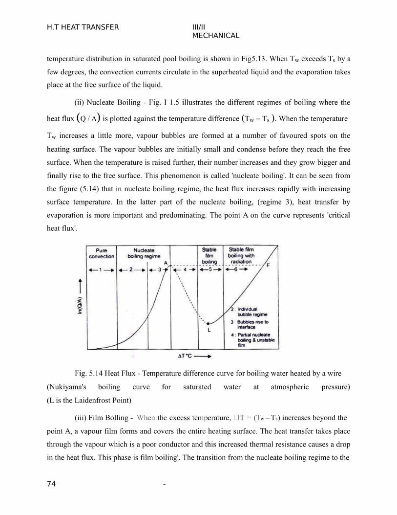
H.T HEAT TRANSFER III/IIMECHANICAL
temperature distribution in saturated pool boiling is shown in Fig5.13. When Tw exceeds Ts by a
few degrees, the convection currents circulate in the superheated liquid and the evaporation takes
place at the free surface of the liquid.
(ii) Nucleate Boiling - Fig. I 1.5 illustrates the different regimes of boiling where the
heat flux Q / A is plotted against the temperature difference Tw Ts . When the temperature
Tw increases a little more, vapour bubbles are formed at a number of favoured spots on the
heating surface. The vapour bubbles are initially small and condense before they reach the free
surface. When the temperature is raised further, their number increases and they grow bigger and
finally rise to the free surface. This phenomenon is called 'nucleate boiling'. It can be seen from
the figure (5.14) that in nucleate boiling regime, the heat flux increases rapidly with increasing
surface temperature. In the latter part of the nucleate boiling, (regime 3), heat transfer by
evaporation is more important and predominating. The point A on the curve represents 'critical
heat flux'.
Fig. 5.14 Heat Flux - Temperature difference curve for boiling water heated by a wire
(Nukiyama's boiling curve for saturated water at atmospheric pressure)
(L is the Laidenfrost Point)
(iii) Film Bolling - w – Ts) increases beyond the
point A, a vapour film forms and covers the entire heating surface. The heat transfer takes place
through the vapour which is a poor conductor and this increased thermal resistance causes a drop
in the heat flux. This phase is film boiling'. The transition from the nucleate boiling regime to the
74 -
H.T HEAT TRANSFER III/IIMECHANICAL
film boiling regime is not a sharp one and the vapour film under the action of circulating currents
collapses and rapidly reforms. In regime 5, the film is stable and the heat flow rate is the lowest.
(iv) Critical Heat Flux and Burnout Point -
temperature of the heating metallic surface is very high and the heat transfer occurs predominantly
by radiation, thereby, increasing the heat flux. And finally, a point is reached at which the heating
surface melts - point F in Fig. 11.5. It can be observed from the boiling curve that the whole
boiling process remains in the unstable state between A and F. Any increase in the heat flux beyond
point A will cause a departure from the boiling curve and there would be a large increase in surface
temperature.
3.5Boiling Curve - Operating Constraints
The boiling curve, shown in Fig. 11.5, is based on the assumption that the temperature
of the heated surface can be maintained at the desired value. In that case, it would be possible to
operate the vapour producing system at the point of maximum flux with nucleate boiling. If the
heat flux instead of the surface temperature, is the independent variable and it IS desired to
operate the system at the point of maximum flux, it is just possible that a slight increase in the
heat flux will increase the surface temperature substantially. And, the equilibrium will be
established at point F. If the material of the heating element has its melting point temperature
lower than the temperature at the equilibrium point F, the heating element will melt.
3.6 Factors Affecting Nucleate Boiling
Since high heat transfer rates and convection coefficients are associated with small values of the
excess temperature, it is desirable that many engineering devices operate in the nucleate boiling
regime. It is possible to get heat transfer coefficients in excess of 104 W/m2 in nucleate boiling
regime and these values are substantially larger than those normally obtained in convection
processes with no phase change. The factors which affect the nucleate boiling are:
(a) Pressure - Pressure controls the rate of bubble growth and therefore affects the
temperature difference causing the heat energy to flow. The maximum allowable heat flux for a
boiling liquid first increases with pressure until critical pressure is reached and then decreases.
(b) Heating Surface Characteristics - The material of the heating element has a
significant effect on the boiling heat transfer coefficient. Copper has a higher value than
75 -

H.T HEAT TRANSFER III/IIMECHANICAL
chromium, steel and zinc. Further, a rough surface gives a better heat transfer rate than a smooth
or coated surface, because a rough surface gets wet more easily than a smooth one.
(c) Thermo-mechanical Properties of Liquids - A higher thermal conductivity of the
liquid will cause higher heat transfer rates and the viscosity and surface tension will have a
marked effect on the bubble size and their rate of formation which affects the rate of heat
transfer.
(d) Mechanical Agitation - The rate of heat transfer will increase with the increasing
degree of mechanical agitation. Forced convection increases mixing of bubbles and the rate of
heat transfer.
3.7HEAT EXCHANGERS TYPES :
Heat Exchangers: Regenerators and Recuperators
A heat exchanger is an equipment where heat energy is transferred from a hot fluid to a
colder fluid. The transfer of heat energy between the two fluids could be carried out (i) either by
direct mixing of the two fluids and the mixed fluids leave at an intermediate temperature
determined from the principles of conservation of energy, (ii) or by transmission through a wall
separating the two fluids. The former types are called direct contact heat exchangers such as
water cooling towers and jet condensers. The latter types are called regenerators, recuperator
surface exchangers.
In a regenerator, hot and cold fluids alternately flow over a surface which provides
alternately a sink and source for heat flow. Fig. 10.1 (a) shows a cylinder containing a matrix that
rotates in such a way that it passes alternately through cold and hot gas streams which are sealed
from each other. Fig. 10.1 (b) shows a
stationary matrix regenerator ill which
hot and cold gases flow through them
alternately.
Fig. 3.1 (a) Rotating matrix
regenerator
76 -

H.T HEAT TRANSFER III/IIMECHANICAL
Fig. 3.1 (b) Stationary matrix regenerator
In a recuperator, hot and cold fluids flow continuously following he same path. The heat
transfer process consists of convection between the fluid and the separating wall, conduction
through the wall and convection between the wall and the other fluid. Most common heat
exchangers are of recuperative type having a Wide variety of geometries:
3.8 Classification of Heat Exchangers
Heat exchangers are generally classified according to the relative directions of hot and cold
fluids:
(a) Parallel Flow – the hot and cold fluids flow in the same direction. Fig 3.2 depicts such a heat
exchanger where one fluid (say hot) flows through the pipe and the other fluid (cold) flows
77 -

H.T HEAT TRANSFER III/IIMECHANICAL
through the annulus.
(b) Counter Flow – the two fluids flow through the pipe but in opposite directions. A
common type of such a heat exchanger is shown in Fig. 3.3. By comparing the temperature
distribution of the two types of heat exchanger
Fig 3.2 Parallel flow heat exchanger with Fig 3.3 Counter-flow heat exchanger
temperature distribution with temperature distribution
we find that the temperature difference between the two fluids is more uniform in
counter flow than in the parallel flow. Counter flow exchangers give the maximum heat transfer
rate and are the most favoured devices for heating or cooling of fluids.
When the two fluids flow through the heat exchanger only once, it is called one-shell-
pass and one-tube-pass as shown in Fig. 3.2 and 3.3. If the fluid flowing through the tube makes
one pass through half of the tube, reverses its direction of flow, and makes a second pass through
the remaining half of the tube, it is called 'one-shell-pass, two-tube-pass' heat exchanger,fig 3.4.
Many other possible flow arrangements exist and are being used. Fig. 10.5 depicts a 'two-shell-
pass, four-tube-pass' exchanger.
(c) Cross-flow - A cross-flow heat exchanger has the two fluid streams flowing at right
angles to each other. Fig. 3.6 illustrates such an arrangement An automobile radiator is a good
example of cross-flow exchanger. These exchangers are 'mixed' or 'unmixed' depending upon the
78 -
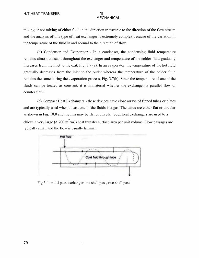
H.T HEAT TRANSFER III/IIMECHANICAL
mixing or not mixing of either fluid in the direction transverse to the direction of the flow stream
and the analysis of this type of heat exchanger is extremely complex because of the variation in
the temperature of the fluid in and normal to the direction of flow.
(d) Condenser and Evaporator - In a condenser, the condensing fluid temperature
remains almost constant throughout the exchanger and temperature of the colder fluid gradually
increases from the inlet to the exit, Fig. 3.7 (a). In an evaporator, the temperature of the hot fluid
gradually decreases from the inlet to the outlet whereas the temperature of the colder fluid
remains the same during the evaporation process, Fig. 3.7(b). Since the temperature of one of the
fluids can be treated as constant, it is immaterial whether the exchanger is parallel flow or
counter flow.
(e) Compact Heat Exchangers - these devices have close arrays of finned tubes or plates
and are typically used when atleast one of the fluids is a gas. The tubes are either flat or circular
as shown in Fig. 10.8 and the fins may be flat or circular. Such heat exchangers are used to a
chieve a very large ( 700 m2/mJ) heat transfer surface area per unit volume. Flow passages are
typically small and the flow is usually laminar.
Fig 3.4: multi pass exchanger one shell pass, two shell pass
79 -

H.T HEAT TRANSFER III/IIMECHANICAL
Fig 3.5: Two shell passes, four-tube passes heat exchanger (baffles increases the
convection coefficient of the shell side fluid by inducing turbulance and a cross flow velocity
component)
Fig 3.6: A cross-flow exchanger
80 -
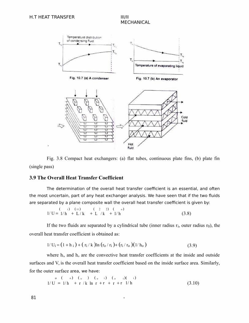
H.T HEAT TRANSFER III/IIMECHANICAL
Fig. 3.8 Compact heat exchangers: (a) flat tubes, continuous plate fins, (b) plate fin
(single pass)
3.9 The Overall Heat Transfer Coefficient
The determination of the overall heat transfer coefficient is an essential, and often
the most uncertain, part of any heat exchanger analysis. We have seen that if the two fluids
are separated by a plane composite wall the overall heat transfer coefficient is given by:
1/ U i
11
2 2
o
(3.8)1/ h L / k L / k 1/ h
If the two fluids are separated by a cylindrical tube (inner radius ri, outer radius r0), the
overall heat transfer coefficient is obtained as:
1/ Ui 1 h i ri / k ln ro / ri ri / ro 1/ ho (3.9)
where hi, and ho are the convective heat transfer coefficients at the inside and outside
surfaces and V, is the overall heat transfer coefficient based on the inside surface area. Similarly,
for the outer surface area, we have:
o
o
o o i
o i i
(3.10)1/ U 1/ h r / k ln r r r r 1/ h
81 -
H.T HEAT TRANSFER III/II MECHANICAL
and U i Ai will be equal to U o Ao ; or, Ui ri U o ro .
The effect of scale formation on the inside and outside surfaces of the tubes of a heat
exchanger would be to introduce two additional thermal resistances to the heat flow path. If hsi
and hso are the two heat transfer coefficients due to scale formation on the inside and outside
surface of the inner pipe, the rate of heat transfer is given by
Q T T / 1/ h A
i 1/ h
si
A
i
ln r r / 2 Lk 1/ h
so
A
o
1/ h A (3.11)
i o
io i o o
where Ti, and To are the temperature of the fluid at the inside and outside of the tube.
Thus, the overall heat transfer coeffiCIent based on the inside and outside surface area of the
tube would be:
1/ Ui 1/ h i 1/ h si ri / k ln ro / ri ri / ro 1/ h so ri / ro 1/ ho ; (3.12)
and
1/ U o ro / ri 1/ h i ro / ri 1/ h si ln ro / ri r0 / k 1/ h so 1/ ho K
3.10 FOULING FACTORS ANALYSIS :
Heat exchanger walls are usually made of single materials. Sometimes the walls are
bimettalic (steel with aluminium cladding) or coated with a plastic as a protection against
corrosion, because, during normal operation surfaces are subjected to fouling by fluid impurities,
rust formation, or other reactions between the fluid and the wall material. The deposition of a
film or scale on the surface greatly increases the resistance to heat transfer between the hot and
cold fluids. And, a scale coefficient of heat transfer h, is defined as:
R s 1/ h sA, oC / W or K / W
82 -
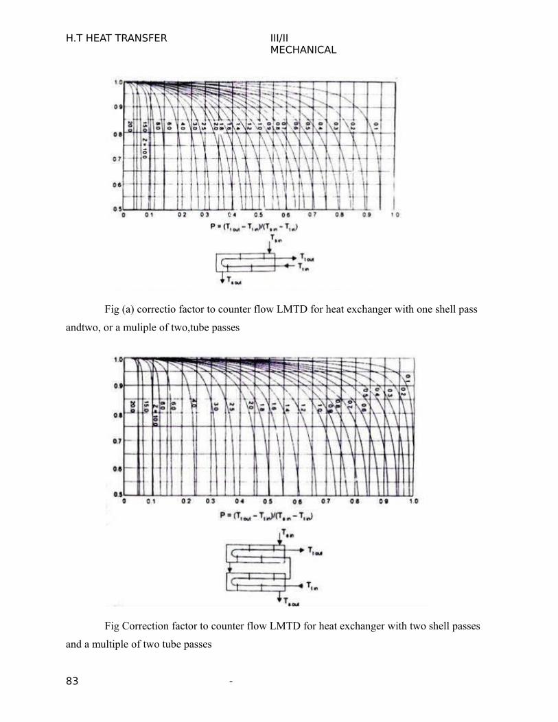
H.T HEAT TRANSFER III/IIMECHANICAL
Fig (a) correctio factor to counter flow LMTD for heat exchanger with one shell pass
andtwo, or a muliple of two,tube passes
Fig Correction factor to counter flow LMTD for heat exchanger with two shell passes
and a multiple of two tube passes
83 -

H.T HEAT TRANSFER III/IIMECHANICAL
where A is the area of the surface before scaling began and l/hs, is called ‘Fouling
Factor'. Its value depends upon the operating temperature, fluid velocity, and length of service of
the heat exchanger. Table 10.1 gives the magnitude of l/h, recommended for inclusion in the
overall heat transfer coefficient for calculating the required surface area of the exchanger
Fig(c) Correction factor to counter flow LMTD for cross flow heat exchangers, fluid on
shell side mixed, other fluid unmixed one tube pass..
Fig. (d) Correction factor to counter flow LMTD for cross flow heat exchangers, both
fluids unmixed, one tube pass.
3.11 LMTD METHOD :
84 -
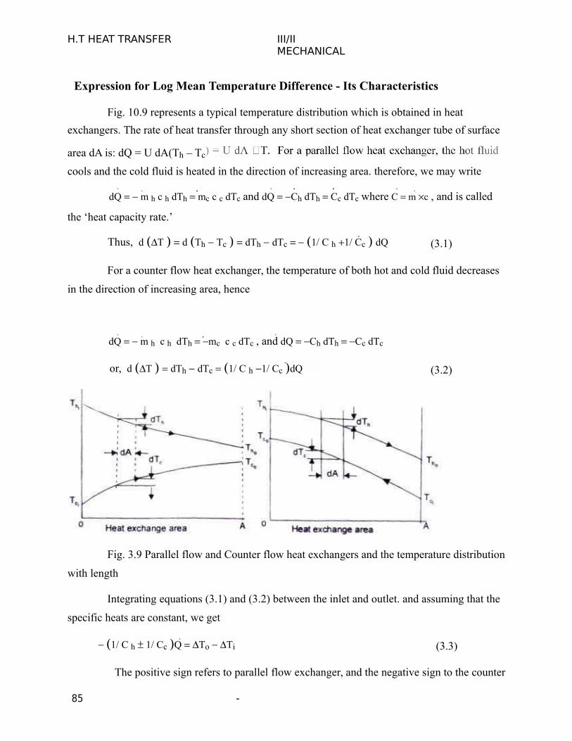
H.T HEAT TRANSFER III/IIMECHANICAL
Expression for Log Mean Temperature Difference - Its Characteristics
Fig. 10.9 represents a typical temperature distribution which is obtained in heat
exchangers. The rate of heat transfer through any short section of heat exchanger tube of surface
area dA is: dQ = U dA(Th – Tc
cools and the cold fluid is heated in the direction of increasing area. therefore, we may write
dQ m h c h dTh mc c c dTc and dQ Ch dTh Cc dTc where C m c , and is called
the ‘heat capacity rate.’
Thus, d T d Th Tc dTh dTc 1/ C h 1/ Cc dQ (3.1)
For a counter flow heat exchanger, the temperature of both hot and cold fluid decreases
in the direction of increasing area, hence
dQ m h c h dTh mc c c dTc , and dQ Ch dTh Cc dTc
or, d T dTh dTc 1/ C h 1/ Cc dQ (3.2)
Fig. 3.9 Parallel flow and Counter flow heat exchangers and the temperature distribution
with length
Integrating equations (3.1) and (3.2) between the inlet and outlet. and assuming that the
specific heats are constant, we get
1/ C h 1/ Cc Q To Ti (3.3)
The positive sign refers to parallel flow exchanger, and the negative sign to the counter
85 -

H.T HEAT TRANSFER III/IIMECHANICAL
flow type. Also, substituting for dQ in equations (10.1) and (10.2) we get
1/ Ch 1/ Cc UdA d T / T (3.3a)
Upon integration between inlet i and outlet 0 and assuming U as a constant,
We have 1/ Ch 1/ Cc U A ln T0 / Ti
By dividing (10.3) by (10.4), we get
o i oi Q UA T T / ln T / T
Thus the mean temperature difference is written
as Log Mean Temperature Difference,
LMTD = T0 Ti / ln To / Ti
(3.5)
(3.6)
(The assumption that U is constant along the heat exchanger is never strictly true but it
may be a good approximation if at least one of the fluids is a gas. For a gas, the physical
properties do not vary appreciably over moderate range of temperature and the resistance of the
gas film is considerably higher than that of the metal wall or the liquid film, and the value of the
gas film resistance effectively determines the value of the overall heat transfer coefficient U.)
It is evident from Fig.1 0.9 that for parallel flow exchangers, the final temperature of
fluids lies between the initial values of each fluid whereas m counter flow exchanger, the
temperature of the colder fluid at exit is higher than the temperature of the hot fluid at exit.
Therefore, a counter flow exchanger provides a greater temperature range, and the LMTD for a
counter flow exchanger will be higher than for a given rate of mass flow of the two fluids and for
given temperature changes, a counter flow exchanger will require less surface area.
3.12 Special Operating Conditions for Heat Exchangers
(i) Fig. 3.7a shows temperature distributions for a heat exchanger (condenser) where the
hot fluid has a much larger heat capacity rate, C h m h ch than that of cold fluid, Cc m c cc and
therefore, the temperature of the hot fluid remains almost constant throughout the exchanger and
the temperature of the cold fluid increases. The LMTD, in this case is not affected by whether the
exchanger is a parallel flow or counter flow.
86 -
H.T HEAT TRANSFER III/IIMECHANICAL
(ii) Fig. 3.7b shows the temperature distribution for an evaporator. Here the cold fluid
expenses a change in phase and remains at a nearly uniform temperature Cc . The same
effect would be achieved without phase change if Cc Ch , and the LMTD will remain the same
for both parallel flow and counter flow exchangers.
(iii) In a counter flow exchanger, when the heat capacity rate of uoth the fluids are
equal, Cc Ch , the temperature difference is the same all along the length of the tube. And in that
case, LMTD should be replaced by Ta Tb , and the temperature profiles of the two fluids
along Its length would be parallel straight lines.
(Since dQ Cc dTc Ch dTh ; dTc dQ / Cc , and dTh dQ / Ch
and, dTc dTh ddQ 1/ Cc 1/ C h 0 (because Cc Ch )
along Its length would be parallel straight lines.)
3.13 LMTD for Cross-flow Heat Exchangers :
LMTD given by Eq (10.6) is strictly applicable to either parallel flow or counter flow
exchangers. When we have multipass parallel flow or counter flow or cross flow exchangers,
LMTD is first calculated for single pass counter flow exchanger and the mean temperature
difference is obtained by multiplying the LMTD with a correction factor F which takes care of
the actual flow arrangement of the exchanger. Or,
Q = U A F (LMTD) (3.7)
The correction factor F for different flow arrangements are obtained from charts given.
3.14 NTU METHOD:
Heat Exchangers Effectiveness - Useful Parameters
In the design of heat exchangers, the efficiency of the heat transfer process is very
important. The method suggested by Nusselt and developed by Kays and London is now being
extensively used. The effectiveness of a heat exchanger is defined as the ratio of the actual heat
transferred to the maximum possible heat transfer.
87 -

H.T HEAT TRANSFER III/IIMECHANICAL
Let mh and mc be the mass flow rates of the hot and cold fluids, ch and cc be the
respective specific heat capacities and the terminal temperatures be Th and T h for the hot fluid
at inlet and outlet, Thi and Th0 for the cold fluid at inlet and outlet. By making an energy
balance and assuming that there is no loss of energy to the surroundings, we write
Q m h c h Th i Th 0 C h Th i Tc0 , and
mc c c Tc0 Tci Cc Tc0 Tci (3.13)
From Eq. (10.13), it can be seen that the fluid with smaller thermal capacity, C, has the
greater temperature change. Further, the maximum temperature change of any fluid would be
Th i Tci and this Ideal temperature change can be obtained with the fluid which has the
minimum heat capacity rate. Thus,
Effectiveness, Q / C min Th i Tci (3.14)
Or, the effectiveness compares the actual heat transfer rate to the maximum heat transfer
rate whose only limit is the second law of thermodynamics. An useful parameter which also
measures the efficiency of the heat exchanger is the 'Number of Transfer Units', NTU, defined as
NTU = Temperature change of one fluid/LMTD.
Thus, for the hot fluid: NTU = Th i Th0 / LMTD , and
for the cold fluid: NTU Tc0 Tci / LMTD
Since Q UA LMTD C h Th i Th0 Cc Tc0
Tci we have NTU h UA / Ch and NTU c UA / Cc
The heat exchanger would be more effective when the NTU is greater, and therefore,
NTU = AU/Cmin (3.15)
An another useful parameter in the design of heat exchangers is the ratio the minimum
to the maximum thermal capacity, i.e., R = Cmin/Cmax,
88 -
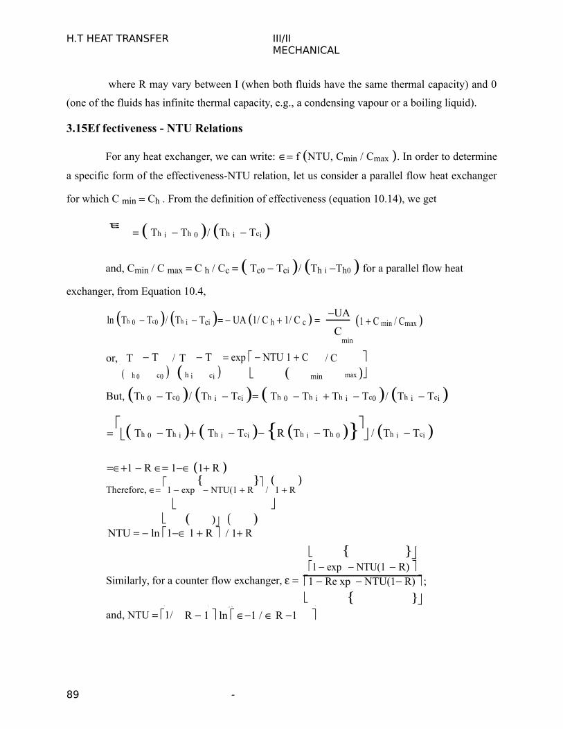
H.T HEAT TRANSFER III/IIMECHANICAL
where R may vary between I (when both fluids have the same thermal capacity) and 0
(one of the fluids has infinite thermal capacity, e.g., a condensing vapour or a boiling liquid).
3.15Ef fectiveness - NTU Relations
For any heat exchanger, we can write: f NTU, Cmin / Cmax . In order to determine
a specific form of the effectiveness-NTU relation, let us consider a parallel flow heat exchanger
for which C min Ch . From the definition of effectiveness (equation 10.14), we get
Th i Th 0 / Th i Tci
and, Cmin / C max C h / Cc Tc0 Tci / Th i Th0 for a parallel flow heat
exchanger, from Equation 10.4,
ln Th 0 Tc0 / Th i Tci UA 1/ C h 1/ C c UA 1 C min / Cmax C
min
or,
T T
/ T T
exp NTU 1 C
min
/ C h 0 c0 h i ci max
But, Th 0 Tc0 / Th i Tci Th 0 Th i Th i Tc0 / Th i Tci
Th 0 Th i Th i Tci R Th i Th 0
/ Th i Tci
1 R 1 1 R Therefore,
1 exp
NTU(1 R
/
1 R
NTU ln 1 1 R / 1 R
exp
Similarly, for a counter flow exchanger, 1 NTU(1 R)
;1 Re xp NTU(1 R)
and, NTU 1/ R 1 ln 1 / R 1
89 -
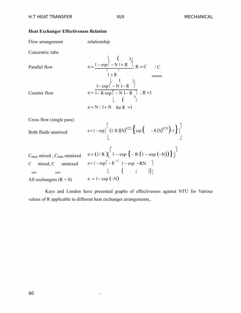
H.T HEAT TRANSFER III/II MECHANICAL
Heat Exchanger Effectiveness Relation
Flow arrangement relationship
Concentric tube
R
Parallel flow 1 exp N 1 ; R C / C
minmax1 R
Counter flow 1 exp N 1 R
; R 11 R exp N 1 R
N / 1 N for R 1
Cross flow (single pass)
Both fluids unmixed 1 exp 1/ R N0.22 exp R N0.78 1
Cmax mixed , Cmin unmixed 1/ R 1 exp R 1 exp N
C
min
mixed, C
max
unmixed 1 exp R 1
1 exp
RN
All exchangers (R = 0) 1 exp N
Kays and London have presented graphs of effectiveness against NTU for Various
values of R applicable to different heat exchanger arrangements,.
90 -
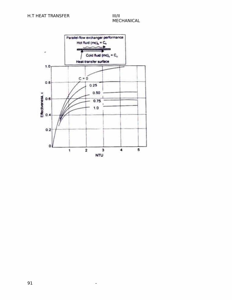
H.T HEAT TRANSFER III/IIMECHANICAL
91 -
H.T HEAT TRANSFER III/IIMECHANICAL
UNIT 3: PHASE CHANGE HEATTRANSFER AND HEAT EXCHANGERS
PART A
TWO MARK QUESTIONS: (AU 2013) 1.What is meant by pool boiling?
If heat is added to a liquid from a submerged solid surface, the boiling process is referred to as
pool boiling. In the case the liquid above the hot surface is essentially stagnant and its motion
near the surface is due to free convection and mixing induced by bubble growth and detachment.
2. State the difference between the drop wise condensation and film wise condensation.
Filmwise condensation:
The liquid condensate wets the solid surface, spreads out and forms a continuous film over the
entire surface is known as film wise condensation.
Drop wise condensation:
In drop wise condensation, the vapor condenses into small liquid droplets of various sizes
which fall down the surface in a random fashion.
3. What is meant by LMTD ? (AU2014)
We know that the temperatures difference between the hot and cold fluids in the heat exchanger
varies from point to point. In addition various modes of heat transfer are involved. Therefore
based on concept of appropriate mean temperature difference, also called logarithmic mean
temperature difference, the total heat transfer rate in the heat exchanger is expressed as
Q= UA( T)m,
Where U – Over all heat coefficient W/ K
A – Area, m
T- Temperature difference.
4. What is meant by Foulingfactor? (AU 2012)
92 -
H.T HEAT TRANSFER III/IIMECHANICAL
We know the surface of a heat exchanger do not remain clean after it has been in use for some
time. The surfaces become fouled with scaling or deposits. The effect of these deposits affecting
the value of overall heat transfer coefficient. This effect is taken care of by introducing an
additional thermal resistance called the fouling factor.
5. What is meant by condensation?
The change of phase from vapor to liquid state is known as condensation.
6. What is compact heat exchanger?
There are many special purpose heat exchangers called compact heat exchangers .They are
generally employed when convective heat transfer coefficient associated with one of the fluids is
much smaller than the associated with the other fluid.
7. Define Effectiveness. (AU 2013)
The heat exchanger effectiveness is defined as the ratio of actual heat transfer to the maximum
possible heat transfer.
Effectiveness = Actual heat transfer/ maximum possible heat transfer.
8. What is meant by parallel flow heat exchangers and counter flow heat exchanger?
Parallel flow heat exchanger:
In this type of heat exchanger, hot and cold fluids move in the same direction.
Counter flow heat exchanger:
In this type of heat exchanger,hot and cold fluids move in parallel but in opposite directions.
9. What is heat exchanger? (AU 2011)
A heat exchanger is defined as anequipment which transfers the heat from a hot fluid to a cold
fluid.
10. Give the expression for NTU. (AU2010)
Number of Transfer Units (NTU) = UA / Cmin.
11. List the various promoters used for maintaining drop wise condensation.
93 -
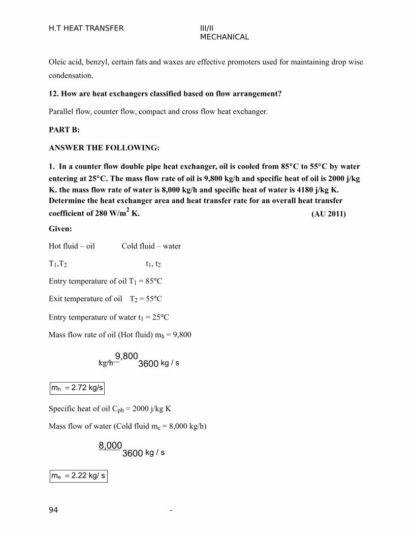
H.T HEAT TRANSFER III/IIMECHANICAL
Oleic acid, benzyl, certain fats and waxes are effective promoters used for maintaining drop wise
condensation.
12. How are heat exchangers classified based on flow arrangement?
Parallel flow, counter flow, compact and cross flow heat exchanger.
PART B:
ANSWER THE FOLLOWING:
1. In a counter flow double pipe heat exchanger, oil is cooled from 85C to 55C by water
entering at 25C. The mass flow rate of oil is 9,800 kg/h and specific heat of oil is 2000 j/kg
K. the mass flow rate of water is 8,000 kg/h and specific heat of water is 4180 j/kg K.Determine the heat exchanger area and heat transfer rate for an overall heat transfer
coefficient of 280 W/m2 K. (AU 2011)
Given:
Hot fluid – oil Cold fluid – water
T1,T2 t1, t2
Entry temperature of oil T1 = 85C
Exit temperature of oil T2 = 55C
Entry temperature of water t1 = 25C
Mass flow rate of oil (Hot fluid) mh = 9,800
kg/h 9,800
3600 kg / s
mh 2.72 kg/s
Specific heat of oil Cph = 2000 j/kg K
Mass flow of water (Cold fluid mc = 8,000 kg/h)
8,0003600 kg / s
me 2.22 kg/ s
94 -

H.T HEAT TRANSFER III/II
Specific heat of water Cpc – 4180 j/kg K
Overall heat transfer coefficient U = 280 W/m2K
To find
1. Heat exchanger area (A)2. Heat transfer rate (Q)
Solution
We know that
Heat lost by oil Hot fluid = Heat gained by water cold fluid
Qh = Qc
mh Cph (T1 T2 ) mc Cpc (t 2 t 1)
2.72 2000 (85-55)=2.22 4180 (t2 25)
163.2 103 9279.6 t2 231.9 103
t2 42.5C
Exit temperature of water t2 42.5C
Heat transfer Q =mc Cpc (t2 t1 ) (or) mh Cph (T1 T2 )
Q 2.22 4180 (42.5
25) Q 162 103 W
Q UA (T)m........1
From HMT data book Page No.154
For counter flow
(T) (T
1t1) - (T2t2)m T t
1In 1 T t 22
From HMT data book Page No.154
(T) (85 42.5) - (55 25)m
In 85 42.5 55 25
(T)m 35.8C
Substitute (T)m U and Q values in Equation (1)
MECHANICAL
95 -
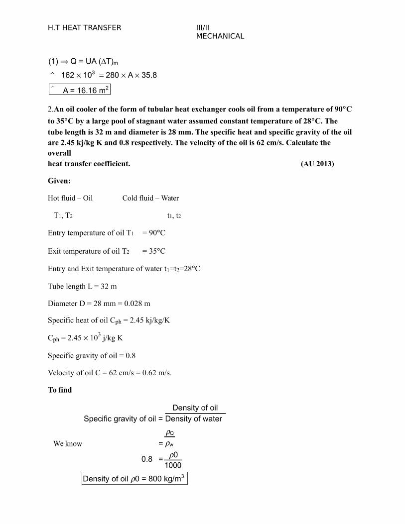
H.T HEAT TRANSFER III/IIMECHANICAL
(1) Q = UA (T)m
162 103 280 A 35.8
A = 16.16 m2
2.An oil cooler of the form of tubular heat exchanger cools oil from a temperature of 90C
to 35C by a large pool of stagnant water assumed constant temperature of 28C. The
tube length is 32 m and diameter is 28 mm. The specific heat and specific gravity of the oil are 2.45 kj/kg K and 0.8 respectively. The velocity of the oil is 62 cm/s. Calculate the overallheat transfer coefficient. (AU 2013)
Given:
Hot fluid – Oil
T1, T2
Cold fluid – Water
t1, t2
Entry temperature of oil T1 = 90C
Exit temperature of oil T2 = 35C
Entry and Exit temperature of water t1=t2=28C
Tube length L = 32 m
Diameter D = 28 mm = 0.028 m
Specific heat of oil Cph = 2.45 kj/kg/K
Cph = 2.45 103 j/kg K
Specific gravity of oil = 0.8
Velocity of oil C = 62 cm/s = 0.62 m/s.
To find
Specific gravity of oil =Density of oil
Density of water
=
Q
We know w
0.8 = 01000
Density of oil 0 = 800 kg/m3

96 -
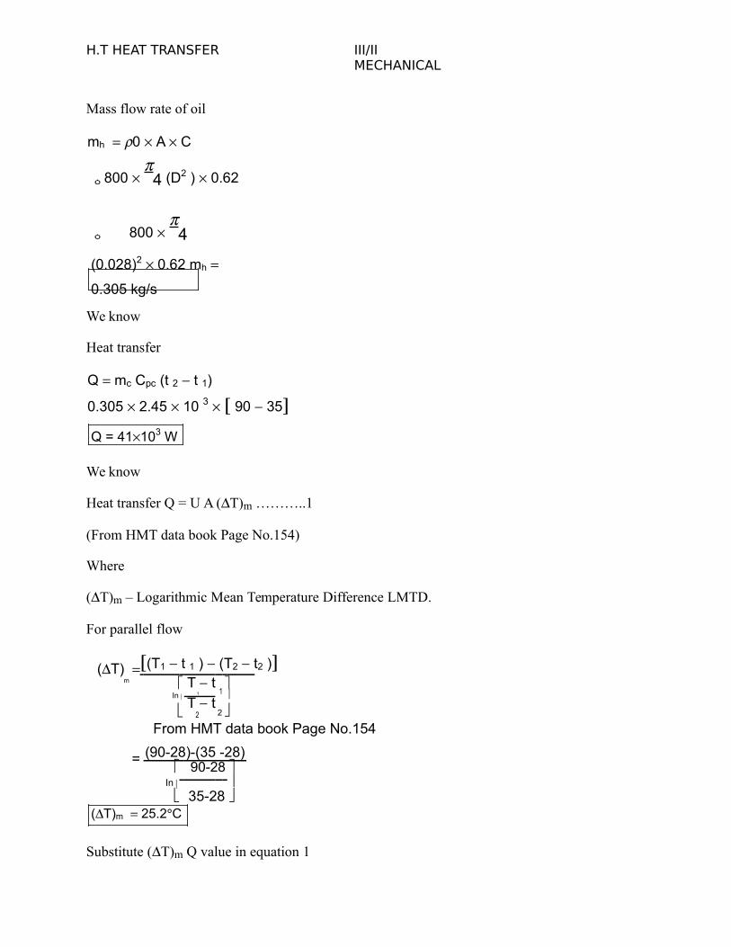
H.T HEAT TRANSFER III/IIMECHANICAL
Mass flow rate of oil
mh 0 A C
800 4 (D2 ) 0.62
800 4
(0.028)2 0.62 mh
0.305 kg/s
We know
Heat transfer
Q mc Cpc (t 2 t 1)
0.305 2.45 10 3 90 35Q = 41103 W
We know
Heat transfer Q = U A (T)m ………..1
(From HMT data book Page No.154)
Where
(T)m – Logarithmic Mean Temperature Difference LMTD.
For parallel flow
(T) (T1 t 1 ) (T2 t2 )T tm
1In 1 T t 2 2
From HMT data book Page No.154
= (90-28)-(35 -28) 90-28
In 35-28
(T)m 25.2C
Substitute (T)m Q value in equation 1

97 -
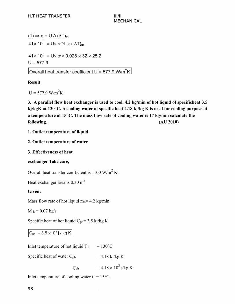
H.T HEAT TRANSFER III/IIMECHANICAL
(1) q = U A (T)m
41 103 U DL ( T)m
41 103 U 0.028 32 25.2
U = 577.9
Overall heat transfer coefficient U = 577.9 W/m2K
Result
U = 577.9 W/m2K
3. A parallel flow heat exchanger is used to cool. 4.2 kg/min of hot liquid of specificheat 3.5
kj/kgK at 130C. A cooling water of specific heat 4.18 kj/kg K is used for cooling purpose at
a temperature of 15C. The mass flow rate of cooling water is 17 kg/min calculate the
following. (AU 2010)
1. Outlet temperature of liquid
2. Outlet temperature of water
3. Effectiveness of heat
exchanger Take care,
Overall heat transfer coefficient is 1100 W/m2 K.
Heat exchanger area is 0.30 m2
Given:
Mass flow rate of hot liquid mh= 4.2 kg/min
M h = 0.07 kg/s
Specific heat of hot liquid Cph= 3.5 kj/kg K
Cph 3.5 103 j / kg K
Inlet temperature of hot liquid T1 = 130C
Specific heat of water Cph = 4.18 kj/kg K
Cph = 4.18 103 j/kg K
Inlet temperature of cooling water t1 = 15C
98 -
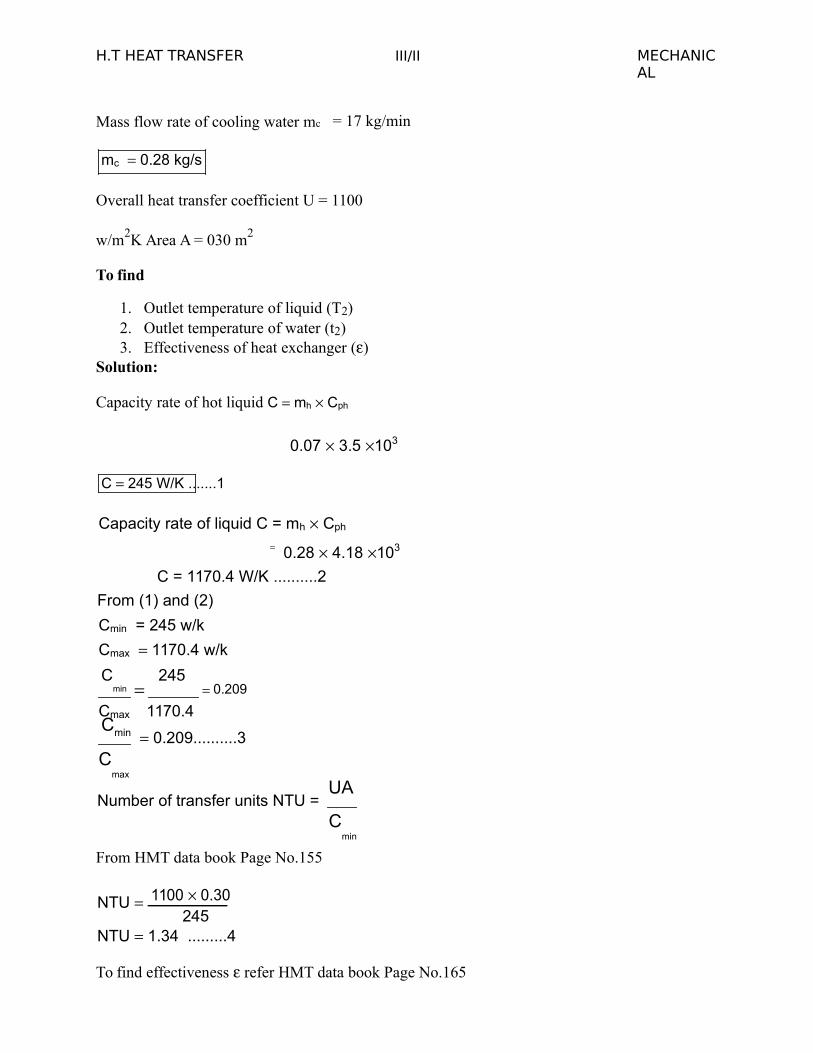
H.T HEAT TRANSFER III/II MECHANICAL
Mass flow rate of cooling water mc = 17 kg/min
mc 0.28 kg/s
Overall heat transfer coefficient U = 1100
w/m2K Area A = 030 m2
To find
1. Outlet temperature of liquid (T2)2. Outlet temperature of water (t2)3. Effectiveness of heat exchanger ()
Solution:
Capacity rate of hot liquid C mh Cph
0.07 3.5 103
C 245 W/K .......1
Capacity rate of liquid C = mh Cph
= 0.28 4.18 103
C = 1170.4 W/K ..........2
From (1) and (2)
Cmin = 245 w/k
Cmax 1170.4 w/k
Cmin
2450.209
Cmax 1170.4Cmin 0.209..........3C
max
Number of transfer units NTU = UA
Cmin
From HMT data book Page No.155
NTU 1100 0.30245
NTU 1.34 .........4
To find effectiveness refer HMT data book Page No.165

99 -
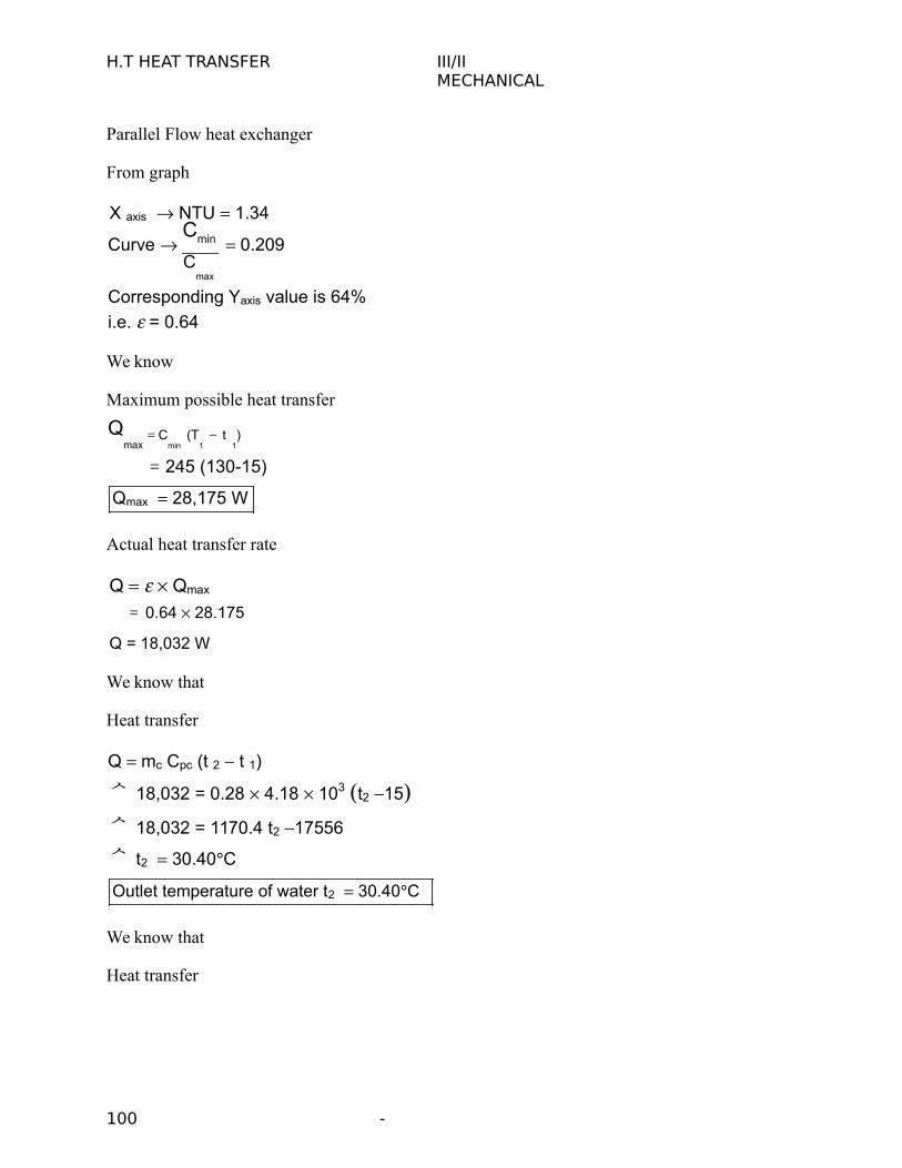
H.T HEAT TRANSFER III/IIMECHANICAL
Parallel Flow heat exchanger
From graph
X axis NTU 1.34
Curve Cmin 0.209C
max
Corresponding Yaxis value is 64%
i.e. = 0.64
We know
Maximum possible heat transfer
Qmax
Cmin(T1t1
)
= 245 (130-15)
Qmax 28,175 W
Actual heat transfer rate
Q Qmax
= 0.64 28.175
Q = 18,032 W
We know that
Heat transfer
Q mc Cpc (t 2 t 1)
18,032 = 0.28 4.18 103 t2 15 18,032 = 1170.4 t2 17556
t2 30.40C
Outlet temperature of water t2 30.40C
We know that
Heat transfer
100 -
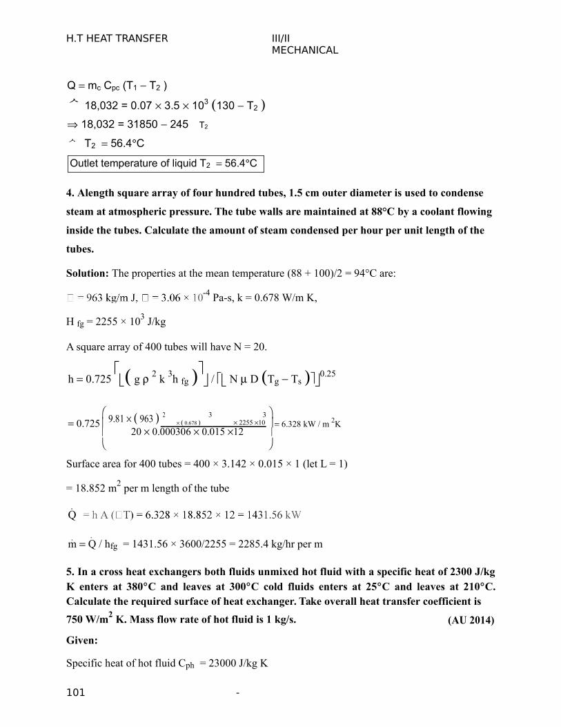
H.T HEAT TRANSFER III/IIMECHANICAL
Q mc Cpc (T1 T2 )
18,032 = 0.07 3.5 103 130 T2 18,032 = 31850 245 T2
T2 56.4C
Outlet temperature of liquid T2 56.4C
4. Alength square array of four hundred tubes, 1.5 cm outer diameter is used to condense
steam at atmospheric pressure. The tube walls are maintained at 88°C by a coolant flowing
inside the tubes. Calculate the amount of steam condensed per hour per unit length of the
tubes.
Solution: The properties at the mean temperature (88 + 100)/2 = 94°C are:
-4 Pa-s, k = 0.678 W/m K,
H fg = 2255 × 103 J/kg
A square array of 400 tubes will have N = 20.
h 0.725 g 2 k 3h fg
/ N D Tg Ts 0.25
9.81 963 2 3 3
0.725 0.678 2255 10 6.328 kW / m 2K20 0.000306 0.015 12
Surface area for 400 tubes = 400 × 3.142 × 0.015 × 1 (let L = 1)
= 18.852 m2 per m length of the tube
Q
m Q / hfg = 1431.56 × 3600/2255 = 2285.4 kg/hr per m
5. In a cross heat exchangers both fluids unmixed hot fluid with a specific heat of 2300 J/kgK enters at 380C and leaves at 300C cold fluids enters at 25C and leaves at 210C.Calculate the required surface of heat exchanger. Take overall heat transfer coefficient is
750 W/m2 K. Mass flow rate of hot fluid is 1 kg/s. (AU 2014)
Given:
Specific heat of hot fluid Cph = 23000 J/kg K
101 -
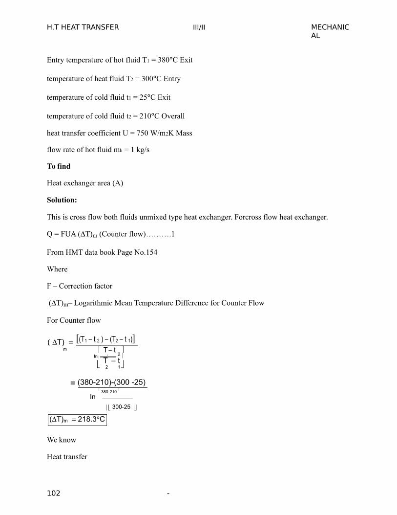
H.T HEAT TRANSFER III/II MECHANICAL
Entry temperature of hot fluid T1 = 380C Exit
temperature of heat fluid T2 = 300C Entry
temperature of cold fluid t1 = 25C Exit
temperature of cold fluid t2 = 210C Overall
heat transfer coefficient U = 750 W/m2K Mass
flow rate of hot fluid mh = 1 kg/s
To find
Heat exchanger area (A)
Solution:
This is cross flow both fluids unmixed type heat exchanger. Forcross flow heat exchanger.
Q = FUA (T)m (Counter flow)……….1
From HMT data book Page No.154
Where
F – Correction factor
(T)m– Logarithmic Mean Temperature Difference for Counter Flow
For Counter flow
( T) (T1 t 2 ) (T2 t 1)m T t
2In 1 T t 2 1
= (380-210)-(300 -25) 380-210
In
300-25
(T)m 218.3C
We know
Heat transfer
102 -
H.T HEAT TRANSFER III/IIMECHANICAL
Q = mh Cph (T1 T2 )
Q 11200 (380-300)
Q = 184 103 W
To find correction factor E refer HMT data book Page No.164.
Singlepass cross flow heat exchanger – Both fluids unmixed.
From graph
X Value P = t 2 t1 210 25 0.52axis
T1 t 1 380 25
Curve value = R= T1 T2 380 300 0.432t2 t 1 210 25
Xaxis Value is 0.52 curve
Value is 0.432 corresponding Yaxis value is 0.97
F = 0.07
Substitute Q, F (T)m and U value in Equation (1)
(1) Q = FU A (T)m
184 103 0.97 750 A 218.3
A 1.15 m2
103 -
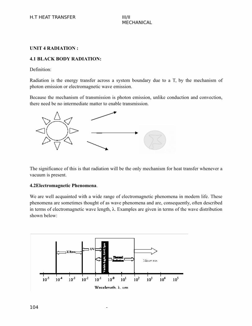
H.T HEAT TRANSFER III/IIMECHANICAL
UNIT 4 RADIATION :
4.1 BLACK BODY RADIATION:
Definition:
Radiation is the energy transfer across a system boundary due to a T, by the mechanism ofphoton emission or electromagnetic wave emission.
Because the mechanism of transmission is photon emission, unlike conduction and convection,there need be no intermediate matter to enable transmission.
The significance of this is that radiation will be the only mechanism for heat transfer whenever avacuum is present.
4.2Electromagnetic Phenomena.
We are well acquainted with a wide range of electromagnetic phenomena in modern life. Thesephenomena are sometimes thought of as wave phenomena and are, consequently, often describedin terms of electromagnetic wave length, λ. Examples are given in terms of the wave distributionshown below:
104 -
H.T HEAT TRANSFER III/IIMECHANICAL
One aspect of electromagnetic radiation is that the related topics are more closely associated withoptics and electronics than with those normally found in mechanical engineering courses.Nevertheless, these are widely encountered topics and the student is familiar with them throughevery day life experiences.
From a viewpoint of previously studied topics students, particularly those with a background inmechanical or chemical engineering, will find the subject of Radiation Heat Transfer a littleunusual. The physics background differs fundamentally from that found in the areas ofcontinuum mechanics. Much of the related material is found in courses more closely identifiedwith quantum physics or electrical engineering, i.e. Fields and Waves. At this point, it isimportant for us to recognize that since the subject arises from a different area of physics, it willbe important that we study these concepts with extra care.
4.3Stefan-Boltzman Law
Both Stefan and Boltzman were physicists; any student taking a course in quantum physics willbecome well acquainted with Boltzman’s work as he made a number of important contributionsto the field. Both were contemporaries of Einstein so we see that the subject is of fairly recentvintage. (Recall that the basic equation for convection heat transfer is attributed to Newton)
where: Eb = Emissive Power, the gross energy emitted from an ideal surface per unit area, time. σ = Stefan Boltzman constant, 5.67⋅10-8 W/m2⋅K4
Tabs = Absolute temperature of the emitting surface, K.
Take particular note of the fact that absolute temperatures are used in Radiation. It is suggested,as a matter of good practice, to convert all temperatures to the absolute scale as an initial step inall radiation problems.
You will notice that the equation does not include any heat flux term, q”. Instead we have a termthe emissive power. The relationship between these terms is as follows. Consider two infiniteplane surfaces, both facing one another. Both surfaces are ideal surfaces. One surface is found tobe at temperature, T1, the other at temperature, T2. Since both temperatures are at temperaturesabove absolute zero, both will radiate energy as described by the Stefan-Boltzman law. The heatflux will be the net radiant flow as given by:
4.4Plank’s Law
105 -
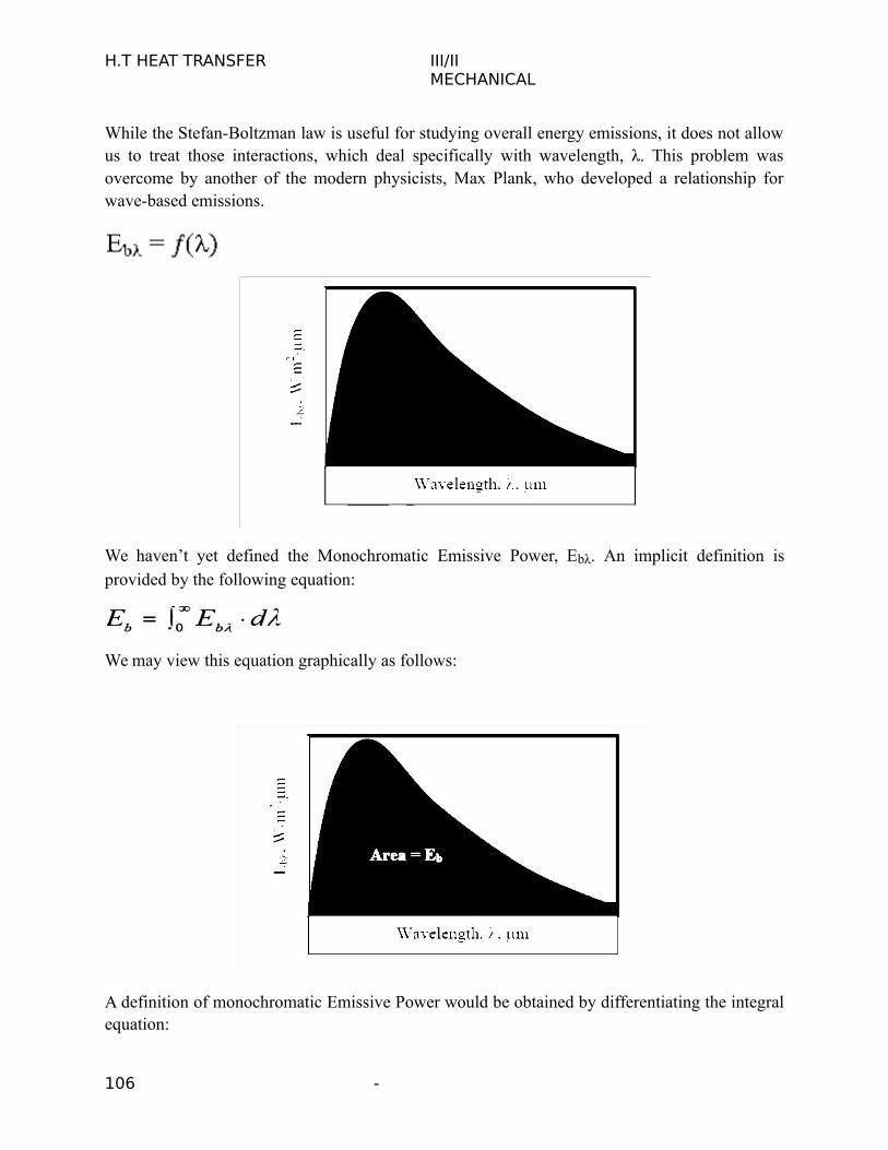
H.T HEAT TRANSFER III/IIMECHANICAL
While the Stefan-Boltzman law is useful for studying overall energy emissions, it does not allowus to treat those interactions, which deal specifically with wavelength, λ. This problem wasovercome by another of the modern physicists, Max Plank, who developed a relationship forwave-based emissions.
We haven’t yet defined the Monochromatic Emissive Power, Ebλ. An implicit definition isprovided by the following equation:
We may view this equation graphically as follows:
A definition of monochromatic Emissive Power would be obtained by differentiating the integralequation:
106 -
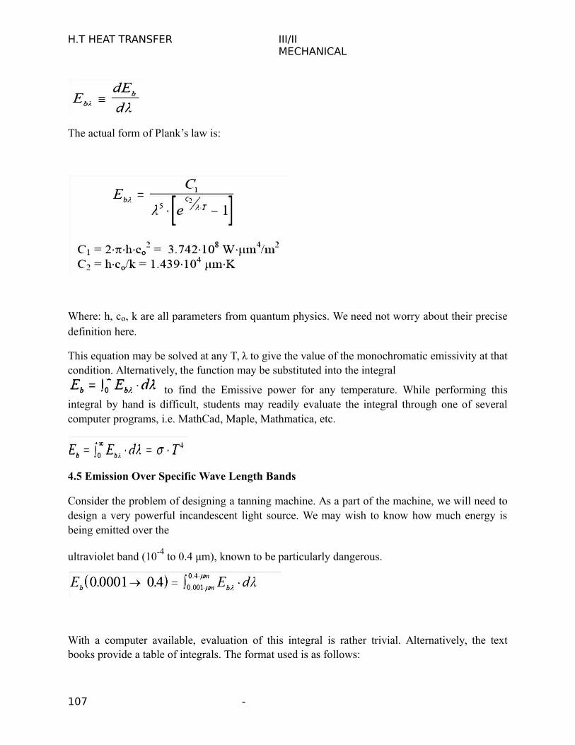
H.T HEAT TRANSFER III/IIMECHANICAL
The actual form of Plank’s law is:
Where: h, co, k are all parameters from quantum physics. We need not worry about their precisedefinition here.
This equation may be solved at any T, λ to give the value of the monochromatic emissivity at thatcondition. Alternatively, the function may be substituted into the integral
to find the Emissive power for any temperature. While performing thisintegral by hand is difficult, students may readily evaluate the integral through one of severalcomputer programs, i.e. MathCad, Maple, Mathmatica, etc.
4.5 Emission Over Specific Wave Length Bands
Consider the problem of designing a tanning machine. As a part of the machine, we will need todesign a very powerful incandescent light source. We may wish to know how much energy isbeing emitted over the
ultraviolet band (10-4 to 0.4 μm), known to be particularly dangerous.
With a computer available, evaluation of this integral is rather trivial. Alternatively, the textbooks provide a table of integrals. The format used is as follows:
107 -
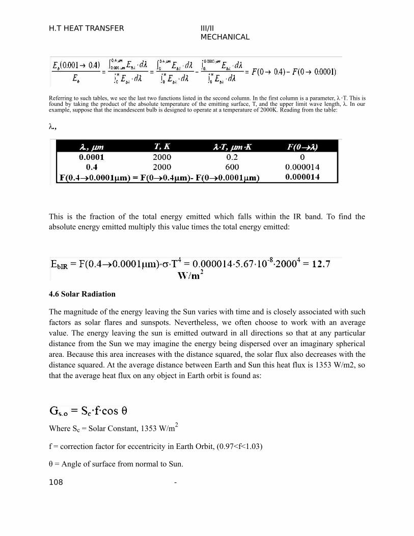
H.T HEAT TRANSFER III/IIMECHANICAL
Referring to such tables, we see the last two functions listed in the second column. In the first column is a parameter, λ ⋅T. This isfound by taking the product of the absolute temperature of the emitting surface, T, and the upper limit wave length, λ. In ourexample, suppose that the incandescent bulb is designed to operate at a temperature of 2000K. Reading from the table:
λ.,
This is the fraction of the total energy emitted which falls within the IR band. To find theabsolute energy emitted multiply this value times the total energy emitted:
4.6 Solar Radiation
The magnitude of the energy leaving the Sun varies with time and is closely associated with suchfactors as solar flares and sunspots. Nevertheless, we often choose to work with an averagevalue. The energy leaving the sun is emitted outward in all directions so that at any particulardistance from the Sun we may imagine the energy being dispersed over an imaginary sphericalarea. Because this area increases with the distance squared, the solar flux also decreases with thedistance squared. At the average distance between Earth and Sun this heat flux is 1353 W/m2, sothat the average heat flux on any object in Earth orbit is found as:
Where Sc = Solar Constant, 1353 W/m2
f = correction factor for eccentricity in Earth Orbit, (0.97<f<1.03)
θ = Angle of surface from normal to Sun.
108 -

H.T HEAT TRANSFER III/IIMECHANICAL
Because of reflection and absorption in the Earth’s atmosphere, this number is significantlyreduced at ground level. Nevertheless, this value gives us some opportunity to estimate thepotential for using solar energy, such as in photovoltaic cells.
Some Definitions
In the previous section we introduced the Stefan-Boltzman Equation to describe radiation froman ideal surface.
This equation provides a method of determining the total energy leaving a surface, but gives noindication of the direction in which it travels. As we continue our study, we will want to be ableto calculate how heat is distributed among various objects.
For this purpose, we will introduce the radiation intensity, I, defined as the energy emitted perunit area, per unit time, per unit solid angle. Before writing an equation for this new property, wewill need to define some of the terms we will be using.
4.7 Angles and Arc Length
We are well accustomed to thinking of an angle as a two dimensional object. It may be used tofind an arc length:
Solid Angle
We generalize the idea of an angle and an arc length to three dimensions and define a solid angle, Ω, which like the standard angle has no dimensions. The solid angle, when multiplied bythe radius squared will have dimensions of length squared, or area, and will have the magnitudeof the encompassed area.
109 -
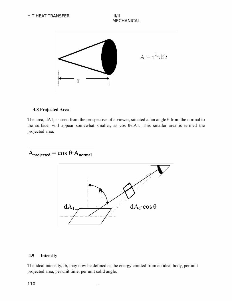
H.T HEAT TRANSFER III/IIMECHANICAL
4.8 Projected Area
The area, dA1, as seen from the prospective of a viewer, situated at an angle θ from the normal tothe surface, will appear somewhat smaller, as cos θ·dA1. This smaller area is termed theprojected area.
4.9 Intensity
The ideal intensity, Ib, may now be defined as the energy emitted from an ideal body, per unitprojected area, per unit time, per unit solid angle.
110 -
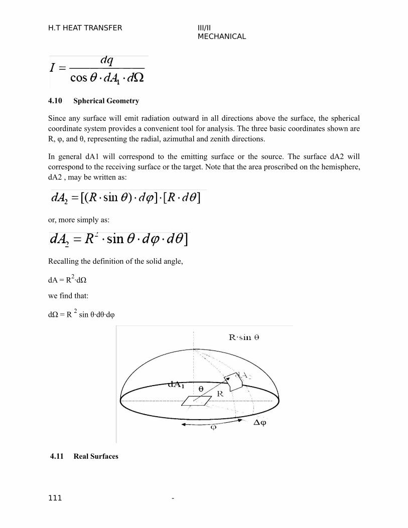
H.T HEAT TRANSFER III/IIMECHANICAL
4.10 Spherical Geometry
Since any surface will emit radiation outward in all directions above the surface, the sphericalcoordinate system provides a convenient tool for analysis. The three basic coordinates shown areR, φ, and θ, representing the radial, azimuthal and zenith directions.
In general dA1 will correspond to the emitting surface or the source. The surface dA2 willcorrespond to the receiving surface or the target. Note that the area proscribed on the hemisphere,dA2 , may be written as:
or, more simply as:
Recalling the definition of the solid angle,
dA = R2·dΩ
we find that:
dΩ = R 2 sin θ·dθ·dφ
4.11 Real Surfaces
111 -

H.T HEAT TRANSFER III/IIMECHANICAL
Thus far we have spoken of ideal surfaces, i.e. those that emit energy according to the Stefan-Boltzman law:
Real surfaces have emissive powers, E, which are somewhat less than that obtained theoreticallyby Boltzman. To account for this reduction, we introduce the emissivity, ε.
so that the emissive power from any real surface is given by:
Receiving Properties
Targets receive radiation in one of three ways; they absorption, reflection or transmission. Toaccount for these characteristics, we introduce three additional properties:
• Absorptivity, α, the fraction of incident radiation absorbed.
• Reflectivity, ρ, the fraction of incident radiation reflected.
• Transmissivity, τ, the fraction of incident radiation transmitted.
We see, from Conservation of Energy, that:
α + ρ + τ = 1
In this course, we will deal with only opaque surfaces, τ = 0, so that:
112 -
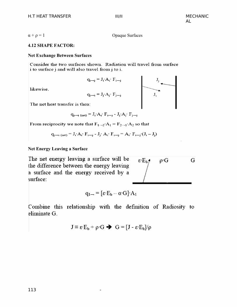
H.T HEAT TRANSFER III/II MECHANICAL
α + ρ = 1 Opaque Surfaces
4.12 SHAPE FACTOR:
Net Exchange Between Surfaces
Net Energy Leaving a Surface
113 -
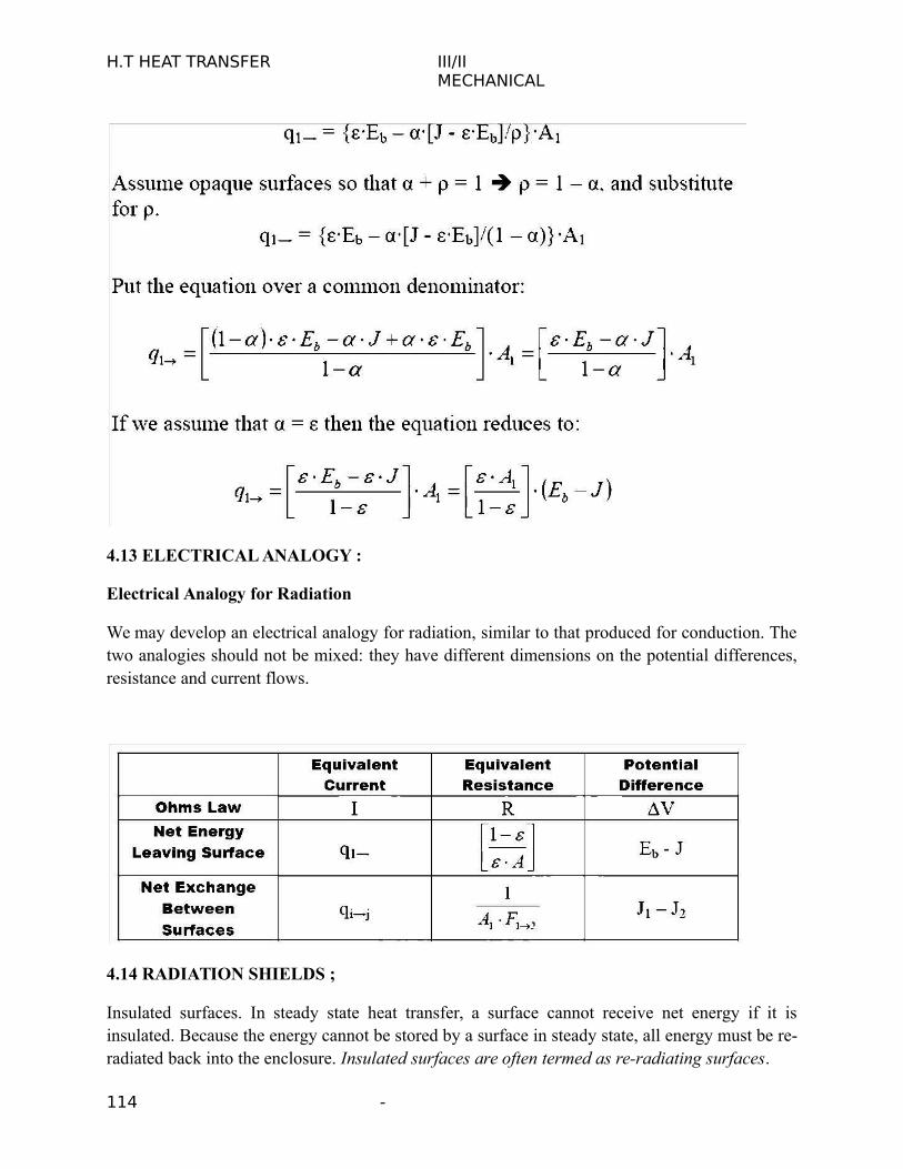
H.T HEAT TRANSFER III/IIMECHANICAL
4.13 ELECTRICAL ANALOGY :
Electrical Analogy for Radiation
We may develop an electrical analogy for radiation, similar to that produced for conduction. Thetwo analogies should not be mixed: they have different dimensions on the potential differences,resistance and current flows.
4.14 RADIATION SHIELDS ;
Insulated surfaces. In steady state heat transfer, a surface cannot receive net energy if it isinsulated. Because the energy cannot be stored by a surface in steady state, all energy must be re-radiated back into the enclosure. Insulated surfaces are often termed as re-radiating surfaces.
114 -

H.T HEAT TRANSFER III/IIMECHANICAL
Electrically cannot flow through a battery if it is not grounded.
Surface 3 is not grounded so that the battery and surface resistance serve no purpose and areremoved from the drawing.
• Black surfaces: A black, or ideal surface, will have no surface resistance:
In this case the nodal Radiosity and emissive power will be equal.
This result gives some insight into the physical meaning of a black surface. Ideal surfaces radiateat the maximum possible level. Non-black surfaces will have a reduced potential, somewhat likea battery with a corroded terminal. They therefore have a reduced potential to cause heat/currentflow.
• Large surfaces: Surfaces having a large surface area will behave as black surfaces, irrespective of the actual surface properties:
Physically, this corresponds to the characteristic of large surfaces that as they reflect energy,there is very little chance that energy will strike the smaller surfaces; most of the energy isreflected back to another part of the same large surface. After several partial absorptions most ofthe energy received is absorbed.
115 -
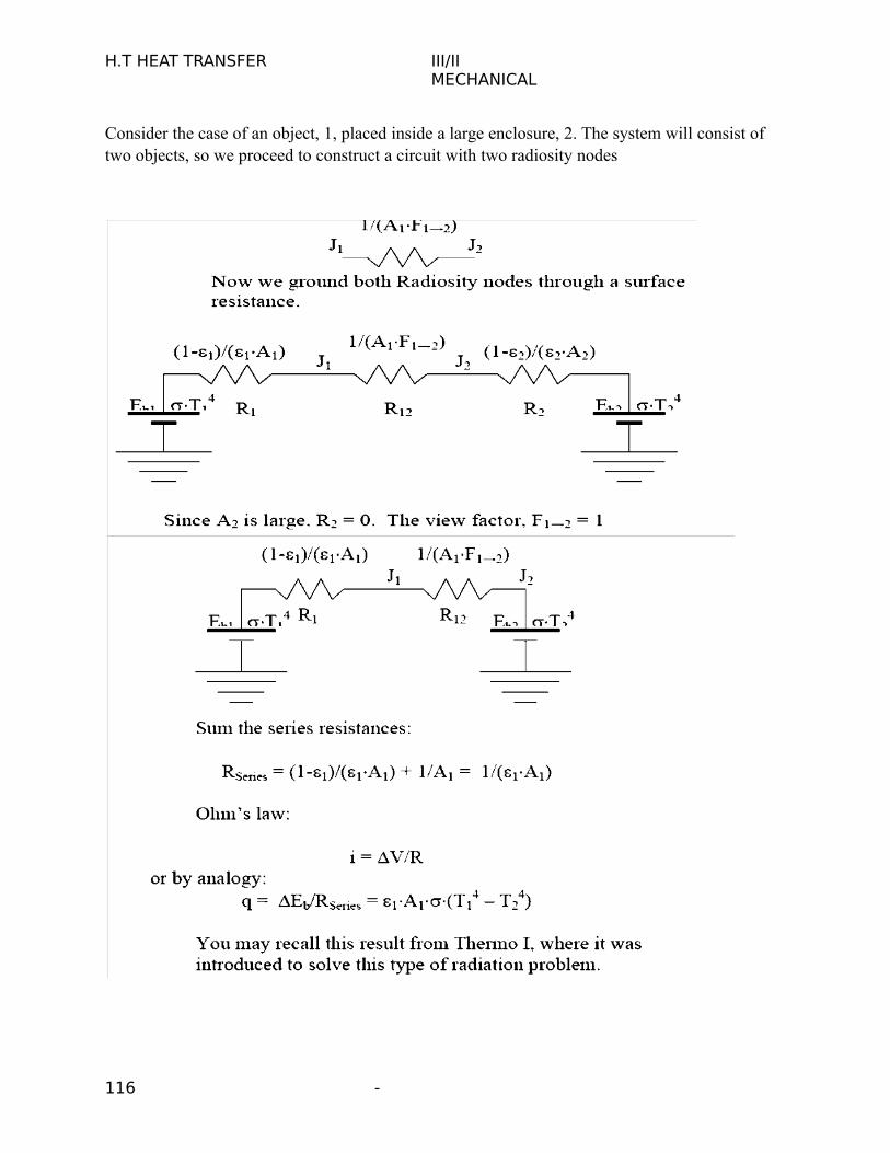
H.T HEAT TRANSFER III/IIMECHANICAL
Consider the case of an object, 1, placed inside a large enclosure, 2. The system will consist of two objects, so we proceed to construct a circuit with two radiosity nodes
116 -

H.T HEAT TRANSFER III/IIMECHANICAL
In this example there are three junctions, so we will obtain three equations. This will allow us to solve for three unknowns.
Radiation problems will generally be presented on one of two ways:
1. The surface net heat flow is given and the surface temperature is to be found.
2. The surface temperature is given and the net heat flow is to be found.
Returning for a moment to the coal grate furnace, let us assume that we know (a) the total heatbeing produced by the coal bed, (b) the temperatures of the water walls and (c) the temperatureof the super heater sections.
Apply Kirchoff’s law about node 1, for the coal bed:
117 -

H.T HEAT TRANSFER III/IIMECHANICAL
(Note how node 1, with a specified heat input, is handled differently than node 2, with a specified temperature.
And for node 3:
The three equations must be solved simultaneously. Since they are each linear in J, matrix methods may be used:
The matrix may be solved for the individual Radiosity. Once these are known, we return to the electrical analogy to find the temperature of surface 1, and the heat flows to surfaces 2 and 3.
Surface 1: Find the coal bed temperature, given the heat flow:
Surface 2: Find the water wall heat input, given the water wall temperature:
Surface 3: (Similar to surface 2) Find the water wall heat input, given the water wall temperature:
118 -

H.T HEAT TRANSFER III/IIMECHANICAL
119 -
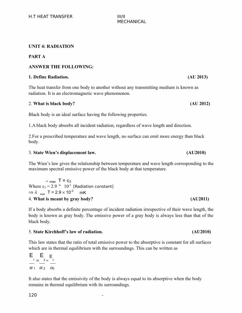
H.T HEAT TRANSFER III/IIMECHANICAL
UNIT 4: RADIATION
PART A
ANSWER THE FOLLOWING:
1. Define Radiation. (AU 2013)
The heat transfer from one body to another without any transmitting medium is known as radiation. It is an electromagnetic wave phenomenon.
2. What is black body? (AU 2012)
Black body is an ideal surface having the following properties.
1.A black body absorbs all incident radiation, regardless of wave length and direction.
2.For a prescribed temperature and wave length, no surface can emit more energy than black body.
3. State Wien’s displacement law. (AU2010)
The Wien’s law gives the relationship between temperature and wave length corresponding to themaximum spectral emissive power of the black body at that temperature.
mas T = c3
Where c3 = 2.9 10 -3 [Radiation constant]
mas T = 2.9 10-3 mK
4. What is meant by gray body? (AU2011)
If a body absorbs a definite percentage of incident radiation irrespective of their wave length, thebody is known as gray body. The emissive power of a gray body is always less than that of theblack body.
5. State Kirchhoff’s law of radiation. (AU2010)
This law states that the ratio of total emissive power to the absorptive is constant for all surfaces which are in thermal equilibrium with the surroundings. This can be written as
E1
E2
E3
1 2 3
It also states that the emissivity of the body is always equal to its absorptive when the body remains in thermal equilibrium with its surroundings.
120 -

H.T HEAT TRANSFER III/II MECHANICAL
1 = E1; 2 = E2 and so on.
6. Define irradiation (G) (AU 2011)
It is defined as the total radiation incident upon a surface per unit time per unit area. It is
expressed in W/m2.
7. What is the purpose of radiation shield?
Radiation shields constructed from low emissivity (high reflective) materials. It is used to reducethe net radiation transfer between two surfaces.
8. Define intensity of radiation (Ib)? (AU2010)
It is defined as the rate of energy leaving a space in a given direction per unit solid angle per unit area of the emitting surface normal to the mean direction in space.
In E
b
9. What is radiosity (J)?
It is used to indicate the total radiation leaving a surface per unit time per unit area. It is
expressed in W/m2.
10. What is meant by shape factor? (AU 2009)
The shape factor is defined as the fraction of the radioactive energy that is diffused from onsurface element and strikes the other surface directly with no intervening reflections. It is
represented by Fij. Other names for radiation shape factor are view factor, angle factor andconfiguration factor.
11. State Stefan – Boltzmann law. (AU2010)
The emissive power of a black body is proportional to the fourth power of absolute temperature.
E T4
b
E = T4
b
Where E b = Emissive power, w/m2
= Stefan. Boltzmann constant
= 5.67 10-8 W/m2 K4
T = Temperature, K
121 -
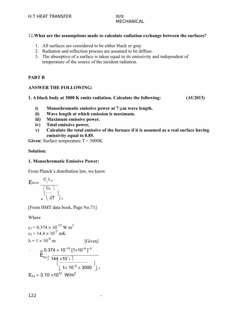
H.T HEAT TRANSFER III/IIMECHANICAL
12.What are the assumptions made to calculate radiation exchange between the surfaces?
1. All surfaces are considered to be either black or gray2. Radiation and reflection process are assumed to be diffuse.3. The absorptive of a surface is taken equal to its emissivity and independent of
temperature of the source of the incident radiation.
PART B
ANSWER THE FOLLOWING:
1. A black body at 3000 K emits radiation. Calculate the following: (AU2013)
i) Monochromatic emissive power at 7 m wave length.ii) Wave length at which emission is maximum.iii) Maximum emissive power.iv) Total emissive power,v) Calculate the total emissive of the furnace if it is assumed as a real surface having
emissivity equal to 0.85.Given: Surface temperature T = 3000K
Solution:
1. Monochromatic Emissive Power:
From Planck’s distribution law, we know
EbC
15
C2
e T
1
[From HMT data book, Page No.71]
Where
c1 = 0.374 10-15 W m2
c2 = 14.4 10-3 mK
= 1 10-6 m [Given]
0.374 1015 [1106 ]5 Eb 144 10
3 1 106 3000
1
Eb 3.10 1012 W/m2
122 -
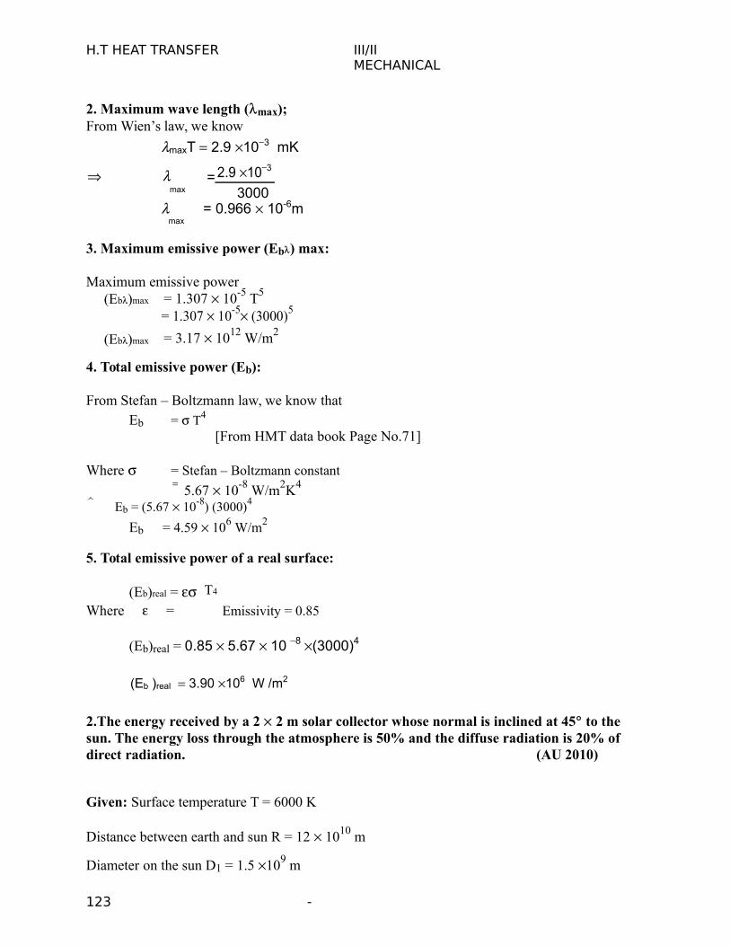
H.T HEAT TRANSFER III/IIMECHANICAL
2. Maximum wave length (max);From Wien’s law, we know
maxT 2.9 103 mK
= 2.9 103
max 3000 = 0.966 10-6m
max
3. Maximum emissive power (Eb) max:
Maximum emissive power(Eb)max = 1.307 10-5 T5
= 1.307 10-5 (3000)5
(Eb)max = 3.17 1012 W/m2
4. Total emissive power (Eb):
From Stefan – Boltzmann law, we know thatEb = T4
[From HMT data book Page No.71]
Where = Stefan – Boltzmann constant= 5.67 10-8 W/m2K4
Eb = (5.67 10-8) (3000)4
Eb = 4.59 106 W/m2
5. Total emissive power of a real surface:
(Eb)real = T4
Where = Emissivity = 0.85
(Eb)real = 0.85 5.67 10 8 (3000)4
(Eb )real 3.90 106 W /m2
2.The energy received by a 2 2 m solar collector whose normal is inclined at 45 to the sun. The energy loss through the atmosphere is 50% and the diffuse radiation is 20% ofdirect radiation. (AU 2010)
Given: Surface temperature T = 6000 K
Distance between earth and sun R = 12 1010 m
Diameter on the sun D1 = 1.5 109 m
123 -
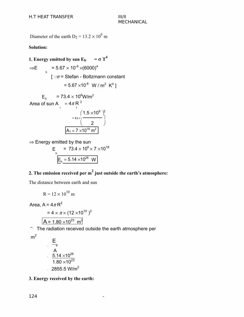
H.T HEAT TRANSFER III/IIMECHANICAL
Diameter of the earth D2 = 13.2 106 m
Solution:
1. Energy emitted by sun Eb = T4
E = 5.67 10-8 (6000)4
b
[ = Stefan - Boltzmann constant
= 5.67 10-8 W / m2 K4 ]
Eb = 73.4 106W/m2
Area of sun A1
4 R 21
1.5 109 2
= 4 2
A1 7 1018 m2
Energy emitted by the sun
E = 73.4 106 7 1018
b
Eb 5.14 1026 W
2. The emission received per m2 just outside the earth’s atmosphere:
The distance between earth and sun
R = 12 1010 m
Area, A = 4 R2
= 4 (12 1010 )2
A = 1.80 1023 m2
The radiation received outside the earth atmosphere per
m2
=
Eb
A= 5.14 1026
1.80 1023
= 2855.5 W/m2
3. Energy received by the earth:
124 -

H.T HEAT TRANSFER III/IIMECHANICAL
Earth area = 4 (D2 )2
= 4 [13.2 106 ]2
Earth area = 1.36 104m2
Energy received by the earth
2855.5 1.36 104
3.88 1017 W
4. The energy received by a 2 2 m solar collector;
Energy loss through the atmosphere is 50%. Soenergy reaching the earth.
100 - 50 = 50% = 0.50
Energy received by the earth
0.50 2855.5
1427.7 W/m2 ......(1)
Diffuse radiation is 20%
0.20 1427.7 = 285.5 W/m2
Diffuse radiation = 285.5 W/m2 .........(2)
Total radiation reaching the collection
142.7 285.5
1713.2 W/m2
Plate area = A cos = 2 2 cos 45= 2.82 m2
Energy received by the collector
2.82 1713.2
4831.2 W
125 -
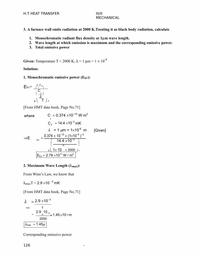
H.T HEAT TRANSFER III/IIMECHANICAL
3. A furnace wall emits radiation at 2000 K.Treating it as black body radiation, calculate
1. Monochromatic radiant flux density at 1m wave length.2. Wave length at which emission is maximum and the corresponding emissive power.3. Total emissive power
Given: Temperature T = 2000 K; = 1 m = 1 10-6
Solution:
1. Monochromatic emissive power (Eb):
Eb c
15
C
2
e
T 1
[From HMT data book, Page No.71]
where C 0.374 1015 W m2
1
C2 14.4 103 mK
= 1 m = 110-6 m [Given]
E 0.374 1015 (1106 )5
b 14.4 103
1 106
e 2000 1
Eb 2.79 1011 W / m2
2. Maximum Wave Length (max):
From Wien’s Law, we know that
maxT = 2.9 10 3 mK
[From HMT data book, Page No.71]
2.9 103
max T
=2.9
103
1.45 106 m
2000
max 1.45
Corresponding emissive power
126 -
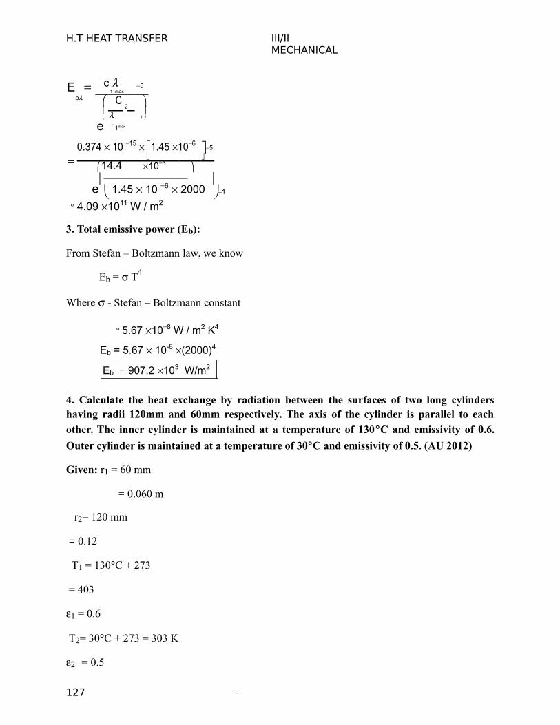
H.T HEAT TRANSFER III/IIMECHANICAL
Eb
c 51 max
C2
T
e 1max
0.374 10 15 1.45 106 5
14.4 103
e 1.45 10 6 2000
1
4.09 1011 W / m2
3. Total emissive power (Eb):
From Stefan – Boltzmann law, we know
Eb = T4
Where - Stefan – Boltzmann constant
5.67 108 W / m2 K4
Eb = 5.67 10-8 (2000)4
Eb 907.2 103 W/m2
4. Calculate the heat exchange by radiation between the surfaces of two long cylindershaving radii 120mm and 60mm respectively. The axis of the cylinder is parallel to each
other. The inner cylinder is maintained at a temperature of 130C and emissivity of 0.6.
Outer cylinder is maintained at a temperature of 30C and emissivity of 0.5. (AU 2012)
Given: r1 = 60 mm
= 0.060 m
r2= 120 mm
= 0.12
T1 = 130C + 273
= 403
1 = 0.6
T2= 30C + 273 = 303 K
2 = 0.5
127 -

H.T HEAT TRANSFER III/IIMECHANICAL
To find: Heat exchange (Q)
Solution: Heat exchange between two large concentric cylinders is given by
Q A T 4 T 4 .....(1) 1 2
[From equation No.27]
1
where 1 A1 1 1
1 A2 2
1
= [ A DL]1 D L 1 1 2 1
0.6 D2L2 0.5
=1
[ L1 L2 1]1 0.12 1 1
0.6 0.24 0.5 0.46
Q 0.46 5.67 108 D L (403)4 (303)4 12 1
= 0.46 5.67 108 0.12 1 (403)4 (303)4
Q12 176.47 W
5. Emissivity's of two large parallel plates maintained at 800C and 300C are 0.5respectively. Find net radiant hat exchange per square meter for these plates. Find thepercentage reduction in heat transfer when a polished aluminums radiation shield ofemissivity 0.06 is placed between them. Also find the temperature of the shield. (AU 2010)
Given: T1 = 800C + 273
= 1073 K
T2= 300C + 273
= 573 K
1= 0.3 2 = 0.5
Shield emissivity 3 = 0.06
To find:
1. Net radiant heat exchange per square meter. (Q/A)
128 -
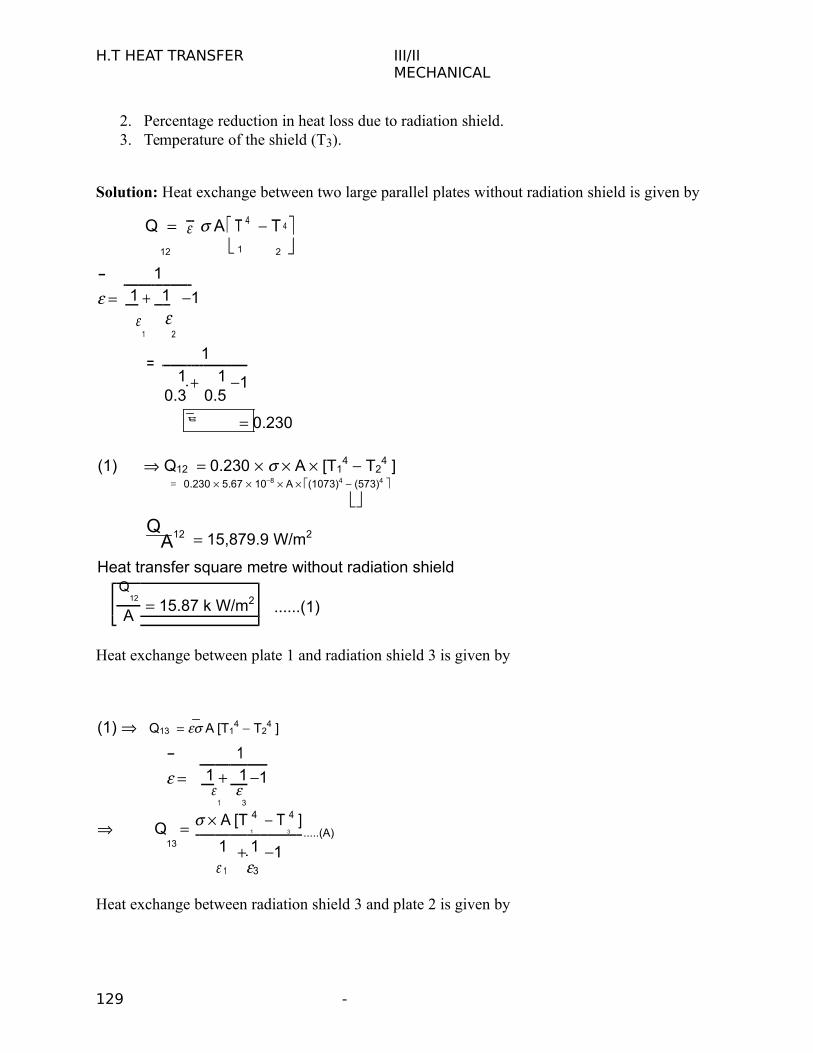
H.T HEAT TRANSFER III/IIMECHANICAL
2. Percentage reduction in heat loss due to radiation shield.3. Temperature of the shield (T3).
Solution: Heat exchange between two large parallel plates without radiation shield is given by
Q A T 4 T 4 12 1 2
1
1 1 1
1
2
=1
1 1 10.3 0.5
0.230
(1) Q12 0.230 A [T14 T2
4 ]= 0.230 5.67 108 A (1073)4 (573)4
QA12 15,879.9 W/m2
Heat transfer square metre without radiation shieldQ
12 15.87 k W/m2 ......(1)A
Heat exchange between plate 1 and radiation shield 3 is given by
(1) Q13 A [T14 T2
4 ]
1
1 1 1
1
3
Q A [T 4 T 4 ]1 3 .....(A)
13 1 1 11 3
Heat exchange between radiation shield 3 and plate 2 is given by
129 -
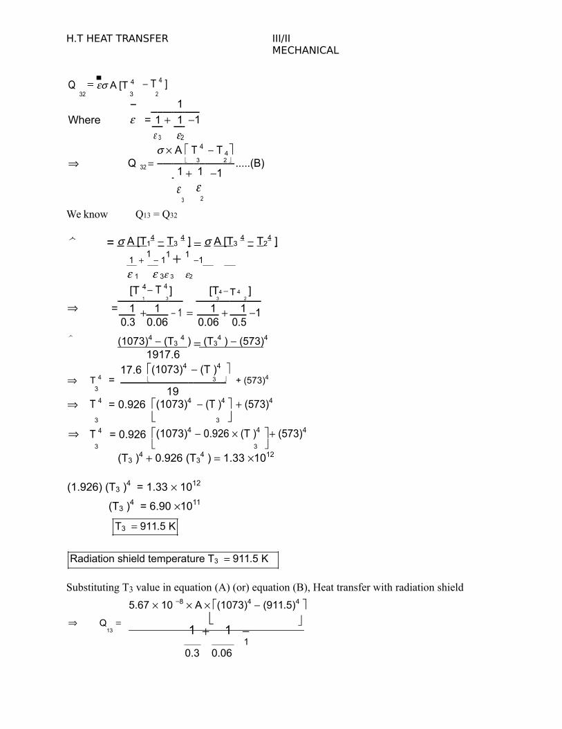
H.T HEAT TRANSFER III/IIMECHANICAL
T 4 ]Q32
A [T 43 2
1
Where = 1 1 13 2
A T 4 T 4 Q 32 3 2 .....(B)
1 1 1
2
3
We know Q13 = Q32
= A [T14 T3 4 ] A [T3 4 T2
4 ]
1 1
11 1 1
1332
[T 4 T 4 ]
[T4 T 4 ]
=1 3 3 2
1 1 1 1 1 10.3 0.06 0.06 0.5
(1073)4 (T3 4 ) (T34 ) (573)4
1917.617.6 (1073)4 (T )4
T 4 = 3 + (573)4
3 19 T 4 = 0.926 (1073)4 (T )4 (573)4
3 3 T 4 = 0.926 (1073)4 0.926 (T )4 (573)4
3 3 (T3 )4 0.926 (T3
4 ) 1.33 1012
(1.926) (T3 )4 = 1.33 1012
(T3 )4 = 6.90 1011
T3 911.5 K
Radiation shield temperature T3 911.5 K
Substituting T3 value in equation (A) (or) equation (B), Heat transfer with radiation shield
5.67 10 8 A (1073)4 (911.5)4 Q
13
1 1
10.3 0.06

130 -
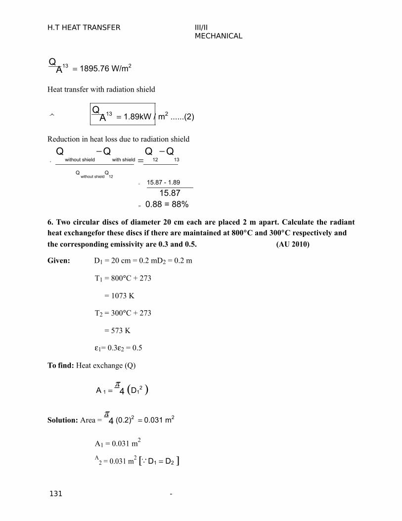
H.T HEAT TRANSFER III/IIMECHANICAL
QA13 1895.76 W/m2
Heat transfer with radiation shield
Q
A13 1.89kW / m2 ......(2)
Reduction in heat loss due to radiation shield
Q without shield
Q
with shield Q
12
Q
13
Q without shield
Q12
= 15.87 - 1.89
15.87
= 0.88 = 88%
6. Two circular discs of diameter 20 cm each are placed 2 m apart. Calculate the radiantheat exchangefor these discs if there are maintained at 800C and 300C respectively and
the corresponding emissivity are 0.3 and 0.5. (AU 2010)
Given: D1 = 20 cm = 0.2 mD2 = 0.2 m
T1 = 800C + 273
= 1073 K
T2 = 300C + 273
= 573 K
1= 0.32 = 0.5
To find: Heat exchange (Q)
A 1 4 D1
2
Solution: Area = 4 (0.2)2 0.031 m2
A1 = 0.031 m2
A2 = 0.031 m2 D1 D2
131 -
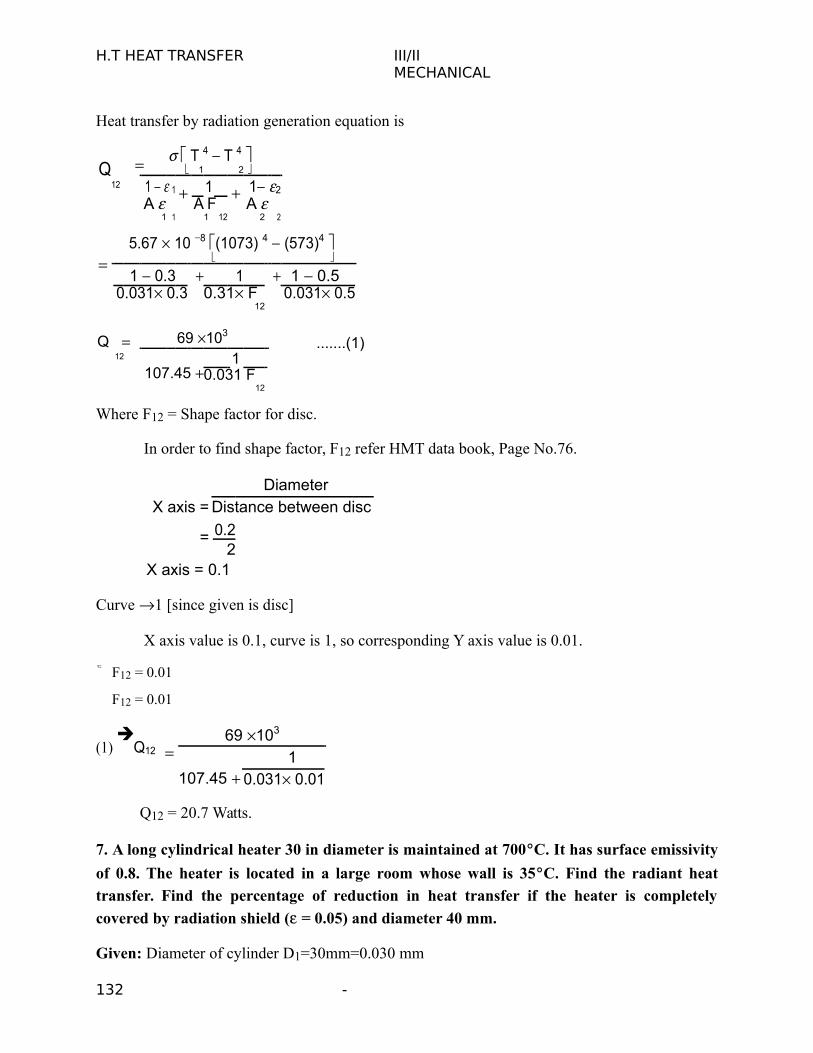
H.T HEAT TRANSFER III/IIMECHANICAL
Heat transfer by radiation generation equation is
T 4 T 4 Q
12
1 2
1 1 1 1 2
A 1
A F A 21 1 12 2
5.67 10 8 (1073) 4 (573)4
1 0.3 1 1 0.50.031 0.3 0.31 F 0.031 0.5
12
Q 69 103.......(1)
12
107.45 1
0.031 F12
Where F12 = Shape factor for disc.
In order to find shape factor, F12 refer HMT data book, Page No.76.
X axis =Diameter
Distance between disc
= 0.22
X axis = 0.1
Curve 1 [since given is disc]
X axis value is 0.1, curve is 1, so corresponding Y axis value is 0.01.
F12 = 0.01
F12 = 0.01
(1)
Q12 69 103
107.45 1
0.031 0.01
Q12 = 20.7 Watts.
7. A long cylindrical heater 30 in diameter is maintained at 700C. It has surface emissivity
of 0.8. The heater is located in a large room whose wall is 35C. Find the radiant heat
transfer. Find the percentage of reduction in heat transfer if the heater is completely
covered by radiation shield ( = 0.05) and diameter 40 mm.
Given: Diameter of cylinder D1=30mm=0.030 mm
132 -
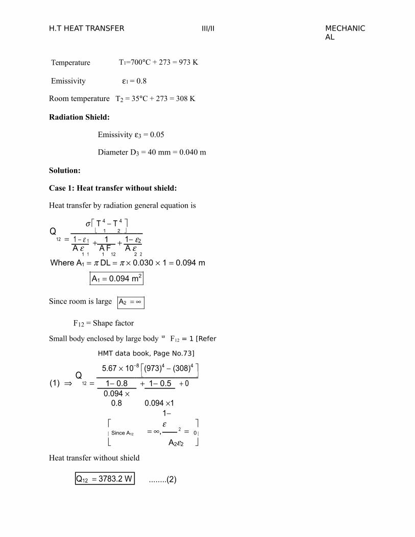
H.T HEAT TRANSFER III/II MECHANICAL
Temperature T1=700C + 273 = 973 K
Emissivity 1 = 0.8
Room temperature T2 = 35C + 273 = 308 K
Radiation Shield:
Emissivity 3 = 0.05
Diameter D3 = 40 mm = 0.040 m
Solution:
Case 1: Heat transfer without shield:
Heat transfer by radiation general equation is
T 4 T 4 Q
12 1 2
1 1 1 1 2
A 1
A F A 21 1 12 2
Where A1 DL 0.030 1 0.094 m
A1 0.094 m2
Since room is large A2
F12 = Shape factor
Small body enclosed by large body F 12 = 1 [Refer
HMT data book, Page No.73]
5.67 108 (973)4 (308)4
(1) Q
12
1 0.8 1 0.5 00.094
0.8 0.094 1
,
1
2
Since A12 0
A22
Heat transfer without shield
Q12 3783.2 W ........(2)

133 -
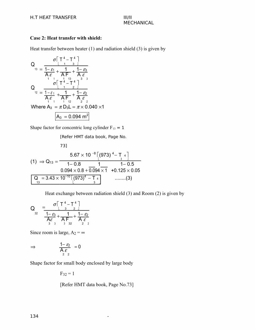
H.T HEAT TRANSFER III/IIMECHANICAL
Case 2: Heat transfer with shield:
Heat transfer between heater (1) and radiation shield (3) is given by
T 4 T 4 Q
13 1 3
1 1 1 1 3
A 1
A F A 31 1 13 3
T 4 T 4 Q
12 1 2
1 1 1 1 2
A 1
A F A 21 1 12 2
Where A3 D3L 0.040 1
A3 0.094 m2
Shape factor for concentric long cylinder F13 = 1
[Refer HMT data book, Page No.
73]
5.67 10 8 (973) 4 T 4 (1) Q13 3
1 0.8
1+
1 0.50.094 0.8 0.094 1 0.125 0.05
Q 3.43 1010 (973)4 T 4 ........(3)13 3
Heat exchange between radiation shield (3) and Room (2) is given by
T 4 T 4 Q
32
3 2
1 3 1 1 2
A3
A F A 23 3 32 2
Since room is large, A2 =
1 2 0A
22
Shape factor for small body enclosed by large body
F32 = 1
[Refer HMT data book, Page No.73]
134 -

H.T HEAT TRANSFER III/IIMECHANICAL
5.67 10 8 T 4 (308)4
Q
32 3
1 0.05 1 +00.125 0.5 0.125 1
Q32
3.54 1010 T 4 (308)4 ........(4) 3
3.43 10-10 (973)4 T 4 3.54 1010 T 4 (308)4 3 3
T3 817 K
Substitute T3 value in (3) or (4).
Heat transfer with radiation shield
Q 3.43 10 10 (973) 4 (817)4 13
Q13 154.6 W
Re duction heat Q Q
loss due to
without shield with shield Qwithout shield
radiation shield
Q12
Q
13
Q12
3783.2 154.6 95.9%3783.2
UNIT 5 MASS TRANSFER
5.1 BASIC CONCEPTS
Air is a mixture of various gases. Whenever we have a multicomponent system with a
concentration gradient, one constituent of the mixture gets transported from the region of higher
concentration to the region of lower concentration till the concentration gradient reduces to zero.
This phenomenon of the transport of mass as a result of concentration gradient is called 'Mass
Transfer'.
The mass transfer phenomenon is analogous to heat transfer phenomenon. In heat
transfer - heat energy flows in a direction of decreasing temperature gradient and ceases when
the temperature gradient reduces to zero. In mass transfer - the transfer of mass takes place in the
135 -
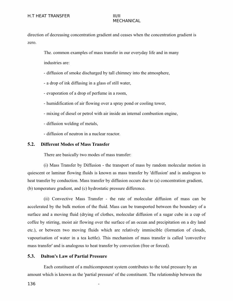
H.T HEAT TRANSFER III/IIMECHANICAL
direction of decreasing concentration gradient and ceases when the concentration gradient is
zero.
The. common examples of mass transfer in our everyday life and in many
industries are:
- diffusion of smoke discharged by tall chimney into the atmosphere,
- a drop of ink diffusing in a glass of still water,
- evaporation of a drop of perfume in a room,
- humidification of air flowing over a spray pond or cooling tower,
- mixing of diesel or petrol with air inside an internal combustion engine,
- diffusion welding of metals,
- diffusion of neutron in a nuclear reactor.
5.2. Different Modes of Mass Transfer
There are basically two modes of mass transfer:
(i) Mass Transfer by Diffusion - the transport of mass by random molecular motion in
quiescent or laminar flowing fluids is known as mass transfer by 'diffusion' and is analogous to
heat transfer by conduction. Mass transfer by diffusion occurs due to (a) concentration gradient,
(b) temperature gradient, and (c) hydrostatic pressure difference.
(ii) Convective Mass Transfer - the rate of molecular diffusion of mass can be
accelerated by the bulk motion of the fluid. Mass can be transported between the boundary of a
surface and a moving fluid (drying of clothes, molecular diffusion of a sugar cube in a cup of
coffee by stirring, moist air flowing over the surface of an ocean and precipitation on a dry land
etc.), or between two moving fluids which are relatively immiscible (formation of clouds,
vapourisation of water in a tea kettle). This mechanism of mass transfer is called 'convectIve
mass transfer' and is analogous to heat transfer by convection (free or forced).
5.3. Dalton's Law of Partial Pressure
Each constituent of a multicomponent system contributes to the total pressure by an
amount which is known as the 'partial pressure' of the constituent. The relationship between the
136 -
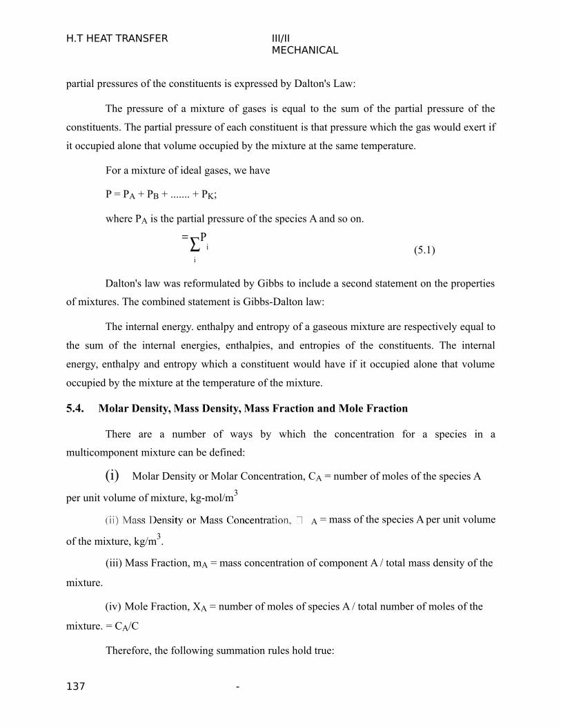
H.T HEAT TRANSFER III/IIMECHANICAL
partial pressures of the constituents is expressed by Dalton's Law:
The pressure of a mixture of gases is equal to the sum of the partial pressure of the
constituents. The partial pressure of each constituent is that pressure which the gas would exert if
it occupied alone that volume occupied by the mixture at the same temperature.
For a mixture of ideal gases, we have
P = PA + PB + ....... + PK;
where PA is the partial pressure of the species A and so on.
P
i (5.1)i
Dalton's law was reformulated by Gibbs to include a second statement on the properties
of mixtures. The combined statement is Gibbs-Dalton law:
The internal energy. enthalpy and entropy of a gaseous mixture are respectively equal to
the sum of the internal energies, enthalpies, and entropies of the constituents. The internal
energy, enthalpy and entropy which a constituent would have if it occupied alone that volume
occupied by the mixture at the temperature of the mixture.
5.4. Molar Density, Mass Density, Mass Fraction and Mole Fraction
There are a number of ways by which the concentration for a species in a
multicomponent mixture can be defined:
(i) Molar Density or Molar Concentration, CA = number of moles of the species A
per unit volume of mixture, kg-mol/m3
A = mass of the species A per unit volume
of the mixture, kg/m3.
(iii) Mass Fraction, mA = mass concentration of component A / total mass density of the
mixture.
(iv) Mole Fraction, XA = number of moles of species A / total number of moles of the
mixture. = CA/C
Therefore, the following summation rules hold true:
137 -
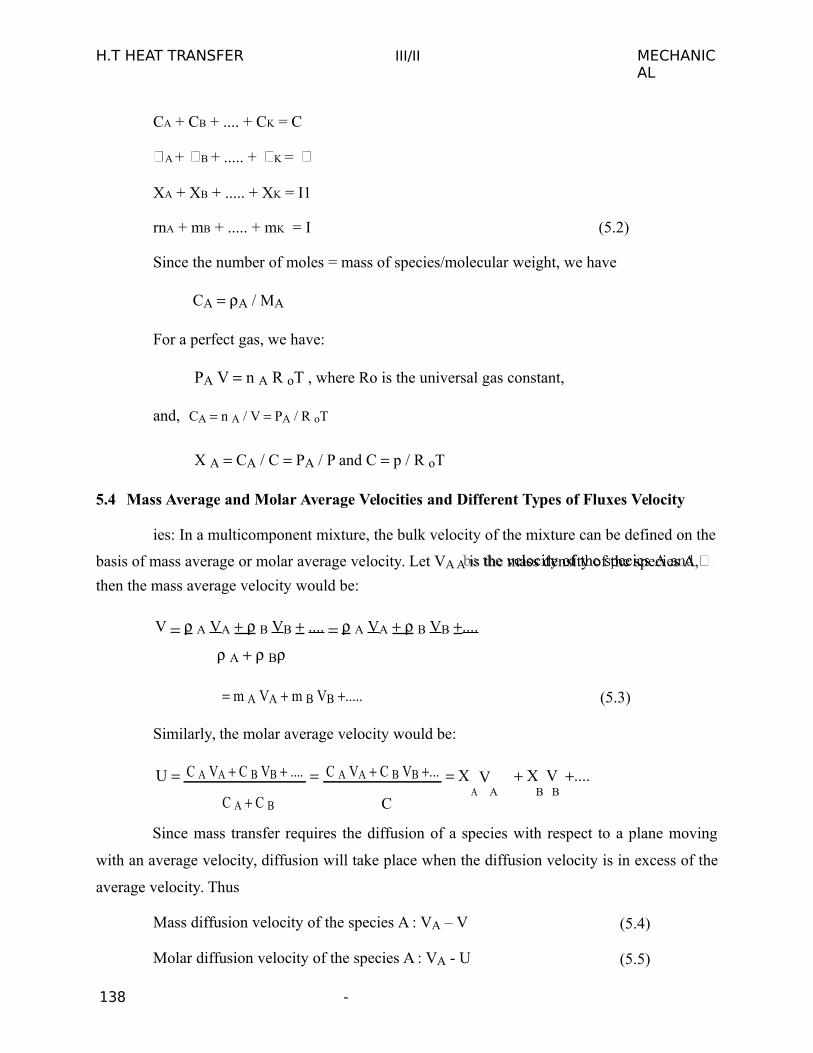
H.T HEAT TRANSFER III/II MECHANICAL
CA + CB + .... + CK = C
A + B + ..... + K =
XA + XB + ..... + XK = I1
rnA + mB + ..... + mK = I (5.2)
Since the number of moles = mass of species/molecular weight, we have
CA A / MA
For a perfect gas, we have:
PA V n A R oT , where Ro is the universal gas constant,
and, CA n A / V PA / R oT
X A CA / C PA / P and C p / R oT
5.4 Mass Average and Molar Average Velocities and Different Types of Fluxes Velocity
ies: In a multicomponent mixture, the bulk velocity of the mixture can be defined on the
basis of mass average or molar average velocity. Let VA A is the mass density of the species A,
then the mass average velocity would be:
V A VA B VB .... A VA B VB ....
AB
m A VA m B VB ..... (5.3)
Similarly, the molar average velocity would be:
U C A VA C B VB .... C A VA C B VB ... XAV X V ....
C A C B CA B B
Since mass transfer requires the diffusion of a species with respect to a plane moving
with an average velocity, diffusion will take place when the diffusion velocity is in excess of the
average velocity. Thus
Mass diffusion velocity of the species A : VA – V (5.4)
Molar diffusion velocity of the species A : VA - U (5.5)
138 -
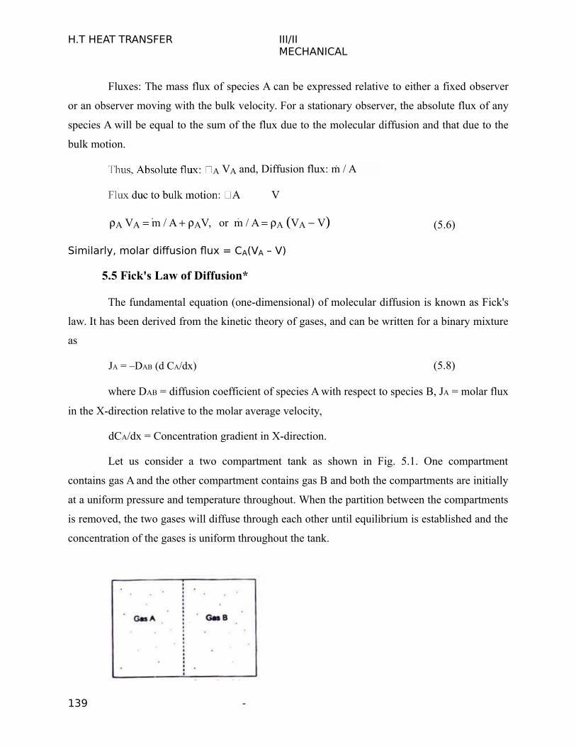
H.T HEAT TRANSFER III/IIMECHANICAL
Fluxes: The mass flux of species A can be expressed relative to either a fixed observer
or an observer moving with the bulk velocity. For a stationary observer, the absolute flux of any
species A will be equal to the sum of the flux due to the molecular diffusion and that due to the
bulk motion.
A VA and, Diffusion flux: m / A
A V
A VA m / A AV, or m / A A VA V (5.6)
Similarly, molar diffusion flux = CA(VA – V)
5.5 Fick's Law of Diffusion*
The fundamental equation (one-dimensional) of molecular diffusion is known as Fick's
law. It has been derived from the kinetic theory of gases, and can be written for a binary mixture
as
JA = –DAB (d CA/dx) (5.8)
where DAB = diffusion coefficient of species A with respect to species B, JA = molar flux
in the X-direction relative to the molar average velocity,
dCA/dx = Concentration gradient in X-direction.
Let us consider a two compartment tank as shown in Fig. 5.1. One compartment
contains gas A and the other compartment contains gas B and both the compartments are initially
at a uniform pressure and temperature throughout. When the partition between the compartments
is removed, the two gases will diffuse through each other until equilibrium is established and the
concentration of the gases is uniform throughout the tank.
139 -

H.T HEAT TRANSFER III/IIMECHANICAL
Fig. 5.1 Diffusion of species A in to species B
Fig 5.2 illustrates the dependence of diffusion on the concentration profile. The
concentration of the species A on the left side of the imaginary plane is greater than that on the
right side. As such, more molecules will cross the plane per unit time from left to right. This
would lead to a net transfer of mass from the region of higher concentration to the region of
lower concentration.
Fig. 5.2 Dependence of diffusion on concentration profile
* This law assumes that fluxes are measured relative to the coordinates that move with
the average velocity of the mixture.
5.6.CONVECTIVE MASS TRANSFER :
(i) Diffusion in Gases - the diffusion rates in gases are dependent on the molecular
speed which is a function of temperature and therefore, the diffusion coefficient depends upon
the temperature of gases.
Gilliland has proposed a semi-empirical equation for diffusion coefficient in a binary
gas mixture –
D 435.7T3 / 2 1 1 1/ 2
(5.9)
p VA1/ 3 VB
1/ 3 2 M
AM
B where D is in square centimeters per second, T is in Kelvin, p is the total pressure of the
140 -
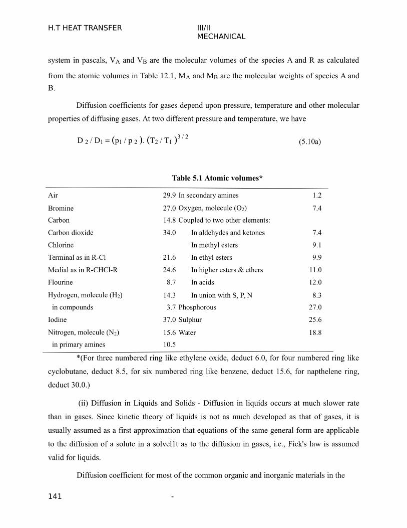
H.T HEAT TRANSFER III/IIMECHANICAL
system in pascals, VA and VB are the molecular volumes of the species A and R as calculated
from the atomic volumes in Table 12.1, MA and MB are the molecular weights of species A and
B.
Diffusion coefficients for gases depend upon pressure, temperature and other molecular
properties of diffusing gases. At two different pressure and temperature, we have
D 2 / D1 p1 / p 2 . T2 / T1 3 / 2(5.10a)
Table 5.1 Atomic volumes*
Air 29.9 In secondary amines 1.2
Bromine 27.0 Oxygen, molecule (O2) 7.4
Carbon 14.8 Coupled to two other elements:
Carbon dioxide 34.0 In aldehydes and ketones 7.4
Chlorine In methyl esters 9.1
Terminal as in R-Cl 21.6 In ethyl esters 9.9
Medial as in R-CHCl-R 24.6 In higher esters & ethers 11.0
Flourine 8.7 In acids 12.0
Hydrogen, molecule (H2) 14.3 In union with S, P, N 8.3
in compounds 3.7 Phosphorous 27.0
Iodine 37.0 Sulphur 25.6
Nitrogen, molecule (N2) 15.6 Water 18.8
in primary amines 10.5
*(For three numbered ring like ethylene oxide, deduct 6.0, for four numbered ring like
cyclobutane, deduct 8.5, for six numbered ring like benzene, deduct 15.6, for napthelene ring,
deduct 30.0.)
(ii) Diffusion in Liquids and Solids - Diffusion in liquids occurs at much slower rate
than in gases. Since kinetic theory of liquids is not as much developed as that of gases, it is
usually assumed as a first approximation that equations of the same general form are applicable
to the diffusion of a solute in a solvel1t as to the diffusion in gases, i.e., Fick's law is assumed
valid for liquids.
Diffusion coefficient for most of the common organic and inorganic materials in the
141 -
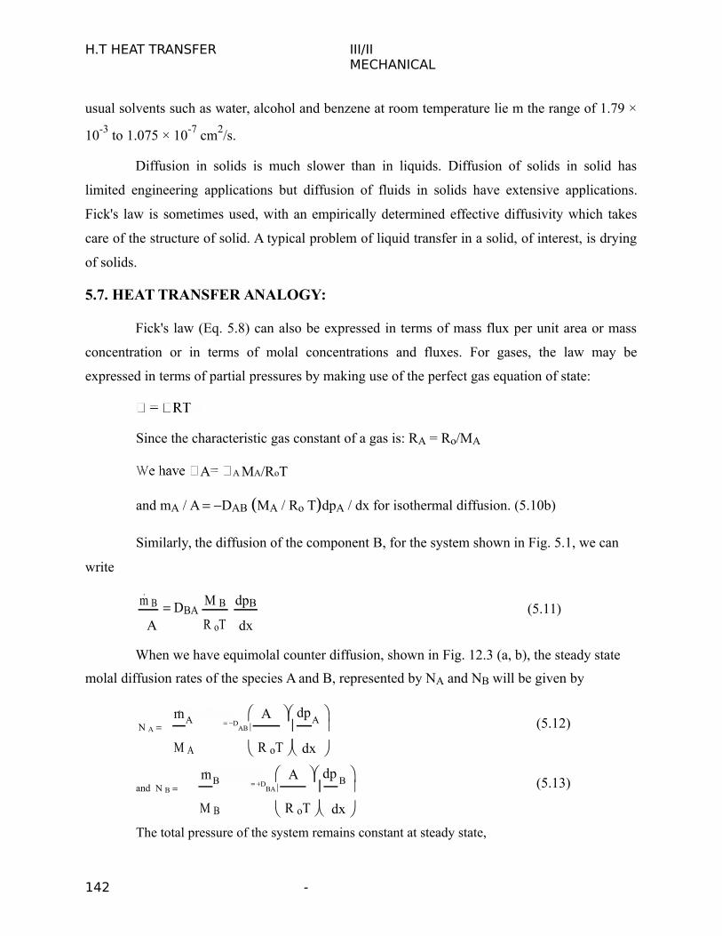
H.T HEAT TRANSFER III/IIMECHANICAL
usual solvents such as water, alcohol and benzene at room temperature lie m the range of 1.79 ×
10-3 to 1.075 × 10⁻⁷ cm2/s.
Diffusion in solids is much slower than in liquids. Diffusion of solids in solid has
limited engineering applications but diffusion of fluids in solids have extensive applications.
Fick's law is sometimes used, with an empirically determined effective diffusivity which takes
care of the structure of solid. A typical problem of liquid transfer in a solid, of interest, is drying
of solids.
5.7. HEAT TRANSFER ANALOGY:
Fick's law (Eq. 5.8) can also be expressed in terms of mass flux per unit area or mass
concentration or in terms of molal concentrations and fluxes. For gases, the law may be
expressed in terms of partial pressures by making use of the perfect gas equation of state:
Since the characteristic gas constant of a gas is: RA = Ro/MA
A A MA/RoT
and mA / A DAB MA / Ro TdpA / dx for isothermal diffusion. (5.10b)
Similarly, the diffusion of the component B, for the system shown in Fig. 5.1, we can
write
m B DBAM B dpB (5.11)R oT dxA
When we have equimolal counter diffusion, shown in Fig. 12.3 (a, b), the steady state
molal diffusion rates of the species A and B, represented by NA and NB will be given by
mA A dp
A
N A DAB
M A R oT dx
mB A dp
B
and N B DBA
M B R oT dx
The total pressure of the system remains constant at steady state,
(5.12)
(5.13)
142 -
H.T HEAT TRANSFER III/IIMECHANICAL
or, p = pA + pB ; and dpA/dx + dpB/dx = 0
as dpA/dx = –dpB/dx
Since each molecule of A is replaced by a molecule of B, the molal diffusion rates must
be equal. Thus: NA = –NB, and
A dpA
A
D
AB DBA
R 0T R 0 T dx
or DAB = DBA = D
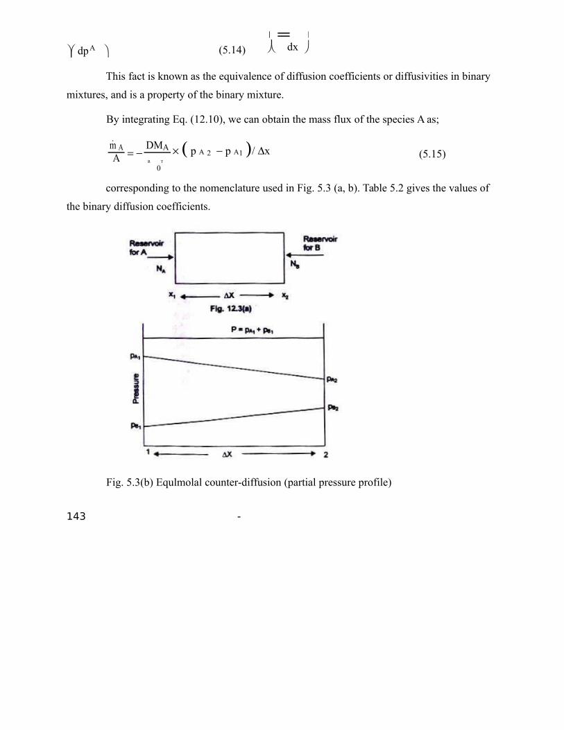
dpA (5.14)
dx
This fact is known as the equivalence of diffusion coefficients or diffusivities in binary
mixtures, and is a property of the binary mixture.
By integrating Eq. (12.10), we can obtain the mass flux of the species A as;
m A DMA p A 2 p A1 / x (5.15)A R T
0
corresponding to the nomenclature used in Fig. 5.3 (a, b). Table 5.2 gives the values of
the binary diffusion coefficients.
Fig. 5.3(b) Equlmolal counter-diffusion (partial pressure profile)
143 -
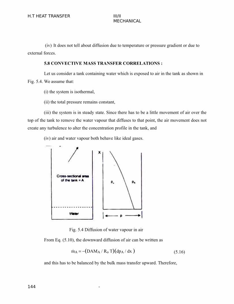
H.T HEAT TRANSFER III/IIMECHANICAL
(iv) It does not tell about diffusion due to temperature or pressure gradient or due to
external forces.
5.8 CONVECTIVE MASS TRANSFER CORRELATIONS :
Let us consider a tank containing water which is exposed to air in the tank as shown in
Fig. 5.4. We assume that:
(i) the system is isothermal,
(ii) the total pressure remains constant,
(iii) the system is in steady state. Since there has to be a little movement of air over the
top of the tank to remove the water vapour that diffuses to that point, the air movement does not
create any turbulence to alter the concentration profile in the tank, and
(iv) air and water vapour both behave like ideal gases.
Fig. 5.4 Diffusion of water vapour in air
From Eq. (5.10), the downward diffusion of air can be written as
mA DAMA / Ro TdpA / dx (5.16)
and this has to be balanced by the bulk mass transfer upward. Therefore,
144 -
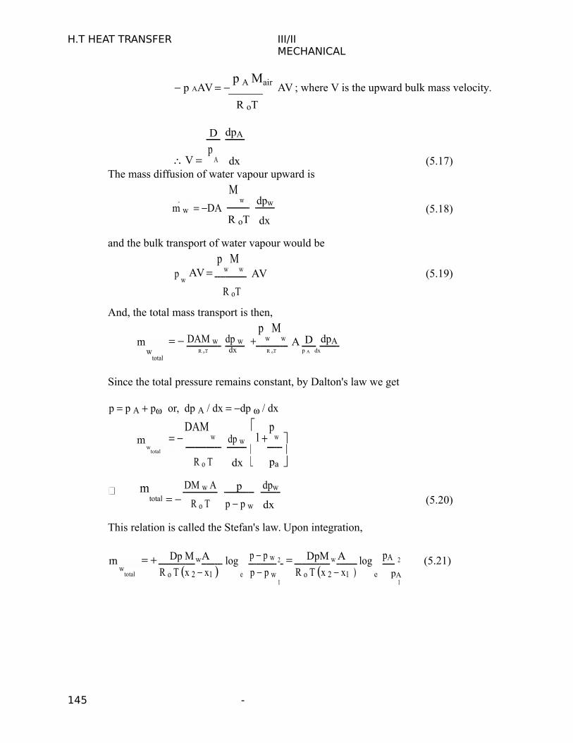
H.T HEAT TRANSFER III/IIMECHANICAL
p AAV p
A Mair AV ; where V is the upward bulk mass velocity.
R oT
V
D dpA
(5.17)p
A dxThe mass diffusion of water vapour upward is
m w DA
M w dpw
(5.18)R oT dx
and the bulk transport of water vapour would be
pw
AV p
w M
w AV (5.19)
R oT
And, the total mass transport is then,
mw
total
DAM w dp w p
w M
w A D dpAdx p A dxR oT R oT
Since the total pressure remains constant, by Dalton's law we get
p p A p or, dp A / dx dp / dx
m DAM
w dp w1
pw
wtotal
R o T dx pa
mtotal
DM w A p dpw
(5.20)R o T p p w dx
This relation is called the Stefan's law. Upon integration,
m Dp M wA log p p w 2 DpM w A log pA 2 (5.21)R o T x 2 x1 e p p w R o T x 2 x1 e
wtotal pA
1 1
145 -

H.T HEAT TRANSFER III/IIMECHANICAL
UNIT 5: MASS TRANSFER
PART A
TWO MARK QUESTIONS:
1. WHAT IS MASS TRANSFER? (AU 2010)
The process of transfer of mass as a result of the species concentration difference in a mixture is known as mass transfer
2. GIVE THE EXAMPLES OF MASS TRANSFER.
1. Humidification of air in cooling tower.
2. The transfer of water vapor into dry air.
3.WHAT ARE THE MODES OF MASS TRANSFER? (AU2013)
There are basically two modes of mass transfer.
1. Diffusion mass transfer.
2.Convective mass transfer.
4. WHAT IS MOLECULAR DIFFUSION? (AU2012)
146 -
H.T HEAT TRANSFER III/IIMECHANICAL
The transport of water on a microscopic level as a result of diffusion from a region of higherconcentration to a region of lower concentration in a mixture of liquids or gases is known asmolecular diffusion.
5.STATE FICK S LAW OF DIFFUSION? (AU2014)
The diffusion rate is given by the Fickslaw , which states that molar flux of an element per unit area is directly proportional to concentration gradient.
JA = –DAB (d CA/dx)
6.DEFINE SCHMIDT NUMBER. (AU 2012)
It is defined as the ratio of the molecular diffusivity of momentum to the molecular diffusivity of mass.
Sc = Molecular diffusivity of momentum / Molecular diffusivity of mass.
7.DEFINE SCHERWOOD NUMBER. (AU 2010)
It is defined as the ratio of concentration gradients at the boundary.
Sh = h MX /Dab.
8. DEFINE MOLARCONCENTRATION:
Numberof moleculesof a component per unit volume of the mixture. It is expressed in kg –
mole/m3.
MOLAR CONCENTRATION = Number of moles of component /Unit Volume of mixture.
9.DEFINE MASS FRACTION.
Themass fraction is defined as the ratio of mass concentration species to the total mass density ofthe mixture.
10. DEFINE MOLE FRACTION. (AU 2014)
The mole fraction is defined as the ratio of mole concentration of a species to the total molar concentration.
Part B
ANSWER THE FOLLOWING:
1. A vessel contains a mixture of2 kmol of CO2 and 4.5 kmol of air at 1 bar and 25°C.ifair
147 -

H.T HEAT TRANSFER III/IIMECHANICAL
contains 21 % oxygen and 79% nitrogen by volume, calculate for themixture:
(i) The mass of CO2, O2 and N2, and the total mass;
(ii) The percentage carbon content by mass;
(iii) The molar mass and the gas constant for the mixture;
(iv) The specific volume of the mixture.
(ii) Percentage of carbon in the mixture; (24/217.48) × 100 = 11.035% by mass.
(iii) Total number of moles = n CO2 n N2 2 0.945 3.555 = 6.5 kmol
Molar mass = n
ni mi
= (2/6.5) × 44 + (0.945; 6.5) × 32 + (3.555/6.5) × 28
= 33.5 kg/kmol
And the gas constant of the mixture; 8314/33.5 = 248.18 J/kgK
(iv)Specific volume of the mixture, v = RT/p = 248.18 × 298/ (l × 105)
= 0.7395 m3/kg.
2. The air pressure inside a synthetic rubber ball (400 mm inside diameter and 15 thick
decreases from 3.5bar to 3.45bar in seven days. Estimate the coefficient of diffusion of air
in synthetic rubber if the temperature is 25°C and the solubility of air in the rubber is 1.8 ×
10-3 kmol/m3 bar. (AU 2012)
Solution: Since the pressure change is very small during a period of seven days, the problem can
be treated as quasi-steady. The initial mass of air inside the ball
148 -

H.T HEAT TRANSFER III/IIMECHANICAL
m p V / RT 3.5 105 4 / 3 0.23 0.137 kg
1 1 287 298
The final mass, m2 =3.45 10 5 4 / 3 0.2 3
0.1352 kg287 298
The rate of leakage 0.137
0.1352
2.976 10 9
kg / s 7 24 3600
The average pressure inside the ball = (3.45 + 3.5)/2 = 3.475 bar
Concentration inside the ball = p1 S 3.475 1.8 103 29 , kg/m3.
= 0.1814 kg/m3
Concentration at the outside surface = p2 S 1 1.8 103 29
0.0522 kg / m3
Since conduction heat transfer is analogous to diffusion mass transfer, the diffusive resistance for
the spherical shell can be written as
R D r2 r1 / 4D r1r2 , and
m A CA1 CA 2 / R D 4 D r1 r2 C A1 C A 2 / r2 r1
Or, D m A r2 r1 / 4 r1 r2 C A1 CA2
2.976 10 9 0.015 6.4 10
10 m 2 / s 3.142 0.2 0.215 0.1814 0.05224
3.Estimate the rate of burning of a pulverized carbon particle in a furnace if the diameter of
the particle is 4 mm, pressure 1 bar. The oxygen is available at 1100 K. Assume that fairly
large layer of CO2 surrounds the carbon particle. Take D = 1 cm2/s. (AU2011)
Solution: The combustion equation is C + O2 CO2, i.e., there will be an Equimolal counter-
diffusion between O2 and CO2,
Since a fairly large blanket of carbon dioxide surrounds the carbon particle, the partial pressure
149 -

H.T HEAT TRANSFER III/IIMECHANICAL
of carbon dioxide at the surface of the carbon particle will be 1 bar and the partial pressure of
oxygen will be zero. Similarly, the partial pressure of carbon dioxide far outside will be zero and
the partial pressure of oxygen will be 1 bar.
From Eq. (12.12), we have: N A D 1 dpA
A R oT dx
Or, N A D dpA
4 r2 R 0T dr
Separating the variables and integrating, we get
4D 0
N A R oT dr / r 2 dpA
r r1 1
Or, p A N A R oT . 1 andN
CO 4 1 10 4 105 2 10
3
4 D r121
8314 1100
2.748 10 8 kgmol / s
Since 1 mol of carbon will produce 1 mol of CO2, the rate of burning of carbon will
be = 2.748 × 10-8 × 12 = 3.298 × 10⁻⁷ kg/so
4. Carbon dioxide at 30°C and at a pressure of 2.5bar is flowing through a rubber pipe,
inside diameter 25 mm and thickness 5 mm. The coefficient of diffusion of carbon dioxide-
rubber combination is 0.11 × 10⁻⁹ m2/s and the solubility of carbondioxide 4 × 10⁻²
k mol/m3 bar. Calculate the loss of CO2 by diffusion per unit length of the pipe.
Solution: The species concentration at the gas-solid interface is obtained in terms of the partial
pressure of the gas adjacent to the solid surface and a solubility factor, S.
Or, Concentration = Partial pressure × S
The carbon dioxide is flowing through the rubber tube at 2.5bar. As such, the partial pressure of
CO, at the rubber-gas interface is 2.5bar and the concentration is then,
C 2.5 4 10 2 kmol / m3 4.4 kg / m3
A
1
150 -
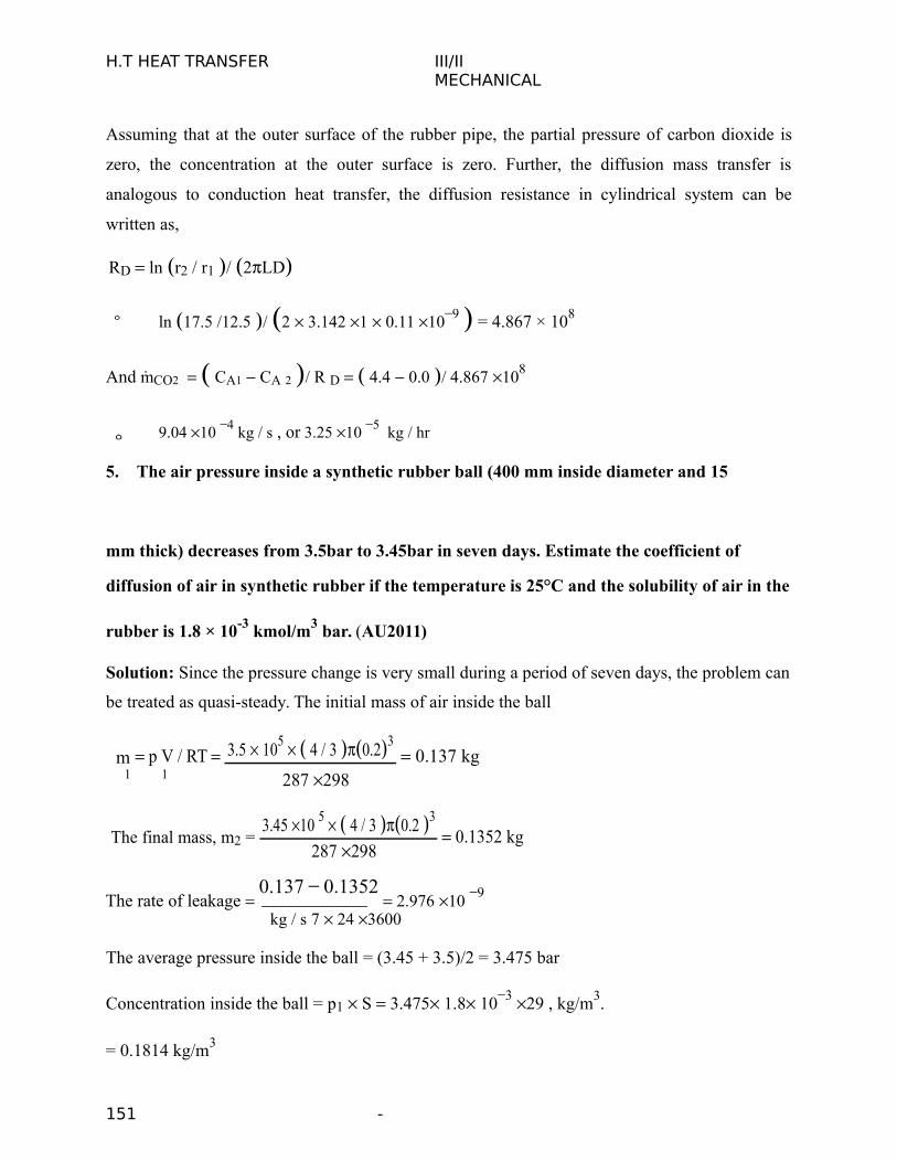
H.T HEAT TRANSFER III/IIMECHANICAL
Assuming that at the outer surface of the rubber pipe, the partial pressure of carbon dioxide is
zero, the concentration at the outer surface is zero. Further, the diffusion mass transfer is
analogous to conduction heat transfer, the diffusion resistance in cylindrical system can be
written as,
RD ln r2 / r1 / 2LD
ln 17.5 /12.5 / 2 3.142 1 0.11 109 = 4.867 × 10⁸
And mCO2 CA1 CA 2 / R D 4.4 0.0 / 4.867 108
9.04 10 4 kg / s , or 3.25 10
5 kg / hr
5. The air pressure inside a synthetic rubber ball (400 mm inside diameter and 15
mm thick) decreases from 3.5bar to 3.45bar in seven days. Estimate the coefficient of
diffusion of air in synthetic rubber if the temperature is 25°C and the solubility of air in the
rubber is 1.8 × 10⁻³ kmol/m3 bar. (AU2011)
Solution: Since the pressure change is very small during a period of seven days, the problem can
be treated as quasi-steady. The initial mass of air inside the ball
m p V / RT 3.5 105 4 / 3 0.23 0.137 kg
1 1 287 298
The final mass, m2 =3.45 10 5 4 / 3 0.2 3
0.1352 kg287 298
The rate of leakage 0.137
0.1352
2.976 10 9
kg / s 7 24 3600
The average pressure inside the ball = (3.45 + 3.5)/2 = 3.475 bar
Concentration inside the ball = p1 S 3.475 1.8 103 29 , kg/m3.
= 0.1814 kg/m3
151 -
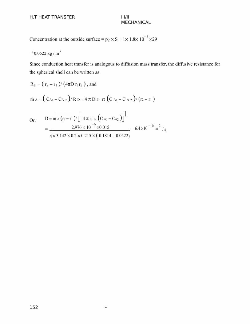
H.T HEAT TRANSFER III/IIMECHANICAL
Concentration at the outside surface = p2 S 1 1.8 103 29
0.0522 kg / m
3
Since conduction heat transfer is analogous to diffusion mass transfer, the diffusive resistance for
the spherical shell can be written as
RD r2 r1 / 4D r1r2 , and
m A CA1 CA 2 / R D 4 D r1 r2 C A1 C A 2 / r2 r1
Or, D m A r2 r1 / 4 r1 r2 C A1 CA2
2.976 10 9 0.015 6.4 10
10 m
2/ s
3.142 0.2 0.215 0.1814 0.05224
152 -