B.tech ME ,4th, Fluid Mechanics.pdf
183
INTERNATIONAL INSTITUTE OF TECHNOLOGY & MANAGEMENT, MURTHAL SONEPAT E-NOTES , Subject : FM and Mechinery, Subject Code: ME302C , Course: B.TECH. , Branch : Mechanical Engineering , Sem.-4 th , Chapter Name: Introduction ( Prepared By: Ms. Promila , Assistant Professor , MED) CHAPTER 1 Introduction INTRODUCTION The word 'Hydraulics' has been derived from a Greek word 'Hudour' which means water. Hydraulics is that branch of engineering which deals with water at rest or in motion. It deals mainly with the practical problems of flow of water and is based upon the results obtained from experiments. It provides various principles to solve practical problems in water supply, irrigation engineering, water power and hydraulic machines. Pneumatics is that branch of engineering which deals with the action of compressed air or any other gas in operating various machines and equipment’s. FLUID Fluid may be defined as a substance which is capable of flowing and offers practically no resistance to the change of shape. A fluid has no definite shape of its own, but takes the shape of the containing vessel. A fluid has no tensile strength or very little of it and it can resist compressive forces when it is kept in a container, When subjected to shearing force, a fluid deforms continuously as long—as force is applied. For mechanical analysis, a fluid is considered to be continuum i.e. a continuous distribution of matter with no void or empty space. Some of the examples of fluids are water, oil, air, gases and vapours. Fluids may be classified as follow: 1. Liquids, 2. Gases including vapours. 1. Liquids: Liquids occupy a definite volume and are not affected appreciably by change in temperature or compression. Water, oil, honey, glycerine, paint, blood etc. are the examples of liquids. 2. Gases including vapours: Gases and vapours do not occupy a definite volume, but take the shape and volume of vessels containing them. Gases and vapours readily respond to change • temperature. These are capable of being compressed to a considerably small volume under high pressure. TYPES OF FLUIDS The fluids may be classified into the following two categories 1. Ideal fluids, 2. Real fluids. 1. Ideal Fluids: the fluids which are incompressible and have no viscosity and surface tension. These are only imaginary fluids and do not exist. However, air and water may be considered as ideal fluids without much error. 2. Real Fluids: The fluids which possess properties such as viscosity, surface tension and compressibility are called real fluids. The fluids actually available in nature are real fluids. These fluids offer a certain amount of resistance when these are set in motion. These are further subdivided into the following categories
-
Upload
khangminh22 -
Category
Documents
-
view
0 -
download
0
Transcript of B.tech ME ,4th, Fluid Mechanics.pdf
INTERNATIONAL INSTITUTE OF TECHNOLOGY & MANAGEMENT, MURTHAL SONEPAT
E-NOTES , Subject : FM and Mechinery, Subject Code: ME302C ,
Course: B.TECH. , Branch : Mechanical Engineering , Sem.-4th , Chapter Name: Introduction
( Prepared By: Ms. Promila , Assistant Professor , MED)
CHAPTER 1
Introduction
INTRODUCTION
The word 'Hydraulics' has been derived from a Greek word 'Hudour' which means
water. Hydraulics is that branch of engineering which deals with water at rest or in
motion. It deals mainly with the practical problems of flow of water and is based
upon the results obtained from experiments. It provides various principles to solve
practical problems in water supply, irrigation engineering, water power and
hydraulic machines.
Pneumatics is that branch of engineering which deals with the action of
compressed air or any other gas in operating various machines and equipment’s.
FLUID Fluid may be defined as a substance which is capable of flowing and offers
practically no resistance to the change of shape.
A fluid has no definite shape of its own, but takes the shape of the containing
vessel. A fluid has no tensile strength or very little of it and it can resist
compressive forces when it is kept in a container, When subjected to shearing force,
a fluid deforms continuously as long—as force is applied. For mechanical analysis,
a fluid is considered to be continuum i.e. a continuous distribution of matter with no
void or empty space. Some of the examples of fluids are water, oil, air, gases and
vapours.
Fluids may be classified as follow:
1. Liquids,
2. Gases including vapours.
1. Liquids: Liquids occupy a definite volume and are not affected appreciably by
change in temperature or compression. Water, oil, honey, glycerine, paint, blood
etc. are the examples of liquids.
2. Gases including vapours: Gases and vapours do not occupy a definite volume,
but take the shape and volume of vessels containing them. Gases and vapours
readily respond to change • temperature. These are capable of being compressed to
a considerably small volume under high pressure.
TYPES OF FLUIDS
The fluids may be classified into the following two categories
1. Ideal fluids,
2. Real fluids.
1. Ideal Fluids: the fluids which are incompressible and have no viscosity and
surface tension. These are only imaginary fluids and do not exist.
However, air and water may be considered as ideal fluids without much error.
2. Real Fluids: The fluids which possess properties such as viscosity, surface
tension and compressibility are called real fluids. The fluids actually available in
nature are real fluids. These fluids offer a certain amount of resistance when these
are set in motion.
These are further subdivided into the following categories

INTERNATIONAL INSTITUTE OF TECHNOLOGY & MANAGEMENT, MURTHAL SONEPAT
E-NOTES , Subject : FM and Mechinery, Subject Code: ME302C ,
Course: B.TECH. , Branch : Mechanical Engineering , Sem.-4th , Chapter Name: Introduction
( Prepared By: Ms. Promila , Assistant Professor , MED)
(i) Newtonian fluids,
(ii) Non-Newtonian fluids,
(iii) Ideal plastic fluids,
(iv) Thixotropic fluids.
(i) Newtonian Fluids: The fluids in which shear stress is directly
proportional to the rate of shear strain (or velocity gradient) are called
Newtonian fluids. These fluids follow Newton's law of viscosity.
(ii) Non-Newtonian Fluids: The fluids in which shear stress is not
proportional to the rate of shear strain (or velocity gradient) are called
non-Newtonian fluids.
(iii) Ideal Plastic Fluids: The fluids in which shear stress is more than yield
stress value r and shear stress is directly proportional to the rate of shear
strain (velocity gradient) are called ideal plastic fluids.
(iv) Thixotropic Fluids: The fluids in which shear stress is more than Yield
stress value and shear stress is not proportional to the rate of shear strain
(or velocity gradient) called thixotropic fluids. e.g. printer's ink.
PROPERTIES OF FLUIDS
Some of the important properties of fluids are as follow
(i) Mass density,
(ii) Specific weight
(iii) Specific volume
(iv) Specific gravity
(v) Viscosity
(vi) Vapour pressure
(vii) Cohesion
(viii) Adhesion
(ix) Surface tension
(x) Capillarity

INTERNATIONAL INSTITUTE OF TECHNOLOGY & MANAGEMENT, MURTHAL SONEPAT
E-NOTES , Subject : FM and Mechinery, Subject Code: ME302C ,
Course: B.TECH. , Branch : Mechanical Engineering , Sem.-4th , Chapter Name: Introduction
( Prepared By: Ms. Promila , Assistant Professor , MED)
(xi) Compressibility
Mass Density
Mass density of fluid may be defined as mass of fluid per unit volume. It is
generally by p (Rho). Its S.I. unit is kg/m3.
The mass density of water is taken as 1000 kg/m3 at 4°C.
Specific Weight
Specific weight of fluid may be defined as weight of fluid per unit volume It is
denoted by w. Its SI unit is N/m3. Specific weight varies from place to place due
to the change of acceleration due to gravity (g).
Mathematically,
Specific weight depends upon mass density and gravitational acceleration. Since gravitational
acceleration varies from place to place, therefore, specific weight also varies from place to place.
Specific weight also decreases with the increase in temperature. It increases with increase in pressure.
However, the specific weight of water is taken as 9810 N/m3 at 4°C.
Specific Volume
Specific volume may be defined as the volume occupied by fluid per unit mass.it is generally denoted
by v. its SI unit is m ^3/kg.
Specific volume is reciprocal of mass density.
Specific gravity,
Specific gravity is the ratio of the density (mass of a unit volume) of a substance to the
density of a given reference material. Specific gravity for liquids is nearly always
measured with respect to water at its densest (at 4 °C or 39.2 °F); for gases, air at room
temperature (20 °C or 68 °F) is the reference. The term "relative density" is often
preferred in scientific usage. It is defined as a ratio of density of particular substance
with that of water.
Viscosity
Viscosity is a measure of a fluid's resistance to flow. It describes the internal friction
of a moving fluid. A fluid with large viscosity resists motion because its molecular
makeup gives it a lot of internal friction.

INTERNATIONAL INSTITUTE OF TECHNOLOGY & MANAGEMENT, MURTHAL SONEPAT
E-NOTES , Subject : FM and Mechinery, Subject Code: ME302C ,
Course: B.TECH. , Branch : Mechanical Engineering , Sem.-4th , Chapter Name: Introduction
( Prepared By: Ms. Promila , Assistant Professor , MED)
A fluid with low viscosity flows easily because its molecular makeup results in very
little friction when it is in motion.
Gases also have viscosity, although it is a little harder to notice it in ordinary
circumstances.
Kinematic viscosity
The ratio of viscosity to mass density of Fluid is called kinematic viscosity.
SI unit m^2/s. Another unit of KV is Stroke.
1 m^2/s=10000 strokes
Compressibility
Compressibility of a fluid may be defined the property by virtue of which the fluid
undergoes a change in volume under the action of external pressure. All the fluids
can be compressed by the application of external pressure and when the pressure is
removed, the compressed volumes of fluids expand to their on volumes, Thus fluids
also possess elastic characteristics just like elastic solids.
The variation in the volume of water with the variation of pressure is so small that
for practical purposes, it is neglected. Thus water is considered as incompressible
fluid, Compressibility of fluid may be expressed as the reciprocal of bulk modulus
of elasticity (K).
Bulk modulus of elasticity (K) may be defined as the ratio of compressive stress to
volumetric strain.
Cohesion
Cohesion is the property of liquid by virtue of which it can withstand tension,
property of liquid is due to the intermolecular attraction between the molecules of
the liquid. The property of surface tension is also due to cohesion. The droplet of
water hanging down the tap keeps its entity together due to the property of cohesion
Adhesion
Adhesion is the property of liquid by virtue of which it adheres (stick.) to the solid
body with which it is in contact. Whereas cohesion is due to its inter-molecular
attraction between the molecules of the liquid, adhesion is due to the forces of
attraction between the molecules of the liquid and the molecules of the solid body,
A droplet of water before falling from the tip of the finger exhibits the property of
adhesion,
Surface Tension
The property of liquid by virtue of which the free surface of the liquid acts as a
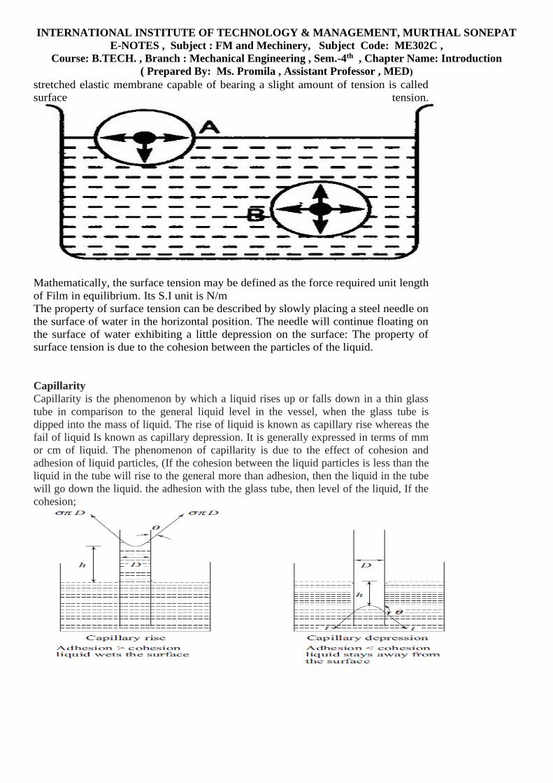
INTERNATIONAL INSTITUTE OF TECHNOLOGY & MANAGEMENT, MURTHAL SONEPAT
E-NOTES , Subject : FM and Mechinery, Subject Code: ME302C ,
Course: B.TECH. , Branch : Mechanical Engineering , Sem.-4th , Chapter Name: Introduction
( Prepared By: Ms. Promila , Assistant Professor , MED)
stretched elastic membrane capable of bearing a slight amount of tension is called
surface tension.
Mathematically, the surface tension may be defined as the force required unit length
of Film in equilibrium. Its S.I unit is N/m
The property of surface tension can be described by slowly placing a steel needle on
the surface of water in the horizontal position. The needle will continue floating on
the surface of water exhibiting a little depression on the surface: The property of
surface tension is due to the cohesion between the particles of the liquid.
Capillarity
Capillarity is the phenomenon by which a liquid rises up or falls down in a thin glass
tube in comparison to the general liquid level in the vessel, when the glass tube is
dipped into the mass of liquid. The rise of liquid is known as capillary rise whereas the
fail of liquid Is known as capillary depression. It is generally expressed in terms of mm
or cm of liquid. The phenomenon of capillarity is due to the effect of cohesion and
adhesion of liquid particles, (If the cohesion between the liquid particles is less than the
liquid in the tube will rise to the general more than adhesion, then the liquid in the tube
will go down the liquid. the adhesion with the glass tube, then level of the liquid, If the
cohesion;

INTERNATIONAL INSTITUTE OF TECHNOLOGY & MANAGEMENT, MURTHAL SONEPAT
E-NOTES , Subject : FM and Mechinery, Subject Code: ME302C ,
Course: B.TECH. , Branch : Mechanical Engineering , Sem.-4th , Chapter Name: Introduction
( Prepared By: Ms. Promila , Assistant Professor , MED)

1
INTERNATIONAL INSTITUTE OF TECHNOLOGY & MANAGEMENT, MURTHAL SONEPAT E-NOTES , Subject : FM and Mechinery, Subject Code: ME302C Course: B.TECH. , Branch : Mechanical Engineering , Sem.-4th , Unit-1 ( Prepared By: Ms. Promila , Assistant Professor , MED)
Hydrostatics
• Pressure distribution in a static fluid and its effects on solid surfaces and on floating and submerged bodies.

Fluid at rest
Fluid Statics M. Bahrami ENSC 283 Spring 2009 2
• hydrostatic condition: when a fluid velocity is zero, the pressure variation is due only to the weight of the fluid.
• There is no pressure change in the horizontal direction.
• There is a pressure change in the vertical direction proportional to the density, gravity, and depth change.
• In the limit when the wedge shrinks to a point,

•
•
The pressure gradient is a surface force that acts on the sides of the element. Note that the pressure gradient (not pressure) causes a net force that must be balanced by gravity or acceleration.
Fluid Statics M. Bahrami ENSC 283 Spring 2009 3
Pressure forces (pressure gradient)
• Assume the pressure vary arbitrarily in a fluid, p=p(x,y,z,t).


Equilibrium
Fluid Statics M. Bahrami ENSC 283 Spring 2009 4
• The pressure gradient must be balanced by gravity force, or weight of the element, for a fluid at rest.
• The gravity force is a body force, acting on the entire mass of the element. Magnetic force is another example of body force.

Gage pressure and vacuum
Fluid Statics M. Bahrami ENSC 283 Spring 2009 5
P
Pgage
Pvac Pabs
Patm Absolute
(vacuum) = 0
• The actual pressure at a given position is called the absolute pressure, and it is measured relative to absolute vacuum.

Hydrostatic pressure distribution
Fluid Statics M. Bahrami ENSC 283 Spring 2009 6
where g = 9.807 m/s2. The pressure gradient vector becomes:
• For a fluid at rest, pressure gradient must be balanced by the gravity force
• Recall: Ap is perpendicular everywhere to surface of constant pressure p.
• In our customary coordinate z is “upward” and the gravity vector is:

Hydrostatic pressure distribution
Fluid Statics M. Bahrami ENSC 283 Spring 2009 7

Hydrostatic pressure distribution
Fluid Statics M. Bahrami ENSC 283 Spring 2009 8
• Pressure in a continuously distributed uniform static fluid varies only with vertical distance and is independent of the shape of the container.
• The pressure is the same at all points on a given horizontal plane in a fluid.
• For liquids, which are incompressible, we have:
• The quantity, p⁄γ is a length called the pressure head of the fluid.

The mercury barometer
Fluid Statics M. Bahrami ENSC 283 Spring 2009 8
Patm = 761 mmHg
• Mercury has an extremely small vapor pressure at room temperature (almost vacuum), thus p1 = 0. One can write:

Hydrostatic pressure in gases
• Note that the Patm is nearly zero (vacuum condition) at z = 30 km.
Fluid Statics M. Bahrami ENSC 283 Spring 2009 9
• Gases are compressible, using the ideal gas equation of state, p=ρRT:
• For small variations in elevation, “isothermal atmosphere” can be assumed:
• In general (for higher altitudes) the atmospheric temperature drops off linearly with z
T≈T0 ‐ Bz
where T0 is the sea‐level temperature (in Kelvin) and B=0.00650 K/m.

Manometry
Fluid Statics M. Bahrami ENSC 283 Spring 2009 10
• A static column of one or multiple fluids can be used to measure pressure difference between 2 points. Such a device is called manometer.
• Adding/ subtracting γ∆z as moving down/up in a fluid column.
• Jumping across U‐tubes: any two points at the same elevation in a continuous mass of the same static fluid will be at the same
pressure.
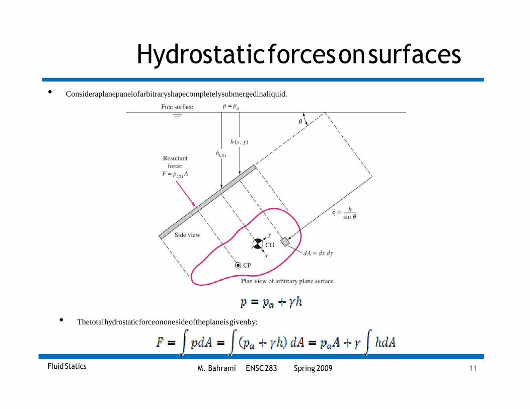
Hydrostatic forces on surfaces
Fluid Statics M. Bahrami ENSC 283 Spring 2009 11
• Consider a plane panel of arbitrary shape completely submerged in a liquid.
• The total hydrostatic force on one side of the plane is given by:

Hydrostatic forces on surfaces
Fluid Statics M. Bahrami ENSC 283 Spring 2009 12
• After integration and simplifications, we find:
• The force on one side of any plane submerged surface in a uniform fluid equals the pressure at the plate centroid times the plate
area, independent of the shape of the plate or angle θ.
• The resultant force acts not through the centroid but below it toward the high pressure side. Its line of action passes through the centre of pressure
CP of the plate (xCP, yCP).

Hydrostatic forces on surfaces
• Centroidal moments of inertia for various cross‐sections.
• Note: for symmetrical plates, Ixy = 0 and thus xCP = 0. As a result, the center of pressure lies directly below the centroid on the y axis.
Fluid Statics M. Bahrami ENSC 283 Spring 2009 13

Hydrostatic forces: curved surfaces
• The easiest way to calculate the pressure forces on a curved surface is to compute the horizontal and vertical forces separately.
• The horizontal force equals the force on the plane area formed by the projection of the curved surface onto a vertical plane normal to the
component.
• The vertical component equals to the weight of the entire column of fluid, both liquid and atmospheric above the curved surface.
FV = W2 + W1 + Wair
Fluid Statics M. Bahrami ENSC 283 Spring 2009 14

INTERNATIONAL INSTITUTE OF TECHNOLOGY & MANAGEMENT, MURTHAL SONEPAT
E-NOTES , Subject : FM and Mechinery, Subject Code: ME302C Course: B.TECH. , Branch : Mechanical
Engineering , Sem.-4th , Unit-1
( Prepared By: Ms. Promila , Assistant Professor , MED)
Fluid Kinematics
a) Description of motion of individual fluid molecules (X)
# of molecules per mm3 ~ 1018 for gases or ~ 1021 for liquids
b) Description of motion of small volume of fluid (fluid particle) (O)
◉ Two effective ways of describing fluid motion
E.g. Smoke discharging from a chimney
Q. Determine the temperature (T) of smoke
Method 1.
Step 1. Attach a thermometer at point 0
Step 2. Record T at point 0 as a function of t
T = T (x0, y0, z0, t)
Step 3. Repeat the measurements at numerous points
T = T (x, y, z, t)
: Temperature information as a function of location
Eulerian method (Practical)
Method 2.
Step 1. Attach a thermometer to a specific particle A
Step 2. Record T of the particle as a function of time
T = TA (t)
Step 3. Repeat the measurements for numerous particles
T = T (t)
: Temperature information of an individual particle
Lagrangian method (Unrealistic)

INTERNATIONAL INSTITUTE OF TECHNOLOGY & MANAGEMENT, MURTHAL SONEPAT
E-NOTES , Subject : FM and Mechinery, Subject Code: ME302C Course: B.TECH. , Branch : Mechanical
Engineering , Sem.-4th , Unit-1
( Prepared By: Ms. Promila , Assistant Professor , MED)
● Visualization of a flow feature
1. Streamline (Analytical purpose): Tangential to Velocity field
Steady flow: Fixed lines in space and time (No shape change)
Unsteady flow: Shape changes with time
e.g. For 2-D flows, Slope of the streamlines,
dy =
v
dx u
Continuous
Video capture
2. Streakline (Experimental purpose): Connecting line of all particles in
a flow previously passing through a common point
Steady flow: Streakline
= Streamline
Unsteady flow: Different
at different time
3. Pathline (Experimental purpose; Lagrangian concept)
: Traced out by a specific particle from a point to another
Steady flow: Pathline = Streamline
Unsteady flow: None of these lines
need to be the same
Time exposure
photograph
Instantaneous
snapshot

INTERNATIONAL INSTITUTE OF TECHNOLOGY & MANAGEMENT, MURTHAL SONEPAT
E-NOTES , Subject : FM and Mechinery, Subject Code: ME302C Course: B.TECH. , Branch : Mechanical
Engineering , Sem.-4th , Unit-1
( Prepared By: Ms. Promila , Assistant Professor , MED)
A
V = u(x, y, z, t)i + v(x, y, z, t) j + w(x, y, z, t)k
◉ Eulerian analysis vs. Lagrangian analysis I (Fluid Velocity)
● Eulerian representation (Field representation)
Step 1. Select a specific point (location) in space
Step 2. Measure the fluid properties ( , p, v , and a ) at the point as
functions of time
Step 3. Repeat Step 1 & 2 for numerous points (locations): Mapping
Results: Fluid properties ( , p, v , and a )
- Function of LOCATION and TIME (Field representation)
e.g. Temperature in a room determined by Eulerian method
T = T (x, y, z, t) : Temperature field
● Velocity Field of Fluid flow
- Velocity information as a function of location and time
where u, v, w : x, y, z components of V at (x,y,z) and time t
(Velocity distribution in space at certain time t)
How to determine Velocity of a specific particle A at time t,
- Must know Location of particle A = (xA, yA, z A ) at time t
r = u(x A, y A, z A, t)iˆ
+ v(xA, yA, z A, t) j
+ w(xA, yA, z A,t)kˆ
V

INTERNATIONAL INSTITUTE OF TECHNOLOGY & MANAGEMENT, MURTHAL SONEPAT
E-NOTES , Subject : FM and Mechinery, Subject Code: ME302C Course: B.TECH. , Branch : Mechanical
Engineering , Sem.-4th , Unit-1
( Prepared By: Ms. Promila , Assistant Professor , MED)
V = u(x, y, z)i + v(x, y, z) j + w(x, y, z)k
◉ Additional conditions
● Steady and Unsteady Flows
a) Steady flow (Time-independent flowing feature)
: Velocity field doesn’t vary with time.
b) Unsteady flow (Time-dependent flowing feature)
V = u(x, y, z, t)iˆ + v(x, y, z, t) j + w(x, y, z, t)k
Type 1. Nonperiodic, unsteady flow:
e.g. Turn off the faucet to stop the water flow.
Type 2. Periodic, unsteady flow
e.g. Periodic injection of air-gasoline mixture into the
cylinder of an automobile engine.
Type 3. : Pure random, unsteady flow: Turbulent flow
c.f. Lagrangian description of the fluid velocity
for individual particles A v
rA = uA (t)i + vA (t) j + wA (t)k
INTERNATIONAL INSTITUTE OF TECHNOLOGY & MANAGEMENT, MURTHAL SONEPAT
E-NOTES , Subject : FM and Mechinery, Subject Code: ME302C Course: B.TECH. , Branch : Mechanical
Engineering , Sem.-4th , Unit-1
( Prepared By: Ms. Promila , Assistant Professor , MED)
ar(t) =
V + u
V + v
V + w
V
t x y z
A A A A
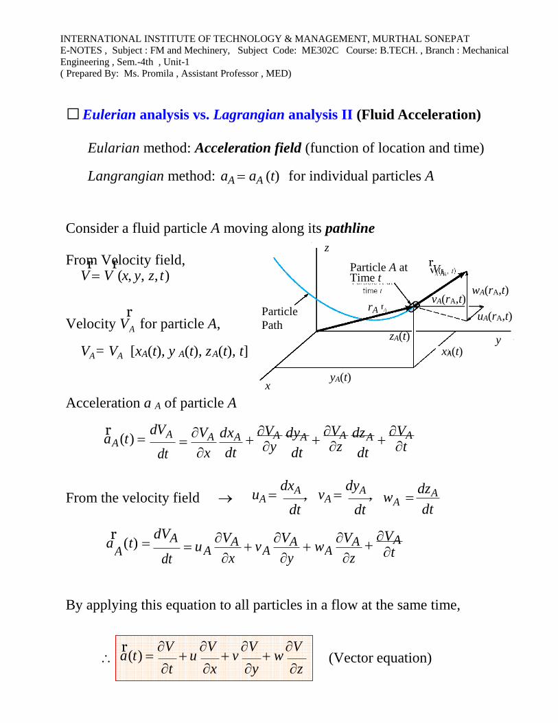
◉ Eulerian analysis vs. Lagrangian analysis II (Fluid Acceleration)
Eularian method: Acceleration field (function of location and time)
Langrangian method: aA = aA (t) for individual particles A
Consider a fluid particle A moving along its pathline
z From Velocity field,
Vr = V
r(x, y, z, t )
Particle A at r Time t
VA
Velocity Vr
for particle A,
Particle
Path
rA
zA(t)
vA(rA ,t) wA(rA,t)
uA(rA,t)
y VA= VA [xA(t), y A(t), z A(t), t]
x
yA(t)
xA(t)
Acceleration a A of particle A
ar
A (t) = dVA
dt =
VA
x
dxA
dt +
VA
y dyA
dt +
VA
z dz A
dt +
VA
t
From the velocity field → uA = dxA ,
dt vA =
dyA , dt
wA = dz A
dt
ar
(t) = dVA
dt = u
VA
x + v
VA
y + w
VA
z +
VA
t
By applying this equation to all particles in a flow at the same time,
(Vector equation)
A

INTERNATIONAL INSTITUTE OF TECHNOLOGY & MANAGEMENT, MURTHAL SONEPAT
E-NOTES , Subject : FM and Mechinery, Subject Code: ME302C Course: B.TECH. , Branch : Mechanical
Engineering , Sem.-4th , Unit-1
( Prepared By: Ms. Promila , Assistant Professor , MED)
t x
= ( )
+ (Vr )( )
t
x-component ax(t) = u + u
u + v
u + w
u
t x y z
y-component ay(t) = v + u
v
+ v v
+ w v
t x y z
z-component az(t) = w+ u
w + v
w + w
w
t x y z
● Simple representation of the equation (Material Derivative)
ar(t) =
V
t + u
V
x + v
V
y + w
V
z
DV
Dt
where =
( ) + u
( ) + v
( ) + w
y
( ) or
z
: Material derivative or Substantial derivative
Material derivative: Time rate of change of fluid properties
- Related with both Time-dependent change and
Fluid’s motion (Velocity field (or u, v, w): Must be known]
e.g. Time rate of change of temperature
dTA =
dt
TA +
t
TA
x
dxA +
dt
TA
y
dyA +
dt
TA
z
dzA (For a particle A) dt
DT =
T
Dt t + u
T
x + v
T
y + w
T =
T
z t + V T (For any particle)
D( ) Dt

INTERNATIONAL INSTITUTE OF TECHNOLOGY & MANAGEMENT, MURTHAL SONEPAT
E-NOTES , Subject : FM and Mechinery, Subject Code: ME302C Course: B.TECH. , Branch : Mechanical
Engineering , Sem.-4th , Unit-1
( Prepared By: Ms. Promila , Assistant Professor , MED)
Local derivative due to unsteady effect
Spatial (or Convective) derivative
- Variation due to the motion of fluid particle
◉ Relation between Material Derivative and Steadiness of the flow
D( ) =
( ) + u
( ) + v
( ) + w
( ) Dt t x y z
e.g. Uniform flow
Consider the situation shown
V = V0 (t)iˆ (Spatially uniform)
Then the acceleration field,
a = V
+ u V
+ v V
+ w
V =
V =
V0 i
t x y z t t
: Uniform, but not necessarily constant in time
◉ Relation between Material Derivative and the Fluid Motion
D( ) =
( ) + u
( ) + v
( ) + w
( ) Dt t x y z
● Convective acceleration = (V )V : Due to the convection (or motion)
of the particle from one point to
another point
V0(t)
x V0(t)
INTERNATIONAL INSTITUTE OF TECHNOLOGY & MANAGEMENT, MURTHAL SONEPAT
E-NOTES , Subject : FM and Mechinery, Subject Code: ME302C Course: B.TECH. , Branch : Mechanical
Engineering , Sem.-4th , Unit-1
( Prepared By: Ms. Promila , Assistant Professor , MED)
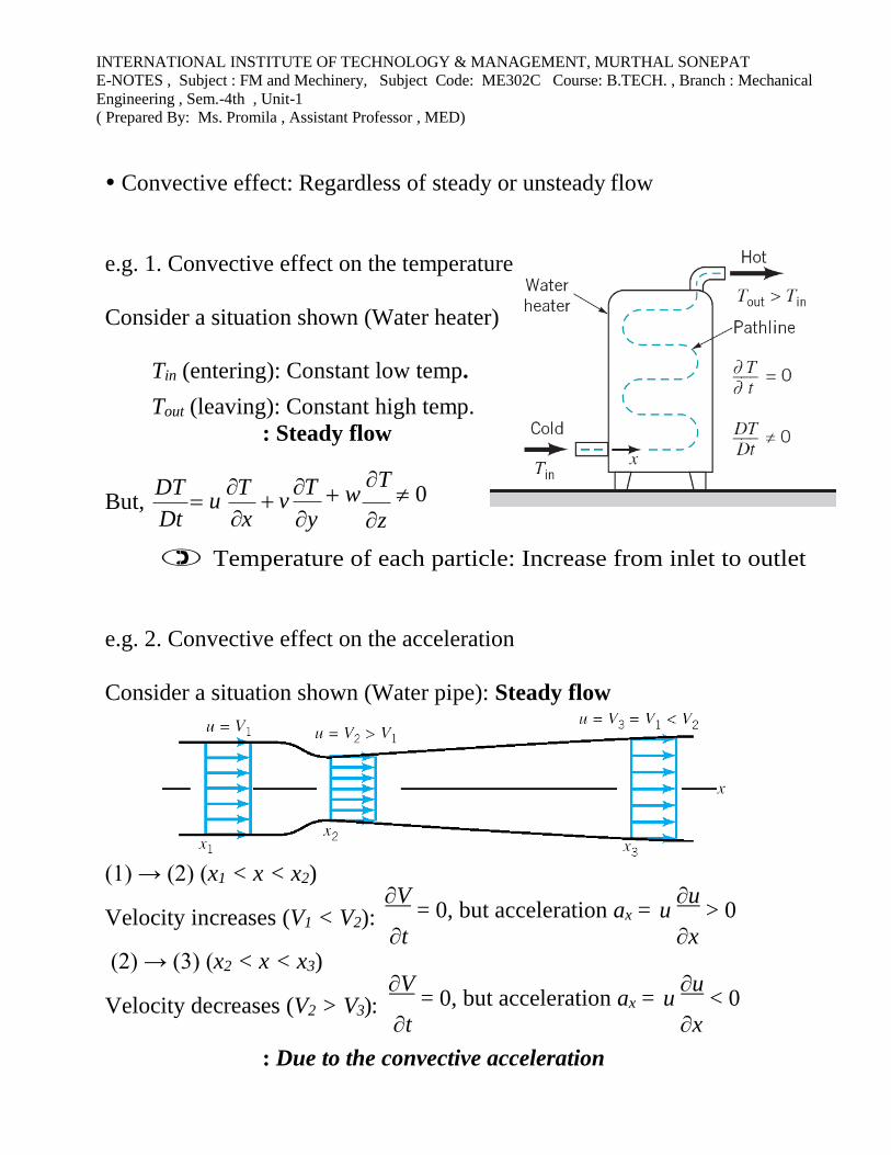
Convective effect: Regardless of steady or unsteady flow
e.g. 1. Convective effect on the temperature
Consider a situation shown (Water heater)
Tin (entering): Constant low temp.
Tout (leaving): Constant high temp.
: Steady flow
But, DT
= u T
Dt x + v
T
y + w
T 0
z
Temperature of each particle: Increase from inlet to outlet
e.g. 2. Convective effect on the acceleration
Consider a situation shown (Water pipe): Steady flow
(1) → (2) (x1 < x < x2)
Velocity increases (V1 < V2):
(2) → (3) (x2 < x < x3)
Velocity decreases (V2 > V3):
V = 0, but acceleration ax =
t V
= 0, but acceleration ax = t
u u
> 0 x
u u
< 0 x
: Due to the convective acceleration

INTERNATIONAL INSTITUTE OF TECHNOLOGY & MANAGEMENT, MURTHAL SONEPAT
E-NOTES , Subject : FM and Mechinery, Subject Code: ME302C Course: B.TECH. , Branch : Mechanical
Engineering , Sem.-4th , Unit-1
( Prepared By: Ms. Promila , Assistant Professor , MED)
V
t
◉ Streamline coordinates again (Easy to describe the fluid motion)
Consider 2-D steady flow shown, y
a) Cartesian coordinates: x, y
: Unit vectors i , j
s = 0
s = s1
s = s2
n = n2 n = n1
n = 0
Stream-
lines
b) Streamline coordinates: s, n
: Unit vectors s , n s
From the definition of velocity field x
V = Vs (always tangent to the streamline direction)
Thus, for steady 2D flow,
ar =
DV
Dt =
DVsˆ =
Dt
DV s + V
Dt
Ds (By the chain rule)
Dt
= as sˆ + an nˆ
Then, a =
+ V ds
+ V dn
sˆ + V sˆ
+ sˆ ds
+ sˆ dn
s dt n dt
t
s dt n dt
a = V ds
s + V s ds
=
V V
s + VV
sˆ
s dt
s dt
s
s
where
ds = V
dt
and
sˆ : Change in direction ( sˆ ) per s
s
0: Steady flow 0: Steady flow
0: along streamline 0: along streamline

INTERNATIONAL INSTITUTE OF TECHNOLOGY & MANAGEMENT, MURTHAL SONEPAT
E-NOTES , Subject : FM and Mechinery, Subject Code: ME302C Course: B.TECH. , Branch : Mechanical
Engineering , Sem.-4th , Unit-1
( Prepared By: Ms. Promila , Assistant Professor , MED)
2
As seen in the Figure,
s =
R
s
s = s
: Comparing OAB and OA’B’
Thus, sˆ
=
lim s =
n
s s→0 s R
Finally,
∴ ar
= V
V
s
s +
V
n R
or as =V
V
s
V 2
, an = R
as =V V
: Convective accel. along the streamline (change in speed) s
V 2
an = R
: Centripetal accel. normal to the streamline(change in direction)
Same as those in the previous chapter
INTERNATIONAL INSTITUTE OF TECHNOLOGY & MANAGEMENT, MURTHAL SONEPAT
E-NOTES , Subject : FM and Mechinery, Subject Code: ME302C Course: B.TECH. , Branch : Mechanical
Engineering , Sem.-4th , Unit-1
( Prepared By: Ms. Promila , Assistant Professor , MED)
Fixed
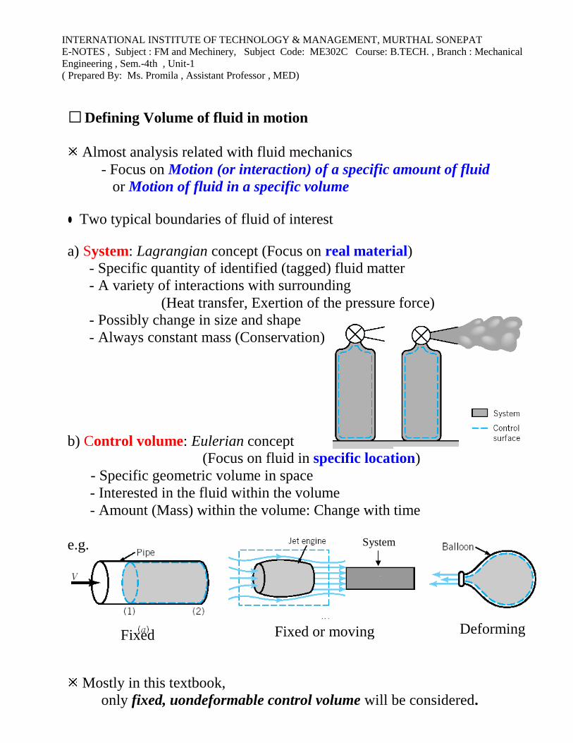
◉ Defining Volume of fluid in motion
Almost analysis related with fluid mechanics
- Focus on Motion (or interaction) of a specific amount of fluid
or Motion of fluid in a specific volume
● Two typical boundaries of fluid of interest
a) System: Lagrangian concept (Focus on real material)
- Specific quantity of identified (tagged) fluid matter
- A variety of interactions with surrounding
(Heat transfer, Exertion of the pressure force)
- Possibly change in size and shape
- Always constant mass (Conservation)
b) Control volume: Eulerian concept
(Focus on fluid in specific location)
- Specific geometric volume in space
- Interested in the fluid within the volume
- Amount (Mass) within the volume: Change with time
e.g.
Deforming
Mostly in this textbook,
only fixed, uondeformable control volume will be considered.
System
Fixed or moving

Fluid Dynamics
FUNDAMENTAL LAWS AND EQUATIONS
Kinematics
What is a fluid? Specification of motion
A fluid is anything that flows, usually a liquid or
a gas, the latter being distinguished by its great rel-
ative compressibility.
Fluids are treated as continuous media, and their
motion and state can be specified in terms of the
velocity u, pressure p, density , etc evaluated at
every point in space x and time t. To define the den-
sity at a point, for example, suppose the point to be
surrounded by a very small element (small com-
pared with length scales of interest in experiments)
which nevertheless contains a very large number of
molecules. The density is then the total mass of all
*Received February 20, 1996. Accepted March 25, 1996.
the molecules in the element divided by the volume
of the element.
Considering the velocity, pressure, etc as func-
tions of time and position in space is consistent with
measurement techniques using fixed instruments in
moving fluids. It is called the Eulerian specification.
However, Newton’s laws of motion (see below) are
expressed in terms of individual particles, or fluid
elements, which move about. Specifying a fluid
motion in terms of the position X(t) of an individual
particle (identified by its initial position, say) is
called the Lagrangian specification. The two are
linked by the fact that the velocity of such an ele-
ment is equal to the velocity of the fluid evaluated at
the position occupied by the element:
dX = uX(t ), t . (1)
dt
The path followed by a fluid element is called a
particle path, while a curve which, at any instant, is
everywhere parallel to the local fluid velocity vector

8 T.J. PEDLEY
(
is called a streamline. Particle paths are coincident
with streamlines in steady flows, for which the
velocity u at any fixed point x does not vary with
time t.
Material derivative; acceleration.
Newton’s Laws refer to the acceleration of a par-
ticle. A fluid element may have acceleration both
because the velocity at its location in space is chang-
ing (local acceleration) and because it is moving to
a location where the velocity is different (convective
acceleration). The latter exists even in a steady flow.
How to evaluate the rate of change of a quantity at a moving fluid element, in the Eulerian specifica-
tion? Consider a scalar such as density (x ,t). Let the particle be at position x at time t, and move to x
+ x at time t + t, where (in the limit of small t)
x = u(x t )t . (2)
FIG. 1. – Mass flow into and out of a small rectangular region of
space.
etc. Combining all three components in vector short-
hand we write
Then the rate of change of following the fluid,
or material derivative, is
Du =
u + (u.)u,
Dt t
(4b)
D = lim
Dt t→0
(x + x t+ t ) − (x, t )
t
but care is needed because the quantity u is not defined in standard vector notation. Note that ∂u/∂t
is the local acceleration, (u.)u the convective acceleration. Note too that the convective accelera-
= x
x t +
y
y t +
z +
z t t
tion is nonlinear in u, which is the source of the
great complexity of the mathematics and physics of
fluid motion.
(by the chain rule for partial differentiation)
=
+ u
+ v
+ w
(3a)
Conservation of mass
This is a fundamental principle, stating that for
(using (2))
t x
=
t
y z
+ u.
(3b)
any closed volume fixed in space, the rate of
increase of mass within the volume is equal to the
net rate at which fluid enters across the surface of
the volume. When applied to the arbitrary small rec-
tangular volume depicted in fig. 1, this principle
in vector notation, where the vector is the gradi-
ent of the scalar field :
gives:
=
, x
,
y
z
xyz
= yz u t x
− u x + x ) +
A similar exercise can be performed for each
component of velocity, and we can write the x-com-
ponent of acceleration as
+zx(vy − vy + y ) +
+xy(wz − wz + z ).
Du =
u + u
u + v
u + w
u ,
Dt t x y z
(4a)
Dividing by ∆x ∆y ∆ z and taking the limit as the
volume becomes very small we get
.

= −
(u) − (v) −
(w) (5a)
t x y z
or (in shorthand)
= −div(u)
t (5b)
where we have introduced the divergence of a vec-
tor. Differentiating the products in (5a) and using
(3), we obtain
FIG. 2. – An arbitrary region of fluid divided up into small rectan- D
= −divu. Dt
(6) gular elements (depicted only in two dimensions).
This says that the rate of change of density of a fluid
element is positive if the divergence of the velocity
field is negative, i.e. if there is a tendency for the
flow to converge on that element.
If a fluid is incompressible (as liquids often are,
effectively) then even if its density is not uniform
everywhere (e.g. in a stratified ocean) the density of
each fluid element cannot change, so
D = 0 (7)
Dt
that, if two elements A and B exert forces on each
other, the force exerted by A on B is the negative of
the force exerted by B on A.
To apply these laws to a region of continuous
fluid, the region must be thought of as split up into
a large number of small fluid elements (fig. 2), one
of which, at point x and time t, has volume ∆V , say.
Then the mass of the element is (x,t) ∆V , and its
acceleration is Du/Dt evaluated at (x,t). What is the
force?
everywhere, and the velocity field must satisfy
divu= 0
or
(8a)
Body force and stress
The force on an element consists in general of
two parts, a body force such as gravity exerted on
u +
v +
w = 0 . (8b)
x y z
This is an important constraint on the flow of an
incompressible fluid.
The Navier-Stokes equations
Newton’s Laws of Motion
Newton’s first two laws state that if a particle (or
fluid element) has an acceleration then it must be
experiencing a force (vector) equal to the product of
the acceleration and the mass of the particle:
force = mass acceleration.
For any collection of particles this becomes
net force = rate of change of momentum
where the momentum of a particle is the product of
its mass and its velocity. Newton’s third law states
the element independently of its neighbours, and
surface forces exerted on the element by all the other
elements (or boundaries) with which it is in contact.
The gravitational body force on the element ∆V is
g (x, t) ∆V , where g is the gravitational accelera-
tion. The surface force acting on a small planar sur-
face, part of the surface of the element of interest,
can be shown to be proportional to the area of the
surface, ∆A say, and simply related to its orientation,
as represented by the perpendicular (normal) unit
vector n (fig. 3). The force per unit area, or stress, is
then given by
FIG. 3. – Surface force on an arbitrary small surface element embed- ded in the fluid, with area ∆A and normal n. F is the force exerted
by the fluid on side 1, on the fluid on side 2.

10 T.J. PEDLEY
Fx = xxnx + xyny + xznz and the deformation is represented by the rate of
Fy = yxnx + yyny + yznz
(9a)
deformation (or rate of strain) e which, like stress, is
a symmetric tensor quantity made up of the sym-
Fz = zx nx + zy ny + zz nz metric part of the velocity gradient tensor. Formally,
or, in shorthand, e = 1 (u+ uT ) (12)
2
F = n (9b)
where is a matrix quantity, or tensor, depending
or, in full component form,
on x and t but not n or ∆A. is called the stress ten-
sor, and can be shown to be symmetric (i.e. yx
= xy
,
u x
1 u
2
y
v +
x
1 u
2 z
w +
x
etc) so it has just 6 independent components. It is an experimental observation that the stress in
a fluid at rest has a magnitude independent of n and
e = 1 v
+ u
2
x y
v 1 v w
y 2
z +
y
(13)
is always parallel to n and negative, i.e. compres-
1 w u 1 w v w
+ + sive. This means that = = = = =
2 x z 2 y z z
xy yz zx xx yy
zz= −p, say, where p is the positive pressure (hydro-
static pressure); alternatively,
Note that the sum of the diagonal elements of e is
= –p I (10) equal to div u.
It is a further matter of experimental observation where I is the identity matrix.
The relation between stress and deformation rate
In a moving fluid, the motion of a general fluid
element can be thought of as being broken up into
three parts: translation as a rigid body, rotation as a
rigid body, and deformation (see fig. 4).
Quantitatively, the translation is represented by the
velocity field u, the rigid rotation is represented by
that, whenever there is motion in which deformation
is taking place, a stress is set up in the fluid which
tends to resist that deformation, analogous to fric-
tion. The property of the fluid that causes this stress
is its viscosity. Leaving aside pathological (‘non-
Newtonian’) fluids the resisting stress is generally
proportional to the deformation rate. Combining this
stress with pressure, we obtain the constitutive equa-
tion for a Newtonian fluid:
the curl of the velocity field, or vorticity, = –p I + 2µ e – 2/3µ div uI (14)
= curlu , (11)
The last term is zero in an incompressible fluid, and
we shall ignore it henceforth. The quantity µ is the
dynamic viscosity of the fluid.
To illustrate the concept of viscosity, consider the
unidirectional shear flow depicted in fig. 4 where
the plane y=0 is taken to be a rigid boundary. The
normal vector n is in the y-direction, so equations
(9) show that the stress on the boundary is
F = ( xy , yy , zy ).
From (14) this becomes
FIG. 4. – A unidirectional shear flow in which the velocity is in the x- direction and varies linearly with the perpendicular component y : u = y. In time ∆t a small rectangular fluid element at level y
0 is
translated a distance y0∆t, rotated through an angle /2, and
deformed so that the horizontal surfaces remain horizontal, and the vertical surfaces are rotated through an angle .
F = (2exy , − p + eyy , ezy ),
but because the velocity is in the x-direction only
and varies with y only, the only non-zero component

(
−
of e is
exy =
1 u
2 y
. Hence
( xx x + x − xx x )yz.
If ∆x is small enough, this is
F =
u
, − p, 0
xx
y
xyz. x
In other words, the boundary experiences a perpen-
dicular stress, downwards, of magnitude p, the pres-
The x-component of the forces on the faces per-
pendicular to the y-axis is
sure, and a tangential stress, in the x-direction, equal
to µ times the velocity gradient ∂u/∂y. (It can be
seen from (9) and (14) that tangential stresses are
xy y + y
zx = xy
xyz, xy y y
always of viscous origin.)
The Navier-Stokes equations
and similarly for the faces perpendicular to the z-
axis. Hence the x-component of Newton’s Law
gives
The easiest way to apply Newton’s Laws to a
moving fluid is to consider the rectangular block
(xyz) Du
= g Dt
)xyz +
element in fig. 5. Newton’s Law says that the mass xx
xy
xz
of the element multiplied by its acceleration is equal to the total force acting on it, i.e. the sum of the body
force and the surface forces over all six faces. The
+ +
x +
y z xyz
resulting equation is a vector equation; we will con-
sider just the x-component in detail. The x-compo-
or, dividing by the element volume,
nent of the stress forces on the faces perpendicular
Du
= g +
xx + xy
+ xz .
to the x-axis is the difference between the perpen-
dicular stress xx
evaluated at the right-hand face Dt x x y z
(15a)
(x+∆x) and that evaluated at the left-hand face (x)
multiplied by the area of those faces, ∆y∆z, i.e.
Similar equations arise for the y- and z-components,
and they can be combined in vector form to give
FIG. 5. – Normal and tangential surface forces per unit area (stress) on a small rectangular fluid element in motion.
x

12 T.J. PEDLEY
y
third
Du
Dt
= g + div
(15b)
permitted are discussed below. When it is allowed,
however, we can put µ = 0 in equations (16) and
these are greatly simplified.
The equations can be further transformed, using
the constitutive equation (14) (with div u = 0) and (13) to express e in terms of u, to give for (15a)
For quantitative purposes we should note the val-
ues of density and viscosity for fresh water and air
at 1 atmosphere pressure and at different tempera-
tures:
Du p
2u
2u
2u
Dt
= gx − x
+ +
x 2 y2
+
2 . z
(16a) Temp Water Air (dry) (kgm-3) µ(kgm-1s-1) (kgm-3) µ(kgm-1s-1)
Similarly in the y- and z-directions:
0˚C 1.0000 x 10³ 1.787 x 10⁻³ 1.293 1.71 x 10⁻⁵
Dv p 2v 2v 2v = g − + + +
Dt y x2 y2 z2
Dw p 2w 2w 2w
(16b)
10˚C 0.9997 x 10³ 1.304 x 10⁻³ 1.247 1.76 x 10⁻⁵
20˚C 0.9982 x 10³ 1.002 x 10⁻³ 1.205 1.81 x 10⁻⁵
Boundary conditions
Dt
= gz − z
+ +
x 2 y2
+
2 . z
(16c) Whether the fluid is viscous or not, it cannot
In these equations, it should not be forgotten that
Du/Dt etc are given by equations (4).
Finally, the above three equations can be com-
pressed into a single vector equation as follows:
Du
cross the interface between itself and another medi-
um (fluid or solid), so the normal component of
velocity of the fluid at the interface must equal the
normal component of the velocity of the interface
itself: = g − p + 2u
Dt
(16d)
un = Un or n. u = n. U
(17a)
where the symbol
2 is shorthand for
where U is the interface velocity. In particular, on a
solid boundary at rest,
2 2
x 2 +
y2 +
z2 .
Equations (16a-c), or (16d), are the Navier-Stokes
equations for the motion of a Newtonian viscous
fluid. Recall that the left side of (16d) represents the
mass-acceleration, or inertia terms in the equation,
while the three terms on the right side are respec-
tively the body force, the pressure gradient, and the
viscous term.
The four equations (16a-c) and (8b) are four non-
linear partial differential equations governing four
unknowns, the three velocity components u,v,w, and
the pressure p, each of which is in general a function
of four variables, x, y, z and t. Note that if the densi-
ty is variable, that is a fifth unknown, and the cor-
responding fifth equation is (7). Not surprisingly,
such equations cannot be solved in general, but they
can be used as a framework to understand the
physics of fluid motion in a variety of circum-
stances.
A particular simplification that can sometimes be
made is to neglect viscosity altogether (to assume
that the fluid is inviscid). Conditions in which this is
n.u = 0 (17b)
In a viscous fluid it is another empirical fact that
the velocity is continuous everywhere, and in partic-
ular that the tangential component of the velocity of
the fluid at the interface is equal to that of the inter-
face - the no-slip condition. Hence
u = U (18)
at the interface (u = 0 on a solid boundary at rest).
There are boundary conditions on stress as
well as on velocity. In general they can be sum-
marised by the statement that the stress F (eq.9)
must be continuous across every surface (not the
stress tensor, note, just .n), a condition that fol-
lows from Newton’s law. At a solid bound- ary this condition tells you what the force per unit
area is and the total stress force on the boundary
as a whole is obtained by integrating the stress
over the boundary (thus the total force exerted by
the fluid on an immersed solid body can be calcu-
lated).

0
When the fluid of interest is water, and the
boundary is its interface with the air, the dynamics
of the air can often be neglected and the atmosphere
can be thought of as just exerting a pressure on the
liquid. Then the boundary conditions on the liquid’s
motion are that its pressure (modified by a small vis-
cous normal stress) is equal to atmospheric pressure
and that the viscous shear stress is zero.
CONSEQUENCES: PHYSICAL PHENOMENA
Hydrostatics
We consider a fluid at rest in the gravitational
field, with a free upper surface at which the pressure
is atmospheric. We choose a coordinate system x, y,
z such that z is measured vertically upwards, so gx =
gy = 0 and g
z = -g, and we choose z = 0 as the level
FIG. 6. – Flow of a uniform stream with velocity U
∞ in the x-direc-
tion past a body with boundary S which has a typical length scale L.
Note that, for constant density problems in which
the pressure does not arise explicitly in the boundary
conditions (e.g. at a free surface), the gravity term
can be removed from the equations by including it in
an effective pressure, pe. Put
of the free surface. The density may vary with height, z. Thus all components of u are zero, and
pe = p + gz (21)
pressure p = patm
at z = 0. The Navier-Stokes equa- tions (16) reduce simply to
in equations (16) (with gx = g
y = 0, g
z= -g) and see
that g disappears from the equations, as long as pe
p =
x
Hence
p = 0,
y
p = −g.
z
replaces p.
Flow past bodies
p= p
atm + gz dz
(19) The flow of a homogeneous incompressible
fluid of density and viscosity µ past bodies has
or, for a fluid of constant density,
p = patm − gz :
the pressure increases with depth below the free sur-
face (z increasingly negative).
The above results are independent of whether
there is a body at rest submerged in the fluid. If there
is, one can calculate the total force exerted by the
fluid by integrating the pressure, multiplied by the
appropriate component of the normal vector n, over
the body surface. The result is that, whatever the
shape of the body, the net force is an upthrust and
equal to g times the mass of fluid displaced by the
body. This is Archimedes’ principle. If the fluid den-
sity is uniform, and the body has uniform density b,
then the net force on the body, gravitational and
upthrust, corresponds to a downwards force equal to
always been of interest to fluid dynamicists in
general and to oceanographers or ocean engineers
in particular. We are concerned both with fixed
bodies, past which the flow is driven at a given
speed (or, equivalently, bodies impelled by an
external force through a fluid otherwise at rest)
and with self-propelled bodies such as marine
organisms.
Non-dimensionalisation: the Reynolds number
Consider a fixed rigid body, with a typical
length scale L, in a fluid which far away has con-
stant, uniform velocity U∞
in the x-direction (fig. 6).
Whenever we want to consider a particular body,
we choose a sphere of radius a, diameter L
= 2a. The governing equations are (8) and (16), and
the boundary conditions on the velocity field are
(b − )Vg
(20) u = v = w = 0 on the body surface, S (22)
where V is the volume of the body. The quantity
(b – ) is called the reduced density of the body.
u → U , v → 0, w → 0
at infinity. (23)
14 T.J. PEDLEY
2
Usually the flow will be taken to be steady, ie where A (proportional to L2)is the frontal area of the
, but we shall also wish to think about devel- body (πL2/4 for a sphere) and C is called the drag
0 coefficient. It is a dimensionless number, computed t by integrating the dimensionless stress over the sur-
opment of the flow from rest.
For a body of given shape, the details of the flow
(i.e. the velocity and pressure at all points in the
fluid, the force on the body, etc) will depend on U∞,
L , µ and as well as on the shape of the body.
However, we can show that the flow in fact depends
only on one dimensionless parameter, the Reynolds
number
Re = LU , (24)
and not on all four quantities separately, so only
one range of experiments (or computations) would
be required to investigate the flow, not four. The
proof arises when we express the equations in
dimensionless form by making the following trans-
formations:
x = x / L, y = y / L, z = z / L, t = Ut / L,
face of the body.
From now on time and space do not permit deriva-
tion of the results from the equations. Results will be
quoted, and discussed physically where appropriate.
It can be seen from (26) that, in order of mag-
nitude terms, Re represents the ratio of the non-
linear inertia terms on the left hand side of the
equation to the viscous terms on the right. The flow
past a rigid body has a totally different char- acter
according as Re is much less than or much greater
than 1.
Low Reynolds number flow
When Re <<1, viscous forces dominate the flow
and inertia is negligible. Reverting to dimensional
form, the Navier-Stokes equations (16d) reduce to
the Stokes equations
u = u / U , v = v / U , w = w / U , p = p / U2 . pe = 2u , (29)
Then the equations become: (8b):
where gravity has been incorporated into pe using
(16a), with
u +
v +
w = 0 ; (25)
x y z
Du
Dt replaced by (4a):
eq. (21). The conservation of mass equation div u = 0, is of course unchanged. Several important con-
clusions can be deduced from this linear set of equa-
tions (and boundary conditions).
(i) Drag The force on the body is linearly related
to the velocity and the viscosity: thus, for example, u
+ u u
+ v' u
+ w' u
= the drag is given by
t x y z
p 1 2u 2u 2u
(26) D = kU L (30) = −
x +
Re x 2
+ y 2
+ z 2
for some dimensionless constant k (thus the drag
coefficient CD
is inversely proportional to Re). In and there are similar equations starting with v´/t´,
w´/t´. The boundary condition (22) is unchanged,
though the boundary S is now non-dimensional, so
its shape is important but L no longer appears.
particular, for a sphere of radius a, k = 3π, so
D = 6U a
(31)
Boundary condition (23) becomes It is interesting to note that the pressure and the
viscous shear stress on the body surface con-
u→ 1, v→ 0, w→ 0 at infinity. (27) tribute comparable amounts to the drag. The net
gravitational force on a sedimenting sphere of Thus Re is the only parameter involving the physi- density , from (20), is ( -)·a3g. This must
b b
cal inputs to the problem that still arises. The drag force on the body (parallel to U
∞)
proves to be of the form:
be balanced by the drag, 6πUsa, where U
s is the
sedimentation speed. Equating the two gives
D = 1 U 2 AC
(28)
Us = 2 (b
9
− )ga2
(32)
D
D

FIG. 7. – (a) Sketch of a swimming spermatozoon, showing its position at two successive times and indicating that, while the organism swims to its left, the wave of bending on its flagellum propagates to the right. (b) Blow up of a small element s of the flagellum indicating the force components normal and tangential to it, proportional to the normal and tangential
components of relative velocity.
For example, a sphere of radius 10 µm, with density
10% greater than water (=103kg m-3, µ≈11kg m-1s-1) will sediment out at only 20 µm-1, whereas if the radius is 100 µm, the sedimentation speed will be 2 mms-1.
(ii) Quasi-steadiness. Because the ∂/∂t term in
the equations vanishes at low Reynolds number, it is
immaterial whether the relative velocity of the body
(or parts of it) and the fluid is steady or not. The
flow at any instant is the same as if the boundary
motions at that instant had been maintained steadily
for a long time - i.e. the flow (and the drag force etc)
is quasi-steady.
(iii) The far field. It can be shown that the far
field flow, that is the departure of the velocity
field from the uniform stream U∞, dies off very
slowly as the distance r from an origin inside the
body becomes large. In fact it dies off as 1/r,
much more slowly, for example, than the inverse
square law of Newtonian gravitation or electro-
statics. This has an important effect on particle -
particle interactions in suspensions. Moreover,
this far field flow is proportional to the net force
vector –D exerted by the body on the fluid, inde-
pendent of the shape of the body. Thus, in vector
form, we can write
1 (P.x)x
Measuring the far field is therefore one potential
way of estimating the force on the body.
The only exception to the above is the case
where the net force on the body (or fluid) is zero,
as for a neutrally buoyant, self-propelled micro-
organism. In that case P is zero, the far field dies
off like 1/r2, and it does depend on the shape of
the body and the details of how it is propelling
itself.
(iv) Uniqueness and Reversibility. If u is a
solution for the velocity field with a given veloci-
ty distribution us on the boundary S, then it is the
only possible solution (that seems obvious, but is
not true for large Re). It also follows that –u is the
(unique) velocity field if the boundary velocities
are reversed, to –us. Thus if a boundary moves
backwards and forwards reversibly, all elements of
the fluid will also move backwards and forwards
reversibly, and will not have moved, relative to the
body, after a whole number of cycles. Hence a
micro-organism must have an irreversible beat in
order to swim.
(v) Flagellar propulsion. Many micro-organ-
isms swim by beating or sending a wave down
one or more flagella. Fig. 7 sketches a monofla-
gellate (e.g. a spermatozoon). It sends a, usually
where
u − U r
P + r
2
P =
-D .
8
(33)
(34)
helical, wave along the flagellum from the head.
This is a non-reversing motion because the wave
constantly propagates along. The reason that
such a wave can produce a net thrust, to over-
come the drag on the head (and on the tail too) is
that about twice as much force is generated by a

16 T.J. PEDLEY
b
c
FIG. 8. – Photographs of streamlines (a, b) or streaklines (c) for steady flow past a circular cylinder at different values of the Reynolds number (M.Van Dyke, 1982): (a) Re <<1, (b) Re ≈ 26, (c) Re ≈ 105.
a
segment of the flagellum moving perpendicular
to itself relative to the water as is generated by
the same segment moving parallel to itself. This
fact forms the basis of resistive force theory for
flagellar propulsion, which is a simple and rea-
sonably accurate model for the analysis of flagel-
lar locomotion.
Higher Reynolds number.
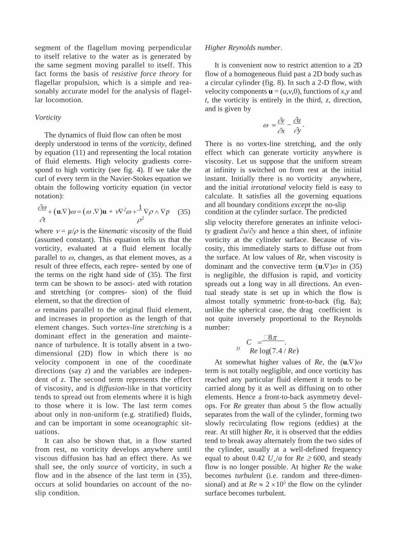
It is convenient now to restrict attention to a 2D
flow of a homogeneous fluid past a 2D body such as
a circular cylinder (fig. 8). In such a 2-D flow, with
velocity components u = (u,v,0), functions of x,y and
t, the vorticity is entirely in the third, z, direction,
and is given by
Vorticity
The dynamics of fluid flow can often be most
= v
x −
u .
y
deeply understood in terms of the vorticity, defined
by equation (11) and representing the local rotation
of fluid elements. High velocity gradients corre-
spond to high vorticity (see fig. 4). If we take the
curl of every term in the Navier-Stokes equation we
obtain the following vorticity equation (in vector
notation):
There is no vortex-line stretching, and the only
effect which can generate vorticity anywhere is
viscosity. Let us suppose that the uniform stream
at infinity is switched on from rest at the initial
instant. Initially there is no vorticity anywhere,
and the initial irrotational velocity field is easy to
calculate. It satisfies all the governing equations
and all boundary conditions except the no-slip + (u.) = ( .)u + 2 +
1 p (35) condition at the cylinder surface. The predicted
t 2
where = µ/ is the kinematic viscosity of the fluid
(assumed constant). This equation tells us that the
vorticity, evaluated at a fluid element locally
parallel to , changes, as that element moves, as a
result of three effects, each repre- sented by one of
the terms on the right hand side of (35). The first
term can be shown to be associ- ated with rotation
and stretching (or compres- sion) of the fluid
element, so that the direction of
remains parallel to the original fluid element,
and increases in proportion as the length of that
element changes. Such vortex-line stretching is a
dominant effect in the generation and mainte-
nance of turbulence. It is totally absent in a two-
dimensional (2D) flow in which there is no
velocity component in one of the coordinate
directions (say z) and the variables are indepen-
dent of z. The second term represents the effect
of viscosity, and is diffusion-like in that vorticity
tends to spread out from elements where it is high
to those where it is low. The last term comes
about only in non-uniform (e.g. stratified) fluids,
and can be important in some oceanographic sit-
uations.
It can also be shown that, in a flow started
from rest, no vorticity develops anywhere until
viscous diffusion has had an effect there. As we
shall see, the only source of vorticity, in such a
flow and in the absence of the last term in (35),
occurs at solid boundaries on account of the no-
slip condition.
slip velocity therefore generates an infinite veloci-
ty gradient ∂u/∂y and hence a thin sheet, of infinite
vorticity at the cylinder surface. Because of vis-
cosity, this immediately starts to diffuse out from
the surface. At low values of Re, when viscosity is
dominant and the convective term (u.) in (35)
is negligible, the diffusion is rapid, and vorticity
spreads out a long way in all directions. An even-
tual steady state is set up in which the flow is
almost totally symmetric front-to-back (fig. 8a);
unlike the spherical case, the drag coefficient is
not quite inversely proportional to the Reynolds
number:
C = 8
. D Re log(7. 4 / Re)
At somewhat higher values of Re, the (u.)
term is not totally negligible, and once vorticity has
reached any particular fluid element it tends to be
carried along by it as well as diffusing on to other
elements. Hence a front-to-back asymmetry devel-
ops. For Re greater than about 5 the flow actually
separates from the wall of the cylinder, forming two
slowly recirculating flow regions (eddies) at the
rear. At still higher Re, it is observed that the eddies
tend to break away alternately from the two sides of
the cylinder, usually at a well-defined frequency
equal to about 0.42 U∞/a for Re 600, and steady
flow is no longer possible. At higher Re the wake
becomes turbulent (i.e. random and three-dimen-
sional) and at Re 2 105 the flow on the cylinder
surface becomes turbulent.

18 T.J. PEDLEY
pp pp
pp
boundary layer
wake
FIG. 9. – Sketch of boundary layer and wake for steady flow at high Reynolds number past a symmetric streamlined body.
Steady flows at relatively high Reynolds number
do seem to be possible past streamlined bodies such
as a wing (or a fish dragged through the fluid), see
fig. 9. Diffusion causes vorticity to occupy a
(boundary) layer of thickness (t)1/2 after time t.
However, even a fluid element near the leading edge
at first will have been swept off downstream past the
trailing edge after a time t = L/U∞, where L is the
length of the wing chord. Hence the greatest thick-
ness that the boundary layer on the body can have is
1/ 2
and it is easy to see that a steady state can develop
everywhere on the body, with a boundary layer of
thickness up to s, and a thin wake region, also con-
taining vorticity, downstream. Note that the bound-
ary layer of vorticity remains thin compared with the
chord length if s << L, i.e. Re >>1. In that case (and
only then) neglecting viscosity altogether, and for-
getting about the boundary layer, is accurate
enough, except in calculating the drag.
Drag on a symmetric body at large Reynolds
number. In order to estimate the force on a body it
s = (L / U ) , (36) is necessary to work out the distribution of pressure
pp
(a)
p=p
(b)
p=p
pp
FIG. 10. – Sketch of streamlines and pressures for flow past a circular cylinder. (a) Idealised flow of a fluid with no viscosity; (b) separated flow at fairly high Reynolds number in a viscous fluid.
A1 pp
S1 S2 pp
A2
pp

100
10
CD
1
0.1
10-1
100 101 102 103 104 105 106
Re=U D
FIG. 11. – Log-log plot of drag coefficient versus Reynolds number for steady flow past a circular cylinder. [The sharp reduction in CD
at Re ≈ 2 105 is associated with the transition to turbulence in the boundary layer]. Redrawn from Schlichting (1968).
round the body. In a steady flow of constant density
fluid in which viscosity is unimportant (e.g. outside
the boundary layer and wake of a body) equation
(16d) can be integrated to give the result that the
metric (fig. 10a). At the front stagnation point S1,
the point of zero velocity where the streamline
dividing flow above from flow below impinges, the
pressure is high (p = p +1/2U2 ), and this high ∞ ∞
quantity
p + pgz + 1
u 2 = constant
(37a)
pressure is balanced by an equally high pressure at
the rear stagnation point S2. The pressure at the sides
(A , A ) is low (p = p –3/2U2 ). The net effect is that 2 1 2 ∞ ∞
along streamlines of the flow. Here z is measured
vertically upwards and |u| is the total fluid speed.
This result is equivalent to the Newtonian principle
of conservation of energy; equation (37a) is called
Bernoulli’s equation. If we forget about the gravita-
tional contribution, replacing p + pgz by the effec-
tive pressure pe (eq. 21), equation (37a) becomes
1
the hydrodynamic force on the cylinder is zero.
In a viscous fluid, as stated above, there is a thin
boundary layer on the front half, in which the
velocity falls from a large value to zero, so the pres-
sure distribution is similar to that described above;
however the flow separates on the rear half and
things are very different. The reason for the separa-
tion is that the adverse pressure gradient (the pres-
sure rise), from A1 to S
2 say, causes the low veloci-
pe = constant –
2 u 2; (37b) ty in the boundary layer to tend to reverse its direc-
tion, and it is observed that separation occurs as
henceforth we just write p for pe. If the fluid speeds
up, the pressure falls, and vice versa, which is intu-
itively obvious since a favourable pressure gradient
is clearly required to give fluid elements positive
acceleration.
soon as flow reversal takes place. In the separated
flow region (fig. 10b) the fluid velocity is low and
the pressure remains close to its value at the sides.
Thus there is a front-to-back pressure difference
proportional to U2 , and the drag coefficient C ∞ D
In the case of flow past a symmetric body, (fig.
10a), all streamlines start from a region of uniform
pressure (p∞
say) and uniform velocity (U∞), so the
constant in (37b) is the same for all streamlines,
p +1/2U2 . If viscosity were really negligible, then
(eq. 28) is approximately constant, independent of
Re as long as Re is large (see fig. 11). The direct
contribution of tangential viscous stresses to the
drag is negligibly small, although it is the presence
of viscosity which causes the flow separation in the ∞ ∞
the flow round a circular cylinder would be sym- first place.
D (mm)
0.05
0.1
0.3
1.0
3.0
7.9
42.0
80.0
300.0
20 T.J. PEDLEY
(b)
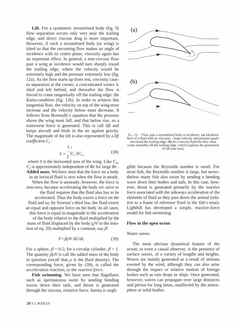
Lift. For a symmetric streamlined body (fig. 9)
flow separation occurs only very near the trailing
edge, and direct viscous drag is more important.
However, if such a streamlined body (or wing) is
tilted so that the oncoming flow makes an angle of
incidence with its centre plane, viscosity again has
an important effect. In general, a non-viscous flow
past a wing at incidence would turn sharply round
the trailing edge, where the velocity would be
extremely high and the pressure extremely low (fig.
12a). As the flow starts up from rest, viscosity caus-
es separation at the corner, a concentrated vortex is
shed and left behind, and thereafter the flow is
forced to come tangentially off the trailing edge: the
Kutta-condition (fig. 12b). In order to achieve this
tangential flow, the velocity on top of the wing must
increase and the velocity below must decrease. It
follows from Bernoulli’s equation that the pressure
above the wing must fall, and that below rise, so a
transverse force is generated. This is call lift and
keeps aircraft and birds in the air against gravity.
The magnitude of the lift is also represented by a lift
coefficient CL :
1 2
FIG. 12. – Flow past a streamlined body at incidence. (a) Idealised flow of a fluid with no viscosity - large velocity and pressure gradi-
ent round the trailing edge. (b) In a viscous fluid the flow must come smoothly off the trailing edge, which explains the generation
of lift (see text).
L = 2
U SCL , (38)
where S is the horizontal area of the wing. Like CD,
CL is approximately independent of Re for large Re .
Added mass. We have seen that the force on a body
in an inviscid fluid is zero when the flow is steady.
When the flow is unsteady, however, the force is
non-zero, because accelerating the body rel- ative to
the fluid requires that the fluid also has to be
accelerated. Thus the body exerts a force on the
fluid and so, by Newton’s third law, the fluid exerts
an equal and opposite force on the body. In all cases,
this force is equal in magnitude to the acceleration
of the body relative to the fluid multiplied by the
mass of fluid displaced by the body (V in the nota-
tion of eq. 20) multiplied by a constant, say :
F=V dU/dt. (39)
For a sphere, = 0.5; for a circular cylinder, = 1.
The quantity V is call the added mass of the body
in question (recall that is the fluid density). The corresponding force, given by (39), is called the acceleration reaction, or the reactive force.
Fish swimming. We have seen that flagellates
such as spermatozoa swim by sending bending
waves down their tails, and thrust is generated
through the viscous, resistive force. Inertia is negli-
gible because the Reynolds number is small. For
most fish, the Reynolds number is large, but never-
theless many fish also swim by sending a bending
wave down their bodies and tails. In this case, how-
ever, thrust is generated primarily by the reactive
force associated with the sideways acceleration of the
elements of fluid as they pass down the animal (rela-
tive to a frame of reference fixed in the fish’s nose).
Lighthill has developed a simple, reactive-force
model for fish swimming.
Flow in the open ocean
Water waves
The most obvious dynamical feature of the
ocean, to even a casual observer, is the presence of
surface waves, of a variety of lengths and heights.
Waves are mainly generated as a result of stresses
exerted by the wind, although they can also arise
through the impact or relative motion of foreign
bodies such as rain drops or ships. Once generated,
however, waves can propagate over large distances
and persist for long times, unaffected by the atmos-
phere or solid bodies.
(a)

In a periodic wave motion, all fluid elements
affected by it experience oscillations. Like all = A cos(t − kx − ), (42)
oscillations, such as that of a simple pendulum,
these oscillations come about as an interaction
between a restoring force, tending to restore a par-
again for constant A and . The speed of propagation
of the wave crests, or phase velocity, is
g 1 2
ticle to a nearby equilibrium position, and inertia, which causes the particle to overshoot each time it
c = k
= k
. (43)
reaches its equilibrium position (in real systems
there is also some viscous damping, which causes
the amplitude of the oscillations to die out after a
long time, if there is no further stimulation; we
ignore damping here). In the case of a simple pen-
dulum (a mass suspended by a light string) the
equilibrium state is one in which the string is ver-
tical and the mass at rest, the restoring force is
Thus long waves (small k) travel more rapidly than
short waves (large k). This explains why, when the
waves are generated by a localised disturbance, such
as a storm at sea, or a stone dropped in a pond, the
longer waves (swell) arrive at the shore first. In this
case, the wave front travels at a different speed,
called the group velocity, cg:
1
gravity and the inertia is the momentum of the c = d
= 1 g 2
, (44)
mass itself. In the case of water waves, the equilib- g dk 2 k
rium state has the free surface horizontal, the
restoring force is again gravity (except for small
wavelengths, when surface tension is also impor-
tant) and the inertia is the momentum of the fluid.
Viscosity is negligible because there are no solid
boundaries generating vorticity.
In an oscillation of small amplitude, every parti-
cle exhibits simple harmonic motion: its vertical dis-
placement, say Y, from equilibrium, varies with time
according to the differential equation
so that wave crests, travelling faster, appear to arise
at the back of the packet of waves, and to disappear
at the front.
When a water wave propagates, with its free sur-
face given by (42), fluid elements at and below the
surface move in circular paths, and the amplitude of
their motion falls off exponentially with depth below
the surface: the amplitude is proportional to Aekz
when the undisturbed surface is at z = 0. Thus the
amplitude is negligibly small at a depth of only half
d 2Y
dt 2 +
2Y = 0.
(40)
a wavelength (kz = -π). This explains why the theo-
ry of waves in very deep water works well in rela-
tively shallow water, too, with depth h greater than
The general solution for Y is a sinusoidal oscilla-
tion of the form
half a wavelength. When the waves are very long, or
the water very shallow, equation (41) is replaced by
Y = Acos(t − )
= (gk tanh kh) (45)
where A and are constants (determined by initial conditions), the amplitude and phase respectively,
and is the angular frequency of the oscillation
(the frequency in Hertz is /2π). In the case of a
simple pendulum, = (g/l)1/2 where l is the length of the string. In the case of simple water waves of
wave length = k (k is the wave number), in an
ocean whose depth is much greater than , we have
Small amplitude wave theory is very useful,
because the equations are linear and a general
motion can be made up from the addition of many
sinusoidal components such as (42) (a Fourier series
or transform). At larger amplitudes, nonlinear
effects become important and the theory becomes
less general, although many interesting and impor-
tant phenomena arise, such as wave breaking.
Internal waves
= (gk)1/2 (41)
as long as surface tension is negligible.
Suppose a parallel-crested (one-dimensional)
train of such waves is propagating in the x-direction.
Then the displacement of the free surface will be
given by
Although the water in the ocean is effectively
incompressible, it does not have uniform density
because it is stratified on account of the variation
with depth of the pressure and, to a lesser extent, the
temperature and the salinity. The temperature/densi-
ty distribution is marked usually by one or more
1/ 2

22 T.J. PEDLEY
thermoclines, in which the density gradient is steep-
er than elsewhere. Whether the density gradient is
uniform or locally sharp, less dense fluid sits, in
equilibrium, above denser fluid. A disturbance to
this state causes some heavy fluid elements to rise
above their original level, and some light ones to fall
below. As in the case of surface waves, gravity then
provides a restoring force and internal gravity waves
can propagate. As for surface waves, a relation can
large-scale circulation of the oceans. To analyse
such motions, it is necessary to recognise that the
natural frame of reference is fixed in the rotating
earth, and the governing equations of motion have to
be changed accordingly. If viscosity is neglected, the
equation of motion of a fluid in a frame of reference
rotating with constant angular velocity becomes
(in place of (16d)):
Du be calculated between the frequency and the wave
number of such waves. For example, if there is a
+ u = g − p. Dt
(50)
sharp interface between two deep regions of fluid with densities
1 (above) and
2, then equation (41)
is replaced by
Here g has been modified to include the small “cen-
trifugal force’’ term, and we could also incorporate
it into the pressure using (21). The additional term
2 u
is called the Coriolis force.
= gk(2 − 1 ) / (2 + 1 ). (46) Time does not permit a thorough investigation of
the dynamics of rotating fluids. We consider only a
This can be seen to give much lower frequencies than (41) if (
2 –
1) is not large: if
2 –
1 = 0.1
2 ,
then the frequency given by (46) is 4.4 times small- er than that given by (41) (with
2 = ). The propa-
gation speed is correspondingly smaller, too.
flow in which the Coriolis force is much larger than
the other inertia terms and therefore must by itself
balance the gradient in (effective) pressure: a
geostrophic flow. For such a flow, (50) reduces to
When the density gradient is uniform, with u = −p.
(51)
g d = − N 2 ,
dz (47) Suppose the flow is horizontal: u= (u, v, 0 ), with z
vertically upwards again. Then the horizontal com-
where N is a constant with the dimensions of a fre-
quency (the Brunt -Väisälä frequency), the situation
is a bit more complicated, because internal waves do
not have to propagate horizontally. Indeed, a wave
ponents of the pressure gradient are given by
p = − v,
p = + u
x y
(52)
whose crests propagate at an angle to the horizon-
tal, so that the displacement of a fluid element is
given by
y = A cos(t − k(x cos + z sin )),
has a frequency given by
= N cos . (48)
However, the group velocity (velocity of a wave
front, or of energy propagation) is perpendicular to
the phase velocity, and in this case is given by the
vector
N
where
is the vertical component of the earth’s
angular velocity (total angular velocity multiplied
by the sine of the latitude). The pressure gradient is
perpendicular to the velocity, or vice versa, indicat-
ing that if there is a horizontal pressure gradient, the
corresponding geostrophic flow will be perpendicu-
lar to it. This explains why the wind goes anticlock-
wise round atmospheric depressions in the northern
hemisphere (clockwise in the southern hemisphere).
Similar flows occur in the oceans, although the bar-
riers formed by the continents are impermeable,
unlike in the atmosphere.
The condition for a steady flow to be geostroph-
ic is that the inertia term (u.)u should be small compared with the Coriolis term. Thus if U is a typ-
cg = sin (sin , 0, − cos ). k
(49) ical velocity magnitude, and L a length scale for the
flow, the geostrophic approximation will be a good
Rotating fluids: geostrophic flows
Gravity waves are (mostly) small-scale phenom-
ena for which the rotation of the earth is unimpor-
one if
U 2
L vU,
tant. That is not the case with ocean currents and the i.e. the Rossby number should be small:

2 1
U 2
1. v L
(53)
equations, and it turns out that a solution of the sup-
posed form exists only if takes a particular value. If that value has negative (or zero) real part, the dis-
If the Rossby number is large, the earth’s rotation can be neglected. Note that the Rossby number is
always large at the equator, where v = 0.
Hydrodynamic instability
A smooth, laminar flow becomes turbulent as a
result of hydrodynamic instability. Small, random
perturbations are inevitably present in any real sys-
tem; if they die away again, the flow is stable, but if
they grow large, the original flow becomes unrecog-
nisable and is unstable. Usually, steady flows which
are slow or weak enough are stable, but they become
unstable above some critical speed or strength.
The way to investigate instabilities mathemati-
cally is to assume that the disturbances to the steady
state are very small and to linearise the equations
accordingly. Thus, if the steady state velocity, pres-
sure and density are given by u0(x), p
0 (x) and
0 (x)
(all functions of position, in general) it is postulated
that, with the perturbation, we have
u = u0 (x) + u' (x, t),
p = p0 (x) + p' (x, t),
= 0 (x) + ' (x, t)
where u, p and are small. Then these are sub-
stituted into the governing equations, and terms
involving squares or products of small quantities
are neglected, so the equations are linearised. For
example, equation (7) which, with (3b), is
turbance dies away (or oscillates at constant ampli-
tude); if it has positive real part it grows exponen-
tially, indicating instability. If any disturbance of the
form (55) (i.e. for any values of k and l) grows, then
the flow is unstable, because in general all distur-
bances are present, infinitesimally, at first.
Consider, for example, the case of two fluids of
different densities, one on top of the other. We have
seen that the frequency of a disturbance of
wavenumber k is given by equation (46) if 2(the
density of the lower fluid) is greater than 1.
2However, if > , as given by (46) is negative.
But if we replace by i, 2 is positive, is real,
and the oscillation cost can be written as 1/2(et +
e-t).Thus exponential growth is predicted. Hence the
interface between a dense fluid and a less dense
fluid below it is unstable.
A similar analysis can be performed for a contin-
uous density distribution, denser on top, caused by a
temperature gradient, say, in a fluid heated from
below. In this case the diffusion of heat (and hence
density) must be allowed for, as well as conserva-
tion of fluid mass and momentum. For example, a
horizontal layer of fluid, contained between two
rigid horizontal planes, distance h apart and main-
tained at temperatures T0
(top) and T0
+ ∆T (bot-
tom) is unstable if the temperature difference ∆T is
large enough. More precisely, instability occurs if
a dimensionless parameter called the Rayleigh
number Ra exceeds the critical value of 1708,
where
gTh3
+ u. = 0,
Ra =
(56)
becomes
t
t
+ u0 . +u .0 = 0
(54)
Here , and are fluid properties, the coefficient
of expansion, the kinematic viscosity () and the
thermal diffusivity respectively. When instability
occurs, for values of Ra not much greater than 1708,
the resulting motion is a regular array of usually and the nonlinear term u is neglected. After
linearisation, it is usually possible to think of the
disturbance as made up of many modes in which
the variables depend sinusoidally on one or more
space coordinates and exponentially on time, e.g.
hexagonal cells (fig. 13), with fluid flow up in the
centre of the cells and down at the edges. Such a
motion is an example of thermal convection, called
Rayleigh-Benard convection. When Ra is much
higher than 1708, the cells themselves become
unstable, the convection becomes very complicated
' = f (z)expi(kx + ly) + t
(55) and eventually turbulent.
Rayleigh-Benard convection is an example in
(cf 42), where i = −1 and we are using complex which instability of the original steady state leads
number notation. Such terms are substituted into the to another, regular, steady motion which itself goes
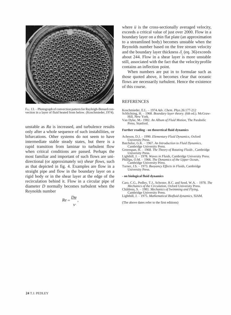
24 T.J. PEDLEY
FIG. 13. – Photograph of convection pattern for Rayleigh-Benard con- vection in a layer of fluid heated from below. (Koschmieder, 1974).
unstable as Ra is increased, and turbulence results
only after a whole sequence of such instabilities, or
bifurcations. Other systems do not seem to have
intermediate stable steady states, but there is a
rapid transition from laminar to turbulent flow
when critical conditions are passed. Perhaps the
most familiar and important of such flows are uni-
directional (or approximately so) shear flows, such
as that depicted in fig. 4. Examples are flow in a
straight pipe and flow in the boundary layer on a
rigid body or in the shear layer at the edge of the
recirculation behind it. Flow in a circular pipe of
diameter D normally becomes turbulent when the
Reynolds number
Re = Du
,
where u– is the cross-sectionally averaged velocity,
exceeds a critical value of just over 2000. Flow in a
boundary layer on a thin flat plate (an approximation
to a streamlined body) becomes unstable when the
Reynolds number based on the free stream velocity
and the boundary layer thickness s
(eq. 36) exceeds
about 244. Flow in a shear layer is more unstable still, associated with the fact that the velocity profile
contains an inflection point.
When numbers are put in to formulae such as
those quoted above, it becomes clear that oceanic
flows are necessarily turbulent. Hence the existence
of this course.
REFERENCES
Koschmieder, E.L. – 1974 Adv. Chem. Phys.26:177-212 Schlichting, H. – 1968. Boundary layer theory. (6th ed.). McGraw-
Hill, New York. Van Dyke, M.- 1982. An Album of Fluid Motion, The Parabolic
Press, Stanford.
Further reading - on theoretical fluid dynamics
Acheson, D.J. – 1990. Elementary Fluid Dynamics, Oxford University Press.
Batchelor, G.K. – 1967. An Introduction to Fluid Dynamics, Cambridge University Press.
Greenspan, H. – 1968. The Theory of Rotating Fluids , Cambridge University Press.
Lighthill, J. – 1978. Waves in Fluids, Cambridge University Press. Phillips, O.M. – 1966. The Dynamics of the Upper Ocean,
Cambridge University Press. Turner, J.S. – 1973. Buoyancy Effects in Fluids, Cambridge
University Press.
- on biological fluid dynamics
Caro, C.G., Pedley, T.J., Schroter, R.C. and Seed, W.A. – 1978. The Mechanics of the Circulation, Oxford University Press.
Childress, S. – 1981. Mechanics of Swimming and Flying, Cambridge University Press.
Lighthill, J. – 1975. Mathematical Biofluid dynamics, SIAM.
(The above dates refer to the first editions)

12 2015 - 16
CONCEPT OF CONTROL VOLUME
.
CONTINUITY EQUATION Concepts
The continuity equation is governed from the principle of conservation of
mass.It states that the mass of fluid flowing through the pipe at the cross-section
remains constants,if there is no fluid is added or removed from the pipe.
Let us make the mass balance for a fluid element as shown below: (an open-faced cube)
This is the continuity equation for every point in a fluid flow whether steady or unsteady , compressible or incompressible.
For steady, incompressible flow, the density is constant and the equation simplifies to
For two dimensional incompressible flow this will simplify still further to
1.1.1 ULER'S EQUATION OF MOTION
This is known as Euler's equation, giving, in differential form the relationship between p, v,
and elevation z, along a streamline for steady flow.
1.1.2 BERNOULLI EQUATION
Concepts
Bernoulli’s Equation relates velocity, pressure and elevation changes of a fluid in motion. It
may be stated as follows “ In an ideal incompressible fluid when the flow is steady and
continuous the sum of pressure energy, kinetic energy and potential energy is constant
along streamline”
--> 1
This is the basic from of Bernoulli equation for steady incompressible inviscid flows. It
may be written for any two points 1 and 2 on the same streamline as
--> 2

14 V.P.KRISHNAMURTHY – AP/MECH 2015 - 16
The constant of Bernoulli equation, can be named as total head (ho) has different values on
different streamlines.
--> 3
The total head may be regarded as the sum of the piezometric head h* = p/g + z and the
kinetic head v2/2g.
Bernoullie equation is arrived from the following assumptions:
1. Steady flow - common assumption applicable to many flows.
2. Incompressible flow - acceptable if the flow Mach number is less than 0.3.
3. Frictionless flow - very restrictive; solid walls introduce friction effects.
4. Valid for flow along a single streamline; i.e., different streamlines may have
different ho.
5. No shaft work - no pump or turbines on the streamline.
6. No transfer of heat - either added or removed.
Range of validity of the Bernoulli Equation:
Bernoulli equation is valid along any streamline in any steady, inviscid,
incompressible flow. There are no restrictions on the shape of the streamline or on the
geometry of the overall flow. The equation is valid for flow in one, two or three dimensions.
Modifications on Bernoulli equation:
Bernoulli equation can be corrected and used in the following form for real cases.
APPLICATIONS
1.Venturimeter.
2.Orificemeter
3.Pitot Tube

15 V.P.KRISHNAMURTHY – AP/MECH 2015 - 16
1.2 MOMENTUM EQUATION
Net force acting on fluid in the direction of x=Rate of change of momentum in x
direction
=Mass per sec× Change in
velocity p1A1-p2A2×cosθ-
Fx=ρQ(v2cosθ-v1)
Fx=ρQ(v1-v2cosθ)-p2A2cosθ+p1A1
Similarlt,the momentum in y-direction is
-p2A2sinθ+Fy=ρQ(v2sinθ-0)
Fy=ρQv2sinθ+p2A2 sinθ
Resultant force acting on the bend,
Fr=√Fx²+Fy²
GLOSSARY
Quantity Unit
Mass in Kilogram Kg
Length in Meter M
Time in Second s or as sec
Temperature in Kelvin K
Mole gmol or simply as mol
Derived quantities:
Quantity Unit
Force in Newton (1 N = 1 kg.m/s2) N
Pressure in Pascal (1 Pa = 1 N/m2) N/m2
Work, energy in Joule ( 1 J = 1 N.m) J
Power in Watt (1 W = 1 J/s) W

16 V.P.KRISHNAMURTHY – AP/MECH 2015 - 16
REVIEW QUESTIONS
PART A
1. Define compressibility of a fluid.
2. What is viscosity? What is the cause of it in liquids and gases.
3. What is the effect of temperature on viscosity of water and that of air?
4. Explain about capillarity.
5. Distinguish between fluid and solid.
6. Define (a) Dynamic viscosity and (b) Kinematic viscosity.
7. Define (a) Surface tension (b) Capillarity
8. What is a real fluid? Give examples.
9. Define cavitation.
10. Define Viscosity
11. Define the following fluid properties:
12. Density, weight density, specific volume and specific gravity of a fluid.
PART B
1. (a) What are the different types fluids? Explain each type. (b) Discuss the
thermodynamic properties of fluids
2. (a) One litter of crude oil weighs 9.6 N. Calculate its Specific weight, density and
specific weight.
(b) The Velocity Distribution for flow over a flat plate is given by u=(2/3)y-y2, Where u
is the point velocity in meter per second at a distance y meter above the plate.
Determine the shear stress at y=0 and y=15 cm. Assume dynamic viscosity as 8.63
poises
3. (a) A plate, 0.025 mm distant from a fixed plate, moves at 50 cm/s and requires a force
of 1.471 N/ m2 to maintain this speed. Determine the fluid viscosity between plates in
the poise.
(b) Determine the intensity of shear of an oil having viscosity =1.2 poise and is used for
lubrication in the clearance between a 10 cm diameter shaft and its journal bearing. The
clearance is 1.0 mm and Shaft rotates at 200 r.p.m
4. (a) Two plates are placed at a distance of 0.15mm apart. The lower plate is fixed while
the upper plate having surface area 1.0 m2 is pulled at 0.3 nm/s. Find the force and
power required to maintain this speed, if the fluid separating them is having viscosity
1.5 poise.
(b) An oil film of thickness 1.5 mm is used for lubrication between a square plate of
size 0.9m *0.9m and an inclined plane having an angle of inclination 200 . . The weight
of square plate is 392.4 N and its slides down the plane with a uniform velocity of 0.2
m/s. find the dynamic viscosity of the oil.

17
5. (a) Assuming the bulk modulus of elasticity of water is 2.07 x10 6 kN/m2 at standard
atmospheric condition determine the increase of pressure necessary to produce one
percent reduction in volume at the same temperature
(b) Calculate the capillary rise in glass tube pf 3mm diameter when immersed in
mercury, take the surface tension and angle of contact of mercury as 0.52 N/m and 1300
respectively. Also determine the minimum size of the glass tube, if it is immersed in
water, given that the surface tension of water is 0.0725 N/m and Capillary rise in tube is
not exceed 0.5mm
6. (a) Calculate the pressure exerted by 5kg of nitrogen gas at a temperature of 100 C.
Assume ideal gas law is applicable.
(b) Calculate the capillary effect in glass tube 5mm diameter, when immersed in (1)
water and (2) mercury. The surface tension of water and mercury in contact with air are
0.0725 N/m and 0.51 N/m respectively. The angle of contact of mercury of mercury is
130.
7. (a) Explain all three Simple manometers with neat sketch.
(b) Explain Differential manometer With Neat sketch.
8. A U-tube differential manometer is connected two pressure pipes A and B.Pipe A
contains Carbon tetrachloride having a specific gravity 1.594 under a pressure of 11.772
N/ Cm2 . The pipe A lies 2.5 m above pipe B. Find the difference of pressure measured
by mercury as a fluid filling U-tube

18
UNIT -II FLOW THROUGH CIRCULAR CONDUITS
PRE REQUEST DISCUSSION
Unit II has an in dept dealing of laminar flow through pipes, boundary layer
concept, hydraulic and energy gradient, friction factor, minor losses, and flow through pipes
in series and parallel.
Boundary layer is the region near a solid where the fluid motion is affected by the
solid boundary. In the bulk of the fluid the flow is usually governed by the theory of ideal
fluids. By contrast, viscosity is important in the boundary layer. The division of the problem
of flow past an solid object into these two parts, as suggested by Prandtl in 1904 has proved
to be of fundamental importance in fluid mechanics.
This concept of hydraulic gradient line and total energy line is very useful in the
study of flow This concept of hydraulic gradient line and total energy line is very useful in
the study of flow of fluids through pipes. f fluids through pipes.
2.1 HYDRAULIC GRADIENT AND TOTAL ENERGY LINE
1.Hydraulic Gradient Line
It is defined as the line which gives the sum of pressure head (p/w)
and datum head (z) of a flowing fluid in a pipe with respect to some reference line or it is
the line which is obtained by joining the top of all vertical ordinates, showing the pressure
head (p/w) of a flowing fluid in a pipe from the centre of the pipe. It is briefly
written as H.G.L (Hydraulic Gradient Line).
2.Total Energy Line
It is defined as the line which gives the sum of pressure head, datum head and
kinetic head of a flowing fluid in a pipe with respect to some reference line. It is also
defined as the line which is obtained by joining the tops of all vertical ordinates
showing the sum of pressure head and kinetic head from the centre of the pipe. It is briefly
written as T.E.L (Total Energy Line).
2.2 BOUNDARY LAYER
Concepts
The variation of velocity takes place in a narrow region in the vicinity of solid boundary.
The fluid layer in the vicinity of the solid boundary where the effects of fluid friction i.e.,
variation of velocity are predominant is known as the boundary layer.

19
2.2.1 FLOW OF VISCOUS FLUID THROUGH CIRCULAR PIPE
For the flow of viscous fluid through circular pipe, the velocity distribution across a
section, the ratio of maximum velocity to average velocity, the shear stress distribution and
drop of pressure fora given length is to be determined. The flow through circular pipe will
be viscous or laminar, if the Reynold’s number is less than 2000.
2.2.2 DEVELOPMENT OF LAMINAR AND TURBULENT FLOWS IN CIRCULAR
PIPES
1. Laminar Boundary Layer
At the initial stage i.e, near the surface of the leading edge of the plate, the thickness of
boundary layer is the small and the flow in the boundary layer is laminar though the main
stream flows turbulent. So, the layer of the fluid is said to be laminar boundary layer.
2. Turbulent Boundary Layer
The thickness boundary layer increases with distance from the leading edge in the
down-stream direction. Due to increases in thickness of boundary layer, the laminar
boundary layer becomes unstable and the motion of the fluid is disturbed. It leads to a
transition from laminar to turbulent boundary layer.
2.2.3 BOUNDARY LAYER GROWTH OVER A FLAT PLATE
Consider a continuous flow of fluid along the surface of a thin flat plate with its sharp
leading edge set parallel to the flow direction as shown in figure 2.7.The fluid approaches
the plate with uniform velocity U known as free stream velocity at the leading edge. As
soon as the fluid comes in contact the leading edge of the plate,its velocity is reduced to
zero as the fluid particles adhere to the plate boundary thereby satisfying no-slip condition.
2.3 FLOW THROUGH CIRCULAR PIPES-HAGEN POISEUILLE’S EQUATION
Due to viscosity of the flowing fluid in a laminar flow,some losses of head take place.The
equation which gives us the value of loss of head due to viscosity in a laminar flow is
known as Hagen-Poiseuille’s law.

20
p1-p2=32μUL/D²
=128μQL/πD4
This equation is called as Hargen-Poiseuille equation for laminar flow in the circular pipes.
2.4 DARCY’S EQUATION FOR LOSS OF HEAD DUE TO FRICTION IN PIPE
A pipe is a closed conduit through which the fluid flows under pressure.When the
fluid flows through the piping system,some of the potential energy is lost due to friction.
hƒ=4ƒLv²/2gD
2.5 MOODY’S DIAGRAM
Moody’s diagram is plotted between various values of friction factor(ƒ),Reynolds
number(Re) and relative roughness(R/K) as shown in figure 2.6.For any turbulent flow
problem,the values of friction factor(ƒ) can therefore be determined from Moody’s
diagram,if the numerical values of R/K for the pipe and Rе of flow are known.
The Moody’s diagram has plotted from the equation
1/√ ƒ-2.0 log10(R/K)=1.74-2.0 log10[1+18.7/(R/K/Re/ ƒ)]
Where,R/K=relative roughness
ƒ=friction factor and Re=Reynolds number.
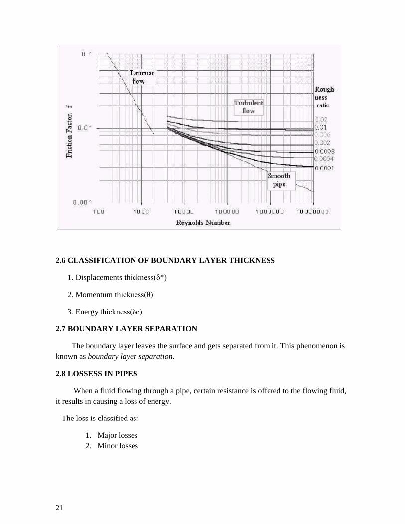
21
2.6 CLASSIFICATION OF BOUNDARY LAYER THICKNESS
1. Displacements thickness(δ*)
2. Momentum thickness(θ)
3. Energy thickness(δe)
2.7 BOUNDARY LAYER SEPARATION
The boundary layer leaves the surface and gets separated from it. This phenomenon is
known as boundary layer separation.
2.8 LOSSESS IN PIPES
When a fluid flowing through a pipe, certain resistance is offered to the flowing fluid,
it results in causing a loss of energy.
The loss is classified as:
1. Major losses
2. Minor losses
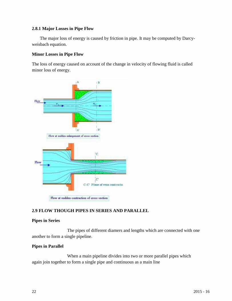
22 2015 - 16
2.8.1 Major Losses in Pipe Flow
The major loss of energy is caused by friction in pipe. It may be computed by Darcy-
weisbach equation.
Minor Losses in Pipe Flow
The loss of energy caused on account of the change in velocity of flowing fluid is called
minor loss of energy.
2.9 FLOW THOUGH PIPES IN SERIES AND PARALLEL
Pipes in Series
The pipes of different diamers and lengths which are connected with one
another to form a single pipeline.
Pipes in Parallel
When a main pipeline divides into two or more parallel pipes which
again join together to form a single pipe and continuous as a main line
23
GLOSSARY
HGL –Hydraulic gradient line
TEL – Total energy line.
Applications
1. To find out friction factor in the flow through pipe.
2. To find out the losses in losses in the pipes.
REVIEW QUESTIONS
PART A
1. Mention the general characteristics of laminar flow.
2. Write down the Navier-stokes equation.
3. Write down the Hagen-Poiseuille equation for laminar flow.
4. What are energy lines and hydraulic gradient lines?
5. What is a siphon? What is its application?
6. What is hydraulic Mean Depth or hydraulic radius?
7. Write the Darcy weishbach and Chezy’s formulas.
8. Where the Darcy weishbach and Chezy’s formulas are used?
9. What are the losses experienced by fluid when it is passing
through a pipe?
10. Write the equation of loss of energy due to sudden enlargement.
11.What do you mean by flow through parallel pipes?
12.What is boundary layer?
PART-B
1. (a) Derive an expression for the velocity distribution for viscous flow through a circular
pipe.
(b) A main pipe divides into two parallel pipes, which again forms one pipe. The length
and diameter for the first parallel pipe are 2000m and 1m respectively, while the length
and diameter of second parallel pipe are 2000 and 0.8 m respectively. Find the rate of
flow in each parallel pipe, if total flow in the main is 3 m³/s. The coefficient of friction
for each parallel pipe is same and equal to 0.005.
2. (a)Two pipes of 15 cm and 30 cm diameters are laid in parallel to pass a total discharge
of 100 liters/ second. Each pipe is 250 m long. Determine discharge through each pipe.
Now these pipes are connected in series to connect two tanks 500 m apart, to carry same
total discharge. Determine water level difference between the tanks. Neglect minor
losses in both cases, f=0.02 fn both pipes.
(b) A pipe line carrying oil of specific gravity 0.85, changes in diameter from 350 mm
at position 1 to 550 mm diameter to a position 2, which is at 6 m at a higher level. If the
pressure at position 1 and 2 are taken as 20 N/cm2 and 15 N/ cm2 respectively and
discharge through the pipe is 0.2 m³/s. determine the loss of head.
24
3. Obtain an expression for Hagen- Poisulle flow. Deduce the condition of maximum
velocity.
4. A flat plate 1.5 m X 1.5 m moves at 50 km / h in a stationary air density 1.15 kg/ m³. If
The coefficient of drag and lift are 0.15 and 0.75 respectively, determine (i) the lift force
(ii) the drag force (iii) the resultant force and (iv) the power required to set the plate in
motion.
5 (a). The rate of flow of water through a horizontal pipe is 0.3 m³/s. The diameter of the
pipe is suddenly enlarged from 25 cm to 50 cm. The pressure intensity in the smaller
pipe is 14N/m².
Determine (i) Loss of head due to sudden enlargement. (ii) Pressure intensity in the
large
pipe and (iii) Power lost due to enlargement.
(b) Water is flowing through a tapering pipe of length 200 m having diameters 500 mm
at the upper end and 250 mm at the lower end, the pipe has a slope of 1 in 40. The rate
of flow through the pipe is 250 lit/ sec. the pressure at the lower end and the upper end
are 20 N/cm² and 10 N/cm² respectively. Find the loss of head and direction of flow.
6. A horizontal pipe of 400 mm diameter is suddenly contracted to a diameter of 200 mm.
The pressure intensities in the large and small pipe is given as 15 N/cm² and 10 N/cm²
respectively. Find the loss of head due to contraction, if Cc=0.62, determine also the
rate of flow of water.
7. Determine the length of an equivalent pipe of diameter 20 cm and friction factor 0.02
for a given pipe system discharging 0.1m³/s. The pipe system consists of the following:
(i) A 10 m line of 20 cm dia with f=0.03
(ii) Three 90º bend, k=0.5 for each
(iii) Two sudden expansion of diameter 20 to 30 cm
(iv) A 15 m line of 30 cm diameter with f=0.025 and
(v) A global valve, fully open, k=10.

25
UNIT 4 DIMENSIONAL ANALYSIS
DIMENSIONAL ANALYSIS
PRE REQUEST DISCUSSION
Unit III deals with dimensional analysis,models and similitude,and application of
dimensionless parameters.
Many important engineering problems cannot be solved completely by theoretical or
mathematical methods. Problems of this type are especially common in fluid-flow, heat-
flow, and diffusional operations. One method of attacking a problem for which no
mathematical equation can be derived is that of empirical experimentations.
For example, the pressure loss from friction in a long, round, straight, smooth pipe
depends on all these variables: the length and diameter of the pipe, the flow rate of the
liquid, and the density and viscosity of the liquid. If any one of these variables is changed,
the pressure drop also changes. The empirical method of obtaining an equation relating
these factors to pressure drop requires that the effect of each separate variable be
determined in turn by systematically varying that variable while keep all others constant.
The procedure is laborious, and is difficult to organize or correlate the results so obtained
into a useful relationship for calculations.
There exists a method intermediate between formal mathematical development and a
completely empirical study. It is based on the fact that if a theoretical equation does exist
among the variables affecting a physical process, that equation must be dimensionally
homogeneous. Because of this requirement it is possible to group many factors into a
smaller number of dimensionless groups of variables. The groups themselves rather than the
separate factors appear in the final equation.
Concepts
Dimensional analysis drastically simplifies the task of fitting experimental data to
design equations where a completely mathematical treatment is not possible; it is also useful
in checking the consistency of the units in equations, in converting units, and in the scale-up
of data obtained in physical models to predict the performance of full-scale model. The
method is based on the concept of dimension and the use of dimensional formulas.
Dimensional analysis does not yield a numerical equation, and experiment is
required to complete the solution of the problem. The result of a dimensional analysis is
valuable in pointing a way to correlations of experimental data suitable for engineering use.

3.1 METHODS OF DIMENSIONAL ANALYSIS
If the number of variables involved in a physical phenomenon are known, then the
relation among the variables can be determined by the following two methods.
1. Rayleigh’s method
2. Buckingham’s π theorem
3.1.1 Rayleigh’s method
This method is used for determining the expression for a variable which depends upon
maximum three or four variables only. If the number of independent variables
becomes more than four then it is very difficult to find the expression for the dependent
variable.
3.1.2 Buckingham’s π theorem.
If there are n variables (independent and dependent variables) in a physical
phenomenon and if these variables contain m fundamental dimensions (M, L, T), then the
variables are arranged into (n-m) dimensionless numbers. Each term is called Buckingham’s
π theorem.
Applications
❖ It is used to justify the dependency of one variable with the other.
❖ Usually this type of situation occurs in structures and hydraulic machines.
❖ To solve this problem efficiently, an excellent tool is identified called dimensional
analysis.


28
3.2 SMILITUDE –TYPES OF SIMILARITIES
Similitude is defined as the similarity between the model and its prototype in
every respect, which means that the model and prototype are completely similar. Three
types of similarities must exist between the model and prototype.
Concepts
Whenever it is necessary to perform tests on a model to obtain information that
cannot be obtained by analytical means alone, the rules of similitude must be applied.
Similitude is the theory and art of predicting prototype performance from model
observations
1. Geometric similarity refers to linear dimensions. Two vessels of different sizes are
geometrically similar if the ratios of the corresponding dimensions on the two scales are the
same. If photographs of two vessels are completely super-impossible, they are
geometrically similar.
2. Kinematic similarity refers to motion and requires geometric similarity and the same
ratio of velocities for the corresponding positions in the vessels.
3. Dynamic similarity concerns forces and requires all force ratios for corresponding
positions to be equal in kinematically similar vessels.
SIGNIFICANCE
The requirement for similitude of flow between model and prototype is that the
significant dimensionless parameters must be equal for model and prototype
3.3 DIMENSIONLESS PARAMETERS
Since the inertia force is always present in a fluid flow, its ratio with each of the
other forces provides a dimensionless number.
1. Reynold’s number
2. Froud’s number
3. Euler’s number
4. Weber’s number
5. Mach’s number
Applications of dimensionless parameters
1. Reynold’s model law
2. Froud’s model law
3. Euler’s model law
4. Weber’s model law
5. Mach’s model law

Concepts
Dimensionless
Number Symbol Formula Numerator Denominator Importance
Reynolds
number
NRe
Dv/
Inertial
force
Viscous force
Fluid flow
involving
viscous and
inertial forces
Froude
number NFr u2/gD
Inertial
force
Gravitational
force
Fluid flow with
free surface
Weber number NWe u2D/ Inertial
force Surface force
Fluid flow with
interfacial forces
Mach number NMa u/c Local
velocity Sonic velocity
Gas flow at high
velocity
Drag
coefficient CD FD/(u2/2)
Total drag
force Inertial force
Flow around
solid bodies
Friction factor f w/(u2/2) Shear force Inertial force Flow though
closed conduits
Pressure
coefficient
CP
p/(u2/2)
Pressure
force
Inertial force
Flow though
closed conduits.
Pressure drop
estimation
31 V.P.KRISHNAMURTHY – AP/MECH 2015 - 16
ce i
Generally, type 1 can be solved directly, where as types 2 and 3 require simple trial and
error.
Three fundamental problems which are commonly encountered in pipe-flow calculations:
Constants: rho, mu, g, L
1. Given D, and v or Q, compute the pressure drop. (pressure-drop problem)
2. Given D, delP, compute velocity or flow rate (flow-rate problem)
3. Given Q, delP, compute the diameter D of the pipe (sizing problem)
REVIEW QUESTIONS
1. Define Dimensional Analysis
2. What you meant by fundamental and derived units?
3. Define dimensionally homogeneous equation.
4. What are the methods of dimensional analysis?
5. State Buckingham’s Π theorem
6. What you meant by Repeating variables
7. What is dimensionless number?
8. Check the dimensional homogeneity for the equation V=u+at
PART-B
1) Check the dimensional homogeneity for the equation V = u + ft.
2) Determine the dimension of the following quantities:
i) Discharge
ii) Kinematic viscosity
iii) Force and
iv) Specific weight.
3) Find an expression for the drag for on smooth sphere of d ameter D, moving with
uniform velocity v, in fluid density and dynamic viscosity .
4) Efficiency of a fan depends on the density , the dynamic viscosity of the fluid ,
the angular velocity , diameter D of the rotor and the discharge Q. Express in
terms of dimensional parameters.
5) The resistance force R of a supersonic plane during flight can be considered as
dependent upon the length of the aircraftl, velocity v, air viscosity , air density
and bulk modulus of air K. Express the functional relationship between these
variables and the resisting force.
6) A partially submerged body is towed in water. The resistance R to its motion
depends on the density , the viscosity of water, length l of the body, velocity v of

32 V.P.KRISHNAMURTHY – AP/MECH 2015 - 16
h
i
ch
ula
e
n
an
r
the body and acceleration due to gravityg. Show that the resistance to motion can be
expressed in the form
R = L2v2 , .
7) The pressure drop ∆p in a pipe of diameter D and length l depends on the
density and viscosity of
fluid flowing, mean velocity v of flow and average height of protuberance t.
Show that the pressure drop can be expressed in the form p =
v2 , , .
8) Find the expression for the drag force on smoot sphere of diameter D moving with
uniform velocity v in fluid density and dynam c viscosity .
9) The efficiency of a fan depends on the density , the dynamic viscosity , ang r
velocity , diameter D of the motor and the dis arge Q. Express the efficiency
in terms of dimensional parameters.
10) The pressure difference p in a pip of diameter D d length l due to turbulent flow
depends on the velocity v, viscosity , density and oughness K. Using
Buckingham’s -theorem, obtain a expression for p.

33 V.P.KRISHNAMURTHY – AP/MECH 2015 - 16
UNIT-IV PUMPS
PRE REQUEST DISCUSSION
Basic concepts of rot dynamic machines, velocity triangles for radial flow and axial
flow machines, centrifugal pumps, turbines and Positive displacement pumps and rotary
pumps its performance curves are discussed in Unit IV.
The liquids used in the chemical industries differ considerably in physical and chemical
properties. And it has been necessary to develop a wide variety of pumping equipment.
The two main forms are the positive displacement type and centrifugal pumps.
the former, the volume of liquid delivered is directly related to the displacement of
the piston and therefore increases directly with speed and is not appreciably influenced by
the pressure. In this group are the reciprocating piston pump and the rotary gear pump, both
of which are commonly used for delivery against high pressures and where nearly constant
delivery rates are required.
The centrifugal type depends on giving the liquid a high kinetic energy which is then
converted as efficiently as possible into pressure energy.
4.1 HEAD AND EFFICIANCES
1. Gross head
2. Effective or Net head
3. Water and Bucket power
4. Hydraulic efficiency
5. Mechanical efficiency
6. Volume efficiency
7. Overall efficiency
Concepts
A pump is a device which converts the mechanical energy supplied into hydraulic energy by
lifting water to higher levels.
4.2 CENTRIFUGAL PUMP
Working principle
If the mechanical energy is converted into pressure energy by means of centrifugal
force acting
on the fluid, the hydraulic machine is called centrifugal pump. The centrifugal pump
acts as a reversed of an inward radial flow reaction turbine
4.2.3 Performance Characteristics of Pumps
The fluid quantities involved in all hydraulic machines are the flow rate (Q) and the
head (H), whereas the mechanical quantities associated with the machine itself are the
power (P), speed (N), size (D) and efficiency ( ). Although they are of equal importance,
the emphasis placed on certain of these quantities is different for different pumps. The

34 V.P.KRISHNAMURTHY – AP/MECH 2015 - 16
output of a pump running at a given speed is the flow rate delivered by it and the head
developed. Thus, a plot of head and flow rate at a given speed forms the fundamental
performance characteristic of a pump. In order to achieve this performance, a power input is
required which involves efficiency of energy transfer. Thus, it is useful to plot also the
power P and the efficiency against Q.
Over all efficiency of a pump ( ) = Fluid power output / Power input to the shaft = gHQ /
P Type number or Specific speed of pump, nS = NQ1/2 / (gH)3/4 (it is a dimensionless number)
Centrifugal pump Performance
In the volute of the centrifugal pump, the cross section of the liquid path is greater than in
the impeller, and in an ideal frictionless pump the drop from the velocity V to the lower
velocity is converted according to Bernoulli's equation, to an increased pressure. This is the
source of the discharge pressure of a centrifugal pump.
If the speed of the impeller is increased from N1 to N2 rpm, the flow rate will increase from
Q1 to Q2 as per the given formula:
The head developed(H) will be proportional to the square of the quantity discharged, so that
The power consumed(W) will be the product of H and Q, and, therefore
These relationships, however, form only the roughest guide to the performance of
centrifugal pumps.
4.2.4 Characteristic curves
Pump action and the performance of a pump are defined interms of their
characteristic curves. These curves correlate the capacity of the pump in unit volume per
unit time versus discharge or differential pressures. These curves usually supplied by pump
manufacturers are for water only.
These curves usually shows the following relationships (for centrifugal pump).
• A plot of capacity versus differential head. The differential head is the difference in
pressure between the suction and discharge.
• The pump efficiency as a percentage versus capacity.
• The break horsepower of the pump versus capacity.
• The net poisitive head required by the pump versus capacity. The required NPSH for
the pump is a characteristic determined by the manufacturer.
35 V.P.KRISHNAMURTHY – AP/MECH 2015 - 16
Centrifugal pumps are usually rated on the basis of head and capacity at the point of
maximum efficiency.
4.3 RECIPROCATING PUMPS
Working principle
If the mechanical energy is converted into hydraulic energy (or pressure energy) by
sucking
the liquid into a cylinder in which a piston is reciprocating (moving backwards and
forwards), which
exerts the thrust on the liquid and increases its hydraulic energy (pressure energy), the pump
is known as reciprocating pump
Main ports of a reciprocating pump
1.A cylinder with a piston, piston rod, connecting rod and a crank, 2. Suction pipe
3.Delivery pipe, 4. Suction valve and 5.Delivery valve.
Slip of Reciprocating Pump
Slip of a reciprocating pump is defined as the difference between the theoretical discharge
and the actual discharge of the pump.
4.3.1Characteristic Curves Of Reciprocatring Pumps
1. According to the water being on contact with one side or both sides of the piston
(i.) Single acting pump (ii.) Double-acting pump
2. According to the number of cylinders provided
(i.) Single acting pump (ii.) Double-acting pump (iii.) Triple-acting pump
Reciprocating pumps Vs centrifugal pumps
The advantages of reciprocating pumps in general over centrifugal pumps may be
summarized as follows:
1. They can be designed for higher heads than centrifugal pumps.
2. They are not subject to air binding, and the suction may be under a pressure less
than atmospheric without necessitating special devices for priming.
3. They are more flexible in operation than centrifugal pumps.
4. They operate at nearly constant efficiency over a wide range of flow rates.
The advantages of centrifugal pumps over reciprocating pumps are:
1. The simplest centrifugal pumps are cheaper than the simplest reciprocating pumps.
2. Centrifugal pumps deliver liquid at uniform pressure without shocks or pulsations.

36 V.P.KRISHNAMURTHY – AP/MECH 2015 - 16
3. They can be directly connected to motor derive without the use of gears or belts.
4. Valves in the discharge line may be completely closed without injuring them.
5. They can handle liquids with large amounts of solids in suspension.
4.4 Rotary Pumps
The rotary pump is good for handling viscous liquids, nut because of the close
tolerances needed, it can not be manufactured large enough to compete with centrifugal
pumps for coping with very high flow rates.
Rotary pumps are available in a variety of configurations.
• Double lobe pump
• Trible lobe pumps
• Gear pump
• Gear Pumps
•
• Spur Gear or External-gear pump
External-gear pump (called as gear pump) consists essentially of two
intermeshing gears which are identical and which are surrounded by a closely fitting
casing. One of the gears is driven directly by the prime mover while the other is
allowed to rotate freely. The fluid enters the spaces between the teeth and the casing
and moves with the teeth along the outer periphery until it reaches the outlet where it
is expelled from the pump.
External-gear pumps are used for flow rates up to about 400 m3/hr working
against pressures as high as 170 atm. The volumetric efficiency of gear pumps is in
the order of 96 percent at pressures of about 40 atm but decreases as the pressure
rises.

37 V.P.KRISHNAMURTHY – AP/MECH 2015 - 16
4.4.1 Internal-gear Pump
The above figure shows the operation of a internal gear pump. In the
internal-gear pump a spur gear, or pinion, meshes with a ring gear with internal
teeth. Both gears are inside the casing. The ring gear is coaxial with the inside of the
casing, but the pinion, which is externally driven, is mounted eccentrically with
respect to the center of the casing. A stationary metal crescent fills the space
between the two gears. Liquid is carried from inlet to discharge by both gears, in the
spaces between the gear teeth and the crescent.
4.4.2 Lobe pumps
In principle the lobe pump is similar to the external gear pump; liquid flows into the
region created as the counter-rotating lobes unmesh. Displacement volumes are formed
between the surfaces of each lobe and the casing, and the liquid is displaced by meshing of
the lobes. Relatively large displacement volumes enable large solids (nonabrasive) to be
handled. They also tend to keep liquid velocities and shear low, making the pump type
suitable for high viscosity, shear-sensitive liquids.
Two lobe pump Three lobe pump
38 V.P.KRISHNAMURTHY – AP/MECH 2015 - 16
The choice of two or three lobe rotors depends upon solids size, liquid viscosity, and
tolerance of flow pulsation. Two lobe handles larger solids and high viscosity but pulsates
more. Larger lobe pumps cost 4-5 times a centrifugal pump of equal flow and head.
4.3 Selection of Pumps
The following factors influence the choice of pump for a particular operation:
1. The quantity of liquid to be handled: This primarily affects the size of the pump and
determines whether it is desirable to use a number of pumps in parallel.
2. The head against which the liquid is to be pumped. This will be determined by the
difference in pressure, the vertical height of the downstream and upstream reservoirs
and by the frictional losses which occur in the delivery line. The suitability of a
centrifugal pump and the number of stages required will largely be determined by
this factor.
3. The nature of the liquid to be pumped. For a given throughput, the viscosity largely
determines the frictional losses and hence the power required. The corrosive nature
will determine the material of construction both for the pump and the packing. With
suspensions, the clearance in the pump must be large compared with the size of the
particles.
4. The nature of power supply. If the pump is to be driven by an electric motor or
internal combustion engine, a high-speed centrifugal or rotary pump will be
preferred as it can be coupled directly to the motor.
5. If the pump is used only intermittently, corrosion troubles are more likely than with
continuous working.
Applications
The handling of liquids which are particularly corrosive or contain abrasive solids in
suspension, compressed air is used as the motive force instead of a mechanical pump.
REVIEW QUESTIONS
PART A
1. What is meant by Pump?
2. Mention main components of Centrifugal pump.
3. What is meant by Priming?
4. Define Manometric head.
5. Define Manometric efficiency
6. Define Mechanical efficiency.
7. Define overall efficiency.
8. Give the range of specific speed for low, medium, high speed
radial flow.
9. Define speed ratio, flow ratio.
10. Mention main components of Reciprocating pump.
11. Define Slip of reciprocating pump. When the negative slip does
occur?
39 V.P.KRISHNAMURTHY – AP/MECH 2015 - 16
PART-B
1. Write short notes on the following (1) Cavitations in hydraulic machines their causes,
effects and remedies. (2) Type of rotary pumps.
2. Draw a neat sketch of centrifugal pump and explain the working principle of the
centrifugal pump.
3. Draw a neat sketch of Reciprocating pump and explain the working principle of single
acing and double acting Reciprocating pump.
4. A radial flow impeller has a diameter 25 cm and width 7.5 cm at exit. It delivers 120
liters of water per second against a head of 24 m at 1440 rpm. Assuming the vanes block
the flow area by 5% and hydraulic efficiency of 0.8, estimate the vane angle at exit.
Also calculate the torque exerted on the driving shaft if the mechanical efficiency is
95%.
5. Find the power required to drive a centrifugal pump which to drive a centrifugal pump
which delivers 0.04 m3 /s of water to a height of 20 m through a 15 cm diameter pipe
and 100 m long. The over all efficiency of the pump is 70% and coefficient of friction is
0.15 in the formula hf=4flv2/2gd.
6. A Centrifugal pump having outer diameter equal to 2 times the inner diameter and
running at 1200 rpm works against a total head of 75 m. The Velocity of flow through
the impeller is constant and equal to 3 m/s. The vanes are set back at an angle of 30º at
out let. If the outer diameter of impeller is 600 mm and width at outlet is 50 mm.
Determine (i) Vane angle at inlet (ii) Work done per second on impeller
(iii) Manometric efficiency.
7. The diameter and stroke of a single acting reciprocating pump are 200 mm and 400 mm
respectively, the pump runs at 60 rpm and lifts 12 liters of water per second through a
height of 25 m. The delivery pipe is 20m long and 150mm in diameter. Find (i)
Theoretical power required to run the pump. (ii) Percentage of slip. (iii) Acceleration
head at the beginning and middle of the delivery stroke.

40 V.P.KRISHNAMURTHY – AP/MECH 2015 - 16
UNIT V TURBINES
PRE REQUEST DISCUSSION
Hydraulic Machines are defined as those machines which convert either
hydraulic energy (energy possessed by water) into mechanical energy (which is
further converted into electrical energy) or mechanical energy into hydraulic energy.
The hydraulic machines, which convert the hydraulic energy into mechanical energy, are
called turbines.
Turbines are defined as the hydraulic machines which convert hydraulic energy into
mechanical energy. This mechanical energy is used in running an electric generator which is
directly coupled to the shaft of the turbine. Thus the mechanical energy is converted
into electrical energy. The electric power which is obtained from the hydraulic energy
(energy of water) is known as Hydro- electro power.
In our subject point of view, the following turbines are important and will be
discussed one by one.
1. Pelton wheel
2. Francis turbine
3. Kaplan turbine
Concept
Turbines are defined as the hydraulic machines which convert hydraulic energy into
mechanical energy. This mechanical energy is used in running an electric generator which is
directly coupled to the shaft of the turbine
FLUID TYPES OF TURBINE
Water Hydraulic Turbine
Steam Steam Turbine
Froen Vapour Turbine
Gas or air Gas Turbine
Wind Wind Mills
5.1 CLASSIFICATION OF HYDRAULIC TURBINES
1. According to the action of the water flowing
2. According to the main direction of flow of water
3. According to the head and quality of water required
4. According to the specific speed
41 V.P.KRISHNAMURTHY – AP/MECH 2015 - 16
5.2 HEAD AND EFFICIANCES OF PELTON WHEEL
1. Gross head
2. Effective or Net head
3. Water and Bucket power
4. Hydraulic efficiency
5. Mechanical efficiency
6. Volume efficiency
7. Overall efficiency
5.3 IMPULSE TURBINE
In an impulse turbine, all the energy available by water is converted into kinetic
energy by passing a nozzle. The high velocity jet coming out of the nozzle then impinges on
a series of buckets fixed around the rim of a wheel.
5.4 Tangential Flow Turbine, Radial And Axial Turbines
1. Tangential flow turbine
In a tangential flow turbine, water flows along the tangent to the path of runner. E.g. Pelton
wheel
2. Radial flow turbine
In a radial flow turbine, water flows along the radial direction and mainly in the plane
normal to the axis of rotation, as it passes through the runner. It may be either inward radial
flow type or outward radial flow type.
3. Axial flow turbine
In axial flow turbines, water flows parallel to the axis of the turbine shaft. E.g. kaplan
turbine
4. Mixed flow turbine
In a mixed flow turbine, the water enters the blades radiallsy and comes out axially and
parallel to the turbine shaft .E.g. Modern Francis turbine.
In our subject point of view, the following turbines are important and will be discussed one
by one
1. Pelton wheel
2. Francis turbine
3. Kaplan turbine

42 V.P.KRISHNAMURTHY – AP/MECH 2015 - 16
5.5 PELTON WHEEL OR PELTON TURBINE
The Pelton wheel is a tangential flow impulse turbine and now in common use.
Leston A Pelton, an American engineer during 1880,develops this turbines. A pelton
wheel consists of following main parts.
1. Penstock
2. Spear and nozzle
3. Runner with buckets
4. Brake nozzle
5. Outer casing
6. Governing mechanism

43 V.P.KRISHNAMURTHY – AP/MECH 2015 - 16
5.5.1 VELOCITY TRIANGLES, WORKDONE, EFFICIENCY OF PELTON
WHEEL INLET AND OUTLET VECTOR DIAGRAMS
Let V = Velocity of the jet
u = Velocity of the vane (cups) at the impact point u
= DN/ 60
where D = Diameter of the wheel corresponding to the impact point
= Pitch circle diameter.
At inlet the shape of the vane is such that the direction of motion of the jet and the
vane is the same. i.e., Ȑ = 0, ș = 0
Relative velocity at inlet Vr = V —u
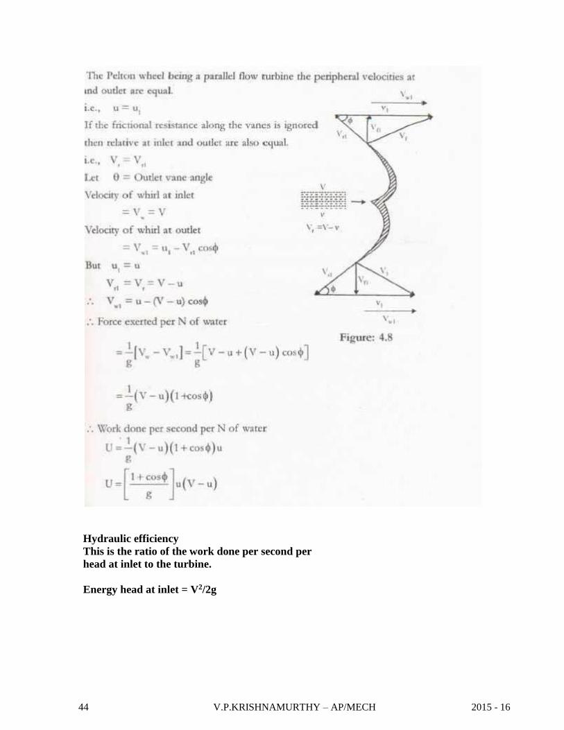
44 V.P.KRISHNAMURTHY – AP/MECH 2015 - 16
Hydraulic efficiency
This is the ratio of the work done per second per
head at inlet to the turbine.
Energy head at inlet = V2/2g

CE 6451-FLUID MECHANICS AND MACHINERY II/III MECHANICAL ENGINEERING
45
Condition for maximum hydraulic efficiency
For a given jet velocity for efficiency to be maximum, word done should be
maximum
Work done per second per N of water
Hence for the condition of maximum hydraulic efficiency, the peripheral speed of
the turbine should reach one half the jet speed.

CE 6451-FLUID MECHANICS AND MACHINERY II/III MECHANICAL ENGINEERING
46
[ The speed of any water turbine is represented by N rpm. A turbine has speed,
known as specific speed and is represented by N
‘ Specific speed of a water turbine in the speed at which a geometrically similar
turbine would run if producing unit power (1 kW) and working under a net head of
1 m. Such a turbine would be an imaginary one and is called specific turbine.
5.6 SPECIFIC SPEED

CE 6451-FLUID MECHANICS AND MACHINERY II/III MECHANICAL ENGINEERING
47

48
5.7 FRANCIS TURBINE
Francis turbine is an inward flow reaction turbine. It is developed by the American engineer
James B. Francis. In the earlier stages, Francis turbine had a purely radial floe runner. But the
modern Francis turbine is a mixed flow reaction turbine in which the water enters the runner
radially at its outer periphery and leaves axially at its centre. This arrangement provides larger
discharge area with prescribed diameter of the runner. The main parts such as
1. Penstock
2. Scroll or Spiral Casing
3. Speed ring or Stay ring
4. Guide vanes or Wickets gates
5. Runner and runner blades
6. Draft tube

49

50
5.8 KAPLAN TURBINE
A Kaplan turbine is an axial flow reaction turbine which was developed by Austrian
engineer V. Kaplan. It is suitable for relatively low heads. Hence, it requires a large quantity of
water to develop large power. The main parts of Kaplan turbine, they are
1. Scroll casing
2. Stay ring
3. Guide vanes
4. Runner
5. Draft tube
5.9 PERFORMANCE OF TURBINES
Turbines are often required to work under varying conditions of head, speed, output and gate
opening. In order to predict their behavior, it is essential to study the performance of the turbines
under the varying conditions. The concept of unit quantities and specific quantities are required to
❖ The behavior of a turbine is predicted working under different conditions.
❖ Comparison is made between the performance of turbine of same type but of different
sizes.

51
❖ The performance of turbine is compared with different types.
5.10 DRAFT TUBE
The pressure at the exit of the runner of a reaction turbine is generally less than atmospheric
pressure. Thus the water at the exit of the runner cannot be directly discharged to the tail race. A
pipe o gradually increasing area is used for discharging water form the exit of the turbine to the tail
race. This pipe of gradually increasing area is called a draft tube.
5.11 SPECIFIC SPEED
Homologus units are required in governing dimensionless groups to use scaled models in
designing turbomachines, based geometric similitude.
Specific speed is the speed of a geometrically similar turbine, which will develop unit
power when working under a unit head. The specific speed is used in comparing the different types
of turbines as every type of turbine has different specific speed. In S.I. units, unit power is taken as
one Kw and unit as one meter.
5.12 GOVERNING OF TURBINES
All the modern hydraulic turbines are directly coupled to the electric generators. The
generators are always required to run at constant speed irrespective of the variations in the load. It
is usually done by regulating the quantity of water flowing through the runner in accordance with
the variations in the load. Such an operation of regulation of speed of turbine runner is known as
governing of turbine and is usually done automatically by means of a governor.
Applications
1. To produce the power by water.
GLOSSARY
HP –Horse power
KW- Kilo watts
REVIEW QUESTIONS
1. Define hydraulic machines.
2. Give example for a low head, medium head and high head turbine.
3. What is impulse turbine? Give example.
4. What is reaction turbine? Give example.
5. What is axial flow turbine?
6. What is the function of spear and nozzle?
9. Define gross head and net or effective head.
7.Define hydraulic efficiency.
8. Define unit speed of turbine.

52
9. Define specific speed of turbine.
10. Give the range of specific speed values of Kaplan , Francis turbine
and pelton wheels
11. Define unit discharge.
12.Define unit power.
13.What is a draft tube? In which type of turbine it is mostly used?
14.Write the function of draft tube in turbine outlet.
PART B
1. Obtain en expression for the work done per second by water on the runner of a pelton wheel.
Hence derive an expression for maximum efficiency of the pelton wheel giving the relationship
between the jet speed and bucket speed.
2. (a) A pelton wheel is having a mean bucket diameter of 1 m and is running at 1000 rpm. The
net head on the pelton wheel is 700 m. If the side clearance angle is 15º and discharge through
nozzle is 0.1 m³/s, find (1) power available at nozzle and (2) hydraulic efficiency of the turbine.
Take Cv=1 (b) A turbine is to operate under a head of 25 m
at 200 rpm. The discharge is 9 m³/s. If the efficiency is 90% determine, Specific speed of the
machine, Power generated and type of turbine.
3. A pelton turbine is required to develop 9000 KW when working under a head of 300 m the
impeller may rotate at 500 rpm. Assuming a jet ratio of 10 And an overall efficiency of 85%
calculate (1) Quantity of water required. (2) Diameter of the wheel (3) Number of jets (4)
Number and size of the bucket vanes on the runner.
4. An Outward flow reaction turbine has internal and external diameters of the runner as 0.5 m and
1.0 m respectively. The turbine is running at 250 rpm and rate of flow of water through the
turbine is 8 m³/s. The width of the runner is constant at inlet and out let and is equal to 30 cm.
The head on the turbine is 10 m and discharge at outlet6 is radial, determine (1) Vane angle at
inlet and outlet. (2) Velocity of flow at inlet and outlet.
5. The Nozzle of a pelton Wheel gives a jet of 9 cm diameter and velocity 75 m/s. Coefficient of
velocity is 0.978. The pitch circle diameter is 1.5 m and the deflection angle of the bucket is
170º. The wheel velocity is 0.46 times the jet velocity. Estimate the speed of the pelton wheel
turbine in rpm, theoretical power developed and also the efficiency of the turbine.
6. (a)A turbine is to operate a head of a 25 m at 200 rpm; the available discharge is 9 m³/s
assuming an efficiency of 90%. Determine (1) Specific speed (2) Power generated (3)
Performance under a head of 20 m (4) The type of turbine. ) (b) A vertical reaction
turbine under 6m head at 400 rpm the area and diameter of runner at inlet are 0.7 m² and 1m
respective the absolute and relative velocities of fluid entering are 15ºand 60º to the tangential
direction. Calculate hydraulic efficiency.
7. A Francis turbine has an inlet diameter of 2.0 m and an outlet diameter of 1.2m. The width of
the blades is constant at 0.2 m. The runner rotates at a speed of 250 rpm with a discharge of 8
m³/s .The vanes are radial at the inlet and the discharge is radially outwards at the outlet.
Calculate the angle of guide vane at inlet and blade angle at the outlet.
53
REFERENCE BOOKS
1.Modi P.N. and Seth, S.M. "Hydraulics and Fluid Mechanics
2.Bansal, R.K., Fluid Mechanics and Hydraulics Machines,
3. G.K.Vijayaraghavan Fluid Mechanics and Machinery

54
QUESTION BANK
1. Define fluids.
UNIT- I FLUID PROPERTIES AND FLOW CHARACTERISTICS
PART – A
Fluid may be defined as a substance which is capable of flowing. It has no definite shape
of its own, but confirms to the shape of the containing vessel.
2. What are the properties of ideal fluid?
Ideal fluids have following properties
i)It is incompressible
ii) It has zero viscosity
iii) Shear force is zero
3. What are the properties of real fluid?
Real fluids have following properties
i)It is compressible
ii) They are viscous in nature
iii) Shear force exists always in such fluids.
4. Explain the Density
Density or mass density is defined as the ratio of the mass of the fluid to its volume.
Thus mass per unit volume of a fluid is called density. It is denoted by the
symbol (ρ).
Density = Mass of the fluid (kg)
Volume of the fluid (m3)
5. Explain the Specific weight or weight density
Specific weight or weight density of a fluid is the ratio between the weight of a fluid
to its volume. Thus weight per uint volume of a fluid is called weight density and is
denoted by the symbol (W).
(W) = Weight of the fluid = Mass x Acceleration due to gravity
Volume of fluid Volume of fluid
W = pg
6. Explain the Specific volume
Specific volume of a fluid is defined as the volume of the fluid occupied by a unit
Mass or volume per unit mass of a fluid is called specific volume.
Specific volume = Volume = m3 = 1
Mass kg p
7. Explain the Specific gravity
Specific gravity is defined as the ratio of weight density of a fluid to the weight
density of a standard fluid. For liquid, standard fluid is water and for gases, it is
air. Specific gravity = Weight density of any liquid or gas
Weight density of standard liquid or gas

55
8. Define Viscosity.
It is defined as the property of a liquid due to which it offers resistance to the movement of
one layer of liquid over another adjacent layer.
9. Define kinematic viscosity.
It is defined as the ratio of dynamic viscosity to mass density. (m²/sec)
10. Define Relative or Specific viscosity.
It is the ratio of dynamic viscosity of fluid to dynamic viscosity of water at
20°C. 11. State Newton's law of viscosity and give examples.
Newton's law states that the shear stress ( ) on a fluid element layer is directly
proportional to the rate of shear strain. The constant of proportionality is called co-
efficient of viscosity.
r = μ du
dy
12. Give the importance of viscosity on fluid motion and its effect on temperature.
Viscosity is the property of a fluid which offers resistance to the movement of one
layer of fluid over another adjacent layer of the fluid. The viscosity is an important property which offers the fluid motion.
The viscosity of liquid decreases with increase in temperature and for gas it
Increases with increase in temperature.
13. Explain the Newtonian fluid
The fluid which obeys the Newton's law of viscosity i.e., the shear stress is directly
proportional to the rate of shear strain, is called Newtonian fluid.
r = μ du
dy
14. Explain the Non-Newtonian fluid
The fluids which does not obey the Newton's law of viscosity i.e., the shear stress is
not directly proportional to the ratio of shear strain, is called non-Newtonian fluid.
15. Define compressibility.
Compressibility is the reciprocal of bulk modulus of elasticity, k which is defined as
the ratio of compressive stress to volume strain.
k = Increase of pressure
Volume strain
Compressibility 1 = Volume of strain
k Increase of pressure
16. Define surface tension.
Surface tension is defined as the tensile force acting on the surface of a liquid in
Contact with a gas or on the surface between two immiscible liquids such that
contact surface behaves like a membrane under tension.
17. Define Capillarity.
56
Capillary is a phenomenon of rise or fall of liquid surface relative to the
adjacent general level of liquid.
18. What is cohesion and adhesion in fluids?
Cohesion is due to the force of attraction between the molecules of the same liquid.
Adhesion is due to the force of attraction between the molecules of two different
Liquids or between the molecules of the liquid and molecules of the solid boundary
surface.
19. State momentum of momentum equation?
It states that the resulting torque acting on a rotating fluid is equal to the rate
of change of moment of momentum.
20. What is momentum equation
It is based on the law of conservation of momentum or on the momentum principle
It states that,the net force acting on a fluid mass is equal to the change in
momentum of flow per unit time in that direction.
21. What is Euler's equation of motion
This is the equation of motion in which forces due to gravity and pressure are taken into
consideration. This is derived by considering the motion of a fluid element along a stream
line.
22. What is venturi meter?
Venturi meter is a device for measuring the rate of fluid flow of a flowing fluid through a
pipe. It consisits of three parts.
a. A short converging part b. Throat c.Diverging part.
It is based on the principle of Bernoalli's equation.
23. What is an orifice meter?
Orifice meter is the device used for measuring the rate of flow of a fluid through a pipe. it
is a cheaper device as compared to venturi meter. it also works on the priniciple as that of venturi
meter. It consists of a flat circular plate which has a circular sharp edged hole called orifice.
24. What is a pitot tube?
Pitot tube is a device for measuring the velocity of a flow at any point in a pipe or a channel.
It is based on the principle that if the velocity of flow at a point becomes zero, the pressure there is
increased due to the conversion of kinetic energy into pressure energy. . What are the types of fluid flow?
Steady & unsteady fluid flow Uniform & Non-uniform flow One dimensional, two-dimensional & three-dimensional flows Rotational & Irrotational flow
25. State the application of Bernouillie’s equation ?
It has the application on the following measuring devices.
1.Orifice meter.
2.Venturimeter.
3.Pitot tube.

PART-B 1.
2.`


3.
4.


5.
6.


7.


8.

9.
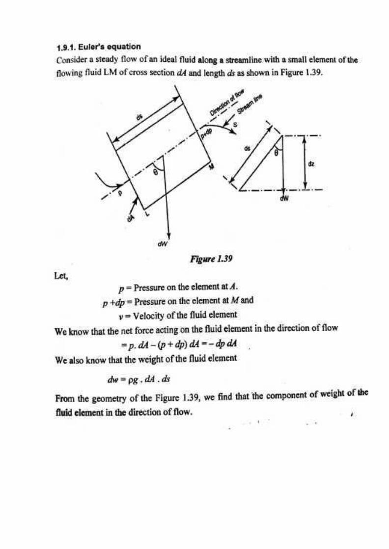


10.


11.

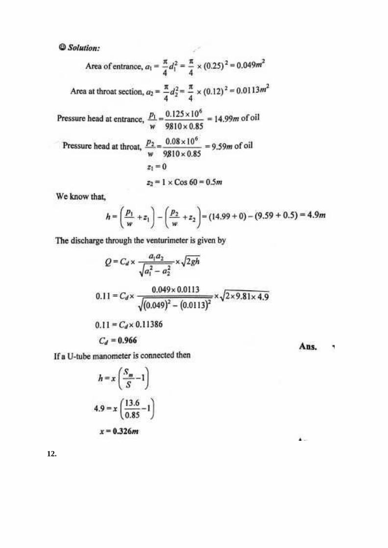
12.


1. Define viscosity (u).
UNIT II FLOW THROUGH CIRCULAR CONDUITS
PART – A
Viscosity is defined as the property of a fluid which offers resistance to the
movement of one layer of fluid over another adjacent layer of the fluid.Viscosity is
also defined as the shear stress required to produce unit rate of shear strain.
2. Define kinematic viscosity.
Kniematic viscosity is defined as the ratio between the dynamic viscosity and
density of fluid. It is denoted by μ.
3. What is minor energy loss in pipes?
The loss of head or energy due to friction in a pipe is known as major loss while loss of
energy due to change of velocity of fluid in magnitude or direction is called minor loss of energy.
These include, a. Loss of head due to sudden enlargement.
b. Loss of head due to sudden contraction.
c. Loss of head at entrance to a pipe.
d. Loss of head at exit of a pipe.
e. Loss of head due to an obstruction in a pipe.
f. Loss of head due to bend in a pipe.
g. Loss of head in various pipe fittings.
4. What is total energy line?
Total energy line is defined as the line which gives the sum of pressure head, datum head
and kinetic head of a flowing fluid in a pipe with respect to some reference line. It is also defined
as the line which is obtained by joining the tops of all vertical ordinates showing sum of the
pressure head and kinetic head from the centre of the pipe.
5. What is hydraulic gradient line?
Hydraulic gradient line gives the sum of (p/w+z) with reference to datum line. Hence
hydraulic gradient line is obtained by subtracting v2 / 2g from total energy line.
6. What is meant by pipes in series?
When pipes of different lengths and different diameters are connected end to end, pipes are
called in series or compound pipe. The rate of flow through each pipe connected in series is same.
7. What is meant by pipes in parallel?
When the pipes are connected in parallel, the loss of head in each pipe is same. The rate of
flow in main pipe is equal to the sum of rate of flow in each pipe, connected in parallel.
8. What is boundary layer and boundary layer theory?
When a solid body immersed in the flowing fluid, the variation of velocity from zero to free
stream velocity in the direction normal to boundary takes place in a narrow region in the vicinity of
solid boundary. This narrow region of fluid is called boundary layer. The theory dealing with
boundary layer flow is called boundary layer theory.
9. What is turbulent boundary layer?
If the length of the plate is more then the distance x, the thickness of boundary layer will go
on increasing in the downstream direction. Then laminar boundary becomes unstable and motion
of fluid within it, is disturbed and irregular which leads to a transition from laminar to turbulent
boundary layer.
10. What is boundary layer thickness?
Boundary layer thickness (S) is defined as the distance from boundary of the solid body
measured in y-direction to the point where the velocity of fluid is approximately equal to 0.99 times

the free steam (v) velocity of fluid.
11. Define displacement thickness
Displacement thickness (S*) is defined as the distances, measured perpendicular to the
boundary of the solid body, by which the boundary should be displaced to compensate for the
reduction inflow rate on account of boundary layer formation.
12. What is momentum thickness?
Momentum thickness (0) is defined as the distance, measured perpendicular to the boundary
of the solid body, by which the boundary should be displaced to compensate for the reduction in
momentum of flowing fluid on account of boundary layer formation.
13. Mention the general characteristics of laminar flow.
• There is a shear stress between fluid layers
• ‘No slip’ at the boundary
• The flow is rotational
• There is a continuous dissipation of energy due to viscous shear
14. What is Hagen poiseuille’s formula ?
P1-P2 / pg = h f = 32 µUL / _gD2
The expression is known as Hagen poiseuille formula .
Where P1-P2 / _g = Loss of pressure head U = Average velocity
µ = Coefficient of viscosity D = Diameter of pipe
L = Length of pipe
15. What are the factors influencing the frictional loss in pipe flow ?
Frictional resistance for the turbulent flow is
i. Proportional to vn where v varies from 1.5 to 2.0 . ii.
Proportional to the density of fluid .
iii. Proportional to the area of surface in contact . iv.
Independent of pressure . v. Depend on the nature of the surface in contact .
16. What is the expression for head loss due to friction in Darcy formula ?
hf = 4fLV2 / 2gD
Where f = Coefficient of friction in pipe L = Length of the pipe
D = Diameter of pipe V = velocity of the fluid
17. What do you understand by the terms
a) major energy losses , b) minor energy losses
Major energy losses : -
This loss due to friction and it is calculated by Darcy weis bach formula and
chezy’s formula .
Minor energy losses :- This is
due to
i. Sudden expansion in pipe .ii. Sudden contraction in pipe .
iii. Bend in pipe .iv. Due to obstruction in pipe .

18. Give an expression for loss of head due to sudden enlargement of the pipe :
he = (V1-V2)2
/2g
Wherehe = Loss of head due to sudden enlargement of pipe . V1 = Velocity of flow at section 1-1
V2 = Velocity of flow at section 2-2
19. Give an expression for loss of head due to sudden contraction :
hc =0.5 V2/2g
Where hc = Loss of head due to sudden contraction . V = Velocity at outlet of pipe.
20. Give an expression for loss of head at the entrance of the pipe
hi =0.5V2/2g
where hi = Loss of head at entrance of pipe .
V = Velocity of liquid at inlet and outlet of the pipe .
21. What is sypon ? Where it is used: _
Sypon is along bend pipe which is used to transfer liquid from a reservoir at a higher
elevation to another reservoir at a lower level .
Uses of sypon : -
1. To carry water from one reservoir to another reservoir separated by a hill ridge .
2. To empty a channel not provided with any outlet sluice .
PART-B
1.

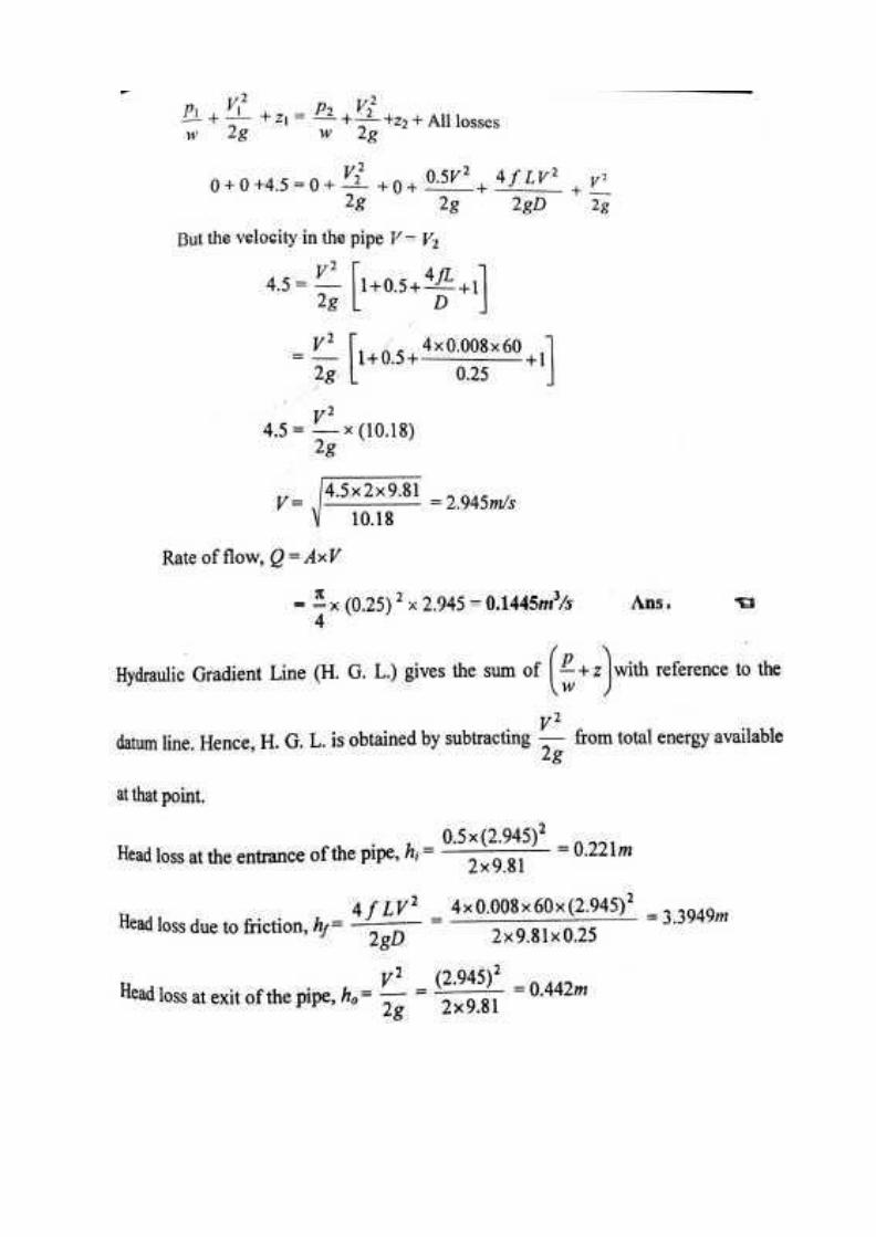

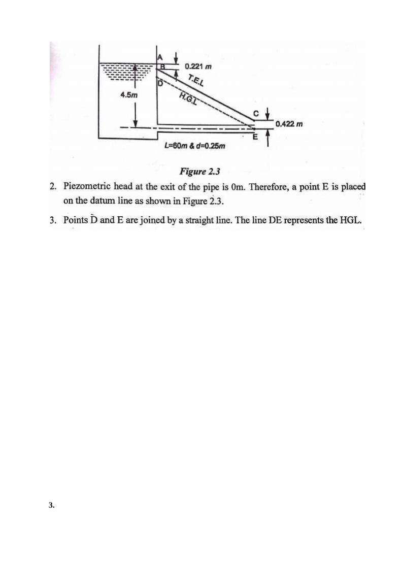
3.
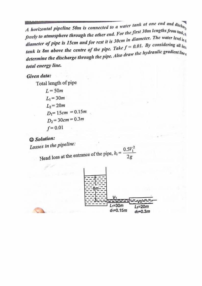
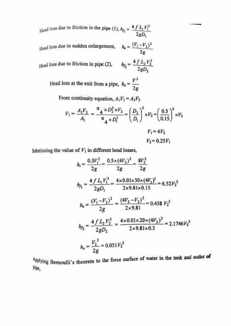
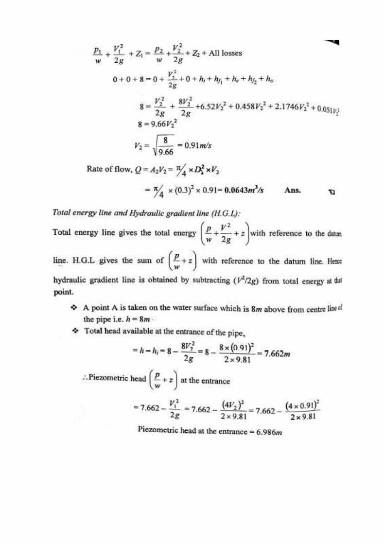


4.
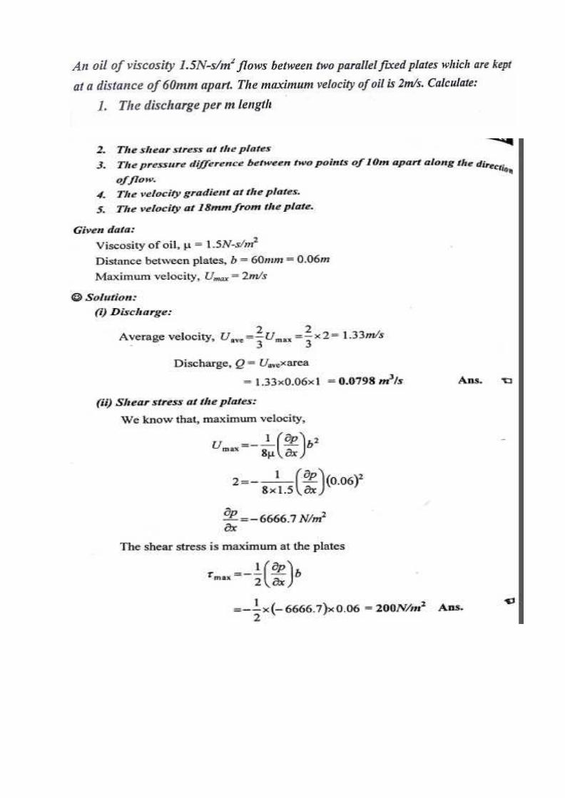

5.

6.


7.
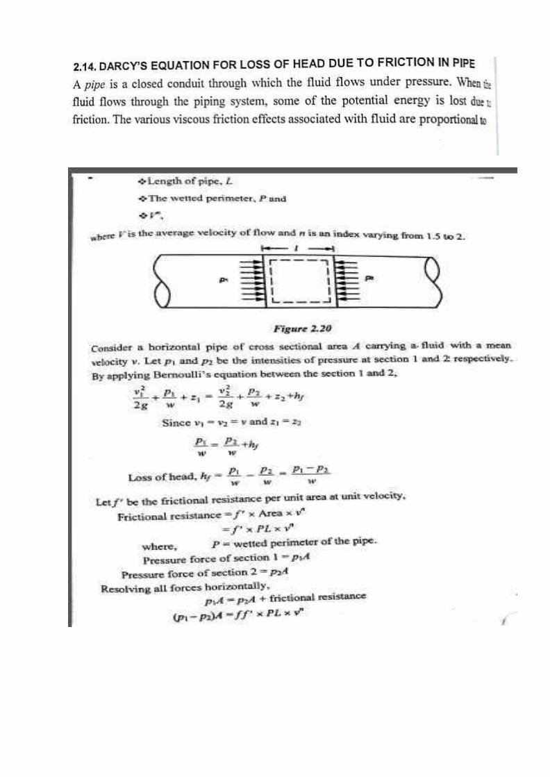


8.

UNIT III DIMENSIONAL ANALYSIS
PART – A
1. What are the methods of dimensional analysis
There are two methods of dimensional analysis. They are,
a. Rayleigh - Retz method
b. Buckingham's theotem method.
Nowadays Buckingham's theorem method is only used.
2. Describe the Rayleigh's method for dimensional analysis.
Rayleigh's method is used for determining the expression for a variable which depends upon
maximum three or four variables only. If the number of independent variables becomes more than
four, then it is very difficult to find the expression for dependent variable.
3. What do you mean by dimensionless number
Dimensionless numbers are those numbers which are obtained by dividing the inertia force
by viscous force or gravity force or pressure force or surface tension or elastic force. As this is a
ratio of one force to other force, it will be a dimensionless number.
4. Name the different forces present in fluid flow
Inertia force
Viscous force
Surface tension force
Gravity force
5. State Buckingham’s Π theorem
It states that if there are ‘n’ variables in a dimensionally homogeneous equation and if
these variables contain ‘m’ fundamental dimensions (M,L,T), then they are grouped into
(n-m), dimensionless independent Π-terms.
6. State the limitations of dimensional analysis.
1. Dimensional analysis does not give any due regarding the selection of variables.
2.The complete information is not provided by dimensional analysis.
3.The values of coefficient and the nature of function can be obtained only by
experiments or from mathematical analysis.
7. Define Similitude
Similitude is defined as the complete similarity between the model and
prototype.
8. State Froude’s model law
Only Gravitational force is more predominant force. The law states ‘The Froude’s
number is same for both model and prototype’
9. What are the similarities between model and prototype?
(i) Geometric Similarity
(ii) Kinematicc Similarity
(iii) Dynamic Similarity
10. Define Weber number.
It is the ratio of the square root of the inertia force to the surface tension force.
PART-B

101 2015 - 16
1.
2.

102 2015 - 16

103 2015 - 16
3.

104 2015 - 16
4.
`

105 2015 - 16
5.

106 2015 - 16

107 2015 - 16

108 2015 - 16
6.
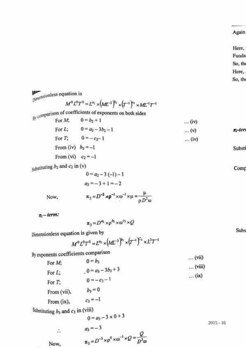
109 V.P.KRISHNAMURTHY – AP/MECH 2015 - 16
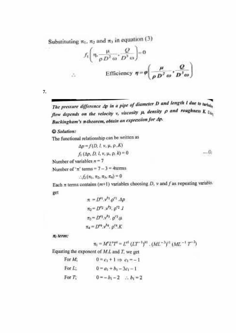
7.

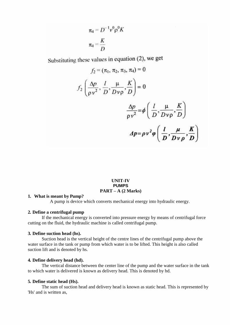
1. What is meant by Pump?
UNIT-IV PUMPS
PART – A (2 Marks)
A pump is device which converts mechanical energy into hydraulic energy.
2. Define a centrifugal pump
If the mechanical energy is converted into pressure energy by means of centrifugal force
cutting on the fluid, the hydraulic machine is called centrifugal pump.
3. Define suction head (hs).
Suction head is the vertical height of the centre lines of the centrifugal pump above the
water surface in the tank or pump from which water is to be lifted. This height is also called
suction lift and is denoted by hs.
4. Define delivery head (hd).
The vertical distance between the center line of the pump and the water surface in the tank
to which water is delivered is known as delivery head. This is denoted by hd.
5. Define static head (Hs).
The sum of suction head and delivery head is known as static head. This is represented by
'Hs' and is written as,

Hs = hs+ hd
6. Mention main components of Centrifugal pump.
i) Impeller ii) Casing
iii) Suction pipe,strainer & Foot valve iv) Delivery pipe & Delivery valve
7. What is meant by Priming?
The delivery valve is closed and the suction pipe, casing and portion of the delivery
pipe upto delivery valve are completely filled with the liquid so that no air pocket is
left. This is called as priming.
8. Define Manometric head.
It is the head against which a centrifugal pump work.
9. Describe multistage pump with
a. impellers in parallel b. impellers in series. In multi stage centrifugal pump,
a. when the impellers are connected in series ( or on the same shaft) high head can be
developed.
b. When the impellers are in parallel (or pumps) large quantity of liquid can be discharged.
10.. Define specific speed of a centrifugal pump (Ns).
The specific speed of a centrifugal pump is defined as the speed of a geometrically circular
pump which would deliver one cubic meter of liquid per second against a head of one meter. It is
denoted by 'Ns'.
11. What do you understand by characteristic curves of the pump?
Characteristic curves of centrifugal pumps are defined those curves which are plotted from
the results of a number of tests on the centrifugal pump.
12. Why are centrifugal pumps used sometimes in series and sometimes in parallel?
The centrifugal pumps used sometimes in series because for high heads and in
parallel for high discharge
13. Define Mechanical efficiency.
I
t is defined as the ratio of the power actually delivered by the impeller to the power
supplied to the shaft.
14. Define overall efficiency.
It is the ratio of power output of the pump to the power input to the pump.
15. Define speed ratio, flow ratio.
Speed ratio: It is the ratio of peripheral speed at outlet to the theoretical velocity of jet
corresponding to manometric head.
Flow ratio: It is the ratio of the velocity of flow at exit to the theoretical
velocity of jet corresponding to manometric head.
16.. Mention main components of Reciprocating pump.
# Piton or Plunger
# Suction and delivery pipe
# Crank and Connecting rod

17.. Define Slip of reciprocating pump. When the negative slip does occur?
The difference between the theoretical discharge and actual discharge is called slip of
the pump.
But in sometimes actual discharge may be higher then theoretical discharge, in such a
case coefficient of discharge is greater then unity and the slip will be negative called
as negative slip.
18. What is indicator diagram?
Indicator diagram is nothing but a graph plotted between the pressure head in the
cylinder and the distance traveled by the piston from inner dead center for one
complete revolution of the crank
19. What is meant by Cavitations?
It is defined phenomenon of formation of vapor bubbles of a flowing liquid in a region
where the pressure of the liquid falls below its vapor pressure and the sudden
collapsing of theses vapor bubbles in a region of high pressure.
20. What are rotary pumps?
Rotary pumps resemble like a centrifugal pumps in appearance. But the working
method differs. Uniform discharge and positive displacement can be obtained by using
these rotary pumps, It has the combined advantages of both centrifugal and
reciprocating pumps.
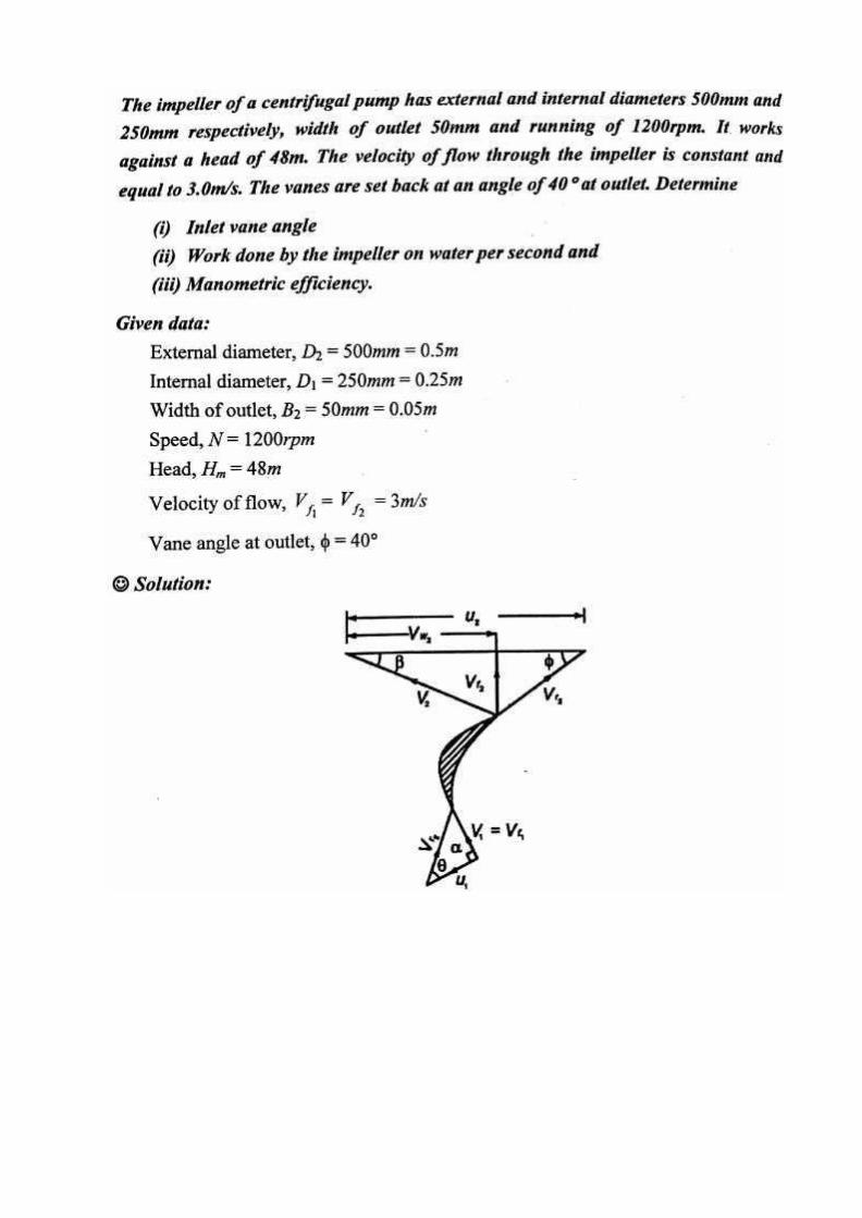
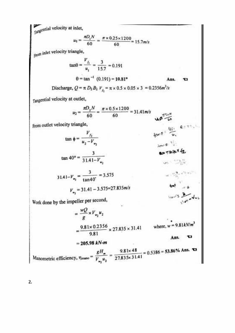
2.


3.
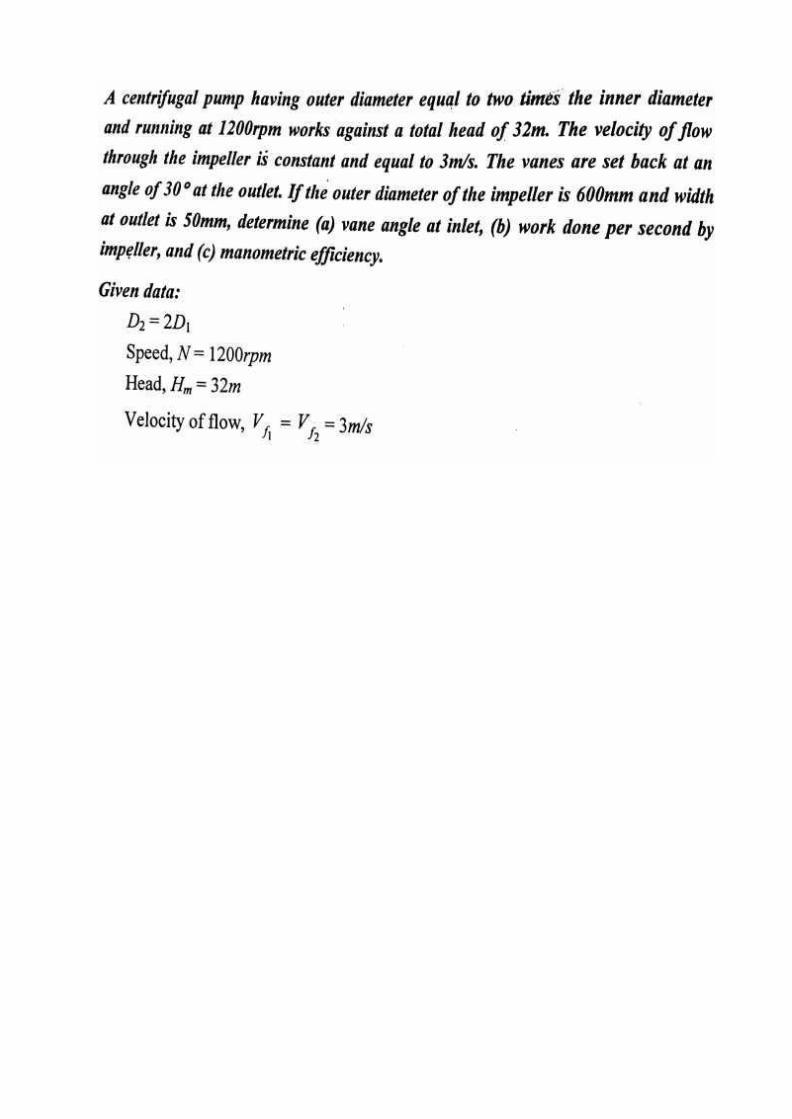


4.


5.
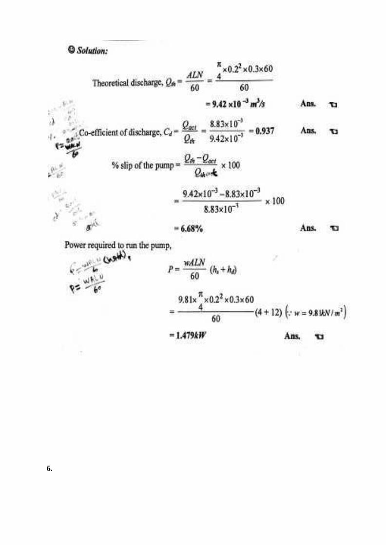
6.

7.
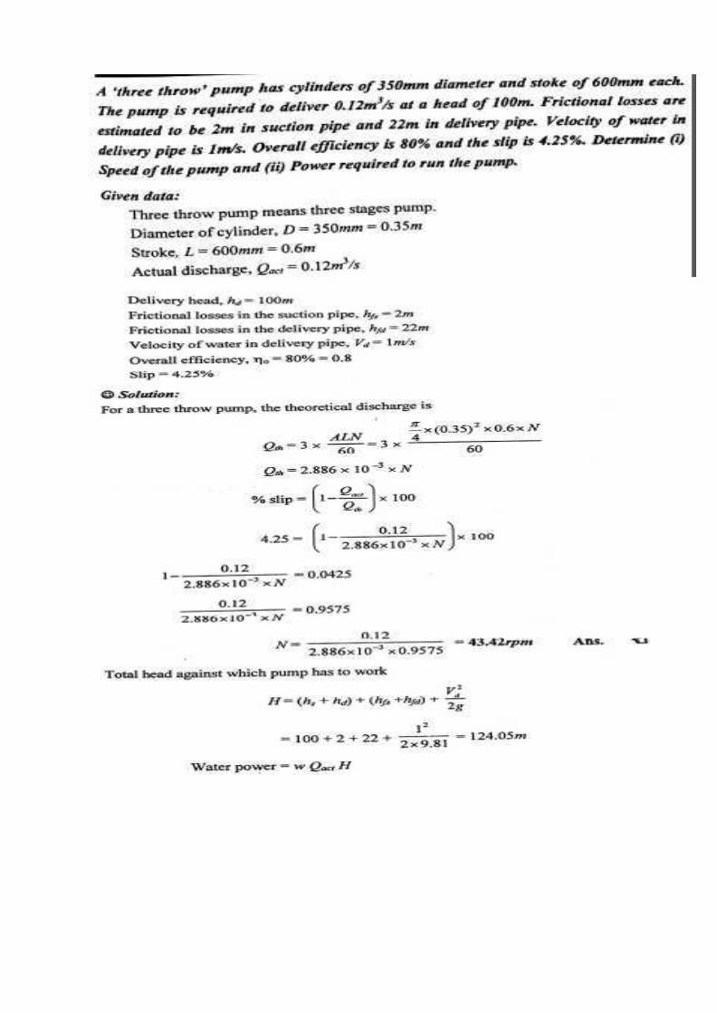

8.


UNIT-V TURBINES
PART – A
1. Define hydraulic machines.
Hydraulic machines which convert the energy of flowing water into mechanical energy.
2. Give example for a low head, medium head and high head turbine.
Low head turbine – Kaplan turbine
Medium head turbine – Modern Francis turbine
High head turbine – Pelton wheel
3. What is impulse turbine? Give example.
In impulse turbine all the energy converted into kinetic energy. From these the turbine
will develop high kinetic energy power. This turbine is called impulse turbine. Example:
Pelton turbine
4. What is reaction turbine? Give example.
In a reaction turbine, the runner utilizes both potential and kinetic energies. Here
portion of potential energy is converted into kinetic energy before entering into the turbine.
Example: Francis and Kaplan turbine.
5. What is axial flow turbine?
In axial flow turbine water flows parallel to the axis of the turbine shaft. Example:
Kaplan turbine
6. What is mixed flow turbine?
In mixed flow water enters the blades radially and comes out axially, parallel to the turbine
shaft. Example: Modern Francis turbine.
7. What is the function of spear and nozzle?
The nozzle is used to convert whole hydraulic energy into kinetic energy. Thus the nozzle
delivers high speed jet. To regulate the water flow through the nozzle and to obtain a good jet
of water spear or nozzle is arranged.
8. Define gross head and net or effective head.
Gross Head: The gross head is the difference between the water level at the reservoir
and the level at the tailstock.
Effective Head: The head available at the inlet of the turbine.

9. Define hydraulic efficiency.
It is defined as the ratio of power developed by the runner to the power supplied by the water
jet.
10. Define mechanical efficiency.
It is defined as the ratio of power available at the turbine shaft to the power developed
by the turbine runner.
11. Define volumetric efficiency.
It is defied as the volume of water actually striking the buckets to the total water supplied
by the jet.
12. Define over all efficiency.
It is defined as the ratio of power available at the turbine shaft to the power available
from the water jet.
13. Define the terms
(a) Hydraulic machines (b) Turbines (c) Pumps.
a. Hydraulic machines:
Hydraulic machines are defined as those machines which convert either hydraulic energy
into mechanical energy or mechanical energy into hydraulic energy.
b. Turbines;
The hydraulic machines which convert hydraulic energy into mechanical energy are called
turbines.
c. Pumps:
The hydraulic Machines which convert mechanical energy into hydraulic energy are called
pumps.
14. What do you mean by gross head?
The difference between the head race level and tail race level when no water is flowing is
known as gross head. It is denoted by Hg.
15. What do you mean by net head?
Net head is also known as effective head and is defined as the head available at the inlet of
te turbine. It is denoted as H
16. What is draft tube? why it is used in reaction turbine?
The pressure at exit of runner of a reaction turbine is generally less than the atmospheric
pressure. The water at exit cannot be directly discharged to tail race. A tube or pipe of gradually
increasing area is used for discharging water from exit of turbine to tail race. This tube of
increasing area is called draft tube.
17. What is the significance of specific speed?
Specific speed plays an important role for selecting the type of turbine. Also the
performance of turbine can be predicted by knowing the specific speed of turbine.
18.. What are unit quantities?
Unit quantities are the quantities which are obtained when the head on the turbine is unity.
They are unit speed, unit power unit discharge.
19. Why unit quantities are important
If a turbine is working under different heads, the behavior of turbine can be easily known
from the values of unit quantities.
20. What do you understand by characteristic curves of turbine?
Characteristic curves of a hydraulic turbine are the curves, with the help of which the exact
behavior and performance of turbine under different working conditions can be known.
21. Define the term 'governing of turbine'.
Governing of turbine is defined as the operation by which the speed of the turbine is kept
constant under all conditions of working. It is done by oil pressure governor.
22. What are the types of draft tubes?
The following are the important types of draft tubes which are commonly used.
a. Conical draft tubes
b. Simple elbow tubes
c. Moody spreading tubes and
d. Elbow draft tubes with circular inlet and rectangular outlet.
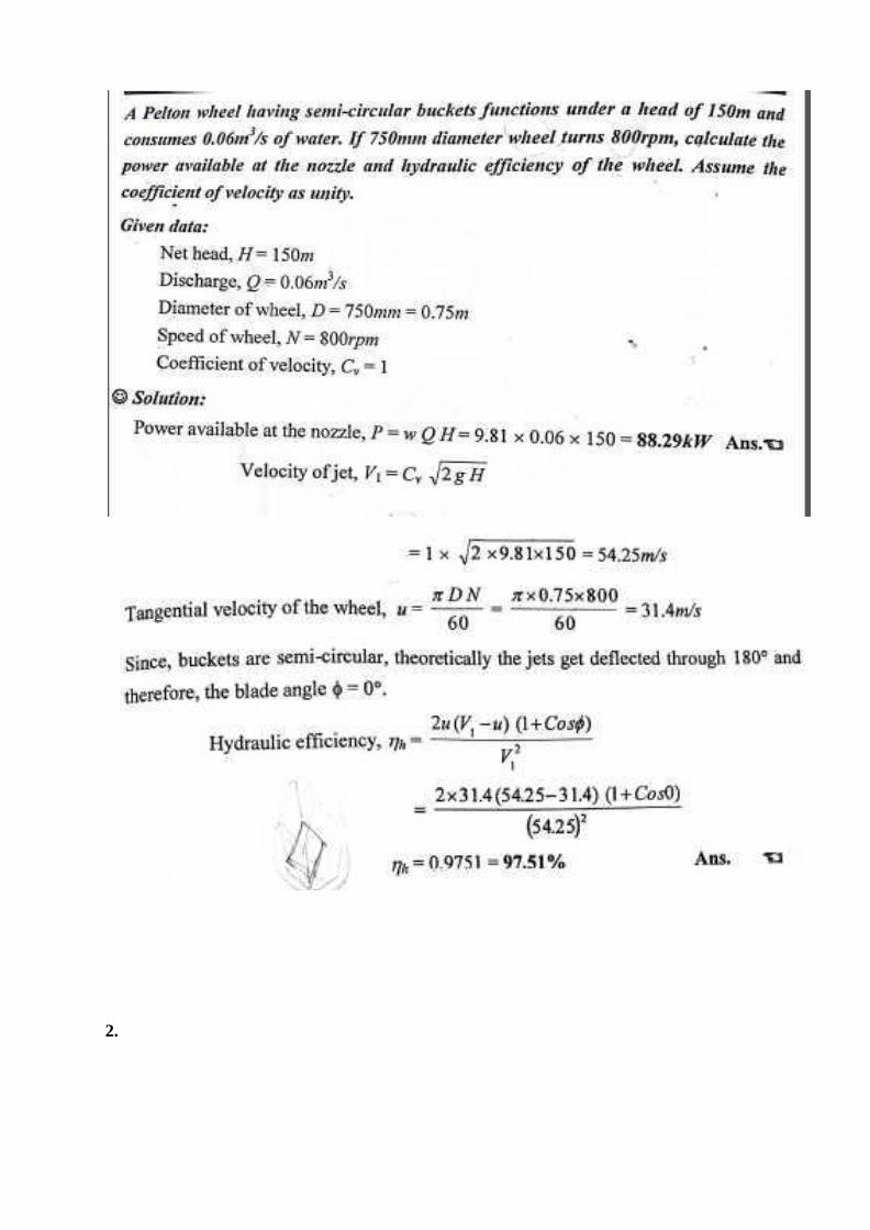
2.

3.

4.


5.
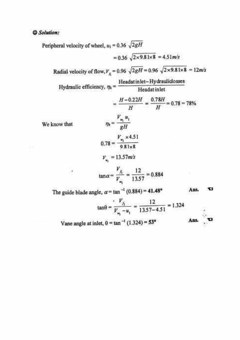
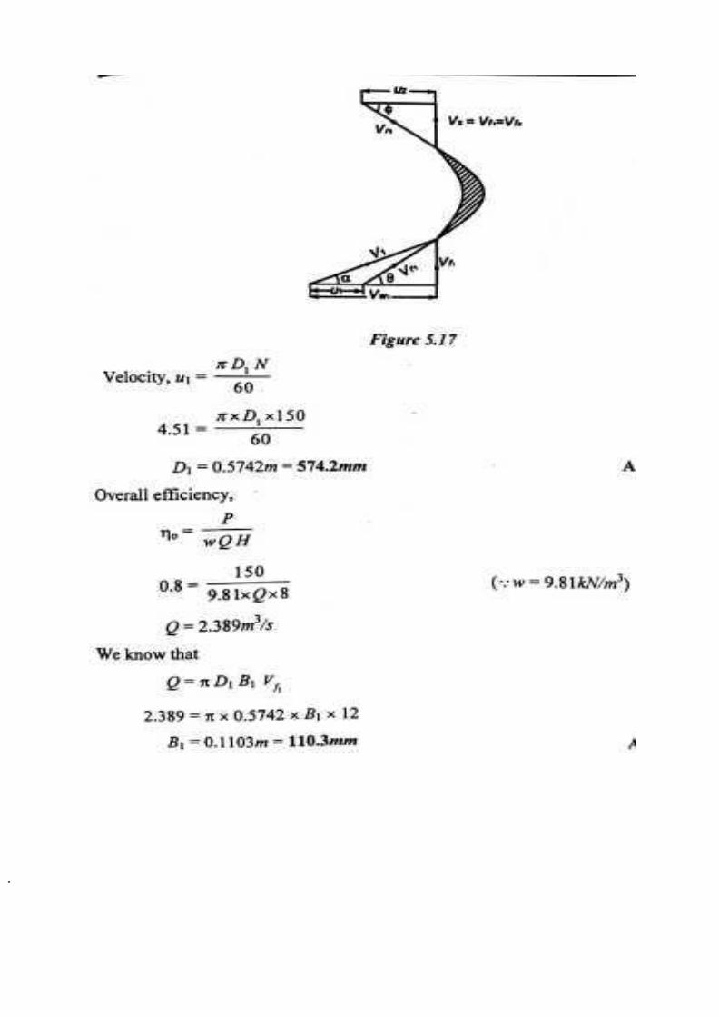
.


7.