Broken Bracelets, Molien Series, Paraffin Wax, and an Elliptic Curve of Conductor 48

BROKEN BRACELETS, MOLIEN SERIES, PARAFFIN WAXAND AN ELLIPTIC CURVE OF CONDUCTOR 48

TEWODROS AMDEBERHAN, MAHIR BILEN CAN, AND VICTOR H. MOLL

Abstract. This paper introduces the concept of necklace binomial co-efficients motivated by the enumeration of a special type of sequences.Several properties of these coefficients are described, including a con-nection between their roots and an elliptic curve. Further links are givento a physical model from quantum mechanical supersymmetry as well asproperties of alkane molecules in chemistry.

1. Introduction

A jeweler is asked to design a necklace consisting of a chain with n place-ments for k pieces of diamond. The client ask for one group of r diamondsto be placed next to each other and the remaining diamonds are to be iso-lated, that is, each one is mounted so that the two adjacent places are leftempty. These special diamonds are called the medallion of the necklace.Figure 1 shows a necklace of length 20, with a medallion of length 5 andfour extra diamonds.

Figure 1. A necklace with a medallion.

Throughout this paper, a necklace is understood to be cyclically symmet-ric (unlabelled) formed by diamonds of two colors (i.e., binary).

Date: June 24, 2011.2000 Mathematics Subject Classification. Primary 05A15, 05E10, Secondary 06A07,

06F05, 20M32.Key words and phrases. necklaces, elliptic curves, Molien series, zeros of polynomials.

1

arX

iv:1

106.

4693

v1 [

mat

h.C

O]

23

Jun

2011

2 T. AMDEBERHAN, MAHIR BILEN CAN, AND VICTOR H. MOLL

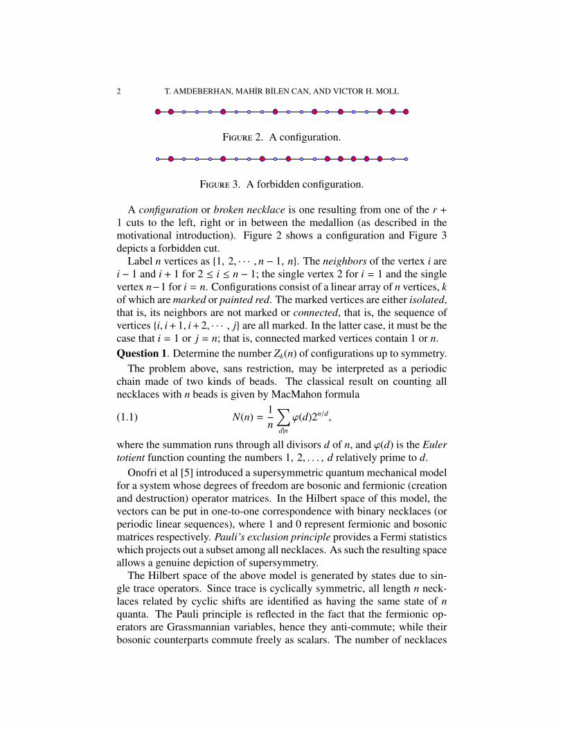
Figure 2. A configuration.

Figure 3. A forbidden configuration.

A configuration or broken necklace is one resulting from one of the r +

1 cuts to the left, right or in between the medallion (as described in themotivational introduction). Figure 2 shows a configuration and Figure 3depicts a forbidden cut.

Label n vertices as {1, 2, · · · , n − 1, n}. The neighbors of the vertex i arei − 1 and i + 1 for 2 ≤ i ≤ n − 1; the single vertex 2 for i = 1 and the singlevertex n−1 for i = n. Configurations consist of a linear array of n vertices, kof which are marked or painted red. The marked vertices are either isolated,that is, its neighbors are not marked or connected, that is, the sequence ofvertices {i, i + 1, i + 2, · · · , j} are all marked. In the latter case, it must be thecase that i = 1 or j = n; that is, connected marked vertices contain 1 or n.Question 1. Determine the number Zk(n) of configurations up to symmetry.

The problem above, sans restriction, may be interpreted as a periodicchain made of two kinds of beads. The classical result on counting allnecklaces with n beads is given by MacMahon formula

(1.1) N(n) =1n

∑d|n

ϕ(d)2n/d,

where the summation runs through all divisors d of n, and ϕ(d) is the Eulertotient function counting the numbers 1, 2, . . . , d relatively prime to d.

Onofri et al [5] introduced a supersymmetric quantum mechanical modelfor a system whose degrees of freedom are bosonic and fermionic (creationand destruction) operator matrices. In the Hilbert space of this model, thevectors can be put in one-to-one correspondence with binary necklaces (orperiodic linear sequences), where 1 and 0 represent fermionic and bosonicmatrices respectively. Pauli’s exclusion principle provides a Fermi statisticswhich projects out a subset among all necklaces. As such the resulting spaceallows a genuine depiction of supersymmetry.

The Hilbert space of the above model is generated by states due to sin-gle trace operators. Since trace is cyclically symmetric, all length n neck-laces related by cyclic shifts are identified as having the same state of nquanta. The Pauli principle is reflected in the fact that the fermionic op-erators are Grassmannian variables, hence they anti-commute; while theirbosonic counterparts commute freely as scalars. The number of necklaces

BROKEN BRACELETS 3

is enumerated by MacMahon’s formula (1.1). Some of these are excludedas a result of anti-symmetry of planar states, dictated by supersymmetry.The following serves as an illustrative example with n = 4. There is a totalof 6 necklaces listed here as linear sequences of period 4, namely

0000, 0001, 0011, 0101, 0111, 1111.

Supersymmetry breaks up this family into forbidden and allowed necklacesas follows. Given a sequence, start shifting a digit from right to left (prefixto suffix) and repeat until the original sequence is recovered. Every timea fermionic operator (that is, a 1) crosses another then a sign change mustbe registered because of anti-commuting; each bosonic operator (i.e., a 0)shifts around without any effect. At the end of the procedure, if the sequencebecomes its own negative then call it forbidden, otherwise it is allowed. Oneof the main results of [5] predicts

(1.2) Nallowed(n) =1n

∑d|n

d odd

ϕ(d)2n/d, and N f orbidden(n) =1n

∑d|n

d even

ϕ(d)2n/d.

Let us take a look at each of the above sequences now: 0000 stays thesame; 0001 → 1000 → 0001; 0011 → −1001 → +1100 → 0011; 0101 →−1010 → −0101; 0111 → +1011 → +1101 → +1110 → 0111; 1111 →−1111. Therefore there are four allowed {0000, 0001, 0011, 0111} and twoforbidden {0101, 1111} sets of necklaces. This agrees with

Nallowed =14

[ϕ(1)24] = 4, and Nforbidden =14

[ϕ(2)22 + ϕ(4)21] = 2.

The interested reader should find the complete story in [5].

The central object of the work presented here is a sequence of numberslabeled necklace binomial coefficients

(tk

)N

. These coefficients have proper-ties similar to the usual binomial coefficients: recurrences (Corollary 2.7),symmetries (Corollary 2.12) and an explicit formula in terms of the bino-mial coefficients (Theorem 2.8). Section 3 discusses a surprising result onthe zeros of the necklace polynomial Nt(y) (this is the generating functionof

(tk

)N

). It turns out that all its zeros are inside an elliptic curve. Moreover,this curve is the same for all values of t. Section 4 presents arithmetical andgeometrical properties of these polynomials via generating function meth-ods. The necklace binomial coefficients also appear in a physical model ofOnofri et al [5] and in the study of symmetries of paraffin molecules in [4].

2. The number of configurations

In this section the counting problem from the Introduction is rephrasedand solved. The current format as well as the original formulation will be


used interchangeably:

determine the number Zk(n) of painting k points in red from a linear arrayof n of them, with the condition that consecutive red points can only appearat the beginning or at end of the array. Moreover, arrays that are reflectionsof each other should be counted only once.

In order to determine the number of configurations Zk(n) it is convenientto begin with a simpler count.

Proposition 2.1. Let fk(n) be the number of arrangements of n verticeswith k marked vertices, no consecutive marked ones where reflections arenot identified. Then

(2.1) fk(n) =

(n − k + 1

k

).

Proof. Each such arrangement can be obtained by placing the k markedvertices and choosing k − 1 places to separate them. The count is obtainedby eliminating the separating spaces. �

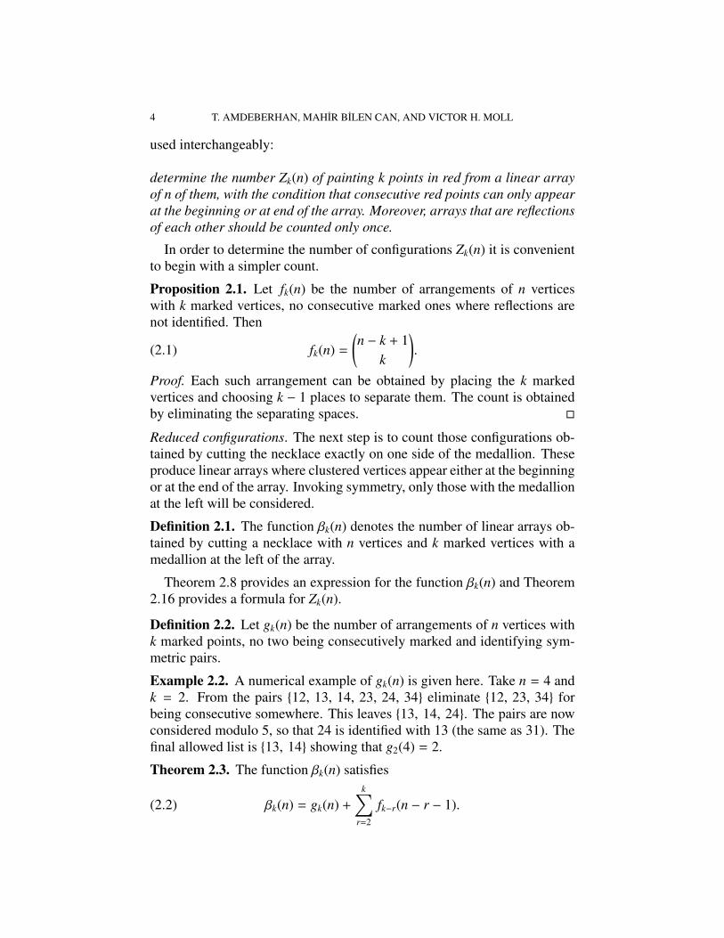
Reduced configurations. The next step is to count those configurations ob-tained by cutting the necklace exactly on one side of the medallion. Theseproduce linear arrays where clustered vertices appear either at the beginningor at the end of the array. Invoking symmetry, only those with the medallionat the left will be considered.

Definition 2.1. The function βk(n) denotes the number of linear arrays ob-tained by cutting a necklace with n vertices and k marked vertices with amedallion at the left of the array.

Theorem 2.8 provides an expression for the function βk(n) and Theorem2.16 provides a formula for Zk(n).

Definition 2.2. Let gk(n) be the number of arrangements of n vertices withk marked points, no two being consecutively marked and identifying sym-metric pairs.

Example 2.2. A numerical example of gk(n) is given here. Take n = 4 andk = 2. From the pairs {12, 13, 14, 23, 24, 34} eliminate {12, 23, 34} forbeing consecutive somewhere. This leaves {13, 14, 24}. The pairs are nowconsidered modulo 5, so that 24 is identified with 13 (the same as 31). Thefinal allowed list is {13, 14} showing that g2(4) = 2.

Theorem 2.3. The function βk(n) satisfies

(2.2) βk(n) = gk(n) +

k∑r=2

fk−r(n − r − 1).

BROKEN BRACELETS 5

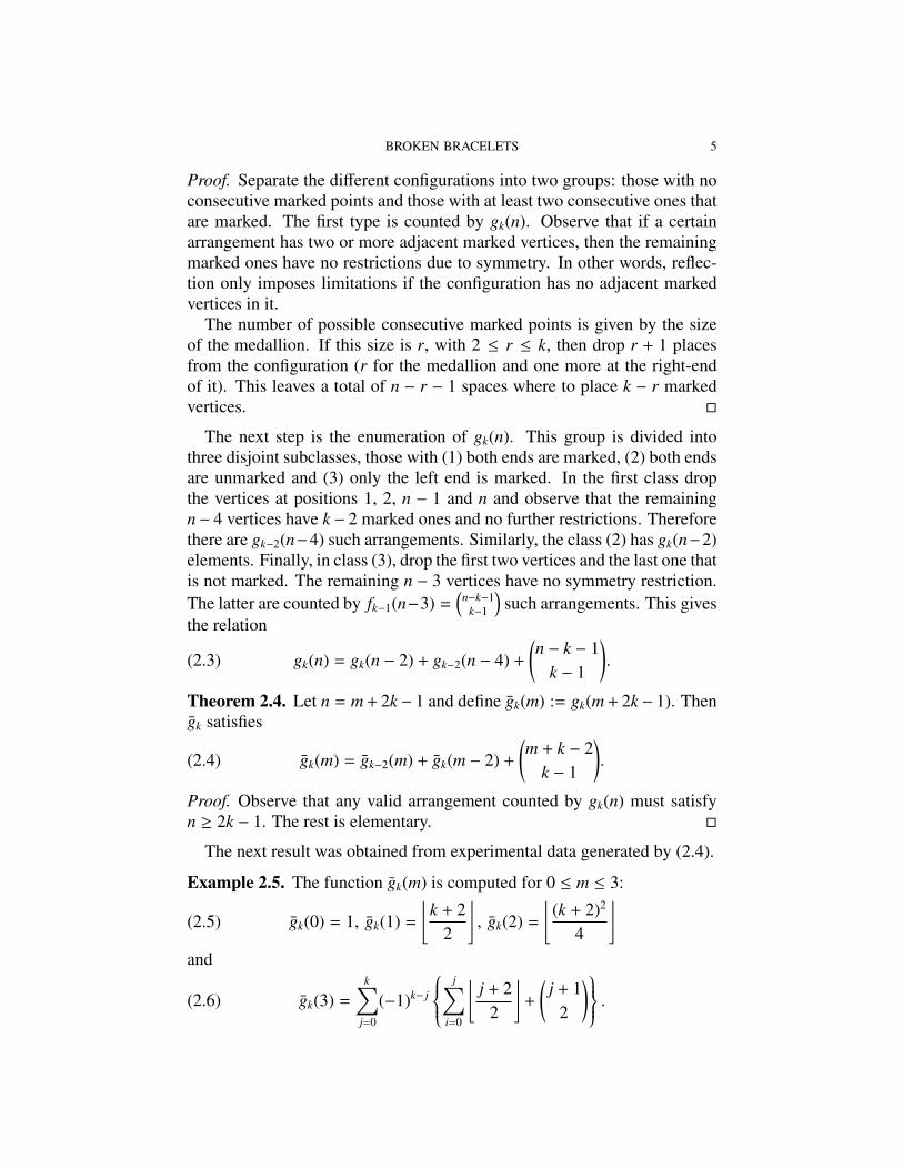
Proof. Separate the different configurations into two groups: those with noconsecutive marked points and those with at least two consecutive ones thatare marked. The first type is counted by gk(n). Observe that if a certainarrangement has two or more adjacent marked vertices, then the remainingmarked ones have no restrictions due to symmetry. In other words, reflec-tion only imposes limitations if the configuration has no adjacent markedvertices in it.

The number of possible consecutive marked points is given by the sizeof the medallion. If this size is r, with 2 ≤ r ≤ k, then drop r + 1 placesfrom the configuration (r for the medallion and one more at the right-endof it). This leaves a total of n − r − 1 spaces where to place k − r markedvertices. �

The next step is the enumeration of gk(n). This group is divided intothree disjoint subclasses, those with (1) both ends are marked, (2) both endsare unmarked and (3) only the left end is marked. In the first class dropthe vertices at positions 1, 2, n − 1 and n and observe that the remainingn− 4 vertices have k − 2 marked ones and no further restrictions. Thereforethere are gk−2(n−4) such arrangements. Similarly, the class (2) has gk(n−2)elements. Finally, in class (3), drop the first two vertices and the last one thatis not marked. The remaining n − 3 vertices have no symmetry restriction.The latter are counted by fk−1(n−3) =

(n−k−1

k−1

)such arrangements. This gives

the relation

(2.3) gk(n) = gk(n − 2) + gk−2(n − 4) +

(n − k − 1

k − 1

).

Theorem 2.4. Let n = m + 2k − 1 and define gk(m) := gk(m + 2k − 1). Thengk satisfies

(2.4) gk(m) = gk−2(m) + gk(m − 2) +

(m + k − 2

k − 1

).

Proof. Observe that any valid arrangement counted by gk(n) must satisfyn ≥ 2k − 1. The rest is elementary. �

The next result was obtained from experimental data generated by (2.4).

Example 2.5. The function gk(m) is computed for 0 ≤ m ≤ 3:

(2.5) gk(0) = 1, gk(1) =

⌊k + 2

2

⌋, gk(2) =

⌊(k + 2)2

4

⌋and

(2.6) gk(3) =

k∑j=0

(−1)k− j

j∑i=0

⌊j + 2

2

⌋+

(j + 1

2

) .


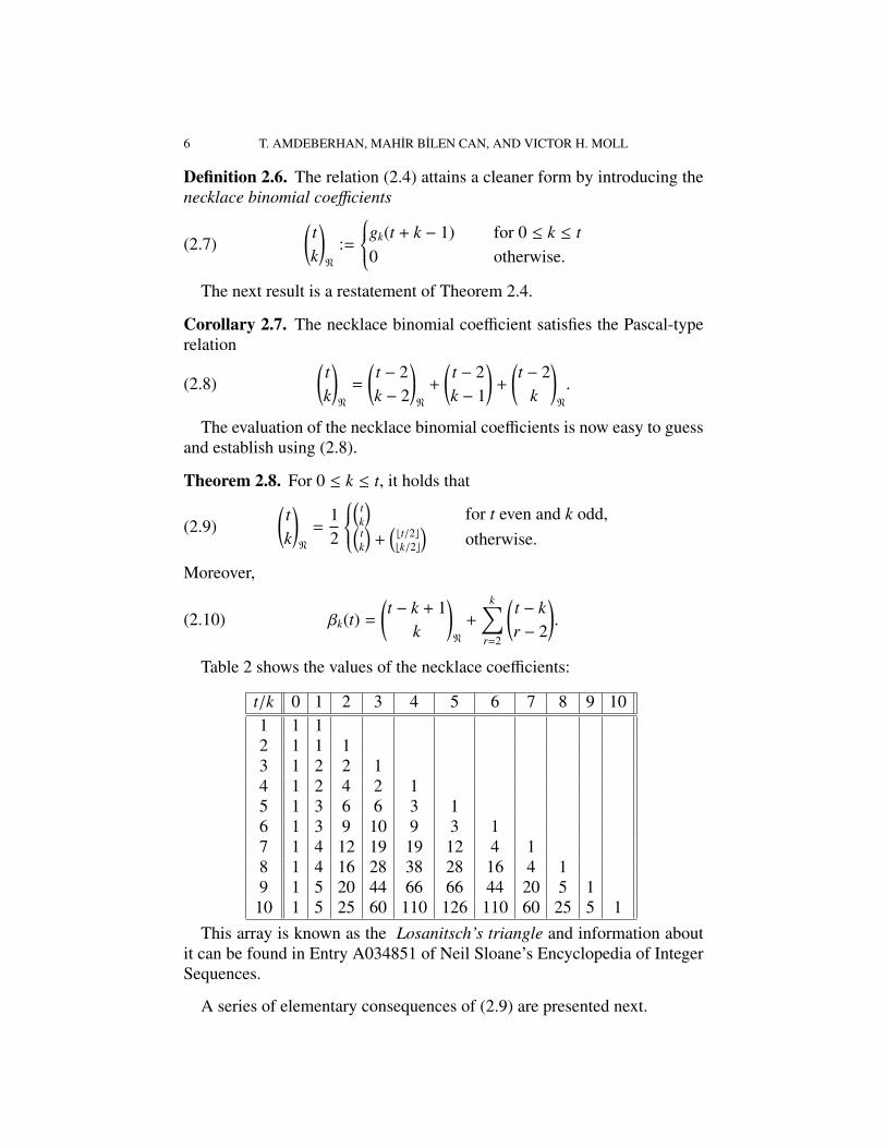
Definition 2.6. The relation (2.4) attains a cleaner form by introducing thenecklace binomial coefficients

(2.7)(tk

)N

:=

gk(t + k − 1) for 0 ≤ k ≤ t0 otherwise.

The next result is a restatement of Theorem 2.4.

Corollary 2.7. The necklace binomial coefficient satisfies the Pascal-typerelation

(2.8)(tk

)N

=

(t − 2k − 2

)N

+

(t − 2k − 1

)+

(t − 2

k

)N

.

The evaluation of the necklace binomial coefficients is now easy to guessand establish using (2.8).

Theorem 2.8. For 0 ≤ k ≤ t, it holds that

(2.9)(tk

)N

=12

(

tk

)for t even and k odd,(

tk

)+

(bt/2cbk/2c

)otherwise.

Moreover,

(2.10) βk(t) =

(t − k + 1

k

)N

+

k∑r=2

(t − kr − 2

).

Table 2 shows the values of the necklace coefficients:

t/k 0 1 2 3 4 5 6 7 8 9 101 1 12 1 1 13 1 2 2 14 1 2 4 2 15 1 3 6 6 3 16 1 3 9 10 9 3 17 1 4 12 19 19 12 4 18 1 4 16 28 38 28 16 4 19 1 5 20 44 66 66 44 20 5 110 1 5 25 60 110 126 110 60 25 5 1

This array is known as the Losanitsch’s triangle and information aboutit can be found in Entry A034851 of Neil Sloane’s Encyclopedia of IntegerSequences.

A series of elementary consequences of (2.9) are presented next.

BROKEN BRACELETS 7

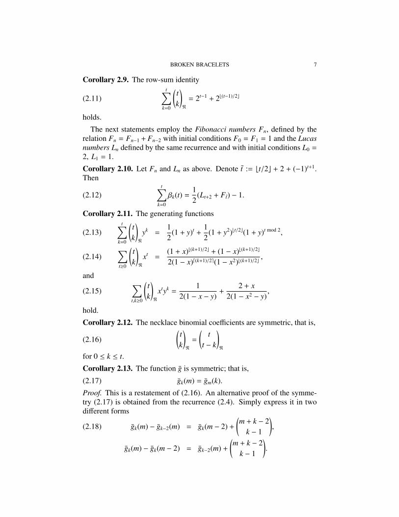
Corollary 2.9. The row-sum identity

(2.11)t∑

k=0

(tk

)N

= 2t−1 + 2b(t−1)/2c

holds.

The next statements employ the Fibonacci numbers Fn, defined by therelation Fn = Fn−1 + Fn−2 with initial conditions F0 = F1 = 1 and the Lucasnumbers Ln defined by the same recurrence and with initial conditions L0 =

2, L1 = 1.

Corollary 2.10. Let Fn and Ln as above. Denote t := bt/2c + 2 + (−1)t+1.Then

(2.12)t∑

k=0

βk(t) =12

(Lt+2 + Ft) − 1.

Corollary 2.11. The generating functionst∑

k=0

(tk

)N

yk =12

(1 + y)t +12

(1 + y2)bt/2c(1 + y)t mod 2,(2.13)

∑t≥0

(tk

)N

xt =(1 + x)b(k+1)/2c + (1 − x)b(k+1)/2c

2(1 − x)d(k+1)/2e(1 − x2)b(k+1)/2c ,(2.14)

and

(2.15)∑t,k≥0

(tk

)N

xtyk =1

2(1 − x − y)+

2 + x2(1 − x2 − y)

,

hold.

Corollary 2.12. The necklace binomial coefficients are symmetric, that is,

(2.16)(tk

)N

=

(t

t − k

)N

for 0 ≤ k ≤ t.

Corollary 2.13. The function g is symmetric; that is,

(2.17) gk(m) = gm(k).

Proof. This is a restatement of (2.16). An alternative proof of the symme-try (2.17) is obtained from the recurrence (2.4). Simply express it in twodifferent forms

gk(m) − gk−2(m) = gk(m − 2) +

(m + k − 2

k − 1

),(2.18)

gk(m) − gk(m − 2) = gk−2(m) +

(m + k − 2

k − 1

).


The result now follows by induction and the symmetry of the binomial co-efficients. �

The next theorem provides a combinatorial proof of the symmetry rule(2.17).

Theorem 2.14. The symmetry gk(m) = gm(k) holds.

Proof. The assertion amounts to gk(m + 2k − 1) = gm(k + 2m − 1). Take alinear array of n nodes and its 2-coloring (red r or white w). By definition,gk(n) enumerates all possible ways of coloring k nodes in red with the rule:(1) no two reds are consecutive; (2) two such arrays are equivalent if theyrelate by reflection. According to (1), it must be that the first k − 1 reds areeach followed by white. Thus, any selection of k reds can be interpreted aschoosing the (k−1) pairs rw and a free r. For each pair rw, trim-off the w aswell as its sitting node. That means, when n = m + 2k − 1 then the numberof nodes reduces to m + k and hence gk(m + 2k − 1) induces an equivalentcounting of (m + k)-nodes of which k are red (note: rule (1) is absent butrule (2) stays). Similarly, gm(k + 2m − 1) tantamount to the counting of(m + k)-nodes of which m are white. But, it is obvious that coloring k nodesred on an (m + k)-array is equivalent to the coloring of m nodes in white.This gives the required bijection. The proof is complete. �

Example 2.15. This example demonstrates the above proof; i.e. gk(m+2k−1) = gm(k + 2m − 1). Take m = 2 and k = 3. Then, g3(7) and g2(6) countrespectively the cardinality of sets

A := {rwrwrww, rwrwwrw, rwrwwwr, rwwrwrw, rwwrwwr,wrwrwrw}

and

B : {rwrwww, rwwrww,wrwrww, rwwwrw,wrwwrw, rwwwwr}.

The set B after color-swapping turns to

B1 := {wrwrrr,wrrwrr, rwrwrr,wrrrwr, rwrrwr,wrrrrw}.

The two sets A and B1 are now mapped (w-trimmed and r-trimmed, respec-tively) to

A1 := {rrrww, rrwrw, rrwwr, rwrrw, rwrwr,wrrrw},

andB11 := {wwrrr,wrwrr, rrwrr,wrrwr, rwrwr,wrrrw}.

The bijection between A1 and B11 is clearly exposed; that is, reflect B11

to get the set

B111 := {rrrww, rrwrw, rrwrr, rwrrw, rwrwr,wrrrw}.

The full counting solution to the configuration problem is presented next.

BROKEN BRACELETS 9

Theorem 2.16. The total number Zk(t) of possible linear configurations ofk diamonds (with or without a medallion) on t nodes is given by

Zk(t) =∑j≥0

(t − k − 1k − 2 j

)N

+∑j≥0

⌊j + 1

2

⌋ (t − k − 1

k − j

).

Proof. Catalog the diamonds according to whether they are: (1) an equalnumber of clusters; (2) unequal number of clustered diamonds on the twoend-nodes. However many are remaining to be mounted in the interior, case(1) is affected by the reflection but those in case (2) are not. It follows thatthe first case is enumerated by the function gk(t) (equivalently, by necklacebinomials) while the function fk(t) is the right choice for the second cate-gory. The details are omitted. �

The necklace coefficients are given as Entry A005994 in Neil Sloane’sEncyclopedia of Integer Sequences. The reader will find there informationon the connection between

(tk

)N

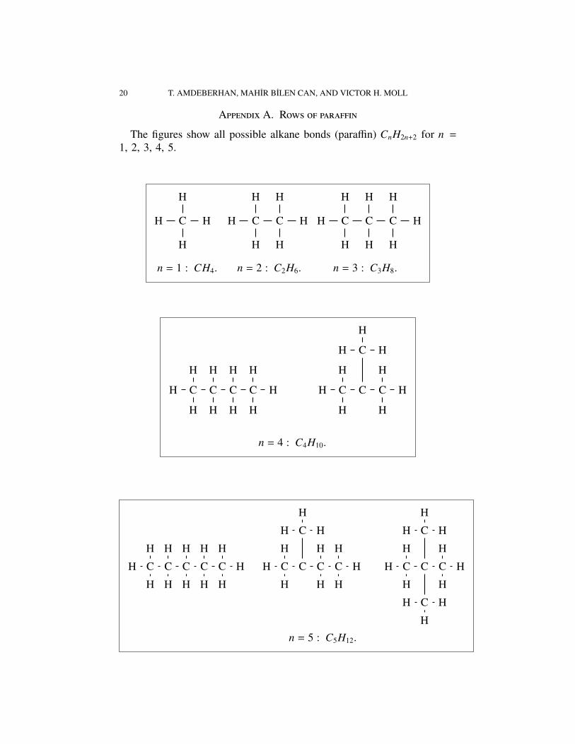
and the so-called paraffin numbers. Thechemist S. M. Losanitsch studied in [4] the so-called alkane numbers (calledhere the necklace numbers) in his investigation of symmetries manifestedby rows of paraffin (hydrocarbons). In the molecule of an alkane (alsoknown as a paraffin), for n carbon atoms there are 2n + 2 hydrogen atoms(i.e. the form CnH2n+2). Each carbon atom C is linked to four other atoms(either C of H); each hydrogen atom is joined to one carbon atom. Thefigures in the Appendix show all possible alkane bonds for 1 ≤ n ≤ 5.There are 1, 1, 1, 2, 3 possible alignments, respectively.

A geometric interpretation. Given a finite group G, it is a classical prob-lem to find the generators of the ring of polynomial invariants under the ac-tion of G. The Molien series M(z; G) is the generating function that countsthe number of linearly independent homogeneous polynomials of a giventotal degree d that are invariants for G. It is given by

(2.19) M(z; G) =1|G|

∑g∈G

1det(I − zg)

=

∞∑i=0

bizi.

Thus, the coefficients bi record the number of linearly independent polyno-mials of total degree i.

Now assume k = 2m − 1. Then (2.14) becomes

(2.20)∑i≥0

(i + 2m − 1

2m − 1

)N

zi =12

1(1 − z)2m +

12

1(1 − z2)m .


This is recognized as

(2.21)12

1(1 − z)2m +

12

1(1 − z2)m =

1|G|

∑g∈G

1det(12m − zg)

,

where G is the symmetric group S 2 and the summation runs through the 2m-dimensional group representation of the elements g in GL2m(C). The argu-ment below shows that the series is indeed a Molien series for the ring of in-variants under the action of S 2. More specifically, the ring of invariants un-der consideration is C[X; Y]∼2 where X = (x1, . . . , xm) and Y = (y1, . . . , ym).The action is given by xl 7→ yl for l = 1, . . . , n.

Let σ be the matrix σ =

(0 11 0

)and let π be the tensor product π = σ⊗1m

resulting in a 2m × 2m matrix which has four blocks of size m ×m with theoff-diagonal blocks being the identity matrix and the diagonals blocks beingzero. The matrix group generated by π in GL2m is S 2. Consequently,

(2.22) det(12m − zπ2) = det(12m − z12m) = (1 − z)2m

and det(12m − zπ) = det(ρ ⊗ 12m), with ρ =

(1 −z−z 1

). Since det(A ⊗ B) =

det(A)m det(B)m, it must be that det(12m − zπ) = (1 − z2)m.

These observations are summarized in the next statement.

Theorem 2.17. Consider the action of Z2 onC[x1, · · · , xm, y1, · · · , ym] givenby xl 7→ yl. Then, the number of linearly independent invariant polynomialsof total degree i is given by the necklace binomial coefficient

(i+2m−12m−1

)N

.

3. The necklace polynomials

In this section we discuss properties of the necklace polynomials definedby

(3.1) Nt(y) =

t∑k=0

(tk

)N

yk.

The explicit formula

(3.2) Nt(y) =12

(1 + y)t +12

(1 + y2)bt/2c(1 + y)t mod 2

is given in (2.13).

BROKEN BRACELETS 11

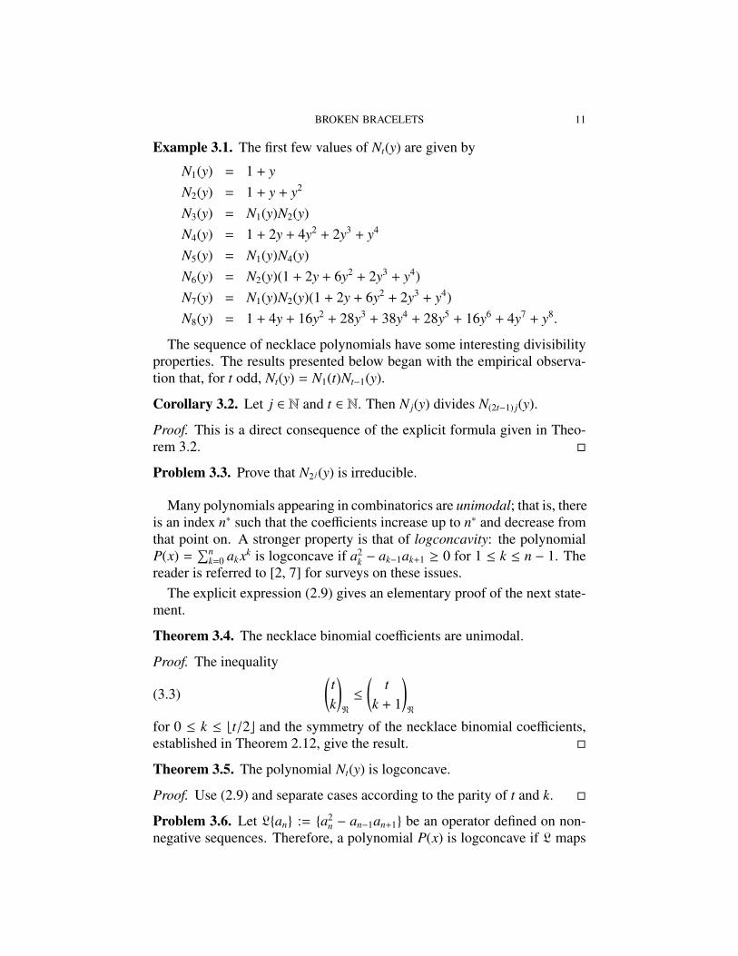
Example 3.1. The first few values of Nt(y) are given by

N1(y) = 1 + yN2(y) = 1 + y + y2

N3(y) = N1(y)N2(y)N4(y) = 1 + 2y + 4y2 + 2y3 + y4

N5(y) = N1(y)N4(y)N6(y) = N2(y)(1 + 2y + 6y2 + 2y3 + y4)N7(y) = N1(y)N2(y)(1 + 2y + 6y2 + 2y3 + y4)N8(y) = 1 + 4y + 16y2 + 28y3 + 38y4 + 28y5 + 16y6 + 4y7 + y8.

The sequence of necklace polynomials have some interesting divisibilityproperties. The results presented below began with the empirical observa-tion that, for t odd, Nt(y) = N1(t)Nt−1(y).

Corollary 3.2. Let j ∈ N and t ∈ N. Then N j(y) divides N(2t−1) j(y).

Proof. This is a direct consequence of the explicit formula given in Theo-rem 3.2. �

Problem 3.3. Prove that N2 j(y) is irreducible.

Many polynomials appearing in combinatorics are unimodal; that is, thereis an index n∗ such that the coefficients increase up to n∗ and decrease fromthat point on. A stronger property is that of logconcavity: the polynomialP(x) =

∑nk=0 akxk is logconcave if a2

k − ak−1ak+1 ≥ 0 for 1 ≤ k ≤ n − 1. Thereader is referred to [2, 7] for surveys on these issues.

The explicit expression (2.9) gives an elementary proof of the next state-ment.

Theorem 3.4. The necklace binomial coefficients are unimodal.

Proof. The inequality

(3.3)(tk

)N

≤

(t

k + 1

)N

for 0 ≤ k ≤ bt/2c and the symmetry of the necklace binomial coefficients,established in Theorem 2.12, give the result. �

Theorem 3.5. The polynomial Nt(y) is logconcave.

Proof. Use (2.9) and separate cases according to the parity of t and k. �

Problem 3.6. Let L{an} := {a2n − an−1an+1} be an operator defined on non-

negative sequences. Therefore, a polynomial P(x) is logconcave if L maps


its coefficients into a nonnegative sequence. The polynomial P is called k-logconcave if L( j)(P) is nonnegative for 0 ≤ j ≤ k. A sequence is calledinfinitely logconcave if it is k-logconcave for every k ∈ N.

A recent result of P. Brändén [1] proves that if a polynomial P has onlyreal and negative zeros, then the sequence of its coefficients is infinitelylogconcave. The sequence of binomial coefficients satisfies this property.

The question proposed here is to prove that Nt(y) is infinitely logconcave.

There is a well-established connection between unimodality questionsand the location of the zeros of a polynomial. For example, a polynomialwith all its zeros real and negative is logconcave [8]. This motivated thecomputation of the zeros of Nt(y). Figure 4 shows the zeros of N100(y).

!1.0 !0.8 !0.6 !0.4 !0.2

!4

!2

2

4

Figure 4. The zeros of the necklace polynomial N100(y).

Theorem 3.7. Let y = a+ ib be a root of the necklace polynomial Nt(y) = 0.For a , −1, define the new coordinates u = 1/(1 + a) and v = b/(1 + a).Then (u, v) is on the elliptic curve v2 = u3 − 2u2 + 2u − 1.

Proof. Any zero of Nt(y) satisfies

(3.4) (1 + y)t = −

(1 + y2)t/2 if t is even(1 + y2)(t−1)/2(1 + y) if t is odd.

Taking the complex modulus produces |1 + y|4 = |1 + y2|2. In terms ofy = a + ib this equation becomes

(3.5) b2 = −a(a2 + a + 1)

1 + a.

BROKEN BRACELETS 13

The transformation 1 + a = 1/u and b = v/u leads to equation

(3.6) v2 = u3 − 2u2 + 2u − 1 = (u − 1)(u2 − u + 1),

as claimed. �

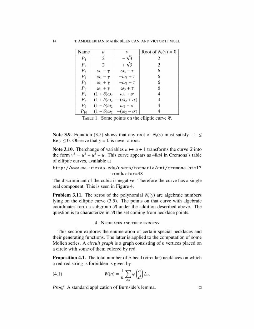
Note 3.8. The collection of points on an elliptic curve E, such as (3.6), hasbeen the subject of research since the 18th century. The general equation ofsuch a curve is written as

(3.7) y2 + a1y = x3 + a2x2 + a4x + a6

and if x, y ∈ P(C2), the complex projective space, then E is a torus. Theaddition of this torus is expressed on the cubic in a geometric form: to addP1 and P2, form the line joining them and define P3 := P1⊕P2 as the reflec-tion of the third point of intersection of this line with the cubic curve. Thisaddition rule is expressed in coordinate form: the general formula given in[6]. Let P1 = (x1, y1) and P2 = (x2, y2). Define

λ =

y2−y1x2−x1

if x2 , x13x2

1−4x1+22y1

if x2 = x1,and ν =

y1 x2−y2 x1

x2−x1if x2 , x1

−x31+2x1−2

2y1if x2 = x1.

The P3 = (x3, y3) is given by

x3 = λ2 + 2 − x1 − x2 and y3 = −λx3 − ν.

Aside from the point P0 = (1, 0), the table below shows a collection ofpoints on the curve E obtained using Mathematica. The notation

γ =

√3 + 2

√3, δ =

√√

5 − 2, τ =

√24 + 14

√3, σ = 2

√2(11 + 5

√5),

ω1 = 2 +√

3, ω2 = 2(3 +√

5), ω3 = 3 + 2√

3

is employed.

The notation necklace point refers to a point (u, v) on the elliptic curveE that is produced by the zero y = a + ib of a necklace polynomial via thetransformation 1 + a = 1/u and b = v/u. The addition of two necklacepoints sometimes yields another one. For instance, P1⊕P1 = P0 and 2P3 :=P3 ⊕ P3 = P2. On the other hand, the set of necklace points is not closedunder addition:

P1⊕P7 =12

(7 + 3

√5 +

√66 + 30

√5)−

I2

(21 + 9

√5 +

√30(29 + 13

√5)

).

The minimal polynomial for this number is y8 − 28y7 + 1948y6 − 5236y5 +

4858y4−3988y3 + 7156y2−6040y + 2245. This polynomial does not dividea Nt(y) for 1 ≤ t ≤ 1000. It is conjectured that it never does.


Name u v Root of Nt(y) = 0P1 2 −

√3 2

P2 2 +√

3 2P3 ω1 − γ ω3 − τ 6P4 ω1 − γ −ω3 + τ 6P5 ω1 + γ −ω3 − τ 6P6 ω1 + γ ω3 + τ 6P7 (1 + δ)ω2 ω2 + σ 4P8 (1 + δ)ω2 −(ω2 + σ) 4P9 (1 − δ)ω2 ω2 − σ 4P10 (1 − δ)ω2 −(ω2 − σ) 4Table 1. Some points on the elliptic curve E.

Note 3.9. Equation (3.5) shows that any root of Nt(y) must satisfy −1 ≤Re y ≤ 0. Observe that y = 0 is never a root.

Note 3.10. The change of variables u 7→ u + 1 transforms the curve E intothe form v2 = u3 + u2 + u. This curve appears as 48a4 in Cremona’s tableof elliptic curves, available athttp://www.ma.utexas.edu/users/tornaria/cnt/cremona.html?

conductor=48

The discriminant of the cubic is negative. Therefore the curve has a singlereal component. This is seen in Figure 4.

Problem 3.11. The zeros of the polynomial Nt(y) are algebraic numberslying on the elliptic curve (3.5). The points on that curve with algebraiccoordinates form a subgroup A under the addition described above. Thequestion is to characterize inA the set coming from necklace points.

4. Necklaces and their progeny

This section explores the enumeration of certain special necklaces andtheir generating functions. The latter is applied to the computation of someMolien series. A circuit graph is a graph consisting of n vertices placed ona circle with some of them colored by red.

Proposition 4.1. The total number of n-bead (circular) necklaces on whicha red-red string is forbidden is given by

(4.1) W(n) =1n

∑d|n

ϕ(nd

)Ld.

Proof. A standard application of Burnside’s lemma. �

http://www.ma.utexas.edu/users/tornaria/cnt/cremona.html?conductor=48

http://www.ma.utexas.edu/users/tornaria/cnt/cremona.html?conductor=48

BROKEN BRACELETS 15

Example 4.2. For n = p prime, formula (4.1) gives

(4.2) W(p) =(p − 1) + Lp

p.

It follows that Lp ≡ 1 mod p. Similarly, for n = p2, (4.1) gives

(4.3) p2W(p2) = Lp2 + (p − 1)Lp + p(p − 1).

It follows that

(4.4) Lp2 ≡ Lp + 1 mod p2.

These are well-known results [3].

A more distinguishing count is provided by defining Wk(n) to be the num-ber of n-bead necklaces on which a red-red string is forbidden, consistingof exactly k red beads. In order to accomodate the possibility that k = 0, wedefine W0(n) := 1 (this is justifiable since W0(n) = 1

n

∑d|n ϕ(d) = 1) .

Theorem 4.3. The function Wk(n) is given by

(4.5) Wk(n) =1

n − k

∑d|n,k

ϕ(d)( n

d −kd

kd

).

Proof. It follows directly from Burnside’s lemma. �

Corollary 4.4. The identity

(4.6)bn/2c∑k=0

1n − k

∑d|n,k

ϕ(d)( n

d −kd

kd

)=

1n

∑d|n

ϕ(d)Ln/d

holds.

Proof. The assertion follows from the combinatorial identity

(4.7)∑k≥0

Wk(n) = W(n).

�

Theorem 4.5. For n ∈ N define

(4.8) Vd(x) =

1 −√

1 + 4x2

d

+

1 +√

1 + 4x2

d

.

Then the row-sum generating function of Wk(n) is given by

(4.9) Fn(x) :=bn/2c∑k=0

Wk(n)xk =1n

∑d|n

ϕ(nd

)Vd

(xn/d

).


Proof. The proof is based on the identity

(4.10)1m

Vm(x) =

bm/2c∑k=0

1m − k

(m − k

k

)xk,

which is easy to verify. This is applied tobn/2c∑k=0

Wk(n)xk =∑d|n

ϕ(d)∑k≥0

1n − dk

( nd − k

k

)xdk

=∑d|n

ϕ(d)d

∑k≥0

1nd − k

( nd − k

k

)xdk.

The result follows from here. �

Example 4.6. For p prime, the polynomial Fp(x), defined in (4.9), is givenby

Fp(x) =

bp/2c∑k=0

1p − k

(p − k

k

)xk

=(p − 1)2p(1 −

√1 + 4x)p + (1 +

√1 + 4x)p

p · 2p .

Example 4.7. Put n = 3k + 1 in (4.3) to obtain Wk(3k + 1) = 12k+1

(2k+1

k

), the

Catalan numbers.

Example 4.8. For n ∈ N, and with Ln denoting the Lucas number,

(4.11)bn/2c∑k=0

1n − k

(n − k

k

)=

1n

Ln.

This is obtained from setting x = 1 in (4.9).

Theorem 4.9. The ordinary generating function for the diagonals of Wk(n)is given by

(4.12)∑n≥k

Wk(n)xn =1k

∑d|k

ϕ(d)x2k

(1 − xd)k/d .

In its lowest terms, the denominator of this rational function takes the form

(4.13)∏d|k

(1 − xd)ϕ(k/d) =∏d|k

Φd(x)k/d,

where Φd(x) is the d-th cyclotomic polynomial given in terms of the Mobiusµ-function as Φd(x) =

∏c|d(1 − xd/c)µ(x).

BROKEN BRACELETS 17

Proof. The result follows from the Taylor series expansion

(4.14)x2m

m(1 − x)m =∑j≥m

1j − m

(j − m

m

)x j.

�

A geometric interpretation. The above generating function∑

n≥k Wk(n)xn

is the Molien series W(x;Zk) for the ring of invariants C[X]Zk where X =

(x1, . . . , xk). In this case, the group Zk is identified with its k-dimensionalgroup representation in GLk(C). More concretely, Zk � 〈ek〉 where ek is thek × k permutation matrix such that e[i, j] = 1 if j = i + 1; e[k, 1] = 1 ande[i, j] = 0, otherwise. Let RP(d) be the set of positive integers less than dand relatively prime to d. Partition the integer interval [k] into the disjointunion

(4.15) [k] = {1, 2, . . . , k} =⋃d|k

kd

RP(d).

This relation is reminiscent of the well-known identity k =∑

d|k ϕ(d). Then,

W(x;Zk) =1|Zk|

k∑j=1

1

det(1k − xe jk)

=1k

∑d|k

ϕ(d)

det(1k − xek/dk )

=1k

∑d|k

ϕ(d)det((1d − xed) ⊗ 1k/d)

=1k

∑d|k

ϕ(d)det((1d − xed)k/d

=1k

∑d|k

ϕ(d)(1 − xd)k/d .

These findings are stated in the next result.

Proposition 4.10. The number of linearly independent homogeneous poly-nomials, of total degree n, for the ring of invariants C[X]Zk equals

1n + k

∑d|n,k

ϕ(d)( n

d + kd

kd

).


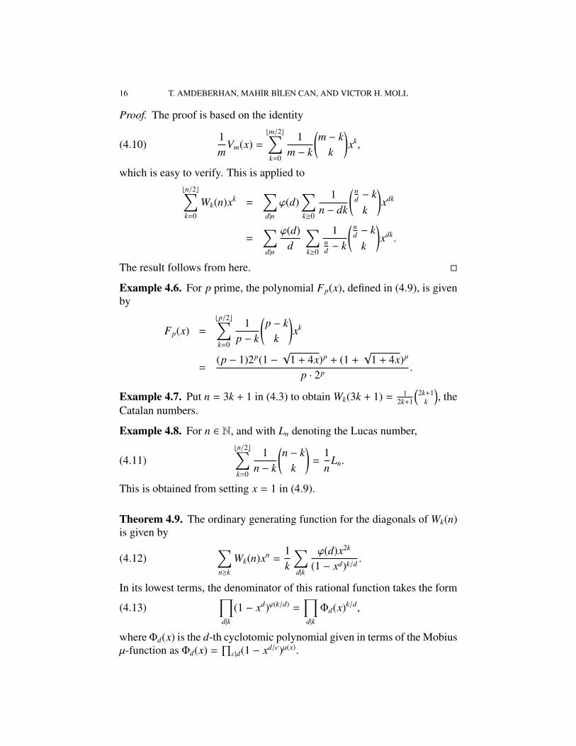
5. A sample of the computation of zeros

Motivated by the interesting properties of the zeros of necklace polyno-mials, this section presents some computational graphics showing the ze-ros of the polynomials Fn(x). Figure 5 shows the location of the roots ofF1000(x).

!8 !6 !4 !2 2 4

!3

!2

!1

1

2

3

Figure 5. The zeros of F1000(x).

BROKEN BRACELETS 19

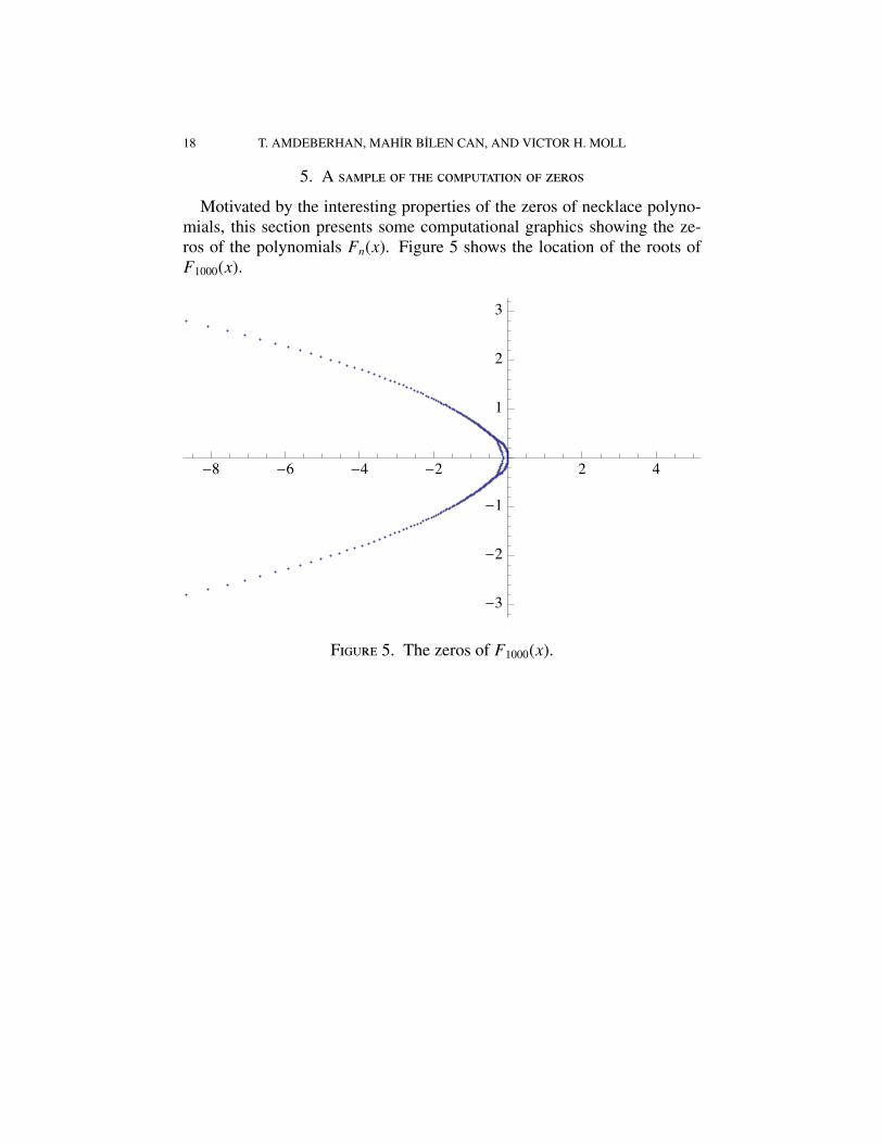
The next four figures show a selection of regions from the set of the rootsof all the polynomials Fn(x) for 3 ≤ n ≤ 1000. The caption indicates therange depicted.

10 !8 !6 !4 !2 2

!2

!1

1

2

Figure 6. [−10, 2] × [−2, 2].

!2.0 !1.5 !1.0 !0.5

!0.6

!0.4

!0.2

0.2

0.4

0.6

Figure 7. [−2, 0.2] × [−0.6, 0.6].

!1.3 !1.2 !1.1 !1.0 !0.9 !0.8 !0.7 !0.6

Figure 8. [−1.4,−0.6] × [−0.5, 0.5].

!50 !40 !30 !20 !10

!6

!4

!2

2

4

6

Figure 9. [−50, 5] × [−6, 6].

The interesting structure depicted in figures 6 to 9 will be explored infuture work.Acknowledgments. The authors wish to thank J. Silverman for providinginformation on the elliptic curve mentioned in the title and to A. Ayyerand A. Waldron regarding information on the quantum mechanical systems.The authors also wish to thanks the referees for comments on an earliermanuscript. The third author was partially funded by NSF-DMS 0070567.


Appendix A. Rows of paraffin

The figures show all possible alkane bonds (paraffin) CnH2n+2 for n =

1, 2, 3, 4, 5.

C

H

H

H H H C

H

H

C

H

H

H H C

H

H

C

H

H

C H

H

H

n = 1 : CH4. n = 2 : C2H6. n = 3 : C3H8.

n = 4 : C4H10.

C C C C

H H H H

H H H H

H H C CC

C

H

HH

H

H

H

H

H

H

C C C C

H H H H

H H H H

H C

H

H

H C CC

C

H

HH

H

H

H

C

H

H H

H

H C CC

C

C

H

HH

H

H

H

H

H

H

H H

H

n = 5 : C5H12.

BROKEN BRACELETS 21

References

[1] P. Brändén. Iterated sequences and the geometry of zeros. ArXiV:Math.CO/0909.1927, 2010.

[2] F. Brenti. Log-concave and unimodal sequences in Algebra, Combinatorics and Ge-ometry: an update. Contemporary Mathematics, 178:71–89, 1994.

[3] G. H. Hardy, E. M. Wright; revised by D. R. Heath-Brown, and J. Silverman. AnIntroduction to the Theory of Numbers. Oxford University Press, 6th edition, 2008.

[4] S. M. Losanitsch. Die Isomerie-Arten bei den Homologen der Paraffin-Reihe. Chem.Ber., 30:1917–1926, 1897.

[5] E. Onofri, G. Veneziano, and J. Wosiek. Supersymmetry and Combinatorics. ArXiV:math-ph/0603082, 2010.

[6] J. H. Silverman. The Arithmetic of Elliptic Curves. Springer Verlag, New York, firstedition, 1986.

[7] R. Stanley. Log-concave and unimodal sequences in Algebra, Combinatorics and Ge-ometry. graph theory and its applications: East and West ( Jinan, 1986). Ann. NewYork Acad. Sci., 576:500–535, 1989.

[8] H. S. Wilf. generatingfunctionology. Academic Press, 1st edition, 1990.

Department ofMathematics, Tulane University, New Orleans, LA 70118E-mail address: [email protected]



Broken Bracelets, Molien Series, Paraffin Wax, and an Elliptic Curve of Conductor 48

Documents

Transcript of Broken Bracelets, Molien Series, Paraffin Wax, and an Elliptic Curve of Conductor 48