Briggs-PhD.pdf - NRAO CASA
439
-
Upload
khangminh22 -
Category
Documents
-
view
0 -
download
0
Transcript of Briggs-PhD.pdf - NRAO CASA

HIGH FIDELITY DECONVOLUTIONOF MODERATELY RESOLVED SOURCES
by
DANIEL SHENON BRIGGS� B�S�� B�S�� M�S�
Submitted in Partial Ful�llment
of the Requirements for the Degree of
DOCTOR OF PHILOSOPHY IN PHYSICS
The New Mexico Institue of Mining and Technology
Socorro� New Mexico
March� ����


To my Mother and the memory of my Father


ABSTRACT
This dissertation contains several topics related to high �delity imaging with in�
terferometers� including deconvolution simulations to show quantitatively how well existing
algorithms do on simple sources� a new deconvolution algorithm which works exceedingly
well but can only be applied to small objects� and a new weighting scheme which o�ers mild
improvement to nearly any observation�
Robust weighting is a new form of visibility weighting that varies smoothly from
natural to uniform weighting as a function of a single real parameter� the robustness� In�
termediate values of the robustness can produce images with moderately improved thermal
noise characteristics compared to uniform weighting at very little cost in resolution� Alter�
natively� an image can be produced with nearly the sensitivity of the naturally weighted
map� and resolution intermediate between that of uniform and natural weighting� This
latter weighting often produces extremely low sidelobes and a particularly good match be�
tween the dirty beam and its �tted Gaussian� making it an excellent choice for imaging
faint extended emission�
A new deconvolver has been developed which greatly outperforms CLEAN or
Maximum Entropy on compact sources� It is based on a preexisting Non�Negative Least
Squares matrix inversion algorithm� NNLS deconvolution is somewhat slower than existing
algorithms for slightly resolved sources� and very much slower for extended objects� The
solution degrades with increasing source size and at the present computational limit ��pixels of signi�cant emission� it is roughly comparable in deconvolution �delity to existing
algorithms� NNLS deconvolution is particularly well suited for use in the self�calibration
loop� and for that reason may prove particularly useful for Very Long Baseline Interferom�
etry� even on size scales where it is no better than existing deconvolvers�
The basic practice of radio interferometric imaging was re�examined to determine
fundamental limits to the highest quality images� As telescopes have become better� tech�
niques which served an earlier generation are no longer adequate in some cases� Contrary to
established belief� the deconvolution process itself can now contribute an error comparable
to that of residual calibration errors� This is true for even the simplest imaging problems�
and only the fact that the error morphology of deconvolution and calibration errors are
similar has masked this contribution until now� In cases where it can be applied� these de�
convolution problems are largely cured by the new NNLS deconvolver� An extensive suite
of simulations has been performed to quantify the expected magnitude of these errors in a
typical observation situation�
v

The new techniques have been demonstrated by observational projects with the
Very Large Array� Australia Telescope Compact Array and Very Long Baseline Array on
the sources �C �� SN����A and DA��� respectively� The �C � project was designed to
trace or exclude extended emission from a VLBI scale disrupted jet� and yielded a null re�
sult at a noise limited dynamic range of ����� from an extended object� The SN����A
project was designed for the highest resolution imaging possible and yielded high con�dence
level astrophysically important structure at half the synthesized uniform beamwidth� The
DA��� project was primarily a test of the new VLBA telescope� but yielded as a by prod�
uct the highest dynamic range images ever produced by VLBI� There are no comparable
observations on other telescopes for comparison� but the observed ������ exceeded the
previous record by more than a factor of ��
vi

Acknowledgments
When �rst I presented a topic to my dissertation committee� it was a somewhat
nebulous collection of problems that I wanted to address� mostly in the area of developing
sophisticated new calibration techniques for radio interferometers� Unfortunately� while
I had initial strategies for these investigations� I lacked a clear vision of which problems
would prove most tractable or most useful� The proposal was based on the theory that
with enough promising beginnings� at least some were likely to succeed� My committee
gifted me with a great deal of freedom in my pursuits� for which vote of con�dence I am
profoundly grateful� That freedom allowed me to follow my nose to this dissertation� whose
results have surprised us all� There is little of the original topic left� the curious behavior
encountered in the initial �warm up� deconvolution project grew so intriguing as to occupy
nearly all of my time� The subject of calibration is now touched on only peripherally in the
pages that follow�
There are many� many people who deserve thanks and acknowledgements in a
work like this� But �rst among them I wish to thank Tim Cornwell� my scienti�c advisor�
I have been tremendously lucky to encounter an advisor with whom I was so professionally
and personally compatible� I could not ask for an advisor more skilled in his art and
generous in his time in explaining it� And while always delivered with compassion� I greatly
appreciate the honesty and candor of his progress assessments � both good and bad� It is
di�cult to properly express the debt I feel� My fond hope is that I come to re�ect well on
him as I continue to grow and mature as a scientist�
I have actually been very lucky with all of the advisors and committee members
that I have come in contact with during my graduate career� Jean Eilek has seen me
through many years as my academic advisor� and taught me much of what I know about
astrophysics� I�m sorry it worked out that she could not be present for the �nal defense�
I would have liked her signature on my dissertation� A friend as well as teacher� she is
one of the rare people on the planet who can out talk me by �� on nearly any subject
of mutual interest� �Pity the poor observer trying to follow an excited discussion between
us�� Alan Blyth has done an admirable job of stepping into her place as academic advisor
and looking after my interests while Jean is on sabbatical� Craig Walker also stands out
in my mind as a particularly signi�cant mentor and companion during the past years� His
un�agging good humor and superb technical competence has been greatly appreciated as
we worked on a number of projects together� both my master�s degree project and the �C �
project which inspired much of the work in this dissertation among them� I�d like to thank
Joan Wrobel for making me welcome at NMT�NRAO and involving me in her research
almost from the moment I arrived in Socorro� In the several years she advised me during
my Master�s degree I have always been struck by her desire to do right by the student� It
vii

has been much appreciated� Tim Hankins is another committee member who could not
participate in the �nal defense due to a sabbatical at extreme distance� His presence was
missed and I thank both Dave Westpfahl and Paul Krehbiel for stepping in to �ll the empty
positions under somewhat di�cult circumstances�
I also particularly wish to thank my supervisor�to�be� Dave Mozurkewich� for
graciously allowing me to defer the start of my �rst postdoc and complete this dissertation
substantially to my satisfaction� There are certainly rough spots� and more work could be
done in a number of areas � but several important lines of research paid o� dramatically
right at the end of my NRAO fellowship and without the cooperation of both Dave and my
supervisors at NRAO� much useful material would not be present in this document� I am
grateful for the extra time and use of NRAO facilities during the awkward transition� and
the dissertation is much the better for it�
I have been present at the Array Operations Center in Socorro during the �nal
construction years and dedication of the Very Long Baseline Array� The VLBA is a superb
new instrument� and everyone associated with it deserves the praise of the astronomical
community� But as I�ve worked �and played� through many long nights at the AOC� I�ve
personally seen the heroic e�orts of Craig Walker and of Jon Romney in bringing the
VLBA to life� The last image of DA��� in Chapter � is more than an order of magnitude
deeper in dynamic range than any other VLBI image of which I am aware� This image is
a testament to the dedication and skill of everyone who worked on VLBA� But in terms of
the human sacri�ce necessary to achieve such incredible instrumental calibration� stability
and correlator performance� I will always associate that with Craig and Jon�
New Mexico Tech happens to require a considerable amount of classwork of its
physics graduate students� and consequently I�ve enjoyed many classes from some �rst rate
people� Jean� of course� Bob Hjellming� Tim Hankins and Albert Petschek� Thanks to you
all� I�m sure it�ll keep me in good stead in the future� And special thanks to Rick Perley not
only for an excellent class in Fourier theory� but also for steering me towards Tim Cornwell
as an advisor�
The list of �helpful discussions� reads much like the scienti�c sta� phone list� Dave
Adler� Durga Bagri� Claire Chandler� Barry Clark� Richard Davis� Phil Diamond� Dwaraka�
Chris Flatters� Ed Fomalont� Dale Frail� Jim Higdon� Mark Holdaway� Ralph Marson�
Frasier Owen� Peter Napier� Michael Rupen� Bob Sault� Fred Schwab� Ulrich Schwarz� Ken
Sowinski� Dick Sramek� Lister Stavely�Smith� Tom Tongue� Juan Uson� Dave Westpfahl�
Doug Woods� Gustaaf van Moorsel and Anton Zensus� Some of these people I�ve worked
with fairly closely� Others have su�ered through being test cases of my experimental soft�
ware or read drafts for me� Still others have o�ered useful comments over co�ee� All of
them have given me something� and I thank them for it�
Ruth Milner� Gustaaf van Moorsel� Wes Young and Jon Spargo have impressed me
particularly as the heart of the computer division here at the AOC� Working under di�cult
viii

budget and manpower limitations� they never loose sight that the purpose of computers is
to help people solve problems� As one of the more computer intensive individuals in the
building I�ve occasionally managed to dig myself into some real holes� and they�ve always
bailed me out�
Harry Andrews � Bobby Hunt deserve mention� even though I have met Bobby
but brie�y and Harry not at all� Their book� Digital Image Restoration �Andrews and Hunt�
����� is simply amazing� and with the bene�t of �� years hindsight seems nothing short of
prescient� If it had been written at a time with the computer resources of today� I might
have had little left to do in Chapter �
I spent the �rst � months of ���� in Australia� as the guest of the Australia Tele�
scope National Facility� I enjoyed my time there tremendously� and it was quite productive
scienti�cally� Chapter � is almost entirely based on work done there� I also wrote the NNLS
algebraic deconvolution program while at the ATNF� but did not recognize at the time how
useful it would become� Ron Ekers� Neil Killeen� Bob Sault and Ralph Marson all made me
feel very welcome� Lister Stavely�Smith did as well� and graciously allowed me to work on
his lovely SN����A data� Also while down under� I fortunate to form a marvelous friendship
with Sue Byleveld�
On the personal side� thanks to Michael Rupen for many things� the incredibly
detailed dissertation comments went far above and beyond the call of duty� and this docu�
ment is much the better for the help� But even more than that� thanks for the friendship and
moral support during some pretty bleak times when �nishing up� Thanks to John Biretta
for the milk and cookies that appeared without fail at every late night Star Trek session� to
Jimbo Higdon for the Nerf wars� to Dave Mo�ett for the movie nights at the bomb shelter
and all too infrequent rock climbs� To Tom � Maggie Tongue� Andrew Lobanov� Kari
Leppanen� Chris Taylor� Beth Hufnagel� Kevin Marvel� Chris de Pree and Lisa Young as
comrades in arms during the long graduate struggle�
As to personal friends beyond work� I could ask for none better than Kathy
Hedges� Whether it�s been out square dancing� an evening�s quiet tea� or being her �best
man�� I�ve enjoyed it all� To Peggi � Kevin Whitmore and all the other nifty people I�ve
met through English� Contra and Morris dancing � I�ve had a great time� Keep dancing�
and I�ll be back to join you occasionally� And no discussion of my life as a graduate student
would be complete without mentioning the joy I�ve found skydiving� The people I�ve met
at the drop zone have been lovely� John Walter� Cynthia Cooper� Mike � Jane Ann Bode
and many many others� Thanks to all my skydiving friends for �ying with me� keeping me
sane� and teaching me how to know what is really important�
And of course� with all my I heart I thank my parents to whom this dissertation
is dedicated� I�m sorry my father could not have lived to see it� and I miss him very much�
Financial support for the research in this dissertation has come from an NRAO
Junior Research Fellowship� from a New Mexico Tech Research Assistantship� and from the
Australia Telescope National Facility�
ix
Finally� except where stated otherwise� all work in this dissertation is original�
I gratefully acknowledge the initial concept of Robust Weighting to Tim Cornwell� and the
initial concept of beam forcing though a Gaussian taper to Bill Cotton� Rick Perley �rst
pointed out to me that the CLEAN algorithm could be solved analytically in the limit of per�
fect u�v sampling and critical sampling� and Craig Walker suggested successive di�erencing
as a superior alternative to boxcar averaging in the estimation of thermal noise�
DANIEL SHENON BRIGGS
The New Mexico Institue of Mining and Technology
March� ����
x

Table of Contents
ABSTRACT v
Acknowledgments vii
Table of Contents xi
List of Figures xvii
List of Tables xxiii
List of Programs xxv
List of Symbols and Functions xxvii
�� Introduction �
��� Overview of Dissertation Structure � � � � � � � � � � � � � � � � � � � � � � �
�� Representation of the Deconvolution Equation �
��� The Visibility Equations � � � � � � � � � � � � � � � � � � � � � � � � � � � � � �
��� The Continuous Dirty Map � � � � � � � � � � � � � � � � � � � � � � � � � � � ��
��� Discretization of the Continuous Equations � � � � � � � � � � � � � � � � � � �
�� Convolutional Gridding and Aliasing � � � � � � � � � � � � � � � � � � � � � � ��
��� Limitations of the even�sized FFT � � � � � � � � � � � � � � � � � � � � � � � ��
����� Non�Power�of�� FFT Performance Analysis � � � � � � � � � � � � � � ��
�� Deconvolution � � � � � � � � � � � � � � � � � � � � � � � � � � � � � � � � � � � �
��� Deconvolution Algorithms � � � � � � � � � � � � � � � � � � � � � � � � � � � � ��
����� CLEAN � � � � � � � � � � � � � � � � � � � � � � � � � � � � � � � � � � ��
����� SDI CLEAN � � � � � � � � � � � � � � � � � � � � � � � � � � � � � � � ��
xi

����� Multi Resolution CLEAN � � � � � � � � � � � � � � � � � � � � � � � � �
���� Maximum Entropy � � � � � � � � � � � � � � � � � � � � � � � � � � � � �
����� Non�Negative Least Squares � � � � � � � � � � � � � � � � � � � � � � � ��
���� Maximum Emptiness � � � � � � � � � � � � � � � � � � � � � � � � � � � ��
����� Gerchberg�Saxon�Papoulis � � � � � � � � � � � � � � � � � � � � � � � � ��
����� Richardson�Lucy � � � � � � � � � � � � � � � � � � � � � � � � � � � � � ��
����� Singular Value Decomposition � � � � � � � � � � � � � � � � � � � � � � ��
�� Robust Weighting ��
��� Introduction � � � � � � � � � � � � � � � � � � � � � � � � � � � � � � � � � � � � ��
��� Thermal noise in the synthesized map � � � � � � � � � � � � � � � � � � � � � �
��� Weighting as the Solution to a Minimization Problem � � � � � � � � � � � �
����� Natural Weighting � � � � � � � � � � � � � � � � � � � � � � � � � � � �
����� Sensitivity to Resolved Sources � � � � � � � � � � � � � � � � � � � � � �
����� Uniform Weighting � � � � � � � � � � � � � � � � � � � � � � � � � � � � �
���� Super�Uniform Weighting � � � � � � � � � � � � � � � � � � � � � � � � �
�� Beamwidth and Thermal Noise � � � � � � � � � � � � � � � � � � � � � � � � � �
��� Catastrophic Gridding Errors � � � � � � � � � � � � � � � � � � � � � � � � � � �
����� Gridless Weighting � � � � � � � � � � � � � � � � � � � � � � � � � � � � ��
�� Robust Uniform Weighting � � � � � � � � � � � � � � � � � � � � � � � � � � � ��
���� Robust Weighting and Wiener Filtering � � � � � � � � � � � � � � � � ��
���� Speci�cation of the Robustness � � � � � � � � � � � � � � � � � � � � � �
���� Example Thermal Noise Calculations � � � � � � � � � � � � � � � � � � �
��� Simulations � � � � � � � � � � � � � � � � � � � � � � � � � � � � � � � � � � � � ��
����� VLA Full Tracks � � � � � � � � � � � � � � � � � � � � � � � � � � � � � �
����� VLA Full Tracks ��C �� � � � � � � � � � � � � � � � � � � � � � � � � � ��
����� VLA � Point Snapshot � � � � � � � � � � � � � � � � � � � � � � � � � ��
���� VLA � Point Snapshot � � � � � � � � � � � � � � � � � � � � � � � � � � ��
xii

����� VLA Multiple Con�gurations �M��� � � � � � � � � � � � � � � � � � � ��
���� AT Full Tracks �SN����A� � � � � � � � � � � � � � � � � � � � � � � � ��
����� VLBA Full Tracks � � � � � � � � � � � � � � � � � � � � � � � � � � � � ��
����� VLBA�VLA�GBT Full Tracks � � � � � � � � � � � � � � � � � � � � � ��
����� VLBA�VLA�GBT�Orbiter � � � � � � � � � � � � � � � � � � � � � � � �
��� RMS�resolution Tradeo� Curves � � � � � � � � � � � � � � � � � � � � � � � � ��
����� Tradeo� Parameterized by Robustness � � � � � � � � � � � � � � � � � ��
����� Thresholding � � � � � � � � � � � � � � � � � � � � � � � � � � � � � � � ���
����� Time Averaging � � � � � � � � � � � � � � � � � � � � � � � � � � � � � ���
���� Super�Uniform Weighting � � � � � � � � � � � � � � � � � � � � � � � � ��
��� Automatic selection of Robustness � � � � � � � � � � � � � � � � � � � � � � � ��
��� Model Deconvolutions � � � � � � � � � � � � � � � � � � � � � � � � � � � � � � ��
���� Tapering � Beam Forcing � � � � � � � � � � � � � � � � � � � � � � � � � � � � ��
������ VLB �Square Root� Weighting � � � � � � � � � � � � � � � � � � � � � ���
���� Future Work � � � � � � � � � � � � � � � � � � � � � � � � � � � � � � � � � � � ��
������ Azimuthally Varying Robustness � � � � � � � � � � � � � � � � � � � � ��
������ Thermal Noise Beam and Visualization � � � � � � � � � � � � � � � � ��
������ Generalized Windows and Minimizing Source Sidelobes � � � � � � � �
���� Summary � � � � � � � � � � � � � � � � � � � � � � � � � � � � � � � � � � � � � �
������ Imaging Recommendations � � � � � � � � � � � � � � � � � � � � � � � �
������ Software Recommendations � � � � � � � � � � � � � � � � � � � � � � � ��
�� Algebraic Deconvolution ���
�� Representation � � � � � � � � � � � � � � � � � � � � � � � � � � � � � � � � � � ���
�� Singular Value Decomposition � � � � � � � � � � � � � � � � � � � � � � � � � � ���
�� NNLS � � � � � � � � � � � � � � � � � � � � � � � � � � � � � � � � � � � � � � � ���
���� The NNLS algorithm � � � � � � � � � � � � � � � � � � � � � � � � � � � ���
���� How Important are the Windows� � � � � � � � � � � � � � � � � � � � ��
xiii

���� Model Deconvolutions � � � � � � � � � � � � � � � � � � � � � � � � � � ��
��� Discussion � � � � � � � � � � � � � � � � � � � � � � � � � � � � � � � � � ��
�� Simulations ���
��� The Resolution Test Deconvolutions � � � � � � � � � � � � � � � � � � � � � � �
��� Error Morphology � � � � � � � � � � � � � � � � � � � � � � � � � � � � � � � � ��
����� Results � � � � � � � � � � � � � � � � � � � � � � � � � � � � � � � � � � ���
��� Residual Behavior � � � � � � � � � � � � � � � � � � � � � � � � � � � � � � � � ���
�� Algorithmic Cross Comparison � � � � � � � � � � � � � � � � � � � � � � � � � ���
��� The E�ect of Fourier Plane Coverage � � � � � � � � � � � � � � � � � � � � � � � �
�� Flux estimation � � � � � � � � � � � � � � � � � � � � � � � � � � � � � � � � � � �
��� Gaussian Pixel Functions � � � � � � � � � � � � � � � � � � � � � � � � � � � � ���
��� Point Sources Between Pixels � � � � � � � � � � � � � � � � � � � � � � � � � � ��
��� Convergence in the Fourier Plane � � � � � � � � � � � � � � � � � � � � � � � � ��
��� �C � Simulations � MEM � � � � � � � � � � � � � � � � � � � � � � � � � � � ��
�� Miscellaneous Topics ���
�� Estimation of Thermal Noise from the Visibility Data � � � � � � � � � � � � ��
�� CLEAN component placement � � � � � � � � � � � � � � � � � � � � � � � � � ���
���� The Gaussian approximation to initial CLEANing � � � � � � � � � � ���
���� The Gaussian Approximation Applied to a VLA PSF � � � � � � � � ���
���� Multiple Orders of Clean Components � � � � � � � � � � � � � � � � � ��
��� Fitting to CLEANed Gaussians � � � � � � � � � � � � � � � � � � � � � ���
�� CLEAN components are Fourier Components in the Limit � � � � � � � � � � ���
� Model Combination in the Fourier and Image Planes � � � � � � � � � � � � � ���
�� Case Study �C� ���
��� Introduction � � � � � � � � � � � � � � � � � � � � � � � � � � � � � � � � � � � � ���
��� The Data and the Noise � � � � � � � � � � � � � � � � � � � � � � � � � � � � � ��
xiv

��� Modelling � � � � � � � � � � � � � � � � � � � � � � � � � � � � � � � � � � � � � ���
�� X Band Images � � � � � � � � � � � � � � � � � � � � � � � � � � � � � � � � � � ��
��� L Band Images � � � � � � � � � � � � � � � � � � � � � � � � � � � � � � � � � � ��
�� Discussion � � � � � � � � � � � � � � � � � � � � � � � � � � � � � � � � � � � � � ���
� Case Study SN���A ���
��� Introduction � � � � � � � � � � � � � � � � � � � � � � � � � � � � � � � � � � � � ���
��� The Data � � � � � � � � � � � � � � � � � � � � � � � � � � � � � � � � � � � � � ��
��� Deconvolution � � � � � � � � � � � � � � � � � � � � � � � � � � � � � � � � � � � ���
����� Support Constraints � � � � � � � � � � � � � � � � � � � � � � � � � � � ���
����� Cross Validation � � � � � � � � � � � � � � � � � � � � � � � � � � � � � ���
�� Algorithmic Convergence � � � � � � � � � � � � � � � � � � � � � � � � � � � � ���
�� �� Linear Summation � � � � � � � � � � � � � � � � � � � � � � � � � � � � ��
�� �� Restored Images � � � � � � � � � � � � � � � � � � � � � � � � � � � � � ���
�� �� Comparison with Other Data � � � � � � � � � � � � � � � � � � � � � � ��
�� � Summary � � � � � � � � � � � � � � � � � � � � � � � � � � � � � � � � � ���
��� Visibility Weighting and Thermal Noise � � � � � � � � � � � � � � � � � � � � ���
�� Modelling � � � � � � � � � � � � � � � � � � � � � � � � � � � � � � � � � � � � � ���
��� Results and Discussion � � � � � � � � � � � � � � � � � � � � � � � � � � � � � � �
�� Case Study DA��� ���
��� VLB Array Memo ���A � � � � � � � � � � � � � � � � � � � � � � � � � � � � � �
����� Introduction � � � � � � � � � � � � � � � � � � � � � � � � � � � � � � � � �
����� Initial Calibration � � � � � � � � � � � � � � � � � � � � � � � � � � � � � �
����� CLEAN Deconvolution � � � � � � � � � � � � � � � � � � � � � � � � � � ��
���� Imaging Presentation and Metrics � � � � � � � � � � � � � � � � � � � ���
����� Model Fit with CLEAN Tidying � � � � � � � � � � � � � � � � � � � � ���
���� NNLS � � � � � � � � � � � � � � � � � � � � � � � � � � � � � � � � � � � ��
xv

����� Noise Comparison � � � � � � � � � � � � � � � � � � � � � � � � � � � � ���
����� Super Resolution � � � � � � � � � � � � � � � � � � � � � � � � � � � � � ���
����� Self�Calibration � � � � � � � � � � � � � � � � � � � � � � � � � � � � � � ��
����� Conclusions and Further Work � � � � � � � � � � � � � � � � � � � � � ��
��� Simulations � � � � � � � � � � � � � � � � � � � � � � � � � � � � � � � � � � � � ��
����� Gaussian Model � � � � � � � � � � � � � � � � � � � � � � � � � � � � � ��
����� Gain Transfer � � � � � � � � � � � � � � � � � � � � � � � � � � � � � � � �
����� Halo Model � � � � � � � � � � � � � � � � � � � � � � � � � � � � � � � � ��
��� Conclusions and Further Work � � � � � � � � � � � � � � � � � � � � � � � � � ���
��� Concluding Comments ���
A� Lagrange Multipliers and the Weighted Mean ���
B� Elliptical Gaussian Convolution ��
C� Beam Fitting ��
D� Generalized Tapers and Beam Forcing ��
E� Gridless Weighting Algorithm ���
E�� Variations of the Algorithm � � � � � � � � � � � � � � � � � � � � � � � � � � � ��
E�� Automatic Bin Size Selection � � � � � � � � � � � � � � � � � � � � � � � � � � ���
F� Complex Fourier Series ���
G� SDE ���
H� Electronic Supplement ���
Bibliography ���
xvi

List of Figures
��� Radiation on the Celestial Sphere � � � � � � � � � � � � � � � � � � � � � � � � �
��� Normalized FFT Runtimes vs� Size � � � � � � � � � � � � � � � � � � � � � � � �
��� Resolution vs� Thermal Noise Tradeo� � � � � � � � � � � � � � � � � � � � � � �
��� Catestrophic Gridding Error in the u�v Plane � � � � � � � � � � � � � � � � � ��
��� Striping in the Dirty Map � � � � � � � � � � � � � � � � � � � � � � � � � � � � ��
�� Striping in the Restored Image � � � � � � � � � � � � � � � � � � � � � � � � � �
��� Isolated u�v Sampling Points � � � � � � � � � � � � � � � � � � � � � � � � � � �
�� Thermal Noise�Resolution Tradeo� � Robustness � � � � � � � � � � � � � � �
��� Thermal Noise�Resolution Tradeo� � Robustness with eccentricity� � � � �
��� Azimuthally Averaged Gridded Total Weights � VLA Full Tracks � � � � � �
��� Azimuthally Averaged Gridded Density Weights � VLA Full Tracks � � � �
��� Density Weight Histograms � VLA Full Tracks � � � � � � � � � � � � � � � � �
���� Model Density Weight Histograms � � � � � � � � � � � � � � � � � � � � � � � �
���� Fourier Plane Coverages � � � � � � � � � � � � � � � � � � � � � � � � � � � � � �
���� PSF Plots vs� Robustness� VLA Full Tracks � � � � � � � � � � � � � � � � � � ��
��� PSF Plots vs� Robustness� VLA Full Tracks ��C �� � � � � � � � � � � � � � � �
���� PSF Plots vs� Robustness� VLA � Point Snapshot � � � � � � � � � � � � � � ��
��� PSF Plots vs� Robustness� VLA � Point Snapshot� Gridless� FOVw �� � �
���� PSF Plots vs� Robustness� VLA � Point Snapshot� FOVw �� � � � � � � � �
���� PSF Plots vs� Robustness� VLA Multiple Con�g �M��� � � � � � � � � � � � ��
���� PSF Plots vs� Robustness� AT Full Tracks �SN����A� � � � � � � � � � � � � �
��� PSF Plots vs� Robustness� VLBA Full Tracks � � � � � � � � � � � � � � � � � ��
���� PSF Plots vs� Robustness� VLBA�VLA�GBT Full Tracks � � � � � � � � � � �
���� PSF Plots vs� Robustness� VLBA�VLA�GBT�Orbiter � � � � � � � � � � � � �
���� Robustness Tradeo� Curves � � � � � � � � � � � � � � � � � � � � � � � � � � � ��
��� Thresholding Tradeo� Curve� VLA Full Tracks � � � � � � � � � � � � � � � � ���
���� Time�averaging Tradeo� Curves � � � � � � � � � � � � � � � � � � � � � � � � � ��
xvii

��� RMS vs� Beamsize� varying FOVw � � � � � � � � � � � � � � � � � � � � � � � ���
���� PSF Plots vs� FOV� VLA Full Tracks ��C �� � � � � � � � � � � � � � � � � � ��
���� Super�Uniform Weighting as a Way to Prevent a Shelf � � � � � � � � � � � � ���
���� Automatic Selection of Robustness by Gaussian Best�Fit � � � � � � � � � � � ���
��� �C � Model Deconvolutions � CLEAN � � � � � � � � � � � � � � � � � � � � ���
���� Error Quantities against Thermal RMS � CLEAN � � � � � � � � � � � � � � ���
���� Beam Circularization by Tapering � � � � � � � � � � � � � � � � � � � � � � � ���
���� Beam Slices Against Simple Tapering � � � � � � � � � � � � � � � � � � � � � � ��
��� Robustness and Tapering � � � � � � � � � � � � � � � � � � � � � � � � � � � � � �
���� PSF Plots vs� Robustness� Tapered� FOVw �� � � � � � � � � � � � � � � � � �
��� PSF Plots vs� Robustness� Tapered� FOVw ��� � � � � � � � � � � � � � � ��
���� PSFs Tapered to Fixed Resolution � � � � � � � � � � � � � � � � � � � � � � � ���
���� Robustness Tradeo� Curves� VLBI Weighting Comparison� � � � � � � � � � ���
���� PSF Plots vs� Robustness� VLBA�VLA�GBT Full Tracks� VLB weighting � ���
�� PSF Plots vs� Robustness� VLBA�VLA�GBT�Orbiter� VLB weighting � � � �
�� � Azimuthally Varying Robustness � AT Full Tracks �SN����A� � � � � � � � ��
�� Singular Value Decomposition of a One�Dimensional PSF � � � � � � � � � � ��
�� Two�Dimensional Beam Matrix � � � � � � � � � � � � � � � � � � � � � � � � � ��
�� Singular Value Spectrum vs� Window Size � � � � � � � � � � � � � � � � � � � ���
� SVD Deconvolutions of �C � Model Source � � � � � � � � � � � � � � � � � � ��
�� �C � Raw and Smoothed Model Source � � � � � � � � � � � � � � � � � � � � ��
� CLEAN Deconvolution � � � � � � � � � � � � � � � � � � � � � � � � � � � � � � ���
�� NNLS Deconvolution with Faint Sources Present � � � � � � � � � � � � � � � ���
�� NNLS Deconvolution without Faint Sources � � � � � � � � � � � � � � � � � � ���
�� Error Quantities against Thermal RMS � NNLS � � � � � � � � � � � � � � � ���
�� Missing Data Deconvolution � � � � � � � � � � � � � � � � � � � � � � � � � � � ���
��� Error Characterization Simulations� CLEAN� Gaussian Model � � � � � � � � �
��� Error Characterization Simulations� MEM� Gaussian Model � � � � � � � � � ��
��� Error Characterization Simulations� NNLS� Gaussian Model � � � � � � � � � ���
�� Error Characterization Simulations� CLEAN� Disk Model � � � � � � � � � � ��
xviii

��� Error Characterization Simulations� MEM� Disk Model � � � � � � � � � � � � ��
�� Error Characterization Simulations� NNLS� Disk Model � � � � � � � � � � � ��
��� Model Error Amplitude in the Fourier Plane � Algorithmic Comparison � � ���
��� Image Plane Residual RMS � � � � � � � � � � � � � � � � � � � � � � � � � � � ���
��� Deconvolution Errors vs� Source Size� Algorithmic Comparison � � � � � � � ��
��� Deconvolution Errors vs� Reconvolution Size� Algorithmic Comparison � � � ���
���� Deconvolution Errors vs� Source Size� Scaled �C � Model� � � � � � � � � � � �
���� Mid Tracks Fourier Plane Coverage and PSF � � � � � � � � � � � � � � � � � � �
���� Perfect VLA Fourier Plane Coverage and PSF � � � � � � � � � � � � � � � � � � �
��� Fourier Plane Coverage and Deconvolution Errors � � � � � � � � � � � � � � � � �
���� Flux Estimation Errors � � � � � � � � � � � � � � � � � � � � � � � � � � � � � � �
��� Smooth Pixel CLEAN Deconvolution Errors vs� Source Size � � � � � � � � � ���
���� Smooth Pixel CLEAN Deconvolution Errors vs� Reconvolution Size � � � � � ��
���� Shifted Point Source � Fourier Plane Coverage and PSF � � � � � � � � � � ���
���� Shifted Point Source Images � � � � � � � � � � � � � � � � � � � � � � � � � � � ���
��� Shifted Point Source � Fourier Plane Convergence � � � � � � � � � � � � � � ��
���� Error Quantities against Thermal RMS � MEM � � � � � � � � � � � � � � � �
�� Creation of Local Maxima in Smooth Emission � � � � � � � � � � � � � � � � ���
�� Example of Initial CLEANing � � � � � � � � � � � � � � � � � � � � � � � � � � ��
�� CLEAN Component Images� Gaussian Beam � � � � � � � � � � � � � � � � � ��
� CLEAN Component Sequence � � � � � � � � � � � � � � � � � � � � � � � � � � ��
�� CLEAN Component Radial Distance vs� Iteration � � � � � � � � � � � � � � ���
� CLEAN Component Images� VLA Beam � � � � � � � � � � � � � � � � � � � � ���
�� CLEAN Component Radial Distance vs� Iteration� VLA PSF � � � � � � � � ���
�� Convolution Behavior of the VLA PSF � � � � � � � � � � � � � � � � � � � � � ���
�� CLEAN Component Radial Distance vs� Iteration � � � � � � � � � � � � � � ���
�� CLEANed Gaussian Model Fits � � � � � � � � � � � � � � � � � � � � � � � � � ��
��� Model Combination in the Fourier Plane � � � � � � � � � � � � � � � � � � � � ���
��� CLEAN ! MEM Sequentially in the Image Plane � � � � � � � � � � � � � � � ���
��� Visibility Amplitude Plot � � � � � � � � � � � � � � � � � � � � � � � � � � � � ��
xix

��� Diagnosis of Deconvolution Problems by Modelling � � � � � � � � � � � � � � ��
��� �C � X�Band Images� Various Weightings and Deconvolvers � � � � � � � � � ��
�� Visibility Amplitude Plot � � � � � � � � � � � � � � � � � � � � � � � � � � � � ��
��� Wide�Field L�Band Naturally Weighted Image � � � � � � � � � � � � � � � � ��
��� Visibility Amplitude Plot � � � � � � � � � � � � � � � � � � � � � � � � � � � � ��
��� Nominal Images for Di�erent Deconvolution Algorithms � � � � � � � � � � � ��
��� Sky Models for Di�erent Deconvolution Algorithms � � � � � � � � � � � � � � ���
�� Windowed and Unwindowed MEM Deconvolution � � � � � � � � � � � � � � � ���
��� Cross Validation � � � � � � � � � � � � � � � � � � � � � � � � � � � � � � � � � ���
�� MEM Convergence � � � � � � � � � � � � � � � � � � � � � � � � � � � � � � � � ��
��� Over�Iteration � � � � � � � � � � � � � � � � � � � � � � � � � � � � � � � � � � � ���
��� Linear Combination of Subset Images � � � � � � � � � � � � � � � � � � � � � ��
��� Super�Resolved Images vs� Algorithm � � � � � � � � � � � � � � � � � � � � � ���
��� Comparison with other Data � � � � � � � � � � � � � � � � � � � � � � � � � � ���
���� PSF Slices vs� Weighting � � � � � � � � � � � � � � � � � � � � � � � � � � � � � ��
���� Sky Models vs� Weighting � � � � � � � � � � � � � � � � � � � � � � � � � � � � ���
���� Modelling of Spurious Peaks � � � � � � � � � � � � � � � � � � � � � � � � � � � � �
��� Modelling of PSF Position Angle Bias � � � � � � � � � � � � � � � � � � � � � � �
��� Observational and Imaging Parameters � � � � � � � � � � � � � � � � � � � � � � �
��� CLEAN Images of Two Di�erent IFs � � � � � � � � � � � � � � � � � � � � � � ���
��� Model�Fitting ! CLEAN� NNLS Images � � � � � � � � � � � � � � � � � � � � ���
�� Best Uniform and Naturally Weighted NNLS Images � � � � � � � � � � � � � ��
��� Super�Resoved Images � � � � � � � � � � � � � � � � � � � � � � � � � � � � � � �
�� Gaussian Model with Thermal Noise � � � � � � � � � � � � � � � � � � � � � � ��
��� Correlated Gain Example � Gaussian Model � � � � � � � � � � � � � � � � � �
��� O�source RMS vs� Self�Cal Iteration � � � � � � � � � � � � � � � � � � � � � � ��
��� Deconvolutions of Self�Calibrated Gaussian Model Data � � � � � � � � � � � ��
��� Correlated Gain Example � NNLS Model � � � � � � � � � � � � � � � � � � � ��
���� Halo Model and Thermal Noise � � � � � � � � � � � � � � � � � � � � � � � � � ��
���� Deconvolutions of Self�Calibrated Halo Model Data � � � � � � � � � � � � � � ���
xx

���� � IF High Dynamic Range Image � � � � � � � � � � � � � � � � � � � � � � � � ��
E�� Geometry of the Binning Array � � � � � � � � � � � � � � � � � � � � � � � � � ��
xxi

xxii

List of Tables
��� Odd FFT Sizes Between �� and ���� with E�ciency Loss Better than ��� ��
��� All FFT Sizes Between �� and ���� with E�ciency Loss Better than ��� � ��
��� Uniform Beamwidth vs� �Innocuous� Imaging Parameters � � � � � � � � � � �
��� Natural Beamwidth vs� �Innocuous� Imaging Parameters � � � � � � � � � � �
��� Thermal Noise vs� �Innocuous� Imaging Parameters� Uniform Weighting � � �
�� Analytical RMS for Case A � � � � � � � � � � � � � � � � � � � � � � � � � � � �
��� Analytical RMS for Case B � � � � � � � � � � � � � � � � � � � � � � � � � � � ��
�� Analytical RMS for Case C � � � � � � � � � � � � � � � � � � � � � � � � � � � ��
��� Simulation Parameters � � � � � � � � � � � � � � � � � � � � � � � � � � � � � � �
��� �C � � Point Source Model Parameters � � � � � � � � � � � � � � � � � � � � ��
��� Gridded�Gridless RMS Comparison � � � � � � � � � � � � � � � � � � � � � � ���
��� Robustness�Taper Tradeo�� RMS Comparison � � � � � � � � � � � � � � � � � �
���� Robustness�Taper Tradeo�� Negative Sidelobe Comparison � � � � � � � � � � �
E�� Run Times for the Gridless Algorithm Main Loop� � � � � � � � � � � � � � �
E�� Run Time Excesses Using Optimum Binning Array Size Approximation � � �
xxiii

xxiv

List of Programs
B�� Conversion of Quadratic Parameters to Elliptical�Hyperbolic Parameters � ��
D�� Beam Forcing Iteration � � � � � � � � � � � � � � � � � � � � � � � � � � � � � ���
E�� Visibility Binning Procedure � � � � � � � � � � � � � � � � � � � � � � � � � � � ���
E�� Simple Gridless Weighting Procedure � � � � � � � � � � � � � � � � � � � � � � ���
E�� Central Decision Tree for Quick Gridless Weighting � � � � � � � � � � � � � � ���
xxv

xxvi

List of Symbols and Functions
Symbols
� wavelength
� frequency
u� v antenna spacing coordinates in units of wavelength
w antenna spacing coordinate in units of wavelength� weighting function
�� m direction cosines on the sky conjugate to u and v
umax� vmax maximum values of u and v present in a data set
"umax� "vmax maximum values of u and v representable on the gridded u�v plane
�max� mmax maximum values of � and m representable in the image
#�� #m pixel spacing on the sky along the � and m axes
#u� #v pixel spacing in the Fourier plane along the u and v axes
#v pixel spacing on the Fourier plane along the v axis
I��� true sky intensity
ID��� dirty map of the sky
B��� dirty beam� also called the point spread function
C��� component model of the sky
P ��� pixel model or pixel function
t true sky distribution vector
d dirty sky distribution vector
r deconvolution residual vector
c component representation vector
Vk true sky visibility at spacing �uk� vk�
Vk measured sky visibility at spacing �uk� vk�
Dk density weight for visibility k
Tk taper for visibility k
wk signal�to�noise weight for visibility k
Wk total weight � TkDkwk
Dpq density weight for gridded visibility p q
Tpq taper for gridded visibility p q
wpq signal�to�noise weight for gridded visibility p q
Wpq total gridded weight � TpqDpqwpq
FOVw weighting �eld of view� FOVw �� uniform weighting
RMS root mean square
k � cpq all indices k such that �uk� vk� is in gridding cell �p� q�
xxvii
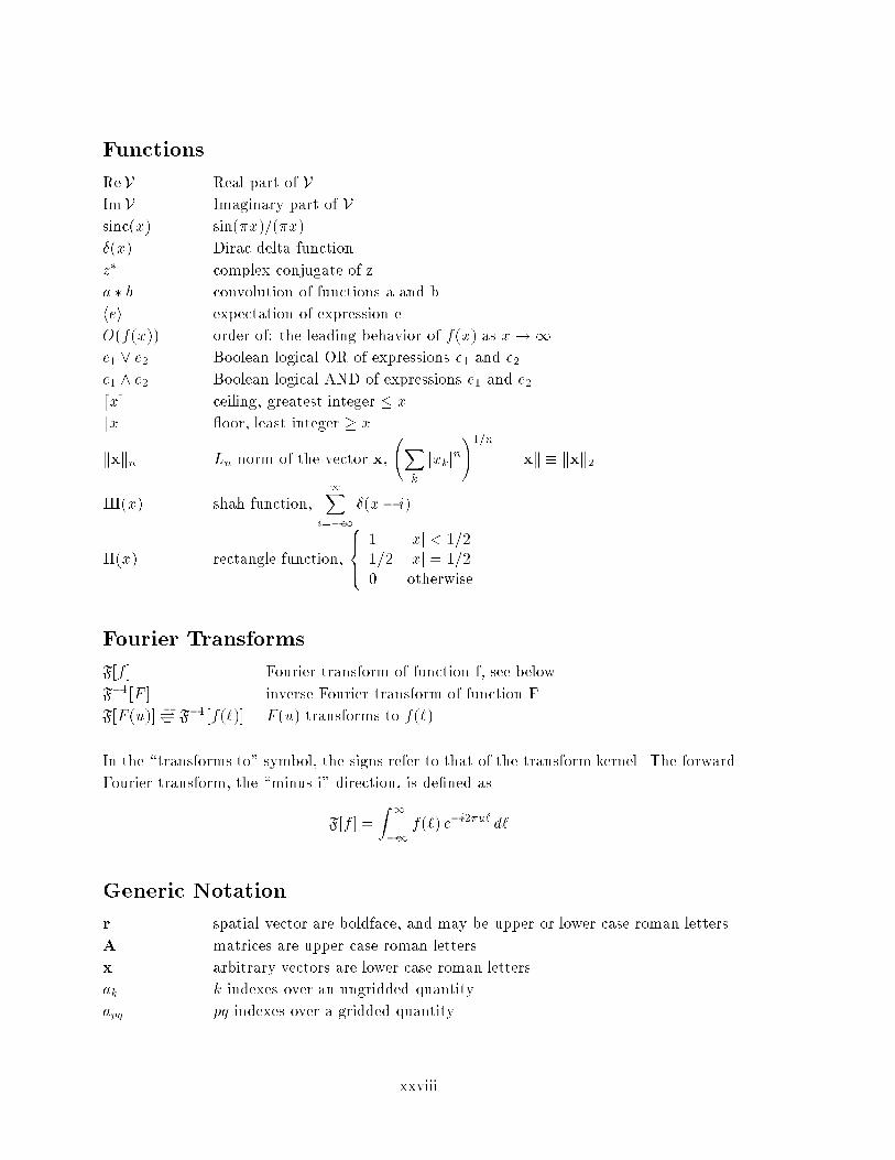
Functions
ReV Real part of VImV Imaginary part of Vsinc�x� sin��x����x�
��x� Dirac delta function
z� complex conjugate of z
a � b convolution of functions a and b
hei expectation of expression e
O�f�x�� order of� the leading behavior of f�x� as x��e� � e� Boolean logical OR of expressions e� and e�e� � e� Boolean logical AND of expressions e� and e�dxe ceiling� greatest integer x
bxc �oor� least integer x
kxkn Ln norm of the vector x�
�Xk
jxkjn���n
kxk � kxk�
X�x� shah function��X
i���
��x� i�
P�x� rectangle function�
������ jxj � ������ jxj ��� otherwise
Fourier Transforms
F$f % Fourier transform of function f� see below
F��$F % inverse Fourier transform of function F
F$F �u�%��� F��$f���% F �u� transforms to f���
In the �transforms to� symbol� the signs refer to that of the transform kernel� The forward
Fourier transform� the �minus i� direction� is de�ned as
F$f %
Z �
��f��� e�i��u� d�
Generic Notation
r spatial vector are boldface� and may be upper or lower case roman letters
A matrices are upper case roman letters
x arbitrary vectors are lower case roman letters
ak k indexes over an ungridded quantity
apq pq indexes over a gridded quantity
xxviii

Chapter �
Introduction
Images are the basic input to spatially resolved studies of nearly everything in
astronomy� In some contexts the problem of imaging is intertwined with additional consid�
erations such as spectroscopy� but in nearly every spatially resolved application there comes
a point where one is interested in making the best images possible given the raw data�
The very concept of �best image� is not easily quanti�able� and will depend on
the application� One might be interested in seeing as much detail in the image as possible
� provided that the detail seen can be believed� One might be interested in minimizing the
cross contamination between di�erent objects in the same �eld� or in recovering a reliable
total �ux in the presence of noise� or in maximizing the sensitivity of the images while
preserving other desirable qualities so far as possible� Or one might even simply desire
the most aesthetic image possible� free of obvious defects and perhaps distorted in some
known way as the easiest image for general morphological understanding� All of this is
hampered by the fact that we generally do not have the true image for comparison� but
there are consistency checks which can be performed to increase the likelihood of telling a
good image from a bad one�
This dissertation addresses a diverse range of topics within astronomical inter�
ferometric imaging� all of which can be loosely grouped together under the topic of �High
Fidelity Deconvolution�� A convolution equation is of the form
f�x� � g�x� �Z �
��f�x�� g�x� x�� dx��
and arises naturally in the analysis of imaging systems� If the imaging system is linear�
f�x� the true intensity distribution� and g�x� the response of the system to a point source�
the measured image is simply f � g�� That is� the convolution of the real sky with the
point spread function �PSF� of the system is a blurring� The inversion of this blurring to
recover the true image is called deconvolution� and is the subject of this dissertation� The
deconvolution problem is naturally addressed in Fourier space� since the Fourier transform
�The blurring is actually the correlation of the PSF with the true image� which is somewhat less tractableanalytically than a convolution� When the di�erence matters� the problem is analysed as the convolutionwith the re�ection of the PSF through the origin� In most interferometric applications� the PSF mustbe symmetric from fundamental considerations� and the di�erence between correlation and convolutiondisappears�
�

�
of the convolution of two functions is the product of their individual Fourier transforms�
F$f � g% F$f %F$g%� where F is the Fourier transform�� In fact� if the Fourier transform of
the PSF is everywhere nonzero� and ignoring the question of measurement error� the direct
solution to the deconvolution problem of determining f from measurements of f � g and gis simply
f�x� F��hF$f � g% � F$g%
i�����
This dissertation primarily concerns interferometric imaging� where the Fourier
transform of the image is measured with an interferometer� Each distinct baseline be�
tween two elements of the interferometer measures the image transform at a speci�c two�
dimensional spatial frequency� �u� v�� The particular spatial frequency sampled is deter�
mined by the geometry of the array and source� In the commonly used technique of earth
rotation synthesis� the relative geometry between array and source changes with time� lead�
ing to a more complete coverage of the Fourier plane� But even with this enhancement�
the coverage of the Fourier plane is less than perfect� The sampling pattern S�u� v�� also
called the u�v coverage� is used to quantify this and is usually a collection of Dirac delta
functions located at the positions of the sampled spatial frequencies� The total information
measured can be represented as S V � where V �u� v� is the transform of the desired image�
Inverse transforming the measured data to the image plane results in the basic convolution
equation that must be inverted�
ID I �B� �����
where ID is the measured dirty image� B is the PSF� and I is the true image that we wish to
determine� ID is the inverse or back transform of SV � B is the back transform of the sam�
pling pattern alone� and is more commonly known as the synthesized dirty beam or point
spread function� Since S F$B% is the analog of F$g% in equation ���� the many zeros present
in the typical sampling pattern show why the simple inverse �ltering approach to deconvo�
lution cannot be used� The unmeasured spatial frequencies are simply not present in the
data� and cannot be recovered by any linear processing� The solution to this deconvolution
equation involves estimating the image at the unmeasured frequencies� and makes implicit
use of a priori information about the image� This a priori information can be that the sky is
mostly empty� that the emission is sitting on an otherwise empty background� that the true
image is constrained to be positive� or more sophisticated measures of image properties such
as smoothness� Many good approaches exist for the solution of equation ���� most notably
CLEAN � Maximum Entropy� but the synthesis imaging art is now well enough advanced
that techniques which were good enough for an earlier generation of instruments are now
found to be lacking in some cases�
�There are several sign and normalization conventions for the Fourier transform in common use� Thisdissertation uses Bracewell�s �System ��� �Bracewell� ��� p� � � and the exact de�nitions are given in thelist of symbols�

�
Some of the techniques developed here will also be applicable to �lled aperture
imaging� such as in conventional optical astronomy� There the convolution equation can
arise as the convolution of the instrument response with the true sky or as a statistical
degradation caused by the atmosphere� The physical reasons resulting in the convolution
equation for �lled aperture and interferometers can be the same� incomplete Fourier cover�
age� but they lead to qualitatively di�erent kinds of �instrumental response�� The purpose
of the deconvolution is typically di�erent� In a �lled aperture case� the PSF is usually well
behaved with modest support� and one can often proceed without deconvolution� The usual
reason for deconvolution is to increase the resolution of the image� By contrast� contem�
porary synthesis imaging instruments typically have Fourier plane coverages which result
in sidelobes at the several to tens of percent level� extending out to in�nity� One must de�
convolve in order to uncover the structure beneath the sidelobes of the brighter sources in
the �eld� The advantage of synthesis imaging is that the array geometry and consequently
the PSF is known a priori to high precision� as opposed to the optical case where it must
usually be measured or approximated� In addition� the Fourier components obtained in
synthesis imaging can conveniently be reweighted to control attributes of the PSF� while at
least some aspects of the PSF are frozen into the optical observation at the time the data
is taken� Collectively� this has resulted in somewhat di�erent attitudes to deconvolution in
the �lled aperture and synthesis imaging communities�
The dissertation title includes the adjective �High Fidelity�� Here this means
both the traditional regime of high dynamic range imaging� where believable structure is
sought around bright objects at peak to o��source RMS dynamic ranges of ���� or more�
and also the low dynamic range regime of super resolution� If high �delity means loosely
�learning something about the source unrevealed by conventional image processing�� then
super resolution is certainly high �delity� It is simply that the conventional base image
for comparison has little high resolution information and any believable high resolution
information is by comparison �high �delity�� Similarly� the de�nition of high �delity is
also somewhat stretched to encompass the new weighting techniques of Chapter �� In
some cases the resolution of the image is increased relative to conventional weightings� and
that is certainly high �delity as just discussed� In other cases the sensitivity limit due to
thermal noise in the receivers is decreased� and this could again be called high �delity when
compared with the conventional higher noise images� The �moderately resolved� in the title
refers fundamentally to the algorithms in the algebraic deconvolution chapter� Because my
interest in the subject of high �delity deconvolution was piqued with compact sources� the
many simulations presented here address this size regime preferentially� For these purposes�
a compact source is one with an area of a few hundred synthesized beam areas or less� The
topic of visibility weighting� which comprises some half the length of this dissertation� is
not limited to any particular source size � though again the particular simulations used
to verify the deconvolution related properties of the weighting happen to use a compact
source�

Beyond the obvious signi�cant results of a new weighting and a new deconvolu�
tion algorithm� a third major conclusion of this work is simply that deconvolution errors
can be signi�cant� even when viewing quite simple emission� and that these errors can often
masquerade as calibration errors� Imaging interferometers have become more capable since
their introduction� and their calibration and use more sophisticated� Deconvolution algo�
rithms which were adequate for earlier use are now found to be undesirable or unsuitable
for some demanding modern projects� The magnitude of the deconvolution errors are larger
than generally appreciated even on perfect data� The deconvolution errors grow worse if the
algorithms are misused� generally meaning insu�cient iteration� And the errors introduced
by the interaction of calibration errors and deconvolution errors can be worse than the sum
of the individual errors� This dissertation includes considerable e�ort trying to quantify
these e�ects� The majority of the simulations address only the deconvolution aspects of the
problem in a lower limit error philosophy� though some have been as end�to�end realistic as
it is possible to do with contemporary software�
��� Overview of Dissertation Structure
The majority of the new techniques are introduced and developed in Chapters ��
and � though some of the more minor �processing tricks� are mentioned in passing in the
case studies of Chapters �&�� Also� the mundane details of some of the weighting techniques
are deferred to the appendices� An e�ort has been made to con�ne images from real data
to the case study chapters� while the examples in the previous chapters are generally from
synthetic data�
In Chapter �� the basic equations of interferometric imaging are derived from
�rst principles� following standard work� The discretization of the continuous equations
is done more carefully than is usual� and the conventional delta function model of a pixel
is generalized to include an arbitrary function as a pixel basis� Some limitations of the
conventional even sized FFTs are discussed and a solution suggested� The chapter concludes
with a discussion of deconvolution issues in general� temporarily ignoring the speci�cs of
individual algorithms�
Chapter � is very long and covers the topic of visibility weighting� It is named
after the primary result of robust weighting� but actually covers a number of weighting
related topics� such as gridless weighting and beam forcing with a generalized Gaussian
taper� This chapter is fairly complete and includes extensive case studies and advice on
how to use existing tools e�ectively and combine them with the new techniques�
By contrast� the algebraic deconvolution Chapter is a very promising beginning�
but far from complete on the topics it addresses� The reintroduction of algebraic techniques
to interferometric imaging has already yielded some spectacular examples compared to ex�
isting algorithms at the highest �delity levels� but it is still very much an active research
topic� This chapter addresses both Singular Value Decomposition deconvolution� which is

�
only adequate compared to existing methods� and Non�Negative Least Squares deconvolu�
tion� which is signi�cantly better than traditional methods for certain regimes of image and
source size� More work needs to be done in exploring the advantages and circumventing the
limitations of these algorithms�
Chapter � is a large collection of simulation results� including an atlas of error
morphologies for the major algorithms on simple sources� and quantitative error curves for
many di�erent algorithms on a wider variety of simple sources� The conclusions from this
chapter are also considered a major result of this dissertation� as the magnitude of these
e�ects had not previously been appreciated� nor the fact that deconvolution errors can often
masquerade as calibration errors�
Chapter is a miscellaneous collection of minor results and techniques that either
did not �t anywhere else� or that would have been too serious a digression in the related
discussion� This includes estimation of the thermal noise from the visibility data� a detailed
discussion of how CLEAN places components around compact sources and the implications
for model��tting� and a discussion of how models from di�erent deconvolution algorithms
may be combined�
Chapter � begins the �rst of three case studies� presenting observational results
from the VLA on the source �C �� As this source was the one which inspired much of the
work in this dissertation� a model of it has been used as a test source in several earlier
chapters� Consequently this chapter is fairly short� with X band images showing that
the weighting and deconvolution techniques do work as advertised on real data� A rather
spectacular L band image shows both the ability of NNLS deconvolution to work on multiple
isolated small sources in a large �eld and also the nonexistence of a potential extended jet
at the ����� dynamic range level�
Chapter � concerns a super�resolved study of the source SN����A with the Aus�
tralia Telescope� The primary algorithm selected for this study was Maximum Entropy
rather than NNLS� though both were used� The work concentrates on how one may best
use existing tools for super�resolved imaging of simple sources� with emphasis on reliability
and avoiding over interpretation� Astrophysically signi�cant and believable structure is seen
in SN����A at a size scale of half the synthesized uniform beamwidth�
The last case study� Chapter � on the source DA���� was part of a test to ex�
plore the limits of the new Very Long Baseline Array� Earlier tests with CLEAN as the
deconvolver had given hints that the compact core might be surrounded by a di�use halo
at the several thousand to one level� Deconvolutions using NNLS showed no such halo�
and simulations of model observations showed NNLS capable of detecting such a halo were
it present� The early NNLS results were later vindicated with noise limited observations
at ������ which also show no halo� This work underscores the importance of NNLS in
the hybrid mapping loop and the importance of gain error correlation structure in good
simulations�

A short summary of the major results of this work is given in the conclusions
Chapter �� Appendices A&E all relate to the visibility weighting chapter� Appendix F
reviews complex Fourier series for Chapter and Appendix G concerns the software package
used for most of the work in the dissertation� and the �nal Appendix H describes how to
obtain several machine readable �les containing more extensive simulation results�

Chapter �
Representation of the Deconvolution Equation
This chapter is a mixture of review� extension� and clari�cation of the basic equa�
tions governing interferometric imaging� We begin with a standard derivation of the theo�
retical measured visibility� making manifest which fundamental assumptions are required for
the particularly simple form of the imaging equations assumed in later chapters� Section ���
derives the form of the continuous dirty map� again following the standard derivation� In
Section ��� we depart from the standard formalism in the discretization of the continuous
equations� We introduce the concept of a continuous pixel model� a limiting case of which
becomes the familiar CLEAN component� This formalism naturally leads to the conclusion
that the component representation is a distinct space from either the image or visibility
data� We demonstrate a problem with the standard representation and transformation of
Hermetian data� and suggest a �x in the form of odd�sized FFTs� The chapter continues
with a discussion of the general issues involved in deconvolution� and concludes with a list
of the particular algorithms used in the dissertation along with a short description of each�
��� The Visibility Equations
In this review section we derive the expected interferometer response to the sky
emission� We start from a very general formulation and introduce su�cient simplifying
assumptions to derive the most common expressions for the observed visibilities� The review
largely follows the excellent derivation by Clark ������� Other modern derivations of similar
and related topics can be found in Thompson ������� Thompson� Moran� � Swenson ������
and Christiansen � H'ogbom �������
The starting point of the formalism is a time�variable electric �eld of astrophysi�
cal origin at location R� in three�dimensional space� This is E�R�� t�� Maxwell�s equations
describe how an electromagnetic wave will propagate from location R� to r� the position
of the later observation� The general time variability of the electric �eld vector introduces
considerable complication into the later analysis� so it is most convenient to work in fre�
quency space� Any �nite interval of a real time varying function can be expressed in terms
of a complex Fourier series� The function is the real part of the sum of complex coe�cients
times a simple time�varying exponential� We can expand each component of the electric
�

�
�eld in such a series� and write
E�R� t� Re
�Xk
E�k �R� e��i�k
�
For our purposes Maxwell�s equations are completely linear �Jackson� ����� pp� �&���� so
we drop this summation and henceforth treat only a single quasi�monochromatic component
of the electric �eld� E� � Invoking that linearity� we superpose the contributions from all
possible sources at the observed position r�
E�
ZZZP��R� r�E��R� dx dydz �����
The function P��R� r� is called the propagator� and describes how the electric �eld at R
a�ects the �eld at r� In full generality� P must be a tensor function to properly account for
the vector nature of E� No polarization phenomena will be treated in this dissertation� so
we may instead take both P and E� to be simple scalars��
The next simplifying assumption we make re�ects the great distances to astronom�
ical sources� We make no attempt to deduce the full three�dimensional spatial structure
of the source� and instead consider the radiation on a given surface� We choose a great
sphere of radius jRj centered on the origin� with the requirement that jrj � jRj�� With thischoice� the electric �eld amplitude on that surface is simply related to the surface bright�
ness� The geometry is given in Figure ���� Having assumed the celestial sphere� we next
assume that space within it is empty� The propagator can be written down simply from
Huygen�s Principle� and equation ��� becomes
E��r�
ZE��R�e
��i�jR�rj�c
jR� rj dS� �����
where dS is the element of surface area on the celestial sphere�
Now consider the spatial correlation of the electromagnetic �eld� This correlation
is de�ned at the points r� and r� by V��r�� r�� � hE��r��E���r��i� The raised asterisk
is a complex conjugate� and the angle brackets indicate an expectation value over time�
Substituting equation ��� for E� and rearranging the integrals over two separate surface
elements� this becomes
V��r�� r��
�ZZE��R��E�� �R��
e��i�jR��r�j�c
jR� � r�je��i�jR��r� j�c
jR� � r�j dS� dS�
�
�Since propagators encountered in practice merely rotate the plane of polarization and preserve the totalintensity� the scalar formalism above is exact for total intensity� even when observing intrinsically polarizedsources�
�The actual requirement for synthesis imaging is that the angle formed by two telescopes and the objectof interest be much less than a fringe spacing� or that jRj � jr� � r�j���

�
R
νε ( )R
Eν R
r
Object
Observer
3)(
Figure ���� Radiation on the Celestial Sphere� adapted fromClark ������� The only quantitywe may measure with synthesis imaging is the equivalent radiation �eld on the surface ofthe celestial sphere� E�R��
The next simplifying assumption is that astronomical sources are not spatially coherent��
that is
hE��R��E��R��i hjE��R�j�i ��R� �R��
For most objects� spatially incoherent emission is an excellent assumption� The notable
exception occurs when a compact source is viewed through a scattering screen such as
the interplanetary medium near the Sun� Special techniques must be used to image such
sources� as detailed in Anantharamaiah et al� ������ This will not be discussed further in
this dissertation� Using the linearity of the expectation value� we exchange the expectation
and integration to give
V��r�� r��
Z DjE��R�j�
E e��i�jR�r� j�c
jR� r�je��i�jR�r� j�c
jR� r�j dS
�There is a signi�cant detail glossed over here� It is not the radiation E�R that is incoherent� but E�R �The free space propagation of the wavefront from the actual source to the celestial sphere does not changethe coherence properties� however�
�
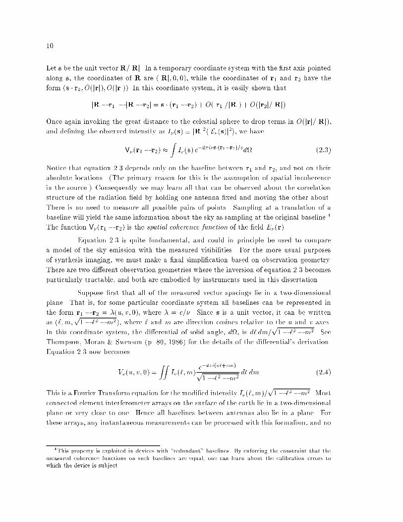
Let s be the unit vectorR�jRj� In a temporary coordinate system with the �rst axis pointedalong s� the coordinates of R are �jRj� � �� while the coordinates of r� and r� have theform �s rk� O�jrj�� O�jrj��� In this coordinate system� it is easily shown that
jR� r�j � jR� r�j s �r� � r�� !O�jr�j�jRj� !O�jr�j�jRj�
Once again invoking the great distance to the celestial sphere to drop terms in O�jrj�jRj��and de�ning the observed intensity as I��s� � jRj�hjE��s�j�i� we have
V��r� � r�� �ZI��s� e
���i�s��r��r���cd( �����
Notice that equation ��� depends only on the baseline between r� and r�� and not on their
absolute locations� �The primary reason for this is the assumption of spatial incoherence
in the source�� Consequently we may learn all that can be observed about the correlation
structure of the radiation �eld by holding one antenna �xed and moving the other about�
There is no need to measure all possible pairs of points� Sampling at a translation of a
baseline will yield the same information about the sky as sampling at the original baseline��
The function V��r� � r�� is the spatial coherence function of the �eld E��r��
Equation ��� is quite fundamental� and could in principle be used to compare
a model of the sky emission with the measured visibilities� For the more usual purposes
of synthesis imaging� we must make a �nal simpli�cation based on observation geometry�
There are two di�erent observation geometries where the inversion of equation ��� becomes
particularly tractable� and both are embodied by instruments used in this dissertation�
Suppose �rst that all of the measured vector spacings lie in a two�dimensional
plane� That is� for some particular coordinate system all baselines can be represented in
the form r� � r� ��u� v� �� where � c��� Since s is a unit vector� it can be written
as ���m�p�� �� �m��� where � and m are direction cosines relative to the u and v axes�
In this coordinate system� the di�erential of solid angle� d(� is d� dm�p�� �� �m�� See
Thompson� Moran � Swenson �p� �� ���� for the details of the di�erential�s derivation�
Equation ��� now becomes
V��u� v� � ZZ
I����m�e���i�u��vm�
p�� �� �m�
d� dm ��� �
This is a Fourier Transform equation for the modi�ed intensity I����m��p�� �� �m�� Most
connected element interferometer arrays on the surface of the earth lie in a two�dimensional
plane or very close to one� Hence all baselines between antennas also lie in a plane� For
these arrays� any instantaneous measurements can be processed with this formalism� and no
�This property is exploited in devices with �redundant� baselines� By enforcing the constraint that themeasured coherence functions on such baselines are equal� one can learn about the calibration errors towhich the device is subject�

��
other assumptions about geometry need be taken into account� For earth rotation synthesis
instruments� however� the baselines will rotate about an axis parallel to that of the earth�
�Visibilities are invariant to baseline translation�� The only arrays which will remain planar
after earth rotation synthesis are east�west arrays� which are popular for this and other
reasons� In Chapter � we present data and images from the Australia Telescope compact
array� which is just such an instrument�
A similarly useful form of the visibility equations results when all sources con�
tributing to the visibility are in a small region of the sky� This form is used when processing
data from intrinsically three�dimensional arrays like the VLBA or two�dimensional arrays
like the VLA used in earth rotation synthesis mode� Data from both these arrays are used
extensively in later chapters� A convenient way to quantify the �small region� concept is
to de�ne s s� ! � and ignore any terms of order j�j�� An immediate consequence of thefact that s and s� are unit vectors is that
� s s s� s� s� s� ! �s� � ! � � � � ! �s� �� �����
so that s� and � are orthogonal� If we choose the w axis to lie along s�� we have r� � r�
��u� v� w�� s� �� � �� and � � ���m� �� Again ignoring terms of order j�j�� we drop thep�� �� �m� term in the di�erential of area and equation ��� becomes
V ���u� v� w� e���iw
ZZI����m� e
���i�u��vm� d� dm ����
It is conventional to absorb the leading exponential term into the left hand side� by con�
sidering the modi�ed quantity V��u� v� w� � e��iwV ���u� v� w�� The resulting equation is
independent of w�
V��u� v�
ZZI����m� e
���i�u��vm� d� dm �����
Finally� we have to account for the directivity of the individual antenna elements�
The individual elements of a radio interferometer do not measure the electric �eld at a single
point� but rather have an angular sensitivity to the direction of the radiation�s propagation�
Thus in equation ��� the integral should be weighted by the antenna directivity� A��s�� which
a�ects all subsequent equations to this point� The antenna directivity can also be called
the primary beam or normalized reception pattern� In particular� equation ��� becomes
V��u� v� ZZ
A����m� I����m� e���i�u��vm� d� dm �����
�Alternatively� this factor may be grouped with the antenna directivity� A����m � in equation ��� Thisis not terribly important� since the dominant source of approximation error comes from the treatment of theexponential�

��
The quantity V��u� v� is called the complex visibility relative to the phase tracking center�
If the two antenna elements are dissimilar� as is frequently found in Very Long Baseline In�
terferometry� the appropriate directivity correction is geometric mean of the two individual
antenna patterns�pA� ����m�A�����m�� VLBI is also the case where the sources imaged
are often su�ciently small that the e�ects of the individual primary beams can be ignored
all together�
Equation ��� is the simplest form of the visibility equation� and will be used for
all subsequent derivations� The alternative geometrical assumption and the correction for
the antenna elements simply modify the form of the e�ective sky brightness� All corrections
of this form should be deferred until the �nal stage of image processing� at which point they
are trivially accounted for� It should be noted that while the antenna directivity appears to
be a nuisance factor� it is this directivity that allows the small region of sky approximation
to be widely used�
In principle� the instrumental response could be made to approach that of an
ideal quasi�monochromatic component by observing with a negligibly small bandwidth� In
practice� observations are often made with a fractional bandwidth of a few percent� and the
measured visibility is reasonably well described by the monochromatic visibility at the center
of the band� The visibility amplitude is modulated by the transform of the instrumental
bandpass� The e�ect in the image plane is to smear sources radially towards the delay
center� with the magnitude of the smear varying linearly with radius� This smear can be
largely removed in software� but such �xes are rarely necessary� A more direct cure is to
observe in spectral mode� where the e�ective bandwidth is divided by the number of spectral
channels� In such a mode� bandwidth smearing is usually quite negligible� The e�ect of
�nite averaging time per visibility measurement also produces a smear whose magnitude
varies linearly with radius from the delay center� but the smear direction is tangential� Time
averaging is considered in the context of visibility weighting� otherwise� neither of these two
e�ects are considered further in this dissertation�
�There are a number of �ducial points on the sky used in interferometry� The pointing center of the arrayelements is �xed at the time of the observation� The delay tracking center is �xed at correlation time� andis that point on the sky where the e�ective path length after compensation is the same for all antennas�Bandwidth smearing e�ects are centered on the delay center� The phase tracking center is de�ned as thatpoint for which a point source has zero expected visibility phase on all baselines� This may be shifted afterthe fact by merely adjusting the phase of the visibility measurements� The phase center determines the centerof the synthesized images� The tangent point is determined by the vector s� in equation ���� and concernsthe mapping from the curved celestial sphere to Cartesian coordinates� Geometric distortions will be leastnear the tangent point� The tangent point may also be shifted after the fact but requires recalculation ofthe u�v� and w coordinates as well as the phase terms� In simple observations� all four of these positions arethe same point� However in a mosaiced observation one may use multiple pointing centers to cover a largeobject� In a VLBI experiment� bandwidth e�ects may limit the �eld of view to a small region about thedelay center� and the data may be correlated more than once with di�erent delay centers� The phase centeris shifted routinely to move interesting positions to the center of the images� If the shift is large enough thatgeometric distortion is important� the tangent point may be moved as well�

��
Summarizing� the simpli�cations necessary to go from the most general formula�
tion of the electric �eld to the simple Fourier transform formalism are
� Analysis in pseudo�monochromatic components Essentially no approximation nec�
essary
� Celestial sphere Cannot get depth information about source
� Polarization phenomena ignored Not needed here
� Space is empty No propagation e�ects
� No spatial coherence Very rarely violated
� Measurements con�ned to a plane or All sources in small region
These assumptions can be relaxed in software
��� The Continuous Dirty Map
Equation ��� is obviously a Fourier transform relationship� Were V �u� v� known
completely� we could simply use the direct inversion for I���m�� namely
I���m� ZZ
V �u� v�e��i�ul�vm� du dv �����
However� a major di�culty is that the visibility function is only sampled incompletely on
the u�v plane� We introduce a sampling function� SV �u� v�� which is zero where no data has
been taken� A convenient factorization of this function which re�ects the discrete nature of
the sampling process is
SV �u� v� �NVXk��
wk ��u� uk���v � vk� �����
where the uk and vk are the coordinates of the sampled data� Note that wk is a weight
here� and not the third Fourier coordinate� The notation is unfortunate� but widely used�
wk as a Fourier coordinate will not subsequently be used in this dissertation� The choice
of wk is completely arbitrary� and selection of these weights allows the user to adjust the
balance between angular resolution� sidelobes of the beam and sensitivity� This topic will
be covered extensively in Chapter ��
We now have su�cient information to calculate a quantity we will call the con�
tinuous dirty map� �The terms map and image are used synonymously in this dissertation�
as are dirty beam and point spread function��
ID���m�
ZZV �u� v�S�u� v�e��i�ul�vm� du dv ������

�
The convolution theorem for Fourier transforms immediately leads to the conclusion that
ID I �B ������
where
B���m�
ZZSV �u� v�e
��i�ul�vm� du dv ������
B is called the synthesized dirty beam� and in general will contain many sidelobes and
unpleasant artifacts of the sampling� It is precisely this convolution of the dirty beam with
the original sky brightness that we wish to invert with the deconvolution algorithms� Since
the sky brightness is known to be real� the visibility data is constrained to be Hermetian�
Thus without loss of generality� we may take SV �u� v� to be symmetric about re�ection
in the origin� This property is then shared by the synthesized beam� which will turn out
to be quite important later� Note also that even before this equation is discretized� there
is no possibility that the deconvolution is unique� Any function "V �u� v� which is equal to
V �u� v� on the support of S�u� v� will have a Fourier transform "I���m� which satis�es the
convolution equation� It is the introduction of additional information about the source by
the deconvolution algorithms which allows us to select between the alternatives�
��� Discretization of the Continuous Equations
Even given the discrete nature of the visibility sampling process� the resulting
convolution equation is continuous� To obtain a set of equations that can be manipulated
by a computer� we need to discretize the continuous equation� Here we do the discretization
in some detail� The standard formalism is generalized to allow for a more general �pixel
model� than the usual scaled delta function� For simplicity of notation� we return to the
one�dimensional case� This is not limiting� in that the argument below can be directly
generalized to the two�dimensional case� much as described in Appendix A of Andrews �
Hunt ������� We begin with equation ����� ID I � B� To invert this convolution� weshall �nd some deconvolution model function� C� such that ID C � B� Under somecircumstances� C may have a direct relationship to I � but for the moment this equation
should be taken as the sole de�nition of C� In particular� we should not blindly apply
physical arguments about the positivity or support of I to C� The name C is to suggest a
Component model� and later on the scalar coe�cients of this model will become the familiar
CLEAN Components� Remember� however� that C��� is a continuous function�
To discretize this equation� we de�ne an image sampling function in analogy to
the visibility sampling function de�ned earlier� Since this function will be used only to force
agreement at the sampled points� there is no need for normalized weights�
SI �N�Xi��
���� �I i� ���� �

��
Most often� we discretize to a regular grid� in which case SI becomes an ordinary shah
function� X���#��� See Bracewell �p� ��� ����� for properties of X� This is solely for
computational convenience� however� The only fundamental limit is set by the criterion
that the sampled visibility must not be aliased� That is� we require that
$V �u�SV �u�% � F$SI���% V �u�SV �u� ������
on the support of SV �u�� For the �nite� regular sampling case� this will be satis�ed auto�
matically if the maximum value of u on the grid� "umax� is greater than the maximum value
of u present in the data� umax� �"umax is set by the frequency of sampling in the image plane�
"umax ���#��� Incidentally� it is this equation which allows us to ignore the high spatial
frequencies which may be present on the sky� The aliasing constraint applies to V �u�SV �u�
not merely V �u�� By de�nition� we have that
IDSI �C �B�SIID��I i� �C �B���I i� �i �� � � � � N�� �����
Z �
��C����B��I i � ��� d��
In general� this is an integral equation� and is di�cult to solve� To progress further� we
must assume a form for C����� It is this arbitrary assumption about the form of C that
severs the link between C and I � We may choose a form for C whose transform is complete
in the visibility plane� �any possible measured visibility function may be represented in this
form�� but there is no guarantee that I or any given function of I may be representable in
the form of C� This is one basis for the statement� CLEAN components model the visibility
data� not the image data� Under some circumstances� it may develop that C becomes a
known function of I � but this is not guaranteed� A second justi�cation for this statement
will be given later in this chapter� and yet a third in Chapter �
Since the Fourier transform is linear� it is convenient to form a model from a linear
combination of components� Each component can be transformed independently into either
domain� Indeed� this property is crucial to the operation of CLEAN and most deconvolution
algorithms� The most general model consistent with our obtaining a discrete convolution
equation is a sum of shifted and scaled replications of some basic pixel model� While a more
complicated model could be used� the algorithm becomes a general model �tting procedure�
and this formalism is no longer appropriate� We thus assume the following form for C
C��� �NCXj��
CjP ��� �C j� ������
NCXj��
Cj �P ��� � ���� �C j��
The term CjP ����C j� is a model component �or generalized CLEAN component�
of magnitude Cj� centered at the location �C j � The function P ��� is the pixel model� If

�
we take P ��� ����� we recover the usual formalism� In addition� the �C j are usually
constrained to be integral multiples of some #�� If the �C j are determined in advance� �such
as the above constraint to a regular grid�� then the convolution process will reduce to a single
matrix multiplication� and the determination of the Cj requires the conceptual �pseudo�
inversion of this matrix� In some deconvolution algorithms like CLEAN� the determination
of the Cj are done iteratively� and the location of the nonzero Cj are determined from the
possible set f�C jg �on the �y�� The CLEAN algorithm can be extended� to determine the
unconstrained �C j on the �y� which leads to the �fractional cell CLEAN�� This modi�cation
is potentially fairly important� but the algorithm no longer �ts into the matrix formalism
and is quite di�cult to analyze� Assuming that the �C j have been predetermined in some
manner� with N potential positions� then equation ��� becomes
�for i �� � � � � N��
�C �B���I i�
��NCXj��
Cj �P ��� � ���� �C j��
A �B
A ��I i�
Z �
��
NCXj��
Cj
Z �
��P ��������� � �C j � ���� d���B��I i � ��� d�� ������
NCXj��
Cj
Z �
��P �����B��I i � �C j � ���� d���
If we write
B��I i � �C j � ���� B��� � ���� � ���� � �I i ! �C j�
then we have that
�C �B���I i� NCXj��
Cj
Z �
��P �����
Z �
��B��� � �������I i � �C j � ��� d�� d���
NCXj��
Cj �P ��� �B������I i � �C j�� ������
We can identify this last equation as a matrix equation of the form Ax b�
��Extended� is actually the wrong word here� Implementations of exactly this local �tting procedurehave been around nearly as long as the original algorithm� But in modern usage it has fallen somewhatout of favor and there is no literature on its analysis � the regular spacing CLEAN is di�cult enough toanalyse�

��
NC
rows
���������������
������� P �B
��������
� �z �N� columns
���� Cj
��������������
N�
rows
������� C �B
��������
���������������
NC
rows�����
P is not necessarily symmetric� although B must be so� Thus in general� P � Bwill not possess any particular symmetries� More usually� P � B� and P � B will all be
symmetric� We will write P �B as B� and refer to it as the modi�ed beam matrix� In the
standard case of � function components� P � �B B�
��� Convolutional Gridding and Aliasing
The formalism is now complete to the extent that the equations could be solved
with a su�ciently powerful computer� We would need to know an analytic form for the
inverse Fourier Transform of P � and apply it to all the weights wk� We would then have
to �nd the forward transform of both the modi�ed weights and the unmodi�ed visibility
samples V �uk�� the beam being evaluated at all points �I i � �C j � and the dirty map at all
points �I i� Remembering that �C � B���I i� �I � B���I i� by de�nition� we insert thesevalues into equation ����� and solve the resulting set of �probably singular� linear equations
for the Cj�
The problem with this direct approach is that it is a formidable computational
challenge for contemporary problems� It is not unthinkably large � we will use exactly
this algebraic approach in Chapter and the computation of Fourier transforms by direct
summation over visibilities is practical for some problems� if too slow to be used in an
iterative manner� We would very much like to use a Fast Fourier Transform� which o�ers
savings in computation times of order N� log�N � where N is the number of pixels in the
transform� The use of an FFT for the computation requires that the data be evenly spaced�
and that the number of elements be highly composite� The evenly spaced criterion leads us
to choose �I i i#� and �C j j#��� Immediately we get that �I i � �C j �i� j�#�� and
the matrix P �B becomes Toeplitz in form� Symmetries in the FFT further force the form
of the matrix to a symmetric circulant matrix� This introduces additional approximations
which can either be tolerated or eliminated by embedding P � B into a larger matrix of
twice the size� But most important of all is that the data in both domains must be regularly
spaced� We had the freedom to choose where we enforced agreement between the dirty
component model and the dirty sky� We had the freedom to choose where we allowed
Obviously this can lead to some creative indexing� i � �� �I i � � is the center of the map�

��
model components to be placed� But we have �in most cases� no control at all over the
detailed placement of the visibility sampling�
The visibilities are usually forced to a grid by evaluating at the grid points a
convolution of the visibilities with some function of modest support� To �rst order� this
convolution is simply a multiplication by the transform of the gridding convolution function
in the image plane� As such� it is easily divided out again� The problem enters because the
convolved function is resampled in the u�v plane and it is the transform of the resampled
function which is corrected for the original convolution� The aliasing introduced by the
resampling cannot be divided out� Modern mapping programs use a convolution function
whose transform has a fairly sharp cuto� at the edge of the image plane� This provides at
least two orders of magnitude isolation at the edge of the map between aliased power and
its image in the �nal corrected map� The map center typically has four orders of magnitude
isolation� The details of the convolutional gridding and the consequent aliasing can be
found in Schramek � Schwab ������ and references therein� We will not be particularly
concerned with aliasing in this dissertation as most of the simulations are run with models
discretized in the image plane where gridding is not an issue� In the remainder of the image
processing� we are usually concerned with compact sources far from the edge of the images
where aliasing is the worst� There have been no signi�cant observed discrepancies which
could be attributed to convolutional gridding or other aliasing e�ects� The other property
that the use of FFTs forces upon us� that the vector length be highly composite� is worth
a bit more comment�
��� Limitations of the even�sized FFT
Since Fourier transforms are central to most of our image processing algorithms� it
is surprising that there are still some fundamental facts about the discrete Fourier transform
of Hermetian data that are unappreciated in the interferometry community�
With the common choice of u�v origin on a pixel center and the standard power�
of�� restriction on FFT size� the discrete sky and visibility planes are not exact Fourier
transform pairs�
The problem is that if the u�v origin is at the center of a pixel� as is normally
desired� the imaginary part of that pixel is constrained to be zero since the image plane
data is real� The Real � Imaginary FFT routines that we use are strictly reciprocal� so
the number of degrees of freedom in the data set is reduced by one and must appear else�
where� The last degree of freedom appears as the real part of the highest spatial frequency�
That is� if the real data spans ��N�� ! ���N��� � � � � N���#�� the Fourier data will span�� �� � � � � N���#u� but the imaginary part of the u and the u N��#u samples will
SDE uses the routines rfftf and rfftb from �Swarztrauber� �� �

��
be forced to zero by the mechanics of the transform� One can see that this is plausible
by remembering that the real property of Fourier transformed Hermetian data comes from
the symmetry property V ��u� V ��u�� In the discrete transform� every element of the
vector is conceptually paired with a conjugate pixel on the other side of the origin� out to
the same length as the real vector� The conjugate pixel is redundant� of course� and not
actually stored� But pixel corresponding to u N��#� has no conjugate element� as that
would result in a vector longer than the original real vector� If the output is to be real�
V �N��#�� must be forced real� When going in the direction Real � Complex� this last
element will simply appear with zero imaginary part� or will be packed in with the �rst
pixel and the application programmer sets the imaginary part to zero when using it� But in
going the Complex � Real direction� the best that can be hoped is that the imaginary part
of that pixel will be ignored or that the mechanics of the packing implicitly assume it to be
so� In some cases� however� the FFT routine will actually get the wrong answer when the
imaginary part of the last pixel is nonzero� And in no case will one be able to �ll the full
complex vector with nonzero values� transform to the real domain and back and preserve
the last pixel� In this sense� the transform is nonreciprocal� though of course from degrees
of freedom arguments� no transform could be so on vectors of even size�
We normally do not see this e�ect� since in the cases where we start in the Fourier
domain� the sampling pattern of the interferometer forces the last row and column of the
gridded data to be zero or very nearly so� In cases where we are transforming data with
nonzero values out to the edge of the Fourier plane� the data has probably been generated in
the image plane as model components� and the requirement that the last row and column be
real is enforced implicitly in the Real � Complex transform� The only time this would be
noticed is if one started in the Fourier domain with a model� transformed to the real domain
and back and compared the results to the original� I know of no algorithms currently in
routine use where this operation is important� In situations where it does matter� the e�ect
can be avoided by the use of an odd�sized FFT� The �N ! � real values exactly map to the
��N ! ��� � values in the complex vector with the imaginary part of the origin pixel heldat zero� In the next section� it�s shown that one need not pay an excessive computational
price for the use of an odd�sized vector�
����� Non�Power�of�� FFT Performance Analysis
Conventional wisdom usually holds that Fast Fourier Transforms are most e�cient
when the size of the data vector is a power of �� This is indeed true� but such knowledge
has often been unfortunately extrapolated to mean �greatly more e�cient� than transforms
on other sizes� Surprisingly� this is not necessarily true� Figure ��� shows the measured
execution times vs data size for one particularly good scalar FFT package that is widely
used and freely available� �Swarztrauber� ������ The upper panel shows that there are
clearly many bad choices of data size� As would be expected� the uppermost trace is the
line of primes� and succeeding lower traces are generated by numbers of the form �p� �p

�
Figure ���� Normalized FFT runtimes vs� data size� The O�N logN� asymptotic behaviorof the algorithm has been divided out of the measured runtime� Average runtimes weremeasured on an unloaded Sparc IPX running the subroutines CFFTI� CFFTF� and CFFTB
from �Swarztrauber� ������ Even sizes are represented with x symbols� and odd sizes withthree pronged stars� The �lled symbols are pure powers of � and ��

��
and so forth� However� if we examine the lower panel� we see that there are many sizes
that are nearly as e�cient as �N � The runtime of this algorithm on vectors of size �N
was comparable or better than that of several common algorithms restricted to this form�
The lower envelope of Figure ��� was drawn by hand� and this was used to determine the
e�ciency loss for a given data size in the obvious manner�
From this� we estimate that if one picks a random odd number within the exam�
ined range of ��&����� one has only a ���� chance of selecting a size with an e�ciency loss
less than ���� Even if one were to deem an e�ciency loss of �� acceptable� doubling the
runtime� one has only a ����� chance of selecting such an odd number by chance� However�
the distribution of highly e�cient odd numbers is such that one can typically select an
e�cient data size no more than �&�� larger than the actual data vector� If the size of the
data vector is �xed in advance� the need for padding to the next higher power of �� �with
its attendant potential for aliasing�� is reduced or eliminated� Similarly the non�Hermetian
e�ects described in this section are avoided� Since the one�dimensional FFT runtime scales
like N lnN � saving an average of �� in the necessary vector length more than outweighs
the typical e�ciency loss of ��� seen for odd sizes�
Two�dimensional FFTs can be viewed as iterated one�dimensional FFTs � they
are often calculated by taking the FFT of each column and then subsequently taking the
FFT of each row� Native two�dimensional FFTs exist� and are usually more e�cient by a
small constant factor in execution time than the iterated one�dimensional FFT� The scaling
of N logN along each axis still holds and the execution time of either approach for a square
N�N image scales as N� logN � I do not know if a good two�dimensional FFT algorithm
exists for an arbitrary length along each axis� �SDE uses iterated one�dimensional FFTs�� so
the execution time argument here becomes somewhat weaker compared to two�dimensional
power�of�two FFTs if a two�dimensional arbitrary�size routine is not available� But notice
that for large images or even large image cubes� the savings in disk space alone may be
su�cient to justify iterated one�dimensional arbitrary�size FFTs� Table ����� lists all highly
e�cient odd sizes in the range ��&����� as measued on a scalar workstation� These numbers
are not necessarily correct for more exotic machine architectures� but still indicate that the
performance issues should be examined� Table ����� lists all e�cient sizes in that range�
both even and odd� but does not show factorization or loss�
One may object that image sizes are often picked for convenience� and that for
many purposes the exact �eld of view of an image is not terribly important� In such
situations� researchers habitually choose image sizes of the form �N and padding losses do
not apply� However� in this case it is just as easy to pick a convenient odd image size
as �N � For example with images sizes of �� or ��� instead of ����� the e�ciency loss
is negligible and one gains the bene�t of an unambiguous image center and freedom from
Hermetian concerns� Consider that nearly any image processing package will place the
reference pixel of a �k ! � pixel axis at the k! �th pixel� but for a �k pixel axis the choice
is not clear� Di�erent packages use either the kth or the k!�th pixel� and AIPS even uses

��
a di�erent convention on each axis� This makes transportation of images between packages
more di�cult for no particularly good reason�
There is a practical danger in the use of arbitrary�N FFTs in contemporary pack�
ages� Power of � FFTs have dominated the �eld for so long that library subroutines often
assume without documentation that image sizes are even or �N � Assumptions about the
location of the phase center of the transform can be subtle and deeply imbedded in the
code��� Consequently one may have less con�dence in FFT based results from these pack�
ages when using arbitrary�N FFTs� The images in this dissertation have generally been
made with sizes of �N for this reason� since there seemed no problem in these cases with
the Hermetian representation� and images sizes were otherwise arbitrary� But transition
uncertainties should not blind us to the fact that arbitrary�N FFTs are clearly superior for
some purposes� and insistence on �N image sizes is archaic� Even if older software is not
converted� we must strive to avoid introducing this restriction into future packages�
There is no reason to restrict FFT data sizes to powers of �� and occasionally
good reasons to avoid it�
��Even worse� in packages such as SDE which transform into the complex half plane� the size of the imageplane axis conjugate to the short Fourier plane axis may not be stored explicitly� If image sizes �prior toentering the FFT are constrained to be even� this may be recovered by calculation� When this constraint isrelaxed� there is a fundamental loss of information and the backtransformed image size is uncertain by one�Retro�tting such older software can be di�cult�
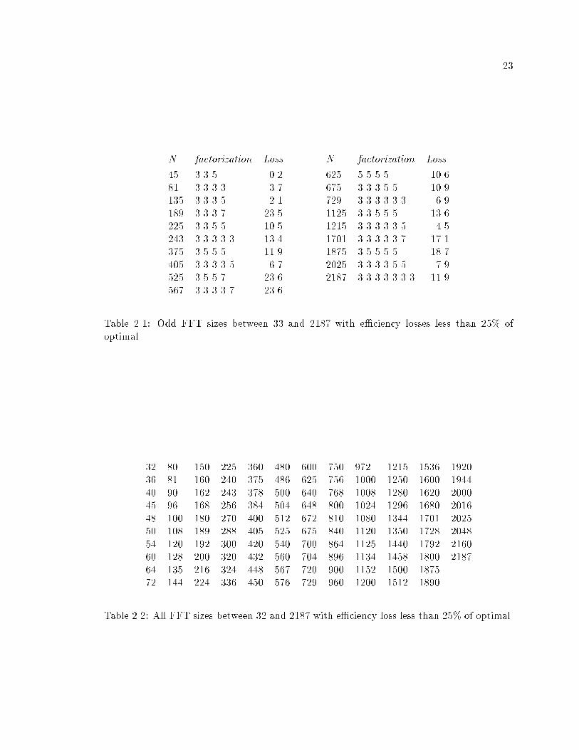
��
N factorization Loss N factorization Loss
� � � � �� �� � � � � ���� � � � � ��� �� � � � � � ������ � � � � ��� ��� � � � � � � ����� � � � � ���� ���� � � � � � ������ � � � � ��� ���� � � � � � � ��� � � � � � � ��� ��� � � � � � � ������� � � � � ���� ���� � � � � � ���� � � � � � � �� ��� � � � � � � ������ � � � � ��� ���� � � � � � � � ������ � � � � � ���
Table ���� Odd FFT sizes between �� and ���� with e�ciency losses less than ��� ofoptimal�
�� � �� ��� � � �� ��� ���� ��� ���� �� � � ��� � �� �� � ��� � �� � �� � � ��� � �� �� ��� �� � � � �� �� �� � � � �� ��� �� �� � � �� �� ��� �� �� �� �� ��� ���� �� ��� ��� � ��� �� � ��� ��� ���� � �� �� ��� � � � � � ���� � ���� �� ��� � �� �� � � �� ��� � �� �� ���� ��� �� �� � �� �� � ���� �� ������ � �� �� � �� ��� � �� ���� ���
Table ���� All FFT sizes between �� and ���� with e�ciency loss less than ��� of optimal�

�
��� Deconvolution
We conclude the chapter with a discussion of the basic issues involved in decon�
volution algorithms� followed by a list of the particular algorithms used in this dissertation
and a short description of each one�
All deconvolution algorithms accumulate some model of the sky�� either itera�
tively or via a direct solution� The model is convolved with the point spread function and
di�erenced with the dirty image� yielding the residuals� The sky model may possess nonzero
spatial frequencies out to the maximum gridded spatial frequency determined by the pixel
spacing on the sky� or the spectral power may roll o� at the higher spatial frequencies
due to a smoothness constraint imposed by the particular algorithm� In either event the
model generally possesses power at frequencies not measured� both interior to and exterior
to the maximum measured spatial frequency� The spatial frequencies estimated beyond
the sampling envelope are somewhat suspect and instead of trying to recover the model
which exactly reproduces the data at all possible spatial frequencies� we generally agree to
seek a model which yields a good reconstruction of the sky at some �nite resolution� Con�
sequently� the model produced by the deconvolution algorithm is usually smoothed down
by convolution in the image plane with a Gaussian �restoring beam� �tted to the main
lobe of the point spread function� This is a multiplication of the model by a Gaussian in
the Fourier domain� In practical terms� the highest measured spatial frequency is usually
down�weighted to of order �� the unsmoothed value for a uniformly weighted PSF� and
to less than a few percent if the restoring beam is �tted to the naturally weighted PSF� In
order to give a reasonable indication of the thermal noise present in the data and account
for the unmodelled residual �ux so far as possible� the �nal restored image is usually formed
from the smoothed model plus the residuals� The practice of adding the residuals back to
the restored image is now nearly universal in the radio community� but was not so in the
past� The optical community seems not yet to have come to a consensus� with some prac�
titioners publishing the raw model from the deconvolution algorithms and others following
the modern radio practice�
There are a few subtleties in this general process� First� the truth image sought
by the algorithm is the actual sky smoothed down to a �nite resolution� But more specif�
ically� it is the smoothed true sky sampled at the image grid points� and not the sampled
sky which is then smoothed� Clearly� something like this must be the case� or a point source
between pixels would yield zero� In many of the simulations in this dissertation� the distinc�
tion is dodged entirely by discretizing the model in the image plane and convolving with
the discretized point spread function yielding a dirty image entirely free of representation
��Once again� I prefer to consider the component model as a representation of the visibility data� notthe sky� None the less� the term �sky model� is too vivid a description to discard entirely� It simply mustbe remembered when discussing aliasing or detailed representation questions that the term is a convenientabbreviation� and not the literal truth�

��
e�ects� In others� the analytic model used to generate the visibilities was smoothed analyt�
ically and the resulting model discretized to provide the comparison image� Comparing the
deconvolved images to a sampled and smoothed model made a considerable di�erence and
was clearly the wrong approach�
There is no really fundamental reason why the restoring beam should be �tted to
the main lobe of the PSF� If all the �ux in the source has been transferred to the model�
then all the restoring beam does is express how much con�dence we have in the high spatial
frequency estimates� In general� using a smaller restoring beam will allow more of the
extrapolated high spatial frequencies into the solution and the deconvolution errors will
become worse� �This statement is not new� but one of the results of this dissertation is a
striking demonstration of how dramatic an e�ect it is�� There is not even any particular
reason that the restoring beam should be a Gaussian� One obvious choice might be the
function which is unity inside the sampling envelope and zero outside it� In such a case� the
restoring beam would allow estimates of the visibilities at spatial frequencies where they
can be interpolated� but would not allow any extrapolation at all� Obviously� in such a case
the restoring beam would look roughly as bad as the dirty beam itself� so such a literal
approach would not be useful� But the principle remains that we do not solve for the sky
so much as for a known function of the sky� One tries to select a function which minimizes
the error in reconstruction yet which allows the extraction of as much useful information
from the image as possible � but the choice is still an arbitrary one�
The one property that a �tted beam does have as a restoring beam is that it
preserves the �ux scale so much as is possible on the residuals� in the event that not all
the �ux is transferred to the model� The only ��ux scale� that the residuals or the dirty
image have is that a point source of magnitude S will have a peak response of S on the
dirty image� No similar statement can be made at all about extended sources� which is
one very good argument for deconvolution in the �rst place� By contrast� the units of the
deconvolution model are usually Janskys per pixel��� The same point source will now have
magnitude S in the component model as well� but it will only occupy one pixel rather than
a collection of them as in the dirty image� After smoothing the model with the restoring
beam� the scale of the smoothed components is adjusted so that the point source maintains
a peak response of S in the restored image� the units of which are now given as Janskys
per restoring beam� The result of this procedure is that to the extent that the dirty beam
�looks like� its �tted Gaussian� a point source which is deconvolved will resemble a point
source which was not and which enters the restored image via the residuals� One often
estimates the total �ux density in a source by integrating up the response in the restored
image and dividing by the volume of the restoring beam� If one chooses a tight integration
��� Jy � ����� W�Hz�m�� and is the standard unit of radio astronomy� Note that it is really a unit of�ux density rather than �ux� but speaking of ��ux density per synthesized beam� quickly becomes tiresome�and one often speaks of ��ux scales� rather than ��ux density scales� as shorthand�

�
window around a compact source and uses a �tted restoring beam� this procedure will not
be too far wrong if the �ux has entered the restored image via the residuals� In that sense�
a �tted restoring beam preserves the �ux scale�
There is also the question of how �nely the dirty image and dirty beam must be
sampled� People tend to measure the degree of oversampling in an image in �points per
beam�� It is a useful concept and a reasonable rule of thumb � especially if the restoring
beam is a �tted one� But implicit in this practice is that there exists a unique beam
for a given sampling and weighting type� In signal processing� the canonical �two points
per cycle� rule is derived from the requirement that the highest frequency in the data be
representable in the transform of the discrete time series� namely that the fmax � ���#t�
In the case of interferometric data� we know the maximum spatial frequency present in the
data� The criterion for critical sampling is then inverted� yielding our #� � ���umax� For
a given data set� this number is �xed� and does not vary with weighting or tapering� The
�tted beam size does vary� however� and the two criteria are consequently not equivalent�
Table ��� in Section �� will later show some explicit examples of how widely the beam size
can vary just by changing the image and cell size in conjunction with uniform weighting�
There are good reasons for wanting to sample the image more �nely than the
simple requirement of critical sampling� Critical sampling guarantees only that information
is not lost going from one plane to the other� not that it is in a particularly useful form�
In a critically sampled time series� for instance� one can recover the original continuous
band limited signal by sinc function interpolation� Each interpolated point becomes a
complicated alternating series with many terms which do not die o� very quickly with
distance from the interpolation point� It is not obvious looking at two adjacent pixels in a
critically sampled series what an intermediate value should be� since it depends so heavily
on nonlocal information� A standard way to do this interpolation� in fact� is to transform
into the frequency domain� pad with zeros� and back transform into the time domain� This�
of course� is exactly what we do when we set the image cell size smaller than the critical
sampling value� the measured visibilities are padded with zeros in the frequency domain�
As the series or image is sampled more �nely� the interpolation series becomes simpler and
eventually approaches linear interpolation� Visually� the images become much easier to
interpret� A more compelling reason to oversample an image comes from the fact that the
nonlinear deconvolution algorithms will create unmeasured spatial frequencies in the data�
extrapolating out past umax and vmax� Loosely speaking� the algorithms need somewhere
to put the power that they generate� or the model will become corrupted by edge e�ects�
In general� high oversampling is a good idea for high �delity imaging� and for such projects
I usually operate in the points per �typical� uniform beam regime� or roughly one third
of the critically sampled limit� For super resolution projects I may sample more �nely still�
Finally� as a generalization to the standard techniques� note how any deconvolu�
tion algorithm can be generalized to use an arbitrary pixel model� Equation ���� showed

��
how the fundamental deconvolution equation is modi�ed when using a general pixel func�
tion� namely ID I � �B � P �� which reduces to the usual form when P is chosen to be a
delta function� In terms of how we use it in a deconvolution algorithm� it means we must
convolve the dirty beam �but not the dirty image� with the desired pixel model prior to
doing the deconvolution� The deconvolution model and residuals are found in the standard
way� The values in the component model are now simply the coe�cients Cj in equation �����
so the model coe�cients are convolved with the pixel function P prior to being smoothed
with the restoring beam� The residuals are then added back as usual� Notice that for a gen�
eralized model C� �P to represent the same visibility data as the conventional model C� thehigh spatial frequency model coe�cients must be ampli�ed by the inverse of the pixel func�
tion transform� The added high frequency spectral power present during the conventional
portion of the deconvolution process may be a destabilizing factor for some algorithms�
��� Deconvolution Algorithms
The following algorithms have been used to deconvolve data in this dissertation�
With the sole exception of the Cotton�Schwab CLEAN� all of these algorithms operate in
the sampled image plane or its discrete transform� That is� the visibility data is used only
to form the dirty image and point spread function� In some cases the SDE task uvmap was
used for this purpose� In others� an existing PSF was convolved with a sampled model to
form a dirty image free of aliasing and representation e�ects� using the tasks imgmodel and
imgconv�
����� CLEAN
The CLEAN algorithm was devised by J� H'ogbom in ��� � �H'ogbom� ��� �� and
represents the sky by a number of point sources on an otherwise empty background� The
algorithm proceeds iteratively� and chooses the peak of the residuals at each iteration as
the point of highest correlation between the PSF and the residuals��� At the location of the
peak residual� a fraction of the value there is accepted as a CLEAN component� Speci�cally�
the dirty beam B� normalized to a unit maximum� is multiplied by the peak residual and
a damping constant� �� is termed the loop gain� This scaled beam is shifted to
the location of the maximum residual� subtracted from residuals� and the corresponding
component added to a list� In this way� �ux is incrementally transferred from the residuals
to an equivalent CLEAN component list� The process is iterated until the maximum residual
is less than some user de�ned threshold� or to some maximum number of iterations� Support
information can be incorporated by limiting the region where the algorithm is allowed to
��This is only strictly true for the uniformly weighted PSF� but in practice is approximately so for allpoint spread functions encountered in radio interferometry�

��
search for the maximum residual� As described before� the component model is smoothed
with a restoring beam and summed with the �nal residuals to form the restored image� For
such a simple algorithm� the results have been quite spectacular� In many cases� the quality
of the solution produced holds up well in comparison to those of algorithms developed two
decades later�
Beyond the simple H'ogbom algorithm� there are two major variations which per�
form essentially the same algorithm� but do so in a more e�cient way� The �rst is the Clark
CLEAN� �Clark� ����� which introduced the concept of major and minor cycles� It uses
the insight that since the repeated shift� scale and add cycle of the H'ogbom algorithm is
essentially convolution of the CLEAN components with the PSF� the process may be im�
proved with the use of FFTs� The minor cycle proceeds largely as in the H'ogbom algorithm�
except that the only residuals considered are those with an intensity greater than times
the peak residual� where is the fractional height of the PSF�s worst exterior sidelobe�
The processing is done in a list based format� and the interaction between pixels further
limited by considering only a region of the beam near the center� called the beam patch�
The result of all this is an approximation to the CLEAN components that would have been
determined by the H'ogbom algorithm� but one that can be computed comparatively quickly�
When the residuals have been CLEANed deeply enough that the approximation starts to
break down� the algorithm enters a major cycle and recomputes the residuals of the entire
CLEAN component model accumulated to that point� via a single FFT pair� The model
is transformed to the Fourier domain� multiplied by the weighted sampling function which
is the Fourier transform of the PSF� back transformed to the image plane� and di�erenced
with the original dirty image� In this way� errors introduced by the approximations in one
minor cycle can be corrected in subsequent cycles�
As the goal of the Clark CLEAN is to duplicate the H'ogbom CLEAN� at cost
in additional approximation� the Clark CLEAN has not been used signi�cantly in this
dissertation� In its defense� the cross comparisons done between Clark and H'ogbom have
shown little to no di�erence in most cases� But given that computational resources existed
to compute the original H'ogbom formulation� I felt there was no need to introduce an
additional source of approximation into these experiments� Note that the Clark CLEAN�
and any iterative algorithm that periodically returns to the original data or dirty image� is
more resistant to accumulated rounding errors than is the H'ogbom CLEAN� This has not
been found a signi�cant problem for fewer than � components or so� Experiments at the
�� component level have created artifacts due to roundo� error� and use of an algorithm
which utilizes major�minor cycles would be well advised at such levels� This does not a�ect
any result presented here� The term CLEAN� without quali�cation� will mean the H'ogbom
CLEAN in this dissertation� The implementation used was the Hogbom algorithm within
the SDE task� clean�
The second variant form of the CLEAN algorithm in common use is the Cotton�
Schwab algorithm� �Schwab� ��� �� which is embodied in the AIPS task MX� As with the

��
Clark CLEAN� this is a major�minor cycle iteration� with the di�erence that during a ma�
jor cycle the model components are subtracted not from the original dirty image� but from
the original visibility data� This is a considerable improvement in that aliasing due to
the convolutional gridding is nearly eliminated� It also allows multiple �elds to be imaged
simultaneously� Each �eld undergoes the minor cycle independently� and its distant side�
lobes are removed from the other �elds during the major cycle� Finally� when the residuals
are computed� the geometric approximations described in Section ��� can be reduced by
proper consideration of the w term for each sub�eld� For many real�world imaging prob�
lems� Cotton�Schwab CLEAN is the algorithm of choice� The particular sources imaged
in this dissertation did not require use of a Cotton�Schwab style algorithm� as single �elds
were su�cient to cover all emission� and for compact sources near the �eld center aliasing is
not a major concern� Only a few tests were performed with MX directly� However� the error
modes of the H'ogbom CLEAN described here will a�ect any more sophisticated algorithms
which uses it as a minor cycle�
The best reference on the practical use of CLEAN in deconvolving radio images is
Cornwell � Braun ������� It also features a short review of CLEAN�s theoretical properties�
not given here� The seminal paper on the theoretical analysis of CLEAN is Schwarz �������
which establishes several necessary criteria for the algorithm�s convergence� This is followed
by the more general review paper on CLEAN� Schwarz ������� For a somewhat pessimistic
extension of Schwarz�s work� covering the initial phases of the iteration as well as the
asymptotic limit� see Tan ������ Marsh � Richardson ������ features an analysis yielding
the objective function minimized by the CLEAN algorithm in the particular case of imaging
an isolated point source� but a result for the more general case is not known� A proper
noise analysis for the general case is also lacking for CLEAN� Much has certainly been done
in the theoretical understanding of the algorithm� but the situation must still be called
unsatisfying� This dissertation is largely a pragmatic one and will certainly add to the
�lore� of the algorithm� but beyond a few very minor analytic results presents no new
analysis on the fundamentals of the algorithm� For our purposes here� the most important
properties of the algorithm to note are that the CLEAN components may be positive or
negative� and that there is nothing in the algorithm which enforces smoothness of the model�
����� SDI CLEAN
The Steer�Dewdney�Ito CLEAN� �Steer et al�� ��� �� is also a variety of CLEAN�
but one which diverges more radically from the original H'ogbom form than the algorithms
just described� The algorithm is one of several which attempts to avoid the production
of stripes in the CLEAN map� as described by Schwarz ���� �� The solution adopted in
SDI CLEAN is simply to shave o� all residuals greater than some trim threshold times the
maximum residual and accept them as components� If the original source is smooth� the
residual map will largely be so and thus the model components as well� The components
selected in the trim stage must be scaled in some manner to account for the di�erent e�ects

�
of the dirty beam on resolved and unresolved sources� One possibility is to convolve the
potential components by the dirty beam and scale the components such that the peak of
the dirty components is equal to the peak dirty residual� The rescaled components are
then multiplied by a conventional loop gain and the new residual image formed just as in
a major cycle of the Clark CLEAN� The implementation used� algorithm SDI within the
SDE program clean� actually scales the model components to minimize the RMS mismatch
between the dirty components and the selected residuals� The algorithm described by Steer
et� al� scales to the peak residual and also includes a provision for processing point sources
separately from the main emission� Neither of these di�erences is believed to a�ect the
results presented here�
����� Multi Resolution CLEAN
Since CLEAN is known to work better on compact emission� a natural extension
is one where a low resolution version of the image is processed �rst to obtain the more
extended structure� and a higher resolution image produced by working on the di�erence
image� A bonus is that fewer components are needed to represent the large scale structure
when working at lower resolution� and very often the signal�to�noise characteristics are more
favorable as well� The same general approach can also be repeated on a number of di�erent
size scales� rather than a single sum and di�erence map� Such an algorithm has been
devised by Wakker � Schwarz ������� The dual resolution version of their algorithm has
been implemented in SDE as the task mrc� This formalism was not appropriate for the single
source resolution tests� though it was attempted on the �C �model source� Disappointingly�
it fared no better than standard CLEAN at the highest �delity levels� This algorithm will
not be used otherwise in this dissertation� though it is certainly promising for many problems
and deserves much wider exposure than it has seen�
����� Maximum Entropy
The second major algorithm which is a standard staple of radio interferometric
deconvolution is Maximum Entropy� In contrast to CLEAN which is procedurally de�ned�
MEM is a maximization over a single criterion� The image is selected which �ts the visibility
data to within the noise� and which also maximizes the �entropy�� The precise de�nition of
and theoretical justi�cation for the form of the entropy is a matter of considerable dispute�
Here we merely note that most of the proposed forms give similar results for the problems
we are interested in� In particular� the SDE task vm maximizes the entropy form
H �Xk
Ik lnIkMk
�
where Mk is a default model image allowing for the incorporation of a priori information
about the source� Support information may be incorporated by limiting the region where

��
the sum is evaluated� and allowing only those pixels to vary� If the default image is constant�
as it was in all images presented in this dissertation� the entropy functions as a smoothness
constraint� The form of the entropy itself forces the image values to be nonnegative� All
maximum entropy methods which purport to optimize the same criterion should yield the
same result� The problem of �nding the global maximum is di�cult enough� however�
that a number of di�erent algorithms have been proposed for its solution� both public
and proprietary� This dissertation exclusively uses the Cornwell and Evans algorithm� as
coded in vm� There are some suggestions that the extremely demanding applications here
may be violating some of the approximations in the algorithm� leading to exceedingly long
converge times for the highest precision images� The Maximum Entropy deconvolutions
given here could be redone with other MEM implementations� to see if the convergence
speed is increased� It is believed that the �nal results given here would be essentially
unchanged�
Also in contrast to CLEAN� the literature on Maximum Entropy is voluminous�
A good practical reference on the use of MEM in deconvolving radio images is once again
Cornwell � Braun ������� The excellent review article Narayan � Nityananda ����� is
highly recommended� and includes a fairly detailed yet pragmatic overview of the theoretical
properties of the MEM solution� Additional papers presenting opinions on the proper form
of the entropy and its possible physical interpretation include Frieden ������� Wernecke �
D�Addario ������ Gull � Daniel ������� Jaynes ������� Narayan � Nityananda ���� �� and
Cornwell � Evans ������� Algorithms for the solution of the Maximum Entropy problem
are given in Wernecke � D�Addario ������ Cornwell � Evans ������ and Skilling � Bryan
���� ��
����� Non�Negative Least Squares
NNLS deconvolution is described in detail in Chapter of this work� The basic
idea behind the deconvolver is extremely simple� The solution minimizes the squared norm
of the residual vector� subject to the constraint that the model components are positive�
Unlike other approaches which include a least squares criterion and positivity� the equations
are not solved iteratively� The full matrix connecting a window on the component image
with a window on the dirty map is formed� and subsequently solved with conventional linear
algebraic numerical methods� namely the subroutine NNLS from Lawson � Hanson ���� ��
The support information is encoded directly in the structure of the linear equations repre�
senting the beam� and is necessary both to improve the quality of the reconstruction and
to reduce the computation to a manageable size� The solution is guaranteed to satisfy the
condition that the partial derivatives of the squared norm against positive model pixels are
zero� and against zero pixels point in the direction of negative �ux� That is� the solution
is a local minimum of the objective in the allowed pixels� and the gradient is orthogonal
to the constraints� Given the highly singular nature of the linear systems generated by
typical interferometric deconvolution equations� there is no guarantee that there will be a

��
unique solution to the problem� even with the positivity and support constraints� Still� the
solutions produced by the particular algorithm used seem to be remarkably stable for com�
pact emission� While quite computationally and memory intensive� this algorithm produces
the best deconvolutions known on compact objects and noiseless data� The desirability of
including positivity in a direct solution of the linear convolution equations has been known
for quite some time� �Andrews and Hunt� ����� p� ����� but until this dissertation these
methods appear not to have been applied to radio astronomical deconvolution�
���� Maximum Emptiness
Marsh and Richardson ������ showed that for the case of an isolated point source�
the CLEAN algorithm approximately minimizes the sum of the pixel values in the com�
ponent model subject to the constraint that CLEAN components are positive� That is� it
minimizes the L� norm of the positivity constrained components and yields a minimum �ux
or maximum emptiness solution� By comparison to empirical results� clearly this analysis is
only an approximation� even in simple cases� It did inspire the creation of an experimental
deconvolver by Tim Cornwell� With the Cornwell�Evans Maximum Entropy deconvolver
conveniently at hand� it was quite simple to modify the optimization criterion to a softened
version of the L� norm� The result is a deconvolver which shares some of the properties of
both CLEAN and MEM� In actual practice it does not seem to be a signi�cant improvement
over either� but it is interesting and useful in deciding which features of the model might
be driven by the mechanics of the optimization and which might derive from the actual
properties of the optimization criterion itself� There is no formal literature reference on this
algorithm�
����� Gerchberg�Saxon�Papoulis
The GSP algorithm is conceptually very attractive in that it is simple and one
can see immediately what information is going into the solution� The algorithm merely
alternates between the image and Fourier planes� enforcing support and positivity and
biasing the solution towards agreement with the data� If one is mistrustful of structure
produced from more complicated criteria� it is comforting when the GSP iteration returns
a similar result� As implemented in the SDE task gsp� the iteration is simply� ��� Set all
model pixels outside the support window to � ��� Add a small fraction of the residuals
to the model image� forcing the model towards agreement with the data� ��� Multiply all
pixels less than zero by � In the usual case that is � this is a simple clip and
enforcement of positivity� � � Re�form the residuals from the modi�ed model and test for
convergence� If not done� return to ���� The fundamental references for this algorithm are
Gerchberg � Saxton ������ and Papoulis ������� It is slower than many algorithms� and
tends to require good support information for convergence� but is still surprisingly e�ective�

��
���� Richardson�Lucy
The Richardson�Lucy algorithm is highly favored in the optical community for
a number of reasons� The algorithm converges to the maximum likelihood solution for
Poisson statistics in the data� which is appropriate for optical data with noise from counting
statistics� The RL solution does not change the total �ux in the model� which is good from
the point of view of someone possessing a lossless optical system such as a defocused �lled
aperture telescope� but unfortunate for interferometry where one rarely has a reliable total
�ux� In the case of the SDE implementation� lucy� the total �ux is left arbitrary during
the iteration� and after the solution has converged the �ux scale is found by minimizing
the RMS mismatch between the dirty component model and the original dirty image� The
RL method interprets the PSF as the probability distribution for scattering a photon from
the true location to the observed one� The probability of seeing a photon at a given pixel
is written as the sum over all pixels of the probability of seeing a photon at an arbitrary
pixel� times the conditional probability of scattering it from that pixel to the one of interest�
Bayes� theorem is used to write the sum as an equivalent one involving the pixel of interest
as an explicit leading factor� which leads to a simple iteration� Alternatively� one can start
from the maximum likelihood estimator for Poisson statistics� and directly derive the RL
iteration� Both derivations are appealingly simple from the optical perspective� but the
method is unfortunate in that it requires the PSF to be positive� The draconian approach
to adapting this deconvolution algorithm to radio astronomy is simply to clip both the PSF
and the dirty image to positive values before entering the RL iterations� In spite of the
fact that the clipped dirty image� dirty beam and true object distribution no longer obey
the convolution equation� this procedure does often yield reasonable results� Clearly� the
Richardson�Lucy algorithm is not an ideal match to the needs of radio interferometry� But
again� it is comforting when algorithms based on very di�erent criteria yield similar results�
The Richardson�Lucy algorithm is used for exactly this reason in Chapter �� where the
super�resolved deconvolution problem is su�ciently delicate that many di�erent algorithms
were tried in an attempt to decide if certain super�resolved structure was believable� Beyond
the primary references Richardson ������ and Lucy ���� �� a good overview of how the
algorithm is used at the Space Telescope Science Institute is given in White �������
����� Singular Value Decomposition
Pseudo�inverse �ltering via a Singular Value Decomposition of the PSF is a stan�
dard technique� and is described in Andrews � Hunt �p� � � ������ When applied to the
interferometric deconvolution problem with no support constraints� the PSF is diagonalized
by the discrete Fourier Transform matrix� and the singular values of the PSF are just the
gridded visibility weights� The pseudo�inverse solution to the convolution equation is simply
the uniformly weighted principal solution� and thus not particularly useful� In Chapter � it
is shown that when the SVD is augmented with support information about the source� the

�
shape of the singular value spectrum changes� and the cuto� in singular value used in de�
termining an approximate pseudo�inverse serves as a regularization parameter� As with the
NNLS algorithm� the support information is encoded in the structure of the windowed beam
matrix� Determining an appropriate cuto� is rather arbitrary� the computational demands
considerable� and the quality of the solution returned only comparable with other methods�
By itself this is not a particularly good deconvolution method� But it is demonstrative of
the role support information plays in regularizing the solution� it provides another algorith�
mic cross comparison method for use on di�cult projects� and in the future it might prove
useful combined with other algebraic methods� This method is used only in Chapter and
also in the supernova project of Chapter ��
With the general issues and preliminaries out of the way� we can now proceed to
a much more speci�c and detailed treatment of visibility weighting�
Chapter �
Robust Weighting
��� Introduction
A new form of visibility weighting is presented that varies smoothly from natural
to uniform weighting as a function of a single real parameter� the robustness� The name of
the parameter refers to a striping instability that can be generated by uniform weighting�
Natural weighting is immune to this problem and hence most �robust�� While originally
derived as a cure for the striping problem� robust weighting has several additional desirable
properties�
Intermediate values of the robustness can produce images with substantially im�
proved thermal noise characteristics at very little cost in resolution� The robust weighting
gains its thermal performance by varying the e�ective weighting as a function of local u�v
weight density� In regions where the weight density is low� the e�ective weighting is nat�
ural� In regions where the weight density is high� the e�ective weighting is uniform� The
combined e�ect is to smooth the large variations in e�ective weight produced by uniform
weighting� resulting in a more e�cient use of the data and a lower thermal noise� Robust
weighting has an elegant derivation as the solution to a minimization problem� The stan�
dard weightings are derived here from minimization principles� and the robust weighting
then derived as a natural extension of this�
Robust weighting can reduce the RMS thermal noise of a typical full track VLA
uniformly weighted map by ���� while increasing the width of the �tted beam by only
��� In the particularly well suited cases of a badly unbalanced VLBI array� the weighting
can produce RMS improvements of a factor of � at a �� loss in resolution� Larger values
of the robustness can produce beams that have very nearly the same point source sensi�
tivity as the naturally weighted beam� but with enhanced resolution� In some cases� this
intermediate beam also has dramatically improved sidelobe characteristics� For the VLA in
particular� this intermediate resolution beam has high sensitivity� low sidelobes� and little
of the extended �shelf� usually found in VLA naturally weighted beams� It is an excellent
choice for general purpose mapping of extended objects� The value of the robustness which
produces this beam can either be selected by eye� or as the result of a procedure which
minimizes the mismatch between the beam and the �tted Gaussian� Robust weighting does
not help as much with snapshot u�v coverage� as there is relatively little di�erence between
uniform and natural weightings� Improvements made with other techniques are signi�cant�
however�
��

�
An alternative method of stabilizing the uniformly weighted beam against strip�
ing is also given in this chapter� It removes the weighting irregularities imposed by the
standard gridded reweighting� but is still vulnerable to irregularities causes by pathologi�
cal u�v sampling� It o�ers some of the same thermal noise improvements as does modest
robustness� Its primary virtue beyond robustness is simplicity� The astronomer need only
specify gridless weighting� and need not worry about choosing an appropriate robustness�
This method can be combined with robustness� but the additional increase in sensitivity
from combining the methods is small� Gridless weighting works particularly well on sparse
u�v coverages�
Finally� the interaction between these new approaches and Gaussian �inverse�
tapering is examined� Tapering is an occasionally overlooked method of beam control� and
it works well with the methods presented here�
��� Thermal noise in the synthesized map
Consider a standard derivation of the noise in an ideal synthesized map� such as
that found in Walker ������ or Thompson� Moran � Swenson ������ We consider only the
thermal noise� and write the dirty image as the Fourier transform of the weighted� sampled�
noise�corrupted visibilities�
ID���m� C F$VW % C F$WV %
C�LXk��
TkDkwkVke��i�uk��vkm� �����
where
W �u� v� �LXk��
TkDkwk��u� uk � v � vk�
Vk Vk ! �k is the measured complex visibility at �uk� vk�� with Vk the true visibilityand �k the complex noise� C is a normalization constant� Tk is a tapering function� wk
re�ects the signal�to�noise ratio of the data point� and Dk is the density weight introduced
to control various properties of the image� The factors Tk� Dk� and wk are in principle
arbitrary� but they are factored out separately for convenience in later manipulation� We
will call Wk � TkDkwk the total weight� The sum is written with �L terms to indicate
the presence of the Hermetian conjugate visibilities� For every visibility Vk�uk� vk� in the
summation there is a conjugate term Vk���uk��vk� V �k ��uk��vk�� All weights are the
same for both conjugations of the visibility� in order to assure that the sky image is real�
The weighting situation is somewhat complicated in contemporary imaging pack�
ages� in that traditionally but a single weight is associated with each visibility� In di�erent
contexts� this is interpreted as di�erent combinations of Tk� Dk� and wk� though most often
it is simply wk� Worse� there is still another weight that is associated with the quality of

��
the calibration� Some programs have been known to modify the visibility weights to re�ect
the scatter of the visibilities in the antenna based calibration solution� There is simply no
way for all programs to treat the weights consistently in all contexts� as several indepen�
dent quantities are being shoehorned together into a single storage quantity� For instance�
most imaging programs calculate the Tk and Dk on the �y from some small set of analytic
parameters entered by the user� However� if a program were to calculate some specialized
version of the Dk to pass onto a later generalized imaging program there would be no place
to put them without sacri�cing wk� The situation is somewhat more cheerful for AIPS��� in
that a minimum of wk will be factored out into a separate storage area� though the precise
model has not yet been speci�ed� For the moment� we must simply accept that existing
solutions will be cumbersome� and keep �rmly in mind which quantities are stored where
at what points in the analysis�
In these derivations� we make two major simplifying assumptions� The �rst is
to restrict ourselves to the noise dominated regime� where calibration errors are negligible�
More speci�cally� we assume that the real and imaginary part of each visibility measurement
is an unbiased estimator of the source visibility� and that both parts are contaminated with
independent realizations of the same Gaussian random variable� Such thermal noise is well
behaved and easy to measure in practice� For a given instrument and observing conditions�
the thermal variance in the correlated signal is proportional to ��#t� where #t is the
integration time� For experiments involving di�erent instruments� as in a mixed VLBI
array� we assume that the proportionality constants can be measured such that the relative
variances in the visibilities are accessible to the investigator��
It can be shown �see Appendix A� that when combining di�erent measurements of
the same quantity to form a weighted mean� the minimum variance in the mean is obtained
by weighting inversely with the variance of each sample� Consequently in equation ��� we
call wk the signal�to�noise�ratio weight� and assume without loss of generality that it is
proportional to the inverse variance of the thermal noise in each visibility� In the case of
the VLA� this is nearly� true by default� In the VLBI case� it is usually true after the
data has been calibrated� In such cases� we say that the weights wk � ����k are statistical�Occasionally we need to convert explicitly from weights to variance and back� The constant
#Suw is the RMS noise on a single correlator channel corresponding to a visibility of unit
weight� Thus wk #S�uw��
�k� #S
�uw is the proportionality constant between wk and the
inverse variance ����k� �k hRe��i��� hIm��i��� is exactly the quantity #S calculated in
�High frequency instruments like the Sub�Millimeter Array can also produce nonuniform thermal variancedue to the atmosphere� As the instrument tracks the source across the sky� the atmospheric contribution tothe system temperature varies in an analytically estimable way which should be re�ected in the snr weights�
�Ed Fomalont reports an improvement of �� in naturally weighted RMS after adjusting an X band dataset to properly re�ect the antenna to antenna variations in receiver temperature� rather than using thenormal assumption that all telescope are identical�
��
the standard references� �Crane and Napier� ����� Eq� ����� and �Walker� ����� Eq� ��� so
#Suw pwk#Sk for any k�
The remainder of this chapter is concerned with determining values of Dk and
Tk that best balance the con�icting requirements of high resolution� low thermal noise� and
immunity to various forms of deconvolution instabilities�
Note that when the data weights are statistical� subsequent processing programs
should maintain this statistical nature whenever possible� Time averaging programs usu�
ally propagate the variances properly� and may o�er several options to estimate the output
variance after nonlinear processing or in the presence of nonthermal noise� But when com�
bining multiple data sets� there is a distressing tendency to allow an arbitrary rescaling of
the relative weights between the data sets� This practice is not recommended because it
destroys the statistical nature of the weights and inevitably leads to a needless degradation
of sensitivity� It arises as a crude method of controlling the total imaging weights� and is
necessary only due to the in�exible nature of some contemporary mapping programs� The
weights wk should be regarded as a description of the data and not as a free parameter�
Control of the imaging should be accomplished with Dk and Tk�
The second simpli�cation we make in the noise analysis is to ignore the convo�
lutional gridding step normally used in synthesis imaging� and described in Section �� �
Even ignoring the aliased power� our simpli�ed calculation is only correct at the map center
where the transform of the convolution function is unity� Both of these e�ects are negligibly
small in practice� however� The noise expressions derived in this chapter were spot checked
by simulation over a wide variety of coverages and imaging parameters� Visibility data sets
were constructed with thermal noise and no sources� The RMS value measured from the
inner quarter of the dirty map was compared to the known amount of simulated thermal
noise and the expected degradation due to the weighting� Typical agreement was found to
be several parts in ��� which in all cases was within the statistical variations expected from
the simulation�
In the usual continuation of the noise analysis� statements similar to the following
quotation are often made� �In the absence of strong sources� the noise at all points in the
image have the same probability distribution � � � �� �Walker� ����� p� ���� While true� this
leads to the erroneous assumption that the variance of the dirty map is a function of source
structure� To the extent that the aliasing due to convolutional gridding can be ignored� the
latter assumption is not true� The Fourier transform is linear� and so the dirty image can
be written as the transform of the true visibilities plus the transform of the complex noise�
ID F$WV % ! F$W�%
The variance of the image is
�#ID�� h�ID��i � hIDi� hF�$WV % ! �F$WV %F$W�% ! F�$W�%i � hF$WV % ! F$W�%i�

��
Since both the real and imaginary parts of the complex noise have zero mean� all of the
hF$W�%i terms vanish and this becomes
�#ID�� hF�$WV %i! hF�$W�%i � hF�$WV %i hF�$W�%i
Examination of equation ��� shows that each term of the sum is spatially variant only
through the phasor� Since the probability density of the complex noise is circularly sym�
metric�
p�Re �� Im �� � exp��Re������� exp��Im������� exp��j�j�������any slice through this density via rotation by a phasor and taking the real part will result
in the same Gaussian probability density� though not necessarily the same realization��
Consequently the noise is the same at all points in the map and we can simply write the
expression for the dirty map at the phase center�
ID�� � �CLX
k��
TkDkwkRe�Vk ! �k�� �����
where we have combined the Hermetian conjugate pairs and now sum over L points� To
make the units come out in terms of �ux density�� we normalize by setting
C � ���
LXk��
TkDkwk
Each term in equation ��� is statistically independent� so noting that hRe��ki ��k we may
simply combine the error terms in quadrature to obtain the standard expression for the
RMS thermal noise in the dirty image�
#ID �C
vuut LXk��
T �kD
�kw
�k�
�k
�C#Suw
vuut LXk��
T �kD
�kwk �����
�vuut LX
k��
T �kD
�kwk
�This can be shown more formally either by convolving the probability densities of cos �Re � � sin � Im �or by integrating the joint probability density of Re � � Im � over Re �� Im ��
�The units of the dirty map are somewhat di�cult� The de�nition we take here assures that a pointsource of �ux density S has a peak numerical value S on the dirty map� Neither the integral of the pointsource response nor any property of an extended source response is rigorously de�ned� Practically speaking�if one integrates the dirty map of a compact source over a region somewhat larger than its support� oneobtains a result similar to that of integrating the true source convolved with a Gaussian �tted to the mainlobe of the �peak normalized dirty beam� Hence the dirty image as normalized above is usually assignedthe rather nebulously de�ned unit� ��ux density per dirty beam��

The last proportionality is with the understanding that the sum of the total weights are to
be held constant� as is usually done� In Section ��� we will consider high�precision methods
of estimating #Suw directly from the visibility data� but for now we will simply assume it
known to su�cient precision via a priori calibration�
��� Weighting as the Solution to a Minimization Problem
We are now in a position to derive the uniform and natural weights via a min�
imization formalism that is not widely known and which provides a motivation for the
subsequent work�
����� Natural Weighting
Suppose we wish to �nd the weights Dk that minimize #ID� subject to the
constraint that the total weights sum to some constant� W ���C� Equation �� involves
the weights both through the term under the radical� and via the �constant� C� The latter
will cause the partial derivatives to become unpleasantly complicated� even though the
total weight is constrained to W � Consequently� we minimize �#ID��C�� and handle the
constraint on the total weights with a Lagrangian multiplier as described in Appendix A�
The same constraint ensures that the weights which minimize this problem also minimize
#ID� Holding the taper and statistical weights �xed� we write
Dk
� �#ID
�C
��
! ��X
TkDkwk �W���
�T �kw
�k�
�kDk ! Tkwk� � k � TkDkwk�
�k ���� const
This leads to a total weight
TkDkwk � ����kThis is natural weighting� and is achieved by setting Tk Dk �� As with
a simple weighted mean� the very best one can do from a signal�to�noise standpoint is
to weight all visibility samples with their inverse variance� This also leads to a simple
normalization of the thermal noise� With natural weighting� equation �� becomes
#IDnat �Cnat
vuut LXk��
w�k�
�k
vuut LXk��
w�k�
�k
�LXj��
wj ��� �
#Suw
�vuut LXk��
wk

�
Even without knowing the proportionality constant between wk and ����k� one can always
form the quantity
#ID�#IDnat �C
vuut LXk��
T �kD
�kw
�k�
�k
��Cnat
vuut LXj��
w�j�
�j
vuut LXk��
T �kD
�kwk
� LXj��
wj
�LXl��
wl
� LXi��
TiDiwi
������
vuut� LXk��
T �kD
�kwk
�� LXj��
wj
��LXi��
TiDiwi
This is the factor by which an arbitrary weighting has degraded the thermal RMS
noise from the optimum natural weighting� It is referred to as the normalized thermal RMS
or the normalized point source sensitivity� Every good visibility mapping program should
print this quantity� though few do� I believe that the surprising lack of progress in visibility
weighting over the last two decades has been partly due to the lack of routine feedback about
the thermal noise� Until the astronomer knows quantitatively what the weighting is doing
to the thermal noise� he cannot make an informed choice between di�erent options� If the
quantity #Suw is available� the program can print the expected image RMS in �ux density
units as well� For coding purposes� it may be easier to assume that #Suw is known� setting
it to unity if not� The normalized RMS may simply be calculated via two applications of
equation �� � and the assumed value will divide out�
����� Sensitivity to Resolved Sources
We make a brief digression to calculate the optimum weighting for the detection
of a resolved source� since the theoretical machinery for the calculation is already in place�
We assume without loss of generality that the source has been phase shifted to the map
center� and write the visibilities as V � to indicate the presence of the phase shift� Divide
equation ��� by equation �� to obtain
ID�� �
#ID
PLj�� TjDjwjRe�V �
j��PLk�� T
�kD
�kw
�k�
�k
���� ����
Consider a naturally weighted� untapered map so that Dk Tk �� Further assume that
all samples have common variance� ��� The SNR for this case becomes
ID�� �
#ID
PLj�� Re�V �
j�
�pL
�The �Sum of gridding weights� reported by many AIPS tasks is proportional toP
TkDkwk� Unfortu�nately� this quantity cannot be used by itself to evaluate equation ����

�
Clearly if the source is highly resolved and only a few samples have signi�cant signal� the
SNR actually goes down with increasing number of samples� Adding additional samples
without signal merely increases the noise and obscures the signal from the good samples�
Conversely� if all samples have a common �ux density� S� then the above equation reduces
to SNR SpL��� and the SNR goes up with increasing number of samples�
What� then� is the proper way to combine samples of an arbitrary resolved source
to maximize the SNR� Notice that there is no particular normalization required for the
total weights� Multiplying all weights by a constant factor will produce exactly the same
image and SNR� Thus we are free to chose any normalization that we like� Once again� we
use a Lagrange multiplier and choose to hold constant the square of the denominator in
equation ��� This �xes the normalization of the weights� Simultaneously� we maximize the
numerator which has the net e�ect of maximizing the entire expression�
Tn
� LXj��
TjDjwjRe�V �j� ! �
�LX
k��
T �kD
�kw
�k�
�k � T
���
DnwnRe�V �n� ! ��TnD
�nw
�n�
�n
Re�V �n�
TnDnwn ���wn�
�n const
The maximum SNR for an arbitrary source at a given point is achieved when the
total weight for each sample is proportional to the source visibility contribution to that point�
When the source is symmetric and reasonably centrally peaked� the dirty map
will be as well� and Re�V �j� jV �
j j� The result becomes the simplerThe maximum SNR for a symmetric centrally peaked source is achieved when the
total weight for each sample is proportional to the source amplitude�
The question of sensitivity to resolved sources is somewhat complicated� Crane �
Napier ������ give a discussion of sensitivity to extended sources and elect to use the SNR
at a point as their measure� Cornwell ���� � advocates least squares �tting of a Gaussian
to noise�corrupted visibility measurements of same� assuming the position and size of the
source are known� The expected error in the �tted �ux density is then used to de�ne the
sensitivity of the array to extended emission at that size scale� The resulting expression is
similar to but quantitatively quite di�erent from the image plane response at a point� In
this chapter we will use the thermal noise �point source sensitivity� as the �gure of merit�
and simply note that the response to smooth emission will scale roughly as the square of
the beam size�
�Certain pathological cases might take a centrally peaked source and produce a dirty map with a centraldepression�

�
����� Uniform Weighting
To explore uniform weighting� we consider a simple form of gridding� cell averag�
ing� This consists of merely assigning each visibility to the nearest grid point and de�ning
the gridded quantities by
WpqVpq PkTkDkwkVk
Wpq P
k TkDkwk
��� for juk � upj�#u��
jvk � vqj �#v�� �����
The two expressions taken together de�ne Vpq� For notational convenience� grid points are
indexed by signed integers� �� � is the center of the grid so that up p#u and vq q#v�
Translating these expressions into computer storage indices is a simple shift of origin� In
later equations we will use the shorthand notation k � cpq to mean all indices k with �uk� vk�
in gridding cell �p� q� as written above� An indexed variable such as Dk appearing outside
a summation over the same index is understood to be constant for all summed indices�
If the Vk in a given grid cell around �up� vq� have a common expectation�� Vpq�
then clearly hVpqi Vpq� Note also that if the Dk and Tk are roughly constant �as is usually
the case�� then the linear sum has exactly the form needed to minimize the variance of Vpq�
This is why we can use the ungridded form of the imaging equation to calculate the map
plane thermal noise� There is little SNR loss in gridding the visibilities � the major loss
comes from combining the gridded visibilities with nonoptimal weights�
The gridded equivalent to the continuous mapping equation ��� is
IDjk ID�j#�� k#m� C
N���Xp�
�N�����
Nm��Xq�
�Nm����
WpqVpq exp���i�p#u�! q#vm�� �����
C ��W �
�Pp�qWpq �
��PkTkDkwk
This has been written out over the entire Fourier plane� assuming each visibility has been
gridded twice to include both conjugations� Since each ungridded visibility enters the sum
through exactly two gridded weights� we recover the same normalization as equation ����
In more elaborate gridding schemes where the two forms of the normalization may not be
exactly the same� the discrete equation is normalized with the sum of the gridded weights�
The sum limits assume that the image size is even� though as shown in Section ���� an odd
image size is often preferable� In such a case� the limits go from �bN���c to bN���c� Neither
�Under the assumption that all visibilities in the cell have a common expectation� equation ��� is thebest that one can do� If the visibilities vary signi�cantly across a gridding cell �or across the support of theconvolution function and one had a perfect visibility model� there is a minimum variance sum with di�erentcoe�cients than these� But then there is little need for data� It remains to be seen if an approximate modelcould be used without degrading the accuracy of the expectation� At best such a technique could only bringthe thermal noise back down to that predicted by equation ����

property a�ects our calculations here� Whatever the image size� we have that #u#� ��N�
and #v#m ��Nm� so the exponential kernel becomes exp���i�jp�N�! kq�Nm���
Suppose now that instead of minimizing the variance of the dirty map we decide
that it is the sidelobes of the dirty beam which are important� The dirty beam� B���m�� is
just the discrete transform of the gridded weights�
Bjk B�j#�� k#m� �
W
N���Xp�
�N�����
Nm��Xq�
�Nm����
Wpq exp���i�jp�N�! kq�Nm��
To minimize the sidelobes� we minimize the squared L� norm of B which is
kBk� N���Xj�
�N�����
Nm��Xk�
�Nm����
jBjk j�
By Parseval�s theorem �Bracewell� ���� p���� this is proportional to the L� norm of the
beam�s discrete Fourier transform� the gridded weights�
kBk� �
N�NmW �
N���Xp�
�N�����
Nm��Xq�
�Nm����
jWpqj�
Once again we minimize a portion of the desired metric� and hold the remainder constant
with a Lagrangian multiplier and normalization constraint� Also� not all Wpq are free
parameters in the minimization� Gridding cells with no visibility points in them or zero
total statistical weight are �xed at zero by equation ���� Hence we minimize only over the
parameters which can vary�
Wpq
�N�NmW
� kBk� ! �
�Xp�q
Wpq �W
��
�Wpq ! � � p� q � Wpq ���� const
Usually the density weight is calculated before the taper� so we will set Tk � here� Since
Wpq Xk
TkDkwk for �uk� vk� in grid cell �p� q��
we see that a constant Dk for all visibility points in the same cell will satisfy the minimiza�
tion�
Dk
�����
const� X
k�cpq
wk
Xk�cpq
wk �
otherwise
�����
This is uniform weighting� the name coming from the fact that the gridded weights are as
uniform as is possible� Since most u�v samplings tend to have the densest coverage near
the origin� the net e�ect of uniform weighting is to upweight the outer visibilities relative to

�
those closer to the origin� Uniform beams are characterized by tighter main lobes �higher
resolution� and poorer thermal noise than their naturally weighted counterparts�
The propertyWpq fconst or g is responsible for the other common de�nition ofuniform weighting� A uniform beam is one which is a multiple of itself after self�convolution�
Since self�convolution is merely a squaring of the gridded weights in the Fourier plane� clearly
W �pq fconst� or g satis�es the uniform minimization criterion and is also a multiple of
the original beam� Any beam derived from two or more unequal nonzero gridded weights
will not scale in this way so the two de�nitions are equivalent�
Some tasks in AIPS are at odds with the literature and do not use these def�initions of �uniform weighting�� Dk is set to the inverse of the number of samples in the
cell� rather than the inverse of the snr weight sum� Since all the visibilities in a gridding
cell are multiplied by a constant in either approach� and the visibilities are still combined
similarly to equation ���� there is no undue loss in sensitivity even when the snr weights
are not equal� But in this number count uniform weighting the gridded weights are not
constant unless all the snr weights are equal� As of the ��JAN�� release� MX� UVMAP� and
HORUS all use number count uniform weighting� The tasks WFCLN and SCMAP use the weight
sum uniform weighting as described here� The imaging tasks in AIPS are scheduled for anoverhaul� so both styles of uniform weighting will probably becomes available to all imaging
tasks in future versions� The task IMAGR has appeared in the ��JUL�� release of AIPS andis extremely �exible in terms of weighting and other features� It seems likely to become the
task of choice for most mapping and CLEAN based deconvolution in AIPS�
����� Super�Uniform Weighting
Since the peak of the dirty beam is normalized to unity� minimizing kBk� willfavor both a tighter main lobe and smaller mean square sidelobes in the rest of the beam�
These requirements often con�ict� with a tighter main lobe leading to higher sidelobes�
The relative importance of these two criteria is in�uenced by the number of pixels in each
category� Minimizing over a smaller area of the map means that a larger fraction of the
pixels in the sum come from the main lobe� This leads to a smaller �tted beamwidth than
uniform weighting� at the expense of higher sidelobes� �Both uniform and super�uniform
weighting will almost certainly have smaller mean squared sidelobes than natural weighting��
Consequently� some control over the tradeo� between beamwidth and far out sidelobes can
be had by varying the faction of the map over which kBk� is minimized�Suppose that we wish to minimize kBk� over a box around the origin with sides
FOVw times those of the original image� �FOVw is called the weighting �eld of view��
We can no longer use Parseval�s theorem to connect this region to the gridded weights�
However� consider a second map exactly the size of the region we wish to minimize over�
with the same pixel spacing as the original image� The uniform density weights derived
for this second image are exactly what we desire� which can then be applied to an image

of any size� The pixel spacing in the gridded Fourier plane is #u ��N�#�� and N� is
a fraction FOVw smaller than before� Hence if we wish to minimize over a linear fraction
FOVw of the original mapsize� we need only calculate the uniform weights over a box in
the visibility plane that is ��FOVw times larger than the normal uniform weight box� This
can be done simply by multiplying the u�v coordinates of each sample by FOVw during the
reweighting process and using the normal uniform reweighting grid� So long as the visibility
samples �t onto the grid� this approach allows both super�uniform weighting �FOVw � ��
and sub�uniform weighting �FOVw � ��� This approach is used in SDE and some tasks
within AIPS�There is nothing particularly special about the region over which sidelobes are
minimized� The particular choice of the size of the map is essentially for convenience and
leads to a simple form of reweighting in the u�v plane� But that should not deter the
astronomer from making a di�erent choice if it leads to better beam properties for a given
application�
* *
Again there are some implementation di�erences between the pure mathematical
formulation of super�uniform weighting and how it is implemented in AIPS� Some tasksimplement super�uniform weighting by summing the visibility weights �or counting the
visibilities� in an adjacent number of normally sized weighting cells� Here we have a situation
where the AIPS parameter UVBOX � �� which implies a � � � cell uvbox� �The box sizein cells is � UVBOX! ��� The corresponding SDE case is speci�ed as FOVw ���� The two
approaches are not quite equivalent� If the visibility to be reweighted is found in the center
third of the large reweighting box� as in the left example� both the scaled cell and integer
box approach will consider all visibilities in the shaded region for the reweighting� In the
case of the right hand example� the target visibility is towards the edge of a large scaled cell�
The scaled cell approach will consider all visibilities in the large box delimited by the heavy
lines� The integer box approach will consider visibilities in the shaded box� That is� the
integer box approach will more closely center the reweighting box on the visibility� There
are merits to both approaches� The scaled cell approach is more �exible in that there is no
need to constrain FOVw to any particular function of an integer� This is particularly useful
when one wishes to change the size of an image and hold the weighting constant� The scaled
cell approach is the result of a analytical minimization� and hence more easily interpreted�
The integer box approach has the virtue of being less susceptible to irregularities of how
the points fall on the reweighting grid� We consider a generalization of the integer box

�
approach in Section ����� for this very reason� As of the ��JAN�� release of AIPS the
tasks MX� UVMAP and HORUS use the integer box approach when processing XY ordered data�
MX and HORUS use the scaled cell approach when processing non�XY ordered data� The tasks
WFCLN and SCMAP always use the scaled cell approach� Unfortunately� even when using the
scaled cell approach� AIPS speci�es the uvbox size with the integer UVBOX argument � it
is not possible to sub�uniform weight in AIPS at the moment� Again� the imaging tasksin AIPS are scheduled for an overhaul� and it is likely that all will become more �exiblein their weighting options�
��� Beamwidth and Thermal Noise
We can now explore a point made in Section ��� that beamwidth and sensitivity
is not a unique function of the sampling and type of weighting� Especially with uniform
weighting� it can vary quite appreciably when modifying �innocuous� parameters like the
image size� The major e�ect is that the uniform reweighting cell size is the inverse of the
physical �eld of view� as stated above� So if one were to decrease the size of a uniformly
weighted map by a linear factor of three� the e�ect on the weighting is the same as specifying
FOV ��� within SDE� In Table ��� there is an example of a �tted beamwidth being �����
with a cell size of ���� and an image size of ���� By simply increasing the image size to
� ��� the �tted beam size rises to �� ��� � a considerable change� The normalized thermal
noise varies from ���� to ���� over the same range� The u�v coverage for this particular
observation �VLA Full Track ��C ��� given as the upper right panel in Figure ����a� is fairly
circular with umax ��� k� and vmax ��� k�� Thus either "umax�umax or "vmax�vmax is
reasonable as an oversampling �gure of merit� The geometric mean of these is tabulated�
here and in later tables�
The beamwidth in these tables is determined by a nonlinear �t of an elliptical
Gaussian to the dirty beam pixels as described in Appendix C� The geometric mean of
Bmaj and Bmin is tabulated� In general� the nonlinear beam�t is used in numerical plots
and tables in this dissertation� Images have generally been restored with a linear �tted
Gaussian� simply because this happens to be the software default� The di�erence between
the two algorithms is typically about a percent in mean beamwidth� In general� the nonlinear
beam�t is recommended� as it should have the highest photometric integrity� but for most
projects it makes little di�erence�
As expected� both increasing the image size while holding cell size �xed and
increasing the cell size while holding image size �xed lead to a larger �eld view� less super�
uniform weighting� a larger main lobe and lower thermal noise� To think about this in the
Fourier plane� consider a gridding cell near the origin with two points in it� Since there
are usually more points near the origin� these multipoint gridding cells will preferentially
also appear near the origin� If we subdivide this cell into two parts and each visibility falls
into a di�erent part� what was one term in the Fourier Sum for the dirty image becomes

�
points per cellsize over� Image Size �pixels�beam �arcsec� sampling �� ��� �� ��� �� � �
� �� ���� �� ���� ���� ��� ���� ��� ���� ��� � � ��� ���� ���� ���� ���� ��� ��� ���� ���� �� � ��� ��� ���� ��� ���� ����� � ��� ��� ��� ��� ��� ��� ��� ���� �� ���� ��� ��� ���� ���� ��� ��� ������� ���� ���� ���� ��� ���� ��� ��� ��� �� �� �� �� ��� �� ���� ���� ��� ���� �� ���� �� ���� ��� ��� ���� ��� ���� ��� ����� �� ��� ��� ��� ���� ��� ��� ���� ������� ���� ��� ��� ��� ��� ��� ��� �� ���
Table ���� Uniform Beamwidth in arcseconds vs� �innocuous� imaging parameters� The�rst column is an approximate points per beam� relative to a nominal beamwidth of �����Oversampling is the geometric mean of "umax�umax and "vmax�vmax� The data set is the�VLA Full Tracks ��C ��� case of Figure ����a� Cases where the beam �t has failed aremarked with asterisks�
two� Uniform weighting assures that each term in the sum contributes equally� A cell
further out with but one visibility in it will remain one term in the sum� Thus as the
size of the gridding cell decreases� the contribution of the lower spatial frequencies and
the beamwidth increases� There are clearly second order e�ects in Table ���� Compare
beamwidth at a cellsize and image size with that at twice the cellsize and half the image
size� At reasonably large image sizes they agree well� but there is also a slight trend towards
smaller images having larger than expected �tted beamwidths� This is probably due to the
�tting algorithms using a maximum of ��� �� points as input to the �t� It may also re�ectconvolutional gridding problems in the smallest images� The lowest line of the table has
the highest spatial frequency points being dropped o� the edge of the transform grid� so
the beamwidth naturally increases�
The naturally weighted maps show much less variation in �tted beamwidth against
image parameters� The slight trend of larger than expected �tted beam widths for small
images and large cell size is still present� and in this table the last three rows are a�ected
by data falling o� the edge of the transform grid� The very slight variations with cellsize
but not image size probably re�ect variations in the �t due to the same continuous function
being sampled at di�erent point�
Finally� we have a tabulation of normalized thermal noise against image parame�
ters for the uniform case� Again as expected� smaller beamwidth is highly correlated with
higher thermal noise� The most extreme examples are obviously in regions of parameter
space rarely used� but there is still considerable variation across more common parameters�
The tradeo� is made much clearer in Figure ��� with a scatter plot of beamwidth against
thermal noise� We will see the general shape of this tradeo� curve many times in this chap�

�
points per cellsize over� Image Size �pixels�beam �arcsec� sampling �� ��� �� ��� �� � �
� ��� ���� ��� ��� ��� ��� ��� ��� ���� ��� ��� ���� ���� ���� ���� ���� ���� ���� ���� ��� ���� ���� ���� ���� ���� ���� ����� ��� ���� ��� ��� ��� ��� ��� ��� ��� ���� �� � ��� ��� ��� ��� ��� ��� ������ ���� ���� ���� ���� ���� ���� ���� ���� ����� ��� ��� ���� ��� ��� ��� ��� ��� ������ ��� ��� ��� ���� ��� ��� ���� ���� ����� ���� ��� ��� ���� ���� ���� ���� ���� ������� �� �� � � ���� ��� ��� ��� ��� ���
Table ���� Same quantities as Table ��� but with natural weighting instead of uniform� anda nominal beamwidth of ������
ter� Most of the processing parameters are interrelated� and varying one while holding the
rest constant will typically produce this kind of curve�
points per cellsize over� Image Size �pixels�beam �arcsec� sampling �� ��� �� ��� �� � �
� �� ���� ���� ���� ��� ���� ���� ����� ������ ��� � � ���� � � ���� ���� ����� ����� ���� ���� ���� ���� � ���� ���� ��� ���� �� ��� � ��� ���� ��� ���� ���� ����� ����� ��� �� ���� � � ���� ���� ����� ����� ���� �������� ���� ���� �� ���� ���� ���� ����� �� �� ����� �� �� ���� ���� ��� � ���� �� �� �� �������� �� ���� ��� ���� ���� ����� ����� ��� ������ �� ��� ��� ����� ����� ����� ���� ����� �������� ���� ��� ����� ����� ������ � � ���� �� �� �����
Table ���� Normalized RMS thermal noise vs� image size and cell size for uniform weighting�All other quantities are as Table ���� Italicized numbers represent the cases where the beam�t has failed�
��� Catastrophic Gridding Errors
The usual approach to implementing uniform weighting� used in both AIPS andSDE� is to grid the visibility weights on the same grid as will later be used to the grid the
visibilities themselves� A second pass is made through the visibility data� and each weight is
multiplied by the inverse of the sum of the number of the weights in that grid cell� Thus the
sum of all modi�ed weights in every occupied cell will be unity� Super�Uniform weighting
is implemented by using a scaled grid for the weights or by counting up weights in adjacent

�
Figure ���� Beamwidth from Table ��� plotted against Thermal noise from Table ���� Notethat some points are o� scale� The solid triangle is the point representing the �standard�case of Figure ��� �
cells on the standard grid� All of these approaches su�ers from the instability that the
local density of points is very susceptible to slight variations in the geometry of the u�v
plane sampling tracks and the grid� Consider the case found in Figure ���� The samples
are taken along an elliptical track� and all snr weights are presumed equal� There is no
signi�cant di�erence in the local density of u�v points and a uniform weighting algorithm
should weight them all equally� However� in this case the u�v track has barely clipped one
corner of a grid cell� and a single visibility will be assigned a weight much larger than the
visibilities in adjacent cells where many visibilities have been gridded together� The thermal
noise in each gridded visibility scales as the inverse square root of the number of samples�
so gridded visibilities of quite di�erent thermal noise levels will contribute equally to the
�nal map� More to the point� equal noise levels in ungridded visibilities will contribute
very unequally to the �nal map� In extreme cases similar to the one shown� normal thermal
variation in a single visibility can be greatly magni�ed by the weighting and cause striping
in the dirty map� Since the striping is actually in the data� the deconvolution algorithms
will try faithfully to �t it� and the striping will be transferred to the �nal map� Even in cases
where the gridding does not fail catastrophically� the drastic departure from the optimum
statistically weighted sum can degrade the sensitivity of the map considerably�
Until this e�ect is appreciated� catastrophic gridding errors can be di�cult to
diagnose� When the dirty map is back transformed to the Fourier plane� the error will
appear to be a single point of interference on a single baseline� A correlator glitch� perhaps�
A plot of the ungridded visibilities will not show any particularly errant points� however�

��
761
66
37
36
8
Figure ���� u�v tracks on a grid� demonstrating catastrophic gridding error� The numbersare the occupancy of each �lled cell� and the weights in later mapping will be the inverse ofthese� The visibility marked with an arrow will weighted much more heavily than adjacentcells and this e�ect may cause striping in both the dirty and deconvolved image�
Nor will a back transform of the dirty beam show any unduly high gridded weights� The
key symptom is that the striping will change when the �eld of view is altered� often in a
dramatic manner after very small changes� This is similar to testing an image feature for
internal aliasing by changing the �eld of view� but di�erent in that aliased features will
only change in a regular manner� This is the �rst example known to me of a �chaotic� error
dependence on incidental imaging parameters�
Figure ��� shows an example of catastrophic gridding error and some later so�
lutions� The source is SN����A� and the aim of the project was the highest resolution
imaging possible� As a consequence� the image was heavily oversampled with "umax�umax �"vmax�vmax � � #� #m ����� and the dirty image size is ����� The data was kept at the
highest time resolution available� � seconds� and the image was super�uniformly weighted
with the scaled cell approach and FOVw �� � All of these factors conspire to create a
situation where the size of the gridding box in the Fourier plane is large� and where there is
a high density of low weighted samples along each track� This is exactly the kind of project
most likely to encounter the problem� The other likely scenario is high �delity mapping
where we oversample to avoid representation problems� In such a project striping problems
will be less severe than in this example� but the required �delity of the �nal image will be
higher as well�
In Figure ���� the striping is clearly visible� A logarithmic grey scale has been
used� but the striping is visible on a linear transfer function as well� It is di�cult to measure

��
quantitatively the amplitude of the striping in the presence of the beam sidelobes and
thermal noise� but a crude attempt was made by di�erencing in quadrature the o��source
RMS in the dirty map with the o��source RMS of a dirty model and measured thermal
RMS from the internal scatter of the visibilities� The remaining contribution should be
that of the stripes� This procedure yields
RMS�stripes � RMS�map � RMS�model � RMS�noise � ��� � ��� � ��� � � �Jy
This suggests that the RMS striping in the dirty map is about equal to that of the thermal
noise� But of course the striping is completely coherent and hence highly visible� This
estimation procedure breaks down when used on the deconvolved map� as the measured
RMS is only ���Jy� ��� � ��� � ���� but with the uncertainties in measurement and howthe noise has been modi�ed� about all one can say is that the striping appears somewhat
less relative to the noise� but still signi�cant�

��
Figure����Stripinginthedirtymap�Seetextfordatadetails�Leftpanelisstandardsuper�uniformweightingwithnormalized
RMSnoise�beamwidthof���� ��������ThemiddlepanelusesthegridlessweightingofAppendixE���������������Theright
panelagainusesthegriddedalgorithm�butaddstherobustweightingfromSection������� ������� ��Allpanelsuseacommon
greyscalewhichissymmetricallylogarithmicaroundzero�

�
Figure�� �Stripingintherestoredimage�Maximum
EntropydeconvolutionsofthemapsfromFigure����Thestripingis
enteringtherestoredimagebothfromthedeconvolutioncomponentmodelandfromtheresiduals�
��
����� Gridless Weighting
The ubiquitousness of gridded weighting is primarily for computational reasons�
It�s true that Section ����� shows that gridded uniform weighting is the unique solution to
the minimization problem on the discrete dirty beam� The gridded nature of the transform
re�ects itself in the gridded nature of the optimum weights� But there seems good use for a
�uniform like� weighting that maintains the uniform density so far as possible� maximizes
the sensitivity by treating equally sensitive points equally where possible� and that is not
susceptible to catastrophic gridding errors� The obvious way to do this is to modify the def�
inition of local density to a region actually centered on each individual visibility�� Arguably�
this is closer to the true local density than the approximation used in gridded weighting�
With an elliptical region� the uniform density weights analogous to equation ��� are simply
Dk const� X
j
wj for �uj�uk��
r�u!
�vj�vk��
r�v� � �����
where ru �����#u�FOVw and similarly for rv� The factor of ����� is so that the area of
the consideration region is the same for both the gridded and gridless algorithms�
In general� computing the centered local density of visibility points is an O�N��
problem in the number of visibilities� With typical data sets in the hundreds of thousands
of points or more� this is a daunting task� Presorting the visibilities in u or v will reduce the
running time substantially� but the problem is still O�N��� and the proportionality constant
degrades badly with decreasing FOVw�
In Appendix E an algorithm is presented that calculates the centered local density
of visibilities� using the de�nition above� It completely eliminates the problem with visibility
tracks nicking gridding boxes� It is conceptually quite simple and might prove useful for
other applications involving testing all pairs of visibilities� such as calibration using crossing
points� It is still an O�N�� algorithm� though the proportionality constant is very good
and running times for most contemporary problems are comparable to other stages of the
mapping�deconvolution process� The algorithm is most suited to problems where the entire
visibility data set and intermediate arrays can �t into virtual memory� but a disk based
implementation would be possible� Running time does degrade substantially with weighting
�eld of view� but not as badly as in simpler algorithms� Since distance comparisons are
made between individual visibility points� we are able to use a circular neighborhood around
each point rather than the rectangular neighborhood used in the usual algorithms� This
removes at least one potential source of grid orientation bias on the sky� It is probable
that a more sophisticated algorithm could be devised with better asymptotic performance�
but the fast leading constant makes this algorithm quite adequate for the near future and
possibly among the better solutions for contemporary problems�
For this reason� I consider the gridless algorithm to be a relative to the integer box method of super�uniform weighting� Both make an e�ort to center the visibility in the box so far as is possible�

�
Figure ���� Isolated u�v sampling points� The circles are the regions in the u�v plane usedto reweight two representative points� The sum of the weights within the two regions is and �� as labeled�
When the gridless weighting was used on the problem described in Section ����
the middle panel of �gures ��� and �� was obtained� The primary striping pattern has
vanished� and the level of the striping has gone down somewhat� but a new set of stripes
has been uncovered beneath the one present before� Examination of the data revealed a
pathology in this particular data set� The full u�v sampling is given in the upper left panel
of Figure ����b� AT Full Tracks �SN����A�� An extreme magni�cation of that sampling is
given in Figure ���� This reveals several isolated u�v sampling points that have probably
been produced by data editing� The points in the circle to the left will be added into the
dirty map with weight ��� � �� times the weight of points within the densely sampledregion to the right� In the case of an east�west array like the Australia Telescope� the
problem is worse still in that anomalously reweighted points tend to occur at the same
position angle� The cluster of three points not circled is also contributing to the striping�
The problem is very similar to that of the catastrophic gridding error discussed in
the previous section� A few visibility points are being weighted anomalously high compared
to others in the same region of the u�v plane� This reweighting is producing stripes in the
map� due to normal thermal noise in the data� The di�erence is that this reweighting
If it is a mechanical problem with the telescopes that is producing the isolated data� say loss of LO lock

��
anomaly is fundamentally due to the geometry of the u�v sampling� and not the particular
reweighting grid used in the imaging step� The gridless weighting is clearly an improvement
with regards to the normal reweighting and striping� but there are pathological cases like
this one where it too will fail�
��� Robust Uniform Weighting
The striping in the middle panel of Figure ��� could of course be eliminated by
simply editing out the isolated data� but of all the visibilities in the data set these are the
most valuable� telling us about the source in an otherwise unmeasured region� Clearly the
�x should be done in software� and the isolated visibilities should be included in the dirty
image at some reasonable weighting level� Since the problem with uniform weighting is the
magni�cation of thermal noise in isolated visibilities� the de�nition of �reasonable� in this
context must include knowledge about the thermal noise in the visibilities� The reweighting
algorithm should �know� that it is allowed to upweight isolated points of high sensitivity
more than isolated points of low sensitivity�
Uniform weighting is explicitly designed to remove all knowledge of the thermal
noise from the gridded visibility� After the data has been gridded� all occupied visibility
cells have the same weight� and there is no way to tell is that data is of high or low quality�
By contrast� natural weighting is exactly the opposite� All possible information about the
sensitivity of the original data is preserved in the gridded visibilities� But the shape of the
synthesized beam is rarely what we desire with natural weighting� We are motivated to seek
a weighting that combines some features of both uniform and natural weighting� maximizing
both the sensitivity and the beam shape while balancing the con�icting requirements against
each other in a reasonable way�
Natural weighting knows about the thermal noise� Uniform weighting knows
about the dirty beam� We now apply the expected minimum L� norm criterion to a noise�
corrupted dirty beam � the dirty image of a point source� If this �ctitious point source
strength is large compared to the thermal noise in the real data� the dirty map is identical
to the dirty beam and we recover uniform weighting� If the source strength is negligible
compared to the noise� we are minimizing the RMS noise per pixel and recover natural
weighting� The strength of the point source is a smooth knob that can be varied� and
at intermediate values we anticipate a beam with some compromise properties of both
weightings� The weights derived from this criterion are then applied to the actual visibility
data�
or tracking� then the points which just survive �ltering on this basis might be prone to abnormally highstatistical variations� exacerbating the striping problem�

��
For the initial portion of the analysis� we will start with the gridded visibilities and
assume that the thermal noise in each visibility is known� with ��pq hRe��pqi hIm��pqi�The �source� visibility is Vpq S ! �pq� Again invoking Parseval�s theoremD
kIDk�E
�Xj�k
jIDjkj��
��
N�NmW �
Xp�q
jWpqVpqj��
�
N�NmW �
Xp�q
DW �
pq jS ! Re �pq ! i Im �pqj�E
������
�
N�NmW �
Xp�q
W �pq
D�S !Re �pq�
� ! Im��pqE
�
N�NmW �
Xp�q
W �pq
DS� ! �SRe �pq !Re
��pq ! Im��pq
E
�
N�NmW �
Xp�q
W �pq�S
� ! ���pq�
Once again we minimize a portion of the metric and hold the remainder constant with the
normalization of the weights��� And once again� we are minimizing only over the gridded
weights that can vary� the rest being �xed at zero�
Wpq
�N�NmW
� kIDk� ! �
�Xp�q
Wpq �W
��
�Wpq�S� ! ���pq� ! � � p� q � Wpq�S
� ! ���pq� ���� const
Wpq � �
S� ! ���pq������
This is the essence of robust weighting� If S � �pq� then the dirty image we are minimizing
over looks very much like the dirty beam� Wpq approaches a constant and we recover
uniform weighting� If S � �pq� then we are essentially minimizing over an image of random
noise� Wpq � const���pq and we recover natural weighting�
Recall from equation ��� that the gridded visibilities are de�ned as
Vpq Xk�cpq
TkDkwkVk� X
j�cpq
TjDjwj
Xk�cpq
TkDkwk�S ! �k�� X
j�cpq
TjDjwj
S !Xk�cpq
TkDkwk�k� X
j�cpq
TjDjwj
��Gridded or ungridded weights makes no di�erence here� since the sum of each is the same as that of theother�

��
Each term in the numerator sum is a complex Gaussian random variable with independent
real and imaginary parts� each with variance �TkDkwk�k��� The real and imaginary parts
of each term will add in quadrature� so
��pq Xk�cpq
�TkDkwk�k��� � X
j�cpq
TjDjwj
��
Again� we assume that the taper is done after the density weighting� so that Tk �� and
we assume that the density weights are the same for all visibilities in a gridding cell����
��pq Xk�cpq
�wk�k��� � X
j�cpq
wj
�� #S�
uw
� Xj�cpq
wj
Substituting this expression for ��pq into equation ����
Wpq Xk�cpq
TkDkwk Dk
Xk�cpq
wk � �
S� ! ���pq
yields the form�
Dk
�����
const� �
S�Xk�cpq
wk ! �#S�uw
� Xk�cpq
wk �
otherwise
������
Clearly when S this recovers the natural weighting Dk const and when S � � we
recover uniform weighting Dk � ��Pk wk�
���� Robust Weighting and Wiener Filtering
There is an interesting cross over to conventional image restoration theory� The
density weighting can be considered a �lter acting on the naturally weighted dirty map and
beam� Viewed in this way� the functional form of robust weighting clearly resembles the
traditional Wiener �lter� �Wiener� �� ��� There is a generalization of the Wiener �lter�
the parametric Wiener �lter �Andrews and Hunt� ����� p� ���� which resembles robust
weighting even more in that it has an adjustable parameter which plays the same role as
the robustness here� The parametric Wiener �lter falls into a family called Constrained
Least�Squares Filters� which minimize some linear operator on the estimated image subject
to some additional constraints� If one chooses to minimize the e�ective noise to signal ratio
of the robust weighted dirty map while simultaneously constraining the norm di�erence
��Obviously� this is an approximation for the gridless weighting described in Section ����� It will still yielda reasonable weighting� if perhaps not precisely the one that minimizes equation �����

between the natural and robust dirty maps to a �xed value� the result is a form of the
parametric Wiener �lter very close to Robust weighting� In Fourier space� the �lter is��
�
� ! ��pq�jVpqj����� �
The parameter is not strictly a free parameter� in that its value is �xed by the equality
constraint in the minimization� But as that norm di�erence was set to an arbitrary constant
in the �rst place� we can view this one as the free parameter and the other as the derived
one� Even if this were not so� is often treated as a free parameter in spite of the formal
constraint� and it normally serves as a means of controlling the relative importance between
the snr maximization and the more usual noise constraint�
Wiener �ltering normally operates on a single image� One makes an estimate
of the spectral signal and noise and possibly assumes a linear blur to be inverted so far
as possible� and then the components of that image are reweighted to achieve the desired
minimization� Here� we determine the �lter coe�cients by looking at a completely di�erent
image than the dirty map� �a point source�� and apply them to the dirty map� In �ltering
parlance� we are using a nontypical prototype image� Alternatively� we can claim that it is
the dirty beam we are �ltering� and that the dirty map is being �ltering in the same way to
maintain the convolution relationship� In this case� the true �signal power� really is unity�
By either justi�cation� setting Vpq � � in equation ��� results in an expression for the �lterexactly equivalent to robust weighting�
It is not clear exactly what the minimization means when robust weighting is
derived via this formalism� Constraining the norm di�erence between the naturally weighted
and robust weighted map to a constant involves both the sidelobes of the beam and the
noise� It is also functioning to keep the weight sum nonzero� though the weight sum is not
strictly held constant� That the functional form of robust weighting can be recovered clearly
indicates a connection between robust and the parametric Wiener �lter� but I do not believe
the formalisms are strictly equivalent� At the least� there seems little physical motivation
for derivation of robustness in this way and certainly the �lter formalism is being used in
a very nonstandard way� More work could certainly be done in connecting the theories of
interferometric weighting and image restoration�
��We make the identi�cation of the noise power� Pn�wx� wy � with the variance of the gridded visibilities�The signal power is clearly the modulus of the true sky visibility at the grid points� and we do not carewhat the �lter is at grid points where there are no sampled visibilities� The original �lter to be inverted� H�is a delta function� and its transform in Fourier space is unity� In the terminology from Andrews � Hunt���� � the objective function is W �IR � k�����r �
���n IRk�� ��kIN � IRk�� const � where IR is the robust
weighted dirty map and �r is its covariance matrix� �n is the covariance matrix of the noise and IN is thenaturally weighted dirty map�
�
���� Speci�cation of the Robustness
Robust weighting can be speci�ed directly in terms of the strength of the �ctitious
point source S in real �ux density units� along with the conversion constant from snr weights
to �ux density� #Suw� This is a self consistent and passably intuitive way to specify the
robustness� in that the minimization problem that is being solved is made manifest� It
is also decidedly inconvenient� in that there is little indication of just how high the point
source should be in order to achieve a given degree of robustness or beam shaping�
A second approach is to abandon the �ux scale interpretation of S and instead
specify it in terms of the gridded weights� With S ���wtarg����#Suw� visibilities withPk wk wtarg will be downweighted by ��� compared to uniform weighting� The SDE
task uvmap can write out an image of the gridded weights� prior to grid correction� When
used with a boxcar convolution function� this is a very powerful means of examining the
e�ect of a given weighting on the transfer function� Specifying S in terms of the gridded
weights is really only useful with such an image as a guide� but it can provide very detailed
control over robustness used to control the striping instability� The weight image is useful
in general to gain insight on how the weighting is a�ecting the image�
For the more usual problem of achieving a reasonable tradeo� of resolution against
sensitivity� it is useful to have a normalized form of the parameter� We don�t really need
to work in terms of S at all� What we really want is a knob that can be turned� with
a convenient and known range where most of the action happens� Since the robustness
changes its behavior based on �pq� it would seem reasonable to specify S proportionally
to some average �pq� We don�t need an absolute �ux scale� so instead we choose to work
with some average value of the gridded snr weights� Experimentally� S varied by about
orders of magnitude as weighting went from the limiting cases of natural to uniform
weighting� For convenience in speci�cation� we de�ne the normalized robustness parameter
to be logarithmic� For the zero point normalization� the value of S was found for all
examined cases that produced an RMS thermal noise exactly halfway between that of the
limiting cases� The scaling factor between the normalized S and this value was found to be
reasonably constant and a convenient value was chosen and written into the de�nition of
the normalized robustness� The �nal result is a normalized robustness parameter� R� which
produces something close to natural weighting �most robust against striping� at a value of
R !�� something close to uniform weighting at R ��� and some intermediate weightingat R � Any individual case will have to determined by experimentation� but this gives
the astronomer a reasonable range to examine� The de�nition of R is
S� �wpq����� ��R�� ������
where
wpq �
Nvis
NvisXj��
Xk�cpq
wk �����

�
wpq is the average snr weight sum over visibilities� not over gridding cells� Several forms of
�average weight� were considered� and this one selected as being most resistant to �uctu�
ations due to isolated points� Unfortunately� it is also slightly less convenient to evaluate
than other choices� When used with the gridless weighting algorithm� this expression �where
the inner sum is over the elliptical centered neighborhood� can be conveniently evaluated
directly� For the gridded algorithm� it is the sum of the snr weights in each cell which is
available after the �rst gridding pass� An additional pass through the visibilities will allow
equation ��� to be used� but this was not deemed necessary� The SDE gridded routines
actually use the simpli�ed form
wpq �Xp�q
� Xk�cpq
wk
�� � NvisXj��
wj� ������
which is derived from equation ��� via the additional approximation that all snr weights
are equal� Either form should su�ce in new implementations� though which ever choice is
used should be well documented�
In exactly the same way as super�uniform weighting is uniform weighting mini�
mized over a smaller region in the image plane� we can extend robust weighting by minimiz�
ing over di�erent regions� As before� this leads to a larger gridding box when determining
the density weights via equation ����� �or a larger centered ellipse when using the analogous
gridless equation��
We can now look at some examples of the basic tradeo�� again using the AT Full
Track data� Many more examples are given in Section ���� The simplest display method
is just to plot the various quantities against the robustness� overlaying two traces to show
the tradeo�� Such a plot is given in Figure ��� The primary advantage to this style is
that is shows the eccentricity of the beam very nicely� With asymmetric u�v coverages� a
common feature is that uniformly weighted beams are more circular than naturally weighted
beams� To some extent this can be controlled with tapering as shown in Section ����� but
with su�ciently poor coverage some degree of eccentricity is unavoidable� In general� the
naturally weighted beam will be more eccentric than the uniform beam� and this sort
of display makes the smooth increase in eccentricity quite manifest� It also shows quite
graphically how the two parameters are anticorrelated� Unfortunately� it is inconvenient to
use for robustness selection�
The primary parameters of interest here are the normalized thermal noise and
the mean �tted beamwidth� The robustness itself is unimportant except that it allows us
to select positions along the curve� Hence all further plots of this tradeo� are of the two
primary quantities against each other� parametrically indexed by the robustness� Such a
plot of the same data is given in Figure ���� Once again we have recovered a curve of the
same general shape as that of Figure ����
The useful regimes in robust weighting are usually obtained by moving inwards
from the endpoints on the tradeo� curve� Moving in from the uniform weighting limit�

�
Figure ��� Thermal Noise�Resolution robustness tradeo�� The three traces for beamFWHM are Bmaj � Bmin and the geometric mean� This style of plot shows the beam eccen�tricity very nicely� but is di�cult to use for practical robustness selection�
one can often obtain a signi�cant decrease in thermal RMS while giving up very little in
resolution� In Figure ���� this might be a robustness of � Working downwards from the
naturally weighted limit� a robustness of � results in a somewhat improved resolution with
almost no less of sensitivity� We might also choose to work in the regime near ��� with
intermediate properties in both parameters� This compromise beam may be particularly
useful� as it often has the most desirable sidelobe properties of any of the weightings� Nearly
all cases with good u�v coverage have these basic regimes�
���� Example Thermal Noise Calculations
We can gain a more intuitive feeling for why these regimes appear by considering
some simple cases� We will qualitatively explain the weight data from the VLA Full Track
case of Figure ����a� In �gures ��� through ��� we show the azimuthally averaged total
gridded weights� the azimuthally averaged total density weights� and the histogram of the
ungridded density weights� The azimuthal averaging was done as a simple mean over all
the pixels which fall into each radial bin� The total weights are averaged over both the
weighting bins with nonzero occupancy and all of the cells� �The former shows the form of

Figure ���� This is a better way to display the same data as in Figure ��� but the beameccentricity is hard to read and suppressed in later plots� Circled values are producedby the indicated value of the normalized robustness� Note that the vertical axis is rathercompressed� The curve is actually quite symmetric� If the range is autoscaled and only themean beam is plotted against thermal RMS� the shape of the curve is almost unchangedafter reversing the axes�
the weighting applied to the data� the later shows the approximate transform of the beam
more clearly�� The density weights are azimuthally averaged over occupied cells only�

�
Figure����AzimuthallyAveragedGriddedWeights�
VLAFullTracks�Uniform
weightingwouldbeperfectly�atonthis
diagramandhasabeamwidthof�������Thereare�binspertickmark�andthelowestbinbeginsatzero�Thesolidtraceis
averagedoverpositiveweightingcellsonly�Thedottedtraceisaveragedoverallcells�

Figure����AzimuthallyAveragedGriddedDensityWeights�
VLAFullTracks�Notethatuniformweightingisshowninthe
samepanelasnaturalweightingintheprevious�gure�Naturalweightingwouldbeperfectly�atonthisdiagram�Thenatural
beamwidthis�������Thereare�binspertickmark�andthelowestbinbeginsatzero�

�
Figure����DensityWeightHistograms�
VLAFullTracks�Thenaturallyweightedhistogramisnotshownandwouldbea
deltafunction�ThenaturallyweightednormalizedRMSis��byde�nition�Thereare�binspertickmark�andthelowest
binbeginsatzero�

�
It is not completely intuitive why these plots look as they do� Consider three
gridded snr weights such that w� � w� � w�� These will likely lie at increasing distance
from the u�v plane origin� but not necessarily� From equation ���� the ratio of any two
density weights at a given robustness is given by
Di
Dj S�wj ! �#S
�uw
S�wi ! �#S�uw
�
where S is the robustness parameter speci�ed in absolute �ux units� Let us start from the
naturally weighted limit and examine the ratios D��D� and D��D�� As S increases from �
the term S�w� will become signi�cant compared to �#S�uw before either S
�w� or S�w�� At
that value of S� we have the relation
D��D� � D��D� � � ! w�S�
�#S�uw
� �
D� and D� have both increased relative to D�� and by the same factor� Since the weighting
is invariant to a constant rescaling� we can divide all weights by the above quantity and see
that the e�ect of the robustness is to drop the density weight D� relative to D� and D�
which remain �xed� Moving in from the natural limit� the e�ect of robustness is to drop
the total weights at the location of the largest gridded snr weights� A similar argument
can be made for the ratios D��D� and D��D� as S decreases from in�nity� The e�ect of
robustness moving in from the uniform limit is to drop the total weights at the location of
the smallest gridded snr weights�
There is one important di�erence in the behavior of these two limits� The
VLA and nearly all arrays that have not been speci�cally designed to avoid it have an
overabundance�� of short spacings� The shortest spacings present will almost certainly
have the highest gridded snr weights� This is true even for the highly unbalanced array
cases of Figure ����b� where the sensitivity of di�erent array elements varies greatly� In the
natural weighting limit� the total weights downweighted by the robustness are consequently
quite localized near the origin of the u�v plane� It is exactly the overabundance of these
low spatial frequencies which are responsible for the wide naturally weighted beamwidth�
and downweighting them relative to the higher frequencies causes the beamwidth to vary
rapidly with robustness� The Robust �� and Robust �� panels in Figure ��� show how
little one has to modify the central spike in the weight distribution in order to achieve a
signi�cant chance in the beamwidth�
In contrast� the u�v locations of particularly low gridded snr weights are not lo�
calized� There is a tendency for these low points to appear towards the outer regions of
the u�v plane� but this is only in a probabilistic sense� The locus all of all points with an
occupancy of one is scattered evenly and sparsely throughout the sampling� with a smooth
��The very shortest spacings may be missing� but that is of no consequence here�

�
gradient increasing towards the higher spatial frequencies� Points with an occupancy of
two are similarly distributed� except that the gradient is less steep� and so on for higher
occupancies� The density weights derived from the gridded snr weights are remarkably reg�
ular� The averaged density weights in Figure ��� are quite typical� even for the unbalanced
arrays� The resulting total weight modi�cation after a mild increase in robustness from the
uniform limit is a smooth and gentle roll o� in the higher frequencies� While partly due to
the low occupancy of the outer regions��� this smooth downweighting does not a�ect the
beamwidth particularly signi�cantly�
Finally� consider the density weight histograms in Figure ���� For the analytic
examples� we treat only the case where all the snr weights are equal and without taper�
Hence the normalized RMS of equation �� becomes a function solely of the density weights�
RMS
rN
Xk
D�k
� Xj
Dj ������
In Figure ����� we have three analytically tractable density weight distributions� roughly
representative of the regimes encountered in robust weighting�
ηNηN
D
(1−η)N
ηN
DA DA D
(1−η)N(1−η)N
DA D D/ACase A Case B Case C
Figure ����� Model density weight histograms�
In case A� we merely have the bulk of the weights concentrated at some density
weight D� and a small fraction � of the weights which have been ampli�ed by a factor A�
Very crudely� this is similar to what happens in uniform weighting�
For this case we have
Xj
Dj ��� ��ND! �NAD
Xk
D�k ��� ��ND�! �N�AD��
RMS q�� � ! �A�
���� � ! �A�
��There are less visibilities in the outer u�v plane� so a comparatively drastic change in the weights therecan produce less e�ect on the beam than a milder change in a more heavily occupied area�

�
Inserting some representative values� we obtain the following matrix� The last
column is particularly interesting� since this is the value of A for which the RMS is equal to
that produced by simply dropping the ampli�ed points all together� From a signal�to�noise
perspective� is it actually worse to add in additional data that are badly ampli�ed beyond
their snr weights� than it is to ignore it�
A���
�� �� � � � � � A�RMS p����� ���
�� ��� ��� �� ��� ��� ���� ��� ���� ��� ���� �� �� �� ��� ��� �� ���� ����� ��� ��� �� �� ���� ��� ���� ���� ������ �� �� �� �� ��� ���� ���� ���� ����� �� �� �� �� �� �� ��� ���� ���� �� �� �� �� �� �� ��� ��� ��
Table �� � Analytical RMS for case A
Reading o� some representative numbers from Figure ���� we see that the ratio
between the mean weight and the highest weight is something like � for uniform weighting
and � for a robustness of � The RMS from the actual simulation is ����� and �����
respectively� There is a tail of high weight points� rather than a single high weight� but
assigning a collective weight of a percent or somewhat less seems reasonable� In the toy
analytic distribution� note that �� of the data ampli�ed by a factor of � beyond the rest
produces a degradation in the RMS noise of ����� Ampli�ed by a factor of �� the RMS
drops to ����� The match to the actual numbers is coincidentally rather good� but clearly
the high end tail of the density weights is very important to the RMS� The combination of
the strong dependence of the highly ampli�ed weights on the robustness� �and hence the
RMS on the robustness�� along with the gentle dependence of the beamwidth on robustness
yields the characteristic uniform weighting limit of the robustness tradeo� curves�
Case B is the rectangular distribution of density weights with a central conden�
sation� Obviously� we are working in the large N limit� where the weight histogram can be
approximated by a continuous distribution� Let n�t� dt be the number of weights between
t and t! dt� For this problem� we take n�t� to be constant on the interval �DA�D�A�� and
�nd the magnitude n from the requirement that the integral of n�t� over this integral be
equal to �N � In this approximation�Z D�A
DAn�t� dt n�D�A�DA� �N
Xj
Dj ��� ��ND!
Z D�A
DAt n�t� dt
ND��� � !�
� �A� ��A����A� � A���

��
Xk
D�k ��� ��ND�!
Z D�A
DAt� n�t� dt
ND���� � !�
� �A� ��A����A� � A���
RMS
s�� � ! �
���A� �A��
� ���A�A�
� ��� � ! �
���A� �A��
� ���A� A�
�������
A���
� ��� � � �
�� �� ��� �� ���� ���� ���� ������ �� ��� �� ���� ���� �� � ����� �� ��� ��� ��� �� � ���� ������ �� �� ��� ��� �� � ���� ��� �� �� �� �� ��� ���� �� ����
Table ���� Analytical RMS for case B
This case is obvious intended to represent the intermediate robustness distribu�
tion� which is characteristically rather �at� Estimating that the ratio of minimum to max�
imum weights in the appropriate panel of Figure ��� is about ��� � �� and that there
is not really a signi�cant condensation� we predict an RMS of ���� which is embarrassingly
close to the actual RMS of ������
Case C is the triangular distribution of weights� with the concentration o� to one
side�
n�t� � at ! b � n�AD� � � b �aADZ D
DAn�t� dt n�D�A �DA� �N � a
��N
D��A� ���
XDj ND��� �� ! �
�aD���� A�� ! �
���aAD�D�A��� A��
ND��� �� ! aD� ��A! ���A� ���
ND��� �� ! ���ND�A! �� ND��� �
�� !���A�X
D�k ND���� �� ! �
�aD���� A�� ! �
���aAD�D���� A��
ND���� �� ! �ND� ��A
� ! �A! ��
ND���� ��� !
���A!
��A
��
RMS q�� �
�� !���A!
��A
�
� ��� �
�� !���A
������

��
A���
�� �� �� � � � � �
�� �� �� ��� ��� �� ��� ��� ���� ���� ����� �� ��� ��� ��� �� ��� ���� ���� �� � ������ ��� ��� ��� ��� �� ��� ���� ���� ��� ������ ��� ��� ��� �� �� ��� ��� ���� ��� ��� �� �� �� �� �� �� �� ��� �� ��� ����
Table ��� Analytical RMS for case C
This distribution is roughly similar to the high robustness case� though perhaps
a more extended tail would have been better� Reading o� from the plot again� values
of A �� and � approaching � seem reasonable� Given the crude model� about all we
can say here is that this predicts an RMS very close to �� The actual measured value
is ���� The very mild dependence of RMS on robustness in this limit� along with the
strong downweighting of low spatial frequencies and consequent dependence of beamwidth
on robustness� is responsible for the behavior of the robustness RMS�resolution tradeo�
curve in the natural weighting limit�
��� Simulations
We now address the more pragmatic question of �what can robustness do for
my data�� A number of di�erent array geometries were simulated� and the basic tradeo�
of resolution against point source sensitivity mapped out by varying the robustness� An
attempt was made to select a reasonable number of geometries that roughly span the typical
parameter space encountered in practice� but of course any given case should examined on
its own particulars� Highly degenerate coverages produced by low declination sources were
not well studied� but in additional simulations varying the imaging parameters for the
geometries given here� there were no signi�cant surprises� These results may be taken as
reasonably typical for nonpathological samplings�
The geometries include several variations on VLA coverages� full track� snapshot
and multi�con�guration� A two track observation from the Australia Telescope Compact
Array shows some properties of east�west arrays� as well as the e�ects of high oversampling�
Both simulated �perfect� observations and data from real observations are given here� real
observations have names with the observation target appended in parentheses� A full track
VLBA observation is presented� Two unbalanced VLBI arrays were included� as this may
well be where robust weighting is most useful� The VLBA plus the phased VLA plus
the Green Bank Telescope is an example of an array of modest sized elements with the
sensitivity completely dominated by a single baseline� Finally� this same array with an
additional orbital element in a VSOP�like orbit is an example of a case where the bulk of
the u�v coverage is composed of very low sensitivity baselines� In these unbalanced cases�

��
the sensitivities were simply taken to be a function of the telescope e�ective diameter��
No attempt was made to accurately simulate di�erent receiver temperatures or the like�
The VLA is described in Thompson et al� ������ the AT in Frater et al� ������� and the
VLBA in Napier et al� ���� �� The only Green Bank Telescope reference currently extant is
the original �Request for Proposals� document� �National Radio Astronomy Observatory�
����� The spacecraft VSOP is described in Hirabayashi ������
Several of the coverages were taken from projects in progress� and the imaging
parameters somewhat re�ect my current work with super resolution and high �delity map�
ping � the relatively small image sizes and high oversampling in the SN����A and �C �
cases mean that the size of the u�v gridding cells �which governs the e�ective degree of
super�uniform weighting� is somewhat higher than might be encounter by people studying
large di�use emission� In an e�ort to be somewhat more representative� the synthetic VLA
cases were done with a lower degree of oversampling� The orbiter is a somewhat patholog�
ical case� and the tapering techniques described later were found to converge better with
the fairly high degree of oversampling used here�
It is certainly possible to present other beam parameters such as most negative
sidelobe� or highest o��peak sidelobe against robustness� but these were often found to be
somewhat misleading in tabular or graphical form� For instance� in general one wishes the
most negative sidelobe to be small in absolute magnitude� But by this criteria� the �best�
beam is usually the naturally weighted beam� Unfortunately� the natural beam usually
gains this property by sitting the entire inner region of the beam on an extended shelf�
which masks the region where the worst sidelobes are to be found� Unfortunately for the
deconvolution� this property of the beam can be worse than the negative sidelobes� Since
addressing the best beam shape is still a somewhat subjective process� we present here slices
though the beam at the position angle of the �tted� major and minor axes� The exact
position angle selected by the �t is sometimes a bit unfortunate� Arguably a better method
would be to select �interesting� position angles by hand� but this is quite subjective� di�cult
to automate and still more di�cult to describe� For better or worse� these plots use the
�tted position angle� and the actual slices taken are shown on the corresponding contour
plots as the light dotted lines� The sole exceptions to this are the snapshot plots� since in
this case there is a well de�ned position angle� These slices are aligned so that one slice is
down the sidelobe nearest to east�west� The slices are indexed by normalized robustness�
and include the two limiting cases of uniform and natural weighting� The numbers found to
the right of the plots are the normalized thermal RMS of equation ��� Visibility data sets
were taken from actual observations or produced by the SDE task vissim or the Caltech
��See equations � and �� of Walker �� for details� Brie�y� the antenna sensitivity Ki is proportional toe�ective antenna area or D�
i � The thermal noise variance is proportional to the inverse sensitivities� ��K�K��Thus wk � ����k � D�
�D���
��The �ts are done with the nonlinear �tting algorithm described in Appendix B�

�
VLBI package program fake� The sets from fake were then reweighted with the SDE task
visrewt� All beams were produced by the SDE task uvmap� Except where noted otherwise�
these are all done with gridded weighting and the normalization of the robustness done
with equations ���� and ���� The textual descriptions and discussion of each simulation
are collected �rst� and these are followed by plots of the beams at di�erent robustness in
�gures ���� through �����
Name Nvis #t wmin wavg wmax Npix #� over� �
�s� ���� samp ���
VLA Full ����� � � � � ��� �� ��� ��VLA �C � �� �� ���� ����� ��� ��� �� ��� ����VLA Snap � ��� � � � � ��� �� ��� ��VLA Snap � ���� � � � ��� �� ��� ��AT Full SN��A ���� �� � ��� � ��� �� �� ����VLBA Full ��� � � � � ��� �� �� � �! VLA�GBT �� ��� ��� ����� ��� �� ��� ! Orbiter ����� ��� ����� ����� ��� �� ��
VLA Multi M�� ������ & ���� ��� �� �� �� ��� ���B con�g ����� � �� �� �� �May �����A con�g ����� � ���� ���� ���� �Dec �����BnA con�g ����� � ��� ��� ��� �Dec �����B con�g ��� � � ��� ��� ��� �Dec �����D con�g ��� � ��� ��� ��� �Dec �����C con�g ����� � ���� ���� ���� �Sep �����
Table ���� Simulation Parameters
����� VLA Full Tracks
Synthetic data produced by SDE vissim� VLA A con�guration� �� GHz� ���
declination� �� second integrations� � hours of data� excellent u�v coverage� moderate over�
sampling
With a robustness of � one can go from an RMS of ��� to �� � while broadening
the beam only slightly from ������ to ������� This corresponds to an e�ective increase in
observing time of ������� ��� � ��� The strong negative sidelobes are softened slightly�essentially without penalty in positive sidelobes� �Note the position angle of the slices�� The
gains are modest� but there is no reason not to use this beam in preference to a uniformly
weighted one� If one increases the robustness further to ��� one obtains the compromise
beam of ���� RMS and ������ beamwidth� The positive sidelobes have increased only slightly�
the negatives have nearly disappeared� This beam has an excellent match to its own �tted
Gaussian� providing a high �delity �ux scale for weak sources� This is an excellent general
purpose beam� providing increased resolution� better sidelobes� and almost the sensitivity of

��
the natural beam� �See the discussion about automatic robustness selection in Section �����
The naturally weighted beamwidth is ������� This sampling is in the regime where super�
uniform weighting or image size makes a considerable di�erence in the thermal RMS� The
uniformly weighted thermal RMS with a weighting �eld of �� is ����� with a corresponding
beamwidth of ������� If the weighting �eld of view is increased to � �or the image size is
increased to � ���� the thermal RMS�resolution decreases to ������������ The practical
e�ects of super uniform weighting is examined in Section ���� �
����� VLA Full Tracks �C��
Observational data of �C � courtesy of R� Craig Walker� VLA A con�guration�
�� GHz� ����� declination� � second integrations� ��� hours of data spanning �� hours on
�� August � for a duty cycle of � ��� excellent u�v coverage� high oversampling
This is the data used in Chapter �� and is a �real� observation that is otherwise
very similar to the previous case� With all the starts and stops for calibration and frequency
changes� this allows more places for visibility points to be isolated than in the previous
synthetic set� and also gives a patchier coverage of the outer spacings� The higher degree
of oversampling in the image plane will tend to increase the noise� and the time averaging
down a factor of two in time will tend to decrease the noise� �See Section ����� for more
discussion of time averaging�� The results are qualitatively very similar to before and by
chance nearly quantitatively so� We have the same regimes� with a modest decrease in the
RMS at nearly no impact on the uniformly weighted beam� and a compromise beam with
degraded resolution but nearly natural thermal noise and excellent sidelobes� Since this
sampling is somewhat more asymmetric than the perfect set� the beam is more eccentric as
well� Notice that the compromise beam is less perfect� since the rising negative sidelobes
along the major and minor axis do not pass through zero at the same value of robustness�
When the two data sets are rigorously compared by averaging the synthetic set down in
time and imaging both on this grid� we �nd that indeed the real coverage has taken a slight
performance degradation from the imperfect sampling� The �tted beamwidth is larger due
to lower weighting of the outer spacing after uniform weighting� ���� �� compared to ������
for the synthetic set�� and yet the RMS noise is worse� Uniform RMS is ���� for this set�
and ���� for the synthetic set�
����� VLA �� Point Snapshot
Synthetic data produced by SDE vissim� �� second integrations� VLA A con�
�guration� �� GHz� ��� declination� � minutes of data at zenith� snapshot u�v coverage�
moderate oversampling
This simulation is included to demonstrate that even with rather sparse u�v cov�
erage� robust weighting can still provide signi�cant sensitivity improvement� Robustness
for snapshots is most e�ective when there are a signi�cant number of points in each track�

�
and this is a rather extreme example with � second averages� The same regimes mentioned
in the full track cases are still present� the uniformly weighted RMS is ����� and can be
dropped to ��� with little change in beam shape� �The mean beamwidth goes from ����� to
������� There is a beam with an RMS�resolution of ������ �� with very slightly improved
resolution and better beam shape than the natural beam with ��������� though the wings
of the beam are already somewhat higher than desirable� For snapshots� other parameters
are as important as robustness and appropriate combinations of conventional parameters
can produce nearly comparable sensitivities� The very best beams will still use a degree of
robustness in addition to the usual parameters�
Notice that for nearly all snapshot coverages and imaging parameters� the u�v
weighting box size �� � in this example� is much smaller than the typical distance
between clusters in the u�v plane� Most points gridded together are from the same baseline�
There is little interaction between di�erent clusters� Consequently the weighting will be
dominated by the details of how the points happen to fall on the uniform weighting grid�
Since every point is a member of a single isolated short track� the snapshot coverage is
particularly vulnerable to gridding irregularities� In the case studied� the longest spacing
will sweep over just ��� gridding cells in the � minutes of observation� Shorter spacings may
fall onto only one or two cells in the course of a track� Super�uniform weighting� which
controls the size of the gridding cell� is of major important for snapshots�
It has previously been appreciated� �Sramek and Schwab� ����� p���� and Fig�
ure ���� that super�uniform weighting often leads to favorable beam properties for VLA
snapshots� One is tempted to believe that it is somehow �smoothing over� the large gaps in
coverage� Yet with moderate increases in the gridding cell size� one is actually smoothing
over small scale gridding irregularities rather than gross features of the sampling� Still� be�
cause of the particular vulnerability of snapshot to gridding� this result actually dominates
over the more usual interpretation of super�uniform weighting as e�ectively upweighting the
outer spacings� The normalized RMS can actually go down with a higher degree of super�
uniform weighting� in contrast to the typical behavior of a dense sampling� If we decrease
the weighting �eld of view to �� for this sampling� �increased super�uniform weighting��
the RMS drops from ���� to �� � while the mean beamwidth also drops from ����� to ������
The beam has also lost some of the shelf along the arms of the pattern� The only disad�
vantage is that the worst negative of the beam has gone from ����� to ������ While thedi�erence in beam parameters is slight� in almost all respects the super�uniformly weighted
beam is superior to the uniform beam for the � point snapshot�
Super�uniform weighting is a good idea for snapshots�
It should be remembered that SDE uses the scaled cell method of super�uniform
weighting� AIPS tasks which use approximately centered integer boxes should perform��
��The software to properly perform this comparison does not currently exist� since AIPS imaging tasks

��
somewhat better in terms of RMS� The gridless weighting scheme of the Section ����� is
better still� since the RMS is so dominated by the gridding irregularities� A second set of
beams from this data set is presented in Figure ���� using the gridless weighting and a
weighting �eld of view of �� � The gridless weighting produces an improved RMS in nearly
all cases� but when combined with a signi�cant robustness the incremental improvement is
usually slight� With snapshots� however� the improvement is dramatic� The super�uniform
gridless beam has an RMS of only ����� and a beamwidth of ������� The sidelobe pattern has
the least shelf of any seen� and a maximum negative of only ����� The gridless weightinghas done a su�ciently good job here that there is little left for the robustness to improve�
At a robustness of ��� the RMS�resolution becomes ������ ��� but the extended shelf
along the arms of the beam has gotten slightly worse� Either of these would be a reasonable
choice depending on the speci�c needs of the project� but the robustness has not made a
signi�cant improvement over the beam provided by the gridless�super�uniform weighting
alone�
Super�uniform weighting is an even better idea for snapshots when combined with
gridless weighting�
����� VLA � Point Snapshot
Synthetic data produced by SDE vissim� � second integration time� VLA A con�
�guration� �� GHz� ��� declination� � minutes of data at zenith� snapshot u�v coverage�
moderate oversampling� Weighting FOV � ��
The u�v coverage is not shown in Figure ����� but is visually equivalent to that of
the � point snapshot� This simulation is completely equivalent to the previous one� after
the data has been time averaged to one minute� In addition� the weighting �eld of view has
again been reduced to �� �
Since there is little interaction between u�v tracks in a snapshot� and the visibil�
ities in a given short track will be combined in the gridding stage anyway� there is little
sensitivity lost by time averaging the visibilities prior to gridding� The only sub�optimal
weighting will come at the slight overlap regions between the arms of the sampling pattern�
and this is a minor e�ect� But time averaging ensures that no single integration can be
isolated from the rest by the uniform weighting grid� which leads to more uniform weights
across visibilities and better sensitivity�
Time averaging snap shots is a good idea� especially if care is taken to select an
averaging time that divides the data into roughly equal sized time bins�
of ��JAN�� and earlier do not calculate the thermal RMS� SDE imaging tasks do not implement the integerbox super�uniform weighting� since the need is largely obviated by gridless weighting�

��
Of course� one should try to ensure that single points are not isolated at the end
of a scan by the time averaging itself� Even in such a case one would have to be doubly
unlucky with a point isolated both by the time averaging and by gridding for a catastrophic
reweighting to occur� Time averaging is explored further in Section ������
The super�uniformly weighted beam is by itself a signi�cant improvement over the
uniform� FOVw � beam of the � point case� though not nearly as good as the gridless
uniform beam� It has RMS�resolution of ���������� compared to the gridded uniform
����������� and the sidelobe structure is improved as well� Adding a robustness of ��� the
RMS drops to ��� and the beamwidth increases to ������ There is a very slight degradation
of sidelobes as well� This beam is very similar to the gridless beam with robustness earlier�
As robustness is added� the gridded and gridless weighting schemes approach each other�
Clearly one can go too far in time averaging a snapshot� If all � minutes of
data are averaged to a single time point� there is essentially no di�erence at all between
uniform and natural weighting at the normal FOVw � case� The uniform thermal RMS
is ���� and the mean beamwidth ������� The sidelobe shelf� of course� is awful� But when
the weighting �eld of view is decreased again to �� � the beams look very much like those
of the corresponding gridless weighting case� which are excellent� If one can tolerate the
time smearing� �or if there is a very small amount of data to begin with�� substantial time
averaging can help snapshot coverage considerably� It is somewhat in�exible and there are
better ways� but if the more exotic weightings are not available then time averaging and
super�uniform weighting are considerably better than nothing�
Summarizing the snapshot results� the recommended approaches ranked roughly
from best to worst are�
� Gridless ! super�uniform weighting
�robustness and time averaging don�t matter much�
� Super�uniform weighting ! moderate time averaging ! robustness
� Super�uniform weighting ! heavy time averaging
� Super�uniform weighting
� Uniform or natural weighting
����� VLA Multiple Con�gurations M��
Observational data of M�� courtesy of Philip Kronberg� Richard Sramek and
Michael Allen� observations with the VLA spanning all con�gurations� ���� GHz� ��
declination� �� second integrations on C � D con�guration data and �� second integrations
otherwise� ���� hours of data out of � hours spanned� Duty cycles range from ���� to
���� with an average of ����� Superb coverage� moderate oversampling�

��
The weights for each individual data set do not re�ect the integration times in
a simple way� as the system temperatures dropped by more than a factor of two after an
upgrade completed in ����� In addition� K band system temperatures can be strongly
a�ected by weather� Reliable e�ective system temperatures were not available for these
data� so the relative weights were determined by Michael Allen and Michael Rupen in the
following way� Remember that for the naturally weighed dirty image
#I�nat #S�uw
� Xj
wj �
where #Suw is understood to be di�erent for each data set� For the �nal weights w�k to be
statistical� we wish
w�k � �
�#S�
k
� wk
�#S�
uw
� wk
� �#I�nat
Xj
wj
��
with j indexing visibilities over a particular data set and k indexing visibilities over the
composite data set� The �constant� #Suw above is understood to be a function of individual
data set� and the proportionality constant for the combined weights is suppressed�
The modi�ed weights were computed from a measured RMS in the dirty Stokes
V naturally weighted images for each epoch and from the AIPS �sum of the gridded
weights�� As with most sources� these Stokes V images are expected to be to source free
and provide a convenient measurement of the thermal noise� The modi�ed weights were
normalized by setting the weights of the most recent observation to unity� The image size
has been increased to �� � for these simulations� to more properly re�ect typical uses for
multi�con�guration data sets� It may be somewhat smaller than typical even so�
This particular data set is actually something of a compromise� in that it is
more heavily dominated by the larger con�gurations than many multiple con�guration
VLA observations� However� the very question of �what is the best ratio of observing
time in di�erent scaled array con�gurations�� is not easily answered� An obvious criterion
would be to seek the most uniform coverage of the u�v plane possible� If the scaled array
con�gurations do not overlap� the density of sampled u�v points will scale as ��L�� One
factor of L comes from the increased linear speed of the u�v tracks �per wavelength� due
to rotation of the earth� and the other comes from the increased radial spacing between
adjacent tracks� If the sampling density in the u�v plane is held constant between two
con�gurations A and B� the ratio of the observation times should be �LA�LB��� with the
larger array observing longer� A similar criterion arises from the speci�cation that the
signal�to�noise ratio should be the same for each array imaged separately� when viewing

�
perfectly smooth emission� The area�� of the synthesized beam scales as ��L� and so also
does the �ux density per synthesized beam� The nominal thermal noise does not change with
scaling� and again we recover a ratio of �LA�LB��� Both of these criteria are approximations�
of course� The array con�gurations do overlap quite signi�cantly� and the actual response
to extended structure is very much a function of that structure� For nonlinear issues such
as deconvolution� one might wish to concentrate measured visibilities in regions where the
source visibility function is changing rapidly� or one might wish to use less time in regions
that will later be downweighted by the restoring beam� But in rough terms one would desire
the square of the scale size ratio� For adjacent con�gurations of the VLA� the squared scale
size ratio is ���� or ���� This rule would lead to a ratio of more than � in observation
time between the D � A con�gurations� In practice� one never has anything like this ratio
to work with� Typically� one might have one or several hours in the smallest con�guration�
several times that in the next largest� and �as much as one can get� after that� Very
often multiple con�guration data sets are combinations of archival data taken for di�erent
projects� Multiple con�guration observations are hence not easily typi�ed� because they are
dominated by pragmatic concerns� If there is a typical �con�guration data set� however�
this one might be characterized as having more high spatial frequency data than typical�
but still less than would be desired from the sensitivity concerns�
The basic point to take from this simulation is that the same regimes as usual are
present� and that the di�erence between uniform and natural weighting is even larger than
for a single data set� If ad hoc reweighting constants are introduced between data sets� the
thermal RMS will change and in most cases likely get even worse�
The uniformly weighted beam has an RMS�resolution of ����������� At a ro�
bustness of ���� this becomes ����������� with almost no e�ect on the e�ect on the beam��The FOVw �� super�uniformly weighted beam is ���������� and a � �� pixel uni�
formly weighted beam is �� ���� ���� At a robustness of � the RMS has dropped by a full
factor of � to ���� though the beamwidth is now ������ The beam has grown a bit of an
extended shelf� though at a level which would likely not impede the deconvolution� At a
robustness of ��� the parameters have become ��������� The far�sidelobe level is fairly
good� though the main lobe has a somewhat peculiar shape� The minimum sidelobe value of
robustness is found somewhere between � ��� and beams in this range might be reason�
able for projects that need high sensitivity� Certainly the �� robustness beam is in every
way superior to the naturally weighted beam� which is ������� and has a tremendous
extended shelf�
�The area of a synthesized dirty beam is of course zero when integrated over the entire dirty beam� Thisuse can be considered an approximation when looking at smooth emission with modest support� Alter�natively� almost no matter what criterion one uses to determine the e�ective area of the dirty beam� thee�ective area will certainly scale as the inverse square of the array size�

��
Finally� it should also be mentioned that if one is willing to sacri�ce signi�cant
resolution� multiple con�guration observations are particularly amenable to beam shaping
by tapering� This data set is used again in Figure ���� of Section ���� � where a beautiful
�low resolution� Gaussian beam is produced without use of robustness�
���� AT Full Tracks SN���A�
Observational data of SN���A courtesy of Lister Stavely�Smith� � con�gurations
of the Australia Telescope Compact Array� ��� hours of data spanning ��� hours in con�g�
uration C on �� October �� ��� hours of data spanning ��� hours in con�guration A on
�� January �� �� ���� GHz� ����� �� second integrations� very good u�v coverage
�nearly full tracks� but with missing wedge and isolated points� system temperature on the
furthest antenna out is half that of the others� very high oversampling
This is the data used in Chapter �� and in the striping demonstration of Sec�
tion ���� Exactly the same regimes are present as in the other good coverage cases� The
uniform RMS�resolution goes from ����������� to ����������� at a robustness of � and to
��������� at a robustness of ��� The naturally weighted beamwidth is �������� Signi�cant
sensitivity can be gained by working with moderate robustness� but the low sidelobe com�
promise beam is essentially not present� A robustness of �� is superior to the naturally
weighted beam� and nearly as sensitive� but sidelobe structure leaves something to be de�
sired� The missing wedge of data is characteristic of east�west array observations with less
than �� hours of coverage and has generated a fairly eccentric beam� No single value of the
robustness can compensate for the near�in sidelobes at all position angles simultaneously�
At the robustness where the near�in sidelobes along the major axis pass through zero� the
minor axis still has a signi�cant �rst negative� At the robustness where the minor axis goes
through zero� the major axis has acquired a signi�cant shelf� An experimental azimuthally
varying version of the robustness is presented in Section ����� but this is only partially
successful � certainly more work could be done with the concept� The periodic sidelobes
are a consequence of the east�west geometry of the array and the regular spacing interval
between the ATCA antenna stations� No weighting scheme is likely to signi�cantly alleviate
the presence of the grating rings�
It is di�cult to control the �rst sidelobes of asymmetric beams with a single value
of robustness� The RMS�resolution tradeo� is still useful�
����� VLBA Full Tracks
Synthetic data produced by SDE vissim� VLBA� �� GHz� ��� declination� ��
second integrations� full tracks �horizon�to�horizon�� excellent u�v coverage� moderate over�
sampling�
The VLBA antenna locations were chosen to optimize imaging performance of
the array� subject to a number of logistical constraints� This is re�ected in the excellent

��
properties of the uniform synthesized beam� In terms of sidelobes� it is di�cult to imagine
an array of this nature doing substantially better� and the low RMS degradation of ���
for uniform weighting re�ects the care taken in array design� Possibly partially due to this
optimization� the coverage responds particularly well to robustness near the uniform end
of the curve� The change in thermal RMS is not dramatic� but the beam itself is almost
unchanged� A robustness of zero produces a beam of �tted beamwidth close to uniform � ��
mas vs� �� mas�� but with somewhat improved thermal RMS� ����� vs� ����� The already
fairly soft negative sidelobes are further softened slightly� As might be expected from the
comparative sparsity of the u�v coverage and analogy to the VLA snapshot simulations�
this case also responds well to gridless weighting� The gridless uniform RMS�resolution is
����� �� mas� which becomes ���� �� mas at a robustness of zero� This beam is not
shown� but it is visually nearly identical to the robust panel in Figure ���� This is a
good choice for medium to high resolution mapping� As the robustness is increased further�
the central plateau in the beam lifts o� before the noise drops substantially� By a robustness
of ��� the plateau is already too wide to recommend� though certainly much improved over
natural weighting� This is a direct consequence of the modest negative sidelobes to start
with� As an alternative to the gridless weighting� it is useful here to super�uniformly weight�
The �rst sidelobes go considerably more negative and are then brought back to near zero
with robustness� With FOVw �� � and a robustness of � � we obtain a similarly nice
beam with an RMS of ���� a mean width of ��� mas� and improved sidelobes� The beam
is again not shown� but is visually very similar to same panel as before� For all but the
highest resolution projects� either of these two choices are good general purpose beams�
Mild robustness or gridless weighting works well for the VLBA case� Improve�
ments are modest� but at almost no cost in beam shape� There is no particularly attractive
medium resolution beam�
���� VLBA�VLA�GBT Full Tracks
Synthetic data produced by Caltech package fake� VLBA � phased VLA � Green
Bank Telescope� �� GHz� ��� declination� � second integrations� full tracks �horizon�to�
horizon�� excellent u�v coverage� moderate oversampling�
This simulation demonstrates the behavior of a badly unbalanced VLBI array�
where the sensitivity of individual array elements varies greatly� The � VLBA stations
have ��m diameter antennas� the Green Bank Telescope was taken to have a diameter of
�m� and the phased VLA was taken to have an e�ective diameter of ���m� As mentioned
before� the snr weight scales as D��D
��� if all other considerations are held constant� These
numbers are approximations and ignore considerations of receiver sensitivities and the like�
but illustrate typical behavior� �Unfortunately� arrays such as this are all too common in
practical VLBI�� The ratio of snr weights between the most sensitive and least sensitive
baselines is ���� Consequently� the Fourier sum for the dirty map is completely dominated
by the baseline between the two large elements� This baseline alone accounts for �� of

��
the total snr weights� Baselines including at least one of the two large antennas makes up
�� of the total weight� Clearly then� the VLBA is providing the u�v coverage� while the
two anchor antennas are providing the bulk of the signal�
Since robust weighting is based on the gridded snr weights� it works just as well
when the nonuniformity in the gridded weights comes from di�ering snr weights instead
of the gridding irregularities� For typical dense samplings� the probability of a signi�cant
gridding irregularity is reasonably smoothly distributed in the u�v plane and rises towards
the outside of the sampling� This means that the e�ect of robustness on the large scale
is similar to a taper� With an array where the snr weights are constant� the sidelobes
smooth out uniformly over the beam as one goes from uniform to natural weighting� In
the case of an unbalanced array� the �irregularities� that the robustness is correcting are
distributed quite regularly� namely along the most heavily weighted baselines� Particularly
in a sparse array� these tracks will be upweighted or downweighted largely as a unit when
the typical gridded weight along the baseline is comparable to the robustness threshold� As
the robustness is varied� the beam sidelobes change in a more chaotic manner than those of
a homogenous array� This is due to the transform of individual tracks being added into the
beam with changing weights� The thermal noise as a function of robustness has essentially
the same behavior as before� The thermal noise is only a function of the weight histogram�
and it is not sensitive to the u�v distribution of the gridded weights�
The RMS�resolution for the uniform beam is ���� ��� mas� compared to the
natural beam�s ������� mas� Clearly there is room for a weighting scheme to improve
things� The gridless uniformly weighted RMS�resolution is ��� �� mas� Clearly it has
helped� but not by a great deal� The fundamental problem with this data set is the varying
snr weights� not the gridding irregularities� and there is little gridless weighting can do to
help there� A robustness of ��� pulls the RMS down to ����� with a resolution of ��� mas�The sidelobe structure is essentially equivalent to that of the uniform beam� and this is a
good choice for general purpose high resolution mapping� At a robustness of � the RMS
is down to ��� and the beamwidth up to ��� mas� This would be a good weighting for
projects needing high sensitivity� Beyond this point� the enormous sidelobe response of the
VLA�GBT baseline becomes unacceptably high� and the beam unsuitable for most projects�
Note that the slices in Figure ���� do not happen to cross the worst sidelobes� Between a
robustness of ��� and � the highest positive sidelobe goes from ����� to ����� This mayor may not be acceptable for a given project� but the factor of �� gained in thermal RMS
over uniform weighting is a strong incentive to live with fairly high sidelobes� �The naturally
weighted beam has a sidelobe of ����� which is ridiculous given the superb quality of the
u�v coverage��
Gridless weighting doesn�t help much for unbalanced arrays� Robustness can help
a lot�
VLBI practitioners often combat the di�cult properties of VLBI beams by ar�
bitrarily taking the square root of the actual snr weights� There are still some situations

�
where this might be useful� but in most cases robustness is a better approach� This is
discussed further in Section �������
����� VLBA�VLA�GBT�Orbiter
Synthetic data produced by Caltech package fake� VLBA � phased VLA � Green
Bank Telescope� �� GHz� ��� declination� � second integrations� full tracks �horizon�to�
horizon�� excellent u�v coverage� heavy oversampling�
Finally� we examine an extreme case of an unbalanced array� To the previous
unbalanced array� we add an element similar to the upcoming Japanese satellite VSOP�
This is a �m antenna in an orbit� designed to give good imaging performance� The
simulated coverage is rather too good for a real observation� but again this is su�cient for
an illustrative example�
If the previous example allowed the weighting schemes some room to work� this is
certainly more so� The uniformly weighted RMS�resolution is ��������� mas� as compared
to the naturally weighted ������� mas� The ratio of maximum to minimum snr weights is
now ���� The naturally weighted beam is essentially identical to that without the orbiter
at all� Once again� gridless weighting is of little use � the gridless uniformly weighted RMS
is ��������� mas� This data set is unique in that gridless weighting produces a sharper
beam than not� It is pathological in other ways as well� The high degree of oversampling was
found necessary for the beam forcing algorithm of Section ���� to converge� �The algorithm
was well behaved in all other cases studied�� Fortunately� robust weighting does work well
with this data� A robustness of ��� yields a beam with RMS�resolution of ������ � mas�
Broadening the beam by only ��� has dropped the thermal RMS by a factor of ���� or
the observing time by a factor of �� � The sidelobes of the beam have de�nitely become
worse� both in terms of the near�in shelf and the far sidelobes� By a robustness of ����the beamwidth has broadened to ���� mas� and the RMS dropped further to ��� � At a
robustness of � the RMS is an appealing ���� but the beamwidth has more than tripled
to ���� mas� By this point� equivalent data could be obtained with the earth bound array
alone and there is little point in pursuing resolutions poorer than this�
Clearly one is paying a price both in resolution and in sidelobes for the consider�
able thermal noise bene�t� It remains to be seen how much these sidelobes will a�ect the
deconvolution� The sidelobes for robustness less than are not that bad� Certainly for the
compact sources likely to be imaged by orbital VLBI� it seems probable that the deconvo�
lution will not be the limiting factor� This should be veri�ed so far as possible in any given
�The actual orbital parameters used in the simulations were� semi�major axis � �������m � ����R��eccentricity � ������ inclination � ������ ascending node � ����� periapsis � ����� mean anomaly � ���epoch � � UT on day ��� of ���

��
case� of course� If observations are proposed based on thermal noise calculations using ro�
bust weighting� more study and simulation would certainly be prudent� If one merely wishes
to extract all the information possible from an existing data set of marginal quality� simply
process the data with various beam shaping parameters� and use the resulting images as a
guide in post hoc modelling�
Robust weighting is a big win for orbital VLBI � but be careful�

�
Figure ����a� u�v Coverages

��
Figure ����b� cont�

��
Figure����a�PSFplotsagainstrobustness�VLAFullTracks�

��
Figure ����b� Factor ofp� between contours� lowest is ���

�
Figure��� a�PSFplotsagainstrobustness�VLAFullTracks��C ���

��
Figure ��� b� Factor ofp� between contours� lowest is ���

��
Figure����a�PSFplotsagainstrobustness�VLA�PointSnapshot�

��
Figure ����b� Factor ofp� between contours� lowest is ���

�
Figure���a�PSFplotsagainstrobustness�VLA�PointSnapshot�Gridless�FOVw �� ��

��
Figure ���b� Factor ofp� between contours� lowest is ���

�
Figure����a�PSFplotsagainstrobustness�VLA�PointSnapshot�FOVw �� ��

��
Figure ����b� Factor ofp� between contours� lowest is ���

��
Figure����a�PSFplotsagainstrobustness�VLAMultipleCon�g�M����

��
Figure ����b� Factor ofp� between contours� lowest is ���

�
Figure����a�PSFplotsagainstrobustness�ATFullTracks�SN����A��

��
Figure ����b� Factor ofp� between contours� lowest is ���
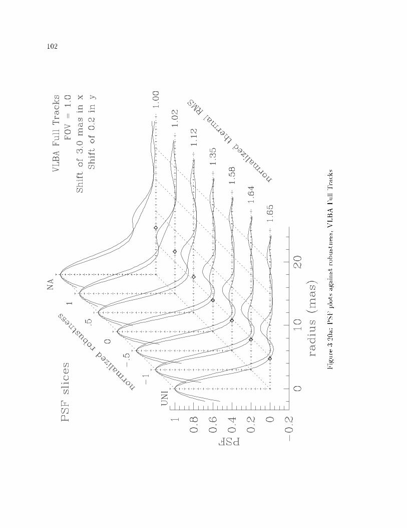
��
Figure���a�PSFplotsagainstrobustness�VLBAFullTracks�

��
Figure ���b� Factor ofp� between contours� lowest is ���

�
Figure����a�PSFplotsagainstrobustness�VLBA�VLA�GBTFullTracks�

��
Figure ����b� Factor ofp� between contours� lowest is ���

�
Figure����a�PSFplotsagainstrobustness�VLBA�VLA�GBT�Orbiter�

��
Figure ����b� Factor ofp� between contours� lowest is ���

��
�� RMSresolution Tradeo� Curves
We now take a closer look at some RMS�resolution tradeo� curves as a function
of di�erent quantities� There are a lot of ways to get to the same place � the curves often
look qualitatively the same when turning quite di�erent knobs� But the whole point of this
chapter is to produce the quantitatively best beam� and that is somewhat more di�cult�
���� Tradeo� Parameterized by Robustness
The shape of the basic tradeo� curve parameterized by robustness is remarkably
constant� Any given tradeo� curve� when plotted such that the uniform and naturally
weighted limits are held at �xed points� looks quite a bit like any other� The interesting
thing about these plots comes primarily from where the endpoints of each curve is relative
to each other� Four curves are shown on each of the next few plots� There are two curves
for two values of the weighting �eld of view� one at the normal uniform weighting and one
super�uniformly weighted� The natural and �super� uniformly weighted limit of each curve
is given as a diamond� Representative points along the curves are circled and the value
of robustness shown next to it� Points along the curve are spaced at intervals of �� in
robustness� In addition� the same curves are presented using gridless weighting�
Figure ���� is quite typical for dense samplings� As with all of these plots� the
naturally weighted limit is the same for all four traces� Super�uniform weighting on dense
samplings produces a beam that has worse thermal noise and a tighter main lobe� moving
the endpoint of the trace down and to the right on these plots� Since the curvature of the
traces for di�erent FOVw is roughly the same� the super�uniform trace is below and behind
the uniform trace� At a given value of thermal RMS� the super�uniform beam has a tighter
main lobe� At a given value of beamwidth� the super�uniform beam has a lower RMS�
The price one pays for this superior performance in the RMS�resolution tradeo� is sidelobe
height� Typically the super�uniform beam will have somewhat higher sidelobes than the
uniform beam at the same value of beamwidth� Still� this is usually a minor e�ect� For dense
samplings� it often is a good idea to super�uniformly weight higher than normal� and then
bring the RMS back to a reasonable value with robustness� Notice also that the gridless
weighting curves are also somewhat �better� than their gridded counterparts� though the
di�erence is slight� Gridless weighting makes a considerable di�erence when compared to
the gridded uniform limit� but the gridded� FOVw �� robust �� case is nearly as good as
the gridless uniform limit� For example� gridless weighting will nearly always help� but when
compared against gridded weighting ! robustness it might not help much� For individual
cases� one needs to examine the sidelobes careful as well as the parameters shown here�
As discussed before� the snapshot case is unusual in that the super�uniformly
weighted RMS is actually less than in the uniform case� Clearly from these traces� super�
uniform weighting is a big win for snapshots� Notice that both traces of the gridless weighting
lie essentially along the gridded super�uniformly weighted curve�

��
Figure ����a� Robustness tradeo� curves for the VLA Full Tracks case�
Figure ����b� Robustness tradeo� curves for the VLA � Point Snapshot case�

��
The robustness curves for the orbiter case are so dominated by the variations
in individual snr weights that both super�uniform and�or gridless weighting make little
di�erence� These techniques both a�ect the gridding irregularities� and that just isn�t the
problem here� The only parameter that makes signi�cant di�erence is the robustness�
Figure ����c� Robustness tradeo� curves for the VLBA�VLA�GBT�Orbiter case�

���
���� Thresholding
It was shown in Section ���� that it can actually be better from a signal�to�
noise standpoint to simply drop highly upweighted points than to include them� It may be
counter intuitive that throwing away good data can decrease the thermal noise� but it is so�
Here we have taken the Full Track VLA data and made an additional �agging pass after
normal uniform weighting� A threshold was set which �agged bad all points where less than
N visibilities were gridded into the same weighting box� Figure ��� plots the resulting
parameters as a tradeo� curve against N � The percentage next to each point is the fraction
of data which is discarded by the threshold� The number in parentheses is N � This is a
very graphic demonstration that the uniform end of the tradeo� curve is driven be a small
fraction of points that are ampli�ed by the weighting� Throwing away these points acts like
a crude version of robustness� Robustness is to be preferred� since the excised data is at
otherwise unmeasured spatial frequencies� and we wish to preserve whatever information
we can at those frequencies� provided that it not a�ect the RMS noise too strongly� But it
is sobering how well this works near the uniform end of the curve� One can actually throw
away ��� of the data and still decrease the RMS from ��� to ����� The thresholding curve
diverges from the robustness curve when the value N approaches the typical occupancy in
the outer tracks�
Figure ��� � Thresholding tradeo� curve� VLA Full Track case� Visibilities less than a giventhreshold in gridded weight are simply eliminated from the data set� The remaining dataare mapped with uniform weighting�
An even more extreme example of thresholding �not shown here� is from the
VLBA�VLA�GBT data set� If one throws away all data from baselines between VLBA
antennas� �presumably after self�calibration�� one obtains a uniform beam super�cially very

���
similar to the robust case of Figure ����� Measured by RMS�resolution� it is really fairly
close� ������ mas instead of the �����mas produced by a robustness of ����� on thefull set� The beam slices along the axes of the beam do not happen to pass through the worst
sidelobes� and these too are strikingly similar to each other� The true behavior is revealed
when we look at contour plots� While all the major features are present in both plots� both
positive and negative sidelobes are much worse in the thresholded beam than in the robust
beam� The worst negative is �� ��� compared to ������ The robustness in this casehas placed the uniform�natural threshold between the typical summed weights encountered
on baselines between VLBA antennas and those encounter on baselines including a large
element� The net e�ect is that all of the baselines with a large element are nearly uniformly
weighted� and this is what is causing correspondence with the thresholded beam� But in the
robust beam� all of the internal VLBA baselines are also present in the data� downweighted
by roughly a factor of �� The spatial frequencies present at this level are not enough to
signi�cantly change the beam features� but they help considerably to lower the beam RMS
sidelobe level�
Thresholding works surprisingly well in terms of thermal RMS�resolution� Ro�
bustness is superior to thresholding because it preserves all the spatial frequencies in the
data�

���
���� Time Averaging
As demonstrated in the snapshot simulations� time averaging can serve a similar
function as does a moderate amount of robustness� at least in cases where the data is not
intrinsically unbalanced by the snr weights� Examined in detail� there is a surprisingly
rich variety of ways that uniform weighting and time averaging can interact to a�ect the
relative weights at di�erent spatial frequencies� But in practice� the dominant e�ects in
most cases do much the same thing� an increased averaging time leads to more weight at
the shorter spacings� a wider beam and lower thermal noise� Snapshots are an exception�
a good choice of averaging time is quite useful� but an inappropriate choice can lead to
dramatic degradation in sensitivity�
Recall that after uniform weighting� each nonzero term in the gridded Fourier
sum contributes equally to the dirty beam� The resolution of the beam is set by the relative
weightings of the di�erent spatial frequencies� so what we want to know is the typical
number of cells occupied at di�erent u�v radii� The easiest case to understand is probably
the densely sampled case� where there are a great many visibilities per cell towards the
center of the sampling� and isolated tracks out towards the edge� As the averaging time is
increased� there will be fewer and fewer occupied cells in the outer tracks� This is true even
in the regime where there are many visibility points per average cell along those tracks�
since the two�dimensional nature of the grid allows intersections of tracks and gridding cells
of any length less than approximately the cell diagonal� Referring back to the catastrophic
gridding error illustration� Figure ���� it is easy to imagine that averaging down by a factor
of two could leave the cell with weight � unoccupied� The distribution of low�occupancy
cells was discussed in Section ���� to explain the uniform limit of the robustness curve�
the probability of �nding a low occupancy cell rises dramatically towards the edge of the
u�v sampling� The probability of an occupied cell becoming empty after time averaging is
related to its original occupancy� so the outer tracks have a greater chance per cell of losing
a term in the Fourier sum after time averaging� The result is a higher emphasis on the
lower spacings and a wider beam� Note that the cells most likely to become empty intersect
the very short tracks that nick the cell corners� Visibilities along these tracks were shown
by the thresholding demonstration to be responsible for the uniform limit of the robustness
curve� Time averaging is acting like a statistical form of thresholding� and once again we
obtain the familiar behavior�
Three time�averaging tradeo� plots are given in Figure ����� covering the two
VLA full track cases and the � point snapshot� The synthetic full track case resembles the
uniform end of the robustness tradeo� curve for the reasons just given� though note that
the magnitude of the averaging time required for a signi�cant e�ect is quite large� Because
of time smearing� we rarely wish to average beyond a few minutes� This only corresponds
to a small amount of robustness� and time averaging is obviously not a terribly e�ective
way to move around in the RMS�resolution plane� Still� if the tools for robust weighting
are not available� the e�ect is worth remembering� A further reason to prefer robustness to

��
extreme time averaging becomes apparent when we examine a more realistic data set� with
many short segments in the u�v plane corresponding to individual scans� Time averaging
has the potential to isolate u�v points at the end of a scan in exactly the same way that
points can be isolated in a reweighting cell� If the typical u�v distance between averaged
points is greater than the grid spacing� the same points which are isolated by time averaging
will also be likely to fall in their own reweighting cell� The result is a new population of
isolated highly�ampli�ed weights which have the usual unpleasant e�ect on the thermal
sensitivity� Figure ����b shows that this e�ect does not become important for a typical
full track observation until well above the averaging times typically used� Figure ����c
shows that this is not true for snap shots� Notice the di�erence between averaging � ��
second time samples into �second time bins versus ��second time bins� It is nearly a ��
degradation in sensitivity�
When time averaging snapshot observations� be sure to choose an averaging time
that divides your data into roughly equal sized bins�
Figure ����a� Time�averaging RMS�resolution tradeo�� VLA Full Tracks� Numbers are theaveraging time in minutes�
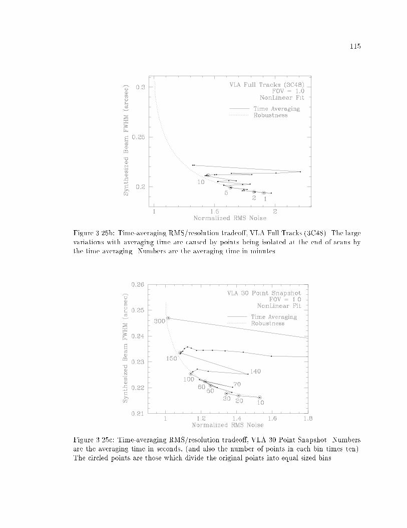
���
Figure ����b� Time�averaging RMS�resolution tradeo�� VLA Full Tracks ��C ��� The largevariations with averaging time are caused by points being isolated at the end of scans bythe time averaging� Numbers are the averaging time in minutes�
Figure ����c� Time�averaging RMS�resolution tradeo�� VLA � Point Snapshot� Numbersare the averaging time in seconds� �and also the number of points in each bin times ten��The circled points are those which divide the original points into equal sized bins�

��
���� Super�Uniform Weighting
Since all of the tradeo� curves go from a limit of natural weighting to a limit
determined by the degree of super�uniform weighting� an obvious question is to ask what
happens to that limit when the tradeo� parameter is held constant and the super�uniform
parameter �weighting �eld of view� is varied� From the theoretical considerations in Sec�
tion ���� � it should come as no surprise that a smaller FOVw leads to a sharper main lobe
and poorer thermal noise� In fact� this e�ect is largely driving the RMS�resolution scatter
plot against image parameters in Figure ���� For a more detailed interpretation� however�
let us consider the e�ect of the reweighting region in the u�v plane�
In the sub�uniform limit �FOVw �� or IMSIZ���� the size of the reweightingbox goes to zero� If every visibility grids to its own u�v reweighting box� the density weights
Dk are just the inverse of the snr weights� ��wk� If the snr weights are all equal� the density
weights are constant and we recover natural weighting� There are two complications in this
limit� The �rst� obviously� is that the snr weights may not all be equal� The second is that
some visibilities may have exactly the same u�v coordinates� No reweighting boxes can split
the two visibilities� and again the natural weighting limit will never be reached��� The limit
will be approached smoothly in resolution� as splitting one reweighting box into two merely
results in one more term among many in the Fourier sum� the extra term preferentially
appearing at the lower spatial frequencies where there are more points� The RMS noise
will be dominated in the limit by the many points which grid into their own cell� and it
will already be fairly close to one� The isolated point is now the norm rather than the
exception� Splitting a cell with multiple points in it will drive the density weights closer
to uniformity rather than producing a catastrophic reweighting� so the limit will also be
approached smoothly in RMS�
The super�uniform limit �FOVw� IMSIZ � or UVBOX � �� comes when theweighting box goes to in�nite radius in the u�v plane� In this limit� every visibility is
considered in the weighting box of every other visibility and all are reweighted by the
�constant� sum of the snr weights� We recover natural weighting no matter what the u�v
coordinates or snr weights of the data� As to how it approaches this limit� however� we
have to consider both forms of super�uniform weighting� The important thing is that the
scaled cell super�uniform weighting will behave badly at with very large weighting boxes�
Exactly the same catastrophic gridding error can happen as in Section ���� but in this case
on a global scale�
The limiting cases are interesting� and of course the most tractable analytically�
but in a practical sense we want to know what happens in the intermediate regions� Fig�
ure ��� gives several examples of actual RMS�resolution tradeo� curves parameterized by
��If one were truly creative� a visibility set could be constructed such that these two e�ects exactly canceleach other � a data set containing two visibilities with the same u�v coordinates and snr weights each halfthat of the rest would preserve natural weighting in the sub�uniform limit�

���
FOVw� The �rst panels are the VLA Full Track ��C �� case from before� Solid points are
scaled box super�uniform weighting� and hollow points are the gridless weighting� Software
limits prevent using the gridded uniform weighting algorithm in the extreme sub�uniform
limit� and prevent using the gridless algorithm in the extreme super�uniform limit� The
region of overlap is �� FOVw � Notice that the gridless weighting curve always liesbelow and to the left of the gridded curve� which is generally an improved beam barring
extreme changes in the sidelobes� The AIPS style integer box super�uniform weighting
is not shown� Numbers next to the circled points are FOVw� The light dotted lines are
robustness tradeo� curves for the gridded FOVw � and FOVw ��� cases� The ro�
bustness curves do not quite reach RMS � due to a minor inconsistency in how SDE
weights the points along the u axis� The limits of Figure ���a are �xed at a reasonable
value� but there are many points outside the plotting area� The worst RMS of the points
examined came at FOVw ���� and resulted in an RMS�resolution of ����� ��� The
highest resolution came at FOVw ���� for ���������� The connecting line between the
gridded points has been suppressed for the uniformly�weighted cases because the points are
jumping around so badly� Figure ���b shows the same data� but with a robustness of �
Since much of the chaotic dependence on the high end tail of the weighting histogram is
reduced by the robustness� we can now see the tradeo� curve approach the super�uniform
limit comparatively smoothly� The sub�uniform limit is always approached smoothly by
the gridless algorithm� when operating on the full track data� The uniform snapshot case
is fairly irregular for both gridded and gridless cases� but it is clear that the weighting �eld
of view is a very important parameters for snapshots� Some values of FOVw produce quite
favorable beam properties� Also� more noticeably here than elsewhere� gridless weighting is
a particular improvement over gridded weighting�
Figure ���� shows beam slices and contours of the �C � case� Notice that the
higher degree of super�uniform weighting leads to a tighter main lobe� as we have seen
before� and also to deeper �rst sidelobes� Perhaps most interesting of all� notice how similar
the sub�uniformly weighted FOVw case is to the Robust �� case of Figure �����

���
Figure ���a� RMS vs� Beamsize as FOVw is varied� VLA Full Tracks case and uniformweighting� Circled points are labeled with FOVw� and the light dotted lines are robustnesstradeo� curves for comparison� See the text for full details�
Figure ���b� Same �gure as before� but with a mild value of robustness instead of uniformweighting� The dependence on FOVw is now smooth enough that the gridded points canbe connected�

���
Figure ���c� RMS vs� Beamsize as FOVw is varied� VLA � Point Snapshot case anduniform weighting� The small number of points in a snapshot lead to irregular behavior�but some values of FOVw are clearly quite favorable�

��
Figure����a�PSFplotsagainstFOV�VLAFullTracks��C ��

���
Figure ����b� Factor ofp� between contours� lowest is ���

���
Occasionally there may be use for extremely large u�v gridding boxes with sparse
coverages� In this case� one is smoothing over not only the local tracks� but also over adjacent
tracks and even over gross features such as the arms of the star pattern� In such cases one
then usually tapers the outer spacings back down to avoid destroying the sensitivity� Since
one is �ghting two con�icting parameters against each other and operating in the region of
compromise� it is di�cult to give general guidelines of exactly when this will be useful or
how much of a given parameter to use� In some cases� however� it can be useful to control
the far out sidelobes of the beam� This should be examined on a case by case basis� but it
is likely to be most useful for imaging crowded �elds with marginal coverage�
Finally� we show an example from the VLA Multiple Con�guration �M��� case�
In this project� a number of images at di�erent resolutions were required to create spectral
index maps� The uniform and naturally weighted resolutions were �����and ������� A map
at a resolution of �����was desired� and the uniform beam was forced to this size with the
tapering routines of Section ����� The image was sampled at ������ ������and the
image size was � ��� which means that the e�ective degree of super�uniform weighting is
a factor of ���� less than simulations in sections ��� and ����� The �tted beamwidth for the
natural beam is a strong function of cellsize in this regime� which explains the di�erence
from the ������reported in the earlier section� The tapered uniform beam is the left panel of
Figure ����� This is a very nice beam� as might be expected from such a good data set� The
signi�cant taper is softening the e�ect of the density weights on the RMS� the resulting RMS
of ��� is a considerable improvement on the untapered uniform weighting�s ����� When
confronted with such a beam� one might well be tempted to stop� There is still a signi�cant
extended shelf on the beam� however� Since an increasing degree of super�uniform weighting
leads to deeper negative sidelobes� an obvious approach is to super�uniformly weight in the
hopes of cancelling the shelf with a near�in negative� As show in the right panel� a FOVw of
�� leads to a considerable improvement in beam shape and also in RMS� In all respects� the
super�uniformly weighted beam is an improvement on the uniform beam� Super uniform
weighting can often be used as a �nal tuning adjustment when the gross properties of the
beam are being controlled by another parameter� After one has found a local optimum in
robustness or tapering� adjust the weighting �eld of view and reoptimize� As just shown�
the results can be surprising and pro�table�

���
Figure ����� Super�uniform weighting as a way to combat an extended shelf� Both beamshave been forced to a width of ������
Summarizing the properties of super�uniform � sub�uniform weighting�
� Sub�uniform limit �FOVw �� or IMSIZ���
� Limiting case is �usually� natural weighting
� Approaches limit smoothly
� Not natural weighting if snr weights not equal
� Not natural weighting if some points have identical coordinates
� Super�uniform limit �FOVw� IMSIZ� or UVBOX���
� Limiting case is always natural weighting
� With scaled cell super�uniform weighting� will approach the limit quite abruptly�
� With integer box or gridless super�uniform weighting� will approach the limit
smoothly�

��
��� Automatic selection of Robustness
The �compromise� beam roughly intermediate in resolution between the uniform
and natural limits can have very favorable properties in terms of close in sidelobes for
some samplings� as demonstrated in the VLA Full Track and other simulations� It�s not
terribly deep why this occurs� Since the VLA among other arrays has an excess of short
spacings� the naturally weighted beam has a strong extended shelf� The uniformly weighted
beams invariably have a strong �rst negative sidelobe� due to the sharp edge at the edge
of the sampling� Since the robust beams vary between these extremes� there will be some
value of the robustness which roughly zeros the �rst sidelobe� If the particular sampling is
suitable for this technique� a single value of the robustness may roughly zero the worst of the
sidelobes at all position angles� If the sampling is intrinsically very azimuthally dependent�
a generalized extension of robustness might help � but preliminary results presented in
Section ���� show this not to be terribly straight forward� For the moment� such samplings
are simply beyond the range of the technique� The other useful properties of robustness
remain� but near�in sidelobe control via robustness isn�t very e�ective�
Since the shelf or the �rst negative is the dominant mismatch between the beam
and its own �tted Gaussian� we can use the integrated mismatch as a �gure of merit and
vary the robustness to minimize it� The important fact to take from this section is that
the particular choice of error metric is not terribly important� The error curves given in
Figure ���� are quite typical� and are not very sensitive to the integration region� In the
case shown� VLA Full Track ��C ��� all three error metrics are suggesting a value near ��
as the best value� Varying the region of integration from a circle with radius ��� times
the �tted half width to � times the �tted halfwidth� �the �tted Gaussian varies from ���
to � � ���� over the same range�� the robustness selected varies at most from extremes
of � to ��� with most estimates being between �� to �� In fact� all of these values of the
robustness are fairly reasonable choices� A subjective choice of between ��� and � as the
optimum value was made after examining all the contour plots by eye� so the automatically
selected and human selected values agree quite well�
The approach of selecting a robustness by minimizing the mis�t to the �tted
Gaussian is implemented as the SDE shellscript findrobust� It uses Brent�s zero �nder as
described in Press et al� �p� ���� ����� and simply begins with an initial guess of ��� ��� ���for values of robustness that bracket the minimum� In all cases examined� the initial guess
was adequate and the convergence quick� typically � executions of the mapping program was
su�cient to constrain the robustness to within ���� A human being can usually home inon a reasonable value of robustness for a Gaussian�like beam by testing a few cases� but this
is a simple enough procedure that is worth implementing for the convenience value alone�

���
Figure ����� Automatic selection of robustness� The curves are possible mis�t criteriabetween the main lobe of the beam and its �tted Gaussian� All here are indicating a valueof Robust �� as the optimum�

��
��� Model Deconvolutions
The end result of the weighting process is a dirty map� which will then be decon�
volved� It is the errors in this deconvolved map which concern us� of course� The subject
of deconvolution errors in general is complicated� and comprises much of the remainder of
this dissertation� Here we simply present one particular deconvolution of a model source
as a function of robustness� The model source is one we will see several times in later
chapters� It is a �component Gaussian model derived from a �t to the X�band images of
�C � in Chapter �� Additionally� point sources have been placed around the main source
to show the e�ect of the thermal noise� The height of the weakest point source was chosen
to be three times the naturally weighted thermal noise� Each additional point source was
increased in magnitude by one contour level� the fourth root of ten � ����� The u�v coverageis that of the synthetic VLA Full Tracks case�
Flux RA o�set Dec o�set Bmaj Bmin Bpa Type�Jy� ���� ���� ���� ���� ���
����� ���� ���� ������ ����� ������ GAUSS����� ���� ����� ����� �� � ��� GAUSS� ��� ��� ����� � � ��� ���� GAUSS��� ���� � ���� ������ �� ��� ��� GAUSS� � ���� ��� & & & POINT��� ���� ���� & & & POINT���� ��� ���� & & & POINT��� ��� ��� & & & POINT
Table ���� �C � � point source model parameters
This is actually a fairly challenging source at high �delity levels� and the NNLS
deconvolution algorithm described in Chapter does a considerably better job than CLEAN
on the noiseless data� For the thermally�dominated data presented here� nearly any rea�
sonable deconvolution algorithm will give roughly the same result� Error plots are given of
the maximum error over the entire image� the maximum error o� the support of the source�
and the RMS error over the support of the source� These three quantities are selected to
show the worst�case error� the worst error that an astronomer might notice on a map� and
the o��source noise�
These simulations were done in the u�v plane � the visibility data was simulated�
rather than forming the dirty map with a discrete convolution� The model shown in Ta�
ble ��� has some serious representation problems� even when oversampled at #� #m
���� as here� The second Gaussian in particular has a minor axis width about the size
of a pixel� Consequently� it makes a considerable di�erence how one generates the truth
image for the error plots� As mentioned in Section ��� the right way to do it is to smooth
the model analytically or in the visibility plane� and then sample� Sampling the model and
then smoothing results in an error of more than �� at the location of the second Gaussian�

���
This is large enough to dominate the full error plots� even the noisy ones� If the comparison
image is made properly� representation problems have almost no e�ect on the error plots�
As demonstrated in Chapter �� the dominant error in CLEAN reconstructions
occurs immediately outside the envelope of the u�v sampling� The size of the restoring
beam determines how much of this spectral error is included in the smoothed components�
Thus if one uses a restoring beam �tted to the main lobe of the dirty beam� as is the usual
practice� the naturally weighted maps have an advantage in that the wider restoring beam
includes less of the deconvolved model from the unsampled regions of the u�v plane� The
error curves here all include two traces� one using a �xed restoring beam which is indicative
of how well the deconvolver has performed in an absolute sense� and another using the �tted
restoring beam which is what the astronomer will see when following usual practice�
Deconvolution simulations are di�cult because there is an enormous parameter
space to be explored� The worst problem is that solutions vary enormously with model �
any given case should be simulated with an appropriate model� and generic results regarded
with caution� But even apart from that� decisions about control parameters can also make
a considerable di�erence in the qualitative nature of the results� Here� the question was
whether to CLEAN the noiseless cases to extreme numbers of iterations� or simply to a
�reasonable� level� A compromise was selected� and all cases were CLEANed to ��
components at �� loop gain� A medium�tight support window of � pixels was used� pro�
duced by smoothing the model with a circular Gaussian of width ���� ��� and allowing �ux
wherever the smoothed model exceeded �� of its peak� These images are CLEANed deeper
than most people would choose� but the noiseless cases are somewhat under CLEANed for
the highest possible �delity� In the noiseless simulations� the maximum residuals rose from a
minimum of �� �Jy�beam for uniform weighting to �� �Jy�beam for natural weighting� The
trend reverses in the noisy case� with the maximum residual being � �Jy�beam for uni�
form weighting and �� �Jy�beam for natural weighting� There numbers can be compared
with the RMS o��source errors in Figure ����c� The RMS degradation�mean beamwidth
for the weightings used are ����������� �� �������� ����������� and ���������� for Uniform�
Robust � Robust �� and Natural weighting respectively� For the noisy case� ���� Jy of
pseudo�random Gaussian noise was added to each real correlator channel in each visibility�
The expected naturally weighted image�plane thermal noise is ���� mJy�beam�
The CLEAN deconvolutions are given in Figure ���a� and the model source
smoothed to the corresponding �tted beam is given in Figure ���b� For the cases dominated
by thermal noise� the smoothed model can be considered the expected improvement in the
image� remember that the deconvolutions given here are only one realization of the thermal
noise� In the plots� the lowest contour is twice the measured o��source RMS for each
individual panel� Hence the apparent noise value stays roughly the same as the weighting
varies� The sources rise up out of the noise �oor as the weighting improves the sensitivity�
For contrast� the similar sequence of plots in Chapter � is done with �xed contour levels�
so the variation of noise with weighting is even more apparent there�
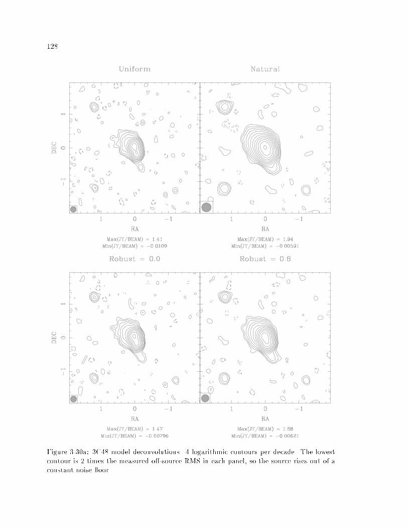
���
Figure ���a� �C � model deconvolutions� logarithmic contours per decade� The lowestcontour is � times the measured o��source RMS in each panel� so the source rises out of aconstant noise �oor�

���
Figure ���b� Model contours to same levels as Figure ���a� Normalized RMS noise isgiven in each panel label�

��
We now examine some quantitative error measures as a function of weighting�
Similar plots to these for the algorithms NNLS and MEM are later given in Figures ��
and ����� Some general comments and points to note about the error plots are�
� Robustness generally makes a di�erence of roughly a factor of � or � in the various errorquantities� In Chapter �� it will be shown that source structure makes a di�erence
measured in orders of magnitude�
� The deconvolution behavior with weighting is complicated in the noiseless case� andvaries greatly with algorithm�
� The maximum error plots tend to have the most structure with weighting� followed
by the maximum o��source error� O��source RMS with weighting is usually fairly
simple�
� The worst deconvolution errors here are similar for the noisy and noiseless cases �even in a fairly noisy image� the worst on�source errors are coming from deconvolution
errors and are not thermally driven�
� The maximum o��source error is signi�cantly di�erent for the noiseless�noisy cases�
The noisy curve has features attributable to both the noise and to deconvolution
errors�
� The noiseless maximum o��source error curve peaks at an intermediate value of ro�
bustness� as does the RMS o��source error� This behavior varies dramatically with
deconvolver� In the CLEAN case� it�s not likely to be a problem� since the cases where
the e�ect is noticeable are where one will likely be using a di�erent deconvolver�
� The measured o��source RMS after deconvolution tracks the predicted thermal RMSalmost exactly for the noisy case� The predicted thermal noise is a good indicator of
what one is likely to measure in an actual deconvolution�
� The uniform beam is a good choice for o��source RMS in the deconvolution error
dominated regime� though this may simply re�ect that the uniform beam tends to
require fewer iterations to converge to a solution than the natural beam� This regime
is somewhat under CLEANed in these simulations� and the residuals are nonneglible�

���
Figure ����a� Error quantities against RMS degradation factor� maximum error� The �ttedrestoring beam corresponds to Figure ���� The �xed beam curve is more representative ofthe absolute deconvolution quality and used
pBnatBuni ���� ���
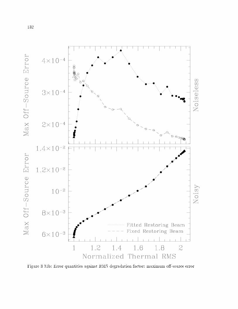
���
Figure ����b� Error quantities against RMS degradation factor� maximum o��source error�
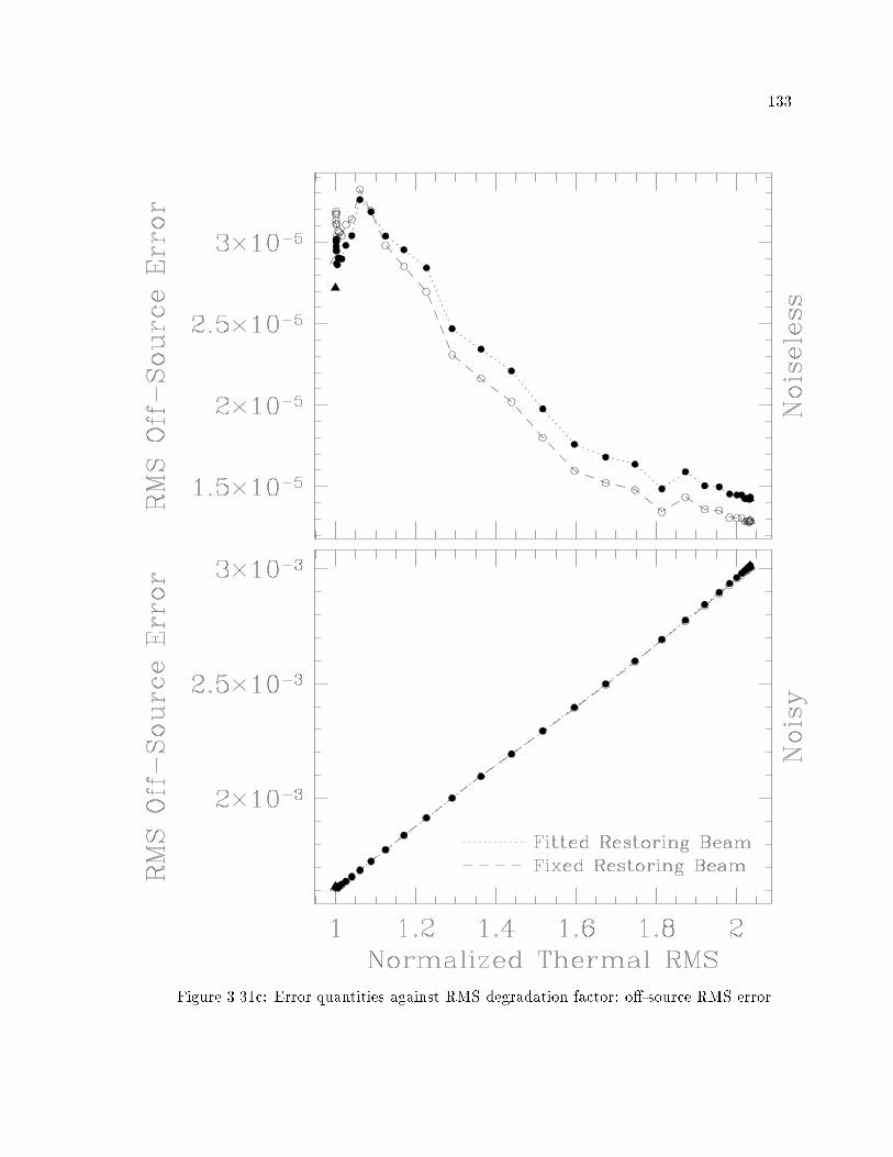
���
Figure ����c� Error quantities against RMS degradation factor� o��source RMS error�

��
���� Tapering � Beam Forcing
Tapering is a method of beam control that I feel is unjustly neglected� Most
packages allow at least a one�dimensional radial taper on the visibility data applied after
the density weighting� AIPS allows a di�erent taper to be applied along the u and v axes�But few packages allow for a taper in full generality� Appendix B describes the necessary
mathematics for a full two�dimensional rotated elliptical Gaussian taper� Appendix D
describes how to generalize the taper to elliptical inverse tapers� or even to a hyperbolic
Gaussian taper which one tapers along one axis and inverse tapers along the other� �A curve
of constant taper is then a hyperbola in the u�v plane�� The reason that one might want
such a general taper is that the solution to the deconvolution of one elliptical gaussian from
another involves such terms� With this formalism� we can work out what generalized taper
we must apply to the data in order to achieve a given beamshape� We approximate this
by analytically deconvolving the desired beamshape from the �tted beam� The resulting
generalized taper is then applied to the visibility data and iterated� With some caveats� this
technique works quite well� The details of such beam forcing are also given in Appendix D�
The �rst and most obvious use of beam forcing is in making spectral index maps�
Within reasonable limits� this allows one to match any two �tted dirty beams to each other
exactly� This is not explored in detail in this dissertation� but it should be quite obvious
that a good match of �tted beams at di�erent frequencies will lead to good spectral index
maps�
A more mundane use of beam forcing is simply to circularize the beams for aes�
thetic reasons� or to minimize the e�ect of the beam position angle on source structure�
This is not as e�ective as one might think for low declination sources for the simple rea�
son that one cannot inverse taper data that is not there� But circularization by tapering
works well with relatively dense samplings� and it can reduce the aspect ratio of extremely
elongated beams at least somewhat� It is natural to worry about inverse tapering to a level
that interferes with the deconvolution� In the limit of extremely high taper� clearly one is
trying to image with just the outer u�v tracks in the data� This is really no di�erent than
the super�uniform weighting case with very small FOVw� As with that case� the normalized
RMS is a reasonable guide for �how much is too much inverse tapering�� Also� note that
the high taper limit of the beam in a case with circularly symmetric sampling is J��r�� the
Bessel function of the �rst kind with order � This function has negative sidelobes of ��
so clearly excess inverse tapering will be re�ected in unreasonable high negative sidelobes�
Figure ���� shows two examples from the AT Full Track �SN����A� case used before� Since
the u�v coverage from the east�west array lacks a pie sliced shaped region� the beams from
this coverage are moderately eccentric� As shown in Figure ��� the degree of eccentricity
increases with robustness� naturally weighting generally being the worst� so here we only
examine the Robust �� and Naturally weighted cases� In the former case� the beam pa�
rameters are ����������� ������ After running findtaper� a beam of ���������� �����
results� For the natural case� the original ������� ��� ����� becomes ��������������������

���
While the naturally weighted beam is not particularly attractive� circularized or not� the
e�ect on the main lobe is quite clear and the RMS has not increased particularly much� The
robust weighted case seems to be an improvement in most respects over its noncircularized
counterpart� possibly excepting extremely high resolution projects�
Figure ����� Beam circularization by tapering
We next examine the e�ect of simple tapering on a data set� Again we return to
the VLA Multiple Con�guration �M��� case� In Figure ����� beam slices are presented after
the has been tapered down to multiples of ������ This was done with beam forcing� but for
most of the larger width curves it could also have been done with conventional packages in
that the required taper was nearly a function of radius only� To avoid undersampling the
higher resolution beams� these slices were done with the imaging parameters of Table ���
and not those of Figure ����� �The e�ective degree of super�uniform weighting is quite
di�erent in these cases�� The points to notice here are that the beam shape approaches a
Gaussian more closely as the taper is increased� that there is a minimum in thermal noise
as a function of taper� and that there are signi�cant di�erences in beam shape as a function
of FOVw� even after signi�cant tapering� None of these points are particularly surprising�
but it is instructive to example the data from an actual observation�

��
Figure����a�Beamslicesagainsttapering

���
Figure����b�Sameasbefore�butwithFOV ��

���
The other particularly useful application of beam forcing is that it allows us to
answer questions like �how much better is one weighting than another� after accounting for
di�erences due to beam shape�� We simply match the beams as best possible using the
beam parameter under study� and then force it the rest of the way with a generalized taper�
Alternatively� we can match one beam to a second with taper� and then match the second
to the �rst with a di�erent taper� If one beam is superior to the other in both cases� we
can claim it is superior without quali�cation as to beam shape� So armed� we tackle the
question of gridded and gridless weighting again� Table ��� show this technique applied to
a number of di�erent cases of u�v coverage� weighting �eld of view and robustness� The
middle columns show the RMS of the beams when the gridless beams are forced to the
size of the gridded beam with a taper� and the rightmost columns show the RMS when the
beams are forced the other way from gridded to gridless� The super�uniform weighting is
done with the SDE scaled cell implementation� The points to note from this table are
� The gridless RMS is almost always superior to the gridded RMS regardless of thedirection of tapering
� The few exceptions to the trend come from the unbalanced array cases� It seems thatthe variations in individual weights are so large that the RMS is determined by how
the tracks happen to line up with each other not by the random e�ects of a single
track on a grid� It is not clear why this e�ect should favor the gridded weighting�
� The di�erence in RMS for the two weightings is greatest for the �super� uniformlyweighted beams� and becomes less as the robustness is increased� At high robustness
the di�erence is negligible�
� The di�erence is more signi�cant for super�uniform weighting than uniform weighting�

���
Cov FOV Rob Beam RMS RMS Beam RMS RMS����mas� GRD GL� Tap ����mas� GRD� Tap GL
VLA �C�� �� Uni ���� ��� ����� � � ���� �����VLA �C�� �� � � �� ���� ���� � � ��� � ����VLA �C�� �� �� � �� ���� ��� � � ��� ��� � ��� �
VLA �C�� � � Uni ���� ���� �� � ���� �� �� ����VLA �C�� � � � ����� ���� ���� ���� ���� ��� VLA �C�� � � �� � � ����� ���� � ��� ����� �����
VLA Snap � �� Uni � �� ���� ���� � � ��� ����VLA Snap � �� � � �� ��� ���� � � �� � ����VLA Snap � �� �� � � � ���� �� � � ��� ���� ����
VLA Snap � � � Uni � �� ���� ��� � � �� ���� ����VLA Snap � � � � � ��� �� � ����� � ��� �� � ���VLA Snap � � � �� � � �� ��� � �� ���� ����
VLBA �� Uni ���� ���� ����� ��� ����� �����VLBA �� � ����� ���� �� � ���� ����� �� �VLBA �� �� ���� ���� ���� ��� ��� � �����
VLBA � � Uni ����� ���� ��� ���� ��� ����VLBA � � � �� �� ���� ����� �� � ���� �����VLBA � � �� ����� ����� ���� �� � ����� �����
� VLA�GBT �� Uni ����� ��� ����� ���� ��� ����� VLA�GBT �� � ����� ����� �� ��� ���� ����� VLA�GBT �� �� ���� ���� ����� �� � �� �� ���
� VLA�GBT � � Uni ���� ��� � ���� ����� ���� ������ VLA�GBT � � � ���� ����� �� ��� � ���� ���� VLA�GBT � � �� ��� �� � �� �� ��� �� �� ����
� Orbiter �� Uni ����� ���� ���� ����� ������ ����� Orbiter �� ��� � �� ����� ���� ���� ���� ��� � Orbiter �� � ���� ����� �� ����� ��� � ��
� Orbiter � � Uni ����� ����� ����� ���� ��� � ������� Orbiter � � ��� ����� ����� ���� ����� ���� ����� Orbiter � � � ���� ��� � �� ���� � �� ����
Table ���� Gridded�Gridless RMS comparison

�
At this point� things have become complicated� We have several possible knobs
which may be turned in order to control the beam shape� Both super�uniform weighting and
robustness produce the typical �L� shaped RMS�resolution tradeo� curve� and to a lesser
extent time averaging and thresholding do as well� As shown in the earlier plots� tapering
down tends to produce a wider beam and usually better thermal RMS� Inverse tapering
goes the other way� so we have yet another way of exploring RMS�resolution space� The
question now is �what is the e�ect of tapering from di�erent starting points�� Figure ���
addresses this for the speci�c case of the synthetic VLA Full Tracks data� The dashed lines
are the same as the main traces in Figure ���� and are produces by varying the robustness�
The point labelled is no taper at all� and each small dot is a taper increment of ����� That
is� the �rst small dot above the has been smoothed with a Gaussian of size ���� � �����
The second with a Gaussian of size ���� � ���� and so on� Every tenth point is circled�
Examining the traces parameterized by taper� we see that while the qualitative
shape of the curve is much the same as that of robustness� the slope at a given point is often
quite di�erent� Tapering decreases the thermal noise when the combination of the starting
point plus taper resembles natural weighting more closely than the starting point alone�
Most array have sampling patterns strongly peaked at low frequencies� so a �at uniform
weighting plus downweighting of the higher spatial frequencies yields a better match and
lower thermal RMS than uniform weighting� The typical problem with tapering is that the
Gaussian taper dies o� too quickly� In order to match the shape of the central portion of
the sampling pattern� a taper must be applied that is essentially zero at the edge of the
pattern� By that point� the outer spacings are being thrown away completely� The high
taper limit actually resembles that of the thresholding curve of Figure ��� � and for much
the same reason as there� This is responsible for the tapered trace being steeper than the
robust trace in the uniform panel of Figure ��� a� According to these plots� a taper is a bad
way to work the RMS�resolution tradeo� when desiring a wide beam� The compensating
factor which is not apparent from these plots is that the tapered low resolution beam is
beautifully Gaussian� while less sensitive than an equivalent resolution robust beam�

� �
Figure��� a�Howmuchrobustnessdowewant�ifwe�regoingtotaper�FOVw �

� �
Figure��� b�Sameaspreviouspanel�butwithFOVw ���

� �
From the �gures� it might appear that natural weighting plus an inverse taper
is much equivalent to robustness� In terms of these two measures of beam quality is is�
though again the measures plotted in these �gures are not su�cient to di�erentiate between
the character of the di�erent beams� We look at some additional tabulated quantities in
Tables ��� and ����� but at this level of detail there is no substitute for looking at more
examples directly� The two tables attempt to answer the question �How much robustness
do we want� if we�re going to taper��� tabulating �rst the RMS and then the most negative
sidelobes when a number of di�erent starting points have been forced to a common beam
size with a taper� The three beam sizes listed in the table as small� medium� and large
are that of the gridded FOVw �� super�uniform beam� the gridded uniform FOVw �
beam and the geometric mean of the gridded uniform and naturally weighted beam� All
forced beams are circular�
The most important conclusion of the �rst table is that �some� robustness is
su�cient to gain the majority of the thermal sensitivity improvement� In most cases there
is a minimum in RMS against robustness� and in others the naturally weighted starting
point still provides the best thermal RMS� even after taper� But in all cases� the minimum
in RMS is rather broad� A normalized robustness of or �� is reasonably close to the
minimum value� and is substantially better than starting from uniform weighting�
The second table tabulates the most negative sidelobes instead of the RMS� It�s
primary use here is to demonstrate why I haven�t often tabulated this quantity� There are
a number of di�erent competing e�ects contributing to this table� and the resulting values
show few clear trends� More often than not� the naturally weighted beams have the smallest
negative sidelobes� but that is usually the result of an extended shelf obscuring the worst of
the near�in sidelobes� Occasionally it the uniform beam with the with the least sidelobes�
or intermediate value of the robustness� The gridless beam usually but not always has a
smaller negative sidelobe than the equivalent gridded case� For every trend in this table�
there is also a counter example� The conclusion is that when using this many parameters
to control the beam shape� there is no scalar measure substitute for direct examination of
the beams and a measure of subjective judgement�
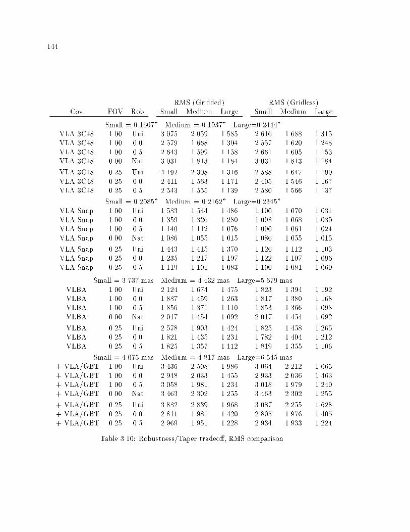
�
RMS �Gridded� RMS �Gridless�Cov FOV Rob Small Medium Large Small Medium Large
Small ���� Medium ������ Large �� �VLA �C � �� Uni ���� ���� ����� ��� ���� �����VLA �C � �� � ����� ��� ��� ����� ��� ��� �VLA �C � �� �� �� � ����� ����� ��� ��� �����VLA �C � � Nat ���� ����� ���� ���� ����� ����
VLA �C � ��� Uni ���� ���� ���� ����� �� � ����VLA �C � ��� � �� �� ���� ����� �� � ��� ����VLA �C � ��� �� ��� � ����� ����� ���� ��� �����
Small ����� Medium ����� Large ��� ��VLA Snap �� Uni ����� ��� �� � ��� ��� ����VLA Snap �� � ����� ���� ���� ���� ��� ���VLA Snap �� �� ��� ����� ��� ��� ��� ��� VLA Snap � Nat ��� ���� ���� ��� ���� ����
VLA Snap ��� Uni �� � �� �� ���� ���� ����� ����VLA Snap ��� � ����� ����� ����� ����� ���� ���VLA Snap ��� �� ����� ���� ���� ��� ���� ��
Small ����� mas Medium � �� mas Large ���� masVLBA �� Uni ���� ��� �� �� ����� ���� �����VLBA �� � ����� �� �� ���� ����� ���� ����VLBA �� �� ���� ����� ���� ����� ��� ����VLBA � Nat ���� �� � ���� ���� �� � ����
VLBA ��� Uni ����� ���� �� � ����� �� �� ����VLBA ��� � ����� �� �� ����� ����� �� �����VLBA ��� �� ����� ����� ����� ����� ����� ���
Small ��� mas Medium ���� mas Large �� � mas! VLA�GBT �� Uni �� � ���� ���� �� ����� ���! VLA�GBT �� � ��� � ���� �� �� ����� ��� �� �! VLA�GBT �� �� ���� ����� ���� ���� ����� ��� ! VLA�GBT � Nat �� � ���� ����� �� � ���� �����
! VLA�GBT ��� Uni ����� ����� ���� ���� ����� ����! VLA�GBT ��� � ����� ����� �� � ���� ���� �� �! VLA�GBT ��� �� ���� ����� ����� ���� ����� ����
Table ���� Robustness�Taper tradeo�� RMS comparison

� �
Negative Sidelobes �Gridded� Negative Sidelobes �Gridless�Cov FOV Rob Small Medium Large Small Medium Large
Small ���� Medium ������ Large �� �VLA �C � �� Uni ������ ���� � ���� ���� ��� � �����VLA �C � �� � ������ ����� �� � ����� ���� ��� �VLA �C � �� �� ������ ���� ����� ����� ��� � ����VLA �C � � Nat ��� ���� �� �� ��� ���� �� ��VLA �C � ��� Uni ������ ����� ��� � ������ ��� ��� �VLA �C � ��� � ���� ����� ����� ����� ���� �����VLA �C � ��� �� ������ ���� ���� ����� ��� ����
Small ����� Medium ����� Large ��� ��VLA Snap �� Uni ����� ����� ����� ������ ����� ����VLA Snap �� � ����� ����� ������ ������ ����� �����VLA Snap �� �� ������ ����� ����� ����� ����� �����VLA Snap � Nat ����� ����� ���� ����� ����� ����VLA Snap ��� Uni ������ ��� ����� ��� ����� ��� ��VLA Snap ��� � ���� � ��� �� ����� ���� ���� ��� �VLA Snap ��� �� ��� ����� ����� ��� �� ����� ���� �
Small ����� mas Medium � �� mas Large ���� masVLBA �� Uni ����� ����� ����� ����� ��� ����VLBA �� � ����� ���� ����� ���� ��� ���VLBA �� �� ��� � ����� �� � ����� ��� �����VLBA � Nat ����� �� �� �� ����� �� �� ��VLBA ��� Uni ��� ��� � ���� ��� � ��� �����VLBA ��� � ������ ��� �� ���� � ����� ����VLBA ��� �� ����� �� �� ���� ����� ���� ����
Small ��� mas Medium ���� mas Large �� � masVLBA! �� Uni ����� ���� ���� ����� ���� �����VLBA! �� � ����� ���� ��� ��� ����� ���VLBA! �� �� ������ ���� ���� ��� �� ��� �����VLBA! � Nat ��� � ���� ���� ��� � ���� ���� VLBA! ��� Uni ���� � ���� ���� ����� ��� � �� VLBA! ��� � ������ ���� ��� ����� ����� �����VLBA! ��� �� ����� ����� �� ������ ���� �� �
Table ����� Robustness�Taper tradeo�� Negative sidelobe comparison

�
In this spirit of direct examination� we show contours and slices of the VLA Full
Track case as a function of robustness� where the �tted beam size has been held constant
with a taper to that of the gridded uniform case� Compare this with the untapered plots
of Figure ����� In general� there is less variation between the di�erent beams� as the gross
properties of the beam are largely held constant and only the second order e�ects allowed
to vary� Again we see the minimum in RMS as a function of starting robustness� The
usual wide shelf around the natural beam is largely suppressed� but still present at a level
too large to recommend� Of the FOVw �� series� the robustness of � or �� isn�t a bad
choice� though one would only inverse taper like this if the highest possible resolution beam
were required� The FOVw �� series in the following plot simply shows that when one
forces the beam to a su�ciently small target� there is little that can be done about ringing
sidelobes�

� �

� �
Figure����a�PSFplotsagainstrobustness�Tapered�FOVw
��

� �
Figure ����b� Factor ofp� between contours� lowest is ���

��
Figure���a�PSFplotsagainstrobustness�Tapered�FOVw
���

���
Figure ���b� Factor ofp� between contours� lowest is ���

���
We conclude this section with one last series of a common taper� combining a
number of the di�erent features discussed� The plots have been extended out considerably
further than the rest in this chapter to show the far�o� sidelobes which have been somewhat
neglected� The �rst panel is the gridded� FOVw �� robust � case from the same VLA
Full Track data set� This is an excellent beam for general purposes� and unless there is
a special requirement for high resolution� it is the one recommended for this data� The
beam parameters are ����������� with a worst negative of ����� At this high a levelof robustness� there is very little di�erence between the gridded and gridless weighting�
The corresponding gridless case forced to this resolution is only ������������ with a ����worst negative� It is not shown� The next panel is the naturally weighted beam forced
to the same resolution with a taper� The only thing that this has bought us is a very
slight increase in the thermal sensitivity� both the near�in sidelobe shelf and far sidelobes
have worsened considerably� The previous beam is so good in thermal noise� that the extra
sensitivity this has bought us is negligible� The gridded and tapered uniform beam is given
next� The thermal RMS has risen considerably to �� ��� and the worst negative dropped
slightly to ������ but of all the cases shown this has the best far�o� sidelobes� The choiceof this or the robust beam would depend on which features of the beam are limiting the
�nal map� In a sensitivity limited situation� the robust beam is the better choice� In a
particularly di�cult deconvolution situation� this might be used� Alternatively� one could
use the gridless uniform beam given as the last panel in the series� Without robustness� the
gridless weighting does make a considerable di�erence in the thermal noise� which drops
back to ������ The near�in negatives are slightly worse at ��� � In general� the far�o�sidelobes of the gridless uniform beam will be worse than the gridded uniform beam� as
the later is the minimum sidelobe solution� It�s usually a judgement call whether this is
a better choice than a robust beam� In this case� I would probably prefer one of the two
previous good choices� but I would try all of them if it was a case where the deconvolution
problem was di�cult�

���
Figure����a�ExamplePSFstaperedtoacommonresolution�Factorof
p �betweencontours�lowestis���

��
Figure����b�PSFstaperedtoacommonresolution�continued�Factorof
p �betweencontours�lowestis��

���
������ VLB Square Root� Weighting
The badly unbalanced arrays sometimes found in VLBI can lead to nearly unus�
able naturally weighted beams� This has lead to a tradition in the community of arbitrarily
downweighting the more sensitive baselines before the density weighting� Common choices
are taking the square root or fourth root of the snr weights� or even setting them to unity�
The Caltech VLBI package and SDE are the most sophisticated in this regard� and allows
one to raise the density weights to an arbitrary power before use� While certainly better
than nothing� this is a rather drastic approach to curing the problem� Modi�cation of the
density weights in this manner is really only appropriate for controlling the relative weights
between baselines that combine together into the same gridded visibility� Modi�cation of
the weights for imaging purposes is best achieved by the operating on the gridded visibilities
with a density weight or taper� Forcing one type of the weight control to do the job of the
other results in a poor use of the available signal and a poorer thermal sensitivity than
necessary�
The robustness tradeo� curves for the two unbalanced array cases are given in
Figure ����� In each� there are traces from the unmodi�ed snr weights� the weights modi�ed
by taking their square root� their fourth root� and by setting all snr weights to unity� That
is� the four traces correspond to snr weight exponents of ��� ��� ���� and �� In addition�
there are traces for the both the uniform and FOVw �� super�uniform weighting cases�
The imaging parameters are again those from Table ����
Modi�cations of this type to the weights makes relatively little di�erence to the
uniformly weighted beam� Clearly the beam shape will change essentially not at all� as
all occupied cells are reweighted to unity by the density weighting and reweighting cannot
change which are occupied� It is interesting that the RMS changes so little� however� There
is more action in the natural weighting limit� As the snr weights are progressively �attened�
the natural limit traces out the curve indicated by the four open diamonds in Figure ����a�
Of interest is that this limiting curve is very un�favorable in terms of the RMS�resolution
tradeo�� As the qualitative shape of the tradeo� curve does not change greatly for this
case� moving the limiting point into an unfavorable regions of the RMS�resolution plane
pulls the entire curve into unfavorable regions compared to the corresponding cases of the
unmodi�ed weights� Similar behavior is seen in the orbiter case� though it is quantitatively
quite di�erent�
As demonstrated before� the RMS � beamwidth do not tell the whole story
about beam properties� The main reason for the VLB weighting in the �rst place is the
desire to avoid the sidelobes caused by a few baselines dominating the sensitivity� Again
we examine some representative beams in detail� Figures ���� and �� are a repeat of
Figures ���� and ����� with the addition of square root modi�cation of the snr weights�
Clearly the sidelobes in Figure ���� are much improved over those in Figure ����� towards the
natural weighting limit� The modi�ed naturally weighted beam has turned the one dominant
sidelobe into an extended shelf at somewhat lower magnitude� While certainly not an

��
attractive beam� it is clear why the practice of weight modi�cation was started� Comparing
beams at �xed values of the robustness� it might appear that the square root modi�cation
allows us to work closer to the naturally weighted limit� The weight modi�cation has
actually changed the robustness scale somewhat� The unmodi�ed beams at a normalized
robustness of R are roughly comparable to the modi�ed beams at a robustness of R !
��� When we compare the appropriate beams� we �nd that at the common values of the
resolution the unmodi�ed beams do substantially better� For instance� at R ��� the
unmodi�ed beam has an RMS�resolution of ������� mas� At R ��� the modi�ed beam
is ��������� mas� The sidelobes of the unmodi�ed beam are at least as good as the modi�ed
one� so in all respects it is a better choice for a high sensitivity beam� The situation is similar
for the orbiter case as exempli�ed by an unmodi�ed beam of ��� ����� mas at R ���compared to the modi�ed �� ����� mas at R �
Robustness is clearly an improvement over the VLB style weighting when imaging
well�calibrated data� and even an improvement over VLB weighting plus robustness� There
is still good practical use for the weighting during calibration� however� The snr weights
really only re�ect the reliability of the data when the calibration is under control� and
certainly do not at the start of the calibration loop� If the visibility phases are completely
random� then the snr weights have nothing to do with the reliability and an appropriate
choice for the �rst iteration of self�calibration might be all snr weights equal� The optimum
weights and strategy for a real calibration can be a very complicated question� and it has
not been investigated here in detail� As a general principle� �attening the weights towards
the beginning of the calibration process and returning to the unmodi�ed snr weights plus
robustness seems like a good strategy�

���
Figure ����a� Robustness tradeo� curves� VLBI weighting comparison�
Figure ����b� Same as previous� but for the extremely unbalanced Orbiter case�

���
Figure����a�PSFplotsagainstrobustness�VLBA�VLA�GBTFullTracks�VLBweighting��

���
Figure ����b� Factor ofp� between contours� lowest is ��

�
Figure�� a�PSFplotsagainstrobustness�VLBA�VLA�GBT�Orbiter�VLBweighting��
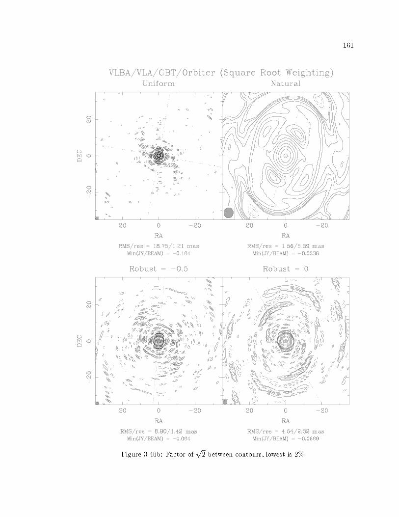
��
Figure �� b� Factor ofp� between contours� lowest is ��

��
���� Future Work
������ Azimuthally Varying Robustness
The sidelobe di�culties in the AT case and to a less extent in the �C � case
suggest that an ad hoc extension of the robust weighting formalism would be useful to
create a beam with the best possible �t to a Gaussian� An obvious approach is to vary the
e�ective degree of robustness as some function of azimuthal angle� in an attempt bring all
sidelobes though zero simultaneously as the robustness is varied� This approach loses the
aesthetic appeal of the minimization formalism� and it creates di�culties for programs which
�nd the robustness automatically� since the search space is expanded to several dimensions�
But for certain sampling patterns it might help considerably�
This was very brie�y explored in SDE� An elliptical extension of robustness was
considered� with the e�ective robustness at each pixel in the gridded visibility plane being
proportional to the �radius� of an ellipse at the position angle of the pixel� Unfortunately�
the de�nition of normalized robustness goes both positive and negative� Even if the radius
were used as a logarithmic parameter� the relative weighting of points at di�erent position
angles would depend strongly on the details of the normalization� Consequently� it was
simply decided to have the e�ective robustness vary linearly with position angle between a
minimum and maximum along orthogonal robustness axes� That is� the e�ective robustness
is a saw tooth function in position angle� with a period of ���� This choice does have the
property that the mean robustness averaged over a circular region in the u�v plane is simply
the arithmetic mean of the robustness along the two primary axes�
Figure �� � demonstrates that this experiment was not entirely successful� Es�
sentially� the �rst sidelobes of the beam have been roughly forced to zero at four points in
azimuth instead of two� and even that not terribly well� The functional form selected for
robustness as a function of azimuth is a disappointingly poor �t to that necessary for a nice
beam at all values of azimuth� A possible solution to this problem would be to abandon
an analytic form in azimuth all together� and simply specify the azimuthal robustness as
a sequence of values� possibly interpolated by a spline� The problem then becomes how
to specify such a list� One could hook such an arbitrary ��D robustness into a numerical
minimizer against the �tted Gaussian in the style of Section ���� and use �nite di�erences
to approximate the necessary derivatives� If such an approach were used� one would pre�
sumably greatly oversample the beam to increase the number of pixels in each azimuthal
bin� and hold the weighting �xed with FOVw � The problem of guiding such a minimizer
to an approximate global minimum is nontrivial� but it doesn�t seem entirely intractable�
More work could be done here�
������ Thermal Noise Beam and Visualization
The ratio between the gridded snr weights and the total gridded weights deter�
mines the degree by which thermal noise at a given spatial frequency is ampli�ed� In analogy

��
Figure �� �� Azimuthally varying robustness� The e�ective robustness is along a positionangle of �� and � along the orthogonal direction� and varies linearly with position angle inbetween�
to the calibration error beam occasionally used to discuss the morphology of antenna�based
calibration errors� one might hope to de�ne a thermal noise beam which in some sense will
give predictions about how the noise is distributed� Unfortunately� we don�t have the phase
of the thermal noise at each gridded weight� all we have is the magnitude� The practical
e�ect of this is that we can�t say that the e�ect of the thermal noise ampli�cation is a
convolution with any particular beam� We can� however� just simulate the thermal noise�
The eye is pretty good at picking out structure� and if there is structure in the simulated
noise that resembles structure in the map� you�ve almost certainly ampli�ed the noise at
some frequencies beyond reasonable limits� Examining this ratio in the Fourier plane is of
course the most precise way to tell� A good mapping program should print the maximum
and minimum visibility weights� both before and after density reweighting� It would seem
reasonable to also print the maximum and minimum value of this ampli�cation as well� My
intuition is that we are not making as good use as we might of the spatial information about
the noise ampli�cation� There is probably room for progress here�

�
������ Generalized Windows and Minimizing Source Sidelobes
It was shown in Section ����� that uniform weighting can be derived by minimizing
the RMS sidelobes over the dirty beam� Later� it was shown that super�uniform weighting
results from scaling the region over which the sidelobes are minimized� The region may be
larger or smaller� but it is still rectangular� Bob Sault ���� � describes how the minimization
criterion for the beam sidelobes may be generalized to include an arbitrary window function�
That is� his method minimizes
�� �Xi�j
qij�bij �mij��
where q is a completely general windowing function� b is the dirty beam� and m is the ideal
dirty beam��� The window speci�es not only where the sidelobes are to be minimized� but
also how important the minimization is as a function of position� The resulting equations
can be solved in an iterative fashion� with the more accurate of the methods he describes
typically requiring & FFTs� and a slightly less accurate version which typically requires
but � FFTs� Several examples of windows were presented� two central disks� a small patch
centered on the worst o��peak sidelobe� and the autocorrelation of the small patch� �All
window are symmetric around the origin�� The o��peak patch was the most impressive� and
it successfully reduced the �� criterion by more than a factor of seven over the uniformly
weighted beam�
A detailed cross�comparison of these techniques with robustness has not been
done� In particular� little is known about the thermal noise characteristics of the Sault
optimally�weighted beams� beyond the obvious relationship to super�uniform weighting
when a central window is used� Since there is no criterion in the Sault optimization which
includes notice of the thermal noise� I suspect that it will su�er the usual problems with
gridding irregularities and the consequent loss of sensitivity� The necessary equations to in�
corporate robustness into Sault�s formalism has been derived� The implementation appears
to be straightforward� but there are no immediate plans to do so�
The Sault formalism is impressive in its sheer �exibility� When used with round
constant windows centered on the origin it seems to be roughly comparable to other beam
shaping techniques� But there are no other techniques extant for minimizing a single given
sidelobe� Sault also presents an optimization strategy for minimizing the sidelobe response
of the source at a given location in the dirty map rather than the dirty beam� but comments
that the resulting equations are di�cult to solve� In spite of the di�culty of the problem�
��The written description is slightly ambiguous� Notice that the obvious way of doing the di�erentiationin the image plane is wrong� as there are more degrees of freedom in the dirty beam than there are in theweighted visibilities� The minimization is consequently a constrained rather than an unconstrained problem�As it happens� doing the calculation properly in the Fourier plane or improperly in the image plane bothreturn exactly the same result�

��
this appears to me to the be the most promising avenue for further research in the area� In
this dissertation� I have uni�ed two distinct properties of the beam� resolution � sensitivity�
In principle� Sault�s work addresses sidelobes of the source� As computers and algorithms
become more advanced� it might be hoped that future techniques could address all of these
issues in a single optimization�
Finally� note that one might even use a di�erent weighting in di�erent regions
of the dirty map� The algebraic deconvolution techniques discussed in Chapter do not
require a shift�invariant dirty beam� though they are limited at present to unfortunately
small images� In the medium to long term future� it is possible that we will deliberately
abandon the Fourier convolution equation with its shift invariant dirty beam in order to take
full advantage of optimal weighting� Particularly if an e�cient means can be found of solving
the optimal weighting equations for a single pixel of the dirty map� a di�erent weighting
could be used for each pixel� The resulting transformation from visibilities to image plane
is no longer a Fourier transform� but it is still a linear transformation and invertible by the
most general deconvolvers� The NNLS algorithm from Chapter is su�ciently successful
that it is not clear the need exists for such heroic measures in weighting� But if ever the
need should arise for ultra�high dynamic range or ultra�high��delity mapping of compacts
objects� this is at least a plausible avenue for future research�

�
���� Summary
I think that I�ve taken optimum weighting by adjusting parameters of the dirty
beam into a region of diminishing returns� There may be better schemes� but the techniques
described here work well enough that there is not tremendous room for improvement� As has
been stated before� there are a lot of ways to get to roughly the same place when tuning beam
parameters� The addition of robustness and a generalized taper adds su�cient �exibility
that I can�t help but thinks that they will be able to roughly approximate the results of
most other simple reweightings on the gridded snr weights� Signi�cant future results will
likely come from generalization of the weighting to include some optimization criterion not
considered here�
I know that the interaction of all these parameters and the characteristics of the
sampling is confusing� and in some sense I�ve only made things worse by introducing yet
another knob to play with� But I hope I�ve added a useful one� and also helped to clarify
some of the interrelationships between existing parameters�
������ Imaging Recommendations
� For long�synthesis sensitivity�limited observations� the intermediate�resolution mini�mum�sidelobe beam is a very good general purpose choice�
� Stick with the shortest integration time that you can stand� and let robustness andgridless weighting do the optimum combination of visibilities for you�
� Super�uniform weighting can be very useful and should be explored in any project
that uses uniform weighting� It�s particularly important for snapshots and detailed
beam shape control� It is also often useful to use a higher degree of super�uniform
weighting and bring the beam back to a reasonable RMS with robustness�
� If you don�t want to go that route� though� time averaging does have several usefulfeatures� It is similar in e�ect to a small amount of robustness in many cases� and it
does provide some immunity to catastrophic gridding errors�
� Moderate time integration and super�uniform weighting can produce nearly as good
a beam for VLA Snapshot coverage as robustness�
� Robust weighting is certainly not the be all and end all of weighting� There are manymore things that could be done� This just happens to be easy� useful� and has an
aesthetically pleasing derivation which leads to be more qualitative understanding of
the properties�

��
������ Software Recommendations
The tradeo�s discussed are complicated� and it is clear that no single set of
imaging strategies or parameters will su�ce for all purposes� The tools should be made
available for the astronomer to work properly� Roughly in order of priority� I recommend�
� Mapping programs should always calculate and display the normalized sensitivity lossdue to weighting
� Implement gridded robust weighting� preferably including the normalized form� It�seasy� and potentially very useful�
� Visualization tools are critical to allow the user to explore the imaging parameter
space� robustness in particular but also FOVw� This is the area most lacking in cur�
rent software� Even the �gures in this dissertation were produced with hand edited
shellscripts� A single program should allow the user to explore the considerable pa�
rameter space of weightings� and plot the result in at least as much detail as here�
� Mapping programs should allow examination of the ungridded weights� All programsshould allow printing of weighting statistics� �min� max� average� dispersion� of wk
and Dkwk and possibly TkDkwk as well�
� Encourage the use of real units in noise calculations� via #Suw� Visibility averagingtasks can and should calculate this number from internal scatter in the data� We can
do much better in routine estimation of actual thermal noise than is done currently�
� Mapping programs should include a full elliptical �inverse� Gaussian taper� Sugges�tions for implementing this are given in Appendix B� Print the statistics of the taper�
� Gridless weighting is handy to have for a number of reasons� It is useful for the highestsensitivity maps� in combination with any other weighting schemes� It is particularly
useful for snapshot observations� It allows for easy implementation of sub�uniform
weighting and is a good debugging aid for diagnosing gridding problems� It also has
the convenience of being a single switch that the astronomer can throw to get �some�
sensitivity improvement from uniform weighting� even if robustness is not used�
� Examination of the gridded weights is useful� Due to the presence of the convolutionfunction� this is not the same as back�transforming the dirty beam� Simple statistics
of the gridded weights are su�cient� but a gridded weight image written out by the
mapping program is better�
� Beam forcing is more for convenience than anything else� in that humans can generallyguide a program to a reasonable answer fairly quickly� But if the generalized taper is
available at all� this is so easy to implement that there�s no excuse not to� Spectral
line observers in particular will appreciate this�

��
� Automatic robustness selection by maximizing the best �t Gaussian is also nice� butthe astronomer will likely be able to do as well by eye as by an automated procedure�
Again the primary advantage is convenience�
� Post�hoc simulations of an existing observation that takes proper account of the snrweights should be easy and convenient� �Good post�hoc tools are useful in the context
of weighting� but absolutely critical later on for diagnosing deconvolution instabilities��

Chapter �
Algebraic Deconvolution
�This chapter is devoted to the use of linear algebra applied to the image restora�
tion problem�� �Andrews and Hunt� ���� p� � ��
This quotation begins Chapter � of the rather prophetic book� Digital Image
Restoration� The quotation served the original authors well� this was the book which largely
introduced the modern concept of analyzing image restoration problems in terms of linear
algebra� As the quote applies as well to my chapter as to theirs� I give their opening sentence
one more use� some �� years later� It is meant to underscore the fact that there is little
fundamentally new in what I am about to describe� Indeed� singular value decomposition is
a device from classical linear algebra� even if the �rst numerically stable algorithm to solve
for the decomposition on a digital computer dates back only to ���� �Golub and Kahan�
����� The NNLS algorithm for the constrained least squares problem which we will make
heavy use of later is from a book of a similar era� �Lawson and Hanson� ��� ��
If the techniques are not new� then what is�
There is one fundamental distinction between the methods of Andrews and Hunt
and those used here� In their methods� linear algebra was primarily used to analyse the
problems � but most often the problems were reduced by clever manipulation of the matrix
representations to more tractable ones in the frequency domain� Rarely were the problems
solved directly� as the systems of equations were too large� While occasionally mention
was made of the particular problems found in astronomy� it was clear that the authors
were thinking in terms of the more usual picture processing� With every pixel �lled with
�ux in varying degree� the general restoration such images is very di�cult and one must
resort to approximation� statistical treatments and cleverness� By contrast� here we will
blunder through the problems using relatively simple and direct methods� Like the rest of
this dissertation� the thrust of this chapter is largely pragmatic� There will be very little
detailed analysis of the methods� some general discussion of why they work� and several
examples demonstrating that NNLS in particular works very well for some problems� The
previous chapter on weighting was a fairly thorough treatment� A few simple ideas were
taken essentially all the way to their logical conclusions� Most of the obvious consequences
were examined at least brie�y� In comparison to that work� this chapter is a very promising
beginning� but most emphatically far from complete�
��

��
Interestingly enough� there seems to be a convergence of research in the astronom�
ical community towards algebraic methods of deconvolution� coming from quite di�erent
directions� I believe this chapter to be the �rst application of NNLS deconvolution to radio�
interferometric imaging� In this �eld� the images were already too large for the computers
of the day when NNLS was popularized as a model��tting technique� It has only been re�
cently realized that the overlap between computationally feasible images and scienti�cally
interesting sources requiring high precision was large enough for algebraic techniques to be
useful� The radio community has had to look backwards somewhat� The images that can
be processed in this way are fairly small by the standards of the �eld� and the formalism is
in the somewhat unfamiliar terms of model��tting�
The high�energy astrophysics community is developing from the other direction�
In the not too distant past� their detectors were of such low angular resolution that model�
�tting was the only sensible type of processing to be done� and it was the image process�
ing problems that were unfamiliar� To someone raised in a culture used to sophisticated
modelling of complicated instrumental response and biases� it would seem only natural to
continue to use such tools as the experimental resolution increased and the detectors be�
came true imaging systems� And now� unlike �� years ago� modern computers are largely
up to the task of direct solution of the convolution equation� It will be interesting to see
how similar the solutions become� starting from such di�erent beginnings�

���
��� Representation
Representation issues were discussed in Section ���� where the continuous equa�
tions ID I � B were forced into agreement with a dirty model representation C � B at a
collection of discrete points in the image plane� �I i� for i � � � �N�� A component�based
representation of C was arbitrarily selected� using scaled and shifted replications of an ar�
bitrary pixel function P � The locations of the model components are �C j � for j � � � �NC �
�The usual form of the model chooses P ��� � ������ The convolution of C with B yielding
ID was discretized into a linear system of the form Ax b� In matrix form� the elements
of the matrix A are samples of the dirty beam B� the elements of the vector b are sam�
ples of the dirty image ID� and the elements of the vector x are the magnitudes of the
delta�function model components of C� If the generalized pixel representation is used� the
A matrix is formed instead from samples of the modi�ed dirty beam B� P � B and the
unknown vector x contains the coe�cients of the pixel function rather than the magnitudes
of the delta functions�
In nearly all interferometric applications� the matrix A will be singular� There
will either be none or in�nitely many solutions to the systemAx b� depending on whether
or not b is in the range of A� �In normal use� b will in the range of A by construction�
though roundo� or approximation error in the calculation of the dirty image and beam
may violate this at a very low level�� The problem of deconvolution� then� becomes how
to select an appropriate solution from the in�nitely many that satisfy or nearly satisfy the
only equations that we have�
The only possible way to do this is to introduce additional information or beliefs
that we have about what a �correct� answer looks like� As argued before� the only connec�
tion between I and C is that they solve the same convolution equation and yield the dirty
map when convolved with the dirty beam� There is no particular guarantee that I will even
be representable in the particular form we have chosen for C� and in general it will certainly
not be so� We must use caution when applying physical constraints on the true sky to our
model of it� But the constraints are all we have to guide the algorithm� so in general we
will press forward and simply try to decide after the fact if some of our assumptions have
been violated�
A particularly useful assumption is bounded support � the sky is mostly empty
at radio wavelengths� This is probably the most important distinction between astronomical
and conventional image processing� It is a strong regularizing operation on the problem�
as demonstrated in a practical sense by the GSP algorithm� �Frequently� this algorithm
will diverge when run with insu�cient support constraints� yet when su�cient support
constraints are given it can produce a high quality result� An example of this is given in
Chapter ��� As well as regularizing� the problem to some extent� bounded support also
�The term �regularization� is used somewhat loosely in this chapter� A formal de�nition of regularization

���
makes the problem considerably more tractable computationally when posed as a linear
system� In the usual Ax b form� we have one equation for every location where we choose
to enforce agreement between the dirty model and the dirty image� N� locations in total�
At each of these locations� we must evaluate a sum of NC model components� Bounded
support� under the slightly questionable assumption that the model will be nonzero in
locations where the image is nonzero� means that we do not have to include regions of the
model where we believe a priori that there is no emission� In the matrix representation
of the linear system� this corresponds to striking out columns� There is also nothing that
compels us to use the equations generated by all the pixel locations in the image plane�
If we believe that we have enough information� we may also arbitrary drop some of the
equations� and choose to work with a subset� In general� more equations would be better�
but we must make some concessions to the realities of computation� I call the collection
of pixel locations which generate the equations we solve� the data window� This is all the
raw data that the deconvolution algorithm will have to work with� The collection of places
that we allow the algorithm to place �ux is the �ux window� and is much the same as
any ordinary deconvolution support constraint� The beam matrix that connects the Nflux
values in the component model vector with the Ndata values in the dirty image vector is of
size Ndata �Nflux�
Until now� I have been deliberately vague about the exact locations of model
components and dirty image samples� The linear algebraic approach lends itself well to
�exibility in discretization of the problem� and one can easily imagine applications that take
advantage of this� One could place more model components in regions where the source
varies quickly� for example� The algebraic formalism is also easily generalized to space�
variant pixel models and point spread functions� though this is not used in this dissertation�
The formalism then begins to converge with the Pixon approach of Puetter and Pi)na ���� �
which does indeed seem a productive line of research� For our purposes here� the full�
sized dirty image� dirty beam� and model components are all sampled or spaced at regular
intervals on a grid�� �I i � i#� and �C j � j#�� NC � N� � N � The discussion here
will use a one�dimensional image for clarity� though the formalism is easily extended to two
dimensions as shown by Andrews � Hunt ������ and others� Inspection of the discretization
for the deconvolution problem is found in Rushforth ��� � A general discussion of regularization at a moregenerally accessible mathematical level is given in Press et al� �pp� ������ �� � Essentially it means totake a problem which is ill�posed or noisy or both and select a particular solution by the introduction ofadditional information� Usually the process is controlled by a regularization parameter which determinesthe relative importance of agreement with the data and agreement with the additional information� Theinformation may be in the form of an extra term in the optimization objective function� in which casethe regularization parameter is simply a scalar multiplying the extra term� or it may be de�ned implicitlyvia �nite iteration of an algorithm� in which case the number of iterations functions as a regularizationparameter�
�Again we choose to work in the indexing system where i � j � � is the center of the image� Indexarithmetic is assumed to operate modulo N� or NC as appropriate�

���
equation ���� repeated here
�C �B���I i� NCXj��
Cj �P ��� �B������I i � �C j�� ������
shows that for the usual case of P ��� � ���� the elements of the full sized beam matrix are
just Bi j B��i � j�#��� which is Toeplitz in form and symmetric due to the symmetry
of the beam� When using the discrete Fourier Transform of length N to calculate the
images� the symmetry of the beam and periodicity of the transform produce the additional
symmetry in the discrete beam B�i#�� B��N � i! ��#���
The periodicity of the transform is su�cient to ensure that the full beam matrix
is a circulant� where a circulant is a matrix determined entirely by the �rst row� Lower rows
are simply the right shift by one element of the row directly above� Circulants are desirable
matrices in that they can easily be diagonalized by the Fourier Transform matrix� The
singular value decomposition of a circulant is similarly trivial to write down� Consequently�
many techniques of algebraic image restoration involve ways of manipulating the problem
until the beam matrix can be transformed into or approximated by a circulant or block
circulant matrix�
That said� here we will do no such manipulations� We wish to encode the a priori
support information about the problem into the beam matrix itself� The way to do that
is exactly what we described above in the context of the linear equations� We pretend
the pixels we do not want in the model do not exist� and strike the columns out of the
beam matrix and the corresponding elements out of the model vector� We retain as many
equations as we can� preferably in region where there is signi�cant �ux� and drop the rest�
That is� we strike out rows of the full beam matrix and elements of the dirty image vector�
We are right back to where we were before we assumed a regular grid� with an arbitrary sized
matrix of no particular symmetry� We have given up the freedom to place �ux anywhere
we like� to no particular gain in computation� Clearly the �exibility of the approach is not
being fully exploited here� But it is still there waiting to be used in future work�
An example of a one�dimensional beam matrix is given in Figure ��� �The other
panels in the plot will be discussed momentarily�� The one�dimensional sampling which
generated this beam is simply
and the corresponding one�dimensional PSF is

��
Figure ��� Singular Value Decomposition of a one�dimensional PSF

���
The data window was a ��pixel�long segment centered at the origin� and the �ux win�
dow was a ���pixel�long segment also centered at the origin� In order to work with two�
dimensional images in one�dimensional vectors� we merely need a stacking operator� In
SDE� there an subroutine which reads an arbitrary portion of an image into a vector� It
simply performs a raster scan of the image� left�to�right� and then top�to�bottom� copying
the appropriate pixel to the vector whenever the corresponding pixel in the mask image is
true� There is the inverse routine which maps a vector back into a masked image� And there
is a routine which takes two masks and a beam image and produces the beam matrix con�
necting them� This is the only geometric knowledge that the deconvolution program needs�
Everything else is encoded in the beam matrix� Figure �� shows what a two�dimensional
beam matrix looks like� It is taken from the supernova project in Chapter �� and maps a
� pixel diameter circle at the center of the dirty map to another circle of the same size on
the component model image� The beam values which �ll it are from the uniform weighting
trace on Figure �����
We now have a fully realized matrix equation equivalent to the original convolu�
tion equation� What do we do with it�

��
Figure ��� Two�Dimensional beam matrix�

���
��� Singular Value Decomposition
An obvious thing one might want to do with a matrix is invert it� Unfortunately�
our matrix equation was derived from a singular integral equation� and will usually also
be singular� A very general linear algebraic tool for dealing with singular or near�singular
matrices is the Singular Value Decomposition� �SVD�� It can be shown� �Noble and Daniel�
����� p� ����� that any m�n matrix A with m n can be written as A UWVT � where
U and V are orthogonal andW is diagonal� �Minor modi�cations are needed to cover the
case m � n� but we will not digress here�� U has the same m� n dimensionality as A� �if
m � n� then U is only column orthogonal��W and V are each n � n� The orthogonality
property means thatUT U VVT I� The elements along the diagonal ofW are singular
values of A and the eigenvalues of AT A� They are hence guaranteed to be nonnegative� If
the matrix A happens not to be singular� these properties mean that we can immediately
write down the solution to the problem Ax UWVTx b� namely
x V $diag���wj�%UT b � ���
This expression makes manifest the dire consequences if one of the singular values happens
to be zero and we naively try to solve the equation in this way� If one of the wj does happen
to be zero� it means thatA is singular� and in that event there will either be no solutions to
the equation or in�nitely many� The SVD has the property� however� that if b is in the range
of A so that there are in�nitely many solutions� we may determine the particular value of
x which has minimum length by replacing all the ��wj terms in equation �� with when
wj � �Press et al�� ���� p� � �� If b is not in the range of A� then the prescription above
will yield the x that best minimizes the residuals kAx�bk� Now it will usually happen thatsome values wj will be very small� This corresponds to linear combinations of the singular
vectors that are not well constrained by the data� In particular� they will be very sensitive
to minor perturbations due to roundo� error or noise� Barring �nite arithmetic� the residual
norm is guaranteed to go down� the more singular values are included� But the reduction
in residual norm caused by adding in negligibly small singular values will likely be tiny� and
will be purchased at the cost of a wildly oscillating system of positive and negative values�
all delicately cancelling out � if it can even be computed in �nite arithmetic� of course� It
is often better to discard more singular values than just the zeros� In general� one can use
the number of singular values included in the solution for b as a regularization parameter�
trading o� agreement with the measured data for the stability of the solution�
Examine Figure �� once again� Notice that the singular values along the diagonal
ofW have been arranged in nonincreasing order� The columns of U and rows of VT that
correspond to the larger singular values are the smoothest ones� These are the singular
vectors of A and it happens pragmatically that when using the number of singular values
as a regularizer� solutions with lower numbers of singular values are smoother� Now examine
Figure ��� These are singular value spectra as the size of the �ux window is varied� The
size both of the data window and the dirty map is ��� pixels� A �ux window of that

���
size corresponds to an unwindowed decomposition� In this case� we can actually calculate
the SVD decomposition analytically� One of the pleasant properties of circulants is that
their singular values are the DFT of their top row� �Hunt� ������ In the case of a dirty
beam� the singular values are the gridded weights� This PSF was created with uniform
gridded weights� so the singular values of the full PSF should be constant or zero� The
entire long shelf of low values are spurious artifacts introduced in the decomposition� For
numerical stability reasons alone� one must trim at a singular value threshold greater than
�� of the peak to remove these artifacts� Of course� after trimming away the spurious
singular values for the unwindowed case� one simply re�obtains the original gridded weights�
Multiplying by the singular vectors of a circulant is a DFT� so one gets back the uniform
dirty map� �Even if the original weighting was not uniform� the gridded weights are divided
by themselves� and one gets back the uniform dirty map�� If one throws away more singular
values than the zeroes in the unwindowed case� one merely obtains another dirty map with
fewer measurements� Clearly� in order to generate unmeasured spatial frequencies� one must
encode some support information into the structure of the beam matrix� I do not know
of a quantitative measure of how much information is included by tightening the support
constraints� but it is worth noting that the fraction of signi�cant singular values above the
obvious cuto� grows as Nflux is decreased� I can say from a pragmatic standpoint that a
window of � pixels out of ��� was su�cient to give reconstruction on a par or better than
CLEAN�
Figure ��� Singular value spectrum against window size�
The computational demands of direct algebraic methods are considerable� Several
hours are required on an IBM RS���� workstation for an SVD deconvolution with

���
Nflux Ndata �� The runtime scales with NdataN�flux� so there is a strong dependence
on problem size� An even worse problem is memory� since that e�ectively sets a hard limit
on the size of the problems which can be solved� At the least� one must hold a copy of the
beam matrix in memory� of size NfluxNdata bytes� for normal real precision arithmetic�
The algorithms examined for the SVD are not optimized for sequential memory access�
If the beam matrix must be swapped to disk� the e�ciency drops by a large factor� and
problem which were just barely practical by runtime become completely unfeasible� SVD
is even worse than other algebraic methods� in that it requires both the U and V matrices
to be in memory at the same time� If the data and �ux windows are the same size� this
doubles the required memory over algorithms like NNLS which operate with a single copy
of the beam matrix� Two di�erent implementations of the SVD were examined� svdcmp
from Numerical Recipes� �Press et al�� ���� and SGESVD from LAPACK� �Anderson et al��
������ While the LAPACK routine was somewhat more robust than the Numerical Recipes
routine� �the NR routine would occasionally fail to converge�� the solutions produced by
both were quite comparable� A more telling di�erence was between the single and double
precision versions of these routines� and the double precision solutions were clearly superior�
I do not wish to belabor the SVD overlong� since by computational requirements
and quality of solution both� it is inferior to NNLS� But it has been worth mentioning as
a direct demonstration of how support information generates unmeasured spatial frequen�
cies� And it can work reasonably well� if a human is examining the output and exercising
judgement about where to make the singular value cuto�� Closing this section� I show two
model deconvolutions of the usual uniformly�weighted �C � Gaussian model source� Com�
paring these reconstructions to Figure ���� we �nd that the single precision deconvolution
is slightly worse than the CLEAN reconstruction� and the double precision deconvolution
slightly better� Certainly the improvement in solution is not worth the dramatic increase
in computation� The SVD by itself is interesting� but not worth pursuing unless it can be
combined with another algorithm that needs the stabilizing properties of the SVD�
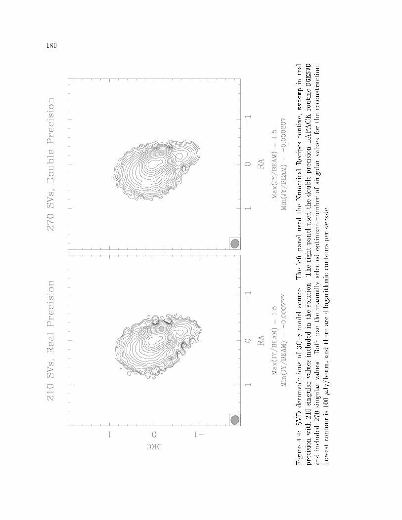
��
Figure � �SVDdeconvolutionsof�C �modelsource�TheleftpanelusedtheNumericalRecipesroutine�svdcmpinreal
precisionwith��singularvaluesincludedinthesolution�TherightpanelusedthedoubleprecisionLAPACKroutineDGESVD
andincluded��singularvalues�Bothusethemanuallyselectedoptimumnumberofsingularvaluesforthereconstruction�
Lowestcontouris��Jy�beam�andthereare logarithmiccontoursperdecade�

���
��� NNLS
SVD deconvolution happened to be the original motivation for the algebraic inves�
tigation� But once the basic framework was in place� it was a simple matter to try another
algorithm which also purported to solve the basic matrix equation� The algorithm� NNLS
from Lawson � Hanson ���� �� also had the considerable advantage of enforcing positivity
on the solution� This experiment was performed while working on a project to image the
recent supernova SN����A� and it was naturally applied there �rst� The project had a
low signal�to�noise ratio� and was relatively simple to deconvolve at the nominal resolution�
NNLS� like most other algorithms� produced an acceptable solution� The slipping point was
that the project required the highest possible resolution and hence direct examination of
the deconvolved model components� As will be shown by example later� the NNLS compo�
nents do not appear terribly physical when examined directly� They tend to be spatially
isolated from each other and spikey to the eye� CLEAN shares this behavior to an extent�
and neither CLEAN nor NNLS was deemed suitable for the needs of the SN����A project�
Due to other concerns� the implementation was largely forgotten until the time came to
write up this chapter as �an interesting exercise but ultimately not a particularly useful
one�� At this point� I resurrected the program and �nally tried it on the model �C � source
which had given so many other algorithms di�culties� I was shocked at how well it did�
After subjecting the algorithm to the same suite of algorithmic test cases as the others� or
at least as many of them as could be accommodated within the computational limit� I was
eventually convinced that it really was performing as well as the initial tests had indicated
� a signi�cant advance in high dynamic�range imaging� The simulations did indicate that
the NNLS solution degrades with source size compared to other algorithms� MEM in par�
ticular� and that the crossover point where it became comparable to other algorithms was
somewhere near the limit of what could be processed computationally� The size scales at
which NNLS excels are sources which are too compact for MEM to do a good job� and
which are too extended for CLEAN to process well� Since the latter limit is surprisingly
small� there are a signi�cant number of scienti�cally interesting sources for which NNLS or
a derivative algorithm is the tool of choice�
In an especially apt case of timing� the NRAO Very Long Baseline Array was
just being brought up to full capacity� For the �rst time� a VLBI array was producing
observations theoretically capable of being imaged at many tens of thousands to one dynamic
range� And the images being produced were su�ering exactly the same CLEAN artifacts
as demonstrated in Chapters � and � NNLS deconvolution was attempted on the test
observation of the bright compact source DA���� and it worked quite well as shown in
Chapter �� In the process� another useful property of NNLS deconvolution was discovered �
it works particularly well as part of the hybrid mapping loop� where the data are iteratively
imaged and self�calibrated� It was found that the interaction of CLEAN and self�calibration
was limiting the composite process to somewhat lower dynamic range than CLEAN was
capable of on perfectly calibrated data� In contrast� NNLS has consistently produced images
of simple sources down to the thermal noise limit�

���
����� The NNLS algorithm
The reference for all of this section is Chapter �� of Lawson � Hanson ���� �� It
provides not only the theory� but also the FORTRAN code that is the heart of the deconvolution
program� I will describe the working of the algorithm in general terms� but it is both
redundant and beyond the scope of the dissertation to do more than that�
The general class of problems to which NNLS belongs is the least squares problem
with linear inequality constraints� That is� let E be a m� � n matrix representing the
experimental design or deconvolution problem� f be the m� element data vector� G be an
m � n constraint matrix and h be an m element constraint vector� The basic problem to
be solved� Problem LSI� is
Minimize kEx� fk subject to Gx h�
For our purposes here� G is the identity matrix� and h is identically zero� There
is a condition which all solutions of the problem LSI must satisfy� called the Kuhn�Tucker
conditions� Conversely� any vector which satis�es them is a solution� First note that the
constraint equations can be interpreted as a series ofm simple linear�inequality constraints�
Every row of the constraint equation� gTi x hi divides the allowed solution space in half
with a bounding hyperplane� A given solution vector x can be either interior to� or on
the bounding hyperplane for each row� The Kuhn�Tucker conditions say that the negative
gradient vector of ��x� � ��kEx�fk� points into the cone spanned by the negative normals to
the constraint hypersurfaces containing x� This means that in some appropriate coordinate
system� the solution must have zero gradient in the directions where the solution is not hard
up against a constraint surface� In the directions where it is on the surfaces� the negative
gradient must point into the surfaces� not away from them�
It may help to visualize the case in Cartesian ��space� where we wish to minimize
k�x� y� z�� ����� ��k� while satisfying y � x ! �� y � �x ! �� and z � �� The �rst two
intersecting planes form an edge at �x� y� �� ��� and clearly the point on that edge nearest
����� �� will be the solution� namely the point �� �� ��� The constraint that z � � is notcoming into play� so there had better be no gradient projection along the z axis� or the
solution cannot be a global minimum� The negative gradient is in fact ����� �� which isnormal to neither constraint plane� but �against� the sense of both�
The actual NNLS algorithm holds two index sets of indices� �or rather� one set
and its complement�� to indicate whether a given tentative solution element is zero �on a
constraint surface� or not� Elements whose index is in the set Z are held at the value zero�Elements whose index is in the set P are free to take arbitrary values�
�� Set all elements of the solution vector x to zero� set all of the indices into the set Z�set P to the empty set�
�� The main loop begins here� Compute the gradient vector w from the current value of
x� w ET �f�Ex�

���
�� If Z is empty or if all elements of w with indices in Z have values � we have a
solution� Terminate the algorithm�
� Find the maximum element of w� which will be positive� Move its index from the set
Z to the set P�
�� A possible secondary loop begins here� Form a modi�ed version of the E matrix� Epos�
where the columns corresponding to indices in Z are replaced with columns of zeros�
Solve the unconstrained least squares problem Eposz f� This will only determine
the components of z corresponding to indices in P� Set the remaining elements of zto �
� If all the elements of z with indices in P are in fact � � this is an acceptable new
trial solution� Set x z and continue with the main loop at ����
�� We can only accept a fraction of z as the new trial solution� Find an index q such
that xq��xq � zq� is the minimum of all such expressions for negative elements in z�
For this q� call the expression �
�� Form the linear sum x x! �z� x�
�� Move from the set P to the set Z all indices for which the corresponding element of
x is zero� This will include q� and may include other elements as well� Continue the
secondary loop at ���
The computation of the subset unconstrained problem in step ��� is not actually
calculated by �lling unused columns with zeros� of course� but rather with an embedded QR
decomposition that knows not to access elements beyond that allowed by the index sets�
Also adding greatly to the e�ciency of the implementation is that at each pass through
step ���� we are solving nearly the same problem as before� The QR decomposition of Epos
is retained across iterations� and updated whenever an index changes sets� �Methods exist
to update a QR decomposition in much less time than computing the entire decomposition
from scratch��
It is proved in Lawson � Hanson that the iteration of the NNLS algorithm is �nite�
Given su�cient time� the algorithm will reach a point where the Kuhn�Tucker conditions
are satis�ed� and it will terminate� There is no arbitrary cuto� in iteration required� in
that sense it is a direct algorithm� It is not direct in the sense that the upper limit on the
possible number of iterations that the algorithm might need to reach the point of optimum
solution is impossibly large� There is no good way of telling exactly how many iterations
it will require in a practical sense� The solution does improve smoothly as the iteration
continues� If it is terminated early� one will obtain a sub�optimal but likely still fairly good
image� De�ning an iteration as the number of times the algorithm passes though step ����
Lawson � Hanson comment that their problems typically terminated after n�� Nflux��

��
iterations� They hard coded a limit of �n iterations into their code� I found it occasionally
necessary to exceed that limit in model testing� and have allowed the maximum iteration
number to be a free parameter� Certainly the algorithm is normally allowed to terminate
on its own� The number of iterations required is also a function of the signal�to�noise ratio
in the data� Noisy data means that the algorithm will try to �t negative �ux to the noise
power and will more quickly reach a situation where it cannot improve the solution by
adding more components� The longest convergence times seen were roughly �Nflux� on
large model objects that had been noiselessly sampled in the sky plane prior to creation of
the dirty map� That is the� the most perfect possible model data set required several times
Lawson � Hanson�s hard coded maximum� All observational data required many fewer
iterations� and none exceeded the original limit of Nflux���
����� How Important are the Windows�
This has not been investigated systematically on model data� but a reasonable
amount of experience has been gained with the DA��� and �C � projects� It appears that
the most critical factor is the size of the source itself� not the size of the window� On the
DA��� project� both data and �ux windows were varied by a wide range without signi�cantly
a�ecting the result� For the very highest precision deconvolutions� however� the window was
edited by hand to exclude the most obvious spurious features at the window�s edge� This
made a small but noticeable di�erence in the solution� It would seem that a reasonable
strategy is to deconvolve with as large a �ux window as one can conveniently compute�
using a data window at least as large as the �ux window and larger if possible� Deconvolve
once or as many times as needed if self calibrating� until one has a good calibration and
reasonable image� At this point� direct examination of the component model image will
likely show the main source and possible a slight scattering of very low level components
o� the main source� The latter can be excluded by hand for the highest quality image�
It cannot be said that this procedure is excluding the existence of low emission at a level
below that found by the wider windows� but one can claim that the image is consistent
with no emission at the lowest level found by any means at all� �A fundamental principle of
VLBI imaging has always been �If you see a scienti�cally interesting feature in your image�
try hard to make it go away� If it does go away� it wasn�t mandated by the data and you
couldn�t have trusted it anyway��� In comparisons on DA���� NNLS generally exhibited
less sensitivity to support constraints than CLEAN� but was not completely immune to the
problem�
����� Model Deconvolutions
Once again� we return to the �C � model source� Since this is shown several places
elsewhere with uniform weighting� it was decided to use an intermediate robustness here�
This was primarily to provide an example of the robust beams� Granted� this decision does

���
favor NNLS somewhat� in that NNLS works particularly well with a robust beam� while
CLEAN would prefer a uniform beam� but perhaps compensating in the other direction� we
have used a model simulated in the visibility plane� and one that has signi�cant image plane
representation problems� CLEAN has reached the maximum �delity it can on this source �
issues of representation are not at all important for CLEAN here� A similar deconvolution
where the model was discretized in the sky plane prior to creation of the dirty image yielded
a nearly identical CLEAN image� apart from e�ects very localized to the region of the worst
representation problems� By contrast� NNLS can go an additional factor of � deeper in
o��source RMS when provided with such an ideal situation� So in selecting the parameters
for this simulation� we have made one arbitrary decision that will favor NNLS and one that
will favor CLEAN� As will be seen� the results are dramatic enough that it really makes
very little di�erence how the details of the simulation are set up�
First� we show the raw and smoothed model in Figure ��� This is the same �C �
model as used in the SVD section and the weighting chapter� Model parameters are given in
Table ���� except that the magnitudes of the four outlier point sources have been adjusted
to ���� �Jy� ��� �Jy� ���� �Jy� and ���� �Jy� The ratio between adjacent point sources
corresponds to one contour in the following plots� the �rd root of � � �����Two support windows were used� The �Large Window� is exactly that used in
the CLEAN simulations presented in Section ���� It contains a fairly generous region for
the central �ux of �C �� and circles of ���pixel radius centered on each o�set point source�
This box is shown as a greyscale superimposed on the model plots in Figure ��� The
�Tight Window� is the same� but without provision for the point sources� The idea is that
the astronomer would initially box the region of the visible source� and have no idea that
the extremely faint sources are there� If the faint sources show up in the residuals� then
they can be properly boxed and the deconvolution run again� The current computational
limits to NNLS are enough for many practical problems� �roughly pixels of emission
can be processed in a few hours on our IBM RS���� workstations�� but they are not
su�cient to allow boxing large regions on the sky just to see what �ux might be there� If
a faint source is to be detected� it must be initially detectable in the residuals� The pixel
and dirty image sizes are the same as before� at ���� and ����� respectively� The CLEAN
used �� components at a loop gain of ��� which was su�cient to reduce the residuals
to ���� �Jy�beam in all cases� Except where noted� all contours in this sequence are at the
same �xed levels�

��
Figure ���Rawandsmoothedmodelsource�Thewidowsaretheshadedregion�Thetightwindowisjustthecentralshaded
region�thefullwindowisallgreyregionscollectively�Threelogarithmiccontoursperdecade�Lowestcontouris����Jy�beam�

���
Figure ��CLEANdeconvolution�Noiselessdata�modelledinthevisibilityplane�Therightpanelisthesameimage�contoured
upbyafactorof��Lowestcontoursare����Jy�beamand�����Jy�beam�
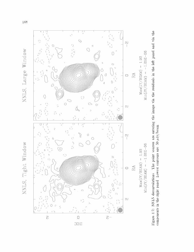
���
Figure ���NNLSdeconvolutions�Thepointsourcesareenteringtheimageviatheresidualsintheleftpanelandviathe
componentsintherightpanel�Lowestcontoursare����Jy�beam�
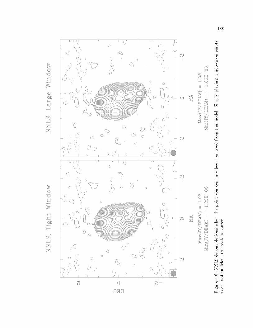
���
Figure ���NNLSdeconvolutionswhenthepointsourceshavebeenremovedfromthemodel�Simplyplacingwindowsonempty
skyisnotsu�cienttocreateasource�

��
Next we present the error characterization plots against weighting for NNLS�
These parallel the similar plots for CLEAN and MEM in Figures ���� and ����� respectively�
The simulation is identical to that described in Section ���� di�ering only by using NNLS
instead of CLEAN� There are fewer points on the noiseless curve than in the other two
�gures� because the noiseless NNLS deconvolutions were quite computationally intensive�
and only enough points to get the general shape of the curve were computed� Things to
note about these plots are�
� The worse on�source error for NNLS is nearly independent of weighting in the noiselesscase�
� NNLS has the strongest dependence of any of the major algorithms of full�imagemaximum error against weighting� with a �tted restoring beam� There must be a
signi�cant reconstruction error just outside the u�v sampling� CLEAN shows a similar
qualitative behavior� if not as strongly�
� There is no signi�cant di�erence between NNLS� CLEAN� and MEM on the noisy
o��source maximum and RMS error cases� They all do pretty well�
� For the noiseless case� the di�erence between NNLS and the other algorithms becomesmore apparent moving from maximum full�image to maximum o��source error� and
still more so in terms of the o��source RMS error�
� The merging of the two lines on the noisy maximum o��source error plot indicates onlythat the worst o� source error is a thermal residual that is not being smoothed� �and
thus has no dependence on restoring beam�� The curves converge on the noisy full�
image maximum error plot when NNLS has dropped the on�source error low enough
that the worst error is the same o� source peak�
� In the noiseless case� the o��source RMS error has a minimum in robustness� right
about where the worst near�in sidelobes of the beam have been minimized� While
it is very well de�ned� it is not terribly signi�cant in a quantitative sense� with the
extremes di�ering by about ����
� It�s interesting that the minimum in o��source RMS is not the uniform beam� which
generally has the best far�o� sidelobes of any weighting� CLEAN obviously prefers
the far uniform beam in the noiseless case� and nearly has a maximum near the same
robustness value�
� In the discrete model runs not shown here� the noiseless o��source RMS error forCLEAN was basically the same as in Figure ����� CLEAN had already bottomed out
due to the algorithm and slight under�CLEANing� the details of the sampling made
little di�erence� The same thing is nearly true for MEM� With the perfect sampling�
NNLS reduced the o��source RMS error to of order �������� Jy�beam� roughly ��
times deeper than CLEAN� and �� times deeper than MEM�

���
Figure ��a� Error quantities against RMS degredation factor� maximum error� The �ttedrestoring beam corresponds to Figure ���� The �xed beam curve is more representative ofthe absolute deconvolution quality and used
pBnatBuni ���� ���

���
Figure ��b� Error quantities against RMS degradation factor� maximum o��source error�The two traces in the lower panel are identical�

���
Figure ��c� Error quantities against RMS degradation factor� o��source RMS error�

��
Finally� we present one fairly amusing example both of the �exibility of the alge�
braic approach and of the robust nature of NNLS deconvolution� At an early stage in the
image processing of DA���� the calibration was such that there was a slight extended halo
around the source� which later turned out not to be real� For the moment we may take it
as the truth image� since that is what is present in the data as far as the deconvolution
algorithm is concerned� In fact� such a �truth image� is slightly unfair to NNLS� in that the
image it is trying to recover has negative values which may partially disrupt the solution
process�
Figure �� shows two deconvolutions of this data set� In the �rst� the data
window is the size of the large grey circle� with a radius of �� pixels and an area of roughly
� square pixels� The �ux window is the smaller grey circle� with radius � pixels and
an area of ��� square pixels� The left panel is the standard NNLS deconvolution using
these windows� and for this demonstration may be considered what the source looks like�
In the right panel� the �ux window was unchanged� the algorithm could place �ux in the
proper location� The data window� however� was changed to be the annulus between the
two circles� The windows are now completely disjoint� The algorithm was not given the
dirty image at the locations where it was placing �ux� It reconstructed the source entirely
through the sidelobes� As can be seen by comparing features� the second deconvolution
is not as good as the �rst� but it is remarkably close� NNLS is even quite capable of
reasonable deconvolutions when there are more pixels in the �ux window than in the data
window� Obviously� this can only be sensible with the addition information introduced via
the positivity constraint� I know of no way to quantify how much additional information
is introduced� but in practice it seems that given a signi�cant piece of the dirty image to
work upon� NNLS will return a reasonable answer�
I have been calling this a �deconvolution party trick�� since I can think of no good
application of this ability in radio interferometry� Locating a far source by its sidelobes leaps
to mind� but unfortunately the NNLS algorithm cannot image a large �eld without knowing
where to place the support windows� In the optical or any image plane detection system� of
course� one may have the problem of missing data due to detector saturation or to cosmic
rays� This has not been pursued at all� but it seems like it could be useful�
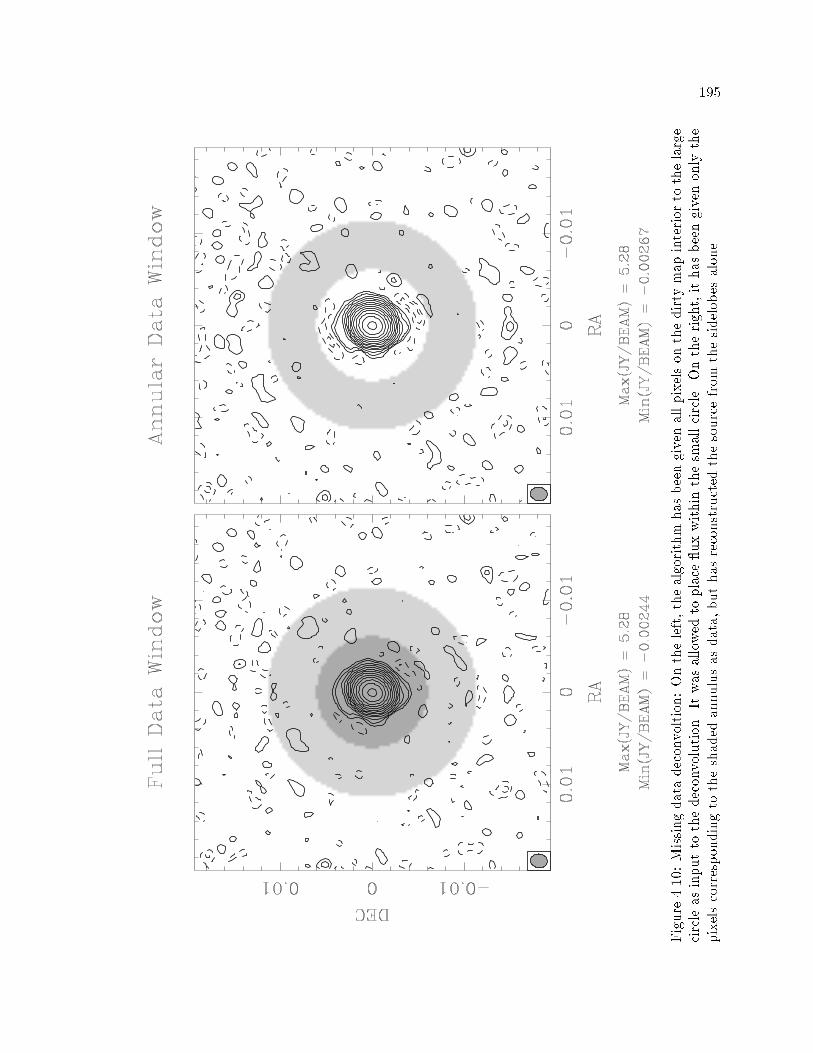
���
Figure ���Missingdatadeconvoltion�Ontheleft�thealgorithmhasbeengivenallpixelsonthedirtymapinteriortothelarge
circleasinputtothedeconvolution�Itwasallowedtoplace�uxwithinthesmallcircle�Ontheright�ithasbeengivenonlythe
pixelscorrespondingtotheshadedannulusasdata�buthasreconstructedthesourcefromthesidelobesalone�

��
����� Discussion
NNLS has plenty of limitations and some problems� But when it works� it works
extremely well� In an absolute sense� it works best on extremely compact emission� Com�
pared to the other algorithms commonly used in radio astronomy� it best distinguishes itself
on sources too extended for CLEAN to process well� and too compact for MEM� It has no
di�culty with sharp edges� which make it a good choice for planetary images and source
involving a shock� It is also very good at producing models for self�calibration� Both of
these properties are presumed related to the fact that NNLS zeros the residuals in the dirty
image nearly completely� Some algorithms like MEM make no particular attempt to zero
the residuals completely� and simply �t the data to within the thermal noise� Unfortunately�
if the residuals are correlated in the image plane� this may result in signi�cant systematic
bias at di�erent locations in the u�v plane � very bad news for self�calibration� CLEAN
will indeed zero the residuals in the asymptotic limit� but at �nite iterations may also suf�
fer a systematic bias in the u�v plane� NNLS makes a choice about the model� and then
essentially jumps right to the solution� This can be a good thing or a bad thing� depending
on the quality of the data� but under�iteration is rarely a problem in NNLS images� And
even with quite noisy data� the solution appears robust�
For practical purposes� the NNLS algorithm lacks a termination criterion� or any
other tuning parameter� This is a good thing� since any parameter which must be set for
proper operation can be set incorrectly� NNLS certainly exceeds the capabilities of CLEAN
and MEM on objects to which it is well suited� But also� it has the advantage that it is
di�cult to misuse and generally produces the best image of which it is capable� The other
algorithms can produce sub�optimal images due to insu�cient iteration or poorly chosen
parameters� A major strength of NNLS as a practical deconvolver is that it is largely �hands
o���
On the negative side� NNLS shares the tendency of CLEAN to compact �ux� A
region of smooth �ux will typically result in a model with regularly spaced components
at intervals of a few pixels� The isolated pixels will contain all the �ux that should be
contained in the zero pixels surrounding them� This behavior seems to be a common failing
of algorithms that operate on small numbers of pixels at a time�
The Kuhn�Tucker conditions do not guarantee a unique solution to the deconvo�
lution problem� merely �a� solution� Clearly� since the performance of the NNLS algorithm
on noiseless� discretely sampled model data is less than perfect� there must be multiple
solutions present that even in the perfect case are indistinguishable by the algorithm from
the real thing� Examinations of the residuals in such perfect cases show that it really has
reduced them to within machine precision of zero� Unless this were so� the real solution
would have a calculably better �t to the data and the algorithm would not terminate� Since
the algorithm typically builds up the model a few components at a time� examining the ter�
mination criteria at each step� it will stop at the �rst solution that satis�es the Kuhn�Tucker
conditions to its precision� In some sense� then� the NNLS algorithm is selecting something

���
like a minimum�number�of�pixels solution� The addition of positivity and support has re�
duced the dimensionality of the null space somewhat� but the problem is still singular� The
�nal implicit criterion in the algorithm is that it stops at the �rst acceptable solution� which
is built up a few pixels at a time� It means that if the real solution has a great many smooth
pixels� the algorithm will always select a �ux compacted solution over the true answer� so
long as both are indistinguishable from the point of view of �tting the data� It de�nitely
would be worth looking into other algorithms that solve the same in di�erent ways� to see
if variations in how the solution is computed make a signi�cant di�erence�
The NNLS algorithm is used in the simulation Chapter �� the �C � case study
Chapter �� the SN����A case study Chapter � and the DA��� case study Chapter �� so we
will see a good deal more of its properties by example� The SVD deconvolution is only used
henceforth in Chapter ��

���

Chapter �
Simulations
This chapter is composed primarily of a number of deconvolution simulations� The
thrust of all of these simulations is to give a lower limit error bound� All of these simulations
are noiseless� and except where representation issues are fundamental to the simulation� all
have been discretized in the image plane� That is� the model of the source was sampled onto
a regular pixel grid� the point spread function treated likewise� and both were discretely
convolved to create the dirty image used as input to the deconvolution algorithm� The
e�ect of this is that the problems set before the deconvolution algorithms possess an answer
that obeys the assumptions of bounded support and positivity� unlike real sources which
may violate these constraints at a low level due to discrete representation e�ects� Thus the
imaging performance on real sources may well be worse than given in these simulations�
for a wide variety of causes including thermal noise� calibration error� and representation
e�ects� The imaging performance is highly unlikely to be better than there simulations�
however� and the results given here show deconvolution errors occurring at a signi�cantly
higher level than many people believe� Whether recognized or not� errors at the levels given
here or higher are probably present in any astronomical image deconvolved with one of the
algorithms listed below�
The bulk of the chapter is a number of simulation series all designed to address the
issue of deconvolution behavior on simple isolated sources� These are the �resolution tests��
since most of these simulation series are indexed by at least the size of the model relative to
the point spread function� This meta�series begins with a catalog of error magnitudes and
morphologies produced by deconvolving an isolated Gaussian or Disk model source using a
Full Track VLA point spread function� taken from an actual high quality observation� For
each of the three major algorithms used in this dissertation� CLEAN� MEM and NNLS� and
each of three model sizes� the magnitude of the model error in the u�v plane is given in both
greyscale and quantitative slice format� Additionally� the component model for each case
is displayed as an image� as is the error in the sky plane between the smoothed model and
reconstructed image� A similar series of deconvolution tests is given with the same model
sources� this time varying the source smoothly through two orders of magnitude in size� and
exploring a wider parameter space of point spread functions and algorithms� The result of
each is graphically presented by the error quantities in the nominal�resolution reconstructed
image� The residuals in both planes are presented� along with the quantities �maximum er�
ror in the reconstructed image�� �maximum error o� the support of the source�� and �RMS
���

�
error o� the support of the source�� There is a series against di�ering point spread func�
tions for the major algorithms� and a cross comparison series against di�erent algorithms
returning to the Full Track VLA PSF and adding in the algorithms Maximum Emptiness�
SDI CLEAN and GSP� The width of the �nal restoring beam was found to be extremely
important in the reconstruction �delity� and the error quantities against algorithm at a
particular source size are presented varying the reconvolution width from half the nominal
to twice the nominal width� Finally� a scaled version of the model �C � source is used with
CLEAN � MEM only� presenting maximum error only� as a demonstration that a somewhat
more realistic model source yields results similar to those of the isolated single component
models�
The thrust of the resolution test meta�series changes slightly as we next present
not error quantities in the restored image� but error quantities in the restored summed �ux
over the support of the source� This is again indexed by model size and all six algorithms�
and is presented for the Full Track VLA PSF and Snapshot VLA PSF� for both the Gaussian
and Disk models� Sadly� this series only addresses a nominal reconvolution width� Last of
all in the meta�series� we consider a modi�cation to CLEAN� where the sky is considered
composed of Gaussians rather than delta functions� This uses the Full Track VLA PSF
again� and indexes against model size� model type� pixel size and convolution width� In an
uncharacteristic nod to brevity� only the maximum error and RMS plots are presented�
Numerous as are the simulations and quantities presented� these plots are really
only slices through a larger parameter space explored� The relatively small ASCII �les
containing the numerical data values which generated the plots in the resolution test meta�
series will be made available for the inde�nite future as part of the SDE software distribution�
See Appendix H for a description of the �Electronic Supplement� and how to obtain it�
The chapter concludes with two �nal series which simulate their data in the u�v
plane� Both use a synthetic Full Track VLA PSF� The �rst addresses the question of a
shifted point source� which happens to lie halfway between two pixels in the sky plane
discretization� It is shown how well a perfect deconvolution algorithm could reconstruct
such a source for two di�erent oversampling factors� and then how well the three major
algorithms do on noiseless u�v data� The last simulation series in the chapter addresses the
issue of how quickly CLEAN and MEM converge� as a function of position in the u�v plane�
Both are run on a shifted point source� for two di�erent oversampling factors� and with and
without a Gaussian pixel function�
��� The Resolution Test Deconvolutions
This section describes most details of the deconvolutions performed in the res�
olution test meta�series� A few later variations are described in the running text� The
algorithms themselves are described in Section ����

��
Most test series use the point spread function from the observation of �C � given
in Figure ��� � with observation parameters and u�v coverage in Table ��� and Figure ����a�
respectively� It is a realistic example of a good single�con�guration VLA observation of a
high declination source� The �tted beamwidth is ����� � ������� for a mean beamwidth
of ��� ��� The dirty images were of size ���� and pixel spacing ����� Model sources were
constructed with full�widths at half�maxima of �n��b� where b is the basic width of the
series� In this case b ������ In the full series� n varied by integers from �� to � for mostalgorithms and from �� to for NNLS� The extreme limits of smoothness were consideredby using a Gaussian and Disk as the model� which probably have edges smoother and
sharper respectively than any source likely to be encountered in practice� The models
were azimuthally symmetric� It should be mentioned that MEM has a somewhat unfair
advantage when run on the Gaussian models� in that the �I ln I form of the entropy can beshown analytically to produce Gaussian peaks around sharp features in the image� �Narayan
and Nityananda� ����� But CLEAN possibly has a similar advantage in the Disk models�
in that it is not burdened with an inappropriate smoothness criterion� About all that can
really be said is that the behavior on true sources will likely lie between these extremes�
The CLEAN deconvolutions for the cases n � were run to � componentsat a loop gain of ��� The n and � cases were run to �� components� n to
��� components� and n � to ��� The algorithm was allowed to place components
wherever it chose� and this was veri�ed to make no signi�cant di�erence in the solution
quality� In general� the support constraints are more important for noisy and ill�calibrated
data� but in these tests it was not usually an important consideration� While the number
of iterations was rather arbitrary� these choices were su�cient to reduce the image plane
residuals to a small fraction of the RMS reconstruction error� Typically the maximum
residual was down by �� from the peak smoothed model� The nature of the residuals
varies considerably with algorithm� CLEAN and NNLS reduce the residuals to near zero�
which may or may not be an advantage depending on the nature of the problem and data�
The other algorithms generally do not� This is discussed in more detail in Section ��� where
a plot is presented of RMS image plane residuals�
All MEM deconvolutions in this series were run to � iterations each� which is
comfortably in excess of the canonical iterations typically used� This was su�cient that
the n � cases had converged completely� and the n �� �� cases nearly so� For emission
more compact than that� the algorithm had entered a regime where tiny improvements
in entropy and �t to the data are traded o� against each other� There is a very gradual
improvement in the solution quality at this point� For practical purposes� the algorithm
may be said to have converged� By spot checking individual cases� the solutions improve by
a small factor when run to extreme iteration� but not by enough to a�ect any qualitative
description given here� Since there is no thermal noise in these simulations� an arbitrary
level had to be selected for the agreement parameter between model and data� These
simulations used Sigma ��� and allowed the algorithm to estimate the total �ux by

��
itself with Tflux ���� Again� spot checking individual cases showed only the weakestdependence on the exact value of the parameters selected� and these results are expected
to be generic for noiseless compact emission�
No termination or tuning parameters were needed for the NNLS deconvolutions�
Though in some cases the number of iterations exceeded the �Nflux limit proposed by
Lawson and Hanson� the algorithm was run until the solution satis�ed its stopping criterion�
NNLS does require support information to make the problem computationally tractable�
however� and was allowed to place �ux in the region where the model� smoothed to the
�tted PSF� exceeded �� of its maximum� The NNLS data window was a circular region
centered on the source� pixels in radius for a total of ��� pixels� or the �ux window�
whichever was larger�
Many of the more detailed results examine only the algorithms CLEAN� MEM
and NNLS� The graphical error plots also examine the Maximum Emptiness �L�� algorithm�
SDI CLEAN and Gerchberg�Saxton�Papoulis� The L� deconvolutions were very similar to
the MEM deconvolution with the parameters of � iterations� Sigma ��� and Tflux
���� The SDI CLEAN deconvolutions are also measured in �components�� the only
thing changing being how the components are selected� The same number of components
were used for SDI CLEAN as with CLEAN� The Trim parameter was ��� and the loop
gain again ��� Finally� the GSP algorithm was run to � iterations for all cases� with
an acceleration parameter Accel of � Like NNLS� the GSP algorithm essentially requires
support information� �In many cases� the deconvolution diverged without it�� The same
support window of �� of the peak smoothed model was used� No support window was
used for the other four algorithms�

��
��� Error Morphology
Figures ��� through ��� attempt to characterize the morphology of the errors
made by the three major algorithms on the model sources� Here we present detailed images
of the n ��� �� and cases� for a beamwidth�to�model�width ratio of ���� ���� and ���respectively� The n case exceeded the limits of the NNLS algorithm� and the n
case is used instead� with a ratio of ��� The most dramatic of the plots provided for each
case is a grey scale plot of the error pattern in the Fourier plane� This is simply���F$M �C%
����where M is the model and C the component representations produced by the algorithms�
Notice that the residuals are not included in these plots� Each panel of each plot has
been allowed a full independent linear range of greyscale� to better show the morphology of
the error pattern� The amplitude of the error pattern is symmetric due to the Hermetian
nature of both sky and component model� and only the Fourier half plane is shown out to a
"umax "vmax �� � M�� The phase information is also interesting� but not su�ciently so
to include here� Color GIFs of these plots showing both amplitude and phase can be found
in the electronic supplement to this dissertation� as documented in Appendix H�
The three lobe �gure traced in white in each panel of the Model Error Amplitude
plots is the envelope of the VLA sampling pattern which generated the beam� and the three
straight lines in each are given quantitatively as slices in the lines plots on the facing page�
In these line plots� the solid lines are slices through the error amplitude plots as indicated�
with heavy dots indicating the point where the slice crosses the sampling envelope� The
large dashed line is the transform of the model� and the upper light dotted line is the
transform of a typical restoring beam� ���� in this case� The lower light dotted lines are
the same slices after smoothing down by the restoring beam� again with a dot where the
slices cross the sampling pattern� Each case also includes grey scale plots of the model
components and the error pattern in the restored image at a resolution of ����� Both the
component model and error pattern are displayed on a logarithmic grey� either zero to the
maximum or two sided logarithmic around zero� depending on whether or not the particular
image can assume negative values� The dotted circles in these plots are locations where the
model smoothed to ���� reaches ���� ���� and �� of the peak smoothed value� so the
outer circle also corresponds to the NNLS support window� One �nal �gure at the end
of this set is a cross�comparison plot for the di�erent algorithms� presenting model error
slices for the Gaussian n � case on a linear scale instead of a log scale� This plots shows
the sharpness of the error pattern at the sampling envelope more dramatically than the
quantitative semi�logarithmic plots�
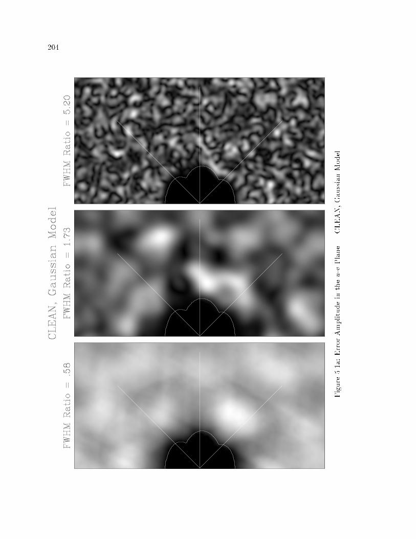
�
Figure���a�ErrorAmplitudeintheu�vPlane�
CLEAN�GaussianModel

��
Figure���b�ModelErrorAmplitudeintheu�vPlane�
CLEAN�GaussianModel

�
Figure���c�ComponentModelintheSkyPlane�
CLEAN�GaussianModel

��
Figure���d�ErrorPatternintheSkyPlane�
CLEAN�GaussianModel

��
Figure���a�ErrorAmplitudeintheu�vPlane�
MEM�GaussianModel

��
Figure���b�ModelErrorAmplitudeintheu�vPlane�
MEM�GaussianModel

��
Figure���c�ComponentModelintheSkyPlane�
MEM�GaussianModel

���
Figure���d�ErrorPatternintheSkyPlane�
MEM�GaussianModel

���
Figure���a�ErrorAmplitudeintheu�vPlane�
NNLS�GaussianModel

���
Figure���b�ModelErrorAmplitudeintheu�vPlane�
NNLS�GaussianModel

��
Figure���c�ComponentModelintheSkyPlane�
NNLS�GaussianModel
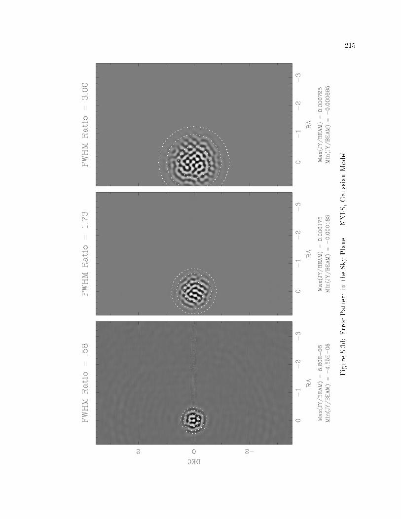
���
Figure���d�ErrorPatternintheSkyPlane�
NNLS�GaussianModel

��
Figure�� a�ErrorAmplitudeintheu�vPlane�
CLEAN�DiskModel

���
Figure�� b�ModelErrorAmplitudeintheu�vPlane�
CLEAN�DiskModel

���
Figure�� c�ComponentModelintheSkyPlane�
CLEAN�DiskModel

���
Figure�� d�ErrorPatternintheSkyPlane�
CLEAN�DiskModel

��
Figure���a�ErrorAmplitudeintheu�vPlane�
MEM�DiskModel

���
Figure���b�ModelErrorAmplitudeintheu�vPlane�
MEM�DiskModel

���
Figure���c�ComponentModelintheSkyPlane�
MEM�DiskModel

���
Figure���d�ErrorPatternintheSkyPlane�
MEM�DiskModel

��
Figure��a�ErrorAmplitudeintheu�vPlane�
NNLS�DiskModel
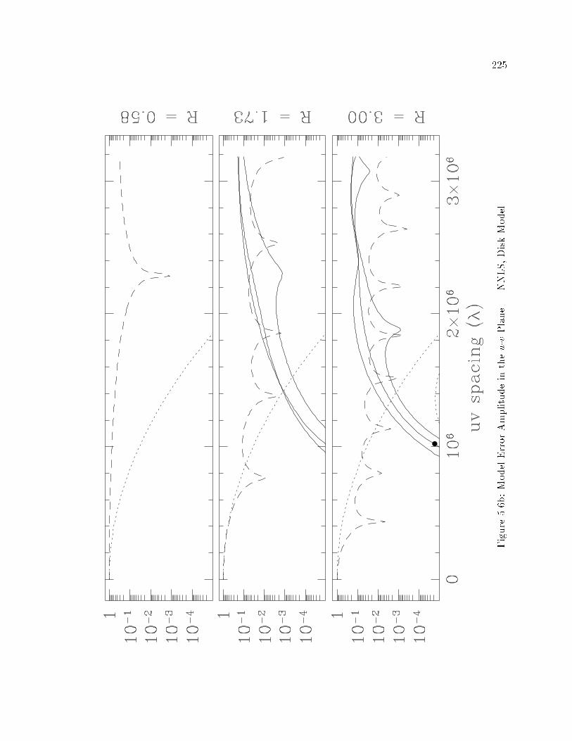
���
Figure��b�ModelErrorAmplitudeintheu�vPlane�
NNLS�DiskModel

��
Figure��c�ComponentModelintheSkyPlane�
NNLS�DiskModel

���
Figure��d�ErrorPatternintheSkyPlane�
NNLS�DiskModel

���
Figure ���� Model Error Amplitude in the Fourier Plane � linear algorithmic comparison�The source is the Gaussian n � case for a model width ���� times the �tted beam width�

���
����� Results
If the deconvolution algorithm approximately zeros the residuals on a noiseless
data set� then clearly the dominant reconstruction error must come from unsampled regions
of the u�v plane� This is hardly new� but previous lore on the CLEAN algorithm has
placed great emphasis on interpolation errors across holes in the sampling pattern� The
most surprising thing about these error plots is how sharp the edge is at the u�v sampling
envelope� Even when downweighted by the restoring beam� the dominant reconstruction
errors almost invariably come at or just outside the sampling envelope� While these plots
are from a well�sampled VLA coverage� the same statement is true even in a full track VLBA
coverage experiment with considerable holes in the outer spacings such as that shown in
Figure ����b� The errors are larger in the holes than in the well sampled areas� but even
after smoothing both are dominated by the errors just outside the sampling�
Reconstruction errors in high�precision observations of simple sources are domi�
nated by extrapolation errors� not interpolation errors�
The immediate corollary to this� of course� is that using a larger restoring beam
will lead to smaller reconstruction errors� Again this is not new� but as we will see quanti�
tatively in Figure ���� it is true to a remarkable extent� Since reconstruction errors quickly
rise to a signi�cant level outside the sampling envelope� the errors in the smoothed model
are strongly in�uenced by the location of the errors relative to the restoring beam trans�
form� The worst errors occur closer in� and often nestle into a �corner� of the sampling
pattern�
More algorithm speci�c observations about the error morphology are
� CLEAN has the worst extrapolation properties of the three major algorithms � the
sharpest edge at the sampling envelope � followed by NNLS and MEM for the Gaus�
sian cases� In the disk cases the ordering changes to CLEAN� MEM� NNLS in de�
creasing order of model error sharpness at the sampling envelope�
� CLEAN and NNLS will place power at high spatial frequencies� whether it is there ornot� and MEM will avoid placing power there� whether it is present or not� This is an
obvious consequence of the smoothness criterion or lack of it built into the algorithms�
Simply putting spatial power into a region where the true source has power does not
guarantee the reconstruction there will be correct� the phase may still be wrong� But
not putting power there will certainly by wrong� By contrast� not placing power in a
region where the source has none is guaranteed to be correct� This dichotomy tends
to favor MEM for reconstruction of extended smooth objects�
� The error patterns produced by CLEAN have a random structure� though a character�istic scale size� NNLS errors are somewhat more structured� with a striking periodic
speckle appearing on smooth emission� which is the transform of the regular spacing
��
of model components� The most regular error patterns are produced be MEM� in par�
ticular on the Disk models where the outer structure in the error pattern is essentially
the pure model�
� CLEAN has a striking inverse correlation between the scale size of the mottling patternon its error pattern and the source size� It is not related in detail to the structure of
the model transform�
� NNLS does a superb job of modelling the source inside the sampling envelope in theu�v plane� CLEAN does a fair job� and MEM the worst of the major algorithms�
� NNLS has no problems with the sharp�edged sources� CLEAN a bit more� and MEMhas real problems with them�
� The CLEAN error morphology in the image plane is nearly constant for n � � varyingonly in absolute scale� It is still similar at n ��
� CLEAN has a ringing structure in the placement of its components that will be in�vestigated in more detail in Section ���
� NNLS tends to place components very regularly on regions of smooth emission� Thiscan be seen most clearly by the strong peaks in the u�v plane model error plots�
� NNLS error patterns are strongly con�ned to the support of the source� Its perfor�mance compared to other algorithms gets better if one considers the o��source errors
as opposed to errors anywhere in the image�
� CLEAN is doing better than MEM at the low spatial frequency reconstruction� and
for all but the smallest and sharpest sources� MEM is doing better than CLEAN at
the highest spatial frequencies� Notice that this is exactly backwards to what one
might expect from the statements �MEM is good at smooth emission� and CLEAN is
good at compact emission��
Acting on the observation that the CLEAN reconstruction error very quickly rises
to nearly a constant level immediately outside the sampling envelope� an e�ort was made to
model the CLEAN errors by an azimuthally�symmetric Heaviside step function in radius�
with an amplitude produced by an incoherent sum of a number of components proportional
to the source area� A correlation was sought between the fraction of the restoring beam
beyond the sampling envelope times the modeled error amplitude� This was not successful�
though it is not known whether the problem was that the model was not detailed enough� or
if the correlation structure of the amplitude errors was causing the problems� Image plane
modelling is an e�ective way to estimate the error due to deconvolution on simple sources�
so the Fourier plane approach of modelling the errors was not pursued�

���
��� Residual Behavior
The previous discussion largely assumed that the residuals of the deconvolution
process were ignorable� that is� that the error in the smoothed model was roughly equivalent
to the error in the reconstructed image� This is only approximately true� In detail� the
algorithms di�er greatly in how well they can �or attempt to� zero the residuals� We now
consider all of the resolution�test algorithms� adding Maximum Emptiness� SDI CLEAN�
and Gerchberg�Saxton�Papoulis�
First� note that Maximum Entropy and Maximum Emptiness do not try to zero
the residuals at all � they try to �t the data only within the thermal noise� and the level
of agreement is regarded as a free parameter to be adjusted by the user� The minimization
of their particular criterion will almost certainly mandate a solution that does not zero the
residuals� and if started at such a solution they will move away from it� The remaining
algorithms will zero the residuals in the sense that if started with an allowed model that
exactly �ts the data� succeeding iterations would remain at that point� In a more practical
sense� however� the convergence behavior of SDI CLEAN and GSP is su�ciently slow in
the high�precision cases that the residuals are never completely zeroed� CLEAN converges
somewhat faster than SDI CLEAN on a �per component� basis� though not necessarily on
a �per machine cycle� basis� Given su�cient time it will reduce the residuals to zero and
the number of components required is modest enough that at least some small sources can
be zeroed of machine precision� Of all the algorithms� NNLS is generally the best at zeroing
the residuals� though of course it can be used only for compact sources� This probably is
related to its usefulness in self�calibration�
Figure ��� presents the image�plane residual level for the basic resolution�test
series� The PSF used is the Full Track VLA PSF from the previous section� so the corre�
sponding points of these plots are exactly the same cases as presented in Section ����

���
Figure ���� RMS residuals in the image plane�

���
��� Algorithmic Cross Comparison
In this section we use only the Full Track VLA point spread function and exam�
ine how well the di�erent algorithms do relative to one another� Figure ��� presents the
error statistics against source size for all six algorithms� restoring at the near�nominal ����
beamwidth� Figure ��� presents the same quantities� but examines only a single source
size and varies instead the restoring beamwidth� These two �gures form slices though the
center of a full two�dimensional parameter space explored� The ASCII data �les necessary
to produce plots like these for the full range of parameters are available in the electronic
supplement to the dissertation� as described in Appendix H� In these plots� a solid circle is
a positive reconstruction error� �too much �ux at a point�� and an open circle is a negative
error�
� Deconvolution errors can be quite signi�cant� even for a well sampled VLA observa�tion� These errors often look like calibration errors� and have probably been misdiag�
nosed in the past� along with whatever calibration errors are actually present�
� Some algorithms almost aways make their errors in one direction or the other� whileothers are nearly random errors�
� CLEAN errors are dominated by u�v plane extrapolation� not holes in the samplingpattern or lack of zero spacings� This makes CLEAN based algorithms very amenable
to smoothing�
� Even very mild resolution produces signi�cant CLEAN deconvolution errors� The
only thing that is a point to CLEAN is a real point source� A source with a width as
much as �� of the �tted beamwidth behave like an extended source when CLEANed�
� MEM errors have a signi�cant zero spacing component� MEM images are often signif�
icantly better than the CLEAN images at nominal resolution� but cannot be improved
by post smoothing� Fractional RMS error may actually get worse with smoothing�
� The source itself masks the on�source CLEAN errors� This leads to a strong peak
in �o��source errors� as a function of source size when the source size is slightly less
than the synthesized beamwidth�
� The algorithms which make their dominant errors outside the u�v sampling envelopeare the ones with steep slopes in Figure ����
� Either CLEAN or MEM is more e�ective than SDI CLEAN for nearly all size scales
� GSP and L� can produce very good reconstructions on some sources� but they behavequite badly on others� In general� these algorithms were not found very robust to
support constraints�

��
Figure ���a� Deconvolution errors against source size� Algorithmic comparison� MaximumError in the smoothed reconstruction� Reconvolving size was ���� and the �tted GaussianFWHM was ��� ��

���
Figure ���b� Same as Figure ���a� but maximum error o� the support of the smoothedsource�

��
Figure ���c� Same as Figure ���a� but root mean square error o� the support of the smoothedsource�

���
Figure ���a� Deconvolution errors against reconvolution size� Algorithmic comparison�Maximum Error in the smoothed reconstruction� Source FHWM was ����� the size of the�tted beam�

���
Figure ���b� Same as Figure ���a� but maximum error o� the support of the smoothedsource�

���
Figure ���c� Same as Figure ���a� but root mean square error o� the support of thesmoothed source�

�
Figure ����a� Deconvolution errors against source size� Unit scaling corresponds the modelin Table ����
Figure ����b� Same model as in Figure ����a at Scale �

� �
��� The E�ect of Fourier Plane Coverage
We now restrict our attention to the three major algorithms once again� and ask
how well they can recover the source when the u�v coverage is varied signi�cantly� The
simulations use the same Gaussian and Disk sources as before� and the uniformly weighted
point spread functions from Figure ���� �VLA Full Tracks ��C ��� referred to here as VLA
Full Tracks�� Figure ���� �VLA � Point Snapshot� and Figure ��� �VLBA Full Tracks��
In addition to the usual samplings� we also include the limiting case of a �perfect�
VLA observations� where the transfer function has been determined by simply tracing the
outline of the VLA sampling pattern and setting all interior points to unity� The Mid Tracks
sampling was intended to loosely represent the practice of interleaving many di�erent sources
in survey style observations� The two special samplings are given in Figure ���� �VLA Mid
Tracks� and Figure ���� �VLA Perfect Coverage��
� The most surprising e�ect is how little e�ect there is� Only the snapshot coveragemakes much di�erence� All the rest are pretty much the same� One should be cautious
about extrapolating this result to more complicated sources�
� MEM is the most sensitive of the three algorithms to u�v coverage� followed by CLEANwhich is much better� �The three largest snapshot cases diverged when run to the full
iteration limit with CLEAN� The points shown were limited to reasonable iteration
values manually�� NNLS is nearly immune to variation in u�v coverage for these cases�

� �
Figure ����� Mid Tracks u�v coverage and PSF� This is one hour of u�v data� divided into� �� minute scans centered at hour angles of ��� ��� � �� and � hours� Integration time is� seconds� and the declination is ���� Minimum contour is ���
Figure ����� Perfect VLA u�v coverage and PSF� This PSF was generated by simply tracingthe outline of the VLA sampling pattern� and setting each interior pixel in the griddedtransform plane to unity� Declination is ���� Minimum contour is ��

� �
Figure ��� a� u�v Coverage and Deconvolution Errors � CLEAN

�
Figure ��� b� u�v Coverage and Deconvolution Errors � MEM

� �
Figure ��� c� u�v Coverage and Deconvolution Errors � NNLS
�
��� Flux estimation
Flux estimation can be a tricky business� and given the importance of photometric
observations� there has not been enough work done on the subject� There are many di�erent
factors that can in�uence the estimated total �ux in a source� namely the shape of the
source� the shape of the beam� the noise level of the observation� the calibration errors in
the observation� and the interaction of the deconvolution algorithm with all of these�
These plots attempt to quantify just the contribution of the deconvolution algo�
rithms on perfect data� in the limit where the algorithms have essentially converged� These
are the same resolution�test deconvolution as before� but now the �ux has been determined
by adding up restored image pixels in the �on�source� window and dividing by the restoring
beam area� Only two beams have been used here� the full�tracks uniform beam and the
snapshot uniform beam� This is a signi�cant omission� and more work should be done here�
In particular� these plots should be repeated with a best��t Gaussian robustly weighted
beam�
� NNLS is the best of the algorithms examined for �ux estimation in terms of the errormagnitude� In addition� it seems to be the only algorithm that is unbiased in the �ux
estimated� All the others estimate systematically too high or too low�
� CLEAN is the next most useful algorithm for �ux estimation� and is the only choice
for larger sources� possibly excepting GSP�

� �
Figure����a�FluxEstimationErrors�GaussianSource�FullTracks

� �
Figure����b�FluxEstimationErrors�GaussianSource�FullTracks

� �
Figure����c�FluxEstimationErrors�GaussianSource�SnapshotCoverage

��
Figure����d�FluxEstimationErrors�DiskSource�SnapshotCoverage

���
��� Gaussian Pixel Functions
I now present a simulation series using the generalized pixel function introduced
in Section ���� This section is not as thoroughly explored as it might be� In particular�
while the generalized pixel function discussed in Chapter � is a feature of the discretization
of the fundamental convolution equation� and not of any particular algorithm� it is here
applied only to CLEAN� and only with a Gaussian pixel function� This technique has been
spot checked on NNLS and it seems to help on the extended sources� but it�s not yet known
how much this practice hurts the algorithmic performance on compact emission�
The most interesting thing about these plots is how much the curves for the
di�erent pixel functions resemble the curves for the di�erent algorithms in the algorithmic
cross comparison earlier� Compare Figure ��� with Figure ���� The resemblance is really
quite striking� This leads one to speculate that much of the behavior di�erence seen between
algorithms on these resolution test plots is in exactly how much interpixel correlation they
implicitly impose�
The one other rather depressing fact about this series is how much the di�erent
curves cross each other� The consequence of this being that there is no unique answer to
�what is the right pixel function width to use�� if there happens to be emission of many
scales in the image� This is hardly surprising� but unfortunate� Since the �tted beam width
for this PSF is quite close to ����� notice that even half a beam width in the pixel model
completely destroys CLEAN�s ability to deconvolve point sources well� This is probably
due to the extended pixel model requiring many more nonzero components to model a
point source� The �nal answer may be reasonable� but we have quite destabilized CLEAN�s
convergence� On the plus side� however� a similar small but extended pixel function consid�
erably improves CLEAN�s ability to reconstruct extended emission� It remains to be seen
if this is a useful tradeo� on actual sources�

���
Figure ���a� Smooth Pixel CLEAN deconvolution errors against source size�

���
Figure ���b� Same as Figure ���a� but the o��source root mean square error�

��
Figure ����a� Smooth Pixel CLEAN deconvolution errors against reconvolution size

���
Figure ����b� Same as Figure ����a� but the o��source root mean square error�
��
�� Point Sources Between Pixels
Next are a few plots which show how well one might hope to do with a point
source that has happened to fall between image pixels�
These simulations were done with a data set that resembles the VLA Full Track
case� but is slightly di�erent� This is a synthetic VLA observation in �C� con�guration�
The data was noiseless� free of calibration error� and complete over the full u�v tracks� The
simulation frequency was ��� GHz� and the declination of the source was �� Uniform
weighting was used and gave a nearly circular synthesized beam with FWHM of ������� The
coarsely sampled maps used here had a pixel size of ���� and the more �nely sampled maps
used a pixel size of ������ The dirty image sizes were the usual ����� The u�v coverage and
PSF for this observation is given in Figure ����� The box surrounding the coverage is the
maximum u�v spacing corresponding to a cellsize of ���� Clearly this cellsize satis�es the
sampling theorem� but not by much� It is a coarser sampling than I would recommend
anyone use in practice� The maximum u�v spacing for a cellsize of ����� is the limits of the
plot� This would be quite reasonable for most projects� though somewhat oversampled if
the image size were a pressing concern�
The �rst �gure shows how well one could do if the deconvolution algorithms were
functioning perfectly� In the centered transform case� the central pixel has merely been set
to unity� and the resulting model smoothed to the nominal �tted restoring beam of ��������
The ringing around the source in the coarsely sampled case is merely a re�ection of the
edge of the gridded u�v plane� The �nely sampled case is clearly not having a problem
with this e�ect� The ideal shifted case was generated by simply calculating the analytic
transform of a point source shifted by half of one cell in Right Ascension� �lling the gridded
Fourier plane with this function� back transforming and smoothing as usual� Notice that
the ringing around the source is now more severe for the coarsely sampled case� while the
smoothly sampled case is very little changed� The analytically expected peak for these two
cases is ���� and ��� Jy�beam respectively� so again we are primarily seeing the e�ects of
the reconvolution and of not sampling the function at their peak� If one �ts a Gaussian
to the �nely sampled source� the total �ux recovered is �� Jy� The coarsely sampled
source cannot sensibly be �t � too few pixels are above the �tting threshold of ��� times
the peak� Resorting instead to summing the �ux out to a radius of � pixels in the coarse
case and � pixels in the �ne� both cases recover �� Jy� The total �ux in the ringing at
the source edge cancels out to a high degree of accuracy�
Things get interesting when we involve the deconvolution algorithms� as shown in
Figures ����b and ����c� The greyscale is two sided logarithmic around � and is common to
all three panels� CLEAN was run for � iteration at a loop gain of ��� with no support
constraint� for a maximum residual of �� and �� �Jy�beam for the coarse and �ne cases�
MEM was run for � iterations� with Flux ��� and Sigma ��� yielding maximum
residuals of and �� mJy�beam� NNLS was run with data and windows of pixel radius
and produced residuals of and � and �� mJy�beam� Clearly� both MEM and NNLS are

���
having di�culties with the negatives in the components that are required to �t the data�
In this case� the positivity constraint in these algorithms is a distinct disadvantage�
Summing the image pixels out to the radii mentioned� CLEAN gives a summed
�ux of �� and �� Jy for the coarse and �ne images� Fitting to the image� we are
sampling the shape of the restored peak more than the ringing around the base� CLEAN
is not quite as good here� and the �ux in the �tted Gaussian is �� Jy� With MEM� the
sum for the coarse image is ����� Jy� The sum for the �nely sampled image is somewhat
better� at ��� Jy� but still really quite poor given that this is noiseless data� Interestingly�
the �tted �ux for MEM is only ����� Jy & it does a better job of reconstructing the peak
than it does near the base� This isn�t really surprising� since that�s where the positivity
constraints are best being satis�ed� NNLS is intermediate between these extremes� The
summed �ux is ���� and ���� Jy for the coarse and �ne images� and the �tted �ux is
��� Jy�
Positivity constraints are only a bene�t when the image to be restored obeys them�
Due to representation e�ects� it may not� CLEAN is the best choice when the image requires
signi�cant negatives�
Finally� in Figure ����d we can see the model that the algorithms were trying to
recover in the �nely sampled case� With negatives �� of the peak� it�s no great wonder that
the positivity constrained algorithms were having trouble� Notice that MEM and NNLS
have taken the one�dimensional ringing pattern and expanded the components out into two
dimensions while trying to �t the negatives�
Figure ����� Shifted Point Source � u�v coverage and PSF

���
Figure ����� Limits set by the �nite cell size� The model is perfect and the artifacts aregenerated by the convolution with the restoring beam� Greyscale is two sided logarithmicaround zero and common to all panels�

���
Figure����b�Deconvolvedimagesofashiftedpointsource�coarsesampling�

�
Figure����c�Deconvolvedimagesofashiftedpointssource��nesampling�

��
Figure ����d� Component models of a shifted point source� �ne sampling�

��
��� Convergence in the Fourier Plane
We now make a brief diversion to examine convergence rates as a function of
position in the u�v plane� This is for the same shifted point source simulations as in
Section ���� Figures ���a and ���b show multiple traces� each corresponding to a particular
point in the u�v plane� Since this is a unit point source model� the true model amplitude is
�� at all spacings� The particular points chose were all along the v axis� and have
u values of k�� � k�� k�� and so forth out to � k�� The maximum value of u in the
data set is �� k�� so the last two traces are in the extrapolated region� For each of the
algorithms� the traces are given for the ����� cellsize and the ����cellsize� Additionally� each
is given for a Gaussian pixel function which is �tted to the size of the beam�
Granted� these are rather extreme cases� involving extreme critical sampling� an
extreme number of components in the true model that the algorithm is trying to recover�
and extremely large pixel functions in the very case where the algorithm is trying to recover
high frequency structure� Few real cases are likely to be this bad� But the interesting
thing is how long CLEAN takes to converge at the outer u�v spacings� Clearly� the inner
spacings converge more quickly than outer spacing� perhaps not a great surprise� But few
people would have predicted that it would require �� iterations for CLEAN to converge
on the longest spacings for a single point source� Cutting the cell size down has helped
speed the process� so again � when faced with representation problems� oversample� The
Gaussian pixel plots show that the smooth pixel function has considerably destabilized the
convergence process� The �nal solution may in fact be better than the delta�function pixel
functions� and almost certainly will be on smooth emission� but getting there may well
take much longer� The MEM plots are harder to interpret� I �nd the bifurcation in the
delta�function� coarsely sampled case to be particularly interesting� but I do not know what
is causing it�

��
Figure���a�Shiftedpointsource�
u�vplaneconvergenceforCLEAN�Thetruemodelamplitudeisunity�Readingfromthe
top�thetracescorrespondto�u�v� ������k������k������

�
Figure���b�Shiftedpointsource�
u�vplaneconvergenceforMEM

��
��� �C� Simulations � MEM
This dissertation has been concentrating on CLEAN� MEM and NNLS as the
three deconvolvers most likely to be used in radio interferometry� The �C � test case has
already been presented for CLEAN in Section ���� and the similar plots for NNLS in
Section ����� Here we present the corresponding MEM plots for completeness� As before�
model parameters and plots are found in Table ���� and Figure ���b� The noisy cases were
run for � iterations with Tflux ��� and Sigma ������� These have certainly
converged completely� The noiseless cases were run for � iterations each� with the same
Tflux and Sigma ����� Conceivably these might bene�t from further iteration� though
the solution was improving only very slowly with iteration� The asymptotic limit is probably
not terribly di�erent from the numbers shown here�
Most of the salient points have been made in the previous presentations� but for
MEM speci�cally�
� MEM has a real problem with naturally weighted beams� It�s most obvious in the
noiseless cases� but even in the on�source noisy case� the naturally weighted beam has
the worst error�
� MEM does adequately with the uniform beam� The uniform beam produces the
smallest o��source RMS error in the noiseless case� and an intermediate value of full�
image maximum error� When noise is added� the maximum error for the uniform
beam approaches that for the natural beam�
� MEM does fairly well with the robustly weighted beams� The best��t�Gaussian beam�
�Robust � �� RMS ����� has the minimum error in some cases� and not terribly farfrom it in the rest� CLEAN seems to be the only major algorithm which occasionally
has problems with a robust beam in the high dynamic range regime�
� MEM is simply not very good at removing the far sidelobes of compact sources� In the
noiseless case� it is a full factor of � worse than CLEAN and nearly three orders of
magnitude worse than NNLS� This is still good enough to be masked by the thermal
noise in the noisy case�

�
Figure ����a� Error quantities against RMS� The �tted restoring beam corresponds toFigure ���b� The �xed beam curve is more representative of the absolute deconvolutionquality and used
pBnatBuni ���� ���

��
Figure ����b� Error quantities against RMS degradation factor� maximum o��source error�

��
Figure ����c� Error quantities against RMS degradation factor� o��source RMS error�

Chapter �
Miscellaneous Topics
This chapter is a small catch�all both of topics unrelated to those covered in
previous chapters� and of several �loose ends� � material that was not judged important
enough to interrupt the �ow of more germane material earlier on� Speci�cally� we have
a method of estimating noise from visibility data� some semi�analytic results about how
CLEAN places its components around compact emission� a result which directly establishes
the connection between CLEAN components and the Fourier coe�cients of the visibility
data in a particular limiting case� and a discussion of combining models from di�erent
deconvolution algorithms�
��� Estimation of Thermal Noise from the Visibility Data
Back in Chapter �� much use was made of the proportionality constant between
weights and inverse thermal noise variance� This quantity was needed to predict the image
plane thermal noise� and hence to gauge the quality of the deconvolution�calibration by how
closely this is achieved� From before� the constant #Suw is the expected RMS thermal noise
on a single correlator channel corresponding to any visibility of unit weight� wk #S�uw��
�k�
where ��k is the variance of the thermal noise in the real or imaginary part of a visibility
with weight wk� �k is often called #S in the usual references� and can be calculated a
priori via the known antenna calibration and the observation parameters� The problem is
that such a priori calculation of #Suw is rarely known accurately enough� With careful a
priori calibration of the instrument� one can do well enough to diagnose many gross errors�
But when wondering about di�erences of tens of percent between predicted and measured
thermal noise� a priori sensitivity calculations are rarely su�cient�
One common expedient is to use the measured RMS in the Stokes V dirty image�
Since in nearly all cases the Stokes V image is expected to be source free� the dirty image
RMS is exactly the desired image plane thermal RMS� When the polarization data are
available� this is a perfectly reasonable procedure� But occasionally it is not� or one may
simply wish to avoid the complications of processing multiple Stokes parameters� There
is another alternative that is equally simple� which estimates the thermal noise from the
internal scatter in the visibility data� One can time average the visibility data� estimate the
thermal noise in the mean sample by the sample variance and then accumulate wk��k over
all the averaged samples as estimates of #S�uw� This works well� though one must worry
��

��
about the proper time bin size and hope that the changing source structure does not bias
the measured variance� Better still is to use a successive di�erence approach� which is really
just a degenerate case of time averaging sample variances� The important thing to note
is that if X� and X� are the real or imaginary part of two visibility measurements with
common mean� then �X� � X���p��w� ! ��w� is a Gaussian random variable with mean
zero and variance #S�uw� This can be trivially accumulated over the entire visibility set�
summing over pairs of adjacent points on the same baseline and skipping pairs separated
by too large a time di�erence� Clearly adjacent pairs of di�erences are correlated� but it is
easy to show that the expectation value of the sample variance with zero mean is #S�uw��
�
N
NXi��
D�i
�
�
N
XD�Xi�� �Xi�
�E
�
N
X �X�i��
!
�X�i
��wi�� ! ��wi
�
N
X ��i�� ! ��i��wi�� ! ��wi
�
N
X�wi���
�i��
� ! wi�wi��!
wi��i
� ! wi���wi
�
#S�
uw
N
X!�
� ! wi�wi��!
�
�! wi���wi
"
#S�
uw
N
X���
#S�uw
One can get an idea of how stationary the source visibility must be to avoid
corrupting the measured noise by considering just one di�erence� If
hX� �X�i �� � �� ��
then it is simple to show that D�X� �X��
�E ��� ! ��� ! ��
Thus if �� �� � and we wish to bias the measured standard deviation by less than a
factor of f � �� we require!q�� ! ����� �
"�� � f � ��� � �
pf
This is a very favorable limit� If the bias must be less than ��� we can tolerate the
visibility real or imaginary parts varying between adjacent measurements by as much as
�� of the single sample RMS noise� There will be almost no contamination from source
structure near the phase center in real problems� Flux far from the phase center may need
to be subtracted from the visibility data set prior to noise estimation� however�

���
Successive di�erences is generally the method of choice� but averaging over �nite
time bins does have one virtue� One can use a median or more exotic average rather than
a weighted mean to estimate the averaged visibilities� If the input noise is Gaussian� the
median average will throw awaymore signal than is necessary� and will degrade the measured
noise in a known way�� However� if the input noise is not Gaussian� then the median
averaged data will degrade less than expected or even improve� The idea is that confusing
sources far from the phase center will vary much more quickly than the program source due
to phase wind� and will e�ectively constitute a noise source rather than a stationary signal
over the averaging time� Other sources such as terrestrial interference will likewise have a
very nonstationary� non�Gaussian structure�
A possible procedure starts by estimating the thermal noise with successive di�er�
ences� Average the data down in time� using both a mean and median averaging procedure�
Estimate the noise again from the averaged data using either successive di�erences or inter�
nal scatter during the average� Is the ratio of the estimated noise in the median averaged
set to the mean averaged set less than expected for Gaussian data� If so� the visibility data
itself is corrupted by nonthermal e�ects� If one chooses to measure the noise in the image
plane after time averaging� the measured RMS will be potentially contaminated by both
non�Gaussian noise in the visibility data itself� and by image plane e�ects like sidelobes due
to calibration errors and simple deconvolution errors� In principle� both the image plane
and visibility based e�ects could be separated by the di�erent measurements of the noise�
Finally� if the input statistics are assumed to be Gaussian� we can easily calculate
the variance in the sample variance itself� This yields a lower limit on the standard error
of #Suw calculated from successive di�erences� namely
��Suw #Suw�p�N
Here N is the number of samples used to estimate #Suw � counting real and imaginary
correlator channels separately� This is a lower limit� and if the noise statistics are not
Gaussian the standard error will be higher� If two estimates from di�erent subsets of the
data agree to within this error� one can consider the data subsets equivalent in terms of
non�Gaussian noise contamination� If the estimates do not agree to this tolerance� the data
subsets may be a�ected di�erently by source structure� the noise may not be Gaussian� or
both�
�Precise values are found in Kendall � Stuart �v� �� p� �� ��� � The degradation of the variance inthe limit of large sample size is ��� Unfortunately� all the formulae referenced assume that the samplesare drawn from the same Gaussian parent population� i�e� that they have the same weights� I know ofno analytic estimate of the variance degradation in the unequal weights case� Fortunately this is rarely aproblem in practice� since the points along a given baseline will nearly always have the same weights� Ifthis does become a problem� one could use the bootstrapped variance as described by Efron and Tibshirani���� �

���
The mean and median boxcar time averages and successive di�erence noise esti�
mation are all available in the SDE task� visavg� The full possibilities of these techniques
have not been investigated particularly well� however� Preliminary results from the case
studies in chapters �&� are that thermal noise can be estimated to within a few percent� At
this level there are often systematic variations with baseline length larger than accountable
by Gaussian noise statistics� Even this is better than typically available a priori� so the
technique seems quite promising�
��� CLEAN component placement
Since CLEAN is so prevalent in radio astronomy� it has been investigated some�
what more carefully than the other deconvolution algorithms in this dissertation� I present
here several modest analytic results that clarify some of the observed behavior� and also
a detailed simulation of the consequences of this behavior on the �tted �ux to isolated
resolved sources�
While some progress has been made with the optimization criteria implicitly sat�
is�ed by CLEAN� �Marsh and Richardson� ������ there is relatively little work on direct
understanding of CLEAN component placement� Previous work by Schwarz ���� � concen�
trated on the well known problem of �CLEAN stripes�� where regularly spaced corrugations
appear superimposed over smooth emission� The power corresponding to these corrugations
appears in unsampled regions of the u�v plane� That is� the stripes are not constrained by
the data� The algorithm must estimate the correlated �ux at the unmeasured spacings�
and is not doing a particularly good job� The explanation given by Schwarz is that after
the �rst subtraction of the beam from smooth emission� the negative �rst sidelobes of the
dirty beam gives rise to local maxima at the position of those sidelobes� Later iterations
will place components at these induced maxima and the process repeats� leading to periodic
placement of the CLEAN components at a spacing of the distance between the �rst side�
lobes� The �rst iteration of this process is shown in Figure ��� Here� an attempt is made
to provide a similar qualitative explanation for the opposite limit to component placement
on smooth emission � the component placement around compact peaks�
���� The Gaussian approximation to initial CLEANing
We can gain a qualitative understanding of the initial component placement for
semi�compact sources by considering the following simpli�ed problem�
Let the full width at half maximum of a Gaussian be �� so that
G�x� k exp��cx������ with c ln ��
Both the source and the dirty beam are assumed to be Gaussians� with half widths �Sand �B � respectively� The dirty map is the convolution of GS and GB� which is again a

���
Figure ��� Creation of local maxima in smooth emission� adapted from Schwarz ���� ��The initial smooth dirty image is the solid line� and the residual after the �rst iteration ofCLEAN is the dotted line� Subsequent CLEAN components will be placed at the locationsof the arrows and the regular placement of components will propagate across the emission�
Gaussian of half width �D q��S ! ��B� CLEAN is a shift invariant process� so we place the
source at the origin� We ignore the discretization for the moment� and treat the functions
as continuous�
Consider a point where the CLEANing process has placed �ux only at the origin�
Less a leading constant� the residual map will be
R�x� exp��cx����D�� � exp��cx����B��
where � is the fractional CLEAN depth and will depend on the loop gain and how deeply
the CLEAN has progressed� At each iteration� CLEAN will pick the point of maximum
residual which is a local maximum� Thus we di�erentiate
R
x ��xc
��
��Dexp��cx����D��
�
��Bexp��cx����B�
�
R
x � x or
�
��Dexp��cx����D�
�
��Bexp��cx����B�
Since we are interested in the �rst minimum o� the central peak� we keep only the latter
case� and solve for the location of the maximum xm�
�
���D��B
� exp
�cx�m
��
��B� �
��D
��
De�ning the ratio of source to beam size �S � �S��B� this becomes
ln���� ! ��S�� c
!xm�B
"���� �
� ! ��S
�
xm�B
�ln���� ! ��S��
c
�� ! ��S�
��S
��������
Clearly there is a critical point when ��� ! ��S� �� De�ne �c � ���� ! ��S�� and note that
for � � �c there are no external maxima� and at � �c� xm goes to zero� This equation also

��
says that the more extended the source relative to the beam� ��S increasing�� the smaller the
fraction of the �ux CLEAN can remove from a single location before moving to another�
The shape of the residual and the location of the maxima as a function of � is given in
Figure ���
Figure ��� Example of initial CLEANing� The left panel shows the dirty beam and dirtyimage� The intrinsic size of the source is the same size as the beam� The right panel showsthe residual image after various multiples of the beam have been subtracted away� Thetraces correspond to � �� ��� ��� � � ���� and the dot on each is the location of themaxima� The dotted line is the approximation to that position� equation ��� For thissource size� �S � and �c ���
A particularly simple form of the expression for the radius of maximum residual
can be found by expanding � around �c� De�ne � � �c ! #�� use ln�� ! x� � x and the
de�nition of �c to obtain
xm�B
�ln
h�c�� ! ��S� ! #��� ! ��S�
i�� ! ��S�
c ��S
����
��#��� ! ��S��
�� ! ��S�
c ��S
����
p#�
�� ! ��S�pc �S
����
In the limit of small overshoot then� the radius of the next component goes as the square
root of the overshoot� Since #� � �� this has the e�ect of moving the radius out rapidly
with overshoot� and then increasing relatively slowly� If CLEAN typically overshoots by
half the loop gain times �c� the appropriate � for use in equation �� is � �c! g��� �c����

���
For �S ���� ��� ��� and a loop gain g ��� xm��B ������ ���� ������ That is� the
radius of the �rst o� peak component is only a weak function of the source size� The factor
of ���S does not cause the expression to diverge� since �S � also implies that � � �� and
in that limit� the original equation �� becomes
xm�B
� �pc�� ! �
���S� � ���� ! �
���S�
Returning to the � dimensional case� we next present CLEAN component images
where both the dirty image and beam are discretely sampled Gaussians� These images are
heavily oversampled for clarity� at � points per beamwidth� but as veri�ed in other tests
not presented� this makes little di�erence in the e�ects shown � it just makes them easier
to see� At this high oversampling� the �rst o� peak component is predicted to be ��� and
�� pixels from the center� for �S �� and ��� respectively� In Figure ��� the �rst o� peak
component in each panel is the nearest one to the center and is indeed two pixels out� The
surprising behavior comes from the more di�cult to analyze later stages of the iteration�
The CLEAN components are placed in distinct rings around the peak� usually alternating
in sign and spaced roughly at half widths of the dirty beam� Furthermore� while the rings
get thicker when run to extreme numbers of iterations� they remain distinct and the central
region about the peak never �lls in� Note that this cannot be a sidelobe driven phenomena
similar to that described by Schwarz� since in these simulations the dirty beam is a perfect
Gaussian and has no sidelobes�
The radial distance of the �rst ring is well outside the distance predicted for the
�rst o� peak component� Figure � gives a more detailed look at the placement of the initial
components� When the �rst component o� the peak is subtracted� it still subtracts o� a
fraction of the central minimum as well� On the other side of the center� the approximation
of two di�erenced Gaussians is still pretty good� and the depth of the central depression is
even lower than after the initial overshoot� The second o� peak component will be across
the center from the �rst� at a radius crudely predicted by equation ��� but with a larger
value of � than before implying a larger radius� The same argument applies again� �so long
as the approximation of the residuals along a line connecting the center and the minimum
by two di�erenced Gaussians holds up�� and the third o� peak component is out at a further
distance still� Since the position directly across from the last subtraction has been �attened
in the iteration before that� the third o� peak residual will occur at some di�erent position
angle� The tendency for the radius to increase and to select a position angle that was not
recently used will result in the components spiraling out from the center as shown in the
�gure�
We can go even one step further in the abuse of the two Gaussian approximation
to the residuals� If one assumes that the residuals always �t this form and takes the value
of the central pixel �and hence the fractional CLEAN depth �� as a measured value� one
can predict the radius of the next CLEAN component� Figure �� does exactly this� for

��
(a) (b)
Figure ��� CLEAN component images� Source and beam are Gaussian with �S ��and �� for the left and right panels respectively� The left panel has been CLEANed to� iterations� and the right to �� both with a loop gain of ��� The dirty beam isheavily oversampled with � points per beam and ��� per pixel� The greyscale is two sidedlogarithmic around zero and common to both panels� The circles have radius �� � � and ��pixels� and the beamsize at half maximum is equal to the smallest circle�
Figure � � CLEAN component sequence� This plot shows the placement and sequence ofthe �rst � CLEAN components from Figure ��b� �S ���

���
the same �S �� case as before� and the agreement between the actual behavior and this
semi�analytic model is surprisingly good�
Figure ��� CLEAN component radial distance vs� iteration for the same case as Figure � �
���� The Gaussian Approximation Applied to a VLA PSF
This is all very encouraging that the agreement between model and observed
behavior is good� but the obvious point is that true points spread functions are rarely
Gaussian� Figure � shows the CLEAN components for the same �S �� case as before�
but this time with the same uniformly weighted VLA Full Track ��C �� data used so
frequently before� �Observation and imaging parameters are given in Table ��� and the
PSF is shown in Figure ��� �� The source is an elliptical Gaussian the size of the �tted
beam� The cell size is ���� in the �rst panel and ����� in the second� giving �� and
�� points per beam� The weighting �eld of view is �� in the �rst image and �� in the
second� resulting in identical gridded weights after uniform weighting� Again we see the
CLEAN components clustering in rings of positives and negatives� even though the rings
are broken due to the azimuthal dependance of the real PSF� The central region about the
peak again does not �ll in� even in the limit of extreme CLEANing� Finally� note that
there is essentially a one to one correspondence between clusters of components� Going
from a high to an extreme oversampling has made essentially no di�erence in where the
components are placed�
The semi�analytical model predicting CLEAN component radius from the central
pixel value of the previous iteration is given in Figure ��� The �t is still remarkably

���
(a) (b)
Figure �� CLEAN component images for a real VLA beam and Gaussian model source�The only di�erence between the two panels is that the pixel size has been halved from panela to b� The cell size makes little di�erence in the placement of the clusters� The greyscaleis two sided logarithmic around zero and common to both panels�
good given the crudity of the residual model� but now only qualitatively correct rather than
quantitatively so� There are two traces due to the fact that it�s no longer clear how �S should
be calculated� Recall that �S �S��B� The problem is that the �tted beam analytically
convolved with the model no longer equals the �tted dirty map� The magnitude of the e�ect
is shown in Figure ��� If we compare the �tted beam with the model� we obtain �S ��
as before� But it�s arguably the dirty image which is more important for the residuals�
Fitting a Gaussian to the dirty image and working backwards� one obtains �S �����
In Figure �� we simply take the pragmatic approach and note that both values give a
qualitatively reasonable �t to the data�
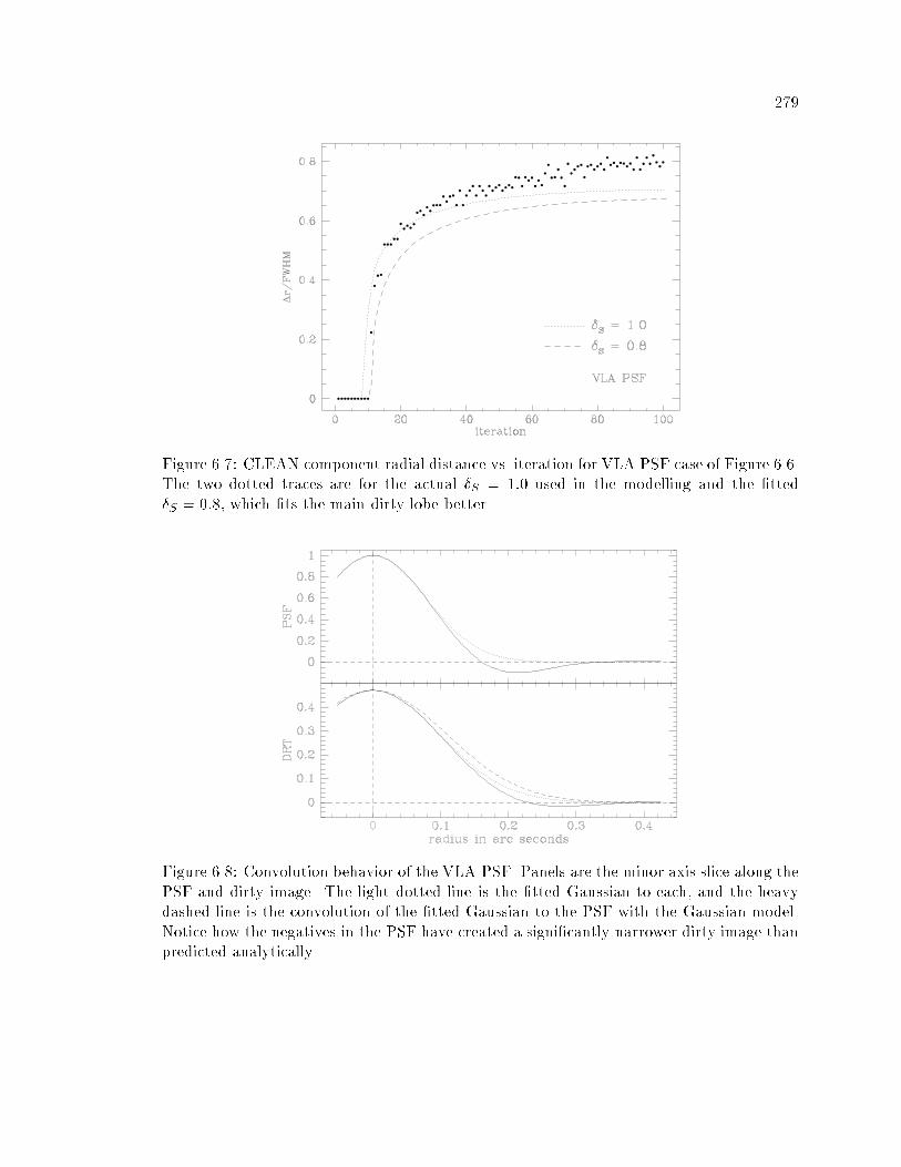
���
Figure ��� CLEAN component radial distance vs� iteration for VLA PSF case of Figure ��The two dotted traces are for the actual �S �� used in the modelling and the �tted�S ��� which �ts the main dirty lobe better�
Figure ��� Convolution behavior of the VLA PSF� Panels are the minor axis slice along thePSF and dirty image� The light dotted line is the �tted Gaussian to each� and the heavydashed line is the convolution of the �tted Gaussian to the PSF with the Gaussian model�Notice how the negatives in the PSF have created a signi�cantly narrower dirty image thanpredicted analytically�

��
���� Multiple Orders of Clean Components
The crude analytic approximation makes no mention of multiple orders in the
clean component spacing at all� much less the spacing between orders� Here we will do little
better� and merely note some suggestive observations� more work could certainly be done on
this topic� First of all� we note that while the bulk of the �ux is in the central spike and �rst
ring� the total CLEANed �ux in the outer rings is signi�cant� For instance� returning to
Figure ��� the �ux contained in the inner components� �rst� second and third rings of the
�S �� case is ���� �� � ��������� ����� Jy� respectively� The summed �ux from these
orders are ���� �� �� �� ������ ���� Jy� so the total �ux oscillates around the correct
as more orders are included� In the wider model �S �� case� the �ux in the orders is
����� ������ � ������� Jy and the summed �ux is ����� ��� � ����� ���� �� In thelater case� only the �rst two components have been counted as part of the central spike�
This order behavior is probably responsible for the tendency of CLEAN to systematically
over�estimate� then under�estimate� the source �ux as the CLEAN progresses� New orders
are added only when the orders interior to it are substantially completed in terms of the
�ux they contain� If one stops the iteration when the �nal signi�cant order is a positive
one� the estimated total �ux will likely be slightly high� If the last ring is negative� the
estimated �ux will be low� A similar behavior will be seen if one CLEANs very deeply and
then estimates the �ux by summing the components within some arbitrary radius of the
peak � the estimated �ux will oscillate around the correct value as a function of integration
radius�
It would be nice to understand the spacing of these orders in detail� but as yet
this is an open question� The order spacing for the �S ��� case is nearly identical to
that of the �S �� case� yet both are very di�erent from that of the �S �� case� In the
small source limit� the spacing seems not terribly di�erent from one half of the beam width
or a bit less� and it seems to become slightly smaller than that as the source size increases�
Estimating the ring spacing is made more complicated by the fact that the width of the
orders grows with the source size� For a �xed source� the width of the ring decreases with
radius� and one might clean extremely deeply and estimate the spacing from the outermost
rings�
One might expect that the distance between maxima in the residual model with
central depression zero would be a characteristic spacing of this problem� This corresponds
to the � �� trace of Figure ��� and the width is given by equation ����� Unfortunately
the limit of �� times the beamwidth does not match any measured scale� Another obvious
possibility is that the loop gain might in�uence the spacing of the rings� But cutting the
loop gain by a factor of two or four and increasing the number of components by the same
factor yields an almost unchanged component image� The only di�erence is in how quickly
the components spiral out to the �rst ring� There is no dependence of either the spacing
or width of the rings on loop gain� The central region never �lls in� even with exceedingly
small loop gain�

���
In Figure ��� we show an expanded version of the radius against iteration plots�
Even more clearly than the component images� this shows the presence of the multiple
orders� Note that in Figure ��� the inner most ring is quite wide and predominantly
positive� with a sharply de�ned negative outer edge� The upper panel of Figure �� shows
this to be the merger of two otherwise distinct orders� The innermost positive ring has
merely grown wide enough to partially obscure its negative neighbor� Additionally� we can
see that at any given point in the iteration there is a clearly de�ned radius for each order�
Typically the ring starts or moves outwards quite abruptly� and then gradually spirals back
inwards resulting in the �nite width� Tabulating the limiting order spacing on plots like
these against �S might provide su�cient leverage to unravel the underlying mechanism in
future work�

���
Figure ��� CLEAN component radial distance vs� iteration� These are the same quantitiesas Figures �� and ��� but with a much extended iteration axis� This clearly shows thebreakup of the traces into multiple orders and the morphological similarity of the plots fora Gaussian PSF and VLA PSF�

���
���� Fitting to CLEANed Gaussians
If working directly with the CLEAN components is a bad idea for estimating �ux�
and if one cannot �t directly to the visibility data due to confusion� one must work with
the restored image� This of course introduces the complication of what restoring beam to
use� In the simple simulation set presented here� an elliptical Gaussian model was �t to
the CLEANed image of an isolated noise�corrupted Gaussian� using all points greater than
��� of the image peak as input to the �t� Using a larger restoring beam will include more
points in the �t� reducing the thermal noise but will making the deconvolution more ill
conditioned� The same VLA PSF was used as before� in the extreme oversampled limit of
� points per beam� For each of the parameters �S ��� ��� �� a database was created
with SNR of � and �� along with a noiseless database� Here SNR is the peak response in
the dirty map over the RMS thermal noise� No calibration errors were introduced� Each
combination of parameters was CLEANed to � components� which most scientists would
consider too many� and also to a �reasonable� stopping point which was determined by eye
as the point when the �ux stopped changing signi�cantly� For all of these� the �tted �ux
of the Gaussian and the mean beamwidth was tabulated as a function of the size of the
restoring beam� Only one realization of the thermal noise was used for each case � there
was no attempt at a Monte Carlo style simulation� A Gaussian PSF case was substituted for
the in�nite SNR case with �eyeballed� stopping criterion� since it is di�cult to over CLEAN
noiseless data� This provided a best case lower limit on the error for each major category�
And �nally� a single �S ��� case was substituted in the point source case where the VLA
PSF was already producing a perfect answer and there was no need for the Gaussian lower
limit� The results of these simulations are given in graphical form in Figure ��� Sizes are
read from the left vertical axis of each panel� and �uxes from the right axis� The results
are normalized such that a width of �S and a �ux of unity is the correct answer� and this is
marked by a solid diamond on the appropriate axis�
The basic results are that a restoring beam of the same size as the �tted beam
is a reasonable choice� It is not necessarily the best choice for any given case� but it is not
too far o� and there is no other single better choice� In the noisy cases� both the �tted �ux
and the �tted size were systematically underestimated� Needless to say� anyone who wishes
to do photometric statistics on CLEANed objects would be well advised to do much more
extensive modelling that this� but I hope this series gives an idea of the magnitude of the
errors which might be encountered� Also� see �Cohen� ����� for a simulation series of MEM
photometry on point sources in a crowded �eld� While addressing a somewhat di�erent
problem than this one� her general result of systematic �ux underestimation is similar to
the results here�

��
Figure��a�CLEANedGaussianModelFits�� S ���Seetextfordetails�
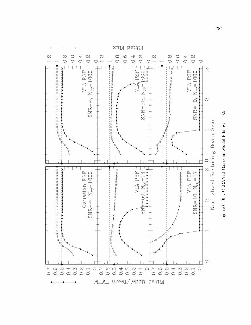
���
Figure��b�CLEANedGaussianModelFits�� S ��

��
Figure��c�CLEANedGaussianModelFits�� S �exceptwherenoted�

���
��� CLEAN components are Fourier Components in theLimit
Since the work of Schwarz� ������� it has been known that CLEAN components
are a �t to the data in the Fourier domain� in a least squares sense� It is also fairly easy
to show that to minimize the L� norm between a real function and a �nite Fourier series
of given length N � the coe�cients must be the �rst N coe�cients of the standard in�nite
Fourier series� See for example� Arfken �p� � ����� In this light� it is not terribly
surprising that CLEAN components become Fourier components in some limit� In a sense
the manipulations in this section are really quite trivial� but this is an important enough
point that I provide an explicit alternative derivation working primarily in the image plane�
As before� S is the sampling function� We specialize to the one�dimensional
perfect sampling case� where
S�u� � ���umP�u��um�
#���um juj � um otherwise
The continuous dirty beam is
B F$S% sinc��um��
In discretizing the problem� we specialize again to
a critically sampled image� This is an image with
cell size #� ���"um ���um� The gridded u�v
plane exactly contains the measured data and exactly satis�es the sampling requirements
of the dirty beam� Other than the central peak� the samples of the beam fall exactly at
the zeros of the sinc function� We can easily visualize the CLEANing process with such a
beam and see that each pixel in the residuals can be reduced to zero independently of its
neighbors� Alternatively in matrix notation� the beam is simply the identity matrix� The
CLEAN process is simply the solution of
r d�Bc� where krk� is to be minimized�Given the trivial nature of the beam� we can immediately write down an exact solution with
r �� namely c d� In this case� the value of the component representation is merely
the value of the sampled dirty image at that location�� Notice that algorithms such as
MEM which only minimize the residuals to within the noise are not guaranteed to return
the solution c d� even with such a beam as this� Writing down the continuous dirty map�
the explicit component representation becomes
cn c�n#�� Z �
��I��� sinc��um�n#�� ��� d��
�This ignores aliasing from the �nite size of the image� For the purposes of the demonstration� the imagemay simply be made �large enough� that the e�ects are negligible�

���
where c�n#�� means the component of c corresponding to the spatial position n#�� In Ap�
pendix F we show that an arbitrary �nite portion of the visibility function can be expanded
as
V �u� �X
n���
an ein�
where an �
�um
Z um
�ume�in�u�umV �u� du
When we substitute the fundamental Fourier transform relationship equation ��� into this
expansion� this becomes
an �
�um
Z um
�ume�in�u�um
Z �
��I���e���iu� du
The in�nite integral will converge by virtue of the implicit antenna directivity� so we may
rearrange to
�
�um
Z �
��I���
hZ um
�ume��iu��n�����du
id�
Since Z um
�umeiau du
�
ia
heiaum � e�iaum
i �
asin�aum�
an �
�um
Z �
��I���
�
����n#�� ��sin�����n#�� ��um� d�
Z �
��I��� sinc��um��n#�� ��� d�
c��n#�� c�n
Thus the CLEAN component representation on the sky has a one�to�one correspondence
with the coe�cients in the complex Fourier decomposition of V �u�� This immediately has
several consequences� as we can now utilize the extensive body of knowledge about Fourier
series� The most important consequence is that the CLEAN component representation is
complete in this limit � there is no possible source that cannot be represented by CLEAN
components� But being coe�cients of a Fourier series� there is no particular reason that
the normal constraints of bounded support and positivity should be satis�ed� In fact� while
applying such constraints generally improves the solution in practice� it is also clearly the
wrong thing to do from the point of completeness� We sacri�ce mathematical completeness
in the name of pragmatically introducing approximate a priori information� There are
theorems about the magnitude of Fourier components decreasing like ��n when applied to
regions containing step function discontinuities� �Raisbeck� ������ but attempts to apply
this prediction to real problems containing shifted point sources have not been successful�
The di�erences between real beams and the idealized one above are just too great� The
importance of this result is mostly philosophical in nature � CLEAN components represent
the visibility data� not the sampled sky�

���
��� Model Combination in the Fourier and Image Planes
Finally� we conclude the chapter with an example of the importance of high spatial
frequency extrapolation in the u�v plane and a few general comments on model combination�
Recall from Section ��� that MEM generally does a better job at high spatial frequency
recovery than CLEAN� though it does have problems with extremely compact emission� By
contrast� CLEAN generally does a slightly better job at total �ux recovery and the very
lowest spatial frequencies� It is clear that the solutions in the di�erent regimes of the u�v
plane may have quite di�erent characters� One is tempted to try and combine the models
produced by di�erent deconvolution algorithms� using the best region of reconstruction
from both� We do this routinely when subtracting o� CLEAN components for compact
emission and deconvolving the residuals with MEM� This is a generally done in the image
plane and in a sequential manner� allowing the second algorithm working on the residuals
to correct whatever it considers a mistake made by the �rst algorithm� One would not
generally perform two independent deconvolutions of the entire data set and then combine
the components piecewise in the image plane� An obvious problem is that there would be no
guarantee that such a patchwork quilt of model components would even satisfy the original
convolution equation� However� by combining the models in the u�v plane instead of the
image plane� nearly this exact prescription works quite nicely� It may or may not produce
a better image� but at the least it will do essentially as well as the individual algorithms�
Figure ��� is yet another deconvolution series of the model �C � source given
in Table ���� In this case there are only the main Gaussian components and no outlying
point sources� The model was discretized in the image plane and convolved with the discrete
uniformly weighted beam from Figure ��� � so the only source of error in these plots is
coming from failures in the deconvolution� The top two panels are standard CLEAN and
MEM reconstructions of the source� both tightly boxed to the support of the model� The
CLEAN used a loop gain of �� and reduced the residuals to � �Jy� The MEM used a sigma
of ��� a small initial �ux estimate and a �at default� It was somewhat arbitrarily run for
� iterations� the large number being needed due to the compact structure of the nearly
unresolved Gaussian� �The MEM reconstruction is still improving at iteration �� but
very slowly��
To investigate u�v plane model combination� the SDE task xfrstat was used
to automatically generate the envelope of the sampling pattern in the u�v plane� and this
envelope was scaled by ��� All points interior to the rescaled envelope were set to unity in
a weighting mask� and the sharp edges in the mask softened by smoothing in the u�v plane
with a circular Gaussian of half width �� of the maximum u�v spacing and unit integral�
Composite models were generated by forming
MODcomp F��hW F$MODinner % ! ���W �F$MODouter%
i�
whereW is the weighting mask just described� Combining the CLEAN and MEMmodels in
this way resulted in the lower two panels of Figure ���� The most striking feature of these
��
two panels is how much the composite images resemble that of the algorithm contributing
the highest spatial frequencies� Using CLEAN for the inner portion of the u�v plane has
improved the pure MEM image slightly� at cost in worse negatives� but in most respects
the composite image is still inferior to the pure CLEAN image� Using MEM to generate
low spatial frequencies for CLEAN� has indeed smoothed the composite image somewhat�
and improved the worst negative a bit� but at cost in image artifacts and a slight increase
in o� source RMS� For this particular case there is no improvement from u�v plane model
combination� but it is an interesting technique and might someday prove useful�

���
Figure ���� Combination of CLEAN � MEM models in the u�v plane� contours perdecade� lowest contour is � �Jy�

���
In Figure ��� the problem has been tackled with the more traditional approach
of CLEANing the compact structure lightly and then using MEM on the residuals� It hasn�t
helped� and in most respects has simply made the reconstruction worse� The problem is
coming from the especially challenging nature of the source� As shown in Chapter �� while
deconvolution errors at this level are to be expected even for the simplest of sources� proper
choice of algorithm should be able to reduce the error on any given size scale to better than
we are doing here� So what is wrong�
The problem here is that the two most compact components appear similar� but
are in fact quite di�erent from the point of view of the deconvolution algorithms� The
northern compact component with the larger peak is extended� with a minor axis � of
the mean beamwidth� By contrast� the sharper southern compact component has a minor
axis only ��� of the mean beamwidth� This makes all the di�erence in the ability of MEM
to deconvolve it well� When MEM alone is run on the model� the center of the error pattern
is the sharp feature� When CLEAN alone is run on the model� the center of the error
pattern is the extended peak� Unfortunately� there is no single threshold where CLEAN
will remove just the �ux from the sharp peak� In fact� it will start removing �ux from the
extended but stronger peak� and by the time it has removed enough �ux to signi�cantly
help the MEM algorithm� it will already have embedded the characteristic CLEAN errors
on di�use peaks into the solution� For such delicate problems as these� one would want
a CLEAN that selects components based on the di�erence of the residuals and a smooth
model of the extended emission � not unlike Multi�Resolution Clean �Wakker and Schwarz�
����� or the algorithm proposed by Dwarakanath et al� ������ Tests trying to crudely
model such a procedure with extremely tight CLEAN boxes were not successful� so it is not
known how well such a procedure would work in this demanding case� In any event� the
combination of two algorithms roughly doubles the number of free parameters that must
be set in the reconstruction process� to say nothing of the modelling required to separate
the components into completely unresolved and marginally resolved categories� Even if
particularly careful and sophisticated use of existing tools could be made to signi�cantly
improve the deconvolution of this source� there is no question that the NNLS algorithm of
Chapter is providing a much better reconstruction with essentially no arbitrary parameters
beyond the rough source support� Methods such as model combination need only be used
when the source size is too large for NNLS based methods� and in such cases� an adequate
model of the source to discriminate between resolutions might be prohibitively di�cult�

���
Figure ���� Combination of CLEAN � MEM� run sequentially in the image plane� Thedirty image was lightly CLEANed with � components� followed by � MEM iterationson the CLEAN residuals� contours per decade� lowest contour is � �Jy�

��

Chapter �
Case Study� �C��
��� Introduction
The initial impetus for much of this dissertation came from an observation of
�C � by Craig Walker that was unaccountably limited to a dynamic range of some ����
signi�cantly above the thermal noise�� A simple image plane model of the source was
constructed and the deconvolution process simulated� The venerable H'ogbom CLEAN pro�
duced a peak�to�RMS dynamic range of over ���� on a noiseless� discretized� perfectly�
calibrated realization of this model� but also produced highly visible artifacts and negatives
at the ��� level� This provided the �rst evidence that the deconvolution process was
a limiting factor comparable to residual calibration errors for high�precision VLA obser�
vations� Moreover� the morphology of the error pattern closely matched that seen in the
observational image� although reduced in amplitude� In subsequent work it was realized
that part of the problem with the real data was in fact residual calibration error and the
neglect of an o�set confusing source� Once the data were well calibrated� the correspondence
between the model and observational error pattern became striking� both qualitatively and
quantitatively�
At the observation frequency of �� GHz and using the high resolution VLA
A con�guration� �C � is a fairly compact source� with two nearly unresolved components
and a modest extended halo� Prior to this dissertation� such a source was considered
close to ideal for CLEAN� so the deconvolution failure was surprising� Other deconvolution
algorithms� including MEM� SDI CLEAN� and Multi�Resolution CLEAN� fared little better�
�The particular implementations used are described in Section ����� Eventually it was
discovered that a similar error morphology was produced with a single isolated Gaussian
model� and this led to the resolution tests described in Chapter �� Still later� it was found
that the particular combination of size scales present in the two compact components did
present a challenge more di�cult than any single isolated component� This was described
brie�y in the context of model combination in Section � � No signi�cant progress was made
in the deconvolution of the �C � model source until the advent of the NNLS algorithm
described in Chapter � NNLS is the only algorithm studied which was capable of reducing
the deconvolution artifacts on the source below the level of the thermal noise� This chapter
�The factor of ��� above the thermal noise� given in Briggs and Cornwell ��� is quite erroneous�
���

��
is somewhat anti�climactic� since we have already used models of this source and observation
as test cases in many other contexts� Here we simply perform a reasonably careful noise
analysis of the observation� present the �nal observational images at X band and L band�
and brie�y describe their astrophysical signi�cance�
��� The Data and the Noise
Interleaved X and L band observations of �C � and calibrators were made on
August ��� ����� spanning a period of approximately �� hours� Of that� ��� hours of good
on�source data at X band were obtained for an after�calibration total of ����� visibilities
at an integration time of seconds� averaged down from the original � second data� The
L band data was left at the original time resolution� and ����� visibility records were
retained after calibration and �agging� for an equivalent on�source time of �� hours� �C �
has a declination of ����� so the u�v coverage was excellent� The X band coverage is given
back in Figure ����� and the associated point spread functions in Figure ��� � The L band
data has coverage and PSFs that are visually nearly identical to the X band data� and they
are not shown� The X band visibility amplitude plot is given in Figure ���� The point to
note is that there is quite signi�cant structure at all size scales� and that the signal�to�noise
ratio is quite high�
Figure ���� Visibility amplitude plot� The visibilities have been time averaged to � minutesin this plot� and all points are shown�
It must be admitted that the a priori predicted thermal noise for this observation
is not a particularly good match to the observed number� but it is worth while going through
the calculations in some detail to show how one might attempt as good an a priori estimate

���
as possible� The VLA Observational Status Summary gives the following expression for the
expected map plane naturally weighted thermal noise�
SRMS�mJy� K
�qN�N � ���n#thrs#�MHz� �����
where K is a measured system constant and is �� mJy both for the current VLA and
at the time of observation� N is the number of antennas� n is the number of intermediate
frequencies recorded�� #thrs is the observation time in hours� and #�MHz is the observation
bandwidth in MHz�
For the purposes of careful a priori noise estimation� it is more useful to have this
equation in a di�erent form� First� note that N�N � �� is twice the number of baselines�and that Nbase#t is the equivalent total time on source for a single baseline� Since data can
be �agged for any number of reasons� and we generally do not conveniently know exactly
how long the array was taking good data on the source� this product is better written as
Nint#tint��� Nint is the total number of integrations� and is usually reported by mapping
programs� #tint is the single integration time� now speci�ed in seconds� Equation ���
becomes
SRMS�mJy� K
�r�n
�Nint#tint#�MHz �����
Now� when a subset of the array happens to drop out for a period� the data it generates
will be �agged bad somewhere in the reduction� By the time the data reaches the mapping
program� the total number of good integrations will re�ect that the �agged data is not
present� as will the estimated thermal noise� If one wishes to take the trouble� one can even
take into account that not all visibilities will have the same weights after time averaging� The
weight and actual time spacing of the averaged visibility data can usually be determined
from a time�baseline listing of the visibilities� A histogram of the visibility weights can
often help sort out confusing situations� uvmap within SDE has this capability� albeit not
conveniently� Once the weight associated with the nominal averaged integration time is
determined� just sum the visibility weights and divide by the nominal single integration
weight� The result is the e�ective number of full weight integration times to be used in a
sensitivity calculation�
In this particular case� the data have been averaged down to seconds from the
original � seconds� Weights are present in the data �le ranging from ���� to ����� The
histogram shows the vast bulk of them to be ������� and the histogram is regularly spaced
at intervals of ����� The highest weight in the �le appears to be the visibility averaging
program occasionally averaging � points together instead of � This behavior can happen
when the speci�ed averaging time is an exact multiple of the original integration time� The
�For most instruments� the number of intermediate frequencies is just the number of polarizations� TheVLA has the ability to observe at two di�erent frequencies within the same band� for a total of four inter�mediate frequencies�

���
total weight sum is �� ������ yielding an e�ective �� integrations of full s weight�
instead of the reported �� � Since the inverse RMS thermal noise scales with the square
root of this quantity� � vs� �� is hardly a signi�cant e�ect � but it might be worth doing
rather than wondering how signi�cant it is�
The observation was done in spectral line mode� as are nearly all high dynamic
range observations� See Perley ������ for details on why this is so important from a hardware
perspective� the most important reason is that it avoids nonclosing phase errors of a few
degrees introduced by the analog phase�shifter in the correlator� In spectral line mode� the
equivalent phase shift is done digitally in the transform domain� Several other e�ects become
important as the bandwith of the observation grows� most notably errors due incorrect
antenna delay settings� In spectral line mode� the e�ective bandwidth for this error is
the width of each individual channel rather than the total observing bandwidth� Finally�
spectral line mode allows the bandpass to be calibrated against frequency� after which the
�lter�corrupted channels on the edges of the bandpass can be discarded� Spectral line mode
improves the �delity of the VLA tremendously� but at signi�cant cost in sensitivity� In order
to obtain su�cient �exibility for a high quality bandpass calibration� �� channels were used
in this experiment and the individual channel width was forced by hardware limitations to
only ��� kHz� After dropping two channels from each end of the bandpass and ignoring the
channel sum� �� channels were left� for a total e�ective bandwidth of ���� MHz with both
RR and LL observed polarizations� Compared to the � MHz obtainable in continuum
mode� we have sacri�ced nearly a factor of ten in usable bandwidth to get the bene�ts of
the spectral line system� This is more than a factor of three in thermal sensitivity�
We now use equation ��� to estimate the expected naturally weighted thermal
noise� remembering that n � for the two polarizations� The result is that the expected
map plane naturally weighted thermal RMS is ��� �Jy�beam� Unfortunately� this does
not agree particularly well with the noise estimated from the scatter in the visibility data�
via the techniques of Section ��� The task visavg using successive di�erences mode and
a threshold of �� seconds predicts a #Suw of ����� Jy for a visibility with unit weight�
uvmap predicts that the naturally weighted thermal RMS will be ��� �����#Suw � which
produces a combined prediction of ���� �Jy�beam � more than �� higher than the a
priori estimate� The estimate of #Suw was checked in a number of ways� Independent
quartiles of the data� binned based on u�v radius� yielded ������ ���� ����� and ����� Jy�
The best model found by NNLS deconvolution was subtracted o� the data to prevent bias
from in�uencing the estimate� and the same quartiles yielded ������ ������ ������ and ����
Jy� Time bin averaging over � seconds yielded ����� Jy� but decreased to ���� Jy when
the model was subtracted o� �rst� In short� the internal estimates of the noise were all
consistent to within a few percent� which casts signi�cant doubt on the reliability of the a
priori estimate�

���
��� Modelling
When confronted with signi�cant errors in the observational data that would not
calibrate out� a simple Gaussian model for the source was determined with the AIPStask� IMFIT� The results are the �rst components in Table ���� Even such a simple model
was at the limits of what IMFIT would do� There is a more general �tting program in
SDE� gfit� which is really just a user friendly interface to an external program� gaussfit�
It will handle an arbitrary number of components� and allows the initial guesses to be
made visually with SAOimage� but it can be di�cult to get the model to converge� even in
simple cases like this one� The VLBI community is probably the most sophisticated group
in astronomy when it comes to model��tting of complicated sources �the Caltech VLBI
program modelfit is clearly better than any similar program currently found in AIPS�but even here the programs are generally fairly di�cult to use� I feel that there is a real
need for improved modelling programs� both in ease of use and robustness of �t� Model�
�tting of simple sources should be a routine part of imaging even for connected element
interferometers� but until the programs become considerably easier to use� people will not
model��t unless absolutely forced by the project�
As a demonstration of the power of model��tting to diagnose deconvolution prob�
lems� consider Figure ���� The left panel is the best uniformly�weighted synthesis image that
could be produced with CLEAN� after multiple rounds of self�calibration and subtraction
of an �� mJy o�set confusing source some ���� to the north�east� This particular CLEAN
image has had the residuals reduced to � �Jy�beam� so the residuals are quite ignorable�
The middle panel is an identical CLEAN of the Gaussian model which has been sampled in
the image plane and convolved with the dirty beam to be produce a noiseless model dirty
map free of aliasing and representation e�ects� It is true that this source contains a nearly
unresolved elliptical Gaussian component that makes it di�cult to represent in discretized
form � but that is not the problem here� The errors in the middle panel are caused by
the CLEAN algorithm� and nothing else� Close examination of the restored images show
there to be a nearly one�to�one correspondence in most of the error features� which is quite
remarkable given the crudity of the model� The third panel shows the source as is it would
be for a perfect reconstruction�
The CLEAN image actually has a peak to far�o��source dynamic range very close
to that predicted by the noise estimate from the visibility data� The measured RMS is
��� �Jy�beam� for a peak�to�noise dynamic range of � ��� The predicted image plane
thermal noise is ��� �Jy�beam� or ����� times the naturally weighted value� The far RMS
in the noiseless model data is much better than this� at � �Jy�beam� though both data
and model are producing negative artifacts at the few thousand to one level� As mentioned
in Chapter �� dynamic range really isn�t a particularly good measure for deconvolution
errors� in that the errors are spatially variable� The numbers quoted in the introduction
are real enough� but any measured dynamic range on a CLEAN image which is limited by
deconvolution will be a strong function of where one chooses to take the RMS� As shown in

�
Section ���� the worst deconvolution errors will be in the close neighborhood of the source
where it is di�cult to measure dynamic ranges� Dynamic ranges are occasionally quoted
in the case studies� but usually with mention of the most obvious error feature as well� A
peak�to�RMS dynamic range is really only meaningful when the worst errors are similar to
the RMS� CLEAN is reasonably good at minimizing the far sidelobes of the source� so it is
quite possible to have the situation as here� where there are obvious strong deconvolution
artifacts in the image� but where the far�o��source RMS is close to the thermal noise�

��
Figure����Diagnosisofdeconvolutionproblemsbymodelling�Allpanelshavecommoncontours�withthelowestbeing��Jy
andfourlogarithmiccontoursperdecade�Therestoringbeamisfroma�ttothePSFandis�������������

��
��� X Band Images
Now that we have some idea of what constitutes a �good� deconvolution of the
source� Figure ��� shows the X band images as a function of the major algorithms and
visibility weightings� In particular� notice that the di�erences between the CLEAN panel of
Figure ���a and the NNLS panel of Figure ���b can all be attributed to improved software
introduced in this dissertation� The contours are common to all four pages� with four
logarithmic contours per decade� The lowest contour is roughly � times the RMS of the
least noisy image�
Using a #Suw of ����� Jy� and the thermal noise equations �� and ��� the
predicted RMS thermal noises for the weightings Uniform� Robust � Robust � and
Natural are ���� ��� ���� and ���� �Jy�beam� respectively� The measured values for
CLEAN are ���� ���� ��� and � �Jy�beam� For NNLS� the measured values are ���
��� �� and ���� �Jy�beam� For MEM they are ����� ����� � �� and ���� �Jy�beam�
For both CLEAN and NNLS� the measured and predicted values track each other fairly
well� indicating that the new weighting scheme is performing as claimed in Chapter ��
Notice that the lowest measured RMS is obtained not with natural weighting� but with the
Robust � weighting� This is the value of robustness that best matches the PSF to its
�tted Gaussian� and which eliminates the extended shelf so often seen in naturally weighted
VLA point spread functions� The di�erence is not enormous� but it is signi�cant and of
course the resolution in the robust beam is somewhat improved over natural weighting�
The CLEAN deconvolutions were done down to a maximum residual of � �Jy
which at a loop gain of �� typically required several hundred thousand components� Bad
as are the imaging artifacts here� if one CLEANs down only to the thermal noise instead
of well below it� the artifacts become much worse� The MEM deconvolutions were run to
� iterations� with a �at default image� Tflux ���� and Sigma ������ The MEM
solutions at � iterations were noticeably better than at � iterations� though the rate
of improvement per iteration at that point was extremely slow� Other values of the control
parameters were tried� and none made a signi�cant di�erence beyond that mentioned here�
All deconvolutions were loosely boxed to the rough support of the source� into a region
determined by eye with ��� allowed pixels� The NNLS deconvolutions also used this box
as the data window�

��
Figure���a��C �X�bandimages�Lowestcontouris��Jy�beam�withfourlogarithmiccontoursperdecade�Predictedthermal
noiseis����Jy�beam�Measuredfar�o��sourceRMSis������and�����Jy�beamforCLEAN�NNLSandMEMrespectively�
TheweightingRMSdegredationandmeanresolutionis�����and��� ���

�
Figure���b�Robustnesssettodecreasethenoiselevelwhilemaintainingresolutionasmuchaspossible�Samecontoursasin
Figure���a�Predictedthermalnoiseis ���Jy�beam�MeasuredRMSis ���� ��and�����Jy�beam�lefttoright�The
weightingRMSdegredation�resolutionis�� ��������

��
Figure���c�Robustnesssettoincreaseresolutionovernaturalweighting�whilenearlypreservingthethermalRMSandimproving
thesidelobes�Samecontoursasbefore�Predictedthermalnoiseis�����Jy�beam�andthemeasuredRMSis������and� ��
�Jy�beam�TheweightingRMSdegredation�resolutionis��� ��� ����

�
Figure���d�Naturallyweightedimages�Samecontoursasbefore�Predictedthermalnoiseis�����Jy�beam�andthemeasured
RMSis � �����and�����Jy�beam�TheweightingRMSdegredationis��byde�nition�andthemeanbeamwidthis����� �

��
��� L Band Images
The X band observations were interleaved with L band observations at a frequency
of �� � GHz� At this frequency and resolution� the source is resolved� but only barely so�
The source amplitude plot is given in Figure �� � showing both the resolution of the source
and the quality of the data� Notice that even at the longest spacings� the lowest visibility
is still about �� of the peak� The source is not resolved by much� Model��tting to the
best image yielded a one component Gaussian model source of � ���� ����� * ���� With
the �tted natural beam of ������� � ������� * �� ��� this means the source width varieswith position angle from extremes of ��� to ���� of the �tted beam� While small� this is
still quite large enough for CLEAN to have trouble� as shown in Figure ���� No algorithmic
comparison was done on this data� as it would have been largely redundant with the DA���
case study in Chapter ��
The L band images were designed for maximum sensitivity� and so natural weight�
ing was used throughout� The source was thought su�ciently compact that NNLS would
not have di�culty removing the extended wings of the beam� and intermediate values of
the robustness were not explored� In retrospect� a robustly weighted beam would proba�
bly have been a good idea� especially given that the image is still limited well above the
thermal noise determined by internal visibility scatter� The problem might be the wings
of the natural beam� or we might be approaching the hardware limits of the instrument�
More work should probably be done on this data� and the image in Figure ��� is regarded
as preliminary�
Figure �� � Visibility amplitude plot� The visibilities have been time averaged down to �minutes in this plot� and all points are shown� Notice the numerical scale� The source isclearly resolved� but only slighly�

��
After calibration� �agging� and several cycles of self�calibration within AIPS by
Craig Walker� the data were exported to SDE for subsequent processing� Since the NNLS
tasks currently lack multiple �eld capability� the data were �rst imaged a �nal time with
MX and lightly CLEANed� Of the total components� �� were removed from the o�set
�eld� yielding ��� mJy CLEANed �ux� This was subtracted from the visibility database
with UVSUB and the data exported to SDE� Several additional cycles of self�calibration and
NNLS imaging of �C � were performed� with results near the source essentially as good as
shown in Figure ���b� The images were made with cellsize of ����� which greatly oversamples
the beam� and the images at this stage were �� pixels on a side� Eventually� however� we
decided to image a large �eld in hopes of detecting extended di�use emission at signi�cant
distances from the main source� The NNLS model components were padded with zeroes out
to � ��� The o�set source CLEAN components were added back into the component model
and the resulting composite used to produce a � �� restored image from a �� dirty map�
While perhaps not surprising in hindsight� the very slight calibration improvements in the
visibility data from the NNLS iterations were not re�ected in the MX CLEAN components
on the o�set source� and a calibration error pattern from a mJy source was visible over
more than half of the restored image� When working at this level� calibration changes
must be done in a consistent manner� The gain corrections from the best o�set subtracted
visibility database were transferred to the original database prior to subtraction� and a �nal
conventional NNLS imaging sequence was performed� working completely with these huge
images� This proved to be possible� though very close to the limit of the workstation�s virtual
memory� SDE operates under the assumption that virtual memory is plentiful and that all
the intermediate images necessary to the deconvolution can be held in memory at once�
In situations like this� the assumption begins to break down� Several normally automated
operations had to be performed �by hand� with separate tasks� but the project was barely
possible� It need hardly be mentioned that the NNLS deconvolution windows are as tiny as
usual� but that they are simply placed on an enormous otherwise�empty region of sky� Once
the deconvolution model is determined by solving for the �ux in these tiny windows� the
restored image can be made as usual over the entire area� NNLS deconvolution certainly
needs to be incorporated into a task with knowledge of multiple �elds� to avoid the necessity
for heroic measures like these� Situations like this might also bene�t from calculation of
the relatively modest number of pixels in the deconvolution window by a direct rather than
a gridded transform� Even the beam elements connecting the pixels in the deconvolution
windows might be calculated in an ungridded manner� though this latter idea is probably
still computationally infeasible at the moment�
Once the data were processed in a consistent manner� the third o�set source to the
south was detected� It is only about � mJy� but still a �� � detection� The image presented
here placed a small �ux window around it� and allowed the deconvolution algorithm to
process it properly� When the small source entered the restored image through the residuals�
the peak �ux was ���� mJy�beam� and when it was deconvolved properly it dropped to
��� mJy�beam� While mildly surprising that the peak �ux drops rather than rises after

��
deconvolution� clearly the photometry of faint sources is not greatly dependent on whether
they enter the image through components or residuals� The source is real� and was also
detected at X band�
The �ux and data windows used in the �nal deconvolution were a circle of radius
� pixels� centered on the southern small source� a circle of radius �� pixels� centered on
the northern o�set source� a circle of radius �� pixels� centered on �C �� the remaining
several thousand pixels out of a total �� were placed in an oblong shape out towards
the north�east from �C �� where earlier images had hinted there might be emission� The
resulting full image is given Figure ���a� and expanded versions of the interesting sub�elds
in Figure ���b� The predicted thermal noise based on the scatter in the data is � � �Jy�
while the measured o��source RMS is ��� �Jy� so clearly there is something limiting the
deconvolution beyond the thermal noise�
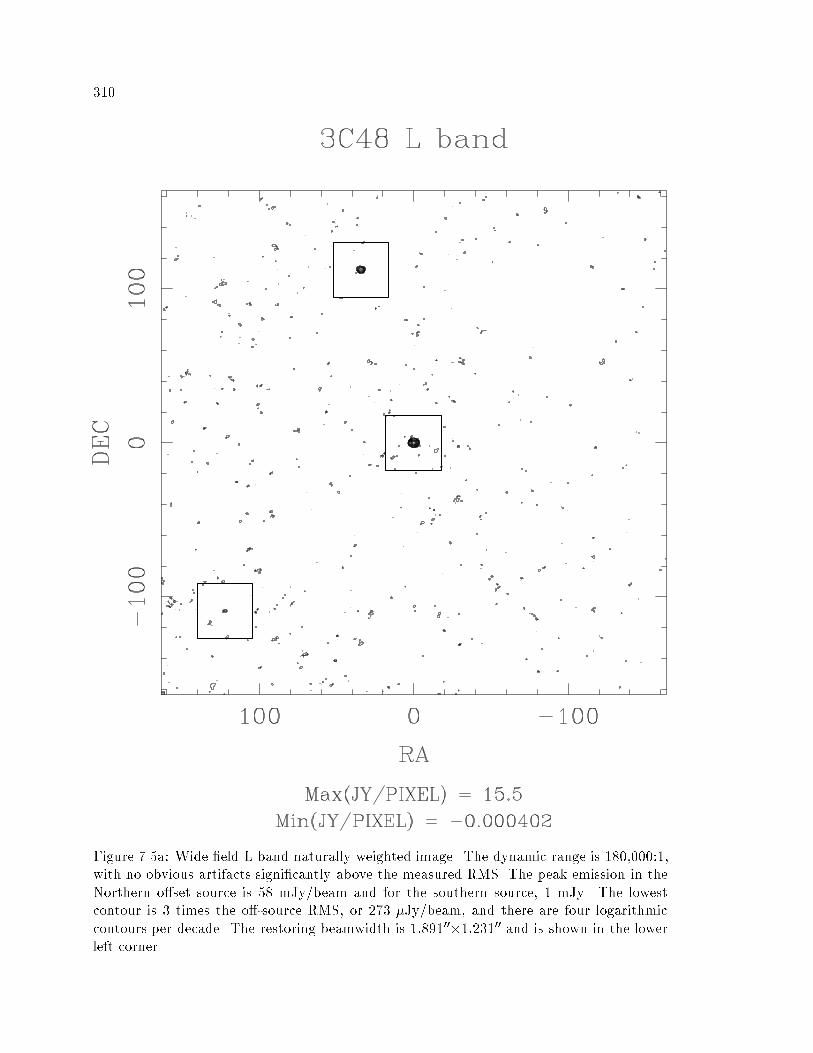
��
Figure ���a� Wide �eld L band naturally weighted image� The dynamic range is ������with no obvious artifacts signi�cantly above the measured RMS� The peak emission in theNorthern o�set source is �� mJy�beam and for the southern source� � mJy� The lowestcontour is � times the o��source RMS� or ��� �Jy�beam� and there are four logarithmiccontours per decade� The restoring beamwidth is ��������������� and is shown in the lowerleft corner�

���
Figure���b�Expandedsub�imagesfromFigure���a�Lowestcontouris�timestheo�sourceRMSinthefullimage�Four
logarithmiccontoursperdecade�

���
��� Discussion
The astrophysics of �C � is discussed extensively in Wilkinson et� al ���� and
������ The germane points here are that the source is extremely small for a radio loud
quasar on both linear and angular scales� It is believed that the central engine is embedded
in a dense clump of gas in the interstellar medium of the host galaxy� which is con�ning
the jet to an abnormal size� An obvious question is whether the jet has been limited in size
over its entire history� or whether the collision with the dense gas is a comparatively recent
event� The objective of the L band observation was to see if the jet had ever punched all
the way through the con�ning gas in the past� If so� there would be some hope of detecting
emission from the older ejected material� which might be at a considerable distance from
the main source� The answer appears to be that if such material is there� it is not detected
in this observation� The northern o�set source is at the position angle of the jet� of course�
but one would expect some sort of di�use emission if they were related� There is nothing
linking the two otherwise distinct compact sources�
The morphology of the �C � jet is extremely unusual� There is a distinct change
in the properties of extended extragalactic radio sources at an absolute luminosity of about
P�� GHz� ��� W�Hz� which divides the sources into the Fanaro� and Riley classes Iand II� �Fanaro� and Riley� ��� �� By power� �C � is well into the FR II category� where
one would expect a supersonic jet� narrow in angle and fairly straight� In this source�
the turbulent�looking wide�angle jet to the north seen on VLBI size scales resembles the
subsonic jet in a far less powerful FR I radio source & or at least half of one� Since turbulent
�ow involves material travelling at many di�erent angles to the line of sight� it is di�cult to
hide such a jet by invoking beaming arguments and nearly all FR I sources are two sided�
Prior to these observations� no counterjet had been seen in �C �� and the source had been
considered intrinsically one sided� The small extension to the south in the X band images is
the �rst detection of the counterjet in this source� Without invoking beaming� it is di�cult
to imagine ways of producing such a powerful asymmetry� to say nothing of a completely
one�sided jet� At least now we have a direct measurement of the degree of asymmetry� Slices
through the source perpendicular to the jet may yield information about the strength of the
con�ning process� and it is here that the high quality deconvolution of the X band images
may prove most scienti�cally useful� A source surrounded by a spurious negative will pass
through zero in a slice much earlier than otherwise� and the measured slope and sharpness
at the edge will be higher than actually true� The interpretation of such detail is a matter
for specialists� but now the observational images are of su�cient quality to warrant the
scrutiny�

Chapter �
Case Study� SN���A
The work in this chapter resulted from a � month visit to the Australia Telescope
National Facility� kindly supported by the Australian Commonwealth Scienti�c Industrial
Research Organization �CSIRO�� Much of this chapter has been published as Stavely�Smith
et al� �����a� and Briggs ���� ��
Supernova ����A in the Large Magellanic Cloud presents an unprecedented op�
portunity to observe the detailed evolution of a supernova at all wavelengths� While optical
observations with the HST Faint Object Camera �FOC� have obtained resolutions of �����
we are limited in the radio to the resolution obtainable with the Australia Telescope Com�
pact Array� At the highest frequency of ��� GHz� this corresponds to a synthesized beam
width of ����� At this resolution the radio supernova is distinct from a point source� but few
physical conclusions can be drawn� We present here super�resolved images from the ATCA
with an e�ective resolution of � ��&������ These reveal a spherical shell�like structure with a
radius of ���� and an additional component of emission aligned with the circumstellar ring
imaged with the FOC� Care is required due to the delicate nature of the imaging problem�
and we present evidence that the overall image structure is plausible�
�� Introduction
The Australia Telescope is the premier imaging radio interferometer in the south�
ern hemisphere� and the only modern instrument able to observe SN����A� The compact
array consists of ��m antennas with amaximum baseline length of kilometers� Additional
Australian antennas can be combined with the ATCA for Very Long Baseline observations�
but to date there are no detections of the supernova on baselines longer than km�
Deconvolution in radio interferometry is more generally used to remove the far�o�
sidelobes caused by the incomplete sampling of the Fourier plane than for super resolution�
Even though it has been known for many years that moderate super resolution can be
successful on simple sources�� in practice it is often the case that desired higher resolution
can be had directly by using data from a di�erent instrument� di�erent array con�guration or
��a modest degree of superresolution �not more than a factor of two will often be possible and need notbe treated with suspicion�� �Narayan and Nityananda� ��� p� ���
���

��
Figure ���� Visibility amplitude plot� The visibilities have been time averaged down to �minutes in this plot� and all points with full weight are shown�
di�erent observing frequency� SN����A is unusual in that it is a crucially important object
where higher resolution radio imaging data is simply not available� While the supernova
will expand with time and thus provide a better look at the remnant to come� the existing
data are all that will ever be obtained of the supernova at the current epoch of evolution�
There is great incentive to extract as much spatial information as possible from the existing
data� Even a map of very low dynamic range will be extremely valuable astrophysically� so
long as the features interpreted are reliable�
�� The Data
The data used for these images were taken by Lister Stavely�Smith on October
��� ���� and January &�� ����� The source was followed for a full �� hour track each
day� with a small amount of data rejected in periods of poor atmospheric phase stability�
After external calibration by him� ���� good visibility record at �� second averaging time
were retained� No self�calibration was performed� The total bandwidth was ��� MHz in
�� � MHz channels� centered on ��� GHz� The typical system temperature was � K�
though the outrigger antenna which participates in the longest baselines had recently been
upgraded with an improved receiver and had a system temperature half that of the others�
The radial visibility amplitude plot in Figure ��� shows that the source is indeed
resolved on these baselines� and that there does appear to be compact structure on the
longest baselines� The u�v coverage was used as a test case for the new weighting routines�
and is given back in Figure ����b�

���
�� Deconvolution
The dirty maps were made with the conventional gridded uniform weighting� The
cell size ���� was selected as adequate to oversample the maximum e�ective resolution� and
most dirty maps were of size ����� This is exactly the case explored in Chapter �� so the
discussion of Section ���� applies here as well� along with the uniformly weighted beam
presented in Figure ����� The dependence of the �nal maps on cell size was very weak�
so long as the PSF was highly oversampled� Iterative algorithms were started with a �at
default� as more sophisticated choices of default were found to make little di�erence� The
averaging time was found to make a signi�cant di�erence in the �nal resolution achieved�
presumably for the reasons discussed in Section ������ and the data were not averaged
beyond the initial �� second records� Several weighting schemes were explored� and the
conventional uniform weighting selected as being the most useful� This topic is covered in
more detail in Section ����
The weights of the visibility data as they come o� the ATCA are simply constant
and did not re�ect the signi�cant di�erences in system temperatures present� The weights
were multiplied by � for all baselines which used the upgraded outrigger antenna� all the
deconvolution programs used treat the weights statistically� Surprisingly� this resulted in
very little di�erence in the �nal maps� when compared with maps prepared from data where
all baselines were weighted equally�
The deconvolution algorithms Maximum Entropy� CLEAN� Non�Negative Least
Squares� Maximum Emptiness� Gerchberg�Saxton�Papoulis� Richardson�Lucy and Singular
Value Decomposition were used for the initial mapping� �Descriptions of these algorithms
are given in Section ���� All algorithms produced nearly identical results at the nominal
�tted restoring beamwidth of ����� � ������ though there were considerable di�erences in
the robustness to support information� super�resolution properties and convergence speed�
Several examples of the images at nominal resolution are given in Figure ����

��
Figure����Nominaluniformlyweightedimagesfordi�erentalgorithms�Thereisnosigni�cantdi�erencebetweentheseimages
orthenominalimagesfromtheotherdeconvolutionalgorithms�Contoursarelinearatintervalsof��oftheMEMpeak�with
anadditionalcontourat���Allcontourslevelsinthischapterarere�ectedsymmetricallyaroundzero�Theshadedellipseis
the�ttedbeamwidthof����������� �

���
All of the algorithms used here operate in the image plane� and all use a compo�
nent model of the sky which is measured in Jy�pixel� This model is then convolved with a
restoring beam representing the desired �nal resolution� and the residuals are added back
to produce the �nal image normally interpreted by the astronomer� For the purposes of the
super resolution study� it is often more productive to examine the sky model directly� though
care should be taken to view features present in the components with proper skepticism� It
is in the nature of the high resolution sky models that the di�erences between algorithms
are apparent� In particular� one of the most fundamental distinctions is that some of these
algorithms incorporate a smoothness constraint� either explicitly or implicitly as a result
of �nite iteration� The result is that these component models have a �nite �possibly space
variant� �maximum resolution� that is roughly independent of the grid spacing� Two of
these algorithms� CLEAN and NNLS� have no such constraint and will generate features at
whatever resolution is requested of them� These sky models must generally be smoothed
down before much sensible interpretation can be done� The following general behavior was
noted in the context of this project�
Maximum Entropy This algorithm produced what appears to be the best
reconstruction found� It agrees with the other algorithms on the major features� produces
a plausible physical image� performs well on simulated data with a high degree of super
resolution� converges smoothly to a reasonable answer� and is robust to support constraints�
For this project it is the algorithm of choice� The only disadvantage is that an extreme
number of iterations is required for the highest resolution�
Non Negative Least Squares NNLS is almost certainly performing better
than MEM at the nominal resolution� yet the limiting factor for both is the thermal and
confusion noise and the images are equivalent� The important question is at exactly what
resolution the NNLS solution breaks down beyond that of the MEM solution� This is not
precisely known� and the prudent investigator should examine both algorithms at a variety
of restoring resolutions�
CLEAN While quite acceptable at the nominal resolution� CLEAN is not rec�
ommended for super�resolution purposes� The component image shares the same speckled
appearance as produced by the NNLS algorithm� but it produces spurious structure much
sooner in simulated tests� An experimental positivity constrained version of CLEAN was
examined� and it faired no better�
Maximum Emptiness This algorithm minimizes the L� norm of the compo�
nent solution while satisfying the convolution equation within the noise� It was inspired
by a paper which suggests that CLEAN is approximately minimizing this criterion� In
fact� when terminated at a reasonable number of iterations� it behaves more similarly to
MEM� The emptiness regularization appears somewhat less powerful than the entropy �
it converges slowly and the degree of super resolution is less than with MEM�
Gerchberg Saxon Papoulis This algorithm merely forces agreement with the
data in the Fourier plane� and enforces positivity and support in the image plane� As such� it

���
is very simple conceptually� and encouraging when it agrees with other methods� It produced
a �nal result very similar to that of MEM� but diverged without support constraint�
Richardson Lucy This algorithm was comparable to Maximum Emptiness in
that it produced a physically reasonable model but at a lower resolution than MEM� This
algorithm is highly favored in the optical community� but less suited to the needs of interfer�
ometry in that it requires a nonnegative PSF� the ad hoc modi�cation of clipping the dirty
map and PSF to nonnegative values is crude� The theoretical formalism is quite di�erent
from the other algorithms� and again it is encouraging that it works here as well as it does�
Singular Value Decomposition Direct inversion of the deconvolution equa�
tion can also be regularized with a Singular Value decomposition of the beam matrix� With
heuristic selection of an appropriate cuto� in singular value� a model was obtained that
resembled the MEM model� but which still contained negative �ux at an unacceptably high
level�
As to the speci�c values of the control parameters� the MEM deconvolutions used
a �at default image� Tflux ���� Sigma ������ and � iterations unless describedotherwise� The Maximum Emptiness deconvolutions used the same control parameters� and
images are given with and � iterations� The CLEAN deconvolution used � compo�
nents at �� loop gain� GSP used an acceleration parameter of and � iterations� The
SVD deconvolutions used both �� and � singular values� All of the windowed deconvolu�
tions used the support window shown in Figure �� � NNLS used this as the �ux window�
and a circle of radius � pixels� centered on the supernova� as the data window�

���
Figure���a�Skymodelsfordi�erentdeconvolutionalgorithms�TheCLEANandMEM
panelshavealightgreyshading
superimposedwhereverthecomponentmodelisnonzero�Numbersinthepaneltitlearethenumberofalgorithmiterations�
Contoursare�����������ofthepeakineachpanel�

��
Figure���b�Moreskymodelsfordi�erentdeconvolutionalgorithms�The�iterationnumber�intheSVDpanelisthenumberof
singularvectorsusedinthesolution�Samepercentagecontoursasbefore�

���
���� Support Constraints
The support constraints ranged from slightly to extremely important� depending
on the algorithm� GSP actually diverged� unless a tight support constraint was used to con�
�ne the emission to the immediate region of the supernova� SVD deconvolution also requires
the support constraint for fundamental reasons � without it� the algorithm simply returns
the dirty map� NNLS requires reasonable support information for more pragmatic reasons�
the problem becomes intractably large without it� MEM� CLEAN� L�� � Richardson�Lucy
all produced reasonable answers with no support information� but all did somewhat better
when it was included� The price one pays for the better deconvolution on source is that
inevitably some of the noise power is transferred into the component model� If a hard
support window is used� the interaction of the noise power in the components and the edge
of the window can produce unsightly isolated artifacts� Since this was a fairly minor e�ect
with MEM� the extra resolution was considered worth the artifacts� The extra information
provided to the algorithm is physically reasonable� after all� The more robust algorithms
were used to verify that there was no emission outside the window that could not be ac�
counted for by the noise� Figure �� shows the MEM model image after deconvolution with
and without a support window� Notice that the ratio of the peak to central depression has
increased considerably� Other than this example� all deconvolutions in this chapter are done
with a hard support window�
Figure �� � MEM sky models with and without a support window� The shaded region in theright panel is the support window where the algorithm has been allowed to place �ux� Theratio of peak to central depression has gone from ����� to ������ by including the supportinformation� Contours are �� �� �� �� � � � of the peak in each panel�

���
���� Cross Validation
An obvious method of trying to decide if image features are believable is to observe
more than once and see if they recur� Or more likely in practice� one can divide the data
into independent subsets and image each individually� In this case� we actually had two
completely distinct observations� where the weather and at least some of the instrumental
systematics were completely distinct� The evolution of the supernova itself was not expected
to be particularly signi�cant on the timescale of three months� While the images of the
data subsets are appreciably noisier than the composite set� the most essential features of
the shell like structure� central depression and hotspots are present in both epochs�
An e�ort was made to determine if it was systematic di�erences due to the two
observation dates that was driving the image di�erences� or simply random �uctuations due
to the independence of the data� Homogenous but independent subsets of the full data set
were created by randomly assigning each visibility to one subset or the other� The resulting
data sets had nearly identical PSFs and common weather e�ects� but were statistically
independent� Typical runs of this procedure produced variations between the subsets of the
same order as shown here� leading to the conclusion that we are seeing primarily statistical
�uctuation�
The ill�conditioned nature of the super�resolution problem means that features
much larger than the thermal noise can vary when the resolution is pushed beyond the
nominal�
Figure ���� Cross validation� maximum entropy models for two independent epochs�

���
�� Algorithmic Convergence
It is commonly held that MEM algorithms require a relatively modest number
of iterations to converge� ��All practical MEM algorithms are found to require on the
order of � to � iterations to converge� This convergence behavior is not now understood
in any fundamental sense�� �Press et al�� ���� p����� Prevailing opinion seems to be
that it is at best useless� and possibly dangerous� to iteration beyond this range� In this
application� �excessive� iteration seems actually to be bene�cial� While the deconvolution
has converged at nominal and mildly super�resolved resolutions by � iterations� the MEM
model continues to sharpen well beyond this point� A strength of the algorithm when used
with a �at default is that the model is only sharpened to increase agreement with the data
within the noise� In that sense� the high spatial frequency structure produced can be taken
as a lower limit to that actually present� There is a danger that forcing agreement to
noisy data better than warranted may create spurious peaks� but in this case the parameter
controlling required agreement to the data has been varied considerably with relatively
little impact on the restored image� The sharpening peaks do seem to be mandated by the
data� The extremely long convergence time demonstrated by Figure �� may actually be
a re�ection of limitations in the simple Cornwell�Evans MEM algorithm� or might merely
be indicative of the demanding and somewhat unusual requirements of this application� It
would be interesting to repeat these tests with one of the more sophisticated MEMSYS
algorithms� but this has not been done� Certainly it does not appear detrimental to run
the MEM implementation vm to extreme numbers of iterations�
The property of converging smoothly in the limit of extreme iteration is de�nitely
not shared by all algorithms examined� Figure ��� shows models from algorithms less
forgiving in this respect� The Richardson�Lucy algorithm is actually doing reasonably well�
It�s sharpened up the image somewhat at the cost of speckling the model and increased
artifacts at the edge and center� but is otherwise still fairly reasonable� The L� algorithm
has completely ceased to resemble a physical model� however� Perhaps more interesting is
that the solution has come to resemble a smoothed version of the CLEAN model� Both
L� and CLEAN have placed the eastern hotspot at the peak of the dirty map � well
inside the shell structure revealed by the other more physically plausible models� Both have
nearly destroyed the central depression and shell� Similarly� the di�erence between using ��
versus � singular vectors in the SVD deconvolution versus � is quite dramatic� and over�
�iteration� completely destroys the physical structure in the model� Unfortunately� while
the residual image gives some clue as to the proper number of iterations� when operating
in the super�resolution regime� there is no substitute for directly examining the model and
terminating the iteration by eye� It is best to choose an algorithm which degrades gracefully
if the wrong number of iterations is selected�

��
Figure���Convergence�maximumentropymodelsasafunctionofiteration�Fromtheleft�����and�iterations�Notice
thatthepeakmodelvalueinJy�pixelisrisingasthehotspotssharpen�Thecentraldepressionisalsodecreasinginabsoluteunits�
Theratioofpeaktominimumvalueinthecentraldepressionis��������and����respectively�Contoursare�����������of
thepeakineachpanel�

���
Figure����Over�iteration�skymodelswherethealgorithm
hasbeeniteratedpastthepointofoptimum
restoration�These
modelsstillrecoveressentiallythesameimageasalltheothers�atthenominalresolution�Contoursare�����������ofthe
peakineachpanel�

��
���� Linear Summation
A �aw with imaging subsets of the data is that each subset is appreciably noisier
than the whole� One is never sure what can or cannot be attributed to the �uctuations of
thermal noise� Another approach is to image subsets independently� and then combine the
resulting models in a linear sum� Deconvolution of interferometer data is an intrinsically
nonlinear operation� and it is the nonlinear operations in the algorithms that make it possible
at all� In most cases� it is a much better idea to deconvolve an entire data set at once than
to deconvolve separately and later linearly combine the resulting images� The data in the
di�erent subsets do not get a chance to combine nonlinearly in the deconvolution� and the
result is usually an inferior image� One can reverse the process and do this deliberately� If
the linear sum image is close to the image from deconvolving all the data globally� one can
have con�dence that it is not some peculiarity in the nonlinear operator of the deconvolution
algorithm that is driving the image features� This technique is demonstrated in Figure ����
and the reconstruction is quite robust to the procedure� In some crowded��eld situations�
the changing PSF due to the di�erent u�v coverage of the data subsets will cause the
deconvolution errors to be distributed diferently in each subset image� and deconvolution
errors far from the source will average down roughly independently� In such a situation�
averaging independent snapshot deconvolutions may help more than it hurts�
Figure ���� Linear combination of subset MEM models� the OCT and JAN subset modelsfrom Figure ��� have been combined with the weights appropriate to the amount of data ineach� ��� and �� respectively� The peak to central depression ratio for the two panels are���� and � �� left to right� Contours are �� �� �� ��� � � of the peak in the global panel�

���
���� Restored Images
Finally� we present the restored super�resolved images with residuals added back
in� Direct examination of the models is very useful� but can be misleading without an
indication of the thermal noise� The relative scale between the residuals and model is
something of a problem in super�resolution work� however� In normal imaging the ��ux
scale� of the residuals� such as it can be de�ned� agrees with the �tted beam� A point
source entering through the residuals has the same height on the �nal map as a point
source which has been converted to model components and back� Similarly� the integral
over the near vicinity of a point source in the residuals is not terribly di�erent from the
integral over the same region of a point source in the components� both point sources
have approximately the same width� Loosely speaking� the pixel values removed from the
dirty map are divided by the volume of the dirty beam� when they are converted to model
components� and multiplied by the volume of the restoring beam when they are transferred
to the �nal image�
When the volumes of the dirty and restoring beam are appreciably di�erent� there
will be a �ux scale mismatch between model components and residuals� The usual practice
of simply adding the residuals back to the �nal image ensures that the peak value of point
sources are correct� regardless of the relative sizes of the two beams� But if the restoring
beam is much smaller than the dirty beam� the point source entering through the residuals
will be too wide� Its �ux calculated by an integral will be wrong� Worse� the numerical
value of an extended source depends on the integral over the beam area� A given pixel in a
perfectly smooth source which has been properly deconvolved and restored will have units
of Janskys per restoring beam� If the restoring beam is R times the volume of the dirty
beam� the numerical value of the extended emission drops by a factor of R� Smooth emission
in the residuals� of course� will undergo no such transformation� and will be too high by
a factor of ��R� The nature of the mismatch varies with the scale size of the residuals�
compact residuals are numerically correct but too wide� smooth residuals are still smooth�
but numerically too high� Notice also that if the program source is partially extended� its
amplitude per beam area will drop after restoration with a super�resolved beam� lowering
the apparent dynamic range relative to the noise� One can rescale the residuals to force
the dynamic range to that measured from the nominal scale image� but this is ad hoc at
best� Rescaling the residuals by the beam ratio R is correct in the limit of a smooth source�
but this is probably too severe an attenuation of the residuals for most sources and di�cult
to justify� A slightly better alternative is simply to CLEAN the residuals to convergence
over the entire image� CLEAN has the property that it can always reduce the residuals
arbitrarily close to zero� barring a few caveats about numerical roundo� error� It can also
be used over fairly wide areas with feasible computation times� When all the noise power as
�In this discussion� it may help to visualize the case where the dirty beam is a Gaussian with a well�de�nedvolume� Essentially the same �ux scale mismatch occurs as in the more complicated case�

���
well as the source power has been converted to CLEAN components� we may restore with
any beam we like and everything will be on a consistent scale� The disadvantage is that
the CLEAN process distorts the histogram of the noise considerably� CLEANed noise often
looks speckley to the eye� even when restored at the nominal resolution� and the RMS value
of the noise will no longer be equal to that calculated with the standard expressions� We
no longer know exactly the noise scale is� other than that it is consistent with the source�
For these reasons� I prefer to avoid CLEANing the noise when possible� In super�resolution
work where the residual scale issue cannot be ignored� the practice is probably better than
the alternatives� Making the best of a bad situation� the images presented here have all
had the residual noise CLEANed to convergence� The residuals from the MEM or NNLS
deconvolution are passed as input to CLEAN� which is then run without a support box
until the �nal residuals are much less than the thermal noise� The component model used
to create the restored image is the sum of the components from the �rst algorithm plus the
CLEAN components� The restored image is created in the usual way from the original dirty
image and the composite model� with no special scaling done on the near�neglible residuals�
Figure ��� presents the restored image from the three major algorithms�

���
Figure����Super�resolvedimagesagainstalgorithm�theresidualshavebeenCLEANedto���Jyovertheentireimagebefore
restoration�inane�orttomaintainaconsistent�uxscale�Theshadedcircleisthe� ���� ��restoringbeam�nota�ttedGaussian
tothePSF�Contoursarecommonacrosspanelsat�����������oftheMEMpeak�

��
���� Comparison with Other Data
Another good check on super�resolved features is comparison of the image with
those from other telescopes or other wavelengths� Figure ��� shows the MEM restored
images on a larger scale� superimposed on a greyscale image from the Hubble Space Tele�
scope� The $O III% line used for the HST image is a primary atomic cooling line� and traces
regions of dense gas� The image is from Jakobsen et al� ������� The relative positioning
of the two images is courtesy of a private communication from the Hipparcos astrometry
group� There is no arbitrary shift involved� the relative positioning is completely a priori�
The separation of the hotspots becomes more plausible� as it is symmetric around the su�
pernova� and the nestling of the hotspots inside the circumstellar ring lends considerable
support to the position angle being real as well� The hint of emission in a north�south di�
rection along the polar axis is suggestive� but when one examines the residual image� both
north�south extensions appear as connected components in a very noise�like and ordinary
appearing residual image� Independent of what the supernova is doing� such an extension
could have been produced by a slightly larger�than�average thermal �uctuation� This may
be the start of a statistically signi�cant feature in later epochs� but for the moment it should
only be regarded as a suggestion� Notice on the radio images that the nominal resolution
image has a �� contour� and the super�resolved image does not� Clearly we have sacri�ced
considerable dynamic range in the name of resolution�

���
Figure����Comparisonwithotherdata�MEMrestoredimagesoverlaidonthe$OIII%imagefromJakobsenetal��������The
nominalbeamradioimagehascontours������������ofitspeak�Thesuper�resolvedimagehascontours����������of
itspeak�

���
���� Summary
There are a number of consistency checks on super�resolved images that can be performed
on the observational data itself�
� Compare the results from di�erent deconvolution algorithms� especially those with
signi�cantly di�ering properties�
� Compare results using di�erent deconvolution parameters� In particular� check theimage as a function of cell size over reasonable ranges of oversampling� Check that
the result does not depend too sharply on iteration� though many algorithms have a
long slow convergent tail� Check that the result does not depend too strongly on the
details of the support constraints�
� Cross validate di�erent subsets of the data� In this case� di�erent epochs were imagedseparately and compared� Also� random partitions of the composite data set were
compared� which smoothed the calibration di�erences between epochs�
� Sum the deconvolutions from di�erent subsets of the data� If the sum is similar to theglobal deconvolution of the combined data� algorithm nonlinearity isn�t the driving
force of the deconvolution and the solution is presumably more robust than otherwise�
� Compare the results carefully with other images at other wavelengths� Here we presentour image superimposed on the ���� $O III% image of Jakobsen et� al�

���
�� Visibility Weighting and Thermal Noise
A major portion of this dissertation discusses ways to optimally weight the visibil�
ity data� so it is only natural to try and apply the techniques of Chapter � here� Somewhat
disappointingly� no weighting was found to be a signi�cant improvement on the standard
gridded uniform weighting for the purposes of super resolution�
In exploring the weighting parameter space� two strategies were employed� The
goals were similar to the two usual regimes in robust weighting� but all available weighting
parameters were utilized� The �rst strategy was simply to �nd a weighting that did every�
thing possible to maximize the signal�to�noise ratio� with the secondary consideration of still
gaining as much resolution as possible over natural weighting� The weighting �eld of view
was increased somewhat to make up for the extreme oversampling� Gridless weighting was
selected to make the best use of the signal� and a fairly high value of robustness was used�
A good choice was found to be FOVw �� a robustness of ��� and gridless weighting� The
RMS thermal degradation was only �� �� a dramatic improvement over the uniform �����
and the beamsize of �������� ����� was also an improvement over the natural ���� ��� ������Clearly some resolution has been lost over the uniform weighting ������ ������� but it seemsa reasonable tradeo� for the extra sensitivity� As a pleasant side e�ect� the worst negative
in the beam has risen from the uniform �� � � to ������� though this is really comingfrom a natural weighting plateau that is starting to form�
The second strategy was to seek the tightest possible �tted beamwidth� while
degrading the noise as little as possible� A very high degree of super�uniform weighting was
selected� plus an inverse taper� Gridless weighting and a moderate amount of robustness was
used to pull the noise back to a reasonable value� Eventually the parameters FOVw ����
Taper ������ Robust � and gridless weighting were selected� From the beam parameters�the compromise seems to have worked quite well� The beamsize has dropped to ������������while the thermal degradation was even lower than the uniform value at ��� �� The price
which has been paid is that the most negative sidelobe has become worse at ������ Slicesthrough the major and minor axes of all of these point spread functions� the low�noise PSF�
the normal uniform PSF� and the high resolution PSF� are given in Figure �����

��
Figure ����� PSF slices against weighting�

���
The MEM sky models for the di�erent weightings are given in Figure ����a� and
the NNLS models in Figure ����b� As described in the next section� the average e�ective
resolution of the MEM model was estimated to be roughly � ��� so the NNLS models were
smoothed down to this resolution for comparison and ease of interpretation�
The weighting results are disappointing� and there seem to be two causes for the
failure of the exotic weightings to improve the reconstruction� The �rst is simply that this
is a fairly crowded �eld in terms of low level emission� both extended and compact� �The
supernova is in the Large Magellanic Cloud� so HII regions are fairly common�� Large maps
of the entire primary beam show a number of faint compact sources� many in the hundreds
of �Jy� scattered evenly throughout the region� Presumably there is a distribution of such
sources� with many more comparable to the noise� and not so easily identi�ed� There is
large scale structure evident in the maps as well� though it is not as clear whether this
is astrophysical or instrumental in origin� The one thing that is abundantly clear is that
this will not be an easy �eld to image down to the thermal limit� A fairly straightforward
demonstration of this is that the measured o��source RMS on the standard ��� nominal
resolution NNLS image centered on the supernova is ���� �Jy�beam for uniform weighting�
compared to the predicted ��� �Jy�beam� Going to natural weighting� the noise actually
rises to ���� �Jy�beam� instead of dropping towards the predicted ��� �Jy�beam� This
statement is true of both the MEM and NNLS images�
The confusion was actually diagnosed prior to mapping the entire primary beam�
and even before the high noise in the naturally weighted image was noticed� by the technique
of comparing median and mean �ltered data discussed in Section ��� The confusion also
shows up as signi�cant variations in the estimates of #Suw from di�erent subsets of the
data and from boxcar averages with di�erent averaging times� �The noise statements above
are based on a successive di�erence determination from the entire data set� Arguably� it
should be adjusted downwards by � to �� to account for the confusion� resulting in a still
larger discrepancy between measured and expected thermal noise�� And the confusion also
manifests itself as higher than expected �� statistics between models and the u�v data� with
very nonstatistical variations as di�erent data are allowed into the �t� It all hangs together
quite nicely� When analysed carefully� noise statistics can be quite indicative of the physics
behind the limiting factors to the imaging�
No attempt was made to CLEAN the entire primary beam at ���� cellsize� though if
this data set is re�processed at a later time when computers are signi�cantly more powerful�
something might be done about reducing the confusion� For the moment� we must simply
live with a higher than thermal noise� and note that it does not seem to be a�ecting the
project signi�cantly� From the point of view of super resolution� this confusion problem
means that improving the thermal noise properties of the PSF does not directly result in
a signal�to�noise improvement� The far sidelobes of the gridded uniform beam are di�cult
to improve upon� even with robust weighting� Consequently the �rst of the two robust

��
weightings has increased the size of the main lobe for no particular bene�t� In this light� it
is not surprising that the e�ective resolution of the MEM model should decrease�
The second weighting attempted to improve the resolution of the deconvolution
model by sharpening the main lobe of the primary beam� As mentioned before� this was
fairly successful from the point of view of the PSF statistics� The PSF is signi�cantly
sharper than the uniform case� and the thermal noise degradation is also signi�cantly better�
This weighting actually does produce the lowest measured image RMS of any weighting
considered� at ��� �Jy�beam for the nominal images� This is probably due to the emphasis
on the higher spatial frequencies �ltering out the confusion noise somewhat� as well as to
the improved thermal degradation factor� �The confusion noise is most signi�cant at the
lower spatial frequencies� though present at all frequencies� One can throw away the inner
��� of the data by u�v radius and decrease the measured RMS of the naturally weighted
image from ���� �Jy�beam to ���� �Jy�beam�� Unfortunately� the improved main lobe and
improved thermal RMS does not translate into higher resolution� The price that was paid
for this weighting was the increase in the �rst sidelobes from �� � � to ������ This aloneseems to prevent MEM from achieving the highest e�ective resolution� More work could be
done with modelling to explore this behavior�
Notice in Figure ���� that the NNLS models seem more robust to variations
in the weighting than the MEM models� as determined by the variation or lack of it in
the central depression� Varying the weighting does change the relative importance of the
statistically�independent visibilities� and might be expected to alter features in the image
that are determined only by statistical �uctuation� The questionable extension to the north�
for instance� is varying in strength somewhat� as is the elongation or breakup of the eastern
hotspot� One does not know whether to claim that the comparative stability in these
features between NNLS and MEM is evidence that they are real� or that the still quite
signi�cant variation in these same features in the NNLS panels is evidence that they are
not� More data is certainly needed to answer this question�
As a whole� the variation of the deconvolution models with weighting was not
terribly signi�cant in this project� A cautious investigator might wish to explore di�erent
weightings in a similar project� but it seems that in cases where the change in thermal
sensitivity between weightings is dominated by confusion or super�resolved deconvolution
errors� the conventional gridded uniform beam does at least as well as other choices� It
remains to be seen how well this result will apply to cases where confusion is not an issue�

���
Figure����a�MEMskymodelsagainstweighting�Theratioofpeaktominimumcentralvalueis��������and���lefttoright�
Theshadedellipsesarethe�ttedGaussiantothePSF�Contoursare������������ofthepeakineachpanel�

���
Figure����b�NNLSsmoothedskymodelsagainstweighting�ThemodelcomponentshavebeensmoothedbyacircularGaussian
ofwidth� ���Theratioofpeaktominimumcentralvalueis��������and����lefttoright�Theshadedellipsesarethe�tted
GaussiantothePSF�Contoursare������������ofthepeakineachpanel�

���
�� Modelling
Comparison of deconvolution algorithms and variation of imaging parameters is
a good �rst step in assessing the reliability of a super�resolved observation� but one always
wonders if some pathology in the data itself is driving all of the deconvolutions to a common
wrong answer� The position angle of the PSF is an obvious example � image features
are commonly extended at that position angle� even though the deconvolution model is
free to �rst order of sampling artifacts� This particular data set su�ers from a problem
commonly found with east�west interferometers� The rising and setting of the source has
left a substantial wedge shaped region of the u�v plane unsampled� as shown in Figure ����b�
This is the reason that robust weighting cannot �nd a good Gaussian�like PSF� the necessary
robustness is very di�erent along the axis of the missing data than along the orthogonal
axis� It is unfortunate in this case that the elongation of the PSF lies along the direction of a
possible extension to the north�east� and is almost exactly orthogonal to the position angle
of the hotspots� There is de�nite cause for concern that this is a�ecting the reconstruction�
The only feasible way to assess the reliability of super�resolved images like these
is by modelling� �Modelling here refers to the model used to generate a simulated data set�
not the implicit modelling performed by the deconvolution algorithms�� Direct �tting of
the models to the u�v data� bypassing the deconvolution step all together� is a good idea
when possible� In this case� the model��tting itself is a form of deconvolution� Here� we
have used u�v plane model��tting to solve for such parameters as the radius of a spherically
symmetric model at earlier epochs than shown here� The single or few parameter models
seem quite robust� and analyses using this procedure on this and earlier data sets are
given in Staveley�Smith et al� �����a and ����b�� Unfortunately� the confusion problem
mentioned earlier becomes more serious as the model becomes more complicated� especially
for u�v plane model��tting� The smaller variations in the model �� parameter used to
di�erentiate between the di�erences in detailed models becomes washed out by the errors
due to confusion noise� It was found that models with a spherical shell and two hotspots
were only mildly favored by the u�v model��tting over a single hotspot� though the second
hotspot is clearly mandated by the imaging� Detailed placement of two or three hotspot
point sources was not possible with u�v plane modelling� Restricting the data entering the
�t to the longer spacings helped somewhat� but not enough to be useful�
The alternative� then� is to model in the image plane� The essential di�erence is
that image plane modelling partially decouples the confusing sources from the model� The
confusing sources enter the modeling only via their sidelobes� and not directly through the
Fourier sum� Obviously� the sum of the squared model residuals is the same in the image
or the u�v plane� but the distinction is that in the image plane one can choose to consider
only the residuals around the source of interest� By �tting in the u�v plane� one is �tting
simultaneously to all the emission in the primary beam�
While one could conceivably automate the process of deconvolution and feature
extraction� and then actually �t for the parameter values in the conventional sense� it would

�
be extremely computer intensive� Each �function evaluation� of the optimization criterion
would involve a full deconvolution� This might one day prove useful� but was not attempted
in the current project� Instead� a small number of Monte Carlo style simulations were run
to gain an understanding of how sensitive the super�resolved imaging process is to statistical
�uctuations and sampling bias�
The forms examined were a spherically symmetric Gaussian� an optically�thin
sphere of emission� an optically thick sphere �a disk in projection�� and an optically�thin
shell of in�nitesimal thickness� The shell was the closest match to the data� and shells with
one� two� three and four delta function hotspots were examined� Finally� the best MEM
model found was iterated back into the process as a model source� Visibility data were
generated from each model and noise added which matched that measured in the image
plane� The noise was purely Gaussian in nature � no attempt was made to model the
confusing sources� and no calibration errors were simulated� The general conclusion from
all of these tests is that the most basic features of the image are quite robust�
By integrating the regions of the hotspots in the best MEM model� and crudely
accounting for the presumed thin shell beneath them� we came to the conclusion that the
hotspots contained roughly �� of the total source �ux� As evidence that the hotspots are
indeed real� consider Figure ����� The model here is a thin shell with � � mJy total �ux�
roughly the same �ux as the supernova� and diameter ������ Smoothing e�ects cause the
radius of peak �ux on the image to be slightly less that the shell radius� The deconvolution
and thermal noise is indeed creating spurious peaks in the model image� and they do resem�
ble the hotspots seen in the real image� However� the average total integrated �ux in the
spurious hotspots seen was of order �� � a factor of ten less than seen in the real image�
Five realizations of the thermal noise were examined� The model images converge more
quickly that the real data� and only � MEM iterations were needed to reach convergence�
The importance of the PSF in determining the measured position angle of the
hotspots was tested by creating new synthetic data sets from the original� rotating each
u�v point by a �xed angle and calculating the model visibility at the new point� That is�
we held the model �xed on the sky� and rotated the point spread function� Again� thermal
noise equal to that seen in the observation was added� and four realizations of thermal noise
examined� The shell plus two point model was used� but an extremely conservative �ux
for the point sources was used� �� of the total �ux instead of ��� The �ux in the shell�
eastern hotspot and western hotspot was ���� � � and ��� mJy� respectively� The PSF was
rotated by an angle of �� ��and ��� The resulting MEM models are given in Figure ��� �
Clearly there is signi�cant variation in the measured position angle between the image
peaks� but it is much less than the angle of rotation� Remember that this test used a very
conservative �ux in the hotspots� As more fractional �ux is placed into the delta function
components� presumably the position angle extraction will become more robust still�
The simulated observations can also be used to determine the e�ective resolution
of the MEM model� The algorithm has a bias towards smoothness� and will only make a
� �
peak as sharp as needed to agree with the data within the noise� Also� higher peaks will
in general be made sharper than lower peaks� Consequently MEM has a �space variant�
internal resolution in the sky model� In deconvolutions where the true answer is known�
an e�ective mean resolution can be determined by simply smoothed the original model for
the visibility data until it best matches the MEM component model� This procedure was
performed on the shell ! � spot model described above and repeated for realizations of the
noise� The resolutions of best �t were determined only roughly� but in all cases were between
���� and � ��� The justi�es the statement that the �nal image smoothed by a restoring beam
of � �� will have an e�ective resolution of approximatelyp� � ! ������ � ���� & ������
Summarizing the basic strategies for using model��tting to verify super resolution
of simple sources� we suggest
� Select plausible models from initial images�
� Model�t for parameters� using the original u�v data directly if possible�
� Check that simulated observations can recover the signi�cant features of the modelreliably� when present in the synthetic data�
� Run plausible models less the features in question though the imaging cycle � can
the features be produced spuriously� At what level�
� Vary the parameters of the observation to alter the PSF signi�cantly� Rotation of theu�v sampling is particularly useful to check for position angle bias�
� Use simulated observations to determine the e�ective resolution of the deconvolutionsky model�

� �
Figure�����Modellingofspuriousfeatures�maximumentropymodelsdemonstratingthatspuriouspeakscanbeproducedby
thedeconvolutionprocess�Thesimulateddataisderivedfromanopticallythinsphereofemission�Allpeaksalongontheridge
arespurious�Theleftmostimageisnoisefree�andtheothertwoimagesdi�eronlyintheparticularrealizationofthesimulated
noiseadded�Themeasured�uxinsuchspuriouspeakswaslessthan��ofthetotal�
muchlessthanthe���foundinthe
actualobservations�

� �
Figure��� �modellingofPSFpositionanglebias�thePSFisrotatedwhileholdingthemodelpositionangle�xed�Themodelis
anopticallythinshellplustwopointsourcesandhasonly��ofthe�uxinthepointsources�
probablyaconservativelower
limit�Thermalnoisehasbeenadded�sotherealreconstructionisprobablyatleastasreliableasthis�Thedashedlineconnects
thetwomodelpointsources�ThePSFisthatoftheoriginalobservationandhasbeenrotatedby�� ��and���Whilenot
constrainedcloserthanperhaps����thepositionangleofthespotsisclearlynotdrivenbythePSFalone�

�
�� Results and Discussion
We have come to the following conclusions about the features in the super�resolved image�
� The central depression is real� It is di�cult to be quantitative about the peak�to�depression ratio at the e�ective � ��&���� resolution� but factors of at least � to �
appear mandated by the data�
� The hotspots are real� and contain a signi�cant portion � perhaps �� � of the
total �ux�
� The position angle of the hotspots agrees well with the FOC image� which is encour�aging� but it is not particularly well constrained by the radio image alone�
� There is a suggestion that the eastern hotspot is elongated in the north�east direction�or that two compact components might be present there�
� The suggestion of emission along the polar axis is not yet judged to be signi�cant� asthere is suspicious correlation between the MEM sky model and the residual image�
Correlation of these last two features with future observations may help resolve the current
ambiguity� General recommendations and comments about the algorithms used are�
� MEM is the best algorithm found for super resolution in this study� NNLS can
also produce good super�resolved images� but requires that the component model be
smoothed prior to interpretation� The compensating factor is that NNLS seems less
susceptible to variations in weighting� In di�cult cases� one is wise to examine both
algorithms�
� GSP� Richardson�Lucy� and Maximum Emptiness are well behaved but su�er in ro�
bustness or resolution� CLEAN and SVD algebraic inversion are not recommended
for super resolution�
� When using MEM for super resolution� many more iterations are required than for
normal suppression of sidelobes� Convention wisdom holds that iterations is usually
su�cient� In this study� the image was still sharpening at � iterations�
� The e�ective resolution of the MEMmodel is a strong function of the close�in sidelobes
of the PSF� A sharper main lobe in the PSF does not always lead to a higher resolution
model� even apart from thermal noise sensitivity considerations�
As to the astrophysics of the source� the radio emission is generated by the shock
between the supernova ejecta and the surrounding material� radio observations can conse�
quently be used to deduce the mass loss history of the progenitor star� Here� we believe that
we are seeing an edge brightened torus of emission� aligned with the equatorial plane of the

� �
remnant de�ned by the circumstellar ring seen in $O III%� The progenitor star of SN����A
spent considerable time as a red supergiant� with a dense� slow stellar wind� Unlike most
type II supernova� the progenitor was actually a blue supergiant with a much faster� less
dense wind� This last phase of the star�s history before the explosion is thought to be short�
having lasted perhaps ����� years� The fast wind from the blue supergiant swept up the
slower red supergiant wind� creating the density enhancement that became the circumstel�
lar ring� The region interior to the ring is a reversed shocked interaction region between
the red and blue winds� and still interior to that is a region where the blue wind is in free
expansion� The expanding shock wave from the supernova is currently in the red�blue wind
interaction region� previously thought to be of roughly�constant density� That the radio
emission is coming from a torus would would indicate that the density in the equatorial
plane is higher than in the polar regions and that the overall density of this interaction
region is not as constant as previously believed� If the shock front is signi�cantly deceler�
ated by the enhanced density in the equatorial plane and continues at the present velocity
in the polar directions� we may possibly be witnessing the start of a classical �barrel�like�
supernova remnant� Our full astrophysical interpretation of these images can be found in
Staveley�Smith et al� �����a and ����c��

�

Chapter
Case Study� DA��
This chapter is a small collection of related material about the source DA����
Section ��� is a near verbatim transcription of VLBA memo ���A� �Briggs et al�� ��� ��
written in collaboration with R�J� Davis� J�E� Conway� and R�C� Walker� Figure ��� showing
the details of the observation parameters has been added� and the memo has been formatted
according to the conventions of the dissertation� While some of the material in the memo
is not surprising in the light of the rest of this dissertation� it does provide an interesting
look at an early practical use of NNLS deconvolution� and the �rst observational example
of the comparatively sparse VLBA u�v coverage� It also provided the motivation for Sec�
tion ���� consisting of simulations of the entire hybrid mapping loop� both deconvolution
and self�calibration� The simulation section is important in a practical sense not only for
the conclusion about the robustness of NNLS� but also for demonstrating the importance
of gain correlation structure in realistic simulations� A simple �x to existing practice is
given for post hoc modelling of existing observations� Finally� in the concluding comments
of Section ��� we provide a glimpse of wonderful things to come with an image from work in
progress by Tim Cornwell & extremely high dynamic range imaging of DA��� with nearly
the full VLBA bandwidth�
� �
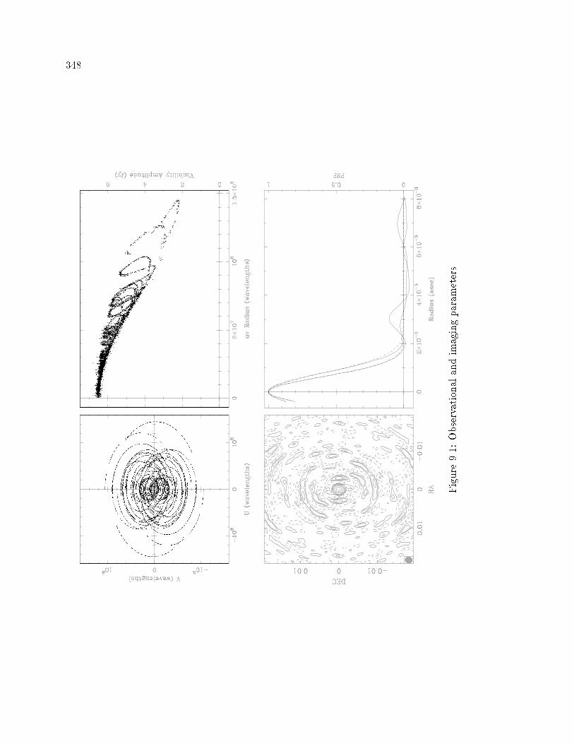
� �
Figure����Observationalandimagingparameters�

� �
��� VLB Array Memo ����A
High Dynamic Range Imaging With the VLBA
D�S� Briggs
R�J� Davis
J�E� Conway
R�C� Walker
National Radio Astronomy Observatory
July� �� ����
����� Introduction
The VLBA is being tested for high dynamic range imaging using a complete
track on DA���� All the data have been fringed� calibrated and edited by Craig Walker�
Here we report on attempts made to image just one of these IF channels� In principle
this data set had the possibility at being imaged at � ����� dynamic range� This is
well beyond current limits achieved in VLBI� Furthermore the VLBA has the potential
in terms of signal to noise to exceed dynamic ranges of ������ At this level we are
concerned about nonclosing errors in the correlator and station hardware� self�calibration
errors� and deconvolution errors� Our current work achieves a measured dynamic range of
���� and extremely good agreement with the a priori thermal noise� The best images
show no sign of any hardware e�ect or processing instability� Signi�cant artifacts are seen
in the CLEAN only deconvolution image� but several other techniques are investigated with
successful results�
����� Initial Calibration
The experiment consisted of full tracks on DA��� at C band� for a total observa�
tion of �� hours� Data were recorded for �� minutes out of every ��� The observation was
single polarization� RR� and after bandpass calibration the e�ective bandwidth was ����
MHz�
The initial calibration was done in AIPS� The amplitude calibration was done
using the a priori gains and system temperatures� Since the overall scaling factor was not
known� it was adjusted to force the total �ux density of DA��� to match that measured
in a special pointing run made a few days before� Large gain adjustments were required
for Pie Town �pointing problem� and Hancock �snow�� The data were edited based on a
priori edit information provided by the VLBA system and based on system temperatures
and known antenna problems� Once all of these edits were done� and low weight points

��
were removed� no further editing was required� Fringe �tting was done with FRING and a
bandpass calibration was done after fringe �tting� The bandpass calibration was done after
fringe �tting so that proper amplitude corrections would be made� to the fully calibrated
data� for amplitude losses due to the phase slopes caused by delay o�sets� Finally the data
were averaged in frequency� omitting the end channels� and in time� No baseline dependent
�closure� calibrations were made�
����� CLEAN Deconvolution
Initial attempts to image IF � were made with CLEAN� strongly favoring only
positive components� This produced images with clear rings of emission around the source
and covering the entire map� Allowing negative components solves this problem and pro�
duces the maps of Figure ����
The extended halo with twin banana like structure is similar to the dirty beam
and is probably nonphysical� At this stage we were worried about the possibility that this
could have been caused by closure problems� To this end we processed IF � through the
same software route� This IF channel has been through completely di�erent hardware on its
route to the workstation disk� The two IFs passed through di�erent �lters at the stations�
di�erent samplers� tracks on the tape� decoding at the correlator� delay lines� phase rotation�
correlator chips and so forth� However� within mapping errors which are bound to be a few
times noise given the selfcal correction� these images are identical� Subsequent images were
all made from IF ��
Examination of the CLEAN components shows alternate rings of positive and
negative CLEAN components� Studies and simulations� $this dissertation%� have shown this
to be due solely to the CLEAN deconvolution algorithm� Tight CLEAN windows actually
make the solution somewhat worse� The peak of the extended emission in these images
is roughly ���� The dynamic range is ���� worse than the theoretical of � ���� It
was clear that a better means of deconvolution is required� especially when the VLBA is
used at the full recording rate of ��� MBits�s instead of the e�ective ��� Mbits�s used in
this experiment� Several additional deconvolution�calibration strategies were explored� all
of which were successful�

���
Figure����CLEANimagesoftwodi�erentIFsproducedindifmapbyRJD�Peaktoo��sourceRMSis�and� forIFs�
and�respectively�

���
����� Imaging Presentation and Metrics
In situations where there is a signi�cant mismatch between the main lobe of the
beam and its �tted Gaussian� the issue of the residual �ux scale is important and directly
e�ects the meaning of �dynamic range�� The images presented here have all had the residual
noise cleaned to convergence� This practice does distort the noise histogram somewhat� and
it also causes the noise RMS to deviate from that calculated with the standard expressions�
�This is not surprising� since the units of these expressions are strictly Janskys per dirty
beam� and the whole point of cleaning to convergence is to to change units to Janskys
per restoring beam�� However� so far as is possible the restored model and noise are on a
common scale and this is our justi�cation for quoting dynamic ranges based on the cleaned
noise images� Dynamic range in our usage is the peak in the image over the o��source RMS
in the cleaned noise images� By contrast� our noise comparison with the a priori sensitivity
calculations are based on the o��source RMS in the images without noise cleaning� For
the naturally weighted �tted beam of ���� ��� milliarcseconds� the noise cleaned o��sourceRMS drops by ��� compared to the image where only the source is cleaned� For the
uniformly weighted beam of ������� mas it drops by ���� For the super resolved restoringbeam of ��� �� mas� it drops by ��� Thus while our de�nition of dynamic range is selfconsistent� measured values can exceed the nominal values derived by simply dividing peak
source strength by thermal noise� Our theoretical dynamic ranges have been corrected for
the noise rescaling e�ect�
All images presented here are contoured logarithmically� with a factor of � between
contours� Unless stated otherwise in the caption� the lowest positive contour is ��� of the
peak�
����� Model Fit with CLEAN Tidying
John Conway has �tted the bulk of the emission with a two component elliptical
Gaussian model� The residuals from the modelling processes were then processed with
CLEAN� This image was then used as the basis for one iteration of self�calibration and
remapped with the same model� The result is Fig � which shows no artifacts in the noise
and a smaller extended region around the source� It seems likely that further work with
self�calibration might improve the image still� but this has not been done� This image is
given in the left half of Figure ���� The dynamic range is �����

���
Figure����TheleftpanelisJEC�simageproducedandcalibratedindifmapviamodel�ttingandcleaningtheresidual�ux�The
rightpanelisDSB�sNNLSimageproducedandcalibratedwithinSDE�Noticetheextremesimilarityinthe�erroneous�extended
structure�Dynamicrangeforthetwoimagesis���and��� respectively�

��
���� NNLS
Dan Briggs has brought into operation a new deconvolver based on on Non�
Negative Least Squares matrix inversion� The current implementation exists in the package
SDE as the task svdconv� and takes FITS format dirty map and beam as input� The algo�
rithm is a quite straightforward application of a rather complicated preexisting constrained
linear algebra algorithm� The task forms the matrix connecting an arbitrary region in the
dirty map with another arbitrary region in the component plane� and solves the resulting al�
gebraic equations with the NNLS algorithm from Lawson � Hanson ���� �� The algorithm
and variations will be presented in more detail in his dissertation� but the initial results
are very encouraging� NNLS deconvolution is somewhat slower than existing algorithms for
compact sources� and very much slower for extended objects� Memory is the limiting factor
to the source size that can be deconvolved� One copy of the beam matrix must be held in
memory� of size NdataNflux� where Ndata is the number of pixels in the dirty map used as
input to the algorithm� and Nflux is the number of pixels where the algorithm is allowed
to place �ux� It is important that this �t into physical memory� as once page swapping
sets in performance degrades dramatically� and problems that were just practical become
quite impractical� Running time is roughly proportional toNdataN�flux� and also varies with
the SNR of the data� with higher quality data taking longer to process� Currently a map
with approximately pixels of signi�cant emission and high SNR can be deconvolved in
several hours on an IBM RS��
The strength of the algorithm is obviously related to the positivity constraint�
without which the problem is extremely ill posed� Since the NNLS algorithm is a direct
solution� it does not su�er the problem of a spatially iterative algorithm like CLEAN� where
an initial error is made at the start of the algorithm before the support constraints have a
chance to become e�ective� This initial error produces the ring like pattern noted earlier
which is never subsequently removed� As NNLS is a direct solver� the support constraints
enter the solution in a globally optimal way� which appears to be quite important for self�
calibration� NNLS shares the positivity constraint with the Maximum Entropy method�
but unlike MEM it has no entropy �smoothness� criterion� This actually seems to be an
advantage for NNLS when deconvolving compact structure� Noiseless simulations on both
Gaussian and disk sources show NNLS to be much better than either MEM or CLEAN
for compact objects less than a few beamwidths across� The deconvolution improvement
degrades with increasing source size� but even at the computational limit of � pixels�it is still the best deconvolution algorithm studied�
The right panel of Figure ��� was made from data calibrated entirely in SDE using
the NNLS deconvolver in the hybrid mapping loop� User input was minimal� with a single
loose window around the entire region containing probable �ux� The entire procedure was
automated in a shell script� and the solution converged after � phase�only self�calibration
iterations� and an additional �� amplitude!phase iteration� Note the striking similarly of
this image to that of the model �t ! CLEAN procedure� These two images calibrated and

���
produced in completely di�erent packages nearly convinced us that the extended emission
might be real�
However� when a human entered the loop and placed a much tighter window on
the allowed �ux� the solution improved still further� Five more iterations of self�calibration
with a tight window yields the left image in Figure ���� A naturally weighted map made
from the same calibrated data set is also given� The extended halo is completely gone� The
dynamic range is ���� for uniform weighting and ���� for natural weighting�

��
Figure�� �DSB�sbestNNLSimages�withuniformandnaturalweighting�Thedi�ferencebetweenthis�gureandtheright
panelofFigure���isthatextremelytightwindowswereusedinthe�nalstagesofself�calibration�Thenaturallyweightedimage
iscontouredanotherfactorof�deeperthanotherimagespresented�sothatthelowestpositivecontouris���ofthepeak�The
uniformdynamicrangeis����andthenaturaldynamicrangeis�����

���
����� Noise Comparison
From the VLBA Observational Status Summary of ���June���� � the zenith
Source Equivalent Flux Density for C band is �� Jy� For a full track observation the
e�ective SEFD will be degraded somewhat by elevation dependent e�ects� but we will use
�� to derive a best case lower limit� Equation � of the status summary gives the following
standard expression for a single polarization naturally weighted map plane dispersion�
#Im �
�S
SEFDp�#� tintNbase
For this observation #� ����� �� The data set contains ����� visibilities� the greatmajority of which are second integrations� We replace tintNbase with #t Nvis� The factor
of ���S accounts for system e�ciency losses and is not yet well measured for the VLBA� In
the same� �lower limit� spirit� we use ���s ���� which is appropriate for a perfect one bit
correlator at Nyquist sampling� The numbers yield an expected #Im ���� mJy�
Software also exists in SDE to allow the estimation of thermal noise directly from
the measured visibility data� The visibility averaging task can solve for the proportionality
constant between the weights and inverse variance from the scatter in �nite averages� After
subtracting o� the transformed NNLS component model� leaving mostly thermal noise� it
seems to work quite well in this case� The SDE mapper takes proper account of weights
and given this constant can calculate both the expected RMS thermal noise in the naturally
weighted map and also the degradation caused by using nonnatural weights�
The averaging task produces the following proportionality constants as a function
of integration time� �� seconds� �� �� � seconds� ����� seconds� �� ��
The point here being that it is well behaved at the one part in several hundred level� The
noise behavior is close to Gaussian�
Using the � second �gure� the expected thermal RMS noise in the maps are
���� and ��� mJy for natural and uniform weighting respectively� The measured o��source
RMS from the uncleaned �nal NNLS images are �� and ���� mJy�
The conclusion we draw from this is that the NNLS images are very close to the
thermal RMS in terms of the noise actually present in the data� In agreement with visual
inspection of the images� neither the deconvolution nor the calibration nor nonclosing errors
�all of which should vary slowly on the scale of � seconds� are signi�cantly contributing
to the o��source RMS� In addition� the measurements are matched exactly by noise limited
observations� theoretical correlator e�ciency� and a mean SEFD of � Jy� Considering
the known problems at Pie Town and Hancock� plus the e�ect of nonzenith observations�
this is extremely good agreement between the measured thermal noise and a priori noise
estimates�

���
���� Super Resolution
In previous super resolution work on SN����A� �Briggs� ��� �� the deconvolver of
choice was MEM� At the low signal�to�noise ratio of the SN����A data� pure deconvolution
error due to incomplete sampling was completely dominated by thermal noise and the
choice of algorithm was made on other criteria than high precision� MEM extrapolates well
in the Fourier domain and has the property that image features are made only as sharp as
mandated by the data� In fact� since agreement between the data and the model is enforced
in a statistical sense only� the MEM model image� will always be smoother than the true
image� Related to this is that the model image has an e�ective resolution greater than
that imposed by the pixel size� and the transform of the model drops towards zero at the
highest spatial frequencies� The net e�ect of these properties is that one can view the MEM
model as an image �without residuals� that has a spatially variable resolution as high as
warranted by the data� Features present in this image are guaranteed to be mandated by
the data though whether by the astrophysical source or by the thermal noise �uctuations
is ambiguous� Conventional astronomical usage convolves the MEM model image with a
restoring beam and adds the residuals back to the image� but the MEM algorithm itself
limits the maximum resolution attempted in the reconstruction� no matter what restoring
beam is selected�
By contrast� while NNLS does a superb job of extrapolation in the Fourier domain
near the envelope of the measured data� the spectral power does not necessarily roll o� at
the highest spatial frequencies� At some resolution the solution must become spurious�
Direct examination of the NNLS model image in simulations shows decidedly nonphysical
structure where �ux in several adjacent pixels has been collapsed into one pixel of greater
value surrounded by several zeros� With NNLS the onus is on the user to select a restoring
beam that provides an acceptable degree of superresolution without producing obvious
artifacts� Unfortunately� the restored image RMS and maximum negative as a function
of restoring beam often gives little guidance as to image �delity and a degree of arbitrary
judgement must be exercised�
By itself� the CLEAN algorithm combines the worst features of the other two
algorithms when used for superresolution� The high spatial frequency reconstruction is not
generally as good as that of NNLS� but it requires a similarly delicate choice of optimum
restoring beam� However it can be used in conjunction with MEM or model �tting� MEM
su�ers from the problem that even when the RMS residuals approaches the noise� there can
still be considerable beam�like structure left in the residuals� Model �tting to the thermal
noise limit is simply very di�cult for all but the simplest sources� In both of these cases�
CLEAN can be used to remove any residual structure from the residuals� Provided that
�Actually� it is the entropy �smoothness in the ratio between the model image and the best a prioriestimate of the image that is maximized� Usually the latter is simply a constant value�

���
the residual structure is small� this does not destroy the superresolution properties of the
solution� and the MEM ! CLEAN approach can be used in situations where computational
limits preclude the use of NNLS�
In Figure ��� we present images superresolved from the nominal �� � �� masto ��� �� mas� These are produced from the same calibrated data as in Figure �� � the
best NNLS calibration� The MEM algorithm was allowed to place �ux in a fairly loose box
around the source� though the details of the window made relatively little di�erence� The
east�west extension of the source traces nicely the jet seen at higher frequencies� Great care
must be exercised in interpreting super resolved images astrophysically� but the structure
here at least seem plausible� A NNLS image superresolved to � mas was rejected for
showing obvious artifacts�

�
Figure����Superresolution�TheleftpanelisproducedwithcombinationofMEMandCLEAN�therightwithNNLS�

��
����� Self�Calibration
Clearly the interaction between the deconvolution step and self�calibration is crit�
ical in the high dynamic range limit� Both CLEAN and MEM produce much better images
on the best calibrated NNLS data set than they do on data calibrated via other methods�
MEM ! CLEAN on the best data set produces an image comparable to NNLS� though
either alone is somewhat worse�
NNLS seems to have several properties that are highly desirable in the self�
calibration loop� With very little user input and loose windows it converged to a solution
as good as that of the best other methods� This property allowed it to be used in an
open loop shellscript where many selfcal iterations were performed automatically without
user interaction� Once converged to this intermediate solution� examination of the model
components provided clear delineation of the source support� and selection of a tighter �ux
window was straight forward� The tighter window quickly drove the iteration to the �nal
solution�
NNLS has a clear advantage over MEM in self�calibration in that it is not biased
against compact structure� NNLS has an advantage over CLEAN in that it makes e�cient
use of the support constraints� With CLEAN� the characteristic errors have already been
introduced into the solution before the support constraints make any di�erence in the iter�
ation� NNLS encodes the support information in the structure of the beam matrix and this
a�ects the solution in a global manner�
The majority of the calibration can also be performed with lower precision de�
convolvers for speed reasons� The calibration required �� iterations to converge to the
highest quality solution with NNLS� using �rst the loose and then the tight �ux window�
The calibration still required nearly the same �� iterations to converge� restarting from
the beginning and using the tight window throughout� Until the last few iterations� the
intermediate solutions were nearly identical� Similar experiments varying the self calibra�
tion integration time yielded similar insensitivity to parameters until the last few iterations�
The �nal calibration allowed independent amplitude and phase solutions for every sec�
ond visibility average� When the calibration was attempted with MEM as the deconvolver�
intermediate solutions were very similar to that of NNLS until the MEM solution ceased to
improve at about �� iterations� Highest quality deconvolution seems necessary only at the
end� and the �nal calibration with NNLS seems stable to di�erent intermediate routes to
the solution�
������ Conclusions and Further Work
� No obvious artifacts at all in the best images� and good agreement with a priorithermal noise� No evidence for closure errors at the ������ level� There appear to
be several workable approaches to high �delity imaging with the VLBA�

��
� NNLS is very promising� It is the best deconvolver when it can be applied� and it hasthe advantage being very forgiving about windowing� This is an excellent algorithm
in the self�calibration cycle�
� Model �tting ! CLEAN is a workable imaging approach and will likely drive self�
calibration well�
� CLEAN � MEM individually produce image artifacts even on the best calibrated
data set� but the combination is very good and not limited by source size� This does
not drive self�calibration well�
� It is a bit disturbing that the �rst NNLS attempt � the Model �tting ! CLEAN areso similar� Be conservative when interpreting such image features�
� NNLS seems to superresolve very nicely in this case & but more work would be neededbefore publishing it as astrophysics�
� Further testing continues on a ��� Mbits�s data set which will enable the VLBA tobe tested at ����� dynamic range�
End of Memo
��� Simulations
Even though it appeared that the halo around DA��� could be entirely accounted
for by processing a�ects� it was desired to verify that the VLBA could distinguish between
the presence or the lack of such a halo�
Initial attempts to model the observation with statistically independent gain er�
rors were disappointing� Rather than attempt a cure with progressively more complicated
attempts to model realistic gains� I present a simple procedure to transfer the gains from the
actual observation to the simulation� This makes a tremendous di�erence in the behavior of
the simulation and yields a very powerful diagnostic technique for investigating the e�ects
of processing on self�calibrated interferometric observations� In this case� with �� of the
total �ux placed in an extended halo� it is concluded that a � ����� VLBA observation
can successfully distinguish unambiguously between the presence or lack of the halo�
����� Gaussian Model
The bulk of the DA��� emission is reasonably �tted with a single Gaussian com�
ponent of size �� � ��� milliarcseconds� at a position angle of ������ There is de�nitely
an extended component of emission to the west that this model lacks� but it is instructive to
examine whether the qualitative deconvolution behavior can be modeled with such a crude
approximation to the source�

��
The e�ective thermal noise in the observations was determined by subtracting
o� the best deconvolved model from the visibility data set� and averaging the residual
noise with the SDE task visavg� The visibilities in the observed data set were replaced
by that of the Gaussian model plus the measured amount of Gaussian distributed thermal
noise generated with a random number generator� The Pie Town and Hancock stations
were seriously degraded in sensitivity by pointing problems and snow� respectively� In
principle this degradation could be modeled properly within SDE by manual adjustment of
the visibility weights� but for the purposes of the simulation all telescopes were assumed of
equal sensitivity� and the mean thermal noise was added�
The smoothed Gaussian model and the best deconvolution of the thermally cor�
rupted data set are given in Figure ��� Except where noted in the captions� all deconvolu�
tions remaining in this chapter are done with the NNLS algorithm� Since this investigation
is not concerned with super resolution and is concerned with the details of the thermal
noise� the images have not had their thermal noise CLEANed to convergence as was done
earlier� The same convention is followed of the lowest contour being ��� of the peak� with
a factor of two between contours�
Figure ��� Gaussian model and best deconvolution of model ! thermal noise�

�
����� Gain Transfer
Initial attempts to model the observation with statistically independent gain er�
rors were disappointing� A data set was created as above� but with �� RMS amplitude
errors and completely random phases� After a single phase�only self�calibration iteration
with a point source model and no time integration� the left panel of Figure ��� was obtained�
Not only is this extremely dissimilar to the more sophisticated simulation in the right panel�
but the calibration convergence of this data set is also unrealistic� Compare the o��source
RMS as a function of self�calibration iteration given in Figure ��� for the actual data and
the independent gain simulation� All self�calibration iterations were started with a point
source model and � iterations of phase�only self�calibration� For the independent�gain sim�
ulations� the solution converged within several subsequent iterations of amplitude � phase
self�calibration� as compared to an additional � iterations required for the real data to
converge to a similar image�
Figure ���� Correlated gains do make a considerble di�erence in simulation �delity� Themodel source is a gaussian� The left panel has had greater calibration error added to it thanthe right panel� but without any correlation structure� After one iteration of amplitude �phase self�cal� it is already better then the more realistic simulation�
The observational image presented in the upper�right panel of Figure ��� used a
tight deconvolution window which produces the best result� When a loose window is used
in the deconvolution step� considerably fewer artifacts are seen in the independent gain

��
Figure ���� O�source RMS against self�calibration iteration� Independent gain errors givea model that converges too fast� The black triangle is the amount of noise introduced intothe model� The measured RMS is lower than that because of noise absorbed by the selfcalibration process�

�
simulation images than in either the real data or the later simulations� The correlation
structure of the initial gain errors obviously makes a di�erence in the self�calibration cycle�
Along with several other packages� SDE has a means of simulating correlated
gains� One creates a model atmosphere with given correlation structure and allows it to
blow over the top of the array while observing through it� This is undoubtedly a reasonable
way to proceed when the simulation is of an instrument not yet built� This procedure
is complicated� however� One must select appropriate values for a number of di�erent
atmospheric parameters� many of them not well constrained by observations� One always
wonders how well the model atmosphere re�ects reality� In the case of a VLBI array� the
assumption of a single atmosphere is clearly wrong� though it does serve to introduce a
correlation structure� if perhaps not the correct one� When a well�calibrated data set of the
observation under study is available� there is a better way� The visibility gains applied to the
well�calibrated data set can be simply transferred to the model� In SDE this is implemented
in the task vissim as
Vis �sim Vissim �Visobs�Viscal !Noisetherm � visibility samples �����
Vis �sim is the corrupted model data� Vissim the noiseless model data� Visobs the data set
whose gain errors are to be transferred� Viscal is the well�calibrated data set� and Noisethermis Gaussian thermal noise generated with a random number generator� In this rather general
formalism� the errors introduced need not be closing� Anything that has been done to the
calibrated data set will be reproduced in the simulation� Of course� residual calibration
errors will not be transferred� but this simple procedure is likely to produce simulations
at least as accurate or better than completely synthetic data sets� Note also that the
model need not resemble the observed sky at all� One could use an observation of an
easily calibrated source like DA��� and apply these gains to a simulation of a much more
complicated object�
The remaining two panels of Figure ��� show deconvolutions of the gaussian model
with gains transferred from the DA��� observation� Both of these images have been pro�
duced after �� iterations of self�calibration� The convergence of the o��source RMS to the
�nal value in Figure ��� now qualitatively closely resembles that of the real data� The black
triangle in that �gure is the level of the thermal noise in the simulated data� �On the scale
of this graph� the di�erences between the measured o��source RMS and the expected RMS
from the thermal noise introduced into the visibility data is entirely negligible�
This simulation also illustrates another e�ect only recently recognized� It has
long been held that the e�ect of self�calibration is to slightly increase the thermal noise in
the map� by dint of reducing the number of good observables�� Unfortunately the iterative
��� � � one should note that the thermal noise level in a self�calibrated map is slightly larger than thatexpected from the data statistics�� �Wilkinson� �� p� See also Cornwell ��� �

��
Figure ���� Deconvolutions of self�calibrated gaussian model data�

��
nature of the calibration process makes analysis of the feedback di�cult� In fact� quite the
opposite is true� As discovered in Wieringa�s PhD dissertation work� �Wieringa� ������ the
measured o��source RMS in the map will in fact decrease by a factor of roughlyq��Nant�Nbase� �����
if every integration time is allowed separate calibration constants� The exact solution is not
known for an arbitrary source� but the e�ect will be of this order� It is an apparent e�ect�
not an actual decrease in the thermal RMS� The self�calibration algorithm has simply been
told that the true sky is �at o� the main source� and it has adjusted the gains so as to make
this the case� introducing low level calibration errors in the process� This is di�cult to avoid�
but the e�ect should be accounted for in the highest quality simulations� When measuring
noise from self�calibrated data� one should either correct by the inverse of equation ���
to �nd the appropriate amount of noise to introduce into the uncalibrated data to match
observation� or one should simply correct by the ratio of expected�to�measured thermal
noise in a �rst pass through the simulations� In this memo� the di�erence of approximately
�� in RMS noise level is not thought to a�ect the �nal conclusions� but if desired another
round of simulations could be done which would presumably produce an RMS convergence
curve quantitatively very similar to the measured trace of Figure ���� In Figure ���� we
show a model observation using an NNLS model which closely agrees with the observational
data after several iterations of self�calibration�
����� Halo Model
The central question of this investigation is� Can we create a halo in the processing
if is none is present in the data� and the related If the halo is present in the data� will we
see it�
Three percent of the source �ux was removed from the single�Gaussian model and
placed in an azimuthally�symmetric halo� The model� smoothed down to the resolution of
the restoring beam� is shown in the upper�left panel of Figure ����� This model is intended
to qualitatively represent the halo seen in early processing stages of the DA��� data� shown
in Figure ���� The upper�right panel shows how well the source can be deconvolved with a
careful selection of window� in this case a circle of radius � mas� centered on the source�
CLEAN� allowed a somewhat larger window of radius � mas� produced the �gure on the
lower�left� Finally� if NNLS is boxed very tightly to the support of the central Gaussian�
the �gure on the lower�right results� In all of these images� the halo is clearly visible� While
the mis�boxed NNLS deconvolution is not so pretty as the others� no one could fail to miss
that there is something wrong�
Now� how well can we hide or �nd the halo when we include self�calibration in the
loop� The next set of images were self calibrated for the same �� iterations as were the other
images� In the upper�left panel the same over�tight window was used in an e�ort to make

��
Figure ���� Correlated gain example with an NNLS model and transferred gains� Theright panel is a simulated data set after � phase only self�calibrations and � iteration ofamplitude and phase self�calibration� The right panel is the observational data� and theytrack each other quite well�

��
Figure ����� Halo model and best deconvolution of model ! thermal noise�

���
the halo vanish� It is certainly less obvious than in the previous image� but I think there
would be little chance of missing its existence here� either� The upper�right image is what
results from iteration on a large window of radius ��� mas� The quality of reconstruction
is not as pretty as before� but the halo is most certainly there� The �nal point to make
is that if one starts with these two images as a model� then resets the �ux window to
the optimum region used in Figure ����� the solution immediate converges within several
additional iterations to the lower two �gures� Whether one starts too tight and expands the
window or starts too loose and contracts the window makes little di�erence� The solution
is fairly robust about the path taken to �nd it�
If a halo was present at the �� or ������ level in the �rst observation described�
we would have seen it� The con�dence in the imaging is high�

���
Figure ����� Deconvolutions of self�calibrated halo model data�

���
��� Conclusions and Further Work
As mentioned in the introduction to the �rst memo� further testing of the VLBA is
indeed underway� In a gratifying con�rmation of the previous conclusion� Tim Cornwell has
been working on a data set with nearly the full sensitivity of the VLBA� His observations
consist of � ��MHz intermediate frequency channels for a total of MHz bandwidth�
Using clock o�sets determined from a previous correlation of the data set� he has been able
to produce what appears to be nearly a noise�limited observation at a dynamic range of
������� Ironically� we are now in a similar position to when we started� wondering if the
di�use emission we see around the source might be real� But now we are wondering about
emission a full order of magnitude fainter� At this level� instrumental e�ects are subtle� to
say the least� and it will be challenging to properly asses the �delity level of observations
like these� But there is not doubt that we are better prepared to do so than we were several
years ago�

��
Figure ����� High dynamic range image of DA���� Peak to o��source RMS is �������

Chapter �
Concluding Comments
This dissertation has largely been driven by a fresh look at several old problems
and established practices� The fresh look paid o� here� and there is probably much material
in a similar vein waiting to be discovered or improved� Uniform and natural weighting have
been around as long as interferometric imaging� and yet a simple alternative was found that
is demonstrably superior for some applications� Just because something has been done one
way for a long time doesn�t mean that it can�t be improved�
We have seen that a simple modi�cation to uniform weighting leads to a smoothly
varying intermediate form between uniform and natural weighting� Di�erent values of the
new weighting parameter� the robustness� can produce images at di�erent points along the
resolution�thermal noise tradeo� curve� One can obtain moderately improved thermal noise
characteristics compared to uniform weighting at little cost in resolution� or higher resolution
compared to natural weighting at little cost in thermal noise limited sensitivity� The near�
uniform regime will be particularly valuable to VLBI arrays with elements of greatly di�ering
individual sensitivities� The near�natural regime will be particularly valuable to arrays like
the VLA which have a preponderance of short spacings� the new weighting often produces
extremely low sidelobes and a particularly good match between the dirty beam and it�s
�tted Gaussian� It is an excellent choice for imaging extended emission�
In addition to robust weighting� several other improvements to existing weighting
practice were given� namely generalized tapering and gridless uniform weighting� My suspi�
cion is these new techniques� plus proper use of the tools that we already have� have entered
the region of diminishing returns in terms of conventional weighting by optimizing a single
criterion independently of the source� �The global minimization of individual weights to
best �t the PSF to a Gaussian over a �nite window is a possible exception�� For the most
part� I consider this project taken to a logical plateau� It may not be �nished� but I think
the next signi�cant step will be another new concept rather than an incremental improve�
ment over the ideas presented here� Quite possibly it will come from directly involving a
model of the source structure in the weighting process� and it may even involve abandoning
the shift invariant point spread function formalism all together� The latter might involve
a di�erent weighting on a per pixel basis to move far sidelobes around� or it might involve
a deconvolution algorithm that operates strictly in the visibility plane� such as given by
Wilczek and Drapatz �������
���

��
By contrast with visibility weighting� algebraic deconvolution is an area where
much work remains to be done� The general strategy of limiting the source size to as
small as necessary and deconvolving directly instead of iteratively has been shown quite
successful for some sources� Still� the constraints imposed by the existing algorithms are
uncomfortably tight� NNLS needs to be extended to larger sources� both from a computa�
tional e�ciency standpoint and from a quality of solution standpoint� An obvious attack
is to enforce a correlation between pixels with a non�delta�function pixel model� This has
already been shown to be e�ective in improving the solution on extended sources� but ex�
actly how e�ective� and how much one is hurt on compact sources is not clear� nor is the
proper selection of pixel function� This is an active research topic at the moment�
The particular nature of the Lawson�Hanson NNLS algorithm needs to be explored�
The algorithm is still selecting a solution from the invisible distribution� albeit a much more
constrained one� NNLS deconvolution should be implemented with other procedures which
solve the equivalent problem� Is the quality of the solution better� worse� or the same�
That is� are the favorable qualities of the deconvolver seen here a generic consequence of
the information being added to the problem� or a particular consequence of the manner in
which this algorithm operates�
The great �exibility of the linear algebraic deconvolution approach needs to be
exploited� Having gone to all the trouble of storing separately each and every redundant
pixel in the beam matrix� it seems a shame not to make use of a more general weighting
scheme than that of a simple convolution equation� Perhaps a space variant pixel function
should be considered� This line of thinking begins to resemble the pixon approach of Puetter
and Pi)na� ���� �� though the exact correspondence is not clear� Granted� the case where
a space variant point spread function is forced upon us by geometrical considerations� is
precisely the large image case that the algebraic methods cannot handle� But there may well
be use for deliberately deforming the convolution equation into something more amenable
to high�precision solution�
I believe that there is still considerable room for improvement left in the rep�
resentation area� in general� This dissertation has shown exactly how the representation
of the convolution equation may be extended with the use of an arbitrary pixel function�
Similar work is given in Conley et al� ���� �� where the pixel function is restricted to
P�x�#x�P�y�#y�� so presumably other authors are also unhappy with the current rep�
resentation methodology� I have long been intrigued by the contrast between the �nite
di�erence and �nite element methodologies of representing partial di�erential equations�
�Lapidus and Pinder� ������ The standard discretization resembles the �nite di�erence ap�
proach in that it represents the variable of interest at a particular point� namely the center
of the pixels� Finite volume� �a particular case of the �nite element methodology�� instead
represents a pixel by the total �ux contained within it� rather than a sample at a particular
point� The di�erential equation to be solved is then posed as a series of boundary condi�
tions between pixels� rather than point equations to be solved at the pixel centers with the

���
approximated derivatives� Might we not do something similar in posing the deconvolution
equation as a series of boundary equations on some suitable function of the sky brightness�
An integral equation is not a di�erential equation� and the direct relationship of the bound�
ary conditions to the fundamental equation to be solved not so apparent� But the problem
need not be posed in terms of the sky brightness itself � one could work in the space of the
derivative or cumulative integral of the sky� for instance� In a suitable space� a boundary
condition formalism might be appropriate and productive�
Another very practical topic for future research involves calibration� The slow
convergence of self�calibration seen in the DA��� examples suggests that it may be produc�
tive to integrate the deconvolution and the calibration step into one larger procedure that
has knowledge of both� so that we may take a step in the direction of the true gradient
instead of merely alternating the steps in the orthogonal subspaces� Succeeding combined
deconvolution and self�calibration steps could use a proper conjugate gradient approach�
and this could potentially reduce the number of total iterations considerably�
Finally� I think the considerabe practical utility of modelling in diagnosing decon�
volution related problems has been well demonstrated here� I believe that modelling needs
to be a more routine part of all deconvolutions where it is feasible� In work not presented�
it was attempted to write a point � click style Gaussian model��tting program� Initial
guesses to the model parameters were generated semi�automatically� with some input being
given by the user and others being calculated� Even with a sophisticated external program
to do the hard work of the minimization� this proved a surprisingly hard problem� Even
so� this is a problem that badly needs to be solved� and needs to become available in the
standard analysis packages� As it stands now� model �tting to all but the simplest images
is a fairly tedious process� and people are reluctant to do so unless forced by the needs of
their particular project� Modelling must be made su�ciently simple that people will use it
as a routine part of their data analysis�
Deconvolution and image�processing are as much a part of modern interferometric
imaging as the telescope� yet there is no substitute for a stable and well calibrated telescope�
Ultimately� if one wishes to know the source visibility function at a given u�v point� the most
reliable method is to measure it� But equally true is that given an observation of some �xed
quality and completeness� we should strive to extract the highest possible quality images
and scienti�c results from it�

���

Appendix A
Lagrange Multipliers and the Weighted Mean
Extremum problems with equality constraints are often solved with Lagrange
multipliers� An unconstrained extremum problem merely sets the gradient of the objective
function to zero� If there additional equality constraints to be satis�ed� the problem can
be transformed into an equivalent unconstrained extremum problem by the introduction
of an additional term into the objective function proportional to an unknown scalar� the
Lagrange multiplier� With a single constraint to be satis�ed� the statement of the method
is particularly simple�
If a scalar �eld f�x�� � � � � xn� has a relative extremum when subject to the con�
straint g�x�� � � � � xn� � then there exists a scalar � such that rf � �rg �
In its full generality� the method is fairly di�cult to derive� However� nearly any
advanced calculus text will provide su�cient information to guide the use of the method
safely� See� for example� Apostol ������ For our purposes� the application of the method
is quite straightforward� Consider the problem of the weighted mean�
Given N independent random variables Ai with common mean �� �nd a linear
sum A with expectation � and minimal variance�
First� note that
hAi hXi
wiAii Xi
wihAii �Xi
wi � �
�Xi
wi �
Of course� if � is zero� then the sum of the weights is not constrained� In this case� we must
choose the weight sum to be unity as part of the problems statement�
��A hA�i � hAi� h�Xi
wiAi��i � �� �A���
To minimize ��A subject toPwi �� we minimize Q � ��A ! ��
Pwi � ��� where � is an
unknown constant�
Q
wk
wk
�h�Xi
wiAi��i � �� � ��
Xi
wi � ���
���

��
$��
Xi
wiAi�
wk�Xi
wiAi�
%� �
h��Xi
wiAi�Ak � �i
h�Xi��k
wiAiAk ! �wkA�k � �i
�Xi��k
wihAiihAki! �wk��� ! ��k�� �
���Xi
wi ! �wk��k � �
� wk��k ���� �� const
� wk � ����kThe normalization of the weights results in the conventional expression
wk �
��k
� Xi
�
��i�A���
Note that in contrast to the usual derivation of this result� no assumptions at
all are needed about the random variables Ai beyond their having a �nite variance� In
particular� they are not assumed to be Gaussian�

Appendix B
Elliptical Gaussian Convolution
Elliptical Gaussians are used frequently in radio astronomical imaging package
such AIPS� SDE� and the Caltech VLBI package� Unfortunately� they are tedious to
deal with analytically� and as a consequence some programs which should support full
elliptical �inverse� tapering and�or convolution� do not� I present here the equations and
algorithms necessary to deal with nearly arbitrary tapers and convolutions as reference and
encouragement to authors of future programs� The derivation is somewhat similar to� but
more general than Wild ������
The representation of tapers and convolutions by signed quadratic coe�cients
leads to a very �exible system� and is probably among the simpler approaches given the
complexity of the problem� The primary disadvantage is that this representation cannot
handle one�dimensional convolutions� This would require an axis of the beam to be zero
and correspondingly in�nite coe�cients� Recasting the formalism to work in terms of the
beam axes instead of their inverses is not su�cient to remove the singularity� Relaxing
the restriction on one�dimensional convolutions would require special purpose code that
completely bypasses this formalism� Fortunately� most practical problems can be solved
with a highly elongated two�dimensional convolution� so the necessity for implementing this
special case is primarily aesthetic�
The elliptical Gaussians are most often described by the major and minor axis
full width at half maximum�� The position angle is that of the major axis measured from
the north through east� or counter clockwise from vertical under the normal mapping con�
ventions� The unrotated ellipse of half maximum is
x�
�Bmaj����!
y�
�Bmin���� � �B���
and the normalization of the gaussian exponent is �xed by
e�k ��� � k ln ��
De�ning A� � ���Bmaj����� C� � ���Bmin���
� and rotating by an angle � � Bpa! ��� we
can write the elliptical gaussian as
g�x� y� exp��Ax� � Bxy � Cy��� with
�Other choices are described in �Sramek and Schwab� �� p� ��� �
���

���
A �A� cos� � ! C� sin
� �� ln �
B ���C� � A�� sin����� ln � �B���
C �A� sin� � ! C� cos
� �� ln �
From the basic Fourier transform pair
e�Ax� ���
q��Ae��
�u��A
We can work out the transform of
Fhe�Ax
��Bxi F
he��Ax
��Bx�B���A� eB���A
i eB
���A Fhe�A�x�B��A�
�i
eB���A e�i����B��A�u F
he�Ax
�i
q��Ae��
�u��A�B���A� i�Bu�A
This in turn allows us to work out the transform of g�x� y�
F� $g�x� y�% FyFx $g�x� y�%
FyFx
hexp��Ax� �By x� exp��Cy��
i Fy
hexp��Cy�� ���A���� exp�B�y�� A� exp�i�Byu�A� exp����u��A�
i Fy
hexp$��C �B�� A�y� ! �i�Bu�A�y% ���A���� exp����u��A�
i
!�
C �B�� A
"���
exp
��i�Bu�A��
�C � B�� A�
�exp
!i���i�Bu�A�vC � B�� A
"
� exp�
���v�C � B�� A
� !�
A
"���
exp
����u�A
�
��� AC �B������
� exp�
��
AC � B�
��B�u��A! Buv ! �B� � AC�u��A � v� A
��
��� AC �B������ exp
� ��
AC �B�
��Cu� ! Buv � Av�
���B���
Thus prepared� we can now calculate the transform of two convolved Gaussians
g��x� y� � exp��A�x
� �B�xy � C�y��
g��x� y� � exp��A�x
� �B�xy � C�y��
F� $g� � g�% F� $g�% F� $g�%
� exp
!� ��
!!C�
A�C� �B��
!C�
A�C� � B��
"u� !

���
We can see by inspection that the resulting exponential will be a quadratic form in u and
v� Hence we write the following identi�cations�
Aout
AoutCout �B�out
A�
A�C� � B��
!A�
A�C� � B��
� RA
Bout
AoutCout �B�out
B�
A�C� � B��
!B�
A�C� � B��
� RB �B� �
Cout
AoutCout �B�out
C�
A�C� � B��
!C�
A�C� � B��
� RC
B might be zero� but both A and C should be nonzero� One can solve for Aout� Bout and
Cout via
Cout AoutRC�RA Bout AoutRB�RA
Aout
A�outRC�RA � A�
outR�B�R
�A
RA � Aout �
RC �R�B�RA
�B���
The solution for Aout in equation B�� can be rather ill�conditioned� In a computer im�
plementation one might solve for both Aout and Cout in this way� and select the solution
path with the larger denominator� These equations can be solved as easily for one input as
for the output� so they can be used for deconvolution as well as convolution� Converting
the resulting coe�cients back to elliptical parameters is straightforward analytic geometry�
In program B�� we present a general algorithm to perform the conversion which can be
used for this and other purposes� Here� we simply note that after calling this routine with
D E and F ��� ln �� the conventional beam parameters of the convolution result
are Bmaj �Smaj � Bmin �Smin and Bpa � ����� ! ��� The position angle is arbi�
trary to multiples of ���� though it is probably wise to constrain it to within ���� Sinceconvolutions are linear� the amplitude can be handled separately� using the fact that
Z �
��
Z �
��exp
�� ln �
�Bmaj����x� !
� ln ��Bmin����
y��dx dy
�
ln �BmajBmin � ������BmajBmin
The conversion factor between �ux density per pixel and per beam is this quantity over
#�#m�
�If the equations are recast in terms of Bmaj and Bmin� RA and RC remain �nite even in the zero limit�Sadly� RB does not and the resulting equations in RA�RB � RC are quite di�cult to solve even when treatingthe limits as special cases�

��
begin Input form is Ax� � Bxy � Cy� �Dx�Ey � F � �if B�
� �AC � � � error� Form is a parabolaif A �� C Find rotation angle that zeros crossterm
� �� tan���B��A� C�� All angles in radiansif � � � � � �� �� �� �� ���
else
� �� ��� Degenerate case assign a valueA� �� A cos� ��B cos� sin�� C sin� � Transform to rotated coordsB� �� ��C � A� sin� cos��B�cos� �� sin� �� B� should be zeroC� �� A sin� �� B cos� sin� � C cos� �D� �� D cos�� E sin�E� �� �D sin� �E cos�xc� �� �D���A� Find center by completing the squareyc� �� �E���C�
xc �� xc� cos�� yc� sin� and rotating back to original coordinatesyc �� xc� sin �� yc� cos�if A� � � � C� � � � error� EllipseHyperbola is degenerateA� �� ��F �D�
���A� �E�
���C���A� Convert to form x��A� � y��C� � �
C� �� ��F �D�
���A� � E�
���C���C�
Smaj � sgn�A��pjA�j SmajSmin � �� Elliptical
Smin � sgn�C��pjC�j SmajSmin � �� Hyperbolic
if jA�j � jC�j Ensure Smaj � Smin
Smaj �� sgn�C��pjC�j
Smin �� sgn�A��pjA�j
� �� �� ���end Results are xc� yc� Smaj � Smin� �
Program B��� Conversion of quadratic parameters to elliptical�hyperbolic parameters

Appendix C
Beam Fitting
In the same spirit as Appendix B� we present an explicit derivation of the Gaussian
beam �tting equations� The problem can be linearized by taking logarithms� This yields
an analytic formulation that is both fairly robust and amenable to direct solution� If one
assumes that beams formed via Fourier synthesis are normalized to a peak of unity and
centered on a reference pixel which we shift to the origin� the function to be �t is simply
G�x� y� � exp��Ax� � Bxy � Cy�
�� lnG Ax� ! Bxy ! Cy��
This is a linear problem for the three constants A� B � C� with the basis functions x�� xy
� y�� The normal equations as described in section � �� of Press et al� ������ become
��
Px�
Px�y
Px�y�P
x�yPx�y�
Pxy�P
x�y�Pxy�
Py�
����� A
BC
���
��
P�x� lnGP�xy lnGP�y� lnG
��� �C���
This set of equations can be solved in usual way� but it is particularly useful to call the
previous matrix �� and de�ne
T � ������ � ����� � ��
��� � ��
��� ! �������
Call the righthand side of equation C��� �� If T is larger than a few times the machine
precision� we can write the quadratic coe�cients as
A ������ � ������ ! ����� � ������� ! ����� � ���������T
B ������ � ������� ! ����� � ������ ! ����� � ���������T
C ������ � ������� ! ����� � ������� ! ����� � ��������T
If T is less than the threshold� the position angle is indeterminate� We set B � and solve
T � ���� � ���
A ����� � ������T
C ����� � ������T
���

��
If T is still less than the threshold� the beam �t is in serious trouble and the routine should
probably issue an error message and return a default value� Alternatively� one could assume
a circularly symmetric beam and use
A C
P��x� ! y�� lnGP�x� ! y���
However determined� the quadratic coe�cients are then converted back into el�
liptic beam parameters by calling program B�� from Appendix B with D E and
F � ln �� The accumulation region for the summations is somewhat arbitrary� WithinAIPS and SDE� a pixel window of size ��� �� is used� centered on the peak� Only pointsgreater than ��� of the peak are considered� and an attempt is made to consider only the
points from the primary lobe of the beam� by starting at the central column in the window
and working outwards� Highly elliptical beams with high sidelobes inclined near �� could
confuse these algorithms� If desired� a more robust algorithm could be devised for recog�
nizing the primary lobe� but in such the cases the beam �t will still be problematical and
the wise astronomer should examine it and override as needed� The physical meaning of
the beam �t in such cases also becomes less clear� and questions of oversampling and the
like are better answered in the u�v plane than in the sky plane�
The disadvantage of the linear algorithms is that the deviations of the true beam
from the Gaussian model are compressed by the logarithm� For the purposes of calculating
a residual �ux scale where integrals over the beam are taken� the full nonlinear beam �tting
is more appropriate in that it is less susceptible to systematically large deviations from the
model� Nearly any nonlinear minimization routine will work� given a su�ciently accurate
initial guess� Starting the nonlinear �t with the results of the linear �t works nicely� The
SDE implementation of the beam �tting uses the Levenberg�Marquardt method� styled after
the routine found in Press et al� ������ and this has proved quite satisfactory� Typical
di�erences in the �tted beam between the linear and nonlinear methods are only about ��
for well behaved data� but there is no reason not to do it correctly� Within AIPS� onecan use the general purpose tasks IMFIT or JMFIT to perform a nonlinear �t� There is no
provision for �ltering high sidelobes in these tasks� but if it is problem they can be removed
with BLANK�
A logic bug exists in the beam �tting algorithm in all versions of AIPS priorto ��JUL��� It results in either the major axis being underestimated or the minor axis
overestimated� biasing all �ts towards a more circular beam� In these versions� the nonlinear
�tting is the only way to get an accurate answer�

Appendix D
Generalized Tapers and Beam Forcing
The elliptical Gaussian convolution calculations presented in Appendix B are
more general than they might �rst appear� Convolving by a Gaussian in the image plane is
multiplying by a Gaussian in the u�v plane is a taper� One might also wish to amplify the
higher spatial freqencies and divide by a Gaussian instead of multiplying by one� It�s not
terribly productive to think of such an inverse taper as a convolution in the image plane�
�the inverse Gaussian lacks a Fourier transform�� but it�s still a well posed problem in the
u�v plane� Inverse tapering on visibility data is held �nite by the limited support of any
real sampling pattern�
The functional form of the Gaussian pro�le is exp��Ax� ! �� so by simplynegating the sign of the quadratic parameters� the taper becomes an inverse taper� Exam�
ining the structure of equations B� � the deconvolution of two elliptical Gaussians by solving
for one of the inputs given the output is exactly the same as �convolution� of an elliptical
Gaussian with an inverse taper and solving for the output� If the result of such a problem
is de�ned in the image plane� it can be treated as ordinary deconvolution� But even if it
is not de�ned in the image plane� the result of the deconvolution is still well de�ned in the
u�v plane� and it may be applied to visibility data as a taper� This taper need not even
be purely a downweighting or purely an upweighting� It is quite possible to have a taper
along one direction in the u�v plane and an inverse taper along the orthogonal direction�
In this case we have hyperbolic Gaussian tapering� since the curve of constant taper is a
hyperbola rather than an ellipse� Though doubtless there are more general forms still� I
call speci�cation of the taper by signed quadratic coe�cients� generalized tapering�
Any nondegenerate set of quadratic taper parameters can be reduced to a taper
or inverse taper along two othogonal axes and a rotation angle� SDE takes advantage of this
fact in how it speci�es the taper� A normal Gaussian taper is speci�ed by the half widths
and position angle of the equivalent convolution in the image plane� The only modi�cation
necessary to specify generalized tapers as well is the convention that the sign of the major
and minor axes is transferred to the equivalent quadratic coe�cient� as in
A� � sgn�Bmaj��B�maj C� � sgn�Bmin��B
�min
It is fairly easy to use a generalized taper to force the �tted beam to any rea�
sonable desired ellipse� The basic strategy is to approximate the initial and desired dirty
���

���
beam by their �tted Gaussians� and analytically deconvolve the dirty beam from the desired
output� The resulting generalized taper is applied to the visibility data and the procedure
iterated� Most well sampled cases will converge within �&� iterations of this simple recipe�
Some cases will oscillate around the correct answer� and the cure here is to apply a con�
vergence parameter to the taper correction determined by deconvolution� A simple linear
scaling of the correction major � minor axes is su�cient for most cases� A more sophisti�
cated covergence scheme could be used� one which keeps track of over and undershoots and
automatically increases the damping when oscillation is detected� but this has not been in�
vestigated� In extremely poor coverage cases this algorithm might diverge� and for a given
coverage there are values of the requested beam which no taper can produce� But with
reasonable values of the requested beam this is usually a well behaved procedure�
The basic algorithm is explicitly given in ProgramD��� and is implemented in SDE
as the Perl script findtaper� The actual implementation is quite crude� being merely the
tasks uvmap and beamcalc called in sequence� There are several minor problems associated
with the implementation and one with the formalism� The latter problem is that quadratic
taper parameters do not deal well with one�dimensional degenerate tapers � one or more
coe�cients become in�nite� This is not a signi�cant problem when specifying the taper
directly� since one can always use an ellipse with an aspect ratio of �� When called from
findtaper� it is possible that a solution which converges exactly on one axis before the
other might generate a one�dimensional correction� but this has never been observed with a
real observation� findtapermerely assumes that if exact convergence is seen on either axis�
then the complete solution has converged� The only concession made to the ��D special
case is liberal use of error trapping� The problems arising from the implementation as a
shellscript rather than an integrated single task are a nontrivial source of roundo� error
in the �xed format ASCII representation of the beam parameters used for comunication
between the tasks� many redundant calculations and much redundant IO between iterations�
and an extremely crude termination criterion� However� even in spite of these problems� the
procedure works quite well enough for practical use� An integrated beam forcing task would
be preferable to the solution currently implemented in SDE� but any interferometric imaging
packing should have provision for some sort of beam forcing� Clearly once generalized
tapering is available within the mapping program� full beam forcing can be implemented
with a minimum of programmer time�

���
begin Find taper T which produces output beam O
T �� � Initialize T or pass in best estimate from previous runfactor �� � Set factor smaller if trouble convergingB �� evaluate beam� Find Bmaj �Bmin�Bpa from initial taperfor i �� � to max iter Finite main loop
C �� deconvolve�B�O�� Deconvolve B from O� giving a correction Cif trap error � done� If error� assume that we�re doneCmaj �� factor Cmaj
Cmin �� factor Cmin
T �� convolve�T�C�� Apply the correction giving the next taper estimateif trap error � done�L �� B Save last value of BeamB �� evaluate beam� Find the new oneif B � O � done� Graceful exitif B � L � done� No improvement in solution
done � Reached iteration limit or found solutionend
Program D��� Beam forcing iteration

Appendix E
Gridless Weighting Algorithm
The central step of a gridless weighting algorithm is to calculate the sum of
the visibility weights in an elliptical neighborhood around each visibility� The simplest
approach to implementing this would be a simple doubly nested loop� For each visibility
we test every visibility in the data set and ask if it is close enough to the visibility under
consideration to include in the local sum� The direct approach is far too slow for normal
use� but it does demonstrate several implementation issues that must be addressed� The
�rst is simply the test for �close enough�� In the usual algorithm for uniform weighting�
the area under consideration is one cell in the gridded u�v plane� That is� a point ui is
within the neighborhood of uk when jui � uk�j � #u��� where #u ����max and uk� is
the coordinate of the center of the grid cell containing uk � A similar condition exists in v
and m� so that the region of consideration is rectangular�
The gridless algorithm is more �exible� so we can use an elliptical region of con�
sideration and also center the region properly around each visibility in turn� The test for
proximity becomes�ui � uk�
�
r�u!�vi � vk�
�
r�v� �� �E���
where ru �����#u�FOVw with #u de�ned as above� The factor of ����� is so that the
area of the consideration region is the same for both the gridded and gridless algorithms�
FOVw � the weighting �eld of view� is the fraction of the image size over which sidelobes
are to be optimized� FOVw � is normal uniform weighting� while FOVw ��� would
correspond to super�uniform weighting over a �x� u�v box� rv is de�ned similarly�
The idea behind the gridless algorithm is to minimize the number of tests for
proximity that must be made to determine all visibilities in the neighborhood of a given
point� To this end we do an initial bucket sort of the visibilities� The result of this sort is
an array of pointers to linked lists� Each entry of the array corresponds to a rectangular
bin in the u�v plane� and all visibilities in that region are linked together in a singly linked
list� This sort requires an arbitrary sized rectangular array of pointers� and an additional
linear array of pointers of the same size as the visibility array� This binning operation is
similar to gridding� with the important distinction that it is used only for e�ciency� There
are no approximations involved in the actual distance calculations between visibilities� and
the �nal answer is independent of the binning parameters� From the basic parameters of
the problem it is simple to calculate a small subset of the rectangular array containing all
��

���
possible visibilities in the neighborhood of �uk� vk�� We merely step over this subset region
examining each head pointer in turn� If it is nil� there are no visibilities in that region�
If it is non�nil� we step through the linked list examining each visibility for proximity to
the target� Thus we must examine only the visibilities in the rough vicinity of the desired
point� The �ner we make the binning array� the more tightly we can approximate the
desired neighborhood� We must also make more tests of the head pointer array� and the
balance between these requirements determines the optimal size for a given problem� In
Section E�� we address the problem of selecting an appropriate bin size� A �xed bin size
will be adequate for many purposes and is particularly simple to code�
A complication is introduced in that each visibility actually represents a Herme�
tian conjugate pair of visibilities� but it is only stored once in the visibility data base� For
each visibility point Vi�ui� vi�� there is an implicit visibility point of V�i ��ui��vi� with the
same weight� The algorithm must test for both signs of the conjugation� if there is any
possibility of confusion� In some imaging packages the visibilities are gridded into a half
plane� and the Hermetian nature of the data taken care of with a Real � Complex FFT
routine� This is the most computationally e�cient way to do the transform� but it intro�
duces considerable complexity into the weighting algorithms� Our binning array need not
bear any particular relationship to the grid used in the FFT of the data� and it is easiest to
use an array that does not have a discontinuity at u � The optimum size of the binning
array can be quite large� possibly several thousand elements on a side � enough to be a
potential problem for workstations already burdened with keeping the entire visibility set
in virtual memory� We can reduce the memory requirements to nearly that of the half plane
case by considering the positive �ui � � conjugation of points to be weighted� In this case
we need only consider neighboring points with uj � �ru� and do not need to bin any ofthe others� If we constrain the origin of the u�v plane to be between bins of the array� then
the image of one bin through re�ection in the origin exactly maps to another bin� Thus the
same visibilities will be grouped together in both cases� and both head pointers can point
to the same linked list� In addition� this choice guarantees that only a single conjugation of
a given visibility can map to the same cell� Hence the algorithm must check only that it has
the right conjugation for the given binning cell and include the weight or not as appropriate�
Since in most cases the outer visibility track will cross u � the minimum and maximum
extent of v will be nearly equal� Thus it is no great penalty to impose that the v origin
be between the center two bins� We will call the size of this array Gu by Gv � and map the
u�v origin to between the bins uorigin � uorigin ! � and similarly for v� Gv will be assumed
even� with vorigin Gv��� The choice of uorigin is slightly more involved� The fundamental
constraint is & jumj! �
#Gu
'!
&ru ! �
#Gu
' Gu �E���
where � is a small constant measured in cells which provides a guard region against roundo�
error at the edge of the binning array� A conservative choice of #Gu and uorigin which risks

���
only wasting some of the binning array is
#Gu jumj! ruGu � � uorigin
&ru ! �
#Gu
'
The alternative is to simply select the smallest value of uorigin that satis�es equation E���
trying each #Gu �jumj! ����Gu � uorigin� in turn� The binning and weighting outlined
in programs E�� and E�� will work with any reasonable value of uorigin�
begin
uscale �� min��Gu � uorigin � ���umax� �uorigin � ���ru� Arrange scale so that umax
vscale �� �vorigin � ���vmax and vmax just �t on gridfor k �� � to Nvis
if weightk � � � skip�if uk � � Ensure proper conjugation
ucell �� uk � uscale u�v coordinates in real cellsvcell �� vk � vscale
else
ucell �� �uk � uscalevcell �� �vk � vscale
ubin �� bucellc uorigin � Convert to cell indexvbin �� bvcellc vorigin � � relative addressing used hereu�
bin �� d�ucelle uorigin � Negative conjugationv�
bin �� d�vcelle vorigin �l �� headubin�vbin Save the old head pointerheadubin �vbin �� k Add the new visibility at the headlinksk �� l Fix the linkif u�
bin � � Only some negative conjugations binnedheadu�
bin�v�
bin�� k Negative conjugation points to the same list
end
Program E��� Visibility binning procedure�
Since weighting is a common operation� we are motivated to �nd the most e�cient
reasonable implementation possible� With another array of size Nvis and a bit more logic�
the running time can be cut by another factor of several� The idea is to identify binning
cells that are completely outside the region of consideration� so that we skip the cell without
traversing the list� Additionally� the sum of all weights in each linked list are accumulated
in the binning step� and when a cell is identi�ed as being completely within the target
neighborhood the summed weights are accumulated again without traversing the list� First�
note that the bin�summed weights can be accumulated by simply adding the lines
if l � nil
bin sumk �� weightkelse
bin sumk �� bin suml � weightk
at the end of the main loop in program E��� After the initial binning� headi�j will point to
the element of weight sum that contains the sum of all weights in the corresponding bin�
Only the elements of weight sum that are pointed to by head are used in the �nal weighting

���
begin
for k �� � to Nvis Main loop of algorithmif weightk � � � skip�if uk � � Select proper conjugation of target
utarget �� uk
vtarget �� vkelse
utarget �� �uk
vtarget �� �vkweight sumk �� � We �nd this for every visibilitybin lowu �� b�utarget � ru� � uscalec � uorigin � �bin highu �� b�utarget � ru� � uscalec � uorigin � �bin lowv �� d�vtarget � rv� � vscalee � vorigin � �bin highv �� d�vtarget � rv� � vscalee � vorigin � �for i �� bin lowu to bin highu Loop over the covering box
for j �� bin lowv to bin highvl �� headi�j May be nil initiallywhile l �� nil Loop over any visibilities present
if �ul � � � i � uorigin� � �ul � � � i � uorigin�utest �� ul Ensure proper conjugationvtest �� vl
else
utest �� �ul
vtest �� �vlif inside�utest� vtest� A fairly expensive test
weight sumk �� weight sumk � weightll �� linksl Follow the link
where
funct inside�u� v� � �u�utarget��
r�u� �v�vtarget��
r�v� �� Centered around �utarget� vtarget�
end
Program E��� Simple gridless weighting procedure�

��
loop� but we have no way of knowing which elements will end up at the heads of the lists
and the remainder of the array is convenient intermediate storage�
Figure E��� Geometry of the binning array�
Consider Figure E�� and program E��� The heavy box in the �gure represents the
rectangular search area around �uk� vk� de�ned in program E��� The lighter shaded bins
are regions where all the weights within the bin should be included into the local density
without needing to test each one individually� We simply test the corner of the bin known
to be farthest from the origin of the ellipse� That is� in the upper left quadrant we test
the upper left corner of the bin� If that is within the ellipse then the whole cell should
be included� The darker shaded bins are those which should be skipped immediately� In
a similar vein if the nearest corner of a given bin is outside the ellipse then the whole cell
should be skipped� In the �gure the starred bins have these corners marked� The remaining
bins are the only ones where we must search the list in the style of program E��� These
latter individual comparisons are responsible for the O�N�� behavior of the algorithm� and
do indeed constitute the majority of the run time for typical sized problems� In program E��
we present the central decision tree required to implement this� For problems where the
u�v coordinates� visibility weights and temporary arrays can �t into virtual memory� this
algorithm is entirely satisfactory for calculation of gridless local weight density�
E�� Variations of the Algorithm
In program E�� every binning cell is examined individually for occupancy� con�
tainment and exclusion from the target ellipse� An alternative approach is to calculate the
intersection of the lines separating the cells in v with the ellipse� By working upwards and

���
begin Same loop structure as program D��if headi�j � nil � skip� Most bins take this case
u �� �i� uorigin� � uscale Fiducial point of bin is upper right cornerv �� �j � vorigin � �� � vscaleif u�u � utarget then Left hand side of ellipse
if v �v � vtarget then Upper left quadrantif inside�u� v�� sum weights�elseif outside�u� u� v �v� � skip�else search list�
elseif v � vtarget then Lower left quadrantif inside�u� v�v� � sum weights�elseif outside�u� u� v� � skip�else search list�
else Straddles center in vif inside�u� v� � inside�u� v�v� � sum weights�else search list�
elseif u � utarget then Right hand side of ellipseif v �v � vtarget then Upper right quadrant
if inside�u�u� v� � sum weights�elseif outside�u� v�v� � skip�else search list�
elseif v � vtarget then Lower right quadrantif inside�u�u� v �v� � sum weights�elseif outside�u� v�� skip�else search list�
else Straddles center in vif inside�u�u� v� � sum weights�elseif outside�u� u� v �v� � skip�else search list�
else Straddles center in uif v �v � vtarget then Upper half of ellipse
if inside�u� v� � inside�u� u� v� � sum weights�elseif v � vtarget then Lower half of ellipse
if inside�u� v�v� � inside�u�u� v �v� � sum weights�else Cell contains center
if inside�u� v� � inside�u� u� v� �inside�u� u� v�v� � inside�u� v�v� � sum weights�
else search list�where
funct outside�u� v� � �inside�u� v��funct sum weights � weight sumk �� weight sumk � bin sumk� skip� �funct search list � �as in inner loop of program D����end
Program E��� Central decision tree for quick gridless weighting

��
downwards from the center lines� one can calculate exactly the limits of the interior and
border cells� which would appear to be much more e�cient than testing each cell� In prac�
tice� however� the �lling factor of the binning array is between � and � percent� Testing a
cell for occupancy is very quick� and must be done in any event even in the calculated limit
variation� In the region of the optimum running time� the ellipse size is near �� points in
diameter� so a comparable number of elliptical calculations are done in each approach� The
direct testing approach is more straightforward to code and slightly faster than calculated
limits� so there is no need to consider this variation further�
The original version developed used strict half plane binning� That is� no conjuga�
tions with ui � were binned at all� All negative conjugations were found by searching the
corresponding region of the positive half plane� The problem is that a rectangular region
including the origin decomposes into four distinct rectangular subregions in the positive
conjugation half plane� with the visibility conjugation in the center regions indeterminate�
This version used slightly less memory for the binning array� but was somewhat slower due
to the redundant checks for conjugation in the central region and much more complicated
to code� The subroutine containing the inner loop was over � lines of FORTRAN long�
This approach is not recommended�
If performance is paramount and memory cheap� one could consider separating
the conjugations� Each visibility would be entered in the database twice� once for each
conjugation� and there would be no need to decode the conjugations in the inner loop� It
is unlikely that this would increase the speed by more than perhaps ��� however� The
binning array would need to be full sized� and the size of the visibility and link arrays
doubled or tripled� For contemporary machines this does not seem a useful tradeo��
The recommended algorithm assumes that all relevant arrays can �t into virtual
memory� For all but the largest problems� this is a reasonable assumption� Still� for some
purposes it may be desirable to create a disk based version that will handle problems of
larger or arbitrary sizes� Assume that the maximum number of visibilities that fall into a
strip of width w � d�ru�#ue ! � bins wide is N �vis� If it is practical to hold in memory
visibility arrays of size N �vis � Nvis and also a head pointer array of size w by Gv � one
can proceed quite straightforwardly� The visibilities are �rst sorted into ascending u� The
visibilities are binned into the array� mapping the strip �ru ! �k� ��#u � u �ru ! k#u
into the bin �k mod w� ! �� stopping at the �rst visibility where uk � �ru ! w#u� The
local weight densities for the visibilities within the strip � u � #u can now be calculated
as before� The link and coordinate arrays are scanned� and any link into the leftmost active
strip is replaced by nil� which trims these visibilities from the binned storage� The �k!��th
portion of the u�v data �le corresponding to a single strip of width #u is read in and binned
to column �k!� mod w�� replacing the previous contents which are no longer needed� The
next strip of densities is calculated and the process repeated� The links are still the visibility
indices� but all references to the link and coordinate arrays are now taken modulo N �vis�

���
If memory is insu�cient for even these reduced bu�ers� the visibilities could be
sorted in v as well as u� arranged so that all visibilities within a bin are contiguous� A
similar strategy as above would be employed to work along the v axis for each set of u� The
house keeping would be involved to say the least� and it is di�cult to imagine a scenario
where this would be required�
There is an advantage to double sorting even for the primary algorithm that we
have advocated above� If many visibility tracks cross the same binning cell� the resulting
linked list of visibilities will stripe across memory with a wide stride� possibly resulting in
excessive page faulting� The best possible sort to cure this problem would the one described
above which knows about the geometry of the binning array� But even a general purpose sort
such as UVSRT from AIPS should serve the purpose of roughly localizing the visibilities inmemory� This assertion has not been tested� however� as page faulting has not been found
to be a problem even with moderately large data sets processed on a Sparc IPX with ��
MB of memory� A ��� visibility data set showed no page faulting on the performance
meter and had identical run times for Time�Baseline and u�v sorted data sets�
E�� Automatic Bin Size Selection
A consideration that has been deferred in the above discussion is exactly how
large the binning array should be� If the array is too small� then the algorithm will spend
inordinate amounts of time searching the linked lists on the edge of the ellipse� and will
not be able to exploit the cached nature of the summed weights interior to the ellipse� If
the array is too large� then the algorithm will spend too much time checking array cells for
containment and exclusion� though fractionally fewer cells will fall on the ellipse boundary�
With an analytic model of the algorithm run time� one could select an appropriate bin size
by simply minimizing the expected run time�
A careful analytic model was developed of the algorithm�s run time� based on
assignment of arbitrary costs to each branch that the inner and outer loops can take�
numerical calculation of the probabilities of each branch from the parameters of the problem�
elimination of linear dependencies in the model� and then least squares determination of the
resulting combined constants by �tting the model to a variety of measured run times� The
hope was that such a model would perform well when extrapolated to regions of parameter
space untested� However� even with a singular value analysis of the �tting matrix� the
resulting constants were not terribly stable against determination from di�erent subsets of
the data� It required a somewhat arbitrary selection of cuto� in singular value to obtain
constants that appeared physically reasonable� As the minimum of expected run time
against array size is fairly wide� all of the various analytic models performed well enough
for practical purposes� The algorithms performed well enough that the calculation of the
analytic minimum was consuming more time than saved by the use of the true optimum
grid size compared to relatively crude estimates� The simple optimum grid size estimates

���
themselves were surprisingly good and comparable to the estimates from the full model� so
there is no need for the details of the analytic model to be presented here�
Examining the optimum solutions found by direct exploration of the parameter
space� it was noted that the ratio kG �p�ru�#Gu��rv�#Gv� �
pkGukGv was remarkably
constant� While it is intuitively clear that the radius of the weighting ellipse in binning
cells should be important� it is not as clear that this quantity should completely dominate
the run time performance� None the less� kG ranged from �� to ��� over a wide range of
imaging parameters� for both data sets� on both a Sun IPX and an IBM RS�� If one
simply assumes that kGu kGv �� is an approximate constant of the algorithm� one can
easily derive a rule for optimum grid size in terms of imaging parameters�
rv#Gv
rv
vmax��Gv� � ��
kG
Gv � �kGp� vmaxFOVw�#v � �� vmaxFOVw�#v �E���
All of these quantities are easily available to a program doing the reweighting� For the
purposes of estimation� consider that the uniformly weighted FWHM beamwidth of a typical
full synthesis observation is ��vmax� where � ranges from about ��� for the ATCA to ���
for the VLA� Remembering that the full angular width of the image is ��#v� we de�ne the
image �eld of view in beamwidths as FOVi � vmax��#v�
Gv � �kG �p� FOVi FOVw � ��FOVi FOVw
The optimum bin size goes as the image �eld of view measured in uniform beam�
widths times the weighting �eld of view�
Gu is determined similarly� and yields
Gu � kGp� umaxFOVw�#u! dkGe � ����FOVi FOVw ! � �E� �
Needless to say� a reasonable value of kG should be determined experimentally for any new
implementation of this algorithm� but it seems likely that the these values will not be too
far o�� And of course� the worst that will happen if they are is that the weighting algorithm
will run slower than optimum�
The primary data sets used for run time determinations were a ��� visibility
set from the A con�guration VLA� and a ��� visibility set from the Australia Telescope
Compact Array� Both were from high declination observations and the u�v coverage fairly
circular� The VLA data was sampled at roughly ��� pixels per uniform beam� ����� image�
#u #v ����� vmax�"vmax � �� The AT data was highly oversampled at roughly ���
pixels per beam� ����� image� #u #v ����� vmax�"vmax ����� The oversampling means
that the run times for the AT case are comparable to that of a more conservative sampling
and a FOVw twice as large� Some example run times as a function of binning array size
are given in Table E��� For these runs� Gu bGv � umax�vmax ! ���c� which is essentially

���
equivalent to equations E�� and E� near the run time minima� The machines used were a
Sun Sparc IPX with �� MB of memory� and an IBM RS��� with heaps of it�
The most germane question is how well the algorithm performs with the binning
array size estimates as compared to the optimum size found by direct examination of the
parameter space� For each case in Table E��� a more densely sampled version of these data
were �tted with a parabola in the region of the minimum to determine the optimum binning
array size� The full analytic model �with coe�cients determined from the composite data
set� but separately for each processor� and the kG �� simple expression were then used
to predict the optimum binning array size� The run time excesses tabulated are simply
the �tted parabolae evaluated at the estimated array sizes� The points to note from these
tables are�
� Run Times for typical parameters and data sets are slower than gridded weighting�
but fast enough for routine use
� The simple kG const method of estimating an optimum binning array size is entirely
adequate
Less important points are
� There is a strong dependence of run time on weighting �eld of view� and a weakerdependence on the size of the binning array
� Both the simple estimation and the full analytic model predict the optimum binning
array size well enough that the run times are within a few percent of optimum�
� The simple method of estimation makes its maximum error in regions of the highest
run time� while the full model may make a signi�cant error anywhere
Clearly there is no great advantage to the sophisticated modelling� It might eventually
prove useful as a diagnostic in cases where the simple approach fails� but until such a case
arises� its use is not recommended�

System Dataset FOVw Gridsize �Gv��� � � �� �
IPX AT �� ���� ����� ����� ����� ����IPX AT �� ����� � ��� ����� ����� � �� IPX AT ��� ����� ���� ����� ����� �����
IPX VLA �� ������ �� �� ����� ���� �����IPX VLA �� ������ ������ ������ ����� ���� IPX VLA ��� ���� ������ ����� ����� ���
IBM AT �� ���� ���� ���� ��� ���IBM AT �� � �� �� ��� ��� �����IBM AT ��� ����� ����� ���� ����� ����
IBM VLA �� ��� ����� ����� ����� ���� IBM VLA �� � ��� ���� ���� ���� �����IBM VLA ��� ���� �� �� ����� ���� ������
Table E��� Running times for the gridless weighting algorithm main loop� Times are inseconds�

�
System
Dataset
FOVw
kGu
kGv
Gv min
RTmin
Gv mod
#RTmod
Gv simp
#RTsimp
IPX
AT
��
��
�� �
������
�� ��
�������
����
�� ����
��
IPX
AT
��
����
����
�����
�� ���
������
�����
������
�
IPX
AT
���
���
���
����
����
�����
� ���
�� ���
����
IPX
VLA
��
�
��
������
�����
������
��
�������
���
IPX
VLA
��
���
����
�� ��
�� ����
� � ��
���
� ���
���
IPX
VLA
���
��
���
������
����
����
���
�� ���
�����
IBM
AT
��
� �
���
�����
����
� � ���
���
�� ����
��
IBM
AT
��
���
���
������
� �
��� ���
����
������
��
IBM
AT
���
����
����
����
����
�� ��
����
�� ���
����
IBM
VLA
��
� �
���
�������
����
�������
���
�������
���
IBM
VLA
��
���
����
������
� ����
� �����
�� �
� ���
���
IBM
VLA
���
���
���
�����
���
������
��
�� ���
���
TableE���Runtimeexcessesusingoptimumbinningarraysizeapproximations�Runtimesareinseconds�arraysizesincells�
andtherestaredimensionless�

Appendix F
Complex Fourier Series
Complex Fourier Series are used less frequently than their real counterparts� but
provide elegant solutions to some problems�
The basic orthogonality of the basis function isZ ��
��eim���ein�d� ���mn
A complex valued function f��� on ���� �� can be mapped to the unit circle bythe function z ei�� Let
f��� g�z� g�ei�� �X
n���
dn ein�
Z �
��f��� e�im�d�
�Xn���
dn
Z �
��e�im�ein�d� ��
�Xn���
dn �mn �� dm
After changing variables to ��� u�um and noting that we normally work with V �u� �f��u�um�� we have derived the expansion
V �u� �X
n���
an ein�
where an �
�um
Z um
�ume�in�u�umV �u� du
�

Appendix G
SDE
The Software Development Environment �SDE� is an attempt to provide a simple�
friendly environment for the development of imaging algorithms� It has many strange and
wonderful algorithms not found in other packages� The useful ones are supposed to migrate
to more common packages� but it doesn�t always work that way�
SDE is available for ftp� but not supported by the authors or by NRAO� Comments
and questions may be sent by email to dbriggs�nrao�edu or tcornwel�nrao�edu� but no
guarantees are made as to subsequent action�
SDE is characterized by relatively close ties to the unix family of operating systems
and by the assumption that virtual memory is plentiful� Rather than reinvent the operating
system and insulate the programmer from the vagaries of many divergent platforms� SDE
sacri�ces some portability in the name of simplicity and relies as much as possible on native
tools and OS support� The assumption of plentiful physical and virtual memory leads to
the common practice of loading all image and visibility data completely into memory for
the duration of their use� This greatly reduces the burden of memory management on the
programmer and has the side e�ect of allowing algorithms to proceed at maximum speed in
the common case where all data can �t within physical memory� The tradeo� is that there
will be some problems that will not �t into virtual memory which might be handled by a
sequential disk based philosophy� Fortunately this is rarely a problem�
The current SDE distribution is available by anonymous ftp from the host
ftp�aoc�nrao�edu ���������� � in the pub�sde subdirectory� This distribution is
merely a snapshot of the SDE source directory tree� along with various tools and installation
instructions� It is not a �polished� release�
Many SDE routines make use of the Numerical Recipes �Press et al�� ���� li�
brary� which for copyright reasons we cannot distribute� The library is available for modest
cost from Cambridge University Press� Ordering information may be found in any of the
Numerical Recipes family of books�
In addition� the SDE programs which produce graphical output use the PGPLOT
graphics library� available from the Caltech astronomy department� Currently the package
may be obtained by anonymous ftp from the host
deimos�caltech�edu ��������������� � in the PGPLOT subdirectory�
�

Appendix H
Electronic Supplement
It is not practical to present the simulations from Chapter � over their entire pa�
rameter space� In addition� there are color versions of several �gures which are interesting�
but not su�ciently so to sacri�ce the black � white nature of this dissertation� This addi�
tional material has been collected into the electronic Appendices section of the dissertation�
and can be obtained as part of the SDE distribution described in Appendix G�
The Appendices can be obtained from the directory data�dbriggs� or as part
of the SDE �tar �les� This distribution might change slightly with time� so check the �le
README in this directory for the current contents�

Bibliography
Anantharamiah� K� R�� Cornwell� T� J�� and Narayan� R� ������� Synthesis imaging of
spatially coherent objects� In �Perley et al�� ������ chapter ��� pages ��& ��
Anderson� E� et al� ������� LAPACK Users Guide� Society for Industrial and Applied
Mathematics� Philadelphia�
Andrews� H� C� and Hunt� B� R� ������� Digital Image Restoration� Signal Processing�
Prentice Hall� Englewood Cli�s� New Jersey�
Apostol� T� M� ������ Calculus� volume II� John Wiley � Sons� New York�
Arfken� G� ������ Mathematical Methods for Physicists� Academic Press� New York� �nd
edition�
Bracewell� R� N� ������ The Fourier Transform and Its Application� McGraw Hill� New
York� �nd edition�
Briggs� D� S� ���� �� Superresolution of sn ����a� A comparative deconvolution study� In
Hanisch� R� J� and White� R� L�� editors� The Restoration of HST Image and Spectra
� II� pages ��&��� �� San Martin Drive� Baltimore� MD ������ Space Telescope
Science Institute�
Briggs� D� S� and Cornwell� T� J� ���� �� Clean�mem deconvolution errors� semicompact
sources� In Robertson� J� G� and Tango� W� J�� editors� Very High Angular Resolution
Imaging� number ��� in International Astronomical Union Symposium� pages ���&�� �
Dordrecht� The Netherlands� Kluwer Academic Publishers�
Briggs� D� S�� Davis� R� J�� Conway� J� E�� and Walker� R� C� ���� �� High dynamic range
imaging with the vlba� VLBA Memo ��� National Radio Astronomy Observatory�
Socorro� New Mexico�
Christiansen� W� N� and H'ogbom� J� A� ������� Radiotelescopes� Cambridge University
Press� Cambridge� �nd edition�
Clark� B� G� ������ An e�cient implementation of the algorithm �clean�� Astronomy and
Astrophysics� ������&����
Clark� B� G� ������� Coherence in radio astronomy� In �Perley et al�� ������ chapter ��
pages �&��
Cohen� J� G� ������� Tests of the photometric accuracy of image restoration using the
maximum entropy algorithm� Astronomical Journal� �������� &����
�

Conley� R� W�� Payne� D� M�� Restaino� S� R�� and Loos� G� C� ���� �� Synthetic images
from simulations of long baseline �d optical interferometers� Technical report� U�S� Air
Force Phillips Laboratory� PL�LIMI ��� Aberdeen SE� KAFB� NM ������
Cornwell� T� and Braun� R� ������� Deconvolution� In �Perley et al�� ������ pages ��&����
Cornwell� T� J� ������� An error analysis of calibration� VLA Scienti�c Memo ���� National
Radio Astronomy Observatory� Socorro� New Mexico�
Cornwell� T� J� ������� A method of stabilizing the clean algorithm� Astronomy and
Astrophysics� �������&����
Cornwell� T� J� and Evans� K� J� ������� A simple maximum entropy deconvolution algo�
rithm� Astronomy and Astrophysics� � ����&���
Cornwelll� T� J� ���� �� Brightness temperature limits for �lled and un�lled apertures�
Millimeter Array Memo � � National Radio Astronomy Observatory� Socorro� New
Mexico�
Crane� P� C� and Napier� P� J� ������� Sensitivity� In �Perley et al�� ������ chapter �� pages
���&���
Dwarakanath� K� S�� Deshpande� A� A�� and Shankar� N� U� ������ A modi�ed algorithm
for cleaning wide��eld maps with extended structures� Journal of Astrophysics and
Astronomy� ������&����
Efron� B� and Tibshirani� R� ������� Statistical data analysis in the computer age� Science�
������&����
Fanaro�� B� L� and Riley� J� M� ���� �� The morphology of extragalactic radio sources of
high and low luminosity� Monthly Notices of the Royal Astronomical Society� �����P&
��P�
Felli� M� and Spencer� R� E�� editors ������� Very Long Baseline Interferometry� Techniques
and Applications� volume ��� of Series C� Mathematical and Physical Sciences� Kluwer
Academic Publishers� Dordrecht� The Netherlands�
Frieden� B� R� ������� Restoring with maximum likelihood and maximum entropy� Journal
of the Optical Society of America� �� �����&����
Gerchberg� R� W� and Saxton� W� O� ������� A practical algorithm for the determination
of phase from image and di�raction plane pictures� Optik� ������&� �
Golub� G� and Kahan� W� ������ Calculating the singular values and pseudo�inverse of a
matrix� SIAM Journal of Numerical Analysis �Series B�� �������&�� �

�
Gonzalez� R� C� and Woods� R� E� ������� Digital Image Processing� Addison�Wesley
Publishing Company�
Gull� S� F� and Daniell� G� J� ������� Image reconstruction from incomplete and noisy data�
Nature� �����&��
H'ogbom� J� A� ���� �� Aperture synthesis with a non�regular distribution of interferometer
baselines� Astronomy and Astrophysics Supplement� ��� ��& ��
Hunt� B� R� ������� A matrix theory proof of the discrete convolution theorem� IEEE
Transactions on Audio and Electroacoustics� ������&����
Hunt� B� R� ������� The application of constrained least squares estimation to image
restoration by digital computer� IEEE Transactions on Computers� C���������&����
Jackson� J� D� ������� Classical Electrodynamics� John Wiley � Sons� Inc�� New York� �nd
edition�
Jakobsen� P�� Albrecht� R�� Barbieri� C�� et al� ������� First results from the faint object
camera� Sn ����a� Astrophysical Journal �Letters�� ���L�&L�
Jaynes� E� T� ������� On the rationale of maximum�entropy methods� Proceedings of the
IEEE� ��������&����
Keel� W� C� ������� The optical continua of extragalactic radio jets� Astrophysical Journal�
�������&���
Kendall� M� K� and Stuart� A� ������� The Advanced Theory of Statistics� MacMillan
Publishing Company� New York� th edition�
Lapidus� L� and Pinder� G� F� ������� Numerical Solution of Partial Di�erential Equations
in Science and Engineering� John Wiley and Sons� New York�
Lawson� C� L� and Hanson� R� J� ���� �� Solving Least Squares Problems� Prentice�Hall�
Inc�� Englewood Cli�s� New Jersey�
Lucy� L� B� ���� �� An iterative technique for the recti�cation of observed distributions�
Astronomical Journal� ������ �&�� �
Marsh� K� A� and Richardson� J� M� ������� The objective function implicit in the clean
algorithm� Astronomy and Astrophysics� ������ &����
Narayan� R� and Nityananda� R� ���� �� Maximum entropy & �exibility versus fundamen�
talism� In �Roberts� ��� �� pages ���&���
Narayan� R� and Nityananda� R� ������ Maximum entropy image restoration in astronomy�
Annual Reviews of Astronomy and Astrophysics� � ����&��

�
National Radio Astronomy Observatory ������ The green bank telescope �a telescope for
the twenty��rst century� Request for proposals� Green Bank� WV�
Noble� B� and Daniel� J� W� ������� Applied Linear Algebra� Prentice�Hall� Inc�� Englewood
Cli�s� N�J�
Papoulis� A� ������� A new algorithm in spectral analysis and band�limited extrapolation�
IEEE Transactions on Circuits and Systems� CAS����������&� ��
Perley� R� A� ������� High dynamic range imaging� In �Perley et al�� ������ chapter ��
pages ���&����
Perley� R� A�� Schwab� F� R�� and Bridle� A� H�� editors ������� Synthesis Imaging in
Radio Astronomy� volume of Astronomy Society of the Paci�c Conference Series�
Astronomical Society of the Paci�c� �� Ashton Ave� San Francisco� CA � ����
Press� W� H�� Flannery� B� P�� Teukolsky� S� A�� and Vetterling� W� T� ������ Numerical
Recipes� Cambridge University Press� �st edition�
Puetter� R� C� and Pi)na� R� K� ���� �� Beyond maximum entropy� Fractal pixon�based
image reconstruction� Experimental Astronomy� �����&���
Raisbeck� G� ������� The order of magnitude of the fourier coe�cients in functions having
isolated singularities� American Mathematical Monthly� ��� �&����
Richardson� W� H� ������� Bayesian�based iterative method of image restoration� Journal
of the Optical Society of America� �������&���
Roberts� J� A�� editor ���� �� Indirect Imaging� Cambridge University Press�
Rushforth� C� K� ������� Signal restoration and fredholm integral equations� In Stark�
H�� editor� Image Recovery� Theory and Application� chapter �� pages �&��� Academic
Press� Inc�� Orlando� FL�
Sault� R� J� ���� �� The weighting of visibility data� VLA Scienti�c Memorandum �� �
NRAO�
Schwab� F� R� ���� �� Relaxing the isoplanaticism assumption in self�calibration� applica�
tions to low�frequency radio interferometry� Astronomical Journal� �����&����
Schwarz� U� J� ������� Mathematical�statistical description of the iterative beam removing
technique �method clean�� Astronomy and Astrophysics� ��� �&���
Schwarz� U� J� ������� The method clean & use� misuse� and variations� In van Schooneveld�
C�� editor� Image Formation from Coherence Functions in Astronomy� number � in
International Astronomical Union Colloquium� pages ��&���� Dordrecht� The Nether�
lands� D� Reidel Publishing Company�
�
Schwarz� U� J� ���� �� The reliability of clean maps and the corrugation e�ect� In �Roberts�
��� �� pages ���&��
Skilling� J� and Bryan� R� K� ���� �� Maximum entropy image reconstruction� general
algorithm� Monthly Notices of the Royal Astronomical Society� ������&�� �
Sramek� R� A� and Schwab� F� R� ������� Imaging� chapter � pages ���&���� Volume of
�Perley et al�� ������
Staveley�Smith� L�� Briggs� D� S�� Rowe� A� C� H�� et al� �����a�� Structure of the radio
remnant of supernova ����a� Nature� ����&����
Staveley�Smith� L�� Manchester� R� N�� Kestevan� M� J�� et al� �����b�� Structure in the
radio remnant of supernova ����a� Proceedings of the Astronomical Society of Australia�
�� �����&�� �
Staveley�Smith� L�� Manchester� R� N�� Tzioumis� A� K�� et al� �����c�� Radio emission
from sn ����a� In IAU Colloquium � �� number � � in IAU Colloquium� page in press�
Xian� China�
Steer� D� G�� Dewdney� P� E�� and Ito� M� R� ���� �� Enhancements to the deconvolution
algorithm �clean�� Astronomy and Astrophysics� �������&���
Swarztrauber� P� N� ������� fftpack� a package of fortran subprograms for the fast fourier�
transform of periodic and other symmetric sequences� National Center for Atmospheric
Research� Boulder� CO� version �
Tan� S� M� ������ An analysis of the properties of clean and smoothness stabilized clean &
some warnings� Monthly Notices of the Royal Astronomical Society� ������&���
Thompson� A� R� ������� The interferometer in practice� In �Perley et al�� ������ chapter ��
pages ��&� �
Thompson� A� R�� Clark� B� G�� Wade� C� M�� and Napier� P� J� ������ The very large
array� Astrophysical Journal Supplement Series� ����&���
Thompson� A� R�� Moran� J� M�� and Swenson� Jr�� G� W� ������ Interferometry and
Synthesis in Radio Astronomy� John Wiley � Sons� New York�
Wakker� B� P� and Schwarz� U� J� ������� The multi�resolution clean and its application
to the short�spacing problem in interferometry� Astronomy and Astrophysics� �����&
����
Walker� R� C� ������� Sensitivity� In �Felli and Spencer� ������ chapter �� pages ��&����
Wernecke� S� J� and D�Addario� L� R� ������ Maximum entropy image reconstruction�
IEEE Transactions on Computers� C������&� �

�
White� R� L� ������� Improvements to the richardson�lucy method� In Image Restoration
Newsletter� pages ��&��� Space Telescope Science Institute�
Wiener� N� ��� ��� Extrapolation� Interpolation� and Smoothing of Stationary Time Series�
MIT Press� Cambridge� Massachusetts�
Wieringa� M� ������� ��� MHz Studies of the High Redshift Universe and the Galactic
Foreground� PhD thesis� University of Leiden�
Wilczek� R� and Drapatz� S� ������� A high accuracy algorithm for maximum entropy image
restoration in the case of small data sets� Astronomy and Astrophysics� pages �&���
Wild� J� P� ������ De�convolution of barely resolved radio sources mapped with aerial
beams of elliptical cross section� Australian Journal of Physics� ������&����
Wilkinson� P� N� ������� An introduction to closure phase and self�calibration� In �Felli and
Spencer� ������ pages �&���
Wilkinson� P� N�� Tzioumis� A� K�� Akujor� C� E�� et al� ������ High�quality images of the
css quasars �c � and �c��� In Zensus� J� A� and Pearson� T� J�� editors� Parsec Scale
Radio Jets� pages ���&�� Cambridge University Press�
Wilkinson� P� N�� Tzioumis� A� K�� Benson� J� M�� et al� ������� A disrupted radio jet inside
the host galaxy of the quasar �c �� Nature� �������&����

��
High Flight
by John G� Magee
Oh� I have slipped the surly bonds of earthAnd danced the skies on laughter�silvered wings�
Sunward I�ve climbed� and joined the tumbling mirthOf sun�split clouds � and done a hundred things
You have not dreamed of � wheeled and soared and swungHigh in the sunlit silence� Hovering there�
I�ve chased the shouting wind along� and �ungMy eager craft though footless halls of air�
Up� up the long� delirious� burning blueI�ve topped the windswept heights with easy grace
Where never lark� or even eagle �ew�And� while with silent� lifting mind I�ve trod
The high untrespassed sanctity of space�Put out my hand� and touched the face of God�