Software Reflexion Models: Bridging the Gap Between Source and High-Level Models
Upload
khangminh22Category
view
0download
0
TECHNISCHE UNIVERSITAT MUNCHEN
PHYSIK DEPARTMENT
LEHRSTUHL FUR THEORETISCHE PHYSIK T37
Aqueous Interfaces: Bridging the Gap
Between Molecular and Continuum Models
Douwe Jan Bonthuis
Vollstandiger Abdruck der von der Fakultat fur Physik der Technischen UniversitatMunchen zur Erlangung des akademischen Grades eines
Doktors der Naturwissenschaften (Dr. rer. nat.)
genehmigten Dissertation.
Vorsitzender: Univ.-Prof. Dr. F. Simmel
Prufer der Dissertation: 1. Univ.-Prof. Dr. R. Netz, Freie Universitat Berlin2. Univ.-Prof. Dr. W. Zwerger
Die Dissertation wurde am 31.05.2012 bei der Technischen Universitat Munchen einge-reicht und durch die Fakultat fur Physik am 27.06.2012 angenommen.


Contents
Abstract v
Zusammenfassung vii
1 Introduction 1
1.1 The Helmholtz-Smoluchowski Equation . . . . . . . . . . . . . . . . . . . . 1
1.2 Dielectric Permittivity . . . . . . . . . . . . . . . . . . . . . . . . . . . . . . 2
1.3 Viscosity . . . . . . . . . . . . . . . . . . . . . . . . . . . . . . . . . . . . . . 3
1.4 Water Rotation . . . . . . . . . . . . . . . . . . . . . . . . . . . . . . . . . . 4
1.5 Ion-Surface Interactions . . . . . . . . . . . . . . . . . . . . . . . . . . . . . 4
1.6 Molecular Modeling: Molecular Dynamics Simulations . . . . . . . . . . . . 5
1.7 Outline . . . . . . . . . . . . . . . . . . . . . . . . . . . . . . . . . . . . . . 6
2 Profile of the Static Permittivity Tensor of Water at Interfaces 7
2.1 Introduction . . . . . . . . . . . . . . . . . . . . . . . . . . . . . . . . . . . . 7
2.2 Theoretical Framework . . . . . . . . . . . . . . . . . . . . . . . . . . . . . . 9
2.2.1 Linear Response . . . . . . . . . . . . . . . . . . . . . . . . . . . . . 9
2.2.2 Multipole Expansion . . . . . . . . . . . . . . . . . . . . . . . . . . . 10
2.2.3 Fluctuation-Dissipation Theorem . . . . . . . . . . . . . . . . . . . . 12
2.2.4 Calculation of the Polarization Density . . . . . . . . . . . . . . . . 13
2.3 Simulations & Results . . . . . . . . . . . . . . . . . . . . . . . . . . . . . . 14
2.3.1 Simulation Setup . . . . . . . . . . . . . . . . . . . . . . . . . . . . . 14
2.3.2 Dielectric Response . . . . . . . . . . . . . . . . . . . . . . . . . . . . 17
2.3.3 Higher-Order Multipole Moments in Interfacial Electrostatics . . . . 21
2.4 Coarse-Grained Modeling Approaches . . . . . . . . . . . . . . . . . . . . . 24
2.4.1 Dielectric Dividing Surface . . . . . . . . . . . . . . . . . . . . . . . 24
2.4.2 Modified Poisson-Boltzmann Equation . . . . . . . . . . . . . . . . . 26
2.4.3 Capacitance of the Double Layer . . . . . . . . . . . . . . . . . . . . 28
2.4.4 Disjoining Pressure between Charged Plates . . . . . . . . . . . . . . 31
2.4.5 Ion-Surface Interactions . . . . . . . . . . . . . . . . . . . . . . . . . 32
2.5 Summary & Conclusions . . . . . . . . . . . . . . . . . . . . . . . . . . . . . 34

ii Contents
3 Hydrodynamic Slip and its Effect on Electrokinetic Flow 35
3.1 Introduction . . . . . . . . . . . . . . . . . . . . . . . . . . . . . . . . . . . . 35
3.2 Pumping & Energy Conversion . . . . . . . . . . . . . . . . . . . . . . . . . 37
3.2.1 Dissipation in Pressure-Driven Flows . . . . . . . . . . . . . . . . . . 37
3.2.2 Electrokinetic Energy Conversion Efficiency . . . . . . . . . . . . . . 40
3.3 Onsager Reciprocal Relation . . . . . . . . . . . . . . . . . . . . . . . . . . . 42
3.4 The ζ-Potential of Air Bubbles . . . . . . . . . . . . . . . . . . . . . . . . . 44
3.5 Radial Flow in Compressible Fluids . . . . . . . . . . . . . . . . . . . . . . 46
3.6 Summary & Conclusions . . . . . . . . . . . . . . . . . . . . . . . . . . . . . 48
4 Electrokinetics at Aqueous Interfaces without Mobile Charges 49
4.1 Introduction . . . . . . . . . . . . . . . . . . . . . . . . . . . . . . . . . . . . 49
4.2 Generalized Navier-Stokes Approach . . . . . . . . . . . . . . . . . . . . . . 51
4.2.1 Conservation of Angular Momentum . . . . . . . . . . . . . . . . . . 51
4.2.2 Material Equations . . . . . . . . . . . . . . . . . . . . . . . . . . . . 52
4.2.3 General Stationary Solution For Planar Substrates . . . . . . . . . . 53
4.2.4 Torque from a Static Uniform Electric Field . . . . . . . . . . . . . . 54
4.2.5 Homogeneous Time-Dependent Electric Fields . . . . . . . . . . . . 55
4.2.6 Torque from a Rotating Electric Field . . . . . . . . . . . . . . . . . 56
4.2.7 Numerical Solution . . . . . . . . . . . . . . . . . . . . . . . . . . . . 60
4.2.8 Cylindrical Geometry . . . . . . . . . . . . . . . . . . . . . . . . . . 64
4.2.9 Viscosity of a Fluid Consisting of Non-Spherical Particles . . . . . . 65
4.3 Molecular Dynamics Simulations . . . . . . . . . . . . . . . . . . . . . . . . 66
4.3.1 Interaction Energy . . . . . . . . . . . . . . . . . . . . . . . . . . . . 66
4.3.2 Flow Profiles . . . . . . . . . . . . . . . . . . . . . . . . . . . . . . . 68
4.3.3 Truncation Length Dependence . . . . . . . . . . . . . . . . . . . . . 70
4.3.4 Dependence of the Flow Velocity on Other Simulation Parameters . 75
4.3.5 Definition of Flux . . . . . . . . . . . . . . . . . . . . . . . . . . . . 76
4.4 Summary & Conclusions . . . . . . . . . . . . . . . . . . . . . . . . . . . . . 77
5 Electro-Osmotic Mobility and Electric Surface Conductivity 79
5.1 Introduction . . . . . . . . . . . . . . . . . . . . . . . . . . . . . . . . . . . . 79
5.2 Mobility and Conductivity . . . . . . . . . . . . . . . . . . . . . . . . . . . . 81
5.2.1 Electrokinetic Surface Charge Density . . . . . . . . . . . . . . . . . 82
5.2.2 Conductive Surface Charge Density . . . . . . . . . . . . . . . . . . 82
5.3 Viscosity & Dielectric Profile . . . . . . . . . . . . . . . . . . . . . . . . . . 83
5.4 Scaling Analysis . . . . . . . . . . . . . . . . . . . . . . . . . . . . . . . . . 84
5.5 Modified Poisson-Boltzmann Equation . . . . . . . . . . . . . . . . . . . . . 85
5.5.1 Numerical Results & Discussion . . . . . . . . . . . . . . . . . . . . 87
5.5.2 Fitting Experimental Data . . . . . . . . . . . . . . . . . . . . . . . 91
5.6 Summary & Conclusions . . . . . . . . . . . . . . . . . . . . . . . . . . . . . 93
6 Final Observations & Outlook 95
Appendix A Literature Values of the Double-Layer Capacitance 99
Appendix B Electrokinetics Within the Gouy-Chapman Model 103

Contents iii
List of Figures 107
List of Tables 109
List of Publications 111
Bibliography 113
Acknowledgments 127

iv Contents
Abstract
At aqueous interfaces, the structure of water differs significantly from the structure inbulk fluid. In particular, the water density at the interface exhibits an oscillating profileand the orientation of the water molecules at the interface is strongly anisotropic. Themolecular structure of the interfacial water has a decisive effect on the local dielectricfunction, as well as on the interfacial viscosity. In addition, the non-spherical shape ofwater molecules affects the fluid dynamics. Despite their importance for the behaviorof liquid flowing under strong confinement – as is ubiquitous in biological systems, incolloidal suspensions and in micro- and nanofluidics – these molecular interfacial effectsare neglected in standard continuum theories of water dynamics. The work describedin this thesis is aimed at incorporating molecular information inferred from moleculardynamics simulations into continuum theory to describe the non-equilibrium dynamics ofaqueous solutions at interfaces.
First, we extract the interfacial profile of the full dielectric tensor of pure water frommolecular dynamics simulations, and incorporate the results into a mean-field descriptionof the interfacial electrostatics. Comparing the results to literature values, we show thatthe dielectric profile of pure water is both necessary and sufficient to explain the exper-imental double-layer capacitance of carbon-based surfaces. Second, we investigate thehydrodynamic properties of the interfacial water layer, and quantify the effect of hydro-dynamic slip or enhanced interfacial viscosity on pressure-driven and electrokinetic flow.Third, we formulate a generalized Navier-Stokes equation, including the effect of rotatingwater dipoles, and calculate the effect of spinning water molecules on electrokinetic flow.We show that whereas a static electric field does not induce flow in a purely dipolar fluid,a rotating electric field can be used to drive an electro-hydraulic pump. Finally, we incor-porate the profiles of the dielectric function and the viscosity into a combined mean-fieldand continuum theory of electrokinetic flow to calculate the electro-osmotic mobility andsurface conductivity of charged solutes. Using this framework, we are able to explain boththe experimentally observed saturation of electro-osmotic mobility as a function of baresurface charge density and the universally measured excess surface conductivity within asingle model.

vi Abstract
Zusammenfassung
An wassrigen Grenzflachen unterscheidet sich die Wasserstruktur wesentlich von der Struk-tur im inneren Volumen des Wassers. Insbesondere weist die Wasserdichte an der Grenz-flache ein oszillierendes Profil auf, und die Orientierung der Wassermolekule an der Grenz-flache ist stark anisotrop. Diese Molekulstruktur des Wassers hat einen entscheidenden Ein-fluss auf die lokale dielektrische Funktion, sowie auf die Grenzflachenviskositat. Daruberhinaus beeinflusst die nichtspharische Form der Wassermolekule die Flussigkeitsdynamik.Trotz ihrer großen Bedeutung fur das Verhalten der Flussigkeit unter starken raumlichenBeschrankungen – welche in biologischen Systemen, kolloidalen Suspensionen sowie mikro-und nanofluidischen Anwendungen universell auftreten – werden diese molekularen Grenz-flachen-Effekte in Standard-Kontinuums Theorien der Wasserdynamik vernachlassigt.Diese Doktorarbeit zielt auf die Einbeziehung molekularer Informationen, abgeleitet ausMolekulardynamik-Simulationen, in Kontinuumstheorien, um damit die Nichtgleichge-wichts-Dynamik von wassrigen Losungen an Grenzflachen zu beschreiben.
Zuerst extrahieren wir das Grenzflachenprofil des vollstandigen dielektrischen Tensorsvon reinem Wasser aus Molekulardynamik-Simulationen. Diese Ergebnisse werden an-schließend in eine molekularfeldtheoretische Beschreibung der Grenzflachen-Elektrostatikaufgenommen. Durch Vergleich mit Literaturwerten zeigen wir, dass das dielektrischeProfil von reinem Wasser sowohl notwendig ist, als auch ausreichend, um die experi-mentelle Oberflachenkapazitat von Kohlenstoff-basierten Oberflachen zu erklaren. Zwei-tens untersuchen wir die hydrodynamischen Eigenschaften des Grenzflachenwassers undquantifizieren die Auswirkung des hydrodynamischen Schlupfs bzw. der erhohten Grenz-flachenviskositat auf druckgetriebene und elektrokinetische Stromungen. Drittens formu-lieren wir eine verallgemeinerte Navier-Stokes Gleichung unter Berucksichtigung rotieren-der Wasserdipole, und berechnen die Auswirkung dieser molekularen Wasserrotation aufelektrokinetische Stromung. Wir zeigen, dass, obwohl ein statisches elektrisches Feld ineiner rein dipolaren Flussigkeit keine Stromung erzeugt, ein rotierendes elektrisches Feldverwendet werden kann, um eine elektro-hydraulische Pumpe anzutreiben. Schließlich neh-men wir die Profile der dielektrischen Funktion und der Viskositat in einer kombiniertenMolekularfeld- und Kontinuumstheorie der elektrokinetischen Stromung auf, und berech-nen die elektroosmotische Mobilitat und die Oberflachenleitfahigkeit geladener Teilchen.Dieser theoretische Rahmen erlaubt uns, sowohl die experimentell beobachtete Sattigungder elektroosmotischen Mobilitat in Abhangigkeit der blanken Oberflachenladungsdichte,als auch die universell gemessene uberschussige Oberflachenleitfahigkeit innerhalb eineseinzigen Modells zu erklaren.

viii Zusammenfassung
Chapter 1Introduction
Water is the primary constituent of biological cells [1], and finds extensive use as a solventas well as a working fluid in technological applications. In particular the number of applica-tions of micro- and nanofluidic technology has been rising rapidly over the past decades [2].Inherent to the small size of nanofluidic devices, surface characteristics dominate the bulkflow properties and as device dimensions shrink even further, interfacial effects becomeever more important. Moreover, a variety of different strategies actually exploit boundaryeffects to manipulate fluids, such as acoustic streaming [3] and electrokinetic effects [4].A limiting case of small-scale fluid flow is found in biological systems, where membranechannels and pumps transport fluids and biological molecules on a single-molecular scale[5, 6]. The ambitious goal of nanofluidics is to reach the single-molecular length scale inman-made devices and to manipulate flows on the scale of biopolymers and single pro-teins. Apart from microscopic applications, such as micrometer-scale laboratories, arraysof nanofluidic channels can be used in macroscopic pumps, desalination devices and elec-trokinetic power plants [7–11]. For all applications, ranging from microscopic analysisdevices to large-scale power plants, a profound comprehension of the behavior of liquidflowing under strong confinement is required [12]. Likewise, to acquire a better understand-ing of proteins such as aquaporin and other membrane channels [13, 14], the mechanismsbehind single molecular flows need elucidation [15]. Because of the large surface-to-volumeratio, describing the fluidic properties on this scale involves a precise determination of theelectrostatic and hydrodynamic characteristics of the aqueous interface.
1.1 The Helmholtz-Smoluchowski Equation
Particles in aqueous solution typically acquire a net charge, which is compensated for byan excess of counterions in the electrolyte. In electrokinetics, this charge separation isused to drive fluid flow along charged surfaces by means of an applied electric field. Forthe understanding of the dynamics of water, ions and macromolecules in biological cells,which are crowded with highly charged molecules, electrokinetics are of great significance.Equally important, electrokinetics are of interest for technological applications, primarilybecause they are the preferred method to drive micro- and nanofluidic flows in “lab-on-a-chip” devices. Moreover, electrokinetic experiments provide a sensitive probe of the

2 Dielectric Permittivity
electrostatic and hydrodynamic properties of the aqueous interface. The basic modelof electrokinetic flow consists of a uniform electric field E applied parallel to a uniformlycharged infinite plane in contact with a continuum electrolyte of relative dielectric constantε and spatially constant viscosity η. At large distances from the interface, the flow velocityu parallel to the charged surface is expressed by the Helmholtz-Smoluchowski equation,
u = −εε0 ζη
E, (1.1)
named after Hermann Helmholtz [16] and Marian Ritter von Smolan Smoluchowski [17].In Eq. 1.1, ε0 is the permittivity of vacuum and ζ is the electrostatic potential at theshear plane. Eq. 1.1 is valid for electrokinetic flow in arbitrary geometry, provided thatthe typical length scale a of the charged objects exceeds the Debye screening length κ−1
of the electrolyte by a large margin, κa ≫ 1. In the opposite limit, κa ≪ 1, a factor 2/3appears on the right-hand-side of Eq. 1.1 [18]. Although the fluid velocity u is measuredfar away from the interface, its origin lies within the first few nanometers directly adja-cent to the surface: the region where the counter-charge accumulates. Within this region,the water density varies appreciably, typically showing a peak close to the interface withsubsequent oscillations, reaching bulk value after ∼ 1 nm. Moreover, the water orienta-tion is highly anisotropic: water molecules directly at the interface tend to orient withtheir hydrogen atoms toward the surface, whereas the second layer of water molecules arepreferentially oriented in the opposite direction, etc., alternating for several layers. Thepolar ordering of the water molecules gives rise to a strong electric field in the interfacialregion, showing sharp oscillations around zero that decay over a similar length scale asthe density fluctuations. Inherent to the varying water structure, the dielectric permit-tivity ε and the viscosity η are not spatially constant, but depend on the distance to thesurface instead. Clearly, these inhomogeneous profiles, and consequently the effects of theinterfacial molecular structure, are missing from the continuum expression of Eq. 1.1.
In the following sections, we will discuss the effects of the interfacial molecular structureon the fluid dynamics, focusing on the dielectric permittivity ε, the viscosity η and theeffect of molecular rotation.
1.2 Dielectric Permittivity
One of the most salient properties of water is its high molecular polarity. As a result,electrostatic interactions in aqueous environments are drastically modified with profoundimplications for the behavior of ions, proteins and membranes in solution [19]. Experimentsand simulations have shown that the dielectric function of homogeneous water exhibits twosingularities for wave vectors at molecular length scales, indicating anomalous screeningeffects in bulk water [20]. To what extent interfacial water exhibits similar anomalies isless clear [21]. Experimental capacitance studies have led Stern to propose a model foran aqueous interface where the dielectric constant is reduced over a nanoscopic width[22]. Whether this layer reflects ionic or rather intrinsic water properties is not specifiedin the original Stern model. However, recent terahertz spectroscopy experiments haveshown that the dielectric properties of water itself are modified at interfaces within a layerof molecular size [23]. Without considering an explicit interfacial dielectric profile, therelation between the non-local dielectric function and the Stern-layer contribution to thecapacitance has been established [24], including non-linear effects [25]. Using approximate
1. Introduction 3
statistical mechanical methods, the decrease of the interfacial capacitance for a dipolarfluid has been related to molecular ordering and orientation [26]. However, a method forextracting dielectric profiles from interfacial water orientational and spatial distributions,as well as detailed knowledge of the profiles themselves have been lacking so far.
A thorough understanding of the interfacial dielectric behavior of water is a prerequisitefor correct modeling of ion distributions [27] and double-layer interactions [28], as well aselectrokinetic effects. Similarly, the interfacial dielectric function is a key ingredient tosolvent-implicit approaches toward protein and macro-molecular modeling [29]. Controlover the interfacial dielectric constant is also crucial for a number of industrial applications,including high power and long duration energy storage devices [30]. Finally, dielectriceffects are one contribution to the hydration repulsion between polar surfaces [19, 31].The dielectric properties of interfacial water have been studied using both simulationsand analytic approaches. One shortcoming of previous analytic approaches is that thewater bulk behavior, including the above-mentioned anomaly, is typically not accountedfor [32, 33]. At the same time, previous simulations with explicit water and ions couldnot be analyzed within the existing theoretical framework. One reason for the complexityis the appearance of higher order multipole moments, which are particularly essential atinterfaces [34].
1.3 Viscosity
A growing amount of literature indicates that on small length scales, the hydrodynamicboundary condition deviates from the usual no-slip condition [35, 36]. Experimentally, theviscosity is defined as the proportionality constant between the shear force per unit areaand the resulting velocity gradient. Close to a wall, this proportionality constant appearsto be different from the bulk value. In the first few molecular layers next to the interface,this is caused by the changing water structure, most notably the dipolar orientation andthe oscillating density profile. In addition, at hydrophobic walls there is a density depletiongap between the wall and the fluid [37–39]. Directly at the wall, the velocity gradient cantherefore be very different from the bulk velocity gradient in a Couette shearing scenario.On a molecular scale, even “true slip” of the first molecular layer along the wall can beimagined.
On a simple level, the assumption that the surface stress is linearly related to thesurface velocity via a friction coefficient, which equates the surface stress to the viscousshear stress, leads to the notion of a slip length [40]. A finite slip length greatly enhancesflow rates through small channels. The slip length exhibits a sensitive dependence onthe microscopic properties of the surface, increasing as the contact angle grows and thesurface becomes more hydrophobic, and scaling proportional to the depletion length to thefourth power [41]. Due to their hydrophobic nature and the large vacuum gap betweenwall and fluid, carbon nanotubes appear to have very large slip lengths, up to tens ofmicrometers [42], making them promising candidates for use as channels [43] and pumps[44] in nanofluidic devices.
Alternatively, the effect of the interfacial hydrodynamics can be modeled by a space-dependent viscosity profile η (r), with r the spatial coordinates. Whether a slip length,a viscosity profile or a combination of the two provides the more accurate model of thehydrodynamic boundary condition depends on surface type and molecular composition.
4 Water Rotation
1.4 Water Rotation
Ever since the first electrophoretic measurements it has been known that nominally un-charged substances in pure water, such as air bubbles and oil droplets, move towardthe positive electrode and thus behave as effectively negatively charged [45]. Based onstreaming-potential [46], titration [45], and thin-film stability studies [47], this behavioris attributed to the interfacial accumulation of negatively charged ions such as oh−. Forthe air-water interface, however, recent second-harmonic generation [48] as well as spec-troscopy experiments and simulations [49] suggest that not oh− but h3o
+ shows enhancedinterfacial adsorption. This discord has stirred fierce discussions [45, 49, 50]. A way outof the dilemma was proposed in recent molecular dynamics (md) simulations of aqueousinterfaces, where pure water without any added ions induced electrophoresis of the samesign and size as observed experimentally for air bubbles or oil droplets [51].
The ability of electric fields to produce hydrodynamic shear at pure-water interfacesopens attractive possibilities in other geometries, such as water-filled carbon nanotubes[52]. For flow through such tiny capillaries, the electrostatic boundary conditions stronglyinfluence the permeability to charged species. The electrostatics of a small channel em-bedded in a medium of very low dielectric constant leads to a large self-energy barrierfor ions to enter the confined region [53, 54]. In many biological channels, transport ofions is facilitated by inclusion of fixed charges in the channel walls [55], coating walls withdipolar surface groups [56, 57] and screening by salt [58]. Fixed charges outside a carbonnanotube are found to affect the pressure-driven passage of water molecules through thenanotube as well [59]. Even more intriguing is the observation that carbon nanotubesfilled with pure water exhibit electro-osmotic flow when either an electric field is applied[60] or point charges are fixed outside the channel [61]. Similarly, electro-osmotic flow isfound in uncharged channels filled with solutions of the relatively symmetric salts sodiumchloride and potassium chloride [62–64].
The mechanism for this water-induced electrophoresis was speculated to be related tothe interfacial water structure, involving static properties such as dipolar ordering [65] anddensity profile [66], as well as dynamic properties such as surface viscosity and slip length[67]. In particular, the appearance of a non-zero ζ-potential in absence of free charges wasspeculated to be related to the electrostatics in the boundary layer: water molecules tendto orient, leading to a strong dipolar field in the first few molecular layers next to theinterface. The coupling of the electric field to this dipole density was thought to induceflow via rotation of individual molecules [51, 60]. Although exciting, these results raiseconcern as fundamental laws of physics appear to be violated. In particular, the effectsseem at odds both with Onsager’s reciprocal theorem, since an externally applied pressuredrop cannot cause a steady electric current because of the absence of free charges, and withthermodynamics, since the electric field performs no work in the steady state. Despite thegreat fundamental importance, a theory that combines hydrodynamics and electric-fieldeffects for interfacial water has been missing until now.
1.5 Ion-Surface Interactions
Apart from charging by an external electric source (for conducting surfaces) and chargingby ionization of chemical surface groups, surface charge can originate from specific adsorp-tion of ions. The propensity of an ion to adsorb on to a surface depends on its chemical
1. Introduction 5
properties, such as size, charge and polarizability, as well as on the chemical properties ofthe surface. A third important factor is the molecular structure of the interfacial water.The combined potential due to the aforementioned effects is termed the potential of meanforce (pmf), which can be incorporated into the Poisson-Boltzmann equation as a non-electrostatic contribution to the potential. In Ref. [xi], we determine the pmfs of br−, i−,cl− and na+ at a hydrophobic self-assembled monolayer (sam) from md simulations, andcalculate the disjoining pressure between two sams from the modified Poisson-Boltzmannequation. The results show that specific adsorption of ions contributes significantly tothe surface charge density and should be taken into account when fitting experimentaldata. Splitting the pmf, however, into contributions from the Lennard-Jones potential,the polarizability, the image charge potential and the electrostatics of the ordered watermolecules, fails to capture the results from the md simulations. In this thesis, we qualita-tively model the pmf, taking into account the effect of the inhomogeneous dielectric profileand the hydration potential due to the varying density profile. To account for specific ionadsorption in all other calculations, we include heuristic non-electrostatic potentials thatare similar to the ones from Ref. [xi] for distances larger than ∼ 3 A.
1.6 Molecular Modeling: Molecular Dynamics Simulations
For direct investigation of interfacial properties, simulation techniques are particularlyvaluable. For the work described in this thesis, the molecular information is obtained fromall-atom classical molecular dynamics (md) simulations, in which Newton’s equations ofmotion are integrated numerically for a system of non-polarizable molecules [68]. The time-step used is typically ∼ 10−15 s, allowing total simulation times of the order of nanosecondsto microseconds for systems of ∼ 104 atoms, which are appropriate time and length scalesto capture the molecular motion (orientational relaxation time ∼ 10−12 s [69–71]) and theequilibrium structure of liquid water. In classical md simulations, the interaction potentialbetween two atoms i and j at distance rij is modeled by the spherically symmetric potential
Uij (rij) = Ucij (rij) + Ulj
ij (rij) , (1.2)
with the Coulomb potential being given by
Ucij (rij) =
qiqj4π εε0 rij
, (1.3)
and the Lennard-Jones potential by
Uljij (rij) = 4 ǫij
[
(
σijrij
)12
−(
σijrij
)6]
. (1.4)
The parameters needed for each atom pair ij are the charges qi and qj, the Lennard-Jonesinteraction strength ǫij and the interaction radius σij. Water molecules are modeled assingle Lennard-Jones spheres, having three (spc/e [72]) or four (tip4p/2005 [73]) partialpoint charges at fixed positions within the molecule. These water models satisfactorilyreproduce, among other quantities, the water structure factor (measured using x-ray orneutron diffraction and calculated in md simulations from the radial distribution func-tion), bulk dielectric constant and water density, which warrants sufficient confidence thatclassical md simulations can be used to quantify the molecular structure of interfacialwater.
6 Outline
1.7 Outline
The work described in this thesis is aimed at the integration of continuum modelingwith molecular information provided by md simulations, in order to describe the staticand dynamic properties of water and electrolytes at charged and uncharged surfaces. InChapter 2, we derive the theoretical framework needed to calculate the dielectric responsetensor from molecular dynamics simulations, and determine its components at the in-terface between a solid surface and pure water using md simulations. We incorporatethe dielectric profile, which includes the effect of molecular interfacial structure, into amean-field (Poisson-Boltzmann) description of the interfacial electrostatics. Similarly, mdsimulations provide detailed insight into the mechanism of surface slip [74], which setsthe hydrodynamic boundary conditions used for the Navier-Stokes equations. In Chap-ter 3, we investigate the effect of interfacial hydrodynamic slip on the energy dissipationin pressure-driven flow and the thermodynamic efficiency of electrokinetic pumping. InChapter 4, we include the dipolar water ordering at interfaces and the molecular rotationof water molecules into a generalized Navier-Stokes equation and determine the conditionsunder which the spin field contributes to the fluid flow. Simulations of ions at interfacesrenders information on the characteristics and extent of ion adsorption, which is used tocomplement the Poisson-Boltzmann equation, see Ref. [xi]. Ultimately, this multi-scalemodeling scheme allows us to formulate a modified Helmholtz-Smoluchowski equation (Eq.1.1), including the effects of molecular structure. In Chapter 5, we combine the effects ofthe viscosity profile, the dielectric profile and the non-electrostatic ion-surface interactionsto calculate electrokinetic mobility, as well as the electric surface conductivity at chargedsurfaces.
Chapter 2Profile of the Static PermittivityTensor of Water at Interfaces
In this chapter, we derive the theoretical framework to calculate the dielectric responsetensor and determine its components for water adjacent to hydrophilic and hydropho-bic surfaces using molecular dynamics simulations. For the non-polarizable water modelused, linear response theory is found to be applicable up to an external perpendicularfield strength of ∼ 2 V/nm, which is well beyond the experimental dielectric breakdownthreshold. The dipole contribution dominates the dielectric response parallel to the inter-face, whereas for the perpendicular component it is essential to keep the quadrupole andoctupole terms. Including the space-dependent dielectric function in a mean-field descrip-tion of the ion distribution at a single charged interface, we reproduce experimental valuesof the interfacial capacitance. At the same time, the dielectric function decreases the elec-trostatic part of the disjoining pressure between two charged surfaces, unlike previouslythought. The difference in interfacial polarizability between hydrophilic and hydrophobicsurfaces can be quantized in terms of the dielectric dividing surface. Using the dielectricdividing surface and the Gibbs dividing surface positions to estimate the free energy of asingle ion close to an interface, ion-specific adsorption effects are found to be more pro-nounced at hydrophobic surfaces than at hydrophilic ones, in agreement with experimentaltrends. The work described in this chapter has been published in Refs. [iii] and [vi].
2.1 Introduction
Electrostatic interactions between charged objects in aqueous solution, such as lipid mem-branes, proteins and ions, are profoundly influenced by the surrounding water [19]. Eachcharge embedded in the dielectric environment of the water couples to the local electricfield, which comprises both the displacement field emanating from the charged objects andthe polarization field stemming from the dielectric medium. In a macroscopic approach,the effect of the water on electrostatic interactions is quantified by means of the staticdielectric tensor ε, which is spatially constant and diagonal in bulk. Close to an interface,however, the effect of the water is more intricate. The water density near an interfacestrongly deviates from its bulk value and the proximity of a surface restricts the molecular
8 Introduction
dynamics [75]. Short-ranged interactions between macroscopic objects in water that gobeyond homogeneous continuum electrostatics, such as hydration forces and hydrophobiceffects, are often attributed to this local variation of the solvent structure [31, 76]. Becauseof the extremely polar nature of water molecules, the water structure directly affects theelectrostatic environment, making the dielectric tensor inherently space-dependent. Theeffect of the solvent structure strongly depends on the nature of the interface: hydrophobicand hydrophilic surfaces have a vastly different influence on the adjacent water [77, 78].
Within the framework of linear response theory, the space-dependent dielectric responsefunction can be expressed as a non-local tensor, depending on the positions of the sourceand the response [24, 25, 79]. In Fourier space, the non-local dielectric tensor of bulkwater exhibits two singularities for wave vectors on molecular length scales [20]. Whethersimilar anomalies appear in the space-dependent static dielectric function of interfacialwater has long remained unclear.
The capacitance formed by a charged interface and its counterions serves as a sensitiveprobe of dielectric interface effects. It has been known for almost a century that the Gouy-Chapman model overestimates the experimental data of interfacial capacitance, which hasbeen ascribed to variations of the dielectric constant at the interface [80, 81]. In theStern model of the electric double layer, the variation of the dielectric tensor is accountedfor by the combination of a length scale and an effective interfacial dielectric constant,reproducing the experimental capacitance [22]. In the limit of low salt concentration,it has been shown how the Stern layer contribution to the capacitance emerges fromthe introduction of a non-local dielectric function, independent of the exact form of thedielectric profile [24]. Also the relation between the dielectric profile and the length scaleappearing in the Stern model has been established [25]. However, an explicit calculationof the interfacial dielectric profile of water has been lacking up to now.
The question of whether the decrease in the dielectric profile reflects ionic or intrinsicwater properties is still subject to debate. The decrease in the dielectric constant has beenattributed to the high ionic concentration close to charged interfaces [82], or to dielectricsaturation due to the corresponding high electric field strength [83]. However, recentterahertz spectroscopy experiments on carbohydrates [84] and lipid membranes [23] haveshown that the dielectric response of water itself is modified within an interfacial layerof molecular size. Theoretical attempts to relate the dielectric response to molecular dy-namics have been based on analytical as well as simulation studies. Analytical approachesinclude approximate statistical mechanical methods, which have been used to show thatthe reduced dielectric constant at the interface is associated with molecular ordering andorientation [26]. In another analytical approach, water polarization has been includedexplicitly in a mean-field description [32, 33], where molecular effects such as the above-mentioned singularities are not accounted for. Simulations with explicit water and ions didnot allow for straightforward interpretation previously, partly because of the appearanceof higher-order multipole moments. In fact, the preferred orientation of water moleculesnear an interface is set by the fundamental asymmetry stemming from the quadrupoleand higher-order even multipole moments [34, 85, 86]. This asymmetrical water structureplays a decisive role in the dielectric response of water at an interface, which is ignoredin many studies [87]. Recently, we have shown that the electric quadrupole and octupolemoments are essential components of the interfacial dielectric function [88].
The dielectric function in thin interfacial layers strongly affects the forces betweenmacromolecules and surfaces as a result of the long range of the electrostatic force. Fur-
2. Permittivity Tensor of Interfacial Water 9
thermore, a knowledge of the space-dependent dielectric tensor is indispensable to theinterpretation of the ionic surface propensity [89] and solvation free energy [27, 90, 91], aswell as the electrophoretic mobility of solutes and the double-layer capacitance [80, 81]. Inaddition, the dielectric tensor is a vital ingredient for coarse-grained calculations, wherethe water is taken into account implicitly. Finally, the electrostatics close to a solid in-terface are crucial from a technological point of view, in particular for the design of novelenergy storage media based on the double-layer capacitance.
In this chapter, we thoroughly investigate the consequences of the interfacial dielectricprofile for the interfacial capacitance, the hydration interaction between charged plates inwater and the ion adsorption energy at hydrophilic and hydrophobic surfaces. First, wepresent a complete derivation of the expressions used to calculate the components of the di-electric response tensor at planar interfaces from molecular dynamics simulations. Second,we calculate the dielectric tensor of pure water adjacent to both hydrophilic (hydroxyl-terminated) and hydrophobic (hydrogen-terminated) diamond surfaces. We show that thesalient differences between the two surface types can be quantified in terms of a singlelength scale, set by the position of the dielectric dividing surface. Third, we investi-gate the effect of the higher-order electric moments on the electric potential profile acrossthe interface. Fourth, we incorporate the space dependence of the dielectric tensor in aPoisson-Boltzmann description of a salt solution at a charged interface. Comparing withexperimental values, we show that including the dielectric response of pure water sufficesto capture the dependence of the double-layer capacitance on the salt concentration. Fifth,we calculate the disjoining pressure between two charged surfaces using the same Poisson-Boltzmann description. On the Poisson-Boltzmann level, the dielectric profile appears tobe insufficient to describe the strong, short-ranged repulsive forces commonly measuredbetween both charged and uncharged surfaces in water [92]. Finally, we estimate the freeenergy of a single ion near a dielectric boundary, and show that the different dielectriccharacteristics of hydrophilic and hydrophobic surfaces have a pronounced effect on ionadsorption. All equations are given in si units.
2.2 Theoretical Framework
2.2.1 Linear Response
Most general, the dielectric response function depends on the position r of the displace-ment field D (r), the position r′ of the local electric field E (r′) and on the field magnitude.In the linear response regime, a change in displacement field is linearly related to a changein electric field,
∆D (r) = ε0
∫
εnl
(
r, r′)
· ∆E(
r′)
dr′, (2.1)
with ε0 the permittivity of vacuum and εnl (r, r′) the non-local dielectric tensor. If the
electric field is constant in space, ∆E (r) = ∆E, the response function is automaticallylocal,
∆D (r) = ε0ε (r) · ∆E with ε (r) =
∫
εnl
(
r, r′)
dr′, (2.2)
making the usual locality assumption εnl (r, r′) = ε (r) δ (r − r′) superfluous. Alterna-
tively, the inverse dielectric response function is defined by [24]
∆E (r) = ε−10
∫
ε−1nl
(
r, r′)
· ∆D(
r′)
dr′, (2.3)
10 Theoretical Framework
with ε−1nl
(r, r′) the functional inverse of εnl (r, r′), defined by
∫
εnl (r, r′) ε−1
nl(r′, r′′) dr′ =
δ (r − r′′). The inverse dielectric response function is automatically local when the dis-placement field is constant in space, yielding
∆E (r) = ε−10ε−1 (r) · ∆D, (2.4)
with ε−1 (r) the inverse dielectric function. Note that the relation ε (r) ε−1 (r) = 1 doesnot hold without additional assumptions.
2.2.2 Multipole Expansion
In a classical approximation, the polar molecules are regarded as being composed of atoms,located at positions rij , carrying point charges qij. The total charge density ρ (r) is given
by averaging over the partial charges qij of all atoms j (i) and all molecules i,
ρ (r) =∑
i
∑
j(i)
qij δ(
r − rij)
. (2.5)
We will now expand the electric field in terms of molecular multipole moments, startingfrom the integral equation for the electric field [93],
ε0E (r) =1
4π
∫
ρ(
r′) r − r′
|r − r′|3 dr′. (2.6)
After inserting Eq. 2.5, the integration variable is shifted from r′ to r′ + rij − ri, leadingto
ε0E (r) =1
4π
∫
∑
i
∑
j(i)
qijδ(
r′ − ri) (r − r′) − (rij − ri)
| (r − r′) − (rij − ri)|3dr′, (2.7)
where ri is some arbitrary reference position in the molecule. The fraction in Eq. 2.7 isthen expanded for the case where the intramolecular distance rij−ri is much smaller thanthe distance between charge and field points r − r′,
ε0E (r) =1
4π
∫
∑
i
∑
j(i)
qijδ(
r′ − ri)
×[
r − r′
|r − r′|3 +(
rij − ri)
· ∇′ r − r′
|r − r′|3
+1
2
(
rij − ri) (
rij − ri)
: ∇′∇′ r − r′
|r − r′|3 + . . .
]
dr′,
(2.8)
where the minus sign of −(rij − ri) cancels the minus sign of ∇′ (r − r′) = −∇ (r − r′).Next, all gradient terms are integrated by parts,
ε0E (r) =1
4π
∫
r − r′
|r − r′|3[
∑
i
∑
j(i)
qijδ(
r′ − ri)
−∇′·∑
i
∑
j(i)
qijδ(
r′ − ri) (
rij − ri)
+1
2∇′∇′ :
∑
i
∑
j(i)
qijδ(
r′ − ri) (
rij − ri) (
rij − ri)
− . . .
]
dr′.
(2.9)
2. Permittivity Tensor of Interfacial Water 11
The separate components appearing in Eq. 2.9 can be expressed in terms of the molecularmultipole moments of order l ∈ 0, 1, 2, . . . , which are defined as
pli =1
l!
∑
j(i)
qij(
rij − ri)l, (2.10)
with j running over all partial charges qij of molecule i. The power inside the summationis understood as a serial direct vector multiplication, making pli a tensor of rank l. Thedensity of each multipole moment is defined as
Pl (r) =∑
i
pli δ (r − ri) , (2.11)
where the summation is carried out over all molecules [94]. Using Eqs. 2.10 and 2.11, Eq.2.9 becomes
ε0E (r) =1
4π
∫
r − r′
|r − r′|3[
P0
(
r′)
−∇′ · P 1
(
r′)
+ ∇′∇′ : P2
(
r′)
− . . .
]
dr′. (2.12)
We use the identity
∇ · r − r′
|r − r′|3 = 4πδ(
r − r′)
(2.13)
to perform the integrals in Eq. 2.12, except for the P0 term, to which we will come backlater. The divergence of Eq. 2.12 equals
∇ · ε0E (r) = ∇ · 1
4π
∫
P0
(
r′) r − r′
|r − r′|3 dr′
+
[
−∇ · P 1 (r) + ∇∇ : P2 (r) − . . .
]
,
(2.14)
from which the electric field E (r) follows as
ε0E (r) = D (r) − m (r) . (2.15)
The first term in the expansion on the right-hand side of Eq. 2.15 is the monopole term,
D (r) =1
4π
∫
P0
(
r′) r − r′
|r − r′|3 dr′, (2.16)
corresponding to the field from the free charges. The second term is the total polarizationdensity m (r),
m (r) = P 1 (r) −∇ · P2 (r) + ∇∇ : P3 (r) − . . . , (2.17)
which comprises contributions from the dipole moment per unit volume P 1, quadrupolemoment P2, octupole moment P3 and all higher-order moments. When calculating thepolarization in basic electrostatics, all multipole terms of order higher than the dipoleare often neglected [93], which is exact for a Stockmayer fluid, for example, where eachmolecule carries an ideal dipole. For water however, the higher-order terms are of majorimportance. Note that we could also calculate the multipole moments from all individualatoms instead of averaging an expansion in molecular multipole moments. Although bothdescriptions of the electrostatics are equivalent, clustering the atoms first to calculatemolecular multipole moments has the advantage of a vanishing monopole moment in thecase of neutral molecules.
12 Theoretical Framework
2.2.3 Fluctuation-Dissipation Theorem
To estimate the dielectric function from the polarization fluctuations, we write a statisticalmechanical expression for the ensemble-average excess polarization. The total interactionenergy of a water-filled volume V in absence of an external electric field is denoted U (X),with X all relevant coordinates. The energy change ∆U upon application of an externalelectric field is given by the coupling of the polarization to the field F inside the dielectric,
∆U =
∫
Vψ (r) ρ (r) dr, (2.18)
with ψ the excess potential caused by the field, ∇ψ (r) = −F , and ρ (r) = ε0∇ · E (r)the total charge density. The field F to which the fluid responds is constant in space.Therefore, F is associated with either E or D/ε0 depending on the boundary conditions.After one partial integration, the excess energy is given by
∆U = −∫
V∇ψ (r) · ε0E (r) dr = −
∫
VF · m (r) dr, (2.19)
where we used that ε0E (r) = −m (r) in absence of free charges. Defining the totalpolarization by
M =
∫
Vm (r) dr, (2.20)
the excess polarization density upon application of the external field F is given by [95–97]
∆m = 〈m〉F − 〈m〉0
=
∫
(m − 〈m〉0) exp [−β (U − M · F )]dX∫
exp [−β (U − M · F )]dX,
(2.21)
where 〈. . . 〉F and 〈. . . 〉0 denote the ensemble average with and without applied electricfield respectively. For molecules without atomic polarizability, the phase space over whichthe integration in Eq. 2.21 is performed consists of the positions ri and orientations Ωi
of the permanent multipole moments, dX =∏
i dridΩi, with i the molecular index. Forsmall field F , Eq. 2.21 can be linearized to yield
∆m ≈∫
(m − 〈m〉0) (1 + βM · F ) exp [−βU ]dX∫
exp [−βU ]dX. (2.22)
Using short-hand notation for the ensemble averages, we obtain the excess polarizationvector as
∆m (r) ≈ β [〈m (r)M〉0 − 〈m (r)〉0〈M 〉0] · F . (2.23)
The term in brackets in Eq. 2.23 includes all nine components of the fluctuation tensor.
Boundary conditions. In a planar system with translational invariance in the x and ydirections and a dielectric discontinuity in z direction, the dielectric tensor is diagonalwith only two unique components: one parallel and one perpendicular to the surface.Additionally, the electric field and the polarization density only depend on the z direction.Maxwell’s equation ∇× E (z) = 0 implies
∇zEx (z) = ∇zEy (z) = 0, (2.24)
2. Permittivity Tensor of Interfacial Water 13
so that E‖, corresponding to Ex or Ey, is independent of z everywhere. Using Eq. 2.2,Eq. 2.15 and the symmetry condition ∆E‖ = E‖ gives
ε‖ (z) = 1 +∆m‖ (z)
ε0E‖. (2.25)
The constant field F‖ in Eq. 2.23 must correspond to the constant field E‖. Therefore,combining Eqs. 2.23 and 2.25 leads to
ε‖ (z) ≈ 1 + ε−10β[
〈m‖ (z)M‖〉0 − 〈m‖ (z)〉0〈M‖〉0]
. (2.26)
Now we turn to the perpendicular component ε⊥ (z). Maxwell’s equation for the displace-ment field, ∇·D (z) = P0 (z), shows that the displacement field is constant in space whenP0 (z) = 0. Using the boundary condition ∆D⊥ (z) = D⊥, the inverse dielectric functiongiven in Eq. 2.4 becomes
ε−1⊥ (z) = 1 − ∆m⊥ (z)
D⊥. (2.27)
In the perpendicular case, the spatially constant field F⊥ must be associated with theconstant displacement field D⊥/ε0 . Consequently, combining Eqs. 2.15, 2.23 and 2.27, wearrive at the fluctuation equation for the inverse perpendicular permittivity,
ε−1⊥ (z) ≈ 1 − ε−1
0β [〈m⊥ (z)M⊥〉0 − 〈m⊥ (z)〉0〈M⊥〉0] . (2.28)
Applying an external electric field, the dielectric tensor can be determined directly usingEqs. 2.25 and 2.27. Eqs. 2.26 and 2.28 can be used when looking at the fluctuations inabsence of an external electric field instead.
2.2.4 Calculation of the Polarization Density
The perpendicular electric field is calculated from an integral over all charges,
E⊥ (z) = E⊥ (0) +
∫ z
0
ρ (z′)
ε0dz′. (2.29)
In Eq. 2.29, E⊥ (0) is the external electric field. Using m (0) = 0 and Eq. 2.15 with thefact that D⊥ is constant, we find the equation for the perpendicular polarization density
m⊥ (z) = −∫ z
0ρ(
z′)
dz′. (2.30)
To derive an expression for the parallel polarization, we virtually cut out a volume from thesimulation box. In the following text, we adopt two different but equivalent viewpoints.First, we consider all partial charges on the atoms of each molecule explicitly. By cuttingthe volume, some water molecules are split, forming a non-zero monopole density P0 (r)on either side of the virtual cut. In the second viewpoint, idealized multipole momentsare located at a single point within each molecule, and the multipole moments are notaffected by cutting.
According to the first viewpoint, the net charge inside the volume that has been carvedout comprises only P0 (r), stemming from the water molecules that have been split bycutting the volume, because the intact water molecules carry no net charge. Because the

14 Simulations & Results
split water molecules are all located near the surface of the volume, the integrated chargetakes the form of a surface charge,
∫
Vρ (r) dr =
∮
∂Vσ (r) dr, (2.31)
with σ (r) the surface charge density arising from P0 (r).
Adopting the second viewpoint, the total charge inside the volume is calculated fromthe polarization,
∫
Vρ (r) dr = −
∫
V∇ · m (r) dr, (2.32)
which can be transformed into a surface integral,
∫
Vρ (r) dr = −
∮
∂Vm (r) · n dr. (2.33)
Realizing that Eqs. 2.31 and 2.33 hold for any volume V, we find σ (r) = −m (r) · n. Tocalculate the polarization in x direction, we introduce a virtual cut perpendicular to thex axis. We only cut the water molecules at the position of the virtual cut, closing thevolume without cutting any other molecules. The surface charge density resulting fromthe split water molecules equals
σ (z) =
∫
P0 (x, z) dx, (2.34)
where the x dependence of P0 (x, z) has the form of a Dirac delta function at the positionof the cut. Along the surface of the cut, m (z) · n = ±m‖ (z), and thus
m‖ (z) = ∓∫
P0 (x, z) dx, (2.35)
where the different signs apply to closing the volume and integrating P0 (x, z) on thedifferent sides of the cut. To calculate m‖ (z), Eq. 2.35 is averaged over many differentcut positions along the x axis.
The polarization density components from Eqs. 2.30 and 2.35 are used to calculatethe components of the dielectric response tensor directly. Alternatively, the polarizationdensity is estimated from the expansion of Eq. 2.17, where the multipole densities arecalculated explicitly according to Eqs. 2.10 and 2.11. For this alternative method, we cal-culate the contributions up to the octupole term. Higher order terms cannot be calculatedfrom the simulations with sufficient accuracy. The molecular multipole moments of Eq.2.10 are calculated with respect to the position of the oxygen atom.
2.3 Simulations & Results
2.3.1 Simulation Setup
We perform molecular dynamics simulations of pure spc/e water in contact with a dia-mond slab consisting of a double fcc lattice of carbon atoms using the gromacs moleculardynamics simulation package [98]. The primary cell contains 928 water molecules and weemploy periodic boundary conditions in all directions. The carbon-water interaction is

2. Permittivity Tensor of Interfacial Water 15
0.5 1.0 1.500.5 1.0 1.50z (nm) z (nm)
80
60
40
20
0
n (
nm
-3)
a b
c d
TIP4P
SPC/E
y
x 1 nm
Hydrophilic Hydrophobic
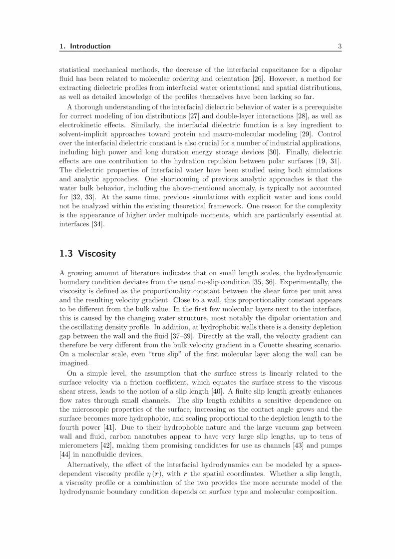
Figure 2.1: Top view of the two diamond surfaces: (a) hydrophilic (hydroxyl-terminated) and (b)hydrophobic (hydrogen-terminated). The oxygen atoms are shown in red, the hydrogen in white andthe carbon in blue. (c – d) Corresponding molecular density profiles n (z) of two different watermodels: spc/e (blue solid lines) and tip4p/2005 (red dashed lines), in absence of an external field.
determined by the Lennard-Jones parameters σcw = 0.3367 nm and ǫcw = 0.4247 kJ/mol(gromos 96). We study two surface types: one terminated with hydroxyl groups, givinga hydrophilic surface, and one terminated with hydrogen atoms, giving a hydrophobicsurface. On the hydrophilic surface, one in four terminal atoms of the diamond has ahydroxyl group attached, corresponding to a surface coverage of xoh = 1/4 in the notationof Ref. [74]. The hydroxyl groups are free to rotate. The hydrogen atoms terminatingthe hydrophobic diamond have neither Lennard-Jones coefficients nor charge. The hy-drogen atoms of the hydroxyl-terminated carbon atoms on the hydrophilic surface carrya partial charge of 0.408 e, the oxygen atoms carry −0.674 e and the connecting carbonatoms carry 0.266 e. The Lennard-Jones parameters of the oxide-water interaction areσow = 0.3017 nm and ǫow = 0.8070 kJ/mol, and the hydrogen atoms have no Lennard-Jones interaction. Images of the two surface types are shown in Fig. 2.1 (a – b). For thehydrophilic surface, the position z = 0 is defined as the position of the oxygen atoms ofthe hydroxyl groups, whereas for the hydrophobic surfaces it corresponds to the positionof the outermost carbon atoms. We simulate both surface types at vanishing externalelectric field for a total time of 80 ns, and at field strengths of E‖ = 0.05 V/nm in paralleldirection and D⊥/ε0 = 0.5, 1.0, 2.0, 4.0 and 8.0 V/nm in perpendicular direction for atotal time of 35−60 ns. Simulations at the hydrophilic interface of up to 1.0 V/nm and atthe hydrophobic interface at 0.5 V/nm are run at constant pressure, using a semi-isotropicBerendsen barostat. Simulations at higher field strength are run at constant volume. TheLennard-Jones interaction is truncated at 1.0 nm using a shifted cutoff scheme. TheCoulomb force is treated using a real-space cutoff at 1.2 nm and pseudo-two-dimensionalparticle mesh Ewald summation for the long-ranged interaction. To extract the excessfields ∆E (z) and ∆D (z), the corresponding fields at vanishing external field are sub-tracted. spc/e is a non-polarizable water model; therefore electronic polarization is not
16 Simulations & Results
0 0.5 1.0 1.5 0 0.5 1.0 1.5
z (nm) z (nm)
Field Fluct.
m
(P1- P2 P3)
m
(P1- P2 P3)
-0.5
0
0.5
1.0
150
100
50
0
ε-1
ε
a
c
Field Fluct.
Hydrophilic Hydrophobic b
d
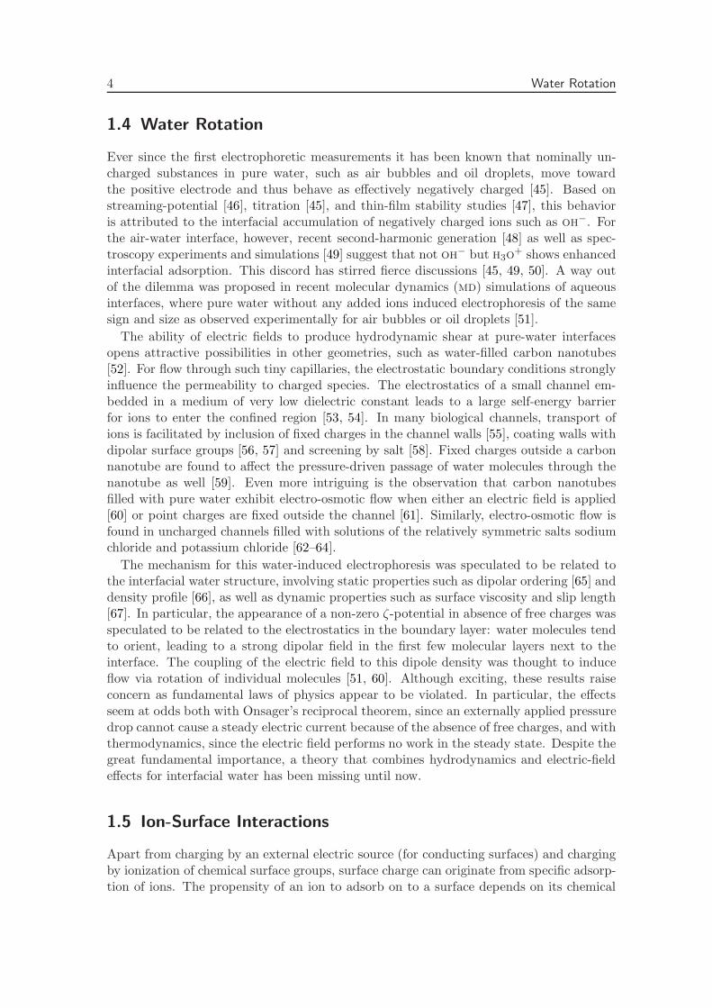
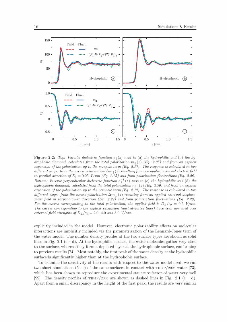
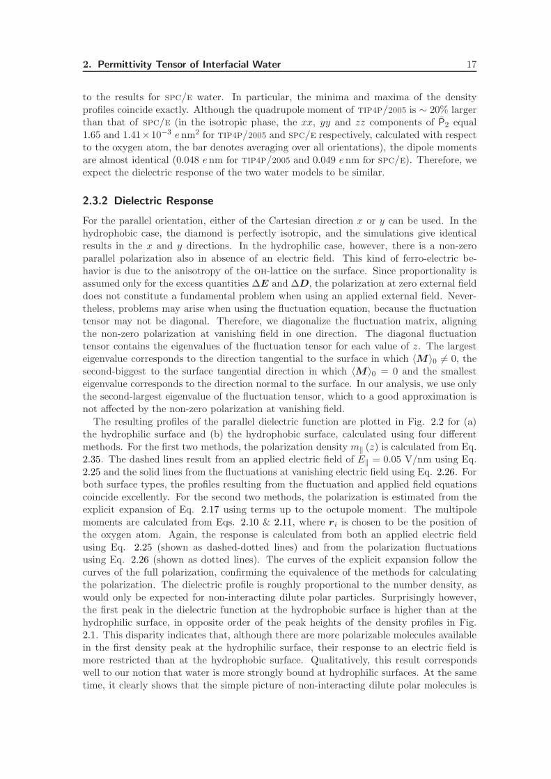
Figure 2.2: Top: Parallel dielectric function ε‖ (z) next to (a) the hydrophilic and (b) the hy-drophobic diamond, calculated from the total polarization m‖ (z) (Eq. 2.35) and from an explicitexpansion of the polarization up to the octupole term (Eq. 2.17). The response is calculated in twodifferent ways: from the excess polarization ∆m‖ (z) resulting from an applied external electric fieldin parallel direction of E‖ = 0.05 V/nm (Eq. 2.25) and from polarization fluctuations (Eq. 2.26).
Bottom: Inverse perpendicular dielectric function ε−1
⊥ (z) next to (c) the hydrophilic and (d) thehydrophobic diamond, calculated from the total polarization m⊥ (z) (Eq. 2.30) and from an explicitexpansion of the polarization up to the octupole term (Eq. 2.17). The response is calculated in twodifferent ways: from the excess polarization ∆m⊥ (z) resulting from an applied external displace-ment field in perpendicular direction (Eq. 2.27) and from polarization fluctuations (Eq. 2.28).For the curves corresponding to the total polarization, the applied field is D⊥/ε0 = 0.5 V/nm.The curves corresponding to the explicit expansion (dashed-dotted lines) have been averaged overexternal field strengths of D⊥/ε0 = 2.0, 4.0 and 8.0 V/nm.
explicitly included in the model. However, electronic polarizability effects on molecularinteractions are implicitly included via the parametrization of the Lennard-Jones term ofthe water model. The number density profiles at the two surface types are shown as solidlines in Fig. 2.1 (c – d). At the hydrophilic surface, the water molecules gather very closeto the surface, whereas they form a depleted layer at the hydrophobic surface, conformingto previous results [74]. Most notably, the first peak of the water density at the hydrophilicsurface is significantly higher than at the hydrophobic surface.
To examine the sensitivity of the results with respect to the water model used, we runtwo short simulations (5 ns) of the same surfaces in contact with tip4p/2005 water [73],which has been shown to reproduce the experimental structure factor of water very well[99]. The density profiles of tip4p/2005 are shown as dashed lines in Fig. 2.1 (c – d).Apart from a small discrepancy in the height of the first peak, the results are very similar
2. Permittivity Tensor of Interfacial Water 17
to the results for spc/e water. In particular, the minima and maxima of the densityprofiles coincide exactly. Although the quadrupole moment of tip4p/2005 is ∼ 20% largerthan that of spc/e (in the isotropic phase, the xx, yy and zz components of P2 equal1.65 and 1.41×10⁻³ enm2 for tip4p/2005 and spc/e respectively, calculated with respectto the oxygen atom, the bar denotes averaging over all orientations), the dipole momentsare almost identical (0.048 enm for tip4p/2005 and 0.049 enm for spc/e). Therefore, weexpect the dielectric response of the two water models to be similar.
2.3.2 Dielectric Response
For the parallel orientation, either of the Cartesian direction x or y can be used. In thehydrophobic case, the diamond is perfectly isotropic, and the simulations give identicalresults in the x and y directions. In the hydrophilic case, however, there is a non-zeroparallel polarization also in absence of an electric field. This kind of ferro-electric be-havior is due to the anisotropy of the oh-lattice on the surface. Since proportionality isassumed only for the excess quantities ∆E and ∆D, the polarization at zero external fielddoes not constitute a fundamental problem when using an applied external field. Never-theless, problems may arise when using the fluctuation equation, because the fluctuationtensor may not be diagonal. Therefore, we diagonalize the fluctuation matrix, aligningthe non-zero polarization at vanishing field in one direction. The diagonal fluctuationtensor contains the eigenvalues of the fluctuation tensor for each value of z. The largesteigenvalue corresponds to the direction tangential to the surface in which 〈M〉0 6= 0, thesecond-biggest to the surface tangential direction in which 〈M〉0 = 0 and the smallesteigenvalue corresponds to the direction normal to the surface. In our analysis, we use onlythe second-largest eigenvalue of the fluctuation tensor, which to a good approximation isnot affected by the non-zero polarization at vanishing field.
The resulting profiles of the parallel dielectric function are plotted in Fig. 2.2 for (a)the hydrophilic surface and (b) the hydrophobic surface, calculated using four differentmethods. For the first two methods, the polarization density m‖ (z) is calculated from Eq.2.35. The dashed lines result from an applied electric field of E‖ = 0.05 V/nm using Eq.2.25 and the solid lines from the fluctuations at vanishing electric field using Eq. 2.26. Forboth surface types, the profiles resulting from the fluctuation and applied field equationscoincide excellently. For the second two methods, the polarization is estimated from theexplicit expansion of Eq. 2.17 using terms up to the octupole moment. The multipolemoments are calculated from Eqs. 2.10 & 2.11, where ri is chosen to be the position ofthe oxygen atom. Again, the response is calculated from both an applied electric fieldusing Eq. 2.25 (shown as dashed-dotted lines) and from the polarization fluctuationsusing Eq. 2.26 (shown as dotted lines). The curves of the explicit expansion follow thecurves of the full polarization, confirming the equivalence of the methods for calculatingthe polarization. The dielectric profile is roughly proportional to the number density, aswould only be expected for non-interacting dilute polar particles. Surprisingly however,the first peak in the dielectric function at the hydrophobic surface is higher than at thehydrophilic surface, in opposite order of the peak heights of the density profiles in Fig.2.1. This disparity indicates that, although there are more polarizable molecules availablein the first density peak at the hydrophilic surface, their response to an electric field ismore restricted than at the hydrophobic surface. Qualitatively, this result correspondswell to our notion that water is more strongly bound at hydrophilic surfaces. At the sametime, it clearly shows that the simple picture of non-interacting dilute polar molecules is
18 Simulations & Results
1.5
1 ∆P1/ε0E
∆P2/ε0E-
∆P3/ε0E
1.00.501.51.00.50
z (nm) z (nm)
150
100
50
0
150
100
50
0
a b
c d
Hydrophilic Hydrophobic
εε
com
pon
ents
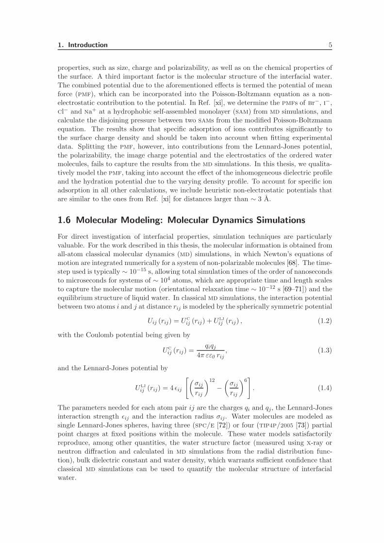
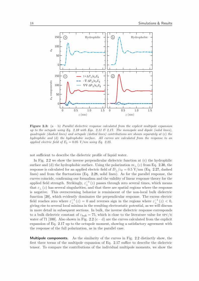
Figure 2.3: (a – b) Parallel dielectric response calculated from the explicit multipole expansionup to the octupole using Eq. 2.10 with Eqs. 2.11 & 2.17. The monopole and dipole (solid lines),quadrupole (dashed lines) and octupole (dotted lines) contributions are shown separately at (c) thehydrophilic and (d) the hydrophobic surface. All curves are calculated from the response to anapplied electric field of E‖ = 0.05 V/nm using Eq. 2.25.
not sufficient to describe the dielectric profile of liquid water.
In Fig. 2.2 we show the inverse perpendicular dielectric function at (c) the hydrophilicsurface and (d) the hydrophobic surface. Using the polarization m⊥ (z) from Eq. 2.30, theresponse is calculated for an applied electric field of D⊥/ε0 = 0.5 V/nm (Eq. 2.27, dashedlines) and from the fluctuations (Eq. 2.28, solid lines). As for the parallel response, thecurves coincide, confirming our formalism and the validity of linear response theory for theapplied field strength. Strikingly, ε−1
⊥ (z) passes through zero several times, which meansthat ε⊥ (z) has several singularities, and that there are spatial regions where the responseis negative. This overscreening behavior is reminiscent of the non-local bulk dielectricfunction [20], which evidently dominates the perpendicular response. The excess electricfield reaches zero where ε−1
⊥ (z) = 0 and reverses sign in the regions where ε−1⊥ (z) < 0,
giving rise to several local minima in the resulting electrostatic potential, as we will discussin more detail in subsequent sections. In bulk, the inverse dielectric response correspondsto a bulk dielectric constant of εbulk = 75, which is close to the literature value for spc/ewater of 71 [100]. Also shown in Fig. 2.2 (c – d) are the curves calculated from the explicitexpansion of Eq. 2.17 up to the octupole moment, showing a satisfactory agreement withthe response of the full polarization, as in the parallel case.
Multipole components. As the similarity of the curves in Fig. 2.2 distinctly show, thefirst three terms of the multipole expansion of Eq. 2.17 suffice to describe the dielectrictensor. To compare the contributions of the individual multipole moments, we show the

2. Permittivity Tensor of Interfacial Water 19
1 ∆P1/D
∆P2/D
∆P3/D
1.51.00.501.51.00.50
z (nm) z (nm)
a
c
Hydrophilic Hydrophobic1.0
-1.0
-0.5
0
0.5
1.0
-1.0
-0.5
0
0.5
ε-1
ε-1 c
ompon
ents
b
d
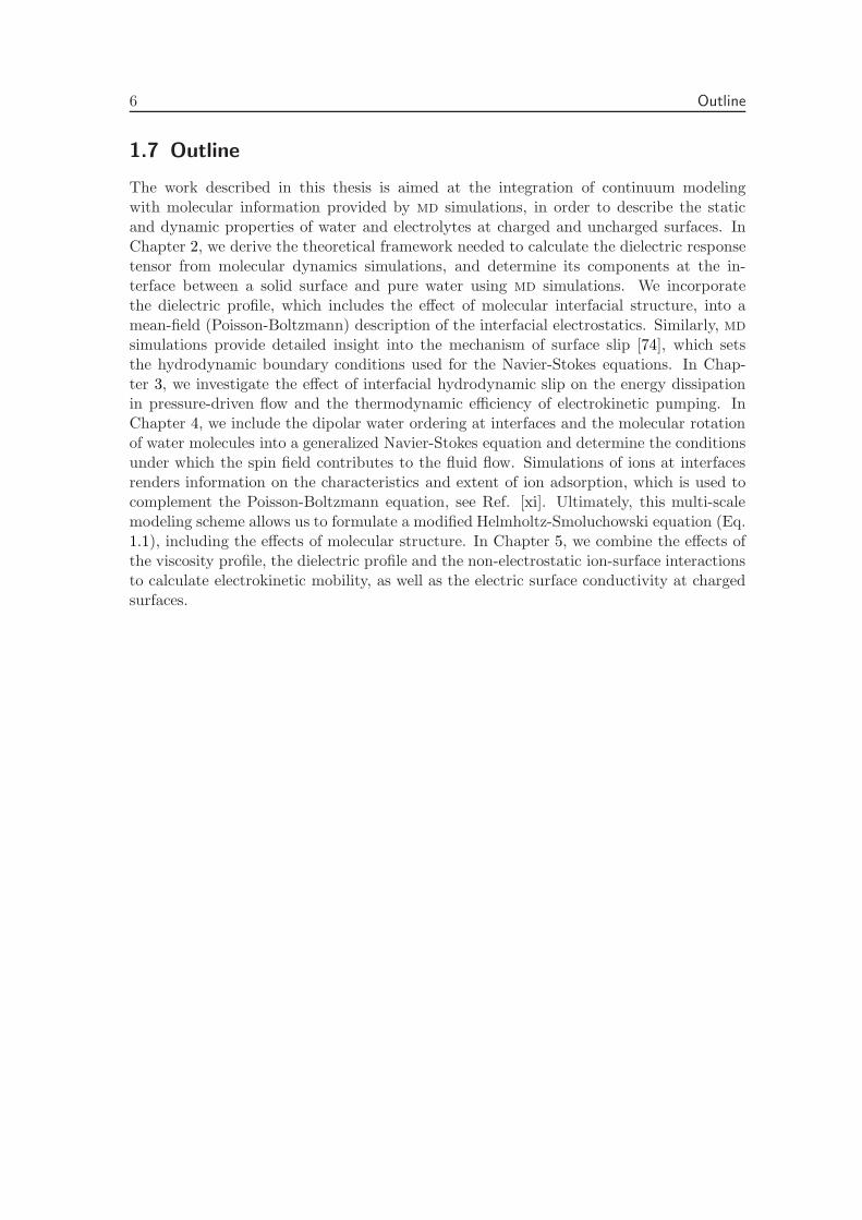
Figure 2.4: (a – b) Inverse perpendicular dielectric response calculated from the explicit multipoleexpansion up to the octupole using Eq. 2.10 with Eqs. 2.11 & 2.17. The monopole and dipole (solidlines), quadrupole (dashed lines) and octupole (dotted lines) contributions are shown separately at(c) the hydrophilic and (d) the hydrophobic surface. All curves are calculated from the averageresponse to applied electric fields of D⊥/ε0 = 2.0, 4.0 and 8.0 V/nm using Eq. 2.27.
first three terms separately. First, the sum of the first three terms of the parallel responseis shown in Fig. 2.3 at (a) the hydrophilic surface and (b) the hydrophobic surface.Second, we show the corresponding components separately in Fig. 2.3 (c – d). Quadrupoleand octupole contributions show similar profiles at the two surface types, but the dipolecontribution clearly dominates the parallel response. In Fig. 2.4 (a – b), we show the sumof the first three contributions to the perpendicular response, and the separate terms in(c – d). Contrary to the parallel case, the higher-order terms are non-negligible. In fact,the effect of the dipole is largely compensated for by the higher-order terms at both surfacetypes. This clearly illustrates the importance of the higher-order electric multipoles forthe perpendicular dielectric response.
Polarizability. For a dilute system of non-interacting particles, the dielectric function canbe written as 1+αn (r) /ε0 , with n (r) the number density of dielectric molecules and α amicroscopic polarizability attributed to each individual water molecule [96]. To describethe dielectric constant in condensed media, corrections to the polarizability appear, asin the famous Clausius-Mosotti expression. To quantify the deviation from the predictedresponse of a dilute system of non-interacting polar particles, we calculate the space-dependent polarizability, defined according to linear theory as
α‖ (z)
ε0=ε‖ (z) − 1
n (z)and
α⊥ (z)
ε0=
1 − ε−1⊥ (z)
n (z). (2.36)
Clearly, because the dielectric profile is calculated using a non-polarizable water model,
20 Simulations & Results
0.60.40.20
z (nm)
1.21.00.8 1.4
0.06
0
0.02
0.04
6
0
2
4
806040200
HydrophilicHydrophobic
a
c
α /
ε 0 (
nm
3 )n (
nm
-3)
α
/ε0
(nm
3 )
b
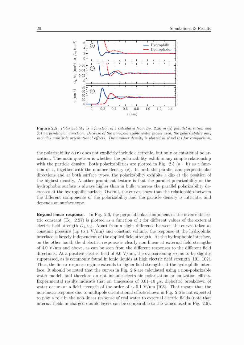
Figure 2.5: Polarizability as a function of z calculated from Eq. 2.36 in (a) parallel direction and(b) perpendicular direction. Because of the non-polarizable water model used, the polarizability onlyincludes multipole orientational effects. The number density is plotted in panel (c) for comparison.
the polarizability α (r) does not explicitly include electronic, but only orientational polar-ization. The main question is whether the polarizability exhibits any simple relationshipwith the particle density. Both polarizabilities are plotted in Fig. 2.5 (a – b) as a func-tion of z, together with the number density (c). In both the parallel and perpendiculardirections and at both surface types, the polarizability exhibits a dip at the position ofthe highest density. Another prominent feature is that the parallel polarizability at thehydrophobic surface is always higher than in bulk, whereas the parallel polarizability de-creases at the hydrophilic surface. Overall, the curves show that the relationship betweenthe different components of the polarizability and the particle density is intricate, anddepends on surface type.
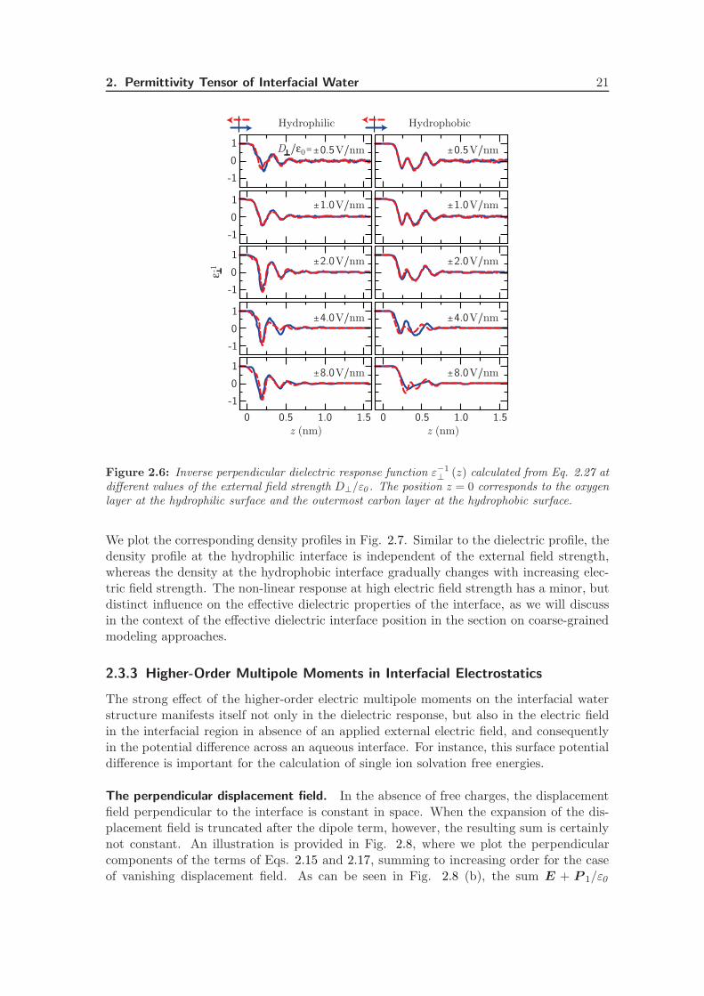
Beyond linear response. In Fig. 2.6, the perpendicular component of the inverse dielec-tric constant (Eq. 2.27) is plotted as a function of z for different values of the externalelectric field strength D⊥/ε0 . Apart from a slight difference between the curves taken atconstant pressure (up to 1 V/nm) and constant volume, the response at the hydrophilicinterface is largely independent of the applied field strength. At the hydrophobic interface,on the other hand, the dielectric response is clearly non-linear at external field strengthsof 4.0 V/nm and above, as can be seen from the different responses to the different fielddirections. At a positive electric field of 8.0 V/nm, the overscreening seems to be slightlysuppressed, as is commonly found in ionic liquids at high electric field strength [101, 102].Thus, the linear response regime extends to higher field strengths at the hydrophilic inter-face. It should be noted that the curves in Fig. 2.6 are calculated using a non-polarizablewater model, and therefore do not include electronic polarization or ionization effects.Experimental results indicate that on timescales of 0.01–10 µs, dielectric breakdown ofwater occurs at a field strength of the order of ∼ 0.1 V/nm [103]. That means that thenon-linear response due to multipole orientational effects shown in Fig. 2.6 is not expectedto play a role in the non-linear response of real water to external electric fields (note thatinternal fields in charged double layers can be comparable to the values used in Fig. 2.6).
2. Permittivity Tensor of Interfacial Water 21
0 0.5 1.0 1.50 0.5 1.0 1.5
1
-1
0
1
-1
0
1
-1
0
1
-1
0
1
-1
0
ε-1
Hydrophilic Hydrophobic
0.5V/nmD /ε0 0.5V/nm
1.0V/nm
2.0V/nm
4.0V/nm
8.0V/nm
1.0V/nm
2.0V/nm
4.0V/nm
8.0V/nm
z (nm) z (nm)
Figure 2.6: Inverse perpendicular dielectric response function ε−1
⊥ (z) calculated from Eq. 2.27 atdifferent values of the external field strength D⊥/ε0 . The position z = 0 corresponds to the oxygenlayer at the hydrophilic surface and the outermost carbon layer at the hydrophobic surface.
We plot the corresponding density profiles in Fig. 2.7. Similar to the dielectric profile, thedensity profile at the hydrophilic interface is independent of the external field strength,whereas the density at the hydrophobic interface gradually changes with increasing elec-tric field strength. The non-linear response at high electric field strength has a minor, butdistinct influence on the effective dielectric properties of the interface, as we will discussin the context of the effective dielectric interface position in the section on coarse-grainedmodeling approaches.
2.3.3 Higher-Order Multipole Moments in Interfacial Electrostatics
The strong effect of the higher-order electric multipole moments on the interfacial waterstructure manifests itself not only in the dielectric response, but also in the electric fieldin the interfacial region in absence of an applied external electric field, and consequentlyin the potential difference across an aqueous interface. For instance, this surface potentialdifference is important for the calculation of single ion solvation free energies.
The perpendicular displacement field. In the absence of free charges, the displacementfield perpendicular to the interface is constant in space. When the expansion of the dis-placement field is truncated after the dipole term, however, the resulting sum is certainlynot constant. An illustration is provided in Fig. 2.8, where we plot the perpendicularcomponents of the terms of Eqs. 2.15 and 2.17, summing to increasing order for the caseof vanishing displacement field. As can be seen in Fig. 2.8 (b), the sum E + P 1/ε0
22 Simulations & Results
Hydrophilic Hydrophobic
0 0.5 1.0 1.50 0.5 1.0 1.5z (nm) z (nm)
0.5V/nmD /ε0 0.5V/nm
1.0V/nm
2.0V/nm
4.0V/nm
8.0V/nm
1.0V/nm
2.0V/nm
4.0V/nm
8.0V/nm
n (
nm
-3)
100
50
0100
50
0
100
50
0100
50
0100
50
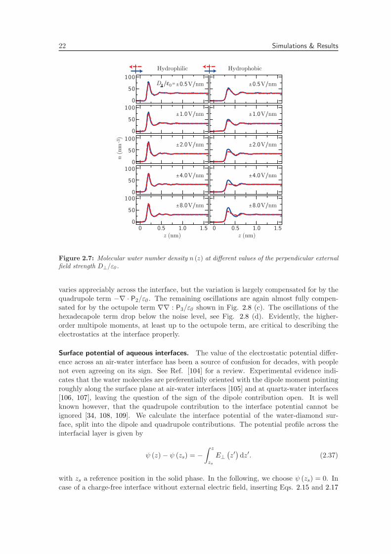
0
Figure 2.7: Molecular water number density n (z) at different values of the perpendicular externalfield strength D⊥/ε0 .
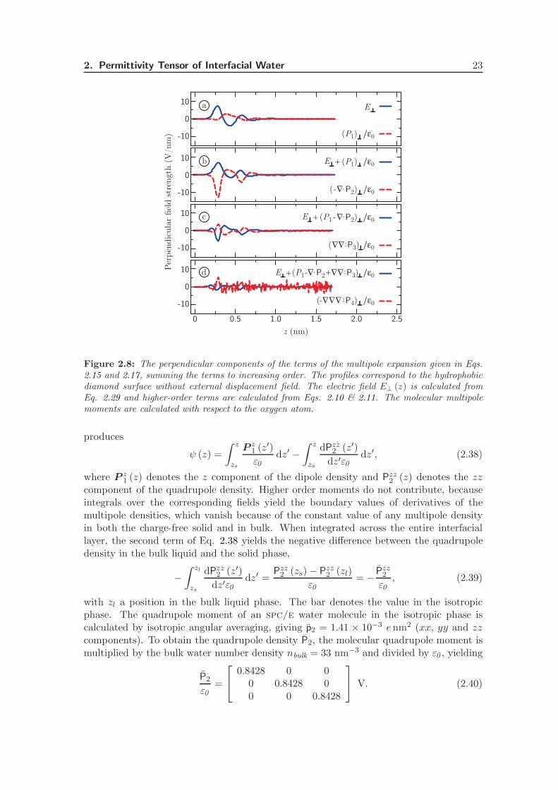
varies appreciably across the interface, but the variation is largely compensated for by thequadrupole term −∇ · P2/ε0 . The remaining oscillations are again almost fully compen-sated for by the octupole term ∇∇ : P3/ε0 shown in Fig. 2.8 (c). The oscillations of thehexadecapole term drop below the noise level, see Fig. 2.8 (d). Evidently, the higher-order multipole moments, at least up to the octupole term, are critical to describing theelectrostatics at the interface properly.
Surface potential of aqueous interfaces. The value of the electrostatic potential differ-ence across an air-water interface has been a source of confusion for decades, with peoplenot even agreeing on its sign. See Ref. [104] for a review. Experimental evidence indi-cates that the water molecules are preferentially oriented with the dipole moment pointingroughly along the surface plane at air-water interfaces [105] and at quartz-water interfaces[106, 107], leaving the question of the sign of the dipole contribution open. It is wellknown however, that the quadrupole contribution to the interface potential cannot beignored [34, 108, 109]. We calculate the interface potential of the water-diamond sur-face, split into the dipole and quadrupole contributions. The potential profile across theinterfacial layer is given by
ψ (z) − ψ (zs) = −∫ z
zs
E⊥
(
z′)
dz′. (2.37)
with zs a reference position in the solid phase. In the following, we choose ψ (zs) = 0. Incase of a charge-free interface without external electric field, inserting Eqs. 2.15 and 2.17
2. Permittivity Tensor of Interfacial Water 23
1.51.00.50
z (nm)
2.52.0
10
-10
0
Per
pen
dic
ula
r fiel
d s
tren
gth (
V/n
m) (P1) /ε0
E
(- P2) /ε0
(P1) /ε0E
(P1E - P2) /ε0
P3) /ε0(
(P1- P2 P3) /ε0E
- P4) /ε0(
a
c10
-10
0
10
-10
0
10
-10
0
b
d
Figure 2.8: The perpendicular components of the terms of the multipole expansion given in Eqs.2.15 and 2.17, summing the terms to increasing order. The profiles correspond to the hydrophobicdiamond surface without external displacement field. The electric field E⊥ (z) is calculated fromEq. 2.29 and higher-order terms are calculated from Eqs. 2.10 & 2.11. The molecular multipolemoments are calculated with respect to the oxygen atom.
produces
ψ (z) =
∫ z
zs
P z1 (z′)
ε0dz′ −
∫ z
zs
dPzz2 (z′)
dz′ε0dz′, (2.38)
where P z1 (z) denotes the z component of the dipole density and Pzz2 (z) denotes the zz
component of the quadrupole density. Higher order moments do not contribute, becauseintegrals over the corresponding fields yield the boundary values of derivatives of themultipole densities, which vanish because of the constant value of any multipole densityin both the charge-free solid and in bulk. When integrated across the entire interfaciallayer, the second term of Eq. 2.38 yields the negative difference between the quadrupoledensity in the bulk liquid and the solid phase,
−∫ zl
zs
dPzz2 (z′)
dz′ε0dz′ =
Pzz2 (zs) − Pzz2 (zl)
ε0= − Pzz2
ε0, (2.39)
with zl a position in the bulk liquid phase. The bar denotes the value in the isotropicphase. The quadrupole moment of an spc/e water molecule in the isotropic phase iscalculated by isotropic angular averaging, giving p2 = 1.41 × 10⁻³ enm2 (xx, yy and zzcomponents). To obtain the quadrupole density P2, the molecular quadrupole moment ismultiplied by the bulk water number density nbulk = 33 nm−3 and divided by ε0 , yielding
P2
ε0=
0.8428 0 00 0.8428 00 0 0.8428
V. (2.40)
24 Coarse-Grained Modeling Approaches
0.5
E (z ) dz
(P1(z )) /ε0 dz
( P2(z )) /ε0 dz
1.0 1.50
1.0
0.5
0
-0.5
-1.0
ψ (
V)
0.40 V
-0.44 V
-0.84 V
z (nm)
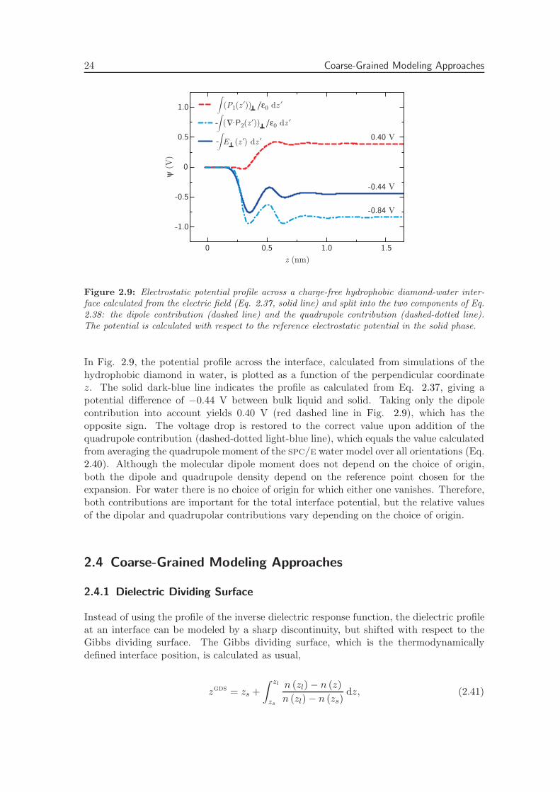
Figure 2.9: Electrostatic potential profile across a charge-free hydrophobic diamond-water inter-face calculated from the electric field (Eq. 2.37, solid line) and split into the two components of Eq.2.38: the dipole contribution (dashed line) and the quadrupole contribution (dashed-dotted line).The potential is calculated with respect to the reference electrostatic potential in the solid phase.
In Fig. 2.9, the potential profile across the interface, calculated from simulations of thehydrophobic diamond in water, is plotted as a function of the perpendicular coordinatez. The solid dark-blue line indicates the profile as calculated from Eq. 2.37, giving apotential difference of −0.44 V between bulk liquid and solid. Taking only the dipolecontribution into account yields 0.40 V (red dashed line in Fig. 2.9), which has theopposite sign. The voltage drop is restored to the correct value upon addition of thequadrupole contribution (dashed-dotted light-blue line), which equals the value calculatedfrom averaging the quadrupole moment of the spc/e water model over all orientations (Eq.2.40). Although the molecular dipole moment does not depend on the choice of origin,both the dipole and quadrupole density depend on the reference point chosen for theexpansion. For water there is no choice of origin for which either one vanishes. Therefore,both contributions are important for the total interface potential, but the relative valuesof the dipolar and quadrupolar contributions vary depending on the choice of origin.
2.4 Coarse-Grained Modeling Approaches
2.4.1 Dielectric Dividing Surface
Instead of using the profile of the inverse dielectric response function, the dielectric profileat an interface can be modeled by a sharp discontinuity, but shifted with respect to theGibbs dividing surface. The Gibbs dividing surface, which is the thermodynamicallydefined interface position, is calculated as usual,
zgds = zs +
∫ zl
zs
n (zl) − n (z)
n (zl) − n (zs)dz, (2.41)
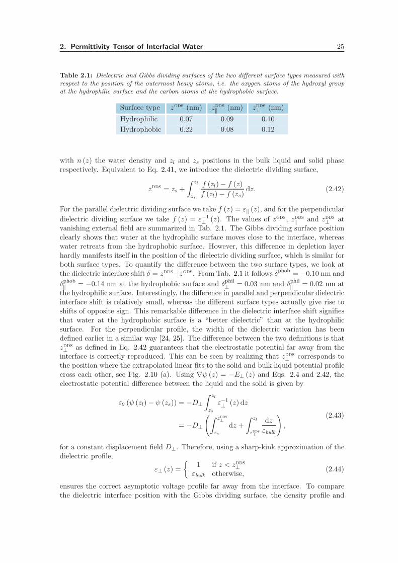
2. Permittivity Tensor of Interfacial Water 25
Table 2.1: Dielectric and Gibbs dividing surfaces of the two different surface types measured withrespect to the position of the outermost heavy atoms, i.e. the oxygen atoms of the hydroxyl groupat the hydrophilic surface and the carbon atoms at the hydrophobic surface.
Surface type zgds (nm) zdds‖ (nm) zdds
⊥ (nm)
Hydrophilic 0.07 0.09 0.10
Hydrophobic 0.22 0.08 0.12
with n (z) the water density and zl and zs positions in the bulk liquid and solid phaserespectively. Equivalent to Eq. 2.41, we introduce the dielectric dividing surface,
zdds = zs +
∫ zl
zs
f (zl) − f (z)
f (zl) − f (zs)dz. (2.42)
For the parallel dielectric dividing surface we take f (z) = ε‖ (z), and for the perpendicular
dielectric dividing surface we take f (z) = ε−1⊥ (z). The values of zgds, zdds
‖ and zdds⊥ at
vanishing external field are summarized in Tab. 2.1. The Gibbs dividing surface positionclearly shows that water at the hydrophilic surface moves close to the interface, whereaswater retreats from the hydrophobic surface. However, this difference in depletion layerhardly manifests itself in the position of the dielectric dividing surface, which is similar forboth surface types. To quantify the difference between the two surface types, we look atthe dielectric interface shift δ = zdds−zgds. From Tab. 2.1 it follows δphob
⊥ = −0.10 nm and
δphob‖ = −0.14 nm at the hydrophobic surface and δphil
⊥ = 0.03 nm and δphil‖ = 0.02 nm at
the hydrophilic surface. Interestingly, the difference in parallel and perpendicular dielectricinterface shift is relatively small, whereas the different surface types actually give rise toshifts of opposite sign. This remarkable difference in the dielectric interface shift signifiesthat water at the hydrophobic surface is a “better dielectric” than at the hydrophilicsurface. For the perpendicular profile, the width of the dielectric variation has beendefined earlier in a similar way [24, 25]. The difference between the two definitions is thatzdds⊥ as defined in Eq. 2.42 guarantees that the electrostatic potential far away from the
interface is correctly reproduced. This can be seen by realizing that zdds⊥ corresponds to
the position where the extrapolated linear fits to the solid and bulk liquid potential profilecross each other, see Fig. 2.10 (a). Using ∇ψ (z) = −E⊥ (z) and Eqs. 2.4 and 2.42, theelectrostatic potential difference between the liquid and the solid is given by
ε0 (ψ (zl) − ψ (zs)) = −D⊥
∫ zl
zs
ε−1⊥ (z) dz
= −D⊥
(
∫ zdds⊥
zs
dz +
∫ zl
zdds⊥
dz
εbulk
)
,
(2.43)
for a constant displacement field D⊥. Therefore, using a sharp-kink approximation of thedielectric profile,
ε⊥ (z) =
1 if z < zdds⊥
εbulk otherwise,(2.44)
ensures the correct asymptotic voltage profile far away from the interface. To comparethe dielectric interface position with the Gibbs dividing surface, the density profile and
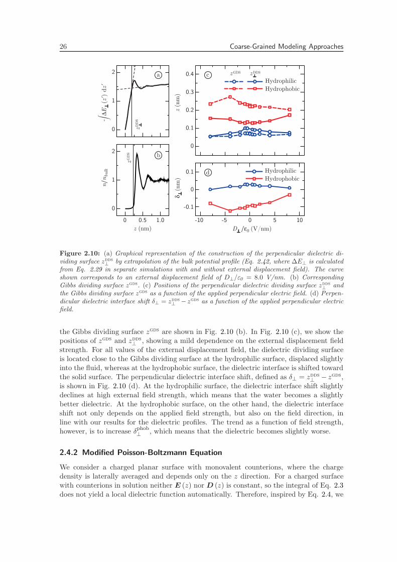
26 Coarse-Grained Modeling Approaches
Hydrophilic
Hydrophobic
10
Hydrophilic
Hydrophobic
zDDSzGDS
zD
DS
zG
DS
∆E
(z )
dz
2
1
0
2
1
0
n/n
bulk
0 0.5 1.0
z (nm)
-10 -5 0 5
D /ε0 (V/nm)
z (n
m)
δ (
nm
)
0.4
0
0.1
0.2
0.3
0.1
0
-0.1
a c
b
d
Figure 2.10: (a) Graphical representation of the construction of the perpendicular dielectric di-viding surface zdds
⊥ by extrapolation of the bulk potential profile (Eq. 2.42, where ∆E⊥ is calculatedfrom Eq. 2.29 in separate simulations with and without external displacement field). The curveshown corresponds to an external displacement field of D⊥/ε0 = 8.0 V/nm. (b) CorrespondingGibbs dividing surface zgds. (c) Positions of the perpendicular dielectric dividing surface zdds
⊥ andthe Gibbs dividing surface zgds as a function of the applied perpendicular electric field. (d) Perpen-dicular dielectric interface shift δ⊥ = zdds
⊥ − zgds as a function of the applied perpendicular electricfield.
the Gibbs dividing surface zgds are shown in Fig. 2.10 (b). In Fig. 2.10 (c), we show thepositions of zgds and zdds
⊥ , showing a mild dependence on the external displacement fieldstrength. For all values of the external displacement field, the dielectric dividing surfaceis located close to the Gibbs dividing surface at the hydrophilic surface, displaced slightlyinto the fluid, whereas at the hydrophobic surface, the dielectric interface is shifted towardthe solid surface. The perpendicular dielectric interface shift, defined as δ⊥ = zdds
⊥ − zgds,is shown in Fig. 2.10 (d). At the hydrophilic surface, the dielectric interface shift slightlydeclines at high external field strength, which means that the water becomes a slightlybetter dielectric. At the hydrophobic surface, on the other hand, the dielectric interfaceshift not only depends on the applied field strength, but also on the field direction, inline with our results for the dielectric profiles. The trend as a function of field strength,however, is to increase δphob
⊥ , which means that the dielectric becomes slightly worse.
2.4.2 Modified Poisson-Boltzmann Equation
We consider a charged planar surface with monovalent counterions, where the chargedensity is laterally averaged and depends only on the z direction. For a charged surfacewith counterions in solution neither E (z) nor D (z) is constant, so the integral of Eq. 2.3does not yield a local dielectric function automatically. Therefore, inspired by Eq. 2.4, we
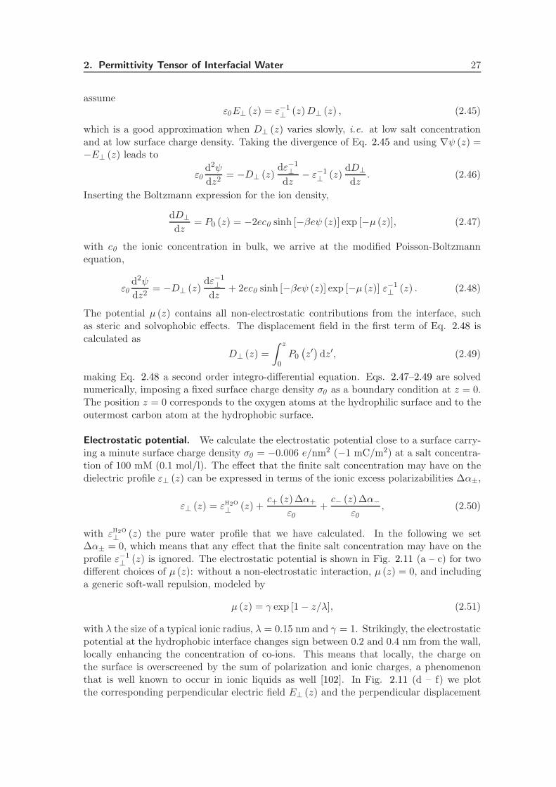
2. Permittivity Tensor of Interfacial Water 27
assumeε0E⊥ (z) = ε−1
⊥ (z)D⊥ (z) , (2.45)
which is a good approximation when D⊥ (z) varies slowly, i.e. at low salt concentrationand at low surface charge density. Taking the divergence of Eq. 2.45 and using ∇ψ (z) =−E⊥ (z) leads to
ε0d2ψ
dz2= −D⊥ (z)
dε−1⊥
dz− ε−1
⊥ (z)dD⊥
dz. (2.46)
Inserting the Boltzmann expression for the ion density,
dD⊥
dz= P0 (z) = −2ec0 sinh [−βeψ (z)] exp [−µ (z)], (2.47)
with c0 the ionic concentration in bulk, we arrive at the modified Poisson-Boltzmannequation,
ε0d2ψ
dz2= −D⊥ (z)
dε−1⊥
dz+ 2ec0 sinh [−βeψ (z)] exp [−µ (z)] ε−1
⊥ (z) . (2.48)
The potential µ (z) contains all non-electrostatic contributions from the interface, suchas steric and solvophobic effects. The displacement field in the first term of Eq. 2.48 iscalculated as
D⊥ (z) =
∫ z
0P0
(
z′)
dz′, (2.49)
making Eq. 2.48 a second order integro-differential equation. Eqs. 2.47–2.49 are solvednumerically, imposing a fixed surface charge density σ0 as a boundary condition at z = 0.The position z = 0 corresponds to the oxygen atoms at the hydrophilic surface and to theoutermost carbon atom at the hydrophobic surface.
Electrostatic potential. We calculate the electrostatic potential close to a surface carry-ing a minute surface charge density σ0 = −0.006 e/nm2 (−1 mC/m2) at a salt concentra-tion of 100 mM (0.1 mol/l). The effect that the finite salt concentration may have on thedielectric profile ε⊥ (z) can be expressed in terms of the ionic excess polarizabilities ∆α±,
ε⊥ (z) = εh2o⊥ (z) +
c+ (z)∆α+
ε0+c− (z) ∆α−
ε0, (2.50)
with εh2o⊥ (z) the pure water profile that we have calculated. In the following we set
∆α± = 0, which means that any effect that the finite salt concentration may have on theprofile ε−1
⊥ (z) is ignored. The electrostatic potential is shown in Fig. 2.11 (a – c) for twodifferent choices of µ (z): without a non-electrostatic interaction, µ (z) = 0, and includinga generic soft-wall repulsion, modeled by
µ (z) = γ exp [1 − z/λ], (2.51)
with λ the size of a typical ionic radius, λ = 0.15 nm and γ = 1. Strikingly, the electrostaticpotential at the hydrophobic interface changes sign between 0.2 and 0.4 nm from the wall,locally enhancing the concentration of co-ions. This means that locally, the charge onthe surface is overscreened by the sum of polarization and ionic charges, a phenomenonthat is well known to occur in ionic liquids as well [102]. In Fig. 2.11 (d – f) we plotthe corresponding perpendicular electric field E⊥ (z) and the perpendicular displacement
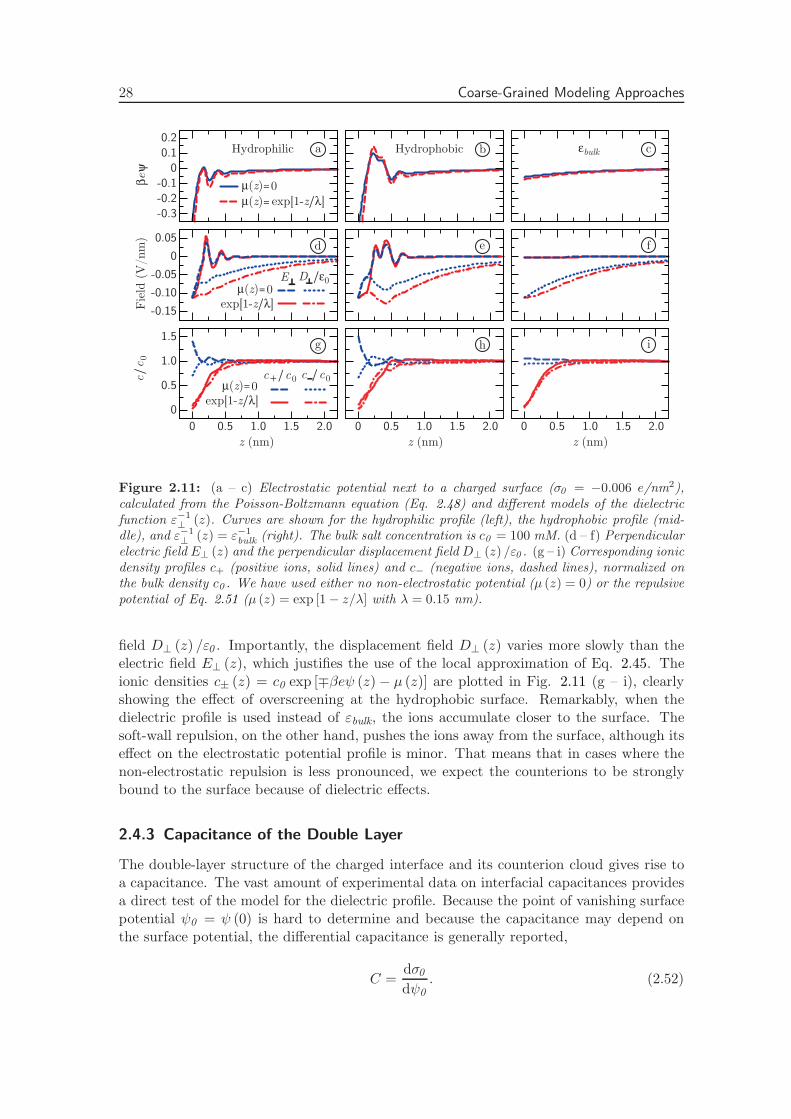
28 Coarse-Grained Modeling Approaches
2.0
µ(z) exp[1-z/λ]
µ(z) 0
µ(z) 0exp[1-z/λ]
E D /ε0
c+/c0 c /c0µ(z) 0
exp[1-z/λ]
1.51.00.50 2.01.51.00.50 2.01.51.00.50
z (nm) z (nm) z (nm)
0.20.1
0-0.1-0.2-0.3
βe
ψ
0.05
0
-0.05
-0.10
-0.15Fie
ld (
V/n
m)
c/c
0
1.5
1.0
0.5
0
Hydrophilic Hydrophobica cεbulk
e f
g h i
b
d
Figure 2.11: (a – c) Electrostatic potential next to a charged surface (σ0 = −0.006 e/nm2),calculated from the Poisson-Boltzmann equation (Eq. 2.48) and different models of the dielectricfunction ε−1
⊥ (z). Curves are shown for the hydrophilic profile (left), the hydrophobic profile (mid-dle), and ε−1
⊥ (z) = ε−1
bulk(right). The bulk salt concentration is c0 = 100 mM. (d – f) Perpendicular
electric field E⊥ (z) and the perpendicular displacement field D⊥ (z) /ε0 . (g – i) Corresponding ionicdensity profiles c+ (positive ions, solid lines) and c− (negative ions, dashed lines), normalized onthe bulk density c0 . We have used either no non-electrostatic potential (µ (z) = 0) or the repulsivepotential of Eq. 2.51 (µ (z) = exp [1 − z/λ] with λ = 0.15 nm).
field D⊥ (z) /ε0 . Importantly, the displacement field D⊥ (z) varies more slowly than theelectric field E⊥ (z), which justifies the use of the local approximation of Eq. 2.45. Theionic densities c± (z) = c0 exp [∓βeψ (z) − µ (z)] are plotted in Fig. 2.11 (g – i), clearlyshowing the effect of overscreening at the hydrophobic surface. Remarkably, when thedielectric profile is used instead of εbulk, the ions accumulate closer to the surface. Thesoft-wall repulsion, on the other hand, pushes the ions away from the surface, although itseffect on the electrostatic potential profile is minor. That means that in cases where thenon-electrostatic repulsion is less pronounced, we expect the counterions to be stronglybound to the surface because of dielectric effects.
2.4.3 Capacitance of the Double Layer
The double-layer structure of the charged interface and its counterion cloud gives rise toa capacitance. The vast amount of experimental data on interfacial capacitances providesa direct test of the model for the dielectric profile. Because the point of vanishing surfacepotential ψ0 = ψ (0) is hard to determine and because the capacitance may depend onthe surface potential, the differential capacitance is generally reported,
C =dσ0dψ0
. (2.52)
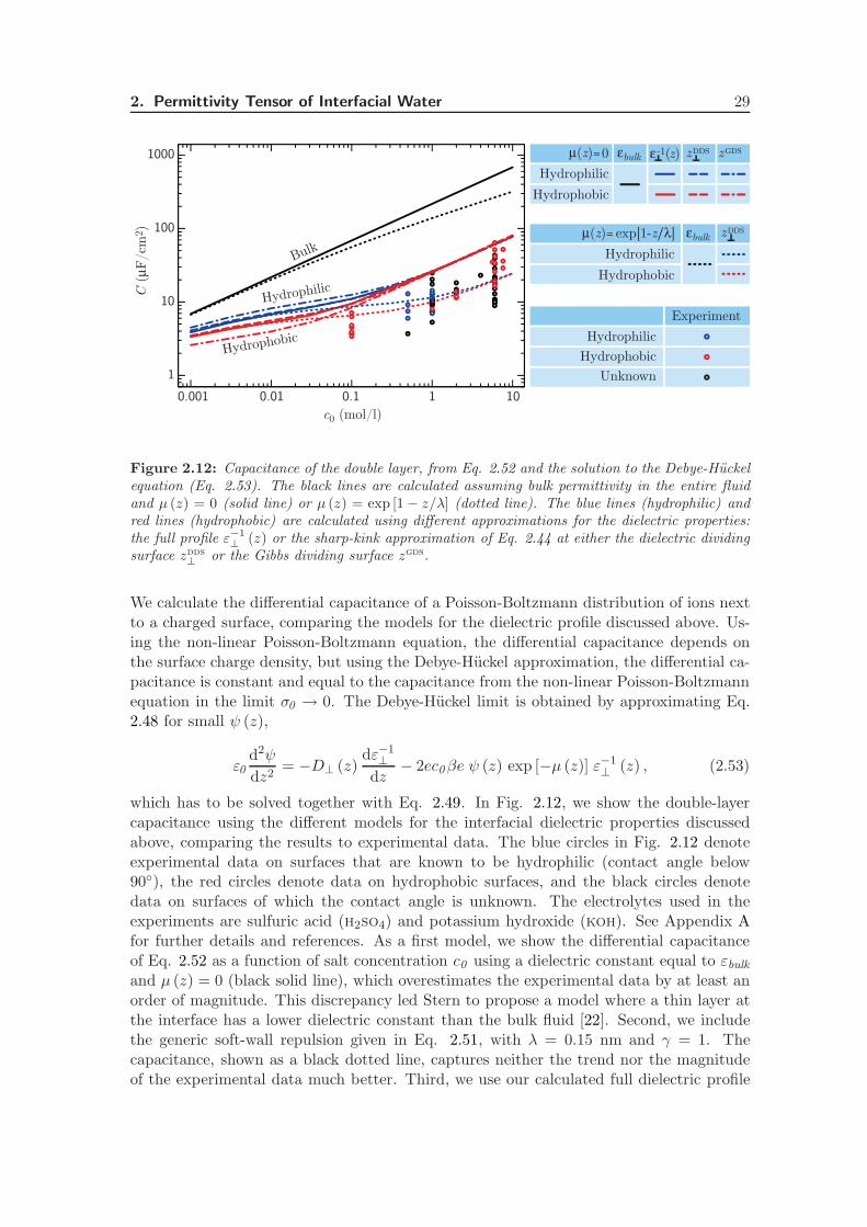
2. Permittivity Tensor of Interfacial Water 29
10
Unknown
Hydrophilic
Hydrophobic
Experiment
εbulk ε -1(z) zDDS zGDS
Hydrophilic
Hydrophobic
µ(z) 0
Hydrophilic
Hydrophobic
µ(z) exp[1-z/λ] εbulk zDDS
10.10.010.001
c0 (mol/l)
1000
100
10
1
C (
µF/c
m2 )
Hydrophilic
Hydrophobic
Bulk
Figure 2.12: Capacitance of the double layer, from Eq. 2.52 and the solution to the Debye-Huckelequation (Eq. 2.53). The black lines are calculated assuming bulk permittivity in the entire fluidand µ (z) = 0 (solid line) or µ (z) = exp [1 − z/λ] (dotted line). The blue lines (hydrophilic) andred lines (hydrophobic) are calculated using different approximations for the dielectric properties:the full profile ε−1
⊥ (z) or the sharp-kink approximation of Eq. 2.44 at either the dielectric dividingsurface zdds
⊥ or the Gibbs dividing surface zgds.
We calculate the differential capacitance of a Poisson-Boltzmann distribution of ions nextto a charged surface, comparing the models for the dielectric profile discussed above. Us-ing the non-linear Poisson-Boltzmann equation, the differential capacitance depends onthe surface charge density, but using the Debye-Huckel approximation, the differential ca-pacitance is constant and equal to the capacitance from the non-linear Poisson-Boltzmannequation in the limit σ0 → 0. The Debye-Huckel limit is obtained by approximating Eq.2.48 for small ψ (z),
ε0d2ψ
dz2= −D⊥ (z)
dε−1⊥
dz− 2ec0βe ψ (z) exp [−µ (z)] ε−1
⊥ (z) , (2.53)
which has to be solved together with Eq. 2.49. In Fig. 2.12, we show the double-layercapacitance using the different models for the interfacial dielectric properties discussedabove, comparing the results to experimental data. The blue circles in Fig. 2.12 denoteexperimental data on surfaces that are known to be hydrophilic (contact angle below90), the red circles denote data on hydrophobic surfaces, and the black circles denotedata on surfaces of which the contact angle is unknown. The electrolytes used in theexperiments are sulfuric acid (h2so4) and potassium hydroxide (koh). See Appendix Afor further details and references. As a first model, we show the differential capacitanceof Eq. 2.52 as a function of salt concentration c0 using a dielectric constant equal to εbulkand µ (z) = 0 (black solid line), which overestimates the experimental data by at least anorder of magnitude. This discrepancy led Stern to propose a model where a thin layer atthe interface has a lower dielectric constant than the bulk fluid [22]. Second, we includethe generic soft-wall repulsion given in Eq. 2.51, with λ = 0.15 nm and γ = 1. Thecapacitance, shown as a black dotted line, captures neither the trend nor the magnitudeof the experimental data much better. Third, we use our calculated full dielectric profile
30 Coarse-Grained Modeling Approaches
ε−1⊥ (z), shown in Fig. 2.2 (c – d), with µ (z) = 0 (solid colored lines), agreeing much
better with experiments. The hydrophilic profile (blue) yields a slightly higher capacitancethan the hydrophobic profile (red) at low salt concentration, which is generally expectedbecause of the better wetting characteristics [30]. The difference is minor however, becausethe dielectric interface shift δ⊥ largely compensates for the depletion gap at hydrophobicsurfaces. Fourth, we use the sharp-kink approximation of Eq. 2.44 with µ (z) = 0 (dashedcolored lines). The results are almost indistinguishable from the curves calculated usingthe full profiles ε−1
⊥ (z), as expected from the fact that the dielectric dividing surface isdesigned to reproduce the electrostatic potential far away from the interface. Nevertheless,the calculated capacitance is still relatively high compared to the experimental data, whichhas to do with the fact that in the Poisson-Boltzmann approach the point-charge ions areallowed to get arbitrarily close to the surface. Therefore, as a fifth model, we use the sharp-kink approximation of Eq. 2.44 together with µ (z) from Eq. 2.51, shown as dotted coloredlines. Clearly, this model follows the experimental data very well. Values of the calculatedcapacitance can be adjusted by fine-tuning the parameters γ and λ, which are expected todepend on the surface and ion type. Finally, we show the capacitance using a sharp-kinkapproximation for ε−1
⊥ (z) located at zgds (dashed-dotted lines), which does not performas well as the sharp-kink approximation located at zdds
⊥ . In fact, when using the Gibbsdividing surface, the difference between hydrophilic and hydrophobic surfaces is quite largeat low salt concentration, which does not seem to be reflected in the experimental data.Turning this argument around, the approximate equality of experimental data for thedouble-layer capacitance on hydrophilic and hydrophobic surfaces displayed in Fig. 2.12can be viewed as a confirmation of one of the main results of the present work, namely thatthe effect of the depletion layer at hydrophobic surfaces is largely compensated for by thedielectric properties of the first few interfacial water layers, effectively yielding dielectricproperties similar to those at hydrophilic surfaces.
Effective Stern layer permittivity. Within the original Stern model of a charge-freeinterfacial region of width d with dielectric constant εint, the capacitance turns out to beCStern = σ0/ψ0 = εint ε0/d. The same model yields Cbulk = εbulk ε0/d when the bulk valueε = εbulk is assumed for the interfacial dielectric constant. Therefore the capacitance ratioreflects the ratio of interfacial dielectric constants,
CStern
Cbulk
=εint
εbulk. (2.54)
Imposing Eq. 2.54, and dividing the capacitance which follows from the solution of thePoisson-Boltzmann equation including the dielectric profile ε−1
⊥ (z) by the capacitance us-ing the bulk assumption ε−1
⊥ (z) = ε−1bulk
, we find that the estimate for εint varies between 10and 30, depending on salt concentration, which corresponds well to earlier estimates basedon experimental data [80, 81]. Our results present a microscopic picture of the electrostaticproperties of the interfacial layer, allowing for the analysis of not only the double-layer ca-pacitance, but also other properties, such as the electrostatic pressure between two platesas a function of separation, as will be detailed next.
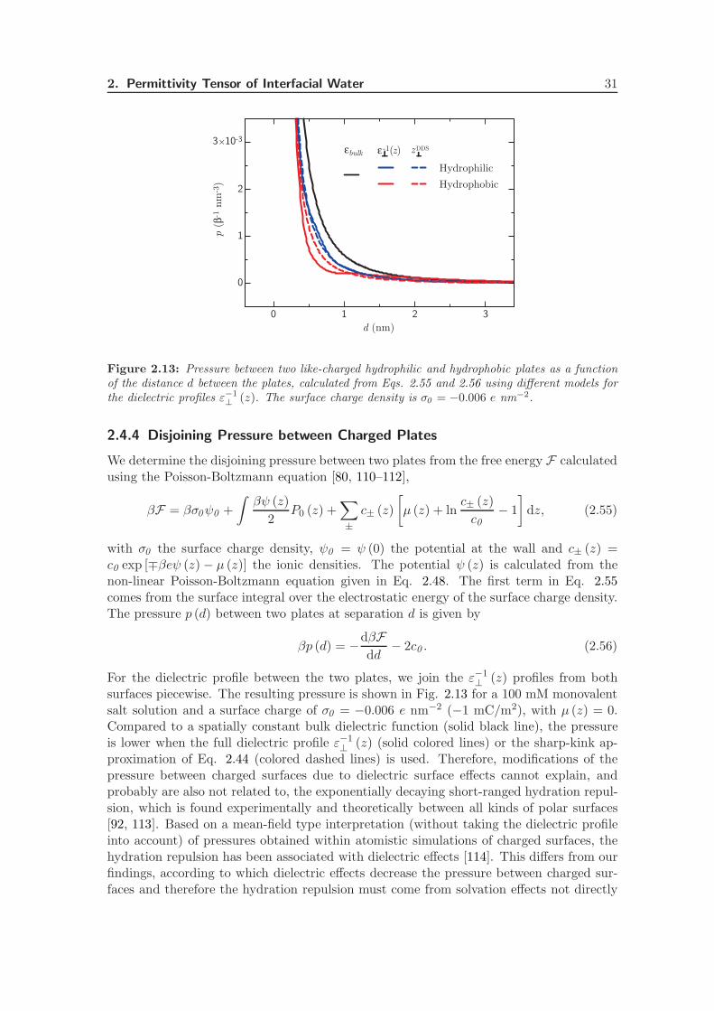
2. Permittivity Tensor of Interfacial Water 31
εbulk ε -1(z) zDDS
Hydrophilic
Hydrophobic
3210
d (nm)
2
1
0
3 10-3
p (
β-1 n
m-3)
Figure 2.13: Pressure between two like-charged hydrophilic and hydrophobic plates as a functionof the distance d between the plates, calculated from Eqs. 2.55 and 2.56 using different models forthe dielectric profiles ε−1
⊥ (z). The surface charge density is σ0 = −0.006 e nm−2.
2.4.4 Disjoining Pressure between Charged Plates
We determine the disjoining pressure between two plates from the free energy F calculatedusing the Poisson-Boltzmann equation [80, 110–112],
βF = βσ0ψ0 +
∫
βψ (z)
2P0 (z) +
∑
±
c± (z)
[
µ (z) + lnc± (z)
c0− 1
]
dz, (2.55)
with σ0 the surface charge density, ψ0 = ψ (0) the potential at the wall and c± (z) =c0 exp [∓βeψ (z) − µ (z)] the ionic densities. The potential ψ (z) is calculated from thenon-linear Poisson-Boltzmann equation given in Eq. 2.48. The first term in Eq. 2.55comes from the surface integral over the electrostatic energy of the surface charge density.The pressure p (d) between two plates at separation d is given by
βp (d) = −dβFdd
− 2c0 . (2.56)
For the dielectric profile between the two plates, we join the ε−1⊥ (z) profiles from both
surfaces piecewise. The resulting pressure is shown in Fig. 2.13 for a 100 mM monovalentsalt solution and a surface charge of σ0 = −0.006 e nm−2 (−1 mC/m2), with µ (z) = 0.Compared to a spatially constant bulk dielectric function (solid black line), the pressureis lower when the full dielectric profile ε−1
⊥ (z) (solid colored lines) or the sharp-kink ap-proximation of Eq. 2.44 (colored dashed lines) is used. Therefore, modifications of thepressure between charged surfaces due to dielectric surface effects cannot explain, andprobably are also not related to, the exponentially decaying short-ranged hydration repul-sion, which is found experimentally and theoretically between all kinds of polar surfaces[92, 113]. Based on a mean-field type interpretation (without taking the dielectric profileinto account) of pressures obtained within atomistic simulations of charged surfaces, thehydration repulsion has been associated with dielectric effects [114]. This differs from ourfindings, according to which dielectric effects decrease the pressure between charged sur-faces and therefore the hydration repulsion must come from solvation effects not directly
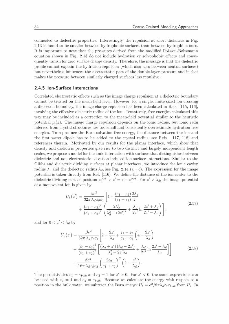
32 Coarse-Grained Modeling Approaches
connected to dielectric properties. Interestingly, the repulsion at short distances in Fig.2.13 is found to be smaller between hydrophobic surfaces than between hydrophilic ones.It is important to note that the pressures derived from the modified Poisson-Boltzmannequation shown in Fig. 2.13 do not include hydration or solvophobic effects and conse-quently vanish for zero surface charge density. Therefore, the message is that the dielectricprofile cannot explain the hydration repulsion (which also acts between neutral surfaces)but nevertheless influences the electrostatic part of the double-layer pressure and in factmakes the pressure between similarly charged surfaces less repulsive.
2.4.5 Ion-Surface Interactions
Correlated electrostatic effects such as the image charge repulsion at a dielectric boundarycannot be treated on the mean-field level. However, for a single, finite-sized ion crossinga dielectric boundary, the image charge repulsion has been calculated in Refs. [115, 116],involving the effective dielectric radius of the ion. Tentatively, free energies calculated thisway may be included as a correction to the mean-field potential similar to the heuristicpotential µ (z). The image charge repulsion depends on the ionic radius, but ionic radiiinferred from crystal structures are too small and consistently overestimate hydration freeenergies. To reproduce the Born solvation free energy, the distance between the ion andthe first water dipole has to be added to the crystal radius, see Refs. [117, 118] andreferences therein. Motivated by our results for the planar interface, which show thatdensity and dielectric properties give rise to two distinct and largely independent lengthscales, we propose a model for the ionic interaction with surfaces that distinguishes betweendielectric and non-electrostatic solvation-induced ion-surface interactions. Similar to theGibbs and dielectric dividing surfaces at planar interfaces, we introduce the ionic cavityradius λc and the dielectric radius λd, see Fig. 2.14 (a – c). The expression for the imagepotential is taken directly from Ref. [116]. We define the distance of the ion center to thedielectric dividing surface position zdds
⊥ as z′ = z − zdds⊥ . For z′ > λd, the image potential
of a monovalent ion is given by
Ui
(
z′)
=βe2
32π λd ε0ε1
[
4 +(ε1 − ε2)
(ε1 + ε2)
2λd
z′
+(ε1 − ε2)
2
(ε1 + ε2)2
(
2λ2d
λ2d− (2z′)2
+λd
2z′ln
2z′ + λd
2z′ − λd
)]
,
(2.57)
and for 0 < z′ < λd by
Ui
(
z′)
=βe2
32π λd ε0ε1
[
2 +2z′
λd
+ε1 − ε2ε1 + ε2
(
4 − 2z′
λd
)
+(ε1 − ε2)
2
(ε1 + ε2)2
[
(λd + z′) (λd − 2z′)
λ2d
+ 2z′λd
+λd
2z′ln
2z′ + λd
λd
]
]
+βe2
16π λd ε0ε2
(
2ε2ε1 + ε2
)2(
1 − z′
λd
)
.
(2.58)
The permittivities ε1 = εbulk and ε2 = 1 for z′ > 0. For z′ < 0, the same expressions canbe used with ε1 = 1 and ε2 = εbulk. Because we calculate the energy with respect to aposition in the bulk water, we subtract the Born energy Ub = e2/8πλdε0εbulk from Ui. In
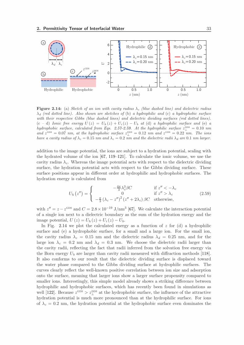
2. Permittivity Tensor of Interfacial Water 33
λc 0.15 nm=
λc 0.20 nm=
λc 0.15 nm=
λc 0.20 nm=
Hydrophilic Hydrophobic e
Hydrophilic Hydrophobic 0 0.5 1.0 0 0.5 1.0z (nm) z (nm)
6
4
2
0
-2
U
a
c zDDSzGDS
λcλd
b
d
Figure 2.14: (a) Sketch of an ion with cavity radius λc (blue dashed line) and dielectric radiusλd (red dotted line). Also shown are sketches of (b) a hydrophilic and (c) a hydrophobic surfacewith their respective Gibbs (blue dashed lines) and dielectric dividing surfaces (red dotted lines).(c – d) Ionic free energy U (z) = Uh (z) + Ui (z) − Ub at (d) a hydrophilic surface and (e) ahydrophobic surface, calculated from Eqs. 2.57-2.59. At the hydrophilic surface zdds
⊥ = 0.10 nmand zgds = 0.07 nm, at the hydrophobic surface zdds
⊥ = 0.12 nm and zgds = 0.22 nm. The ionshave a cavity radius of λc = 0.15 nm and λc = 0.2 nm and the dielectric radii λd are 0.1 nm larger.
addition to the image potential, the ions are subject to a hydration potential, scaling withthe hydrated volume of the ion [67, 119–121]. To calculate the ionic volume, we use thecavity radius λc. Whereas the image potential acts with respect to the dielectric dividingsurface, the hydration potential acts with respect to the Gibbs dividing surface. Thesesurface positions appear in different order at hydrophilic and hydrophobic surfaces. Thehydration energy is calculated from
Uh
(
z′′)
=
−4π3 λ
3cβC if z′′ < −λc
0 if z′′ > λc
−π3 (λc − z′′)2 (z′′ + 2λc) βC otherwise,
(2.59)
with z′′ = z−zgds and C = 2.8×10⁻¹⁹ J/nm3 [67]. We calculate the interaction potentialof a single ion next to a dielectric boundary as the sum of the hydration energy and theimage potential, U (z) = Uh (z) + Ui (z) − Ub.
In Fig. 2.14 we plot the calculated energy as a function of z for (d) a hydrophilicsurface and (e) a hydrophobic surface, for a small and a large ion. For the small ion,the cavity radius λc = 0.15 nm and the dielectric radius λd = 0.25 nm, and for thelarge ion λc = 0.2 nm and λd = 0.3 nm. We choose the dielectric radii larger thanthe cavity radii, reflecting the fact that radii inferred from the solvation free energy viathe Born energy Ub are larger than cavity radii measured with diffraction methods [118].It also conforms to our result that the dielectric dividing surface is displaced towardthe water phase compared to the Gibbs dividing surface at hydrophilic surfaces. Thecurves clearly reflect the well-known positive correlation between ion size and adsorptiononto the surface, meaning that larger ions show a larger surface propensity compared tosmaller ions. Interestingly, this simple model already shows a striking difference betweenhydrophilic and hydrophobic surfaces, which has recently been found in simulations aswell [122]. Because zgds > zdds
⊥ at the hydrophobic surface, the influence of the attractivehydration potential is much more pronounced than at the hydrophilic surface. For ionsof λc = 0.2 nm, the hydration potential at the hydrophobic surface even dominates the

34 Summary & Conclusions
interaction for 0.09 < z < 0.26 nm, which means that large ions adsorb onto hydrophobicsurfaces, but not onto hydrophilic surfaces. For distances larger than ∼ 0.3 nm from theinterface all potentials resemble the exponential function used previously for µ (z).
2.5 Summary & Conclusions
We have established the theoretical framework for calculating the dielectric response ten-sor of water at an interface from molecular fluctuations and from an applied external field.Whereas the parallel response can be calculated from the dipole moment only and roughlyfollows the density profile, the perpendicular response exhibits several singularities thatcan be captured properly only when higher-order multipole moments are taken into ac-count. For the perpendicular dielectric response, the linear response regime extends toan external field strength of at least D⊥/ε0 ≃ 2 V/nm, after which the response at thehydrophobic interface becomes non-linear. Because on timescales larger than ∼ 10 ns,dielectric breakdown in real water occurs at external field strengths one order of magni-tude lower, the non-linear response of the non-polarizable, non-ionizable water model thatwe use in our simulations is not expected to play a role in the dielectric response of realwater. Including the dielectric profile in a mean-field description of ion distributions ata charged interface, we find that the experimental double-layer capacitance can be wellreproduced. In particular, this shows that the Stern layer is predominantly caused by thedielectric interfacial features of water itself. Additionally accounting for the repulsive ion-substrate interaction – corresponding to steric exclusion of ions from the direct proximityof the wall – further improves the agreement with experimental data, but these direction-surface interactions are not decisive for the features seen in the experimental capaci-tance data. We quantify the difference between the dielectric response at hydrophilic andhydrophobic surfaces in terms of a single length scale that we call the dielectric dividingsurface. Using this length scale, the similarity that is found experimentally between thedouble-layer capacitance at both surface types can be rationalized very simply: althougha pronounced depletion layer exists at the hydrophobic interface, and therefore less wa-ter is available than at the hydrophilic interface, the dielectric dividing surface positionis very similar at both surface types, measured with respect to the top layer of heavysubstrate atoms. In other words, water at the hydrophobic surface is a “better dielectric”than at the hydrophilic surface. From the same mean-field description, we find that theeffect of the dielectric profile is to decrease the disjoining pressure between two chargedplates. Dielectric interface effects therefore cannot explain the universally observed hydra-tion repulsion between polar surfaces directly. Finally, a simple model for the adsorptionof spherical ions at interfaces that distinguishes between dielectric and depletion effects,both at the planar interfaces and around the ions, reveals the characteristic differencebetween adsorption at hydrophilic and hydrophobic surfaces. In particular, it predicts theadsorption of large ions onto hydrophobic surfaces, but not onto hydrophilic surfaces. Infuture research, the effect of ions and finite surface separation on the dielectric profile andthe consequences of the full dielectric profile on the ionic free energy need to be addressedin order to understand the interaction of charged and neutral surfaces in full detail.
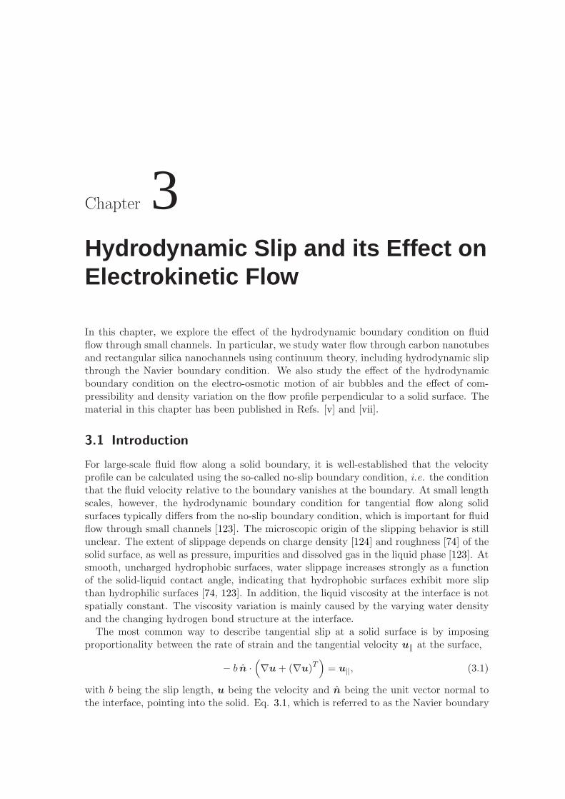
Chapter 3Hydrodynamic Slip and its Effect onElectrokinetic Flow
In this chapter, we explore the effect of the hydrodynamic boundary condition on fluidflow through small channels. In particular, we study water flow through carbon nanotubesand rectangular silica nanochannels using continuum theory, including hydrodynamic slipthrough the Navier boundary condition. We also study the effect of the hydrodynamicboundary condition on the electro-osmotic motion of air bubbles and the effect of com-pressibility and density variation on the flow profile perpendicular to a solid surface. Thematerial in this chapter has been published in Refs. [v] and [vii].
3.1 Introduction
For large-scale fluid flow along a solid boundary, it is well-established that the velocityprofile can be calculated using the so-called no-slip boundary condition, i.e. the conditionthat the fluid velocity relative to the boundary vanishes at the boundary. At small lengthscales, however, the hydrodynamic boundary condition for tangential flow along solidsurfaces typically differs from the no-slip boundary condition, which is important for fluidflow through small channels [123]. The microscopic origin of the slipping behavior is stillunclear. The extent of slippage depends on charge density [124] and roughness [74] of thesolid surface, as well as pressure, impurities and dissolved gas in the liquid phase [123]. Atsmooth, uncharged hydrophobic surfaces, water slippage increases strongly as a functionof the solid-liquid contact angle, indicating that hydrophobic surfaces exhibit more slipthan hydrophilic surfaces [74, 123]. In addition, the liquid viscosity at the interface is notspatially constant. The viscosity variation is mainly caused by the varying water densityand the changing hydrogen bond structure at the interface.
The most common way to describe tangential slip at a solid surface is by imposingproportionality between the rate of strain and the tangential velocity u‖ at the surface,
− b n ·(
∇u + (∇u)T)
= u‖, (3.1)
with b being the slip length, u being the velocity and n being the unit vector normal tothe interface, pointing into the solid. Eq. 3.1, which is referred to as the Navier boundary
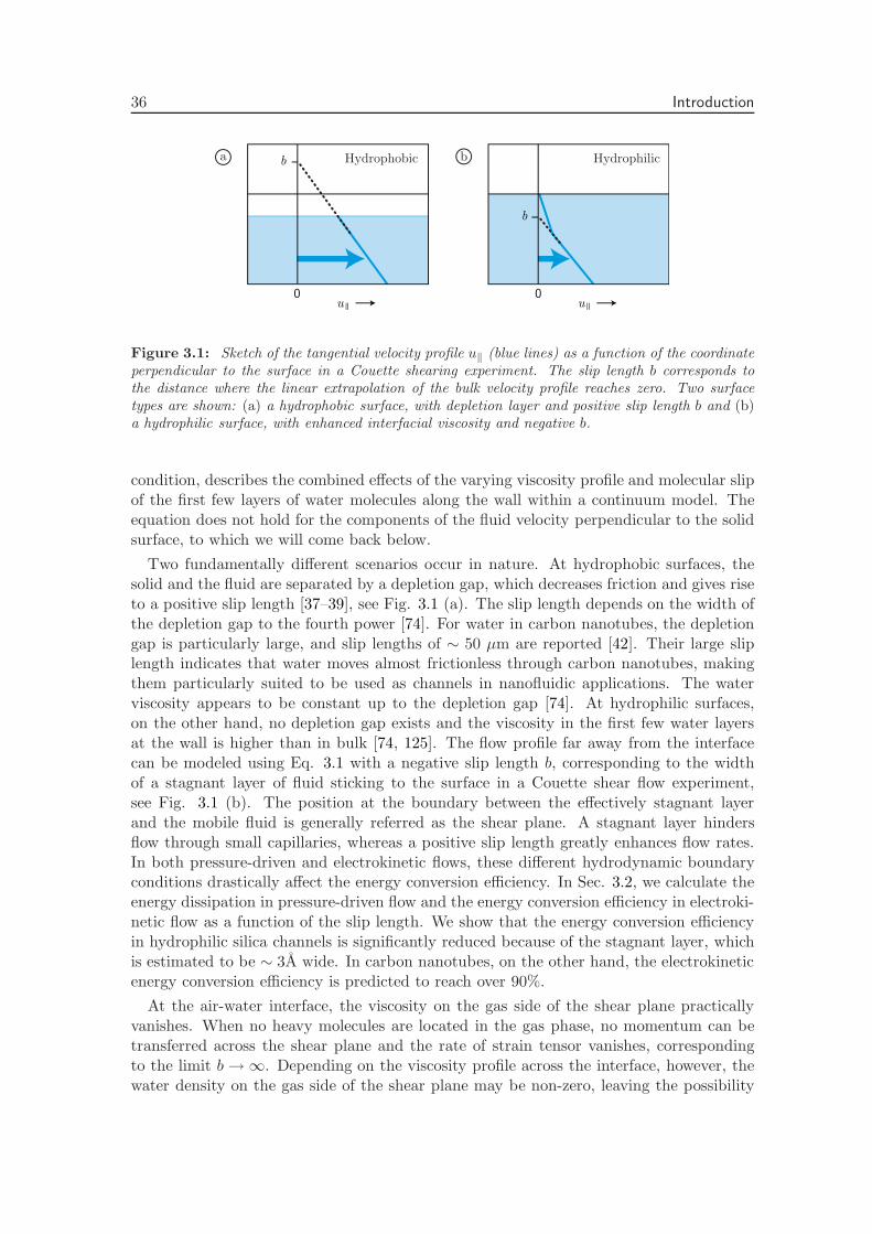
36 Introduction
b
0
b
0
a b HydrophilicHydrophobic
uu
Figure 3.1: Sketch of the tangential velocity profile u‖ (blue lines) as a function of the coordinateperpendicular to the surface in a Couette shearing experiment. The slip length b corresponds tothe distance where the linear extrapolation of the bulk velocity profile reaches zero. Two surfacetypes are shown: (a) a hydrophobic surface, with depletion layer and positive slip length b and (b)a hydrophilic surface, with enhanced interfacial viscosity and negative b.
condition, describes the combined effects of the varying viscosity profile and molecular slipof the first few layers of water molecules along the wall within a continuum model. Theequation does not hold for the components of the fluid velocity perpendicular to the solidsurface, to which we will come back below.
Two fundamentally different scenarios occur in nature. At hydrophobic surfaces, thesolid and the fluid are separated by a depletion gap, which decreases friction and gives riseto a positive slip length [37–39], see Fig. 3.1 (a). The slip length depends on the width ofthe depletion gap to the fourth power [74]. For water in carbon nanotubes, the depletiongap is particularly large, and slip lengths of ∼ 50 µm are reported [42]. Their large sliplength indicates that water moves almost frictionless through carbon nanotubes, makingthem particularly suited to be used as channels in nanofluidic applications. The waterviscosity appears to be constant up to the depletion gap [74]. At hydrophilic surfaces,on the other hand, no depletion gap exists and the viscosity in the first few water layersat the wall is higher than in bulk [74, 125]. The flow profile far away from the interfacecan be modeled using Eq. 3.1 with a negative slip length b, corresponding to the widthof a stagnant layer of fluid sticking to the surface in a Couette shear flow experiment,see Fig. 3.1 (b). The position at the boundary between the effectively stagnant layerand the mobile fluid is generally referred as the shear plane. A stagnant layer hindersflow through small capillaries, whereas a positive slip length greatly enhances flow rates.In both pressure-driven and electrokinetic flows, these different hydrodynamic boundaryconditions drastically affect the energy conversion efficiency. In Sec. 3.2, we calculate theenergy dissipation in pressure-driven flow and the energy conversion efficiency in electroki-netic flow as a function of the slip length. We show that the energy conversion efficiencyin hydrophilic silica channels is significantly reduced because of the stagnant layer, whichis estimated to be ∼ 3A wide. In carbon nanotubes, on the other hand, the electrokineticenergy conversion efficiency is predicted to reach over 90%.
At the air-water interface, the viscosity on the gas side of the shear plane practicallyvanishes. When no heavy molecules are located in the gas phase, no momentum can betransferred across the shear plane and the rate of strain tensor vanishes, correspondingto the limit b → ∞. Depending on the viscosity profile across the interface, however, thewater density on the gas side of the shear plane may be non-zero, leaving the possibility

3. Hydrodynamic Slip 37
of a finite slip length open. In Sec. 3.4, we calculate the electrophoretic mobility ofan air bubble as a function of the position of the shear plane for different values of theslip length, using a charge density profile that originates from charge transfer across thehydrogen bonds between water molecules [126].
Contrary to the fluid velocity tangential to the surface, the fluid velocity perpendicularto the surface strictly meets the no-slip boundary condition at impermeable surfaces, whichmeans that the perpendicular fluid velocity at an immobilized surface equals zero,
u · n = 0. (3.2)
In this case, the vanishing flow velocity is enforced by the condition that the water masscannot penetrate the solid surface. In contrast, a published molecular dynamics study ofwater flow in carbon nanotubes suggests that the flow perpendicular to the surface can benon-zero, which is speculated to be related to the interfacial structure and the microscopiccompressibility of water [62]. In Sec. 3.5, we refute these suggestions and show thatthe no-slip boundary condition holds rigidly for the perpendicular component of the fluidvelocity, also for compressible fluids of spatially varying density.
3.2 Pumping & Energy Conversion
3.2.1 Dissipation in Pressure-Driven Flows
Conservation of momentum for a fluid flowing with space-dependent and time-dependentvelocity u (x, t) is expressed by the Navier-Stokes equation, which reads
du
dt= ∇ · P + F with
d
dt=
∂
∂t+ u · ∇, (3.3)
with F being an external force. We assume the fluid to be incompressible, leaving themass density constant. For fluids of spherically symmetric constituents, the stress tensorP in Eq. 3.3 is given by
P = −pU + Π with Πij = η (∇jui + ∇iuj) . (3.4)
The hydrostatic pressure is denoted p, U is the unit tensor and η is the viscosity. Thebalance equation for the kinetic energy contained in a flowing liquid follows from a scalarproduct of the Navier-Stokes equation with the velocity, which in absence of external forcesgives [127]
d
dt
u2
2= ∇ · (P · u) − P : (∇u) . (3.5)
In steady state ∂u/∂t = 0 and Eq. 3.5 reduces to
0 = ∇ ·(
−1/2 u2u + P · u
)
− P : (∇u) , (3.6)
where the first term on the right-hand side represents the convective energy flow, equal to1/2 (u · ∇)u2 = 1/2 ∇ ·
(
u2u)
, which needs not be zero in steady state. Integration overa volume V and application of Gauss’s theorem yields
0 =
∫
∂Vn ·(
−u2u
2+ P · u
)
dA−∫
VP : (∇u) dV. (3.7)

38 Pumping & Energy Conversion
Using Einstein’s summation convention, we write the integral component-wise and insertEq. 3.4,
0 =
∫
∂Vnj
[
−u2iuj2
− puj + η (∇jui + ∇iuj) ui
]
dA
−∫
Vη (∇jui + ∇iuj)∇jui dV,
(3.8)
where we used P · u = −pδijui + η (∇jui + ∇iuj)ui and P : (∇u) = Pij∇jui and theincompressibility of the fluid, ∇iui = 0. The surface of the volume ∂V consists of threeparts: an inlet, an outlet and a wall. At impenetrable walls njuj = 0. For flow througha translationally invariant channel also the integrals over the inlet and outlet of the firstterm in the surface integral vanish. The second term in the surface integral represents theinput power Q∆p, with the volume flux
Q =
∫
Ωnjuj dA, (3.9)
where Ω is the cross section of the channel and ∆p is the static pressure difference betweenthe inlet and outlet. The remaining term in the surface integral in Eq. 3.8 represents thepower dissipated by friction at the walls and depends on the extent of slip. The volumeintegral represents the power dissipated within the fluid because of velocity gradients. Inour continuum description, we take the viscosity as a constant and introduce a slip lengthb as a boundary condition,
− njb∇jui|±d/2 = ui|±d/2, (3.10)
with d the height of the channel. For single-directional fluid flow, as appropriate foran incompressible fluid flowing through a translationally invariant channel, the balanceequation becomes
Q∆p = −η∫
∂V
u2i
bdA− η
∫
V(∇jui)
2 dV, (3.11)
where the right-hand side equates to the dissipated power Pdiss..
We now calculate the dissipation as a function of the slip length b for a given volumeflux Q. Ignoring edge effects, a pressure-driven fluid flow in a slit-like rectangular channelforms a Poiseuille flow profile (calculated from Eq. 3.3 with Eq. 3.10),
ui = −∇ip
8η
[
d2 + 4bd− 4x2j
]
, (3.12)
with ui the fluid velocity lengthways, xj the spatial coordinate along the height of thechannel and ∇ip = ∆p/l the pressure gradient along the length of the channel l. For agiven volume flux Q, the dissipation from Eq. 3.11 in a channel of width w becomes
Pdiss. =12Q2ηl
w (d3 + 6d2b), (3.13)
from which it can be seen that increasing the slip length greatly reduces the power requiredto achieve a flux Q when b becomes of the order of d.
A pressure difference across a cylindrical channel, such as a carbon nanotube, producesa Hagen-Poiseuille flow profile. At the wall of the tube of diameter d we use the boundary
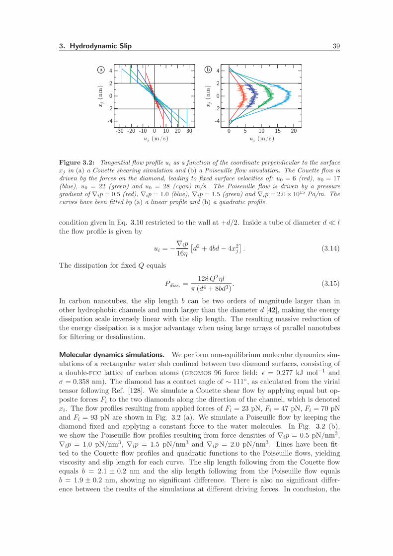
3. Hydrodynamic Slip 39
-30 -20 -10
-4
-2
0
2
4
0 5 10 15 20
-4
-2
0
2
4a b
3020100
u i (m/s) u i (m/s)
xj
(nm
)
xj
(nm
)
Figure 3.2: Tangential flow profile ui as a function of the coordinate perpendicular to the surfacexj in (a) a Couette shearing simulation and (b) a Poiseuille flow simulation. The Couette flow isdriven by the forces on the diamond, leading to fixed surface velocities of: u0 = 6 (red), u0 = 17(blue), u0 = 22 (green) and u0 = 28 (cyan) m/s. The Poiseuille flow is driven by a pressuregradient of ∇ip = 0.5 (red), ∇ip = 1.0 (blue), ∇ip = 1.5 (green) and ∇ip = 2.0× 10¹⁵ Pa/m. Thecurves have been fitted by (a) a linear profile and (b) a quadratic profile.
condition given in Eq. 3.10 restricted to the wall at +d/2. Inside a tube of diameter d≪ lthe flow profile is given by
ui = −∇ip
16η
[
d2 + 4bd− 4x2j
]
. (3.14)
The dissipation for fixed Q equals
Pdiss. =128Q2ηl
π (d4 + 8bd3). (3.15)
In carbon nanotubes, the slip length b can be two orders of magnitude larger than inother hydrophobic channels and much larger than the diameter d [42], making the energydissipation scale inversely linear with the slip length. The resulting massive reduction ofthe energy dissipation is a major advantage when using large arrays of parallel nanotubesfor filtering or desalination.
Molecular dynamics simulations. We perform non-equilibrium molecular dynamics sim-ulations of a rectangular water slab confined between two diamond surfaces, consisting ofa double-fcc lattice of carbon atoms (gromos 96 force field: ǫ = 0.277 kJ mol−1 andσ = 0.358 nm). The diamond has a contact angle of ∼ 111, as calculated from the virialtensor following Ref. [128]. We simulate a Couette shear flow by applying equal but op-posite forces Fi to the two diamonds along the direction of the channel, which is denotedxi. The flow profiles resulting from applied forces of Fi = 23 pN, Fi = 47 pN, Fi = 70 pNand Fi = 93 pN are shown in Fig. 3.2 (a). We simulate a Poiseuille flow by keeping thediamond fixed and applying a constant force to the water molecules. In Fig. 3.2 (b),we show the Poiseuille flow profiles resulting from force densities of ∇ip = 0.5 pN/nm3,∇ip = 1.0 pN/nm3, ∇ip = 1.5 pN/nm3 and ∇ip = 2.0 pN/nm3. Lines have been fit-ted to the Couette flow profiles and quadratic functions to the Poiseuille flows, yieldingviscosity and slip length for each curve. The slip length following from the Couette flowequals b = 2.1 ± 0.2 nm and the slip length following from the Poiseuille flow equalsb = 1.9 ± 0.2 nm, showing no significant difference. There is also no significant differ-ence between the results of the simulations at different driving forces. In conclusion, the
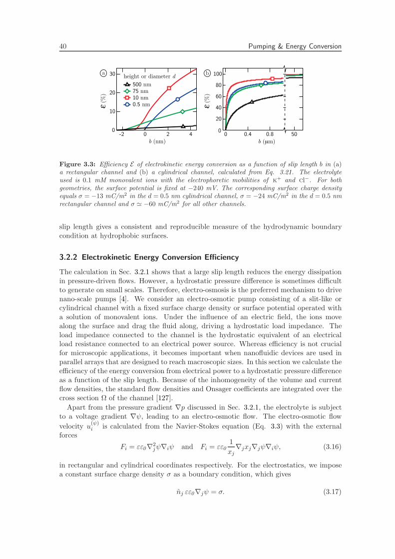
40 Pumping & Energy Conversion
(%)
-2b (nm)
0
10
20
30
0.5 nm10 nm75 nm500 nm
height or diameter d
0 2 4 0 0.4 0.8b (μm)
0
20
40
60
80
100
50
ε
a b
(%)
ε
Figure 3.3: Efficiency E of electrokinetic energy conversion as a function of slip length b in (a)a rectangular channel and (b) a cylindrical channel, calculated from Eq. 3.21. The electrolyteused is 0.1 mM monovalent ions with the electrophoretic mobilities of k+ and cl−. For bothgeometries, the surface potential is fixed at −240 mV. The corresponding surface charge densityequals σ = −13 mC/m2 in the d = 0.5 nm cylindrical channel, σ = −24 mC/m2 in the d = 0.5 nmrectangular channel and σ ≃ −60 mC/m2 for all other channels.
slip length gives a consistent and reproducible measure of the hydrodynamic boundarycondition at hydrophobic surfaces.
3.2.2 Electrokinetic Energy Conversion Efficiency
The calculation in Sec. 3.2.1 shows that a large slip length reduces the energy dissipationin pressure-driven flows. However, a hydrostatic pressure difference is sometimes difficultto generate on small scales. Therefore, electro-osmosis is the preferred mechanism to drivenano-scale pumps [4]. We consider an electro-osmotic pump consisting of a slit-like orcylindrical channel with a fixed surface charge density or surface potential operated witha solution of monovalent ions. Under the influence of an electric field, the ions movealong the surface and drag the fluid along, driving a hydrostatic load impedance. Theload impedance connected to the channel is the hydrostatic equivalent of an electricalload resistance connected to an electrical power source. Whereas efficiency is not crucialfor microscopic applications, it becomes important when nanofluidic devices are used inparallel arrays that are designed to reach macroscopic sizes. In this section we calculate theefficiency of the energy conversion from electrical power to a hydrostatic pressure differenceas a function of the slip length. Because of the inhomogeneity of the volume and currentflow densities, the standard flow densities and Onsager coefficients are integrated over thecross section Ω of the channel [127].
Apart from the pressure gradient ∇p discussed in Sec. 3.2.1, the electrolyte is subjectto a voltage gradient ∇ψ, leading to an electro-osmotic flow. The electro-osmotic flow
velocity u(ψ)i is calculated from the Navier-Stokes equation (Eq. 3.3) with the external
forces
Fi = εε0∇2jψ∇iψ and Fi = εε0
1
xj∇jxj∇jψ∇iψ, (3.16)
in rectangular and cylindrical coordinates respectively. For the electrostatics, we imposea constant surface charge density σ as a boundary condition, which gives
nj εε0∇jψ = σ. (3.17)

3. Hydrodynamic Slip 41
Solving Eq. 3.3 with the forces of Eq. 3.16 and the boundary conditions Eqs. 3.10 and3.17 gives
u(ψ)i (xj) =
∇iψ
η(εε0 [ψ (d/2) − ψ (xj)] + bσ) , (3.18)
for both the rectangular and the cylindrical geometry.
Linear response theory. In the linear response regime, the electrical current I and fluidvolume flux Q are related to the pressure gradient ∇p and the voltage gradient ∇ψ via
[
QI
]
=
[
Λ11 Λ12
Λ21 Λ22
] [
−∇p−∇ψ
]
. (3.19)
The hydrostatic output power per unit length of the channel equals Pout = −Q · ∇p, andthe electrical input power equals Pin = −I · ∇ψ. For electrokinetic power generation bypressure-driven flow, input and output power are defined the other way around, but theefficiency is calculated in the same way. The electrokinetic energy conversion efficiencyis given by the ratio E = Pout/Pin, which can be expressed in terms of the electrokineticresponse functions via Eq. 3.19. In the channel, the fluid velocity and electrostatic po-tential (apart from the constant voltage gradient driving the pump) depend only on thecoordinate perpendicular to the channel wall, throughout the following calculation denotedxj . The velocity, the electric current and the pressure gradient are only non-zero in thedirection along the channel wall, denoted xi. The Onsager coefficients can be expressedas
Λ11 = −∫
Ω
u(p)i
∇ipdA
Λ21 = −e∫
Ω[n+ (xj) − n− (xj)]
u(p)i
∇ipdA
Λ12 = −∫
Ω
u(ψ)i
∇iψdA
Λ22 = e
∫
Ω[ν+n+ (xj) + ν−n− (xj)] − [n+ (xj) − n− (xj)]
u(ψ)i
∇iψdA,
(3.20)
where the monovalent ions have electrophoretic mobilities ν± and number densities n± =n0 exp (∓eψ/kbT ) with n0 the bulk density and kbT the thermal energy. The electrostaticpotential ψ (xj) is calculated numerically from the Poisson-Boltzmann equation, which
holds sufficiently well on small scales [124]. The pressure-driven flow velocity u(p)i (xj) is
given in Eqs. 3.12 and 3.14 for the rectangular and cylindrical geometries respectively,
and the electro-osmotic flow velocity u(ψ)i (xj) is given in Eq. 3.18. The surface of a
carbon nanotube is uncharged, but a finite surface potential can be achieved for nanotubesby application of an external potential. Surface potentials also arise naturally due tounequal surface adsorption of cations and anions. Note that in an experimental setupthe driving electric field will be at least partially screened by electron transport throughthe nanotube, which will reduce the electric fields strength inside the nanotube. Thepressure gradient generated is linearly related to the volume flux via the hydrostatic loadimpedance Zl, Q = ∇ip/Zl. The efficiency is maximized for a specific value of ZlΛ11,which is the hydrostatic load impedance divided by the hydrostatic channel impedance

42 Onsager Reciprocal Relation
Λ−111 . The value of the maximum efficiency E has a very simple form in terms of the
variable α = Λ212/Λ11Λ22 [129]:
E =α
2 + 2√
1 − α− α. (3.21)
Using the no-slip boundary condition, the predicted maximum efficiency is only 7%,whereas the measured efficiency in a silicon oxide channel of d = 75 nm reaches no morethan 3% [130]. To investigate the effect of slip, we use the hydrodynamic boundary con-dition of Eq. 3.10. The efficiency from Eq. 3.21 is shown in Fig. 3.3 as a function ofslip length for different channel dimensions. We use the ion mobilities of k+ and cl− anda bulk concentration of 0.1 mM, giving a Debye screening length of 30 nm. Clearly, theefficiency increases drastically with increasing slip length. The variation of the efficiencywith respect to the channel diameter d is non-monotonic and different for different valuesof the slip length. For a slip length of ∼ 2 nm, which is a reasonable number for hydropho-bic surfaces [74], the efficiency in the 10 nm high rectangular channel reaches ∼ 20%. Inextension to the work of Ref. [131] we plot the efficiency for negative slip lengths. Themeasured efficiency of 3% in a 75 nm high channel and 1% in a 490 nm high channel [130]with a surface charge density of −60 mC/m2, which is the measured surface charge densityof silicon oxide [132], is consistent with a slip length of b = −0.3 nm, corresponding to onestatic molecular layer, in good agreement with predictions by Ref. [74] for an oh-coveredsurface.
In Fig. 3.3 (b), the efficiency is calculated for a cylindrical channel. The increase inefficiency is similar to the planar case, but in carbon nanotubes the slip length can be asmuch as ∼ 50 µm [42]. In all nanotubes considered, the efficiency for slip lengths of thatorder is over 90%.
3.3 Onsager Reciprocal Relation
The electrokinetic phenomena described in Eq. 3.19 are an example of coupled irreversibleprocesses for which the Onsager reciprocal relations between the thermodynamic fluxesand forces should hold [127, 133, 134]. The Onsager relation connects the electro-osmoticfluid flow in response to an electric field directly to the electric current in response to apressure gradient, Λ12 = Λ21, first proven by Saxen using the no-slip boundary condition[135]. Using the expressions of Eq. 3.20, we will proof this identity explicitly using theboundary condition of Eq. 3.10.
Rectangular geometry. Using the Poisson equation, the streaming conductance Λ21 isexpressed as
Λ21 = εε0
∫
Ω∇2jψu
(p)i
∇ipdA. (3.22)
A double partial integration of Eq. 3.22 yields
Λ21 = εε0
∫
∂Ω∇jψ
u(p)i
∇ipnjdΓ − εε0
∫
∂Ωψ∇ju
(p)i
∇ipnjdΓ + εε0
∫
Ωψ∇2ju
(p)i
∇ipdA, (3.23)
with Γ the path along the edge of the channel cross-section ∂Ω, located at xj = ±d/2.Inserting the pressure-driven velocity of Eq. 3.12 and the electrostatic boundary condition
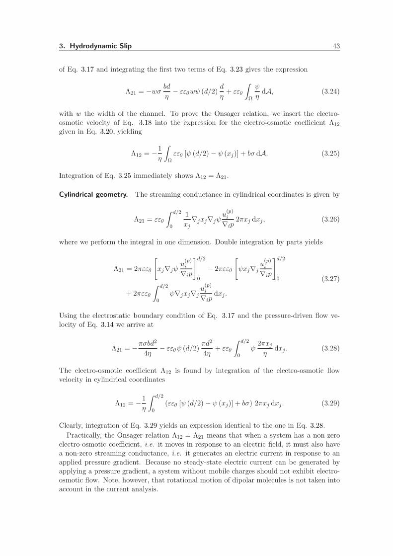
3. Hydrodynamic Slip 43
of Eq. 3.17 and integrating the first two terms of Eq. 3.23 gives the expression
Λ21 = −wσ bdη
− εε0wψ (d/2)d
η+ εε0
∫
Ω
ψ
ηdA, (3.24)
with w the width of the channel. To prove the Onsager relation, we insert the electro-osmotic velocity of Eq. 3.18 into the expression for the electro-osmotic coefficient Λ12
given in Eq. 3.20, yielding
Λ12 = −1
η
∫
Ωεε0 [ψ (d/2) − ψ (xj)] + bσ dA. (3.25)
Integration of Eq. 3.25 immediately shows Λ12 = Λ21.
Cylindrical geometry. The streaming conductance in cylindrical coordinates is given by
Λ21 = εε0
∫ d/2
0
1
xj∇jxj∇jψ
u(p)i
∇ip2πxj dxj, (3.26)
where we perform the integral in one dimension. Double integration by parts yields
Λ21 = 2πεε0
[
xj∇jψu
(p)i
∇ip
]d/2
0
− 2πεε0
[
ψxj∇ju
(p)i
∇ip
]d/2
0
+ 2πεε0
∫ d/2
0ψ∇jxj∇j
u(p)i
∇ipdxj.
(3.27)
Using the electrostatic boundary condition of Eq. 3.17 and the pressure-driven flow ve-locity of Eq. 3.14 we arrive at
Λ21 = −πσbd2
4η− εε0ψ (d/2)
πd2
4η+ εε0
∫ d/2
0ψ
2πxjη
dxj . (3.28)
The electro-osmotic coefficient Λ12 is found by integration of the electro-osmotic flowvelocity in cylindrical coordinates
Λ12 = −1
η
∫ d/2
0(εε0 [ψ (d/2) − ψ (xj)] + bσ) 2πxj dxj . (3.29)
Clearly, integration of Eq. 3.29 yields an expression identical to the one in Eq. 3.28.
Practically, the Onsager relation Λ12 = Λ21 means that when a system has a non-zeroelectro-osmotic coefficient, i.e. it moves in response to an electric field, it must also havea non-zero streaming conductance, i.e. it generates an electric current in response to anapplied pressure gradient. Because no steady-state electric current can be generated byapplying a pressure gradient, a system without mobile charges should not exhibit electro-osmotic flow. Note, however, that rotational motion of dipolar molecules is not taken intoaccount in the current analysis.
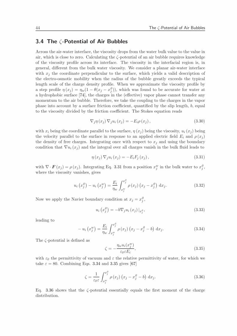
44 The ζ-Potential of Air Bubbles
3.4 The ζ-Potential of Air Bubbles
Across the air-water interface, the viscosity drops from the water bulk value to the value inair, which is close to zero. Calculating the ζ-potential of an air bubble requires knowledgeof the viscosity profile across its interface. The viscosity in the interfacial region is, ingeneral, different from the bulk water viscosity. We consider a planar air-water interfacewith xj the coordinate perpendicular to the surface, which yields a valid description ofthe electro-osmotic mobility when the radius of the bubble greatly exceeds the typicallength scale of the charge density profile. When we approximate the viscosity profile bya step profile η (xj) = ηw(1 − θ(xj − x0
j )), which was found to be accurate for water ata hydrophobic surface [74], the charges in the (effective) vapor phase cannot transfer anymomentum to the air bubble. Therefore, we take the coupling to the charges in the vaporphase into account by a surface friction coefficient, quantified by the slip length, b, equalto the viscosity divided by the friction coefficient. The Stokes equation reads
∇jη (xj)∇jui (xj) = −Eiρ (xj) , (3.30)
with xi being the coordinate parallel to the surface, η (xj) being the viscosity, ui (xj) beingthe velocity parallel to the surface in response to an applied electric field Ei and ρ (xj)the density of free charges. Integrating once with respect to xj and using the boundarycondition that ∇ui (xj) and the integral over all charges vanish in the bulk fluid leads to
η (xj)∇jui (xj) = −EiFj (xj) , (3.31)
with ∇ ·F (xj) = ρ (xj). Integrating Eq. 3.31 from a position xwj in the bulk water to x0j ,
where the viscosity vanishes, gives
ui(
x0j
)
− ui(
xwj)
=Eiηw
∫ x0j
xwj
ρ (xj)(
xj − x0j
)
dxj. (3.32)
Now we apply the Navier boundary condition at xj = x0j ,
ui(
x0j
)
= −b∇jui (xj) |x0j, (3.33)
leading to
− ui(
xwj)
=Eiηw
∫ x0j
xwj
ρ (xj)(
xj − x0j − b
)
dxj. (3.34)
The ζ-potential is defined as
ζ = −ηwui(x
wj )
ε0εEi, (3.35)
with ε0 the permittivity of vacuum and ε the relative permittivity of water, for which wetake ε = 80. Combining Eqs. 3.34 and 3.35 gives [67]
ζ =1
ε0ε
∫ x0j
xwj
ρ (xj)(
xj − x0j − b
)
dxj. (3.36)
Eq. 3.36 shows that the ζ-potential essentially equals the first moment of the chargedistribution.
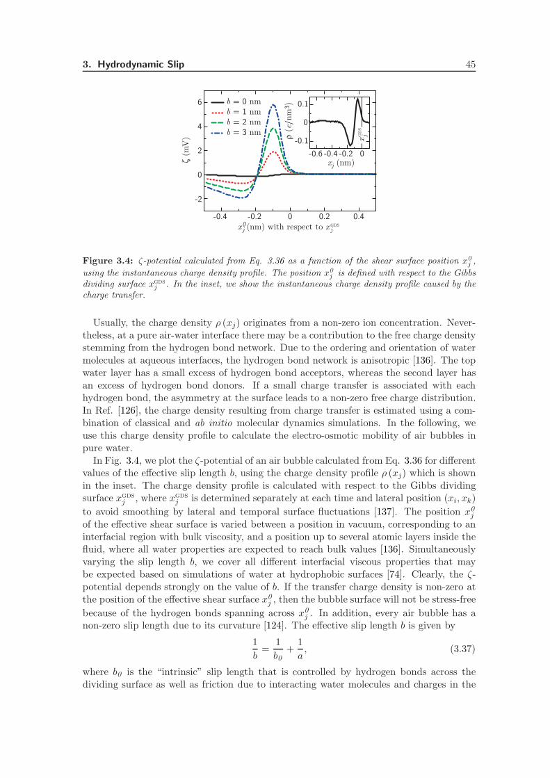
3. Hydrodynamic Slip 45
-0.4 -0.2 0 0.2 0.4
-0.6 -0.4 -0.2 0
-0.1
0
0.1
ρ (
e/nm
3 )
xj (nm)
xG
DS
x j (nm) with respect to xGDS
-2
0
2
4
6
ζ (m
V)
b = 0 nm
b = 3 nm
b = 1 nmb = 2 nm
j
j
0
Figure 3.4: ζ-potential calculated from Eq. 3.36 as a function of the shear surface position x0
j ,
using the instantaneous charge density profile. The position x0
j is defined with respect to the Gibbsdividing surface xgds
j . In the inset, we show the instantaneous charge density profile caused by thecharge transfer.
Usually, the charge density ρ (xj) originates from a non-zero ion concentration. Never-theless, at a pure air-water interface there may be a contribution to the free charge densitystemming from the hydrogen bond network. Due to the ordering and orientation of watermolecules at aqueous interfaces, the hydrogen bond network is anisotropic [136]. The topwater layer has a small excess of hydrogen bond acceptors, whereas the second layer hasan excess of hydrogen bond donors. If a small charge transfer is associated with eachhydrogen bond, the asymmetry at the surface leads to a non-zero free charge distribution.In Ref. [126], the charge density resulting from charge transfer is estimated using a com-bination of classical and ab initio molecular dynamics simulations. In the following, weuse this charge density profile to calculate the electro-osmotic mobility of air bubbles inpure water.
In Fig. 3.4, we plot the ζ-potential of an air bubble calculated from Eq. 3.36 for differentvalues of the effective slip length b, using the charge density profile ρ (xj) which is shownin the inset. The charge density profile is calculated with respect to the Gibbs dividingsurface xgds
j , where xgdsj is determined separately at each time and lateral position (xi, xk)
to avoid smoothing by lateral and temporal surface fluctuations [137]. The position x0j
of the effective shear surface is varied between a position in vacuum, corresponding to aninterfacial region with bulk viscosity, and a position up to several atomic layers inside thefluid, where all water properties are expected to reach bulk values [136]. Simultaneouslyvarying the slip length b, we cover all different interfacial viscous properties that maybe expected based on simulations of water at hydrophobic surfaces [74]. Clearly, the ζ-potential depends strongly on the value of b. If the transfer charge density is non-zero atthe position of the effective shear surface x0
j , then the bubble surface will not be stress-free
because of the hydrogen bonds spanning across x0j . In addition, every air bubble has a
non-zero slip length due to its curvature [124]. The effective slip length b is given by
1
b=
1
b0+
1
a, (3.37)
where b0 is the “intrinsic” slip length that is controlled by hydrogen bonds across thedividing surface as well as friction due to interacting water molecules and charges in the

46 Radial Flow in Compressible Fluids
-0.6 -0.4 -0.2 0 0.2 0.4 0.6
-2
0
2
4
6
-1.0 0xj (nm)
-0.02
0
0.02b = 0 nm
x0 (nm) with respect to xGDS
ζ (m
V) ρ (
e/nm
3 )
b = 3 nm
b = 1 nmb = 2 nm
xG
DS
j
j j
Figure 3.5: ζ-potential calculated from Eq. 3.36 as a function of the shear surface position x0
j .
The position x0
j is defined with respect to the Gibbs dividing surface. In the inset, we show thelaterally averaged charge density profile caused by the charge transfer.
vapor and liquid phases, and a is the curvature of the bubble surface. Because of thelarge number of hydrogen bonds across the effective plane of shear, we expect b0 to besmall for x0
j < 0.1 nm. For x0j > 0.1 nm, the water density is very small, and b0 is
expected to be large. For values of b of several nanometers, which we consider as anupper limit because this is the value for very hydrophobic surfaces, we find a ζ-potentialof several millivolts, that is, about an order of magnitude smaller than the ζ-potential of∼ −35 mV measured for air bubbles in water [138]. Assuming that the transition frombulk-like to vapor-like hydrodynamic properties occurs effectively at one molecular layerbeneath the surface, which is realistic in the view of the high self-diffusion constant ofthe top water layer found in molecular dynamics simulations [139, 140], the ζ-potentialis negative. A negative peak is found at x0
j = −0.28 nm, that is, about one water layerbelow the surface, effectively leaving the air bubble with a net negative charge. However,the ζ-potential varies depending on the hydrodynamic properties of the interfacial region,and a positive peak is obtained at x0
j = −0.10 nm. In Fig. 3.5, we show the ζ-potentialwhen the charge density profile is calculated with respect to the laterally averaged xgds
j
(ρ (xj) is shown in the inset). Qualitatively, the graph shows the same features as Fig.3.4, but the amplitude of the ζ-potential is lower because the charge profile is smoothedby lateral averaging.
In conclusion, the ζ-potential resulting from the charge transfer is small, even whenfinite slip between the charges in the water and vapor phase is taken into account. Thesign of the ζ-potential can be positive or negative, depending on the nature of the viscosityprofile. To improve the current model, the viscosity profile across the air-water interfaceneeds to be calculated explicitly.
3.5 Radial Flow in Compressible Fluids
In Ref. [62], a non-zero radial velocity component is reported in a pressure-driven flowinside a (16, 16) carbon nanotube, see Fig. 3.6 (b), in stark contrast with continuumPoiseuille-flow predictions. The non-zero radial flow is claimed to be related to the in-homogeneous density profile. Let us analyze the effect of compressibility and a space-
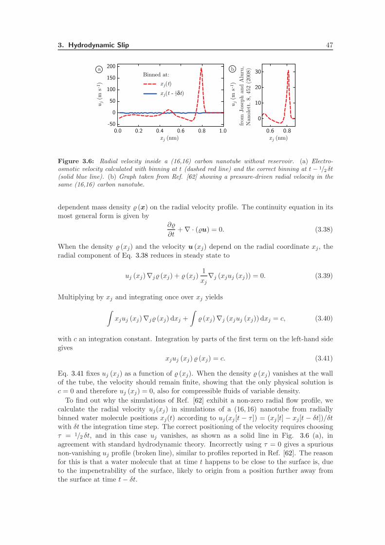
3. Hydrodynamic Slip 47
0.0 0.2 0.4 0.6 0.8 1.0
0
50
100
150
200
-50
Binned at:
x j(t)
x j(t - δt)12
from
Jos
eph a
nd A
luru
, N
anol
ett. 8
, 45
2 (2
008)
x j (nm)
uj (m
s-1)
0.6 0.8
0
10
20
30
uj (m
s-1)
x j (nm)
a b
Figure 3.6: Radial velocity inside a (16,16) carbon nanotube without reservoir. (a) Electro-osmotic velocity calculated with binning at t (dashed red line) and the correct binning at t− 1/2 δt(solid blue line). (b) Graph taken from Ref. [62] showing a pressure-driven radial velocity in thesame (16,16) carbon nanotube.
dependent mass density (x) on the radial velocity profile. The continuity equation in itsmost general form is given by
∂
∂t+ ∇ · (u) = 0. (3.38)
When the density (xj) and the velocity u (xj) depend on the radial coordinate xj, theradial component of Eq. 3.38 reduces in steady state to
uj (xj)∇j (xj) + (xj)1
xj∇j (xjuj (xj)) = 0. (3.39)
Multiplying by xj and integrating once over xj yields
∫
xjuj (xj)∇j (xj) dxj +
∫
(xj)∇j (xjuj (xj)) dxj = c, (3.40)
with c an integration constant. Integration by parts of the first term on the left-hand sidegives
xjuj (xj) (xj) = c. (3.41)
Eq. 3.41 fixes uj (xj) as a function of (xj). When the density (xj) vanishes at the wallof the tube, the velocity should remain finite, showing that the only physical solution isc = 0 and therefore uj (xj) = 0, also for compressible fluids of variable density.
To find out why the simulations of Ref. [62] exhibit a non-zero radial flow profile, wecalculate the radial velocity uj(xj) in simulations of a (16, 16) nanotube from radiallybinned water molecule positions xj(t) according to uj(xj [t − τ ]) = (xj [t] − xj[t − δt])/δtwith δt the integration time step. The correct positioning of the velocity requires choosingτ = 1/2 δt, and in this case uj vanishes, as shown as a solid line in Fig. 3.6 (a), inagreement with standard hydrodynamic theory. Incorrectly using τ = 0 gives a spuriousnon-vanishing uj profile (broken line), similar to profiles reported in Ref. [62]. The reasonfor this is that a water molecule that at time t happens to be close to the surface is, dueto the impenetrability of the surface, likely to origin from a position further away fromthe surface at time t− δt.
48 Summary & Conclusions
3.6 Summary & Conclusions
We study the effect of a deviation from the no-slip boundary condition on the propertiesof pressure-driven and electrokinetic flow through rectangular nanochannels and carbonnanotubes, as well as the electrophoretic motion of gas bubbles. The extremely large sliplength measured in carbon nanotubes greatly reduces the fluidic resistance to pressure-driven flow and at the same time enhances the efficiency of electrokinetic energy conversion.Experimental values of the electrokinetic energy conversion efficiency in hydrophilic siliconoxide channels can be modeled using a slip length of b = −0.3 nm, corresponding to onehighly viscous layer of water molecules at the interface. In the direction perpendicularto the tube wall, the no-slip boundary condition holds rigidly, also for systems with spa-tially varying density. Using the standard Navier-Stokes equation, we explicitly prove theOnsager reciprocal relation for electrokinetic flow, namely that the electro-osmotic con-ductance and the streaming conductance are equal. From the equality we conclude thatsystems of spherically symmetric particles, as considered in this chapter, do not exhibitelectro-osmotic flow in static electric fields if no mobile charges are present. Rotation ofwater molecules, which has not been taken into account so far, will be treated in detail inChapter 4. Finally, we show that the mobile charge density resulting from charge transferbetween water molecules does not contribute significantly to the electrophoretic mobilityof air bubbles in water, regardless of the hydrodynamic boundary conditions.

Chapter 4Electrokinetics at AqueousInterfaces without Mobile Charges
We theoretically consider the possibility of using electric fields in aqueous channels ofcylindrical and planar geometry to induce transport in the absence of mobile ionic charges.Using the Navier-Stokes equation, generalized to include the effects of water spinning,dipole orientation and relaxation, we show analytically that pumping of a dipolar liquidthrough an uncharged hydrophobic channel can be achieved by injecting torque into theliquid, based on the coupling between molecular spinning and fluid vorticity. Pumping ispossible continuously, using rotating electric fields and suitably chosen interfacial boundaryconditions, or transiently, by suddenly switching on a homogeneous electric field. A staticelectric field, however, does not induce a steady-state flow in channels, irrespective of thegeometry. Using molecular dynamics (md) simulations, we confirm that static fields donot lead to any pumping, in contrast to earlier publications. The origin of the pumpingobserved in md simulations of carbon nanotubes and oil droplets in a static electric fieldis tracked down to an imprudent implementation of Lennard-Jones interaction truncationschemes. The work described in this chapter has been published in Refs. [iv], [vii], [ix]and [x].
4.1 Introduction
Efficient conversion of power from one form to another is nowadays a pressing issue. In flu-idic applications, this mainly comes down to conversion between electrical and mechanicalenergy: the key elements of fluidic systems are pumps for converting electrical power intoa hydrostatic pressure difference, and turbines or electro-osmotic power generators for thereverse process. The realization of the full potential of laboratory minimization dependscrucially on the design and fabrication of these active fluidic components on the nanoscale. In particular, pumps are of critical importance for the two principal functionalitiesof chip-sized laboratories: transport and mixing [2, 3].
It has long been recognized that electro-osmosis is a very efficient and scalable mech-anism to use in nano-scale pumps [4]. The classical electro-osmotic pump is based on acharged surface and operated with ionic solutions. Under influence of an electric field,

50 Introduction
the ions move along the surface and drag the fluid along. Alternatively, electro-osmoticpumping can be achieved at a neutral channel surface with a salt solution of which thecations and anions have different affinities for the surface [67, 141]. In this case, the asym-metric distribution of ions generates a finite torque in the interfacial liquid layer, causingthe fluid to move in one direction.
The use of carbon nanotubes as channels and pumps in nanofluidic devices has beena major aim for the nanofluidic community ever since the discovery that water movesalmost frictionless through carbon nanotubes, see Chapter 3 [42, 43]. However, the factthat nanotubes are uncharged limits the possibilities for their use as active electro-osmoticcomponents. Different ways of pumping fluid with carbon nanotubes have been suggested.Using molecular dynamics simulations, Insepov et al. demonstrated that gas moleculescan be moved peristaltically through a nanotube under influence of a traveling acousticwave [142]. A little later, Longhurst and Quirke showed that a temperature gradientmoves decane molecules through a nanotube, also using molecular dynamics simulations[143]. A slightly different method was proposed by Kral and Tomanek, making use of thesemi-conducting properties of nanotubes to move particles through the tube due to thecoupling to laser-excited propagating electrons [144].
Many examples of efficient nano-scale pumps and channels are found in nature, wheredifferent protein channels transport water, ions and macromolecules in a highly specificmanner across membranes [5, 6]. A synthetic channel exhibiting some of the selectivetransport and fast flow properties of biological channels would have a wide range of possibleapplications, not only for pumping, but also for filtering and desalination. To realize thisgoal, Gong et al. designed a nanotube with a fixed external charge distribution mimickingthe charge distribution on an aquaporin channel. In molecular dynamics simulations, theyobserved a finite water flow through the tube [61]. Fixed charges outside a carbon nanotubealso influence the pressure-driven passage of water molecules [59]. Finally, unchargedchannels filled with solutions of the relatively symmetric salts sodium chloride or potassiumchloride were found to exhibit electro-osmotic flow [62–64].
The pumping efficiency and performance of electrokinetically driven channels can be ex-pressed in terms of the ζ-potential, which is a material property defined by the Helmholtz-Smoluchowski equation
ζ = − ηu
εε0E, (4.1)
with η the shear viscosity, εε0 the permittivity, E the electric field and u the bulk fluidvelocity in the direction of E. According to standard theory, a non-zero ζ-potential arisesonly in the presence of mobile charged species, which limits the use of electrokinetic ef-fects in uncharged nano-channels. However, the ζ-potential of solutes in water has beena source of controversy for many years [45, 49, 50]. Ever since the first electrophoreticmeasurements it has been known that nominally uncharged substances like air bubblesand oil droplets in pure water exhibit a negative ζ-potential [45]. Generally, this negativeζ-potential of uncharged solutes is attributed to the accumulation of negatively chargedions at the solute surface [45–47]. In contrast with this traditional view, a recent simula-tion paper reports non-zero ζ-potentials for heptane droplets in pure h2o without mobileions [51]. Similarly, several molecular dynamics simulations show electro-osmotic flowin hydrophobic channels: Joseph and Aluru report flow in a carbon nanotube under aconstant electric field [60] and Gong et al. report flows in carbon nanotubes induced byfixed charges outside the nanotube [44, 61]. Most of these simulations [51, 60, 61], theresults of which we will critically re-evaluate in this chapter, have been performed using
4. Electrokinetics without Mobile Charges 51
the molecular dynamics simulation package gromacs [145]. Apart from their ability tospecifically adsorb different types of ions, aqueous interfaces have a strong ordering effecton the first few molecular layers next to the interface. Molecules in the outermost inter-facial water layer are preferentially oriented with their h-atoms pointing outward, givingrise to a considerable dipole density [65]. This structured water next to the interface hasa profound influence on the dielectric properties, the viscosity and the interaction withions, among many other surface characteristics [36, 67]. In an attempt to rationalize thesurprising results of the simulation exhibiting electrokinetic effects at uncharged aqueousinterfaces, the coupling of the electric field to the dipolar surface layer was speculated toprovide an alternative mechanism for the appearance of a non-zero ζ-potential, inducingflow through rotation of the ordered water molecules [51, 60].
In this chapter we discuss two central questions: First, can the dipolar ordering ofthe water surface layer give rise to a non-zero ζ-potential in a static and uniform electricfield? And second, can the dipolar nature of water be exploited for electro-hydraulic powerconversion, and in that way enable the use of uncharged channels as active electrokineticcomponents? We show that using a static electric field, electro-osmotic pumping of purewater in a planar or cylindrical hydrophobic channel is impossible. This result, whichis confirmed by extensive molecular dynamics simulations, comes from an analysis basedon a generalized Navier-Stokes formulation that includes angular momentum in the formof spinning molecules as well as dipolar ordering and relaxation. Employing rotatingelectric fields combined with suitable boundary conditions, on the other hand, the couplingbetween water molecular rotation and vorticity can be used to pump a dipolar fluid througha nanofluidic channel.
4.2 Generalized Navier-Stokes Approach
4.2.1 Conservation of Angular Momentum
Whenever an internal force F int acts on some element of a continuum, stress builds upthat is described by a non-vanishing stress tensor P for which PijnjdA = dF int
i , with dAthe surface area of the element and n the vector normal to the surface. Note that in thefollowing we denote Pij as the shear stress tensor in order to distinguish it from the stresstensor associated with the spinning of molecules. The shear stress tensor can be split intoa part corresponding to the hydrostatic pressure p and a friction part Π, which in turncan be split into a symmetric part Πs and an antisymmetric part Πa,
P = −pU + Π and Π = Πs + Πa, (4.2)
with U the unit tensor. For a mono-atomic fluid the antisymmetric part Πa of the shearstress tensor is zero. In a polar fluid, the interaction between two points in the fluid is notonly modeled via the internal force vector and the associated stress tensor, but also viathe torque per unit mass Γint. Equivalent to Cauchy’s stress principle for the force F int,there is a spin stress tensor C for which Cij njdA = dΓint
i holds. The total rate of changeof the angular momentum per unit mass L, integrated over a material volume V, can bewritten as
∫∫∫
V
∂
∂t(L) dV + ©
∫∫
∂V(L) u · ndA =
∫∫∫
V
dL
dtdV, (4.3)
with u the velocity of the molecules and (x, t) the mass density. The material derivatived/dt is defined as d/dt = ∂/∂t+ u · ∇. These considerations lead to the following balance
52 Generalized Navier-Stokes Approach
equation for the total rate of change of L,
∫∫∫
V
dL
dtdV =
∫∫∫
V (Γ + x × F ) dV + ©
∫∫
∂Vn · (C + x × P) dA
=
∫∫∫
V (Γ + x × F ) + ∇ · C + ∇ · (x × P) dV,
(4.4)
with x the position vector. Rearranging the last term on the right-hand side of Eq. 4.4yields ∇· (x × P) = x× (∇ · P)+2Πa, where Πa
k = −1/2 ǫijkΠaij is the antisymmetric part
of the shear stress tensor in axial vector representation, with ǫijk the Levi-Civita tensor.Realizing that Eq. 4.4 holds for any volume V yields the local conservation of total angularmomentum:
dL
dt= (Γ + x × F ) + ∇ · C + x × (∇ · P) + 2Πa. (4.5)
The total angular momentum can be written as the sum of the vorticity contribution x×u
and a spin contribution Iω, accounting for molecular rotation,
L = x × u + Iω, (4.6)
with I the moment of inertia per unit mass and ω the average angular velocity of theconstituent particles. The moment of inertia I is a tensor depending on the mass distri-bution within the particles and on the local orientational distribution. Because of theapproximate mass isotropy of the water molecules, the tensor I is almost diagonal even ifthe orientational distribution of water molecules is very anisotropic, as happens to be thecase close to an interface [146]. We therefore take I to be a diagonal tensor with value I.For the first part of Eq. 4.6 we write down a separate conservation law, starting from theconservation law for linear momentum,
du
dt= F + ∇ · P. (4.7)
We take the vectorial product of x with Eq. 4.7, leading to
d
dt(x × u) = (x × F ) + x × (∇ · P) . (4.8)
The difference between Eqs. 4.5 and 4.8 gives the conservation law for the spin part ofthe angular momentum density:
Idω
dt= Γ + ∇ · C + 2Πa. (4.9)
To leading order, C only depends on ω. Equation 4.9 then shows that to leading order,the only coupling between the vorticity part and the spin part of the angular momentumcomes from the antisymmetric part of the shear stress tensor Πa.
4.2.2 Material Equations
We now derive expressions for the terms occurring on the right-hand side of Eq. 4.9. Iftwo neighboring fluid elements moving with velocity u are rotating each with the angularvelocity ω = 1/2∇×u, the internal spin and the vorticity are synchronized, and no stressresults. The antisymmetric part of the shear stress tensor should therefore be a function

4. Electrokinetics without Mobile Charges 53
a b
x3
x2
x1
x3
x1
x2
Figure 4.1: Sketches of (a) the rectangular geometry and (b) the cylindrical geometry.
of 1/2∇× u − ω. Additionally, Πa should vanish when ∇× u = 2ω, and the axial vectorof Πa should have the same direction as ∇×u− 2ω [147]. Therefore, to leading order wecan write
Πa = ηr (∇× u − 2ω) , (4.10)
with ηr the vortex viscosity. To leading order, the spin stress tensor C should depend onspatial differences in the spin field ω only. By equilibrating the second moments of theforce, the spin stress tensor can be proven to be symmetric [148]. Disregarding higherderivatives as for the shear stress tensor we write
Cij = νv∇kωkδij + ν (∇jωi + ∇iωj − 2/3∇kωkδij) , (4.11)
with ν the spin viscosity, νv the volume spin viscosity and using the Einstein summationconvention as in the rest of the chapter. Combining Eqs. 4.9, 4.10 and 4.11 yields
Idω
dt= Γ + 2ηr (∇× u − 2ω) + ν∆ω + (ν + 1/3 νv)∇∇ · ω. (4.12)
The flow velocity is described by the Navier-Stokes equation for incompressible fluids inthe absence of a body force,
du
dt= −∇p+ η∆u − ηr∇× (∇× u − 2ω) , (4.13)
with p the hydrostatic pressure and η the shear viscosity.
4.2.3 General Stationary Solution For Planar Substrates
Considering a rectangular geometry with the fluid confined to a slab between two sur-faces, as sketched in Fig. 4.1 (a), both the velocity and spin field depend only on x3
because of translational invariance along the x1 and x2 directions. Additionally, becauseof incompressibility, the velocity is restricted to the x1 direction, leading to u = e1u1 (x3)and ω = ω (x3). Thus, the only non-zero component of the vorticity ∇ × u is the x2
component. In steady state, Eq. 4.12 reduces to
0 =Γ1 + ν∇23ω1 − 4ηrω1
0 =Γ2 + ν∇23ω2 + 2ηr (∇3u1 − 2ω2)
0 =Γ3 + ν∇23ω3 − 4ηrω3 + (ν + 1/3 νv)∇2
3ω3,
(4.14)
54 Generalized Navier-Stokes Approach
so if no torque is applied in x1 and x3 directions, the angular velocity in these directionsis zero. Assuming spatially constant hydrostatic pressure p, we work out Eq. 4.13 for theassumptions mentioned above and integrate once over x3, leading to
(η + ηr)∇3u1 = 2ηrω2 + c1 (η + ηr) , (4.15)
where c1 is an integration constant that has to be determined from the boundary con-ditions. Eq. 4.15 indicates that the vorticity arising from molecular rotation is a linearfunction of the angular velocity of the molecules. Inserting Eq. 4.15 in the x2 componentof Eq. 4.14 yields the following differential equation for ω2,
0 =Γ2
ν+(
∇23 − κ2
)
ω2 +2c1ηrν
, (4.16)
which is valid for arbitrary torque Γ2. The square of the spin screening length κ used inEq. 4.16 is defined as
κ2 =4ηηr
ν (η + ηr). (4.17)
If Γ2 has a spatial dependence, but is independent of ω2, Eq. 4.16 has the followingsolution,
ω2 (x3) = c2eκx3 + c3e
−κx3 +
∫ ∞
−∞
Γ2 (x ′3) + 2ηrc12κν
e−κ|x3−x ′3| dx ′
3, (4.18)
where the constants ci are determined by the boundary conditions. The flow profile followsfrom Eq. 4.15 as
u1 (x3) = c1x3 +νκ2
2η
[
c2κeκx3 − c3
κe−κx3 +
c4κ
+
∫∫ ∞
−∞
Γ2 (x ′3) + 2ηrc12κν
e−κ|x3−x ′3| dx ′
3 dx3
]
.
(4.19)
4.2.4 Torque from a Static Uniform Electric Field
The ζ-potential is given by the bulk fluid flow induced in the direction of a static electricfield. To solve Eq. 4.16 for this situation, we calculate the torque Γ = µ × E for aconstant electric field E0
1 in x1 direction. We model the dipolar ordering of the interfacialwater layer by an additional x3-dependent electric field Eµ3 (x3) in x3 direction. This fieldaccounts for the interaction between neighboring water molecules and plays the role of thecrystal field that is used in ordinary mean-field theory for magnetic systems. The totalelectric field in the system becomes E = e3E
µ3 (x3) + e1E
01 . The linear evolution equation
for the polarization density µ = µ (x3) is given by
dµ
dt=
1
τ(αE − µ) + ω × µ, (4.20)
with τ the relaxation time of the orientation and α the polarizability per unit mass.Because of translational invariance and directional symmetry in x2 direction, the dipolemoment in x2 direction vanishes: µ2 = 0. Since also E2 = 0, it follows that the torque
4. Electrokinetics without Mobile Charges 55
Γ1 = Γ3 = 0, and therefore ω1 = ω3 = 0 by virtue of Eq. 4.14. Eq. 4.20 is solved for µ insteady state, yielding
µ1 =αE0
1 + τω2αEµ3
1 + τ2ω22
and µ3 =αEµ3 − τω2αE
01
1 + τ2ω22
. (4.21)
For the x2 component of the torque density, Γ2 = µ3E1 − µ1E3, it follows
Γ2 = −τω2α(
E012+Eµ3
2)
1 + τ2ω22
. (4.22)
Inserting Eq. 4.22 into Eq. 4.16 yields the following equation for the spin field,
0 = −τω2α(
E012+ Eµ3
2)
ν(
1 + τ2ω22
) +(
∇23 − κ2
)
ω2 +2c1ηrν
. (4.23)
Strikingly, Eq. 4.23 is quadratic in the external field strength E01 , which means that
switching the sign of E01 leaves the equation invariant. Also, since c1 is an arbitrary
integration constant only subject to the spinning boundary conditions at the surface,the sign of ω2 is undetermined, meaning that a non-zero value of ω2 would require aspontaneous symmetry breaking, which seems unphysical. In fact, it can be shown thatin hydrodynamics, the stable solution corresponds to the solution of minimal dissipationor minimal entropy production, which is obviously the solution corresponding to ω2 = 0[127]. Therefore, the only physical and also stable solution is the one corresponding to avanishing spin field, ω2 = 0 and thus the integration constant c1 also vanishes, c1 = 0. Ifω2 = 0, the vorticity also vanishes according to Eq. 4.15, and no flow results. From theHelmholtz-Smoluchowski equation (Eq. 4.1) it is directly evident that this means thatneutral solutes in a pure dipolar fluid without mobile charges have zero ζ-potential, inaccord with the Onsager reciprocal relation discussed in Sec. 3.3. This stands in contrastwith a few published molecular dynamics simulation results [51, 60, 61], as mentioned inthe introduction, and will be discussed and resolved with the help of molecular dynamicssimulations further below.
4.2.5 Homogeneous Time-Dependent Electric Fields
For time-dependent electric fields, the time derivatives on the left-hand sides of Eqs. 4.12and 4.13 do not vanish. For homogeneous fields, however, all substantial time derivativesreduce to partial time derivatives, due to the assumption that u1 (x3, t) is the only non-zero component of the fluid velocity. Again, we consider the case where no electric fieldis applied in x2 direction, and µ2 = 0 because of symmetry and translational invariance.Because from Eq. 4.14 it follows that ω1 = ω3 = 0, the equations for the polarizationdensity (Eq. 4.20) reduce to
∂µ1
∂t=
1
τ(αE1 − µ1) + ω2µ3
∂µ3
∂t=
1
τ(αE3 − µ3) − ω2µ1.
(4.24)
Via ω2, changes in the polarization in x1 direction are coupled to changes in x3 directionand vice versa, so the whole system of equations has to be solved simultaneously. The
56 Generalized Navier-Stokes Approach
homogeneous solution (E = 0) to Eq. 4.24 equals
µ1 (x3, t) = e−t/τ (C1 sin Ω2 + C2 cos Ω2)
µ3 (x3, t) = e−t/τ (C1 cos Ω2 − C2 sin Ω2) ,(4.25)
with Ci denoting integration constants and
Ω2 =
∫ t
0ω2
(
x3, t′)
dt ′. (4.26)
The particular solutions of Eq. 4.24 depend on the electric field applied.
Torque from an electric field step function. For an electric field Eµ3 (x3) in x3 directionthat is constant in time and a spatially constant field in x1 direction of strength E0
1 thatis switched on at t = 0, the particular solution is a constant dipole density, leading to thefull solution
µ1 (x3, t) = e−t/τ (C1 sin Ω2 + C2 cos Ω2) +αE0
1 + ατω2 (x3, t)Eµ3 (x3)
1 + τ2ω2 (x3, t)2
µ3 (x3, t) = e−t/τ (C1 cos Ω2 − C2 sin Ω2) +αEµ3 (x3) − ατω2 (x3, t)E
01
1 + τ2ω2 (x3, t)2 .
(4.27)
We determine C1 and C2 from the initial conditions: µ1 = 0 and µ3 (x3) = αEµ3 (x3) att = 0, giving non-zero expressions for both C1 and C2:
C1 (x3) =αEµ3 (x3) τ
2ω2 (x3, 0)2 − ατω2 (x3, 0)E
01
1 + τ2ω2 (x3, 0)2
C2 (x3) = −αE01 + ατω2 (x3, 0)E
µ3 (x3)
1 + τ2ω2 (x3, 0)2 ,
(4.28)
with ω2 (x3, 0) the spin field at t = 0. The torque density Γ2 = µ3E1 − µ1E3 becomes
Γ2 (x3, t) = e−t/τ[
(
C1E01 − C2E
µ3 (x3)
)
cos Ω2 −(
C2E01 + C1E
µ3 (x3)
)
sinΩ2
]
− ατω2 (x3, t)(
E012+ Eµ3 (x3)
2)
1 + τ2ω2 (x3, t)2 .
(4.29)
The conservation law for the angular momentum (Eq. 4.12) and the Navier Stokes equation(Eq. 4.13) form another set of coupled partial differential equations which are difficult tosolve in the general case. However, considering the fact that Γ2 contains both sines andcosines of Ω2 it is clear that ω2 (x3, t) = 0 is no longer a solution. For t → ∞, Eq. 4.29reduces to the torque from a constant electric field (Eq. 4.22), and the flow vanishes.In conclusion, suddenly switching on a spatially constant electric field will give rise to atransient pumping effect that quickly fades away.
4.2.6 Torque from a Rotating Electric Field
Continuous pumping of fluid can only be achieved when a steady-state torque is injectedinto the system. The easiest way to apply a steady-state torque to a dipolar fluid is using
4. Electrokinetics without Mobile Charges 57
a rotating electric field. Adding an electric field that is rotating in the x1 − x3 plane tothe dipolar ordering field Eµ3 , the total electric field is given by
E1 = Eγ sin γt and E3 = Eγ cos γt+ Eµ3 (x3) , (4.30)
with γ the frequency and Eγ the amplitude of the rotating field. Again, we assumeu = e1u1 (x3) and ω = ω (x3). Because of the combination of the rotating field and thetime-independent field Eµ3 , the torque, and therefore the spin and velocity fields, depend ontime. This time dependence, however, is a periodically varying contribution to otherwiseconstant quantities. Because we are not interested in the short-time scale behavior of theflow, we time-average Eqs. 4.12 and 4.13 over one cycle of the rotating field, leading tothe analogues of Eqs. 4.14 and 4.15, now containing the time-averaged quantities Γ2 (x3),ω2 (x3) and u1 (x3). Inserting the rotating electric field into Eq. 4.20 for the time evolutionof the dipole moment, we find the following solution,
µ1 (x3, t) = αEγ cosφ sin (γt− φ) +αEµ3ω2τ
1 + ω22τ
2
+ e−t/τ (C1 cosω2t+ C2 sinω2t)
µ3 (x3, t) = αEγ cosφ cos (γt− φ) +αEµ3
1 + ω22τ
2
+ e−t/τ (C2 cosω2t− C1 sinω2t) ,
(4.31)
where we use the definition φ = arctan [(γ − ω2) τ ]. In Eq. 4.31, ω2 depends on x3, andC1 and C2 are constants that can be determined from the initial conditions. Therefore,if the field has persisted for a sufficient amount of time, the dipole density will follow theelectric field with a phase difference φ. The time-averaged torque is given by
Γ2 =γ
2π
∫ 2πγ
0(µ3E1 − µ1E3) dt. (4.32)
Inserting E from Eq. 4.30 and µ from Eq. 4.31 we find in the long-time limit
Γ2 =αE2
γ (γ − ω2) τ
1 + (γ − ω2)2 τ2
− αEµ32ω2τ
1 + ω22τ
2. (4.33)
The appearance of Eµ3 in the equation for the time-averaged torque comes from the factthat the spin field couples the dipole density in x3 direction to the dipole density inx1 direction. Because Eµ3 depends on x3, the equation for ω2 (Eq. 4.16 with Γ2 andω2 replaced by Γ2 and ω2 respectively) does not have an analytical solution anymore.To proceed, we first solve for u1 analytically using a perturbative approximation for thetorque, afterwards we solve for u1 numerically.
Perturbative analysis. For the sake of power counting we assume the electric fields Eγand Eµ3 to be of order E. Because the polarization µ depends linearly on the electricfield, the torque Γ = µ × E is proportional to E2. To leading order, the spin field ω2
is proportional to the torque Γ2, and therefore also to E2. Performing a perturbationanalysis of Eq. 4.33 in powers of E yields to leading order
Γ2 =αE2
γγτ
1 + γ2τ2+ O
(
E4)
. (4.34)
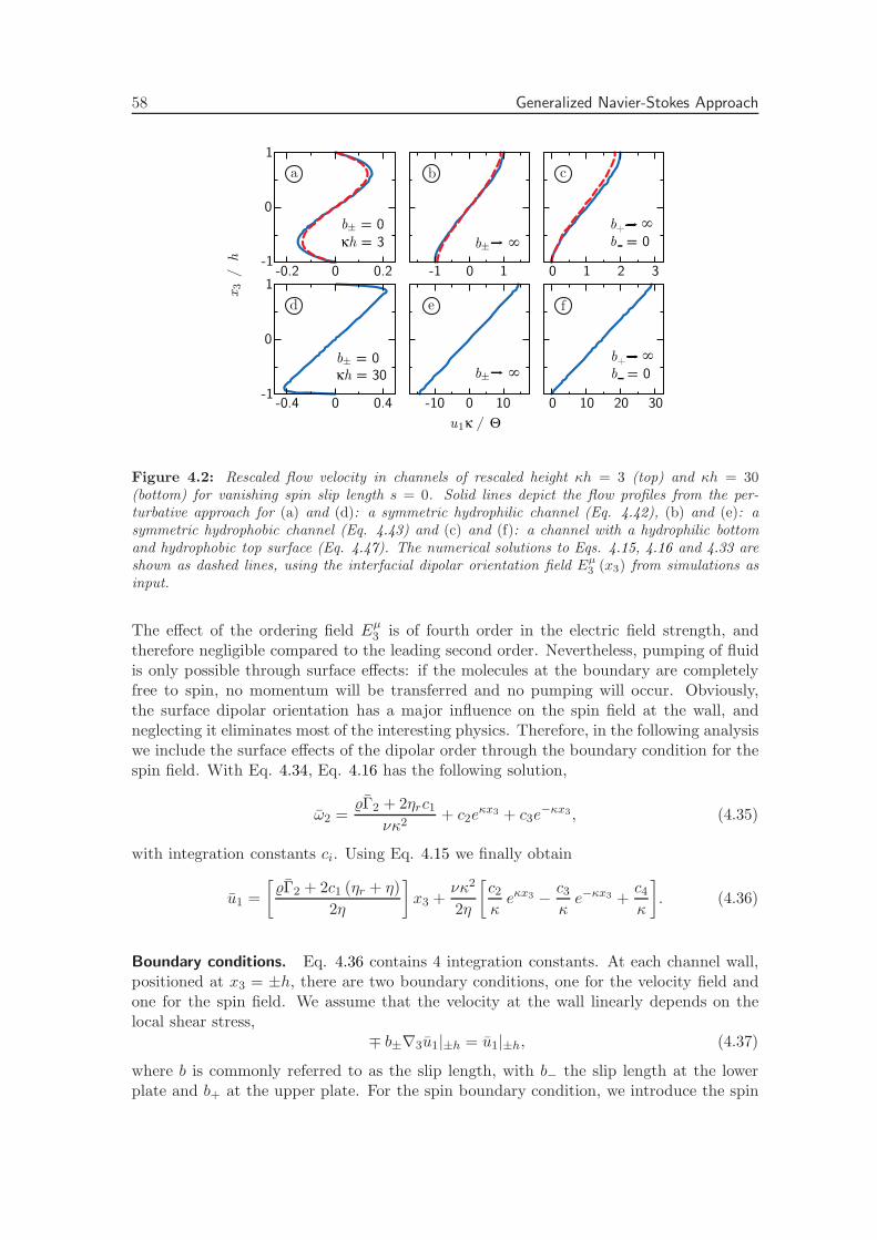
58 Generalized Navier-Stokes Approach
-1
0
1
κh = 3
-0.2 0 0.2
b± = 0
-1 10
b± ∞
-0.4 0 0.4 3020100
0 1 32
-1
0
1
-10 0 10
b+ ∞
b = 0
κh = 30b± = 0
b± ∞b+ ∞
b = 0
u1κ / Θ
x3 /
h
a b c
ed f
Figure 4.2: Rescaled flow velocity in channels of rescaled height κh = 3 (top) and κh = 30(bottom) for vanishing spin slip length s = 0. Solid lines depict the flow profiles from the per-turbative approach for (a) and (d): a symmetric hydrophilic channel (Eq. 4.42), (b) and (e): asymmetric hydrophobic channel (Eq. 4.43) and (c) and (f): a channel with a hydrophilic bottomand hydrophobic top surface (Eq. 4.47). The numerical solutions to Eqs. 4.15, 4.16 and 4.33 areshown as dashed lines, using the interfacial dipolar orientation field Eµ
3 (x3) from simulations asinput.
The effect of the ordering field Eµ3 is of fourth order in the electric field strength, andtherefore negligible compared to the leading second order. Nevertheless, pumping of fluidis only possible through surface effects: if the molecules at the boundary are completelyfree to spin, no momentum will be transferred and no pumping will occur. Obviously,the surface dipolar orientation has a major influence on the spin field at the wall, andneglecting it eliminates most of the interesting physics. Therefore, in the following analysiswe include the surface effects of the dipolar order through the boundary condition for thespin field. With Eq. 4.34, Eq. 4.16 has the following solution,
ω2 =Γ2 + 2ηrc1
νκ2+ c2e
κx3 + c3e−κx3, (4.35)
with integration constants ci. Using Eq. 4.15 we finally obtain
u1 =
[
Γ2 + 2c1 (ηr + η)
2η
]
x3 +νκ2
2η
[
c2κeκx3 − c3
κe−κx3 +
c4κ
]
. (4.36)
Boundary conditions. Eq. 4.36 contains 4 integration constants. At each channel wall,positioned at x3 = ±h, there are two boundary conditions, one for the velocity field andone for the spin field. We assume that the velocity at the wall linearly depends on thelocal shear stress,
∓ b±∇3u1|±h = u1|±h, (4.37)
where b is commonly referred to as the slip length, with b− the slip length at the lowerplate and b+ at the upper plate. For the spin boundary condition, we introduce the spin
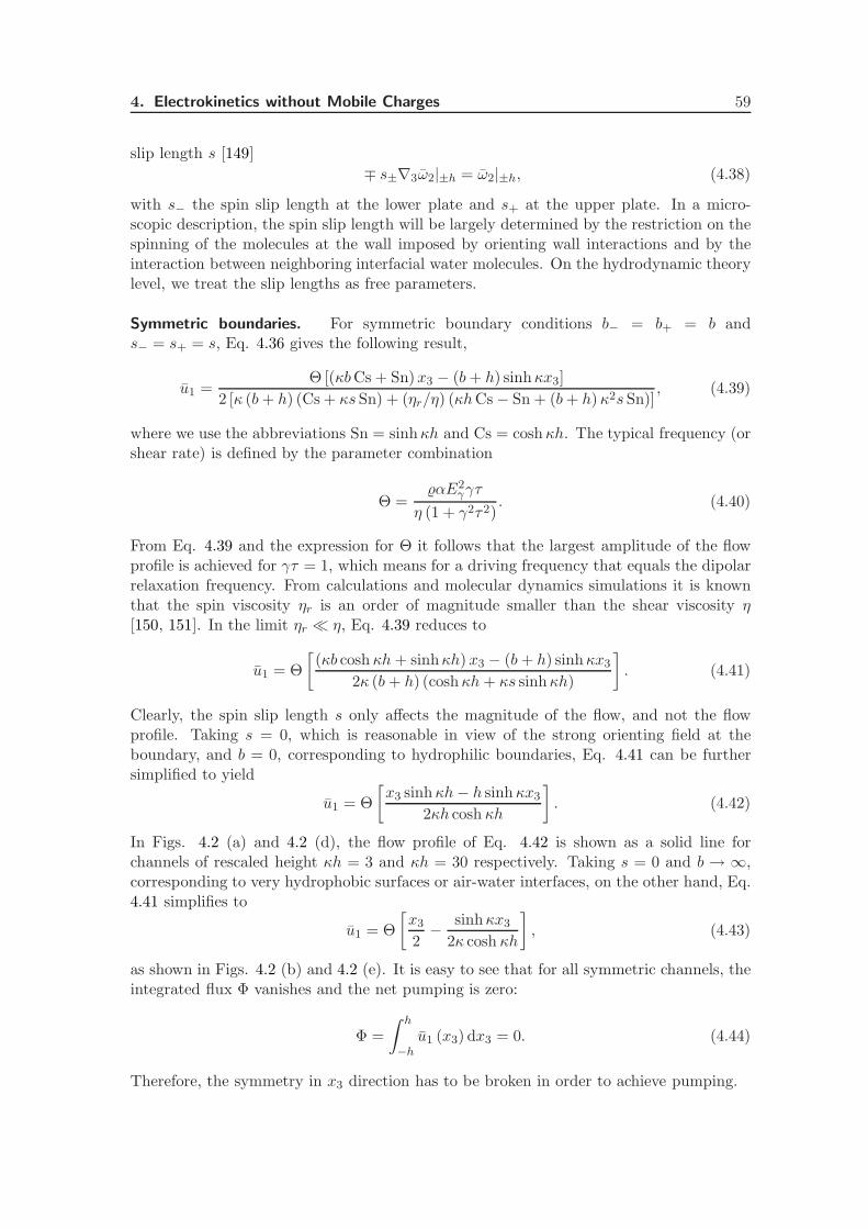
4. Electrokinetics without Mobile Charges 59
slip length s [149]
∓ s±∇3ω2|±h = ω2|±h, (4.38)
with s− the spin slip length at the lower plate and s+ at the upper plate. In a micro-scopic description, the spin slip length will be largely determined by the restriction on thespinning of the molecules at the wall imposed by orienting wall interactions and by theinteraction between neighboring interfacial water molecules. On the hydrodynamic theorylevel, we treat the slip lengths as free parameters.
Symmetric boundaries. For symmetric boundary conditions b− = b+ = b ands− = s+ = s, Eq. 4.36 gives the following result,
u1 =Θ [(κbCs + Sn)x3 − (b+ h) sinhκx3]
2 [κ (b+ h) (Cs + κs Sn) + (ηr/η) (κhCs − Sn + (b+ h)κ2s Sn)], (4.39)
where we use the abbreviations Sn = sinhκh and Cs = coshκh. The typical frequency (orshear rate) is defined by the parameter combination
Θ =αE2
γγτ
η (1 + γ2τ2). (4.40)
From Eq. 4.39 and the expression for Θ it follows that the largest amplitude of the flowprofile is achieved for γτ = 1, which means for a driving frequency that equals the dipolarrelaxation frequency. From calculations and molecular dynamics simulations it is knownthat the spin viscosity ηr is an order of magnitude smaller than the shear viscosity η[150, 151]. In the limit ηr ≪ η, Eq. 4.39 reduces to
u1 = Θ
[
(κb cosh κh+ sinhκh) x3 − (b+ h) sinhκx3
2κ (b+ h) (coshκh+ κs sinhκh)
]
. (4.41)
Clearly, the spin slip length s only affects the magnitude of the flow, and not the flowprofile. Taking s = 0, which is reasonable in view of the strong orienting field at theboundary, and b = 0, corresponding to hydrophilic boundaries, Eq. 4.41 can be furthersimplified to yield
u1 = Θ
[
x3 sinhκh− h sinhκx3
2κh cosh κh
]
. (4.42)
In Figs. 4.2 (a) and 4.2 (d), the flow profile of Eq. 4.42 is shown as a solid line forchannels of rescaled height κh = 3 and κh = 30 respectively. Taking s = 0 and b → ∞,corresponding to very hydrophobic surfaces or air-water interfaces, on the other hand, Eq.4.41 simplifies to
u1 = Θ
[
x3
2− sinhκx3
2κ cosh κh
]
, (4.43)
as shown in Figs. 4.2 (b) and 4.2 (e). It is easy to see that for all symmetric channels, theintegrated flux Φ vanishes and the net pumping is zero:
Φ =
∫ h
−hu1 (x3) dx3 = 0. (4.44)
Therefore, the symmetry in x3 direction has to be broken in order to achieve pumping.

60 Generalized Navier-Stokes Approach
Asymmetric boundaries. We consider the limiting case of a channel with a hydrophilicbottom surface (b− = 0) and a hydrophobic top surface (b+ → ∞). For symmetric spinslip conditions s− = s+ = s we find from Eq. 4.36
u1 = Θ
[
(x3 + h)κ cosh κh− sinhκh− sinhκx3
2κ (coshκh+ (1 + ηr/η) κs sinhκh)
]
, (4.45)
which for ηr ≪ η reduces to
u1 = Θ
[
(x3 + h)κ cosh κh− sinhκh− sinhκx3
2κ (coshκh+ κs sinhκh)
]
. (4.46)
For reasons already mentioned – and because again the spin slip length does not affect theshape of the flow profile – we set it to zero, s = 0, leading to
u1 = Θ
[
x3 + h
2− sinhκh+ sinhκx3
2κ cosh κh
]
. (4.47)
The profile of Eq. 4.47 is shown in Figs. 4.2 (c) and 4.2 (f) as solid lines. In the asymmetriccase, the integrated flow of the channel is for large channels (κh ≪ 1) given by
Φ =
∫ h
−hu1dx3 ≃ Θh2, (4.48)
and thus Φ is clearly finite. It follows by comparison with simple shear flow that Θ is ameasure of the shear rate in the channel.
4.2.7 Numerical Solution
To verify the validity of the assumptions inherent to the perturbative approximation,we solve Eq. 4.16 with Eq. 4.33 for the spin field and Eq. 4.15 for the velocity fieldnumerically, subject to the boundary conditions of Eqs. 4.37 and 4.38. As input, thepolarizability α and relaxation time τ are needed, as well as the interfacial orientingdipole field Eµ3 . To obtain those parameters we perform a series of molecular dynamicssimulations.
Relaxation parameters. We simulate a box of 2180 spc/e water molecules (4.0 × 4.0 ×4.0 nm, isotropic pressure coupling, periodic boundary conditions in all directions) withan initially isotropic distribution of water dipoles. At t = 0 we turn on an electric field inx1 direction of strength E0
1 = 0.1 Vnm−1. Relative to experimental values this is a strongelectric field, but it is verified that the response is still reasonably linear. We perform 10cycles of orientation (field turned on for 25 ps) and relaxation (field turned off for 25 ps),and average the result of the orientation part of each cycle. In Fig. 4.3 (a), we plot theaverage dipole moment per water molecule as a function of time. With a molecular dipolemoment of spc/e water of µspc/e = 0.05 nm e, we see that the dipolar orientation issufficiently far from being saturated and we are thus in the linear-response regime. WithE = E0
1 e1 and µ1 = 0 at t = 0, the solution to Eq. 4.20 is
µ1 = αE01
(
1 − e−t/τ)
. (4.49)
Fitting Eq. 4.49 to the curve in Fig. 4.3 (a) gives a dipolar relaxation time of τ = 7±2 psand a polarizability per unit mass of α = 3.3±0.3×10⁶ m2eV−1kg−1, with e the elementary
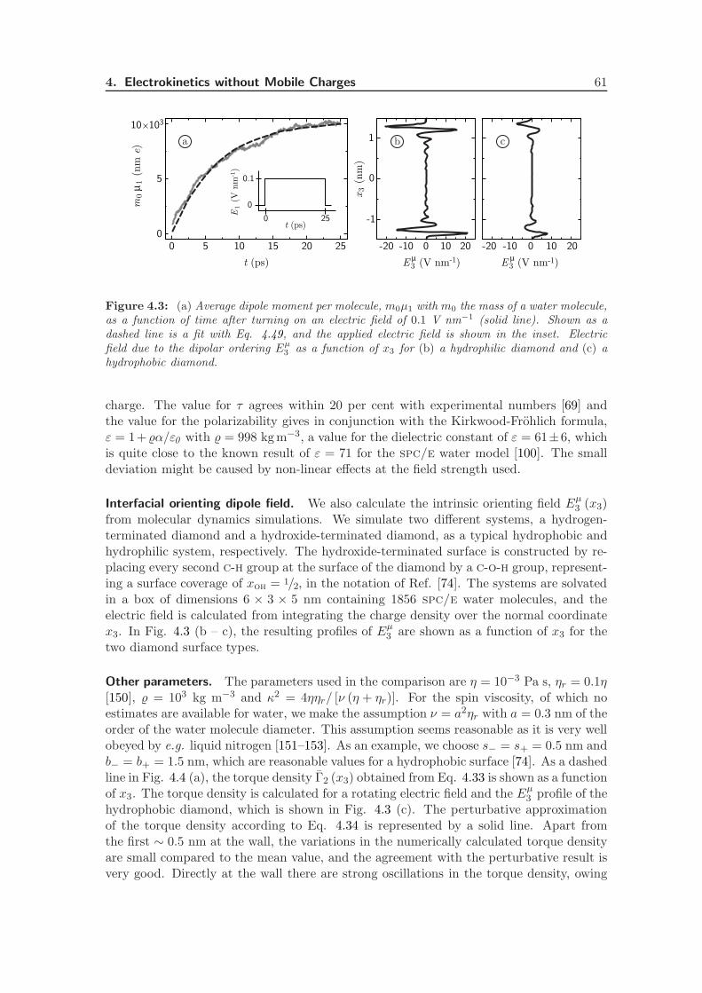
4. Electrokinetics without Mobile Charges 61
0 5 10 15 20 250
0
0
25
0.1
-20 -10 20 -20 -10 20
-1
0
1
5
10310m
0 µ
1 (
nm
e)
100 100
t (ps) E3 (V nm-1)µE3 (V nm-1)µ
x3 (
nm
)
t (ps)E
1 (
V n
m-1)
a b c
Figure 4.3: (a) Average dipole moment per molecule, m0µ1 with m0 the mass of a water molecule,as a function of time after turning on an electric field of 0.1 V nm−1 (solid line). Shown as adashed line is a fit with Eq. 4.49, and the applied electric field is shown in the inset. Electricfield due to the dipolar ordering Eµ
3 as a function of x3 for (b) a hydrophilic diamond and (c) ahydrophobic diamond.
charge. The value for τ agrees within 20 per cent with experimental numbers [69] andthe value for the polarizability gives in conjunction with the Kirkwood-Frohlich formula,ε = 1+α/ε0 with = 998 kgm−3, a value for the dielectric constant of ε = 61±6, whichis quite close to the known result of ε = 71 for the spc/e water model [100]. The smalldeviation might be caused by non-linear effects at the field strength used.
Interfacial orienting dipole field. We also calculate the intrinsic orienting field Eµ3 (x3)from molecular dynamics simulations. We simulate two different systems, a hydrogen-terminated diamond and a hydroxide-terminated diamond, as a typical hydrophobic andhydrophilic system, respectively. The hydroxide-terminated surface is constructed by re-placing every second c-h group at the surface of the diamond by a c-o-h group, represent-ing a surface coverage of xoh = 1/2, in the notation of Ref. [74]. The systems are solvatedin a box of dimensions 6 × 3 × 5 nm containing 1856 spc/e water molecules, and theelectric field is calculated from integrating the charge density over the normal coordinatex3. In Fig. 4.3 (b – c), the resulting profiles of Eµ3 are shown as a function of x3 for thetwo diamond surface types.
Other parameters. The parameters used in the comparison are η = 10−3 Pa s, ηr = 0.1η[150], = 103 kg m−3 and κ2 = 4ηηr/ [ν (η + ηr)]. For the spin viscosity, of which noestimates are available for water, we make the assumption ν = a2ηr with a = 0.3 nm of theorder of the water molecule diameter. This assumption seems reasonable as it is very wellobeyed by e.g. liquid nitrogen [151–153]. As an example, we choose s− = s+ = 0.5 nm andb− = b+ = 1.5 nm, which are reasonable values for a hydrophobic surface [74]. As a dashedline in Fig. 4.4 (a), the torque density Γ2 (x3) obtained from Eq. 4.33 is shown as a functionof x3. The torque density is calculated for a rotating electric field and the Eµ3 profile of thehydrophobic diamond, which is shown in Fig. 4.3 (c). The perturbative approximationof the torque density according to Eq. 4.34 is represented by a solid line. Apart fromthe first ∼ 0.5 nm at the wall, the variations in the numerically calculated torque densityare small compared to the mean value, and the agreement with the perturbative result isvery good. Directly at the wall there are strong oscillations in the torque density, owing
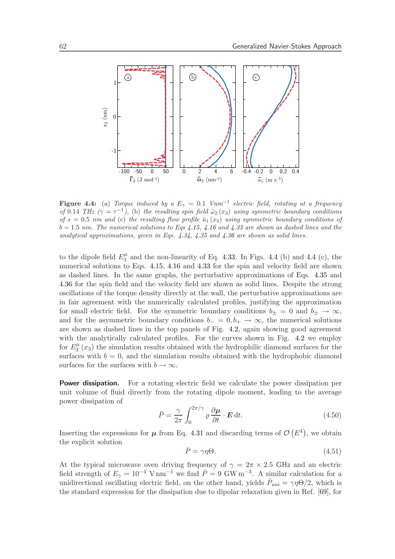
62 Generalized Navier-Stokes Approach
-0.4 -0.2 0 0.2 0.4
Γ2 (J mol-1) ω2 (nm-1) u1 (m s -1)
6420
-1
0
1
-100 -50 0 50
x3 (
nm
)
a b c
Figure 4.4: (a) Torque induced by a Eγ = 0.1 Vnm−1 electric field, rotating at a frequencyof 0.14 THz (γ = τ−1), (b) the resulting spin field ω2 (x3) using symmetric boundary conditionsof s = 0.5 nm and (c) the resulting flow profile u1 (x3) using symmetric boundary conditions ofb = 1.5 nm. The numerical solutions to Eqs 4.15, 4.16 and 4.33 are shown as dashed lines and theanalytical approximations, given in Eqs. 4.34, 4.35 and 4.36 are shown as solid lines.
to the dipole field Eµ3 and the non-linearity of Eq. 4.33. In Figs. 4.4 (b) and 4.4 (c), thenumerical solutions to Eqs. 4.15, 4.16 and 4.33 for the spin and velocity field are shownas dashed lines. In the same graphs, the perturbative approximations of Eqs. 4.35 and4.36 for the spin field and the velocity field are shown as solid lines. Despite the strongoscillations of the torque density directly at the wall, the perturbative approximations arein fair agreement with the numerically calculated profiles, justifying the approximationfor small electric field. For the symmetric boundary conditions b± = 0 and b± → ∞,and for the asymmetric boundary conditions b− = 0, b+ → ∞, the numerical solutionsare shown as dashed lines in the top panels of Fig. 4.2, again showing good agreementwith the analytically calculated profiles. For the curves shown in Fig. 4.2 we employfor Eµ3 (x3) the simulation results obtained with the hydrophilic diamond surfaces for thesurfaces with b = 0, and the simulation results obtained with the hydrophobic diamondsurfaces for the surfaces with b→ ∞.
Power dissipation. For a rotating electric field we calculate the power dissipation perunit volume of fluid directly from the rotating dipole moment, leading to the averagepower dissipation of
P =γ
2π
∫ 2π/γ
0∂µ
∂t· E dt. (4.50)
Inserting the expressions for µ from Eq. 4.31 and discarding terms of O(
E4)
, we obtainthe explicit solution
P = γηΘ. (4.51)
At the typical microwave oven driving frequency of γ = 2π × 2.5 GHz and an electricfield strength of Eγ = 10−4 Vnm−1 we find P = 9 GWm−3. A similar calculation for aunidirectional oscillating electric field, on the other hand, yields Puni = γηΘ/2, which isthe standard expression for the dissipation due to dipolar relaxation given in Ref. [69], for
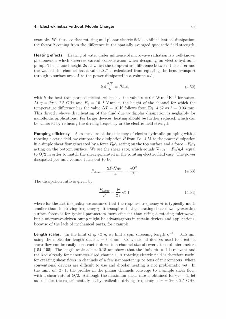
4. Electrokinetics without Mobile Charges 63
example. We thus see that rotating and planar electric fields exhibit identical dissipation;the factor 2 coming from the difference in the spatially averaged quadratic field strength.
Heating effects. Heating of water under influence of microwave radiation is a well-knownphenomenon which deserves careful consideration when designing an electro-hydraulicpump. The channel height 2h at which the temperature difference between the center andthe wall of the channel has a value ∆T is calculated from equating the heat transportthrough a surface area A to the power dissipated in a volume hA,
kA∆T
h= P hA, (4.52)
with k the heat transport coefficient, which has the value k = 0.6 Wm−1K−1 for water.At γ = 2π × 2.5 GHz and Eγ = 10−4 Vnm−1, the height of the channel for which thetemperature difference has the value ∆T = 10 K follows from Eq. 4.52 as h = 0.03 mm.This directly shows that heating of the fluid due to dipolar dissipation is negligible fornanofluidic applications. For larger devices, heating should be further reduced, which canbe achieved by reducing the driving frequency or the electric field strength.
Pumping efficiency. As a measure of the efficiency of electro-hydraulic pumping with arotating electric field, we compare the dissipation P from Eq. 4.51 to the power dissipationin a simple shear flow generated by a force F0e1 acting on the top surface and a force −F0e1acting on the bottom surface. We set the shear rate, which equals ∇3u1 = F0/ηA, equalto Θ/2 in order to match the shear generated in the rotating electric field case. The powerdissipated per unit volume turns out to be
Pshear =2F0∇3u1
A =ηΘ2
2. (4.53)
The dissipation ratio is given by
Pshear
P=
Θ
2γ≪ 1, (4.54)
where for the last inequality we assumed that the response frequency Θ is typically muchsmaller than the driving frequency γ. It transpires that generating shear flows by exertingsurface forces is for typical parameters more efficient than using a rotating microwave,but a microwave-driven pump might be advantageous in certain devices and applications,because of the lack of mechanical parts, for example.
Length scales. In the limit of ηr ≪ η, we find a spin screening length κ−1 = 0.15 nm,using the molecular length scale a = 0.3 nm. Conventional devices used to create ashear flow can be easily constructed down to a channel size of several tens of micrometers[154, 155]. The length scale κ−1 ≃ 0.15 nm shows that the limit κh ≫ 1 is relevant andrealized already for nanometer-sized channels. A rotating electric field is therefore usefulfor creating shear flows in channels of a few nanometer up to tens of micrometers, whereconventional devices are difficult to use and dipolar heating is not problematic yet. Inthe limit κh ≫ 1, the profiles in the planar channels converge to a simple shear flow,with a shear rate of Θ/2. Although the maximum shear rate is obtained for γτ = 1, letus consider the experimentally easily realizable driving frequency of γ = 2π × 2.5 GHz,

64 Generalized Navier-Stokes Approach
which is the driving frequency of a common microwave oven. For a realistic external fieldstrength Eγ = 10−4 V nm−1, water viscosity η = 10−3 Pa s and density = 103 kg m−3
we find a response frequency of Θ = 570 s−1 and thus predict sizeable shear effects.
4.2.8 Cylindrical Geometry
We take x1 to be the axial coordinate, x2 the angular coordinate and x3 the radial co-ordinate, see Fig. 4.1 (b). Note that this is an uneven permutation of the usual form ofthe cylindrical coordinates. Again, we assume u = e1u1 (x3) (axial flow) and ω = ω (x3)(only dependent on the radial coordinate). The Navier Stokes equation transforms to
du1
dt=
η
x3
∂
∂x3
(
x3∂u1
∂x3
)
+ηrx3
∂
∂x3
(
x3∂u1
∂x3− 2x3ω2
)
(4.55)
Integrating Eq. 4.55 once over x3 yields in the stationary state
0 = (η + ηr)∂u1
∂x3− 2ηrω2 −
c1 (η + ηr)
x3. (4.56)
At the same time,
Idω2
dt= Γ2 + 2ηr
(
∂u1
∂x3− 2ω2
)
+ν
x3
∂
∂x3
(
x3∂ω2
∂x3
)
. (4.57)
Combining Eqs. 4.56 and 4.57 gives the cylindrical equivalent of Eq. 4.16,
0 =Γ2
ν+(
∇23 − κ2
)
ω2 +2c1ηrνx3
, (4.58)
with ∇23 = x−1
3 (∂/∂x3) x3 (∂/∂x3). In this section we solve Eqs. 4.56 and 4.58 for differentscenarios.
Static electric field. The torque resulting from a static electric field is given again byEq. 4.22. In analogy to the planar case, a static field does not induce a flow through thenanotube.
Constant torque. A steady-state torque, on the other hand, will induce a flow in thecylindrical geometry. Equivalent to the planar case, the torque resulting from a rotatingelectric field is in good approximation a constant given by Eq. 4.34. Different from theplanar situation, however, Eq. 4.58 with constant Γ2 does not have an analytical solution.Therefore, we solve Eq. 4.58 numerically, after which the velocity profile is calculated fromintegrating Eq. 4.56. The geometry needed to generate an electric field rotating in thex1 −x3 plane consists of two concentric cylinders with radii R1 and R2, with the radius ofthe inner cylinder R1 > 0 because Eq. 4.58 diverges in the limit x3 → 0. A rotating fieldis generated by applying a sine-like potential difference between the inner cylinder and theouter cylinder, and a cosine-like potential difference between two additional electrodes atboth ends of the tube. The boundary conditions at x3 = R1, R2 are given by the equivalentexpressions of Eqs. 4.37 and 4.38. Due to the intrinsic asymmetry of the system in x3
direction, the velocity profile not only depends on the difference R2 −R1, but also on theabsolute value of R1. For R1 → ∞, Eq. 4.58 approaches Eq. 4.16, so we only treat thecase for small R1 here. In Fig. 4.5, the numerically calculated flow profile is shown for two
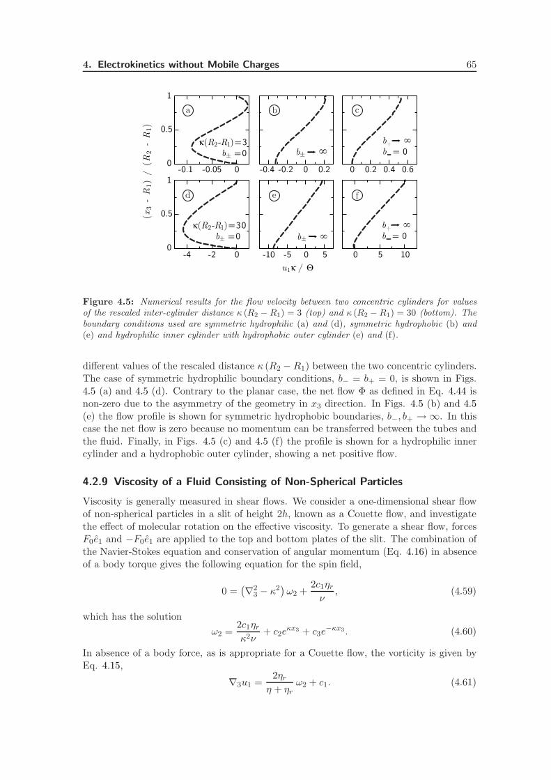
4. Electrokinetics without Mobile Charges 65
0
0.5
1
-0.1 -0.05 0 -0.4 -0.2 0 0.2
-4 -2 0 -10 -5 0 5 0 5 10
0 0.2 0.4 0.6
u1κ / Θ
(x3 -
R1)
/ (
R2 -
R1)
0
0.5
1
a b c
ed f
b± =0 b± ∞b+ ∞
b = 0κ(R2-R1)=3
b± =0κ(R2-R1)=30
b± ∞b+ ∞
b = 0
Figure 4.5: Numerical results for the flow velocity between two concentric cylinders for valuesof the rescaled inter-cylinder distance κ (R2 −R1) = 3 (top) and κ (R2 −R1) = 30 (bottom). Theboundary conditions used are symmetric hydrophilic (a) and (d), symmetric hydrophobic (b) and(e) and hydrophilic inner cylinder with hydrophobic outer cylinder (e) and (f).
different values of the rescaled distance κ (R2 −R1) between the two concentric cylinders.The case of symmetric hydrophilic boundary conditions, b− = b+ = 0, is shown in Figs.4.5 (a) and 4.5 (d). Contrary to the planar case, the net flow Φ as defined in Eq. 4.44 isnon-zero due to the asymmetry of the geometry in x3 direction. In Figs. 4.5 (b) and 4.5(e) the flow profile is shown for symmetric hydrophobic boundaries, b−, b+ → ∞. In thiscase the net flow is zero because no momentum can be transferred between the tubes andthe fluid. Finally, in Figs. 4.5 (c) and 4.5 (f) the profile is shown for a hydrophilic innercylinder and a hydrophobic outer cylinder, showing a net positive flow.
4.2.9 Viscosity of a Fluid Consisting of Non-Spherical Particles
Viscosity is generally measured in shear flows. We consider a one-dimensional shear flowof non-spherical particles in a slit of height 2h, known as a Couette flow, and investigatethe effect of molecular rotation on the effective viscosity. To generate a shear flow, forcesF0e1 and −F0e1 are applied to the top and bottom plates of the slit. The combination ofthe Navier-Stokes equation and conservation of angular momentum (Eq. 4.16) in absenceof a body torque gives the following equation for the spin field,
0 =(
∇23 − κ2
)
ω2 +2c1ηrν
, (4.59)
which has the solution
ω2 =2c1ηrκ2ν
+ c2eκx3 + c3e
−κx3. (4.60)
In absence of a body force, as is appropriate for a Couette flow, the vorticity is given byEq. 4.15,
∇3u1 =2ηrη + ηr
ω2 + c1. (4.61)
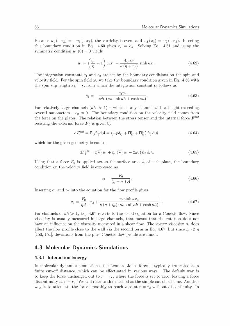
66 Molecular Dynamics Simulations
Because u1 (−x3) = −u1 (−x3), the vorticity is even, and ω2 (x3) = ω2 (−x3). Insertingthis boundary condition in Eq. 4.60 gives c2 = c3. Solving Eq. 4.61 and using thesymmetry condition u1 (0) = 0 yields
u1 =
(
ηrη
+ 1
)
c1x3 +4ηrc2
κ (η + ηr)sinhκx3. (4.62)
The integration constants c1 and c2 are set by the boundary conditions on the spin andvelocity field. For the spin field ω2 we take the boundary condition given in Eq. 4.38 withthe spin slip length s± = s, from which the integration constant c2 follows as
c2 = − c1ηrκ2ν (κs sinhκh+ coshκh)
. (4.63)
For relatively large channels (κh ≫ 1) – which is any channel with a height exceedingseveral nanometers – c2 ≈ 0. The boundary condition on the velocity field comes fromthe force on the plates. The relation between the stress tensor and the internal force F int
resisting the external force F 0 is given by
dF inti = PijnjdA =
(
−pδij + Πsij + Πaij)
nj dA, (4.64)
which for the given geometry becomes
dF int1 = η∇3u1 + ηr (∇3u1 − 2ω2) n3 dA. (4.65)
Using that a force F0 is applied across the surface area A of each plate, the boundarycondition on the velocity field is expressed as
c1 =F0
(η + ηr)A. (4.66)
Inserting c1 and c2 into the equation for the flow profile gives
u1 =F0
ηA
[
x3 +ηr sinhκx3
κ (η + ηr) (κs sinhκh+ coshκh)
]
. (4.67)
For channels of kh ≫ 1, Eq. 4.67 reverts to the usual equation for a Couette flow. Sinceviscosity is usually measured in large channels, that means that the rotation does nothave an influence on the viscosity measured in a shear flow. The vortex viscosity ηr doesaffect the flow profile close to the wall via the second term in Eq. 4.67, but since ηr ≪ η[150, 151], deviations from the pure Couette flow profile are minor.
4.3 Molecular Dynamics Simulations
4.3.1 Interaction Energy
In molecular dynamics simulations, the Lennard-Jones force is typically truncated at afinite cut-off distance, which can be effectuated in various ways. The default way isto keep the force unchanged out to r = rc, where the force is set to zero, leaving a forcediscontinuity at r = rc. We will refer to this method as the simple cut-off scheme. Anotherway is to attenuate the force smoothly to reach zero at r = rc without discontinuity. In

4. Electrokinetics without Mobile Charges 67
0.4 0.6 0.8 1.0 1.2
r (nm)
-6
-5
-4
-3
-2
-1
0
1
OriginalSimpleShifted
0.7 0.8 0.9
-0.2
-0.1
0
0.7 0.8 0.9
-0.2
-0.1
0F
O-O
(kJ m
ol-1
nm
-1)
Figure 4.6: Truncated Lennard-Jones force between two water molecules for rc = 0.8 nm for thetwo different truncation schemes. Also shown is the original Lennard-Jones force. Details of thetruncation region are shown in the insets for the simple cut-off (left) and the shifted cut-off scheme(right).
gromacs, this so-called shifted force Fs is implemented by adding a non-linear functionto the original force Fo,
Fs =
Fo + ar2 + br3 if r < rc0 if r ≥ rc.
(4.68)
The coefficients a and b are given by
a = −768 ǫ σ12 r−15c + 240 ǫ σ6 r−9
c
b = 720 ǫ σ12 r−16c − 216 ǫ σ6 r−10
c , (4.69)
with ǫ and σ the parameters of the Lennard-Jones interaction and rc the truncation lengthin nanometers. The original Lennard-Jones force is given by
Fo = 4ǫ
[
12σ12
r13− 6
σ6
r7
]
. (4.70)
The interactions between dissimilar atoms are calculated by ǫij =√ǫiǫj and σij =
√σiσj,
with i and j indices denoting atom type. Examples of the simple and the shifted force areplotted in Fig. 4.6. The curves have been verified by running simulations of two collidingparticles.
Other simulation details. The long-range electrostatics are handled using particle meshEwald summation. For the simple cut-off scheme, the real-space truncation length forboth the Coulomb interaction and the Lennard-Jones interaction is set equal to the listradius, which is the default option in gromacs. For the simple cut-off scheme, settingthe list radius larger than the truncation length is not allowed in gromacs. For theshifted scheme, the real-space truncation length for the Coulomb interaction and thelist radius is set 0.2 nm larger than the Lennard-Jones interaction. The temperature is
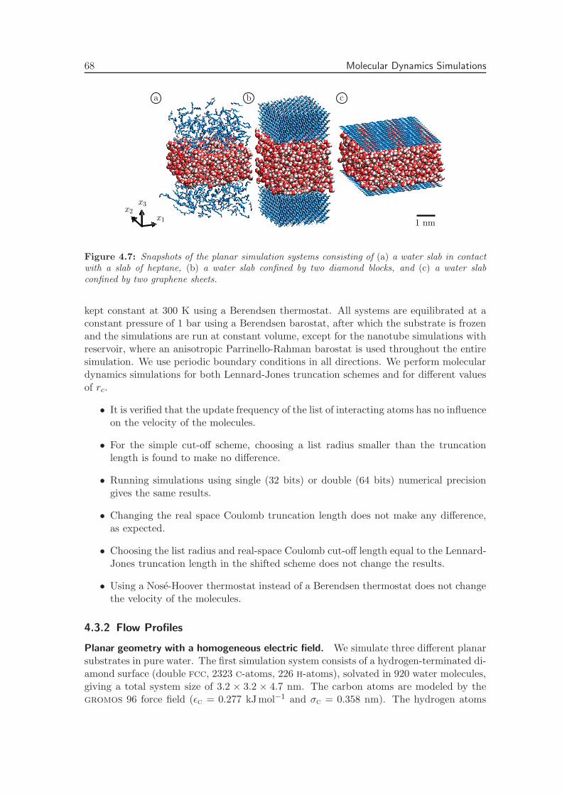
68 Molecular Dynamics Simulations
1 nm
a b c
x1
x3x2
Figure 4.7: Snapshots of the planar simulation systems consisting of (a) a water slab in contactwith a slab of heptane, (b) a water slab confined by two diamond blocks, and (c) a water slabconfined by two graphene sheets.
kept constant at 300 K using a Berendsen thermostat. All systems are equilibrated at aconstant pressure of 1 bar using a Berendsen barostat, after which the substrate is frozenand the simulations are run at constant volume, except for the nanotube simulations withreservoir, where an anisotropic Parrinello-Rahman barostat is used throughout the entiresimulation. We use periodic boundary conditions in all directions. We perform moleculardynamics simulations for both Lennard-Jones truncation schemes and for different valuesof rc.
• It is verified that the update frequency of the list of interacting atoms has no influenceon the velocity of the molecules.
• For the simple cut-off scheme, choosing a list radius smaller than the truncationlength is found to make no difference.
• Running simulations using single (32 bits) or double (64 bits) numerical precisiongives the same results.
• Changing the real space Coulomb truncation length does not make any difference,as expected.
• Choosing the list radius and real-space Coulomb cut-off length equal to the Lennard-Jones truncation length in the shifted scheme does not change the results.
• Using a Nose-Hoover thermostat instead of a Berendsen thermostat does not changethe velocity of the molecules.
4.3.2 Flow Profiles
Planar geometry with a homogeneous electric field. We simulate three different planarsubstrates in pure water. The first simulation system consists of a hydrogen-terminated di-amond surface (double fcc, 2323 c-atoms, 226 h-atoms), solvated in 920 water molecules,giving a total system size of 3.2 × 3.2 × 4.7 nm. The carbon atoms are modeled by thegromos 96 force field (ǫc = 0.277 kJ mol−1 and σc = 0.358 nm). The hydrogen atoms
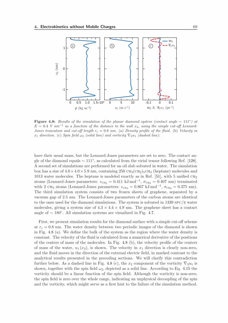
4. Electrokinetics without Mobile Charges 69
0 0.5 1.0
-1
0
1
-0.1 0 0.10 5 10
∆a b c
x3 (
nm
)
1031.5
ω2
3u1
ρ (kg m -3) u1 (m s -1) ω2 & 3u1 (ps -1)∆
Figure 4.8: Results of the simulation of the planar diamond system (contact angle ∼ 111) atE = 0.4 V nm−1 as a function of the distance to the wall x3, using the simple cut-off Lennard-Jones truncation and cut-off length rc = 0.8 nm. (a) Density profile of the fluid. (b) Velocity inx1 direction. (c) Spin field ω2 (solid line) and vorticity ∇3u1 (dashed line).
have their usual mass, but the Lennard-Jones parameters are set to zero. The contact an-gle of the diamond equals ∼ 111, as calculated from the virial tensor following Ref. [128].A second set of simulations are performed for an oil slab solvated in water. The simulationbox has a size of 4.0×4.0×5.9 nm, containing 250 ch3(ch2)5ch3 (heptane) molecules and1013 water molecules. The heptane is modeled exactly as in Ref. [51], with 5 unified ch2
atoms (Lennard-Jones parameters: ǫch2= 0.411 kJ mol−1, σch2
= 0.407 nm) terminatedwith 2 ch3 atoms (Lennard-Jones parameters: ǫch3
= 0.867 kJ mol−1, σch3= 0.375 nm).
The third simulation system consists of two frozen sheets of graphene, separated by avacuum gap of 2.5 nm. The Lennard-Jones parameters of the carbon atoms are identicalto the ones used for the diamond simulations. The system is solvated in 1339 spc/e watermolecules, giving a system size of 4.3 × 4.4 × 4.9 nm. The graphene sheet has a contactangle of ∼ 180. All simulation systems are visualized in Fig. 4.7.
First, we present simulation results for the diamond surface with a simple cut-off schemeat rc = 0.8 nm. The water density between two periodic images of the diamond is shownin Fig. 4.8 (a). We define the bulk of the system as the region where the water density isconstant. The velocity of the fluid is calculated from a numerical derivative of the positionsof the centers of mass of the molecules. In Fig. 4.8 (b), the velocity profile of the centersof mass of the water, u1 (x3), is shown. The velocity in x1 direction is clearly non-zero,and the fluid moves in the direction of the external electric field, in marked contrast to theanalytical results presented in the preceding sections. We will clarify this contradictionfurther below. As a dashed line in Fig. 4.8 (c), the x2 component of the vorticity ∇3u1 isshown, together with the spin field ω2, depicted as a solid line. According to Eq. 4.15 thevorticity should be a linear function of the spin field. Although the vorticity is non-zero,the spin field is zero over the whole range, indicating an unphysical decoupling of the spinand the vorticity, which might serve as a first hint to the failure of the simulation method.
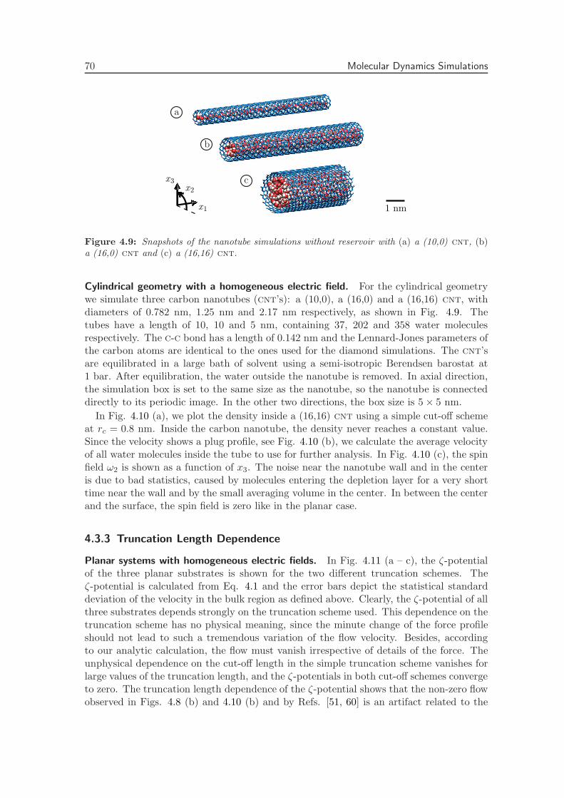
70 Molecular Dynamics Simulations
1 nm
a
b
c
x1
x3x2
Figure 4.9: Snapshots of the nanotube simulations without reservoir with (a) a (10,0) cnt, (b)a (16,0) cnt and (c) a (16,16) cnt.
Cylindrical geometry with a homogeneous electric field. For the cylindrical geometrywe simulate three carbon nanotubes (cnt’s): a (10,0), a (16,0) and a (16,16) cnt, withdiameters of 0.782 nm, 1.25 nm and 2.17 nm respectively, as shown in Fig. 4.9. Thetubes have a length of 10, 10 and 5 nm, containing 37, 202 and 358 water moleculesrespectively. The c-c bond has a length of 0.142 nm and the Lennard-Jones parameters ofthe carbon atoms are identical to the ones used for the diamond simulations. The cnt’sare equilibrated in a large bath of solvent using a semi-isotropic Berendsen barostat at1 bar. After equilibration, the water outside the nanotube is removed. In axial direction,the simulation box is set to the same size as the nanotube, so the nanotube is connecteddirectly to its periodic image. In the other two directions, the box size is 5 × 5 nm.
In Fig. 4.10 (a), we plot the density inside a (16,16) cnt using a simple cut-off schemeat rc = 0.8 nm. Inside the carbon nanotube, the density never reaches a constant value.Since the velocity shows a plug profile, see Fig. 4.10 (b), we calculate the average velocityof all water molecules inside the tube to use for further analysis. In Fig. 4.10 (c), the spinfield ω2 is shown as a function of x3. The noise near the nanotube wall and in the centeris due to bad statistics, caused by molecules entering the depletion layer for a very shorttime near the wall and by the small averaging volume in the center. In between the centerand the surface, the spin field is zero like in the planar case.
4.3.3 Truncation Length Dependence
Planar systems with homogeneous electric fields. In Fig. 4.11 (a – c), the ζ-potentialof the three planar substrates is shown for the two different truncation schemes. Theζ-potential is calculated from Eq. 4.1 and the error bars depict the statistical standarddeviation of the velocity in the bulk region as defined above. Clearly, the ζ-potential of allthree substrates depends strongly on the truncation scheme used. This dependence on thetruncation scheme has no physical meaning, since the minute change of the force profileshould not lead to such a tremendous variation of the flow velocity. Besides, accordingto our analytic calculation, the flow must vanish irrespective of details of the force. Theunphysical dependence on the cut-off length in the simple truncation scheme vanishes forlarge values of the truncation length, and the ζ-potentials in both cut-off schemes convergeto zero. The truncation length dependence of the ζ-potential shows that the non-zero flowobserved in Figs. 4.8 (b) and 4.10 (b) and by Refs. [51, 60] is an artifact related to the
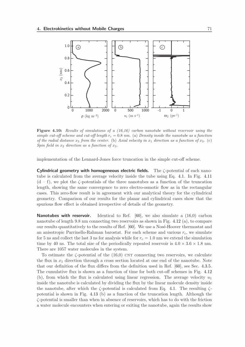
4. Electrokinetics without Mobile Charges 71
0 1000 20000
0.2
0.4
0.6
0.8
1.0
0 500 1000 -1 0 1
x3 (
nm
)
a b c
ρ (kg m -3) u1 (m s -1) ω2 (ps -1)
Figure 4.10: Results of simulations of a (16,16) carbon nanotube without reservoir using thesimple cut-off scheme and cut-off length rc = 0.8 nm. (a) Density inside the nanotube as a functionof the radial distance x3 from the center. (b) Axial velocity in x1 direction as a function of x3. (c)Spin field in x2 direction as a function of x3.
implementation of the Lennard-Jones force truncation in the simple cut-off scheme.
Cylindrical geometry with homogeneous electric fields. The ζ-potential of each nano-tube is calculated from the average velocity inside the tube using Eq. 4.1. In Fig. 4.11(d – f), we plot the ζ-potentials of the three nanotubes as a function of the truncationlength, showing the same convergence to zero electro-osmotic flow as in the rectangularcases. This zero-flow result is in agreement with our analytical theory for the cylindricalgeometry. Comparison of our results for the planar and cylindrical cases show that thespurious flow effect is obtained irrespective of details of the geometry.
Nanotubes with reservoir. Identical to Ref. [60], we also simulate a (16,0) carbonnanotube of length 9.8 nm connecting two reservoirs as shown in Fig. 4.12 (a), to compareour results quantitatively to the results of Ref. [60]. We use a Nose-Hoover thermostat andan anisotropic Parrinello-Rahman barostat. For each scheme and various rc, we simulatefor 5 ns and collect the last 3 ns for analysis while for rc = 1.0 nm we extend the simulationtime by 40 ns. The total size of the periodically repeated reservoir is 4.0 × 3.6 × 1.8 nm.There are 1057 water molecules in the system.
To estimate the ζ-potential of the (16,0) cnt connecting two reservoirs, we calculatethe flux in x1 direction through a cross section located at one end of the nanotube. Notethat our definition of the flux differs from the definition used in Ref. [60], see Sec. 4.3.5.The cumulative flux is shown as a function of time for both cut-off schemes in Fig. 4.12(b), from which the flux is calculated using linear regression. The average velocity u1
inside the nanotube is calculated by dividing the flux by the linear molecule density insidethe nanotube, after which the ζ-potential is calculated from Eq. 4.1. The resulting ζ-potential is shown in Fig. 4.13 (b) as a function of the truncation length. Although theζ-potential is smaller than when in absence of reservoirs, which has to do with the frictiona water molecule encounters when entering or exiting the nanotube, again the results show
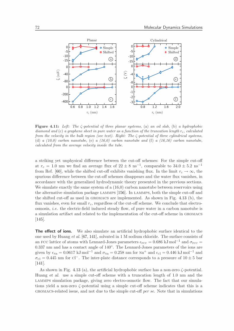
72 Molecular Dynamics Simulations
-15
-10
-5
0 Simple
Shifted
-80
-40
0
0.6 0.8 1.0 1.2 1.4 1.6
-400
-200
0
rc (nm)
ζ (m
V)
-15
-10
-5
0
-8
-4
0
0.8 1.2 1.6 2.0
-3
-2
-1
0
Simple
Shifted
rc (nm)
ζ (V
)
a
b
c
e
d
f
Planar Cylindrical
Figure 4.11: Left: The ζ-potential of three planar systems, (a) an oil slab, (b) a hydrophobicdiamond and (c) a graphene sheet in pure water as a function of the truncation length rc, calculatedfrom the velocity in the bulk region (see text). Right: The ζ-potential of three cylindrical systems,(d) a (10,0) carbon nanotube, (e) a (16,0) carbon nanotube and (f) a (16,16) carbon nanotube,calculated from the average velocity inside the tube.
a striking yet unphysical difference between the cut-off schemes: For the simple cut-offat rc = 1.0 nm we find an average flux of 22 ± 8 ns−1, comparable to 34.0 ± 5.2 ns−1
from Ref. [60], while the shifted cut-off exhibits vanishing flux. In the limit rc → ∞, thespurious difference between the cut-off schemes disappears and the water flux vanishes, inaccordance with the generalized hydrodynamic theory presented in the previous sections.We simulate exactly the same system of a (16,0) carbon nanotube between reservoirs usingthe alternative simulation package lammps [156]. In lammps, both the simple cut-off andthe shifted cut-off as used in gromacs are implemented. As shown in Fig. 4.13 (b), theflux vanishes, even for small rc, regardless of the cut-off scheme. We conclude that electro-osmosis, i.e. the electric-field induced steady flow, of pure water in a carbon nanotube isa simulation artifact and related to the implementation of the cut-off scheme in gromacs[145].
The effect of ions. We also simulate an artificial hydrophobic surface identical to theone used by Huang et al. [67, 141], solvated in 1 M sodium chloride. The surface consists ofan fcc lattice of atoms with Lennard-Jones parameters ǫfcc = 0.686 kJ mol−1 and σfcc =0.337 nm and has a contact angle of 140. The Lennard-Jones parameters of the ions aregiven by ǫna = 0.0617 kJ mol−1 and σna = 0.258 nm for na+ and ǫcl = 0.446 kJ mol−1 andσcl = 0.445 nm for cl−. The inter-plate distance corresponds to a pressure of 10 ± 5 bar[141].
As shown in Fig. 4.13 (a), the artificial hydrophobic surface has a non-zero ζ-potential.Huang et al. use a simple cut-off scheme with a truncation length of 1.0 nm and thelammps simulation package, giving zero electro-osmotic flow. The fact that our simula-tions yield a non-zero ζ-potential using a simple cut-off scheme indicates that this is agromacs-related issue, and not due to the simple cut-off per se. Note that in simulations

4. Electrokinetics without Mobile Charges 73
1 nm
x1
x3x2
t (ns)
0
200
400
600
800
cum
ula
tive
flux (
#)
rc = 1.0 nm
0 10 20 30 40
Simple
Shifted
a b
Figure 4.12: (a) Snapshot of the (16,0) nanotube simulations with reservoir. (b) Cumulativeflux through the tube as a function of time for an electric field strength of 1 V/nm for the twodifferent Lennard-Jones cut-off schemes with rc = 1.0 nm, simulated with gromacs. For eachcut-off length, the ζ-potential is calculated from the derivative of the cumulative flux as shown in(b), the line density inside the tube and Eq. 4.1.
of electrolyte solutions at neutral surfaces a small, but finite electrokinetic effect can existin principle, because the sodium and chloride ions have slightly dissimilar surface affinities,giving rise to a small electrostatic surface potential. However, this small contribution istotally dominated by the erroneous flow generated within the simple cut-off scheme.
Zero-field flux. As a simple test of the effect of the electric field, we perform longsimulations of a 9.8 nm long (10, 0) nanotube between reservoirs with and without electricfield. The results are shown in Fig. 4.14 for zero and non-zero external electric fields.Most strikingly, the flux is non-zero for the simple cut-off scheme, shown in Fig. 4.14 (b),regardless of whether an external electric field is applied or not. The same effect is in factdisplayed in Fig. 1 of Ref. [60]. Again, in the shifted scheme this unphysical effect isabsent. Since it is self-evident that in the absence of an electric field no flux should result,this proves our point most forcefully that something is fundamentally wrong with thesimple cut-off scheme as implemented in gromacs, leading to erroneous coupling betweenorientation and flux. The residual flux fluctuations for the shifted cut-off scheme shownin Fig. 4.14 (a) suggest that the simulations in the (10, 0) nanotube have not convergedon the time scale of 40 ns, which simply makes the (10, 0) nanotube unsuited for studyingequilibrium properties in general.
Point charges at carbon nanotubes. For a set of fixed point charges the electric field isspatially inhomogeneous. We simulate the system shown in Fig. 4.15 (a) for 5 ns, collectthe last 3 ns for analysis and calculate the flux as a function of the cut-off length for thetwo different cut-off schemes. We use a Berendsen thermostat and update the neighborlist every 10 timesteps. We define the three negative charges next the to nanotube to bein one charge group and the three compensating positive charges in another (see belowfor further explanation). The differences between our system and the system used in Ref.[61] are that the charges next to our tube are negative, external charges and tube atomsare frozen, our tube is longer and our reservoir is larger. From the flux and the averagenumber of particles per unit length we calculate the average velocity inside the tube, shownin Fig. 4.15 (b) as a function of the cut-off length for the two different truncation schemes.Clearly, the velocity depends on the cut-off length like in the case of a homogeneous electric

74 Molecular Dynamics Simulations
ζ (m
V)
ζ (m
V)
0.6 0.8 1.0 1.2 1.4
-20
-10
0
rc (nm)
a
0.6 0.8 1.0 1.2 1.4 1.6
-40
-20
0
rc (nm)
bGROMACS
LAMMPS
Simple Shifted
Figure 4.13: (a) The ζ-potential of a (16,0) nanotube connecting two reservoirs as a functionof the Lennard-Jones cut-off length, simulated with gromacs (circles and squares), and simulatedwith lammps (cross and plus), for both cut-off schemes. For each cut-off length, the ζ-potential iscalculated from a linear fit to the cumulative flux, the line density inside the tube and Eq. 4.1. (b)The ζ-potential of an artificial hydrophobic surface (consisting of an fcc lattice of Lennard-Jonesatoms) in the presence of a 1 M sodium chloride solution as a function of the truncation length rc.
cum
ula
tive
flux (
#)
0
100
200
300
E1 = 0 V/nm
E1 = 1 V/nm
t (ns)
0
100
200
300Simple cutoffShifted cutoff
0 10 20 30 40
t (ns)
0 10 20 30 40
a b
cum
ula
tive
flux (
#)
Figure 4.14: Cumulative flux through a (10,0) carbon nanotube with (red lines, field strength1 V/nm) and without (blue lines) external electric field. Cutoff schemes used are (a) shifted and(b) simple, both at rc = 1.0 nm. The flux is calculated according to the unconditional definition(see Sec. 4.3.5 “Definition of Flux” in the text). The system size is 3.0× 2.7× 13.7 nm containing1008 spc/e water molecules.
field and simple cut-off. However, the velocity resulting from an inhomogeneous electricfield also shows a cut-off length dependence for a shifted cut-off scheme. This shows thatusing a shifted cut-off scheme does not necessarily prevent the flow. Indeed, since thereis nothing unphysical about the simple cut-off per se, we have no reason to believe thata shifted cut-off should perform better in any case; it is the numerical implementation ofthe cut-off scheme in gromacs that produces questionable results.
Following a recent publication [157], we also investigate the effect of the use of chargegroups. For a charge group, Coulomb interactions are calculated for all individual chargesin the group, but the position of each individual charge is approximated by the geometricalmean of the constituent particles [158]. In the simulations by Ref. [61] and the simulationsshown in Fig. 4.15 the fixed charges close to the nanotube are grouped within a singlecharge group. The artificial pumping disappears for both cut-off schemes even for a shortcut-off length of 0.7 nm if we do not use a charge group for the fixed external charges.This confirms the findings of Ref. [157]. Finally, using the alternative simulation packagenamd 2, the directional flux vanishes altogether [159].
Nanoscale pumping of water by AC electric fields. Contrary to static electric fields,time-dependent electric fields can in principle be used to drive a system without free
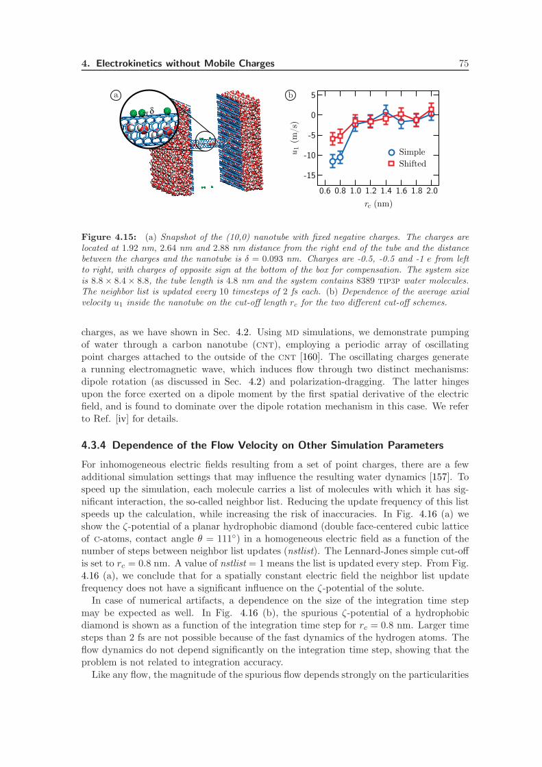
4. Electrokinetics without Mobile Charges 75
0.6 0.8 1.0 1.2 1.4 1.6 1.8 2.0
-15
-10
-5
0
5
δ
u1 (
m/s
)
rc (nm)
Simple
Shifted
a b
Figure 4.15: (a) Snapshot of the (10,0) nanotube with fixed negative charges. The charges arelocated at 1.92 nm, 2.64 nm and 2.88 nm distance from the right end of the tube and the distancebetween the charges and the nanotube is δ = 0.093 nm. Charges are -0.5, -0.5 and -1 e from leftto right, with charges of opposite sign at the bottom of the box for compensation. The system sizeis 8.8 × 8.4 × 8.8, the tube length is 4.8 nm and the system contains 8389 tip3p water molecules.The neighbor list is updated every 10 timesteps of 2 fs each. (b) Dependence of the average axialvelocity u1 inside the nanotube on the cut-off length rc for the two different cut-off schemes.
charges, as we have shown in Sec. 4.2. Using md simulations, we demonstrate pumpingof water through a carbon nanotube (cnt), employing a periodic array of oscillatingpoint charges attached to the outside of the cnt [160]. The oscillating charges generatea running electromagnetic wave, which induces flow through two distinct mechanisms:dipole rotation (as discussed in Sec. 4.2) and polarization-dragging. The latter hingesupon the force exerted on a dipole moment by the first spatial derivative of the electricfield, and is found to dominate over the dipole rotation mechanism in this case. We referto Ref. [iv] for details.
4.3.4 Dependence of the Flow Velocity on Other Simulation Parameters
For inhomogeneous electric fields resulting from a set of point charges, there are a fewadditional simulation settings that may influence the resulting water dynamics [157]. Tospeed up the simulation, each molecule carries a list of molecules with which it has sig-nificant interaction, the so-called neighbor list. Reducing the update frequency of this listspeeds up the calculation, while increasing the risk of inaccuracies. In Fig. 4.16 (a) weshow the ζ-potential of a planar hydrophobic diamond (double face-centered cubic latticeof c-atoms, contact angle θ = 111) in a homogeneous electric field as a function of thenumber of steps between neighbor list updates (nstlist). The Lennard-Jones simple cut-offis set to rc = 0.8 nm. A value of nstlist = 1 means the list is updated every step. From Fig.4.16 (a), we conclude that for a spatially constant electric field the neighbor list updatefrequency does not have a significant influence on the ζ-potential of the solute.
In case of numerical artifacts, a dependence on the size of the integration time stepmay be expected as well. In Fig. 4.16 (b), the spurious ζ-potential of a hydrophobicdiamond is shown as a function of the integration time step for rc = 0.8 nm. Larger timesteps than 2 fs are not possible because of the fast dynamics of the hydrogen atoms. Theflow dynamics do not depend significantly on the integration time step, showing that theproblem is not related to integration accuracy.
Like any flow, the magnitude of the spurious flow depends strongly on the particularities

76 Molecular Dynamics Simulations
1 10 100
nstlist
-60
-40
-20
0.1 10
time step (fs)
-60
-40
-20
1 0 60 120 180
θ ( )o
-60
-40
-20
28 30 32 34 36-15
-10
-5
0ζ
(mV
) a b c d
N/V (nm -3)
Figure 4.16: (a) Dependence of the spurious ζ-potential of a hydrophobic diamond (contact angleof 111) on the number of steps between neighbor list updates (nstlist) using a timestep of 1 fs and(b) dependence on the integration time step using nstlist = 50. (c) The ζ-potential of a diamondsurface as a function of contact angle and (d) the ζ potential of an artificial hydrophobic surface(θ = 140) with 1 M nacl as a function of the molecular water density N/V, using a timestep of1 fs and neighbor list update frequency of 1/50 timesteps. Dashed lines are drawn as a guide tothe eye. We use a simple Lennard-Jones cut-off at rc = 0.8 nm (a-c) and rc = 1.0 nm (d). Theelectric field strength is 0.4 V/nm (a-d) and the system size in (a-c) is 3.2×3.2×4.7 nm containing928 spc/e water molecules and one diamond. System size in (d) is 3.9×3.9×16.4 nm, containing2052 spc/e water, 40 na+ and 40 cl− molecules confined between two slabs.
of the system, most notably the contact angle of the substrate and the pressure in thesystem. In Fig. 4.16 (c) we show the ζ-potential of the diamond surface in contact withpure water. The contact angle of the diamond is modified by adjusting the Lennard-Jones interaction strength ǫ between the carbon atoms and the water molecules. Foreach simulation system, the contact angle is determined from the virial according to themethod employed by Ref. [128]. All simulations are done using a simple cut-off truncationscheme and a truncation length of rc = 0.8 nm. Using shifted truncation, the electro-osmotic flow is zero for any contact angle. Shown in Fig. 4.16 (d) is the ζ-potential of anartificial single face-centered cubic lattice (Lennard-Jones parameters ǫfcc = 0.686 kJ/mol,σfcc = 0.337 nm, θ = 140) in a solution of 1 M nacl in water as a function of the averagenumber density of water N/V in the volume between the plates. Calculating the pressurefrom the force on the center of mass of each plate divided by the plate area gives a pressureof 1 bar at an average density of 29 nm−3. We use a simple cut-off scheme for the LennardJones interaction with a truncation length of 1.0 nm. The apparent ζ-potential decreaseswith increasing density. We note that the dependence of the ζ-potential on the surfacecontact angle and the water density shown in Fig. 4.16 are spurious, in the sense that theelectro-osmotic flow should vanish altogether in this case. This is also true for the saltsolution, since the cations and anions of nacl show almost the same adsorption affinitieson a hydrophobic surface. Fig. 4.16 does show, however, that the magnitude of the artifactvaries appreciably depending on the particularities of the system, and that the spuriousflow is most pronounced for hydrophobic systems with a low average density of watermolecules, a class of systems to which carbon nanotubes belong as well.
4.3.5 Definition of Flux
In the first paper on water in carbon nanotubes, Hummer et al. found that the filling ofnanotubes goes in bursts [43]. This bursting behavior seems manifest also in simulationtrajectories of Ref. [60], particularly in the (10,0) nanotube. Let us discuss the way burstsin the cumulative flux emerge in the original analysis of Ref. [60]. Due to conservationof mass, the average flux through a given cross section of the carbon nanotube does not

4. Electrokinetics without Mobile Charges 77
0
100
200
300
Conditional flux
Flux
(10,0) CNT
0
200
400
600
800(16,0) CNT
t (ns)
0 10 20 30 40
t (ns)
0 10 20 30 40
cum
ula
tive
flux (
#)
cum
ula
tive
flux (
#)a b
Figure 4.17: Axial flux (x1 direction) through a (10,0) nanotube (a) and a (16,0) nanotube (b)at E1 = 1.0 V nm−1 using simple cut-off at rc = 1 nm. Shown in red is the flux calculated usingthe straightforward counting of molecules, shown in blue is the conditional flux, where moleculesexiting the tube are counted only if they previously entered from the other side. Simulation boxesare identical to the ones described in Figs. 4.13 and 4.14. We use a time step of 1 fs and neighborlist update every 50 steps.
depend on the position of the cross section. Therefore, without restricting the generalityof our arguments, we define the flux as the number of water molecules passing the edge ofthe simulation box. This we call the cumulative flux. In Ref. [60], on the other hand, theflux is defined as the number of particles exiting the tube on one end that have previouslyentered on the other end. This definition we denote as the conditional cumulative flux andit implicitly contains a tube length dependence. We perform simulations of 40 ns witha 5 ns equilibration period using a 1.0 nm simple cut-off scheme and an electric field of1 V/nm. In Fig. 4.17 (a – b) we show the results for two tube diameters, (10,0) and (16,0)respectively, both connecting two reservoirs. The results have been analyzed using boththe straightforward counting of molecules passing the edge of the box (denoted as flux),and using the definition from Ref. [60] (denoted as conditional flux). For long times, bothdefinitions of the flux converge to the same value but for shorter times, there are distinctdifferences. The first, obvious effect of the conditional definition of the flux is that thefirst particles exiting the tube, which are the particles that were located in the tube fromthe start, do not contribute to the conditional flux since they did not previously enter thetube. This explains the initial 4−8 ns waiting time and suggests that using the conditionaldefinition of the flux is not very efficient in terms of computer time. The second effect isa suppression of noise: particles moving back and forth are only counted if their motionpersists for the full tube length. This explains the striking lack of noise in the resultsshown in Ref. [60], as well as a large part of the alleged bursting behavior. From theunconditional flux, the bursting is by far not as pronounced as in the filling curves fromHummer et al. [43].
4.4 Summary & Conclusions
Using a combination of analytical theory based on a generalized Navier-Stokes equationand molecular dynamics simulations, we show that interfacial water ordering does notgive rise to steady-state flow in static electric fields. This means that the interfacial dipolepotential due to the water ordering does not contribute to the ζ-potential. Nevertheless,electro-hydraulic pumping of dipolar fluids is possible: an electric field step function gives
78 Summary & Conclusions
rise to transient flow, while a rotating electric field in an asymmetric channel can be used todrive flows in steady state. In a symmetric channel, a rotating electric field induces a shearprofile, but no net pumping. An electric field in the shape of a traveling wave, producedby phase-shifted ac voltages applied to an array of external electrodes, can also be used todrive pure water through a carbon nanotube. The equilibrium flow observed with staticelectric fields in previous molecular dynamics simulations of pure water, however, werecaused by particularities of the simple Lennard Jones force truncation scheme in gromacs.The unphysical dependence of the flow velocity on the Lennard-Jones truncation schemevanishes for truncation length rc → ∞ for all simulated geometries and surfaces. Using ashifted Lennard-Jones truncation scheme within gromacs, pure water does not give riseto a non-zero ζ-potential for any value of the truncation length, in agreement with theanalytical theory presented. Using the lammps molecular dynamics package, the spuriousflow effect is not observed, regardless of the truncation scheme used. Small values of thetruncation length also lead to spurious flow in the presence of the static inhomogeneouselectric field produced by fixed charged outside a carbon nanotube. In contrast with thesituation for homogeneous electric fields, the spurious flow persists when using a shiftedtruncation scheme, vanishing only for large values of the truncation length. We concludethat the spurious flow observed in molecular dynamics simulations of both planar andcylindrical geometries is an implementation-related issue in gromacs, and not caused bythe use of truncation schemes per se.
Chapter 5Electro-Osmotic Mobility andElectric Surface Conductivity
We calculate the electro-osmotic mobility and surface conductivity at a solid-liquid in-terface from a modified Poisson-Boltzmann equation, including spatial variations of thedielectric function and the viscosity that where extracted previously from molecular dy-namics simulations of aqueous interfaces. The low-dielectric region directly at the interfaceleads to a substantially reduced surface capacitance. At the same time, ions accumulateinto a highly condensed interfacial layer, leading to the well-known saturation of theelectro-osmotic mobility at large surface charge density regardless of the hydrodynamicboundary conditions. The experimentally well-established apparent excess surface conduc-tivity follows from our model for all hydrodynamic boundary conditions without additionalassumptions. Our theory fits multiple published sets of experimental data on hydrophilicand hydrophobic surfaces with striking accuracy, using the non-electrostatic ion-surfaceinteraction as the only fitting parameter. This chapter is based on Ref. [ii].
5.1 Introduction
When immersed in water, particles typically acquire a net surface charge, which is com-pensated for by a cloud of counterions in solution. This surface charge usually dominatesthe interactions between particles in colloidal suspensions. The bare surface charge densitycan be measured using charge titration [161]. It is well established, however, that the baresurface charge density cannot be used directly in classical models to describe dynamicproperties of colloidal suspensions, such as coagulation kinetics, electro-osmotic mobilityand effective viscosity [80, 162–164]. Instead, the ions and water molecules within a fewmolecular diameters from the surfaces of the colloidal particles decisively affect the suspen-sion’s macroscopic kinetic behavior. A deep understanding of the relation between baresurface charge, electro-osmotic mobility and the closely related phenomenon of surfaceconductivity is of supreme importance in many areas of physical chemistry. For instance,electrophoresis is commonly used in modern-day biochemistry for separation of chemicalsbased on minute differences in surface properties [165]. Furthermore, electrokinetic drivingis the method of choice to generate flow in microfluidic devices [2, 3], which are becoming
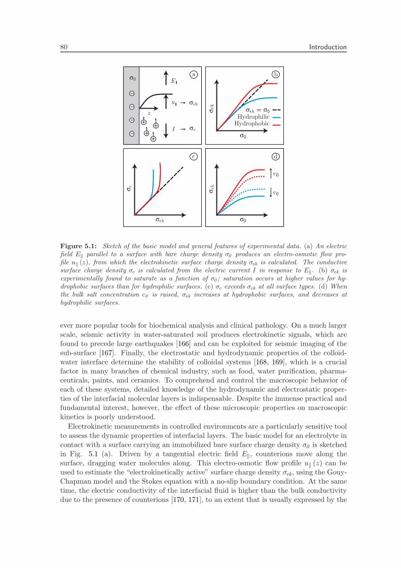
80 Introduction
σ0
σek
c0
c0
σek
σc
c d
σek
σ0
σek = σ0
b
u
I
Eσ0
σek
σc
z
a
HydrophilicHydrophobic
Figure 5.1: Sketch of the basic model and general features of experimental data. (a) An electricfield E‖ parallel to a surface with bare charge density σ0 produces an electro-osmotic flow pro-file u‖ (z), from which the electrokinetic surface charge density σek is calculated. The conductivesurface charge density σc is calculated from the electric current I in response to E‖. (b) σek isexperimentally found to saturate as a function of σ0 ; saturation occurs at higher values for hy-drophobic surfaces than for hydrophilic surfaces. (c) σc exceeds σek at all surface types. (d) Whenthe bulk salt concentration c0 is raised, σek increases at hydrophobic surfaces, and decreases athydrophilic surfaces.
ever more popular tools for biochemical analysis and clinical pathology. On a much largerscale, seismic activity in water-saturated soil produces electrokinetic signals, which arefound to precede large earthquakes [166] and can be exploited for seismic imaging of thesub-surface [167]. Finally, the electrostatic and hydrodynamic properties of the colloid-water interface determine the stability of colloidal systems [168, 169], which is a crucialfactor in many branches of chemical industry, such as food, water purification, pharma-ceuticals, paints, and ceramics. To comprehend and control the macroscopic behavior ofeach of these systems, detailed knowledge of the hydrodynamic and electrostatic proper-ties of the interfacial molecular layers is indispensable. Despite the immense practical andfundamental interest, however, the effect of these microscopic properties on macroscopickinetics is poorly understood.
Electrokinetic measurements in controlled environments are a particularly sensitive toolto assess the dynamic properties of interfacial layers. The basic model for an electrolyte incontact with a surface carrying an immobilized bare surface charge density σ0 is sketchedin Fig. 5.1 (a). Driven by a tangential electric field E‖, counterions move along thesurface, dragging water molecules along. This electro-osmotic flow profile u‖ (z) can beused to estimate the “electrokinetically active” surface charge density σek, using the Gouy-Chapman model and the Stokes equation with a no-slip boundary condition. At the sametime, the electric conductivity of the interfacial fluid is higher than the bulk conductivitydue to the presence of counterions [170, 171], to an extent that is usually expressed by the
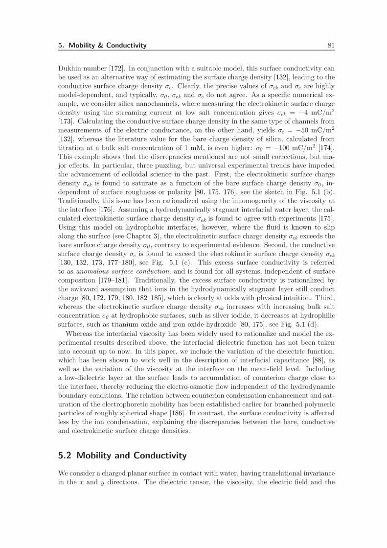
5. Mobility & Conductivity 81
Dukhin number [172]. In conjunction with a suitable model, this surface conductivity canbe used as an alternative way of estimating the surface charge density [132], leading to theconductive surface charge density σc. Clearly, the precise values of σek and σc are highlymodel-dependent, and typically, σ0 , σek and σc do not agree. As a specific numerical ex-ample, we consider silica nanochannels, where measuring the electrokinetic surface chargedensity using the streaming current at low salt concentration gives σek = −4 mC/m2
[173]. Calculating the conductive surface charge density in the same type of channels frommeasurements of the electric conductance, on the other hand, yields σc = −50 mC/m2
[132], whereas the literature value for the bare charge density of silica, calculated fromtitration at a bulk salt concentration of 1 mM, is even higher: σ0 = −100 mC/m2 [174].This example shows that the discrepancies mentioned are not small corrections, but ma-jor effects. In particular, three puzzling, but universal experimental trends have impededthe advancement of colloidal science in the past. First, the electrokinetic surface chargedensity σek is found to saturate as a function of the bare surface charge density σ0 , in-dependent of surface roughness or polarity [80, 175, 176], see the sketch in Fig. 5.1 (b).Traditionally, this issue has been rationalized using the inhomogeneity of the viscosity atthe interface [176]. Assuming a hydrodynamically stagnant interfacial water layer, the cal-culated electrokinetic surface charge density σek is found to agree with experiments [175].Using this model on hydrophobic interfaces, however, where the fluid is known to slipalong the surface (see Chapter 3), the electrokinetic surface charge density σek exceeds thebare surface charge density σ0 , contrary to experimental evidence. Second, the conductivesurface charge density σc is found to exceed the electrokinetic surface charge density σek[130, 132, 173, 177–180], see Fig. 5.1 (c). This excess surface conductivity is referredto as anomalous surface conduction, and is found for all systems, independent of surfacecomposition [179–181]. Traditionally, the excess surface conductivity is rationalized bythe awkward assumption that ions in the hydrodynamically stagnant layer still conductcharge [80, 172, 179, 180, 182–185], which is clearly at odds with physical intuition. Third,whereas the electrokinetic surface charge density σek increases with increasing bulk saltconcentration c0 at hydrophobic surfaces, such as silver iodide, it decreases at hydrophilicsurfaces, such as titanium oxide and iron oxide-hydroxide [80, 175], see Fig. 5.1 (d).
Whereas the interfacial viscosity has been widely used to rationalize and model the ex-perimental results described above, the interfacial dielectric function has not been takeninto account up to now. In this paper, we include the variation of the dielectric function,which has been shown to work well in the description of interfacial capacitance [88], aswell as the variation of the viscosity at the interface on the mean-field level. Includinga low-dielectric layer at the surface leads to accumulation of counterion charge close tothe interface, thereby reducing the electro-osmotic flow independent of the hydrodynamicboundary conditions. The relation between counterion condensation enhancement and sat-uration of the electrophoretic mobility has been established earlier for branched polymericparticles of roughly spherical shape [186]. In contrast, the surface conductivity is affectedless by the ion condensation, explaining the discrepancies between the bare, conductiveand electrokinetic surface charge densities.
5.2 Mobility and Conductivity
We consider a charged planar surface in contact with water, having translational invariancein the x and y directions. The dielectric tensor, the viscosity, the electric field and the
82 Mobility and Conductivity
displacement field only depend on the perpendicular coordinate z.
5.2.1 Electrokinetic Surface Charge Density
For laminar flows, the electro-osmotic flow velocity profile u‖ (z) in response to a parallelelectric field E‖ is calculated from the Stokes equation,
∇η (z)∇u‖ (z) = −ρ (z)E‖, (5.1)
with spatially varying viscosity η (z) and charge density ρ (z). Note that ρ (z) is the ioniccharge density and polarization charges do not enter the force balance, as shown earlier[187]. The hydrodynamic boundary condition of either slip or a high-viscosity layer istaken into account via the viscosity profile η (z), which in conjunction with the conditionu‖ (0) = 0 is designed to reproduce the flow profile at macroscopic distances from theinterface, as will be elaborated later. The electro-osmotic mobility is found by integratingEq. 5.1 twice using u‖ (0) = 0 as a boundary condition,
u‖ (z)
E‖= −
∫ z
0
D⊥ (z′)
η (z′)dz′, (5.2)
with D⊥ (z) being the displacement field perpendicular to the surface, which obeys Gauss’slaw, ∇D⊥ (z) = ρ (z). Experimentally, electro-osmotic velocity is measured far away fromthe interface. Assuming that the permittivity is spatially constant and equal to its bulkvalue εbulk, and η (z) = ηbulk in Eq. 5.2, the electro-osmotic mobility is given by theHelmholtz-Smoluchowski equation,
limz→∞
u‖ (z)
E‖= −ε0εbulk
ηbulkζ, (5.3)
with ζ =∫∞0 (D⊥ (z) /ε0 εbulk) dz being the electrostatic potential at z = 0. A derivation
of Eq. 5.3 is given in Appendix B. Because the surface potential is typically not measureddirectly, it is often more convenient to express ζ in terms of the equivalent surface chargedensity. Using the standard Poisson-Boltzmann relation between the surface potentialand the surface charge density, which is valid on the mean-field level, the electro-osmoticmobility of Eq. 5.2 is expressed as an equivalent surface charge density, referred to as theelectrokinetic surface charge density σek,
σek =
√
8c0 ε0εbulkβ
sinh
[
βe ζ
2
]
, (5.4)
with c0 the bulk salt concentration. Eq. 5.4 is known as the Grahame equation. The ζ-potential is calculated using Eq. 5.3, where the electro-osmotic mobility is either measuredexperimentally or calculated from Eq. 5.2. A derivation of Eq. 5.4 is given in AppendixB.
5.2.2 Conductive Surface Charge Density
The electric conductivity close to charged surfaces is enhanced with respect to the bulkdue to the presence of excess ionic charges. This surface conductivity can be convenientlymeasured in small channels at low salt concentration, in which case the contribution from
5. Mobility & Conductivity 83
the bulk vanishes [132]. The surface conductivity is given by the sum of a convective part,due to the electro-osmotic flow, and a conductive part, due to the electrophoretic mobilityof the ions,
I
E‖=
∫ ∞
0e[
c+ (z) − c− (z)] [
u‖ (z)/E‖
]
dz
+
∫ ∞
0e[
ν+ (c+ (z) − c0 ) + ν− (c− (z) − c0 )]
dz,
(5.5)
with ν± the electrophoretic mobility of the positive and negative ions. Note that wesubtract the bulk contribution to the conductive part of Eq. 5.5. Similar to the Grahameequation (Eq. 5.4), the surface conductivity can be expressed as an equivalent surfacecharge density using the Gouy-Chapman theory, giving
σc =κ2ηbulk
4ec0 + νκ2ηbulk
√
I
E‖
√
I
E‖+
32e2c20
κ3ηbulk+
8ec0 ν
κ. (5.6)
A derivation of Eq. 5.6 is given in Appendix B. Since the predominant salt types beingconsidered in the experiments that we compare our results with (Sec. 5.5.2) are k+ (ν+ =7.62 × 10⁻⁸ m2/Vs), cl− (ν− = 7.91 × 10⁻⁸ m2/Vs) and no−
3 (ν− = 7.40 × 10⁻⁸ m2/Vs),we assume ν+ = ν− = ν, which is a good approximation for both kcl and kno3.
5.3 Viscosity & Dielectric Profile
Viscosity profile. We model the variations in viscosity at the interface by a step function,
η (z) =
ηi if z < zsηbulk otherwise,
(5.7)
with ηi the viscosity in a layer of width zs and ηbulk the bulk viscosity. Note that thedefinition of a viscosity at sub-atomic length scales is problematic, and the profile of Eq.5.7 is only intended to reproduce, within a continuum model, the flow characteristics foundexperimentally at distances z > zs. For most hydrophobic surfaces the fluid slips along thewall [36], which is commonly taken into account by the Navier hydrodynamic boundarycondition, b∇u‖ (z) |0 = u‖ (z) |0, with positive slip length b. In simulations of water at avery hydrophobic diamond surface, the viscosity is found to be constant and equal to thebulk value ηbulk for z > 0.15 nm, leading to a slip length of b = 2.15 nm. Setting u‖ (0) = 0,we reproduce the same flow profile for z > zs by assigning ηi = ηbulk/15 and zs = 0.15 nm.For most hydrophilic surfaces, on the other hand, the fluid in the first molecular layeradjacent to the wall sticks to the surface [36]. Molecular dynamics simulation on smoothhydrophilic surfaces have shown that the interfacial layer is not truly stagnant, it merelyhas an enhanced viscosity [74, 125]. Following the simulation results of Ref. [74] we takezs = 0.3 nm and ηi = 3ηbulk. In Fig. 5.2 (a), we show the viscosity profile η (z) of Eq.5.7 at hydrophilic and very hydrophobic surfaces. For easy reference, we characterize eachviscosity profile by its apparent slip length,
b = zs (ηbulk/ηi − 1) . (5.8)
Electrophoretic mobility. In general, the electrophoretic mobility of ions ν± depends onthe ion concentration and the viscosity of the fluid [188]. The ion mobility directly at
84 Scaling Analysis
the interface is not known (note that the conclusion that the interfacial mobility equalsthe bulk mobility [182] relies heavily on the electrostatic model used). Here, we use thesimplest approach, where only the bulk-like viscous drag on the ions is taken into account,resulting in a mobility that is inversely proportional to the local viscosity.
Dielectric profile. In order to describe the dielectric profile at a similarly simplistic levelas the viscosity, we use a step function as well,
ε⊥ (z) =
1 if z < zdds⊥
εbulk otherwise,(5.9)
with zdds⊥ the dielectric dividing surface as defined in Sec. 2.4.1 [88]. The profile in Eq.
5.9 is designed to reproduce the electrostatic potential calculated in molecular dynamicssimulations at positions z & 1 nm from the interface [88]. For zdds
⊥ we use two differentvalues: zdds
⊥ = 0.10 nm, corresponding to a hydrophilic surface, and zdds⊥ = 0.12 nm,
corresponding to a very hydrophobic surface, as directly taken from Sec. 2.4.1. Theinverse dielectric profiles ε−1
⊥ (z) in the approximation of Eq. 5.9 are shown in Fig. 5.2 (b)for hydrophilic and very hydrophobic surfaces.
5.4 Scaling Analysis
In this section, we qualitatively investigate how the dielectric profile ε⊥ (z) as given in Eq.5.9 affects the counterion distribution, and consequently σek and σc.
Counterions at a charged plate. The electrokinetic and conductive surface charge den-sities defined in Eqs. 5.4 and 5.6 are directly affected by the viscosity profile η (z). Thedielectric profile ε⊥ (z) does not affect σek and σc directly, but it does have a decisiveinfluence on the ion distribution, which in turn has a major impact on σek and σc. For aqualitative picture of the effect of ε⊥ (z), we consider the situation of an infinite chargedplate in contact with a solution containing only counterions. We keep the viscosity con-stant, η (z) = ηbulk. According to the Gouy-Chapman model, the ions form a diffuse layerwhen ε⊥ (z) = εbulk, and by definition σek = σc = σ0 . This relation is also valid in the limitof low salt concentration (c0 → 0), in which case the solution contains only counterions.Using the profile of Eq. 5.9, on the other hand, a large portion of the ions will condenseinto the low-dielectric area because of the steep increase of the electric potential resultingfrom the low dielectric constant. This model of a low-dielectric layer of condensed ionshas been proposed long ago by Otto Stern based on experimental double-layer capaci-tance data [22], and we have confirmed in Sec. 2.4.3 that Eq. 5.9 in conjunction with amean-field model indeed reproduces the salt-concentration dependence of the double-layercapacitance [88]. In our present scaling analysis, we use a delta function as a model forthe charge distribution to mimic the condensed layer of ions,
ρ (z) = −σ0δ (z − d) , (5.10)
with d the typical distance to the surface. A typical value of d would be the radius of anion. The electrophoretic mobility of Eq. 5.2 is integrated by parts, which leads to
ζ = − 1
ε0εbulk
∫ ∞
0z ρ (z) dz, (5.11)
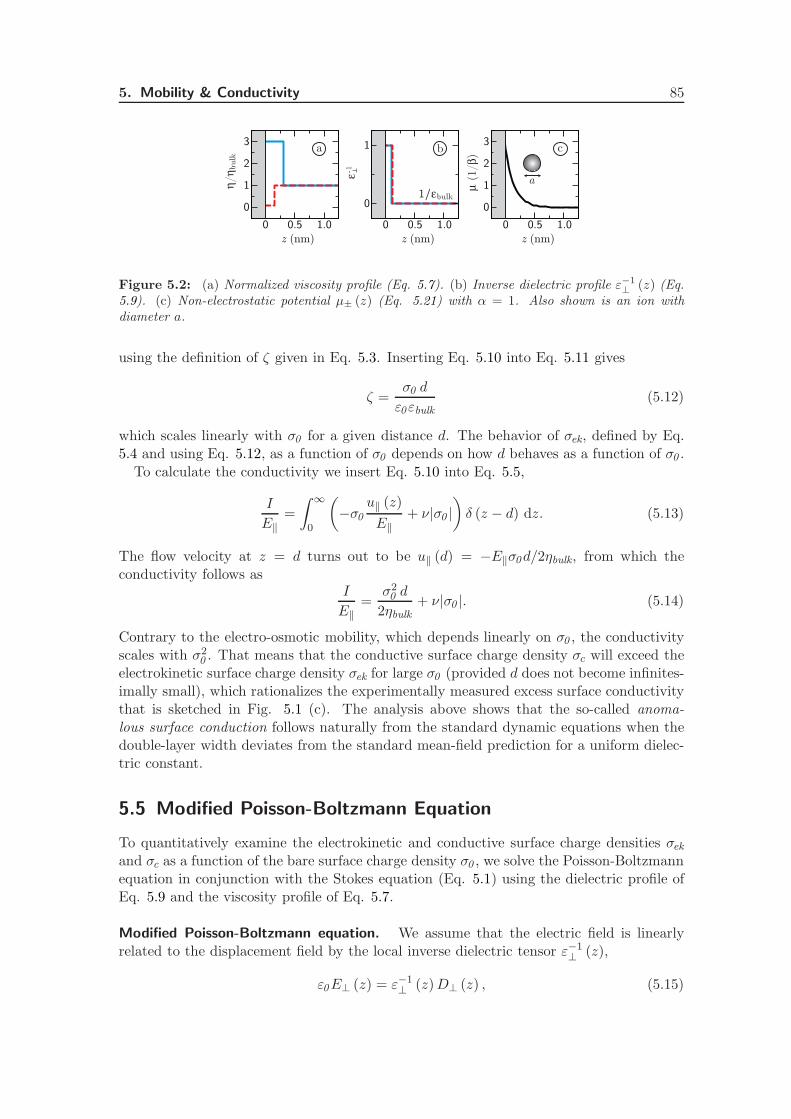
5. Mobility & Conductivity 85
0 0.5 1.0z (nm)
0
1
ε-1
0
1
2
3
a
0 0.5 1.0z (nm)
µ (
1/β)
0
1
2
3
η/ηbulk
0 0.5 1.0z (nm)
1/εbulk
a b c
Figure 5.2: (a) Normalized viscosity profile (Eq. 5.7). (b) Inverse dielectric profile ε−1
⊥ (z) (Eq.5.9). (c) Non-electrostatic potential µ± (z) (Eq. 5.21) with α = 1. Also shown is an ion withdiameter a.
using the definition of ζ given in Eq. 5.3. Inserting Eq. 5.10 into Eq. 5.11 gives
ζ =σ0 d
ε0εbulk(5.12)
which scales linearly with σ0 for a given distance d. The behavior of σek, defined by Eq.5.4 and using Eq. 5.12, as a function of σ0 depends on how d behaves as a function of σ0 .
To calculate the conductivity we insert Eq. 5.10 into Eq. 5.5,
I
E‖=
∫ ∞
0
(
−σ0u‖ (z)
E‖+ ν|σ0 |
)
δ (z − d) dz. (5.13)
The flow velocity at z = d turns out to be u‖ (d) = −E‖σ0d/2ηbulk, from which theconductivity follows as
I
E‖=
σ20 d
2ηbulk+ ν|σ0 |. (5.14)
Contrary to the electro-osmotic mobility, which depends linearly on σ0 , the conductivityscales with σ2
0. That means that the conductive surface charge density σc will exceed the
electrokinetic surface charge density σek for large σ0 (provided d does not become infinites-imally small), which rationalizes the experimentally measured excess surface conductivitythat is sketched in Fig. 5.1 (c). The analysis above shows that the so-called anoma-lous surface conduction follows naturally from the standard dynamic equations when thedouble-layer width deviates from the standard mean-field prediction for a uniform dielec-tric constant.
5.5 Modified Poisson-Boltzmann Equation
To quantitatively examine the electrokinetic and conductive surface charge densities σekand σc as a function of the bare surface charge density σ0 , we solve the Poisson-Boltzmannequation in conjunction with the Stokes equation (Eq. 5.1) using the dielectric profile ofEq. 5.9 and the viscosity profile of Eq. 5.7.
Modified Poisson-Boltzmann equation. We assume that the electric field is linearlyrelated to the displacement field by the local inverse dielectric tensor ε−1
⊥ (z),
ε0E⊥ (z) = ε−1⊥ (z)D⊥ (z) , (5.15)
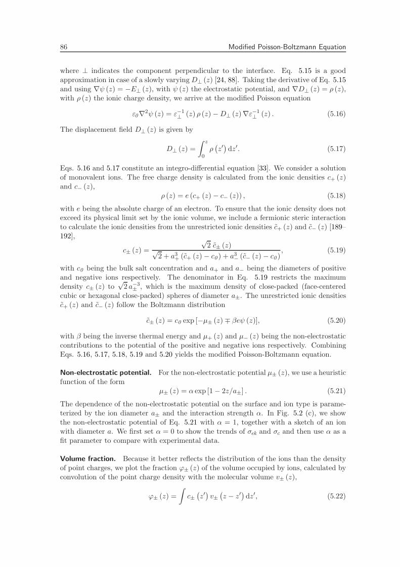
86 Modified Poisson-Boltzmann Equation
where ⊥ indicates the component perpendicular to the interface. Eq. 5.15 is a goodapproximation in case of a slowly varyingD⊥ (z) [24, 88]. Taking the derivative of Eq. 5.15and using ∇ψ (z) = −E⊥ (z), with ψ (z) the electrostatic potential, and ∇D⊥ (z) = ρ (z),with ρ (z) the ionic charge density, we arrive at the modified Poisson equation
ε0∇2ψ (z) = ε−1⊥ (z) ρ (z) −D⊥ (z)∇ε−1
⊥ (z) . (5.16)
The displacement field D⊥ (z) is given by
D⊥ (z) =
∫ z
0ρ(
z′)
dz′. (5.17)
Eqs. 5.16 and 5.17 constitute an integro-differential equation [33]. We consider a solutionof monovalent ions. The free charge density is calculated from the ionic densities c+ (z)and c− (z),
ρ (z) = e (c+ (z) − c− (z)) , (5.18)
with e being the absolute charge of an electron. To ensure that the ionic density does notexceed its physical limit set by the ionic volume, we include a fermionic steric interactionto calculate the ionic densities from the unrestricted ionic densities c+ (z) and c− (z) [189–192],
c± (z) =
√2 c± (z)√
2 + a3+ (c+ (z) − c0 ) + a3
− (c− (z) − c0 ), (5.19)
with c0 being the bulk salt concentration and a+ and a− being the diameters of positiveand negative ions respectively. The denominator in Eq. 5.19 restricts the maximumdensity c± (z) to
√2 a−3
± , which is the maximum density of close-packed (face-centeredcubic or hexagonal close-packed) spheres of diameter a±. The unrestricted ionic densitiesc+ (z) and c− (z) follow the Boltzmann distribution
c± (z) = c0 exp [−µ± (z) ∓ βeψ (z)], (5.20)
with β being the inverse thermal energy and µ+ (z) and µ− (z) being the non-electrostaticcontributions to the potential of the positive and negative ions respectively. CombiningEqs. 5.16, 5.17, 5.18, 5.19 and 5.20 yields the modified Poisson-Boltzmann equation.
Non-electrostatic potential. For the non-electrostatic potential µ± (z), we use a heuristicfunction of the form
µ± (z) = α exp [1 − 2z/a±] . (5.21)
The dependence of the non-electrostatic potential on the surface and ion type is parame-terized by the ion diameter a± and the interaction strength α. In Fig. 5.2 (c), we showthe non-electrostatic potential of Eq. 5.21 with α = 1, together with a sketch of an ionwith diameter a. We first set α = 0 to show the trends of σek and σc and then use α as afit parameter to compare with experimental data.
Volume fraction. Because it better reflects the distribution of the ions than the densityof point charges, we plot the fraction ϕ± (z) of the volume occupied by ions, calculated byconvolution of the point charge density with the molecular volume v± (z),
ϕ± (z) =
∫
c±(
z′)
v±(
z − z′)
dz′, (5.22)
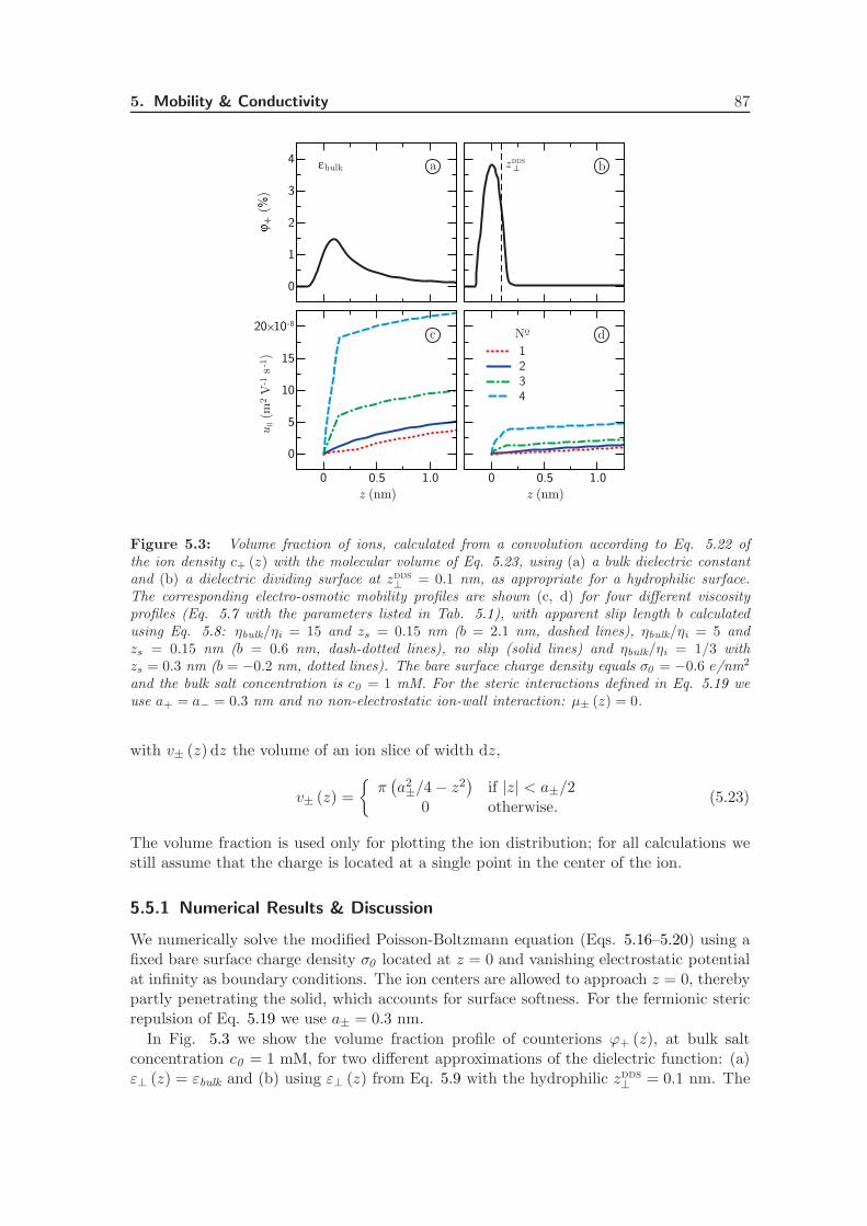
5. Mobility & Conductivity 87
0
1
2
3
4
ϕ+ (
%)
0 0.5 1.0
z (nm)
0
5
10
15
0 0.5 1.0
z (nm)
u (m
2 V
-1 s
-1)
zDDSεbulk
10-820
4321
No
a b
c d
Figure 5.3: Volume fraction of ions, calculated from a convolution according to Eq. 5.22 ofthe ion density c+ (z) with the molecular volume of Eq. 5.23, using (a) a bulk dielectric constantand (b) a dielectric dividing surface at zdds
⊥ = 0.1 nm, as appropriate for a hydrophilic surface.The corresponding electro-osmotic mobility profiles are shown (c, d) for four different viscosityprofiles (Eq. 5.7 with the parameters listed in Tab. 5.1), with apparent slip length b calculatedusing Eq. 5.8: ηbulk/ηi = 15 and zs = 0.15 nm (b = 2.1 nm, dashed lines), ηbulk/ηi = 5 andzs = 0.15 nm (b = 0.6 nm, dash-dotted lines), no slip (solid lines) and ηbulk/ηi = 1/3 withzs = 0.3 nm (b = −0.2 nm, dotted lines). The bare surface charge density equals σ0 = −0.6 e/nm2
and the bulk salt concentration is c0 = 1 mM. For the steric interactions defined in Eq. 5.19 weuse a+ = a− = 0.3 nm and no non-electrostatic ion-wall interaction: µ± (z) = 0.
with v± (z) dz the volume of an ion slice of width dz,
v± (z) =
π(
a2±/4 − z2
)
if |z| < a±/20 otherwise.
(5.23)
The volume fraction is used only for plotting the ion distribution; for all calculations westill assume that the charge is located at a single point in the center of the ion.
5.5.1 Numerical Results & Discussion
We numerically solve the modified Poisson-Boltzmann equation (Eqs. 5.16–5.20) using afixed bare surface charge density σ0 located at z = 0 and vanishing electrostatic potentialat infinity as boundary conditions. The ion centers are allowed to approach z = 0, therebypartly penetrating the solid, which accounts for surface softness. For the fermionic stericrepulsion of Eq. 5.19 we use a± = 0.3 nm.
In Fig. 5.3 we show the volume fraction profile of counterions ϕ+ (z), at bulk saltconcentration c0 = 1 mM, for two different approximations of the dielectric function: (a)ε⊥ (z) = εbulk and (b) using ε⊥ (z) from Eq. 5.9 with the hydrophilic zdds
⊥ = 0.1 nm. The
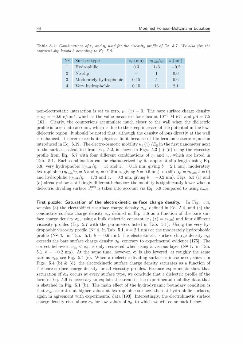
88 Modified Poisson-Boltzmann Equation
Table 5.1: Combinations of zs and ηi used for the viscosity profile of Eq. 5.7. We also give theapparent slip length b according to Eq. 5.8.
No Surface type zs (nm) ηbulk/ηi b (nm)
1 Hydrophilic 0.3 1/3 −0.2
2 No slip – 1 0.0
3 Moderately hydrophobic 0.15 5 0.6
4 Very hydrophobic 0.15 15 2.1
non-electrostatic interaction is set to zero, µ± (z) = 0. The bare surface charge densityis σ0 = −0.6 e/nm2, which is the value measured for silica at 10−3 M kcl and ph = 7.5[161]. Clearly, the counterions accumulate much closer to the wall when the dielectricprofile is taken into account, which is due to the steep increase of the potential in the low-dielectric region. It should be noted that, although the density of ions directly at the wallis enhanced, it never exceeds its physical limit because of the fermionic steric repulsionintroduced in Eq. 5.19. The electro-osmotic mobility u‖ (z) /E‖ in the first nanometer nextto the surface, calculated from Eq. 5.2, is shown in Figs. 5.3 (c)–(d) using the viscosityprofile from Eq. 5.7 with four different combinations of ηi and zs, which are listed inTab. 5.1. Each combination can be characterized by its apparent slip length using Eq.5.8: very hydrophobic (ηbulk/ηi = 15 and zs = 0.15 nm, giving b = 2.1 nm), moderatelyhydrophobic (ηbulk/ηi = 5 and zs = 0.15 nm, giving b = 0.6 nm), no slip (ηi = ηbulk, b = 0)and hydrophilic (ηbulk/ηi = 1/3 and zs = 0.3 nm, giving b = −0.2 nm). Figs. 5.3 (c) and(d) already show a strikingly different behavior: the mobility is significantly lower when adielectric dividing surface zdds
⊥ is taken into account via Eq. 5.9 compared to using εbulk.
First puzzle: Saturation of the electrokinetic surface charge density. In Fig. 5.4,we plot (a) the electrokinetic surface charge density σek, defined in Eq. 5.4, and (c) theconductive surface charge density σc, defined in Eq. 5.6 as a function of the bare sur-face charge density σ0 , using a bulk dielectric constant (ε⊥ (z) = εbulk) and four differentviscosity profiles (Eq. 5.7 with the parameters listed in Tab. 5.1). Using the very hy-drophobic viscosity profile (No 4. in Tab. 5.1, b = 2.1 nm) or the moderately hydrophobicprofile (No 3. in Tab. 5.1, b = 0.6 nm), the electrokinetic surface charge density σekexceeds the bare surface charge density σ0 , contrary to experimental evidence [175]. Thecorrect behavior, σek < σ0 , is only recovered when using a viscous layer (No 1. in Tab.5.1, b = −0.2 nm). At the same time, however, σc is also lowered, at roughly the samerate as σek, see Fig. 5.4 (c). When a dielectric dividing surface is introduced, shown inFigs. 5.4 (b) & (d), the electrokinetic surface charge density saturates as a function ofthe bare surface charge density for all viscosity profiles. Because experiments show thatsaturation of σek occurs at every surface type, we conclude that a dielectric profile of theform of Eq. 5.9 is necessary to explain the trend of the experimental mobility data thatis sketched in Fig. 5.1 (b). The main effect of the hydrodynamic boundary condition isthat σek saturates at higher values at hydrophobic surfaces then at hydrophilic surfaces,again in agreement with experimental data [193]. Interestingly, the electrokinetic surfacecharge density rises above σ0 for low values of σ0 , to which we will come back below.
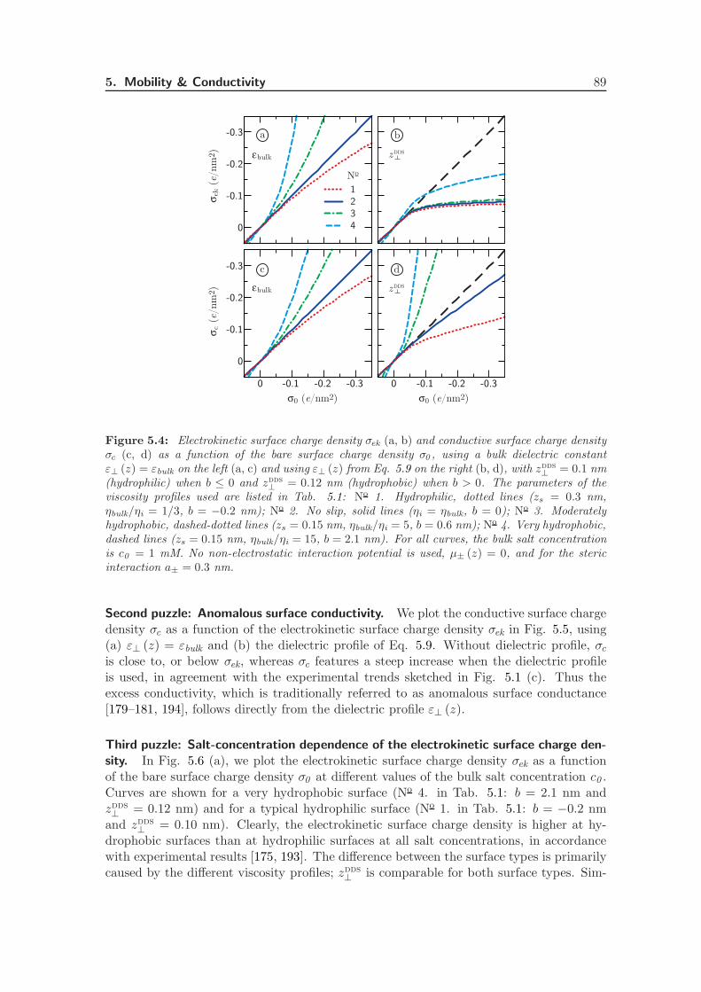
5. Mobility & Conductivity 89
-0.3
-0.2
-0.1
0
-0.3-0.2-0.10
-0.3
-0.2
-0.1
0
-0.3-0.2-0.10
σek (
e/nm
2 )σc (
e/nm
2 )
σ0 (e/nm2) σ0 (e/nm2)
εbulk
εbulk
zDDS
zDDS
4321
No
a b
c d
Figure 5.4: Electrokinetic surface charge density σek (a, b) and conductive surface charge densityσc (c, d) as a function of the bare surface charge density σ0 , using a bulk dielectric constantε⊥ (z) = εbulk on the left (a, c) and using ε⊥ (z) from Eq. 5.9 on the right (b, d), with zdds
⊥ = 0.1 nm(hydrophilic) when b ≤ 0 and zdds
⊥ = 0.12 nm (hydrophobic) when b > 0. The parameters of theviscosity profiles used are listed in Tab. 5.1: No 1. Hydrophilic, dotted lines (zs = 0.3 nm,ηbulk/ηi = 1/3, b = −0.2 nm); No 2. No slip, solid lines (ηi = ηbulk, b = 0); No 3. Moderatelyhydrophobic, dashed-dotted lines (zs = 0.15 nm, ηbulk/ηi = 5, b = 0.6 nm); No 4. Very hydrophobic,dashed lines (zs = 0.15 nm, ηbulk/ηi = 15, b = 2.1 nm). For all curves, the bulk salt concentrationis c0 = 1 mM. No non-electrostatic interaction potential is used, µ± (z) = 0, and for the stericinteraction a± = 0.3 nm.
Second puzzle: Anomalous surface conductivity. We plot the conductive surface chargedensity σc as a function of the electrokinetic surface charge density σek in Fig. 5.5, using(a) ε⊥ (z) = εbulk and (b) the dielectric profile of Eq. 5.9. Without dielectric profile, σcis close to, or below σek, whereas σc features a steep increase when the dielectric profileis used, in agreement with the experimental trends sketched in Fig. 5.1 (c). Thus theexcess conductivity, which is traditionally referred to as anomalous surface conductance[179–181, 194], follows directly from the dielectric profile ε⊥ (z).
Third puzzle: Salt-concentration dependence of the electrokinetic surface charge den-
sity. In Fig. 5.6 (a), we plot the electrokinetic surface charge density σek as a functionof the bare surface charge density σ0 at different values of the bulk salt concentration c0 .Curves are shown for a very hydrophobic surface (No 4. in Tab. 5.1: b = 2.1 nm andzdds⊥ = 0.12 nm) and for a typical hydrophilic surface (No 1. in Tab. 5.1: b = −0.2 nm
and zdds⊥ = 0.10 nm). Clearly, the electrokinetic surface charge density is higher at hy-
drophobic surfaces than at hydrophilic surfaces at all salt concentrations, in accordancewith experimental results [175, 193]. The difference between the surface types is primarilycaused by the different viscosity profiles; zdds
⊥ is comparable for both surface types. Sim-
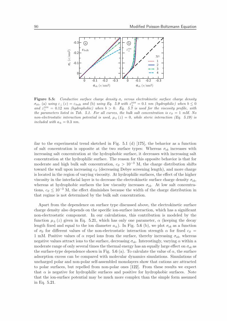
90 Modified Poisson-Boltzmann Equation
-0.3-0.2-0.10
-0.3
-0.2
-0.1
0
-0.3-0.2-0.10
εbulk zDDS
4321
σc (
e/nm
2 )
σek (e/nm2) σek (e/nm2)
No
a b
Figure 5.5: Conductive surface charge density σc versus electrokinetic surface charge densityσek, (a) using ε⊥ (z) = εbulk and (b) using Eq. 5.9 with zdds
⊥ = 0.1 nm (hydrophilic) when b ≤ 0and zdds
⊥ = 0.12 nm (hydrophobic) when b > 0. Eq. 5.7 is used for the viscosity profile, withthe parameters listed in Tab. 5.1. For all curves, the bulk salt concentration is c0 = 1 mM. Nonon-electrostatic interaction potential is used, µ± (z) = 0, while steric interaction (Eq. 5.19) isincluded with a± = 0.3 nm.
ilar to the experimental trend sketched in Fig. 5.1 (d) [175], the behavior as a functionof salt concentration is opposite at the two surface types: Whereas σek increases withincreasing salt concentration at the hydrophobic surface, it decreases with increasing saltconcentration at the hydrophilic surface. The reason for this opposite behavior is that formoderate and high bulk salt concentration, c0 > 10−3 M, the charge distribution shiftstoward the wall upon increasing c0 (decreasing Debye screening length), and more chargeis located in the region of varying viscosity. At hydrophilic surfaces, the effect of the higherviscosity in the interfacial layer is to decrease the electrokinetic surface charge density σek,whereas at hydrophobic surfaces the low viscosity increases σek. At low salt concentra-tions, c0 ≤ 10−3 M, the effect diminishes because the width of the charge distribution inthat regime is not determined by the bulk salt concentration.
Apart from the dependence on surface type discussed above, the electrokinetic surfacecharge density also depends on the specific ion-surface interaction, which has a significantnon-electrostatic component. In our calculations, this contribution is modeled by thefunction µ± (z) given in Eq. 5.21, which has only one parameter, α (keeping the decaylength fixed and equal to the ion diameter a±). In Fig. 5.6 (b), we plot σek as a functionof σ0 for different values of the non-electrostatic interaction strength α for fixed c0 =1 mM. Positive values of α repel ions from the surface, thereby increasing σek, whereasnegative values attract ions to the surface, decreasing σek. Interestingly, varying α within amoderate range of only several times the thermal energy has an equally large effect on σek asthe surface-type dependence shown in Fig. 5.6 (a). To calculate the value of α, the surfaceadsorption excess can be compared with molecular dynamics simulations. Simulations ofuncharged polar and non-polar self-assembled monolayers show that cations are attractedto polar surfaces, but repelled from non-polar ones [122]. From these results we expectthat α is negative for hydrophilic surfaces and positive for hydrophobic surfaces. Notethat the ion-surface potential may be much more complex than the simple form assumedin Eq. 5.21.
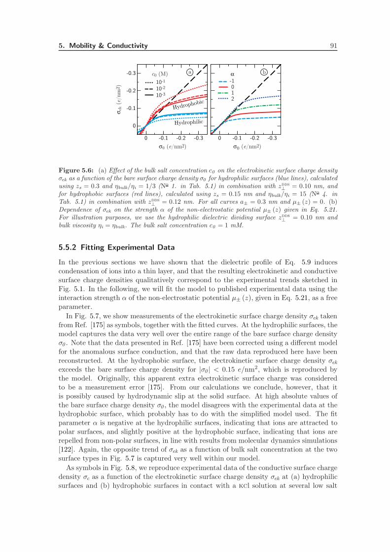
5. Mobility & Conductivity 91
-0.3-0.2-0.10
α
-0.3-0.2-0.10
-0.3
-0.2
-0.1
0
Hydrophobic
Hydrophilicσek (
e/nm
2 )
σ0 (e/nm2) σ0 (e/nm2)
-1012
10-1
10-2
10-3
c0 (M) a b
Figure 5.6: (a) Effect of the bulk salt concentration c0 on the electrokinetic surface charge densityσek as a function of the bare surface charge density σ0 for hydrophilic surfaces (blue lines), calculatedusing zs = 0.3 and ηbulk/ηi = 1/3 (No 1. in Tab. 5.1) in combination with zdds
⊥ = 0.10 nm, andfor hydrophobic surfaces (red lines), calculated using zs = 0.15 nm and ηbulk/ηi = 15 (No 4. inTab. 5.1) in combination with zdds
⊥ = 0.12 nm. For all curves a± = 0.3 nm and µ± (z) = 0. (b)Dependence of σek on the strength α of the non-electrostatic potential µ± (z) given in Eq. 5.21.For illustration purposes, we use the hydrophilic dielectric dividing surface zdds
⊥ = 0.10 nm andbulk viscosity ηi = ηbulk. The bulk salt concentration c0 = 1 mM.
5.5.2 Fitting Experimental Data
In the previous sections we have shown that the dielectric profile of Eq. 5.9 inducescondensation of ions into a thin layer, and that the resulting electrokinetic and conductivesurface charge densities qualitatively correspond to the experimental trends sketched inFig. 5.1. In the following, we will fit the model to published experimental data using theinteraction strength α of the non-electrostatic potential µ± (z), given in Eq. 5.21, as a freeparameter.
In Fig. 5.7, we show measurements of the electrokinetic surface charge density σek takenfrom Ref. [175] as symbols, together with the fitted curves. At the hydrophilic surfaces, themodel captures the data very well over the entire range of the bare surface charge densityσ0 . Note that the data presented in Ref. [175] have been corrected using a different modelfor the anomalous surface conduction, and that the raw data reproduced here have beenreconstructed. At the hydrophobic surface, the electrokinetic surface charge density σekexceeds the bare surface charge density for |σ0 | < 0.15 e/nm2, which is reproduced bythe model. Originally, this apparent extra electrokinetic surface charge was consideredto be a measurement error [175]. From our calculations we conclude, however, that itis possibly caused by hydrodynamic slip at the solid surface. At high absolute values ofthe bare surface charge density σ0 , the model disagrees with the experimental data at thehydrophobic surface, which probably has to do with the simplified model used. The fitparameter α is negative at the hydrophilic surfaces, indicating that ions are attracted topolar surfaces, and slightly positive at the hydrophobic surface, indicating that ions arerepelled from non-polar surfaces, in line with results from molecular dynamics simulations[122]. Again, the opposite trend of σek as a function of bulk salt concentration at the twosurface types in Fig. 5.7 is captured very well within our model.
As symbols in Fig. 5.8, we reproduce experimental data of the conductive surface chargedensity σc as a function of the electrokinetic surface charge density σek at (a) hydrophilicsurfaces and (b) hydrophobic surfaces in contact with a kcl solution at several low salt
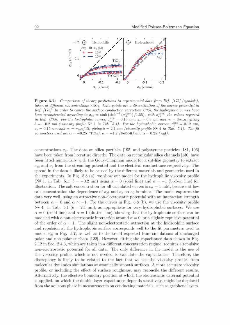
92 Modified Poisson-Boltzmann Equation
-0.2-0.10
-0.2
-0.1
0
-0.2-0.10
σ0 (e/nm2)
σek (
e/nm
2 )
σ0 (e/nm2)
10-2
AgITiO2
FeOOH
10-3
exp. fit c0 (M)
ba Hydrophilic Hydrophobic
Figure 5.7: Comparison of theory predictions to experimental data from Ref. [175] (symbols),taken at different concentrations kno3. Data points are a discretization of the curves presented inRef. [175]. In order to cancel the surface conduction correction [175], the hydrophilic curves havebeen reconstructed according to σek = sinh
(
sinh−1 (σcorr.
ek) /1.55
)
, with σcorr.
ekthe values reported
in Ref. [175]. For the hydrophilic curves, zdds⊥ = 0.10 nm, zs = 0.3 nm and ηi = 3ηbulk, giving
b = −0.2 nm (viscosity profile No 1 in Tab. 5.1). For the hydrophobic curves, zdds⊥ = 0.12 nm,
zs = 0.15 nm and ηi = ηbulk/15, giving b = 2.1 nm (viscosity profile No 4 in Tab. 5.1). The fitparameters used are α = −0.25 (tio2), α = −1.7 (feooh) and α = 0.25 (agi).
concentrations c0 . The data on silica particles [195] and polystyrene particles [181, 196]have been taken from literature directly. The data on rectangular silica channels [130] havebeen fitted numerically with the Gouy-Chapman model for a slit-like geometry to extractσek and σc from the streaming potential and the electrical conductance respectively. Thespread in the data is likely to be caused by the different materials and geometries used inthe experiments. In Fig. 5.8 (a), we show our model for the hydrophilic viscosity profile(No 1. in Tab. 5.1: b = −0.2 nm) using α = 0 (solid line) and α = −1 (broken line) forillustration. The salt concentration for all calculated curves is c0 = 1 mM, because at lowsalt concentration the dependence of σek and σc on c0 is minor. The model captures thedata very well, using an attractive non-electrostatic potential with an interaction strengthbetween α = 0 and α ≃ −1. For the curves in Fig. 5.8 (b), we use the viscosity profileNo 4. in Tab. 5.1 (b = 2.1 nm), as appropriate for very hydrophobic surfaces. We useα = 0 (solid line) and α = 1 (dotted line), showing that the hydrophobic surface can bemodeled with a non-electrostatic interaction around α = 0, or a slightly repulsive potentialof the order of α = 1. The slight non-electrostatic attraction at the hydrophilic surfaceand repulsion at the hydrophobic surface corresponds well to the fit parameters used tomodel σek in Fig. 5.7, as well as to the trend expected from simulations of unchargedpolar and non-polar surfaces [122]. However, fitting the capacitance data shown in Fig.2.12 in Sec. 2.4.3, which are taken in a different concentration regime, requires a repulsivenon-electrostatic potential for all data. The only difference in the model is the use ofthe viscosity profile, which is not needed to calculate the capacitance. Therefore, thediscrepancy is likely to be related to the fact that we use the viscosity profiles frommolecular dynamics simulations at atomically smooth surfaces. A more accurate viscosityprofile, or including the effect of surface roughness, may reconcile the different results.Alternatively, the effective boundary position at which the electrostatic external potentialis applied, on which the double-layer capacitance depends sensitively, might be displacedfrom the aqueous phase in measurements on conducting materials, such as graphene layers.
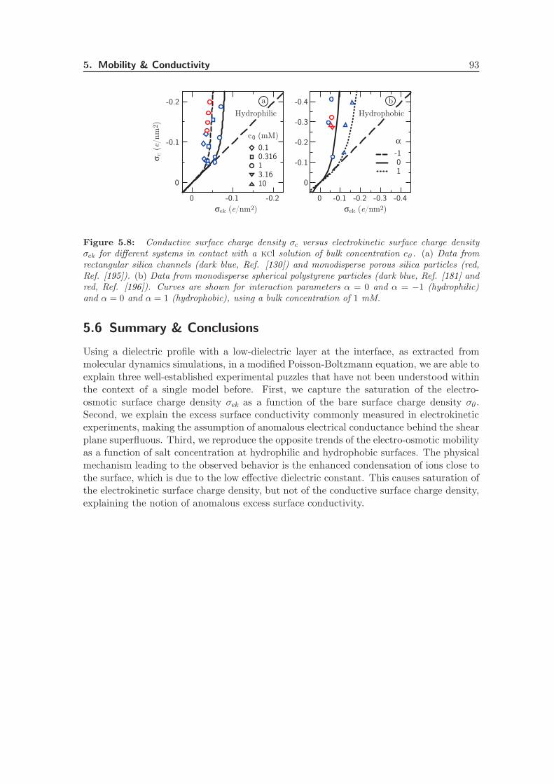
5. Mobility & Conductivity 93
-0.2-0.10
-0.2
-0.1
0
-0.4-0.3-0.2-0.10
σc (
e/nm
2 )
σek (e/nm2) σek (e/nm2)
-0.4
-0.3
-0.2
-0.1
0
c0 (mM)
0.31613.1610
10
α
-10.1
HydrophobicHydrophilic
ba
Figure 5.8: Conductive surface charge density σc versus electrokinetic surface charge densityσek for different systems in contact with a kcl solution of bulk concentration c0 . (a) Data fromrectangular silica channels (dark blue, Ref. [130]) and monodisperse porous silica particles (red,Ref. [195]). (b) Data from monodisperse spherical polystyrene particles (dark blue, Ref. [181] andred, Ref. [196]). Curves are shown for interaction parameters α = 0 and α = −1 (hydrophilic)and α = 0 and α = 1 (hydrophobic), using a bulk concentration of 1 mM.
5.6 Summary & Conclusions
Using a dielectric profile with a low-dielectric layer at the interface, as extracted frommolecular dynamics simulations, in a modified Poisson-Boltzmann equation, we are able toexplain three well-established experimental puzzles that have not been understood withinthe context of a single model before. First, we capture the saturation of the electro-osmotic surface charge density σek as a function of the bare surface charge density σ0 .Second, we explain the excess surface conductivity commonly measured in electrokineticexperiments, making the assumption of anomalous electrical conductance behind the shearplane superfluous. Third, we reproduce the opposite trends of the electro-osmotic mobilityas a function of salt concentration at hydrophilic and hydrophobic surfaces. The physicalmechanism leading to the observed behavior is the enhanced condensation of ions close tothe surface, which is due to the low effective dielectric constant. This causes saturation ofthe electrokinetic surface charge density, but not of the conductive surface charge density,explaining the notion of anomalous excess surface conductivity.

94 Summary & Conclusions
Chapter 6Final Observations & Outlook
The aim of the work described in the preceding chapters is to incorporate informationabout the molecular structure of interfacial water into the description of the static anddynamic properties of aqueous solutes, using molecular dynamics (md) simulations tocomplement continuum theory. We show that the use of continuum theory enables us toreach length and time scales that are unattainable using only md simulations. At the sametime, it provides us with the flexibility to easily vary system parameters such as geometry,salt concentration and surface charge density. One of the most significant advantages ofthis combination of molecular detail, flexibility of model parameters and sufficiently largescale is that it allows direct comparison with experimental data. Our multiscale modelingapproach thus provides us with the means for experimental verification of our theoreticalmodels, and simultaneously offers new insight into the molecular origin of experimentalobservations.
Summarizing the results of our work, we first establish the framework to extract thefull tensorial dielectric interface profiles from md data (Chapter 2). Especially the per-pendicular dielectric profiles ε−1
⊥ (z) exhibit rich structure and distinct differences betweenhydrophobic and hydrophilic surfaces. In the context of coarse-grained Poisson-Boltzmannmodeling, experimental capacitance data are well reproduced, indicating the validity ofour theoretical approach. We show that a low-dielectric interfacial layer – a concept knownas the Stern layer – arises naturally from dielectric interfacial effects of pure water, at leastat low salt concentration. In this way, we establish the molecular origin of the Stern layer,which has been used in models of the electric double layer for almost a century. The di-electric dividing surface position is suggested as a straightforward definition of the widthof a Stern layer with ε = 1.
Second, we quantify how the hydrodynamic boundary condition influences electrokineticflow (Chapter 3). In particular, we show that the electrokinetic energy conversion efficiencyin hydrophilic nanofluidic channels agrees well with the hydrodynamic model of a singleinterfacial water layer with strongly enhanced viscosity. In addition, using estimates fromab initio simulations, we show that charge transfer between water molecules – which isone of the molecular effects disregarded in classical md simulations – does not contributesignificantly to the electrophoretic mobility of gas bubbles.
Third, we incorporate molecular spinning of water into the Navier Stokes equation,showing that electrokinetic pumping of water in absence of mobile charges is possible with
96 Final Observations & Outlook
rotating electric fields, which opens the way for efficient power conversion in nanoscopicdevices (Chapter 4). Similarly, an electric field in the shape of a running wave, generatedby an array of externally attached electrodes, may be used to drive the flow of pure waterthrough a carbon nanotube. Static electric fields in an electro-neutral dipolar fluid do notgive rise to flow, however, even in the presence of dipolar surface ordering. That meansthat, although the polar molecular ordering has a decisive influence on the interfacialelectrostatics as well as on the distribution of ions at charged interfaces, it does not havea direct effect on the mobility of solutes in static electric fields. This result marks the endof a surge of debate and speculation about molecular ordering as the possible origin of theobserved electrophoretic mobility of nominally uncharged oil droplets and gas bubbles inpure water, proving that its source must be found elsewhere.
Finally, we incorporate the combined effects of the varying dielectric permittivity andthe viscosity profile into a modified continuum theory, and numerically calculate theelectro-osmotic flow and the electric surface conductivity of charged surfaces (Chapter5). Our model captures the experimental trends of the electro-osmotic flow as a functionof the bare surface charge density, as well as its dependence on the bulk salt concentrationwith high accuracy. Moreover, the experimentally well-established excess surface conduc-tivity, generally referred to as anomalous surface conductivity follows directly from ourmodel. The latter result makes the assumption of electrical conductance through other-wise static water layers – which has been the common explanation of the experimentalobservations – superfluous. Our model provides direct insight into the molecular origin ofthe dynamic properties of interfacial water layers, which have been elusive and subject tospeculation for a long time.
In conclusion, we show that classical molecular dynamics simulations can be used to pro-vide the molecular information missing from standard continuum theory, and that takingthe profiles from md simulations into account yields very good agreement with experimen-tal data on a wide range of static and dynamic properties of aqueous interfaces. Therefore,at the current stage, our modeling scheme seems to contain sufficient complexity to ex-plain a number of at-first-sight disconnected and hitherto puzzling experimental findingsand trends. Needless to say, however, it only constitutes a first step toward a completedescription of the intricate electrostatic and electrokinetic properties of charged surfacesin a unified framework.
Future work could be aimed at extending our modeling to include a number of importanteffects that have been left out up to now; examples include charge regulation at thesurface as a function of varying salt concentration, surface roughness and curvature andelectrofriction effects [197], as well as electrostatic correlation effects beyond the mean-fieldlevel [198]. We have also made some rigorous simplifying approximations, e.g. in studyingplanar surfaces in contact with pure water and modeling the viscosity and dielectric profilesby simple square-well functions (Chapter 5). In the remainder of this chapter, we listpossible directions for future research.
Ions at interfaces. All profiles calculated in this thesis are extracted from md simulationsof pure water at uncharged surfaces. The influence that ions and surface charges have onthe hydrodynamic interfacial properties and on the dielectric profile comprises both theeffect of atomic polarizability and the effect of highly charged objects on the local waterstructure. Modifications to the dielectric profile and non-linear effects are expected at highsalt concentrations. In addition, surface charges cause electrofriction, which affects the
6. Final Observations & Outlook 97
hydrodynamic properties of the interface. It is unclear whether such contributions can becalculated from classical md simulations, or whether e.g. quantum-chemical simulationsare needed.
Another simplification used in our current work is to treat the non-electrostatic surface-ion interaction using a simple exponentially decaying function. Ion adsorption potentialsmay be much more complex, and deserve attention in future investigations.
Polar ions. Propensity of the water ions hydronium (h3o+) and hydroxide (oh−) for
adsorption on different surface types remains controversial. Different experimental resultshave contradictory interpretations, and conclusions from md simulations are questionablebecause of the lack of reliable force fields. In Ref. [i], we report on the optimizationof a classical md force field for hydronium and hydroxide with respect to the solvationfree energy and the activity coefficient. In future work, these force fields can be used togain insight in the molecular properties that determine the behavior of the water ions ataqueous interfaces.
Non-local dielectric effects. High surface charge density reduces the typical decay lengthof the displacement field. When the characteristic length scale of the displacement fieldvariation reaches the typical length scale on which the dielectric profile varies, the fullnon-local dielectric tensor is needed to properly calculate the electrostatics. The limitsof applicability of our current approach, as well as a suitable theoretical framework totreat non-local dielectric effects on a molecular level have not been established and needattention in future studies.
Effects beyond mean-field theory. In this thesis, all electrostatics have been treated onthe mean-field level, which provides an excellent description of some of the most commonlyencountered systems, namely monovalent ions at moderate salt concentrations. The ap-proximation breaks down, however, for high surface charge density, as well as for highcounterion valency, in which case correlated effects such as image-charge interactions andion-ion correlations gain importance.
Non-ideal surfaces and complex geometries. Finally, the viscosity profile, density anddielectric profile at inhomogeneously charged, corrugated and curved surfaces deviate fromthe predictions for smooth planar surfaces, but to which extent is unclear. Therefore, moreresearch is needed to establish whether our current theoretical models of the interfacialproperties can be used as building blocks to extend our current theoretical framework tomore complicated geometries and surface types.

98 Final Observations & Outlook

Appendix ALiterature Values of theDouble-Layer Capacitance
This appendix contains an overview of published experimental values of the double-layercapacitance on various carbon-based surfaces in aqueous electrolytes. The capacitanceof the electrical double layer is measured using cyclic voltammetry, galvanostatic charge-discharge or ac impedance spectroscopy. The accessible surface area is determined usingn2 adsorption.
In the tables below, we have grouped the different measurements based on the contactangle in aqueous solution; when below 90, the substrate is classified as hydrophilic (listedin Tab. A.1), otherwise as hydrophobic (listed in Tab. A.2). The scattering in the databetween substrates and electrolytes is larger than the structural difference between hy-drophilic and hydrophobic substrates. Nevertheless, when a specific substrate is modifiedto become more hydrophilic, for example using functional groups or doping, the double-layer capacitance increases [30, 199]. Materials of which the contact angle is unknown orunclear are displayed in Tab. A.3. Many of the materials used for double-layer capacitorsbelong to the class of so-called activated carbons, which are treated with a gas plasma ora strong acid or base solution to make the surface more porous. The specific capacitanceof the activated carbons is shown in Tab. A.4. While increasing the total capacitance ofthe sample, activation of a carbon surface often decreases the capacitance per unit surfacearea dramatically [200, 201]. Although the mechanism leading to this decrease is unclear,we can safely assume that a part of the additional surface area created by the activationprocess is inaccessible to the electrolyte, and therefore does not contribute to the double-layer capacitance. Because of these poorly defined surface characteristics, Fig. 2.12 of Sec.2.4.3 only contains the data from Tabs. A.1, A.2 and A.3.

100 Appendix
Table A.1: Double-layer capacitance of hydrophilic carbon-based materials.Surface material Contact angle Electrolyte Concentration Capacitance Ref.
() (M) (µF/cm2)
Carbon fibers 24 - 37 [202] h2so4 0.5 6.0 [203]a
7.5
9.2
12.9
Carbon-coated al2o3 57 h2so4 1 7.0 [199]
Nitrogen-doped 41 11.4
Boron-doped 60 12.9
Oxidated polyvinyl- 45 - 67 h2so4 1 13.2 [204]b
pyridine [205, 206]
Blend with coal-tar 14.3
pitch
aDifferent values correspond to different commercial samples (untreated).bValues estimated by voltammetry at 1 mVs−1. The blend with coal tar pitch is 1 : 1.
Table A.2: Double-layer capacitance of hydrophobic carbon-based materials.Surface material Contact angle Electrolyte Concentration Capacitance Ref.
() (M) (µF/cm2)
Boron-doped diamond > 90 [207] h2so4 0.1 3.7 [208]a
7.1
kcl 0.1 3.4
4.5
nano3 0.1 3.8
6.3
naoh 0.1 3.9
4.8
Carbide-derived carbon > 90 [209] h2so4 2 11.4 [210]
tic, sic & sic/tic 13.8
11.8
Graphite 98 [211] koh 6 17.5 [212]b
16.7
19.2
25.9
33.9
41.6
51.4
64.0
Graphene nanosheets 127 [211] koh 7.6 29 [213]c
26
52
Carbon black h2so4 1 8 [214]
Graphite powder nacl 5.6 35
aThe different values correspond to ac impedance and cyclic voltametry measurements, respectively.bThe surface area of natural graphite was increased using ball-milling; different values correspond to
different milling times.cDifferent values correspond to different concentrations of oxidant used to prepare the graphene sheets.

A. Double-Layer Capacitance Literature 101
Table A.3: Double-layer capacitance of materials with unknown contact angle.Surface material Electrolyte Concentration Capacitance Ref.
(M) (µF/cm2)
Porous carbon h2so4 1 5.3 [215]
Porous carbon with polyaniline 9.0
Silica-templated mesoporous carbon h2so4 1 12.8 [204]
10.1
7.4
9.3
11.4
9.4
Silica-templated mesoporous carbon h2so4 1 7.3 [216]
2 14 [217]
2 13 [218]
Silica-templated mesoporous carbon h2so4 1 10.2 [219]a
10.6
10.7
10.9
koh 6 9.8
10.9
8.9
10.6
Mesoporous carbon with nio koh 2 18.2 [220]
Carbon aerogel koh 4 23 [214]
koh 6 28.5 [221]
Porous carbon koh 6 33 [201]
Self-ordered mesoporous carbon lipf6 1 10 [222]
Nitrogen-containing mesoporous carbon koh 6 39.2 [200]b
Ordered mesoporous carbon 10.0
Porous carbon from carbonization koh 6 20.8 [223]c
of poly(vinylidene chloride) 22.0
20.8
18.2
15.2
12.9
Diamond film nacl 0.5 3.7 [224]d
Polyacrylonitrile h2so4 1 24.9 [204]
Blend with coal tar pitch 20.3
17.5
tic/tio2 h2so4 2 14.8 [210]
Carbon composite from waste paper koh 6 43.2 [221]
aData taken at two different samples, using galvanostatic discharge at 100 mAg−1 and using cyclicvoltammetry at 1 mVs−1.
bData taken at the lowest scan rate (2 mVs−1).cDifferent values correspond to different carbonization temperatures (400C – 900C).dAfter equilibration in electrolyte, assuming complete wetting at the maximum of the capacitance.

102 Appendix
Table A.4: Double-layer capacitance of different kinds of activated carbons.Surface material Electrolyte Concentration Capacitance Ref.
(M) (µF/cm2)
co2 activated porous carbon koh 6 13 [201]
9.6
koh activated porous carbon 10
8.8
Nitrogen-containing mesoporous koh 6 26.2 [200]
carbon, activated with koh 13.7
11.3
Ordered mesoporous carbon, koh 6 11.2 [200]
activated with koh 12.7
12.4
koh-activated carbon h2so4 1 20.4 [225]a
25.1
26.9
naoh-activated carbon 24.7
25.0
28.9
Wood-origin hno3-activated carbon h2so4 1 11.6 [226]b
10.3
19.1
25.5
23.0
32.6
Activated carbon nacl 5.6 19 [214]
o2-activated carbon fibers 6.6 [203]
7.0
9.1
13.2
aDifferent values correspond to different carbonization temperatures (600C – 700C).bData taken using galvanostatic charge-discharge at 50 − 100 mAg−1; Different values correspond to
samples with different surface functional groups.
Appendix BElectrokinetics Within theGouy-Chapman Model
We derive the electro-osmotic mobility, the electrokinetic surface charge density and theconductive surface charge density from the Gouy-Chapman model.
Gouy-Chapman model. The standard Poisson equation is given by
ε0εbulk∇2ψ (z) = −ρ (z) . (B.1)
According to the standard Boltzmann equation, the charge density ρ (z) equals
ρ (z) = −2ec0 sinh [βeψ (z)] . (B.2)
The solution to the Poisson-Boltzmann equation (Eqs. B.1–B.2) for a monovalent elec-trolyte at a charged plane is
ψ (z) = − 2
βeln
1 + γ exp [−κz]1 − γ exp [−κz] , (B.3)
withγ = −κλ+
√
κ2λ2 + 1. (B.4)
The inverse Debye screening length κ and the Gouy-Chapman length λ are given by
κ =
√
2e2c0β
ε0εbulkand λ =
2ε0εbulkβe|σ| . (B.5)
The electro-osmotic mobility is related to the charge density by the Stokes equation, whichreads
ηbulk∇2u‖ (z) = −ρ (z)E‖, (B.6)
for spatially constant viscosity ηbulk.
Electro-osmotic mobility. Eliminating the charge density ρ (z) from Eqs. B.1 and B.6yields
ε0εbulk∇2ψ (z) =ηbulkE‖
∇2u‖ (z) . (B.7)
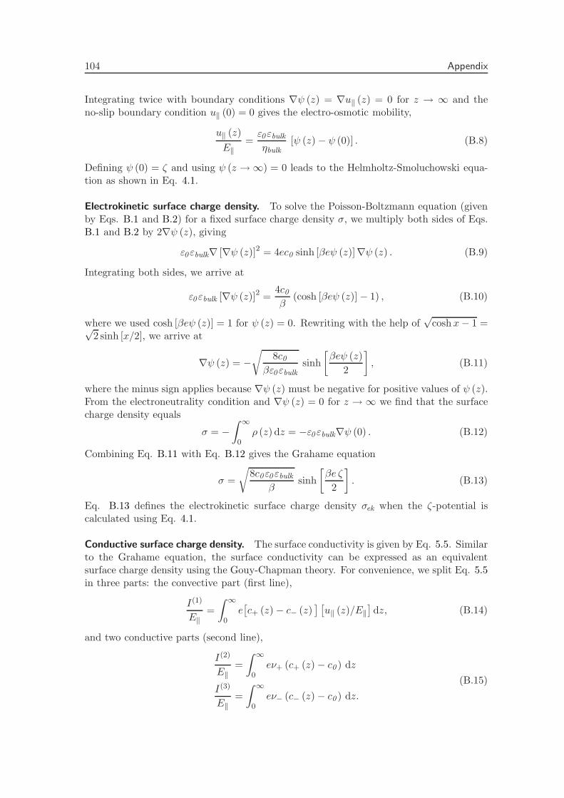
104 Appendix
Integrating twice with boundary conditions ∇ψ (z) = ∇u‖ (z) = 0 for z → ∞ and theno-slip boundary condition u‖ (0) = 0 gives the electro-osmotic mobility,
u‖ (z)
E‖=ε0εbulkηbulk
[ψ (z) − ψ (0)] . (B.8)
Defining ψ (0) = ζ and using ψ (z → ∞) = 0 leads to the Helmholtz-Smoluchowski equa-tion as shown in Eq. 4.1.
Electrokinetic surface charge density. To solve the Poisson-Boltzmann equation (givenby Eqs. B.1 and B.2) for a fixed surface charge density σ, we multiply both sides of Eqs.B.1 and B.2 by 2∇ψ (z), giving
ε0εbulk∇ [∇ψ (z)]2 = 4ec0 sinh [βeψ (z)]∇ψ (z) . (B.9)
Integrating both sides, we arrive at
ε0εbulk [∇ψ (z)]2 =4c0β
(cosh [βeψ (z)] − 1) , (B.10)
where we used cosh [βeψ (z)] = 1 for ψ (z) = 0. Rewriting with the help of√
coshx− 1 =√2 sinh [x/2], we arrive at
∇ψ (z) = −√
8c0βε0εbulk
sinh
[
βeψ (z)
2
]
, (B.11)
where the minus sign applies because ∇ψ (z) must be negative for positive values of ψ (z).From the electroneutrality condition and ∇ψ (z) = 0 for z → ∞ we find that the surfacecharge density equals
σ = −∫ ∞
0ρ (z) dz = −ε0εbulk∇ψ (0) . (B.12)
Combining Eq. B.11 with Eq. B.12 gives the Grahame equation
σ =
√
8c0ε0εbulkβ
sinh
[
βe ζ
2
]
. (B.13)
Eq. B.13 defines the electrokinetic surface charge density σek when the ζ-potential iscalculated using Eq. 4.1.
Conductive surface charge density. The surface conductivity is given by Eq. 5.5. Similarto the Grahame equation, the surface conductivity can be expressed as an equivalentsurface charge density using the Gouy-Chapman theory. For convenience, we split Eq. 5.5in three parts: the convective part (first line),
I(1)
E‖=
∫ ∞
0e[
c+ (z) − c− (z)] [
u‖ (z)/E‖
]
dz, (B.14)
and two conductive parts (second line),
I(2)
E‖=
∫ ∞
0eν+ (c+ (z) − c0 ) dz
I(3)
E‖=
∫ ∞
0eν− (c− (z) − c0 ) dz.
(B.15)

B. Gouy-Chapman Model 105
Inserting the electro-osmotic mobility of Eq. B.8 and the charge density of Eq. B.1 in Eq.B.14 gives
I(1)
E‖= −ε
20ε
2bulk
ηbulk
∫ ∞
0∇2ψ (z) [ψ (z) − ψ (0)] dz, (B.16)
which can be integrated by parts to give
I(1)
E‖=ε20ε
2bulk
ηbulk
∫ ∞
0[∇ψ (z)]2 dz, (B.17)
using ∇ψ (z) = 0 for z → ∞. Inserting the derivative of Eq. B.3 in Eq. B.17 yields
I(1)
E‖=ε20ε2bulk
ηbulk
∫ ∞
0
[
4κγ exp [−κz]βe (1 − γ2 exp [−2κz])
]2
dz
=ε20ε
2bulk
ηbulk
[
− 8κγ2 exp [−2κz]
β2e2 (1 − γ2 exp [−2κz])
]∞
0
=ε20ε2bulk
ηbulk
8κγ2
β2e2 (1 − γ2).
(B.18)
The second part of the conductivity equals
I(2)
E‖=
∫ ∞
0eν+c0
[
(
1 + γ exp [−κz]1 − γ exp [−κz]
)2
− 1
]
dz
=
∫ ∞
0eν+c0
[
4γ exp [−κz](1 − γ exp [−κz])2
]
dz
= eν+c0
[
− 4γ exp [−κz]κ (1 − γ exp [−κz])
]∞
0
= eν+c04γ
κ (1 − γ).
(B.19)
Similarly,I(3)
E‖= −eν−c0
4γ
κ (1 + γ). (B.20)
Summing up I =∑
i I(i) and rewriting in terms of κ gives the total excess conductivity
I
E‖=
32γ2e2c20κ3 (1 − γ2) ηbulk
+4γec0 ν+
κ (1 + γ)− 4γec0 ν−κ (1 − γ)
. (B.21)
For simplicity, we assume ν+ = ν− = ν, so Eq. B.21 becomes
I
E‖=
γ2
1 − γ2
[
32e2c20κ3ηbulk
+8ec0 ν
κ
]
, (B.22)
which is inverted to give the following surface charge density, using Eqs. B.4 and B.5
σ =κ2ηbulk
4ec0 + νκ2ηbulk
√
I
E‖
√
I
E‖+
32e2c20
κ3ηbulk+
8ec0 ν
κ. (B.23)
Eq. B.23 defines the conductive surface charge density σc when the conductivity is calcu-lated using Eq. 5.5.

106 Appendix

List of Figures
2.1 Top view of the diamond surfaces and density of the adjacent water . . . . . . 15
2.2 Dielectric function at hydrophilic & hydrophobic surfaces . . . . . . . . . . . . 16
2.3 Multipole components of the parallel dielectric function . . . . . . . . . . . . . 18
2.4 Multipole components of the inverse perpendicular dielectric function . . . . . 19
2.5 Parallel & perpendicular polarizability . . . . . . . . . . . . . . . . . . . . . . . 20
2.6 Electric-field dependence of the inverse perpendicular dielectric function . . . . 21
2.7 Electric-field dependence of the water density . . . . . . . . . . . . . . . . . . . 22
2.8 Multipole components of the perpendicular displacement field . . . . . . . . . 23
2.9 Multipole components of the electrostatic potential profile . . . . . . . . . . . . 24
2.10 Dielectric & Gibbs dividing surfaces . . . . . . . . . . . . . . . . . . . . . . . . 26
2.11 Electrostatic potential, fields & ion densities at a charged interface . . . . . . . 28
2.12 Double-layer capacitance as a function of salt concentration . . . . . . . . . . . 29
2.13 Disjoining pressure between like-charged plates . . . . . . . . . . . . . . . . . . 31
2.14 Ion-surface interaction potential . . . . . . . . . . . . . . . . . . . . . . . . . . 33
3.1 Slip processes at hydrophobic and hydrophilic surfaces . . . . . . . . . . . . . . 36
3.2 Flow profiles at hydrophobic surfaces . . . . . . . . . . . . . . . . . . . . . . . 39
3.3 Efficiency of electrokinetic energy conversion . . . . . . . . . . . . . . . . . . . 40
3.4 ζ-potential of an air bubble using the instantaneous charge density . . . . . . . 45
3.5 ζ-potential of an air bubble using the laterally averaged charge density . . . . 46
3.6 Radial velocity inside a (16,16) carbon nanotube without reservoir . . . . . . . 47
4.1 Sketches of the rectangular and cylindrical geometries . . . . . . . . . . . . . . 53
4.2 Flow velocity in a rectangular channel . . . . . . . . . . . . . . . . . . . . . . . 58
4.3 Dipole density vs. time and dipole ordering field . . . . . . . . . . . . . . . . . 61
4.4 Torque density, spin field and flow velocity . . . . . . . . . . . . . . . . . . . . 62
4.5 Numerical results for the flow between two concentric cylinders . . . . . . . . . 65
4.6 Lennard-Jones force truncation . . . . . . . . . . . . . . . . . . . . . . . . . . . 67
4.7 Simulation snapshots of the planar systems: Oil, diamond & graphene . . . . . 68
4.8 Density, flow velocity, spin & vorticity in a planar diamond system . . . . . . . 69
4.9 Snapshots of the carbon nanotube simulations without reservoir . . . . . . . . 70
4.10 Density, flow velocity & spin in a (16,16) carbon nanotube . . . . . . . . . . . 71
4.11 The ζ-potentials of planar and cylindrical systems vs. cut-off length . . . . . . 72
4.12 Snapshot of, and cumulative flux through a cnt with reservoir . . . . . . . . . 73
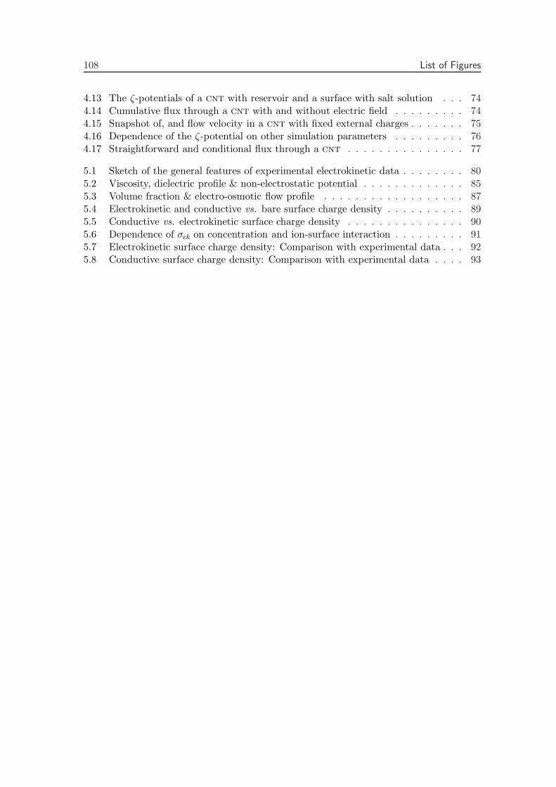
108 List of Figures
4.13 The ζ-potentials of a cnt with reservoir and a surface with salt solution . . . 744.14 Cumulative flux through a cnt with and without electric field . . . . . . . . . 744.15 Snapshot of, and flow velocity in a cnt with fixed external charges . . . . . . . 754.16 Dependence of the ζ-potential on other simulation parameters . . . . . . . . . 764.17 Straightforward and conditional flux through a cnt . . . . . . . . . . . . . . . 77
5.1 Sketch of the general features of experimental electrokinetic data . . . . . . . . 805.2 Viscosity, dielectric profile & non-electrostatic potential . . . . . . . . . . . . . 855.3 Volume fraction & electro-osmotic flow profile . . . . . . . . . . . . . . . . . . 875.4 Electrokinetic and conductive vs. bare surface charge density . . . . . . . . . . 895.5 Conductive vs. electrokinetic surface charge density . . . . . . . . . . . . . . . 905.6 Dependence of σek on concentration and ion-surface interaction . . . . . . . . . 915.7 Electrokinetic surface charge density: Comparison with experimental data . . . 925.8 Conductive surface charge density: Comparison with experimental data . . . . 93

List of Tables
2.1 Dielectric & Gibbs dividing surfaces . . . . . . . . . . . . . . . . . . . . . . . . 25
5.1 Parameter combinations of the viscosity profile . . . . . . . . . . . . . . . . . . 88
A.1 Double-layer capacitance of hydrophilic carbon-based materials . . . . . . . . . 100A.2 Double-layer capacitance of hydrophobic carbon-based materials . . . . . . . . 100A.3 Double-layer capacitance of materials with unknown contact angle . . . . . . . 101A.4 Double-layer capacitance of different kinds of activated carbons . . . . . . . . . 102

110 List of Tables

List of Publications
This thesis is based on the following papers, which have been published in, or have
been submitted to, or are being prepared to be submitted to peer-reviewed journals:
[i] Douwe Jan Bonthuis and Roland R. Netz, Optimization of a classical molec-ular dynamics force field for hydronium and hydroxide: In preparation
[ii] Douwe Jan Bonthuis and Roland R. Netz, Unraveling the combined effects ofdielectric and viscosity profiles on surface capacitance, electro-osmotic mobilityand electric surface conductivity : Submitted
[iii] Douwe Jan Bonthuis, Stephan Gekle and Roland R. Netz, Profile of the staticpermittivity tensor of water at interfaces: Consequences for capacitance, hydra-tion interaction and ion adsorption, Langmuir 28, 7679 (2012): Cover article
[iv] Klaus F. Rinne, Stephan Gekle, Douwe Jan Bonthuis and Roland R. Netz,Nanoscale pumping of water by ac electric fields, Nano Letters 12, 1780 (2012)
[v] Robert Vacha, Ondrej Marsalek, Adam P. Willard, Douwe Jan Bonthuis,Roland R. Netz and Pavel Jungwirth, Charge transfer between water moleculesas the possible origin of the observed charging at the surface of pure water, TheJournal of Physical Chemistry Letters 3, 107 (2012)
[vi] Douwe Jan Bonthuis, Stephan Gekle and Roland R. Netz, Dielectric profileof interfacial water and its effect on double layer capacitance, Physical ReviewLetters 107, 166102 (2011)
[vii] Douwe Jan Bonthuis, Klaus F. Rinne, Kerstin Falk, C. Nadir Kaplan, Do-minik Horinek, A. Nihat Berker, Lyderic Bocquet and Roland R. Netz, Theoryand simulations of water flow through carbon nanotubes: Prospects and pitfalls,Journal of Physics: Condensed Matter 23, 184110 (2011)
[viii] Douwe Jan Bonthuis, Kerstin Falk, C. Nadir Kaplan, Dominik Horinek, A.Nihat Berker, Lyderic Bocquet and Roland R. Netz, Comment on “Pumping ofconfined water in carbon nanotubes by rotation-translation coupling”, PhysicalReview Letters 105, 209401 (2010)
[ix] Douwe Jan Bonthuis, Dominik Horinek, Lyderic Bocquet and Roland R. Netz,Electrokinetics at aqueous interfaces without mobile charges, Langmuir 26, 12614(2010): Cover article
112 List of Publications
[x] Douwe Jan Bonthuis, Dominik Horinek, Lyderic Bocquet and Roland R. Netz,Electrohydraulic power conversion in planar nanochannels, Physical Review Let-ters 103, 144503 (2009): With Synopsis in the aps magazine “Physics”
[xi] Dominik Horinek, Andreas Serr, Douwe Jan Bonthuis, Mathias Bostrom,Werner Kunz and Roland R. Netz, Molecular hydrophobic attraction and ion-specific effects studied by molecular dynamics, Langmuir 24, 1271 (2008)
Publications not discussed in the present thesis:
[xii] Douwe Jan Bonthuis, Christine Meyer, Derek Stein and Cees Dekker, Confor-mation and dynamics of dna confined in slitlike nanofluidic channels, PhysicalReview Letters 101, 108303 (2008)
[xiii] Frank H. J. van der Heyden, Douwe Jan Bonthuis, Derek Stein, ChristineMeyer and Cees Dekker, Power generation by pressure-driven transport of ionsin nanofluidic channels, Nano Letters 7, 1022 (2007)
[xiv] Frank H. J. van der Heyden, Douwe Jan Bonthuis, Derek Stein, ChristineMeyer and Cees Dekker, Electrokinetic energy conversion efficiency in nanofluidicchannels, Nano Letters 6, 2232 (2006)
[xv] Douwe Jan Bonthuis, Jingshan Zhang, Breton Hornblower, Jerome Mathe,Boris I. Shklovskii and Amit Meller, Self-energy-limited ion transport in sub-nanometer channels, Physical Review Letters 97, 128104 (2006)

Bibliography
[1] Ball, P. Water as an active constituent in cell biology. Chem. Rev. 108, 74 (2008).
[2] Stone, H. A., Stroock, A. D., and Ajdari, A. Engineering flows in small devices:Microfluidics toward a lab-on-a-chip. Annu. Rev. Fluid Mech. 36, 381 (2004).
[3] Squires, T. M. and Quake, S. R. Microfluidics: Fluid physics at the nanoliter scale.Rev. Mod. Phys. 77, 977 (2005).
[4] Lyklema, J. Electrokinetics after Smoluchowski. Colloids and Surfaces A 222, 5(2003).
[5] Catterall, W. A. Structure and function of voltage-gated ion channels. Annu. Rev.Biochem 64, 193 (1995).
[6] Terry, L. J., Shows, E. B., and Wente, S. R. Crossing the nuclear envelope: Hierar-chical regulation of nucleocytoplasmic transport. Science 318, 1412 (2007).
[7] Yao, S., Herzog, D. E., Zeng, S., Mikkelsen, J. C., and Santiago, J. G. Porous glasselectroosmotic pumps: design and experiments. J. Colloid Int. Sci. 268, 143 (2003).
[8] Yang, J., Lu, F., Kostiuk, L. W., and Kwok, D. Y. Electrokinetic microchannelbattery by means of electrokinetic and microfluidic phenomena. J. Micromech. Mi-croeng. 13, 963 (2003).
[9] Daiguji, H., Yang, P., Szeri, A. J., and Majumder, A. Electrochemomechanical energyconversion in nanofluidic channels. Nanoletters 4, 2315 (2004).
[10] Olthuis, W., Schippers, B., Eijkel, J. C. T., and Van den Berg, A. Energy fromstreaming current and potential. Sens. Actuators B 111, 385 (2005).
[11] Service, R. F. Desalination freshens up. Science 313, 1088 (2006).
[12] Sparreboom, W., Van den Berg, A., and Eijkel, J. C. T. Principles and applicationsof nanofluidic transport. Nature Nanotech. 4, 713 (2009).
[13] MacKinnon, R. Potassium channels and the atomic basis of selective ion conduction.Angew. Chem. Int. Ed. 43, 4265 (2004).
[14] Agre, P. Aquaporin water channels. Angew. Chem. Int. Ed. 43, 4278 (2004).
114 Bibliography
[15] Kuyucak, S., Andersen, O. S., and Chung, S.-H. Models of permeation in ion chan-nels. Rep. Prog. Phys. 64, 1427 (2001).
[16] Helmholtz, H. Studien uber elektrische Grenzschichten. Wied. Ann. 7, 337 (1879).
[17] Von Smoluchowski, M. Zur Theorie der electrischen Kataphorese und derOberflachenleitung. Phys. Z. 6, 529 (1905).
[18] Huckel, E. Die Kataphorese der Kugel. Physik. Z. 25, 204 (1924).
[19] Israelachvili, J. and Wennerstrom, H. Role of hydration and water structure inbiological and colloidal interactions. Nature 379, 219 (1996).
[20] Bopp, P. A., Kornyshev, A. A., and Sutmann, G. Frequency and wave-vector depen-dent dielectric function of water: Collective modes and relaxation spectra. J. Chem.Phys. 109, 1939 (1998).
[21] Faraudo, J. and Bresme, F. Anomalous dielectric behavior of water in ionic newtonblack films. Phys. Rev. Lett. 92, 236102 (2004).
[22] Stern, O. Zur Theorie der elektrolytischen Doppelschicht. Z. Elektrochem. 30, 508(1924).
[23] Tielrooij, K. J. et al. Dielectric relaxation dynamics of water in model membranesprobed by terahertz spectroscopy. Biophysical J. 97, 2484 (2009).
[24] Kornyshev, A. A., Schmickler, W., and Vorotyntsev, M. A. Nonlocal electrostaticapproach to the problem of a double layer at a metal-electrolyte interface. Phys. Rev.B 25, 5244 (1982).
[25] Kornyshev, A. A. and Vorotyntsev, M. A. Nonlocal dielectric response of theelectrode-solvent interface in the double-layer problem. Can. J. Chem. 59, 2031(1981).
[26] Blum, L. and Henderson, D. Mixtures of hard ions and dipoles against a chargedwall - the Ornstein-Zernike equation, some exact results, and the mean sphericalapproximation. J. Chem. Phys. 74, 1902 (1981).
[27] Levin, Y. Polarizable ions at interfaces. Phys. Rev. Lett. 102, 147803 (2009).
[28] Kornyshev, A. A. On the nonlocal electrostatic theory of hydration force. J. Elec-troanal. Chem. 204, 79 (1986).
[29] Dzubiella, J., Swanson, J. M. J., and McCammon, J. A. Coupling hydrophobicity,dispersion, and electrostatics in continuum solvent models. Phys. Rev. Lett. 96,087802 (2006).
[30] Kim, Y.-T. et al. Drastic change of electric double layer capacitance by surfacefunctionalization of carbon nanotubes. Applied Phys. Lett. 87, 234106 (2005).
[31] Marcelja, S. et al. Role of solvent structure in solution theory. J. Chem. Soc. FaradayTrans. II 73, 630 (1977).

Bibliography 115
[32] Abrashkin, A., Andelman, D., and Orland, H. Dipolar Poisson-Boltzmann equation:Ions and dipoles close to charge interfaces. Phys. Rev. Lett. 99, 077801 (2007).
[33] Paillusson, F. and Blossey, R. Slits, plates, and Poisson-Boltzmann theory in a localformulation of nonlocal electrostatics. Phys. Rev. E 82, 052501 (2010).
[34] Stillinger, F. H. and Ben-Naim, A. Liquid-vapor interface potential for water. J.Chem. Phys. 47, 4431 (1967).
[35] Barrat, J. and Bocquet, L. Large slip effect at a nonwetting fluid-solid interface.Phys. Rev. Lett. 82, 4671 (1999).
[36] Joly, L., Ybert, C., Trizac, E., and Bocquet, L. Hydrodynamics within the electricdouble layer on slipping surfaces. Phys. Rev. Lett. 93, 257805 (2004).
[37] Chandler, D. Physical chemistry - oil on troubled waters. Nature 445, 831 (2007).
[38] Vinogradova, O. I. Drainage of a thin liquid-film confined between hydrophobic sur-faces. Langmuir 11, 2213 (1995).
[39] Mamatkulov, S. I., Khabibullaev, P. K., and Netz, R. R. Water at hydrophobicsubstrates: Curvature, pressure, and temperature effects. Langmuir 20, 4756 (2004).
[40] De Gennes, P.-G. On fluid/wall slippage. Langmuir 18, 3413 (2002).
[41] Huang, D. M. et al. Water slippage versus contact angle: A quasiuniversal relation-ship. Phys. Rev. Lett. 101, 226101 (2008).
[42] Majumder, M. et al. Enhanced flow in carbon nanotubes. Nature 438, 44 (2005).
[43] Hummer, G., Rasaiah, J. C., and Noworyta, J. P. Water conduction through thehydrophobic channel of a carbon nanotube. Nature 414, 188 (2001).
[44] Hinds, B. A blueprint for a nanoscale pump. Nature Nanotech. 2, 673 (2007).
[45] Beattie, J. K., Djerdjev, A. M., and Warr, G. G. The surface of neat water is basic.Faraday Discuss. 141, 31 (2009).
[46] Schweiss, R. et al. Dissociation of surface functional groups and preferential ad-sorption of ions on self-assembled monolayers assessed by streaming potential andstreaming current measurements. Langmuir 17, 4304 (2001).
[47] Ciunel, K. et al. Evidence of surface charge at the air/water interface from thin-filmstudies on polyelectrolyte-coated substrates. Langmuir 21, 4790 (2005).
[48] Petersen, P. and Saykally, R. Is the liquid water surface basic or acidic? Macroscopicvs. molecular-scale investigations. Chem. Phys. Lett. 458, 255 (2008).
[49] Buch, V. et al. Water surface is acidic. Proc. Nat. Acad. Sci. USA 104, 7342 (2007).
[50] Vacha, R. et al. Autoionization at the surface of neat water: Is the top layer phneutral, basic, or acidic? Phys. Chem. Chem. Phys. 9, 4736 (2007).
[51] Knecht, V. et al. Electrophoretic mobility does not always reflect the charge on anoil droplet. J. Coll. Int. Sci. 318, 477 (2008).
116 Bibliography
[52] Berezhkovskii, A. and Hummer, G. Single-file transport of water molecules througha carbon nanotube. Phys. Rev. Lett. 89, 064503 (2002).
[53] Parsegian, A. Energy of an ion crossing a low dielectric membrane - solutions to 4relevant electrostatic problems. Nature 221, 844 (1969).
[54] Bonthuis, D. J. et al. Self-energy-limited ion transport in subnanometer channels.Phys. Rev. Lett. 97, 128104 (2006).
[55] Zhang, J., Kamenev, A., and Shklovskii, B. I. Conductance of ion channels andnanopores with charged walls: A toy model. Phys. Rev. Lett. 95, 148101 (2005).
[56] Doyle, D. A. et al. The structure of the potassium channel: Molecular basis of k+
conduction and selectivity. Science 280, 69 (1998).
[57] Kienker, P. K., Degrado, W. F., and Lear, J. D. A helical-dipole model describes thesingle-channel current rectification of an uncharged peptide ion-channel. Proc. Nat.Acad. Sci. USA 91, 4859 (1994).
[58] Kamenev, A., Zhang, J., Larkin, A. I., and Shklovskii, B. I. Transport in one-dimensional Coulomb gases: From ion channels to nanopores. Physica A 359, 129(2006).
[59] Li, J. et al. Electrostatic gating of a nanometer water channel. Proc. Nat. Acad.Sci. USA 104, 3687 (2007).
[60] Joseph, S. and Aluru, N. R. Pumping of confined water in carbon nanotubes byrotation-translation coupling. Phys. Rev. Lett. 101, 064502 (2008).
[61] Gong, X. et al. A charge-driven molecular water pump. Nature Nanotech. 2, 709(2007).
[62] Joseph, S. and Aluru, N. R. Why are carbon nanotubes fast transporters of water?Nanolett. 8, 452 (2008).
[63] Kim, D. and Darve, E. High-ionic-strength electroosmotic flows in uncharged hy-drophobic nanochannels. J. Coll. Int. Sci. 330, 194 (2009).
[64] Joseph, S. and Aluru, N. R. Hierarchical multiscale simulation of electrokinetictransport in silica nanochannels at the point of zero charge. Langmuir 22, 9041(2006).
[65] Lee, C., McCammon, J., and Rossky, P. The structure of liquid water at an extendedhydrophobic surface. J. Chem. Phys 80, 4448 (1984).
[66] Huang, D. M. and Chandler, D. The hydrophobic effect and the influence of solute–solvent attractions. J. Phys. Chem. B 106, 2047 (2002).
[67] Huang, D. M., Cottin-Bizonne, C., Ybert, C., and Bocquet, L. Aqueous electrolytesnear hydrophobic surfaces: Dynamic effects of ion specificity and hydrodynamic slip.Langmuir 24, 1442 (2008).
[68] Frenkel, D. and Smit, B. Understanding molecular simulation: From algorithms toapplications. Academic Press, New York, second edition, (2002).

Bibliography 117
[69] Gabriel, C. et al. Dielectric parameters relevant to microwave dielectric heating.Chem. Soc. Rev. 27, 213 (1998).
[70] Buchner, R., Barthel, J., and Stauber, J. The dielectric relaxation of water between0 C and 35 C. Chem. Phys. Lett. 306, 57 (1999).
[71] Rezus, Y. L. A. and Bakker, H. J. On the orientational relaxation of hdo in liquidwater. J. Chem. Phys. 123, 114502 (2005).
[72] Berendsen, H. J. C., Grigera, J. R., and Straatsma, T. P. The missing term ineffective pair potentials. J. Phys. Chem. 91, 6269 (1987).
[73] Abascal, J. L. F. and Vega, C. A general purpose model for the condensed phases ofwater: tip4p/2005. J. Chem. Phys. 123, 234505 (2005).
[74] Sendner, C., Horinek, D., Bocquet, L., and Netz, R. R. Interfacial water at hy-drophobic and hydrophilic surfaces: Slip, viscosity, and diffusion. Langmuir 25,10768 (2009).
[75] Benjamin, I. Chemical reactions and solvation at liquid interfaces: A microscopicperspective. Chem. Rev. 96, 1449 (1996).
[76] Marcelja, S. and Radic, N. Repulsion of interfaces due to boundary water. Chem.Phys. Lett. 42, 129 (1976).
[77] Ball, P. Chemical physics: How to keep dry in water. Nature 423, 25 (2003).
[78] Chandler, D. Interfaces and the driving force of hydrophobic assembly. Nature 437,640 (2005).
[79] Kornyshev, A. A., Spohr, E., and Vorotyntsev, M. A. Electrochemical interfaces: Atthe border line, In Encyclopedia of electrochemistry, chapter 2.1, 33. Wiley, NewYork (2002).
[80] Lyklema, J. Fundamentals of interface and colloid science, volume II. AcademicPress, London, (1995).
[81] Hunter, R. J. Foundations of colloid science. Oxford University Press, Oxford,second edition, (2001).
[82] Hasted, J. B., Ritson, D. M., and Collie, C. H. Dielectric properties of aqueous ionicsolutions. J. Chem. Phys. 16, 1 (1948).
[83] Grahame, D. C. Effects of dielectric saturation upon the diffuse double layer and thefree energy of hydration of ions. J. Chem. Phys. 18, 903 (1950).
[84] Heugen, U. et al. Solute-induced retardation of water dynamics probed directly byterahertz spectroscopy. Proc. Nat. Acad. Sci. USA 103, 12301 (2006).
[85] Frenkel, J. Kinetic theory of liquids. Dover Publications, New York, (1955).
[86] Shen, Y. R. and Ostroverkhof, V. Sum-frequency vibrational spectroscopy on waterinterfaces: Polar orientation of water molecules at interfaces. Chem. Rev. 106, 1140(2006).
118 Bibliography
[87] Ballenegger, V. and Hansen, J. Local dielectric permittivity near an interface. Eu-rophys. Lett. 63, 381 (2003).
[88] Bonthuis, D. J., Gekle, S., and Netz, R. R. Dielectric profile of interfacial water andits effect on double-layer capacitance. Phys. Rev. Lett. 107, 166102 (2011).
[89] Kharkats, Y. I., Kornyshev, A. A., and Vorotyntsev, M. A. Electrostatic models intheory of solutions. J. Chem. Soc. Faraday Trans. II 72, 361 (1976).
[90] Noyes, R. M. Thermodynamics of ion hydration as a measure of effective dielectricproperties of water. J. Am. Chem. Soc. 84, 513 (1962).
[91] Fedorov, M. V. and Kornyshev, A. A. Unravelling the solvent response to neutraland charged solutes. Mol. Phys. 105, 1 (2007).
[92] Leikin, S., Parsegian, V. A., Rau, D. C., and Rand, R. P. Hydration forces. Annu.Rev. Phys. Chem. 44, 369 (1993).
[93] Jackson, J. D. Classical electrodynamics. John Wiley & Sons, USA, third edition,(1998).
[94] Russakoff, G. Derivation of macroscopic Maxwell equations. Am. J. Physics 38,1188 (1970).
[95] Kirkwood, J. G. The dielectric polarization of polar liquids. J. Chem. Phys. 7, 911(1939).
[96] Frohlich, H. Theory of dielectrics. Clarendon Press, Oxford, (1949).
[97] Ballenegger, V. and Hansen, J. Dielectric permittivity profiles of confined polarfluids. J. Chem. Phys. 122, 114711 (2005).
[98] Lindahl, E., Hess, B., and Van der Spoel, D. Gromacs 3.0: a package for molecularsimulation and trajectory analysis. J. Mol. Mod. 7, 306 (2001).
[99] Sedlmeier, F., Horinek, D., and Netz, R. R. Spatial correlations of density andstructural fluctuations in liquid water: A comparative simulation study. J. Am.Chem. Soc. 133, 1391 (2011).
[100] Reddy, M. R. and Berkowitz, M. The dielectric constant of spc/e water. Chem.Phys. Lett. 155, 173 (1989).
[101] Fedorov, M. V. and Kornyshev, A. A. Towards understanding the structure andcapacitance of electrical double layer in ionic liquids. Electrochim. Acta. 53, 6835(2008).
[102] Bazant, M. Z., Storey, B. D., and Kornyshev, A. A. Double layer in ionic liquids:Overscreening versus crowding. Phys. Rev. Lett. 106, 046102 (2011).
[103] Kolb, J. F., Joshi, R. P., Xiao, S., and Schoenbach, K. H. Streamers in water andother dielectric liquids. J. Phys. D: Appl. Phys. 41, 234007 (2008).
[104] Paluch, M. Electrical properties of free surface of water and aqueous solutions. Adv.Colloid Interface Sci. 84, 27 (2000).

Bibliography 119
[105] Du, Q., Superfine, R., Freysz, E., and Shen, Y. R. Vibrational spectroscopy of waterat the vapor water interface. Phys. Rev. Lett. 70, 2313 (1993).
[106] Du, Q., Freysz, E., and Shen, Y. R. Vibrational spectra of water molecules atquartz/water interfaces. Phys. Rev. Lett. 72, 238 (1994).
[107] Du, Q., Freysz, E., and Shen, Y. R. Surface vibrational spectroscopic studies ofhydrogen bonding and hydrophobicity. Science 264, 826 (1994).
[108] Wilson, M. A., Pohorille, A., and Pratt, L. R. Study on the liquid vapor inter-face of water. 1: Simulation results of thermodynamic properties and orientationalstructure. J. Chem. Phys. 90, 5211 (1989).
[109] Sokhan, V. P. and Tildesley, D. J. The free surface of water: molecular orientation,surface potential and nonlinear susceptibility. Mol. Phys. 92, 625 (1997).
[110] Lyklema, J. Fundamentals of interface and colloid science, volume I. AcademicPress, London, (1991).
[111] Andelman, D. Introduction to electrostatics in soft and biological matter, In Softcondensed matter physics in molecular and cell biology, chapter 6, 97. Taylor &Francis, New York (2006).
[112] Edwards, S. A. and Williams, D. R. M. Double layers and interparticle forces incolloid science and biology: Analytic results for the effect of ionic dispersion forces.Phys. Rev. Lett. 92, 248303 (2004).
[113] Schneck, E. and Netz, R. R. From simple surface models to lipid membranes: Uni-versal aspects of the hydration interaction from solvent-explicit simulations. Curr.Opin. Colloid Interface Sci. 16, 607 (2011).
[114] Faraudo, J. and Bresme, F. Origin of the short-range, strong repulsive force betweenionic surfactant layers. Phys. Rev. Lett. 94, 077802 (2005).
[115] Kharkats, Y. I. and Ulstrup, J. The electrostatic Gibbs energy of finite-size ions neara planar boundary between 2 dielectric media. J. Electroanal. Chem. 308, 17 (1991).
[116] Markin, V. S. and Volkov, A. G. Quantitative theory of surface tension and surfacepotential of aqueous solutions of electrolytes. J. Phys. Chem. B 106, 11810 (2002).
[117] Jayaram, B., Fine, R., Sharp, K., and Honig, B. Free-energy calculations of ionhydration - an analysis of the Born model in terms of microscopic simulations. J.Phys. Chem. 93, 4320 (1989).
[118] Marcus, Y. Ionic radii in aqueous solutions. Chem. Rev. 88, 1475 (1988).
[119] Horinek, D. et al. Specific ion adsorption at the air/water interface: The role ofhydrophobic solvation. Chem. Phys. Lett. 479, 173 (2009).
[120] Huang, D. M., Geissler, P. L., and Chandler, D. Scaling of hydrophobic solvationfree energies. J. Phys. Chem. B 105, 6704 (2001).
[121] Hummer, G., Garde, S., Garcıa, A. E., Paulaiti, M. E., and Pratt, L. R. Hydrophobiceffects on a molecular scale. J. Phys. Chem. B 102, 10469 (1998).

120 Bibliography
[122] Schwierz, N., Horinek, D., and Netz, R. R. Reversed anionic Hofmeister series: Theinterplay of surface charge and surface polarity. Langmuir 26, 7370 (2010).
[123] Lauga, E., Brenner, M. P., and Stone, H. A. Microfluidics: The no-slip boundarycondition, In Handbook of experimental fluid dynamics, chapter 19, 1219. Springer,New York (2007).
[124] Joly, L. et al. Liquid friction on charged surfaces: From hydrodynamic slippage toelectrokinetics. J. Chem. Phys. 125, 204716 (2006).
[125] Wu, P. and Qiao, R. Physical origins of apparently enhanced viscosity of interfacialfluids in electrokinetic transport. Phys. Fluids 23, 072005 (2011).
[126] Vacha, R. et al. Charge transfer between water molecules as the possible origin of theobserved charging at the surface of pure water. J. Phys. Chem. Lett. 3, 107 (2012).
[127] De Groot, S. R. and Mazur, P. Non-equilibrium thermodynamics. North-HollandPublishing Company, Amsterdam, (1969).
[128] Janecek, J. and Netz, R. R. Interfacial water at hydrophobic and hydrophilic surfaces:Depletion versus adsorption. Langmuir 23, 8417 (2007).
[129] Van der Heyden, F. H. J., Bonthuis, D. J., Stein, D., Meyer, C., and Dekker, C.Electrokinetic energy conversion efficiency in nanofluidic channels. Nano Lett. 7,1022 (2006).
[130] Van der Heyden, F. H. J., Bonthuis, D. J., Stein, D., Meyer, C., and Dekker,C. Power generation by pressure-driven transport of ions in nanofluidic channels.Nanolett. 7, 1022 (2007).
[131] Ren, Y. and Stein, D. Slip-enhanced electrokinetic energy conversion in nanofluidicchannels. Nanotechnology 19, 195707 (2008).
[132] Stein, D., Kruithof, M., and Dekker, C. Surface-charge-governed ion transport innanofluidic channels. Phys. Rev. Lett. 93, 035901 (2004).
[133] Onsager, L. Reciprocal relations in irreversible processes I. Phys. Rev. 37, 405(1931).
[134] Onsager, L. Reciprocal relations in irreversible processes II. Phys. Rev. 38, 2265(1931).
[135] Saxen, U. Uber die Reciprocitat der electrischen Endosmose und derStromungsstrome. Wied. Ann. 47, 46 (1892).
[136] Stiopkin, I. V. et al. Hydrogen bonding at the water surface revealed by isotopicdilution spectroscopy. Nature 474, 192 (2011).
[137] Willard, A. P. and Chandler, D. Instantaneous liquid interfaces. J. Phys. Chem. B114, 1954 (2010).
[138] Takahashi, M. ζ potential of microbubbles in aqueous solutions: Electrical propertiesof the gas-water interface. J. Phys. Chem. B 109, 21858 (2005).
Bibliography 121
[139] Taylor, R. S., Dang, L. X., and Garrett, B. C. Molecular dynamics simulations ofthe liquid/vapor interface of spc/e water. J. Phys. Chem. 100, 11720 (1996).
[140] Townsend, R. M. and Rice, S. A. Molecular dynamics studies of the liquid-vaporinterface of water. J. Chem. Phys 94, 2207 (1991).
[141] Huang, D. M. et al. Ion-specific anomalous electrokinetic effects in hydrophobicnanochannels. Phys. Rev. Lett. 98, 177801 (2007).
[142] Insepov, Z., Wolf, D., and Hassanein, A. Nanopumping using carbon nanotubes.Nanolett. 6, 1893 (2006).
[143] Longhurst, M. J. and Quirke, N. Temperature-driven pumping of fluid through single-walled carbon nanotubes. Nanolett. 7, 3324 (2007).
[144] Kral, P. and Tomanek, D. Laser-driven atomic pump. Phys. Rev Lett. 82, 5373(1999).
[145] Van der Spoel, D. et al. Gromacs: Fast, flexible, and free. J. Comp. Chem. 26,1701 (2005).
[146] Sedlmeier, F. et al. Water at polar and nonpolar solid walls. Biointerphases 3, FC23(2008).
[147] Condiff, D. W. and Dahler, J. S. Fluid mechanical aspects of antisymmetric stress.Physics of Fluids 7, 842 (1964).
[148] Yang, F. et al. Couple stress based strain gradient theory for elasticity. Int. J. SolidsStruct. 39, 2731 (2002).
[149] Hynes, J., Kapral, R., and Weinberg, M. Particle rotation and translation in a fluidwith spin. Physica A 87, 427 (1977).
[150] Bertolini, D. and Tani, A. Stress tensor and viscosity of water: Molecular dynamicsand generalized hydrodynamics results. Phys. Rev. E 52, 1699 (1995).
[151] Evans, D. J. and Hanley, H. J. M. Fluctuation expressions for fast thermal transportprocesses - vortex viscosity. Phys. Rev. A 25, 1771 (1982).
[152] Hansen, J. S., Todd, B. D., and Daivis, P. J. Dynamical properties of a confineddiatomic fluid undergoing zero mean oscillatory flow: Effect of molecular rotation.Phys. Rev. E 77, 066707 (2008).
[153] Evans, D. J. and Streett, W. B. Transport properties of homonuclear diatomics II:Dense fluids. Mol. Phys. 36, 161 (1978).
[154] Smith, D. E., Babcock, H. P., and Chu, S. Single-polymer dynamics in steady shearflow. Science 283, 1724 (1999).
[155] Gerashchenko, S. and Steinberg, V. Statistics of tumbling of a single polymermolecule in shear flow. Phys. Rev. Lett. 96, 038304 (2006).
[156] Plimpton, S. Fast parallel algorithms for short-range molecular dynamics. J. Com-put. Phys. 117, 1 (1995).

122 Bibliography
[157] Wong-ekkabut, J., Miettinen, M. S., Dias, C., and Karttunen, M. Static chargescannot drive a continuous flow of water molecules through a carbon nanotube. NatureNanotech. 5, 555 (2010).
[158] Hess, B., Kutzner, C., Van der Spoel, D., and Lindahl, E. Gromacs 4: Algorithmsfor highly efficient, load-balanced, and scalable molecular simulation. J. Chem. The-ory Comput. 4, 435 (2008).
[159] Zuo, G., Shen, R., Ma, S., and Guo, W. Transport properties of single-file watermolecules inside a carbon nanotube biomimicking water channel. ACS Nano 4, 205(2010).
[160] Rinne, K. F., Gekle, S., Bonthuis, D. J., and Netz, R. R. Nanoscale pumping ofwater by ac electric fields. Nanolett. 12, 1780 (2012).
[161] Tadros, T. F. and Lyklema, J. Adsorption of potential-determining ions at the silica-aqueous electrolyte interface and the role of some cations. J. Electroanal. Chem. 17,267 (1968).
[162] Gonzenbach, U. T. et al. Tailoring the microstructure of particle-stabilized wet foams.Langmuir 23, 1025 (2007).
[163] Hansen, J. and Lowen, H. Effective interactions between electric double layers. Annu.Rev. Phys. Chem. 51, 209 (2000).
[164] Quemada, D. and Berli, C. Energy of interaction in colloids and its implications inrheological modeling. Adv. Colloid Interface Sci. 98, 51 (2002).
[165] Tiselius, A. A new apparatus for electrophoretic analysis of colloidal mixtures. Trans.Faraday Soc. 33, 524 (1937).
[166] Varotsos, P. A., Sarlis, N. V., and Skordas, E. S. Electric fields that “arrive” beforethe time derivative of the magnetic field prior to major earthquakes. Phys. Rev. Lett.91, 148501 (2003).
[167] Glover, P. W. J. and Jackson, M. D. Borehole electrokinetics. The Leading Edge29, 724 (2010).
[168] Hidalgo-Alvarez, R. et al. Electrokinetic properties, colloidal stability and aggregationkinetics of polymer colloids. Adv. Colloid Interface Sci. 67, 1 (1996).
[169] Verwey, E. J. W. The electrical double layer and the stability of lyophobic colloids.Chem. Rev. 16, 363 (1935).
[170] Bikerman, J. J. Ionic theory of electroosmosis, the current flow and the surfaceconductivity. Z. Phys. Chem. A 163, 378 (1933).
[171] Bikerman, J. J. Die Oberflachenleitfahigkeit und ihre Bedeutung. Kolloid Zeitschrift72, 100 (1935).
[172] Lyklema, J. Surface conduction. J. Phys.: Condens. Matter 13, 5027 (2001).
[173] Van der Heyden, F. H. J., Stein, D., and Dekker, C. Streaming currents in a singlenanofluidic channel. Phys. Rev. Lett. 95, 116104 (2005).
Bibliography 123
[174] Iler, R. K. and Aler, R. K. The chemistry of silica. Wiley, New York, (1978).
[175] Lyklema, J. On the slip process in electrokinetics. Colloids Surf. A 92, 41 (1994).
[176] Lyklema, J. and Overbeek, J. T. G. On the interpretation of electrokinetic potentials.J. Colloid Sci. 16, 501 (1961).
[177] Van der Put, A. G. and Bijsterbosch, B. H. Electrokinetic measurements on concen-trated polystyrene dispersions and their theoretical interpretation. J. Colloid InterfaceSci. 92, 499 (1982).
[178] O’Brien, R. W. and Perrins, W. T. The electrical conductivity of a porous plug. J.Colloid Interface Sci. 99, 20 (1984).
[179] Zukoski, C. F. and Saville, D. A. The interpretation of electrokinetic measurementsusing a dynamic model of the Stern layer: I. The dynamic model. J. Colloid InterfaceSci. 114, 32 (1986).
[180] Zukoski, C. F. and Saville, D. A. The interpretation of electrokinetic measurementsusing a dynamic model of the Stern layer: II. Comparisons between theory andexperiment. J. Colloid Interface Sci. 114, 45 (1986).
[181] Van der Put, A. G. and Bijsterbosch, B. H. Electrokinetic measurements on concen-trated polystyrene dispersions and their theoretical interpretation. J. Colloid InterfaceSci. 92, 499 (1983).
[182] Dukhin, S. S. Nonequilibrium electric surface phenomena. Adv. Colloid InterfaceSci. 44, 1 (1993).
[183] Lyklema, J. and Minor, M. On surface conduction and its role in electrokinetics.Colloids Surf. A 140, 33 (1998).
[184] Hunter, R. J. The significance of stagnant layer conduction in electrokinetics. Adv.Colloid Interface Sci. 100, 153 (2003).
[185] Hunter, R. J. Foundations of colloid science. Oxford University Press, Oxford,(2001).
[186] Guo, X., Kirton, G. F., and Dubin, P. L. Carboxylated ficolls: Preparation, char-acterization, and electrophoretic behavior of model charged nanospheres. J. Phys.Chem. B 110, 20815 (2006).
[187] Bonthuis, D. J. et al. Electrokinetics at aqueous interfaces without mobile charges.Langmuir 26, 12614 (2010).
[188] Jouyban, A. and Kenndler, E. Theoretical and empirical approaches to express themobility of small ions in capillary electrophoresis. Electrophoresis 27, 992 (2006).
[189] Eigen, M. and Wicke, E. The thermodynamics of electrolytes at higher concentration.J. Phys. Chem. 58, 702 (1954).
[190] Kralj-Iglic, V. and Iglic, A. Influence of finite size of ions on elecrostatic properties ofelectric double layer. Electrotechnical Review (Ljubljana, Slovenija) 61, 127 (1994).
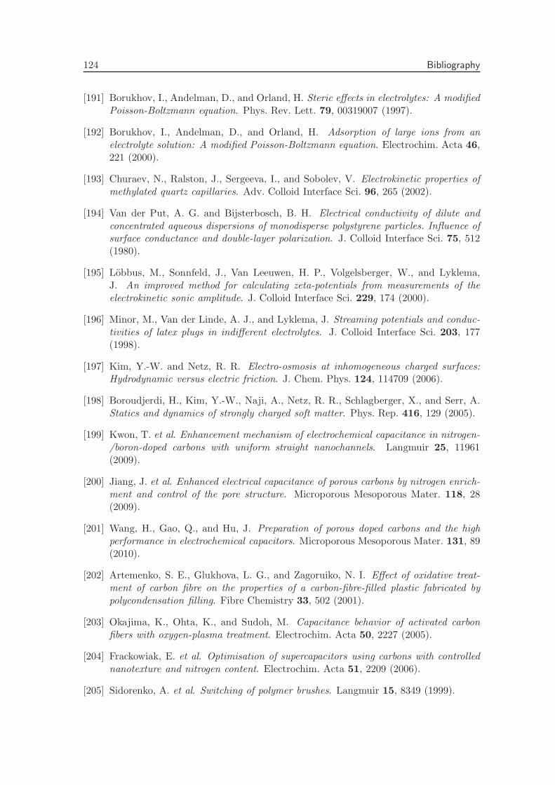
124 Bibliography
[191] Borukhov, I., Andelman, D., and Orland, H. Steric effects in electrolytes: A modifiedPoisson-Boltzmann equation. Phys. Rev. Lett. 79, 00319007 (1997).
[192] Borukhov, I., Andelman, D., and Orland, H. Adsorption of large ions from anelectrolyte solution: A modified Poisson-Boltzmann equation. Electrochim. Acta 46,221 (2000).
[193] Churaev, N., Ralston, J., Sergeeva, I., and Sobolev, V. Electrokinetic properties ofmethylated quartz capillaries. Adv. Colloid Interface Sci. 96, 265 (2002).
[194] Van der Put, A. G. and Bijsterbosch, B. H. Electrical conductivity of dilute andconcentrated aqueous dispersions of monodisperse polystyrene particles. Influence ofsurface conductance and double-layer polarization. J. Colloid Interface Sci. 75, 512(1980).
[195] Lobbus, M., Sonnfeld, J., Van Leeuwen, H. P., Volgelsberger, W., and Lyklema,J. An improved method for calculating zeta-potentials from measurements of theelectrokinetic sonic amplitude. J. Colloid Interface Sci. 229, 174 (2000).
[196] Minor, M., Van der Linde, A. J., and Lyklema, J. Streaming potentials and conduc-tivities of latex plugs in indifferent electrolytes. J. Colloid Interface Sci. 203, 177(1998).
[197] Kim, Y.-W. and Netz, R. R. Electro-osmosis at inhomogeneous charged surfaces:Hydrodynamic versus electric friction. J. Chem. Phys. 124, 114709 (2006).
[198] Boroudjerdi, H., Kim, Y.-W., Naji, A., Netz, R. R., Schlagberger, X., and Serr, A.Statics and dynamics of strongly charged soft matter. Phys. Rep. 416, 129 (2005).
[199] Kwon, T. et al. Enhancement mechanism of electrochemical capacitance in nitrogen-/boron-doped carbons with uniform straight nanochannels. Langmuir 25, 11961(2009).
[200] Jiang, J. et al. Enhanced electrical capacitance of porous carbons by nitrogen enrich-ment and control of the pore structure. Microporous Mesoporous Mater. 118, 28(2009).
[201] Wang, H., Gao, Q., and Hu, J. Preparation of porous doped carbons and the highperformance in electrochemical capacitors. Microporous Mesoporous Mater. 131, 89(2010).
[202] Artemenko, S. E., Glukhova, L. G., and Zagoruiko, N. I. Effect of oxidative treat-ment of carbon fibre on the properties of a carbon-fibre-filled plastic fabricated bypolycondensation filling. Fibre Chemistry 33, 502 (2001).
[203] Okajima, K., Ohta, K., and Sudoh, M. Capacitance behavior of activated carbonfibers with oxygen-plasma treatment. Electrochim. Acta 50, 2227 (2005).
[204] Frackowiak, E. et al. Optimisation of supercapacitors using carbons with controllednanotexture and nitrogen content. Electrochim. Acta 51, 2209 (2006).
[205] Sidorenko, A. et al. Switching of polymer brushes. Langmuir 15, 8349 (1999).
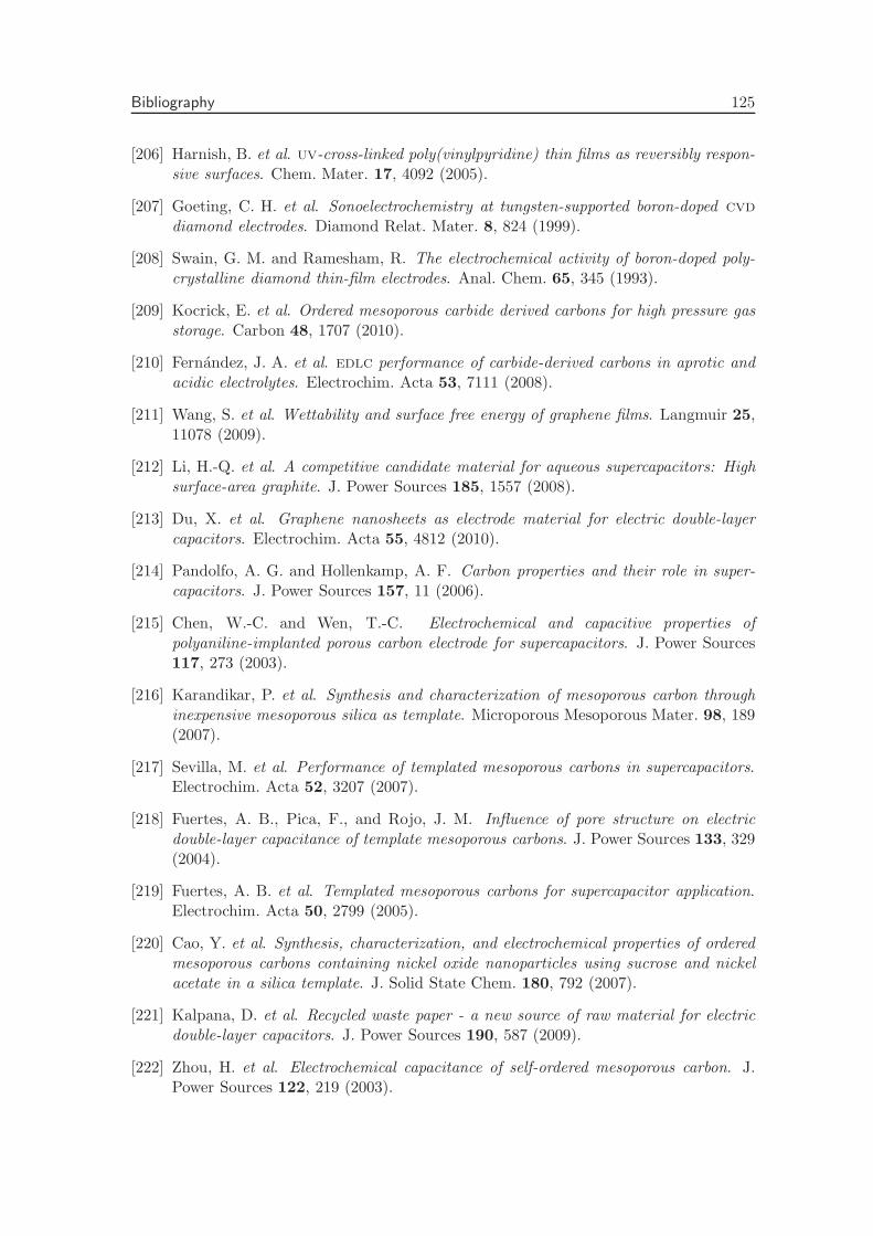
Bibliography 125
[206] Harnish, B. et al. uv-cross-linked poly(vinylpyridine) thin films as reversibly respon-sive surfaces. Chem. Mater. 17, 4092 (2005).
[207] Goeting, C. H. et al. Sonoelectrochemistry at tungsten-supported boron-doped cvddiamond electrodes. Diamond Relat. Mater. 8, 824 (1999).
[208] Swain, G. M. and Ramesham, R. The electrochemical activity of boron-doped poly-crystalline diamond thin-film electrodes. Anal. Chem. 65, 345 (1993).
[209] Kocrick, E. et al. Ordered mesoporous carbide derived carbons for high pressure gasstorage. Carbon 48, 1707 (2010).
[210] Fernandez, J. A. et al. edlc performance of carbide-derived carbons in aprotic andacidic electrolytes. Electrochim. Acta 53, 7111 (2008).
[211] Wang, S. et al. Wettability and surface free energy of graphene films. Langmuir 25,11078 (2009).
[212] Li, H.-Q. et al. A competitive candidate material for aqueous supercapacitors: Highsurface-area graphite. J. Power Sources 185, 1557 (2008).
[213] Du, X. et al. Graphene nanosheets as electrode material for electric double-layercapacitors. Electrochim. Acta 55, 4812 (2010).
[214] Pandolfo, A. G. and Hollenkamp, A. F. Carbon properties and their role in super-capacitors. J. Power Sources 157, 11 (2006).
[215] Chen, W.-C. and Wen, T.-C. Electrochemical and capacitive properties ofpolyaniline-implanted porous carbon electrode for supercapacitors. J. Power Sources117, 273 (2003).
[216] Karandikar, P. et al. Synthesis and characterization of mesoporous carbon throughinexpensive mesoporous silica as template. Microporous Mesoporous Mater. 98, 189(2007).
[217] Sevilla, M. et al. Performance of templated mesoporous carbons in supercapacitors.Electrochim. Acta 52, 3207 (2007).
[218] Fuertes, A. B., Pica, F., and Rojo, J. M. Influence of pore structure on electricdouble-layer capacitance of template mesoporous carbons. J. Power Sources 133, 329(2004).
[219] Fuertes, A. B. et al. Templated mesoporous carbons for supercapacitor application.Electrochim. Acta 50, 2799 (2005).
[220] Cao, Y. et al. Synthesis, characterization, and electrochemical properties of orderedmesoporous carbons containing nickel oxide nanoparticles using sucrose and nickelacetate in a silica template. J. Solid State Chem. 180, 792 (2007).
[221] Kalpana, D. et al. Recycled waste paper - a new source of raw material for electricdouble-layer capacitors. J. Power Sources 190, 587 (2009).
[222] Zhou, H. et al. Electrochemical capacitance of self-ordered mesoporous carbon. J.Power Sources 122, 219 (2003).
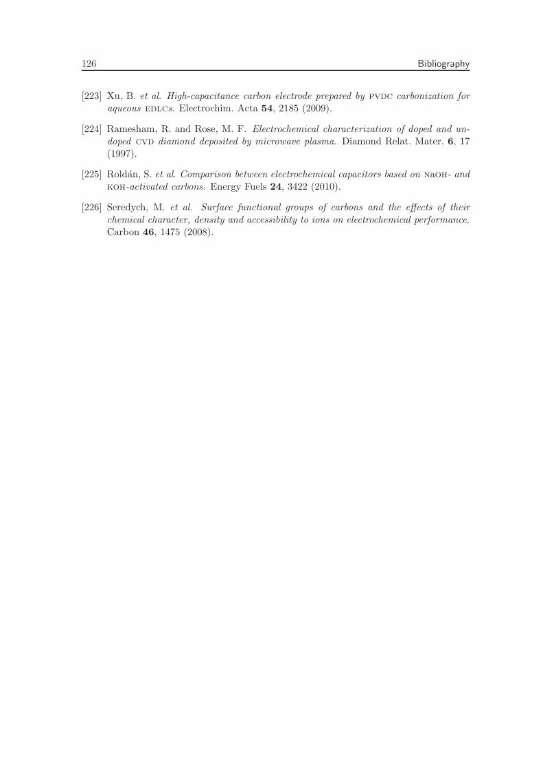
126 Bibliography
[223] Xu, B. et al. High-capacitance carbon electrode prepared by pvdc carbonization foraqueous edlcs. Electrochim. Acta 54, 2185 (2009).
[224] Ramesham, R. and Rose, M. F. Electrochemical characterization of doped and un-doped cvd diamond deposited by microwave plasma. Diamond Relat. Mater. 6, 17(1997).
[225] Roldan, S. et al. Comparison between electrochemical capacitors based on naoh- andkoh-activated carbons. Energy Fuels 24, 3422 (2010).
[226] Seredych, M. et al. Surface functional groups of carbons and the effects of theirchemical character, density and accessibility to ions on electrochemical performance.Carbon 46, 1475 (2008).

Acknowledgments
First and foremost I would like to thank my advisor Roland R. Netz for giving me theopportunity to work with him and for his dedicated supervision. Thank you for our ef-ficient and productive teamwork; I have learned a lot and it has been a great pleasureto work with you. Furthermore I would like to thank my collaborators, in particularDominik Horinek, Lyderic Bocquet, Stephan Gekle and Klaus Rinne for their help andadvice. For the fruitful discussions and work on our joint projects I would like to expressmy gratitude to Nihat Berker, Nadir Kaplan, Kerstin Falk and Pavel Jungwirth. Manythanks also to my friends and colleagues from the soft matter group: Christian Sendner,Sebastian Fischer, Andreas Serr, Manu Schneck, Felix Sedlmeier, Matej Kanduc, MariaFyta, Joe Dzubiella, Yann von Hansen, Julius Schulz, David Hofmann, Alex Herz, ShavkatMamatkulov, Vladimir Lobaskin, Hirofumi Wada and Michael Hinczewski. In particular,I would like to thank my friends Aykut Erbas, Immanuel Kalcher, Tom Einert and IoannisDaotidis for our many no-so-work-related projects. Ich bedanke mich ganz herzlich beiSonja Ortner, insbesondere fur die Organisation der Winterschulen und fur die Hilfe beimAusfullen von Formularen.
I acknowledge the Deutsche Forschungsgemeinschaft for funding via the Nanosystems Ini-tiative Munich and the Leibniz Rechenzentrum for providing the necessary computationalresources.
I would like to thank all my friends from abroad for visiting Munchen every now andthen. Finally, I thank my family, and especially Angelique, for their continuous help andsupport.

Copyright © 2022 FDOKUMEN